Retouched bloom filters

Retouched Bloom Filters:Allowing Networked Applications to Trade Off

Selected False Positives Against False Negatives

Benoit DonnetUniv. Catholique de Louvain

Bruno BaynatUniv. Pierre et Marie Curie

Timur FriedmanUniv. Pierre et Marie Curie

ABSTRACT

Where distributed agents must share voluminous set mem-bership information, Bloom filters provide a compact, thoughlossy, way for them to do so. Numerous recent networkingpapers have examined the trade-offs between the bandwidthconsumed by the transmission of Bloom filters, and the er-ror rate, which takes the form of false positives, and whichrises the more the filters are compressed. In this paper, weintroduce the retouched Bloom filter (RBF), an extensionthat makes the Bloom filter more flexible by permitting theremoval of selected false positives at the expense of gen-erating random false negatives. We analytically show thatRBFs created through a random process maintain an overallerror rate, expressed as a combination of the false positiverate and the false negative rate, that is equal to the falsepositive rate of the corresponding Bloom filters. We furtherprovide some simple heuristics that decrease the false posi-tive rate more than than the corresponding increase in thefalse negative rate, when creating RBFs. Finally, we demon-strate the advantages of an RBF over a Bloom filter in a dis-tributed network topology measurement application, whereinformation about large stop sets must be shared amongroute tracing monitors.

Categories and Subject Descriptors

C.2.1 [Network Architecture and Design]: NetworkTopology; E.4 [Coding and Information Theory]: DataCompaction and Compression

General Terms

Algorithms, Performance

Keywords

Bloom filters, false positive, false negative, bit clearing,measurement, traceroute

Permission to make digital or hard copies of all or part of this work forpersonal or classroom use is granted without fee provided that copies arenot made or distributed for profit or commercial advantage and that copiesbear this notice and the full citation on the first page. To copy otherwise, torepublish, to post on servers or to redistribute to lists, requires prior specificpermission and/or a fee.CoNEXT 2006, Lisbon, PortugalCopyright 2006 ACM 1595934561/06/0012 ...$5.00.

1. INTRODUCTIONThe Bloom filter is a data structure that was introduced

in 1970 [1] and that has been adopted by the networkingresearch community in the past decade thanks to the band-width efficiencies that it offers for the transmission of setmembership information between networked hosts. A senderencodes the information into a bit vector, the Bloom filter,that is more compact than a conventional representation.Computation and space costs for construction are linear inthe number of elements. The receiver uses the filter to testwhether various elements are members of the set. Thoughthe filter will occasionally return a false positive, it will neverreturn a false negative. When creating the filter, the sendercan choose its desired point in a trade-off between the falsepositive rate and the size. The compressed Bloom filter,an extension proposed by Mitzenmacher [2], allows furtherbandwidth savings.

Broder and Mitzenmacher’s survey of Bloom filters’ net-working applications [3] attests to the considerable interestin this data structure. Variants on the Bloom filter con-tinue to be introduced. For instance, Bonomi et al.’s [4]d-left counting Bloom filter is a more space-efficient versionof Fan et al.’s [5] counting Bloom filter, which itself goes be-yond the standard Bloom filter to allow dynamic insertionsand deletions of set membership information. The presentpaper also introduces a variant on the Bloom filter: onethat allows an application to remove selected false positivesfrom the filter, trading them off against the introduction ofrandom false negatives.

This paper looks at Bloom filters in the context of a net-work measurement application that must send informationconcerning large sets of IP addresses between measurementpoints. Sec. 5 describes the application in detail. But here,we cite two key characteristics of this particular applica-tion; characteristics that many other networked applicationsshare, and that make them candidates for use of the variantthat we propose.

First, some false positives might be more troublesomethan others, and these can be identified after the Bloomfilter has been constructed, but before it is used. For in-stance, when IP addresses arise in measurements, it is notuncommon for some addresses to be encountered with muchgreater frequency than others. If such an address triggers afalse positive, the performance detriment is greater than ifa rarely encountered address does the same. If there were away to remove them from the filter before use, the applica-tion would benefit.

Second, the application can tolerate a low level of false

negatives. It would benefit from being able to trade off themost troublesome false positives for some randomly intro-duced false negatives.

The retouched Bloom filter (RBF) introduced in this pa-per permits such a trade-off. It allows the removal of se-lected false positives at the cost of introducing random falsenegatives, and with the benefit of eliminating some randomfalse positives at the same time. An RBF is created froma Bloom filter by selectively changing individual bits from1 to 0, while the size of the filter remains unchanged. AsSec. 3.2 shows analytically, an RBF created through a ran-dom process maintains an overall error rate, expressed as acombination of the false positive rate and the false negativerate, that is equal to the false positive rate of the corre-sponding Bloom filter. We further provide a number of sim-ple algorithms that lower the false positive rate by a greaterdegree, on average, than the corresponding increase in thefalse negative rate. These algorithms require at most a smallconstant multiple in storage requirements. Any additionalprocessing and storage related to the creation of RBFs fromBloom filters are restricted to the measurement points thatcreate the RBFs. There is strictly no addition to the criticalresource under consideration, which is the bandwidth con-sumed by communication between the measurement points.

Some existing Bloom filter variants do permit the suppres-sion of selected false positives, or the removal of informationin general, or a trade-off between the false positive rate andthe false negative rate. However, as Sec. 6 describes, theRBF is unique in doing so while maintaining the size of theoriginal Bloom filter and lowering the overall error rate ascompared to that filter.

The remainder of this paper is organized as follows: Sec. 2presents the standard Bloom filter; Sec. 3 presents the RBF,and shows analytically that the reduction in the false pos-itive rate is equal, on average, to the increase in the falsenegative rate even as random 1s in a Bloom filter are re-set to 0s; Sec. 4 presents several simple methods for selec-tively clearing 1s that are associated with false positives,and shows through simulations that they reduce the falsepositive rate by more, on average, than they increase thefalse negative rate; Sec. 5 describes the use of RBFs in anetwork measurement application; Sec. 6 discusses severalBloom filter variants and compares RBFs to them; finally,Sec. 7 summarizes the conclusions and future directions forthis work.

2. BLOOM FILTERSA Bloom filter [1] is a vector v of m bits that codes the

membership of a subset A = {a1, a2, . . . , an} of n elementsof a universe U consisting of N elements. In most papers,the size of the universe is not specified. However, Bloomfilters are only useful if the size of U is much bigger thanthe size of A.

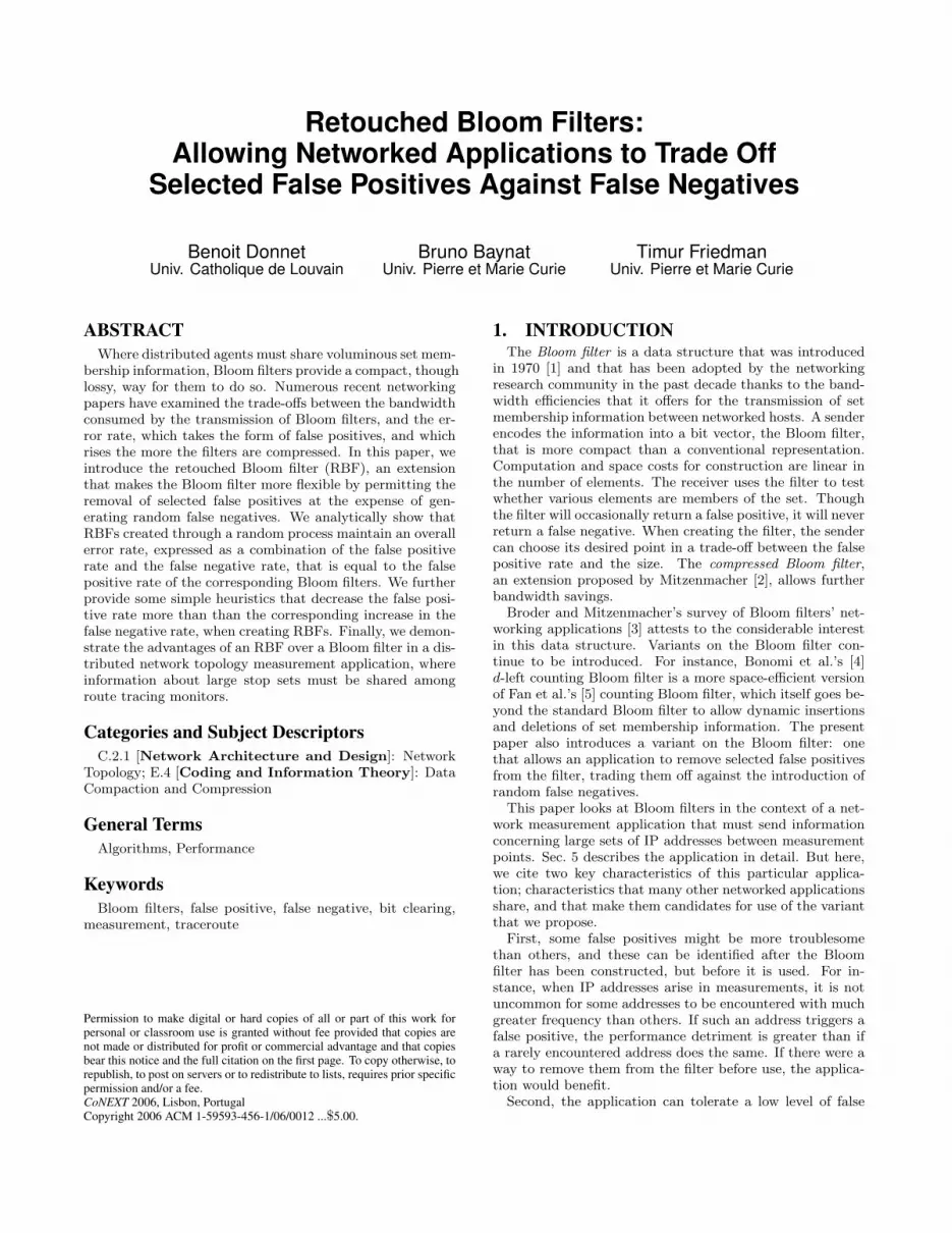
The idea is to initialize this vector v to 0, and then takea set H = {h1, h2, . . . , hk} of k independent hash functionsh1, h2, . . . , hk, each with range {1, . . . , m}. For each elementa ∈ A, the bits at positions h1(a), h2(a), . . . , hk(a) in v areset to 1. Note that a particular bit can be set to 1 severaltimes, as illustrated in Fig. 1.

In order to check if an element b of the universe U belongsto the set A, all one has to do is check that the k bits atpositions h1(b), h2(b), . . . , hk(b) are all set to 1. If at leastone bit is set to 0, we are sure that b does not belong to

h1(b)

h2(b)h2(a)

h1(a)

1 1 1 0000000

Figure 1: A Bloom filter with two hash functions

U

A

B

FP

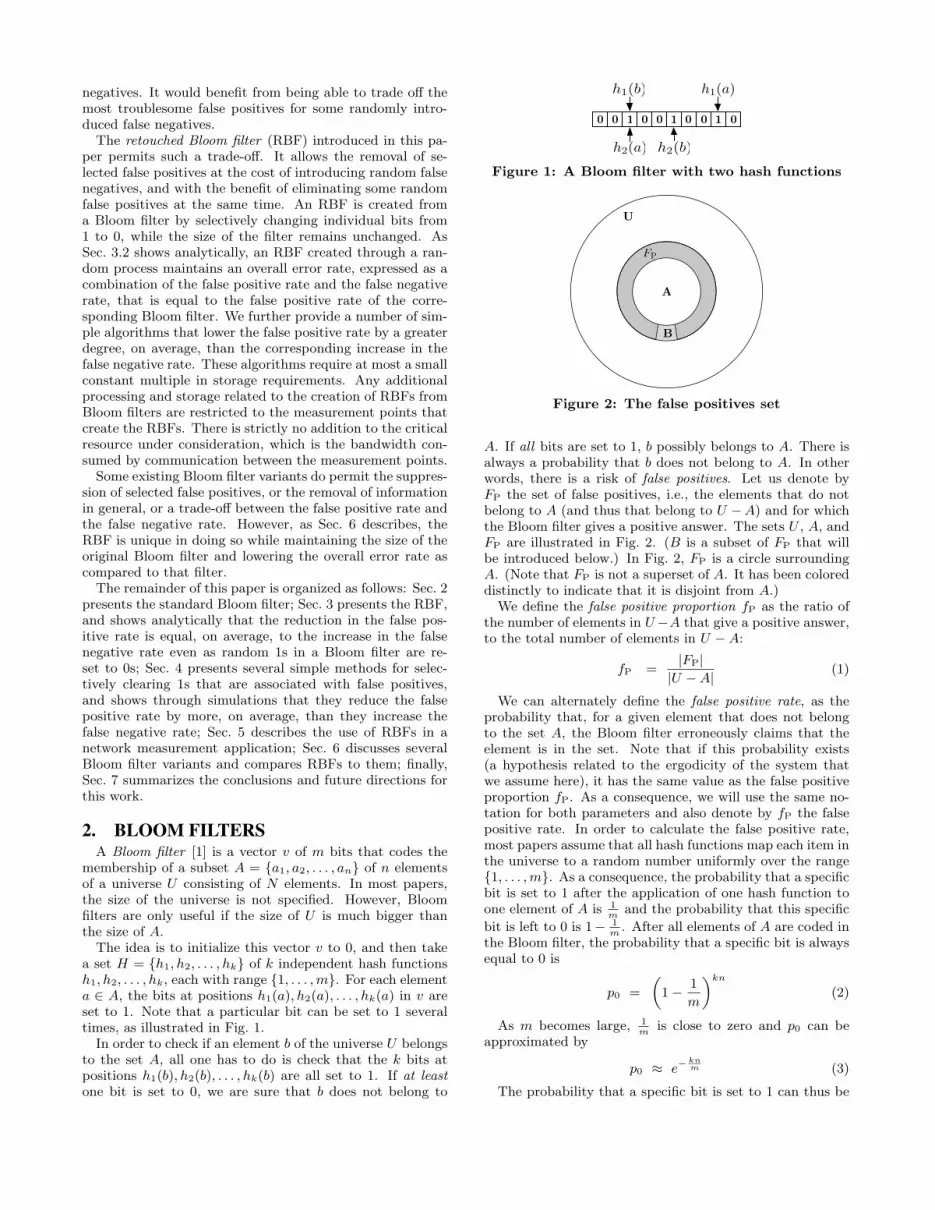
Figure 2: The false positives set

A. If all bits are set to 1, b possibly belongs to A. There isalways a probability that b does not belong to A. In otherwords, there is a risk of false positives. Let us denote byFP the set of false positives, i.e., the elements that do notbelong to A (and thus that belong to U −A) and for whichthe Bloom filter gives a positive answer. The sets U , A, andFP are illustrated in Fig. 2. (B is a subset of FP that willbe introduced below.) In Fig. 2, FP is a circle surroundingA. (Note that FP is not a superset of A. It has been coloreddistinctly to indicate that it is disjoint from A.)

We define the false positive proportion fP as the ratio ofthe number of elements in U−A that give a positive answer,to the total number of elements in U −A:

fP =|FP|

|U −A|(1)

We can alternately define the false positive rate, as theprobability that, for a given element that does not belongto the set A, the Bloom filter erroneously claims that theelement is in the set. Note that if this probability exists(a hypothesis related to the ergodicity of the system thatwe assume here), it has the same value as the false positiveproportion fP. As a consequence, we will use the same no-tation for both parameters and also denote by fP the falsepositive rate. In order to calculate the false positive rate,most papers assume that all hash functions map each item inthe universe to a random number uniformly over the range{1, . . . , m}. As a consequence, the probability that a specificbit is set to 1 after the application of one hash function toone element of A is 1

mand the probability that this specific

bit is left to 0 is 1− 1m

. After all elements of A are coded inthe Bloom filter, the probability that a specific bit is alwaysequal to 0 is

p0 =

„

1−1

m

«kn

(2)

As m becomes large, 1m

is close to zero and p0 can beapproximated by

p0 ≈ e−

kn

m (3)

The probability that a specific bit is set to 1 can thus be

Figure 3: fP as a function of k, m and n.

expressed as

p1 = 1− p0 (4)

The false positive rate can then be estimated by the prob-ability that each of the k array positions computed by thehash functions is 1. fP is then given by

fP = pk1

=“

1−`

1− 1m

´kn”k

≈“

1 − e−kn

m

”k

(5)

The false positive rate fP is thus a function of three pa-rameters: n, the size of subset A; m, the size of the filter;and k, the number of hash functions. Fig. 3 illustrates thevariation of fP with respect to the three parameters individ-ually (when the two others are held constant). Obviously,and as can be seen on these graphs, fP is a decreasing func-tion of m and an increasing function of n. Now, when k

varies (with n and m constant), fP first decreases, reachesa minimum and then increases. Indeed there are two con-tradicting factors: using more hash functions gives us morechances to find a 0 bit for an element that is not a memberof A, but using fewer hash functions increases the fractionof 0 bits in the array. As stated, e.g., by Fan et al. [5], fP isminimized when

k =m ln 2

n(6)

for fixed m and n. Indeed, the derivative of fP (estimatedby eqn. 3) with respect to k is 0 when k is given by eqn. 6,and it can further be shown that this is a global minimum.

Thus the minimum possible false positive rate for givenvalues of m and n is given by eqn. 7. In practice, of course,k must be an integer. As a consequence, the value furnishedby eqn. 6 is rounded to the nearest integer and the resultingfalse positive rate will be somewhat higher than the optimalvalue given in eqn. 7.

fP =

„

1

2

« m ln 2

n

≈ (0.6185)m

n (7)

Finally, it is important to emphasize that the absolutenumber of false positives is relative to the size of U−A (andnot directly to the size of A). This result seems surprising asthe expression of fP depends on n, the size of A, and doesnot depend on N , the size of U . If we double the size ofU −A (and keep the size of A constant) we also double the

absolute number of false positives (and obviously the falsepositive rate is unchanged).

3. RETOUCHED BLOOM FILTERSAs shown in Sec. 2, there is a trade-off between the size

of the Bloom filter and the probability of a false positive.For a given n, even by optimally choosing the number ofhash functions, the only way to reduce the false positiverate in standard Bloom filters is to increase the size m ofthe bit vector. Unfortunately, although this implies a gainin terms of a reduced false positive rate, it also implies aloss in terms of increased memory usage. Bandwidth usagebecomes a constraint that must be minimized when Bloomfilters are transmitted in the network.

3.1 Bit ClearingIn this paper, we introduce an extension to the Bloom

filter, referred to as the retouched Bloom filter (RBF). TheRBF makes standard Bloom filters more flexible by allow-ing selected false positives to be traded off against randomfalse negatives. False negatives do not arise at all in thestandard case. The idea behind the RBF is to remove acertain number of these selected false positives by resettingindividually chosen bits in the vector v. We call this pro-cess the bit clearing process. Resetting a given bit to 0 notonly has the effect of removing a certain number of falsepositives, but also generates false negatives. Indeed, anyelement a ∈ A such that (at least) one of the k bits at posi-tions h1(a), h2(a), . . . , hk(a) has been reset to 0, now triggersa negative answer. Element a thus becomes a false negative.

To summarize, the bit clearing process has the effects ofdecreasing the number of false positives and of generating anumber of false negatives. Let us use the labels F ′

P and F ′

N

to describe the sets of false positives and false negatives afterthe bit clearing process. The sets F ′

P and F ′

N are illustratedin Fig. 4.

After the bit clearing process, the false positive and falsenegative proportions are given by

f ′

P =|F ′

P|

|U −A|(8)

f ′

N =|F ′

N|

|A|(9)

Obviously, the false positive proportion has decreased (asF ′

P is smaller than FP) and the false negative proportion

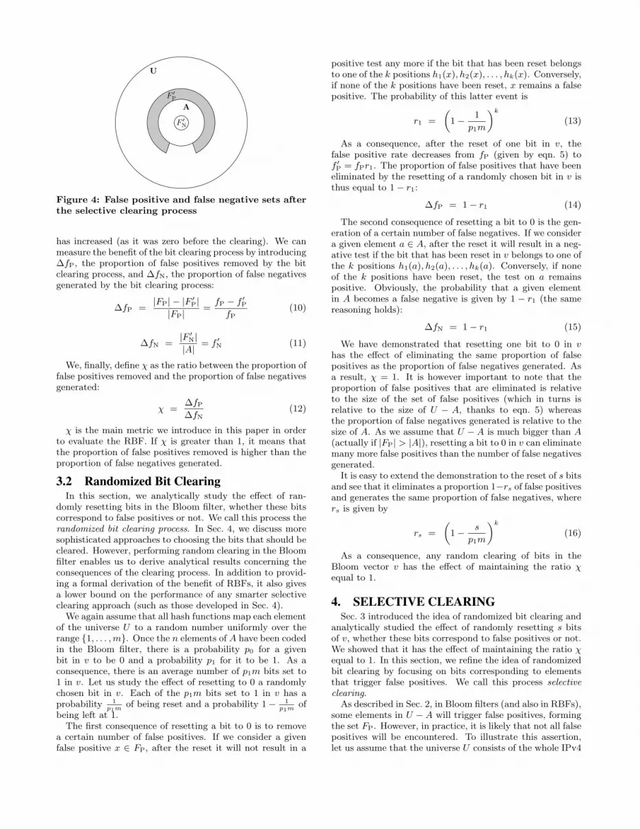
F′

P

F′

N

U

A

Figure 4: False positive and false negative sets after

the selective clearing process

has increased (as it was zero before the clearing). We canmeasure the benefit of the bit clearing process by introducing∆fP, the proportion of false positives removed by the bitclearing process, and ∆fN, the proportion of false negativesgenerated by the bit clearing process:

∆fP =|FP| − |F

′

P|

|FP|=

fP − f ′

P

fP(10)

∆fN =|F ′

N|

|A|= f

′

N (11)

We, finally, define χ as the ratio between the proportion offalse positives removed and the proportion of false negativesgenerated:

χ =∆fP

∆fN(12)

χ is the main metric we introduce in this paper in orderto evaluate the RBF. If χ is greater than 1, it means thatthe proportion of false positives removed is higher than theproportion of false negatives generated.

3.2 Randomized Bit ClearingIn this section, we analytically study the effect of ran-

domly resetting bits in the Bloom filter, whether these bitscorrespond to false positives or not. We call this process therandomized bit clearing process. In Sec. 4, we discuss moresophisticated approaches to choosing the bits that should becleared. However, performing random clearing in the Bloomfilter enables us to derive analytical results concerning theconsequences of the clearing process. In addition to provid-ing a formal derivation of the benefit of RBFs, it also givesa lower bound on the performance of any smarter selectiveclearing approach (such as those developed in Sec. 4).

We again assume that all hash functions map each elementof the universe U to a random number uniformly over therange {1, . . . , m}. Once the n elements of A have been codedin the Bloom filter, there is a probability p0 for a givenbit in v to be 0 and a probability p1 for it to be 1. As aconsequence, there is an average number of p1m bits set to1 in v. Let us study the effect of resetting to 0 a randomlychosen bit in v. Each of the p1m bits set to 1 in v has aprobability 1

p1mof being reset and a probability 1− 1

p1mof

being left at 1.The first consequence of resetting a bit to 0 is to remove

a certain number of false positives. If we consider a givenfalse positive x ∈ FP, after the reset it will not result in a

positive test any more if the bit that has been reset belongsto one of the k positions h1(x), h2(x), . . . , hk(x). Conversely,if none of the k positions have been reset, x remains a falsepositive. The probability of this latter event is

r1 =

„

1−1

p1m

«k

(13)

As a consequence, after the reset of one bit in v, thefalse positive rate decreases from fP (given by eqn. 5) tof ′

P = fPr1. The proportion of false positives that have beeneliminated by the resetting of a randomly chosen bit in v isthus equal to 1− r1:

∆fP = 1− r1 (14)

The second consequence of resetting a bit to 0 is the gen-eration of a certain number of false negatives. If we considera given element a ∈ A, after the reset it will result in a neg-ative test if the bit that has been reset in v belongs to one ofthe k positions h1(a), h2(a), . . . , hk(a). Conversely, if noneof the k positions have been reset, the test on a remainspositive. Obviously, the probability that a given elementin A becomes a false negative is given by 1 − r1 (the samereasoning holds):

∆fN = 1− r1 (15)

We have demonstrated that resetting one bit to 0 in v

has the effect of eliminating the same proportion of falsepositives as the proportion of false negatives generated. Asa result, χ = 1. It is however important to note that theproportion of false positives that are eliminated is relativeto the size of the set of false positives (which in turns isrelative to the size of U − A, thanks to eqn. 5) whereasthe proportion of false negatives generated is relative to thesize of A. As we assume that U −A is much bigger than A

(actually if |FP| > |A|), resetting a bit to 0 in v can eliminatemany more false positives than the number of false negativesgenerated.

It is easy to extend the demonstration to the reset of s bitsand see that it eliminates a proportion 1−rs of false positivesand generates the same proportion of false negatives, wherers is given by

rs =

„

1−s

p1m

«k

(16)

As a consequence, any random clearing of bits in theBloom vector v has the effect of maintaining the ratio χ

equal to 1.

4. SELECTIVE CLEARINGSec. 3 introduced the idea of randomized bit clearing and

analytically studied the effect of randomly resetting s bitsof v, whether these bits correspond to false positives or not.We showed that it has the effect of maintaining the ratio χ

equal to 1. In this section, we refine the idea of randomizedbit clearing by focusing on bits corresponding to elementsthat trigger false positives. We call this process selectiveclearing.

As described in Sec. 2, in Bloom filters (and also in RBFs),some elements in U −A will trigger false positives, formingthe set FP. However, in practice, it is likely that not all falsepositives will be encountered. To illustrate this assertion,let us assume that the universe U consists of the whole IPv4

Algorithm 1 Random Selection

Require: v, the bit vector.Ensure: v updated, if needed.1: procedure RandomSelection(B)2: for all bi ∈ B do

3: if MembershipTest(bi, v) then

4: index ← Random(h1(bi), . . . , hk(bi))5: v[index] ← 06: end if

7: end for

8: end procedure

addresses range. To build the Bloom filter or the RBF, wedefine k hash functions based on a 32 bit string. The subsetA to record in the filter is a small portion of the IPv4 addressrange. Not all false positives will be encountered in practicebecause a significant portion of the IPv4 addresses in FP

have not been assigned.We record the false positives encountered in practice in

a set called B, with B ⊆ FP (see Fig. 2). Elements in B

are false positives that we label as troublesome keys, as theygenerate, when presented as keys to the Bloom filter’s hashfunctions, false positives that are liable to be encounteredin practice. We would like to eliminate the elements of B

from the filter.In the following sections, we explore several algorithms for

performing selective clearing (Sec. 4.1). We then evaluateand compare the performance of these algorithms (Sec. 4.2).

4.1 AlgorithmsIn this section, we propose four different algorithms that

allow one to remove the false positives belonging to B. Allof these algorithms are simple to implement and deploy. Wefirst present an algorithm that does not require any intel-ligence in selective clearing. Next, we propose refined al-gorithms that take into account the risk of false negatives.With these algorithms, we show how to trade-off false posi-tives for false negatives.

The first algorithm is called Random Selection. The mainidea is, for each troublesome key to remove, to randomlyselect a bit amongst the k available to reset. The maininterest of the Random Selection algorithm is its extremecomputational simplicity: no effort has to go into selecting abit to clear. Random Selection differs from random clearing(see Sec. 3) by focusing on a set of troublesome keys toremove, B, and not by resetting randomly any bit in v,whether it corresponds to a false positive or not. RandomSelection is formally defined in Algorithm 1.

Recall that B is the set of troublesome keys to remove.This set can contain from only one element to the whole setof false positives. Before removing a false positive element,we make sure that this element is still falsely recorded inthe RBF, as it could have been removed previously. Indeed,due to collisions that may occur between hashed keys in thebit vector, as shown in Fig. 1, one of the k hashed bit po-sitions of the element to remove may have been previouslyreset. Algorithm 1 assumes that a function Random is de-fined and returns a value randomly chosen amongst its uni-formly distributed arguments. The algorithm also assumesthat the function MembershipTest is defined. It takes twoarguments: the key to be tested and the bit vector. Thisfunction returns true if the element is recorded in the bit

Algorithm 2 Minimum FN Selection

Require: v, the bit vector and vA, the counting vector.Ensure: v and vA updated, if needed.1: procedure MinimumFNSelection(B)2: CreateCV(A)3: for all bi ∈ B do


5: index ← MinIndex(bi)6: v[index] ← 07: vA[index] ← 08: end if

9: end for

10: end procedure

11:12: procedure CreateCV(A)13: for all ai ∈ A do

14: for j = 1 to k do

15: vA[hj(ai)]++16: end for

17: end for

18: end procedure

vector (i.e., all the k positions corresponding to the hashfunctions are set to 1). It returns false otherwise.

The second algorithm we propose is called Minimum FNSelection. The idea is to minimize the false negatives gener-ated by each selective clearing. For each troublesome key toremove that was not previously cleared, we choose amongstthe k bit positions the one that we estimate will generate theminimum number of false negatives. This minimum is givenby the MinIndex procedure in Algorithm 2. This can beachieved by maintaining locally a counting vector, vA, stor-ing in each vector position the quantity of elements recorded.This algorithm effectively takes into account the possibilityof collisions in the bit vector between hashed keys of ele-ments belonging to A. Minimum FN Selection is formallydefined in Algorithm 2.

For purposes of algorithmic simplicity, we do not entirelyupdate the counting vector with each iteration. The costcomes in terms of an over-estimation, for the heuristic, inassessing the number of false negatives that it introducesin any given iteration. This over-estimation grows as thealgorithm progresses. We are currently studying ways toefficiently adjust for this over-estimation.

The third selective clearing mechanism is called Maxi-mum FP Selection. In this case, we try to maximize thequantity of false positives to remove. For each troublesomekey to remove that was not previously deleted, we chooseamongst the k bit positions the one we estimate to allowremoval of the largest number of false positives, the positionof which is given by the MaxIndex function in Algorithm 3.In the fashion of the Minimum FN Selection algorithm, thisis achieved by maintaining a counting vector, vB , storing ineach vector position the quantity of false positive elementsrecorded. For each false positive element, we choose thebit corresponding to the largest number of false positivesrecorded. This algorithm considers as an opportunity therisk of collisions in the bit vector between hashed keys ofelements generating false positives. Maximum FP Selectionis formally described in Algorithm 3.

Finally, we propose a selective clearing mechanism calledRatio Selection. The idea is to combine Minimum FN Se-

Algorithm 3 Maximum FP Selection

Require: v, the bit vector and vB , the counting vector.Ensure: v and vB updated, if needed.1: procedure MaximumFP(B)2: CreateFV(B)3: for all bi ∈ B do


5: index ← MaxIndex(bi)6: v[index] ← 07: vB [index] ← 08: end if

9: end for

10: end procedure

11:12: procedure CreateFV(B)13: for all bi ∈ B do

14: for j = 1 to k do

15: vB [hj(bi)]++16: end for

17: end for

18: end procedure

lection and Maximum FP Selection into a single algorithm.Ratio Selection provides an approach in which we try tominimize the false negatives generated while maximizing thefalse positives removed. Ratio Selection therefore takes intoaccount the risk of collision between hashed keys of elementsbelonging to A and hashed keys of elements belonging to B.It is achieved by maintaining a ratio vector, r, in whicheach position is the ratio between vA and vB . For eachtroublesome key that was not previously cleared, we choosethe index where the ratio is the minimum amongst the k

ones. This index is given by the MinRatio function in Algo-rithm 4. Ratio Selection is defined in Algorithm 4. This al-gorithm makes use of the CreateCV and CreateFV func-tions previously defined for Algorithms 2 and 3.

Details on the algorithmic and spatial complexity of theseselective clearing algorithms are to be found in our technicalreport [6].

4.2 EvaluationWe conduct an experiment with a universe U of 2,000,000

elements (N = 2,000,000). These elements, for the sake ofsimplicity, are integers belonging to the range [0; 1,999,9999].The subset A that we want to summarize in the Bloom filtercontains 10,000 different elements (n = 10,000) randomlychosen from the universe U . Bloom’s paper [1] states that|U | must be much greater than |A|, without specifying aprecise scale.

The bit vector v we use for simulations is 100,000 bitslong (m = 100,000), ten times bigger than |A|. The RBFuses five different and independent hash functions (k = 5).Hashing is emulated with random numbers. We simulaterandomness with the Mersenne Twister MT19937 pseudo-random number generator [7]. Using five hash functionsand a bit vector ten times bigger than n is advised by Fanet al. [5]. This permits a good trade-off between membershipquery accuracy, i.e., a low false positive rate of 0.0094 whenestimated with eqn. 5, memory usage and computation time.As mentioned earlier in this paper (see Sec. 2), the falsepositive rate may be decreased by increasing the bit vectorsize but it leads to a lower compression level.

Algorithm 4 Ratio Selection

Require: v, the bit vector, vB and vA, the counting vectorsand r, the ratio vector.

Ensure: v, vA, vB and r updated, if needed.1: procedure Ratio(B)2: CreateCV(A)3: CreateFV(B)4: ComputeRatio()5: for all bi ∈ B do


7: index ← MinRatio(bi)8: v[index] ← 09: vA[index] ← 0

10: vB [index] ← 011: r[index] ← 012: end if

13: end for

14: end procedure

15:16: procedure ComputeRatio

17: for i = 1 to m do

18: if v[i] ∧ vB [i] > 0 then

19: r[i] ← vA[i]vB [i]

20: end if

21: end for

22: end procedure

For our experiment, we define the ratio of troublesomekeys compared to the entire set of false positives as

β =|B|

|FP |(17)

We consider the following values of β: 1%, 2%, 5%, 10%,25%, 50%, 75% and 100%. When β = 100%, it means thatB = FP and we want to remove all the false positives.

Each data point in the plots represents the mean valueover fifteen runs of the experiment, each run using a newA, FP, B, and RBF. We determine 95% confidence intervalsfor the mean based on the Student t distribution.

We perform the experiment as follows: we first create theuniverse U and randomly affect 10,000 of its elements to A.We next build FP by applying the following scheme. Ratherthan using eqn. 5 to compute the false positive rate and thencreating FP by randomly affecting positions in v for the falsepositive elements, we prefer to experimentally compute thefalse positives. We query the RBF with a membership testfor each element belonging to U −A. False positives are theelements that belong to the Bloom filter but not to A. Wekeep track of them in a set called FP. This process seemsto us more realistic because we evaluate the real quantity offalse positive elements in our data set. B is then constructedby randomly selecting a certain quantity of elements in FP,the quantity corresponding to the desired cardinality of B.We next remove all troublesome keys from B by using oneof the selective clearing algorithms, as explained in Sec. 4.1.We then build F ′

N, the false negative set, by testing all el-ements in A and adding to F ′

N all elements that no longerbelong to A. We also determine F ′

P, the false positive setafter removing the set of troublesome keys B.

Fig. 5 compares the four algorithms in terms of the num-ber s of reset bits required to remove troublesome keys inB. The horizontal axis gives β and the vertical axis, in log

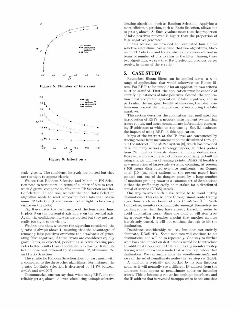
Figure 5: Number of bits reset

Figure 6: Effect on χ

scale, gives s. The confidence intervals are plotted but theyare too tight to appear clearly.

We see that Random Selection and Minimum FN Selec-tion need to work more, in terms of number of bits to reset,when β grows, compared to Maximum FP Selection and Ra-tio Selection. In addition, we note that the Ratio Selectionalgorithm needs to reset somewhat more bits than Maxi-mum FP Selection (the difference is too tight to be clearlyvisible on the plots).

Fig. 6 evaluates the performance of the four algorithms.It plots β on the horizontal axis and χ on the vertical axis.Again, the confidence intervals are plotted but they are gen-erally too tight to be visible.

We first note that, whatever the algorithm considered, theχ ratio is always above 1, meaning that the advantages ofremoving false positives overcome the drawbacks of gener-ating false negatives, if these errors are considered equallygrave. Thus, as expected, performing selective clearing pro-vides better results than randomized bit clearing. Ratio Se-lection does best, followed by Maximum FP, Minimum FN,and Ratio Selection.

The χ ratio for Random Selection does not vary much withβ compared to the three other algorithms. For instance, theχ ratio for Ratio Selection is decreased by 31.3% betweenβ=1% and β=100%.

To summarize, one can say that, when using RBF, one canreliably get a χ above 1.4, even when using a simple selective

clearing algorithm, such as Random Selection. Applying amore efficient algorithm, such as Ratio Selection, allows oneto get a χ above 1.8. Such χ values mean that the proportionof false positives removed is higher than the proportion offalse negatives generated.

In this section, we provided and evaluated four simpleselective algorithms. We showed that two algorithms, Max-imum FP Selection and Ratio Selection, are more efficient interms of number of bits to clear in the filter. Among thesetwo algorithms, we saw that Ratio Selection provides betterresults, in terms of the χ ratio.

5. CASE STUDYRetouched Bloom filters can be applied across a wide

range of applications that would otherwise use Bloom fil-ters. For RBFs to be suitable for an application, two criteriamust be satisfied. First, the application must be capable ofidentifying instances of false positives. Second, the applica-tion must accept the generation of false negatives, and inparticular, the marginal benefit of removing the false posi-tives must exceed the marginal cost of introducing the falsenegatives.

This section describes the application that motivated ourintroduction of RBFs: a network measurement system thattraces routes, and must communicate information concern-ing IP addresses at which to stop tracing. Sec. 5.1 evaluatesthe impact of using RBFs in this application.

Maps of the internet at the IP level are constructed bytracing routes from measurement points distributed through-out the internet. The skitter system [8], which has provideddata for many network topology papers, launches probesfrom 24 monitors towards almost a million destinations.However, a more accurate picture can potentially be built byusing a larger number of vantage points. Dimes [9] heralds anew generation of large-scale systems, counting, at present8,700 agents distributed over five continents. As Donnetet al. [10] (including authors on the present paper) havepointed out, one of the dangers posed by a large numberof monitors probing towards a common set of destinationsis that the traffic may easily be mistaken for a distributeddenial of service (DDoS) attack.

One way to avoid such a risk would be to avoid hittingdestinations. This can be done through smart route tracingalgorithms, such as Donnet et al.’s Doubletree [10]. WithDoubletree, monitors communicate amongst themselves re-garding routes that they have already traced, in order toavoid duplicating work. Since one monitor will stop trac-ing a route when it reaches a point that another monitorhas already traced, it will not continue through to hit thedestination.

Doubletree considerably reduces, but does not entirelyeliminate, DDoS risk. Some monitors will continue to hitdestinations, and will do so repeatedly. One way to furtherscale back the impact on destinations would be to introducean additional stopping rule that requires any monitor to stoptracing when it reaches a node that is one hop before thatdestination. We call such a node the penultimate node, andwe call the set of penultimate nodes the red stop set (RSS).

A monitor is typically not blocked by its own first-hopnode, as it will normally see a different IP address from theaddresses that appear as penultimate nodes on incomingtraces. This is because a router has multiple interfaces, andthe IP address that is revealed is supposed to be the one that

sends the probe reply. The application that we study in thispaper conducts standard route traces with an RSS. We donot use Doubletree, so as to avoid having to disentangle theeffects of using two different stopping rules at the same time.

How does one build the red stop set? The penultimatenodes cannot be determined a priori. However, the RSScan be constructed during a learning round in which eachmonitor performs a full set of standard traceroutes, i.e., untilhitting a destination. Monitors then share their RSSes. Forsimplicity, we consider that they all send their RSSes to acentral server, which combines them to form a global RSS,that is then redispatched to the monitors. The monitorsthen apply the global RSS in a stopping rule over multiplerounds of probing.

Destinations are only hit during the learning round andas a result of errors in the probing rounds. DDoS risk di-minishes with an increase in the ratio of probing rounds tolearning rounds, and with a decrease in errors during theprobing rounds. DDoS risk would be further reduced if weapply Doubletree in the learning round, as the number ofprobes that reach destinations during the learning roundwould then scale less then linearly in the number of mon-itors. However, our focus here is on the probing rounds,which use the global RSS, and not on improving the effi-ciency of the learning round, which generates the RSS, andfor which we already have known techniques.

The communication cost for sharing the RSS among mon-itors is linear in the number of monitors and in the size ofthe RSS representation. It is this latter size that we wouldlike to reduce by a constant compression factor. If the RSSis implemented as a list of 32-bit vectors, skitter’s milliondestinations would consume 4 MB. We therefore proposeencoding the RSS information in Bloom filters. Note thatthe central server can combine similarly constructed Bloomfilters from multiple monitors, through bitwise logical or

operations, to form the filter that encodes the global RSS.The cost of using Bloom filters is that the application will

encounter false positives. A false positive, in our case study,corresponds to an early stop in the probing, i.e., before thepenultimate node. We call such an error stopping short, andit means that part of the path that should have been dis-covered will go unexplored. Stopping short can also arisethrough network dynamics, when additional nodes are in-troduced, by routing changes or IP address reassignment,between the previously penultimate node and the destina-tion. In contrast, a trace that stops at a penultimate node isdeemed a success. A trace that hits a destination is called acollision. Collisions might occur because of a false negativefor the penultimate node, or simply because routing dynam-ics have introduced a new path to the destination, and thepenultimate node on that path was previously unknown.

As we show in Sec. 5.1, the cost of stopping short is farfrom negligible. If a node that has a high betweenness cen-trality (Dall’Asta et al. [11] point out the importance ofthis parameter for topology exploration) generates a falsepositive, then the topology information loss might be high.Consequently, our idea is to encode the RSS in an RBF.

As described in the Introduction, there are two criteriafor being able to profitably employ RBFs, and they are bothmet by this application. First, false positives can be iden-tified and removed. Once the topology has been revealed,each node can be tested against the Bloom filter, and thosethat register positive but are not penultimate nodes are false

positives. The application has the possibility of removingthe most troublesome false positives by using one of the se-lective algorithms discussed in Sec. 4. Second, a low rateof false negatives is acceptable and the marginal benefit ofremoving the most troublesome false positives exceeds themarginal cost of introducing those false negatives. Our aimis not to eliminate collisions; if they are considerably re-duced, the DDoS risk has been diminished and the RSSapplication can be deemed a success. On the other hand,systematically stopping short at central nodes can severelyrestrict topology exploration, and so we are willing to ac-cept a low rate of random collisions in order to trace moreeffectively. These trade-offs are explored in Sec. 5.1.

Table 1 summarizes the positive and negative aspects ofeach RSS implementation we propose. Positive aspects area success, stopping at the majority of penultimate nodes,topology information discovered, the eventual compressionratio of the implementation, and a low number of collisionswith destinations. Negative aspects of an implementationcan be the topology information missed due to stoppingshort, the load on the network when exchanging the RSSand the risk of hitting destinations too many times. Sec. 5.1examines the positive and negative aspects of each imple-mentation.

5.1 EvaluationIn this section, we evaluate the use of RBFs in a tracerout-

ing system based on an RSS. We first present our method-ology and then, discuss our results.

Our study is based on skitter data [8] from January 2006.This data set was generated by 24 monitors located in theUnited States of America, Canada, the United Kingdom,France, Sweden, the Netherlands, Japan, and New Zealand.The monitors share a common destination set of 971,080IPv4 addresses. Each monitor cycles through the destina-tion set at its own rate, taking typically three days to com-plete a cycle.

For the purpose of our study, in order to reduce computingtime to a manageable level, we work from a limited set of10 skitter monitors, all the monitors sharing a list of 10,000destinations, randomly chosen from the original set. In ourdata set, the RSS contains 8,006 different IPv4 addresses.

We compare the following three RSS implementations:list, Bloom filter and RBF. The list would not return any er-rors if the network were static, however, as discussed above,network dynamics lead to a certain error rate of both colli-sions and instances of stopping short. For the RBF imple-mentation, we consider β values (see eqn. 17) of 1%, 5%,10% and 25%. We employ the Ratio Selection algorithm, asdefined in Sec. 4.1. For the Bloom filter and RBF implemen-tations, the hashing is emulated with random numbers. Wesimulate randomness with the Mersenne Twister MT19937pseudo-random number generator [7].

To obtain our results, we simulate one learning round ona first cycle of traceroutes from each monitor, to generatethe RSS. We then simulate one probing round, using a sec-ond cycle of traceroutes. In this simulation, we replay thetraceroutes, but apply the stopping rule based on the RSS,noting instances of stopping short, successes, and collisions.

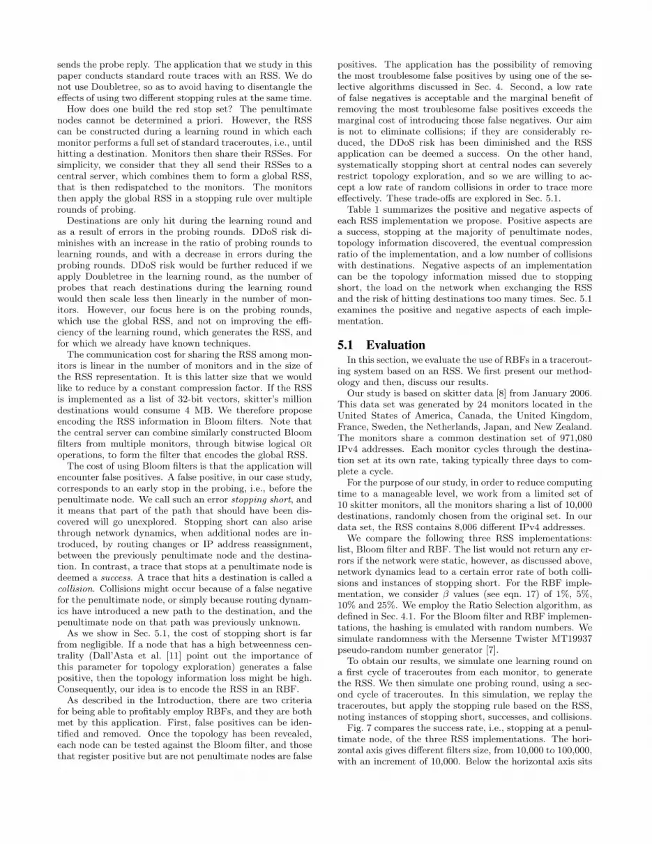
Fig. 7 compares the success rate, i.e., stopping at a penul-timate node, of the three RSS implementations. The hori-zontal axis gives different filters size, from 10,000 to 100,000,with an increment of 10,000. Below the horizontal axis sits

Implementation Positive Negative

Success Topo. discovery Compression No Collision Topo. missed Load CollisionList X X X XBloom filter X X XRBF X X X X

Table 1: Positive and negative aspects of each RSS implementation

Figure 7: Success rate

another axis that indicates the compression ratio of the fil-ter, compared to the list implementation of the RSS. Thevertical axis gives the success rate. A value of 0 would meanthat using a particular implementation precludes stoppingat the penultimate node. On the other hand, a value of 1means that the implementation succeeds in stopping eachtime at the penultimate node.

Looking first at the list implementation (the horizontalline), we see that the list implementation success rate is not1 but, rather, 0.7812. As explained in Sec. 5.1, this can beexplained by the network dynamics such as routing changesand dynamic IP address allocation.

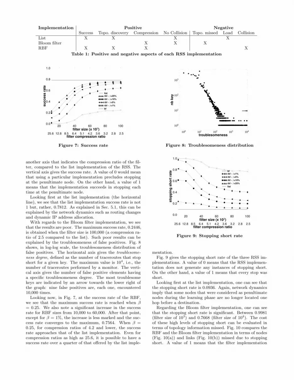
With regards to the Bloom filter implementation, we seethat the results are poor. The maximum success rate, 0.2446,is obtained when the filter size is 100,000 (a compression ra-tio of 2.5 compared to the list). Such poor results can beexplained by the troublesomeness of false positives. Fig. 8shows, in log-log scale, the troublesomeness distribution offalse positives. The horizontal axis gives the troublesome-ness degree, defined as the number of traceroutes that stopshort for a given key. The maximum value is 104, i.e., thenumber of traceroutes performed by a monitor. The verti-cal axis gives the number of false positive elements havinga specific troublesomeness degree. The most troublesomekeys are indicated by an arrow towards the lower right ofthe graph: nine false positives are, each one, encountered10,000 times.

Looking now, in Fig. 7, at the success rate of the RBF,we see that the maximum success rate is reached when β

= 0.25. We also note a significant increase in the successrate for RBF sizes from 10,000 to 60,000. After that point,except for β = 1%, the increase is less marked and the suc-cess rate converges to the maximum, 0.7564. When β =0.25, for compression ratios of 4.2 and lower, the successrate approaches that of the list implementation. Even forcompression ratios as high as 25.6, it is possible to have asuccess rate over a quarter of that offered by the list imple-

Figure 8: Troublesomeness distribution

Figure 9: Stopping short rate

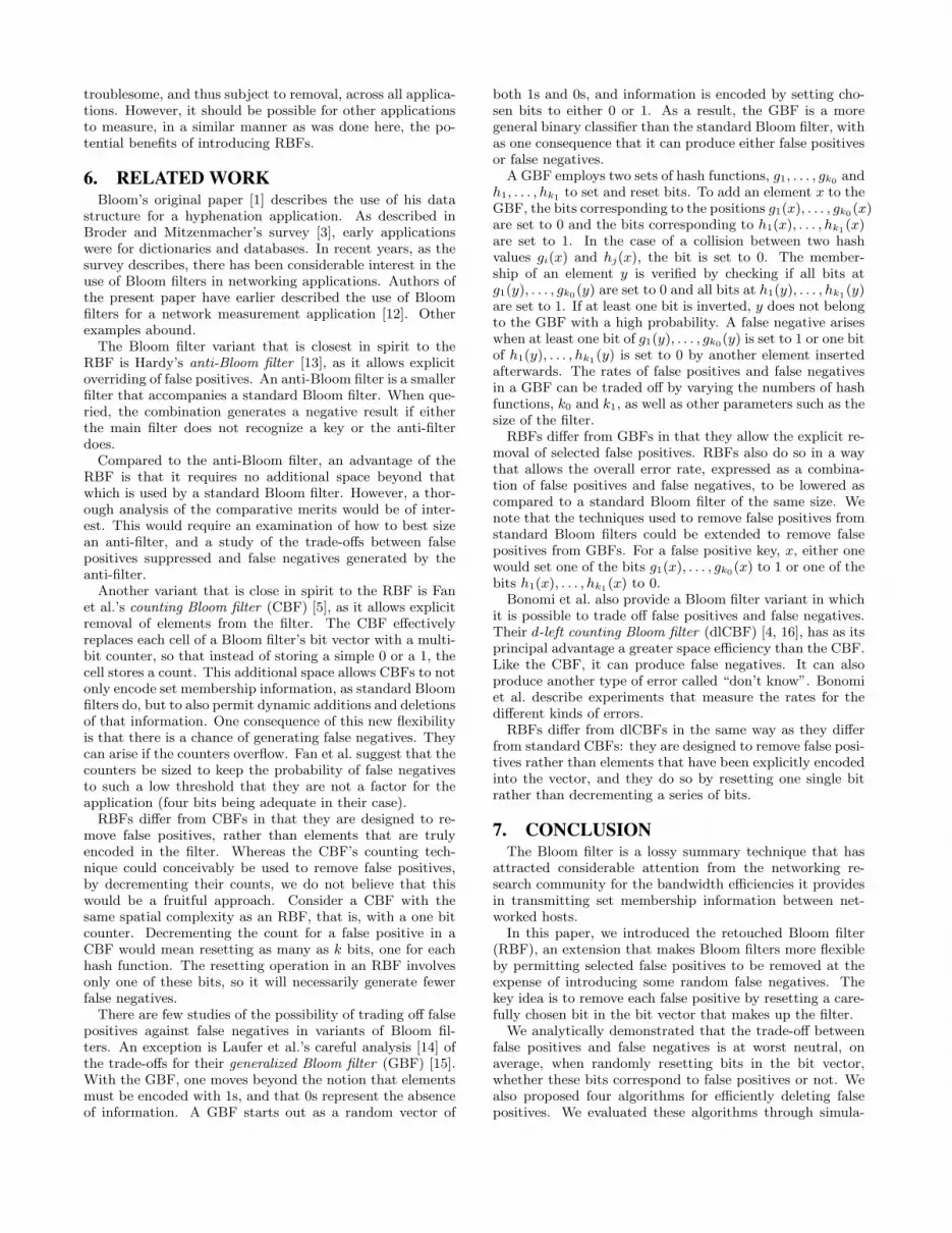
mentation.Fig. 9 gives the stopping short rate of the three RSS im-

plementations. A value of 0 means that the RSS implemen-tation does not generate any instances of stopping short.On the other hand, a value of 1 means that every stop wasshort.

Looking first at the list implementation, one can see thatthe stopping short rate is 0.0936. Again, network dynamicsimply that some nodes that were considered as penultimatenodes during the learning phase are no longer located onehop before a destination.

Regarding the Bloom filter implementation, one can seethat the stopping short rate is significant. Between 0.9981(filter size of 103) and 0.7668 (filter size of 104). The costof these high levels of stopping short can be evaluated interms of topology information missed. Fig. 10 compares theRBF and the Bloom filter implementation in terms of nodes(Fig. 10(a)) and links (Fig. 10(b)) missed due to stoppingshort. A value of 1 means that the filter implementation

(a) nodes

(b) links

Figure 10: Topology information missed

missed all nodes and links when compared to the list im-plementation. On the other hand, a value of 0 mean thatthere is no loss, and all nodes and links discovered by thelist implementation are discovered by the filter implementa-tion. One can see that the loss, when using a Bloom filter,is above 80% for filter sizes below 70,000.

Implementing the RSS as an RBF allows one to decreasethe stopping short rate. When removing 25% of the mosttroublesome false positives, one is able to reduce the stop-ping short between 76.17% (filter size of 103) and 84,35%(filter size of 104). Fig. 9 shows the advantage of using anRBF instead of a Bloom filter. Fig. 10 shows this advantagein terms of topology information. We miss a much smallerquantity of nodes and links with RBFs than Bloom filtersand we are able to nearly reach the same level of coverageas with the list implementation.

Fig. 11 shows the cost in terms of collisions. Collisionswill arise under Bloom filter and list implementations onlydue to network dynamics. Collisions can be reduced underall RSS implementations due to a high rate of stopping short(though this is, of course, not desired). The effect of stop-ping short is most pronounced for RBFs when β is low, asshown by the curve β = 0.01. One startling revelation ofthis figure is that even for fairly high values of β, such asβ = 0.10, the effect of stopping short keeps the RBF collisioncost lower than the collision cost for the list implementation,over a wide range of compression ratios. Even at β = 0.25,

Figure 11: Collision cost

Figure 12: Metrics for an RBF with m=60,000

the RBF collision cost is only slightly higher.Fig. 12 compares the success, stopping short, and collision

rates for the RBF implementation with a fixed filter size of60,000 bits. We vary β from 0.01 to 1 with an incrementof 0.01. We see that the success rate increases with β untilreaching a peak at 0.642 (β = 0.24), after which it decreasesuntil the minimum success rate, 0.4575, is reached at β =1. As expected, the stopping short rate decreases with β,varying from 0.6842 (β = 0) to 0 (β = 1). On the other hand,the collision rate increases with β, varying from 0.0081 (β= 0) to 0.5387 (β = 1).

The shaded area in Fig. 12 delimits a range of β values forwhich success rates are highest, and collision rates are rel-atively low. This implementation gives a compression ratioof 4.2 compared to the list implementation. The range ofβ values (between 0.1 and 0.3) gives a success rate between0.7015 and 0.7218 while the list provides a success rate of0.7812. The collision rate is between 0.1073 and 0.1987,meaning that in less than 20% of the cases a probe will hita destination. On the other hand, a probe hits a destinationin 12.51% of the cases with the list implementation. Finally,the stopping short rate is between 0.2355 and 0.1168 whilethe list implementation gives a stopping short rate of 0.0936.

In closing, we emphasize that the construction of B andthe choice of β in this case study are application specific. Wedo not provide guidelines for a universal means of determin-ing which false positives should be considered particularly

troublesome, and thus subject to removal, across all applica-tions. However, it should be possible for other applicationsto measure, in a similar manner as was done here, the po-tential benefits of introducing RBFs.

6. RELATED WORKBloom’s original paper [1] describes the use of his data

structure for a hyphenation application. As described inBroder and Mitzenmacher’s survey [3], early applicationswere for dictionaries and databases. In recent years, as thesurvey describes, there has been considerable interest in theuse of Bloom filters in networking applications. Authors ofthe present paper have earlier described the use of Bloomfilters for a network measurement application [12]. Otherexamples abound.

The Bloom filter variant that is closest in spirit to theRBF is Hardy’s anti-Bloom filter [13], as it allows explicitoverriding of false positives. An anti-Bloom filter is a smallerfilter that accompanies a standard Bloom filter. When que-ried, the combination generates a negative result if eitherthe main filter does not recognize a key or the anti-filterdoes.

Compared to the anti-Bloom filter, an advantage of theRBF is that it requires no additional space beyond thatwhich is used by a standard Bloom filter. However, a thor-ough analysis of the comparative merits would be of inter-est. This would require an examination of how to best sizean anti-filter, and a study of the trade-offs between falsepositives suppressed and false negatives generated by theanti-filter.

Another variant that is close in spirit to the RBF is Fanet al.’s counting Bloom filter (CBF) [5], as it allows explicitremoval of elements from the filter. The CBF effectivelyreplaces each cell of a Bloom filter’s bit vector with a multi-bit counter, so that instead of storing a simple 0 or a 1, thecell stores a count. This additional space allows CBFs to notonly encode set membership information, as standard Bloomfilters do, but to also permit dynamic additions and deletionsof that information. One consequence of this new flexibilityis that there is a chance of generating false negatives. Theycan arise if the counters overflow. Fan et al. suggest that thecounters be sized to keep the probability of false negativesto such a low threshold that they are not a factor for theapplication (four bits being adequate in their case).

RBFs differ from CBFs in that they are designed to re-move false positives, rather than elements that are trulyencoded in the filter. Whereas the CBF’s counting tech-nique could conceivably be used to remove false positives,by decrementing their counts, we do not believe that thiswould be a fruitful approach. Consider a CBF with thesame spatial complexity as an RBF, that is, with a one bitcounter. Decrementing the count for a false positive in aCBF would mean resetting as many as k bits, one for eachhash function. The resetting operation in an RBF involvesonly one of these bits, so it will necessarily generate fewerfalse negatives.

There are few studies of the possibility of trading off falsepositives against false negatives in variants of Bloom fil-ters. An exception is Laufer et al.’s careful analysis [14] ofthe trade-offs for their generalized Bloom filter (GBF) [15].With the GBF, one moves beyond the notion that elementsmust be encoded with 1s, and that 0s represent the absenceof information. A GBF starts out as a random vector of

both 1s and 0s, and information is encoded by setting cho-sen bits to either 0 or 1. As a result, the GBF is a moregeneral binary classifier than the standard Bloom filter, withas one consequence that it can produce either false positivesor false negatives.

A GBF employs two sets of hash functions, g1, . . . , gk0and

h1, . . . , hk1to set and reset bits. To add an element x to the

GBF, the bits corresponding to the positions g1(x), . . . , gk0(x)

are set to 0 and the bits corresponding to h1(x), . . . , hk1(x)

are set to 1. In the case of a collision between two hashvalues gi(x) and hj(x), the bit is set to 0. The member-ship of an element y is verified by checking if all bits atg1(y), . . . , gk0

(y) are set to 0 and all bits at h1(y), . . . , hk1(y)

are set to 1. If at least one bit is inverted, y does not belongto the GBF with a high probability. A false negative ariseswhen at least one bit of g1(y), . . . , gk0

(y) is set to 1 or one bitof h1(y), . . . , hk1

(y) is set to 0 by another element insertedafterwards. The rates of false positives and false negativesin a GBF can be traded off by varying the numbers of hashfunctions, k0 and k1, as well as other parameters such as thesize of the filter.

RBFs differ from GBFs in that they allow the explicit re-moval of selected false positives. RBFs also do so in a waythat allows the overall error rate, expressed as a combina-tion of false positives and false negatives, to be lowered ascompared to a standard Bloom filter of the same size. Wenote that the techniques used to remove false positives fromstandard Bloom filters could be extended to remove falsepositives from GBFs. For a false positive key, x, either onewould set one of the bits g1(x), . . . , gk0

(x) to 1 or one of thebits h1(x), . . . , hk1

(x) to 0.Bonomi et al. also provide a Bloom filter variant in which

it is possible to trade off false positives and false negatives.Their d-left counting Bloom filter (dlCBF) [4, 16], has as itsprincipal advantage a greater space efficiency than the CBF.Like the CBF, it can produce false negatives. It can alsoproduce another type of error called “don’t know”. Bonomiet al. describe experiments that measure the rates for thedifferent kinds of errors.

RBFs differ from dlCBFs in the same way as they differfrom standard CBFs: they are designed to remove false posi-tives rather than elements that have been explicitly encodedinto the vector, and they do so by resetting one single bitrather than decrementing a series of bits.

7. CONCLUSIONThe Bloom filter is a lossy summary technique that has

attracted considerable attention from the networking re-search community for the bandwidth efficiencies it providesin transmitting set membership information between net-worked hosts.

In this paper, we introduced the retouched Bloom filter(RBF), an extension that makes Bloom filters more flexibleby permitting selected false positives to be removed at theexpense of introducing some random false negatives. Thekey idea is to remove each false positive by resetting a care-fully chosen bit in the bit vector that makes up the filter.

We analytically demonstrated that the trade-off betweenfalse positives and false negatives is at worst neutral, onaverage, when randomly resetting bits in the bit vector,whether these bits correspond to false positives or not. Wealso proposed four algorithms for efficiently deleting falsepositives. We evaluated these algorithms through simula-

tion and showed that RBFs created in this manner will in-crease the false negative rate by less than the amount bywhich the false positive rate is decreased.

In this paper, we described a network measurement appli-cation for which RBFs can profitably be used. In this casestudy, traceroute monitors, rather than stopping probing ata destination, terminate their measurement at the penulti-mate node. The monitors share information on the set ofpenultimate nodes, the red stop set (RSS). We comparedthree different implementations for representing the RSS in-formation: list, Bloom filter, and RBF. Using filters reducesthe bandwidth requirements, but the false positives can sig-nificantly impact the amount of topology information thatthe system gleans. We demonstrated that using an RBF,in which the most troublesome false positives are removed,will increase the coverage of a filter implementation. Whilethe rate of collisions with destinations will increase, it canstill be lower than for the list implementation.

In future work, we hope to demonstrate techniques to ap-ply the RBF concept earlier in the construction of the filter.At present, we allow the Bloom filter to be built, and thenremove the most troublesome false positives. It should bepossible to avoid recording some of these false positives inthe filter to begin with.

Acknowledgements

Mr. Donnet’s work was partially supported by a SATINgrant provided by the E-NEXT doctoral school, by an in-ternship at Caida, and by the European Commission-fundedOneLab project. Mark Crovella introduced us to Bloom fil-ters and encouraged our work. Rafael P. Laufer suggesteduseful references regarding Bloom filter variants. Otto Car-los M. B. Duarte helped us clarify the relationship of RBFsto such variants. We thank k claffy and her team at Caida

for allowing us to use the skitter data.

8. REFERENCES[1] B. H. Bloom, “Space/time trade-offs in hash coding

with allowable errors,” Communications of the ACM,vol. 13, no. 7, pp. 422–426, 1970.

[2] M. Mitzenmacher, “Compressed Bloom filters,”IEEE/ACM Trans. on Networking, vol. 10, no. 5,2002.

[3] A. Broder and M. Mitzenmacher, “Networkapplications of Bloom filters: A survey,” InternetMathematics, vol. 1, no. 4, 2002.

[4] F. Bonomi, M. Mitzenmacher, R. Panigraphy,S. Singh, and G. Varghese, “Beyond Bloom filters:From approximate membership checks to approximatestate machines,” in Proc. ACM SIGCOMM, Sept.2006.

[5] L. Fan, P. Cao, J. Almeida, and A. Z. Broder,“Summary cache: a scalable wide-area Web cachesharing protocol,” IEEE/ACM Trans. on Networking,vol. 8, no. 3, pp. 281–293, 2000.

[6] B. Donnet, B. Baynat, and T. Friedman, “RetouchedBloom filters: Allowing networked applications totrade off selected false positives against falsenegatives,” arXiv, cs.NI 0607038, Jul. 2006.

[7] M. Matsumoto and T. Nishimura, “Mersenne Twister:A 623-dimensionally equidistributed uniformpseudorandom number generator,” ACM Trans. onModeling and Computer Simulation, vol. 8, no. 1, pp.3–30, Jan. 1998.

[8] B. Huffaker, D. Plummer, D. Moore, and k. claffy,“Topology discovery by active probing,” in Proc.SAINT, Jan. 2002.

[9] Y. Shavitt and E. Shir, “DIMES: Let the internetmeasure itself,” ACM SIGCOMM ComputerCommunication Review, vol. 35, no. 5, 2005.

[10] B. Donnet, P. Raoult, T. Friedman, and M. Crovella,“Efficient algorithms for large-scale topologydiscovery,” in Proc. ACM SIGMETRICS, 2005.

[11] L. Dall’Asta, I. Alvarez-Hamelin, A. Barrat,A. Vasquez, and A. Vespignani, “A statisticalapproach to the traceroute-like exploration ofnetworks: Theory and simulations,” in Proc. CAANWorkshop, Aug. 2004.

[12] B. Donnet, T. Friedman, and M. Crovella, “Improvedalgorithms for network topology discovery,” in Proc.PAM Workshop, 2005.

[13] N. Hardy, “A little Bloom filter theory (and a bag offilter tricks),” 1999, seehttp://www.cap-lore.com/code/BloomTheory.html.

[14] R. P. Laufer, P. B. Velloso, and O. C. M. B. Duarte,“Generalized Bloom filters,” Electrical EngineeringProgram, COPPE/UFRJ, Tech. Rep., 2005.

[15] R. P. Laufer, P. B. Velloso, D. de O. Cunha, I. M.Moraes, M. D. D. Bicudo, and O. C. M. B. Duarte,“A new IP traceback system against distributeddenial-of-service attacks,” in Proc. 12th ICT, 2005.

[16] F. Bonomi, M. Mitzenmacher, R. Panigrahy, S. Singh,and G. Varghese, “An improved construction forcounting Bloom filters,” in Proc. ESA, Sept. 2006.

Documents

Retouched bloom filters