Embed Size (px)
Citation preview
This document is downloaded from DR‑NTU (https://dr.ntu.edu.sg)Nanyang Technological University, Singapore.
Resource provisioning under uncertainty in cloudcomputing
Sivadon Chaisiri
2013
Sivadon Chaisiri. (2013). Resource provisioning under uncertainty in cloud computing.Doctoral thesis, Nanyang Technological University, Singapore.
https://hdl.handle.net/10356/52945
https://doi.org/10.32657/10356/52945
Downloaded on 16 Feb 2022 03:30:32 SGT
RESOURCE PROVISIONING UNDER
UNCERTAINTY IN CLOUD COMPUTING
SIVADON CHAISIRI
SCHOOL OF COMPUTER ENGINEERING
2013
RESO
UR
CE P
RO
VISIO
NIN
G U
ND
ER U
NC
ERTA
INTY IN
CLO
UD
CO
MP
UTIN
G
SIVA
DO
N C
HA
ISIRI
20
13

Resource Provisioning Under Uncertainty in
Cloud Computing
Sivadon Chaisiri
School of Computer Engineering
A thesis submitted to the Nanyang Technological University
in fulfillment of the requirement for the degree of
Doctor of Philosophy
2013
SIVA
DO
N C
HA
ISIRI
Acknowledgements
First, I would like to express my extremely sincerest gratefulness to my supervisor, As-
soc. Prof. Bu Sung Lee, for his patience, invaluable advice and suggestions, and encourage-
ment for my research work and the writing up of this thesis.
I would also like to express my thankfulness and whole-hearted gratitude to Asst. Prof. Dusit
Niyato for his patience, invaluable advice, suggestions, and comments for my research work.
I would like to express my sincere appreciation to my friends and colleagues in Parallel and
Distributed Computing Centre (PDCC), especially Alan Tan Yu Shyang, Irene Ng-Goh Siew
Lai, Zhang Junwei, Jin Jiangming, Tang ShanJiang, Chonho Lee, Rakpong Kaewpuang,
Dinh Thai Hoang, and Changbing Chen, for their helpful discussions, kind assistance, and
supports.
I would like to thank the Institute of High Performance Computing (IHPC) and the High
Performance Computing Centre at the Nanyang Technological University for providing me
the data of historical resource usage used in the experiments in this thesis.
Last but not least, I am deeply grateful to my parents, wife, and sisters, for their everlasting
support and endless love. This thesis is dedicated to them.
Contents
Acknowledgements . . . . . . . . . . . . . . . . . . . . . . . . . . . . . . . . . . . ii
List of Figures . . . . . . . . . . . . . . . . . . . . . . . . . . . . . . . . . . . . . vii
List of Tables . . . . . . . . . . . . . . . . . . . . . . . . . . . . . . . . . . . . . . x
Abstract . . . . . . . . . . . . . . . . . . . . . . . . . . . . . . . . . . . . . . . . . xii
1 Introduction 1
1.1 Motivation . . . . . . . . . . . . . . . . . . . . . . . . . . . . . . . . . . . . 1
1.2 Objectives . . . . . . . . . . . . . . . . . . . . . . . . . . . . . . . . . . . . . 6
1.3 Major Contributions of The Thesis . . . . . . . . . . . . . . . . . . . . . . . 7
1.4 Organization of The Thesis . . . . . . . . . . . . . . . . . . . . . . . . . . . 8
2 Literature Review 11
2.1 Resource Provisioning Techniques Classification by Optimization Methods . 11
2.2 Resource Provisioning Techniques Classification by Provisioning Options . . 15
2.3 Resource Provisioning Techniques Classification by Optimization Objectives 18
2.4 Resource Provisioning Techniques Classification by Uncertain Parameters . 20
2.5 Resource Provisioning Techniques Classification by Other Characteristics . 21
2.6 Novelty of This Thesis . . . . . . . . . . . . . . . . . . . . . . . . . . . . . . 26
3 Resource Provisioning on Consumers’ Side 27
3.1 System Model of Cloud Computing Environment . . . . . . . . . . . . . . . 28
iii
Contents iv
3.2 Deterministic Resource Provisioning . . . . . . . . . . . . . . . . . . . . . . 31
3.3 Resource Provisioning for Two Provisioning Stages . . . . . . . . . . . . . . 32
3.3.1 System Model and Assumption for Two Provisioning Stages . . . . . 32
Provisioning Stages . . . . . . . . . . . . . . . . . . . . . . . . . . . . 32
Uncertain Parameters . . . . . . . . . . . . . . . . . . . . . . . . . . 33
Provisioning Costs . . . . . . . . . . . . . . . . . . . . . . . . . . . . 34
3.3.2 Stochastic Programming Model with Two-Stage Recourse . . . . . . 35
3.3.3 Proposed Optimal Virtual Machine Placement Algorithm . . . . . . 36
Algorithmic Complexity . . . . . . . . . . . . . . . . . . . . . . . . . 37
3.3.4 Resource Provisioning with Benders Decomposition . . . . . . . . . 38
3.3.5 Performance Evaluation . . . . . . . . . . . . . . . . . . . . . . . . . 42
3.4 Resource Provisioning with Robust Optimization . . . . . . . . . . . . . . . 51
3.4.1 Overview of Resource Provisioning with Robust Optimization . . . . 51
3.4.2 General Form of Robust Optimization Model . . . . . . . . . . . . . 51
3.4.3 Solution and Model Robustness . . . . . . . . . . . . . . . . . . . . . 53
3.4.4 Robust Cloud Resource Provisioning Algorithm . . . . . . . . . . . . 54
3.4.5 Performance Evaluation . . . . . . . . . . . . . . . . . . . . . . . . . 55
3.5 Resource Provisioning for Multiple Provisioning Stages . . . . . . . . . . . . 62
3.5.1 System Model and Assumption for Multiple Provisioning Stages . . 63
Provisioning Stages . . . . . . . . . . . . . . . . . . . . . . . . . . . . 63
Reservation Contracts . . . . . . . . . . . . . . . . . . . . . . . . . . 64
Uncertain Parameters . . . . . . . . . . . . . . . . . . . . . . . . . . 65
3.5.2 Stochastic Programming Model with Multi-stage Recourse . . . . . . 66
3.5.3 Deterministic Equivalent of Stochastic Programming Model with Mul-tiple Stage Recourse . . . . . . . . . . . . . . . . . . . . . . . . . . . 68
3.5.4 Resource Provisioning with Sample-Average Approximation . . . . . 70
Sample-Average Approximation-based Optimization Model . . . . . 70
NTU - School of Computer Engineering
Contents v
Sampling Techniques . . . . . . . . . . . . . . . . . . . . . . . . . . . 75
3.5.5 Numerical Study . . . . . . . . . . . . . . . . . . . . . . . . . . . . . 76
3.6 Conclusion . . . . . . . . . . . . . . . . . . . . . . . . . . . . . . . . . . . . 77
4 Case Study: Server Provisioning in Amazon Elastic Compute Cloud 79
4.1 Overview of Server Provisioning in Amazon Elastic Compute Cloud . . . . 80
4.2 System Model and Assumption of Amazon EC2 . . . . . . . . . . . . . . . . 82
4.3 Long-term and Short-term Provisioning Algorithms . . . . . . . . . . . . . . 87
4.3.1 Long-term Provisioning Algorithm . . . . . . . . . . . . . . . . . . . 88
4.3.2 Short-term Provisioning Algorithm . . . . . . . . . . . . . . . . . . . 90
4.4 Performance Evaluation . . . . . . . . . . . . . . . . . . . . . . . . . . . . . 93
4.4.1 Evaluation of Long-term Provisioning Algorithm . . . . . . . . . . . 93
4.4.2 Evaluation of Short-term Provisioning Algorithm . . . . . . . . . . . 96
4.5 Conclusion . . . . . . . . . . . . . . . . . . . . . . . . . . . . . . . . . . . . 102
5 Resource Provisioning on Providers’ Side 103
5.1 Joint Power Optimization and Cloud Resource Management for Datacenters 104
5.1.1 Introduction to Joint Optimization Model for Cloud Provider . . . . 104
5.1.2 Related Work . . . . . . . . . . . . . . . . . . . . . . . . . . . . . . . 106
5.1.3 System Model and Assumption . . . . . . . . . . . . . . . . . . . . . 107
Major Entities . . . . . . . . . . . . . . . . . . . . . . . . . . . . . . 108
Decision Stages and Global Solution . . . . . . . . . . . . . . . . . . 110
Uncertain Parameters . . . . . . . . . . . . . . . . . . . . . . . . . . 112
5.1.4 Proposed Optimization Model . . . . . . . . . . . . . . . . . . . . . . 114
Stochastic Programming Model . . . . . . . . . . . . . . . . . . . . . 114
Scenario Tree Reduction and Construction . . . . . . . . . . . . . . 118
5.1.5 Performance Evaluation . . . . . . . . . . . . . . . . . . . . . . . . . 124
NTU - School of Computer Engineering
Contents vi
5.2 Profit Maximization Model for Cloud Retailer . . . . . . . . . . . . . . . . . 133
5.2.1 System Model and Assumption . . . . . . . . . . . . . . . . . . . . . 135
5.2.2 Profit Maximization Formulation . . . . . . . . . . . . . . . . . . . . 137
5.2.3 Numerical Studies . . . . . . . . . . . . . . . . . . . . . . . . . . . . 138
5.3 Conclusion . . . . . . . . . . . . . . . . . . . . . . . . . . . . . . . . . . . . 141
6 Summary and Future Works 143
6.1 Conclusions . . . . . . . . . . . . . . . . . . . . . . . . . . . . . . . . . . . . 143
6.2 Future Works . . . . . . . . . . . . . . . . . . . . . . . . . . . . . . . . . . . 145
6.2.1 Extension of the Current Work . . . . . . . . . . . . . . . . . . . . . 146
6.2.2 Cost-benefit analysis of resource provisioning . . . . . . . . . . . . . 147
6.2.3 Optimal Capacity Planning Algorithm . . . . . . . . . . . . . . . . . 149
6.2.4 Study of Interactions among Cloud Stakeholders . . . . . . . . . . . 150
Bibliography 151
A Nomenclature 164
A.1 Nomenclature used in Chapter 3 and Chapter 4 . . . . . . . . . . . . . . . . 164
A.2 Nomenclature used in Chapter 5 . . . . . . . . . . . . . . . . . . . . . . . . 167
B Other Resource Provisioning Optimization Models 170
B.1 Fixed Reservation Provisioning Model . . . . . . . . . . . . . . . . . . . . . 170
B.2 Adhoc On-demand Provisioning Model . . . . . . . . . . . . . . . . . . . . . 171
B.3 Expected-value of Uncertainty Provisioning Model . . . . . . . . . . . . . . 172
B.4 Maximum Reservation Provisioning . . . . . . . . . . . . . . . . . . . . . . . 172
C Historical Data 174
D Author’s Publications 176
NTU - School of Computer Engineering
List of Figures
1.1 Architectural layers of cloud computing services. . . . . . . . . . . . . . . . 2
1.2 Resource provisioning outcome (a) best provisioning, (b) underprovisioning,and (c) overprovisioning. . . . . . . . . . . . . . . . . . . . . . . . . . . . . . 4
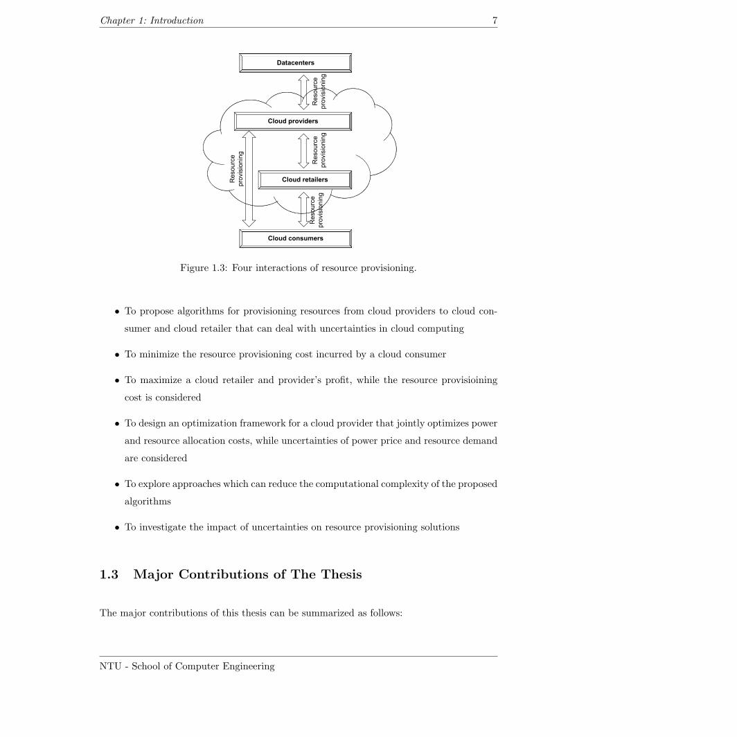
1.3 Four interactions of resource provisioning. . . . . . . . . . . . . . . . . . . . 7
3.1 System model of cloud computing environment. . . . . . . . . . . . . . . . . 28
3.2 Transition of provisioning phases. . . . . . . . . . . . . . . . . . . . . . . . . 30
3.3 Relationship between provisioning phases and stages for two provisioningstages. . . . . . . . . . . . . . . . . . . . . . . . . . . . . . . . . . . . . . . . 33
3.4 Flowchart of Benders decomposition algorithm. . . . . . . . . . . . . . . . . 40
3.5 Optimal solution of resource provisioning. . . . . . . . . . . . . . . . . . . . 45
3.6 Comparison between total costs of resource provision with and without reser-vation. . . . . . . . . . . . . . . . . . . . . . . . . . . . . . . . . . . . . . . . 46
3.7 Costs in different provisioning phases. . . . . . . . . . . . . . . . . . . . . . 47
3.8 Convergence of the upper and lower bounds by applying the Benders decom-position algorithm. . . . . . . . . . . . . . . . . . . . . . . . . . . . . . . . . 50
3.9 Tradeoff between solution- and model-robustness. . . . . . . . . . . . . . . . 56
3.10 Tradeoff between overprovisioning and underprovisioning. . . . . . . . . . . 57
3.11 Standard deviation of total provisioning cost. . . . . . . . . . . . . . . . . . 58
3.12 Expected reservation cost. . . . . . . . . . . . . . . . . . . . . . . . . . . . . 59
3.13 Expected oversubscribed cost. . . . . . . . . . . . . . . . . . . . . . . . . . . 59
vii
List of Figures viii
3.14 Expected on-demand cost. . . . . . . . . . . . . . . . . . . . . . . . . . . . . 60
3.15 Expected total provisioning cost. . . . . . . . . . . . . . . . . . . . . . . . . 60
3.16 Difference between two- and multi-stage recourse models. . . . . . . . . . . 62
3.17 Relationship between provisioning phases and provisioning stages. . . . . . 64
3.18 Example of advance reservations with 3-month (K1) and 6-month (K2) con-tracts. . . . . . . . . . . . . . . . . . . . . . . . . . . . . . . . . . . . . . . . 65
4.1 Discrete probability distribution of spot prices of Linux/UNIX t1.micro inNorthern Virginia region (recorded in October 2010). . . . . . . . . . . . . . 81
4.2 Relationship between long-term plan (L) and short-term plan (S). . . . . . 84
4.3 Probability distribution in October 2010 of spot prices of Linux/UNIX c1.xlargein Northern Virginia region. . . . . . . . . . . . . . . . . . . . . . . . . . . . 96
4.4 Probability distribution in October 2010 of spot prices of Linux/UNIXm1.xlargein Northern Virginia region. . . . . . . . . . . . . . . . . . . . . . . . . . . . 97
4.5 Probability distribution of demand. . . . . . . . . . . . . . . . . . . . . . . . 97
4.6 Probability distribution of integrated multivariate scenarios. . . . . . . . . . 97
5.1 System model of a cloud provider. . . . . . . . . . . . . . . . . . . . . . . . 108
5.2 Example of VM classes for cloud services. . . . . . . . . . . . . . . . . . . . 108
5.3 Example of decision stages for the daily forward contract basis. . . . . . . . 111
5.4 Example of decision stages for the daily forward contract basis. . . . . . . . 118
5.5 Number of VMs hosted in datacenters under different scenarios. . . . . . . . 125
5.6 Average number of VMs hosted in datacenters under different decision stages. 126
5.7 Average number of VMs hosted in each datacenter given different applicationdata size. . . . . . . . . . . . . . . . . . . . . . . . . . . . . . . . . . . . . . 127
5.8 Average number of VMs hosted in each datacenter for different scenarios. . 127
5.9 Probability distribution of leaf nodes in original tree. . . . . . . . . . . . . . 130
5.10 Probability distribution of leaf nodes in reduced tree with ε = 0.005. . . . . 130
5.11 Probability distribution of leaf nodes in reduced tree with ε = 0.05. . . . . . 131
NTU - School of Computer Engineering
List of Figures ix
5.12 Cost comparison between different optimization models obtained from thesimulation. . . . . . . . . . . . . . . . . . . . . . . . . . . . . . . . . . . . . 132
5.13 System model of the cloud provider’s computational service. . . . . . . . . . 134
5.14 Impact of on-demand price on the number of base units. . . . . . . . . . . . 139
5.15 Impact of on-demand price on the average profit. . . . . . . . . . . . . . . . 139
5.16 Impact of on-demand price on the number of base units. . . . . . . . . . . . 140
C.1 Histogram of test data. . . . . . . . . . . . . . . . . . . . . . . . . . . . . . . 175
C.2 Probability distribution of test data. . . . . . . . . . . . . . . . . . . . . . . 175
NTU - School of Computer Engineering
List of Tables
2.1 Comparison of resource provisioning techniques . . . . . . . . . . . . . . . . 23
3.1 Expected annual resource demand for a single VM of each VM class. . . . . 42
3.2 Resource prices of cloud providers for evaluating the OVMP algorithm. . . 43
3.3 Number of reserved VMs and costs given different probability distributions. 48
3.4 Number of reserved VMs and average costs given different resource provi-sioning algorithms. . . . . . . . . . . . . . . . . . . . . . . . . . . . . . . . . 49
3.5 Pricing of cloud providers for evaluating the RCRP algorithm. . . . . . . . 55
3.6 Comparison among different resource provisioning algorithms. . . . . . . . . 61
3.7 Estimation of lower and upper bounds of provisioning costs in the twelveprovisioning stage problem. . . . . . . . . . . . . . . . . . . . . . . . . . . . 77
4.1 Detail about instance types in Northern Virginia region used in the numericalstudies. . . . . . . . . . . . . . . . . . . . . . . . . . . . . . . . . . . . . . . 93
4.2 Number of reserved instances and costs given different variance and overpro-visioning weights. . . . . . . . . . . . . . . . . . . . . . . . . . . . . . . . . . 94
4.3 Costs incurred by solving deterministic and on-demand optimization models. 95
4.4 Costs incurred by solving stochastic programming and robust optimizationmodels. . . . . . . . . . . . . . . . . . . . . . . . . . . . . . . . . . . . . . . 95
4.5 Expected total costs and numbers of bid server-hours given different spotprice distributions. . . . . . . . . . . . . . . . . . . . . . . . . . . . . . . . . 99
4.6 Estimation of lower and upper bounds and bid server-hours of spot instancesobtained from Monte Carlo sampling. . . . . . . . . . . . . . . . . . . . . . 99
x
List of Tables xi
4.7 Estimation of lower and upper bounds and bid server-hours of spot instancesobtained from Latin Hypercube sampling. . . . . . . . . . . . . . . . . . . . 100
5.1 Demand, spot prices, and probability of each scenario. . . . . . . . . . . . . 119
5.2 Cost comparison among different optimization models. . . . . . . . . . . . . 128
5.3 Applying scenario reduction with different tolerance. . . . . . . . . . . . . . 129
5.4 Performance evaluation of scenario reduction with different tolerance. . . . 132
5.5 Compute instances offered by Windows Azure. . . . . . . . . . . . . . . . . 135
5.6 Cost comparison among different numbers of base units. . . . . . . . . . . . 141
A.1 List of sets and indices used in Chapter 3 and Chapter 4 . . . . . . . . . . . 164
A.2 List of constants and parameters used in Chapter 3 and Chapter 4 . . . . . 165
A.3 List of decision variables used in Chapter 3 and Chapter 4 . . . . . . . . . . 166
A.4 List of sets and indices used in Chapter 5 . . . . . . . . . . . . . . . . . . . 167
A.5 List of constants and parameters used in Chapter 5 . . . . . . . . . . . . . . 168
A.6 List of decision variables used in Chapter 5 . . . . . . . . . . . . . . . . . . 169
NTU - School of Computer Engineering
Abstract
In this thesis, we mainly focus on the resource provisioning in cloud computing. Resources
can be provisioned from cloud providers to cloud consumers through two options, i.e.,
reservation and on-demand. The reservation option is cheaper and able to guarantee the
availability and prices of resources. However, a cloud consumer has to purchase the reserva-
tion option with prior commitment for specific resources. Due to uncertainties, the common
problems encountered in resource provisioning with the two options are overprovisioning and
underprovisioning. In this thesis, we consider different uncertainties in the resource provi-
sioning problems, i.e., uncertainties of resource demand, resource price, power price, and
availability of resources. For our major contributions, we propose the resource provision-
ing algorithms and framework to deal with the uncertainties for three cloud stakeholders,
namely cloud consumer, cloud provider, and cloud retailer. The contributions are as follows:
First, we propose novel algorithms for a cloud consumer to provision resources from cloud
providers. The algorithms can minimize the expected resource provisioning cost incurred
by overprovisioning and underprovisioning of resources, while the uncertainties are taken
into account. We formulate optimization models to obtain the optimal solution for the
algorithms. The models are derived by stochastic programming with two- and multi-stage
recourse so that the optimal solution from the algorithms can be applied for long-term
resource provisioning plans. We also apply the robust optimization to handle the impact
of the uncertainties on the optimal solution. The performance evaluation shows that the
proposed algorithms have the lowest resource provisioning cost when they are compared with
other well-known algorithms. To reduce the computational complexity of the algorithms,
we also apply Benders decomposition and sample-average approximation methods.
Second, we propose a novel resource provisioning framework for a cloud provider. The
framework considers the cloud provider owning datacenters where the smart grid technol-
ogy is available. Inside the framework, we derive a stochastic programming model with
Abstract xiii
multi-stage recourse that jointly optimizes the power and resource allocation costs, while
uncertainties of power price and compute demand are addressed. In the framework, we
provide an approach to construct a scenario tree which represents uncertainties. Then, we
apply a scenario reduction technique to reduce the size of scenario trees and the computa-
tional time for solving the model. The performance evaluation based on both theoretical and
real trace data reveals the importance of joint power management and resource allocation
optimization.
Finally, we investigate a cloud computing market where a cloud retailer sells value-added
services on top of other cloud providers’ resources. We propose a novel resource provision-
ing algorithm based on stochastic programming with two-stage recourse for provisioning
resources under uncertainty from cloud providers to the cloud retailer such that the re-
tailer’s profit can be maximized. In the experiment, we compare the proposed algorithm
with others. The results show that the proposed algorithm gives the highest profit to the
cloud retailer when it is compared with other well-known algorithms.
Thus, in this thesis, we have addressed the resource provisioning problems from different
cloud stakeholders, i.e., consumer, provider, and reseller. We have proposed new algorithms
and framework to optimize the cloud stakeholders’ profit taking the uncertainties into ac-
count. The proposed algorithms and framework will be useful for cloud providers who
want to optimally operate the cloud computing business and cloud consumers who want to
optimally utilize resources located in cloud computing.
NTU - School of Computer Engineering
Chapter 1
Introduction
1.1 Motivation
Cloud computing has emerged as an information technology (IT) solution in which the re-
sources can be virtualized as services operated and provided by a third-party, and utilized
on demand [1–8]. Resources in cloud computing can be CPU, storage, and network band-
width. Gartner forecasted that cloud computing would be a disruptive technology changing
the way of resource provisioning [9]. Regarding its definition, cloud computing could be re-
ferred to as an available and scalable utility grid whose resources can be accessed as a public
utility [2, 5, 10]. This kind of computational model was firstly coined by John McCarthy
in 1955, i.e., “computing may someday be organized as a public utility just as the telephone
system is a public utility” [10]. McCarthy’s outlook has become more concrete due to the
technology advancement including high speed Internet, rapid software development tools,
advance virtualization technology, faster multicore processors, larger storage, as well as the
emergence of cloud computing model.
In cloud computing, customers can reduce the total cost of ownership (or TCO) of IT as-
sets [8,11]. TCO related to on-premise IT assets (i.e., private cloud [12]) includes both direct
and indirect costs, e.g., purchasing, licensing, development and deployment, maintenance,
power and cooling costs. The indirect cost spent for power and cooling could be significant
and exceed the cost spent for IT equipment [13]. Cloud computing is able to reduce the
TCO by outsourcing some IT operations to cloud providers.
1
Chapter 1: Introduction 2
Software-as-a-Service (SaaS)
Platform-as-a-Service (PaaS)Platform as a Service (PaaS)
Infrastructure-as-a-Service (IaaS)
Hardware-as-a-Service (HaaS)
Figure 1.1: Architectural layers of cloud computing services.
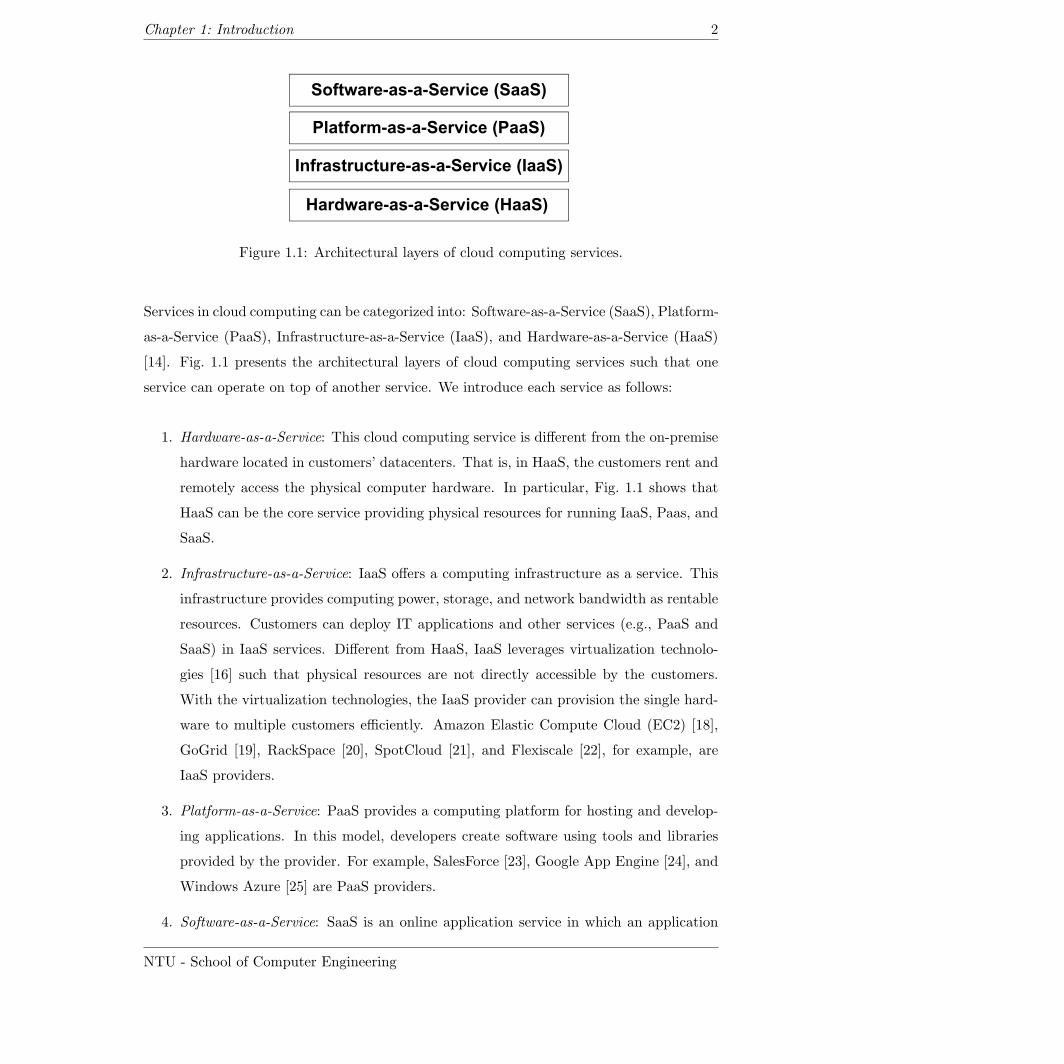
Services in cloud computing can be categorized into: Software-as-a-Service (SaaS), Platform-
as-a-Service (PaaS), Infrastructure-as-a-Service (IaaS), and Hardware-as-a-Service (HaaS)
[14]. Fig. 1.1 presents the architectural layers of cloud computing services such that one
service can operate on top of another service. We introduce each service as follows:
1. Hardware-as-a-Service: This cloud computing service is different from the on-premise
hardware located in customers’ datacenters. That is, in HaaS, the customers rent and
remotely access the physical computer hardware. In particular, Fig. 1.1 shows that
HaaS can be the core service providing physical resources for running IaaS, Paas, and
SaaS.
2. Infrastructure-as-a-Service: IaaS offers a computing infrastructure as a service. This
infrastructure provides computing power, storage, and network bandwidth as rentable
resources. Customers can deploy IT applications and other services (e.g., PaaS and
SaaS) in IaaS services. Different from HaaS, IaaS leverages virtualization technolo-
gies [16] such that physical resources are not directly accessible by the customers.
With the virtualization technologies, the IaaS provider can provision the single hard-
ware to multiple customers efficiently. Amazon Elastic Compute Cloud (EC2) [18],
GoGrid [19], RackSpace [20], SpotCloud [21], and Flexiscale [22], for example, are
IaaS providers.
3. Platform-as-a-Service: PaaS provides a computing platform for hosting and develop-
ing applications. In this model, developers create software using tools and libraries
provided by the provider. For example, SalesForce [23], Google App Engine [24], and
Windows Azure [25] are PaaS providers.
4. Software-as-a-Service: SaaS is an online application service in which an application
NTU - School of Computer Engineering
Chapter 1: Introduction 3
with its data is centrally hosted in cloud computing server, generally in either PaaS or
IaaS. In particular, a single instance of application simultaneously supports multiple
users. Various SaaS-based applications are available in the market, e.g., collaboration,
content management, enterprise resource planning, and customer relationship man-
agement. SalesForce [23], Google App [26], and Zoho [27], for example, are providers
offering SaaS applications.
In a cloud computing environment, there are two major entities, namely cloud consumer and
cloud provider. Cloud consumers have the compute demand to run their IT applications,
while cloud providers supply computing resources to meet cloud consumers’ demand. This
cloud computing environment is similar to an open marketplace where the cloud providers
sell (i.e., rent out) their resources to the cloud consumers. The cloud consumers have the
opportunity to choose resources from the different cloud providers to meet their needs.
Utilizing computing resources by the consumers is charged on a pay-per-use basis. That is,
resources can be provisioned at the moment when the resources are needed by the cloud
consumers. When the provisioned resources are no longer utilized, the resources can be
released to the providers. With this pay-per-use basis, the consumers pay according to the
amount of resource usage. As a result, the cloud consumers could flexibly resize the amount
of provisioned resource to meet their IT systems and efficiently control their budgets [8].
Cloud computing is an efficient resource provisioning solution. As reported by a Berkeley
research lab, the elasticity of cloud computing is an economic benefit for tackling the risks
of resource provisioning problems, i.e., underprovisioning and overprovisioning [8]. The
overprovisioning problem refers to as the situation when the purchased resources are not
fully utilized. This problem results in higher TCO. As presented by W. Vogels, (CTO of
Amazon.com), resource utilization of most computer systems is merely 15 - 20 percent [16].
This low utilization implies that the investment on the resources is wasted. In contrast, for
the underprovisioning problem, purchased resources are not sufficient to meet the actual
demand, which can result in performance degradation and service-level-agreement (SLA)
violation.
Cloud providers such as Amazon [18], GoGrid [19], and Microsoft [25], provide on-demand
and reservation options for provisioning resources. With the on-demand option, resources
can be dynamically provisioned by a cloud consumer anytime without a commitment (i.e.,
pay-per-use basis). In contrast, with the reservation option, the resources need to be sub-
NTU - School of Computer Engineering
Chapter 1: Introduction 4
scribed with a contract. The contract will guarantee the availability and prices of resources
over a certain duration (e.g., 1 month, 1 year, and 3 years). In particular, the cost of
resources purchased using the reservation option is considerably cheaper than that of the
on-demand option. The cloud consumers could apply the reservation option for the long-
term utilization and the on-demand option for the short-term utilization.
Current Future
Reserve N VMs Utilize N VMsNo on-demand
provisioning
Actual demand is N VMs
provisioning
(a) Best provisioning
Current
Utilize N VMsProvision 2N VMsReserve N VMs
Future
Actual demand is 3N VMs
Utilize N VMson-demand
(b) Underprovisioning
Current
Utilize N/2 VMsReserve N VMs No
Future
Actual demand is N/2 VMs
Utilize N/2 VMs
(c) Overprovisioning
on-demand
provisioning
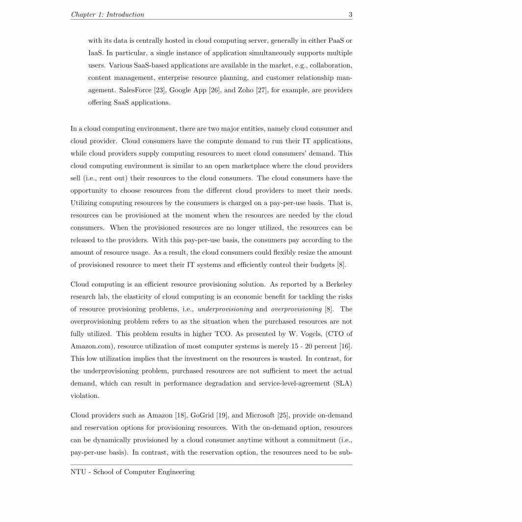
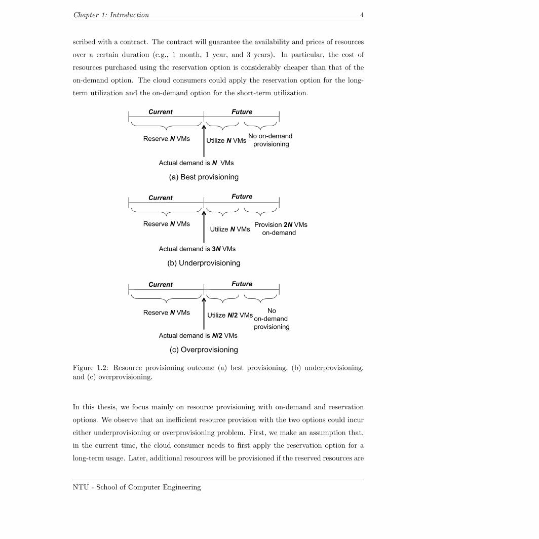
Figure 1.2: Resource provisioning outcome (a) best provisioning, (b) underprovisioning,and (c) overprovisioning.
In this thesis, we focus mainly on resource provisioning with on-demand and reservation
options. We observe that an inefficient resource provision with the two options could incur
either underprovisioning or overprovisioning problem. First, we make an assumption that,
in the current time, the cloud consumer needs to first apply the reservation option for a
long-term usage. Later, additional resources will be provisioned if the reserved resources are
NTU - School of Computer Engineering
Chapter 1: Introduction 5
not sufficient. Fig. 1.2 illustrates the three possible outcomes of the resource provisioning.
Suppose virtual machines (VMs) [17] (e.g., Unix servers) are the resources that a cloud
consumer wants to purchase from a cloud provider. The cloud consumer’s demand refers to
as the number of VMs needed to meet the cloud consumer’s IT applications. As depicted
in Fig. 1.2 (a), the best provisioning is to provision the number of VMs with the reservation
option in the current time (i.e., to reserve N VMs) such that the VMs meet to the actual
demand. Hence, the more expensive on-demand option will not be required. Since the
future demand is generally not known in advance, the best provisioning could not always
be achieved. Therefore, either underprovisioning or overprovisioning problem will happen.
Fig. 1.2 (b) depicts the underprovisioning problem, i.e., the cloud consumer reserves only
N VMs but 3N VMs will be required. Therefore, the cloud consumer needs to additionally
provision 2N VMs with the on-demand option. In contrast, as shown in Fig. 1.2 (c), the
overprovisioning problem is the situation when the cloud consumer purchases N VMs which
is more than the actual demand (i.e., only N/2 VMs will be needed). In other words, some
VMs (i.e., N/2 VMs) will not be ever utilized.
For cloud consumers, obtaining the best provisioning solution is not trivial since there are
uncertainties. The uncertainties in cloud computing could occur when demand, price, and
availability of resources are not known by a cloud consumer. For example, as presented
in Fig. 1.2 (b) and Fig. 1.2 (c), the demand uncertainty results in underprovisioning and
overprovisioning problems, respectively. In particular, the underprovisioning problem po-
tentially induces a much higher cost of the on-demand option. In addition, the price of the
on-demand option may fluctuate (i.e., price uncertainty). Last but not least, the availability
uncertainty also results in an underprovisioning problem since resources provisioned from
a cloud provider may not be available (e.g., power outage in the cloud provider’s datacen-
ter). Therefore, additional resources will be provisioned from other cloud providers with the
more expensive on-demand option. Allocating appropriate cloud providers for provisioning
resources under the uncertainties is also another challenge.
In this thesis, we propose the algorithms to obtain the optimal solution for provisioning
resources on the cloud consumer’s side. The optimal solution can be obtained by formulating
and solving the stochastic programming and robust optimization models [28,29]. The major
optimization objective of the models is to minimize the resource provisioning cost under
uncertainties by avoiding the underprovisioning and overprovisioning problems.
NTU - School of Computer Engineering
Chapter 1: Introduction 6
In this thesis, we also consider resource provisioning on the cloud provider’s side. First,
we consider the cloud provider owning datacenters connecting to smart grid. The smart
grid features the realtime pricing, i.e., electric power price can be changed dynamically
depending on the load and power generation conditions [30]. Therefore, the cloud provider
could encounter a risk of fluctuating spot prices of electricity. Such a fluctuating price is a
major uncertainty which directly affects the total cost incurred to the cloud provider. The
cloud provider can hedge against such the risk by signing forward contracts in electricity
futures markets [31]. In this thesis, we propose a stochastic programming model for the
forward contract portfolio optimization of the joint power and resource management. The
optimization model is formulated to minimize the expected cost under power price and
demand uncertainty. Specifically, the important activities considered in the optimization
model are server consolidation [16], carbon emission [32], and application data transfer [33].
Finally, we focus on a cloud computing market where a cloud retailer sells services to cloud
consumers. The cloud retailer is a cloud provider whose resources are provisioned from other
cloud providers. Then, to earn a profit, value-added services, e.g., SaaS and PaaS, can be
built on top of the provisioned resources. The cloud retailer can encounter overprovisioning
and underprovisioning problems as same as cloud consumers, since the retailer rents other
cloud providers’ provisioning options under uncertainty. To tackle the problems, we propose
a resource provisioning algorithm based on stochastic programming from the cloud retailer’s
perspective. The objective of the algorithm is to maximize the cloud retailer’s profit.
1.2 Objectives
For this research, we focus on resource provisioning for three entities in cloud computing,
namely cloud consumers, cloud retailers, and cloud providers. As shown in Fig. 1.3, the
cloud consumers can provision resources from cloud retailers and cloud providers. Similar
to the cloud consumers, the cloud retailers rent resources from other cloud providers. Then,
the cloud retailers can earn profits by integrating value-added services to the provisioned
resources and sell the services to cloud consumers. For the cloud providers, resources are
provisioned from their datacenters to the cloud consumers.
In this thesis, the main objectives can be summarized as follows:
NTU - School of Computer Engineering
Chapter 1: Introduction 7
source
visioning
Datacenters
Cloud providers
e ng
Res
prov
Cloud retailersResource
rovisioning
Resource
provisionin
Cloud retailersR
pr
Resource
rovisioning
Cloud consumers
p
Figure 1.3: Four interactions of resource provisioning.
• To propose algorithms for provisioning resources from cloud providers to cloud con-
sumer and cloud retailer that can deal with uncertainties in cloud computing
• To minimize the resource provisioning cost incurred by a cloud consumer
• To maximize a cloud retailer and provider’s profit, while the resource provisioining
cost is considered
• To design an optimization framework for a cloud provider that jointly optimizes power
and resource allocation costs, while uncertainties of power price and resource demand
are considered
• To explore approaches which can reduce the computational complexity of the proposed
algorithms
• To investigate the impact of uncertainties on resource provisioning solutions
1.3 Major Contributions of The Thesis
The major contributions of this thesis can be summarized as follows:
NTU - School of Computer Engineering
Chapter 1: Introduction 8
• Resource provisioning algorithms for a cloud consumer [34–37]: We propose the novel
resource provisioning algorithms for provisioning resources from IaaS-based cloud
providers to a cloud consumer. To obtain the optimal solution of resource provision-
ing (i.e., to minimize the provisioning cost), we formulate the stochastic programming
models with two- and multi-stage recourse [28] such that the solution can be applied
for long-term resource provisioning. The algorithms can deal with the overprovision-
ing and underprovisioning problems caused by uncertainties of price, demand, and
availability of resources. The algorithms give the lowest resource provisioning cost.
In addition, we improve the stochastic programming models using robust optimiza-
tion [29] such that the optimal solution will be less sensitive to the uncertainties.
To tackle the complexity of the proposed algorithms, we apply Benders decomposi-
tion [38] and sample-average approximation [39] methods to the algorithms. Finally,
as a case study, we evaluate the algorithms using real data of resource usage and prices
to provision resources from Amazon EC2 to a cloud consumer.
• Joint power optimization and resource management for a cloud provider [40–42]:
We design a cost management framework for cloud computing datacenters. In the
framework, we formulate the stochastic programming model primarily from the cloud
provider’s perspective to minimize the expected cost under power price and compute
demand uncertainties. The expected cost is composed of the virtual machine hosting,
electric power, and application data transfer costs. We also apply a scenario reduction
technique [43] to reduce the computational complexity of the proposed model.
• Resource provisioning algorithm for a cloud retailer [44]: We present a cloud com-
puting market where a cloud retailer profits by implementing and selling value-added
services built on top of other cloud providers’ resources. Then, we propose the re-
source provisioning algorithm for provisioning resources under demand uncertainty
from IaaS-based cloud providers to the cloud retailer such that the retailer’s profit
can be maximized. The optimal solution of the algorithm is obtained by formulating
and solving a stochastic programming model.
1.4 Organization of The Thesis
The rest of the thesis is organized as follows:
NTU - School of Computer Engineering
Chapter 1: Introduction 9
• Chapter 2: In this chapter, the literature survey of resource provisioning techniques
is presented. The resource provisioning techniques are categorized by optimization
methods, provisioning options, optimization objectives, uncertain parameters, service-
level-agreement orientation, energy-aware orientation, cloud provider/consumer ori-
entation, and application domains. The comparison among the resource provisioning
techniques is also provided.
• Chapter 3: In this chapter, we present the proposed resource provisioning algorithms
for a cloud consumer. First, the chapter presents the algorithm based on stochastic
programming with two-stage recourse for provisioning resources under two provision-
ing stages (i.e., current and future stages). That is, the algorithm can obtain the
resource provisioning solution for the current time epoch and also generate a set of
solutions for provisioning resources in the future time epoch. Next, the algorithm is
improved by robust optimization so that the solution of the algorithm could be less
sensitive to uncertainties.
The algorithm for two provisioning stages is improved by stochastic programming with
multi-stage recourse. Similarly, this improved algorithm can obtain the resource pro-
visioning solution for the current time epoch. In addition, the algorithm can generate
a set of resource provisioning solutions for multiple future stages. Sampling-average
approximation and Benders decomposition methods are also applied to the proposed
algorithms to address the computational complexity of the proposed algorithm.
• Chapter 4: In this chapter, we present a case study to apply the algorithms in
Chapter 3. The case study focuses on resource provisioning from Amazon EC2 to
accommodate a cloud consumer’s demand. In Amazon EC2, the cloud consumer
can provision resources with three options, namely on-demand, reservation, and spot
options. Each provisioning option has different price and yields different benefit to
the consumer. Especially, spot price (i.e., price of spot option) could be the cheapest.
However, the spot price fluctuates and could be sometime more expensive than the
prices of on-demand and reservation options due to supply and demand of available
resources in Amazon EC2. Although the reservation and on-demand options have
stable prices, their costs are mostly more expensive than that of the spot option.
The challenge is to find the solution in which the cloud consumer can optimally
purchase the provisioning options under the uncertainties of spot prices and demand.
To address this issue, two resource provisioning algorithms are proposed to minimize
NTU - School of Computer Engineering
Chapter 1: Introduction 10
the provisioning cost for long- and short-term planning.
• Chapter 5: In this chapter, we address resource provisioning for cloud providers.
First, we present the resource provisioning framework for a cloud provider in which
the power and resource management costs are mainly optimized. We assume that the
public utility for the cloud provider implements smart grid. One important feature of
the smart grid is the realtime pricing (i.e., power price can be changed dynamically de-
pending on the load and power generation conditions). Therefore, the cloud provider
could encounter risk of fluctuating spot prices of electric power. The cloud provider
can hedge against such a risk by signing forward contracts in electricity futures mar-
kets. In this framework, we formulate a multi-stage stochastic programming model
for the forward contract portfolio optimization of power supply and optimization of
resource management (i.e., virtual machine allocation). The optimization model is
formulated primarily from the cloud provider’s perspective to minimize the expected
cost under power price and compute demand uncertainty. Specifically, the important
activities are considered including carbon emission, server consolidation, and applica-
tion data transfer in the joint optimization framework. To reduce the computational
complexity of the proposed model, a scenario reduction technique is applied.
Next, we present the resource provisioning algorithm to maximize the profit for a cloud
retailer. We define the term “cloud retailer” as a cloud provider whose resources are
provisioned from other cloud providers. Then, the cloud retailer can integrate value-
added services (e.g., applications) to the resources and sell the services to cloud con-
sumers. We illustrate a case study of a cloud retailer whose resources are provisioned
from Windows Azure.
• Chapter 6: In this chapter, we provide a summary of the results presented in this
thesis. We outline a few research issues which can be pursued as an extension of this
research.
NTU - School of Computer Engineering
Chapter 2
Literature Review
In distributed systems (e.g., computational clusters, grid computing, and cloud comput-
ing), resource provisioning is the action to supply resources for users’ applications, e.g., to
process jobs and to store data. Resources could be computing power (i.e., CPU), storage,
and network bandwidth. In this chapter, the literature survey of resource provisioning tech-
niques is presented. The resource provisioning techniques are categorized by optimization
methods, provisioning options, optimization objectives, uncertain parameters, service-level-
agreement orientation, energy-aware orientation, cloud provider/consumer orientation, and
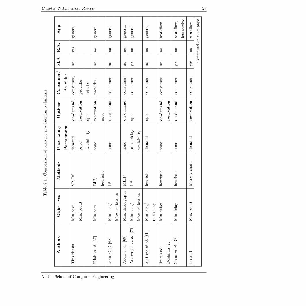
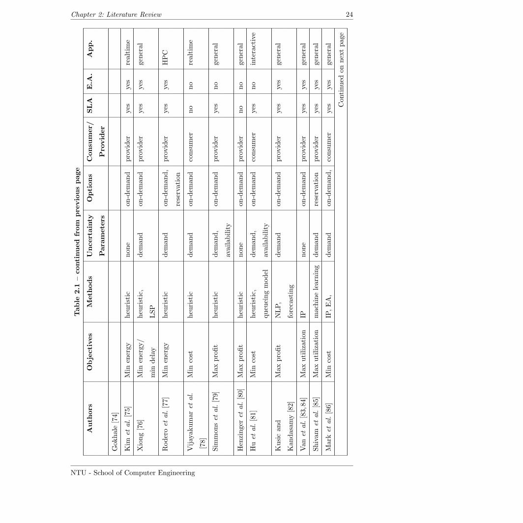
application domains. The comparison among the resource provisioning techniques is sum-
marized in Table 2.1.
2.1 Resource Provisioning Techniques Classification by Op-
timization Methods
As appeared in the reviewed literature, resource provisioning can apply different optimiza-
tion methods to achieve the optimal solutions as follows:
1. Mathematical Optimization – The mathematical optimization or mathematical pro-
gramming is the way to solve optimization problems [45]. An optimization could be
considered as a minimization or maximization problem described by an objective func-
tion (or a set of objective functions). Note that this chapter extensively investigates
11
Chapter 2: Literature Review 12
resource provisioning techniques for distributed systems based on the mathematical
optimization.
The mathematical optimization could be further classified as follows:
(a) Linear programming – Linear programming (LP) is a process to find an opti-
mal solution of a linear objective function with constraints [45,46]. LP has been
applied in several areas such as financial planning, transportation, scheduling, re-
source allocation, farming, and industrial production. LP was used in well-known
companies such as FedEx, Welch’s, Pacific Lumber, Samsung, and Continental
Airlines [47–51].
A general form of linear program can be formulated as follows:
Minimize: Z = CTX (2.1)
Subject to: A X ≤ B (2.2)
X ≥ 0. (2.3)
The objective function shown in (2.1) is to minimize X, where X or decision
variable denotes a vector of decisions. C and B are vectors of known coefficients
(e.g., parameters and constants). A is a known matrix of coefficients. The
constraints are governed by inequalities (2.2) and (2.3) which control the feasible
solution for assigning values to X with the condition X | A X ≤ B, X ≥ 0.
To solve a LP problem, simplex method [46] is an efficient algorithm. The sim-
plex method has been used to solve huge linear programs on today computers.
The simplex method was implemented in several computer-based software which
is also called solvers. GLPK [57], CPLEX [58], FortMP [59], COIN [60], and
Xpress-MP [61] are, for example, the LP solvers using the simplex method. Free
solvers for linear programs are also available in NEOS Server [62,66].
Although LP can solve several optimization problems, linear programming does
have a limitation. The limitation of linear programming model is that non-integer
values is only allowable for decision variables. To tackle such a limitation, integer
programming (IP) and mixed integer linear programming (MILP) [52] are the ap-
proaches in which all and some of decision variables are restricted to take integer
values, respectively. Binary programming (BIP) is the special IP where decision
variables are restricted to be 0 or 1. The branch-and-bound algorithm is a tech-
NTU - School of Computer Engineering
Chapter 2: Literature Review 13
nique to solve a mixed integer programming problem. GLPK [57], CPLEX [58]
and Xpress-MP [61] are, for example, solvers for IP and MILP problems. Some
free solvers to solve integer programming problems also can be found in NEOS
Server.
In the literature, resource provisioning techniques based on LP, IP, MILP, and
BIP were formulated. For example, Filali et al. [67] developed the BIP based
resource provisioning to maximize a cloud provider’s profit in which a heuris-
tic method is developed to solve the BIP model. Aoun et al. [69] formulated
the MILP model such that resources can be efficiently provisioned and the job
throughput can be maximized. Andrzejak et al. [70] developed the LP based
resource provisioning to purchase additional resources in cloud computing while
the provisioning cost is minimized. Xiong [76] formulated an IP model for provi-
sioning resources in which the job delay can be minimized. Meinl [90] proposed
the LP based resource provisioning to minimize the cost of resource reservation.
(b) Nonlinear programming – Nonlinear programming (NLP) is the process of solving
a mathematical optimization problem where some of constraints or the objective
function are nonlinear. CONOPT [63] and KNITRO [64], for example, are solvers
for the NLP problems. Xiong [76] , Bi et al. [92], Kusic and Kandasamy [82]
proposed NLP based resource provisioning techniques.
(c) Stochastic programming – Commonly, linear or integer programming is able to
solve only the problems where all parameters are known in advance. For exam-
ple, the parameters B and C shown in formulation (2.1) − (2.3) are precisely
known. In many cases, however; these parameters cannot be perfectly known and
are represented as random variables. Such parameters are called uncertain pa-
rameters. In particular, traditional linear programming (or deterministic linear
programming) cannot solve problems containing the random variables.
To solve the problems containing such uncertain parameters, stochastic program-
ming (SP) is a potential approach [28]. For the resource provisioning in dis-
tributed systems (e.g., cloud computing), uncertain parameters could be demand,
resource prices, and resource availability (which will be discussed later). Prac-
tically, the stochastic programming consisting of linear objective function and
constraints can be transformed into a deterministic equivalence form of linear
programming. Then, the deterministic equivalence can be solved by traditional
NTU - School of Computer Engineering
Chapter 2: Literature Review 14
algorithms (e.g., simplex method).
Stochastic programming has been developed to solve resource planning under
uncertainties [53] in various fields, e.g., production planning, financial manage-
ment, and capacity planning. For example, Jirutitijaroen and Singh [54] applied
the stochastic programming approach for the electrical power generation and
transmission line expansion planning while some uncertainties affecting to the
planning were taken into account. It is shown that stochastic programming is
the promising mathematical tool which is able to address the optimal decision
making in the stochastic environment.
A stochastic programming model can be extended to a robust optimization (RO)
model [29]. Under uncertainties, the robust optimization model can be flexibly
managed by users of the model to meet their risk preference and to obtain the
model- and solution-robustness. With the solution-robustness, a solution ob-
tained from the model converges to the optimal solution. In contrast, undesir-
able effects or risks can be mitigated with the model robustness. In practice, the
users can adjust the tradeoff between solution- and model-robustness to obtain
desired solutions (e.g., to obtain a nearly optimal solution and avoid unwanted
risks).
In the literature, some works derived optimization models for resource provi-
sioning while uncertain parameters are taken into account without applying SP.
Kusic and Kandasamy [82], and Mark et al. [86] dealt with uncertain parameters
for solving models with forecasting techniques [45]. Xiong [76] applied Laplace
Stieltijes transform (LST) to estimate the delay of jobs before provisioning re-
sources to the jobs. Andrzejak et al. [70] derived a probabilistic model in which
the resource availability (i.e., uptime of resources), execution time for the job
completion, and resource prices are estimated. Then, the LP model was derived
to be solved with the estimated uncertain parameters. Similarly, Simmons et
al. [79] and Rogers et al. [87] used the expectation of uncertain parameters for
their optimization models. The works in [70,79,87] were based on the Jensen’s in-
equality [55] approach. That is, the optimal solution obtained from the approach
cannot be better than that of SP.
2. Artificial Intelligence – In the literature, the methods from the artificial intelligence
field were applied for resource provisioning as follows. Mark et al. [86] and You et
NTU - School of Computer Engineering
Chapter 2: Literature Review 15
al. [89] used evolutionary algorithms (EAs) to achieve near optimal solutions for re-
source provisioning. Shivam et al. [85] and Nae et al. [95] applied machine learning and
neural network, respectively, to predict the resource demand such that the resources
can be efficiently provisioned.
3. Heuristics – A heuristic method is a procedure to achieve a feasible solution of an
optimization problem in which the solution is not guaranteed to be optimal [45]. Nor-
mally, the heuristic methods are simple solutions for achieving feasible solutions. The
evolutionary algorithm is, for example, the heuristic method (i.e., metaheuristic). In
the literature, several works were based on heuristic methods, e.g., Mattess et al. [71],
Kim et al. [75], Rodero et al. [77], Vijayakumar et al. [78], and Ostermann et al. [88].
4. Others – Other methods were applied or together used with the other aforemen-
tioned methods for resource provisioning as follows. As studied by Kusic and Kan-
dasamy [82], Mark et al. [86] and You et al. [89], online forecasting techniques were
used to predict the resource demand. Then, the uncertain demand can be replaced by
the predicted demand so that the optimization models can be solved by traditional
LP or MILP. Markov chain [45] was applied to deal with uncertain parameters as
applied by Lu and Gokhale [74]. Queueing models [45] were applied by Hu et al. [81]
and Bi et al. [92] as the analytical performance models for provisioning resources.
Zhu and Agrawal [94] proposed a dynamic resource provisioning algorithm based on
control theory [56] so that the number of resources can be dynamically adjusted to
maximize a desired quality of service (QoS).
2.2 Resource Provisioning Techniques Classification by Pro-
visioning Options
There are three major provisioning options to purchase computational resources in cloud
computing, namely on-demand, reservation, and spot options. Each option has different
price and yields different benefit to the cloud consumer. The on-demand option which is
commonly called pay-as-you-go or pay-per-use option is the default option which is avail-
able in most cloud providers (e.g., Amazon Elastic Compute Cloud (EC2) [18], GoGrid [19],
Rackspace [20], SpotCloud [21], FlexiScale [22], Google App Engine [24], and Microsoft Win-
dows Azure [25]). With the on-demand option, resources can be dynamically provisioned by
NTU - School of Computer Engineering
Chapter 2: Literature Review 16
the cloud consumer anytime without a commitment. In contrast, with the reservation op-
tion, resources need to be subscribed (or signed) with a reservation contract. The contract
states the time duration of the signed resources which will be available to the signing cloud
consumer. The consumer pays a one-time fee for the contract, and when the resources are
utilized, the usage price which is significantly cheaper than the on-demand price (i.e., price
of on-demand option) is charged additionally. For the spot option, the prices of resources
fluctuate due to supply and demand of available resources of a cloud provider. Some cloud
provider (for example, Amazon EC2 [18]) sets spot prices based on an auction mechanism.
In the literature, most works focused on resource provisioning with only the on-demand
option, e.g., Vijayakumar et al. [78], Zhou et al., Mao et al. [68], Aoun et al. [69], Simmon et
al., Van et al. [83, 84], Xiong [76] , Ostermann et al. [88]. In particular, Zhou et al. [73]
proposed an autoscaling method to resize the amount of resource provisioned with the on-
demand option. Xiong [76] applied queueing theory and Laplace Stieltijes transform (LST)
to estimate the job delay. The resource provisioning based on a heuristic method was
proposed to minimize the provisioning cost that takes only the on-demand option while the
delay and energy consumption can be maintained.
Some works focused on resource provisioning with only the reservation option. The reser-
vation option or advance reservation has been addressed in the literature for serveral years,
e.g., Filali et al. [67], Nurmi et al. [93], Kee et al. [91], and Shivam et al. [85]. In particular,
Nurmi et al. [93] developed the virtual advance reservations for queues (VARQ). VARQ
applies the time series method to predict the delay of arrival jobs so that a set of resources
will be virtually reserved for each job in certain period of time. Then, a job can be sched-
uled and assigned to the reserved resources when the time reserved for the job reaches. The
advantage of VARQ is that it works with any existing best effort scheduler since it will
buffer jobs in separate queues before submitting the jobs to the scheduler according to its
scheduling policy. Kee et al. [91] is similar to VARQ in which the delay is estimated before
an advance reservation will be performed.
Resource provisioning with the spot option has been a new hot research topic since the spot
option is the newest option offered by a cloud provider (i.e., Amazon EC2). Especially,
the option could be the cheapest option. As found in the literature, Henzinger et al. [80]
developed a resource provisioning framework named FlexPRICE. The framework applies a
pricing model to set the spot prices of resources. With FlexPRICE, a user firstly sends a
NTU - School of Computer Engineering
Chapter 2: Literature Review 17
job to a cloud provider. Then, the cloud provider returns a set of quotes which state job
schedules. In particular, the schedule specifies the price and duration for the job. Hence,
the user can choose a quote to meet a goal. Given a desired service level agreement (SLA),
Andrzejak et al. [70] proposed a probabilistic model used to set a bid price which is a cloud
consumer’s maximum affordable cost to acquire spot instances (i.e., virtual machines provi-
sioned with a spot option in EC2). In EC2, spot instances can be successfully provisioned
only when the bid price is higher than the current spot price set by EC2. Since the avail-
ability of the spot instances cannot be guaranteed, the model was applied together with
checkpointing mechanisms by Yi et al.. That is, the provisioning cost can be reduced, while
the availability of the provisioned spot instances can be maintained. Mattess et al. [71] de-
veloped the provisioning policies to acquire spot instances. The policies can manage peak
loads in a local server cluster by supplying additional spot instances in EC2. Mattess et
al. [71] also applied an estimation technique to obtain the execution time and delay of jobs
which will be assigned to the provisioned spot instances. You et al. [89] developed a re-
source allocation strategy based on market mechanism (RAS-M). In particular, the RAS-M
leverages a pricing model to set resource prices and control the balance of demand and
supply of a cloud provider’s resources.
It is observed that provisioning resources with a single type of provisioning option could be
inefficient. A few works addressed the resource provisioning problem with more than one
provisioning option. Juve and Deelman [72] stated that the resource provisioning methods
could be applied with both reservation and on-demand options. Each option has different
benefits. The reservation option can guarantee the resource availability and incur a cheaper
cost for the long-term usage that than for on-demand option. That is, the reservation
option provisions resources for a long-term usage, while the on-demand option provisions
additional resources for a short-term usage whenever the resources provisioned with the
reservation option are insufficient. For example, Mark et al. [86] applied an algorithm for
provisioning resources with reservation and on-demand options. Redero et al. proposed an
online provisioning method for high performance computing that utilizes both reservation
and on-demand options. Meinl [90] considered on-demand, reservation, and spot options for
provisioning resources. That is, an amount of resource is firstly signed with a reservation
contract. If the contract is not signed, resources will be provisioned with the spot option
in which the spot price fluctuates and could be considerably expensive. The on-demand
option will be utilized when the amount of resource provisioned with either reservation or
NTU - School of Computer Engineering
Chapter 2: Literature Review 18
spot option cannot meet the fluctuating demand.
2.3 Resource Provisioning Techniques Classification by Op-
timization Objectives
A resource provisioning technique has an objective to optimize an objective function value
or a set of objective function values. Resource provisioning could be a maximization or
minimization problem. In the literature, resource provisioning techniques can be classified
by optimization objectives as follows:
1. Cost optimization provisioning – The cost optimization problem is to minimize mone-
tary costs or maximize profits/revenue. For example, The evolutionary algorithm de-
veloped by Mark et al. [86] can allocate resources from multiple cloud providers such
that the resource provisioning cost can be minimized. Resource provisioning proposed
by Lu and Gokhale [74] can prevent the loss of reputation of a cloud provider by sup-
plying resources to meet an acceptable service performance such that the provider’s
profit can be maximized. Kusic and Kandasamy [82] proposed a resource provision-
ing framework that increases a cloud provider’s revenue such that the provisioned
resources conform to multiple quality of services required by cloud consumers. Hu et
al. [81] addressed a cost minimization problem by provisioning the smallest number
of servers in cloud computing exclusively for interactive jobs.
2. Time minimization provisioning – For cloud consumers, their jobs (or transactions)
submitted to be computed by the provisioned resources should be completed quickly
or able to meet their deadlines. In other words, the delay or execution time of jobs
needs to be minimized. For example, Xiong [76] proposed a technique for a cloud
provider to supply resources to cloud consumers that can minimize the job delay
incurred to the consumers while the energy consumption of the provider’s datacenter
can be reduced to meet the energy saving target. For the response time minimization
problem, resource provisioning proposed by Zhou et al. [73] allocates the sufficient
amount of resource for cloud consumers’ workflow applications.
3. Resource utilization maximization provisioning – Some cloud providers try to maxi-
mize the global utilization of resources in their datacenters so that the invested re-
NTU - School of Computer Engineering
Chapter 2: Literature Review 19
sources will not be wasted. Similarly, for cloud consumers, resources provisioned to
the consumers should be efficiently utilized to avoid the overprovisioning problem. For
example, Shivam et al. [85] proposed a resource provisioning which can predict the
resource usage of applications such that the maximum utilization of the provisioned
resources can be achieved. Given service-level-agreements (SLAs), the resource man-
agement was developed by Van et al. [83, 84] which can maximize a global system
utility of a datacenter by consolidating multiple virtual machines to the same server.
A resource provisioning framework developed by Kee et al. [91] proposed a resource
management paradigm called resource slot. A resource slot defines consumers’ ap-
plication requirement and providers’ resource availability. Then, the framework can
efficiently allocate resources for certain applications such that the global resource
utilization can be maximized.
4. Energy consumption minimization provisioning – As appeared in [110, 111], the total
cost of ownership (TCO) of a cloud datacenter is the energy cost, cloud providers
try to minimize the energy consumption for their datacenters. For example, Kim et
al. [75] applied the dynamic voltage frequency scaling (DVFS) scheme to adjust the
processor clocks of the physical servers for hosting virtual machines such that the
energy consumption in a datacenter can be reduced. Rodero et al. [77] proposed an
energy-aware provisioning method that clusters the characteristics of incoming job.
Then, appropriate resources will be allocated to the jobs. A non-linear programming
problem was derived by Xiong [76] to minimize the energy consumption while the
delay of incoming jobs can be controlled to be lower than desired targets.
5. Throughput maximization provisioning – Throughputs are the number of jobs (or
transactions) which are completely processed per unit of time. To address the through-
put maximization problem, Aoun et al. [69] developed an algorithm based on MILP
that mainly maximizes the number of completed service requests (i.e., throughputs in
terms of processed requests).
6. Quality of service maximization provisioning – The quality of service of certain appli-
cations (or jobs) can be maximized. For example, Zhu and Agrawal [94] applied the
control theory to maximize application benefits which are represented as QoS metrics
while the execution time of the applications and costs of provisioned resources are
controlled.
NTU - School of Computer Engineering
Chapter 2: Literature Review 20
2.4 Resource Provisioning Techniques Classification by Un-
certain Parameters
Uncertainty has a direct impact on a resource provisioning decision. Resource provisioning
needs to be made before uncertain parameters will be observed. The uncertain parameters
can lead the inefficient resource provision. That is, either underprovisioning or overpro-
visioning problem can occur. In the literature, resource provisioning techniques can be
classified according to uncertain parameters as follows:
1. Non uncertainty provisioning – Several resource provisioning techniques did not take
uncertain parameters into account, e.g., Filali et al. [67], Mao et al. [68], Aoun et
al. [69], Juve and Deelman [72], Zhou et al. [73], and Kim et al. [75]. Without consid-
ering uncertain parameters, the amount of provisioned resource could be underprovi-
sioned or overprovisioned.
2. Demand uncertainty oriented provisioning – Demand is considered as workloads that
need to be processed on the provisioned resources. The demand is commonly unknown
in advance. Demand could be determined as the number of arrival jobs/transactions
and the number of hours required by a job. Many resource provisioning techniques
consider the demand uncertainty, e.g., Mattess et al. [71], Xiong [76], Rodero et al. [77],
Vijayakumar et al. [78], Kusic and Kandasamy [82], Mark et al. [86], and Rogers et
al. [87].
3. Price uncertainty oriented provisioning – Prices could be resource prices set by cloud
providers and energy prices set by energy supplies. Prices, especially spot prices, often
fluctuate. Generally, future spot prices are not precisely observed. A few resource
provisioning techniques did consider the price uncertainty, i.e., Andrzejak et al. [70]
and Meinl [90].
4. Availability uncertainty oriented provisioning – Availability of provisioned resources
could be uncertain. Cloud providers define SLAs to guarantee the resource availability
to cloud consumers. Andrzejak et al. [70], Simmons et al. [79] , and Kee et al. [91]
took the availability uncertainty into account.
5. Delay uncertainty provisioning – Delay is the time of jobs/transactions which wait in
a queue before they can be executed. Generally, the delay of a job cannot be perfectly
NTU - School of Computer Engineering
Chapter 2: Literature Review 21
estimated. Andrzejak et al. [70], Hu et al. [81], and Nurmi et al. [93] considered the
delay uncertainty in their works.
Since multiple uncertain parameters could influence the decision of resource provisioning, a
few works took two different uncertain parameters into account. For example, Andrzejak et
al. [70] considered both price and availability uncertainties. Simmons et al. [79] considered
both demand and availability uncertainties. Meinl [90] addressed both demand and price
uncertainties.
2.5 Resource Provisioning Techniques Classification by Other
Characteristics
Resource provisioning techniques can be classified based on other characteristics as follows:
1. Application Domains – Generally, resource provisioning can be applied to any appli-
cation domains (i.e., non-specific domain), e.g., Mao et al. [68], Mattess et al. [71],
Zhou et al. [73], Simmons et al. [79], and Meinl [90]. However, some resource provi-
sioning techniques discussed in the literature may be specifically designed for certain
application domains. For example, Juve and Deelman [72], Zhou et al. [73], and
Ostermann et al. [88] addressed resource provisioning techniques for workflow appli-
cations. Resource provisioning for high performance computing (HPC) applications
was investigated by Rodero et al. [77] and Henzinger et al. [80]. Lu and Gokhale [74]
addressed the resource provisioning technique for electronic commerce application.
Nae et al. [95] proposed the resource provisioning model for massively multiplayer on-
line games (MMOGs). In Table 2.1, application domains of the resource provisioning
techniques in the literature are shown.
2. Provider- or Consumer-based resource provisioning – Although resource provision-
ing could be applied for both cloud providers and consumers, resource provisioning
techniques presented in the literature were originally designed for either provider or
consumer. It is observed that resource provisioning techniques for cloud providers
mostly have the main objectives to maximize profits. In contrast, resource provision-
ing techniques for cloud consumers generally have the objectives to minimize mone-
NTU - School of Computer Engineering
Chapter 2: Literature Review 22
tary provisioning costs, minimize delay, and maximize throughputs. In Table 2.1, each
work is classified as either cloud provider- or consumer-based resource provisioning.
3. Energy-aware resource provisioning – In the literature, some resource provisioning
techniques considered the energy conservation issue. Such techniques are commonly
called power- or energy-aware (E.A.) resource provisioning. Resource provisioning
techniques may directly minimize the energy consumption as mentioned in Section 2.3.
Some techniques may take the energy consumption as optimization constraints. In Ta-
ble 2.1, each work is identified as if it addressed the energy conservation issue.
4. Service-level-agreement oriented resource provisioning – In cloud computing, cloud
providers need to supply resources to conform to SLAs. Violating SLAs could incur
higher costs on both cloud providers’ and consumers’ sides. Therefore, resource pro-
visioning techniques may take SLAs as constraints which need to be controlled. For
example, the optimization models proposed by Simmons et al. [79], Kusic and Kan-
dasamy [82], Xiong [76], and Van et al. [83,84] took the SLA constraints into account.
In Table 2.1, each work is identified as if it considered the SLA constraints.
NTU - School of Computer Engineering
Chapter 2: Literature Review 23
Table
2.1:Comparisonofresourceprovisioningtechniques.
Auth
ors
Objectives
Meth
ods
Uncertainty
Options
Consu
mer/
SLA
E.A
.App.
Para
meters
Pro
vider
This
thesis
Min
cost,
SP,RO
dem
and,
on-dem
and,
consumer,
no
yes
general
Max
profit
price,
reservation,
provider,
availability
spot
retailer
Filaliet
al.[67]
Min
cost
BIP,
none
reservation,
provider
no
no
general
heuristic
spot
Mao
etal.[68]
Min
cost/
IPnone
on-dem
and
consumer
no
no
general
Max
utilization
Aou
net
al.[69]
Max
through
put
MILP
none
on-dem
and
consumer
no
no
general
Andrzejak
etal.[70]
Min
cost/
LP
price,delay
spot
consumer
yes
no
general
Max
utilization
availability
Mattess
etal.[71]
Min
cost/
heuristic
dem
and
spot
consumer
no
no
general
min
delay
Juve
and
Min
delay
heuristic
none
on-dem
and,
consumer
no
no
workflow
Deelm
an[72]
reservation
Zhou
etal.[73]
Min
delay
heuristic
none
on-dem
and
consumer
yes
no
workflow
,
interactive
Luan
dMax
profit
Markov
chain
dem
and
reservation
consumer
yes
no
workflow
Continued
onnextpage
NTU - School of Computer Engineering
Chapter 2: Literature Review 24
Table
2.1
–continued
from
pre
viouspage
Auth
ors
Objectives
Meth
ods
Uncertainty
Options
Consu
mer/
SLA
E.A
.App.
Para
meters
Pro
vider
Gok
hale[74]
Kim
etal.[75]
Min
energy
heuristic
none
on-dem
and
provider
yes
yes
realtime
Xiong[76]
Min
energy
/heuristic,
dem
and
on-dem
and
provider
yes
yes
general
min
delay
LSP
Roderoet
al.[77]
Min
energy
heuristic
dem
and
on-dem
and,
provider
yes
yes
HPC
reservation
Vijayak
umar
etal.
Min
cost
heuristic
dem
and
on-dem
and
consumer
no
no
realtime
[78]
Sim
mon
set
al.[79]
Max
profit
heuristic
dem
and,
on-dem
and
provider
yes
no
general
availability
Henzingeret
al.[80]
Max
profit
heuristic
none
on-dem
and
provider
no
no
general
Huet
al.[81]
Min
cost
heuristic,
dem
and,
on-dem
and
consumer
yes
no
interactive
queueingmodel
availability
Kusican
dMax
profit
NLP,
dem
and
on-dem
and
provider
yes
yes
general
Kan
dasam
y[82]
forecasting
Van
etal.[83,84
]Max
utilization
IPnone
on-dem
and
provider
yes
yes
general
Shivam
etal.[85]
Max
utilization
machinelearning
dem
and
reservation
provider
yes
yes
general
Market
al.[86]
Min
cost
IP,EA,
dem
and
on-dem
and,
consumer
yes
yes
general
Continued
onnextpage
NTU - School of Computer Engineering
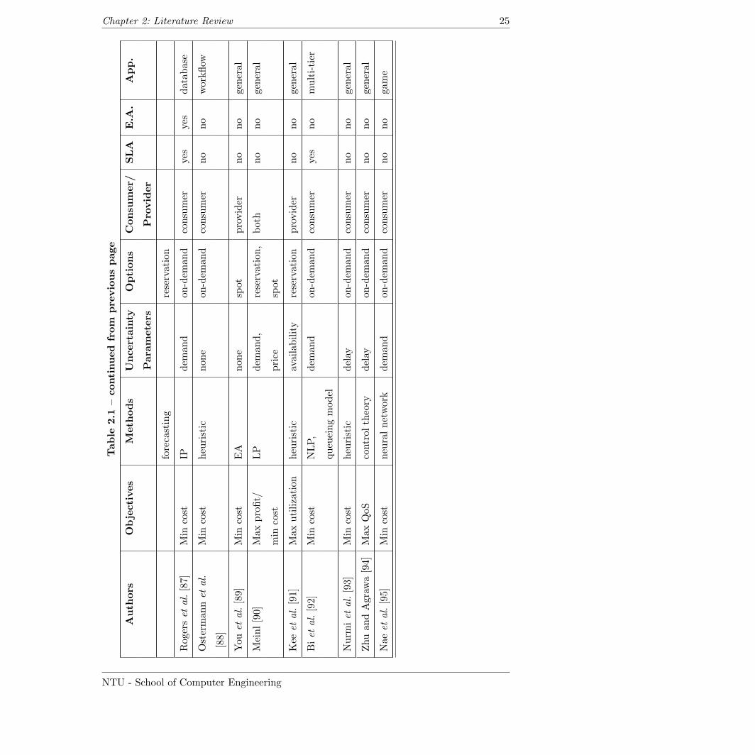
Chapter 2: Literature Review 25
Table
2.1
–continued
from
pre
viouspage
Auth
ors
Objectives
Meth
ods
Uncertainty
Options
Consu
mer/
SLA
E.A
.App.
Para
meters
Pro
vider
forecasting
reservation
Rogerset
al.[87]
Min
cost
IPdem
and
on-dem
and
consumer
yes
yes
datab
ase
Osterman
net
al.
Min
cost
heuristic
none
on-dem
and
consumer
no
no
workflow
[88]
You
etal.[89]
Min
cost
EA
none
spot
provider
no
no
general
Meinl[90]
Max
profit/
LP
dem
and,
reservation,
both
no
no
general
min
cost
price
spot
Kee
etal.[91]
Max
utilization
heuristic
availability
reservation
provider
no
no
general
Biet
al.[92]
Min
cost
NLP,
dem
and
on-dem
and
consumer
yes
no
multi-tier
queueingmodel
Nurm
iet
al.[93]
Min
cost
heuristic
delay
on-dem
and
consumer
no
no
general
Zhuan
dAgraw
a[94]
Max
QoS
controltheory
delay
on-dem
and
consumer
no
no
general
Nae
etal.[95]
Min
cost
neuralnetwork
dem
and
on-dem
and
consumer
no
no
game
NTU - School of Computer Engineering
Chapter 2: Literature Review 26
2.6 Novelty of This Thesis
In the present state-of-the-art, we propose the novel resource provisioning algorithms for
obtaining the optimal amount of computational resource under uncertainties. In this thesis,
different algorithms are derived for three cloud stakeholders, namely cloud consumer, cloud
provider, and cloud retailer. In particular, the optimal solution for provisioning resources
obtained by the proposed algorithms can be guaranteed to be optimal under uncertainties.
We specifically consider different uncertainties, i.e., demand, availability, and price uncer-
tainties. Our proposed algorithms for consumers also consider the solution- and model-
robustness which were not taken into account in all works in the literature. For a cloud
provider owning a datacenter, our algorithm uniquely considers both the forward contract
portfolio optimization of power supply and optimization of resource management. To apply
our proposed algorithms for a large scale problem (with a great number of parameters), we
have applied mathematical methods (i.e., sample-average approximation [39] and scenario
reduction technique [43]) to reduce the problem complexity such that the problem can be
efficiently solved.
NTU - School of Computer Engineering
Chapter 3
Resource Provisioning
on Consumers’ Side
Cloud providers, e.g., Amazon [18], GoGrid [19], and Microsoft [25], provide on-demand and
reservation options to cloud consumers. With the on-demand option, the resources can be
dynamically provisioned by a cloud consumer anytime without a commitment (i.e., pay-per-
use basis). In contrast, with the reservation option, the resources need to be subscribed with
a contract. The contract will guarantee the availability and prices of the resources within
a certain duration. In particular, the cost of the resources purchased using the reservation
option is cheaper than that of the on-demand option. The cloud consumer could apply the
reservation option for the long-term utilization and the on-demand option for the short-term
utilization.
In this chapter, we focus mainly on resource provisioning from the cloud consumer’s per-
spective. We make an assumption that the cloud consumer needs to first apply the reserva-
tion option for a long-term usage. Later, additional resources will be provisioned with the
on-demand option if the reserved resources are not sufficient. Overprovisioning and under-
provisioning problems will occur due to the demand uncertainty. To deal with the problems,
we develop the novel resource provisioning algorithms by stochastic programming [28]. Nu-
merical studies and simulation are performed to evaluate the developed algorithms.
This chapter is organized as follows. First, in Section 3.1, we present a designed system
model of cloud computing environment where a cloud consumer can purchase reservation
27
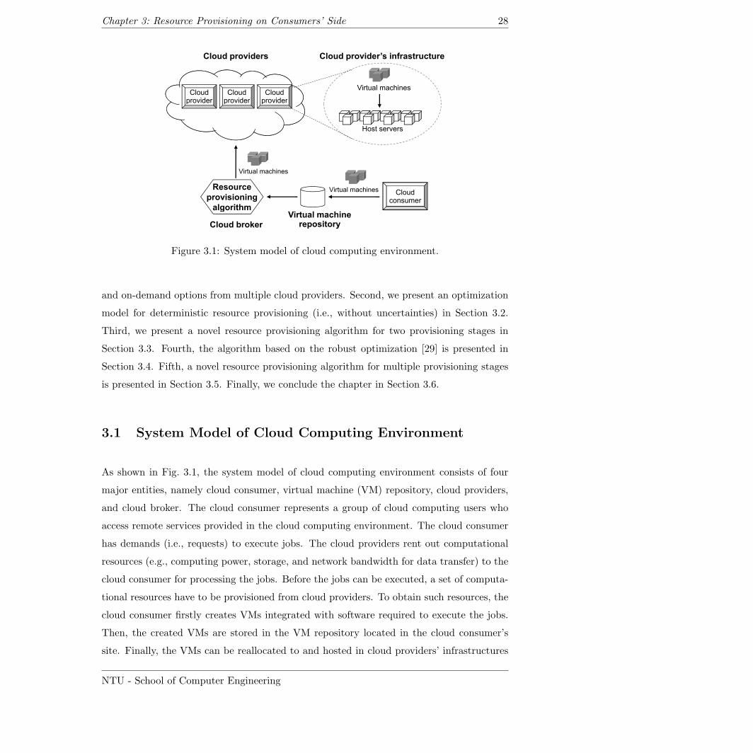
Chapter 3: Resource Provisioning on Consumers’ Side 28
Cloud provider’s infrastructure
Cloudprovider
Cloud providers
Cloudprovider
Cloudprovider
Virtual machines
Host servers
providerprovider provider
Cloudconsumer
Resource
provisioning
algorithm
Virtual machines
Virtual machines
algorithmVirtual machine
repositoryCloud broker
Figure 3.1: System model of cloud computing environment.
and on-demand options from multiple cloud providers. Second, we present an optimization
model for deterministic resource provisioning (i.e., without uncertainties) in Section 3.2.
Third, we present a novel resource provisioning algorithm for two provisioning stages in
Section 3.3. Fourth, the algorithm based on the robust optimization [29] is presented in
Section 3.4. Fifth, a novel resource provisioning algorithm for multiple provisioning stages
is presented in Section 3.5. Finally, we conclude the chapter in Section 3.6.
3.1 System Model of Cloud Computing Environment
As shown in Fig. 3.1, the system model of cloud computing environment consists of four
major entities, namely cloud consumer, virtual machine (VM) repository, cloud providers,
and cloud broker. The cloud consumer represents a group of cloud computing users who
access remote services provided in the cloud computing environment. The cloud consumer
has demands (i.e., requests) to execute jobs. The cloud providers rent out computational
resources (e.g., computing power, storage, and network bandwidth for data transfer) to the
cloud consumer for processing the jobs. Before the jobs can be executed, a set of computa-
tional resources have to be provisioned from cloud providers. To obtain such resources, the
cloud consumer firstly creates VMs integrated with software required to execute the jobs.
Then, the created VMs are stored in the VM repository located in the cloud consumer’s
site. Finally, the VMs can be reallocated to and hosted in cloud providers’ infrastructures
NTU - School of Computer Engineering
Chapter 3: Resource Provisioning on Consumers’ Side 29
whose resources can be utilized by the VMs. In Fig. 3.1, the cloud broker is located in the
cloud consumer’s site and is responsible on behalf of the cloud consumer for provisioning
resources in the cloud providers. In particular, the cloud broker rents resources from cloud
providers and allocates the VMs originally stored in the VM repository to appropriate cloud
providers. Thus, the cloud broker implements a resource provisioning algorithm to make
the allocation decision.
There are multiple VM classes used to classify different types of VM. Let I ⊂ N11 denote the
set of VM classes. We assume that each VM class represents a different type of jobs, e.g., a
VM class for a certain web application and another class for a certain scientific application.
Each VM class requires a specific amount of computational resources to execute a single
VM. Furthermore, a number of VMs needs to be provisioned for a certain VM class. In this
thesis, the number of VMs required for a certain VM class is called demand. In particular,
the cloud broker is responsible for provisioning resources from cloud providers to meet
demands of all VM classes.
In Fig. 3.1, let J ⊂ N1 denote the set of cloud providers. Each cloud provider supplies
a pool of resources to the cloud consumer. Let R denote the set of resource types which
can be provided by cloud providers. Resource types can be processing power, storage, and
network bandwidth for Internet data transfer.
A cloud provider offers the cloud consumer two provisioning options, i.e., reservation and/or
on-demand options. The reservation option has to be subscribed under a reservation con-
tract. The contract states the advance reservation of resources with regard to the specific
time duration of resource availability. For example, the reservation option offered by Ama-
zon EC2 has two reservation contracts [18], i.e., 1-year and 3-year contracts). A certain
amount of resource is reserved (e.g., single VM with some limited storage and memory
capacities) and available for one year under the 1-year contract and three years under the
3-year contract starting from the time the resources are provisioned. For the on-demand
option, resources can be dynamically provisioned at the moment they are needed.
Computational resources can be provisioned at different points of time, also called provi-
sioning phases. As illustrated in Fig. 3.2, there are three different provisioning phases as
follows:
1 N1 = 1, 2, 3, . . .
NTU - School of Computer Engineering
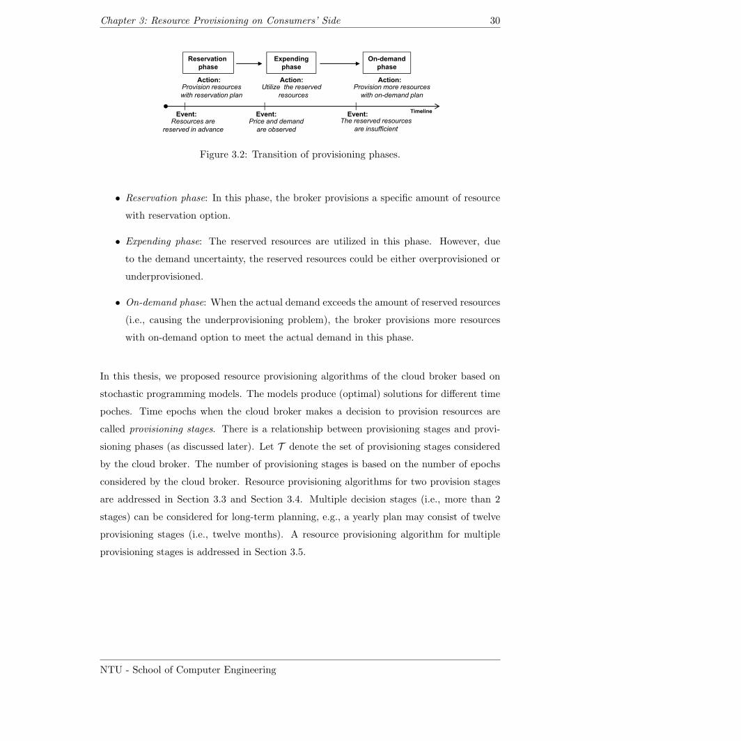
Chapter 3: Resource Provisioning on Consumers’ Side 30
Reservation
phase
Expending
phase
On-demand
phase
Provision resources
with reservation plan
Utilize the reserved
resources
Provision more resources
with on-demand plan
Action: Action: Action:
Timeline
Price and demand
are observed
Resources are
reserved in advance
The reserved resources
are insufficient
Event: Event: Event:
Figure 3.2: Transition of provisioning phases.
• Reservation phase: In this phase, the broker provisions a specific amount of resource
with reservation option.
• Expending phase: The reserved resources are utilized in this phase. However, due
to the demand uncertainty, the reserved resources could be either overprovisioned or
underprovisioned.
• On-demand phase: When the actual demand exceeds the amount of reserved resources
(i.e., causing the underprovisioning problem), the broker provisions more resources
with on-demand option to meet the actual demand in this phase.
In this thesis, we proposed resource provisioning algorithms of the cloud broker based on
stochastic programming models. The models produce (optimal) solutions for different time
poches. Time epochs when the cloud broker makes a decision to provision resources are
called provisioning stages. There is a relationship between provisioning stages and provi-
sioning phases (as discussed later). Let T denote the set of provisioning stages considered
by the cloud broker. The number of provisioning stages is based on the number of epochs
considered by the cloud broker. Resource provisioning algorithms for two provision stages
are addressed in Section 3.3 and Section 3.4. Multiple decision stages (i.e., more than 2
stages) can be considered for long-term planning, e.g., a yearly plan may consist of twelve
provisioning stages (i.e., twelve months). A resource provisioning algorithm for multiple
provisioning stages is addressed in Section 3.5.
NTU - School of Computer Engineering
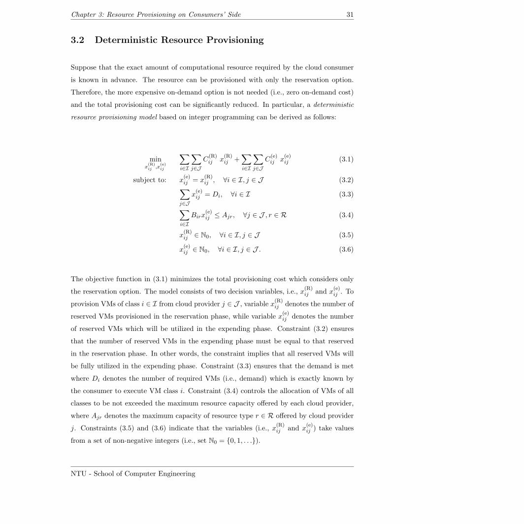
Chapter 3: Resource Provisioning on Consumers’ Side 31
3.2 Deterministic Resource Provisioning
Suppose that the exact amount of computational resource required by the cloud consumer
is known in advance. The resource can be provisioned with only the reservation option.
Therefore, the more expensive on-demand option is not needed (i.e., zero on-demand cost)
and the total provisioning cost can be significantly reduced. In particular, a deterministic
resource provisioning model based on integer programming can be derived as follows:
minx(R)ij ,x
(e)ij
∑i∈I
∑j∈J
C(R)ij x
(R)ij +
∑i∈I
∑j∈J
C(e)ij x
(e)ij (3.1)
subject to: x(e)ij = x
(R)ij , ∀i ∈ I, j ∈ J (3.2)∑
j∈Jx(e)ij = Di, ∀i ∈ I (3.3)
∑i∈I
Birx(e)ij ≤ Ajr, ∀j ∈ J , r ∈ R (3.4)
x(R)ij ∈ N0, ∀i ∈ I, j ∈ J (3.5)
x(e)ij ∈ N0, ∀i ∈ I, j ∈ J . (3.6)
The objective function in (3.1) minimizes the total provisioning cost which considers only
the reservation option. The model consists of two decision variables, i.e., x(R)ij and x
(e)ij . To
provision VMs of class i ∈ I from cloud provider j ∈ J , variable x(R)ij denotes the number of
reserved VMs provisioned in the reservation phase, while variable x(e)ij denotes the number
of reserved VMs which will be utilized in the expending phase. Constraint (3.2) ensures
that the number of reserved VMs in the expending phase must be equal to that reserved
in the reservation phase. In other words, the constraint implies that all reserved VMs will
be fully utilized in the expending phase. Constraint (3.3) ensures that the demand is met
where Di denotes the number of required VMs (i.e., demand) which is exactly known by
the consumer to execute VM class i. Constraint (3.4) controls the allocation of VMs of all
classes to be not exceeded the maximum resource capacity offered by each cloud provider,
where Ajr denotes the maximum capacity of resource type r ∈ R offered by cloud provider
j. Constraints (3.5) and (3.6) indicate that the variables (i.e., x(R)ij and x
(e)ij ) take values
from a set of non-negative integers (i.e., set N0 = 0, 1, . . .).
NTU - School of Computer Engineering
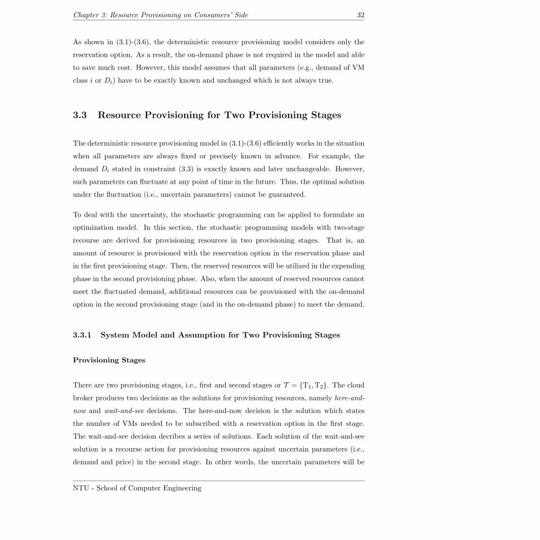
Chapter 3: Resource Provisioning on Consumers’ Side 32
As shown in (3.1)-(3.6), the deterministic resource provisioning model considers only the
reservation option. As a result, the on-demand phase is not required in the model and able
to save much cost. However, this model assumes that all parameters (e.g., demand of VM
class i or Di) have to be exactly known and unchanged which is not always true.
3.3 Resource Provisioning for Two Provisioning Stages
The deterministic resource provisioning model in (3.1)-(3.6) efficiently works in the situation
when all parameters are always fixed or precisely known in advance. For example, the
demand Di stated in constraint (3.3) is exactly known and later unchangeable. However,
such parameters can fluctuate at any point of time in the future. Thus, the optimal solution
under the fluctuation (i.e., uncertain parameters) cannot be guaranteed.
To deal with the uncertainty, the stochastic programming can be applied to formulate an
optimization model. In this section, the stochastic programming models with two-stage
recourse are derived for provisioning resources in two provisioning stages. That is, an
amount of resource is provisioned with the reservation option in the reservation phase and
in the first provisioning stage. Then, the reserved resources will be utilized in the expending
phase in the second provisioning phase. Also, when the amount of reserved resources cannot
meet the fluctuated demand, additional resources can be provisioned with the on-demand
option in the second provisioning stage (and in the on-demand phase) to meet the demand.
3.3.1 System Model and Assumption for Two Provisioning Stages
Provisioning Stages
There are two provisioning stages, i.e., first and second stages or T = T1,T2. The cloud
broker produces two decisions as the solutions for provisioning resources, namely here-and-
now and wait-and-see decisions. The here-and-now decision is the solution which states
the number of VMs needed to be subscribed with a reservation option in the first stage.
The wait-and-see decision decribes a series of solutions. Each solution of the wait-and-see
solution is a recourse action for provisioning resources against uncertain parameters (i.e.,
demand and price) in the second stage. In other words, the uncertain parameters will be
NTU - School of Computer Engineering
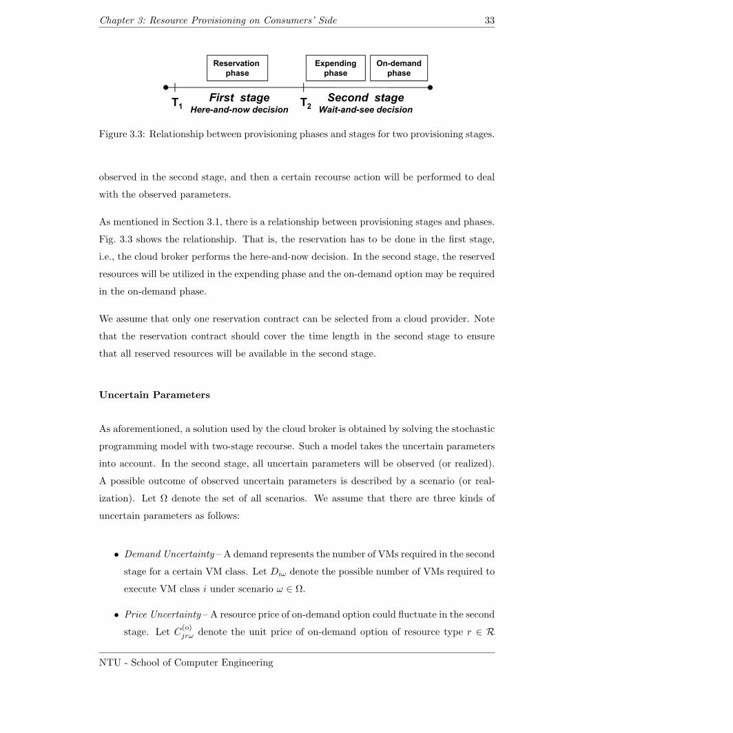
Chapter 3: Resource Provisioning on Consumers’ Side 33
Fi t t S d t
Reservation
phase
Expending
phase
On-demand
phase
First stageHere-and-now decision
Second stageWait-and-see decision
T1 T2
Figure 3.3: Relationship between provisioning phases and stages for two provisioning stages.
observed in the second stage, and then a certain recourse action will be performed to deal
with the observed parameters.
As mentioned in Section 3.1, there is a relationship between provisioning stages and phases.
Fig. 3.3 shows the relationship. That is, the reservation has to be done in the first stage,
i.e., the cloud broker performs the here-and-now decision. In the second stage, the reserved
resources will be utilized in the expending phase and the on-demand option may be required
in the on-demand phase.
We assume that only one reservation contract can be selected from a cloud provider. Note
that the reservation contract should cover the time length in the second stage to ensure
that all reserved resources will be available in the second stage.
Uncertain Parameters
As aforementioned, a solution used by the cloud broker is obtained by solving the stochastic
programming model with two-stage recourse. Such a model takes the uncertain parameters
into account. In the second stage, all uncertain parameters will be observed (or realized).
A possible outcome of observed uncertain parameters is described by a scenario (or real-
ization). Let Ω denote the set of all scenarios. We assume that there are three kinds of
uncertain parameters as follows:
• Demand Uncertainty – A demand represents the number of VMs required in the second
stage for a certain VM class. Let Diω denote the possible number of VMs required to
execute VM class i under scenario ω ∈ Ω.
• Price Uncertainty – A resource price of on-demand option could fluctuate in the second
stage. Let C(o)jrω denote the unit price of on-demand option of resource type r ∈ R
NTU - School of Computer Engineering
Chapter 3: Resource Provisioning on Consumers’ Side 34
offered by cloud provider j under scenario ω. The total cost of all resource types
offered by cloud provider j incurred to VM class i under scenario ω denoted by C(o)ijω
is expressed as follows:
C(o)ijω =
∑r∈R
BirC(o)jrω (3.7)
where Bir denotes the amount of resource of type r required by a single VM of class i.
• Availability Uncertainty – Resources could be unavailable for some reasons, e.g., power
outage and system failure. Let Ajrω denote the amount of resource of type r which is
available in cloud provider j under scenario ω.
Scenario ω ∈ Ω can be described by a random vector denoted by ξ(ω), namely ξ(ω) =(C
(o)ijω, Diω, Ajrω
). We assume that a discrete probability distribution of Ω has finite support,
i.e., Ω contains a finite number of scenarios with respective probabilities πω.
Provisioning Costs
As shown in Fig. 3.2, there are three provisioning phases. Three different provisioning costs,
namely reservation, expending, and on-demand costs, are charged to respective provisioning
phases. For example, as shown in (3.7), C(o)ijω is the on-demand cost charged to the cloud
consumer for executing VM class i by cloud provider j where C(o)jrω is the price of resource
type r. For the other provisioning costs, let C(R)jr denote the price to reserve resources type
r from provider j for a single VM and let C(e)jr denote the unit price of resource type r
from provider j. Then, the reservation and expending costs (denoted by C(R)ij and C
(e)ij ,
respectively) charged to VM class i by provider j can be defined as follows:
C(R)ij =
∑r∈R
C(R)jr (3.8)
C(e)ij =
∑r∈R
BirC(e)jr . (3.9)
NTU - School of Computer Engineering
Chapter 3: Resource Provisioning on Consumers’ Side 35
3.3.2 Stochastic Programming Model with Two-Stage Recourse
First, a stochastic programming model with two-stage recourse for two provisioning stages
is derived by following the basic properties of stochastic programming with two-stage re-
course [97] as follows:
minx(R)ij ,x
(e)ijω ,x
(o)ijω
∑i∈I
∑j∈J
C(R)ij x
(R)ij + EΩ
[Q(x(R)ij , ω
)](3.10)
subject to: (3.5)
x(e)ijω ∈ N0, ∀i ∈ I, j ∈ J , ω ∈ Ω (3.11)
x(o)ijω ∈ N0, ∀i ∈ I, j ∈ J , ω ∈ Ω. (3.12)
The objective function in (3.10) minimizes the expected total provisioning cost for two pro-
visioning stages. Variable x(R)ij denotes the number of reserved VMs of class i provisioned
from cloud provider j in the first provisioning stage. In the second stage, variables x(e)ijω
and x(o)ijω denote the numbers of VMs of class i provisioned from cloud provider j in the
expending and on-demand phases under scenario ω ∈ Ω, respectively. A scenario describes
a possible outcome of uncertain parameters which can be represented by a random vector,
i.e., ξ(ω) =(C
(o)ijω, Diω, Ajrω
). As shown in (3.5), (3.11) and (3.12), the constraints indicate
that all decision variables take values from a set of non-negative integers.
Due to the uncertainty, the cost in the second provisioning stage associates with the expected
provisioning cost of all scenarios represented by function EΩ
[Q(x(R)ij , ω
)]as shown in
(3.10) where EΩ
[·]represents the expectation of provisioning costs in the second stage for
all scenarios ∀ω ∈ Ω. Function Q(x(R)ij , ω
)represents the minimized provisioning cost in
the second stage given variable x(R)ij and scenario ω. Then, function Q
(x(R)ij , ω
)is fully
expressed as follows:
NTU - School of Computer Engineering
Chapter 3: Resource Provisioning on Consumers’ Side 36
Q(x(R)ij , ω
)= min
x(e)ijω ,x
(o)ijω
∑i∈I
∑j∈J
(C
(e)ij x
(e)ijω + C
(o)ijω x
(o)ijω
) (3.13)
subject to: x(e)ijω ≤ x
(R)ij , ∀i ∈ I, j ∈ J (3.14)
Diω ≤∑j∈J
(x(e)ijω + x
(o)ijω
), ∀i ∈ I (3.15)
∑i∈I
Bir
(x(e)ijω + x
(o)ijω
)≤ Ajrω, ∀j ∈ J , r ∈ R (3.16)
In (3.13), function Q(x(R)ij , ω
)minimizes the provisioning cost in the second provisioning
stage, i.e., the costs in the expending and on-demand phases. Function Q(x(R)ij , ω
)is an
optimization problem associated with constraints as shown in (3.14)-(3.16) given scenario
ω. Constraint (3.14) ensures that the number of VMs which will be provisioned in the
expending phase must not exceed the number of VMs reserved in the reservation phase.
Constraint (3.15) ensures that the number of provisioned VMs of class i in the expending
and on-demand phases must accommodate the demand of class i, i.e., the number of required
VMs denoted by Diω. For each resource type r ∈ R in cloud provider j, constraint (3.16)
ensures that the amount of computational resource consumed by the VMs provisioned in
the expending and on-demand phases must not exceed the maximum amount of resource
offered by the cloud provider denoted by Ajrω.
3.3.3 Proposed Optimal Virtual Machine Placement Algorithm
When the probability distribution of ω has finite support, a deterministic equivalent of
stochastic programming model can be formulated. That is, Ω has the finite number of
scenarios. In other words, Ω is a finite set. Each scenario ω is associated with a probability
0 ≤ πω ≤ 1. The deterministic equivalent of stochastic programming model derived in
(3.10)-(3.16) can be derived as follows:
NTU - School of Computer Engineering
Chapter 3: Resource Provisioning on Consumers’ Side 37
minx(R)ij ,x
(e)ijω ,x
(o)ijω
∑i∈I
∑j∈J
C(R)ij x
(R)ij +
∑i∈I
∑j∈J
∑ω∈Ω
πω
(C
(e)ij x
(e)ijω + C
(o)ijω x
(o)ijω
)(3.17)
subject to: (3.5), (3.11), (3.12)
x(e)ijω ≤ x
(R)ij , ∀i ∈ I, j ∈ J , ω ∈ Ω (3.18)
Diω ≤∑j∈J
(x(e)ijω + x
(o)ijω
), ∀i ∈ I, ω ∈ Ω (3.19)
∑i∈I
Bir
(x(e)ijω + x
(o)ijω
)≤ Ajrω, ∀j ∈ J , r ∈ R, ω ∈ Ω (3.20)
The model in (3.17)-(3.20) can be solved by traditional optimization solver software e.g.,
GNU Linear Programming Kit [57], GAMS solvers [65], and solvers in the NEOS server [66].
Then, an algorithm called optimal virtual machine placement (OVMP) is proposed as shown
in Algorithm 1.
Algorithm 1 Optimal Virtual Machine Placement Algorithm
Input: πω, C(R)ij , C
(e)ij , C
(o)ijω, Diω, Bir, Ajrω.
Output: x∗.
1: x∗ ← solve model in (3.17)-(3.20).
2: Wait until the second provisioning stage occurs.
3: Observe scenario ω.
4: Apply the recourse action for observed scenario ω based on x∗.
5: return x∗.
As presented in Algorithm 1, x∗ =(x∗(R)ij , x
∗(e)ijω , x
∗(o)ijω
)denotes a composite variable that
represents an optimal solution of the model in (3.17)-(3.20) solved by optimization solver
software where x∗(R)ij , x
∗(e)ijω , and x
∗(o)ijω denote the optimal values for respective x
(R)ij , x
(e)ijω,
and x(o)ijω.
Algorithmic Complexity
As aforementioned, the execution of the OVMP algortihm requires optimization solver
software to solve the stochastic optimization model based on integer programming. Hence,
the complexity of the proposed OVMP algortihm is based on the algorithm provided by the
NTU - School of Computer Engineering
Chapter 3: Resource Provisioning on Consumers’ Side 38
optimization solver software.
In this thesis, every proposed resource provisioning algorithm requires stochastic program-
ming models based on integer programing to generate an optimal solution to provision
resources. The branch-and-bound algorithm, one of the algorithms for integer program-
ming, is chosen to solve the models. Hence, the complexity of all proposed algorithms in
this thesis is equivalent to the complexity of the branch-and-bound algorithm. That is, the
algorithm requires O(n log n) running time [98].
3.3.4 Resource Provisioning with Benders Decomposition
The Benders decomposition algorithm [38] is applied to solve the OVMP algorithm as
shown in Algorithm 1. The goal of the Benders decomposition algorithm is to break down
a linear/integer programming problem into multiple smaller linear/integer programming
problems which can be solved independently and in parallel. As a result, the computational
time to obtain the solution of the OVMP algorithm can be reduced. The Benders decom-
position algorithm can decompose a linear/integer programming problem with complicating
variables into two major types of problems: master problem and subproblem. Note that
complicating variables are variables that prevent the decomposability of the problem.
We can verify that the OVMP algorithm has a structure which can be decomposed by the
Benders decomposition algorithm as follows:
Property 1 The stochastic programming model derived for the OVMP algorithm is the
problem whose structure has multiple complicating variables.
Proof: Variable x(e)ijω in the stochastic programming model in (3.17)-(3.20) derived for
the OVMP algorithm is considered as the complicating variable [38]. Since variable x(e)ijω
exists in constraints (3.18)-(3.20), the variable prevents the decomposability of the model. If
variable x(e)ijω is given a fixed value denoted by x
(fix)ijω as described by the equation as follows:
x(e)ijω = x
(fix)ijω , ∀i ∈ I, j ∈ J , ω ∈ Ω (3.21)
NTU - School of Computer Engineering
Chapter 3: Resource Provisioning on Consumers’ Side 39
, the model can be decomposed into two classes of independent integer programming sub-
problems, namely S1 and S2(ω) presented as follows:
[S1]
minx(R)ij
z(R)ν =
∑i∈I
∑j∈J
C(R)ij x
(R)ij (3.22)
subject to: (3.5), (3.18), (3.21)
[S2(ω)
]minx(o)ijω
z(o)ν (ω) =∑i∈I
∑j∈J
πωC(o)ijωx
(o)ijω (3.23)
subject to: (3.12), (3.19), (3.20), (3.21)
From the above decomposition, it can be concluded that the stochastic programming model
defined in (3.17)-(3.20) of the OVMP algorithm has the structure with multiple complicating
variables.
From Property 1, the stochastic programming model of OVMP algorithm can be solved
by the Benders decomposition algorithm. The Benders decomposition algorithm consists
of iterative steps. In each iteration, the master problem constituted by the complicating
variables and subproblems constituted by the other decision variables are solved. Both mas-
ter problem and subproblems are considered multiple smaller integer/linear programming
problems. The subproblems can be solved independently and in a parallel fashion. Then,
lower and upper bounds of the solutions obtained from the solved smaller problems are cal-
culated. The Benders decomposition algorithm stops when the optimal solution converges,
i.e., the lower and upper bounds are satisfactorily close to each other.
In Fig. 3.4, the flowchart of the Benders decomposition algorithm is illustrated. The al-
gorithm for solving the stochastic programming model of OVMP algorithm has four steps
(i.e., Step-0 to Step-3) as folows:
• Step-0: Initialization of the master problem – This step initializes the master prob-
lem which is constituted by complicating variable x(e)ijω. Step-0 is performed only
once, while Step-1 to Step-3 are repeatable. Let ν denote the iteration counter and
NTU - School of Computer Engineering
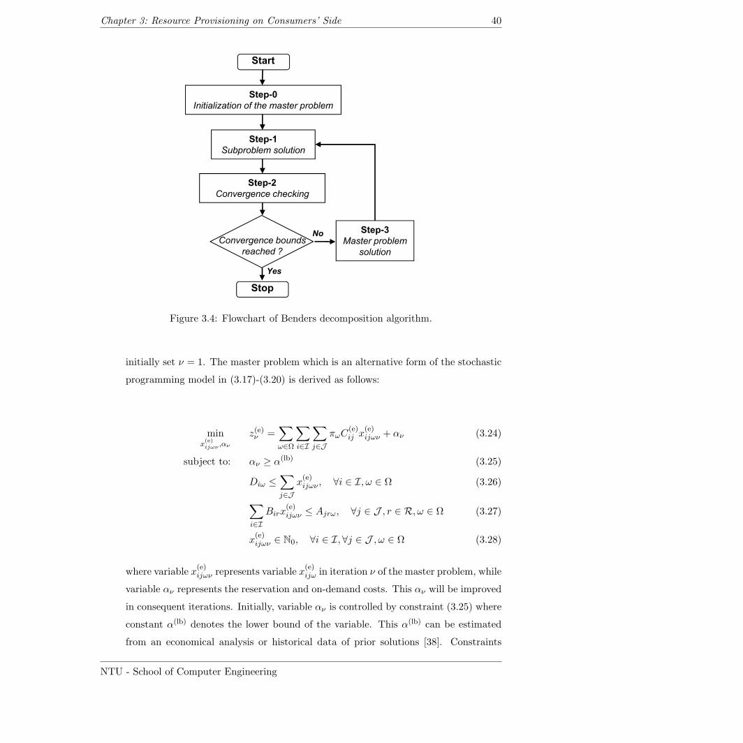
Chapter 3: Resource Provisioning on Consumers’ Side 40
Step-0
Initialization of the master problem
Start
Step-1
Subproblem solution
Step-2
Convergence checking
Step-3
Master problem
solution
Convergence bounds
reached ?
Yes
No
Stop
Figure 3.4: Flowchart of Benders decomposition algorithm.
initially set ν = 1. The master problem which is an alternative form of the stochastic
programming model in (3.17)-(3.20) is derived as follows:
minx(e)ijων ,αν
z(e)ν =∑ω∈Ω
∑i∈I
∑j∈J
πωC(e)ij x
(e)ijων + αν (3.24)
subject to: αν ≥ α(lb) (3.25)
Diω ≤∑j∈J
x(e)ijων , ∀i ∈ I, ω ∈ Ω (3.26)
∑i∈I
Birx(e)ijων ≤ Ajrω, ∀j ∈ J , r ∈ R, ω ∈ Ω (3.27)
x(e)ijων ∈ N0, ∀i ∈ I, ∀j ∈ J , ω ∈ Ω (3.28)
where variable x(e)ijων represents variable x
(e)ijω in iteration ν of the master problem, while
variable αν represents the reservation and on-demand costs. This αν will be improved
in consequent iterations. Initially, variable αν is controlled by constraint (3.25) where
constant α(lb) denotes the lower bound of the variable. This α(lb) can be estimated
from an economical analysis or historical data of prior solutions [38]. Constraints
NTU - School of Computer Engineering
Chapter 3: Resource Provisioning on Consumers’ Side 41
(3.26)–(3.28) govern the boundary of variable x(e)ijων . After the master problem is
solved, the algorithm proceeds to Step-1.
• Step-1: Subproblem solution – Subproblems are formulated and solved. Value of
x(e)ijων obtained from the master problem is assigned to variables x
(fix)ijω . Given the fixed
solution of x(fix)ijω , two aforementioned classes of subproblems, i.e., S1 and S2(ω) can be
solved independently and concurrently. Note that, for the current iteration, variable
x(e)ijω in (3.21) is equivalent to variable x
(e)ijων .
The objective functions of S1 in (3.22) and S2(ω) in (3.23) minimize the reservation
and on-demand costs, respectively. Since subproblem S2(ω) associates with the num-
ber of scenarios |Ω|, independent |Ω| optimization problems can be generated. Let
variables λ(R)ijων and λ
(o)ijων denote the solutions of the dual problems of S1 and S2(ω)
associated with constraint (3.21), respectively. The solution of variables λ(R)ijων and
λ(o)ijων will be later used in Step-3.
• Step-2: Convergence checking – Next, the convergence of lower and upper bounds of
the solutions obtained from master problem and subproblems is checked. Both bounds
are adjusted at each iteration. The lower bound in iteration ν denoted by z(lb)ν can
be obtained from the objective function value of the master problem as follows:
z(lb)ν = z∗(e)ν (3.29)
where z∗(e)ν denotes the objective function value of the solved master problem. The
upper bound in iteration ν denoted by z(ub)ν can be obtained as follows:
z(ub)ν = z∗(e)ν − αν + z∗(R)ν +
∑ω∈Ω
z∗(o)ν (ω) (3.30)
where z∗(R)ν and z
∗(o)ν (ω) denote the objective function values of the solved subproblems
S1 and S2(ω), respectively.
Let ε denote a small tolerance value to verify the convergence of both lower and upper
bounds. The Benders decomposition algorithm stops when the following condition is
met, i.e.,
NTU - School of Computer Engineering
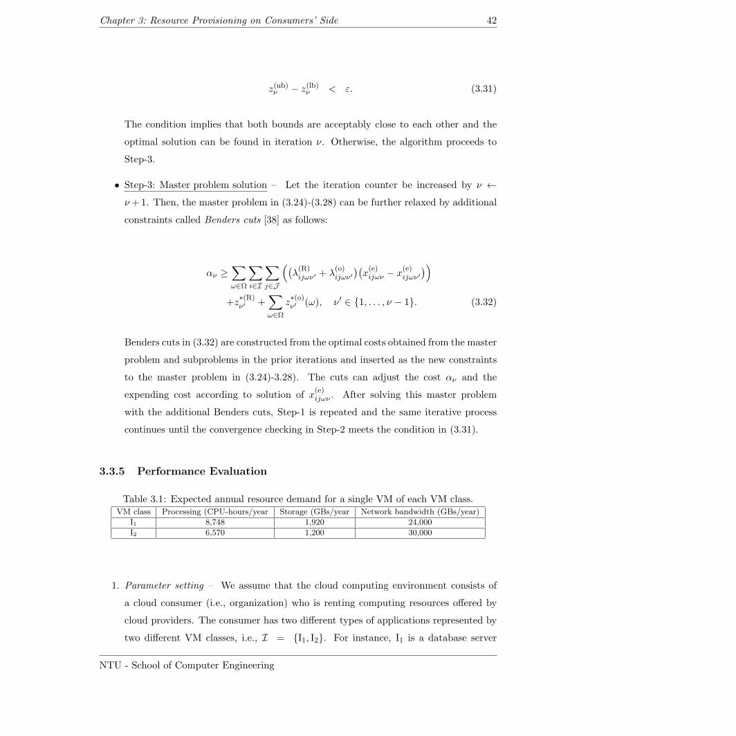
Chapter 3: Resource Provisioning on Consumers’ Side 42
z(ub)ν − z(lb)ν < ε. (3.31)
The condition implies that both bounds are acceptably close to each other and the
optimal solution can be found in iteration ν. Otherwise, the algorithm proceeds to
Step-3.
• Step-3: Master problem solution – Let the iteration counter be increased by ν ←
ν+1. Then, the master problem in (3.24)-(3.28) can be further relaxed by additional
constraints called Benders cuts [38] as follows:
αν ≥∑ω∈Ω
∑i∈I
∑j∈J
((λ(R)ijων′ + λ
(o)ijων′
)(x(e)ijων − x
(e)ijων′
))+z
∗(R)ν′ +
∑ω∈Ω
z∗(o)ν′ (ω), ν ′ ∈ 1, . . . , ν − 1. (3.32)
Benders cuts in (3.32) are constructed from the optimal costs obtained from the master
problem and subproblems in the prior iterations and inserted as the new constraints
to the master problem in (3.24)-3.28). The cuts can adjust the cost αν and the
expending cost according to solution of x(e)ijων . After solving this master problem
with the additional Benders cuts, Step-1 is repeated and the same iterative process
continues until the convergence checking in Step-2 meets the condition in (3.31).
3.3.5 Performance Evaluation
Table 3.1: Expected annual resource demand for a single VM of each VM class.VM class Processing (CPU-hours/year Storage (GBs/year Network bandwidth (GBs/year)
I1 8,748 1,920 24,000
I2 6,570 1,200 30,000
1. Parameter setting – We assume that the cloud computing environment consists of
a cloud consumer (i.e., organization) who is renting computing resources offered by
cloud providers. The consumer has two different types of applications represented by
two different VM classes, i.e., I = I1, I2. For instance, I1 is a database server
NTU - School of Computer Engineering
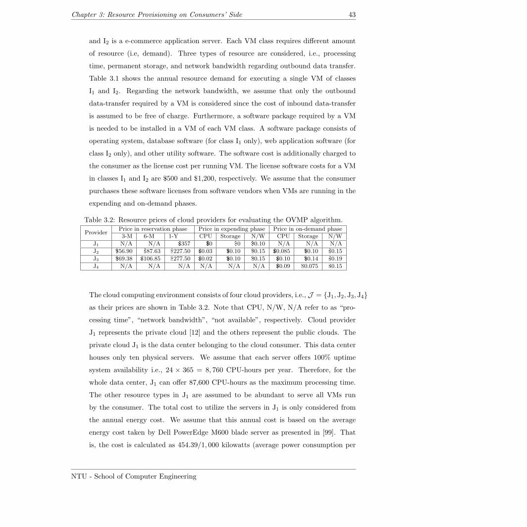
Chapter 3: Resource Provisioning on Consumers’ Side 43
and I2 is a e-commerce application server. Each VM class requires different amount
of resource (i.e, demand). Three types of resource are considered, i.e., processing
time, permanent storage, and network bandwidth regarding outbound data transfer.
Table 3.1 shows the annual resource demand for executing a single VM of classes
I1 and I2. Regarding the network bandwidth, we assume that only the outbound
data-transfer required by a VM is considered since the cost of inbound data-transfer
is assumed to be free of charge. Furthermore, a software package required by a VM
is needed to be installed in a VM of each VM class. A software package consists of
operating system, database software (for class I1 only), web application software (for
class I2 only), and other utility software. The software cost is additionally charged to
the consumer as the license cost per running VM. The license software costs for a VM
in classes I1 and I2 are $500 and $1,200, respectively. We assume that the consumer
purchases these software licenses from software vendors when VMs are running in the
expending and on-demand phases.
Table 3.2: Resource prices of cloud providers for evaluating the OVMP algorithm.
ProviderPrice in reservation phase Price in expending phase Price in on-demand phase3-M 6-M 1-Y CPU Storage N/W CPU Storage N/W
J1 N/A N/A $357 $0 $0 $0.10 N/A N/A N/A
J2 $56.90 $87.63 $227.50 $0.03 $0.10 $0.15 $0.085 $0.10 $0.15
J3 $69.38 $106.85 $277.50 $0.02 $0.10 $0.15 $0.10 $0.14 $0.19
J4 N/A N/A N/A N/A N/A N/A $0.09 $0.075 $0.15
The cloud computing environment consists of four cloud providers, i.e., J = J1, J2, J3, J4
as their prices are shown in Table 3.2. Note that CPU, N/W, N/A refer to as “pro-
cessing time”, “network bandwidth”, “not available”, respectively. Cloud provider
J1 represents the private cloud [12] and the others represent the public clouds. The
private cloud J1 is the data center belonging to the cloud consumer. This data center
houses only ten physical servers. We assume that each server offers 100% uptime
system availability i.e., 24 × 365 = 8, 760 CPU-hours per year. Therefore, for the
whole data center, J1 can offer 87,600 CPU-hours as the maximum processing time.
The other resource types in J1 are assumed to be abundant to serve all VMs run
by the consumer. The total cost to utilize the servers in J1 is only considered from
the annual energy cost. We assume that this annual cost is based on the average
energy cost taken by Dell PowerEdge M600 blade server as presented in [99]. That
is, the cost is calculated as 454.39/1, 000 kilowatts (average power consumption per
NTU - School of Computer Engineering
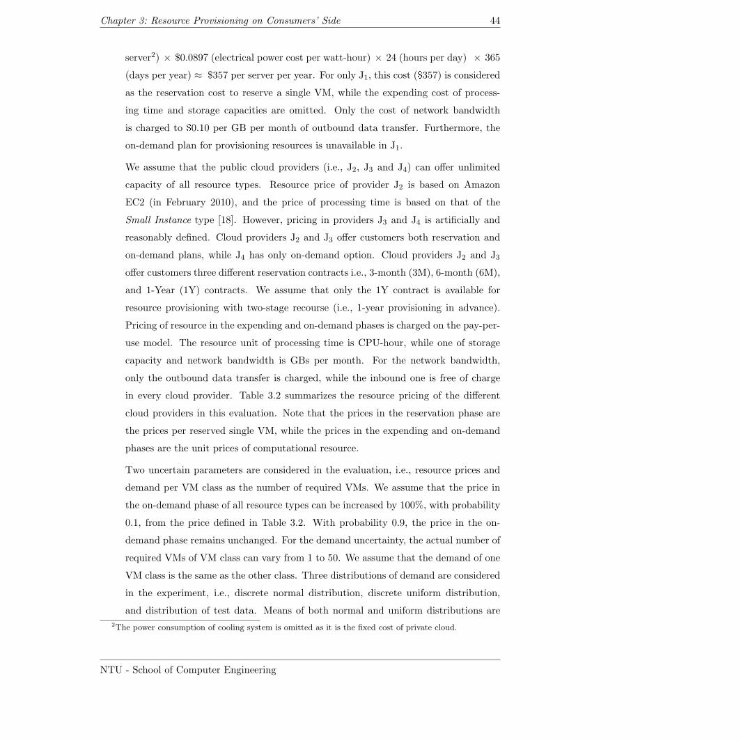
Chapter 3: Resource Provisioning on Consumers’ Side 44
server2) × $0.0897 (electrical power cost per watt-hour) × 24 (hours per day) × 365
(days per year) ≈ $357 per server per year. For only J1, this cost ($357) is considered
as the reservation cost to reserve a single VM, while the expending cost of process-
ing time and storage capacities are omitted. Only the cost of network bandwidth
is charged to $0.10 per GB per month of outbound data transfer. Furthermore, the
on-demand plan for provisioning resources is unavailable in J1.
We assume that the public cloud providers (i.e., J2, J3 and J4) can offer unlimited
capacity of all resource types. Resource price of provider J2 is based on Amazon
EC2 (in February 2010), and the price of processing time is based on that of the
Small Instance type [18]. However, pricing in providers J3 and J4 is artificially and
reasonably defined. Cloud providers J2 and J3 offer customers both reservation and
on-demand plans, while J4 has only on-demand option. Cloud providers J2 and J3
offer customers three different reservation contracts i.e., 3-month (3M), 6-month (6M),
and 1-Year (1Y) contracts. We assume that only the 1Y contract is available for
resource provisioning with two-stage recourse (i.e., 1-year provisioning in advance).
Pricing of resource in the expending and on-demand phases is charged on the pay-per-
use model. The resource unit of processing time is CPU-hour, while one of storage
capacity and network bandwidth is GBs per month. For the network bandwidth,
only the outbound data transfer is charged, while the inbound one is free of charge
in every cloud provider. Table 3.2 summarizes the resource pricing of the different
cloud providers in this evaluation. Note that the prices in the reservation phase are
the prices per reserved single VM, while the prices in the expending and on-demand
phases are the unit prices of computational resource.
Two uncertain parameters are considered in the evaluation, i.e., resource prices and
demand per VM class as the number of required VMs. We assume that the price in
the on-demand phase of all resource types can be increased by 100%, with probability
0.1, from the price defined in Table 3.2. With probability 0.9, the price in the on-
demand phase remains unchanged. For the demand uncertainty, the actual number of
required VMs of VM class can vary from 1 to 50. We assume that the demand of one
VM class is the same as the other class. Three distributions of demand are considered
in the experiment, i.e., discrete normal distribution, discrete uniform distribution,
and distribution of test data. Means of both normal and uniform distributions are
2The power consumption of cooling system is omitted as it is the fixed cost of private cloud.
NTU - School of Computer Engineering
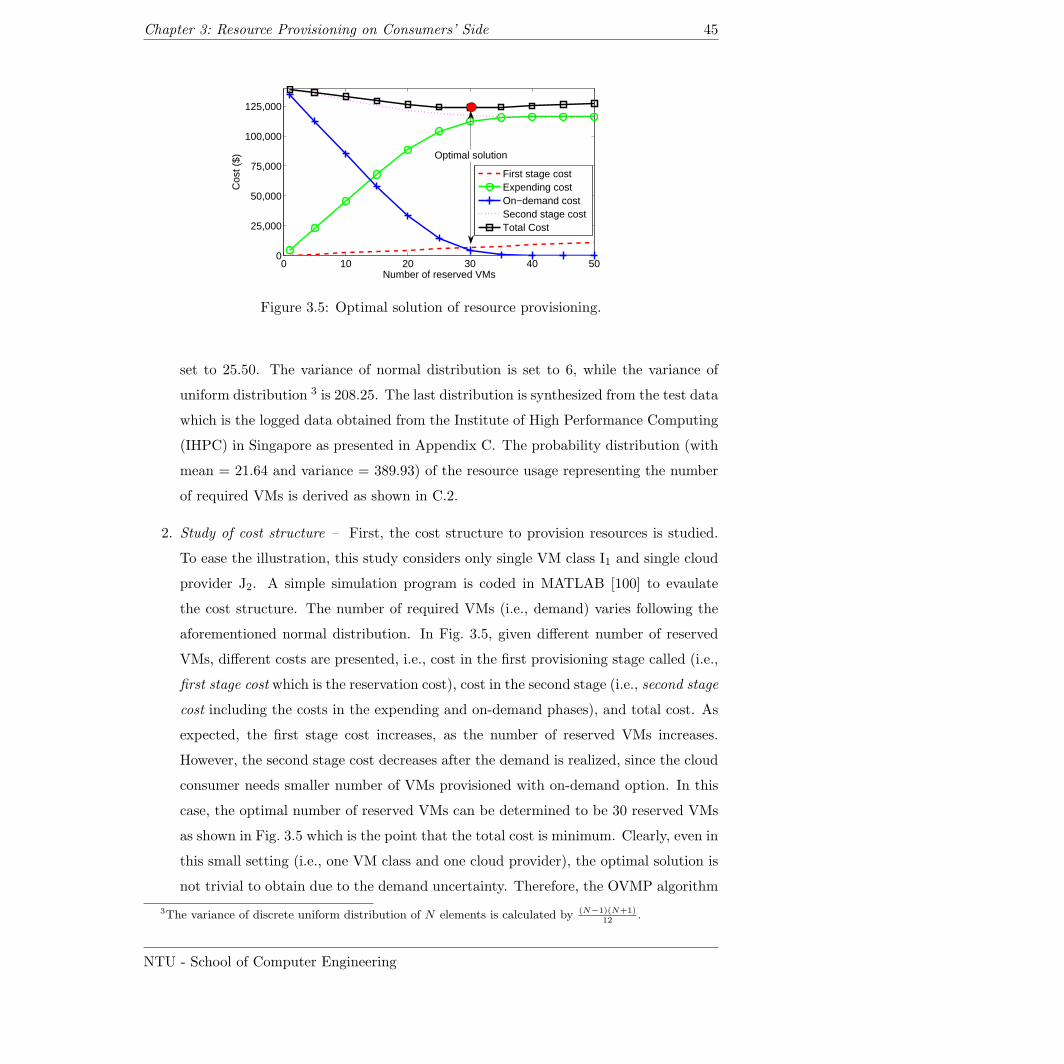
Chapter 3: Resource Provisioning on Consumers’ Side 45
0 10 20 30 40 500
25,000
50,000
75,000
100,000
125,000
Number of reserved VMs
Cos
t ($)
First stage costExpending costOn−demand costSecond stage costTotal Cost
Optimal solution
Figure 3.5: Optimal solution of resource provisioning.
set to 25.50. The variance of normal distribution is set to 6, while the variance of
uniform distribution 3 is 208.25. The last distribution is synthesized from the test data
which is the logged data obtained from the Institute of High Performance Computing
(IHPC) in Singapore as presented in Appendix C. The probability distribution (with
mean = 21.64 and variance = 389.93) of the resource usage representing the number
of required VMs is derived as shown in C.2.
2. Study of cost structure – First, the cost structure to provision resources is studied.
To ease the illustration, this study considers only single VM class I1 and single cloud
provider J2. A simple simulation program is coded in MATLAB [100] to evaulate
the cost structure. The number of required VMs (i.e., demand) varies following the
aforementioned normal distribution. In Fig. 3.5, given different number of reserved
VMs, different costs are presented, i.e., cost in the first provisioning stage called (i.e.,
first stage cost which is the reservation cost), cost in the second stage (i.e., second stage
cost including the costs in the expending and on-demand phases), and total cost. As
expected, the first stage cost increases, as the number of reserved VMs increases.
However, the second stage cost decreases after the demand is realized, since the cloud
consumer needs smaller number of VMs provisioned with on-demand option. In this
case, the optimal number of reserved VMs can be determined to be 30 reserved VMs
as shown in Fig. 3.5 which is the point that the total cost is minimum. Clearly, even in
this small setting (i.e., one VM class and one cloud provider), the optimal solution is
not trivial to obtain due to the demand uncertainty. Therefore, the OVMP algorithm
3The variance of discrete uniform distribution of N elements is calculated by (N−1)(N+1)12
.
NTU - School of Computer Engineering
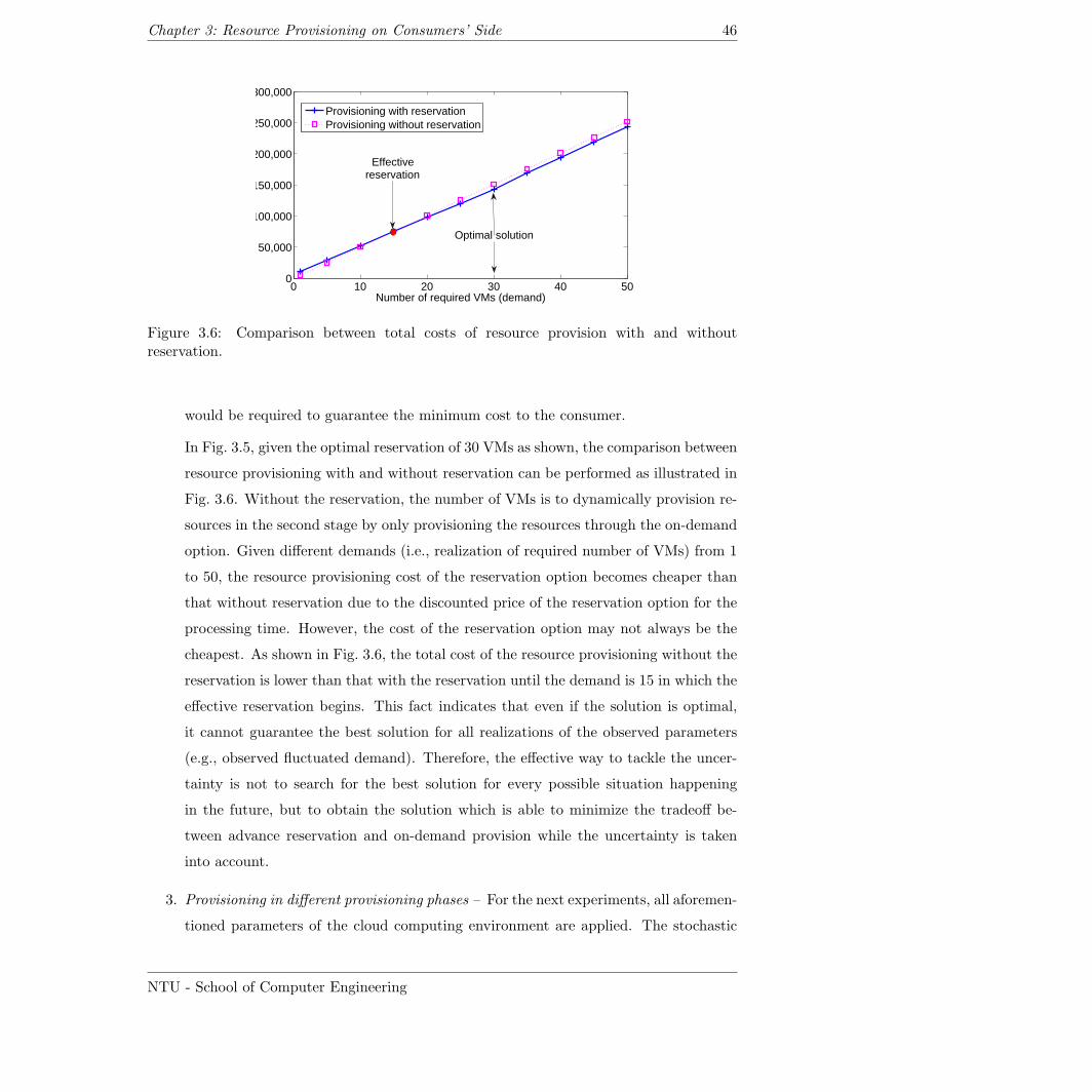
Chapter 3: Resource Provisioning on Consumers’ Side 46
0 10 20 30 40 500
50,000
100,000
150,000
200,000
250,000
300,000
Number of required VMs (demand)
Provisioning with reservationProvisioning without reservation
Optimal solution
Effectivereservation
Figure 3.6: Comparison between total costs of resource provision with and withoutreservation.
would be required to guarantee the minimum cost to the consumer.
In Fig. 3.5, given the optimal reservation of 30 VMs as shown, the comparison between
resource provisioning with and without reservation can be performed as illustrated in
Fig. 3.6. Without the reservation, the number of VMs is to dynamically provision re-
sources in the second stage by only provisioning the resources through the on-demand
option. Given different demands (i.e., realization of required number of VMs) from 1
to 50, the resource provisioning cost of the reservation option becomes cheaper than
that without reservation due to the discounted price of the reservation option for the
processing time. However, the cost of the reservation option may not always be the
cheapest. As shown in Fig. 3.6, the total cost of the resource provisioning without the
reservation is lower than that with the reservation until the demand is 15 in which the
effective reservation begins. This fact indicates that even if the solution is optimal,
it cannot guarantee the best solution for all realizations of the observed parameters
(e.g., observed fluctuated demand). Therefore, the effective way to tackle the uncer-
tainty is not to search for the best solution for every possible situation happening
in the future, but to obtain the solution which is able to minimize the tradeoff be-
tween advance reservation and on-demand provision while the uncertainty is taken
into account.
3. Provisioning in different provisioning phases – For the next experiments, all aforemen-
tioned parameters of the cloud computing environment are applied. The stochastic
NTU - School of Computer Engineering
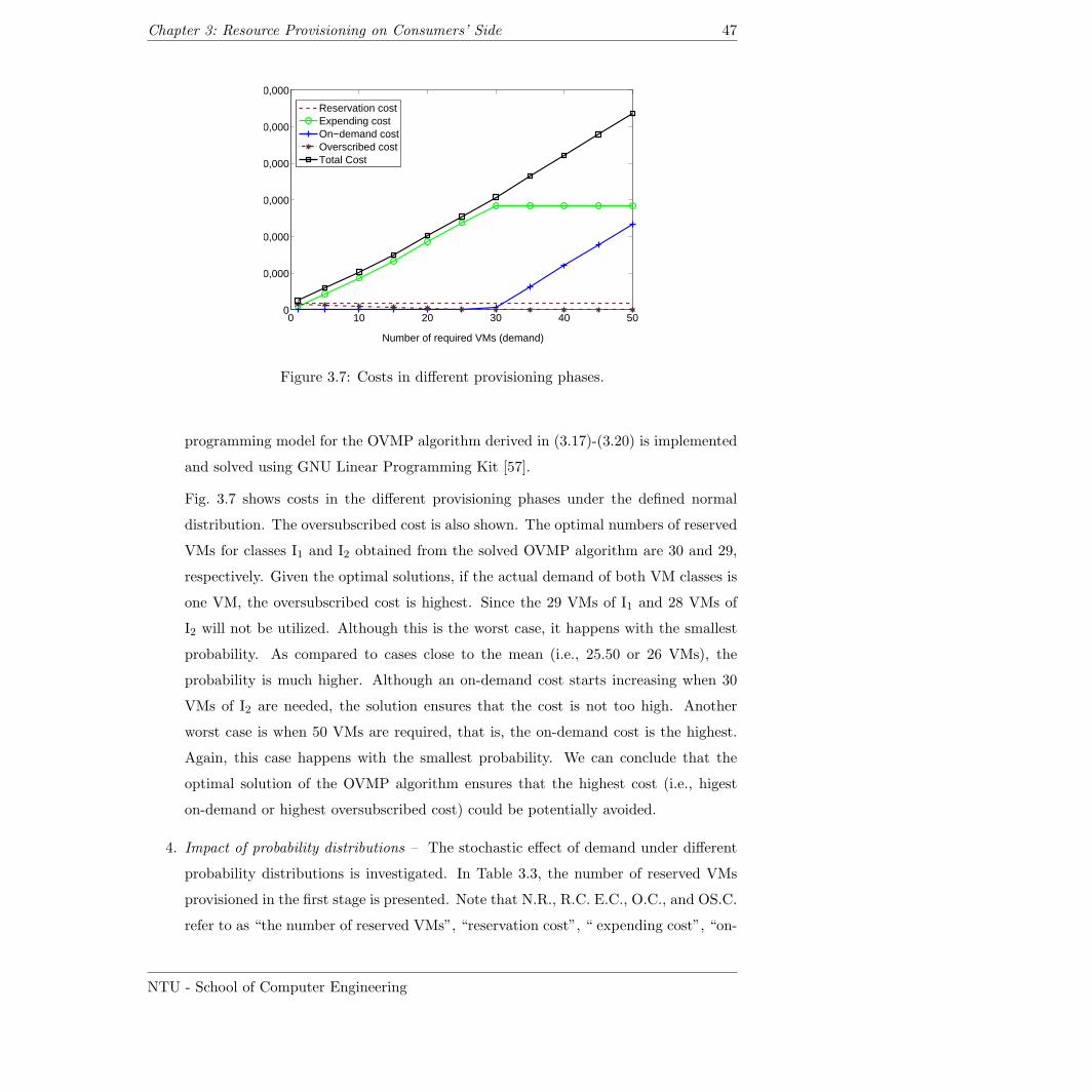
Chapter 3: Resource Provisioning on Consumers’ Side 47
0 10 20 30 40 500
100,000
200,000
300,000
400,000
500,000
600,000
Number of required VMs (demand)
Reservation costExpending costOn−demand costOverscribed costTotal Cost
Figure 3.7: Costs in different provisioning phases.
programming model for the OVMP algorithm derived in (3.17)-(3.20) is implemented
and solved using GNU Linear Programming Kit [57].
Fig. 3.7 shows costs in the different provisioning phases under the defined normal
distribution. The oversubscribed cost is also shown. The optimal numbers of reserved
VMs for classes I1 and I2 obtained from the solved OVMP algorithm are 30 and 29,
respectively. Given the optimal solutions, if the actual demand of both VM classes is
one VM, the oversubscribed cost is highest. Since the 29 VMs of I1 and 28 VMs of
I2 will not be utilized. Although this is the worst case, it happens with the smallest
probability. As compared to cases close to the mean (i.e., 25.50 or 26 VMs), the
probability is much higher. Although an on-demand cost starts increasing when 30
VMs of I2 are needed, the solution ensures that the cost is not too high. Another
worst case is when 50 VMs are required, that is, the on-demand cost is the highest.
Again, this case happens with the smallest probability. We can conclude that the
optimal solution of the OVMP algorithm ensures that the highest cost (i.e., higest
on-demand or highest oversubscribed cost) could be potentially avoided.
4. Impact of probability distributions – The stochastic effect of demand under different
probability distributions is investigated. In Table 3.3, the number of reserved VMs
provisioned in the first stage is presented. Note that N.R., R.C. E.C., O.C., and OS.C.
refer to as “the number of reserved VMs”, “reservation cost”, “ expending cost”, “on-
NTU - School of Computer Engineering
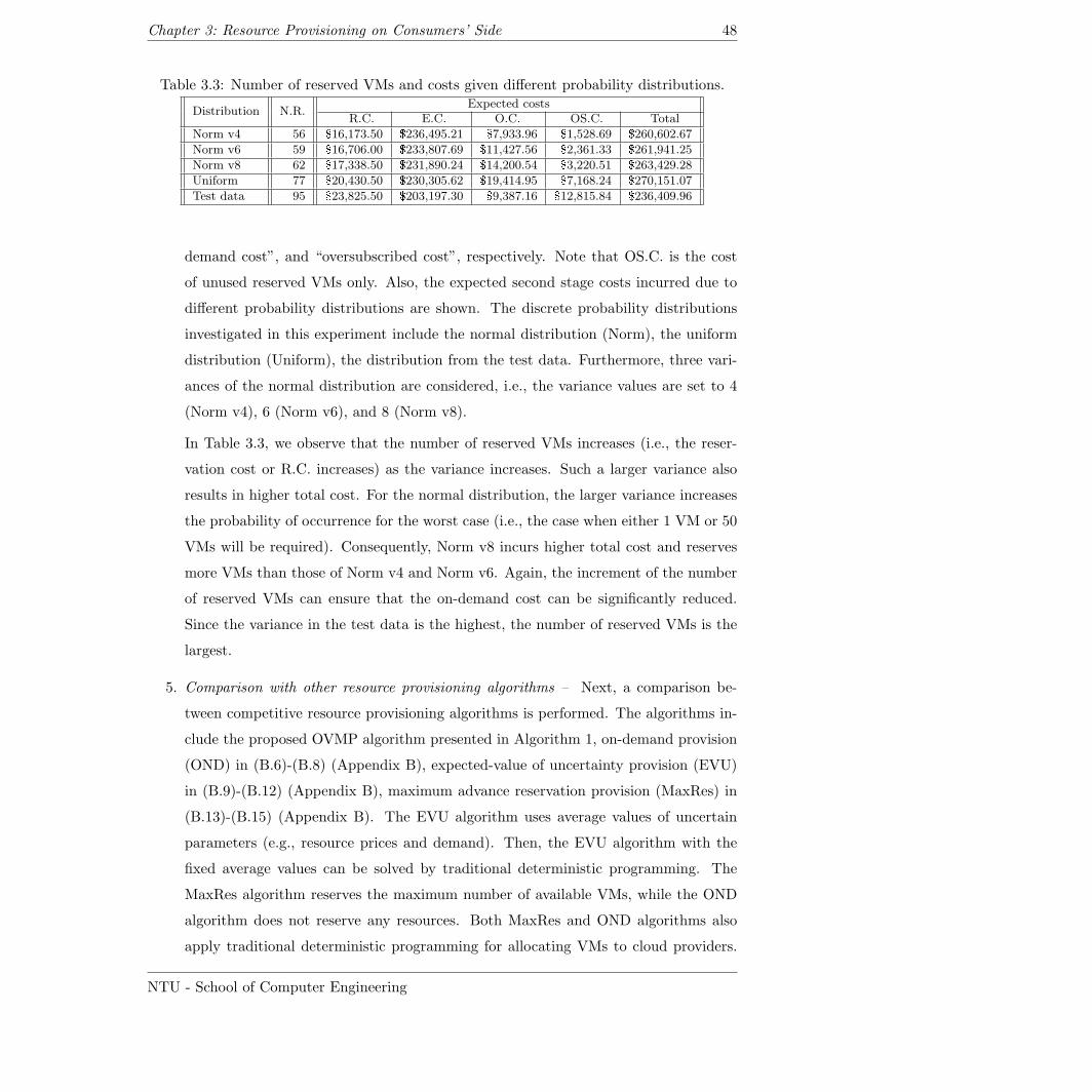
Chapter 3: Resource Provisioning on Consumers’ Side 48
Table 3.3: Number of reserved VMs and costs given different probability distributions.
Distribution N.R.Expected costs
R.C. E.C. O.C. OS.C. Total
Norm v4 56 $16,173.50 $236,495.21 $7,933.96 $1,528.69 $260,602.67
Norm v6 59 $16,706.00 $233,807.69 $11,427.56 $2,361.33 $261,941.25
Norm v8 62 $17,338.50 $231,890.24 $14,200.54 $3,220.51 $263,429.28
Uniform 77 $20,430.50 $230,305.62 $19,414.95 $7,168.24 $270,151.07
Test data 95 $23,825.50 $203,197.30 $9,387.16 $12,815.84 $236,409.96
demand cost”, and “oversubscribed cost”, respectively. Note that OS.C. is the cost
of unused reserved VMs only. Also, the expected second stage costs incurred due to
different probability distributions are shown. The discrete probability distributions
investigated in this experiment include the normal distribution (Norm), the uniform
distribution (Uniform), the distribution from the test data. Furthermore, three vari-
ances of the normal distribution are considered, i.e., the variance values are set to 4
(Norm v4), 6 (Norm v6), and 8 (Norm v8).
In Table 3.3, we observe that the number of reserved VMs increases (i.e., the reser-
vation cost or R.C. increases) as the variance increases. Such a larger variance also
results in higher total cost. For the normal distribution, the larger variance increases
the probability of occurrence for the worst case (i.e., the case when either 1 VM or 50
VMs will be required). Consequently, Norm v8 incurs higher total cost and reserves
more VMs than those of Norm v4 and Norm v6. Again, the increment of the number
of reserved VMs can ensure that the on-demand cost can be significantly reduced.
Since the variance in the test data is the highest, the number of reserved VMs is the
largest.
5. Comparison with other resource provisioning algorithms – Next, a comparison be-
tween competitive resource provisioning algorithms is performed. The algorithms in-
clude the proposed OVMP algorithm presented in Algorithm 1, on-demand provision
(OND) in (B.6)-(B.8) (Appendix B), expected-value of uncertainty provision (EVU)
in (B.9)-(B.12) (Appendix B), maximum advance reservation provision (MaxRes) in
(B.13)-(B.15) (Appendix B). The EVU algorithm uses average values of uncertain
parameters (e.g., resource prices and demand). Then, the EVU algorithm with the
fixed average values can be solved by traditional deterministic programming. The
MaxRes algorithm reserves the maximum number of available VMs, while the OND
algorithm does not reserve any resources. Both MaxRes and OND algorithms also
apply traditional deterministic programming for allocating VMs to cloud providers.
NTU - School of Computer Engineering
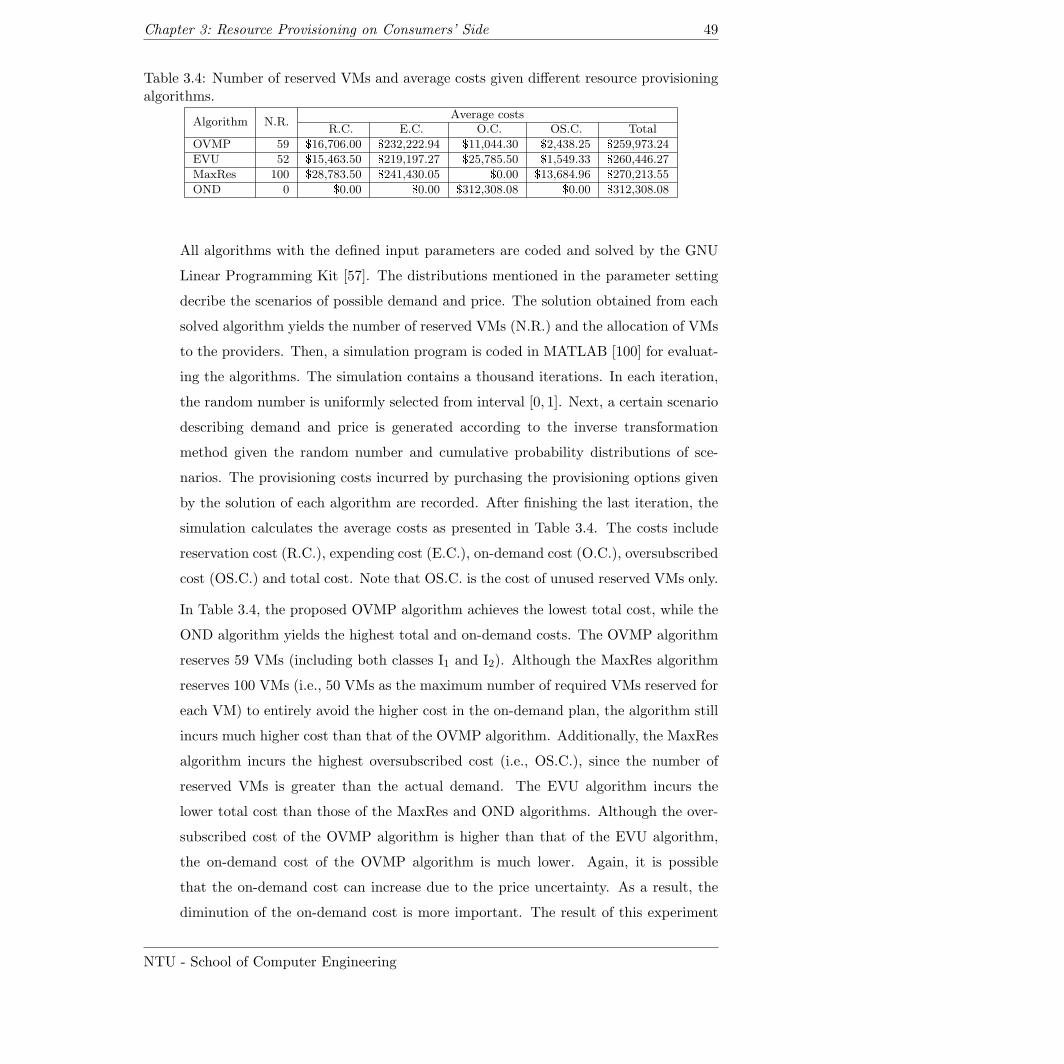
Chapter 3: Resource Provisioning on Consumers’ Side 49
Table 3.4: Number of reserved VMs and average costs given different resource provisioningalgorithms.
Algorithm N.R.Average costs
R.C. E.C. O.C. OS.C. Total
OVMP 59 $16,706.00 $232,222.94 $11,044.30 $2,438.25 $259,973.24
EVU 52 $15,463.50 $219,197.27 $25,785.50 $1,549.33 $260,446.27
MaxRes 100 $28,783.50 $241,430.05 $0.00 $13,684.96 $270,213.55
OND 0 $0.00 $0.00 $312,308.08 $0.00 $312,308.08
All algorithms with the defined input parameters are coded and solved by the GNU
Linear Programming Kit [57]. The distributions mentioned in the parameter setting
decribe the scenarios of possible demand and price. The solution obtained from each
solved algorithm yields the number of reserved VMs (N.R.) and the allocation of VMs
to the providers. Then, a simulation program is coded in MATLAB [100] for evaluat-
ing the algorithms. The simulation contains a thousand iterations. In each iteration,
the random number is uniformly selected from interval [0, 1]. Next, a certain scenario
describing demand and price is generated according to the inverse transformation
method given the random number and cumulative probability distributions of sce-
narios. The provisioning costs incurred by purchasing the provisioning options given
by the solution of each algorithm are recorded. After finishing the last iteration, the
simulation calculates the average costs as presented in Table 3.4. The costs include
reservation cost (R.C.), expending cost (E.C.), on-demand cost (O.C.), oversubscribed
cost (OS.C.) and total cost. Note that OS.C. is the cost of unused reserved VMs only.
In Table 3.4, the proposed OVMP algorithm achieves the lowest total cost, while the
OND algorithm yields the highest total and on-demand costs. The OVMP algorithm
reserves 59 VMs (including both classes I1 and I2). Although the MaxRes algorithm
reserves 100 VMs (i.e., 50 VMs as the maximum number of required VMs reserved for
each VM) to entirely avoid the higher cost in the on-demand plan, the algorithm still
incurs much higher cost than that of the OVMP algorithm. Additionally, the MaxRes
algorithm incurs the highest oversubscribed cost (i.e., OS.C.), since the number of
reserved VMs is greater than the actual demand. The EVU algorithm incurs the
lower total cost than those of the MaxRes and OND algorithms. Although the over-
subscribed cost of the OVMP algorithm is higher than that of the EVU algorithm,
the on-demand cost of the OVMP algorithm is much lower. Again, it is possible
that the on-demand cost can increase due to the price uncertainty. As a result, the
diminution of the on-demand cost is more important. The result of this experiment
NTU - School of Computer Engineering
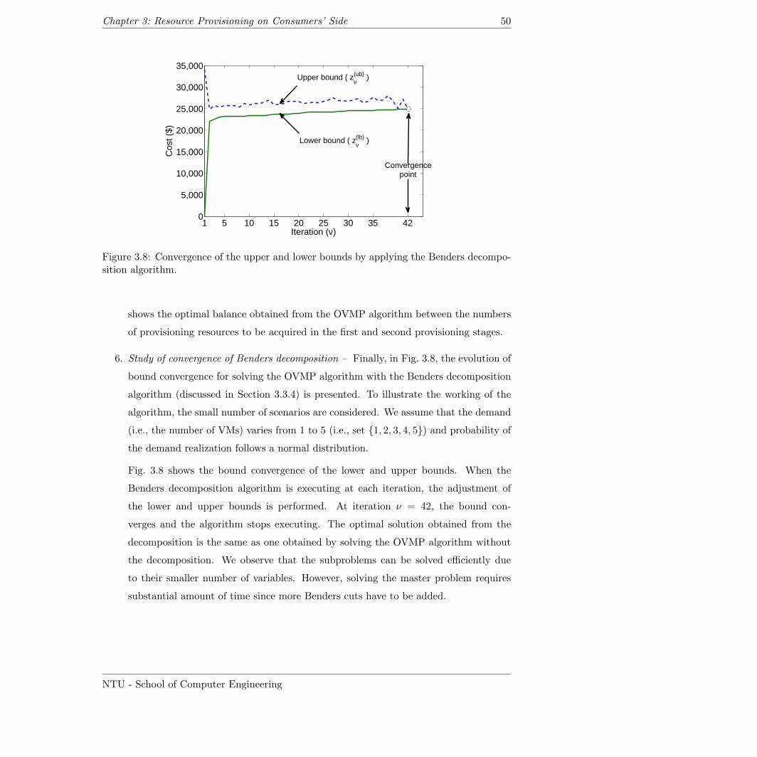
Chapter 3: Resource Provisioning on Consumers’ Side 50
1 5 10 15 20 25 30 35 420
5,000
10,000
15,000
20,000
25,000
30,000
35,000
Iteration (ν)
Cos
t ($)
Convergencepoint
Upper bound ( zν(ub) )
Lower bound ( zν(lb) )
Figure 3.8: Convergence of the upper and lower bounds by applying the Benders decompo-sition algorithm.
shows the optimal balance obtained from the OVMP algorithm between the numbers
of provisioning resources to be acquired in the first and second provisioning stages.
6. Study of convergence of Benders decomposition – Finally, in Fig. 3.8, the evolution of
bound convergence for solving the OVMP algorithm with the Benders decomposition
algorithm (discussed in Section 3.3.4) is presented. To illustrate the working of the
algorithm, the small number of scenarios are considered. We assume that the demand
(i.e., the number of VMs) varies from 1 to 5 (i.e., set 1, 2, 3, 4, 5) and probability of
the demand realization follows a normal distribution.
Fig. 3.8 shows the bound convergence of the lower and upper bounds. When the
Benders decomposition algorithm is executing at each iteration, the adjustment of
the lower and upper bounds is performed. At iteration ν = 42, the bound con-
verges and the algorithm stops executing. The optimal solution obtained from the
decomposition is the same as one obtained by solving the OVMP algorithm without
the decomposition. We observe that the subproblems can be solved efficiently due
to their smaller number of variables. However, solving the master problem requires
substantial amount of time since more Benders cuts have to be added.
NTU - School of Computer Engineering
Chapter 3: Resource Provisioning on Consumers’ Side 51
3.4 Resource Provisioning with Robust Optimization
In this section, we present the resource provisioning algorithm based on the robust opti-
mization. With the robust optimization, the optimal solution obtained from the algorithm
can offer both solution- and model-robustness which is not addressed in the stochastic
programming.
3.4.1 Overview of Resource Provisioning with Robust Optimization
As presented in the previous sections, the resource provisioning algorithms based on stochas-
tic programming (SP) are applied to address the resource provisioning under the uncertain-
ties. However, the algorithms ignore moderate and high-risk decisions which are preferred
by risk averse decision makers. To address this issue, the robust optimization (RO) can
be applied to satisfy the decision makers’ preferences to tackle risks under the uncertain-
ties [29]. While SP considers only the first moment of probability distribution to describe
the uncertainty (i.e., an expected value), RO leverages higher moments (e.g., a variance).
With the higher moments, the optimal solution obtained from RO is less sensitive to the un-
certainties and the solution-robustness can be achieved. Furthermore, unlike SP, a penalty
function can be used to deal with constraint violations and increase the model-robustness.
In this section, a robust cloud resource provisioning (RCRP) algorithm is proposed to min-
imize the total resource provisioning cost, while the uncertainties (e.g., price and demand
uncertainties) are taken into account. The solution of the algorithm is obtained by formulat-
ing and solving a robust optimization model. Numerical studies are extensively performed
in which the results show that the obtained solution can achieve both solution- and model-
robustness. That is, the total resource provisioning cost is close to the optimality (i.e.,
solution robustness) and both on-demand and oversubscribed costs as the risks in resource
provisioning can be significantly decreased (i.e., model robustness).
3.4.2 General Form of Robust Optimization Model
The system model of cloud computing and assumption defined in Section 3.1 and Sec-
tion 3.3.1 are applied for deriving the robust optimization model. The stochastic program-
NTU - School of Computer Engineering
Chapter 3: Resource Provisioning on Consumers’ Side 52
ming model derived in (3.17)-(3.20) can be extended to the robust optimization model as
follows:
minx(R)ij ,x
(e)ijω ,x
(o)ijω
∑ω∈Ω
πω ξω + γ∑ω∈Ω
πω σω + β∑ω∈Ω
πω ρω (3.33)
subject to (3.5), (3.11), (3.12), (3.18), (3.19), (3.20)
where ξω represents the total resource provisioning cost in all provisioning phases given
scenario ω, namely
ξω =∑i∈I
∑j∈J
(C
(R)ij x
(R)ij + C
(e)ij x
(e)ijω + c
(o)ijω x
(o)ijω
). (3.34)
As shown in objective function (3.33), the model is considered a multi-criteria optimization
consisting of three terms. The first term (i.e.,∑
ω∈Ω πω ξω) represents the expected total
resource provisioning cost which is the first moment of distribution of ξω. The second term
weighted by γ forms higher moments of the distribution of ξω. Based on the mean/variance
models [29], the variance of the distribution can be applied to σω. A value of weighting
constant γ represents the cost of deviation from the mean. The last term weighted by β
represents a feasibility penalty function ρω. To deal with the uncertainties, this function is
used to penalize violations of constraints in (3.18)–(3.20) under some scenarios. With the
penalty function, the variables with the uncertainties (i.e., x(e)ijω and x
(o)ijω) will be adjusted
to avoid the cost of the penalty defined by the weighting constant β.
Function σω represents the variance of distribution of ξω. A quadratic function can be
applied for function σω as follows:
σω =
(ξω −
∑ω′∈Ω
πω′ ξω′
)2
(3.35)
The goal of penalty function ρω with weight β in (3.33) is to avoid the undesired over-
provisioning and underprovisioning problems (i.e., the risks in resource provisioning). The
function can be formulated as follows:
NTU - School of Computer Engineering
Chapter 3: Resource Provisioning on Consumers’ Side 53
ρω = ρ+ω + ρ−ω (3.36)
where ρ+ω =∑i∈I
∑j∈J
β+ijω
(x(R)ij − x
(e)ijω
)ρ−ω =
∑i∈I
∑j∈J
β−ijω x(o)ijω.
Function ρω in (3.36) embraces two cost functions representing two different violation con-
straints, i.e., ρ+ω and ρ−ω to penalize overprovisioning (i.e., x(R)ij − x
(e)ijω > 0) and underpro-
visioning (i.e., x(o)ijω > 0), respectively. Two types of penalty weights, i.e., β+ijω or overpro-
visioning weights and β−ijω or underprovisioning weights represent the penalty costs of ρ+ω
and ρ−ω , respectively. For our guideline, the values of β+ijω and β−ijω should be proportional
to the reservation and on-demand costs, respectively. For ease of setting, let β+ijω = b+c(R)ij
and β−ijω = b−C(o)ijω, where b
+ ≥ 0 and b− ≥ 0 denote the coefficients of C(R)ij and C
(o)ijs ,
respectively.
3.4.3 Solution and Model Robustness
The RO model integrates the goal programming, since γ ≥ 0 and β ≥ 0 in objective function
(3.33) can vary to adjust the tradeoff between solution- and model-robustness. In terms of
RO, the obtained solution is solution-robust when it is almost optimal for any realization
ω ∈ Ω. The solution is model-robust when it is almost feasible, that is, the violation of
constraints can almost be avoided for any realizations ω ∈ Ω. In (3.33), the first and second
terms are formulated for the solution-robustness, whereas the last term is formulated for
the model-robustness.
A decision maker can seek a desirable balance of both robustness by varying the values of
γ and β. For example, a decision maker can apply a larger value of γ when the decision
maker prefers the solution-robustness which results less deviate from the optimality for
any realization. In contrast, the decision maker can set a larger value of β to achieve the
model-robustness which is to avoid underprovisioning and overprovisioning problems for
any realization. Note that if both γ and β are set to be zero, the RO model becomes the
equivalent SP model [101].
NTU - School of Computer Engineering
Chapter 3: Resource Provisioning on Consumers’ Side 54
3.4.4 Robust Cloud Resource Provisioning Algorithm
In this part, the robust cloud resource provisioning (RCRP) algorithm is presented by im-
proving the robust optimization model derived in Section (3.4.2). In Section (3.4.2), the
disadvantage of quadratic function σω in (3.35) results in higher computational complexity.
In particular, the optimization model in (3.33) can be considered a quadratic programming
model which requires more computational time to solve the model. To deal with the com-
plexity, the approach used in [102] can be applied, that is, non-negative variables θω are
added to the model to redefine function σω as follows:
σω = ξω −∑ω′∈Ω
πω′ ξω′ + 2 θω. (3.37)
σω in (3.37) is a linear function whose complexity is much less than that of (3.35). Additional
constraints to govern θω must be inserted to the model as follows:
ξω −∑ω′∈Ω
πω′ ξω′ + θω ≥ 0, ∀ω ∈ Ω (3.38)
θω ≥ 0, ∀ω ∈ Ω. (3.39)
In (3.37)–(3.39), σω always generates a non-negative value by adjusting θω. It can be verified
that if ξω −∑
ω′∈Ω πω′ ξω′ < 0, then θω =∑
ω′∈Ω πω′ ξω′ − ξω and σω = θω. Otherwise,
θω = 0 and σω = ξω −∑
ω′∈Ω πω′ ξω′ .
Algorithm 2 Robust Cloud Resource Provisioning Algorithm
Input: πω, C(R)ij , C
(e)ij , C
(o)ijω, Diω, Bir, Ajrω, γ, β
+ijω, and β
−ijω.
Output: x∗.
1: x∗ ← solve model in (3.40).
2: Wait until the second provisioning stage occurs.
3: Observe scenario ω.
4: Apply the recourse action for observed scenario ω based on x∗.
5: return x∗.
NTU - School of Computer Engineering
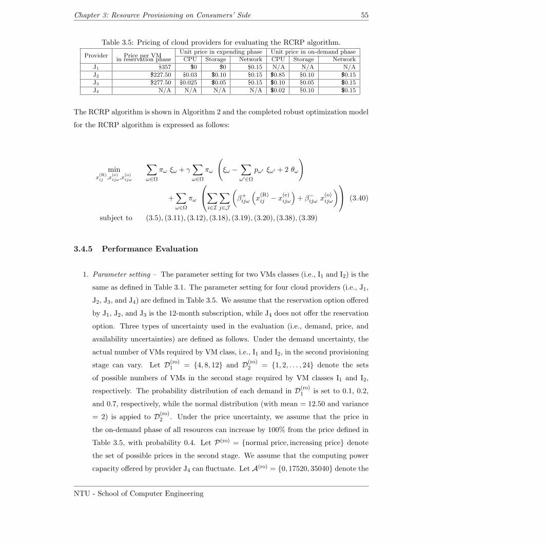
Chapter 3: Resource Provisioning on Consumers’ Side 55
Table 3.5: Pricing of cloud providers for evaluating the RCRP algorithm.
Provider Price per VMUnit price in expending phase Unit price in on-demand phase
in reservation phase CPU Storage Network CPU Storage Network
J1 $357 $0 $0 $0.15 N/A N/A N/A
J2 $227.50 $0.03 $0.10 $0.15 $0.85 $0.10 $0.15
J3 $277.50 $0.025 $0.05 $0.15 $0.10 $0.05 $0.15
J4 N/A N/A N/A N/A $0.02 $0.10 $0.15
The RCRP algorithm is shown in Algorithm 2 and the completed robust optimization model
for the RCRP algorithm is expressed as follows:
minx(R)ij ,x
(e)ijω ,x
(o)ijω
∑ω∈Ω
πω ξω + γ∑ω∈Ω
πω
(ξω −
∑ω′∈Ω
pω′ ξω′ + 2 θω
)
+∑ω∈Ω
πω
∑i∈I
∑j∈J
(β+ijω
(x(R)ij − x
(e)ijω
)+ β−ijω x
(o)ijω
) (3.40)
subject to (3.5), (3.11), (3.12), (3.18), (3.19), (3.20), (3.38), (3.39)
3.4.5 Performance Evaluation
1. Parameter setting – The parameter setting for two VMs classes (i.e., I1 and I2) is the
same as defined in Table 3.1. The parameter setting for four cloud providers (i.e., J1,
J2, J3, and J4) are defined in Table 3.5. We assume that the reservation option offered
by J1, J2, and J3 is the 12-month subscription, while J4 does not offer the reservation
option. Three types of uncertainty used in the evaluation (i.e., demand, price, and
availability uncertainties) are defined as follows. Under the demand uncertainty, the
actual number of VMs required by VM class, i.e., I1 and I2, in the second provisioning
stage can vary. Let D(ro)1 = 4, 8, 12 and D(ro)
2 = 1, 2, . . . , 24 denote the sets
of possible numbers of VMs in the second stage required by VM classes I1 and I2,
respectively. The probability distribution of each demand in D(ro)1 is set to 0.1, 0.2,
and 0.7, respectively, while the normal distribution (with mean = 12.50 and variance
= 2) is appied to D(ro)2 . Under the price uncertainty, we assume that the price in
the on-demand phase of all resources can increase by 100% from the price defined in
Table 3.5, with probability 0.4. Let P(ro) = normal price, increasing price denote
the set of possible prices in the second stage. We assume that the computing power
capacity offered by provider J4 can fluctuate. Let A(ro) = 0, 17520, 35040 denote the
NTU - School of Computer Engineering
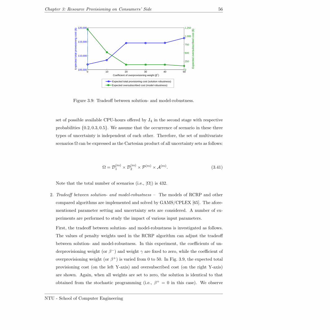
Chapter 3: Resource Provisioning on Consumers’ Side 56
0 10 20 30 40 50105,000
110,000
115,000
120,000
Coefficient of overprovisioning weight (β+)
Exp
ecte
d to
tal p
rovi
sion
ing
cost
($)
0
250
500
750
1,000
1,250
Exp
ecte
d ov
ersu
bscr
ibed
cos
t ($)
Expected total provisioning cost (solution robustness)
Expected oversubscribed cost (model robustness)
Figure 3.9: Tradeoff between solution- and model-robustness.
set of possible available CPU-hours offered by J4 in the second stage with respective
probabilities 0.2, 0.3, 0.5. We assume that the occurrence of scenario in these three
types of uncertainty is independent of each other. Therefore, the set of multivariate
scenarios Ω can be expressed as the Cartesian product of all uncertainty sets as follows:
Ω = D(ro)1 ×D(ro)
2 × P(ro) ×A(ro). (3.41)
Note that the total number of scenarios (i.e., |Ω|) is 432.
2. Tradeoff between solution- and model-robustness – The models of RCRP and other
compared algorithms are implemented and solved by GAMS/CPLEX [65]. The afore-
mentioned parameter setting and uncertainty sets are considered. A number of ex-
periments are performed to study the impact of various input parameters.
First, the tradeoff between solution- and model-robustness is investigated as follows.
The values of penalty weights used in the RCRP algorithm can adjust the tradeoff
between solution- and model-robustness. In this experiment, the coefficients of un-
derprovisioning weight (or β−) and weight γ are fixed to zero, while the coefficient of
overprovisioning weight (or β+) is varied from 0 to 50. In Fig. 3.9, the expected total
provisioning cost (on the left Y-axis) and oversubscribed cost (on the right Y-axis)
are shown. Again, when all weights are set to zero, the solution is identical to that
obtained from the stochastic programming (i.e., β+ = 0 in this case). We observe
NTU - School of Computer Engineering
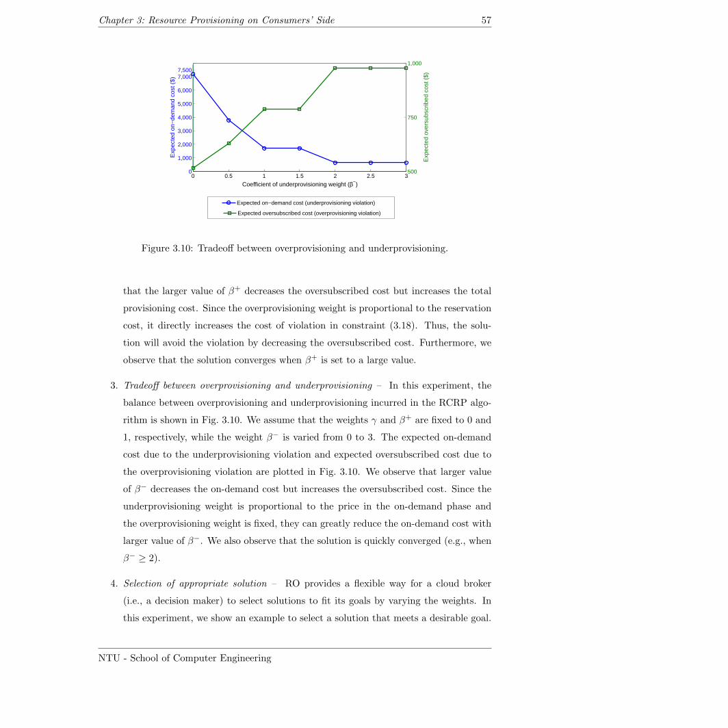
Chapter 3: Resource Provisioning on Consumers’ Side 57
0 0.5 1 1.5 2 2.5 30
1,000
2,000
3,000
4,000
5,000
6,000
7,0007,500
Coefficient of underprovisioning weight (β−)E
xpec
ted
on−
dem
and
cost
($)
500
750
1,000
Exp
ecte
d ov
ersu
bscr
ibed
cos
t ($)
Expected on−demand cost (underprovisioning violation)
Expected oversubscribed cost (overprovisioning violation)
Figure 3.10: Tradeoff between overprovisioning and underprovisioning.
that the larger value of β+ decreases the oversubscribed cost but increases the total
provisioning cost. Since the overprovisioning weight is proportional to the reservation
cost, it directly increases the cost of violation in constraint (3.18). Thus, the solu-
tion will avoid the violation by decreasing the oversubscribed cost. Furthermore, we
observe that the solution converges when β+ is set to a large value.
3. Tradeoff between overprovisioning and underprovisioning – In this experiment, the
balance between overprovisioning and underprovisioning incurred in the RCRP algo-
rithm is shown in Fig. 3.10. We assume that the weights γ and β+ are fixed to 0 and
1, respectively, while the weight β− is varied from 0 to 3. The expected on-demand
cost due to the underprovisioning violation and expected oversubscribed cost due to
the overprovisioning violation are plotted in Fig. 3.10. We observe that larger value
of β− decreases the on-demand cost but increases the oversubscribed cost. Since the
underprovisioning weight is proportional to the price in the on-demand phase and
the overprovisioning weight is fixed, they can greatly reduce the on-demand cost with
larger value of β−. We also observe that the solution is quickly converged (e.g., when
β− ≥ 2).
4. Selection of appropriate solution – RO provides a flexible way for a cloud broker
(i.e., a decision maker) to select solutions to fit its goals by varying the weights. In
this experiment, we show an example to select a solution that meets a desirable goal.
NTU - School of Computer Engineering
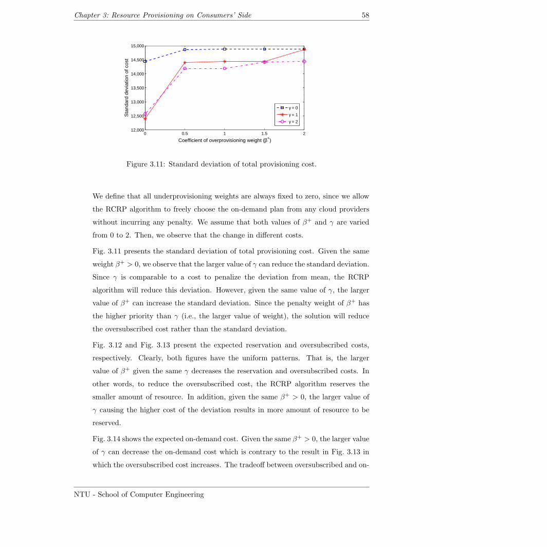
Chapter 3: Resource Provisioning on Consumers’ Side 58
0 0.5 1 1.5 212,000
12,500
13,000
13,500
14,000
14,500
15,000
Coefficient of overprovisioning weight (β+)
Sta
ndar
d de
viat
ion
of c
ost
γ = 0
γ = 1
γ = 2
Figure 3.11: Standard deviation of total provisioning cost.
We define that all underprovisioning weights are always fixed to zero, since we allow
the RCRP algorithm to freely choose the on-demand plan from any cloud providers
without incurring any penalty. We assume that both values of β+ and γ are varied
from 0 to 2. Then, we observe that the change in different costs.
Fig. 3.11 presents the standard deviation of total provisioning cost. Given the same
weight β+ > 0, we observe that the larger value of γ can reduce the standard deviation.
Since γ is comparable to a cost to penalize the deviation from mean, the RCRP
algorithm will reduce this deviation. However, given the same value of γ, the larger
value of β+ can increase the standard deviation. Since the penalty weight of β+ has
the higher priority than γ (i.e., the larger value of weight), the solution will reduce
the oversubscribed cost rather than the standard deviation.
Fig. 3.12 and Fig. 3.13 present the expected reservation and oversubscribed costs,
respectively. Clearly, both figures have the uniform patterns. That is, the larger
value of β+ given the same γ decreases the reservation and oversubscribed costs. In
other words, to reduce the oversubscribed cost, the RCRP algorithm reserves the
smaller amount of resource. In addition, given the same β+ > 0, the larger value of
γ causing the higher cost of the deviation results in more amount of resource to be
reserved.
Fig. 3.14 shows the expected on-demand cost. Given the same β+ > 0, the larger value
of γ can decrease the on-demand cost which is contrary to the result in Fig. 3.13 in
which the oversubscribed cost increases. The tradeoff between oversubscribed and on-
NTU - School of Computer Engineering
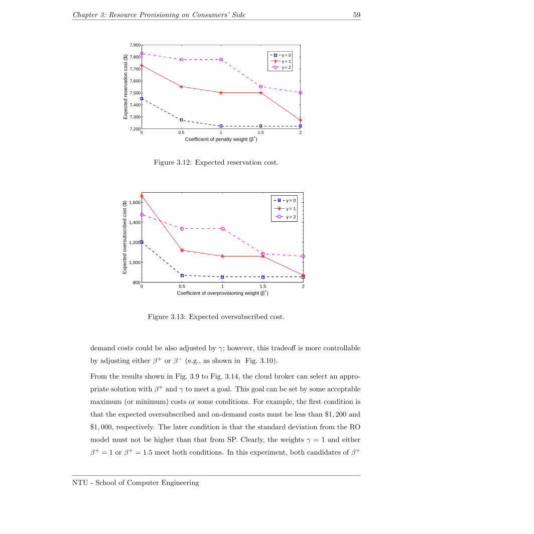
Chapter 3: Resource Provisioning on Consumers’ Side 59
0 0.5 1 1.5 27,200
7,300
7,400
7,500
7,600
7,700
7,800
7,900
Coefficient of penalty weight (β+)
Exp
ecte
d re
serv
atio
n co
st (
$)
γ = 0γ = 1γ = 2
Figure 3.12: Expected reservation cost.
0 0.5 1 1.5 2800
1,000
1,200
1,400
1,600
Coefficient of overprovisioning weight (β+)
Exp
ecte
d ov
ersu
bscr
ibed
cos
t ($)
γ = 0
γ = 1
γ = 2
Figure 3.13: Expected oversubscribed cost.
demand costs could be also adjusted by γ; however, this tradeoff is more controllable
by adjusting either β+ or β− (e.g., as shown in Fig. 3.10).
From the results shown in Fig. 3.9 to Fig. 3.14, the cloud broker can select an appro-
priate solution with β+ and γ to meet a goal. This goal can be set by some acceptable
maximum (or minimum) costs or some conditions. For example, the first condition is
that the expected oversubscribed and on-demand costs must be less than $1, 200 and
$1, 000, respectively. The later condition is that the standard deviation from the RO
model must not be higher than that from SP. Clearly, the weights γ = 1 and either
β+ = 1 or β+ = 1.5 meet both conditions. In this experiment, both candidates of β+
NTU - School of Computer Engineering
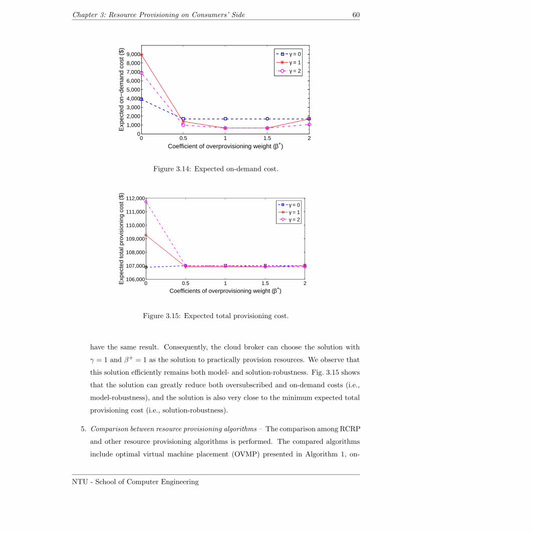
Chapter 3: Resource Provisioning on Consumers’ Side 60
0 0.5 1 1.5 20
1,000
2,000
3,000
4,000
5,000
6,000
7,000
8,000
9,000
Coefficient of overprovisioning weight (β+)
Exp
ecte
d on
−de
man
d co
st (
$)
γ = 0
γ = 1
γ = 2
Figure 3.14: Expected on-demand cost.
0 0.5 1 1.5 2106,000
107,000
108,000
109,000
110,000
111,000
112,000
Coefficients of overprovisioning weight (β+)
Exp
ecte
d to
tal p
rovi
sion
ing
cost
($)
γ = 0γ = 1γ = 2
Figure 3.15: Expected total provisioning cost.
have the same result. Consequently, the cloud broker can choose the solution with
γ = 1 and β+ = 1 as the solution to practically provision resources. We observe that
this solution efficiently remains both model- and solution-robustness. Fig. 3.15 shows
that the solution can greatly reduce both oversubscribed and on-demand costs (i.e.,
model-robustness), and the solution is also very close to the minimum expected total
provisioning cost (i.e., solution-robustness).
5. Comparison between resource provisioning algorithms – The comparison among RCRP
and other resource provisioning algorithms is performed. The compared algorithms
include optimal virtual machine placement (OVMP) presented in Algorithm 1, on-
NTU - School of Computer Engineering
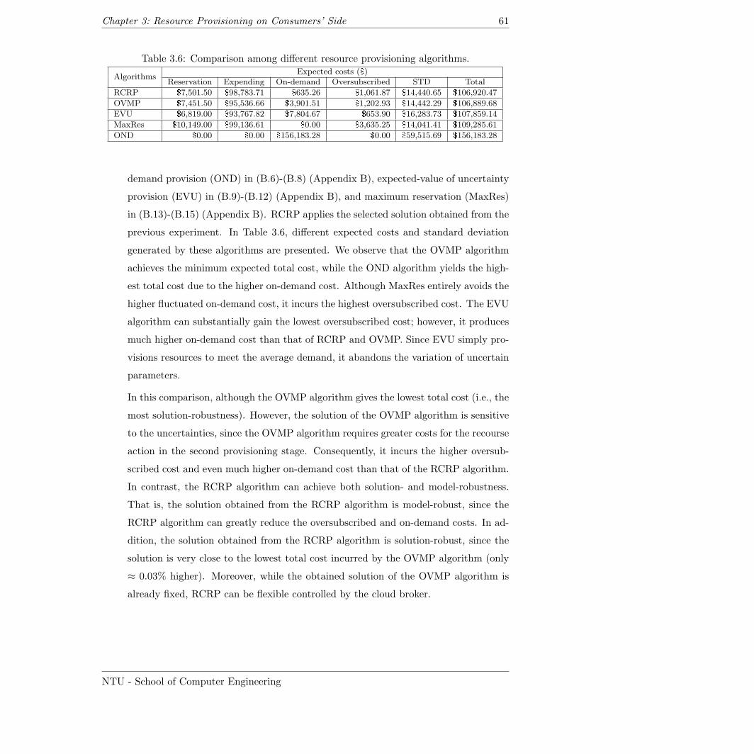
Chapter 3: Resource Provisioning on Consumers’ Side 61
Table 3.6: Comparison among different resource provisioning algorithms.
AlgorithmsExpected costs ($)
Reservation Expending On-demand Oversubscribed STD Total
RCRP $7,501.50 $98,783.71 $635.26 $1,061.87 $14,440.65 $106,920.47
OVMP $7,451.50 $95,536.66 $3,901.51 $1,202.93 $14,442.29 $106,889.68
EVU $6,819.00 $93,767.82 $7,804.67 $653.90 $16,283.73 $107,859.14
MaxRes $10,149.00 $99,136.61 $0.00 $3,635.25 $14,041.41 $109,285.61
OND $0.00 $0.00 $156,183.28 $0.00 $59,515.69 $156,183.28
demand provision (OND) in (B.6)-(B.8) (Appendix B), expected-value of uncertainty
provision (EVU) in (B.9)-(B.12) (Appendix B), and maximum reservation (MaxRes)
in (B.13)-(B.15) (Appendix B). RCRP applies the selected solution obtained from the
previous experiment. In Table 3.6, different expected costs and standard deviation
generated by these algorithms are presented. We observe that the OVMP algorithm
achieves the minimum expected total cost, while the OND algorithm yields the high-
est total cost due to the higher on-demand cost. Although MaxRes entirely avoids the
higher fluctuated on-demand cost, it incurs the highest oversubscribed cost. The EVU
algorithm can substantially gain the lowest oversubscribed cost; however, it produces
much higher on-demand cost than that of RCRP and OVMP. Since EVU simply pro-
visions resources to meet the average demand, it abandons the variation of uncertain
parameters.
In this comparison, although the OVMP algorithm gives the lowest total cost (i.e., the
most solution-robustness). However, the solution of the OVMP algorithm is sensitive
to the uncertainties, since the OVMP algorithm requires greater costs for the recourse
action in the second provisioning stage. Consequently, it incurs the higher oversub-
scribed cost and even much higher on-demand cost than that of the RCRP algorithm.
In contrast, the RCRP algorithm can achieve both solution- and model-robustness.
That is, the solution obtained from the RCRP algorithm is model-robust, since the
RCRP algorithm can greatly reduce the oversubscribed and on-demand costs. In ad-
dition, the solution obtained from the RCRP algorithm is solution-robust, since the
solution is very close to the lowest total cost incurred by the OVMP algorithm (only
≈ 0.03% higher). Moreover, while the obtained solution of the OVMP algorithm is
already fixed, RCRP can be flexible controlled by the cloud broker.
NTU - School of Computer Engineering
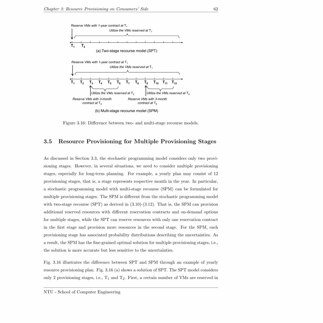
Chapter 3: Resource Provisioning on Consumers’ Side 62
Reserve VMs with 1-year contract at T1
Utilize the VMs reserved at T1
T1
T2
Reserve VMs with 1-year contract at T1
Utili th VM d t T
(a) Two-stage recourse model (SPT)
T1
T2
T3
T4
T5
T6
T7
T8
T9
T10
T11
T12
Utilize the VMs reserved at T1
Reserve VMs with 3-month
contract at T3
Utilize the VMs reserved at T3 Utilize the VMs reserved at T9
Reserve VMs with 3-month
contract at T9
(b) Multi-stage recourse model (SPM)
Figure 3.16: Difference between two- and multi-stage recourse models.
3.5 Resource Provisioning for Multiple Provisioning Stages
As discussed in Section 3.3, the stochastic programming model considers only two provi-
sioning stages. However, in several situations, we need to consider multiple provisioning
stages, especially for long-term planning. For example, a yearly plan may consist of 12
provisioning stages, that is, a stage represents respective month in the year. In particular,
a stochastic programming model with multi-stage recourse (SPM) can be formulated for
multiple provisioning stages. The SPM is different from the stochastic programming model
with two-stage recourse (SPT) as derived in (3.10)-(3.12). That is, the SPM can provision
additional reserved resources with different reservation contracts and on-demand options
for multiple stages, while the SPT can reserve resources with only one reservation contract
in the first stage and provision more resources in the second stage. For the SPM, each
provisioning stage has associated probability distributions describing the uncertainties. As
a result, the SPM has the fine-grained optimal solution for multiple provisioning stages, i.e.,
the solution is more accurate but less sensitive to the uncertainties.
Fig. 3.16 illustrates the difference between SPT and SPM through an example of yearly
resource provisioning plan. Fig. 3.16 (a) shows a solution of SPT. The SPT model considers
only 2 provisioning stages, i.e., T1 and T2. First, a certain number of VMs are reserved in
NTU - School of Computer Engineering
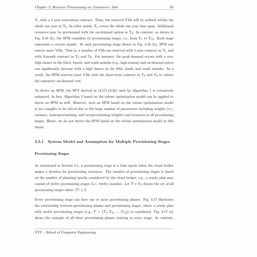
Chapter 3: Resource Provisioning on Consumers’ Side 63
T1 with a 1-year reservation contract. Then, the reserved VMs will be utilized within the
whole one year in T2. In other words, T2 covers the whole one year time span. Additional
resources may be provisioned with the on-demand option in T2. In contrast, as shown in
Fig. 3.16 (b), the SPM considers 12 provisioning stages, i.e., from T1 to T12. Each stage
represents a certain month. At each provisioning stage shown in Fig. 3.16 (b), SPM can
reserve more VMs. That is, a number of VMs are reserved with 1-year contract in T1 and
with 3-month contract in T3 and T9. For instance, the peak demand occurs with a very
high chance in the third, fourth, and tenth months (e.g., high season) and on-demand prices
can significantly increase with a high chance in the fifth, ninth, and tenth months. As a
result, the SPM reserves more VMs with the short-term contract in T3 and T9 to reduce
the expensive on-demand cost.
To derive an SPM, the SPT derived in (3.17)-(3.20) used by Algorithm 1 is extensively
enhanced. In fact, Algorithm 2 based on the robust optimization model can be applied to
derive an SPM as well. However, such an SPM based on the robust optimization model
is too complex to be solved due to the large number of parameters including weights (i.e.,
variance, underprovisioning, and overprovisioning weights) and scenarios in all provisioning
stages. Hence, we do not derive the SPM based on the robust optimization model in this
thesis.
3.5.1 System Model and Assumption for Multiple Provisioning Stages
Provisioning Stages
As mentioned in Section 3.1, a provisioning stage is a time epoch when the cloud broker
makes a decision for provisioning resources. The number of provisioning stages is based
on the number of planning epochs considered by the cloud broker, e.g., a yearly plan may
consist of twelve provisioning stages (i.e., twelve months). Let T ∈ N1 denote the set of all
provisioning stages where |T | ≥ 2.
Every provisioning stage can have one or more provisioning phases. Fig. 3.17 illustrates
the relationship between provisioning phases and provisioning stages, where a yearly plan
with twelve provisioning stages (e.g., T = T1,T2, . . . ,T12) is considered. Fig. 3.17 (a)
shows the example of all three provisioning phases existing in every stage. In contrast,
NTU - School of Computer Engineering
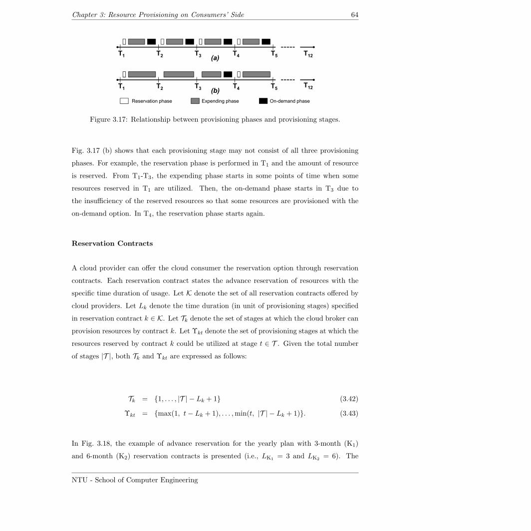
Chapter 3: Resource Provisioning on Consumers’ Side 64
T1
T2
T3
T4
T12(a)
T5
T1
T2
T3
T4
T12
(b)
Reservation phase Expending phase On-demand phase
T5
Figure 3.17: Relationship between provisioning phases and provisioning stages.
Fig. 3.17 (b) shows that each provisioning stage may not consist of all three provisioning
phases. For example, the reservation phase is performed in T1 and the amount of resource
is reserved. From T1-T3, the expending phase starts in some points of time when some
resources reserved in T1 are utilized. Then, the on-demand phase starts in T3 due to
the insufficiency of the reserved resources so that some resources are provisioned with the
on-demand option. In T4, the reservation phase starts again.
Reservation Contracts
A cloud provider can offer the cloud consumer the reservation option through reservation
contracts. Each reservation contract states the advance reservation of resources with the
specific time duration of usage. Let K denote the set of all reservation contracts offered by
cloud providers. Let Lk denote the time duration (in unit of provisioning stages) specified
in reservation contract k ∈ K. Let Tk denote the set of stages at which the cloud broker can
provision resources by contract k. Let Υkt denote the set of provisioning stages at which the
resources reserved by contract k could be utilized at stage t ∈ T . Given the total number
of stages |T |, both Tk and Υkt are expressed as follows:
Tk = 1, . . . , |T | − Lk + 1 (3.42)
Υkt = max(1, t− Lk + 1), . . . ,min(t, |T | − Lk + 1). (3.43)
In Fig. 3.18, the example of advance reservation for the yearly plan with 3-month (K1)
and 6-month (K2) reservation contracts is presented (i.e., LK1 = 3 and LK2 = 6). The
NTU - School of Computer Engineering
Chapter 3: Resource Provisioning on Consumers’ Side 65
T1
T2
T3
T4
T5
T6
T7
T8
T9
T10
T11
T12
K2
K1 K
2
K1
K1
Figure 3.18: Example of advance reservations with 3-month (K1) and 6-month (K2)contracts.
boxes above the timeline represent the time coverage of some reserved contracts. As shown
in (3.42), TK1 = T1,T2, . . . ,T10 and TK2 = T1,T2, . . . ,T7 are the sets of stages at
which resources can be provisioned by K1 and K2, respectively. Contract K1 is subscribed
3 times (e.g., T7-T9), while contract K2 is subscribed twice (e.g., T5-T10). Fig. 3.18 also
shows that some stages can be covered by two (or more) subscribed contracts e.g., T1-T3
are covered by contracts K1 and K2. In Fig. 3.18, any set Fkt in (3.43) can be obtained
e.g., FK1T4 = T2,T3,T4, FK1T11 = T9,T10, and FK2T12 = T7.
Uncertain Parameters
The solution used by the cloud broker is obtained by solving a stochastic programming
model with multi-stage recourse [28]. Uncertain parameters described by scenarios (i.e.,
realizations) are taken by the cloud broker into account. Let Ω denote the set of all scenarios
in all provisioning stages and Ωt denote the set of all scenarios in only provisioning stage t.
Ω is defined as the Cartesian product of all Ωt as follows:
Ω =∏t∈T
Ωt = Ω1 × Ω2 × · · · × Ω|T |. (3.44)
There are three kinds of uncertain parameters as follows:
• Demand Uncertainty – A demand represents the number of VMs required in the
expending and on-demand phases of a certain VM class. Let Ditω denote the possible
number of VMs required to execute VM class i in provisioning stage t under scenario
ω.
• Price Uncertainty – Resource prices fluctuate over time. Let C(r)jkrtω and C
(e)jkrtω denote
NTU - School of Computer Engineering
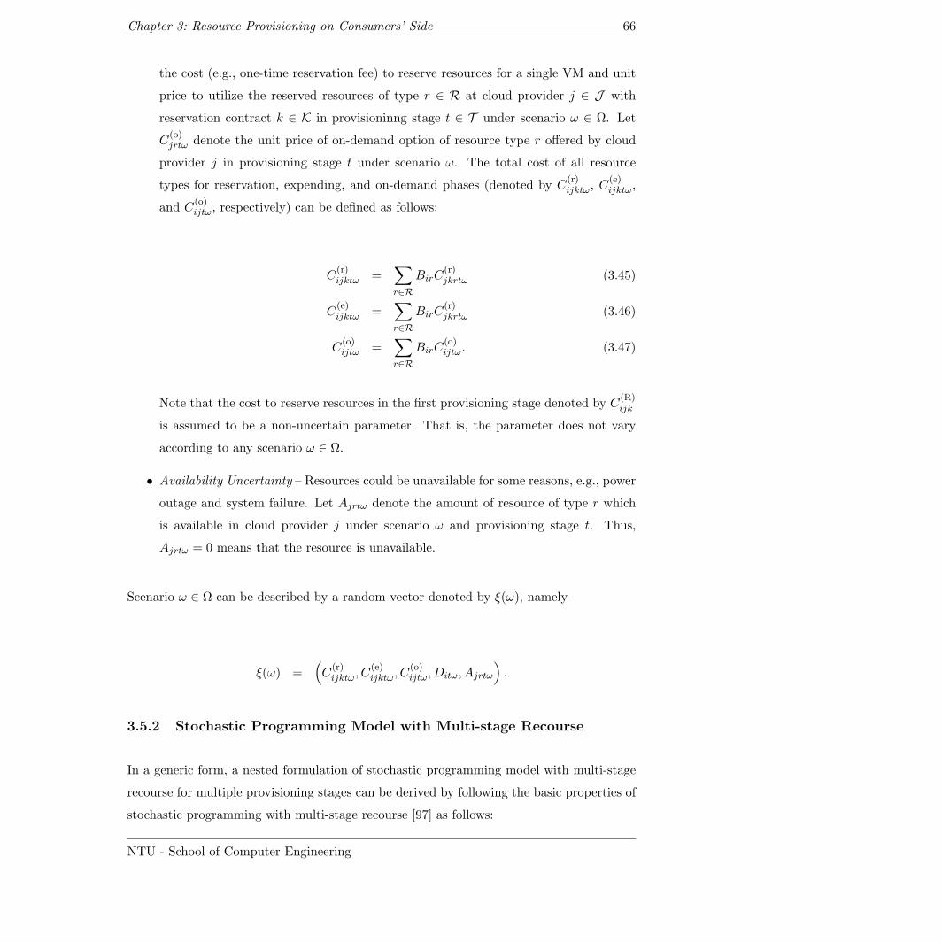
Chapter 3: Resource Provisioning on Consumers’ Side 66
the cost (e.g., one-time reservation fee) to reserve resources for a single VM and unit
price to utilize the reserved resources of type r ∈ R at cloud provider j ∈ J with
reservation contract k ∈ K in provisioninng stage t ∈ T under scenario ω ∈ Ω. Let
C(o)jrtω denote the unit price of on-demand option of resource type r offered by cloud
provider j in provisioning stage t under scenario ω. The total cost of all resource
types for reservation, expending, and on-demand phases (denoted by C(r)ijktω, C
(e)ijktω,
and C(o)ijtω, respectively) can be defined as follows:
C(r)ijktω =
∑r∈R
BirC(r)jkrtω (3.45)
C(e)ijktω =
∑r∈R
BirC(r)jkrtω (3.46)
C(o)ijtω =
∑r∈R
BirC(o)ijtω. (3.47)
Note that the cost to reserve resources in the first provisioning stage denoted by C(R)ijk
is assumed to be a non-uncertain parameter. That is, the parameter does not vary
according to any scenario ω ∈ Ω.
• Availability Uncertainty – Resources could be unavailable for some reasons, e.g., power
outage and system failure. Let Ajrtω denote the amount of resource of type r which
is available in cloud provider j under scenario ω and provisioning stage t. Thus,
Ajrtω = 0 means that the resource is unavailable.
Scenario ω ∈ Ω can be described by a random vector denoted by ξ(ω), namely
ξ(ω) =(C
(r)ijktω, C
(e)ijktω, C
(o)ijtω, Ditω, Ajrtω
).
3.5.2 Stochastic Programming Model with Multi-stage Recourse
In a generic form, a nested formulation of stochastic programming model with multi-stage
recourse for multiple provisioning stages can be derived by following the basic properties of
stochastic programming with multi-stage recourse [97] as follows:
NTU - School of Computer Engineering
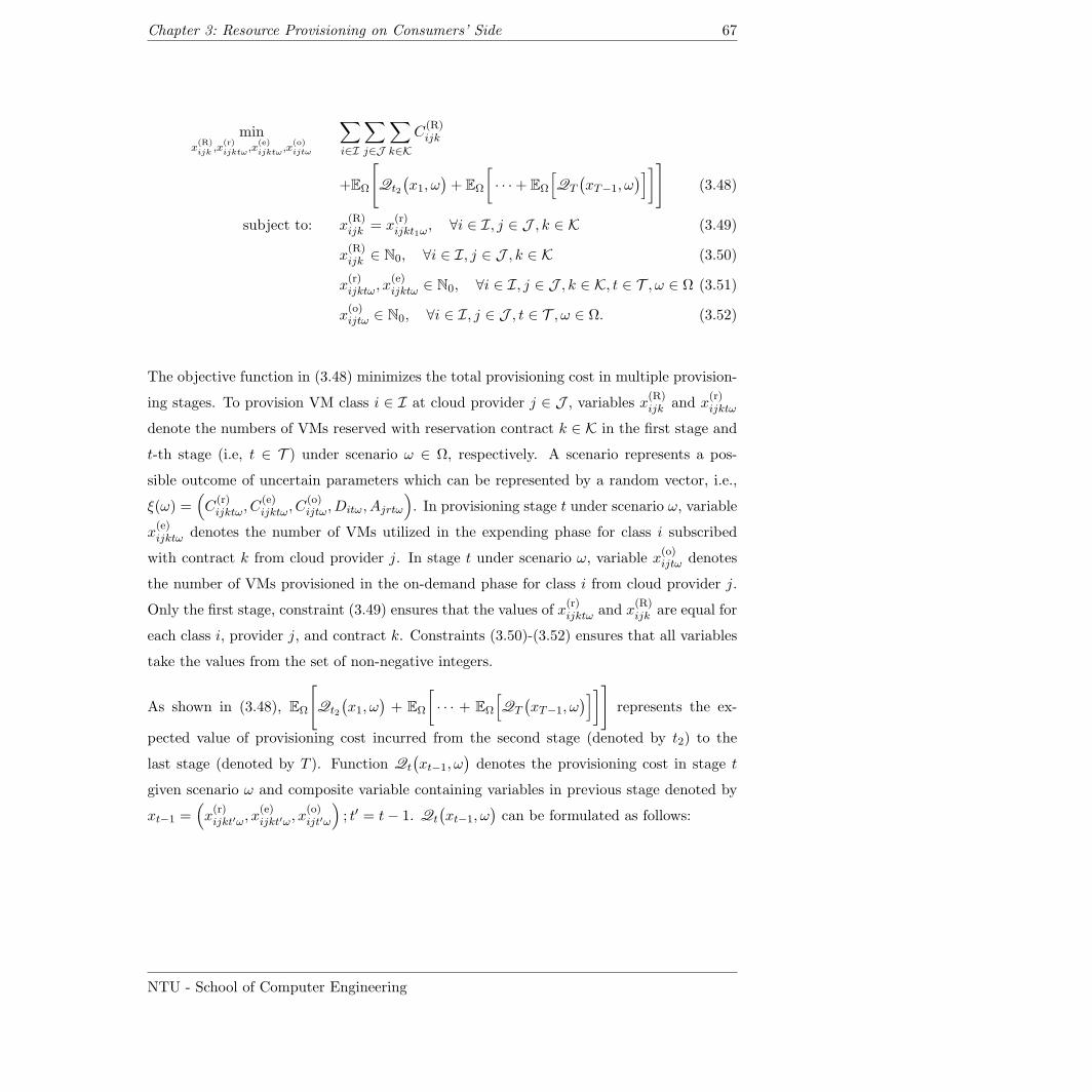
Chapter 3: Resource Provisioning on Consumers’ Side 67
minx(R)ijk ,x
(r)ijktω ,x
(e)ijktω ,x
(o)ijtω
∑i∈I
∑j∈J
∑k∈K
C(R)ijk
+EΩ
[Qt2
(x1, ω
)+ EΩ
[· · ·+ EΩ
[QT
(xT−1, ω
)]]](3.48)
subject to: x(R)ijk = x
(r)ijkt1ω
, ∀i ∈ I, j ∈ J , k ∈ K (3.49)
x(R)ijk ∈ N0, ∀i ∈ I, j ∈ J , k ∈ K (3.50)
x(r)ijktω, x
(e)ijktω ∈ N0, ∀i ∈ I, j ∈ J , k ∈ K, t ∈ T , ω ∈ Ω (3.51)
x(o)ijtω ∈ N0, ∀i ∈ I, j ∈ J , t ∈ T , ω ∈ Ω. (3.52)
The objective function in (3.48) minimizes the total provisioning cost in multiple provision-
ing stages. To provision VM class i ∈ I at cloud provider j ∈ J , variables x(R)ijk and x
(r)ijktω
denote the numbers of VMs reserved with reservation contract k ∈ K in the first stage and
t-th stage (i.e, t ∈ T ) under scenario ω ∈ Ω, respectively. A scenario represents a pos-
sible outcome of uncertain parameters which can be represented by a random vector, i.e.,
ξ(ω) =(C
(r)ijktω, C
(e)ijktω, C
(o)ijtω, Ditω, Ajrtω
). In provisioning stage t under scenario ω, variable
x(e)ijktω denotes the number of VMs utilized in the expending phase for class i subscribed
with contract k from cloud provider j. In stage t under scenario ω, variable x(o)ijtω denotes
the number of VMs provisioned in the on-demand phase for class i from cloud provider j.
Only the first stage, constraint (3.49) ensures that the values of x(r)ijktω and x
(R)ijk are equal for
each class i, provider j, and contract k. Constraints (3.50)-(3.52) ensures that all variables
take the values from the set of non-negative integers.
As shown in (3.48), EΩ
[Qt2
(x1, ω
)+ EΩ
[· · · + EΩ
[QT
(xT−1, ω
)]]]represents the ex-
pected value of provisioning cost incurred from the second stage (denoted by t2) to the
last stage (denoted by T ). Function Qt
(xt−1, ω
)denotes the provisioning cost in stage t
given scenario ω and composite variable containing variables in previous stage denoted by
xt−1 =(x(r)ijkt′ω, x
(e)ijkt′ω, x
(o)ijt′ω
); t′ = t− 1. Qt
(xt−1, ω
)can be formulated as follows:
NTU - School of Computer Engineering
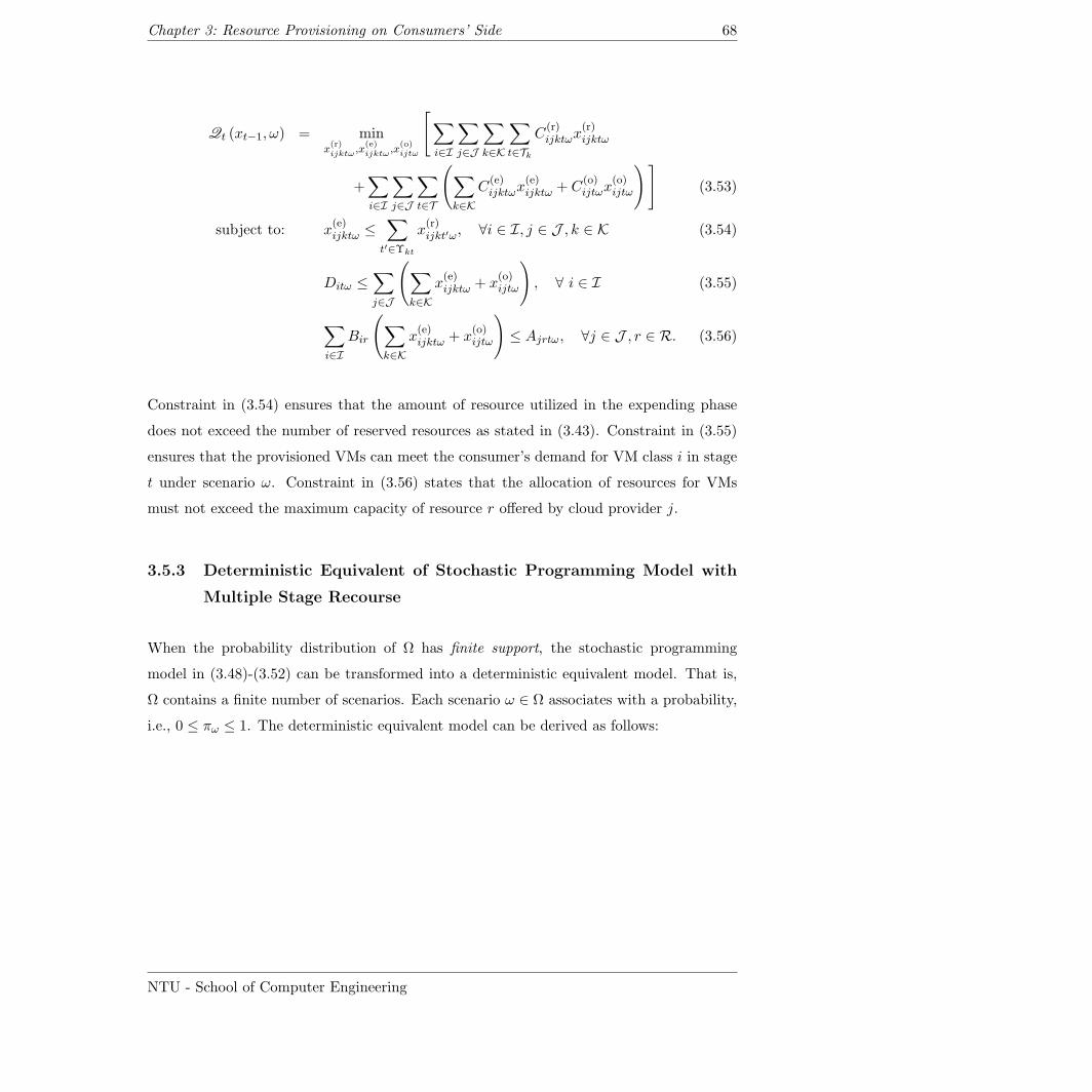
Chapter 3: Resource Provisioning on Consumers’ Side 68
Qt (xt−1, ω) = minx(r)ijktω ,x
(e)ijktω ,x
(o)ijtω
[∑i∈I
∑j∈J
∑k∈K
∑t∈Tk
C(r)ijktωx
(r)ijktω
+∑i∈I
∑j∈J
∑t∈T
(∑k∈K
C(e)ijktωx
(e)ijktω + C
(o)ijtωx
(o)ijtω
)](3.53)
subject to: x(e)ijktω ≤
∑t′∈Υkt
x(r)ijkt′ω, ∀i ∈ I, j ∈ J , k ∈ K (3.54)
Ditω ≤∑j∈J
(∑k∈K
x(e)ijktω + x
(o)ijtω
), ∀ i ∈ I (3.55)
∑i∈I
Bir
(∑k∈K
x(e)ijktω + x
(o)ijtω
)≤ Ajrtω, ∀j ∈ J , r ∈ R. (3.56)
Constraint in (3.54) ensures that the amount of resource utilized in the expending phase
does not exceed the number of reserved resources as stated in (3.43). Constraint in (3.55)
ensures that the provisioned VMs can meet the consumer’s demand for VM class i in stage
t under scenario ω. Constraint in (3.56) states that the allocation of resources for VMs
must not exceed the maximum capacity of resource r offered by cloud provider j.
3.5.3 Deterministic Equivalent of Stochastic Programming Model with
Multiple Stage Recourse
When the probability distribution of Ω has finite support, the stochastic programming
model in (3.48)-(3.52) can be transformed into a deterministic equivalent model. That is,
Ω contains a finite number of scenarios. Each scenario ω ∈ Ω associates with a probability,
i.e., 0 ≤ πω ≤ 1. The deterministic equivalent model can be derived as follows:
NTU - School of Computer Engineering
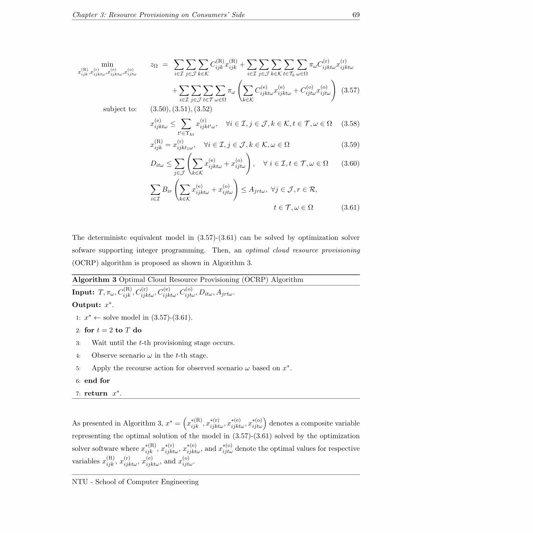
Chapter 3: Resource Provisioning on Consumers’ Side 69
minx(R)ijk ,x
(r)ijktω ,x
(e)ijktω ,x
(o)ijtω
zΩ =∑i∈I
∑j∈J
∑k∈K
C(R)ijk x
(R)ijk +
∑i∈I
∑j∈J
∑k∈K
∑t∈Tk
∑ω∈Ω
πωC(r)ijktωx
(r)ijktω
+∑i∈I
∑j∈J
∑t∈T
∑ω∈Ω
πω
(∑k∈K
C(e)ijktωx
(e)ijktω + C
(o)ijtωx
(o)ijtω
)(3.57)
subject to: (3.50), (3.51), (3.52)
x(e)ijktω ≤
∑t′∈Υkt
x(r)ijkt′ω, ∀i ∈ I, j ∈ J , k ∈ K, t ∈ T , ω ∈ Ω (3.58)
x(R)ijk = x
(r)ijkt1ω
, ∀i ∈ I, j ∈ J , k ∈ K, ω ∈ Ω (3.59)
Ditω ≤∑j∈J
(∑k∈K
x(e)ijktω + x
(o)ijtω
), ∀ i ∈ I, t ∈ T , ω ∈ Ω (3.60)
∑i∈I
Bir
(∑k∈K
x(e)ijktω + x
(o)ijtω
)≤ Ajrtω, ∀j ∈ J , r ∈ R,
t ∈ T , ω ∈ Ω (3.61)
The deterministc equivalent model in (3.57)-(3.61) can be solved by optimization solver
sofware supporting integer programming. Then, an optimal cloud resource provisioning
(OCRP) algorithm is proposed as shown in Algorithm 3.
Algorithm 3 Optimal Cloud Resource Provisioning (OCRP) Algorithm
Input: T, πω, C(R)ijk , C
(r)ijktω, C
(e)ijktω, C
(o)ijtω, Ditω, Ajrtω.
Output: x∗.
1: x∗ ← solve model in (3.57)-(3.61).
2: for t = 2 to T do
3: Wait until the t-th provisioning stage occurs.
4: Observe scenario ω in the t-th stage.
5: Apply the recourse action for observed scenario ω based on x∗.
6: end for
7: return x∗.
As presented in Algorithm 3, x∗ =(x∗(R)ijk , x
∗(r)ijktω, x
∗(e)ijktω, x
∗(o)ijtω
)denotes a composite variable
representing the optimal solution of the model in (3.57)-(3.61) solved by the optimization
solver software where x∗(R)ijk , x
∗(r)ijktω, x
∗(e)ijktω, and x
∗(o)ijtω denote the optimal values for respective
variables x(R)ijk , x
(r)ijktω, x
(e)ijktω, and x
(o)ijtω.
NTU - School of Computer Engineering
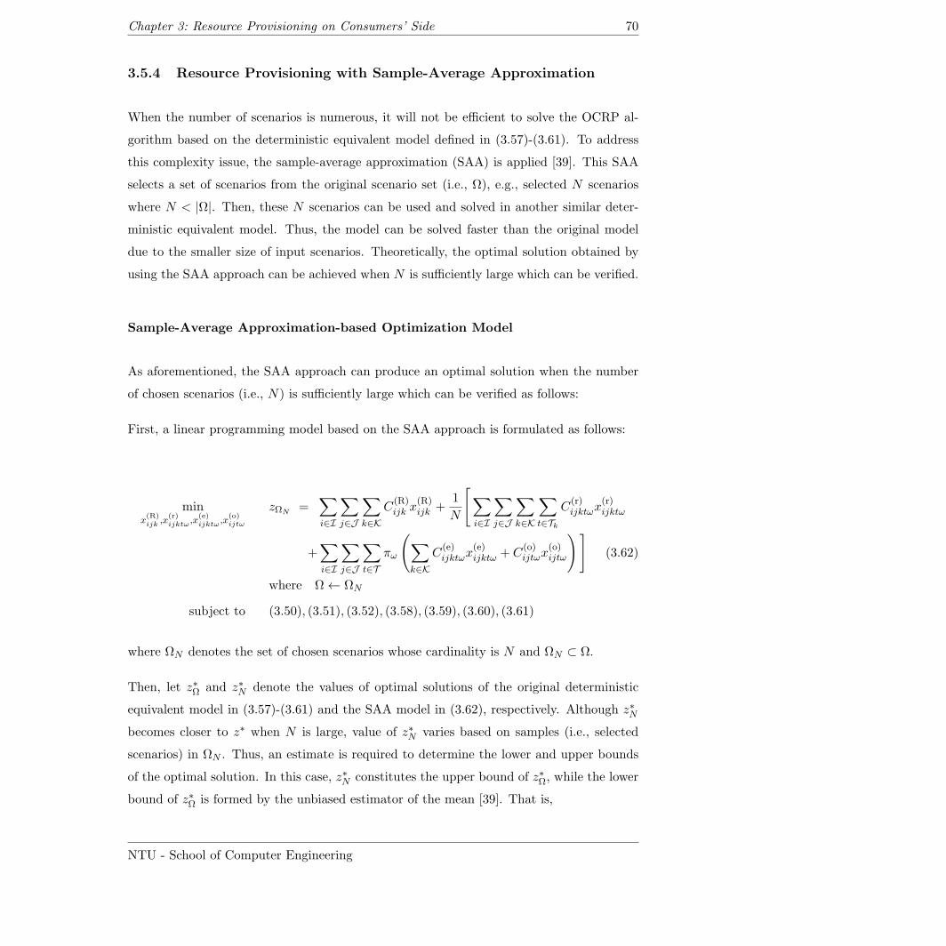
Chapter 3: Resource Provisioning on Consumers’ Side 70
3.5.4 Resource Provisioning with Sample-Average Approximation
When the number of scenarios is numerous, it will not be efficient to solve the OCRP al-
gorithm based on the deterministic equivalent model defined in (3.57)-(3.61). To address
this complexity issue, the sample-average approximation (SAA) is applied [39]. This SAA
selects a set of scenarios from the original scenario set (i.e., Ω), e.g., selected N scenarios
where N < |Ω|. Then, these N scenarios can be used and solved in another similar deter-
ministic equivalent model. Thus, the model can be solved faster than the original model
due to the smaller size of input scenarios. Theoretically, the optimal solution obtained by
using the SAA approach can be achieved when N is sufficiently large which can be verified.
Sample-Average Approximation-based Optimization Model
As aforementioned, the SAA approach can produce an optimal solution when the number
of chosen scenarios (i.e., N) is sufficiently large which can be verified as follows:
First, a linear programming model based on the SAA approach is formulated as follows:
minx(R)ijk ,x
(r)ijktω ,x
(e)ijktω ,x
(o)ijtω
zΩN=∑i∈I
∑j∈J
∑k∈K
C(R)ijk x
(R)ijk +
1
N
[∑i∈I
∑j∈J
∑k∈K
∑t∈Tk
C(r)ijktωx
(r)ijktω
+∑i∈I
∑j∈J
∑t∈T
πω
(∑k∈K
C(e)ijktωx
(e)ijktω + C
(o)ijtωx
(o)ijtω
)](3.62)
where Ω← ΩN
subject to (3.50), (3.51), (3.52), (3.58), (3.59), (3.60), (3.61)
where ΩN denotes the set of chosen scenarios whose cardinality is N and ΩN ⊂ Ω.
Then, let z∗Ω and z∗N denote the values of optimal solutions of the original deterministic
equivalent model in (3.57)-(3.61) and the SAA model in (3.62), respectively. Although z∗N
becomes closer to z∗ when N is large, value of z∗N varies based on samples (i.e., selected
scenarios) in ΩN . Thus, an estimate is required to determine the lower and upper bounds
of the optimal solution. In this case, z∗N constitutes the upper bound of z∗Ω, while the lower
bound of z∗Ω is formed by the unbiased estimator of the mean [39]. That is,
NTU - School of Computer Engineering
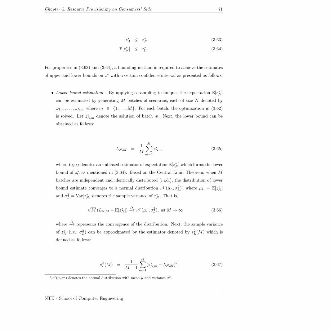
Chapter 3: Resource Provisioning on Consumers’ Side 71
z∗Ω ≤ z∗N (3.63)
E[z∗N ] ≤ z∗Ω. (3.64)
For properties in (3.63) and (3.64), a bounding method is required to achieve the estimates
of upper and lower bounds on z∗ with a certain confidence interval as presented as follows:
• Lower bound estimation – By applying a sampling technique, the expectation E[z∗N ]
can be estimated by generating M batches of scenarios, each of size N denoted by
ω1,m, . . . , ωN,m where m ∈ 1, . . . ,M. For each batch, the optimization in (3.62)
is solved. Let z∗N,m denote the solution of batch m. Next, the lower bound can be
obtained as follows:
LN,M =1
M
M∑m=1
z∗N,m (3.65)
where LN,M denotes an unbiased estimator of expectation E[z∗N ] which forms the lower
bound of z∗Ω as mentioned in (3.64). Based on the Central Limit Theorem, when M
batches are independent and identically distributed (i.i.d.), the distribution of lower
bound estimate converges to a normal distribution N (µL, σ2L)
4 where µL = E[z∗N ]
and σ2L = Var[z∗N ] denotes the sample variance of z∗N . That is,
√M (LN,M − E[z∗N ])
D−→ N (µL, σ2L), as M →∞ (3.66)
whereD−→ represents the convergence of the distribution. Next, the sample variance
of z∗N (i.e., σ2L) can be approximated by the estimator denoted by s2L(M) which is
defined as follows:
s2L(M) =1
M − 1
M∑m=1
(z∗N,m − LN,M )2. (3.67)
4N (µ, σ2) denotes the normal distribution with mean µ and variance σ2.
NTU - School of Computer Engineering
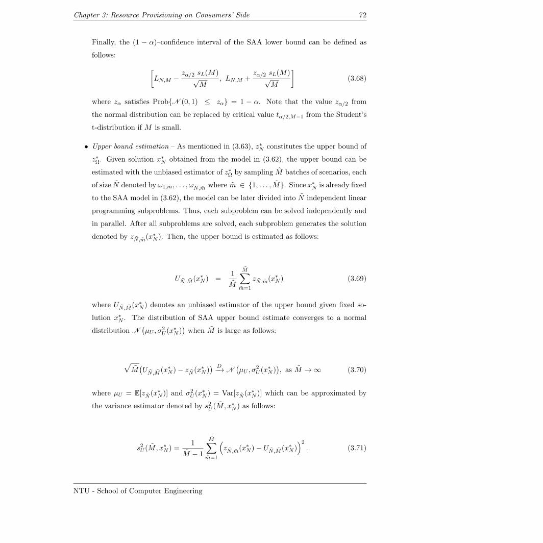
Chapter 3: Resource Provisioning on Consumers’ Side 72
Finally, the (1 − α)–confidence interval of the SAA lower bound can be defined as
follows: [LN,M −
zα/2 sL(M)√M
, LN,M +zα/2 sL(M)√M
](3.68)
where zα satisfies ProbN (0, 1) ≤ zα = 1 − α. Note that the value zα/2 from
the normal distribution can be replaced by critical value tα/2,M−1 from the Student’s
t-distribution if M is small.
• Upper bound estimation – As mentioned in (3.63), z∗N constitutes the upper bound of
z∗Ω. Given solution x∗N obtained from the model in (3.62), the upper bound can be
estimated with the unbiased estimator of z∗Ω by sampling M batches of scenarios, each
of size N denoted by ω1,m, . . . , ωN,m where m ∈ 1, . . . , M. Since x∗N is already fixed
to the SAA model in (3.62), the model can be later divided into N independent linear
programming subproblems. Thus, each subproblem can be solved independently and
in parallel. After all subproblems are solved, each subproblem generates the solution
denoted by zN,m(x∗N ). Then, the upper bound is estimated as follows:
UN,M (x∗N ) =1
M
M∑m=1
zN,m(x∗N ) (3.69)
where UN,M (x∗N ) denotes an unbiased estimator of the upper bound given fixed so-
lution x∗N . The distribution of SAA upper bound estimate converges to a normal
distribution N(µU , σ
2U (x
∗N ))when M is large as follows:
√M(UN,M (x∗N )− zN (x∗N )
) D−→ N(µU , σ
2U (x
∗N )), as M →∞ (3.70)
where µU = E[zN (x∗N )] and σ2U (x∗N ) = Var[zN (x∗N )] which can be approximated by
the variance estimator denoted by s2U (M, x∗N ) as follows:
s2U (M, x∗N ) =1
M − 1
M∑m=1
(zN,m(x∗N )− UN,M (x∗N )
)2. (3.71)
NTU - School of Computer Engineering
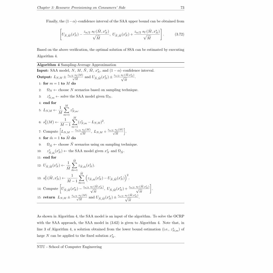
Chapter 3: Resource Provisioning on Consumers’ Side 73
Finally, the (1−α)–confidence interval of the SAA upper bound can be obtained from[UN,M (x∗N )−
zα/2 sU (M, x∗N )√M
, UN,M (x∗N ) +zα/2 sU (M, x∗N )√
M
]. (3.72)
Based on the above verification, the optimal solution of SSA can be estimated by executing
Algorithm 4.
Algorithm 4 Sampling-Average Approximation
Input: SAA model, N , M , N , M , x∗N , and (1− α)–confidence interval.
Output: LN,M ±zα/2 sL(M)√
Mand UN,M (x∗N )± zα/2 sU (M,x∗
N )√M
.
1: for m = 1 to M do
2: ΩN ← choose N scenarios based on sampling technique.
3: z∗N,m ← solve the SAA model given ΩN .
4: end for
5: LN,M ←1
M
M∑m=1
z∗N,m.
6: s2L(M)← 1
M − 1
M∑m=1
(z∗N,m − LN,M )2.
7: Compute[LN,M −
zα/2 sL(M)√M
, LN,M +zα/2 sL(M)√
M
].
8: for m = 1 to M do
9: ΩN ← choose N scenarios using on sampling technique.
10: z∗N,m
(x∗N )← the SAA model given x∗N and ΩN .
11: end for
12: UN,M (x∗N )← 1
M
M∑m=1
zN,m(x∗N ).
13: s2U (M, x∗N )← 1
M − 1
M∑m=1
(zN,m(x∗N )− UN,M (x∗N )
)2.
14: Compute
[UN,M (x∗N )− zα/2 sU (M,x∗
N )√M
, UN,M (x∗N ) +zα/2 sU (M,x∗
N )√M
].
15: return LN,M ±zα/2 sL(M)√
Mand UN,M (x∗N )± zα/2 sU (M,x∗
N )√M
.
As shown in Algorithm 4, the SAA model is an input of the algorithm. To solve the OCRP
with the SAA approach, the SAA model in (3.62) is given to Algorithm 4. Note that, in
line 3 of Algorithm 4, a solution obtained from the lower bound estimation (i.e., z∗N,m) of
large N can be applied to the fixed solution x∗N .
NTU - School of Computer Engineering
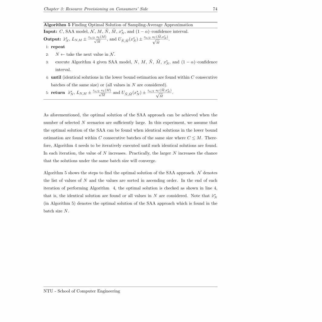
Chapter 3: Resource Provisioning on Consumers’ Side 74
Algorithm 5 Finding Optimal Solution of Sampling-Average Approximation
Input: C, SAA model, N , M , N , M , x∗N , and (1− α)–confidence interval.
Output: x∗N , LN,M ±zα/2 sL(M)√
M, and UN,M (x∗N )± zα/2 sU (M,x∗
N )√M
.
1: repeat
2: N ← take the next value in N .
3: execute Algorithm 4 given SAA model, N , M , N , M , x∗N , and (1 − α)–confidence
interval.
4: until (identical solutions in the lower bound estimation are found within C consecutive
batches of the same size) or (all values in N are considered).
5: return x∗N , LN,M ±zα/2 sL(M)√
Mand UN,M (x∗N )± zα/2 sU (M,x∗
N )√M
.
As aforementioned, the optimal solution of the SAA approach can be achieved when the
number of selected N scenarios are sufficiently large. In this experiment, we assume that
the optimal solution of the SAA can be found when identical solutions in the lower bound
estimation are found within C consecutive batches of the same size where C ≤ M . There-
fore, Algorithm 4 needs to be iteratively executed until such identical solutions are found.
In each iteration, the value of N increases. Practically, the larger N increases the chance
that the solutions under the same batch size will converge.
Algorithm 5 shows the steps to find the optimal solution of the SAA approach. N denotes
the list of values of N and the values are sorted in ascending order. In the end of each
iteration of performing Algorithm 4, the optimal solution is checked as shown in line 4,
that is, the identical solution are found or all values in N are considered. Note that x∗N
(in Algorithm 5) denotes the optimal solution of the SAA approach which is found in the
batch size N .
NTU - School of Computer Engineering
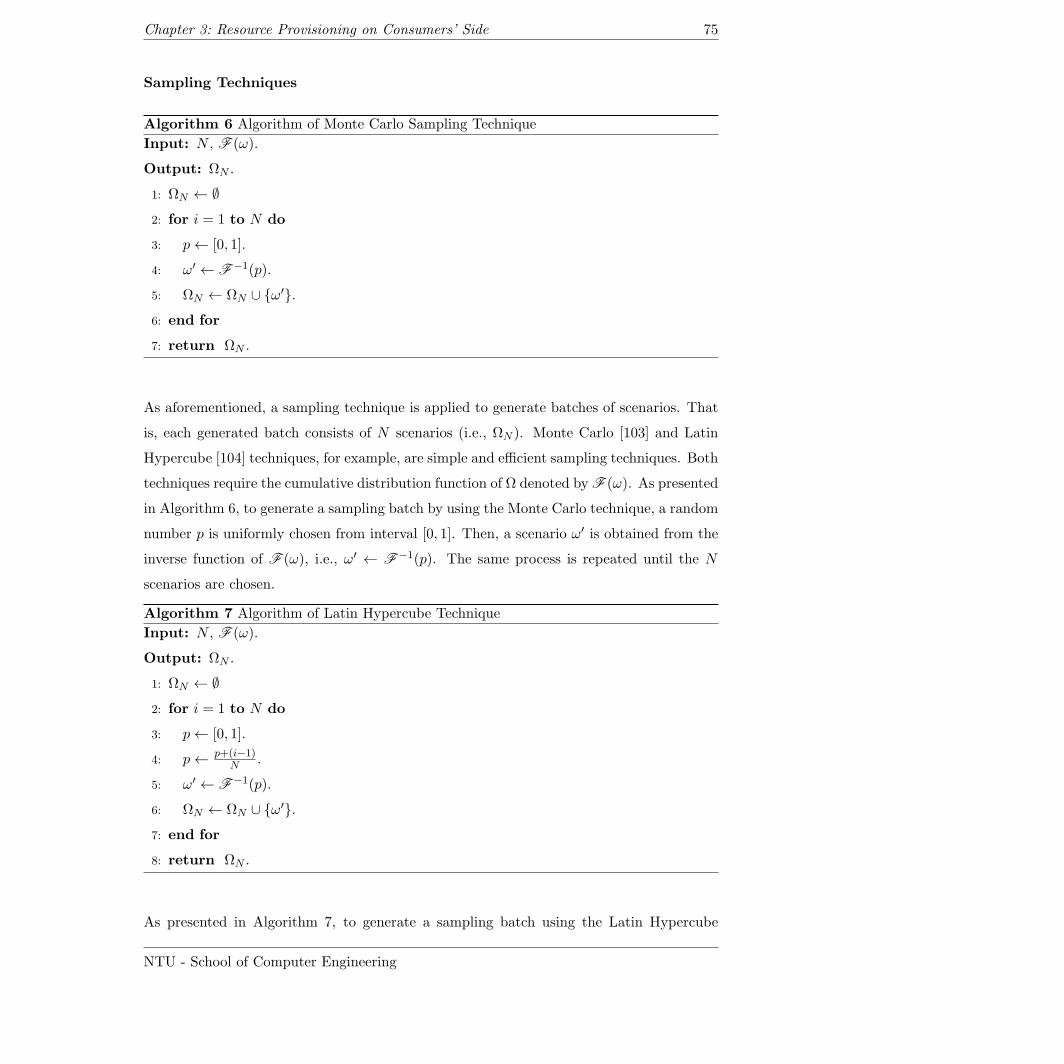
Chapter 3: Resource Provisioning on Consumers’ Side 75
Sampling Techniques
Algorithm 6 Algorithm of Monte Carlo Sampling Technique
Input: N , F (ω).
Output: ΩN .
1: ΩN ← ∅
2: for i = 1 to N do
3: p← [0, 1].
4: ω′ ← F−1(p).
5: ΩN ← ΩN ∪ ω′.
6: end for
7: return ΩN .
As aforementioned, a sampling technique is applied to generate batches of scenarios. That
is, each generated batch consists of N scenarios (i.e., ΩN ). Monte Carlo [103] and Latin
Hypercube [104] techniques, for example, are simple and efficient sampling techniques. Both
techniques require the cumulative distribution function of Ω denoted by F (ω). As presented
in Algorithm 6, to generate a sampling batch by using the Monte Carlo technique, a random
number p is uniformly chosen from interval [0, 1]. Then, a scenario ω′ is obtained from the
inverse function of F (ω), i.e., ω′ ← F−1(p). The same process is repeated until the N
scenarios are chosen.
Algorithm 7 Algorithm of Latin Hypercube Technique
Input: N , F (ω).
Output: ΩN .
1: ΩN ← ∅
2: for i = 1 to N do
3: p← [0, 1].
4: p← p+(i−1)N .
5: ω′ ← F−1(p).
6: ΩN ← ΩN ∪ ω′.
7: end for
8: return ΩN .
As presented in Algorithm 7, to generate a sampling batch using the Latin Hypercube
NTU - School of Computer Engineering
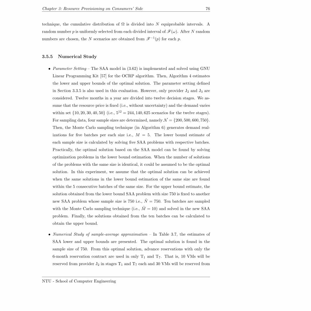
Chapter 3: Resource Provisioning on Consumers’ Side 76
technique, the cumulative distribution of Ω is divided into N equiprobable intervals. A
random number p is uniformly selected from each divided interval of F (ω). After N random
numbers are chosen, the N scenarios are obtained from F−1(p) for each p.
3.5.5 Numerical Study
• Parameter Setting – The SAA model in (3.62) is implemented and solved using GNU
Linear Programming Kit [57] for the OCRP algorithm. Then, Algorithm 4 estimates
the lower and upper bounds of the optimal solution. The parameter setting defined
in Section 3.3.5 is also used in this evaluation. However, only provider J2 and J3 are
considered. Twelve months in a year are divided into twelve decision stages. We as-
sume that the resource price is fixed (i.e., without uncertainty) and the demand varies
within set 10, 20, 30, 40, 50 (i.e., 512 = 244, 140, 625 scenarios for the twelve stages).
For sampling data, four sample sizes are determined, namely N = 200, 500, 600, 750.
Then, the Monte Carlo sampling technique (in Algorithm 6) generates demand real-
izations for five batches per each size i.e., M = 5. The lower bound estimate of
each sample size is calculated by solving five SAA problems with respective batches.
Practically, the optimal solution based on the SAA model can be found by solving
optimization problems in the lower bound estimation. When the number of solutions
of the problems with the same size is identical, it could be assumed to be the optimal
solution. In this experiment, we assume that the optimal solution can be achieved
when the same solutions in the lower bound estimation of the same size are found
within the 5 consecutive batches of the same size. For the upper bound estimate, the
solution obtained from the lower bound SAA problem with size 750 is fixed to another
new SAA problem whose sample size is 750 i.e., N = 750. Ten batches are sampled
with the Monte Carlo sampling technique (i.e., M = 10) and solved in the new SAA
problem. Finally, the solutions obtained from the ten batches can be calculated to
obtain the upper bound.
• Numerical Study of sample-average approximation – In Table 3.7, the estimates of
SAA lower and upper bounds are presented. The optimal solution is found in the
sample size of 750. From this optimal solution, advance reservations with only the
6-month reservation contract are used in only T1 and T7. That is, 10 VMs will be
reserved from provider J2 in stages T1 and T7 each and 30 VMs will be reserved from
NTU - School of Computer Engineering
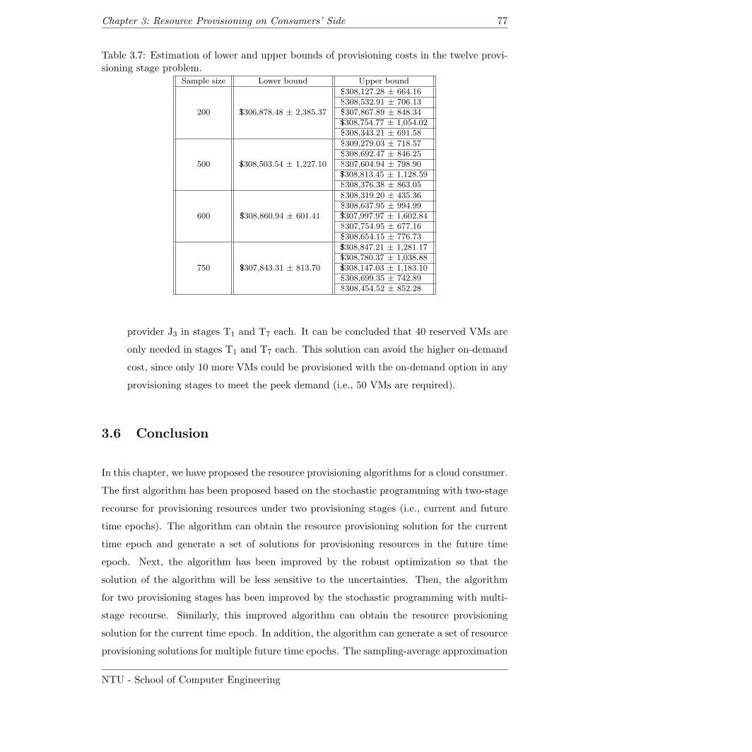
Chapter 3: Resource Provisioning on Consumers’ Side 77
Table 3.7: Estimation of lower and upper bounds of provisioning costs in the twelve provi-sioning stage problem.
Sample size Lower bound Upper bound
200 $306,878.48 ± 2,385.37
$308,127.28 ± 664.16$308,532.91 ± 706.13$307,867.89 ± 848.34$308,754.77 ± 1,054.02$308,343.21 ± 691.58
500 $308,503.54 ± 1,227.10
$309,279.03 ± 718.57$308,692.47 ± 846.25$307,604.94 ± 798.90$308,813.45 ± 1,128.59$308,376.38 ± 863.05
600 $308,860.94 ± 601.41
$308,319.20 ± 435.36$308,637.95 ± 994.99$307,997.97 ± 1,602.84$307,754.95 ± 677.16$308,654.15 ± 776.73
750 $307,843.31 ± 813.70
$308,847.21 ± 1,281.17$308,780.37 ± 1,038.88$308,147.03 ± 1,183.10$308,699.35 ± 742.89$308,454.52 ± 852.28
provider J3 in stages T1 and T7 each. It can be concluded that 40 reserved VMs are
only needed in stages T1 and T7 each. This solution can avoid the higher on-demand
cost, since only 10 more VMs could be provisioned with the on-demand option in any
provisioning stages to meet the peek demand (i.e., 50 VMs are required).
3.6 Conclusion
In this chapter, we have proposed the resource provisioning algorithms for a cloud consumer.
The first algorithm has been proposed based on the stochastic programming with two-stage
recourse for provisioning resources under two provisioning stages (i.e., current and future
time epochs). The algorithm can obtain the resource provisioning solution for the current
time epoch and generate a set of solutions for provisioning resources in the future time
epoch. Next, the algorithm has been improved by the robust optimization so that the
solution of the algorithm will be less sensitive to the uncertainties. Then, the algorithm
for two provisioning stages has been improved by the stochastic programming with multi-
stage recourse. Similarly, this improved algorithm can obtain the resource provisioning
solution for the current time epoch. In addition, the algorithm can generate a set of resource
provisioning solutions for multiple future time epochs. The sampling-average approximation
NTU - School of Computer Engineering
Chapter 3: Resource Provisioning on Consumers’ Side 78
and Benders decomposition methods have been also applied to the proposed algorithms for
addressing the computational complexity. We have performed the numerical studies and
simultion. The results show that the algorithms can minimize the total provisioning cost
under the uncertainties. In the next chapter, we have applied the algorithms to Amazon
Elastic Compute Cloud (EC2) as a case study.
NTU - School of Computer Engineering
Chapter 4
Case Study: Server Provisioning in
Amazon Elastic Compute Cloud
In this chapter, we demonstrate how the stochastic programming and robust optimiza-
tion models proposed in Section 3.3 and Section 3.4 can be applied to Amazon Elastic
Compute Cloud (EC2) [18], a widely used commercial IaaS-service, as a case study. EC2
provides three different provisioning options, namely reservation, on-demand, and spot op-
tions. Generally, both on-demand and spot options are suitable for short-term provisioning.
In contrast, the reservation option is for long-term provisioning (e.g., 1 year or 3 years). We
propose two algorithms for both long-term and short-term resource provisioning in EC2.
This chapter is organized as follows. First, we introduce how a virtual server can be pro-
visioned from EC2 in Section 4.1. We present the system model and assumption of the
proposed algorithms in Section 4.2. Then, the proposed algorithms are discussed in Sec-
tion 4.3. Next, the numerical studies are presented in Section 4.4. Finally, the conclusion
is stated in Section 4.5.
79
Chapter 4: Case Study: Server Provisioning in Amazon Elastic Compute Cloud 80
4.1 Overview of Server Provisioning in Amazon Elastic Com-
pute Cloud
Amazon EC2 provides a cloud computing service by renting out computational resources
(e.g., CPU, storage, and network bandwidth) to customers [3, 18]. Amazon EC2 leverages
virtualization technologies in which customers’ EC2 instances (i.e., virtual servers) can
be provisioned in datacenters operated by Amazon. When the provisioned servers utilize
resources, Amazon charges the customers by the usage cost on a pay-per-use basis.
To provision EC2 instances, Amazon offers three purchasing options (i.e., provisioning op-
tions), namely on-demand, reservation, and spot options [18]. With the on-demand option,
EC2 instances can be dynamically provisioned by a customer anytime without a commit-
ment. In contrast, with the reservation option, EC2 instances need to be subscribed with
1- or 3-year contract. The customer pays a one-time fee for the contract. When the EC2
instances are run, the discounted usage price is charged additionally. With the spot option,
the customer has to submit the request for EC2 instances (i.e., spot instances). This re-
quest includes a bid price which is the customer’s maximum affordable cost to execute the
requested EC2 instances. Then, Amazon sets an offer price or spot price, i.e., the actual
resource usage price of the spot option. This spot price is often varied by Amazon based on
supply-and-demand of available resources in EC2. Only the customers whose bid prices are
higher than the latest spot price can run their spot instances. Every running spot instance
is charged with the same spot price regardless of the bid price.
NTU - School of Computer Engineering
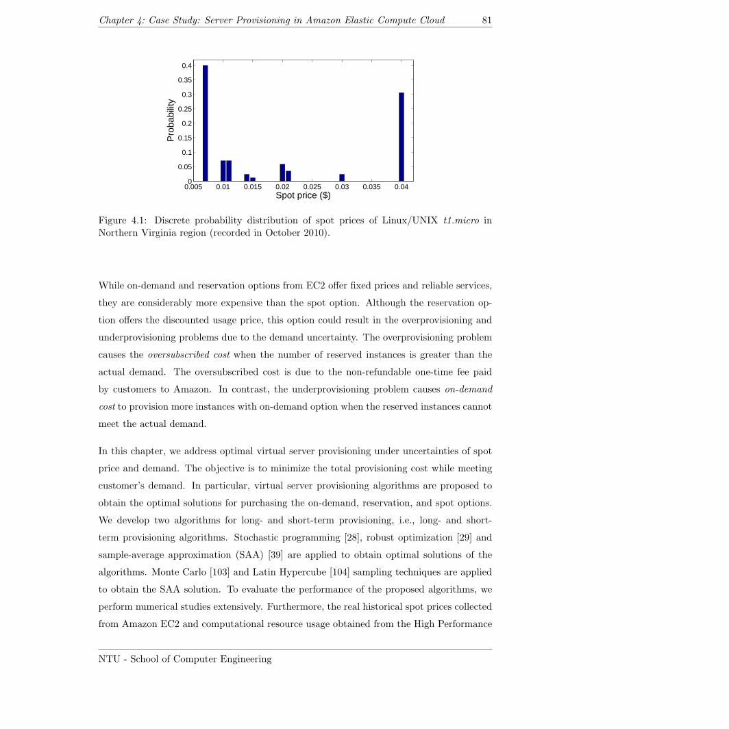
Chapter 4: Case Study: Server Provisioning in Amazon Elastic Compute Cloud 81
0.005 0.01 0.015 0.02 0.025 0.03 0.035 0.040
0.05
0.1
0.15
0.2
0.25
0.3
0.35
0.4
Spot price ($)
Pro
babi
lity
Figure 4.1: Discrete probability distribution of spot prices of Linux/UNIX t1.micro inNorthern Virginia region (recorded in October 2010).
While on-demand and reservation options from EC2 offer fixed prices and reliable services,
they are considerably more expensive than the spot option. Although the reservation op-
tion offers the discounted usage price, this option could result in the overprovisioning and
underprovisioning problems due to the demand uncertainty. The overprovisioning problem
causes the oversubscribed cost when the number of reserved instances is greater than the
actual demand. The oversubscribed cost is due to the non-refundable one-time fee paid
by customers to Amazon. In contrast, the underprovisioning problem causes on-demand
cost to provision more instances with on-demand option when the reserved instances cannot
meet the actual demand.
In this chapter, we address optimal virtual server provisioning under uncertainties of spot
price and demand. The objective is to minimize the total provisioning cost while meeting
customer’s demand. In particular, virtual server provisioning algorithms are proposed to
obtain the optimal solutions for purchasing the on-demand, reservation, and spot options.
We develop two algorithms for long- and short-term provisioning, i.e., long- and short-
term provisioning algorithms. Stochastic programming [28], robust optimization [29] and
sample-average approximation (SAA) [39] are applied to obtain optimal solutions of the
algorithms. Monte Carlo [103] and Latin Hypercube [104] sampling techniques are applied
to obtain the SAA solution. To evaluate the performance of the proposed algorithms, we
perform numerical studies extensively. Furthermore, the real historical spot prices collected
from Amazon EC2 and computational resource usage obtained from the High Performance
NTU - School of Computer Engineering
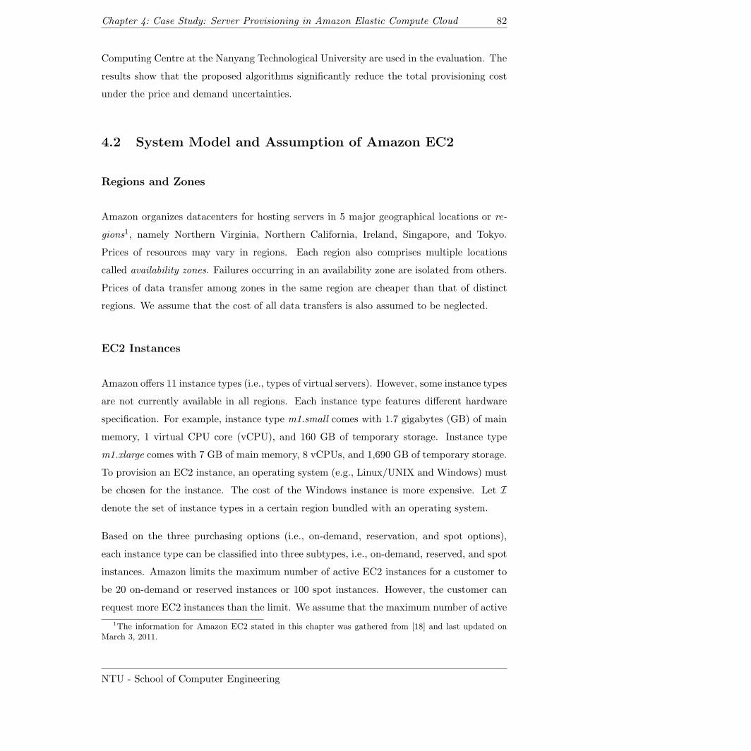
Chapter 4: Case Study: Server Provisioning in Amazon Elastic Compute Cloud 82
Computing Centre at the Nanyang Technological University are used in the evaluation. The
results show that the proposed algorithms significantly reduce the total provisioning cost
under the price and demand uncertainties.
4.2 System Model and Assumption of Amazon EC2
Regions and Zones
Amazon organizes datacenters for hosting servers in 5 major geographical locations or re-
gions1, namely Northern Virginia, Northern California, Ireland, Singapore, and Tokyo.
Prices of resources may vary in regions. Each region also comprises multiple locations
called availability zones. Failures occurring in an availability zone are isolated from others.
Prices of data transfer among zones in the same region are cheaper than that of distinct
regions. We assume that the cost of all data transfers is also assumed to be neglected.
EC2 Instances
Amazon offers 11 instance types (i.e., types of virtual servers). However, some instance types
are not currently available in all regions. Each instance type features different hardware
specification. For example, instance type m1.small comes with 1.7 gigabytes (GB) of main
memory, 1 virtual CPU core (vCPU), and 160 GB of temporary storage. Instance type
m1.xlarge comes with 7 GB of main memory, 8 vCPUs, and 1,690 GB of temporary storage.
To provision an EC2 instance, an operating system (e.g., Linux/UNIX and Windows) must
be chosen for the instance. The cost of the Windows instance is more expensive. Let I
denote the set of instance types in a certain region bundled with an operating system.
Based on the three purchasing options (i.e., on-demand, reservation, and spot options),
each instance type can be classified into three subtypes, i.e., on-demand, reserved, and spot
instances. Amazon limits the maximum number of active EC2 instances for a customer to
be 20 on-demand or reserved instances or 100 spot instances. However, the customer can
request more EC2 instances than the limit. We assume that the maximum number of active
1The information for Amazon EC2 stated in this chapter was gathered from [18] and last updated onMarch 3, 2011.
NTU - School of Computer Engineering
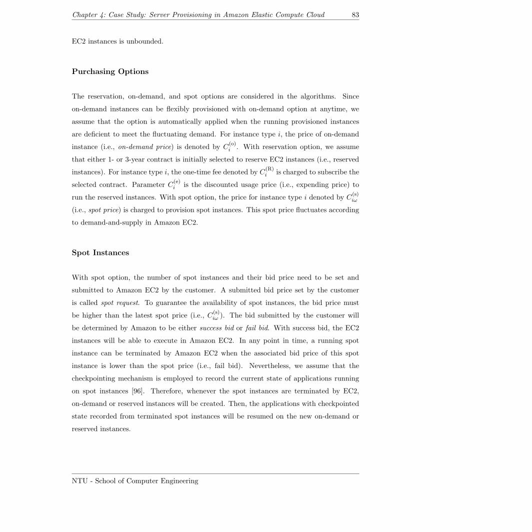
Chapter 4: Case Study: Server Provisioning in Amazon Elastic Compute Cloud 83
EC2 instances is unbounded.
Purchasing Options
The reservation, on-demand, and spot options are considered in the algorithms. Since
on-demand instances can be flexibly provisioned with on-demand option at anytime, we
assume that the option is automatically applied when the running provisioned instances
are deficient to meet the fluctuating demand. For instance type i, the price of on-demand
instance (i.e., on-demand price) is denoted by C(o)i . With reservation option, we assume
that either 1- or 3-year contract is initially selected to reserve EC2 instances (i.e., reserved
instances). For instance type i, the one-time fee denoted by C(R)i is charged to subscribe the
selected contract. Parameter C(e)i is the discounted usage price (i.e., expending price) to
run the reserved instances. With spot option, the price for instance type i denoted by C(s)iω
(i.e., spot price) is charged to provision spot instances. This spot price fluctuates according
to demand-and-supply in Amazon EC2.
Spot Instances
With spot option, the number of spot instances and their bid price need to be set and
submitted to Amazon EC2 by the customer. A submitted bid price set by the customer
is called spot request. To guarantee the availability of spot instances, the bid price must
be higher than the latest spot price (i.e., C(s)iω ). The bid submitted by the customer will
be determined by Amazon to be either success bid or fail bid. With success bid, the EC2
instances will be able to execute in Amazon EC2. In any point in time, a running spot
instance can be terminated by Amazon EC2 when the associated bid price of this spot
instance is lower than the spot price (i.e., fail bid). Nevertheless, we assume that the
checkpointing mechanism is employed to record the current state of applications running
on spot instances [96]. Therefore, whenever the spot instances are terminated by EC2,
on-demand or reserved instances will be created. Then, the applications with checkpointed
state recorded from terminated spot instances will be resumed on the new on-demand or
reserved instances.
NTU - School of Computer Engineering
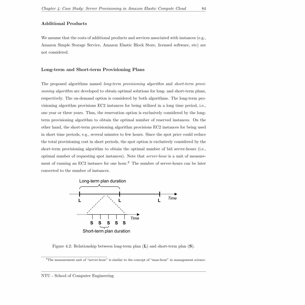
Chapter 4: Case Study: Server Provisioning in Amazon Elastic Compute Cloud 84
Additional Products
We assume that the costs of additional products and services associated with instances (e.g.,
Amazon Simple Storage Service, Amazon Elastic Block Store, licensed software, etc) are
not considered.
Long-term and Short-term Provisioning Plans
The proposed algorithms named long-term provisioning algorithm and short-term provi-
sioning algorithm are developed to obtain optimal solutions for long- and short-term plans,
respectively. The on-demand option is considered by both algorithms. The long-term pro-
visioning algorithm provisions EC2 instances for being utilized in a long time period, i.e.,
one year or three years. Thus, the reservation option is exclusively considered by the long-
term provisioning algorithm to obtain the optimal number of reserved instances. On the
other hand, the short-term provisioning algorithm provisions EC2 instances for being used
in short time periods, e.g., several minutes to few hours. Since the spot price could reduce
the total provisioning cost in short periods, the spot option is exclusively considered by the
short-term provisioning algorithm to obtain the optimal number of bid server-hours (i.e.,
optimal number of requesting spot instances). Note that server-hour is a unit of measure-
ment of running an EC2 instance for one hour.2 The number of server-hours can be later
converted to the number of instances.
Long-term plan duration
L L LTime
S S SS
Short-term plan duration
S
Time
Figure 4.2: Relationship between long-term plan (L) and short-term plan (S).
2The measurement unit of “server-hour” is similar to the concept of “man-hour” in management science.
NTU - School of Computer Engineering
Chapter 4: Case Study: Server Provisioning in Amazon Elastic Compute Cloud 85
Fig. 4.2 illustrates the relationship between long- and short-term plans. The long-term plan
is determined by the long-term provisioning algorithm by subscribing reserved instances for
the long-term usage (e.g., one year). However, the reserved instances may not be sufficient
to accommodate the fluctuating demand. Hence, the on-demand and spot options need to
be considered. As shown in Fig. 4.2, inside the long-term plan, multiple short-term plans
are determined by the short-term provisioning algorithm to obtain the optimal number of
new spot instances. Since the price and availability of spot instances cannot be guaranteed,
the short-term plans are periodically performed. In addition, the duration of the plans is
short (e.g., hours). Moreover, when the running spot instances are more expensive than
that of on-demand instances or the running spot instances are terminated by EC2, new
on-demand instances can be created to replace the spot instances. In practice, the long-
term provisioning algorithm must be executed to achieve the optimal number of reserved
instances before executing short-term provisioning plans. The number of reserved instances
obtained from the long-term plan will be used as a parameter in the short-term provisioning
plans.
Applications and Instance Pool
An EC2 instance is provisioned for a certain application. Let A denote the set of applica-
tions. All provisioned EC2 instances are collected into the instance pool where applications
can be partitioned and assigned to the EC2 instances from this pool. Each application re-
quires the sufficient number of server-hours to finish its workload processing. The number
of required server-hours is referred to as demand denoted by Daω, i.e., the demand of appli-
cation a. We assume that multiple instances can be grouped together to offer the sufficient
server-hours to the same application. Multiple instances in the same group can also run
in a parallel fashion to speedup the application. We assume that each EC2 instance is ex-
clusively assigned to a certain application. Load balancing mechanism, distributed system
middleware, and job scheduler are assumed to be available to manage the group of EC2
instances.
NTU - School of Computer Engineering
Chapter 4: Case Study: Server Provisioning in Amazon Elastic Compute Cloud 86
Performance Factor
The number of required server-hours of application a (i.e., Daω) is based on the total
execution time spending to execute in a certain server called base server. The base server
has to be benchmarked with a suitable performance metric to determine the computational
performance [105]. Let Ba denote the performance measured on the base server, and Ei
denote the performance measured on instance type i of Amazon EC2. The performance
factor is a ratio defined as follows:
λai =1
⌈Ba/Ei⌉(4.1)
where ⌈·⌉ denotes the ceiling function.
Uncertainty
Optimal solutions of the proposed algorithms are obtained by solving stochastic program-
ming models [28]. The models take the uncertainty of parameters into account. The uncer-
tain parameter is described by scenarios, and there is a probability distribution associated
with the uncertain parameter. Three uncertain parameters are considered, namely de-
mand, spot price, and bid outcome. The set of scenarios for demand uncertainty denoted
by Ω[demand]a contains the possible numbers of server-hours required by application a. The
set of scenarios for spot price uncertainty denoted by Ω[price]i consists of the possible spot
prices of instance type i. Given a certain bid price, the set of scenarios for bid outcome is
denoted by Ω[outcome]i = 0, 1 where values 0 and 1 represent the failure and success bids,
respectively. We assume that the probability distribution of each scenario set has finite
support. For instance, Ω[price]i has a finite number of scenarios. Each scenario associates
with probability 0 ≤ π′ω ≤ 1. Note that∑
ω′∈Ω[price]i
πω′ = 1. The uncertain parameters
are assumed to be independent of each other.
The set of all possible scenarios denoted by Ω can be obtained through the Cartesian product
as follows:
NTU - School of Computer Engineering
Chapter 4: Case Study: Server Provisioning in Amazon Elastic Compute Cloud 87
Ω =∏a∈A
Ω[demand]a ×
∏i∈I
Ω[price]i ×
∏i∈I
Ω[outcome]i . (4.2)
Next, scenario ω ∈ Ω can be described by a random vector denoted by ξ(ω), namely
ξ(ω) =(Daω, C
(s)iω , µiω
).
In practice, the long-term provisioning plan considers only the uncertain parameter of the
demand, i.e., Ω[demand]a . This parameter with its probability distribution can be obtained by
analyzing historical information of demand in past several months to years. In contrast, the
short-term provisioning plan considers every uncertain parameter. However, the information
about demand, spot prices, bid outcomes should be periodically analyzed to obtain all
uncertain parameters with their up-to-date probability distributions due to their frequent
fluctuation. For our guideline, the uncertain parameters for the short-term plan should
be updated by analyzing the lastest 10 days of historical information. Such a duration of
updating historical information was also applied in [96] to generate a probability distribution
of resource availability based on the latest 10 days of price history. The frequency to
perform the short-term plan can vary. We provide a discussion regarding such a frequency
in Section 4.4.2-4.
4.3 Long-term and Short-term Provisioning Algorithms
The long- and short-term provisioning algorithms are proposed to optimally purchase the
provisioning options for long- and short-term planning, respectively. Optimal solutions
of the algorithms are obtained by formulating and solving stochastic programming (SP)
models [28]. Each model consists of first- and second-stage decision variables, i.e., here-
and-now and wait-and-see decisions, respectively. The here-and-now decisions have to be
made before the value of uncertain parameter (i.e., ω ∈ Ω) will be observed. In contrast,
the wait-and-see decisions will be made based on the observed value of uncertain parameter.
The stochastic programming formulations can be transformed into deterministic equivalent
models which are conveniently solved by linear optimization solver software, e.g., GNU
Linear Programming Kit (GLPK) [57], solvers supported by General Algebraic Modeling
System (GAMS) [65], and solvers provided in the NEOS Server[66].
NTU - School of Computer Engineering
Chapter 4: Case Study: Server Provisioning in Amazon Elastic Compute Cloud 88
4.3.1 Long-term Provisioning Algorithm
The deterministic equivalent model of long-term provisioning algorithm is derived by follow-
ing the basic properties of stochastic programming with two-stage recourse [97] as follows:
minx(R)ai ,x
(e)aiω ,x
(o)aiω
∑a∈A
∑i∈I
C(R)i x
(R)ai +
∑i∈I
∑a∈A
∑ω∈Ω
πω
(C
(e)i x
(e)aiω + C
(o)i x
(o)aiω
)(4.3)
subject to: x(e)aiω ≤ L x
(R)ai , ∀a ∈ A, i ∈ I, ω ∈ Ω (4.4)
Daω =∑i∈I
λai
(x(e)aiω + x
(o)aiω
), ∀a ∈ A, ω ∈ Ω (4.5)
x(R)ai ∈ N0, ∀a ∈ A, i ∈ I (4.6)
x(e)aiω, x
(o)aiω ≥ 0, ∀a ∈ A, i ∈ I, ω ∈ Ω. (4.7)
The objective function in (4.3) minimizes the expected total provisioning cost. The model
consists of three decision variables as follows. Variable x(R)ij represents the here-and-now
decision. Variables x(e)ijω and x
(o)ijω represent the wait-and-see decisions. Specifically, variable
x(R)ij denotes the number of reserved instances subscribed in the first provisioning stage.
Variable x(e)ijω denotes the number of utilized server-hours taken from the reserved instances,
while x(o)ijω is the number of server-hours to be provisioned with on-demand option. For long-
term planning, set Ω contains only Ω[demand]a in which the probability distribution of demand
is determined from the historical data.
Constraint (4.4) ensures that the number of utilized reserved server-hours must not exceed
the total number of reserved hours. Constant L denotes the time duration of the availability
of reserved instances associated with the signed contract, i.e., L = 8, 760 hours for 1-year
contract and L = 26, 280 hours for 3-year contract. Constraint (4.5) governs the number of
provisioned server-hours which needs to meet the demand under scenario ω. Performance
factor λai defined in (4.1) is applied to scale the performance of instance types to that of
demand which is determined from the base server. Constraints (4.6) and (4.7) indicate that
the variables take the values from the sets of non-negative integers and non-negative real
numbers, respectively.
The optimization model in (4.3)-(4.7) mainly employs the reservation option for the here-
NTU - School of Computer Engineering
Chapter 4: Case Study: Server Provisioning in Amazon Elastic Compute Cloud 89
and-now decision (i.e., x(R)ij ), since this option has the fixed discounted price (i.e., C
(e)i ) and
guarantees the availability of reserved instances for a certain time duration.
The solution obtained from the long-term provisioning algorithm (i.e., value of x(R)ai ) can
be employed to the short-term provisioning algorithm as the utilizable number of reserved
server-hours with instance type i provisioned for application a denoted by Rai follows:
Rai = L x(R)ai . (4.8)
The optimization model defined in (4.3)-(4.7) can be extended into a robust optimization
(RO) model [29]. As discussed in Section 3.4, the term “robust” means that the solution
is less sensitive to any occurrence of uncertainty. When the solution is close to the optimal
solution, the solution is solution-robust. In addition, the RO model introduces penalty
functions to penalize undesirable costs for each scenario ω. The solution that almost avoids
the undesirable costs is model-robust. To achieve both solution- and model-robustness in
the long-term plan, the RO model is formulated as follows:
minx(R)ij ,x
(e)ijω ,x
(o)ijω ,θω
∑ω∈Ω
πωξ(ero)ω + γ
∑ω∈Ω
πωσ(ero)ω + β
∑ω∈Ω
πωρ(ero)ω (4.9)
subject to: (4.4)− (4.7)
ξω −∑ω′∈Ω
πω′ ξω′ + θω ≥ 0, ∀ω ∈ Ω (4.10)
θω ≥ 0, ∀ω ∈ Ω (4.11)
where ξ(ero)ω denotes the total provisioning cost given scenario ω defined as follows:
ξ(ero)ω =∑a∈A
∑i∈I
C(R)i x
(R)ai + C
(e)i x
(e)aiω + C
(o)i x
(o)aiω. (4.12)
In (4.9), θω is an additional slack variable introduced to avoid a quadratic function as
aforementioned in Section 3.4.4. As a result, constraints (4.10) and (4.11) need to be
NTU - School of Computer Engineering
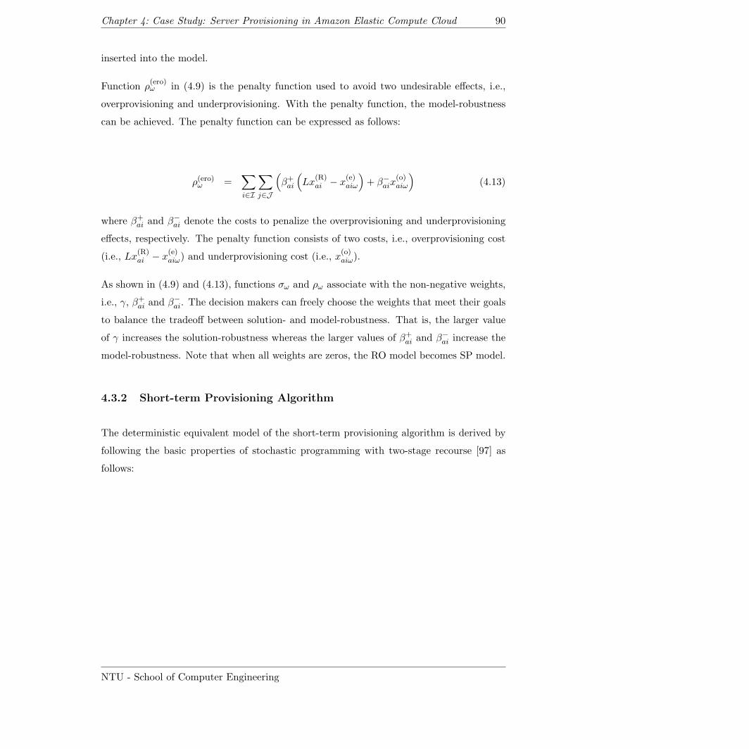
Chapter 4: Case Study: Server Provisioning in Amazon Elastic Compute Cloud 90
inserted into the model.
Function ρ(ero)ω in (4.9) is the penalty function used to avoid two undesirable effects, i.e.,
overprovisioning and underprovisioning. With the penalty function, the model-robustness
can be achieved. The penalty function can be expressed as follows:
ρ(ero)ω =∑i∈I
∑j∈J
(β+ai
(Lx
(R)ai − x
(e)aiω
)+ β−aix
(o)aiω
)(4.13)
where β+ai and β−ai denote the costs to penalize the overprovisioning and underprovisioning
effects, respectively. The penalty function consists of two costs, i.e., overprovisioning cost
(i.e., Lx(R)ai − x
(e)aiω) and underprovisioning cost (i.e., x
(o)aiω).
As shown in (4.9) and (4.13), functions σω and ρω associate with the non-negative weights,
i.e., γ, β+ai and β−ai. The decision makers can freely choose the weights that meet their goals
to balance the tradeoff between solution- and model-robustness. That is, the larger value
of γ increases the solution-robustness whereas the larger values of β+ai and β−ai increase the
model-robustness. Note that when all weights are zeros, the RO model becomes SP model.
4.3.2 Short-term Provisioning Algorithm
The deterministic equivalent model of the short-term provisioning algorithm is derived by
following the basic properties of stochastic programming with two-stage recourse [97] as
follows:
NTU - School of Computer Engineering
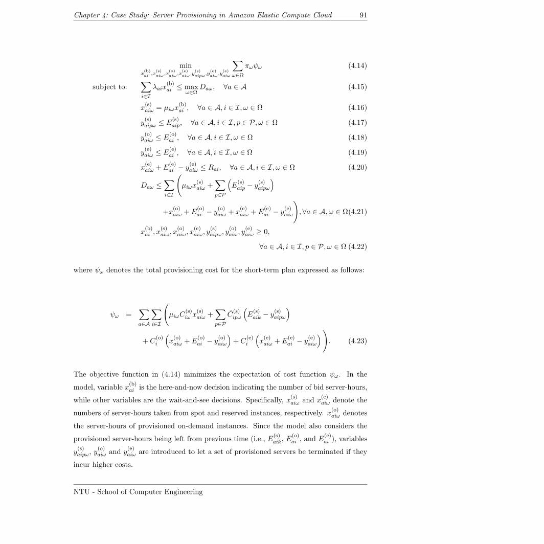
Chapter 4: Case Study: Server Provisioning in Amazon Elastic Compute Cloud 91
minx(b)ai ,x
(s)aiω ,x
(o)aiω ,x
(e)aiω ,y
(s)aipω ,y
(o)aiω ,y
(e)aiω
∑ω∈Ω
πωψω (4.14)
subject to:∑i∈I
λaix(b)ai ≤ max
ω∈ΩDaω, ∀a ∈ A (4.15)
x(s)aiω = µiωx
(b)ai , ∀a ∈ A, i ∈ I, ω ∈ Ω (4.16)
y(s)aipω ≤ E
(s)aip, ∀a ∈ A, i ∈ I, p ∈ P, ω ∈ Ω (4.17)
y(o)aiω ≤ E
(o)ai , ∀a ∈ A, i ∈ I, ω ∈ Ω (4.18)
y(e)aiω ≤ E
(e)ai , ∀a ∈ A, i ∈ I, ω ∈ Ω (4.19)
x(e)aiω + E
(e)ai − y
(e)aiω ≤ Rai, ∀a ∈ A, i ∈ I, ω ∈ Ω (4.20)
Daω ≤∑i∈I
(µiωx
(s)aiω +
∑p∈P
(E
(s)aip − y
(s)aipω
)
+x(o)aiω + E
(o)ai − y
(o)aiω + x
(e)aiω + E
(e)ai − y
(e)aiω
), ∀a ∈ A, ω ∈ Ω(4.21)
x(b)ai , x
(s)aiω, x
(o)aiω, x
(e)aiω, y
(s)aipω, y
(o)aiω, y
(e)aiω ≥ 0,
∀a ∈ A, i ∈ I, p ∈ P, ω ∈ Ω (4.22)
where ψω denotes the total provisioning cost for the short-term plan expressed as follows:
ψω =∑a∈A
∑i∈I
(µiωC
(s)iω x
(s)aiω +
∑p∈P
C(s)ipω
(E
(s)aik − y
(s)aipω
)
+ C(o)i
(x(o)aiω + E
(o)ai − y
(o)aiω
)+ C
(e)i
(x(e)aiω + E
(e)ai − y
(e)aiω
)). (4.23)
The objective function in (4.14) minimizes the expectation of cost function ψω. In the
model, variable x(b)ai is the here-and-now decision indicating the number of bid server-hours,
while other variables are the wait-and-see decisions. Specifically, x(s)aiω and x
(e)aiω denote the
numbers of server-hours taken from spot and reserved instances, respectively. x(o)aiω denotes
the server-hours of provisioned on-demand instances. Since the model also considers the
provisioned server-hours being left from previous time (i.e., E(s)aik, E
(o)ai , and E
(e)ai ), variables
y(s)aipω, y
(o)aiω and y
(e)aiω are introduced to let a set of provisioned servers be terminated if they
incur higher costs.
NTU - School of Computer Engineering
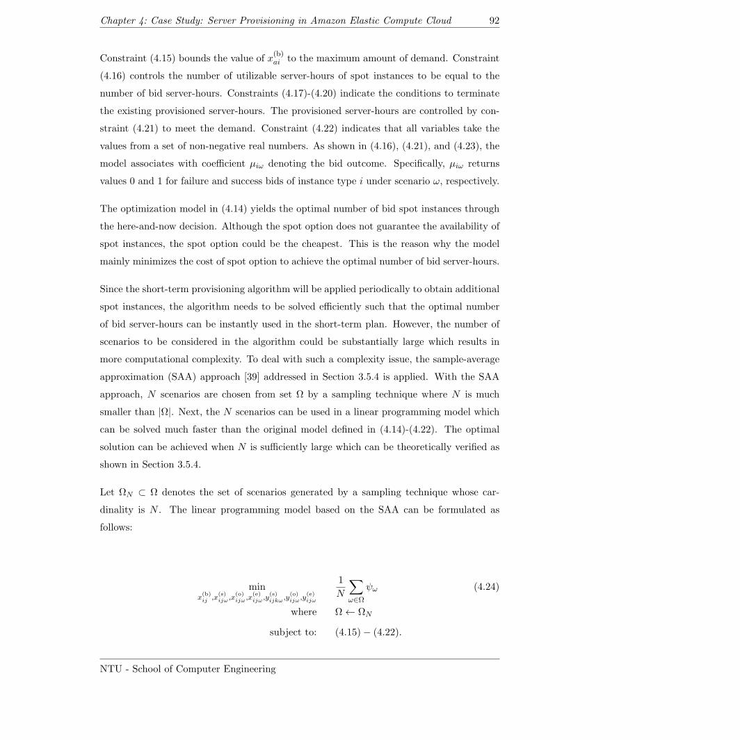
Chapter 4: Case Study: Server Provisioning in Amazon Elastic Compute Cloud 92
Constraint (4.15) bounds the value of x(b)ai to the maximum amount of demand. Constraint
(4.16) controls the number of utilizable server-hours of spot instances to be equal to the
number of bid server-hours. Constraints (4.17)-(4.20) indicate the conditions to terminate
the existing provisioned server-hours. The provisioned server-hours are controlled by con-
straint (4.21) to meet the demand. Constraint (4.22) indicates that all variables take the
values from a set of non-negative real numbers. As shown in (4.16), (4.21), and (4.23), the
model associates with coefficient µiω denoting the bid outcome. Specifically, µiω returns
values 0 and 1 for failure and success bids of instance type i under scenario ω, respectively.
The optimization model in (4.14) yields the optimal number of bid spot instances through
the here-and-now decision. Although the spot option does not guarantee the availability of
spot instances, the spot option could be the cheapest. This is the reason why the model
mainly minimizes the cost of spot option to achieve the optimal number of bid server-hours.
Since the short-term provisioning algorithm will be applied periodically to obtain additional
spot instances, the algorithm needs to be solved efficiently such that the optimal number
of bid server-hours can be instantly used in the short-term plan. However, the number of
scenarios to be considered in the algorithm could be substantially large which results in
more computational complexity. To deal with such a complexity issue, the sample-average
approximation (SAA) approach [39] addressed in Section 3.5.4 is applied. With the SAA
approach, N scenarios are chosen from set Ω by a sampling technique where N is much
smaller than |Ω|. Next, the N scenarios can be used in a linear programming model which
can be solved much faster than the original model defined in (4.14)-(4.22). The optimal
solution can be achieved when N is sufficiently large which can be theoretically verified as
shown in Section 3.5.4.
Let ΩN ⊂ Ω denotes the set of scenarios generated by a sampling technique whose car-
dinality is N . The linear programming model based on the SAA can be formulated as
follows:
minx(b)ij ,x
(s)ijω ,x
(o)ijω ,x
(e)ijω ,y
(s)ijkω ,y
(o)ijω ,y
(e)ijω
1
N
∑ω∈Ω
ψω (4.24)
where Ω← ΩN
subject to: (4.15)− (4.22).
NTU - School of Computer Engineering
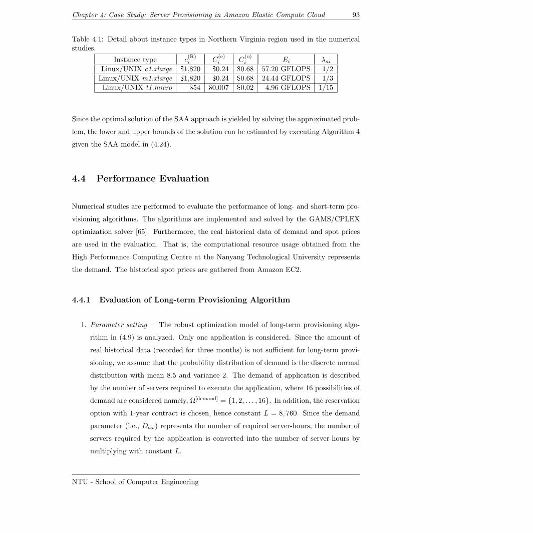
Chapter 4: Case Study: Server Provisioning in Amazon Elastic Compute Cloud 93
Table 4.1: Detail about instance types in Northern Virginia region used in the numericalstudies.
Instance type c(R)i C
(e)i C
(o)i Ei λai
Linux/UNIX c1.xlarge $1,820 $0.24 $0.68 57.20 GFLOPS 1/2
Linux/UNIX m1.xlarge $1,820 $0.24 $0.68 24.44 GFLOPS 1/3
Linux/UNIX t1.micro $54 $0.007 $0.02 4.96 GFLOPS 1/15
Since the optimal solution of the SAA approach is yielded by solving the approximated prob-
lem, the lower and upper bounds of the solution can be estimated by executing Algorithm 4
given the SAA model in (4.24).
4.4 Performance Evaluation
Numerical studies are performed to evaluate the performance of long- and short-term pro-
visioning algorithms. The algorithms are implemented and solved by the GAMS/CPLEX
optimization solver [65]. Furthermore, the real historical data of demand and spot prices
are used in the evaluation. That is, the computational resource usage obtained from the
High Performance Computing Centre at the Nanyang Technological University represents
the demand. The historical spot prices are gathered from Amazon EC2.
4.4.1 Evaluation of Long-term Provisioning Algorithm
1. Parameter setting – The robust optimization model of long-term provisioning algo-
rithm in (4.9) is analyzed. Only one application is considered. Since the amount of
real historical data (recorded for three months) is not sufficient for long-term provi-
sioning, we assume that the probability distribution of demand is the discrete normal
distribution with mean 8.5 and variance 2. The demand of application is described
by the number of servers required to execute the application, where 16 possibilities of
demand are considered namely, Ω[demand] = 1, 2, . . . , 16. In addition, the reservation
option with 1-year contract is chosen, hence constant L = 8, 760. Since the demand
parameter (i.e., Daω) represents the number of required server-hours, the number of
servers required by the application is converted into the number of server-hours by
multiplying with constant L.
NTU - School of Computer Engineering
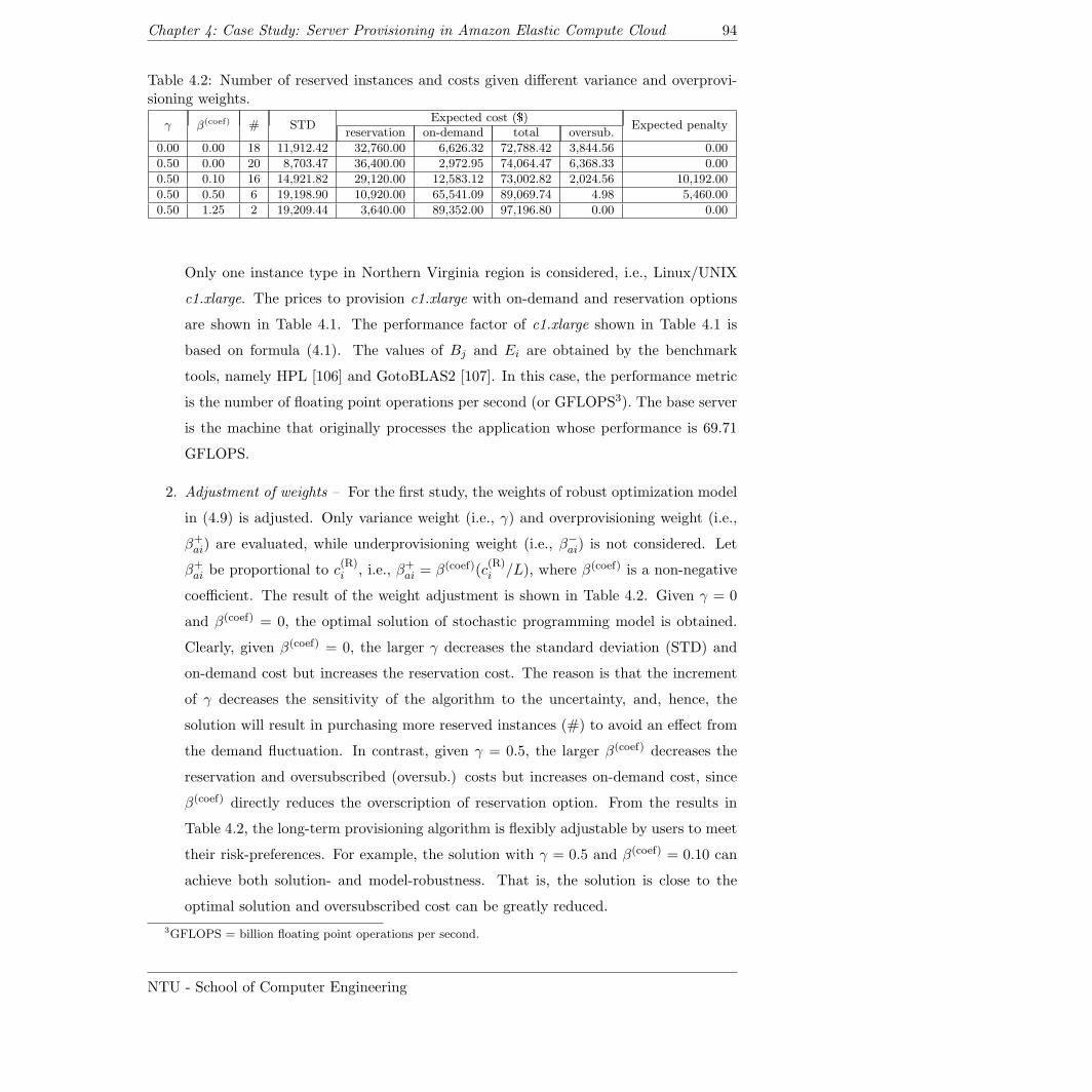
Chapter 4: Case Study: Server Provisioning in Amazon Elastic Compute Cloud 94
Table 4.2: Number of reserved instances and costs given different variance and overprovi-sioning weights.
γ β(coef) # STDExpected cost ($)
Expected penaltyreservation on-demand total oversub.
0.00 0.00 18 11,912.42 32,760.00 6,626.32 72,788.42 3,844.56 0.00
0.50 0.00 20 8,703.47 36,400.00 2,972.95 74,064.47 6,368.33 0.00
0.50 0.10 16 14,921.82 29,120.00 12,583.12 73,002.82 2,024.56 10,192.00
0.50 0.50 6 19,198.90 10,920.00 65,541.09 89,069.74 4.98 5,460.00
0.50 1.25 2 19,209.44 3,640.00 89,352.00 97,196.80 0.00 0.00
Only one instance type in Northern Virginia region is considered, i.e., Linux/UNIX
c1.xlarge. The prices to provision c1.xlarge with on-demand and reservation options
are shown in Table 4.1. The performance factor of c1.xlarge shown in Table 4.1 is
based on formula (4.1). The values of Bj and Ei are obtained by the benchmark
tools, namely HPL [106] and GotoBLAS2 [107]. In this case, the performance metric
is the number of floating point operations per second (or GFLOPS3). The base server
is the machine that originally processes the application whose performance is 69.71
GFLOPS.
2. Adjustment of weights – For the first study, the weights of robust optimization model
in (4.9) is adjusted. Only variance weight (i.e., γ) and overprovisioning weight (i.e.,
β+ai) are evaluated, while underprovisioning weight (i.e., β−ai) is not considered. Let
β+ai be proportional to c(R)i , i.e., β+ai = β(coef)(c
(R)i /L), where β(coef) is a non-negative
coefficient. The result of the weight adjustment is shown in Table 4.2. Given γ = 0
and β(coef) = 0, the optimal solution of stochastic programming model is obtained.
Clearly, given β(coef) = 0, the larger γ decreases the standard deviation (STD) and
on-demand cost but increases the reservation cost. The reason is that the increment
of γ decreases the sensitivity of the algorithm to the uncertainty, and, hence, the
solution will result in purchasing more reserved instances (#) to avoid an effect from
the demand fluctuation. In contrast, given γ = 0.5, the larger β(coef) decreases the
reservation and oversubscribed (oversub.) costs but increases on-demand cost, since
β(coef) directly reduces the overscription of reservation option. From the results in
Table 4.2, the long-term provisioning algorithm is flexibly adjustable by users to meet
their risk-preferences. For example, the solution with γ = 0.5 and β(coef) = 0.10 can
achieve both solution- and model-robustness. That is, the solution is close to the
optimal solution and oversubscribed cost can be greatly reduced.
3GFLOPS = billion floating point operations per second.
NTU - School of Computer Engineering
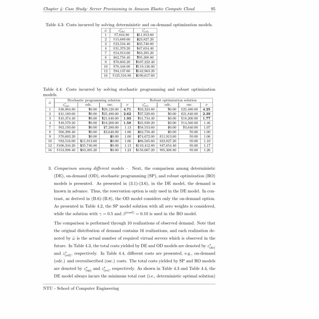
Chapter 4: Case Study: Server Provisioning in Amazon Elastic Compute Cloud 95
Table 4.3: Costs incurred by solving deterministic and on-demand optimization models.ω z∗(de) z∗(od)1 $7,844.80 $11,913.60
2 $15,689.60 $23,827.20
3 $23,534.40 $35,740.80
4 $31,379.20 $47,654.40
7 $54,913.60 $83,395.20
8 $62,758.40 $95,308.80
9 $70,603.20 $107,222.40
10 $78,448.00 $119,136.00
12 $94,137.60 $142,963.20
16 $125,516.80 $190,617.60
Table 4.4: Costs incurred by solving stochastic programming and robust optimizationmodels.
ωStochastic programming solution Robust optimization solution
z∗(sp) odc. osc. ν z∗(ro) odc. osc. ν
1 $36,964.80 $0.00 $29,120.00 4.71 $33,324.80 $0.00 $25,480.00 4.25
2 $41,169.60 $0.00 $25,480.00 2.62 $37,529.60 $0.00 $21,840.00 2.39
3 $45,374.40 $0.00 $21,840.00 1.93 $41,734.40 $0.00 $18,200.00 1.77
4 $49,579.20 $0.00 $18,200.00 1.58 $45,939.20 $0.00 $14,560.00 1.46
7 $62,193.60 $0.00 $7,280.00 1.13 $58,553.60 $0.00 $3,640.00 1.07
8 $66,398.40 $0.00 $3,640.00 1.06 $62,758.40 $0.00 $0.00 1.00
9 $70,603.20 $0.00 $0.00 1.00 $74,672.00 $11,913.60 $0.00 1.06
10 $82,516.00 $11,913.60 $0.00 1.06 $86,585.60 $23,827.20 $0.00 1.10
12 $106,344.20 $35,740.80 $0.00 1.13 $110,412.80 $47,654.40 $0.00 1.17
16 $153,998.40 $83,395.20 $0.00 1.23 $158,067.20 $95,308.80 $0.00 1.26
3. Comparison among different models – Next, the comparison among deterministic
(DE), on-demand (OD), stochastic programming (SP), and robust optimization (RO)
models is presented. As presented in (3.1)-(3.6), in the DE model, the demand is
known in advance. Thus, the reservation option is only used in the DE model. In con-
trast, as derived in (B.6)-(B.8), the OD model considers only the on-demand option.
As presented in Table 4.2, the SP model solution with all zero weights is considered,
while the solution with γ = 0.5 and β(coef) = 0.10 is used in the RO model.
The comparison is performed through 10 realizations of observed demand. Note that
the original distribution of demand contains 16 realizations, and each realization de-
noted by ω is the actual number of required virtual servers which is observed in the
future. In Table 4.3, the total costs yielded by DE and OD models are denoted by z∗(de)
and z∗(od), respectively. In Table 4.4, different costs are presented, e.g., on-demand
(odc.) and oversubscribed (osc.) costs. The total costs yielded by SP and RO models
are denoted by z∗(sp) and z∗(ro), respectively. As shown in Table 4.3 and Table 4.4, the
DE model always incurs the minimum total cost (i.e., deterministic optimal solution)
NTU - School of Computer Engineering
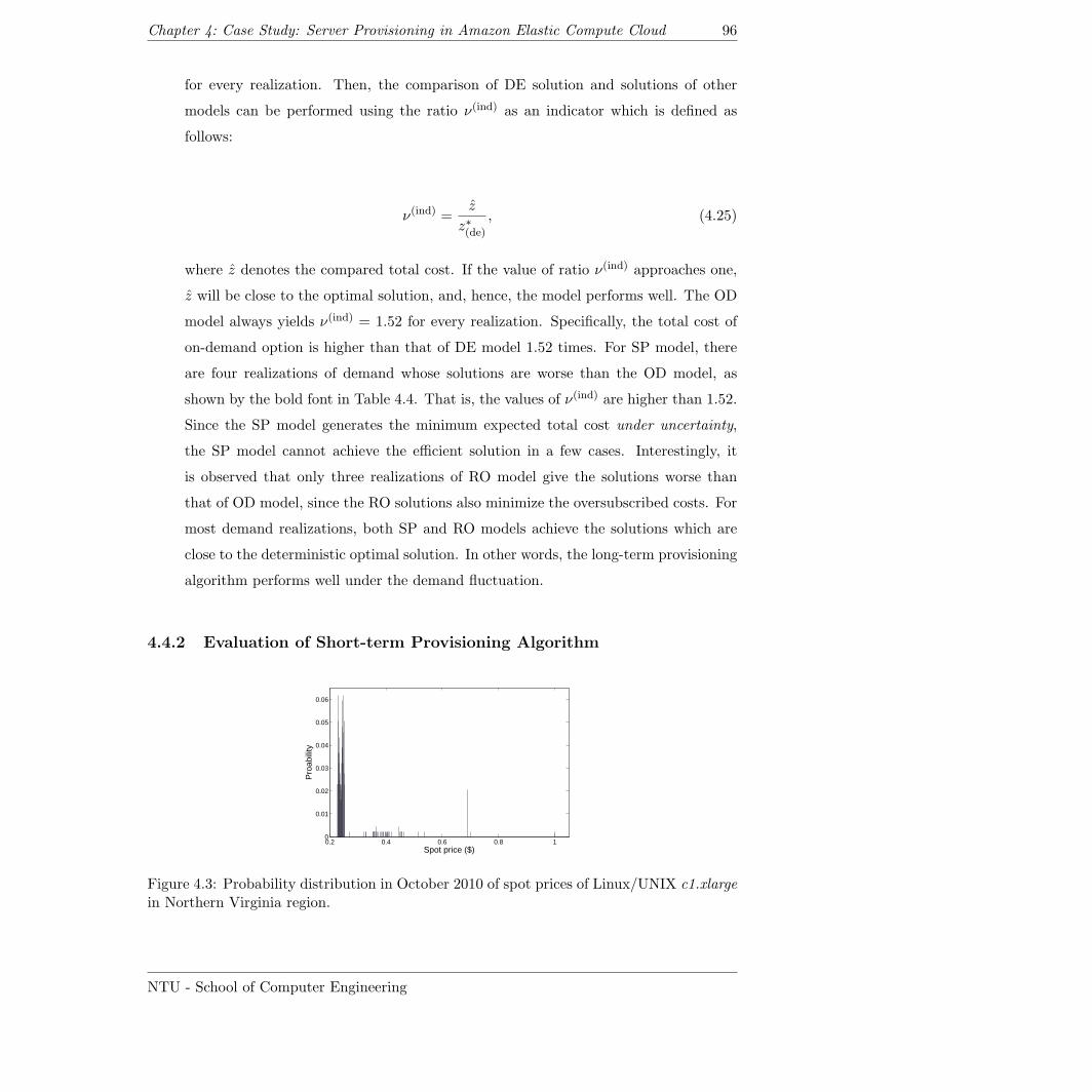
Chapter 4: Case Study: Server Provisioning in Amazon Elastic Compute Cloud 96
for every realization. Then, the comparison of DE solution and solutions of other
models can be performed using the ratio ν(ind) as an indicator which is defined as
follows:
ν(ind) =z
z∗(de), (4.25)
where z denotes the compared total cost. If the value of ratio ν(ind) approaches one,
z will be close to the optimal solution, and, hence, the model performs well. The OD
model always yields ν(ind) = 1.52 for every realization. Specifically, the total cost of
on-demand option is higher than that of DE model 1.52 times. For SP model, there
are four realizations of demand whose solutions are worse than the OD model, as
shown by the bold font in Table 4.4. That is, the values of ν(ind) are higher than 1.52.
Since the SP model generates the minimum expected total cost under uncertainty,
the SP model cannot achieve the efficient solution in a few cases. Interestingly, it
is observed that only three realizations of RO model give the solutions worse than
that of OD model, since the RO solutions also minimize the oversubscribed costs. For
most demand realizations, both SP and RO models achieve the solutions which are
close to the deterministic optimal solution. In other words, the long-term provisioning
algorithm performs well under the demand fluctuation.
4.4.2 Evaluation of Short-term Provisioning Algorithm
0.2 0.4 0.6 0.8 10
0.01
0.02
0.03
0.04
0.05
0.06
Spot price ($)
Pro
abili
ty
Figure 4.3: Probability distribution in October 2010 of spot prices of Linux/UNIX c1.xlargein Northern Virginia region.
NTU - School of Computer Engineering
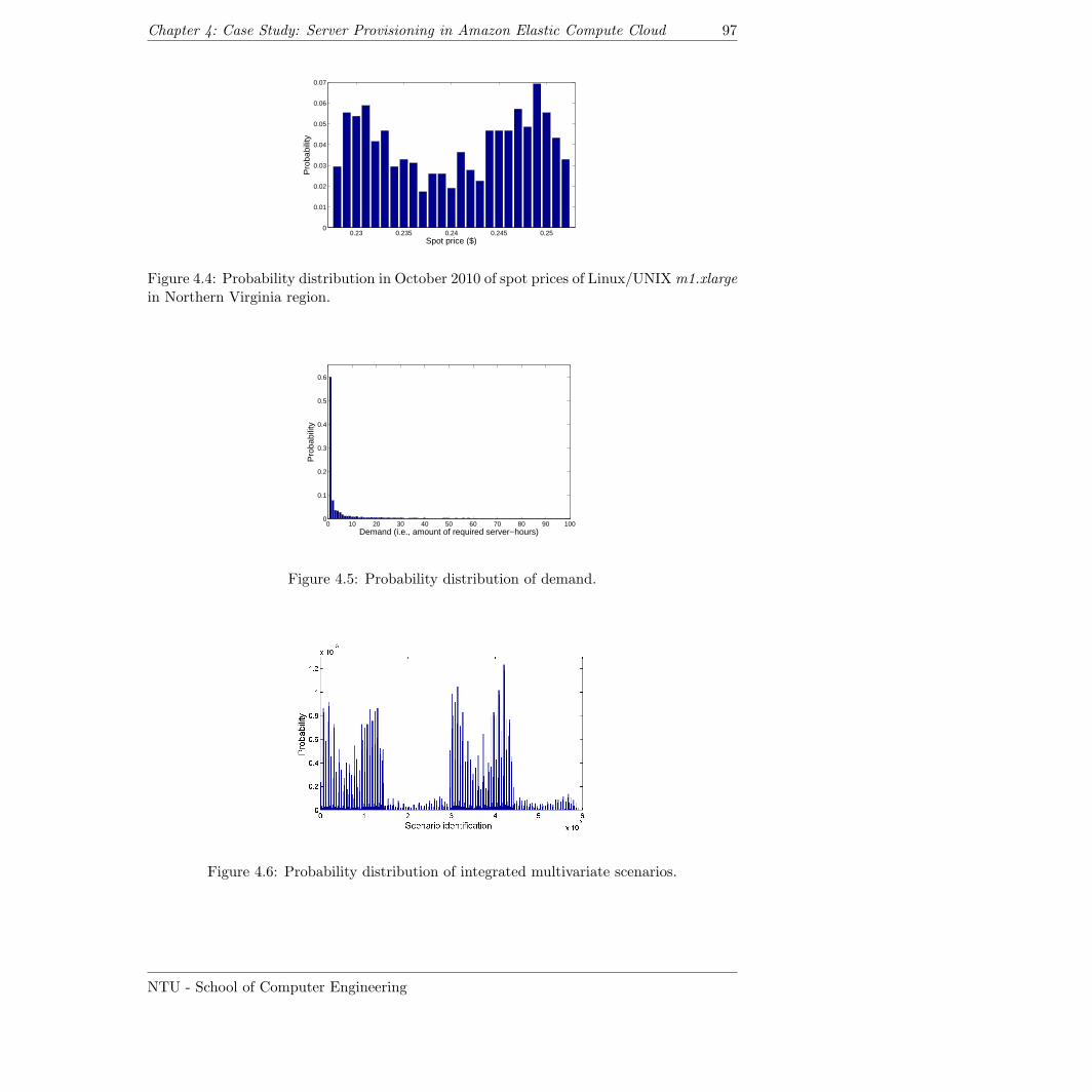
Chapter 4: Case Study: Server Provisioning in Amazon Elastic Compute Cloud 97
0.23 0.235 0.24 0.245 0.250
0.01
0.02
0.03
0.04
0.05
0.06
0.07
Spot price ($)
Pro
babi
lity
Figure 4.4: Probability distribution in October 2010 of spot prices of Linux/UNIXm1.xlargein Northern Virginia region.
0 10 20 30 40 50 60 70 80 90 1000
0.1
0.2
0.3
0.4
0.5
0.6
Demand (i.e., amount of required server−hours)
Pro
babi
lity
Figure 4.5: Probability distribution of demand.
Figure 4.6: Probability distribution of integrated multivariate scenarios.
NTU - School of Computer Engineering
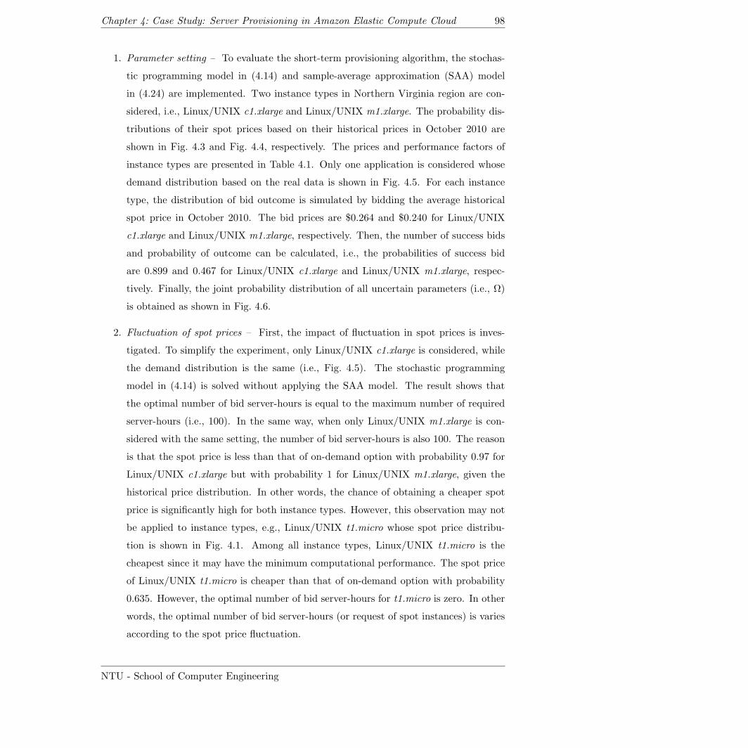
Chapter 4: Case Study: Server Provisioning in Amazon Elastic Compute Cloud 98
1. Parameter setting – To evaluate the short-term provisioning algorithm, the stochas-
tic programming model in (4.14) and sample-average approximation (SAA) model
in (4.24) are implemented. Two instance types in Northern Virginia region are con-
sidered, i.e., Linux/UNIX c1.xlarge and Linux/UNIX m1.xlarge. The probability dis-
tributions of their spot prices based on their historical prices in October 2010 are
shown in Fig. 4.3 and Fig. 4.4, respectively. The prices and performance factors of
instance types are presented in Table 4.1. Only one application is considered whose
demand distribution based on the real data is shown in Fig. 4.5. For each instance
type, the distribution of bid outcome is simulated by bidding the average historical
spot price in October 2010. The bid prices are $0.264 and $0.240 for Linux/UNIX
c1.xlarge and Linux/UNIX m1.xlarge, respectively. Then, the number of success bids
and probability of outcome can be calculated, i.e., the probabilities of success bid
are 0.899 and 0.467 for Linux/UNIX c1.xlarge and Linux/UNIX m1.xlarge, respec-
tively. Finally, the joint probability distribution of all uncertain parameters (i.e., Ω)
is obtained as shown in Fig. 4.6.
2. Fluctuation of spot prices – First, the impact of fluctuation in spot prices is inves-
tigated. To simplify the experiment, only Linux/UNIX c1.xlarge is considered, while
the demand distribution is the same (i.e., Fig. 4.5). The stochastic programming
model in (4.14) is solved without applying the SAA model. The result shows that
the optimal number of bid server-hours is equal to the maximum number of required
server-hours (i.e., 100). In the same way, when only Linux/UNIX m1.xlarge is con-
sidered with the same setting, the number of bid server-hours is also 100. The reason
is that the spot price is less than that of on-demand option with probability 0.97 for
Linux/UNIX c1.xlarge but with probability 1 for Linux/UNIX m1.xlarge, given the
historical price distribution. In other words, the chance of obtaining a cheaper spot
price is significantly high for both instance types. However, this observation may not
be applied to instance types, e.g., Linux/UNIX t1.micro whose spot price distribu-
tion is shown in Fig. 4.1. Among all instance types, Linux/UNIX t1.micro is the
cheapest since it may have the minimum computational performance. The spot price
of Linux/UNIX t1.micro is cheaper than that of on-demand option with probability
0.635. However, the optimal number of bid server-hours for t1.micro is zero. In other
words, the optimal number of bid server-hours (or request of spot instances) is varies
according to the spot price fluctuation.
NTU - School of Computer Engineering
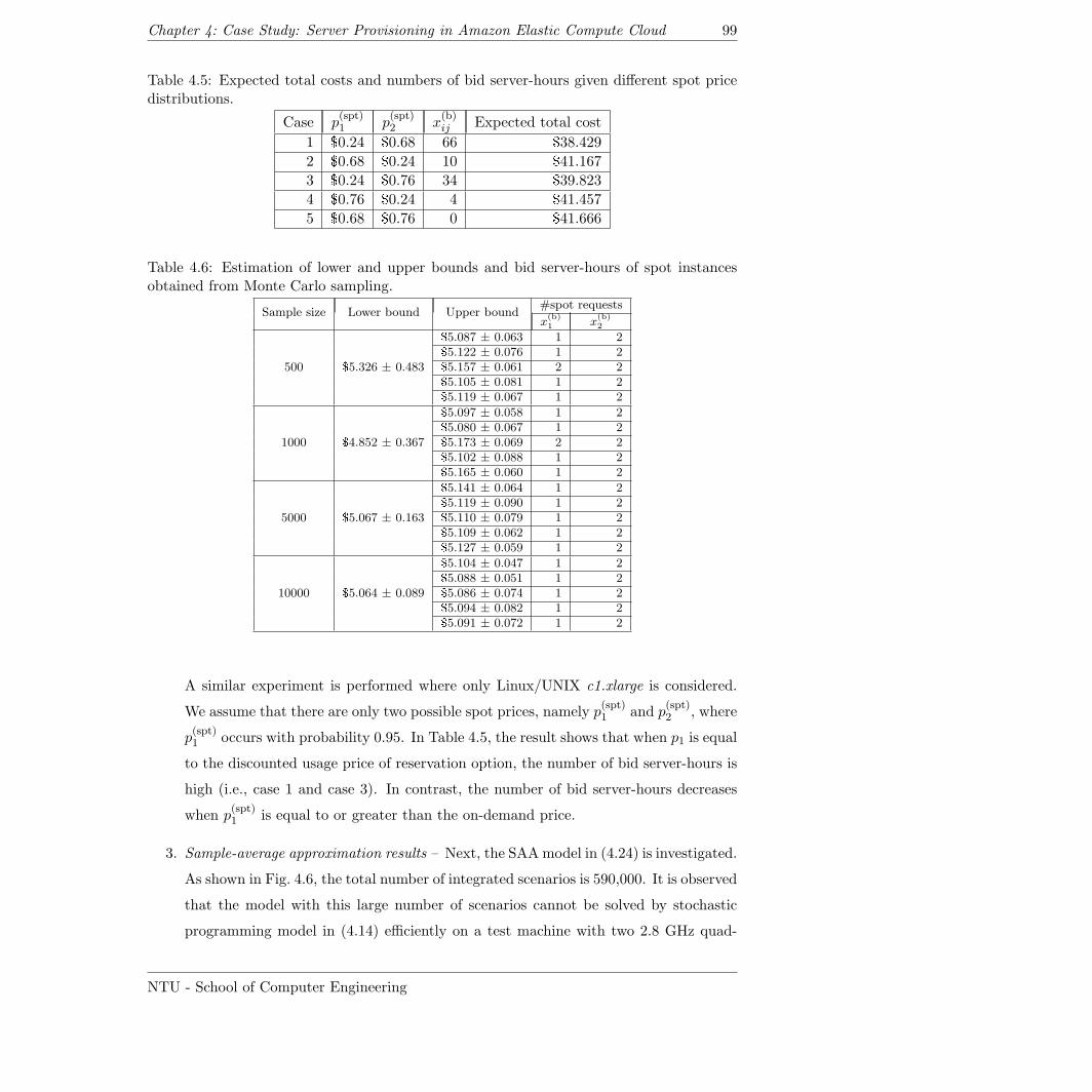
Chapter 4: Case Study: Server Provisioning in Amazon Elastic Compute Cloud 99
Table 4.5: Expected total costs and numbers of bid server-hours given different spot pricedistributions.
Case p(spt)1 p
(spt)2 x
(b)ij Expected total cost
1 $0.24 $0.68 66 $38.429
2 $0.68 $0.24 10 $41.167
3 $0.24 $0.76 34 $39.823
4 $0.76 $0.24 4 $41.457
5 $0.68 $0.76 0 $41.666
Table 4.6: Estimation of lower and upper bounds and bid server-hours of spot instancesobtained from Monte Carlo sampling.
Sample size Lower bound Upper bound#spot requests
x(b)1 x
(b)2
500 $5.326 ± 0.483
$5.087 ± 0.063 1 2$5.122 ± 0.076 1 2$5.157 ± 0.061 2 2$5.105 ± 0.081 1 2$5.119 ± 0.067 1 2
1000 $4.852 ± 0.367
$5.097 ± 0.058 1 2$5.080 ± 0.067 1 2$5.173 ± 0.069 2 2$5.102 ± 0.088 1 2$5.165 ± 0.060 1 2
5000 $5.067 ± 0.163
$5.141 ± 0.064 1 2$5.119 ± 0.090 1 2$5.110 ± 0.079 1 2$5.109 ± 0.062 1 2$5.127 ± 0.059 1 2
10000 $5.064 ± 0.089
$5.104 ± 0.047 1 2$5.088 ± 0.051 1 2$5.086 ± 0.074 1 2$5.094 ± 0.082 1 2$5.091 ± 0.072 1 2
A similar experiment is performed where only Linux/UNIX c1.xlarge is considered.
We assume that there are only two possible spot prices, namely p(spt)1 and p
(spt)2 , where
p(spt)1 occurs with probability 0.95. In Table 4.5, the result shows that when p1 is equal
to the discounted usage price of reservation option, the number of bid server-hours is
high (i.e., case 1 and case 3). In contrast, the number of bid server-hours decreases
when p(spt)1 is equal to or greater than the on-demand price.
3. Sample-average approximation results – Next, the SAAmodel in (4.24) is investigated.
As shown in Fig. 4.6, the total number of integrated scenarios is 590,000. It is observed
that the model with this large number of scenarios cannot be solved by stochastic
programming model in (4.14) efficiently on a test machine with two 2.8 GHz quad-
NTU - School of Computer Engineering
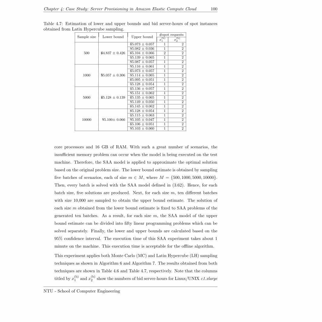
Chapter 4: Case Study: Server Provisioning in Amazon Elastic Compute Cloud 100
Table 4.7: Estimation of lower and upper bounds and bid server-hours of spot instancesobtained from Latin Hypercube sampling.
Sample size Lower bound Upper bound#spot requests
x(b)1 x
(b)2
500 $4.837 ± 0.426
$5.073 ± 0.057 1 2$5.082 ± 0.036 1 2$5.104 ± 0.066 2 2$5.139 ± 0.065 1 2$5.087 ± 0.057 1 2
1000 $5.057 ± 0.306
$5.116 ± 0.061 1 2$5.073 ± 0.057 1 2$5.114 ± 0.065 1 2$5.095 ± 0.051 1 2$5.128 ± 0.054 1 2
5000 $5.128 ± 0.139
$5.136 ± 0.057 1 2$5.151 ± 0.062 1 2$5.135 ± 0.065 1 2$5.149 ± 0.050 1 2$5.145 ± 0.062 1 2
10000 $5.100± 0.066
$5.128 ± 0.054 1 2$5.115 ± 0.063 1 2$5.105 ± 0.047 1 2$5.106 ± 0.051 1 2$5.103 ± 0.060 1 2
core processors and 16 GB of RAM. With such a great number of scenarios, the
insufficient memory problem can occur when the model is being executed on the test
machine. Therefore, the SAA model is applied to approximate the optimal solution
based on the original problem size. The lower bound estimate is obtained by sampling
five batches of scenarios, each of size m ∈ M , where M = 500, 1000, 5000, 10000.
Then, every batch is solved with the SAA model defined in (3.62). Hence, for each
batch size, five solutions are produced. Next, for each size m, ten different batches
with size 10,000 are sampled to obtain the upper bound estimate. The solution of
each size m obtained from the lower bound estimate is fixed to SAA problems of the
generated ten batches. As a result, for each size m, the SAA model of the upper
bound estimate can be divided into fifty linear programming problems which can be
solved separately. Finally, the lower and upper bounds are calculated based on the
95% confidence interval. The execution time of this SAA experiment takes about 1
minute on the machine. This execution time is acceptable for the offline algorithm.
This experiment applies both Monte Carlo (MC) and Latin Hypercube (LH) sampling
techniques as shown in Algorithm 6 and Algorithm 7. The results obtained from both
techniques are shown in Table 4.6 and Table 4.7, respectively. Note that the columns
titled by x(b)1 and x
(b)2 show the numbers of bid server-hours for Linux/UNIX c1.xlarge
NTU - School of Computer Engineering
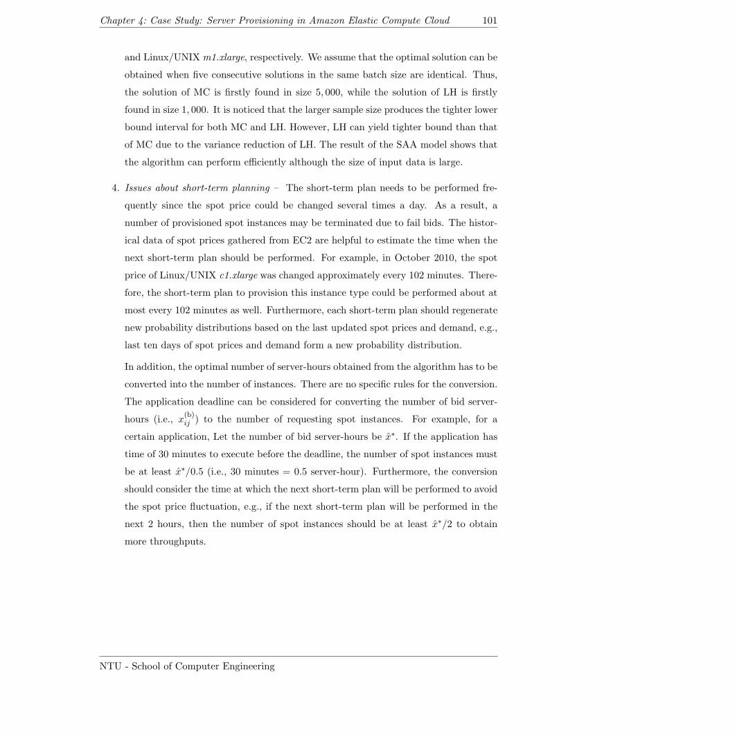
Chapter 4: Case Study: Server Provisioning in Amazon Elastic Compute Cloud 101
and Linux/UNIX m1.xlarge, respectively. We assume that the optimal solution can be
obtained when five consecutive solutions in the same batch size are identical. Thus,
the solution of MC is firstly found in size 5, 000, while the solution of LH is firstly
found in size 1, 000. It is noticed that the larger sample size produces the tighter lower
bound interval for both MC and LH. However, LH can yield tighter bound than that
of MC due to the variance reduction of LH. The result of the SAA model shows that
the algorithm can perform efficiently although the size of input data is large.
4. Issues about short-term planning – The short-term plan needs to be performed fre-
quently since the spot price could be changed several times a day. As a result, a
number of provisioned spot instances may be terminated due to fail bids. The histor-
ical data of spot prices gathered from EC2 are helpful to estimate the time when the
next short-term plan should be performed. For example, in October 2010, the spot
price of Linux/UNIX c1.xlarge was changed approximately every 102 minutes. There-
fore, the short-term plan to provision this instance type could be performed about at
most every 102 minutes as well. Furthermore, each short-term plan should regenerate
new probability distributions based on the last updated spot prices and demand, e.g.,
last ten days of spot prices and demand form a new probability distribution.
In addition, the optimal number of server-hours obtained from the algorithm has to be
converted into the number of instances. There are no specific rules for the conversion.
The application deadline can be considered for converting the number of bid server-
hours (i.e., x(b)ij ) to the number of requesting spot instances. For example, for a
certain application, Let the number of bid server-hours be x∗. If the application has
time of 30 minutes to execute before the deadline, the number of spot instances must
be at least x∗/0.5 (i.e., 30 minutes = 0.5 server-hour). Furthermore, the conversion
should consider the time at which the next short-term plan will be performed to avoid
the spot price fluctuation, e.g., if the next short-term plan will be performed in the
next 2 hours, then the number of spot instances should be at least x∗/2 to obtain
more throughputs.
NTU - School of Computer Engineering
Chapter 4: Case Study: Server Provisioning in Amazon Elastic Compute Cloud 102
4.5 Conclusion
In this chapter, we have proposed the two virtual server provisioning algorithms for long-
and short-term provisioning of virtual servers in Amazon EC2. For long-term planning, we
can achieve the optimal number of reserved virtual servers by formulating and solving the
robust optimization model. The performance evaluation results show that the long-term
provisioning algorithm is adjustable to meet a decision maker’s goal in which the solution-
and model-robustness can be achieved. That is, the solution is close to the deterministic
optimal solution (i.e., solution-robustness), while the overprovisioning and underprovision-
ing problems can be avoided (i.e., model-robustness). For short-term planning, we can
achieve the optimal number of bid server-hours (i.e., optimal number of spot instances)
by formulating and solving the stochastic programming model. Also, we have applied the
sample-average approximation to address the complexity issue. The results show that the
short-term provisioning algorithm can minimize the total provisioning cost under the un-
certainties of price and demand. The combination of both algorithms can potentially save
the total provisioning cost in Amazon EC2 for both short and long terms. In addition,
both algorithms can be practically applied to other cloud providers, e.g., GoGrid [19] and
Windows Azure [25] as well.
NTU - School of Computer Engineering
Chapter 5
Resource Provisioning on
Providers’ Side
In this chapter, we focus mainly on resource provisioning from the cloud provider’s per-
spective. We present two main contributions in this chapter. For the first contribution, we
propose the joint optimization framework for a cloud provider owning multiple datacenters
where the smart grid technology is involved. We derive the multi-stage stochastic program-
ming model for the power and resource management. In this chapter, the terms “power”
and “electricity” are synonymous. For the second contribution, we propose the resource
provisioning algorithm for a cloud retailer. We demonstrate a case study where the cloud
retailer rents resources from Windows Azure and makes a profit by selling value-added
services built on top of the provisioned resources to cloud consumers.
This chapter is organized as follows. First, we present the joint optimization framework in
Section 5.1. Then, we present the resource provisioning algorithm derived from the cloud
retailer’s perspective in Section 5.2. Finally, we conclude the chapter in Section 5.3.
103
Chapter 5: Resource Provisioning on Providers’ Side 104
5.1 Joint Power Optimization and Cloud Resource Manage-
ment for Datacenters
In cloud computing, a cloud provider owns datacenters to deliver services to a large number
of cloud consumers. The datacenters consume a large amount of power which is the major
operating cost of the cloud provider. In addition, the public utility can implement smart
grid, whose one of the important features is the realtime pricing (i.e., electric power price can
be changed dynamically depending on the load and power generation conditions). Therefore,
the cloud provider could encounter a risk of fluctuating spot prices of electric power. The
cloud provider can hedge against such a risk by signing forward contracts in electricity
futures markets. In this section, a multi-stage stochastic programming model is proposed
for the forward contract portfolio optimization of power supply and optimization of resource
management (i.e., virtual machine allocation) of the datacenters. The optimization model
is formulated primarily from the cloud provider’s perspective to minimize the expected cost
under power price and compute demand uncertainties. Specifically, the important activities
are considered including carbon emission, server consolidation, and application data transfer
in the joint optimization framework. Moreover, a scenario reduction technique is applied
to reduce the computational complexity of the proposed model. Numerical studies and
simulation are extensively performed. The results clearly show that the proposed model
can significantly reduce the cost of operating datacenters under the uncertainty of demand
and power spot prices in the smart grid environment.
5.1.1 Introduction to Joint Optimization Model for Cloud Provider
Cloud computing is a large scale distributed computing environment where a pool of com-
pute resources and cloud services located in datacenters are available to users via the Inter-
net [2,3]. The services could be social network, online office suite, compute-/data-intensive
application, web/application hosting, and MapReduce-based data analysis [109] services.
Several studies have reported that datacenters for cloud computing can consume a large
amount of energy. For example, about 10-15% of the total cost of ownership (TCO) of a
datacenter is the electrical cost [110,111]. The U.S. Department of Energy (DoE) reported
that the amount of energy consumed by datacenters is up to 100 times more than a typical
NTU - School of Computer Engineering
Chapter 5: Resource Provisioning on Providers’ Side 105
office building [112]. Furthermore, DoE presented that the power costs for the datacenter
will expectedly exceed the cost of the original capital investment by 2012 and the carbon
footprint of datacenters will exceed the airline industry by 2020 [113].
Electrical cost accounts for large proportion of the operating costs. Thus, the electrical cost
to operate the servers, cooling systems, and other equipment are crucial and need to be
optimized by the cloud provider [111]. Several studies have proposed solutions to reduce the
electrical costs for datacenters [42, 83, 84, 108, 114–118]. Typically, the server consolidation
and virtualization technologies (i.e., virtual machine allocation) are leveraged to address
such costs [16]. In addition, smart grid will be implemented by the public utility in the near
future. One of the important features of the smart grid is the demand side management
(DSM) through realtime power pricing [30]. In the realtime pricing, the spot power price
can be changed dynamically [31] and the cloud provider will require an intelligent power
management to minimize the electric power cost.
Unlike other works, the optimization model derived in this section considers the electric-
ity futures markets to minimize the expected cost to operate datacenters [31], while other
factors are altogether taken into consideration, e.g., carbon emission [32], server consolida-
tion [16], and application data transfer [33]. The cloud provider as a consumer of electricity
markets can significantly reduce the power cost through purchasing a forward contract in
an electricity futures market, since the power price is fixed at a specified future time [119].
A forward contract could be signed through hourly, daily, weekly, monthly, and yearly
terms [117, 120]. Without the forward contracts, the cloud provider could inevitably en-
counter higher non-fixed power prices in spot markets (i.e., spot prices) [121].
Specifically, the stochastic programming model with multi-stage recourse [55] is derived to
minimize the cost of datacenters incurred to the cloud provider. Given the uncertainties
of spot prices of power and the compute demand of accessing virtual machines in the
datacenters, the stochastic programming model provides the optimal solution in terms of
electric power to be purchased in the futures market and the virtual machines to be allocated
to the physical servers.
NTU - School of Computer Engineering
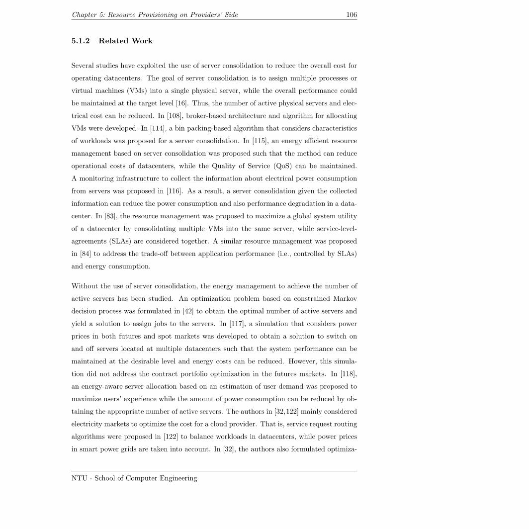
Chapter 5: Resource Provisioning on Providers’ Side 106
5.1.2 Related Work
Several studies have exploited the use of server consolidation to reduce the overall cost for
operating datacenters. The goal of server consolidation is to assign multiple processes or
virtual machines (VMs) into a single physical server, while the overall performance could
be maintained at the target level [16]. Thus, the number of active physical servers and elec-
trical cost can be reduced. In [108], broker-based architecture and algorithm for allocating
VMs were developed. In [114], a bin packing-based algorithm that considers characteristics
of workloads was proposed for a server consolidation. In [115], an energy efficient resource
management based on server consolidation was proposed such that the method can reduce
operational costs of datacenters, while the Quality of Service (QoS) can be maintained.
A monitoring infrastructure to collect the information about electrical power consumption
from servers was proposed in [116]. As a result, a server consolidation given the collected
information can reduce the power consumption and also performance degradation in a data-
center. In [83], the resource management was proposed to maximize a global system utility
of a datacenter by consolidating multiple VMs into the same server, while service-level-
agreements (SLAs) are considered together. A similar resource management was proposed
in [84] to address the trade-off between application performance (i.e., controlled by SLAs)
and energy consumption.
Without the use of server consolidation, the energy management to achieve the number of
active servers has been studied. An optimization problem based on constrained Markov
decision process was formulated in [42] to obtain the optimal number of active servers and
yield a solution to assign jobs to the servers. In [117], a simulation that considers power
prices in both futures and spot markets was developed to obtain a solution to switch on
and off servers located at multiple datacenters such that the system performance can be
maintained at the desirable level and energy costs can be reduced. However, this simula-
tion did not address the contract portfolio optimization in the futures markets. In [118],
an energy-aware server allocation based on an estimation of user demand was proposed to
maximize users’ experience while the amount of power consumption can be reduced by ob-
taining the appropriate number of active servers. The authors in [32,122] mainly considered
electricity markets to optimize the cost for a cloud provider. That is, service request routing
algorithms were proposed in [122] to balance workloads in datacenters, while power prices
in smart power grids are taken into account. In [32], the authors also formulated optimiza-
NTU - School of Computer Engineering
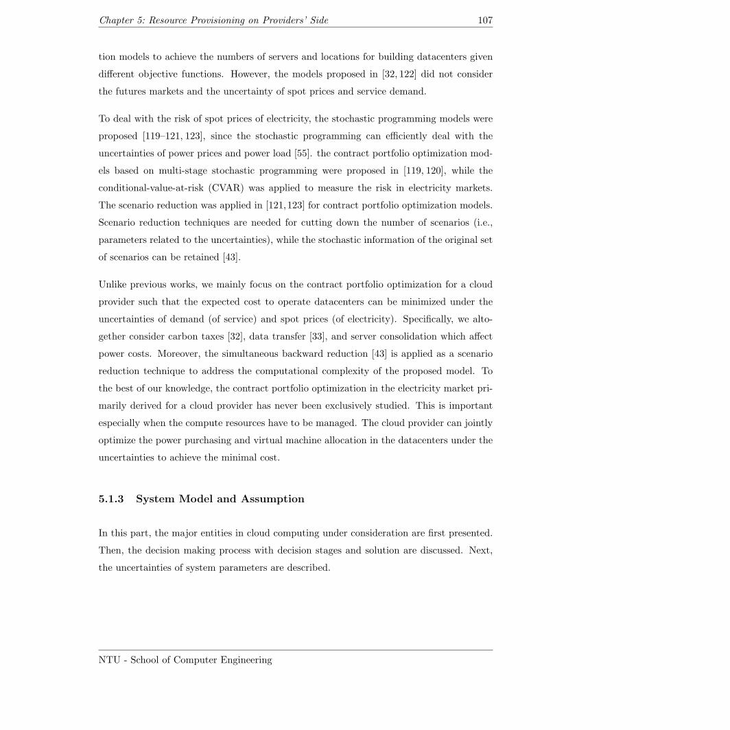
Chapter 5: Resource Provisioning on Providers’ Side 107
tion models to achieve the numbers of servers and locations for building datacenters given
different objective functions. However, the models proposed in [32, 122] did not consider
the futures markets and the uncertainty of spot prices and service demand.
To deal with the risk of spot prices of electricity, the stochastic programming models were
proposed [119–121, 123], since the stochastic programming can efficiently deal with the
uncertainties of power prices and power load [55]. the contract portfolio optimization mod-
els based on multi-stage stochastic programming were proposed in [119, 120], while the
conditional-value-at-risk (CVAR) was applied to measure the risk in electricity markets.
The scenario reduction was applied in [121,123] for contract portfolio optimization models.
Scenario reduction techniques are needed for cutting down the number of scenarios (i.e.,
parameters related to the uncertainties), while the stochastic information of the original set
of scenarios can be retained [43].
Unlike previous works, we mainly focus on the contract portfolio optimization for a cloud
provider such that the expected cost to operate datacenters can be minimized under the
uncertainties of demand (of service) and spot prices (of electricity). Specifically, we alto-
gether consider carbon taxes [32], data transfer [33], and server consolidation which affect
power costs. Moreover, the simultaneous backward reduction [43] is applied as a scenario
reduction technique to address the computational complexity of the proposed model. To
the best of our knowledge, the contract portfolio optimization in the electricity market pri-
marily derived for a cloud provider has never been exclusively studied. This is important
especially when the compute resources have to be managed. The cloud provider can jointly
optimize the power purchasing and virtual machine allocation in the datacenters under the
uncertainties to achieve the minimal cost.
5.1.3 System Model and Assumption
In this part, the major entities in cloud computing under consideration are first presented.
Then, the decision making process with decision stages and solution are discussed. Next,
the uncertainties of system parameters are described.
NTU - School of Computer Engineering
Chapter 5: Resource Provisioning on Providers’ Side 108
Major Entities
Power gridUsers
Virtual machines
Allocate VMs to host servers
Access cloud
services in
datacenters
Internet
Datacenter
Power
management
Virtual machine
management
Supply power to operate datacenter
Cloud provider’s infrastructureCloud provider’s infrastructureShared storage
Servers
Private network
Figure 5.1: System model of a cloud provider.
Cloud service A
(shopping service)
VM class I1
(web servers)
VM class I2
(application servers)
VM class I3
(database servers)
VM l I
Cloud service B
(data mining service)
VM class I4
(MapReduce servers)
Figure 5.2: Example of VM classes for cloud services.
The system model of a cloud provider is illustrated in Fig. 5.1. The model consists of
five major entities, i.e., users (i.e., cloud consumers), datacenters, servers, virtual machines
(VMs), and power grids. The cloud provider owns datacenters which provide cloud services
to the users. The VMs provide the computing facility to deliver the cloud service to users.
The VMs are grouped into the class. The set of VM classes is denoted by I where VM
class i ∈ I has αi VMs which are able to run on different datacenters. Multiple VM classes
could be provisioned for one cloud service. For example, Fig. 5.2 shows two cloud services,
i.e., shopping and data mining services. The shopping service requires 3 VM classes as the
three-tier architecture [124] (i.e., web, application, and database servers), while the data
mining service requires only one VM class of MapReduce servers [109]. Each VM class may
require different number of VMs to execute tasks or transactions.
NTU - School of Computer Engineering
Chapter 5: Resource Provisioning on Providers’ Side 109
Datacenters are connected through a wide area network. As a result, all datacenters work
as a single unified computing infrastructure. Let D denote the set of datacenters. Each
datacenter d ∈ D houses a number of (physical) servers. Each server hosts VMs to provide
services. Let S and Sd denote the set of all servers in the infrastructure and the set of servers
in datacenter d, respectively, where Sd ⊆ S. Server s ∈ S has the number of CPU cores and
amount of main memory denoted by S[cpu]s cores and S
[mem]s gigabytes (GB), respectively.
Each datacenter supplies a shared storage (e.g., storage area network). The capacity of
shared storage in datacenter d is denoted by D[sto]d GB. The network bandwidth capacities
of server s and datacenter d are denoted by S[net]s GB per hour (GBph) and D
[net]d GBph,
respectively.
In Fig. 5.1, two major modules for managing a datacenter are power management and
virtual machine management. The power management decides the purchase of electric
power from the power grid. The virtual machine management allocates VMs to the phys-
ical servers for maintaining the power consumption in datacenters. We assume that the
necessary distributed system middleware and tools (e.g., load balancer, process synchro-
nization mechanism, data caching process, monitoring tools, and distributed job scheduler)
are available to manage VMs in each class. We assume that the operating system and
software are preinstalled in the VMs. The VM in each class requires different amount of
compute resource. For class i ∈ I, the number of CPU cores, the amounts of main memory,
permanent storage, and network bandwidth required by one VM are denoted by I[cpu]i cores,
I[mem]i GB, I
[sto]i GB, and I
[net]it GBph, respectively. To efficiently place multiple VMs into
the same server, we assume that the average CPU utilization ratios (i.e., expected-values
of the number of busy CPU cores in an hour divided by the total number of available CPU
cores) of servers and VMs are known. Let µ[vir]i ∈ (0, 1] and µ
[hos]s ∈ (0, 1] denote the average
CPU utilization ratio of one VM of class i and the average CPU utilization ratio of server
s, respectively.
The VM can access application/service data. This application data is stored in the shared
storage of a datacenter. If the VM is allocated to the physical server in the different dat-
acenter, the application data has to be transferred to the storage in the target datacenter.
However, in this case, the cost of transferring application data to the datacenter will be in-
curred (e.g., bandwidth consumption) and the virtual machine management has to minimize
this cost as well.
NTU - School of Computer Engineering
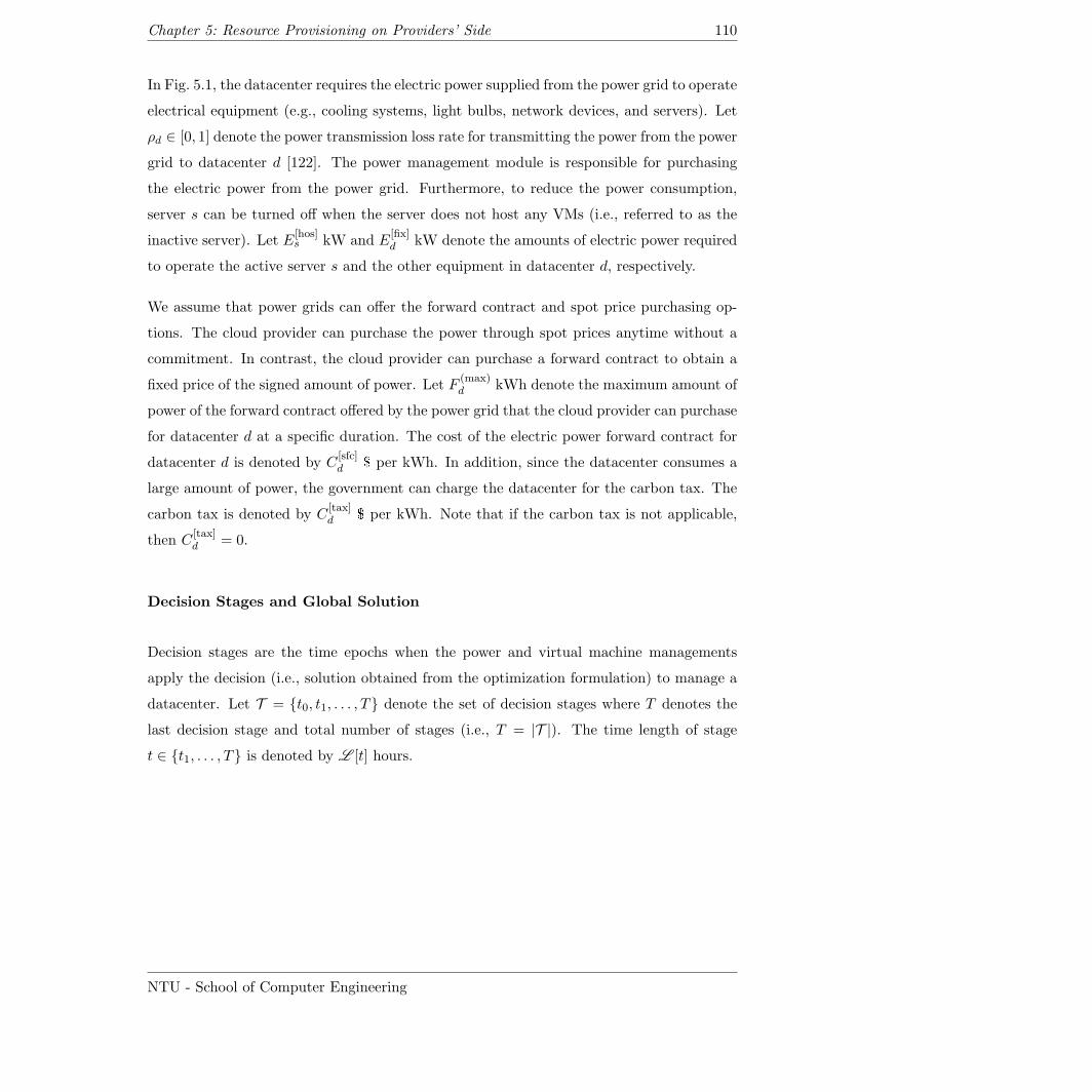
Chapter 5: Resource Provisioning on Providers’ Side 110
In Fig. 5.1, the datacenter requires the electric power supplied from the power grid to operate
electrical equipment (e.g., cooling systems, light bulbs, network devices, and servers). Let
ρd ∈ [0, 1] denote the power transmission loss rate for transmitting the power from the power
grid to datacenter d [122]. The power management module is responsible for purchasing
the electric power from the power grid. Furthermore, to reduce the power consumption,
server s can be turned off when the server does not host any VMs (i.e., referred to as the
inactive server). Let E[hos]s kW and E
[fix]d kW denote the amounts of electric power required
to operate the active server s and the other equipment in datacenter d, respectively.
We assume that power grids can offer the forward contract and spot price purchasing op-
tions. The cloud provider can purchase the power through spot prices anytime without a
commitment. In contrast, the cloud provider can purchase a forward contract to obtain a
fixed price of the signed amount of power. Let F(max)d kWh denote the maximum amount of
power of the forward contract offered by the power grid that the cloud provider can purchase
for datacenter d at a specific duration. The cost of the electric power forward contract for
datacenter d is denoted by C[sfc]d $ per kWh. In addition, since the datacenter consumes a
large amount of power, the government can charge the datacenter for the carbon tax. The
carbon tax is denoted by C[tax]d $ per kWh. Note that if the carbon tax is not applicable,
then C[tax]d = 0.
Decision Stages and Global Solution
Decision stages are the time epochs when the power and virtual machine managements
apply the decision (i.e., solution obtained from the optimization formulation) to manage a
datacenter. Let T = t0, t1, . . . , T denote the set of decision stages where T denotes the
last decision stage and total number of stages (i.e., T = |T |). The time length of stage
t ∈ t1, . . . , T is denoted by L [t] hours.
NTU - School of Computer Engineering
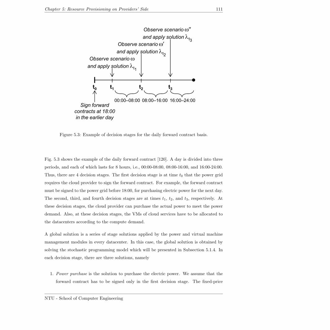
Chapter 5: Resource Provisioning on Providers’ Side 111
Observe scenario
Observe scenario !
and apply solution "t2
Observe scenario #
and apply solution "t3
t0
t1
t2
t3
00:00–08:00 16:00–24:0008:00–16:00
Sign forward
Observe scenario
and apply solution "t1
Sign forward
contracts at 18:00
in the earlier day
Figure 5.3: Example of decision stages for the daily forward contract basis.
Fig. 5.3 shows the example of the daily forward contract [120]. A day is divided into three
periods, and each of which lasts for 8 hours, i.e., 00:00-08:00, 08:00-16:00, and 16:00-24:00.
Thus, there are 4 decision stages. The first decision stage is at time t0 that the power grid
requires the cloud provider to sign the forward contract. For example, the forward contract
must be signed to the power grid before 18:00, for purchasing electric power for the next day.
The second, third, and fourth decision stages are at times t1, t2, and t3, respectively. At
these decision stages, the cloud provider can purchase the actual power to meet the power
demand. Also, at these decision stages, the VMs of cloud services have to be allocated to
the datacenters according to the compute demand.
A global solution is a series of stage solutions applied by the power and virtual machine
management modules in every datacenter. In this case, the global solution is obtained by
solving the stochastic programming model which will be presented in Subsection 5.1.4. In
each decision stage, there are three solutions, namely
1. Power purchase is the solution to purchase the electric power. We assume that the
forward contract has to be signed only in the first decision stage. The fixed-price
NTU - School of Computer Engineering
Chapter 5: Resource Provisioning on Providers’ Side 112
electric power purchased with the forward contracts will be available for the follow-
ing decision stages. Alternatively, the electric power can be additionally purchased
through spot prices from the second stage and so on. The decision variables of power
purchase are y[ufc]d , y
[rem]d , and y
[pow]d . y
[ufc]d is the amount of power signed for a forward
contract. y[rem]d is the amount of power remaining in the forward contract. y
[pow]d is
the amount of addition power purchased using the spot price to meet the immediate
power demand.
2. VM allocation is the solution to allocate VMs to physical servers. It is assumed that a
VM migration can be applied to reallocate VMs among physical servers. It is assumed
that the servers which do not host any VMs can be turned off. The solution of VM
allocation will be applied after the first stage, i.e., the forward contract is purchased.
The decision variables of VM allocation are x[hos]is and z
[hos]s . x
[hos]is is the number of
VMs of class i to be allocated to physical server s. z[hos]s is the indication whether
server s is active or not.
3. Application data transfer is the solution to transfer application data to the datacen-
ter. This solution will be applied in every decision stage. The decision variables of
the application data transfer are z[dat]idd′ and z
[req]id . z
[dat]idd′ is the indication whether the
application data required by VM in class i is transferred from datacenter d to data-
center d′ or not. z[req]id is the indication whether the application data in datacenter d
is required by VM in class i or not.
Uncertain Parameters
For power and virtual machine management modules, there are uncertain parameters. The
uncertain parameter can be described by a scenario associated with the possible outcome.
Let Ω and Ωt denote the sets of scenarios in every decision stage and only stage t, re-
spectively, where Ωt ⊂ Ω. Let τ(ω) ∈ T denote the decision epoch (i.e., time when the
decision is made) given scenario ω ∈ Ω. Two uncertain parameters considered in the power
management and virtual machine management modules are as follows:
• Demand uncertainty – There are two types of demand uncertainty, namely processing
demand and power demand. The processing demand denoted by αiω is the number
of VMs required for class i under scenario ω. On the other hand, the power demand
NTU - School of Computer Engineering
Chapter 5: Resource Provisioning on Providers’ Side 113
denoted by βdω kWh is the amount of power required to operate datacenter d under
scenario ω. This βdω can be defined as follows:
βdω = L [τ(ω)] E[pue]d
E[fix]d +
∑s∈Sd
E[hos]s µ[hos]s z[hos]sω
(5.1)
where z[hos]sω ∈ 0, 1 denotes the binary decision variable indicating whether server
s is active (i.e., z[hos]sω = 1) or inactive (i.e., z
[hos]sω = 0). E
[pue]d denotes the power
usage effectiveness (PUE) applied in datacenter d [111]. Clearly, the power demand
is directly proportional to the processing demand [122]. That is, the larger value of
αiω can result in larger value of βdω, since the number of active servers has to be
increased as the number of VMs increases. The relationship between power demand
and processing demand will be presented later by the constraints in (5.16)-(5.32).
• Cost uncertainty – The costs can vary, namely spot price, carbon tax, hosting cost,
and data transfer cost. Let C[pow]dω $ per kWh and C
[tax]dω $ per kWh denote the spot
price and carbon tax charged to datacenter d under scenario ω, respectively. For a
datacenter where a power price is not fluctuating or spot prices are not available (e.g.,
the datacenter has its own power generators), C[pow]dω for such a datacenter is set to the
same constant for every scenario ω. Let C[hos]isω $ per VM per hour denote the hosting
cost for one VM of class i hosted in physical server s under scenario ω. Let C[net]dd′ω $
per GB denote the data transfer cost to transfer application data from datacenter d
to datacenter d′ ∈ D under scenario ω.
The outcomes of uncertain parameters of scenario ω ∈ Ω = ω0, ω1, . . . , ωM (i.e., |Ω| =
M + 1) can be described by a vector denoted as follows:
ξ(ω) =(αiω, C
[pow]dω , C
[tax]dω , C
[hos]isω , C
[net]dd′ω
). (5.2)
Note that ω0 is the scenario in the first decision stage (i.e., root scenario) which is not
associated with any uncertain parameters. In contrast, scenarios in other decision stages
(i.e., from t1 to T ) are associated with the uncertain parameters.
Due to the uncertainties, the cloud provider can realize the scenario (i.e., ω ∈ Ω) and apply
the decision accordingly. Therefore, some decision variables will be associated with the
scenario ω. These decision variables are for power purchase (i.e., y[ufc]dω , y
[rem]dω , and y
[pow]dω ),
NTU - School of Computer Engineering
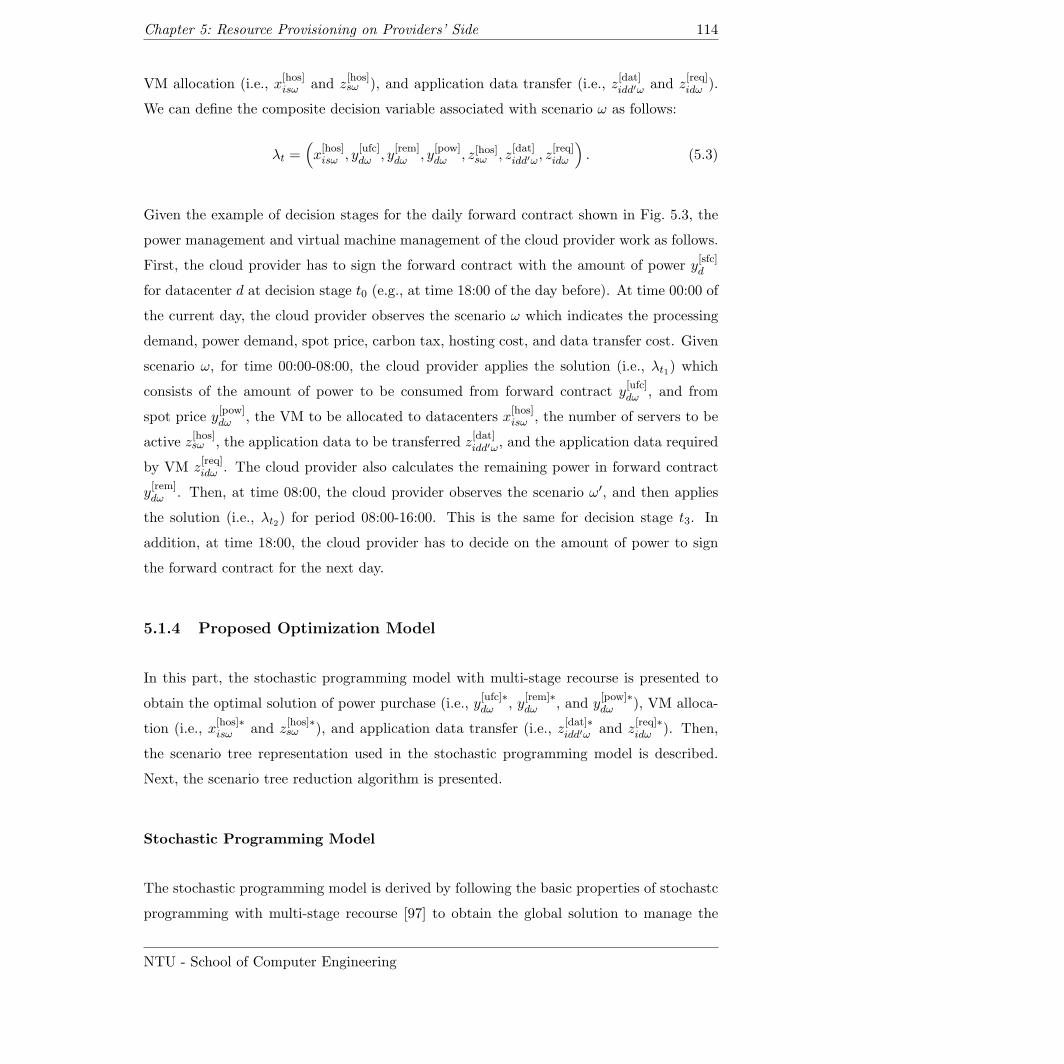
Chapter 5: Resource Provisioning on Providers’ Side 114
VM allocation (i.e., x[hos]isω and z
[hos]sω ), and application data transfer (i.e., z
[dat]idd′ω and z
[req]idω ).
We can define the composite decision variable associated with scenario ω as follows:
λt =(x[hos]isω , y
[ufc]dω , y
[rem]dω , y
[pow]dω , z[hos]sω , z
[dat]idd′ω, z
[req]idω
). (5.3)
Given the example of decision stages for the daily forward contract shown in Fig. 5.3, the
power management and virtual machine management of the cloud provider work as follows.
First, the cloud provider has to sign the forward contract with the amount of power y[sfc]d
for datacenter d at decision stage t0 (e.g., at time 18:00 of the day before). At time 00:00 of
the current day, the cloud provider observes the scenario ω which indicates the processing
demand, power demand, spot price, carbon tax, hosting cost, and data transfer cost. Given
scenario ω, for time 00:00-08:00, the cloud provider applies the solution (i.e., λt1) which
consists of the amount of power to be consumed from forward contract y[ufc]dω , and from
spot price y[pow]dω , the VM to be allocated to datacenters x
[hos]isω , the number of servers to be
active z[hos]sω , the application data to be transferred z
[dat]idd′ω, and the application data required
by VM z[req]idω . The cloud provider also calculates the remaining power in forward contract
y[rem]dω . Then, at time 08:00, the cloud provider observes the scenario ω′, and then applies
the solution (i.e., λt2) for period 08:00-16:00. This is the same for decision stage t3. In
addition, at time 18:00, the cloud provider has to decide on the amount of power to sign
the forward contract for the next day.
5.1.4 Proposed Optimization Model
In this part, the stochastic programming model with multi-stage recourse is presented to
obtain the optimal solution of power purchase (i.e., y[ufc]∗dω , y
[rem]∗dω , and y
[pow]∗dω ), VM alloca-
tion (i.e., x[hos]∗isω and z
[hos]∗sω ), and application data transfer (i.e., z
[dat]∗idd′ω and z
[req]∗idω ). Then,
the scenario tree representation used in the stochastic programming model is described.
Next, the scenario tree reduction algorithm is presented.
Stochastic Programming Model
The stochastic programming model is derived by following the basic properties of stochastc
programming with multi-stage recourse [97] to obtain the global solution to manage the
NTU - School of Computer Engineering
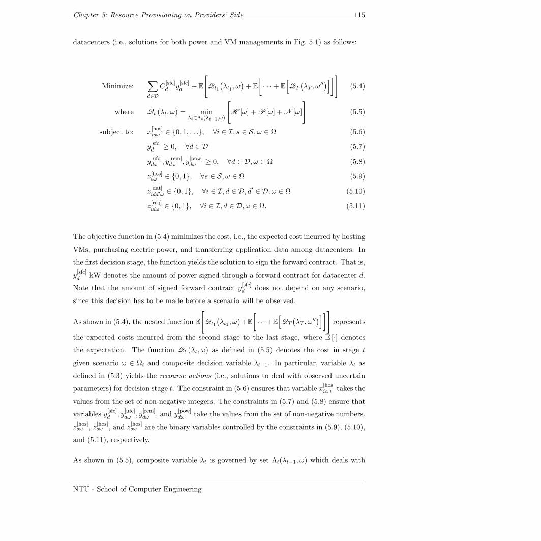
Chapter 5: Resource Provisioning on Providers’ Side 115
datacenters (i.e., solutions for both power and VM managements in Fig. 5.1) as follows:
Minimize:∑d∈D
C[sfc]d y
[sfc]d + E
[Qt1
(λt1 , ω
)+ E
[· · ·+ E
[QT
(λT , ω
′′)]]] (5.4)
where Qt (λt, ω) = minλt∈Λt(λt−1,ω)
[H [ω] + P[ω] + N [ω]
](5.5)
subject to: x[hos]isω ∈ 0, 1, . . ., ∀i ∈ I, s ∈ S, ω ∈ Ω (5.6)
y[sfc]d ≥ 0, ∀d ∈ D (5.7)
y[ufc]dω , y
[rem]dω , y
[pow]dω ≥ 0, ∀d ∈ D, ω ∈ Ω (5.8)
z[hos]sω ∈ 0, 1, ∀s ∈ S, ω ∈ Ω (5.9)
z[dat]idd′ω ∈ 0, 1, ∀i ∈ I, d ∈ D, d′ ∈ D, ω ∈ Ω (5.10)
z[req]idω ∈ 0, 1, ∀i ∈ I, d ∈ D, ω ∈ Ω. (5.11)
The objective function in (5.4) minimizes the cost, i.e., the expected cost incurred by hosting
VMs, purchasing electric power, and transferring application data among datacenters. In
the first decision stage, the function yields the solution to sign the forward contract. That is,
y[sfc]d kW denotes the amount of power signed through a forward contract for datacenter d.
Note that the amount of signed forward contract y[sfc]d does not depend on any scenario,
since this decision has to be made before a scenario will be observed.
As shown in (5.4), the nested function E
[Qt1
(λt1 , ω
)+E[· · ·+E
[QT
(λT , ω
′′)]]] represents
the expected costs incurred from the second stage to the last stage, where E [·] denotes
the expectation. The function Qt (λt, ω) as defined in (5.5) denotes the cost in stage t
given scenario ω ∈ Ωt and composite decision variable λt−1. In particular, variable λt as
defined in (5.3) yields the recourse actions (i.e., solutions to deal with observed uncertain
parameters) for decision stage t. The constraint in (5.6) ensures that variable x[hos]isω takes the
values from the set of non-negative integers. The constraints in (5.7) and (5.8) ensure that
variables y[sfc]d , y
[ufc]dω , y
[rem]dω , and y
[pow]dω take the values from the set of non-negative numbers.
z[hos]sω , z
[hos]sω , and z
[hos]sω are the binary variables controlled by the constraints in (5.9), (5.10),
and (5.11), respectively.
As shown in (5.5), composite variable λt is governed by set Λt(λt−1, ω) which deals with
NTU - School of Computer Engineering
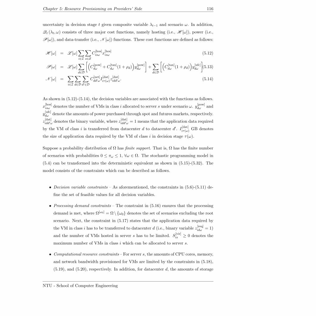
Chapter 5: Resource Provisioning on Providers’ Side 116
uncertainty in decision stage t given composite variable λt−1 and scenario ω. In addition,
Qt (λt, ω) consists of three major cost functions, namely hosting (i.e., H [ω]), power (i.e.,
P[ω]), and data-transfer (i.e., N [ω]) functions. These cost functions are defined as follows:
H [ω] = L [ω]∑i∈I
∑s∈S
C[hos]isω x
[hos]isω (5.12)
P[ω] = L [ω]∑d∈D
[(C
[pow]dω + C
[tax]dω (1 + ρd)
)y[pow]dω
]+∑d∈D
[(C
[tax]dω (1 + ρd)
)y[ufc]dω
](5.13)
N [ω] =∑i∈I
∑d∈D
∑d′∈D
C[net]dd′ωI
[dat]iτ(ω)z
[dat]idd′ω. (5.14)
As shown in (5.12)-(5.14), the decision variables are associated with the functions as follows.
x[hos]isω denotes the number of VMs in class i allocated to server s under scenario ω. y
[pow]dω and
y[ufc]dω denote the amounts of power purchased through spot and futures markets, respectively.
z[dat]idd′ω denotes the binary variable, where z
[dat]idd′ω = 1 means that the application data required
by the VM of class i is transferred from datacenter d to datacenter d′. I[dat]iτ(ω) GB denotes
the size of application data required by the VM of class i in decision stage τ(ω).
Suppose a probability distribution of Ω has finite support. That is, Ω has the finite number
of scenarios with probabilities 0 ≤ πω ≤ 1, ∀ω ∈ Ω. The stochastic programming model in
(5.4) can be transformed into the deterministic equivalent as shown in (5.15)-(5.32). The
model consists of the constraints which can be described as follows.
• Decision variable constraints – As aforementioned, the constraints in (5.6)-(5.11) de-
fine the set of feasible values for all decision variables.
• Processing demand constraints – The constraint in (5.16) ensures that the processing
demand is met, where Ω[ω0] = Ω\ω0 denotes the set of scenarios excluding the root
scenario. Next, the constraint in (5.17) states that the application data required by
the VM in class i has to be transferred to datacenter d (i.e., binary variable z[req]idω = 1)
and the number of VMs hosted in server s has to be limited. S[vir]is ≥ 0 denotes the
maximum number of VMs in class i which can be allocated to server s.
• Computational resource constraints – For server s, the amounts of CPU cores, memory,
and network bandwidth provisioned for VMs are limited by the constraints in (5.18),
(5.19), and (5.20), respectively. In addition, for datacenter d, the amounts of storage
NTU - School of Computer Engineering
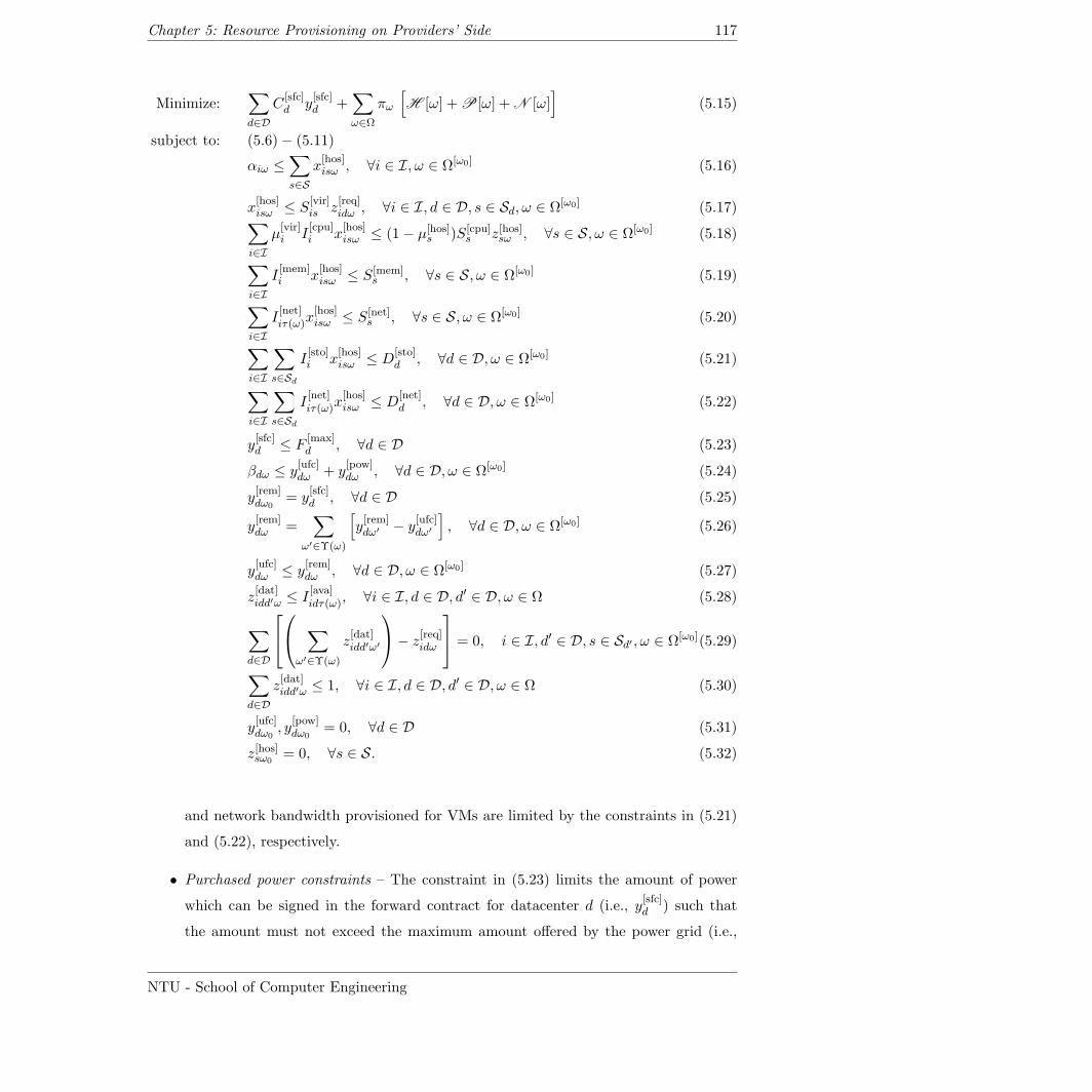
Chapter 5: Resource Provisioning on Providers’ Side 117
Minimize:∑d∈D
C[sfc]d y
[sfc]d +
∑ω∈Ω
πω
[H [ω] + P[ω] + N [ω]
](5.15)
subject to: (5.6)− (5.11)
αiω ≤∑s∈S
x[hos]isω , ∀i ∈ I, ω ∈ Ω[ω0] (5.16)
x[hos]isω ≤ S
[vir]is z
[req]idω , ∀i ∈ I, d ∈ D, s ∈ Sd, ω ∈ Ω[ω0] (5.17)∑
i∈Iµ[vir]i I
[cpu]i x
[hos]isω ≤ (1− µ[hos]s )S[cpu]
s z[hos]sω , ∀s ∈ S, ω ∈ Ω[ω0] (5.18)∑i∈I
I[mem]i x
[hos]isω ≤ S
[mem]s , ∀s ∈ S, ω ∈ Ω[ω0] (5.19)∑
i∈II[net]iτ(ω)x
[hos]isω ≤ S
[net]s , ∀s ∈ S, ω ∈ Ω[ω0] (5.20)∑
i∈I
∑s∈Sd
I[sto]i x
[hos]isω ≤ D
[sto]d , ∀d ∈ D, ω ∈ Ω[ω0] (5.21)
∑i∈I
∑s∈Sd
I[net]iτ(ω)x
[hos]isω ≤ D
[net]d , ∀d ∈ D, ω ∈ Ω[ω0] (5.22)
y[sfc]d ≤ F [max]
d , ∀d ∈ D (5.23)
βdω ≤ y[ufc]dω + y
[pow]dω , ∀d ∈ D, ω ∈ Ω[ω0] (5.24)
y[rem]dω0
= y[sfc]d , ∀d ∈ D (5.25)
y[rem]dω =
∑ω′∈Υ(ω)
[y[rem]dω′ − y[ufc]dω′
], ∀d ∈ D, ω ∈ Ω[ω0] (5.26)
y[ufc]dω ≤ y[rem]
dω , ∀d ∈ D, ω ∈ Ω[ω0] (5.27)
z[dat]idd′ω ≤ I
[ava]idτ(ω), ∀i ∈ I, d ∈ D, d′ ∈ D, ω ∈ Ω (5.28)
∑d∈D
∑ω′∈Υ(ω)
z[dat]idd′ω′
− z[req]idω
= 0, i ∈ I, d′ ∈ D, s ∈ Sd′ , ω ∈ Ω[ω0](5.29)
∑d∈D
z[dat]idd′ω ≤ 1, ∀i ∈ I, d ∈ D, d′ ∈ D, ω ∈ Ω (5.30)
y[ufc]dω0
, y[pow]dω0
= 0, ∀d ∈ D (5.31)
z[hos]sω0= 0, ∀s ∈ S. (5.32)
and network bandwidth provisioned for VMs are limited by the constraints in (5.21)
and (5.22), respectively.
• Purchased power constraints – The constraint in (5.23) limits the amount of power
which can be signed in the forward contract for datacenter d (i.e., y[sfc]d ) such that
the amount must not exceed the maximum amount offered by the power grid (i.e.,
NTU - School of Computer Engineering
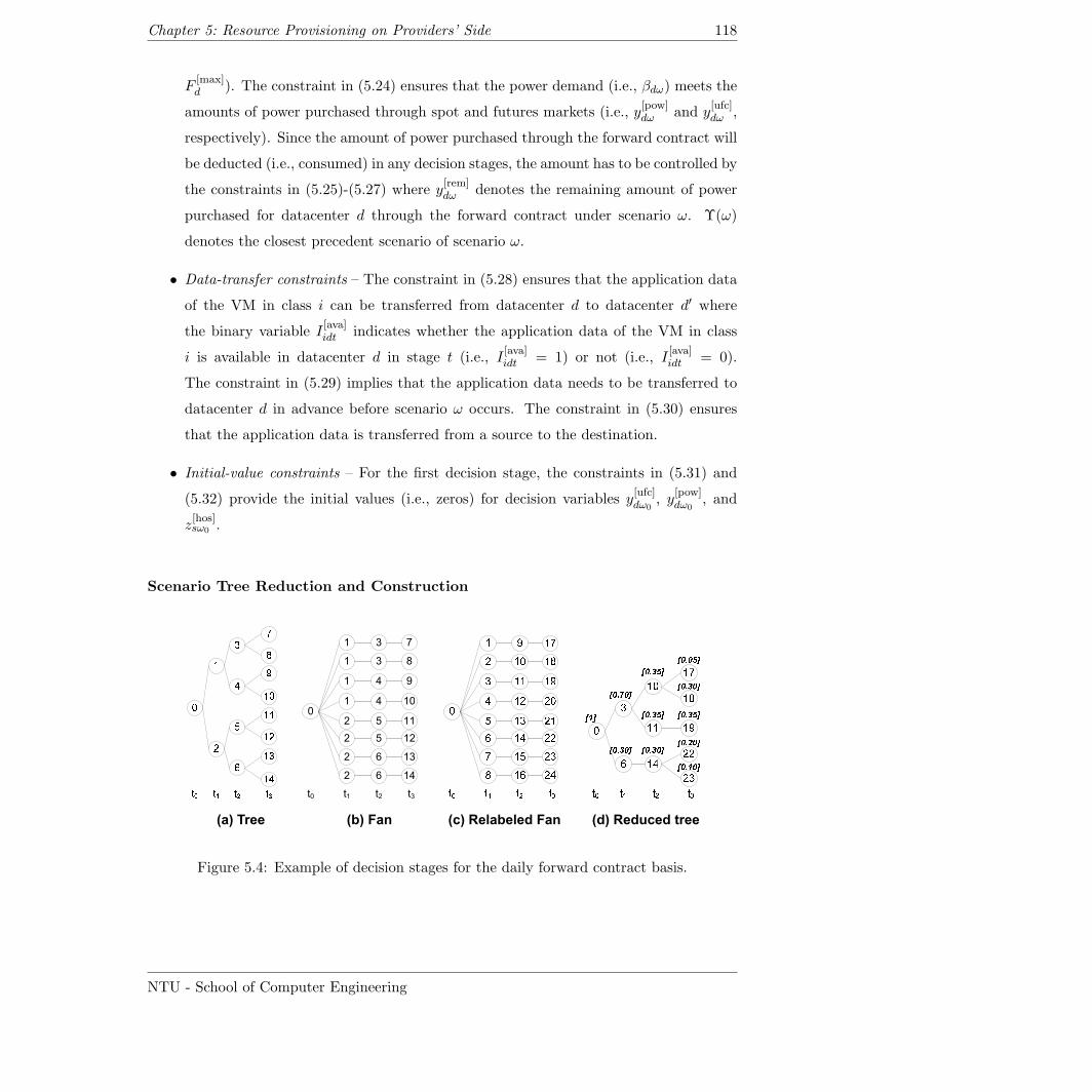
Chapter 5: Resource Provisioning on Providers’ Side 118
F[max]d ). The constraint in (5.24) ensures that the power demand (i.e., βdω) meets the
amounts of power purchased through spot and futures markets (i.e., y[pow]dω and y
[ufc]dω ,
respectively). Since the amount of power purchased through the forward contract will
be deducted (i.e., consumed) in any decision stages, the amount has to be controlled by
the constraints in (5.25)-(5.27) where y[rem]dω denotes the remaining amount of power
purchased for datacenter d through the forward contract under scenario ω. Υ(ω)
denotes the closest precedent scenario of scenario ω.
• Data-transfer constraints – The constraint in (5.28) ensures that the application data
of the VM in class i can be transferred from datacenter d to datacenter d′ where
the binary variable I[ava]idt indicates whether the application data of the VM in class
i is available in datacenter d in stage t (i.e., I[ava]idt = 1) or not (i.e., I
[ava]idt = 0).
The constraint in (5.29) implies that the application data needs to be transferred to
datacenter d in advance before scenario ω occurs. The constraint in (5.30) ensures
that the application data is transferred from a source to the destination.
• Initial-value constraints – For the first decision stage, the constraints in (5.31) and
(5.32) provide the initial values (i.e., zeros) for decision variables y[ufc]dω0
, y[pow]dω0
, and
z[hos]sω0 .
Scenario Tree Reduction and Construction
7
8
9
10
3
3
4
4
1
1
1
1
0
t0 t1 t2 t3
10
11
12
13
14
4
5
5
6
6
1
2
2
2
2
(a) Tree (c) Relabeled Fan (d) Reduced tree(b) Fan
Figure 5.4: Example of decision stages for the daily forward contract basis.
NTU - School of Computer Engineering
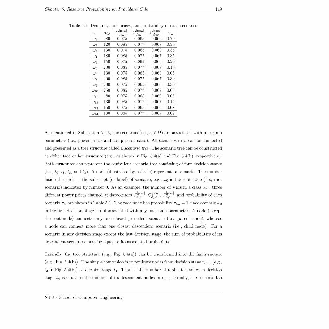
Chapter 5: Resource Provisioning on Providers’ Side 119
Table 5.1: Demand, spot prices, and probability of each scenario.
ω αiω C[pow]d1ω
C[pow]d2ω
C[pow]d3ω
πωω1 80 0.075 0.065 0.060 0.70
ω2 120 0.085 0.077 0.067 0.30
ω3 130 0.075 0.065 0.060 0.35
ω4 180 0.085 0.077 0.067 0.35
ω5 150 0.075 0.065 0.060 0.20
ω6 200 0.085 0.077 0.067 0.10
ω7 130 0.075 0.065 0.060 0.05
ω8 200 0.085 0.077 0.067 0.30
ω9 200 0.075 0.065 0.060 0.30
ω10 250 0.085 0.077 0.067 0.05
ω11 80 0.075 0.065 0.060 0.05
ω12 130 0.085 0.077 0.067 0.15
ω13 150 0.075 0.065 0.060 0.08
ω14 180 0.085 0.077 0.067 0.02
As mentioned in Subsection 5.1.3, the scenarios (i.e., ω ∈ Ω) are associated with uncertain
parameters (i.e., power prices and compute demand). All scenarios in Ω can be connected
and presented as a tree structure called a scenario tree. The scenario tree can be constructed
as either tree or fan structure (e.g., as shown in Fig. 5.4(a) and Fig. 5.4(b), respectively).
Both structures can represent the equivalent scenario tree consisting of four decision stages
(i.e., t0, t1, t2, and t3). A node (illustrated by a circle) represents a scenario. The number
inside the circle is the subscript (or label) of scenario, e.g., ω0 is the root node (i.e., root
scenario) indicated by number 0. As an example, the number of VMs in a class αiω, three
different power prices charged at datacenters C[pow]d1ω
, C[pow]d2ω
, C[pow]d3ω
, and probability of each
scenario πω are shown in Table 5.1. The root node has probability πω0 = 1 since scenario ω0
in the first decision stage is not associated with any uncertain parameter. A node (except
the root node) connects only one closest precedent scenario (i.e., parent node), whereas
a node can connect more than one closest descendent scenario (i.e., child node). For a
scenario in any decision stage except the last decision stage, the sum of probabilities of its
descendent scenarios must be equal to its associated probability.
Basically, the tree structure(e.g., Fig. 5.4(a)
)can be transformed into the fan structure(
e.g., Fig. 5.4(b)). The simple conversion is to replicate nodes from decision stage tT−1
(e.g.,
t2 in Fig. 5.4(b))to decision stage t1. That is, the number of replicated nodes in decision
stage tn is equal to the number of its descendent nodes in tn+1. Finally, the scenario fan
NTU - School of Computer Engineering
Chapter 5: Resource Provisioning on Providers’ Side 120
will have the number of branches as the number of leaf nodes. Except for the root node, all
scenarios in the same branch have the same probability as that of its respective leaf node.
For example, the scenarios in the first branch (i.e., ω1, ω3, and ω7) have the probability
of 0.05. Then, the subscriptions of scenarios in Fig. 5.4(b) can be relabeled as shown in
Fig. 5.4(c).
Generally, the number of scenarios can be considerably large which may result in high
computational complexity to solve using stochastic programming model. Thus, the scenario
reduction algorithms can be applied to reduce the number of scenarios while maintaining
the stochastic information of the original set of scenarios [43]. In addition, the model with
the reduced set of scenarios can be efficiently solved but yield the solution close to the
optimal solution of the model with the original set of scenarios.
• Scenario Reduction – The goal of the scenario reduction algorithm is to choose the
scenarios to be deleted from the original set of scenarios in decision stage t (i.e.,
Ωt). First, the scenario reduction algorithm measures the probability distance between
scenarios in Ωt and Φt, where Φt ⊂ Ωt denotes the set of the deleted scenarios in
decision stage t. Then, the algorithm searches for the set Φt such that the probability
distance is minimized. That is, the cardinality of Φt is maximal while retaining most
of the stochastic information of the scenario set. In this case, the Kantorovich distance
denoted by function D [Ωt,Φt] can be applied as follows:
D [Ωt,Φt] =∑ω∈Φt
πω minω′∈Ωt\Φt
Ct
[ω, ω′] (5.33)
where function Ct [ω, ω′] measures the probability distance between scenarios ω and ω′
on the time horizon of decision stages t0, . . . , t ⊆ T . In particular, function Ct [ω, ω′]
can be described as the Wasserstein metric of order r [125] as follows:
Ct
[ω, ω′] =
∑t∈t0,...,t
∥ξ(ω(t))− ξ(ω′(t))∥r (5.34)
where ξ(ω(t)) denotes the random vector of scenario ω(t) in decision stage t. Finally,
the minimization problem, namely minΦt⊂Ωt D [Ωt,Φt], can be formulated and solved
to obtain the maximum cardinality of Φt, i.e., the minimum cardinality of preserved
scenarios (denoted by Ω′t = Ωt \Φt) can be obtained. However, such a problem could
NTU - School of Computer Engineering
Chapter 5: Resource Provisioning on Providers’ Side 121
be NP-hard. To solve such a problem efficiently, we adopt the heuristic method to
obtain the set of reduced scenarios, which works as follows.
1. Given the number of scenarios to be deleted N (i.e., the cardinality of Φt), the
simultaneous backward reduction algorithm [43] is used (Algorithm 8). From
line 1 to line 11 of Algorithm 8, the algorithm chooses a deleted scenario from
the original set Ωt. Φ[ν] denotes the deleted scenario set in iteration ν. Therefore,
Φt = Φ[N ] is the set of the deleted scenarios at the last iteration N .
2. Algorithm 9 is applied to redistribute the probabilities of remaining scenarios
(i.e., probability redistribution algorithm).
3. The maximal reduction strategy [43] is applied to check if the probability distance
between the original set of scenarios and the set of the deleted scenarios is less
than the threshold or not, i.e.,
D [Ωt,Φt] ≤ εt (5.35)
where εt > 0 denotes the small tolerance value.
If the condition in (5.35) is true, the solution solved with the preserved scenario set
(i.e., Ω′t = Ωt \ Φ[N ]) is acceptable. Otherwise, the probability distance between the
original set of scenarios and the set of the deleted scenarios is too big. As a result,
the value of N has to be decreased, and the all steps are repeated.
• Scenario Construction – The scenario reduction technique presented in Algorithm 8
can reduce the scenarios for a certain decision stage t. When all the scenarios in
Ω are considered by the scenario reduction algorithm, the preserved scenario tree
needs to be reconstructed by the scenario tree construction algorithm [43] as shown
in Algorithm 10.
To apply Algorithm 10, we assume that a scenario tree is represented as a fan struc-
ture, e.g., the fan in Fig. 5.4(c). Let(Ω, (Ωt, t ∈ T ), (Υ(ω), ω ∈ Ω), (F [pre](ω), ω ∈
Ω), (F [des](ω), ω ∈ Ω), (πω, ω ∈ Ω))and
(Ω′, (Ω′
t, ∀t ∈ T ), (Υ′(ω), ∀ω ∈ Ω′), (F ′[pre](ω), ∀ω ∈
Ω′), (F ′[des](ω), ∀ω ∈ Ω′), (π′ω, ∀ω ∈ Ω′))denote the original and preserved scenarios
trees, respectively. F [pre](ω) and F [des](ω) denote the functions which yield the sets of
all the precedent scenarios and the closest descendent scenarios of scenario ω, respec-
tively. As shown in lines 2 and 9 of Algorithm 10, for each decision stage t starting
NTU - School of Computer Engineering
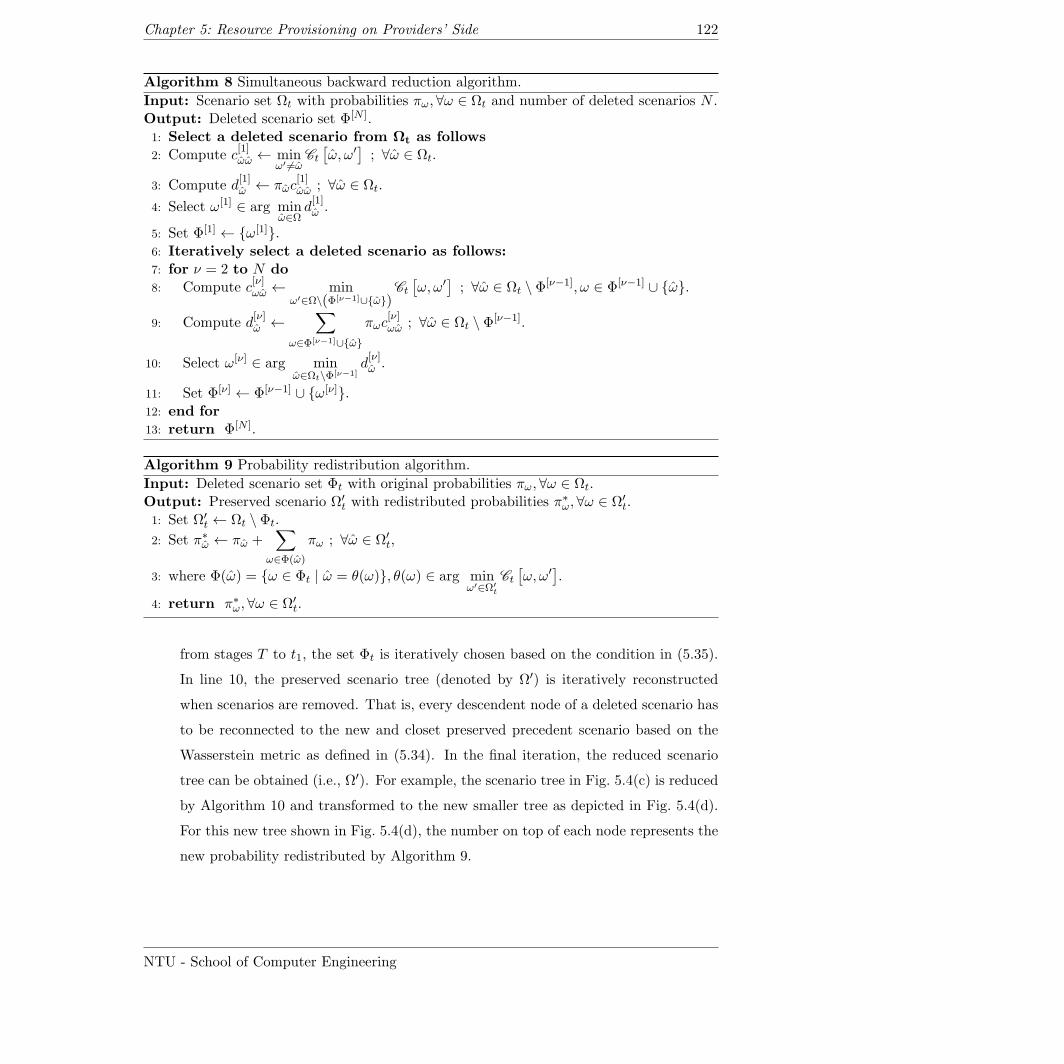
Chapter 5: Resource Provisioning on Providers’ Side 122
Algorithm 8 Simultaneous backward reduction algorithm.
Input: Scenario set Ωt with probabilities πω,∀ω ∈ Ωt and number of deleted scenarios N .Output: Deleted scenario set Φ[N ].1: Select a deleted scenario from Ωt as follows2: Compute c
[1]ωω ← min
ω′ =ωCt
[ω, ω′] ; ∀ω ∈ Ωt.
3: Compute d[1]ω ← πωc
[1]ωω ; ∀ω ∈ Ωt.
4: Select ω[1] ∈ arg minω∈Ω
d[1]ω .
5: Set Φ[1] ← ω[1].6: Iteratively select a deleted scenario as follows:7: for ν = 2 to N do8: Compute c
[ν]ωω ← min
ω′∈Ω\(Φ[ν−1]∪ω)Ct
[ω, ω′] ; ∀ω ∈ Ωt \ Φ[ν−1], ω ∈ Φ[ν−1] ∪ ω.
9: Compute d[ν]ω ←
∑ω∈Φ[ν−1]∪ω
πωc[ν]ωω ; ∀ω ∈ Ωt \ Φ[ν−1].
10: Select ω[ν] ∈ arg minω∈Ωt\Φ[ν−1]
d[ν]ω .
11: Set Φ[ν] ← Φ[ν−1] ∪ ω[ν].12: end for13: return Φ[N ].
Algorithm 9 Probability redistribution algorithm.
Input: Deleted scenario set Φt with original probabilities πω, ∀ω ∈ Ωt.Output: Preserved scenario Ω′
t with redistributed probabilities π∗ω, ∀ω ∈ Ω′t.
1: Set Ω′t ← Ωt \ Φt.
2: Set π∗ω ← πω +∑
ω∈Φ(ω)
πω ; ∀ω ∈ Ω′t,
3: where Φ(ω) = ω ∈ Φt | ω = θ(ω), θ(ω) ∈ arg minω′∈Ω′
t
Ct
[ω, ω′].
4: return π∗ω, ∀ω ∈ Ω′t.
from stages T to t1, the set Φt is iteratively chosen based on the condition in (5.35).
In line 10, the preserved scenario tree (denoted by Ω′) is iteratively reconstructed
when scenarios are removed. That is, every descendent node of a deleted scenario has
to be reconnected to the new and closet preserved precedent scenario based on the
Wasserstein metric as defined in (5.34). In the final iteration, the reduced scenario
tree can be obtained (i.e., Ω′). For example, the scenario tree in Fig. 5.4(c) is reduced
by Algorithm 10 and transformed to the new smaller tree as depicted in Fig. 5.4(d).
For this new tree shown in Fig. 5.4(d), the number on top of each node represents the
new probability redistributed by Algorithm 9.
NTU - School of Computer Engineering
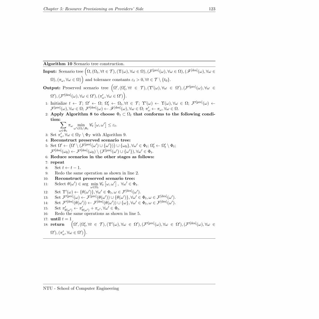
Chapter 5: Resource Provisioning on Providers’ Side 123
Algorithm 10 Scenario tree construction.
Input: Scenario tree(Ω, (Ωt, ∀t ∈ T ), (Υ(ω), ∀ω ∈ Ω), (F [pre](ω),∀ω ∈ Ω), (F [des](ω),∀ω ∈
Ω), (πω,∀ω ∈ Ω))and tolerance constants εt > 0, ∀t ∈ T \ t0.
Output: Preserved scenario tree(Ω′, (Ω′
t, ∀t ∈ T ), (Υ′(ω), ∀ω ∈ Ω′), (F ′[pre](ω), ∀ω ∈
Ω′), (F ′[des](ω), ∀ω ∈ Ω′), (π′ω, ∀ω ∈ Ω′)).
1: Initialize t ← T ; Ω′ ← Ω; Ω′t ← Ωt, ∀t ∈ T ; Υ′(ω) ← Υ(ω), ∀ω ∈ Ω; F ′[pre](ω) ←
F [pre](ω), ∀ω ∈ Ω; F ′[des](ω)← F [des](ω), ∀ω ∈ Ω; π′ω ← πω,∀ω ∈ Ω.2: Apply Algorithm 8 to choose Φt ⊂ Ωt that conforms to the following condi-
tion:∑ω∈Φt
πω minω′∈Ωt\Φt
Ct
[ω, ω′] ≤ εt.
3: Set π′ω, ∀ω ∈ ΩT \ ΦT with Algorithm 9.4: Reconstruct preserved scenario tree:5: Set Ω′ ←
(Ω′ \ (F [pre](ω′) ∪ ω′)
)∪ ω0,∀ω′ ∈ Φt; Ω
′t ← Ω′
t \ Φt;
F ′[des](ω0)← F ′[des](ω0) \ (F [pre](ω′) ∪ ω′), ∀ω′ ∈ Φt.6: Reduce scenarios in the other stages as follows:7: repeat8: Set t← t− 1.9: Redo the same operation as shown in line 2.
10: Reconstruct preserved scenario tree:11: Select θ(ω′) ∈ arg min
ω∈Ωt
Ct
[ω, ω′] , ∀ω′ ∈ Φt.
12: Set Υ′(ω)← θ(ω′), ∀ω′ ∈ Φt, ω ∈ F [des](ω′).13: Set F ′[pre](ω)← F [pre](θ(ω′)) ∪ θ(ω′), ∀ω′ ∈ Φt, ω ∈ F [des](ω′).14: Set F ′[des](θ(ω′))← F [des](θ(ω′)) ∪ ω, ∀ω′ ∈ Φt, ω ∈ F [des](ω′).15: Set π′θ(ω′) ← π′θ(ω′) + πω′ , ∀ω′ ∈ Φt.16: Redo the same operations as shown in line 5.17: until t = 118: return
(Ω′, (Ω′
t,∀t ∈ T ), (Υ′(ω), ∀ω ∈ Ω′), (F ′[pre](ω), ∀ω ∈ Ω′), (F ′[des](ω), ∀ω ∈
Ω′), (π′ω, ∀ω ∈ Ω′)).
NTU - School of Computer Engineering
Chapter 5: Resource Provisioning on Providers’ Side 124
5.1.5 Performance Evaluation
To evaluate the proposed optimization model in Section 5.1.4, the deterministic equivalent
in (5.15)-(5.32) and other models for comparison are implemented by the General Algebraic
Modeling System (GAMS) and solved by IBM ILOG CPLEX (i.e., GAMS/CPLEX) [65].
The solutions obtained from the models are used for numerical studies and simulation.
1. Parameter Setting – In this evaluation, we assume that a cloud provider owns three
datacenters, i.e., D = d1, d2, d3. Each datacenter is located in a different geograph-
ical location possibly connected to different power grids. We assume that only the
power grids connecting to datacenters d1 and d2 offer forward contracts for the daily
basis (24-hour). All the datacenters can purchase the power from the spot markets
(i.e., with spot prices). The maximum amount of power which can be purchased
through forward contracts by datacenters d1 and d2 is 1.5 MWh each. The fixed
prices of the contracts are $0.012 and $0.010 per kWh for d1 and d2, respectively.
The carbon taxes charged to d1, d2, and d3 are fixed to be 0.20, 0.40, and 0.50 cents
per kWh, respectively. We assume that the loss rate to transmit the power from any
power grids to datacenters is 0.01.
The network costs to transfer the application data between datacenters d1 and d2,
d2 and d3, d1 and d3 are $0.10, $0.20, and $0.30 per GB, respectively. Datacenters
d1, d2, and d3 house 100, 100, and 32 servers, respectively. Servers in d1, d2, and
d3 contain 2 CPU cores with 4 GB of RAM each, 4 CPU cores with 8 GB of RAM
each, and 4 CPU cores with 16 GB of RAM each, respectively. The average power
consumed by a server in d1, d2, and d3 is 380, 440, and 440 watts, respectively. We
assume that the maximum number of VMs of any class which can be allocated to the
server will be fixed to 16. We assume that the maximum amount of shared storage in
all datacenters is unbounded. In this evaluation, one VM class is evaluated. The VM
of this class consists of 2 CPU cores, 4 GB of main memory, and 160 GB of storage.
The average CPU utilization ratios of the VM in this class and all servers are 0.50
and 0.10, respectively. The hosting cost for one VM of any class is fixed at $0.015 per
hour.
Three data sets of uncertain parameters (i.e., price and demand) are considered in
this evaluation. The first dataset (i.e., dataset A) is the smallest dataset described by
the scenario tree with 4 decision stages and 15 tree nodes as shown in Fig. 5.4(a). This
NTU - School of Computer Engineering
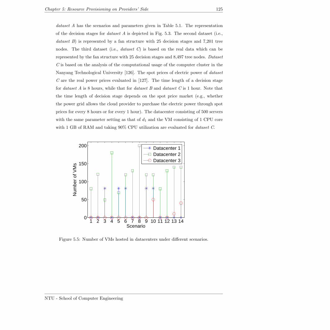
Chapter 5: Resource Provisioning on Providers’ Side 125
dataset A has the scenarios and parameters given in Table 5.1. The representation
of the decision stages for dataset A is depicted in Fig. 5.3. The second dataset (i.e.,
dataset B) is represented by a fan structure with 25 decision stages and 7,201 tree
nodes. The third dataset (i.e., dataset C) is based on the real data which can be
represented by the fan structure with 25 decision stages and 8,497 tree nodes. Dataset
C is based on the analysis of the computational usage of the computer cluster in the
Nanyang Technological University [126]. The spot prices of electric power of dataset
C are the real power prices evaluated in [127]. The time length of a decision stage
for dataset A is 8 hours, while that for dataset B and dataset C is 1 hour. Note that
the time length of decision stage depends on the spot price market (e.g., whether
the power grid allows the cloud provider to purchase the electric power through spot
prices for every 8 hours or for every 1 hour). The datacenter consisting of 500 servers
with the same parameter setting as that of d1 and the VM consisting of 1 CPU core
with 1 GB of RAM and taking 90% CPU utilization are evaluated for dataset C.
1 2 3 4 5 6 7 8 9 10 11 12 13 140
50
100
150
200
Scenario
Num
ber
of V
Ms
Datacenter 1Datacenter 2Datacenter 3
Figure 5.5: Number of VMs hosted in datacenters under different scenarios.
NTU - School of Computer Engineering
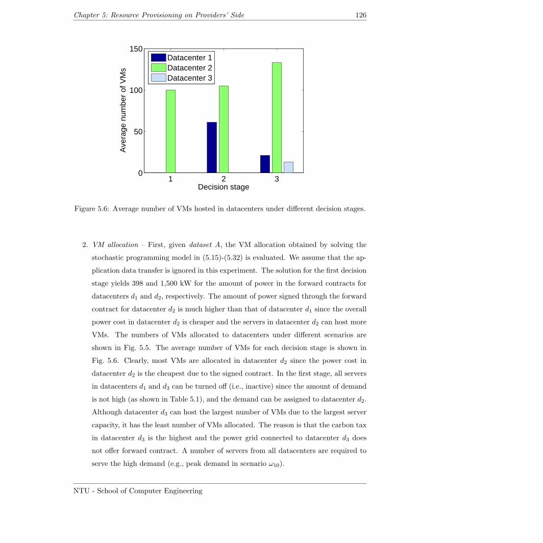
Chapter 5: Resource Provisioning on Providers’ Side 126
1 2 30
50
100
150
Decision stage
Ave
rage
num
ber
of V
Ms
Datacenter 1Datacenter 2Datacenter 3
Figure 5.6: Average number of VMs hosted in datacenters under different decision stages.
2. VM allocation – First, given dataset A, the VM allocation obtained by solving the
stochastic programming model in (5.15)-(5.32) is evaluated. We assume that the ap-
plication data transfer is ignored in this experiment. The solution for the first decision
stage yields 398 and 1,500 kW for the amount of power in the forward contracts for
datacenters d1 and d2, respectively. The amount of power signed through the forward
contract for datacenter d2 is much higher than that of datacenter d1 since the overall
power cost in datacenter d2 is cheaper and the servers in datacenter d2 can host more
VMs. The numbers of VMs allocated to datacenters under different scenarios are
shown in Fig. 5.5. The average number of VMs for each decision stage is shown in
Fig. 5.6. Clearly, most VMs are allocated in datacenter d2 since the power cost in
datacenter d2 is the cheapest due to the signed contract. In the first stage, all servers
in datacenters d1 and d3 can be turned off (i.e., inactive) since the amount of demand
is not high (as shown in Table 5.1), and the demand can be assigned to datacenter d2.
Although datacenter d3 can host the largest number of VMs due to the largest server
capacity, it has the least number of VMs allocated. The reason is that the carbon tax
in datacenter d3 is the highest and the power grid connected to datacenter d3 does
not offer forward contract. A number of servers from all datacenters are required to
serve the high demand (e.g., peak demand in scenario ω10).
NTU - School of Computer Engineering
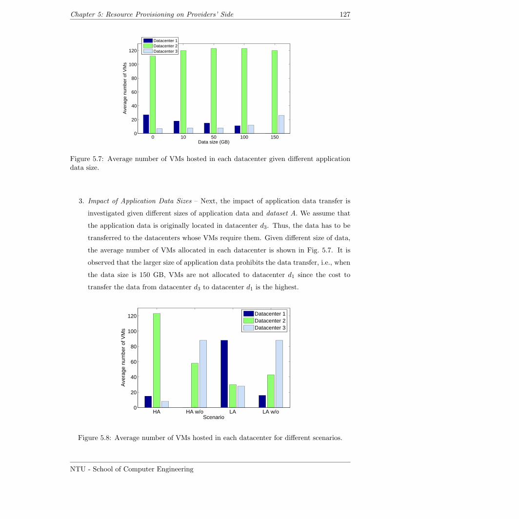
Chapter 5: Resource Provisioning on Providers’ Side 127
0 10 50 100 1500
20
40
60
80
100
120
Data size (GB)
Ave
rage
num
ber
of V
Ms
Datacenter 1Datacenter 2Datacenter 3
Figure 5.7: Average number of VMs hosted in each datacenter given different applicationdata size.
3. Impact of Application Data Sizes – Next, the impact of application data transfer is
investigated given different sizes of application data and dataset A. We assume that
the application data is originally located in datacenter d3. Thus, the data has to be
transferred to the datacenters whose VMs require them. Given different size of data,
the average number of VMs allocated in each datacenter is shown in Fig. 5.7. It is
observed that the larger size of application data prohibits the data transfer, i.e., when
the data size is 150 GB, VMs are not allocated to datacenter d1 since the cost to
transfer the data from datacenter d3 to datacenter d1 is the highest.
HA HA w/o LA LA w/o0
20
40
60
80
100
120
Scenario
Ave
rage
num
ber
of V
Ms
Datacenter 1Datacenter 2Datacenter 3
Figure 5.8: Average number of VMs hosted in each datacenter for different scenarios.
NTU - School of Computer Engineering
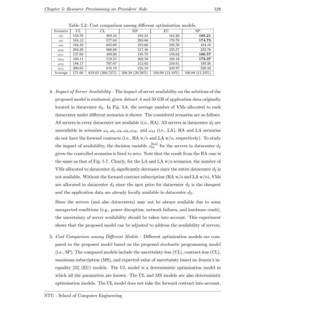
Chapter 5: Resource Provisioning on Providers’ Side 128
Table 5.2: Cost comparison among different optimization models.Scenario UL CL MS EU SP
ω7 133.76 369.42 194.34 161.26 165.21
ω8 164.12 577.84 203.86 170.78 174.73
ω9 184.16 685.60 210.66 195.50 184.16
ω10 204.20 866.88 217.46 235.57 223.76
ω11 137.69 409.00 195.70 158.62 166.57
ω12 160.11 519.55 202.50 168.42 173.37
ω13 188.17 707.67 212.02 216.61 193.26
ω14 200.65 816.19 216.10 245.97 220.32
Average 171.60 619.02 (260.72%) 206.58 (20.38%) 194.09 (13.10%) 190.88 (11.23%)
4. Impact of Server Availability – The impact of server availability on the solutions of the
proposed model is evaluated, given dataset A and 50 GB of application data originally
located in datacenter d3. In Fig. 5.8, the average number of VMs allocated to each
datacenter under different scenarios is shown. The considered scenarios are as follows.
All servers in every datacenter are available (i.e., HA). All servers in datacenter d2 are
unavailable in scenarios ω4, ω6, ω8, ω9, ω10, and ω14 (i.e., LA). HA and LA scenarios
do not have the forward contracts (i.e., HA w/o and LA w/o, respectively). To study
the impact of availability, the decision variable z[hos]sω for the servers in datacenter d2
given the controlled scenarios is fixed to zero. Note that the result from the HA case is
the same as that of Fig. 5.7. Clearly, for the LA and LA w/o scenarios, the number of
VMs allocated to datacenter d2 significantly decreases since the entire datacenter d2 is
not available. Without the forward contract subscription (HA w/o and LA w/o), VMs
are allocated in datacenter d3 since the spot price for datacenter d3 is the cheapest
and the application data are already locally available in datacenter d3.
Since the servers (and also datacenters) may not be always available due to some
unexpected conditions (e.g., power disruption, network failures, and hardware crash),
the uncertainty of server availability should be taken into account. This experiment
shows that the proposed model can be adjusted to address the availability of servers.
5. Cost Comparison among Different Models – Different optimization models are com-
pared to the proposed model based on the proposed stochastic programming model
(i.e., SP). The compared models include the uncertainty-less (UL), contract-less (CL),
maximum subscription (MS), and expected-value of uncertainty based on Jensen’s in-
equality [55] (EU) models. The UL model is a deterministic optimization model in
which all the parameters are known. The CL and MS models are also deterministic
optimization models. The CL model does not take the forward contract into account,
NTU - School of Computer Engineering
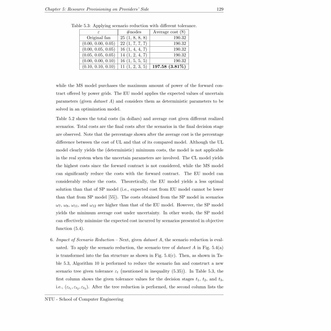
Chapter 5: Resource Provisioning on Providers’ Side 129
Table 5.3: Applying scenario reduction with different tolerance.
ε #nodes Average cost ($)
Original fan 25 (1, 8, 8, 8) 190.32
(0.00, 0.00, 0.05) 22 (1, 7, 7, 7) 190.32
(0.00, 0.05, 0.05) 16 (1, 4, 4, 7) 190.32
(0.05, 0.05, 0.05) 14 (1, 2, 4, 7) 190.32
(0.00, 0.00, 0.10) 16 (1, 5, 5, 5) 190.32
(0.10, 0.10, 0.10) 11 (1, 2, 3, 5) 197.58 (3.81%)
while the MS model purchases the maximum amount of power of the forward con-
tract offered by power grids. The EU model applies the expected values of uncertain
parameters (given dataset A) and considers them as deterministic parameters to be
solved in an optimization model.
Table 5.2 shows the total costs (in dollars) and average cost given different realized
scenarios. Total costs are the final costs after the scenarios in the final decision stage
are observed. Note that the percentage shown after the average cost is the percentage
difference between the cost of UL and that of its compared model. Although the UL
model clearly yields the (deterministic) minimum costs, the model is not applicable
in the real system when the uncertain parameters are involved. The CL model yields
the highest costs since the forward contract is not considered, while the MS model
can significantly reduce the costs with the forward contract. The EU model can
considerably reduce the costs. Theoretically, the EU model yields a less optimal
solution than that of SP model (i.e., expected cost from EU model cannot be lower
than that from SP model [55]). The costs obtained from the SP model in scenarios
ω7, ω8, ω11, and ω12 are higher than that of the EU model. However, the SP model
yields the minimum average cost under uncertainty. In other words, the SP model
can effectively minimize the expected cost incurred by scenarios presented in objective
function (5.4).
6. Impact of Scenario Reduction – Next, given dataset A, the scenario reduction is eval-
uated. To apply the scenario reduction, the scenario tree of dataset A in Fig. 5.4(a)
is transformed into the fan structure as shown in Fig. 5.4(c). Then, as shown in Ta-
ble 5.3, Algorithm 10 is performed to reduce the scenario fan and construct a new
scenario tree given tolerance εt(mentioned in inequality (5.35)
). In Table 5.3, the
first column shows the given tolerance values for the decision stages t1, t2, and t3,
i.e., (εt1 , εt2 , εt3). After the tree reduction is performed, the second column lists the
NTU - School of Computer Engineering
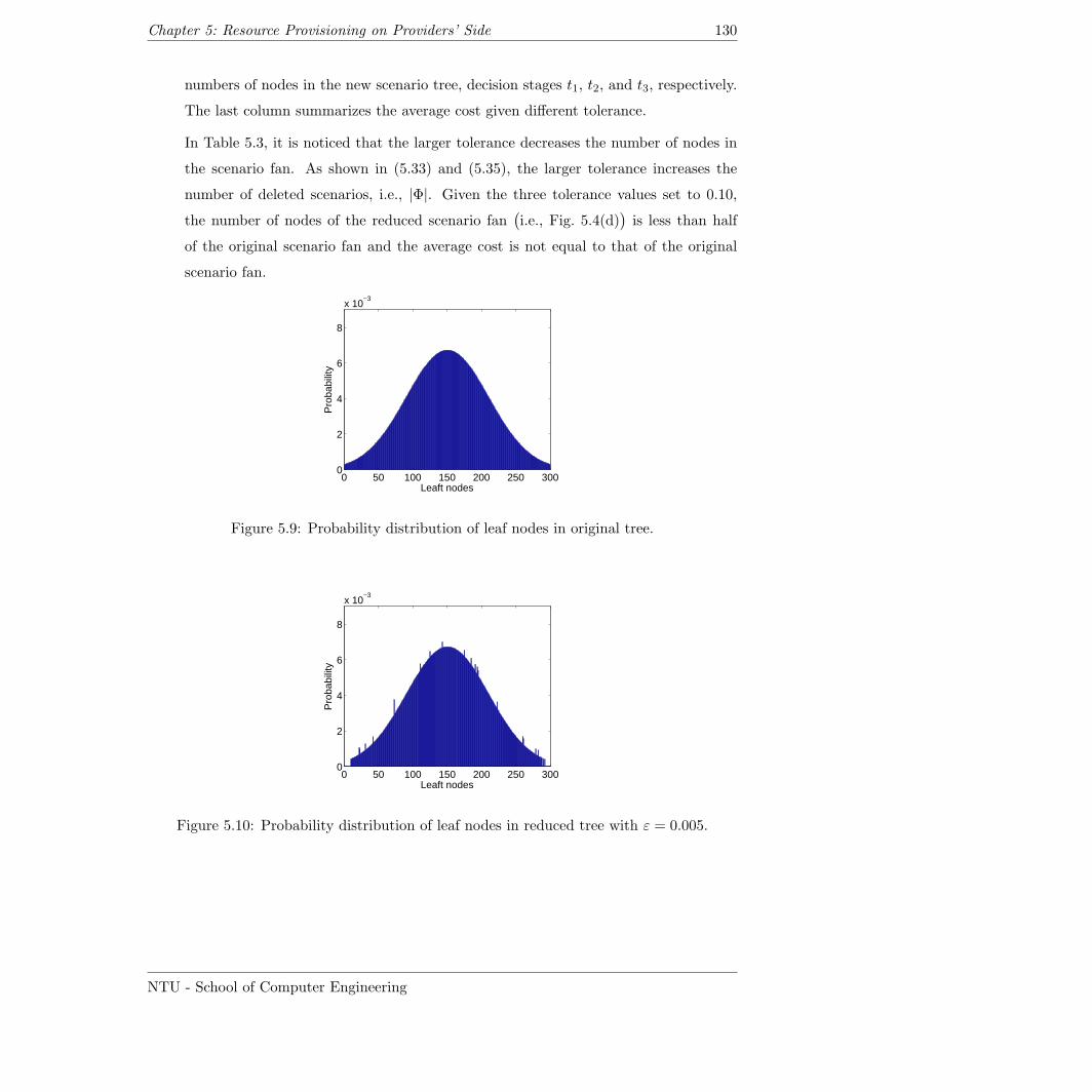
Chapter 5: Resource Provisioning on Providers’ Side 130
numbers of nodes in the new scenario tree, decision stages t1, t2, and t3, respectively.
The last column summarizes the average cost given different tolerance.
In Table 5.3, it is noticed that the larger tolerance decreases the number of nodes in
the scenario fan. As shown in (5.33) and (5.35), the larger tolerance increases the
number of deleted scenarios, i.e., |Φ|. Given the three tolerance values set to 0.10,
the number of nodes of the reduced scenario fan(i.e., Fig. 5.4(d)
)is less than half
of the original scenario fan and the average cost is not equal to that of the original
scenario fan.
0 50 100 150 200 250 3000
2
4
6
8
x 10−3
Leaft nodes
Pro
babi
lity
Figure 5.9: Probability distribution of leaf nodes in original tree.
0 50 100 150 200 250 3000
2
4
6
8
x 10−3
Leaft nodes
Pro
babi
lity
Figure 5.10: Probability distribution of leaf nodes in reduced tree with ε = 0.005.
NTU - School of Computer Engineering
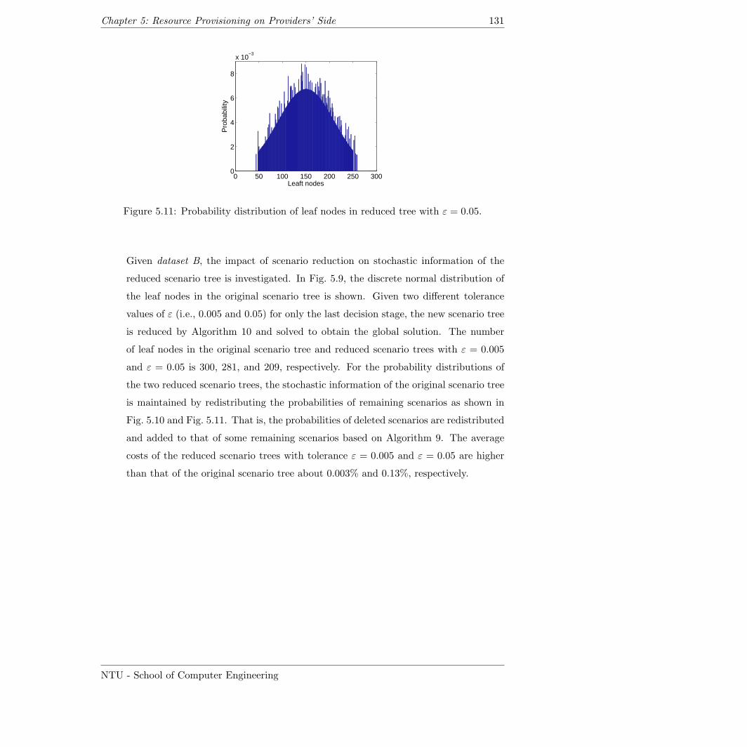
Chapter 5: Resource Provisioning on Providers’ Side 131
0 50 100 150 200 250 3000
2
4
6
8
x 10−3
Leaft nodes
Pro
babi
lity
Figure 5.11: Probability distribution of leaf nodes in reduced tree with ε = 0.05.
Given dataset B, the impact of scenario reduction on stochastic information of the
reduced scenario tree is investigated. In Fig. 5.9, the discrete normal distribution of
the leaf nodes in the original scenario tree is shown. Given two different tolerance
values of ε (i.e., 0.005 and 0.05) for only the last decision stage, the new scenario tree
is reduced by Algorithm 10 and solved to obtain the global solution. The number
of leaf nodes in the original scenario tree and reduced scenario trees with ε = 0.005
and ε = 0.05 is 300, 281, and 209, respectively. For the probability distributions of
the two reduced scenario trees, the stochastic information of the original scenario tree
is maintained by redistributing the probabilities of remaining scenarios as shown in
Fig. 5.10 and Fig. 5.11. That is, the probabilities of deleted scenarios are redistributed
and added to that of some remaining scenarios based on Algorithm 9. The average
costs of the reduced scenario trees with tolerance ε = 0.005 and ε = 0.05 are higher
than that of the original scenario tree about 0.003% and 0.13%, respectively.
NTU - School of Computer Engineering
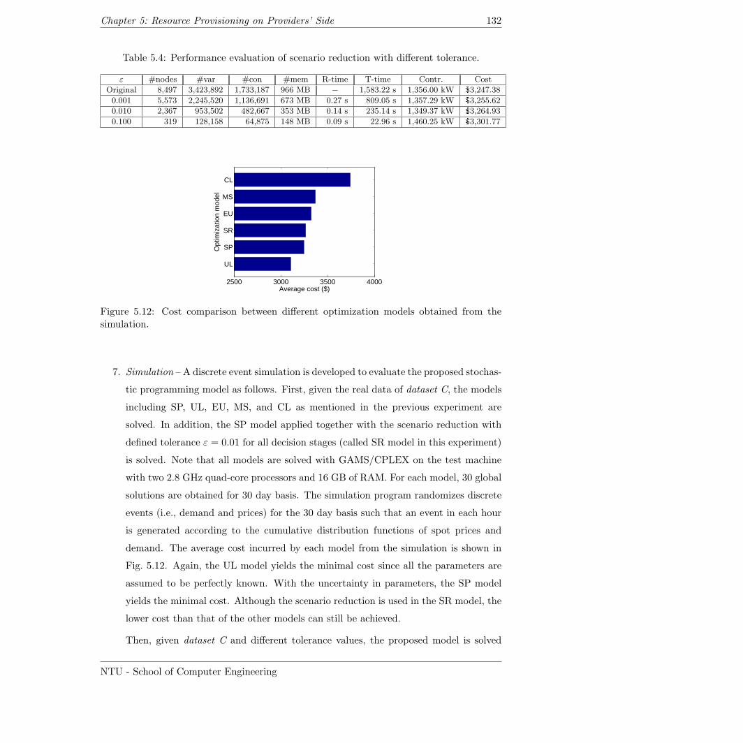
Chapter 5: Resource Provisioning on Providers’ Side 132
Table 5.4: Performance evaluation of scenario reduction with different tolerance.
ε #nodes #var #con #mem R-time T-time Contr. Cost
Original 8,497 3,423,892 1,733,187 966 MB − 1,583.22 s 1,356.00 kW $3,247.38
0.001 5,573 2,245,520 1,136,691 673 MB 0.27 s 809.05 s 1,357.29 kW $3,255.62
0.010 2,367 953,502 482,667 353 MB 0.14 s 235.14 s 1,349.37 kW $3,264.93
0.100 319 128,158 64,875 148 MB 0.09 s 22.96 s 1,460.25 kW $3,301.77
2500 3000 3500 4000
UL
SP
SR
EU
MS
CL
Average cost ($)
Opt
imiz
atio
n m
odel
Figure 5.12: Cost comparison between different optimization models obtained from thesimulation.
7. Simulation – A discrete event simulation is developed to evaluate the proposed stochas-
tic programming model as follows. First, given the real data of dataset C, the models
including SP, UL, EU, MS, and CL as mentioned in the previous experiment are
solved. In addition, the SP model applied together with the scenario reduction with
defined tolerance ε = 0.01 for all decision stages (called SR model in this experiment)
is solved. Note that all models are solved with GAMS/CPLEX on the test machine
with two 2.8 GHz quad-core processors and 16 GB of RAM. For each model, 30 global
solutions are obtained for 30 day basis. The simulation program randomizes discrete
events (i.e., demand and prices) for the 30 day basis such that an event in each hour
is generated according to the cumulative distribution functions of spot prices and
demand. The average cost incurred by each model from the simulation is shown in
Fig. 5.12. Again, the UL model yields the minimal cost since all the parameters are
assumed to be perfectly known. With the uncertainty in parameters, the SP model
yields the minimal cost. Although the scenario reduction is used in the SR model, the
lower cost than that of the other models can still be achieved.
Then, given dataset C and different tolerance values, the proposed model is solved
NTU - School of Computer Engineering
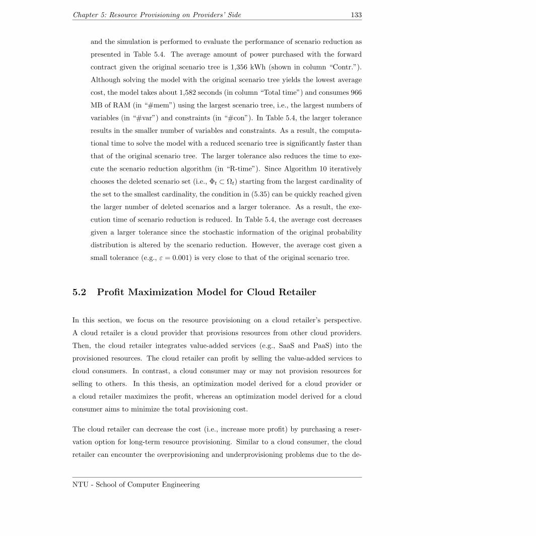
Chapter 5: Resource Provisioning on Providers’ Side 133
and the simulation is performed to evaluate the performance of scenario reduction as
presented in Table 5.4. The average amount of power purchased with the forward
contract given the original scenario tree is 1,356 kWh (shown in column “Contr.”).
Although solving the model with the original scenario tree yields the lowest average
cost, the model takes about 1,582 seconds (in column “Total time”) and consumes 966
MB of RAM (in “#mem”) using the largest scenario tree, i.e., the largest numbers of
variables (in “#var”) and constraints (in “#con”). In Table 5.4, the larger tolerance
results in the smaller number of variables and constraints. As a result, the computa-
tional time to solve the model with a reduced scenario tree is significantly faster than
that of the original scenario tree. The larger tolerance also reduces the time to exe-
cute the scenario reduction algorithm (in “R-time”). Since Algorithm 10 iteratively
chooses the deleted scenario set (i.e., Φt ⊂ Ωt) starting from the largest cardinality of
the set to the smallest cardinality, the condition in (5.35) can be quickly reached given
the larger number of deleted scenarios and a larger tolerance. As a result, the exe-
cution time of scenario reduction is reduced. In Table 5.4, the average cost decreases
given a larger tolerance since the stochastic information of the original probability
distribution is altered by the scenario reduction. However, the average cost given a
small tolerance (e.g., ε = 0.001) is very close to that of the original scenario tree.
5.2 Profit Maximization Model for Cloud Retailer
In this section, we focus on the resource provisioning on a cloud retailer’s perspective.
A cloud retailer is a cloud provider that provisions resources from other cloud providers.
Then, the cloud retailer integrates value-added services (e.g., SaaS and PaaS) into the
provisioned resources. The cloud retailer can profit by selling the value-added services to
cloud consumers. In contrast, a cloud consumer may or may not provision resources for
selling to others. In this thesis, an optimization model derived for a cloud provider or
a cloud retailer maximizes the profit, whereas an optimization model derived for a cloud
consumer aims to minimize the total provisioning cost.
The cloud retailer can decrease the cost (i.e., increase more profit) by purchasing a reser-
vation option for long-term resource provisioning. Similar to a cloud consumer, the cloud
retailer can encounter the overprovisioning and underprovisioning problems due to the de-
NTU - School of Computer Engineering
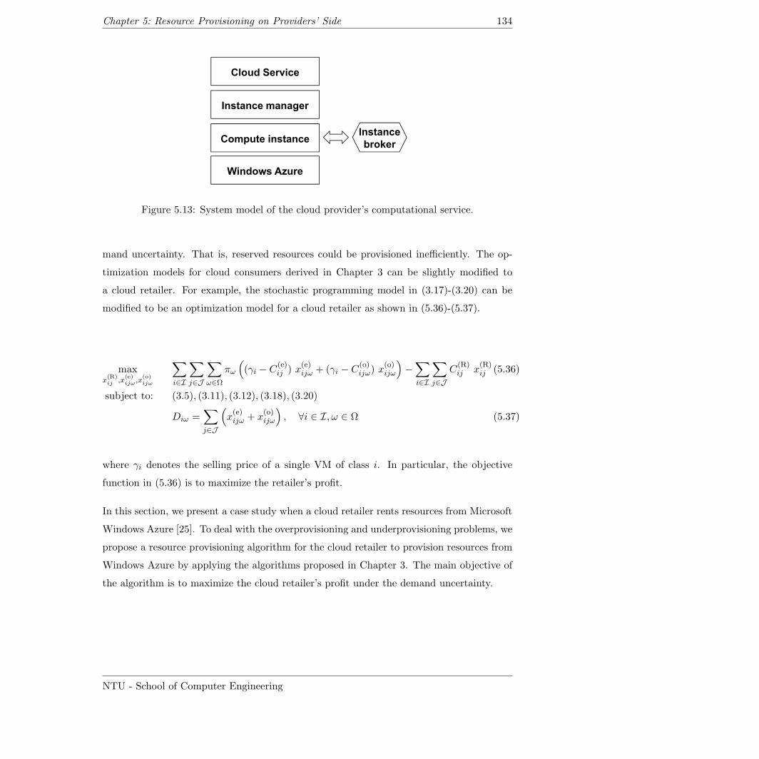
Chapter 5: Resource Provisioning on Providers’ Side 134
Cloud Service
Instance managerInstance manager
Windows Azure
Compute instanceInstance
broker
Windows Azure
Figure 5.13: System model of the cloud provider’s computational service.
mand uncertainty. That is, reserved resources could be provisioned inefficiently. The op-
timization models for cloud consumers derived in Chapter 3 can be slightly modified to
a cloud retailer. For example, the stochastic programming model in (3.17)-(3.20) can be
modified to be an optimization model for a cloud retailer as shown in (5.36)-(5.37).
maxx(R)ij ,x
(e)ijω ,x
(o)ijω
∑i∈I
∑j∈J
∑ω∈Ω
πω
((γi − C(e)
ij ) x(e)ijω + (γi − C(o)
ijω) x(o)ijω
)−∑i∈I
∑j∈J
C(R)ij x
(R)ij (5.36)
subject to: (3.5), (3.11), (3.12), (3.18), (3.20)
Diω =∑j∈J
(x(e)ijω + x
(o)ijω
), ∀i ∈ I, ω ∈ Ω (5.37)
where γi denotes the selling price of a single VM of class i. In particular, the objective
function in (5.36) is to maximize the retailer’s profit.
In this section, we present a case study when a cloud retailer rents resources from Microsoft
Windows Azure [25]. To deal with the overprovisioning and underprovisioning problems, we
propose a resource provisioning algorithm for the cloud retailer to provision resources from
Windows Azure by applying the algorithms proposed in Chapter 3. The main objective of
the algorithm is to maximize the cloud retailer’s profit under the demand uncertainty.
NTU - School of Computer Engineering
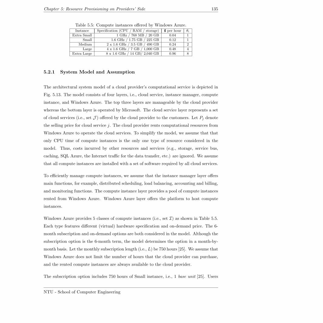
Chapter 5: Resource Provisioning on Providers’ Side 135
Table 5.5: Compute instances offered by Windows Azure.Instance Specification (CPU / RAM / storage) $ per hour θi
Extra Small 1 GHz / 768 MB / 20 GB 0.04 1
Small 1.6 GHz / 1.75 GB / 225 GB 0.12 1
Medium 2 x 1.6 GHz / 3.5 GB / 490 GB 0.24 2
Large 4 x 1.6 GHz / 7 GB / 1,000 GB 0.48 4
Extra Large 8 x 1.6 GHz / 14 GB/ 2,040 GB 0.96 8
5.2.1 System Model and Assumption
The architectural system model of a cloud provider’s computational service is depicted in
Fig. 5.13. The model consists of four layers, i.e., cloud service, instance manager, compute
instance, and Windows Azure. The top three layers are manageable by the cloud provider
whereas the bottom layer is operated by Microsoft. The cloud service layer represents a set
of cloud services (i.e., set J ) offered by the cloud provider to the customers. Let Pj denote
the selling price for cloud service j. The cloud provider rents computational resources from
Windows Azure to operate the cloud services. To simplify the model, we assume that that
only CPU time of compute instances is the only one type of resource considered in the
model. Thus, costs incurred by other resources and services (e.g., storage, service bus,
caching, SQL Azure, the Internet traffic for the data transfer, etc.) are ignored. We assume
that all compute instances are installed with a set of software required by all cloud services.
To efficiently manage compute instances, we assume that the instance manager layer offers
main functions, for example, distributed scheduling, load balancing, accounting and billing,
and monitoring functions. The compute instance layer provides a pool of compute instances
rented from Windows Azure. Windows Azure layer offers the platform to host compute
instances.
Windows Azure provides 5 classes of compute instances (i.e., set I) as shown in Table 5.5.
Each type features different (virtual) hardware specification and on-demand price. The 6-
month subscription and on-demand options are both considered in the model. Although the
subscription option is the 6-month term, the model determines the option in a month-by-
month basis. Let the monthly subscription length (i.e., L) be 750 hours [25]. We assume that
Windows Azure does not limit the number of hours that the cloud provider can purchase,
and the rented compute instances are always available to the cloud provider.
The subscription option includes 750 hours of Small instance, i.e., 1 base unit [25]. Users
NTU - School of Computer Engineering
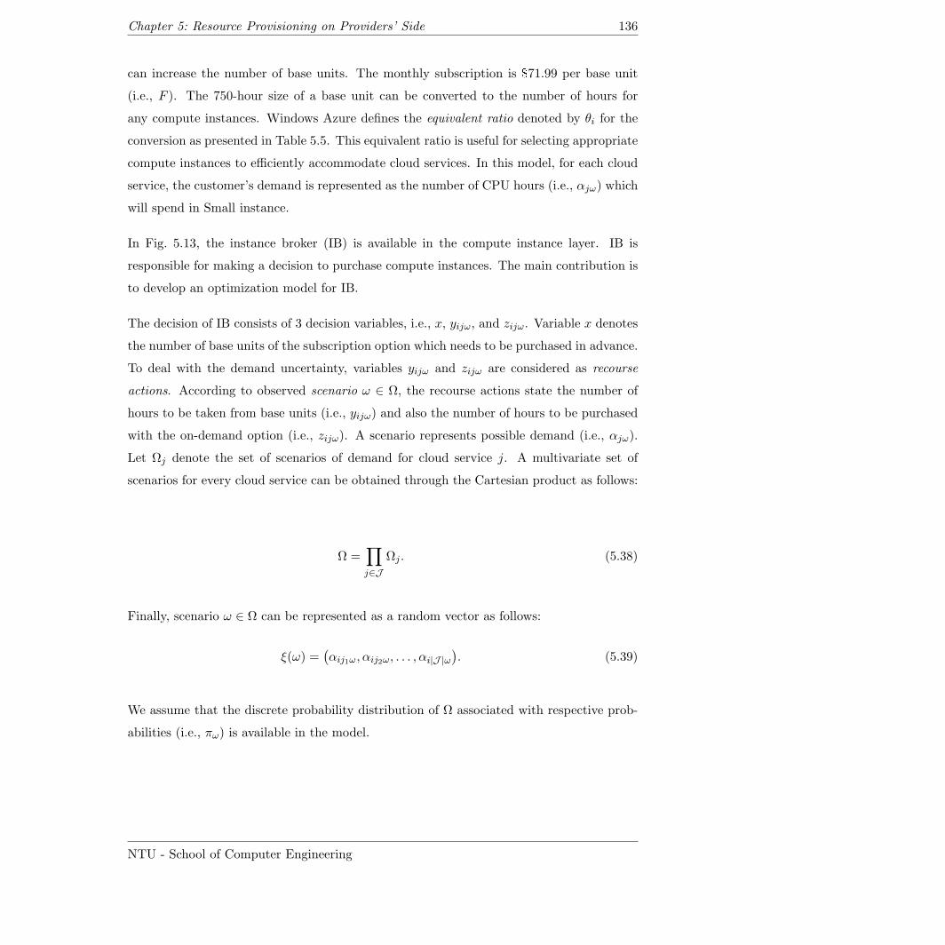
Chapter 5: Resource Provisioning on Providers’ Side 136
can increase the number of base units. The monthly subscription is $71.99 per base unit
(i.e., F ). The 750-hour size of a base unit can be converted to the number of hours for
any compute instances. Windows Azure defines the equivalent ratio denoted by θi for the
conversion as presented in Table 5.5. This equivalent ratio is useful for selecting appropriate
compute instances to efficiently accommodate cloud services. In this model, for each cloud
service, the customer’s demand is represented as the number of CPU hours (i.e., αjω) which
will spend in Small instance.
In Fig. 5.13, the instance broker (IB) is available in the compute instance layer. IB is
responsible for making a decision to purchase compute instances. The main contribution is
to develop an optimization model for IB.
The decision of IB consists of 3 decision variables, i.e., x, yijω, and zijω. Variable x denotes
the number of base units of the subscription option which needs to be purchased in advance.
To deal with the demand uncertainty, variables yijω and zijω are considered as recourse
actions. According to observed scenario ω ∈ Ω, the recourse actions state the number of
hours to be taken from base units (i.e., yijω) and also the number of hours to be purchased
with the on-demand option (i.e., zijω). A scenario represents possible demand (i.e., αjω).
Let Ωj denote the set of scenarios of demand for cloud service j. A multivariate set of
scenarios for every cloud service can be obtained through the Cartesian product as follows:
Ω =∏j∈J
Ωj . (5.38)
Finally, scenario ω ∈ Ω can be represented as a random vector as follows:
ξ(ω) =(αij1ω, αij2ω, . . . , αi|J |ω
). (5.39)
We assume that the discrete probability distribution of Ω associated with respective prob-
abilities (i.e., πω) is available in the model.
NTU - School of Computer Engineering
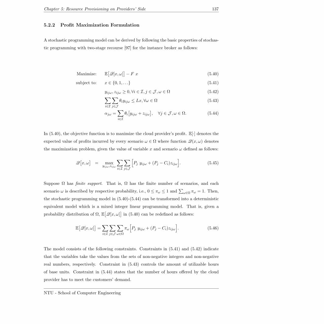
Chapter 5: Resource Provisioning on Providers’ Side 137
5.2.2 Profit Maximization Formulation
A stochastic programming model can be derived by following the basic properties of stochas-
tic programming with two-stage recourse [97] for the instance broker as follows:
Maximize: E[Q[x, ω]
]− F x (5.40)
subject to: x ∈ 0, 1, . . . (5.41)
yijω, zijω ≥ 0, ∀i ∈ I, j ∈ J , ω ∈ Ω (5.42)∑i∈I
∑j∈J
θiyijω ≤ Lx, ∀ω ∈ Ω (5.43)
αjω =∑i∈I
θi[yijω + zijω
], ∀j ∈ J , ω ∈ Ω. (5.44)
In (5.40), the objective function is to maximize the cloud provider’s profit. E[·] denotes the
expected value of profits incurred by every scenario ω ∈ Ω where function Q(x, ω) denotes
the maximization problem, given the value of variable x and scenario ω defined as follows:
Q[x, ω
]= max
yijω ,zijω
∑i∈I
∑j∈J
[Pj yijω + (Pj − Ci)zijω
]. (5.45)
Suppose Ω has finite support. That is, Ω has the finite number of scenarios, and each
scenario ω is described by respective probability, i.e., 0 ≤ πω ≤ 1 and∑
ω∈Ω πω = 1. Then,
the stochastic programming model in (5.40)-(5.44) can be transformed into a deterministic
equivalent model which is a mixed integer linear programming model. That is, given a
probability distribution of Ω, E[Q[x, ω]
]in (5.40) can be redefined as follows:
E[Q[x, ω]
]=∑i∈I
∑j∈J
∑ω∈Ω
πω
[Pj yijω + (Pj − Ci)zijω
]. (5.46)
The model consists of the following constraints. Constraints in (5.41) and (5.42) indicate
that the variables take the values from the sets of non-negative integers and non-negative
real numbers, respectively. Constraint in (5.43) controls the amount of utilizable hours
of base units. Constraint in (5.44) states that the number of hours offered by the cloud
provider has to meet the customers’ demand.
NTU - School of Computer Engineering
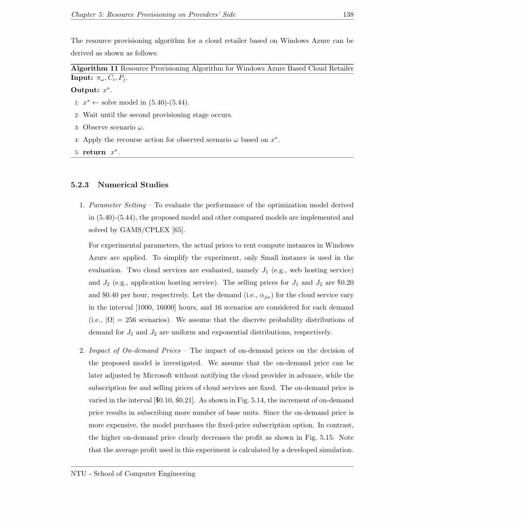
Chapter 5: Resource Provisioning on Providers’ Side 138
The resource provisioning algorithm for a cloud retailer based on Windows Azure can be
derived as shown as follows:
Algorithm 11 Resource Provisioning Algorithm for Windows Azure Based Cloud Retailer
Input: πω, Ci, Pj .
Output: x∗.
1: x∗ ← solve model in (5.40)-(5.44).
2: Wait until the second provisioning stage occurs.
3: Observe scenario ω.
4: Apply the recourse action for observed scenario ω based on x∗.
5: return x∗.
5.2.3 Numerical Studies
1. Parameter Setting – To evaluate the performance of the optimization model derived
in (5.40)-(5.44), the proposed model and other compared models are implemented and
solved by GAMS/CPLEX [65].
For experimental parameters, the actual prices to rent compute instances in Windows
Azure are applied. To simplify the experiment, only Small instance is used in the
evaluation. Two cloud services are evaluated, namely J1 (e.g., web hosting service)
and J2 (e.g., application hosting service). The selling prices for J1 and J2 are $0.20
and $0.40 per hour, respectively. Let the demand (i.e., αjω) for the cloud service vary
in the interval [1000, 16000] hours, and 16 scenarios are considered for each demand
(i.e., |Ω| = 256 scenarios). We assume that the discrete probability distributions of
demand for J1 and J2 are uniform and exponential distributions, respectively.
2. Impact of On-demand Prices – The impact of on-demand prices on the decision of
the proposed model is investigated. We assume that the on-demand price can be
later adjusted by Microsoft without notifying the cloud provider in advance, while the
subscription fee and selling prices of cloud services are fixed. The on-demand price is
varied in the interval [$0.10, $0.21]. As shown in Fig. 5.14, the increment of on-demand
price results in subscribing more number of base units. Since the on-demand price is
more expensive, the model purchases the fixed-price subscription option. In contrast,
the higher on-demand price clearly decreases the profit as shown in Fig. 5.15. Note
that the average profit used in this experiment is calculated by a developed simulation.
NTU - School of Computer Engineering
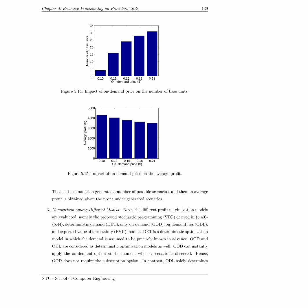
Chapter 5: Resource Provisioning on Providers’ Side 139
0.10 0.12 0.15 0.18 0.210
5
10
15
20
25
30
35
On−demand price ($)
Num
ber
of b
ase
units
Figure 5.14: Impact of on-demand price on the number of base units.
0.10 0.12 0.15 0.18 0.210
1000
2000
3000
4000
5000
On−demand price ($)
Ave
rage
pro
fit (
$)
Figure 5.15: Impact of on-demand price on the average profit.
That is, the simulation generates a number of possible scenarios, and then an average
profit is obtained given the profit under generated scenarios.
3. Comparison among Different Models – Next, the different profit maximization models
are evaluated, namely the proposed stochastic programming (STO) derived in (5.40)-
(5.44), deterministic-demand (DET), only-on-demand (OOD), on-demand-less (ODL),
and expected-value of uncertainty (EVU) models. DET is a deterministic optimization
model in which the demand is assumed to be precisely known in advance. OOD and
ODL are considered as deterministic optimization models as well. OOD can instantly
apply the on-demand option at the moment when a scenario is observed. Hence,
OOD does not require the subscription option. In contrast, ODL solely determines
NTU - School of Computer Engineering
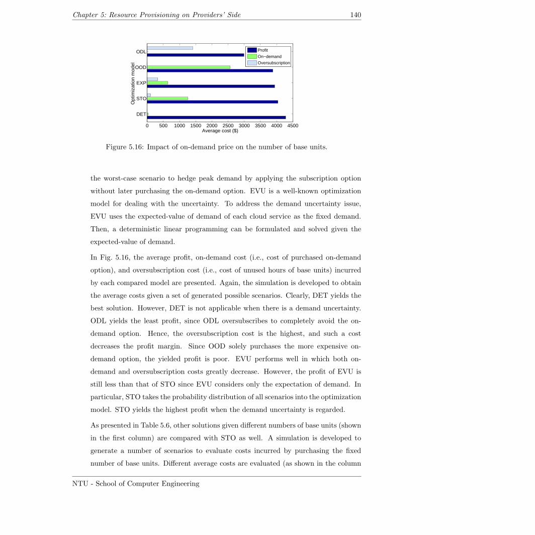
Chapter 5: Resource Provisioning on Providers’ Side 140
0 500 1000 1500 2000 2500 3000 3500 4000 4500
DET
STO
EXP
OOD
ODL
Average cost ($)
Opt
imiz
atio
n m
odel
Profit
On−demand
Oversubscription
Figure 5.16: Impact of on-demand price on the number of base units.
the worst-case scenario to hedge peak demand by applying the subscription option
without later purchasing the on-demand option. EVU is a well-known optimization
model for dealing with the uncertainty. To address the demand uncertainty issue,
EVU uses the expected-value of demand of each cloud service as the fixed demand.
Then, a deterministic linear programming can be formulated and solved given the
expected-value of demand.
In Fig. 5.16, the average profit, on-demand cost (i.e., cost of purchased on-demand
option), and oversubscription cost (i.e., cost of unused hours of base units) incurred
by each compared model are presented. Again, the simulation is developed to obtain
the average costs given a set of generated possible scenarios. Clearly, DET yields the
best solution. However, DET is not applicable when there is a demand uncertainty.
ODL yields the least profit, since ODL oversubscribes to completely avoid the on-
demand option. Hence, the oversubscription cost is the highest, and such a cost
decreases the profit margin. Since OOD solely purchases the more expensive on-
demand option, the yielded profit is poor. EVU performs well in which both on-
demand and oversubscription costs greatly decrease. However, the profit of EVU is
still less than that of STO since EVU considers only the expectation of demand. In
particular, STO takes the probability distribution of all scenarios into the optimization
model. STO yields the highest profit when the demand uncertainty is regarded.
As presented in Table 5.6, other solutions given different numbers of base units (shown
in the first column) are compared with STO as well. A simulation is developed to
generate a number of scenarios to evaluate costs incurred by purchasing the fixed
number of base units. Different average costs are evaluated (as shown in the column
NTU - School of Computer Engineering
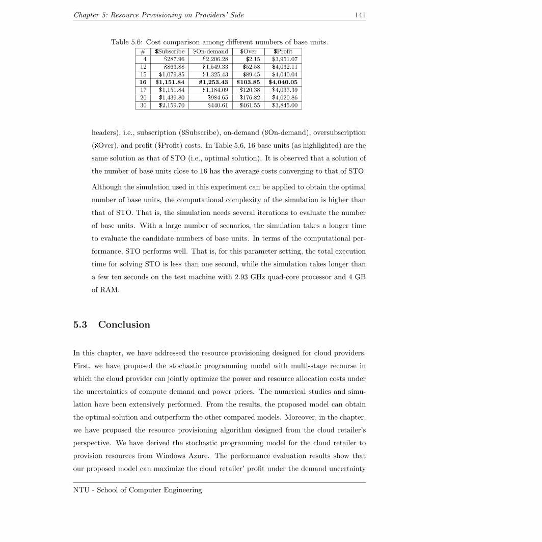
Chapter 5: Resource Provisioning on Providers’ Side 141
Table 5.6: Cost comparison among different numbers of base units.# $Subscribe $On-demand $Over $Profit
4 $287.96 $2,206.28 $2.15 $3,951.07
12 $863.88 $1,549.33 $52.58 $4,032.11
15 $1,079.85 $1,325.43 $89.45 $4,040.04
16 $1,151.84 $1,253.43 $103.85 $4,040.05
17 $1,151.84 $1,184.09 $120.38 $4,037.39
20 $1,439.80 $984.65 $176.82 $4,020.86
30 $2,159.70 $440.61 $461.55 $3,845.00
headers), i.e., subscription ($Subscribe), on-demand ($On-demand), oversubscription
($Over), and profit ($Profit) costs. In Table 5.6, 16 base units (as highlighted) are the
same solution as that of STO (i.e., optimal solution). It is observed that a solution of
the number of base units close to 16 has the average costs converging to that of STO.
Although the simulation used in this experiment can be applied to obtain the optimal
number of base units, the computational complexity of the simulation is higher than
that of STO. That is, the simulation needs several iterations to evaluate the number
of base units. With a large number of scenarios, the simulation takes a longer time
to evaluate the candidate numbers of base units. In terms of the computational per-
formance, STO performs well. That is, for this parameter setting, the total execution
time for solving STO is less than one second, while the simulation takes longer than
a few ten seconds on the test machine with 2.93 GHz quad-core processor and 4 GB
of RAM.
5.3 Conclusion
In this chapter, we have addressed the resource provisioning designed for cloud providers.
First, we have proposed the stochastic programming model with multi-stage recourse in
which the cloud provider can jointly optimize the power and resource allocation costs under
the uncertainties of compute demand and power prices. The numerical studies and simu-
lation have been extensively performed. From the results, the proposed model can obtain
the optimal solution and outperform the other compared models. Moreover, in the chapter,
we have proposed the resource provisioning algorithm designed from the cloud retailer’s
perspective. We have derived the stochastic programming model for the cloud retailer to
provision resources from Windows Azure. The performance evaluation results show that
our proposed model can maximize the cloud retailer’ profit under the demand uncertainty
NTU - School of Computer Engineering
Chapter 5: Resource Provisioning on Providers’ Side 142
and outperform the other competitive models. The proposed model can be extended to
cloud retailers based on other cloud providers rather than Windows Azure as well.
NTU - School of Computer Engineering
Chapter 6
Summary and Future Works
6.1 Conclusions
In this thesis, we have focused mainly on the resource provisioning in cloud computing.
On-demand and reservation options offered by cloud providers have been applied for pro-
visioning resources. Each option has different price and benefit. Due to uncertainties, the
common problems encountered in resource provisioning with the two options are overprovi-
sioning and underprovisioning. We have considered three uncertainties causing the resource
provisioning problems, i.e., uncertainties of demand, price, and availability of resources. We
have proposed novel algorithms and framework to deal with the uncertainties and optimize
the resource provisioning cost for different cloud stakeholders (i.e., cloud consumer, cloud
provider, and cloud retailer).
The research contributions presented in this thesis can be summarized as follows:
• Resource provisioning algorithms for a cloud consumer: We have proposed novel re-
source provisioning algorithms for provisioning the resources from IaaS-based cloud
providers to a cloud consumer. The main objective of the algorithms is to minimize
the resource provisioning cost incurred to the cloud consumer, while the uncertainties
are taken into account.
First, we have formulated a stochastic programming model with two-stage recourse
for the first proposed algorithm. With stochastic programming, the uncertainties are
143
Chapter 6: Summary and Future Works 144
described as scenarios associated with a probability distribution. We have applied
Benders decomposition to divide this optimization problem into smaller independent
problems which can be solved faster.
Second, we have proposed a new algorithm by extending the two-stage stochastic pro-
gramming model using the robust optimization. This new algorithm can be adjusted
according to the cloud consumer’s risk preference for balancing the tradeoff between
the solution- and model-robustness. That is, the solution will be close to the deter-
ministic optimal solution for the solution-robustness, while the overprovisioning and
underprovisioning problems will be reduced for the model-robustness.
Third, we have proposed a resource provisioning algorithm based on stochastic pro-
gramming with multi-stage recourse. The algorithm is useful for provisioning resources
when multiple reservation contracts offered by cloud providers and multiple provision-
ing stages are involved. To deal with a large number of scenarios, we have applied
the sample-average approximation (SAA) technique. With the SAA technique, the
number of scenarios can be reduced such that the computational complexity of the
algorithm can be reduced, while the near optimal solution can be achieved.
Fourth, we have demonstrated how the proposed resource provisioning algorithms
can be applied to Amazon EC2 (a well-known cloud provider) using real data. In
particular, we have developed two resource provisioning algorithms for the long- and
short-term resource provisioning plans. That is, the long-term provisioning algorithm
is for purchasing the reservation option, while the short-term algorithm is for pur-
chasing the spot option. The on-demand option will be additionally purchased when
the provisioned resources are not sufficient.
We have performed numerical studies and simulation to evaluate the proposed algo-
rithms. The results show that the algorithms can give the lowest resource provisioning
cost when the algorithms are compared with other well-known algorithms.
• Joint power optimization and resource management for a cloud provider: We have
designed a joint power and resource management framework for a cloud provider. We
have focused on the smart grid technology for the cloud provider’s datacenters. In
this smart grid environment, the cloud provider encounters risk of fluctuating spot
prices of electric power. To deal with the problem in our proposed framework, we
have formulated a stochastic programming model with multi-stage recourse from the
cloud provider’s perspective to minimize the expected cost under power price and
NTU - School of Computer Engineering
Chapter 6: Summary and Future Works 145
compute demand uncertainties. The expected cost is composed of the virtual machine
hosting, electric power, and application data transfer costs. We have used the scenario
tree construction for describing uncertainties of the multi-stage recourse problem. In
addition, we have applied the scenario reduction technique to reduce the size of a
scenario tree such that the computational complexity of the problem can be reduced.
We have performed numerical studies to evaluate the framework. The results show
that the proposed framework can give the lowest cost. Although the size of scenario
tree taken into the framework is reduced, the near optimal solution can be achieved.
• Resource provisioning algorithm for a cloud retailer: We have focused on a cloud
computing market where a cloud retailer can earn a profit by implementing and selling
value-added services on top of other cloud providers’ resources. We have proposed a
resource provisioning algorithm from the cloud retailer’s perspective for provisioning
resources under uncertainty from IaaS-based cloud providers to the cloud retailer.
The main objective of the algorithm is to maximize the retailer’s profit. The optimal
solution of this algorithm is obtained by solving stochastic programming with two-
stage recourse. To show how the algorithm can be derived, a case-study is presented
where the cloud retailer implements cloud services on top of resources provisioned
from Windows Azure. The results show that the cloud retailer can maximize the
profit.
Thus, in this thesis, we have addressed the resource provisioning problems from three cloud
stakeholders, i.e., cloud consumer, cloud provider, and cloud reseller. We have proposed
novel algorithms and framework to optimize the cloud stakeholders’ profit taking uncer-
tainties into account. Our contributions will be useful for the resource provisioning opti-
mization in cloud computing. The proposed algorithms and framework will be useful for
cloud providers who want to optimally operate the cloud computing business and cloud
consumers who want to optimally utilize resources located in cloud computing.
6.2 Future Works
Some of the issues will be addressed in our future research as follows:
NTU - School of Computer Engineering
Chapter 6: Summary and Future Works 146
6.2.1 Extension of the Current Work
The resource provisioning algorithms proposed in this thesis could be extended as follows:
• Integrating a scheduling policy to resource provisioning: One future research direc-
tion is to integrate a scheduling policy to resource provisioning. The scheduling
policy describes a set of actions that jobs submitted from cloud consumers will be
dispatched to provisioned resources. There are a number of scheduling policies for a
distributed system environment [128], e.g., first-come-first-serve (FCFS), round-robin,
and shortest remaining time policies. Each scheduling policy potentially affects a re-
source provisioning solution. Currently, our proposed algorithms mainly address the
resource provisioning without taking any scheduling policies into consideration. We
could investigate the impact of differrent scheduling policy on the optimal resource
provisioning solution.
• Biologically inspired resource provisioning: In this thesis, our proposed resource pro-
visioning algorithms were developed by stochastic programming. With stochastic
programming, information about stochastic parameters (i.e., probability distribution
of demand and price) needs to be publicly available. However, such information
might not be available in a real situation. To overcome this problem, a resource pro-
visioning algorithm with learning and evolution capability could be explored using
bio-inspired computing [129], e.g., evolutionary algorithm [130] together with a fore-
casting method [45] to handle the uncertainties in multiple provisioning stages. This
algorithm will be able to observe, learn, and adapt a resource provisioning decision
without complete and perfect information about the stochastic parameters. The com-
putational complexity of the algorithm is smaller than that of stochastic programming
and can be implemented with small overhead.
This biologically inspired resource provisioning algorithm will be able to gradually
learn how the resources will be provisioned. In each provisioning stage, the algo-
rithm collects historical information (e.g., cloud consumers’ demand, resource prices
and availability) to be used in the forecasting method. Then, in each provisioning
stage, the algorithm will make a decision to provision resources with the on-demand
option from appropriate cloud providers. In addition, the algorithm will adapt a re-
source provisioning solution to deal with the incoming provisioning stages, e.g., the
NTU - School of Computer Engineering
Chapter 6: Summary and Future Works 147
algorithm will provision more resources with the reservation option or release some
unused provisioned resources.
• Resource provisioning optimization with probabilistic constraints: For the next re-
search issue, an optimization model with probabilistic constraints [131] could be de-
rived for resource provisioning. Such a model imposes constraints on the probability
of events. For example, the optimization model of the OVMP algorithm in (3.17)-
(3.20) may include a probabilistic constraint. Suppose a cloud provider would like the
probability that the demand of every VM class be satisfied to be larger than some
fixed service level 1 − α, where α ∈ (0, 1) is small. The demand constraint in (3.19)
could be redefined as a probabilistic constraint as follows:
Pr
Diω ≤∑j∈J
(x(e)ijω + x
(o)ijω
) ≥ 1− α, ∀i ∈ I, ω ∈ Ω (6.1)
Such an imposing constraint on probability is important when high uncertainty is
involved and reliability is a major issue. For example, a certain level of SLA for
the cloud consumer’ demand has to be strictly controlled, while the cloud consumer’
demand is highly fluctuated. As a future work, we will need to explore appropriate
probabilistic constraints which will be included in an optimization model for resource
provisioning in cloud computing. In addition, a method for efficiently solving the
optimization model with the probabilistic constraints needs to be investigated, since
the probabilistic constraints increase the computational complexity.
6.2.2 Cost-benefit analysis of resource provisioning
Cost-benefit analysis (CBA) is a technique for analyzing costs and benefits of projects [132].
Between two or more mutually exclusive projects, a decision maker (or analyst) can use CBA
to choose a project which will be operated. In the literature about cloud computing, CBA
was applied. For example, Kondo et al. [133] calculated and compared the costs and benefits
of cloud computing and desktop grid. Assuncao et al. [134] determined the costs to expand
the size of local clusters by using cloud computing.
As a future work, we can apply CBA to determine the costs and benefits of upgrading
NTU - School of Computer Engineering
Chapter 6: Summary and Future Works 148
on-premise resources (e.g., private cloud [12]) versus deploying some or all IT applications
to public clouds. For example, some IT applications might be hosted in a current IT
system (e.g., legacy system of servers) in which they could not operate efficiently to serve
the current amount of workload. Some resources (e.g., storage and main memory) might
not be sufficient to serve the applications. The amount of data may exponentially increase
until the current system cannot sustain to store and process the data in the near future.
Moreover, new applications (e.g., compute- and data-intensive applications) might not be
able to perform well in the current system. Upgrading the current system or purchasing
additional physical resources (e.g., latest-model servers) could be a possible option; however,
it definitely results in higher TCO [8]. In contrast, the resources can be provisioned in cloud
computing for such IT applications and large data.
Different from the previous works [133, 134], multiple cloud providers with various provi-
sioning options, QoS, SLAs, resources, and prices will be analyzed with CBA. First, costs
and benefits of physical resources for upgrading the current system will be calculated. Then,
cloud computing will be evaluated with different aspects as follows.
Each provisioning options offered by providers has different benefits. Some providers offers
an auction-based provisioning option such that the prices of resources could be the cheapest,
e.g., the spot option from Amazon EC2 [18]. However, the auction-based option may
not guarantee the resource availability. Moreover, a similar resource of cloud providers
could be different in terms of prices, QoS, and SLAs. A benchmark tool [105] would be
required to determine the average performance of resources, since an IT application usually
requires a target performance and a certain number of resources. Then, benefits of utilizing
resources from multiple cloud providers need to be compared such that an appropriate
number of resources from cloud providers can be chosen for a specific application. In
addition, the benefit could be determined from the security and data size aspects. For
example, deploying some applications with sensitive data and applications with a big data
set in cloud computing may not be suitable. Finally, we could make a decision whether
upgrading the current system or deploying the system to the cloud providers will be chosen.
NTU - School of Computer Engineering
Chapter 6: Summary and Future Works 149
6.2.3 Optimal Capacity Planning Algorithm
For a cloud provider, a capacity expansion planning is to determine the resource capacity
needed by cloud consumers [135]. With capacity expansion planning, the cloud provider
can prepare the number of servers and other resources in advance to meet cloud consumers’
demand in a long-term plan such that the cloud provider can maximize the profit. In
particular, the cloud provider supplies a set of physical resources for serving demands.
When the physical resources are not sufficient or not available to conform to a target
service-level-agreement (SLA), the cloud provider can purchase additional resources from
suppliers. A supplier gives a price list of selling resources to the cloud provider. Then, the
price list is considered by the cloud provider for purchasing and provisioning more resources
in the future. This purchasing process usually takes a long time due to the availability of
products in suppliers’ warehouses and time to deliver the products. Therefore, the cloud
provider must carefully perform the capacity expansion plan in advance.
An optimal capacity planning (OCP) algorithm could be developed as another future re-
search direction. The main objective of the OCP algorithm from a cloud provider’s per-
spective is to maximize the profit, while target system utilization and SLAs held by the
cloud provider and cloud consumers are maintained. Uncertainties, e.g., demand, price, and
availability of resource, will be considered in the algorithm as well.
This OCP algorithm could be applied with the optimization model for a cloud provider
addressed in Section 5.1. That is, the joint optimization of power and resource manage-
ment will be considered together with the capacity expansion planning optimization. The
power and resource management will be applied for short- or medium-term planning, while
the capacity expansion planning will be the long-term plan. To integrate the short- and
long-term optimization models as a single unified optimization model, a bilevel optimiza-
tion [136] can be applied. The bilevel optimization is a problem where one optimization
problem is embedded in another optimization problem, i.e., the short-term power and re-
source management problem is dependent on the long-term capacity expansion planning
problem.
NTU - School of Computer Engineering
Chapter 6: Summary and Future Works 150
6.2.4 Study of Interactions among Cloud Stakeholders
In this thesis, we have proposed the resource provisioning algorithms for each cloud stake-
holder. Three cloud stakeholders are considered, i.e., cloud consumer, cloud provider, and
cloud retailer. The interactions among the stakeholders could be studied in the future work.
For example, the resource price uncertainty on the cloud provider’s side could affect the
demand on the cloud consumer’s side. The interactions among the cloud stakeholders could
be analyzed by game theory [137]. This analytical study will be able to show the impact of
one fluctuating uncertain parameter (e.g., a cloud provider’s resource price) on other uncer-
tain parameters (e.g., other cloud providers/retailers’ resource prices, and cloud consumers’
demands).
NTU - School of Computer Engineering
Bibliography
[1] J. M. Willis, “Who Coined the Phrase Cloud Computing?,” http://www.johnmwillis.
com/cloud-computing/who-coined-the-phrase-cloud-computing/, 2008.
[2] A. Weiss, “Computing in the Clouds”, ACM netWorker, pp. 16-25, Dec. 2007,
doi:10.1145/1327512.1327513.
[3] I. Foster, Y. Zhao, I. Raicu, and S. Lu, “Cloud Computing and Grid Computing 360-
degree Compared,” in Proceedings Grid Computing Environments Workshop, Nov. 2008,
doi:10.1109/GCE.2008.4738445.
[4] K. A. Delic and M. A. Walker, “Emergence of the Academic Computing Clouds”, ACM
Ubiquity, vol. 9 issue. 31, August 2008.
[5] R. Buyya, C. S. Yeo, S. Venugopal, J. Broberg, and I. Brandic, “Cloud Computing and
Emerging IT Platforms: Vision, Hype, and Reality for Delivering Computing as the 5th
Utility”, Future Generation Computer Systems, vol. 25 pp. 599-616, 2009.
[6] L. M. Vaquero, L. R. Merino, J. Caceres, and M. Lindner, “A Break in the Clouds:
Towards a Cloud Definition”, ACM SIGCOMM Computer Communication Review, pp.
50-55, January 2009.
[7] N. Leavitt, “Is Cloud Computing Really Ready for Prime Time?”, Computer, IEEE
Computer Society, vol. 42 pp. 15-20, 2009.
[8] M. Armbrust, A. Fox, R. Griffith, A. D. Joseph, R. H. Katz, A. Konwinski, G. Lee,
D. A. Patterson, A. Rabkin, I. Stoica, M. Zaharia, “Above the Clouds: A Berkeley
View of Cloud Computing”, Technical Report No. UCB/EECS-2009-28, Feb. 2009.
[9] Gartner, “Gartner Identifies Top Ten Disruptive Technologies for 2008 to 2012,” http:
//www.gartner.com/it/page.jsp?id=681107, 2008.
151
Bibliography 152
[10] I. I. Ivanov, “Utility Computing: Reality and Beyond”, in Proceedings of the Interna-
tional joint Conference on e-Business and Telecommunications 2007 (ICETE), 2007.
[11] L. M. Ellram, “Total cost of ownership: an analysis approach for purchasing”, Inter-
national Journal of Physical Distribution & Logistics Management, vol. 25 pp. 4-23,
1995.
[12] R. L. Grossman, “The Case for Cloud Computing,” IT Professional, vol. 11, no 2,
pp. 23-27, Mar.-Apr. 2009, doi:10.1109/MITP.2009.40.
[13] D. Wang, “Meeting Green Computing Challenges,” in Proceedings of International
Symposium on High Density Packaging and Microsystem Integration (HDP), pp. 1-4,
June 2007.
[14] B. P. Rimal, E. Choi, and I. Lumb, “A Taxonomy and Survey of Cloud Computing Sys-
tems,” in 2009 Fifth International Joint Conference on INC, IMS and IDC, Aug. 2009,
doi:10.1109/NCM.2009.218.
[15] M. A.Vouk, “Cloud Computing - Issues, Research, and Implementation”, in Interna-
tional Conference on Information Technology Interfaces (ITI, 2008.
[16] W. Vogels, “Beyond Server Consolidation”, ACM QUEUE, vol. 6, no. 1, pp. 20-26,
January/Febuary 2008.
[17] P. Barham, B. Dragovic, K. Fraser, S. Hand, T. Harris, A. Ho, R. Neugebauer, I. Pratt,
and A. Warfield, “Xen and the Art of Virtualization”, in Proceedings of ACM Symposium
on Operating Systems Principles (SOSP), 2003.
[18] Amazon EC2 website, http://aws.amazon.com/ec2/
[19] GoGrid, http://www.gogrid.com/
[20] Rackspace Cloud, http://www.rackspacecloud.com/
[21] SpotCloud, http://www.spotcloud.com/
[22] Flexiscale, http://www.flexiscale.com
[23] Salesforce, http://www.salesforce.com
[24] Google App Engine, https://developers.google.com/appengine/
NTU - School of Computer Engineering
Bibliography 153
[25] Windows Azure, http://www.windowsazure.com/
[26] Google Apps, https://www.google.com/apps
[27] Zoho, http://www.zoho.com
[28] J. R. Birge and F. Louveaux, Introduction to Stochastic Programming, Springer-Verlag
Newyork, Inc., 1997.
[29] J. M. Mulvey, R. J. Vanderbei, and S. A. Zenios, “Robust Optimization of Large-Scale
Systems,” Operations Research, vol. 43 no. 2 pp. 264-281, 1995.
[30] C. Cecati, G. Mokryani, A. Piccolo, and P. Siano, “An Overview on The Smart Grid
Concept, ” in 36th Annual Conference on IEEE Industrial Electronics Society (IECON),
pp. 3322-3327, Nov. 2010, doi:10.1109/IECON.2010.5675310.
[31] S. Stoft, T. Belden, C. Goldman, and S. Pickle, “Primer on Electricity Futures and
Other Derivatives,” University of California Berkeley, Jan. 1998.
[32] A.-H. Mohsenian-Rad and A. Leon-Garcia, “Energy-Information Transmission Tradeoff
in Green Cloud Computing,” in Proceedings of IEEE Conference on Global Communi-
cations (GLOBECOM10), Miami, FL, December 2010.
[33] D. T. Nukarapu, B. Tang, L. Wang, and S. Lu, “Data Replication in Data Intensive Sci-
entific Applications with Performance Guarantee,” IEEE Transactions Parallel and Dis-
tributed Systems, vol. 22, no. 8, pp. 1299-1306, Aug. 2011, doi:10.1109/TPDS.2010.207.
[34] S. Chaisiri, B. S. Lee, and D. Niyato,“Optimal Virtual Machine Placement across
Multiple Cloud Providers”, in Proceedings of IEEE Asia-Pacific Services Computing
Conference (APSCC), Dec. 2009, doi:10.1109/APSCC.2009.5394134.
[35] S. Chaisiri, B. S. Lee, and D. Niyato,“Robust Cloud Resource Provisioning
for Cloud Computing Environments”, in the 2nd IEEE International Confer-
ence on Service-Oriented Computing and Applications (SOCA 2010), Dec. 2010,
doi:10.1109/SOCA.2010.5707147.
[36] S. Chaisiri, R. Kaewpuang, B. S. Lee, and D. Niyato,“Cost Minimization for Pro-
visioning Virtual Servers in Amazon Elastic Compute Cloud”, in the 19th Annual
Meeting of the IEEE International Symposium on Modeling, Analysis and Simula-
tion of Computer and Telecommunication Systems (MASCOTS 2011), Aug. 2011,
doi:10.1109/MASCOTS.2011.30.
NTU - School of Computer Engineering
Bibliography 154
[37] S. Chaisiri, B. S. Lee, and D. Niyato,“Optimization of Resource Provisioning Cost in
Cloud Computing”, IEEE Transactions on Services Computing (TSC), vol. 5 no. 2,
pp. 164-177, Apr.-Jun. 2012, doi:10.1109/TSC.2011.7.
[38] A. J. Conejo, E. Castillo, R. Minguez, and R. G. -Bertrand, “Chapter 3 Decomposi-
tion in Linear Programming: Complicating Variables,” in Decomposition Techniques in
Mathematical Programming, pp. 107-139, Springer Berlin Heidelberg, 2006.
[39] J. Linderoth, A. Shapiro, and S. Wright, “The Empirical Behavior of Sampling Methods
for Stochastic Programming,” Ann. Oper. Res., vol. 142, no. 1, pp. 215-241, 2006.
[40] R. Kaewpuang, S. Chaisiri, D. Niyato, B. S. Lee, and P. Wang, “Adaptive Power
Management for Data Center in Smart Grid Environment,” in the 10th IEEE Interna-
tional Symposium on Parallel and Distributed Processing with Applications (ISPA-12),
Jul. 2012, doi:.
[41] S. Chaisiri, B. S. Lee, and D. Niyato,“Joint Power Optimization and Cloud Resource
Management for Datacenters in Smart Grid Environment”, submitted to IEEE Transac-
tions on Parallel and Distributed Systems (TPDS) - Special Issue on Cloud Computing,
2012.
[42] D. Niyato, S. Chaisiri, and B. S. Lee, “Optimal Power Management for Server
Farm to Support Green Computing,” in 9th IEEE/ACM International Sympo-
sium on Cluster Computing and the Grid (CCGRID ’09), pp. 84-91, May 2009,
doi:10.1109/CCGRID.2009.89.
[43] H. Heitsch, and W. Romisch, “Scenario Reduction Algorithms in Stochastic Program-
ming,” Computational Optimization and Applications, vol. 24, pp. 187-206, 2003.
[44] S. Chaisiri, B. S. Lee, and D. Niyato, “Profit Maximization Model for Cloud Provider
Based on Windows Azure Platform,” in the 9th Annual International Conference Orga-
nized by Electrical Engineering/Electronics, Computer, Telecommunications and Infor-
mation Technology (ECTI-CON 2012), May 2012.
[45] F. S. Hillier and G. J. Lieberman, “Introduction to Operations Research,” Ninth Edi-
tion, McGRAW-Hill International Edition, 2010.
[46] G. B. Dantzig and M. N. Thapa, Linear Programming 1: Introduction, Springer-Verlag
Newyork, 1997.
NTU - School of Computer Engineering
Bibliography 155
[47] R. O. Mason, J. L. McKenny, W. Carlson, and D. Copeland, “Absolutely, Positively
Operations Research: The Federal Express Story”, Interfaces, vol. 27 no. 2 pp. 17-36,
March-April 1997.
[48] E. W. Schuster and S. J.Allen, “Raw Material Management at Welch’s”, Interfaces,
vol. 28 no. 5 pp. 13-24, September-October 1998.
[49] L. R. Fletcher, H. Alden, S. P. Holmen, D. P. Angelis, and M. J. Etzenhouser, “Long-
Term Forest Ecosystem Planning at Pacific Lumber”, , Interfaces, vol. 29 no. 1 pp.
90-112, January-February 1999.
[50] R. C. Leachman, J. Kang, and Y. Lin, “SLIM: Short Cycle Time and Low Inventory in
Manufacturing at Samsung Electronics”, Interfaces, vol. 32 no. 1 pp. 61-77, January-
February 2002.
[51] G. Yu, M. Arguello, G. Song, S. M. McCowan, and A. White , “A New Era for Crew
Recovery at Continental Airlines”, Interfaces, vol. 33 no. 1 pp. 5-22, January-February
2003.
[52] H. P. Williams, “Integer Programming”, in Logic and Integer Programming, Springer
US, 2009.
[53] F. V. Louveaux, “Stochastic Integer Programming,” Handbooks in OR & MS, vol. 10,
pp. 213-266, 2003.
[54] P. Jirutitijaroen and C. Singh, “Reliability Constrained Multi-Area Adequacy Planning
Using Stochastic Programming with Sample-Average Approximations,” IEEE Transac-
tions on Power Systems, vol. 23, no. 2, pp. 504-513, 2008.
[55] J. L. Higle, “Chapter 1: Stochastic Programming: Optimization When Uncertainty
Matters,” Tutorials in Operations Research, INFORMS, 2005.
[56] N. Andrei, “Modern Control Theory - A Historical Perspective,” http://camo.ici.
ro/neculai/history.pdf, 2005.
[57] GNU Linear Programming Kit (GLPK) website, http://www.gnu.org/software/
glpk/.
[58] ILOG CPLEX website®, http://www.ilog.com/products/cplex/.
NTU - School of Computer Engineering
Bibliography 156
[59] FortMP manual, http://www.optirisk-systems.com/documents/Fortmp/PDF/
FortmpManual.pdf.
[60] COIN OR LP (CLP) website, https://projects.coin-or.org/Clp.
[61] Xpress-MP whitepaper, http://www.dashoptimization.com/home/downloads/pdf/
Modeling\_with\_Xpress-MP.pdf.
[62] NEOS Server website, http://neos.mcs.anl.gov/neos/solvers/index.html.
[63] GAMS/CONOPT manual, http://www.gams.com/dd/docs/solvers/conopt.pdf.
[64] GAMS/KNITRO manual, http://www.gams.com/dd/docs/solvers/knitro.pdf.
[65] GAMS Solvers, http://www.gams.com/solvers/index.htm
[66] J. Czyzyk, M. Mesnier, and J. More, “The NEOS Server”, IEEE Journal on Compu-
tational Science and Engineering, vol. 5 pp. 68-75, 1998.
[67] A. Filali, A. S. Hafid, and M. Gendreau, “Adaptive Resources Provisioning for Grid
Applications and Services,” in IEEE International Conference on Communications,
pp. 186-191, May 2008, doi:10.1109/ICC.2008.42.
[68] M. Mao, J. Li, and M. Humphrey, “Cloud Auto-scaling with Deadline and Budget
Constraints,” in IEEE/ACM International Conference on Grid Computing, pp. 41-48,
Oct. 2010, doi:10.1109/GRID.2010.5697966.
[69] R. Aoun, E. A. Doumith and M. Gagnaire, “Resource Provisioning for Enriched Ser-
vices in Cloud Environment,” in IEEE Second International Conference on Cloud Com-
puting Technology and Science, pp. 296-303, Nov. 2010, doi:10.1109/CloudCom.2010.43.
[70] A. Andrzejak, D. Kondo, and S. Yi, “Decision Model for Cloud Computing under
SLA Constraints,” in IEEE International Symposium on Modeling, Analysis Simulation
of Computer and Telecommunication Systems (MASCOTS), pp. 257-266, Aug. 2010,
doi:10.1109/MASCOTS.2010.34.
[71] M. Mattess, C. Vecchiola, and R. Buyya, “Managing Peak Loads by Leasing Cloud
Infrastructure Services from a Spot Market,” in 12th IEEE International Conference on
High Performance Computing and Communications (HPCC), pp. 180-188, Sept. 2010,
doi:10.1109/HPCC.2010.77.
NTU - School of Computer Engineering
Bibliography 157
[72] G. Juve and E. Deelman, “Resource Provisioning Options for Large-Scale Scien-
tific Workflows,” in Proceedings of IEEE Fourth International Conference on eScience,
pp. 608-613, Dec. 2008, doi:10.1109/eScience.2008.160.
[73] H.-Z. Zhou, K.-C. Huang, and F.-J. Wang, “Dynamic Resource Provisioning for In-
teractive Workflow Applications on Cloud Computing Platform,” in Proceedings of the
Second Russia-Taiwan Conference on Methods and Tools of Parallel Programming Mul-
ticomputers (MTPP ’10), pp. 115-125, 2010.
[74] J. Gokhale, and S. S. Gokhale, “Resource Provisioning in an E-commerce Applica-
tion,” in 10th IEEE Conference on E-Commerce Technology and the Fifth IEEE Con-
ference on Enterprise Computing, E-Commerce and E-Services, pp. 209-214, Jul. 2008,
doi:10.1109/CECandEEE.2008.118.
[75] K. H. Kim, A. Beloglazov, and R. Buyya, “Power-aware Provisioning of
Cloud Resources for Real-time Services,” in Proceedings of the 7th International
Workshop on Middleware for Grids, Clouds and e-Science (MGC ’09), 2009,
doi:10.1145/1657120.1657121.
[76] K. Xiong, “Power-aware Resource Provisioning in Cluster Computing,” in IEEE Inter-
national Symposium on Parallel & Distributed Processing (IPDPS), pp. 1-11, Apr. 2010,
doi:10.1109/IPDPS.2010.5470395.
[77] I. Rodero, J. Jaramillo, A. Quiroz, M. Parashar, F. Guim, and S. Poole, “Energy-
efficient Application-aware Online Provisioning for Virtualized Clouds and Data
Centers,” in International Green Computing Conference, pp. 31-45, Aug. 2010,
doi:10.1109/GREENCOMP.2010.5598283.
[78] S. Vijayakumar, Q. Zhu, and G. Agrawal, “Automated and Dynamic Application
Accuracy Management and Resource Provisioning in a Cloud Environment,” in 11th
IEEE/ACM International Conference on Grid Computing (GRID), pp. 33-40, Oct. 2010,
doi:10.1109/GRID.2010.5697963.
[79] B. Simmons, A. McCloskey, and H. Lutfiyya, “Dynamic Provisioning of Resources in
Data Centers,” in 3rd International Conference on Autonomic and Autonomous Systems
(ICAS07), Jun. 2007, doi:10.1109/CONIELECOMP.2007.73.
[80] T. A. Henzinger, A. V. Singh, V. Singh, T. Wies, and D. Zufferey, “Flex-
PRICE: Flexible Provisioning of Resources in a Cloud Environment,” in IEEE
NTU - School of Computer Engineering
Bibliography 158
3rd International Conference on Cloud Computing (CLOUD), pp. 83-90, Jul. 2010,
doi:10.1109/CLOUD.2010.71.
[81] Y. Hu, J. Wong, G. Iszlai, and M. Litoiu, “Resource Provisioning for Cloud Com-
puting,” in Proceedings of the 2009 Conference of the Center for Advanced Studies on
Collaborative Research, pp. 101-111, Nov. 09, doi:10.1145/1723028.1723041.
[82] D. Kusic and N. Kandasamy, “Risk-Aware Limited Lookahead Control for Dy-
namic Resource Provisioning in Enterprise Computing Systems,” in IEEE In-
ternational Conference on Autonomic Computing (ICAC ’06), pp. 74-83, 2006,
doi:10.1109/ICAC.2006.1662384.
[83] H. N. Van, F. D. Tran, and J.-M. Menaud, “SLA-aware Virtual Resource Management
for Cloud Infrastructures,” in IEEE 9th International Conference on Computer and
Information Technology, pp. 357-362, Oct. 2009, doi:10.1109/CIT.2009.109.
[84] H. N. Van, F. D. Tran, and J.-M. Menaud, “Performance and Power Management
for Cloud Infrastructures,” in IEEE 3rd International Conference on Cloud Computing
(CLOUD), pp. 329-336, Jul. 2010, doi:10.1109/CLOUD.2010.25.
[85] P. Shivam, S. Babu, and J. S. Chase, “Learning Application Models for Utility Resource
Planning,” in Proceedings of the 2006 IEEE International Conference on Autonomic
Computing (ICAC ’06), pp. 255-264, 2006, doi:10.1109/ICAC.2006.1662406.
[86] C. C. T. Mark, D. Niyato, C.-K. Tham, “Evolutionary Optimal Virtual Machine Place-
ment and Demand Forecaster for Cloud Computing,” in 2011 IEEE International Con-
ference on Advanced Information Networking and Applications (AINA), pp. 348-355,
Mar. 2011, doi:10.1109/AINA.2011.50.
[87] J. Rogers, O. Papaemmanouil, and U. Cetintemel, “A Generic Auto-provisioning
Framework for Cloud Databases,” in IEEE 26th International Conference on Data Engi-
neering Workshops (ICDEW), pp. 63-68, Mar. 2010, doi:10.1109/ICDEW.2010.5452746.
[88] S. Ostermann, R. Prodan, and T. Fahringer, “Dynamic Cloud provisioning for scien-
tific Grid workflows,” in 11th IEEE/ACM International Conference on Grid Computing
(GRID), pp. 97-104, Oct. 2010, doi:10.1109/GRID.2010.5697953.
[89] X. You, X. Xu, J. Wan, and D. Yu, “RAS-M: Resource Allocation Strategy Based
NTU - School of Computer Engineering
Bibliography 159
on Market Mechanism in Cloud Computing,” in 4th ChinaGrid Annual Conference
(ChinaGrid ’09), pp. 256-263, Aug. 2009, doi:10.1109/ChinaGrid.2009.41.
[90] T. Meinl, “Advance Reservation of Grid Resources via Real Options,” in
10th IEEE Conference on E-Commerce Technology and the Fifth IEEE Confer-
ence on Enterprise Computing, E-Commerce and E-Services, pp. 3-10, Jul. 2008,
doi:10.1109/CECandEEE.2008.126.
[91] Y.-S. Kee and C. Kesselman, “Grid Resource Abstraction, Virtualization, and
Provisioning for Time-target Applications,” in Proceedings of the 8th IEEE In-
ternational Symposium on Cluster Computing and the Grid (CCGrid), May 2008,
doi:10.1109/CCGRID.2008.115.
[92] J. Bi, Z. Zhu, R. Tian, and Q. Wang, “Dynamic Provisioning Modeling for Virtualized
Multi-tier Applications in Cloud Data Center,” in IEEE 3rd International Conference
on Cloud Computing (CLOUD), pp. 370-377, Jul. 2010, doi:10.1109/CLOUD.2010.53.
[93] D. Nurmi, R. Wolski, and J. Brevik, “VARQ: Virtual Advance Reservations for
Queues,” in International Symposium on High Performance Distributed Computing
(HPDC ’08), pp. 75-86, 2008, doi:10.1145/1383422.1383433.
[94] Q. Zhu, and G. Agrawal, “Resource Provisioning with Budget Constraints for Adap-
tive,” IEEE Transactions on Services Computing, 2012, doi:10.1109/TSC.2011.61.
[95] V. Nae, A. Iosup, and R. Prodan, “Dynamic Resource Provisioning in Massively Multi-
player Online Games,” IEEE Transactions on Parallel and Distributed Systems, pp. 380-
395, vol. 22 no. 3, Mar. 2011, doi:10.1109/TPDS.2010.82.
[96] S. Yi, D. Kondo, and A. Andrzejak, “Reducing Costs of Spot Instances via Checkpoint-
ing in the Amazon Elastic Compute Cloud,” in IEEE 3rd International Conference on
Cloud Computing (CLOUD), pp. 236-243, Jul. 2010, doi:10.1109/CLOUD.2010.35.
[97] A. Shapiro, D. Dentcheva, and A. Ruszczynski, “Lectures on Stochastic Programming:
Modeling and Theory,” SIAM-Society for Industrial and Applied Mathematics, 2009.
[98] K. T. Herley, A. Pietracaprina, and G. Pucci, “Deterministic Branch-and-Bound on
Distributed Memory Machines,” International Journal of Foundations of Computer Sci-
ence, 1999.
NTU - School of Computer Engineering
Bibliography 160
[99] R. Chheda, D. Shookowsky, S. Stefanovich, and J. Toscano, “Profiling Energy Usage
for Efficient Consumption,” in the Archecture Journal, Jan. 2009.
[100] MATLAB website, http://www.mathworks.com/products/matlab/.
[101] S. A. Malcolm, and S. A. Zenios, “Robust Optimization for Power Systems Capacity
Expansion Under Uncertainty,” Journal of Opertional Research Society, vol. 45 no. 9
pp. 1040-1049, 1994.
[102] C.-S. Yu, and H.-L. Li, “A Robust Optimization Model for Stochastic Logistic Prob-
lems,” International Journal of Production Economics, vol. 64 pp. 385-397, 2000.
[103] W.-K. Mak, D. P.Morton, and R. K. Wood, “Monte Carlo Bounding Techniques
for Determining Solution Quality in Stochastic Programs,” Operations Research Letter,
vol. 24, pp. 47-56, 1999.
[104] M. D. McKay, R. J. Beckman, and W. J. Conover, “A Comparison of Three Methods
for Selecting Values of Input Variables in the Analysis of Output from a Computer
Code,” Technometrics (American Statistical Association), vol. 21, no. 2, 1979.
[105] S. Akioka, and Y. Muraoka, “HPC Benchmarks on Amazon EC2,” in IEEE 24th Inter-
national Conference on Advanced Information Networking and Applications Workshops
(WAINA), 2010.
[106] A. Petitet, R. C. Whaley, J. Dongarra, and A. Cleary. “HPL - A Portable Implementa-
tion of the High-Performance Linpack Benchmark for Distributed-Memory Computers,”
http://www.netlib.org/benchmark/hpl/.
[107] GotoBLAS2 website, http://www.tacc.utexas.edu/tacc-projects/gotoblas2/.
[108] L. Grit, D. Irwin, A. Yumerefendi. and J. Chase, “Virtual Machine Hosting for Net-
worked Clusters: Building the Foundations for Autonomic Orchestration,” in Proceed-
ings IEEE International Workshop on Virtualization Technology in Distributed Com-
puting, Nov. 2006, doi:10.1109/VTDC.2006.17.
[109] A. Pavlo, E. Paulson, A. Rasin, D. J. Abadi, D. J. DeWitt, S. Madden, and M. Stone-
braker, “A Comparison of Approaches to Large-scale Data Analysis,” in Proceed-
ings of the 35th SIGMOD International Conference on Management of Data, 2009,
doi:10.1145/1559845.1559865.
NTU - School of Computer Engineering
Bibliography 161
[110] J. Koomey, C. Belady, M. Patterson, A. Santos, and K. D. Lange, “Assessing Trends
over Time in Performance, Costs, and Energy Use for Servers,” Final report to Microsoft
Corporation and Intel Corporation, Aug. 2009.
[111] A. Greenberg, J. Hamilton, D. A. Maltz, and P. Patel, “The Cost of a Cloud: Re-
search Problems in Datacenter Networks,” ACM SIGCOMM Computer Communication
Review, vol. 39, no. 1, Jan. 2009, doi:10.1145/1496091.1496103.
[112] The Federal Energy Management Program of the U.S. Department of Energy,
“Data Center Energy Consumption Trends,” http://www1.eere.energy.gov/femp/
program/dc_energy_consumption.html, May 2009.
[113] The Federal Energy Management Program of the U.S. Department of Energy, “A
Quick Start to Energy Efficiency,”, http://www1.eere.energy.gov/femp/pdfs/data_
center_qsguide.pdf.
[114] S. Srikantaiah, A. Kansal, and F. Zhao, “Energy Aware Consolidation for Cloud
Computing,” in HotPower ’08 Proceedings of the 2008 Conference on Power Aware
Computing and Systems, 2008.
[115] A. Beloglazov and R. Buyya, “Energy Efficient Resource Management in Virtualized
Cloud Data Centers,” in 2010 10th IEEE/ACM International Conference on Cluster,
Cloud and Grid Computing, May 2010, doi:10.1109/CCGRID.2010.46.
[116] A. Corradi, M. Fanelli, and L. Foschini, “Increasing Cloud Power Efficiency through
Consolidation Techniques,” in 2011 IEEE Symposium on Computers and Communica-
tions (ISCC), pp. 129-134, Aug. 2011, doi:10.1109/ISCC.2011.5984005.
[117] A. Qureshi, “Plugging Into Energy Market Diversity,” in 7th ACM Workshop on Hot
Topics in Networks (HotNets), Oct. 2008.
[118] M. Mazzucco, and D. Dyachuk, “Optimizing Cloud Providers Revenues via Energy
Efficient Server Allocation,” Sustainable Computing: Informatics and Systems, 2011,
doi:10.1016/j.suscom.2011.11.001.
[119] R. Hochreiter, and D. Wozabal, “A Multi-stage Stochastic Programming Model for
Managing Risk-optimal Electricity Portfolios,” Handbook of Power Systems II, Energy
Systems, pp. 383-404, 2010, doi:10.1007/978-3-642-12686-4.
NTU - School of Computer Engineering
Bibliography 162
[120] J. Kettunen, A. Salo, and D. W. Bunn, “Optimization of Electricity Retailer’s Con-
tract Portfolio Subject to Risk Preferences,” IEEE Transactions Power Systems, vol. 25,
no. 1, Feb. 2010, doi:10.1109/TPWRS.2009.2032233.
[121] J. M. Morales, S. Pineda, A. J. Conejo, and M. Carrion, “Scenario Reduction for
Futures Market Trading in Electricity Markets,” IEEE Transactions Power Systems,
vol. 24, no. 2, pp. 878-888, May 2009, doi:10.1109/TPWRS.2009.2016072.
[122] A.-H. Mohsenian-Rad and A. Leon-Garcia, “Coordination of Cloud Computing and
Smart Power Grids,” in 2010 First IEEE International Conference on Smart Grid Com-
munication (SmartGridComm), 2010.
[123] A. J. Conejo, R. Garcıa-Bertrand, M. Carrion, A. Caballero, and A. de Andres,
“Optimal Involvement in Futures Markets of a Power Producer,” IEEE Transactions
Power Systems, vol. 23, no. 2, pp. 703-711, May 2008, doi:10.1109/TPWRS.2008.919245.
[124] W. W. Eckerson, “Three Tier Client/Server Architectures: Achieving Scalability, Per-
formance, and Efficiency in Client/Server Applications,” Open Information Systems,
1995.
[125] L. Ruschendorf, “The Wasserstein distance and approximation theorems,” Probability
Theory and Related Fields, vol. 70 no. 1 pp. 117-129, 1985.
[126] The cluster in the Nanyang Technological University in TOP500, http://i.top500.
org/system/10104, June 2008.
[127] M. Zhou, Z. Yan, Y.X. Ni, G. Li, and Y. Nie, “Electricity Price Forecasting with
Confidence-interval Estimation Through an Extended ARIMA Approach,” in IEEE Pro-
ceedings Generation, Transmission and Distribution, pp. 187-195, 2006, doi:10.1049/ip-
gtd:20045131.
[128] T. L. Casavant, and J. G. Kuhl, “A Taxonomy of Scheduling in General-purpose
Distributed Computing Systems,” IEEE Transactions Software Engineering, vol. 14,
no. 2, Feb. 1998, doi:10.1109/32.4634.
[129] N. Forbes, “Biologically inspired computing,” Computing in Science and Engineering,
vol. 2, no. 6, pp. 83-87, Nov. 2000.
[130] T. Back, “Evoluationary Algorithms in Theory and Practice”, Oxford University
Press, December 1995.
NTU - School of Computer Engineering
Bibliography 163
[131] A. Prekopa, B. Vizvari, and T. Badics, “Programming under Probabilistic Constraint
with Discrete Random Variable,” In New trends in mathematical programming, pp. 235-
255, 1998.
[132] R. O. Zerbe Jr., and A. S. Bellas, “A Primer for Benefit-Cost Analysis,”, Edward
Elgar Publishing Inc., Dec. 2006.
[133] D. Kondo, B. Javadi, P. Malecot, F. Cappello, and D. P. Anderson, “Cost-
benefit Analysis of Cloud Computing Versus Desktop Grids,”, in IEEE Inter-
national Symposium on Parallel & Distributed Processing (IPDPS), May 2009,
doi:10.1109/IPDPS.2009.5160911.
[134] M. D. de Assuncao, A. di Costanzo, and R. Buyya, “A Cost-benefit Analysis of Using
Cloud Computing to Extend the Capacity of Clusters,” Cluster Computing, vol. 13,
no. 3, 2010, doi:10.1007/s10586-010-0131-x.
[135] A. Afzal, A. Stephen McGough, and J. Darlington, “Capacity Planning and
Scheduling in Grid Computing Environments”, Future Generation Computer Systems,
vol.24 pp. 404-414, 2007.
[136] B. Colson, P. Marcotte, and G. Savard, “An Overview of Bilevel Optimization”,
Annals of Operations Research, pp. 235-256, 2007, doi:10.1007/s10479-007-0176-2.
[137] M. J. Osborne, “An Introduction to Game Theory”, Oxford University Press, August
2003.
NTU - School of Computer Engineering
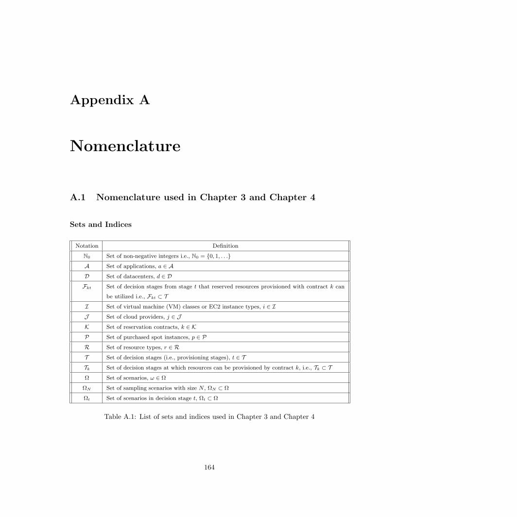
Appendix A
Nomenclature
A.1 Nomenclature used in Chapter 3 and Chapter 4
Sets and Indices
Notation Definition
N0 Set of non-negative integers i.e., N0 = 0, 1, . . .
A Set of applications, a ∈ A
D Set of datacenters, d ∈ D
Fkt Set of decision stages from stage t that reserved resources provisioned with contract k can
be utilized i.e., Fkt ⊂ T
I Set of virtual machine (VM) classes or EC2 instance types, i ∈ I
J Set of cloud providers, j ∈ J
K Set of reservation contracts, k ∈ K
P Set of purchased spot instances, p ∈ P
R Set of resource types, r ∈ R
T Set of decision stages (i.e., provisioning stages), t ∈ T
Tk Set of decision stages at which resources can be provisioned by contract k, i.e., Tk ⊂ T
Ω Set of scenarios, ω ∈ Ω
ΩN Set of sampling scenarios with size N , ΩN ⊂ Ω
Ωt Set of scenarios in decision stage t, Ωt ⊂ Ω
Table A.1: List of sets and indices used in Chapter 3 and Chapter 4
164
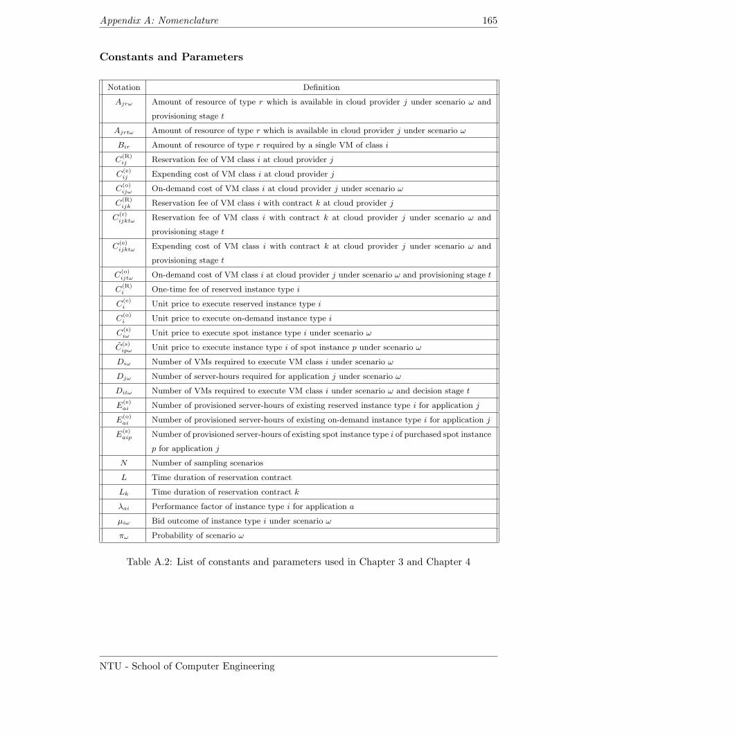
Appendix A: Nomenclature 165
Constants and Parameters
Notation Definition
Ajrω Amount of resource of type r which is available in cloud provider j under scenario ω and
provisioning stage t
Ajrtω Amount of resource of type r which is available in cloud provider j under scenario ω
Bir Amount of resource of type r required by a single VM of class i
C(R)ij Reservation fee of VM class i at cloud provider j
C(e)ij Expending cost of VM class i at cloud provider j
C(o)ijω On-demand cost of VM class i at cloud provider j under scenario ω
C(R)ijk Reservation fee of VM class i with contract k at cloud provider j
C(r)ijktω Reservation fee of VM class i with contract k at cloud provider j under scenario ω and
provisioning stage t
C(e)ijktω Expending cost of VM class i with contract k at cloud provider j under scenario ω and
provisioning stage t
C(o)ijtω On-demand cost of VM class i at cloud provider j under scenario ω and provisioning stage t
C(R)i One-time fee of reserved instance type i
C(e)i Unit price to execute reserved instance type i
C(o)i Unit price to execute on-demand instance type i
C(s)iω Unit price to execute spot instance type i under scenario ω
C(s)ipω Unit price to execute instance type i of spot instance p under scenario ω
Diω Number of VMs required to execute VM class i under scenario ω
Djω Number of server-hours required for application j under scenario ω
Ditω Number of VMs required to execute VM class i under scenario ω and decision stage t
E(e)ai Number of provisioned server-hours of existing reserved instance type i for application j
E(o)ai Number of provisioned server-hours of existing on-demand instance type i for application j
E(s)aip Number of provisioned server-hours of existing spot instance type i of purchased spot instance
p for application j
N Number of sampling scenarios
L Time duration of reservation contract
Lk Time duration of reservation contract k
λai Performance factor of instance type i for application a
µiω Bid outcome of instance type i under scenario ω
πω Probability of scenario ω
Table A.2: List of constants and parameters used in Chapter 3 and Chapter 4
NTU - School of Computer Engineering
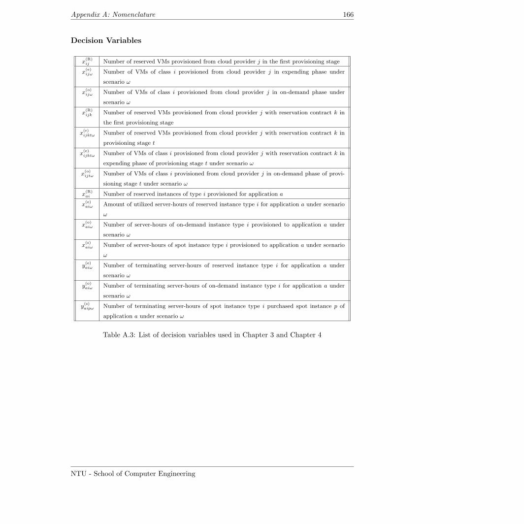
Appendix A: Nomenclature 166
Decision Variables
x(R)ij Number of reserved VMs provisioned from cloud provider j in the first provisioning stage
x(e)ijω Number of VMs of class i provisioned from cloud provider j in expending phase under
scenario ω
x(o)ijω Number of VMs of class i provisioned from cloud provider j in on-demand phase under
scenario ω
x(R)ijk Number of reserved VMs provisioned from cloud provider j with reservation contract k in
the first provisioning stage
x(r)ijktω Number of reserved VMs provisioned from cloud provider j with reservation contract k in
provisioning stage t
x(e)ijktω Number of VMs of class i provisioned from cloud provider j with reservation contract k in
expending phase of provisioning stage t under scenario ω
x(o)ijtω Number of VMs of class i provisioned from cloud provider j in on-demand phase of provi-
sioning stage t under scenario ω
x(R)ai Number of reserved instances of type i provisioned for application a
x(e)aiω Amount of utilized server-hours of reserved instance type i for application a under scenario
ω
x(o)aiω Number of server-hours of on-demand instance type i provisioned to application a under
scenario ω
x(s)aiω Number of server-hours of spot instance type i provisioned to application a under scenario
ω
y(e)aiω Number of terminating server-hours of reserved instance type i for application a under
scenario ω
y(o)aiω Number of terminating server-hours of on-demand instance type i for application a under
scenario ω
y(s)aipω Number of terminating server-hours of spot instance type i purchased spot instance p of
application a under scenario ω
Table A.3: List of decision variables used in Chapter 3 and Chapter 4
NTU - School of Computer Engineering
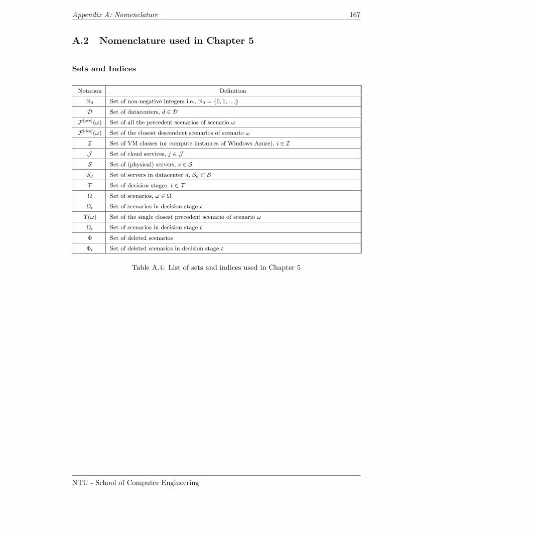
Appendix A: Nomenclature 167
A.2 Nomenclature used in Chapter 5
Sets and Indices
Notation Definition
N0 Set of non-negative integers i.e., N0 = 0, 1, . . .
D Set of datacenters, d ∈ D
F [pre](ω) Set of all the precedent scenarios of scenario ω
F [des](ω) Set of the closest descendent scenarios of scenario ω
I Set of VM classes (or compute instances of Windows Azure), i ∈ I
J Set of cloud services, j ∈ J
S Set of (physical) servers, s ∈ S
Sd Set of servers in datacenter d, Sd ⊂ S
T Set of decision stages, t ∈ T
Ω Set of scenarios, ω ∈ Ω
Ωt Set of scenarios in decision stage t
Υ(ω) Set of the single closest precedent scenario of scenario ω
Ωt Set of scenarios in decision stage t
Φ Set of deleted scenarios
Φt Set of deleted scenarios in decision stage t
Table A.4: List of sets and indices used in Chapter 5
NTU - School of Computer Engineering
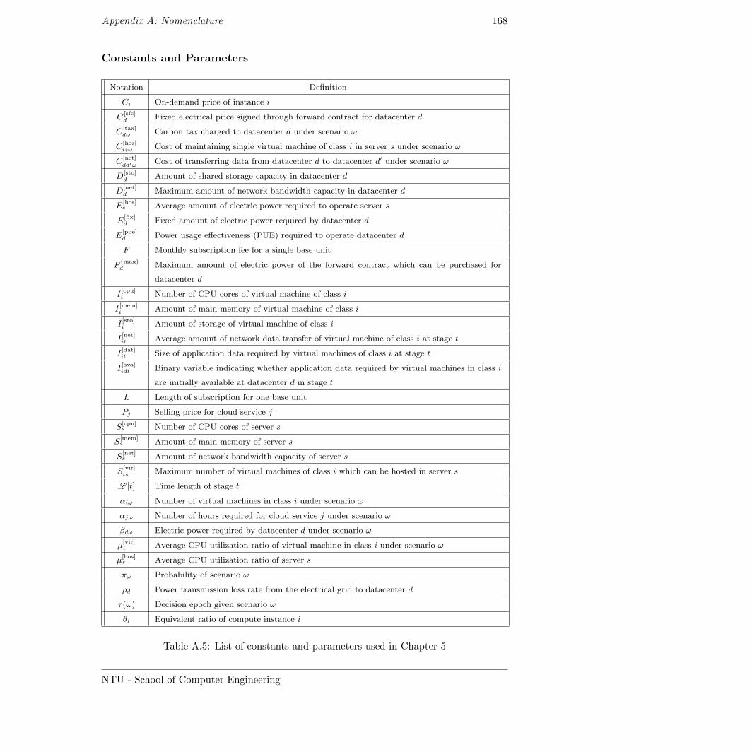
Appendix A: Nomenclature 168
Constants and Parameters
Notation Definition
Ci On-demand price of instance i
C[sfc]d Fixed electrical price signed through forward contract for datacenter d
C[tax]dω Carbon tax charged to datacenter d under scenario ω
C[hos]isω Cost of maintaining single virtual machine of class i in server s under scenario ω
C[net]
dd′ω Cost of transferring data from datacenter d to datacenter d′ under scenario ω
D[sto]d Amount of shared storage capacity in datacenter d
D[net]d Maximum amount of network bandwidth capacity in datacenter d
E[hos]s Average amount of electric power required to operate server s
E[fix]d Fixed amount of electric power required by datacenter d
E[pue]d Power usage effectiveness (PUE) required to operate datacenter d
F Monthly subscription fee for a single base unit
F(max)d Maximum amount of electric power of the forward contract which can be purchased for
datacenter d
I[cpu]i Number of CPU cores of virtual machine of class i
I[mem]i Amount of main memory of virtual machine of class i
I[sto]i Amount of storage of virtual machine of class i
I[net]it Average amount of network data transfer of virtual machine of class i at stage t
I[dat]it Size of application data required by virtual machines of class i at stage t
I[ava]idt Binary variable indicating whether application data required by virtual machines in class i
are initially available at datacenter d in stage t
L Length of subscription for one base unit
Pj Selling price for cloud service j
S[cpu]s Number of CPU cores of server s
S[mem]s Amount of main memory of server s
S[net]s Amount of network bandwidth capacity of server s
S[vir]is Maximum number of virtual machines of class i which can be hosted in server s
L [t] Time length of stage t
αiω Number of virtual machines in class i under scenario ω
αjω Number of hours required for cloud service j under scenario ω
βdω Electric power required by datacenter d under scenario ω
µ[vir]i Average CPU utilization ratio of virtual machine in class i under scenario ω
µ[hos]s Average CPU utilization ratio of server s
πω Probability of scenario ω
ρd Power transmission loss rate from the electrical grid to datacenter d
τ(ω) Decision epoch given scenario ω
θi Equivalent ratio of compute instance i
Table A.5: List of constants and parameters used in Chapter 5
NTU - School of Computer Engineering
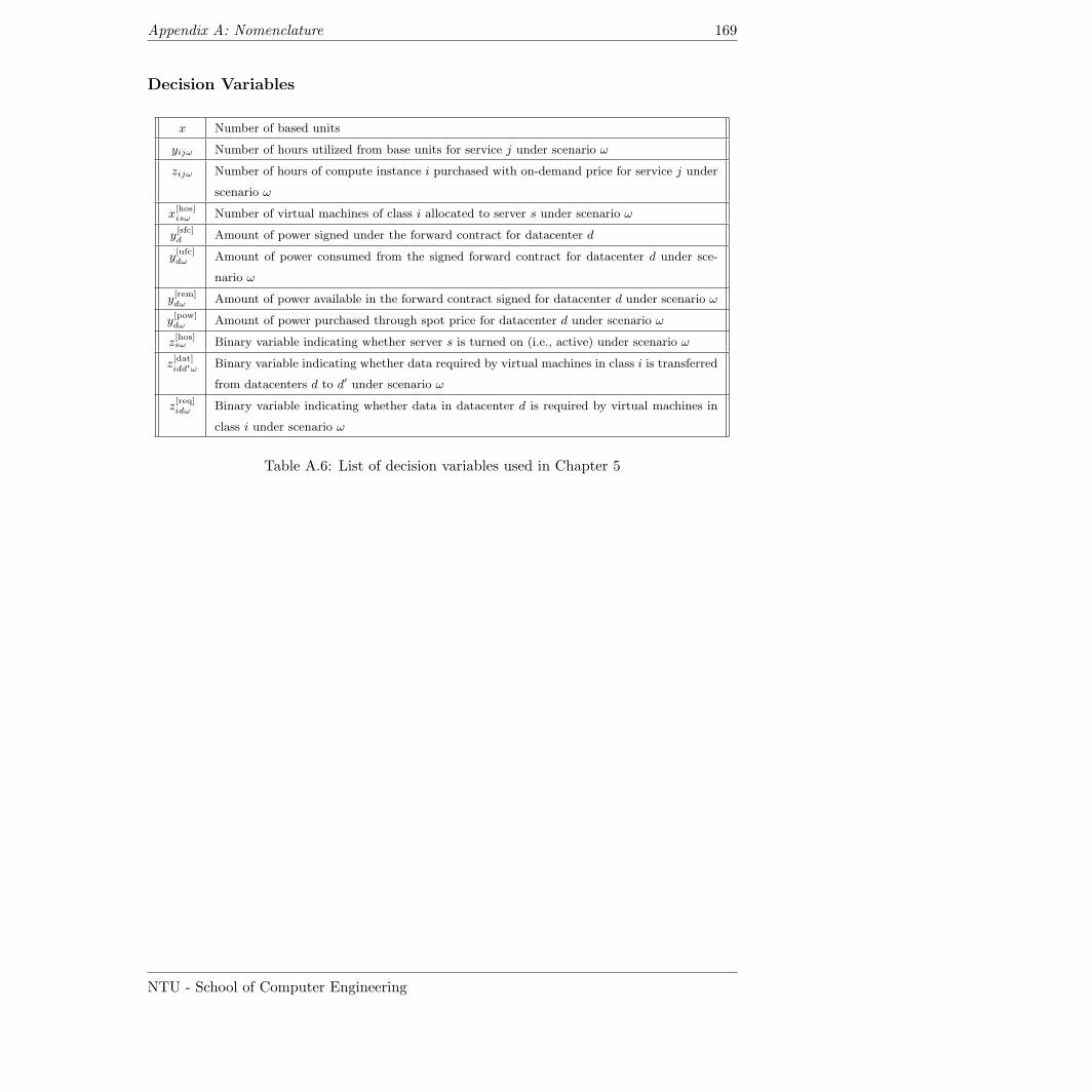
Appendix A: Nomenclature 169
Decision Variables
x Number of based units
yijω Number of hours utilized from base units for service j under scenario ω
zijω Number of hours of compute instance i purchased with on-demand price for service j under
scenario ω
x[hos]isω Number of virtual machines of class i allocated to server s under scenario ω
y[sfc]d Amount of power signed under the forward contract for datacenter d
y[ufc]dω Amount of power consumed from the signed forward contract for datacenter d under sce-
nario ω
y[rem]dω Amount of power available in the forward contract signed for datacenter d under scenario ω
y[pow]dω Amount of power purchased through spot price for datacenter d under scenario ω
z[hos]sω Binary variable indicating whether server s is turned on (i.e., active) under scenario ω
z[dat]
idd′ω Binary variable indicating whether data required by virtual machines in class i is transferred
from datacenters d to d′ under scenario ω
z[req]idω Binary variable indicating whether data in datacenter d is required by virtual machines in
class i under scenario ω
Table A.6: List of decision variables used in Chapter 5
NTU - School of Computer Engineering
Appendix B
Other Resource Provisioning
Optimization Models
In this thesis, other resource provisioning optimization models are investigated with the
proposed models as follows:
B.1 Fixed Reservation Provisioning Model
The fixed reservation provisioning (FixRes) model fixes the number of VMs which is provi-
sioned with the reservation option. Next, a number of VMs could be instantly and addition-
ally provisioned with the on-demand option when the fixed number of reserved VMs cannot
meet the observed demand. When the number of reserved VMs are fixed, a deterministic
optimization model can be formulated and solved much faster than a stochastic program-
ming model. Let constant X(R)ij denote the fixed number of reserved VMs provisioned for
VM class i ∈ I at cloud provider j ∈ J . Then, the model can be formulated as follows:
170
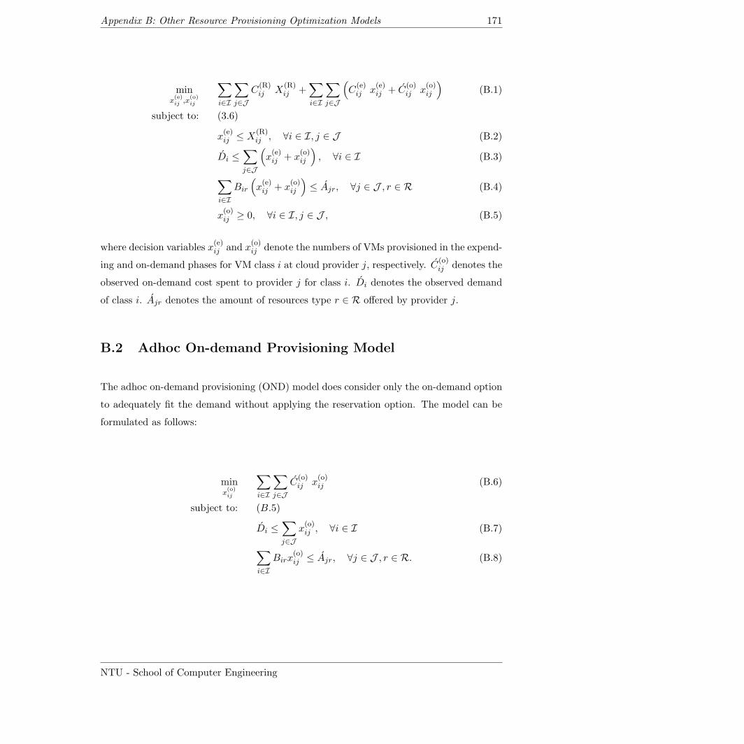
Appendix B: Other Resource Provisioning Optimization Models 171
minx(e)ij ,x
(o)ij
∑i∈I
∑j∈J
C(R)ij X
(R)ij +
∑i∈I
∑j∈J
(C
(e)ij x
(e)ij + C
(o)ij x
(o)ij
)(B.1)
subject to: (3.6)
x(e)ij ≤ X
(R)ij , ∀i ∈ I, j ∈ J (B.2)
Di ≤∑j∈J
(x(e)ij + x
(o)ij
), ∀i ∈ I (B.3)
∑i∈I
Bir
(x(e)ij + x
(o)ij
)≤ Ajr, ∀j ∈ J , r ∈ R (B.4)
x(o)ij ≥ 0, ∀i ∈ I, j ∈ J , (B.5)
where decision variables x(e)ij and x
(o)ij denote the numbers of VMs provisioned in the expend-
ing and on-demand phases for VM class i at cloud provider j, respectively. C(o)ij denotes the
observed on-demand cost spent to provider j for class i. Di denotes the observed demand
of class i. Ajr denotes the amount of resources type r ∈ R offered by provider j.
B.2 Adhoc On-demand Provisioning Model
The adhoc on-demand provisioning (OND) model does consider only the on-demand option
to adequately fit the demand without applying the reservation option. The model can be
formulated as follows:
minx(o)ij
∑i∈I
∑j∈J
C(o)ij x
(o)ij (B.6)
subject to: (B.5)
Di ≤∑j∈J
x(o)ij , ∀i ∈ I (B.7)
∑i∈I
Birx(o)ij ≤ Ajr, ∀j ∈ J , r ∈ R. (B.8)
NTU - School of Computer Engineering
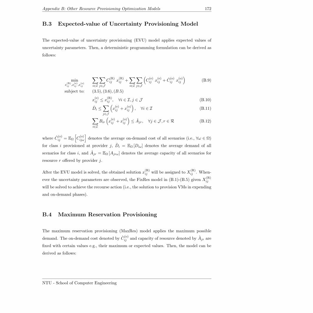
Appendix B: Other Resource Provisioning Optimization Models 172
B.3 Expected-value of Uncertainty Provisioning Model
The expected-value of uncertainty provisioning (EVU) model applies expected values of
uncertainty parameters. Then, a deterministic programming formulation can be derived as
follows:
minx(R)ij ,x
(e)ij ,x
(o)ij
∑i∈I
∑j∈J
C(R)ij x
(R)ij +
∑i∈I
∑j∈J
(C
(e)ij x
(e)ij + C
(o)ij x
(o)ij
)(B.9)
subject to: (3.5), (3.6), (B.5)
x(e)ij ≤ x
(R)ij , ∀i ∈ I, j ∈ J (B.10)
Di ≤∑j∈J
(x(e)ij + x
(o)ij
), ∀i ∈ I (B.11)
∑i∈I
Bir
(x(e)ij + x
(o)ij
)≤ Ajr, ∀j ∈ J , r ∈ R (B.12)
where C(o)ij = EΩ
[C
(o)ijω
]denotes the average on-demand cost of all scenarios (i.e., ∀ω ∈ Ω)
for class i provisioned at provider j, Di = EΩ [Diω] denotes the average demand of all
scenarios for class i, and Ajr = EΩ [Ajrω] denotes the average capacity of all scenarios for
resource r offered by provider j.
After the EVU model is solved, the obtained solution x(R)ij will be assigned to X
(R)ij . When-
ever the uncertainty parameters are observed, the FixRes model in (B.1)-(B.5) given X(R)ij
will be solved to achieve the recourse action (i.e., the solution to provision VMs in expending
and on-demand phases).
B.4 Maximum Reservation Provisioning
The maximum reservation provisioning (MaxRes) model applies the maximum possible
demand. The on-demand cost denoted by C(o)ij and capacity of resource denoted by Ajr are
fixed with certain values e.g., their maximum or expected values. Then, the model can be
derived as follows:
NTU - School of Computer Engineering
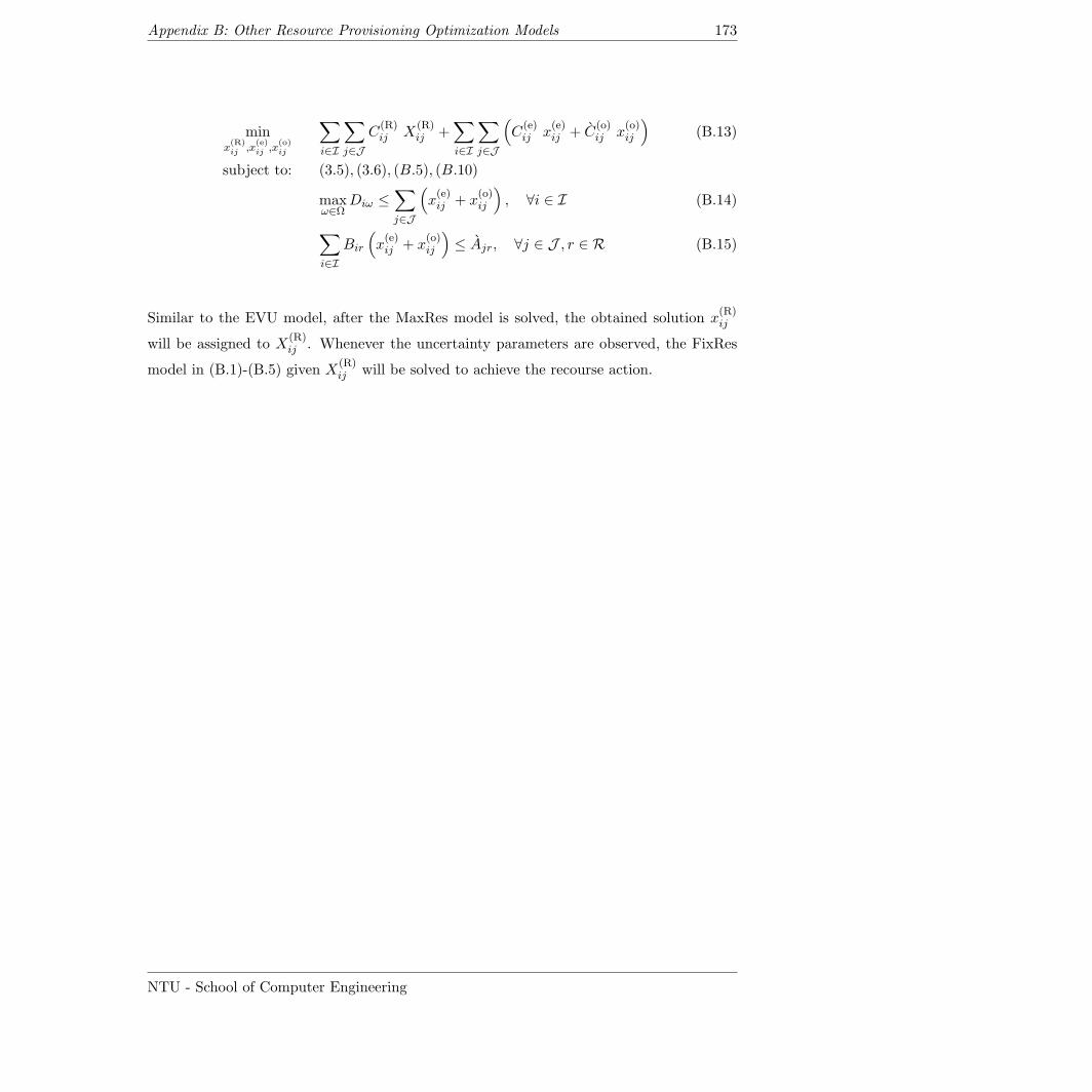
Appendix B: Other Resource Provisioning Optimization Models 173
minx(R)ij ,x
(e)ij ,x
(o)ij
∑i∈I
∑j∈J
C(R)ij X
(R)ij +
∑i∈I
∑j∈J
(C
(e)ij x
(e)ij + C
(o)ij x
(o)ij
)(B.13)
subject to: (3.5), (3.6), (B.5), (B.10)
maxω∈Ω
Diω ≤∑j∈J
(x(e)ij + x
(o)ij
), ∀i ∈ I (B.14)
∑i∈I
Bir
(x(e)ij + x
(o)ij
)≤ Ajr, ∀j ∈ J , r ∈ R (B.15)
Similar to the EVU model, after the MaxRes model is solved, the obtained solution x(R)ij
will be assigned to X(R)ij . Whenever the uncertainty parameters are observed, the FixRes
model in (B.1)-(B.5) given X(R)ij will be solved to achieve the recourse action.
NTU - School of Computer Engineering
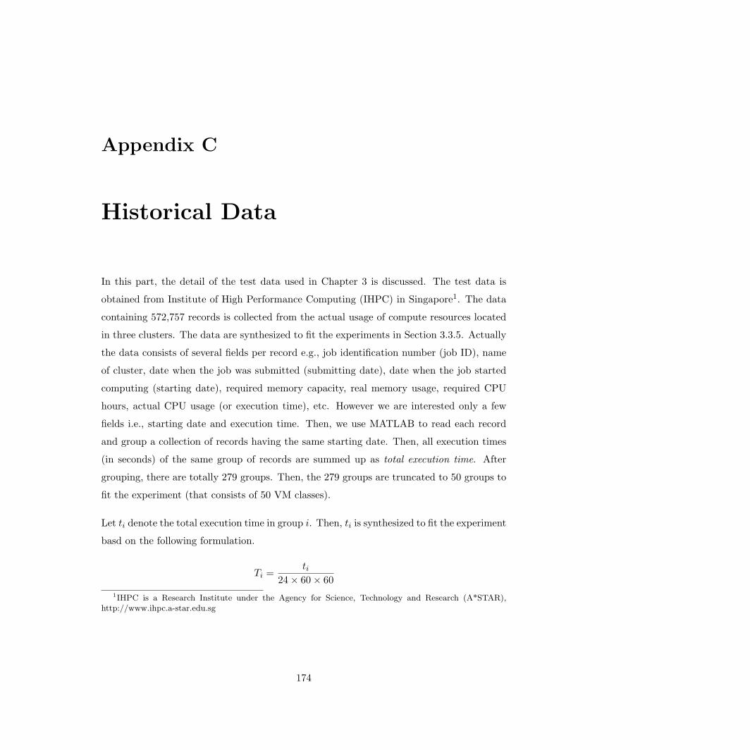
Appendix C
Historical Data
In this part, the detail of the test data used in Chapter 3 is discussed. The test data is
obtained from Institute of High Performance Computing (IHPC) in Singapore1. The data
containing 572,757 records is collected from the actual usage of compute resources located
in three clusters. The data are synthesized to fit the experiments in Section 3.3.5. Actually
the data consists of several fields per record e.g., job identification number (job ID), name
of cluster, date when the job was submitted (submitting date), date when the job started
computing (starting date), required memory capacity, real memory usage, required CPU
hours, actual CPU usage (or execution time), etc. However we are interested only a few
fields i.e., starting date and execution time. Then, we use MATLAB to read each record
and group a collection of records having the same starting date. Then, all execution times
(in seconds) of the same group of records are summed up as total execution time. After
grouping, there are totally 279 groups. Then, the 279 groups are truncated to 50 groups to
fit the experiment (that consists of 50 VM classes).
Let ti denote the total execution time in group i. Then, ti is synthesized to fit the experiment
basd on the following formulation.
Ti =ti
24× 60× 60
1IHPC is a Research Institute under the Agency for Science, Technology and Research (A*STAR),http://www.ihpc.a-star.edu.sg
174
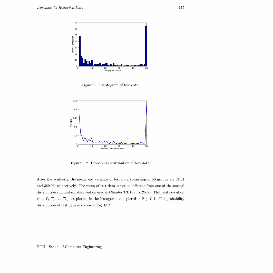
Appendix C: Historical Data 175
0 10 20 30 40 500
10
20
30
40
50
60
70
Group (VM Class)
Num
ber
of r
ecor
ds
Figure C.1: Histogram of test data.
0 10 20 30 40 500
0.05
0.1
0.15
0.2
0.25
Number of required VMs
Pro
babi
lity
Figure C.2: Probability distribution of test data.
After the synthesis, the mean and variance of test data consisting of 50 groups are 21.64
and 389.93, respectively. The mean of test data is not so different from one of the normal
distribution and uniform distribution used in Chapter 3.3, that is, 25.50. The total execution
time T1, T2, . . . , T50 are plotted in the histogram as depicted in Fig. C.1. The probability
distribution of test data is shown in Fig. C.2.
NTU - School of Computer Engineering
Appendix D
Author’s Publications
• S. Chaisiri, B. S. Lee, and D. Niyato,“Joint Power Optimization and Cloud Re-
source Management for Datacenters in Smart Grid Environment”, submitted to IEEE
Transactions on Parallel and Distributed Systems (TPDS) - Special Issue on Cloud
Computing, 2012.
• R. Kaewpuang, S. Chaisiri, D. Niyato, B. S. Lee, and P. Wang, “Cooperative Virtual
Machine Management in Smart Grid Environment,” submitted to IEEE Transactions
on Services Computing (TSC), 2012.
• S. Chaisiri, B. Zoebir, B. S. Lee, P. Sessomboon, T. Saisillapee, and T. Achalakul,
in “Workflow Framework to Support Data Analytics in Cloud Computing,” in IEEE
CloudCom 2012, Taiwan, December 2012.
• R. Kaewpuang, S. Chaisiri, D. Niyato, B. S. Lee, and P. Wang, “Adaptive Power
Management for Data Center in Smart Grid Environment,” in the 10th IEEE Interna-
tional Symposium on Parallel and Distributed Processing with Applications (ISPA-12),
Madrid, Spain, July 10-13, 2012.
• S. Chaisiri, B. S. Lee, and D. Niyato, “Profit Maximization Model for Cloud Provider
Based on Windows Azure Platform,” in the 9th Annual International Conference
Organized by Electrical Engineering/Electronics, Computer, Telecommunications and
Information Technology (ECTI-CON 2012), Hua Hin, Thailand, May 16-18, 2012.
• S. Chaisiri, B. S. Lee, and D. Niyato,“Optimization of Resource Provisioning Cost
in Cloud Computing,” IEEE Transactions on Services Computing (TSC), vol. 5 no.
176
Appendix D: Author’s Publications 177
2, Apr.-Jun. 2012.
• S. Chaisiri, R. Kaewpuang, B. S. Lee, and D. Niyato,“Cost Minimization for Pro-
visioning Virtual Servers in Amazon Elastic Compute Cloud,” in the 19th Annual
Meeting of the IEEE International Symposium on Modeling, Analysis and Simulation
of Computer and Telecommunication Systems (MASCOTS 2011), Singapore, July
25-27, 2011 (Best Paper Candidate).
• S. Chaisiri, B. S. Lee, and D. Niyato,“Robust Cloud Resource Provisioning for Cloud
Computing Environments,” in the 2nd IEEE International Conference on Service-
Oriented Computing and Applications (SOCA 2010), Perth, Australia, 2010.
• D. Niyato, S. Chaisiri, and B. S. Lee,“Economic Analysis of Resource Market in
Cloud Computing Environment,” in Proceedings of IEEE Asia-Pacific Services Com-
puting Conference (APSCC), Singapore, 2009.
• S. Chaisiri, B. S. Lee, and D. Niyato,“Optimal Virtual Machine Placement across
Multiple Cloud Providers,” in Proceedings of IEEE Asia-Pacific Services Computing
Conference (APSCC), Singapore, 2009.
• D. Niyato, S. Chaisiri, and B. S. Lee, “Optimal Power Management for Server Farm
to Support Green Computing,” in the 9th IEEE/ACM International Symposium on
Cluster Computing and the Grid (CCGrid 09), Shanghai, China, May 18-21, 2009.
NTU - School of Computer Engineering


