Resource Assessment for

Livestock and Agro-Industrial Wastes – Mexico

Prepared for:

Global Methane Initiative

Prepared by:

Eastern Research Group, Inc.

Tetra Tech CySTE

November 2, 2010

i

EXECUTIVE SUMMARY

The Global Methane Initiative is an initiative to reduce global methane emissions with the purpose of enhancing economic growth, promoting energy security, improving the environment, and reducing greenhouse gases (GHGs). The initiative focuses on cost-effective, near-term methane recovery and use as a clean energy source. The initiative functions internationally through collaboration among developed countries, developing countries, and countries with economies in transition—together with strong participation from the private sector.

The Global Methane Initiative works in four main sectors: agriculture, landfills, oil and gas exploration and production, and coal mining. The Agriculture Subcommittee was created in November 2005 to focus on anaerobic digestion of livestock wastes; it has since expanded to include anaerobic digestion of wastes from agro-industrial processes. Representatives from Argentina, the United Kingdom, and India currently serve as co-chairs of the subcommittee.

As part of the Global Methane Initiative, the U.S. Environmental Protection Agency (U.S. EPA) is conducting livestock and agro-industry resource assessment in M2M participating countries to identify and evaluate the potential for incorporating anaerobic digestion into livestock manure and agro-industrial (agricultural commodity processing) waste management systems to reduce methane emissions and provide a renewable source of energy.

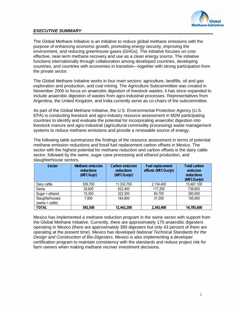
The following table summarizes the findings of the resource assessment in terms of potential methane emission reductions and fossil fuel replacement carbon offsets in Mexico. The sector with the highest potential for methane reduction and carbon offsets is the dairy cattle sector, followed by the swine, sugar cane processing and ethanol production, and slaughterhouse sectors.

Sector Methane emission reductions (MTCH4/yr)

Carbon emission reductions

(MTCO2e/yr)

Fuel replacement offsets (MTCO2e/yr)

Total carbon emission

reductions (MTCO2e/yr)

Dairy cattle 539,700 11,332,700 2,134,400 13,467,100 Swine 29,600 622,400 117,200 739,600 Sugar + ethanol 15,300 322,300 60,700 383,000 Slaughterhouses (swine + cattle)

7,900 164,800 31,000 195,900

TOTAL 592,500 12,442,200 2,343,400 14,785,600

Mexico has implemented a methane reduction program in the swine sector with support from the Global Methane Initiative. Currently, there are approximately 170 anaerobic digesters operating in Mexico (there are approximately 390 digesters but only 43 percent of them are operating at the present time). Mexico has developed National Technical Standards for the Design and Construction of Bio-Digesters. Mexico is also implementing a developer certification program to maintain consistency with the standards and reduce project risk for farm owners when making methane recover investment decisions.

ii

ACKNOWLEDGEMENTS

This work has relied on the support of the Ministry of Environment and Natural Resources (SEMARNAT) and the Federal Attorney for Environmental Protection (PROFEPA) of Mexico.

We give our special thanks to Araceli Arredondo, Directora de Regulación Ambiental Agropecuaria, and Armando Rodríguez, Subdirector de Suelos at SEMARNAT.

We also want to thank Laura Medina, Mónica Domínguez Carranza, Armando Romero Barajas, and Ana Gabriela Magaña from the delegations of SEMARNAT in Jalapa and Jalisco.

Finally, we want to acknowledge the significant contributions of Ana Silvia Arrocha Contreras, Directora General Técnica en Auditorías, and Antonio Ibarra Cerecer, Director General Adjunto de Proyectos at PROFEPA.

iii

TABLE OF CONTENTS

Executive Summary .................................................................................................... i

Acknowledgements .................................................................................................... ii

1. Introduction ................................................................................................ 1-1 1.1 Methane emissions from livestock wastes .................................................. 1-2 1.2 Methane emissions from agro-industrial wastes ......................................... 1-2 1.3 Methane emissions in Mexico ..................................................................... 1-3

2. Background and criteria for selection ...................................................... 2-1 2.1 Methodology used ...................................................................................... 2-1 2.2 Estimation of methane emissions in the livestock and agro-industrial

sectors........................................................................................................ 2-2 2.3 Description of specific criteria for determining potential sectors .................. 2-6 2.4 examples of methane emission reduction projects in Mexico ...................... 2-6

3. Sector characterization .............................................................................. 3-1 3.1 Introduction ................................................................................................ 3-1 3.2 Subsectors with potential for methane emission reduction ......................... 3-2 3.3 Swine PRODUCTION ................................................................................. 3-4 3.4 Dairy farms ................................................................................................. 3-7 3.5 Sugar ....................................................................................................... 3-10 3.6 Slaughterhouses ...................................................................................... 3-12

4. Potential for methane emission reduction ............................................... 4-1 4.1 Methane Emission reduction ...................................................................... 4-1 4.2 Technology options .................................................................................... 4-5 4.3 Costs and potential benefits ....................................................................... 4-8 4.4 Centralized projects .................................................................................. 4-10

APPENDIX A: Mexico GHG Inventory 2000 ..................................................................... A-1APPENDIX B: Legislation in Mexico ................................................................................. B-1APPENDIX C: Typical Wastewater Treatment Unit Process Sequence ............................ C-1APPENDIX D: Additional SUBsector information .............................................................. D-1APPENDIX E: Glossary .................................................................................................... E-1APPENDIX F: Bibliography .............................................................................................. F-1

iv

List of Abbreviations

AMBR Anaerobic migrating blanket reactor

ASBR Anaerobic sequencing batch reactor

BOD Biochemical oxygen demand

CH4 Methane (chemical formula)

COD Chemical oxygen demand

COFEPRIS Comisión Federal para la Protección contra Riesgos Sanitarios (Federal Commission for the Protection Against Sanitary Risks)

DAF Dissolved air flotation

FAO United Nations Food and Agriculture Organization

FIRCO Fideicomiso de Riesgo Compartido (Shared Risk Trust)

FIT Federal Inspection Type

GDP Gross domestic product

GHG Greenhouse gas

HRT Hydraulic retention times

INEGI Instituto Nacional de Estadística y Geografía (National Institute of Statistics and Geography)

IPCC Intergovernmental Panel on Climate Change

LGEEPA Ley General de Equilibrio Ecológico y Protección al Ambiente (General Law for Ecological Balance and Environmental Protection)

LPG Liquefied petroleum gas

MCF Methane conversion factor

MMTCO2e Million metric tons of carbon dioxide equivalent

MT Metric tons

MTCO2e Metric tons of carbon dioxide equivalent

PROFEPA Procuraduría Federal de Protección al Ambiente (Federal Attorney for Environmental Protection)

SAGARPA Secretaría de Agricultura, Desarrollo Rural Pesca y Alimentación (Ministry of Agriculture, Rural Development, Fisheries, and Food)

SEMARNAT Secretaría del Medio Ambiente y Recursos Naturales (Ministry of Environment and Natural Resources)

SIAP Servicio de Información Agropecuario y Pecuarios (Agrifood and Fishery Information Service)

SRT Solids retention times

TS Total solids

TSS Total suspended solids

v

UASB Upflow Anaerobic Sludge Blanket

UNFCCC United Nations Framework Convention on Climate Change

U.S. EPA United States Environmental Protection Agency

VS Volatile solids

1-1

1. INTRODUCTION

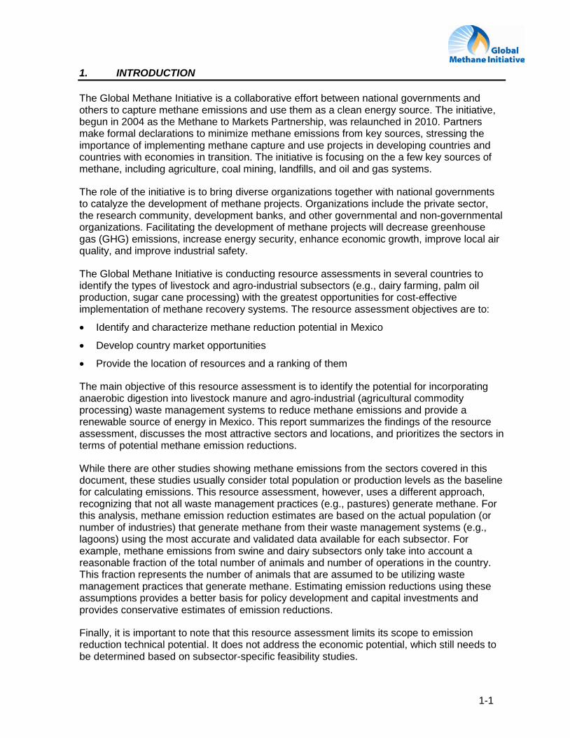
The Global Methane Initiative is a collaborative effort between national governments and others to capture methane emissions and use them as a clean energy source. The initiative, begun in 2004 as the Methane to Markets Partnership, was relaunched in 2010. Partners make formal declarations to minimize methane emissions from key sources, stressing the importance of implementing methane capture and use projects in developing countries and countries with economies in transition. The initiative is focusing on the a few key sources of methane, including agriculture, coal mining, landfills, and oil and gas systems.

The role of the initiative is to bring diverse organizations together with national governments to catalyze the development of methane projects. Organizations include the private sector, the research community, development banks, and other governmental and non-governmental organizations. Facilitating the development of methane projects will decrease greenhouse gas (GHG) emissions, increase energy security, enhance economic growth, improve local air quality, and improve industrial safety.

The Global Methane Initiative is conducting resource assessments in several countries to identify the types of livestock and agro-industrial subsectors (e.g., dairy farming, palm oil production, sugar cane processing) with the greatest opportunities for cost-effective implementation of methane recovery systems. The resource assessment objectives are to:

• Identify and characterize methane reduction potential in Mexico

• Develop country market opportunities

• Provide the location of resources and a ranking of them

The main objective of this resource assessment is to identify the potential for incorporating anaerobic digestion into livestock manure and agro-industrial (agricultural commodity processing) waste management systems to reduce methane emissions and provide a renewable source of energy in Mexico. This report summarizes the findings of the resource assessment, discusses the most attractive sectors and locations, and prioritizes the sectors in terms of potential methane emission reductions.

While there are other studies showing methane emissions from the sectors covered in this document, these studies usually consider total population or production levels as the baseline for calculating emissions. This resource assessment, however, uses a different approach, recognizing that not all waste management practices (e.g., pastures) generate methane. For this analysis, methane emission reduction estimates are based on the actual population (or number of industries) that generate methane from their waste management systems (e.g., lagoons) using the most accurate and validated data available for each subsector. For example, methane emissions from swine and dairy subsectors only take into account a reasonable fraction of the total number of animals and number of operations in the country. This fraction represents the number of animals that are assumed to be utilizing waste management practices that generate methane. Estimating emission reductions using these assumptions provides a better basis for policy development and capital investments and provides conservative estimates of emission reductions.

Finally, it is important to note that this resource assessment limits its scope to emission reduction technical potential. It does not address the economic potential, which still needs to be determined based on subsector-specific feasibility studies.

1-2

1.1 METHANE EMISSIONS FROM LIVESTOCK WASTES

In 2005, livestock manure management globally contributed more than 230 million metric tons of carbon dioxide equivalents (MMTCO2e) of methane emissions, or roughly 4 percent of total anthropogenic (human-induced) methane emissions. Three groups of animals accounted for more than 80 percent of total emissions: swine (40 percent); non-dairy cattle (20 percent); and dairy cattle (20 percent). In certain countries, poultry was also a significant source of methane emissions. Figure 1.1 represents countries with significant methane emissions from livestock manure management.

Figure 1.1 – Estimated Global Methane Emissions From Livestock Manure Management (2005), Total = 234.57 MMTCO2e

Source: Global Methane Initiative, Background Information

1.2 METHANE EMISSIONS FROM AGRO-INDUSTRIAL WASTES

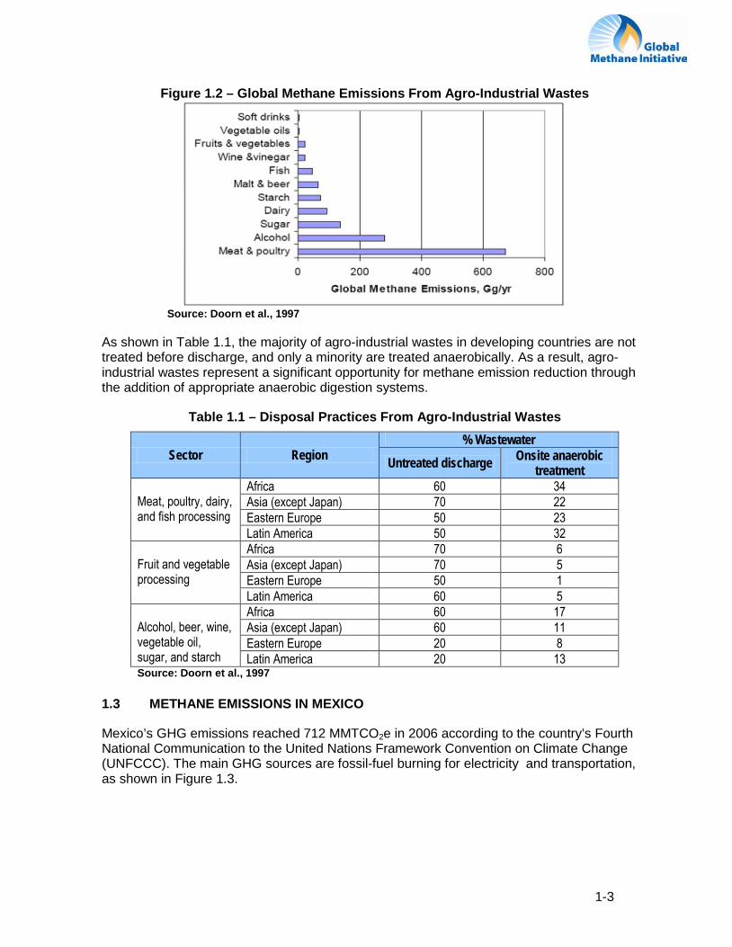
Waste from agro-industrial activities is an important source of methane emissions. The organic fraction of agro-industrial wastes typically is more readily biodegradable than the organic fraction of manure. Thus, greater reductions in biochemical oxygen demand (BOD), chemical oxygen demand (COD), and volatile solids (VS) during anaerobic digestion can be realized. In addition, the higher readily biodegradable fraction of agro-industrial wastes translates directly into higher methane production potential than from manure. Figure 1.2 shows global estimates of methane (CH4) emissions from agro-industrial wastes.

1-3

Figure 1.2 – Global Methane Emissions From Agro-Industrial Wastes

Source: Doorn et al., 1997

As shown in Table 1.1, the majority of agro-industrial wastes in developing countries are not treated before discharge, and only a minority are treated anaerobically. As a result, agro-industrial wastes represent a significant opportunity for methane emission reduction through the addition of appropriate anaerobic digestion systems.

Table 1.1 – Disposal Practices From Agro-Industrial Wastes

Sector Region % Wastewater

Untreated discharge Onsite anaerobic treatment

Meat, poultry, dairy, and fish processing

Africa 60 34 Asia (except Japan) 70 22 Eastern Europe 50 23 Latin America 50 32

Fruit and vegetable processing

Africa 70 6 Asia (except Japan) 70 5 Eastern Europe 50 1 Latin America 60 5

Alcohol, beer, wine, vegetable oil, sugar, and starch

Africa 60 17 Asia (except Japan) 60 11 Eastern Europe 20 8 Latin America 20 13

Source: Doorn et al., 1997

1.3 METHANE EMISSIONS IN MEXICO

Mexico’s GHG emissions reached 712 MMTCO2e in 2006 according to the country’s Fourth National Communication to the United Nations Framework Convention on Climate Change (UNFCCC). The main GHG sources are fossil-fuel burning for electricity and transportation, as shown in Figure 1.3.

1-4

Figure 1.3 – Mexico’s GHG Emissions by Sector (Percentage of Total CO2e)

Source: Mexico’s fourth national communication to the UNFCCC (2009),

http://unfccc.int/resource/docs/natc/mexnc4s.pdf

The principal GHGs in Mexico are carbon dioxide (CO2, 75 percent of the total GHG emissions in CO2e), methane (CH4, 23 percent) and nitrous oxide (N2O, 2 percent) (See Figure 1.4). In 2006, Mexico was the 12th largest emitter of CO2 in the world, with 436,150 MMTCO2.1

Figure 1.4 – Mexico GHG Emissions by Gas (Percentage of Total CO2e)

Source: Mexico’s second national communication to the UNFCCC, 2001

http://unfccc.int/resource/docs/natc/mexnc2.pdf

1 Source: Data from the United Nations Statistics Division, available online at: http://mdgs.un.org/unsd/mdg/SeriesDetail.aspx?srid=749&crid=.

2-1

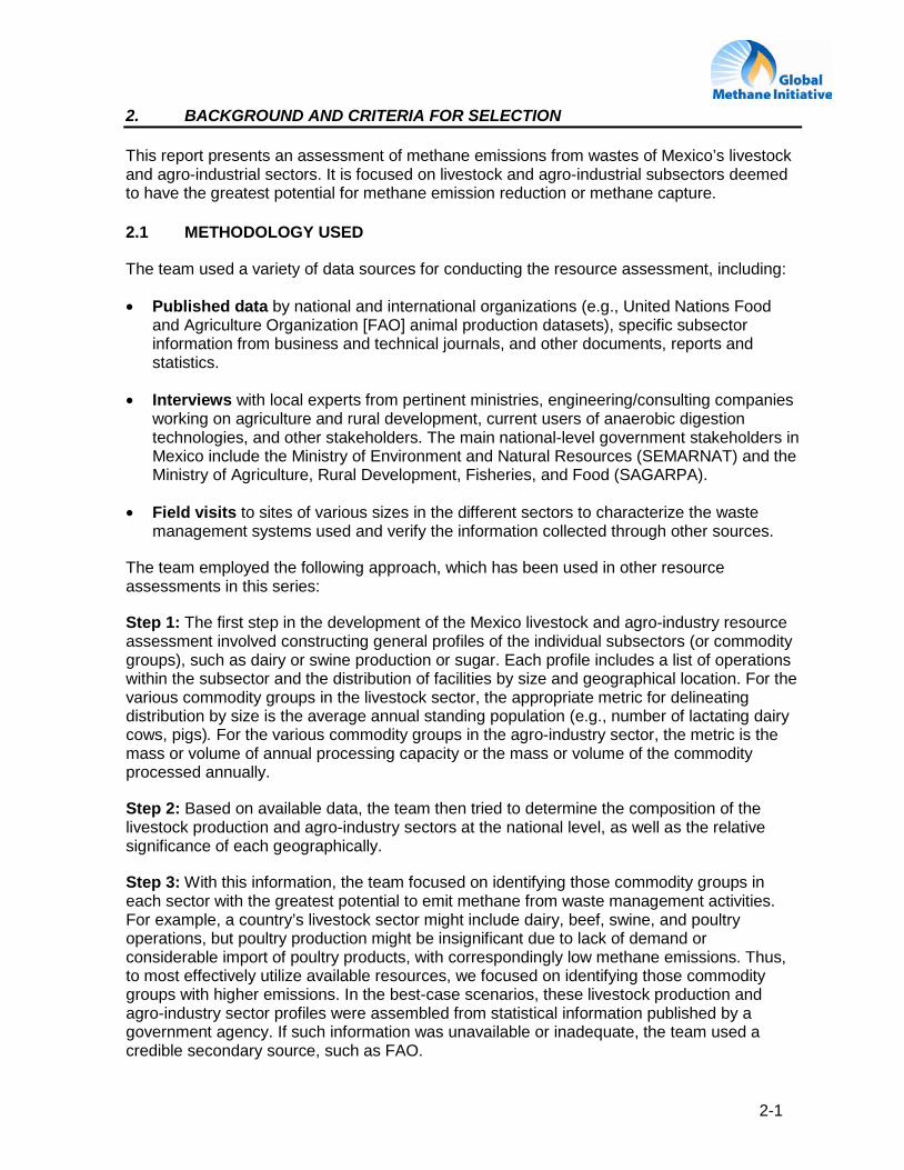
2. BACKGROUND AND CRITERIA FOR SELECTION

This report presents an assessment of methane emissions from wastes of Mexico’s livestock and agro-industrial sectors. It is focused on livestock and agro-industrial subsectors deemed to have the greatest potential for methane emission reduction or methane capture.

2.1 METHODOLOGY USED

The team used a variety of data sources for conducting the resource assessment, including:

• Published data by national and international organizations (e.g., United Nations Food and Agriculture Organization [FAO] animal production datasets), specific subsector information from business and technical journals, and other documents, reports and statistics.

• Interviews with local experts from pertinent ministries, engineering/consulting companies working on agriculture and rural development, current users of anaerobic digestion technologies, and other stakeholders. The main national-level government stakeholders in Mexico include the Ministry of Environment and Natural Resources (SEMARNAT) and the Ministry of Agriculture, Rural Development, Fisheries, and Food (SAGARPA).

• Field visits to sites of various sizes in the different sectors to characterize the waste management systems used and verify the information collected through other sources.

The team employed the following approach, which has been used in other resource assessments in this series:

Step 1: The first step in the development of the Mexico livestock and agro-industry resource assessment involved constructing general profiles of the individual subsectors (or commodity groups), such as dairy or swine production or sugar. Each profile includes a list of operations within the subsector and the distribution of facilities by size and geographical location. For the various commodity groups in the livestock sector, the appropriate metric for delineating distribution by size is the average annual standing population (e.g., number of lactating dairy cows, pigs). For the various commodity groups in the agro-industry sector, the metric is the mass or volume of annual processing capacity or the mass or volume of the commodity processed annually.

Step 2: Based on available data, the team then tried to determine the composition of the livestock production and agro-industry sectors at the national level, as well as the relative significance of each geographically.

Step 3: With this information, the team focused on identifying those commodity groups in each sector with the greatest potential to emit methane from waste management activities. For example, a country’s livestock sector might include dairy, beef, swine, and poultry operations, but poultry production might be insignificant due to lack of demand or considerable import of poultry products, with correspondingly low methane emissions. Thus, to most effectively utilize available resources, we focused on identifying those commodity groups with higher emissions. In the best-case scenarios, these livestock production and agro-industry sector profiles were assembled from statistical information published by a government agency. If such information was unavailable or inadequate, the team used a credible secondary source, such as FAO.

2-2

Step 4: The team characterized the waste management practices utilized by the largest operations in each sector. Typically, only a small percentage of the total number of operations in each commodity group will be responsible for the majority of production and thus, the majority of the methane emissions. Additionally, the waste management practices employed by the largest producers in each commodity group should be relatively uniform. When information about waste management practices is incomplete or not readily accessible, the team identified and directly contacted producer associations and local consultants and visited individual operations to obtain this information.

Step 5: The team then assessed the magnitudes of current methane emissions to identify those commodity groups that should receive further analysis. As an example, in the livestock production sector, large operations in a livestock commodity group that relies primarily on a pasture-based production system will have only nominal methane emissions because manure decomposition will be primarily by aerobic microbial activity. Similarly, an agro-industry subsector with large operations that perform direct discharge of untreated wastewater to a river, lake, or ocean will not be a source of significant methane emissions. Thus, the process of estimating current methane emissions was focused on those sectors that could most effectively utilize available resources. This profiling exercise will aid in identifying the more promising candidate sectors and/or operations for technology demonstration.

2.2 ESTIMATION OF METHANE EMISSIONS IN THE LIVESTOCK AND AGRO-INDUSTRIAL SECTORS

This section describes the generally accepted methods for estimating methane emissions from livestock manures and agricultural commodity processing wastes, along with the modification of these methods to estimate the methane production potential with the addition of anaerobic digestion as a waste management system component.

2.2.1 Manure Related Emissions

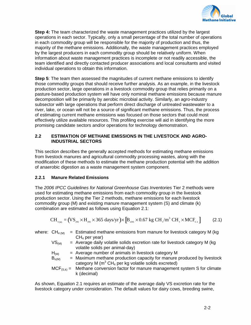
The 2006 IPCC Guidelines for National Greenhouse Gas Inventories Tier 2 methods were used for estimating methane emissions from each commodity group in the livestock production sector. Using the Tier 2 methods, methane emissions for each livestock commodity group (M) and existing manure management system (S) and climate (k) combination are estimated as follows using Equation 2.1:

CH4 (M)= VS(M) × H(M) × 365 days/yr( )× Bo(M) × 0.67 kg CH4/m

3 CH4 × MCFS, k[ ] (2.1) where: CH4 (M) = Estimated methane emissions from manure for livestock category M (kg

CH4 per year) VS(M) = Average daily volatile solids excretion rate for livestock category M (kg

volatile solids per animal-day) H(M) = Average number of animals in livestock category M Bo(M) = Maximum methane production capacity for manure produced by livestock

category M (m3 CH4 per kg volatile solids excreted) MCF(S,k) = Methane conversion factor for manure management system S for climate

k (decimal)

As shown, Equation 2.1 requires an estimate of the average daily VS excretion rate for the livestock category under consideration. The default values for dairy cows, breeding swine,

2-3

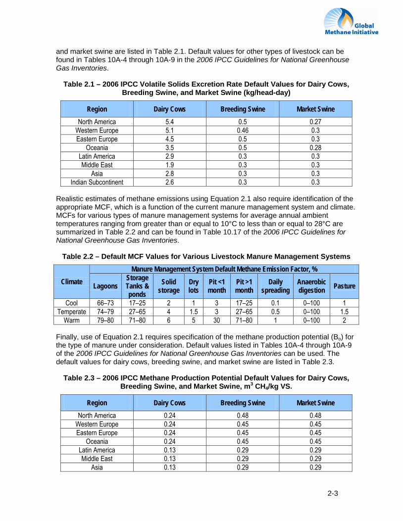
and market swine are listed in Table 2.1. Default values for other types of livestock can be found in Tables 10A-4 through 10A-9 in the 2006 IPCC Guidelines for National Greenhouse Gas Inventories.

Table 2.1 – 2006 IPCC Volatile Solids Excretion Rate Default Values for Dairy Cows, Breeding Swine, and Market Swine (kg/head-day)

Region Dairy Cows Breeding Swine Market Swine North America 5.4 0.5 0.27

Western Europe 5.1 0.46 0.3 Eastern Europe 4.5 0.5 0.3

Oceania 3.5 0.5 0.28 Latin America 2.9 0.3 0.3 Middle East 1.9 0.3 0.3

Asia 2.8 0.3 0.3 Indian Subcontinent 2.6 0.3 0.3

Realistic estimates of methane emissions using Equation 2.1 also require identification of the appropriate MCF, which is a function of the current manure management system and climate. MCFs for various types of manure management systems for average annual ambient temperatures ranging from greater than or equal to 10°C to less than or equal to 28°C are summarized in Table 2.2 and can be found in Table 10.17 of the 2006 IPCC Guidelines for National Greenhouse Gas Inventories.

Table 2.2 – Default MCF Values for Various Livestock Manure Management Systems

Climate Manure Management System Default Methane Emission Factor, %

Lagoons Storage Tanks & ponds

Solid storage

Dry lots

Pit <1 month

Pit >1 month

Daily spreading

Anaerobic digestion Pasture

Cool 66–73 17–25 2 1 3 17–25 0.1 0–100 1 Temperate 74–79 27–65 4 1.5 3 27–65 0.5 0–100 1.5

Warm 79–80 71–80 6 5 30 71–80 1 0–100 2

Finally, use of Equation 2.1 requires specification of the methane production potential (Bo) for the type of manure under consideration. Default values listed in Tables 10A-4 through 10A-9 of the 2006 IPCC Guidelines for National Greenhouse Gas Inventories can be used. The default values for dairy cows, breeding swine, and market swine are listed in Table 2.3.

Table 2.3 – 2006 IPCC Methane Production Potential Default Values for Dairy Cows, Breeding Swine, and Market Swine, m3 CH4/kg VS.

Region Dairy Cows Breeding Swine Market Swine North America 0.24 0.48 0.48

Western Europe 0.24 0.45 0.45 Eastern Europe 0.24 0.45 0.45

Oceania 0.24 0.45 0.45 Latin America 0.13 0.29 0.29 Middle East 0.13 0.29 0.29

Asia 0.13 0.29 0.29

2-4

Region Dairy Cows Breeding Swine Market Swine Indian Subcontinent 0.13 0.29 0.29

2.2.2 Agricultural Commodity Processing Waste-Related Emissions

Agricultural commodity processing can generate two sources of methane emissions: wastewater and solid organic wastes. The latter can include raw material not processed or material discarded after processing due to spoilage, poor quality, or other reasons. One example is the combination of wastewater and the solids removed by screening before wastewater treatment or direct disposal. These solid organic wastes may have relatively high moisture content and are commonly referred to as wet wastes. Appendix C illustrates a typical wastewater treatment unit process sequence. The method for estimating methane emissions from wastewater is presented below.

2.2.2.1 Wastewater

For agricultural commodity processing wastewaters, such as meat and poultry processing wastewaters from slaughterhouses, the 2006 IPCC Guidelines for National Greenhouse Gas Inventories Tier 2 methods (Section 6.2.3.1) are an acceptable methodology for estimating methane emissions. This methodology utilizes COD and wastewater flow data. Using the Tier 2 methods, the gross methane emissions for each waste category (W) and prior treatment system and discharge pathway (S) combination should be estimated using Equation 2.2:

CH4 (W)= [(TOW(W) -S(W) ) × EF(W, S) ] - R(W) )] (2.2)

where: CH4 (W) = Annual methane emissions from agricultural commodity processing

waste W (kg CH4 per year) TOW(W) = Annual mass of waste W COD generated (kg per year) S(W) = Annual mass of waste W COD removed as settled solids (sludge) (kg per

year) EF(W, S) = Emission factor for waste W and existing treatment system and

discharge pathway S (kg CH4 per kg COD) R(W) = Mass of CH4 recovered (kg per year)

As indicated above, the methane emission factor in Equation 2.2 is a function of the type of waste and existing treatment system and discharge pathway and is estimated using Equation 2.3:

EF(W, S) = Bo (W) × MCF (S) (2.3) where: Bo (W) = Maximum CH4 production capacity (kg CH4 per kg COD) MCF(S) = Methane conversion factor for the existing treatment system and

discharge pathway (decimal)

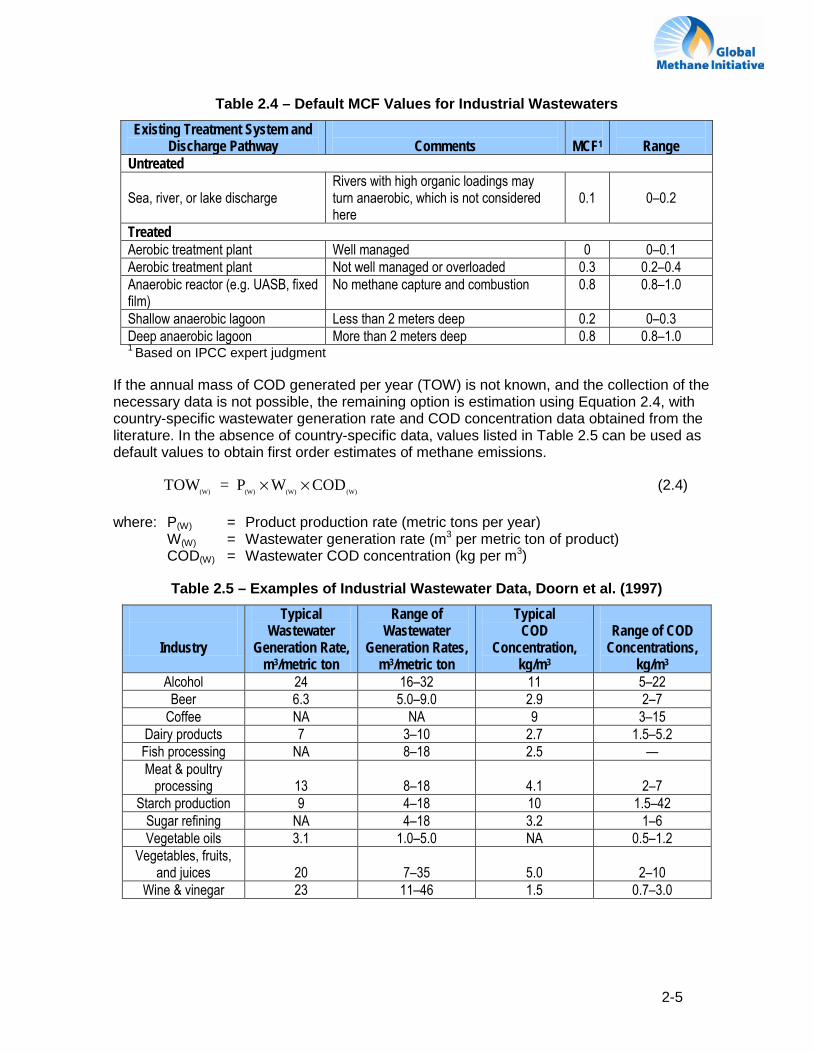
If country and waste-sector-specific values for Bo are not available, the 2006 IPCC Guidelines for National Greenhouse Gas Inventories default value of 0.25 kg CH4 per kg COD should be used. In the absence of more specific information, the appropriate MCF default value selected from Table 2.4 also should be used.

2-5

Table 2.4 – Default MCF Values for Industrial Wastewaters

Existing Treatment System and Discharge Pathway

Comments

MCF1

Range

Untreated Sea, river, or lake discharge

Rivers with high organic loadings may turn anaerobic, which is not considered here

0.1

0–0.2

Treated Aerobic treatment plant Well managed 0 0–0.1 Aerobic treatment plant Not well managed or overloaded 0.3 0.2–0.4 Anaerobic reactor (e.g. UASB, fixed film)

No methane capture and combustion 0.8 0.8–1.0

Shallow anaerobic lagoon Less than 2 meters deep 0.2 0–0.3 Deep anaerobic lagoon More than 2 meters deep 0.8 0.8–1.0 1 Based on IPCC expert judgment

If the annual mass of COD generated per year (TOW) is not known, and the collection of the necessary data is not possible, the remaining option is estimation using Equation 2.4, with country-specific wastewater generation rate and COD concentration data obtained from the literature. In the absence of country-specific data, values listed in Table 2.5 can be used as default values to obtain first order estimates of methane emissions.

TOW(W) = P(W) × W(W) × COD(W) (2.4) where: P(W) = Product production rate (metric tons per year) W(W) = Wastewater generation rate (m3 per metric ton of product) COD(W) = Wastewater COD concentration (kg per m3)

Table 2.5 – Examples of Industrial Wastewater Data, Doorn et al. (1997)

Industry

Typical Wastewater

Generation Rate, m3/metric ton

Range of Wastewater

Generation Rates, m3/metric ton

Typical COD

Concentration, kg/m3

Range of COD

Concentrations, kg/m3

Alcohol 24 16–32 11 5–22 Beer 6.3 5.0–9.0 2.9 2–7

Coffee NA NA 9 3–15 Dairy products 7 3–10 2.7 1.5–5.2 Fish processing NA 8–18 2.5 — Meat & poultry

processing

13

8–18

4.1

2–7 Starch production 9 4–18 10 1.5–42

Sugar refining NA 4–18 3.2 1–6 Vegetable oils 3.1 1.0–5.0 NA 0.5–1.2

Vegetables, fruits, and juices

20

7–35

5.0

2–10

Wine & vinegar 23 11–46 1.5 0.7–3.0

2-6

2.3 DESCRIPTION OF SPECIFIC CRITERIA FOR DETERMINING POTENTIAL SECTORS

The specific criteria to determine methane emission reduction potential and feasibility of anaerobic digestion systems are the following:

• Large sector/subsector: The category is one of the major livestock production or agro-industries in the country.

• Waste volume: The livestock production or agro-industry generates a high volume of waste discharged to conventional anaerobic lagoons.

• Waste strength: The wastewater generated has a high concentration of organic compounds as measured in terms of its BOD or COD or both.

• Geographic distribution: There is a concentration of priority sectors in specific regions of the country, making centralized or comingling projects potentially feasible.

• Energy intensive: There is sufficient energy consumption to absorb the generation from recovered methane.

The top industries that meet all of the above criteria in Mexico are swine and dairy farms, slaughterhouses, sugar cane mills, and sugar cane mills with distilleries.

2.4 EXAMPLES OF METHANE EMISSION REDUCTION PROJECTS IN MEXICO

Mexico has implemented a methane reduction program in the swine sector with the Global Methane Initiative. Currently, there are approximately 170 anaerobic digesters operating in Mexico (there are approximately 390 digesters but only 43 percent of them are operating at the present time). Mexico has developed National Technical Standards for the Design and Construction of Bio-Digesters. Mexico is also implementing a developer certification program to maintain consistency with the standard and reduce project risk for farm owners when making methane recover investment decisions.

Unfortunately, many of the farms with digesters are not currently taking full advantage of the biogas generated. However, a law promoting the use of renewable energy was passed in November 2008 which will provide the incentive for biogas utilization. SAGARPA and the Shared Risk Trust (FIRCO) are also promoting the development of renewable energy in the agriculture sector. FIRCO's program increased the installation of covered lagoon-type digesters in Yucatán, Nuevo León, and Guanajuato, among other states. The following section describes four successful projects on swine farms.

The swine farm Ana Margarita in the municipality of Montemorelos, Nuevo León,2

2 Example of successful project published in Revista Claridades No. 167, July 2007.

has 1,200 sows. The farm also has small numbers of cows, sheep, and chickens. The farm has its own feed mill to produce animal feed and utilizes mechanical ventilation systems in the swine pens. A digester with a volume of 8,516 m3 and biogas production of 20,478 m3 per day was installed on the farm in 2005. A portion of the biogas is burned to obtain certificates of emissions reduction and the remaining biogas is used to generate electricity. The system has an engine-generator set that consumes nearly 19 m3 of biogas per hour. The total electricity

2-7

generation potential of the digester is 812,772 kWh per month; only 40,000 kWh per month are needed for operating the farm lighting, ventilation, feeding systems, semen laboratories, and water pumping. The digester produces enough electricity to save the farm approximately $20,000 pesos a month on electricity.3

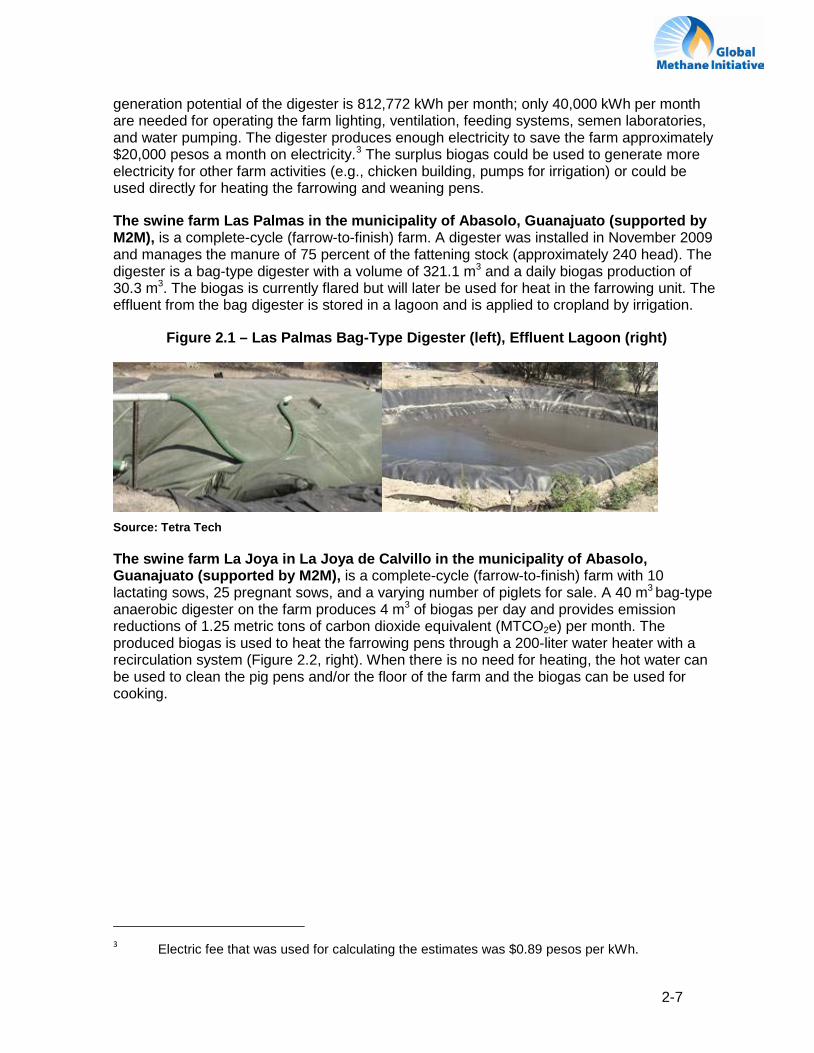
The swine farm Las Palmas in the municipality of Abasolo, Guanajuato (supported by M2M), is a complete-cycle (farrow-to-finish) farm. A digester was installed in November 2009 and manages the manure of 75 percent of the fattening stock (approximately 240 head). The digester is a bag-type digester with a volume of 321.1 m3 and a daily biogas production of 30.3 m3. The biogas is currently flared but will later be used for heat in the farrowing unit. The effluent from the bag digester is stored in a lagoon and is applied to cropland by irrigation.

The surplus biogas could be used to generate more electricity for other farm activities (e.g., chicken building, pumps for irrigation) or could be used directly for heating the farrowing and weaning pens.

Figure 2.1 – Las Palmas Bag-Type Digester (left), Effluent Lagoon (right)

Source: Tetra Tech

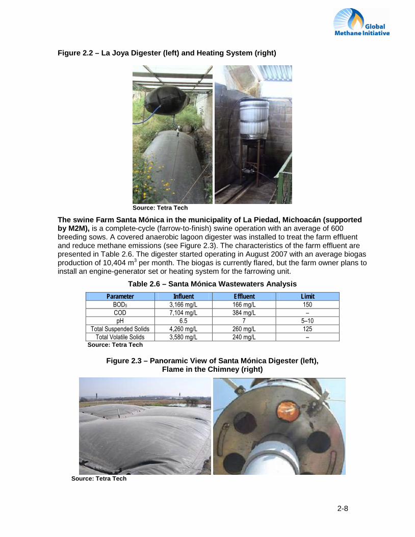
The swine farm La Joya in La Joya de Calvillo in the municipality of Abasolo, Guanajuato (supported by M2M), is a complete-cycle (farrow-to-finish) farm with 10 lactating sows, 25 pregnant sows, and a varying number of piglets for sale. A 40 m3 bag-type anaerobic digester on the farm produces 4 m3 of biogas per day and provides emission reductions of 1.25 metric tons of carbon dioxide equivalent (MTCO2e) per month. The produced biogas is used to heat the farrowing pens through a 200-liter water heater with a recirculation system (Figure 2.2, right). When there is no need for heating, the hot water can be used to clean the pig pens and/or the floor of the farm and the biogas can be used for cooking.

3 Electric fee that was used for calculating the estimates was $0.89 pesos per kWh.

2-8

Figure 2.2 – La Joya Digester (left) and Heating System (right)

Source: Tetra Tech

The swine Farm Santa Mónica in the municipality of La Piedad, Michoacán (supported by M2M), is a complete-cycle (farrow-to-finish) swine operation with an average of 600 breeding sows. A covered anaerobic lagoon digester was installed to treat the farm effluent and reduce methane emissions (see Figure 2.3). The characteristics of the farm effluent are presented in Table 2.6. The digester started operating in August 2007 with an average biogas production of 10,404 m3 per month. The biogas is currently flared, but the farm owner plans to install an engine-generator set or heating system for the farrowing unit.

Table 2.6 – Santa Mónica Wastewaters Analysis Parameter Influent Effluent Limit

BOD5 3,166 mg/L 166 mg/L 150 COD 7,104 mg/L 384 mg/L – pH 6.5 7 5–10

Total Suspended Solids 4,260 mg/L 260 mg/L 125 Total Volatile Solids 3,580 mg/L 240 mg/L –

Source: Tetra Tech

Figure 2.3 – Panoramic View of Santa Mónica Digester (left), Flame in the Chimney (right)

Source: Tetra Tech

3-1

3. SECTOR CHARACTERIZATION

3.1 INTRODUCTION

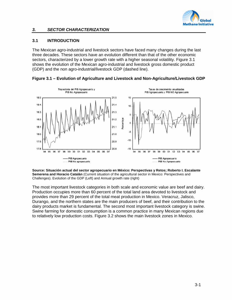
The Mexican agro-industrial and livestock sectors have faced many changes during the last three decades. These sectors have an evolution different than that of the other economic sectors, characterized by a lower growth rate with a higher seasonal volatility. Figure 3.1 shows the evolution of the Mexican agro-industrial and livestock gross domestic product (GDP) and the non agro-industrial/livestock GDP (dashed line).

Figure 3.1 – Evolution of Agriculture and Livestock and Non-Agriculture/Livestock GDP

Source: Situación actual del sector agropecuario en México: Perspectivas y Retos; Roberto I. Escalante Semerena and Horacio Catalán (Current situation of the agricultural sector in Mexico: Perspectives and Challenges). Evolution of the GDP (Left) and Annual growth rate (right)

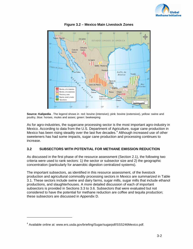
The most important livestock categories in both scale and economic value are beef and dairy. Production occupies more than 60 percent of the total land area devoted to livestock and provides more than 29 percent of the total meat production in Mexico. Veracruz, Jalisco, Durango, and the northern states are the main producers of beef, and their contribution to the dairy products market is fundamental. The second most important livestock category is swine. Swine farming for domestic consumption is a common practice in many Mexican regions due to relatively low production costs. Figure 3.2 shows the main livestock zones in Mexico.

3-2

Figure 3.2 – Mexico Main Livestock Zones

Source: Kalipedia . The legend shows in red: bovine (intensive); pink: bovine (extensive), yellow: swine and poultry, blue: horses, mules and asses; green: beekeeping

As for agro-industries, the sugarcane processing sector is the most important agro-industry in Mexico. According to data from the U.S. Department of Agriculture, sugar cane production in Mexico has been rising steadily over the last five decades.4

3.2 SUBSECTORS WITH POTENTIAL FOR METHANE EMISSION REDUCTION

Although increased use of other sweeteners has had some impacts, sugar cane production and processing continues to increase.

As discussed in the first phase of the resource assessment (Section 2.1), the following two criteria were used to rank sectors: 1) the sector or subsector size and 2) the geographic concentration (particularly for anaerobic digestion centralized systems).

The important subsectors, as identified in this resource assessment, of the livestock production and agricultural commodity processing sectors in Mexico are summarized in Table 3.1. These sectors include swine and dairy farms, sugar mills, sugar mills that include ethanol productions, and slaughterhouses. A more detailed discussion of each of important subsectors is provided in Sections 3.3 to 3.6. Subsectors that were evaluated but not considered to have the potential for methane reduction are coffee and tequila production; these subsectors are discussed in Appendix D.

4 Available online at: www.ers.usda.gov/briefing/Sugar/sugarpdf/SSS246Mexico.pdf.

3-3

Table 3.1 – Main Subsectors With Potential for Methane Emission Reduction

Subsector Size (production/year) Geographical location

Swine 15,230,630 pigs in 2008 Central region, Yucatán Peninsula, and southeast regions of the country (Veracruz)

Dairies 6,800,000 dairy cows with a total milk production of 10.6 billion L/year

Jalisco, Coahuila Durango, and Chihuahua

Sugar mills 57 sugar mills with a total sugar production of ~ 5 million MT in 2008

Southeast region of the country, mainly Veracruz, where 22 mills are located

Sugar mills with ethanol production

4 sugar mills also produce ethanol with a total production of ~19.4 million L/yr Distributed throughout the country

Slaughterhouses Production of pork meat: 1,160,675 MT, bovine: 1,667,139 MT in 2008 Distributed throughout the country

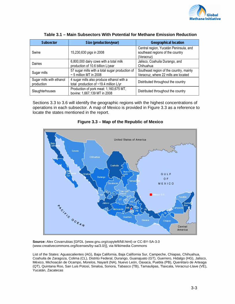
Sections 3.3 to 3.6 will identify the geographic regions with the highest concentrations of operations in each subsector. A map of Mexico is provided in Figure 3.3 as a reference to locate the states mentioned in the report.

Figure 3.3 – Map of the Republic of Mexico

Source: Alex Covarrubias [GFDL (www.gnu.org/copyleft/fdl.html) or CC-BY-SA-3.0 (www.creativecommons.org/licenses/by-sa/3.0/)], via Wikimedia Commons

List of the States: Aguascalientes (AG), Baja California, Baja California Sur, Campeche, Chiapas, Chihuahua, Coahuila de Zaragoza, Colima (CL), Distrito Federal, Durango, Guanajuato (GT), Guerrero, Hidalgo (HG), Jalisco, México, Michoacán de Ocampo, Morelos, Nayarit (NA), Nuevo León, Oaxaca, Puebla (PB), Querétaro de Arteaga (QT), Quintana Roo, San Luis Potosí, Sinaloa, Sonora, Tabasco (TB), Tamaulipas, Tlaxcala, Veracruz-Llave (VE), Yucatán, Zacatecas

3-4

Because methane production is temperature-dependant, an important consideration in evaluating locations for potential methane capture is the temperature. In Mexico, the annual average annual temperature ranges between 13 and 29°C (Figure 3.4).

Figure 3.4. Annual Average Temperatures in Mexico

Livestock activities (both cattle and swine) are concentrated mainly in the central region of the country, which has the lowest annual temperatures (10 to 22°C). Swine production is also present on the Yucatán Peninsula and in Veracruz, where average annual temperatures exceed 22°C. Sugar cane mills are located mainly in the southeast region of the country, in some portions of the central region (Morelos), and in the Pacific (Guadalajara) region; these locations have average annual temperatures exceeding 22°C.

3.3 SWINE PRODUCTION

3.3.1 Description of Size, Scale, and Geographic Location of Operations

Mexico has the 8th largest swine population in the world, with more than 15.2 million pigs in 2008 according to the Information Service for Farms and Cattle (SIAP) (15.5 million in the 2008 FAOSTAT inventory).

Swine production is concentrated in the center of the country, mainly in the Balsas river basin. The states of Jalisco, Michoacán, and Guanajuato have a combined total of 4.3 million pigs. Sonora, Puebla, and Veracruz all have more than 1 million pigs each (Table 3.2).

Table 3.2 – Mexico Swine Population Per State in 2008 State Head State Head

Aguascalientes 105,225 Nayarit 71,101 Baja California 13,154 Nuevo León 198,381 Baja California Sur 20,170 Oaxaca 760,016 Campeche 102,613 Puebla 1,143,843 Coahuila 78,737 Querétaro 226,567 Colima 44,505 Quintana Roo 154,696

3-5

State Head State Head Chiapas 780,429 San Luis Potosí 226,027 Chihuahua 263,104 Sinaloa 363,219 Distrito Federal 19,973 Sonora 1,392,203 Durango 172,619 Tabasco 280,292 Guanajuato 987,938 Tamaulipas 390,876 Guerrero 801,193 Tlaxcala 195,994 Hidalgo 428,302 Veracruz 1,010,358 Jalisco 2,595,303 Yucatán 898,729 México 461,067 Zacateca 230,607 Michoacán 720,784 Total 15,230,630 Morelos 92,605

Source: Prepared by SIAP, with information of SAGARPA's delegations. Preliminary data for 2008.

Swine production in Mexico can be classified as one of the following three types:

• Backyard operations have a maximum of about 10 animals. The pigs are kept in rural pens and occasionally in open areas where they forage and are fed a small amount of supplemental corn.

• Small to medium scale operations have at least 100 animals. Feed consists of a mixture of ingredients to provide a balanced ration that meets nutritional requirements according to the animals’ needs and developmental stage. Feed is purchased from a local feed dealer.

• Large scale, highly automated operations can have up to 100,000 pigs of different ages distributed in different locations in highly automated total confinement facilities. Again, feed consists of a mixture of ingredients to provide a balanced ration that meets nutritional requirements. The food is typically prepared on site and contains maize and sorghum as typical ingredients.

It is estimated that 46 percent of the pigs in Mexico are raised in large scale, 20 percent in small to medium scale operations and 34 percent in backyard operations (as shown in Table 3.3).

Table 3.3 – Swine Population Per Type of Operations Farms Percentage of animals Number of animals

Large scale 46% 7,006,090 Small to medium scale 20% 3,046,126 Backyard 34% 5,178,415 Total 100% 15,230,631

Source: Pérez Espejo Rosario, Granjas porcinas y medio ambiente, Contaminación del agua en La Piedad Michoacán 2006.

Swine farms can further be divided into four types depending on the developmental stages of the animals.

• Weaned pig operations. These are operations that produce weaned pigs for sale to grow/finish operations that produce fed pigs for slaughter.

3-6

• Grow/finish operations. These are operations that feed purchased wean pigs until they reach slaughter weight.

• Farrow-to-finish operations. These are operations that produce weaned pigs that are then fed until they reach slaughter weight.

• Gilt and boar production operations. These are operations that produce gilts (immature females) and boars for sale as replacements for sows and boars that have been culled from weaned pig and farrow-to-finish operations as well as possibly producing semen for artificial insemination.

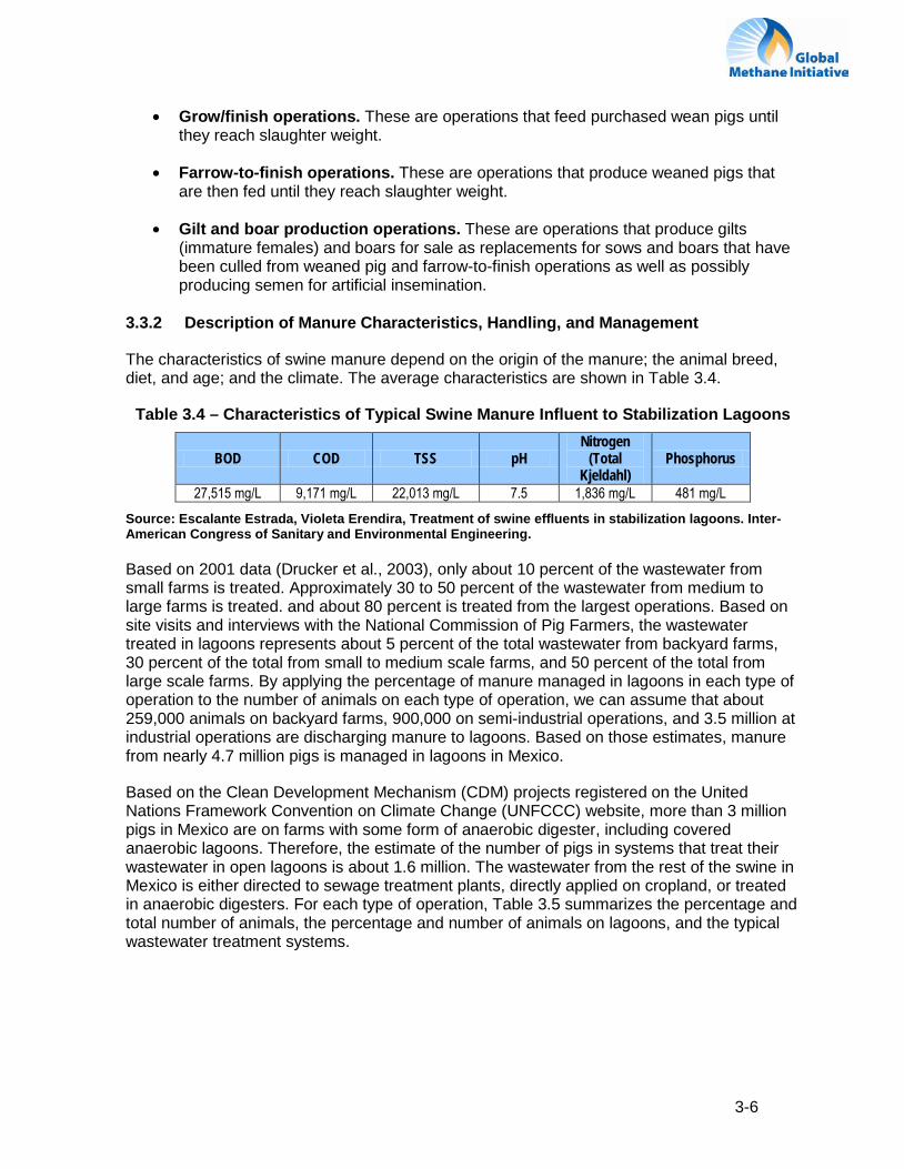
3.3.2 Description of Manure Characteristics, Handling, and Management

The characteristics of swine manure depend on the origin of the manure; the animal breed, diet, and age; and the climate. The average characteristics are shown in Table 3.4.

Table 3.4 – Characteristics of Typical Swine Manure Influent to Stabilization Lagoons

BOD COD TSS pH Nitrogen

(Total Kjeldahl)

Phosphorus

27,515 mg/L 9,171 mg/L 22,013 mg/L 7.5 1,836 mg/L 481 mg/L Source: Escalante Estrada, Violeta Erendira, Treatment of swine effluents in stabilization lagoons. Inter-American Congress of Sanitary and Environmental Engineering.

Based on 2001 data (Drucker et al., 2003), only about 10 percent of the wastewater from small farms is treated. Approximately 30 to 50 percent of the wastewater from medium to large farms is treated. and about 80 percent is treated from the largest operations. Based on site visits and interviews with the National Commission of Pig Farmers, the wastewater treated in lagoons represents about 5 percent of the total wastewater from backyard farms, 30 percent of the total from small to medium scale farms, and 50 percent of the total from large scale farms. By applying the percentage of manure managed in lagoons in each type of operation to the number of animals on each type of operation, we can assume that about 259,000 animals on backyard farms, 900,000 on semi-industrial operations, and 3.5 million at industrial operations are discharging manure to lagoons. Based on those estimates, manure from nearly 4.7 million pigs is managed in lagoons in Mexico.

Based on the Clean Development Mechanism (CDM) projects registered on the United Nations Framework Convention on Climate Change (UNFCCC) website, more than 3 million pigs in Mexico are on farms with some form of anaerobic digester, including covered anaerobic lagoons. Therefore, the estimate of the number of pigs in systems that treat their wastewater in open lagoons is about 1.6 million. The wastewater from the rest of the swine in Mexico is either directed to sewage treatment plants, directly applied on cropland, or treated in anaerobic digesters. For each type of operation, Table 3.5 summarizes the percentage and total number of animals, the percentage and number of animals on lagoons, and the typical wastewater treatment systems.

3-7

Table 3.5 – Percentage of Wastewater Treated in Lagoons and Number of Animals per Type of Operation

Type of farm Animal

population Animals on farms

with lagoons (open or covered)

Wastewater treatment systems

Large ~46% of total ~7,006,090

50% of industrial 3,503,045

3 options: lagoons (50%), anaerobic digesters, or direct land application. In lagoons and digesters, the treated wastewater is then used for crop irrigation or any other activity of the site, and the solids are used as compost or sold as fertilizer.

Small to medium ~20% of total ~3,046,126

30% of semi-industrial 913,838

3 options: sedimentation and/or oxidation lagoons (30%), anaerobic digesters, or direct land application. The solid residues are used as compost.

Backyard ~34% of total ~5,178,415

5% of backyard 258,921

Only 5% with lagoons; the rest direct the effluent to sewage treatment plants or irrigation on land, and solid residue is taken to a silo or used for compost. A few anaerobic digesters have been installed as demonstration projects.

Total lagoons (open or covered)

15,230,631 ~31% of total 4,675,804

Total covered lagoons 3,091,417

Animals in system that already have anaerobic digesters (estimation based on the number of CDM registered projects).

Total open lagoons 1,584,386 Animals in system that use open lagoons.

Source: Estimation based on the information provided by SEMARNAT, INEGI, CNP and SAGARPA

3.4 DAIRY FARMS

3.4.2 Description of Size, Scale, and Geographical Location of Operations

The total number of cattle in Mexico is about 32 million (FAOSTAT, 2008) of which 6.8 million are dairy cows (USDA, 2007). The milk production is about 10 billion liters per year (SIAP/SAGARPA 2002). The main milk-producing states in Mexico are Jalisco (18 percent of the total milk production), Durango (10 percent), Coahuila (10 percent), Chihuahua (8 percent), Veracruz (7 percent), and Guanajato (7 percent), as shown in Figure 3.5.

Figure 3.5 – Main Milk-Producing States in Mexico

Source: SAGARPA, 2002

3-8

The production can be classified in three different types that are briefly described below.

• Extensive. Grazing provides 100 percent of the animal’s nutritional requirements. Any supplemental feeding usually is limited to minerals.

• Semi-intensive. Animals have access to pasture or rangeland, which supplies a portion of nutritional requirements with supplemental feeding in an open or enclosed confinement facility providing the remainder.

• Intensive. Animals have no access to pasture or rangeland. Harvested crops provide 100 percent of nutritional requirements in an open or enclosed confinement facility.

Another classification of dairy farms in Mexico was used in this report and is briefly described below:

• Total confinement. Specialized systems that have specific livestock for milk production. The most common breed of cow on these farms is Holstein and to a lesser extent, Brown Swiss and Jersey. These farms have highly specialized technology. Animals are predominantly confined in barns, and their diet is based on specially mixed rations. Milking is mechanized and production is mainly for dairy processing plants.

• Partial confinement. Operations that combine confinement in barns or corrals with access to pasture. Grazing may be the only source of nutrients or be supplemented with grains and minerals. Milking may occur at a central location or in confinement facilities. Holstein Friesian and Brown Swiss are the predominate breeds

• Dual-purpose. These operations produce both milk and meat primarily using pasture and rangeland with a minimum amount of supplemental feed. Any confinement occurs only at night. Zebu and Zebu crosses are the predominate breed; the Zebu breed is a dual-purpose breed that originated in Southeast Asia. Milking may occur outdoors. .

• Backyard. These farms utilize small pasture areas to house dairy cows to provide milk for a family or possibly a family and a few neighbors. Cows may be Holstein Friesian, Brown Swiss, or a crossbreed.

Total confinement systems are found mainly in the northern region of Mexico, while partial confinement operations are more common in the central states, and dual-purpose operations are most common in the south (USDA, 2007).

It is estimated that 2.2 million head (32 percent of the total number of animals on dairy farms) are dairy cows, and 4.6 million head are dual-purpose cows (USDA, 2007). These two categories can further be divided into 25 percent in total confinement systems5

5 Centro de Estudio Estratégicos, Tecnológico de Monterrey, Campus Ciudad de México.

, 7 percent in

3-9

partial confinement systems, 48 percent in dual-purpose systems, and 20 percent in backyard systems6

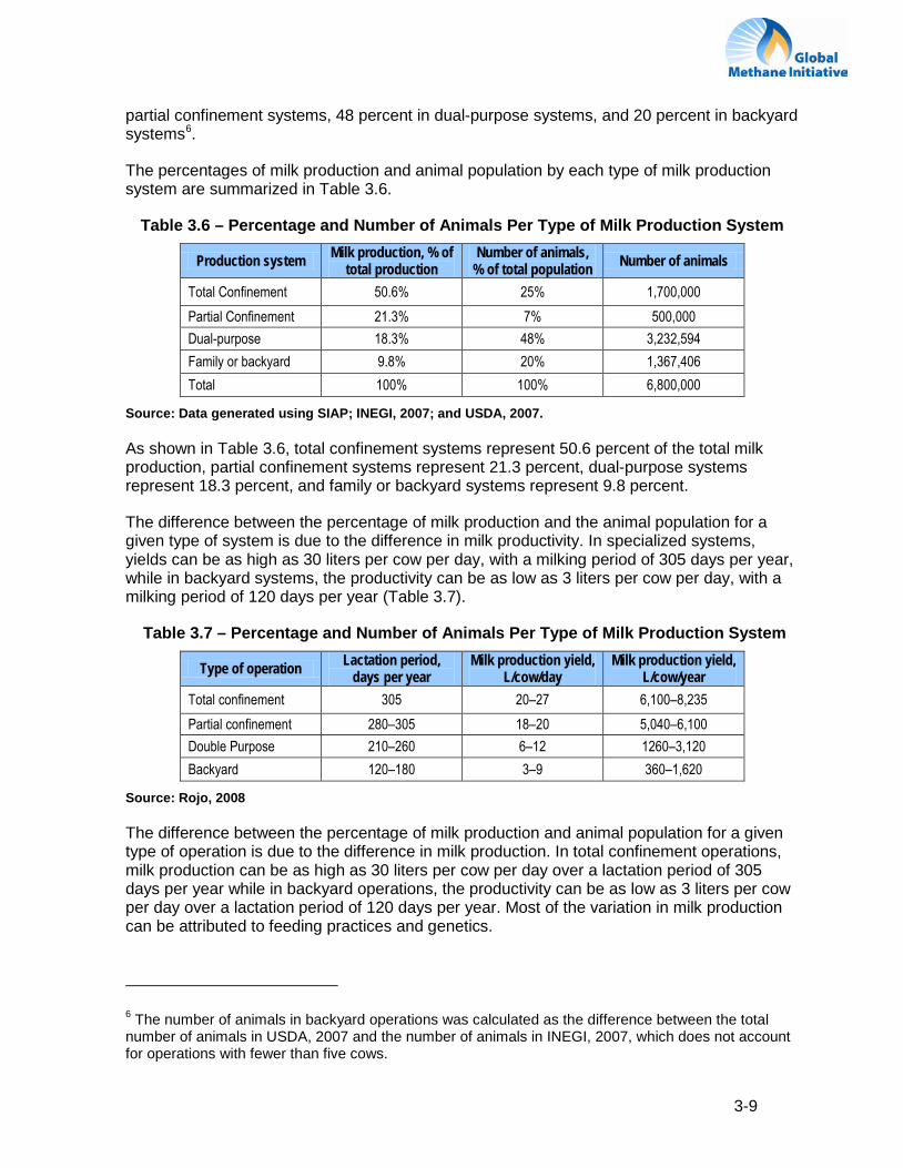
The percentages of milk production and animal population by each type of milk production system are summarized in Table 3.6.

.

Table 3.6 – Percentage and Number of Animals Per Type of Milk Production System

Production system Milk production, % of total production

Number of animals, % of total population Number of animals

Total Confinement 50.6% 25% 1,700,000 Partial Confinement 21.3% 7% 500,000 Dual-purpose 18.3% 48% 3,232,594 Family or backyard 9.8% 20% 1,367,406 Total 100% 100% 6,800,000

Source: Data generated using SIAP; INEGI, 2007; and USDA, 2007.

As shown in Table 3.6, total confinement systems represent 50.6 percent of the total milk production, partial confinement systems represent 21.3 percent, dual-purpose systems represent 18.3 percent, and family or backyard systems represent 9.8 percent.

The difference between the percentage of milk production and the animal population for a given type of system is due to the difference in milk productivity. In specialized systems, yields can be as high as 30 liters per cow per day, with a milking period of 305 days per year, while in backyard systems, the productivity can be as low as 3 liters per cow per day, with a milking period of 120 days per year (Table 3.7).

Table 3.7 – Percentage and Number of Animals Per Type of Milk Production System

Type of operation Lactation period, days per year

Milk production yield, L/cow/day

Milk production yield, L/cow/year

Total confinement 305 20–27 6,100–8,235 Partial confinement 280–305 18–20 5,040–6,100 Double Purpose 210–260 6–12 1260–3,120 Backyard 120–180 3–9 360–1,620

Source: Rojo, 2008

The difference between the percentage of milk production and animal population for a given type of operation is due to the difference in milk production. In total confinement operations, milk production can be as high as 30 liters per cow per day over a lactation period of 305 days per year while in backyard operations, the productivity can be as low as 3 liters per cow per day over a lactation period of 120 days per year. Most of the variation in milk production can be attributed to feeding practices and genetics.

6 The number of animals in backyard operations was calculated as the difference between the total number of animals in USDA, 2007 and the number of animals in INEGI, 2007, which does not account for operations with fewer than five cows.

3-10

3.4.3 Description of Waste Characteristics, Handling, and Management

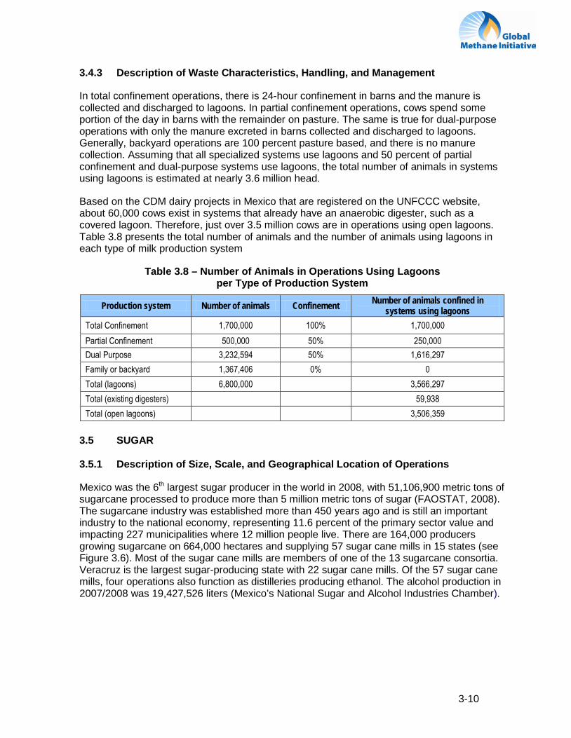
In total confinement operations, there is 24-hour confinement in barns and the manure is collected and discharged to lagoons. In partial confinement operations, cows spend some portion of the day in barns with the remainder on pasture. The same is true for dual-purpose operations with only the manure excreted in barns collected and discharged to lagoons. Generally, backyard operations are 100 percent pasture based, and there is no manure collection. Assuming that all specialized systems use lagoons and 50 percent of partial confinement and dual-purpose systems use lagoons, the total number of animals in systems using lagoons is estimated at nearly 3.6 million head.

Based on the CDM dairy projects in Mexico that are registered on the UNFCCC website, about 60,000 cows exist in systems that already have an anaerobic digester, such as a covered lagoon. Therefore, just over 3.5 million cows are in operations using open lagoons. Table 3.8 presents the total number of animals and the number of animals using lagoons in each type of milk production system

Table 3.8 – Number of Animals in Operations Using Lagoons per Type of Production System

Production system Number of animals Confinement Number of animals confined in systems using lagoons

Total Confinement 1,700,000 100% 1,700,000 Partial Confinement 500,000 50% 250,000 Dual Purpose 3,232,594 50% 1,616,297 Family or backyard 1,367,406 0% 0 Total (lagoons) 6,800,000 3,566,297 Total (existing digesters) 59,938 Total (open lagoons) 3,506,359

3.5 SUGAR

3.5.1 Description of Size, Scale, and Geographical Location of Operations

Mexico was the 6th largest sugar producer in the world in 2008, with 51,106,900 metric tons of sugarcane processed to produce more than 5 million metric tons of sugar (FAOSTAT, 2008). The sugarcane industry was established more than 450 years ago and is still an important industry to the national economy, representing 11.6 percent of the primary sector value and impacting 227 municipalities where 12 million people live. There are 164,000 producers growing sugarcane on 664,000 hectares and supplying 57 sugar cane mills in 15 states (see Figure 3.6). Most of the sugar cane mills are members of one of the 13 sugarcane consortia. Veracruz is the largest sugar-producing state with 22 sugar cane mills. Of the 57 sugar cane mills, four operations also function as distilleries producing ethanol. The alcohol production in 2007/2008 was 19,427,526 liters (Mexico’s National Sugar and Alcohol Industries Chamber).

3-11

Figure 3.6 – Geographical Location of the Sugar Industry in Mexico

Source: Data from COAAZUCAR

3.5.2 Description of the Characteristics of Wastes, Handling, and Management

The sugar industry generates large volumes of wastewater: about 11 liters per ton of sugar in sugar mills, and from 10 to 15 liters of vinasses per liter of distilled alcohol in distilleries. The average COD levels are 3,200 mg/L for the sugar cane mill wastewater and 100,000 mg/L (maximum value can reach 150,000 mg/L) for the vinasses from ethanol production.

Approximately 17 of the 57 sugar cane mills in Mexico have one or more open lagoons for the effluent from cane processing (see Table 3.9). Effluent not treated in lagoons is discharged to the local municipal wastewater treatment system. Therefore, it is estimated that about 29 percent of the wastewater from the sugar mills is treated in open lagoons. All four distilleries use open lagoons to treat their effluent.

Table 3.9 – Number of Lagoons in the Sugar Cane Mills Sector

State Sugar production, MT Number of mills Lagoons

Puebla 189,913 2 Morelos 157,532 2 Jalisco 624,703 6 Michoacán 146,197 3 Chiapas 245,436 2 Colima 96,391 1 Nayarit 226,729 2 Veracruz 2,010,889 22 12 Oaxaca 290,680 3 1 Sinaloa 164,028 3 1 Tamaulipas 203,682 2 San Luis Potosí 443,804 4 2 Quintana Roo 139,640 1

3-12

State Sugar production, MT Number of mills Lagoons

Tabasco 170,198 3 Campeche 27,857 1 3 Total 5,137,679 57 19

Source: Data from COAAZUCAR

3.6 SLAUGHTERHOUSES

3.6.1 Description of Size, Scale, and Geographical Location of Operations

In Mexico, slaughterhouses are classified according to the type of activities they perform, the equipment they use, and the purpose for which they were created. The three main categories are Federal Inspection Type (FIT) slaughterhouses (regulated by SAGARPA), municipal slaughterhouses (regulated by the Ministry of Health), and private slaughterhouses. Nearly 50.5 percent of the slaughtering is performed in municipal slaughterhouses, 21 percent is carried out in FIT slaughterhouses, and about 27.9 percent occurs in private slaughterhouses.

a. SWINE SLAUGHTERHOUSES

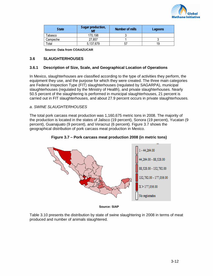
The total pork carcass meat production was 1,160,675 metric tons in 2008. The majority of the production is located in the states of Jalisco (19 percent), Sonora (19 percent), Yucatan (9 percent), Guanajuato (9 percent), and Veracruz (6 percent). Figure 3.7 shows the geographical distribution of pork carcass meat production in Mexico.

Figure 3.7 – Pork carcass meat production 2008 (in metric tons)

Source: SIAP

Table 3.10 presents the distribution by state of swine slaughtering in 2008 in terms of meat produced and number of animals slaughtered.

3-13

Table 3.10 – Production, Weight, Slaughtered Animals, Weight of Carcass Meat (Swine), 2008

States Pork production, metric tons

Slaughtered animals, head States Pork production,

metric tons Slaughtered

animals, head Aguascalientes 11,364 135,345 Nayarit 4,553 69,174 Baja California 1,316 15,680 Nuevo León 15,038 195,890 Baja California Sur 1,033 13,269 Oaxaca 28,189 568,271 Campeche 5,153 80,908 Puebla 101,441 1,386,406 Coahuila 9,363 124,995 Quintana Roo 6,414 86,529 Colima 7,477 97,857 Querétaro 14,666 192,537 Chiapas 22,957 367,822 San Luis Potosí 8,162 120,903 Chihuahua 7,669 89,503 Sinaloa 19,649 235,356 Distrito Federal 2,015 25,196 Sonora 222,356 2,583,601 Durango 4,443 75,037 Tabasco 13,398 171,614 Guanajuato 103,657 1,360,159 Tamaulipas 32,953 412,122 Guerrero 22,486 338,335 Tlaxcala 15,837 215,000 Hidalgo 19,268 265,059 Veracruz 68,204 950,659 Jalisco 216,800 2,804,016 Yucatán 100,247 1,298,176 México 21,914 282,783 Zacateca 7,408 94,024 Michoacán 42,311 556,817 Total 1,160,675 15,264,759 Morelos 2,934 51,716

Source: Prepared SIAP, with information of SAGARPA's delegations.

b. BEEF CATTLE SLAUGHTERHOUSES

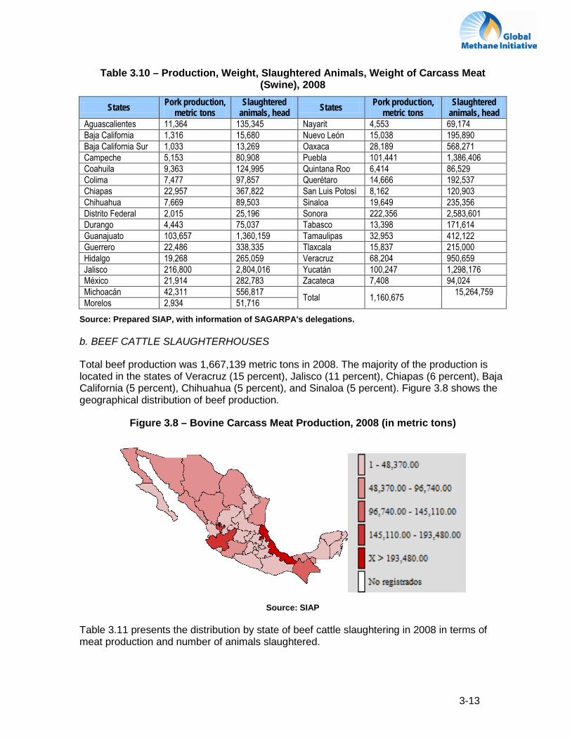
Total beef production was 1,667,139 metric tons in 2008. The majority of the production is located in the states of Veracruz (15 percent), Jalisco (11 percent), Chiapas (6 percent), Baja California (5 percent), Chihuahua (5 percent), and Sinaloa (5 percent). Figure 3.8 shows the geographical distribution of beef production.

Figure 3.8 – Bovine Carcass Meat Production, 2008 (in metric tons)

Source: SIAP

Table 3.11 presents the distribution by state of beef cattle slaughtering in 2008 in terms of meat production and number of animals slaughtered.

3-14

Table 3.11 – Production, Weight, Value, Slaughtered Animals, Carcass Meat Weight (Bovine), 2008

States Beef production, metric tons

Slaughtered animals, heads States Beef production,

metric tons Slaughtered

animals, heads

Aguascalientes 15,127 71,330 Nayarit 25,042 143,873 Baja California 78,447 278,365 Nuevo León 36,560 184,279 Baja California Sur 5,602 30,321 Oaxaca 43,113 225,217 Campeche 22,793 109,478 Puebla 37,337 161,285 Coahuila 58,213 297,331 Quintana Roo 26,626 110,773 Colima 9,666 43,340 Querétaro 4,777 22,602 Chiapas 101,466 522,558 San Luis Potosí 47,577 208,548 Chihuahua 84,793 427,581 Sinaloa 78,042 344,816 Distrito Federal 690 3,181 Sonora 74,443 442,354 Durango 65,678 463,393 Tabasco 62,891 302,219 Guanajuato 36,211 204,113 Tamaulipas 55,126 267,697 Guerrero 37,300 201,811 Tlaxcala 12,475 63,061 Hidalgo 34,363 149,574 Veracruz 242,543 1,053,707 Jalisco 180,292 789,662 Yucatán 27,869 129,716 México 41,128 176,539 Zacateca 45,936 249,742 Michoacán 69,930 370,762 Total 1,667,139 8,074,451 Morelos 5,083 25,223

Source: Prepared by SIAP, with information of SAGARPA's delegations.

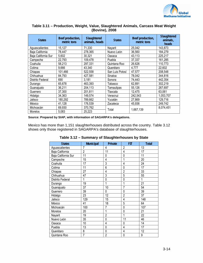
Mexico has more than 1,151 slaughterhouses distributed across the country. Table 3.12 shows only those registered in SAGARPA's database of slaughterhouses.

Table 3.12 – Summary of Slaughterhouses by State States Municipal Private FIT Total

Aguascalientes 7 4 2 13 Baja California 2 11 4 17 Baja California Sur 11 0 0 11 Campeche 15 4 1 20 Coahuila 17 3 4 24 Colima 11 6 0 17 Chiapas 27 4 2 33 Chihuahua 47 3 5 55 Distrito Federal 1 0 0 1 Durango 19 1 1 21 Guanajuato 37 10 7 54 Guerrero 39 0 0 39 Hidalgo 23 12 2 37 Jalisco 129 15 4 148 México 41 18 5 64 Michoacán 100 7 0 107 Morelos 20 1 0 21 Nayarit 19 2 1 22 Nuevo León 35 0 11 46 Oaxaca 10 4 0 14 Puebla 13 0 4 17 Querétaro 8 0 4 12 Quintana Roo 7 2 0 9

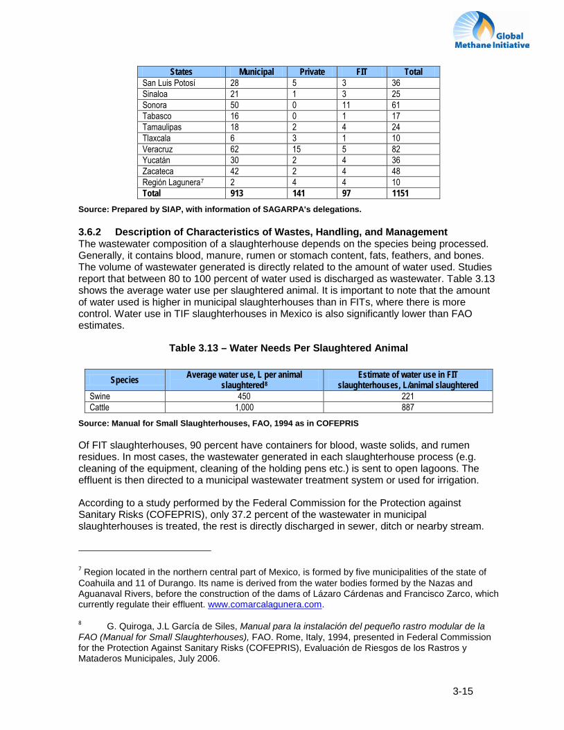
3-15

States Municipal Private FIT Total San Luis Potosí 28 5 3 36 Sinaloa 21 1 3 25 Sonora 50 0 11 61 Tabasco 16 0 1 17 Tamaulipas 18 2 4 24 Tlaxcala 6 3 1 10 Veracruz 62 15 5 82 Yucatán 30 2 4 36 Zacateca 42 2 4 48 Región Lagunera7 2 4 4 10 Total 913 141 97 1151

Source: Prepared by SIAP, with information of SAGARPA's delegations.

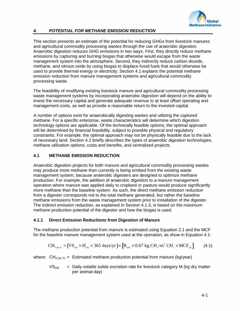
3.6.2 Description of Characteristics of Wastes, Handling, and Management The wastewater composition of a slaughterhouse depends on the species being processed. Generally, it contains blood, manure, rumen or stomach content, fats, feathers, and bones. The volume of wastewater generated is directly related to the amount of water used. Studies report that between 80 to 100 percent of water used is discharged as wastewater. Table 3.13 shows the average water use per slaughtered animal. It is important to note that the amount of water used is higher in municipal slaughterhouses than in FITs, where there is more control. Water use in TIF slaughterhouses in Mexico is also significantly lower than FAO estimates.

Table 3.13 – Water Needs Per Slaughtered Animal

Species Average water use, L per animal slaughtered8

Estimate of water use in FIT slaughterhouses, L/animal slaughtered

Swine 450 221 Cattle 1,000 887

Source: Manual for Small Slaughterhouses, FAO, 1994 as in COFEPRIS

Of FIT slaughterhouses, 90 percent have containers for blood, waste solids, and rumen residues. In most cases, the wastewater generated in each slaughterhouse process (e.g. cleaning of the equipment, cleaning of the holding pens etc.) is sent to open lagoons. The effluent is then directed to a municipal wastewater treatment system or used for irrigation.

According to a study performed by the Federal Commission for the Protection against Sanitary Risks (COFEPRIS), only 37.2 percent of the wastewater in municipal slaughterhouses is treated, the rest is directly discharged in sewer, ditch or nearby stream.

7 Region located in the northern central part of Mexico, is formed by five municipalities of the state of Coahuila and 11 of Durango. Its name is derived from the water bodies formed by the Nazas and Aguanaval Rivers, before the construction of the dams of Lázaro Cárdenas and Francisco Zarco, which currently regulate their effluent. www.comarcalagunera.com.

8 G. Quiroga, J.L García de Siles, Manual para la instalación del pequeño rastro modular de la FAO (Manual for Small Slaughterhouses), FAO. Rome, Italy, 1994, presented in Federal Commission for the Protection Against Sanitary Risks (COFEPRIS), Evaluación de Riesgos de los Rastros y Mataderos Municipales, July 2006.

3-16

Based on site visits, it was assumed in this study that 70 percent of the treated wastewater is treated in open anaerobic lagoons. The rest of the wastewater is only treated by screening or with other solids separation unit processes.

4-1

4. POTENTIAL FOR METHANE EMISSION REDUCTION

This section presents an estimate of the potential for reducing GHGs from livestock manures and agricultural commodity processing wastes through the use of anaerobic digestion. Anaerobic digestion reduces GHG emissions in two ways. First, they directly reduce methane emissions by capturing and burning biogas that otherwise would escape from the waste management system into the atmosphere. Second, they indirectly reduce carbon dioxide, methane, and nitrous oxide by using biogas to displace fossil fuels that would otherwise be used to provide thermal energy or electricity. Section 4.1 explains the potential methane emission reduction from manure management systems and agricultural commodity processing waste.

The feasibility of modifying existing livestock manure and agricultural commodity processing waste management systems by incorporating anaerobic digestion will depend on the ability to invest the necessary capital and generate adequate revenue to at least offset operating and management costs, as well as provide a reasonable return to the invested capital.

A number of options exist for anaerobically digesting wastes and utilizing the captured methane. For a specific enterprise, waste characteristics will determine which digestion technology options are applicable. Of the technically feasible options, the optimal approach will be determined by financial feasibility, subject to possible physical and regulatory constraints. For example, the optimal approach may not be physically feasible due to the lack of necessary land. Section 4.2 briefly describes the types of anaerobic digestion technologies, methane utilization options, costs and benefits, and centralized projects.

4.1 METHANE EMISSION REDUCTION

Anaerobic digestion projects for both manure and agricultural commodity processing wastes may produce more methane than currently is being emitted from the existing waste management system, because anaerobic digesters are designed to optimize methane production. For example, the addition of anaerobic digestion to a manure management operation where manure was applied daily to cropland or pasture would produce significantly more methane than the baseline system. As such, the direct methane emission reduction from a digester corresponds not to the total methane generated, but rather the baseline methane emissions from the waste management system prior to installation of the digester. The indirect emission reduction, as explained in Section 4.1.3, is based on the maximum methane production potential of the digester and how the biogas is used.

4.1.1 Direct Emission Reductions from Digestion of Manure

The methane production potential from manure is estimated using Equation 2.1 and the MCF for the baseline manure management system used at the operation, as show in Equation 4.1:

CH4 (M, P) = VS(M) × H(M) × 365 days/yr( )× Bo(M) × 0.67 kg CH4/m3 CH4 × MCFAD[ ] (4.1)

where: CH4 (M, P) = Estimated methane production potential from manure (kg/year)

VS(M) = Daily volatile solids excretion rate for livestock category M (kg dry matter per animal-day)

4-2

H(M) = Average daily number of animals in livestock category M

Bo(M) = Maximum methane production capacity for manure produced by livestock category M (m3 CH4 per kg volatile solids excreted)

MCFAD = Methane conversion factor for anaerobic digestion (decimal)

Table 4.1 shows the estimated GHG emission reduction potential for pig and dairy operations in Mexico. The dairy sector has the largest potential, with more than 13 MMTCO2e per year. Together, these two sectors have an emission reduction potential of approximately 14 MMTCO2e per year.

Table 4.1 – Methane and Carbon Emission Reductions From Manure

Parameters Swine Dairy

Small/Medium Large Small/Medium Large VS (kg/head-day) 0.30 0.27 2.9 5.4 H (#) 1,172,759 411,628 1,866,297 1,640,062 Bo (m3 CH4/kg VS) 0.29 0.48 0.13 0.24 MCF 0.78 0.78 0.78 0.78 CH4 (MT/yr) 19,462 10,176 134,210 405,441 CO2 (MTCO2e/yr) 408,705 213,693 2,818,407 8,514,259 Indirect emission reduction (MTCO2e/yr)

76,977 40,248

530,830 1,603,609

Total CO2 (MTCO2e/yr) 485,682 253,941 3,349,237 10,117,868

Total CO2 (MTCO2e/yr) 739,623 13,467,105

The assumptions used in the calculations are as follows:

• Swine: Consider 50% of the wastewaters from animals in large scale systems, 30% of small to medium scale, and 5% in backyard operations, less the wastewaters treated in existing anaerobic digesters.

• Cows: Consider 100% of the wastewaters from animals in total confinement systems and 50% of partial confinement and dual-purpose, less the wastewaters treated in existing anaerobic digesters.

• VS and Bo values are IPCC default values for Latin America (small/medium farms) and North America (large farms)

• Assumed all existing digesters are installed in large scale farms

4-3

• Indirect emission reduction: assume biogas is used to generate electricity and replace distillate fuel oil.

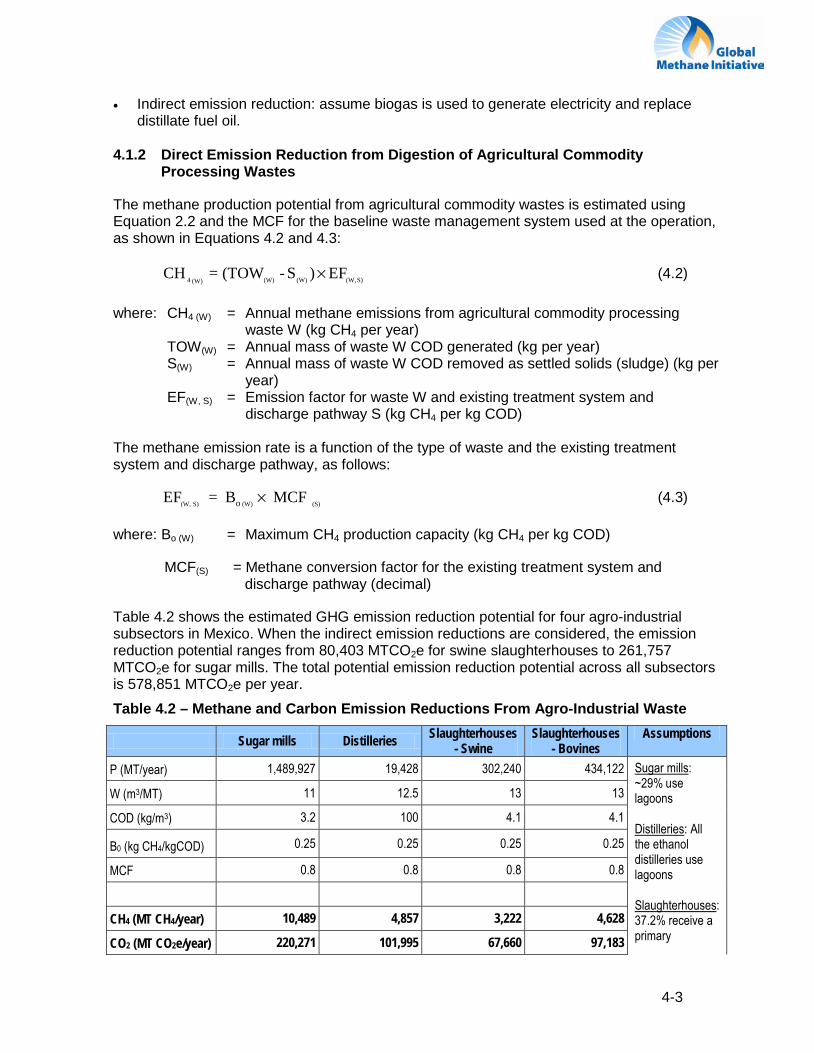
4.1.2 Direct Emission Reduction from Digestion of Agricultural Commodity Processing Wastes

The methane production potential from agricultural commodity wastes is estimated using Equation 2.2 and the MCF for the baseline waste management system used at the operation, as shown in Equations 4.2 and 4.3:

S) (W,(W)(W)(W)4 EF )S- (TOW=CH × (4.2) where: CH4 (W) = Annual methane emissions from agricultural commodity processing

waste W (kg CH4 per year) TOW(W) = Annual mass of waste W COD generated (kg per year) S(W) = Annual mass of waste W COD removed as settled solids (sludge) (kg per

year) EF(W, S) = Emission factor for waste W and existing treatment system and

discharge pathway S (kg CH4 per kg COD) The methane emission rate is a function of the type of waste and the existing treatment system and discharge pathway, as follows:

EF(W, S) = Bo (W) × MCF (S) (4.3) where: Bo (W) = Maximum CH4 production capacity (kg CH4 per kg COD)

MCF(S) = Methane conversion factor for the existing treatment system and discharge pathway (decimal)

Table 4.2 shows the estimated GHG emission reduction potential for four agro-industrial subsectors in Mexico. When the indirect emission reductions are considered, the emission reduction potential ranges from 80,403 MTCO2e for swine slaughterhouses to 261,757 MTCO2e for sugar mills. The total potential emission reduction potential across all subsectors is 578,851 MTCO2e per year.

Table 4.2 – Methane and Carbon Emission Reductions From Agro-Industrial Waste

Sugar mills Distilleries Slaughterhouses - Swine

Slaughterhouses - Bovines

Assumptions

P (MT/year) 1,489,927 19,428 302,240 434,122 Sugar mills

: ~29% use lagoons

Distilleries

: All the ethanol distilleries use lagoons

Slaughterhouses

W (m3/MT)

: 37.2% receive a primary

11 12.5 13 13

COD (kg/m3) 3.2 100 4.1 4.1

B0 (kg CH4/kgCOD) 0.25 0.25 0.25 0.25

MCF 0.8 0.8 0.8 0.8

CH4 (MT CH4/year) 10,489 4,857 3,222 4,628

CO2 (MT CO2e/year) 220,271 101,995 67,660 97,183

4-4

Sugar mills Distilleries Slaughterhouses - Swine

Slaughterhouses - Bovines

Assumptions

Indirect emission reduction (MTCO2e/yr)

41,487 19,210 12,743 18,304 treatment, of which 70% is assumed to be open lagoons Assumes biogas replaces distillate fuel oil

Total CO2 (MTCO2e/yr) 261,757 121,205 80,403 115,486

4.1.3 Indirect GHG Emission Reductions

The use of anaerobic digestion systems has the financial advantage of offsetting energy costs at the production facility. Biogas can be used to generate electricity or supplant the use of thermal fuels. Using biogas energy also reduces carbon emissions from the fossil fuels that are displaced by using the recovered biogas. The degree of emission reduction depends on how the biogas is used. Table 4.3 shows the potential uses of the biogas in each of the subsectors.

Table 4.3 – Potential Biogas Energy Use by Sector

Sector Electricity use Thermal energy replacement Swine Feed mills Liquefied Petroleum Gas (LPG) to heat

farrowing houses and nurseries Dairy farm Energy intensive, particularly during milking

operations LPG for water heating

Slaughterhouses Energy intensive—coolers, freezers, pumps, and general equipment.

Natural gas for water heating

Sugar/distilleries Energy intensive. Sugar mills don’t require electricity from the grid during harvest because they burn bagasse. However, they could sell electricity generated from captured methane.

Natural gas for steam generation. Large demand for steam, particularly for evaporation and crystallization operations.

When biogas is used to generate electricity, the emission reduction depends on the energy sources used by the central power company to power the generators. Table 4.4 shows the associated carbon emission reduction rate from the replacement of fossil fuels when biogas is used to generate electricity in Mexico.

Table 4.4 – Carbon Emissions by Type of Fuel Fuel Replaced CO2 Emissions Factors

Generating electricity—depends on fuel mix 100% coal 100% hydro or nuclear

1.02 kg/kWh from CH4 0 kg/kWh from CH4

Natural gas 2.01 kg/m3 CH4 LPG 2.26 kg/m3 CH4 Distillate fuel oil 2.65 kg/m3 CH4 Source: Developed by Hall Associates, Georgetown, Delaware USA.

4-5

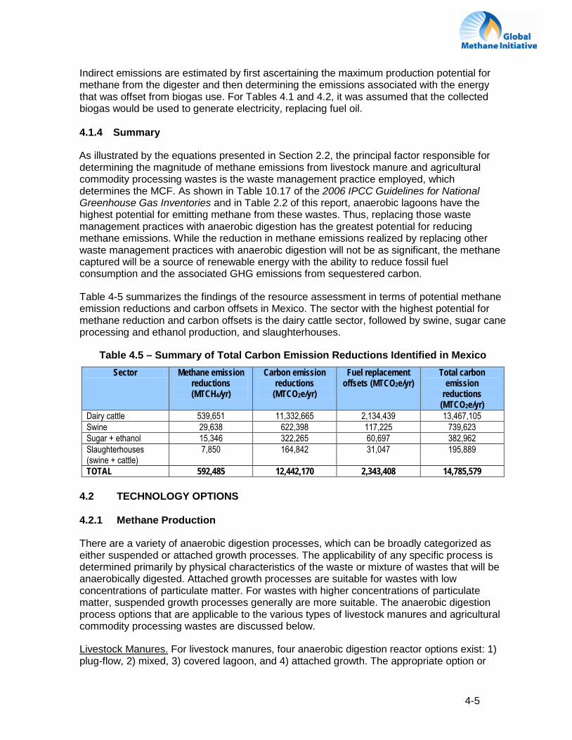
Indirect emissions are estimated by first ascertaining the maximum production potential for methane from the digester and then determining the emissions associated with the energy that was offset from biogas use. For Tables 4.1 and 4.2, it was assumed that the collected biogas would be used to generate electricity, replacing fuel oil.

4.1.4 Summary

As illustrated by the equations presented in Section 2.2, the principal factor responsible for determining the magnitude of methane emissions from livestock manure and agricultural commodity processing wastes is the waste management practice employed, which determines the MCF. As shown in Table 10.17 of the 2006 IPCC Guidelines for National Greenhouse Gas Inventories and in Table 2.2 of this report, anaerobic lagoons have the highest potential for emitting methane from these wastes. Thus, replacing those waste management practices with anaerobic digestion has the greatest potential for reducing methane emissions. While the reduction in methane emissions realized by replacing other waste management practices with anaerobic digestion will not be as significant, the methane captured will be a source of renewable energy with the ability to reduce fossil fuel consumption and the associated GHG emissions from sequestered carbon.

Table 4-5 summarizes the findings of the resource assessment in terms of potential methane emission reductions and carbon offsets in Mexico. The sector with the highest potential for methane reduction and carbon offsets is the dairy cattle sector, followed by swine, sugar cane processing and ethanol production, and slaughterhouses.

Table 4.5 – Summary of Total Carbon Emission Reductions Identified in Mexico Sector Methane emission

reductions (MTCH4/yr)

Carbon emission reductions

(MTCO2e/yr)

Fuel replacement offsets (MTCO2e/yr)

Total carbon emission

reductions (MTCO2e/yr)

Dairy cattle 539,651 11,332,665 2,134,439 13,467,105 Swine 29,638 622,398 117,225 739,623 Sugar + ethanol 15,346 322,265 60,697 382,962 Slaughterhouses (swine + cattle)

7,850 164,842 31,047 195,889

TOTAL 592,485 12,442,170 2,343,408 14,785,579

4.2 TECHNOLOGY OPTIONS

4.2.1 Methane Production

There are a variety of anaerobic digestion processes, which can be broadly categorized as either suspended or attached growth processes. The applicability of any specific process is determined primarily by physical characteristics of the waste or mixture of wastes that will be anaerobically digested. Attached growth processes are suitable for wastes with low concentrations of particulate matter. For wastes with higher concentrations of particulate matter, suspended growth processes generally are more suitable. The anaerobic digestion process options that are applicable to the various types of livestock manures and agricultural commodity processing wastes are discussed below.

Livestock Manures. For livestock manures, four anaerobic digestion reactor options exist: 1) plug-flow, 2) mixed, 3) covered lagoon, and 4) attached growth. The appropriate option or

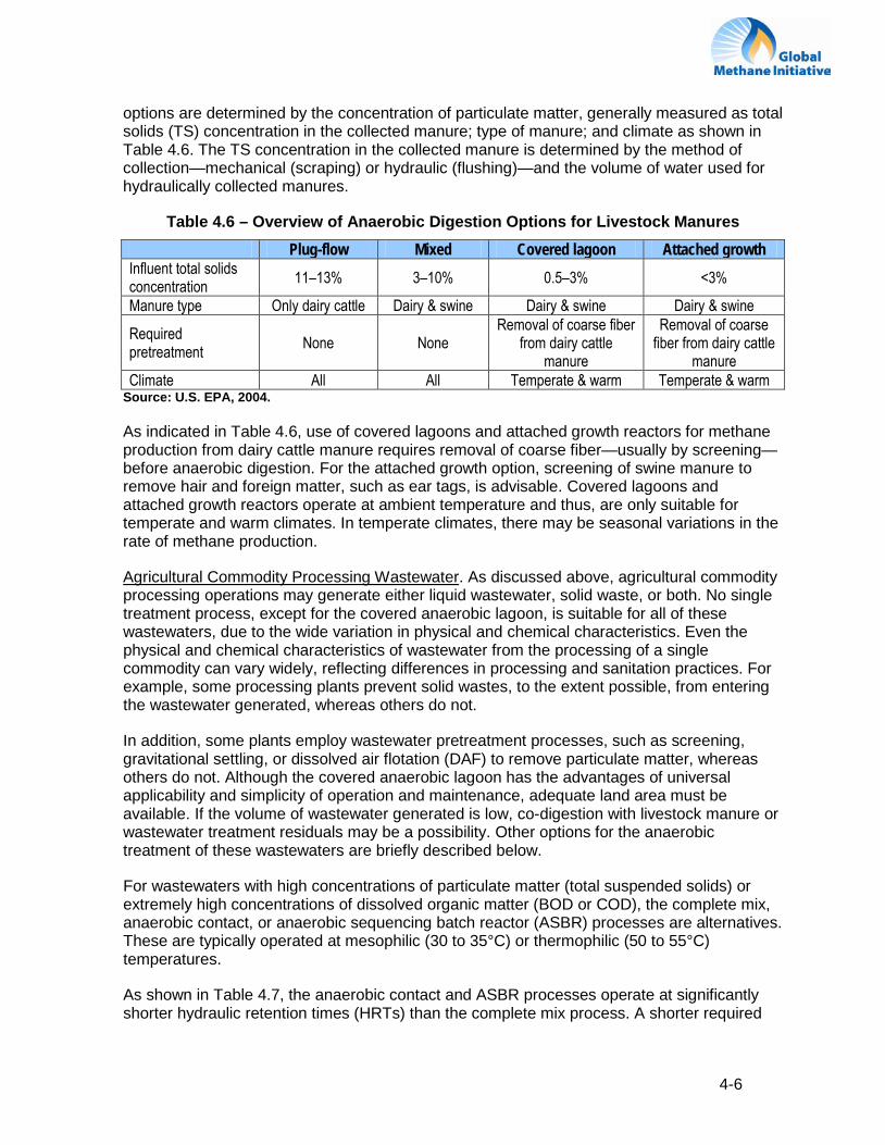
4-6

options are determined by the concentration of particulate matter, generally measured as total solids (TS) concentration in the collected manure; type of manure; and climate as shown in Table 4.6. The TS concentration in the collected manure is determined by the method of collection—mechanical (scraping) or hydraulic (flushing)—and the volume of water used for hydraulically collected manures.

Table 4.6 – Overview of Anaerobic Digestion Options for Livestock Manures

Plug-flow Mixed Covered lagoon Attached growth Influent total solids concentration 11–13% 3–10% 0.5–3% <3%

Manure type Only dairy cattle Dairy & swine Dairy & swine Dairy & swine

Required pretreatment None None

Removal of coarse fiber from dairy cattle

manure

Removal of coarse fiber from dairy cattle

manure Climate All All Temperate & warm Temperate & warm

Source: U.S. EPA, 2004.

As indicated in Table 4.6, use of covered lagoons and attached growth reactors for methane production from dairy cattle manure requires removal of coarse fiber—usually by screening—before anaerobic digestion. For the attached growth option, screening of swine manure to remove hair and foreign matter, such as ear tags, is advisable. Covered lagoons and attached growth reactors operate at ambient temperature and thus, are only suitable for temperate and warm climates. In temperate climates, there may be seasonal variations in the rate of methane production.

Agricultural Commodity Processing Wastewater

In addition, some plants employ wastewater pretreatment processes, such as screening, gravitational settling, or dissolved air flotation (DAF) to remove particulate matter, whereas others do not. Although the covered anaerobic lagoon has the advantages of universal applicability and simplicity of operation and maintenance, adequate land area must be available. If the volume of wastewater generated is low, co-digestion with livestock manure or wastewater treatment residuals may be a possibility. Other options for the anaerobic treatment of these wastewaters are briefly described below.

. As discussed above, agricultural commodity processing operations may generate either liquid wastewater, solid waste, or both. No single treatment process, except for the covered anaerobic lagoon, is suitable for all of these wastewaters, due to the wide variation in physical and chemical characteristics. Even the physical and chemical characteristics of wastewater from the processing of a single commodity can vary widely, reflecting differences in processing and sanitation practices. For example, some processing plants prevent solid wastes, to the extent possible, from entering the wastewater generated, whereas others do not.

For wastewaters with high concentrations of particulate matter (total suspended solids) or extremely high concentrations of dissolved organic matter (BOD or COD), the complete mix, anaerobic contact, or anaerobic sequencing batch reactor (ASBR) processes are alternatives. These are typically operated at mesophilic (30 to 35°C) or thermophilic (50 to 55°C) temperatures.

As shown in Table 4.7, the anaerobic contact and ASBR processes operate at significantly shorter hydraulic retention times (HRTs) than the complete mix process. A shorter required

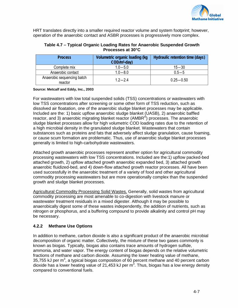
4-7

HRT translates directly into a smaller required reactor volume and system footprint; however, operation of the anaerobic contact and ASBR processes is progressively more complex.

Table 4.7 – Typical Organic Loading Rates for Anaerobic Suspended Growth Processes at 30°C

Process Volumetric organic loading (kg COD/m3-day)

Hydraulic retention time (days)

Complete mix 1.0―5.0 15―30 Anaerobic contact 1.0―8.0 0.5―5

Anaerobic sequencing batch reactor 1.2―2.4 0.25―0.50

Source: Metcalf and Eddy, Inc., 2003

For wastewaters with low total suspended solids (TSS) concentrations or wastewaters with low TSS concentrations after screening or some other form of TSS reduction, such as dissolved air floatation, one of the anaerobic sludge blanket processes may be applicable. Included are the: 1) basic upflow anaerobic sludge blanket (UASB), 2) anaerobic baffled reactor, and 3) anaerobic migrating blanket reactor (AMBR®) processes. The anaerobic sludge blanket processes allow for high volumetric COD loading rates due to the retention of a high microbial density in the granulated sludge blanket. Wastewaters that contain substances such as proteins and fats that adversely affect sludge granulation, cause foaming, or cause scum formation are problematic. Thus, use of anaerobic sludge blanket processes generally is limited to high-carbohydrate wastewaters.

Attached growth anaerobic processes represent another option for agricultural commodity processing wastewaters with low TSS concentrations. Included are the:1) upflow packed-bed attached growth, 2) upflow attached growth anaerobic expanded bed, 3) attached growth anaerobic fluidized-bed, and 4) down-flow attached growth reactor processes. All have been used successfully in the anaerobic treatment of a variety of food and other agricultural commodity processing wastewaters but are more operationally complex than the suspended growth and sludge blanket processes.

Agricultural Commodity Processing Solid Wastes.

4.2.2 Methane Use Options

Generally, solid wastes from agricultural commodity processing are most amenable to co-digestion with livestock manure or wastewater treatment residuals in a mixed digester. Although it may be possible to anaerobically digest some of these wastes independently, the addition of nutrients, such as nitrogen or phosphorus, and a buffering compound to provide alkalinity and control pH may be necessary.

In addition to methane, carbon dioxide is also a significant product of the anaerobic microbial decomposition of organic matter. Collectively, the mixture of these two gases commonly is known as biogas. Typically, biogas also contains trace amounts of hydrogen sulfide, ammonia, and water vapor. The energy content of biogas depends on the relative volumetric fractions of methane and carbon dioxide. Assuming the lower heating value of methane, 35,755 kJ per m3, a typical biogas composition of 60 percent methane and 40 percent carbon dioxide has a lower heating value of 21,453 kJ per m3. Thus, biogas has a low energy density compared to conventional fuels.

4-8

Although the principal objective of the anaerobic digestion of livestock manure and agricultural commodity processing wastes is to reduce methane emissions to the atmosphere, biogas has value as a renewable fuel. It can be used in place of a fossil fuel in stationary internal combustion engines or microturbines connected to generator sets or pumps, and for water or space heating. Direct use for cooling or refrigeration is also a possibility.

Use of biogas in place of coal, natural gas, liquefied petroleum gas (LPG), or distillate or heavy fuel oil for water or space heating is the most attractive option due to simplicity and the possibility of utilizing existing boilers or furnaces modified to burn a lower energy density fuel. Conversion of a natural gas- or LPG-fueled boiler or furnace to a biogas furnace generally only requires replacement of the existing metal combustion assembly with a ceramic burner assembly with larger orifices. If there is seasonal variation in demand for water or space heating, biogas compression and storage is an option that should be considered if the cost of suitable storage can be justified.

Using biogas to fuel a modified natural gas internal combustion engine or microturbine to generate electricity is more complex. Livestock manures and most agricultural commodity processing wastes contain sulfur compounds, which are reduced to hydrogen sulfide during anaerobic digestion. Thus, hydrogen sulfide, in trace amounts, is a common constituent of biogas and can cause serious corrosion problems in biogas-fueled internal combustion engines and microturbines. Hydrogen sulfide combines with the water produced during combustion to form sulfuric acid. Consequently, scrubbing to remove hydrogen sulfide may be necessary when biogas is used to generate electricity.

Using biogas to generate electricity also may require interconnection with the local electricity provider for periods when electricity demand exceeds biogas generation capacity, when generation capacity exceeds demand, or when generator shutdown for maintenance or repairs is necessary. One of the advantages of using biogas to generate electricity connected to the grid is the ability to use biogas as it is produced and use the local electricity grid to dispose of excess electrical energy when generation capacity exceeds onsite demand. Specifically in the case of Mexico, the Ministry of Energy is promoting an initiative that aims to supply at least 8 percent of the total national energy consumption through renewable energy systems by 2016. Mexico has developed several tariff rates to support new electricity generation projects. The use of biogas to generate electricity not only will reduce farm operating costs, but also will provide a steady revenue stream for the farm.

When avoided methane emissions and associated carbon credits are considered, simply flaring biogas produced from the anaerobic digestion of livestock manures and agricultural commodity processing wastes also can be considered an option. However, this can be considered an option only to the degree that replacing the current methane-emitting waste management practice with anaerobic digestion reduces methane emissions. Although systems utilizing biogas from anaerobic digestion as a boiler or furnace fuel or for generating electricity should have the ability to flare excess biogas, flaring should be considered an option only if biogas production greatly exceeds the opportunity for utilization.

4.3 COSTS AND POTENTIAL BENEFITS

The cost of anaerobically digesting livestock manures and agricultural commodity processing wastes and utilizing the methane captured as a fuel depends on the type of digester constructed and the methane utilization option employed. In addition, these costs will vary geographically, reflecting local financing, material, and labor costs. However, it can be

4-9

assumed that capital costs will increase as the level of technology employed increases. For digestion, the covered anaerobic lagoon generally will require the lowest capital investment, with anaerobic sludge blanket and attached growth processes requiring the highest. As the complexity of the anaerobic digestion process increases, operating and maintenance costs also increase. For example, only basic management and operating skills are required for covered lagoon operation, whereas a more sophisticated level of understanding of process fundamentals is required for anaerobic sludge blanket and attached growth processes.

For captured methane utilization, the required capital investment for flaring will be the lowest and generating electricity the will be highest. Based on past projects developed in the United States and Latin America, the cost of an engine-generator set will be at least 25 percent of total project cost, including the anaerobic digester. In addition, while the operating and maintenance costs for flaring are minimal, they can be substantial for generating electricity. For example, using captured biogas to generate electricity requires a continuous engine-generator set maintenance program and may include operation and maintenance of a biogas hydrogen sulfide removal process.

4.3.2 Potential Benefits

Anaerobic digestion of livestock manure and agricultural commodity processing wastes can generate revenue to at least offset and ideally exceed capital and operation and maintenance costs. There are three potential sources of revenue. The first is the carbon credits that can be realized from the reduction of methane emissions by the addition of anaerobic digestion. MCFs, and therefore reduction in methane emissions and the accompanying carbon credits earned, are determined by the existing waste management system and vary from essentially 0 to 100 percent. Thus, carbon credits will be a significant source of revenue for some projects and nearly nothing for others.

The second potential source of revenue is from the use of the biogas captured as a fuel. However, the revenue realized depends on the value of the form of energy replaced and its local cost. Because biogas has no market-determined monetary value, the revenue realized from its use in place of a conventional source of energy is determined by the cost of the conventional source of energy replaced. If low-cost hydropower-generated electricity is available, the revenue derived from using biogas to generate electricity may not justify the required capital investment and operating and maintenance costs. Another factor that must be considered in evaluating the use of biogas to generate electricity is the ability to sell excess electricity to the local electricity provider and the price that would be paid. There may be a substantial difference between the value of electricity used on site and the value of electricity delivered to the local grid. The latter may not be adequate to justify the use of biogas to generate electricity. Ideally, the ability to deliver excess generation to the local grid during periods of low on-site demand and the subsequent ability to reclaim it during periods of high on-site demand under some type of a net metering contract should exist.

The third potential source of revenue is from the carbon credits realized from the reduction in the fossil fuel carbon dioxide emissions when use of biogas reduces fossil fuel use. As with the revenue derived directly from using biogas as a fuel, the carbon credits generated depend on the fossil fuel replaced. In using biogas to generate electricity, the magnitude of the reduction in fossil fuel-related carbon dioxide emissions will depend on the fuel mix used to generate the electricity replaced. Thus, the fuel mix will have to be determined to support the validity of the carbon credits claimed.

4-10

4.4 CENTRALIZED PROJECTS

Generally, small livestock production and agricultural commodity processing enterprises are not suitable candidates for anaerobic digestion to reduce methane emissions from their waste streams due to high capital and operating costs. The same is true for enterprises that only generate wastes seasonally. If all of the enterprises are located in a reasonably small geographical area, combining compatible wastes from two or more enterprises for anaerobic digestion located at one of the waste sources or a centralized location is a possible option. By increasing project scale, unit capital cost will be reduced. However, operating costs will increase and centralized digestion will not always be a viable option if the ability to generate adequate revenue to at least offset the increased operating costs is lacking.

There are two possible models for centralized anaerobic digestion projects. In the first model, digestion occurs at one of the sources of waste, with the waste from the other generators transported to that site. In the model that typically is followed, wastes from one or more agricultural commodity processing operations are co-digested with livestock manure. In the second model, wastes from all sources are transported to a separate site for digestion. The combination of the geographic distribution of waste sources and the options for maximizing revenue from the captured methane should be the basis for determining which model should receive further consideration in the analysis of a specific situation.

For centralized anaerobic digestion projects, the feasibility analysis should begin with the determination of a project location that will minimize transportation requirements for the wastes to be anaerobically digested and for the effluent to be disposed. The optimal digester location could be determined by trial and error, but constructing and applying a simple transportation model would be a more efficient approach. Although obtaining the optimal solution manually is possible, use of linear programming should be considered. With this approach, optimal locations with respect to minimizing transportation costs for a number of scenarios can be obtained and compared. For example, the transportation costs associated with locating the anaerobic digester at the largest waste generator versus a geographically central location can be delineated and compared.

Next, the revenue that will be generated from the selling the carbon credits realized from reducing methane emissions and utilizing the captured methane as a fuel should be estimated. The latter will depend on a number of factors, including the location of the digester and opportunities to use the captured methane in place of conventional sources of energy. Generally, captured methane that can be used to meet on-site electricity or heating demand will have the greatest monetary value and produce the most revenue to at least offset and ideally exceed system capital and operation and maintenance costs. Thus, an energy-use profile for each source of waste in a possible centralized system should be developed to determine the potential for on-site methane use, the revenue that would be realized, and the allocation of this revenue among the waste sources. .

Ideally, the digester location that minimizes transportation costs will be at the waste source with the highest on-site opportunity for methane utilization. Thus, waste transportation costs will be minimized while revenue will be maximized. However, the digester location that minimizes transportation costs may not maximize revenue from methane utilization due to low on-site energy demand. Thus, alternative digester locations should be evaluated to identify the location that maximizes the difference between revenue generation from methane utilization and transportation cost. Again, using a simple transportation-type model to determine the optimal digester location is recommended. If the optimal location is not at one

4-11

of the waste sources, additional analysis incorporating site acquisition costs will be necessary.

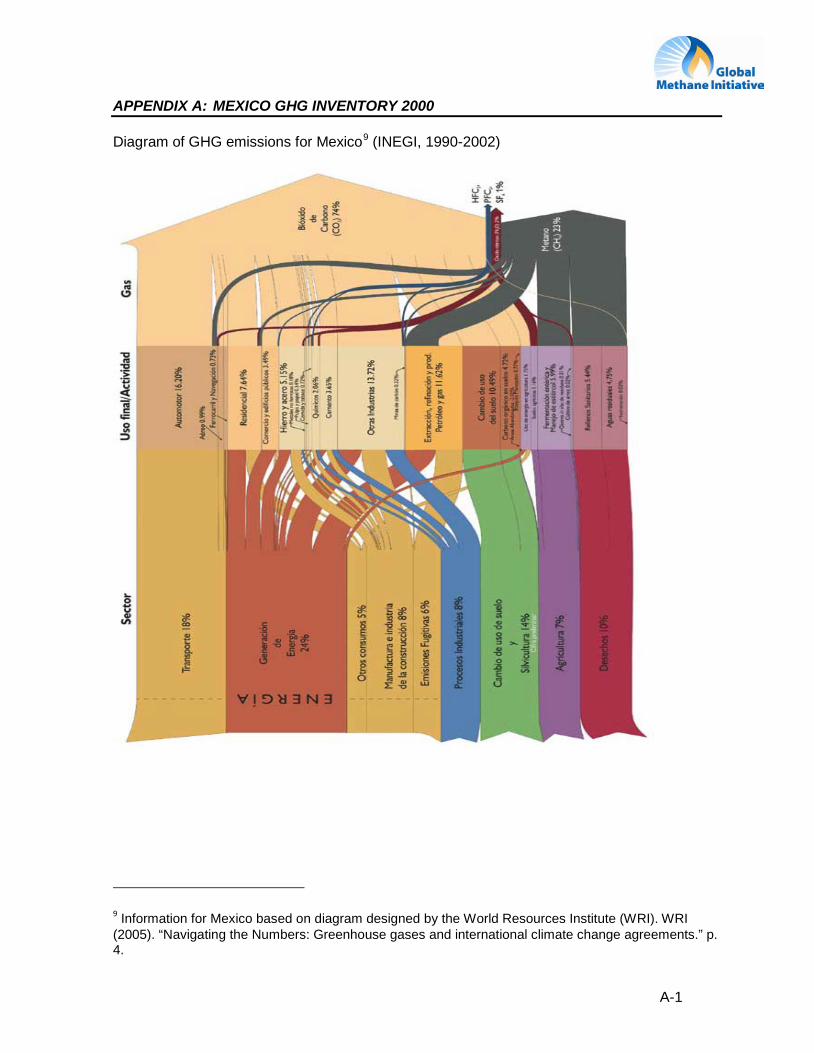
A-1

APPENDIX A: MEXICO GHG INVENTORY 2000

Diagram of GHG emissions for Mexico9 (INEGI, 1990-2002)

9 Information for Mexico based on diagram designed by the World Resources Institute (WRI). WRI (2005). “Navigating the Numbers: Greenhouse gases and international climate change agreements.” p. 4.

B-1

APPENDIX B: LEGISLATION IN MEXICO

The rulings applied in Mexico where permissible limits are established for wastewater discharges to different receiving bodies are mentioned below.

"Mexican Official Standard NOM-002-ECOL-1993, which establishes maximum permissible limits of pollutants in wastewater discharges to receiving bodies coming from the sugarcane producer industry."

"Mexican Official Standard NOM-007-ECOL-1993, which establishes maximum permissible limits of pollutants in wastewater discharges to receiving bodies coming from the beer and the malt industries."

"Mexican Official Standard NOM-009-ECOL-1993, which establishes maximum permissible limits of pollutants in wastewater discharges to receiving bodies coming from the milk and derivatives industry."

"Mexican Official Standard NOM-022-ECOL-1993, which establishes maximum permissible limits of pollutants in wastewater discharges to receiving bodies coming from the animal slaughtering and packed meat products industry."

"Mexican Official Standard NOM-023-ECOL-1993, which establishes maximum permissible limits of pollutants in wastewater discharges to receiving bodies coming from the canned food packaging."

"Mexican Official Standard NOM-027-ECOL-1993, which establishes maximum permissible limits of pollutants in wastewater discharges to receiving bodies coming from the coffee processing industry."

The environmental legislation associated with livestock operations is framed by the General Law for Ecological Balance and Atmospheric Protection (LGEEPA), published in 1988. This law establishes that wastewater discharges from agriculture and livestock activities are subjected to federal and local regulation (Article 120, II) and that discharges into the sewage systems of cities and receiving water bodies, as well as those spilled on the ground or that filter into groundwater, must comply with the necessary conditions for avoiding water pollution. Accordingly, Comisión Nacional del Agua (CONAGUA), in coordination with state and municipal authorities, is responsible for establishing the conditions for waste discharges, issuing permits and licenses for water use and discharge, and establishing and enforcing the corresponding Mexican official standards.

Regarding wastewater discharges, SEMARNAT has published two Mexican official standards applicable to livestock operations:

• NOM-001-ECOL-1996, which establishes the maximum permissible limits of pollutants in wastewater discharges into national water and goods.

• NOM-002-ECOL-1996, which establishes the maximum permissible limits of pollutants in discharges into the urban and municipal sewage systems.

NOM-001 regulates the receiving body and not the activity that carries out the discharge, establishing the maximum permissible levels as a function of two elements: receiving body (rivers, natural and artificial dams, coast waters, soil and natural wetlands) and the subsequent use of the water (agriculture irrigation or urban public supply). Thus, monitoring

APPENDIX B..LEGISLATION IN MEXICO

B-2

the wastewater quality is done prior to the discharge into receiving bodies. Further, the application of NOM-001 is gradual, according to the measured pollutant load based on the biochemical oxygen discharge (BOD) or the total suspended solids (TSS).

At state level, environmental laws regulate mainly the wastewater discharges from agriculture and livestock uses, and in most cases, the authorization of permits and the verification of its compliance is transferred to the municipal governments.

It is worth mentioning that the Law of Livestock of the state of Michoacán, published in 2007, establishes in its Article 106 that the Secretary of Rural Development of the state, in coordination with local livestock organizations, will establish agreed upon mandatory programs of excreta management in relevant localities according to their animal concentrations and will supervise their compliance. At the municipal level, several environmental rulings require the treatment of cattle manure, and the treatment, use, and disposal systems shall be authorized by the municipal institutions.

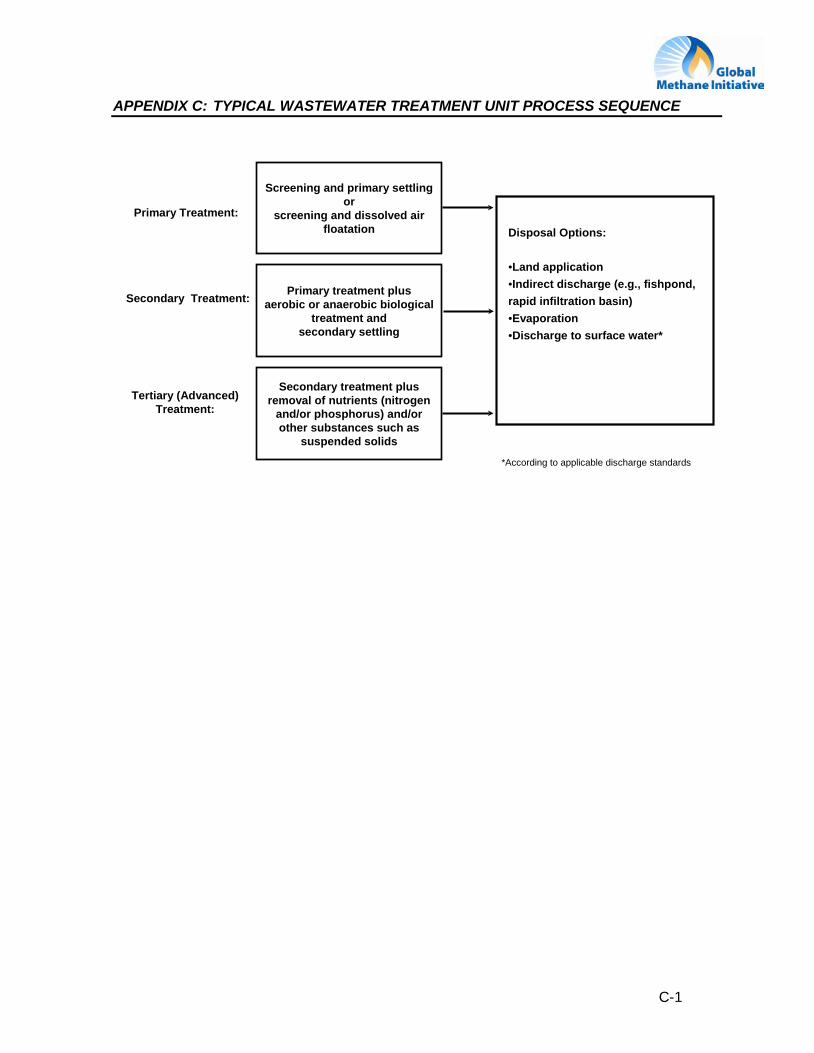
C-1

APPENDIX C: TYPICAL WASTEWATER TREATMENT UNIT PROCESS SEQUENCE

Primary Treatment:

Secondary Treatment:

Tertiary (Advanced) Treatment:

Secondary treatment plus removal of nutrients (nitrogen

and/or phosphorus) and/or other substances such as

suspended solids

Screening and primary settling or

screening and dissolved air floatation

Primary treatment plus aerobic or anaerobic biological

treatment and secondary settling

*According to applicable discharge standards

•Land application •Indirect discharge (e.g., fishpond, rapid infiltration basin)•Evaporation•Discharge to surface water*

Disposal Options:

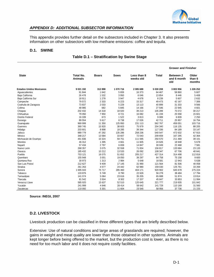
D-1

APPENDIX D: ADDITIONAL SUBSECTOR INFORMATION

This appendix provides further detail on the subsectors included in Chapter 3. It also presents information on other subsectors with low methane emissions: coffee and tequila.

D.1. SWINE Table D.1 – Stratification by Swine Stage

Source: INEGI, 2007

D.2. LIVESTOCK

Livestock production can be classified in three different types that are briefly described below.

Extensive: Use of natural conditions and large areas of grasslands are required; however, the gains in weight and meat quality are lower than those obtained in other systems. Animals are kept longer before being offered to the market, but the production cost is lower, as there is no need for too much labor and it does not require costly facilities.

Grower and Finisher

State Total No. Animals

Boars Sows Less than 8 weeks old

Total Between 2 and 6 month old

Older than 6 months

Estados Unidos Mexicanos 9 021 192 312 898 1 070 716 2 085 688 5 030 208 3 803 956 1 226 252 Aguascalientes 91 844 1 642 5 659 16 373 64 467 58 860 5 607 Baja California 26 478 1 532 3 950 6 046 13 854 8 446 5 408 Baja California Sur 18 911 1 278 3 947 4 678 8 239 5 607 2 632 Campeche 79 572 2 333 6 223 15 317 49 473 42 167 7 306 Coahuila de Zaragoza 73 837 2 033 5 229 13 113 40 899 31 333 9 566 Colima 48 985 682 5 845 14 166 27 546 22 945 4 601 Chiapas 202 432 14 318 18 020 39 213 105 289 75 072 30 217 Chihuahua 79 050 7 950 8 721 16 082 41 159 25 558 15 601 Distrito Federal 16 339 673 1 522 3 813 9 089 6 839 2 250 Durango 89 554 5 617 8 738 17 026 42 711 25 957 16 754 Guanajuato 969 999 11 350 125 950 231 113 562 767 459 051 103 716 Guerrero 369 745 15 920 38 603 75 979 204 340 116 135 88 205 Hidalgo 203 601 8 898 18 285 39 344 117 336 84 189 33 147 Jalisco 989 779 47 292 135 286 258 236 540 547 472 632 67 915 México 348 217 13 584 33 607 72 043 209 659 167 295 42 364 Michoacán de Ocampo 451 836 10 324 59 751 111 595 250 570 211 469 39 101 Morelos 46 312 1 395 4 661 11 605 24 626 18 948 5 678 Nayarit 57 434 2 797 6 659 14 847 30 049 22 468 7 581 Nuevo León 268 357 3 075 32 558 71 834 156 817 133 684 23 133 Oaxaca 185 432 10 212 13 533 26 092 108 347 67 706 40 641 Puebla 753 121 16 075 51 652 205 217 427 314 314 498 112 816 Querétaro 155 948 3 001 19 050 39 297 84 758 75 158 9 600 Quintana Roo 30 973 1 313 2 984 5 648 18 581 12 943 5 638 San Luis Potosí 212 627 9 409 17 145 31 990 121 564 81 506 40 058 Sinaloa 261 263 4 577 24 442 62 980 159 030 125 761 33 269 Sonora 1 695 043 75 717 285 460 404 171 920 902 645 678 275 224 Tabasco 133 876 5 749 8 790 22 626 56 278 38 484 17 794 Tamaulipas 141 074 5 064 23 616 35 205 65 688 51 874 13 814 Tlaxcala 81 542 3 504 8 302 17 207 45 847 33 853 11 994 Veracruz Llave 585 920 15 637 52 510 120 645 321 777 219 935 101 842 Yucatán 241 999 4 646 28 414 58 642 141 729 110 169 31 560 Zacatecas 110 092 5 301 11 604 23 545 58 956 37 736 21 220

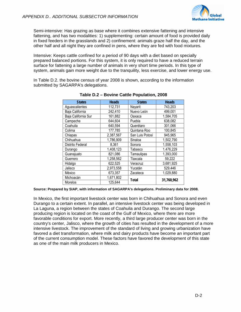
APPENDIX D.. ADDITIONAL SUBSECTOR INFORMATION

D-2

Semi-intensive: Has grazing as base where it combines extensive fattening and intensive fattening, and has two modalities: 1) supplementing: certain amount of food is provided daily in fixed feeders in the grasslands and 2) confinement: animals graze half the day, and the other half and all night they are confined in pens, where they are fed with food mixtures.

Intensive: Keeps cattle confined for a period of 90 days with a diet based on specially prepared balanced portions. For this system, it is only required to have a reduced terrain surface for fattening a large number of animals in very short time periods. In this type of system, animals gain more weight due to the tranquility, less exercise, and lower energy use.

In Table D.2. the bovine census of year 2008 is shown, according to the information submitted by SAGARPA's delegations.

Table D.2 – Bovine Cattle Population, 2008 States Heads States Heads

Aguascalientes 112,731 Nayarit 743,203 Baja California 242,410 Nuevo León 499,001 Baja California Sur 161,882 Oaxaca 1,584,705 Campeche 644,604 Puebla 638,082 Coahuila 640,594 Querétaro 301,066 Colima 177,785 Quintana Roo 100,845 Chiapas 2,387,567 San Luis Potosí 945,965 Chihuahua 1,786,909 Sinaloa 1,502,790 Distrito Federal 8,361 Sonora 1,558,103 Durango 1,408,123 Tabasco 1,476,229 Guanajuato 821,086 Tamaulipas 1,393,000 Guerrero 1,258,562 Tlaxcala 59,222 Hidalgo 622,525 Veracruz 3,681,925 Jalisco 2,973,558 Yucatán 529,446 México 673,357 Zacateca 1,029,880 Michoacán 1,671,802 Total 31,760,962 Morelos 125,644

Source: Prepared by SIAP, with information of SAGARPA's delegations. Preliminary data for 2008.

In Mexico, the first important livestock center was born in Chihuahua and Sonora and even Durango to a certain extent. In parallel, an intensive livestock center was being developed in La Laguna, a region between the states of Coahuila and Durango. The second large producing region is located on the coast of the Gulf of Mexico, where there are more favorable conditions for export. More recently, a third large producer center was born in the country's center, Jalisco, where the growth of cities has resulted in the development of a more intensive livestock. The improvement of the standard of living and growing urbanization have favored a diet transformation, where milk and dairy products have become an important part of the current consumption model. These factors have favored the development of this state as one of the main milk producers in Mexico.

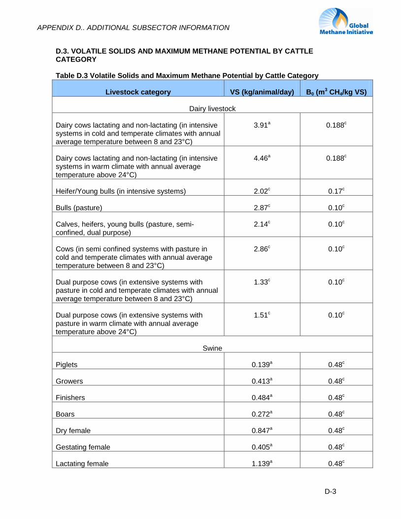
APPENDIX D.. ADDITIONAL SUBSECTOR INFORMATION

D-3

D.3. VOLATILE SOLIDS AND MAXIMUM METHANE POTENTIAL BY CATTLE CATEGORY

Table D.3 Volatile Solids and Maximum Methane Potential by Cattle Category

Livestock category VS (kg/animal/day) B0 (m3 CH4/kg VS)

Dairy livestock

Dairy cows lactating and non-lactating (in intensive systems in cold and temperate climates with annual average temperature between 8 and 23°C)

3.91a 0.188c

Dairy cows lactating and non-lactating (in intensive systems in warm climate with annual average temperature above 24°C)

4.46a 0.188c

Heifer/Young bulls (in intensive systems) 2.02c 0.17c

Bulls (pasture) 2.87c 0.10c

Calves, heifers, young bulls (pasture, semi-confined, dual purpose)

2.14c 0.10c

Cows (in semi confined systems with pasture in cold and temperate climates with annual average temperature between 8 and 23°C)

2.86c 0.10c

Dual purpose cows (in extensive systems with pasture in cold and temperate climates with annual average temperature between 8 and 23°C)

1.33c 0.10c

Dual purpose cows (in extensive systems with pasture in warm climate with annual average temperature above 24°C)

1.51c 0.10c

Swine

Piglets 0.139a 0.48c

Growers 0.413a 0.48c

Finishers 0.484a 0.48c

Boars 0.272a 0.48c

Dry female 0.847a 0.48c

Gestating female 0.405a 0.48c

Lactating female 1.139a 0.48c

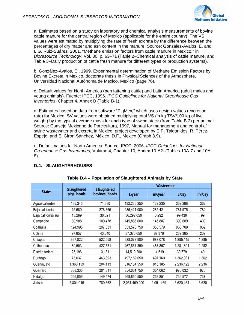
APPENDIX D.. ADDITIONAL SUBSECTOR INFORMATION

D-4

a. Estimates based on a study on laboratory and chemical analysis measurements of bovine cattle manure for the central region of Mexico (applicable for the entire country). The VS values were estimated by multiplying the rate of fresh excreta by the difference between the percentages of dry matter and ash content in the manure. Source: González-Ávalos, E. and L.G. Ruiz-Suárez, 2001. "Methane emission factors from cattle manure in Mexico," in Bioresource Technology, Vol. 80, p. 63–71 (Table 2–Chemical analysis of cattle manure, and Table 3–Daily production of cattle fresh manure for different types or production systems).

b. González-Ávalos, E., 1999. Experimental determination of Methane Emission Factors by Bovine Excreta in Mexico, doctorate thesis in Physical Sciences of the Atmosphere, Universidad Nacional Autónoma de Mexico, Mexico (page 76).

c. Default values for North America (pen fattening cattle) and Latin America (adult males and young animals). Fuente: IPCC, 1996. IPCC Guidelines for National Greenhouse Gas Inventories, Chapter 4, Annex B (Table B-1).

d. Estimates based on data from software “PigMex,” which uses design values (excretion rate) for Mexico. SV values were obtained multiplying total VS (in kg TSV/100 kg of live weight) by the typical average mass for each type of swine stock (from Table B.2) per animal. Source: Consejo Mexicano de Porcicultura, 1997, Manual for management and control of swine wastewater and excreta in Mexico, project developed by E.P. Taiganides, R. Pérez-Espejo, and E. Girón-Sánchez, México, D.F., Mexico (Graph 3.9).

e. Default values for North America. Source: IPCC, 2006. IPCC Guidelines for National Greenhouse Gas Inventories, Volume 4, Chapter 10, Annex 10-A2. (Tables 10A-7 and 10A-8).

D.4. SLAUGHTERHOUSES

Table D.4 – Population of Slaughtered Animals by State

States Slaughtered pigs, heads

Slaughtered bovines, heads

Wastewater

L/year m3/year L/day m3/day

Aguascalientes 135,345 71,330 132,235,250 132,235 362,288 362 Baja california 15,680 278,365 285,421,000 285,421 781,975 782 Baja california sur 13,269 30,321 36,292,050 6,292 99,430 99 Campeche 80,908 109,478 145,886,600 145,887 399,689 400 Coahuila 124,995 297,331 353,578,750 353,579 968,709 969 Colima 97,857 43,340 87,375,650 87,376 239,385 239 Chiapas 367,822 522,558 688,077,900 688,078 1,885,145 1,885 Chihuahua 89,503 427,581 467,857,350 467,857 1,281,801 1,282 Distrito federal 25,196 3,181 14,519,200 14,519 39,779 40 Durango 75,037 463,393 497,159,650 497,160 1,362,081 1,362 Guanajuato 1,360,159 204,113 816,184,550 816,185 2,236,122 2,236 Guerrero 338,335 201,811 354,061,750 354,062 970,032 970 Hidalgo 265,059 149,574 268,850,550 268,851 736,577 737 Jalisco 2,804,016 789,662 2,051,469,200 2,051,469 5,620,464 5,620

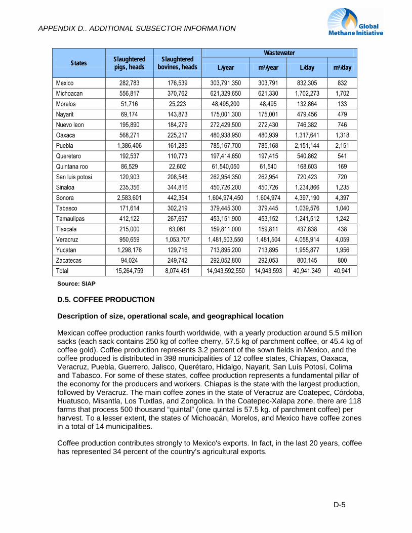
APPENDIX D.. ADDITIONAL SUBSECTOR INFORMATION

D-5

States Slaughtered pigs, heads

Slaughtered bovines, heads

Wastewater

L/year m3/year L/day m3/day

Mexico 282,783 176,539 303,791,350 303,791 832,305 832 Michoacan 556,817 370,762 621,329,650 621,330 1,702,273 1,702 Morelos 51,716 25,223 48,495,200 48,495 132,864 133 Nayarit 69,174 143,873 175,001,300 175,001 479,456 479 Nuevo leon 195,890 184,279 272,429,500 272,430 746,382 746 Oaxaca 568,271 225,217 480,938,950 480,939 1,317,641 1,318 Puebla 1,386,406 161,285 785,167,700 785,168 2,151,144 2,151 Queretaro 192,537 110,773 197,414,650 197,415 540,862 541 Quintana roo 86,529 22,602 61,540,050 61,540 168,603 169 San luis potosi 120,903 208,548 262,954,350 262,954 720,423 720 Sinaloa 235,356 344,816 450,726,200 450,726 1,234,866 1,235 Sonora 2,583,601 442,354 1,604,974,450 1,604,974 4,397,190 4,397 Tabasco 171,614 302,219 379,445,300 379,445 1,039,576 1,040 Tamaulipas 412,122 267,697 453,151,900 453,152 1,241,512 1,242 Tlaxcala 215,000 63,061 159,811,000 159,811 437,838 438 Veracruz 950,659 1,053,707 1,481,503,550 1,481,504 4,058,914 4,059 Yucatan 1,298,176 129,716 713,895,200 713,895 1,955,877 1,956 Zacatecas 94,024 249,742 292,052,800 292,053 800,145 800 Total 15,264,759 8,074,451 14,943,592,550 14,943,593 40,941,349 40,941

Source: SIAP

D.5. COFFEE PRODUCTION

Description of size, operational scale, and geographical location

Mexican coffee production ranks fourth worldwide, with a yearly production around 5.5 million sacks (each sack contains 250 kg of coffee cherry, 57.5 kg of parchment coffee, or 45.4 kg of coffee gold). Coffee production represents 3.2 percent of the sown fields in Mexico, and the coffee produced is distributed in 398 municipalities of 12 coffee states, Chiapas, Oaxaca, Veracruz, Puebla, Guerrero, Jalisco, Querétaro, Hidalgo, Nayarit, San Luís Potosí, Colima and Tabasco. For some of these states, coffee production represents a fundamental pillar of the economy for the producers and workers. Chiapas is the state with the largest production, followed by Veracruz. The main coffee zones in the state of Veracruz are Coatepec, Córdoba, Huatusco, Misantla, Los Tuxtlas, and Zongolica. In the Coatepec-Xalapa zone, there are 118 farms that process 500 thousand “quintal” (one quintal is 57.5 kg. of parchment coffee) per harvest. To a lesser extent, the states of Michoacán, Morelos, and Mexico have coffee zones in a total of 14 municipalities.

Coffee production contributes strongly to Mexico's exports. In fact, in the last 20 years, coffee has represented 34 percent of the country’s agricultural exports.

APPENDIX D.. ADDITIONAL SUBSECTOR INFORMATION

D-6

According to Figure D.1, a production volume in a range between 1 and 102,427 MT is distributed in the states of Colima, Guerrero, Hidalgo, Jalisco, México, Michoacán, Morelos, Nayarit Querétaro, San Luis Potosí, and Tabasco.

Figure D.1 – Range and Location of Coffee Producers

Source: www.campomexicano.gob.mx/portal_sispro/index.php?portal=cafe

In Oaxaca there are more coffee municipalities (139); however, the highest production (409,708 MT) is distributed between Chiapas municipalities. One of the distinctive characteristics of Mexican coffee culture is its contrast in all the stages of the production chain. There is a large difference in the scale of the farms; 92 percent of producers are smallholders with less than 5 hectares in production, while only 0.1 percent of producers have more than 50 hectare. This contrast is not so marked if the average surface area per producer is considered in each state, as shown in Table D-5.

Table D.5 – Coffee Production, 2008

State No. municipalities

Sown surface, Ha

Harvested surface, Ha

Lost surface, Ha

Volume produced, MT

Yield, MT/Ha

Colima 5 2,699 2,699 0 2,730 1.01 Guerrero 21 52,444 52,059 385 49,045 0.94 Hidalgo 24 26,434 26,335 99 36,991 1.41 Jalisco 10 4,494 2,552 1,942 4,154 1.63 México 8 460 460 0 2,064 4.49 Michoacán 1 14 14 0 46 3.3 Morelos 6 109 107 2 334 3.14 Nayarit 11 20,863 20,863 0 28,436 1.36 Querétaro 1 300 300 0 270 0.9 San Luis Potosí 9 22,567 22,567 0 17,834 0.79 Tabasco 3 1,039 861 178 858 1 Oaxaca 139 187,544 163,284 24,260 170,029 1.04 Puebla 54 70,169 70,169 0 298,942 4.26 Veracruz 100 153,413 153,413 0 290,752 1.9 Chiapas 84 254,276 251,302 2,974 512,184 2.04 Total 476 796,825 766,985 29,840 1,414,669 1.84

Source: www.campomexicano.gob.mx

APPENDIX D.. ADDITIONAL SUBSECTOR INFORMATION

D-7

From a socioeconomic viewpoint, the importance of the coffee sector lies in the more than 481,000 producers that are devoted to its cultivation, generating nearly 700,000 direct and indirect jobs, including the personnel related to the transformation and commercialization of the crop. Including the families dependent on those directly or indirectly employed in the coffee-producing industry, coffee production supports approximately 3 million Mexicans.

Coffee is a crop of huge significance, not only from a socioeconomic viewpoint, but also from cultural and ecological perspectives. An important part of coffee production in Mexico is performed by indigenous populations. Indigenous populations represent 65.5 percent of the coffee producers in Mexico (185,000 producers). From the 382 coffee producing municipalities, 200 municipalities have indigenous population (i.e. 25 percent or more of their population is indigenous). Among these 200 municipalities with indigenous populations, 94 are indigenous municipalities (i.e. more than 75 percent of the population speaks a language other than Spanish).

Coffee cultivation is also important for environmental conservation efforts because it reduces the greenhouse effect as it absorbs significant volumes of carbon dioxide. Further, because coffee is cultivated in hilly areas, it reduces soil erosion by maintaining a constant plant covering..

Characteristics of wastes, handling, and management

There are two types of “beneficios” for coffee: dry and wet. Most Mexican coffee is processed by the wet method (86 percent), which is performed in five main stages: pulping, fermentation, washing, drying, and storage. During this process, two types of pollutant wastes are generated: wastewater coming from the grain washing and fermentation stages, and organic solid wastes (coffee pulp) coming mainly from the pulping stage.

The dry method represents the traditional way to process coffee cherries. This process is different from the wet method because it eliminates activities such as pulping and washing. Coffee fruit is not in contact with water during this process; it is dried, peeled, and classified producing no wastewater. But it is a coffee of inferior quality.

Generally, solid wastes are stored near the beneficios10

During the processing of the coffee fruit, pulping and washing are the operations generating effluent with the highest environmental impact. This effluent has COD values between 67 and 75 kg/MT, respectively. Effluent from wet coffee beneficio are acidic (pH 3.8), have high color units due to the suspended solids, and have organic matter loads of up to 32,000 MT/year. Furthermore, the generated effluent contains compounds such as tannins and chlorogenic acids that increase the toxicity.

and produce bad odors, water table pollution problems, and eutrophication of rivers and lagoons. As a treatment and use alternative, coffee pulp is used in the production of biofertilizers, as a food supplement for livestock, or as fuel for drying furnaces. However, few of these techniques are really applied in Mexico, where coffee pulp continues to be a huge pollution issue.

10 The term “beneficio” refers to the separation of the external skin and the pulp of the coffee cherry. Biological/photo-catalytic treatment of wastewater from the wet beneficio of coffee.

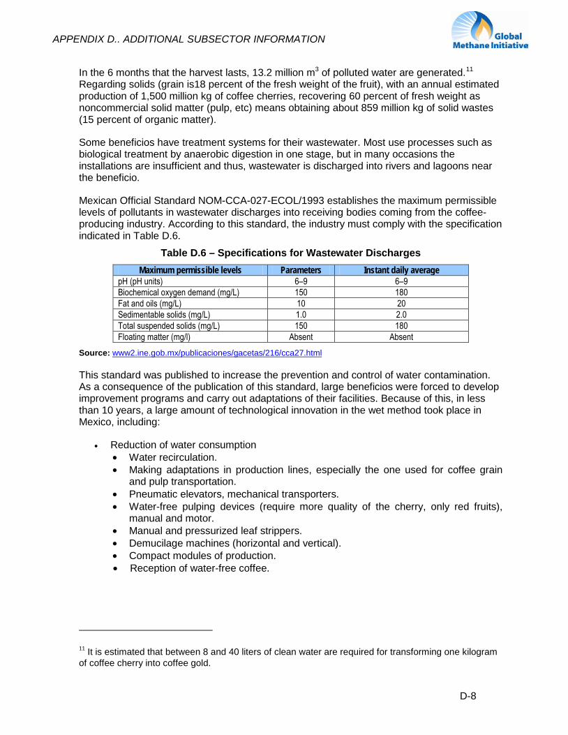
APPENDIX D.. ADDITIONAL SUBSECTOR INFORMATION

D-8

In the 6 months that the harvest lasts, 13.2 million m3 of polluted water are generated.11

Some beneficios have treatment systems for their wastewater. Most use processes such as biological treatment by anaerobic digestion in one stage, but in many occasions the installations are insufficient and thus, wastewater is discharged into rivers and lagoons near the beneficio.

Regarding solids (grain is18 percent of the fresh weight of the fruit), with an annual estimated production of 1,500 million kg of coffee cherries, recovering 60 percent of fresh weight as noncommercial solid matter (pulp, etc) means obtaining about 859 million kg of solid wastes (15 percent of organic matter).

Mexican Official Standard NOM-CCA-027-ECOL/1993 establishes the maximum permissible levels of pollutants in wastewater discharges into receiving bodies coming from the coffee-producing industry. According to this standard, the industry must comply with the specification indicated in Table D.6.

Table D.6 – Specifications for Wastewater Discharges Maximum permissible levels Parameters Instant daily average

pH (pH units) 6–9 6–9 Biochemical oxygen demand (mg/L) 150 180 Fat and oils (mg/L) 10 20 Sedimentable solids (mg/L) 1.0 2.0 Total suspended solids (mg/L) 150 180 Floating matter (mg/l) Absent Absent

Source: www2.ine.gob.mx/publicaciones/gacetas/216/cca27.html

This standard was published to increase the prevention and control of water contamination. As a consequence of the publication of this standard, large beneficios were forced to develop improvement programs and carry out adaptations of their facilities. Because of this, in less than 10 years, a large amount of technological innovation in the wet method took place in Mexico, including:

• Reduction of water consumption • Water recirculation. • Making adaptations in production lines, especially the one used for coffee grain

and pulp transportation. • Pneumatic elevators, mechanical transporters. • Water-free pulping devices (require more quality of the cherry, only red fruits),

manual and motor. • Manual and pressurized leaf strippers. • Demucilage machines (horizontal and vertical). • Compact modules of production. • Reception of water-free coffee.

11 It is estimated that between 8 and 40 liters of clean water are required for transforming one kilogram of coffee cherry into coffee gold.

APPENDIX D.. ADDITIONAL SUBSECTOR INFORMATION

D-9

• Improvements in the drying stage • Vertical aerators. • Humidity gauges. • Sun-dried sieves.

• Wastewater treatment • Biodigesters. • Sedimentation lagoons. • Absorption lagoons.

• Byproducts treatment • Composts. • Vermicomposts (use of worms).

Most coffee processing plants and most of the capacity of the dry beneficio are located in Chiapas (48.5 percent), followed by Veracruz and Puebla, with 17.8 percent and 13.8 percent, respectively. Other plants are located mainly in the state of Mexico, Mexico City, Tlaxcala, and Hidalgo.

As mentioned in the preceding paragraphs, wastewater from coffee production is currently treated without lagoons and therefore generates little methane emissions. Consequently, this sector was not included in the main study. It is mentioned here as coffee waste characteristics indicate that methane could be generated under another waste management system.

D.5. TEQUILA PRODUCTION

Description of size, operational scale, and geographical location

Between the municipalities of Arandas, Jesús María, San Ignacio Cerro Gordo, and Atotonilco, there are about 40 tequila producers, which for the most part, do not have treatment plants. Tequila can only be produced in zones favorable to the growth of agave azul, including the state of Jalisco and four other Mexican states considered to be “geographical areas of origin.”12

Since 1994,133 new tequila producers have been established, and the number of tequila trademarks has reached a record high of 774. In 2008, 307,482 million liters of tequila were produced in the country; 94 million liters were produced in the municipality of Tequila in the state of Jalisco.

(see Figure D-2). Most tequila distilleries discharge vinasses wastewater and distillate product without performing any treatment as established by the Mexican official standard (NOM-001-ECOL-1996).

13

12 Tequila is a Mexican spirit protected by denomination of origin, comprising all of the state of Jalisco, 29 municipalities of Michoacán, six municipalities of Guanajuato, and seven municipalities of Nayarit (all located in the central and western regions of the country), as well as 10 municipalities of the state of Tamaulipas

13 Alert, contamination from tequila industry. Adriana Alatorre. Reforma on line.

APPENDIX D.. ADDITIONAL SUBSECTOR INFORMATION

D-10

Figure D.2 – States Where Agave Azul Can Be Produced, Protected by Denomination of Origin

Source: Scielo, Venezuelan organization

Description of characteristics of wastes, handling, and management

For each tequila liter produced in Mexico, 10 liters of wastewater (or vinasse) are produced.14 In Jalisco, only one of the 67 tequila producers was determined to comply with the environmental law regarding waste discharges into rivers and lakes. According to Mexican Official Standard 001, the maximum allowable limit for effluent is 150 milliliters per liter of COD.15

The wastewater that is disposed of during the tequila distillation process, also called vinasses, has a high content of organic matter and inorganic salts, a high temperature of about 90°C, and a pH value ranging between 3.5 and 4.5; with a COD concentration of 66 grams per liter.

Companies may produce wastewater with 27 to 30 thousand milligrams per liter or more of COD.

Discharges of vinasses have been made in open air without any treatment, letting them run by gravity, contaminating the environment and damaging soils, rivers, and creeks through which they pass and to the lower lands they settle in. The noncompliance of environmental regulations by the tequila industry is not due to the companies’ negligence or deliberate lack of compliance, but because vinasses treatment is considerably complicated because of the large amount of organic matter and sugars that agave contains.16

Some companies buy agave from the farmers under the condition that wastewater may be applied to their land. Thus, the soils where agave is grown are very acidic, and a thick, dark

14 José de Jesús Hernández López. Mexican Science Academy 15 Secretary of Environment for Sustainable Development, SEMADES, Jalisco. 16 Comments from Ernesto Naranjo Castellanos, Director of Standards Verification of the Secretary of Environment from Sustainable Development, SEMADES, Jalisco. Interview June 7, 2009. http://nuestrotequila.blogspot.com/2009/06/alerta-contaminacion-de-tequileras.html.

APPENDIX D.. ADDITIONAL SUBSECTOR INFORMATION

D-11

liquid, which may possess toxic characteristics, remains after fermentation and distillation.. This is illustrated in the quote below from José de Jesús Hernández López of the Mexican Academy of Sciences:

“Due to the vinasse's chemical composition, what they do is that the water tables or ground lateralization are contaminated, because one of the main characteristics of vinasses is that due to the waxes they contain, they can turn the soil hard not letting the growth of any type of vegetation”17

There have been efforts to decrease the organic content of the effluent by applying biological processes, which up to now have shown organic matter removal efficiencies of around 70 to 80 percent (Alvarez et al., 1995; Alvarez, 1996). This treatment is insufficient, however, because the treated effluent being discharged still has a high concentration of organic matter and an intense color (which is modified slightly after the treatment).

Most tequila companies have opted to compost. The common composting practice is set up such that the bagasse of residues that exit the extraction is on one side of the composting area, and vinasses is on the other side. Some tequila companies have advanced systems to treat waste; there are even some tequila companies that have an ozonification system for reusing water in sanitary or irrigation services.18

There is a lack of data on the amount of treatment taking place in the tequila sector. For example, it is estimated that approximately 10 percent of primary treatment takes place in oxidation or sedimentation lagoons. Yet there is no exact quantification of the number of plants with primary treatment. In the state of Jalisco, only four or five tequila companies have treatment plants for their effluents.

17 José de Jesús Hernández López. Mexican Science Academy.

18 President of the Tequila Industry National Chamber, CNIT.

E-1

APPENDIX E: GLOSSARY

Acetogenesis—The formation of acetate (CH3CO2) from carbon dioxide and hydrogen. Many methanogens grow and form methane from acetate.

Acidogenesis—The formation of primarily short-chain volatile acids such as acetic, proprionic, butyric, valeric, and caproic from simple soluble compounds produced during hydrolysis.

Activated Sludge Process—A biological wastewater treatment process in which a mixture of wastewater and activated sludge (biosolids) is agitated and aerated. The activated sludge is subsequently separated from the treated wastewater by sedimentation and wasted or returned to the process as needed.

Advanced Waste Treatment—Any physical, chemical, or biological process used to accomplish a degree of treatment greater than achieved by secondary treatment.

Aerated Pond or Lagoon—A wastewater treatment pond or lagoon in which mechanical or diffused aeration is used to supplement the oxygen supplied by diffusion from the atmosphere.

Aerobic—Requiring the presence of free elemental oxygen.

Aerobic Bacteria—Bacteria that require free elemental oxygen to sustain life.

Aerobic Digestion—The degradation of organic matter, including manure, by the action of micro-organisms in the presence of free elemental oxygen.

Aerobic Waste Treatment—Waste treatment brought about through the action of micro-organisms in the presence of air or elemental oxygen. The activated sludge process is an example of an aerobic waste treatment.

Anaerobic—The absence of air or free elemental oxygen.

Anaerobic Bacteria—Bacteria that grow only in the absence of free elemental oxygen.

Anaerobic Contact Process—Any anaerobic process in which biomass is separated from the effluent and returned to a complete mix or contact reactor so that the solids retention time (SRT) is longer than the hydraulic retention time (HRT).

Anaerobic Digester—A tank or other vessel for the decomposition of organic matter under anaerobic conditions.

Anaerobic Digestion—The degradation of organic matter, including manure, by the action of micro-organisms in the absence of free elemental oxygen.

Anaerobic Pond or Lagoon—An open treatment or stabilization structure that involves retention under anaerobic conditions.

Anaerobic Sequencing Batch Reactor (ASBR) Process—A batch anaerobic digestion process that consists of the repetition of following four steps: 1) feed, 2) mix, 3) settle, and 4) decant/effluent withdrawal.

APPENDIX E.. GLOSSARY

E-2

Anaerobic Waste Treatment—Waste stabilization brought about through the action of micro-organisms in the absence of air or elemental oxygen. Usually refers to waste treatment by methane fermentation. Anaerobic digestion is an anaerobic waste treatment process.

Attached Film Digester—An anaerobic digester in which the micro-organisms responsible for waste stabilization and biogas production are attached to inert media.

Bagasse- The fibrous residue remaining after sugarcane or sorghum stalks are crushed to extract their juice. Bagasse is currently used as a renewable resource in the manufacture of pulp and paper products and building materials.

Bacteria—A group of universally distributed and normally unicellular micro-organisms lacking chlorophyll.

Biochemical Oxygen Demand (BOD)—A measure of the quantity of oxygen utilized in the biochemical oxidation of organic matter in a specified time and at a specified temperature. It is not related to the oxygen requirements in chemical combustion, being determined entirely by the availability of the material as biological food and by the amount of oxygen utilized by the micro-organisms during oxidation.

Biogas—A mixture of methane and carbon dioxide produced by the bacterial decomposition of organic wastes and used as a fuel.

Biological Treatment Processes—There are two general types of biological waste treatment processes: suspended and attached growth. Suspended growth processes generally involve mixing to enhance contact between the microbial population and the wastewater constituents. Suspended growth processes can be either aerobic or anaerobic. The activated sludge process is an example of suspended growth wastewater treatment process.

Attached growth processes are characterized by the development of a microbial population attached to a natural or artificial media when exposed to wastewater constituents. The trickling filter is an example of an attached growth wastewater treatment process. Attached growth processes also can be either aerobic or anaerobic.

Cesspool—A lined or partially lined underground pit into which wastewater is discharged and from which the liquid seeps into the surrounding soil. Sometimes called a leaching cesspool.

Chemical Oxygen Demand (COD)—A quantitative measure of the amount of oxygen required for the chemical oxidation of carbonaceous (organic) material in wastewater using inorganic dichromate or permanganate salts as oxidants in a two-hour test.

Chemical Unit Processes—Processes that remove dissolved and suspended wastewater constituents by chemically induced coagulation and precipitation or oxidation. An example is the addition of alum or lime to remove phosphorus by precipitation in tertiary treatment.

Clarifier—Any large circular or rectangular sedimentation tank used to remove settleable solids from water or wastewater. A special type of clarifiers, called upflow clarifiers, use floatation rather than sedimentation to remove solids.

APPENDIX E.. GLOSSARY

E-3

Complete Mix Digester—A controlled temperature, constant volume, mechanically or hydraulically mixed vessel operated for the stabilization of organic wastes, including manures, anaerobically with the capture of biogas generated as a product of waste stabilization.

Compost—The production of the microbial oxidation of organic wastes, including livestock manures, at an elevated temperature.

Composting—The process of stabilizing organic wastes, including livestock manures, by microbial oxidation with the conservation of microbial heat production to elevate process temperature.

Covered Lagoon Digester—A pond or lagoon operated for the stabilization of organic wastes, including manures, anaerobically and fitted with an impermeable cover to capture the biogas generated as the product of waste stabilization.

Digester—A tank or other vessel for the aerobic or anaerobic decomposition of organic matter present in biosolids or other concentrated forms of organic matter, including livestock manures.

Dissolved Air Floatation (DAF)—A separation process in which air bubbles emerging from a supersaturated solution become attached to suspended solids in the liquid undergoing treatment and float them up to the surface for removal by skimming.

Effluent—The discharge from a waste treatment or stabilization unit process.

Evaporation Pond—A pond or lagoon used for the disposal of wastewater by evaporation.

Facultative—Having the ability to live under different conditions (e.g., with or without free oxygen).

Facultative Bacteria—Bacteria that can carry out metabolic activities, including reproduction, in the presence or absence of free elemental oxygen.

Facultative Pond or Lagoon—A natural or constructed pond or lagoon with an aerobic upper section and an anaerobic bottom section so that both aerobic and anaerobic processes occur simultaneously.

Five-Day BOD—That part of oxygen demand usually associated with biochemical oxidation of carbonaceous material within five days at 20°C.

Greenhouse Gas (GHG)—A gas present in the atmosphere that is transparent to incoming solar radiation but absorbs the infrared radiation reflected from the earth’s surface. The principal GHGs are carbon dioxide, methane, and chlorofluorocarbons..

Human Sewage (Domestic Wastewater)—Human sewage is wastewater that contains human urine and feces. It also usually contains wastewater from bathing and washing dishes, kitchen utensils, clothing, etc. and may include food preparation wastes. It may be discharged directly, treated on site prior to discharge, or transported by a collection system for direct discharge or treatment in a centralized wastewater treatment plant followed by discharge. Human sewage also is known as domestic wastewater.

APPENDIX E.. GLOSSARY

E-4

Hydraulic Retention Time (HRT)—The volume of a reactor divided by the volumetric flow rate.

Hydrolysis—The reduction of insoluble organic and complex soluble organic compounds to simple soluble organic compounds.

Influent—Wastewater flowing into a unit waste treatment or stabilization process.

Lagoon—Any large holding or detention structure, usually with earthen dikes, used to contain wastewater while sedimentation and biological oxidation or reduction occurs.

Liquid Manure—Manure having a total solids (dry matter) content not exceeding 5 percent.

Manure—The mixture of the fecal and urinary excretions of livestock, which may or may not contain bedding material.

Mesophilic Digestion—Digestion by biological action at 27°C to 38°C.

Methane—A colorless, odorless, flammable gaseous hydrocarbon that is produced from the anaerobic, microbial decomposition of organic matter.

Methanogenesis—The formation of methane from CO2-type methyl and acetoclastic-type substrates.

Municipal Wastewater—Wastewater that can contain domestic, commercial, and industrial wastewaters and is treated in a municipal (publicly owned) treatment plant.

Organic Matter—Chemical substances of animal or vegetable origin, or more accurately, containing carbon and hydrogen.

Oxidation Pond—A relatively shallow body of wastewater contained in an earthen basin of controlled shape, in which biological oxidation of organic matter is effected by the natural or artificially accelerated transfer of oxygen.

Physical Unit Processes—Processes that remove particulate matter in wastewater. Screening and gravity separation to remove particulate matter are examples of physical unit processes. These processes are used for primary treatment and following secondary and tertiary treatment. A typical example of the use of physical unit processes in a wastewater treatment system is primary settling followed by the activated sludge treatment process, which is then followed by secondary settling before final effluent discharge.

Plug-Flow—Flow in which fluid particles are discharged from a tank or pipe in the same order in which they entered it. The particles retain their discrete identities and remain in the tank for a time equal to the theoretical retention time.

Plug-Flow Digester—A controlled temperature, constant volume, unmixed vessel operated for the stabilization of organic wastes, including manures, anaerobically with the capture of biogas generated as a product of waste stabilization.

Primary Treatment*—(1) The first major treatment in a wastewater treatment facility, usually sedimentation but not biological oxidation. (2) The removal of a substantial amount of suspended matter but little or no colloidal and dissolved matter. (3) Wastewater treatment

APPENDIX E.. GLOSSARY

E-5

processes usually consisting of clarification with or without chemical treatment to accomplish solid-liquid separation.

Psychrophilic Digestion—Digestion by biological action below 27°C.

Raw Wastewater—Wastewater before it receives any treatment.

Secondary Treatment*—(1) Generally, a level of treatment that produces removal efficiencies for BOD and suspended solids of at least 85 percent. (2) Sometimes used interchangeably with the concept of biological wastewater treatment, particularly the activated sludge process. Commonly applied to treatment that consists chiefly of clarification followed by a biological process, with separate sludge collection and handling.

Solids Retention Time (SRT)—The average time in which solids, including the population of active microbial biomass, remain in a reactor.

Septic Tank—An underground vessel for treating wastewater by a combination of settling and anaerobic digestion. Effluent usually is disposed of by leaching. Settled solids are removed periodically for further treatment or disposal.

Settling Pond—An earthen basin in which wastewater containing settleable solids is retained to remove a part of suspended matter by gravity. Also called a settling or sedimentation basin.

Stabilization—Reduction in the concentration of putrescible material by either an aerobic or anaerobic process. Both aerobic and anaerobic digestion are examples of waste stabilization processes.

Suspended Solids—(1) Insoluble solids that either float on the surface of, or are in suspension in water, wastewater, or other liquids. (2) Solid organic or inorganic particles (colloidal, dispersed, coagulated, flocculated) physically held in suspension by agitation or flow. (3) The quantity of material removed from wastewater in a laboratory test, as prescribed in “Standard Methods for the Examination of Water and Wastewater” and referred to as nonfilterable residue.

Tertiary Treatment*—The treatment of wastewater beyond the secondary or biological stage. Term normally implies the removal of nutrients, such as nitrogen and phosphorus, and a high percentage of suspended solids. Term now being replaced by preferable term, “advanced waste treatment.”

Thermophilic Digestion—Digestion carried on at a temperature approaching or within the thermophilic range, generally between 43°C and 60°C.

Total Solids—The sum of dissolved and suspended solid constituents in water or wastewater. Total Suspended Solids (TSS)—Solid organic or inorganic particles (colloidal, dispersed, coagulated, flocculated) physically held in suspension by agitation or flow. May be referred to as nonfilterable residue.

APPENDIX E.. GLOSSARY

E-6

Treatment—The use of physical, chemical, or biological processes to remove one or more undesirable constituents from a waste.

Upflow Anaerobic Sludge Blanket (UASB) Reactor—An upflow anaerobic reactor in which influent flows upward through a blanket of flocculated sludge that has become granulated.

Volatile Solids (VS)—Materials, generally organic, that can be driven off by heating, usually to 550°C; nonvolatile inorganic solids (ash) remain.

Vinasse— The residual liquid from the distillation of ethanol. Sugarcane or sugar beet is processed to produce crystalline sugar, pulp and molasses. The latter are further processed by fermentation to ethanol, ascorbic acid, or other products. After the removal of the desired product (alcohol, ascorbic acid, etc.) the remaining material is called vinasse.

Wastewater—The spent or used water of a community or industry, which contains dissolved and suspended matter.

Wastewater Treatment System*—A sequence of unit processes designed to produce a final effluent that satisfies standards for discharge to surface or ground waters. Typically will include the combination of primary and secondary treatment processes.

*Appendix C illustrates the typical wastewater treatment process.

F-1

APPENDIX F: BIBLIOGRAPHY

• Alvarez A. E., Lineiro J., Espinosa A., Briones R., Ilangovan K., Noyola R. A., (1995) Tratamiento Anaerobio de Vinazas Tequileras, en un Reactor de Lecho de Lodos y Flujo Ascendente (Anaerobic Treatment of Tequila Vinasse), Memorias del Congreso Nacional de Biotecnología y Bioingeniería, Ixtapa Gro., pp. 96.

• Alvarez A. E., (1996), Tratamiento Anaerobio de Vinazas Tequileras en un Reactor de Lecho de Lodos y Flujo Ascendente (Anaerobic Treatment of Tequila Vinasse), Tesis de Licenciatura.

• Beneficios ambientales por el aprovechamiento del biogás. Claridades Agropecuarias, No 167 julio 2007, pág. 38-39.

• Díaz Cárdenas, Salvador. Plan rector del sistema producto café en México, Agosto 2005

• Doorn, M.R.J., R. Strait, W. Barnard, and B. Eklund (1997). Estimate of Global Greenhouse Gas Emissions from Industrial and Domestic Wastewater Treatment, Final Report, EPA-600/R-97-091, Prepared for United States Environmental Protection Agency, Research Triangle Park, NC, USA.

• Drucker A., Escalante R., Gómez V. y Magaña S. (2003), “La industria porcina en Yucatán” (The Swine Industry in Yucatan), Problemas del Desarrollo: Revista Latinoamericana de Economía, Vol. 34, núm. 135, X-XI, pp. 105-124

• Escalante Semerena, Roberto I. and Horacio Catalán, Situación actual del sector agropecuario en México: perspectivas y retos (Current situation of the agricultural sector in Mexico: perspectives and challenges), 2008.

• Estrada, Escalante and Violeta Erendira, Treatment of swine effluents in stabilization lagoons. Inter-American Congress of Sanitary and Environmental Engineering.

• Escoto, Fernando Cervantes; Alfredo Cesín Vargas, Sandra Laura Pérez Sánchez. La calidad estándar de la leche como eje de la coordinación vertical entre la agroindustria láctea y sus proveedores: El caso del estado de Hidalgo, México. CIESTAMM, Universidad Autónoma de Chapingo.

• Houbron Eric. Proyecto: Desarrollo de procesos de tratamiento integral de residuos generados por al industria del beneficio húmedo de café. Facultad de Ciencias Químicas. Campus Orizaba.

• IPCC, 2006 IPCC Guidelines for National Greenhouse Gas Inventories, 2006, http://www.ipcc-nggip.iges.or.jp/public/2006gl/index.html

• Macias Macias, Alejandro. El cluster en la industria del tequila en Jalisco, México¹. Agroalim, dic. 2001, vol.6, no.13, p.55-72. ISSN 1316-0354.

• Meza Pérez Arturo, Briones Méndez Roberto, Ilangovan Kuppusamy, Floculación-coagulación como postratamiento del efluente de un reactor anaerobio que trata vinazas tequileras. Coordinación de bioprocesos ambientales, Instituto de Ingeniería UNAM.

APPENDIX F.. BIBLIOGRAPHY

F-2

• National Institute of Statistics and Geography (INEGI), Censo Agropecuario 2007, VIII Censo Agrícola, Ganadero y Forestal. Aguascalientes, Ags. 2009. (Mexican Livestock Census)

• Programa estratégico de necesidades de investigación y transferencia de tecnología del estado de Chiapas. Fundación Produce Chiapas, Instituto Tecnológico de Estudios Superiores de Monterrey campus Chiapas, abril 2003. www.snitt.org.mx/pdfs/demanda/cafe.pdf

• G. Quiroga, J.L García de Siles, Manual para la instalación del pequeño rastro modular de la FAO (Manual for Small Slaughterhouses), FAO. Rome, Italy, 1994, presented in Federal Commission for the Protection Against Sanitary Risks (COFEPRIS), Evaluación de Riesgos de los Rastros y Mataderos Municipales, July 2006.

• Rojo, R., 2008. Dual purpose cattle production in Mexico, Springer Science + Business Media B.V.

• Rosario, Pérez Espejo, Granjas porcinas y medio ambiente, Contaminación del agua en La Piedad Michoacán 2006.

• SAGARPA, 2002. Situación actual y perspectiva de la producción de leche de bovino en México 1990-2000

• SEMARNAT, Mexico’s second national communication to the UNFCCC (2001) http://unfccc.int/resource/docs/natc/mexnc2.pdf.

• SEMARNAT, Mexico’s fourth national communication to the UNFCCC (2009), http://unfccc.int/resource/docs/natc/mexnc4s.pdf.

• SEMARNAT and SAGARPA, Technical Standards for the Design and Construction of Bio-Digesters in Mexico, March 2010

• Solleiro, José Luis; María del Carmen del Valle, Estrategias competitivas de la industria alimentaria. UNAM Ed. Plaza y Valdés S.A. de C.V., primera edición 2003. pág. 30-31.

• Suárez, Luis Gerardo Ruiz, Xochitl Cruz Núñez. Los gases de efecto invernadero y sus emisiones en México. Centro de Ciencias de la Atmosfera. UNAM.

• Tapia Orozco Natalia, Rodríguez Vázquez Refugio. Tratamiento biológico/fotocatalítico de aguas residuales del beneficio húmedo de café. Contaminación ambiental. Biotecnología y Bioingeniería CINVESTAV-IPN.

• Tecnológico de Monterrey, Centro de Estudios Estrategicos, Capítulo II: Diagnóstico del sector de producción de leche bovina, www.sedesol.gob.mx/archivos/802482/file/diagnostico_leche.pdf

• USDA Foreign Agricultural Service, 2007. GAIN Report - Mexico Dairy and Products Dairy Semi-Annual 2007.

• U.S. EPA, 2004. AgSTAR Handbook, 2nd ed., K.F. Roos, J.H. Martin,Jr. and M.A. Moser eds. EPA-430-B-97-015. Office of Air and Radiation, Washington, DC.

APPENDIX F.. BIBLIOGRAPHY

F-3

• World Resources Institute (WRI). WRI (2005). “Navigating the Numbers: Greenhouse gases and international climate change agreements.”

• www.ejournal.unam.mx/atm/vol20-1/ATM20105.pdf

Websites consulted in October and November 2009

• www2.ine.gob.mx/publicaciones/libros/437/ruiz.html

• www.infoagro.net/es/apps/library/search_library.cfm?vsys=a5&term=6725&field=NUM&lang=&vmedia=

• www.campomexicano.gob.mx

• www.cepis.org.pe/bvsaidis/aresidua/mexico/01336e14.pdf.

• www.siap.gob.mx

• http://www.sra.gob.mx/internet/informacion_general/programas/fondo_tierras/manuales/Benef_ecol_tost_mol_Caf_.pdf

• www.sra.gob.mx/internet/informacion_general/programas/fondo_tierras/manuales/Benef_ecol_tost_mol_Caf_.pdf

• Brock, T.D. and M.T. Madigan. 1988 Biology of Microorganisms, 5th ed. Prentice-Hall, Inc. Englewood Cliffs, New Jersey.

Glossary References

• Glossary Water and Wastewater Control Engineering, 3rd ed. 1981. Prepared by Joint Editorial Board Representing the American Public Health Association, Washington, DC; the American Society of Civil Engineers, New York, NY; the American Water Works Association, Denver, CO; and the Water Pollution Control Federation, Washington, DC.

• Grady, C.P.L. Jr. and H.C. Lim. 1980. Biological Wastewater Treatment. Marcel Dekker, Inc. New York, New York.

• Merriam-Webster’s Collegiate Dictionary, 10th ed. 1999. Merriam-Webster, Inc. Springfield, Massachusetts.

• Metcalf and Eddy, Inc. 2003. Wastewater Engineering—Treatment and Reuse, 4th ed. Revised by G. Tchobanoglous, F.L. Burton, and H.D. Stencil. McGraw-Hill, New York, New York.