Research result: Wind energy prediction in

Germany

Alexander Aprelkin

Technische Universität München

August 21, 2013

1 Introduction

Wind power usage is set to be a key power source in energy supply of Germany.In [10] is shown that the wind power energy production steadily rises over therecent years and that the technology is an emerging market with a great fu-ture, having priority among other power sources. Unfortunately, wind powerprediction is considered to be a hard problem.

One of the key issues is to analyze the numerical weather predictions andcalculate the power output of a wind turbine or a wind farm based on weatherconditions. Normally, power forecast needs to be available up to 3 days beforethe actual feed-in values arrive.

An important problem is the availability and quality of weather data at thelocation of a wind turbine. Often, the wind speed values have to be interpo-lated given several weather stations' values around the turbine. Typically, winddirection and velocity, air pressure/temperature and humidity are used as themain quantities for the wind power prediction.

As mentioned in [5] the problem of a precise forecasting of wind power outputis important since forecast errors are related to the use of balancing power andmay cause additional costs of the order of millions Euros after several hours.Moreover, �uctuations of power quality can occur due to an erroneous powerforecast. Therefore, precise forecasts are very important and desirable.

The state-of-the-art day ahead forecast [5] has a root mean square error ofabout 5.8 percent and decreases for short time periods down to 3.8 percent.

Two main approaches exist: a statistical and a physical [6]. The physicalapproach uses local dynamic weather information and power curves of a giventurbine, whereas the statistical approach uses historical data and interpolatedweather values and is based on a statistical model, e.g. an arti�cial neuralnetwork.

We will consider the statistical approach and analyze if it is possible tocombine di�erent state-of-the-art methods or provide an improvement of one ofthem in order to obtain a better forecast in terms of a minimal error.

1

2 Related Work

As there are a lot of di�erent standard and complicated methods, each withits advantages and drawbacks, we will �rst consider all of them separately andwill try to �nd an optimal solution as either a combination of them or an im-provement of one of them. Our work will be concentrated on learning a forecastfunction for each of the TSOs separately, based on NWP data and installedcapacity of the wind turbines. This way, we will try to learn some local powercurves and combine them into a single aggregated model of a TSO.

Authors of [1] propose an approach of minimizing the error between forecastand sample data using some weighting coe�cients for interpolation of wind farmlocation. In [32] authors are considering the power curve of a whole wind farm,given weather data and power output. Di�erent data mining algorithms basedon the forecast period are considered in [3].

In [4] authors propose that the forecast error of a region is in general smallerthan a forecast error for a single wind farm. This has an advantage that someerrors caused by one site can be canceled out by another one.

In [5], [12] is mentioned, that the prediction system currently used by someGerman TSOs is statistically based and works on arti�cial neural networks,trained on historical data. [7] provides a large overview over several wind powerforecasting approaches.

One of the closely related papers is [9], where a power curve of a whole windfarm is being learned using a neural network technique. A di�erent interestingapproach is considered in [11], where clustering of weather data is used.

In [13], authors also follow a statistical approach and their system is duringthe learning process able to decide, how good is the quality of given weathermeasurement.

Authors of [15] consider two di�erent data mining methods: one is predictingthe power directly from the NWP, and the other one predicts the wind speedfrom the NWP and then calculates the power output from the wind speedforecast.

Authors of [18],[19],[21] are using some other non-standard methods to solvethe problem of power prediction.

3 Research Question

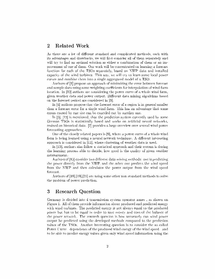
Germany is divided into 4 transmission system operator zones , as shown onFigure 1. All of them provide information about produced and predicted energywith wind turbines. The predicted energy is not always equal to the producedpower but has to be equal in order to save money and control the balance ofthe power network. The research question is how accurately can wind poweroutput be predicted using the developed methods compared to the predictionvalues of the TSOs. Another interesting question is to consider the so calledPower Curve - dependance of the produced wind energy of the wind speed - andto be able to predict energy values given only wind speed information using the

2

Figure 1: Division of Germany by 4 TSOs.

3

learned Power Curve.The goal will be to predict energy production for the next day in hourly

time steps, given the weather conditions and energy production values of theprevious 4 days, in the time range: 11.07.2013 15:00 till 15.07.2013 23:59. Thetarget day is the 16.07.2013. Since the goal lies already in the past, actual valuesalready exist and can be used for error estimation of the models.

4 Software

In order to achieve the goals of the project the following software was used.R was used for weather interpolation and krigging at wind turbines' locations.Furthermore, it contains a packages 'stats' and 'forecast' with state of the artsmethods for time series analysis and forecasting, like ARIMA. Additionally,there is a special R package '�elds' which was used for krigging. R was alsoused to join two data tables into one, based on one common �eld, in our casecoordinates of a wind turbine with based on the post index. Furthermore,software MATLAB was used for Neural Networks creation and simulation.

5 Data set and data preprocessing

Data set of numerical weather predictions (NWP) was obtained from the serviceWebWerdis of the Deutscher Wetterdienst. The user account was provided bythe Chair of Financial Mathematics of the TUM.

The considered data set consists of 4 parts:

• Climatological time serie: hourly means of wind speed (in m/sec) - productde.dwd.nkdz.FFHM

• Climatological time serie: hourly values of station pressure (in hpa) -product de.dwd.nkdz.PSHV

• Climatological time serie: hourly values of air temperature (in degree C)- product de.dwd.nkdz.TAHV and

• Climatological time serie: hourly values of relative humidity (in %) - prod-uct de.dwd.nkdz.UUHV.

We concentrated on these time series because power generation of a single windturbine depends on exactly these parameters, regardless the technical parame-ters of the machine.

The kinetic energy of a wind turbine can be expressed with the formula

P =1

2Atρw3, (1)

where w is the wind speed, ρ the density of the air , t the time, and A therotor area of the turbine. Air density depends on temperature and humidity.

4

Normally, wind turbines achieve an e�ciency of about 59 percent of the kineticenergy.

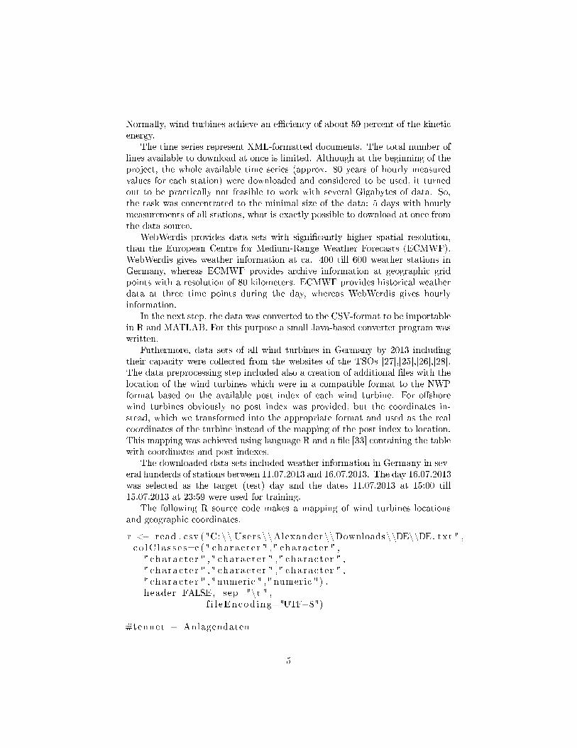
The time series represent XML-formatted documents. The total number oflines available to download at once is limited. Although at the beginning of theproject, the whole available time series (approx. 80 years of hourly measuredvalues for each station) were downloaded and considered to be used, it turnedout to be practically not feasible to work with several Gigabytes of data. So,the task was concentrated to the minimal size of the data: 5 days with hourlymeasurements of all stations, what is exactly possible to download at once fromthe data source.

WebWerdis provides data sets with signi�cantly higher spatial resolution,than the European Centre for Medium-Range Weather Forecasts (ECMWF).WebWerdis gives weather information at ca. 400 till 600 weather stations inGermany, whereas ECMWF provides archive information at geographic gridpoints with a resolution of 80 kilometers. ECMWF provides historical weatherdata at three time points during the day, whereas WebWerdis gives hourlyinformation.

In the next step, the data was converted to the CSV-format to be importablein R and MATLAB. For this purpose a small Java-based converter program waswritten.

Futhermore, data sets of all wind turbines in Germany by 2013 includingtheir capacity were collected from the websites of the TSOs [27],[25],[26],[28].The data preprocessing step included also a creation of additional �les with thelocation of the wind turbines which were in a compatible format to the NWPformat based on the available post index of each wind turbine. For o�shorewind turbines obviously no post index was provided, but the coordinates in-stead, which we transformed into the appropriate format and used as the realcoordinates of the turbine instead of the mapping of the post index to location.This mapping was achieved using language R and a �le [33] containing the tablewith coordinates and post indexes.

The downloaded data sets included weather information in Germany in sev-eral hunderds of stations between 11.07.2013 and 16.07.2013. The day 16.07.2013was selected as the target (test) day and the dates 11.07.2013 at 15:00 till15.07.2013 at 23:59 were used for training.

The following R source code makes a mapping of wind turbines locationsand geographic coordinates.

r <− read . csv ("C:\\ Users \\Alexander \\Downloads\\DE\\DE. txt " ,c o lC l a s s e s=c (" charac t e r " ," cha rac t e r " ," cha rac t e r " ," cha rac t e r " ," charac t e r " ," cha rac t e r " ," cha rac t e r " ," charac t e r " ," cha rac t e r " ," numeric " ," numeric " ) ,header=FALSE, sep="\t " ,

f i l eEncod ing="UTF−8")

#tennet − Anlagendaten

5

s <− read . csv ("C:\\ Praktikum\\Praktikum Dataset \\Anlagen_Stammdaten b i s 2013\\Tennet\\ on_f ina l . csv " ,c o lC l a s s e s=c (" charac t e r " ," cha rac t e r " ," cha rac t e r " ," cha rac t e r " , " cha rac t e r " ," cha rac t e r " ,

" charac t e r " ," cha rac t e r " , " cha rac t e r " ," charac t e r " , " cha rac t e r " ," numeric " ,

" charac t e r " ," cha rac t e r " ," charac t e r " ," charac t e r " , " cha rac t e r " ," cha rac t e r " ," charac t e r " ," cha rac t e r " , " cha rac t e r " ) ,header=TRUE, sep =";")

t t <− merge ( r , s , by . x="V2" , by . y="PLZ")xt <− t t [ , c ("V2" ,"V10" ,"V11" ," Le i s tung " ," Inbetriebnahmedatum " ) ]s ink (" c :\\ tennetLocat ions . txt ")xts ink ( )

s <− read . csv ("C:\\ Praktikum\\Praktikum Dataset \\Anlagen_Stammdaten b i s 2013\\Tennet\\ o f f_ f i n a l . csv " ,

c o lC l a s s e s=c (" charac t e r " ," cha rac t e r " ," charac t e r " ," cha rac t e r " , " cha rac t e r " ," charac t e r " , " cha rac t e r " ," cha rac t e r " ,

" cha rac t e r " ," cha rac t e r " , " cha rac t e r " ,"numeric " , " cha rac t e r " ," cha rac t e r " ," charac t e r " ," cha rac t e r " , " cha rac t e r " ," charac t e r " , " cha rac t e r " ," cha rac t e r " ," charac t e r " ," cha rac t e r " , " cha rac t e r " ," charac t e r " , " charac t e r " ) ,header=TRUE, sep =";")

xt <− s [ , c ("PLZ" ," Lat i tude " , "Longitude " , " Le i s tung " ," Inbetriebnahmedatum" ) ]s ink (" c :\\ t enne tOf f sho reLoca t i ons . txt ")xts ink ( )

After this step was run for all TSOs, �les with location of the turbines and�les with the weather measurements at the weather stations were available.

Weather values for locations of the wind turbines, locations between theweather stations had to be interpolated in language R using a krigging method(package �elds, function Krig) provided by the package �elds of R. For thispurpose, an R program was run for each combination of weather and turbinelocation �le. This process turned out to be quite time expensive and not al-ways accurate (for example negative values occured due to special interpolationfunction form).

The next R source code describes how to make krigging (calculation of ir-regular weather measurements into the irregular positions of wind turbines).

6

# read i n f o about weatherd0 <− read . csv ("C:\\ wind5days22 . csv " , header=TRUE, sep="\t ")# add time componentd0$time = ISOdate ( d0$year , d0$month , d0$day , d0$hours , d0$minutes )# order by timed0 <− d0 [ with (d0 , order ( time ) ) , ]

# read l o c a t i o n o f weather s t a t i o n sd1 <− read . csv ("C:\\ wind5days22_loc . csv " , header=TRUE, sep="\t ")

# c r ea t e l a t i t u d ed1$y = as . numeric ( char2dms ( as . cha rac t e r ( d1 [ [ " l a t i t u d e " ] ] ) ) )

#c r ea t e l ong i tuded1$x = as . numeric ( char2dms ( as . cha rac t e r ( d1 [ [ " l ong i tude " ] ] ) ) )

# read l o c a t i o n s o f wind s t a t i o n st t t1_loc <− read . csv ("C:\\50 hertzOf fLocat ions_1 . csv " ,c o lC l a s s e s=c (" charac t e r " , "numeric " , "numeric " ,"numeric " , " cha rac t e r " ) , sep="", header=FALSE)

# cr ea t e empty matrixr <− matrix ( l i s t ( ) , nrow=length ( d0$time ) , nco l=length ( ttt1_loc$V2 ) ) ;

# f i l l matrix with kr igged data us ing i n f o sf o r ( i in 1 : l ength ( d0$time ) ) {

f i t <− Krig ( d1 [ 4 : 5 ] , t ( d0 [ i , 6 : ( nco l ( d0 )−1) ]) ,Covariance="Matern " , theta=25, smoothness =0.5)

r [ i , ] <− p r ed i c t ( f i t , rb ind ( cbind ( ttt1_loc$V2 , ttt1_loc$V3 ) ) )cat ( i , "\ n")f l u s h . con so l e ( )

}

# wr i t e out the r e s u l twr i t e . csv ( r , "C:\\1\\ r e s u l t \\wind_50hertzOff . csv ")

The data sets of prediction and actual values monthwise were obtained fromthe websites of the TSOs [28],[31],[29],[30]. TransnetBW GmbH provides thedata since January 2010, TennetTSO GmbH - since July 2005, Ampirion GmbH- since April 2008 and 50Hertz Transmission GmbH - since January 2005. Thepower values are given in 15-minutes-steps and the prediction values are gener-ated 24 hours before the actual power feed-in value is measured. Old data sets(before 2009) of 50Hertz are provided in XLS-data format, which is di�erent tothe newer ones (CSV).

7

6 Methods

Several models were considered, for 6 problems (wind energy prediction of Ten-net O�shore, Tennet Onshore, 50Hertz O�shore, 50Hertz Onshore, Ampirionand TransnetBW) to be solved. The result Root Mean Squared Error (RMSE)and Mean Absolute Error (MAE) of every method was compared to the RMSEand MAE of the o�cial predictions of the TSOs.

The models are:

• "All stations (formula)": Each data set with weather conditions at everywind turbine is used as the input of the neural net, which results in 4 neuralnets: for humidity, wind, pressure and temperature. After the training theneural nets are applied on the weather conditions (resp. humidity, wind,pressure or temperature) of the target day. The result is calculated aswind ∗ 0.7 + temperature ∗ 0.1 + pressure ∗ 0.1 + humidity ∗ 0.1, due tomore important in�uence of wind speed on the energy output.

• "All stations (mean)": Each data set with weather conditions at everywind turbine is used as the input of the neural net, which results in 4 neuralnets: for humidity, wind, pressure and temperature. After the training theneural nets are applied on the weather conditions (resp. humidity, wind,pressure or temperature) of the target day. The result is calculated aswind ∗ 0.25 + temperature ∗ 0.25 + pressure ∗ 0.25 + humidity ∗ 0.25.

• "All stations (wind)": Only wind data set at all stations is used as inputto the neural net and the resulting net is applied on the wind of the targetday. The result is calculated using only the wind component.

• "Average (formula)": Each data set with weather conditions at every windturbine is used as the input of the neural net, which results in 4 neuralnets: for humidity, wind, pressure and temperature. However, the weathervalues are averaged among the stations, so that there is exactly one averagevalue for every hour. After the training the neural nets are applied on theappropriate average weather conditions (resp. humidity, wind, pressure ortemperature) of the target day. The result is calculated as wind ∗ 0.7 +temperature∗0.1+pressure∗0.1+humidity∗0.1, due to more importantin�uence of wind speed on the energy output.

• "Average (mean)": Each data set with weather conditions at every windturbine is used as the input of the neural net, which results in 4 neuralnets: for humidity, wind, pressure and temperature. However, the weathervalues are averaged among the stations, so that there is exactly one averagevalue for every hour. After the training the neural nets are applied on theappropriate average weather conditions (resp. humidity, wind, pressure ortemperature) of the target day. The result is calculated as wind ∗ 0.25 +temperature ∗ 0.25 + pressure ∗ 0.25 + humidity ∗ 0.25.

• "Average (wind)": Only wind data set at average values of all stations isused as input to the neural net and the resulting net is applied on the

8

average wind of the target day. The result is calculated using only thewind component.

• "Single �le": All four weather parameters are averaged and put into one�le for every operator and used as input for the neural net simultaneously.

• "Arima": Autoregressive integrated moving average model is used to fore-cast the following energy production values given only the previous onesin form of time series without consideration of weather parameters.

• "HoltWinters": analysis of time series of energy production in the pastwithout consideration of weather parameters, forecasts based on HoltWin-ters model.

• "Power curve": consider regression between wind speed and power gen-eration in order to �nd a dependence, power curve for energy generationprediction.

Since no prediction values for 50Hertz O�shore and Tennet O�shore wereavailable, but instead only predictions for whole zones (including on- and o�-shore) we used the prediction values for the whole operator region and took thequote of the o�shore power capacity as a quote for prediction value.

Exactly, the sum of the capacities of Onshore turbines of Tennet is 42551641MW, whereas on O�shore 300000 MW can be produced, which is less than onepercent of the Onshore value. As a heuristic for the o�shore prediction value, weused 1 percent of the total prediction. Analogously, for 50Hertz the capacity is:134831206 MW Onshore and 48300 MW O�shore. We also calculated 1 percentof every Onshore predicted value as the prediction of O�shore at the same timestep.

As a neural net implementation, MATLAB application Neural Net TimeSeries of the Neural Network Toolbox was used. Speci�cally, the type of theproblem is called by MATLAB Nonlinear autoregressive with external exogenousinput (NARX).

This type of neural net allows to adjust the following parameters: input andtarget time series, percentage of validation and test data, number of hiddenneurons and number of delays.

As the input, the appropriate weather data had to be provided (105 timesteps from 11.07.2013 15:00h till 15.07.2013 23:59). The target time series is thehourly values of generated energy at these time steps. For the quote of training,validation and test data, the percentage 80/20/20 was chosen. For the numberof hidden neurons 5 was the best choice and the number of delays the defaultvalue 2 was left.

In order to be able to supply the neural net with information we prepared sev-eral �les, divided by categories Input, Output as well as some subcategories ac-cording to the used model as following examples: Input\Avg\hum_avg_50HertzOff.csv,Input\Avg\hum_avg_50HertzOn.csv, Input\Avg\pressure_avg_Ampirion.csv,Input\Full\transnetBW\temperature_TransnetBW.csv etc.

for the input of the appropriate neural net.

9

The output for training of the neural net which is 105 energy values for everyconsidered training hour was prepared in the folder Output:

e.g. Output\TRAIN_ampirion_Werte.csv, Output\TRAIN_transnetBW_Werte.csv.After the neural net is trained, it is applied to the weather information of

the target day: �les in the folder target:target\targetDayKriggedWeather\temperature_targetDay_50hertzOff.csv,

target\avg\SINGLEFILE_50hertzoff.csv etc.The result is compared to the values stored in another �le of the folder target:

target\50HertzWerte16_07\TARGET_OnShore.csv. And the RMSE of theprediction is calculated according to the values of the �le PREDICTED_50Hertz.csvof the same folder. The �le format in every case is self-explanatory.

The structure of the folders used for di�erent models is as follows:For "SingleFile"-model: Input �les are in result\Input\SingleF ile\. Out-

put data is in result\Output\. Target weather is intarget\targetDayKriggedWeather\avg\SINGLEFILExxx.csv. And tar-

get result is in target\XXXWerte16_07.For "Avg"-model: Input �les are in result\Input\Avg\. Output data is in

result\Output\. Target weather is in target\targetDayKriggedWeather\avg\TARGETxxx.csv.And target result is in target\XXXWerte16_07.

For "All Stations"-model: Input �les are in result\Input\Full\. Outputdata is in result\Output\. Target weather is in target\targetDayKriggedWeather\∗.csv. And target result is in target\XXXWerte16_07.

For the purpose of �nding a dependence (regression) between the wind speedand produced energy we used the average wind speed among one operator atone time step and the appropriate produced energy at this time step. For thiscase we used the Curve Fitting Tool of the Curve Fitting Toolbox of MATLAB.In this tool, in our 2D case X and Y axes values can be adjusted as well as themethod of curve �tting. As X-values average hourly wind speeds of one operatorwere selected, and as Y-values the appropriate produced amounts of energy. Inorder to �nd a dependence between these variables several models were tried:polynomial, gaussian, etc.

Since predictions and actual energy generation values are given every 15-minutes, but the weather data is provided hourly, the energy generation valueswere aggregated by 4. For this purpose and for the purpose of averaging theweather values, small Java parser-programs were written.

10

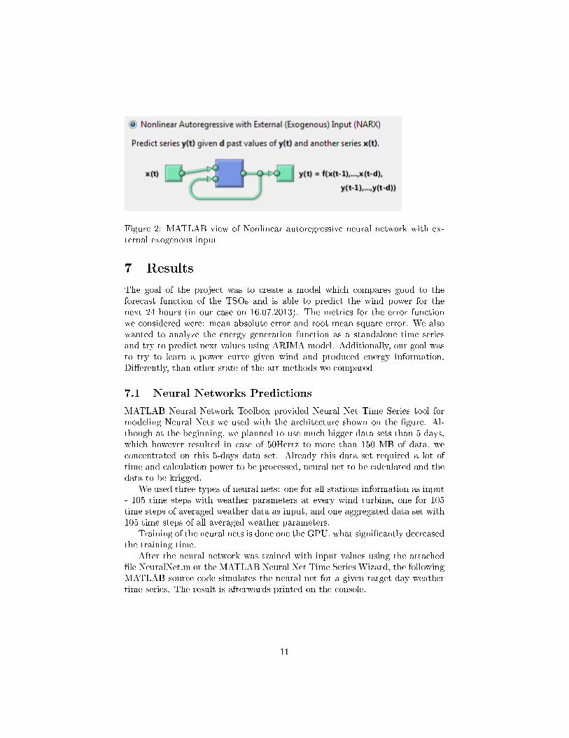
Figure 2: MATLAB view of Nonlinear autoregressive neural network with ex-ternal exogenous input

7 Results

The goal of the project was to create a model which compares good to theforecast function of the TSOs and is able to predict the wind power for thenext 24 hours (in our case on 16.07.2013). The metrics for the error functionwe considered were: mean absolute error and root mean square error. We alsowanted to analyze the energy generation function as a standalone time seriesand try to predict next values using ARIMA model. Additionally, our goal wasto try to learn a power curve given wind and produced energy information.Di�erently, than other state-of-the-art methods we compared

7.1 Neural Networks Predictions

MATLAB Neural Network Toolbox provided Neural Net Time Series tool formodeling Neural Nets we used with the architecture shown on the �gure. Al-though at the beginning, we planned to use much bigger data sets than 5 days,which however resulted in case of 50Hertz to more than 150 MB of data, weconcentrated on this 5-days data set. Already this data set required a lot oftime and calculation power to be processed, neural net to be calculated and thedata to be krigged.

We used three types of neural nets: one for all stations information as input- 105 time steps with weather parameters at every wind turbine, one for 105time steps of averaged weather data as input, and one aggregated data set with105 time steps of all averaged weather parameters.

Training of the neural nets is done one the GPU, what signi�cantly decreasedthe training time.

After the neural network was trained with input values using the attached�le NeuralNet.m or the MATLAB Neural Net Time Series Wizard, the followingMATLAB source code simulates the neural net for a given target day weathertime series. The result is afterwards printed on the console.

11

RMSE p MAE p RMSE f MAE f RMSE m MAE m RMSE w MAE w10.35364 -8.9625 24.4809 23.75699 37.7110 36.98304 22.47725 21.15987

Table 1: Errors on solving the prediction problem using All-stations-model for50Hertz onshore. p means prediction, f means calculated using neural networkand formula as above, m means calculated mean value, w means calculated usingonly wind.

inp = tonndata (TARGETDAYWEATHER, f a l s e , f a l s e )netc ( inp , ' u s ePa ra l l e l ' , ' yes ' , 'useGPU ' , ' yes ' )str2num (mat2str ( ce l l 2mat ( ans ) ) ) '

The results of the neural nets we calculated based on three models: resultof energy based on wind speed output only, prediction of energy based on all 4outputs as average and as weighted sum with a bigger part of wind componentin�uence.

Almost always, the calculated prediction curve for 24 hours followed the formof the 24 hours o�cial prediction curve, although it had higher values than theo�cial one. Especially the results of the �rst 5-6 time steps were good.

We calculated the RMSE and MAE for each of the 6 problems (6 data sets:Tennet on and o� shore, 50 Hertz on and o� shore, Ampirion and transnetBW)for every model.

Although in "All Stations"-model more data is available for the neural net-work and more complex and accurate model could theoretically be achieved,it still did not perform better than averaged models and shows a high RMSEand MAE. Tables 1, 2 and 3 show how RMSE and MAE of di�erent calcula-tion scenarios inside one model (All stations) were compared. For other models(Average weather, and average weather in single �le) RMSE and MAE werecompared in the same way.

On �gure 3 one can see that the calculated result using only the wind compo-nent in "All stations"-model performs slightly worse than the o�cial prediction,still the form of the curve is almost the same.

On the �gure we can see that even the prediction not always delivers goodresult. On the �gure is the production of energy transnetBW, where our calcu-lated prediction is better than the o�cial.

As we ca see from the tables 1 - 3, the best results can be achieved almostin all cases using the wind-component alone and the mean value of all fourcalculated energy-results. Similar tables were considered for all other calculationmodels and formulas. They are not shown in this document to save place. Atthe end of the document (subsection Common Results) some summary graphsare provided.

Interestingly, the worst results are achieved, when using single �les of inputdata, having all four weather components, but as average values over the TSOregion. In no case the o�cial prediction is outperformed.

12

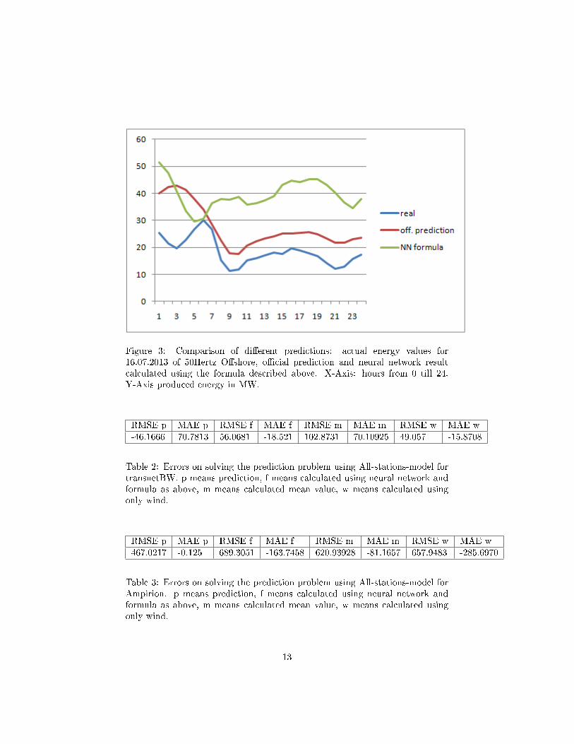
Figure 3: Comparison of di�erent predictions: actual energy values for16.07.2013 of 50Hertz O�shore, o�cial prediction and neural network resultcalculated using the formula described above. X-Axis: hours from 0 till 24.Y-Axis produced energy in MW.

RMSE p MAE p RMSE f MAE f RMSE m MAE m RMSE w MAE w-46.1666 70.7813 56.0681 -18.521 102.8731 70.10925 49.057 -15.8708

Table 2: Errors on solving the prediction problem using All-stations-model fortransnetBW. p means prediction, f means calculated using neural network andformula as above, m means calculated mean value, w means calculated usingonly wind.

RMSE p MAE p RMSE f MAE f RMSE m MAE m RMSE w MAE w467.0217 -0.125 689.3051 -163.7458 620.93928 -81.1657 657.9483 -285.6970

Table 3: Errors on solving the prediction problem using All-stations-model forAmpirion. p means prediction, f means calculated using neural network andformula as above, m means calculated mean value, w means calculated usingonly wind.

13

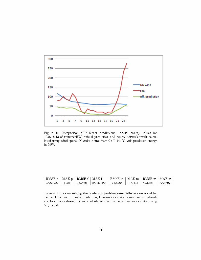
Figure 4: Comparison of di�erent predictions: actual energy values for16.07.2013 of transnetBW, o�cial prediction and neural network result calcu-lated using wind speed. X-Axis: hours from 0 till 24. Y-Axis produced energyin MW.

RMSE p MAE p RMSE f MAE f RMSE m MAE m RMSE w MAE w33.86902 11.503 95.9621 88.766585 121.5708 118.431 82.6461 68.9897

Table 4: Errors on solving the prediction problem using All-stations-model forTennet O�shore. p means prediction, f means calculated using neural networkand formula as above, m means calculated mean value, w means calculated usingonly wind.

14

7.2 Time Series Prediction

After the neural nets information was collected, some additional experimentsneeded to be done. It was interesting to know if it is possible to predict theenergy values without the knowledge of the weather, but having only the val-ues of previous energy productions instead. For this purpose R was used withpackages 'stats', 'forecast' with time series analysis models ARIMA (Autore-gressive Integrated Moving Average) and Holt-Winters exponential smoothing.The �rst one is used when the time series is stationary, the second one makesno assumptions about stationarity of time series, but can be used if the timeseries has a increasing or decreasing trend or seasonality. Each of the modelsreceived a time series of 105 time steps (hourly values between 11.07.2013 at15:00 and 15.07.2013 23:59) and had to produce a prediction for the next 24time steps (24 hours of 16.07.2013. The RMSE and MAE of both methods wasthen compared to the o�cial predictions of the TSOs.

The following R source code shows the use of Holt-Winters model in R fortime series forecasting.

l i b r a r y (" f o r e c a s t ")l i b r a r y (" s t a t s ")x <− read . csv ("C:\\1\\ r e s u l t \\Output\\TRAIN_transnetBW_Werte . csv " ,header=FALSE, sep="\n")t s <− t s ( x )hw <− HoltWinters ( ts , gamma=FALSE)hw2 <− f o r e c a s t . HoltWinters (hw, h=24)p l o t . f o r e c a s t (hw2)hw2

HoltWinters forecast result was always almost constant line of values, whereasARIMA delivered more interesting results. The time series for ARIMA has to bestationary (mean, deviation and autocorrelation have to be constant over time),therefore in the �rst step, if the time series appeared to be non-stationary on theplot, one or more 'di�erences' of it were needed using the function di�. ARIMAfunction requires 3 parameters: p,q and d, where d is number of di�erencesuntil a stationary time series remains. p and q partial autocorellation and au-tocorelation values respectively and can be obtained by the functions pacf andacf. Numbers of lags when the values of p and q start vanishing and going tozero are used as parameters of the function ARIMA. Functions forecast.Arimaand forecast.HoltWinters were used to obtain the predicted values. How theparameters for ARIMA can be chosen is described in this tutorial [34].

The following R source code shows how ARIMA model can be applied forforecasting.

l i b r a r y (" f o r e c a s t ")l i b r a r y (" s t a t s ")x <− read . csv ("C:\\1\\ r e s u l t \\Output\\TRAIN_transnetBW_Werte . csv " ,header=FALSE, sep="\n")t s <− t s ( x )

15

p lo t ( t s )p l o t ( d i f f ( t s ) )s <− d i f f ( ts , d i f f e r e n c e s =2) # good s t a t i ona ryac f ( s , l ag .max=20)pac f ( s , l ag .max=20)t s a r <− arima ( ts , order=c (4 , 2 , 2 ) )f a <− f o r e c a s t . Arima ( tsar , h=24)p l o t ( f a )f a

Forecast for 50Hertz Onshore was calculated using ARIMA(14,0,2).Forecast for 50Hertz O�shore was calculated using ARIMA(12,0,2).Forecast for Ampirion was calculated using ARIMA(4,3,2).Forecast for transnetBW was calculated using ARIMA(4,2,2).Forecast for Tennet Onshore was calculated using ARIMA(7,0,2).Forecast for Tennet O�shore was calculated using ARIMA(7,1,2).An example of Holt-Winters for Ampirion and ARIMA forecast for Tennet

OnShore is shown on �gures 6 and 7. The results both functions deliveredwere on average better than the results of the neural networks and competitiveto the o�cial predictions, but could not outperform the o�cial predictions.

16

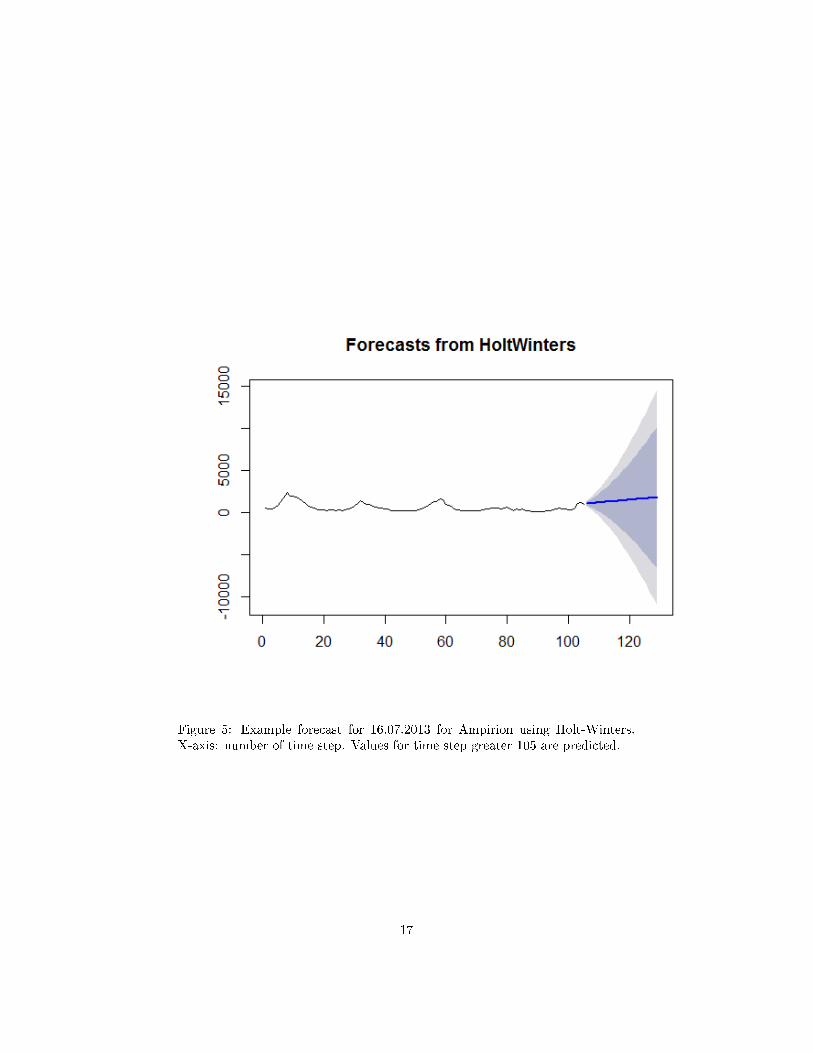
Figure 5: Example forecast for 16.07.2013 for Ampirion using Holt-Winters.X-axis: number of time step. Values for time step greater 105 are predicted.

17

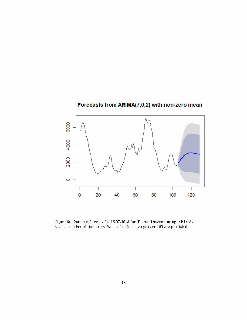
Figure 6: Example forecast for 16.07.2013 for Tennet Onshore using ARIMA.X-axis: number of time step. Values for time step greater 105 are predicted.

18

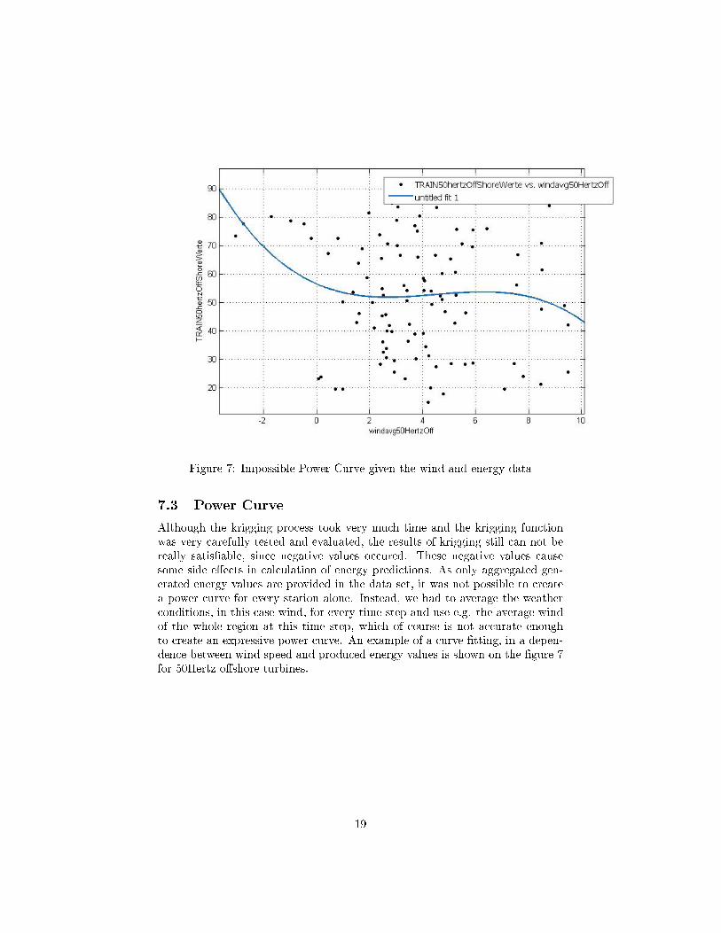
Figure 7: Impossible Power Curve given the wind and energy data

7.3 Power Curve

Although the krigging process took very much time and the krigging functionwas very carefully tested and evaluated, the results of krigging still can not bereally satis�able, since negative values occured. These negative values causesome side e�ects in calculation of energy predictions. As only aggregated gen-erated energy values are provided in the data set, it was not possible to createa power curve for every station alone. Instead, we had to average the weatherconditions, in this case wind, for every time step and use e.g. the average windof the whole region at this time step, which of course is not accurate enoughto create an expressive power curve. An example of a curve �tting, in a depen-dence between wind speed and produced energy values is shown on the �gure 7for 50Hertz o�shore turbines.

19

7.4 Common Results

Figures 8 - 13 show the distribution of the RMSE among di�erent calculationmodels compared to the o�cial prediction for di�erent prediction problems (6�gures for 6 TSOs). In case of Tennet Onshore and 50 Hertz Onshore no cal-culation using the "All-stations" model was performed due to lack of neededmemory by MATLAB.

Figure 14 shows a summary of rankings of calculation models based onRMSE in all 6 prediction problems (lowest RMSE means rank 1, highest rank10). As we can see, most of the time the o�cial prediction has the ranks 1 to 3.

Figure 15 shows the average ranking in solving 6 prediction problems amongdi�erent calculation models. One can see, that the o�cial prediction de�nitelywas better in average, followed by simple time series prediction models, whereno weather considerations were met at all.

The result of quality of ARIMA model can be easily explained by the peri-odicity of the energy production, which can easily be understood by the timeseries model.

Interestingly, more data did not mean more quality: models, involving dataof all wind turbines of a TSO at a time step instead of averaged weather valuesperformed worse than the models with averaged values. Also, more parametersat once (Single File) did not lead to success.

One of the best performance was achieved using the average wind speed inthe TSO region only, followed by the formulas where other weather componentswere more involved.

Results however can not be extrapolated to a general case, because only 105time steps were used for training. In order to be able to speak about a generalcase, signi�cantly more data than 5 days is required for training.

20

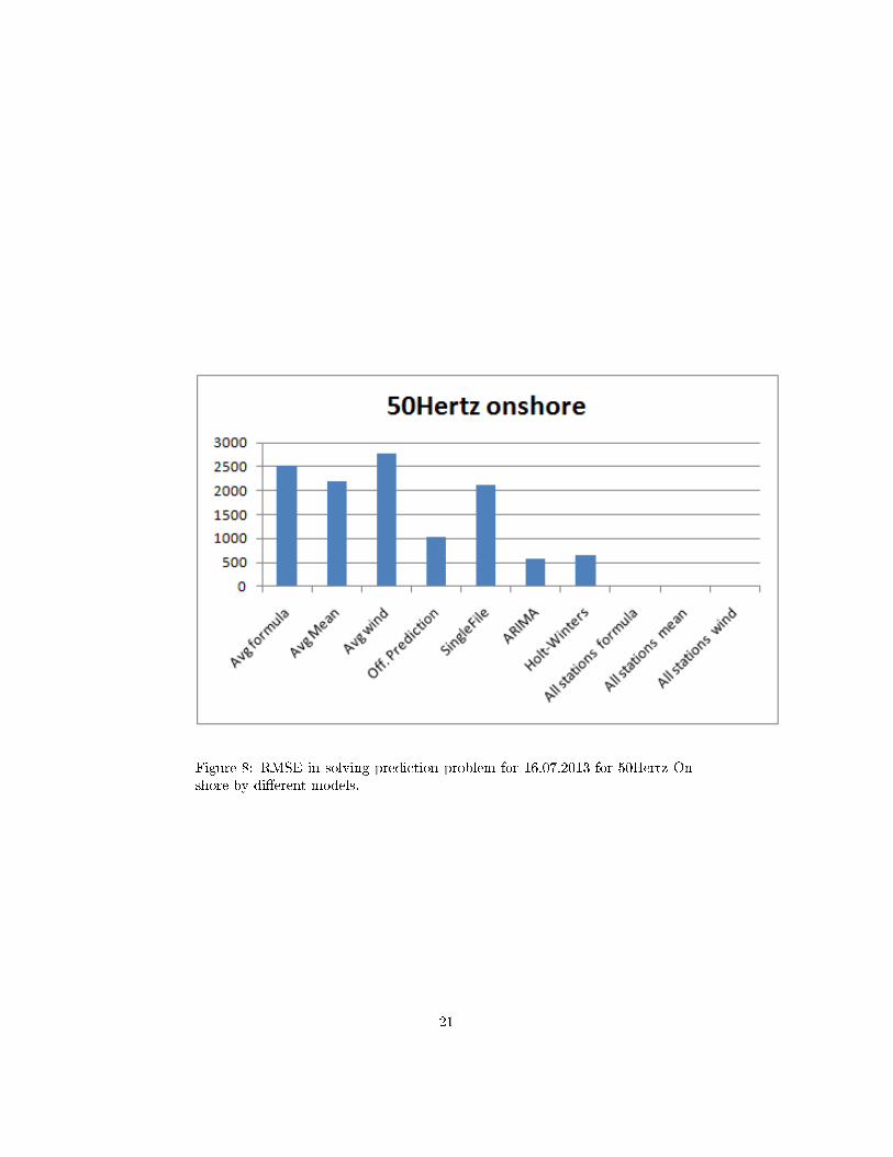
Figure 8: RMSE in solving prediction problem for 16.07.2013 for 50Hertz On-shore by di�erent models.

21

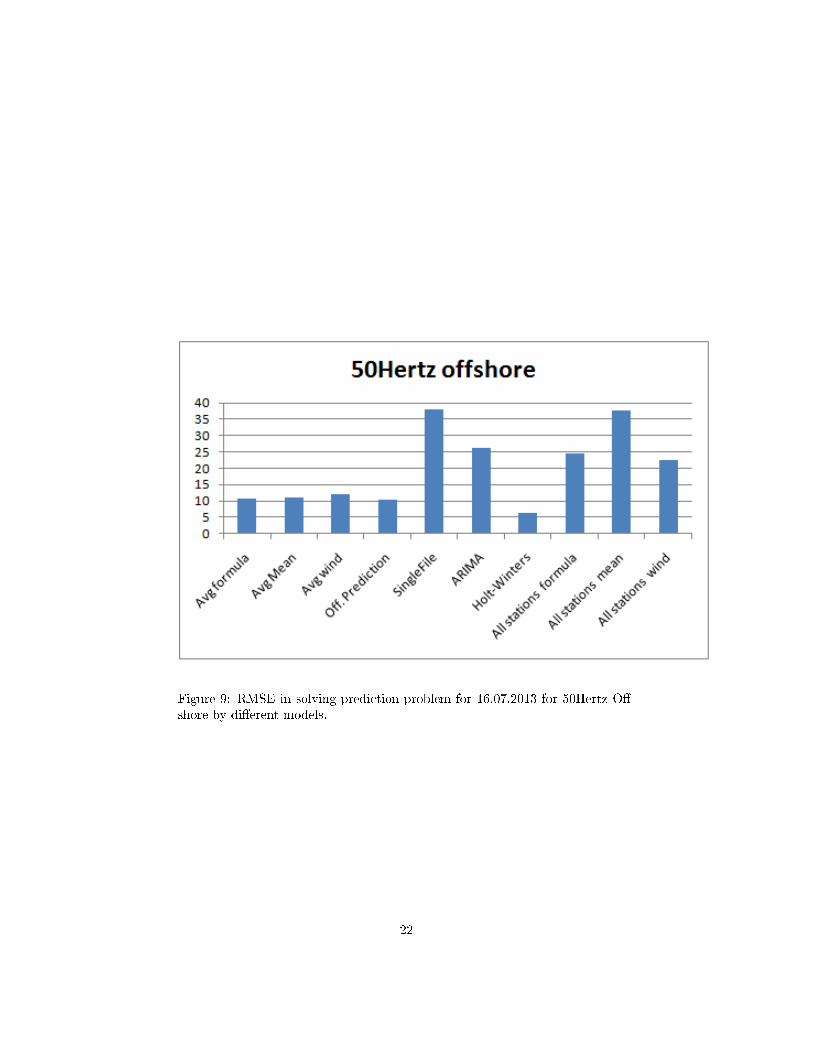
Figure 9: RMSE in solving prediction problem for 16.07.2013 for 50Hertz O�-shore by di�erent models.

22

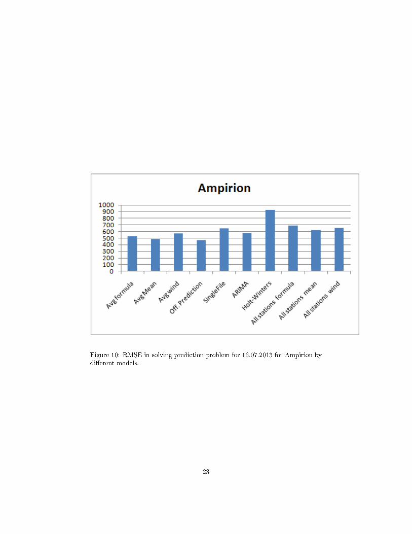
Figure 10: RMSE in solving prediction problem for 16.07.2013 for Ampirion bydi�erent models.

23

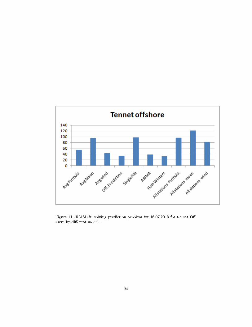
Figure 11: RMSE in solving prediction problem for 16.07.2013 for tennet O�-shore by di�erent models.

24

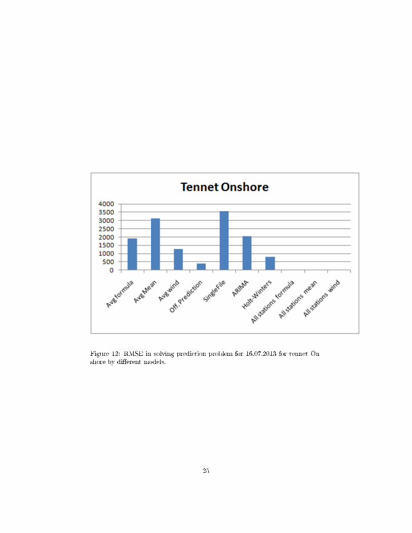
Figure 12: RMSE in solving prediction problem for 16.07.2013 for tennet On-shore by di�erent models.

25

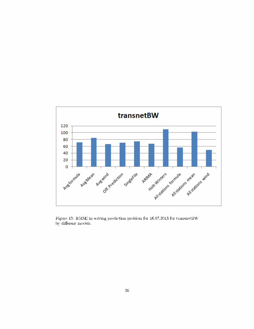
Figure 13: RMSE in solving prediction problem for 16.07.2013 for transnetBWby di�erent models.

26

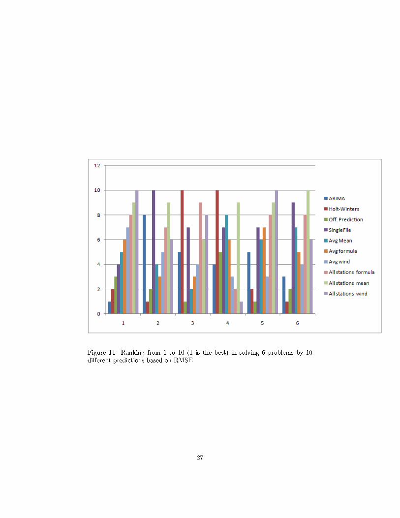
Figure 14: Ranking from 1 to 10 (1 is the best) in solving 6 problems by 10di�erent predictions based on RMSE

27

Figure 15: Average (ranking from 1 to 10 where 1 is the best) for each usedprediction in solving 6 problems.

28

8 Outlook and Conclusion

The results of the neural networks and time series prediction functions weresatisfying and competitive delivering a relatively small error, although did notoutperform the o�cial predictions.

The models could de�nitely perform better if more data would be available.In our case there were only 105 time steps and we had to predict the next24, which was a hard task even for reliable methods. Another problem wasthe availability of the weather data at wind turbine stations. The weatherparameters had to be krigged, which caused an additional error source. Negativevalues could be avoided using more expensive krigging methods. Time costscould be decreased in case of calculation of krigging on the GPU, which wasnot possible in R in our case. Another important issue of availability of data isthe problem that the individual generated energy values for every wind turbinewere not provided, so we had to deal with aggregated values, which of course isnot accurate enough for method to be competitive with the o�cial predictions.Of course, it would be better, if o�shore prediction values were also availableand we would not have to estimate it using the capacity information.

Nevertheless, the process included many interesting issues and we came withresults, that slightly underperform the o�cial forecasts. Also, we came up withthe result, that more parameters for the neural network does not help to achievebetter performance and use of average wind component per time step alone givesbetter results than involvement of other weather components, which obviouslyonly disturb the performance. Time series analysis methods brought best resultsbecause of the periodicity of data.

In future, the amount of wind energy will de�nitely raise and it will be moreand more important to use strong and accurate methods to predict the windenergy of the next day. The data providers will hopefully o�er more detaileddata to the public and better methods forecasting will be developed.

References

[1] Á. Székely, T. Barbarics. Budapest University of Technology and Economics,Short-Term Prediction of the Power Generation of Wind Turbines.

[2] European Centre for Medium-Range Weather Forecasts http:

//data-portal.ecmwf.int/data/d/interim_full_daily/.

[3] A. Kusiak, H. Zheng and Z. Song, Short-Term Prediction of Wind FarmPower: A Data Mining Approach.

[4] G. Giebel, P. Sørensen, H. Holttinen Risø National Laboratory, Forecasterror of aggregated wind power.

[5] M. Lange, U. Focken, State-of-the-Art in Wind Power Prediction in Ger-many and International Developments.

29

[6] G. Kariniotakis, P. Pinson, N. Siebert, G. Giebel, R. Barthelmie, The Stateof the Art in Short-Term Prediction of Wind Power Normally, .

[7] Argonne National Laboratory, Wind Power Forecasting: State-of-the-Art2009.

[8] S. Dutta, T.J. Overbye, Prediction of Short Term Power Output of WindFarms based on Least Squares Method.

[9] A. Marvuglia1, A. Messineo, Learning a wind farm Power Curve with aData-Driven Approach.

[10] Fraunhofer IWES, Windenergie Report Deutschland 2011

[11] René Jursa, Bernhard Lange, Kurt Rohrig, Institut für Solare Energiever-sorgungstechnik e. V, Wind Power Prediction with Optimization and Clus-tering Techniques.

[12] Bernhard Lange, Kurt Rohrig, Bernhard Ernst, Florian Schlögl, Ümit Cali,Rene Jursa, Javad Moradi, Wind Power Prediction in Germany � RecentAdvances and Future Challenges.

[13] Sideratos, G., Hatziargyriou, N.D., An Advanced Statistical Method forWind Power Forecasting.

[14] W. David Lubitz, Bruce R. White, Measuring Error in Wind Power Fore-casting Using a New Forecasting System.

[15] A. Kusiak, H. Zheng, Z. Song, Wind Farm Power Prediction: A Data-Mining Approach.

[16] P. Gopi, S. Ganesh Vadiyanathan, G. Umma Habi, Comparative Analysisof Wind Power. Forecasting Using Arti�cial Neural Network.

[17] G. Giebel et al., Delivarable Report. The State of the Art in Short-TermPrediction of Wind Power. A Literature Overview, 2nd Edition.

[18] Yang Lin, Wind power production forecasting: Nonlinear approach.

[19] Oliver Kramer, Fabian Gieseke, Short-Term Wind Energy Forecasting Us-ing Support Vector Regression.

[20] S. Mathew., J. Hazra, S. A. Husain, C. Basu, L. C. DeSilva, D. Seetharam,N. Y. Voo, S. Kalyanaraman and Z. Sulaiman, An Advanced Model for theShort-Term Forecast of Wind Energy.

[21] Amjady, N. ; Keynia, F. ; Zareipour, H., Wind Power Prediction by aNew Forecast Engine Composed of Modi�ed Hybrid Neural Network andEnhanced Particle Swarm Optimization.

[22] Audun Botterud, Jianhui Wang, Wind Power Forecasting and ElectricityMarket Operations.

30

[23] J. W. Taylor, P. E. McSharry, R. Buizza, Wind Power Density ForecastingUsing Ensemble Predictions and Time Series Models.

[24] J. Dobschinski, A. Wessel, B. Lange ISET e.V., Wind Power PredictionErrors of a Shortest-Term Forecast of the Total German Wind Power Gen-eration.

[25] http://www.50hertz.com/de/165.htm, Master data for EEG generatorsof 50Hertz GmbH.

[26] http://www.amprion.net/eeg-anlagenstammdaten-aktuell, Masterdata for EEG generators of Ampirion GmbH.

[27] http://www.tennet.eu/de/kunden/eegkwk-g/erneuerbare-energien-gesetz/eeg-daten-nach-52/

einspeisung-und-anlagenregister.html, Master data for EEG genera-tors of TennetTSO GmbH.

[28] http://www.transnetbw.de/eeg-and-kwk-g/eeg-anlagendaten/, Mas-ter data for EEG generators of TransnetBW GmbH.

[28] http://www.50hertz.com/de/151.htm, Forecast wind power feed-in of50Hertz GmbH.

[29] http://www.amprion.net/windenergieeinspeisung, Forecast windpower feed-in of Ampirion GmbH.

[30] http://transnetbw.com/key-figures/renewable-energies-res/wind-infeed/?app=wind&activeTab=csv&auswahl=month&selectMonat=

40, Forecast wind power feed-in of TransnetBW GmbH.

[31] http://www.tennettso.de/site/en/Transparency/publications/network-figures/actual-and-forecast-wind-energy-feed-in, Fore-cast wind power feed-in of TennetTSO GmbH.

[32] Andrew Kusiak, Haiyang Zheng, Zhe Song, Models for monitoring windfarm power.

[33] http://www.50hertz.com/de/151.htm, Mapping of post index to geo-graphic coordinates.

[34] http://a-little-book-of-r-for-time-series.readthedocs.org/en/latest/src/timeseries.html#holt-winters-exponential-smoothing,Time series analysis with R.

31