Regression analysis in modeling of airsurface temperature and factorsaffecting its value in PeninsularMalaysia

Jasim Mohammed RajabMohd. Zubir Mat JafriHwee San LimKhiruddin Abdullah

Regression analysis in modeling of air surfacetemperature and factors affecting its valuein Peninsular Malaysia

Jasim Mohammed RajabUniversiti Sains MalaysiaSchool of Physics11800 Penang, Malaysiaand

Mosul UniversityCollege of SciencePhysics DepartmentMosul, IraqE-mail: jasim_rijab@yahoo.com

Mohd. Zubir Mat JafriHwee San LimKhiruddin AbdullahUniversiti Sains MalaysiaSchool of Physics11800 Penang, Malaysia

Abstract. This study encompasses air surface temperature (AST) mod-eling in the lower atmosphere. Data of four atmosphere pollutant gases(CO, O3, CH4, and H2Ovapor) dataset, retrieved from the National Aeronau-tics and Space Administration Atmospheric Infrared Sounder (AIRS), from2003 to 2008 was employed to develop a model to predict AST value in theMalaysian peninsula using the multiple regression method. For the entireperiod, the pollutants were highly correlated (R ¼ 0.821) with predictedAST. Comparisons among five stations in 2009 showed close agreementbetween the predicted AST and the observed AST from AIRS, especiallyin the southwest monsoon (SWM) season, within 1.3 K, and for in situdata, within 1 to 2 K. The validation results of AST with AST fromAIRS showed high correlation coefficient (R ¼ 0.845 to 0.918), indicatingthe model’s efficiency and accuracy. Statistical analysis in terms of βshowed that H2Ovapor (0.565 to 1.746) tended to contribute significantlyto high AST values during the northeast monsoon season. Generally,these results clearly indicate the advantage of using the satellite AIRSdata and a correlation analysis study to investigate the impact of atmo-spheric greenhouse gases on AST over the Malaysian peninsula. Amodel was developed that is capable of retrieving the Malaysian peninsu-lan AST in all weather conditions, with total uncertainties ranging between1 and 2 K. © 2012 Society of Photo-Optical Instrumentation Engineers (SPIE). [DOI: 10.1117/1.OE.51.10.101702]

Subject terms: air surface temperature; greenhouse gases; atmosphere infraredsounder.

Paper 111287SS received Oct. 17, 2011; revised manuscript received Dec. 20,2011; accepted for publication Jan. 5, 2012; published online May 21, 2012.

1 IntroductionMinute changes in the temperature of the human body canlead to sickness and even death. Similarly, the Earth is highlysensitive to small changes in temperature. In particular,increases in temperature are referred to as the greenhouseeffect. There is a growing consensus that since the start ofthe industrial revolution in the 19th century, the concentra-tion of greenhouse gases (GHG) in the atmosphere hasincreased due to continuous increases in anthropogenic emis-sions resulting from increased human activity, industrializa-tion, and deforestation. This increase in GHG concentrationhas led to a rise in atmospheric and ocean temperatures, melt-ing glaciers and ice caps, and increasing sea levels,1 whichhave caused regional shifts in precipitation patterns andincreases in the occurrence of severe weather. Natural causesalone cannot satisfactorily explain the observed warming.2

Climate change is now a prominent issue that has beenwidely discussed throughout the world. The excessive emis-sion of global GHGs into the atmosphere is one of the majorcauses of climate change. The important external variablesthat control climate include aerosols, solar irradiance, andGHGs of methane (CH4), ozone (O3), nitric acid (NO2),water vapor (H2Ovapor), and carbon dioxide (CO2).

3

Although the emission of GHGs and other factors, such

as changes in land use, make only a minor contribution toglobal warming (1%) compared to solar input, this slightmodification to the energy budget is still significant and con-tributes to the observed increase in oceanic and atmospherictemperature.4

In the Earth’s atmosphere, the dominant infrared absorb-ing and emitting gases, which have different influences onthe greenhouse effect, are CO2 9 to 26%, H2Ovapor 36 to 70%(not including clouds), CH4 4 to 9%, and O3 3 to 7%. Cloudsaffect radiation differently from water vapor because they arecomposed of water or ice.5 GHGs lead to problems for theenvironment, especially in areas with ambient air tempera-ture, and they also have negative impacts on health. There-fore, it is necessary to observe and accurately document notonly changes in temperature but also changes in the atmo-sphere GHGs to assess their impact on the environment.

Southeast Asia is experiencing rapid economic growthsimilar to that in Northeast Asia, and it has become oneof the most heavily populated regions of the world with avibrant mixture of cultures.6 Furthermore, it is a large sourceof several air pollutants due to increasing anthropogenicemissions associated with biogenic emissions from large tro-pical forests. The greater oxidizing capacity in the tropicalregions is due to a higher ultraviolet (UV) intensity, humid-ity, rapid development, and industrialization.7 In Malaysia,industrialization, urbanization and rapid traffic growthhave contributed significantly to economic growth. Pockets0091-3286/2012/$25.00 © 2012 SPIE

Optical Engineering 101702-1 October 2012/Vol. 51(10)

Optical Engineering 51(10), 101702 (October 2012)

of heavy pollution are being created by emissions from majorindustrial zones, an increase in the number of motor vehicles,and trans-boundary pollution. Furthermore, Malaysia is situ-ated in a humid tropical zone with heavy rainfall and hightemperatures;8,9 the cloudy conditions are an obstacle tothe acquisition of high-quality and high-resolution satellitedata.

Multiple regression analysis (MRA) is the most commontechnique used to obtain a linear input-output model for agiven data set, and it is the methodology used in theatmospheric sciences. It is one of the most familiar meth-odologies utilized in the atmospheric sciences for expressingthe dependence of a response variable on several indepen-dent (predictor) variables by fitting a linear equation toobserved data. Such a relationship has been examined inseveral studies that have used a combination of statisticalregression.10–13

Over the past three decades, the abundances of atmo-spheric gases have been measured using balloons, airplanes,and sparsely distributed measurement sites. The observationswere mostly confined to the surface of the site. The measure-ments are unable to make continuous recordings of globalvariation over the long term and cost a lot in terms ofmoney and staff. Therefore, there is a lack of data bothin the lower and upper troposphere,14 particular over landin the lower troposphere.

Satellite remote sensing has very good global coverageand has increased our capability to assess the influence ofhuman activities on the chemical composition of the atmo-sphere and on climate change.15 Furthermore, this techniquecan provide continuous data with high spatial and temporalresolution.16 However, the cloudy conditions are an obstacleto the acquisition of high-quality and high-resolution satellitedata. The free download satellite Atmospheric InfraredSounder (AIRS) data makes it as a useful space instrumentfor observing the Earth’s atmospheric temperature, watervapor, and the reaction of the several atmospheric GHGswith a cloud-clearing system.17

AIRS is the first of a new generation of meteorologicallyadvanced sounders for operational and research use. It isone of several instruments of the Earth Observing System(EOS) aboard the Aqua satellite, which was launched bythe National Aeronautics and Space Administration(NASA) on May 4, 2002. AIRS, together with the Advanced

Microwave Sounding Unit (AMSU) and the HumiditySounder for Brazil (HSB) microwave radiometers, hasachieved a global retrieval accuracy of better than 1 K inthe lower troposphere under clear and partly cloudy condi-tions.18 The capability of AIRS/AMSU/HSB is to supplysimultaneous observations of the Earth’s atmospheric,land surface, and ocean surface temperatures; water vapor;cloud amount and cloud height; albedo; and GHGs and aero-sols makes AIRS the most important EOS instrument forinvestigating several interdisciplinary issues to be addressedin earth science.

In this study, the MRAwas employed to obtain predictionmodel for air surface temperature (AST) with GHGs (CH4,O3

and H2Ovapor) and carbon monoxide (CO) as predictor vari-ables. The idea is to use results from the analysis of theretrieved gases in the atmosphere for the period between2003 and 2008 obtained from the AIRS data to develop ageneral regression equation for calculating the AST overthe Malaysian peninsula. In addition, we wanted to investigateand analyze the influences of the GHGs (CH4, O3, andH2Ovapor) and CO in the AST values using statistical methods.

2 Material and Methods

2.1 Study Area and Data Collection

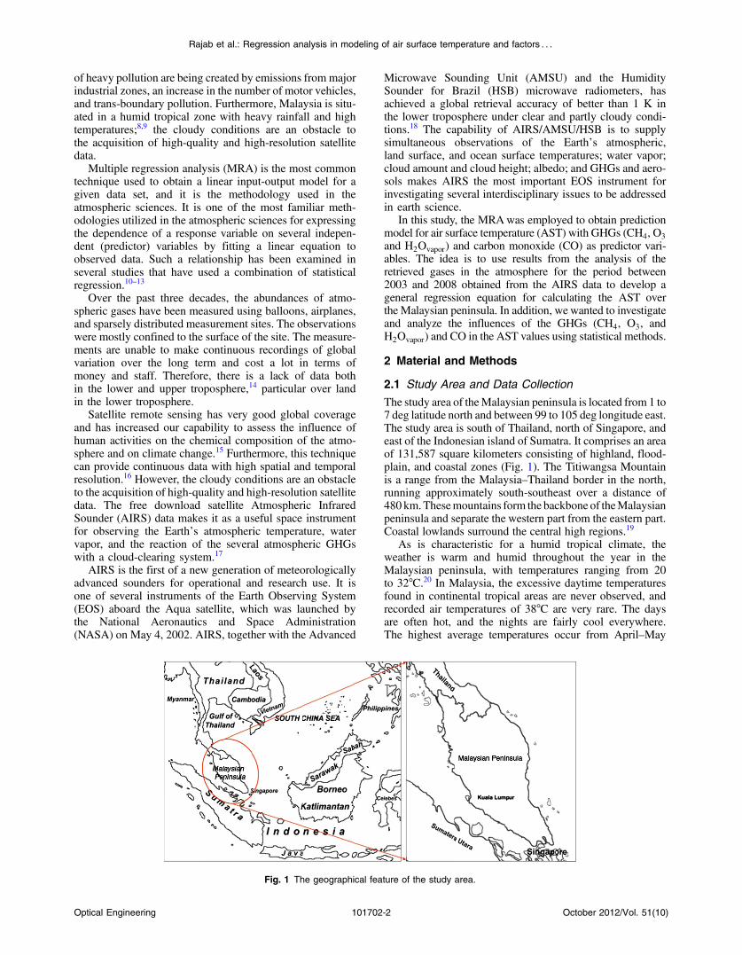
The study area of theMalaysian peninsula is located from 1 to7 deg latitude north and between 99 to 105 deg longitude east.The study area is south of Thailand, north of Singapore, andeast of the Indonesian island of Sumatra. It comprises an areaof 131,587 square kilometers consisting of highland, flood-plain, and coastal zones (Fig. 1). The Titiwangsa Mountainis a range from the Malaysia–Thailand border in the north,running approximately south-southeast over a distance of480 km.Thesemountains form the backbone of theMalaysianpeninsula and separate the western part from the eastern part.Coastal lowlands surround the central high regions.19

As is characteristic for a humid tropical climate, theweather is warm and humid throughout the year in theMalaysian peninsula, with temperatures ranging from 20to 32°C.20 In Malaysia, the excessive daytime temperaturesfound in continental tropical areas are never observed, andrecorded air temperatures of 38°C are very rare. The daysare often hot, and the nights are fairly cool everywhere.The highest average temperatures occur from April–May

Fig. 1 The geographical feature of the study area.

Optical Engineering 101702-2 October 2012/Vol. 51(10)

Rajab et al.: Regression analysis in modeling of air surface temperature and factors : : :

and July–August in most places, and the lowest averagemonthly temperatures occur from November–January.

There is a definite variation of the monthly mean tempera-ture that coincides with the monsoons, and there are annualfluctuations of roughly 1.5 to 2°C. The monsoons signifi-cantly affect the climate of the Malaysian peninsula. Itexperiences two rainy seasons throughout the year, asso-ciated with the northeast monsoon (NEM) from Novemberto February and the SWM from May to August.21 During theinter-monsoon months (usually between April and October),the wind and light are variable and thunderstorms develop,causing substantial rainfall in each of the two transition per-iods, especially in the west coast states. Monsoon changesand the effects of topography are the main factors that affectthe rainfall distributions. The monsoon rainfalls account for81% of the annual rain that falls in the entire Malaysianpeninsula and is estimated at approximately 2300 mm.22

These monsoons have different influences on the atmo-spheric parameters, in terms of the effects on climate orthe amounts of pollutants, that they bring to Malaysia,besides the contribution of the many regional pollutantsources.

The mean focus of the study is to develop a regressionequation for monthly AST and ozone throughout the yearover the Malaysian peninsula by processing the satellitedata for the retrieved atmosphere parameter. Seven years ofsatellite data were collected from January 2003 to December2009. The first six years of this data were collected duringthis duration for analysis and development of the predictiveAST regression equations. Data from the last year, 2009,were used for validations, comparisons, and mapping of thedata. The satellite data were collected online from NASA.In addition to the satellite data, we also used in situ datacollected from the Malaysian Meteorology Department(MMD). The various kinds of software that were used duringthe process include Statistical Package for Social Sciences(SPSS), SigmaPlot 11, Microsoft Excel, and Photoshop CS.

AIRS Level-3 standard product files were stored in theHDF-EOS4 format. Therefore, the data can be easily arrangein Excel. Then SPSS software was used for analysis of theAIRS satellite data to find correlations between atmosphericparameters and predicted values of AST and O3 using multi-ple regression equations and component analysis methods.The Kriging Interpolation technique is a geostatistical tech-nique that can be conducted in SigmaPlot 11. This methoduses high correlation coefficients R2 and low root meansquare (RMS) to generate the maps of AST, O3, and othergases.23 SigmaPlot was also used to correlate the predictedand the observed ASTs and O3 and to plot their values indifferent months and regions for comparison. The validationprocesses for the predicted AST and O3 were carried outusing Excel. The graphics editing program Photoshop wasused to generate the AST and the concentration maps forO3 and the other gases to better assess their distributionsover the study area.

Generally, 84 monthly L3 ascending AIRX3STM1 deg×1 deg spatial resolution granules were downloadedfrom the AIRS website http://disc.sci.gsfc.nasa.gov/AIRS toobtain the desired output. Atmospheric parameters measuredincluded carbonmonoxide (CO), ozone (O3), methane (CH4),and water vapor (H2Ovapor). The AST data were also acquiredfrom the MMD. The data were collected in monthly intervals

from January 2003 to December 2009 for five stations: KotaBahru,Penang,Kuantan,Subang, and Johor.These in situdatawere used for comparison with the data from the developedregression equation and observed data from AIRS, in orderto check the efficiency and accuracy of the equation.

2.2 Method of Analysis

Regression analysis was used to predict the future(the unknown) based upon data collected from the past(the known). Therefore, it was the process of looking for pre-dictors and determining how well they predict future values.A regression analysis determines the mathematical equationto be used to predict an outcome within a certain range ofprobability. The analysis shows how a dependent variablewill be affected by one or more independent variables.When one independent variable is taken into account, it iscalled a simple regression; if there is more than one indepen-dent variable, it is called a multiple regression.24 The esti-mated regression coefficients are given under the headingCoefficients B (β), which explain, for each of the explana-tory variables, the predicted change in the dependent variablewhen the explanatory variable is raised by one unit, so longas all the other variables in the model remains constant. βwas used in this study to develop the regression equationsfor calculating the AST over the study area using the datafor several gases.

The Coefficients Beta (β) measure the change in thedependent variable in units of its standard deviation whenthe explanatory variable rises by one standard deviation.The standardization mean influenced by values does notdepend on units and enables the comparison of impactsacross explanatory variables. β was used in this study toanalyze the impacts of GHGs on AST.25

The relationships between AST and the set of data wereexamined statistically using the multiple linear regressionmethod. The predictive equation for monthly AST obtainedthis value by using the terms of β. The multiple regressionequation for a response variable y with monitor valuesy1; y2 : : : yn (where n is the sample size) is as follows:

Yi ¼ β0þ β1x1iþ β2x2iþ β3x3iþ β4x4iþ · · · þβqxqi; (1)

where q is explanatory variables x1; x2 : : : xq with observedvalues x1i; x2i : : : xqi for i ¼ 1; : : : ; n; β0 is an regressionequation constant; and β1; β2; β3; β4 : : : βq are explanatoryvariable constants.

3 Results and Discussion

3.1 Generating Regression Equation AST UsingStandard AIRX3STM Data

Data on the value of four atmosphere pollutant gases (CO,O3, CH4, and H2Ovapor) from the standard monthly productAIRX3STM 1 deg×1 deg spatial resolution, Version 5descriptive data for the entire period (from January 2003to December 2008) were employed as a predictor (indepen-dent variables) to generate the AST regression equation (pre-dicted AST value) using the multiple linear regressionmethod, as in Eq. (3).

As explained in Sec. 2.2, the regression in terms of β wasused to generate the AST regression equation for data fromthe entire period (from January 2003 to December 2008) in

Optical Engineering 101702-3 October 2012/Vol. 51(10)

Rajab et al.: Regression analysis in modeling of air surface temperature and factors : : :

the study area, and from Eq. (1), the formula is given asfollows:

AST¼ β0þ βCOCOþ βO3O3þ βCH4

CH4þ βH2OH2O; (2)

where β0 is a regression equation constant, and βCO, βO3,βCH4, and βH2O

are explanatory CO, O3, CH4, and H2Oconstants, respectively. For the entire period:

AST ¼ 245.6þ ð2.83 × 108ÞCOþ ð0.128ÞO3

þ ð−5.16 × 106ÞCH4 þ ð970ÞH2O: (3)

These four pollutant gases have a strong relationship withthe AST, as indicated by the high correlation coefficientvalue (R ¼ 0.821), and are strongly correlated, as indicatedby the adjusted R2 of approximately 0.683 for time observa-tions. This mean of 68% of the variation in the AST1 is clar-ified by these independent four atmosphere pollutant gases(CO, O3, CH4, and H2Ovapor).

Then, separate multiple regressions were also carried outfor each monthly average during the 2003–2008 period tofind the value of R for each average. For this period, thepollutants (gases) were highly correlated with AST. Themultiple regression results for the average monthly data areoutlined in Table 1 in terms of the β, the amount of coeffi-cient of determination (R2), and the multiple correlationcoefficients (R).

3.2 Regression Analysis of the Impact of GHGs onAST

As discussed in Sec. 2.2, MRA in terms of β was used toclarify the impact of CO, O3, CH4, and H2Ovapor on theAST values. Separate multiple regressions were carriedout for each monthly average for the 2003 to 2008 periodin terms of β for the study area. The results outlined in Table 2are for both the NEM season (November–April) and SWM

season (May–October), where βCO, βO3, βCH4

, and βH2Oare

the change in the dependent variable in units of its standarddeviation for CO, O3, CH4, and H2Ovapor, respectively. Thediscussion was separated into two periods due to the differenteffects of both the NEM and SWM, in terms of the effects onclimate or the amount of pollutants, that they bring to thestudy area.

3.2.1 Northeast monsoon season

The overall AST in the Malaysian peninsula during the NEMseason was most affected by H2Ovapor, as indicated bythe strong positive β (0.565 to 1.746) associated with thisvariable, and CO (0.312 to 0.913) and O3 (0.426 to 0.762)had a moderate positive β. CH4 (−0.124 to 0.426) was alsoan important parameter in determining the variability of theAST value, recognizable in December–March, as shown inTable 2.

The positive relationship is a result of the onset of theNEM, cold surges originating from Siberia and northeastAsia that bring a significant amount of pollution to southeastAsia while crossing through the heavily polluted regions ofeast Asia,26 and heavy rains that lead to severe flooding inDecember of certain years along the east coast and Johor.9

At the same time, with strong subsidence early in the NEMseason, there are important increases in air pollutant levels incontinental Southeast Asia.27

Maximum air pollutant levels occur over continentalSoutheast Asia in the late months of a dry season as a resultof high levels of regional biomass burning and long-rangetransport of air masses from western Asia and the MiddleEast.26

3.2.2 SWM season

The overall AST in the Malaysian peninsula during theSWM season was most affected by H2Ovapor (1.042 to2.036) and O3 (0.421 to 0.864), as indicated by the strong

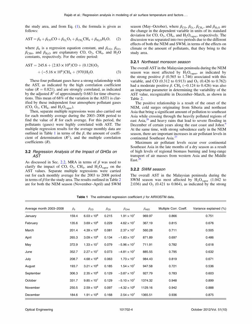
Table 1 The estimated regression coefficient β for AIRX3STM data.

Average month 2003–2008 β0 βCO βO3 βCH4 βH2O Multiple Corr. Coeff. Variance explained (%)

January 159.4 6.03 × 108 0.215 1.91 × 107 969.97 0.866 0.751

February 135.6 3.69 × 108 0.229 4.62 × 107 367.19 0.815 0.676

March 201.4 4.39 × 108 0.081 2.37 × 107 560.28 0.711 0.505

April 265.3 3.09 × 108 0.134 −1.83 × 107 871.89 0.697 0.486

May 372.9 1.33 × 107 0.079 −5.96 × 107 711.91 0.782 0.618

June 352.7 2.27 × 107 0.073 −4.81 × 107 885.55 0.795 0.632

July 208.7 4.68 × 108 0.063 1.73 × 107 984.43 0.819 0.671

August 193.7 3.21 × 108 0.185 1.54 × 107 947.58 0.721 0.536

September 306.3 2.35 × 108 0.129 −3.87 × 107 927.79 0.783 0.603

October 331.7 9.85 × 107 0.129 −5.10 × 107 1374.32 0.948 0.899

November 250.5 2.59 × 108 0.097 −4.32 × 106 1129.16 0.942 0.888

December 184.6 1.91 × 108 0.168 2.54 × 107 1365.51 0.936 0.875

Optical Engineering 101702-4 October 2012/Vol. 51(10)

Rajab et al.: Regression analysis in modeling of air surface temperature and factors : : :

positive β associated with this variable. The CO (0.125 to0.748) also had a moderate positive β and important param-eters in determining the variability of temperature in thisperiod, and CH4 (−0.526 to 0.118) had a moderate positiveβ in July and August, as summarized in Table 2.

The positive relationship is the result of the increase in airpollutants in the continent. Marine air masses from the mid-dle and low latitudes of the Indian Ocean in the SouthernHemisphere dominate continental Southeast Asia andcarry small to moderate amounts of air pollution duringthe SWM season in addition to the local large anthropogenicsources within continental Southeast Asia.26

3.3 Comparison and Validation of the RegressionEquations

3.3.1 Comparison of AST with observed AST fromAIRS and in situ measurements

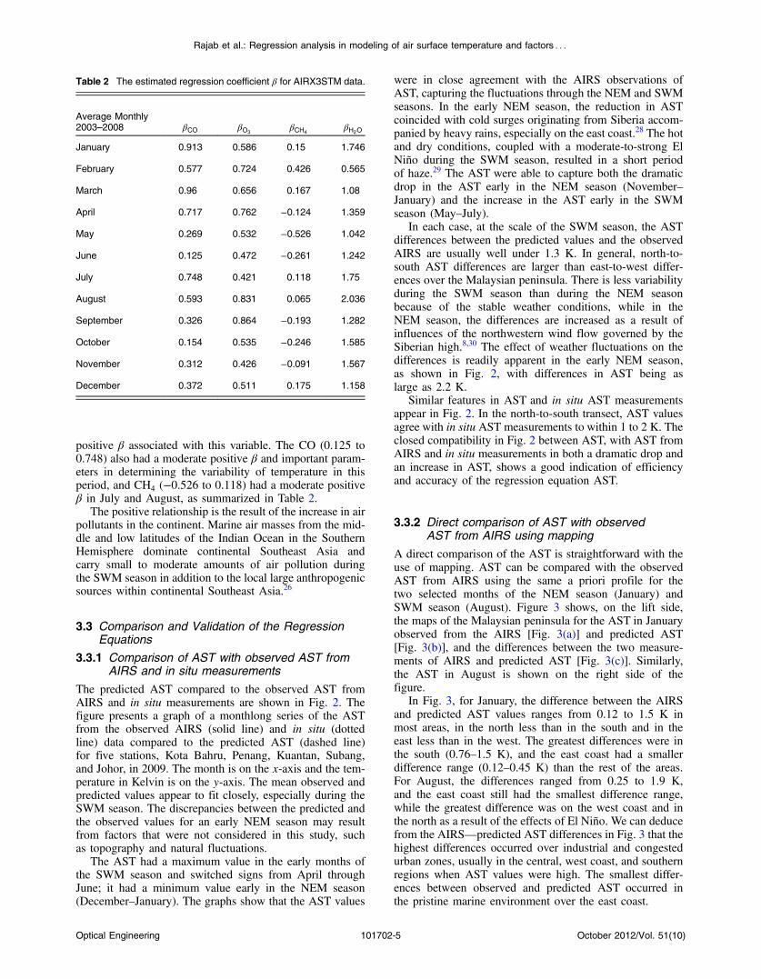
The predicted AST compared to the observed AST fromAIRS and in situ measurements are shown in Fig. 2. Thefigure presents a graph of a monthlong series of the ASTfrom the observed AIRS (solid line) and in situ (dottedline) data compared to the predicted AST (dashed line)for five stations, Kota Bahru, Penang, Kuantan, Subang,and Johor, in 2009. The month is on the x-axis and the tem-perature in Kelvin is on the y-axis. The mean observed andpredicted values appear to fit closely, especially during theSWM season. The discrepancies between the predicted andthe observed values for an early NEM season may resultfrom factors that were not considered in this study, suchas topography and natural fluctuations.

The AST had a maximum value in the early months ofthe SWM season and switched signs from April throughJune; it had a minimum value early in the NEM season(December–January). The graphs show that the AST values

were in close agreement with the AIRS observations ofAST, capturing the fluctuations through the NEM and SWMseasons. In the early NEM season, the reduction in ASTcoincided with cold surges originating from Siberia accom-panied by heavy rains, especially on the east coast.28 The hotand dry conditions, coupled with a moderate-to-strong ElNiño during the SWM season, resulted in a short periodof haze.29 The AST were able to capture both the dramaticdrop in the AST early in the NEM season (November–January) and the increase in the AST early in the SWMseason (May–July).

In each case, at the scale of the SWM season, the ASTdifferences between the predicted values and the observedAIRS are usually well under 1.3 K. In general, north-to-south AST differences are larger than east-to-west differ-ences over the Malaysian peninsula. There is less variabilityduring the SWM season than during the NEM seasonbecause of the stable weather conditions, while in theNEM season, the differences are increased as a result ofinfluences of the northwestern wind flow governed by theSiberian high.8,30 The effect of weather fluctuations on thedifferences is readily apparent in the early NEM season,as shown in Fig. 2, with differences in AST being aslarge as 2.2 K.

Similar features in AST and in situ AST measurementsappear in Fig. 2. In the north-to-south transect, AST valuesagree with in situ AST measurements to within 1 to 2 K. Theclosed compatibility in Fig. 2 between AST, with AST fromAIRS and in situ measurements in both a dramatic drop andan increase in AST, shows a good indication of efficiencyand accuracy of the regression equation AST.

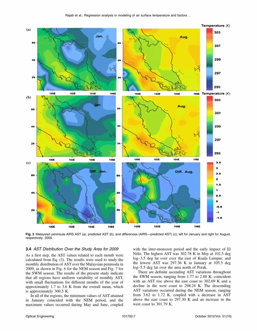
3.3.2 Direct comparison of AST with observedAST from AIRS using mapping

A direct comparison of the AST is straightforward with theuse of mapping. AST can be compared with the observedAST from AIRS using the same a priori profile for thetwo selected months of the NEM season (January) andSWM season (August). Figure 3 shows, on the lift side,the maps of the Malaysian peninsula for the AST in Januaryobserved from the AIRS [Fig. 3(a)] and predicted AST[Fig. 3(b)], and the differences between the two measure-ments of AIRS and predicted AST [Fig. 3(c)]. Similarly,the AST in August is shown on the right side of thefigure.

In Fig. 3, for January, the difference between the AIRSand predicted AST values ranges from 0.12 to 1.5 K inmost areas, in the north less than in the south and in theeast less than in the west. The greatest differences were inthe south (0.76–1.5 K), and the east coast had a smallerdifference range (0.12–0.45 K) than the rest of the areas.For August, the differences ranged from 0.25 to 1.9 K,and the east coast still had the smallest difference range,while the greatest difference was on the west coast and inthe north as a result of the effects of El Niño. We can deducefrom the AIRS—predicted AST differences in Fig. 3 that thehighest differences occurred over industrial and congestedurban zones, usually in the central, west coast, and southernregions when AST values were high. The smallest differ-ences between observed and predicted AST occurred inthe pristine marine environment over the east coast.

Table 2 The estimated regression coefficient β for AIRX3STM data.

Average Monthly2003–2008 βCO βO3

βCH4βH2O

January 0.913 0.586 0.15 1.746

February 0.577 0.724 0.426 0.565

March 0.96 0.656 0.167 1.08

April 0.717 0.762 −0.124 1.359

May 0.269 0.532 −0.526 1.042

June 0.125 0.472 −0.261 1.242

July 0.748 0.421 0.118 1.75

August 0.593 0.831 0.065 2.036

September 0.326 0.864 −0.193 1.282

October 0.154 0.535 −0.246 1.585

November 0.312 0.426 −0.091 1.567

December 0.372 0.511 0.175 1.158

Optical Engineering 101702-5 October 2012/Vol. 51(10)

Rajab et al.: Regression analysis in modeling of air surface temperature and factors : : :

3.3.3 Validation of AST with observed AST fromAIRS

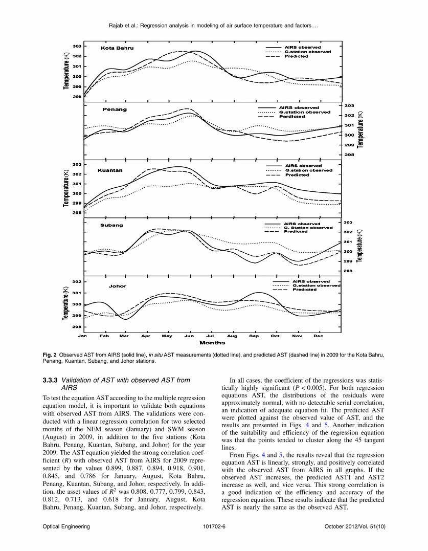
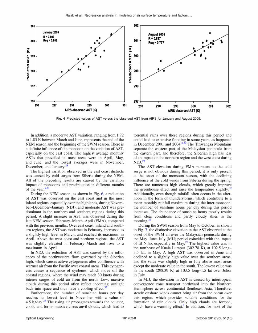
To test the equation ASTaccording to the multiple regressionequation model, it is important to validate both equationswith observed AST from AIRS. The validations were con-ducted with a linear regression correlation for two selectedmonths of the NEM season (January) and SWM season(August) in 2009, in addition to the five stations (KotaBahru, Penang, Kuantan, Subang, and Johor) for the year2009. The AST equation yielded the strong correlation coef-ficient (R) with observed AST from AIRS for 2009 repre-sented by the values 0.899, 0.887, 0.894, 0.918, 0.901,0.845, and 0.786 for January, August, Kota Bahru,Penang, Kuantan, Subang, and Johor, respectively. In addi-tion, the asset values of R2 was 0.808, 0.777, 0.799, 0.843,0.812, 0.713, and 0.618 for January, August, KotaBahru, Penang, Kuantan, Subang, and Johor, respectively.

In all cases, the coefficient of the regressions was statis-tically highly significant (P < 0.005). For both regressionequations AST, the distributions of the residuals wereapproximately normal, with no detectable serial correlation,an indication of adequate equation fit. The predicted ASTwere plotted against the observed value of AST, and theresults are presented in Figs. 4 and 5. Another indicationof the suitability and efficiency of the regression equationwas that the points tended to cluster along the 45 tangentlines.

From Figs. 4 and 5, the results reveal that the regressionequation AST is linearly, strongly, and positively correlatedwith the observed AST from AIRS in all graphs. If theobserved AST increases, the predicted AST1 and AST2increase as well, and vice versa. This strong correlation isa good indication of the efficiency and accuracy of theregression equation. These results indicate that the predictedAST is nearly the same as the observed AST.

Fig. 2 Observed AST from AIRS (solid line), in situ AST measurements (dotted line), and predicted AST (dashed line) in 2009 for the Kota Bahru,Penang, Kuantan, Subang, and Johor stations.

Optical Engineering 101702-6 October 2012/Vol. 51(10)

Rajab et al.: Regression analysis in modeling of air surface temperature and factors : : :

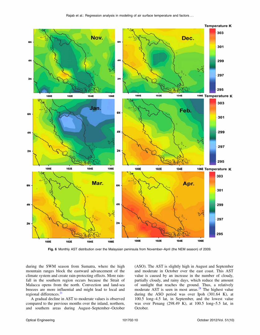
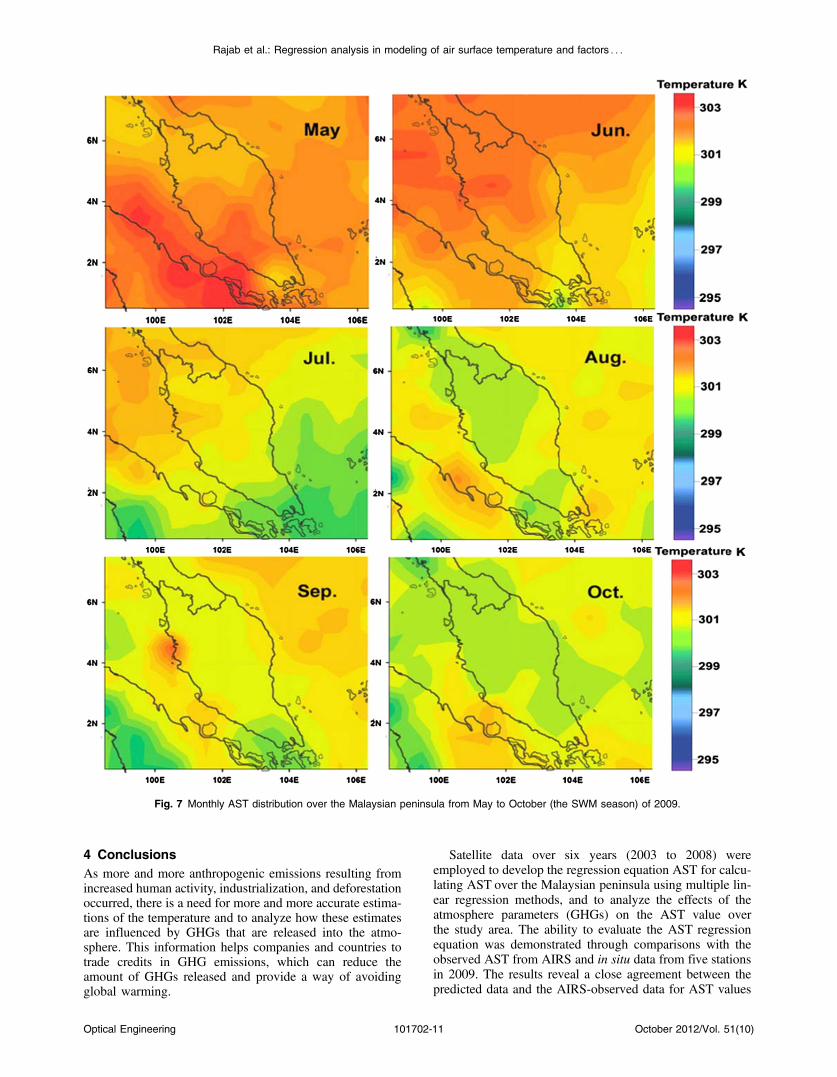
3.4 AST Distribution Over the Study Area for 2009

As a first step, the AST values related to each month werecalculated from Eq. (3). The results were used to study themonthly distribution of ASTover the Malaysian peninsula in2009, as shown in Fig. 6 for the NEM season and Fig. 7 forthe SWM season. The results of the present study indicatethat all regions have uniform variability of monthly AST,with small fluctuations for different months of the year ofapproximately 1.7 to 3.6 K from the overall mean, whichis approximately 300.5 K.

In all of the regions, the minimum values of AST attainedin January coincided with the NEM period, and themaximum values occurred during May and June, coupled

with the inter-monsoon period and the early impact of ElNiño. The highest AST was 302.78 K in May at 102.5 deglog–3.5 deg lat over over the east of Kuala Lumpur, andthe lowest AST was 297.36 K in January at 105.5 deglog–5.5 deg lat over the area north of Perak.

There are definite ascending AST variations throughoutthe SWM season, ranging from 1.77 to 2.88 K, coincidentwith an AST rise above the east coast to 302.69 K and adecline in the west coast to 298.24 K. The descendingAST variations occurred during the NEM season, rangingfrom 3.62 to 1.72 K, coupled with a decrease in ASTabove the east coast to 297.30 K and an increase in thewest coast to 301.79 K.

Fig. 3 Malaysian peninsula AIRS AST (a), predicted AST (b), and differences (AIRS—predicted AST) (c); left for January and right for August,respectively, 2009.

Optical Engineering 101702-7 October 2012/Vol. 51(10)

Rajab et al.: Regression analysis in modeling of air surface temperature and factors : : :

In addition, a moderate AST variation, ranging from 1.72to 1.83 K between March and June, represents the end of theNEM season and the beginning of the SWM season. There isa definite influence of the monsoon on the variation of AST,especially on the east coast. The highest average monthlyASTs that prevailed in most areas were in April, May,and June, and the lowest averages were in November,December, and January.28

The highest variation observed in the east coast districtswas caused by cold surges from Siberia during the NEM.All of the preceding results are caused by the variationimpact of monsoons and precipitation in different monthsof the year.9,31

During the NEM season, as shown in Fig. 6, a reductionof AST was observed on the east coast and in the mostinland regions, especially over the highlands, during Novem-ber–December–January (NDJ), and moderate AST was pre-dominant in the northern and southern regions during thisperiod. A slight increase in AST was observed during thelate NEM season, February–March–April (FMA), comparedwith the previous months. Over east coast, inland and south-ern regions, the ASTwas moderate in February, increased toa slightly high level in March, and reached its maximum inApril. Above the west coast and northern regions, the ASTwas slightly elevated in February–March and rose to amaximum in April.

In NDJ, the reduction of AST was caused by the influ-ences of the northwestern flow governed by the Siberianhigh, which causes active cytogenesis after confluence withwarmer air from the Pacific over coastal areas. This cytogen-esis causes a sequence of cyclones, which move off thecoastal regions, where the wind may reach 30 knots duringintense surges of cold air from the north. Low, massiveclouds during this period often reflect incoming sunlightback into space and thus have a cooling effect.32

Furthermore, the number of sunshine hours per dayreaches its lowest level in November with a value of4.5 h∕day.28 The rising air propagates towards the equator,cools, and forms massive cirrus anvil clouds, which lead to

torrential rains over these regions during this period andcould lead to extensive flooding in some years, as happenedin December 2001 and 2004.8,30 The Titiwangsa Mountainsseparate the western part of the Malaysian peninsula fromthe eastern part, and therefore, the Siberian high has lessof an impact on the northern region and the west coast duringNDJ.19

The AST elevation during FMA pursuant to the coldsurge is not obvious during this period; it is only presentat the onset of the monsoon season, with the declininginfluence of the cold winds from Siberia during the spring.There are numerous high clouds, which greatly improvethe greenhouse effect and raise the temperature slightly.32

Additionally, even though rainfall often occurs in the after-noon in the form of thunderstorms, which contribute to amean monthly rainfall maximum during the inter-monsoon,the number of sunshine hours per day during this periodincreases. The abundance of sunshine hours mostly resultsfrom clear conditions and partly cloudy skies in themorning.22

During the SWM season from May to October, as shownin Fig. 7, the distinctive elevation in the AST observed at theonset of the SWM all over the Malaysian peninsula duringthe May–June–July (MJJ) period coincided with the impactof El Niño, especially in May.29 The highest value was inthe northeast of Kuala Lumpur (302.78 K), at 102.5 long–3.5 lat, in May. A high AST was observed in June anddeclined to a slightly high value over the southern areas,and the value was slightly high in July above most areasexcept the moderate value in the south. The lowest value wasin the south (298.39 K) at 103.5 long–1.5 lat over Johorin July.

In MJJ, the elevation in AST is caused by intertropicalconvergence zone transport northward into the NorthernHemisphere across continental Southeast Asia. Therefore,steady onshore winds cannot bring air from the ocean overthis region, which provides suitable conditions for theformation of rain clouds. Only high clouds are formed,which have a warming effect.6 In addition, for most of the

Fig. 4 Predicted values of AST versus the observed AST from AIRS for January and August 2009.

Optical Engineering 101702-8 October 2012/Vol. 51(10)

Rajab et al.: Regression analysis in modeling of air surface temperature and factors : : :

afternoon, the clouds converge and are forced to drift land-ward because of the reinforcing of the sea breezes in theopposite direction of the land winds, thereby producinghigh rainfall in the coastal region in the late afternoon.21

The Indian Ocean Dipole (IOD) influence also commencesin this period and increases the warming trends.9

In the southern area, the elevation in the AST occursbecause most of the winds come to the Malaysian peninsula

Fig. 5 Predicted values of AST versus the observed AST from AIRS for the Kota Bahru, Penang, Kuantan, Subang, and Johor stations for 2009.

Optical Engineering 101702-9 October 2012/Vol. 51(10)

Rajab et al.: Regression analysis in modeling of air surface temperature and factors : : :

during the SWM season from Sumatra, where the highmountain ranges block the eastward advancement of theclimate system and create rain-protecting effects. More rain-fall in the southern region occurs because the Strait ofMalacca opens from the north. Convection and land-seabreezes are more influential and might lead to local andregional differences.21

A gradual decline in AST to moderate values is observedcompared to the previous months over the inland, northern,and southern areas during August–September–October

(ASO). The AST is slightly high in August and Septemberand moderate in October over the east coast. This ASTvalue is caused by an increase in the number of cloudy,partially cloudy, and rainy days, which reduce the amountof sunlight that reaches the ground. Thus, a relativelymoderate AST is seen in most areas.28 The highest valueduring the ASO period was over Ipoh (301.64 K), at100.5 long–4.5 lat, in September, and the lowest valuewas over Penang (298.49 K), at 100.5 long–5.5 lat, inOctober.

Fig. 6 Monthly AST distribution over the Malaysian peninsula from November–April (the NEM season) of 2009.

Optical Engineering 101702-10 October 2012/Vol. 51(10)

Rajab et al.: Regression analysis in modeling of air surface temperature and factors : : :

4 ConclusionsAs more and more anthropogenic emissions resulting fromincreased human activity, industrialization, and deforestationoccurred, there is a need for more and more accurate estima-tions of the temperature and to analyze how these estimatesare influenced by GHGs that are released into the atmo-sphere. This information helps companies and countries totrade credits in GHG emissions, which can reduce theamount of GHGs released and provide a way of avoidingglobal warming.

Satellite data over six years (2003 to 2008) wereemployed to develop the regression equation AST for calcu-lating AST over the Malaysian peninsula using multiple lin-ear regression methods, and to analyze the effects of theatmosphere parameters (GHGs) on the AST value overthe study area. The ability to evaluate the AST regressionequation was demonstrated through comparisons with theobserved AST from AIRS and in situ data from five stationsin 2009. The results reveal a close agreement between thepredicted data and the AIRS-observed data for AST values

Fig. 7 Monthly AST distribution over the Malaysian peninsula from May to October (the SWM season) of 2009.

Optical Engineering 101702-11 October 2012/Vol. 51(10)

Rajab et al.: Regression analysis in modeling of air surface temperature and factors : : :

throughout the year, especially in the SWM season, within1.3 K. Similar features appeared in the predicted AST and insitumeasurements and were in agreement with a precision of1 to 2 K.

Validation using linear regression correlation was donefor ASTwith observed AST from AIRS. The results revealedthat AST had values that were nearly the same as theobserved AST from AIRS. In addition, AST had good accu-racy and efficiency in all cases resulting from good correla-tion coefficients (R, 0.845–0.918) and adjusted coefficients(R2, 0.713–0.843), except for the Johor station.

Multiple regression analysis revealed thatH2Ovapor tendedto contribute significantly to the high AST value during theNEM season, indicated by the strong positive β (0.565 to1.746), while CO (0.312 to 0.96) and O3 (0.511 to 0.727)had moderately positive β associated with AST values. CH4

wasalsoan importantparameters indetermining thevariabilityof AST value (−0.124 to 0.426), especially in December–March.Thesepositive relationshipswere causedby the impactof the NEM, strong regional biomass burning, and long-rangetransport of air masses.

During the SWM season, AST was most affected byH2Ovapor (1.042 to 2.036) and O3, indicated by the stronglypositive β (0.421 to 0.864) associated with this variable. COalso had a moderately positive β (0.154 to 0.748) and was animportant parameter in determining the variability of tem-perature values during this period, along with CH4 in Julyand August (−0.526 to 0.118). These positive relationshipswere caused by the impact of SWM carrying small to mod-erate amounts of air pollution, large local anthropogenicsources, and the increasing number of sunny days.

The predicted AST values in 2009 were studied in greaterdetail by mapping over the study area. All regions haveuniform variability of monthly AST with small fluctuationsfor different months of the year of approximately 1.7 to 3.6 Kof the overall mean, which is approximately 300.5 K.The lowest AST occurred in January and coincided withthe NEM period, while the highest AST occurred duringMay and June in conjunction with the inter-monsoon periodand the early impact of El Niño.

Overall, these results clearly indicate the advantage ofusing satellite AIRS data and correlation analysis to inves-tigate the impact of atmospheric GHGs on AST over theMalaysian peninsula. A regression equation was developedthat is capable of retrieving peninsular Malaysia AST in allweather conditions, with total uncertainties ranging from 1 to2 K. The validation and comparison conducted in this studysuccessfully demonstrate the high accuracy of the regressionequation, supporting the research. The study also fulfills andachieves the objectives of this study and shows that satelliteAIRS data can be used effectively to evaluate the atmo-spheric changes caused by GHGs.

From this study, we found that AIRS data are useful andsuitable to be utilized to investigate the impact of atmo-spheric GHGs in Southeast Asia. This method is stronglysuggested to be used in 7-SEAS/DongshaExperimentsince one of the experiment’s purposes is to perform inter-disciplinary research in the field of aerosol-meteorology andclimate interaction in the Southwest Asian region. Thepresent study involved the western part of Malaysia, wherethe algorithms have been generated for this region. It is alsopossible to apply the same study in Southeast Asia to analyze

the effects of GHGs. Thus, AIRS data are suggested becausethese data can be used to enhance the experiment results aswell as help to develop a new algorithm/model for furtheranalysis and to interpret GHG effects to Southeast Asiaeven to the whole world.

AcknowledgmentsThe authors gratefully acknowledge the financial supportfrom the RU grant, Relationship Between Heavy Rain, FlashFloods, and Central Pressure in Malaysia Grant, accountnumber: 1001/PFIZIK/811152; and USM-RU-PRGS Grant,account number: 1001/PFIZIK/841029, used to carry outthis project. We would like to thank the technical staffwho participated in this project. Thanks are also extendedto USM for support and encouragement.

References

1. Intergovernmental Panel on Climate Change (IPCC), “Contribution ofworking group I to the fourth assessment report of the intergovernmen-tal panel on climate change” Climate Change 2007, the PhysicalScience Basis, Cambridge University Press, Cambridge (UK) (2007).

2. N. P. Gillett et al., “Attribution of polar warming to human influence,”Nat. Geosci., 1, 750–754 (2008).

3. L. Lau et al., “A comparative study on the energy policies in Japan andMalaysia in fulfilling their nations’ obligations towards the KyotoProtocol,” Energ. Policy 37(11), 4771–4778 (2009).

4. P. M. Mather, Computer Processing of Remotely Sensed Images: AnIntroduction, John Wiley & Sons, Ltd., Nottingham (2004).

5. A. M. Blais, S. Lorrain, A. Tremblay, and A., “Greenhouse gas fluxes(CO2, CH4 and N2O) in forests and wetlands of boreal, temperate andtropical regions,” in Greenhouse Gas Emissions—Fluxes and Pro-cesses, R. Allan, U. Förstner, and W. Salomons, Eds., Springer Verlag,Berlin Heidelberg (2005).

6. M. G. Lawrence, “Export of air pollution from Southern Asia and itslarge-scale effects,” in The Handbook of Environmental Chemistry,A. Stohl, Ed., Vol. 4, pp. 131–172, Springer, Berlin (2004).

7. D. Streets et al., “Trends in emissions of acidifying species in Asia,1987–1997,” Water, Air Soil Poll. 130, 187–192 (2001).

8. M. Mahmud and T. S. V. V. Kumar, “Forecasting severe rainfall in theequatorial southeast Asia,” GEOFIZIKA 25(2), 109–127 (2008).

9. F. T. Tangang, L. Juneng, and S. Ahmad, “Trend and interannual varia-bility of temperature in Malaysia: 1961–2002,” Theor. Appl. Climatol.89, 127–141 (2007).

10. J. P. Shi and R. M. Harrison, “Regression modeling of hourly NO andNO2 concentrations in urban air in London,” Atmos. Environ. 31(24),4081–4094 (1997).

11. S. A. Abdul-Wahaba, C. S. Bakheitb, andM. Al-Alawi Saleh, “Principalcomponent and multiple regression analysis in modelling of ground-level ozone and factors affecting its concentrations,” Environ. Model.Softw. 20, 1263–1271 (2005).

12. S. M. Al-Alawi, S. A. Abdul-Wahab, and C. S. Bakheit, “Combiningprincipal component regression and artificial neural networks for moreaccurate predictions of ground-level ozone,” Environ. Model. Softw.23(4), 396–403 (2008).

13. S. Hassanzadeh, F. Hosseinibalam, and M. Omidvari, “Statistical meth-ods and regression analysis of stratospheric ozone and meteorologicalvariables in Isfahan,” Physica A 387(10), 2317–2327 (2008).

14. Y. K. Tiwari et al., “Comparing model predicted atmospheric CO2 withsatellite retrievals and in-situ observations—implications for the use ofupcoming satellite data in atmospheric inversions,” Geophys. Res.Abstr. 7, 09823 (2005).

15. C. Clerbaux et al., “Trace gas measurements from infrared satellite forchemistry and climate applications,” Atmos. Chem. Phys. 3, 1495–1508(2003).

16. B. Dousset and F. Gourmelon, “Satellite multi-sensor data analysis ofurban surface temperatures and landcover,” ISPRS J. Photogramm.Remote Sens. 58, 43–54 (2003).

17. W. W. McMillan et al., “Daily global maps of carbon monoxide fromNASA’s Atmospheric Infrared Sounder,” Geophys. Res. Lett. 32,L11801 (2005).

18. H. H. Aumann et al., “AIRS/AMSU/HSB on the Aqua mission: design,science objectives, data products, and processing systems,” IEEE Trans.Geosci. Remote Sens. 41(2), 253–264 (2003).

19. J. Suhaila and A. A. Jemain, “Fitting daily rainfall amount in Malaysiausing the normal transform distribution,” J. Appl. Sci. 7(14), 1880–1886(2007).

20. B. O. Dasimah, “Urban form and sustainability of a hot humid city ofKuala Lumpur,” Eur. J. Soc. Sci. 8(2), 353–359 (2009).

Optical Engineering 101702-12 October 2012/Vol. 51(10)

Rajab et al.: Regression analysis in modeling of air surface temperature and factors : : :

21. C. L. Wong et al., “Variability of rainfall in peninsular Malaysia,”Hydrol. Earth Syst. Sci. Discuss. 6, 5471–5503 (2009).

22. J. Suhaila and A. A. Jemain, “Investigating the impacts of adjoiningwet days on the distribution of daily rainfall amounts in peninsularMalaysia,” J. Hydrol. 368(1–4), 17–25.

23. J.M. Rajab et al., “Daily carbon monoxide (CO) abundance from AIRSover peninsular Malaysia,” J. Mater. Sci. Eng. 4, 93–99 (2010).

24. S. Landau and A. Griffith, SPSS for Dummies, Wiley Publishing, Inc.,Indiana (2004).

25. S. Landau and B. S. Everitt, A Handbook of Statistical Analyses UsingSPSS, Chapman and Hall/CRC, USA (2004).

26. P. Pochanart et al., “Carbon monoxide, regional-scale transport, and bio-mass burning in tropical continental Southeast Asia: observations inrural Thailand,” J. Geophys. Res. 108(D17), 4552–4561 (2003).

27. P. Pochanart, O. Wild, and H. Akimoto, “Air Pollution Import to andExport from East Asia,” in The Handbook of Environmental ChemistryA. Stohl, Ed., Vol. 4, pp. 99–130, Springer, Berlin (2005).

28. A. Shaharuddin and E. Teo, “Extreme temperature and climate changein Malaysia,” in 7th SEAGA International Conference on Developmentand change in an Era of Globalisation, 29th November–2nd December2004, Charoen Thani Princess Hotel, KhonKaen, Thailand.

29. Department Of Environment (DOE), Malaysia Environmental QualityReport, Ministry of Natural Resources and Environment Malaysia.Petaling Jaya, Sasyaz Holdings Sdn Bhd (2009).

30. L. Juneng, F. T. Tangang, and C. J. C. Reason, “Numerical case study ofan extreme rainfall event during 9–11 December 2004 over the eastcoast of Peninsular Malaysia,” Meteorol. Atmos. Phys. 98(1–2),81–98 (2007).

31. H. Varikoden, A. A. Samah, and C. A. Babu, “Spatial and temporalcharacteristics of rain intensity in the Malaysian peninsula usingTRMM rain rate,” J. Hydrol. 387(3–4), 312–319, (2010).

32. P. Pochanart, O. Wild, and H. Akimoto, “Air pollution import to andexport from East Asia,” The Handbook of Environmental Chemistry,Vol. 4, A. Stohl, Ed., pp. 99–130, Springer, Berlin (2004).

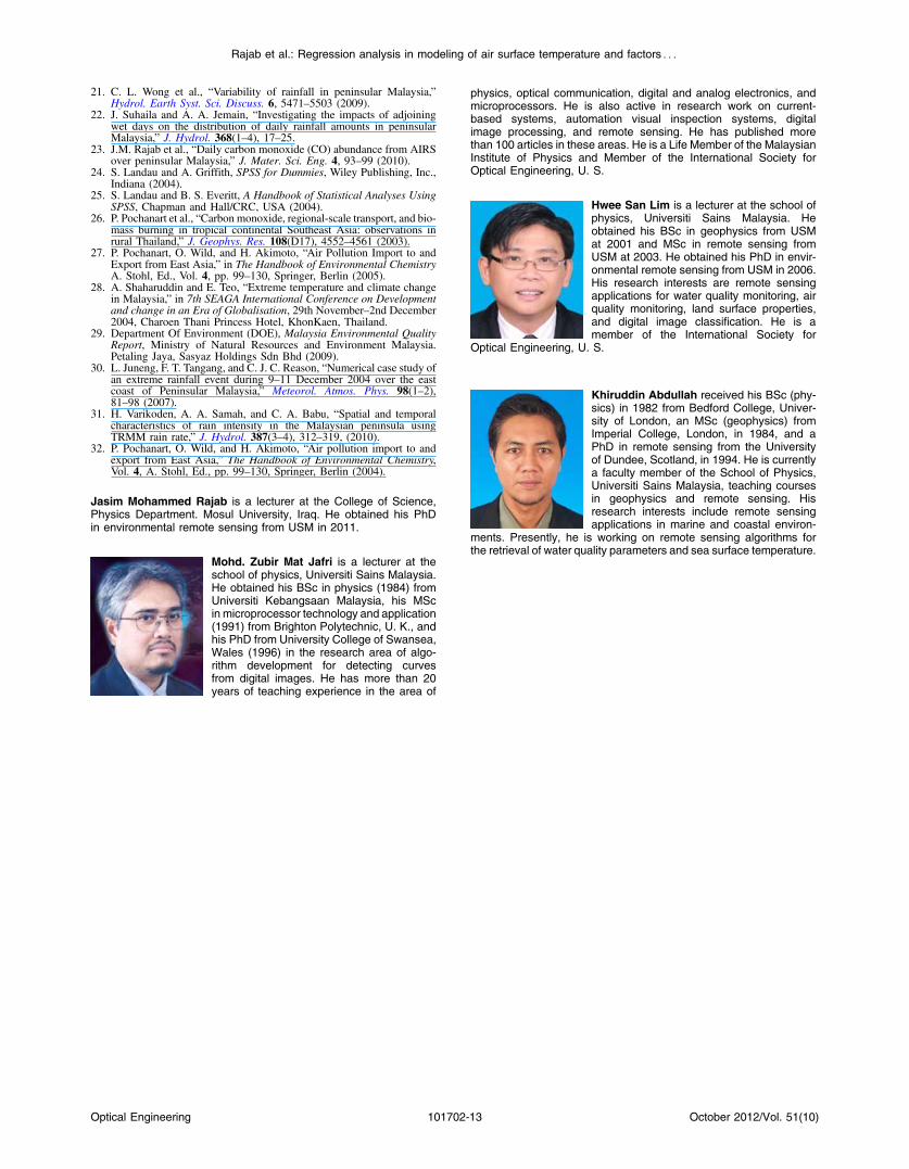
Jasim Mohammed Rajab is a lecturer at the College of Science,Physics Department. Mosul University, Iraq. He obtained his PhDin environmental remote sensing from USM in 2011.

Mohd. Zubir Mat Jafri is a lecturer at theschool of physics, Universiti Sains Malaysia.He obtained his BSc in physics (1984) fromUniversiti Kebangsaan Malaysia, his MScin microprocessor technology and application(1991) from Brighton Polytechnic, U. K., andhis PhD from University College of Swansea,Wales (1996) in the research area of algo-rithm development for detecting curvesfrom digital images. He has more than 20years of teaching experience in the area of

physics, optical communication, digital and analog electronics, andmicroprocessors. He is also active in research work on current-based systems, automation visual inspection systems, digitalimage processing, and remote sensing. He has published morethan 100 articles in these areas. He is a Life Member of the MalaysianInstitute of Physics and Member of the International Society forOptical Engineering, U. S.

Hwee San Lim is a lecturer at the school ofphysics, Universiti Sains Malaysia. Heobtained his BSc in geophysics from USMat 2001 and MSc in remote sensing fromUSM at 2003. He obtained his PhD in envir-onmental remote sensing from USM in 2006.His research interests are remote sensingapplications for water quality monitoring, airquality monitoring, land surface properties,and digital image classification. He is amember of the International Society for

Optical Engineering, U. S.

Khiruddin Abdullah received his BSc (phy-sics) in 1982 from Bedford College, Univer-sity of London, an MSc (geophysics) fromImperial College, London, in 1984, and aPhD in remote sensing from the Universityof Dundee, Scotland, in 1994. He is currentlya faculty member of the School of Physics,Universiti Sains Malaysia, teaching coursesin geophysics and remote sensing. Hisresearch interests include remote sensingapplications in marine and coastal environ-

ments. Presently, he is working on remote sensing algorithms forthe retrieval of water quality parameters and sea surface temperature.

Optical Engineering 101702-13 October 2012/Vol. 51(10)

Rajab et al.: Regression analysis in modeling of air surface temperature and factors : : :