Reformulation of Global Constraints Based onConstraints Checkers

Nicolas Beldiceanu1, Mats Carlsson2, Romuald Debruyne1, and Thierry Petit1

1 LINA FRE CNRS 2729, Ecole des Mines de Nantes, FR-44307 Nantes Cedex 3, France.{Nicolas.Beldiceanu,Romuald.Debruyne,Thierry.Petit}@emn.fr

2 SICS, P.O. Box 1263, SE-164 29 Kista, Sweden.Mats.Carlsson@sics.se

Abstract. This article deals with global constraints for which the set of solu-tions can be recognized by an extended finite automaton whose size is boundedby a polynomial in n, where n is the number of variables of the correspondingglobal constraint. By reducing the automaton to a conjunction of signature andtransition constraints we show how to systematically obtain an automaton re-formulation. Under some restrictions on the signature and transition constraints,this reformulation maintains arc-consistency. An implementation based on someconstraints as well as on the metaprogramming facilities of SICStus Prolog isavailable. For a restricted class of automata we provide an automaton reformu-lation for the relaxed case, where the violation cost is the minimum number ofvariables to unassign in order to get back to a solution.

1 Introduction

Developing filtering algorithms for global constraints is usually a very work-intensiveand error-prone activity. As a first step toward a methodology for semi-automatic de-velopment of filtering algorithms for global constraints, Carlsson and Beldiceanu in-troduced [1] an approach to designing filtering algorithms by derivation from a finiteautomaton. As quoted in their discussion, constructing the automaton was far from obvi-ous since it was mainly done as a rational reconstruction of an emerging understandingof the necessary case analysis related to the required pruning. However, it is commonlyadmitted that coming up with a checker which tests whether a ground instance is a so-lution or not is usually straightforward. As shown by the following chronological list ofrelated work, automata were already used for handling constraints:

– Vempaty introduced the idea of representing the solution set of a constraint net-work by a minimized deterministic finite state automaton [2]. He showed how touse this canonical form to answer queries related to constraints, as satisfiability,validity (i.e., the set of allowed tuples of a constraint), or equivalence between twoconstraints. This was essentially done by tracing paths in an acyclic graph derivedfrom the automaton.

– Later, Amilhastre [3] generalized this approach to nondeterministic automata andintroduced heuristics to reduce their size. The goal was to obtain a compact repre-sentation of the set of solutions of a CSP. That work was applied to configurationproblems in [4].

– Boigelot and Wolper [5] also used automata for arithmetic constraints.– Within the context of global constraints on a finite sequence of variables, the recent

work of Pesant [6] also uses a finite automaton for representing the solution set. Inthis context, it provides a filtering algorithm which maintains arc-consistency.

This article focuses on those global constraints that can be checked by scanningonce through their variables without using any extra data structure. As a second steptoward a methodology for semi-automatic development of filtering algorithms, we in-troduce a new approach which only requires defining a finite automaton that checks aground instance. We extend traditional finite automata in order not to be limited onlyto regular expressions. Our first contribution is to show how to reduce the automatonassociated with a global constraint to a conjunction of signature and transition con-straints. We characterize some restrictions on the signature and transition constraintsunder which the filtering induced by this reduction maintains arc-consistency and applythis new methodology to the following problems:

– The design of automaton reformulations for a fairly large set of global constraints.– The design of automaton reformulations for handling the conjunction of several

global constraints.– The design of constraints between two sequences of variables.

While all previous related work (see Vempaty, Amilhastre et al. and Pesant) relieson simple automata and uses an ad-hoc filtering algorithm, our approach is based on au-tomata with counters and reformulation into constraints for which filtering algorithmsalready exist. Note also that all previous work restricts a transition of the automaton tochecking whether or not a given value belongs to the domain of a variable. In contrast,our approach permits to associate any constraint to a transition. As a consequence, wecan model concisely a larger class of global constraints and prove properties on theconsistency by reasoning directly on the constraint hypergraph. As an illustrative ex-ample, consider the lexicographical ordering constraint between two vectors. As shownby Fig. 1, we come up with an automaton with two states where a transition constraintcorresponds to comparing two domain variables. Now, if we forbid the use of compari-son, this would lead to an automaton whose size depends of the number of values in thedomains of the variables.

Our second contribution is to provide for a restricted class of automata an automa-ton reformulation for the relaxed case. This technique relies on the variable based vio-lation cost introduced in [7, 8]. This cost was advocated as a generic way for expressingthe violation of a global constraint. However, algorithms were only provided for thesoft alldifferent constraint [7]. We come up with an algorithm for computinga sharp bound of the minimum violation cost and with an automaton reformulation forpruning in order to avoid to exceed a given maximum violation cost.

Section 2 describes the kind of finite automaton used for recognizing the set ofsolutions associated with a global constraint. Section 3 shows how to come up withan automaton reformulation which exploits the previously introduced automaton. Sec-tion 4 describes typical applications of this technique. Finally, for a restricted class ofautomata, Section 5 provides a filtering algorithm for the relaxed case.

2 Description of the Automaton Used for Checking GroundInstances

We first discuss the main issues behind the task of selecting what kind of automatonto consider for concisely expressing the set of solutions associated with a global con-straint. We consider global constraints for which any ground instance can be checkedin linear time by scanning once through their variables without using any data struc-ture. In order to concretely illustrate this point, we first select a set of global constraintsand write down a checker for each of them1. Observe that a constraint, like for in-stance the cycle(n, [x1, x2, . . . , xm]) constraint, which enforces that a permutation[x1, x2, . . . , xm] has n cycles, does not belong to this class since it requires to jumpfrom one position to another position of the sequence x1, x2, . . . , xm. Finally, we givefor each checker a sketch of the corresponding automaton. Based on these observations,we define the type of automaton we will use.

2.1 Selecting an Appropriate Description

As we previously said, we focus on those global constraints that can be checked byscanning once through their variables. This is for instance the case of element [9],minimum [10], pattern [11], global contiguity [12], lexicographicordering [13], among [14] and inflexion [15]. Since they illustrate key pointsneeded for characterizing the set of solutions associated with a global constraint, ourdiscussion will be based on the last four constraints for which we now recall the defini-tion:

– The global contiguity(vars) constraint enforces for the sequence of 0-1variables vars to have at most one group of consecutive 1. For instance, the con-straint global contiguity([0, 1, 1, 0]) holds since we have only one group ofconsecutive 1.

– The lexicographic ordering constraint−→x≤lex−→y over two vectors of variables−→x =

〈x0, . . . , xn−1〉 and −→y = 〈y0, . . . , yn−1〉 holds iff n = 0 or x0 < y0 or x0 = y0

and 〈x1, . . . , xn−1〉≤lex〈y1, . . . , yn−1〉.– The among(nvar , vars , values) constraint restricts the number of variables of the

sequence of variables vars that take their value from a given set values to be equalto the variable nvar . For instance, among(3, [4, 5, 5, 4, 1], [1, 5, 8]) holds since ex-actly 3 values of the sequence 45541 are in {1, 5, 8}.

– The inflexion(ninf , vars) constraint enforces the number of inflexions of thesequence of variables vars to be equal to the variable ninf . An inflexion isdescribed by one of the following patterns: a strict increase followed by a strictdecrease or, conversely, a strict decrease followed by a strict increase. For instance,inflexion(4, [3, 3, 1, 4, 5, 5, 6, 5, 5, 6, 3]) holds since we can extract from thesequence 33145565563 the four subsequences 314, 565, 6556 and 563, which allfollow one of these two patterns.

1 We don’t skip the checker since, in the long term, we consider that the goal would be to turnany existing code performing a check into a constraint.

<lex

<lexx[i]<y[i] $

$

vars[i]notin values

x[i]=y[i]

vars[i]in values,c++

t nvar=ct:

c=0s:

s

1 BEGIN2 i=0;3 WHILE i<n AND vars[i]=0 DO i++;4 WHILE i<n AND vars[i]=1 DO i++;5 WHILE i<n AND vars[i]=0 DO i++;6 RETURN (i=n);7 END.

global_contiguity(vars[0..n−1]):BOOLEAN among

1 BEGIN2 i=0;3 WHILE i<n AND x[i]=y[i] DO i++;4 RETURN (i=n OR x[i]<y[i]);5 END.

among1 BEGIN2 i=0; c=0;3 WHILE i<n DO4 IF vars[i] in values THEN c++;

6 RETURN (nvar=c);5 i++;

7 END.

01 BEGIN02 i=0; c=0;03 WHILE i<n−1 AND vars[i]=vars[i+1] DO i++;04 IF i<n−1 THEN less=(vars[i]<vars[i+1]);05 WHILE i<n−1 DO06 IF less THEN

08 ELSE

10 i++;11 RETURN (ninf=c);12 END.

(nvar,vars[0..n−1],values):BOOLEAN

vars[i]=0

vars[i]=1

vars[i]=0

vars[i]=0

$

$

vars[i]=1

$

t

z

n

s

global_contiguity

i j

$

vars[i+1]

vars[i]=

$

vars[i]=vars[i+1]

vars[i]<vars[i+1]

vars[i]<vars[i+1]

vars[i]=vars[i+1]

$

vars[i+1]

vars[i]>vars[i+1]

vars[i]>

ninf=ct:

c=0s:

c++vars[i]>vars[i+1],

vars[i]<vars[i+1],c++

(A1)

(B1)

(C1)

(D1)

(A2) (B2) (C2)

(D2)

(x[0..n−1],y[0..n−1]):BOOLEAN

07 IF vars[i]>vars[i+1] THEN c++; less=FALSE;

09 IF vars[i]<vars[i+1] THEN c++; less=TRUE;

inflexion

inflexion

(ninf,vars[0..n−1]):BOOLEAN

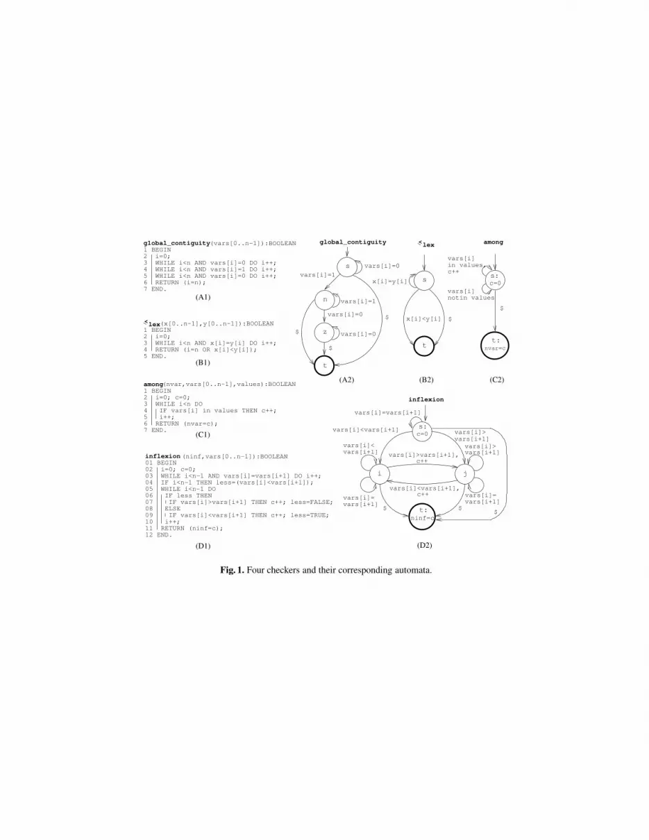
Fig. 1. Four checkers and their corresponding automata.

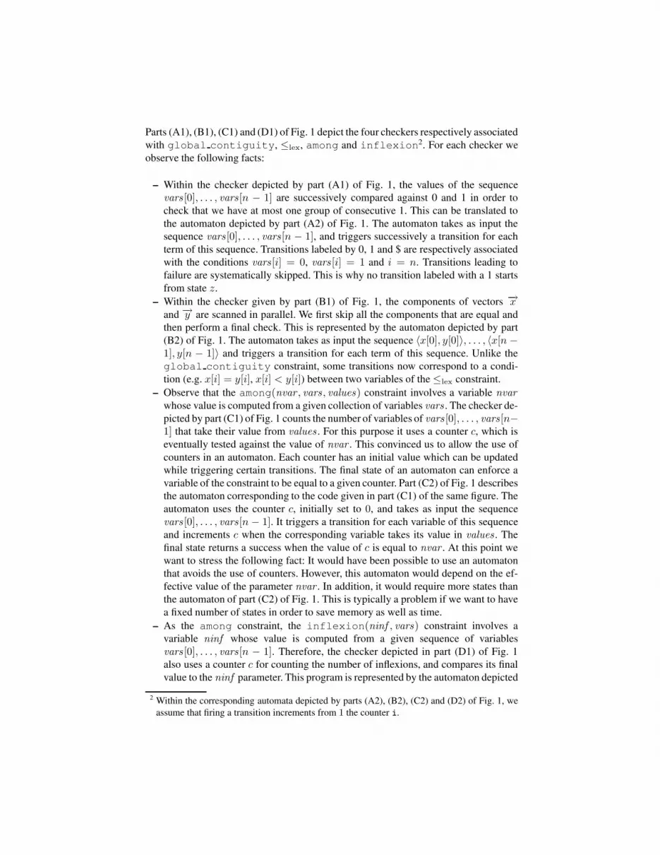
Parts (A1), (B1), (C1) and (D1) of Fig. 1 depict the four checkers respectively associatedwith global contiguity, ≤lex, among and inflexion2. For each checker weobserve the following facts:

– Within the checker depicted by part (A1) of Fig. 1, the values of the sequencevars [0], . . . , vars [n − 1] are successively compared against 0 and 1 in order tocheck that we have at most one group of consecutive 1. This can be translated tothe automaton depicted by part (A2) of Fig. 1. The automaton takes as input thesequence vars [0], . . . , vars [n − 1], and triggers successively a transition for eachterm of this sequence. Transitions labeled by 0, 1 and $ are respectively associatedwith the conditions vars [i] = 0, vars [i] = 1 and i = n. Transitions leading tofailure are systematically skipped. This is why no transition labeled with a 1 startsfrom state z.

– Within the checker given by part (B1) of Fig. 1, the components of vectors −→xand −→y are scanned in parallel. We first skip all the components that are equal andthen perform a final check. This is represented by the automaton depicted by part(B2) of Fig. 1. The automaton takes as input the sequence 〈x[0], y[0]〉, . . . , 〈x[n −1], y[n − 1]〉 and triggers a transition for each term of this sequence. Unlike theglobal contiguity constraint, some transitions now correspond to a condi-tion (e.g. x[i] = y[i], x[i] < y[i]) between two variables of the ≤lex constraint.

– Observe that the among(nvar , vars , values) constraint involves a variable nvarwhose value is computed from a given collection of variables vars . The checker de-picted by part (C1) of Fig. 1 counts the number of variables of vars [0], . . . , vars [n−1] that take their value from values . For this purpose it uses a counter c, which iseventually tested against the value of nvar . This convinced us to allow the use ofcounters in an automaton. Each counter has an initial value which can be updatedwhile triggering certain transitions. The final state of an automaton can enforce avariable of the constraint to be equal to a given counter. Part (C2) of Fig. 1 describesthe automaton corresponding to the code given in part (C1) of the same figure. Theautomaton uses the counter c, initially set to 0, and takes as input the sequencevars [0], . . . , vars [n − 1]. It triggers a transition for each variable of this sequenceand increments c when the corresponding variable takes its value in values . Thefinal state returns a success when the value of c is equal to nvar . At this point wewant to stress the following fact: It would have been possible to use an automatonthat avoids the use of counters. However, this automaton would depend on the ef-fective value of the parameter nvar . In addition, it would require more states thanthe automaton of part (C2) of Fig. 1. This is typically a problem if we want to havea fixed number of states in order to save memory as well as time.

– As the among constraint, the inflexion(ninf , vars) constraint involves avariable ninf whose value is computed from a given sequence of variablesvars [0], . . . , vars [n − 1]. Therefore, the checker depicted in part (D1) of Fig. 1also uses a counter c for counting the number of inflexions, and compares its finalvalue to the ninf parameter. This program is represented by the automaton depicted

2 Within the corresponding automata depicted by parts (A2), (B2), (C2) and (D2) of Fig. 1, weassume that firing a transition increments from 1 the counter i.

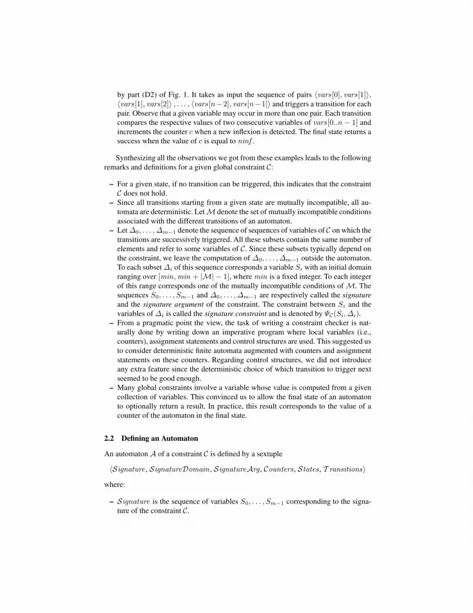
by part (D2) of Fig. 1. It takes as input the sequence of pairs 〈vars [0], vars [1]〉,〈vars [1], vars [2]〉 , . . . , 〈vars [n−2], vars [n−1]〉 and triggers a transition for eachpair. Observe that a given variable may occur in more than one pair. Each transitioncompares the respective values of two consecutive variables of vars [0..n− 1] andincrements the counter c when a new inflexion is detected. The final state returns asuccess when the value of c is equal to ninf .

Synthesizing all the observations we got from these examples leads to the followingremarks and definitions for a given global constraint C:

– For a given state, if no transition can be triggered, this indicates that the constraintC does not hold.

– Since all transitions starting from a given state are mutually incompatible, all au-tomata are deterministic. LetM denote the set of mutually incompatible conditionsassociated with the different transitions of an automaton.

– Let∆0, . . . , ∆m−1 denote the sequence of sequences of variables of C on which thetransitions are successively triggered. All these subsets contain the same number ofelements and refer to some variables of C. Since these subsets typically depend onthe constraint, we leave the computation of ∆0, . . . , ∆m−1 outside the automaton.To each subset∆i of this sequence corresponds a variable Si with an initial domainranging over [min,min + |M| − 1], where min is a fixed integer. To each integerof this range corresponds one of the mutually incompatible conditions ofM. Thesequences S0, . . . , Sm−1 and ∆0, . . . , ∆m−1 are respectively called the signatureand the signature argument of the constraint. The constraint between Si and thevariables of ∆i is called the signature constraint and is denoted by ΨC(Si, ∆i).

– From a pragmatic point the view, the task of writing a constraint checker is nat-urally done by writing down an imperative program where local variables (i.e.,counters), assignment statements and control structures are used. This suggested usto consider deterministic finite automata augmented with counters and assignmentstatements on these counters. Regarding control structures, we did not introduceany extra feature since the deterministic choice of which transition to trigger nextseemed to be good enough.

– Many global constraints involve a variable whose value is computed from a givencollection of variables. This convinced us to allow the final state of an automatonto optionally return a result. In practice, this result corresponds to the value of acounter of the automaton in the final state.

2.2 Defining an Automaton

An automatonA of a constraint C is defined by a sextuple

〈Signature , SignatureDomain , SignatureArg , Counters, States , T ransitions〉

where:

– Signature is the sequence of variables S0, . . . , Sm−1 corresponding to the signa-ture of the constraint C.

– SignatureDomain is an interval which defines the range of possible values of thevariables of Signature .

– SignatureArg is the signature argument ∆0, . . . , ∆m−1 of the constraint C. Thelink between the variables of ∆i and the variable Si (0 ≤ i < m) is done bywriting down the signature constraintΨC(Si, ∆i) in such a way that arc-consistencyis maintained. In our context this is done by using standard features of the CLP(FD)solver of SICStus Prolog [16] such as arithmetic constraints between two variables,propositional combinators or the global constraints programming interface.

– Counters is the, possibly empty, list of all counters used in the automatonA. Eachcounter is described by a term t(Counter , InitialValue , FinalVariable) whereCounter is a symbolic name representing the counter, InitialValue is an integergiving the value of the counter in the initial state ofA, and FinalVariable gives thevariable that should be unified with the value of the counter in the final state of A.

– States is the list of states ofA, where each state has the form source(id ), sink(id )or node(id ). id is a unique identifier associated with each state. Finally, source(id )and sink(id) respectively denote the initial and the final state of A.

– T ransitions is the list of transitions of A. Each transition t has the formarc(id 1, label , id2) or arc(id 1, label , id2, counters). id 1 and id2 respectively cor-respond to the state just before and just after t, while label depicts the value that thesignature variable should have in order to trigger t. When used, counters gives foreach counter of Counters its value after firing the corresponding transition. Thisvalue is specified by an arithmetic expression involving counters, constants, as wellas usual arithmetic functions such as +, −, min or max. The order used in thecounters list is identical to the order used in Counters.

Example 1. As an illustrative example we give the description of the automaton associated withthe inflexion(ninf , vars) constraint. We have:

– Signature = S0, S1, . . . , Sn−2,– SignatureDomain = 0..2,– SignatureArg = 〈vars [0], vars [1]〉, . . . , 〈vars [n − 2], vars [n− 1]〉,– Counters = t(c, 0, ninf ),– States = [source(s), node(i), node(j), sink(t)],– T ransitions = [arc(s, 1, s), arc(s, 2, i), arc(s, 0, j), arc(s, $, t), arc(i, 1, i), arc(i, 2, i),

arc(i, 0, j, [c + 1]), arc(i, $, t), arc(j, 1, j), arc(j, 0, j), arc(j, 2, i, [c + 1]), arc(j, $, t)].

The signature constraint relating each pair of variables 〈vars [i], vars [i+ 1]〉 to the signaturevariable Si is defined as follows: Ψinflexion(Si, vars [i], vars [i+1]) ≡ vars [i] > vars [i+1]⇔Si = 0 ∧ vars [i] = vars [i + 1]⇔ Si = 1 ∧ vars [i] < vars [i + 1]⇔ Si = 2. The sequenceof transitions triggered on the ground instance inflexion(4, [3, 3, 1, 4, 5, 5, 6, 5, 5, 6, 3]) issc=0

3=3⇔S0=1−−−−−−−→ s3>1⇔S1=0−−−−−−−→ j

1<4⇔S2=2−−−−−−−→c=1

i4<5⇔S3=2−−−−−−−→ i

5=5⇔S4=1−−−−−−−→ i5<6⇔S5=2−−−−−−−→

i6>5⇔S6=0−−−−−−−→

c=2j

5=5⇔S7=1−−−−−−−→ j5<6⇔S8=2−−−−−−−→

c=3i

6>3⇔S9=0−−−−−−−→c=4

j$−→ t

ninf =4. Each transition gives the

corresponding condition and, eventually, the value of the counter c just after firing that transition.

3 Automaton Reformulation

The automaton reformulation is based on the following idea. For a given global con-straint C, one can think of its automaton as a procedure that repeatedly maps a current

state Qi and counter vector−→K i, given a signature variable Si, to a new state Qi+1

and counter vector−→K i+1, until a terminal state is reached. We then convert this pro-

cedure into a transition constraint ΦC(Qi,−→K i, Si, Qi+1,

−→K i+1) as follows. Qi is a

variable whose values correspond to the states that can be reached at step i. Simi-larly,

−→K i is a vector of variables whose values correspond to the potential values of

the counters at step i. Assuming that the automaton associated with C has na arcsarc(q1, s1, q

′1,−→f1(−→K)), . . . , arc(qna , sna , q

′na ,−→fna(−→K)), the transition constraint has

the following form:

na∨

j=1

[(Qi = qj) ∧ (Si = sj) ∧ (Qi+1 = q′j) ∧ (−→K i+1 =

−→fj (−→K i))]

Consider first the case when no counter is used, i.e. the constraint is effectivelyΦC(Qi, Si, Qi+1). This can be encoded with a ternary relation defined by extension (e.g.SICStus Prolog’s case [16, page 463], ECLiPSe’s Propia [17], or Ilog Solver’s tableconstraint [18]). If that relation maintains arc-consistency, as does case, it follows thatΦC maintains arc-consistency.

Consider now the case when one counter is used. Then we need to extend the ternaryrelation by one argument corresponding to j. This argument can be used as an indexinto a vector [

−→f1(−→K i), . . . ,

−→fna(−→K i)], selecting the value that

−→K i+1 should equal. Thus

to encode ΦC we need:

– a 4-ary relation defined by extension,– na arithmetic constraints to compute the vector, and– an element constraint to select a value from the vector.

As an optimization, identical−→fj (−→K i) expressions can be merged, yielding a shorter vec-

tor and fewer arithmetic constraints. In general, arc-consistency can not be guaranteedfor ΦC .

Finally, consider the case when two or more counters are used. This is a straightfor-ward generalization of the single counter case.

We can then arrive at an automaton reformulation for C by decomposing it into aconjunction of ΦC constraints, “threading” the state and counter variables through theconjunction. In addition to this, we need the signature constraints ΨC(Si, ∆i) (0 ≤i < m) that relate each signature variables Si to the variables of its correspondingsignature argument ∆i. Filtering for the constraint C is provided by the conjunctionof all signature and transitions constraints, (s being the start state and t being the endstate):

ΨC(S0,∆0) ∧ ΦC(s,−→K0, S0, Q1,

−→K1) ∧

ΨC(S1,∆1) ∧ ΦC(Q1,−→K1, S1, Q2,

−→K2) ∧

...ΨC(Sm−1,∆m−1) ∧ ΦC(Qm−1,

−→Km−1, Sm−1, Qm,

−→Km) ∧

ΦC(Qm,−→Km, $, t,

−→Km+1)

A couple of examples will help clarify this idea. In these examples, the relationdefined by extension is depicted in a compact form as a decision tree. Note that the

Qi=tQi=s

Qi+1=s Qi+1=t

iS =2

iS =1

Qi=s

iS =0

iS =$

iS =1

Qi=t

t

s2

$1 iS =$

automaton decision tree

nvar=ct:

c=0s:

decision tree

1,c++

0

$

automaton

(A) (B)

i+1 i

Qi+1=s

=c i+1 i+1 i+1 i

Qi+1=s Qi+1=t

=c =cc c c

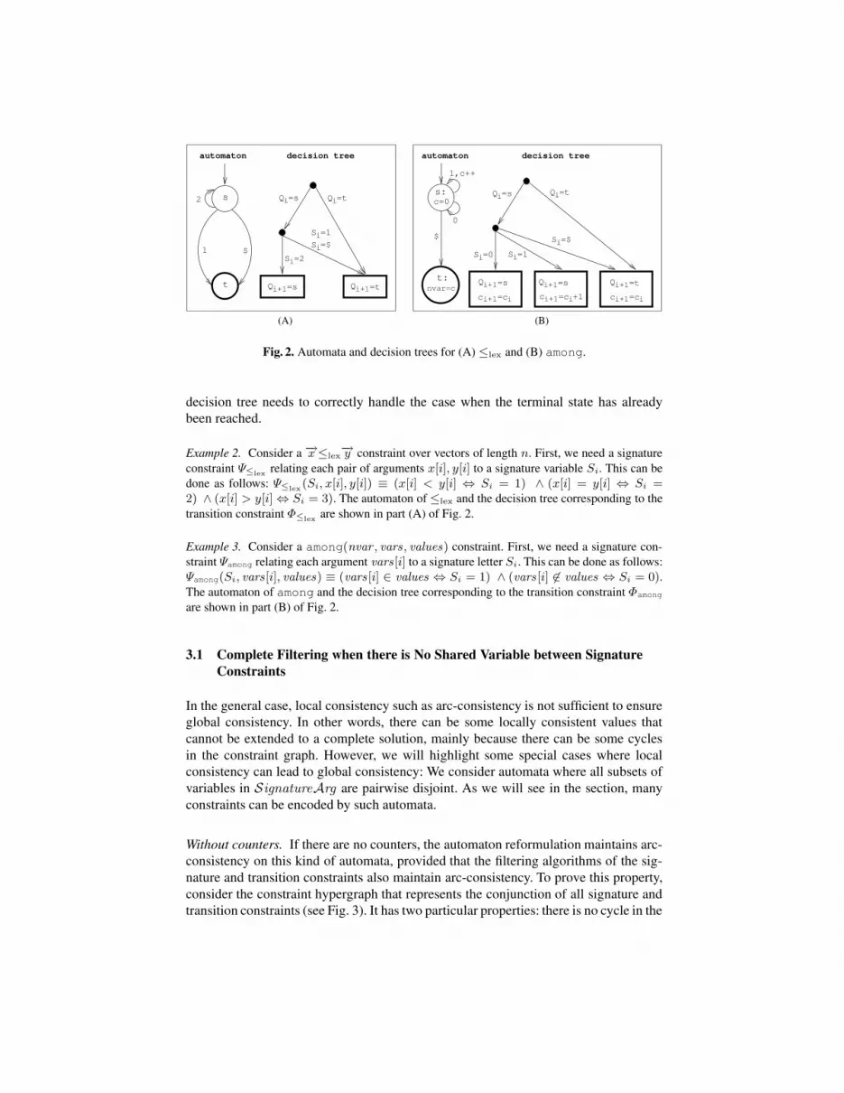
Fig. 2. Automata and decision trees for (A) ≤lex and (B) among.

decision tree needs to correctly handle the case when the terminal state has alreadybeen reached.

Example 2. Consider a −→x≤lex−→y constraint over vectors of length n. First, we need a signature

constraint Ψ≤lexrelating each pair of arguments x[i], y[i] to a signature variable Si. This can be

done as follows: Ψ≤lex(Si, x[i], y[i]) ≡ (x[i] < y[i] ⇔ Si = 1) ∧ (x[i] = y[i] ⇔ Si =

2) ∧ (x[i] > y[i]⇔ Si = 3). The automaton of ≤lex and the decision tree corresponding to thetransition constraint Φ≤lex

are shown in part (A) of Fig. 2.

Example 3. Consider a among(nvar , vars , values) constraint. First, we need a signature con-straint Ψamong relating each argument vars [i] to a signature letter Si. This can be done as follows:Ψamong(Si, vars [i], values) ≡ (vars [i] ∈ values ⇔ Si = 1) ∧ (vars [i] 6∈ values ⇔ Si = 0).The automaton of among and the decision tree corresponding to the transition constraint Φamong

are shown in part (B) of Fig. 2.

3.1 Complete Filtering when there is No Shared Variable between SignatureConstraints

In the general case, local consistency such as arc-consistency is not sufficient to ensureglobal consistency. In other words, there can be some locally consistent values thatcannot be extended to a complete solution, mainly because there can be some cyclesin the constraint graph. However, we will highlight some special cases where localconsistency can lead to global consistency: We consider automata where all subsets ofvariables in SignatureArg are pairwise disjoint. As we will see in the section, manyconstraints can be encoded by such automata.

Without counters. If there are no counters, the automaton reformulation maintains arc-consistency on this kind of automata, provided that the filtering algorithms of the sig-nature and transition constraints also maintain arc-consistency. To prove this property,consider the constraint hypergraph that represents the conjunction of all signature andtransition constraints (see Fig. 3). It has two particular properties: there is no cycle in the

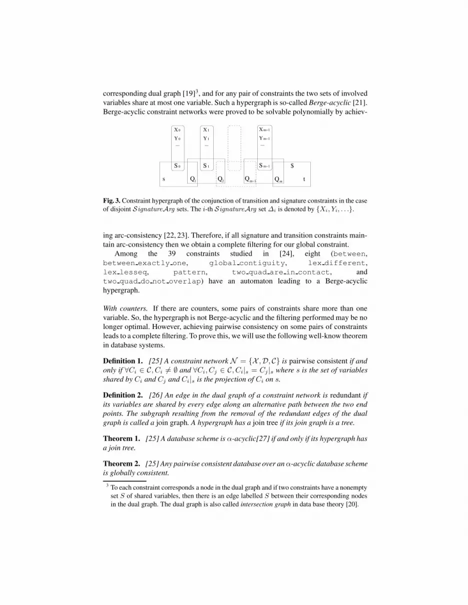
corresponding dual graph [19]3, and for any pair of constraints the two sets of involvedvariables share at most one variable. Such a hypergraph is so-called Berge-acyclic [21].Berge-acyclic constraint networks were proved to be solvable polynomially by achiev-

s

Y 0

X 1

Y 1

S 0

... ...Y m−1

...

S m−1

m−1X

t

$

X 0

S 1

QQ Q1 2 m−1 mQ

Fig. 3. Constraint hypergraph of the conjunction of transition and signature constraints in the caseof disjoint SignatureArg sets. The i-th SignatureArg set ∆i is denoted by {Xi, Yi, . . .}.

ing arc-consistency [22, 23]. Therefore, if all signature and transition constraints main-tain arc-consistency then we obtain a complete filtering for our global constraint.

Among the 39 constraints studied in [24], eight (between,between exactly one, global contiguity, lex different,lex lesseq, pattern, two quad are in contact, andtwo quad do not overlap) have an automaton leading to a Berge-acyclichypergraph.

With counters. If there are counters, some pairs of constraints share more than onevariable. So, the hypergraph is not Berge-acyclic and the filtering performed may be nolonger optimal. However, achieving pairwise consistency on some pairs of constraintsleads to a complete filtering. To prove this, we will use the following well-know theoremin database systems.

Definition 1. [25] A constraint network N = {X ,D, C} is pairwise consistent if andonly if ∀Ci ∈ C, Ci 6= ∅ and ∀Ci, Cj ∈ C, Ci|s = Cj |s where s is the set of variablesshared by Ci and Cj and Ci|s is the projection of Ci on s.

Definition 2. [26] An edge in the dual graph of a constraint network is redundant ifits variables are shared by every edge along an alternative path between the two endpoints. The subgraph resulting from the removal of the redundant edges of the dualgraph is called a join graph. A hypergraph has a join tree if its join graph is a tree.

Theorem 1. [25] A database scheme is α-acyclic[27] if and only if its hypergraph hasa join tree.

Theorem 2. [25] Any pairwise consistent database over anα-acyclic database schemeis globally consistent.

3 To each constraint corresponds a node in the dual graph and if two constraints have a nonemptyset S of shared variables, then there is an edge labelled S between their corresponding nodesin the dual graph. The dual graph is also called intersection graph in data base theory [20].

If we translate these theorems we obtain the following corollary on constraint net-works.

Corollary 1. If a constraint hypergraph has a join tree then any pairwise consistentconstraint network having this constraint hypergraph is globally consistent.

In the automata we consider here, there are no signature constraints sharing a vari-able. So, the dual graph of the constraint hypergraph is a tree and the hypergraph has ajoin tree. Therefore, the hypergraph is α-acyclic and if the constraint network is pair-wise consistent, the filtering is complete for our global constraint.

A solution to reach global consistency on the network representing our global con-straint is therefore to maintain pairwise consistency. In fact, if constraints share no morethan one variable, pairwise consistency is nothing more than arc-consistency [23]. So,pairwise consistency has to be enforced only on pairs of constraints sharing more thanone variable and only the transition constraints are therefore concerned. In the worstcase, pairwise consistency will have to consider all the possible tuples of values for theset of shared variables. So, the pairs of constraints must not share too many variables ifwe do not want the filtering to become prohibitive.

Among the 39 constraints studied in [24], seven (among, atleast, atmost,count, counts, differ from atleast k pos, and sliding card skip0)require only one counter, two (group, and group skip isolated item) needtwo counters and max index requires three counters.

When the automaton involves only one counter, consecutive transition constraintsshare two variables. The sweep algorithm presented in [28] can be used to enforcepairwise consistency on each pair of transition constraints sharing two variables. Indeed,the sweep algorithm on two constraintsCi andCj will forbid the tuples for the variablesshared by Ci and Cj that cannot be extended on both Ci and Cj . To summarize, ifthe automaton uses one single counter, the sweep algorithm must consider each pair oftransition constraints sharing variables, and arc-consistency on each constraint will leadto a complete filtering for our global constraint.

3.2 Complexity

Our approach allows the representation of a global constraint by a network of con-straints of small arities. As seen in the previous section, the filtering obtained using thisreformulation of the global constraint depends on the filtering performed by the solver.If the solver maintains arc-consistency using the general schema [29, 30], the complex-ity is inO(er2dr) 4 where e is the number of constraints, r the maximum arity and d thesize of the largest domain. However, this is a rough bound and the practical time com-plexity can be far from this limit. Indeed, the constraints have very different arities andsome domains involve only very few values. Furthermore, on some constraints a spe-cialized algorithm can be used to reduce the filtering cost. Finally, one would want toenforce only a partial form of arc-consistency (a directional arc-consistency for exam-ple in the case of a Berge-acyclic constraint network), or a stronger filtering (enforcing

4 We assume here that the cost of a constraint check is linear in the constraint arity while it issometimes assumed to be constant.

pairwise consistency for example on a constraint network having a join tree). Both thepruning efficiency and the complexity of the pruning rely on the filtering performed bythe solver.

3.3 Performance

It is reasonable to ask the question whether the automaton reformulation describedherein performs anywhere near the performance delivered by a specific implementa-tion of a given constraint. To this end, we have compared a version of the BalancedIncomplete Block Design problem [31, prob028] that uses a built-in ≤lex constraint tobreak column symmetries with a version using our filtering based on a finite automatonfor the same constraint. In a second experiment, we measured the time to find all solu-tions to a single ≤lex constraint. The experiments were run in SICStus Prolog 3.11 ona 600MHz Pentium III. The results are shown in Table 1.

A third experiment was designed to measure the overhead of an automaton reformu-lation wrt. decomposing into built-in constraints. To this end, we produced random in-stances of the following constraints studied in [24]: among, between, lex lesseq.These constraints were chosen because their automata formulations maintain the sameconsistency as their decomposed formulations, that is, they perform exactly the samedomain filtering. Hence, comparing the time it takes to compute all solutions shouldgive an accurate measurement of the overhead. among is not a built-in constraint; itcan be decomposed into a number of reified membership constraints and a sum con-straint. It is worth noting that its automaton uses a counter. between, lex lesseqcan be expressed as built-in lex chain constraints. The results are presented in threescatter plots in Figure 4. Each graph compares times for finding all solutions to a ran-dom constraint instance, using a randomly chosen labeling strategy. The X coordinateof each point is the runtime for an automaton reformulation. The Y coordinate is theruntime for a decomposition into built-in constraints. A line, least-square fitted to thedata points, is shown in each graph. Runtimes are in seconds.

From these experiments, we observe that an automaton reformulation typically runsa few times slower than its hard-coded counterpart, roughly the same ratio as betweeninterpreted and compiled code in a typical programming language. This slowdown islikely to have much less impact on the overall execution time of the program. Theconclusion is that the automaton reformulation is a feasible and very reasonable way ofrapidly prototyping new global constraints, before embarking on developing a specificfiltering algorithm, should that be deemed necessary.

4 Applications of this Technique

4.1 Designing Automaton Reformulations for Global Constraints

We apply this new methodology for designing automaton reformulations for the fol-lowing fairly large set of global constraints. We came up with an automaton5 for thefollowing constraints:

5 These automata are available in the technical report [24]. All signature constraints are encodedin order to maintain arc-consistency.

0

5

10

15

20

25

30

35

40

0 5 10 15 20 25 30 35 40

built

-in

automaton

among

0

5

10

15

20

25

30

35

40

0 5 10 15 20 25 30 35 40

built

-in

automaton

between

0

5

10

15

20

25

30

35

40

0 5 10 15 20 25 30 35 40

built

-in

automaton

lex_lesseq

Fig. 4. Scatter plots for finding all solutions to random instances: automaton reformulation vs.decomposition to built-ins.

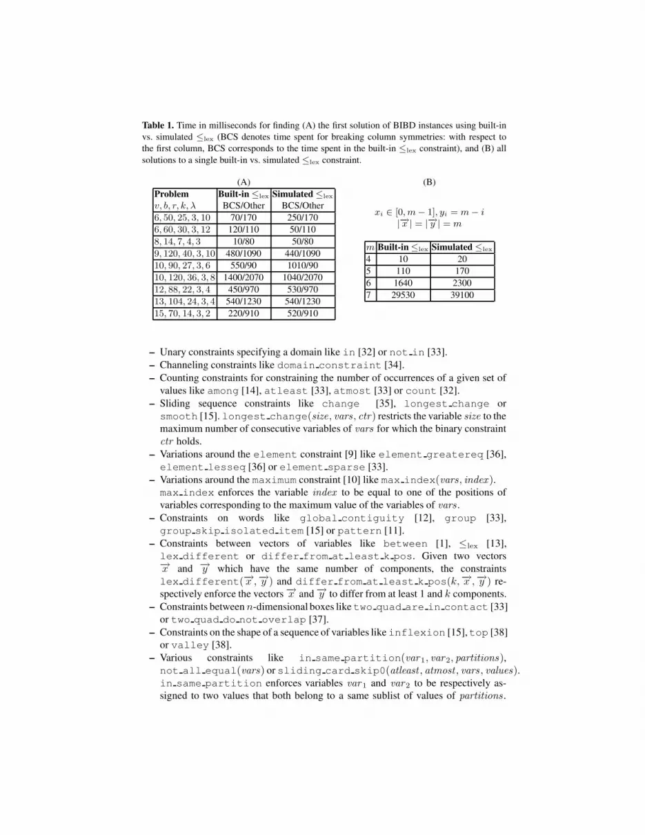
Table 1. Time in milliseconds for finding (A) the first solution of BIBD instances using built-invs. simulated ≤lex (BCS denotes time spent for breaking column symmetries: with respect tothe first column, BCS corresponds to the time spent in the built-in ≤lex constraint), and (B) allsolutions to a single built-in vs. simulated ≤lex constraint.

(A) (B)Problem Built-in≤lex Simulated≤lex

v, b, r, k, λ BCS/Other BCS/Other6, 50, 25, 3, 10 70/170 250/1706, 60, 30, 3, 12 120/110 50/1108, 14, 7, 4, 3 10/80 50/809, 120, 40, 3, 10 480/1090 440/109010, 90, 27, 3, 6 550/90 1010/9010, 120, 36, 3, 8 1400/2070 1040/207012, 88, 22, 3, 4 450/970 530/97013, 104, 24, 3, 4 540/1230 540/123015, 70, 14, 3, 2 220/910 520/910

xi ∈ [0, m− 1], yi = m− i|−→x | = |−→y | = m

m Built-in≤lex Simulated ≤lex

4 10 205 110 1706 1640 23007 29530 39100

– Unary constraints specifying a domain like in [32] or not in [33].– Channeling constraints like domain constraint [34].– Counting constraints for constraining the number of occurrences of a given set of

values like among [14], atleast [33], atmost [33] or count [32].– Sliding sequence constraints like change [35], longest change orsmooth [15]. longest change(size, vars , ctr) restricts the variable size to themaximum number of consecutive variables of vars for which the binary constraintctr holds.

– Variations around the element constraint [9] like element greatereq [36],element lesseq [36] or element sparse [33].

– Variations around the maximum constraint [10] like max index(vars, index ).max index enforces the variable index to be equal to one of the positions ofvariables corresponding to the maximum value of the variables of vars .

– Constraints on words like global contiguity [12], group [33],group skip isolated item [15] or pattern [11].

– Constraints between vectors of variables like between [1], ≤lex [13],lex different or differ from at least k pos. Given two vectors−→x and −→y which have the same number of components, the constraintslex different(−→x ,−→y ) and differ from at least k pos(k,−→x ,−→y ) re-spectively enforce the vectors−→x and−→y to differ from at least 1 and k components.

– Constraints between n-dimensional boxes like two quad are in contact [33]or two quad do not overlap [37].

– Constraints on the shape of a sequence of variables like inflexion [15],top [38]or valley [38].

– Various constraints like in same partition(var1, var2, partitions),not all equal(vars) or sliding card skip0(atleast , atmost , vars , values).in same partition enforces variables var 1 and var2 to be respectively as-signed to two values that both belong to a same sublist of values of partitions .

not all equal enforces the variables of vars to take more than a single value.sliding card skip0 enforces that each maximum non-zero subsequence ofconsecutive variables of vars contain at least atleast and at most atmost valuesfrom the set of values values .

4.2 Automaton Reformulation for a Conjunction of Global Constraints

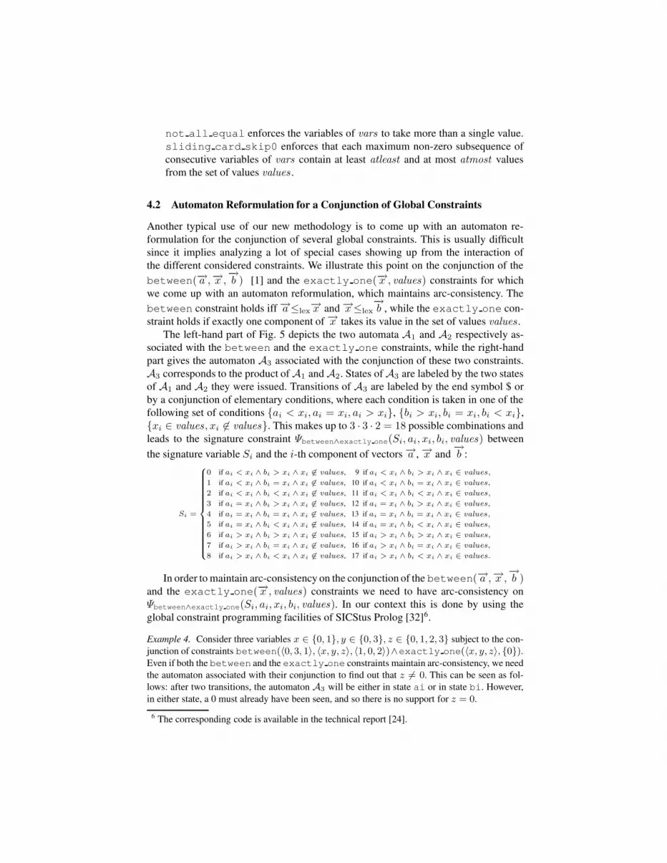
Another typical use of our new methodology is to come up with an automaton re-formulation for the conjunction of several global constraints. This is usually difficultsince it implies analyzing a lot of special cases showing up from the interaction ofthe different considered constraints. We illustrate this point on the conjunction of thebetween(−→a ,−→x ,−→b ) [1] and the exactly one(−→x , values) constraints for whichwe come up with an automaton reformulation, which maintains arc-consistency. Thebetween constraint holds iff −→a≤lex

−→x and −→x≤lex−→b , while the exactly one con-

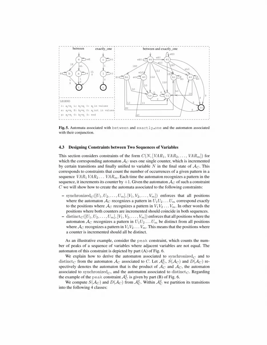
straint holds if exactly one component of −→x takes its value in the set of values values .The left-hand part of Fig. 5 depicts the two automata A1 and A2 respectively as-

sociated with the between and the exactly one constraints, while the right-handpart gives the automaton A3 associated with the conjunction of these two constraints.A3 corresponds to the product ofA1 andA2. States ofA3 are labeled by the two statesof A1 and A2 they were issued. Transitions of A3 are labeled by the end symbol $ orby a conjunction of elementary conditions, where each condition is taken in one of thefollowing set of conditions {ai < xi, ai = xi, ai > xi}, {bi > xi, bi = xi, bi < xi},{xi ∈ values , xi 6∈ values}. This makes up to 3 · 3 · 2 = 18 possible combinations andleads to the signature constraint Ψbetween∧exactly one(Si, ai, xi, bi, values) betweenthe signature variable Si and the i-th component of vectors −→a , −→x and

−→b :

Si =

8>>>>>>>>>>>>>><>>>>>>>>>>>>>>:

0 if ai < xi ∧ bi > xi ∧ xi 6∈ values, 9 if ai < xi ∧ bi > xi ∧ xi ∈ values,

1 if ai < xi ∧ bi = xi ∧ xi 6∈ values, 10 if ai < xi ∧ bi = xi ∧ xi ∈ values,

2 if ai < xi ∧ bi < xi ∧ xi 6∈ values, 11 if ai < xi ∧ bi < xi ∧ xi ∈ values,

3 if ai = xi ∧ bi > xi ∧ xi 6∈ values, 12 if ai = xi ∧ bi > xi ∧ xi ∈ values,

4 if ai = xi ∧ bi = xi ∧ xi 6∈ values, 13 if ai = xi ∧ bi = xi ∧ xi ∈ values,

5 if ai = xi ∧ bi < xi ∧ xi 6∈ values, 14 if ai = xi ∧ bi < xi ∧ xi ∈ values,

6 if ai > xi ∧ bi > xi ∧ xi 6∈ values, 15 if ai > xi ∧ bi > xi ∧ xi ∈ values,

7 if ai > xi ∧ bi = xi ∧ xi 6∈ values, 16 if ai > xi ∧ bi = xi ∧ xi ∈ values,

8 if ai > xi ∧ bi < xi ∧ xi 6∈ values, 17 if ai > xi ∧ bi < xi ∧ xi ∈ values.

In order to maintain arc-consistency on the conjunction of the between(−→a ,−→x ,−→b )and the exactly one(−→x , values) constraints we need to have arc-consistency onΨbetween∧exactly one(Si, ai, xi, bi, values). In our context this is done by using theglobal constraint programming facilities of SICStus Prolog [32]6.

Example 4. Consider three variables x ∈ {0, 1}, y ∈ {0, 3}, z ∈ {0, 1, 2, 3} subject to the con-junction of constraints between(〈0, 3, 1〉, 〈x, y, z〉, 〈1, 0, 2〉)∧exactly one(〈x, y, z〉, {0}).Even if both the between and the exactly one constraints maintain arc-consistency, we needthe automaton associated with their conjunction to find out that z 6= 0. This can be seen as fol-lows: after two transitions, the automaton A3 will be either in state ai or in state bi. However,in either state, a 0 must already have been seen, and so there is no support for z = 0.

6 The corresponding code is available in the technical report [24].

bo bi ai

to

ao

ti

t

o

iab

t

e eo ei

tti i ii

i ii i

i i i i

i

i

between

eEOeEI

eLO

lEO

lEI

lLO

lLI

lLO

eLI

eLOlEO

O

EO

lO

EI

eI

eO

lO

LOO

LI lI

I

LO

EO eO

$$

$

$

eEO

$

I

O

O

l$

lL$eE

eLlE

L$

eE

between and exactly_oneexactly_one

LEGEND

l: a L: b

e: a

$: endg: a

E: b

G: b

<x

=x

>x

>x

=x

<x

I: x in values

O: x not in values

Fig. 5. Automata associated with between and exactly one and the automaton associatedwith their conjunction.

4.3 Designing Constraints between Two Sequences of Variables

This section considers constraints of the form C(N, [VAR1,VAR2, . . . ,VARm]) forwhich the corresponding automatonAC uses one single counter, which is incrementedby certain transitions and finally unified to variable N in the final state of AC . Thiscorresponds to constraints that count the number of occurrences of a given pattern in asequence VAR1VAR2 . . .VARm. Each time the automaton recognizes a pattern in thesequence, it increments its counter by +1. Given the automatonAC of such a constraintC we will show how to create the automata associated to the following constraints:

– synchronizedC([U1, U2, . . . , Um], [V1, V2, . . . , Vm]) enforces that all positionswhere the automaton AC recognizes a pattern in U1U2 . . . Um correspond exactlyto the positions where AC recognizes a pattern in V1V2 . . . Vm. In other words thepositions where both counters are incremented should coincide in both sequences.

– distinctC([U1, U2, . . . , Um], [V1, V2, . . . , Vm]) enforces that all positions where theautomaton AC recognizes a pattern in U1U2 . . . Um be distinct from all positionswhereAC recognizes a pattern in V1V2 . . . Vm. This means that the positions wherea counter is incremented should all be distinct.

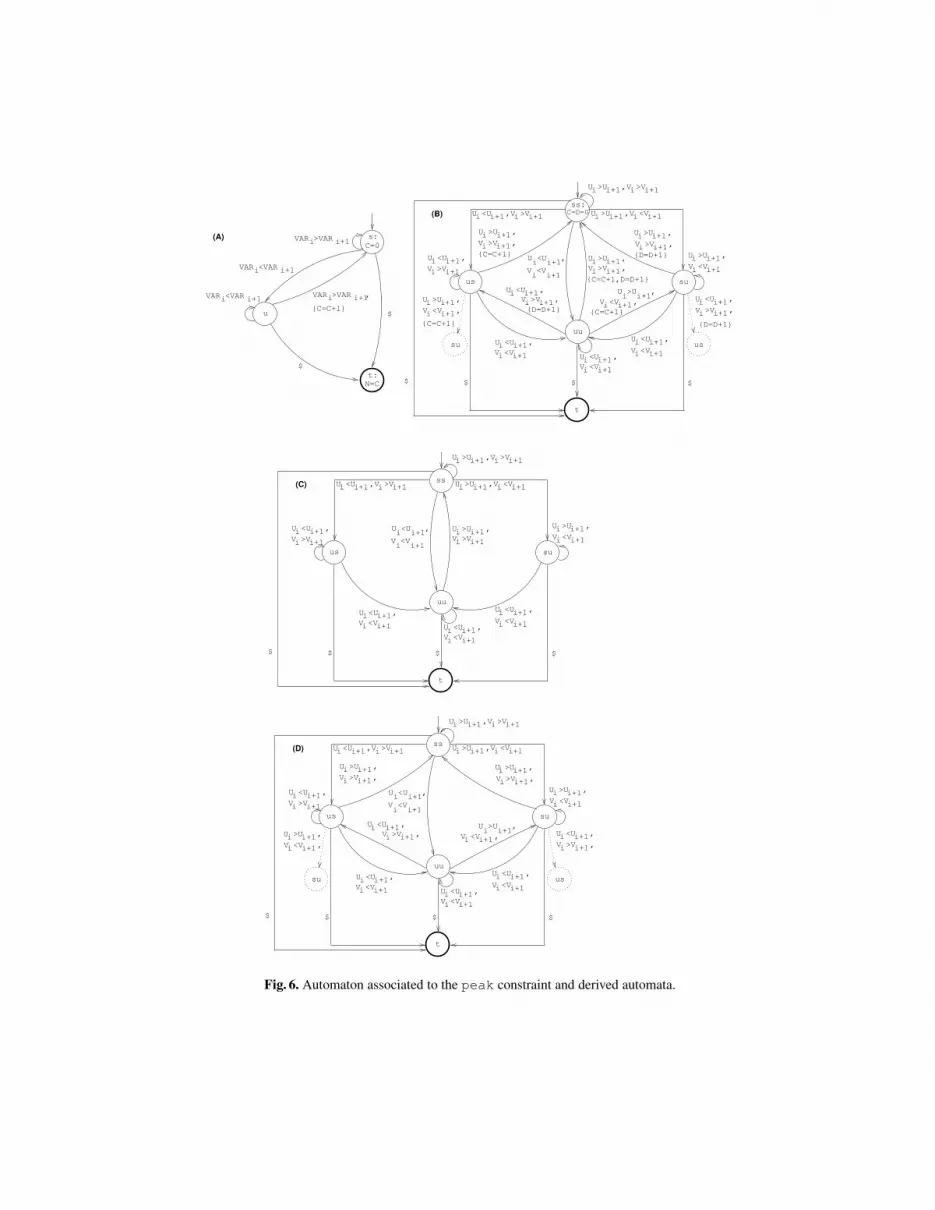
As an illustrative example, consider the peak constraint, which counts the num-ber of peaks of a sequence of variables where adjacent variables are not equal. Theautomaton of this constraint is depicted by part (A) of Fig. 6.

We explain how to derive the automaton associated to synchronizedC and todistinctC from the automaton AC associated to C. Let A2

C , S(AC) and D(AC) re-spectively denotes the automaton that is the product of AC and AC , the automatonassociated to synchronizedC , and the automaton associated to distinctC . Regardingthe example of the peak constraintA2

C is given by part (B) of Fig. 6.We compute S(AC) and D(AC) from A2

C . Within A2C we partition its transitions

into the following 4 classes:

i+1VAR >VARi

i+1VAR <VARi

i+1VAR <VARi i+1VAR >VAR ,i

(A)

{C=C+1}

$

u

N=C

C=0s:

t:

$

U >U ,V <Vi i+1 i i+1

U >U ,i i+1V >V ,i i+1{C=C+1} U <U ,i i+1

V <Vi i+1

U >U ,i i+1

V <V ,i i+1

U <U ,i i+1V >V ,i i+1{D=D+1}

i i+1V <Vi i+1

U <U , i i+1V <Vi i+1

U <U ,

U <U ,i i+1V >Vi i+1

i i+1V <Vi i+1

U >U ,

{D=D+1}

us

ss:

uu

su

t

C=D=0

$ $ $

i i+1V <Vi i+1

i i+1

i i+1 i i+1U >U ,V >V

i i+1 i i+1U <U ,V >V

U <U ,

i i+1V >V ,i i+1{D=D+1}U >U ,

V >V ,i i+1{C=C+1,D=D+1}

{C=C+1}

(B)

U >U ,

ussu

$

{C=C+1}

i i+1U >U , i i+1U <U ,

i i+1i i+1V <V , V >V ,

U >U ,V <Vi i+1 i i+1

U <U ,i i+1V <Vi i+1

U >U ,i i+1

V <V ,i i+1

U <U ,i i+1V >V ,i i+1

i i+1V <Vi i+1

U <U , i i+1V <Vi i+1

U <U ,

U <U ,i i+1V >Vi i+1

i i+1V <Vi i+1

U >U ,

us

uu

su

t

$ $ $

i i+1V <Vi i+1

i i+1 i i+1U >U ,V >V

i i+1 i i+1U <U ,V >V

U <U ,

i i+1V >V ,i i+1

U >U ,

ussu

$

i i+1U >U , i i+1U <U ,

i i+1i i+1V <V , V >V ,

(D)

U >U ,i i+1V >V ,i i+1

ss

U >U ,V <Vi i+1 i i+1

U <U ,i i+1V <Vi i+1

i i+1V <Vi i+1

U <U , i i+1V <Vi i+1

U <U ,

U <U ,i i+1V >Vi i+1

i i+1V <Vi i+1

U >U ,

us

uu

su

t

$ $ $

i i+1V <Vi i+1

i i+1

i i+1 i i+1U >U ,V >V

i i+1 i i+1U <U ,V >V

U <U ,

U >U ,

i i+1

$

(C) ss

V >V

Fig. 6. Automaton associated to the peak constraint and derived automata.

– Those transitions that do not increment any counter,– Those transitions that only increment the counter associated to the sequenceU1U2 . . . Um.

– Those transitions that only increment the counter associated to the sequenceV1V2 . . . Vm.

– Finally, those transitions that increment both counters.

S(AC) corresponds toA2C from which we remove all transitions where only one single

counter is incremented, and D(AC) corresponds to A2C from which we remove all

transitions where both counters are incremented. We also remove from the resultingautomata all counter variables. Coming back to the example of the peak constraint,S(AC) and D(AC) respectively correspond to part (C) and (D) of Fig. 6.

5 Handling Relaxation for a Counter-Free Automaton

This section presents a filtering algorithm for handling constraint relaxation under theassumption that we don’t use any counter in our automaton. It can be seen as a general-ization of the algorithm used for the regular constraint [6].

Definition 3. The violation cost of a global constraint is the minimum number of sub-sets of its signature argument for which it is necessary to change at least one variablein order to get back to a solution.

When these subsets form a partition over the variables of the constraint and when theyconsist of a single element, this cost is in fact the minimum number of variables tounassign in order to get back to a solution. As in [7], we add a cost variable cost asan extra argument of the constraint. Our filtering algorithm first evaluates the minimumcost valueMin. Then, according to max(cost), it prunes values that cannot belong toa solution.

Example 5. Consider the constraint global contiguity([V0, V1, V2, V3, V4, V5, V6]) withthe following current domains for variables Vi: [{0, 1}, {1}, {1}, {0}, {1}, {0, 1}, {1}]. Theconstraint is violated because there are necessarily at least two distinct sequences of con-secutive 1. To get back to a state that can lead to a solution, it is enough to turnthe fourth value to 1. One can deduce Min = 1. Consider now the relaxed formsoft global contiguity([V0, V1, V2, V3, V4, V5, V6], cost ) and assume max(cost) = 1.The filtering algorithm should remove value 0 from V5. Indeed, selecting value 0 for variableV5 entails a minimum violation cost of 2. Observe that for this constraint the signature variablesS0, S1, S2, S3, S4, S5, S6 are V0, V1, V2, V3, V4, V5, V6.

As in the algorithm of Pesant [6], our consistency algorithm builds a layered acyclicdirected multigraph G. Each layer of G contains a different node for each state of ourautomaton. Arcs only appear between consecutive layers. Given two nodes n1 and n2 oftwo consecutive layers, q1 and q2 denote their respective associated state. There is an arca from n1 to n2 iff, in the automaton, there is an arc arc(q1, v, q2) from q1 to q2. The arca is labeled with the value v. Arcs corresponding to transitions that cannot be triggeredaccording to the current domain of the signature variables S0, . . . , Sm−1 are markedas infeasible. All other arcs are marked as feasible. Finally, we discard isolated nodes

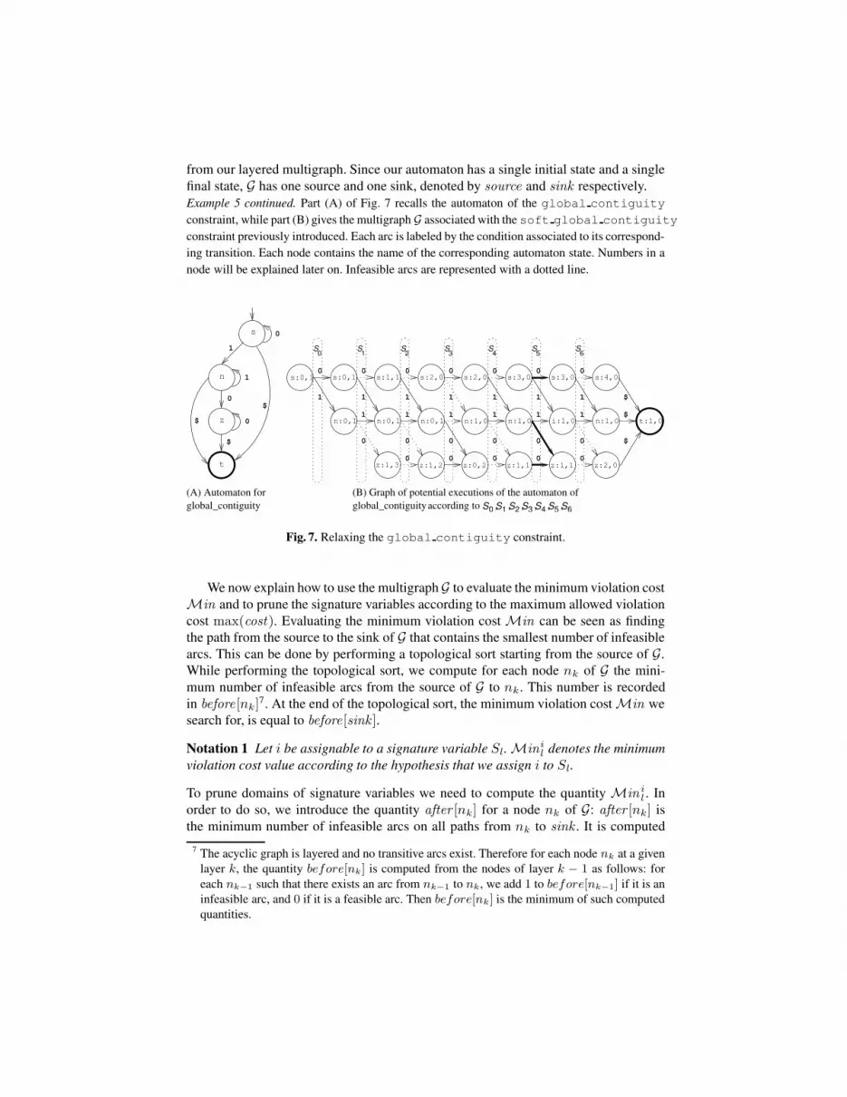
from our layered multigraph. Since our automaton has a single initial state and a singlefinal state, G has one source and one sink, denoted by source and sink respectively.Example 5 continued. Part (A) of Fig. 7 recalls the automaton of the global contiguity

constraint, while part (B) gives the multigraph G associated with the soft global contiguity

constraint previously introduced. Each arc is labeled by the condition associated to its correspond-ing transition. Each node contains the name of the corresponding automaton state. Numbers in anode will be explained later on. Infeasible arcs are represented with a dotted line.

z:1,2 z:0,2 z:1,1 z:1,1 z:2,0z:1,3

s

n

z

0

1

1

0

0

$

$

$

t

s:0,1 s:0,1 s:1,1 s:2,0 s:2,0 s:3,0 s:3,0 s:4,0

n:0,1 n:0,1 n:0,1 n:1,0 n:1,0 i:1,0 n:1,0 t:1,0

1

0 0

0

1

0

1

1

0

0

0

1

1

0

0

0

1

1

0

0

0

1

1

0

0

0

1

1

0

0

$

$

$

(A) Automaton forglobal_contiguity

(B) Graph of potential executions of the automaton ofglobal_contiguity

1

1 2 3S

0 4 5 6S S S S S S

0 , 2 ,1 , 3 , 4 , 5 , 6according to S S S S S S S

Fig. 7. Relaxing the global contiguity constraint.

We now explain how to use the multigraphG to evaluate the minimum violation costMin and to prune the signature variables according to the maximum allowed violationcost max(cost). Evaluating the minimum violation cost Min can be seen as findingthe path from the source to the sink of G that contains the smallest number of infeasiblearcs. This can be done by performing a topological sort starting from the source of G.While performing the topological sort, we compute for each node nk of G the mini-mum number of infeasible arcs from the source of G to nk. This number is recordedin before [nk]7. At the end of the topological sort, the minimum violation costMin wesearch for, is equal to before [sink ].

Notation 1 Let i be assignable to a signature variable Sl.Minil denotes the minimumviolation cost value according to the hypothesis that we assign i to Sl.

To prune domains of signature variables we need to compute the quantity Min il . Inorder to do so, we introduce the quantity after [nk] for a node nk of G: after [nk] isthe minimum number of infeasible arcs on all paths from nk to sink . It is computed

7 The acyclic graph is layered and no transitive arcs exist. Therefore for each node nk at a givenlayer k, the quantity before[nk] is computed from the nodes of layer k − 1 as follows: foreach nk−1 such that there exists an arc from nk−1 to nk, we add 1 to before[nk−1] if it is aninfeasible arc, and 0 if it is a feasible arc. Then before[nk] is the minimum of such computedquantities.

by performing a second topological sort starting from the sink of G. Let Ail denotethe set of arcs of G, labeled by i, for which the origin has a rank of l. The quantity

mina→b∈Ail

(before [a] + after [b]) represents the minimum violation cost under the hypoth-

esis that Sl remains assigned to i. If that quantity is greater thanMin then there is nopath from source to sink that uses an arc ofAil and that has a number of infeasible arcsequal toMin. In that case the smallest cost we can achieve isMin + 1. Therefore wehave:

Minil = min( mina→b∈Ail

(before [a] + after [b]),Min + 1)

The filtering algorithm is then based on the following theorem:

Theorem 3. Let i be a value from the domain of a signature variable Sl. If Minil >max(cost) then i can be removed from Sl.

The cost of the filtering algorithm is dominated by the two topological sorts. They havea cost proportional to the number of arcs of G, which is bounded by the number of sig-nature variables times the number of arcs of the automaton.

Example 5 continued. Let us come back to the instance of Fig. 7. Beside the state’s name,each node nk of part (B) of Fig. 7 gives the values of before [nk] and of after [nk]. Sincebefore [sink ] = 1 we have that the minimum cost violation is equal to 1. Pruning can be po-tentially done only for signature variables having more than one value. In our example this corre-sponds to variables V0 and V5. So we evaluate the four quantitiesMin0

0 = min(0 + 1, 2) = 1,Min1

0 = min(0 + 1, 2) = 1, Min05 = min(min(3 + 0, 1 + 1, 1 + 1), 2) = 2, Min1

5 =

min(min(3 + 0, 1 + 0), 2) = 1. If max(cost) is equal to 1 we can remove value 0 from V5. Thecorresponding arcs are depicted with a thick line in Fig. 7.

6 Conclusion and Perspectives

The automaton description introduced in this article can be seen as a restricted program-ming language. This language is used for writing down a constraint checker, which ver-ifies whether a ground instance of a constraint is satisfied or not. This checker allowspruning the variables of a non-ground instance of a constraint by simulating all poten-tial executions of the corresponding program according to the current domain of thevariables of the relevant constraint. This simulation is achieved by encoding all poten-tial executions of the automaton as a conjunction of signature and transition constraintsand by letting the usual constraint propagation deducing all the relevant information.We want to stress the key points and the different perspectives of this approach:

– Within the context of global constraints, it was implicitly assumed that providing aconstraint checker is a much easier task than coming up with a filtering algorithm.It was also commonly admitted that the design of filtering algorithms is a difficulttask, which involves creativity and which cannot be automatized. We have shownthat this is not the case any more if one can afford to provide a constraint checker.

– Non-determinism has played a key role by augmenting programming languageswith backtracking facilities [39], which was the origin of logic programming. Non-determinism also has a key role to play in the systematic design of filtering algo-rithms: finding a filtering algorithm can be seen as the task of executing in a non-deterministic way the deterministic program corresponding to a constraint checkerand to extract the relevant information that is common to all execution paths. Thiscan indeed be achieved by using constraint programming.

– A natural continuation would be to extend the automaton description in order to getcloser to a classical imperative programming language. This would allow the directuse of available checkers in order to systematically get a automaton reformulation.

– Other structural conditions on the signature and transition constraints could be iden-tified to guarantee arc-consistency for the original global constraint.

– An extension of our approach may give a systematic way to get an algorithm (notnecessarily polynomial) for decision problems for which one can provide a poly-nomial certificate. From [40] the decision version of every problem in NP can beformulated as follows: Given x, decide whether there exists y so that |y| ≤ m(x)and R(x, y). x is an instance of the problem; y is a short YES-certificate for thisinstance; R(x, y) is a polynomial time decidable relation that verifies certificate yfor instance x; and m(x) is a computable and polynomially bounded complexityparameter that bounds the length of the certificate y. In our context, if |y| is fixedand known, x is a global constraint and its |y| variables with their domains; y is asolution to that global constraint;R(x, y) is an automaton, which encodes a checkerfor that global constraint.

Acknowledgments. We are grateful to I. Katriel for suggesting the use of topological sort for therelaxation part, and to C. Bessiere for his helpful comments wrt. Berge-acyclic CSP’s.

References

1. M. Carlsson and N. Beldiceanu. From constraints to finite automata to filtering algorithms.In D. Schmidt, editor, Proc. ESOP2004, volume 2986 of LNCS, pages 94–108. Springer-Verlag, 2004.

2. N. R. Vempaty. Solving constraint satisfaction problems using finite state automata. In Na-tional Conference on Artificial Intelligence (AAAI-92), pages 453–458. AAAI Press, 1992.

3. J. Amilhastre. Representation par automate d’ensemble de solutions de problemes de satis-faction de contraintes. PhD Thesis, 1999.

4. J. Amilhastre, H. Fargier, and P. Marquis. Consistency restoration and explanations in dy-namic CSPs – application to configuration. Artificial Intelligence, 135:199–234, 2002.

5. B. Boigelot and P. Wolper. Representing arithmetic constraints with finite automata: Anoverview. In Peter J. Stuckey, editor, ICLP’2002, Int. Conf. on Logic Programming, volume2401 of LNCS, pages 1–19. Springer-Verlag, 2002.

6. G. Pesant. A regular language membership constraint for sequence of variables. In Workshopon Modelling and Reformulation Constraint Satisfaction Problems, pages 110–119, 2003.

7. T. Petit, J.-C. Regin, and C. Bessiere. Specific filtering algorithms for over-constrained prob-lems. In T. Walsh, editor, Principles and Practice of Constraint Programming (CP’2001),volume 2239 of LNCS, pages 451–463. Springer-Verlag, 2001.

8. M. Milano. Constraint and integer programming. Kluwer Academic Publishers, 2004. ISBN1-4020-7583-9.

9. P. Van Hentenryck and J.-P. Carillon. Generality vs. specificity: an experience with AI andOR techniques. In National Conference on Artificial Intelligence (AAAI-88), 1988.

10. N. Beldiceanu. Pruning for the minimum constraint family and for the number of distinctvalues constraint family. In T. Walsh, editor, CP’2001, Int. Conf. on Principles and Practiceof Constraint Programming, volume 2239 of LNCS, pages 211–224. Springer-Verlag, 2001.

11. S. Bourdais, P. Galinier, and G. Pesant. HIBISCUS: A constraint programming applicationto staff scheduling in health care. In F. Rossi, editor, CP’2003, Principles and Practice ofConstraint Programming, volume 2833 of LNCS, pages 153–167. Springer-Verlag, 2003.

12. M. Maher. Analysis of a global contiguity constraint. In Workshop on Rule-Based ConstraintReasoning and Programming, 2002. held along CP-2002.

13. A. Frisch, B. Hnich, Z. Kızıltan, I. Miguel, and T. Walsh. Global constraints for lexico-graphic orderings. In Pascal Van Hentenryck, editor, Principles and Practice of ConstraintProgramming (CP’2002), volume 2470 of LNCS, pages 93–108. Springer-Verlag, 2002.

14. N. Beldiceanu and E. Contejean. Introducing global constraints in CHIP. Mathl. Comput.Modelling, 20(12):97–123, 1994.

15. N. Beldiceanu. Global constraints as graph properties on structured network of elementaryconstaints of the same type. In R. Dechter, editor, CP’2000, Principles and Practice ofConstraint Programming, volume 1894 of LNCS, pages 52–66. Springer-Verlag, 2000.

16. M. Carlsson et al. SICStus Prolog User’s Manual. Swedish Institute of Computer Science,3.11 edition, January 2004. http://www.sics.se/sicstus/.

17. T. Le Provost and M. Wallace. Domain-independent propagation. In Proc. of the In-ternational Conference on Fifth Generation Computer Systems, pages 1004–1011, 1992.http://www.icparc.ic.ac.uk/eclipse/.

18. ILOG. ILOG Solver Reference Manual, 6.0 edition. http://www.ilog.com.19. R. Dechter and J. Pearl. Tree clustering for constraint networks. Artificial Intelligence,

38:353–366, 1989.20. D. Maier. The Theory of Relational Databases. Computer Science Pres, Rockville, MD,

1983.21. C. Berge. Graphs and hypergraphs. Dunod, Paris, 1970.22. P. Janssen and M-C. Vilarem. Problemes de satisfaction de contraintes: techniques de

resolution et application a la synthese de peptides. Research Report C.R.I.M., 54, 1988.23. P. Jegou. Contribution a l’etude des problemes de satisfaction de contraintes: algorithmes de

propagation et de resolution. Propagation de contraintes dans les reseaux dynamiques. PhDThesis, 1991.

24. N. Beldiceanu, M. Carlsson, and T. Petit. Deriving filtering algorithms from constraintcheckers. Technical Report T2004-08, Swedish Institute of Computer Science, 2004.

25. C. Beeri, R. Fagin, D. Maier, and M. Yannakakis. On the desirability of acyclic databaseschemes. JACM, 30:479–513, 1983.

26. R. Dechter and J. Pearl. Tree clustering for constraint networks. Artificial Intelligence,38:353–366, 1989.

27. R. Fagin. Degrees of acyclicity for hypergraphs and relational database schemes. JACM,30:514–550, July 1983.

28. N. Beldiceanu and M. Carlsson. Sweep as a generic pruning technique applied to the non-overlapping rectangles constraints. In T. Walsh, editor, Principles and Practice of ConstraintProgramming (CP’2001), volume 2239 of LNCS, pages 377–391. Springer-Verlag, 2001.

29. C. Bessiere, E. C. Freuder, and J.-C. Regin. Using constraint metaknowledge to reduce arcconsistency computation. Artificial Intelligence, 107:125–148, 1999.

30. C. Bessiere, J.-C. Regin, R.H.C. Yap, and Y. Zhang. An optimal coarse-grained arc consis-tency algorithm. Artificial Intelligence, 2005. to appear.

31. I.P. Gent and T. Walsh. CSPLib: a benchmark library for constraints. Technical ReportAPES-09-1999, APES, 1999. http://www.csplib.org.

32. M. Carlsson, G. Ottosson, and B. Carlson. An open-ended finite domain constraint solver.In H. Glaser, P. Hartel, and H. Kuchen, editors, Programming Languages: Implementations,Logics, and Programming, volume 1292 of LNCS, pages 191–206. Springer-Verlag, 1997.

33. COSYTEC. CHIP Reference Manual, v5 edition, 2003.34. P. Refalo. Linear formulation of constraint programming models and hybrid solvers. In

R. Dechter, editor, Principles and Practice of Constraint Programming (CP’2000), volume1894 of LNCS, pages 369–383. Springer-Verlag, 2000.

35. N. Beldiceanu and M. Carlsson. Revisiting the cardinality operator and introducing thecardinality-path constraint family. In P. Codognet, editor, ICLP’2001, Int. Conf. on LogicProgramming, volume 2237 of LNCS, pages 59–73. Springer-Verlag, 2001.

36. G. Ottosson, E. Thorsteinsson, and J. N. Hooker. Mixed global constraints and inference inhybrid IP-CLP solvers. In CP’99 Post-Conference Workshop on Large-Scale CombinatorialOptimization and Constraints, pages 57–78, 1999.

37. N. Beldiceanu, Q. Guo, and S. Thiel. Non-overlapping constraints between convex poly-topes. In T. Walsh, editor, Principles and Practice of Constraint Programming (CP’2001),volume 2239 of LNCS, pages 392–407. Springer-Verlag, 2001.

38. N. Beldiceanu and E. Poder. Cumulated profiles of minimum and maximum resource utili-sation. In Ninth Int. Conf. on Project Management and Scheduling, pages 96–99, 2004.

39. J. Cohen. Non-deterministic algorithms. ACM Computing Surveys, 11(2):79–94, 1979.40. G. J. Woeginger. Exact algorithms for NP-hard problems: A survey. In M. Juenger,

G. Reinelt, and G. Rinaldi, editors, Combinatorial Optimization - Eureka! You shrink!, vol-ume 2570 of LNCS, pages 185–207. Springer-Verlag, 2003.