Real Options

C H A P T E R 25Real Options

Honda Motor Company spent $400 million dollars on something it might

not need—production flexibility. If demand for its vehicles changed in

predictable ways, then Honda would have wasted the $400 million

dollars. But as we have seen in the global economic recession, demand

for automobiles is highly volatile, with consumer preferences swinging

wildly every time oil prices change. To prepare for such volatility, Honda

has been building flexibility into its factories and now boasts the most

flexibility of any auto maker in the United States.

Honda’s plant in Liberty, Ohio, can stop Civic production, set up for the

CR-V crossover, and start producing CR-Vs in less than 10 minutes,

incurring virtually no additional cost in the process. Many of its other

plants have similar capabilities. For example, Honda has been able to

quickly reduce output of its Ridgeline pickup truck and boost production of

more fuel-efficient vehicles. In contrast, Ford will take over a year to

convert a factory now producing gas-guzzling sport utility vehicles, with

the switchover costing over $75 million. GM has similar problems and will

spend $370 million to change models at one of its factories.

Honda’s flexibility is due to several factors, beginning with designs for

vehicles and production processes that share components and assembly

techniques. For example, the assembly process for doors is very similar,

no matter what vehicle is being produced. Honda’s robots also give

it flexibility. For example, the same robots are used to weld different

vehicles.

It costs more initially to build in flexibility at a factory, but the payoff can

be well worth the cost. As you read this chapter and learn more about

options, think about how option pricing techniques can lead to better

capital budgeting decisions.

Sources: Kate Linebaugh, “Honda’s Flexible Plants Provide Edge,” The Wall Street Journal, September 23,

2008, p. B1.

971

Traditional discounted cash flow (DCF) analysis—in which an asset’s cash flows areestimated and then discounted to obtain the asset’s NPV—has been the cornerstonefor valuing all types of assets since the 1950s. Accordingly, most of our discussion ofcapital budgeting has focused on DCF valuation techniques. However, in recent yearsacademics and practitioners have demonstrated that DCF valuation techniques do notalways tell the complete story about a project’s value and that rote use of DCF can, attimes, lead to incorrect capital budgeting decisions.1

DCF techniques were originally developed to value securities such as stocks andbonds. Securities are passive investments: Once they have been purchased, most inves-tors have no influence over the cash flows the assets produce. However, real assets arenot passive investments because managerial actions after an investment has been madecan influence its results. Furthermore, investing in a new project often brings with itthe potential for increasing the firm’s future investment opportunities. Such opportu-nities are, in effect, options—the right (but not the obligation) to take some action inthe future. As we demonstrate in the next section, options are valuable, so projects thatexpand the firm’s set of opportunities have positive option values. Similarly, any proj-ect that reduces the set of future opportunities destroys option value. Since a project’simpact on the firm’s opportunities, or its option value, may not be captured by conven-tional NPV analysis, this option value should be considered separately, as we do in thischapter.

25.1 VALUING REAL OPTIONSRecall from Chapter 11 that real options are opportunities for management tochange the timing, scale, or other aspects of an investment in response to changesin market conditions. These opportunities are options in the sense that managementcan, if it is in the company’s best interest, undertake some action; management is notrequired to undertake the action. These opportunities are real (as opposed to finan-cial) because they involve decisions regarding real assets—such as plants, equipment,and land—rather than financial assets like stocks or bonds. Four examples of realoptions are investment timing options, growth options, abandonment options, andflexibility options. This chapter provides an example of how to value an investmenttiming option and a growth option. Web Extension 25A on the textbook’s Web siteshows how to value an abandonment option.

Valuing a real option requires judgment, both to formulate the model and to esti-mate the inputs. Does this mean the answer won’t be useful? Definitely not. Forexample, the models used by NASA only approximate the centers of gravity for themoon, the earth, and other heavenly bodies, yet even with these “errors” in theirmodels, NASA has been able to put astronauts on the moon. As one professor said,“All models are wrong, but some are still quite useful.” This is especially true for realoptions. We might not be able to find the exact value of a real option, but the valuewe find can be helpful in deciding whether or not to accept the project. Equallyimportant, the process of looking for and then valuing real options often identifiescritical issues that might otherwise go unnoticed.

Five possible procedures can be used to deal with real options. Starting with thesimplest, they are as follows.

1For an excellent general discussion of the problems inherent in discounted cash flow valuation techni-ques as applied to capital budgeting, see Avinash K. Dixit and Robert S. Pindyck, “The Options Approachto Capital Investment,” Harvard Business Review, May/June 1995, pp. 105–115.

resource

The textbook’s Web site

contains an Excel file that

will guide you through the

chapter’s calculations.

The file for this chapter is

Ch25 Tool Kit.xls, and

we encourage you to

open the file and follow

along as you read the

chapter.

972 Part 10: Advanced Issues

1. Use discounted cash flow (DCF) valuation and ignore any real options byassuming their values are zero.

2. Use DCF valuation and include a qualitative recognition of any real option’svalue.

3. Use decision-tree analysis.4. Use a standard model for a financial option.5. Develop a unique, project-specific model using financial engineering techniques.

The following sections illustrate these procedures.

Self-Test List the five possible procedures for dealing with real options.

25.2 THE INVESTMENT TIMING OPTION: AN ILLUSTRATIONThere is frequently an alternative to investing immediately—the decision to invest ornot can be postponed until more information becomes available. By waiting, a better-informed decision can be made, and this investment timing option adds value to theproject and reduces its risk.

Murphy Systems is considering a project for a new type of handheld device thatprovides wireless Internet connections. The cost of the project is $50 million, butthe future cash flows depend on the demand for wireless Internet connections, whichis uncertain. Murphy believes there is a 25% chance that demand for the new devicewill be high, in which case the project will generate cash flows of $33 million eachyear for 3 years. There is a 50% chance of average demand, with cash flows of $25million per year, and a 25% chance that demand will be low and annual cash flowswill be only $5 million. A preliminary analysis indicates that the project is somewhatriskier than average, so it has been assigned a cost of capital of 14% versus 12% foran average project at Murphy Systems. Here is a summary of the project’s data:

Demand Probabil ity Annual Cash Flow

High 0.25 $33 millionAverage 0.50 25 millionLow 0.25 5 millionExpected annual cash flow $22 million

Project’s cost of capital 14%Life of project 3 yearsRequired investment,or cost of project $50 million

Murphy could accept the project and implement it immediately; however, sincethe company has a patent on the device’s core modules, it could also choose to delaythe decision until next year, when more information about demand will be available.The cost will still be $50 million if Murphy waits, and the project will still beexpected to generate the indicated cash flows, but each flow will be pushed back1 year. However, if Murphy waits then it will know which of the demand conditions—and hence which set of cash flows—will obtain. If Murphy waits then it will, of course,make the investment only if demand is sufficient to yield a positive NPV.

Observe that this real timing option resembles a call option on a stock. A call givesits owner the right to purchase a stock at a fixed strike price, but only if the stock’sprice is higher than the strike price will the owner exercise the option and buy thestock. Similarly, if Murphy defers implementation, then it will have the right to

resource

All calculations for the

analysis of the investment

timing option are shown

in Ch25 Tool Kit.xls on

the textbook’s Web site.

Chapter 25: Real Options 973

“purchase” the project by making the $50 million investment if the NPV as calcu-lated next year, when new information is available, is positive.

Approach 1. DCF Analysis Ignoring the Timing OptionBased on probabilities for the different levels of demand, the expected annual cashflows are $22 million per year:

Expected cash flow per year¼ 0:25ð$33Þ þ 0:50ð$25Þ þ 0:25ð$5Þ¼ $22 million

Ignoring the investment timing option, the traditional NPV is $1.08 million, foundas follows:

NPV ¼ −$50þ$22

ð1þ 0:14Þ1þ

$22

ð1þ 0:14Þ2þ

$22

ð1þ 0:14Þ3¼ $1:08

The present value of the cash inflows is $51.08 million while the cost is $50 million,leaving an NPV of $1.08 million.

Based just on this DCF analysis, Murphy should accept the project. Note, how-ever, that if the expected cash flows had been slightly lower—say, $21.5 million peryear—then the NPV would have been negative and the project would have beenrejected. Also, note that the project is risky: there is a 25% probability that demandwill be weak, in which case the NPV will turn out to be a negative $38.4 million.

Approach 2. DCF Analysis with a QualitativeConsideration of the Timing OptionThe discounted cash flow analysis suggests that the project should be accepted, butjust barely, and it ignores the existence of a possibly valuable real option. If Murphyimplements the project now, it gains an expected (but risky) NPV of $1.08 million.However, accepting now means that it is also giving up the option to wait and learnmore about market demand before making the commitment. Thus, the decision isthis: Is the option Murphy would be giving up worth more or less than $1.08 million?If the option is worth more than $1.08 million then Murphy should not give up theoption, which means deferring the decision—and vice versa if the option is worth lessthan $1.08 million.

Based on the discussion of financial options in Chapter 8, what qualitative assess-ment can we make regarding the option’s value? Put another way: Without doing anyadditional calculations, does it appear that Murphy should go forward now or wait?In thinking about this decision, first note that the value of an option is higher if thecurrent value of the underlying asset is high relative to its strike price, other thingsheld constant. For example, a call option with a strike price of $50 on a stock with acurrent price of $50 is worth more than if the current price were $20. The strikeprice of the project is $50 million, and our first guess at the value of its cash flows is$51.08 million. We will calculate the exact value of Murphy’s underlying asset later,but the DCF analysis does suggest that the underlying asset’s value will be close tothe strike price, so the option should be valuable. We also know that an option’svalue is higher the longer its time to expiration. Here the option has a 1-year life,which is fairly long for an option, and this also suggests that the option is probablyvaluable. Finally, we know that the value of an option increases with the risk of theunderlying asset. The data used in the DCF analysis indicate that the project is quiterisky, which again suggests that the option is valuable.


Thus, our qualitative assessment indicates that the option to delay might well be morevaluable than the expected NPV of $1.08 if we undertake the project immediately. Thisconclusion is quite subjective, but the qualitative assessment suggests that Murphy’smanagement should go on to make a quantitative assessment of the situation.

Approach 3. Scenario Analysis and Decision TreesPart 1 of Figure 25-1 presents a scenario analysis and decision tree similar to theexamples in Chapter 11. Each possible outcome is shown as a “branch” on the tree.Each branch shows the cash flows and probability of a scenario laid out as a time line.Thus, the top line, which gives the payoffs of the high-demand scenario, has positivecash flows of $33 million for the next 3 years, and its NPV is $26.61 million. Theaverage-demand branch in the middle has an NPV of $8.04 million, while the NPVof the low-demand branch is a negative $38.39 million. Since Murphy will suffer a

F IGURE 25-1 DCF and Decision-Tree Analysis for the Investment Timing Option (Millions of Dollars)

Part 1. Scenario Analysis: Proceed with Project TodayNPV of this

ScenariocProbability

x NPVNow: Year 0 Year 1 Year 2 Year 3 Probability

$33 $33 $33 $26.61 0.25 $6.65

High–$50 Average $25 $25 $25 $8.04 0.50 $4.02

Low

$5 $5 $5 –$38.39 0.25 –$9.60

1.00

Expected value of NPVs = $1.08

Standard Deviationa = $24.02

Coefficient of Variationb = 22.32

Part 2. Decision-Tree Analysis: Implement in One Year Only If OptimalNPV of this

ScenariodProbability

x NPVNow: Year 0 Year 1 Year 2 Year 3 Year 4 Probability

–$50 $33 $33 $33 $23.35 0.25 $5.84

High

Wait Average –$50 $25 $25 $25 $7.05 0.50 $3.53

Low$0 $0 $0 $0 $0.00 0.25 $0.00

1.00




Future Cash Flows

Future Cash Flows

0.25

0.25

0.50

0.25

0.25

0.50

Notes:aThe WACC is 14%.bThe standard deviation is calculated as explained in Chapter 6.cThe coefficient of variation is the standard deviation divided by the expected value.dThe NPV in Part 2 is as of Year 0. Therefore, each of the project cash flows is discounted back one more year than in Part 1.


$38.39 million loss if demand is weak and since there is a 25% probability of weakdemand, the project is clearly risky.

The expected NPV is the weighted average of the three possible outcomes, where theweight for each outcome is its probability. The sum in the last column in Part 1 showsthat the expected NPV is $1.08 million, the same as in the original DCF analysis. Part 1also shows a standard deviation of $24.02 million for the NPV and a coefficient of varia-tion (defined as the ratio of standard deviation to the expected NPV) of 22.32, which israther large. Clearly, the project is quite risky under the analysis thus far.

Part 2 is set up similarly to Part 1 except that it shows what happens if Murphydelays the decision and then implements the project only if demand turns out to behigh or average. No cost is incurred now at Year 0—here the only action is to wait.Then, if demand is average or high, Murphy will spend $50 million at Year 1 andreceive either $33 million or $25 million per year for the following 3 years. If demandis low, as shown on the bottom branch, Murphy will spend nothing at Year 1 and willreceive no cash flows in subsequent years. The NPV of the high-demand branch is$23.35 million and that of the average-demand branch is $7.05 million. Because allcash flows under the low-demand scenario are zero, the NPV in this case will also bezero. The expected NPV if Murphy delays the decision is $9.36 million.

This analysis shows that the project’s expected NPV will be much higher if Mur-phy delays than if it invests immediately. Also, since there is no possibility of losingmoney under the delay option, this decision also lowers the project’s risk. Thisplainly indicates that the option to wait is valuable; hence Murphy should wait untilYear 1 before deciding whether to proceed with the investment.

Before we conclude the discussion of decision trees, note that we used the same cost ofcapital, 14%, to discount cash flows in the “proceed immediately” scenario analysis in Part1 and under the “delay 1 year” scenario in Part 2. However, this is not appropriate for threereasons. First, since there is no possibility of losing money if Murphy delays, theinvestment under that plan is clearly less risky than if Murphy charges ahead today. Sec-ond, the 14% cost of capital might be appropriate for risky cash flows, yet the investmentin the project at Year 1 in Part 2 is known with certainty. Perhaps, then, we should discountit at the risk-free rate.2 Third, the project’s cash inflows (excluding the initial investment)are different in Part 2 than in Part 1 because the low-demand cash flows are eliminated.This suggests that if 14% is the appropriate cost of capital in the “proceed immediately”case then some lower rate would be appropriate in the “delay decision” case.

In Figure 25-2, Part 1, we repeat the “delay decision” analysis but with one excep-tion. We continue to discount the operating cash flows in Year 2 through Year 4 at the14% WACC, but now we discount the project’s cost at Year 1 using the risk-free rateof 6%. This increases the PV of the cost, which lowers the NPV from $9.36 million to$6.88 million. Yet we really don’t know the precise WACC for this project—the 14%we used might be too high or too low for the operating cash flows in Year 2 throughYear 4.3 Therefore, in Part 2 of Figure 25-2 we show a sensitivity analysis of the NPV

2For a more detailed explanation of the rationale behind using the risk-free rate to discount the projectcost, see Timothy A. Luehrman, “Investment Opportunities as Real Options: Getting Started on theNumbers,” Harvard Business Review, July/August 1998, pp. 51–67. This paper also provides a discussionof real option valuation. Professor Luehrman also wrote a follow-up paper that provides an excellent dis-cussion of the ways real options affect strategy: “Strategy as a Portfolio of Real Options,” Harvard BusinessReview, September/October 1998, pp. 89–99.3Murphy might gain information by waiting, which could reduce risk; but if a delay would enable othersto enter and perhaps preempt the market, this could increase risk. In our example, we assumed that Mur-phy has a patent on critical components of the device, precluding the entrance of a competitor that couldpreempt its position in the market.


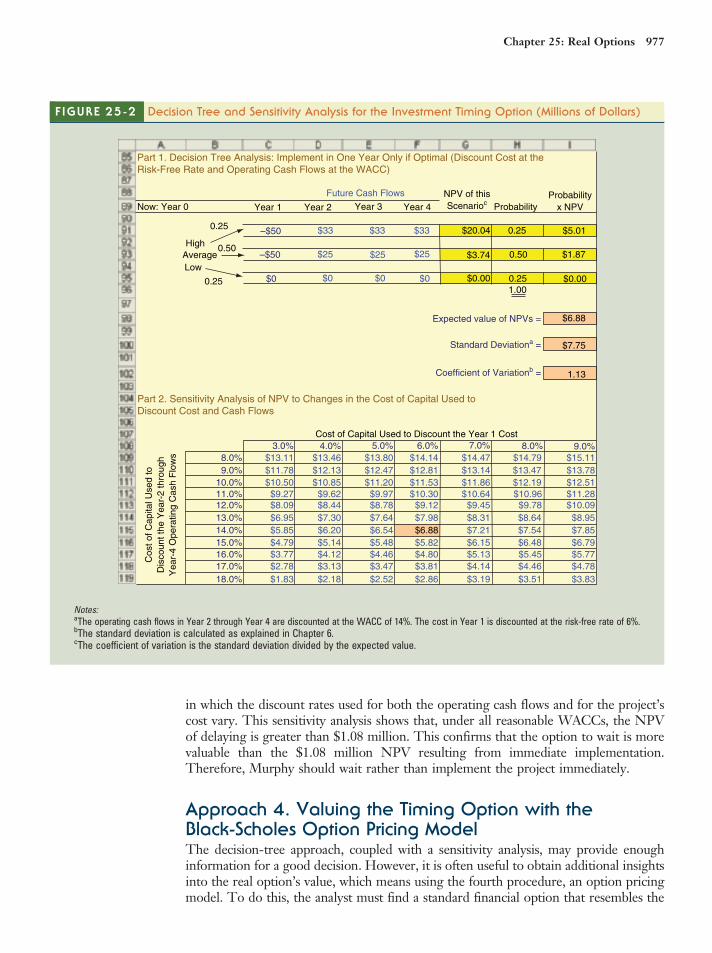
in which the discount rates used for both the operating cash flows and for the project’scost vary. This sensitivity analysis shows that, under all reasonable WACCs, the NPVof delaying is greater than $1.08 million. This confirms that the option to wait is morevaluable than the $1.08 million NPV resulting from immediate implementation.Therefore, Murphy should wait rather than implement the project immediately.

Approach 4. Valuing the Timing Option with theBlack-Scholes Option Pricing ModelThe decision-tree approach, coupled with a sensitivity analysis, may provide enoughinformation for a good decision. However, it is often useful to obtain additional insightsinto the real option’s value, which means using the fourth procedure, an option pricingmodel. To do this, the analyst must find a standard financial option that resembles the

F IGURE 25-2 Decision Tree and Sensitivity Analysis for the Investment Timing Option (Millions of Dollars)

NPV of this


x NPVNow: Year 0 Year 1 Year 2 Year 3 Year 4 Probability

–$50 $33 $33 $33 $20.04 0.25 $5.01

High

Average –$50 $25 $25 $25 $3.74 0.50 $1.87

Low$0 $0 $0 $0 $0.00 0.25 $0.00

1.00




3.0% 4.0% 5.0% 6.0% 7.0% 8.0% 9.0%8.0% $13.11 $13.46 $13.80 $14.14 $14.47 $14.79 $15.11

9.0% $11.78 $12.13 $12.47 $12.81 $13.14 $13.47 $13.78

10.0% $10.50 $10.85 $11.20 $11.53 $11.86 $12.19 $12.5111.0% $9.27 $9.62 $9.97 $10.30 $10.64 $10.96 $11.2812.0% $8.09 $8.44 $8.78 $9.12 $9.45 $9.78 $10.09

13.0% $6.95 $7.30 $7.64 $7.98 $8.31 $8.64 $8.95

14.0% $5.85 $6.20 $6.54 $6.88 $7.21 $7.54 $7.85

15.0% $4.79 $5.14 $5.48 $5.82 $6.15 $6.48 $6.79

16.0% $3.77 $4.12 $4.46 $4.80 $5.13 $5.45 $5.77

17.0% $2.78 $3.13 $3.47 $3.81 $4.14 $4.46 $4.78

18.0% $1.83 $2.18 $2.52 $2.86 $3.19 $3.51 $3.83

Part 2. Sensitivity Analysis of NPV to Changes in the Cost of Capital Used toDiscount Cost and Cash Flows

Cost of C

apital U

sed to

Dis

count th

e Y

ear-

2 thro

ugh

Year-

4 O

pera

ting C

ash F

low

s

Part 1. Decision Tree Analysis: Implement in One Year Only if Optimal (Discount Cost at theRisk-Free Rate and Operating Cash Flows at the WACC)

Future Cash Flows

Cost of Capital Used to Discount the Year 1 Cost

0.25

0.25

0.50

Notes:aThe operating cash flows in Year 2 through Year 4 are discounted at the WACC of 14%. The cost in Year 1 is discounted at the risk-free rate of 6%.bThe standard deviation is calculated as explained in Chapter 6.cThe coefficient of variation is the standard deviation divided by the expected value.


project’s real option.4 As noted earlier, Murphy’s option to delay the project is similar toa call option on a stock. Hence, the Black-Scholes option pricing model can be used.This model requires five inputs: (1) the risk-free rate, (2) the time until the optionexpires, (3) the strike price, (4) the current price of the stock, and (5) the variance ofthe stock’s rate of return. Therefore, we need to estimate values for those five inputs.

First, if we assume that the rate on a 52-week Treasury security is 6%, then thisrate can be used as the risk-free rate. Second, Murphy must decide within a yearwhether or not to implement the project, so there is 1 year until the option expires.Third, it will cost $50 million to implement the project, so $50 million can be usedfor the strike price. Fourth, we need a proxy for the value of the underlying asset,which in Black-Scholes is the current price of the stock. Note that a stock’s currentprice is the present value of its expected future cash flows. For Murphy’s real option,the underlying asset is the project itself, and its current “price” is the present value ofits expected future cash flows. Therefore, as a proxy for the stock price we can usethe present value of the project’s future cash flows. And fifth, the variance of the pro-ject’s expected return can be used to represent the variance of the stock’s return inthe Black-Scholes model.

Figure 25-3 shows how one can estimate the present value of the project’s cashinflows. We need to find the current value of the underlying asset—that is, the proj-ect. For a stock, the current price is the present value of all expected future cashflows, including those that are expected even if we do not exercise the call option.Note also that the strike price for a call option has no effect on the stock’s current

F IGURE 25-3Estimating the Input for Stock Price in the Option Analysis of the Investment Timing Option(Millions of Dollars)

PV of this


x PVNow: Year 0 Year 1 Year 2 Year 3 Year 4 Probability

$33 $33 $33 $67.21 0.25 $16.80

High

Average $25 $25 $25 $50.91 0.50 $25.46

Low$5 $5 $5 $10.18 0.25 $2.55

1.00

Expected value of PVs =

Standard Deviationa =

Coefficient of Variationb =

Future Cash Flows

0.25

0.25

0.50

$44.80

$21.07

0.47

Notes:aThe WACC is 14%. All cash flows in this scenario are discounted back to Year 0.bHere we find the PV, not the NPV, because the project’s cost is ignored.cThe standard deviation is calculated as explained in Chapter 6.dThe coefficient of variation is the standard deviation divided by the expected value.

4In theory, financial option pricing models apply only to assets that are continuously traded in a market.Even though real options usually don’t meet this criterion, financial option models often provide a rea-sonably accurate approximation of the real option’s value.


price.5 For our real option, the underlying asset is the delayed project, and its current“price” is the present value of all its future expected cash flows. Just as the price of astock includes all of its future cash flows, so should the present value of the projectinclude all of its possible future cash flows. Moreover, since the price of a stock is notaffected by the strike price of a call option, we ignore the project’s “strike price,” orcost, when we find its present value. Figure 25-3 shows the expected cash flows if theproject is delayed. The PV of these cash flows as of now (Year 0) is $44.80 million,and this is the input we should use for the current price in the Black-Scholes model.

The last required input is the variance of the project’s return. Three differentapproaches could be used to estimate this input. First, we could use judgment—an edu-cated guess. Here we would begin by recalling that a company is a portfolio of projects(or assets), with each project having its own risk. Since returns on the company’s stockreflect the diversification gained by combining many projects, we might expect the vari-ance of the stock’s returns to be lower than the variance of one of its average projects.The variance of an average company’s stock return is about 12%, so we might expect thevariance for a typical project to be somewhat higher, say, 15% to 25%. Companies in theInternet infrastructure industry are riskier than average, so we might subjectively esti-mate the variance of Murphy’s project to be in the range of 18% to 30%.

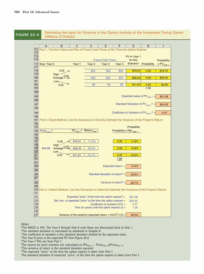
The second approach, called the direct method, is to estimate the rate of return foreach possible outcome and then calculate the variance of those returns. First, Part 1 inFigure 25-4 shows the PV for each possible outcome as of Year 1, the time when theoption expires. Here we simply find the present value of all future operating cash flowsdiscounted back to Year 1, using theWACC of 14%. The Year-1 present value is $76.61million for high demand, $58.04 million for average demand, and $11.61 million for lowdemand. Then, in Part 2, we show the percentage return from the current time until theoption expires for each scenario, based on the $44.80 million starting “price” of the proj-ect at Year 0 as calculated in Figure 25-3. If demand is high, we will obtain a return of71.0%: ($76.61 − $44.80)/$44.80 = 0.710 = 71.0%. Similar calculations show returns of29.5% for average demand and −74.1% for low demand. The expected percentagereturn is 14%, the standard deviation is 53.6%, and the variance is 28.7%.6

The third approach for estimating the variance is also based on the scenario data,but the data are used in a different manner. First, we know that demand is not reallylimited to three scenarios; rather, a wide range of outcomes is possible. Similarly, thestock price at the time a call option expires could take one of many values. It is reason-able to assume that the value of the project at the time when we must decide on under-taking it behaves similarly to the price of a stock at the time a call option expires.Under this assumption, we can use the expected value and standard deviation of theproject’s value to calculate the variance of its rate of return, σ2, with this formula:7

σ2 ¼

lnðCV2 þ 1Þ

t(25-1)

5The company itself is not involved with traded stock options. However, if the option were a warrant issuedby the company, then the strike price would affect the company’s cash flows and hence its stock price.6Two points should be made about the percentage return. First, for use in the Black-Scholes model, we need apercentage return calculated as shown, not an IRR return. The IRR is not used in the option pricing approach.Second, the expected return comes to 14%, the same as the WACC. This is because the Year-0 price and theYear-1 PVs were all calculated using the 14% WACC and because we measured return over only 1 year. If wemeasure the compound return over more than 1 year, then the average return generally will not equal 14%.7For a more detailed discussion, see David C. Shimko, Finance in Continuous Time (Miami, FL: KolbPublishing, 1992).


F IGURE 25-4Estimating the Input for Variance in the Option Analysis of the Investment Timing Option(Millions of Dollars)

Part 1. Find the Value and Risk of Future Cash Flows at the Time the Option Expires

PV in Year 1

for this


x PVYear 1Now: Year 0 Year 1 Year 2 Year 3 Year 4 Probability

$33 $33 $33 $76.61 0.25 $19.15

High

Average $25 $25 $25 $58.04 0.50 $29.02

Low$5 $5 $5 $11.61 0.25 $2.90

1.00

Expected value of PVYear 1 = $51.08

Standard Deviation of PVYear 1

a = $24.02

Coefficient of Variation of PVYear 1b = 0.47

Part 2. Direct Method: Use the Scenarios to Directly Estimate the Variance of the Project's Return

Probability

PriceYear 0d PVYear 1

e ReturnYear 1f Probability x Ret.Year 1

$76.61 71.0% 0.25 17.8%

High$44.80 Average $58.04 29.5% 0.50 14.8%

Low

$11.61 –74.1% 0.25

1.00

–18.5%

Expected return = 14.0%

Standard deviation of returna = 53.6%

Variance of returng = 28.7%

Part 3. Indirect Method: Use the Scenarios to Indirectly Estimate the Variance of the Project's Return

Expected "price" at the time the option expiresh = $51.08

Std. dev. of expected "price" at the time the option expiresi = $24.02

Coefficient of variation (CV) = 0.47Time (in years) until the option expires (t) = 1.00

Variance of the project's expected return = ln(CV2+1)/t = 20.0%

Future Cash Flows

0.25

0.25

0.50

0.25

0.25

0.50

Notes:aThe WACC is 14%. The Year-2 through Year-4 cash flows are discounted back to Year 1.bThe standard deviation is calculated as explained in Chapter 6.cThe coefficient of variation is the standard deviation divided by the expected value.dThe Year-0 price is the expected PV from Figure 25-3.eThe Year-1 PVs are from Part 1.fThe returns for each scenario are calculated as (PVYear 1− PriceYear 0)/PriceYear 0.gThe variance of return is the standard deviation squared.hThe expected “price” at the time the option expires is taken from Part 1.iThe standard deviation of expected “price” at the time the option expires is taken from Part 1.


Here CV is the coefficient of variation of the underlying asset’s price at the time theoption expires, and t is the time until the option expires. Although the three outcomes inthe scenarios represent a small sample of the many possible outcomes, we can still usethe scenario data to estimate the variance that the project’s rate of return would have ifthere were an infinite number of possible outcomes. For Murphy’s project, this indirectmethod produces the following estimate of the variance of the project’s return:

σ2 ¼

lnð0:472 þ 1Þ

1¼ 0:20 ¼ 20% (25-1a)

Which of the three approaches is best? Obviously, they all involve judgment, so ananalyst might want to consider all three. In our example, all three methods producesimilar estimates, but for illustrative purposes we will simply use 20% as our initialestimate for the variance of the project’s rate of return.

In Part 1 of Figure 25-5, we calculate the value of the option to defer investmentin the project based on the Black-Scholes model, and the result is $7.04 million.

F IGURE 25-5Estimating the Value of the Investment Timing Option Using a Standard Financial Option(Millions of Dollars)

Option Value

Part 1. Find the Value of a Call Option Using the Black-Scholes Model

Real Option

rRF = Risk-free interest rate = 6%

t = Time until the option expires = 1

a

b

X = Cost to implement the project = $50.00

P = Current value of the project = $44.80

σ2 = Variance of the project's rate of return = 20.0%

d1 = { ln (P/X) + [rRF + (σ2 /2) ] t } / (σ t1/2) = 0.112

d2 = d1 – σ (t1/2) = –0.33

N(d1) = = 0.54

N(d2) = = 0.37

V = P[ N (d1) ] – Xe–r

RFt [ N (d2) ] = $7.04

Part 2. Sensitivity Analysis of Option Value to Changes in Variance

Variance

12.0% $5.24

14.0% $5.7416.0% $6.20

18.0% $6.63

20.0% $7.04

22.0% $7.4224.0% $7.79

26.0% $8.1528.0% $8.49

30.0% $8.81

32.0% $9.13

Notes:aThe current value of the project is taken from Figure 25-3.bThe variance of the project’s rate of return is taken from Part 3 of Figure 25-4.


Since this is significantly higher than the $1.08 million NPV under immediate imple-mentation and since the option would be forfeited if Murphy goes ahead right now,we conclude as before that the company should defer the final decision until moreinformation is available.

Because judgmental estimates were made at many points in the analysis, it wouldbe useful to see how sensitive the final outcome is to certain of the key inputs.Therefore, in Part 2 of Figure 25-5 we show the sensitivity of the option’s value todifferent estimates of the variance. It is reassuring to see that, for all reasonable esti-mates of variance, the option to delay remains more valuable than immediateimplementation.

Approach 5. Financial EngineeringSometimes an analyst might not be satisfied with the results of a decision-tree analy-sis and cannot find a standard financial option that corresponds to the real option. Insuch a situation the only alternative is to develop a unique model for the specific realoption being analyzed, a process called financial engineering. When financial engi-neering is applied on Wall Street, where it was developed, the result is a newlydesigned financial product.8 When it is applied to real options, the result is the valueof a project that contains embedded options.

Although financial engineering was originally developed on Wall Street, manyfinancial engineering techniques have been applied to real options during the last 10years. We expect this trend to continue, especially in light of the rapid improvementsin computer processing speed and spreadsheet software capabilities. One financialengineering technique is called risk-neutral valuation. This technique uses simula-tion, and we discuss it in Web Extension 25B. Most other financial engineering tech-niques are too complicated for a course in financial management, so we leave adetailed discussion of them to a specialized course.

Self-Test What is a decision tree?

In a qualitative analysis, what factors affect the value of a real option?

25.3 THE GROWTH OPTION: AN ILLUSTRATIONAs we saw with the investment timing option, there is frequently an alternative tomerely accepting or rejecting a static project. Many investment opportunities, ifsuccessful, lead to other investment opportunities. The production capacity of a suc-cessful product line can later be expanded to satisfy increased demand, or distributioncan be extended to new geographic markets. A company with a successful namebrand can capitalize on its success by adding complementary or new products underthe same brand. These growth options add value to a project and explain, for exam-ple, why companies are flocking to make inroads into the very difficult business envi-ronment in China.

Kidco Corporation designs and manufactures products aimed at the pre-teen mar-ket. Most of its products have a very short life, given the rapidly changing tastes ofpre-teens. Kidco is now considering a project that will cost $30 million. Managementbelieves there is a 25% chance that the project will “take off” and generate operatingcash flows of $34 million in each of the next 2 years, after which pre-teen tastes willchange and the project will be terminated. There is a 50% chance of averagedemand, in which case cash flows will be $20 million annually for 2 years. Finally,

8Financial engineering techniques are widely used for the creation and valuation of derivative securities.


there is a 25% chance that the pre-teens won’t like the product at all, and it will gen-erate cash flows of only $2 million per year. The estimated cost of capital for theproject is 14%.

Based on its experience with other projects, Kidco believes it will be able to launcha second-generation product if demand for the original product is average or above.This second-generation product will cost the same as the first-generation product,$30 million, and the cost will be incurred at Year 2. However, given the success ofthe first-generation product, Kidco believes that the second-generation productwould be just as successful as the first-generation product.

This growth option resembles a call option on a stock, since it gives Kidco theopportunity to “purchase” a successful follow-on project at a fixed cost if the valueof the project is greater than the cost. Otherwise, Kidco will let the option expireby not implementing the second-generation product.

The following sections apply the first four valuation approaches: (1) DCF, (2)DCF and qualitative assessment, (3) decision-tree analysis, and (4) analysis with astandard financial option.

Approach 1. DCF Analysis Ignoring the Growth OptionBased on probabilities for the different levels of demand, the expected annual operat-ing cash flows for the project are $19 million per year:

0:25ð$34Þ þ 0:50ð$20Þ þ 0:25ð$2Þ ¼ $19:00

Ignoring the investment timing option, the traditional NPV is $1.29 million:

NPV ¼ −$30þ$19

ð1þ 0:14Þ1þ

$19

ð1þ 0:14Þ2¼ $1:29

Based on this DCF analysis, Kidco should accept the project.

Approach 2. DCF Analysis with a QualitativeConsideration of the Growth OptionAlthough the DCF analysis indicates that the project should be accepted, it ignores apotentially valuable real option. The option’s time to maturity and the volatility ofthe underlying project provide qualitative insights into the option’s value. Kidco’sgrowth option has 2 years until maturity, which is a relatively long time, and thecash flows of the project are volatile. Taken together, this qualitative assessmentindicates that the growth option should be quite valuable.

Approach 3. Decision-Tree Analysis of the Growth OptionPart 1 of Figure 25-6 shows a scenario analysis for Kidco’s project. The top line, whichdescribes the payoffs for the high-demand scenario, has operating cash flows of $34 mil-lion for the next 2 years. The NPV of this branch is $25.99 million. The NPV of theaverage-demand branch in the middle is $2.93 million, and it is −$26.71 million for thelow-demand scenario. The sum in the last column of Part 1 shows the expected NPV of$1.29 million. The coefficient of variation is 14.54, indicating that the project is very risky.

Part 2 of Figure 25-6 shows a decision-tree analysis in which Kidco undertakes thesecond-generation product only if demand is average or high. In these scenarios,shown on the top two branches of the decision tree, Kidco will incur a cost of$30 million at Year 2 and receive operating cash flows of either $34 million or $20million for the next 2 years, depending on the level of demand. If the demand is low,


shown on the bottom branch, Kidco has no cost at Year 2 and receives no additionalcash flows in subsequent years. All operating cash flows (which do not include thecost of implementing the second-generation project at Year 2) are discounted at theWACC of 14%. Because the $30 million implementation cost is known, it is dis-counted at the risk-free rate of 6%. As shown in Part 2 of Figure 25-6, the expectedNPV is $4.70 million, indicating that the growth option is quite valuable.

F IGURE 25-6 Scenario Analysis and Decision-Tree Analysis for the Kidco Project (Millions of Dollars)

Part 1. Scenario Analysis of Kidco's First-Generation Project

Future Cash Flows NPV of thisScenarioc

Probabilityx NPVNow: Year 0 Year 1 Year 2 Probability

$34 $34 $25.99 0.25 $6.50

High–$30 Average $20 $20 $2.93 0.50 $1.47

Low$2 $2 –$26.71 0.25 –$6.68

1.00

Expected Value of NPVs = $1.29



Part 2. Decision Tree Analysis of the Growth Option

NPV of thisScenarioe

Probabilityx NPVNow: Year 0 Year 1 Year 2d Year 3 Year 4 Probability

$34 $34 $34 $34 $42.37 0.25 $10.59–$30High

–$30 Average $20 $20 $20 $20 $1.57 0.50 $0.79–$30

Low$2 $2 $0 $0 –$26.71 0.25 –$6.68

1.00

Expected Value of NPVs = $4.70



Future Cash Flows

0.25

0.25

0.50

0.25

0.25

0.50

Notes:aThe operating cash flows are discounted by the WACC of 14%.bThe standard deviation is calculated as in Chapter 6.cThe coefficient of variation is the standard deviation divided by the expected value.dThe total cash flows at Year 2 are equal to the operating cash flows for the first-generation product minus the $30 million cost toimplement the second-generation product, if the firm chooses to do so. For example, the Year-2 cash flow in the high-demandscenario is $34 − $30 = $4 million. Based on Part 1, it makes economic sense to implement the second-generation product only ifdemand is high or average.

eThe operating cash flows in Year 1 through Year 2, which do not include the $30 million cost of implementing the second-generationproject at Year 2 for the high-demand and average-demand scenarios, are discounted at the WACC of 14%. The $30 million implemen-tation cost at Year 2 for the high-demand and average-demand scenarios is discounted at the risk-free rate of 6%.


The option itself alters the risk of the project, which means that 14% is probablynot the appropriate cost of capital. Table 25-1 presents the results of a sensitivityanalysis in which the cost of capital for the operating cash flows varies from 8% to18%. The sensitivity analysis also allows the rate used to discount the implementa-tion cost at Year 2 to vary from 3% to 9%. The resulting NPV is positive for allreasonable combinations of discount rates.

Approach 4. Valuing the Growth Option with theBlack-Scholes Option Pricing ModelThe fourth approach is to use a standard model for a corresponding financial option.As we noted earlier, Kidco’s growth option is similar to a call option on a stock, sowe will use the Black-Scholes model to find the value of the growth option. The timeuntil the growth option expires is 2 years. The rate on a 2-year Treasury security is6%, and this provides a good estimate of the risk-free rate. Implementing the projectwill cost $30 million, which is the strike price.

The input for stock price in the Black-Scholes model is the current value of theunderlying asset. For the growth option, the underlying asset is the second-generation project, and its current value is the present value of its cash flows. Thecalculations in Figure 25-7 show that this value is $24.07 million. Because the strikeprice of $30 million is greater than the current “price” of $24.07 million, the growthoption is currently out-of-the-money.

Figure 25-8 shows the estimates for the variance of the project’s rate of return usingthe two methods described earlier in the chapter for the analysis of the investmenttiming option. The direct method, shown in Part 2 of the figure, produces an estimateof 17.9% for the variance of return. The indirect method, in Part 3, estimates the vari-ance as 15.3%. Both estimates are somewhat higher than the 12% variance of a typicalcompany’s stock return, which is consistent with the idea that a project’s variance ishigher than a stock’s because of diversification effects. Thus, an estimated variance of15% to 20% seems reasonable. We use an initial estimate of 15.3% in our initial appli-cation of the Black-Scholes model, shown in Part 1 of Figure 25-9.

Sensi t iv i ty Analys is of the Kidco Decis ion-Tree Analys is in F igure 25-6

(Mi l l ions of Dol lars)TABLE 25-1

3.0% 4.0% 5.0% 6.0% 7.0% 8.0% 9.0%

8.0% $10.96 $11.36 $11.76 $12.14 $12.51 $12.88 $13.239.0% $9.61 $10.01 $10.41 $10.79 $11.16 $11.52 $11.88

10.0% $8.30 $8.71 $9.10 $9.49 $9.86 $10.22 $10.5711.0% $7.04 $7.45 $7.84 $8.23 $8.60 $8.96 $9.3112.0% $5.83 $6.23 $6.63 $7.01 $7.38 $7.75 $8.10

13.0% $4.65 $5.06 $5.45 $5.84 $6.21 $6.57 $6.9214.0% $3.52 $3.92 $4.32 $4.70 $5.07 $5.44 $5.7915.0% $2.42 $2.83 $3.22 $3.61 $3.98 $4.34 $4.6916.0% $1.36 $1.77 $2.16 $2.54 $2.92 $3.28 $3.6317.0% $0.33 $0.74 $1.13 $1.52 $1.89 $2.25 $2.60

18.0% –$0.66 –$0.25 $0.14 $0.52 $0.90 $1.26 $1.61

Cost of Capital Used to Discount the $30 Million Implementation Cost in Year 2 of the Second–Generation Project

Co

st

of

Ca

pita

l U

se

d t

oD

isco

un

t th

e Y

ea

r–1

th

ou

gh

Ye

ar–

4 O

pe

ratin

g C

ash

Flo

ws

a

Note:aThe operating cash flows do not include the $30 million implementation cost of the second-generation project in Year 2.


Using the Black-Scholes model for a call option, Figure 25-9 shows a $4.34 millionvalue for the growth option. The total NPV is the sum of the first-generation project’sNPV and the value of the growth option: Total NPV = $1.29 + $4.34 = $5.63 million,which is much higher than the NPV of the first-generation project alone. As thisanalysis shows, the growth option adds considerable value to the original project. Inaddition, the sensitivity analysis in Part 2 of Figure 25-9 indicates that the growthoption’s value is large for all reasonable values of variance. Kidco should thereforeaccept the project.

For an illustrative valuation of an abandonment option, see Web Extension 25A.

Self-Test Explain how growth options are like call options.

25.4 CONCLUDING THOUGHTS ON REAL OPTIONSWe don’t deny that real options can be pretty complicated. Keep in mind, however,that 50 years ago very few companies used NPV because it seemed too complicated.Now NPV is a basic tool used by virtually all companies and taught in all businessschools. A similar but more rapid pattern of adoption is occurring with real options.Ten years ago very few companies used real options, but a recent survey of CFOsreported that more than 26% of companies now use real option techniques whenevaluating projects.9 Just as with NPV, it’s only a matter of time before virtually allcompanies use real option techniques.

F IGURE 25-7Estimating the Input for Stock Price in the Growth Option Analysis of the Investment TimingOption (Millions of Dollars)

PV of thisScenarioa

Probabilityx PVNow: Year 0 Year 1 Year 2 Year 3 Year 4 Probability

$34 $34 $43.08 0.25 $10.77

HighAverage $20 $20 $25.34 0.50 $12.67

Low$2 $2 $2.53 0.25 $0.63

1.00

Expected value of PVs = $24.07

Standard Deviationb = $14.39

Coefficient of Variationc = 0.60

Future Cash Flows

0.25

0.25

0.50

Notes:aThe WACC is 14%. All cash flows in this scenario are discounted back to Year 0.bThe standard deviation is calculated as in Chapter 6.cThe coefficient of variation is the standard deviation divided by the expected value.

9See John R. Graham and Campbell R. Harvey, “The Theory and Practice of Corporate Finance:Evidence from the Field,” Journal of Financial Economics, May 2001, pp. 187–243.


F IGURE 25-8 Estimating the Input for Stock Return Variance in the Growth Option Analysis (Millions of Dollars)

Part 1. Find the Value and Risk of Future Cash Flows at the Time the Option Expires

PV in Year 2for this

ScenarioaProbabilityx PVYear 2Now: Year 0 Year 1 Year 2 Year 3 Year 4 Probability

$34 $34 $55.99 0.25 $14.00

HighAverage $20 $20 $32.93 0.50 $16.47

Low$2 $2 $3.29 0.25

1.00$0.82

Expected value of PVYear 2 = $31.29

Standard Deviation of PVYear 2b = $18.70

0.60Coefficient of Variation of PVYear 2c =

Part 2. Direct Method: Use the Scenarios to Directly Estimate the Variance of the Project's Return

ProbabilityProbability x ReturnYear 2PriceYear 0

d PVYear 2e ReturnYear 2

f

$55.99 52.5% 0.25 13.1%

High$24.07 Average $32.93 17.0% 0.50 8.5%

Low$3.29 –63.0% 0.25 –15.8%

1.00

Expected returng = 5.9%

Standard deviation of returna = 42.3%

Variance of returnh = 17.9%

Part 3. Indirect Method: Use the Scenarios to Indirectly Estimate the Variance of the Project's Return

Expected "price" at the time the option expiresi = $31.29

Std. dev. of expected "price" at the time the option expires j = $18.70Coefficient of variation (CV) = 0.60

Time (in years) until the option expires (t) = 2

Variance of the project's expected return = ln(CV2+1)/t = 15.3%

Future Cash Flows

0.25

0.25

0.50

0.25

0.25

0.50

Notes:aThe WACC is 14%. The Year-3 through Year-4 cash flows are discounted back to Year 2.bThe standard deviation is calculated as in Chapter 6.cThe coefficient of variation is the standard deviation divided by the expected value.dThe Year-0 price is the expected PV from Figure 25-7.eThe Year-2 PVs are from Part 1.fThe returns for each scenario are calculated as (PVYear 2/PriceYear 0)

0.5− 1.

gThe expected 1-year return is not equal to the cost of capital, 14%. However, if you do the calculations then you’ll see thatthe expected 2-year return is 14% compounded twice, or (1.14)2− 1 = 29.26%.hThe variance of return is the standard deviation squared.iThe expected “price” at the time the option expires is taken from Part 1.jThe standard deviation of the expected “price” at the time the option expires is taken from Part 1.


We have provided you with some basic tools necessary for evaluating real options,starting with the ability to identify real options and make qualitative assessmentsregarding a real option’s value. Decision trees are another important tool, since theyfacilitate an explicit identification of the embedded options, which is critical in thedecision-making process. However, keep in mind that the decision tree should notuse the original project’s cost of capital. Although finance theory has not yetprovided a way to estimate the appropriate cost of capital for a decision tree,sensitivity analysis can identify the effect that different costs of capital have on theproject’s value.

Many real options can be analyzed using a standard model for an existing financialoption, such as the Black-Scholes model for calls and puts. There are also otherfinancial models for a variety of options. These include the option to exchange oneasset for another, the option to purchase the minimum or the maximum of two or

F IGURE 25-9 Estimating the Value of the Growth Option Using a Standard Financial Option (Millions of Dollars)

Part 1. Find the Value of a Call Option Using the Black-Scholes Model

Real OptionrRF = Risk-free interest rate = 6%

t = Time until the option expires = 2

X = Cost to implement the project = $30.00a

bP = Current value of the project = $24.07

σ2 = Variance of the project's rate of return = 15.3%

d1 = { ln (P/X) + [rRF + (σ2 /2) ] t } / (σ t1/2) = 0.096

d2 = d1 – σ (t1/2) = –0.46

N(d1) = = 0.54N(d2) = = 0.32

V = P[ N (d1) ] – Xe–rRF

t [ N (d2) ] = $4.34

Part 2. Sensitivity Analysis of Option Value to Changes in Variance

Variance Option Value

11.3% $3.60

13.3% $3.98

15.3% $4.34

17.3% $4.68

19.3% $4.9921.3% $5.29

23.3% $5.57

25.3% $5.84

27.3% $6.10

29.3% $6.3531.3% $6.59

Notes:aThe current value of the project is taken from Figure 25-7.bThe variance of the project’s rate of return is taken from Part 3 of Figure 25-8.

resource

See Ch25 Tool Kit.xls

on the textbook’s Web

site for all calculations.


more assets, the option on an average of several assets, and even an option on anoption.10 In fact, there are entire textbooks that describe even more options.11 Giventhe large number of standard models for existing financial options, it is often possibleto find a financial option that resembles the real option being analyzed.

Sometimes there are some real options that don’t resemble any financial options.But the good news is that many of these options can be valued using techniques fromfinancial engineering. This is frequently the case if there is a traded financial assetthat matches the risk of the real option. For example, many oil companies use oilfutures contracts to price the real options that are embedded in various explorationand leasing strategies. With the explosion in the markets for derivatives, there arenow financial contracts that span an incredible variety of risks. This means that anever-increasing number of real options can be valued using these financial instru-ments. Most financial engineering techniques are beyond the scope of this book,but Web Extension 25B on the textbook’s Web site describes one particularly usefulfinancial engineering technique called risk-neutral valuation.12

Self-Test How widely used is real option analysis?

What techniques can be used to analyze real options?

Summary

In this chapter we discussed some topics that go beyond the simple capital budgetingframework, including the following.

• Investing in a new project often brings with it a potential increase in the firm’sfuture opportunities. Opportunities are, in effect, options—the right but not theobligation to take some future action.

• A project may have an option value that is not accounted for in a conventionalNPV analysis. Any project that expands the firm’s set of opportunities has posi-tive option value.

• Real options are opportunities for management to respond to changes in marketconditions and involve “real” rather than “financial” assets.

10See W. Margrabe, “The Value of an Option to Exchange One Asset for Another,” Journal of Finance,March 1978, pp. 177–186; R. Stulz, “Options on the Minimum or Maximum of Two Risky Assets: Analy-sis and Applications,” Journal of Financial Economics, Vol. 10, 1982, pp. 161–185; H. Johnson, “Options onthe Maximum or Minimum of Several Assets,” Journal of Financial and Quantitative Analysis, September1987, pp. 277–283; P. Ritchken, L. Sankarasubramanian, and A. M. Vijh, “Averaging Options for CappingTotal Costs,” Financial Management, Autumn 1990, pp. 35–41; and R. Geske, “The Valuation of Com-pound Options,” Journal of Financial Economics, March 1979, pp. 63–81.11See John C. Hull, Options, Futures, and Other Derivatives, 7th ed. (Upper Saddle River, NJ: Prentice-Hall, 2009).12For more on real options, see Martha Amram, Value Sweep: Mapping Corporate Growth Opportunities(Boston: Harvard Business School Press, 2002); Martha Amram and Nalin Kulatilaka, Real Options: Man-aging Strategic Investment in an Uncertain World (Boston: Harvard Business School Press, 1999); MichaelBrennan and Lenos Trigeorgis, Project Flexibility, Agency, and Competition: New Developments in the Theoryand Application of Real Options (New York: Oxford University Press, 2000); Eduardo Schwartz and LenosTrigeorgis, Real Options and Investment Under Uncertainty (Cambridge, MA: MIT Press, 2001); Han T. J.Smit and Lenos Trigeorgis, Strategic Investment: Real Options and Games (Princeton, NJ: PrincetonUniversity Press, 2004); Lenos Trigeorgis, Real Options in Capital Investment: Models, Strategies, and Appli-cations (Westport, CT: Praeger, 1995); and Lenos Trigeorgis, Real Options: Managerial Flexibility and Strat-egy in Resource Allocation (Cambridge, MA: MIT Press, 1996).


• There are five possible procedures for valuing real options: (1) DCF analysisonly, and ignore the real option; (2) DCF analysis and a qualitative assessment ofthe real option’s value; (3) decision-tree analysis; (4) analysis with a standardmodel for an existing financial option; and (5) financial engineering techniques.

• Many investment timing options and growth options can be valued using theBlack-Scholes call option pricing model.

• See Web Extension 25A at the textbook’s Web site for an illustration of valuingthe abandonment option.

• See Web Extension 25B at the textbook’s Web site for a discussion of risk-neutral valuation.

Questions

(25–1) Define each of the following terms:a. Real option; managerial option; strategic option; embedded optionb. Investment timing option; growth option; abandonment option; flexibility optionc. Decision tree

(25–2) What factors should a company consider when it decides whether to invest in aproject today or to wait until more information becomes available?

(25–3) In general, do timing options make it more or less likely that a project will beaccepted today?

(25–4) If a company has an option to abandon a project, would this tend to make thecompany more or less likely to accept the project today?

Self-Test Problem Solution Appears in Appendix A

(ST–1)Real Options

Katie Watkins, an entrepreneur, believes that consolidation is the key to profit in thefragmented recreational equine industry. In particular, she is considering starting abusiness that will develop and sell franchises to other owner-operators, who willthen board and train hunter-jumper horses. The initial cost to develop and imple-ment the franchise concept is $8 million. She estimates a 25% probability of highdemand for the concept, in which case she will receive cash flows of $13 million atthe end of each year for the next 2 years. She estimates a 50% probability of mediumdemand, in which case the annual cash flows will be $7 million for 2 years, and a25% probability of low demand with an annual cash flow of $1 million for 2 years.She estimates the appropriate cost of capital is 15%. The risk-free rate is 6%.

a. Find the NPV of each scenario, and then find the expected NPV.b. Now assume that the expertise gained by taking on the project will lead to an

opportunity at the end of Year 2 to undertake a similar venture that will have thesame cost as the original project. The new project’s cash flows would followwhichever branch resulted for the original project. In other words, there wouldbe an $8 million cost at the end of Year 2 and then cash flows of $13 million,$7 million, or $1 million for Years 3 and 4. Use decision-tree analysis to estimatethe combined value of the original project and the additional project (but imple-ment the additional project only if it is optimal to do so). Assume that the$8 million cost at Year 2 is known with certainty and should be discounted at


the risk-free rate of 6%. (Hint: Do one decision tree that discounts the operatingcash flows at the 15% cost of capital and another decision tree that discounts thecosts of the projects—that is, the costs at Year 0 and Year 2—at the risk-free rateof 6%; then sum the two decision trees to find the total NPV.)

c. Instead of using decision-tree analysis, use the Black-Scholes model toestimate the value of the growth option. Assume that the variance of theproject’s rate of return is 15%. Find the total value of the project withthe option to expand—that is, the sum of the original expected value andthe growth option. (Hint: You will need to find the expected present value ofthe additional project’s operating cash flows in order to estimate the currentprice of the option’s underlying asset.)

Problems Answers Appear in Appendix B

INTERMEDIATE PROBLEMS 1–5

(25–1)Investment Timing

Option: Decision-TreeAnalysis

Kim Hotels is interested in developing a new hotel in Seoul. The company estimatesthat the hotel would require an initial investment of $20 million. Kim expects thehotel will produce positive cash flows of $3 million a year at the end of each of thenext 20 years. The project’s cost of capital is 13%.a. What is the project’s net present value?b. Kim expects the cash flows to be $3 million a year, but it recognizes that the cash

flows could actually be much higher or lower, depending on whether the Koreangovernment imposes a large hotel tax. One year from now, Kim will knowwhether the tax will be imposed. There is a 50% chance that the tax will be im-posed, in which case the yearly cash flows will be only $2.2 million. At the sametime, there is a 50% chance that the tax will not be imposed, in which case theyearly cash flows will be $3.8 million. Kim is deciding whether to proceed withthe hotel today or to wait a year to find out whether the tax will be imposed. IfKim waits a year, the initial investment will remain at $20 million. Assume thatall cash flows are discounted at 13%. Use decision-tree analysis to determinewhether Kim should proceed with the project today or wait a year beforedeciding.



The Karns Oil Company is deciding whether to drill for oil on a tract of land thecompany owns. The company estimates the project would cost $8 million today.Karns estimates that, once drilled, the oil will generate positive net cash flows of $4million a year at the end of each of the next 4 years. Although the company is fairlyconfident about its cash flow forecast, in 2 years it will have more information aboutthe local geology and about the price of oil. Karns estimates that if it waits 2 yearsthen the project would cost $9 million. Moreover, if it waits 2 years, then there is a90% chance that the net cash flows would be $4.2 million a year for 4 years and a10% chance that they would be $2.2 million a year for 4 years. Assume all cash flowsare discounted at 10%.a. If the company chooses to drill today, what is the project’s net present value?b. Using decision-tree analysis, does it make sense to wait 2 years before deciding

whether to drill?




Hart Lumber is considering the purchase of a paper company, which would requirean initial investment of $300 million. Hart estimates that the paper company wouldprovide net cash flows of $40 million at the end of each of the next 20 years. Thecost of capital for the paper company is 13%.a. Should Hart purchase the paper company?b. Hart’s best guess is that cash flows will be $40 million a year, but it realizes

that the cash flows are as likely to be $30 million a year as $50 million. Oneyear from now, it will find out whether the cash flows will be $30 million or$50 million. In addition, Hart could sell the paper company at Year 3 for $280million. Given this additional information, does decision-tree analysis indicatethat it makes sense to purchase the paper company? Again, assume that all cashflows are discounted at 13%.

(25–4)Real Options: Decision-

Tree Analysis

Utah Enterprises is considering buying a vacant lot that sells for $1.2 million. If theproperty is purchased, the company’s plan is to spend another $5 million today (t = 0)to build a hotel on the property. The after-tax cash flows from the hotel will dependcritically on whether the state imposes a tourism tax in this year’s legislative session.If the tax is imposed, the hotel is expected to produce after-tax cash inflows of$600,000 at the end of each of the next 15 years, versus $1,200,00 if the tax is notimposed. The project has a 12% cost of capital. Assume at the outset that the com-pany does not have the option to delay the project. Use decision-tree analysis toanswer the following questions.a. What is the project’s expected NPV if the tax is imposed?b. What is the project’s expected NPV if the tax is not imposed?c. Given that there is a 50% chance that the tax will be imposed, what is the

project’s expected NPV if the company proceeds with it today?d. Although the company does not have an option to delay construction, it does

have the option to abandon the project 1 year from now if the tax is imposed. Ifit abandons the project, it would sell the complete property 1 year from now atan expected price of $6 million. Once the project is abandoned, the companywould no longer receive any cash inflows from it. If all cash flows are discountedat 12%, would the existence of this abandonment option affect the company’sdecision to proceed with the project today?

e. Assume there is no option to abandon or delay the project but that thecompany has an option to purchase an adjacent property in 1 year at a price of$1.5 million. If the tourism tax is imposed, then the net present value of devel-oping this property (as of t = 1) is only $300,000 (so it wouldn’t make sense topurchase the property for $1.5 million). However, if the tax is not imposed, thenthe net present value of the future opportunities from developing the propertywould be $4 million (as of t = 1). Thus, under this scenario it would make senseto purchase the property for $1.5 million. Given that cash flows are discounted at12% and that there’s a 50-50 chance the tax will be imposed, how much wouldthe company pay today for the option to purchase this property 1 year from nowfor $1.5 million?

(25–5)Growth Option:

Decision-Tree Analysis

Fethe’s Funny Hats is considering selling trademarked, orange-haired curly wigs forUniversity of Tennessee football games. The purchase cost for a 2-year franchise tosell the wigs is $20,000. If demand is good (40% probability), then the net cash flowswill be $25,000 per year for 2 years. If demand is bad (60% probability), then the netcash flows will be $5,000 per year for 2 years. Fethe’s cost of capital is 10%.


a. What is the expected NPV of the project?b. If Fethe makes the investment today, then it will have the option to renew the

franchise fee for 2 more years at the end of Year 2 for an additional paymentof $20,000. In this case, the cash flows that occurred in Years 1 and 2 will berepeated (so if demand was good in Years 1 and 2, it will continue to be good inYears 3 and 4). Write out the decision tree and use decision-tree analysis to cal-culate the expected NPV of this project, including the option to continue for anadditional 2 years. Note: The franchise fee payment at the end of Year 2 isknown, so it should be discounted at the risk-free rate, which is 6%.

CHALLENGING PROBLEMS 6–8


Option: OptionAnalysis

Rework Problem 25-1 using the Black-Scholes model to estimate the value of theoption. Assume that the variance of the project’s rate of return is 6.87% and that therisk-free rate is 8%.


Option: OptionAnalysis

Rework Problem 25-2 using the Black-Scholes model to estimate the value ofthe option. Assume that the variance of the project’s rate of return is 1.11% andthat the risk-free rate is 6%.

(25–8)Growth Option: Option

Analysis

Rework Problem 25-5 using the Black-Scholes model to estimate the value of theoption. Assume that the variance of the project’s rate of return is 20.25% and that therisk-free rate is 6%.

SPREADSHEET PROBLEM

(25-9)Build a Model: Real

Options

Start with the partial model in the file Ch25 P09 Build a Model.xls on the textbook’sWeb site. Bradford Services Inc. (BSI) is considering a project with a cost of $10 millionand an expected life of 3 years. There is a 30% probability of good conditions, in whichcase the project will provide a cash flow of $9 million at the end of each of the next3 years. There is a 40% probability of medium conditions, in which case the annual cashflows will be $4 million, and there is a 30% probability of bad conditions with a cash flowof −$1 million per year. BSI uses a 12% cost of capital to evaluate projects like this.a. Find the project’s expected present value, NPV, and the coefficient of variation

of the present value.b. Now suppose that BSI can abandon the project at the end of the first year by

selling it for $6 million. BSI will still receive the Year-1 cash flows, but willreceive no cash flows in subsequent years.

c. Now assume that the project cannot be shut down. However, expertise gained bytaking it on would lead to an opportunity at the end of Year 3 to undertake aventure that would have the same cost as the original project, and the new pro-ject’s cash flows would follow whichever branch resulted for the original project.In other words, there would be a second $10 million cost at the end of Year 3followed by cash flows of either $9 million, $4 million, or −$1 million for thesubsequent 3 years. Use decision-tree analysis to estimate the value of the proj-ect, including the opportunity to implement the new project at Year 3. Assumethat the $10 million cost at Year 3 is known with certainty and should be dis-counted at the risk-free rate of 6%.

d. Now suppose the original project (no abandonment option or additional growthoption) could be delayed a year. All the cash flows would remain unchanged, butinformation obtained during that year would tell the company exactly which set

resource


of demand conditions existed. Use decision-tree analysis to estimate the value ofthe project if it is delayed by 1 year. (Hint: Discount the $10 million cost at therisk-free rate of 6% because the cost is known with certainty.)

e. Go back to part c. Instead of using decision-tree analysis, use the Black-Scholesmodel to estimate the value of the growth option. The risk-free rate is 6%, andthe variance of the project’s rate of return is 22%.

Mini Case

Assume you have just been hired as a financial analyst by Tropical Sweets Inc., a mid-sizedCalifornia company that specializes in creating exotic candies from tropical fruits such as man-goes, papayas, and dates. The firm’s CEO, George Yamaguchi, recently returned from anindustry corporate executive conference in San Francisco, and one of the sessions he attendedaddressed real options. Because no one at Tropical Sweets is familiar with the basics of realoptions, Yamaguchi has asked you to prepare a brief report that the firm’s executives can useto gain at least a cursory understanding of the topic.

To begin, you gathered some outside materials on the subject and used these materials todraft a list of pertinent questions that need to be answered. Now that the questions havebeen drafted, you must develop the answers.

a. What are some types of real options?b. What are five possible procedures for analyzing a real option?c. Tropical Sweets is considering a project that will cost $70 million and will generate

expected cash flows of $30 million per year for 3 years. The cost of capital for this typeof project is 10%, and the risk-free rate is 6%. After discussions with the marketingdepartment, you learn that there is a 30% chance of high demand with associated futurecash flows of $45 million per year. There is also a 40% chance of average demand withcash flows of $30 million per year as well as a 30% chance of low demand with cashflows of only $15 million per year. What is the expected NPV?

d. Now suppose this project has an investment timing option, since it can be delayed for ayear. The cost will still be $70 million at the end of the year, and the cash flows for thescenarios will still last 3 years. However, Tropical Sweets will know the level of demandand will implement the project only if it adds value to the company. Perform a qualita-tive assessment of the investment timing option’s value.

e. Use decision-tree analysis to calculate the NPV of the project with the investmenttiming option.

f. Use a financial option pricing model to estimate the value of the investment timingoption.

g. Now suppose that the cost of the project is $75 million and the project cannot bedelayed. However, if Tropical Sweets implements the project then the firm will have agrowth option: the opportunity to replicate the original project at the end of its life.What is the total expected NPV of the two projects if both are implemented?

h. Tropical Sweets will replicate the original project only if demand is high. Usingdecision-tree analysis, estimate the value of the project with the growth option.

i. Use a financial option model to estimate the value of the project with the growthoption.

j. What happens to the value of the growth option if the variance of the project’s return is14.2%? What if it is 50%? How might this explain the high valuations of many startuphigh-tech companies that have yet to show positive earnings?


Documents

Real Options