Re-evaluation of experimental data on the second virial coefficient for steam and development of its analytical representation as a function of the internal energy

M. Duška1 and J. Hrubý1

1Institute of Thermomechanics AS CR, v.v.i, Dolejškova 5, Prague 8, CZ-18200, Czech Republic

Abstract. A re-evaluation of the second virial coefficient of steam is presented in the paper. The work is a part of broader effort to develop a formulation of the properties of dry and metastable steam suitable for CFD

computations. The re-evaluation follows up previous work by Harvey and Lemmon [1], however with a special care for the lower temperature region close to the triple point and including more experimental data. The second virial coefficient was evaluated from volumetric (pvT) data, calorimetric measurements for saturated vapor, steam expansion experiments (measurements of the Joule–Thomson coefficient and the isothermal throttling coefficient) and measurements of the speed of sound. To accurately evaluate the uncertainty of calorimetric measurements, the uncertainty of the temperature derivative of the saturation pressure was determined based on refitting of the IAPWS saturation pressure formula to the experimental data. In the second step, the evaluated data and their uncertainties were used to develop an analytical formula to compute the second virial coefficient as function of internal energy in a range corresponding to the ideal-gas temperatures from 273.16 K to 1073.15 K. The choice of internal energy and density as independent variables is required for the CFD computations to avoid time-consuming iterations.

1 Introduction

A new formulation of thermodynamic property of steam and water designed for CFD computation [2] describes residual entropy as a function of density and internal energy in the form of a virial equation. Therefore the virial coefficients as the function of internal energy instead of thermodynamic temperature are required. Moreover there is another need for re-evaluation of the virial coefficients. The accuracy of virial coefficients is critical to proper description of the metastable region because of the multiplicative affect of virial coefficients error on the thermodynamic property accuracy (eg. compressibility factor from equation (1)), increasing progressively with density.

The lower temperature region is usually out of interest because of a little difference of steam properties from the ideal gas ones on the other hand, the metastable region connected with the low temperature region in direction of increasing density lies in centre of low-pressure turbine interests [3]. The re-evaluation of second virial coefficient is therefore focusing on correct interpretation of its uncertainty with main interest in the lower temperature region where measured data are scarce.

2 Methodologies

The virial equation of state is a fundamental equation describing thermodynamic properties of gases at low to moderate densities

2,, 1

p TZ T B T C T

RT

, (1)

where p is the pressure, T the thermodynamic temperature, ρ the density, R the gas constant, Z the compressibility factor and B and C are the second and the third virial coefficients, respectively. This formulation can be transformed to describe various thermodynamic properties.

The virial coefficients can be determined for isothermal data sets separately, or by fitting virial equation and functions of virial coefficients at once on whole set of measured data. The first method was chosen to determined second virial coefficient because of its simplicity and because of simpler elimination of a mutual influence the virial coefficients have on each other during the fitting procedure.

EPJ Web of ConferencesDOI: 10.1051/C© Owned by the authors, published by EDP Sciences, 2013

,epjconf 201/

01024 (2013)4534501024

This is an Open Access article distributed under the terms of the Creative Commons Attribution License 2 0 , which . permits unrestricted use, distributiand reproduction in any medium, provided the original work is properly cited.

on,

Article available at http://www.epj-conferences.org or http://dx.doi.org/10.1051/epjconf/20134501024

EPJ Web of Conferences

2.1 Determination of the second virial coefficient

There are two approaches based on different kinds of available measured data to determined second virial coefficient. Thermodynamic properties on the vapour-liquid boundary can be used to determine only the second virial coefficient. One measured point for every temperature can together with a theoretical point of ideal gas property form only linear relationship. The equation (1) reduce to

, 1Z T B T z , (2)

where Δz is the correction for ignoring higher order virial coefficients. The correction based on IAPWS95 multi-parameter equation of state [4] (Δz is for particular temperature calculated from equation (2) while all other variables were based on IAPWS95) should be added to its uncertainty.

22

1

l

iii

B zB

t

, (3)

where t are the measured thermodynamic properties and their uncertainty σ.

The second method is based on isothermal data of thermodynamic property of steam. The equation (1) is directly fitted on experimental data. It is important to decide an order of the virial equation or extend of the experimental data used in fitting procedure to satisfied preconditions of regression method described later.

A third order virial equation was usually used or second order one if it describes data correctly. To ensure that select order of virial equation describes data set correctly without significant influence of higher virial coefficients, the regression residuals were checked if they do not exceed the standard deviation of measurement uncertainty. If the third order virial equation failed this test the data set was reduced on a side of high density or pressure respectively and checked again.

2.2 Weighted linear regression

Weighted linear regression was applied to fined regression coefficients in terms of the column vector of regression parameters

-1-1 -1a = X Σ X X Σ y , (4)

where y is column vector of the variables, X the matrix with known regression coefficients and Σ the covariance weight matrix. There is several condition considered to be meet by measured data and regression function. The regression residuals are fully explained by uncertainty of measurement and uncertainty of measurement is random error only with known standard deviation. Then the weighted matrix is diagonal matrix with elements

232 2

1

ii li

lilt

, (5)

where t are the measured thermodynamic properties and their uncertainty σ and

1

m

i i ij j

j

y x a

. (6)

Then a covariance matrix of a is

-1-1V a = X Σ X (7)

and a confidence interval of the regression parameter is

2,i i ia V a m , (8)

where 2 is Chi-square inverse cumulative distribution

function with m degrees of freedom and probability α is set to be equal to probability of standard deviation.

3 The second virial coefficient from thermodynamic properties on the vapour-liquid boundary

3.1 Calorimetric property of vaporization

Three special calorimetric properties were measured by Osborne et al. [5] and [6] from the triple to the critical points. A special calorimetric property γ can be used to calculate the saturated density with the Clapeyron equation

sd

d

pT

T

, (9)

where ps is the saturated pressure. Then the second virial coefficient can be calculated

s2

ss

1dddd

p zB T

pTpTTR TT

. (10)

The main challenge is to determine the uncertainty of the virial coefficient. The uncertainty of variables (saturated pressure and its derivative and calorimetric property γ) should be determined. There is also a possibility of their interdependence which should be considered.

The regression of saturated vapour pressure and its derivative was published in [7] and in details in [8] (at ITS-90 temperature scale in [9]). There were also published the percentage uncertainties in vapour pressure [4] for IAPWS95 formulation based on the regression but no data for the uncertainty of the saturated vapour pressure derivative are available. The uncertainty of the

01024-p.2

EFM 2012

saturated pressure derivative was therefore developed and given in appendix A.1.

The development of the uncertainty of the saturated pressure derivative is based on assumptions described in section 2.2 where only random error is considered. A possible systematic error of measurement leads to higher uncertainties of the regression.

On a purely random error an uncertainty of special calorimetric property γ is biased. The uncertainty was calculated as a standard deviation of measured data.

A statistical meaning of the uncertainty of vapour pressure published in [4] is less clear but was used in this study for its recognition and as considerably conservative estimate compare to the pervious uncertainties.

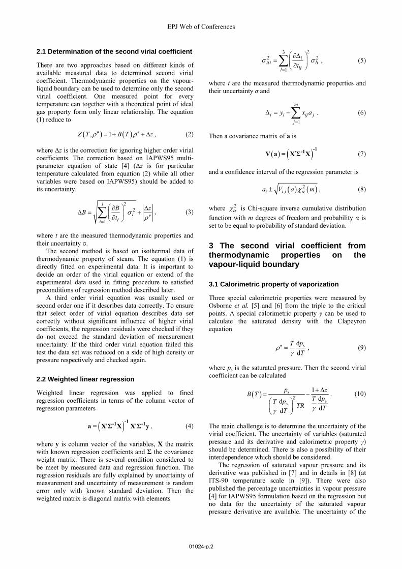
Fig. 1. Components of second virial coefficient uncertainty for the calorimetric measurement.

The influence of the uncertainties on the uncertainty of the second virial coefficient can be seen from figure 1. The results are surprisingly similar. The uncertainties of saturated pressure and its derivative should be somehow correlated on the other side the uncertainty of special calorimetric property γ is probably uncorrelated on the pressure measurement. Despite possible correlation all three uncertainties were used to determine the uncertainty of second virial coefficient.

The correction for neglecting higher order virial coefficients has a dominant role for higher temperatures. A local minimum which can be seen in figure 1 is caused by change between the positive and the negative effect it has on the second virial coefficient.

The selected results can be seen from table 1.

Table 1. Selected results of the second virial coefficient and its uncertainty from calorimetric measurement.

u (J/kg) T (K) B (cm3/mol) ΔB (cm3/mol)

2417375 303.134 -1203 181

2431424 313.13 -969 92

2445503 323.127 -834 68

2459613 333.124 -722 42

2473760 343.124 -630 30

2487942 353.123 -557 25

2502164 363.123 -496 21

2516427 373.124 -453 24

2516427 373.124 -447 25

2588422 423.134 -287 20

2661692 473.153 -201 16

2736361 523.171 -148 10

2766642 543.178 -133 7

2797161 563.182 -120 4

2812513 573.184 -114 2

2827926 583.185 -108 0.2

2843402 593.186 -103 2

2858938 603.186 -99 5

2874540 613.187 -94 8

3.2 Speed of sound

The speed of sound was measured in saturated and under saturated steam by Novikov and Avdonin [10]. The measurement for the saturated vapor would be a valuable source because it was carried out in low temperatures from 273 K to 583 K, the total error of speed of sound measurement was within 1% limit. Therefore this set of measurement was selected to analyze its suitability to determine the second virial coefficient.

The relation between the speed of sound and the second virial coefficient can be described according to [11] by the flowing equation

2 2 20 1 2w A A p A p w , (11)

where

0 0A k RT , (12)

201 0 0

0

12 2 1 tt

tB k

A k B B kk

, (13)

22

BaA

RT , (14)

Δw is the correction for ignoring higher order virial coefficients described in appendix A.2 and

0

0 0

p

p

ck

c R

, (15)

300 350 400 450 500 550 60010

−8

10−6

10−4

10−2

100

102

T / (K)

Δ B

i / (m

3 /kg)

p

s

dps / dT

γΔz

01024-p.3

EPJ Web of Conferences

2 32 2 22 0 0 0 0

20 0

1 1 2 1 1

1 2 4 2

B t tt

t tt t tt

a k B k k B k B

k BB BB k B B

,

(16)

tB

B TT

, (17)

22

2ttB

B TT

. (18)

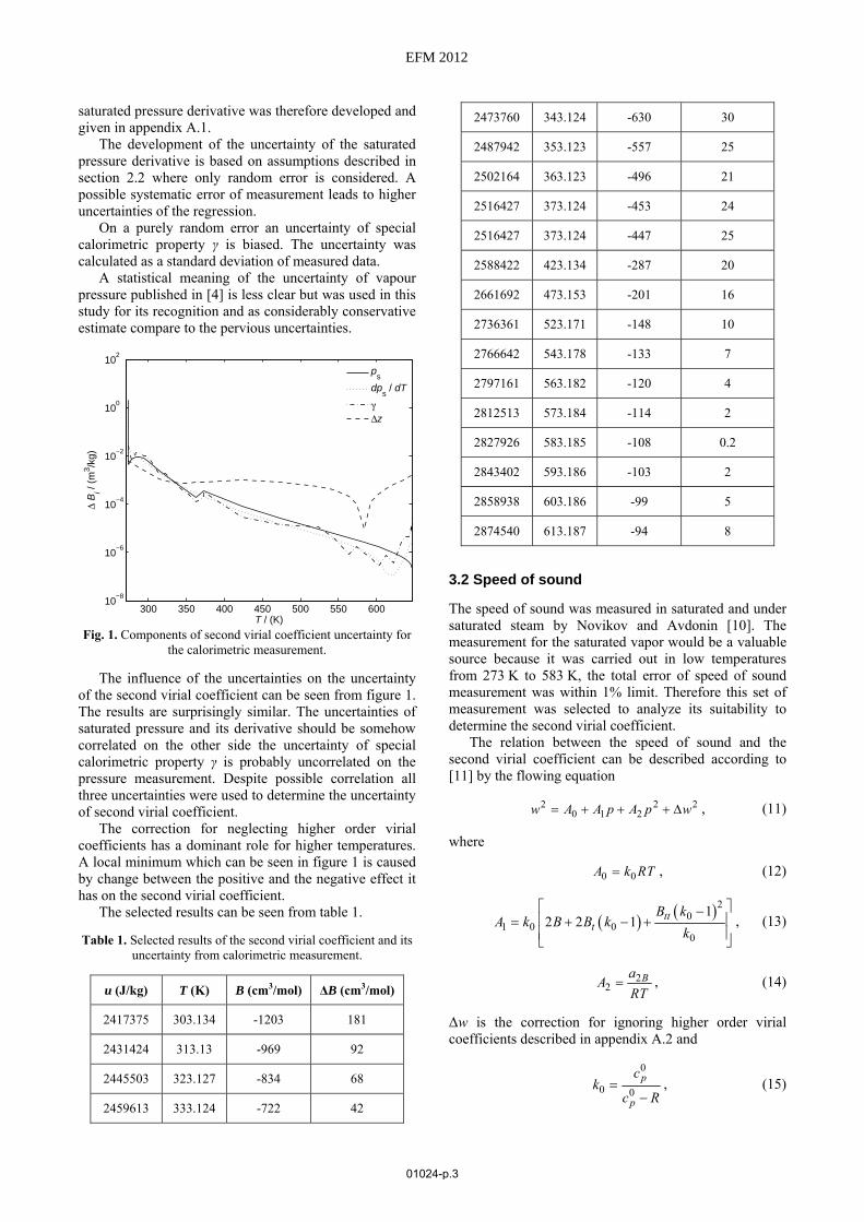
The valuable second virial coefficient can be determined only if the real thermodynamic property differs from the ideal significantly compared to its uncertainty of measurement. On the other hand the correction for neglecting higher order virial coefficients should not increase the overall uncertainty significantly. Figure 2 compares the measurement and its uncertainty with the ideal gas speed of sound, speed of sound calculated from IAPWS 95 and one calculated from equation (11) where the correction is set to be zero and the second virial coefficient is calculated from IAPWS 95.

As can be seen from the figure the measured data are in a very good agreement with the IAPWS 95 formulation. But uncertainty of measurement is too high compared to the difference between the real and the ideal property for much of the measurements at least up to 500 K. The temperature of 500 K is also a region where the correction for neglecting higher orders virial coefficients starts to be the dominant source of uncertainty.

Based on the preliminary analyses the speed of sound measurement, we found that it cannot be used for determining accurate second virial coefficient because of the too high uncertainty of the measurement.

Fig. 2. Speed of sound measured data with context of mathematical models.

4 The second virial coefficient from isothermal data

4.1 PVT data

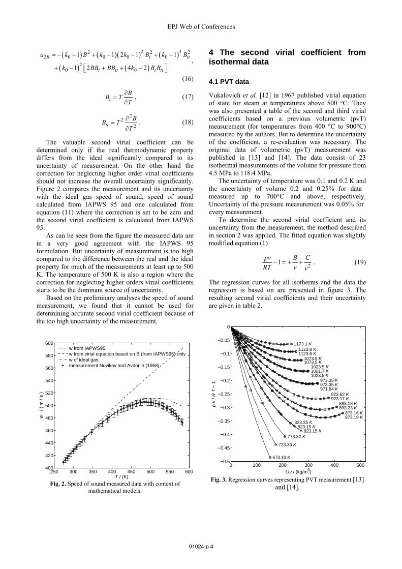
Vukalovich et al. [12] in 1967 published virial equation of state for steam at temperatures above 500 °C. They was also presented a table of the second and third virial coefficients based on a previous volumetric (pvT) measurement (for temperatures from 400 °C to 900°C) measured by the authors. But to determine the uncertainty of the coefficient, a re-evaluation was necessary. The original data of volumetric (pvT) measurement was published in [13] and [14]. The data consist of 23 isothermal measurements of the volume for pressure from 4.5 MPa to 118.4 MPa.

The uncertainty of temperature was 0.1 and 0.2 K and the uncertainty of volume 0.2 and 0.25% for data measured up to 700°C and above, respectively. Uncertainty of the pressure measurement was 0.05% for every measurement.

To determine the second virial coefficient and its uncertainty from the measurement, the method described in section 2 was applied. The fitted equation was slightly modified equation (1)

21

pv B C

RT v v . (19)

The regression curves for all isotherms and the data the regression is based on are presented in figure 3. The resulting second virial coefficients and their uncertainty are given in table 2.

Fig. 3. Regression curves representing PVT measurement [13] and [14].

250 300 350 400 450 500 550 600400

420

440

460

480

500

520

540

560

580

600

T / (K)

w

/ ( m

/ s

)

w from IAPWS95w from virial equation based on B (from IAPWS95) onlyw of ideal gasmeasurement Novikov and Avdonin (1968)

0 100 200 300 400 500−0.5

−0.45

−0.4

−0.35

−0.3

−0.25

−0.2

−0.15

−0.1

−0.05

0

1/v / (kg/m3)

p v

/ R

T −

1

673.10 K

723.36 K

773.32 K823.15 K

823.15 K823.35 K

873.16 K873.19 K

893.18 K893.23 K

923.17 K923.62 K

973.35 K971.84 K

973.35 K1023.5 K1021.7 K1023.5 K

1073.5 K1073.5 K

1123.6 K1123.8 K

1173.1 K

01024-p.4

EFM 2012

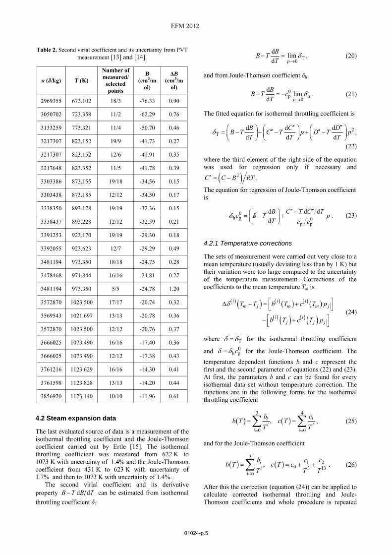
Table 2. Second virial coefficient and its uncertainty from PVT measurement [13] and [14].

u (J/kg) T (K)

Number of measured/

selected points

B (cm3/m

ol)

ΔB (cm3/m

ol)

2969355 673.102 18/3 -76.33 0.90

3050702 723.358 11/2 -62.29 0.76

3133259 773.321 11/4 -50.70 0.46

3217307 823.152 19/9 -41.73 0.27

3217307 823.152 12/6 -41.91 0.35

3217648 823.352 11/5 -41.78 0.39

3303386 873.155 19/18 -34.56 0.15

3303438 873.185 12/12 -34.50 0.17

3338350 893.178 19/19 -32.36 0.15

3338437 893.228 12/12 -32.39 0.21

3391253 923.170 19/19 -29.30 0.18

3392055 923.623 12/7 -29.29 0.49

3481194 973.350 18/18 -24.75 0.28

3478468 971.844 16/16 -24.81 0.27

3481194 973.350 5/5 -24.78 1.20

3572870 1023.500 17/17 -20.74 0.32

3569543 1021.697 13/13 -20.78 0.36

3572870 1023.500 12/12 -20.76 0.37

3666025 1073.490 16/16 -17.40 0.36

3666025 1073.490 12/12 -17.38 0.43

3761216 1123.629 16/16 -14.30 0.41

3761598 1123.828 13/13 -14.20 0.44

3856920 1173.140 10/10 -11.96 0.61

4.2 Steam expansion data

The last evaluated source of data is a measurement of the isothermal throttling coefficient and the Joule-Thomson coefficient carried out by Ertle [15]. The isothermal throttling coefficient was measured from 622 K to 1073 K with uncertainty of 1.4% and the Joule-Thomson coefficient from 431 K to 623 K with uncertainty of 1.7% and then to 1073 K with uncertainty of 1.4%.

The second virial coefficient and its derivative property d dB T B T can be estimated from isothermal

throttling coefficient δT

T0

dlim

d p

BB T

T

, (20)

and from Joule-Thomson coefficient δh

0p h

0

dlim

d p

BB T c

T

. (21)

The fitted equation for isothermal throttling coefficient is

2T

d d d

d d d

B C DB T C T p D T p

T T T

,

(22)

where the third element of the right side of the equation was used for regression only if necessary and

2C C B RT .

The equation for regression of Joule-Thomson coefficient is

0h p 0

p p

d d d

d

B C T C Tc B T p

T c c

. (23)

4.2.1 Temperature corrections

The sets of measurement were carried out very close to a mean temperature (usually deviating less than by 1 K) but their variation were too large compared to the uncertainty of the temperature measurement. Corrections of the coefficients to the mean temperature Tm is

i i im j m m j

i ij j j

T T b T c T p

b T c T p

(24)

where T for the isothermal throttling coefficient

and 0h pc for the Joule-Thomson coefficient. The

temperature dependent functions b and c represent the first and the second parameter of equations (22) and (23). At first, the parameters b and c can be found for every isothermal data set without temperature correction. The functions are in the following forms for the isothermal throttling coefficient

3 4

0 0

,i ii i

i i

b cb T c T

T T

, (25)

and for the Joule-Thomson coefficient

3

1 20 3 13

0

,ii

i

b c cb T c T c

T T T

. (26)

After this the correction (equation (24)) can be applied to calculate corrected isothermal throttling and Joule-Thomson coefficients and whole procedure is repeated

01024-p.5

EPJ Web of Conferences

until the parameters b and c do not change more than by 0.001 %.

4.2.2 Second virial coefficient

The regression parameter 1 d da B T B T can be

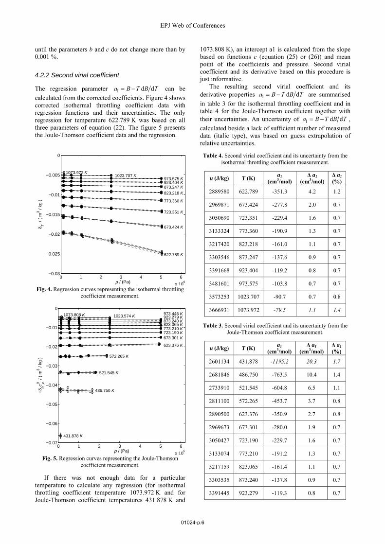
calculated from the corrected coefficients. Figure 4 shows corrected isothermal throttling coefficient data with regression functions and their uncertainties. The only regression for temperature 622.789 K was based on all three parameters of equation (22). The figure 5 presents the Joule-Thomson coefficient data and the regression.

Fig. 4. Regression curves representing the isothermal throttling coefficient measurement.

Fig. 5. Regression curves representing the Joule-Thomson coefficient measurement.

If there was not enough data for a particular temperature to calculate any regression (for isothermal throttling coefficient temperature 1073.972 K and for Joule-Thomson coefficient temperatures 431.878 K and

1073.808 K), an intercept a1 is calculated from the slope based on functions c (equation (25) or (26)) and mean point of the coefficients and pressure. Second virial coefficient and its derivative based on this procedure is just informative.

The resulting second virial coefficient and its derivative properties 1 d da B T B T are summarised

in table 3 for the isothermal throttling coefficient and in table 4 for the Joule-Thomson coefficient together with their uncertainties. An uncertainty of 1 d da B T B T ,

calculated beside a lack of sufficient number of measured data (italic type), was based on guess extrapolation of relative uncertainties.

Table 4. Second virial coefficient and its uncertainty from the isothermal throttling coefficient measurement.

u (J/kg) T (K) a1

(cm3/mol) Δ a1

(cm3/mol) Δ a1 (%)

2889580 622.789 -351.3 4.2 1.2

2969871 673.424 -277.8 2.0 0.7

3050690 723.351 -229.4 1.6 0.7

3133324 773.360 -190.9 1.3 0.7

3217420 823.218 -161.0 1.1 0.7

3303546 873.247 -137.6 0.9 0.7

3391668 923.404 -119.2 0.8 0.7

3481601 973.575 -103.8 0.7 0.7

3573253 1023.707 -90.7 0.7 0.8

3666931 1073.972 -79.5 1.1 1.4

Table 3. Second virial coefficient and its uncertainty from the Joule-Thomson coefficient measurement.

u (J/kg) T (K) a1

(cm3/mol) Δ a1

(cm3/mol) Δ a1 (%)

2601134 431.878 -1195.2 20.3 1.7

2681846 486.750 -763.5 10.4 1.4

2733910 521.545 -604.8 6.5 1.1

2811100 572.265 -453.7 3.7 0.8

2890500 623.376 -350.9 2.7 0.8

2969673 673.301 -280.0 1.9 0.7

3050427 723.190 -229.7 1.6 0.7

3133074 773.210 -191.2 1.3 0.7

3217159 823.065 -161.4 1.1 0.7

3303535 873.240 -137.8 0.9 0.7

3391445 923.279 -119.3 0.8 0.7

0 1 2 3 4 5 6

x 106

−0.03

−0.025

−0.02

−0.015

−0.01

−0.005

0

p / (Pa)

δT /

( m

3 / kg

)

622.789 K

673.424 K

723.351 K

773.360 K

823.218 K873.247 K923.404 K973.575 K

1023.707 K1073.972 K

0 1 2 3 4 5 6

x 106

−0.07

−0.06

−0.05

−0.04

−0.03

−0.02

−0.01

0

p / (Pa)

−δ hc p0 /

( m

3 / kg

)

431.878 K

486.750 K

521.545 K

572.265 K

623.376 K

673.301 K723.190 K773.210 K823.065 K873.240 K923.279 K973.446 K1023.574 K1073.808 K

01024-p.6

EFM 2012

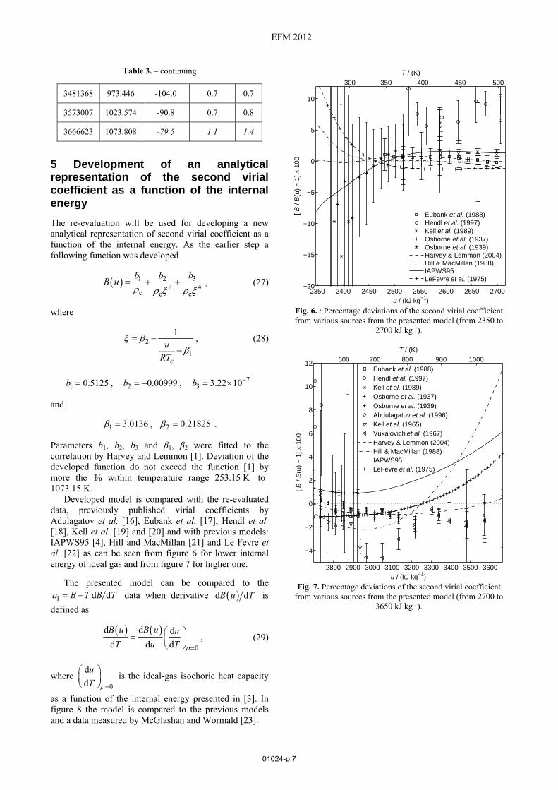
Table 3. – continuing

3481368 973.446 -104.0 0.7 0.7

3573007 1023.574 -90.8 0.7 0.8

3666623 1073.808 -79.5 1.1 1.4

5 Development of an analytical representation of the second virial coefficient as a function of the internal energy

The re-evaluation will be used for developing a new analytical representation of second virial coefficient as a function of the internal energy. As the earlier step a following function was developed

31 22 4

c c c

bb bB u

, (27)

where

2

1

1

c

u

RT

, (28)

71 2 30.5125 , 0.00999 , 3.22 10b b b

and

1 23.0136 , 0.21825 .

Parameters b1, b2, b3 and β1, β2 were fitted to the correlation by Harvey and Lemmon [1]. Deviation of the developed function do not exceed the function [1] by more the 1% within temperature range 253.15 K to 1073.15 K.

Developed model is compared with the re-evaluated data, previously published virial coefficients by Adulagatov et al. [16], Eubank et al. [17], Hendl et al. [18], Kell et al. [19] and [20] and with previous models: IAPWS95 [4], Hill and MacMillan [21] and Le Fevre et al. [22] as can be seen from figure 6 for lower internal energy of ideal gas and from figure 7 for higher one.

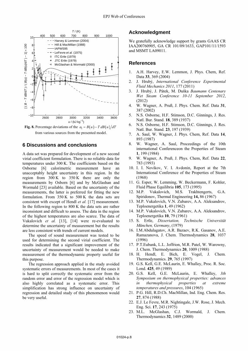
The presented model can be compared to the

1 d da B T B T data when derivative d dB u T is

defined as

0

d d d

d d d

B u B u u

T u T

, (29)

where 0

d

d

u

T

is the ideal-gas isochoric heat capacity

as a function of the internal energy presented in [3]. In figure 8 the model is compared to the previous models and a data measured by McGlashan and Wormald [23].

Fig. 6. : Percentage deviations of the second virial coefficient from various sources from the presented model (from 2350 to

2700 kJ kg-1).

Fig. 7. Percentage deviations of the second virial coefficient from various sources from the presented model (from 2700 to

3650 kJ kg-1).

2350 2400 2450 2500 2550 2600 2650 2700−20

−15

−10

−5

0

5

10

u / (kJ kg−1)[ B

/ B

(u)

− 1

] × 1

00

Eubank et al. (1988)Hendl et al. (1997)Kell et al. (1989)Osborne et al. (1937)Osborne et al. (1939)Harvey & Lemmon (2004)Hill & MacMillan (1988)IAPWS95LeFevre et al. (1975)

300 350 400 450 500

T / (K)

2800 2900 3000 3100 3200 3300 3400 3500 3600

−4

−2

0

2

4

6

8

10

12

u / (kJ kg−1)

[ B /

B(u

) −

1] ×

100

Eubank et al. (1988)Hendl et al. (1997)Kell et al. (1989)Osborne et al. (1937)Osborne et al. (1939)Abdulagatov et al. (1996)Kell et al. (1965)Vukalovich et al. (1967)Harvey & Lemmon (2004)Hill & MacMillan (1988)IAPWS95LeFevre et al. (1975)

600 700 800 900 1000

T / (K)

01024-p.7

EPJ Web of Conferences

Fig. 8. Percentage deviations of the 1a B u T dB u dT from various sources from the presented model.

6 Discussions and conclusions

A data set was prepared for development of a new second virial coefficient formulation. There is no reliable data for temperatures under 300 K. The coefficients based on the Osborne [6] calorimetric measurement have an unacceptably height uncertainty in this region. In the region from 300 K to 350 K there are only the measurements by Osborn [6] and by McGlashan and Wormald [23] available. Based on the uncertainty of the measurements, the latter is preferred for fitting the new formulation. From 350 K to 500 K the data sets are consistent with except of Hendl et al. [17] measurement. In the following region to 800 K the data sets are rather inconsistent and difficult to assess. The data in the region of the highest temperatures are also scarce. The data of Vukalovich et al. [13], [14] were re-evaluated to determine the uncertainty of measurement but the results are less consistent with trends of current models.

The speed of sound measurement was tested to be used for determining the second virial coefficient. The results indicated that a significant improvement of the uncertainty of measurement would be needed to make measurement of the thermodynamic property useful for this purpose.

The regression approach applied in the study avoided systematic errors of measurements. In most of the cases it is hard to split correctly the systematic error from the random error and error of the regression model which is also highly correlated as a systematic error. This simplification has strong influence on uncertainty of regression and detailed study of this phenomenon would be very useful.

Acknowledgment

We gratefully acknowledge support by grants GAAS CR IAA200760905, GA CR 101/09/1633, GAP101/11/1593 and MSMT LA09011.

References

1. A.H. Harvey, E.W. Lemmon, J. Phys. Chem, Ref. Data 33, 369 (2004)

2. J. Hrubý, International Conference Experimental Fluid Mechanics 2011, 177 (2011)

3. J. Hrubý, J. Pátek, M. Duška Baumann Centenary Wet Steam Conference 10-11 September 2012, (2012)

4. W. Wagner, A. Pruß, J. Phys. Chem. Ref. Data 31, 387 (2002)

5. N.S. Osborne, H.F. Stimson, D.C. Ginnings, J. Res. Natl. Bur. Stand. 18, 389 (1937)

6. N.S. Osborne, H.F. Stimson, D.C. Ginnings, J. Res. Natl. Bur. Stand. 23, 197 (1939)

7. A. Saul, W. Wagner, J. Phys. Chem, Ref. Data 14, 893 (1987)

8. W. Wagner, A. Saul, Proceedings of the 10th international Conferenceon the Properties of Steam 1, 199 (1984)

9. W. Wagner, A. Pruß, J. Phys. Chem, Ref. Data 22, 783 (1993)

10. I. I. Novikov, V. I. Avdonin, Report at the 7th International Conference of the Properties of Steam (1968)

11. G. Esper, W. Lemming, W. Beckermann, F. Kohler, Fluid Phase Equilibria 105, 173 (1995)

12. M.P. Vukalovich, M.S. Trakhtengerts, G.A. Spiridonov, Thermal Engineering 14, 86 (1967)

13. M.P. Vukalovich, V.N. Zubarev, A.A. Aleksandrov, Teploenergetika 1, 49 (1962)

14. M.P. Vukalovich, V.N. Zubarev, A.A. Aleksandrov, Teploenergetika 10, 79 (1961)

15. S. Ertle, Dissertation, Technische Universität München, Germany, (1979)

16. I.M.Abdulagatov, A.R. Bazaev, R.K. Gasanov, A.E. Ramazanova, J. Chem. Thermodynamics 28, 1037 (1996)

17. P.T.Eubank, L.L. Joffrion, M.R. Patel, W. Warowny, J. Chem. Thermodynamics 20, 1009 (1988)

18. H. Hendl, E. Bich, E. Vogel, J. Chem. Thermodynamics. 29, 765 (1997)

19. G.S. Kell, G.E. McLaurin, E. Whalley, Proc. R. Soc. Lond. 425, 49 (1989)

20. G.S. Kell, G.E. McLaurin, E. Whalley, 3th Symposium on thermophysical properties: advances in thermophysical properties at extreme temperatures and pressures, 104 (1965)

21. P.G. Hill, R.D.Ch. MacMillan, Ind. Eng. Chem. Res. 27, 874 (1988)

22. E.J. Le Fevre, M.R. Nightingale, J.W. Rose, J. Mech. Eng. Sci. 17, 243 (1975)

23. M.L. McGlashan, C.J. Wormald, J. Chem. Thermodynamics 32, 1489 (2000)

2600 2800 3000 3200 3400 3600−10

−8

−6

−4

−2

0

2

4

6

8

10

u / (kJ kg−1)

[ ( B

− T

dB

/dT

) /

( B

(u)

− T

dB

(u)/

dT )

− 1

] × 1

00

Harvey & Lemmon (2004)Hill & MacMillan (1988)IAPWS95LeFevre et al. (1975)ITC Ertle (1979)JTC Ertle (1979)McGlashan & Wormald (2000)

400 500 600 700 800 900 1000

T / (K)

01024-p.8

EFM 2012

Appendices

A.1 Uncertainty of the derivation of the saturation pressure

To develop uncertainty of the regression of saturation pressure derivative, a couple of assumptions were applied. Some of them were mentioned above in the description of regression procedure

1.5 3 3.5 4 7.5s1 2 3 4 5 6

c

lnp Tc

a a a a a ap T

(A1)

The six coefficients of saturation vapour pressure regression function were originally selected from twenty-one “bank of terms” using the evolutionary optimization method [12]. But after the setting the coefficients regression the weighted linear regression can be used to refitting the regression and to determined covariance matrix of regression coefficients (equations (4) - (7)).

According to [11] the original regression is based on measurements of [5], [6], [8], [1], [2] and [3] and uncertainty of measurement to determine the weight was published also in [11].

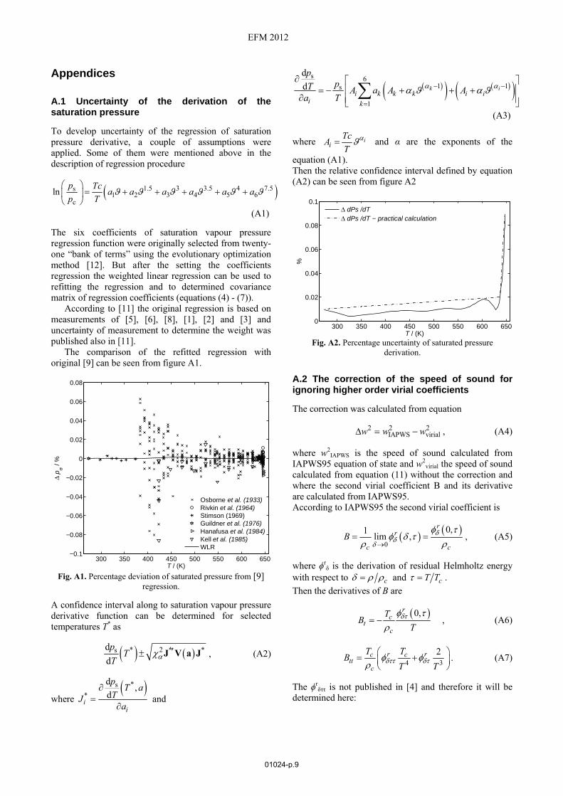
The comparison of the refitted regression with original [9] can be seen from figure A1.

Fig. A1. Percentage deviation of saturated pressure from [9] regression.

A confidence interval along to saturation vapour pressure derivative function can be determined for selected temperatures T* as

* 2sd

d

pT

T * *J V a J , (A2)

where *s

*

d,

di

i

pT a

TJa

and

s 6

1 1s

1

d

d k ii k k k i i

i k

ppT A a A A

a T

(A3)

where ii

TcA

T and α are the exponents of the

equation (A1). Then the relative confidence interval defined by equation (A2) can be seen from figure A2

Fig. A2. Percentage uncertainty of saturated pressure derivation.

A.2 The correction of the speed of sound for ignoring higher order virial coefficients

The correction was calculated from equation

2 2 2IAPWS virialw w w , (A4)

where w2IAPWS is the speed of sound calculated from

IAPWS95 equation of state and w2virial the speed of sound

calculated from equation (11) without the correction and where the second virial coefficient B and its derivative are calculated from IAPWS95. According to IAPWS95 the second virial coefficient is

0

0,1lim ,

rr

c c

B

, (A5)

where ϕrδ is the derivation of residual Helmholtz energy

with respect to c and cT T .

Then the derivatives of B are

0,rc

tc

TB

T

, (A6)

4 3

2r rc ctt

c

T TB

T T

. (A7)

The ϕrδττ is not published in [4] and therefore it will be

determined here:

300 350 400 450 500 550 600 650−0.1

−0.08

−0.06

−0.04

−0.02

0

0.02

0.04

0.06

0.08

T / (K)

Δ p σ /

%

Osborne et al. (1933)Rivkin et al. (1964)Stimson (1969)Guildner et al. (1976)Hanafusa et al. (1984)Kell et al. (1985)WLR

300 350 400 450 500 550 600 6500

0.02

0.04

0.06

0.08

0.1

T / (K)

%

Δ dPs /dT Δ dPs /dT − practical calculation

01024-p.9

EPJ Web of Conferences

1

1

2 2

1

71 2

1

511 2

8

541

52

22

2 3

2 2

1

1

2

21 2 1 2

i

cii i

i i i ii

i

i

d tri i i i

i

d cti i i i i

i

di i i i

i

i itti i i i i

bi

n d t t

n t t d c e

n e d

tt t

n

56

55

2 2

2

2 3 2 3

2 2 2

2 2

2

i

i i i

i

b

b b b

(A8)

where

3

22

2 1 1 2 2 1i i iD D C

(A9)

3 1 2 1222

2

2 1 4 1

21 2

i ii

bb i

i ii

i

Ab b

b

(A10)

01024-p.10