Embed Size (px)
Citation preview
3
Delay Modelsin Data Networks
3.1 INTRODUCTION
One of the most important perfonnance measures of a data network is the average delayrequired to deliver a packet from origin to destination. Furthennore, delay considerationsstrongly influence the choice and perfonnance of network algorithms, such as routing andflow control. For these reasons, it is important to understand the nature and mechanismof delay, and the manner in which it depends on the characteristics of the network.
Queueing theory is the primary methodological framework for analyzing networkdelay. Its use often requires simplifying assumptions since, unfortunately, more real-istic assumptions make meaningful analysis extremely difficult. For this reason, it issometimes impossible to obtain accurate quantitative delay predictions on the basis ofqueueing models. Nevertheless, these models often provide a basis for adequate delayapproximations, as well as valuable qualitative results and worthwhile insights.
In what follows, we will mostly focus on packet delay within the communicationsubnet (i.e., the network layer). This delay is the sum of delays on each subnet linktraversed by the packet. Each link delay in tum consists of four components.
149
150 Delay Models in Data Networks Chap. 3
1. The processinR delay between the time the packet is correctly received at the headnode of the link and the time the packet is assigned to an outgoing link queuefor transmission. (In some systems, we must add to this delay some additionalprocessing time at the DLC and physical layers.)
2. The queueinR delay between the time the packet is assigned to a queue for trans-mission and the time it starts being transmitted. During this time, the packet waitswhile other packets in the transmission queue are transmitted.
3. The transmission delay between the times that the first and last bits of the packetare transmitted.
4. The propagation delay between the time the last bit is transmitted at the headnode of the link and the time the last bit is received at the tail node. This isproportional to the physical distance between transmitter and receiver; it can berelatively substantial, particularly for a satellite link or a very high speed link.
This accounting neglects the possibility that a packet may require retransmissionon a link due to transmission errors or various other causes. For most links in practice,other than multiaccess links to be considered in Chapter 4, retransmissions are rare andwill be neglected. The propagation delay depends on the physical characteristics of thelink and is independent of the traffic carried by the link. The processing delay is alsoindependent of the amount of traffic handled by the corresponding node if computationpower is not a limiting resource. This will be assumed in our discussion. Otherwise,a separate processing queue must be introduced prior to the transmission queues. Mostof our subsequent analysis focuses on the queueing and transmission delays. We firstconsider a single transmission line and analyze some classical queueing models. We thentake up the network case and discuss the type of approximations involved in derivinganalytical delay models.
While our primary emphasis is on packet-switched network models, some of themodels developed are useful in a circuit-switched network context. Indeed, queueingtheory was developed extensively in response to the need for perfonnance models intelephony.
3.1.1 Multiplexing of Traffic on a Communication Link
The communication link considered is viewed as a bit pipe over which a given numberof bits per second can be transmitted. This number is called the transmission capacity ofthe link. It depends on both the physical channel and the interface (e.g., modems), and issimply the rate at which the interface accepts bits. The link capacity may serve severaltraffic streams (e.g., virtual circuits or groups of virtual circuits) multiplexed on the link.The manner of allocation of capacity among these traffic streams has a profound effecton packet delay.
In the most common scheme, statistical multiplexinR, the packets of all trafficstreams are merged into a single queue and transmitted on a first-come first-serve basis. Avariation of this scheme, which has roughly the same average delay per packet, maintains
Sec. 3.1 Introduction 151
a separate queue for each traffic stream and serves the queues in sequence one packetat a time. However, if the queue of a traffic stream is empty, the next traffic stream isserved and no communication resource is wasted. Since the entire transmission capacityC (bits/sec) is allocated to a single packet at a time, it takes L / C seconds to transmit apacket that is L bits long.
In time-division (TOM) and frequency-division multiplexing (FOM) with m trafficstreams, the link capacity is essentially subdivided into m portions-one per trafficstream. In FOM, the channel bandwidth W is subdivided into m channels each withbandwidth W /m (actually slightly less because of the need for guard bands betweenchannels). The transmission capacity of each channel is roughly C /m, where C isthe capacity that would be obtained if the entire bandwidth were allocated to a singlechannel. The transmission time of a packet that is L bits long is Lm/C, or m timeslarger than in the corresponding statistical multiplexing scheme. In TOM, allocation isdone by dividing the time axis into slots of fixed length (e.g., one bit or one byte long,or perhaps one packet long for fixed length packets). Again, conceptually, we may viewthe communication link as consisting of m separate links with capacity C /m. In the casewhere the slots are short relative to packet length, we may again regard the transmissiontime of a packet L bits long as Lm/C. In the case where the slots are of packet length,the transmission time of an L bit packet is L/C, but there is a wait of (m - 1) packettransmission times between packets of the same stream.
One of the themes that will emerge from our queueing analysis is that statisticalmultiplexing has smaller average delay per packet than either TOM or FOM. This isparticularly true when the traffic streams multiplexed have a relatively low duty cycle.The main reason for the poor delay performance of TOM and FOM is that communicationresources are wasted when allocated to a traffic stream with a momentarily empty queue,while other traffic streams have packets waiting in their queue. For a traffic analogy,consider an m-lane highway and two cases. In one case, cars are not allowed to crossover to other lanes (this corresponds to TOM or FOM), while in the other case, cars canchange lanes (this corresponds roughly to statistical multiplexing). Restricting crossoverincreases travel time for the same reason that the delay characteristics of TOM or FOMare poor: namely, some system resources (highway lanes or communication channels)may not be utilized, while others are momentarily stressed.
Under certain circumstances, TOM or FOM may have an advantage. Suppose thateach traffic stream has a "regular" character (i.e., all packets arrive sufficiently apartso that no packet has to wait while the preceding packet is transmitted.) If these trafficstreams are merged into a single queue, it can be shown that the average delay per packetwill decrease, but the variance of waiting time in queue will generally become positive(for an illustration, see Prob. 3.7). Therefore, if maintaining a small variability of delayis more important than decreasing delay, it may be preferable to use TOM or FOM.Another advantage of TOM and FOM is that there is no need to include identification ofthe traffic stream on each packet, thereby saving some overhead and simplifying packetprocessing at the nodes. Note also that when overhead is negligible, one can afford tomake packets very small, thereby reducing delay through pipelining (cf. Fig. 2.37).
152 Delay Models in Data Networks Chap. 3
3.2 QUEUEING MODELS-LITTLE'S THEOREM
We consider queueing systems where customers arrive at random times to obtain service.In the context of a data network, customers represent packets assigned to a communicationlink for transmission. Service time corresponds to the packet transmission time and isequal to LIC, where L is the packet length in bits and C is the link transmission capacityin bits/sec. In this chapter it is convenient to ignore the layer 2 distinction betweenpackets and frames; thus packet lengths are taken to include frame headers and trailers.In a somewhat different context (which we will not emphasize very much), customersrepresent ongoing conversations (or virtual circuits) between points in a network andservice time corresponds to the duration of a conversation. In a related context, customersrepresent active calls in a telephone or circuit switched network and again service timecorresponds to the duration of the call.
We shall be typically interested in estimating quantities such as:
1. The average number of customers in the system (i.e., the "typical" number ofcustomers either waiting in queue or undergoing service)
2. The average delay per customer (i.e., the "typical" time a customer spends waitingin queue plus the service time).
These quantities will be estimated in terms of known information such as:
1. The customer arrival rate (i.e., the "typical" number of customers entering thesystem per unit time)
2. The customer service rate (i.e., the "typical" number of customers the system servesper unit time when it is constantly busy)
In many cases the customer arrival and service rates are not sufficient to determinethe delay characteristics of the system. For example, if customers tend to arrive ingroups, the average customer delay will tend to be larger than when their arrival timesare regularly spaced apart. Thus to predict average delay, we will typically need moredetailed (statistical) information about the customer interarrival and service times. Inthis section, however, we will largely ignore the availability of such information and seehow far we can go without it.
3.2.1 Little's Theorem
We proceed to clarify the meaning of the terms "average" and "typical" that we usedsomewhat liberally above in connection with the number of customers in the system, thecustomer delay, and so on. In doing so we will derive an important result known asLittle's Theorem.
Suppose that we observe a sample history of the system from time t = 0 tothe indefinite future and we record the values of various quantities of interest as time
Sec. 3.2 Queueing Models-Little's Theorem 153
(3.1)
progresses. In particular, let
N(t) = Number of customers in the system at time t
aCt) = Number of customers who arrived in the interval [0, t]
T; = Time spent in the system by the i th arriving customer
Our intuitive notion of the "typical" number of customers in the system observed up totime t is
Nt = t N(T) dT. t io
which we call the time average of N(T) up to time t. Naturally, Nt changes with thetime t, but in many systems of interest, Nt tends to a steady-state N as t increases, thatis,
N = lim Nt
In this case, we call N the steady-state time average (or simply time average) of N(T).It is also natural to view
At = a(t)t
as the time GI'erage arrival rate over the interval [0. tj. The steady-state arrival rate isdefined as
A= lim Att-x
(assuming that the limit exists). The time average of the customer delay up to time t issimilarly defined as
,\,0(1) TT - 6;=0 I
t - net)
that is, the average time spent in the system per customer up to time t. The steady-statetime average customer delay is defined as
T = lim T t
(assuming that the limit exists).It turns out that the quantities N, A, and T above are related by a simple formula
that makes it possible to determine one given the other. This result, known as Little'sTheorem, has the form
N=AT
Little's Theorem expresses the natural idea that crowded systems (large N) are associatedwith long customer delays (large T) and reversely. For example, on a rainy day, trafficon a rush hour moves slower than average (large T), while the streets are more crowded(large N). Similarly, a fast-food restaurant (small T) needs a smaller waiting room(small N) than a regular restaurant for the same customer arrival rate.

154 Delay Models in Data Networks
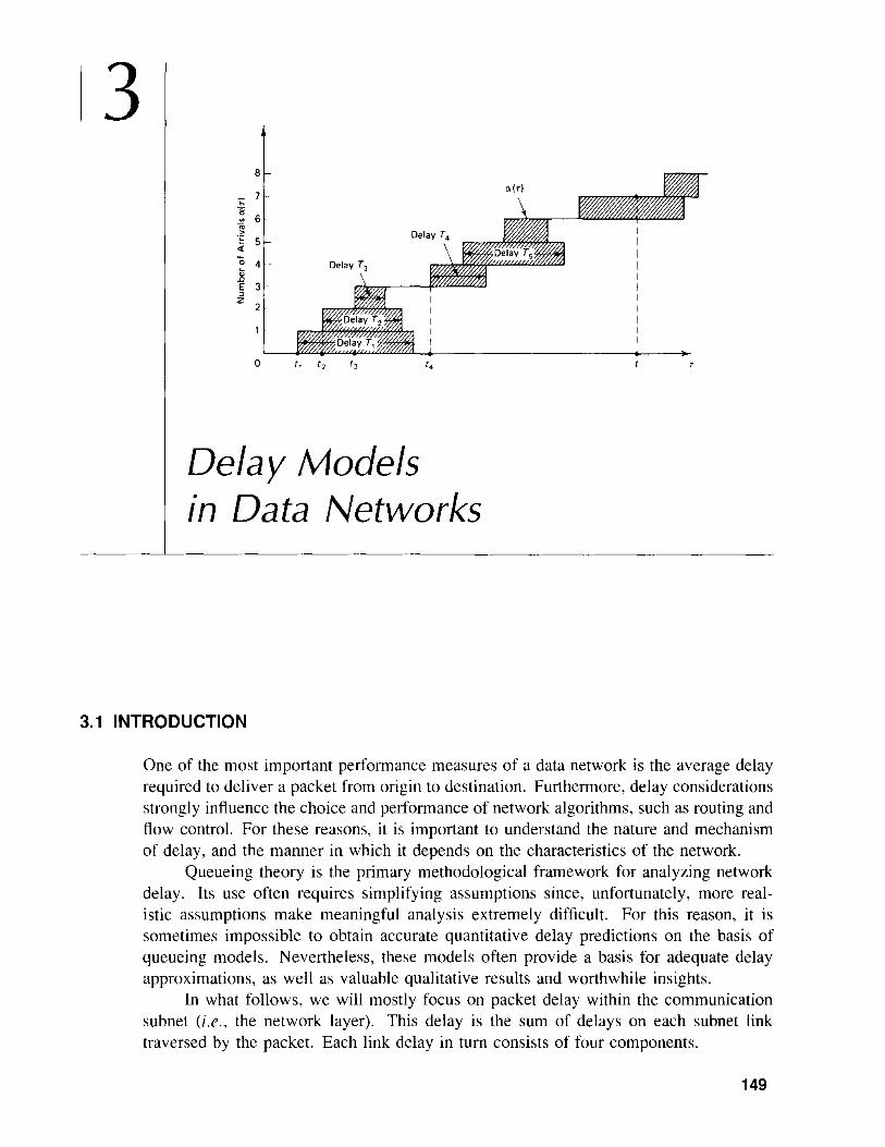
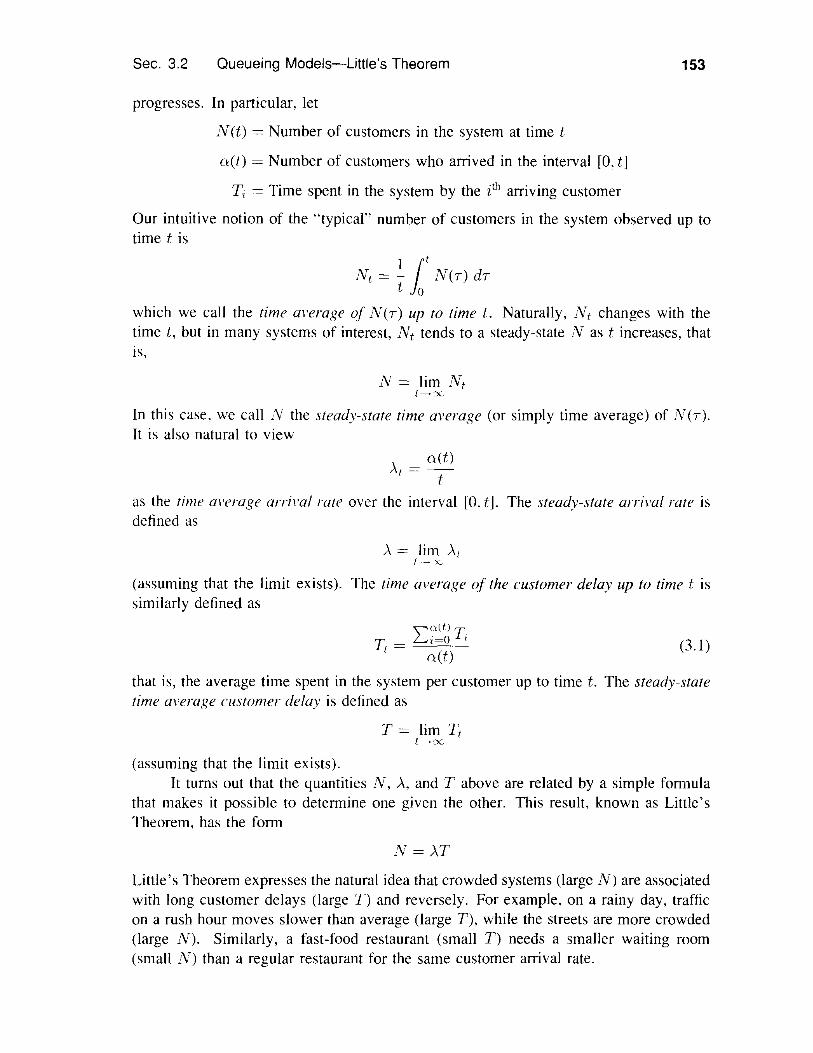
The theorem is really an accounting identity and its derivation is very simple. We will give a graphical proof under some simplifying assumptions. Suppose that the system is initially empty [N(O) = 0] and that customers depart from the system in the order they arrive. Then the number of arrivals aCt) and departures /3(t) up to time t form a staircase graph as shown in Fig. 3.1. The difference aCt) - /3(t) is the number in the system N(t) at time t. The shaded area between the graphs of aCT) and /3(T) can be expressed as
lot N(T)dT
and if t is any time for which the system is empty [N(t) = 0], the shaded area is also equal to
Dividing both expressions above with t, we obtain
1 it 1 a(t) aCt) I:,:,,(t) Ti - N(T) dT = - '\;"""' Ti = -'- .=\ tot 6 t aCt) ,
<""j
or equivalently,
Little's Theorem is obtained assuming that
Nt -+ N, At -+ A, Tt -+ T
and that the system becomes empty infinitely often at arbitrarily large times. With a mi- ' nor modification'in the preceding argument, the latter assumption becomes unnecessary. To see this, note that the shaded area in Fig. 3.1 lies between I:flt{ Ti and Ti , so we obtain
/3(t) Ti < N < A 1', t /3(t) - t - t t
Assuming that Nt -+ N, At -+ A, Tt -+ T, and that the departure rate /3(t)/t up to time t tends to the steady-state arrival rate A, we obtain Little's Theorem.
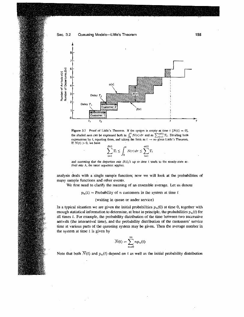
The simplifying assumptions used in the preceding graphical proof can be relaxed considerably, and one can construct an analytical proof that requires only that the limits A = limt-->oc a(t)/t, 8 limt-->oc /3(t)/t, and T limt-->oo Tt exist, and that A 8. In particular, it is not necessary that customers are served in the order they arrive, and the system is initially empty (see Problem 3.41). Figure 3.2 explains why the order customer service is not essential for the validity of Little's Theorem.
3.2.2 Probabilistic Form of Little's Theorem
Little's Theorem admits also a prdbabilistic interpretation provided that we can time averages with statistical or ensemble averages, as we now discuss. Our precedlmg
Sec. 3.2 Queueing Models-Little's Theorem
8
7
1l1l 3E E :::J :::J
Z Z 2
Figure 3.1 Proof of Little's Theorem. If the systllm is empt,y at time t [N(t) = 0], the shaded area can be expressed both as lot N(r) dr and as T;. Dividing both expressions by t, equating them, and taking the limit as t --+ ex:) gives Little's Theorem. If N(t) > 0, we have
and assuming that tbe departUre rate (J(t)/t up to time t tends to the steady-state ar-rival rate A, the same argument applies.
155
T
analysis deals with a· sii1gle sample function; now we will look at the probabilities of ma,ny sample functions and other events.
We first need to clarify the meaning of an ensemble average. Let us denote
Pn(t) = Probability of n customers in the system at time t
(waiting in queue or under service)
In a typical situation we are given the initial probabilities Pn(O) at time 0, together with enough statistical information to determine, at least in principle, the probabilities Pn(t) for all times t. For example, the probability distribution of the time between two successive arrivals (the interarrival time), and the probability distribution of the customers' service time at various parts of the queueing system may be given. Then the average number in the system at time t is g!ven by
00
N(t) = L npn(t) n=O
Note that both N(t) and Pn(t) depend on t as well as the initial probability distribution
156
8
-;: 7"B"
6'"n;>.;:
5..i.....0 4<;.DE 3"z 2
Delay Models in Data Networks
Figure 3.2 Infonnal justification of Little's Theorem without assuming first-in first-out customer service. The shaded area can be expressed both as J; N (T) dT and as
LiED(t) T, + L'EDlf)(t - til, where D(t) is the set of customers that have departedup to time t, D(t) is the set of customers that are still in the system at time t, and t, isthe time of arrival of the i 1h customer. Dividing both expressions by t, equating them,and taking the limit as t --> co gives Little's Theorem.
Chap. 3
{PoCO), PI (0), ...}. However, the queueing systems that we will consider typically reacha steady-state in the sense that for some P" (independent of the initial distribution), wehave
lim p"(t)=p,,. n=O.l. ...
The average number in the system at steady-state is given by
N= LnPnn=O
and we typically have
N = lim N(t)
Regarding average delay per customer, we are typically given enough statisticalinformation to determine in principle the probability distribution of delay of each indi-vidual customer (i.e., the first, second, etc.). From this, we can determine the averagedelay of each customer. The average delay of the kth customer, denoted Tko typicallyconverges as k ---7 X to a steady-state value
T = lim T k
To make the connection with time averages, we note that almost every system ofinterest to us is ergodic in the sense that the time average, N = lim/_x Nf, of a sample

Sec. 3.2 Queueing Models-Little's Theorem 157
function is, with probability I, equal to the steady-state average N = liml_x N(t), thatIS,
N = lim N I = lim N(t) = NI-x I-x
Similarly, for the systems of interest to us, the time average of customer delay T is alsoequal (with probability I) to the steady-state average delay T, that is,
kI", --T = lim - L T; = lim T k = T
k-x k k-x;=1
Under these circumstances, Little's formula, N = AT, holds with Nand T beingstochastic averages and with A given by
\ . Expected number of arrivals in the interval [0. t]/\ = hmI-x t
The equality of long term time and ensemble averages of various stochastic pro-cesses will often be accepted in this chapter on intuitive grounds. This equality canoften be shown by appealing to general results from the theory of Markov chains (seeAppendix A, at the end of this chapter, which states these results without proof). Inother cases, this equality, though highly plausible, requires a specialized mathematicalproof. Such a proof is typically straightforward for an expert in stochastic processes butrequires background that is beyond what is assumed in this book. In what follows wewill generally use the time average notation T and N in place of the ensemble averagenotation T and N, respectively, implicitly assuming the equality of the correspondingtime and ensemble averages.
3.2.3 Applications of Little's Theorem
The significance of Little's Theorem is due in large measure to its generality. It holds foralmost every queueing system that reaches a steady-state. The system need not consistof just a single queue. Indeed, with appropriate interpretation of the terms N, A, and T,the theorem holds for many complex arrival-departure systems. The following examplesillustrate its broad applicability.
Example 3.1
If )., is the arrival rate in a transmission line, NQ is the average number of packets waitingin queue (but not under transmission). and ric' is the average time spent by a packet waitingin queue (not including the transmission time), Little's Theorem gives
NQ=).,W
Furthermore. if X is the average transmission time, then Little's Theorem gives the averagenumber of packets under transmission as
p=).,X
Since at most one packet can be under transmission, p is also the line's utili:ation factor.(i.e .. the proportion of time that the line is busy transmitting a packet).
158 Delay Models in Data Networks Chap. 3
Example 3.2Consider a network of transmission lines where packets arrive at n different nodes withcorresponding rates )1] •...• An. If N is the average total number of packets inside thenetwork. then (regardless of the packet length distribution and method for routing packets)the average delay per packet is
Furthermore, Little's Theorem also yields Ni = AiTi, where Ni and Ti are the averagenumber in the system and average delay of packets arriving at nodei, respectively.
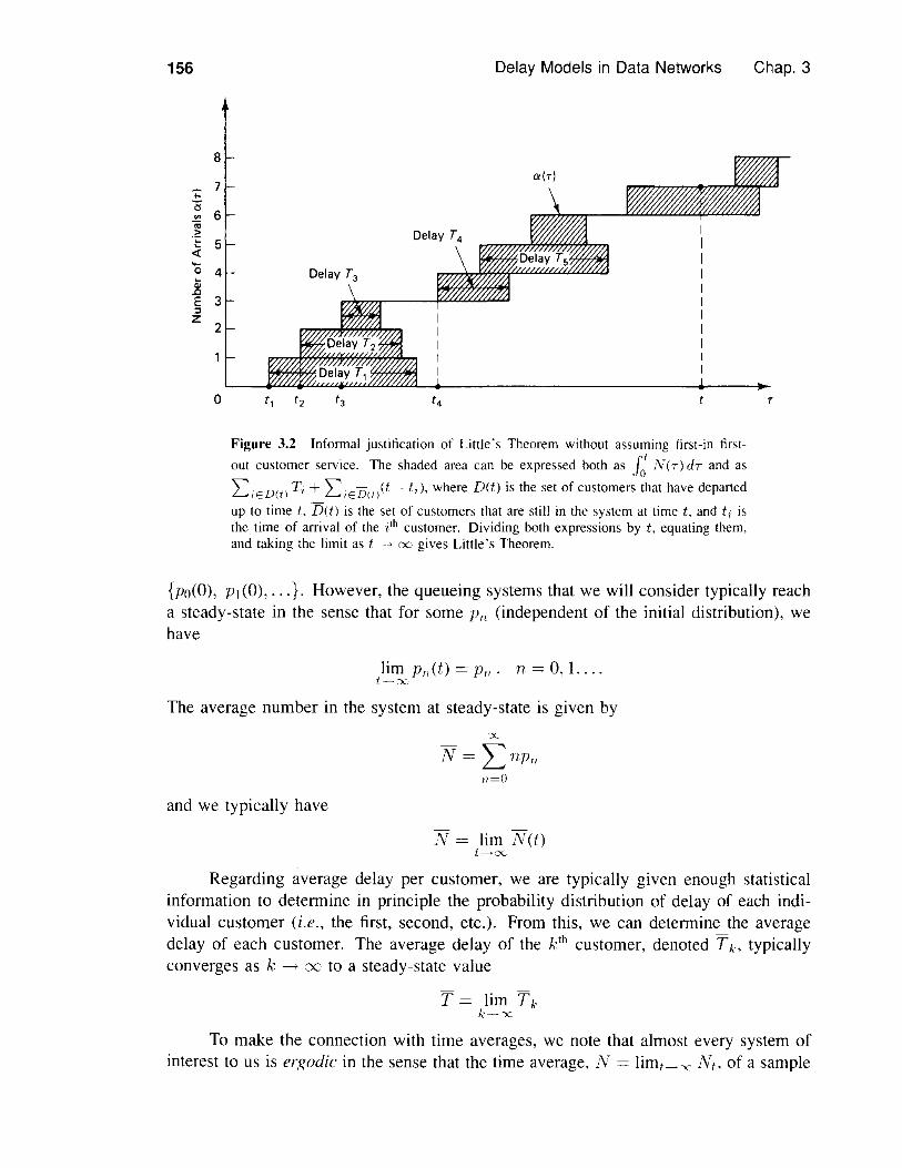
Example 3.3
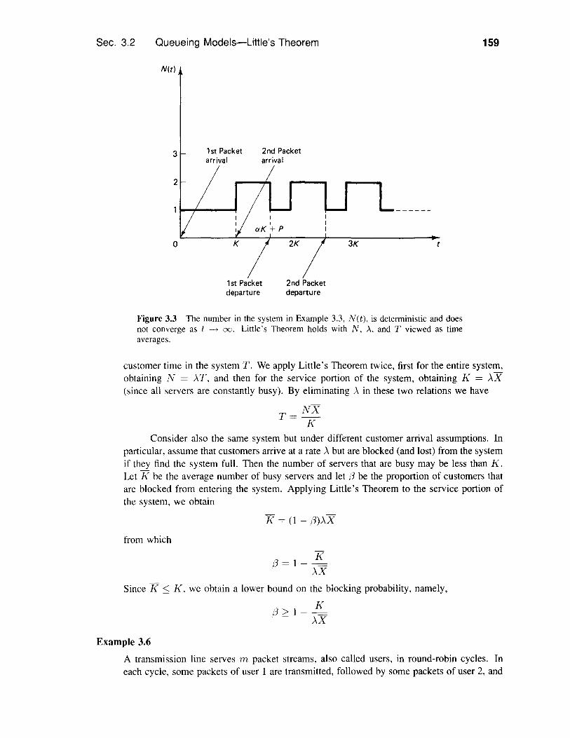
A packet arrives at a transmission line every K seconds with the first packet arriving at timeO. All packets have equal length and require aK seconds for transmission where a < I.The processing and propagation delay per packet is P seconds. The arrival rate here isA = 1/K. Because packets arrive at a regular rate (equal interarrival times), there is nodelay for queueing, so the time T a packet spends in the system (including the propagationdelay) is
T=aK+P
According to Little's Theorem, we have
PN = AT = a +-
KHere the number in the system N(t) is a deterministic function of time. Its form is shownin Fig. 3.3 for the case where K < aK + P < 2K, and it can be seen that N(t) does notconverge to any value (the system never reaches statistical equilibrium). However, Little'sTheorem holds with N viewed as a time average.
Example 3.4
Consider a window flow control system (as described in Section 2.8.1) with a window ofsize W for each session. Since the number of packets in the system per session is alwaysno more than W, Little's Theorem asserts that the arrival rate A of packets into the systemfor each session, and the average packet delay are related by W 2: AT. Thus, if congestionbuilds up in the network and T increases, A must eventually decrease. Next, suppose thatthe network is congested and capable of delivering only A packets per unit time for eachsession. Assuming that acknowledgment delays are negligible relative to the forward packetdelays, we have W AT. Then, increasing the window size TV for all sessions merelyserves to increase the delay T without appreciably changing A.
Example 3.5
Consider a queueing system with K servers, and with room for at most N 2: K customers(either in queue or in service). The system is always full; we assume that it starts withN customers and that a departing customer is immediately replaced by a new customer.(Queueing systems of this type are called closed and are discussed in detail in Section3.8.) Suppose that the average customer service time is X. We want to find the average
Sec. 3.2 Queueing Models-Little's Theorem
N(t)
159
3 1st Packetarrival
2nd Packetarrival
1st Packetdeparture
2nd Packetdeparture
Figure 3.3 The number in the system in Example 3.3, Net), is deterministic and doesnot converge as t -+ =. Little's Theorem holds with N, A, and T viewed as timeaverages.
customer time in the system T. We apply Little's Theorem twice, first for the entire system,obtaining N = )"T, and then for the service portion of the system, obtaining K = )"X(since all servers are constantly busy). By eliminating)" in these two relations we have
T= NXK
Consider also the same system but under different customer arrival assumptions. Inparticular, assume that customers arrive at a rate)" but are blocked (and lost) from the systemif they find the system full. Then the number of servers that are busy may be less than K.Let K be the average number of busy servers and let (3 be the proportion of customers thatare blocked from entering the system. Applying Little's Theorem to the service portion ofthe system, we obtain
K = (I - (3)"X
from which
K(3=1---=
)"X
Since K K, we obtain a lower bound on the blocking probability, namely,
K/3>1---=- )"X
Example 3.6
A transmission line serves m packet streams, also called users, in round-robin cycles. Ineach cycle, some packets of user I are transmitted, followed by some packets of user 2, and
160 Delay Models in Data Networks Chap. 3
so on, until finally, some packets of user m are transmitted. An overhead period of averagelength Ai precedes the transmission of the packets of user i in each cycle. Systems of thistype are called polling systems and are discussed in detail in Section 3.5.2.
The arrival rate and the average transmission time of the packets of user i are Ai andXi, respectively. From Little's theorem we know that the fraction of time the transmissionline is busy transmitting packets of user i is AiX;, Consider now the time intervals used foroverhead of user i. We can view these intervals as "packets" with average transmission timeAi. The arrival rate of these "packets" is IlL, where L is the average cycle length, and asbefore, we may use Little's theorem to assert that the fraction of time used for transmissionof these "packets" is AIL, where A = Al + A2 + ... + Am. Therefore, we have
A TTl _
1= - + AXL 1 1
;=1
which yields the average cycle length
AL= TTl
1- L;=1 Ai X ;
Example 3.7 Estimating Throughput in a Time-Sharing System
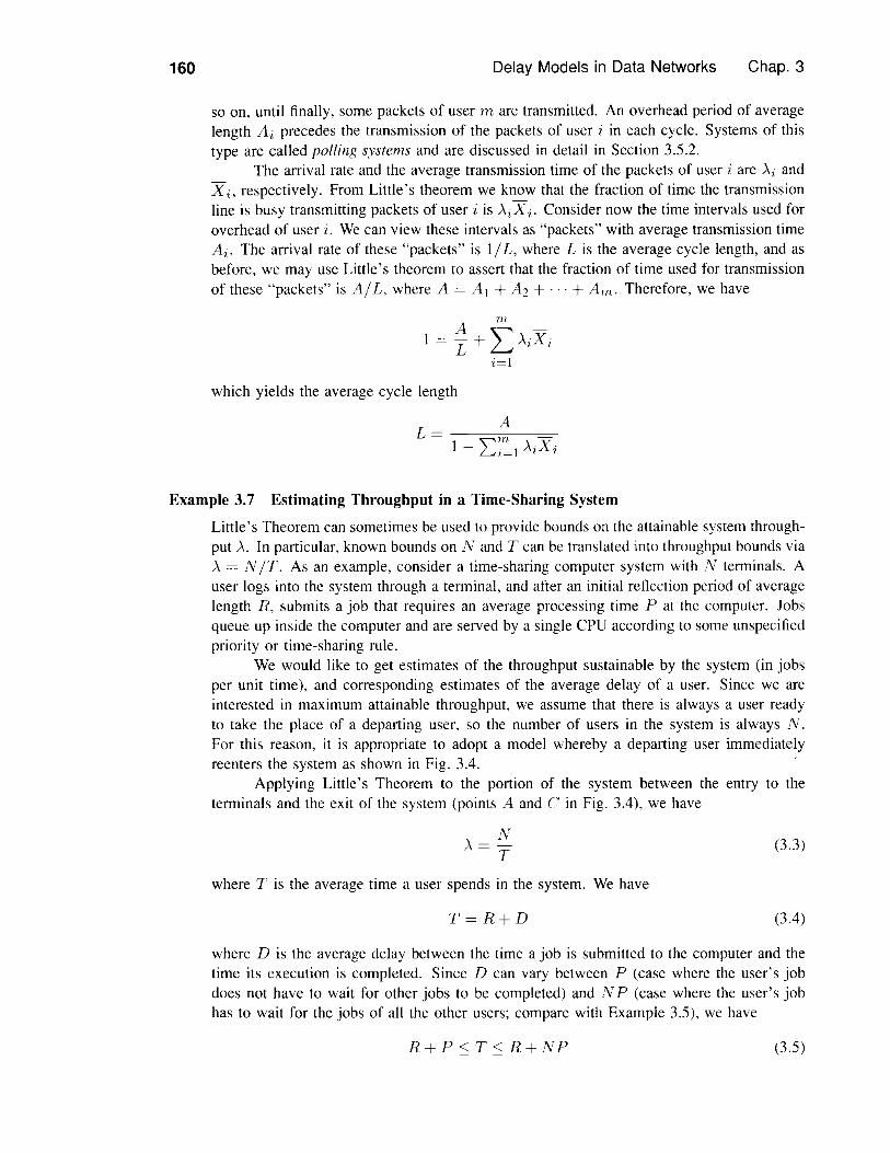
Little's Theorem can sometimes be used to provide bounds on the attainable system through-put A. In particular, known bounds on ]V and T can be translated into throughput bounds viaA = ]VIT. As an example, consider a time-sharing computer system with ]V terminals. Auser logs into the system through a terminal, and after an initial reflection period of averagelength R, submits a job that requires an average processing time P at the computer. Jobsqueue up inside the computer and are served by a single CPU according to some unspecifiedpriority or time-sharing rule.
We would like to get estimates of the throughput sustainable by the system (in jobsper unit time), and corresponding estimates of the average delay of a user. Since we areinterested in maximum attainable throughput, we assume that there is always a user readyto take the place of a departing user, so the number of users in the system is always ]V.For this reason, it is appropriate to adopt a model whereby a departing user immediatelyreenters the system as shown in Fig. 3.4.
Applying Little's Theorem to the portion of the system between the entry to theterminals and the exit of the system (points A and C in Fig. 3.4), we have
(3.3)
where T is the average time a user spends in the system. We have
T=R+D (3.4)
where D is the average delay between the time a job is submitted to the computer and thetime its execution is completed. Since D can vary between P (case where the user's jobdoes not have to wait for other jobs to be completed) and ]VP (case where the user's jobhas to wait for the jobs of all the other users; compare with Example 3.5), we have
(3.5)
Sec. 3.2 Queueing Models-Little's Theorem
Average reflectiontime R
ComputerB
Average job processingtime P
C
161
(3.6)
Figure 3.4 N terminals connected with a time-sharing computer system. Toestimate maximum attainable throughput, we assume that a departing user im-mediately reenters the system or, equivalently, is immediately replaced by a newuser.
Combining this relation with A = NIT [cf. Eq. (3.3)], we obtain
N-R+P
The throughput A is also bounded above by the processing capacity of the computer. Inparticular, since the execution time of a job is P units on the average, it follows that thecomputer cannot process in the long run more than II P jobs per unit time, that is,
IA<--P (3.7)
(3.8)
(This conclusion can also be reached by applying Little's Theorem between the entry andexit points of the computer's CPU.)
By combining the preceding two relations, we obtain the bounds
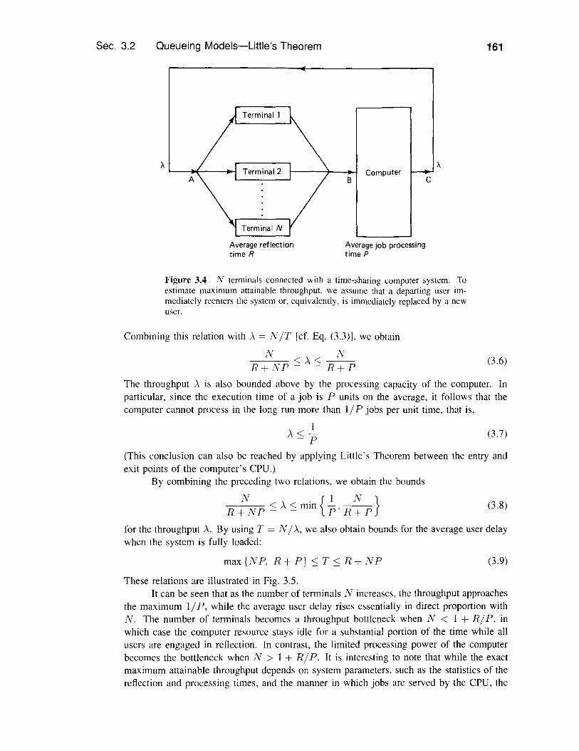
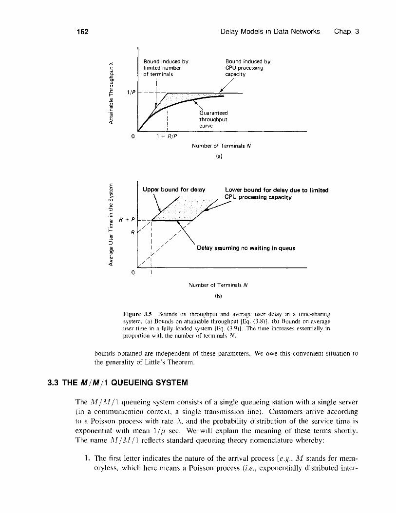
N {I N}---::-:-:c- < A < min - ---R+NP- - P'R+Pfor the throughput A. By using T = N I A, we also obtain bounds for the average user delaywhen the system is fully loaded:
max {NP, R+ P} -s; T -s; R+ NP (3.9)
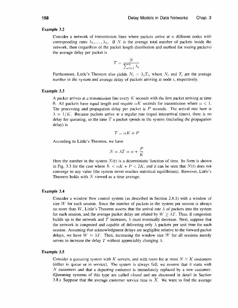
These relations are illustrated in Fig. 3.5.It can be seen that as the number of terminals N increases, the throughput approaches
the maximum liP, while the average user delay rises essentially in direct proportion withN. The number of terminals becomes a throughput bottleneck when N < I + RIP, inwhich case the computer resource stays idle for a substantial portion of the time while allusers are engaged in reflection. In contrast, the limited processing power of the computerbecomes the bottleneck when N > I + RIP. It is interesting to note that while the exactmaximum attainable throughput depends on system parameters, such as the statistics of thereflection and processing times, and the manner in which jobs are served by the CPU, the
162
,<....::J0..r::Cl::Jo1:I-
'"::c'"c:t
11P
Bound induced byIimited numberof terminals
Delay Models in Data Networks
Bound induced byCPU processingcapacity
Guaranteedthroughputcurve
Chap. 3
Upper bound for delayE'"1;;>en'".sc
'"Ei=
:::>'"Cl:;>'"><{
o 1 + RIP
R+P/1
R/ I
II1/V
//1
0
Number of Terminals N
(a)
Lower bound for delay due to limitedCPU processing capacity
Delay assuming no waiting in queue
Number of Terminals N
(b)
Figure 3.5 Bounds on throughput and average user delay in a time-sharingsystem. (a) Bounds on attainable throughput [Eq. (3.8)]. (b) Bounds on averageuser time in a fully loaded system [Eq. (3.9)]. The time increases essentially inproportion with the number of terminals N.
bounds obtained are independent of these parameters. We owe this convenient situation tothe generality of Little's Theorem.
3.3 THE M /M /1 QUEUEING SYSTEM
The M / ]\[ / I queueing system consists of a single queueing station with a single server(in a communication context, a single transmission line). Customers arrive accordingto a Poisson process with rate A, and the probability distribution of the service time isexponential with mean 1/ f.1 sec. We will explain the meaning of these terms shortly.The name AI/AI / I reflects standard queueing theory nomenclature whereby:
1. The first letter indicates the nature of the arrival process [e.g., !vI stands for mem-oryless, which here means a Poisson process (i.e., exponentially distributed inter-

Sec. 3.3 The M / M / 1 Queueing System 163
arrival times), G stands for a general distribution of interarrival times, D standsfor deterministic interarrival times].
2. The second letter indicates the nature of the probability distribution of the servicetimes (e.g., "U, G, and D stand for exponential, general, and deterministic distri-butions, respectively). In all cases, successive interarrival times and service timesare assumed to be statistically independent of each other.
3. The last number indicates the number of servers.
We have already established, via Little's Theorem, the relations
N=AT. NQ = AVV
between the basic quantities,
N = Average number of customers in the system
T = Average customer time in the system
NQ = Average number of customers waiting in queue
IV = Average customer waiting time in queue
However, N, T, 1VQ , and VV cannot be specified further unless we know somethingmore about the statistics of the system. Given these statistics, we will be able to derivethe steady-state probabilities
p" = Probability of n customers in the system, n = O. I ....
From these probabilities, we can getx
N= LnPnn=O
and using Little's Theorem,
NA
Similar formulas exist for 1VQ and W. Appendix B provides a summary of the resultsfor the M / 1'1/1 system and the other major systems analyzed later.
The analysis of the Al/M /1 system as well as several other related systems,such as the 1'1/1'1/m or M / M / x systems, is based on the theory of Markov chainssummarized in Appendix A. An alternative approach is to use simple graphical argumentsbased on the concept of mean residual time introduced in Section 3.5. This approachdoes not require that the service times are exponentially distributed (i.e., it applies to theM /G / I system). The price paid for this generality is that the characterization of thesteady-state probabilities is more complicated than for the M /M / I system. The readerwishing to circumvent the Markov chain analysis may start directly with the M /G/1system in Section 3.5 after a reading of the preliminary facts on the Poisson processgiven in Sections 3.3.1 and 3.3.2.
164
3.3.1 Main Results
Delay Models in Data Networks Chap. 3
We first introduce our assumptions on the arrival and service statistics of the M /M / Isystem.
Arrival statistics-the Poisson process. In the AI /M / I system, customersarrive according to a Poisson process which we now define:
A stochastic process {A(t) I t 2 o} taking nonnegative integer values is said to bea Poisson process with rate A if
1. A(t) is a counting process that represents the total number of arrivals that haveoccurred from °to time t [i.e., A(O) = 0], and for s < t, A(t) - A(s) equals thenumbers of arrivals in the interval (8, t].
2. The numbers of arrivals that occur in disjoint time intervals are independent.3. The number of arrivals in any interval of length T is Poisson distributed withparameter AT. That is, for all t, T > 0,
(AT)nP {A(t + T) - A(t) = n} = C- AT__ ,
n!n = 0, I, .. , (3.10)
The average number of arrivals within an interval of length T is AT (based on themean of the Poisson distribution). This leads to the interpretation of A as an arrivalrate (average number of arrivals per unit time).
We list some of the properties of the Poisson process that will be of interest:
1. Interarrival times are independent and exponentially distributed with parameter A;that is, if t n denotes the time of the nth arrival, the intervals Tn = t n+1 - t n havethe probability distribution
820 (3.11 )
and are mutually independent. [The corresponding probability density function isp(Tn) = AC- ATn . The mean and variance of Tn are I/A and I/A2, respectively.]For a proof of this property, see [Ros83], p. 35.
2. For every t 2 °and b 2 0,P {A(t + b) - A(t) = O} = 1 - Ab + o(b)
P{A(t+b)-A(t)= I} =Ab+o(b)
P{A(t+b)-A(t)22} =o(b)
where we generically denote by o(b) a function of b such that
lim o(b) = °Ii
(3.12)
(3.13)
(3.14)

Sec. 3.3 The M / M / 1 Queueing System 165
These equations can be verified by expanding the Poisson distribution on the num-ber of arrivals in an interval of length fJ [Eq. (3.1O)J in a Taylor series [or equiva-lently, by writing e-)..o = I - AfJ + (AfJ)2/2 - ...].
3. If two or more independent Poisson processes AI, .... A k are merged into a singleprocess A = Al + A2 + ... + A k , the latter process is Poisson with a rate equal tothe sum of the rates of its components (see Problem 3.10).
4. If a Poisson process is split into two other processes by independently assigningeach arrival to the first (second) of these processes with probability p (I - p,respectively), the two arrival processes thus obtained are Poisson (see Problem3.11). (For this it is essential that the assignment of each arrival be independentof the assignment of other arrivals. If, for example, the assignment is done byalternation, with even-numbered arrivals assigned to one process and odd-numberedarrivals assigned to the other, the two generated processes are not Poisson. Thiswill prove to be significant in the context of data networks; see Example 3.17 inSection 3.6.)
A Poisson process is generally considered to be a good model for the aggregatetraffic of a large number of similar and independent users. In particular, suppose that wemerge n independent and identically distributed packet arrival processes. Each processhas arrival rate A/n, so that the aggregate process has arrival rate A. The interarrivaltimes T between packets of the same process have a given distribution F(s) = P{T :S s}and are independent [F(s) need not be an exponential distribution]. Then under relativelymild conditions on F fe.R., F(O) = 0, dF(O)/ds > 0], the aggregate arrival process canbe approximated well by a Poisson process with rate A as n ---+ x (see [KaT75], p. 221).
Service statistics. Our assumption regarding the service process is that thecustomer service times have an exponential distribution with parameter 11, that is, if s"is the service time of the nth customer,
P { > < s} - I -fl8Sn _ - - e ,
[The probability density function of s" is pes,,) = 11e- flsn , and its mean and variance are1//1 and 1//12, respectivelY.J Furthermore, the service times Sn are mutually independentand also independent of all interarrival times. The parameter 11 is called the servicerate and represents the rate (in customers served per unit time) at which the serveroperates when busy. In the context of a packet transmission system, the independence ofinterarrival and service times implies, among other things, that the length of an arrivingpacket does not affect the arrival time of the next packet. It will be seen in Section 3.6that this condition is often violated in practice, particularly when the arriving packetshave just departed from another queue.
An important fact regarding the exponential distribution is its memoryless character,which can be expressed as
P {Tn > T + t I Tn > t} = P {Tn > r} ,
P {Sri > T+ tisn > t} = P {s" > T} ,
for T. t > 0
for T. t 0
166 Delay Models in Data Networks Chap. 3
for the interarrival and service times Tn and 8 n, respectively. This means that theadditional time needed to complete a customer's service in progress is independent ofwhen the service started. Similarly, the time up to the next arrival is independent of whenthe previous arrival occurred. Verification of the memoryless property follows from thecalculation
} P {Tn> I' + t}P {Tn > I' + t I Tn > t =P{Tn>t}
(P { }= e = Til > I'
Markov chain formulation. An important consequence of the memorylessproperty is that it allows the use of the theory of Markov chains. Indeed, this property,together with our earlier independence assumptions on interarrival and service times,imply that once we know the number N(t) of customers in the system at time t, thetimes at which customers will arrive or complete service in the future are independent ofthe arrival times of the customers presently in the system and of how much service thecustomer currently in service (if any) has already received. This means that the futurenumbers of customers depend on past numbers only through the present number; that is.{N(t) It 2: O} is a continuous-time Markov chain.
We could analyze the process N(t) in terms of continuous-time Markov chainmethodology; most of the queueing literature follows this line of analysis (see alsoProblem 3.12). It is sufficient, however, for our purposes in this section to use thesimpler theory of discrete-time Markov chains (briefly summarized in Appendix A).
Let us focus attention at the times
O. b. 26.. .. . ltb....
where b is a small positive number. We denote
N k = Number of customers in the system at time ltb
Since ]'h: = N(kb) and, as discussed, N(t) is a continuous-time Markov chain, we seethat {Nk I k = 0, I, ... } is a discrete-time Markov chain with steady-state occupancyprobabilities equal to those of the continuous chain. Let P,) denote the correspondingtransition probabilities
Note that Pij depends on b, but to keep notation simple, we do not show this dependence.By using Eqs. (3.12) through (3.14), one can show that
p(W = 1 - Ab + o(b)
P1i = 1 - Ab - f.1b + o(b),
Pii+1 = Ab + u(b),
Pi,i-l = lIb + o(b),
Pij = o(b).
i 2: 1i2:0i 2: Ii and j oF i. i + l.i - 1
(3.15)
(3.16)
(3.17)
(3.18)

Sec. 3.3 The M / M /1 Queueing System 167
To see how these equations are verified, note that when at a state i 2: 1, the proba-bility of 0 arrivals and 0 departures in a b-interva1 h = (kb. (ki-1)b] is (e- AD )(e-/1D); thisis because the number of arrivals and the number of departures are Poisson distributedand independent of each other. Expanding this in a power series in D,
P {O customers arrive and 0 depart in h} = 1 - Ab - f.1b + 0(15) (3.19)
The probability of 0 arrivals and I departure in the interval h is e-AD(l - e-/1D) ifi = 1 (since 1 - e-/1D is the probability that the customer in service will complete itsservice within h), and e-AD (f.1be-/l D) if i > 1 (since f.1be-/lD is the probability that withinthe interval h, the customer in service will complete its service while the subsequentcustomer will not). In both cases we have
P{O customers arrive and I departs in Id = f.1b + 0(15)
Similarly, the probability of 1 arrival and 0 departures in h is (Abe-AD)e-/l D, so
P {1 customer amves and 0 depart in h} = AD + 0(15)
These probabilities add up to 1 plus o(b). Thus, the probability of more than one arrivalor departure is negligible for 15 small. It follows that for i 2: 1, Pi;, which is theprobability of an equal number of arrivals and departures in h, is within 0(15) of thevalue in Eq. (3.19); this verifies Eq. (3.16). Equations (3.15), (3.17), and (3.18) areverified in the same way.
The state transition diagram for the Markov chain {,Vk} is shown in Fig. 3.6, wherewe have omitted the terms o(b).
Derivation of the stationary distribution. Consider now the steady-stateprobabilities
Pn = lim P{Nk = n} = lim P{N(t) = n}k---+x i-x·
Note that during any time interval, the total number of transitions from state n to n + 1must differ from the total number of transitions from n + 1 to n by at most 1. Thusasymptotically, the frequency of transitions from n to n + 1 is equal to the frequency oftransitions from n + 1 to n. Equivalently, the probability that the system is in state nandmakes a transition to n + I in the next transition interval is the same as the probabilitythat the system is in state n + 1 and makes a transition to n, that is,
PnAb + o(b) = Pn+lf.1b + 0(15)
1- M 1 - AS -IJ.O 1 - AS - /lO
Figure 3.6 Discrete-time Markov chain for the :\1/ '\1 /1 system. The state n corresponds to ncustomers in the system. Transition probabilities shown are correct up to an 0(6) term.
168 Delay Models in Data Networks Chap. 3
By taking the limit in this equation as b --+ 0, we obtain
Pn A = Pn+lj1 (3.20)
(The preceding equations are called global balance equations, corresponding to the setof states {O, 1, ... , n} and {n + 1, n + 2, ... }. See Appendix A for a more generalstatement of these equations and for an interpretation that parallels the argument givenabove.) These equations can also be written as
where
It follows that
Pn+l = PPn,
AP= -
j1
n = O. 1. ...
Pn+l = pn+1Po, n = 0, 1, ... (3.21 )
If P < 1 (service rate exceeds arrival rate), the probabilities Pn are all positive and addup to unity, so
Combining the last two equations, we finally obtain
(3.22)
n =0.1 .... (3.23)
(3.24)
We can now calculate the average number of customers in the system in steady-state:
x· x
N = E {N(t)} = L npn = L npn(l - p),,=0 n=O
= p(l - p) npn-l = p(l _ p) :p
= p(l - p) :p = p(l - P)_(1 1_p)--=-2
and finally, using p = AI j1, we haveN- _P A_-1-p-j1-A
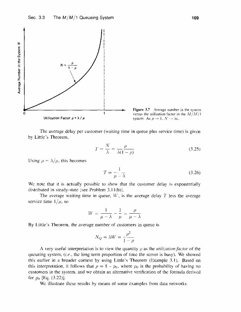
The graph of this equation is shown in Fig. 3.7. As p increases, so does N, and asp --+ 1, we have N --+ 00. The graph is valid for p < 1. If p > 1, the server cannot keepup with the arrival rate and the queue length increases without bound. In the context ofa packet transmission system, p > 1 means that AL > C, where A is the arrival rate inpackets/sec, L is the average packet length in bits, and C is the transmission capacity inbits/sec.
Sec. 3.3 The M / M /1 Queueing System 169
oUtilization Factor p = X/ IJ.
Figure 3.7 Average number in the systemversus the utilization factor in the AI /}'vI /1system. As p I. IV =.
The average delay per customer (waiting time in queue plus service time) is givenby Little's Theorem,
Using p = /\jp, this becomes
N PT=-=---,\ ,\(1 - p)
(3.25)
(3.26)T=_I-p - ,\
We note that it is actually possible to show that the customer delay is exponentiallydistributed in steady-state [see Problem 3.ll(b)].
The average waiting time in queue, lV, is the average delay T less the averageservice time 1/p, so
Til PHp-'\ p p-'\
By Little's Theorem, the average number of customers in queue is
p2NQ ='\W=--
I-p
A very useful interpretation is to view the quantity p as the utilization factor of thequeueing system, (i.e., the long-term proportion of time the server is busy). We showedthis earlier in a broader context by using Little's Theorem (Example 3.1). Based onthis interpretation, it follows that p = 1 - Po, where Po is the probability of having nocustomers in the system, and we obtain an alternative verification of the formula derivedfor Po [Eq. (3.22)].
We illustrate these results by means of some examples from data networks.

170 Delay Models in Data Networks Chap. 3
Example 3.8 Increasing the Arrival and Transmission Rates by the Same FactorConsider a packet transmission system whose arrival rate (in packets/sec) is increased fromA to K A, where K > 1 is some scalar factor. The packet length distribution remains thesame but the transmission capacity is increased by a factor of K, so the average packettransmission time is now I/(K /1) instead of 1//1. It follows that the utilization factor p,and therefore the average number of packets in the system, remain the same:
N= _P_ = _A_1-p /1-A
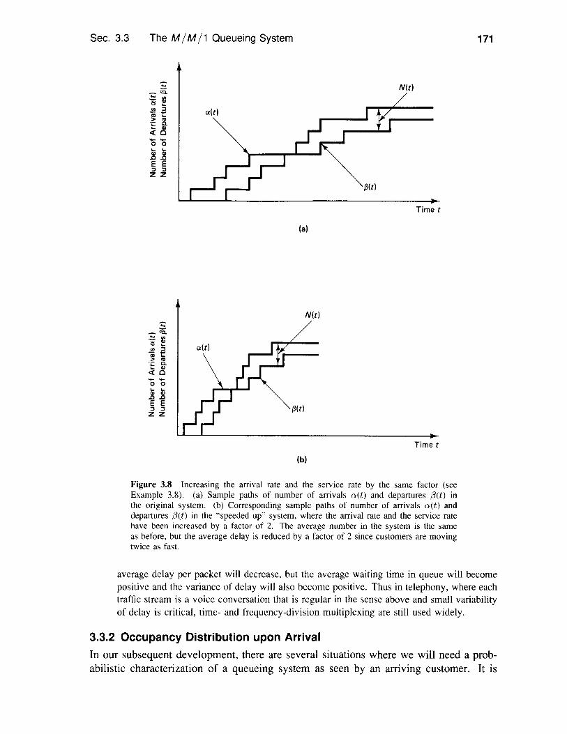
However, the average delay per packet is now T = N /(KA) and is therefore decreased bya factor of K. In other words, a transmission line K times as fast will accommodate Ktimes as many packets/sec at K times smaller average delay per packet. This result is quitegeneral, even applying to networks of queues. What is happening, as illustrated in Fig. 3.8,is that by increasing arrival rate and service rate by a factor K, the statistical characteristicsof the queueing process are unaffected except for a change in time scale-the process isspeeded up by a factor K. Thus, when a packet arrives, it will see ahead of it statisticallythe same number of packets as with a slower transmission line. However, the packets aheadof it will be moving K times faster.
Example 3.9 Statistical Multiplexing Compared with Time- and Frequency-DivisionMultiplexing
Assume that m statistically identical and independent Poisson packet streams each with anarrival rate of A/m packets/sec are transmitted over a communication line. The packetlengths for all streams are independent and exponentially distributed. The average transmis-sion time is 1//1. If the streams are merged into a single Poisson stream, with rate A, as instatistical multiplexing, the average delay per packet is
T=_l_/1-A
If, instead, the transmission capacity is divided into m equal portions, one per packet streamas in time- and frequency-division multiplexing, each portion behaves like an M / M /1queue with arrival rate A/m and average service rate /1/m. Therefore, the average delayper packet is
T= --'!!!...--../1-A
that is, m times larger than for statistical multiplexing.The preceding argument indicates that multiplexing a large number of traffic streams
on separate channels in a transmission line performs very poorly in terms of delay. The per-formance is even poorer if the capacity of the channels is not allocated in direct proportionto the arrival rates of the corresponding streams-something that cannot be done (at least inthe scheme considered here) if these arrival rates change over time. This is precisely whydata networks, which most of the time serve many low duty cycle traffic streams, are typi-cally organized on the basis of some form of statistical multiplexing. An argument in favorof time- and frequency-division multiplexing arises when each traffic stream is "regular" (asopposed to Poisson) in the sense that no packet arrives while another is transmitted, and thusthere is no waiting in queue if that stream is transmitted on a dedicated transmission line.If several streams of this type are statistically multiplexed on a single transmission line, the
Sec. 3.3 The M / M /1 Queueing System
..........o 0OJ OJ.0.0E E" "zz
N(t)
171
Time t
(a)
N(t)
........o 0OJ OJ.0.0E E" "zz
Time t
(b)
Figure 3.8 Increasing the arrival rate and the service rate by the same factor (seeExample 3.8). (a) Sample paths of number of anivals n(t) and departures (3(t) inthe original system. (b) Corresponding sample paths of number of arrivals n(t) anddepartures (3(t) in the "speeded up" system, where the arrival rate and the service ratehave been increased by a factor of 2. The average number in the system is the sameas before, but the average delay is reduced by a factor of 2 since customers are movingtwice as fast.
average delay per packet will decrease, but the average waiting time in queue will becomepositive and the variance of delay will also become positive. Thus in telephony, where eachtrafflc stream is a voice conversation that is regular in the sense above and small variabilityof delay is critical, time- and frequency-division multiplexing are still used widely.
3.3.2 Occupancy Distribution upon ArrivalIn our subsequent development, there are several situations where we will need a prob-abilistic characterization of a queueing system as seen by an arriving customer. It is

172 Delay Models in Data Networks Chap. 3
possible that the times of customer arrivals are in some sense nontypical, so that thesteady-state occupancy probabilities upon arrival,
an = lim P{N(t) = n I an arrival occurred just after time t} (3.27)t----t(X)
need not be equal to the corresponding unconditional steady-state probabilities,
Pn = lim P{N(t) = n} (3.28)t----+CX)
It turns out, however, that for the JIll /M / I system, we have
n = 0, I, ... (3.29)
so that an arriving customer finds the system in a "typical" state. Indeed, this holdsunder very general conditions for queueing systems with Poisson arrivals regardless ofthedistrihution of the service times. The only additional requirement we need is that futurearrivals are independent of the current number in the system. More precisely, we assumethat for every time t and increment 6 > 0, the number of arrivals in the interval (t, t + 6)is independent of the number in the system at time t. Given the Poisson hypothesis,essentially this amounts to assuming that, at any time, the service times of previouslyarrived customers and the future interarrival times are independent-something that isreasonable for packet transmission systems. In particular, the assumption holds if thearrival process is Poisson and interarrival times and service times are independent.
For a formal proof of the equality an = Pn under the preceding assumption, letA(t, t + 8) be the event that an arrival occurs in the interval (t, t + 6). Let
Pn(t) = P {N(t) = n}
an(t) = P{N(t) = n I an arrival occurred just after time t}We have, using Bayes' rule,
(3.30)
(3.31)
(3.32)
an(t) = lim P {N(t) = n IA(t, t + 6)}0--->0
. P{N(t)=n, A(t,t+6)}= hm0--->0 P{A(t,t+6)}
= lim P {A(t, t + 6) I N(t) = n} P{N(t) = n}0--->0 P{A(t,t+6)}
By assumption, the event A(t, t + 6) is independent of the number in the system at timet. Therefore,
P{A(t, t + 6) IN(t) = n} = P{A(t, t + 6)}and we obtain from Eq. (3.32)
an(t) = P {N(t) = n} = Pn(t)
Taking the limit as t ----+ 00, we obtain an = Pn.As an example of what can happen if the arrival process is not Poisson, suppose
that interarrival times are independent and uniformly distributed between 2 and 4 sec,
Sec. 3.4 The M/M/m, M/M/oo, M/M/m/m, and Other Markov Systems 173
while customer service times are all equal to I sec. Then an arriving customer alwaysfinds an empty system. On the other hand, the average number in the system as seenby an outside observer looking at a system at a random time is 1/3. (The time in thesystem of each customer is 1 sec, so by Little's Theorem, N is equal to the arrival rateA, which is 1/3 since the expected time between arrivals is 3.)
For a similar example where the arrival process is Poisson but the service timesof customers in the system and the future arrival times are correlated, consider a packettransmission system where packets arrive according to a Poisson process. The transmis-sion time of the nth packet equals one half the interarrival time between packets nandn + I. Upon arrival, a packet finds the system empty. However, the average number inthe system, as seen by an outside observer, is easily seen to be 1/2.
3.3.3 Occupancy Distribution upon Departure
Let us consider the distribution of the number of customers in the system just after adeparture has occurred, that is, the probabilities
dn(t) = P{N(t) = n I a departure occurred just before time t}
The corresponding steady-state values are denoted
It turns out that
dn = lim dn(t),t--7X
dn = (In,
n = 0, I, ...
n=O,l, ...
under very general assumptions-the only requirement essentially is that the systemreaches a steady-state with all n having positive steady-state probabilities, and that N(t)changes in unit increments. [These assumptions certainly hold for a stable M /M /1system (p < 1), but they also hold for most stable single-queue systems of interest.]For any sample path of the system and for every n, the number in the system will ben infinitely often (with probability 1). This means that for each time the number in thesystem increases from n to n + 1 due to an arrival, there will be a corresponding futuredecrease from n + 1 to n due to a departure. Therefore, in the long run, the frequency oftransitions from n to n + lout of transitions from any k to k + 1 equals the frequencyof transitions from n + 1 to n out of transitions from any k + 1 to k, which impliesthat dn = an. Therefore, in steady-state, the system appears statistically identical toan arriving and a departing customer. When arrivals are Poisson, we saw earlier thatan = Pn; so, in this case, both an arriving and a departing customer in steady-state seea system that is statistically identical to the one seen by an observer looking at the systemat an arbitrary time.
3.4 THE M/M/m, M/M/OCJ, M/M/m/m, AND OTHER MARKOVSYSTEMS
We consider now a number of queueing systems that are similar to 1M/ lvI /1 in thatthe arrival process is Poisson and the service times are independent, exponentially dis-
174 Delay Models in Data Networks Chap. 3
tributed, and independent of the interarrival times. Because of these assumptions, thesesystems can be modeled with continuous- or discrete-time Markov chains. From the cor-responding state transition diagram, we can derive a set of equations that can be solvedfor the steady-state occupancy probabilities. Application of Little's Theorem then yieldsthe average delay per customer.
3.4.1 M / M /m: The m-Server Case
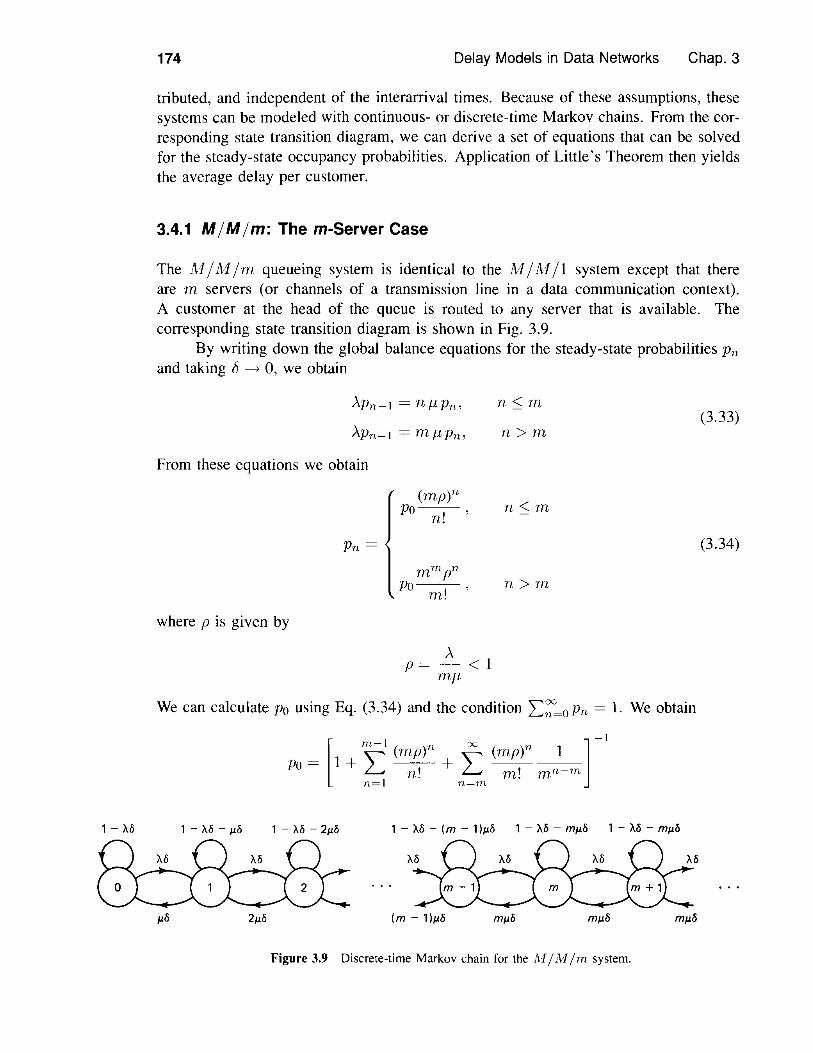
The M /M /m queueing system is identical to the M /M / I system except that thereare m servers (or channels of a transmission line in a data communication context).A customer at the head of the queue is routed to any server that is available. Thecorresponding state transition diagram is shown in Fig. 3.9.
By writing down the global balance equations for the steady-state probabilities Pnand taking fJ ----7 0, we obtain
(3.33)n>m
From these equations we obtain
(mp)nPo--,- ,n.
where p is given by
Pn =rnmpn
Po--,-,rn.n>m
(3.34)
Ap= - < I
mJL
We can calculate Po using Eq. (3.34) and the condition 2::=oPn = 1. We obtain
[T.n-1 (mp)n x (mp)n I ]-1
Po = 1+ '"' -- + '"' -----L n! L m! mn-mn=l n=rn
Figure 3.9 Discrete-time Markov chain for the fefIM 1m system.
Sec. 3.4
and finally,
The M/M/rn, M/M/oo, M/M/rn/rn, and Other Markov Systems
_ [mL-l (mp)n (mp)m]-1
Po - -- + ---,---'-----,-n! m!(l - p)
n=O
175
(3.35)
The probability that an arrival will find all servers busy and will be forced to waitin queue is an important measure of performance of the M /M /m system. Since anarriving customer finds the system in "typical" state (see Section 3.3.2), we have
P{Q '} Loc
LX pommpn po(mp)m LX n-mueuemg = Pn = = pm! m!n=m n=m n=m
and, finally,t::,. • po(mp)m
PQ = P{Queuemg} = , (3.36)m.(l - p)
where Po is given by Eq. (3.35). This is known as the Erlang C formula, honoringDenmark's A. K. Erlang, the foremost pioneer of queueing theory. This equation isoften used in telephony (and more generally in circuit switching systems) to estimatethe probability of a call request finding all of the m circuits of a transmission line busy.In an M /M /m model it is assumed that such a call request "remains in queue," thatis, continuously attempts to find a free circuit. The alternative model where such a calldeparts from the system and never returns is discussed in the context of the M /M /m/msystem in Section 3.4.3.
The expected number of customers waiting in queue (not in service) is given byOC
NQ = LnPm+nn=O
Using the expression for Pm+n [Eq. (3.34)], we obtain
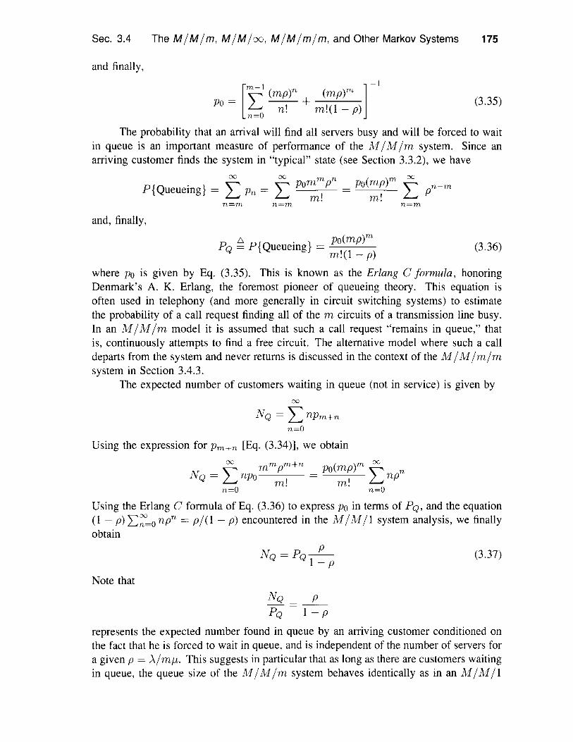
Using the Erlang C formula of Eq. (3.36) to express Po in terms of PQ' and the equation(I - p) 2:::=0 npn = p/ (I - p) encountered in the M / M / I system analysis, we finallyobtain
Note that
PNQ =PQ--l-p(3.37)
NQ pPQ 1- P
represents the expected number found in queue by an arriving customer conditioned onthe fact that he is forced to wait in queue, and is independent of the number of servers fora given p = A/mIL. This suggests in particular that as long as there are customers waitingin queue, the queue size of the M /M / m system behaves identically as in an M /M /1
176 Delay Models in Data Networks Chap. 3
system with service rate mtL-the aggregate rate of the m servers. Some thought showsthat indeed this is true in view of the memoryless property of the exponential distribution.
Using Little's Theorem and the expression (3.37) for NQ, we obtain the averagetime W a customer has to wait in queue:
W = NQ = pPQA A(l - p)
The average delay per customer is, therefore,
T- - W- pPQ- tL + - tL + A(1 - p)
and using p = A/mtL, we obtain
T= +W= + PQtL tL mtL - A
Using Little's Theorem again, the average number of customers in the system is
and using p = A/mtL, we finally obtain
N = mp+ pPQl-p
(3.38)
Example 3.10 Using One vs. Using Multiple Channels in Statistical MultiplexingConsider a communication link serving m independent Poisson traffic streams with overallrate A. Suppose that the link is divided into m separate channels with one channel assignedto each traffic stream. However, if a traffic stream has no packet awaiting transmission, itscorresponding channel is used to transmit a packet of another traffic stream. The transmissiontimes of packets on each of the channels are exponentially distributed with mean II f.L. Thesystem can be modeled by the same Markov chain as the M1M1m queue. Let us comparethe average delays per packet of this system, and an M IMil system with the same arrivalrate ,\ and service rate mf.L (statistical multiplexing with one channel having m times largercapacity). In the fonner case, the average delay per packet is given by the M IM 1m averagedelay expression (3.38)
f.L mf.L-'\
while in the latter case, the average delay per packet is
A I PQT=-+---mf.L mf.L-'\
where PQ and PQ denote the queueing probability in each case. When p « I (lightlyloaded system) we have PQ 0, PQ 0, and
--;c=mT
Sec. 3.4 The M/M/m, M/M/oo, M/M/m/m, and Other Markov Systems 177
When p is only slightly less than 1, we have PQ ':'::' 1, PQ ':'::' 1, l/p« l/(Tnp- A), and
T- "'" 1f-
Therefore, for a light load, statistical multiplexing with Tn channels produces a delay almostTn times larger than the delay of statistical multiplexing with the Tn channels combined inone (about the same as time- and frequency-division multiplexing). For a heavy load, theratio of the two delays is close to 1.
3.4.2 M1MI 00: The Infinite-Server Case
In the limiting case where m = 00 in the M IM 1m system, we obtain from the globalbalance equations (3.33)
APn-l = np,Pn,
so
Pn = p, n.
From the condition 2:::'=0 Pn = I, we obtain
n = 1,2, ...
n = 1,2, ...
n = 0, 1, ...
so finally,
_ e-A/ flPn - , 'p, n.
Therefore, in steady-state, the number in the system is Poisson distributed with parameterAIp,. The average number in the system is
p,
By Little's Theorem, the average delay is N IA or1T=-P,
This last equation can also be obtained simply by arguing that in an M IM I 00 system,there is no waiting in queue, so T equals the average service time 1I p,. It can be shownthat the number in the system is Poisson distributed even if the service time distributionis not exponential (i.e., in the MIGloo system; see Problem 3.47).
Example 3.11 The Quasistatic Assumption
It is often convenient to assume that the external packet traffic entering a subnet node anddestined for some other subnet node can be modeled by a stationary stochastic process thathas a constant bit arrival rate (average bits/sec). This approximates a situation where the
178 Delay Models in Data Networks Chap. 3
arrival rate changes slowly with time and constitutes what we refer to as the quasistaticassumption.
When there are only a few active sessions (i.e., user pairs) for the given origin-destination pair, this assumption is seriously violated since the addition or termination of asingle session can change the total bit arrival rate by a substantial factor. When, however,there are many active sessions, each with a bit arrival rate that is small relative to the total,it seems plausible that the quasistatic assumption is approximately valid. The reason is thatsession additions are statistically counterbalanced by session terminations, with variationsin the total rate being relatively small. For an analytical substantiation, assume that sessionsare generated according to a Poisson process with rate .\., and terminate after a time which isexponentially distributed with mean 1/J.1. Then the number of active sessions n evolves likethe number of customers in an IvI /M / CXJ system (i.e., is Poisson distributed with parameter)..j J.1 in steady-state). In particular, the mean and standard deviation of n are
N = E {n} =J.1
Suppose the i th active session generates traffic according to a stationary stochastic processhaving a bit arrival rate Ii bits/sec. Assume that the rates Ii are independent randomvariables with common mean E {Ii} = r and second moment = E {,f}. Then the totalbit arrival rate for n active sessions is the random variable f = Ii, which has mean
F = E{f} =J.1
The standard deviation of f, denoted 17f, can be obtained by writing
I7J = E{ - F2
and carrying out the corresponding calculations (Problem 3.28). The result is
(
.\.) 1/2I7f = -;; s,
Therefore, we have
Suppose now that the average bit rate r of a session is small relative to the total F; thatis, a "many-small-sessions assumption" holds. Then, since r /F = J.1/.\., we have that J.1/.\.is small. If we reasonably assume that s, /r has a moderate value, it follows from theequation above that 17f / F is small. Therefore, the total arrival rate f is approximatelyconstant, thereby justifying the quasistatic assumption.
3.4.3 M IM Im1m: The m-Server Loss SystemConsider a system which is identical to the M IM 1m system except that if an arrivalfinds all m servers busy, it does not enter the system and is lost instead; the last m in the
Sec. 3.4 The M/M/m, M/M/oo, M/M/m/m, and Other Markov Systems 179
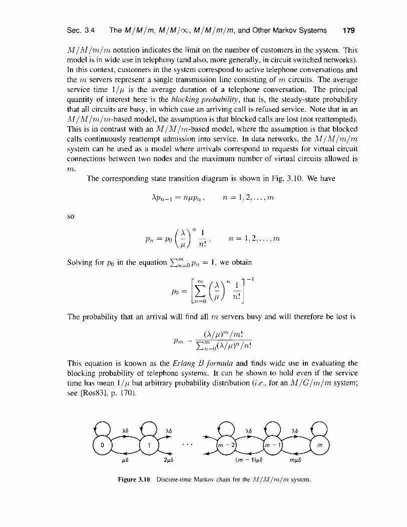
!v! /M /m/m notation indicates the limit on the number of customers in the system. Thismodel is in wide use in telephony (and also, more generally, in circuit switched networks).In this context, customers in the system correspond to active telephone conversations andthe m servers represent a single transmission line consisting of m circuits. The averageservice time 1/It is the average duration of a telephone conversation. The principalquantity of interest here is the blocking probability, that is, the steady-state probabilitythat all circuits are busy, in which case an arriving call is refused service. Note that in anM /M /m/m-based model, the assumption is that blocked calls are lost (not reattempted).This is in contrast with an M /M /m-based model, where the assumption is that blockedcalls continuously reattempt admission into service. In data networks, the !v! /M /m/msystem can be used as a model where arrivals correspond to requests for virtual circuitconnections between two nodes and the maximum number of virtual circuits allowed ism.
The corresponding state transition diagram is shown in Fig. 3.10. We have
so
Pn = Po n ,IL n.
n = 1,2, ... ,'m
n = 1,2, ... ,rn
Solving for Po in the equation Pn = I, we obtain
_ [Tn (A)n 1]-1Po - L It n!
n=O
The probability that an arrival will find all m servers busy and will therefore be lost is
This equation is known as the Erlang B formula and finds wide use in evaluating theblocking probability of telephone systems. It can be shown to hold even if the servicetime has mean 1/IL but arbitrary probability distribution (i.e., for an M /G/m/m system;see [Ros83], p. 170).
Figure 3.10 Discrete-time Markov chain for the M / M /m/m system.
180 Delay Models in Data Networks Chap. 3
3.4.4 Multidimensional Markov Chains-Applications in CircuitSwitching
We have considered so far queueing systems with a single type of customer where thestate can be described by the number of customers in the system. In some importantsystems there are several classes of customers, each with its own statistical characteristicsfor arrival and service, which cannot be lumped into a single class for the purpose ofanalysis. Here are some examples:
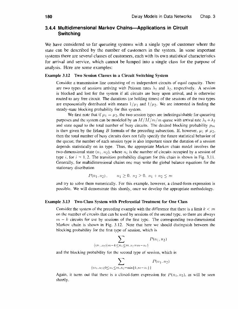
Example 3.12 Two Session Classes in a Circuit Switching SystemConsider a transmission line consisting of m independent circuits of equal capacity. Thereare two types of sessions arriving with Poisson rates )'1 and '\2, respectively. A sessionis blocked and lost for the system if all circuits are busy upon arrival, and is otherwiserouted to any free circuit. The durations (or holding times) of the sessions of the two typesare exponentially distributed with means 1//11 and 1//12' We are interested in finding thesteady-state blocking probability for this system.
We first note that if /11 = ti2, the two session types are indistinguishable for queueingpurposes and the system can be modeled by an Al/M / m/m queue with arrival rate .\ 1+.\2and state equal to the total number of busy circuits. The desired blocking probability pmis then given by the Erlang B formula of the preceding subsection. If, however, /11 =I=- /12,then the total number of busy circuits does not fully specify the future statistical behavior ofthe queue; the number of each session type is also important since the duration of a sessiondepends statistically on its type. Thus, the appropriate Markov chain model involves thetwo-dimensional state (nl_ 712), where ni is the number of circuits occupied by a session oftype i, for i = 1,2. The transition probability diagram for this chain is shown in Fig. 3.11.Generally, for multidimensional chains one may write the global balance equations for thestationary distribution
and try to solve them numerically. For this example, however, a closed-form expression ispossible. We will demonstrate this shortly, once we develop the appropriate methodology.
Example 3.13 Two-Class System with Preferential Treatment for One ClassConsider the system of the preceding example with the difference that there is a limit k < mon the number of circuits that can be used by sessions of the second type, so there are alwaysm - k circuits for use by sessions of the first type. The corresponding two-dimensionalMarkov chain is shown in Fig. 3.12. Note that here we should distinguish between theblocking probability for the first type of session, which is
P(71I,712)
and the blocking probability for the second type of session. which is
{(n"n2J!O:'On,:'Om,n2=min{k,m-n,} }
Again, it turns out that there is a closed-form expression for P( n I . n2), as will be seenshortly.

Sec. 3.4 The M/M/m, M/M/x, M/M/m/m, and Other Markov Systems 181
•
o 2
... Figure 3.11 Markov chain for thetwo-class queue of Example 3.12. Tosimplify the diagram. we do not showself-transitions and o(,s) transitions.
m -1 m5J11 mm-k
• • •
2
•
'-' -'-'-__-'-'-.... • • • • ..r- ..-/
o
2
Figure 3.t2 Markov chain for the two class queue with preferential treatment for oneclass (cf. Example 3.13). Self-transitions and 0(") transitions are not shown.
Multidimensional Markov chains usually involve K customer types. Their statesare of the form (71t. 712 • ...• 71K), where Tli is the number of customers of type i in thesystem. Such chains are usually harder to analyze than their one-dimensional counter-parts, but in many interesting special cases one can obtain a closed-form solution for the

182 Delay Models in Data Networks Chap. 3
stationary distribution P(T/j. n2 . .... nK). Important examples of properties that makethis possible are:
1. The detailed balance equations
AiP(nj ..... ni-I· ni. ni+j ..... nK) = /1iP(n I.···. ni-l. ni + I. ni+j····. nK)
hold for all pairs of adjacent states
and
where Ai and IIi are the arrival rate and service rate, respectively, of the customersof type i. These equations imply that the frequency of transitions between anytwo adjacent states is the same in both directions (see Appendix A). We willexplain in Section 3.7 that chains for which these equations hold are statisticallyindistinguishable when looked in forward and in reverse time, and for this reasonthey will be called reversible. Note that these equations hold for all the single-customer class systems discussed so far.
2. The stationary distribution can be expressed in product form, that is,
P(nl. n2 ..... nK) = P j(nl)P2(n2)'" PK(nK)
where for each i, Pi(ni) is an expression depending only on the number ni ofcustomers of type i. Several important types of networks of queues admit productform solutions, as will be seen in Section 3.8.
In this section we restrict ourselves to a class of multidimensional Markov chains,constructed from single-customer class systems using a process called truncation, forwhich we will see that both of the properties above hold.
Truncation of independent single-class systems. For a trivial exampleof a multidimensional Markov chain that admits a product form solution, consider Kindependent AlIAlI I queues. The number of customers in the i th queue has distribution
Pi(ni) = p;"(l - Pi)
whereAi
Pi =-/1;
Ai and /1i are the corresponding arrival and service rates, respectively, and we assumethat Pi < I for all i. Since the K queues are independent, we have the product form
P(nj. n2 . ...• nK) = P j (nj )P2(n2) ... PK(nK)
Note that the reasoning above would also apply if each of the M IMil queueswere replaced by a birth-death type of queue (two successive states can differ only bya single unit: for example, the M I1\llm, M IMIX), and M IM Imlm queues). Theonly requirement is that the queues are independent.
Sec. 3.4
•The M/M/m, M/M/x, M/M/m/m, and Other Markov Systems 183
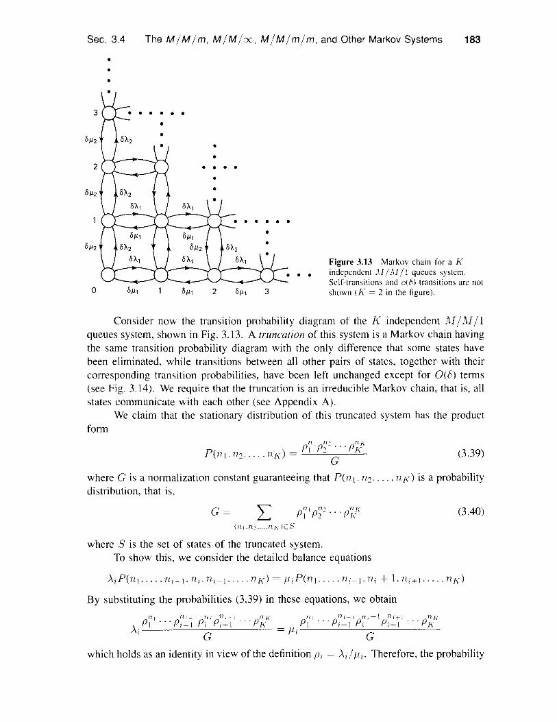
. . . Figure 3.13 Markov chain for a Kindependent M / M /1 queues system.Self-transitions and 0(6) transitions are notshown (K = 2 in the figure).
(3.39)
Consider now the transition probability diagram of the K independent AI/AI /1queues system, shown in Fig. 3.13. A truncation of this system is a Markov chain havingthe same transition probability diagram with the only difference that some states havebeen eliminated, while transitions between all other pairs of states, together with theircorresponding transition probabilities, have been left unchanged except for 0(8) terms(see Fig. 3.14). We require that the truncation is an irreducible Markov chain, that is, allstates communicate with each other (see Appendix A).
We claim that the stationary distribution of this truncated system has the productform
.. . p'l<KP(nl.n2 ..... nK) = -G
where G is a normalization constant guaranteeing that P(n I. n2 . ... , nK) is a probabilitydistribution, that is,
G = L p;ll p;12 .. ·llt(nl.n2, .... nKJES
where 5 is the set of states of the truncated system.To show this, we consider the detailed balance equations
(3.40)
AiP(n\ ..... ni-I. ni· ni+I.··.· nK) = /iiP(nl ..... ni-I' ni + 1. n,+! ..... nK)
By substituting the probabilities (3.39) in these equations, we obtain
G
nj ni-l rl-i rli ....... j .nKAPI ... Pi-I Pi P,+I ... PK
1 Gnl ... pn;-lpTli+lpTI;+1 ... pnKPI i-I I ,-;-1 K= /ii
which holds as an identity in view of the definition Pi = Ai / /ii. Therefore, the probability
184 Delay Models in Data Networks Chap. 3
distribution given by the expression (3.39) satisfies the detailed balance equations for thetruncated chain, so it must be its unique stationary distribution (see Appendix A).
It should be noted here that there is a generic difficulty with product form solutions.To obtain the stationary distribution, one needs to compute the normalization constantG of Eq. (3.40). For some systems, this involves a large amount of computation. Analternative to computing G directly from Eq. (3.40) is to approximate it using MonteCarlo simulation. Here, a fairly large number of independent samples of (n!, ... ,nK)are generated using the distribution
K
P(nt, ... , nK) = ITo - Pi)p7 i
i=l
and G is approximated by the proportion of samples that belong to the truncated spaceS. We will return to the computation of normalization constants in Section 3.8 in thecontext of queueing networks; see also Problem 3.51.
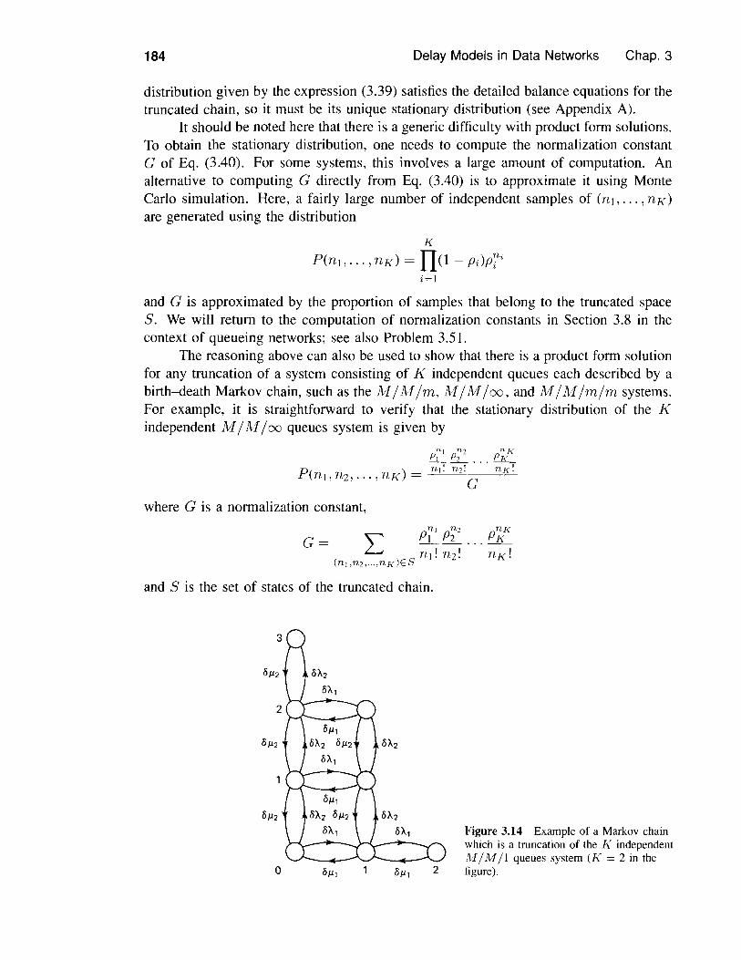
The reasoning above can also be used to show that there is a product form solutionfor any truncation of a system consisting of K independent queues each described by abirth-death Markov chain, such as the M/M/m, M/M/oo, and M/M/m/m systems.For example, it is straightforward to verify that the stationary distribution of the Kindependent M /M / 00 queues system is given by
where G is a normalization constant,
and S is the set of states of the truncated chain.
Figure 3.14 Example of a Markov chainwhich is a truncation of the K independentAIlM 11 queues system (K = 2 in thefigure).
Sec. 3.4 The M/M/m, M/M/=, M/M/m/m, and Other Markov Systems 185
Blocking probabilities for circuit switching systems. Using the productform solution (3.39), it is straightforward to write closed-form expressions for the block-ing probabilities of the circuit switching systems with two session classes of Examples3.12 and 3.13. The two-dimensional chains of these examples are truncations of the twoindependent M /M / 00 queues system (Figs. 3.11 to 3.13). Thus, in the case of Example3.13, the blocking probability for the first type of session is
The blocking probability for the second type of session is
The following important example illustrates the wide applicability of product formsolutions in circuit switching networks.
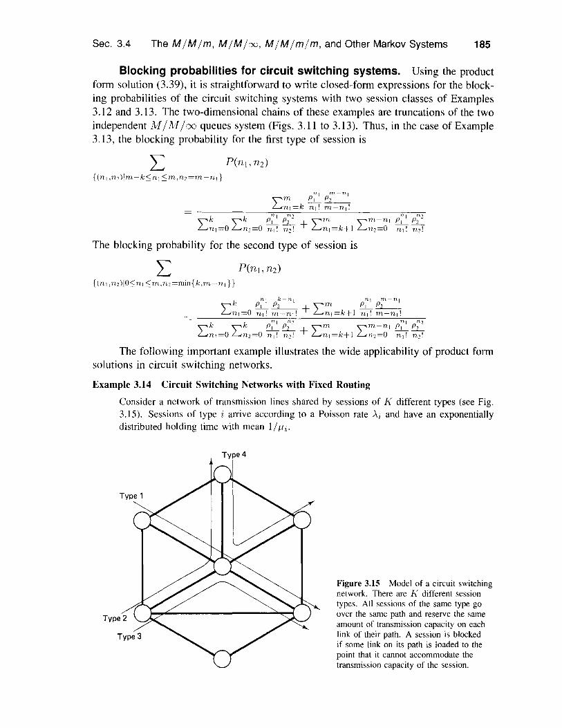
Example 3.14 Circuit Switching Networks with Fixed Routing
Consider a network of transmission lines shared by sessions of K different types (see Fig.3.15). Sessions of type i arrive according to a Poisson rate Ai and have an exponentiallydistributed holding time with mean IlfLi'
Type 4
Figure 3.15 Model of a circuit switchingnetwork. There are K different sessiontypes. All sessions of the same type goover the same path and reserve the sameamount of transmission capacity on eachlink of their path. A session is blockedif some link on its path is loaded to thepoint that it cannot accommodate thetransmission capacity of the session.
186 Delay Models in Data Networks Chap. 3
(3.41 )
(3.42)
We assume that all sessions of a given type i traverse the same set of network links(fixed routing) and reserve a fixed amount bi of transmission capacity at each link. Thus ifCj is the transmission capacity of a link j and I(j) is the set of session types using thislink, we must have
L bini::; C jiEI(j)
where ni is the number of sessions of type i in the network. A session of a given type mis blocked from entering the network (and is assumed lost to the system) if upon arrival itfinds that it cannot be accommodated due to insufficient link capacity, that is,
bm + L bini> CjiEI(j)
for some link j that the session must traverse.The quality of service of this system may be described by the blocking probabilities
for the different session types. To obtain these probabilities, we model the system as atruncation of the K independent AI/ 1'v[ / 00 queues system. The truncated chain is the sameas for the latter system, except that all states (n I , n2 , ... , nK) for which the inequalityLiEI(j) bini ::; C j is violated for some link j have been eliminated. The stationarydistribution has a product form, which yields the desired blocking probabilities.
A remarkable fact about the product form solution of this example is that it is validfor a broad class of holding time distributions that includes the exponential as a special case(see [BLL84] and [Kau81]).
3.5 THE MIG11 SYSTEM
Consider a single-server queueing system where customers arrive according to a Poissonprocess with rate A, but the customer service times have a general distribution-notnecessarily exponential as in the 1111Mil system. Suppose that customers are served inthe order they arrive and that Xi is the service time of the i th arrival. We assume thatthe random variables (XI, X 2 , .•. ) are identically distributed, mutually independent, andindependent of the interarrival times.
Let- IX = E{X} = - = Average service time
J1
X2 = E {X2} = Second moment of service time
Our objective is to derive and understand the Pollaczek-Khinchin (P-K) formula:
AX2w=---2(1 - p)
where W is the expected customer waiting time in queue and p = AIJ1 = AX. Giventhe P-K formula (3.41), the total waiting time, in queue and in service, is
T = X + AX22(1 - p)
Sec. 3.5 The M / G/1 System 187
Applying Little's fonnula to Wand T, we get the expected number of customers in thequeue NQ and the expected number in the system N:
>?X2NQ = 2(1 _ p)
,.\2 X2N=p+---
2(1 - p)
(3.43)
(3.44)
For example, when service times are exponentially distributed, as in the M / Ai /1 system,we have X2 = 2/J12, and the P-K fonnula (3.41) reduces to the equation (see Section3.3.2)
W= pJ1(1 - p)
(M/M/I)
When service times are identical for all customers (the M / D / I system, where D meansdetenninistic), we have X2 = 1/J12, and
(M/D/I) (3.45)
Since the M / D /1 case yields the minimum possible value of X2 for given J1, itfollows that the values ofW, T, NQ, and N for an M / D/I queue are lower bounds tothe corresponding quantities for an M / G /1 queue of the same ,.\ and J1. It is interestingto note that Wand NQ for the M / D /1 queue are exactly one half their values for theM /M /1 queue of the same ,.\ and J1. The values of T and N for M /D/1, on theother hand, range from the same as M /M /1 for small p to one half of M /M /1 as papproaches 1. The reason is that the expected service time is the same in the two cases,and for p small, most of the waiting occurs in service, whereas for p large, most of thewaiting occurs in the queue.
We provide a proof of the Pollaczek-Khinchin fonnula based on the concept ofthe mean residual service time. This same concept will prove useful in a number ofsubsequent developments. One example is Jlv1/G/1 queues with priorities. Another isreservation systems where part of the service time is occupied with sending packets (i.e.,serving customers), and part with sending control infonnation or making reservations forsending the packets.
Denote
Wi = Waiting time in queue of the ith customerR i = Residual service time seen by the ith customer. By this we mean that if
customer j is already being served when i arrives, R i is the remaining timeuntil customer j's service time is complete. If no customer is in service(i.e., the system is empty when i arrives), then R i is zero
Xi = Service time of the ith customerNi = Number of customers found waiting in queue by the ith customer upon arrival
188
We have
Delay Models in Data Networks
i-I
Wi=Ri + L X jj=i-N;
Chap. 3
By taking expectations and using the independence of the random variables Ni andXi-I, ... ,Xi - Ni , we have
Taking the limit as i ----+ 00, we obtain
IW = R+ -NQ
/1where
(3.46)
R = Mean residual time, defined as R = E{R;}.
In Eq. (3.46) (and throughout this section) all long-term average quantities should beviewed as limits when time or customer index increases to infinity. Thus, W, R, andNQ are limits (as i ----+ 00) of the average waiting time, residual time, and number foundin queue, respectively, corresponding to the i th customer. We assume that these limitsexist, and this is true of almost all systems of interest to us provided that A < /1. Notethat in the waiting time equation (3.46), the average number in queue NQ and the meanresidual time R as seen by an arriving customer are also equal to the average numberin queue and mean residual time seen by an outside observer at a random time. Thisis due to the Poisson character of the arrival process, which implies that the occupancydistribution upon arrival is typical (see Section 3.3.2).
By Little's Theorem, we have
and by substitution in the waiting time formula (3.46), we obtain
W = R+pW (3.47)
(3.48)
where p = AI/1 is the utilization factor; so, finally,
I-p
We can calculate R by a graphical argument. In Fig. 3.16 we plot the residualservice time reT) (i.e., the remaining time for completion of the customer in service attime T) as a function of T. Note that when a new service of duration X begins, reT)starts at X and decays linearly for X time units. Consider a time t for which ret) = O.The time average of reT) in the interval [0, t] is
1 i· t I M(t) I 2- r(T) dT = - " - Xt t 2 'o ;=1
(3.49)
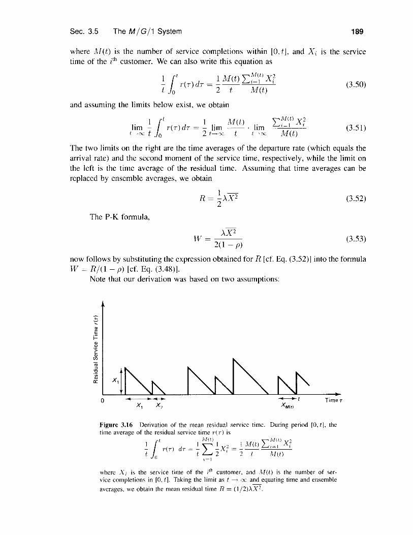
Sec. 3.5 The MIG11 System 189
where M(t) is the number of service completions within lO, tJ, and Xi is the servicetime of the i th customer. We can also write this equation as
(3.50)
(3.51)
and assuming the limits below exist, we obtain
. I it I . M(t) . X 2hm - reT) dT = - hm hm I-I I
t 0 2 t M(t)
The two limits on the right are the time averages of the departure rate (which equals thearrival rate) and the second moment of the service time, respectively, while the limit onthe left is the time average of the residual time. Assuming that time averages can bereplaced by ensemble averages, we obtain
(3.52)
(3.53)
The P-K formula,
AX220 - p)
now follows by substituting the expression obtained for R lcf. Eq. (3.52)J into the formulaW = RiO - p) lcf. Eq. (3.48)J.
Note that our derivation was based on two assumptions:
-;::--.:'"Ei='"u'"(/)'":::J"0a: X,
o TimerX,
Figure 3.16 Derivation of the mean residual service time. During period [0, t], thetime average of the residual service time T(r) is
1t kIlt) ",M(t) 2T(r) dr = = M(t) L....i=! X,tot L 2' 2 t M(t)
1=1
where X, is the service time of the i th customer, and 1\1(t) is the number of ser-vice completions in [0, t]. Taking the limit as t -t 00 and equating time and ensembleaverages, we obtain the mean residual time R = (I /2»"X2.
190 Delay Models in Data Networks Chap. 3
1. The existence of the steady-state averages TF, R, and NQ
2. The equality (with probability one) of the long-tenn time averages appearing inEq. (3.51) with the corresponding ensemble averages
These assumptions can be justified by careful applications of the law of largenumbers, but the details are beyond the scope of this book. However, these are naturalassumptions for the systems of interest to us, and we will base similar derivations ongraphical arguments and interchange of time averages with ensemble averages withoutfurther discussion.
One curious feature of the P-K fonnula (3.53) is that an 1'11/G / I queue can havep < I but infinite W if the second moment X 2 is x. What is happening in this caseis that a small fraction of customers have incredibly long service times. When one ofthese customers is served, an incredible number of arrivals are queued and delayed by asignificant fraction of that long service time. Thus, the contribution to W is proportionalto the square of the service time, leading to an infinite W if X2 is infinite.
The derivation of the P-K fonnula above assumed that customers were served inorder of arrival, that is, that the number of customers served between the i th arrival andservice is just the number in queue at the i th arrival. It turns out, however, that thisfonnula is valid for any order of servicing customers as long as the order is detenninedindependently of the required service time. To see this, suppose that the i th and ph
customers are both in the queue and that they exchange places. The expected queueingtime of customer i (over the service times of the customers in queue) will then beexchanged with that for customer j, but the average, over all customers, is unchanged.Since any service order can be considered as a sequence of reversals in queue position,the P-K fonnula remains valid (see also Problem 3.32).
To see why the P-K fonnula is invalid if the service order can depend on servicetime, consider a queue with two customers requiring 10 and I units of service time,respectively. Assuming that the server becomes available at time 0, serving the firstcustomer first results in one customer starting service at time 0 and the other at time 10.Serving the second customer first results in one customer starting at time 0 and the otherat time I. Thus, the average queueing time over the two customers is 5 in the first caseand 0.5 in the second case. Clearly, queueing time is reduced by serving customers withsmall service time first. For this situation, the derivation of the P-K fonnula breaks downat Eq. (3.46) since the customers that will be served before a newly arriving customerno longer have a mean service time equal to 1/Ji.
Example 3.15 Delay Analysis of an ARQ SystemConsider a go back TI ARQ system such as the one discussed in Section 2.4. Assume thatpackets are transmitted in frames that are one time unit long, and there is a maximum waitfor an acknowledgment of n - I frames before a packet is retransmitted (see Fig. 3.17). Inthis system packets are retransmitted for two reasons:
1. A given packet transmitted in frame i might be rejected at the receiver due to errors,in which case the transmitter will transmit packets in frames i+ I, i +2..... i +n - I,(if any are available), and then go back to retransmit the given packet in frame i+ n.
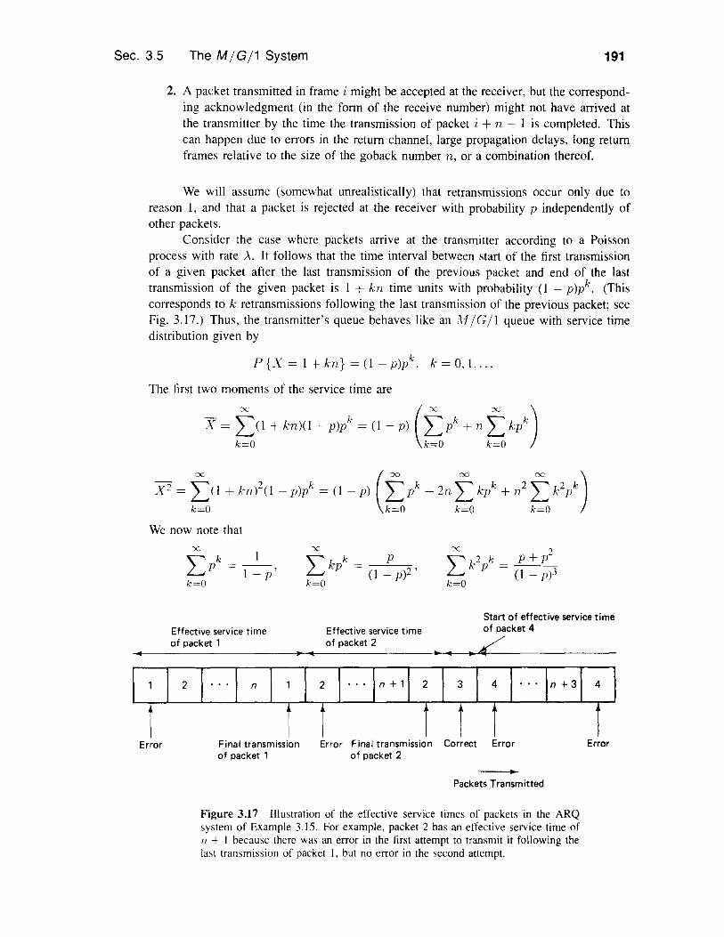
Sec. 3.5 The MIG11 System 191
2. A packet transmitted in frame i might be accepted at the receiver, but the correspond-ing acknowledgment (in the form of the receive number) might not have arrived atthe transmitter by the time the transmission of packet i + n - I is completed. Thiscan happen due to errors in the return channel, large propagation delays, long returnframes relative to the size of the goback number n, or a combination thereof.
We will assume (somewhat unrealistically) that retransmissions occur only due toreason I, and that a packet is rejected at the receiver with probability p independently ofother packets.
Consider the case where packets arrive at the transmitter according to a Poissonprocess with rate .\. It follows that the time interval between start of the first transmissionof a given packet after the last transmission of the previous packet and end of the lasttransmission of the given packet is I + kn time units with probability (I - p)pk. (Thiscorresponds to k retransmissions following the last transmission of the previous packet; seeFig. 3.17.) Thus, the transmitter's queue behaves like an MIGII queue with service timedistribution given by
kP{X=I+kn}=(l-p)p, k=O.I. ...
The first two moments of the service time are
x (X X)
x (00 00 00)- 2 k k k 2 2k=(l-p) +n
We now note thatX
,",pk = _1_,I-p
k=O
X
'"'kk __P_P - (I _ )2'
k=O P
Effective service timeof packet 1
Effective service timeof packet 2
,. II .. 'II
Start of effective service timeof packet 4
Error Final transmissionof packet 1
Error Final transmission Correct Errorof packet 2 -Packets Transmitted
Error
Figure 3.17 Illustration of the effective service times of packets in the ARQsystem of Example 3.15. For example, packet 2 has an effective service time ofn + 1 because there was an error in the first attempt to transmit it following thelast transmission of packet 1. but no error in the second attempt.

192 Delay Models in Data Networks Chap. 3
(The first sum is the usual geometric series sum, while the other two sums are obtained bydifferentiating the first sum twice.) Using these formulas in the equations for X and X2above, we obtain
I-p
X2 _ I + 2np + n2(p + p")
- 1 - p (I - p)2
The P-K formula gives the average packet time in queue and in the system (up to the endof the last transmission):
T=X+W
3.5.1 M / G/1 Queues with Vacations
Suppose that at the end of each busy period, the server goes on "vacation" for somerandom interval of time. Thus, a new arrival to an idle system, rather than going intoservice immediately, waits for the end of the vacation period (see Fig. 3.18). If thesystem is still idle at the completion of a vacation, a new vacation starts immediately.For data networks, vacations correspond to the transmission of various kinds of controland record-keeping packets when there is a lull in the data traffic; other applications willbecome apparent later.
Let VI, V2 , be the durations of the successive vacations taken by the server. Weassume that VI. Y2 are independent and identically distributed (lID) random variables,also independent of the customer interarrival times and service times. As before, thearrivals are Poisson and the service times are lID with a general distribution. A newarrival to the system has to wait in the queue for the completion of the current service orvacation and then for the service of all the customers waiting before it. Thus, the waitingtime formula TV = R/O - p) is still valid [cf. Eq. (3.48)], where now R is the meanresidual time for completion of the service or vacation in process when the i th customerarrives.
The analysis of this new system is the same as that of the P-K formula except thatvacations must be included in the graph of residual service times r(T) (see Fig. 3.19).Let Al(t) be the number of services completed by time t and L(t) be the number ofvacations completed by time t. Then [as in Eq. (3.49)], for any t where a service orvacation is just completed, we have
! r r T dT _ ! M(I) ! X2 + ! L. (I) ! V 2 _ M.(t) 1xl + L(.t) v,2t./o () - t I: 2 i t I: 2 i - t M(t) t L(t)
1=1 ,=1(3.54)
As before, assuming that a steady-state exists, Ivl(t)/t approaches A with increasingt, and the first term on the right side of Eq. (3.54) approaches AX2/2 as in the derivation
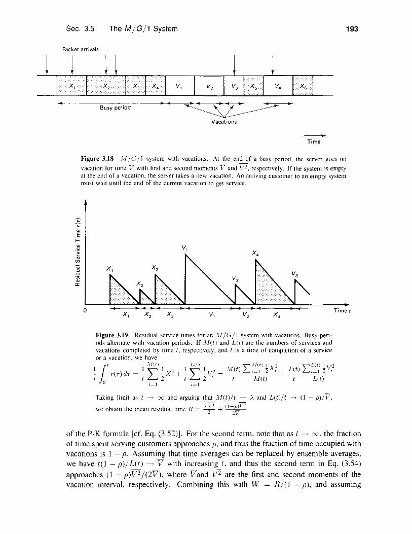
Sec. 3.5
Packet arrivals
..
The MIG/1 System
Busy period
Vacations
-------Time
193
Figure 3.18 AIIG11 system with vacations. At the end of a busy period. the server goes onvacation for time V with first and second moments V and V2, respectively. If the system is emptyat the end of a vacation, the server takes a new vacation. An arriving customer to an empty systemmust wait until the end cif the current vacation to get service.
-;::-COJEi=OJu
OJr.tl
'":J'0
a:
v,
o TimeT
Figure 3.19 Residual service times for an MIGI I system with vacations. Busy peri-ods alternate with vacation periods. If AI(t) and L(t) are the numbers of services andvacations completed by time t, respectively, and t is a time of completion of a serviceor a vacation, we have
t M(t) L(t) "" ,\lit)!) ""L(t)])1r T)dT = ""'. + ""' = M(t) L..,=! 2: X ; + L(t) L..i=t 2:v,-t 0 ( t 2 1 t 2 1 t lvf(t) t L(t)
1=1 1=1
Taking limit as t ---+ CXJ and arguing that 1\!I(t)lt ---+ A and L(t)lt ---+ (I - p)/V.we obtain the mean residual time R = A'i' +
of the P-K formula [cf. Eq. (3.52)]. For the second term, note that as t ----+ x, the fractionof time spent serving customers approaches p, and thus the fraction of time occupied withvacations is 1 - p. Assuming that time averages can be replaced by ensemble averages,we have to - p)1L(t) ----+ V with increasing t, and thus the second term in Eq. (3.54)approaches (1 - p)V2 I (2V), where Vand V2 are the first and second moments of thevacation interval, respectively. Combining this with W = RI(1 - p), and assuming

194 Delay Models in Data Networks Chap. 3
(3.55)
(3.56)
equality of the time and ensemble averages of R, we get
),X2 V2w= +---=2(1 - p) 2V
as the expected waiting time in queue for an !vI /G/ I system with vacations.If we look carefully at the derivation of the preceding equation, we see that the
mutual independence of the vacation intervals is not required (although the time andensemble averages of the vacation intervals must still be equal) and the length of avacation iAt!n'al need not be independent of the",customer arrival and service times.Naturally, with this kind of dependence, it becomes more difficult to calculate V andV2, as these quantities might be functions of the underlying !vI /G /1 process.
Example 3.16 Frequency- and Time-Division Multiplexing on a Slot BasisWe have m traffic streams of equal-length packets arriving according to a Poisson processwith rate Aim each. If the traffic streams are frequency-division multiplexed on m sub-channels of an available channel, the transmission time of each packet is m time units.Then, each subchannel can be represented by an Af IDI I queueing system and the MIDI Iformula W = pI(2f1(1 - p» [cf. Eq. (3.45)] with p = A, /1 = 11m, gives the averagequeueing delay per packet,
W _ AmFDM - 2(1 - A)
Consider the same FOM scheme with the difference that packet transmissions canstart only at times m, 2m, 3m, . .. (i.e., at the beginning of a slot of rn time units). We callthis scheme slotted ji"equency-division multiplexing (SFOM), and note that it can be viewedas an l\if ID I I queue with vacations. When there are no packets in the queue for a givenstream at the beginning of a slot, the server takes a vacation for one slot, or m time units.Thus, 17 = m, V 2 = Tn
2, and the vacation system waiting time formula (3.55) becomes
WSFDM = W FDM + r; (3.57)
(3.58)
Finally, consider the case where the m traffic streams are time-division multiplexedin a scheme whereby the time axis is divided in Tn-slot frames with one slot dedicated toeach traffic stream (see Fig. 3.20). Each slot is one time unit long and can carry a singlepacket. Then, if we compare this TOM scheme with the SFOM scheme, we see that thequeue for a given stream in TOM is precisely the same as the queue for SFOM, and
WTDM = W SFDM = W FDM + ; = 2(1r: A)If we now look at the total delay for TOM, we get a different picture, since the service
time is I unit of time rather than Tn units as in SFOM. By adding the service times to thequeueing delays, we obtain
AmTFDM = m + 2(1 _ A)
rnTSFDY! = TFDM + :2
Tn. (Tn)TTDY! = 1+ 2(1 _ A) = TFDM - :2 - I (3.59)

Sec. 3.5 The M / G/1 System 195
Stream 1 Stream 2 Stream 3 Stream 4
--,--IttM-'-------'--...l...----..!-1-!--I__.I. Framek .1_. t
Frame (k + 1)One time unit per slot
Figure 3.20 TOM with m = 4 traffic streams.
Thus, the customer's average total delay is more favorable in TDM than in FDM (assumingthat In > 2). The longer average waiting time in queue for TDM is more than compensatedby the faster service time. Contrast this with the Example 3.9, which treats TDM withslots that are a very small portion of the packet size. Problem 3.33 outlines an altemativeapproach for deriving the TDM average delay.
3.5.2 Reservations and Polling
Organizing transmissions from several packet streams into a statistical multiplexing sys-tem requires some form of scheduling. In some cases, this scheduling is naturally andeasily accomplished; in other cases, however, some form of reservation or polling systemis required.
Situations of this type arise often in multiaccess channels, which will be treatedextensively in Chapter 4. For a typical example, consider a communication channel thatcan be accessed by several spatially separated users; however, only one user can transmitsuccessfully on the channel at anyone time. The communication resource of the channelcan be divided over time into a portion used for packet transmissions and another portionused for reservation or polling messages that coordinate the packet transmissions. In otherwords, the time axis is divided into data intervals, where actual data are transmitted, andreservation intervals, used for scheduling future data. For uniform presentation, we usethe term "reservation" even though "polling" may be more appropriate to the practicalsituation.
We will consider Tn traffic streams (also called users) and assume that each datainterval contains packets of a sinfile user. Reservations for these packets are made in theimmediately preceding reservation interval. All users are taken up in cyclic order (seeFig. 3.21). There are several versions of this system differing in the rule for decidingwhich packets are transmitted during the data interval of each user. In the fiated system,the rule is that only those packets that arrived prior to the user's preceding reservationinterval are transmitted. By contrast, in the exhaustive system, the rule is that all availablepackets of a user are transmitted during the corresponding data interval, including thosethat arrived in this data interval or the preceding reservation interval. An intermediateversion, which we call the partially fiated system, results when the packets transmitted ina user's data interval are those that arrived up to the time this data interval began (and thecorresponding reservation interval ended). A typical example of such reservation systems

196
.. 7 t3
Delay Models in Data Networks
2
-Time
Chap. 3
Reservation and data Reservation and data Reservation and dataintervals for user 1 intervals for user 2 intervals for user 3
Transmission intervalfor user 1
I.. -IArrival interval for user 1 in an exhaustive system
Arrival interval for user 1 in a partially gated system
Arrival interval for user 1 in a gated system
Packets arriving in the arrival interval shown aretransmitted in the transmission interval shown
Reservation intervals
Figure 3.21 Reservation or polling system with three users. In the exhaustive version,a packet of a user that arrives during the user's reservation or data interval is transmittedin the same data interval. In the partially gated version. a packet of a user arriving duringthe user's data interval must wait for an entire cycle and be transmitted during the nextdata mterval of the user. In the fully gated version, packets arriving during the user'sreservation interval must also wait for an entire cycle. The figure shows, for the threesystems, the association between the interval in which a packet arrives and the intervalin which the packet is transmitted.
is one of the most common local area networks, the token ring. The users are connectedby cable in a unidirectional loop. Each user transmits the current packet backlog, thengives the opportunity to a neighbor to transmit, and the process is repeated. (A moredetailed description of the token ring is given in Chapter 4.)
We assume that the arrival processes of all users are independent Poisson withrate A/m, and that the first and second moments of the packet transmission times areX = 1/11 and X2, respectively. The utilization factor is p = A/Jl. Interarrival timesand transmission times are, as usual, assumed independent. While we assume that allusers have identical arrival and service statistics, we allow the reservation intervals ofdifferent users to have different statistics.
Single-user system. Our general line of analysis of reservation systems canbe better understood in tenns of the special case where m = I, so we consider thiscase first. We may also view this as a system where all users share reservation and dataintervals. Let Vp be the duration of the fth reservation interval and assume that successivereservation intervals are independent and identically distributed random variables withfirst and second moments V and V2, respectively. We consider a gated system and

Sec. 3.5 The M / G/1 System 197
(3.60)
assume that the reservation intervals are statistically independent of the arrival timesand service durations. Finally, for convenience of exposition, we assume that packetsare transmitted in the order of their arrival. As in our derivation of the P-K formula,expected delays and queue lengths are independent of service order as long as serviceorder is independent of service requirement (i.e., packet length).
Consider the i th data packet arriving at the system. This packet must wait in queuefor the residual time Hi until the end of the current packet transmission or reservationinterval. It must also wait for the transmission of the Ni packets currently in the queue(this includes both packets for which reservations were already made in the last reserva-tion interval and earlier arrivals waiting to make a reservation). Finally, the packet mustwait during the next reservation interval vt(i), say, in which its reservation will be made(see Fig. 3.22). Thus, the expected queueing delay for the i th packet is given by
E{Wd = E{R i } + E{Nd + E{vt(i)}f1
The similarity of this reservation system to the Al/G/1 queue with vacations shouldbe noted. The only difference is that in the gated reservation system, a reservation intervalstarts when all packets that arrived prior to the start of the preceding reservation intervalhave been served, whereas in the vacation system, a vacation interval starts when allarrivals up to the current time have been served and the system is empty. (Thus inthe gated reservation system, every packet has to wait in queue for a full reservationinterval, while in the vacation system, only the packets that find the system empty uponarrival have to wait for part of a vacation interval. Note that the exhaustive version ofthis reservation system is equivalent to the vacation system.) The time-average meanresidual time for the two systems is the same (the calculation based on Fig. 3.19 stillapplies) and is given by AX2/2 + (l - p)V2 /2V. The value of Iimi_:>0 E {Nd / f1 ispW in both systems, and finally the value of E{VC(i)} is just V. Thus, from
Waiting time in queue W;
Arrival timeof ith packet
Residual Waiting timetime R; for N, packets
ahead of packeti in queue
Transmissionof ith packetstarts
Transm iss ionReservation of ith packetinterval V,U! ends
'-Time
Figure 3.22 Calculation of the average waiting time in the single-user gated system.The expeeted waiting time E {W,} of the ,til packet is
" E{NdE{H/,} = E{Ild + -- +E{ViI,dII
198 Delay Models in Data Networks Chap. 3
(single user, gated)
Eq. (3.60) the expected time in queue for the single-user reservation system is
..\X2 V2 VW= +-=+--20 - p) 2V 1 - P
(3.61 )
(3.62)
(3.63)
(3.64)
In the common situation where the reservation interval is a constant A, this simplifies to
w _ ..\X2 +.:'! (3 -p)20 - p) 2 1 - P
There is an interesting paradox associated with the waiting time formula (3.61).We have seen that a fraction 1 - P of time is used on reservations. Since there is onereservation interval of mean duration V per cycle, we can conclude that the expectedcycle length must be V10 - p) (see also Example 3.6). The mean queueing delay inEq. (3.61) can be an arbitrarily large multiple of this mean cycle length, which seemsparadoxical since each packet is transmitted on the cycle following its arrival. Theexplanation of this is that more packets tend to arrive in long cycles than in short cycles,and thus mean cycle length is not representative of the cycle lengths seen by arrivingpackets; this is the same phenomenon that makes the mean residual service time used inthe P-K formula derivation larger than one might think (see also Problem 3.31).
Multiuser system. Suppose that the system has m users, each with independentPoisson arrivals of rate ..\Im. Again X and X2 are the first two moments of the servicetime for each user's packets. We denote by Vi and V?' respectively, the first two momentsof the reservation intervals of user i. The service times and reservation intervals are allindependent. We number the users 0, 1, ... , m - I and assume that the eth reservationinterval is used to make reservations for user emod m and the subsequent (£th) datainterval is used to send the packets corresponding to those reservations.
Consider the i th packet arrival into the system (counting packets in order of arrival,regardless of user). As before, the expected delay for this packet consists of three terms:first, the mean residual time for the packet or reservation in progress; second, the expectedtime to transmit the number Ni of packets that must be transmitted before packet i; andthird, the expected duration of reservation intervals (see Fig. 3.23). Thus,
E{Wd = E{Rd + E{N;} + E{Yi }f1
where Y; is the duration of all the whole reservation intervals during which packet imust wait before being transmitted. The time average mean residual time is calculatedas before, and is given by
..\X2 0 - ) ,\,,:,-1 \;;2R = __ + p L.t=o t2 2 ,\,m-l V
L.bO f
The number of packets N i that i must wait for is not equal to the number already inqueue, but the order of serving packets is independent of packet service time; thus,each packet served before i still has a mean transmission time 1I f1 as indicated inEq. (3.63) and by Little's formula, the value of E{ N;} I f1 is pW as before.
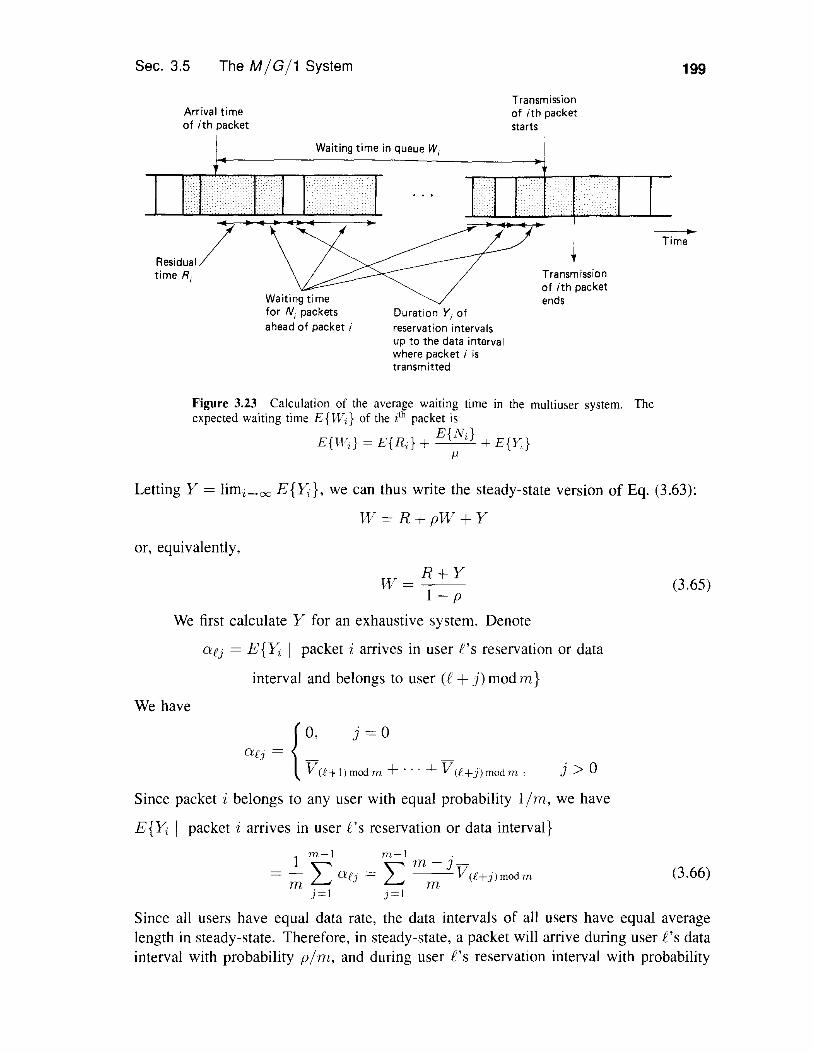
Sec. 3.5 The MIG11 System 199
Arrival timeof ith packet
Transmissionof ith packetstarts
Waiting time in queue Wi
..Residual/time Ri
Waiting timefor Ni packetsahead of packet i
Duration Yi ofreservation intervalsup to the data intervalwhere packet i istransm itted
Transm issionof ith packetends
-Time
Figure 3.23 Calculation of the average waiting time in the multiuser system. Theexpected waiting time E{Wi } of the ith packet is
E{N}E{W,} = E{R;} + __i + E{Y,}J1
Letting Y = limi_oo E{Y;}, we can thus write the steady-state version of Eq. (3.63):
W=R+pW+Yor, equivalently,
W=R+YI-p
We first calculate Y for an exhaustive system. Denote
aij = E {Y; I packet i arrives in user f's reservation or data
interval and belongs to user (t + j) mod m}We have
{
0, j = 0aij =
V(£+I) mod m + ... + V(f+j) mod m , j > 0Since packet i belongs to any user with equal probability 11m, we have
E{Y; I packet i arrives in user t's reservation or data interval}
(3.65)
1 m-l= - L aij =m
j=1
m-l .'" m-J----V(£+j)modmmj=1
(3.66)
Since all users have equal data rate, the data intervals of all users have equal averagelength in steady-state. Therefore, in steady-state, a packet will arrive during user f's datainterval with probability plm, and during user f's reservation interval with probability

200 Delay Models in Data Networks Chap. 3
(1 - p) V £/ V k). Using this fact in Eq. (3.66), we obtain the following equationfor Y = E{Yi }:
m-lm-l .
--V£V<£+j)modrnTn
£=0 j=l
(3.67)
The last sum above can be written
m-lm-l. I--V£V(£+j)modm = -2rn
£=0 j=l
(To see this, note that the right side above is the sum of all possible products V £V £' fore-I e. The left side is the sum of all possible terms (j / rn)V £V t' and [( rn - j) / rn]V £V£"where j = It - el and t -I e.) Using this expression, and denoting
m-l-V = - V£
rn£=0
as the reservation interval averaged over all users, we can write Eq. (3.67) as- - m 1-2
Y = pV(rn - I) + (1 - p)rnV _ (1 - p) V£2 2 2rnV
(rn - p)V2
",m-l -2(I - p) L-t=o V£
2rnV(3.68)
Combining Eqs. (3.64), (3.65), and (3.68), we obtain
,\X2 (rn _ p)V (-Vl-w= + +----'--=------'---2(I-p) 2(1-p) 2rnV
Denoting
",m-l (V2 _v2)L-£=o £ £
rnas the variance of the reservation intervals averaged over all users, we finally obtain
(3.69)(exhaustive)w = ,\X2 + (rn - p)V +2(1 - p) 2(1 - p) 2V
The partially gated system is the same as the exhaustive except that if a packet ofa user arrives during a user's own data interval (an event of probability p/rn in steady-state), it is delayed by an additional rnV, the average sum of reservation intervals in a
Sec. 3.5 The M / G/1 System 201
(3.71 )(gated)
cycle. Thus, Y is increased by pV in the preceding calculation, and we obtain
"'X2 (rn + p)V a'v"W = + + ---= (partially gated) (3 70)2(1 - p) 2(1 - p) 2V .
Consider, finally, the fully gated system. This is the same as the partially gatedsystem except that if a packet of a user arrives during a user's own reservation interval[an event of probability (I - p)/m in steady-state], it is delayed by an additional mV.This increases Y by an additional (I - p)V and results in the equation
W = "'X2 + (rn + 2 - p)V +2(1 - p) 2(1 - p) 2V
(3.74)
(3.72)
(3.73)
(gated)
(exhaustive)
(partially gated)
In comparing these results with the single-user system, consider the case wherethe reservation interval is a constant A/m. Thus, A is the overhead or reservationtime for an entire cycle of reservations for each user, which is usually the appropriateparameter to compare with A in the single-user waiting-time formula (3.62). We thenhave (V = A/m. = 0)
"'X2 A(I- p/m)W= +-2(1 - p) 2 I - P
W = "'Xl + (1 + p/m)2(1-p) 2 I-p
W = "'Xl + (I + (2 - p)/rn)2(1 - p) 2 1 - P
It can be seen that delay is somewhat reduced in the multiuser case; essentially,packets are delayed by roughly the same amount until the reservation time in all cases,but delay is quite small after the reservation in the multiuser case.
Limited service systems. We now consider a variation of the multiuser systemwhereby, in each user's data interval, only the first packet of the user waiting in queue(if any) is transmitted (rather than all waiting packets). We concentrate on the gated andpartially gated versions of this system, since an exhaustive version does not make sense.As before, we have
E{N}E{W;} = E{R;} + --' + E{Yi }
11
and by taking the limit as i -+ x, we obtain
W=R+pW+Y (3.75)
Here R is given by Eq. (3.64) as before. To calculate the new formula for Y for thepartially gated system, we argue as follows. A packet arriving during user fi's dataor reservation interval will belong to anyone of the users with equal probability 1/m.Therefore, in steady-state, the expected number of packets waiting in the queue of the userthat owns the arriving packet, averaged over all users, is limi_x E{Ni}/m = "'vV' /m.

202 Delay Models in Data Networks Chap. 3
Each of these packets causes an extra cycle of reservations mV, so Y is increased byan amount .A.WV. Using this fact in Eq. (3.75), we see that
R+YW=------=
1-p-AV
where Y is the value of Y obtained earlier for the partially gated system without thesingle-packet-per-data-interval restriction. Equivalently, we see from Eq. (3.65) that thesingle-packet-per-data-interval restriction results in an increase of the average waitingtime for the partially gated system by a factor
1-p1 - P - AV
Using this fact in Eq. (3.70), we obtain
AX2 (m + p)V - p)W= +
2(1-p-AV) 2(1-p-AV) 2V(1-p-.A.V)
(limited service, partially gated) (3.76)
Consider now the gated version. 1"; is the same as for the partially gated systemexcept for an additional cycle of reservation intervals of average length mV associatedwith the event where packet i arrives during the reservation interval of its owner, and thesubsequent data interval is empty. It is easily verified (Problem 3.34) that the latter eventoccurs with steady-state probability (1 - p - AV)/m. Therefore, for the gated system Yequals the corresponding value for the partially gated system plus (1 - p - AV)V. Thisadds V to the value of W for the partially gated system, and the average waiting timenow is
AX2 (m + 2 - p - 2AV)V - p)W = + +
2(1-p-AV) 2(l-p-AV) 2V(1-p-AV)
(limited service, gated) (3.77)
Note that it is not enough that p = AIf1 < 1 for W to be bounded; rather,p + AV < 1 is required or, equivalently,
.A. (* +V) < 1
This is due to the fact that each packet requires a separate reservation interval of averagelength V, thereby effectively increasing the average transmission time from 1I f1 to 1I f1 +V.
As a final remark, consider the case of a very large number of users m and avery small average reservation interval V. An examination of the equation given forthe average waiting time W of every multiuser system considered so far shows that asm --> 00, V --> 0, IV --> 0, and mV --> A, where A is a constant, we have
AX2 AM-' --> + -,,-----
2(1 - p) 2(1 - p)
Sec. 3.5 The M IG/1 System 203
It can be shown (see Example 3.6) that AI(l - p) is the average length of a cycle (msuccessive reservation and data intervals). Thus, W approaches the AI10I I averagewaiting time plus one half the average cycle length.
3.5.3 Priority Queueing
Consider the M 10I I system with the difference that arriving customers are dividedinto n different priority classes. Class I has the highest priority, class 2 has the secondhighest, and so on. The arrival rate and the first two moments of service time of eachclass k are denoted Ak, X k = I II1k, and Xl.:, respectively. The arrival processes of allclasses are assumed independent, Poisson, and independent of the service times.
Nonpreemptive priority. We first consider the nonpreemptive priority rulewhereby a customer undergoing service is allowed to complete service without inter-ruption even if a customer of higher priority arrives in the meantime. A separate queueis maintained for each priority class. When the server becomes free, the first customerof the highest nonempty priority queue enters service. This priority rule is one of themost appropriate for modeling packet transmission systems.
We will develop an equation for average delay for each priority class, which issimilar to the P-K formula and admits a similar derivation. Denote
= Average number in queue for priority k
Wk = Average queueing time for priority k
Pk = Akll1k = System utilization for priority k
R = Mean residual service timeWe assume that the overall system utilization is less than I, that is,
PI + P2 + ... + Pn < I
When this assumption is not satisfied, there will be some priority class k such that theaverage delay of customers of priority k and lower will be infinite while the averagedelay of customers of priority higher than k will be finite. Problem 3.39 takes a closerlook at this situation.
As in the derivation of the P-K formula given earlier, we have for the highest-priority class,
WI111
Eliminating N¢ from this equation using Little's Theorem,
Nb=AIW1
we obtain

204
and finally,
Delay Models in Data Networks Chap. 3
(3.79)
RWI = -- (3.78)
1 - PI
For the second priority class, we have a similar expression for the queueing delayW2 except that we have to count the additional queueing delay due to customers ofhigher priority that arrive while a customer is waiting in queue. This is the meaning ofthe last term in the formula
• 1 1 I 2 1= R+ -NQ + -NQ + -)qW2fJl fJ2 fJl
Using Little's Theorem = AkWk), we obtain
W2 = R + PI WI + P2W2+ PI W2
which yields
W2 = R+PIW1
I - PI - P2
Using the expression WI = RI(1 - PI) obtained earlier, we finally have
TXT _ RvV2 -
(1 - p])(1 - PI - P2)
The derivation is similar for all priority classes k > I. The formula for the waitingtime in queue is
W. _ Rk- (1 - PI - ... - Pk-l)(1 - PI - ... - P"J
The average delay per customer of class k is
Tk = +W k (3.80)fJk
The mean residual service time R can be derived as for the P-K formula (compare withFig. 3.16). We have
In _R = - '" AX2
2 L.. ' ,i=1
(3.81 )
(3.82)
(3.83)
The average waiting time in queue and the average delay per customer for each class isobtained by combining Eqs. (3.79) to (3.81):
2::n AX2VVk = i=1 1 i
2(1 - PI - ... - Pk-I)(1- PI - ... - Pk)
Tk = +WkfJk
The analysis given above does not extend easily to the case of multiple servers,primarily because there is no simple formula for the mean residual time R. If, however,

Sec. 3.5 The M /G/1 System 205
the service times of all priority classes are identically and exponentially distributed,there is a convenient characterization of R. Equation (3.79) then yields a closed-formexpression for the average waiting times Wk (see Problem 3.38).
Note that it is possible to affect the average delay per customer by choosing thepriority classes appropriately. It is generally true that average delay tends to be reducedwhen customers with short service times are given higher priority. (For an examplefrom common experience, consider the supermarket practice of having special checkoutcounters for customers with few items. A similar situation can be seen in copyingmachine waiting lines, where people often give priority to others who need to make justa few copies.) For an analytical substantiation, consider a nonpreemptive system andtwo customer classes A and B, with respective arrival and service rates AA, {LA, andAB, ILn. A straightforward calculation using the formulas above shows that if {LA > {LB,then the average delay per customer (averaged over both classes)
T = AATA + AnTsAA +AB
is smaller when A is given priority over B than when B is given priority over A. Forrelated results, see Problem 3.40.
Preemptive resume priority. One of the features of the nonpreemptive pri-ority rule is that the average delay of a priority class depends on the arrival rate oflower-priority classes. This is evident from Eq. (3.82), which gives the average waitingtimes Wko and is due to the fact that a high-priority customer must wait for a lower-priority customer already in service. This dependence is not present in the preemptiveresume priority discipline, whereby service of a customer is interrupted when a higher-priority customer arrives and is resumed from the point of interruption once all customersof higher priority have been served.
As an example of an (approximation to) such a system, consider a transmission lineserving several Poisson packet streams of different priorities. The packets of each streamare subdivided into many small "subpackets" (e.g., ATM cells), which in the absence ofpackets of higher priority, are contiguously transmitted on the line. The transmission ofthe subpackets of a given packet is halted when a packet of higher priority arrives andis resumed when no subpackets of higher priority packets are left in the system.
As we consider the calculation of Tko the average time in the system of priorityk customers, we should keep in mind that the presence of customers of priorities k + Ithrough n does not affect this calculation. Therefore, we can treat each priority class asif it were the lowest in the system. The system time Ti.. consists of three terms:
1. The customer's average service time I/p.k'2. The average time required, upon arrival of a priority k customer, to service cus-tomers of priority I to k already in the system (i.e., the average unfinished workcorresponding to priorities I through k). It can be seen that this time is equal tothe average waiting time in the corresponding, ordinary Ai/G/ I system (withoutpriorities), where the customers of priorities k + I through n are neglected, that is
206
[cf. Eq. (3.48)],
Delay Models in Data Networks Chap. 3
(3.84)
I - PI - ... - Pk
where Rk is the mean residual time
""k \ X 2R - L..i=1 /Ii ik - 2
The reason is that at all times, the unfinished work (sum of remaining service timesof all customers in the system) of an MIG1I-type system is independent of thepriority discipline of the system. This is true for any system where the server isalways busy while the system is nonempty, and customers leave the system onlyafter receiving their required service. (An example of a system that does not havethis property is the vacation system of Section 3.5.1.)
3. The average waiting time for customers of priorities I through k - I who arrivewhile the customer of class k is in the system. This term is
for k > I, and is zero for k = 1.
Collecting the three terms above, we obtain the equation
I Rk (k-1 )Tk = - + + Pi TkJ.Lk I - PI - ... - Pk
The final result is, for k = I,
T] = (l/J.L1)(I - PI) + R 1
I - PIand for k > I,
(3.85)
(3.86)
(3.87)
where R k is given by Eq. (3.84). As for the nonpreemptive system, there is no easyextension of this formula to the case of multiple servers unless the service times of allpriority classes are identically and exponentially distributed (see Problem 3.38).
3.5.4 An Upper Bound for the GIG11 System
Consider the GIG1I system, which is the same as MIG1I except that the interarrivaltimes have a general rather than exponential distribution. We continue to assume thatthe interarrival times and service times are all independent. We want to show that theaverage waiting time in queue satisfies
+W ::; ---"'-----"--2(1 - p) .
(3.88)
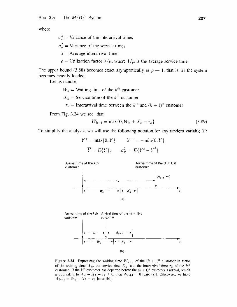
Sec. 3.5
where
The M / G/1 System 207
(3.89)
0"; = Variance of the interarrival times
O"t = Variance of the service timesA = Average interarrival time
p = Utilization factor AIJi, where 1/Ji is the average service timeThe upper bound (3.88) becomes exact asymptotically as p ----> 1, that is, as the systembecomes heavily loaded.
Let us denote
Wk = Waiting time of the k1h customerX k = Service time of the k1h customerTk = Interarrival time between the k1h and (k + l)st customer
From Fig. 3.24 we see that
Wk+1 = max{O, Wk + X k - Td
To simplify the analysis, we will use the following notation for any random variable Y:
y+ = max{O, Y}, Y- = - min{O,Y}
Y = E{Y}, = E{y2 _ y 2}
Arrival time of the kth Arrival time of the (k + 1)stcustomer customer
l__ -0
F Xk4r-----l-----,l·-t(a)
Arrival time of the kth Arrival time of the (k + 1)stcustomer customer
t
(b)
Figure 3.24 Expressing the waiting time VVk+l of the (k + l)st customer in termsof the waiting time vVko the service time X ko and the interarrival time Tk of the k!hcustomer. If the k!h customer has departed before the (k + l)S! customer's arrival, whichis equivalent to W k + X k - Tk :s: 0, then Wk+l = 0 [case (a)]. Otherwise. we haveWk+l = Wk + X k - Tk [case (b)].
208
Note that we have
from which we see that
y = y+ - y-,
Delay Models in Data Networks
y+. y- = 0
Chap. 3
Y = Y+ - Y-, 2 2 2 -----=-o-y=o-y++o-y_+2Y·Y (3.90)
Let us now write the expression (3.89) as
W k+ 1 = (Wk + Vk)+
where
Let us also denote
(3.91 )
(3.92)
(3.93)
From Fig. 3.24 we see that I k is the length of the idle period between the arrival of thekth and the arrival of the (k + l)st customer.
We have, using Eq. (3.90),
o-{Wk+Vk) = o-{WdVk)+ + o-{WdVkl- + 2(Wk + Vk )+ . (Wk + Vk )-
Since Wk and Vk are independent, we also have
Combining Eqs. (3.91) to (3.95), we obtain2222 2--
O-Wk + O-a + O-b = o-Wk-t-l + 0-1, + 2Wk+lhWe now take the limit as k ----7 oc, assuming that steady-state values exist, that is,
(3.94)
(3.95)
W k ----7W,
We obtain
(3.96)
(3.97)
The average idle time I between two successive arrivals is equal to (1 - p) (the fractionof time the system is idle) multiplied by the average interarrival time 1/'\, that is,I = (1 - p)/'\. Thus, we can write Eq. (3.96) as
'\(0-2 + 0-2 ) '\0-2W= a b _ 12(1 - p) 2(1 - p)
Since 0-7 2: 0, we obtain the inequality
W < +- 2(1 - p)
(3.98)

Sec. 3.6 Networks of Transmission Lines 209
which is the desired result. Note that as the system becomes more heavily loaded, theaverage idle time h tends to diminish and so does the variance 0-1, thereby making theupper bound increasingly accurate.
As an example, consider the M / G / I queue. By the Pollatcheck-Khinchin formulawe have
..\X2
w=---2(1 - p)+ I/I-i)
2(1 - p)(3.99)
Since for the Poisson arrival process with rate ..\ we have = 1/..\2 , by comparing Eqs.(3.97) and (3.99) we see that
J 1 I0-1 = ..\2 - {12
Thus the term that was neglected to derive the upper bound (3.98) for W is equal to
..\0-1 ..\ ( I 1) 1(1 I)2(1 - p) = 2(1 - ..\jl-L) ..\2 - {12 = 2 >:. + -;;
This term is always less than the average interarrival time 1/..\ when p < 1. As p ----+ I,it approaches 1/ I-L and is negligible relative to the upper bound of Eq. (3.98).
We finally note that several other bounds and approximations for the G / G/ I queuehave been obtained. A particularly simple improvement to the one we have given here is
+ ..\(1 -W< -------"'-- 2(1 - p) 2
Its derivation is outlined in Problem 3.48.
3.6 NETWORKS OF TRANSMISSION LINES
In a data network, there are many transmission queues that interact in the sense thata traffic stream departing from one queue enters one or more other queues, perhapsafter merging with portions of other traffic streams departing from yet other queues.Analytically, this has the unfortunate effect of complicating the character of the arrivalprocesses at downstream queues. The difficulty is that the packet interarrival timesbecome strongly correlated with packet lengths once packets have traveled beyond theirentry queue. As a result it is impossible to carry out a precise and effective analysiscomparable to the one for the M /M /1 and M / G/1 systems.
As an illustration of the phenomena that complicate the analysis, consider twotransmission lines of equal capacity in tandem, as shown in Fig. 3.25. Assume thatPoisson arrivals of rate ..\ packets/sec enter the first queue, and that all packets haveequal length. Therefore, the first queue is M / D /1 and the average packet delay there isgiven by the Pollaczek-Khinchin formula. However, at the second queue the interarrivaltimes must be greater than or equal to 1/{1 (the packet transmission time). Furthermore,because the packet transmission times are equal at both queues, each packet arriving at
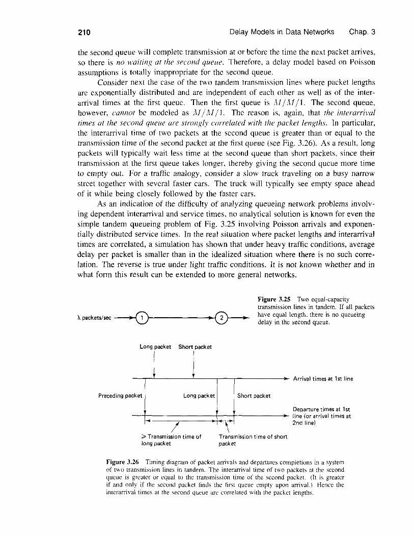
210 Delay Models in Data Networks Chap. 3
the second queue will complete transmission at or before the time the next packet arrives,so there is no "'aiting at the second queue. Therefore, a delay model based on Poissonassumptions is totally inappropriate for the second queue.
Consider next the case of the two tandem transmission lines where packet lengthsare exponentially distributed and are independent of each other as well as of the inter-arrival times at the first queue. Then the first queue is J\[ / ,U/1. The second queue,however, cannot be modeled as AI/AI/I. The reason is, again, that the interarrivaltimes at the second queue are strongly correlated with the packet lengths. In particular,the interarrival time of two packets at the second queue is greater than or equal to thetransmission time of the second packet at the first queue (see Fig. 3.26). As a result, longpackets will typically wait less time at the second queue than short packets, since theirtransmission at the first queue takes longer, thereby giving the second queue more timeto empty out. For a traffic analogy, consider a slow truck traveling on a busy narrowstreet together with several faster cars. The truck will typically see empty space aheadof it while being closely followed by the faster cars.
As an indication of the difficulty of analyzing queueing network problems involv-ing dependent interarrival and service times, no analytical solution is known for even thesimple tandem queueing problem of Fig. 3.25 involving Poisson arrivals and exponen-tially distributed service times. In the real situation where packet lengths and interarrivaltimes are correlated, a simulation has shown that under heavy traffic conditions, averagedelay per packet is smaller than in the idealized situation where there is no such corre-lation. The reverSe is true under light traffic conditions. It is not known whether and inwhat form this result can be extended to more general networks.
;>., packets/sec
Long packet Short packet
Figure 3.25 Two equal-capacitytransmission lines in tandem. If all packetshave equal length. there is no queueingdelay in the second queue.
Preced ing packet Long packet Short packet
I \
Arrival times at 1st line
Departure times at 1stline (or arrival times at2nd line)
;;. Transmission time oflong packet
Transmission time of shortpacket
Figure 3.26 Timing diagram of packet arrivals and departures completions in a systemof two transmission lines in tandem. The interarrival time of two packets at the secondqueue is greater or equal to the transmission time of the second packet. (It is greaterif and only if the second packet finds the first queue empty upon arrival.) Hence theinterarrival times at the second queue are correlated with the packet lengths.
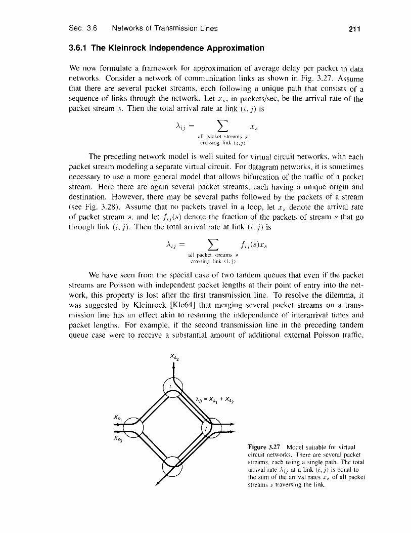
Sec. 3.6 Networks of Transmission Lines 211
3.6.1 The Kleinrock Independence Approximation
We now fonnulate a framework for approximation of average delay per packet in datanetworks. Consider a network of communication links as shown in Fig. 3.27. Assumethat there are several packet streams, each following a unique path that consists of asequence of links through the network. Let x" in packets/sec, be the arrival rate of thepacket stream s. Then the total arrival rate at link (i.j) is
all packet streams ,';crossing link ('i.j)
The preceding network model is well suited for virtual circuit networks, with eachpacket stream modeling a separate virtual circuit. For datagram retworks, it is sometimesnecessary to use a more general model that allows bifurcation of the traffic of a packetstream. Here there are again several packet streams, each having a unique origin anddestination. However, there may be several paths followed by the packets of a stream(see Fig. 3.28). Assume that no packets travel in a loop, let x" denote the arrival rateof packet stream 8, and let Ii] (8) denote the fraction of the packets of stream 8 that gothrough link (I, j). Then the total arrival rate at link (i. j) is
AiJ =all packet streams .'3
crossing link (i.J)
Iij(8)X"
We have seen from the special case of two tandem queues that even if the packetstreams are Poisson with independent packet lengths at their point of entry into the net-work, this property is lost after the first transmission line. To resolve the dilemma, itwas suggested by Kleinrock [Kle64J that merging several packet streams on a trans-mission line has an effect akin to restoring the independence of interarrival times andpacket lengths. For example, if the second transmission line in the preceding tandemqueue case were to receive a substantial amount of additional external Poisson traffic,
Figure 3.27 Model suitable for virtualcircuit networks. There are several packetstreams. each using a single path. The totalarrival rate Ai) at a link (i, j) is equal tothe sum of the arrival rates x" of all packetstreams s traversing the link.
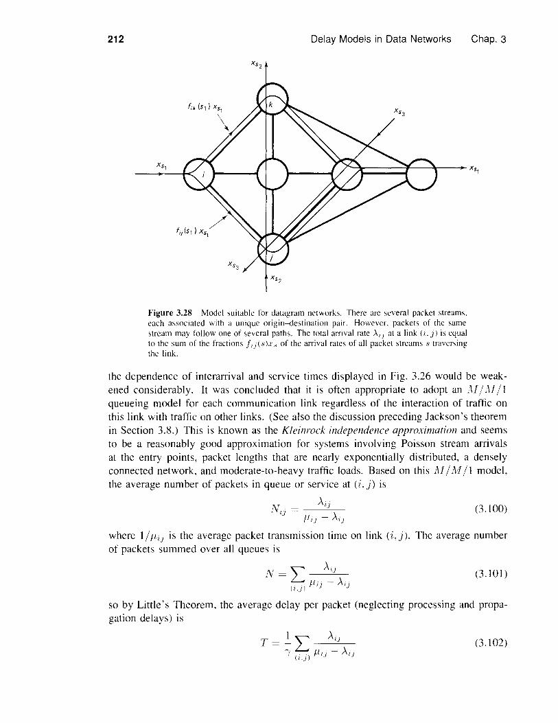
212 Delay Models in Data Networks Chap. 3
Xs,Xs,
(3.100)
Figure 3.28 Model suitable for datagram networks. There are several packet streams.each associated with a unique origin-destination pair. However. packets of the samestream may follow one of several paths. The total arrival rate >"/1 at a link (/.j) is equalto the sum of the fractions I,j (s ).1', of the arrival rates of all packet streams .5 traversingthe link.
the dependence of interarrival and service times displayed in Fig. 3.26 would be weak-ened considerably. It was concluded that it is often appropriate to adopt an JU/ JI / Iqueueing model for each communication link regardless of the interaction of traffic onthis link with traffic on other links. (See also the discussion preceding Jackson's theoremin Section 3.8.) This is known as the Kleinrock independence approximation and seemsto be a reasonably good approximation for systems involving Poisson stream arrivalsat the entry points, packet lengths that are nearly exponentially distributed, a denselyconnected network, and moderate-to-heavy traffic loads. Based on this AI / JU/ I model,the average number of packets in queue or service at (i. j) is
7\T. _ A,}"I} -
Pi} - Ai}
where 1/IIi} is the average packet transmission time on link (i, j). The average numberof packets summed over all queues is
(3.101)
so by Little's Theorem, the average delay per packet (neglecting processing and propa-gation delays) is
(3.102)

Sec. 3.6 Networks of Transmission Lines
V2
V2
B
213
Figure 3.29 Poisson process with rate .\divided among two links. If division isdone by randomization, each link behaveslike an M I JIII queue. If division is doneby metering, the whole system behaves Iikean 1\111'v112 queue.
(3.103)
(3.104)
where! = L8.rS is the total arrival rate in the system. If the average processing andpropagation delay el ij at link (i. j) is not negligible, this formula should be adjusted to
I L ( Ai) )T = - . + Aij elij11" - A"r (i.j) I) 1)
Finally, the average delay per packet of a traffic stream traversing a path p is given by
'"' (Ai) 1 )Tp = L . . . . _ .. + -. + eli)'. ILI)(p,) AI)) 11i)all (I,))on path p
where the three terms in the sum above represent average waiting time in queue, averagetransmission time, and processing and propagation delay, respectively.
In many networks, the assumption of exponentially distributed packet lengths is notappropriate. Given a different type of probability distribution of the packet lengths, onemay keep the approximation of independence between queues but use the P-K formula foraverage number in the system in place of the AI/M /1 formula (3.100). Equations (3.101)to (3.104) for average delay would then be modified in an obvious way.
For virtual circuit networks (cf. Fig. 3.27), the main approximation involved in theI\I /M /1 formula (3.101) is due to the correlation of the packet lengths and the packetinterarrival times at the various queues in the network. If somehow this correlation wasnot present (e.g., if a packet upon departure from a transmission line was assigned a newlength drawn from an exponential distribution), then the average number of packets inthe system would be given indeed by the formula
This fact (by no means obvious) is a consequence of Jackson's Theorem, which will bediscussed in Section 3.8.
In datagram networks that involve multiple path routing for some origin-destinationpairs (cf. Fig. 3.28), the accuracy of the M / M /1 approximation deteriorates for anotherreason, which is best illustrated by an example.
Example 3.17
Suppose that node A sends traffic to node B along two links with service rate 11 in thenetwork of Fig. 3.29. Packets arrive at A according to a Poisson process with rate .\packets/sec. Packet transmission times are exponentially distributed and independent ofinterarrival times as in the AI/M / I system. Assume that the arriving traffic is to bedivided equally among the two links. However, how should this division be implemented?Consider the following possibilities.
214 Delay Models in Data Networks Chap. 3
1. Randomization. Here each packet is assigned upon arrival at A to one of the two linksbased on the outcome of a fair coin flip. It is then possible to show that the arrivalprocess on each of the two queues is Poisson and independent of the packet lengths(see Problem 3.11). Therefore, each of the two queues behaves like an Al/Al/lqueue with arrival rate A/2 and average delay per packet
ITR = -/1---A-/-'---2
221L - A
(3.105)
(3.106)
which is consistent with the Kleinrock independence approximation.2. Metering. Here each arriving packet is assigned to a queue that currently has thesmallest total backlog in bits and will therefore empty out first. An equivalent systemmaintains a common queue for the two links and routes the packet at the head of thequeue to the link that becomes idle first. This works like an 11.1/1\;1/2 system witharrival rate A and with each link playing the role of a server. Using the result ofSection 3.4.1, the average delay per packet can be calculated to be
2TAI = --:------:-c--,----(2/1. - A)(I + p)
where p = A/2IL.
Comparing the average delay expressions (3.105) and (3.106), we see that meteringperforms better than randomization in terms of delay by a factor 1/(1 + p). This is basicallythe same advantage that statistical multiplexing with multiple channels holds over time-division multiplexing as discussed in Example 3.10. Generally, it is preferable to usesome form of metering rather than randomization when dividing traffic among alternativeroutes. However, in contrast with randomization, metering destroys the Poisson characterof the arrival process at the point of division. In our example, when metering is used,the interarrival times at each link are neither exponentially distributed nor independentof preceding packet lengths. Therefore, the use of metering (which is recommended forperformance reasons) tends to degrade the accuracy of the 1'vl/1v1 / I approximation.
We finally mention an alternative approach for approximating average delay in anetwork of transmission lines. This approach uses G/ G/ I approximations in place ofM /M / I or M / G/ I approximations. The key idea is that given the first two momentsof the interarrival and service times of each of the external packet streams, one mayapproximate reasonably well the first two moments of the interarrival and service times ofthe total packet arrival stream at each queue (see [Whi83a], [Whi83b], and the referencesquoted there). Then the average delay at each queue can be estimated using G/ G /1bounds and approximations of the type discussed in Section 3.5.4.
3.7 TIME REVERSIBILITY-BURKE'S THEOREM
The analysis of the M/M/l, M/M/Tn, M/M/oo, and M/M/m/Tn systems wasbased on the equality of the steady-state frequency of transitions from j to j + I, thatis, PjPj(j+l), with the steady-state frequency of transitions from j + I to j, that is,Pj+ 1P(j+1)j' These relations, called detailed balance equations, are valid for any Markov
Sec. 3.7 Time Reversibility-Burke's Theorem 215
chain with integer states in which transitions can occur only between neighboring states(i.e., from j to j - 1, j, or j + 1); these Markov chains are called hirth-death processes.The detailed balance equations lead to an important property called time reversibility, aswe now explain.
Consider an irreducible, aperiodic, discrete-time Markov chain X n , X n+1, ••• hav-ing transition probabilities Pi.; and stationary distribution {p] I j ;:::: O} with Pj > 0 forall j. Suppose that the chain is in steady-state, that is,
P{Xn = j} = Pj , for all n
(This occurs if the initial state is chosen according to the stationary distribution, and isequivalent to imagining that the process began at time -00.)
Suppose that we trace the sequence of states going backward in time. That is,starting at some n, consider the sequence of states X n, X n - 1, ••• • This sequence isitself a Markov chain, as seen by the following calculation:
P{Xm = j I X m +1 = i, X m +2 = i2 , ... , X m +k = i k }
P{Xm = j, X m +1 = i, X m +2 = i2 , .•. , X m +k =ik }P{Xm + 1 = i, X m +2 = 12, ... , X m +k = Ik}
P{Xm = j, X m +1 =i} P{Xm +2 = 12, ... , X m +k = i k I X m = j, X m +1 = i}P{Xm +1 = i}P{Xm +2 = i2 , ••. , X m +k = ik I X m +1 = i}
P{Xm = j, X m +1 = I}P{Xm +1 = i}
P{Xm = j} P{Xm +1 =i I X m = j}P{Xm +1 = i}
PjPjiPi
where the third equality follows from the Markov property of the chain X n , X n+1, •••
Thus, conditional on the state at timem + I, the state at timem is independent of thatat times m + 2, Tn + 3, .... The backward transition probabilities are given by
Pt] = P{Xm = j I X m +1 = i} = pjPji , i,j ;:::: 0 (3.107)Pi
If Pti = Pi] for all i, j (i.e., the transition probabilities of the forward and reversed chainare identical), we say that the chain is time reversible.
We list some properties of the reversed chain:
1. The reversed chain is irreducible, aperiodic, and has the same stationary distri-bution as the forward chain. [This property can be shown either by elementaryreasoning using the definition of the reversed chain, or by verifying the equalityPj = using Eq. (3.107).J The intuitive idea here is that the reversedchain corresponds to the same process, looked at in the reversed time direction.Thus, if the steady-state probabilities are viewed as proportions of time the process

216 Delay Models in Data Networks Chap. 3
visits the states, then the steady-state occupancy distributions of the forward andthe reverse chains are equal. Note that in view of this equality, the fonn of thetransition probabilities of the reversed chain P;'j = PjPj,jPi [cf. Eq. (3.107)J canbe intuitively explained. It expresses the fact that (with probability I) the propor-tion of transitions from j to i out of all transitions in the forward chain (which ispjPji ) equals the proportion of transitions fromi to j out of all transitions in thereversed chain (which is PiP;';).
2. If we can find positive numbers Pi,i 2 0, summing to unity and such that thescalars
P* = PjPji7J Pi
form a transition probability matrix, that is,:x:
i, j 20 (3.108)
i = O. I....LPtj = l,j=O
then {Pi I i 2 O} is the stationary distribution and Pt7 are the transition probabilitiesof the reversed chain. [To see this, note that by multiplying with Pi Eq. (3.108)and adding over j, we obtain
:x:
LpjPji = Pi L Pij = Pij=O J=O
which is the global balance equation and implies that {Pi I i 2 O} is the stationarydistribution.] This property, which holds regardless of whether the chain is timereversible, is useful if through an intelligent guess, we can verify Eq. (3.108),thereby obtaining both the Pj and Pi}; for examples of such applications, seeSection 3.8.
3. A chain is time reversible if and only if the detailed balance equations hold:
i, j 20This follows from the equality PiP;'j = PjPji [cf. Eq. (3.107)] and the definition oftime reversibility. In other words, a system is time reversible if in a typical systemhistory, transitions fromi to j occur with the same frequency as transitions fromj to i (and therefore also with the same frequency as transitions from i to j whenthis system history is reversed in time). In particular, the chains correspondingto the queueing systems MIM/I, MIMlrn, MIMlx, and MIMlrn/rn dis-cussed in Sections 3.3 and 3.4 are time reversible (in the limit as 6 -+ 0). Moregenerally, chains corresponding to birth-death processes (Pij = 0 if Ii - jl > I)are time reversible. Figure 3.30 gives some additional examples of reversible andnonreversible systems.
The idea of time reversibility extends in a straightforward manner to irreduciblecontinuous-time Markov chains. The corresponding analysis can be carried out eitherdirectly or by discretizing time in intervals of length 6, considering the corresponding
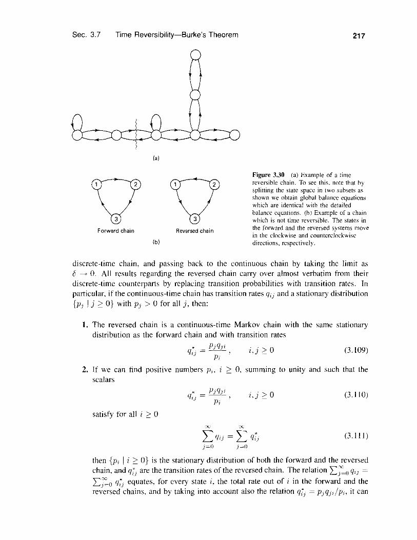
Sec. 3.7 Time Reversibility-Burke's Theorem 217
(a)
vvForward chain
(b)
Reversed chai n
Figure 3.30 (a) Example of a timereversible chain. To see this. note that bysplitting the state space in two subsets asshown we obtain global balance equationswhich are identical with the detailedbalance equations. (b) Example of a chainwhich is not time reversible. The states inthe forward and the reversed systems movein the clockwise and counterclockwisedirections, respectively.
discrete-time chain, and passing back to the continuous chain by taking the limit asb ---.f O. All results regarding the reversed chain carryover almost verbatim from theirdiscrete-time counterparts by replacing transition probabilities with transition rates. Inparticular, if the continuous-time chain has transition rates qi.1 and a stationary distribution{P.1 I j 2: O} with Pj > 0 for all j, then:
1. The reversed chain is a continuous-time Markov chain with the same stationarydistribution as the forward chain and with transition rates
(3.109)i,j 2: 0* PJqjiqij = --,Pi
2. If we can find positive numbers P" i > 0, summing to unity and such that thescalars
i,j 2: 0 (3.110)
satisfy for alii 2: 0
2: qij = 2: q:j.1=0 .1=0
(3. I 11)
then {Pi I i 2: O} is the stationary distribution of both the forward and the reversedchain, and qtJ are the transition rates of the reversed chain. The relation qi.j =
q:j equates, for every state i, the total rate out of i in the forward and thereversed chains, and by taking into account also the relation qtj = Pjqj;jPi, it can
218 Delay Models in Data Networks
be seen to be equivalent to the global balance equation
PiL% = LPjqjij=O j=O
Chap. 3
[ef. Eq. (3A.IO) of Appendix A].3. The forward chain is time reversible if and only if its stationary distribution andtransition rates satisfy the detailed balanced equations
i,j 20
Consider now the M /M / I, M /M / m, and M /M / ex queueing systems. Weassume that the initial state is chosen according to the stationary distribution so that thequeueing systems are in steady-state at all times. The reversed process can be representedby another queueing system where departures correspond to arrivals of the original systemand arrivals correspond to departures of the original system (see Fig. 3.31). Because timereversibility holds for all these systems as discussed above, the forward and reversedsystems are statistically indistinguishable in steady-state. In particular by using the factthat the departure process of the forward system corresponds to the arrival process of thereversed system, we obtain the following result:
Burke's Theorem. Consider an M /M / I, M /M / m, or M /M / ex system witharrival rate A. Suppose that the system starts in steady-state. Then the following holdtrue:
(a) The departure process is Poisson with rate A.(b) At each time t, the number of customers in the system is independent of the
sequence of departure times prior to t.
Proof: (a) This follows from the fact that the forward and reversed systems arestatistically indistinguishable in steady-state, and the departure process in the forwardsystem is the arrival process in the reversed system.
(b) As shown in Fig. 3.32, for a fixed time t, the departures prior to t in theforward process are also the arrivals after t in the reversed process. The arrival processin the reversed system is independent Poisson, so the future arrival process does notdepend on the current number in the system, which in forward system terms means thatthe past departure process does not depend on the current number in the system. Q.E.D.
Note that part (b) of Burke's Theorem is quite counterintuitive. One would expectthat a recent stream of closely spaced departures suggests a busy system with an atypicallylarge number of customers in queue. Yet Burke's Theorem shows that this is not so.Note, however, that Burke's Theorem says nothing about the state of the system beforea stream of closely spaced departures. Such a state would tend to have abnormally manycustomers in queue, in accordance with intuition.

Sec. 3.7 Time Reversibility-Burke's Theorem 219
1Nom.... of 0..."""T - t
rL.,__(a)
_ tT
T1
Number of
- L- .._ T = T - tT - d3
1Number of Departures
___________________...L T = T - tT - a2 T - a, T
1Nom"" __
- _ T= T - tT - d3 T - d2 T - d, T - a3 T - a2 T - a, T
(b)
Figure 3.31 (a) Forward system number of arrivals, number of departures, and occu-pancy during [0, T]. (b) Reversed system number of arrivals, number of departures, andoccupancy during [0, T].

220
Departures prior to tin the forward process
Delay Models in Data Networks Chap. 3
Arrivals after t inthe reversed process
Time direction in theforward process
-Time direction inthe reverse process
Figure 3.32 Customer dcpartures prior to time t in the forward systcm become cus-tomer arrivals alia time t in the reversed system.
__o_u_el'_u_e_, "_..._1 oue:e 2
Figure 3.33 Two queues in tandem. Theservice times at the two queues arcexponentially distributed and mutuallyindependent. Using Burkc's Theorem. wecan show that thc numbcr of customers inqueues I and 2 are indepcndent at a giventime and
P{ n at queuc I. m at queue 2}= p;'(l - PI)p2"(1 - P2)
that is. the two queues behave as if they areindcpendent AI/AI/I queues in isolation.
Example 3.18 Two M IM II Queues in TandemConsider a queueing network involving Poisson arrivals and two queues in tandem withexponential service times (see Fig. 3.33). There is a major difference between this systemand the one discussed in Section 3.6 in that here we assume that the service times of acustomer at the first and second queues are mutually independent as well as independent ofthe arrival process. As a result of this assumption. we will see that the occupancy distributionin the two queues is the same as if they were independent 1\1I 1\1I I queues in isolation.This fact will also be shown in a more general context in the next section.
Let the rate of the Poisson arrival process be A, and let the mean service times atqueues I and 2 be I/!LI and Ilp2. respectively. Let PI = ,\fPI and P2 = Alp2 be thecorresponding utilization factors. and assume that PI < I and P2 < I. We will show thatunder steady-state conditions the number of customers at queue I and at queue 2 at anygiven time are independent. Furthermore.
P{n at queue I. rn at queue 2} = p;'(l - PI)p2"(l - P2) (3.112)
To prove this we first note that queue I is an M /-11I I queue. so by part (a) ofBurke's Theorem. the departure process from queue I is Poisson. By assumption. it is alsoindependent of the service times at queue 2. Therefore. queue 2. viewed in isolation. is anAi I 1\1I I queue. Thus. from the results of Section 3.1.
P{n at queue I} = p;'(l - PI)(3.113)
P{m at queue 2} = p2"(1 - P2)
From part (b) of Burke's Theorem it follows that the number of customers presently inqueue I is independent of the sequence of earlier arrivals at queue 2 and therefore also of

Sec. 3.8 Networks of Queues-Jackson's Theorem 221
the number of customers presently in queue 2. This implies that
P{n at queue I. m at queue 2} = P{n at queue I}· P{m at queue 2}
and using Eq. (3.113) we obtain the desired product form (3.112).
We note that, by part (a) of Burke's Theorem, the arrival and the departure processesat both queues of the preceding example are Poisson. This fact can be similarly shownfor a much broader class of queueing networks with Poisson arrivals and independent,exponentially distributed service times. We call such networks acyclic and define themas follows. We say that queue j is a downstream neighhor of queue i if there is a positiveprobability that a departing customer from queue i will next enter queue j. We say thatqueue j lies downstream of queue i if there is a sequence of queues starting from i andending at j such that each queue after i in the sequence is a downstream neighbor of itspredecessor. A queueing network is called acyclic if it is impossible to find two queuesi and j such that j lies downstream of i. and i lies downstream of j. Having an acyclicnetwork is essential for the Poisson character of the arrival and departure processes ateach queue to be maintained (see Section 3.8). However, the product form (3.112) ofthe occupancy distribution generalizes in a natural way to networks that are not acyclic,as we show in the next section.
3.8 NETWORKS OF QUEUES-JACKSON'S THEOREM
As discussed in Section 3.6, the main difficulty with analysis of networks of transmissionlines is that the packet interarrival times after traversing the first queue are correlatedwith their lengths. It turns out that if somehow this correlation were eliminated (which isthe premise of the Kleinrock independence approximation) and randomization is used todivide traffic among different routes, then the average number of packets in the systemcan be derived as if each queue in the network were M /M / I. This is an importantresult known as Jackson's Theorem. In this section we derive a simple version of thistheorem and some of its extensions.
Consider a network of K first-come first-serve, single-server queues in whichcustomers arrive from outside the network at each queue i in accordance with independentPoisson processes at rate ri. We allow the possibility that ri = O. in which case thereare no external arrivals at queue i, but we require that ri > 0 for at least onei. Once acustomer is served at queue i. it proceeds to join each queue j with probability Pi] orto exit the network with probability I - L:f= 1Pi].
The routing probabilities Pi) together with the external input rates r J can be usedto determine the total arrival rate of customers A) at each queue j. that is. the sum of r)and the arrival rate of customers coming from other queues. Calculating Aj is fairly easywhen the network is of the acyclic type discussed at the end of Section 3.7. If there isa positive probability that a customer may visit the same queue twice, a more complex

222 Delay Models in Data Networks Chap. 3
computation is necessary, based on the equations
K
Aj = T") + LAiPi) 'i=l
j = I, ... ,K (3.114)
(3.115)j=l, ... ,K
These equations represent a linear system in which the rates Aj, j = 1, ... ,K, constitutea set of K unknowns. To guarantee that they can be solved uniquely to yield Aj,j = I, ... ,K in terms of T" j, Pij , i, j = I, ... ,K, we make a fairly natural assumptionthat essentially asserts that each customer will eventually exit the system with probability1, This assumption is that for every queue i l , there is a queue i with I - L.f=l Pi) > °and a sequence i l , i2, ... , ik, i such that Pili, > 0, ... , Pi"i > 0.*
The service times of customers at the ph queue are assumed exponentially dis-tributed with mean 1/M) and are assumed mutually independent and independent of thearrival process at the queue. The utilization factor of each queue is denoted
Pj = Aj ,Mj
and we assume that Pj < I for all j.In order to model a packet network such as the one considered in Section 3.6 within
the framework described above, it is necessary to accept several simplifying conditions inaddition to assuming Poisson arrivals and exponentially distributed packet lengths. Thefirst is the independence of packet lengths and interarrival times discussed earlier. Thesecond is relevant to datagram networks, and has to do with the assumption that bifur-cation of traffic at a network node can be modeled reasonably well by a randomizationprocess whereby each departing packet from queue i joins queue j with probability Pij -this need not be true, as discussed in Section 3.6. Still a packet network differs from themodel of this section because it involves several traffic streams which may have differentrouting probabilities at each node, and which maintain their identity as they travel alongdifferent routes (see the virtual circuit and datagram network models of Figs. 3.27 and3.28). This difficulty can be partially addressed by using an extension of Jackson's Theo-rem that applies to a network with multiple classes of customers. Within this more generalframework, we can model traffic streams corresponding to different origin-destinationpairs as different classes of customers. If all traffic streams have the same averagepacket length, it turns out that Jackson's Theorem as stated below is valid assuming thesimplifying conditions mentioned earlier; see the analysis in the next subsection.
* For a brief explanation aimed at the advanced reader. consider the Markov chain with states 0, I, ... , Kand transition probabilities from states i 'I 0 to states j 'I 0 equal to Pij, and transition probabilities to stateoequal to Poo = I. P,O = 1 - p') for i '10. (Thus state 0 is an absorbing state that corresponds toexit of a customer from the system.) Let P be the K x K matrix with elements Pij. The sum of the i th rowelements of the matrix pm (P to the m th power) is the probability that the Markov chain has not arrived atstate 0 after m transitions starting from state i. Our hypothesis on p') implies that the chain will eventually(with probability I) arrive at state 0 regardless of the initial state. It follows that pm = 0, so unityis not an eigenvalue of P. Therefore. I - P is nonsingular. where I is the identity matrix. from which it canbe seen that the system of equations (3.114) has a unique solution.
Sec. 3.8 Networks of Queues-Jackson's Theorem 223
For an analysis, we view the system as a continuous-time Markov chain in whichthe state n is the vector (nl, n2, ... , nK), where ni denotes the number of customers atqueue i. At a given state
the possible successor states correspond to a single customer arrival and/or departure. Inparticular, the transition from n to state
n(j+) = (nl, ... ,nj-l,nj + I,nj+l, ... ,nK)
corresponding to an external arrival at queue j, has transition rate
The transition from n to state
n(j -) = (n I, ... , n j _ I , n j - 1, n j+ I , ... , nK )
corresponding to a departure from queue j to the outside, has transition rate
The transition from n to state
n(i+,j-) = (nl .... ,TLi-l,ni + I,TLi+I, ... ,nj_l,nj -1,nj+l, ... ,nK)
corresponding to a customer moving from queue j to queue oi, has transition rate
Let P(nl, .... nK) denote the stationary distribution of the chain. We have:
Jackson's Theorem. Assuming that Pj < 1, j = 1, ... ,K, we have for allnl,··· ,nK 2: 0,
(3.116)
where n = (nl, ... ,nK) and
Pj(nj) = p7 j (l - PJ)' nJ 2: 0 (3.117)
Proof In our proof we will assume that Aj > 0 for all j. There is no loss ofgenerality in doing so because every queue j with AJ = 0 is empty in steady-state, so wehave PJ(O) = I and Pj(nj) = 0 for nj > 0, and queue j can be ignored in deriving thestationary distribution of Eqs. (3.116) and (3.117). It can be verified that the conditionAj > 0 for all j together with the assumption made earlier to guarantee the uniquenessof solution of Eq. (3.114) imply that the Markov chain with states n = (nl,oo.,nK)describing the system is irreducible; we leave the proof of this for the reader. We willuse a technique outlined in Section 3.7 whereby we guess at the transition rates of thereversed process and verify that, together with the probability distribution of Eqs. (3.116)and (3.117), they satisfy the total departure rate equation (3.111). (The Markov chain is

224 Delay Models in Data Networks Chap. 3
not time reversible here. Nonetheless, the use of the reversed process is both analyticallyconvenient and conceptually useful.)
For any two state vectors nand n ' , let qnn' be the corresponding transition rate.Jackson's Theorem will be proved if the rates q;'n' defined for all n, n ' by the equation
* P(n')qn'nqnn' = pen)
satisfy, for all n, the total rate equation
Lqnm = Lq;'mTn rn
(3.118)
(3.119)
which as mentioned in Section 3.7, is equivalent to the global balance equations.For transitions between states n, n(j+), and n(j-), we have
(3.120)
(3.121)
(3.123)
qnn(j-) = Poi (I - Pji)
The rates q* ( +) and q* ( _) are defined by Eqs. (3.118), (3.120), and (3.121). Usingnn] nn Jthe fact P(n(Y+») = pjP(n) = AjP(n)/pj [cf. Eqs. (3.115)-(3.117)], we obtain
q;m(j+) = A] (I - LiPji) (3.122)
* iljTjqnn(j-) = T
]
Next consider transitions between states nand n( i+ , j -) corresponding to a cus-tomer moving from queue j to queue i. We have
and using the fact that P (n(i+ ,r))from Eq. (3.118) as
PiP(n)/ p]
(3.124)
Aiilj P(n)/(Aj!li), we obtain
* iliAjP]iqn(i+ ,j- )n - Ai
Since for all other types of pairs of state vectors n, n' , we have
it follows from Eq. (3.118) that
q;"n = 0
(3.125)
(3.126)
(3.127)
There remains to verify that the rates qnm and q;'/m satisfy the total rate equationL m qnm = Lm q;'m' We have for the forward system, using Eqs. (3.120), (3.121), and(3.124),
K
Lqnm = Lqnnu+) + L qnn(i+,j-) + L qnn(j-)m j=1 {(j,i)lnj>O} {jlnj>O}

Sec. 3.8 Networks of Queues-Jackson's Theorem
K
= Lrj + L Pjj=! Liln}>O}
225
(3.128)
Similarly, using Eqs. (3.122), (3.123), (3.125), and (3.114), we obtain for the reversedsystem
I,'
Lq;'1II = Lq;'nU+I +m j=!
L I];'n(i+j-I +{U.illn,>O}
L l];'nU-ILiln) >O}
(3.129)
By writing Eq. (3.114) as r} = Aj - AiP;j and adding over jobtain
I ..... K, we
(3.130)
By combining the last three equations, we see that the total rate equation LIII I]mn =Lm I];,m is satisfied. Q.E.D.
Note that the transition rates q;'nl defined by Eqs. (3.122), (3.123), (3.125), and(3.127) are those of the reversed process. It can be seen that the reversed processcorresponds to a network of queues where traffic arrives at queue i from outside thenetwork according to a Poisson process with rate '\ (1- LjPij) [cf. Eq. (3.122)].The routing probability from queue i to queue j in the reversed process is
AjPj }
r, + Lk AkPki[cf. Eqs. (3.123) and (3.125) I. This is also the probability that an arriving customer atqueue i just departed from queue j in the forward process. Note that the processes ofdeparture out of the forward system are the exogenous arrival processes of the reversedsystem, which suggests that the processes of departure out of the system are independent
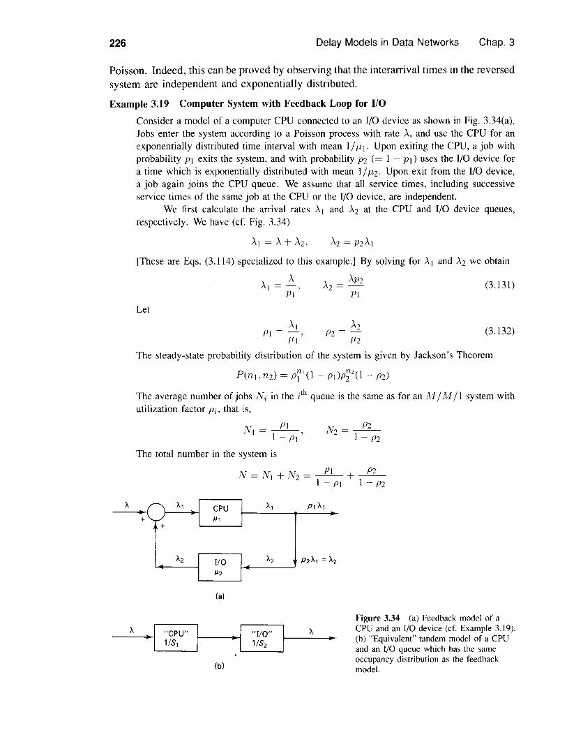
226 Delay Models in Data Networks Chap. 3
Poisson. Indeed, this can be proved by observing that the interarrival times in the reversedsystem are independent and exponentially distributed.
Example 3.19 Computer System with Feedback Loop for I/OConsider a model of a computer CPU connected to an I/O device as shown in Fig. 3.34(a).Jobs enter the system according to a Poisson process with rate A, and use the CPU for anexponentially distributed time interval with mean 1/til. Upon exiting the CPU, a job withprobability PI exits the system, and with probability P2 (= 1 - PI) uses the I/O device fora time which is exponentially distributed with mean 1/ti2. Upon exit from the I/O device,a job again joins the CPU queue. We assume that all service times, including successiveservice times of the same job at the CPU or the I/O device, are independent.
We first calculate the arrival rates AI and A2 at the CPU and I/O device queues,respectively. We have (cf. Fig. 3.34)
[These are Eqs. (3.114) specialized to this example.] By solving for Al and A2 we obtain
(3.131)
Let
(3.132)
The steady-state probability distribution of the system is given by Jackson's Theorem
P(nl,n2) = - PI)P;'(l- P2)
The average number of jobs N i in the ith queue is the same as for an AI/AI/1 system withutilization factor Pi, that is,
N, = _P_I-I - PI'
The total number in the system is
N = N I + N2 = _P_I- +1 - PI 1 - P2
+
(a)
-IA "CPU" -I "I/O"liS, l/S2
(b)
Figure 3.34 (a) Feedback model of aCPU and an I/O device (cf. Example 3.19).(b) "Equivalent" tandem model of a CPUand an I/O queue which has the sameoccupancy distribution as the feedbackmodel.
Sec. 3.8 Networks of Queues-Jackson's Theorem 227
and the average time in the system is
T N PI + P2= T = A(I - pd A(I - P2)
Using Eqs. (3.131) and (3.132) we can write this relation as
Aj(J.LIPI) + AP2/(J.L2PI)A (1 - A/(/lIPI)) A (1 - AP2I(JL2PI))
(3.133)
where
51 = _1_, f:h = (3.134)PIPI J.L2PI
Since the utilization factor of the CPU queue is PI = Ad/ll = Aj(PIPI), while the arrivalrate of new job arrivals at the CPU (as opposed to feedback arrivals) is A, we see fromLittle's Theorem that 51 is the total CPU time ajob requires on the average (this includes allvisits of the job to the CPU). Similarly, 52 is the total I/O time a job requires on the average.
An interesting interpretation of Eqs. (3.133) and (3.134) is that the average numberof jobs and time in the system are the same as in an "equivalent" tandem model of CPUand I/O queues with service rates 1/51 and 1/52, respectively, as shown in Fig. 3.34(b).However, the probability density function of the time in the system is not the same in thefeedback and tandem systems. To get some idea of this fact, suppose that PI = P2 = 1/2and that the CPU service rate is much faster than the I/O service rate (J.L 1 >> J.L2)' Thenhalf the jobs in the feedback system do not require any I/O service and their average timein the system is much smaller than the average time of the other half. This is not so inthe tandem system where the average job time in the "CPU" queue is very small and thesystem time is distributed approximately as in the "I/O" queue, that is, as in an 11,1/11,1/ Iqueue with Poisson rate A and service rate 1/5I.
Jackson's Theorem says in effect that the numbers of customers in the system'squeues are distributed as if each queue is !v! /!v! /1 and is independent of the otherqueues [compare Eq. (3.117) and the corresponding equations in Section 3.3]. Despitethis fact, the total arrival process at each queue need not be Poisson. As an example(see Fig. 3.35), suppose that there is a single queue with a service rate which is verylarge relative to the arrival rate from the outside. Suppose also that with probability pnear unity, a customer upon completion of service is fed back into the queue. Hence,when an arrival occurs at the queue, there is a large probability of another arrival at thequeue in a short time (namely, the feedback arrivaI), whereas at an arbitrary time point,there will be only a very slight chance of an arrivd occurring shortly since A is small.In other words, queue arrivals tend to occur in bursts triggered by the arrival of a singlecustomer from the outside. Hence, the queue arrival process does not have independentinterarrival times and cannot be Poisson.
Heuristic explanation of Jackson's Theorem. Our proof of Jackson's the-orem is based on algebraic manipulation and gives little insight as to why this remarkableresult holds. For this reason we provide a heuristic explanation for the case of the feed-
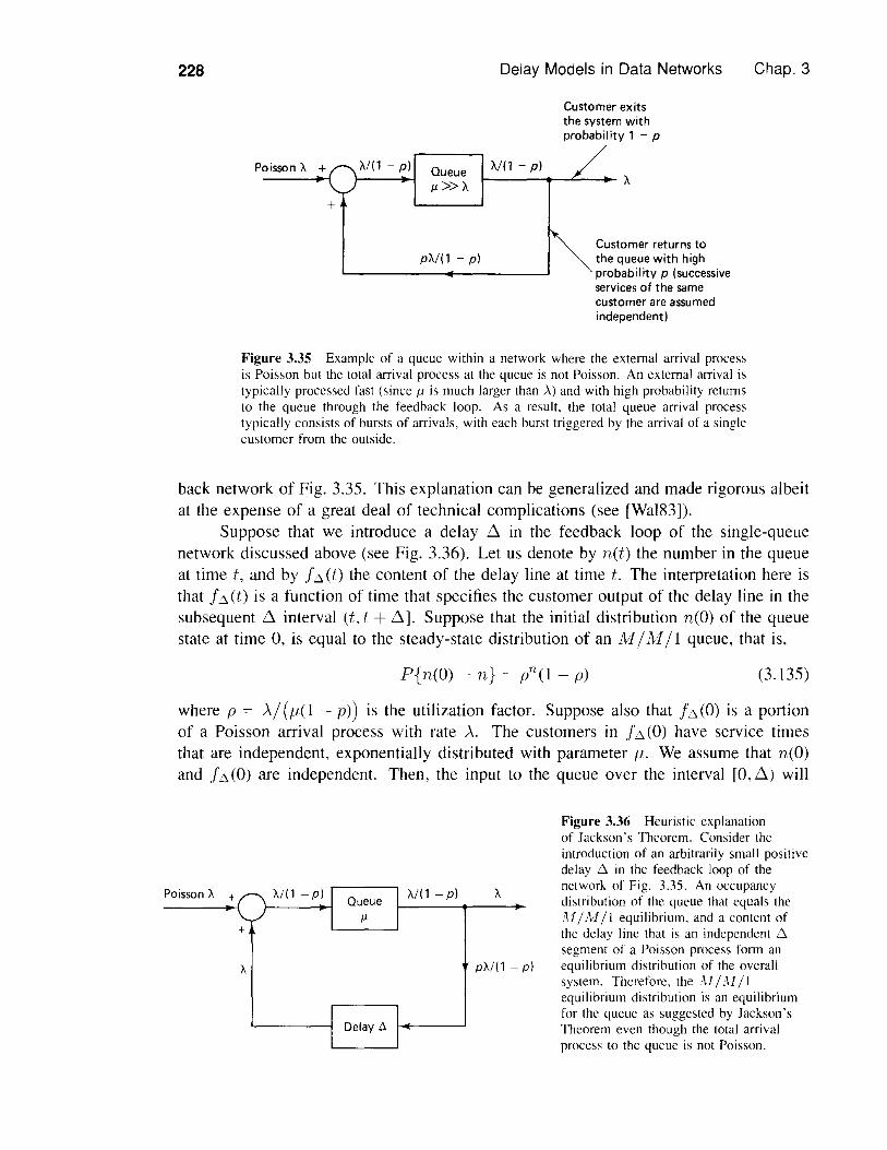
228
Poisson A +
+
A/(1 - p) Queue/J.»A
Delay Models in Data Networks
Customer exitsthe system withprobability 1 - p
AI(l - p)
Chap. 3
pA/(1 - p)Customer returns tothe queue with highprobability p (successiveservices of the samecustomer are assumedindependent)
Figure 3.35 Example of a queue within a network where the external arrival processis Poisson but the total arrival process at the queue is not Poisson. An external arrival istypically processed fast (since /l is much larger than ).) and with high probability returnsto the queue through the feedback loop. As a result, the total queue arrival processtypically consists of bursts of arrivals, with each burst triggered by the arrival of a singlecustomer from the outside.
back network of Fig. 3.35. This explanation can be generalized and made rigorous albeitat the expense of a great deal of technical complications (see [WaI83]).
Suppose that we introduce a delay ,0. in the feedback loop of the single-queuenetwork discussed above (see Fig. 3.36). Let us denote by n(t) the number in the queueat time t, and by .h (t) the content of the delay line at time t. The interpretation here isthat f Do (t) is a function of time that specifies the customer output of the delay line in thesubsequent ,0. interval (t, t + D.]. Suppose that the initial distribution n(O) of the queuestate at time 0, is equal to the steady-state distribution of an !v! / M / I queue, that is,
P{n(O) = n} = pn(l - p) (3.135)
where p = A/ (IL(1 - p») is the utilization factor. Suppose also that f Do (0) is a portionof a Poisson arrival process with rate A. The customers in .h (0) have service timesthat are independent, exponentially distributed with parameter p.. We assume that n(O)and f Do (0) are independent. Then, the input to the queue over the interval [0, D.) will
Poisson A + AI(l -pI A
pAl(l -pI
Figure 3.36 Heuristic explanationof Jackson's Theorem. Consider theintroduction of an arbitrarily small positivedelay 6 in the feedback loop of thenetwork of Fig. 3.35. An occupancydistribution of the queue that equals theM 1MI I equilibrium, and a content ofthe delay line that is an independent 6segment of a Poisson process form anequilibrium distribution of the overallsystem. Therefore, the M I;\fI Iequilibrium distribution is an equilibriumfor the queue as suggested by Jackson'sTheorem even though the total arrivalprocess to the queue is not Poisson.

Sec. 3.8 Networks of Queues-Jackson's Theorem 229
be the sum of two independent Poisson streams which are independent of the numberin queue at time O. It follows that the queue will behave in the interval [0,6) like anM 1MI I queue in equilibrium. Therefore, n(6) will be distributed according to theMIMII steady-state distribution of Eq. (3.135), and by part (b) of Burke's theorem,n(6) will be independent of the departure process from the queue in the interval [0,6),or, equivalently, of -the delay line content at time 6. Furthennore, by part (a)of Burke's Theorem, 12,(6) will be Poisson. Thus, to summarize, we started out withindependent initial conditions nCO) and f D. (0) which had the equilibrium distribution ofan M IMil queue and the statistics of a Poisson process, respectively, and 6 secondslater we obtained corresponding quantities n(6) and f D. (6) with the same properties.Using the same reasoning, we can show that for all t which are multiples of 6, net) andh (t) have the same properties. It follows that the M IMil steady-state distribution ofEq. (3.135) is an equilibrium distribution for the queueing system for an arbitrary positivevalue of the feedback delay 6, and this strongly suggests the validity of Jackson'sTheorem. Note that this argument does not suggest that the feedback process, andtherefore also the total arrival process to the queue, are Poisson. Indeed, it can beseen that successive 6 portions of the feedback arrival stream are correlated since, withprobability p, a departing customer from the queue appears as an arrival 6 secondslater. Therefore, over the interval [0, x), the feedback process is not Poisson. This isconsistent with our earlier observations regarding the example of Fig. 3.35.
3.8.1 Extensions of Jackson's Theorem
There are a number of interesting extensions and variations of Jackson's Theorem, andin this and the next subsections we will describe a few of them.
State-dependent service rates. The model for Jackson's Theorem assumedso far requires that all queues have a single server. An extension to the multi server casecan be obtained by allowing the service rate at each queue to depend on the numberof customers at that queue. Thus the model is the same as before but the servicetime at the j'h queue is exponentially distributed with mean I/pJ(m), where m is thenumber of customers in the j'h queue just before the customer's departure (m includesthe customer). The single-queue version of this model includes as special cases theM I M 1m and ]\l I Mix queues, and can be analyzed by means of a Markov chain(see Problem 3.16). The corresponding network of queues model can also be analyzedby means of a Markov chain, and is characterized by a product form structure for thestationary distribution.
Let us defineAJ(Jj(m) = --. j = 1, ....K.m = 1,2.... (3.136)
. p)(m)
where A) is the total arrival rate at the /h queue detennined by Eq. (3.114). Let us alsodefine
if Tl J = 0if TI) > 0 (3.137)
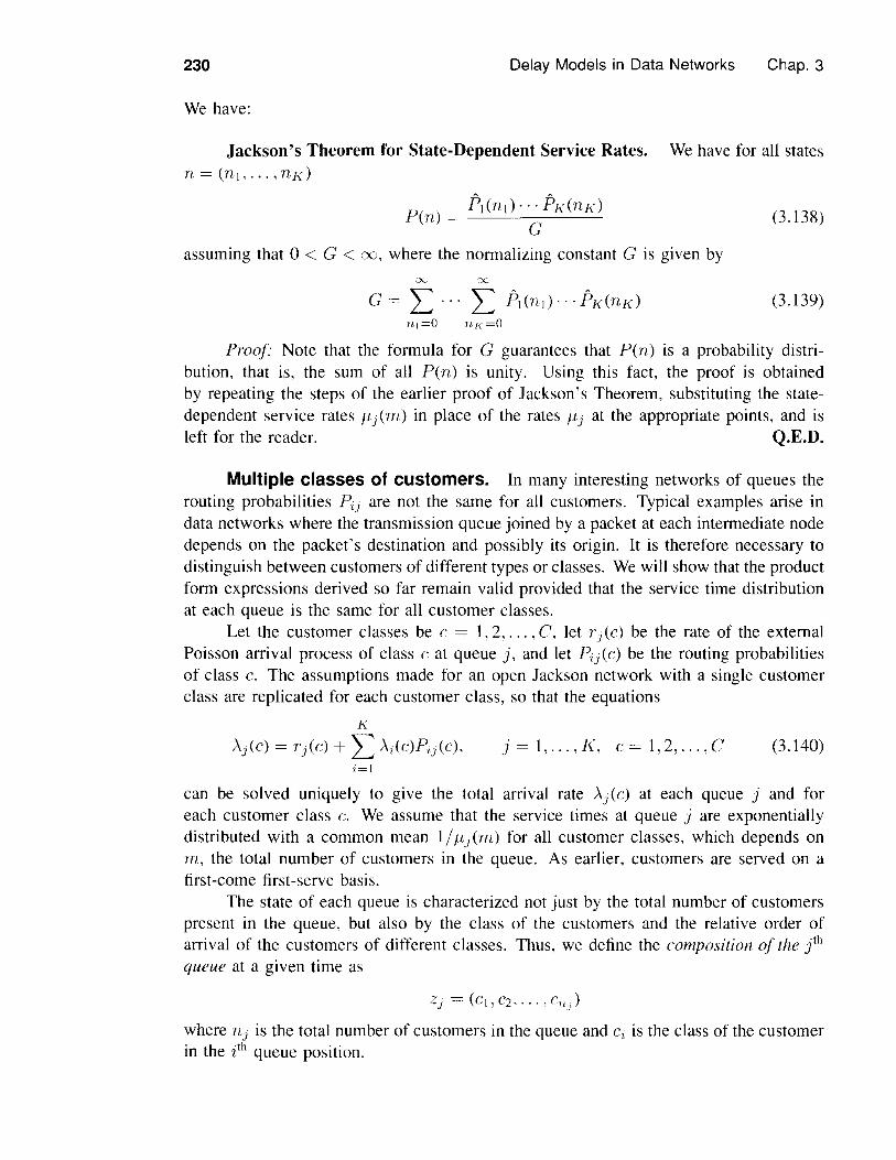
230 Delay Models in Data Networks Chap. 3
We have:
Jackson's Theorem for State-Dependent Service Rates. We have for all statesn=(nl,··.,nK)
Fj(nd···FK(nK)pen) = G (3.138)
assuming that 0 < G < 00, where the normalizing constant G is given by::x x
G = L'" L Fj(nj)" ·FK(nK)n\=(J ng=(J
(3.139)
Proof: Note that the formula for G guarantees that pen) is a probability distri-bution, that is, the sum of all pen) is unity. Using this fact, the proof is obtainedby repeating the steps of the earlier proof of Jackson's Theorem, substituting the state-dependent service rates flj(m) in place of the rates flj at the appropriate points, and isleft for the reader. Q.E.D.
(3.140)j = I, ... ,K, C = 1,2, ... , C
MUltiple classes of customers. In many interesting networks of queues therouting probabilities Pij are not the same for all customers. Typical examples arise indata networks where the transmission queue joined by a packet at each intermediate nodedepends on the packet's destination and possibly its origin. It is therefore necessary todistinguish between customers of different types or classes. We will show that the productform expressions derived so far remain valid provided that the service time distributionat each queue is the same for all customer classes.
Let the customer classes be C = 1,2, ... , C, let Tj(C) be the rate of the externalPoisson arrival process of class C at queue j, and let Pij(c) be the routing probabilitiesof class c. The assumptions made for an open Jackson network with a single customerclass are replicated for each customer class, so that the equations
K
Aj(c) = Tj(C) +L Ai(c)Pij(c),i=l
can be solved uniquely to give the total arrival rate AJ(c) at each queue j and foreach customer class c. We assume that the service times at queue j are exponentiallydistributed with a common mean 1/flJ(m) for all customer classes, which depends onm, the total number of customers in the queue. As earlier, customers are served on afirst-come first-serve basis.
The state of each queue is characterized not just by the total number of customerspresent in the queue, but also by the class of the customers and the relative order ofarrival of the customers of different classes. Thus, we define the composition of the jlhqueue at a given time as
Zj = (CI,C2"",C/l.J)
where nj is the total number of customers in the queue and Ci is the class of the customerin the i th queue position.
Sec. 3.8 Networks of Queues-Jackson's Theorem 231
The state of the queueing network at a given time is
Z = (Zl,Z2, ... ,ZK)
where Zj is the composition of the ph queue at that time. It can be viewed as the stateof a Markov chain the transition probabilities of which can be described in terms of thegiven quantities Aj(c), ILj(rn), and Pij(c). To state the appropriate form of Jackson'sTheorem, define
A Aj(C)pj(c,m) = -(-)'
ILj mj = 1, ... ,K, C = 1,2, ... ,C (3.141)
K
G = L II Pj(Zj)(ZI, ... ,ZK)j=1
if nj = 0if nj > 0 (3.142)
(3.143)
(3.144)
The proof of the following theorem follows the same pattern as the corresponding prooffor the single customer class case, and is left for the reader.
Jackson's Theorem for Multiple Classes of Customers. Assuming that 0 <G < 00, the steady-state probability p(z) of state Z = (Zl, Z2, ... , ZK) is given by
A P1(Zl)",PK(ZK)P(z) = G
The steady-state probability pen) = P(nl,"" nK) of having a total of nj cus-tomers at queue j = 1, ... ,K (irrespective of class) is given by
pen) = L p(z)zEZ(n)
where Zen) is the set of states for which there is a total of nj customers in queue j. Byadding the expression (3.144) over Z E Zen), it is straighforward to verify that when theservice rate at each queue is the same for all customer classes and is independent of thequeue size, we have
where
K
Pen) = II p7j (l - Pj)j=1
(3.145)
Pj = Aj(c) (3.146)ILj
and ILj is the service rate at queue j. In other words, the expression for Pen) is the sameas when there is a single customer class with total arrival rate at each queue j equal tothe sum of the arrival rates of all customer classes Aj(c).
232 Delay Models in Data Networks Chap. 3
We note that when the service rates at the queues are state dependent (but identicalfor all classes) the steady-state probabilities P(n) can be shown to be given by the (singleclass) fonnulas (3.136) to (3.139). (See the references cited at the end of the chapter.)
The following example addresses the first data network model discussed in Section3.6 (cf. Fig. 3.27). A similar analysis can be used for the datagram network model ofFig. 3.28.
Example 3.20 Virtual Circuit NetworkConsider the network of communication links discussed in Section 3.5 (cf. Fig. 3.27). Thereare several traffic streams (or virtual circuits) denoted c = I. 2..... C. Virtual circuit c usesa path pc and has a Poisson arrival rate :rc. The total arrival rate of each link (i. j) is
Aij ={cIU,)1 lies on the path P.}
Assume that the transmission times of all packets at link (i.j) are exponentially distributedwith mean 1/Ili.). which is the same for all virtual circuits. Assume also that the transmissiontimes of all packets are independent. including the transmission times of the same packet attwo different links (this is the essence of the Kleinrock independence approximation). Thenthe multiple-class model of this subsection applies and based on Eq. (3.145), the averagenumber of packets in the system, .Y. is the same as if each link were an jI/.u /1 queue inisolation, that is,
A.Y = L I).. Ill) - Ai)(1,)1
Example 3.20 shows how multiple customer classes can be used to model datanetwork situations where the route used by a packet depends on its origin and destination.There is still an unrealistic assumption in this example, namely that the transmission timesof the same packet at two different links are independent. Furthennore, the assumptionthat all packet transmission times are exponentially distributed with common mean isoften violated in practice. For a more realistic model, we would like to be able toassume more general transmission time distributions (e.g., detenninistic transmissiontimes). It turns out that the product fonn of Eqs. (3.141) to (3.144) holds even when theservice time distributions belong to a broad class of "phase-type" distributions, which canapproximate arbitrarily closely detenninistic service times (see [GeP871 and [WaI88]).For this, however, we need to assume that the service discipline at each queue is eitherprocessor sharing or last-come first-serve instead of first-come first-serve. Processorsharing refers to a situation where all customers in the queue are simultaneously servedat the same rate (which is p / n when p is the total service rate and n is the number ofcustomers). Last-come first-serve refers to the situation where upon arrival at a queue,a customer goes immediately into service, replacing the customer who is in service atthe time (if any) on a preemptive-resume basis. While processor sharing or last-comefirst-serve may not be reasonable models for most data networks, the validity of theproduct fonn expression (3.141) to (3.144) under a variety of different assumptions isreassuring. It suggests that product fonns provide a good first approximation in manypractical situations where their use cannot be rigorously justified. Current practice and
Sec. 3.8 Networks of Queues-Jackson's Theorem 233
experience seems to be supporting this view. We note, however, that for special types ofpriority disciplines, there are queueing networks that are unstable (some queue lengthsgrow indefinitely) even though the arrival rate is smaller than the service rate at eachqueue [KuS89]. We refer to the sources given at the end of the chapter for more detailsand discussion on the subject.
3.8.2 Closed Queueing Networks
Many interesting queueing problems involve a network of queues where the total numberof customers is fixed because no customers are allowed to arrive or depart. Networksof this type are called closed, emphasizing the distinction from the earlier networks inthis section which are called open. Examples 3.5 and 3.7 illustrate applications of closednetworks. In both examples the fixed number of customers in the network dependson some limited resource, and the main purpose of analysis is to understand how theavailability of this resource affects performance characteristics such as system throughput.
Closed networks can also be analyzed using Markov chains and it can be shownthat the steady-state occupancy distribution has a product form under assumptions similarto those used earlier for open networks. For simplicity, we assume a single customerclass, but extensions involving multiple customer classes are possible. Let AI be thefixed number of customers in the system and let Pij be the routing probability that acustomer that departs from queue i will next visit queue j. Note that because no customercan exit the system, we have
K
2..: Pi) = 1. i = 1..... Kj=l
(3.147)j=I. ... ,KK
A) = 2..: AiPij,i=l
Let also JiJ(m) be the service rate at the ph queue when the number of customers at thatqueue is m.
An important difference from the open network case is that the total arrival rates,denoted Aj (,\1), at the queues j = I. ... K are not easily determined. We still have theequations
obtained by setting to zero the external arrival rates rJ in Eq. (3.114). These equationsdo not have a unique solution anymore, but under some fairly natural assumptions, theydetermine the arrival rates Aj(M) up to a multiplicative constant. In particular, let usassume that the Markov chain with states I.... ,K and transition probabilities Pij isirreducible (see Appendix A). Then it can be shown that all solutions Aj, j = I, ... ,K,of Eq. (3.147) are of the form*
*For a brief explanation. fh )'1 at some positive value a and consider the system of equations Aj
a?lj + A,?,), j = 2..... 1\'. Because of Ihe irreducibility assumption. this system has a uniquesolution. [See the explanation given in connection with the uniqueness of solution of the corresponding opennetwork equation (3.114).J This unique solution is proportional to (l and it can be shown to have positiveelements.
234 Delay Models in Data Networks Chap. 3
j = 1, ... ,K
where a is a scalar and "Xj , j = 1, ... ,K is a particular solution with "Xj > 0 for all j.Thus the true arrival rates are given by
j = 1, ... ,K (3.148)
where a(M) is the constant of proportionality corresponding to M. Note that while "Xjcan be chosen to be independent of M, both a(M) and the true total arrival rates Aj(M)increase with M. In the case where the queue service rates ILj are independent of thenumber of customers, a(M) tends asymptotically to the value that makes the maximumutilization factor max{>q (M)/ ILl, ... ,AK(M)/ILK} equal to one.
We now describe the form of Jackson's Theorem for closed networks. Let
(3.149)j = I, ... , K, m = I, 2, ...A
pj(m) = _(1)'ILj m
where {"X j I j = 1, ... ,K} is some positive solution of the system of equations (3.147).Denote
(3.150)
G(M) = (3.151)
We have:
(3.152)
Jackson's Theorem for Closed Networks. Under the preceding assumptions,we have for all states n = (nl, ... , nK) with nl + ... + nK = M
P ) _ FI(nl)'" FK(nK)(n - G(M)
[Note that because all solutions of Eq. (3.147) are scalar multiples of each other, theexpression (3.152) for the probabilities pen) is not affected by the choice of the solutionas long as this solution is nonzero. Note also that G(M) is a normalization constant thatensures that pen) is a probability distribution.]
Proof: The proof is similar to the proof of Jackson's Theorem for open networks.We consider state vectors nand n/ of the form
n = (nl, ,ni, ... , n j , ... , n K )
n/ = (nl, ,ni-l,ni + I,ni+l, ... ,nj_l,nj -l,nj+I, ... ,nK)
(3.153)
Let qnn' be the corresponding transition rate. Jackson's Theorem will be proved if therates defined for all n, n' by the equation
* P(n/)qn1nqnn' = pen)
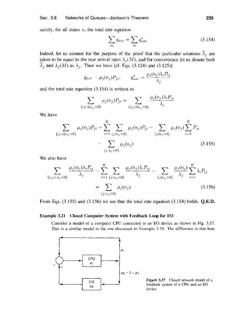
Sec. 3.8 Networks of Queues-Jackson's Theorem 235
satisfy, for all states n, the total rate equation
Lqnm ='In m
(3.154)
Indeed, let us assume for the purpose of the proof that the particular solutions Aj aretaken to be equal to the true arrival rates Aj(A1), and for convenience let us denote both"X j and Aj(M) as AJ . Then we have lcf. Eqs. (3.124) and (3.125)]
* jLj(nj)AiPijqnn' = A.]
and the total rate equation (3.154) is written as
L fLj(nj)Pji = L{(j,iJln) >O} {(j,illnJ >O}
We have
fLj(nj)AiPijAj
K K
L fLj(nj)Pji = L L fLj(nj)Pji = L fLj(nj)L Pji{(j,illn]>O} i=l {jlnJ>O} UlnJ>O} i=]
L fLj(nj)Uln]>O}
We also have
(3.155)
L{(j,iljn,>O}
fLj(nj)AiPi]Aj
fL](nj)AiPijAj
L fLj(nj){jln) >O}
(3.156)
From Eqs. (3.155) and (3.156) we see that the total rate equation (3.154) holds. Q.E.D.
Example 3.21 Closed Computer System with Feedback Loop for I/OConsider a model of a computer CPU connected to an I/O device as shown in Fig. 3.37.This is a similar model to the one discussed in Example 3.19. The difference is that here
p,
I CPU I+ I III I+
P2 = 1 -PI
I I/O I Figure 3.37 Closed network model of a
I 112 I feedback system of a CPU and an I/Odevice.
236 Delay Models in Data Networks Chap. 3
we have a closed network with each job reentering the CPU directly (with probability PI) orafter using the I/O device (with probability P2 = I - PI). There are 1\11 jobs in the system.We select
as the particular solution of the system Aj = I AiP,j, j = L 2. With this choice wehave
PI = I, P2 = P2/Lj/12
and the steady-state distribution of the system is given by [cf. Eqs. (3.149) to (3.151) J
P(AI - n n) = ---- n = 0 .. I. .. " AI,. G(lv1)'
where the normalizing constant G(A1) is given byM
G(1\II) = L P;'n=O
The CPU utilization factor is given byM
U(AI) = I - P(O,]V1) = 1 _ = G(lvI - 1)G(AI) G(Iv1)
and from Little's Theorem we obtain the arrival rate at the CPU as AI(lH) = U(M)/1I.The expression above for the utilization factor U(M) is a special case of a more generalformula (see Problem 3.65).
Example 3.22 Throughput of a Time-Sharing System
Consider the time-sharing computer system with N terminals discussed in Example 3.7 [cf.Fig. 3.38(a)]. We will make detailed statistical assumptions on the times spent by jobs atthe terminals and the CPU. We will consequently be able to obtain a closed-form expressionfor the throughput of the system in place of the upper and lower bounds obtained in Section3.2.
In particular, let us assume that the reflection time of a job at a terminal is exponen-tially distributed with mean R and the processing time of a job at the CPU is exponentiallydistributed with mean P. All reflection and processing times are assumed independent.Then the terminal and CPU queues, viewed in isolation, can be modeled as an AlIAlI exand an AIINI/l queue, respectively [see Fig. 3.38(b)]. Let); = liP be the particularsolution of the arrival rate equation for the system [ef. Eq. (3.147)]. With this choice wehave
RPI = p' P2 = I
The steady-state probability distribution is given by [cf. Eqs. (3.149) to (3.151)]
(RIP)HP(n, N - n) = -.-G--n! (N)
where the normalizing constant G(N) is given by
G(N) = I + (RI P) + + ... +
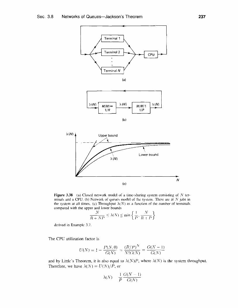
Sec. 3.8 Networks of Queues-Jackson's Theorem
(a)
(b)
237
"A(N) Upper bound
(e)N
Figure 3.38 (a) Closed network model of a time-sharing system consisting of N ter-minals and a CPU. (b) Network of queues model of the system. There are at N jobs inthe system at all times. (c) Throughput A(N) as a function of the number of terminalscompared with the upper and lower boundsIV {I N}__J__ < A(N) < min _. __
R+NP- - P·R+P
derived in Example 3.7.
The CPU utilization factor isNTV __ P(N,O) _ (RIP)
U(" ) - 1 G(N) - N!G(N)G(N-I)G(N)
and by Little's Theorem, it is also equal to )"(N)P, where )"(N) is the system throughput.Therefore, we have )"(N) = U(N)IP, or
, I G(N - 1)).,(Jv) = P G(N)

238 Delay Models in Data Networks Chap. 3
This expression for >-'(IV) is shown in Fig. 3.38(c) and is contrasted with the upper andlower bounds
1V \M .{I IV}R + IVP S ,,(lY) S mm p' R + P
obtained in Section 3.2.
(3.157)
3.8.3 Computational Aspects-Mean Value Analysis
Given a closed queueing network with Al customers, One is typically interested in cal-culating
Nj(lv!) = Average number of customers in the ph queueT](lv!) = Average customer time spent per visit in the ph queue
From these one can obtain the arrival rate at the ph queue given by Little's Theorem as
(3.158)N(M)
A(M)= -]-] TJClV!)
One possibility is to calculate first the normalizing constant G(M) of Eq. (3.151) andthen to use the steady-state distribution Pen) of Eq. (3.152) to obtain all quantities ofinterest. Several different algorithms can be used for this computation, which is oftennontrivial when lvl is large. We will describe an alternative approach, known as meanvalue analysis, which calculates Nj(M) and Tj(M) directly. The normalizing constantG(M) can then be obtained from these quantities and the arrival rates of Eq. (3.158).[See Problem 3.65 for the case where the service rates J.Lj(m) do not depend on thenumber of customers m.]
Let us assume for simplicity that the service rate at the ph queue is J.Lj and doesnot depend on the number of customers in the queue. The main idea in mean valueanalysis is to start with the known quantities
Tj (0). = N] (0) = 0, j = 1, ... ,K (3.159)
(corresponding to an empty system) and then calculate Tj (l) and N j (l) (corresponding toone customer in the system), then calculate Tj (2) and N j (2), and so on until the desiredquantities Tj(M) and Nj(M) are obtained. This calculation is based on the equation (tobe justified shortly)
(3.160)j=l, ... ,K, o5=l, ... ,Al1
Tj(s) = -(1 + N](o5 - I)),J.LJ
which obtains Tj(s) from Nj(05 - 1) for all j. Then Nj(05) is calculated from Tj(05) forall j, using the equation (which is in effect Little's Theorem, as will be seen shortly)
AjTj(05)Nj(05) = 05 K ' j=l, ... ,K, o5=l, ... ,M (3.161):L:i=l AiTi(05)
where>'j, j = 1, ... , K is a positive solution of the system of equations Aj = 1AiPij ,j = 1, ... ,K [ef. Eq. (3.147)].

Sec. 3.8 Networks of Queues-Jackson's Theorem 239
We proceed to derive Eqs. (3.160) and (3.161). Since we have for all j, Aj(s) =for some scalar (l(s) > 0, Eq. (3.161) can be written as
Nj(s) = S ;]CS)Tj(s)Li=1 Ai(s)Ti(s)
and becomes evident once we observe that we have Ai(s)Ti(s) = Ni(s) for all i (byLittle's Theorem) and s = Ni(s) [by the definition of Ni(s)].
To derive Eq. (3.160), we need an important result known as the Arrival Theorem.It states that the occupancy distribution found by a customer upon arrival at the lh queueis the same as the steady-state distribution of the lh queue in a closed network with thearriving customer removed. Thus, in an s-customer closed network, the average numberof customers found upon arrival by a customer at the lh queue is equal to Nj(s - 1),the average number seen by a random observer in the (s - 1)-customer closed network.This explains the form of Eq. (3.160).
An intuitive explanation of the Arrival Theorem is given in Problem 3.59. For ananalytical justification, assume that the s-customer closed network is in steady-state attime t and let x(t) denote the state at that time. For each state n = (nj, ... ,nK) withni > 0, we want to calculate(lij(n) = P{x(t) = n I a customer moved from queue i to queue j just after time t}
(3.162)Let us denote by Mij(t) the event of a customer move from queue i to queue j just aftertime t, and let us denote by .!'vli(t) the event of a customer move from queue i just aftertime t. Then Eq. (3.162) can be written as
p{x(t) = n, Mij(t) IMi(t)}(lij(n) = P{Mij(t) IMi(t)}
p{x(t) = n IMi(t) }p{Mij(t) I x(t) = n, Mi(t)}P{Mij(t) IMi(t)}
P(n)PijL{n'=(n;, .. P(n')?ij
and finally, using Eqs. (3.149) to (3.152) for the steady-state probabilities pen),
F I (nl)' .. FK(nK)(lij(n) = A A (3.163)L{(n;, ... .. n;>O} P1(n;)··· PK(n'r;)
The numerator and the denominator of this equation contain a common factor Pi becauseni > 0 in the numerator and > 0 in each term of the denominator. By dividing withPi, and by using the expression (3.150) for Fj(nj), we obtain
F j (nj)' .. F i - I (ni-I)Fi(ni - 1)Fi+1 (ni+l) ... FK(nK)(lij(n) = A A
L{(n; .... PI(nD··· PK(n'r;)
Therefore, (lij(n) is equal to the steady-state probability of state (nl, ... ,ni-l,ni-1, ni+l, ... , nK) in the (s-l )-customer closed network, as stated by the Arrival Theorem.
240 Delay Models in Data Networks Chap. 3
We note that the Arrival Theorem holds also in some cases where there are multipleclasses of customers and where the queues have multiple servers. Mean value analysiscan also be used in these cases, with Eq. (3.160) replaced by the appropriate formula.
Finally, a number of approximate methods based on mean value analysis have beenproposed. As an example, suppose that an approximate relation of the form
is hypothesized; for large M, one reasonable possibility is
M -11VAM - 1) =
Then Eqs. (3.160) and (3.161) yield the system of nonlinear equations
TJ(M) = ;j (1 + !j (1VJ(M»)) , j = 1.. .. ,K
T _ .. AJTj (1\1)Iv J (AI) - M K j = 1.. .. ,KL;=1 A;T;(M)
which can be solved by iterative methods to yield approximate values for Tj(M) andNj(M).
SUMMARY
Queueing models provide qualitative insights on the performance of data networks,and quantitative predictions of average packet delay. An example of the former is thecomparison of time-division and statistical multiplexing, while an example of the latteris the delay analysis of reservation systems.
To obtain tractable queueing models for data networks, it is frequently necessaryto make simplifying assumptions. A prime example is the Kleinrock independence ap-proximation discussed in Section 3.6. Delay predictions based on this approximation areadequate for many uses. A more accurate alternative is simulation, which, however, canbe slow, expensive, and lacking in insight.
Little's Theorem is a simple but extremely useful result since it holds under verygeneral conditions. To proceed beyond this theorem we assumed Poisson arrivals andindependent interarrival and service times. This led to the Al /G /1 system and itsextensions in reservation and priority queueing systems. We analyzed a surprisinglylarge number of important delay models using simple graphical arguments. An alternativeanalysis was based on the use of Markov chain models and led to the derivation of theoccupancy probability distribution of the I\! /M /1, M / iII /m, and related systems.
Reversibility is an important notion that helps to prove and understand Jackson'sTheorem and provides a taste of advanced queueing topics.
Chap. 3 Notes, Sources, and Suggested Reading
NOTES, SOURCES, AND SUGGESTED READING
241
Section 3.2. Little's Theorem was formalized in [Lit61]. Rigorous proofs undervarious assumptions are given in [Sti72] and [Sti74]. Several applications in findingperformance bounds of computer systems are described in [StA85].
Section 3.3. For a general background on the Poisson process, Markov chains,and related topics, see [Ros80], [Ros83], and [KaT75]. Standard texts on queueing theoryinclude [Co081], [GrH85], [HeS82], [Kle75], and [WoI89]. A reference for the fact thatPoisson arrivals see a typical occupancy distribution (Section 3.3.2) is [WoI82a].
Section 3.4. Queueing systems that admit analysis via Markov chain theory in-clude those where the service times have an Erlang distribution; see [Kle76], Chap. 4.For extensions to more general models and computational methods, see [Kei79], [Neu81],[Haj82], and [Twe82]. For methods to calculate the blocking probability in circuit switch-ing networks (Example 3.14), see [Kau81], [KeI86], [LeG89], [RoT90], and [TsR90].
Section 3.5. The P-K formula is often derived by using z-transforms; see [Kle75].This derivation is not very insightful, but gives the probability distribution of the systemoccupancy (not just the mean that we obtained via our much simpler analysis). For moreon delay analysis of ARQ systems, see [AnP86] and [ToW79].
The results on polling and reservation systems are fairly recent; see [Co070],[Eis79], [FeA85], [FuC85], [IEE86], and [Kue79]. The original references that areclosest to our analysis are [Has72] for unlimited service systems, [NoT78] for limitedservice systems, and [Hum78] for nonsymmetric polling systems. Reference [Tak86] isa monograph devoted to polling. There are two main reservation and polling systemsconsidered in the literature: the symmetric case, where all users have identical arrivaland reservation interval statistics, and the nonsymmetric case, where these statistics areuser dependent. The former case admits simple expressions for the mean waiting timeswhile the latter does not. We have considered the partially symmetric case, where allusers have identical arrival statistics but different reservation interval statistics. Thefact that simple expressions hold for this case has not been known earlier, and in thisrespect, our formulas are original. Our treatment in terms of simple graphical argumentsis also original. Approximate formulas for nonsymmetric polling systems are given in[BoM86] and [IbC89]. The result of Problem 3.35 on limited service systems with sharedreservation and data intervals is new.
An extensive treatment of priority queueing systems is [Jai68]. A simpler, lesscomprehensive exposition is given in [Kle75].
The material on the GIG/I queue is due to [Kin62]. For further material, seeChapter 11 of [WoI89j, [Whi83a], [Whi83b], and the references quoted there.
Section 3.6. Delay analysis for data networks in terms of M I Iv!I I approxima-tions was introduced in [Kle64]. References [WoI82b] and [PiW82] study via analysisand simulation the behavior of two queues in tandem when the service times of a cus-tomer at the two queues are dependent. The special issue [IEE86] provides a view ofrecent work on the subject.
242 Delay Models in Data Networks Chap. 3
Section 3.7. The notion of reversibility was used in Markov chain analysis byKolmogorov [KoI36], and was explored in depth in [KeI79] and [WaI88].
Section 3.8. There is an extensive literature on product form solutions of queue-ing networks following Jackson's original paper [Jac57]. The survey [DiK85] lists 314references. There are also several books on the subject: [KeI79], [BrB80], [GeP87J,[WaI88], and [CoG89]. The heuristic explanation of Jackson's theorem is due to[WaI83].
PROBLEMS
3.1 Customers arrive at a fast-food restaurant at a rate of five per minute and wait to receivetheir order for an average of 5 minutes. Customers eat in the restaurant with probability 0.5and carry out their order without eating with probability 0.5. A meal requires an average of20 minutes. What is the average number of customers in the restaurant? (Answer: 75.)
3.2 Two communication nodes I and 2 send files to another node 3. Files from I and 2 requireon the average R] and R2 time units for transmission, respectively. Node 3 processes afile of node i (i = 1,2) in an average of Pi time units and then requests another file fromeither node I or node 2 (the rule of choice is left unspecified). If '\i is the throughput ofnode i in files sent per unit time, what is the region of all feasible throughput pairs (,\ 1, '\2)for this system?
3.3 A machine shop consists of N machines that occasionally fail and get repaired by one ofthe shop's m repairpersons. A machine will fail after an average of R time units followingits previous repair and requires an average of P time units to get repaired. Obtain upperand lower bounds (functions of R, N, P, and m) on the number of machine failures perunit time and on the average time between repairs of the same machine.
3.4 The average time T a car spends in a certain traffic system is related to the average numberof cars N in the system by a relation of the form T = Q + ,3N2 , where Q > 0, /3 > 0 aregiven scalars.(a) What is the maximal car arrival rate ,\* that the system can sustain?(b) When the car arrival rate is less than ,\*, what is the average time a car spends in the
system assuming that the system reaches a statistical steady state? Is there a uniqueanswer? Try to argue against the validity of the statistical steady-state assumption.
3.5 An absent-minded professor schedules two student appointments for the same time. Theappointment durations are independent and exponentially distributed with mean 30 minutes.The first student arrives on time, but the second student arrives 5 minutes late. What isthe expected time between the arrival of the first student and the departure of the secondstudent? (Answer: 60.394 minutes.)
3.6 A person enters a bank and finds all of the four clerks busy serving customers. There are noother customers in the bank, so the person will start service as soon as one of the customersin service leaves. Customers have independent, identical, exponential distribution of servicetime.(a) What is the probability that the person will be the last to leave the bank assuming that
no other customers arrive?
Chap. 3 Problems 243
(b) If the average service time is I minute, what is the average time the person will spendin the bank?
(c) Will the answer in part (a) change if there are some additional customers waiting in acommon queue and customers begin service in the order of their arrival?
3.7 A communication line is divided in two identical channels each of which will serve apacket traffic stream where all packets have equal transmission time T and equal interarrivaltime R > T. Consider, alternatively, statistical multiplexing of the two traffic streamsby combining the two channels into a single channel with transmission time T /2 for eachpacket. Show that the average system time of a packet will be decreased from T to somethingbetween T /2 and 3T/4, while the variance of waiting time in queue will be increased fromoto as much as T 2 /16.
3.8 Consider a packet stream whereby packets arrive according to a Poisson process with rate10 packets/sec. If the interarrival time between any two packets is less than the transmissiontime of the first to arrive, the two packets are said to collide. (This notion will be mademore meaningful in Chapter 4 when we discuss multiaccess schemes.) Find the probabilitiesthat a packet does not collide with either its predecessor or its successor, and that a packetdoes not collide with another packet assuming:(a) All packets have a transmission time of 20 msec. (Answer: Both probabilities are equal
to 0.67.)(b) Packets have independent, exponentially distributed transmission times with mean 20
msec. (This part requires the 1\II/AI / CX) results.) (Answer: The probability of nocollision with predecessor or successor is 0.694. The probability of no collision is0.682.)
3.9 A communication line capable of transmitting at a rate of 50 Kbits/sec will be used toaccommodate 10 sessions each generating Poisson traffic at a rate 150 packets/min. Packetlengths are exponentially distributed with mean 1000 bits.(a) For each session, find the average number of packets in queue, the average number in
the system, and the average delay per packet when the line is allocated to the sessionsby using:(1) 10 equal-capacity time-division multiplexed channels. (Answer: NQ = 5, N = 10,
T = 0.4 sec.)(2) Statistical multiplexing. (Answer: NQ = 0.5, N = I, T = 0.04 sec.)
(b) Repeat part (a) for the case where five of the sessions transmit at a rate of 250 pack-ets/min while the other five transmit at a rate of 50 packets/min. (Answer: NQ = 21,N = 26, T = 1.038 sec.)
3.10 This problem deals with some of the basic properties of the Poisson process.(a) Derive Eqs. (3.11) to (3.14).(b) Show that if the arrivals in two disjoint time intervals are independent and Poisson
distributed with parameters ATI' AT2, then the number of arrivals in the union of theintervals is Poisson distributed with parameter A(T) + T2)' (This shows in particularthat the Poisson distribution of the number of arrivals in any interval [ef. Eq. (3.10)] isconsistent with the independence requirement in the definition of the Poisson process.)Hint: Verify the correctness of the following calculation, where N) and N2 are thenumber of arrivals in the two disjoint intervals:
244 Delay Models in Data Networks
n
P{N[ + N2 = n} = LP{NI = k}P{N2 = n - k}k=O
Chap. 3
(c) Show that if k independent Poisson processes AI .... ,A k are combined into a singleprocess A = A [ + A2 + + A b then A is Poisson with rate A equal to the sum ofthe rates A" ... Ak of AI' A k. Show also that the probability that the first arrivalof the combined process comes from A, is A, / A independently of the time of arrival.Hint: For k = 2 write
n
= L P{AI(t + T) - A,(t) = m}P{A2(t + T) - A2(t) = n - m}rn=O
and continue as in the hint for part (b). Also write for any t
P{ I arrival from Al prior to t I I occurred}
P{l arrival from A, prior to t, 0 from A 2 }
P{loccurred}
A[te-Alte-A2t A,Ate-At A
(d) Suppose we know that in an interval [tl, t2] only one arrival of a Poisson processhas occurred. Show that, conditional on this knowledge, the time of this arrival isuniformly distributed in [t[, t21. Hint: Verify that if t is the time of arrival, we havefor all s E [tl, t2],
P{f < s II arrival occurred in [fl,f2l}P{ I arrival occurred in [t[, s), 0 arrivals occurred in [s, f2l}
P{ I arrival occurred}s - flf2 - t[
3.11 Packets arrive at a transmission facility according to a Poisson process with rate A. Eachpacket is independently routed with probability p to one of two transmission lines and withprobability (I - p) to the other.(a) Show that the arrival processes at the two transmission lines are Poisson with rates Ap
and A(I - p), respectively. Furthermore, the two processes are independent. Hint: LetN I (t) and N 2(t) be the number of arrivals in [0, f] in lines I and 2, respectively. Verifythe correctness of the following calculation:
Chap. 3 Problems
P{NI(t) = n,Nz(t) = m}, . . e->-.t(At)n+m
= P{NI(t) = n,Nz(t) = m I N(t) = n +m}-----(n+m)!
e-Atp(Atp)n e->-.t(l-p)(At(l p»)Tn
n! m!
245
(b) Use the result of part (a) to show that the probability distribution of the customer delayin a (first-come first-serve) Al/Al/1 queue with arrival rate A and service rate p isexponential, that is, in steady-state we have
where T i is the delay of the ith customer. Hint: Consider a Poisson process A witharrival rate p, which is split into two processes, Al and Az, by randomization accordingto a probability p = A/p.; that is, each arrival of A is an arrival of Al with probabilityp and an arrival of Az with probability (l - p), independently of other arrivals. Showthat the interarrival times of Az have the same distribution as T,.
3.12 Let T] and TZ be two exponentially distributed, independent random variables with means1/Al and 1/Az. Show that the random variable min{TI, TZ} is exponentially distributed withmean I/(AI + A2) and that P{TI < TZ} = AI/(AI + AZ). Use these facts to show that theAl/Al/ I queue can be described by a continuous-time Markov chain with transition ratesI1n(n+l) = A, q(n+lln = 11, n = 0, I, .... (See Appendix A for material on continuous-timeMarkov chains.)
3.13 Persons arrive at a taxi stand with room for VV taxis according to a Poisson process withrate A. A person boards a taxi upon arrival if one is available and otherwise waits in a line.Taxis arrive at the stand according to a Poisson process with rate p. An arriving taxi thatfinds the stand full departs immediately; otherwise, it picks up a customer if at least one iswaiting, or else joins the queue of waiting taxis.(a) Use an 1'\11/AI/I queue formulation to obtain the steady-state distribution of the person's
queue. What is the steady-state probability distribution of the taxi queue size whenIV = 5 and A and p are equal to I and 2 per minute, respectively? (Answer: Let Pi =Probability of i taxis waiting. Then Po = 1/32, PI = 1/32, P2 = 1/16, P3 = 1/8,P4 = 1/4, PS = 1/2.)
(b) In the leaky bucket flow control scheme to be discussed in Chapter 6, packets arrive ata network entry point and must wait in a queue to obtain a permit before entering thenetwork. Assume that pennits are generated by a Poisson process with given rate andcan be stored up to a given maximum number; permits generated while the maximumnumber of permits is available are discarded. Assume also that packets arrive accordingto a Poisson process with given rate. Show how to obtain the occupancy distribution ofthe queue of packets waiting for permits. Hint: This is the same system as the one ofpart (a).
246 Delay Models in Data Networks Chap. 3
*'ftA-3.14
(el Consider the flow control system of part (bl with the difference that pertnits are notgenerated according to a Poisson process but are instead generated periodically at agiven rate. (This is a more realistic assumption.) Fortnulate the problem of finding theoccupancy distribution of the packet queue as an lvl / D / I roblem.
A communication node A receives Poisson packet traffic rom two other nodes, I and 2, atrates AI and A2' respectively, and transmits it, on a first-come first-serve basis, using a linkwith capacity C bits/sec. The two input streams are assumed independent and their packetlengths are identically and exponentially distributed with mean L bits. A packet from nodeI is always accepted by A. A packet from node 2 is accepted only if the number of packetsin A (in queue or under transmission) is less than a given number K > 0; otherwise, it isassumed lost.(al What is the range of values of Al and A2 for which the expected number of packets in
A will stay bounded as time increases?(b) For Al and A2 in the range of part (a) find the steady-state probability of having n
packets in A (0 :s; n < (0). Find the average time needed by a packet from source Ito clear A once it enters A, and the average number of packets in A from source 1.Repeat for packets from source 2.
3.15 Consider a system that is identical to AI / AI/I except that when the system empties out,service does not begin again until k customers are present in the system (k is given).Once service begins it proceeds nortnally until the system becomes empty again. Find thesteady-state probabilities of the number in the system, the average number in the system,and the average delay per customer. [Answer: The average number in the system is N =p/(1 - p) + (k - 1)/2.]
3.16 MIMI/-Like System with State-Dependent Arrival and Service Rate. Consider a system whichis the same as lvI/AI / I except that the rate An and service rate p,n when there are ncustomers in the system depend on 11. Show that
Pn+1 = (po··· Pn)PO
Po = [I + f(Po ... Pk)] -Ik=O
3.17 Discrete-Time Version of the MIMIl System. Consider a queueing system where interarrivaland service times are integer valued, so customer arrivals and departures occur at integertimes. Let A be the probability that an arrival occurs at any time k, and assume that at mostone arrival can occur. Also let p, be the probability that a customer who was in service attime k will complete service at time k + I. Find the occupancy distribution pn in tertns ofA and p,.
3.18 Empty taxis pass by a street comer at a Poisson rate of 2 per minute and pick up a passengerif one is waiting there. Passengers arrive at the street comer at a Poisson rate of I per minuteand wait for a taxi only if there are fewer than four persons waiting; otherwise, they leave andnever return. Find the average waiting time of a passenger who joins the queue. (Answer:13/15 min.)
3.19 A telephone company establishes a direct connection between two cities expecting Poissontraffic with rate 30 calls/min. The durations of calls are independent and exponential1ydistributed with mean 3 min. Interarrival times are independent of cal1 durations. How manycircuits should the company provide to ensure that an attempted cal1 is blocked (because al1
Chap. 3 Problems 247
3.20
3.21
circuits are busy) with probability less than 0.01? It is assumed that blocked calls are lost(i.e., a blocked call is not attempted again).A mail-order company receives calls at a Poisson rate of one per 2 min and the durationof the calls is exponentially distributed with mean 3 min. A caller who finds all telephoneoperators busy patiently waits until one becomes available. Write a computer program todetermine how many operators the company should use so that the average waiting time ofa customer is half a minute or less?Consider the Ai / lvl / I / m system which is the same as Ai / lvl/ I except that there can beno more than m customers in the system and customers arriving when the system is full arelost. Show that the steady-state occupancy probabilities are given by
pn(1 _ p)pn = 1- pm+l '
3.22 An athletic facility has five tennis courts. Players arrive at the courts at a Poisson rate ofone pair per 10 min and use a court for an exponentially distributed time with mean 40 min.(a) Suppose that a pair of players arrives and finds all courts busy and k other pairs waiting
in queue. How long will they have to wait to get a court on the average?(b) What is the average waiting time in queue for players who find all courts busy on
arrival?3.23 Consider an Ai / Al / x queue with servers numbered 1,2, ... There is an additional restric-
tion that upon arrival a customer will choose the lowest-numbered server that is idle at thetime. Find the fraction of time that each server is busy. Will the answer change if the num-ber of servers is finite? Hint: Argue that in steady-state the probability that all of the firstm servers are busy is given by the Erlang B formula of the AI / 1'vl/m/m system. Find thetotal arrival rate to servers (m + I) and higher, and from this, the arrival rate to each server.
3.24 lvl /1'vl /1 Shared Service System. Consider a system which is the same as lvI/AI/1except that whenever there are n customers in the system they are all served simultane-ously at an equal rate 1/n per unit time. Argue that the steady-state occupancy distributionis the same as for the AI/AI /1 system. Note: It can be shown that the steady-state occu-pancy distribution is the same as for 1'vl/Ai/I even if the service time distribution is notexponential (i.e., for an AI/G/I type of system) ([Ros83], p. 171).
3.25 Blocking Probability for Single-Cell Radio Systems ([BaA81] and [BaA82j). A cellular radi-otelephone system serves a given geographical area with Tn radiotelephone channels con-nected to a single switching center. There are two types of calls: radio-to-radio calls, whichoccur with a Poisson rate AI and require two radiochannels per call, and radio-to-nonradiocalls, which occur with a Poisson rate A2 and require one radiochannel per call. The durationof all calls is exponentially distributed with mean 1//1. Calls that cannot be accommodatedby the system are blocked. Give formulas for the blocking probability of the two types ofcalls.
3.26 A facility of m identical machines is sharing a single repairperson. The time to repair afailed machine is exponentially distributed with mean 1/A. A machine, once operational,fails after a time that is exponentially distributed with mean 1//1. All failure and repair timesare independent. What is the steady-state proportion of time where there is no operationalmachine?
3.27 Ai/AI/2 System with Heterogeneous Servers. Derive the stationary distribution of anlH/ lvl/2 system where the two servers have different service rates. A customer that arriveswhen the system is empty is routed to the faster server.
248 Delay Models in Data Networks Chap. 3
3.28 In Example 3.11, verify the formula IJf = ().. / /1)1/2 sr' Hint: Write
and use the fact that n is Poisson distributed.3.29 Customers arrive at a grocery store's checkout counter according to a Poisson process with
rate I per minute. Each customer carries a number of items that is uniformly distibutedbetween I and 40. The store has two checkout counters, each capable of processing itemsat a rate of 15 per minute. To reduce the customer waiting time in queue, the store managerconsiders dedicating one of the two counters to customers with x items or less and dedicatingthe other counter to customers with more than x items. Write a small computer program tofind the value of :r that minimizes the average customer waiting time.
3.30 In the 1\[ / G / I system, show that
P {the system is empty} = I - AX
Average length of time between busy periods
. XAverage length of busy penod =------=
I-AX
IA
Average number of customers served in a busy periodI
I-AX
3.31 Consider the following argument in the l'v1/G/ I system: When a customer arrives, theprobability that another customer is being served is AX. Since the served customer hasmean service time X, the average time to complete the service is X /2. Therefore, the meanresidual service time is AX2 /2. What is wrong with this argument?
3.32 1'1'1/G / I System with Arbitrary Order of Service. Consider the 1\;1/G / I system with thedifference that customers are not served in the order they arrive. Instead, upon completionof a customer's service, one of the waiting customers in queue is chosen according tosome rule, and is served next. Show that the P-K formula for the average waiting time inqueue IV remains valid provided that the relative order of arrival of the customer chosen isindependent of the service times of the customers waiting in queue. Hint: Argue that theindependence hypothesis above implies that at any time t, the number NQ(t) of customerswaiting in queue is independent of the service times of these customers. Show that this intum implies that U = R + plV, where R is the mean residual time and U is the averagesteady-state unfinished work in the system (total remaining service time of the customers inthe system). Argue that U and R are independent of the order of customer service.
3.33 Show that Eq. (3.59) for the average delay of time-division multiplexing on a slot basis canbe obtained as a special case of the results for the limited service reservation system. Hint:Consider the gated system with zero packet length.
3.34 Consider the limited service reservation system. Show that for both the gated and thepartially gated versions:(a) The steady-state probability of arrival of a packet during a reservation interval is I - p.(b) The steady-state probability of a reservation interval being followed by an empty data
interval is (I - p - AV)/(l p). Hint: If p is the required probability, argue that theratio of the times used for data intervals and for reservation intervals is (I - p )XIV.

Chap. 3 Problems 249
3.35 Limited Service Reservation System with Shared Reservation and Data Intervals. Considerthe gated version of the limited service reservation system with the difference that the musers share reservation and data intervals, (i.e., all users make reservations in the sameinterval and transmit at most one packet each in the subsequent data interval). Show that
TV = A_X_2-=-_ + (I - p)V2 + (1- pa - AV/m)Y2(1-p-AV/m) 2(1-p-AV/m)V I-p-AV/m
where V and V2 are the first two moments of the reservation interval, and a satisfies
K + (X - 1)(2K - X) 1 1 1-------==------'- - - < a < - - -
2mK 2m - - 2 2m
where
K= AV1 - P
is the average number of packets per data interval, and X is the smallest integer which islarger than K. Verify that the formula for TV becomes exact as p -t 0 (light load) and asp -t I - AV1m (heavy load). Hint: Verify that
-5)Vwhere 5 = E {5i} and 5i is the number (0 or 1) of packets of the owner of packeti that will start transmission between the time of arrival of packet i and the end of the cyclein which packet i arrives. Try to obtain bounds for 5 by considering separately the caseswhere packeti arrives in a reservation and in a data interval.
3.36 Repeat part (a) of Problem 3.9 for the case where packet lengths are not exponentiallydistributed, but 10% of the packets are 100 bits long and the rest are 1500 bits long. Repeatthe problem for the case where the short packets are given nonpreemptive priority over thelong packets. (Answer: NQ = 0.791, N = 1.47, T = 0.588 sec.)
3.37 Persons arrive at a Xerox machine according to a Poisson process with rate one per minute.The number of copies to be made by each person is uniformly distributed between I and10. Each copy requires 3 sec. Find the average waiting time in queue when:(a) Each person uses the machine on a first-come first-serve basis. (Answer: TV = 3.98.)(b) Persons with no more than 2 copies to make are given nonpreemptive priority over other
persons.3.38 Priority Systems with Multiple Servers. Consider the priority systems of Section 3.5.3 as-
suming that there are m servers and that all priority classes have exponentially distributedservice times with common mean 1//1.(a) Consider the nonpreemptive system. Show that Eq. (3.79) yields the average queueing
times with the mean residual time R given by
R= PQmp
where PQ is the steady-state probability of queueing given by the Erlang C formula ofEq. (3.36). [Here Pi = Ai!(m/1) and p = 2:7=1 Pi.]
(b) Consider the preemptive resume system. Argue that VV(k)' defined as the average time inqueue averaged over the first k priority classes, is the same as for an lvI/AI1m systemwith arrival rate Al + ... + Ak and mean service time 1//1. Use Little's Theorem to
250 Delay Models in Data Networks Chap. 3
k = 2,3, ... , n
show that the average time in queue of a kth priority class customer can be obtainedrecursively from
= Alk [W(k)t Ai - W(k-l) Ai]
3.39 Consider the nonpreemptive priority queueing system of Section 3.5.3 for the case wherethe available capacity is sufficient to handle the highest-priority traffic but cannot handle thetraffic of all priorities, that is,
PI < I < PI + P2 + ... + pn
Find the average delay per customer of each priority class. Hint: Determine the departurerate of the highest-priority class that will experience infinite average delay and the meanresidual service time.
3.40 Optimization of Class Ordering in a Nonpreemptive System. Consider an n-class, nonpre-emptive priority system:(a) Show that the sum PkWk is independent of the priority order of classes, and in
factn
L TIT RpPkvVk = --I-p
k=l
where P = PI +P2+" ·+Pn. (This is known as the Ai IG/l conservation law [Kle64).)Hint: Use Eq. (3.79). Alternatively, argue that U = R + PkWko where U isthe average steady-state unfinished work in the system (total remaining service time ofcustomers in the system), and U and R are independent of the priority order of theclasses.
(b) Suppose that there is a cost Ck per unit time for each class k customer that waits inqueue. Show that cost is minimized when classes are ordered so that
Xl < X 2 < ... < X n
CI C2 Cn
Hint: Express the cost as and use part (a). Also use the factthat interchanging the order of any two adjacent classes leaves the waiting time of allother classes unchanged.
3.41 Little's Theorem for Arbitrary Order of Service; Analytical Proof [Sti74]. Consider theanalysis of Little's Theorem in Section 3.2 and the notation introduced there. We allow thepossibility that the initial number in the system is positive [i.e., N(O) > 0). Assume thatthe time-average arrival and departure rates exist and are equal:
A = lim aCt) = lim ;3(t)t t
and that the following limit defining the time-average system time exists:
T = N(O) o(t) ( L T{+ L (t - t i ))iED(t) iED(t)

Chap. 3 Problems 251
Ti
where D(t) is the set of customers departed by time t and D(t) is the set of customers thatare in the system at time t. (For all customers that are initially in the system, the time Tiis counted starting at time 0.) Show that regardless of the order in which customers areserved, Little's Theorem (N = AT) holds with
N= tN(T)dTt-x t io
Show also that
k
T = lim '"' Tik:-= k
;=1
Hint: Take t -" DC below:
I I rt It .L Ti <:: t io N(T) dT <:: t L'ED(t) 0 iED(t)UD(t)
3.42 A Generalization ofLittle's Theorem. Consider an arrival-departure system with arrival rateA, where entering customers are forced to pay money to the system according to some rule.(a) Argue that the following identity holds:
Average rate at which the system earns = A . (Average amount a customer pays)
(b) Show that Little's Theorem is a special case.(c) Consider the M / G / I system and the following cost rule: Each customer pays at a rate
of y per unit time when its remaining service time is y, whether in queue or in service.Show that the formula in (a) can be written as
W = A (XW +
which is the Pollaczek-Khinchin formula.3.43 AI/G/I Queue with Random-Sized Batch Arrivals. Consider the lvI/G/1 system with the
difference that customers are arriving in batches according to a Poisson process with rateA. Each batch has n customers, where n has a given distribution and is independent ofcustomer service times. Adapt the proof of Section 3.5 to show that the waiting time inqueue is given by
XnX2 X(n2 - n)W = +2(1 - p) 2n(l - p)
Hint: Use the equation W = R + plY +WE, where WE is the average waiting time of acustomer for other customers who arrived in the same batch.
3.44 lvI / G / I Queue with Overhead for Each Busy Period. Consider the J\J / G / I queue with thedifference that the service of the first customer in each busy period requires an increment .6-over the ordinary service time of the customer. We assume that .6- has a given distributionand is independent of all other random variables in the model. Let p = AX be the utilizationfactor. Show that(a) Po = P{the system is empty} = (1 - p)/O + A6).(b) Average length of busy period = (X + 6)/0 - pl.(c) The average waiting time in queue is

252 Delay Models in Data Networks Chap. 3
w = AX2 + A[(X + 6)2 X2]2(1 - p) 2(1 + A6)
(d) Parts (a), (b), and (c) also hold in the case where 6 may depend on the interarrival andservice time of the first customer in the corresponding busy period.
3.45 Consider a system that is identical to J'vl / G /1 except that when the system empties out,service does not begin again until k customers are present in the system (k is given). Onceservice begins, it proceeds normally until the system becomes empty again. Show that:(a) In steady-state:
1-pP { system empty} = -k-'-
{.. } (k - 1)(1 - p)
P system nonempty and waltmg = k
P { system nonempty and serving} = p
(b) The average length of a busy period is
p+k-lA(I - p)
Verify that this average length is equal to the average time between arrival and start ofservice of the first customer in a busy period, plus k times the average length of a busyperiod for the corresponding M / G / I system (k = 1).
(e) Suppose that we divide a busy period into a busy/waiting portion and a busy/servingportion. Show that the average number in the system during a busy/waiting portion isk/2 and the average number in the system during a busy/serving portion is
iVM / G / 1 k - I----'------'-- + --p 2
where Nlvl/G/I is the average number in the system for the corresponding AI/G/Isystem (k = I). Hint: Relate a busy/serving portion of a busy period with k independentbusy periods of the corresponding Al / G /1 system where k = 1.
(d) The average number in the system is
V k - I"M/G/l + -2-
3.46 Single-Vacation Al / G /1 System. Consider the M / G /1 system with the difference that eachbusy period is followed by a single vacation interval. Once this vacation is over, an arrivingcustomer to an empty system starts service immediately. Assume that vacation intervalsare independent, identically distributed, and independent of the customer interarrival andservice times. Prove that the average waiting time in queue is
AX2 V 22( I - p) 21
where 1 is the average length of an idle period, and show how to calculate 1.3.47 The 1\;I/G/= System. Consider a queueing system with Poisson arrivals at rate A. There are
an infinite number of servers, so that each arrival starts service at an idle server immediatelyon arrival. Each server has a general service time distribution and Fx(x) = P{X s: :r}
Chap. 3 Problems 253
denotes the probability that a service starting at any given time T is completed by timeT + x [Fx(x) = °for:r -:; 0]. The servers have independent and identical service timedistributions.(a) For x and b (0 < b < x) very small, find the probability that there was an arrival in
the interval IT - X, T - X + b] and that this arrival is still being served at time T.
(b) Show that the mean service time for any arrival is given by
X = (= [I - Fx(.r)] d.r,10
HiIII: Use a graphical argument.(c) Use parts (a) and (b) to verify that the number in the system is Poisson distributed with
mean ..\X.3.48 An Improved Bound/or the GIGII Queue.
(a) Let l' be a nonnegative random variable and let .r be a nonnegative scalar. Show that
?(max{O,r-x}f
2(max{O,l' - x})
where overbar denotes expected value. Hint: Prove that the left-hand expression IS
monotonically nondecreasing as a function of J:.(b) Using the notation of Section 3.5.4, show that
and that
w < + iTT,)- 2(1 - p)
..\(1 -2
Hilll: Use part (a) with,. being the customer interarrival time and .1' equal to the timein the system Icf. Eq. (3.93)].
3.49 Last-Come First-Serve AI IGII System. Consider an AI IGII system with the differencethat upon arrival at the queue, a customer goes immediately into service, replacing thecustomer who is in service at the time (if any) on a preemptive-resume basis. When acustomer completes service, the customer most recently preempted resumes service. Showthat:(a) The expected length of a busy period, denoted E{B}, is the same as in the ordinary
AI IGII queue.(b) Show that the expected time in the system of a customer is equal to E {B}. Hint: Argue
that a customer who starts a busy period stays in the system for the entire duration ofthe busy period.
(c) Let C be the average time in the system of a customer requiring one unit of servicetime. Argue that the average time in the system of a customer requiring X units ofservice time is XC. Hint: Argue that a customer requiring two units of service timeis "equivalent" to two customers with one unit service time each. and with the secondcustomer arriving at the time that the first departs.
(d) Show that
C= E{B} =E{X} I - p
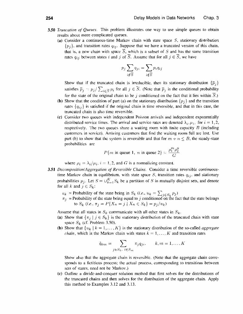
254 Delay Models in Data Networks Chap. 3
3.50 Truncation of Queues. This problem illustrates one way to use simple queues to obtainresults about more complicated queues.(a) Consider a continuous-time Markov chain with state space 5, stationary distribution
{Pj}, and transition rates qij. Suppose that we have a truncated version of this chain,that is, a new chain with space S, which is a subset of 5 and has the same transitionrates qij between states i and j of S. Assume that for all j E S, we have
Pj L qji = LPiqijir{S ir{s
Show that if the truncated chain is irreducible, then its stationary distribution {Pj}
satisfies Pj = Pj / "LiES Pi for all j E S. (Note that Pj is the conditional probabilityfor the state of the original chain to be j conditioned on the fact that it lies within S.)
(b) Show that the condition of part (a) on the stationary distribution {Pj} and the transitionrates {qij} is satisfied if the original chain is time reversible, and that in this case, thetruncated chain is also time reversible.
(c) Consider two queues with independent Poisson arrivals and independent exponentiallydistributed service times. The arrival and service rates are denoted Ai, P.i, fori = 1,2,respectively. The two queues share a waiting room with finite capacity E (includingcustomers in service). Arriving customers that find the waiting room full are lost. Usepart (b) to show that the system is reversible and that for m + n :s; E, the steady-stateprobabilities are
m nP{m in queue 1, n in queue 2} = Pl!:2
where Pi = AdPi, i = 1,2, and G is a normalizing constant.3.51 Decomposition/Aggregation of Reversible Chains. Consider a time reversible continuous-
time Markov chain in equilibrium, with state space 5, transition rates qij, and stationaryprobabilities Pj. Let 5 = uf:= I 5 k be a partition of S in mutually disjoint sets, and denotefor all k and j E 5 k :Uk =Probability of the state being in 5k (i.e., Uk = "LjES
kPJ)
7fj =Probability of the state being equal to j conditioned on the fact that the state belongsto 5k (i.e., 7fj = P{Xn = j IX n E 5d = Pj/Uk)
Assume that all states in Sk communicate with all other states in 5k.(a) Show that {7fj I j E Sd is the stationary distribution of the truncated chain with state
space 5k (cf. Problem 3.50).(b) Show that {Uk I k = I, ... , K} is the stationary distribution of the so-called aggregate
chain, which is the Markov chain with states k = I, ... , K and transition rates
iikm = L 7fjqji,jESk. iESm
k,m=I, ... ,K
Show also that the aggregate chain is reversible. (Note that the aggregate chain corre-sponds to a fictitious process; the actual process, corresponding to transitions betweensets of states, need not be Markov.)
(c) Outline a divide-and-conquer solution method that first solves for the distributions ofthe truncated chains and then solves for the distribution of the aggregate chain. Applythis method to Examples 3.12 and 3.13.

Chap. 3 Problems 255
(d) Suppose that the truncated chains are reversible but the original chain is not. Showthat the results of parts (a) and (b) hold except that the aggregate chain need not bereversible.
3.52 An Extension of Burke's Theorem. Consider an !vI/M /1 system in steady state wherecustomers are served in the order that they arrive. Show that given that a customer departsat time t, the arrival time of that customer is independent of the departure process priorto t. Hint: Consider a customer arriving at time tl and departing at time tz. In reversedsystem terms, the arrival process is independent Poisson, so the arrival process to the leftof tz is independent of the times spent in the system of customers that arrived at or to theright of tz.
3.53 Consider the model of two queues in tandem of Section 3.7 and assume that customers areserved at each queue in the order they arrive.(a) Show that the times (including service) spent by a customer in queue 1 and in queue
2 are mutually independent, and independent of the departure process from queue 2prior to the customer's departure from the system. Hint: By Burke's Theorem, thetime spent by a customer in queue 1 is independent of the sequence of arrival times atqueue 2 prior to the customer's arrival at queue 2. These arrival times (together withthe corresponding independent service times) determine the time the customer spends atqueue 2 as well as the departure process from queue 2 prior to the customer's departurefrom the system.
(b) Argue by example that the times a customer spends waiting before entering service atthe two queues are not independent.
3.54 Use reversibility to characterize the departure process of the M / AI/1/m queue.3.55 Consider the feedback model of a CPU and I/O device of Example 3.19 with the difference
that the CPU consists of m identical parallel processors. The service time of a job ateach parallel processor is exponentially distributed with mean 1/MI. Derive the stationarydistribution of the system.
3.56 Consider the discrete-time approximation to the AI/lvI/l queue of Fig. 3.6. Let X n bethe state of the system at time nfl and let Dn be a random variable taking on the value 1if a departure occurs between nfl and (n + 1)fl, and the value °if no departure occurs.Assume that the system is in steady-state at time nfl. Answer the following without usingreversibility.(a) Find P{Xn = i, Dn = j} for i 2: 0, j = 0, I.(b) Find P{Dn = I}.(e) Find P{Xn = i,Dn = I} for i 2: 0.(d) Find P{Xn+1 = i, Dn = I} and show that X n+1 is statistically independent of Dn .
Hint: Use part (c); also show that P{Xn+1 = i} = P{Xn+1 = i I Dn = I} for alli 2: °is sufficient to show independence.
(e) Find P{Xn+k = i, D n+ l = j I Dn } and show that the pair of variables (Xn+1, Dn+l)is statistically independent of D n .
(f) For each k > I, find P{Xn+k = i,Dn+k = j I Dn+k-l,Dn+k-Z,· .. ,Dn} andshow that the pair (Xn+ko Dn+k ) is statistically independent of (Dn+k- 1, Dn+k- Z,... ,D n ). Hint: Use induction on k.
(g) Deduce a discrete-time analog to Burke's Theorem.3.57 Consider the network in Fig. 3.39. There are four sessions: ACE, ADE, BCEF, and BDEF
sending Poisson traffic at rates 100, 200, 500, and 600 packets/min, respectively. Packetlengths are exponentially distributed with mean 1000 bits. All transmission lines have capac-

256 Delay Models in Data Networks Chap. 3
ity 50 kbits/sec, and there is a propagation delay of 2 msec on each line. Using the Kleinrockindependence approximation, find the average number of packets in the system, the averagedelay per packet (regardless of session), and the average delay per packet of each session.
3.58 Jackson Networks with a Limit on the Total Number ofCustomers. Consider an open Jacksonnetwork as described in the beginning of Section 3.8, with the difference that all customerswho arrive when there are a total of JvI customers in the network are blocked from enteringand are lost for the system. Derive the stationary distribution. Hint: Convert the system intoa closed network with 1''11 customers by introducing an additional queue K + I with servicerate equal to L:= I Tj. A customer exiting queue i E {I, ... , K} enters queue K + I withprobability I Lj Pij , and a customer exiting queue K + I enters queuei E {I, ... ,K}
with probability Til L:=1 Tj.
3.59 Justify the Arrival Theorem for closed networks by inserting a very fast AI / !vI / I queuebetween every pair of queues. Argue that conditioning on a customer moving from onequeue to another is essentially equivalent to conditioning on a single customer being in thefast !vI / 1'vI / I queue that lies between the two queues.
3.60 Consider a closed Jackson network where the service time at each queue is independent ofthe number of customers at the queue. Suppose that for a given number of customers, theutilization factor of one of the queues, say queue I, is strictly larger than the utilizationfactors of the other queues. Show that as the number of customers increases, the proportionof time that a customer spends in queue I approaches unity.
3.61 Consider a model of a computer CPU connected to In I/O devices as shown in Fig. 3.40.Jobs enter the system according to a Poisson process with rate .\, use the CPU and with
A
BFigure 3.39 Network of transmissionlines for Problem 3.57.
Po X
Figure 3.40 Model of a computer CPUconnected to m I/O devices for Problem3.61.
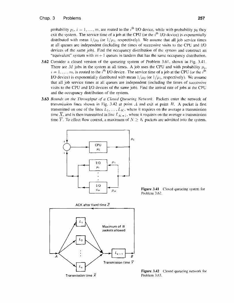
Chap. 3 Problems 257
probability Pi,i = I, ... , m, are routed to thei th I/O device, while with probability Po theyexit the system. The service time of a job at the CPU (or the i th I/O device) is exponentiallydistributed with mean 1/110 (or lilli, respectively). We assume that all job service timesat all queues are independent (including the times of successive visits to the CPU and I/Odevices of the same job). Find the occupancy distribution of the system and construct an"equivalent" system with rn+ I queues in tandem that has the same occupancy distribution.
3.62 Consider a closed version of the queueing system of Problem 3.61, shown in Fig. 3.41.There are l'vl jobs in the system at all times. A job uses the CPU and with probability Pi,i = I, ... ,m, is routed to the i th I/O device. The service time of a job at the CPU (or the i th
I/O device) is exponentially distributed with mean II flo (or IIfli, respectively). We assumethat all job service times at all queues are independent (including the times of successivevisits to the CPU and I/O devices of the same job). Find the arrival rate of jobs at the CPUand the occupancy distribution of the system.
3.63 Bounds on the Throughput of a Closed Queueing Network. Packets enter the network oftransmission lines shown in Fig. 3.42 at point A and exit at point B. A packet is firsttransmitted on one of the lines L I, ... , L K, where it requires on the average a transmissiontime X, and is then transmitted in line L K +1, where it requires on the average a transmissiontime Y. To effect flow control, a maximum of N 2> K packets are admitted into the system.
Po
Figure 3.41 Closed queueing system forProblem 3.62.
ACK after fixed time Z
Transmission time X
Maximum of Npackets allowed
Transmission time Y
Figure 3.42 Closed queueing network forProblem 3.63.
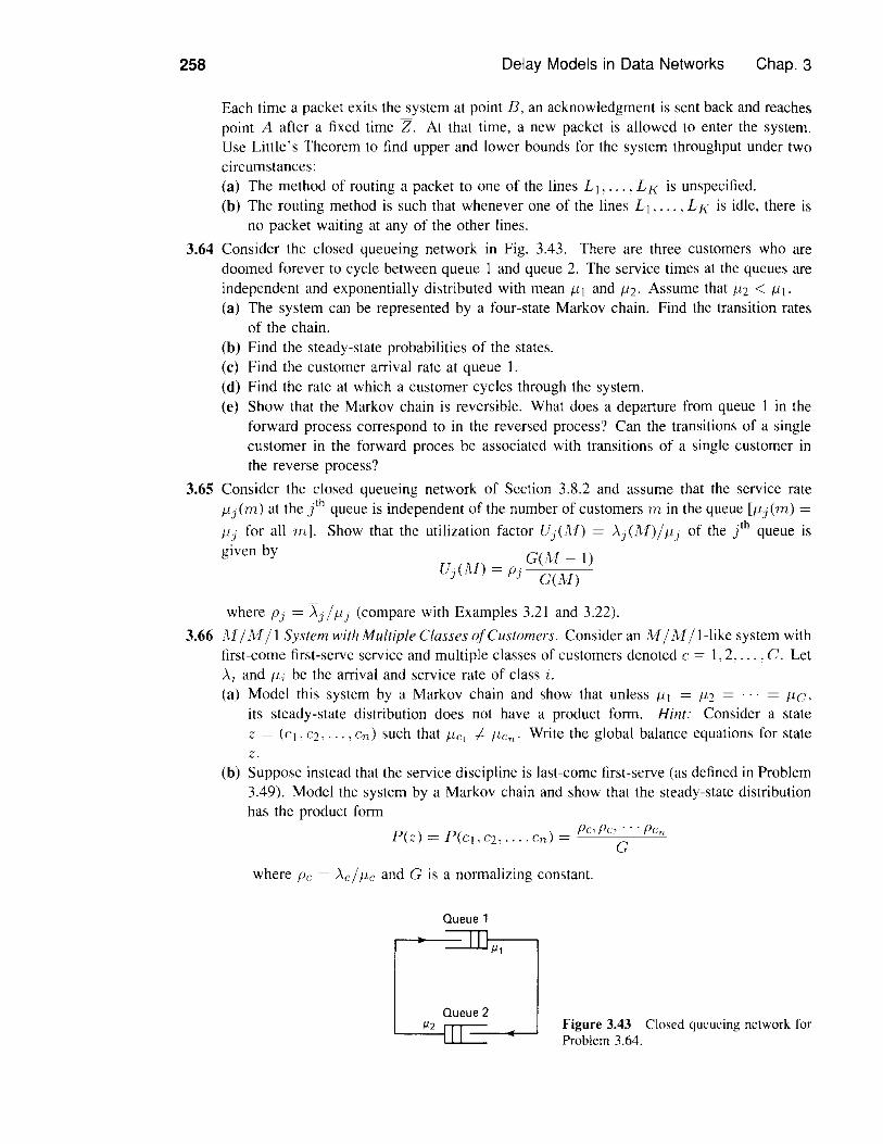
258 Delay Models in Data Networks Chap. 3
G(1vI- I)Uj (Al) = Pj G(1\:1)
3.64
3.65
3.66
Each time a packet exits the system at point B, an acknowledgment is sent back and reachespoint A after a fixed time Z. At that time, a new packet is allowed to enter the system.Use Little's Theorem to find upper and lower bounds for the system throughput under twocircumstances:(a) The method of routing a packet to one of the lines L I, ... , L K is unspecified.(b) The routing method is such that whenever one of the lines L I , ... , L K is idle, there is
no packet waiting at any of the other lines.Consider the closed queueing network in Fig. 3.43. There are three customers who aredoomed forever to cycle between queue I and queue 2. The service times at the queues areindependent and exponentially distributed with mean /11 and /12. Assume that /12 < /11·(a) The system can be represented by a four-state Markov chain. Find the transition rates
of the chain.(b) Find the steady-state probabilities of the states.(c) Find the customer arrival rate at queue I.(d) Find the rate at which a customer cycles through the system.(e) Show that the Markov chain is reversible. What does a departure from queue I in the
forward process correspond to in the reversed process? Can the transitions of a singlecustomer in the forward proces be associated with transitions of a single customer inthe reverse process?
Consider the closed queueing network of Section 3.8.2 and assume that the service rate/1j(m) at the /h queue is independent of the number of customers m in the queue [/1j(m) =/lj for all mJ. Show that the utilization factor Uj(Al) = Aj(1I;1)//1j of the /h queue isgiven by
where Pj = Aj / /1] (compare with Examples 3.21 and 3.22).AI / lvI / I System with Multiple Classes ofCustomers. Consider an Al/Al / I-like system withfirst-come first-serve service and multiple classes of customers denoted c = 1,2.... , C. LetAi and /1; be the arrival and service rate of class i.(a) Model this system by a Markov chain and show that unless /11 = /12 = ... = /le,
its steady-state distribution does not have a product form. Hint: Consider a stateZ = (cl, C2, ... ,en) such that /1CI # /1c n . Write the global balance equations for state
(b) Suppose instead that the service discipline is last-come first-serve (as defined in Problem3.49). Model the system by a Markov chain and show that the steady-state distributionhas the product form
P() P( ) PCI pc, ... PCnZ = CI , C2, ... , Cn = G
where pc = Ac/ /1c and G is a normalizing constant.
Queue 1
Figure 3.43 Closed queueing network forProblem 3.64.
App. A. Review of Markov Chain Theory 259
APPENDIX A: REVIEW OF MARKOV CHAIN THEORY
The purpose of this appendix is to provide a brief summary of the results we need fromdiscrete- and continuous-time Markov chain theory. We refer the reader to books onstochastic processes for detailed accounts.
3A.1 Discrete-Time Markov Chains
Consider a discrete-time stochastic process {Xn In = 0, 1,2, ...} that takes values fromthe set of nonnegative integers, so the states that the process can be in are i = 0, 1 ....The process is said to be a Markov chain if whenever it is in state i, there is a fixedprobability Pij that it will next be in state j regardless of the process history prior toarriving at i. That is, for all n > 0, in-I, ... ,io, i, j.
Pij = P{Xn+1 = j IX n = i, X n- I = in-I, ... ,Xo = io}
=P{Xn+l=jIXn=i}
We refer to Plj as the transition probabilities. They must satisfyex
Pij :::: 0, L Pij = 1 ,j=O
i=O,I,oo.
The corresponding transition probability matrix is denoted
Poo POI P02
PIO P I1 PI2
P=
PiO Pi! Pi2
We will concentrate on the case where the number of states is infinite. There are analo-gous notions and results for the case where the number of states is finite.
Consider the n-step transition probabilities
P[j = P{Xn+rn = j I Xm = i}, n:::: O,i,j :::: 0.
n,m:::: O,i,j:::: °The Chapman-Kolmogorov equations provide a method for calculating Pt;. They aregiven by
xpn+rn = '""" pn.. pmIJ Ik kJ'
k=O
From these equations, we see that Pij are the elements of the matrix p" (the transitionprobability matrix P raised to the nth power).
We say that two states i and j communicate if for some nand n', we have Pt; > °and > 0. If all states communicate, we say that the Markov chain is irreducible.
260 Delay Models in Data Networks Chap. 3
We say that a state i of a Markov chain is periodic if there exists some integer Tn 2: Isuch that PI!' > °and some integer d> I such that Pti > °only if n is a multiple ofd. A Markov chain is said to be aperiodic if none of its states is periodic. A probabilitydistribution {Pi I ,j 2: o} is said to be a stationary distribution for the Markov chain if
%
Pj = LPiPiji=O
,j =0, I, ... (3A.I)
We will restrict attention to irreducible and aperiodic Markov chains, since this isthe only type we will encounter. For such a chain, it can be shown that the limit
]JJ = lim P {X" = ,j I X o = i}, i = 0, L ...
exists and is independent of the starting state X o = i. Furthermore, we have (withprobability I)
. Number of visits to state ,j up to time kPj = hm k
which leads to the interpretation that Pj is the proportion of time or the frequency withwhich the process visits ,j, a time average interpretation. Note again that this frequencydoes not depend on the starting state. The following result will be of primary interest:
Theorem. In an irreducible, aperiodic Markov chain, there are two possibilitiesfor the scalars Pj = P{X" =,j I X o = i}:
1. PJ = 0 for all ,j 2: 0, in which case the chain has no stationary distribution.2. Pj > 0 for all j 2: 0, in which case {PJ l,j 2: o} is the unique stationary distributionof the chain [i.e., it is the only probability distribution satisfying Eq. (3A.I )].
A typical example of case I is a queueing system where the arrival rate exceedsthe service rate, and the number of customers in the system increases to ex, so thesteady-state probability PJ of having any finite number of customers ,j in the system iszero. Note that case I never arises when the number of states is finite. In particular, forevery irreducible and aperiodic Markov chain with states j = 0, I, ... , Tn, there exists aunique probability distribution {Pj I j = 0, I, ... , m} satisfying Pj = "£::0 PiPij andPl > °for all ,j-
In case 2, there arises the issue of characterizing the stationary distribution {Pj Ij 2: O}. For queueing systems, the following equations are often useful. Multiplying theequation Pii = I by PJ and using Eq. (3A.I), we have
(3A.2)j = 0, L ...,x x
Pj L P J ; = LP;Pi},;=0 1=0
These equations are known as the global balance equations. Note that PiPij may beviewed as the long-term frequency of transitions from i to j. Thus the global balanceequations state that at equilibrium, the frequency of transitions out of ,j [left side ofEq. (3A.2)] equals the frequency of transitions into j [right side of Eq. (3A.2)].

App. A. Review of Markov Chain Theory 261
A typical approach for finding the stationary distribution of an irreducible, aperiodicMarkov chain is to try to solve the global balance equations. If a distribution satisfy-ing these equations is found, then by the preceding theorem, it must be the stationarydistribution.
The global balance equations can be generalized to apply to an entire set of states.Consider a subset of states S. By adding Eq. (3A.2) over all j E S, we obtain
LP} LPj; = LPiLPi}JES if/cSif/cS JES
(3A.3)
An intuitive explanation of these equations is based on the fact that when the Markovchain is irreducible, the state (with probability I) will return to the set S infinitely manytimes. Therefore, for each transition out of S there must be (with probability 1) a reversetransition into S at some later time. As a result, the frequency of transitions out of Sequals the frequency of transitions into S. This is precisely the meaning of the globalbalance equations (3A.3).
3A.2 Detailed Balance Equations
As an application of the global balance equations, consider a Markov chain typical ofqueueing systems and, more generally, birth-death systems where two successive statescan only differ by unity, that is, Pi.} = 0 if Ii - jl > I, cf. Fig. 3A.1. We assume thatPi.i+l > 0 and Pi+1•i > 0 for all i. This is a necessary and sufficient condition for thechain to be irreducible. Consider the sets of states
S = {D. L .... n}
Application of Eq. (3A.3) yields
n = 0.1 .... (3A.4)
(i.e .• in steady-state), the frequency of transitions from n to n + I equals the frequencyof transitions from n + 1 to n. These equations can be very useful in computing thestationary distribution {Pj I j O} (see Sections 3.3 and 3.4).
Equation (3A.4) is a special case of the equations
i.j D (3A.5)
known as the detailed balance equations. These equations imply the global balanceequations (3A.2) but need not hold in any given Markov chain. However. in manyimportant special cases. they do hold and greatly simplify the calculation of the stationary
Figure 3A.l Transition probability diagram for a birth-death process.
262 Delay Models in Data Networks Chap. 3
distribution. A common approach is to hypothesize the validity of the detailed balanceequations and to try to solve them for the steady-state probabilities Pj, j O. There aretwo possibilities; either the system (3A.5) together with Lj Pj = 1 is inconsistent orelse a distribution {Pj I j O} satisfying Eq. (3A.5) will be found. In the latter case,this distribution will also satisfy the global balance equations (3A.2), so by the theoremgiven earlier, it is the unique stationary distribution.
3A.3 Partial Balance Equations
Some Markov chains have the property that their stationary distribution {Pj I j O} sat-isfies a set of equations which is intermediate between the global and the detailed balanceequations. For every node j, consider a partition 5J, .... 5j of the complementary setof nodes {i Ii O. i f ,j} and the equations
Pj L Pji = L PiPij • m = 1.2•... ,k (3A.6)
Equations of the form above are known as a set of partial balance equations. If adistribution {Pj I j O} solves a set of partial balance equations, it will also solve theglobal balance equations, so it will be the unique stationary distribution of the chain. Atechnique that often proves useful is to guess the right set of partial balance equationssatisfied by the stationary distribution and then proceed to solve them.
3A.4 Continuous-Time Markov Chains
A continuous-time Markov chain is a process {X(t) I t O} taking values from the setof states i = 0, 1, ... that has the property that each time it enters state i:1. The time it spends in state i is exponentially distributed with parameter Vi. Wemay view Vi as the rate (in transitions/sec) at which the process makes a transitionwhen at state i.
2. When the process leaves state 'i, it will enter state j with probability Pij , whereLj Pij = 1.
We may viewqiJ = l/iPij
as the rate (in transitions/sec) at which the process makes a transition to j when at statei. Consequently, we call qiJ the transition rate fromi to j.
We will be interested in chains for which the discrete-time Markov chain withtransition probabilities Pij (called the embedded chain) is irreducible. We also require atechnical condition, namely that the number of transitions in any finite length of time isfinite with probability 1; chains with this property are called regular. (Nonregular chainsalmost never arise in queueing systems of interest. For an example, see [Ros83), p. 142.)
Under the preceding conditions, it can be shown that the limit
Pj = lim P{X(t) = j I X(O) = i}t-----x
(3A.7)
App. A. Review of Markov Chain Theory 263
exists and is independent of the initial state i. We refer to Pj as the steady-state occupancyprobability of state j. It can be shown that ifT/t) is the time spent in state j up to timet, then, regardless of the initial state, we have with probability 1,
p. = lim Tj(t) (3A.8)J t
that is, Pj can be viewed as the long-term proportion of time the process spends in statej. It can be shown also that either the occupancy probabilities are all zero or else theyare all positive and they sum to unity. Queueing systems where the arrival rate is largerthan the service rate provide examples where all occupancy probabilities are zero.
The global balance equations for a continuous-time Markov chain take the formx x
Pj L qji = LPi%,i=O i=O
j = 0, 1, ... (3A.9)
It can be shown that if a probability distribution {Pj 1 j 2: O} satisfies these equations,then each Pj is the steady-state occupancy probability of state j.
To interpret the global balance equations, we note that since Pi is the proportionof time the process spends in state i, it follows that Piqij is the frequency of transitionsfrom i to j (average number of transitions from i to j per unit time). It is seen thereforethat the global balance equations (3A.9) express the natural fact that the frequency oftransitions out of state j (the left-side term Pj qji) is equal to the frequency oftransitions into state j (the right-side term Piqij).
The continuous-time analog of the detailed balance equations for discrete-timechains is
i, j = 0, 1, ...
These equations hold in birth-death systems where % = 0 for Ii - jl > 1, but neednot hold in other types of Markov chains. They express the fact that the frequencies oftransitions from i to j and from j to i are equal. One can also write a set of partialbalance equations and attempt to solve them for the distribution {Pj I j 2: O}. If asolution can be found, it provides the stationary distribution of the continuous chain.
To understand the relationship between the global balance equations (3A.9) forcontinuous-time chains and the global balance equations (3A.2) for discrete-time chains,consider any 8 > 0, and the discrete-time Markov chain {Xn I n 2: O}, where
X n = X(n8), n = 0, 1, ...The stationary distribution of {Xn } is clearly {Pj I j 2: O}, the occupancy distribution ofthe continuous chain [ef. Eq. (3A.7)]. The transition probabilities of {Xn I n 2: O} canbe derived by using the properties of the exponential distribution and a derivation whichis very similar to the one used in Section 3.3.1 for the Markov chain of the M / M /1queue. We obtain
x
P jj = 1 - 8L qji + 0(8)i=Oi¥-]
264 Delay Models in Data Networks Chap. 3
Using these expressions and Eq. (3A.1), which is equivalent to the global balance equa-tions for the discrete chain, we obtain
::x; ::x;
Pj = LPiPij = Pj (1 - 8 L qji + 0(8») + LPi(8qij + 0(8»)i=O i=O i=Oi#j i#j
and dividing by 8 and letting 8 ---> 0, we obtain the global balance equations (3A.9) forthe continuous chain.
3A.5 Drift and Stability
Suppose that we are given an irreducible, aperiodic, discrete-time Markov chain. In manysituations one is particularly interested in whether the chain has a stationary distribution{p]}. In this case, Pj > 0 for all j and the chain is "stable" in the sense that all statesare visited infinitely often with probability 1. The notion of drift, defined as
'x
Di = E{Xn+1- X n I X n = i} = L kPi(i+k) ,k=-i
i = 0, 1, ...
is particularly useful in this respect. Roughly speaking, the sign of Di indicates whether,starting at i, the state tends to increase (Di > 0) or decrease (Di < 0). Intuitively, thechain will be stable if the drift is negative for all large enough states. This is establishedin the following lemma:
Stability Lemma [Pak69]. Suppose that D i < ex: for alli, and that for somescalar 8 > 0 and integer l ;::: 0 we have
Di <::: -8, for all i > lThen the Markov chain has a stationary distribution.
Proof: Let 6 = maxi::;:; D i . We have for each state i
n
E{Xn IXo = i} - i = L E{Xk - X k- 1 I Xo = i}k=1n x'
= L L E{Xk - X k- I I X k- 1 = j}P{Xk- 1= j I X o = i}k=1 j=O
n [ i<::: {; tJ];P{Xk-1 = j IXo = i}

App. B. Summary of Results
n '[
= (0 + 8)L L P{Xk-l = j I Xo = i} - n8k=] j=O
265
from which we obtain
0<; E(Xn IX" i} <;n[Uil 8) (n-' - j IXo i l ) - 8] +,
Dividing by n and taking the limit as n -+ Xi, we obtain
0:::; ({J + 8) LPj - 8j=O
which implies that Pj > °for some j E {O, ... ,z}. Since the chain is assumed irreducibleand aperiodic, it follows from the theorem of Section 3A.l that there exists a stationarydistribution. Q.E.D.
We also give without proof a converse to the preceding lemma:
Instability Lemma [Kap79]. Suppose that there exist integers z::::: 0 and k suchthat
and
Di > 0, for all i > z
for all i and j such that 0 :::; j :::; i - k
Then the Markov chain does not have a stationary distribution; that is, Pj = 0 for all j.
APPENDIX B: SUMMARY OF RESULTS
NotationPn = Steady-state probability of having n customers in the system
A =Arrival rate (inverse of average interarrival time)JI =Service rate (inverse of average service time)N = Average number of customers in the system
NQ =Average number of customers waiting in queueT =Average customer time in the systemVV =Average customer waiting time in queue (does not include service time)X =Average service timeX2 =Second moment of service time
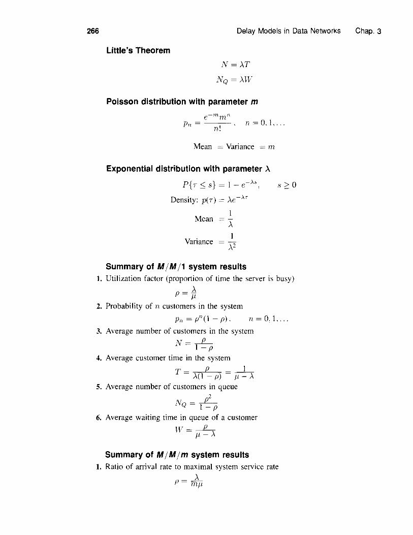
266 Delay Models in Data Networks
Little's TheoremN=AT
NQ=AW
Poisson distribution with parameter m
Chap. 3
Pn = ---n! n = O. 1, ...
Mean = Variance = m
Exponential distribution with parameter ,\
P{T ::; s} = I - e-)..S, s 0
Density: peT) = Ae-)..T
Mean
Variance
Summary of M /M /1 system results1. Utilization factor (proportion of time the server is busy)
P - .6-Jl2. Probability of n customers in the system
Pn = pn(l - p). n = O. 1.. ..3. Average number of customers in the system
N ---E--I-p4. Average customer time in the system
T- p __1_- A(l - p) - Jl - A
5. Average number of customers in queue2
NQ=L-I-p6. Average waiting time in queue of a customer
W =-f!.-Jl-A
Summary of M /M/m system results1. Ratio of arrival rate to maximal system service rate
_ Ap - mJl
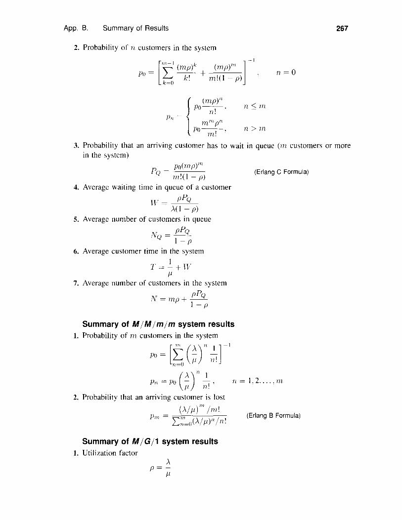
App. B. Summary of Results 267
2. Probability of n customers in the system
Po = [
",-I k ] -I(mp) + (rnp)'"I: k! rn!(1 p)k=O
n=O
n > Tn
Pn = { Po .mmpn
Po--,-,m.
3. Probability that an arriving customer has to wait in queue (rn customers or morein the system)
_ po(rnp)'"Q - m!(1 - p)
4. Average waiting time in queue of a customer
w= p?QA(1 - p)
s. Average number of customers in queueN - p?QQ - 1- P
6. Average customer time in the system
J.17. Average number of customers in the system
N = mp+ p?QI-p
Summary of M IM Im Im system results1. Probability of m customers in the system
_ [m (A) n I ]-1po-I: p ;T
n=O
(Erlang C Formula)
Pn = Po n A' n = 1.2..... Tn/1 n.
2. Probability that an arriving customer is lost(AlJi)m 1m!
Pm = ",m ('I )nl' (Erlang 8 Formula)L.n=O /\ /1 n.
Summary of MIG11 system results1. Utilization factor
Ap= -
/1
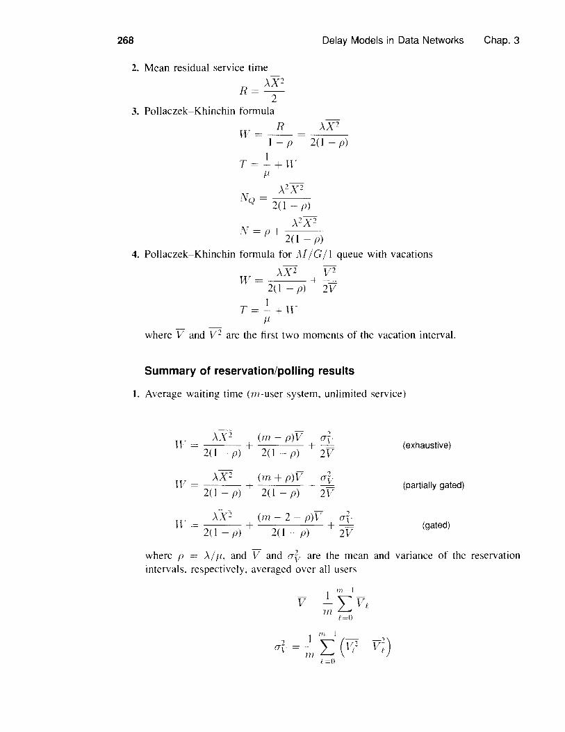
268
2. Mean residual service timeAX2
R= -2-3. Pollaczek-Khinchin formula
Delay Models in Data Networks Chap. 3
R AX2W = -- = c:------,-
I - p 2(1 - p)
PA2X2
[ITQ = -2(-1---/-))
A2X2N=p+---
2(1 - p)4. Pollaczek-Khinchin formula for ]\1/G / I queue with vacations
AX2 V2HT = +--=2(1 - p) 2V
IT=-+W11
where V and V2 are the first two moments of the vacation interval.
Summary of reservation/polling results
I. Average waiting time (rn-user system, unlimited service)
w AX2 (m - p)V O"?-H= + +--=2(1-p) 2(1-p) 2V
\X2 ( )V 21:1' = /\ + TIl + P + O"v2( 1 - p) 2(1 - p) 2V
AX2 (m + 2 - p)V (J2,"W= + +--=2(1 - p) 2(1 - p) 2V
(exhaustive)
(partially gated)
(gated)
where p = A/I', and V and are the mean and variance of the reservationintervals. respectively. averaged over all users
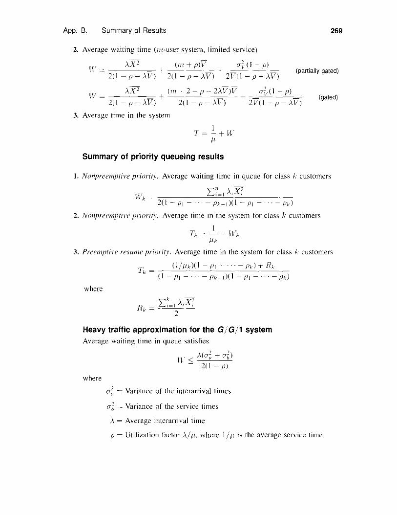
App. B. Summary of Results 269
2. Average waiting time (m-user system, limited service)
'X 2 ()IT 0 (I )w= /\ + m+pv + aT -p2( 1 p - AV) 2(1 - P - AV) 2V(I - p - AV)
(partially gated)
w= AX2 + (m+2-p-2AV)V +2( 1 - p - AV) 2(1 - P - AV) 2V(I - p - AV)
3. Average time in the system
1 .Ji
Summary of priority queueing results
(gated)
1. Nonpreemptive priority. Average waiting time in queue for class k customers
L TI AX2= {=I I I
2(1-PI-"'-Pk-I)(I-PI-"'-p!J
2. Nonpreemptive priority. Average time in the system for class k customers
1 •Tic = - +
Jilc3. Preemptive resume priority. Average time in the system for class k customers
(llliAl(l - PI - .. , - pkl + Ric(I - PI - ... - Plc-I)(I - PI - ... - pAl
where"\"'Ic -0
L....i=1 A,Xi2
Heavy traffic approximation for the GIG11 systemAverage waiting time in queue satisfies
W :s: A( +2(1 - p)
where
= Variance of the interarrival times
= Variance of the service times
A= Average interarrival time
P = Utilization factor AIIi, where 11 /l is the average service time


