Quasimultipliers on F-Algebras

Hindawi Publishing CorporationAbstract and Applied AnalysisVolume 2011, Article ID 235273, 30 pagesdoi:10.1155/2011/235273

Research ArticleQuasimultipliers on F-Algebras

Marjan Adib,1 Abdolhamid Riazi,2 and Liaqat Ali Khan3

1 Department of Mathematics, Payamenoor University-Aligodarz Branch, Aligodarz, Iran2 Department of Mathematics and Computer Science, Amirkabir University of Technology,P.O. Box 15914, Tehran, Iran

3 Department of Mathematics, King Abdulaziz University, P.O. Box 80203, Jeddah 21589, Saudi Arabia

Correspondence should be addressed to Liaqat Ali Khan, [email protected]

Received 7 June 2010; Revised 24 October 2010; Accepted 25 January 2011

Academic Editor: Wolfgang Ruess

Copyright q 2011 Marjan Adib et al. This is an open access article distributed under the CreativeCommons Attribution License, which permits unrestricted use, distribution, and reproduction inany medium, provided the original work is properly cited.

We investigate the extent to which the study of quasimultipliers can be made beyond Banachalgebras. We will focus mainly on the class of F-algebras, in particular on complete k-normedalgebras, 0 < k ≤ 1, not necessarily locally convex. We include a few counterexamples todemonstrate that some of our results do not carry over to general F-algebras. The bilinearity andjoint continuity of quasimultipliers on an F-algebraA are obtained under the assumption of strongfactorability. Further, we establish several properties of the strict and quasistrict topologies on thealgebra QM(A) of quasimultipliers of a complete k-normed algebra A having a minimal ultra-approximate identity.

1. Introduction

A quasimultiplier is a generalization of the notion of a left (right, double) multiplier andwas first introduced by Akemann and Pedersen in [1, Section 4]. The first systematic accountof the general theory of quasimultipliers on a Banach algebra with a bounded approximateidentity was given in a paper by McKennon [2] in 1977. Further developments have beenmade, among others, by Vasudevan and Goel [3], Kassem and Rowlands [4], Lin [5, 6],Dearden [7], Argun and Rowlands [8], Grosser [9], Yılmaz and Rowlands [10], and Kaneda[11, 12].

In this paper, we consider the notion of quasimultipliers on certain topologicalalgebras and give an account, how far one can get beyond Banach algebras, usingcombination of standard methods. In particular, we are able to establish some results of theabove authors in the framework of F-algebras or complete k-normed algebras.

2 Abstract and Applied Analysis

2. Preliminaries

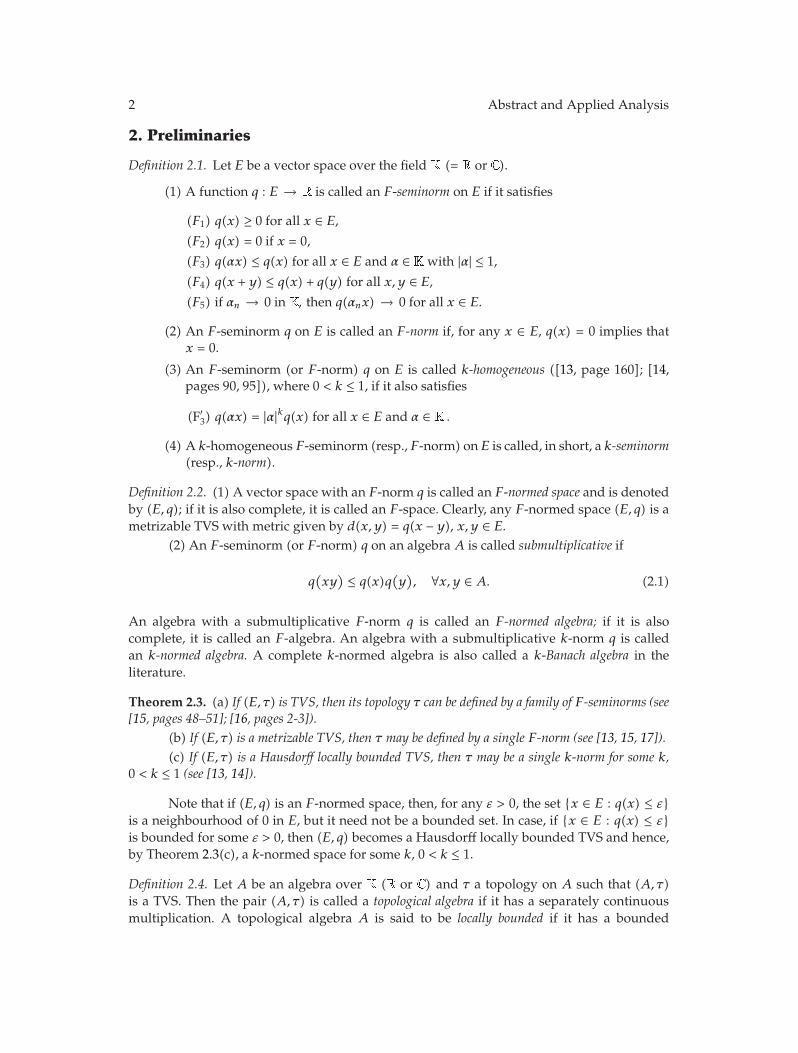
Definition 2.1. Let E be a vector space over the field � (= � or � ).

(1) A function q : E → � is called an F-seminorm on E if it satisfies

(F1) q(x) ≥ 0 for all x ∈ E,

(F2) q(x) = 0 if x = 0,

(F3) q(αx) ≤ q(x) for all x ∈ E and α ∈ � with |α| ≤ 1,

(F4) q(x + y) ≤ q(x) + q(y) for all x, y ∈ E,

(F5) if αn → 0 in � , then q(αnx) → 0 for all x ∈ E.

(2) An F-seminorm q on E is called an F-norm if, for any x ∈ E, q(x) = 0 implies thatx = 0.

(3) An F-seminorm (or F-norm) q on E is called k-homogeneous ([13, page 160]; [14,pages 90, 95]), where 0 < k ≤ 1, if it also satisfies

(F′3) q(αx) = |α|kq(x) for all x ∈ E and α ∈ � .

(4) A k-homogeneous F-seminorm (resp.,F-norm) onE is called, in short, a k-seminorm(resp., k-norm).

Definition 2.2. (1) A vector space with an F-norm q is called an F-normed space and is denotedby (E, q); if it is also complete, it is called an F-space. Clearly, any F-normed space (E, q) is ametrizable TVS with metric given by d(x, y) = q(x − y), x, y ∈ E.

(2) An F-seminorm (or F-norm) q on an algebra A is called submultiplicative if

q(xy

) ≤ q(x)q(y), ∀x, y ∈ A. (2.1)

An algebra with a submultiplicative F-norm q is called an F-normed algebra; if it is alsocomplete, it is called an F-algebra. An algebra with a submultiplicative k-norm q is calledan k-normed algebra. A complete k-normed algebra is also called a k-Banach algebra in theliterature.

Theorem 2.3. (a) If (E, τ) is TVS, then its topology τ can be defined by a family of F-seminorms (see[15, pages 48–51]; [16, pages 2-3]).

(b) If (E, τ) is a metrizable TVS, then τ may be defined by a single F-norm (see [13, 15, 17]).(c) If (E, τ) is a Hausdorff locally bounded TVS, then τ may be a single k-norm for some k,

0 < k ≤ 1 (see [13, 14]).

Note that if (E, q) is an F-normed space, then, for any ε > 0, the set {x ∈ E : q(x) ≤ ε}is a neighbourhood of 0 in E, but it need not be a bounded set. In case, if {x ∈ E : q(x) ≤ ε}is bounded for some ε > 0, then (E, q) becomes a Hausdorff locally bounded TVS and hence,by Theorem 2.3(c), a k-normed space for some k, 0 < k ≤ 1.

Definition 2.4. Let A be an algebra over � (� or � ) and τ a topology on A such that (A, τ)is a TVS. Then the pair (A, τ) is called a topological algebra if it has a separately continuousmultiplication. A topological algebra A is said to be locally bounded if it has a bounded

Abstract and Applied Analysis 3

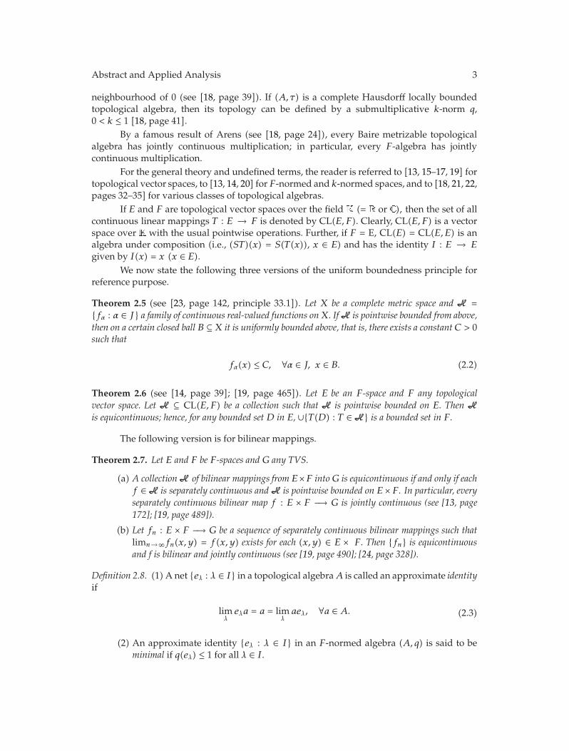
neighbourhood of 0 (see [18, page 39]). If (A, τ) is a complete Hausdorff locally boundedtopological algebra, then its topology can be defined by a submultiplicative k-norm q,0 < k ≤ 1 [18, page 41].

By a famous result of Arens (see [18, page 24]), every Baire metrizable topologicalalgebra has jointly continuous multiplication; in particular, every F-algebra has jointlycontinuous multiplication.

For the general theory and undefined terms, the reader is referred to [13, 15–17, 19] fortopological vector spaces, to [13, 14, 20] for F-normed and k-normed spaces, and to [18, 21, 22,pages 32–35] for various classes of topological algebras.

If E and F are topological vector spaces over the field � (= � or � ), then the set of allcontinuous linear mappings T : E → F is denoted by CL(E, F). Clearly, CL(E, F) is a vectorspace over � with the usual pointwise operations. Further, if F = E, CL(E) = CL(E, E) is analgebra under composition (i.e., (ST)(x) = S(T(x)), x ∈ E) and has the identity I : E → Egiven by I(x) = x (x ∈ E).

We now state the following three versions of the uniform boundedness principle forreference purpose.

Theorem 2.5 (see [23, page 142, principle 33.1]). Let X be a complete metric space and H ={fα : α ∈ J} a family of continuous real-valued functions onX. IfH is pointwise bounded from above,then on a certain closed ball B ⊆ X it is uniformly bounded above, that is, there exists a constantC > 0such that

fα(x) ≤ C, ∀α ∈ J, x ∈ B. (2.2)

Theorem 2.6 (see [14, page 39]; [19, page 465]). Let E be an F-space and F any topologicalvector space. Let H ⊆ CL(E, F) be a collection such that H is pointwise bounded on E. Then His equicontinuous; hence, for any bounded set D in E, ∪{T(D) : T ∈ H} is a bounded set in F.

The following version is for bilinear mappings.

Theorem 2.7. Let E and F be F-spaces and G any TVS.

(a) A collectionH of bilinear mappings from E×F into G is equicontinuous if and only if eachf ∈ H is separately continuous andH is pointwise bounded on E × F. In particular, everyseparately continuous bilinear map f : E × F −→ G is jointly continuous (see [13, page172]; [19, page 489]).

(b) Let fn : E × F −→ G be a sequence of separately continuous bilinear mappings such thatlimn→∞fn(x, y) = f(x, y) exists for each (x, y) ∈ E × F. Then {fn} is equicontinuousand f is bilinear and jointly continuous (see [19, page 490]; [24, page 328]).

Definition 2.8. (1)Anet {eλ : λ ∈ I} in a topological algebraA is called an approximate identityif

limλ

eλa = a = limλ

aeλ, ∀a ∈ A. (2.3)

(2) An approximate identity {eλ : λ ∈ I} in an F-normed algebra (A, q) is said to beminimal if q(eλ) ≤ 1 for all λ ∈ I.


(3) An algebraA is said to be left (resp., right) faithful if, for any a ∈ A, aA = {0} (resp.,Aa = {0}) implies that a = 0; A is called faithful if it is both left and right faithful.One mentions that A is faithful in each of the following cases:

(i) A is a topological algebra with an approximate identity (e.g., A is a locallyC∗-algebra);

(ii) A is a topological algebra with an orthogonal basis [25].

Definition 2.9. A topological algebraA is called

(1) factorable if, for each a ∈ A, there exist b, c ∈ A such that a = bc,

(2) strongly factorable if, for any sequence {an} in A with an → 0, there exist a ∈ A anda sequence {bn} (resp., {cn}) in A with bn → 0 (resp., cn → 0) such that an = abn(resp., an = cna) for all n ≥ 1.

Clearly, every strongly factorable algebra is factorable. Factorization in Banach andtopological algebras plays an important role in the study of multipliers and quasimultipliers.There are several versions of the famous Hewitt-Cohen’s factorization theorem in theliterature (see, e.g., the book [26] and its references). Using the terminology of [27], we statethe following version in the nonlocally convex case.

Theorem 2.10 (see [27]). Let A be a fundamental F-algebra with a uniformly bounded leftapproximate identity. Then A is strongly factorable.

Definition 2.11. Let (A, q) be an F-normed space (in particular, an F-normed algebra). For anyT ∈ CL(A), let

‖T‖q = sup{q(T(x))q(x)

: x ∈ A, x /= 0}. (∗)

It is easy to see that if q is a k-norm, 0 < k ≤ 1, (resp., a seminorm) onA, then ‖ · ‖q is a k-norm(resp., a seminorm) on CL(A); further, in these cases, we have alternate formulas for ‖T‖q as

‖T‖q = sup{q(T(x)) : x ∈ A, q(x) = 1

}

= sup{q(T(x)) : x ∈ A, q(x) ≤ 1

},

(2.4)

for each T ∈ CL(A) (see [14, pages 101-102]; [28, pages 3–5]; [19, page 87]).

Remark 2.12. In an earlier version of this paper, the authors had erroneously made the blankassumption that, for q an F-norm on A, ‖T‖q given by (∗) always exists for each T ∈ CL(A).We are grateful to referee for pointing out that this assumption cannot be justified in view ofthe following counterexamples.

(1) First, ‖T‖q need not be finite for a general F-norm. For example, let A = �2 ,q(x1, x2) = |x1|+|x2|1/2, T(x1, x2) = (x2, x1). Then q is an F-norm onA, but ‖T‖q = ∞:for any n ∈ �,

‖T‖q ≥q[T(n, n2)]

q(n, n2)=

q(n2, n

)

q(n, n2)=n2 + n1/2

2n−→ ∞. (2.5)


(2) Even when considering the subspace of those T for which ‖T‖q < ∞, then ‖ · ‖qneed not always be an F-norm, since (F5) need not hold. For example, for a fixedsequence (pn) with 0 < pn ≤ 1, pn → 0, consider the F-algebra A of sequences(xn) ⊆ � with |xn|pn → 0 and q((xn)) = supn≥1|xn|pn . Then ‖T‖q < ∞ for allmultipliers of A, but ‖ · ‖q is not an F-norm, that is, it makes the space CL(A) intoan additive topological group but not into a topological vector space (as it wouldlack the continuity of scalar multiplication in the absence of (F5) (cf. [14, Example1.2.3, page 8]).

In view of the above remark, we will need to assume that (A, q) is a k-normed space(or a k-normed algebra)whenever ‖T‖q is considered for T ∈ CL(A) or CL(A ×A,A).

Some useful properties of (CL(A), ‖ · ‖q) are summarized as follows.

Theorem 2.13 (see [14, pages 101-102]). Let (A, q) be a k-normed space (in particular, a k-normedalgebra) with 0 < k ≤ 1. Then:

(a) a linear mapping T : A → A is continuous ⇔ ‖T‖q < ∞;

(b) ‖ · ‖q is a k-norm on CL(A);

(c) q(T(x)) ≤ ‖T‖q · q(x) for all x ∈ A;

(d) for any S, T ∈ CL(A), ‖ST‖q ≤ ‖S‖q‖T‖q; hence (CL(A), ‖ · ‖q) is a k-normed algebra;

(e) if A is complete, then (CL(A), ‖ · ‖q) is a complete k-normed algebra.

Remark 2.14. The referee has enquired if the present theory can be considered for the classof locally convex F-algebras. It is well known (e.g., [22, page 33]; [21, page 9]) that, for thisclass of topological algebras, the topology can be generated by an increasing countable familyof seminorms {qn}, which need not be submultiplicative but satisfy the weaker conditionqn(xy) ≤ qn+1(x)qn+1(y); however, for locally m-convex F-algebras, the seminorms can bechosen to be submultiplicative. In view of this, we believe that a study of quasimultiplierscan possibly be made on locally m-convex algebra F-algebras parallel to the one given byPhillips (see [29, pages 177–180]) for multipliers.

3. Multipliers on F-Normed Algebras

In this section, we recall definitions and results on various notions of multipliers on an algebraA (as given in [30–33]) which we shall require later in the study of quasimultipliers (see also[25, 29, 34–40]). In fact, we shall see that the proofs of most of the results on quasimultipliersare based on the properties of left, right, and double multipliers.

Definition 3.1 (see [31]). LetA be an algebra over the field � (� or � ).

(1) A mapping T : A → A is called a

(i) multiplier on A if aT(b) = T(a)b for all a, b ∈ A,(ii) left multpilier on A if T(ab) = T(a)b for all a, b ∈ A,(iii) right multiplier on A if T(ab) = aT(b) for all a, b ∈ A.

(2) A pair (S, T) of mappings S, T : A → A is called a double multiplier on A if aS(b) =T(a)b for all a, b ∈ A.


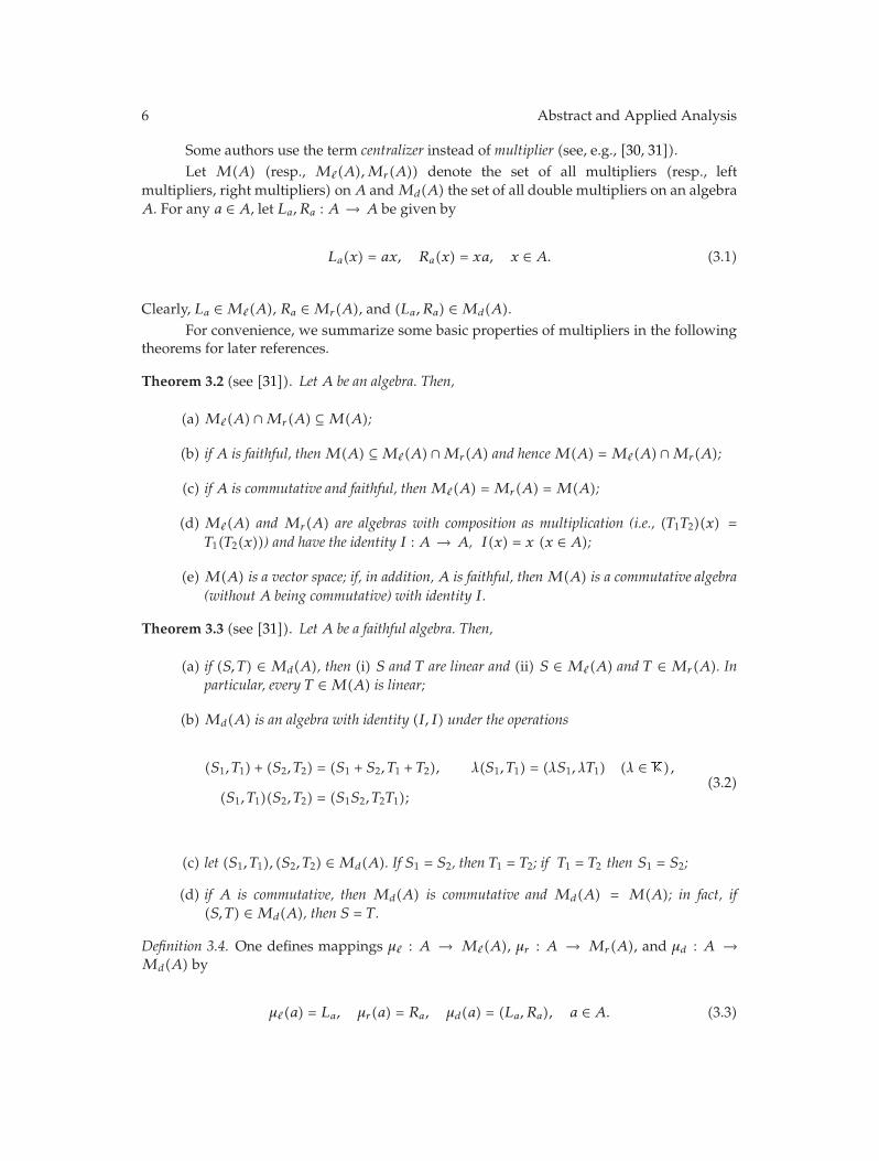
Some authors use the term centralizer instead of multiplier (see, e.g., [30, 31]).Let M(A) (resp., M�(A),Mr(A)) denote the set of all multipliers (resp., left

multipliers, right multipliers) onA andMd(A) the set of all double multipliers on an algebraA. For any a ∈ A, let La, Ra : A → A be given by

La(x) = ax, Ra(x) = xa, x ∈ A. (3.1)

Clearly, La ∈ M�(A), Ra ∈ Mr(A), and (La, Ra) ∈ Md(A).For convenience, we summarize some basic properties of multipliers in the following

theorems for later references.

Theorem 3.2 (see [31]). Let A be an algebra. Then,

(a) M�(A) ∩Mr(A) ⊆ M(A);

(b) if A is faithful, thenM(A) ⊆ M�(A) ∩Mr(A) and henceM(A) = M�(A) ∩Mr(A);

(c) if A is commutative and faithful, thenM�(A) = Mr(A) = M(A);

(d) M�(A) and Mr(A) are algebras with composition as multiplication (i.e., (T1T2)(x) =T1(T2(x))) and have the identity I : A → A, I(x) = x (x ∈ A);

(e) M(A) is a vector space; if, in addition, A is faithful, then M(A) is a commutative algebra(without A being commutative) with identity I.

Theorem 3.3 (see [31]). Let A be a faithful algebra. Then,

(a) if (S, T) ∈ Md(A), then (i) S and T are linear and (ii) S ∈ M�(A) and T ∈ Mr(A). Inparticular, every T ∈ M(A) is linear;

(b) Md(A) is an algebra with identity (I, I) under the operations

(S1, T1) + (S2, T2) = (S1 + S2, T1 + T2), λ(S1, T1) = (λS1, λT1) (λ ∈ � ),

(S1, T1)(S2, T2) = (S1S2, T2T1);(3.2)

(c) let (S1, T1), (S2, T2) ∈ Md(A). If S1 = S2, then T1 = T2; if T1 = T2 then S1 = S2;

(d) if A is commutative, then Md(A) is commutative and Md(A) = M(A); in fact, if(S, T) ∈ Md(A), then S = T .

Definition 3.4. One defines mappings μ� : A → M�(A), μr : A → Mr(A), and μd : A →Md(A) by

μ�(a) = La, μr(a) = Ra, μd(a) = (La, Ra), a ∈ A. (3.3)


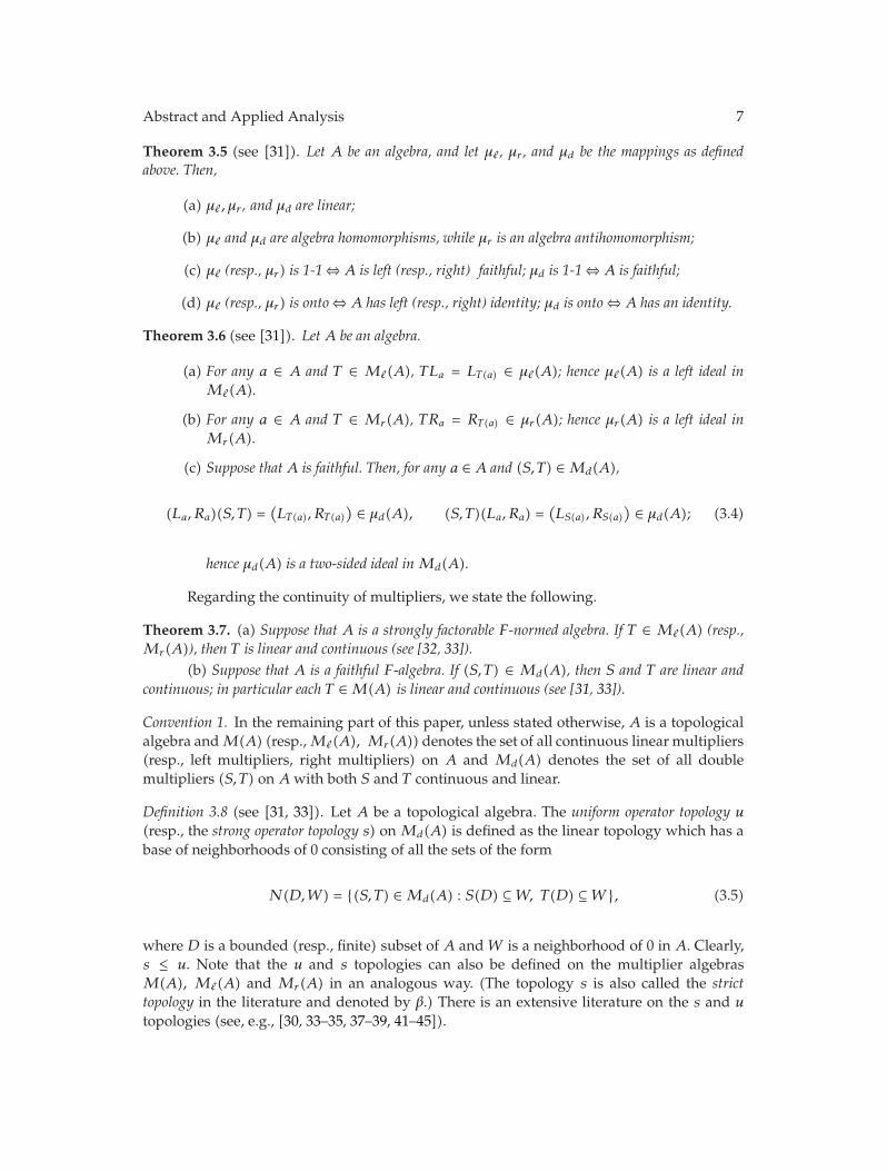
Theorem 3.5 (see [31]). Let A be an algebra, and let μ� , μr , and μd be the mappings as definedabove. Then,

(a) μ�, μr , and μd are linear;

(b) μ� and μd are algebra homomorphisms, while μr is an algebra antihomomorphism;

(c) μ� (resp., μr) is 1-1⇔ A is left (resp., right) faithful; μd is 1-1⇔ A is faithful;

(d) μ� (resp., μr) is onto⇔ A has left (resp., right) identity; μd is onto ⇔ A has an identity.

Theorem 3.6 (see [31]). Let A be an algebra.

(a) For any a ∈ A and T ∈ M�(A), TLa = LT(a) ∈ μ�(A); hence μ�(A) is a left ideal inM�(A).

(b) For any a ∈ A and T ∈ Mr(A), TRa = RT(a) ∈ μr(A); hence μr(A) is a left ideal inMr(A).

(c) Suppose thatA is faithful. Then, for any a ∈ A and (S, T) ∈ Md(A),

(La, Ra)(S, T) =(LT(a), RT(a)

) ∈ μd(A), (S, T)(La, Ra) =(LS(a), RS(a)

) ∈ μd(A); (3.4)

hence μd(A) is a two-sided ideal in Md(A).

Regarding the continuity of multipliers, we state the following.

Theorem 3.7. (a) Suppose that A is a strongly factorable F-normed algebra. If T ∈ M�(A) (resp.,Mr(A)), then T is linear and continuous (see [32, 33]).

(b) Suppose that A is a faithful F-algebra. If (S, T) ∈ Md(A), then S and T are linear andcontinuous; in particular each T ∈ M(A) is linear and continuous (see [31, 33]).

Convention 1. In the remaining part of this paper, unless stated otherwise, A is a topologicalalgebra andM(A) (resp.,M�(A), Mr(A)) denotes the set of all continuous linear multipliers(resp., left multipliers, right multipliers) on A and Md(A) denotes the set of all doublemultipliers (S, T) on Awith both S and T continuous and linear.

Definition 3.8 (see [31, 33]). Let A be a topological algebra. The uniform operator topology u

(resp., the strong operator topology s) on Md(A) is defined as the linear topology which has abase of neighborhoods of 0 consisting of all the sets of the form

N(D,W) = {(S, T) ∈ Md(A) : S(D) ⊆ W, T(D) ⊆ W}, (3.5)

where D is a bounded (resp., finite) subset of A and W is a neighborhood of 0 in A. Clearly,s ≤ u. Note that the u and s topologies can also be defined on the multiplier algebrasM(A), M�(A) and Mr(A) in an analogous way. (The topology s is also called the stricttopology in the literature and denoted by β.) There is an extensive literature on the s and u

topologies (see, e.g., [30, 33–35, 37–39, 41–45]).


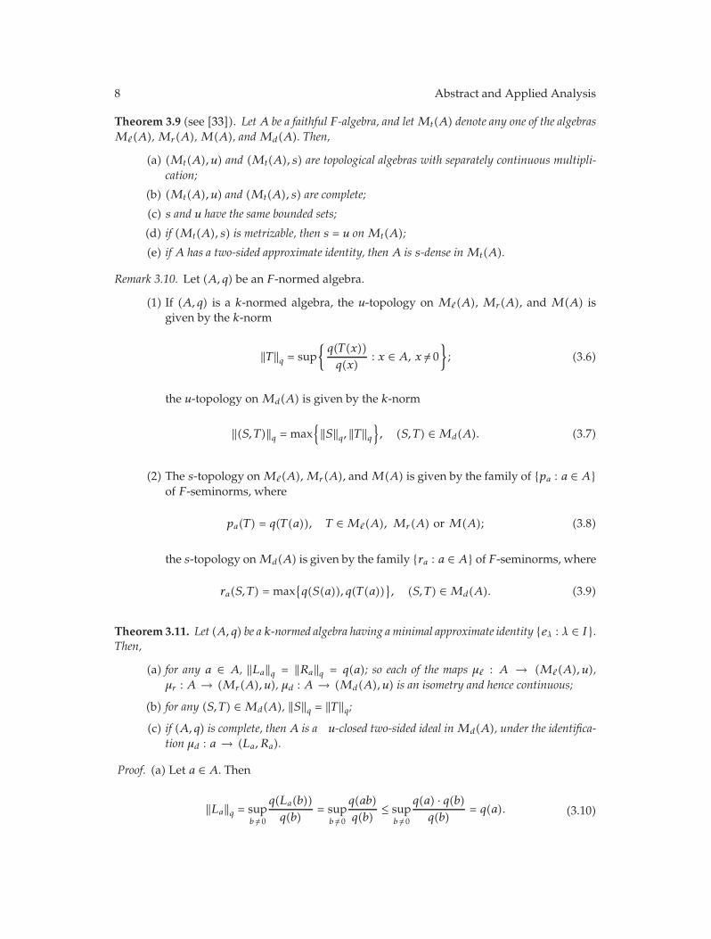
Theorem 3.9 (see [33]). Let A be a faithful F-algebra, and letMt(A) denote any one of the algebrasM�(A), Mr(A), M(A), andMd(A). Then,

(a) (Mt(A), u) and (Mt(A), s) are topological algebras with separately continuous multipli-cation;

(b) (Mt(A), u) and (Mt(A), s) are complete;

(c) s and u have the same bounded sets;

(d) if (Mt(A), s) is metrizable, then s = u on Mt(A);

(e) if A has a two-sided approximate identity, then A is s-dense in Mt(A).

Remark 3.10. Let (A, q) be an F-normed algebra.

(1) If (A, q) is a k-normed algebra, the u-topology on M�(A), Mr(A), and M(A) isgiven by the k-norm

‖T‖q = sup{q(T(x))q(x)

: x ∈ A, x /= 0}; (3.6)

the u-topology on Md(A) is given by the k-norm

‖(S, T)‖q = max{‖S‖q, ‖T‖q

}, (S, T) ∈ Md(A). (3.7)

(2) The s-topology onM�(A),Mr(A), andM(A) is given by the family of {pa : a ∈ A}of F-seminorms, where

pa(T) = q(T(a)), T ∈ M�(A), Mr(A) or M(A); (3.8)

the s-topology onMd(A) is given by the family {ra : a ∈ A} of F-seminorms, where

ra(S, T) = max{q(S(a)), q(T(a))

}, (S, T) ∈ Md(A). (3.9)

Theorem 3.11. Let (A, q) be a k-normed algebra having a minimal approximate identity {eλ : λ ∈ I}.Then,

(a) for any a ∈ A, ‖La‖q = ‖Ra‖q = q(a); so each of the maps μ� : A → (M�(A), u),μr : A → (Mr(A), u), μd : A → (Md(A), u) is an isometry and hence continuous;

(b) for any (S, T) ∈ Md(A), ‖S‖q = ‖T‖q;(c) if (A, q) is complete, thenA is a u-closed two-sided ideal inMd(A), under the identifica-

tion μd : a → (La, Ra).

Proof. (a) Let a ∈ A. Then

‖La‖q = supb /= 0

q(La(b))q(b)

= supb /= 0

q(ab)q(b)

≤ supb /= 0

q(a) · q(b)q(b)

= q(a). (3.10)


On the other hand,

‖La‖q = supb /= 0

q(ab)q(b)

≥ q(aeλ)q(eλ)

≥ q(aeλ), ∀λ ∈ I; (3.11)

so

‖La‖q ≥ limλ

q(aeλ) = q

(limλ

aeλ

)= q(a). (3.12)

Hence ‖μ�(a)‖q = ‖La‖q = q(a). Similarly, ‖μr(a)‖q = ‖Ra‖q = q(a). Thus

∥∥μd(a)

∥∥q= max

{‖La‖q, ‖Ra‖q

}= q(a). (3.13)

(b) Let (S, T) ∈ Md(A). Using (a), we have

‖S‖q = supa/= 0

q(S(a))q(a)

= supa/= 0

∥∥RS(a)∥∥q

q(a)= sup

a/= 0supb /= 0

1q(a)

· q[RS(a)(b)

]

q(b)

= supa/= 0

supb /= 0

q[bS(a)]q(a) · q(b) = sup

a/= 0supb /= 0

q[T(b)a]q(a) · q(b)

≤ supa/= 0

supb /= 0

q(T(b)) · q(a)q(a) · q(b) = sup

b /= 0

q(T(b))q(b)

= ‖T‖q.

(3.14)

Similarly,

‖T‖q = supa/= 0

∥∥LT(a)∥∥q

q(a)= sup

a/= 0supb /= 0

q[T(a)b]q(a) · q(b)

= supa/= 0

supb /= 0

q[a · S(b)]q(a) · q(b) ≤ ‖S‖q.

(3.15)

Thus, ‖S‖q = ‖T‖q.(c) In view of Theorem 3.6(c), we only need to show that μd(A) is u-closed inMd(A).

Let (S, T) ∈ Md(A) with (S, T) ∈ u-cl(μd(A)). Choose {aα : α ∈ J} ⊆ A such that {Laα, Raα}u−→

(S, T). By part (a), μd is an isometry. Hence {aα : α ∈ J} is a Cauchy net in A. Then

(S, T) = u − limα

μd(aα) ∈ μd(A). (3.16)

Thus μd(A) is u-closed inMd(A).


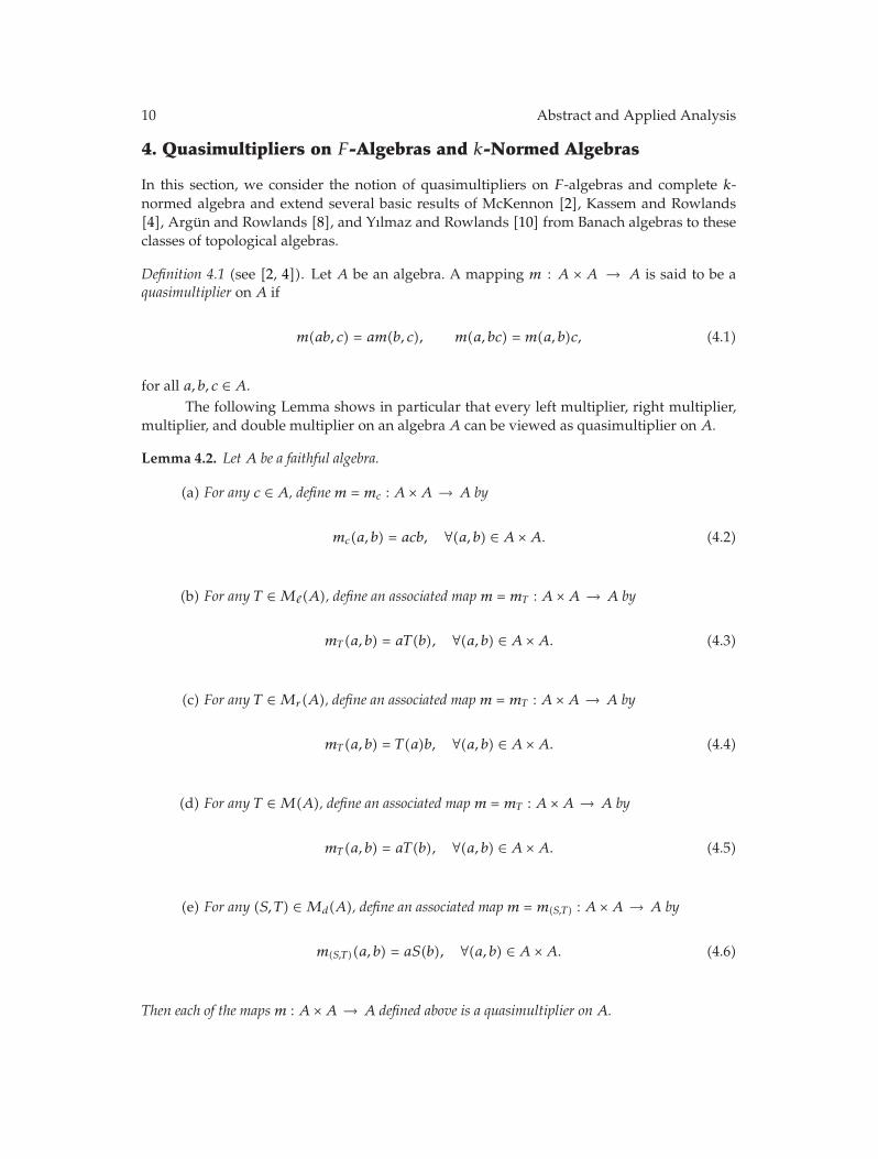
4. Quasimultipliers on F-Algebras and k-Normed Algebras

In this section, we consider the notion of quasimultipliers on F-algebras and complete k-normed algebra and extend several basic results of McKennon [2], Kassem and Rowlands[4], Argun and Rowlands [8], and Yılmaz and Rowlands [10] from Banach algebras to theseclasses of topological algebras.

Definition 4.1 (see [2, 4]). Let A be an algebra. A mapping m : A × A → A is said to be aquasimultiplier on A if

m(ab, c) = am(b, c), m(a, bc) = m(a, b)c, (4.1)

for all a, b, c ∈ A.The following Lemma shows in particular that every left multiplier, right multiplier,

multiplier, and double multiplier on an algebraA can be viewed as quasimultiplier on A.

Lemma 4.2. Let A be a faithful algebra.

(a) For any c ∈ A, definem = mc : A ×A → A by

mc(a, b) = acb, ∀(a, b) ∈ A ×A. (4.2)

(b) For any T ∈ M�(A), define an associated mapm = mT : A ×A → A by

mT (a, b) = aT(b), ∀(a, b) ∈ A ×A. (4.3)

(c) For any T ∈ Mr(A), define an associated mapm = mT : A ×A → A by

mT (a, b) = T(a)b, ∀(a, b) ∈ A ×A. (4.4)

(d) For any T ∈ M(A), define an associated mapm = mT : A ×A → A by

mT (a, b) = aT(b), ∀(a, b) ∈ A ×A. (4.5)

(e) For any (S, T) ∈ Md(A), define an associated mapm = m(S,T) : A ×A → A by

m(S,T)(a, b) = aS(b), ∀(a, b) ∈ A ×A. (4.6)

Then each of the mapsm : A ×A → A defined above is a quasimultiplier onA.


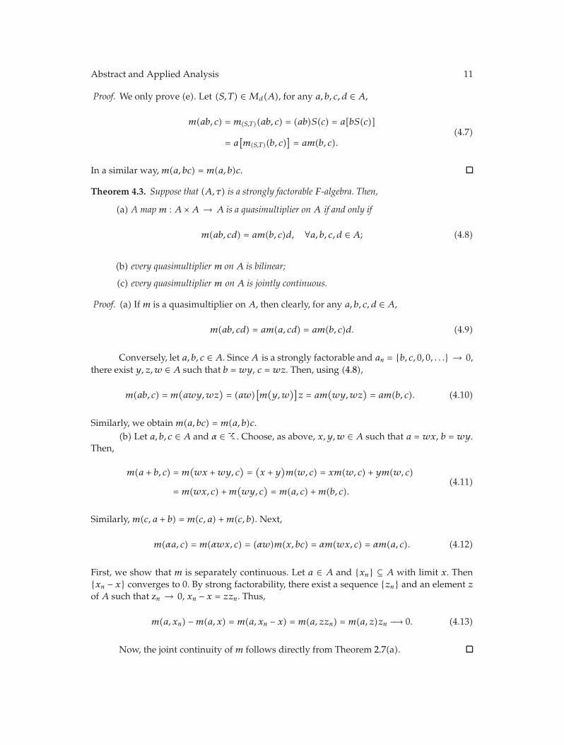
Proof. We only prove (e). Let (S, T) ∈ Md(A), for any a, b, c, d ∈ A,

m(ab, c) = m(S,T)(ab, c) = (ab)S(c) = a[bS(c)]

= a[m(S,T)(b, c)

]= am(b, c).

(4.7)

In a similar way,m(a, bc) = m(a, b)c.

Theorem 4.3. Suppose that (A, τ) is a strongly factorable F-algebra. Then,

(a) A mapm : A ×A → A is a quasimultiplier on A if and only if

m(ab, cd) = am(b, c)d, ∀a, b, c, d ∈ A; (4.8)

(b) every quasimultiplier m onA is bilinear;

(c) every quasimultiplier m onA is jointly continuous.

Proof. (a) If m is a quasimultiplier on A, then clearly, for any a, b, c, d ∈ A,

m(ab, cd) = am(a, cd) = am(b, c)d. (4.9)

Conversely, let a, b, c ∈ A. SinceA is a strongly factorable and an = {b, c, 0, 0, . . .} → 0,there exist y, z,w ∈ A such that b = wy, c = wz. Then, using (4.8),

m(ab, c) = m(awy,wz

)= (aw)

[m(y,w

)]z = am

(wy,wz

)= am(b, c). (4.10)

Similarly, we obtainm(a, bc) = m(a, b)c.(b) Let a, b, c ∈ A and α ∈ � . Choose, as above, x, y,w ∈ A such that a = wx, b = wy.

Then,

m(a + b, c) = m(wx +wy, c

)=(x + y

)m(w, c) = xm(w, c) + ym(w, c)

= m(wx, c) +m(wy, c

)= m(a, c) +m(b, c).

(4.11)

Similarly, m(c, a + b) = m(c, a) +m(c, b). Next,

m(αa, c) = m(αwx, c) = (αw)m(x, bc) = αm(wx, c) = αm(a, c). (4.12)

First, we show that m is separately continuous. Let a ∈ A and {xn} ⊆ A with limit x. Then{xn − x} converges to 0. By strong factorability, there exist a sequence {zn} and an element zof A such that zn → 0, xn − x = zzn. Thus,

m(a, xn) −m(a, x) = m(a, xn − x) = m(a, zzn) = m(a, z)zn −→ 0. (4.13)

Now, the joint continuity of m follows directly from Theorem 2.7(a).


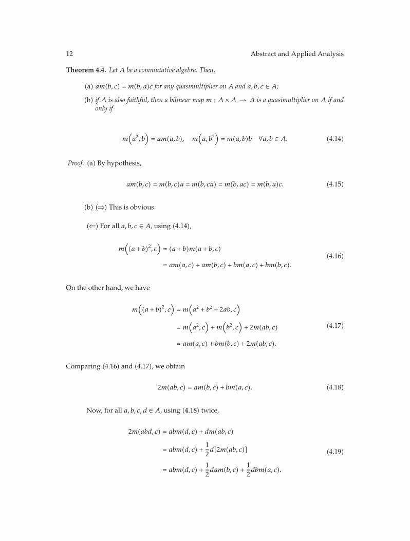
Theorem 4.4. Let A be a commutative algebra. Then,

(a) am(b, c) = m(b, a)c for any quasimultiplier onA and a, b, c ∈ A;

(b) if A is also faithful, then a bilinear map m : A ×A → A is a quasimultiplier on A if andonly if

m(a2, b

)= am(a, b), m

(a, b2

)= m(a, b)b ∀a, b ∈ A. (4.14)

Proof. (a) By hypothesis,

am(b, c) = m(b, c)a = m(b, ca) = m(b, ac) = m(b, a)c. (4.15)

(b) (⇒) This is obvious.

(⇐) For all a, b, c ∈ A, using (4.14),

m((a + b)2, c

)= (a + b)m(a + b, c)

= am(a, c) + am(b, c) + bm(a, c) + bm(b, c).(4.16)

On the other hand, we have

m((a + b)2, c

)= m

(a2 + b2 + 2ab, c

)

= m(a2, c

)+m

(b2, c

)+ 2m(ab, c)

= am(a, c) + bm(b, c) + 2m(ab, c).

(4.17)

Comparing (4.16) and (4.17), we obtain

2m(ab, c) = am(b, c) + bm(a, c). (4.18)

Now, for all a, b, c, d ∈ A, using (4.18) twice,

2m(abd, c) = abm(d, c) + dm(ab, c)

= abm(d, c) +12d[2m(ab, c)]

= abm(d, c) +12dam(b, c) +

12dbm(a, c).

(4.19)


By commutativity of A and using (4.18) twice as above,

2m(abd, c) = 2m(adb, c) = adm(b, c) + bm(ad, c)

= adm(b, c) +12[bam(d, c) + bdm(a, c)]

= adm(b, c) +12abm(d, c) +

12dbm(a, c).

(4.20)

Comparing (4.19) and (4.20), abm(d, c) = adm(b, c). Since this holds for all a ∈ A and A isfaithful, bm(d, c) = dm(b, c). Hence, for all d ∈ A,

dm(ab, c) = abm(d, c) = a[bm(d, c)] = adm(b, c) = dam(b, c). (4.21)

Since this holds for all d ∈ A and A is faithful,m(ab, c) = am(b, c).A similar computation shows that m(a, bc) = m(a, b)c. Hence m is a quasimultiplier.

Definition 4.5. Let QM(A) denote the set of all bilinear jointly continuous quasimultiplierson a topological algebra A. Clearly, QM(A) is a vector space under the usual pointwiseoperations. Further, QM(A) becomes an A-bimodule as follows. For any m ∈ QM(A) anda ∈ A, we can define the products a ◦m andm ◦ a as mappings fromA ×A into A given by

(a ◦m)(x, y

)= m

(xa, y

), (m ◦ a)(x, y) = m

(x, ay

), x, y ∈ A. (4.22)

Then a ◦m, m ◦ a ∈ QM(A), so thatQM(A) is an A-bimodule.

Definition 4.6. Let (A, q) be an F-normed algebra. Following [2, 4, 8], we can definemappings

φA : A −→ QM(A), φ� : M�(A) −→ QM(A),

φr : Mr(A) −→ QM(A), φd : Md(A) −→ QM(A),(4.23)

by

(φA(a)

)(x, y

)= xay, a ∈ A,

(φ�(T)

)(x, y

)= xT

(y), T ∈ M�(A),

(φr(T)

)(x, y

)= T(x)y, T ∈ Mr(A),

(φd(S, T)

)(x, y

)= xS

(y), (S, T) ∈ Md(A),

(4.24)

for all (x, y) ∈ A ×A. By Lemma 4.2, these mappings are well defined.


Definition 4.7. (1) A bounded approximate identity {eλ : λ ∈ I} in a topological algebra A issaid to be ultra-approximate if, for all m ∈ QM(A) and a ∈ A, the nets {m(a, eλ) : λ ∈ I} and{m(eλ, a) : λ ∈ I} are Cauchy in A (see [2]).

(2)A topological algebraA is calledm-symmetric if, for each S ∈ M�(A)∪Mr(A), thereis a T ∈ M�(A) ∪Mr(A) such that either (S, T) ∈ Md(A) or (T, S) ∈ Md(A)(see [4]).

Theorem 4.8. Let (A, q) be an F-algebra with a bounded approximate identity {eλ : λ ∈ I}. Considerthe following conditions.

(a) {eλ : λ ∈ I} is ultra-approximate.

(b) For any a ∈ A, S ∈ M�(A), and T ∈ Mr(A), the nets {aS(eλ)} and {T(eλ)a} are Cauchyin A.

(c) A ism-symmetric.

Then (a)⇒ (b)⇔ (c). If A is factorable, then (c)⇒ (a); hence (a), (b), and (c) are equivalent.

Proof. (a)⇒ (b) Suppose that {eλ : λ ∈ I} in A is ultra-approximate. Let S ∈ M�(A) andT ∈ Mr(A). Put m1 = φ�(S) and m2 = φr(T). Then m1, m2 ∈ QM(A) and, for any a ∈A, {m1(a, eλ)} = {aS(eλ)} and {m1(eλ, a)} = {T(eλ)a} which are Cauchy inA by hypothesis.

(b)⇒ (c) Suppose that (b) holds, let S ∈ M�(A)∪Mr(A), and suppose that S ∈ M�(A).Since A is complete, the map T : A → A given by

T(a) = limλ

aS(eλ), a ∈ A, (4.25)

is well-defined. Since S is continuous, for any a, b ∈ A,

aS(b) = a limλ

S(eλb) = a limλ

S(eλ)b =[limλ

aS(eλ)]b = T(a)b. (4.26)

Since A is a faithful F-algebra, by Theorem 3.7(b), (S, T) ∈ Md(A). Hence A is m-symmetric.(c)⇒ (b) Suppose that (c) holds. Let S ∈ M�(A) and T ∈ Mr(A). By (c), there exist

T1 ∈ Mr(A), S1 ∈ M�(A) such that (S, T1),(S1, T) ∈ Md(A). Then, for any a ∈ A,

aS(eλ) = T1(a)eλ −→ T1(a),

T(eλ)a = eλS1(a) −→ S1(a).(4.27)

Thus, both {aS(eλ)} and {T(eλ)a}, being convergent, are Cauchy in A.Suppose that A is factorable. Then (c)⇒ (a), as follows. Let m ∈ QM(A) and a ∈ A.

By factorability, a = bc for some b, c ∈ A. Define the mappings S, T : A → A by

S(x) = m(c, x), T(x) = m(x, b), x ∈ A. (4.28)


Then, for any x, y ∈ A,

S(xy

)= m

(c, xy

)= m(c, x)y = S(x)y,

T(xy

)= m

(xy, b

)= xm

(y, b

)= xT

(y),

(4.29)

and so S ∈ M�(A) and T ∈ Mr(A). By (c), there exist T1 ∈ Mr(A), S1 ∈ M�(A) such that(S, T1), (S1, T) ∈ Md(A). Then

m(a, eλ) = m(bc, eλ) = bm(c, eλ) = bS(eλ) = T1(b)eλ −→ T1(b),

m(eλ, a) = m(eλ, bc) = m(eλ, b)c = T(eλ)c = eλS1(c) −→ S1(c).(4.30)

Hence {m(a, eλ) : λ ∈ I} and {m(eλ, a) : λ ∈ I} are Cauchy in A. So {eλ : λ ∈ I} is ultra-approximate.

Theorem 4.9. Let (A, q) be an F-algebra having an ultra-approximate identity {eλ : λ ∈ I}. Then,

(a) each of the maps φA, φ� , φr , and φd is a bijection;

(b) φd | M(A) = φ� | M(A) = φr | M(A);

(c) φd | μd(A) = φA.

Proof. (a) We give the proof only for φd : Md(A) → QM(A). To show that φd is onto, letm ∈ QM(A). Since {eλ} is ultra-approximate, for each x ∈ A, the nets {m(x, eλ) : λ ∈ I} and{m(eλ, x) : λ ∈ I} are convergent. For each x ∈ A, define S, T : A → A by

S(x) = limλ

m(eλ, x), T(x) = limλ

m(x, eλ). (4.31)

Then (S, T) ∈ Md(A) since, for any x, y ∈ A,

xS(y)= x lim

λm(eλ, y

)= lim

λm(xeλ, y

)= m

(x, y

)

= limλ

m(x, eλy

)= lim

λm(x, eλ)y = T(x)y.

(4.32)

Further, we have for any (a, b) ∈ A ×A,

[φd(S, T)

](a, b) = aS(b) = a lim

λm(eλ, b) = lim

λm(aeλ, b) = m(a, b); (4.33)

that is, φd(S, T) = m.To show that, φd is one to one, let (S1, T1), (S2, T2) ∈ Md(A) with φd(S1, T1) =

φd(S2, T2). Then, for any a, b ∈ A,

φd(S1, T1)(a, b) = φd(S2, T2)(a, b), or aS1(b) = aS2(b). (4.34)


Since A is faithful, S1(b) = S2(b), b ∈ A. So S1 = S2. Consequently, by Theorem 3.3(c), alsoT1 = T2. Thus (S1, T1) = (S2, T2).

(b) Let T ∈ M(A) and x, y ∈ A. Then, since T ∈ M�(A) ∩Mr(A) and (T, T) ∈ Md(A),

φd(T)(x, y

)= φd(T, T)

(x, y

)= xT

(y)= T

(xy

). (4.35)

Also

φ�(T)(x, y

)= xT

(y)= T

(xy

); φr(T)

(x, y

)= T(x)y = T

(xy

). (4.36)

(c) For any a ∈ A and (x, y) ∈ A ×A,

φd

(μd(a)

)(x, y

)= φd(La, Ra)

(x, y

)= xLa

(y)= xay = φA(a)

(x, y

). (4.37)

Thus φd | μd(A) = φA.

We obtain the following lemma for later use.

Lemma 4.10. (a) If (A, q) is a factorable F-normed algebra having an approximate identity {eλ : λ ∈I}, then

limλ

q(eλaeλ − a) = 0, ∀a ∈ A. (4.38)

(b) If (A, q) is an F-algebra having a minimal ultra-approximate identity {eλ : λ ∈ I}, then,for any m ∈ QM(A),

limλ

eλm(eλ, x) = limλ

m(eλ, x) (exists), ∀x ∈ A. (4.39)

Compare with [10, page 124].

Proof. (a) Let a ∈ A. Since A is factorable, there exist x, y ∈ A such that a = xy. Then

−−limλ

q(eλaeλ − a) =−−limλ

q[(eλxyeλ − eλxy

)+(eλxy − xy

)]

≤−−limλ

q(eλx) · q(yeλ − y

)+

−−limλ

q(eλxy − xy

)

= q(x) · q(0) + q(0) = 0.

(4.40)

Since A is complete and {eλ} is ultra-approximate, for any x ∈ A, limλ m(eλ, x) = y (say)exists. Since q(eλ) ≤ 1,

q[y − eλm(eλ, x)

] ≤ q(y − eλy

)+ q

[eλy − eλm(eλ, x)

]

≤ q(y − eλy

)+ q(eλ)q

(y −m(eλ, x)

)

≤ q(y − eλy

)+ q

(y −m(eλ, x)

) −→ 0.

(4.41)


Definition 4.11. Let (A, q) be a k-normed algebra. For any m ∈ QM(A), we define

‖m‖q = sup

{q[m(x, y

)]

q(x)q(y) : x, y ∈ A, x, y /= 0

}

. (4.42)

Clearly,

q[m(x, y

)] ≤ ‖m‖q q(x)q(y), ∀x, y ∈ A. (4.43)

Theorem 4.12. Let (A, q) be a k-normed algebra. Then,

(a) ‖ · ‖q is a k-norm on QM(A);

(b) if (A, q) is complete, then so is (QM(A), ‖ · ‖q).

Proof. (a) For any m ∈ QM(A),

‖m‖q = 0 ⇐⇒ supx /= 0,y /= 0

q[m(x, y

)]

q(x)q(y) = 0

⇐⇒ q[m(x, y

)]= 0, ∀x, y ∈ A, x /= 0, y /= 0

⇐⇒ q[m(x, y

)]= 0, ∀x, y ∈ A

⇐⇒ m = 0.

(4.44)

Also, for any α ∈ � , q(αx) = |α|kq(x) and so it follows that ‖αm‖q = |α|k‖m‖q.Next, letm, u ∈ QM(A), and let ε > 0. Choose x, y ∈ A such that

‖m + u‖q ≤q[(m + u)

(x, y

)]

q(x)q(y) − ε. (4.45)

Then,

‖m + u‖q ≤q[m(x, y

)+ u

(x, y

)]

q(x)q(y) − ε

≤ q[m(x, y

)]

q(x)q(y) +

q[u(x, y

)]

q(x)q(y) − ε

≤ ‖m‖q + ‖u‖q − ε.

(4.46)

Since ε > 0 is arbitrary, ‖m + u‖q ≤ ‖m‖q + ‖u‖q. Thus ‖ · ‖q is a k-norm on QM(A).


(b) Let {mi : i ∈ �} be a ‖ · ‖q-Cauchy sequence in QM(A). Then, for any x, y ∈ A,

−−−limi,j

q[mi

(x, y

) −mj

(x, y

)]=

−−−limi,j

q[(mi −mj

)(x, y

)]

≤−−−limi,j

∥∥mi −mj

∥∥q· q(x)q(y) = 0.

(4.47)

Therefore, for any x, y in A, {mi(x, y)} is a Cauchy sequence in A. Since A is complete, themap m : A ×A → A given by

m(x, y

)= lim

imi

(x, y

), x, y ∈ A, (4.48)

is welldefined. Clearly,m is bilinear and, by Theorem 2.7(b),m is jointly continuous. Further,for any a, b, x, y ∈ A,

m(ax, yb

)= lim

imi

(ax, yb

)= lim

i

[ami

(x, y

)b]= a

[limimi

(x, y

)]b = am

(x, y

)b. (4.49)

Hence, m ∈ QM(A). Next, ‖mi −m‖q → 0 as follows. Let ε > 0. Since {mi} is ‖ · ‖q-Cauchy,there exists an integer N ≥ 1 such that

∥∥mi −mj

∥∥q<

ε

2, ∀ pairs i, j ≥ N, (4.50)

that is,

q[(mi −mj

)(x, y

)]

q(x)q(y) <

ε

2, ∀ pairs i, j ≥ N, x, y ∈ A, x, y /= 0. (4.51)

Let x, y ∈ A, x, y /= 0. Fix any io ≥ N in (4.51); since mj(x, y) → m(x, y) in A, letting j → ∞in (4.51),

q[mio

(x, y

) −m(x, y

)]

q(x)q(y) ≤ ε

2. (4.52)

Then, for any i ≥ N, using (4.51) and (4.52),

q[mi

(x, y

) −m(x, y

)]

q(x)q(y) ≤ q

[mi

(x, y

) −mio

(x, y

)]

q(x)q(y) +

q[mio

(x, y

) −m(x, y

)]

q(x)q(y)

<ε

2+ε

2= ε.

(4.53)

Thus mi

‖·‖q−−−→ m.


Theorem 4.13. Let (A, q) be a factorable k-normed algebra having a minimal approximate identity{eλ : λ ∈ I}. Then

(a) each of the maps φA, φ� , φr , and φd defined above is a linear isometry;

(b) for any a, b ∈ A andm ∈ QM(A), ‖a ◦m ◦ b‖q = q(m(a, b)).

Proof. (a)We give the proof only for φd : Md(A) → QM(A). Clearly, φd is linear. Let (S, T) ∈Md(A). Then

∥∥φd(S, T)

∥∥q= sup

x/= 0,y /= 0

q[φd(S, T)

(x, y

)]

q(x)q(y) = sup

x /= 0,y /= 0

q[xS

(y)]

q(x)q(y)

≤ supx/= 0,y /= 0

q(x)q(S(y))

q(x)q(y) = sup

y /= 0

q(S(y))

q(y) = ‖S‖q.

(4.54)

To prove the reverse inequality, let ε > 0. There exists (y /= 0) ∈ A such that ‖S‖q <

q(S(y))/q(y) + ε. For any λ ∈ I, since 0 < q(yeλ) ≤ q(y)q(eλ) ≤ q(y),

∥∥φd(S, T)

∥∥q≥ q

[φd(S, T)

(eλ, yeλ

)]

q(eλ)q(yeλ

) ≥ q[eλS

(yeλ

)]

q(yeλ

) ≥ q[eλS

(y)eλ]

q(y) ; (4.55)

hence, in view of factorability, using Lemma 4.10(a),

∥∥φd(S, T)∥∥q ≥ lim

λ

q[eλS

(y)eλ]

q(y) =

q(S(y))

q(y) > ‖S‖q − ε. (4.56)

Since ε > 0 is arbitrary, we obtain ‖φd(S, T)‖q = ‖S‖q = ‖(S, T)‖q, and so φd is an isometry.(b) By (a), φA is an isometry and so

‖a ◦m ◦ b‖q = supx/= 0,y /= 0

q[(a ◦m ◦ b)(x, y)]

q(x)q(y) = sup

x /= 0,y /= 0

q[m(xa, by

)]

q(x)q(y)

= supx/= 0,y /= 0

q[xm(a, b)y

]

q(x)q(y) = sup

x/= 0,y /= 0

q[φA(m(a, b))

(x, y

)]

q(x)q(y)

=∥∥φA(m(a, b))

∥∥q= q(m(a, b)).

(4.57)

We next consider multiplication in QM(A) in various equivalent ways.

Definition 4.14 (see [2, 4]). LetA be an F-algebra with an ultra-approximate identity {eλ : λ ∈I} andm1, m2 ∈ QM(A). Since φd is onto, there exist (S1, T1), (S2, T2) ∈ Md(A) such that

φd(S1, T1) = m1, φd(S2, T2) = m2. (4.58)


By the definitions of φ� and φr ,

φ�(S1) = m1 = φr(T1), φ�(S2) = m2 = φr(T2). (4.59)

Therefore, the product of m1, m2 can be defined in any of the following ways:

(i) m1◦φdm2 = φd(S1, T1)◦φdφd(S2, T2) = φd[(S1, T1)(S2, T2)] = φd(S1S2, T2T1),

(ii) m1◦φ�m2 = φ�(S1)◦φ�φ�(S2) = φ�(S1S2),

(iii) m1◦φrm2 = φr(T1)◦φrφr(T2) = φr(T2T1).

Note that, for any (x, y) ∈ A ×A,

[φd(S1S2, T2T1)

](x, y

)= x(S1S2)

(y)=[φ�(S1S2)

](x, y

), (4.60)

also

x(S1S2)(y)= (T2T1)(x)y =

[φr(T2T1)

](x, y

). (4.61)

Hence, m1◦φdm2 = m1◦φ�m2 = m1◦φrm2.

Remark 4.15. (1) Ifm = φ�(T) with T ∈ M�(A) and a ∈ A, then, by Theorem 3.6(a),

m◦φ�φA(a) = φ�(T)◦φ�φ�(La) = φ�(TLa) = φ�

(LT(a)

)= φA(T(a)) ∈ φA(A). (4.62)

(2) If m = φr(T) with T ∈ Mr(A) and a ∈ A, then, by Theorem 3.6(b),

φA(a)◦φrm = φr(Ra)◦φrφr(T) = φr(TRa) = φr

(RT(a)

)= φA(T(a)) ∈ φA(A). (4.63)

(3) If m = φd(S, T) and a ∈ A, then, by Theorem 3.6(c),

m◦φdφA(a) = φd[(S, T)(La, Ra)] = φd(SLa, RaT)

= φd

(LS(a), RS(a)

)= φA(S(a)) ∈ φA(A).

(4.64)

In the sequel, we denote the product on QM(A) arising from (i), (ii), or (iii) by �. Someproperties of this product are given as follows.

Theorem 4.16. Let A be a factorable complete k-normed algebra with a minimal ultra-approximateidentity {eλ : λ ∈ I}. Then,

(a) for any m1, m2 ∈ QM(A),

(m1 �m2)(x, y

)= m1

(x, lim

λm2

(eλ, y

)) ((x, y

) ∈ A ×A), (4.65)

defines a product � on QM(A) so that (QM(A), ‖ · ‖q) is a complete k-normed algebrawith identitymo = φd(I, I);


(b) for any m ∈ QM(A) and a ∈ A,

φA(a) �m = a ◦m, m � φA(a) = m ◦ a; (4.66)

(c) φA(A) is a two-sided ideal in QM(A);

(d) If A is factorable, then bothM�(A) andMd(A) are isometrically algebraically isomorphicto QM(A), whileMr(A) is isometrically algebraically anti-isomorphic to QM(A);

Proof. (a) Let m1, m2 ∈ QM(A) and (x, y) ∈ A × A. Choose (S1, T1), (S2, T2) ∈ Md(A) suchthat

φd(S1, T1) = m1, φd(S2, T2) = m2, (4.67)

that is,

xS1(y)= m1

(x, y

), xS2

(y)= m2

(x, y

). (4.68)

Then,

(m1 �m2)(x, y

)=[φd(S1S2, T2T1)

](x, y

)= x(S1S2)

(y)

= x[S1

(S2

(y))]

= x

[S1

(limλ

eλS2(y))]

= m1

(x, lim

λeλS2

(y))

= m1

(x, lim

λm2

(eλ, y

)).

(4.69)

It is easy to verify that ‖m1 � m2‖q ≤ ‖m1‖q‖m2‖q, so that (QM(A), ‖ · ‖q) is an F-normedalgebra. Further, by Theorem 4.12, (QM(A), ‖ · ‖q) is also complete.

(b) Letm ∈ QM(A) and a ∈ A. Using (a), for any (x, y) ∈ A ×A,

[m � φA(a)

](x, y

)= m

(x, lim

λφA(a)

(eλ, y

))= m

(x, lim

λmeλay

)

= m(x, ay

)= (m ◦ a)(x, y).

(4.70)

Similarly, [φA(a) �m](x, y) = (a ◦m)(x, y).(c) To show that φA(A) is a two-sided ideal, let m ∈ QM(A) and a ∈ A. By

Theorem 4.9(a), there exists (S, T) ∈ Md(A) such that φd(S, T) = m. Using (b), for any(x, y) ∈ A ×A,

[m � φA(a)

](x, y

)= (m ◦ a)(x, y) = m

(x, ay

)= φd(S, T)

(x, ay

)

= xS(ay

)= xS(a)y = φA(S(a))

(x, y

).

(4.71)

Hence, m � φA(a) = φA(S(a)) ∈ φA(A). Similarly, φA(a) �m = φA(T(a)) ∈ φA(A).


(d) Suppose that A is factorable. Then, by Theorem 4.13(a), each of the maps φd, φ� ,φr , and φA is a linear isometry. If (S1, T1), (S2, T2) ∈ Md(A), then by definition

φd(S1, T1) ◦φd φd(S2, T2) = φd[(S1, T1)(S2, T2)]. (4.72)

If S1, S2 ∈ M�(A), then by definition

φ�(S1) ◦φ� φ�(S2) = φ�(S1S2). (4.73)

If T1, T2 ∈ Mr(A), then by definition

φr(T1) ◦φr φr(T2) = φr(T2T1). (4.74)

Hence, φd : Md(A) → QM(A) and φ� : M�(A) → QM(A) are algebraic isomorphisms andφr : Mr(A) → QM(A) is algebraic anti-isomorphism.

Remark 4.17. If A has an identity e, then A may be identified with QM(A) as follows. Letm ∈ QM(A). Thenm(e, e) ∈ A and, for any x, y ∈ A,

φA(m(e, e))(x, y

)= xm(e, e)y = m

(xe, ey

)= m

(x, y

). (4.75)

5. Quasistrict and Strict Topologies on QM(A)

In this section, we consider the quasistrict and strict topologies onQM(A) and extend severalresults from [2, 4, 8]. Throughout we will assume, unless stated otherwise, that (A, q) is afactorable complete k-normed algebra having a minimal ultra-approximate identity {eλ : λ ∈I}.

Definition 5.1. For any m ∈ QM(A) and a, b ∈ A, we define mappings a ◦m,m ◦ a, a ◦m ◦ b :A ×A → A by

(a ◦m)(x, y

)= m

(xa, y

), (m ◦ a)(x, y) = m

(x, ay

),

(a ◦m ◦ b)(x, y) = m(xa, by

),

(x, y

) ∈ A ×A.(5.1)

Lemma 5.2. Let m ∈ QM(A) and a, b ∈ A. Then

(a) ‖a ◦m‖q ≤ ‖m‖qq(a), ‖m ◦ a‖q ≤ ‖m‖qq(a),

(b) ‖a ◦m ◦ b‖q = q(m(a, b)) ≤ ‖m‖qq(a)q(b).


Proof. (a) By definition,

‖a ◦m‖q = supx/= 0,y /= 0

q[(a ◦m)

(x, y

)]

q(x)q(y) = sup

x/= 0,y /= 0

q[x ·m(

a, y)]

q(x)q(y)

≤ supx/= 0,y /= 0

q(x)q(m(a, y

))

q(x)q(y) = sup

y /= 0

q(m(a, y

))

q(y)

= supy /= 0

‖m‖qq(a)q(y)

q(y) = ‖m‖qq(a).

(5.2)

Similarly, ‖m ◦ a‖q ≤ ‖m‖qq(a).(b) By Theorem 4.13(b), q(m(a, b)) = ‖a ◦m ◦ b‖q. Further, using (a),

‖a ◦m ◦ b‖q ≤ ‖a ◦m‖qq(b) ≤ ‖m‖qq(a)q(b). (5.3)

Definition 5.3. (1) The quasistrict topology γ on QM(A) is determined by the family {ξa,b(m) :a, b ∈ A} of k-seminorms, where

ξa,b(m) = ‖a ◦m ◦ b‖q = q(m(a, b)), m ∈ QM(A). (5.4)

Compare with [2, page 109]; [4, page 558].(2) The strict topology β on QM(A) is determined by the family {ηa(m) : a ∈ A} of

k-seminorms, where

ηa(m) = max{‖a ◦m‖q, ‖m ◦ a‖q

}, m ∈ QM(A). (5.5)

Compare with [8, page 227].Let τ denote the topology on QM(A) generated by the k-norm ‖ · ‖q.

Lemma 5.4. γ ⊆ β ⊆ τ on QM(A).

Proof. To show that γ ⊆ β, let a, b ∈ A. Then

ξa,b(m) = ‖a ◦m ◦ b‖q ≤ ‖a ◦m‖qq(b) ≤ ηa(m)q(b), m ∈ QM(A), (5.6)

also

ξa,b(m) = ‖a ◦m ◦ b‖q ≤ ‖m ◦ b‖qq(a) ≤ ηb(m)q(a), m ∈ QM(A). (5.7)


Hence,

ξa,b(m) ≤ max{ηa(m), ηb(m)

}q(a)q(b), m ∈ QM(A). (5.8)

Let {mα : α ∈ J} be a net in QM(A) with mαβ−→ m ∈ QM(A). Then, for any a, b ∈ A,

ηa(mα −m) → 0 and ηb(mα −m) → 0. Hence,

ξa,b(mα −m) ≤ max{ηa(mα −m), ηb(mα −m)

}q(a)q(b) −→ 0. (5.9)

Thus mαγ−→ m, and so γ ⊆ β.

To show that β ⊆ τ , Let a ∈ A. Note that, for any x, y ∈ A,

(a ◦m)(x, y

)= m

(xa, y

)= x ·m(

a, y), m ∈ QM(A),

(m ◦ a)(x, y) = m(x, ay

)= m(x, a)y, m ∈ QM(A).

(5.10)

By Lemma 5.2(a), ‖a ◦m‖q ≤ ‖m‖qq(a) and ‖m ◦ a‖q ≤ ‖m‖qq(a); hence,

ηa(m) = max{‖a ◦m‖q, ‖m ◦ a‖q

}≤ ‖m‖qq(a), m ∈ QM(A). (5.11)

Consequently, if {mα} is a net in QM(A) with mατ−→ m ∈ QM(A), then ‖mα −m‖q → 0, and

so, for any a, b ∈ A,

ηa(mα −m) ≤ ‖mα −m‖qq(a) −→ 0. (5.12)

Thus mαβ−→ m; that is, β ⊆ τ .

Theorem 5.5. φA(A) is β-dense in QM(A) and hence γ -dense in QM(A).

Proof. Let m ∈ QM(A). Clearly {m(eλ, eλ)}λ∈I ⊆ A. We claim that φA(m(eλ, eλ))β−→ m. Let

a ∈ A. We need to show that

ηa

[φA(m(eλ, eλ)) −m

] −→ 0. (5.13)

For any x, y ∈ A, by joint continuity of m,

q[a ◦ {φA(m(eλ, eλ)) −m

}(x, y

)]

= q[{φA(m(eλ, eλ)) −m

}(xa, y

)]= q

[xam(eλ, eλ)y −m

(xa, y

)]

= q[m(xaeλ, eλy

) −m(xa, y

)] −→ q[m(xa, y

) −m(xa, y

)]= 0.

(5.14)


Hence ‖a ◦ {φA(m(eλ, eλ)) −m}‖q → 0. Similarly, ‖{φA(m(eλ, eλ)) −m} ◦ a‖q → 0. Thus,

ηa

[φA(m(eλ, eλ)) −m

] −→ 0; (5.15)

that is, φA(A) is β-dense in QM(A). Since γ ⊆ β, it follows that φA(A) is γ -dense in QM(A).

Theorem 5.6. (a) (QM(A), γ) and (QM(A), β) are sequentially complete.(b) If, in addition, (A, q) is strongly factorable, then (QM(A), γ) and (QM(A), β) are

complete.

Proof. (a) Let {mi : i ∈ �} be a γ -Cauchy sequence in QM(A). For any x, y ∈ A, usingTheorem 4.13(b),

q[mi

(x, y

) −mj

(x, y

)]= q

[(mi −mj

)(x, y

)]

=∥∥x ◦ (mi −mj

) ◦ y∥∥q= ξx,y

(mi −mj

),

(5.16)

which implies that {mi(x, y)} is a Cauchy sequence inA. Definem : A×A → A bym(x, y) =limi mi(x, y). Clearly, m is bilinear and, by Theorem 2.7(b), m is jointly continuous. Further,for any a, b, x, y ∈ A,

m(ax, yb

)= lim

imi

(ax, yb

)= a

[limi

mi

(x, y

)]b = am

(x, y

)b, (5.17)

and som ∈ QM(A). Further, for any a, b ∈ A,

ξa,b(mi −m) = ‖a ◦mi ◦ b − a ◦m ◦ b‖q = q[(mi −m)(a, b)] −→ 0. (5.18)

Hence miγ−→ m. So (QM(A), γ) is sequentially complete.

Next we show that (QM(A), β) is sequentially complete. We first note that, if m ∈QM(A), then, for each c ∈ A, the mappings Sc, Tc : A → A given by

Sc(x) = m(c, x), Tc(x) = m(x, c), x ∈ A, (5.19)

define elements inM�(A) andMr(A), respectively, and it is easy to see that

φ�(Sc) = c ◦m, φr(Tc) = m ◦ c. (5.20)

Let {mi : i ∈ �} be a β-Cauchy sequence in QM(A), and let c ∈ A. It followsfrom the definition of the β-topology that the sequences {φ�(Sc)i} and {φr(Tc)i}, where(Sc)i(x) = mi(c, x) and (Tc)i(x) = mi(x, c), are τ-Cauchy in QM(A). Since φ� and φr aretopological embeddings, the sequences {(Sc)i} and {(Tc)i} are ‖ · ‖q-Cauchy in M�(A) and


Mr(A), respectively. Both M�(A) and Mr(A) are complete (Theorem 3.9) and so there existS(c) in M�(A) and T (c) inMr(A) such that

∥∥∥(Sc)i − S(c)∥∥∥q−→ 0,

∥∥∥(Tc)i − T (c)∥∥∥q−→ 0. (5.21)

Since γ ⊆ β, the sequence {mi} is γ -Cauchy. As proved above, the space QM(A) isγ -complete and so there exists an element mo in QM(A) such that

limimi

(x, y

)= mo

(x, y

), ∀x, y ∈ A. (5.22)

For any a, b ∈ A,

[φ�

(S(c)

)](a, b) = lim

i

[φ�

(S(c)

)

i

](a, b) = lim

iami(c, b) = (c ◦mo)(a, b), (5.23)

which implies that φ�(S(c)) = c ◦mo. Similarly, we can prove that φr(T (c)) = mo ◦ c. Thus, by(5.21),

‖c ◦mi − c ◦mo‖q =∥∥∥φ�

(S(c)

)

i− φ�

(S(c)

)∥∥∥q=∥∥∥(S(c)

)

i− S(c)

∥∥∥q−→ 0,

‖mi ◦ c −mo ◦ c‖q =∥∥∥φr

(T (c)

)

i− φr

(T (c)

)∥∥∥q=∥∥∥(T (c)

)

i− T (c)

∥∥∥q−→ 0,

(5.24)

which implies thatmo is the β-limit of the sequence {mi} that is, QM(A) is β-complete.(b) Suppose that A is strongly factorable. Let {mα : α ∈ J} be a γ -Cauchy net in

QM(A). Replacing the sequence {mi : i ∈ �} by the net {mα : α ∈ J} in part (a), we obtaina map m : A ×A → A given by m(x, y) = limαmα(x, y). Then m is bilinear; further, for anya, b, x, y ∈ A,

m(ax, yb

)= lim

αmα

(ax, yb

)= a

[limα

mα

(x, y

)]b = am

(x, y

)b. (5.25)

Hence, using strong factorability as in Theorem 4.3(c), it follows that m is jointly continuous

and so m ∈ QM(A). Again, as in part (a), it follows that mαγ−→ m and consequently

(QM(A), γ) is complete. That QM(A) is β-complete also follows by the argument similarto the above one.

Remark 5.7. The authors do not know whether part (b) of the above theorem can be provedwithout the assumption of the strong factorability of A.


Theorem 5.8. (QM(A), γ), (QM(A), β), and (QM(A), τ) have the same bounded sets.

Proof. (a) Since γ ⊆ τ , every τ-bounded set is γ -bounded. Let H be any γ -bounded set inQM(A). Then, for each a, b ∈ A, there exists a constant r = r(a, b) > 0 such that

‖a ◦m ◦ b‖q ≤ r, ∀m ∈ H,

or q[m(a, b)] ≤ r, ∀m ∈ H(using Theorem 4.13(b)

).

(5.26)

For each a ∈ A and m ∈ H , define Ma : A → A by

Ma(x) = m(a, x), x ∈ A. (5.27)

Then, F = {Ma : m ∈ H} ⊆ CL(A). By (5.26), for any x ∈ A

q[Ma(x)] = q[m(a, x)] ≤ r(a, x), ∀m ∈ H ; (5.28)

hence F is pointwise bounded. Then, by the uniform boundedness principle (Theorem 2.6),there exists c = c(a) > 0 such that

‖Ma‖q ≤ c, ∀m ∈ H. (5.29)

Consider now the family P = {pm : m ∈ H} of k-seminorms on A defined by

pm(a) = ‖Ma‖q = supb /= 0

q[Ma(b)]q(b)

= supb /= 0

q[m(a, b)]q(b)

, a ∈ A. (5.30)

For eachm ∈ H, pm is continuous on A since, if {an} ⊆ Awith an → ao in A, then

∣∣pm(an) − pm(ao)

∣∣ ≤ pm(an − ao) = sup

b /= 0

q[Man−ao(b)]q(b)

= supb /= 0

q[m(an − ao, b)]q(b)

≤ supb /= 0

‖m‖qq(an − ao)q(b)

q(b)

= ‖m‖qq(an − ao) −→ 0.

(5.31)

Then, by (5.29), the family P is pointwise bounded. Applying Theorem 2.5, there exists a ballB = B(xo, r) = {x ∈ A : q(x − xo) ≤ r} and a constant C > 0 such that

pm(x) ≤ C, ∀m ∈ H, x ∈ B(xo, r). (5.32)


For any fixed a ∈ A, we claim that

pm(a) ≤2C · q(a)

r. (5.33)

If a = 0, this is obvious. Suppose that a/= 0. For simplification, put t = (r/q(a))1/k. Then, q isk-homogeneous, and we have ta + xo, xo ∈ B(xo, r), as follows:

q(ta + xo − xo) = q(ta) = tk · q(a) ≤ r

q(a)q(a) = r,

q(xo − xo) = q(0) = 0 < r.

(5.34)

So, by (5.32),

pm(ta + xo) ≤ C, pm(xo) ≤ C. (5.35)

Now, using (5.35) and the properties of k-norm again,

pm(a) = pm

(1tta

)=(1t

)k

pm(ta) ≤q(a)r

pm[ta + xo − xo]

≤ q(a)r

[pm(ta + xo) + pm(xo)

]

≤ q(a)r

[C + C] =2C · q(a)

r.

(5.36)

This proves our claim. Hence, using (5.33), for any m ∈ H ,

‖m‖q = supa,b /= 0

q[m(a, b)]q(a)q(b)

= supa/= 0

1q(a)

supb /= 0

q[m(a, b)]q(b)

= supa/= 0

1q(a)

pm(a) ≤ supa/= 0

1q(a)

.2C · q(a)

r≤ 2C

r.

(5.37)

Consequently, H is τ-bounded.(b) This follows from (a) since γ ⊆ β ⊆ τ .

Acknowledgment

The authors are grateful to the referees for their several useful suggestions, including thosementioned in Remarks 2.12 and 2.14, which improved significantly the quality of this paper.


References

[1] C. A. Akemann and G. K. Pedersen, “Complications of semicontinuity in C∗-algebra theory,” DukeMathematical Journal, vol. 40, pp. 785–795, 1973.

[2] K. McKennon, “Quasi-multipliers,” Transactions of the American Mathematical Society, vol. 233, pp. 105–123, 1977.

[3] R. Vasudevan and S. Goel, “Embedding of quasimultipliers of a Banach algebra into its second dual,”Mathematical Proceedings of the Cambridge Philosophical Society, vol. 95, no. 3, pp. 457–466, 1984.

[4] M. S. Kassem and K. Rowlands, “The quasistrict topology on the space of quasimultipliers of a B∗-algebra,” Mathematical Proceedings of the Cambridge Philosophical Society, vol. 101, no. 3, pp. 555–566,1987.

[5] H. X. Lin, “Fundamental approximate identities and quasi-multipliers of simple AFC∗-algebras,”Journal of Functional Analysis, vol. 79, no. 1, pp. 32–43, 1988.

[6] H. X. Lin, “Support algebras of σ-unital C∗-algebras and their quasi-multipliers,” Transactions of theAmerican Mathematical Society, vol. 325, no. 2, pp. 829–854, 1991.

[7] B. Dearden, “Quasi-multipliers of Pedersen’s ideal,” The Rocky Mountain Journal of Mathematics,vol. 22, no. 1, pp. 157–163, 1992.

[8] Z. Argun and K. Rowlands, “On quasi-multipliers,” Studia Mathematica, vol. 108, no. 3, pp. 217–245,1994.

[9] M. Grosser, “Quasi-multipliers of the algebra of approximable operators and its duals,” StudiaMathematica, vol. 124, no. 3, pp. 291–300, 1997.

[10] R. Yılmaz and K. Rowlands, “On orthomorphisms, quasi-orthomorphisms and quasi-multipliers,”Journal of Mathematical Analysis and Applications, vol. 313, no. 1, pp. 120–131, 2006.

[11] M. Kaneda, “Quasi-multipliers and algebrizations of an operator space,” Journal of Functional Analysis,vol. 251, no. 1, pp. 346–359, 2007.

[12] M. Kaneda and V. I. Paulsen, “Quasi-multipliers of operator spaces,” Journal of Functional Analysis,vol. 217, no. 2, pp. 347–365, 2004.

[13] G. Kothe, Topological Vector Spaces I, Springer, Berlin, Germany, 1969.[14] S. Rolewicz, Metric Linear Spaces, vol. 20 of Mathematics and Its Applications (East European Series), D.

Reidel, Dordrecht, The Netherlands, 2nd edition, 1985.[15] J. L. Kelley and I. Namioka, Linear Topological Spaces, D. Van Nostrand, Princeton, NJ, USA; Springer,

New York, NY, USA, 1976.[16] L. Waelbroeck, Topological Vector Spaces and Algebras, Lecture Notes in Mathematics, Vol. 230, Springer,

Berlin, Germany, 1971.[17] H. H. Schaefer, Topological Vector Spaces, Springer, New York, NY, USA, 1971.[18] A. Mallios, Topological Algebras. Selected Topics, vol. 124 of North-Holland Mathematics Studies, North-

Holland, Amsterdam, The Netherlands, 1986.[19] R. E. Edwards, Functional Analysis. Theory and Applications, Holt, Rinehart and Winston, New York,

NY, USA, 1965.[20] N. J. Kalton, N. T. Peck, and J. W. Roberts, An F-Space Sampler, vol. 89 of London Mathematical Society

Lecture Note Series, Cambridge University Press, Cambridge, UK, 1984.[21] M. Fragoulopoulou, Topological Algebras with Involution, vol. 200 ofNorth-Holland Mathematics Studies,

Elsevier Science B.V., Amsterdam, The Netherlands, 2005.[22] W. Zelazko, Banach Algebras, Elsevier, Amsterdam, The Netherlands, 1973.[23] H. G. Heuser, Functional Analysis, John Wiley & Sons, Chichester, UK, 1982.[24] C. Swartz, “Continuity and hypocontinuity for bilinear maps,” Mathematische Zeitschrift, vol. 186,

no. 3, pp. 321–329, 1984.[25] T. Husain, “Multipliers of topological algebras,” Dissertationes Mathematicae. Rozprawy Matematyczne,

vol. 285, p. 40, 1989.[26] R. S. Doran and J. Wichmann, Approximate Identities and Factorization in Banach Modules, vol. 768 of

Lecture Notes in Mathematics, Springer, Berlin, Germany, 1979.[27] E. Ansari-Piri, “A class of factorable topological algebras,” Proceedings of the Edinburgh Mathematical

Society, vol. 33, no. 1, pp. 53–59, 1990.[28] A. Bayoumi, Foundations of Complex Analysis in Non-locally Convex Spaces, Functions Theory without

Convexity Conditions, vol. 193 of North-Holland Mathematics Studies, Elsevier, Amsterdam, TheNetherlands, 2003.

[29] N. C. Phillips, “Inverse limits of C∗-algebras,” Journal of Operator Theory, vol. 19, no. 1, pp. 159–195,1988.


[30] R. C. Busby, “Double centralizers and extensions of C∗-algebras,” Transactions of the AmericanMathematical Society, vol. 132, pp. 79–99, 1968.

[31] B. E. Johnson, “An introduction to the theory of centralizers,” Proceedings of the London MathematicalSociety, vol. 14, pp. 299–320, 1964.

[32] B. E. Johnson, “Continuity of centralisers on Banach algebras,” Journal of the London MathematicalSociety, vol. 41, pp. 639–640, 1966.

[33] L. A. Khan, N. Mohammad, and A. B. Thaheem, “Double multipliers on topological algebras,”International Journal of Mathematics and Mathematical Sciences, vol. 22, no. 3, pp. 629–636, 1999.

[34] C. A. Akemann, G. K. Pedersen, and J. Tomiyama, “Multipliers of C∗-algebras,” Journal of FunctionalAnalysis, vol. 13, pp. 277–301, 1973.

[35] R. A. Fontenot, “The double centralizer algebra as a linear space,” Proceedings of the AmericanMathematical Society, vol. 53, no. 1, pp. 99–103, 1975.

[36] R. Larsen, An Introduction to the Theory of Multipliers, Springer, New York, NY, USA, 1971.[37] F. D. Sentilles and D. C. Taylor, “Factorization in Banach algebras and the general strict topology,”

Transactions of the American Mathematical Society, vol. 142, pp. 141–152, 1969.[38] D. C. Taylor, “The strict topology for double centralizer algebras,” Transactions of the American

Mathematical Society, vol. 150, pp. 633–643, 1970.[39] B. J. Tomiuk, “Multipliers on Banach algebras,” Studia Mathematica, vol. 54, no. 3, pp. 267–283, 1976.[40] J. Wang, “Multipliers of commutative Banach algebras,” Pacific Journal of Mathematics, vol. 11,

pp. 1131–1149, 1961.[41] S. K. Jain and A. I. Singh, “Quotient rings of algebras of functions and operators,” Mathematische

Zeitschrift, vol. 234, no. 4, pp. 721–737, 2000.[42] L. A. Khan, “The general strict topology on topological modules,” in Function Spaces, vol. 435 of

Contemporary Mathematics, pp. 253–263, American Mathematical Society, Providence, RI, USA, 2007.[43] L. A. Khan, “Topological modules of continuous homomorphisms,” Journal of Mathematical Analysis

and Applications, vol. 343, no. 1, pp. 141–150, 2008.[44] L. A. Khan, N. Mohammad, and A. B. Thaheem, “The strict topology on topological algebras,”

Demonstratio Mathematica, vol. 38, no. 4, pp. 883–894, 2005.[45] W. Ruess, “On the locally convex structure of strict topologies,” Mathematische Zeitschrift, vol. 153,

no. 2, pp. 179–192, 1977.

Documents

Quasimultipliers on F-Algebras