Quantum Tomography twenty years later

Quantum Tomography twenty years later

M. Asoreya, A. Ibortb, G. Marmoc, F. Ventrigliac

a Departamento de Fısica Teorica, Universidad de Zaragoza. 50009 Zaragoza, Spain.b ICMAT & Departamento de Matematicas, Universidad. Carlos III de Madrid,

Avda. de la Universidad 30, 28911 Leganes, Madrid, Spainc Dipartimento di Fisica dell’ Universita Federico II e Sezione INFN di Napoli,

Complesso Universitario di Monte S. Angelo, via Cintia, 80126 Naples, Italy

E-mail: [email protected], [email protected], [email protected],

[email protected]

Abstract. A sample of some relevant developments that have taken place during the

last twenty years in classical and quantum tomography are displayed. We will present

a general conceptual framework that provides a simple unifying mathematical picture

for all of them and, as an effective use of it, three subjects have been chosen that offer a

wide panorama of the scope of classical and quantum tomography: tomography along

lines and submanifolds, coherent state tomography and tomography in the abstract

algebraic setting of quantum systems.

Key words Quantum Tomography, Radon Transform, C?-algebras, Coherent States.

PACS: 03.65-w, 03.65.Wj

Quantum Tomography twenty years later 2

1. Introduction

Almost twenty years ago O.V. Man’ko and V.I. Ma’ko wrote their first contributions to

the foundations of Quantum Tomography ([Ar96], [Mn96], [Ma97]). We would like to

join Man’ko’s celebration and highlight some of the beautiful mathematical structures

in Classical and Quantum Tomography uncovered since then. In order to do that

we will present first a general conceptual framework that provides a simple unifying

mathematical picture for all of them and three instances that illustrate well both the

widespread scope of its applications and its conceptual unifying strength.

1.1. The scope of tomography

Tomography plays a very important role in nowadays science because it allows to

determine structural properties of an object by means of methods which are not invasive,

i.e., they leave the object under scrutiny in an undamaged state. Therefore, the

technique may be applied in medicine, astrophysics, geophysics, material science, physics

and nano physics.

In each field of application, tomography acquires a different form, uses different

procedures and techniques so that the unifying ideology behind it is sometimes obscured

and not immediately available.

In this paper we would like to show what are its abstract mathematical aspects and

framework. Due to the large and wide applicability of tomography, contributors and

researchers are disseminated in a large variety of fields and therefore it is not always

possible to attribute with certainty one idea or the other to a well identified scientist,

however what it is possible is to recognize one pioneer in the field in Johannes Radon

and his paper of 1917 [Ra17].

In mathematical terms, the problem formulated by Radon was the following: By

integrating a function f , say of two variables x and y, that satisfies some regularity

conditions, along all possible straight lines of a plane, one obtains a function depending

on the lines, let us say F (l), where l denotes a line. The problem that Radon solved

was to reconstruct the initial function f out of F .

Of course a few questions related to the previous statements are immediate: is every

function of lines, satisfying suitable regularity conditions, obtainable by this process? In

the affirmative, is the function f uniquely determined by F and what is the procedure

to find it?

Some generalisations of the procedure occur immediately, going from the plane to

generic manifolds, replace lines with more general submanifolds. As straight lines may

be thought of as solutions of the second order equations of motion for a free particle,

replace the free particle motion with a more general one. When lines are replaced by

submanifolds, describe the family of appropriate submanifolds as solutions of suitable

differential equations. If the plane is identified with a phase-space of a particle with on

degree of freedom, is it possible to extend the procedure to general phase-spaces and


interpret the original function f as a distribution probability function for a statistical

mechanical system? These questions will be explored in Sect. 2

By thinking of the plane as an Abelian vector group, one can introduce the Wigner-

Weyl formulation of Quantum Mechanics and consider the plane (phase-space) as the

carrier space of a quantum mechanical picture in terms of “quantizer-dequantizer”

description. In this manner the original treatment of the problem devised by Radon

is carried over to the quantum situation by considering a composition of the Radon

procedure with the Wigner-Weyl map. The presence of Weyl’s map allows to introduce

also coherent states and therefore extend the various applications to quantum optics.

When the original function f is thought of as a Wigner function, then function on

lines F becomes a probability distribution. Thus the probabilistic aspects of Quantum

Mechanics enters for free in the “tomographic picture”, therefore many of the questions

naturally associated with probabilities also enter this description, most notably entropies

and thermodynamical concepts. See for instance [Ib09, Ib10] for a discussion of these

aspects and many others as well as a proof of the completeness of the the tomographic

picture of Quantum Mechanics.

This approach to the tomographic description of quantum mechanical systems will

be discussed in Sect. 3 where it will be shown that the coherent-state tomographic point

of view provides a unifying description that encompasses various descriptions of states of

quantum systems like the Wigner quasi-distribution function [Wi32], the Husimi-Kano

K−function [Hu40, ka56], and Sudarshan’s φ-diagonal coherent-state representation

[Su63, Gl63].

1.2. General considerations on the mathematical background of tomography

At this stage, and because of the widespread use of tomographic notions, it is relevant

to extract the main structures behind the many use of it.

In order to accomplish that we will replace the space of functions subjected to a

tomographic treatment with a (subset of a) generic vector space V . The integration

procedure along a line may be considered as a linear functional on V , i.e., an element

α in the dual space V ∗. The family of all ‘lines’ identifies a subset in V ∗, say N . Now

with any vector v ∈ V , it is possible to associate a function Fv on N by setting,

Fv(α) = α(v) . (1)

The ‘reconstruction process’ may now be formulated in the following terms. Given

a function F (α) is it possible to find a unique vector v ∈ V such that F = Fv? Which

functions on N are associated with vectors in V ?

When the vector space V itself is realised as a space of functions on a manifold M ,

our procedure associates a function F on N out of a function f on M . Thus the Radon

transform from a vector space V = F(M) and uses a subspace of linear functionals,

immersion of N into the dual space of F(M), so that with any function ϕ ∈ F(M), a

function Fϕ ∈ F(N ) can be constructed.


The reconstruction procedure amounts to invert the previous map. It is now clear

that M should be a space with a measure, to be able to define integrals, and the measure

should have regularity properties so that it also induces measures on submanifolds of M .

the chosen family of submanifolds should have a manifold structure so that we identify

N and a measure on it.

All various ingredients should be judiciously chosen so that the direct map from

F(M) to F(N ) should have an inverse. it may happen, and it does, that both the

domain, in F(M), and the codomain in F(N ) should be properly restricted to achieve

the invertibility of the constructed maps.

In what follows we are going to carefully explain how these domains and codomains

are chosen in specific instances of classical and quantum tomography.

As tomography allows to provide a unified picture of classical and quantum systems,

we shall first indulge on some general comments concerning the mathematical description

of classical and quantum systems.

1.3. Description of classical and quantum systems and tomography

A formal description of a physical system requires the identification of the following

entities:

i. A space of observables A.

ii. A space of states S,

iii. A pairing between states and observables which gives a real number, the outcome

of a measurement of an observable A of the system in the state ρ.

To take into account specific aspects of the measuring process, we require that a

map µ:A × S → Bo(R), where Bo(R) denotes the space of probability measures on

the Borelian sets of R, is given. Then, the probability PA,ρ(∆) that the outcome of

measuring A on the state ρ will lie in the interval ∆ is given by the measure of the

interval ∆ with respect to the Borelian measure µ(A, ρ). If the measure µ(A, ρ) is

absolutely continuous with respect to the standard Lebesgue measure dx on R, then we

will get

PA,ρ(∆) =

∫∆

µA,ρ(x)dx ,

where µA,ρ(x) is the density determined by the measure µ(A, ρ), i.e., the Radon-Nikodym

derivative of µ(A, ρ) with respect to dx.

As for the evolution of the system, we require that a flow structure is given on A:

Φ(t, s):A → A ,

such that

Φ(t, t) = I , Φ(t, s) ◦ Φ(s, r) = Φ(t, r) .

What we have stated are minimal requirements to have a reasonable description of

physical systems.


Often additional structures are imposed on observables, states and evolution, as

a consequence of the experiments performed on them. For instance, the space of

observables of a quantum system can be required to carry the structure of a Jordan

algebra. With the help of ifs derivation algebra and a compatibility condition we can

construct a Lie-Jordan algebra and from here a C∗-algebra.

Where the previous assumptions are made, states are positive normalized elements

in the dual space of A and they constitute a convex body.

The evolution is required to provide automorphisms of the algebra A. When the

flow Φ(t, s) depends only on the differences t − s, we get a one-parameter group (or

semigroup) of transformations, and from here we derive an infinitesimal generator for

the flow that allows to write the evolution in terms of a differential equation.

In Sect. 4 it will be discussed the tomographic description of quantum states in

such abstract algebraic setting. A group representation will be used to obtain the

tomographic representation and its relation with other tomographic pictures will be

analyzed.

2. Tomography along lines and submanifolds

As it was discussed in the introduction, the Radon transform as originally formulated

solves the following problem: to reconstruct a function of two variables from its integrals

over arbitrary lines. The original Radon transform [Ra17] maps functions defined on

a two-dimensional plane onto functions defined on a two-dimensional cylinder. The

key feature is that the transform is invertible, i.e. the function can always be fully

recovered from its Radon transform. There exist several important generalizations

of the Radon transform [Ge66, Mi65, He73, He80, He84]. More recent analysis have

focused on affine symplectic transforms [Mn95], on the deep relationship with classical

systems and classical dynamics [Ma97, As07], and on the study of marginals along

curved submanifolds [As08].

The aim of this work is to review the study of generalizations of the Radon transform

to multidimensional phase spaces and to frameworks based on marginals along curves

or surfaces described by quadratic equations. There are interesting applications of these

generalizations to both classical and quantum systems. For classical systems the Radon

transform of probability densities in phase space of a classical particle can be used to

obtain the initial probability densities.

The generalization for quantum systems can be achieved by means of the

corresponding tomograms of Wigner functions in the phase space [As12]. Notice that

the major advantage of the tomographic approach to quantum systems is that it allows

a formulation of quantum systems in terms of pure classical probability distributions in

phase space.


q

p

d

✓

Figure 1. Tomography on the plane.

2.1. Radon transform on the plane

In the R2 plane, a line

d = q cos θ + p sin θ, (q, p) ∈ R2 (2)

is parametrized by the distance of the line to the origin d ∈ R+ and its angle θ with

a reference line crossing the origin. Considering the phase eiθ ∈ S1, the family of lines

acquires a cylinder manifold structure R+× S1 (See Fig. 1). There is an alternative

group theoretical description of the manifold of straight lines of R, which can be used

for higher dimensional generalizations. The Euclidean group E(2) acts transitively on

the set of lines in the plane, with a stability group given by the translations R along the

line and the reflections with respect to it Z2. Therefore the family of lines is given by

E(2)/(Z2 × R), which is isomorphic to R+× S1.

It is interesting to observe that depending on which subgroup we use to quotient

E(2) we either obtain the plane R2 or the cylinder R+× S1

R2 = E(2)/O(2), R+× S1 = E(2)/(Z2 × R). (3)

The Radon transform is a map of L1 functions of R2 into L1 functions on R+×S1 given

by

f(d, θ) =

∫ +∞

−∞ds f(s sin θ + d cos θ,−s cos θ + d sin θ), (4)

where s is the parameter along the line given by (2). The inversion formula, as given

by Radon [Ra17], amounts to consider first the average value of F on all lines tangent

to the circle of center (q, p) and radius r

fr(p, q) =1

2π

∫ 2π

0

dθ f(q cos θ + p sin θ + r, θ) (5)


and then use the Hilbert transform

f(q, p) = − 1

π

∫ ∞0

dr

rf ′r(p, q), (6)

to reconstruct the original function.

Later on we will provide an alternative expression for the inverse Radon transform in

an affine language that extends easily to more general situations, see Eq. (30). Now we

will discuss how the Radon transform can be generalized to higher dimensional spaces.

2.2. Radon transform on the Euclidean space Rn

The manifold of straight lines of Rn crossing the origin is the real projective space

RPn−1. This manifold can also be identified with the space of hyperplanes of dimension

n− 1 crossing the origin, and with the quotient of the Sn−1 unit sphere by the reflection

symmetry Z2,

RPn−1 = Sn−1/Z2. (7)

In the Rn space, any hyperplane of dimension n− 1

d = |n · x|, x ∈ Rn (8)

is parametrized by its distance to the origin d ∈ R+ and a unit normal vector n ∈ Sn−1

of Rn, or what is equivalent a real number ±d = n ·x and a ray of the projective RPn−1.

Thus, the family (n− 1)-hyperplanes of Rn acquires a manifold structure

R+ × Sn−1 ≡ R/Z2 × Sn−1 ≡ R× Sn−1/Z2 ≡ R× RPn−1, (9)

i.e. the manifold of all (n−1)-hyperplanes of Rn which can be identified with R×RPn−1.

There is another interesting group theoretical description of this manifold which is useful

for the analysis of Radon transform. The Euclidean group E(n) acts transitively on the

set of (n−1)−hyperplanes with a stability group given by the Euclidean transformations

along the (n − 1)-hyperplane and the Z2 reflections with respect to it. Therefore, the

family of (n− 1)-hyperplanes is given

R× RPn−1 = E(n)/(Z2 × E(n− 1)). (10)

It is interesting to observe that depending on which subgroup we use to quotient we

either obtain the Euclidean space Rn or the space of its (n− 1)-hyperplanes,

Rn = E(n)/O(n), R× RPn−1 = E(n)/(Z2 × E(n− 1)). (11)

The natural generalization of the Radon transform for higher dimensional Euclidean

spaces Rn is a map of L1 functions of Rn into L1 functions on R×RPn−1given by

f(ξ) =

∫x∈ξ

dxf(x) (12)

where the (n − 1)-dimensional integral is over the points of x ∈ Rn contained in the

(n− 1)-hyperplane ξ = (d,n) ∈ R+ × Sn−1.


There is a dual Radon map which maps L1 functions of R×RPn−1into L1 functions

on Rn given by

f(x) =

∫x∈ξx

dµ(ξx)f(ξx) =Γ(n

2)

2πn2

∫Sn−1

dn f(x · n,n), (13)

where the (n−1)-dimensional integral is extended to all (n−1)-hyperplanes ξx crossing

at the point x with the probability measure induced from the measure of the projective

space RPn−1obtained by projection of the standard homogeneous measure of Sn−1.

The inverse of the generalized Radon transform can then given in terms of the

dual Radon map. However, the explicit formulas originally given by Radon and John

[Ra17, Jo55] are different for the cases of even and odd Euclidean spaces,

f(x) =Γ(1/2)

(4π)n−12 Γ(n/2)

∆n−22

∫ ∞0

dr

r(−∂r)fr(y), for n even

∆n−12 f(x), for n odd,

(14)

where ∆ = −∑n

i=1 ∂i∂i and

fr(x) =

∫x∈ξx

dµ(ξx)f(x · n + r,n) =Γ(n

2)

2πn2

∫Sn−1

dn f(x · n + r,n). (15)

Both cases can be described in a unified way in terms of pseudo-differential operators

by the following formula [He73, He80, Fa10]

f(x) =Γ(1

2)

(4π)n−12 Γ(n

2)∆

n−12 f(x), (16)

or using an equivalent formulation in terms of Riesz potentials [Lu66]

f(x) =1

πn−1

Γ(n− 12)

Γ(n2)Γ(1

2− n

2)

∫Rndny

1

‖x− y‖2n−1f(y). (17)

2.3. Radon transform on k-planes of Euclidean space Rn

The manifold of hyperplanes of dimension k of Rn (k-planes) crossing the origin is the

real Grassmannian manifold Gr(k, n) , which can also be identified with

Gr(k, n) =O(n)

O(n− k)×O(k). (18)

The family of k-planes of Rn acquires a manifold structure

Rn−k × Gr(k, n) =E(n)

E(k)×O(n− k). (19)

The generalized Radon transform is a map of L1 functions of Rn into L1 functions

on Rn−k× Gr(k, n) given by

f(ξ) =

∫x∈ξ

dxf(x) (20)

where the k-dimensional integral is over the points of x ∈ Rn contained in the hyperplane

line ξ ∈ Gr(k, n) .


There is a dual Radon map which maps L1 functions of Rn−k× Gr(k, n) into L1

functions on Rn given by

f(x) =

∫x∈ξx

dµ(ξx)f(ξx), (21)

where the k(n− k)-dimensional integral is extended to all k-hyperplanes ξx crossing at

the point x with the probability measure induced from the measure of the Grassmannian

manifold Gr(k, n) obtained by projection of the Haar measure of O(n).

The inverse of the generalized Radon transform can then given in terms of the dual

Radon map [He73, He80, Fa10]

f(x) =Γ(n−k

2)

(4π)k2 Γ(n

2)∆

k2 f(x), (22)

or using an equivalent formulation in terms of Riesz potentials [Lu66]

f(x) =1

πn+k2

Γ(n−k2

)Γ(n+k2

)

Γ(n2)Γ(−k

2)

∫Rndny

1

‖x− y‖n+kf(y) (23)

The k-planes are geodesic submanifolds of Rn. The generalization of Radon transform

for complete geodesic manifolds is possible. Let us analyze the simplest cases of

hyperbolic spaces Hn.

2.4. Radon transform in hyperbolic spaces Hn

The hyperbolic space Hn is a negative constant curvature Riemanian manifold which

can be identified with an hyperboloid inmersed in a n+ 1 Minkowski space-time. This

space is geodesically complete. Let us denote by Ξξx the space of all geodesics which

are tangent to a k-plane ξ of the tangent space at x. For a given k-plane ξ ⊂ TxHn

the corresponding submanifold in Ξξx is a totally geodesic manifold. Due to the special

properties of Hn, the identification of the space Ξx of all totally geodesic submanifolds

of the same type Ξξx containing x and the Grassmannian Gr(k, n) is one-to-one. The

group of isometries of Hn is the Lorentz group O(n, 1) and the subgroup of isometries

which leave invariant a k-dimensional geodesic submanifold Ξξx can be identified with

O(n−k)×O(k, 1). The space of totally geodesic submanifolds Ξk can be identified with

Ξk =O(n, 1)

O(n− k)×O(k, 1). (24)

The generalized Radon transform can be defined as

f(Ξξ) =

∫x∈Ξξ

dµΞξ(x)f(x) (25)

where the k-dimensional integral is over the geodesically complete submanifold Ξξ of

Hn endowed with the probability measure defined by the Riemannian metric induced

by its immersion into Hn.

In the case of hyperbolic spaces Hn the dual map

f(x) =

∫Ξξx∈Ξkx

dµ(Ξξx)f(Ξξ

x), (26)


is defined in terms of the probability measure induced from the Haar measure of O(n, 1)

by means of the identification (24).

In hyperbolic spaces Hn the inverse Radon transform is obtained by [He80, He84]

f(x) =Γ(n−k

2)

(4π)k2 Γ(n

2)

Pk(∆)f(x), for k even

Γ(n−12

)

2πn2 Γ(1

2)

∫Hndy sinh1−n d(y,x) cosh d(y,x)Pk(∆)f(y)), for k odd,

(27)

where d(y,x) denotes the geodesic distance between two points y,x ∈ Hn, and

Pk(∆) =

[ k2

]−1∏l=0

((k − 2l − n)(k − 2l − 1) + ∆)) k > 1

∆ k = 1,

(28)

[k2] being the integer part of k

2.

A similar analysis can be applied to spaces with constant positive curvature [He80].

2.5. Affine symplectic tomography on the plane

The generalization of Radon transform to more general tomographic submanifolds which

are not totally geodesic it is possible by changing the perspective of Radon transform

and to consider it as a special case of Fourier transform which allow then the use of

harmonic analysis.

Let us define the Radon transform in the affine language (we called it tomographic

map) [Ra17, Ge66]

f(λ, µ, ν) = 〈δ(λ− µq − νp)〉

=

∫R2

dq dp f(q, p)δ(λ− µq − νp), (29)

where δ is the Dirac function and the parameters λ, µ, ν ∈ R.

The main advantage of this affine approach is that the inverse transform acquires

a simple form [Ge66]

f(q, p) =

∫R3

dλ dµ dν

(2π)2f(λ, µ, ν)ei(λ−µq−νp). (30)

We remark the affine tomographic map is homogeneous

f(sλ, sµ, sν) =1

|s|f(λ, µ, ν). (31)

2.6. Tomography by hyperplanes

The above construction can be generalized for higher dimensional spaces in a

straightforward way. Let us consider a function f(x) on the n-dimensional space x ∈ Rn.

It is possible to reconstruct the function f from its integrals over arbitrary (n − 1)-

dimensional hyperplanes.


A generic hyperplane is given by the equation

λ− µ · x = 0, (32)

with λ ∈ R and µ ∈ Rn.

We recall that we have seen in subsection 2.3 that the space of (n-1)-hyperplanes

is diffeomorphic to R × RP n−1, which is the set of pairs (λ, [µ]), where λ ∈ R is an

arbitrary real number and [µ] denotes the projective ray of the vector µ ∈ Rn.

The Radon transform is given by

f(λ,µ) = 〈δ(λ− µ · x)〉

=

∫Rndnx f(x)δ(λ− µ · x), (33)

where δ is the Dirac function and the parameters λ ∈ R and µ ∈ Rn. When n = 2

Eq. (29) is recovered.

It is very easy to show that the inverse transform of (33) reads

f(x) =

∫Rn+1

dλ dnµ

(2π)nf(λ,µ)ei(λ−µ ·x). (34)

In quantum mechanics this version of affine symplectic Radon transform can be

applied to Wigner functions providing a center of mass tomography [Ar05]. Moreover

in [Am09] the classical limit for this tomogram was calculated under some additional

conditions.

2.7. Tomography with more general submanifolds

A simple mechanism which allow non-linear generalizations of Radon transform is the

combination of the standard affine transform with a diffeomorphism of the underlying

Rn space. Let us consider a function f(x) on the n-dimensional space x ∈ Rn. The

problem one needs to solve is to reconstruct f from its integrals over an n-parameter

family of codimension one submanifolds.

We can construct such a family by diffeomorphic deformations of the hyperplanes

of Rn

λ− µ · x = 0, (35)

with λ ∈ R and µ ∈ Rn. Let us consider a diffeomorphism ϕ of Rn

q ∈ Rn 7→ x = ϕ(q) ∈ Rn. (36)

The hyperplanes (35) are deformed by means of ϕ into a family of submanifolds in the

q space (see Fig. (2))

λ− µ ·ϕ(q) = 0. (37)

The Radon transform can be rewritten as

f(λ,µ) = 〈δ(λ− µ ·ϕ(q))〉

=

∫Rndnx f(x)δ(λ− µ · x)

=

∫Rndnq f(ϕ(q))δ(λ− µ ·ϕ(q))J(q), (38)


Figure 2. Diffeomorphism ϕ on the plane x = ϕ(q).

where

J(q) =

∣∣∣∣∂xi∂qj

∣∣∣∣ =

∣∣∣∣∂ϕi(q)

∂qj

∣∣∣∣ (39)

is the Jacobian of the transformation and f(x) is an arbitrary function.

Now, since

f(x)dnx = f(ϕ(q))J(q)dnq, (40)

the Radon transform can be rewritten as

f(λ,µ) = 〈δ(λ− µ ·ϕ(q))〉

=

∫Rndnq f(q)δ(λ− µ ·ϕ(q)) , (41)

with λ ∈ R and µ ∈ Rn.

The inverse transform is given by

f(q) =

∫Rn+1

dλ dnµ

(2π)nf(λ,µ)J(q)ei(λ−µ·ϕ(q)), (42)

with a modified kernel

K(q;λ,µ)=J(q)ei(λ−µ·ϕ(q)) =

∣∣∣∣∂ϕi(q)

∂qj

∣∣∣∣ ei(λ−µ·ϕ(q)). (43)

We can now consider different applications of this deformed generalizations of

Radon transform.

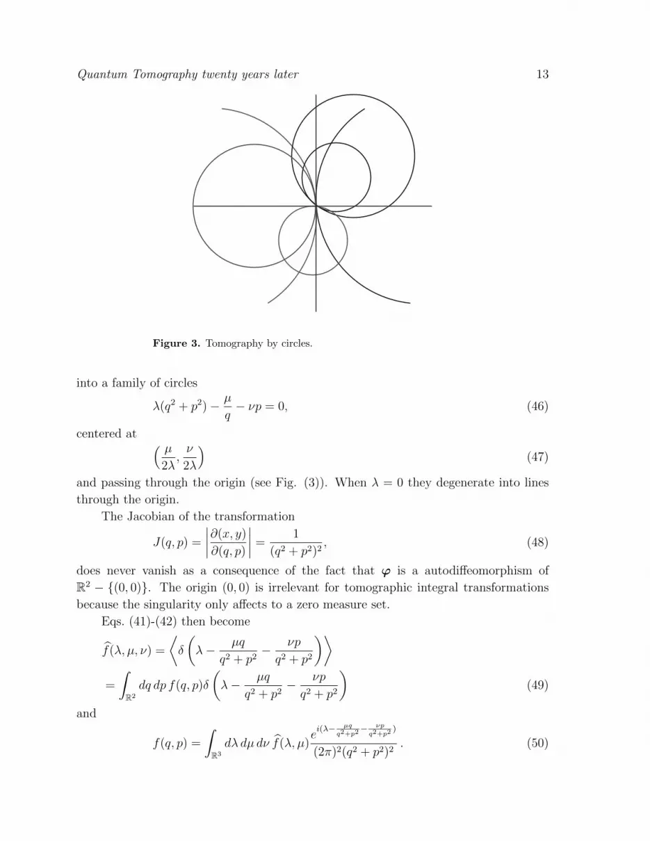
2.8. Tomography by circles in the plane

The conformal inversion

(x, y) = ϕ(q, p) =

(q

q2 + p2,

p

q2 + p2

), (44)

maps the family of lines

λ− µx− νy = 0 (45)


Figure 3. Tomography by circles.

into a family of circles

λ(q2 + p2)− µ

q− νp = 0, (46)

centered at ( µ2λ,ν

2λ

)(47)

and passing through the origin (see Fig. (3)). When λ = 0 they degenerate into lines

through the origin.

The Jacobian of the transformation

J(q, p) =

∣∣∣∣∂(x, y)

∂(q, p)

∣∣∣∣ =1

(q2 + p2)2, (48)

does never vanish as a consequence of the fact that ϕ is a autodiffeomorphism of

R2 − {(0, 0)}. The origin (0, 0) is irrelevant for tomographic integral transformations

because the singularity only affects to a zero measure set.

Eqs. (41)-(42) then become

f(λ, µ, ν) =

⟨δ

(λ− µq

q2 + p2− νp

q2 + p2

)⟩=

∫R2

dq dp f(q, p)δ

(λ− µq

q2 + p2− νp

q2 + p2

)(49)

and

f(q, p) =

∫R3

dλ dµ dν f(λ, µ)ei(λ− µq

q2+p2− νp

q2+p2)

(2π)2(q2 + p2)2. (50)


Figure 4. Tomography by hyperbolas induced by the map ϕ (54).

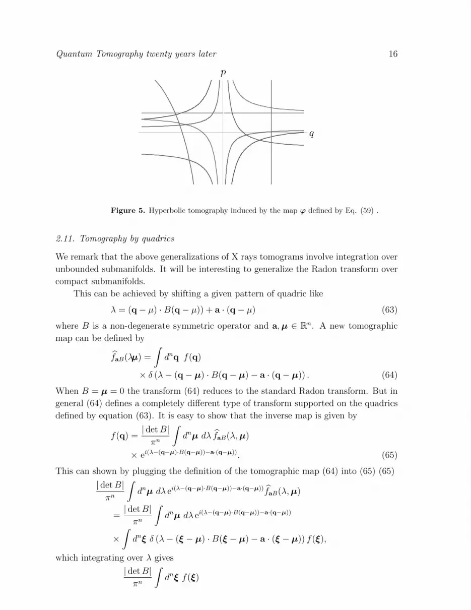
2.9. Tomography by hyperbolas in the plane

The family of lines

λ− µx− νy = 0 (51)

on the plane is mapped into a family of hyperbolas

λ− µ

q− νp = 0, (52)

with asymptotes

q = 0, p =λ

ν(53)

by the transformation

(x, y) = ϕ(q, p) =

(1

q, p

). (54)

For µ > 0 the hyperbolas are in the second and fourth quadrants, while for µ < 0 they

are in the first and third quadrants (see Fig. (4)). When µ = 0 or ν = 0 they degenerate

into lines respectively horizontal or vertical.

The Jacobian

J(q, p) =

∣∣∣∣∂(x, y)

∂(q, p)

∣∣∣∣ =1

q2, (55)

does not vanish again because ϕ is diffeomorphism in R2 − {(0, y), y ∈ R}.Eqs. (41)-(42) become

f(λ, µ, ν) =

⟨δ

(λ− µ

q− νp

)⟩=

∫R2

dq dp f(q, p)δ

(λ− µ

q− νp

)(56)


and

f(q, p) =

∫R3

dλdµ dν

(2π)2f(λ, µ)

1

q2ei(λ−

µq−νp). (57)

2.10. Hyperbolic tomography in Rn

It is possible to generalize this kind of hyperbolic tomography in terms of quadratic

forms. Let us consider the following tomographic map

f(ξ, ν, λ)=

∫dnp dnq δ (λ− ξ · q− ν(p,q)) f(p,q),

where p and q are vectors in Rn and

ν(p,q) =n∑j=1

qjνjpj. (58)

is a bilinear non-degenerate diagonal form defined by a vector ν = (ν1, ν2, · · · , νn) ∈ Rn.

This map corresponds to the deformation of standard multidimensional Radon

transform by means of the following local diffeomorphism

ϕ(qi, pj) = (qi, qjpj) , (59)

whose Jacobian is

J(q,p) =

∣∣∣∣∂(x,y)

∂(q,p)

∣∣∣∣ =n∏j=1

|qj| (60)

Thus, the inverse map is given by

f(p,q) =1

(2π)2n

∫dnξ dnν dλ f(ξ,ν, λ)

n∏j=1

|qj| ei(λ−ξ·q−ν(p,q)). (61)

as can be derived from integration over λ

f(p,q) =1

(2π)2n

∫dnξ dnν dnp′ dnq′ f(p′,q′)

×n∏j=1

|qj| ei(ξ·q′+ν(p′,q′)−ξ·q−ν(p,q))

=

∫dnν dnp′

n∏j=1

∣∣∣ qj2π

∣∣∣ eiν(p′−p,q)f(p′,q)

=

∫dnp′ δ(p′ − p)f(p′,q). (62)

This corresponds to the higher dimensional generalization of the Bertrand-Bertrand

tomography [Be87]

Notice that the distribution of hyperboloids in the plane when n = 2 is quite

different from those analyzed in the previous subsection (see Fig. (5)).


Figure 5. Hyperbolic tomography induced by the map ϕ defined by Eq. (59) .

2.11. Tomography by quadrics

We remark that the above generalizations of X rays tomograms involve integration over

unbounded submanifolds. It will be interesting to generalize the Radon transform over

compact submanifolds.

This can be achieved by shifting a given pattern of quadric like

λ = (q− µ) ·B(q− µ)) + a · (q− µ) (63)

where B is a non-degenerate symmetric operator and a,µ ∈ Rn. A new tomographic

map can be defined by

faB(λ,µ) =

∫dnq f(q)

× δ (λ− (q− µ) ·B(q− µ)− a · (q− µ)) . (64)

When B = µ = 0 the transform (64) reduces to the standard Radon transform. But in

general (64) defines a completely different type of transform supported on the quadrics

defined by equation (63). It is easy to show that the inverse map is given by

f(q) =| detB|πn

∫dnµ dλ faB(λ,µ)

× ei(λ−(q−µ)·B(q−µ))−a·(q−µ)). (65)

This can shown by plugging the definition of the tomographic map (64) into (65) (65)

| detB|πn

∫dnµ dλ ei(λ−(q−µ)·B(q−µ))−a·(q−µ))faB(λ,µ)

=| detB|πn

∫dnµ dλ ei(λ−(q−µ)·B(q−µ))−a·(q−µ))

×∫dnξ δ (λ− (ξ − µ) ·B(ξ − µ)− a · (ξ − µ)) f(ξ),

which integrating over λ gives

| detB|πn

∫dnξ f(ξ)


µ

Figure 6. Tomography on circles in the plane for the Hall effect.

×∫dnµ ei((ξ−µ)·B(ξ−µ)−(q−µ)·B(q−µ)−a·(q−ξ))

=| detB|πn

∫dnξ dnµ f(ξ)ei[ξ·Bξ−q·Bq+(q−ξ)·2B(µ−B−1a/2)]

=

∫dnξ f(ξ)ei[ξ·Bξ−q·Bq)]δn (q− ξ) = f(q).

The meaning of the above tomographic map depends on the physical character of B.

If we assume that B is strictly positive (elliptic case), the map corresponds to averages

of f along the ellipsoids defined by the equation (63). In particular if a = 0 and all

eigenvalues of B are equal to b2 it corresponds to integration over spheres centered at

µ (see Fig. (6))

b2(q− µ)2 = λ. (66)

In the two dimensional case corresponds to trajectories of particles moving under

the action of a constant magnetic field on a plane (Hall effect).

In the case that B has positive and negative eigenvalues this correspond to the

hyperbolic tomography which averages of f along the hyperboloids defined by the

equation (63), e.g.,

b2(q1 − µ1)2 − c2(q2 − µ2)2 = λ. (67)

In the case of degenerated B forms we have an hybrid transform. B can be

decomposed into a non-degenerated bilinear form and a linear form. In that case

the tomography of the linear components should be treated as the standard Radon

transform, whereas the non-degenerate variables should transform as above.

Notice that the distribution of circles is quite different from those obtained by the

Radon transform defined by rescaling in subsection (2.8). In that case the centers and the

radius changed from one circle to another, whereas here all the circles are of fixed radius

and only the center of the circles are varying by shifts. The new tomographic map makes

possible a local implementation of tomography because the marginals involved into the

resconstruction of f(p, q) only involve integrations in compact domain around the point

(p, q). The trajectories involved in the construction the tomogram are all trajectories

of a charged particle with the same energy moving in a constant magnetic field. This


points out the possible applications to tomography by charged particles moving on a

transversal magnetic fields over samples with smaller sizes than the cyclotron radius

mv/eB.

Finally we remark that the symplicity of the inverse formula seems to be related to

the integrable character of the underlying dynamical system whose ray trajectories are

involved in the construction of the tomogram. We conjecture that this a generic issue,

i.e. tomograms defined by phase space trajectories of integrable systems have simple

analytic inversion formulas.

3. Tomography and coherent states

There are several representations of quantum states providing the possibility to present

equivalent, but different in their form, formulations of quantum mechanics [St02].

Among them, the Wigner quasi-distribution function [Wi32] and the well known Husimi-

Kano K−function [Hu40, ka56], (in this paper we have decided to keep up with the

original notations of the pioneer papers on the subject). Quasi-distributions are usually

referred to as phase-space representations of quantum states. Another important

phase-space representation is related to the Sudarshan’s φ diagonal coherent-state

representation [Su63, Gl63]. Interestingly, the last two phase space representations,

K and φ, are based on the use of coherent states and allow for an interpretation in a

tomographic scheme which fits nicely in the general description given above.

In the quantum case, tomography may also be casted in a quantizer-dequantizer

scheme. In this sense, the Husimi-Kano function is a dequantization, and the

Sudarshan’s φ is just its dual symbol. So, the coherent-state tomographic point of

view provides a unifying description that encompasses also the so called photon number

tomography. Here, we limit to the coherent-state (CS) tomography for a single degree

of freedom, and we adopt a pedagogical style which is reminiscent of many joint papers

with Volodya Man’ko.

3.1. Coherent states: main properties

In the case of a single degree of freedom, the Weyl map associates with any point (x, α)

of the phase-space of the system a unitary operator W (x, α) acting on a Hilbert space

H, which can be realized in terms of square integrable functions ψ(x) [Es14]. Upon

switching to complex numbers z = (x + iα)/√

2, we recognize that W (x, α) is nothing

but the usual displacement operator

D (z) = exp(za† − z∗a

), (68)

which acting on the vacuum Fock state |0〉 , a|0〉 = 0, generates the coherent state |z〉,where

|z〉 = exp(−|z|2

2) exp

(za†)

exp (−z∗a) |0〉 = exp(−|z|2

2)∞∑j=0

zj

j!a†j |0〉 .(69)


We recall that the coherent states are a (over-) complete set in the Hilbert space H.Any bounded set containing a limit point z0 in the complex z−plane defines a complete

set of coherent states containing a limit point, the coherent state |z0〉 , in the Hilbert

space H. In particular, any Cauchy sequence {zk} of complex numbers defines a Cauchy

sequence of coherent states {|zk〉} , which is a complete set. The same holds for any

extracted subsequence. This completeness property holds as exp(|z|2 /2

)〈z|ψ〉 is an

entire analytic function of the complex variable z∗, for any |ψ〉 ∈ H. Then

〈zk|ψ〉 = 0 ∀k ⇒ |ψ〉 = 0 , (70)

because z∗0 is a non-isolated zero of an analytic function.

Besides, any bounded operator Amay be completely reconstructed from its diagonal

matrix elements⟨zk

∣∣∣A∣∣∣ zk⟩ . In fact, exp(|z|2 /2 + |z′|2 /2

) ⟨z∣∣∣A∣∣∣ z′⟩ is an analytical

function of the complex variables z∗, z′, so it is uniquely determined by its value

exp(|z|2) ⟨z∣∣∣A∣∣∣ z⟩ on the diagonal z′ = z. This is an entire function of the real

variables <z,=z, which is in turn uniquely determined by its values on any set with

an accumulation point.

3.2. Tomographic sets in infinite dimensional spaces

The nice properties of the coherent states previously discussed are the ground on which

the CS tomography can be builded. To this aim, we need to introduce a linear space V

and its dual V ∗.

Preliminarly, consider an abstract case. Suppose we have chosen in V ∗ the

tomographic set of observables N parametrzed as{Pν

}, ν ∈ I, where ν is a multi-

index belonging to a set of indices I. In the infinite dimensional case there are several

relevant spaces that one could choose as V , like the space of bounded operators B(H)

and that of compact operators C(H), the space of Hilbert-Schmidt operators I2 and

that of trace-class operators I1. Their mutual relations are:

I1 ⊂ I2 ⊂ C(H) ⊂ B(H). (71)

B(H) (and C(H)) are Banach spaces, with the norm∥∥∥A∥∥∥ = sup(‖ψ‖=1)

∥∥∥Aψ∥∥∥ , while

I2 is a Hilbert space with scalar product⟨A|B

⟩= Tr

(A†B

). Finally, I1 is a Banach

space with the norm∥∥∥A∥∥∥

1= Tr

(∣∣∣A∣∣∣) . The following inequalities hold true:∥∥∥A∥∥∥ ≤ ∥∥∥A∥∥∥2≤∥∥∥A∥∥∥

1. (72)

So I2, the only Hilbert space at our disposal to implement our definition of tomographic

set, is endowed with a topology which, when restricted to the trace-class operators, is

not equivalent to the topology of I1. Similar problems show up in the identification of

states and maps in infinite dimensions [Gr].


However, as any density state is associated with a trace class operator ρ, the natural

choice is to identify the space V with I1. Then, recalling that I1 is a ∗−ideal in its dual

space B(H):

I∗1 = B(H), (73)

we have V ∗ = B(H). So, the tomographic map Fρ defined on the tomographic set

N ={Pν

}, ν ∈ I, is just the value of the linear functional Tr

(Pν ·)

in ρ. In other

words, we can write the tomographic pairing between states and observables as

µ(Pν , ρ) := Fρ

(Pν

):= Tr

(Pν ρ)

(74)

The invertibility of the map Fρ, or, equivalently, the full reconstruction of any density

state ρ from its tomograms is guaranteed if we choose a tomographic set of trace

class observables, e.g., rank-one projectors, complete in I1. The completeness of the

tomographic set yields

Fρ

(Pν

)= Tr

(Pν ρ)

= 0 ∀ν ∈ I =⇒ ρ = 0. (75)

The choice of tomographic sets as complete sets of rank-one projectors gives the

possibility to extend the tomographic representation to observables or, in general, to

bounded operators. To do that, we have to interchange the role of states and observable.

We can use the self-duality of the Hilbert-Schmidt space I2. So, the tomographic set

is a set of density states, complete in I2, and the invertibility of the tomographic map

associated to a bounded operator A reads

FA

(Pν

):=⟨Pν |A

⟩= Tr

(PνA

)= 0 ∀ν ∈ I =⇒ A = 0 & A ∈ I2(76)

Then, as I2 is a ∗−ideal in B(H), there may exist a non-zero operator B, which is

bounded but not Hilbert-Schmidt, such that

Tr(PνB

)= 0 ∀ν ∈ I (77)

So, different operators may be tomographically separated only when their difference is

Hilbert-Schmidt. In other words, by choosing V = V ∗ = I2 one cannot get tomographic

representations of bounded, not Hilbert-Schmidt operators.. Nevertheless, there exists

the possibility of such a representationn, when the set{Pν

}of rank-one projectors is

complete even in I1. Then, recalling that I1 is a ∗−ideal in its dual space B(H), the

expression Tr (PµA) is nothing but the value of the linear functional Tr(·A)

in Pν and

the invertibility condition hods without constraints:

Tr(PνA

)= 0 ∀ν ∈ I =⇒ 0 = ‖Tr (·A)‖ = ‖A‖ =⇒ A = 0. (78)

So, any bounded operator can have a tomographic representation based on sets of

rank-one projectors which are complete both in I2 and in I1. As it turns out, this is the

case for the main tomographic sets. The rank-one projectors Pz = |z〉〈z| associated with

a complete set of coherent states are complete in the Hilbert space I2. In particular,


any Cauchy sequence {|zk〉} generates a tomographic set {|zk〉〈zk|}. In fact, bearing in

mind the previous remark on the reconstruction of a bounded operator, it results

Tr(A |zk〉〈zk|) = 〈zk |A| zk〉 = 0 ∀k ⇒ A = 0 & A ∈ B(H). (79)

This shows that a tomographic set of coherent state projectors is complete even in I1.

3.3. The coherent state tomography

Hereafter, we address the case when z varies in the whole complex plane, and call

CS tomography only the tomography based on the whole set of rank-one projectors

{Pz} = {|z〉〈z|} , z ∈ C.

It is possible to interpret the well known Husimi-Kano K-symbol of a (bounded)

operator A as the CS tomographic representation of A:

KA(z) :=⟨z∣∣∣A∣∣∣ z⟩ =: Tr(|z〉〈z| A). (80)

In particular, when A is chosen as a density operator ρ, the identity holds∫d2z

π〈z |ρ| z〉 = Tr(ρ) = 1, (81)

which allows for the probabilistic interpretation of the CS tomography. As a matter of

fact [Su68] the K-symbol exists also for a number of non-bounded operators. The CS

tomographic set is complete both in I2, the space of Hilbert-Schmidt operators, and in

I1, the space of trace class operators acting on the space of states. In fact, the formulae

A =

∫d2z

π

d2z′

π

⟨z∣∣∣A∣∣∣ z′⟩ |z〉〈z′| (82)

and [Ma95] ⟨z∣∣∣A∣∣∣ z′⟩ = e−

|z|2+|z′|22

∞∑n,m=0

(z∗)n(z′)m

n!m!

[∂n+m

∂z∗n∂zm

(e|z|

2⟨z∣∣∣A∣∣∣ z⟩)]

z∗=0z=0

(83)

show that if the tomograms⟨z∣∣∣A∣∣∣ z⟩ of a bounded operator A vanish for any z ∈ C ,

then A is the zero operator.

So, a resolution of the unity exists, which allows for the full reconstruction of any

density state or (bounded) operator from its CS tomograms. We are interested in the

explicit determination of such a formula. Now, the Sudarshan’s diagonal coherent state

representation φA(z) of an operator A is defined through the equation

A =

∫d2z

πφA(z) |z〉〈z| . (84)

So, to get the tomographic reconstruction formula we have to invert the well-known

relation

KA(z′) =⟨z′∣∣∣A∣∣∣ z′⟩ =

∫d2z

πφA(z) |〈z|z′〉|2 =

∫d2z

πφA(z)e−|z−z

′|2 (85)

which follows at once from Eq.(84) defining φA(z). This relation shows that KA(z′) is

given by the convolution product of φA times a gaussian function. Then, denoting with


KA(u′, v′) and φA(u, v) the K and φ symbols, with z′ = u′ + iv′ and z = u + iv, the

Fourier transform [Sc01] of Eq.(85) reads:∫du′dv′

2πKA(u′, v′)e−i(ξu

′+ηv′) = (86)∫du′v′

2π

∫dudv

πφA(u, v)e−(u−u′)2−(v−v′)2e−i(ξu

′+ηv′)

and we readily obtain

KA(ξ, η) = e−(ξ2+η2)/4φA(ξ, η), (87)

from which

φA(ξ, η) = e(ξ2+η2)/4KA(ξ, η), (88)

that formally yields

φA(u, v) =

∫dξdη

2πe(ξ2+η2)/4KA(ξ, η)ei(ξu+ηv). (89)

The presence of the anti-gaussian factor shows that the inverse Fourier transform of

φA(ξ, η) exists only when the asymptotic decay of KA(ξ, η) is faster than the growth

of e(ξ2+η2)/4. However, the integral always exists as a distribution, as was proven in

Ref.[Me65]. By virtue of this remark, we may go on and substitute the previous

expression into Eq.(84) getting

A =

∫d2z

π

[∫dξdη

2πe(ξ2+η2)/4KA(ξ, η)ei(ξu+ηv)

]|z〉〈z| = (90)∫

d2z

π

[∫dξdη

2π

∫du′dv′

2πKA(u′, v′)e(ξ2+η2)/4ei[ξ(u−u

′)+η(v−v′)]]|z〉〈z| .

Upon interchanging the order of integration, we may write the expected reconstruction

formula as

A =

∫d2z′

πG(z′)KA(z′), (91)

where the operator G(z′) reads:

G(z′) :=

∫d2z

2π

∫dξdη

2πe(ξ2+η2)/4ei[ξ(u−u

′)+η(v−v′)] |z〉〈z| . (92)

In other words, the CS tomographic set, like any other tomographic set, is associated

with a resolution of the unity

I =

∫d2z′

πG(z′)Tr(|z′〉〈z′| ·) . (93)

In a quantizer-dequantizer scheme, the operator Pz = |z′〉〈z′| is the dequantizer, while

G(z) is the quantizer. Since

|z〉〈z| =∫d2z′

πφ|z〉〈z| (z

′) |z′〉〈z′| ⇔ φ|z〉〈z| (z′) = πδ(z − z′) , (94)


we observe that

KG(z′)(z) =⟨z∣∣∣G(z′)

∣∣∣ z⟩ =

∫dξdη

2πei[−ξu

′−ηv′]e(ξ2+η2)/4K|z〉〈z| (ξ, η)

=

∫dξdη

2πei[−ξu

′−ηv′]φ|z〉〈z| (ξ, η) = φ|z〉〈z| (z′) = πδ(z − z′) , (95)

and remark that this result amounts to the orthonormality relations of the pair

quantizer-dequantizer:

KG(z′)(z) = Tr(|z〉〈z| G(z′)) = πδ(z − z′). (96)

If one exchange the roles in the pair, and bears in mind the definition of G(z), one

recovers the dual symbol of an operator as its Sudarshan’s symbol φ,

Tr(G(z′)A) =

∫dξdη

2πei[−ξu

′−ηv′]e(ξ2+η2)/4KA (ξ, η)

=

∫dξdη

2πei[−ξu

′−ηv′]φA (ξ, η) = φA (z′) . (97)

In this dual theory, the definition of the Sudarshan’s symbol as diagonal representation,

Eq.(84), appears as a reconstruction formula, the quantizer being Pz. In a tomographic

picture of quantum mechanics, this gives the possibility of representing in tomographic,

i.e., ”inner” terms, quantities such as expectation values of observables

Tr(ρA) =

∫d2z

πKρ(z)Tr(G(z)A) =

∫d2z

πKρ(z)φA(z). (98)

We remark that, in the context of the Agarval-Wolf operator ordering theory [Ma95,

Ag68], the K and φ symbols, appearing in our direct and dual reconstruction formulae,

are related to the Wick (i.e., normal) and anti-Wick ordering respectively. Of course,

if one insists in requiring only the use of CS tomographic representation, one needs to

introduce a star-product by means of an integral kernel:

Tr(ρA) = KρA(z) = (Kρ ? KA)(z) :=

∫d2z1

π

d2z2

πKρ(z1)KA(z2)Q(z1, z2, z)

Q(z1, z2, z) := Tr(G(z1)(G(z2)Pz). (99)

More details on star-product kernels are contained in a recent work with Volodya

Man’ko [Ib13]. We conclude by observing that the CS tomography can be generalized

by using coherent states and nonlinear coherent states of deformed oscillators, including

q−oscillators. This generalization was analyzed in [Ma08].

4. Tomography and the algebraic description of quantum systems

As it was discussed in the introduction the algebraic description of quantum systems

based on the theory of C∗-algebras emerges from an analysis of the fundamental

structures needed to describe physical systems. The tomographic description of them

has been started recently in [Ib13], (see also [Lo14] and references therein).

Jordan algebras were introduced by P. Jordan as an attempt to unfold the algebraic

structure of quantum systems, but it was only after the work of Alfsen and Schultz


[Al98] that the exact relation with the theory of C∗-algebras was established. Recently,

such relation was revisited by Falceto et al [Fa13], [Fa13b] and the relation between

C∗-algebas and Lie-Jordan Banach algebras was clearly established. Such equivalence

was used too to describe the theory of reduction of C∗-algebras described in terms of

Lie-Jordan Banach algebras.

In this section the first steps towards a tomographic description of quantum systems

based on C∗ and Lie-Jordan algebras will be established. One of the main outcomes

of the theory is that it fits nicely with the tomographic description based on groups as

it will be shown in what follows. Thus, we will review first the basic notions from the

theory of C∗ and Lie-Jordan algebras that will be needed in what follows and after this

the tomographic description of a quantum system described by a Lie-Jordan algebra

and a group representation will be sucintly described.

4.1. C∗-tomography

We will consider a quantum system described by a unital C∗-algebra A, whose self–

adjoint part constitute the Lie-Jordan-Banach algebra of observables of the theory. The

states of the system are normalized positive functionals ρ:A → C,

ρ(I) = 1 , ρ(a∗a) ≥ 0 , ∀a ∈ A

and they determine a weak*–compact subset S(A) of the topological dual A′.Given a ∈ A, the number ρ(a) is the expected value of the observable measured in

the state ρ, also denoted as: 〈a〉ρ. Hence for each self-adjoint element a ∈ A, we may

define a continuous affine function a:S(A)→ R, a(ρ) = ρ(a). Kadison theorem [Ka51]

states that the correspondence a 7→ a is an isometric isomorphism from the self-adjoint

part of A onto the space of all real continuous affine functions on S(A). Notice that the

Hilbert space picture of the system, once a state is given, can be recovered by means of

the GNS construction [Na72].

If we consider now the general background of tomography as stated in Sect. 1.2, we

may consider that the space of states is a subset of the linear space V = A′. Moreover

because A ⊂ A′′, then we may think that the elements α in the dual V ∗ are going to lie

in A ⊂ V ∗.

Thus the tomographic description of the state ρ of A will consist in assigning to

this state a probability density function Wρ, that we will call “tomogram”, on some

auxiliary space N such that given Wρ the state ρ can be reconstructed unambiguously.

Hence we consider a family of elements in A parametrized by an index which can be

discrete or continuous, the elements of N , or, in other words, consider a map U :N → Aand we will denote by U(x) the element in A associated to the element x ∈ N . The

family {U(x) |x ∈ N} will be called a tomographic set if it separates states, i.e., given

ρ1, ρ2 ∈ S(A), if ρ1 6= ρ2, then ∃x ∈ N such that 〈ρ1, U(x)〉 6= 〈ρ2, U(x)〉.Given a state ρ and a tomographic set U , we will call the function Fρ:N → C,

defined as, recall Eq. (1):

Fρ(x) = 〈ρ, U(x)〉 ,


the sampling function of ρ with respect to U .

Let us assume that N is a topological space and a positive Borel measure µ on it.

We will also assume that the map U is continuous and integrable in the sense that for

any ρ ∈ S(A), the sampling function Fρ:N → C is integrable, that is, Fρ ∈ L1(N , µ).

The auxiliary space N (and the measure µ on it) used in the theory could depend on

the specific problem. Later on a rather general way of selecting the auxiliary spaces by

means of groups and their unitary representations will be discussed (see §4.3).

In order to guarantee that the assignament ρ 7→ Fρ is invertible, we will assume

that there exists another map D:N → A′ which is integrable in the sense that for any

a ∈ A the function Ga(x) = 〈D(x), a〉 is integrable, and such that

〈D(x), U(x′)〉 = δ(x, x′), x, x′ ∈ N , (100)

where δ(x, x′) is the delta distribution along the diagonal on N ×N , that is:

φ(x) =

∫Nδ(x, x′)φ(x′)dµ(x′) , (101)

where φ is a continuous function with compact support on N . If a map D exists

satisfying the property (101) we will say that U and D are biorthogonal.

If we denote now by ρ(x) = Fρ(x) = 〈ρ, U(x)〉 and by

φ =

∫Nφ(x)D(x)dµ(x) ,

with φ an integrable function, then it is easy to see thatˇφ(x) = φ(x) and ˆρ = ρ.

It is also noticeable that because∫NFρ(x)dµ(x) =

∫N〈ρ, U(x)〉dµ(x) = ρ

(∫NU(x)dµ(x)

),

it is convenient to assume that ∫NU(x)dµ(x) = 1 .

If U(x) satisfies this, then we will say that U(x) is normalized. In such case it is clear

that ∫MFρ(x)dµ(x) = 1 .

We may recast the previous theorem by computing first the ˆ map and later the

ˇ map on Fρ:

Fρ =

∫ND(x)Fρ(x)dµ(x) , (102)

then if we apply the ˇ map first, we get

ˇF ρ(x

′) = 〈Fρ(x), U(x′)〉 =

∫NFρ(x)〈D(x), U(x′)〉 dµ(x) = Fρ(x

′) , ∀x′ ∈ N . (103)


We may also define another function Fρ(x, x′) depending of two arguments instead

of one: Fρ(x, x′) = 〈ρ, U(x)∗U(x′)〉 for any x,x′ ∈ N . We will say that a function

F :N ×N → C is positive, or of positive type, or positive semidefinite, if ∀N ∈ N and

ξi ∈ C, xi ∈ N , i = 1 . . . , N , we have:

N∑i,j=1

ξiξjF (xi, xj) ≥ 0 . (104)

Then it is easy to check that given a state ρ and a tomographic set U :N → A in a

C∗-algebra A, then the function Fρ(x, x′) = 〈ρ, U(x)∗U(x′)〉 is positive semidefinite. In

fact, the following simple computation shows it.

N∑i,j=1

ξiξjFρ(xi, xj) =N∑

i,j=1

ξiξj〈ρ, U(xi)∗U(xj)〉 =

⟨ρ,

N∑i,j=1

ξiξjU(xi)∗U(xj)

⟩

=

⟨ρ,

(N∑i=1

ξiU(xi)

)∗( N∑j=1

ξjU(xj)

)⟩≥ 0 .

We will take advantage of this property later on when dealing with tomography in

groups.

4.2. Equivariant tomographic theories on C*–algebras

We will encounter in many situations the presence of a group in the theory whose states

we want to describe tomographically. Such group could be a group of symmetries of the

dynamics of the system or a group which is describing the background of the theory.

In any of these circumstances we will assume that there is a Lie group G acting on the

C∗-algebra A, i.e., we have a strongly continuous map T :G→ Aut(A) such that

Te = I , Tg1Tg2 = Tg1g2 , ∀g1, g2 ∈ G .

In such case we will need to assume that the group G acts on the auxiliary spaces used

to construct the tomographic picture. Thus, the group G will act on N , and such action

will be simply denoted as x 7→ g · x, x ∈ N .

The natural compatibility condition for a tomographic map U :N → A to be

compatible with the group G present in the theory is equivariance, i.e.,

U(g · x) = Tg(U(x)) , ∀x ∈ N , g ∈ G . (105)

This could be interpreted by saying that if the parameters x, x′ parametrizing two

sampling elements U(x) and U(x′) in A, are related by an element g of the group,

i.e., x′ = g · x, then the two sampling observables U(x),U(x′) are also related by the

same element of G.

Under these conditions, it is easy to conclude that the sampling function Fρcorresponding to the state ρ satisfies the following:

Fρ(g · x) = FT ∗g ρ(x) , (106)


because

Fρ(g · x) = 〈ρ, U(g · x)〉 = 〈ρ, Tg(U(x))〉 = 〈T ∗g ρ, U(x)〉 = FT ∗g ρ(x) , (107)

where T ∗g ρ denotes the adjoint action of G on A′. Notice that if ρ is an invariant state,

T ∗g ρ = ρ then the corresponding samping function will be invariant too.

Fρ(g · x) = Fρ(x) . ∀ ∈ G , x ∈M . (108)

We will also consider that situation where the group G acts on the space M defining

the space of classical functions whose tomograms we would like to obtain. We will denote

again such action by y 7→ g ·y, y ∈M . The generalised Radon transformR:N → F(M)′

should be equivariant, this is

R(g · y) = g∗R(y) , (109)

where g∗ indicates now the natural action induced on the space F(M)′ in the dual of

the space of functions on M , by the action of G on M . More explicitly

〈g∗(R(y)), F 〉 = 〈R(y), g∗F 〉 and g∗F (x) = F (g · x) . (110)

Now, if R is actually a generalized Radon transform and Wρ denote the tomogram of

the state ρ, we will have:

Wρ(g·y) = 〈R(g·y), Fρ〉 = 〈g∗R(y), Fρ〉 = 〈R(y), g∗Fρ〉 = 〈R(y), Fg∗ρ〉 = Wg∗ρ(y) .(111)

Then we conclude this discussion by observing that if ρ is an invariant state, the

tomogram defined by it, is actually invariant:

Wρ(g · y) = Wρ(y) ∀g ∈ G . (112)

4.3. Unitary group representations on C∗-algebras

We will discuss now a particular instance of the tomographic programme discussed above

where a Lie group G plays a paramount role. We will find this situation for instance

in spin tomography where the group G will be the group SU(N), but such situation

is found also in standard homodyne tomography that could be understood in similar

terms with the group G being the Heisenberg–Weyl group.

Now we will assume that the auxiliary space N is a group G and the tomographic

map U :G → A is provided by a continuous unitary representation of G on A,

that is, U(g)∗ = U(g)−1 = U(g−1) is a unitary element in the C∗-algebra A, and

U(g1g2) = U(g1)U(g2) and U(e) = 1. Then we may denote by T :G → Aut(A), the

action of G on A by inner automorphism given by

Tg(a) = U(g)∗ · a · U(g) , a ∈ A , g ∈ G .

Then we can see immediately that we have the equivariance property for the tomographic

map with respect to the action of G on itself by conjugation:

U(g−1hg) = U(g−1) · U(h) · U(g) = Tg(U(h)) , g, h ∈ G . (113)


The sampling function corresponding to the state ρ is given by

Fρ(g) = 〈ρ, U(g)〉 , (114)

and we may check that the map Fρ : G→ C is a positive semidefinite map in the sense

that the map Fρ(g, h) of two arguments defined as

Fρ(g, h) = Fρ(g−1h) g, h ∈ G ,

is positive semidefinite, i.e. ∀N ∈ N, ξi ∈ C, gi ∈ G, i = 1, . . . , N , then

N∑i,j=1

ξiξjFρ(g−1i gj) ≥ 0 . (115)

Naimark’s theorem [Na72] establishes that given a positive semidefinite function

F on a group G, there exists a Hilbert space HF , a continuous unitary representation

UF : G→ U(HF ) and a vector |0〉 ∈ HF such that

F (g) = 〈0|UF (g)|0〉 . (116)

The relation between the state |0〉〈0| = ρF , the representation UF , the original state ρ

and the original representation U has been discussed recently [Ib11].

In order to define now the generalized Radon transform that will describe the

tomogram corresponding to the state ρ, we will consider now the Lie algebra g of the

group G and the auxiliary space g×R. In g×R we have defined the natural extension

of the standard exponential map exp : g×R→ G given by exp(ξ, s) = exp(sξ).

The unitary representation of G on A, defines a Lie algebra homomorphism from g

into Asa, where Asa denotes the self-adjoint part of A, that is, Asa = {a ∈ A | a∗ = a}.Given any ξ ∈ g, we denote by ξ the element of Asa defined as:

ξ = −i d

dsU (exp(isξ))

∣∣∣∣s=0

= −i ∂∂sU(exp(ξ, s))

∣∣∣∣s=0

, (117)

Clearly ξ∗ = ξ and

[ξ, ζ] = [ξ, ζ] , ∀ξ, ζ ∈ g . (118)

4.4. The GNS construction and unitary group representations on C∗-algebras

Given the state ρ, the GNS construction allows to represent the C∗-algebra A as

operators acting on a Hilbert space Hρ. To be precise consider the Hilbert space Hρ

obtained as the completion of the space A/Jρ, where Jρ = ker ρ is the Gelfand ideal

defined by ρ, with respect to the inner product is defined as:

〈[a], [b]〉 = ρ(a∗b) , ∀[a] = a+ Jρ, [b] = b+ Jρ ∈ A/Jρ . (119)

Then there is a natural representation πρ : A → B(H) given by:

πρ(a)[b] = [a · b] , ∀[b] ∈ Hρ . (120)


The unitary representation U :G → Aut(A) of the group G becomes a unitary

representation Uρ of G on Hρ by means of Uρ = πρ ◦ U , i.e., Uρ : G → U(Hρ) is

the map defined by

Uρ(g) = πρ (U(g)) .

Notice that because U is unitary, U(g) is a unitary element in A, then πρ (U(g)) is a

unitary operator on Hρ. In fact, for all [a], [b] ∈ Hρ we have:

〈Uρ(g)[a], Uρ(g)[b]〉ρ = 〈πρ (Uρ(g)) [a], πρ (Uρ(g)) [b]〉ρ = 〈[Uρ(g)a], [Uρ(g)b]〉ρ (121)

= ρ ((Uρ(g)a)∗ Uρ(g)b) = ρ(a∗b) = 〈[a], [b]〉ρ. (122)

If we consider now the induced map g→ Asa, we will obtain that the element ξ ∈ g

will be mapped by the representation πρ into a self-adjoint operator on Hρ. We will

denote the operator defined this way by ξρ, that is:

iξρ ([a]) =d

dsUρ (exp(sξ)[a])

∣∣∣∣s=0

=d

dsπρ (U (exp(sξ)[a]))

∣∣∣∣s=0

(123)

=d

ds[U (exp(sξ)) a]

∣∣∣∣s=0

=

[d

dsU (exp(sξ))

∣∣∣∣s=0

· a]

= [iξa] .(124)

Because of Stone’s theorem, we know that there exists a unique strongly continuous

one-parameter group of unitary operators U ξs on Hρ such that

d

dsU ξs [a]

∣∣∣∣s=0

= iξρ[a] , (125)

thus:

eisξρ = U ξs = Uρ (exp(sξ)) = πρ ◦ U (exp(sξ)) . (126)

Finally, the spectral theorem applied to the self-adjoint operators ξρ asserts that

there is a Borelian spectral measure Eξρ in the real line such that

ξρ =

∫λ dEξρ(λ) , (127)

hence

U ξs =

∫eisλdEξρ(λ) .

Now, we will consider as auxiliary space N the space g×R, and we will define the map

R: g× R→ (F(G))′ as follows:

R(ξ;λ)(F ) =1

(2π)2

∫e−isλF (exp(sξ)) ds . (128)

To be precise, the map R is defined from g×R into the space of continuous functions

on the exponential of g, exp(g) ⊂ G. For groups such that exp(g) = G, i.e. exponential

groups, we have the map written above.

Then we will call the function R(ξ;λ)(Fρ) corresponding to the tomographic

function Fρ defined by the state ρ, the tomogram of ρ and will be denoted by Wρ(ξ;λ).

Notice that we may fix λ = 1 to get:

Wρ(ξ) =1

(2π)2

∫e−isFρ (exp(isξ)) ds. (129)


Notice that if we compute the inverse Fourier transform of the tomogram Wρ, we

have:

Fρ (exp(sξ)) =

∫eisλWρ(ξ;λ) dλ (130)

and if we consider now that

Fρ (exp(sξ)) = 〈ρ, U (exp(sξ))〉 = 〈0|Uρ (exp(sξ)) |0〉 (131)

= 〈0|∫

eisλdEξρ(λ)|0〉 =

∫eisλ〈0|dEξρ(λ)|0〉 . (132)

Then if the measure µξ,ρ = 〈0|dEξρ|0〉 is absolutely continuous with respect to the

Lebesgue measure, we will have that µξ,ρ(λ) = Wρ(ξ;λ)dλ, and Wρ(ξ;λ) will be the

Radon-Nikodym derivative of µξ,ρ with respect to dλ. Hence, we have obtained that,

under these conditions, the tomogram Wρ of the state ρ can be written as:

Wρ(ξ;λ) =δµξ,ρδλ

, (133)

where δµξ,ρ/δλ denotes the Radon-Nikodym derivative of µξ,ρ with respect to the

Lebesgue measure dλ.

Finally, suppose that ω is a density operator on Hρ. We will define its tomographic

function by Fω(g) = Tr(ωUρ(g)) and its tomogram Wω(ξ;λ) as;

Wω(ξ;λ) =1

(2π)2

∫e−isλFω (exp(sξ)) ds .

Then computing the inverse Fourier transform of Wω(ξ;λ) we will get:

Fω (exp(sξ)) =

∫eisλWω(ξ;λ) dλ .

A simple computation shows that:

Wω(ξ;λ) =1

(2π)2

∫e−isλFω (exp(sξ)) ds =

1

(2π)2

∫e−isλTr (ωUρ (exp(sξ))) ds

= Tr

(1

(2π)2

∫e−isλωUρ (exp(sξ)) ds

)= Tr

(1

(2π)2

∫e−isλωeisξρds

)= Tr

(ω

1

(2π)2

∫e−is(λI−ξρ)ds

)= Tr

(ω δ(λI− ξρ)

),

which is the formula for the tomogram Wρ that resembles closely the classical Radon

transform Eq. (29) in the affine language.

Acknowledgments

We thank Volodya and Margarita Man’ko for many invaluable discussions and intense

collaboration on tomography and related subjects. This work was partially supported by

MEC grant MTM2010-21186-C02-02 and QUITEMAD+ programme. The work of MA

has been partially supported by Spanish DGIID-DGA grant 2014-E24/2 and Spanish

MICINN grants FPA2012-35453 and CPAN-CSD2007-00042.


References

[Ag68] G. S. Agarwal and E. Wolf, Phys, Rev. Lett. 21, 180 (1968); Phys, Rev. D 2, 2161 (1970);

Phys, Rev. D 2, 2187 (1970); Phys, Rev. D 2 (1970) 2206.

[Al98] E. M. Alfsen, F. W. Shultz, On Orientation and Dynamics in Operator Algebras. Part I,

Commun. Math. Phys. 194 (1998) 87.

[Am09] G. G. Amosov, V. I. Manko, A classical limit of a center-of-mass tomogram in view of the

central limit theorem, Phys. Scr., 80:2, 025006 (2009).

[Ar96] G. M. D’Ariano, S. Mancini, V. I. Man’ko and P. Tombesi, Quantum Semiclass. Opt., 8 (1996)

1017.

[Ar05] A. S. Arkhipov and V. I. Man’ko Phys. Rev. A 71 (2005) 012101.

[As07] M. Asorey, P. Facchi, V.I. Man’ko, G. Marmo, S. Pascazio and E. C. G. Sudarshan, Phys.

Rev. A 76, 012117 (2007).

[As08] M. Asorey, P. Facchi, V. I. Man’ko, G. Marmo, S. Pascazio and E. C. G. Sudarshan, Phys.

Rev. A 77, 042115 (2008).

[As12] M. Asorey, P. Facchi, V.I. Manko, G. Marmo, S. Pascazio, E.C.G. Sudarshan, Generalized

quantum tomographic maps, Physica Scripta 85, 065001(2012).

[Be87] J. Bertrand and P. Bertrand, Found. Phys. 17 (1987) 397.

[Es14] G. Esposito, G. Marmo, G. Miele and G. Sudarshan, Advanced Concepts in Quantum

Mechanics, Cambridge University Press, Cambridge (2014).

[Fa10] P. Facchi, and M. Ligab, In AIP Conference Series 1260, (2010) 3-34).

[Fa13] F. Falceto, L. Ferro, A. Ibort, G. Marmo. Reduction of Lie–Jordan Banach algebras and

quantum states. J. Phys. A: Math. Theor. 46 (2013) 015201.

[Fa13b] F. Falceto, L. Ferro, A. Ibort, G. Marmo. Reduction of Lie–Jordan algebras: Quantum. Il

Nuovo Cimento C. 36 (3) 107–115 (2013).

[Ge66] I.M. Gelfand, M.I. Graev, N.Ya. Vilenkin. Generalized functions: Inte- gral geometry and

representation theory, Vol. 5 (Academic Press, 1966).

[Gl63] R. J. Glauber, Phys. Rev. Lett., 10 (1963) 84; ibid. 131 (1963) 2766.

[Gr] J. Grabowski, M. Kus, G. Marmo, Open Systems & Information Dynamics, 14 (2007) 355.

[He73] S. Helgason, Ann. of Math. 98, 451 (1973)

[He80] S. Helgason, The Radon Transform (Birkhauser, Boston, 1980).

[He84] S. Helgason, Groups and Geometric Analysis (Academic Press, Orlando, 1984).

[Hu40] K. Husimi, Proc. Phys. Math. Soc. Jpn., 22 (1940) 264.

[Ib09] A Ibort, V. I. Man’ko, G. Marmo, A. Simoni, and F. Ventriglia, Phys. Scr., 79 (2009) 065013.

[Ib10] A. Ibort, V. I. Man’ko, G. Marmo, A. Simoni, and F. Ventriglia, Phys. Lett. A, 374 (2010)

2614.

[Ib11] A. Ibort, V. I. Man’ko, G. Marmo, A. Simoni and F. Ventriglia. Phys. Scr. 84 (2011) 065006.

[Ib13] A. Ibort, V. I. Man’ko, G. Marmo, A. Simoni, C. Stornaiolo, F. Ventriglia. Tomography and

C∗-algebras, Phys. Scr. 87, 038107 (2013).

[Jo55] F. John, Plane waves and spherical means: Applied to Partial Differential Equations, Wiley

Interscience, New York, 1955.

[Ka51] R. V. Kadison, A representation theory for commutative topological algebra, Mem. Amer.

Math. Soc. No. 7 (1951).

[ka56] Y. Kano, J. Math. Phys. 6 (1965)1913.

[Lo14] A. Lopez-Yela. Ph. D. Thesis (2014).

[Lu66] D. Ludwig, Commun. Pure and Appl. Math., 19, (1966) 49-81.

[Ma95] L. Mandel and E. Wolf, Optical coherence and Quantum Optics, Cambridge University Presss,

Cambridge, (1995).

[Mn95] S. Mancini, V. I. Man’ko and P. Tombesi, Quantum Semiclass. Opt. 7, 615 (1995).

[Mn96] S. Mancini, V. I. Man’ko and P. Tombesi, Phys. Lett. A, 213 (1996) 1.

[Ma97] O. V. Man’ko and V. I. Man’ko, J. Russ. Laser Res., 25 (1997) 477.


[Ma00] O. V. Man’ko, V. I. Man’ko, and G. Marmo, Phys. Scr., 62 (2000) 446.

[Ma02] O. V. Man’ko, V. I. Man’ko, and G. Marmo, J. Phys. A: Math. Gen., 35 (2002) 699.

[Ma04] O. V. Man’ko and V. I. Man’ko, JETP, 85 (2004) 430.

[Ma05] V. I. Man’ko, G. Marmo, P. Vitale, Phys. Lett. A, 334 (2005) 1.

[Ma05] V. I. Man’ko, G. Marmo, A. Simoni, A. Stern, F. Ventriglia, Phys. Lett. A, 343 (2005) 251.

[Ma06] V. I. Man’ko, G. Marmo, A. Simoni, A. Stern, E. C. G. Sudarshan, F. Ventriglia, Phys. Lett.

A, 351 (2006) 1.

[Ma06b] V. I. Man’ko, G. Marmo, A. Simoni, F. Ventriglia, Open Sys. and Information Dyn., 13 (2006)

239.

[Ma07] O. V. Man’ko, V. I. Man’ko, G. Marmo, P. Vitale, Phys. Lett. A, 360 (2007) 522.

[Me00] V. I. Manko and R. Vilela Mendes, Physica D, 145 (2000) 330–348.

[Ma08] V. I. Man’ko, G. Marmo, A. Simoni, E. C. G. Sudarshan, F. Ventriglia, Rep. Mat. Phys. 61,

337 (2008).

[Ma09] M.A. Man’ko, V.I. Man’ko, N.C. Thanh, N.H. Son, Y.P. Timoreev, S.D. Zakharov. J. Russ.

Laser Res., 30, (2009) 1-11.

[Me65] C. L. Mehta and E. C. G. Sudarshan, Phys. Rev. B 138 (1965) 274.

[Mi65] S. G. Mihlin, Multi-dimensional singular integrals and integral equations, Pergamon Press,

New York (1965).

[Na72] M. Naimark, Normed Rings, P. Noordhoff NV, The Netherlands (1964) or the more recent

Normed algebras, Wolters-Noordhoff, Groheningen (1972).

[Ra17] J. Radon. Uber die bestimmung von funktionen durch ihre integralwerte langs gewisser

mannigfaltigkeiten. Ber. Ver. Sachs. Akad. Wiss. keipzing. mahtj-Phys., KL., 69:262–

277 (1917). English translation in S.R. Deans: The Radon Transform and Some of Its

applications, app. A Krieger Publ. Co., Florida 2nd ed. (1993).

[Sc01] W. P. Schleich, Quantum Optics in Phase Space, Wiley-VCH, Berlin, (2001).

[St02] D. F. Styer, M. S. Balkin, K. M. Becker, M. R. Burns, C. E. Dudley, S. T. Forth, J. S. Gaumer,

M. A. Kramer, D. C. Oertel, L. H. Park, M. T. Rinkoski, C. T. Smith, T. D. Wotherspoon,

Am. J. Phys. 70 (2002) 288.

[Su63] E. C. G. Sudarshan, Phys. Rev. Lett., 10 (1963) 277.

[Su68] J. R. Klauder and E. C. G. Sudarshan, Fundamentals of Quantum Optics, Benjamin, New

York, (1968).

[Wi32] E. Wigner, Phys. Rev., 40 (1932) 749.

Documents

Quantum Tomography twenty years later