Embed Size (px)
Citation preview
Quantifying Patterns of Agent-Environment
Interaction
Danesh Tarapore1, Max Lungarella2,∗ and Gabriel Gomez3
1School of Information Technology, Indian Institute of Technology, Bombay, India2Lab. for Intelligent Systems and Informatics, The University of Tokyo, Japan
3Artificial Intelligence Lab., University of Zurich, Switzerland
Abstract
This article explores the assumption that a deeper (quantitative) understanding ofthe information-theoretic implications of sensory-motor coordination can help en-dow robots not only with better sensory morphologies, but also with better explo-ration strategies. Specifically, we investigate by means of statistical and information-theoretic measures, to what extent sensory-motor coordinated activity can generateand structure information in the sensory channels of a simulated agent interactingwith its surrounding environment. The results show how the usage of correlation,entropy, and mutual information can be employed (a) to segment an observed be-havior into distinct behavioral states, (b) to analyze the informational relationshipbetween the different components of the sensory-motor apparatus, and (c) to iden-tify patterns (or fingerprints) in the sensory-motor interaction between the agentand its local environment.
Key words: Self-structuring of information, sensory-motor coordination,agent-environment interaction
1 Introduction
Manual haptic perception is the ability to gather information about objectsby using the hands. Haptic exploration is a task-dependent activity, and whenpeople seek information about a particular object property, such as size, tem-perature, hardness, or texture, they perform stereotyped exploratory handmovements. In fact, spontaneously executed hand movements are the best
1 Corresponding author: M.L. ([email protected])
Preprint submitted to Elsevier Science 17 May 2004
ones to use, in the sense that they maximize the availability of relevant sen-sory information gained by haptic exploration (Lederman and Klatzky, 1990).The same holds for visual exploration. Eye movements, for instance, dependon the perceptual judgement that people are asked to make, and the eyesare typically directed toward areas of a visual scene or an image that deliveruseful and essential perceptual information (Yarbus, 1967). To reason aboutthe organization of saccadic eye movements, Lee and Yu (1999) proposed atheoretical framework based on information maximization. The basic assump-tion of their theory is that due to the small size of our foveas (high resolutionpart of the eye), our eyes have to continuously move to maximize the infor-mation intake from the world. Differences between tasks obviously influencethe statistics of visual and tactile inputs, as well as the way people acquireinformation for object discrimination, recognition, and categorization.
Clearly, the common denominator underlying our perceptual abilities seemsto be a process of sensory-motor coordination which couples perception andaction. It follows that coordinated movements must be considered part of theperceptual system (Thelen and Smith, 1994), and whether the sensory stim-ulation is visual, tactile, or auditory, perception always includes associatedmovements of eyes, hands, arms, head and neck (Ballard, 1991; Gibson, 1988).Sensory-motor coordination is important, because (a) it induces correlationsbetween various sensory modalities (such as vision and haptics) that can beexploited to form cross-modal associations, and (b) it generates structure inthe sensory data that facilitates the subsequent processing of those data (Lun-garella and Pfeifer, 2001; Lungarella and Sporns, 2004; Nolfi, 2002; Sporns andPegors, 2003). Exploratory activity of hands and eyes is a particular instance ofcoordinated motor activity that extracts different kinds of information throughinteraction with the environment. In other words, robots and other agents arenot passively exposed to sensory information, but they can actively shape suchinformation. Our long-term goal is to quantitatively understand what sort ofcoordinated motor activities lead to what sort of information. We also aim atidentifying “fingerprints” (or patterns of sensory or sensory-motor activation)characterizing the agent-environment interaction. Our approach builds on topof previous studies on category learning (Pfeifer and Scheier, 1997; Scheier andPfeifer, 1997), as well as on work on the information-theoretic and statisticalanalysis of sensory and motor data (Lungarella and Pfeifer, 2001; Sporns andPegors, 2003; Te Boekhorst et al., 2003).
The experimental tool of the study presented in this article is a simulatedrobotic agent, which was programmed to search its local environment for redobjects, approach them, and explore them for a while. The analysis of therecorded sensory and motor data shows that different types of sensory-motoractivities displayed distinct fingerprints reproducible across many experimen-tal runs. In the two following sections, we give a detailed overview of ourexperimental setup, and describe the actual experiments. Then, in Section 4,
2
we expose our methods of analysis. In Section 5, we present our results anddiscuss them. Eventually, in Section 6, we conclude and point to some futureresearch directions.
2 Experimental Setup
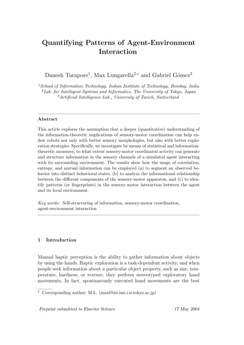
The study was conducted in simulation. The experimental setup consisted ofa two-wheeled robot and of a closed environment cluttered with randomlydistributed, colored cylindrical objects. A bird’s eye view on the robot andits ecological niche is shown in Fig. 1 a. The robot was equipped with elevenproximity sensors (d0−10) to measure the distance to the objects and a pan-controlled camera unit (image sensor) (see Fig. 1 b). The pan-angle of thecamera was constrained to vary in an interval of ±60o relative to the agent’smidline. The proximity sensors had a position-dependent range, that is, thesensors in the front and the ones in the back had a short range, whereas theones on the sides had a longer range (see caption of Fig. 1). The output ofeach sensor was affected by additive white noise with an amplitude of 10%the sensor range, and was partitioned into a space having 32 discrete states,leading to sensory signals with a 5 bits resolution. To reduce the dimensionalityof the input data, we divided the camera image into 24 vertical rectangularslices (i1−24), with width of two pixels for the slices close to the center (i7−18),and width of six pixels for the slices in the periphery (i1−6 and i19−24). Wecomputed the amount of the “effective” red color in each slice as R = r− (b+g)/2, where r, g, and b are the red, green, and blue components of the colorassociated with each pixel of the slice. Negative values of R were set to zero.This operation guaranteed that the red channel gave maximum response forfully saturated red color, that is, for r=31, g=b=0. Subsequently, the red colorslices will also be referred to as red channels or red receptors.
For the control of the robot, we opted for the Extended Braitenberg Archi-tecture (Pfeifer and Scheier, 1999) (see Figure 1 c). In this architecture, eachof the robot’s sensors is connected to a number of processes which run inparallel, continuously influencing the agent’s internal state, and governingits behavior. Because our goal is to illustrate how standard statistical andinformation-theoretic measures can be employed to quantify (and fingerprint)the agent-environment interaction, we started by decomposing the robot’s be-havior into three distinct behavioral states: (a) “explore the environment” and“find red objects”, (b) “track red objects”, and (c) “circle around red objects.”Two points are noteworthy. First, while the agent is exploring the environ-ment, its behavioral activity is only “weakly” sensory-motor coordinated, inthe sense that its motor activity is mainly driven by the random activity af-fecting its sensors. The two latter behavioral states, however, display “strong”sensory-motor coordinated activity, that is, motor activity characterized by a
3
(a)
camera
m0 m1
d10d9
d0
d4
d1
d2 d3
d7 d8
d6 d5
(b)
(c)
Fig. 1. (a) Bird’s eye view on the robot and its ecological niche. The trace depictsthe path of the robot during a typical experiment. (b) Schematic representation ofthe simulated agent. The sensors have a position-dependent range: if rl is the lengthof the robot, the range of d0, d1, d9, and d10 is 1.8 rl, the one of d2 and d3 is 1.2 rl,and the one of d4, d5, d6, d7, and d8 is 0.6 rl. (c) Extended Braitenberg ControlArchitecture: As shown, four processes govern the agent’s behavior.
tight coupling between sensing and acting. Second – and this point is moresubtle – the segmentation of the observed behavior into distinct behavioralstates is an important, maybe even necessary, step to simplify the analysistowards quantifying the agent-environment interaction and identifying stablepatterns of interaction. It is crucial to understand that the goal here is toshow how statistical and information-theoretic measures can be employed toidentify patterns in sensory data, and not how those patterns can be identi-fied automatically. In the latter case, despite being possible (see Fig. 7) thesegmentation of the observed behavior in distinct states would make less sense.
4
3 Experiments
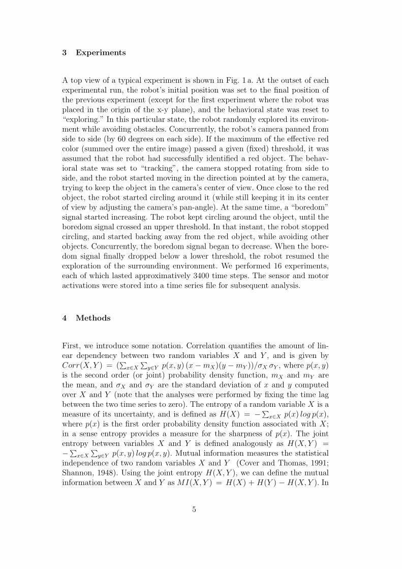
A top view of a typical experiment is shown in Fig. 1 a. At the outset of eachexperimental run, the robot’s initial position was set to the final position ofthe previous experiment (except for the first experiment where the robot wasplaced in the origin of the x-y plane), and the behavioral state was reset to“exploring.” In this particular state, the robot randomly explored its environ-ment while avoiding obstacles. Concurrently, the robot’s camera panned fromside to side (by 60 degrees on each side). If the maximum of the effective redcolor (summed over the entire image) passed a given (fixed) threshold, it wasassumed that the robot had successfully identified a red object. The behav-ioral state was set to “tracking”, the camera stopped rotating from side toside, and the robot started moving in the direction pointed at by the camera,trying to keep the object in the camera’s center of view. Once close to the redobject, the robot started circling around it (while still keeping it in its centerof view by adjusting the camera’s pan-angle). At the same time, a “boredom”signal started increasing. The robot kept circling around the object, until theboredom signal crossed an upper threshold. In that instant, the robot stoppedcircling, and started backing away from the red object, while avoiding otherobjects. Concurrently, the boredom signal began to decrease. When the bore-dom signal finally dropped below a lower threshold, the robot resumed theexploration of the surrounding environment. We performed 16 experiments,each of which lasted approximatively 3400 time steps. The sensor and motoractivations were stored into a time series file for subsequent analysis.
4 Methods
First, we introduce some notation. Correlation quantifies the amount of lin-ear dependency between two random variables X and Y , and is given byCorr(X, Y ) = (
∑x∈X
∑y∈Y p(x, y) (x−mX)(y −mY ))/σX σY , where p(x, y)
is the second order (or joint) probability density function, mX and mY arethe mean, and σX and σY are the standard deviation of x and y computedover X and Y (note that the analyses were performed by fixing the time lagbetween the two time series to zero). The entropy of a random variable X is ameasure of its uncertainty, and is defined as H(X) = −∑
x∈X p(x) log p(x),where p(x) is the first order probability density function associated with X;in a sense entropy provides a measure for the sharpness of p(x). The jointentropy between variables X and Y is defined analogously as H(X, Y ) =−∑
x∈X
∑y∈Y p(x, y) log p(x, y). Mutual information measures the statistical
independence of two random variables X and Y (Cover and Thomas, 1991;Shannon, 1948). Using the joint entropy H(X,Y ), we can define the mutualinformation between X and Y as MI(X,Y ) = H(X) + H(Y ) − H(X, Y ). In
5
comparison with correlation, mutual information provides a better and moregeneral criterion to investigate statistical dependencies between random vari-ables (Steuer et al., 2002). For entropy as well as for mutual information, weassumed the binary logarithm.
Correlation, entropy and joint entropy were computed by first approximatingp(x) and p(x, y). The most straightforward approach is to use a histogram-based technique, described, for instance, in (Steuer et al., 2002). Because thesensors had a resolution of 5 bits, we estimated the histograms by setting thenumber of bins to 32 (which led to a bin-size of one). Having a unitary binsize allowed us to map the discretized value of the sensory stimulus directlyonto the corresponding bin for the approximation of the joint probability den-sity function. Because of the limited number of available data samples, theestimates of the entropy and of the mutual information were affected by asystematic error (Roulston, 1999). We compensated for this bias by adding asmall corrective term T to the computed estimates: T = (B − 1)/2 N to theentropy estimate (where N is the size of the temporal window over which theentropy is computed, and B is the number of states for which p(xi) 6= 0), andT = (Bx + By −Bx,y − 1)/2 N to the mutual information estimate (where Bx,By, Bx,y, and N have an analogous meaning to the previous case).
5 Data Analysis and Results
We analyzed the collected datasets by means of three measures: correlation,mutual information, and entropy (which is a particular instance of mutualinformation). In this section we describe, and in part discuss, the results ofour analyses.
5.1 Correlation
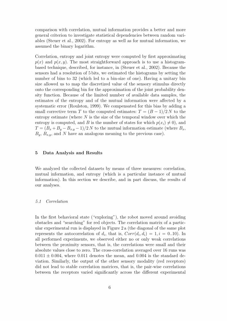
In the first behavioral state (“exploring”), the robot moved around avoidingobstacles and “searching” for red objects. The correlation matrix of a partic-ular experimental run is displayed in Figure 2 a (the diagonal of the same plotrepresents the autocorrelation of di, that is, Corr(di, di) = 1, i = 0..10). Inall performed experiments, we observed either no or only weak correlationsbetween the proximity sensors, that is, the correlations were small and theirabsolute values close to zero. The cross-correlation averaged over 16 runs was0.011 ± 0.004, where 0.011 denotes the mean, and 0.004 is the standard de-viation. Similarly, the output of the other sensory modality (red receptors)did not lead to stable correlation matrices, that is, the pair-wise correlationsbetween the receptors varied significantly across the different experimental
6
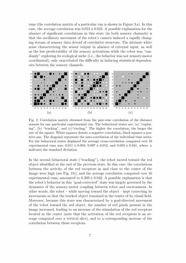
runs (the correlation matrix of a particular run is shown in Figure 3 a). In thiscase, the average correlation was 0.053± 0.023. A possible explanation for theabsence of significant correlations in this state (in both sensory channels) isthat the oscillatory movement of the robot’s camera induced a rapidly chang-ing stream of sensory data devoid of correlative structure. The intrinsic whitenoise characterizing the sensor output in absence of external input, as wellas the low predictability of the sensory activations while the robot was “ran-domly” exploring its ecological niche (i.e., the behavior was not sensory-motorcoordinated), only exacerbated the difficulty in inducing statistical dependen-cies between the sensory channels.
d0 d1 d2 d3 d4 d5 d6 d7 d8 d9 d10
d0
d1
d2
d3
d4
d5
d6
d7
d8
d9
d10
(a) d0 d1 d2 d3 d4 d5 d6 d7 d8 d9 d10
d0
d1
d2
d3
d4
d5
d6
d7
d8
d9
d10
(b) d0 d1 d2 d3 d4 d5 d6 d7 d8 d9 d10
d0
d1
d2
d3
d4
d5
d6
d7
d8
d9
d10
(c)
Fig. 2. Correlation matrix obtained from the pair-wise correlation of the distancesensors for one particular experimental run. The behavioral states are: (a) “explor-ing”, (b) “tracking”, and (c)“circling.” The higher the correlation, the larger thesize of the square. White squares denote a negative correlation, black squares a pos-itive one. The diagonal represents the auto-correlation of the individual time series.For the behavioral states displayed the average cross-correlation computed over 16experimental runs was: 0.011 ± 0.004, 0.097 ± 0.012, and 0.083 ± 0.041, where ±indicates the standard deviation.
In the second behavioral state (“tracking”), the robot moved toward the redobject identified at the end of the previous state. In this case, the correlationsbetween the activity of the red receptors in and close to the center of theimage were high (see Fig. 3 b), and the average correlation computed over 16experimental runs, amounted to 0.309± 0.042. A possible explanation is thatthe robot’s behavior in this “goal-corrected” state was largely governed by thedynamics of the sensory-motor coupling between robot and environment. Inother words, the robot – while moving toward the object – kept correcting itsmovements so that the tracked object remained in the center of its visual field.Moreover, because this state was characterized by a goal-directed movementof the robot toward the red object, the number of red pixels present in theimage increased, leading to an increase of the stimulation of the red receptorslocated in the center (note that the activation of the red receptors is an av-erage computed over a vertical slice), and to a corresponding increase of thecorrelation between those receptors.
7
2 4 6 8 10 12 14 16 18 20 22 24
2
4
6
8
10
12
14
16
18
20
22
24
(a) 2 4 6 8 10 12 14 16 18 20 22 24
2
4
6
8
10
12
14
16
18
20
22
24
(b)2 4 6 8 10 12 14 16 18 20 22 24
2
4
6
8
10
12
14
16
18
20
22
24
(c)
Fig. 3. Correlation matrix obtained from the pair-wise correlation of the red chan-nels for one particular experimental run. The behavioral states are: (a) “exploring”,(b) “tracking”, and (c) “circling.” The higher the correlation, the larger the sizeof the square. White squares denote a negative correlation, black squares a posi-tive one. The diagonal represents the auto-correlation of the individual time series.For the behavioral states displayed the average cross-correlation computed over 16experimental runs was: 0.053 ± 0.023, 0.309 ± 0.042, and 0.166 ± 0.031, where ±indicates the standard deviation.
In the third behavioral state (“circling”), we observed negative correlationsbetween the pairs of proximity sensors located on the ipsi-lateral (that is,same) side of the robot, such as (d2, d9) or (d3, d10). The correlation matrixshown in Figure 2 c, for instance, displays such a negative correlation for thesensor pair (d2, d9) (the correlation is −0.671). The negative correlation findsexplanation in the fact that the robot’s trajectory was not perfectly circular,but somewhat wobbly, thus leading to out-of-phase activation of the sensorsin the front (d9) and in the one in the back (d2), and hence to a negativecorrelation. In this state, we also observed – in all performed experimentalruns – strong correlations between the output of two groups of red receptorslocated off-center (see Figure 3 c). In that particular experimental run, thecorrelation was 0.920 for the receptors i4− i12 (a very high value indeed). Theoverall average (computed over 16 experimental runs) was 0.166± 0.031. Theevident asymmetry of the correlation matrix is a consequence of the limitationsof the camera’s pan-angle (±60o), which caused the object to appear on theside and not in the center of the visual field.
5.2 Entropy and mutual information
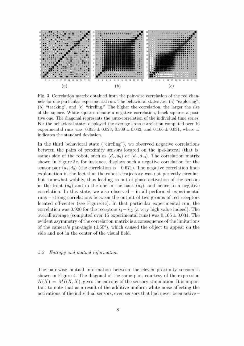
The pair-wise mutual information between the eleven proximity sensors isshown in Figure 4. The diagonal of the same plot, courtesy of the expressionH(X) = MI(X, X), gives the entropy of the sensory stimulation. It is impor-tant to note that as a result of the additive uniform white noise affecting theactivations of the individual sensors, even sensors that had never been active –
8
due to some object – were characterized by a large entropy (refer also to graphof cumulated activation in Fig. 6). A first observation is that in the first and
d0 d1 d2 d3 d4 d5 d6 d7 d8 d9 d10
d0
d1
d2
d3
d4
d5
d6
d7
d8
d9
d10
(a)d0 d1 d2 d3 d4 d5 d6 d7 d8 d9 d10
d0
d1
d2
d3
d4
d5
d6
d7
d8
d9
d10
(b)d0 d1 d2 d3 d4 d5 d6 d7 d8 d9 d10
d0
d1
d2
d3
d4
d5
d6
d7
d8
d9
d10
(c)
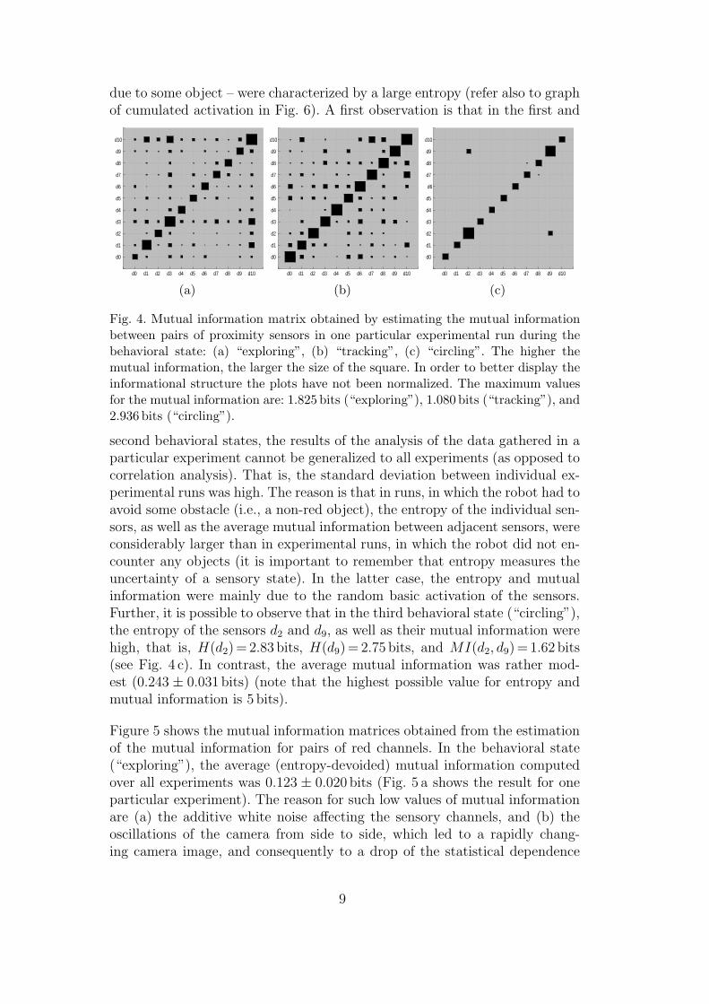
Fig. 4. Mutual information matrix obtained by estimating the mutual informationbetween pairs of proximity sensors in one particular experimental run during thebehavioral state: (a) “exploring”, (b) “tracking”, (c) “circling”. The higher themutual information, the larger the size of the square. In order to better display theinformational structure the plots have not been normalized. The maximum valuesfor the mutual information are: 1.825 bits (“exploring”), 1.080 bits (“tracking”), and2.936 bits (“circling”).
second behavioral states, the results of the analysis of the data gathered in aparticular experiment cannot be generalized to all experiments (as opposed tocorrelation analysis). That is, the standard deviation between individual ex-perimental runs was high. The reason is that in runs, in which the robot had toavoid some obstacle (i.e., a non-red object), the entropy of the individual sen-sors, as well as the average mutual information between adjacent sensors, wereconsiderably larger than in experimental runs, in which the robot did not en-counter any objects (it is important to remember that entropy measures theuncertainty of a sensory state). In the latter case, the entropy and mutualinformation were mainly due to the random basic activation of the sensors.Further, it is possible to observe that in the third behavioral state (“circling”),the entropy of the sensors d2 and d9, as well as their mutual information werehigh, that is, H(d2)= 2.83 bits, H(d9)= 2.75 bits, and MI(d2, d9)= 1.62 bits(see Fig. 4 c). In contrast, the average mutual information was rather mod-est (0.243 ± 0.031 bits) (note that the highest possible value for entropy andmutual information is 5 bits).
Figure 5 shows the mutual information matrices obtained from the estimationof the mutual information for pairs of red channels. In the behavioral state(“exploring”), the average (entropy-devoided) mutual information computedover all experiments was 0.123 ± 0.020 bits (Fig. 5 a shows the result for oneparticular experiment). The reason for such low values of mutual informationare (a) the additive white noise affecting the sensory channels, and (b) theoscillations of the camera from side to side, which led to a rapidly chang-ing camera image, and consequently to a drop of the statistical dependence
9
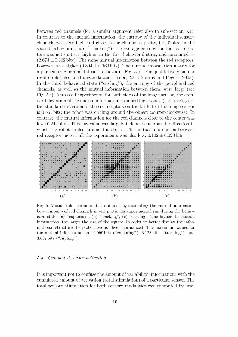
between red channels (for a similar argument refer also to sub-section 5.1).In contrast to the mutual information, the entropy of the individual sensorychannels was very high and close to the channel capacity, i.e., 5 bits. In thesecond behavioral state (“tracking”), the average entropy for the red recep-tors was not quite as high as in the first behavioral state, and amounted to(2.674± 0.362 bits). The same mutual information between the red receptors,however, was higher (0.804 ± 0.160 bits). The mutual information matrix fora particular experimental run is shown in Fig. 5 b). For qualitatively similarresults refer also to (Lungarella and Pfeifer, 2001; Sporns and Pegors, 2003).In the third behavioral state (“circling”), the entropy of the peripheral redchannels, as well as the mutual information between them, were large (seeFig. 5 c). Across all experiments, for both sides of the image sensor, the stan-dard deviation of the mutual information assumed high values (e.g., in Fig. 5 c,the standard deviation of the six receptors on the far left of the image sensoris 0.561 bits; the robot was circling around the object counter-clockwise). Incontrast, the mutual information for the red channels close to the center waslow (0.244 bits). This low value was largely independent from the direction inwhich the robot circled around the object. The mutual information betweenred receptors across all the experiments was also low: 0.102± 0.020 bits.
2 4 6 8 10 12 14 16 18 20 22 24
2
4
6
8
10
12
14
16
18
20
22
24
(a)2 4 6 8 10 12 14 16 18 20 22 24
2
4
6
8
10
12
14
16
18
20
22
24
(b) 2 4 6 8 10 12 14 16 18 20 22 24
2
4
6
8
10
12
14
16
18
20
22
24
(c)
Fig. 5. Mutual information matrix obtained by estimating the mutual informationbetween pairs of red channels in one particular experimental run during the behav-ioral state: (a) “exploring”, (b) “tracking”, (c) “circling”. The higher the mutualinformation, the larger the size of the square. In order to better display the infor-mational structure the plots have not been normalized. The maximum values forthe mutual information are: 0.999 bits (“exploring”), 3.128 bits (“tracking”), and3.637 bits (“circling”).
5.3 Cumulated sensor activation
It is important not to confuse the amount of variability (information) with thecumulated amount of activation (total stimulation) of a particular sensor. Thetotal sensory stimulation for both sensory modalities was computed by inte-
10
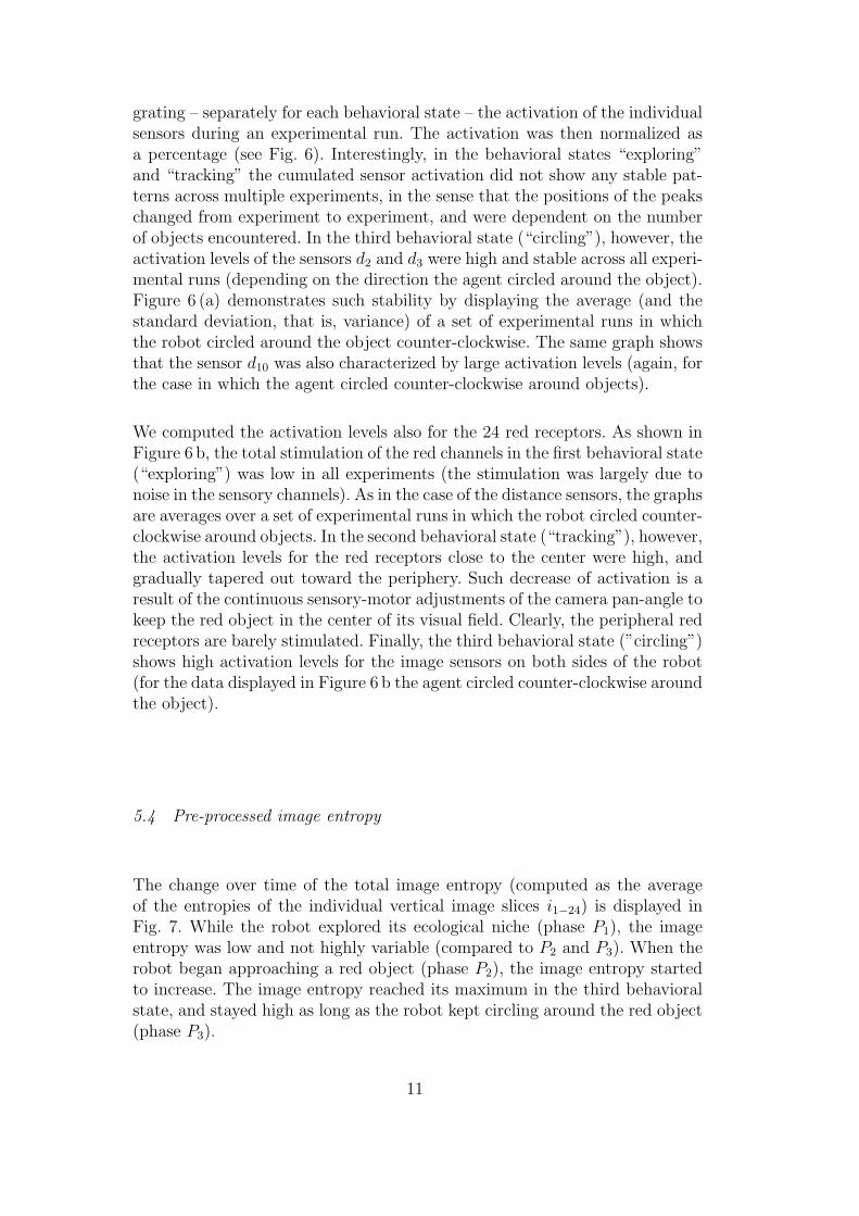
grating – separately for each behavioral state – the activation of the individualsensors during an experimental run. The activation was then normalized asa percentage (see Fig. 6). Interestingly, in the behavioral states “exploring”and “tracking” the cumulated sensor activation did not show any stable pat-terns across multiple experiments, in the sense that the positions of the peakschanged from experiment to experiment, and were dependent on the numberof objects encountered. In the third behavioral state (“circling”), however, theactivation levels of the sensors d2 and d3 were high and stable across all experi-mental runs (depending on the direction the agent circled around the object).Figure 6 (a) demonstrates such stability by displaying the average (and thestandard deviation, that is, variance) of a set of experimental runs in whichthe robot circled around the object counter-clockwise. The same graph showsthat the sensor d10 was also characterized by large activation levels (again, forthe case in which the agent circled counter-clockwise around objects).
We computed the activation levels also for the 24 red receptors. As shown inFigure 6 b, the total stimulation of the red channels in the first behavioral state(“exploring”) was low in all experiments (the stimulation was largely due tonoise in the sensory channels). As in the case of the distance sensors, the graphsare averages over a set of experimental runs in which the robot circled counter-clockwise around objects. In the second behavioral state (“tracking”), however,the activation levels for the red receptors close to the center were high, andgradually tapered out toward the periphery. Such decrease of activation is aresult of the continuous sensory-motor adjustments of the camera pan-angle tokeep the red object in the center of its visual field. Clearly, the peripheral redreceptors are barely stimulated. Finally, the third behavioral state (”circling”)shows high activation levels for the image sensors on both sides of the robot(for the data displayed in Figure 6 b the agent circled counter-clockwise aroundthe object).
5.4 Pre-processed image entropy
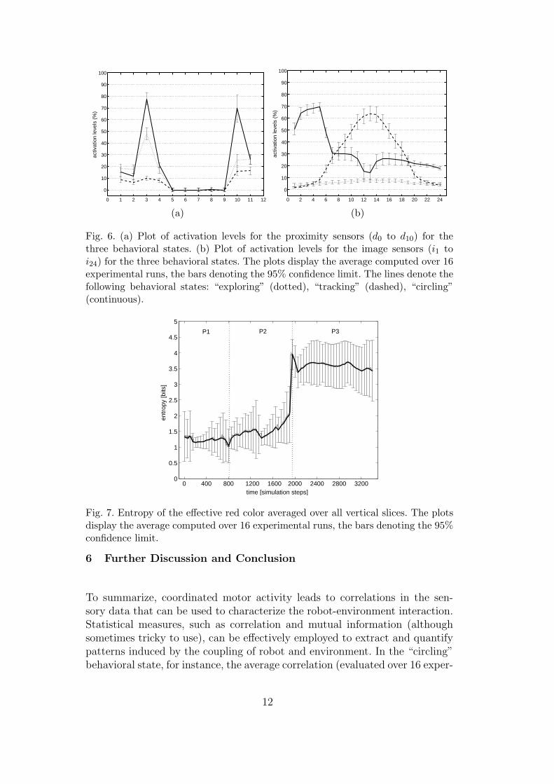
The change over time of the total image entropy (computed as the averageof the entropies of the individual vertical image slices i1−24) is displayed inFig. 7. While the robot explored its ecological niche (phase P1), the imageentropy was low and not highly variable (compared to P2 and P3). When therobot began approaching a red object (phase P2), the image entropy startedto increase. The image entropy reached its maximum in the third behavioralstate, and stayed high as long as the robot kept circling around the red object(phase P3).
11
0 1 2 3 4 5 6 7 8 9 10 11 12
0
10
20
30
40
50
60
70
80
90
100
activ
atio
n le
vels
(%
)
(a)0 2 4 6 8 10 12 14 16 18 20 22 24
0
10
20
30
40
50
60
70
80
90
100
activ
atio
n le
vels
(%
)
(b)
Fig. 6. (a) Plot of activation levels for the proximity sensors (d0 to d10) for thethree behavioral states. (b) Plot of activation levels for the image sensors (i1 toi24) for the three behavioral states. The plots display the average computed over 16experimental runs, the bars denoting the 95% confidence limit. The lines denote thefollowing behavioral states: “exploring” (dotted), “tracking” (dashed), “circling”(continuous).
0 400 800 1200 1600 2000 2400 2800 32000
0.5
1
1.5
2
2.5
3
3.5
4
4.5
5
time [simulation steps]
entr
opy
[bits
]
P2 P1 P3
Fig. 7. Entropy of the effective red color averaged over all vertical slices. The plotsdisplay the average computed over 16 experimental runs, the bars denoting the 95%confidence limit.
6 Further Discussion and Conclusion
To summarize, coordinated motor activity leads to correlations in the sen-sory data that can be used to characterize the robot-environment interaction.Statistical measures, such as correlation and mutual information (althoughsometimes tricky to use), can be effectively employed to extract and quantifypatterns induced by the coupling of robot and environment. In the “circling”behavioral state, for instance, the average correlation (evaluated over 16 exper-
12
imental runs) normalized by the number of distance sensors or red receptorswas 0.083 ± 0.041 for the distance sensors and 0.166 ± 0.031 for the imagesensors. The “tracking” behavioral state displayed an even higher stability,and the average correlation was 0.097 ± 0.012 (for the distance sensors) and0.309 ± 0.042 (for the image sensors). Mean and standard deviation clearlyshow that correlation analysis leads to stable sensory patterns across multipleexperimental runs, and thus define quantitative measures for behavioral finger-prints. A similar results holds for mutual information. It is important to notethat such stability is the direct consequence of a sensory-motor coordinatedinteraction. And indeed, for the case in which the agent tracked the object(in this case the agent’s sensory-motor coupling with the environment wasstrong) the fingerprints displayed least variance. A possible conclusion is thatthe particular combination of (a) morphological setup (that is, two wheels, 24image sensors, and 11 distance sensors) and (b) control architecture is wellsuited for tracking objects.
Our analyses also show that although correlation and mutual informationprovide appropriate statistical measures for fingerprinting interaction, theydiffer in at least one important aspect. Correlation can be used to identifyfingerprints of robot-environment interaction only if the sensory activationsbetween different sensors are temporally contiguous (that is, temporally closerelative to the time scale of the agent’s control structure). We hypothesizethat such temporal contiguity in the raw (that is, unprocessed) sensory datacan be induced by coordinated motor activity. It may indeed be the case thatsensory-motor coordination provides a very natural mechanism to achieve amatching of the various time scales affecting an agent’s behavior: environment,neural, and body-related.
A further result (that will be elaborated in future work) is that even if thesensory channels are affected by additive white noise, adequate sensory-motorcoordination interaction can indeed induce stable fingerprints. In this sense,it is possible to put forward the hypothesis that sensory-motor coordinatedinteraction can act as some sort of “behavioral denoising filter.”
7 Acknowledgments
Max Lungarella would like to thank the University of Tokyo, and a SpecialCoordination Fund for Promoting Science and Technology from the Ministryof Education, Culture, Sports, Science, and Technology of the Japanese gov-ernment. For Gabriel Gomez funding has been provided by grant number NF-10-101827/1 of the Swiss National Science Foundation and the EU-ProjectADAPT (IST-2001-37173).
13
References
Ballard, D., 1991. Animate vision. Artificial Intelligence 48 (1), 57–86.Cover, T., Thomas, J., 1991. Elements of Information Theory. New York: John
Wiley.Gibson, E., 1988. Exploratory behavior in the development of perceiving, act-
ing, and the acquiring of knowledge. Annual Review of Psychology 39, 1–41.Lederman, S. J., Klatzky, R. L., 1990. Haptic exploration and object represen-
tation. In: Goodale, M. (Ed.), Vision and Action: The Control of Grasping.New Jersey: Ablex, pp. 98–109.
Lee, T. S., Yu, S. X., 1999. An information-theoretic framework for under-standing saccadic behaviors. In: Proc. of the First Intl. Conf. on NeuralInformation Processing. Cambridge, MA: MIT Press.
Lungarella, M., Pfeifer, R., 2001. Robots as cognitive tools: Information-theoretic analysis of sensory-motor data. In: Proc. of the 2nd Int. IEEE/RSJConf. on Humanoid Robotics. pp. 245–252.
Lungarella, M., Sporns, O., 2004. Methods for quantifying the informationalstructure of sensory and motor data. Neuroinformatics In preparation.
Nolfi, S., 2002. Power and limit of reactive agents. Neurocomputing 49, 119–145.
Pfeifer, R., Scheier, C., 1997. Sensory-motor coordination: The metaphor andbeyond. Robotics and Autonomous Systems 20, 157–178.
Pfeifer, R., Scheier, C., 1999. Understanding Intelligence. Cambridge, MA:MIT Press.
Roulston, M., 1999. Estimating the errors on measured entropy and mutualinformation. Physica D 125, 285–294.
Scheier, C., Pfeifer, R., 1997. Information theoretic implications of embodi-ment for neural network learning. In: ICANN 97. pp. 691–696.
Shannon, C., 1948. A mathematical theory of communication. Bell SystemTech. Journal 27.
Sporns, O., Pegors, J., 2003. Generating structure in sensory data through co-ordinated motor activity. In: Proc. of Intl. Joint Conf. on Neural Networks.p. 2796.
Steuer, R., Kurths, J., Daub, C., Weise, J., Selbig, J., 2002. The mutual in-formation: detecting and evaluating dependencies between variables. Bioin-formatics 18, 231–240, suppl.2.
Te Boekhorst, R., Lungarella, M., Pfeifer, R., 2003. Dimensionality reductionthrough sensory-motor coordination. In: Kaynak, O., Alpaydin, E., Oja, E.,Xu, L. (Eds.), Proc. of the Joint Inlt. Conf. ICANN/ICONIP. pp. 496–503,lNCS 2714.
Thelen, E., Smith, L., 1994. A Dynamic Systems Approach to the Developmentof Cognition and Action. Cambridge, MA: MIT Press. A Bradford Book.
Yarbus, A., 1967. Eye movements and vision. Plenum Press.
14


