Quantifying Corn Yield and Water Use Efficiency under Growth Stage–Based Deficit Irrigation Conditions

1

Copyright © 2014. ASA, CSSA, SSSA, 5585 Guilford Rd., Madison, WI 53711-5801, USA. Practical Applications of Agricultural System Models to Optimize the Use of Limited Water Lajpat R. Ahuja, Liwang Ma, and Robert J. Lascano, EditorsAdvances in Agricultural Systems Modeling, Volume 5. Lajpat R. Ahuja, Series Editor

Quantifying Corn Yield and Water Use Efficiency under Growth Stage–Based Deficit Irrigation ConditionsQuan X. Fang,* L. Ma, David C. Nielsen, Thomas J. Trout, and L.R. Ahuja

AbstractAn agricultural system model can help optimize limited irrigation for higher grain yield and water use efficiency (WUE) across varied climatic conditions. In this study, the Root Zone Water Quality Model (RZWQM2) was first cali-brated to simulate soil water, ET, and corn (Zea mays L.) yield under a range, 40 to 100% of crop ET under well-watered conditions (i.e., ETc, calculated by the reference ET and crop coefficient), of irrigation treatments from 2008 to 2011 in Colorado. The model was then used to explore grain yield responses to irrigation levels of 40, 60, 80, and 100% ETc (the Shuttleworth–Wallace ET, ETsw, was used as a surrogate for ETc in the model) under 300, 400, and 500 mm of total irrigation water and to provide guidelines to man-age limited irrigation using weather data from 1992 to 2013. With 500 mm of irrigation water, high grain yield and WUE were obtained from the 100% ETsw for the vegetative stage and 80 to 100% ETsw for the reproductive stage. With 400 mm of irrigation water, high grain yield and WUE were simulated at 80 to 100% ETsw irrigation targets between the vegetative and reproduc-tive stages. With 300 mm of irrigation water, however, meeting 100% ETsw at the reproductive and 60% ETsw at the vegetative stage achieved the high-est grain yield and WUE. Simulations showed that meeting the crop water requirement during the reproductive stage is more important than during the vegetative stage to achieve high grain yield and WUE under water-lim-ited conditions.

Abbreviations: CoAgMet, Colorado Agricultural Meteorological Network; CV, coefficient of variance; LAI, leaf area index; MD, mean difference; ME, model efficiency; RZWQM2, Root Zone Water Quality Model (version 2.6); UAN, urea–ammonium nitrate; WUE, water use efficiency.

Q.X. Fang, Agronomy College, Qingdao Agricultural University, Changcheng Road 700, Chengyang District, Qingdao, Shandong, China, 266108. *Corresponding author ([email protected]).

L. Ma ([email protected]) and L.R. Ahuja ([email protected]), USDA-ARS-NPA-ASRU 2150 Centre Ave., Bldg. D, STE. 200 Fort Collins, CO 80526.

D.C. Nielsen, USDA-ARS, Central Plains Resources Management Research, 40335 County Rd GG, Akron, CO 80720-0400 ([email protected]).

T.J. Trout, USDA-ARS Water Management Research Unit, 2150 Centre Avenue, Bldg D, Suite 320 Fort Collins, CO 80526 ([email protected]).

doi:10.2134/advagricsystmodel5.c1

Published December 5, 2014

mailto:[email protected]





10.2134/advagricsystmodel

USDA-ARS

3

Water is often the limiting factor for crop yield in semiarid areas or water-limited regions. Increasing WUE (crop yield/evapotranspira-

tion, kg m−3) is the key to mitigating water crises in these regions. Previous field results have shown high variability in WUE due to varied seasonal weather vari-ability, especially precipitation, for regions such as the U.S. Great Plains (Angus and van Herwaarden, 2001; Howell, 2001) and the North China Plain (Fang et al., 2010). Yearly variations in WUE have limited the extension of field experimental results to guide irrigation management. Recently, Saseendran et al. (2014) gener-alized average corn crop water production functions across years and locations and provided useful guidelines for managing limited water for higher corn pro-duction, but the yearly variation in WUE needs to be further investigated.

Besides weather variability, the intensity of water stress (the degree of meet-ing crop ET demand) and time (phenological stage) can influence WUE under deficit irrigation conditions (e.g., Lorite et al., 2007; Pereira et al., 2009). Field stud-ies have explored the response of WUE to various irrigation levels or water stress levels and provide useful options to improve WUE in different regions (e.g., Fer-eres and Soriano, 2007; Howell, 2001), but these results were limited because of weather variations. Improper irrigation amounts or times may produce severe water stress due to the uneven rainfall distribution and different sensitivities of corn to water stress at different growth stages (Shaw, 1977; Nielsen et al., 2010). Variable irrigation based on soil water deficiency or crop water requirement (such as crop ET) can be a more precise and suitable method for deficit irrigation. Geerts and Raes (2009) reviewed deficit irrigation methods (application of water below full crop water requirements) to maximize WUE in dry areas and found deficit irrigation can increase WUE for various crops without substantially reduc-ing crop yield, but effective use of deficit irrigation required precise knowledge of crop response to water stress at different phenological stages. Molden et al. (2010) also discussed the need for a better understanding of the biophysical and socioeconomic impacts for developing better deficit irrigation strategies. Using field experiments to explore optimal irrigation schedules is rather difficult, costly, and time-consuming because the response of WUE to water stress (or irrigation) becomes complex due to the effect of weather variations (such as rainfall) on both soil water deficits (timing and intensity) and crop yield.

Integrating soil, crop, and climate factors is required to quantify the response of WUE to water stress. System modeling can aid in the design of field

4 Fang et al.

experiments in quantifying crop responses under various climate and irriga-tion conditions. Stockle and James (1989) used the Cropping Systems Simulation Model (CROPSYST) to explore the effect of different irrigation strategies on corn yield and found that a slight water deficit produced greater grain yields than full irrigation, but severe deficits were detrimental to plant growth and grain yield. Various crop models or agricultural system models have been used to explore def-icit irrigation strategies for improving WUE across various climate conditions in different regions, such as the Agricultural Production Systems Simulator (APSIM) (Heng et al., 2007; Kloss et al., 2012), Crop Environment Resource Synthesis (CERES)-Wheat model housed in the Decision Support System for Agrotechnol-ogy Transfer (DSSAT) (Behera and Panda, 2009; Singh et al., 2008), CROPSYST (Singh et al., 2008), AquaCrop (Steduto et al., 2009), and RZWQM (Fang et al., 2010; Saseendran et al., 2008). These simulation results provided useful guidelines for deficit irrigation strategies under various weather conditions. However, most of these simulation studies used fixed irrigation amounts and timing and did not consider (i) the water availability for the crop season in a region, which may influence how to optimize the limited water for higher WUE, and (ii) the vari-able irrigation amounts or timing based on phenological growth stages, such as vegetative and reproductive stages. The objective of this study was to use the RZWQM2, calibrated for northeastern Colorado conditions, to simulate corn ET and grain yield under various growth stage–based irrigation schedules to meet a proportion of ET as calculated from the Shuttleworth–Wallace equation (ETsw) and under various seasonal water limitation.

MATERIALS AND METHODSField Experiment and Data MeasurementsThe field experiment was initiated in 2008 near Greeley, CO (40.45° N, 104.64° W). The soil is an alluvial sandy loam with coarser and finer textured layers in the 2-m soil profile. Weather data were recorded on site (station designation GLY04) with a standard Colorado Agricultural Meteorological Network (CoAgMet) (http://ccc.atmos.colostate.edu/~coagmet/) weather station. From 2008 to 2011, the grow-ing season precipitation was 245, 237, 211, and 237 mm, respectively. A detailed description of the experiment can be found in Trout et al. (2010), Ma et al. (2012), and Saseendran et al. (2014).

Six irrigation treatments (area in 9 by 44 m, and microirrigation with surface drip tubing adjacent to each row) replicated four times (randomized complete block) were designed to meet a certain percentage of ETc of a nonstressed, well-watered crop during the growing seasons calculated on the basis of the reference

http://ccc.atmos.colostate.edu

http://ccc.atmos.colostate.edu

Quantifying Corn Yield and Water Use Efficiency 5

ET (ETr) for a tall crop [alfalfa (Medicago sativa L.)] and crop coefficient (Allen et al., 1998, 2005, 2007). The treatments were 100% (T1), 85% (T2), 70% (T3), 70% (T4), 55% (T5), and 40% (T6) of ETc. For all treatments except for T1 and T3, about 20% of the estimated target irrigation amounts during the vegetative growth period were saved and added during the reproductive stage. Corn (‘Dekalb 52–59’) was planted at an average rate of 81,000 seed ha−1 with 0.8-m row spacing on 12 May 2008, 11 May 2009, 11 May 2010, and 2 May 2011 and harvested on 6 Nov. 2008, 12 Nov. 2009, 19 Oct. 2010, and 22 Oct. 2011. Fertilizer as urea–ammonium nitrate (UAN) was applied uniformly to all treatments at planting and then with irriga-tion water during the growing seasons as needed on the basis of estimated plant requirements for the 100% ETc treatment. Total N applied was 134 kg N ha−1 in 2008, 160 kg N ha−1 in 2009, 146 kg N ha−1 in 2010, and 146 kg N ha−1 in 2011.

Leaf area index (LAI) was estimated from canopy ground cover (Fc) mea-sured with a nadir view digital camera according to Farahani and DeCoursey (2000). Soil water content was measured twice a week during the growing sea-son with a portable time domain reflectometry water meter for the surface 0- to 0.15-m soil layer and with a neutron attenuation water meter between 0.15 and 2 m below the soil surface at 0.3-m intervals. Actual ET was estimated from the soil water balance (ET = irrigation + rainfall + profile soil water difference between measurement times). Soil water drainage below the soil profile and water runoff were assumed to be zero in the water balance calculation of actual ET, but some water drainage below the soil profile or runoff may have occurred because of high rain events such as during an 86-mm rainfall occurring on 15 and 16 August 2008. Additional measurement information can be found in Ma et al. (2012).

Description and Parameterization of the Root Zone Water Quality ModelThe RZWQM2 (version 2.6) with the DSSAT 4.0 crop modules were used in this study (Ma et al., 2006). On the basis of Ma et al. (2012), we used soil water content at 333 kPa (q1/3) and 15,000 kPa (q15) to estimate Brooks–Corey parameters (Brooks and Corey, 1964), where q15 was assumed equal to one-half of q1/3 (Ma et al., 2012).

The equations relating volumetric soil water content (q, m3 m−3) and matric suction head (y, where y > 0 for negative soil water pressures) in Brooks and Corey (1964) are:

s b

rb

s r b

for

for-

q =q y<y

æ öq-q y ÷ç ÷ç= y³y÷ç ÷÷çq -q yè ø

l , [1]

where qs and qr are saturated and residual soil water contents, yb is the air entry water suction (negative “bubbling pressure”), and l is the slope of the log(q)-log(y)

6 Fang et al.

curve or the “pore-size distribution index.” Similarly, assuming the log-log slope of the water retention curve is linearly related to the log-log slope of the unsaturated conductivity curve, the hydraulic conductivity K versus suction head is

( )s b

s bb

( ) for2 3

( ) for

K K

K K-

y = y<y+ læ öy ÷ç ÷çy = y³y÷ç ÷÷çyè ø

, [2]

where Ks is the saturated hydraulic conductivity in cm h−1.The Brooks–Corey parameters can be calculated from q1/3 and q15 (Ma et al.,

2012):

( ) ( )( )

1/3 r 15 rln

ln 15,000 333

é ùq -q q -qê úë ûl = . [3]

( ) ( ) ( )1/3 r s rb

ln ln ln 333exp

é ùq -q - q -q +lê úy = ê úlê úë û . [4]

The Ks was estimated using an empirical relationship with effective porosity based on the formula by Ahuja et al. (1989):

( )3.288s s 1/3764.5K = q -q . [5]

Data from 2008 to 2010 were previously used to calibrate the model via trial and error method (Ma et al., 2012; Saseendran et al., 2014), where the highest irriga-tion treatment (100% ETc) was used for calibration and the remaining treatments were used for validation. In this study, we used the measured data from all six treatments from 2008 to 2011 to calibrate the model using PEST, an automatic opti-mization parameter estimation software (Doherty, 2010). The model was run from 1 January to 31 December every year for all the treatments with the actual irrigation amount implemented. The RMSE from each treatment and year were combined to define an objective function for parameter optimization (Nolan et al., 2011).

To cope with the sensitivity of PEST to initial values and ranges of the model parameters (Doherty, 2010), we used initial parameter values from a previous study at this site (Ma et al., 2012). The ranges for these parameters were obtained from either field experiment measurements (Table 1–1) or from the calibrated database released in the DSSAT model (Table 1–2) (Ma et al., 2012). The measured data of soil water content, LAI, and final aboveground biomass and grain yield from 2008 to 2011 were used to parameterize the RZWQM2 with PEST. The cali-brated soil and crop genetic parameters along with their ranges are presented in Table 1–1 and Table 1–2. Model performance was quantified with statistical mea-


sures of RMSE, mean difference (MD), coefficient of determination (r2), and the Nash Sutcliffe model efficiency (ME; Nash and Sutcliffe, 1970).

Long-Term Simulations for Deficit Irrigation ManagementAfter calibrating the model for all the treatments and years with actual irrigation amounts as scheduled in the field, the RZWQM2 was used for long-term simu-lations (1992–2013) of corn under various irrigation management scenarios. To simulate crop ET (ETc) in the model to schedule irrigation, we would need a crop

Table 1–1. Initial ranges and final soil water content at 333 kPa (q1/3) and the final bulk density (rb), saturated water content (qs), air entry water suction (yb), and pore size distribution index (l) used for calibrating the Root Zone Water Quality Model (version 2.6) with the parameter estimation software PEST (Doherty, 2010).†

Soil depth rb Initial q1/3 Min. q1/3 Max. q1/3 Final q1/3 Final qs Final l Final yb

m 103 kg m−3 ––––––––––––––––––– m3 m−3 ––––––––––––––––––– cm0.00–0.15 1.492 0.262 0.18 0.32 0.231 0.44 0.23 15.340.15–0.30 1.492 0.249 0.14 0.32 0.242 0.44 0.23 18.730.30–0.60 1.492 0.220 0.13 0.38 0.230 0.44 0.23 15.060.60–0.90 1.568 0.187 0.13 0.37 0.206 0.41 0.24 13.190.90–1.20 1.568 0.173 0.13 0.32 0.205 0.41 0.24 12.971.20–1.50 1.617 1.62 0.13 0.31 0.263 0.39 0.23 47.361.50–2.00 1.617 0.198 0.13 0.31 0.310 0.39 0.22 103.35

† The initial values were based on a previous study at the experimental site (Ma et al., 2012), and the ranges were based on the field measured minimum and maximum soil water content from 2008 to 2011.

Table 1–2. Initial ranges and final values for crop cultivar genetic parameters for calibrating the Root Zone Water Quality Model (version 2.6) with the parameter estimation software PEST (Doherty, 2010).

Crop cultivar genetic parameter Parameter description Initial Ranges Final

P1 degree days (base temperature of 8°C) from seedling emergence to end of juvenile phase (thermal degree days)

250 200–290 245.6

P2 day length sensitivity coefficient [the extent (days) that development is delayed for each hour increase in photoperiod above the longest photoperiod (12.5 h) at which development proceeds at maximum rate]

0.2 0.05–0.6 0.1562

P5 degree days (base temperature of 8°C) from silking to physiological maturity (thermal degree days)

600 550–670 704.4

G2 potential kernel number 900 800–1000 994.1G3 potential kernel growth rate (mg kernel−1 d−1) 6 3–10 6.239PHINT degree days required for a leaf tip to emerge

(phyllochron interval) (thermal degree days)50 45–55 52.89

8 Fang et al.

coefficient that is not estimated in the RZWQM2. However, the Shuttleworth–Wallace ET (ETsw) (Shuttleworth and Wallace, 1985) simulated in the RZWQM2 was intended to take care of crop effects (i.e., LAI) on ET and can be used as a surrogate for ETc in the model. Ma et al. (2012) showed that when the ETsw was used as the basis for irrigation to replace ETc, model simulated irrigation amounts matched actual irrigation amounts for all the irrigation levels. Therefore, we used ETsw to replace ETc in the long-term simulation study.

Irrigation began 3 d after planting at a 20 mm h−1 rate and ended on or before 16 Sept. each year. Irrigation was scheduled every 3 d to target a certain percentage of ETsw (100, 80, 60, and 40%) calculated for the past 3 d, minus any precipitation, which was similar to the irrigation experiment. These irrigation targets, defined as 100%ETsw, 80%ETsw, 60%ETsw, and 40%ETsw, were implemented separately dur-ing the vegetative (before tasseling) and reproductive (after tasseling) stages. On the basis of the experimental data, we assumed the reproductive stage started 77 d after planting (28 July). All combinations of these ETsw–based irrigation targets resulted in 16 irrigation scenarios (e.g., 100%–40%ETsw denotes an irrigation level of 100%ETsw at the vegetative stage and 40%ETsw at the reproductive stage). N was applied at 150 kg N ha−1 as UAN at planting. Corn was planted on 12 May and harvested at harvest maturity as determined by the model, which was generally between late September and late October.

Each of these 16 scenarios was simulated with an unlimited seasonal irriga-tion condition and with a 300-, 400-, and 500-mm irrigation limit, for a total of 64 scenarios (i.e., 16 ´ 4). Seasonal water limitations such as these are imposed on farmers by river flows that decline as the summer progresses until flows drop below the level that allows diversions for irrigation. Model simulations for each of the 64 scenarios were run continuously for 22 yr from 1 Jan. 1992 to 17 Dec. 2013. Weather data for the simulations, including precipitation, were taken from nearby CoAgMet weather stations.

RESULTS AND DISCUSSION

Model Calibration

Soil Water and ET SimulationsAs shown in Table 1–3, a better soil water content simulation was obtained for the deeper soil layers with lower RMSE values for the 0.9- to 1.2-m soil layers than for the 0.3- to 0.6-m soil layers. For the deepest layer of 1.2 to 2.0 m, overestimations of soil water content occurred, with a high MD value of 0.016 m3 m−3. The overall MD and RMSE values for total soil water storage in the profile were 20 and 35 mm across the six treatments from 2008 to 2011 (Table 1–3). The overestimated soil


water in the profile was mainly due to overestimating soil water content below 1.2-m depth, and the model only slightly overestimated soil water in the 0.0- to 1.2-m soil profiles with an MD of 5 mm and an RMSE of 20 mm. These results were comparable with the previous simulation study using data from 2008 to 2010 with an RMSE value of 32 mm for profile soil water (Ma et al., 2012).

Both RZWQM2-simulated and measured ETa showed similar decreases with deficit irrigation from T1 to T6 across the 4 yr (Fig. 1–1). Underestimation of ETa occurred in 2010 and 2011 and a closer agreement to measured ETa was obtained in 2008 and 2009. Across the 4 yr, the MD, RMSE, ME, and r2 values for simulated ETa were −41 mm, 57 mm, 0.61, and 0.81, respectively (Table 1–4). Both simulated and measured ETa decreased slightly from T3 to T4 in 2009 and 2011 (Fig. 1–1).

Table 1–3. Statistical results for simulated soil water content (q) at the different depths and soil water storage in a 0- to 2-m layer across the six deficit irrigation treatments from 2008 to 2011.†

Soil depthMeasured qaverage

Simulated q average MD RMSE ME r 2

m –––––––––––––––––––– m3 m−3 ––––––––––––––––––––

0.00–0.15 0.169 0.181 0.013 0.053 0.04 0.460.15–0.30 0.177 0.181 0.005 0.040 −0.05 0.580.30–0.60 0.163 0.160 −0.003 0.037 −0.44 0.550.60–0.90 0.147 0.154 0.007 0.023 0.05 0.620.90–1.20 0.150 0.153 0.003 0.020 0.25 0.531.20–1.50 0.156 0.180 0.024 0.035 −0.19 0.661.50–2.00 0.184 0.201 0.016 0.032 −0.40 0.300.00–2.00 (SWS)‡ 321.6 342.0 20 35 0.41 0.81

† MD, mean deviation; ME, model efficiency; r2, coefficient of determination.‡ SWS, soil water storage (mm).

Fig. 1–1. Comparisons between measured and simulated seasonal crop actual evapotranspiration (ETa) across six irrigation treatments [T1 (100%ETc), T2 (85%ETc), T3 (70%ETc without moving 20% of vegetative stage irrigation to the reproductive stage), T4 (70%ETc), T5 (55%ETc), and T6 (40% ETc), where ETc is crop ET for a well-watered crop calculated from reference ET and crop coefficient] from 2008 to 2011.

10 Fang et al.

Leaf Area Index, Crop Yield, and Water Use Efficiency SimulationsThe model-calculated LAI agreed well with the measured data with mean values of 2.2 m2 m−2 and 2.1 m2 m−2 across the 4 yr. The corresponding RMSE, ME, and r2 values are 0.9 m2 m−2, 0.7, and 0.70, respectively. Both measured and simulated grain yield decreased with the deficit irrigation treatments from T1 to T6 across the 4 yr (Fig. 1–2a), with good agreement between measured and simulated (MD

= 86 kg ha−1, RMSE = 354 kg ha−1, and ME = 0.97, Table 1–4). In 2008, grain yield was overestimated for treatment T4. From 2009 to 2011, both measured and calculated grain yields showed similar trends between T3 and T4, which suggested that the model was able to simulate the differences in grain yield due to differential irri-gation scheduling between vegetative and reproductive growth stages. Similar simulation results were obtained for biomass across the 4 yr with MD, RMSE, and ME values of −160 kg ha−1, 1203 kg ha−1, and 0.90, respectively (Table 1–4). These simulation results for LAI, grain yield, and biomass were generally better than

Table 1–4. Statistical results for simulated seasonal ET, leaf area index, final grain yield, aboveground biomass, and water use efficiency for the six irrigation treatments from 2008 to 2011.†

Variables‡Measuredaverage

Simulatedaverage MD RMSE ME r 2

ET (mm) 585.4 544.3 −41.1 56.5 0.61 0.81GY (kg ha−1) 8491 8577 86 354 0.97 0.98LAI (m2 m−2) 2.09 2.15 0.06 0.77 0.69 0.70AGB (kg ha−1) 17102 16941 −160 1203 0.90 0.90WUE (kg m−3) 1.44 1.55 0.11 0.16 0.67 0.89

† MD, mean deviation; ME, model efficiency; r2, coefficient of determination.‡ GY, final grain yield; LAI, leaf area index; AGB, aboveground biomass; WUE, water use efficiency.

Fig. 1–2. Comparisons between measured and simulated grain yield and water use efficiency (WUE) for six irrigation treatments [T1 (100%ETc), T2 (85%ETc), T3 (70%ETc without moving 20% of vegetative stage irrigation to the reproductive stage), T4 (70%ETc), T5 (55%ETc), and T6 (40% ETc), where ETc is crop ET for a well-watered crop calculated from reference ET and crop coefficient] from 2008 to 2011.


those obtained by Ma et al. (2012), who calibrated the RZWQM2 via a trial and error method using data from 2008 to 2010.

The simulated WUE also showed similar trends with measured data across these treatments from 2008 to 2011 (Fig. 1–2b), but overcalculation of WUE was obtained mainly because of the under-simulated ET (Fig. 1–1). In 2008, similar to grain yield, the model oversimulated WUE for treatment T4. The MD, RMSE, ME, and r2 values for the simulated WUE were 0.11 kg m−3, 0.16 kg m−3, 0.67, and 0.89 across all the 4 yr, which were also better than a previous simulation study in North China Plain using the model (Fang et al., 2010).

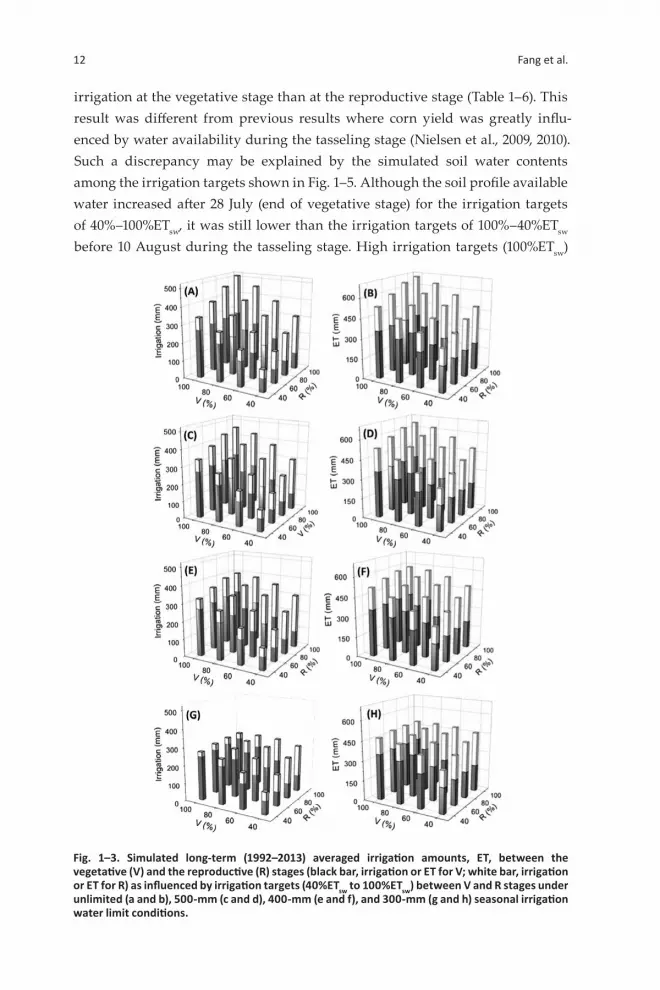
Long-Term Simulation of Crop Water Use and ProductionUnlimited Irrigation Water AvailableWith the unlimited irrigation water available condition, the average irrigation amounts increased from 73 to 285 mm during the vegetative stage and from 50 to 224 mm during the reproductive stage (Fig. 1–3a), with the irrigation targets varying from 40%ETsw to 100%ETsw. Correspondingly, the average ET increased from 195 to 362 mm during the vegetative stage and from 122 to 316 mm during the reproductive stage (Fig. 1–3b). Greater irrigation amounts were required dur-ing the vegetative stage than during the reproductive stage in part because of the slightly longer vegetative growing season (Fig. 1–3a). The simulated average sea-sonal irrigation amount increased from 123 to 509 mm (Table 1–5) as irrigation targets varying from 40%ETsw to 100%ETsw. The yearly variations in the irrigation amount due to weather variations (SD across seasons) ranged from 61 to 97 mm, which were much lower than the range of irrigation amounts for these irrigation scenarios (Table 1–5).

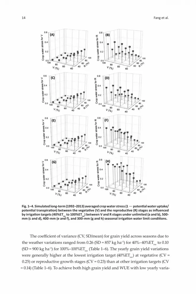
Average crop water stress, which is defined as [1 - (potential water uptake/potential transpiration)] (Ma et al., 2006), decreased with increased irrigation tar-gets at both the vegetative and reproductive stages and was generally lower for the vegetative stage than for the reproductive stage at the same irrigation tar-gets (Fig. 1–4a vs. Fig. 1–4b). The simulated lower water stress at the vegetative stage than at the reproductive stage under the lowest irrigation target (40%ETsw) indicated severe water deficits during the reproductive stage. Conversely, at the lower irrigation targets for the reproductive stage (e.g., 40%ETsw or 60%ETsw), lower water stress occurred at the highest irrigation target (100%ETsw) at the veg-etative stage (e.g., 80%ETsw) (Fig. 1–4b), which indicated that maintaining higher irrigation targets during the vegetative stage can increase soil water supply and alleviate plant water stress at the reproductive stage.

Grain yield increased with irrigation targets at both vegetative and repro-ductive growth stages, but the response was more pronounced by increasing

12 Fang et al.

irrigation at the vegetative stage than at the reproductive stage (Table 1–6). This result was different from previous results where corn yield was greatly influ-enced by water availability during the tasseling stage (Nielsen et al., 2009, 2010). Such a discrepancy may be explained by the simulated soil water contents among the irrigation targets shown in Fig. 1–5. Although the soil profile available water increased after 28 July (end of vegetative stage) for the irrigation targets of 40%‒100%ETsw, it was still lower than the irrigation targets of 100%‒40%ETsw before 10 August during the tasseling stage. High irrigation targets (100%ETsw)

Fig. 1–3. Simulated long-term (1992–2013) averaged irrigation amounts, ET, between the vegetative (V) and the reproductive (R) stages (black bar, irrigation or ET for V; white bar, irrigation or ET for R) as influenced by irrigation targets (40%ETsw to 100%ETsw) between V and R stages under unlimited (a and b), 500-mm (c and d), 400-mm (e and f), and 300-mm (g and h) seasonal irrigation water limit conditions.


during the vegetative stage resulted in high soil profile available water during the early reproductive stage (tasseling stage) and benefited the final grain yield (Table 1–6).

Grain yield generally maximized at irrigation targets >80%ETsw for both vegetative and reproductive stages, but showed a reduced response to irrigation targets from 80%ETsw to 100%ETsw (Table 1–6). However, simulated average grain yield with the highest irrigation target of 100%–100%ETsw (Table 1–6) was slightly lower than measured grain yield from T1 (Fig. 1–2), which was partly caused by the simulated crop N stress under the highest irrigation target (100%–100%ETsw) where 150 kg N ha−1 was applied at planting as compared with fertigation in the T1 treatment. The weather variations from 1992 to 2013 also contributed to the differences between measured and long-term simulated corn yield. The WUE also increased with the increase in irrigation targets, but showed less response to irrigation than grain yield (Table 1–7). No significant (P > 0.01) difference in simulated WUE was found for irrigation levels of 80%–100%ETsw, 100%–80%ETsw, and 100%–100%ETsw (Table 1–7), but significantly (P < 0.01) higher grain yield was obtained for the 100%–100%ETsw (Table 1–6).

Table 1–5. Long-term (1992–2013) simulated average irrigation amounts and standard deviations across seasons for different irrigation targets (40% to 100% of ETsw), between vegetative and reproductive growth stages under various irrigation water availability conditions.†

Water limitTargets for reproductive stage

Targets for vegetative stage

40%ETsw 60%ETsw 80%ETsw 100%ETsw

–––––––––––––––––––––––– mm ––––––––––––––––––––––––Unlimitedwater

40%ETsw 123 ± 61 204 ± 71 277 ± 80 338 ± 9360%ETsw 180 ± 65 263 ± 75 337 ± 83 399 ± 9280%ETsw 243 ± 72 323 ± 80 395 ± 88 463 ± 96100% ETsw 307 ± 76 380 ± 89 452 ± 92 509 ± 97

500-mmseasonalwater limit

40%ETsw 123 ± 61 204 ± 71 277 ± 80 338 ± 9360%ETsw 180 ± 65 263 ± 75 337 ± 83 394 ± 8680%ETsw 243 ± 72 323 ± 80 392 ± 84 438 ± 66100%ETsw 307 ± 76 379 ± 86 435 ± 71 466 ± 49


40%ETsw 123 ± 61 204 ± 71 276 ± 79 324 ± 7860% ETsw 180 ± 65 263 ± 75 328 ± 7.1 35.8 ± 5.180%ETsw 243 ± 72 318 ± 73 359 ± 50 387 ± 29100%ETsw 304 ± 73 353 ± 60 383 ± 35 395 ± 19


40%ETsw 123 ± 61 203 ± 69 253 ± 54 274 ± 3760%ETsw 180 ± 65 247 ± 58 282 ± 34 294 ± 1680%ETsw 236 ± 63 277 ± 36 295 ± 16 300 ± 01100%ETsw 271 ± 42 292 ± 21 299 ± 06 300 ± 00

† Numbers in bold are the most reasonable irrigation targets with the highest grain yield and water use efficiency and the lowest yearly variations for each water limit condition. ETsw, Shuttleworth–Wallace calculated ET.

14 Fang et al.

The coefficient of variance (CV, SD/mean) for grain yield across seasons due to the weather variations ranged from 0.26 (SD = 857 kg ha−1) for 40%–40%ETsw to 0.10 (SD = 900 kg ha−1) for 100%–100%ETsw (Table 1–6). The yearly grain yield variations were generally higher at the lowest irrigation target (40%ETsw) at vegetative (CV = 0.25) or reproductive growth stages (CV = 0.23) than at other irrigation targets (CV

= 0.14) (Table 1–6). To achieve both high grain yield and WUE with low yearly varia-

Fig. 1–4. Simulated long-term (1992–2013) averaged crop water stress (1 - potential water uptake/potential transpiration) between the vegetative (V) and the reproductive (R) stages as influenced by irrigation targets (40%ETsw to 100%ETsw) between V and R stages under unlimited (a and b), 500-mm (c and d), 400-mm (e and f), and 300-mm (g and h) seasonal irrigation water limit conditions.


tions, the most reasonable irrigation strategy should be 100%–100%ETsw between the vegetative and reproductive stage (Table 1–6 and Table 1–7).

High Seasonal Irrigation Water AvailableThe grain yield results obtained with the 500-mm seasonal irrigation water availability condition were similar to the grain yields obtained from the unlim-ited irrigation water condition (Fig. 1–3c, 1–3d, 1–4c, and 1–4d). The irrigation amounts and grain yields were also similar to the unlimited irrigation water simulations except for 80%–100%ETsw, 100%–80%ETsw, and 100%–100%ETsw, when irrigation water became limited at the reproductive stage (Table 1–6). Similar to the unlimited water simulations, the 100%–100%ETsw produced the highest grain yield and WUE with relatively low yearly variations and can be considered as the most reasonable irrigation strategy under the 500-mm seasonal irrigation condi-tion (Table 1–6 and Table 1–7).

Table 1–6. Long-term (1992–2013) simulated average corn yield and standard deviations across seasons for different irrigation targets (40% to 100% of ETsw), between vegetative and reproductive growth stages under various water availability conditions.†

Water limit

Targets for reproductive stage

Targets for vegetative stage‡


––––––––––––––––––––––––– kg ha−1 –––––––––––––––––––––––––––Unlimitedwater

40%ETsw 3340 ± 857j 4447 ± 1004i 5674 ± 1653gh 7245 ± 1689def60%ETsw 4363 ± 965i 5854 ± 1023H 7261 ± 1476ef 8941 ± 1408c80%ETsw 5582 ± 1163h 7249 ± 1058E 8834 ± 1263cd 10,051 ± 1009b100%ETsw 6584 ± 1505fg 8260 ± 1210cd 9846 ± 992b 10,256 ± 900a


40%ETsw 3340 ± 857j 4447 ± 1004i 5674 ± 1653gh 7245 ± 1689cde60%ETsw 4363 ± 965i 5854 ± 1023g 7261 ± 1476de 8854 ± 1367c80%ETsw 5582 ± 1163h 7249 ± 1058d 8782 ± 1280c 9791 ± 1086b100%ETsw 6584 ± 1505ef 8251 ± 1219c 9749 ± 995b 10,016 ± 994a


40% ETsw 3340 ± 857j 4447 ± 1004i 5666 ± 1652gh 6903 ± 1593de60%ETsw 4363 ± 965i 5854 ± 1023g 7124 ± 1527de 7962 ± 1592bc80%ETsw 5582 ± 1163h 7211 ± 1104d 8241 ± 1599b 8665 ± 1789ab100%ETsw 6554 ± 1445ef 8048 ± 1302b 8834 ± 1621a 8800 ± 1809a


40%ETsw 3340 ± 857j 4427 ± 1014hi 5292 ± 1839g 5088 ± 2088ghi60%ETsw 4363 ± 965hi 5654 ± 1137efg 5963 ± 2259c 5730 ± 2654cde80%ETsw 5519 ± 1137efg 6707 ± 1540a 6456 ± 2499ab 5930 ± 2809bcde100%ETsw 6298 ± 1351abc 7113 ± 1800a 6620 ± 2649a 5940 ± 2803bcde


‡ The different letters behind these numbers for each water limit conditions mean significant difference at P < 0.01 level based on a paired t test.

16 Fang et al.

Medium Seasonal Irrigation Water AvailableThe simulated average seasonal irrigation amounts and ET ranged from 123 to 395 mm and from 195 to 359 mm with the irrigation varying from 40%ETsw to 100%ETsw, respectively (Table 1–5 and Fig. 1–3e and 1–3f). Compared with the 500-mm seasonal irrigation available conditions, the irrigation amount during the reproductive stage was reduced noticeably at the high irrigation targets (80%ETsw or 100%ETsw) when the irrigation targets increased from 60%ETsw to 100%ETsw during the vegetative stages (Fig. 1–3c vs. Fig. 1–3e), mainly caused by the lim-ited seasonal available water (400-mm total application). Similar trends were also obtained for the simulated ET (Fig. 1–3d vs. Fig. 1–3f).

Similar responses of crop water stress during the vegetative stage were found among the unlimited, 500-, and 400-mm irrigation water available conditions (Fig. 1–4a to 1–4f). During the reproductive stage, however, greater crop water stress was simulated with the high irrigation targets of 80%ETsw and 100%ETsw during

Table 1–7. Long-term (1992–2013) simulated average water use efficiency and standard deviations across seasons for different irrigation targets (40% to 100% of ETsw), between vegetative and repro-ductive stages under various water availability conditions. †

Water limit

Targets for reproductive stage

Targets for vegetative stage‡


–––––––––––––––––––––––– kg m−3 ––––––––––––––––––––––––

Unlimitedwater

40%ETsw 1.06 ± 0.21f 1.12 ± 0.19ef 1.20 ± 0.29def 1.35 ± 0.22cd60%ETsw 1.18 ± 0.23e 1.29 ± 0.20d 1.37 ± 0.23cd 1.51 ± 0.18ab80%ETsw 1.29 ± 0.23d 1.42 ± 0.22bc 1.51 ± 0.19ab 1.54 ± 0.13a100%ETsw 1.35 ± 0.25cd 1.48 ± 0.22abc 1.55 ± 0.14a 1.51 ± 0.12ab


40%ETsw 1.06 ± 0.21h 1.12 ± 0.19gh 1.20 ± 0.29efgh 1.35 ± 0.22bc60%ETsw 1.18 ± 0.23g 1.29 ± 0.20ef 1.37 ± 0.23bcd 1.51 ± 0.18ab80%ETsw 1.29 ± 0.23f 1.42 ± 0.22b 1.51 ± 0.19ab 1.55 ± 0.15a100%ETsw 1.35 ± 0.25bcd 1.48 ± 0.22a 1.56 ± 0.13a 1.54 ± 0.13a


40%ETsw 1.06 ± 0.21f 1.12 ± 0.19ef 1.20 ± 0.29def 1.32 ± 0.24bc60%ETsw 1.18 ± 0.23de 1.29 ± 0.20cd 1.36 ± 0.24bc 1.44 ± 0.23b80%ETsw 1.29 ± 0.23cd 1.42 ± 0.22b 1.49 ± 0.22b 1.48 ± 0.22b100%ETsw 1.35 ± 0.25b 1.49 ± 0.22ab 1.53 ± 0.19a 1.49 ± 0.21b


40%ETsw 1.06 ± 0.21g 1.11 ± 0.19efg 1.16 ± 0.32defg 1.06 ± 0.36fg60%ETsw 1.18 ± 0.23def 1.28 ± 0.21cde 1.23 ± 0.35cde 1.13 ± 0.42efg80%ETsw 1.30 ± 0.23c 1.42 ± 0.25ab 1.29 ± 0.37bcd 1.15 ± 0.43defg100%ETsw 1.36 ± 0.24bcd 1.46 ± 0.26a 1.30 ± 0.39cd 1.16 ± 0.43defg


‡ The different letters behind these numbers for each water limit conditions mean significant difference at P < 0.01 level based on a paired t test.


both vegetative and reproductive stages compared with the unlimited or 500-mm seasonal irrigation water available conditions (Fig. 1–4c and 1–4d vs. Fig. 1–4e and 1–4f). This result was mainly due to less irrigation water available during the reproductive stage under high irrigation targets at the vegetative stage (Fig. 1–3c and 1–3d vs. Fig. 1–3e and 1–3f).

The grain yield and WUE responses to irrigation targets were similar to the 500-mm seasonal irrigation water availability conditions (Table 1–6 and Table 1–7). The yearly grain yield variations across seasons were higher than the 500-mm seasonal water availability condition (Table 1–6). No significant (P > 0.01) difference in simulated grain yield was found among the irrigation levels of 80%–100%ETsw, 100%–80%ETsw, and 100%–100%ETsw (Table 1–6), but significantly (P < 0.01) higher WUE was obtained for the irrigation level of 80%–100%ETsw (Table 1–7), which also produced low yearly variations (SD) in both grain yield and WUE and can be considered as the most reasonable irrigation strategy when only 400 mm of water is available.

Low Seasonal Irrigation Water AvailableUnder the 300-mm seasonal irrigation water available condition, the simulated average seasonal irrigation amounts increased from 123 to 300 mm and simu-lated average seasonal ET increased from 317 to 495 mm with the irrigation varying from 40%ETsw to 100%ETsw (Table 1–5 and Fig. 1–3g and 1–3h). An obvi-ous decline in simulated irrigation amount and ET during the reproductive stage was simulated with the increase of irrigation targets during the vegetative stage (Fig. 1–3g and 1–3h), as compared with the 500- and 400-mm seasonal irrigation water available conditions (Fig. 1–3c to 1–3f). Simulated water stress during the vegetative stage showed similar responses to irrigation targets as that under the 400-mm seasonal irrigation water available conditions (Fig. 1–4e vs. Fig. 1–4g), but greater crop water stress was simulated during the reproductive stage due to limited water availability, especially when large amounts of irrigation water were applied during the vegetative stage (Fig. 1–4f vs. Fig. 1–4h).

Different from the unlimited and 500-mm seasonal irrigation water available simulations, higher grain yield and WUE with lower yearly variations were gen-erally obtained for lower irrigation targets during the vegetative stage and higher irrigation targets during the reproductive stage (Table 1–6). The response of grain yield or WUE to irrigation was more pronounced by increasing irrigation at the reproductive stage than at the vegetative stage, which was also different from the unlimited and 500-mm seasonal irrigation water available conditions (Table 1–6 and Table 1–7). This result was mainly associated with the simulated higher soil profile water content after 4 August (tasseling, the most water-sensitive growth

18 Fang et al.

stage) for 40%–100%ETsw than for 100%–40%ETsw irrigation targets (Fig. 1–5). This result was consistent with previous results where corn yield was greatly influ-enced by water availability during the tasseling stage (Nielsen et al., 2009, 2010). The 60%–100%ETsw irrigation level produced the highest grain yield and WUE with low yearly variations (SDs) across the seasons (Table 1–6 and Table 1–7). Compared with the unlimited, 500-, 400-, and 300-mm seasonal irrigation water available conditions, the higher grain yield and WUE can be obtained with more irrigation applied at the reproductive stage than at the vegetative stage when sea-sonal irrigation amounts decreased from unlimited and 500- to 300-mm water available conditions.

Crop Water Production Response to Irrigation Water AvailabilitySince there was an obvious linear relationship between the long-term (1992–2013) simulated average irrigation and ETa (y = 0.98x + 19.7, r2 = 1, without forcing to through the origin), we only present the relationships between grain yield and ETa for the various irrigation conditions (Fig. 1–6). The simulated average grain yield increased linearly with increasing ETa under the various seasonal irrigation water availability conditions (r2 > 0.76, Fig. 1–6a to 1–6d). Similar relationships were also found between measured experimental grain yield and ETa from 2008 to 2011 (r2 = 0.60, Fig. 1–6a). The slope (kg ha−1 mm−1) of the relationship between corn yield and ETa declined as seasonal irrigation water available varied from 500 to 300 mm. Similarly, simulated WUE also increased linearly with ET (r2 > 0.60, Fig. 1–6e to 1–6g), except for the 300-mm seasonal irrigation water condi-

Fig. 1–5. Simulated long-term (1992–2013) averaged soil profile available water [soil water storage minus soil water at wilting point (15,000 kPa) in 0- to 2-m depth] during the vegetative stage (before 28 July) and the reproductive stage (after 28 July) of corn at irrigation targets of 100%–40%ETsw and 40%–100%ETsw under unlimited, 500-, 400-, and 300-mm irrigation water available conditions.


tion (r2 = 0.15, Fig. 1–6h). The above results suggested that the long-term simulated grain yield and WUE were mainly related to ETa (or irrigation), and the different irrigation targets at vegetative or reproductive stages had less effect on average grain yield and WUE across these seasons under higher irrigation available con-ditions, especially considering the high yearly variations of grain yield and WUE. Under low (300-mm) irrigation water conditions, however, great differences in crop yield and WUE may occur among the irrigation targets (Fig. 1–6d and 1–6h),

Fig. 1–6. Responses of long-term (1992–2013) simulated corn yield or water use efficiency (WUE) to actual evapotranspiration (ETa) as influenced by different irrigation targets between the vegetative and reproductive stages under various seasonal irrigation water availabilities. (K = slope of the relationship between ETa and corn yield, kg ha−1 mm−1).

20 Fang et al.

suggesting that higher crop yield and WUE can be achieved with a better irriga-tion ratio between the vegetative and reproductive stages (more irrigation water at reproductive stage than at vegetative stage as discussed above, see also Table 1–6 and Table 1–7). Therefore, under limited irrigation water conditions, higher corn yield and WUE may be obtained by partitioning irrigation water more to the reproductive stage.

Best Irrigation Strategies for Corn in the RegionOn the basis of the results of the long-term simulations from 1992 to 2013, the most reasonable irrigation strategies based on meeting a certain targeted percent of ETsw at vegetative and reproductive stages were selected for these different seasonal irrigation water limitations (i.e., 300, 400, and 500 mm) and are shown in Table 1–5 and Table 1–6. For the most reasonable irrigation strategies, meet-ing crop water requirement during the reproductive stage is most important for higher corn yield and WUE under water-limited conditions as confirmed by pre-vious corn production studies (Çakir, 2004; Domínguez et al., 2012, Saseendran et al., 2008). The long-term simulation results also showed that allocating more of the limited irrigation water to the reproductive growth stage produced lower yearly variability and thus lower risk due to the weather variations. These irriga-tion strategies were based on the long-term average weather conditions. However, specific irrigation amount for a given year depended greatly on the distributions of rain during the growing seasons.

As shown in Fig. 1–7, both 100%–80%ETsw under unlimited water conditions and 100%–100%ETc under 500-mm irrigation water conditions produced higher grain yield than the 80%–100%ETsw irrigation under 400-mm irrigation limit con-ditions, but all produced similar WUE across the 1992 to 2013 seasons. These irrigation strategies produced higher corn yield than the average regional corn yield (7842 ± 737 kg ha−1) in northeastern Colorado for the same period (Fig. 1–7a, http://quickstats.nass.usda.gov/). Under 300-mm seasonal irrigation water avail-able conditions, the 60%–100%ETsw produced higher corn yield than the regional survey data in 9 of the 22 yr. The 60%–100%ETsw under the 400-mm seasonal irri-gation water available limitation (350-mm actual irrigation amount) achieved similar corn yields across these seasons (8047 ± 1302 kg ha−1) to the average corn yield in northeastern Colorado. On the basis of the irrigation water levels at a local area, the farmers can partition irrigation water between the vegetative and reproductive growth stages for higher grain yield and WUE according to the long-term simulation results. Conversely, the farmers should be aware of the high yearly variability in grain yield and WUE associated with the weather variations as shown in Fig. 1–7.

http://quickstats.nass.usda.gov


CONCLUSIONSSimulations obtained with the calibrated RZWQM2 and thereafter used to eval-uate different irrigations strategies to maximize corn grain yield and WUE for northeastern Colorado showed acceptable model performance in simulating ET, grain yield, LAI, and aboveground biomass. A summary of the MD, RMSE, ME, and r2 between measured and simulated values is given in Table 1–4. The long-term simulations with various irrigation targets showed a higher water requirement at the vegetative stage than at the reproductive stage. Under the unlimited and the 500-mm irrigation water available conditions, the higher irri-gation targets at both vegetative and reproductive stages produced the highest

Fig. 1–7. Accumulative probabilities for grain yield and water use efficiency (WUE) from 1992 to 2013 simulated by the Root Zone Water Quality Model (version 2.6) for the selected most reasonable irrigation targets at vegetative and productive stages (Table 1–6) under these different irrigation water available levels (unlimited, 500-, 400-, and 300-mm irrigation water available conditions). The survey corn yield data for the northeast Colorado (including Boulder, Jefferson, Larimer, Logan, and Morgan counties) were obtained from the National Agricultural Statistics Service (http://quickstats.nass.usda.gov/).


22 Fang et al.

corn yield and WUE. Under 400- and 300-mm irrigation water available condi-tions, maintaining higher irrigation targets during the reproductive stage and lower irrigation targets at the vegetative stage can produce high grain yield and WUE. These results were consistent with the experimental results from Saseen-dran et al. (2008) and Domínguez et al. (2012) in the same region and from Fang et al. (2010) in the North China Plain.

Irrigation strategies for different irrigation water available conditions pro-vide useful guidelines to optimize the selection of an irrigation strategy to achieve high WUE and grain yield. When there is an unlimited irrigation water condi-tion or a 500-mm irrigation water condition for a season, the best grain yield and WUE can be obtained by an irrigation level of 100%–100%ETsw at both vegetative and reproductive growth stages. Under a 400-mm seasonal irrigation water avail-able condition, the highest grain yield and WUE were simulated at 80%–100%ETsw irrigation levels. With a 300-mm seasonal irrigation water available condition, the highest corn yield and WUE were obtained at irrigation level of 60%–100%ETsw. Meeting 60%ETsw at the vegetative stage and 100%ETsw at the reproductive stage under a 400-mm irrigation water available condition can achieve similar average corn yield as reported in annual surveys in northeastern Colorado (http://quick-stats.nass.usda.gov/). The simulated irrigation water was about 350 mm, averaged from 1992 to 2013, which was lower than the average available irrigation water for corn in Colorado (about 430 mm for a normal year) (Frank and Carlson, 1999; http://www.ext.colostate.edu/pubs/crops/04718.html).

REFERENCESAhuja, L.R., D.K. Cassel, R.R. Bruce, and B.B. Barnes. 1989. Evaluation of spatial distribution

of hydraulic conductivity using effective porosity data. Soil Sci. 148:404–411. doi:10.1097/00010694-198912000-00002

Allen, R.G., L.S. Pereira, D. Raes, and M. Smith. 1998. Crop evapotranspiration: Guidelines for computing crop water requirements. Irrig. Drain. Pap. 56. FAO, Rome.

Allen, R.G., L.S. Pereira, M. Smith, D. Raes, and J.L. Wright. 2005. FAO-56 dual crop coefficient method for estimating evaporation from soil and application extensions. J. Irrig. Drain. Eng. 131:2–13. doi:10.1061/(ASCE)0733-9437(2005)131:1(2)

Allen, R.G., J.L. Wright, W.O. Pruitt, L.S. Pereira, and M.E. Jensen. 2007. Water requirements. In: G.J. Hoffman et al., editors, Design and operation of farm irrigation systems. 2nd ed. Chap. 8. ASAE, St. Joseph, MI. p. 208–288.

Angus, J.F., and A.F. van Herwaarden. 2001. Increasing water use and water use efficiency in dryland wheat. Agron. J. 93:290–298. doi:10.2134/agronj2001.932290x

Behera, S.K., and R.K. Panda. 2009. Integrated management of irrigation water and fertilizers for wheat crop using field experiments and simulation modeling. Agric. Water Manage. 96:1532–1540. doi:10.1016/j.agwat.2009.06.016

Brooks, R.H., and A.T. Corey. 1964. Hydraulic properties of porous media. Hydrol. Pap. 3, Colorado State Univ., Fort Collins.

Çakir, R. 2004. Effect of water stress at different development stages on vegetative and reproductive growth of corn. Field Crops Res. 89:1–16. doi:10.1016/j.fcr.2004.01.005



http://www.ext.colostate.edu/pubs/crops/04718.html

http://dx.doi.org/10.1097/00010694-198912000-00002

http://dx.doi.org/10.1061/(ASCE)0733-9437(2005)131%3A1(2)

http://dx.doi.org/10.2134/agronj2001.932290x

http://dx.doi.org/10.1016/j.agwat.2009.06.016

http://dx.doi.org/10.1016/j.fcr.2004.01.005


Doherty, J. 2010. PEST: Model-independent parameter estimation. Watermark Numerical Computing, Brisbane, Australia. http://www.pesthomepage.org (accessed 22 May 2014).

Domínguez, A., J.A. de Juan, J.M. Tarjuelo, R.S. Martínez, and A. Martínez-Romero. 2012. Determination of optimal regulated deficit irrigation strategies for maize in a semi-arid environment. Agric. Water Manage. 110:67–77. doi:10.1016/j.agwat.2012.04.002

Fang, Q., L. Ma, Q. Yu, L.R. Ahuja, R.W. Malone, and G. Hoogenboom. 2010. Irrigation strategies to improve the water use efficiency of wheat–maize double cropping systems in North China Plain. Agric. Water Manage. 97:1165–1174. doi:10.1016/j.agwat.2009.02.012

Farahani, H.J., and D.G. DeCoursey. 2000. Evaporation and transpiration processes in the soil-residue-canopy system. In: L.R. Ahuja et al., editors, The root zone water quality model. Water Resour. Publ., Highlands Ranch, CO. p. 51–80.

Fereres, E., and M.A. Soriano. 2007. Deficit irrigation for reducing agricultural water use. J. Exp. Bot. 58:147–159. doi:10.1093/jxb/erl165

Frank, A., and D. Carlson. 1999. Colorado’s net irrigation requirements for agriculture, 1995. Colorado Department of Agriculture, Denver.

Geerts, S., and D. Raes. 2009. Deficit irrigation as an on-farm strategy to maximize crop water productivity in dry areas. Agric. Water Manage. 96:1275–1284. doi:10.1016/j.agwat.2009.04.009

Heng, L.K., S. Asseng, K. Mejahed, and M. Rusan. 2007. Optimizing wheat productivity in two rain-fed environments of the West Asia–North Africa region using a simulation model. Eur. J. Agron. 26:121–129. doi:10.1016/j.eja.2006.09.001

Howell, T.A. 2001. Enhancing water use efficiency in irrigated agriculture. Agron. J. 93:281–289. doi:10.2134/agronj2001.932281x

Kloss, S., R. Pushpalatha, K.J. Kamoyo, and N. Schuetze. 2012. Evaluation of crop models for simulating and optimizing deficit irrigation systems in arid and semi-arid countries under climate variability. Water Resour. Manage. 26:997–1014.

Lorite, I.J., L. Mateos, F. Orgaz, and E. Fereres. 2007. Assessing deficit irrigation strategies at the level of an irrigation district. Agric. Water Manage. 91:51–60. doi:10.1016/j.agwat.2007.04.005

Ma, L., G. Hoogenboom, L.R. Ahuja, J.C. Ascough, II, and S.A. Saseendran. 2006. Evaluation of the RZWQM-Ceres-Maize hybrid model for maize production. Agric. Syst. 87:274–295. doi:10.1016/j.agsy.2005.02.001

Ma, L., T.J. Trout, L.R. Ahuja, W.C. Bausch, S.A. Saseendran, R.W. Malone, and D.C. Nielsen. 2012. Calibrating RZWQM2 model for maize responses to deficit irrigation. Agric. Water Manage. 103:140–149. doi:10.1016/j.agwat.2011.11.005

Molden, D., T. Oweis, P. Steduto, P. Bindraban, M.A. Hanjra, and J. Kijne. 2010. Improving agricultural water productivity: Between optimism and caution. Agric. Water Manage. 97:528–535. doi:10.1016/j.agwat.2009.03.023

Nash, J.E., and J.V. Sutcliffe. 1970. River flow forecasting through conceptual models. Part I—A discussion of principles. J. Hydrol. 10:282–290. doi:10.1016/0022-1694(70)90255-6

Nielsen, D.C., A.D. Halvorson, and M.F. Vigil. 2010. Critical precipitation period for dryland maize production. Field Crops Res. 118:259–263. doi:10.1016/j.fcr.2010.06.004

Nielsen, D.C., M.F. Vigil, and J.G. Benjamin. 2009. The variable response of dryland corn grain yield to soil water content at planting. Agric. Water Manage. 96:330–336. doi:10.1016/j.agwat.2008.08.011

Nolan, B.T., R.W. Malone, L. Ma, C.T. Green, M.N. Fienen, and D.B. Jaynes. 2011. Inverse modeling with RZWQM2 to predict water quality. In: L.R. Ahuja and L. Ma, editors, Methods of introducing system models into agricultural research. Adv. Agric. Syst. Model. 2. ASA, CSSA, and SSSA, Madison, WI. p. 327–363.

Pereira, L.S., P. Paredes, E.D. Sholpankulov, O.P. Inchenkova, P.R. Teodoro, and M.G. Horst. 2009. Irrigation scheduling strategies for cotton to cope with water scarcity in the Fergana Valley, Central Asia. Agric. Water Manage. 96:723–735. doi:10.1016/j.agwat.2008.10.013

Saseendran, S.A., L.R. Ahuja, L. Ma, D.C. Nielsen, T.J. Trout, A.A. Andeles, J.L. Chavez, and J. Ham. 2014. Enhancing the water stress factors for simulation of corn in RZWQM2. Agron. J. 106:81–94. doi:10.2134/agronj2013.0300

http://www.pesthomepage.org



http://dx.doi.org/10.1093/jxb/erl165



http://dx.doi.org/10.1016/j.eja.2006.09.001

http://dx.doi.org/10.2134/agronj2001.932281x


http://dx.doi.org/10.1016/j.agsy.2005.02.001



http://dx.doi.org/10.1016/0022-1694(70)90255-6

http://dx.doi.org/10.1016/j.fcr.2010.06.004




http://dx.doi.org/10.2134/agronj2013.0300

24 Fang et al.

Saseendran, S.A., L.R. Ahuja, D.C. Nielsen, T.J. Trout, and L. Ma. 2008. Use of crop simulation models to evaluate limited irrigation management options for corn in a semiarid environment. Water Resour. Res. 44:W00E02. doi:10.1029/2007WR006181

Shaw, R.H. 1977. Climatic requirement. In: G.F. Sprague, editor, Corn and corn improvement. ASA, CSSA, and SSSA, Madison, WI. p. 609–638.

Shuttleworth, W.J., and J.S. Wallace. 1985. Evaporation from sparse crops—An energy combination theory. Q. J. R. Meteorol. Soc. 111:839–855. doi:10.1002/qj.49711146910

Singh, A.K., R. Tripathy, and U.K. Chopra. 2008. Evaluation of CERES-Wheat and CropSyst models for water–nitrogen interactions in wheat crop. Agric. Water Manage. 95:776–786. doi:10.1016/j.agwat.2008.02.006

Steduto, P., T.C. Hsiao, D. Raes, and E. Fereres. 2009. AquaCrop—The FAO crop model to simulate yield response to water: I. Concepts and underlying principles. Agron. J. 101:426–437. doi:10.2134/agronj2008.0139s

Stockle, C.O., and L.G. James. 1989. Analysis of deficit irrigation strategies for corn using crop growth simulation. Irrig. Sci. 10:85–98. doi:10.1007/BF00265686

Trout, T.J., W.C. Bausch, and G.W. Buchleiter. 2010. Water production functions for Central Plains crops. In: Proceedings of the 5th National Decennial Irrigation Conference, Phoenix, AZ. 5–8 Dec. 2010. ASABE, St. Joseph, MI.

http://dx.doi.org/10.1029/2007WR006181

http://dx.doi.org/10.1002/qj.49711146910



http://dx.doi.org/10.2134/agronj2008.0139s

http://dx.doi.org/10.1007/BF00265686

Documents

Quantifying Corn Yield and Water Use Efficiency under Growth Stage–Based Deficit Irrigation Conditions