h uses thesducerispertion

cy. Twoe vicinityaterial hasis secondn by Lamb

harmonicvelocitywill be

uation isquency

T). Thisconditionr develops

obtainedtegrand.ponents,

ts of pulse

European Journal of Mechanics A/Solids 22 (2003) 283–294

Pulse propagation in plate elements

E. Morenoa, P. Acevedob,∗, M. Castilloa

a Ultrasonic Center, ICIMAF, CITMA, Calle 15 No. 551, Vedado, La Habana, 10 400, Cubab DISCA-IIMAS-UNAM, Apdo. Postal 20-726 Admon. No. 20, 01000, Mexico D.F., Mexico

Received 11 March 2002; accepted 10 January 2003

Abstract

This paper describes a theoretical and experimental study of pulse propagation in plates. Specifically, this approacFourier–Laplace Transform (FLT), for the solution of the Lame equation with the boundary condition given by the tranover one side of the plate. It is shown that a pulse in plates is formed by three fundamental components with its own drelationship. Experiments were performed in elastic plates to validate the model. 2003 Éditions scientifiques et médicales Elsevier SAS. All rights reserved.

Keywords: Lamb waves; Pulses in plates

1. Introduction

Dispersion in wave propagation means a relationship between the phase and group velocity with the frequenmechanisms can be identified, the geometric and the viscoelastic. In the first case the geometric condition given by thof boundaries has the effect of guiding the waves producing this phenomena. In the second case the rheology of the ma similar property on the wave propagation. Examples of geometric dispersion may be found in bars and plates. In thcase, when the plate is isotropic and has a free boundary, the harmonic solution for the transverse propagation is givewaves (Achenbach, 1973; Auld, 1990).

The dispersion law obtained from Lamb waves, cannot describe the pulse propagation case neither by ansuperposition of Fourier components traveling with phase velocity nor by wavelets components traveling with the group(Kolsky, 1964). Fig. 1 shows the dispersion curves for Lamb waves. According to this, the head of a pulse in a platecomposed by low frequency components instead of high frequency components experimentally obtained. This sitvery similar to the one found in an isotropic rod (Tu et al., 1955) where there is the same contradiction with high frecomponents at the head of the pulse experimentally obtained (Moreno, 1994).

Historically, pulse propagation in isotropic plates has been analyzed using the Fourier–Laplace Transform (FLtool has been applied to the transient waves generated by the application of a normal line load as a boundary(Achenbach, 1973). Nevertheless, the classic method can not completely describe the head part of a pulse. This papea theoretical method for pulse propagation in plates with the use of the FLT. As in previous models the final solution isusing the inverse FLT which is evaluated in the complex plane, by the sum of the residues of the poles of the inHowever, in this case the pole analysis is made using the zero analysis, obtaining a solution formed by three comLamb, cuasilongitudinal, and cuasitransversal. These all three components have their own dispersion law. Experimenpropagation in plate elements are presented in order to validate the model.

* Corresponding author.E-mail addresses: moreno@cidet.icmf.inf.cu (E. Moreno), pedro@uxdea4.iimas.unam.mx (P. Acevedo).

0997-7538/03/$ – see front matter 2003 Éditions scientifiques et médicales Elsevier SAS. All rights reserved.

doi:10.1016/S0997-7538(03)00014-7

284 E. Moreno et al. / European Journal of Mechanics A/Solids 22 (2003) 283–294

g. 2.a line

ely.the

blems as

Fig. 1. Antisymmetric and symmetric fundamental Lamb modes.

2. Theory

Considering an homogeneous isotropic plate of thickness 2h, with a transducer coupled to one of its sides as shown in FiLet u andv the displacement in thex andy direction respectively. The wave motion generated by a transducer acting asload on the surface, can be evaluated by a receiver transducer at a distancex along the surface. At this point,u andv will befunctions of the positionx and timet respectively.

The boundary condition atx = 0 may be expressed as

y = +h, τy = −Qf (t)δ(x), τyx = 0, y = −h, τy = 0, τyx = 0, (1)

whereQ is the amplitude andf (t) the response of the transducer.τy and τyx are the normal and shear stress respectivδ(x) is the Dirac delta function. The applied load is independent of thez-direction. This is not an ideal condition, becauseexperiments were made in a similar situation (Moreno, 1994; Moreno and Acevedo, 1998).

Rather than work with the boundary condition given by (1), the problem may be decomposed in two separate proilustrated in Fig. 3. The respective boundary conditions are:

Antisymmetric:

y = +h, τy = −1

2Qf (t)δ(x), τyx = 0,

(2)y = −h, τy = 1

2Qf (t)δ(x), τyx = 0.

Symmetric:

y = +h, τy = −1

2Qf (t)δ(x), τyx = 0,

(3)y = −h, τy = −1

2Qf (t)δ(x), τyx = 0.

Fig. 2. Homogeneous, isotropic plate (thickness 2h). Fig. 3. Decomposition scheme.

E. Moreno et al. / European Journal of Mechanics A/Solids 22 (2003) 283–294 285

The displacement can be obtained from the potentialsϕ andψ . According toz-direction symmetry can be expressed as

ressed as

onditions

tose

(Achenbach, 1973):

u= ∂ϕ

∂x+ ∂ψ

∂y, v = ∂ϕ

∂y− ∂ψ

∂x. (4)

The solution can be obtained from the wave equation given by Achenbach (1973):

∂2ϕ

∂x2+ ∂2ϕ

∂y2= 1

C2L

∂2ϕ

∂t2,

∂2ψ

∂x2+ ∂2ψ

∂y2= 1

C2T

∂2ψ

∂t2. (5)

WhereCL andCT are the longitudinal and transversal velocities respectively. The normal and shear stress are exp(Achenbach, 1973):

τx = λ

(∂2ϕ

∂x2+ ∂2ϕ

∂y2

)+ 2µ

(∂2ϕ

∂x2+ ∂2ψ

∂x∂y

),

τy = λ

(∂2ϕ

∂x2+ ∂2ϕ

∂y2

)+ 2µ

(∂2ϕ

∂y2− ∂2ψ

∂x∂y

), (6)

τxy = µ

(2∂2ϕ

∂x∂y− ∂2ψ

∂x2+ ∂2ψ

∂y2

),

whereλ andµ and are the Lame constants. These equations are used to describe the boundary conditions. The initial care:

ϕ(x, y,0)= ϕ̇(x, y,0)=ψ(x,y,0)= ψ̇(x, y,0) = 0, (7)

where the dot represent the time derivative.We consider the following direct and inverse transforms of an arbitrary functionG(x,y, t):

G∗(k, y,ω)=∞∫

−∞eikx dx

∞∫0

G(x,y, t)e−iωt dt,

(8)

G(x,y, t)= 1

4π2

∞∫−∞

e−ikx dk

∞−iγ∫−∞−iγ

G∗(k, y,ω)eiωt dω.

The transform pairs (8) are a Fourier Transform respect to propagation directionx and the Laplace Transform respecttime t . In Eq. (8)k andω are the wavenumber and the angular frequency respectively,γ is the classic parameter in the InverLaplace Transform. Using Eq. (8) the motion equation given by (5) can be described as:

∂2ϕ∗∂y2

−(k2 − ω2

C2L

)ϕ∗ = 0,

∂2ψ∗∂y2

−(k2 − ω2

C2T

)ψ∗ = 0, (9)

which solution can be expressed as:

ϕ∗(k, y,ω)=A1 sinh(αy)+A2 cosh(αy),

(10)ψ∗(k, y,ω)= B1 sinh(βy)+B2 cosh(βy),

where

α2 = k2 − ω2

C2L

, β2 = k2 − ω2

C2T

. (11)

We consider first the antisymmetric problem. The potentialsϕ andψ are reduced as:

ϕ∗(k, y,ω)=A1 sinh(αy), ψ∗(k, y,ω)=B2 cosh(βy). (12)

From Eqs. (6) and (12) using the initial conditions (2), the following systems are obtained:

τ∗y = [

λ(−k2 + α2) + 2µα2]

A1 sinh(αh)+ 2iµkβB2 sinh(βh)= −1

2Qf ∗(ω),

(13)τ∗xy = −2ikαA1 cosh(αh)+ (

k2 + β2)B2 cosh(βh)= 0,

286 E. Moreno et al. / European Journal of Mechanics A/Solids 22 (2003) 283–294

wheref ∗(ω) is the Laplace Transform of the transducer functionf (t). The solutions of Eq. (13) for the coefficientsA1andB2

ses withcek,

are given by:

A1 = −1

2

Q

µ

(k2 + β2)cosh(βh)

FAf ∗(ω), B2 = −1

2

Q

µ

2ikα cosh(αh)

FAf ∗(ω), (14)

where

FA = (k2 + β2)2 sinh(αh)cosh(βh)− 4k2αβ sinh(βh)cosh(αh) (15)

finally using Eq. (12) we obtain:

ϕ∗(k, y,ω)= −1

2

Q

µ

(k2 + β2)cosh(βh)sinh(αy)

FAf ∗(ω),

(16)ψ∗(k, y,ω)= −Q

µ

ikα cosh(αh)cosh(βy)

FAf ∗(ω).

To obtain the final solution is necessary to use the inverse FLT. However, previously, we can consider two cadispersion laws, where the potentialsϕ∗ or ψ∗ are zero. This idea was applied by Martincek for the band case (Martin1975).

First case. Using Eq. (16), the values ofα = αL whereψ∗ = 0 are given by:

αLh= (2n− 1)iπ

2, n= 1,2,3, . . . , (17)

from Eq. (11) we can find the values ofω for αL expressed asωAL:

ωAL(n, k)= ±CLk√

1+ (2n− 1)2π2

4k2h2. (18)

The corresponding potentialϕ∗ = ϕ∗L from (16) is:

ϕ∗L(k, y,n)= (−1)nQ

2µ(k2 + β2AL)

sin

[(2n− 1)πy

2h

]f ∗a (n, k), (19)

wheref ∗a (n, k)= f ∗(ω) evaluated forω= ωAL (18) andβAL is obtained from (11).

Second case. The potentialϕ∗ = 0 if:

βT h= (2n− 1)iπ

2, n= 1,2,3, . . . . (20)

In a similar way, using Eq. (11) we obtain the following dispersion law:

ωAT (n, k)= ±CT k√

1+ (2n− 1)2π2

4k2h2(21)

and the corresponding potentialψ∗ =ψ∗T

is given by:

ψ∗T (k, y,n)= (−1)niQh

2µk(2n− 1)πcos

[(2n− 1)πy

2h

]g∗a(n, k), (22)

whereg∗a(n, k)= f ∗(ω) evaluated forω= ωAT (21).

Potential expressed by Eq. (16) without the frequenciesωAL andωAT , are denoted byϕLamb andψLamb respectively. Thisdescription will be justified later. Then Eqs. (16) reduces to:

ϕ∗(k, y,ω)= ϕ∗Lamb(k, y,ω)+ ϕ∗

L(k, y,ω),

(23)ψ∗(k, y,ω)=ψ∗Lamb(k, y,ω)+ψ∗

T (k, y,ω).

Using Eqs. (4) and (8) we obtain forv:

va(x, y, t)= 1

4π2

{− Q

2µ

∞∫−∞

e−ikx dk

∞−iγ∫−∞−iγ

1

FA

[α(k2 + β2)

cosh(βh)cosh(αy)

E. Moreno et al. / European Journal of Mechanics A/Solids 22 (2003) 283–294 287

− 2k2α cosh(αh)cosh(βy)]eiωtf ∗(ω)dω

tour.

s

+ Q

4µ

∞∫−∞

e−ikx dk∞∑n

(2n− 1)(−1)nπ

(k2 + β2AL)h

cos

[(2n− 1)πy

2h

]eiωAL(n,k)tf ∗

a (n, k)

− Q

2µ

∞∫−∞

e−ikx dk∞∑n

(−1)nh

(2n− 1)πcos

[(2n− 1)πy

2h

]eiωAL(n,k)tg∗

a(n, k). (24)

The first term that corresponds toϕLamb andψLamb respectively, may be calculated by the residue theorem, by conintegration show in Fig. 4. This contour in the complex plane has no values ofωAL andωAT given by Eqs. (18) and (21)Finally Eq. (24) may then be written as:

va(x, y, t)= 1

4π2

{− Q

2µ

∞∫−∞

e−ikx dk∑ωaLamb

1

∂FA/∂ω

[α(k2 + β2)

cosh(βh)cosh(αy)

− 2k2α cosh(αh)cosh(βy)]eiωaLambt f ∗(

ωaLamb)

+ Q

4µ

∞∫−∞

e−ikx dk∞∑n

(2n− 1)(−1)nπ

(k2 + β2AL)h

cos[(2n− 1)πy

2h

]eiωAL(n,k)t f ∗

a (n, k)

− Q

2µ

∞∫−∞

e−ikx dk∞∑n

(−1)nh

(2n− 1)πcos

[(2n− 1)πy

2h

]eiωAT (n,k)t g∗

a(n, k)

}, (25)

where the series in the first term is evaluated onωaLamb. These values correspond to the roots ofFA = 0, which are the equationof the antisymmetric Lamb mode (Auld, 1990). This justify the denomination of the potentialsϕLamb andψLamb given by theexpression (23).

In the same manner we can obtainu:

ua(x, y, t)= 1

4π2

{iQ

2µ

∞∫−∞

e−ikx dk∑ωaLamb

1

∂FA/∂ω

[k2(k2 + β2)

cosh(βh)sinh(αy)

− 2kαβ cosh(αh)sinh(βy)]eiωaLambt f ∗(

ωaLamb)

− iQ

2µ

∞∫−∞

e−ikx dk∞∑n

(−1)nk

k2 + β2AL

sin[(2n− 1)πy

2h

]eiωAL(n,k)t f ∗

a (n, k)

− iQ

4µ

∞∫−∞

e−ikx dk∞∑n

(−1)n

ksin

[(2n− 1)πy

2h

]eiωAT (n,k)tg∗

a(n, k)

}. (26)

Fig. 4. Integration contour.

288 E. Moreno et al. / European Journal of Mechanics A/Solids 22 (2003) 283–294

For the symmetric problem, the displacementu andv are calculated in a similar form:

e

b

orrespondution isnd (29).spond tonsdinal andseparationexpected

en by the

a limitencents in the

vs(x, y, t)= 1

4π2

{− Q

2µ

∞∫−∞

e−ikx dk∑ωsLamb

1

∂FS/∂ω

[α(k2 + β2)

sinh(βh)sinh(αy)

− 2k2α sinh(αh)sinh(βy)]eiωsLambt f ∗(

ωsLamb)

− Q

2µ

∞∫−∞

e−ikx dk∞∑n

(2n− 1)π

(k2 + β2SL)h

sin

[(2n− 1)πy

h

]eiωSL(n,k)tf ∗

s (n, k)

− Q

4µ

∞∫−∞

e−ikx dk∞∑n

h

(2n− 1)πsin

[(2n− 1)πy

h

]eiωST (n,k)tg∗

s (n, k)

}, (27)

us(x, y, t)= 1

4π2

{iQ

2µ

∞∫−∞

e−ikx dk∑ωsLamb

1

∂FS/∂ω

[k(k2 + β2)

sinh(βh)cosh(αy)

− 2kαβ sinh(αh)cosh(βy)]eiωsLambt f ∗(

ωsLamb)

− iQ

2µ

∞∫−∞

e−ikx dk∞∑n

k

k2 + β2SL

cos

[(2n− 1)πy

h

]eiωSL(n,k)tf ∗

s (n, k)

− iQ

4µ

∞∫−∞

e−ikx dk∞∑n

1

kcos

[(2n− 1)πy

h

]eiωST (n,k)t g∗

s (n, k)

}, (28)

where

FS = (k2 + β2)2 sinh(βh)cosh(αh)− 4k2αβ sinh(αh)cosh(βh). (29)

In this casef ∗s (n, k) andg∗

s (n, k) correspond tof ∗(ω) evaluated usingωSL andωST respectively, which are given by thexpressions:

ωSL(n, k)= ±CLk√

1+ (2n− 1)2π2

k2h2, (30)

ωST (n, k)= ±CT k√

1+ (2n− 1)2π2

k2h2. (31)

As in the antisymmetric problem,ωsLamb corresponds to the solution of the equationFS = 0, which is the symmetric Lamdispersion law (Auld, 1990).

The solutions given by Eqs. (25)–(28) show the fact that in pulse propagation in plates, there are components that cto the symmetric and antisymmetric Lamb waves, given by the first term in the integral solution. This part of the solobtained according of a pole evaluation in the residue method and are connected according to the roots of Eqs. (15) a

Additional, there are other terms that present dispersion laws given by Eqs. (18), (21), (30) and (31), which corremechanical waves asociated with a potencialϕ for L and potencialψ for T . From the physics point of view, these equatiocorrespond to what we can call cuasilongitudinal and cuasitransversal waves respectively, whose limits are the longitutransversal velocities and then show the existence of components that travel faster than Lamb waves. Also the wavepresented in (25)–(28) is really a separation in waves according to the dependence on the boundary condition. As it isLamb wave do not depend, but the cuasilongitudinal and cuasitransversal depend on the boundary conditions, givaction of the transducer.

The head of a pulse has very high frequency components, so it is expected that it will travel with a velocity atconditionkh→ ∞. Then this limit is the longitudinal velocity that Leeman call signal velocity (Leeman et al., 2002). Hthe model explains the existence of high frequency components in the head of the pulse with Lamb waves componemiddle part.

E. Moreno et al. / European Journal of Mechanics A/Solids 22 (2003) 283–294 289

3. Experimental procedure

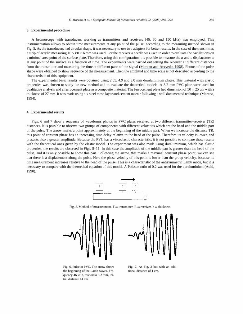
ed. Thisshown intransmitter,ions on

istancesthe pulserding to the

th elasticused for

(Moreno,

ver (TR)iddle partance TR,wer, andese resultss elastic

ead of thecan seecause itse, but it ism (Auld,

A betanoscope with transducers working as transmitters and receivers (46, 80 and 150 kHz) was employinstrumentation allows to obtain time measurements at any point of the pulse, according to the measuring methodFig. 5. As the transducers had circular shape, it was necessary to use two adapters for better results. In the case of thea strip of acrylic measuring 10× 80× 6 mm was used. For the receiver a needle was used in order to evaluate the oscillata minimal area point of the surface plate. Therefore, using this configuration it is possible to measure theu andv displacementsat any point of the surface as a function of time. The experiments were carried out setting the receiver at different dfrom the transmitter and measuring the time at different parts of the signal (Moreno and Acevedo, 1998). Photos ofshape were obtained to show sequence of the measurement. Then the amplitud and time scale is not described accocharacteristic of this equipment.

The experimental basic results were obtained using 2.05, 4.9 and 9.8 mm duraluminium plates. This material wiproperties was chosen to study the new method and to evaluate the theoretical models. A 3.2 mm PVC plate werequalitative analysis and a ferrocement plate as a composite material. The ferrocement plate had dimension of 50× 25 cm with athickness of 27 mm. It was made using six steel mesh layer and cement mortar following a well documented technique1994).

4. Experimental results

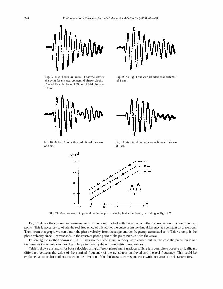
Figs. 6 and 7 show a sequence of waveforms photos in PVC plates received at two different transmitter–receidistances. It is possible to observe two groups of components with different velocities which are the head and the mof the pulse. The arrow marks a point approximately at the beginning of the middle part. When we increase the distthis point of constant phase has an increasing time delay relative to the head of the pulse. Therefore its velocity is lopresents also a greater amplitude. Because the PVC has a viscoelastic characteristic, it is not possible to compare thwith the theoretical ones given by the elastic model. The experiment was also made using duraluminium, which haproperties, the results are observed in Figs. 8–11. In this case the amplitude of the middle part is greater than the hpulse, and it is only possible to show this part. Following the arrow, that marks a maximal constant phase point, wethat there is a displacement along the pulse. Here the phase velocity of this point is lower than the group velocity, betime measurement increases relative to the head of the pulse. This is a characteristic of the antisymmetric Lamb modnecessary to compare with the theoretical equation of this model. A Poisson ratio of 0.2 was used for the duraluminiu1990).

Fig. 5. Method of measurement. T= transmitter, R= receiver, h= thickness.

Fig. 6. Pulse in PVC. The arrow showsthe beginning of the Lamb waves. Fre-quency 46 kHz, thickness 3.2 mm, ini-tial distance 14 cm.

Fig. 7. As Fig. 2 but with an addi-tional distance of 1 cm.

290 E. Moreno et al. / European Journal of Mechanics A/Solids 22 (2003) 283–294

maximallacement.ity is the

n is not

ignificantcould beeristics.

Fig. 8. Pulse in duraluminium. The arrows showsthe point for the measurement of phase velocity,f = 46 kHz, thickness 2.05 mm, initial distance14 cm.

Fig. 9. As Fig. 4 but with an additional distanceof 1 cm.

Fig. 10. As Fig. 4 but with an additional distanceof 2 cm.

Fig. 11. As Fig. 4 but with an additional distanceof 3 cm.

Fig. 12. Measurements of space–time for the phase velocity in duraluminium, according to Figs. 4–7.

Fig. 12 shows the space–time measurements of the point marked with the arrow, and the successive minimal andpoints. This is necessary to obtain the real frequency of this part of the pulse, from the time difference at a constant dispThen, from this graph, we can obtain the phase velocity from the slope and the frequency associated to it. This velocphase velocity since it corresponds to the constant phase point of the pulse marked with the arrow.

Following the method shown in Fig. 13 measurements of group velocity were carried out. In this case the precisiothe same as in the previous case, but it helps to identify the antisymmetric Lamb modes.

Table 1 shows the results for both velocities using different plates and transducers. Here it is possible to observe a sdifference between the value of the nominal frequency of the transducer employed and the real frequency. Thisexplained as a condition of resonance in the direction of the thickness in correspondence with the transducer charact

E. Moreno et al. / European Journal of Mechanics A/Solids 22 (2003) 283–294 291

ring these

and group

Fig. 13. Method of measurement of group velocity.

Table 1Experimental results of measured frequency, phase and group velocities

Thickness Nominal transducer Measured Phase velocity Group velocityfrequency frequency

(mm) (KHz) (KHz) (m/s) (m/s)

2.05 46 51.4 997 16912.05 80 69.2 1128 20182.05 150 107 1352 19574.9 46 55.2 1534 25614.9 80 63.6 1629 –4.9 150 111.4 1979 30799.8 46 54.6 1982 28219.8 80 77.4 2239 29349.8 150 91.8 2278 3076

Fig. 14. Experimental results in duraluminium for phase and group velocity compared with theoretical curve. Poisson’s ratio= 0.2. Frequency: − 46 kHz,� − 80 kHz,◦− 150 kHz.

The experimental results above-mentioned are shown in Fig. 14. A good correspondence is observed when comparesults with the theoretical curve for the phase and group velocities of the fundamental antisymmetric Lamb mode.

Figs. 15 and 16 show the sequence for the ferrocement case. A similar phenomenon of difference between phasevelocities in a portion of the pulse is observed as in the previous case.

292 E. Moreno et al. / European Journal of Mechanics A/Solids 22 (2003) 283–294

(25)–(28)cases.

Fig. 15. Pulse in ferrocement. The arrow shows thebeginning of the Lamb waves. Frequency 46 kHz,thickness 2.7 mm, initial distance 14 cm.

Fig. 16. As Fig. 11 but with an additional distanceof 1 cm.

5. Validation of model

In this section experimental results are presented in order to validate the model previously described. Using Eqs.developed above, and considering fundamental modes equivalent to the first term of the series we have the following

Antisymmetric case:

va(x, y, t)= 1

4π2

{− Q

2µ

∞∫−∞

eikx dk1

∂FA/∂ω

[α(k2 + β2)

cosh(βh)cosh(αy)

− 2k2α cosh(αh)cosh(βy)]eiωaLambt f ∗(

ωaLamb)

− Q

4µcos

(πy

2h

)π

h

∞∫−∞

e−ikx f ∗a (k)

k2 + β2AL

eiωAL(k)t dk

+ Q

2µ

h

πcos

(πy

2h

) ∞∫−∞

e−ikxg∗a(k)e

iωAT (k)t dk

}, (32)

ua(x, y, t)= 1

4π2

{iQ

2µ

∞∫−∞

e−ikx dk1

∂FA/∂ω

[k(k2 + β2)

cosh(βh)sinh(αy)

− 2kαβ cosh(αh)sinh(βy)]eiωaLambt f ∗(

ωaLamb)

+ iQ

2µsin

(πy

2h

) ∞∫−∞

e−ikxf ∗a (k)

k

k2 + β2AL

eiωAL(k)t dk

+ iQ

4µsin

(πy

2h

) ∞∫−∞

e−ikx g∗a(k)

keiωAT (k)t dk

}. (33)

For thesymmetric case we obtained analogue expressions:

vs(x, y, t)= 1

4π2

{− Q

2µ

∞∫−∞

eikx dk1

∂FS/∂ω

[α(k2 + β2)

sinh(βh)sinh(αy)

− 2k2α sinh(αh)sinh(βy)]eiωsLambt f ∗(

ωsLamb)

E. Moreno et al. / European Journal of Mechanics A/Solids 22 (2003) 283–294 293

l may bengitudinale of thesethe valueleplitudeby high

ponding

ent withts

des therets have aaper, thecity

Fig. 17. Variation of the relative amplitude of displacementu and v, as a function of the position inside the plate.s = symmetrical,a = antisymmetrical andy = thickness direction.

− Q

2µsin

(πy

h

)π

h

∞∫−∞

e−ikx f ∗s (k)

k2 + β2SL

eiωSL(k)t dk

− Q

4µ

h

πsin

(πy

h

) ∞∫−∞

e−ikxg∗s (k)e

iωST (k)t dk

}, (34)

us(x, y, t)= 1

4π2

{iQ

2µ

∞∫−∞

e−ikx dk1

∂FS/∂ω

[k(k2 + β2)

sinh(βh)cosh(αy)

− 2kαβ sinh(αh)cosh(βy)]eiωsLambt f ∗(

ωsLamb)

− iQ

2µcos

(πy

h

) ∞∫−∞

e−ikxf ∗s (k)

k

k2 + β2SL

eiωSL(k)t dk

− iQ

4µcos

(πy

h

) ∞∫−∞

e−ikx g∗s (k)

keiωST (k)t dk

}. (35)

In all previous equations the first integral term corresponds to the Lamb fundamental components. This integrasimplified using the stationary-phase aproximation (Achenbach, 1973). The second integral term corresponds to the lopredominant and the third one to the predominant shearing stress. Fig. 17 shows the variation of the relative amplitudtwo last terms for both cases, as a function of the position and inside the plate. Observing Fig. 17 we deduce thaton the surface for bothva is zero, this is not the case for displacementua which value is maximum. In relation to the needshaped receiver transducer, theu displacement represents a shearing stress and this explains in a part the low relative amto the Lamb mode that presents the front end of the pulse. Due to the fact that the front end of a pulse is formedfrequency boundary components its longitudinal velocity isCL which is characterized by the displacementu of the longitudinaldisplacement.

The absence of symmetric Lamb components it can be due to the absence of components in thef (ωSLamb) term, which in partis justified by the turning radius of the transmitting transducer on one of the faces of the plate which favors the corresantisymmetric action. A similar situation could corresponds withus andvs .

As a resume we can establish that the receiving transducer receives a strong antisymmetric Lamb compondeformationsva andua , and also it receives components with longitudinal deformationu, being one of these componenvelocityCL.

6. Conclusion

A theoretical model of pulse propagation in plates has been presented. The model shows that within the Lamb moare high frequency components with their own dispersion law, travelling faster than Lamb waves. These componenpredominant longitudinal and transversal strain. According to the corresponding dispersion law developed in this ppresence of high frequency components at the head of a pulse, make the head travel at the longitudinal limit veloCL.

294 E. Moreno et al. / European Journal of Mechanics A/Solids 22 (2003) 283–294

The experiments confirm part of the model relative to the presence of antisymmetric Lamb waves and a longitudinal velocityinal andkness of

Imaging.

in the head of the pulse. Another experiement could be made for testing the dispersion laws for the cuasilongitudcuasitransversal waves. Using this model it is possible to obtain information about elastic characteristics and thiccomposite and coarse grain materials that is not possible to obtain using classical echo-pulse methods.

References

Achenbach, J.D., 1973. Waves Propagation in Elastic Solids. North-Holland, Amsterdam.Auld, B.A., 1990. Acoustical Field and Waves in Solids. II. R.E. Frieber, Malabar, Florida.Kolsky, H., 1964. Stress waves in solids. J. Sound Vib. 1, 1–10.Leeman, S., Healey, A., Costa, E., 2002. The impact of loss on ultrasonic propagation. In: Maev, R. (Ed.), Proc. 26th Acoustical

Kluwer Academic/Plenum Press, New-York.Martincek, G., 1975. Theory and Methods of Dynamic Nondestructive Testing of Plane Elements. Veda, Bratislava.Moreno, E., 1994. Propagation of mechanic waves in plane elements of composite materials. Ph.D. thesis, ICIMAF, Havana.Moreno, P., Acevedo, E., 1998. Thickness measurements in composite material using Lamb waves. Ultrasonic 35, 581–586.Tu, J.Y., Brennan, J.N., Saver, J.A., 1955. Dispersion of ultrasonic pulse velocity in cylindrical rods. J. Acoust. Soc. Am. 27, 550.