Catena 214 (2022) 106203

Available online 11 April 20220341-8162/© 2022 The Authors. Published by Elsevier B.V. This is an open access article under the CC BY license (http://creativecommons.org/licenses/by/4.0/).

Exploring the dynamics of a complex, slow-moving landslide in the Austrian Flysch Zone with 4D surface and subsurface information

M.J. Stumvoll a,*, E.M. Schmaltz b, R. Kanta a, H. Roth a, B. Grall a, J. Luhn a, A. Flores-Orozco c, T. Glade a

a ENGAGE – Geomorphological Systems and Risk Research, Faculty of Earth Sciences, Geography and Astronomy, University of Vienna, Universitatsstraße 7, 1010 Vienna, Austria b Federal Agency for Water Management, Institute for Land and Water Management Research, Pollnbergstraße 1, 3252 Petzenkirchen, Austria c Geophysics Research Division, Department of Geodesy and Geoinformation, TU-Wien, Wiedner Hauptstr. 8, 1040 Vienna, Austria

A R T I C L E I N F O

Keywords: Slow moving landslide Subsurface monitoring Slope hydrology Flysch and Klippen Zone Lower Austria

A B S T R A C T

Complex, slow-moving landslides are common in deeply weathered soils with clay-rich layers, as can be found in the Flysch Zone of Lower Austria. Complex process behaviour on differing spatio-temporal scales calls for long- term measurement series on both surface and subsurface parameters. Only then, dynamics and interrelations with possible triggering mechanisms might be further understood. This study investigates a small, slow-moving earth slide - earth flow system.

Information on surface changes, based on digital elevation models (DEMs) of Difference (DoDs) using terrestrial laser scanning (TLS), is available since 2015 (2009, including ALS). Subsurface monitoring started in 2018. Data was analysed comparatively for overlapping periods: A conceptual subsurface model was generated with geotechnical information (penetration tests/ drill core samples), incorporating regolith thickness and po-tential shear surfaces. For four periods between 2018-11-14 and 2020-11-18 (~2 years), interrelations of hydro- meteorological input data (precipitation/ temperature), changes in the spatio-temporal development of sub-surface hydrology (piezometers), subsurface dynamics (inclinometer) and surface dynamics (DoDs) were ana-lysed in detail.

Total dynamics in the 2-year period were marginal. Total inclinometer displacements were max. ~1.65 cm; these changes were too small to be depictable on the surface with TLS based DoDs. Nonetheless, several relations of present state and known former dynamics were found: Regolith thickness could be reasonably described via penetration tests, being relatively shallower in areas of known process activity. Interpolated shear surfaces based on drill core analyses, penetration tests and inclinometer data are highly simplified; nevertheless, they depict relations to locations of known activity with respect to depth and geometry. Locations of shallowest groundwater levels and highest fluctuations correspond with areas of recent minor and former larger dynamics. Inclinometer displacement rates exhibit relations to hydro-meteorological input data and are in locations known from former bigger process magnitudes.

1. Introduction

Understanding slow-moving landslides is of high interest, both with respect to their role in landscape evolution (Crozier, 2010b), but also with respect to hazard evaluation (Glade et al., 2005). Process rates inherent to slow-moving landslides, but also complexity and non- linearity of natural hillslope systems impede the significance of short- term measurements (Cruden and Varnes, 1996; van Asch et al., 2007).

One of the primary predisposing factors of slow-moving landslides is the textural composition of the soil, while one major hydrological trig-gering mechanism are changes in groundwater level (c.f. Lacroix et al., 2020 and references therein). Soils with clay-rich layers and, thus, low hydraulic conductivity, have been found to be exceptionally prone to sliding processes following an increase in groundwater level (e.g. Baum et al., 1998; Bievre et al., 2018; Gallistl et al., 2018; Jaboyedoff et al., 2009; van Asch et al., 1996). In Austria, the Flysch- and Klippen Zone,

* Corresponding author at: Faculty of Earth Sciences, Geography and Astronomy, Department of Geography and Regional Research, University of Vienna, Austria, Universitatsstraße 7, 1010 Vienna, Austria.

E-mail address: margherita.stumvoll@univie.ac.at (M.J. Stumvoll).

Contents lists available at ScienceDirect

Catena

journal homepage: www.elsevier.com/locate/catena

https://doi.org/10.1016/j.catena.2022.106203 Received 21 November 2021; Received in revised form 3 March 2022; Accepted 4 March 2022

Catena 214 (2022) 106203

2

located alongside the northern fringe of the Eastern Alps, is composed of clay-rich and deeply weathered regolith layers (Schnabel, 1980; Schnabel, 1999). Its high susceptibility to sliding and flowing processes has been investigated for example by Petschko et al. (2014); Schwenk (1992); Steger et al. (2020); Stumvoll et al. (2020); Stumvoll et al. (2021); Tilch (2014). Particularly changes in groundwater level and related changes in pore water pressure, induced by heavy rainfalls or rapid snow melt, have been found to be a dominant forcing mechanism of sliding processes for those clay-rich layers (Lacroix et al., 2020; van Asch et al., 1999). Changes in pore water pressure and increasing soil water content lead to changes in shear strength, which again is considered to be the main cause of (slope) failure, although this is a crude oversimplification (McColl, 2015). The interrelation of precipi-tation and landslide occurrence is thus of high interest – especially with respect to changing precipitation patterns in the light of climate change (Crozier, 2010a; Gariano and Guzzetti, 2016) – but remains hard to evaluate (Caine, 1980; Crozier, 1999; Guzzetti et al., 2007; Wieczorek and Guzzetti, 2000).

Predisposing factors have a low temporal variability and influence landslide potential, whilst actual triggering mechanisms vary over time, depending on the state and history of a hillslope system (c.f. Crozier, 1986; Glade and Crozier, 2005; McColl, 2015). Threshold dependency and complex, non-linear behaviour restrict our understanding of land-slide processes (c.f. Phillips, 1992; Phillips, 2003; Phillips, 2006; Schumm, 1979). Slope systems might respond differently over time or not at all to the same disturbance (sensitivity concept, c.f. Brunsden, 2001; Brunsden and Thornes, 1979). Their reaction is also influenced by former processes (path-dependency, refer e.g. to Samia et al., 2017). Both reaction to and recovery from system disturbance – for example to landslide processes – comprise time-lags, which are shorter the smaller the scale (Bull, 1991; De Boer, 1992). Accordingly, gaining information about surface and subsurface properties over extended observation pe-riods is critical to better understand the actual connection between meteorological events, subsurface processes and landslides (Lacroix et al., 2020).

Quantitative approaches of multi-temporal landslide investigation cover a variety of methods and techniques for both the surface and subsurface (for a concise review c.f. Chae et al., 2017). Methods on surface investigation include mapping and change detection based on multi-temporal data, utilizing high-resolution digital elevation models (DEMs) generated for example with Terrestrial Laser Scanning (TLS) (Jaboyedoff et al., 2012; Telling et al., 2017) or Unmanned Aerial Vehicle (UAV) based Structure from Motion (SfM) (Giordan et al., 2018). These techniques can be used across a broad range of spatial and tem-poral scales (Scaioni et al., 2014). However, they are limited in the case of slow-moving landslides due to multiple reasons, such as technical restrictions, vegetation cover and data inaccuracies (c.f. Chae et al., 2017; Prokop and Panholzer, 2009; Stumvoll et al., 2021). For subsur-face landslide investigation, both static (soil type, subsurface structure, regolith thickness) and dynamic parameters (groundwater, soil mois-ture, slope movement) are of interest (Rogers and Chung, 2017). The aim of subsurface investigation in relation to landslide processes is to detect depths of potential shear surfaces (e.g. D’Amato Avanzi et al., 2013) and to unravel the interrelation of hydro-meteorological trig-gering mechanisms (Bievre et al., 2018; Schulz et al., 2009).

The combination of both surface and subsurface monitoring data to better understand slow-moving landslides is both a necessity – and a challenge. Monitoring setups need to cover different spatial scales in order to investigate both extensive changes on slope scale as well as detailed changes on local scale and their interrelations (e.g. Uhlemann et al., 2016). However, such studies remain sparse due to the costs associated with accessibility, instrumentation, the analysis of the data inter alia. Due to its high potential for landslide processes, two such monitoring setups are currently operated in the Flysch Zone of Lower Austria (Salcher and Hofermühle observatory, see Stumvoll et al., 2020; Stumvoll et al., 2021). However, both surface and subsurface

interrelations on detailed scale at a spatially representative landslide observatory site was not presented for the Austrian Flysch Zone. In this study, detailed static and dynamic subsurface and surface data covering approx. 2 years is analysed comparatively for the Hofermühle observa-tory to assess the following questions: 1) How is the subsurface char-acterized with respect to hydrogeological and geotechnical parameters? 2) How are hydro-meteorological input and hydrogeological patterns characterized over time? 3) Are there links between hydrogeological patterns, subsurface displacement and surface changes over time? And 4) what are the implications on the landslides system state when incorporating knowledge on former landslide dynamics? The research strategy included the generation of a static subsurface model using geotechnical information, incorporating regolith thickness and potential shear surfaces. Piezometer information is used to evaluate changes in groundwater level over time. Interrelations of hydro-meteorological input data, changes in the spatio-temporal development of subsurface hydrology as well as surface and subsurface dynamics are assessed for four periods between 2018-11-14 and 2020-11-18.

2. Study area

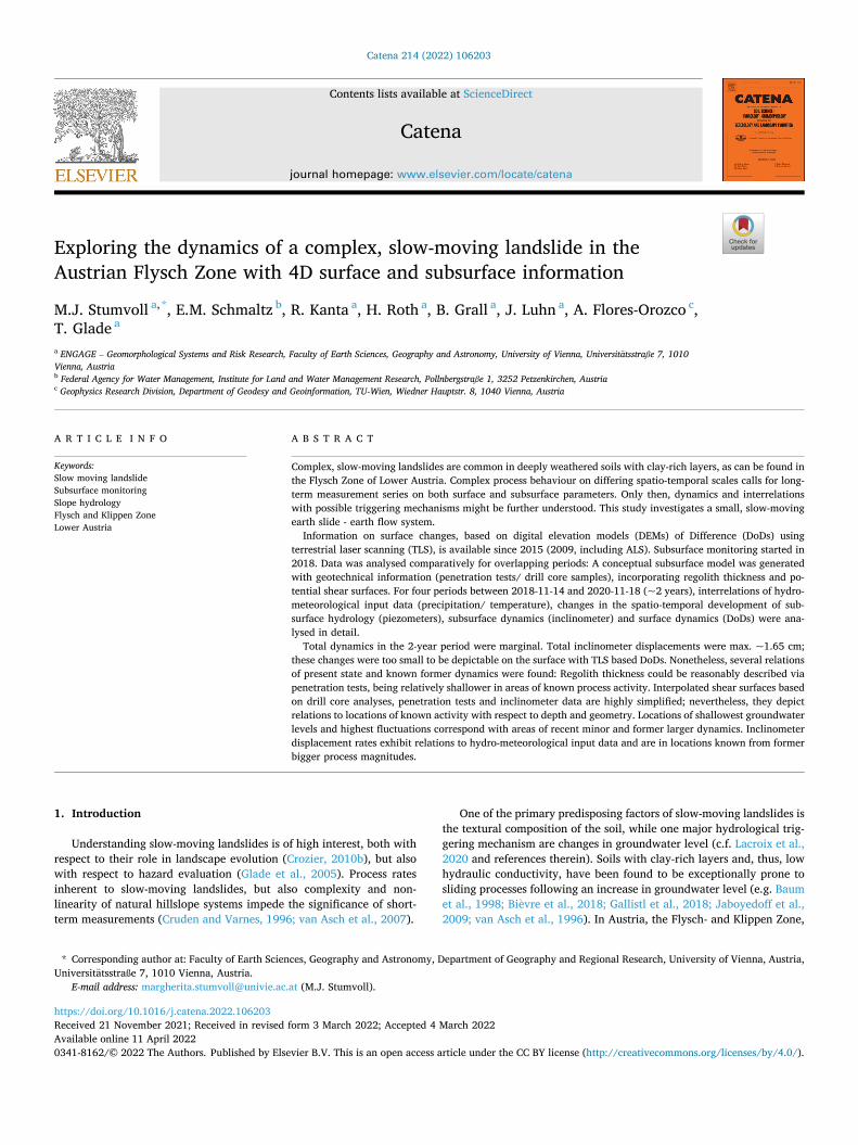
The area under investigation is located in Konradsheim, Waidhofen a.d. Ybbs in Lower Austria (Fig. 1a,b). The respective slope (Hofermühle (Hfm) catchment; ~0.15 km2; ~160 m height difference, Fig. 1c) is situated in the northern part of the Redtenbach catchment (~15 km2).

The study area is situated in the geological transition zone of Hel-vetic, Penninic and Austroalpine units (Fig. 1a). The southern part of the Redtenbach catchment consists of dolomite, marls and calcareous marls (Austroalpine). Clays, marls and sandstones of the Flysch (Penninic) and Klippen Zone (Helvetic) can be found in the northern part (Schnabel, 1999; Schnabel et al., 2002; Thenius, 1974). The Flysch and Klippen Zone is particularly prone to sliding processes (Petschko et al., 2013; Schwenk, 1992; Steger et al., 2020; Stumvoll et al., 2020; Tilch, 2014). Climate conditions support both weathering (disposition) and mobili-zation (trigger) of the Flysch materials. After Schweigl and Hervas (2009), extreme rainfall and snow melt rates are found to be the main triggers of landslides in the area. Being situated at the northern fringe of the eastern calcareous alps, the study area exhibits mean yearly pre-cipitation rates of ~1.197 mm (period 1896–2020; Histalp data from Waidhofen a. d. Ybbs, Auer et al. (2007)).

Both natural and artificial landcover and slope changes (changes in vegetation cover, slope levelling and draining) can be considered vari-able disposition factors. They are of major importance when it comes to short and mid-term hillslope development in association with landslide processes (Papathoma-Kohle and Glade, 2013; Schmaltz et al., 2017; Sidle and Bogaard, 2016; Sidle and Ochiai, 2006; Sidle et al., 2006). At the study site, hillslopes with lower gradient (upper part) are used for hay production, while steeper areas are forested (Fig. 1c). A similar land use can be assumed to having been present for the last 100 years at least (historic cadastre). Fast growing coniferous trees mark the orographic right of the lower catchment (reforested in 1970s), deciduous trees, mostly beech, the orographic left. With respect to (subsurface) slope hydrology, artificial water drainages and basins are of major interest. As far as known, respective installations for the main study area (Fig. 1d,e) include drainages in greater depths of approx. 4–6 m using gravel, drainages in depths up to 1.5 m using perforated plastic pipes of different sizes and transport pipes (plastic/ concrete). There is no full documentation about their position, age and condition. Only the most recently installed drainages (~2014; in ~1.5 m depth, ~0.25 m diam-eter) are known and their route still detectable in recently acquired high- resolution TLS data (see Y- like formation in lower right of Fig. 1d,e). A concrete well gathers water from upslope drainages of unknown age and position; it is situated above the upper left corner of Subsystem I in Fig. 1d. The well’s drainpipe runs towards south-southwest into the torrent’s flow path. Local residents described the main landslide area to having been wetland-like in former times (no absolute date available,

M.J. Stumvoll et al.

Catena 214 (2022) 106203

3

Fig. 1. Location of study site and areas of investigation. a) Location of the Redtenbach catchment in Lower Austria, Austria (geological map after Weber (1997)). b) Location of the Hofermühle study site within the Redtenbach catchment. c) Hydrological catchment of the Hofermühle torrent. d) Main study area. Simplified morphological landslide features and changes in surface height between 2009 and 2019 are indicated. Main areas of investigation and recent process activity (Subsystems I & II) are highlighted. e) Direct investigations and installations at the study site. Profiles given in Fig. 4 are indicated [white, dotted]. Relief shadings in a-c) are based on a Austrian 10 m DEM (BMDW, 2015) and a 1 m ALS-DEM (NOEL GV, 2009), respectively. Orthophoto in c) is provided by the Federal State Government of Lower Austria (NOEL GV, 2011). Relief shading in d-e) is based on a 0.05 m TLS-DEM (2019-12-05). Simplified morphological mapping in d) is based on Stumvoll et al. (2021). DEM of Difference (DoD) calculation in d) is based on 1 m ALS-DEM (NOEL GV, 2009) and a 0.05 m TLS-DEM (2019-12-05).

M.J. Stumvoll et al.

Catena 214 (2022) 106203

4

personal communication Hornbachner (2020-08-19)). According to the definition given by Cruden and Varnes (1996), the

Hofermühle landslide is defined as slow-moving and complex; it can be described as a compound, retrogressive earth slide – earth flow, showing different phases of activity on different parts of the landslide mass. In the last 10 years, slow sliding processes concentrated in the upper part adjacent to the Hofermühle torrent, where material can be mobilized for faster processes like earth flows (Fig. 1d). Former activities have proven this interrelation of sliding and flowing processes to be possible (Kotz-maier, 2013; Sausgruber, 2013). Major activation occurred in 2011 (subsidence via sliding by 2 m in 2 weeks, Sausgruber (2013)), re- activation in 2013 (formation of earth flow with 20 m/h, Sausgruber (2013)) and processes have slowed down significantly since then to only a few cm to dm per year on the parts affected by sliding – as far as known. The study area has been intensively investigated regarding changes in surface morphology and elevation for the period 2009 – 2019 using high-resolution (0.05 m) digital elevation data generated via TLS (multi-temporal datasets between 2015 and 2019) as well as ALS data (1 m, 2009), see Stumvoll et al. (2021). Landslide processes focus on the upper to middle orographic left of the torrent (Fig. 1d). Between 2009 and 2015 the main landslide area developed (Fig. 1d, landslide [main]), including the processes from 2011 and 2013; in the following years, the respective area was overgrown by bushes, small trees and shrubbery. Two extensions of this main area developed since then (Subsystems I and II), being situated above the main scarp and at its lower right border (Fig. 1d, landslide [active]). The study shows these areas to exhibit surficial changes in both slope shape and landslide feature distribution. Between 2009 and 2015, Subsystems I (~3300 m2) and II (~2100 m2) experienced changes in surface height of up to 0.30 m and 1.60 m, respectively. Changes in volume accounted for approx. − 94 m3/+64 m3

in Subsystem I and − 214 m3/+41 m3 in Subsystem II, both showing morphological features related to sliding. Both rotational and trans-lational sliding are assumed to occur. After 2015, processes slowed down; minor and locally confined changes in surface height of approx. up to ±0.20 m in Subsystem I and − 1.00 m/+0.40 m in Subsystem II occurred until 2018/2019 (Stumvoll et al., 2021). Results on surface change have not been correlated with information on subsurface struc-ture, subsurface dynamics or hydro-meteorological data, yet. In a geotechnical report, Sausgruber (2013) gives an evaluation of max. volume possibly to be activated in approx. the same locations as are delineated by the Subsystems following WP/WLI (1994): approx. 16 000 m2 (50 m in length, 50 m in width, 12 m in depth) for Subsystem I and 3000 m2 (25 m in length, 25 m in width, 7 m in depth) for Subsystem II.

3. Materials and methods

Experts’ reports were available from the Austrian Torrent and Avalanche Control (WLV) (Sausgruber, 2013; Sausgruber, 2016). In this study, multitemporal data (meteorological/ piezometer/ inclinometer/ TLS) was analysed for the observation period 2018-11-14(15) – 2020- 11-18, covering 736 days (~2 years).

3.1. Subsurface investigation

Dynamic probing was performed in 32 locations to investigate sub-surface structure (Fig. 1e). The time of acquisition varies (08-2017, 09- and 10-2018, 03-2019, 03-2020); locations are named according to consecutive acquisition campaign (1 to 4) and location. Type of probing is defined as dynamic probing heavy (DPH, DIN EN ISO 22476-2:2005); blows per 10 cm (N10) were counted. Regolith depth and internal structure are estimated via visualization and interpretation of DPH penetration resistance and maximum penetration depth.

Via percussion drilling nine cores were taken in fall 2018, six of which (B1, B3, B4, B7, B8 and B9) were analysed and used for this study (for locations see Fig. 1e). Core sample analysis included wet sieving

(B7, B8 and B9: ONORM L 1061-1; B1, B3 and B4: ONORM EN ISO 17892-4), sedimentation (B7, B8 and B9: ONORM L 1061-2) and laser diffraction analysis (B1, B3 and B4: ISO 13320) to investigate grain size (>63 µm) and fine fraction (<63 µm) distribution. Whilst definite ho-rizons were specified for B1, B3 and B4 and results are interpolated on these, certain depths were investigated for B7, B8 and B9 in more detail, only. For the entire cores of B7, B8 and B9 texture (finger testing ac-cording to DIN 19682-2) was determined for almost each consecutive 0.10 m instead. Results on texture are given as descriptive text differ-entiating between clay (clayey), silt (silty), loam (loamy), sand (sandy) and gravel (gravelly). Descriptions were transformed into values ranging between 0 and 0.5 for graphical illustration, with 0.1 standing for clay, 0.2 for silt etc. and 0.01 for clayey, 0.02 for silty etc. Determination of gravimetric water content has been conducted according to ONORM EN ISO 17892-1 for B1, B3 and B4. Additional investigations included total carbonate content (Scheibler method, ON L 1084) and Atterberg limits (Casagrande method, ON B 4411).

In fall 2018, eight piezometers (Geokon 4500AL Standard Piezom-eter, see Geokon, 2020) were installed (Fig. 1e) to measure the depth to the groundwater with 5-minute resolution (2018-11-15 – 2020-11-18). The divers were installed in plastic pipes at depths varying between ~6 and ~3.50 m. Material infiltration is avoided using special protec-tive stocking. Piezometer data was analysed for each of the eight sen-sors. The data is not corrected barometrically (see Geokon, 2018), as barometric data is not available for the entire observation period.

Four inclinometers (Fig. 1e) are installed at the study site (one automatic, three manual). The automatic inclinometer (INC Auto: Measurand ShapeAccelArray Field (SAAF), ±1.5 mm accuracy; see Measurand, 2019) is available since 2018-11-15 (5-min resolution). The total length is 8 m, being installed 0.50 m below surface. Information on deformation is available for each 0.50 m (16 segments) in two directions (+X downslope, Y perpendicular to X with positive values being downslope counter clockwise). Manual inclinometers (INC M1: 2018-12 (4.50 m), INC M2: 2019-03 (6.00 m), INC M3: 2019-07 (7.00 m)) were installed using flexible inclinometer casings (55 mm diameter) and are read out manually approx. every month (for hardware specifications refer to Glotzl, 2016; Glotzl, 2019). The respective reading probe (±0.1 mm accuracy) gives information on deformation every 0.50 m in depth for two directions (+A downslope, B perpendicular to A with positive values being downslope clockwise). Both automatic and manual inclinometer casings were installed for one direction to be the direction of expected movement (+A/ +X). In spring 2020 manual measurements were not possible due to access limitations. INC M1 and INC Auto are presented here.

3.2. Surface investigation

High-resolution, multi-temporal digital elevation models were generated via TLS observations. Between the start of the subsurface monitoring in fall 2018 and the end of the observation period covered in this study (2020-11-18), five campaigns (epochs) were generated or used, respectively. Epochs from 2018-11-14, 2019-02-26 and 2019-12- 05 were already available (see Stumvoll et al., 2021), data for 2020- 05-12 and 2020-11-18 was acquired additionally. TLS campaigns were conducted with a Riegl VZ 6000 terrestrial laser scanner (hardware specifications are provided in Riegl LMS, 2020). An angular distance of 0.004◦ used for both horizontal (Phi [◦]) and vertical (Theta [◦]) resulted in a ~0.05 m point spacing for the area of interest. Multiple TLS point clouds were registered via Multi Station Adjustment (MSA - ICP- Algorithm (Besl and McKay, 1992) implemented in Riegl RiSCAN Pro). After vegetation filtering and point density homogenisation (octree filtering, 0.05 m), point clouds were triangulated (mesh) and used to calculate changes in surface and volume (implemented in RiSCAN Pro, grid size 0.05 m, excluding values from − 0.05 to +0.05 m). The analysis focuses on Subsystem I, which is known to having been active in the last 10 years (refer to Stumvoll et al., 2021); the main landslide area is

M.J. Stumvoll et al.

Catena 214 (2022) 106203

5

excluded. Additionally, raster DEMs were generated from the TLS-point clouds with a raster cell size of 0.05 m, applying a linear interpolation method to fill gaps. For detailed information regarding data processing and DEM generation, the reader is referred to Stumvoll et al. (2021). Raster DEMs are used to calculate basic surface hydrology (flow accu-mulation, D8 and multiple flow direction and accumulation (MFD) (see Qin et al., 2007), implemented in ESRI ArcGIS Pro). MFD was calculated for epochs 2009, 2018-11-14 and 2019-12-05; for improved comparison of results, data was resampled to 0.50 m raster size.

The TLS based DEM from 2019-12-05 with 0.05 m raster size was utilized to visualize the recent surface elevation via slope profiles and to recalculate GNSS based z-value (height) information of all sensor loca-tions. This step ensured absolute correct positioning of the respective sensors.

3.3. Conceptual model and spatio-temporal analysis of subsurface and surface data

Maximum depths achieved with DPH were used to calculate assumed bedrock depth and geometry utilizing IDW interpolation (0.05 m raster size). Results on the laboratory analysis of particle size distribution where interpreted comparatively with results on water content for B1, B3 and B4, but also with parameters on carbonate content, Atterberg limits, shear parameters and clay minerals not presented here. For B7 and B9, inclinometer and DPH data were utilized for a comparative interpretation. Depths of distinct changes in DPH penetration resistance (from N10 4 to >8 and 8 to 15 or >15) and inclinometer displacements were visualized in combination and interpreted regarding subsurface structure. Depths based on these comparative interpretations were used for the interpolation of potential layers of instability (shear surfaces; IDW). Piezometer data was aggregated to monthly means and assigned to piezometer locations. Groundwater surfaces were interpolated using Simple Kriging in ArcGIS Pro (smoothing, value 0.2). Kriging interpo-lation was chosen based on suggestions in c.f. Ohmer et al. (2017). To improve the approximation of these surfaces, the Hofermühle torrent (points in flow path) was included in this interpolation. Interpolation methods were not further assessed regarding their statistical signifi-cance. Results on drill core analyses are presented together with closely located DPH measurements, with four representative locations discussed in more detail. To visualize calculated sub-surfaces, slope sections are presented with a longitudinal and a transverse profile through the main study area. They intersect at the location of INC M1. Inclinometer dis-placements for INC M1 (21 measurements; observation period 2018-12- 18 to 2020-11-18; 735 d, less than total period) are embedded in the profiles in direction +A (super-elevated *100) and in direction − B (super-elevated *1000). INC Auto is situated in the lower third of the longitudinal profile. Within the observation period, displacements of INC Auto were too small to be visualized in the profile. TLS campaigns cover four DoDs; respective periods (I-IV) were analysed in detail for one of the recently most active process areas (Subsystem I) by comparing and comparatively investigating data on precipitation, temperature, piezometers, inclinometer displacements (INC Auto and M1) and rates (INC M1) with the DoDs.

Automatic data acquisition (meteorological, piezometer, automatic inclinometer) is performed with a CR1000 datalogger and AVW200 analyser module from ©Campbell Scientific. For data analysis and compilation of figures, we used ©Riegl RiSCAN Pro Processing Software, ©ESRI ArcGIS Pro, ©Glotzl GLNP, ©Measurand SAASuite, ©Adobe Photoshop CC, ©IrfanView, ©MS Office, ©Spyder (MIT) and the following Python (Version 3.8) packages: numpy (1.16.5; Oliphant (2015), pandas (0.25.1; The Pandas Development Team (2020)) and matplotlib (3.1.3; Hunter (2007)).

4. Results

4.1. Surface hydrology

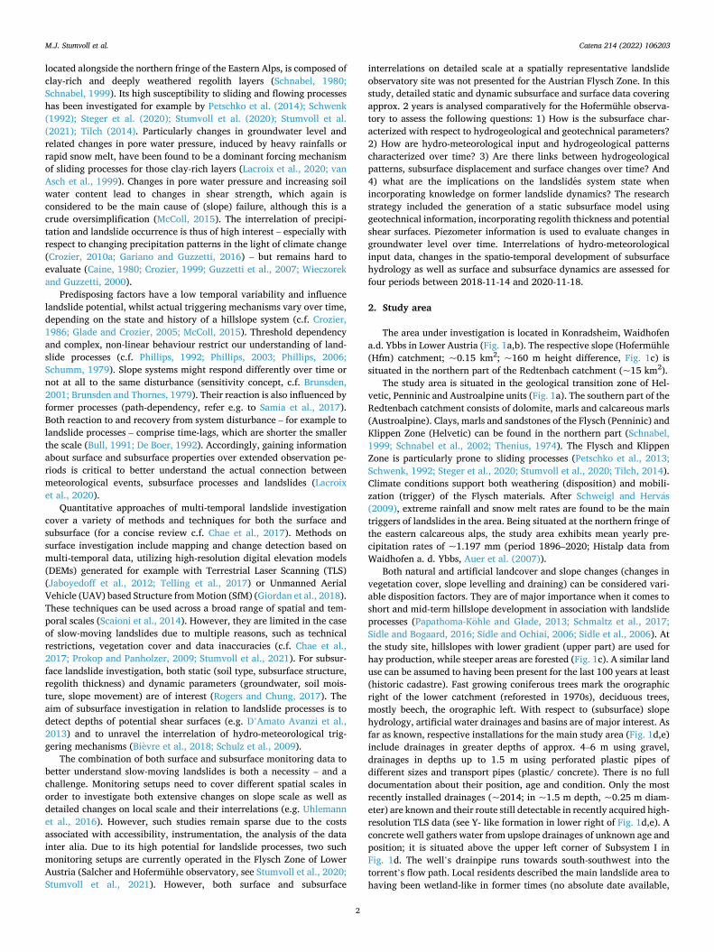
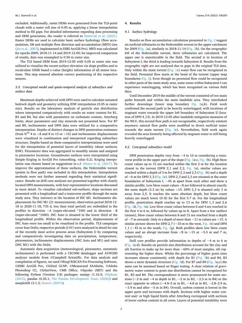
Results on flow accumulation calculation presented in Fig. 2 suggest six surficial tributaries to the Hofermühle torrent in the upper catchment for 2009 (Fig. 2a), similarly to 2018-11-14 (Fig. 2b). On the orographic left of the Hofermühle torrent, three tributaries are calculated. The upper one is unnoticeable in the field. The second is in location of Subsystem I, the third is leading towards Subsystem II. Results from the orographic right are not analysed due to gaps in the original TLS data. Only within the main torrent (Fig. 1c) water flow can be recognized in the field. Perennial flow starts at the bend of the torrent (upper map boundaries Fig. 2). Even though no perennial flow could be recognized in other parts of the main study area, some zones within Subsystem I can experience waterlogging, which has been recognized on various field days.

Until December 2019 the middle of the torrent consisted of two main paths beneath and within the main landslide area. They interlinked further downslope (lower map boundary Fig. 2a,b). Field work confirmed the second path to be heavily waterlogged, with locations of stagnant water towards the upper left boundary of Subsystem II (loca-tion of DPH 4_13). In 2019-12-05 after landslide mitigation measures of the WLV, this second flow path is not recognisable, respectively existent anymore; natural flow paths were modified to divert surficial water towards the main torrent (Fig. 2c). Nevertheless, field work again revealed the area formerly being affected by stagnant water to still being heavily waterlogged.

4.2. Conceptual subsurface model

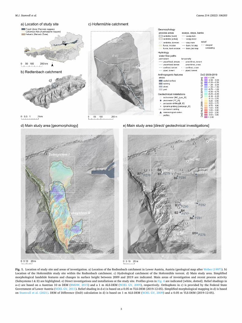
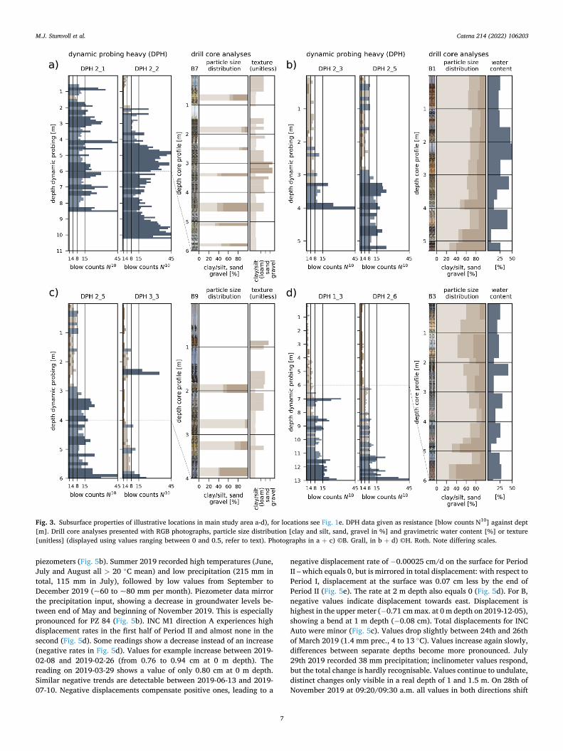
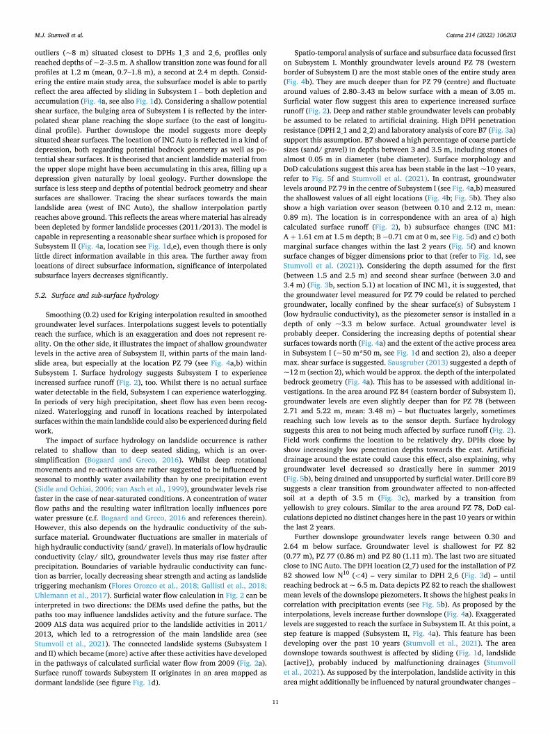
DPH penetration depths vary from ~4 to 10 m considering a trans-verse profile in the upper part of the slope (Fig. 3a-c, Fig. 4b). High blow count values up to 15 are reached within the first 2 m for the location closest to the torrent (DPH 2_1 and 2_2, Fig. 3a), similar values are reached within a depth of 3 m for DPH 2_3 and 2_5 (Fig. 3b) and a depth of ~6 m for DPH 3_3 (Fig. 3c). DPH 2_3 and 2_5 are situated at the outer boundaries of Subsystem I, ~45 m apart from each other and show a similar profile. Low blow count values <8 are followed in almost exactly the same depth (3.3 m) by values >15. DPH 3_3 is situated only 3 m away from 2_5. It reaches the same absolute depth, but blow count values are much lower (0–8) for the first 5.7 m. For the longitudinal profile, penetration depth reaches up to 13 m for DPH 1_3 and 2_6 (Fig. 3d, Fig. 4a). Low blow count values between 0 and 4 are reached in the first 4 to 6 m, followed by values up to 8. Apart from a few outliers (stones), blow count values between 8 and 15 are reached from a depth of ~7 m onwards. Only in a depth of more than ~11 m values are >15. A similar picture shows for DPH 2_7 (~33 m to the west, Fig. 3e) and DPH 1_1 (~43 m to the south, Fig. 3g). Both profiles show low blow count values and an abrupt increase from <8 to >15 at ~5.5 m and 7 m, respectively.

Drill core profiles provide information to depths of ~4 m to 6 m (Fig. 3a-d). Results on particle size distribution account for the clay and silt fraction to make up for more than ~60% of most samples, silt rep-resenting the higher share. Whilst the percentage of higher grain sizes increases almost consistently with depth for B1 (Fig. 3b) and B4, B3 shows a more dynamic structure (Fig. 3d). For B7 and B9 (Fig. 3a,c) the same can be assumed based on finger testing. A clear relation of gravi-metric water content to grain size distribution cannot be recognized for B1, B3 and B4. The correspondence is more pronounced for some sec-tions (~2 m and ~4 m depth in B1, ~2 m in B3, ~2.5 m in B4) or the exact opposite in others (~4.8–5 m in B1, ~4.8 m in B3, ~2.8–2.9 m, ~3.9 m and after ~5 m in B4). Overall, carbon content is lowest in the upper parts and increases with depth. Sections with higher water con-tent and/ or high liquid limits after Atterberg correspond with sections of lower carbon content in all cores. Layers of potential instability were

M.J. Stumvoll et al.

Catena 214 (2022) 106203

6

found to be located in depths of ~1.0 to up to 2.5 m, between ~2.5 and 3.4 m and between ~3.4 and 4.6 m - to up to 6 m (B1: 1.5–2.5 m, 3.0–3.4 m and 4.0–4.6 m/ B7: ~1.5 m and 2.7 m/ B3: 2.0–2.4 m and 1.0–1.85 m/ B9: 1.8 m and 2.4 m/ B4: 1.7–1.85 m, 2.0–2.5 m and 3.0–3.7 m).

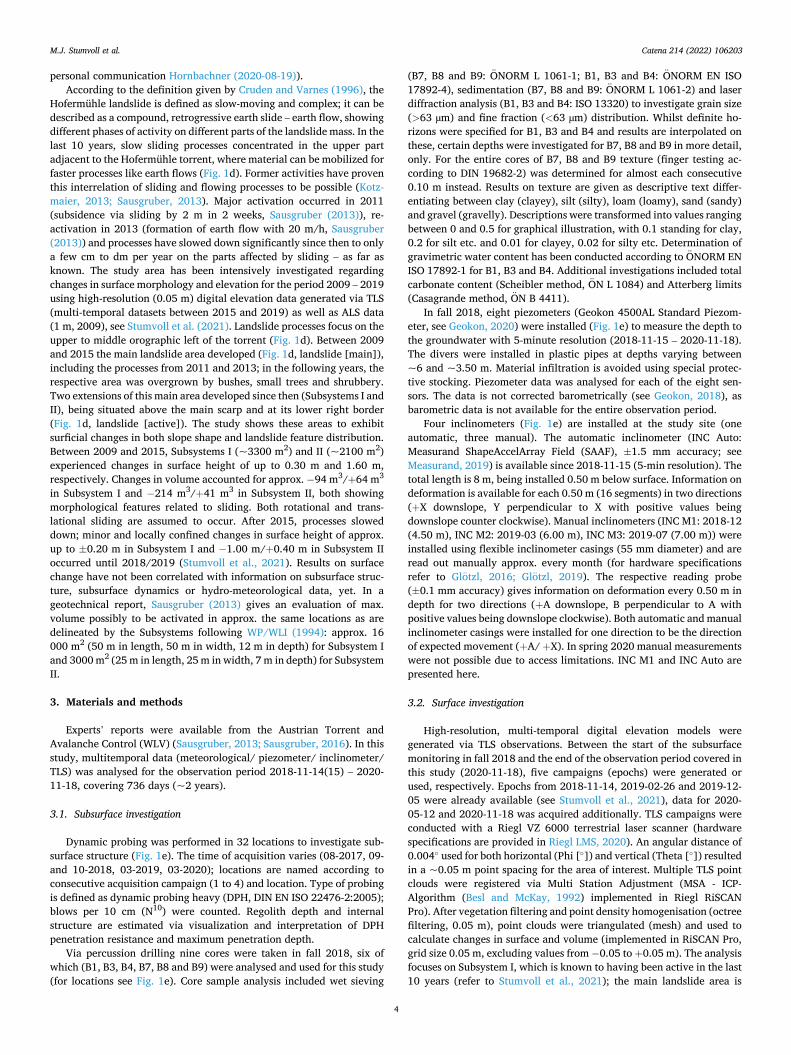
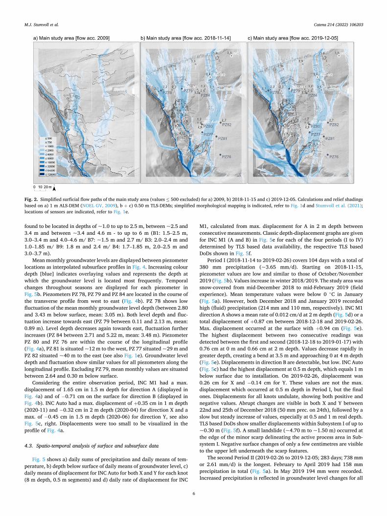
Mean monthly groundwater levels are displayed between piezometer locations as interpolated subsurface profiles in Fig. 4. Increasing colour depth [blue] indicates overlaying values and represents the depth at which the groundwater level is located most frequently. Temporal changes throughout seasons are displayed for each piezometer in Fig. 5b. Piezometers PZ 78, PZ 79 and PZ 84 are located in the course of the transverse profile from west to east (Fig. 4b). PZ 78 shows low fluctuation of the mean monthly groundwater level depth (between 2.80 and 3.43 m below surface, mean: 3.05 m). Both level depth and fluc-tuation increase towards east (PZ 79 between 0.11 and 2.13 m, mean: 0.89 m). Level depth decreases again towards east, fluctuation further increases (PZ 84 between 2.71 and 5.22 m, mean: 3.48 m). Piezometer PZ 80 and PZ 76 are within the course of the longitudinal profile (Fig. 4a), PZ 81 is situated ~12 m to the west, PZ 77 situated ~29 m and PZ 82 situated ~40 m to the east (see also Fig. 1e). Groundwater level depth and fluctuation show similar values for all piezometers along the longitudinal profile. Excluding PZ 79, mean monthly values are situated between 2.64 and 0.30 m below surface.

Considering the entire observation period, INC M1 had a max. displacement of 1.65 cm in 1.5 m depth for direction A (displayed in Fig. 4a) and of − 0.71 cm on the surface for direction B (displayed in Fig. 4b). INC Auto had a max. displacement of +0.35 cm in 1 m depth (2020-11) and − 0.32 cm in 2 m depth (2020-04) for direction X and a max. of − 0.45 cm in 1.5 m depth (2020-06) for direction Y, see also Fig. 5c, right. Displacements were too small to be visualized in the profile of Fig. 4a.

4.3. Spatio-temporal analysis of surface and subsurface data

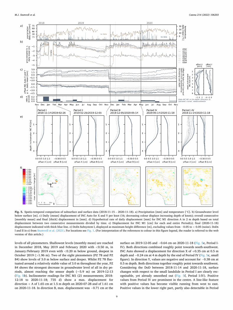
Fig. 5 shows a) daily sums of precipitation and daily means of tem-perature, b) depth below surface of daily means of groundwater level, c) daily means of displacement for INC Auto for both X and Y for each knot (8 m depth, 0.5 m segments) and d) daily rate of displacement for INC

M1, calculated from max. displacement for A in 2 m depth between consecutive measurements. Classic depth-displacement graphs are given for INC M1 (A and B) in Fig. 5e for each of the four periods (I to IV) determined by TLS based data availability, the respective TLS based DoDs shown in Fig. 5f.

Period I (2018-11-14 to 2019-02-26) covers 104 days with a total of 380 mm precipitation (~3.65 mm/d). Starting on 2018-11-15, piezometer values are low and similar to those of October/November 2019 (Fig. 5b). Values increase in winter 2018/2019. The study area was snow-covered from mid-December 2018 to mid-February 2019 (field experience). Mean temperature values were below 0 ◦C in January (Fig. 5a). However, both December 2018 and January 2019 recorded high (fluid) precipitation (214 mm and 110 mm, respectively). INC M1 direction A shows a mean rate of 0.012 cm/d at 2 m depth (Fig. 5d) or a total displacement of +0.87 cm between 2018-12-18 and 2019-02-26. Max. displacement occurred at the surface with +0.94 cm (Fig. 5e). The highest displacement between two consecutive readings was detected between the first and second (2018-12-18 to 2019-01-17) with 0.76 cm at 0 m and 0.66 cm at 2 m depth. Values decrease rapidly in greater depth, creating a bend at 3.5 m and approaching 0 at 4 m depth (Fig. 5e). Displacements in direction B are detectable, but low. INC Auto (Fig. 5c) had the highest displacement at 0.5 m depth, which equals 1 m below surface due to installation. On 2019-02-26, displacement was 0.26 cm for X and − 0.14 cm for Y. These values are not the max. displacement which occurred at 0.5 m depth in Period I, but the final ones. Displacements for all knots undulate, showing both positive and negative values. Abrupt changes are visible in both X and Y between 22nd and 25th of December 2018 (50 mm prec. on 24th), followed by a slow but steady increase of values, especially at 0.5 and 1 m real depth. TLS based DoDs show smaller displacements within Subsystem I of up to ~0.30 m (Fig. 5f). A small landslide (~4.70 m to ~1.50 m) occurred at the edge of the minor scarp delineating the active process area in Sub-system I. Negative surface changes of only a few centimetres are visible to the upper left underneath the scarp features.

The second Period II (2019-02-26 to 2019-12-05; 283 days; 738 mm or 2.61 mm/d) is the longest. February to April 2019 had 158 mm precipitation in total (Fig. 5a). In May 2019 194 mm were recorded. Increased precipitation is reflected in groundwater level changes for all

Fig. 2. Simplified surficial flow paths of the main study area (values ≤ 500 excluded) for a) 2009, b) 2018-11-15 and c) 2019-12-05. Calculations and relief shadings based on a) 1 m ALS-DEM (NOEL GV, 2009), b + c) 0.50 m TLS-DEMs; simplified morphological mapping is indicated, refer to Fig. 1d and Stumvoll et al. (2021); locations of sensors are indicated, refer to Fig. 1e.

M.J. Stumvoll et al.

Catena 214 (2022) 106203

7

piezometers (Fig. 5b). Summer 2019 recorded high temperatures (June, July and August all > 20 ◦C mean) and low precipitation (215 mm in total, 115 mm in July), followed by low values from September to December 2019 (~60 to ~80 mm per month). Piezometer data mirror the precipitation input, showing a decrease in groundwater levels be-tween end of May and beginning of November 2019. This is especially pronounced for PZ 84 (Fig. 5b). INC M1 direction A experiences high displacement rates in the first half of Period II and almost none in the second (Fig. 5d). Some readings show a decrease instead of an increase (negative rates in Fig. 5d). Values for example increase between 2019- 02-08 and 2019-02-26 (from 0.76 to 0.94 cm at 0 m depth). The reading on 2019-03-29 shows a value of only 0.80 cm at 0 m depth. Similar negative trends are detectable between 2019-06-13 and 2019- 07-10. Negative displacements compensate positive ones, leading to a

negative displacement rate of − 0.00025 cm/d on the surface for Period II – which equals 0, but is mirrored in total displacement: with respect to Period I, displacement at the surface was 0.07 cm less by the end of Period II (Fig. 5e). The rate at 2 m depth also equals 0 (Fig. 5d). For B, negative values indicate displacement towards east. Displacement is highest in the upper meter (− 0.71 cm max. at 0 m depth on 2019-12-05), showing a bend at 1 m depth (− 0.08 cm). Total displacements for INC Auto were minor (Fig. 5c). Values drop slightly between 24th and 26th of March 2019 (1.4 mm prec., 4 to 13 ◦C). Values increase again slowly, differences between separate depths become more pronounced. July 29th 2019 recorded 38 mm precipitation; inclinometer values respond, but the total change is hardly recognisable. Values continue to undulate, distinct changes only visible in a real depth of 1 and 1.5 m. On 28th of November 2019 at 09:20/09:30 a.m. all values in both directions shift

Fig. 3. Subsurface properties of illustrative locations in main study area a-d), for locations see Fig. 1e. DPH data given as resistance [blow counts N10] against dept [m]. Drill core analyses presented with RGB photographs, particle size distribution [clay and silt, sand, gravel in %] and gravimetric water content [%] or texture [unitless] (displayed using values ranging between 0 and 0.5, refer to text). Photographs in a + c) ©B. Grall, in b + d) ©H. Roth. Note differing scales.

M.J. Stumvoll et al.

Catena 214 (2022) 106203

8

by almost the entire total displacement value in the opposite direction (e.g. X at 0.5 m real depth from 2.18 to 0.72 mm, at 1 m depth from 2.79 to − 0.71 mm). For the DoD of Period II minor surface changes were calculated (Fig. 5f). Negative changes are detectable in the form of two parallel lines from north to south and in the location of the small landslide from Period I. Positive changes are distributed in a patchy manner.

2020 is represented by two Periods, III (2019-12-05 to 2020-05-14; 162 days; 469 mm or 2.89 mm/d) and IV (2020-05-14 to 2020-11-18; 189 days; 889 mm or 4.71 mm/d). For Period III, winter 2019 and spring 2020 are similar to the preceding year regarding piezometer and precipitation values, but not regarding temperature (Fig. 5a,b). January to April 2020 achieved 292 mm in total. February alone had 148 mm. Mean monthly temperature did not fall below 0 ◦C. February had a mean of 5 ◦C and there was no snow cover (field experience). Groundwater levels start decreasing by mid of March 2020 and – similarly to 2019 – increase in May (beginning of Period IV). However, in summer 2020 groundwater levels remain shallow due to high precipitation values (May and June ~ 300 mm each, July and August 250 mm in total) (Fig. 5a,b). Mean monthly temperature stays below 20 ◦C from June to August, even daily means seldom reaching 23 ◦C, compared to 28 ◦C in June 2019. INC M1 direction A shows a mean rate of 0.0018 cm/d for Period III at the surface, resulting in additional 0.29 cm (1.16 cm total) compared to Period II. At 2 m depth, the rate is 0.0015 cm/d, resulting in additional 0.25 cm (1.27 cm total) (Fig. 5d). Whilst displacement was highest near the surface in Period I, it is highest at a depth of 1.5 m by the end of Period IV (0.61 cm total). The overall picture of distortion slightly changes (Fig. 5e). This is not the max. displacement which occurred: the overall max. displacement is 1.65 cm at 1.5 m depth on 2020-07-28. Displacements than turn negative; on 2020-11-18, displacement was only 1.61 cm. Whilst displacement was again posi-tive with 2020-10-12 and 2020-11-18, it did not reach the max. values of 2020-07-28. In the last Period IV, INC M1 direction A has a positive mean rate of 0.0018 cm/d at the surface and 0.0015 cm/d at 2 m depth (Fig. 5d). Even though Period IV experienced negative displacements,

especially between July and August 2020, displacement in total is pos-itive and accounts for additional 0.34 cm at the surface (1.50 cm total) and additional 0.29 cm at 2 m depth (1.56 cm total) compared to Period III. Direction B shows almost no displacement for Period III. Period IV experiences positive values, indicating a reversed trend towards west (Fig. 5e). Most pronounced is an abrupt change from 2020-05-14 to 2020-07-28 and to 2020-10-12: at a depth of 1 m values change from − 0.10 cm to +0.09 cm to − 0.21 cm; on 2020-11-18, the value is − 0.16 cm. For INC Auto, values for direction X and Y are still decreasing end of December 2019 before increasing again between 2nd and 4th of February 2020 (~70 mm prec., Fig. 5a,c). For Period III, highest changes are visible at 0.5 m real depth whilst almost no changes occur at 8.5 m real depth. With May 2020 and the beginning of Period IV, all knot displacements start increasing again slightly. Differences between separate depths become more pronounced, especially for the upper part of direction X. By the end of Period IV, displacement is 0.35 cm at 0.5 m real depth. Displacement in direction Y is negative with − 0.38 cm at the same depth. DoDs show minor positive and negative trends in both Period III and IV (Fig. 5f). Negative trends from Period II (parallel lines) show slight positive values in Period III. The area underneath the scarp features experienced small negative values of up to ~ 0.10 m. These are distributed rather randomly, without a structure. Period IV shows pos-itive values in the centre of Subsystem I, again in a patchy way with no clear structure.

Considering the entire observation period (Period I-IV, 2018-11-14 to 2020-11-18, 736 days, 2476 mm) the following was observed: Whilst summer (June-August) 2019 was dry and hot (>20 ◦C, ~215 mm), summer 2020 was colder and wetter (<20 ◦C, ~550 mm) (Fig. 5a). This meteorological input is reflected in groundwater. Six of the eight piezometers give out levels between 0 and ~2.5 m below surface (PZ 76, PZ 77, PZ 79, PZ 80, PZ 81, PZ 82, Fig. 5b). Precipitation events are mirrored similarly in all six, PZ 82 showing the largest response in groundwater level increase, PZ 76 and PZ 79 the fastest. Dry periods show higher impact on PZ 79 than on PZ 82 and PZ 77. Apart from peak values in location PZ 82, PZ 79 shows some of the shallowest

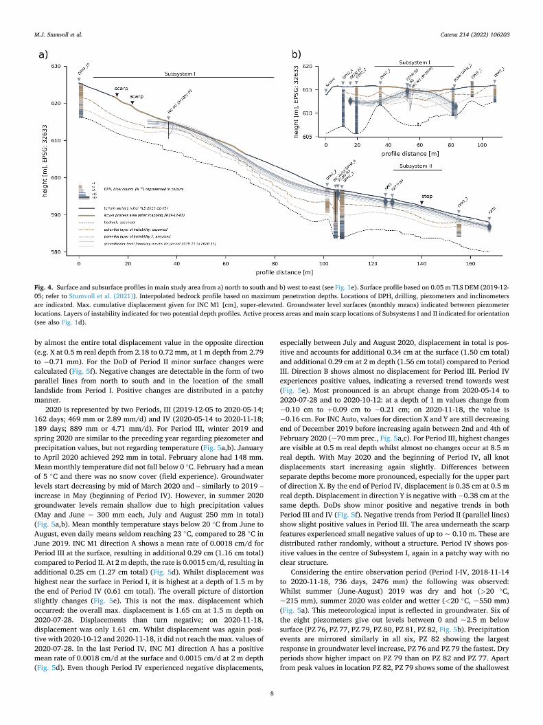
Fig. 4. Surface and subsurface profiles in main study area from a) north to south and b) west to east (see Fig. 1e). Surface profile based on 0.05 m TLS DEM (2019-12- 05; refer to Stumvoll et al. (2021)). Interpolated bedrock profile based on maximum penetration depths. Locations of DPH, drilling, piezometers and inclinometers are indicated. Max. cumulative displacement given for INC M1 [cm], super-elevated. Groundwater level surfaces (monthly means) indicated between piezometer locations. Layers of instability indicated for two potential depth profiles. Active process areas and main scarp locations of Subsystems I and II indicated for orientation (see also Fig. 1d).

M.J. Stumvoll et al.

Catena 214 (2022) 106203

9

levels of all piezometers. Shallowest levels (monthly mean) are reached in December 2018, May 2019 and February 2020 with <0.50 m, in January/February 2019 even with <0.20 m below ground, deepest in October 2019 (>1.96 m). Two of the eight piezometers (PZ 78 and PZ 84) show levels of 3.0 m below surface and deeper. Whilst PZ 78 fluc-tuated around a relatively stable value of 3.0 m throughout the year, PZ 84 shows the strongest decrease in groundwater level of all in dry pe-riods, almost reaching the sensor depth (~5.9 m) on 2019-12-13 (Fig. 5b). Inclinometer readings for INC M1 (21 measurements; 2018- 12-18 to 2020-11-18; 735 d) show a max. displacement for direction + A of 1.65 cm at 1.5 m depth on 2020-07-28 and of 1.61 cm on 2020-11-18. In direction B, max. displacement was − 0.71 cm at the

surface on 2019-12-05 and − 0.64 cm on 2020-11-18 (Fig. 5e, Period I- IV). Both directions combined roughly point towards south-southwest. INC Auto showed a displacement for direction X of +0.35 cm at 0.5 m depth and − 0.24 cm at 4 m depth by the end of Period IV (Fig. 5c, small figure). In direction Y, values are negative and account for − 0.38 cm at 0.5 m depth. Both directions together roughly point towards southwest. Considering the DoD between 2018-11-14 and 2020-11-18, surface changes with respect to the small landslide in Period I are clearly rec-ognisable, yet already smoothed out (Fig. 5f, Period I-IV). Positive values from Period IV are prominent in the centre. A line-like feature with positive values has become visible running from west to east. Positive values in the lower right part, partly also detectable in Period

Fig. 5. Spatio-temporal comparison of subsurface and surface data (2018-11-15 – 2020-11-18). a) Precipitation [mm] and temperature [◦C]. b) Groundwater level below surface [m]. c) Daily [mean] displacement of INC Auto for X and Y per knot (16; decreasing colour displays increasing depth of knots); overall consecutive [monthly mean] and final [thick] displacement in [mm]. d) Hypothetical rate of daily displacement [mm] for INC M1 direction A in 2 m depth based on total displacement between two consecutive measurements divided by time. e) Displacement for INC M1 [cm] for each and entire Period(s); final (2020-11-18) displacement indicated with thick blue line. e) DoDs Subsystem I, displayed as maximum height difference [m], excluding values from − 0.05 to + 0.05 (noise). DoDs I and II in e) from Stumvoll et al. (2021). For locations see Fig. 1. (For interpretation of the references to colour in this figure legend, the reader is referred to the web version of this article.)

M.J. Stumvoll et al.

Catena 214 (2022) 106203

10

III, have materialised more clearly. Patchy areas of positive values are recognizable in the entire area.

5. Discussion

5.1. Subsurface model: Implications on shear surfaces

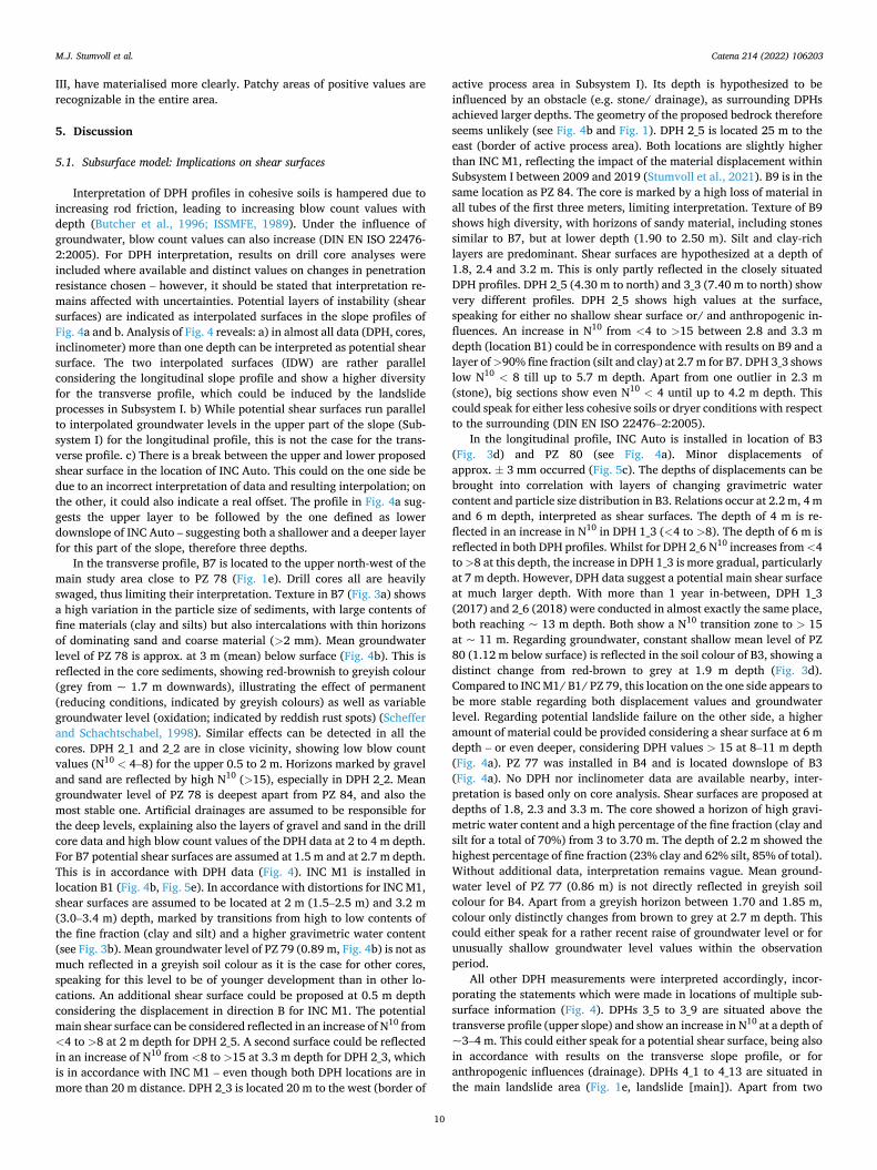
Interpretation of DPH profiles in cohesive soils is hampered due to increasing rod friction, leading to increasing blow count values with depth (Butcher et al., 1996; ISSMFE, 1989). Under the influence of groundwater, blow count values can also increase (DIN EN ISO 22476- 2:2005). For DPH interpretation, results on drill core analyses were included where available and distinct values on changes in penetration resistance chosen – however, it should be stated that interpretation re-mains affected with uncertainties. Potential layers of instability (shear surfaces) are indicated as interpolated surfaces in the slope profiles of Fig. 4a and b. Analysis of Fig. 4 reveals: a) in almost all data (DPH, cores, inclinometer) more than one depth can be interpreted as potential shear surface. The two interpolated surfaces (IDW) are rather parallel considering the longitudinal slope profile and show a higher diversity for the transverse profile, which could be induced by the landslide processes in Subsystem I. b) While potential shear surfaces run parallel to interpolated groundwater levels in the upper part of the slope (Sub-system I) for the longitudinal profile, this is not the case for the trans-verse profile. c) There is a break between the upper and lower proposed shear surface in the location of INC Auto. This could on the one side be due to an incorrect interpretation of data and resulting interpolation; on the other, it could also indicate a real offset. The profile in Fig. 4a sug-gests the upper layer to be followed by the one defined as lower downslope of INC Auto – suggesting both a shallower and a deeper layer for this part of the slope, therefore three depths.

In the transverse profile, B7 is located to the upper north-west of the main study area close to PZ 78 (Fig. 1e). Drill cores all are heavily swaged, thus limiting their interpretation. Texture in B7 (Fig. 3a) shows a high variation in the particle size of sediments, with large contents of fine materials (clay and silts) but also intercalations with thin horizons of dominating sand and coarse material (>2 mm). Mean groundwater level of PZ 78 is approx. at 3 m (mean) below surface (Fig. 4b). This is reflected in the core sediments, showing red-brownish to greyish colour (grey from ~ 1.7 m downwards), illustrating the effect of permanent (reducing conditions, indicated by greyish colours) as well as variable groundwater level (oxidation; indicated by reddish rust spots) (Scheffer and Schachtschabel, 1998). Similar effects can be detected in all the cores. DPH 2_1 and 2_2 are in close vicinity, showing low blow count values (N10 < 4–8) for the upper 0.5 to 2 m. Horizons marked by gravel and sand are reflected by high N10 (>15), especially in DPH 2_2. Mean groundwater level of PZ 78 is deepest apart from PZ 84, and also the most stable one. Artificial drainages are assumed to be responsible for the deep levels, explaining also the layers of gravel and sand in the drill core data and high blow count values of the DPH data at 2 to 4 m depth. For B7 potential shear surfaces are assumed at 1.5 m and at 2.7 m depth. This is in accordance with DPH data (Fig. 4). INC M1 is installed in location B1 (Fig. 4b, Fig. 5e). In accordance with distortions for INC M1, shear surfaces are assumed to be located at 2 m (1.5–2.5 m) and 3.2 m (3.0–3.4 m) depth, marked by transitions from high to low contents of the fine fraction (clay and silt) and a higher gravimetric water content (see Fig. 3b). Mean groundwater level of PZ 79 (0.89 m, Fig. 4b) is not as much reflected in a greyish soil colour as it is the case for other cores, speaking for this level to be of younger development than in other lo-cations. An additional shear surface could be proposed at 0.5 m depth considering the displacement in direction B for INC M1. The potential main shear surface can be considered reflected in an increase of N10 from <4 to >8 at 2 m depth for DPH 2_5. A second surface could be reflected in an increase of N10 from <8 to >15 at 3.3 m depth for DPH 2_3, which is in accordance with INC M1 – even though both DPH locations are in more than 20 m distance. DPH 2_3 is located 20 m to the west (border of

active process area in Subsystem I). Its depth is hypothesized to be influenced by an obstacle (e.g. stone/ drainage), as surrounding DPHs achieved larger depths. The geometry of the proposed bedrock therefore seems unlikely (see Fig. 4b and Fig. 1). DPH 2_5 is located 25 m to the east (border of active process area). Both locations are slightly higher than INC M1, reflecting the impact of the material displacement within Subsystem I between 2009 and 2019 (Stumvoll et al., 2021). B9 is in the same location as PZ 84. The core is marked by a high loss of material in all tubes of the first three meters, limiting interpretation. Texture of B9 shows high diversity, with horizons of sandy material, including stones similar to B7, but at lower depth (1.90 to 2.50 m). Silt and clay-rich layers are predominant. Shear surfaces are hypothesized at a depth of 1.8, 2.4 and 3.2 m. This is only partly reflected in the closely situated DPH profiles. DPH 2_5 (4.30 m to north) and 3_3 (7.40 m to north) show very different profiles. DPH 2_5 shows high values at the surface, speaking for either no shallow shear surface or/ and anthropogenic in-fluences. An increase in N10 from <4 to >15 between 2.8 and 3.3 m depth (location B1) could be in correspondence with results on B9 and a layer of >90% fine fraction (silt and clay) at 2.7 m for B7. DPH 3_3 shows low N10 < 8 till up to 5.7 m depth. Apart from one outlier in 2.3 m (stone), big sections show even N10 < 4 until up to 4.2 m depth. This could speak for either less cohesive soils or dryer conditions with respect to the surrounding (DIN EN ISO 22476–2:2005).

In the longitudinal profile, INC Auto is installed in location of B3 (Fig. 3d) and PZ 80 (see Fig. 4a). Minor displacements of approx. ± 3 mm occurred (Fig. 5c). The depths of displacements can be brought into correlation with layers of changing gravimetric water content and particle size distribution in B3. Relations occur at 2.2 m, 4 m and 6 m depth, interpreted as shear surfaces. The depth of 4 m is re-flected in an increase in N10 in DPH 1_3 (<4 to >8). The depth of 6 m is reflected in both DPH profiles. Whilst for DPH 2_6 N10 increases from <4 to >8 at this depth, the increase in DPH 1_3 is more gradual, particularly at 7 m depth. However, DPH data suggest a potential main shear surface at much larger depth. With more than 1 year in-between, DPH 1_3 (2017) and 2_6 (2018) were conducted in almost exactly the same place, both reaching ~ 13 m depth. Both show a N10 transition zone to > 15 at ~ 11 m. Regarding groundwater, constant shallow mean level of PZ 80 (1.12 m below surface) is reflected in the soil colour of B3, showing a distinct change from red-brown to grey at 1.9 m depth (Fig. 3d). Compared to INC M1/ B1/ PZ 79, this location on the one side appears to be more stable regarding both displacement values and groundwater level. Regarding potential landslide failure on the other side, a higher amount of material could be provided considering a shear surface at 6 m depth – or even deeper, considering DPH values > 15 at 8–11 m depth (Fig. 4a). PZ 77 was installed in B4 and is located downslope of B3 (Fig. 4a). No DPH nor inclinometer data are available nearby, inter-pretation is based only on core analysis. Shear surfaces are proposed at depths of 1.8, 2.3 and 3.3 m. The core showed a horizon of high gravi-metric water content and a high percentage of the fine fraction (clay and silt for a total of 70%) from 3 to 3.70 m. The depth of 2.2 m showed the highest percentage of fine fraction (23% clay and 62% silt, 85% of total). Without additional data, interpretation remains vague. Mean ground-water level of PZ 77 (0.86 m) is not directly reflected in greyish soil colour for B4. Apart from a greyish horizon between 1.70 and 1.85 m, colour only distinctly changes from brown to grey at 2.7 m depth. This could either speak for a rather recent raise of groundwater level or for unusually shallow groundwater level values within the observation period.

All other DPH measurements were interpreted accordingly, incor-porating the statements which were made in locations of multiple sub-surface information (Fig. 4). DPHs 3_5 to 3_9 are situated above the transverse profile (upper slope) and show an increase in N10 at a depth of ~3–4 m. This could either speak for a potential shear surface, being also in accordance with results on the transverse slope profile, or for anthropogenic influences (drainage). DPHs 4_1 to 4_13 are situated in the main landslide area (Fig. 1e, landslide [main]). Apart from two

M.J. Stumvoll et al.

Catena 214 (2022) 106203

11

outliers (~8 m) situated closest to DPHs 1_3 and 2_6, profiles only reached depths of ~2–3.5 m. A shallow transition zone was found for all profiles at 1.2 m (mean, 0.7–1.8 m), a second at 2.4 m depth. Consid-ering the entire main study area, the subsurface model is able to partly reflect the area affected by sliding in Subsystem I – both depletion and accumulation (Fig. 4a, see also Fig. 1d). Considering a shallow potential shear surface, the bulging area of Subsystem I is reflected by the inter-polated shear plane reaching the slope surface (to the east of longitu-dinal profile). Further downslope the model suggests more deeply situated shear surfaces. The location of INC Auto is reflected in a kind of depression, both regarding potential bedrock geometry as well as po-tential shear surfaces. It is theorised that ancient landslide material from the upper slope might have been accumulating in this area, filling up a depression given naturally by local geology. Further downslope the surface is less steep and depths of potential bedrock geometry and shear surfaces are shallower. Tracing the shear surfaces towards the main landslide area (west of INC Auto), the shallow interpolation partly reaches above ground. This reflects the areas where material has already been depleted by former landslide processes (2011/2013). The model is capable in representing a reasonable shear surface which is proposed for Subsystem II (Fig. 4a, location see Fig. 1d,e), even though there is only little direct information available in this area. The further away from locations of direct subsurface information, significance of interpolated subsurface layers decreases significantly.

5.2. Surface and sub-surface hydrology

Smoothing (0.2) used for Kriging interpolation resulted in smoothed groundwater level surfaces. Interpolations suggest levels to potentially reach the surface, which is an exaggeration and does not represent re-ality. On the other side, it illustrates the impact of shallow groundwater levels in the active area of Subsystem II, within parts of the main land-slide area, but especially at the location PZ 79 (see Fig. 4a,b) within Subsystem I. Surface hydrology suggests Subsystem I to experience increased surface runoff (Fig. 2), too. Whilst there is no actual surface water detectable in the field, Subsystem I can experience waterlogging. In periods of very high precipitation, sheet flow has even been recog-nized. Waterlogging and runoff in locations reached by interpolated surfaces within the main landslide could also be experienced during field work.

The impact of surface hydrology on landslide occurrence is rather related to shallow than to deep seated sliding, which is an over-simplification (Bogaard and Greco, 2016). Whilst deep rotational movements and re-activations are rather suggested to be influenced by seasonal to monthly water availability than by one precipitation event (Sidle and Ochiai, 2006; van Asch et al., 1999), groundwater levels rise faster in the case of near-saturated conditions. A concentration of water flow paths and the resulting water infiltration locally influences pore water pressure (c.f. Bogaard and Greco, 2016 and references therein). However, this also depends on the hydraulic conductivity of the sub-surface material. Groundwater fluctuations are smaller in materials of high hydraulic conductivity (sand/ gravel). In materials of low hydraulic conductivity (clay/ silt), groundwater levels thus may rise faster after precipitation. Boundaries of variable hydraulic conductivity can func-tion as barrier, locally decreasing shear strength and acting as landslide triggering mechanism (Flores Orozco et al., 2018; Gallistl et al., 2018; Uhlemann et al., 2017). Surficial water flow calculation in Fig. 2 can be interpreted in two directions: the DEMs used define the paths, but the paths too may influence landslides activity and the future surface. The 2009 ALS data was acquired prior to the landslide activities in 2011/ 2013, which led to a retrogression of the main landslide area (see Stumvoll et al., 2021). The connected landslide systems (Subsystem I and II) which became (more) active after these activities have developed in the pathways of calculated surficial water flow from 2009 (Fig. 2a). Surface runoff towards Subsystem II originates in an area mapped as dormant landslide (see figure Fig. 1d).

Spatio-temporal analysis of surface and subsurface data focussed first on Subsystem I. Monthly groundwater levels around PZ 78 (western border of Subsystem I) are the most stable ones of the entire study area (Fig. 4b). They are much deeper than for PZ 79 (centre) and fluctuate around values of 2.80–3.43 m below surface with a mean of 3.05 m. Surficial water flow suggest this area to experience increased surface runoff (Fig. 2). Deep and rather stable groundwater levels can probably be assumed to be related to artificial draining. High DPH penetration resistance (DPH 2_1 and 2_2) and laboratory analysis of core B7 (Fig. 3a) support this assumption. B7 showed a high percentage of coarse particle sizes (sand/ gravel) in depths between 3 and 3.5 m, including stones of almost 0.05 m in diameter (tube diameter). Surface morphology and DoD calculations suggest this area has been stable in the last ~10 years, refer to Fig. 5f and Stumvoll et al. (2021). In contrast, groundwater levels around PZ 79 in the centre of Subsystem I (see Fig. 4a,b) measured the shallowest values of all eight locations (Fig. 4b; Fig. 5b). They also show a high variation over season (between 0.10 and 2.12 m, mean: 0.89 m). The location is in correspondence with an area of a) high calculated surface runoff (Fig. 2), b) subsurface changes (INC M1: A + 1.61 cm at 1.5 m depth; B − 0.71 cm at 0 m, see Fig. 5d) and c) both marginal surface changes within the last 2 years (Fig. 5f) and known surface changes of bigger dimensions prior to that (refer to Fig. 1d, see Stumvoll et al. (2021)). Considering the depth assumed for the first (between 1.5 and 2.5 m) and second shear surface (between 3.0 and 3.4 m) (Fig. 3b, section 5.1) at location of INC M1, it is suggested, that the groundwater level measured for PZ 79 could be related to perched groundwater, locally confined by the shear surface(s) of Subsystem I (low hydraulic conductivity), as the piezometer sensor is installed in a depth of only ~3.3 m below surface. Actual groundwater level is probably deeper. Considering the increasing depths of potential shear surfaces towards north (Fig. 4a) and the extent of the active process area in Subsystem I (~50 m*50 m, see Fig. 1d and section 2), also a deeper max. shear surface is suggested. Sausgruber (2013) suggested a depth of ~12 m (section 2), which would be approx. the depth of the interpolated bedrock geometry (Fig. 4a). This has to be assessed with additional in-vestigations. In the area around PZ 84 (eastern border of Subsystem I), groundwater levels are even slightly deeper than for PZ 78 (between 2.71 and 5.22 m, mean: 3.48 m) – but fluctuates largely, sometimes reaching such low levels as to the sensor depth. Surface hydrology suggests this area to not being much affected by surface runoff (Fig. 2). Field work confirms the location to be relatively dry. DPHs close by show increasingly low penetration depths towards the east. Artificial drainage around the estate could cause this effect, also explaining, why groundwater level decreased so drastically here in summer 2019 (Fig. 5b), being drained and unsupported by surficial water. Drill core B9 suggests a clear transition from groundwater affected to non-affected soil at a depth of 3.5 m (Fig. 3c), marked by a transition from yellowish to grey colours. Similar to the area around PZ 78, DoD cal-culations depicted no distinct changes here in the past 10 years or within the last 2 years.

Further downslope groundwater levels range between 0.30 and 2.64 m below surface. Groundwater level is shallowest for PZ 82 (0.77 m), PZ 77 (0.86 m) and PZ 80 (1.11 m). The last two are situated close to INC Auto. The DPH location (2_7) used for the installation of PZ 82 showed low N10 (<4) – very similar to DPH 2_6 (Fig. 3d) – until reaching bedrock at ~ 6.5 m. Data depicts PZ 82 to reach the shallowest mean levels of the downslope piezometers. It shows the highest peaks in correlation with precipitation events (see Fig. 5b). As proposed by the interpolations, levels increase further downslope (Fig. 4a). Exaggerated levels are suggested to reach the surface in Subsystem II. At this point, a step feature is mapped (Subsystem II, Fig. 4a). This feature has been developing over the past 10 years (Stumvoll et al., 2021). The area downslope towards southwest is affected by sliding (Fig. 1d, landslide [active]), probably induced by malfunctioning drainages (Stumvoll et al., 2021). As supposed by the interpolation, landslide activity in this area might additionally be influenced by natural groundwater changes –

M.J. Stumvoll et al.

Catena 214 (2022) 106203

12

or exclusively. This and surface runoff (Fig. 2) lead to high water availability. Field work confirmed the area underneath the step feature to experience waterlogging, which is also reflected by local vegetation (sort of marsh grass). At location of PZ 76, situated furthest downslope, groundwater levels decrease again. This could partly be influenced by a drainage pipe, running underneath profile line A (see section 2 and Y- like formation in the DEM of Fig. 1d,e). Field work and, respectively or DoD calculations confirm this part of the slope to not being affected by high soil moisture and surface changes.

5.3. Surface and subsurface change detection

Considering the active process area in Subsystem I, small subsurface dynamics could be recorded with INC M1. With respect to the suggested direction of movement (A and B), south-southwest seems reasonable: it is the direction of the main landslide. Considering the rate for direction A at 2 m depth (refer to Fig. 5d) in comparison with precipitation (Fig. 5a) and changes in groundwater level (Fig. 5b), following aspects can be noticed: a) the rate between the first and second reading is highest, which is most probably due to the subsidence of the inclinom-eter pipe after installation (Mikkelsen, 2003; Stark and Choi, 2008); b) rates in January are low, which is most likely due to low temperature and snow cover; c) rates are highest in February and March, which might be due to snow melt and additional rainfall, being in accordance with general assumptions on this relation (c.f. Bogaard and Greco, 2016; Lacroix et al., 2020; Sidle and Ochiai, 2006; Uhlemann et al., 2016); d) rates are low or ~0 in periods of low or no precipitation, which

especially becomes evident in 2019 (June to November) and 2020 (end of March to May); e) there can be periods of “negative” movement rates, where displacements move in the opposite direction of a preceding period. They could be related to a rotation of the inclinometer casing in the vertical (rotation error, c.f. Stark and Choi, 2008).

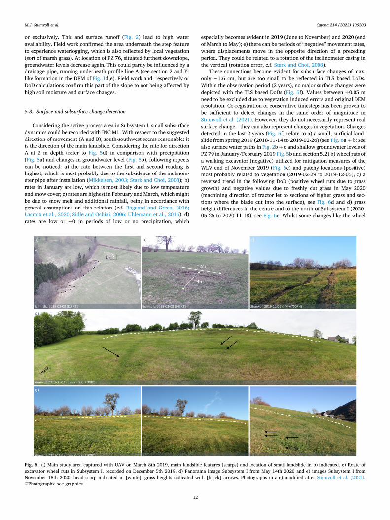
These connections become evident for subsurface changes of max. only ~1.6 cm, but are too small to be reflected in TLS based DoDs. Within the observation period (2 years), no major surface changes were depicted with the TLS based DoDs (Fig. 5f). Values between ±0.05 m need to be excluded due to vegetation induced errors and original DEM resolution. Co-registration of consecutive timesteps has been proven to be sufficient to detect changes in the same order of magnitude in Stumvoll et al. (2021). However, they do not necessarily represent real surface change – they can also represent changes in vegetation. Changes detected in the last 2 years (Fig. 5f) relate to a) a small, surficial land-slide from spring 2019 (2018-11-14 to 2019-02-26) (see Fig. 6a + b; see also surface water paths in Fig. 2b + c and shallow groundwater levels of PZ 79 in January/February 2019 Fig. 5b and section 5.2) b) wheel ruts of a walking excavator (negative) utilized for mitigation measures of the WLV end of November 2019 (Fig. 6c) and patchy locations (positive) most probably related to vegetation (2019-02-29 to 2019-12-05), c) a reversed trend in the following DoD (positive wheel ruts due to grass growth) and negative values due to freshly cut grass in May 2020 (machining direction of tractor let to sections of higher grass and sec-tions where the blade cut into the surface), see Fig. 6d and d) grass height differences in the centre and to the north of Subsystem I (2020- 05-25 to 2020-11-18), see Fig. 6e. Whilst some changes like the wheel

Fig. 6. a) Main study area captured with UAV on March 8th 2019, main landslide features (scarps) and location of small landslide in b) indicated. c) Route of excavator wheel ruts in Subsystem I, recorded on December 5th 2019. d) Panorama image Subsystem I from May 14th 2020 and e) images Subsystem I from November 18th 2020; head scarp indicated in [white], grass heights indicated with [black] arrows. Photographs in a-c) modified after Stumvoll et al. (2021). ©Photographs: see graphics.

M.J. Stumvoll et al.

Catena 214 (2022) 106203

13

ruts, do not get depicted when calculating a DoD for the entire obser-vation period (2018-11-14 to 2020-11-18), others become even more pronounced, like for example the diverse grass heights in the centre of Subsystem I: they are due to differing types of grass and newly sowed grass after trench digging in fall 2018.

INC Auto showed minor displacements of max. + 0.35 cm at 1 m depth and − 0.32 cm at 2 m depth for direction X and a max. of − 0.45 cm at 1.5 m depth for direction Y. Even though values are smaller than for INC M1, changes with respect to precipitation and groundwater are reflected in small deflections (see Fig. 5c). Displacements in direction X seem to be directed rather upslope in 2018 and 2019. These “negative” displacements could – similarly to INC M1 – be related to a rotation error; this needs further investigation in the future. The sudden shift for all knots of both X and Y on 28th of November 2019 at ~ 09:25 a.m. is not related to natural causes. The walking excavator of the WLV crossed INC M1 (explaining a sudden change of direction in the upper meters of both A and B between 2019-10-01 and 2019-12-05) and INC Auto. The wheel ruts are detectable in the DoD of Period II (Fig. 5f). Subsurface dynamics within the observation period were marginal, ranging in millimetres, which could also be related to measurement uncertainties (c.f. Mikkelsen, 2003). No distinct surface changes have been detected for the area around INC Auto within the last 10 (or 2) years.

6. Conclusion

In this study, surface and subsurface investigations have been con-ducted and respective data been analysed for a slow-moving, complex landslide in the Flysch Zone of Lower Austria. For an observation period of 2 years (2018-11 to 2020-11), data on hydro-meteorological param-eters (precipitation, temperature, groundwater), on geotechnical pa-rameters (DPH, drill core analysis, inclinometers) and on surface information (TLS based DEMs and DoDs) have been analysed and evaluated to assess a) the slopes subsurface structure, b) potential layers of instability (shear surfaces), c) relations on hydro-meteorological and geotechnical parameters and interrelations with respect to landslide processes and d) relations on surface and subsurface dynamics.

Following main conclusions can be drawn by evaluating the results obtained in this study:

• Bedrock depth and geometry can be reasonably computed with maximum depths of DPH data. The thickness of the regolith cover decreases relatively in areas of recent and former process activity (Subsystem I and main landslide area only ~6 to 2 m) compared to stable areas (up to ~13 m).

• Drill core analyses depict the fine fraction to make up more than ~60% in most samples, with layers of more than 80% clay and silt possible. These could function as shear surfaces due to low hydraulic conductivity of the respective material and were included in shear surface interpolation.

• Interpolated shear surfaces are highly simplified, but depict relations to locations of known activity (Subsystem I + II/ main landslide). (Still) stable areas depict deeper potential shear planes.

• Locations of shallowest groundwater levels and largest fluctuations correspond with areas of recent minor dynamics (2018–2020) and former larger dynamics (2009–2018/19). Perched groundwater ta-bles, confined by clay-rich layers, could be the cause for shallow levels, especially in Subsystem I.

• Surface hydrology (flow paths) is supposed to have a high, locally confined impact on the groundwater body, increasing water infil-tration and influencing pore water pressure. Piezometers not in the paths of calculated flow accumulation did not show such high vari-ations or fast responses on precipitation events as those that are.

• Considering inclinometer displacement rates and hydro- meteorological input data, it was found that a) rates in January are low (low temperature/ snow cover), b) rates are highest in February

and March (snow melt/ additional rainfall) and c) rates are low or ~ 0 in periods of low or none precipitation, which is all in good accordance with general assumptions on these interrelations and d) “negative” rates can occur, most probably related to a rotation error of the casing.

• Process magnitudes captured with inclinometer data were too small to be mirrored in surface changes. TLS based DoDs did not show any distinct changes within the 2 years (2018–2020) for one of the recently most active process areas (Subsystem I; 2009–2018/19). High-resolution surface change detection for example based on TLS needs to be combined with for example inclinometer data to detect both subtle subsurface movements for single locations and events of higher magnitude on larger spatial scale. Both need to be evaluated on an elongated temporal scale, hence confirming the need for long- term multi-parameter monitoring.

Evaluation of direct subsurface data, for example DPH and drill cores, remains subjective. Short-term observations can give “false” re-sults on landslide dynamics. Without in-depth knowledge about study areas disposition and process history, a temporal classification of recent, short-term behaviour is hampered. It remains a short glimpse into the spatio-temporal complexity of the respective landslide. Nevertheless, data shows specific relations, for example the impact of hydro- meteorological conditions on subsurface displacements visualized with inclinometer data. The study area and results found can be received as being characteristic for other watersheds and areas affected by land-slides of similar conditions close by and in other regions of the Flysch Zone. It also highlights the need for long-term data series to further assess such complex landslide dynamics.

In a next step, data is to be analysed in a more detailed temporal resolution to assess suggestions concerning potential landslide activa-tion. To evaluate the validity of the subsurface model proposed here, including bedrock depth and geometry, potential layers of instability and groundwater level depths, geophysical methods (ERT, magnetic induction, seismic) have been applied in the study area and are subject of present research.

Declaration of Competing Interest

The authors declare that they have no known competing financial interests or personal relationships that could have appeared to influence the work reported in this paper.

Acknowledgements

The authors express their gratitude to the Federal State Government of Lower Austria, especially Joachim Schweigl and Michael Bertagnoli for data provisioning and project support (NoeSLIDE), and the Torrent and Avalanche Control Lower Austria West, especially Eduard Kotz-maier, for providing internal reports, additional information and project support (MillSLIDE). The authors further kindly thank the land owners, particularly Johannes Oberbramberger for his enthusiastic support of and interest in our work as well as Christian and Rosa Hornbachner. Sincere thanks to the colleagues of the ENGAGE working group at the University of Vienna, especially William Ries, Nina Marlovits, Stefan Haselberger, Hannah Schechtner and Katalin Gillemot as well as to all students involved in field work.

References

Auer, I., et al., 2007. HISTALP—historical instrumental climatological surface time series of the Greater Alpine Region. Int. J. Climatol. 27, 17–46.

Baum, R.L., Messerich, J., Fleming, R.W., 1998. Surface deformation as a guide to kinematics and three-dimensional shape of slow-moving, clay-rich landslides, Honolulu, Hawaii. Environ. Eng. Geosci. 4, 283–306.

Besl, P.J., McKay, N.D., 1992. A method for registration of 3-D shapes. IEEE Trans. Pattern Anal. Mach. Intell. 14, 239–256.

M.J. Stumvoll et al.

Catena 214 (2022) 106203

14

Bievre, G., Joseph, A., Bertrand, C., 2018. Preferential water infiltration path in a slow- moving clayey earthslide evidenced by cross-correlation of hydrometeorological time series (Charlaix Landslide, French Western Alps). Geofluids 2018, 9593267.

BMDW, 2015. Digital elevation model (DEM) based on airborne laserscan data of the austrian federal states; raster resolution 10m. in: Bundesministerium für Digitalisierung und Wirtschaftsstandort (BMDW) - geoland.at (Ed.). data.gv.at (Open Data Osterreich) Austria.

Bogaard, T.A., Greco, R., 2016. Landslide hydrology: from hydrology to pore pressure. WIREs Water 3, 439–459.

Brunsden, D., 2001. A critical assessment of the sensitivity concept in geomorphology. Catena 42, 99–123.

Brunsden, D., Thornes, J.B., 1979. Landscape sensitivity and change. Trans. Inst. Brit. Geogr. 463–484.

Bull, W.B., 1991. Geomorphic Responses to Climatic Change. Oxford University Press, New York, Oxford.

Butcher, A.P., McElmeel, K., Powell, J.J.M., 1996. In: Dynamic probing and its use in clay soils, Advances in site investigation practice. Thomas Telford Publishing, London, England, pp. 383–395.

Caine, N., 1980. The rainfall intensity-duration control of shallow landslides and debris flows. Geografiska Annaler, Series A 62, 23–27.

Chae, B.-G., Park, H.-J., Catani, F., Simoni, A., Berti, M., 2017. Landslide prediction, monitoring and early warning: a concise review of state-of-the-art. Geosci. J. 21, 1033–1070.

Crozier, M.J., 1986. Landslides: Causes, Consequences and Environment. Croom Helm, London.

Crozier, M.J., 1999. Prediction of rainfall-triggered landslides: A test of the antecedent water status model. Earth Surf. Proc. Land. 24, 825–833.

Crozier, M.J., 2010a. Deciphering the effect of climate change on landslide activity: A review. Geomorphology 124, 260–267.

Crozier, M.J., 2010b. Landslide geomorphology: An argument for recognition, with examples from New Zealand. Geomorphology 120, 3–15.

Cruden, D.M., Varnes, D.J., 1996. Landslide types and processes. In: Turner, A.K., Schuster, R.L. (Eds.), Landslides: investigation and mitigation. National Academey Press, Washington, D.C., pp. 36–75

D’Amato Avanzi, G., Galanti, Y., Giannecchini, R., Lo Presti, D., Puccinelli, A., 2013. Estimation of soil properties of shallow landslide source areas by dynamic penetration tests: first outcomes from Northern Tuscany (Italy). Bull. Eng. Geol. Environ. 72, 609–624.

De Boer, D.H., 1992. Hierarchies and spatial scale in process geomorphology: a review. Geomorphology 4, 303–318.

Flores Orozco, A., Bücker, M., Steiner, M., Malet, J.-P., 2018. Complex-conductivity imaging for the understanding of landslide architecture. Eng. Geol. 243, 241–252.

Gallistl, J., et al., 2018. Delineation of subsurface variability in clay-rich landslides through spectral induced polarization imaging and electromagnetic methods. Eng. Geol. 245, 292–308.

Gariano, S.L., Guzzetti, F., 2016. Landslides in a changing climate. Earth Sci. Rev. 162, 227–252.

Geokon, 2018. Instruction Manual Model 4500 Series Vibrating Wire Piezometer. New Hampshire, Geokon Trusted Measurements, USA, p. 40.

Geokon, 2020. Datasheet VM Piezometers & Pressure Transducers. New Hampshire, Geokon Trusted Measurements, USA, p. 4.

Giordan, D., Hayakawa, Y., Nex, F., Remondino, F., Tarolli, P., 2018. Review article: the use of remotely piloted aircraft systems (RPASs) for natural hazards monitoring and management. Nat. Hazards Earth Syst. Sci. 18, 1079–1096.

Glade, T., Anderson, M.G., Crozier, M.J., 2005. Landslide Hazard and Risk. Wiley, Chichester.

Glade, T., Crozier, M.J., 2005. The nature of landslide hazard impact. In: Glade, T., Anderson, M.G., Crozier, M.J. (Eds.), Landslide Hazard and Risk. Wiley, Chichester, pp. 43–74.

Glotzl, 2016. Datasheet Neigungsmessrohre ABS 50, ABS 74, PVC 60, ALU 48. GLOTZL Gesellschaft für Baumesstechnik mbH, Deutschland, Rheinstetten, pp. 2.

Glotzl, 2019. Datasheet NMGD Vertikalneigungsmesser. GLOTZL Gesellschaft für Baumesstechnik mbH, Deutschland, Rheinstetten, pp. 1.

Guzzetti, F., Peruccacci, S., Rossi, M., Stark, C.P., 2007. Rainfall thresholds for the initiation of landslides in central and southern Europe. Meteorol. Atmos. Phys. 98, 239–267.

Hornbachner, R.C., 2020-08-19. Personal communication. In: Stumvoll, M.J. (Ed.), Konradsheim, Waidhofen a.d. Ybbs, Austria.

Hunter, J.D., 2007. Matplotlib: a 2D graphics environment. Comput. Sci. Eng. 9, 90–95. ISSMFE, 1989. Report of the ISSMFE Technical Committee on Penetration Testing of

Soils - TC 16 with Reference Test Procedures CPT-SPT-DP-WST, International Society for Soil Mechanics and Foundation Engineering (ISSMFE). Swedish Geotechnical Institute, Sweden.

Jaboyedoff, M., et al., 2009. Use of terrestrial laser scanning for the characterization of retrogressive landslides in sensitive clay and rotational landslides in river banks. Can. Geotech. J. 46, 1379+.

Jaboyedoff, M., et al., 2012. Use of LIDAR in landslide investigations: a review. Nat. Hazards 61, 5–28.

Kotzmaier, E., 2013. Aktenvermerk Krojer Rutschung (Hofermühle) 03.05.2013, Wildbach und Lawinenverbauung Niederosterreich West, Melk, Austria.

Lacroix, P., Handwerger, A.L., Bievre, G., 2020. Life and death of slow-moving landslides. Nat. Rev. Earth Environ. 1, 404–419.

McColl, S.T., 2015. Chapter 2 - landslide causes and triggers. In: Shroder, J.F., Davies, T. (Eds.), Landslide Hazards, Risks and Disasters. Academic Press, Boston, pp. 17–42.

Measurand, 2019. Datasheet SAAF Model 003. Measurand, Kanada, New Brunswick, p. 6.

Mikkelsen, N., 2003. Advances in Inclinometer Data Analysis. In: Myrvoll, F. (Ed.), Proceedings of the 6th International Symposium on Field Measurements in Geomechanics, Oslo, Norway, 23–26 September.

NOEL GV, 2009. Digital elevation model (DEM) based on airborne laserscan data; raster resolution 1m. In: Department for Hydrology and Geoinformation. Federal State Government of Lower Austria (Ed.), St. Polten, Lower Austria.

NOEL GV, 2011. Digital orthophoto (2011-04-09). In: Department for Hydrology and Geoinformation. Federal State Government of Lower Austria (Ed.), St. Polten, Lower Austria.

Ohmer, M., Liesch, T., Goeppert, N., Goldscheider, N., 2017. On the optimal selection of interpolation methods for groundwater contouring: An example of propagation of uncertainty regarding inter-aquifer exchange. Adv. Water Resour. 109, 121–132.

Oliphant, T.E., 2015. Guide to NumPy, second ed. CreateSpace Independent Publishing Platform.

Papathoma-Kohle, M., Glade, T., 2013. The role of vegetation cover change for landslide hazard and risk. In: Renaud, G., Sudmeier-Rieux, K., Estrella, M. (Eds.), The Role of Ecosystems in Disaster Risk Reduction. UNU-Press, Tokyo, pp. 293–320.

Petschko, H., Bell, R., Leopold, P., Heiss, G., Glade, T., 2013. Landslide Inventories for Reliable Susceptibility Maps in Lower Austria. In: Margottini, C., Canuti, P., Sassa, K. (Eds.), Landslide Science and Practice: Volume 1: Landslide Inventory and Susceptibility and Hazard Zoning. Springer, Berlin Heidelberg, Berlin, Heidelberg, pp. 281–286.

Petschko, H., Brenning, A., Bell, R., Goetz, J., Glade, T., 2014. Assessing the quality of landslide susceptibility maps - case study Lower Austria. Nat. Hazards Earth Syst. Sci. 14, 95–118.

Phillips, J.D., 1992. The end of equilibrium. Geomorphology 5, 195–201. Phillips, J.D., 2003. Sources of nonlinearity and complexity in geomorphic systems. Prog.

Phys. Geogr. 27, 1–23. Phillips, J.D., 2006. Evolutionary geomorphology: thresholds and nonlinearity in

landform response to environmental change. Hydrol. Earth Syst. Sci. 10, 731–742. Prokop, A., Panholzer, H., 2009. Assessing the capability of terrestrial laser scanning for

monitoring slow moving landslides. Nat. Hazards Earth Syst. Sci. (NHESS) 9, 1921–1928.

Qin, C., et al., 2007. An adaptive approach to selecting a flow partition exponent for a multiple flow direction algorithm. Int. J. Geogr. Inf. Sci. 21, 443–458.

Riegl, L.M.S., 2020. Datasheet RIEGL VZ-6000. Riegl Laser Measurement Systems GmbH, Austria, Horn.

Rogers, J.D., Chung, J., 2017. A review of conventional techniques for subsurface characterization of landslides. Environ. Earth Sci. 76, 120.

Samia, J., et al., 2017. Do landslides follow landslides? Insights in path dependency from a multi-temporal landslide inventory. Landslides 14, 547–558.

Sausgruber, T., 2013. Hofermühlrutschung Waidhofen/ Ybbs (intern). Mit zwei Anhangen (Kartierung), Forsttechnischer Dienst für Wildbach und Lawinenverbauung. Geologische Stelle, Innsbruck, Austria.

Sausgruber, T., 2016. Protokoll zum Lokalaugenschein Hangprozess Hofermühle / Hofermühlrutschung. Forsttechnischer Dienst für Wildbach und Lawinenverbauung. Geologische Stelle, Innsbruck, Austria, Mit einem Anhang (Kartierung).

Scaioni, M., Longoni, L., Melillo, V., Papini, M., 2014. Remote sensing for landslide investigations: an overview of recent achievements and perspectives. Remote Sensing 6, 9600–9652.

Scheffer, P., Schachtschabel, P., 1998. Lehrbuch der Bodenkunde, 14 ed. Enke, Stuttgart. Schmaltz, E.M., Steger, S., Glade, T., 2017. The influence of forest cover on landslide

occurrence explored with spatio-temporal information. Geomorphology. Schnabel, W., 1980. Die Geologie des Voralpengebietes im Abschnitt Waidhofen an der

Ybbs - Ybbsitz - Gresten. Waidhofner Heimatblatter. Musealverein Waidhofen an der Ybbs, Waidhofen, Ybbs, pp. 13–27.

Schnabel, W., 1999. The Flysch Zone of the Eastern Alps. In: Mandl, G.W. (Ed.), FOREGS ’99 <Vienna>, Field trip guide Vienna - Dachstein - Hallstatt - Salzkammergut (UNESCO World Heritage Area), August 30th - September 2nd, 1999: 150 Years Geological Survey of Austria. Verlag der Geologischen Bundesanstalt (GBA), Wien, pp. 27–35.

Schnabel, W., et al., 2002. Geologische Karte von Niederosterreich 1:200.000. Geologische Bundesanstalt, Wien, Osterreich.

Schulz, W.H., McKenna, J.P., Kibler, J.D., Biavati, G., 2009. Relations between hydrology and velocity of a continuously moving landslide—evidence of pore-pressure feedback regulating landslide motion? Landslides 6, 181–190.

Schumm, S.A., 1979. Geomorphic thresholds: the concept and its applications. Trans. Inst. Brit. Geogr. (New Series) 4, 485–515.

Schweigl, J., Hervas, J., 2009. Landslide Mapping in Austria, European Commission OPOCE, Luxembourg: Office for Official Publications of the European Communities.

Schwenk, H., 1992. Massenbewegungen in Niederosterreich 1953–1990. Jahrb. Geol. Bundesanst. 135, 597–660.

Sidle, R.C., Bogaard, T.A., 2016. Dynamic earth system and ecological controls of rainfall-initiated landslides. Earth Sci. Rev. 159, 275–291.

Sidle, R.C., Ochiai, H., 2006. Landslides: Processes, Prediction, and Land Use. American Geophysical Union, Washington, DC.

Sidle, R.C., et al., 2006. Erosion processes in steep terrain–Truths, myths, and uncertainties related to forest management in Southeast Asia. For. Ecol. Manage. 224, 199–225.

Stark, T.D., Choi, H., 2008. Slope inclinometers for landslides. Landslides 5, 339. Steger, S., Schmaltz, E., Seijmonsbergen, A.C., Glade, T., 2020. The Walgau – a landscape

shaped by landslides. In: Embleton-Hamann, C. (Ed.), Landscapes and Landforms of Austria, World Geomorphological Landscapes. Springer (accepted).

Stumvoll, M.J., et al., 2020. The “Salcher” landslide observatory—experimental long- term monitoring in the Flysch Zone of Lower Austria. Bull. Eng. Geol. Environ. 79, 1831–1848.

M.J. Stumvoll et al.

Catena 214 (2022) 106203

15

Stumvoll, M.J., Schmaltz, E.M., Glade, T., 2021. Dynamic characterization of a slow- moving landslide system – Assessing the challenges of small process scales utilizing multi-temporal TLS data. Geomorphology 389, 107803.

Telling, J., Lyda, A., Hartzell, P., Glennie, C., 2017. Review of Earth science research using terrestrial laser scanning. Earth Sci. Rev. 169, 35–68.

The Pandas Development Team, 2020. pandas-dev/pandas: Pandas, latest. Zenodo. Thenius, E., 1974. Geologie der osterreichischen Bundeslander in kurzgefaßten

Einzeldarstellungen. Niederosterreich, Geologische Bundesanstalt, Wien, Osterreich. Tilch, N., 2014. Identifizierung gravitativer Massenbewegungen mittles multitemporaler

Luftbildauswertung in Vorarlberg und angrenzender Gebiete. Jahrbuch der Kaiserlich-Koniglichen Geologischen Bundesanstalt 154, 21–39.

Uhlemann, S., et al., 2017. Four-dimensional imaging of moisture dynamics during landslide reactivation. J. Geophys. Res. Earth Surf. 122, 398–418.

Uhlemann, S., et al., 2016. Assessment of ground-based monitoring techniques applied to landslide investigations. Geomorphology 253, 438–451.

van Asch, T.W.J., Buma, J., Van Beek, L.P.H., 1999. A view on some hydrological triggering systems in landslides. Geomorphology 30, 25–32.

van Asch, T.W.J., Hendriks, M.R., Hessel, R., Rappange, F.E., 1996. Hydrological triggering conditions of landslides in varved clays in the French Alps. Eng. Geol. 42, 239–251.

van Asch, T.W.J., Van Beek, L.P.H., Bogaard, T.A., 2007. Problems in predicting the mobility of slow-moving landslides. Eng. Geol. 91, 46–55.

Wieczorek, G.F., Guzzetti, F., 2000. A review of rainfall thresholds for triggering landslides. In: Mediterranean Storms - Proceedings of the EGS Plinius Conference, Maratea, Italy, October 1999, pp. 407–414.

Weber, L., 1997. Flachendeckende Beschreibung der Geologie von Osterreich 1:500.000 im Vektorformat. Exzerpt (Basiskarte Geologie) aus der Metallogenetischen Karte von Osterreich 1:500.000. Geologische Bundesanstalt, Wien, Osterreich.

WP/WLI, 1994. A suggested method for describing the causes of a landslide. Bull. Int. Assoc. Eng. Geol. 50, 71–74.

M.J. Stumvoll et al.