Projecting Rates of Spread for Invasive Species

Risk Analysis, Vol. 24, No. 4, 2004

Projecting Rates of Spread for Invasive Species

Michael G. Neubert1∗ and Ingrid M. Parker2

All else being equal, the faster an invading species spreads, the more dangerous its invasion.The projection of spread rate therefore ought to be a central part of the determination ofinvasion risk. Originally formulated in the 1970s to describe the spatial spread of advantageousalleles, integrodifference equation (IDE) models have since been co-opted by populationbiologists to describe the spread of populations. More recently, they have been modified toinclude population structure and environmental variability. We review how IDE models areformulated, how they are parameterized, and how they can be analyzed to project spread ratesand the sensitivity of those rates to changes in model parameters. For illustrative purposes, weapply these models to Cytisus scoparius, a large shrub in the legume family that is considereda noxious invasive species in eastern and western North America, Chile, Australia, and NewZealand.

KEY WORDS: Cytisus scoparius; demography; integrodifference equations; invasion rates; matrixmodels; nonnative; spread

1. INTRODUCTION

The invasion of nonindigenous species is now con-sidered to be one of the most serious problems fac-ing native ecosystems,(1) and invaders have receivedincreasing attention for their considerable economicand social impacts.(2,3) National governments have re-sponded with demands for more effective nationaland regional policies to combat the introduction andspread of harmful invaders.(2,4) Such policies, how-ever, are likely to come with significant costs. Reg-ulations on interstate and international trade, quar-antine and inspection services at state borders, andgovernment-sponsored eradication programs are allexamples of programs that could reduce the negativeeffects of introduced species, but will be costly. To be

1 Biology Department, MS 34, Woods Hole Oceanographic Insti-tution, Woods Hole, MA 02543, USA.

2 Department of Ecology and Evolutionary Biology, University ofCalifornia at Santa Cruz, Santa Cruz, CA 95064, USA.

∗ Address correspondence to Michael G. Neubert, Biology De-partment, MS 34, Woods Hole Oceanographic Institution, WoodsHole, MA 02543, USA; [email protected].

justifiable, policy actions for exotic species should bebased on explicit assessments of risks.(5,6)

At the local level, managers of protected nat-ural landscapes are faced every day with decisionsabout which invasive species to control with limitedfunds. Most nature reserves have significant prob-lems caused by more than one, and sometimes many,problematic nonindigenous species.(7) Often, deci-sions about which species to eradicate or control aremade on an ad hoc basis, in part based on the totalcurrent acreage of a species and therefore its visibility.While this decision-making process can seem idiosyn-cratic, some attempts have been made to develop sys-tematic procedures.(8) Under the best circumstances,decisions on how to allocate resources to nonnativespecies management should be based on a risk analy-sis that evaluates the potential for long-term, negativeeffects on natural ecosystems, including populationsof native species.

Such an analysis needs to consider several fac-tors. First is the projected effect of the species overthe whole protected landscape, which requires know-ing the likelihood that a species will invade different

817 0272-4332/04/0100-0817$22.00/1 C© 2004 Society for Risk Analysis

818 Neubert and Parker

types of habitats. Second is the actual response of theecosystem to the presence of sustained populationsof the invader, which will be a function of the species’density as well as its per-capita effects.(9) Introducedspecies can have effects at the individual level (e.g.,by changing the behavior or size of native species), atthe population level (e.g., by changing the abundanceor extinction risk of native populations), at the com-munity level (by affecting diversity or composition),and at the ecosystem level (by altering functions suchas carbon storage or hydrology).

At least initially, the costs associated with each ofthese effects will grow with time as the invader occu-pies new habitat. If costs are proportional to the areaoccupied,(9) these costs will grow at a rate propor-tional to the invasion rate—the rate at which the in-vader spreads through the habitat. Remediation andremoval costs will also increase with the area occu-pied, and may increase with the amount of time a sitehas been invaded.(10) Thus a projection of invasionrate is a crucial element of a cost-benefit analysis. Thehigher the projected invasion rate, the more quicklycosts will accumulate, and the more expensive inac-tion becomes.

In this article, we describe the use of various popu-lation models for projecting the spread of an invasivespecies. We begin, in Section 2, with a brief reviewof the classic approach to the problem using Fisher’sequation, and then summarize the shortcomings ofthis approach. We then describe the formulation ofintegrodifference equation (IDE) models for popu-lation growth and dispersal.(11,12) Rather than jump-ing directly to the most general model, we will buildfrom the simplest case and develop examples alongthe way. In Section 3.1, we construct scalar IDEs that,while treating all individuals as identical in their vitaland dispersal rates, allow for a very flexible descrip-tion of dispersal. We review how to calculate invasionrates for these models in Section 3.2. In Section 3.3, wedescribe how to incorporate dispersal data into IDEmodels, and investigate the effects of environmentalvariability in Section 3.4. In Section 3.5, we constructintegrodifference matrix population (IMP) modelsthat allow us to specify stage-specific vital rates anddispersal distributions. Finally, in Section 4, we endwith a discussion of potential uses and misuses of ourapproach.

1.1. Cytisus scoparius

To illustrate the use of IDE and IMP models, wewill apply them to the invasive plant Cytisus scoparius

(Scotch broom or broom). Broom is a large shrub inthe legume family. Native to Europe and the BritishIsles, it has been introduced into many regions whereit is considered a noxious invasive species, includingeastern and western North America, Chile, Australia,and New Zealand.(13–15) The economic importance ofbroom is tied to its aggressive invasion of pastures, re-forested areas, and roadsides.(13,16) Although a com-prehensive study of its economic impact has not beendone, over $220,000 per year is spent to control broomalong roadsides in the State of Oregon alone.(16) Asidefrom economic factors, broom is also a conservationthreat. Thick stands of broom have eliminated nativeherbs and tree seedlings in Australia(17) and reducednative plant diversity in prairies of the Pacific North-west.(18) Ecosystem effects of broom include an in-crease in carbon and nitrogen pools and a dramaticincrease in nitrogen availability.(19)

The population dynamics and dispersal of broomwere studied in Washington State, USA, where theplant invades both anthropogenically disturbed ur-ban fields and relatively undisturbed glacial outwashprairies.(18,20) Broom has two dispersal mechanisms.First, pods dry out and burst, ballistically dispersingseeds. Second, seeds are attached to elaiosomes (lipid-rich bodies), which are attractive to ants. Ants carryseeds toward or into their nests, then remove the elaio-some and discard the seed.(21) Strong density depen-dence results in significant variation in demographicrates from the edge to the center of a broom infes-tation.(20) Demographic rates also vary among sites;population growth is more rapid in prairies than ur-ban fields. For this article, we will use demographicparameters estimated at the expanding edge of oneurban population in Discovery Park, Seattle.(20)

2. FISHER’S EQUATION

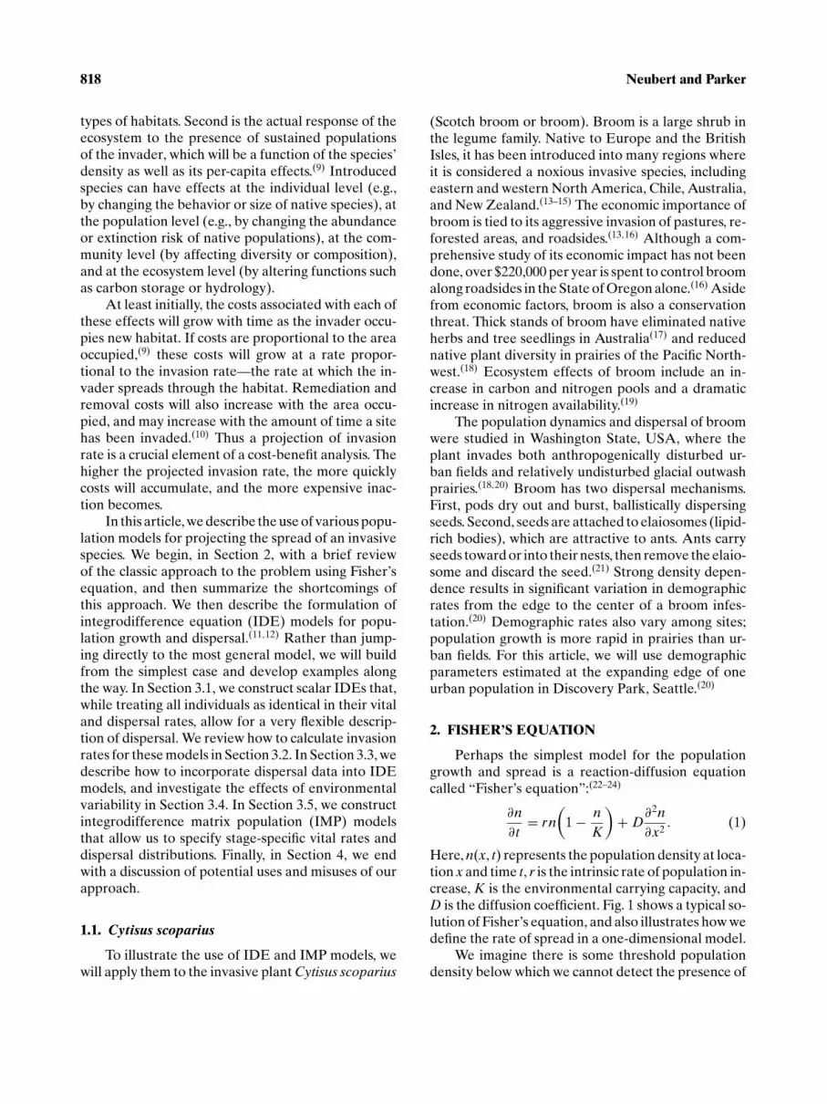
Perhaps the simplest model for the populationgrowth and spread is a reaction-diffusion equationcalled “Fisher’s equation”:(22–24)

∂n∂t

= rn(

1 − nK

)+ D

∂2n∂x2

. (1)

Here, n(x, t) represents the population density at loca-tion x and time t, r is the intrinsic rate of population in-crease, K is the environmental carrying capacity, andD is the diffusion coefficient. Fig. 1 shows a typical so-lution of Fisher’s equation, and also illustrates how wedefine the rate of spread in a one-dimensional model.

We imagine there is some threshold populationdensity below which we cannot detect the presence of

Projecting Rates of Spread for Invasive Species 819

-50 -40 -30 -20 -10 0 10 20 30 40 500

0.2

0.4

0.6

0.8

1

space ( x )

popu

lati

on d

ensi

ty (

n )

0 5 10 15 20-50

-40

-30

-20

-10

0

10

20

30

40

50

time ( t )

spac

e (

x )

(a) (b)

0

5

10

15

20

Fig. 1. A typical solution of Fisher’sequation exhibits the essential dynamicof an invasion: population growth andspread. For this simulation, we set r = D= 1. In (a) we plot the solution at t = 0, 5,10, 15, 20. In (b), the gray area marks theregion in space where the population sizeis larger than 0.1. The boundaries of thisarea have slopes equal to the rate ofspread, c = 2

√r D = 2.

the population. We call this threshold density n, andwe use x(t) for the location where the population den-sity equals n. The asymptotic rate of spread is definedas the rate of increase of x(t) as t becomes large:

c = limt→∞

dx(t)dt

. (2)

For Equation (1),

c = 2√

rD (3)

(see References 25 and 26).Fisher’s equation has been used to study the rates

of spread of a wide variety of invasive species.(27,28)

There are, however, a number of shortcomings withthe model that make a different approach, which wedescribe in the next section, more appealing. The firstshortcoming is that Fisher’s equation assumes diffu-sive movement; i.e., it assumes that the distributionof dispersal distances is normal. This is rarely true.In fact, there are a wide variety of measured distribu-tions and many of these are leptokurtic,(29) being morepeaked about their mode and having fatter tails than anormal distribution with the same variance. Second, itassumes that the individuals within the population areidentical in both their vital rates and in their propen-sity for dispersal. Again, this is rarely true. Vital ratesand dispersal rates are usually strongly determinedby the stage of the individual within the life cycle. Forexample, seeds are dispersed and typically suffer highmortality rates, while mature plants do not dispersebut have relatively low mortality rates.

IDE models address some of the shortcomingsof Fisher’s equation. In the next sections we describethe formulation of these models.(11,12) We build fromrelatively simple to more complex cases, using broomto illustrate each formulation.

3. INTEGRODIFFERENCEEQUATION MODELS

3.1. Scalar Models

We begin by considering a population of a singlespecies composed of identical individuals distributedalong an infinite one-dimensional habitat. We imag-ine that the change in population density from onetime to the next is the result of two processes: popula-tion growth and dispersal. We assume that these pro-cesses act sequentially. First, population growth actsto change local population density via the function

n(y, t + 1) = f [n(y, t)]. (4)

Then, dispersal acts to spatially redistribute individu-als. If the probability of dispersing from location y tolocation x is given by the probability density functionk(x, y), then after dispersal the population density isgiven by the IDE(11)

n(x, t + 1) =∫ ∞

−∞k(x, y) f [n(y, t)] dy. (5)

If, in addition, the probability of moving from pointy to point x only depends upon the relative locationsof the two points, then k(x, y) = k(x − y), and Equa-tion (5) becomes

n(x, t + 1) =∫ ∞

−∞k(x − y) f [n(y, t)] dy. (6)

Because the integral in Equation (6) is a convolutionintegral, this model is easier to analyze and to numer-ically simulate than Equation (5).(30)

3.2. Rates of Spread

Solutions to the IDE Equation (6) on an infinitedomain are often qualitatively similar to solutions to


the reaction-diffusion Equation (1). In fact, the ratesof spread they generate can be made quantitativelyequivalent(31) by using a normal distribution for k, anda compensatory growth function for f . With the rightparameters, we would then exactly duplicate Fig. 1b,using Equation (6).

As long as the population can grow when small(i.e., λ = f ′(0) > 1) and increased density has a nega-tive effect on vital rates (i.e., λn > f (n) for all n), thena population initially restricted to a finite portion ofspace grows and spreads under Equation (6). If, in ad-dition, the dispersal kernel has a moment-generatingfunction M(s) defined by

M(s) =∫ ∞

−∞k(x)esx dx, (7)

then the solution eventually converges to a travel-ing wave(32) with constant speed. Weinberger(33,34)

showed that the eventual rate of spread (or invasionrate) is given by

c = mins>0

{1s

ln[λM(s)]}

. (8)

It should be noted that there are kernels withoutmoment-generating functions. These kernels have fattails (i.e., they are not exponentially bounded), andproduce accelerating invasion rates. In most cases, therate of acceleration cannot be computed analytically,but if the kernel has finite moments of all orders thenKot et al.(31) showed how to approximate the rate ofacceleration. For the remainder of our presentationhere, we will assume that all dispersal kernels haveexponentially bounded tails. All kernels that have amaximum potential dispersal distance fall into thiscategory.

3.3. Dispersal Kernels

The principal advantage of the IDE Equation (6)over the reaction-diffusion Equation (1) is that a va-riety of dispersal distributions can be incorporatedthrough the dispersal kernel k(x, y).(35) In this sec-tion, we review how one might construct a dispersalkernel depending on the questions and data at hand.

3.3.1. Mechanistic Models

In many instances, while one may have very littledata on the actual dispersal patterns of a given speciesin a given habitat, one may have a good idea aboutthe mechanisms an organism uses for dispersal. Al-ternatively, one may be interested in the relative im-

-1.0 -0.5 0.0 0.5 1.0x

0.0

0.2

0.4

0.6

0.8

1.0

k(x)

0.0

0.1

0.2

0.3

0.4

0.5

y(x)

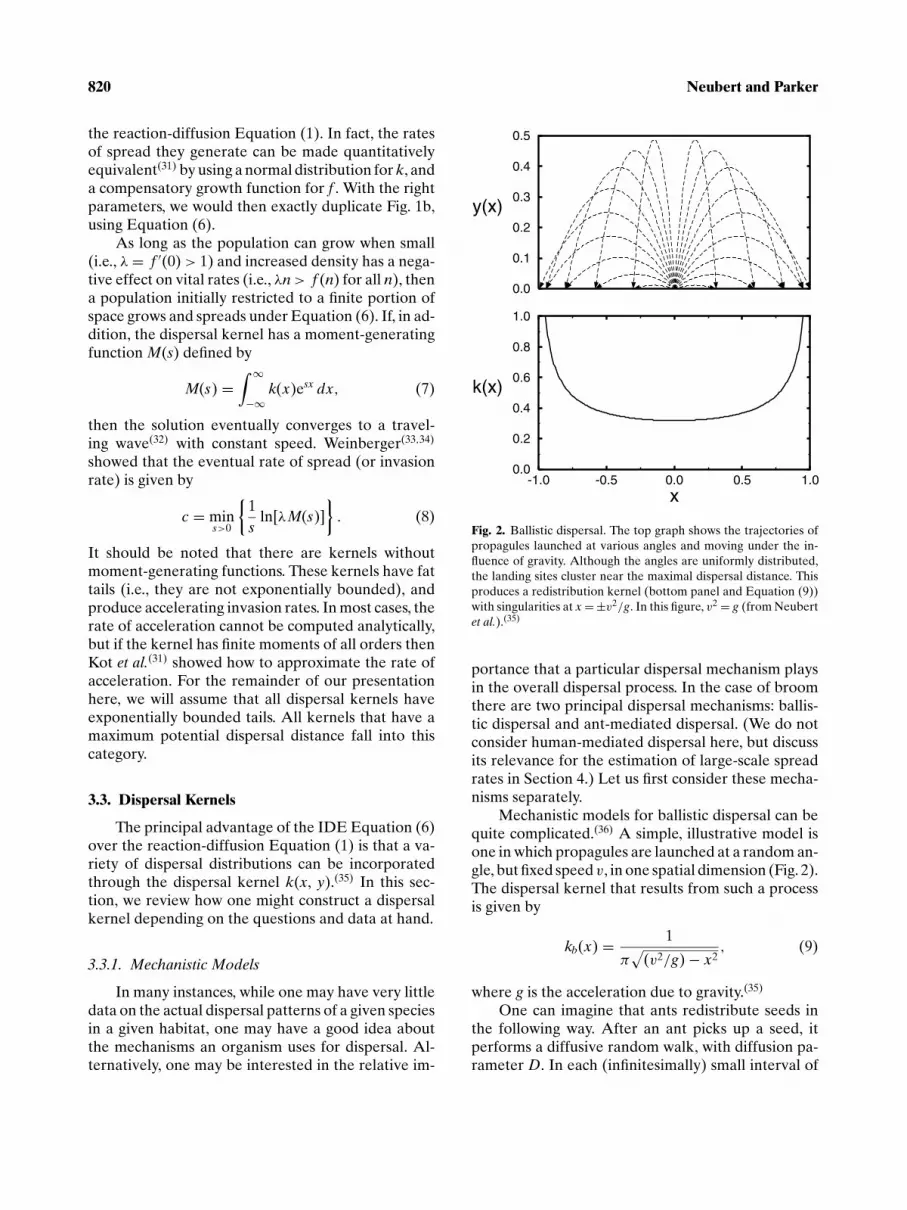
Fig. 2. Ballistic dispersal. The top graph shows the trajectories ofpropagules launched at various angles and moving under the in-fluence of gravity. Although the angles are uniformly distributed,the landing sites cluster near the maximal dispersal distance. Thisproduces a redistribution kernel (bottom panel and Equation (9))with singularities at x = ±v2/g. In this figure, v2 = g (from Neubertet al.).(35)

portance that a particular dispersal mechanism playsin the overall dispersal process. In the case of broomthere are two principal dispersal mechanisms: ballis-tic dispersal and ant-mediated dispersal. (We do notconsider human-mediated dispersal here, but discussits relevance for the estimation of large-scale spreadrates in Section 4.) Let us first consider these mecha-nisms separately.

Mechanistic models for ballistic dispersal can bequite complicated.(36) A simple, illustrative model isone in which propagules are launched at a random an-gle, but fixed speed v, in one spatial dimension (Fig. 2).The dispersal kernel that results from such a processis given by

kb(x) = 1

π√

(v2/g) − x2, (9)

where g is the acceleration due to gravity.(35)

One can imagine that ants redistribute seeds inthe following way. After an ant picks up a seed, itperforms a diffusive random walk, with diffusion pa-rameter D. In each (infinitesimally) small interval of


time t, the ant has a small probability of releasingthe seed given by ht . Given these two processes, theprobability that a seed starting at the origin moves tolocation x is given by the Laplace distribution(37)

ka(x) =√

h4D

exp

[−|x|

√hD

]. (10)

This distribution is often used in theoretical studies ofdispersal because it captures the leptokurtosis foundin many observed dispersal distributions and lendsitself to simple mathematical analyses.

Combining two dispersal processes (e.g., ballisticand ant dispersal) is relatively simple. As long as thetwo processes are independent, the combined disper-sal kernel is formally given by the convolution of thetwo kernels kb and ka

kc(x) =∫ ∞

−∞ka(x − y)kb(y) dy. (11)

In some cases, the convolution of Equation (11)is not given in terms of elementary functions. Thisis the case when we convolve the ballistic andant-dispersal kernels of Equations (9) and (10)(Fig. 3). A convenient consequence of Equation(11) is that the moment-generating function forthe combined kernel is simply the product of themoment-generating functions of the two kernelsseparately:

Mc(s) = Ma(s)Mb(s). (12)

5 4 3 2 1 0 1 2 3 4 50

0.05

0.1

0.15

0.2

0.25

0.3

0.35

0.4

0.45

0.5

x

k(x)

Fig. 3. Ballistic plus ant dispersal. As in Fig. 2, v2 = g. When antdispersal is large relative to ballistic dispersal, the kernel resultingfrom the combined action of ants and ballistic dispersal is unimodal(dashed curve,

√h/D = 1). The kernel is bimodal if ant dispersal

is relatively short range (solid curve,√

h/D = 5).

Thus, if we are only interested in a projection of thespeed (cf. Equation (8)), we need never actually com-pute the convolution of Equation (11).

3.3.2. Measured Distributions

If one is lucky enough to have measurements ofdispersal distance, one can use them directly. This isperhaps the most appealing feature of IDE models.In the literature, these measurements are often re-ported as histograms of dispersal distance. Some caremust be taken in translating these histograms intoone-dimensional dispersal kernels, since the data areoften collected in two spatial dimensions.3

Fig. 4A shows a two-dimensional histogramof ballistic seed dispersal distances collected forbroom.(39) Rectangular strips 1 m × 8 m were placedaround isolated plants and coated with Tanglefootglue to catch seeds. The number of seeds within each0.5 m segment was adjusted by the proportion of thetotal area searched, to estimate the total number ofseeds landing within the annulus at that distance. Con-verting these data into a bivariate probability densityfunction, then taking the marginal distribution overany direction,(38) gives the one-dimensional dispersalkernel (Fig. 4B)

kb(x) =

2∑m

i= j (gi − gi+1)√

x2i − x2,

if xj−1 < |x| ≤ xj , j = 1, 2, . . . , m,

0, otherwise,(13)

where gi = φi/Ai, Ai is the area of the annular re-gion bounded by the radii xi−1 and xi, and φi is thefrequency of seeds in that annular region.

Secondary dispersal of broom seeds after theirballistic dispersal from the plant was quantified bymeasuring the distances to seedlings in the spring frompoints where seed piles were put out at the time ofseed maturation in the fall.(39) These data are differentfrom those used to form the kernel in Equation (13)in that they are a set of distances rather than frequen-cies in ranges. Assuming radial symmetry then gives atwo-dimensional “histogram” as shown in Fig. 4C. Inthis figure, each cylinder, with radius ri and height bi,is a representation of the two-dimensional Dirac deltafunction(40) with intensity bi, in polar coordinates:biδ2(r − r i). bi is the number of seedlings found at

3 These issues are dealt with more thoroughly in Reference 38. Werepeat some of that material here for the reader’s convenience.


63

03

6 63

03

60

0.02

0.04

0.06

0.08

0.1

0.12

0.14

yx

prob

abil

ity

dens

ity

64

20

24

6 64

20

24

6

0

5

10

15

20

yx

freq

uenc

y

-8 -6 -4 -2 0 2 4 6 80

0.05

0.1

0.15

0.2

0.25

0.3

0.35

x

xk b

()

-8 -6 -4 -2 0 2 4 6 810

-4

10-3

10-2

10-1

100

101

102

x

k a(x

)

-10 -8 -6 -4 -2 0 2 4 6 8 100

0.05

0.1

0.15

0.2

0.25

x

k c(x

)

(A)

(B) (D)

(C)

(E)

marginalize

convolve

Fig. 4. Estimated dispersal kernels for broom. Two-dimensional histograms of dispersal distances were constructed from measurements(39)

of ballistic dispersal (A) and ant dispersal (C). These were marginalized (i.e., integrated over one direction) to obtain one-dimensionaldispersal kernels (B, D). The convolution of these one-dimensional kernels produces the composite dispersal kernel kc (E).


that distance. Given � seedlings, the marginal distribu-tion in the x direction is then obtained by integratingover y yielding(38)

ka(x) =�∑

i=1

hi (x), (14)

with

hi (x) ={

[π2(r2i − x2)]−1/2, if |x| < ri ,

0, otherwise.(15)

There is a convenient expression for the moment-generating function of ka

Ma(s) = 1�

�∑i=1

I0(ri s), (16)

where I0 is the modified Bessel function of the firstkind.(41) Equation (16) can be thought of as an un-biased nonparametric estimator for the moment-generating function of ka.(42) We know of no simpleexpression for the moment-generating function forkb; it must be computed numerically.

If every seed is dispersed by an ant, then the com-posite dispersal kernel, taking into account both dis-persal processes, is given by Equation (11) (Fig. 4E),and the moment-generating function for the compos-ite kernel is given by Equation (12). Of course someseeds are never touched by an ant. If each seed hasa probability p of being dispersed by an ant, then thecomposite kernel is given by

kc(x; p) =∫ ∞

−∞[pka(x − y)

+ (1 − p)δ(x − y)]kb(y) dy, (17)

and the moment-generating function is given by

Mc(s) = [1 − p + pMa(s)]Mb(s). (18)

Using Equation (8) with Equation (18), along with theestimate of population growth rate for broom in Dis-covery Park during the 1993–1994 season(39) (λ1993 =1.2167), we computed the invasion rate (c) as a func-tion of the ant-dispersal probability (p). A graph ofthis function (Fig. 5) shows that invasion rate increasesroughly linearly and by approximately 17% as theant-dispersal probability increases from 0 to 1. As es-timated by a field experiment,(39) ants dispersed ap-proximately 90% of the seeds, resulting in an esti-mated invasion rate of 1.35 m/yr. We will set p = 0.9in the examples that follow.

0 0.2 0.4 0.6 0.8 11.15

1.2

1.25

1.3

1.35

1.4

probability of ant dispersal (p)

inva

sion

rat

e (c

, m y

-1)

Fig. 5. Invasion rate (c) as a function of the probability of ant dis-persal (p). Invasion rate was calculated using Equations (8) and(18), with the numerically estimated moment-generating functionsfor the estimated ballistic and ant-dispersal kernels (cf. Fig. 4). Pop-ulation growth rate was taken to be λ1993 = 1.2167, as estimatedfor Discovery Park, Seattle, Washington.(20) The value of p esti-mated from the data (≈0.9) and the resulting speed (≈1.35 m/yr)are marked with a circle.

3.4. Periodic and Stochastic Environments

The models we have described so far assumea temporally homogeneous environment. In somecases, this assumption will be too far from the truthto be useful. In addition, one may be interestedin how environmental variability affects invasionrates. Neubert et al.(43) show how to calculate time-averaged invasion rates in periodic environments, andexpected time-averaged invasion rates in stochasticenvironments.

Environmental stochasticity can be incorporatedinto Equation (6) by choosing the growth rates anddispersal kernels at random from a set of choices. Themodel then becomes

N (t + 1, x) =∫ ∞

−∞Kt (x − y) f (N (t, y); �t ) dy,

(19)

where the Kt (x − y) are independent and identicallydistributed (i.i.d.) random dispersal kernels, and thegrowth rates �t are i.i.d. random variables indepen-dent of the kernels. (The scriptN is used to emphasizethat population density is now a random function.)


At any time t, the population has a random ex-tent Xt , defined to be the location farthest from theinvasion’s origin with N (t, x) ≥ n. The average speedsince the invasion began is also a random variable,given by Ct = (Xt − x0)/t . Neubert et al.(43) showedthat Ct is asymptotically normally distributed withmean (µ) and variance (σ 2) given by

µ = mins

E{

ln[�0 M0(s)]s

}, (20)

and

σ 2 = 1t

Var{

ln[�0 M0(s∗)]s∗

}, (21)

where s∗ is the value of s that gives the minimum forµ. As t → ∞, the variance decays to zero and Ct → c,where

c = mins

(1s

E{ln[�0 M0(s)]})

. (22)

The estimate of population growth rate for broom inDiscovery Park between 1994 and 1995(20) (λ1994 =1.0842) is lower than the 1993–1994 estimate (λ1993 =1.2167). Fig. 6 shows the results of including this tem-poral variability in the model. In these simulations,we used the same dispersal kernel (kc, Fig. 4E) everyyear and selected the growth rate �t at random fromthe set {λ1993, λ1994}. The projected average asymp-totic speed c is 1.13 m/yr: 16% slower than projectedunder constant 1993–1994 conditions and 36% fasterthan under constant 1994–1995 conditions.

While the speed of each realization eventuallyconverges to c, it should be noted that the spatialextent of a realized invasion would not, in general,converge to ct . In fact, for large t, Xt ≈ t Ct , so

Var [Xt ] = t2Var[Ct ] = tVar{

ln[�0 M0(s∗)]s∗

}. (23)

Thus the variance in extent grows linearly with time.

3.5. Stage-Structured Models

3.5.1. Formulation

While the IDE of Equation (5) permits a widerrange of dispersal distributions than does its reaction-diffusion counterpart of Equation (1), it still treatsall individuals within the population as identical. Infact, vital rates and dispersal abilities of individuals of-ten vary dramatically with life history stage. Considerthe life cycle of broom(20) (Fig. 7). For this species,only adult stages reproduce and only seeds disperse.The seed production of the largest plants is 300 times

higher than that of small reproductive plants, andthe mortality rates of seedlings are much higher thanthose of adults.

Lui(44) and Neubert and Caswell(45) show how toincorporate this stage structure into IDE models andhow to calculate spread rates. We briefly review theirresults here. To begin, we must first expand Equation(5) to a system of m difference equations (one equa-tion for each of the m stages). Designating ni as thepopulation density in the ith stage and bij as the per-capita production of stage i individuals at time t + 1by stage j individuals at time t, we have

ni (y, t + 1) =m∑

j=1

bij(n1(y, t), . . . , nm(y, t))nj (y, t),

(24)

for i = 1, . . . , m, or in the more familiar matrixnotation,

n(y, t + 1) = Bnn(y, t), (25)

where Bn is the density-dependent population projec-tion matrix. (We assume that density dependence actsin the same way at every location.)

To allow for stage-specific dispersal, we mustspecify a dispersal kernel for each of the m2 possi-ble transitions between stages. We define kij(x, y) tobe the probability that an individual making the tran-sition from stage j to stage i moves from location y tolocation x. If there is no dispersal during a given transi-tion, the associated kernel is the Dirac delta function.

The stage-structured analog of Equation (6) isthen given as follows:

ni (x, t + 1) =∫ ∞

−∞

m∑j=1

kij(x − y)bij(n1(y, t), . . . , nm(y, t))nj (y, t) dy,

(26)

for i = 1, . . . , m. Just as the notation of Equation (24)is simplified by Equation (25), if we create the matrixK(x − y) from the kernels kij(x − y), the complexnotation of Equation (26) is simplified to

n(x, t + 1) =∫ ∞

−∞[K(x − y) ◦ Bn] n(y, t) dy. (27)

The symbol “◦” stands for the Hadamard product,(46)

whereby matrices are multiplied element-wise. (Thatis, the element in the ith row and jth column ofK(x − y) ◦ Bn is kij(x − y) bij(y).)


0 20 40 60 80 100 120 140 160 180 2000

50

100

150

200

250

0 100 200 300 400 500 600 700 800 900 10000

0.5

1

1.5

2

2.5

3

3.5

4

time

time

time

time

Var

[C

t]V

ar [

Xt]

aver

age

inva

sion

spe

ed (

Ct)

spat

ial e

xten

t (X

t)

c

(a)

(b)

100 101 102 10310-3

10-2

10-1

100

101

102

100 101 102 10310-5

10-4

10-3

10-2

10-1

Fig. 6. Invasion dynamics in a stochasticenvironment. Using the compositeant/ballistic dispersal kernel with p = 1(Fig. 4E), we simulated 20 realizations ofEquation (19) by choosing λ at randombetween λ1993 = 1.2167 and λ1994 =1.0842 at each time step. (a) Extent (Xt )of each realization as a function of time.The variance in extent, over the ensembleof realizations, grows linearly with time(inset). For each realization, the averageinvasion speed converges to the constantc as predicted by Equation (22), and theensemble variance grows like t (inset).

3.5.2. Stage-Structured Invasion Dynamics

As long as the matrices K and Bn meet certain bi-ologically reasonable technical assumptions,(44,45) andthere are no Allee effects, then all populations gov-erned by Equation (27) that start in a confined areaconverge to a traveling wave solution with speed givenby

c = mins>0

[1s

ln ρ1(s)]

. (28)

In Equation (28), ρ1(s) is the largest eigenvalue of thematrix M(s) ◦ B0, the elements of the matrix M(s) arethe moment-generating functions of the elements ofK(x), and the matrix B0 is the matrix Bn evaluated atlow population densities (n ≈ 0).

The life cycle graph for broom is shown in Fig. 7.Dashed lines indicate transitions during which disper-sal occurs. There are seven stages: seeds, seedlings(one-year olds), juveniles, and four size classes ofadults. The projection interval is one year, with a


1 2 3 4 5 6 7

Fig. 7. Life cycle graph for broom (Cytisus scoparius). Stages arenumbered as follows: (1) seeds, (2) seedlings, (3) juveniles, (4) smalladults (<100 g), (5) medium adults (100–400 g), (6) large adults(400–900 g), and (7) extra-large adults (>900 g). Dashed arrowsrepresent transitions during which there is dispersal.

census performed at the end of the dry season, af-ter all seeds have matured. Parker(20) estimated thedemographic matrix B0 in Discovery Park, at the lead-ing edge of an invasion front, over the 1993–1994 and1994–1995 seasons. It is from these matrices that wecalculated the population growth rates used in the un-structured models above. We will use the 1993–1994matrix for our illustration here

A = B0 =

0.741 0 3.4 47.1 108.7 1120 3339

0.00105 0.31 0 0 0 0 0

0 0.35 0.31 0.024 0 0 0

0 0.038 0.29 0.39 0 0 0

0 0 0.069 0.44 0.32 0 0.091

0 0 0 0 0.44 0.53 0.091

0 0 0 0 0.029 0.4 0.73

.

(29)

If seed dispersal is independent of plant size (thereis no evidence in our data to suggest otherwise(39)),the matrix of dispersal kernels for broom is the 7 × 7matrix

K(x) =

δ(x) kc(x) kc(x) kc(x) kc(x) kc(x) kc(x)

δ(x) δ(x) δ(x) δ(x) δ(x) δ(x) δ(x)...

......

......

......

δ(x) δ(x) δ(x) δ(x) δ(x) δ(x) δ(x)

, (30)

and the matrix of moment-generating functions forbroom is given by

M(s) =

1 Mc(s) Mc(s) Mc(s) Mc(s) Mc(s) Mc(s)

1 1 1 1 1 1 1...

......

......

......

1 1 1 1 1 1 1

. (31)

Note that while seedlings produce no seed (a12 = 0)we include the possibility of dispersal during thetransition from seedling to seed (k12(x) = kc(x),m12(s) = Mc(s)) because if seedlings did produce

seeds we assume that they would disperse like all therest.

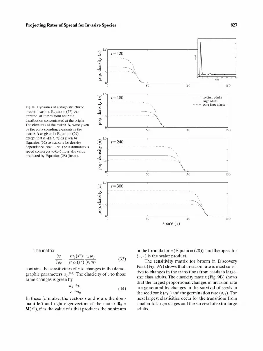
In Fig. 8 we show the result of simulating Equa-tion (27). In order to prevent the population at anylocation from growing without bound, we introducednegative density dependence in the transitions fromseedlings to juvenile and adult stages of the form

bj2(n(t, y)) = a j2 exp

[−

7∑i=4

ni (y, t)

]for 3 ≤ j ≤ 7.

(32)

This form of density dependence is consistent withthe observation that very few seedlings mature whensurrounded by adult plants.(20) We assumed that allother transitions were density independent and givenby their entries in A.

The pattern of invasion shown in Fig. 8 is typical.The population density in each stage forms a travelingwave and, asymptotically, each wave moves with thesame speed (given by Equation (28)) of c ≈ 0.46 m/yr.This speed is 66% less than the projection based onthe unstructured Equation (6).

It is a straightforward exercise to show that,all else being equal, invasion rate projections basedon unstructured models overestimate actual inva-sion rates compared with projections from structuredmodels.(45) This is because unstructured models ig-nore the fact that some transitions do not involvedispersal. But reducing this bias is only one of theadvantages of including stage structure. More impor-tantly, stage-structured models link invasion rates toprocesses that occur within the life cycle of an indi-vidual. It is these processes that can be changed bymanagement tactics, manipulated in experiments, oraltered by changes in the environment. Thus stage-structured models are more useful than unstructuredmodels, as well as potentially more accurate.

3.5.3. Perturbation Analyses

We now present the formulae for the sensitivityand elasticity of invasion rate to changes in the vitalrates (i.e., the entries in the matrix A). There are anumber of compelling reasons to carry out such ananalysis.(45,47) For example, the errors in estimatingthe parameters result in errors in c. The most im-portant errors will be in the parameters to which c ismost sensitive. Information on the sensitivity of c canthus be used to design sampling procedures that maxi-mize the precision of the estimates of the most criticalparameters. Sensitivity analysis of invasion rates mayalso be valuable in the evaluation of managementstrategies for the control of invasive species.(48)


0 50 100 1500

0.5

1

1.5

0 50 100 1500

0.5

1

1.5medium adultslarge adultsextra large adults

0 50 100 1500

0.5

1

1.5

0 50 100 1500

0.5

1

1.5

space (x)

pop.

den

sity

(n)

pop.

den

sity

(n)

pop.

den

sity

(n)

pop.

den

sity

(n)

t = 120

t = 180

t = 240

t = 300

0 5 10 15 20 25 30 35 400

1

2

3

4

5

6

7

8

time

spee

d

Fig. 8. Dynamics of a stage-structuredbroom invasion. Equation (27) wasiterated 300 times from an initialdistribution concentrated at the origin.The elements of the matrix Bn were givenby the corresponding elements in thematrix A as given in Equation (29),except that bj2(n(t , y)) is given byEquation (32) to account for densitydependence. As t → ∞, the instantaneousspeed converges to 0.46 m/yr, the valuepredicted by Equation (28) (inset).

The matrix∂c∂aij

= mij(s∗)s∗ρ1(s∗)

viw j

〈v, w〉 (33)

contains the sensitivities of c to changes in the demo-graphic parameters aij.(45) The elasticity of c to thosesame changes is given by

aij

c∂c∂aij

. (34)

In these formulae, the vectors v and w are the dom-inant left and right eigenvectors of the matrix B0 ◦M(s∗), s∗ is the value of s that produces the minimum

in the formula for c (Equation (28)), and the operator〈 ·, · 〉 is the scalar product.

The sensitivity matrix for broom in DiscoveryPark (Fig. 9A) shows that invasion rate is most sensi-tive to changes in the transitions from seeds to large-size class adults. The elasticity matrix (Fig. 9B) showsthat the largest proportional changes in invasion rateare generated by changes in the survival of seeds inthe seed bank (a11) and the germination rate (a21). Thenext largest elasticities occur for the transitions fromsmaller to larger stages and the survival of extra-largeadults.


12

34

56

7

12

34

56

7

0

1000

2000

3000

4000

5000

6000

row (i)column (j)

sens

itivi

ty o

f c to

aij

12

34

56

7

12

34

56

7

0

0.1

0.2

0.3

0.4

row (i)column (j)

elas

ticity

of c

to a

ij

(A)

(B)

Fig. 9. Matrices of (A) sensitivity and (B) elasticity of invasionrate to demographic parameters, as calculated in Equations (33)and (34), respectively.

4. DISCUSSION

4.1. IDEs and Other Models

IMP models are a convenient way to combine de-mographic models with models for spatial dispersal.They have several strengths. First, because they arein matrix form, they are particularly well suited fordealing with stage-structured populations, and classi-fication of individuals by stage is often more biologi-cally useful than a classification by age. Second, theyare relatively easy to analyze; computation of invasionspeed amounts to the calculation of an eigenvalue of amatrix (Equation (28)). Finally, they are particularlyeasy to connect with data. There are statistical pro-cedures for parameterizing matrix models from manykinds of data,(47) and dispersal kernels and moment-

generating functions also lend themselves to empiricalestimation.(42,49–51)

There are, of course, alternatives to IDEs formodeling spatial population dynamics. For example,continuous-time models(52,53) that amount to spatialextensions of Lotka’s integral equation have beenused to project rates of spread for a variety of plant,animal, and fungal species.(54) As is often the casein data analysis, the mathematical model one finallychooses is as likely to depend on the tastes and tal-ents of the analyst as it is to depend on the dictates ofbiology.

4.2. Conservation and Management

Demographic models, and in particular matrixpopulation models, have become influential tools inconservation biology.(47,55) They are used to helpchoose among management alternatives by projectingthe likely result of various interventions. For conser-vation questions that involve spatial processes, suchas curbing the spread of an invasive species or assess-ing relative risk, IMP models can be used in the sameway.

The objective of nonnative species managementis to slow the spread of invading populations, but themanagement tools at hand usually target particularvital rates of the organism. For example, a biocon-trol agent might kill seeds; a prescribed fire mightkill adults but increase germination. To meet theirobjectives, managers must choose among these tools,and they need demographic information to guide theirchoices. As a result, prospective perturbation analyses(i. e., sensitivity and elasticity analyses) are a usefullink between models and management.(56) When ap-plied sensibly, these analyses help to distinguish thechanges to the vital rates that are likely to have a sig-nificant impact and thereby help to identify potentialmanagement strategies.

A perturbation analysis of invasion rate, as out-lined in Section 3.5, should accompany any projec-tion of invasion rate used to guide management. Forbroom, the perturbation analysis indicates that transi-tions involving the survival and germination of seedshave the highest elasticities, but these were not vastlylarger than the elasticities for other transitions. Broomdoes not seem to have any particular “Achilles heel”when it comes to invasion speed, a result consistentwith previous analyses.(20)

Because invasion speed is a nonlinear functionof the elements of the matrix from which it is de-rived, and because sensitivity and elasticity analyses


0 10 20 30 40 50 60 70 80 90 1000

0.05

0.1

0.15

0.2

0.25

0.3

0.35

0.4

0.45

0.5

% reduction in fecundity

inva

sion

spe

ed

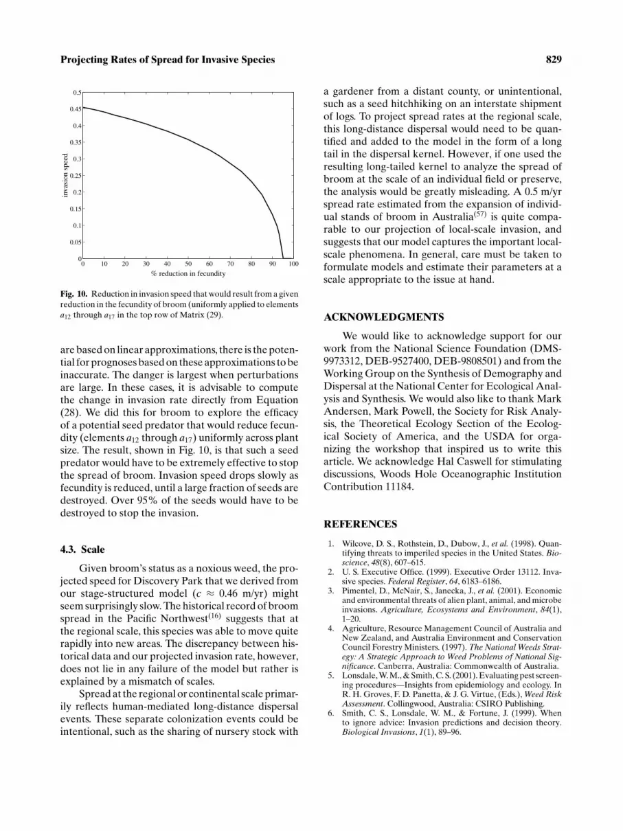
Fig. 10. Reduction in invasion speed that would result from a givenreduction in the fecundity of broom (uniformly applied to elementsa12 through a17 in the top row of Matrix (29).

are based on linear approximations, there is the poten-tial for prognoses based on these approximations to beinaccurate. The danger is largest when perturbationsare large. In these cases, it is advisable to computethe change in invasion rate directly from Equation(28). We did this for broom to explore the efficacyof a potential seed predator that would reduce fecun-dity (elements a12 through a17) uniformly across plantsize. The result, shown in Fig. 10, is that such a seedpredator would have to be extremely effective to stopthe spread of broom. Invasion speed drops slowly asfecundity is reduced, until a large fraction of seeds aredestroyed. Over 95% of the seeds would have to bedestroyed to stop the invasion.

4.3. Scale

Given broom’s status as a noxious weed, the pro-jected speed for Discovery Park that we derived fromour stage-structured model (c ≈ 0.46 m/yr) mightseem surprisingly slow. The historical record of broomspread in the Pacific Northwest(16) suggests that atthe regional scale, this species was able to move quiterapidly into new areas. The discrepancy between his-torical data and our projected invasion rate, however,does not lie in any failure of the model but rather isexplained by a mismatch of scales.

Spread at the regional or continental scale primar-ily reflects human-mediated long-distance dispersalevents. These separate colonization events could beintentional, such as the sharing of nursery stock with

a gardener from a distant county, or unintentional,such as a seed hitchhiking on an interstate shipmentof logs. To project spread rates at the regional scale,this long-distance dispersal would need to be quan-tified and added to the model in the form of a longtail in the dispersal kernel. However, if one used theresulting long-tailed kernel to analyze the spread ofbroom at the scale of an individual field or preserve,the analysis would be greatly misleading. A 0.5 m/yrspread rate estimated from the expansion of individ-ual stands of broom in Australia(57) is quite compa-rable to our projection of local-scale invasion, andsuggests that our model captures the important local-scale phenomena. In general, care must be taken toformulate models and estimate their parameters at ascale appropriate to the issue at hand.

ACKNOWLEDGMENTS

We would like to acknowledge support for ourwork from the National Science Foundation (DMS-9973312, DEB-9527400, DEB-9808501) and from theWorking Group on the Synthesis of Demography andDispersal at the National Center for Ecological Anal-ysis and Synthesis. We would also like to thank MarkAndersen, Mark Powell, the Society for Risk Analy-sis, the Theoretical Ecology Section of the Ecolog-ical Society of America, and the USDA for orga-nizing the workshop that inspired us to write thisarticle. We acknowledge Hal Caswell for stimulatingdiscussions, Woods Hole Oceanographic InstitutionContribution 11184.

REFERENCES

1. Wilcove, D. S., Rothstein, D., Dubow, J., et al. (1998). Quan-tifying threats to imperiled species in the United States. Bio-science, 48(8), 607–615.

2. U. S. Executive Office. (1999). Executive Order 13112. Inva-sive species. Federal Register, 64, 6183–6186.

3. Pimentel, D., McNair, S., Janecka, J., et al. (2001). Economicand environmental threats of alien plant, animal, and microbeinvasions. Agriculture, Ecosystems and Environment, 84(1),1–20.

4. Agriculture, Resource Management Council of Australia andNew Zealand, and Australia Environment and ConservationCouncil Forestry Ministers. (1997). The National Weeds Strat-egy: A Strategic Approach to Weed Problems of National Sig-nificance. Canberra, Australia: Commonwealth of Australia.

5. Lonsdale, W. M., & Smith, C. S. (2001). Evaluating pest screen-ing procedures—Insights from epidemiology and ecology. InR. H. Groves, F. D. Panetta, & J. G. Virtue, (Eds.), Weed RiskAssessment. Collingwood, Australia: CSIRO Publishing.

6. Smith, C. S., Lonsdale, W. M., & Fortune, J. (1999). Whento ignore advice: Invasion predictions and decision theory.Biological Invasions, 1(1), 89–96.


7. Randall, J. M. (1996). Assessment of the invasive weed prob-lem on preserves across the United States. Endangered SpeciesUpdate, 12, 4–6.

8. Hiebert, R. D. (1997). Prioritizing invasive plants and plan-ning for management. In J. O. Luken & J. W. Theiret (Eds.),Assessment and Management of Plant Invasions (pp. 195–212).New York: Springer-Verlag.

9. Parker, I. M., Simberloff, D., Lonsdale, W. M., et al. (1999).Impact: Toward a framework for understanding the ecologicaleffects of invaders. Biological Invasions, 1(1), 3–19.

10. Zavaleta, E. (2000). Valuing ecosystem services lost toTamarix invasion in the United States. In H. A. Mooney & R. J.Hobbs (Eds.), Invasive Species in a Changing World (pp. 261–300). Washington, DC: Island Press.

11. Kot, M., & Schaffer, M. W. (1986). Discrete-time growth-dispersal models. Mathematical Biosciences, 80, 109–136.

12. Kot, M. (in press). Do invading organisms do the wave? Cana-dian Quarterly of Applied Mathematics.

13. Hosking, J. R., Smith, J. M. B., & Sheppard, A. W. (1996).The biology Australian weeds: 28. Cytisus scoparius (l.)link subsp. scoparius. Plant Protection Quarterly, 11(3), 102–108.

14. Paynter, Q. S., Fowler, S. V., Memmott, J., et al. (1998). Fac-tors affecting the establishment of Cytisus scoparius in south-ern France: Implications for managing both native and exoticpopulations. Journal of Applied Ecology, 35, 582–595.

15. Luken, J. O., & Thieret, J. W. (1997). Assessment and Manage-ment of Plant Invasions. New York: Springer-Verlag.

16. Isaacson, D. L. (2000). Impacts of broom (Cytisus scoparius)in western North America. Plant Protection Quarterly, 15(4),145–148.

17. Smith, J. M. B. (1994). The changing ecological impact ofbroom (Cytisus scoparius) at Barrington Tops, New SouthWales. Plant Protection Quarterly, 9, 6–11.

18. Parker, I. M., & Reichard, S. H. (1997). Critical issues in inva-sion biology for conservation science. In P. Fiedler & P. Kareiva(Eds.), Conservation Biology. New York: Chapman andHall.

19. Haubensak, K. A., & Parker, I. M. (in press). Soil changesaccompanying invasion of the exotic shrub Cytisus scoparius inglacial outwash prairies of western Washington (USA). PlantEcology.

20. Parker, I. M. (2000). Invasion dynamics of Cytisus scoparius:A matrix model approach. Ecological Applications, 10, 726–743.

21. Bossard, C. C. (1990). Tracing of ant-dispersed seeds: A newtechnique. Ecology, 71(6), 2370–2371.

22. Hotelling, H. (1921). A Mathematical Theory of Migration.Master’s thesis, University of Washington.

23. Hotelling, H. (1978). A mathematical theory of migration.Environment and Planning A, 10, 1223–1239.

24. Fisher, R. A. (1937). The wave of advance of advantageousgenes. Annals of Eugenics, 7, 353–369.

25. Kolmogorov, A. N., Petrovsky, N., & Piscounov, N. S. (1937).Etude de l’equations de la diffusion avec croissance de la quan-tite de matiere et son application a un probleme biologique.Moscow University Bulletin of Mathematics, 1, 1–25.

26. Aronson, D. G., & Weinberger, H. F. (1975). Nonlinear dif-fusion in population genetics, combustion, and nerve propa-gation. In J. Goldstein (Ed.), Partial Differential Equationsand Related Topics, Vol. 446 (pp. 5–49). Berlin, Germany:Springer-Verlag.

27. Andow, D. A., Kareiva, P. M., Levin, S. A., et al. (1990). Spreadof invading organisms. Landscape Ecology, 4, 177–188.

28. Shigesada, N., & Kawasaki, K. (1997). Biological Invasions:Theory and Practice. Oxford, UK: Oxford University Press.

29. Okubo, A. (1980). Diffusion and Ecological Problems: Math-ematical Models. New York: Springer-Verlag.

30. Andersen, M. (1991). Properties of some density-dependentintegrodifference equation population models. MathematicalBiosciences, 104, 135–157.

31. Kot, M., Lewis, M. A., & van den Driessche, P. (1996). Disper-sal data and the spread of invading organisms. Ecology, 77,2027–2042.

32. Kot, M. (1992). Discrete-time travelling waves: Ecological ex-amples. Journal of Mathematical Biology, 30, 413–436.

33. Weinberger, H. F. (1978). Asymptotic behavior of a modelof population genetics. In J. Chadam (Ed.), Nonlinear PartialDifferential Equations and Applications, Vol. 684 (pp. 47–96).Berlin, Germany: Springer-Verlag.

34. Weinberger, H. F. (1982). Long-time behavior of a class ofbiological models. SIAM Journal of Mathematical Analysis,13, 353–396.

35. Neubert, M. G., Kot, M., & Lewis, M. A. (1995). Dispersaland pattern formation in a discrete-time predator-prey model.Theoretical Population Biology, 48(1), 7–43.

36. Beer, T., & Swain, M. D. (1977). On the theory of explosivelydispersed seeds. New Phytologist, 78, 681–694.

37. Broadbent, S. R., & Kendall, D. G. (1953). The random walkof trichostrongylus retortaeformis. Biometrika, 9, 460–465.

38. Lewis, M. A., Neubert, M. G., Clark, J., et al. (in prepara-tion). A guide to the construction and interpretation of 1-dintegrodifference equation models for biological invasions.

39. Parker, I. M. (1996). Ecological Factors Affecting Rates of Pop-ulation Growth and Spread in Cytisus scoparius, an InvasiveExotic Shrub. PhD thesis, University of Washington.

40. Bracewell, R. N. (1986). The Fourier Transform and Its Appli-cations, 2nd ed. New York: McGraw-Hill.

41. Abramowitz, M., & Stegun, I. A. (1965). Handbook ofMathematical Functions with Formulas, Graphs, and Mathe-matical Tables. Washington, DC: U.S. Government PrintingOffice.

42. Clark, J., Horvath, L., & Lewis, M. A. (2001). On the estima-tion of spread rate for a biological population. Statistics andProbability Letters, 51, 225–234.

43. Neubert, M. G., Kot, M., & Lewis, M. A. (2000). Invasionspeeds in fluctuating environments. Proceedings of the RoyalSociety of London, Series B: Biological Sciences, 267(1453),1603–1610.

44. Lui, R. (1989). Biological growth and spread modeled by sys-tems of recursions. I. Mathematical theory. Mathematical Bio-sciences, 93, 269–295.

45. Neubert, M. G., & Caswell, H. (2000). Demography anddispersal: Calculation and sensitivity analysis of invasionspeed for structured populations. Ecology, 81(6), 1613–1628.

46. Horn, R. A., & Johnson, C. R. (1985). Matrix Analysis. Cam-bridge, UK: Cambridge University Press.

47. Caswell, H. (2001). Matrix Population Models: Construction,Analysis, and Interpretation, 2nd ed. Sunderland, MA: SinauerAssociates.

48. Sharov, A. A., & Liebhold, A. M. (1998). Bioeconomics ofmanaging the spread of exotic pest species with barrier zones.Ecological Applications, 8(3), 833–845.

49. Silverman, B. W. (1986). Density Estimation for Statistics andData Analysis. London, UK: Chapman and Hall.

50. Hardle, W. (1990). Applied Nonparametric Regression. Cam-bridge, UK: Cambridge University Press.

51. de Wit, T. D., & Floriani, E. (1998). Estimating probabilitydensities from short samples: A parametric maximum likeli-hood approach. Physical Review E, 58, 5115–5122.

52. Van den Bosch, F., Metz, J. A. J., & Diekmann, O. (1990). Thevelocity of spatial population expansion. Journal of Mathe-matical Biology, 28, 529–565.

53. Diekmann, O., Gyllenberg, M., Metz, J. A. J., et al. (1998).On the formulation and analysis of general deterministic


structured population models. I. Linear theory. Journal ofMathematical Biology, 36, 349–388.

54. Hengeveld, R. (1994). Small-step invasion research. Trends inEcology and Evolution, 9, 339–342.

55. Morris, W. F., & Doak, D. F. (2002). Quantitative ConservationBiology: Theory and Practice of Population Viability Analysis.Sunderland, MA: Sinauer.

56. Caswell, H. (2000). Prospective and retrospective perturba-tion analyses and their use in conservation biology. Ecology,81, 619–627.

57. Downey, P. O., & Smith, J. M. B. (2000). Demography of theinvasive shrub scotch broom (Cytisus scoparius) at Barring-ton Tops, New South Wales: Insights for management. AustralEcology, 25, 477–485.

Documents

Projecting Rates of Spread for Invasive Species