Embed Size (px)
Citation preview
Proceedings of the Fourth Glacier Bay Science Symposium
Sponsored by: U.S. Geological Survey Alaska Science Center, National Park Service Alaska Regional Office, andGlacier Bay National Park and Preserve
U.S. Department of the InteriorU.S. Geological Survey
Scientific Investigations Report 2007–5047

Cover: Photograph of Geikie Inlet looking into the main bay of Glacier Bay National Park, Alaska. (Photograph taken by Bill Eichenlaub, Gustavus, Alaska, 2005.)
Proceedings of the Fourth Glacier Bay Science SymposiumOctober 26-28, 2004Juneau, Alaska
Edited by John F. Piatt and Scott M. Gende
Sponsored by: U.S. Geological Survey Alaska Science Center, National Park Service Alaska Regional Office, and Glacier Bay National Park and Preserve
U.S. Department of the InteriorU.S. Geological Survey
Scientific Investigations Report 2007-5047
U.S. Department of the InteriorDIRK KEMPTHORNE, Secretary
U.S. Geological SurveyMark D. Myers, Director
U.S. Geological Survey, Reston, Virginia: 2007
For product and ordering information: World Wide Web: http://www.usgs.gov/pubprod Telephone: 1-888-ASK-USGS
For more information on the USGS--the Federal source for science about the Earth, its natural and living resources, natural hazards, and the environment: World Wide Web: http://www.usgs.gov Telephone: 1-888-ASK-USGS
Any use of trade, product, or firm names is for descriptive purposes only and does not imply endorsement by the U.S. Government.
Although this report is in the public domain, permission must be secured from the individual copyright owners to reproduce any copyrighted materials contained within this report.
Suggested citation:Piatt, J.F., and Gende, S.M., eds., 2007, Proceedings of the Fourth Glacier Bay Science Symposium: U.S. Geological Survey Scientific Investigations Report 2007-5047, 246 p.
iii
Foreword
Glacier Bay was established as a National Monument in 1925, in part to protect its unique character and natural beauty, but also to create a natural laboratory to examine evolution of the glacial landscape. Today, Glacier Bay National Park and Preserve is still a place of profound natural beauty and dynamic landscapes. It also remains a focal point for scientific research and includes continuing observations begun decades ago of glacial processes and terrestrial ecosystems. In recent years, research has focused on glacial-marine interactions and ecosystem processes that occur below the surface of the bay. In October 2004, Glacier Bay National Park convened the fourth in a series of science symposiums to provide an opportunity for researchers, managers, interpreters, educators, students and the general public to share knowledge about Glacier Bay. The Fourth Glacier Bay Science Symposium was held in Juneau, Alaska, rather than at the Park, reflecting a desire to maximize attendance and communication among a growing and diverse number of stakeholders interested in science in the park.
More than 400 people attended the symposium. Participants provided 46 oral presentations and 41 posters covering a wide array of disciplines including geology, glaciology, oceanography, wildlife and fisheries biology, terrestrial and marine ecology, socio-cultural research and management issues. A panel discussion focused on the importance of connectivity in Glacier Bay research, and keynote speakers (Gary Davis and Terry Chapin) spoke of long-term monitoring and ecological processes. These proceedings include 56 papers from the symposium. A summary of the Glacier Bay Science Plan— itself a subject of a meeting during the symposium and the result of ongoing discussions between scientists and resource managers—also is provided.
We hope these proceedings illustrate the diversity of completed and ongoing scientific studies, conducted within the Park. To this end, we invited all presenters to submit brief technical summaries of their work, to capture the gist of their study and its main findings without an overload of details and methodology. We also asked authors to include a few words on the management implications of their work to help bridge the gap between scientists and managers in understanding how specific research questions may translate to management practice. Papers in this volume are laid out by subject matter, from terrestrial and freshwater subjects to glacial-marine geology, to the ecology of marine animals and ending with risk assessment, human impacts and science-management considerations. In summary, we hope the proceedings will serve as a useful reference to completed and ongoing studies in Glacier Bay National Park, and thereby provide park enthusiasts, scientists, and managers with a road map of scientific progress.
John Piatt and Scott Gende
Editors
iv
Welcome
I extend a heart-felt “thank you” to all participants in the fourth Glacier Bay Science Symposium and welcome all readers to these published proceedings of the symposium. The symposium provided both recognition of, and an opportunity for, the exchange of a valuable body of work resulting from the long and on-going tradition of science, research, and resource management in Glacier Bay National Park and Preserve. We had the opportunity to learn much from each other and material was presented on a wide range of scientific topics over the course of the two and one-half days of meetings. It was also an opportunity to enjoy the fellowship of those who believe in the value of science for protection and management of the park and its natural and cultural resources. I sincerely hope that these proceedings capture some sense of accomplishment and greater scientific knowledge that resulted from the symposium. I also hope it will inspire a renewed dedication to the protection of Glacier Bay National Park and Preserve for future generations.
Tomie Patrick Lee, Superintendent
Glacier Bay National Park and Preserve
v
Acknowledgments
The symposium and proceedings would not have been possible without the support of many individuals and agencies, including Glacier Bay National Park, U.S. Geological Survey (USGS) Alaska Science Center, National Park Service (NPS) Alaska Region Inventory and Monitoring Program, Pacific Northwest Cooperative Ecosystem Studies Unit, NPS Regional Office, and George Wright Society. The symposium steering committee included Susan Boudreau, Bill Brown, Jed Davis, Emily Dekker-Fiala, Joy Geiselman, Scott Gende, Wayne Howell, Tomie Lee, Alexander Milner, John Morris, Kris Nemeth, John Piatt, Tom Shirley, Sherry Tamone, and Bob Winfree. Papers submitted for publication in the symposium proceedings underwent peer review, and the editors are very grateful to all those reviewers who contributed their time and energy to make this a better product. We are especially grateful to Michelle St. Peters for her considerable time devoted to managing the flow and distribution of 56 papers, working with authors to finalize documents, and for preparing the InDesign templates for printing. We also thank Kirsten Bixler for help in editing of the entire proceedings and organizing the final layout. Funding for these proceedings was provided by the NPS Regional Office (Bob Winfree) and the USGS Alaska Science Center.

vi
This page is intentionally left blank.
vii
Contents
Foreword ........................................................................................................................................................iiiWelcome ........................................................................................................................................................ivAcknowledgments .........................................................................................................................................v
Agents of Change in Freshwater and Terrestrial EnvironmentsEcological Development of the Wolf Point Creek Watershed; A 25-Year Colonization
Record from 1977 to 2001, Alexander M. Milner, Kieran Monaghan, Elizabeth A. Flory, Amanda J. Veal, and Anne Robertson ..........................................................................................3
Coupling Between Primary Terrestrial Succession and the Trophic Development of Lakes at Glacier Bay, D.R. Engstrom and S.C. Fritz ................................................................................8
Spruce Beetle Epidemic and Successional Aftermath in Glacier Bay, Mark Schultz and Paul Hennon ....................................................................................................................................12
Preliminary Assessment of Breeding-Site Occurrence, Microhabitat, and Sampling of Western Toads in Glacier Bay, Sanjay Pyare, Robert E. Christensen III, and Michael J. Adams...........................................................................................................................16
Effects of Moose Foraging on Soil Nutrient Dynamics in the Gustavus Forelands, Alaska, Eran Hood, Amy Miller, and Kevin White....................................................................................20
Ecology of Moose on the Gustavus Forelands: Population Irruption, Nutritional Limitation, and Conservation Implications, Kevin S. White, Neil Barten, and John Crouse .................25
The Cultural Ecology of Berries in Glacier Bay, Thomas F. Thornton..................................................29
Glacial-Marine Geology and Climate ChangeGeologic Characteristics of Benthic Habitats in Glacier Bay, Alaska, Derived from
Geophysical Data, Videography, and Sediment Sampling, Jodi Harney, Guy Cochrane, Lisa Etherington, Pete Dartnell, and Hank Chezar ........................................37
Assessing Contemporary and Holocene Glacial and Glacial-Marine Environments, David C. Finnegan, Daniel E. Lawson, and Sarah E. Kopczynski ............................................42
High Frequency Climate Signals in Fjord Sediments of Glacier Bay National Park, Alaska, Ellen A. Cowan and Ross D. Powell ............................................................................................46
Geology and Oral History—Complementary Views of a Former Glacier Bay Landscape, Daniel Monteith, Cathy Connor, Gregory Streveler, and Wayne Howell ...............................50
Early to Mid-Holocene Glacier Fluctuations in Glacier Bay, Alaska, Daniel E. Lawson, David C. Finnegan, Sarah E. Kopczynski, and Susan R. Bigl ...................................................54
Post Little Ice Age Rebound in the Glacier Bay Region, Roman J. Motyka, Christopher F. Larsen, Jeffrey T. Freymueller, and Keith A. Echelmeyer ...............................57
Documenting More than a Century of Glacier Bay Landscape Evolution with Historical Photography, Bruce F. Molnia, Ronald D. Karpilo, Jr., and Harold S. Pranger .....................60
Animating Repeat Glacier Photography—A Tool for Science and Education, Ronald D. Karpilo, Jr., Bruce F. Molina, and Harold S. Pranger ..............................................66
viii
Contents—Continued
Physical and Biological Patterns in the Marine EnvironmentGlacier Bay Seafloor Habitat Mapping and Classification—First Look at Linkages with
Biological Patterns, Lisa Etherington, Guy Cochrane, Jodi Harney, Jim Taggart, Jennifer Mondragon, Alex Andrews, Erica Madison, Hank Chezar, and Jim de la Bruere ....................................................................................................................................71
Physical and Biological Oceanographic Patterns in Glacier Bay, Lisa L. Etherington, Philip N. Hooge, and Elizabeth R. Hooge ....................................................................................76
A Transect of Glacier Bay Ocean Currents Measured by Acoustic Doppler Current Profiler (ADCP), Edward D. Cokelet, Antonio J. Jenkins, and Lisa L. Etherington .............................80
Spatial Distribution and Abundance of Tanner and Red King Crab Inside and Outside of Marine Reserves in Glacier Bay, Alaska, Jennifer Mondragon, Spencer J. Taggart, Alexander G. Andrews, Julie K. Nielsen, and Jim De Le Bruere ...........................................84
Testing the Effectiveness of a High Latitude Marine Reserve Network: a Multi-Species Movement Study, Alex G. Andrews, S. James Taggart, Jennifer Mondragon, and Julie K. Nielsen ...............................................................................................................................87
Glacial Fjords in Glacier Bay National Park: Nursery Areas for Tanner Crabs?, Julie K. Nielsen, S. James Taggart, Thomas C. Shirley, Jennifer Mondragon, and Alexander G. Andrews...................................................................................................................90
Ecdysteroid Levels in Glacier Bay Tanner Crab: Evidence for a Terminal Molt, Sherry L. Tamone, S. James Taggart, Alexander G. Andrews, Jennifer Mondragon, and Julie K. Nielsen .......................................................................................................................93
Geochemical Signatures as Natural Fingerprints to Aid in Determining Tanner Crab Movement in Glacier Bay National Park, Alaska, Bronwen Wang, Robert R. Seal, S. James Taggart, Jennifer Mondragon, Alex Andrews, Julie Nielsen, James G. Crock, and Gregory A. Wandless .............................................................................................................97
Distribution of Forage Fishes in Relation to the Oceanography of Glacier Bay, Mayumi L. Arimitsu, John F. Piatt, Marc D. Romano, and David C. Douglas ......................102
The Distribution and Abundance of Pacific Halibut in a Recently Deglaciated Fjord: Implications for Marine Reserve Design, Jennifer Mondragon, Lisa L. Etherington, S. James Taggart, and Philip N. Hooge ....................................................................................107
Preliminary Analysis of Sockeye Salmon Colonization in Glacier Bay Inferred from Genetic Methods, Christine Kondzela and A. J. Gharrett ......................................................110
Populations and Marine Ecology of Birds and MammalsTemporal and Spatial Variability in Distribution of Kittlitz’s Murrelet in Glacier Bay, Marc D. Romano, John F. Piatt, Gary S. Drew, and James L. Bodkin ..................................117First Successful Radio-Telemetry Study of Kittlitz’s Murrelet: Problems and Potential,
Marc D. Romano, John F. Piatt, and Harry R. Carter ..............................................................120Distribution and Abundance of Kittlitz’s Murrelets Along the Outer Coast of Glacier Bay
National Park and Preserve, Michelle Kissling, Kathy Kuletz, and Steve Brockmann .....124Population Status and Trends of Marine Birds and Mammals in Glacier Bay National
Park, Gary S. Drew, John F. Piatt, and James Bodkin ............................................................129Perspectives on an Invading Predator: Sea Otters in Glacier Bay, James L. Bodkin, B.E.
Ballachey, G.G. Esslinger, K.A. Kloecker, D.H. Monson, and H.A. Coletti ...........................133
ix
Contents—Continued
Populations and Marine Ecology of Birds and Mammals—ContinuedDeclines in a Harbor Seal Population in a Marine Reserve, Glacier Bay, Alaska,
1992–2002, Elizabeth A. Mathews and Grey W. Pendleton ...................................................137Harbor Seal Research in Glacier Bay National Park, Gail M. Blundell, Scott M. Gende, and
Jamie N. Womble .........................................................................................................................141Population Trends, Diet, Genetics, and Observations of Steller Sea Lions in Glacier Bay
National Park, Tom Gelatt, Andrew W. Trites, Kelly Hastings, Lauri Jemison, Ken Pitcher, and Greg O’Corry-Crowe ......................................................................................145
Ecosystem Models of the Aleutian Islands and Southeast Alaska Show that Steller Sea Lions are Impacted by Killer Whale Predation when Sea Lion Numbers are Low, Sylvie Guénette, Sheila J.J. Heymans, Villy Christensen, and Andrew W. Trites ..........................................................................................................................150
Killer Whale Feeding Ecology and Non-Predatory Interactions with other Marine Mammals in the Glacier Bay Region of Alaska, Dena R. Matkin, Janice M. Straley, and Christine M. Gabriele ...................................................................................................................155
Age at First Calving of Female Humpback Whales in Southeastern Alaska, Christine M. Gabriele, Janice M. Straley, and Janet L. Neilson .................................................................159
Risk Assessment and Human ImpactsLandslide-Induced Wave Hazard Assessment: Tidal Inlet, Glacier Bay National Park,
Alaska, Gerald F. Wieczorek, Eric L. Geist, Matthias Jakob, Sandy L. Zirnheld, Ellie Boyce, Roman J. Motyka, and Patricia Burns ................................................................165
Glacier Bay Underwater Soundscape, Blair Kipple and Chris Gabriele ..........................................168Underwater Noise from Skiffs to Ships, Blair Kipple and Chris Gabriele .........................................172Vessel Use and Activity in Glacier Bay National Park’s Outer Waters, C. Soiseth, J. Kroese,
R. Libermann, and S. Bookless ...................................................................................................176Causes and Costs of Injury in Trapped Dungeness Crabs, Julie S. Barber and
Katie E. Lotterhos..........................................................................................................................181The Diffusion of Fishery Information in a Charter Boat Fishery: Guide-Client Interactions
in Gustavus, Alaska, Jason R. Gasper, Marc L. Miller, Vincent F. Gallucci, and Chad Soiseth............................................................................................................................................183
Simulating the Effects of Predation and Egg-harvest at a Gull Colony, Stephani Zador and John F. Piatt ...........................................................................................................................188
Huna Tlingit Gull Egg Harvests in Glacier Bay National Park, Eugene S. Hunn, Darryll R. Johnson, Priscilla N. Russell, and Thomas F. Thornton .........................................................193
Ground-Nesting Marine Bird Distribution and Potential for Human Impacts in Glacier Bay, Mayumi L. Arimitsu, Marc D. Romano, and John F. Piatt ..............................................196
Bear-Human Conflict Risk Assessment at Glacier Bay National Park and Preserve, Tom Smith, Terry D. Debruyn, Tania Lewis, Rusty Yerxa, and Steven T. Partridge ............201
Humpback Whale Entanglement in Fishing Gear in Northern Southeastern Alaska, Janet L. Neilson, Christine M. Gabriele, and Janice M. Straley ..........................................204
Distribution and Numbers of Back Country Visitors in Glacier Bay National Park, 1996-2003, Mary L. Kralovec, Allison H. Banks, and Hank Lentfer .......................................208
Wilderness Camp Impacts: Assessment of Human Effects on the Shoreline of Glacier Bay, Tania M. Lewis, Nathanial K. Drumheller, and Allison H. Banks..................................213
x
Contents—Continued
Science and Management1,500 Kilometers of Shoreline Resource Information: Glacier Bay’s Coastal Resources
Inventory and Mapping Program, Lewis C. Sharman, Bill Eichenlaub, Phoebe B.S. Vanselow, Jennifer C. Burr, and Whitney Rapp ......................................................................219
Conceptual Ecosystem Models for Glacier Bay National Park and Preserve, Christopher L. Fastie and Chiska C. Derr ..................................................................................224
Toward an Integrated Science Plan for Glacier Bay National Park and Preserve: Results from a Workshop, 2004, J.L. Bodkin and S.L. Boudreau ........................................................228
Peripheral Vision as an Adjunct to Rigor, Greg Steveler .....................................................................236
TributesThe Legacy of W.O. Field in Glacier Bay, C. Suzanne Brown .............................................................241A Tribute to Don Lawrence, Greg Streveler ..........................................................................................245
Conversion Factors
Multiply By To obtain
centimeter (cm) 0.3937 inch (in.)gram (g) 0.03527 ounce, avoirdupois square kilometer (km2) 0.38611 square mile (mi2)kilogram per day 0.0010 metric ton per daykilometer (km) 0.6214 mile (mi) kilometer (km) 0.5400 mile, nautical (nmi) millimeter (mm) 0.03937 inch (in.) meter (m) 1.094 yard (yd) square centimeter (cm2) 0.1550 square inch (in2) square meter (m2) 10.76 square foot (ft2)
Temperature in degrees Celsius (°C) may be converted to degrees Fahrenheit (°F) as follows:°F=(1.8×°C)+32
Temperature in degrees Fahrenheit (°F) may be converted to degrees Celsius (°C) as follows:°C=(°F-32)/1.8
Concentrations of chemical constituents in water are given either in milligrams per liter (mg/L) or micrograms per liter (µg/L).
Agents of Change in Freshwater and Terrestrial Environments
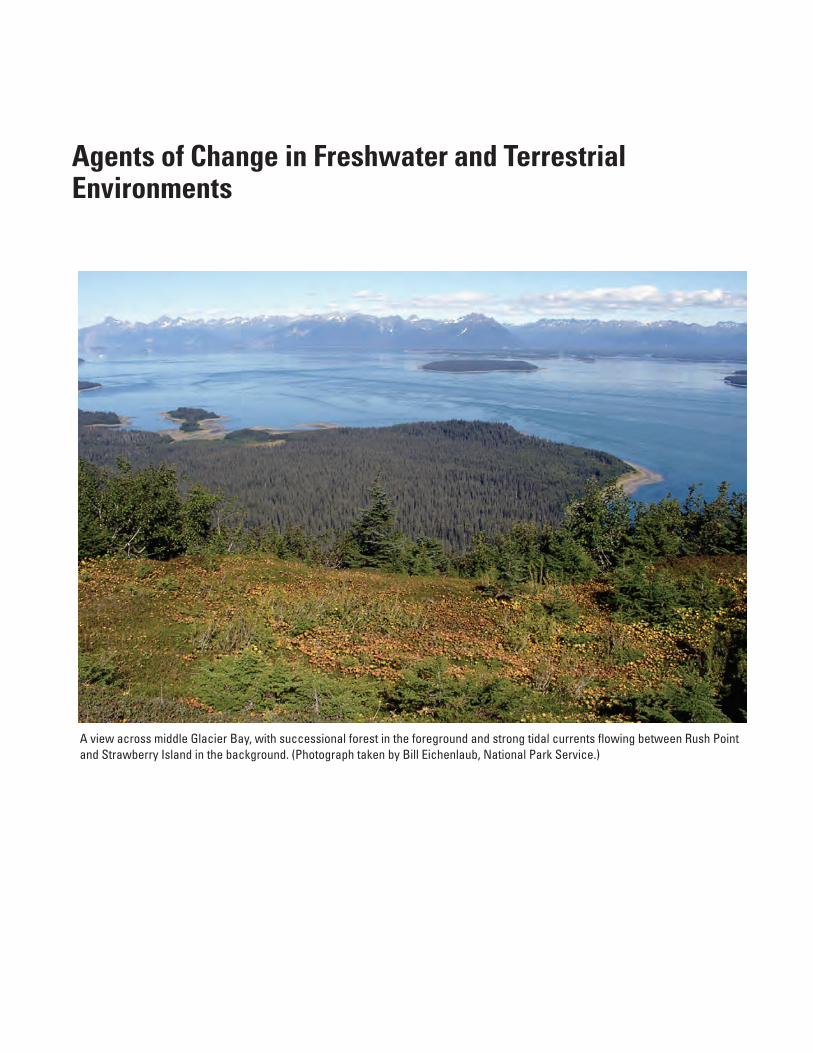
A view across middle Glacier Bay, with successional forest in the foreground and strong tidal currents flowing between Rush Point and Strawberry Island in the background. (Photograph taken by Bill Eichenlaub, National Park Service.)

Ecological Development of the Wolf Point Creek Watershed; A 25-Year Colonization Record from 1977 to 2001
Alexander M. Milner1,2,5, Kieran Monaghan1, Elizabeth A. Flory3, Amanda J. Veal1 and Anne Robertson4
Introduction
Whereas Engstrom and others (2000) studied 33 lakes of differing ages in Glacier Bay to infer development of the lake environment, environmental conditions must remain constant for the chronosequence approach to correctly represent historical development (Matthews, 1992). Climate change or other potential confounding variables may introduce non-linearities (Kaufmann, 2002) and thus direct observation is necessary to accurately determine succession sequences (Matthews, 1992). We have made almost continuous observations of Wolf Point Creek in Muir Inlet from 1977 and here we summarize the 25-year period from 1977 to 2001. Our aim has been to document the year in which macroinvertebrate taxa and fish species first colonized the stream and document if any taxa have become extinct. We are interested in the environmental and biotic variables driving colonization processes that are important in community assemblages.
Study Site
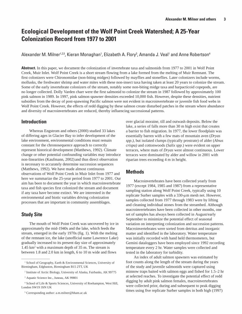
The mouth of Wolf Point Creek was uncovered by ice in approximately the mid-1940s and the lake, which feeds the stream, emerged in the early 1970s (fig. 1). With the melting of the remnant ice, the lake (unofficial name Lawrence Lake) gradually increased to its present day size of approximately 1.45 km2 with a maximum depth of 35 m. The stream is between 1.8 and 2.0 km in length, 6 to 10 m wide and flows
Abstract. In this paper, we document the colonization of invertebrate taxa and salmonids from 1977 to 2001 in Wolf Point Creek, Muir Inlet. Wolf Point Creek is a short stream flowing from a lake formed from the melting of Muir Remnant. The first colonizers were Chironomidae (non-biting midges) followed by mayflies and stoneflies. Later colonizers include worms, mollusks, the freshwater shrimp and water mites with these non-insect taxa having taken at least 20 years to colonize the stream. Some of the early invertebrate colonizers of the stream, notably some non-biting midge taxa and harpacticoid copepods, are no longer collected. Dolly Varden charr were the first salmonid to colonize the stream in 1987 followed by approximately 100 pink salmon in 1989. In 1997, pink salmon spawner densities exceeded 10,000 fish. However, despite these densities, nutrient subsidies from the decay of post-spawning Pacific salmon were not evident in macroinvertebrate or juvenile fish food webs in Wolf Point Creek. However, the effects of redd digging by these salmon create disturbed patches in the stream where abundance and diversity of macroinvertebrates are reduced, thereby influencing successional patterns.
over glacial moraine, till and outwash deposits. Below the lake, a series of falls more than 30 m high exist that creates a barrier to fish migration. In 1977, the lower floodplain was essentially barren with a few mats of mountain aven (Dryas spp.), but isolated clumps (typically prostrate) of alder (Alnus crispa) and cottonwoods (Salix spp.) were evident on upper terraces, where mats of Dryas were almost continuous. Lower terraces were dominated by alder and willow in 2001 with riparian trees exceeding 4 m in height.
Methods
Macroinvertebrates have been collected yearly from 1977 (except 1984, 1985 and 1987) from a representative sampling station along Wolf Point Creek, typically using 10 replicate Surber samples with a 330-µm mesh net. However, samples collected from 1977 through 1983 were by lifting and cleaning individual stones from the streambed. Although macroinvertebrates have been collected in other months, one set of samples has always been collected in August/early September to minimize the potential effect of seasonal variation on interpreting colonization and succession patterns. Macroinvertebrates were sorted from detritus and inorganic matter and identified in the laboratory. Water temperature was initially recorded with hand held thermometers, but Gemini dataloggers have been employed since 1992 recording temperature every 2 hr. Water samples were collected and tested in the laboratory for turbidity.
An index of adult salmon spawners was estimated by foot counts along the length of the stream during the years of the study and juvenile salmonids were captured using minnow traps baited with salmon eggs and fished for 1.5–2 hr at selected reaches. To investigate the potential effect of redd digging by adult pink salmon females, macroinvertebrates were collected prior, during and subsequent to peak digging times using five replicate Surber samples in both high (1997)
1 School of Geography, Earth & Environmental Sciences, University of Birmingham, Edgbaston, Birmingham B15 2TT, UK
2 Institute of Arctic Biology, University of Alaska, Fairbanks, AK 99775
3 Aquatic Science Inc., Juneau, AK 99801
4 School of Life & Sports Sciences, University of Roehampton, West Hill, London SW19 3SN UK
5 Corresponding author: [email protected]
Alexander M. Milner and others �

Figure 1. Wolf Point Creek drainage and the location of Lawrence Lake.
and low pink salmon (1996 and 1998) years. Drift samples over 24 hr also were collected in 1997 and 1998, between the end of July and early September downstream of known redds. Marked salmon carcasses also were staked into the streambed in 1997 to observe potential direct utilization by scavenger macroinvertebrates as a food source.
In 1997 and 1998 samples of vegetation, macroinvertebrates and juvenile fish were collected for stable isotope analysis of N15 to determine if marine-derived nutrients from salmon carcasses were being incorporated into the food chain. New foliage was taken from riparian willows with forceps and stored in plastic sample bags. Invertebrates were collected from stones (two representative genera [typically collectors and grazers] were used for comparison). Three juvenile coho salmon captured by minnow trapping were sacrificed and dorsal muscle tissue between the skull and dorsal fin removed for analysis. These samples were then analyzed for marine-derived N using the techniques outlined in Milner and others (2000).
Results
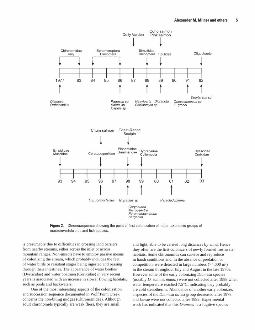
Turbidity in Wolf Point Creek decreased from 140 NTU in 1977 to <10 NTU in 2003. With water temperature increasing from a maximum 2°C in August 1977 to 18.5°C in July 2003, the number of degree-days has increased from <500 to 1,945 CTU. The year in which macroinvertebrates (orders, families and some specific genera) and fish first colonized Wolf Point Creek is summarized in figure 2. Macroinvertebrate taxon richness, cumulative taxon richness and cumulative taxa lost all showed a strong significant relationship with water temperature (r2=0.90, 0.97, and 0.93, respectively; P <0.05) (fig. 3).
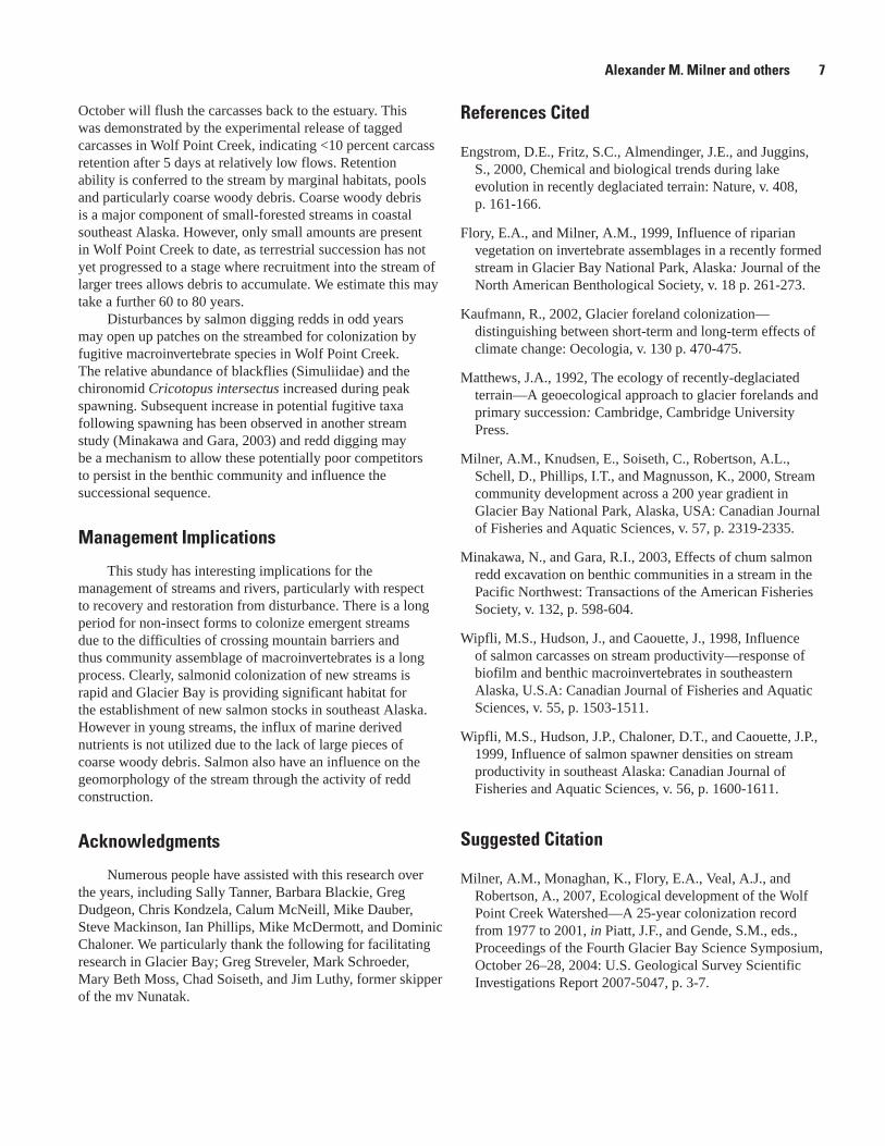
The first salmonids to colonize were Dolly Varden charr, as indicated by the first collection of their juvenile fry in 1988. Approximately 100 pink salmon colonized Wolf Point Creek in 1989 following a massive run of pink salmon throughout southeast Alaska during that year. Two years later in 1991, an index of spawning pink salmon was estimated at 1,250, in 1993, 3,600, and by 1997 the index exceeded 10,000 spawners (fig. 4). No evidence indicated that marine derived N was being incorporated into the stream foodweb or the riparian vegetation (Milner and others, 2000), even though macroinvertebrates were observed feeding directly on the salmon carcasses.
Macroinvertebrate abundance in reaches with redds during peak spawning periods in late August 1997 was significantly lower than abundance in August 1996 or 1998 or in the period prior to spawning in 1997. Macroinvertebrate densities were reduced to less than 100/0.1 m2 from a mean
of 480/0.1 m2 whereas total taxon richness was reduced from 18 to 10. Drift densities of macroinvertebrates were fourfold higher during peak spawning compared to the low salmon run year of 1998.
Discussion
Although water temperature was clearly an important determinant for colonization by some macroinvertebrates, other taxa, notably caddisflies and some chironomids, were related more to the growth of riparian vegetation along the stream and the provision of willow catkins as a food source or alder roots as a substrate (Flory and Milner, 1999). Of particular interest is the time taken for non-insect taxa to colonize the stream, as they lack obvious inter-stream dispersal mechanisms. The first non-insects were Oligochaeta in 1992 followed by snails (Planorbidae) and a gammarid shrimp in 1998. In 1992 maximum water temperature in Wolf Point Creek was 9°C, which would appear well above the threshold for Oligochaeta and thus the delay in colonization
� Proceedings of the Fourth Glacier Bay Science Symposium
is presumably due to difficulties in crossing land barriers from nearby streams, either across the inlet or across mountain ranges. Non-insects have to employ passive means of colonizing the stream, which probably includes the feet of water birds or resistant stages being ingested and passing through their intestines. The appearance of water beetles (Dysticidae) and water boatmen (Corixidae) in very recent years is associated with an increase in slower flowing habitats, such as pools and backwaters.
One of the most interesting aspects of the colonization and succession sequence documented in Wolf Point Creek concerns the non-biting midges (Chironomidae). Although adult chironomids typically are weak fliers, they are small
and light, able to be carried long distances by wind. Hence they often are the first colonizers of newly formed freshwater habitats. Some chironomids can survive and reproduce in harsh conditions and, in the absence of predation or competition, were detected in large numbers (>4,000 m2) in the stream throughout July and August in the late 1970s. However some of the early colonizing Diamesa species (notably D. sommermanni) were not collected after 1988 when water temperature reached 7.5°C, indicating they probably are cold stenotherms. Abundance of another early colonizer, a species of the Diamesa davisi group decreased after 1978 and larvae were not collected after 1992. Experimental work has indicated that this Diamesa is a fugitive species
Figure 2. Chronosequence showing the point of first colonization of major taxonomic groups of macroinvertebrates and fish species.
Alexander M. Milner and others 5
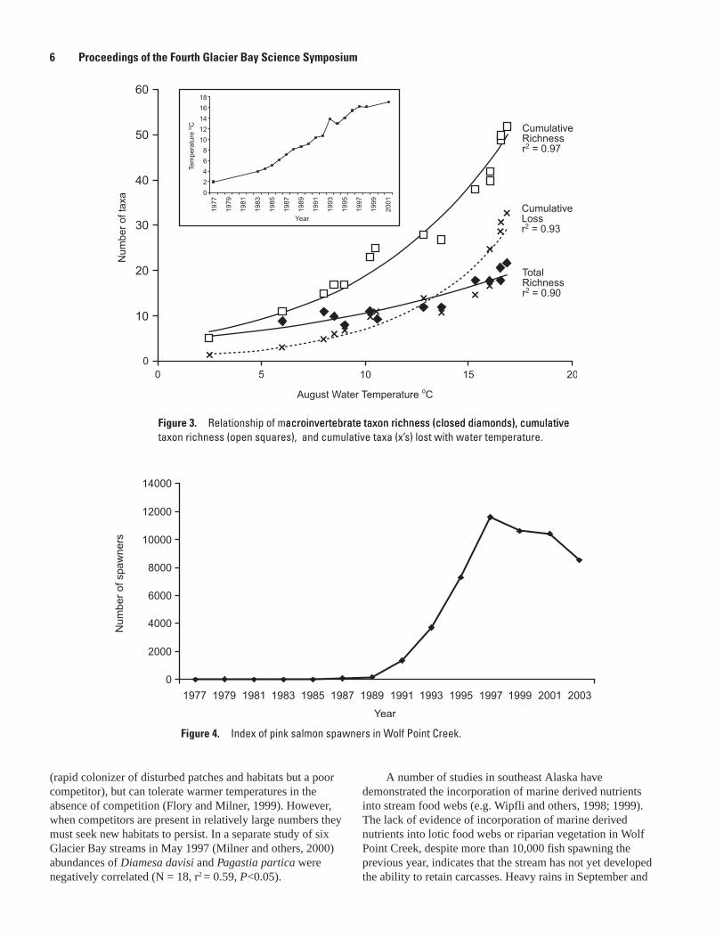
Figure �. Relationship of macroinvertebrate taxon richness (closed diamonds), cumulativeacroinvertebrate taxon richness (closed diamonds), cumulative taxon richness (open squares), and cumulative taxa (x’s) lost with water temperature.
(rapid colonizer of disturbed patches and habitats but a poor competitor), but can tolerate warmer temperatures in the absence of competition (Flory and Milner, 1999). However, when competitors are present in relatively large numbers they must seek new habitats to persist. In a separate study of six Glacier Bay streams in May 1997 (Milner and others, 2000) abundances of Diamesa davisi and Pagastia partica were negatively correlated (N = 18, r2 = 0.59, P<0.05).
A number of studies in southeast Alaska have demonstrated the incorporation of marine derived nutrients into stream food webs (e.g. Wipfli and others, 1998; 1999). The lack of evidence of incorporation of marine derived nutrients into lotic food webs or riparian vegetation in Wolf Point Creek, despite more than 10,000 fish spawning the previous year, indicates that the stream has not yet developed the ability to retain carcasses. Heavy rains in September and
Figure �. Index of pink salmon spawners in Wolf Point Creek.
� Proceedings of the Fourth Glacier Bay Science Symposium
October will flush the carcasses back to the estuary. This was demonstrated by the experimental release of tagged carcasses in Wolf Point Creek, indicating <10 percent carcass retention after 5 days at relatively low flows. Retention ability is conferred to the stream by marginal habitats, pools and particularly coarse woody debris. Coarse woody debris is a major component of small-forested streams in coastal southeast Alaska. However, only small amounts are present in Wolf Point Creek to date, as terrestrial succession has not yet progressed to a stage where recruitment into the stream of larger trees allows debris to accumulate. We estimate this may take a further 60 to 80 years.
Disturbances by salmon digging redds in odd years may open up patches on the streambed for colonization by fugitive macroinvertebrate species in Wolf Point Creek. The relative abundance of blackflies (Simuliidae) and the chironomid Cricotopus intersectus increased during peak spawning. Subsequent increase in potential fugitive taxa following spawning has been observed in another stream study (Minakawa and Gara, 2003) and redd digging may be a mechanism to allow these potentially poor competitors to persist in the benthic community and influence the successional sequence.
Management Implications
This study has interesting implications for the management of streams and rivers, particularly with respect to recovery and restoration from disturbance. There is a long period for non-insect forms to colonize emergent streams due to the difficulties of crossing mountain barriers and thus community assemblage of macroinvertebrates is a long process. Clearly, salmonid colonization of new streams is rapid and Glacier Bay is providing significant habitat for the establishment of new salmon stocks in southeast Alaska. However in young streams, the influx of marine derived nutrients is not utilized due to the lack of large pieces of coarse woody debris. Salmon also have an influence on the geomorphology of the stream through the activity of redd construction.
Acknowledgments
Numerous people have assisted with this research over the years, including Sally Tanner, Barbara Blackie, Greg Dudgeon, Chris Kondzela, Calum McNeill, Mike Dauber, Steve Mackinson, Ian Phillips, Mike McDermott, and Dominic Chaloner. We particularly thank the following for facilitating research in Glacier Bay; Greg Streveler, Mark Schroeder, Mary Beth Moss, Chad Soiseth, and Jim Luthy, former skipper of the mv Nunatak.
References Cited
Engstrom, D.E., Fritz, S.C., Almendinger, J.E., and Juggins, S., 2000, Chemical and biological trends during lake evolution in recently deglaciated terrain: Nature, v. 408, p. 161-166.
Flory, E.A., and Milner, A.M., 1999, Influence of riparian vegetation on invertebrate assemblages in a recently formed stream in Glacier Bay National Park, Alaska: Journal of the North American Benthological Society, v. 18 p. 261-273.
Kaufmann, R., 2002, Glacier foreland colonization—distinguishing between short-term and long-term effects of climate change: Oecologia, v. 130 p. 470-475.
Matthews, J.A., 1992, The ecology of recently-deglaciated terrain—A geoecological approach to glacier forelands and primary succession: Cambridge, Cambridge University Press.
Milner, A.M., Knudsen, E., Soiseth, C., Robertson, A.L., Schell, D., Phillips, I.T., and Magnusson, K., 2000, Stream community development across a 200 year gradient in Glacier Bay National Park, Alaska, USA: Canadian Journal of Fisheries and Aquatic Sciences, v. 57, p. 2319-2335.
Minakawa, N., and Gara, R.I., 2003, Effects of chum salmon redd excavation on benthic communities in a stream in the Pacific Northwest: Transactions of the American Fisheries Society, v. 132, p. 598-604.
Wipfli, M.S., Hudson, J., and Caouette, J., 1998, Influence of salmon carcasses on stream productivity—response of biofilm and benthic macroinvertebrates in southeastern Alaska, U.S.A: Canadian Journal of Fisheries and Aquatic Sciences, v. 55, p. 1503-1511.
Wipfli, M.S., Hudson, J.P., Chaloner, D.T., and Caouette, J.P., 1999, Influence of salmon spawner densities on stream productivity in southeast Alaska: Canadian Journal of Fisheries and Aquatic Sciences, v. 56, p. 1600-1611.
Suggested Citation
Milner, A.M., Monaghan, K., Flory, E.A., Veal, A.J., and Robertson, A., 2007, Ecological development of the Wolf Point Creek Watershed—A 25-year colonization record from 1977 to 2001, in Piatt, J.F., and Gende, S.M., eds., Proceedings of the Fourth Glacier Bay Science Symposium, October 26–28, 2004: U.S. Geological Survey Scientific Investigations Report 2007-5047, p. 3-7.
Alexander M. Milner and others 7
Coupling Between Primary Terrestrial Succession and the Trophic Development of Lakes at Glacier Bay
D.R. Engstrom1,3 and S.C. Fritz2
Abstract. We use sediment cores from lakes in Glacier Bay National Park to examine the relationship between successional changes in catchment vegetation and trends in water-column nitrogen (a limiting nutrient) and lake primary production. Terrestrial succession at Glacier Bay follows several different pathways, with older sites in the lower bay being colonized directly by spruce (Picea) and by-passing a prolonged alder (Alnus) stage that characterizes younger upper-bay sites. Sediment cores from three sites spanning this successional gradient demonstrate that the variability in trophic development among lakes is a consequence of the establishment and duration of N-fixing alder in the lake catchment.
1 St. Croix Watershed Research Station, Science Museum of Minnesota, 16910 152nd North, Marine-on-St. Croix, MN 55047
2 Department of Geosciences and School of Biological Sciences, University of Nebraska, 214 Bessey Hall, Lincoln, NE 68588 ([email protected], 402-472-6431)
3 Corresponding author: [email protected], 651-433-5953
Introduction
The natural eutrophication of lakes is a widely held concept in limnology, arising from the earliest efforts to classify lakes and place them in an evolutionary sequence. Recent studies of newly formed lakes at Glacier Bay, Alaska, only partially support this idea, and suggest more variable trends in lake trophic development (Engstrom and others, 2000; Fritz and others, 2004). This variability is thought to relate to successional trends in catchment vegetation, which have been shown to differ between sites in upper and lower Glacier Bay. Rather than a single successional pathway going from early colonizers to alder (Alnus crispa v. sinuata) to spruce (Picea sitchensis), terrestrial succession actually follows several pathways depending on seed availability and the life-history traits of the dominant species (Chapin and others, 1994). Thus, older sites in the lower bay were colonized directly by spruce and effectively by-passed the prolonged alder stage that characterizes younger upper-bay sites.
The purpose of this study is to explore the consequences of these contrasting pathways in terrestrial succession on lake trophic development—in particular, nitrogen levels and primary productivity. Because lake sediments record both vegetation (through pollen) and lake chemistry (though diatoms), it should be possible to test the idea that the local presence of N-fixing alder influences lake ontogeny at Glacier Bay. The study lakes are particularly well-suited to this task, as most are small (1-5 ha surface area), have a strong local-pollen signature, and are nitrogen limited, so fossil diatom assemblages provide a robust indicator of historical lake-water N. Moreover, the accumulation rate of diatoms in the sediments provides a direct measure of whole-lake primary productivity. Diatoms are well preserved in most sediments
(unlike carbon), and sediments integrate year-round diatom production from all habitats, including benthic, which is not captured in any manner by conventional measurement of water-column productivity.
Study Sites
Our original study of lakes in Glacier Bay National Park included 32 sites ranging in age from 10 years to >10,000 years (Engstrom and others, 2000). Three lakes from this original set are the focus of the current study: Bartlett Lake, adjacent to the terminal neoglacial moraine, Lester Island (Lester-1 in the original chronosequence), also in the lower bay, but in the Beardslee Islands and far from the terminal moraine, and Blue Mouse Cove at the lower end of the west arm of the Glacier Bay fjord (fig. 1). The first two sites, Bartlett Lake and Lester Island occupy land surfaces deglaciated about 200 years ago and are today vegetated by closed spruce/hemlock (Tsuga heterophylla) forest. The third site at Blue Mouse Cove is about 110 years old, and has a catchment cloaked in dense alder thickets with scattered spruce and cottonwood (Populus balsamifera) poking through the alder canopy. The lakes range from 4.0 to 8.0 m maximum depth, and except for Bartlett Lake (62 ha) are small (1.7–3.5 ha).
Methods
A single sediment core was collected from the deepwater zone of each lake with a piston corer operated from the lake surface by rigid drive rods. Cores were sectioned in the field at 0.5–1.0 cm intervals and later analyzed for diatoms and pollen and dated by 210Pb. Subsamples for diatom analysis were oxidized in HNO
3/K
2Cr
2O
7, spiked with a calibrated
microsphere solution, dried onto coverslips, and mounted with Naphrax. A minimum of 400 individual diatoms were counted at 1000x under oil immersion. Standard laboratory procedures were used to prepare subsamples for pollen analysis, and a sum of 200–250 pollen and spores were counted. Lead-210 was measured by 210Po-distillation and alpha-spectrometry methods, and dates were determined according to the c.r.s.
� Proceedings of the Fourth Glacier Bay Science Symposium
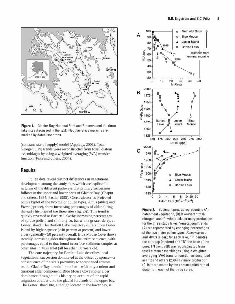
Figure 1. Glacier Bay National Park and Preserve and the three lake sites discussed in the text. Neoglacial ice margins are marked by dated isochrons.
(constant rate of supply) model (Appleby, 2001). Total-nitrogen (TN) trends were reconstructed from fossil diatom assemblages by using a weighted averaging (WA) transfer function (Fritz and others, 2004).
Results
Pollen data reveal distinct differences in vegetational development among the study sites which are explicable in terms of the different pathways that primary succession follows in the upper and lower parts of Glacier Bay (Chapin and others, 1994; Fastie, 1995). Core trajectories projected onto a biplot of the two major pollen types, Alnus (alder) and Picea (spruce), show increasing percentages of alder during the early histories of the three sites (fig. 2A). This trend is quickly reversed at Bartlett Lake by increasing percentages of spruce pollen, and similarly so, but with a greater delay, at Lester Island. The Bartlett Lake trajectory differs from Lester Island by higher spruce (>40 percent at present) and lower alder (generally<50 percent) overall. Blue Mouse Cove shows steadily increasing alder throughout the entire sequence, with percentages equal to that found in surface-sediment samples at other sites in Muir Inlet (all less than 80 years old).
The core trajectory for Bartlett Lake describes local vegetational succession dominated at the outset by spruce—a consequence of the site’s proximity to spruce seed sources on the Glacier Bay terminal moraine—with only a minor and transient alder component. Blue Mouse Cove shows alder dominance throughout its history on account of the rapid migration of alder onto the glacial forelands of the upper bay. The Lester Island site, although located in the lower bay, is
Figure 2. Sediment proxies representing (A) catchment vegetation, (B) lake-water total-nitrogen, and (C) whole-lake primary production for the three study lakes. Vegetational trends (A) are represented by changing percentages of the two major pollen types, Picea (spruce) and Alnus (alder); for each lake, “T” denotes the core top (modern) and “B” the base of the core. TN trends (B) are reconstructed from fossil diatom assemblages using a weighted averaging (WA) transfer function as described in Fritz and others (2004). Primary production (C) is represented by the accumulation rate of diatoms in each of the three cores.
D.R. Engstrom and S.C. Fritz 9
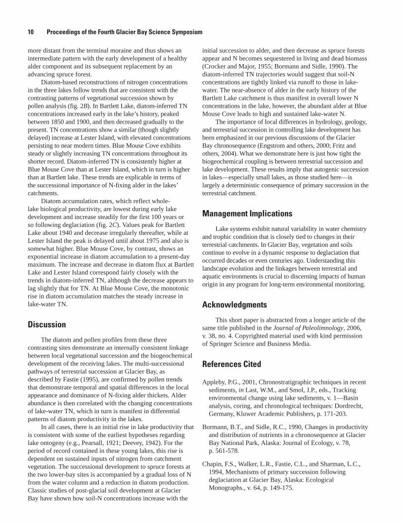
more distant from the terminal moraine and thus shows an intermediate pattern with the early development of a healthy alder component and its subsequent replacement by an advancing spruce forest.
Diatom-based reconstructions of nitrogen concentrations in the three lakes follow trends that are consistent with the contrasting patterns of vegetational succession shown by pollen analysis (fig. 2B). In Bartlett Lake, diatom-inferred TN concentrations increased early in the lake’s history, peaked between 1850 and 1900, and then decreased gradually to the present. TN concentrations show a similar (though slightly delayed) increase at Lester Island, with elevated concentrations persisting to near modern times. Blue Mouse Cove exhibits steady or slightly increasing TN concentrations throughout its shorter record. Diatom-inferred TN is consistently higher at Blue Mouse Cove than at Lester Island, which in turn is higher than at Bartlett lake. These trends are explicable in terms of the successional importance of N-fixing alder in the lakes’ catchments.
Diatom accumulation rates, which reflect whole-lake biological productivity, are lowest during early lake development and increase steadily for the first 100 years or so following deglaciation (fig. 2C). Values peak for Bartlett Lake about 1940 and decrease irregularly thereafter, while at Lester Island the peak is delayed until about 1975 and also is somewhat higher. Blue Mouse Cove, by contrast, shows an exponential increase in diatom accumulation to a present-day maximum. The increase and decrease in diatom flux at Bartlett Lake and Lester Island correspond fairly closely with the trends in diatom-inferred TN, although the decrease appears to lag slightly that for TN. At Blue Mouse Cove, the monotonic rise in diatom accumulation matches the steady increase in lake-water TN.
Discussion
The diatom and pollen profiles from these three contrasting sites demonstrate an internally consistent linkage between local vegetational succession and the biogeochemical development of the receiving lakes. The multi-successional pathways of terrestrial succession at Glacier Bay, as described by Fastie (1995), are confirmed by pollen trends that demonstrate temporal and spatial differences in the local appearance and dominance of N-fixing alder thickets. Alder abundance is then correlated with the changing concentrations of lake-water TN, which in turn is manifest in differential patterns of diatom productivity in the lakes.
In all cases, there is an initial rise in lake productivity that is consistent with some of the earliest hypotheses regarding lake ontogeny (e.g., Pearsall, 1921; Deevey, 1942). For the period of record contained in these young lakes, this rise is dependent on sustained inputs of nitrogen from catchment vegetation. The successional development to spruce forests at the two lower-bay sites is accompanied by a gradual loss of N from the water column and a reduction in diatom production. Classic studies of post-glacial soil development at Glacier Bay have shown how soil-N concentrations increase with the
initial succession to alder, and then decrease as spruce forests appear and N becomes sequestered in living and dead biomass (Crocker and Major, 1955; Bormann and Sidle, 1990). The diatom-inferred TN trajectories would suggest that soil-N concentrations are tightly linked via runoff to those in lake-water. The near-absence of alder in the early history of the Bartlett Lake catchment is thus manifest in overall lower N concentrations in the lake, however, the abundant alder at Blue Mouse Cove leads to high and sustained lake-water N.
The importance of local differences in hydrology, geology, and terrestrial succession in controlling lake development has been emphasized in our previous discussions of the Glacier Bay chronosequence (Engstrom and others, 2000; Fritz and others, 2004). What we demonstrate here is just how tight the biogeochemical coupling is between terrestrial succession and lake development. These results imply that autogenic succession in lakes—especially small lakes, as those studied here—is largely a deterministic consequence of primary succession in the terrestrial catchment.
Management Implications
Lake systems exhibit natural variability in water chemistry and trophic condition that is closely tied to changes in their terrestrial catchments. In Glacier Bay, vegetation and soils continue to evolve in a dynamic response to deglaciation that occurred decades or even centuries ago. Understanding this landscape evolution and the linkages between terrestrial and aquatic environments is crucial to discerning impacts of human origin in any program for long-term environmental monitoring.
Acknowledgments
This short paper is abstracted from a longer article of the same title published in the Journal of Paleolimnology, 2006, v. 38, no. 4. Copyrighted material used with kind permission of Springer Science and Business Media.
References Cited
Appleby, P.G., 2001, Chronostratigraphic techniques in recent sediments, in Last, W.M., and Smol, J.P., eds., Tracking environmental change using lake sediments, v. 1—Basin analysis, coring, and chronological techniques: Dordrecht, Germany, Kluwer Academic Publishers, p. 171-203.
Bormann, B.T., and Sidle, R.C., 1990, Changes in productivity and distribution of nutrients in a chronosequence at Glacier Bay National Park, Alaska: Journal of Ecology, v. 78, p. 561-578.
Chapin, F.S., Walker, L.R., Fastie, C.L., and Sharman, L.C., 1994, Mechanisms of primary succession following deglaciation at Glacier Bay, Alaska: Ecological Monographs., v. 64, p. 149-175.
10 Proceedings of the Fourth Glacier Bay Science Symposium
Crocker, R.L., and Major, J., 1955, Soil development in relation to vegetation and surface age at Glacier Bay, Alaska: Journal of Ecology, v. 43, p. 427-448.
Deevey, E.S., 1942, Studies on Connecticut Lake sediments, III—The biostratonomy of Linsley Pond: American Journal of Science, v. 240, p. 313-324.
Engstrom, D.R., Fritz, S.C., Almendinger, J.E. and Juggins, S., 2000, Chemical and biological trends during lake evolution in recently deglaciated terrain: Nature, v. 408, p. 161-166.
Fastie, C.L., 1995, Causes and ecosystem consequences of multiple successional pathways of primary succession at Glacier Bay, Alaska: Ecology, v. 76, p. 1899-1916.
Fritz, S.C., Engstrom, D.R., and Juggins, S., 2004, Patterns of early lake evolution in boreal landscapes—a comparison of stratigraphic inferences with a modern chronosequence in Glacier Bay, Alaska: The Holocene, v. 14, p. 828-840.
Pearsall, W.H., 1921, The development of vegetation in the English Lakes, considered in relation to the general evolution of glacial lakes and rock basins: Proceedings of the Royal Society B., v. 92, p. 259-284.
Suggested Citation
Engstrom, D.R., and Fritz, S.C., 2006, Coupling between primary terrestrial succession and the trophic development of lakes at Glacier Bay, in Piatt, J.F., and Gende, S.M., eds., Proceedings of the Fourth Glacier Bay Science Symposium, October 26–28, 2004: U.S. Geological Survey Scientific Investigations Report 2007-5047, p. 8-11.
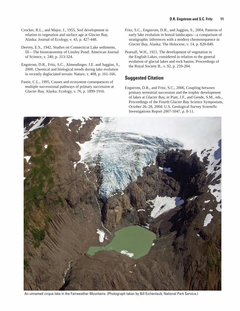
An unnamed cirque lake in the Fairweather Mountains. (Photograph taken by Bill Eichenlaub, National Park Service.)
D.R. Engstrom and S.C. Fritz 11
Spruce Beetle Epidemic and Successional Aftermath in Glacier Bay
Mark Schultz1,2 and Paul Hennon1
Abstract. A spruce beetle (Dendroctonus rufipennis Kby.) epidemic that began in the mid-1970s and persisted to the 1990s caused significant Sitka spruce (Picea sitchensis (Bong.) Carr.) mortality in the Beardslee Islands and in a few neighboring mainland areas of lower Glacier Bay. Entomologists of the U.S. Forest Service installed vegetation plots in 1982 and have followed the progression of the outbreak and its influence on forest structure and plant succession for 20 years. Stagnant tree growth from low nutrient availability probably contributed to the spruce beetle epidemic. Tree death was heavy in some sites resulting in a large volume of dead wood and the formation of forest gaps, which are now occupied by tree seedlings, shrubs, and herbaceous plants. This secondary disturbance by spruce beetle appears to have accelerated succession in the direction of an old-growth forest condition as these forests now have a more complex structure than forests with a similar age structure unaffected by spruce beetle.
1 U.S. Department of Agriculture, Forest Service, Alaska Region, Forest Health Protection, 2770 Sherwood Lane, Suite 2A, Juneau, AK 99801
2 Corresponding author: [email protected], 907-586-8883
Introduction
Most of the work conducted on forest succession across the chronosequence of Glacier Bay National Park has focused on colonization of forbs, shrubs, and trees that eventually develop into a homogenous conifer forest composed of a relatively even-aged condition (Goldthwait, 1966; Bormann and Sidle, 1990; Fastie, 1995). However, the next transitional stage that represents the breakup of the even-age forest as it enters the more complex structure and composition of old-growth condition is not well understood in the Park, or anywhere else in coastal Alaska.
Until the mid-1970s much of the lower bay was occupied by relatively dense stands of Sitka spruce and western hemlock in the 120 to 140 year age class. The ‘O’ (organic) horizon in the soils associated with these stands had accumulated much of the nitrogen in these forests and consequently the spruce stands began to lose their foliar nitrogen in this age class (Bormann and Sidle, 1990). This foliar nitrogen decrease was strongly correlated to the slowing of height and radial growth (productivity) of trees and led to stagnation over the last 50 years in that study.
As a result of nutrient immobilization and resultant decreased tree vigor, extensive blow-down in the late 1970s and dry conditions in the early 1980s, spruce beetle became epidemic sometime before 1980. Aerial photographs taken in 1979 revealed spruce mortality on about 600 ha in the lower bay on Young and Strawberry Islands, and between Berg Bay and Ripple Cove. The infestation spread dramatically between 1982 and 1985 (the greatest epidemic years for spruce beetle), and by 1996 covered nearly 14,000 ha. Spruce mortality exceeded 75 percent of the stand in some areas. Spruce beetle mortality spread east of the original outbreak area, near Excursion Ridge, but has now subsided in the Park.
The objective of this investigation was to document the role of spruce beetle and tree death on changes in forest vegetation composition and structure in beetle-impacted forests of lower Glacier Bay.
Methods
In 1982, 45 one-twelfth hectare plots were installed in the Sitakaday Narrows area of the Park to document the effect of a spruce beetle epidemic (Eglitis, 1987). In 1998, tree data were collected on every tagged live and dead tree that could be found (the tags on fallen dead trees could not always be found). In 2004, overstory tree data on the 1/12-ha plot was collected from the 21 plots near Berg Bay, Ripple Cove, and Lester Island. Plots originally were installed in locations that were dominated by Sitka spruce. Western hemlock (Tsuga heterophylla (Raf.) Sarg.) comprised only a small amount of the total basal area. As a measure of disturbance, the mean percentage of live basal area (from both live and dead basal area) on plots from five general locations was displayed graphically from 1977 to 1998.
Tree measurements (diameter at breast-height and tree height) and condition (beetle attacks, fungal fruiting bodies, and height-to-break) were noted. Spruce beetle was recorded as the cause of death if sufficient galleries could be found under the bark of dead trees; otherwise, trees were recorded as dead from unknown causes. Cores used in assessing tree growth were removed from trees at breast height with an increment borer, mounted, and sanded before ring counting with a dissecting microscope. The number of regenerating trees and cover estimates for 35 understory plant species found on the plots were recorded to determine vegetation richness and to give an interpretation on future successional trends. Seedlings of trees greater than one foot tall were counted by species on a randomly-chosen quarter-section of 27 plots in 1998 and on most of the plot area of 21 plots in 2004. Understory plant cover was estimated in nested 18×18-m plots in the 21 overstory plots measured in 2004 (described above). A GPS location was taken at each plot center and all trees that could be assigned a tag number were stem-mapped.
12 Proceedings of the Fourth Glacier Bay Science Symposium
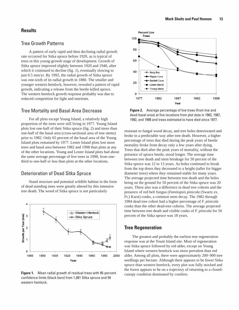
Figure 1. Mean radial growth of residual trees with 95-percent confidence limits (black bars) from 1,081 Sitka spruce and 59 western hemlock.
resistant to fungal wood decay, and tree boles deteriorated and broke in a predictable way after tree death. However, a higher percentage of trees that died during the peak years of beetle mortality broke from decay only a few years after dying. Trees that died after the peak years of mortality, without the presence of spruce beetle, stood longer. The average time between tree death and stem breakage for 50 percent of the Sitka spruce was 12 to 13 years. As boles continued to break from the top down they decreased to a height (taller for bigger diameter trees) where they remained stable for many years. The average projected time between tree death and the boles being on the ground for 50 percent of the Sitka spruce was 20 years. There also was a difference in dead tree cohorts and the presence of red belt fungus (Fomitopsis pinicola (Swartz ex. Fr.) Karst) conks, a common stem decay. The 1982 through 1984 dead tree cohort had a higher percentage of F. pinicola conks than the other dead-tree cohorts. The average projected time between tree death and visible conks of F. pinicola for 50 percent of the Sitka spruce was 18 years.
Tree Regeneration
The greatest and probably the earliest tree regeneration response was at the Yount Island site. Most of regeneration was Sitka spruce followed by red alder, except on Young Island where western hemlock was more prevalent than red alder. Among all plots, there were approximately 200–900 tree seedlings per hectare. Although there appears to be fewer Sitka spruce than western hemlock, every plot was fully stocked and the forest appears to be on a trajectory of returning to a closed-canopy condition dominated by conifers.
Results
Tree Growth PatternsA pattern of early rapid and then declining radial growth
rate occurred for Sitka spruce before 1920, as is typical of trees in this young-growth stage of development. Growth of Sitka spruce improved slightly between 1920 and 1940, after which it continued to decline (fig. 1), eventually slowing to just 0.5 mm/yr. By 1992, the radial growth of Sitka spruce was one-sixth of its radial growth in 1880. The smaller and younger western hemlock, however, revealed a pattern of rapid growth, indicating a release from the beetle-killed spruce. The western hemlock growth response probably was due to reduced competition for light and nutrients.
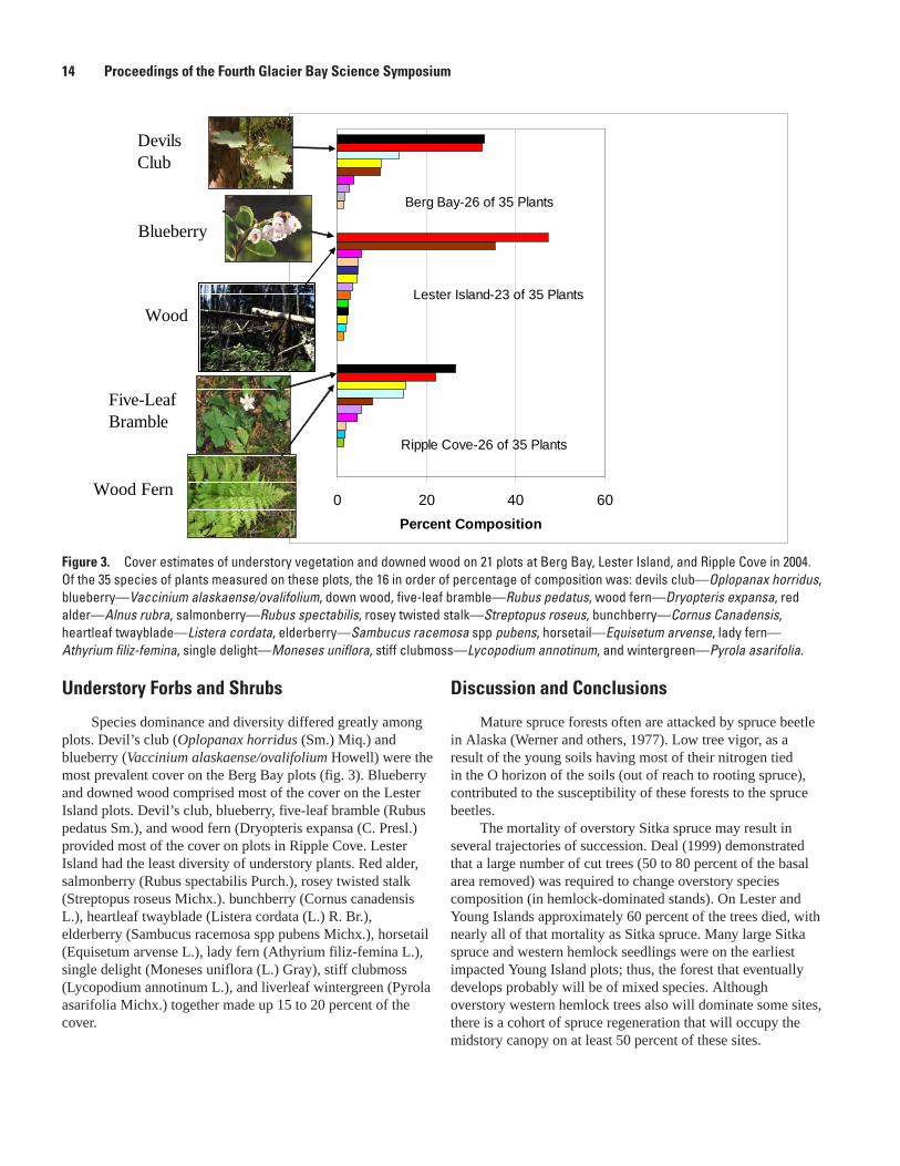
Tree Mortality and Basal Area DecreaseFor all plots except Young Island, a relatively high
proportion of the trees were still living in 1977. Young Island plots lost one-half of their Sitka spruce (fig. 2) and more than one-half of the basal area (cross-sectional area of tree stems) prior to 1982. Only 65 percent of the basal area of the Young Island plots remained by 1977. Lester Island plots lost more trees and basal area between 1982 and 1998 than plots at any of the other locations. Young and Lester Island plots had about the same average percentage of live trees in 1998, from one-third to one-half or less than plots at the other locations.
Deterioration of Dead Sitka SpruceStand structure and potential wildlife habitat in the form
of dead standing trees were greatly altered by this intensive tree death. The wood of Sitka spruce is not particularly
Figure 2. Average percentage of live trees (from live and dead basal area) at five locations from plot data in 1982, 1987, 1992, and 1998 and trees estimated to have died since 1977.
Mark Shultz and Paul Hennon 1�
Understory Forbs and Shrubs
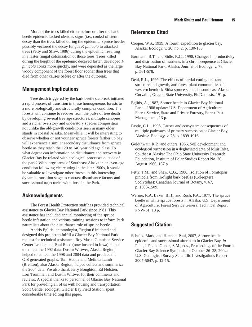
Species dominance and diversity differed greatly among plots. Devil’s club (Oplopanax horridus (Sm.) Miq.) and blueberry (Vaccinium alaskaense/ovalifolium Howell) were the most prevalent cover on the Berg Bay plots (fig. 3). Blueberry and downed wood comprised most of the cover on the Lester Island plots. Devil’s club, blueberry, five-leaf bramble (Rubus pedatus Sm.), and wood fern (Dryopteris expansa (C. Presl.) provided most of the cover on plots in Ripple Cove. Lester Island had the least diversity of understory plants. Red alder, salmonberry (Rubus spectabilis Purch.), rosey twisted stalk (Streptopus roseus Michx.). bunchberry (Cornus canadensis L.), heartleaf twayblade (Listera cordata (L.) R. Br.), elderberry (Sambucus racemosa spp pubens Michx.), horsetail (Equisetum arvense L.), lady fern (Athyrium filiz-femina L.), single delight (Moneses uniflora (L.) Gray), stiff clubmoss (Lycopodium annotinum L.), and liverleaf wintergreen (Pyrola asarifolia Michx.) together made up 15 to 20 percent of the cover.
Discussion and Conclusions
Mature spruce forests often are attacked by spruce beetle in Alaska (Werner and others, 1977). Low tree vigor, as a result of the young soils having most of their nitrogen tied in the O horizon of the soils (out of reach to rooting spruce), contributed to the susceptibility of these forests to the spruce beetles.
The mortality of overstory Sitka spruce may result in several trajectories of succession. Deal (1999) demonstrated that a large number of cut trees (50 to 80 percent of the basal area removed) was required to change overstory species composition (in hemlock-dominated stands). On Lester and Young Islands approximately 60 percent of the trees died, with nearly all of that mortality as Sitka spruce. Many large Sitka spruce and western hemlock seedlings were on the earliest impacted Young Island plots; thus, the forest that eventually develops probably will be of mixed species. Although overstory western hemlock trees also will dominate some sites, there is a cohort of spruce regeneration that will occupy the midstory canopy on at least 50 percent of these sites.
Figure �. Cover estimates of understory vegetation and downed wood on 21 plots at Berg Bay, Lester Island, and Ripple Cove in 2004. Of the 35 species of plants measured on these plots, the 16 in order of percentage of composition was: devils club—Oplopanax horridus, blueberry—Vaccinium alaskaense/ovalifolium, down wood, five-leaf bramble—Rubus pedatus, wood fern—Dryopteris expansa, red alder—Alnus rubra, salmonberry—Rubus spectabilis, rosey twisted stalk—Streptopus roseus, bunchberry—Cornus Canadensis, heartleaf twayblade—Listera cordata, elderberry—Sambucus racemosa spp pubens, horsetail—Equisetum arvense, lady fern—Athyrium filiz-femina, single delight—Moneses uniflora, stiff clubmoss—Lycopodium annotinum, and wintergreen—Pyrola asarifolia.
0 20 40 60Percent Composition
Berg Bay-26 of 35 Plants
Lester Island-23 of 35 Plants
Ripple Cove-26 of 35 Plants
Devils Club
Five-Leaf Bramble
Blueberry
Wood Fern
Wood
1� Proceedings of the Fourth Glacier Bay Science Symposium
More of the trees killed either before or after the bark beetle epidemic lacked obvious signs (i.e., conks) of stem decay than the trees killed during the epidemic. Spruce beetles possibly vectored the decay fungus F. pinicola to attacked trees (Petty and Shaw, 1986) during the epidemic, resulting in a faster fungal colonization of those trees. Trees killed during the height of the epidemic decayed faster, developed F. pinicola conks more quickly, and were deposited as the large woody component of the forest floor sooner than trees that died from other causes before or after the outbreak.
Management Implications
Tree death triggered by the bark beetle outbreak initiated a rapid process of transition in these homogeneous forests to a more biologically and structurally complex condition. The forests will continue to recover from the pulse of tree death by developing several tree age structures, multiple canopies, and a richer overstory and understory species composition not unlike the old-growth conditions seen in many older stands in coastal Alaska. Meanwhile, it will be interesting to observe whether or not younger spruce forests farther up bay will experience a similar secondary disturbance from spruce beetle as they reach the 120 to 140 year old age class. To what degree can information on disturbance and recovery in Glacier Bay be related with ecological processes outside of the park? With large areas of Southeast Alaska in an even-age condition following clearcutting in the later 1900s, it would be valuable to investigate other forests in this interesting dynamic transition stage to contrast disturbance factors and successional trajectories with those in the Park.
Acknowledgments
The Forest Health Protection staff has provided technical assistance to Glacier Bay National Park since 1981. This assistance has included annual monitoring of the spruce beetle infestation and various training sessions to inform Park naturalists about the disturbance role of spruce beetle.
Andris Eglitis, entomologist, Region 6 initiated and designed this project to fulfill a Glacier Bay National Park request for technical assistance. Roy Mask, Gunnison Service Center Leader, and Paul Reed (now located in Iowa) helped to collect the 1992 data. Dustin Wittwer, Alaska Region, helped to collect the 1998 and 2004 data and produce the GIS generated graphs. Tom Heutte and Melinda Lamb (Brenton), also Alaska Region, helped collect and summarize the 2004 data. We also thank Jerry Boughton, Ed Holsten, Lori Trummer, and Dustin Wittwer for their comments and reviews. A special thanks to personnel of Glacier Bay National Park for providing all of us with housing and transportation. Scott Gende, ecologist, Glacier Bay Field Station, spent considerable time editing this paper.
References Cited
Cooper, W.S., 1939, A fourth expedition to glacier bay, Alaska: Ecology, v. 20, no. 2, p. 130-155.
Bormann, B.T., and Sidle, R.C., 1990, Changes in productivity and distribution of nutrients in a chronosequence at Glacier Bay National Park, Alaska: Journal of Ecology, v. 78, p. 561-578.
Deal, R.L., 1999, The effects of partial cutting on stand structure and growth, and forest plant communities of western hemlock-Sitka spruce stands in southeast Alaska: Corvallis, Oregon State University, Ph.D. thesis, 191 p.
Eglitis, A., 1987, Spruce beetle in Glacier Bay National Park—1986 update: U.S. Department of Agriculture, Forest Service, State and Private Forestry, Forest Pest Management, 13 p.
Fastie, C.L., 1995, Causes and ecosystem consequences of multiple pathways of primary succession at Glacier Bay, Alaska\:. Ecology, v. 76, p. 1899-1916.
Goldthwait, R.P., and others, 1966, Soil development and ecological succession in a deglaciated area of Muir Inlet, Southeast Alaska: The Ohio State University Research Foundation, Institute of Polar Studies Report No. 20, August 1966, 167 p.
Petty, T.M., and Shaw, C.G., 1986, Isolation of Fomitopsis pinicola from in-flight bark beetles (Coleoptera: Scolytidae): Canadian Journal of Botany, v. 67, p. 1508-1509.
Werner, R.A, Baker, B.H., and Rush, P.A., 1977, The spruce beetle in white spruce forests in Alaska: U.S. Department of Agriculture, Forest Service General Technical Report PNW-61, 13 p.
Suggested Citation
Schultz, Mark, and Hennon, Paul, 2007, Spruce beetle epidemic and successional aftermath in Glacier Bay, in Piatt, J.F., and Gende, S.M., eds., Proceedings of the Fourth Glacier Bay Science Symposium, October 26–28, 2004: U.S. Geological Survey Scientific Investigations Report 2007-5047, p. 12-15.
Mark Shultz and Paul Hennon 15
Preliminary Assessment of Breeding-Site Occurrence, Microhabitat, and Sampling of Western Toads in Glacier Bay
Sanjay Pyare1,4, Robert E. Christensen III2, and Michael J. Adams3
Abstract. To investigate the potential for future monitoring of western toads (Bufo boreas) in Glacier Bay, we: (1) conducted a preliminary assessment of breeding-site occurrence; (2) evaluated microhabitat associations of toad occurrence; and (3) investigated sampling designs appropriate for situations in which breeding-site occupancy is low. We observed low breeding-site encounter rates (0.04; n=94). Microhabitat comparisons between occupied and putatively unoccupied sites did not reveal clear differences, but sample size available for this analysis was relatively low. Initial GIS-based simulations suggest that sampling designs composed of grid cells that are 0.0625 km2 (250×250 m) to 0.25 km2 (500×500 m), and cover at least 60 percent of an area of interest, may be effective approaches for estimating occupancy at scales larger than individual wetlands. To monitor toads in low-occupancy landscapes, we recommend the use of a monitoring design that (1) establishes trends in higher-occupancy breeding-site types, while documenting simple occurrence in lower-occupancy sites; and (2) sampling at appropriately large spatial scales, (e.g. sub-watersheds, watersheds, rather than individual wetlands).
1 University of Alaska Southeast, 11120 Glacier Hwy, Juneau, AK 99801
2 SEAWEAD, 3845 N. Douglas Hwy, Juneau, AK 99801
3 U.S. Geological Survey, Forest and Rangeland Ecosystem Science Center, 3200 SW Jefferson Way, Corvallis, OR 97331
4 Corresponding author: [email protected], 907-796-6007
Introduction
Anecdotal records of western toads (Bufo boreas) in Southeast Alaska suggest that they may have undergone declines in some locales during the last 10–20 years (Carstensen and others, 2003). Quantitative, baseline estimates of existing population levels and distribution, however, are not available to meet future monitoring needs for the species. A promising method for meeting inventory and monitoring needs over large and complex landscapes like Glacier Bay National Park (GLBA) is through estimation of site occupancy rates (Mackenzie and others, 2002). Recent developments in occupancy-based estimation have resulted in statistically robust methods to assess changes in amphibian distribution and identify areas where conservation action is imperative. When breeding-site occupancy is low (<0.10), however, ascertaining trends is difficult. Two possible means to overcome this challenge are to emphasize sampling in higher-occupancy breeding habitats and (or) to sample units of landscapes that are larger than individual breeding sites (e.g. watersheds, grid cells). To explore the potential for western toad monitoring in Glacier Bay landscapes, we conducted a preliminary study focused on the following questions:
What are breeding-site encounter rates for toads in lower GLBA?
What microhabitat characteristics are associated with breeding sites?
What spatial scales are appropriate for future toad monitoring in GLBA?
1.
2.
3.
Methods
We used 30 m pixel satellite, 2 m pixel B/W digital orthophoto imagery, and 0.6 m pixel, color infra-red “Coastwalker” imagery to identify four general areas with an abundance of wetlands in lower GLBA: Taylor Bay, Ripple Cove, Berg Bay, and Bartlett Cove. These areas overlapped with high-density wetland clusters (e.g. hotspots) in the region (Christensen and others, 2004). We generated walking-survey routes in these four areas to maximize the number and diversity of potential breeding sites we could access in a single visit. We also opportunistically visited a small number of wetlands in two nearby outlying areas: Gustavus and Chichagof Island. We conducted surveys at wetlands by visually searching shorelines and shallower margins for evidence of breeding (egg masses, larvae). We measured 10 microhabitat variables at all sites with eggs and larvae and a select number of sites with no signs of breeding. To investigate the utility of alternate sampling designs when occupancy at the scale of individual wetlands was hypothetically low, we also conducted spatially-explicit simulations using larger scale sampling units (i.e. grid cells) of varying sizes. We used ArcGIS 8.x and Arcview 3.x with the Animal Movement Extension to simulate a random distribution of ponds using a wetland occupancy rate of 0.1, overlaid a grid cell-based sampling design that varied with respect to grid cell size and proportion of grid cells surveyed, and derived grid-cell based occurrence rates for each design. We ran five iterations for four grid cell sizes ranging from 0.1 to 1 km on a side; and 10 iterations of each sample-size ranging from 10 to 90 percent of grid cells surveyed, in 10 percent increments. Although detection probability for toad breeding sites is approximately 0.85 (S. Pyare, University of Alaska Southeast, personal commun.), we did not incorporate this term into these preliminary simulations.
1� Proceedings of the Fourth Glacier Bay Science Symposium
Results
The breeding-site encounter rate was less than 5 percent (4 of 94 ponds surveyed); an uncorrected estimate that assumes detection error is negligible. We found general evidence of toad occurrence at 9 percent (8) of these wetlands. We measured and compared 10 microhabitat variables at 23 wetlands (table 1). Breeding sites ranged in size from uplifted tidal ponds less than 1 m2 to large wetland complexes greater than 9 km2 (http://www.seawead.org/tidings.html). Few significant microhabitat differences were determined between wetlands at which toads were and were not detected. Floating vegetation was significantly less at sites with eggs and (or) larvae present. Solar exposure (i.e., mean distance to forest cover in three directions) was nearly significant (p <0.07) at sites with breeding activity. In addition, 3 of 4 breeding sites and 7 of 8 sites with general evidence of toad activity were associated with disturbance phenomena such as uplift, glacial recession, and anthropogenic modification.
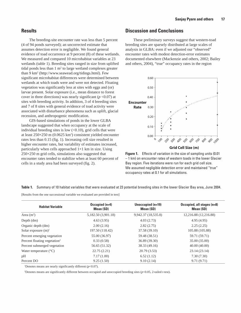
GIS-based simulations of ponds in the lower GLBA landscape suggested that when occupancy at the scale of individual breeding sites is low (<0.10), grid cells that were at least 250×250 m (0.0625 km2) consistent yielded encounter rates less than 0.15 (fig. 1). Increasing cell size resulted in higher encounter rates, but variability of estimates increased, particularly when cells approached 1×1 km in size. Using 250×250 m grid cells, simulations also suggested that encounter rates tended to stabilize when at least 60 percent of cells in a study area had been surveyed (fig. 2).
Habitat VariableOccupied (n=�)
Mean (SD)Unoccupied (n=19)
Mean (SD)Occupied, all stages (n=�)
Mean (SD)
Area (m2) 5,182.50 (3,901.18) 9,942.37 (18,535.8) 12,216.88 (12,216.88)
Depth (dm) 4.63 (3.95) 4.03 (2.73) 4.95 (4.95)
Organic depth (dm) 2.00 (2.16) 2.82 (2.75) 2.25 (2.25)Solar exposure (m)1 197.50 (118.42) 37.58 (39.10) 105.88 (105.88)
Percent emerging vegetation 55.00 (36.97) 59.48 (38.51) 59.71 (59.71)Percent floating vegetation2 0.33 (0.58) 36.89 (39.30) 35.00 (35.00)Percent submerged vegetation 56.65 (51.32) 38.33 (49.16) 40.00 (40.00)
Water temperature (°C) 22.75 (2.21) 20.79 (3.53) 23.14 (23.14)
pH 7.17 (1.00) 6.52 (1.12) 7.30 (7.30)Percent DO 9.25 (1.50) 9.10 (2.14) 9.71 (9.71)
1Denotes means are nearly significantly different (p<0.07).
2Denotes means are significantly different between occupied and unoccupied breeding sites (p<0.05, 2-tailed t-test).
Table 1. Summary of 10 habitat variables that were evaluated at 23 potential breeding sites in the lower Glacier Bay area, June 2004.
[Results from the one successional variable we evaluated are provided in text]
Figure 1. Effects of variation in the size of sampling units (0.01 – 1 km) on encounter rates of western toads in the lower Glacier Bay region. Five iterations were run for each grid cell size. We assumed negligible detection error and maintained “true” occupancy rates at 0.1 for all simulations.
0100
200300
400500
600700
800900
1000
EncounterRate
0.60
0.50
0.40
0.30
0.20
0.10
0.00
Grid Cell Size (m)
Discussion and Conclusions
These preliminary surveys suggest that western-toad breeding sites are sparsely distributed at large scales of analysis in GLBA: even if we adjusted our “observed” encounter rates with modest detection-error estimates documented elsewhere (Mackenzie and others, 2002; Bailey and others, 2004), “true” occupancy rates in the region
Sanjay Pyare and others 17
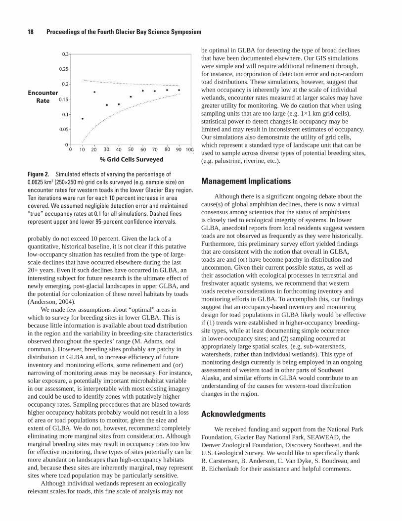
be optimal in GLBA for detecting the type of broad declines that have been documented elsewhere. Our GIS simulations were simple and will require additional refinement through, for instance, incorporation of detection error and non-random toad distributions. These simulations, however, suggest that when occupancy is inherently low at the scale of individual wetlands, encounter rates measured at larger scales may have greater utility for monitoring. We do caution that when using sampling units that are too large (e.g. 1×1 km grid cells), statistical power to detect changes in occupancy may be limited and may result in inconsistent estimates of occupancy. Our simulations also demonstrate the utility of grid cells, which represent a standard type of landscape unit that can be used to sample across diverse types of potential breeding sites, (e.g. palustrine, riverine, etc.).
Management Implications
Although there is a significant ongoing debate about the cause(s) of global amphibian declines, there is now a virtual consensus among scientists that the status of amphibians is closely tied to ecological integrity of systems. In lower GLBA, anecdotal reports from local residents suggest western toads are not observed as frequently as they were historically. Furthermore, this preliminary survey effort yielded findings that are consistent with the notion that overall in GLBA, toads are and (or) have become patchy in distribution and uncommon. Given their current possible status, as well as their association with ecological processes in terrestrial and freshwater aquatic systems, we recommend that western toads receive considerations in forthcoming inventory and monitoring efforts in GLBA. To accomplish this, our findings suggest that an occupancy-based inventory and monitoring design for toad populations in GLBA likely would be effective if (1) trends were established in higher-occupancy breeding-site types, while at least documenting simple occurrence in lower-occupancy sites; and (2) sampling occurred at appropriately large spatial scales, (e.g. sub-watersheds, watersheds, rather than individual wetlands). This type of monitoring design currently is being employed in an ongoing assessment of western toad in other parts of Southeast Alaska, and similar efforts in GLBA would contribute to an understanding of the causes for western-toad distribution changes in the region.
Acknowledgments
We received funding and support from the National Park Foundation, Glacier Bay National Park, SEAWEAD, the Denver Zoological Foundation, Discovery Southeast, and the U.S. Geological Survey. We would like to specifically thank R. Carstensen, B. Anderson, C. Van Dyke, S. Boudreau, and B. Eichenlaub for their assistance and helpful comments.
Figure 2. Simulated effects of varying the percentage of 0.0625 km2 (250×250 m) grid cells surveyed (e.g. sample size) on encounter rates for western toads in the lower Glacier Bay region. Ten iterations were run for each 10 percent increase in area covered. We assumed negligible detection error and maintained “true” occupancy rates at 0.1 for all simulations. Dashed lines represent upper and lower 95-percent confidence intervals.
EncounterRate
0.25
0.2
0.15
0.1
0.05
00 10 20 30 40 50 60 70 80 90 100
% Grid Cells Surveyed
0.3
probably do not exceed 10 percent. Given the lack of a quantitative, historical baseline, it is not clear if this putative low-occupancy situation has resulted from the type of large-scale declines that have occurred elsewhere during the last 20+ years. Even if such declines have occurred in GLBA, an interesting subject for future research is the ultimate effect of newly emerging, post-glacial landscapes in upper GLBA, and the potential for colonization of these novel habitats by toads (Anderson, 2004).
We made few assumptions about “optimal” areas in which to survey for breeding sites in lower GLBA. This is because little information is available about toad distribution in the region and the variability in breeding-site characteristics observed throughout the species’ range (M. Adams, oral commun.). However, breeding sites probably are patchy in distribution in GLBA and, to increase efficiency of future inventory and monitoring efforts, some refinement and (or) narrowing of monitoring areas may be necessary. For instance, solar exposure, a potentially important microhabitat variable in our assessment, is interpretable with most existing imagery and could be used to identify zones with putatively higher occupancy rates. Sampling procedures that are biased towards higher occupancy habitats probably would not result in a loss of area or toad populations to monitor, given the size and extent of GLBA. We do not, however, recommend completely eliminating more marginal sites from consideration. Although marginal breeding sites may result in occupancy rates too low for effective monitoring, these types of sites potentially can be more abundant on landscapes than high-occupancy habitats and, because these sites are inherently marginal, may represent sites where toad population may be particularly sensitive.
Although individual wetlands represent an ecologically relevant scales for toads, this fine scale of analysis may not
1� Proceedings of the Fourth Glacier Bay Science Symposium
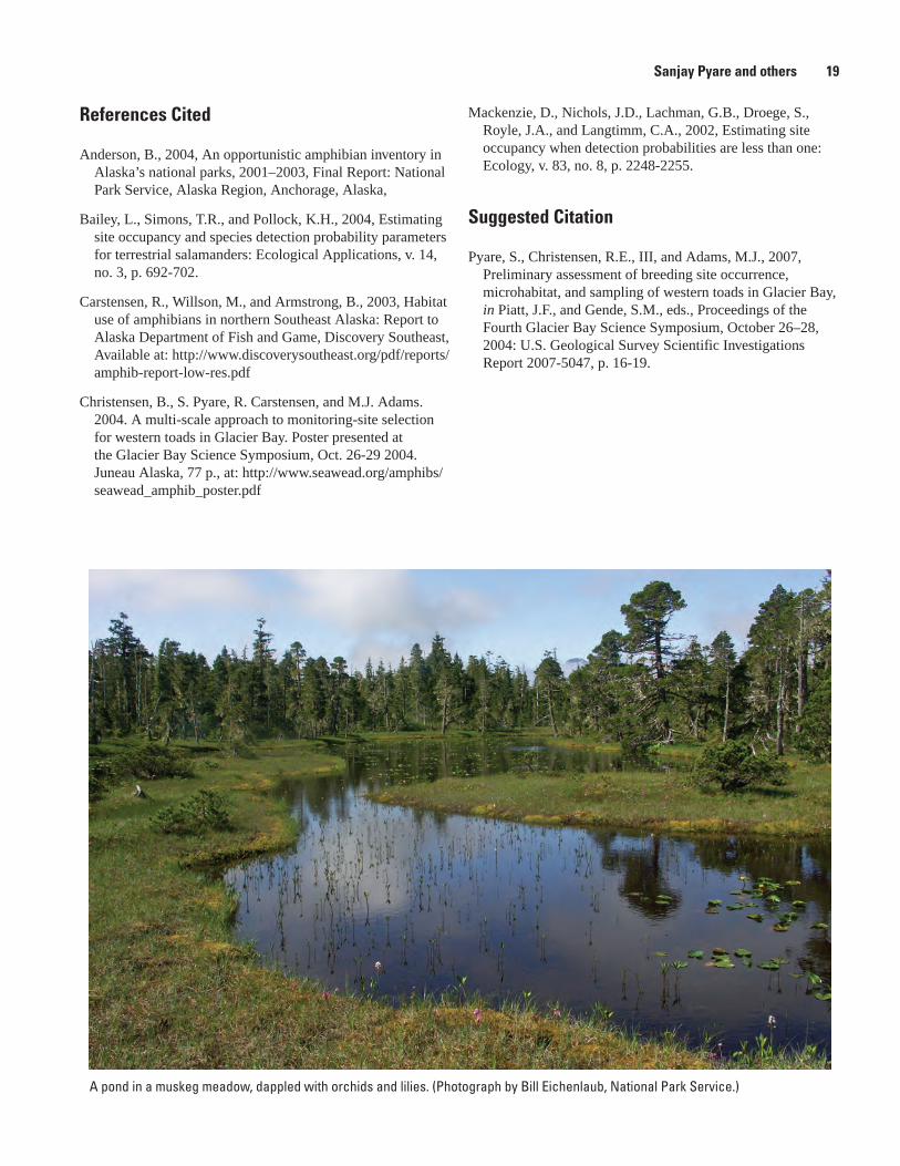
References Cited
Anderson, B., 2004, An opportunistic amphibian inventory in Alaska’s national parks, 2001–2003, Final Report: National Park Service, Alaska Region, Anchorage, Alaska,
Bailey, L., Simons, T.R., and Pollock, K.H., 2004, Estimating site occupancy and species detection probability parameters for terrestrial salamanders: Ecological Applications, v. 14, no. 3, p. 692-702.
Carstensen, R., Willson, M., and Armstrong, B., 2003, Habitat use of amphibians in northern Southeast Alaska: Report to Alaska Department of Fish and Game, Discovery Southeast, Available at: http://www.discoverysoutheast.org/pdf/reports/amphib-report-low-res.pdf
Christensen, B., S. Pyare, R. Carstensen, and M.J. Adams. 2004. A multi-scale approach to monitoring-site selection for western toads in Glacier Bay. Poster presented at the Glacier Bay Science Symposium, Oct. 26-29 2004. Juneau Alaska, 77 p., at: http://www.seawead.org/amphibs/seawead_amphib_poster.pdf
Mackenzie, D., Nichols, J.D., Lachman, G.B., Droege, S., Royle, J.A., and Langtimm, C.A., 2002, Estimating site occupancy when detection probabilities are less than one: Ecology, v. 83, no. 8, p. 2248-2255.
Suggested Citation
Pyare, S., Christensen, R.E., III, and Adams, M.J., 2007, Preliminary assessment of breeding site occurrence, microhabitat, and sampling of western toads in Glacier Bay, in Piatt, J.F., and Gende, S.M., eds., Proceedings of the Fourth Glacier Bay Science Symposium, October 26–28, 2004: U.S. Geological Survey Scientific Investigations Report 2007-5047, p. 16-19.
A pond in a muskeg meadow, dappled with orchids and lilies. (Photograph by Bill Eichenlaub, National Park Service.)
Sanjay Pyare and others 19
Effects of Moose Foraging on Soil Nutrient Dynamics in the Gustavus Forelands, Alaska
Eran Hood1,4, Amy Miller2, and Kevin White3
Abstract. We are studying how selective foraging by moose is affecting soil nutrient dynamics in the Gustavus forelands, where current over-winter moose densities (ca. 3.9 animals/km2) are among the highest recorded in Alaska. We examined variation in inorganic N and microbial N pools between paired exclosure-control plots located in willow thicket habitats, both within and adjacent to the Gustavus airport, and used buried bags to measure in situ net nitrogen (N) mineralization rates. The fence surrounding the airport has functioned as a moose exclosure since 1998, and thus samples collected inside the airport boundary were treated as unbrowsed controls. Results of this study provide preliminary insight into the extent to which the moose population on the Gustavus forelands may be altering soil nutrient dynamics. In addition to this baseline sampling, we also have established three 12×12 m moose exclosures in other areas of the forelands that span a gradient of soil moisture and willow cover. These additional exclosures will allow a more rigorous evaluation of the impact of moose herbivory on local plant community structure and soil nutrient dynamics.
1 Environmental Science Program, University of Alaska Southeast, 11120 Glacier Hwy, Juneau, AK 99801
2 National Park Service, 240 W 5th St, Anchorage, AK, 99501
3 Alaska Department of Fish and Game, Division of Wildlife Conservation, P.O. Box 240020, Douglas, AK, 99824
4 Corresponding author: [email protected]
Introduction
Ungulate herbivores can modify ecosystem structure and function through the timing and extent of their activities and may have pronounced effects on soil nutrient dynamics. In Alaska, moose are an important component of many ecosystems and have the potential, at high densities, to significantly alter soil processes (cf. Pastor and others, 1993) and community composition (Butler, 2003). Although both grazers and browsers are expected to reduce above-ground plant biomass and litter inputs, their effects on soil C and N availability and turnover appear to be mediated by differences in the timing and selectivity of their foraging (Danell and others, 1994). Grazers generally enhance net N turnover (Frank and Groffman, 1998; Stark and others, 2000) and N retention (Frank and others, 2000), although browsers such as moose tend to reduce soil N pools and net N mineralization (Pastor and others, 1988; Pastor and others, 1993), perhaps through enhanced carbon turnover and sequestration.
The exclusion of moose has been shown to increase soil nutrient availability, microbial activity, and C and N mineralization rates in a boreal forest system, where moose densities were estimated to be 2.8 animals/km2 (Pastor and others, 1993). In the Gustavus forelands and parts of Glacier Bay National Park (GBNP), the moose population has increased from low, colonization levels in the 1960s, to an over-winter density (ca. 3.9 animals/km2) that is among the highest recorded in the states. The nearly two-fold increase
in winter moose densities over the last 5 years has resulted in high levels of foraging and changes in plant community structure in preferred foraging habitats (i.e. Salix thickets; White and others, this issue). However, the effects of moose foraging on soil nutrient dynamics are unknown.
The objective of this study was to examine how the current level and timing of moose activity observed in the Gustavus forelands may be affecting soil nutrient dynamics and site productivity, and to relate these findings to projected population trends for the Gustavus moose population. We sampled soils inside and outside of the Gustavus airport boundary to examine short-term effects of moose browsing on inorganic N pools, microbial N, and net N turnover. The area surrounding the Gustavus airport is heavily utilized by over-wintering moose, and the fence surrounding the airport has functioned as a moose exclosure since its construction in 1998. Thus, productivity measurements and soil samples collected inside the airport boundary were treated as unbrowsed controls.
Methods
Soils of the Gustavus forelands consist of weathered and reworked glacial till derived from metamorphosed sandstone, limestone and igneous intrusions. Open stands of willow (Salix barclayi, S. commutata, S. sitchensis) provide winter forage areas for moose. Plots were located in a bluejoint-forb meadow vegetation type, dominated by bluejoint reedgrass (Calamagrostis canadensis) and fireweed (Chamerion angustifolium). No nitrogen-fixing species were present. We measured soil parameters at three sites near the Gustavus airport, two of which utilized the fence surrounding the airport as a moose exclosure (Sites A, B), and one of which was in a browsed area about 1 km south of the airport (Site C; fig. 1). Sites A and B were characterized by loamy, well-drained soils dominated by willow, while Site C was characterized by
20 Proceedings of the Fourth Glacier Bay Science Symposium
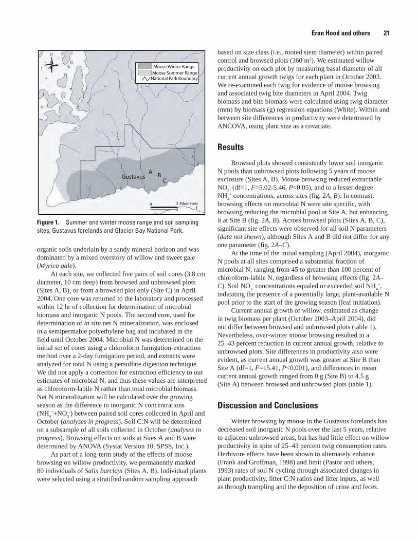
based on size class (i.e., rooted stem diameter) within paired control and browsed plots (360 m2). We estimated willow productivity on each plot by measuring basal diameter of all current annual growth twigs for each plant in October 2003. We re-examined each twig for evidence of moose browsing and associated twig bite diameters in April 2004. Twig biomass and bite biomass were calculated using twig diameter (mm) by biomass (g) regression equations (White). Within and between site differences in productivity were determined by ANCOVA, using plant size as a covariate.
Results
Browsed plots showed consistently lower soil inorganic N pools than unbrowsed plots following 5 years of moose exclosure (Sites A, B). Moose browsing reduced extractable NO
3- (df=1, F=5.02-5.46, P<0.05), and to a lesser degree
NH4
+ concentrations, across sites (fig. 2A, B). In contrast, browsing effects on microbial N were site specific, with browsing reducing the microbial pool at Site A, but enhancing it at Site B (fig. 2A, B). Across browsed plots (Sites A, B, C), significant site effects were observed for all soil N parameters (data not shown), although Sites A and B did not differ for any one parameter (fig. 2A–C).
At the time of the initial sampling (April 2004), inorganic N pools at all sites comprised a substantial fraction of microbial N, ranging from 45 to greater than 100 percent of chloroform-labile N, regardless of browsing effects (fig. 2A–C). Soil NO
3- concentrations equaled or exceeded soil NH
4+,
indicating the presence of a potentially large, plant-available N pool prior to the start of the growing season (leaf initiation).
Current annual growth of willow, estimated as change in twig biomass per plant (October 2003–April 2004), did not differ between browsed and unbrowsed plots (table 1). Nevertheless, over-winter moose browsing resulted in a 25–43 percent reduction in current annual growth, relative to unbrowsed plots. Site differences in productivity also were evident, as current annual growth was greater at Site B than Site A (df=1, F=15.41, P<0.001), and differences in mean current annual growth ranged from 0 g (Site B) to 4.5 g (Site A) between browsed and unbrowsed plots (table 1).
Discussion and Conclusions
Winter browsing by moose in the Gustavus forelands has decreased soil inorganic N pools over the last 5 years, relative to adjacent unbrowsed areas, but has had little effect on willow productivity in spite of 25–43 percent twig consumption rates. Herbivore effects have been shown to alternately enhance (Frank and Groffman, 1998) and limit (Pastor and others, 1993) rates of soil N cycling through associated changes in plant productivity, litter C:N ratios and litter inputs, as well as through trampling and the deposition of urine and feces.
organic soils underlain by a sandy mineral horizon and was dominated by a mixed overstory of willow and sweet gale (Myrica gale).
At each site, we collected five pairs of soil cores (3.8 cm diameter, 10 cm deep) from browsed and unbrowsed plots (Sites A, B), or from a browsed plot only (Site C) in April 2004. One core was returned to the laboratory and processed within 12 hr of collection for determination of microbial biomass and inorganic N pools. The second core, used for determination of in situ net N mineralization, was enclosed in a semipermable polyethylene bag and incubated in the field until October 2004. Microbial N was determined on the initial set of cores using a chloroform fumigation-extraction method over a 2-day fumigation period, and extracts were analyzed for total N using a persulfate digestion technique. We did not apply a correction for extraction efficiency to our estimates of microbial N, and thus these values are interpreted as chloroform-labile N rather than total microbial biomass. Net N mineralization will be calculated over the growing season as the difference in inorganic N concentrations (NH
4++NO
3-) between paired soil cores collected in April and
October (analyses in progress). Soil C:N will be determined on a subsample of all soils collected in October (analyses in progress). Browsing effects on soils at Sites A and B were determined by ANOVA (Systat Version 10, SPSS, Inc.).
As part of a long-term study of the effects of moose browsing on willow productivity, we permanently marked 80 individuals of Salix barclayi (Sites A, B). Individual plants were selected using a stratified random sampling approach
Figure 1. Summer and winter moose range and soil sampling sites, Gustavus forelands and Glacier Bay National Park.
GustavusA
BC
Moose Winter RangeMoose Summer Range
National Park Boundary
Kilometers0 3
Eran Hood and others 21
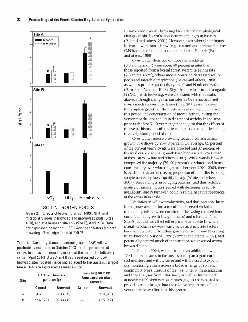
In some cases, winter browsing has induced morphological changes in shrubs without concurrent changes in biomass (Peinetti and others, 2001). However, even where litter inputs increased with moose browsing, concomitant increases in litter C:N have resulted in a net reduction in soil N pools (Pastor and others, 1988).
Over-winter densities of moose in Gustavus (3.9 animals/km2) were about 40 percent greater than those reported from a boreal forest system in Minnesota (2.8 animals/km2), where moose browsing decreased soil N pools and microbial respiration (Pastor and others, 1988), as well as primary productivity and C and N mineralization (Pastor and Naiman, 1993). Significant reductions in inorganic N (NO
3-) with browsing, were consistent with the results
above, although changes at our sites in Gustavus occurred over a much shorter time frame (5 vs. 20+ years). Indeed, the irruptive growth of the Gustavus moose population over this period, the concentration of moose activity during the winter months, and the limited extent of activity in the area prior to the last 5–10 years together suggest that the effects of moose herbivory on soil nutrient stocks can be manifested in a relatively short period of time.
Over-winter moose browsing reduced current annual growth in willows by 25–43 percent. On average, 85 percent of the current year’s twigs were browsed and 37 percent of the total current annual growth twig biomass was consumed at these sites (White and others, 2007). While woody browse comprised the majority (76–90 percent) of winter food items consumed by over-wintering moose between 2001–2004, there is evidence that an increasing proportion of their diet is being supplemented by lower quality forage (White and others, 2007). Such changes in foraging patterns (and thus reduced quality of moose inputs), paired with decreases in soil N availability and N turnover, could result in negative feedbacks at the ecosystem scale.
Variation in willow productivity, and thus potential litter inputs, may account for some of the observed variation in microbial pools between our sites, as browsing reduced both current annual growth (twig biomass) and microbial N at Site A, but did not affect either parameter at Site B, where overall productivity was nearly twice as great. Site factors have had a greater effect than grazers on soil C and N cycling in Yellowstone National Park (Verchot and others, 2002), and potentially control much of the variation we observed across browsed sites.
In October 2004, we constructed an additional two 12×12 m exclosures in the area, which span a gradient of soil moisture and willow cover and will be used to expand our monitoring efforts across a broader range of soil and community types. Results of the in situ net N mineralization and C:N analyses from Sites A–C, as well as future work at newly established exclosure sites (fig. 3) are expected to provide greater insight into the relative importance of site versus herbivore effects in this system.
Table 1. Summary of current annual growth (CAG) willow productivity estimated in October 2003 and the proportion of willow biomass consumed by moose at the end of the following winter (April 2004). Sites A and B represent paired control-browsed sites located inside and adjacent to the Gustavus airport fence. Data are expressed as means ±1 SE.
SiteCAG twig biomass
per plant (g)
CAG twig biomassConsumed per plant
(percent)
Control Browsed Control Browsed
A 14.6 10.1 (2.6) — 26.4 (4.3)
B 22.4 (6.0) 22.4 (4.8) — 42.5 (2.7)
Site A
0 1 2 3 4
0
2
4
6
8
browsedunbrowsed
Site B
SOIL NITROGEN POOLS
0 1 2 3 4
µ gN
/gso
il
0
2
4
6
8
NO 3- NH 4
+ Microbial N
Site C
0 1 2 3 40
2
4
6
8
b
b
a
a
a'
b'
Figure 2. Effects of browsing on soil NO3–, NH4+ and microbial N pools in browsed and unbrowsed plots (Sites A, B), and at a browsed site only (Site C), April 2004. Data are expressed as means ±1 SE. Lower case letters indicate browsing effects significant at P<0.05.
22 Proceedings of the Fourth Glacier Bay Science Symposium
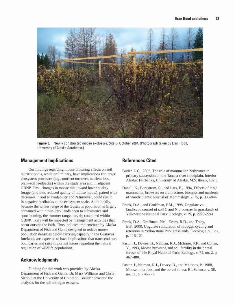
Management Implications
Our findings regarding moose browsing effects on soil nutrient pools, while preliminary, have implications for larger ecosystem processes (e.g., nutrient turnover, nutrient loss, plant-soil feedbacks) within the study area and in adjacent GBNP. First, changes in moose diet toward lower quality forage (and thus reduced quality of moose inputs), paired with decreases in soil N availability and N turnover, could result in negative feedbacks at the ecosystem scale. Additionally, because the winter range of the Gustavus population is largely contained within non-Park lands open to subsistence and sport hunting, the summer range, largely contained within GBNP, likely will be impacted by management activities that occur outside the Park. Thus, policies implemented by Alaska Department of Fish and Game designed to reduce moose population densities below carrying capacity in the Gustavus forelands are expected to have implications that transcend park boundaries and raise important issues regarding the natural regulation of wildlife populations.
Acknowledgments
Funding for this work was provided by Alaska Department of Fish and Game. Dr. Mark Williams and Chris Siebold at the University of Colorado, Boulder provided the analyses for the soil nitrogen extracts.
References Cited
Butler, L.G., 2003, The role of mammalian herbivores in primary succession on the Tanana river floodplain, Interior Alaska: Fairbanks, University of Alaska, M.S. thesis, 102 p.
Danell, K., Bergstrom, R., and Lars, E., 1994, Effects of large mammalian browsers on architecture, biomass and nutrients of woody plants: Journal of Mammalogy, v. 75, p. 833-844.
Frank, D.A., and Groffman, P.M., 1998, Ungulate vs. landscape control of soil C and N processes in grasslands of Yellowstone National Park: Ecology, v. 79, p. 2229-2241.
Frank, D.A., Groffman, P.M., Evans, R.D., and Tracy, B.F., 2000, Ungulate stimulation of nitrogen cycling and retention in Yellowstone Park grasslands: Oecologia, v. 123, p. 116-121.
Pastor, J., Dewey, B., Naiman, R.J., McInnes, P.F., and Cohen, Y., 1993, Moose browsing and soil fertility in the boreal forests of Isle Royal National Park: Ecology, v. 74, no. 2, p. 467-480.
Pastor, J., Naiman, R.J., Dewey, B., and McInnes, P., 1988, Moose, microbes, and the boreal forest: BioScience, v. 38, no. 11, p. 770-777.
Figure �. Newly constructed moose exclosure, Site B, October 2004. (Photograph taken by Eran Hood, University of Alaska Southeast.)
Eran Hood and others 2�
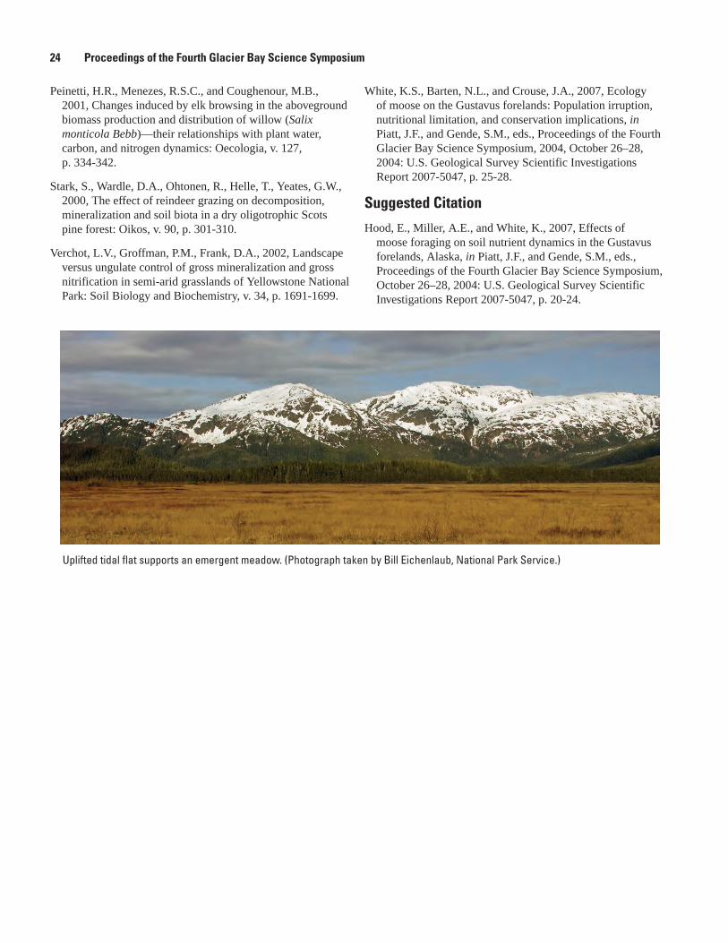
Peinetti, H.R., Menezes, R.S.C., and Coughenour, M.B., 2001, Changes induced by elk browsing in the aboveground biomass production and distribution of willow (Salix monticola Bebb)—their relationships with plant water, carbon, and nitrogen dynamics: Oecologia, v. 127, p. 334-342.
Stark, S., Wardle, D.A., Ohtonen, R., Helle, T., Yeates, G.W., 2000, The effect of reindeer grazing on decomposition, mineralization and soil biota in a dry oligotrophic Scots pine forest: Oikos, v. 90, p. 301-310.
Verchot, L.V., Groffman, P.M., Frank, D.A., 2002, Landscape versus ungulate control of gross mineralization and gross nitrification in semi-arid grasslands of Yellowstone National Park: Soil Biology and Biochemistry, v. 34, p. 1691-1699.
White, K.S., Barten, N.L., and Crouse, J.A., 2007, Ecology of moose on the Gustavus forelands: Population irruption, nutritional limitation, and conservation implications, in Piatt, J.F., and Gende, S.M., eds., Proceedings of the Fourth Glacier Bay Science Symposium, 2004, October 26–28, 2004: U.S. Geological Survey Scientific Investigations Report 2007-5047, p. 25-28.
Suggested Citation
Hood, E., Miller, A.E., and White, K., 2007, Effects of moose foraging on soil nutrient dynamics in the Gustavus forelands, Alaska, in Piatt, J.F., and Gende, S.M., eds., Proceedings of the Fourth Glacier Bay Science Symposium, October 26–28, 2004: U.S. Geological Survey Scientific Investigations Report 2007-5047, p. 20-24.
Uplifted tidal flat supports an emergent meadow. (Photograph taken by Bill Eichenlaub, National Park Service.)
2� Proceedings of the Fourth Glacier Bay Science Symposium
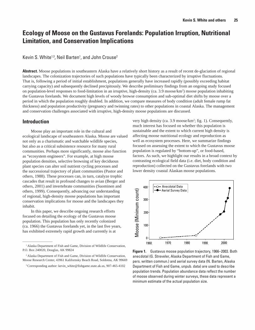
Ecology of Moose on the Gustavus Forelands: Population Irruption, Nutritional Limitation, and Conservation Implications
Kevin S. White1,3, Neil Barten1, and John Crouse2
Abstract. Moose populations in southeastern Alaska have a relatively short history as a result of recent de-glaciation of regional landscapes. The colonization trajectories of such populations have typically been characterized by irruptive fluctuations. That is, following a period of initial establishment, populations generally have increased rapidly (possibly exceeding habitat carrying capacity) and subsequently declined precipitously. We describe preliminary findings from an ongoing study focused on population-level responses to food-limitation in an irruptive, high-density (ca. 3.9 moose/km2) moose population inhabiting the Gustavus forelands. We document high levels of woody browse consumption and sub-optimal diet shifts by moose over a period in which the population roughly doubled. In addition, we compare measures of body condition (adult female rump fat thickness) and population productivity (pregnancy and twinning rates) to other populations in coastal Alaska. The management and conservation challenges associated with irruptive, high-density moose populations are discussed.
Figure 1. Gustavus moose population trajectory, 1966–2003. Both anecdotal (G. Streveler, Alaska Department of Fish and Game, pers. written commun.) and aerial survey data (N. Barten, Alaska Department of Fish and Game, unpub. data) are used to describe population trends. Population abundance data reflect the number of moose observed during winter surveys, these data represent a minimum estimate of the actual population size.
Moo
se (M
inim
um c
ount
) Anecdotal DataAerial Survey Data
Year
400
300
200
100
01960 1970 1980 1990 2000
Kevin S. White and others 25
1 Alaska Department of Fish and Game, Division of Wildlife Conservation, P.O. Box 240020, Douglas, AK 99824
2 Alaska Department of Fish and Game, Division of Wildlife Conservation, Moose Research Center, 43961 Kalifornsky Beach Road, Soldotna, AK 99669
3 Corresponding author: [email protected], 907-465-4102
Introduction
Moose play an important role in the cultural and ecological landscape of southeastern Alaska. Moose are valued not only as a charismatic and watchable wildlife species, but also as a critical subsistence resource for many rural communities. Perhaps more significantly, moose also function as “ecosystem engineers”. For example, at high moose population densities, selective browsing of key deciduous plant species can alter soil nutrient cycling processes and the successional trajectory of plant communities (Pastor and others, 1988). These processes can, in turn, catalyze trophic cascades that result in profound changes to avian (Berger and others, 2001) and invertebrate communities (Suominen and others, 1999). Consequently, advancing our understanding of regional, high-density moose populations has important conservation implications for moose and the landscapes they inhabit.
In this paper, we describe ongoing research efforts focused on detailing the ecology of the Gustavus moose population. This population has only recently colonized (ca. 1966) the Gustavus forelands yet, in the last five years, has exhibited extremely rapid growth and currently is at
very high density (ca. 3.9 moose/km2; fig. 1). Consequently, much interest has focused on whether this population is sustainable and the extent to which current high density is affecting moose nutritional ecology and reproduction as well as ecosystem processes. Here, we summarize findings focused on assessing the extent to which the Gustavus moose population is regulated by “bottom-up”, or food-based, factors. As such, we highlight our results in a broad context by contrasting ecological field data (i.e. diet, body condition and reproduction) collected on the Gustavus forelands with two lower density coastal Alaskan moose populations.
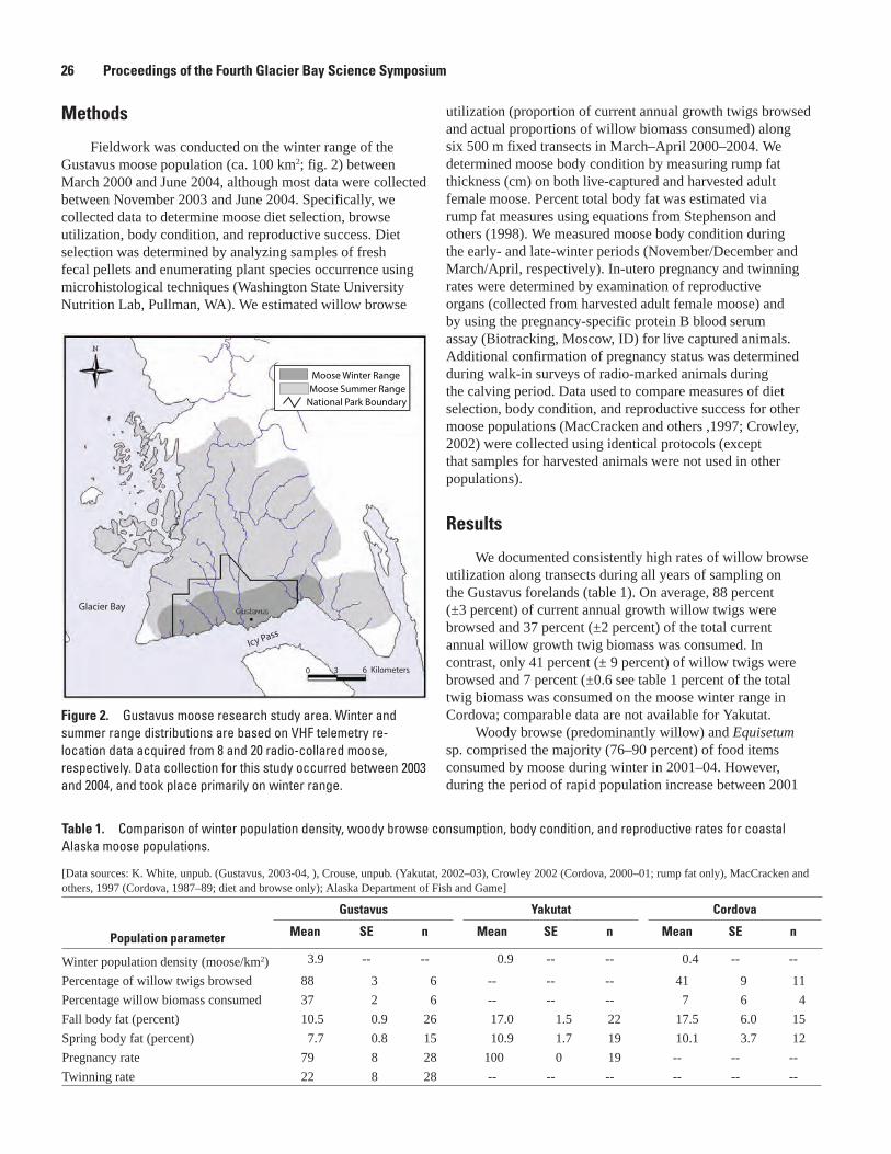
Methods
Fieldwork was conducted on the winter range of the Gustavus moose population (ca. 100 km2; fig. 2) between March 2000 and June 2004, although most data were collected between November 2003 and June 2004. Specifically, we collected data to determine moose diet selection, browse utilization, body condition, and reproductive success. Diet selection was determined by analyzing samples of fresh fecal pellets and enumerating plant species occurrence using microhistological techniques (Washington State University Nutrition Lab, Pullman, WA). We estimated willow browse
utilization (proportion of current annual growth twigs browsed and actual proportions of willow biomass consumed) along six 500 m fixed transects in March–April 2000–2004. We determined moose body condition by measuring rump fat thickness (cm) on both live-captured and harvested adult female moose. Percent total body fat was estimated via rump fat measures using equations from Stephenson and others (1998). We measured moose body condition during the early- and late-winter periods (November/December and March/April, respectively). In-utero pregnancy and twinning rates were determined by examination of reproductive organs (collected from harvested adult female moose) and by using the pregnancy-specific protein B blood serum assay (Biotracking, Moscow, ID) for live captured animals. Additional confirmation of pregnancy status was determined during walk-in surveys of radio-marked animals during the calving period. Data used to compare measures of diet selection, body condition, and reproductive success for other moose populations (MacCracken and others ,1997; Crowley, 2002) were collected using identical protocols (except that samples for harvested animals were not used in other populations).
Results
We documented consistently high rates of willow browse utilization along transects during all years of sampling on the Gustavus forelands (table 1). On average, 88 percent (±3 percent) of current annual growth willow twigs were browsed and 37 percent (±2 percent) of the total current annual willow growth twig biomass was consumed. In contrast, only 41 percent (± 9 percent) of willow twigs were browsed and 7 percent (±0.6 see table 1 percent of the total twig biomass was consumed on the moose winter range in Cordova; comparable data are not available for Yakutat.
Woody browse (predominantly willow) and Equisetum sp. comprised the majority (76–90 percent) of food items consumed by moose during winter in 2001–04. However, during the period of rapid population increase between 2001
Figure 2. Gustavus moose research study area. Winter and summer range distributions are based on VHF telemetry re-location data acquired from 8 and 20 radio-collared moose, respectively. Data collection for this study occurred between 2003 and 2004, and took place primarily on winter range.
Table 1. Comparison of winter population density, woody browse consumption, body condition, and reproductive rates for coastal Alaska moose populations.
[Data sources: K. White, unpub. (Gustavus, 2003-04, ), Crouse, unpub. (Yakutat, 2002–03), Crowley 2002 (Cordova, 2000–01; rump fat only), MacCracken and others, 1997 (Cordova, 1987–89; diet and browse only); Alaska Department of Fish and Game]
Population parameter
Gustavus Yakutat Cordova
Mean SE n Mean SE n Mean SE n
Winter population density (moose/km2) 3.9 -- -- 0.9 -- -- 0.4 -- --
Percentage of willow twigs browsed 88 3 6 -- -- -- 41 9 11
Percentage willow biomass consumed 37 2 6 -- -- -- 7 6 4
Fall body fat (percent) 10.5 0.9 26 17.0 1.5 22 17.5 6.0 15
Spring body fat (percent) 7.7 0.8 15 10.9 1.7 19 10.1 3.7 12
Pregnancy rate 79 8 28 100 0 19 -- -- --
Twinning rate 22 8 28 -- -- -- -- -- --
Glacier Bay
Icy Pass
Moose Winter RangeMoose Summer Range
National Park Boundary
0 3 6 Kilometers
2� Proceedings of the Fourth Glacier Bay Science Symposium
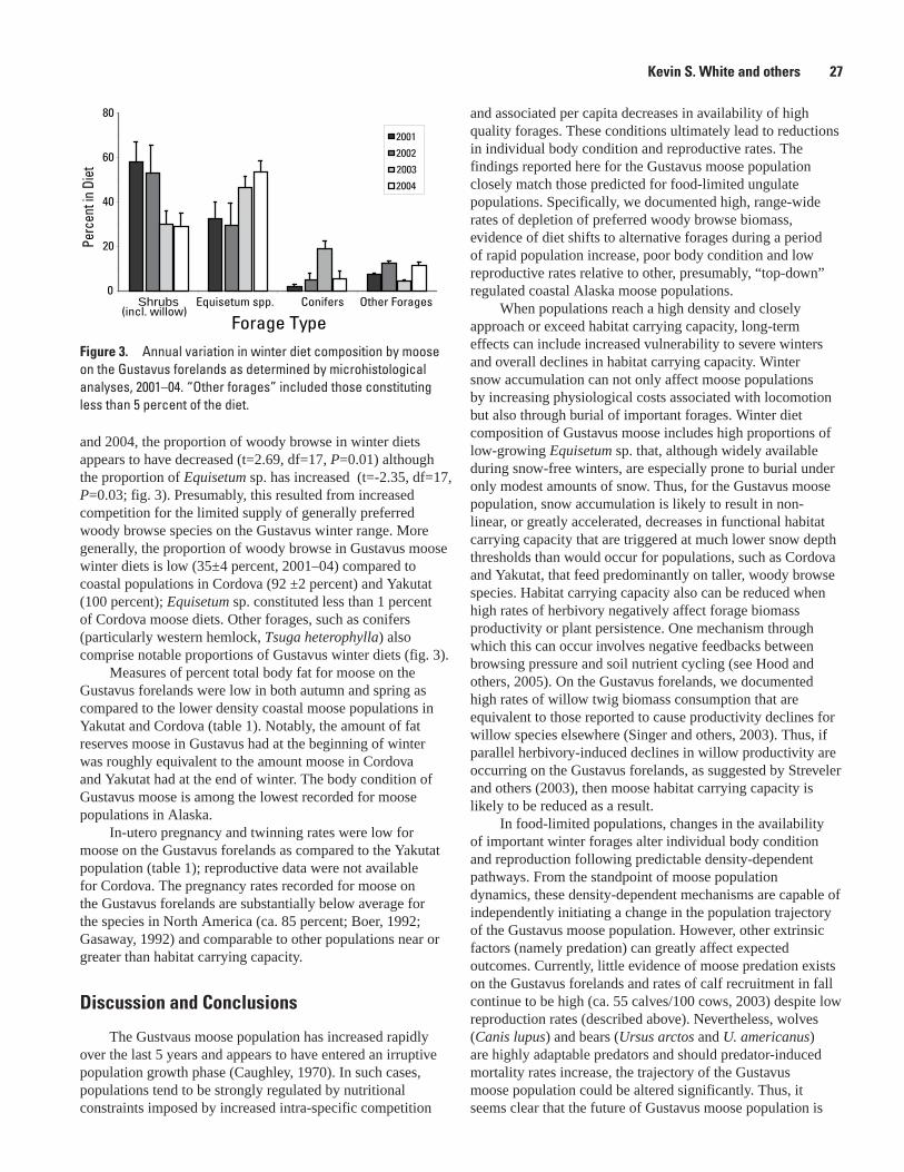
and 2004, the proportion of woody browse in winter diets appears to have decreased (t=2.69, df=17, P=0.01) although the proportion of Equisetum sp. has increased (t=-2.35, df=17, P=0.03; fig. 3). Presumably, this resulted from increased competition for the limited supply of generally preferred woody browse species on the Gustavus winter range. More generally, the proportion of woody browse in Gustavus moose winter diets is low (35±4 percent, 2001–04) compared to coastal populations in Cordova (92 ±2 percent) and Yakutat (100 percent); Equisetum sp. constituted less than 1 percent of Cordova moose diets. Other forages, such as conifers (particularly western hemlock, Tsuga heterophylla) also comprise notable proportions of Gustavus winter diets (fig. 3).
Measures of percent total body fat for moose on the Gustavus forelands were low in both autumn and spring as compared to the lower density coastal moose populations in Yakutat and Cordova (table 1). Notably, the amount of fat reserves moose in Gustavus had at the beginning of winter was roughly equivalent to the amount moose in Cordova and Yakutat had at the end of winter. The body condition of Gustavus moose is among the lowest recorded for moose populations in Alaska.
In-utero pregnancy and twinning rates were low for moose on the Gustavus forelands as compared to the Yakutat population (table 1); reproductive data were not available for Cordova. The pregnancy rates recorded for moose on the Gustavus forelands are substantially below average for the species in North America (ca. 85 percent; Boer, 1992; Gasaway, 1992) and comparable to other populations near or greater than habitat carrying capacity.
Discussion and Conclusions
The Gustvaus moose population has increased rapidly over the last 5 years and appears to have entered an irruptive population growth phase (Caughley, 1970). In such cases, populations tend to be strongly regulated by nutritional constraints imposed by increased intra-specific competition
and associated per capita decreases in availability of high quality forages. These conditions ultimately lead to reductions in individual body condition and reproductive rates. The findings reported here for the Gustavus moose population closely match those predicted for food-limited ungulate populations. Specifically, we documented high, range-wide rates of depletion of preferred woody browse biomass, evidence of diet shifts to alternative forages during a period of rapid population increase, poor body condition and low reproductive rates relative to other, presumably, “top-down” regulated coastal Alaska moose populations.
When populations reach a high density and closely approach or exceed habitat carrying capacity, long-term effects can include increased vulnerability to severe winters and overall declines in habitat carrying capacity. Winter snow accumulation can not only affect moose populations by increasing physiological costs associated with locomotion but also through burial of important forages. Winter diet composition of Gustavus moose includes high proportions of low-growing Equisetum sp. that, although widely available during snow-free winters, are especially prone to burial under only modest amounts of snow. Thus, for the Gustavus moose population, snow accumulation is likely to result in non-linear, or greatly accelerated, decreases in functional habitat carrying capacity that are triggered at much lower snow depth thresholds than would occur for populations, such as Cordova and Yakutat, that feed predominantly on taller, woody browse species. Habitat carrying capacity also can be reduced when high rates of herbivory negatively affect forage biomass productivity or plant persistence. One mechanism through which this can occur involves negative feedbacks between browsing pressure and soil nutrient cycling (see Hood and others, 2005). On the Gustavus forelands, we documented high rates of willow twig biomass consumption that are equivalent to those reported to cause productivity declines for willow species elsewhere (Singer and others, 2003). Thus, if parallel herbivory-induced declines in willow productivity are occurring on the Gustavus forelands, as suggested by Streveler and others (2003), then moose habitat carrying capacity is likely to be reduced as a result.
In food-limited populations, changes in the availability of important winter forages alter individual body condition and reproduction following predictable density-dependent pathways. From the standpoint of moose population dynamics, these density-dependent mechanisms are capable of independently initiating a change in the population trajectory of the Gustavus moose population. However, other extrinsic factors (namely predation) can greatly affect expected outcomes. Currently, little evidence of moose predation exists on the Gustavus forelands and rates of calf recruitment in fall continue to be high (ca. 55 calves/100 cows, 2003) despite low reproduction rates (described above). Nevertheless, wolves (Canis lupus) and bears (Ursus arctos and U. americanus) are highly adaptable predators and should predator-induced mortality rates increase, the trajectory of the Gustavus moose population could be altered significantly. Thus, it seems clear that the future of Gustavus moose population is
Figure �. Annual variation in winter diet composition by moose on the Gustavus forelands as determined by microhistological analyses, 2001–04. “Other forages” included those constituting less than 5 percent of the diet.
80
Forage Type
0
20
40
60
Shrubs(incl. willow)
Equisetum spp. Conifers Other Forages
Perc
enti
nDi
et
2001
2002
2003
2004
Kevin S. White and others 27
dependent upon a dynamic array of both intrinsic and extrinsic interactions whose outcomes are complex and difficult to predict but represent surmountable challenges for future scientific investigations.
Management Implications
The Gustavus moose population plays an important local role not only as a key resource for human wildlife viewing and subsistence activities, but also through “ecosystem engineering” functions that span multiple trophic levels. In this context, the Gustavus moose population presents an interesting case study for resource scientists and managers. The Gustavus moose population is largely migratory and moves seasonally between distinct, but somewhat overlapping, summer and winter ranges. Specifically, about 75 percent of the radio-collared moose in this study (n=21) made “trans-boundary” movements between a small winter range on the Gustavus forelands to summer range areas in the Beardslee Islands and tributary drainages associated with Excursion Ridge. More importantly, the moose winter range occurs predominantly on non-park lands where moose are harvested by local and regional subsistence and sport hunters, whereas the summer range is mostly encompassed within protected National Park Service lands. Consequently, State-implemented management activities, focused on reducing population density well below habitat carrying capacity are likely to alter moose population density and associated ecosystem-level processes and wildlife-viewing opportunities inside Glacier Bay National Park. As a result, resource managers are faced with important challenges that involve balancing management policies that emphasize sustaining hunting opportunity, and natural regulation of wildlife populations and associated ecosystem processes.
AcknowledgmentsThis study was funded by the Alaska Department of Fish
and Game with additional support from Glacier Bay National Park. For their invaluable contributions to this project we wish to thank Gustavus community members, G. Streveler, J. Brakel, D. Pederson and B. Kruger; Alaska Department of Fish and Game staff and volunteers, S. Jenkins, J. Womble, M. Kirchhoff, P. Hessing, C. Rice, V. Beier, R. Piehl and K. Beckmen; NPS staff, S. Boudreau, M. Kralovec, M. Sharp, R. Yerxa, and the NPS rangers.
References Cited
Berger, J., Stacey, P.B., Bellis, L., and Johnson, M.P., 2001, A mammalian predator-prey imbalance: grizzly bear and wolf extinction affect avian neotropical migrants: Ecological Applications, v. 11, p. 957-960.
Caughley, G., 1970, Eruption of ungulate populations, with emphasis on Himalayan thar in New Zealand: Ecology, v. 51, p. 53-72.
Crowley, D.W., 2002, Unit 6 moose management report, in Healy, C., ed., Moose management report of survey and inventory activities: Alaska Deptartment Fish and Game, Juneau, Alaska.
Hood, E., Miller, A., and White, K., 2007, Effects of moose foraging on soil nutrient dynamics in the Gustavus forelands, Alaska, in Piatt, J.F., and Gende, S.M., eds., Proceedings of the Fourth Glacier Bay Science Symposium, 2004, October 26–28, 2004: U.S. Geological Survey Scientific Investigations Report 2007-5047, p. 20-24.
MacCracken, J.G., VanBallenberghe, V., and Peek, J.M., 1997, Habitat relationships of moose on the Copper river delta in coastal south-central Alaska: Wildlife Monograph, v. 136, p. 1-52.
Pastor, J., Naiman, R.J., Dewey, B., and McInnes, P.F., 1988, Moose, microbes and the boreal forest: BioScience, v. 38, p. 770-777.
Singer, F.J., Wang, G., and Hobbs, N.T., 2003, The role of ungulates and large predators on plant communities and ecosystem processes in western national parks, in Zabel, C.J., and Anthony, R.G., eds, Mammal community dynamics—management and conservation in the coniferous forests of western North America, Cambridge, Cambridge University Press, p. 444-486.
Stephenson, T.R., Hundertmark, K.J., Schwartz, C.C., and VanBallenberghe, V., 1998, Predicting body fat and body mass in moose with ultrasonography: Canadian Journal of Zoology, v. 76, p. 717-722.
Streveler, G.P., Bosworth, K.Z., Christensen, R.E., Lentfer, H.P. and Farley, M.C., 2003, Gustavus plant communities—their composition, history and use by fish, wildlife and people: Report, Icy Straits Environmental Services, Gustavus, Alaska, 28 p.
Suominen, O., Danell, K. and Bryant, J.P., 1999, Indirect effects of mammalian browsers on vegetation and ground-dwelling insects in an Alaskan floodplain: Ecoscience, v. 6, p. 505-510.
Suggested Citation
White, K.S., Barten, N.L., and Crouse, J.A., 2006, Ecology of moose on the Gustavus forelands: Population irruption, nutritional limitation and conservation implications, in Piatt, J.F., and Gende, S.M., eds., Proceedings of the Fourth Glacier Bay Science Symposium, October 26–28, 2004: U.S. Geological Survey Scientific Investigations Report 2007-5047, p. 25-28.
2� Proceedings of the Fourth Glacier Bay Science Symposium
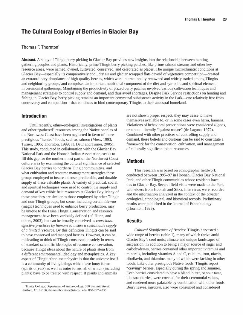
Abstract. A study of Tlingit berry picking in Glacier Bay provides new insights into the relationship between hunting-gathering peoples and plants. Historically, prime Tlingit berry picking patches, like prime salmon streams and other key resource areas, were named, owned, cultivated, conserved, and celebrated as places. The unique microclimatic conditions at Glacier Bay—especially its comparatively cool, dry air and glacier scrapped flats devoid of vegetative competition—created an extraordinary abundance of high-quality berries, which were internationally renowned and widely traded among Tlingits and neighboring groups, and comprised an important nutritional component of the diet and symbolic and spiritual element in ceremonial gatherings. Maintaining the productivity of prized berry patches involved various cultivation techniques and management strategies to control supply and demand, and thus avoid shortages. Despite Park Service restrictions on hunting and fishing in Glacier Bay, berry picking remains an important communal subsistence activity in the Park—one relatively free from controversy and competition—that continues to bind contemporary Tlingits to their ancestral homeland.
Introduction
Until recently, ethno-ecological investigations of plants and other “gathered” resources among the Native peoples of the Northwest Coast have been neglected in favor of more prestigious “hunted” foods, such as salmon (Moss, 1993; Turner, 1995; Thornton, 1999; cf. Deur and Turner, 2005). This study, conducted in collaboration with the Glacier Bay National Park and the Hoonah Indian Association, seeks to fill this gap for the northernmost part of the Northwest Coast culture area by examining the cultural significance of selected Glacier Bay berries to northern Tlingit communities, and what cultivation and resource management strategies these groups employed to insure a dense, predictable, and durable supply of these valuable plants. A variety of practical, social, and spiritual techniques were used to control the supply and demand of key edible fruit resources at Glacier Bay. Many of these practices are similar to those employed by other Tlingit and non-Tlingit groups; but some, including certain héiwaa (magic) techniques used to enhance berry production, may be unique to the Huna Tlingit. Conservation and resource management have been variously defined (cf. Hunn, and others, 2003), but can be broadly conceived as conscious, effective practices by humans to insure a sustainable supply of a limited resource. By this definition Tlingits can be said to have conserved and managed berries. However, it can be misleading to think of Tlingit conservation solely in terms of standard scientific ideologies of resource conservation, because Tlingit ideas about the nature of plants stem from a different environmental ideology and metaphysics. A key aspect of Tlingit ethno-metaphysics is that the universe itself is a community of living beings which have inner forms (spirits or yeik) as well as outer forms, all of which (including plants) have to be treated with respect. If plants and animals
Thomas F. Thornton 29
The Cultural Ecology of Berries in Glacier Bay
Thomas F. Thornton1
are not shown proper respect, they may cease to make themselves available to, or in some cases even harm, humans. Violations of behavioral prescriptions were considered tligaas, or taboo—literally “against nature” (de Laguna, 1972). Combined with other practices of controlling supply and demand, these beliefs and customs can be said to constitute a framework for the conservation, cultivation, and management of culturally significant plant resources.
Methods
This research was based on ethnographic fieldwork conducted between 1995–97 in Hoonah, Glacier Bay National Park, and other Tlingit communities whose residents have ties to Glacier Bay. Several field visits were made to the Park with elders from Hoonah and Sitka. Interviews were recorded and the information analyzed in the context of the broader ecological, ethnological, and historical records. Preliminary results were published in the Journal of Ethnobiology (Thornton, 1999).
Results
Cultural Significance of Berries: Tlingits harvested a wide range of berries (table 1), many of which thrive amid Glacier Bay’s cool moist climate and unique landscapes of succession. In addition to being a major source of sugar and carbohydrates, berries contained other important vitamins and minerals, including vitamins A and C, calcium, iron, niacin, riboflavin, and thiamine, many of which were lacking in other foods. Like other prestigious Native foods, Tlingits report “craving” berries, especially during the spring and summer. Even berries considered to have a bland, bitter, or sour taste, like soapberries, were coveted for their ceremonial values, and rendered more palatable by combination with other foods. Berry leaves, kayaaní, also were consumed and considered
1Trinity College, Department of Anthropology, 300 Summit Street, Hartford, CT 06106, [email protected], 860-297-4235
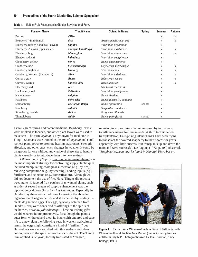
referring to extraordinary techniques used by individuals to influence nature for human ends. A third technique was transplantation. Enterprising island Tlingit have been trying to transplant the coveted soapberry to their shores for years, apparently with little success. But transplants up and down the mainland were successful. De Laguna (1972, p. 409) observed, “Soapberries…can now be found in Nunatak Fjord but are
Table 1. Edible Fruit Resources in Glacier Bay National Park.
Common Name Tlingit Name Scientific Name Spring Summer Autumn
Berries tléikw x x
Bearberry (kinnikinnick) tínx Arctostaphylos uva-ursi x x
Blueberry, (generic and oval-leaved) kanat’á Vaccinium ovalifolium x
Blueberry, Alaskan (ripens later) naanyaa kanat’aayí Vaccinium alaskaense x x
Blueberry, bog ts’éekáxk’w Vaccinium uliginosum x x
Blueberry, dwarf kakatlaax Vaccinium caespitosum x
Cloudberry, yellow néx’w Rubus chamaemorus x
Cranberry, bog k’eishkaháagu Oxycoccus microcarpus x x
Cranberry, highbush kaxwéix Viburnum edule x x
Cranberry, lowbush (ligonberry) dáxw Vaccinium vitis-idaea x x
Current, gray shaax Ribes bracteosum x x
Current, swamp kaneilts’ákw Ribes lacustre x x
Elderberry, red yéil’ Sambucus racemosa x
Huckleberry, red tleikatánk Vaccinium parvifolium x
Nagoonberry neigóon Rubus Arcticus x
Raspberry tlekw yádi Rubus idaeus (R. pedatus) x
Salmonberry was’x’aan tléigu Rubus spectabilis shoots x
Soapberry xákwl’i Sheperdia canadensis x
Strawberry, seaside shákw Fragaria chiloensis x
Thimbleberry ch’eix’ Rubus parviflorus shoots x
Figure 1. Richard Amy Winnie—The late Richard Dalton Sr. with Winnie Smith and the late Amy Marvin (center) sharing berries at Glacier Bay N.P. (Photograph taken by Tom Thornton, rinity College, 1996.)
a vital sign of spring and potent medicine. Bearberry leaves were smoked as tobacco, and other plant leaves were used to make teas. The term kayaaní is a synonym for medicine in Tlingit. Shamans were trained in the arts of kayaaní and could harness plant power to promote healing, awareness, strength, affection, and other ends, even changes in weather. It could be dangerous for one without knowledge of these arts to handle plants casually or to introduce them into new settings.
Ethnoecology of Supply: Environmental manipulation was the most important strategy for controlling supply. Techniques included manipulating ecological succession (e.g., by fire), reducing competition (e.g., by weeding), adding inputs (e.g., fertilizer), and selection (e.g., domestication). Although we did not document the use of fire, Huna Tlingits did practice weeding to rid favored fruit patches of unwanted plants, such as alder. A second means of supply enhancement was the input of dog salmon (Oncorhynchus keta) eggs. Especially in Dundas Bay there was a tradition of ensuring the abundant regeneration of nagoonberries and strawberries by feeding the plants dog salmon eggs. The eggs, typically obtained from Dundas River, were conceived as offerings to the spirits of the berries, or tleikw yakwaheiyagu. These nourishing gifts would enhance future productivity, for although the plant’s outer form withered and died, its inner spirit endured and gave life to a new plant the following year. In western agricultural terms, the eggs might constitute a kind of “fertilizer;” but Huna elders were not satisfied with this analogy, as it does not do justice to the spiritual mechanics of the act. The Tlingit term applied is héixwaa, loosely translated as “magic”,
�0 Proceedings of the Fourth Glacier Bay Science Symposium

apparently a recent intrusion. In the last century they were imported from southeastern Alaska, probably derived from the interior via the Chilkat.” Transplantation of other species, including salmon, has been documented (Thornton, 1997), and the custom likely predates 18th century European contact.
Another set of techniques revolved around redistribution of the resource in space and time. Spatial redistribution was accomplished through exchange. Berries were traded widely, especially across ecologically diverse zones, such as between island, mainland, and interior Native communities. Temporal redistribution, through preservation and storage, also helped to mitigate issues of supply. In Glacier Bay, berries were air dried (with the help of smudge fires), preserved in seal oil, and in the modern era, jarred and frozen. A jar of soapberries still fetches a good price in island communities, which do not have direct access to them.
A third supply strategy was to make the resource more available or useable through technological and sociological means. Some of the material inputs (e.g., dog salmon eggs discussed above) and technologies associated with berry picking (including baskets such as the wide-mouthed táal), are discussed elsewhere (Thornton, 1998, 1999). Overall, berry picking was a labor intensive endeavor; thus organization of labor was among the most crucial factors in raising supply. Tlingit labor was organized along matrilineal lines, but productivity was boosted by non-kin slaves, who assisted with harvesting and processing. This labor allowed surplus supplies of berries to be generated for purposes beyond consumption, such as gifts, ceremonial exchange, and trade. In the post-slave era, families, including children of all ages, worked together to facilitate production. Contrary to some ethnographic accounts, berry picking was not “women’s work.” Although women oversaw processing, picking was a family affair and often a time of great joy, song, laughter, and good cheer.
Ethnoecology of Demand: Territoriality and resource tenure helped limit demand and overharvesting. The economic defendability hypothesis, (Dyson-Hudson and Smith, 1978; Richardson, 1982), predicts that territorial systems will develop, “when the costs of exclusive use and defense of an area are outweighed by the benefits gained from this pattern of resource utilization.” Such a situation generally develops
Figure 2. Herman and Martha—Herman Kitka Sr. and the late Martha Kitka picking bearberries near Point Carolus, Glacier Bay. (Photograph taken by Tom Thornton, Trinity College, 1996.)
Figure �. Taal and berry basket—The large-mouthed basket, or táal, is used to pick soapberries, a favorite Tlingit ceremonial fruit. The cylindrical basket inside it is hung around the neck and used for picking most other varieties of berries. (Photograph courtesy of Alaska State Museum.)
Thomas F. Thornton �1
“under conditions of high density and predictability of critical resources” without a “superabundance” (meaning more than enough resources for all users, thus rendering territorial behavior unnecessary). Many berry patches in Glacier Bay and elsewhere met these conditions and thus were claimed as matrilineal property (and later, in the allotment era of Federal Indian policy, as individual and family property). While this ownership carried with it the power to regulate access, in practice outsiders rarely were forbidden from gathering, provided they “paid tribute” by asking permission (or sometimes by paying a fee of blankets, food, or even cash) and, if possible, citing a kinship link to the owners. Among older Tlingits harvesting berries in Glacier Bay, this protocol is still practiced, as evidenced on our 1996 harvesting trip (see A Time of Gathering, University of Alaska, 1999), where elders made speeches relating themselves to Dundas Bay’s T’akdeintaan owners before commencing to pick nagoonberries (from the Tlingit neigóon, a rare instance of an English noun borrowed from Tlingit). Failure to seek permission might result in sanctions through communicative structures (insults, gossip, etc.), or even physical violence (such as the destruction of ones berry basket or canoe).
Tlingit leaders also showed stewardship in controlling timing of harvests. Berry productivity is not continuous, nor is demand. Localized shortages and profound seasonal variations of food resources were not uncommon in Tlingit country. In the case of berries, these shortages could be exacerbated, if not precipitated, by periods of high demand. Preseason berry poaching or overharvesting, a phenomenon reported during heavy potlatch years (Garfield, n.d.), could compromise the productivity of good patches. Thus, the key to managing productive berry patches was to structure demand through stewardship so as to insure high yields for the owners and, if surpluses allowed, the community at large. According to Chilkat elder Suzie Nasook, the “chief who owned a berrying
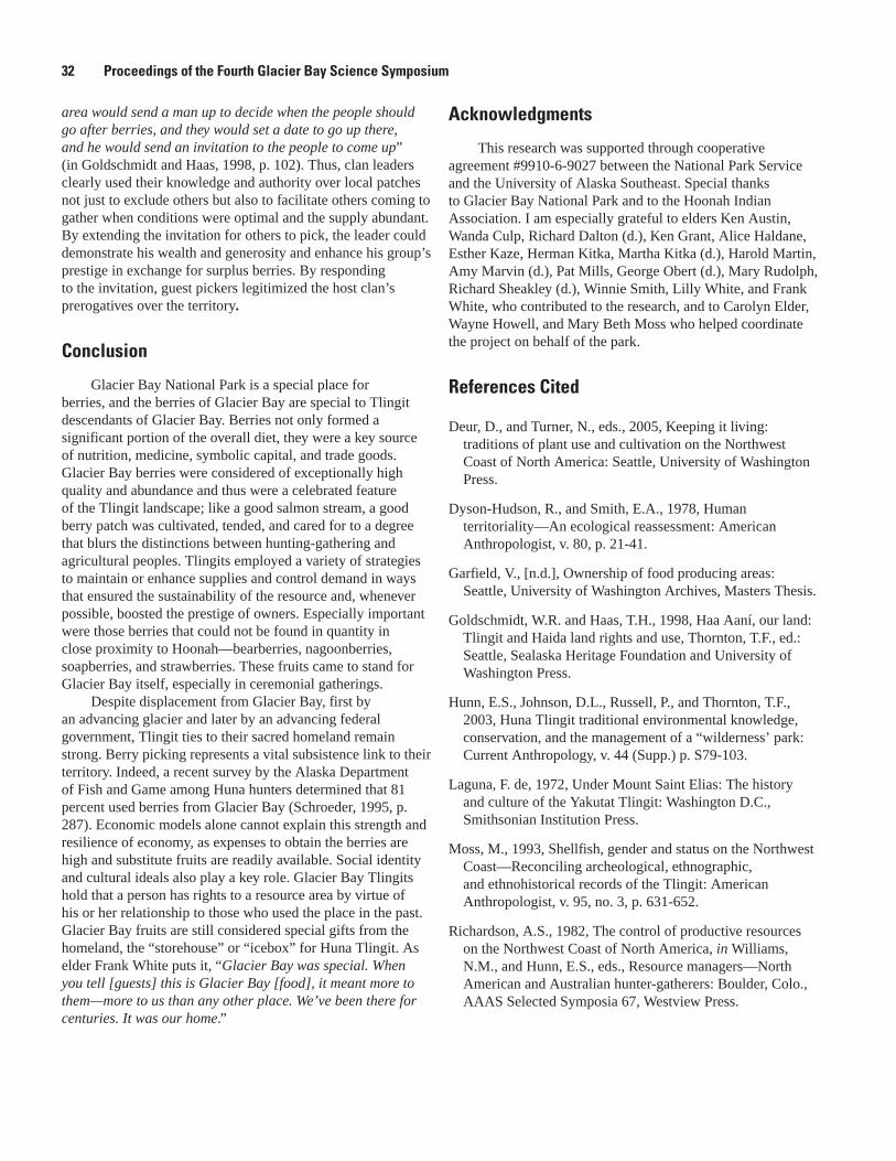
Acknowledgments
This research was supported through cooperative agreement #9910-6-9027 between the National Park Service and the University of Alaska Southeast. Special thanks to Glacier Bay National Park and to the Hoonah Indian Association. I am especially grateful to elders Ken Austin, Wanda Culp, Richard Dalton (d.), Ken Grant, Alice Haldane, Esther Kaze, Herman Kitka, Martha Kitka (d.), Harold Martin, Amy Marvin (d.), Pat Mills, George Obert (d.), Mary Rudolph, Richard Sheakley (d.), Winnie Smith, Lilly White, and Frank White, who contributed to the research, and to Carolyn Elder, Wayne Howell, and Mary Beth Moss who helped coordinate the project on behalf of the park.
References Cited
Deur, D., and Turner, N., eds., 2005, Keeping it living: traditions of plant use and cultivation on the Northwest Coast of North America: Seattle, University of Washington Press.
Dyson-Hudson, R., and Smith, E.A., 1978, Human territoriality—An ecological reassessment: American Anthropologist, v. 80, p. 21-41.
Garfield, V., [n.d.], Ownership of food producing areas: Seattle, University of Washington Archives, Masters Thesis.
Goldschmidt, W.R. and Haas, T.H., 1998, Haa Aaní, our land: Tlingit and Haida land rights and use, Thornton, T.F., ed.: Seattle, Sealaska Heritage Foundation and University of Washington Press.
Hunn, E.S., Johnson, D.L., Russell, P., and Thornton, T.F., 2003, Huna Tlingit traditional environmental knowledge, conservation, and the management of a “wilderness’ park: Current Anthropology, v. 44 (Supp.) p. S79-103.
Laguna, F. de, 1972, Under Mount Saint Elias: The history and culture of the Yakutat Tlingit: Washington D.C., Smithsonian Institution Press.
Moss, M., 1993, Shellfish, gender and status on the Northwest Coast—Reconciling archeological, ethnographic, and ethnohistorical records of the Tlingit: American Anthropologist, v. 95, no. 3, p. 631-652.
Richardson, A.S., 1982, The control of productive resources on the Northwest Coast of North America, in Williams, N.M., and Hunn, E.S., eds., Resource managers—North American and Australian hunter-gatherers: Boulder, Colo., AAAS Selected Symposia 67, Westview Press.
area would send a man up to decide when the people should go after berries, and they would set a date to go up there, and he would send an invitation to the people to come up” (in Goldschmidt and Haas, 1998, p. 102). Thus, clan leaders clearly used their knowledge and authority over local patches not just to exclude others but also to facilitate others coming to gather when conditions were optimal and the supply abundant. By extending the invitation for others to pick, the leader could demonstrate his wealth and generosity and enhance his group’s prestige in exchange for surplus berries. By responding to the invitation, guest pickers legitimized the host clan’s prerogatives over the territory.
Conclusion
Glacier Bay National Park is a special place for berries, and the berries of Glacier Bay are special to Tlingit descendants of Glacier Bay. Berries not only formed a significant portion of the overall diet, they were a key source of nutrition, medicine, symbolic capital, and trade goods. Glacier Bay berries were considered of exceptionally high quality and abundance and thus were a celebrated feature of the Tlingit landscape; like a good salmon stream, a good berry patch was cultivated, tended, and cared for to a degree that blurs the distinctions between hunting-gathering and agricultural peoples. Tlingits employed a variety of strategies to maintain or enhance supplies and control demand in ways that ensured the sustainability of the resource and, whenever possible, boosted the prestige of owners. Especially important were those berries that could not be found in quantity in close proximity to Hoonah—bearberries, nagoonberries, soapberries, and strawberries. These fruits came to stand for Glacier Bay itself, especially in ceremonial gatherings.
Despite displacement from Glacier Bay, first by an advancing glacier and later by an advancing federal government, Tlingit ties to their sacred homeland remain strong. Berry picking represents a vital subsistence link to their territory. Indeed, a recent survey by the Alaska Department of Fish and Game among Huna hunters determined that 81 percent used berries from Glacier Bay (Schroeder, 1995, p. 287). Economic models alone cannot explain this strength and resilience of economy, as expenses to obtain the berries are high and substitute fruits are readily available. Social identity and cultural ideals also play a key role. Glacier Bay Tlingits hold that a person has rights to a resource area by virtue of his or her relationship to those who used the place in the past. Glacier Bay fruits are still considered special gifts from the homeland, the “storehouse” or “icebox” for Huna Tlingit. As elder Frank White puts it, “Glacier Bay was special. When you tell [guests] this is Glacier Bay [food], it meant more to them—more to us than any other place. We’ve been there for centuries. It was our home.”
�2 Proceedings of the Fourth Glacier Bay Science Symposium
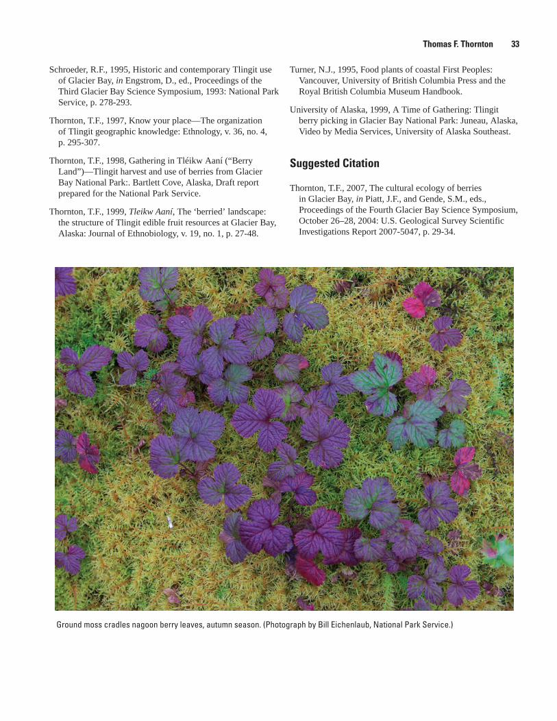
Schroeder, R.F., 1995, Historic and contemporary Tlingit use of Glacier Bay, in Engstrom, D., ed., Proceedings of the Third Glacier Bay Science Symposium, 1993: National Park Service, p. 278-293.
Thornton, T.F., 1997, Know your place—The organization of Tlingit geographic knowledge: Ethnology, v. 36, no. 4, p. 295-307.
Thornton, T.F., 1998, Gathering in Tléikw Aaní (“Berry Land”)—Tlingit harvest and use of berries from Glacier Bay National Park:. Bartlett Cove, Alaska, Draft report prepared for the National Park Service.
Thornton, T.F., 1999, Tleikw Aaní, The ‘berried’ landscape: the structure of Tlingit edible fruit resources at Glacier Bay, Alaska: Journal of Ethnobiology, v. 19, no. 1, p. 27-48.
Ground moss cradles nagoon berry leaves, autumn season. (Photograph by Bill Eichenlaub, National Park Service.)
Thomas F. Thornton ��
Turner, N.J., 1995, Food plants of coastal First Peoples: Vancouver, University of British Columbia Press and the Royal British Columbia Museum Handbook.
University of Alaska, 1999, A Time of Gathering: Tlingit berry picking in Glacier Bay National Park: Juneau, Alaska, Video by Media Services, University of Alaska Southeast.
Suggested Citation
Thornton, T.F., 2007, The cultural ecology of berries in Glacier Bay, in Piatt, J.F., and Gende, S.M., eds., Proceedings of the Fourth Glacier Bay Science Symposium, October 26–28, 2004: U.S. Geological Survey Scientific Investigations Report 2007-5047, p. 29-34.

�� Proceedings of the Fourth Glacier Bay Science Symposium, 200�
This page is intentionally left blank.
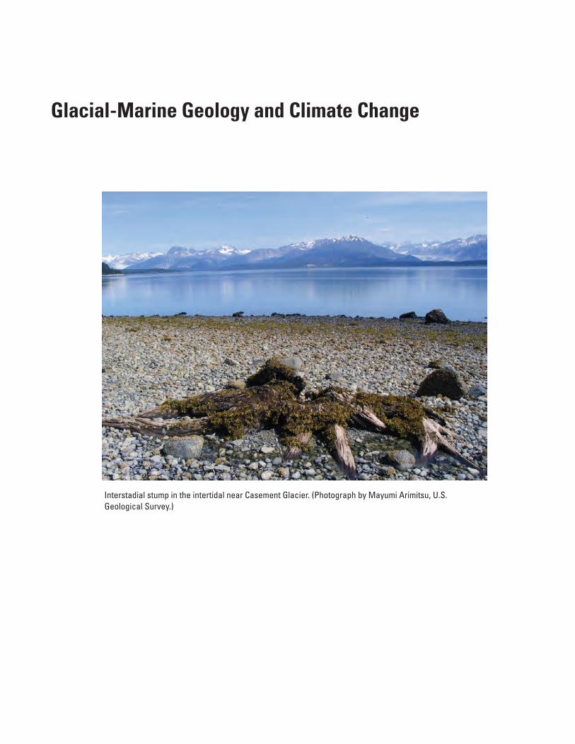
Glacial-Marine Geology and Climate Change
Interstadial stump in the intertidal near Casement Glacier. (Photograph by Mayumi Arimitsu, U.S. Geological Survey.)

�� Proceedings of the Fourth Glacier Bay Science Symposium 200�
This page is intentionally left blank.
Abstract. In April 2004, more than 40 hours of georeferenced submarine digital video were collected in water depths of 15–370 m in Glacier Bay to: ground-truth existing geophysical data (bathymetry and acoustic reflectance); examine and record geologic characteristics of the seafloor; investigate the relationships between substrate types and benthic communities; and create a habitat map. Common substrates observed include rock, boulders, cobbles, rippled sand, bioturbated mud, and extensive beds of living Modiolus (horse mussels) and scallops. Four principal seafloor geomorphic types were distinguished using video observations:
1. High complexity/high slope/boulder and rock substrate;
2. High complexity/low slope/boulder and rock substrate;
3. Moderate complexity/sand, gravel, and cobble substrate;
4. Low complexity/fine-grained sediment.
The distribution of these seafloor types in lower and central Glacier Bay was predicted using a hierarchical decision-tree statistical classification analysis of geophysical data.
Introduction
Geologic substrates of the sea floor in southeast Alaska provide benthic habitats for recreationally and commercially important species, including king, dungeness, and tanner crabs, halibut, rockfish, and shrimp. In Glacier Bay, where historical rates of glacier retreat are among the highest documented worldwide, the potential for rapid change in seafloor properties is high owing to paraglacial sedimentation. We use geophysical data, underwater video, and sedimentological tools to understand the distribution, character, and rate of change of geologic substrates and benthic communities in this dynamic environment. Seafloor features are revealed in bathymetry and acoustic reflectance data collected in Glacier Bay in 1998 using multibeam and side-scan sonar techniques (Carlson and others, 2002, 2003; Cochrane and others, 1998, 2000). Characterizing the seafloor in real-time while towing video is useful for ground-truthing these geophysical data, resolving unique features, examining areas of transition between contrasting substrate types, and linking the geology and biology of benthic environments.
Jodi Harney and others �7
Geologic Characteristics of Benthic Habitats in Glacier Bay, Alaska, Derived from Geophysical Data, Videography, and Sediment Sampling
Jodi Harney1,4, Guy Cochrane1, Lisa Etherington2, Pete Dartnell3, and Hank Chezar3
1 U.S. Geological Survey, Pacific Science Center, 400 Natural Bridges Dr., Santa Cruz, CA 95060
2 U.S. Geological Survey, Alaska Science Center, P.O. Box 140, Gustavus, AK 99826
3 U.S. Geological Survey, 345 Middlefield Rd., MS999, Menlo Park, CA 95060
4 Corresponding author: [email protected], 250-655-4035
Methods
The principal objectives of video data collection were to ground-truth geophysical data and construct maps of substrate morphology and habitat distribution, thus transect locations were selected based on the existence, quality, and complexity of geophysical data and on regions of geologic transition and (or) biologic significance. A video sled equipped with forward- and downward-looking video cameras, lights, altimeter, and a pressure (depth) sensor was towed 1–2 m above the seafloor to record geologic and biologic features. Two lasers spaced 20 cm apart provided scale. Height above the seafloor, pitch, roll, water depth, ship GPS position, speed (generally <1.5 knots), heading, and time were imprinted on the digital video tape. Real-time observations of seafloor characteristics were digitally recorded at 30-second intervals during 52 video transects (~41 hours) collected in the lower and central bay, the Beardslee and Marble Islands, off Tlingit Point, and in parts of the east and west arms. Observations at each point included primary and secondary substrate type (e.g. rock, sand, mud), substrate complexity (rugosity), seafloor slope, benthic biomass (low, medium, or high), the presence and absence of benthic organisms and demersal fish, and small-scale seafloor features (e.g. ripples, tracks, burrows). Real-time observations were recorded to a digital data file along with time, GPS position, and other ship data (after Anderson and others, unpub. data.).
In addition to towed video, an underwater sediment-bed camera was deployed to collect in situ digital macro images of seafloor sediment to measure the grain-size distribution using a mathematical autocorrelation algorithm (Rubin, 2004). With an image resolution of 65 pixels per mm, changes in grain size as small as 0.04 mm (40 μm, the difference between silt and clay) can be calculated. This technique enables the rapid mapping of sediment properties over a range of spatial and temporal scales, information that is useful in assessing sediment sources and the physical processes that are at work in the depositional environment. Sediment samples (n=24) and short gravity cores (n=28, ranging from 10 cm to 1 m in length) also were collected in water depths of 50–120 m.
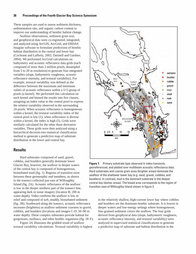
in the relatively shallow, high-current lower bay where cobbles and boulders are the dominant benthic substrate. It is lowest in deeper waters and low-energy settings where homogeneous, fine-grained sediment covers the seafloor. The four grids derived from geophysical data (slope, bathymetric roughness, acoustic reflectance intensity, and textural variability) were analyzed in supervised statistical classifications to generate a predictive map of substrate and habitat distribution in the
WestArm
MuirInlet
TLINGITPOINT
WILLOUGHBYISLAND
Figure 1. Primary substrate type observed in video transects, georeferenced, and plotted over multibeam acoustic reflectance data. Hard substrates and coarse grain sizes (brighter areas) dominate the seafloor of the shallower lower bay (e.g. sand, gravel, cobbles, and boulders). In contrast, mud is the dominant substrate in the deeper central bay (darker areas). The boxed area corresponds to the region of transition east of Willoughby Island shown in figure 2.
relief and composed of soft, muddy, bioturbated sediment (fig. 2B). Southward along the transect, acoustic reflectance increases (brightens) as seafloor sediment coarsens to gravel, cobbles, and boulders (locations and images C-D; 50–90 m water depth). These complex substrates provide habitat for gorgonians, molluscs, and other benthic organisms (fig. 2E-F).
Figure 3A illustrates the gridded result of seafloor textural variability calculations. Textural variability is highest
These samples are used to assess sediment thickness, sedimentation rate, and organic carbon content to improve our understanding of benthic habitat change.
Seafloor observations, sediment grain size, and geophysical data were co-registered, integrated, and analyzed using ArcGIS, ArcGrid, and ERDAS Imagine software to formulate predictions of benthic habitat distribution in the central and lower bay (Cochrane and Lafferty, 2002; Dartnell and Gardner, 2004). We performed ArcGrid calculations on bathymetry and acoustic reflectance data grids (each composed of more than 3 million pixels, desampled from 5 to 20 m resolution) to generate four integrated variables (slope, bathymetric roughness, acoustic reflectance intensity, and textural variability). For example, textural variability was defined as the difference between the maximum and minimum values of acoustic reflectance within a 5×5 group of pixels (a kernel). We performed this calculation on each kernel and binned the results into five classes, assigning an index value to the central pixel to express the relative variability observed in the surrounding 24 pixels. When acoustic reflectance is homogeneous within a kernel, the textural variability index of the central pixel is low (1); when reflectance is diverse within a kernel, the index is high (5). Grids were similarly calculated for the other three derivative variables. These grids were then analyzed using a hierarchical decision-tree statistical classification method to generate a predictive map of substrate distribution in the lower and central bay.
Results
Hard substrates composed of sand, gravel, cobbles, and boulders generally dominate lower Glacier Bay, however, the seafloor in deeper waters of the central bay is composed of homogeneous, bioturbated mud (fig. 1). Regions of transition exist between these geomorphic end members, as shown in the transect collected just east of Willoughby Island (fig. 2A). Acoustic reflectance of the seafloor is low in the deeper northern part of the transect line, appearing dark in sonar imagery (location B; 200 m water depth). Video confirms the seafloor is low in
�� Proceedings of the Fourth Glacier Bay Science Symosium
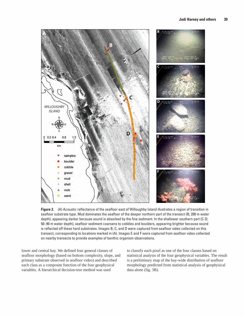
B
A
D
C
WILLOUGHBYISLAND
C
E
B
D
F
Figure 2. (A) Acoustic reflectance of the seafloor east of Willoughby Island illustrates a region of transition in seafloor substrate type. Mud dominates the seafloor of the deeper northern part of the transect (B; 200 m water depth), appearing darker because sound is absorbed by the fine sediment. In the shallower southern part (C-D; 50–90 m water depth), seafloor sediment coarsens to cobbles and boulders, appearing brighter because sound is reflected off these hard substrates. Images B, C, and D were captured from seafloor video collected on this transect, corresponding to locations marked in (A). Images E and F were captured from seafloor video collected on nearby transects to provide examples of benthic organism observations.
lower and central bay. We defined four general classes of seafloor morphology (based on bottom complexity, slope, and primary substrate observed in seafloor video) and described each class as a composite function of the four geophysical variables. A hierarchical decision-tree method was used
to classify each pixel as one of the four classes based on statistical analysis of the four geophysical variables. The result is a preliminary map of the bay-wide distribution of seafloor morphology predicted from statistical analysis of geophysical data alone (fig. 3B).
Jodi Harney and others �9
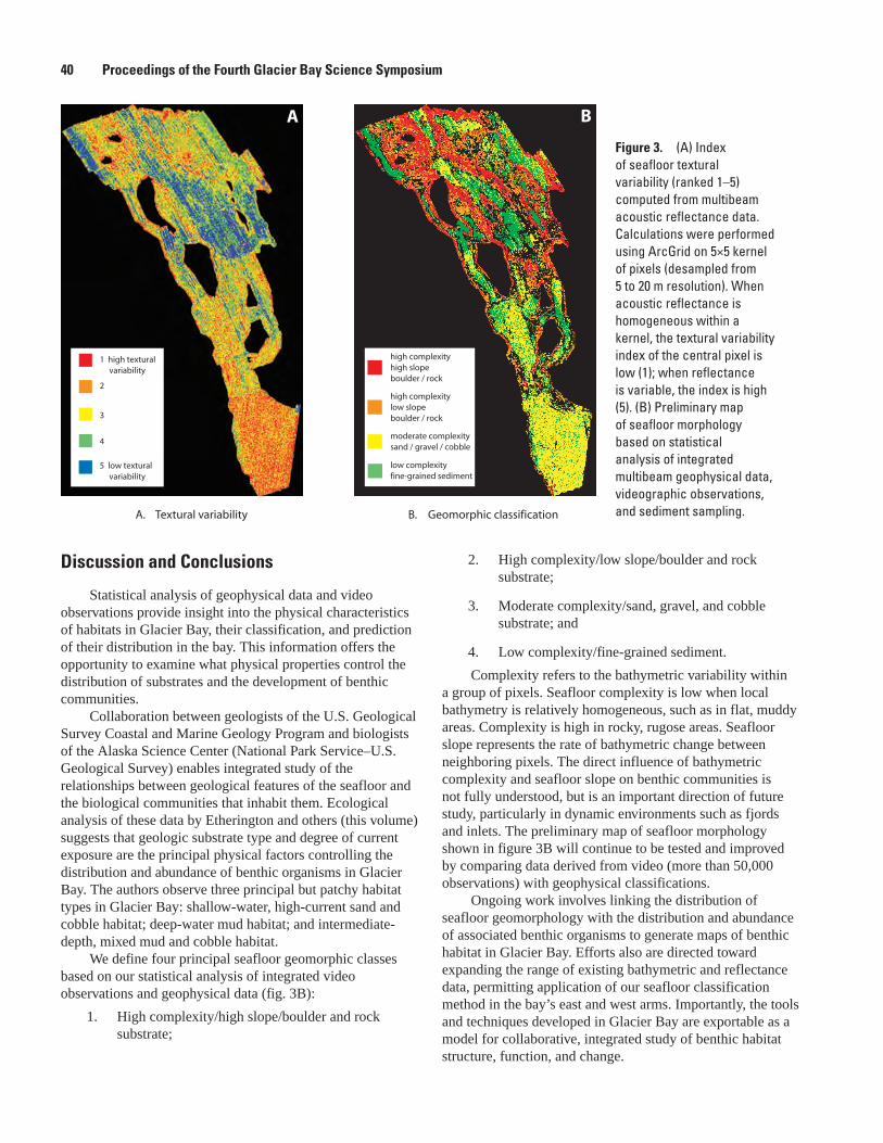
2. High complexity/low slope/boulder and rock substrate;
3. Moderate complexity/sand, gravel, and cobble substrate; and
4. Low complexity/fine-grained sediment.
Complexity refers to the bathymetric variability within a group of pixels. Seafloor complexity is low when local bathymetry is relatively homogeneous, such as in flat, muddy areas. Complexity is high in rocky, rugose areas. Seafloor slope represents the rate of bathymetric change between neighboring pixels. The direct influence of bathymetric complexity and seafloor slope on benthic communities is not fully understood, but is an important direction of future study, particularly in dynamic environments such as fjords and inlets. The preliminary map of seafloor morphology shown in figure 3B will continue to be tested and improved by comparing data derived from video (more than 50,000 observations) with geophysical classifications.
Ongoing work involves linking the distribution of seafloor geomorphology with the distribution and abundance of associated benthic organisms to generate maps of benthic habitat in Glacier Bay. Efforts also are directed toward expanding the range of existing bathymetric and reflectance data, permitting application of our seafloor classification method in the bay’s east and west arms. Importantly, the tools and techniques developed in Glacier Bay are exportable as a model for collaborative, integrated study of benthic habitat structure, function, and change.
Discussion and Conclusions
Statistical analysis of geophysical data and video observations provide insight into the physical characteristics of habitats in Glacier Bay, their classification, and prediction of their distribution in the bay. This information offers the opportunity to examine what physical properties control the distribution of substrates and the development of benthic communities.
Collaboration between geologists of the U.S. Geological Survey Coastal and Marine Geology Program and biologists of the Alaska Science Center (National Park Service–U.S. Geological Survey) enables integrated study of the relationships between geological features of the seafloor and the biological communities that inhabit them. Ecological analysis of these data by Etherington and others (this volume) suggests that geologic substrate type and degree of current exposure are the principal physical factors controlling the distribution and abundance of benthic organisms in Glacier Bay. The authors observe three principal but patchy habitat types in Glacier Bay: shallow-water, high-current sand and cobble habitat; deep-water mud habitat; and intermediate-depth, mixed mud and cobble habitat.
We define four principal seafloor geomorphic classes based on our statistical analysis of integrated video observations and geophysical data (fig. 3B):
1. High complexity/high slope/boulder and rock substrate;
B
B. Geomorphic classification
high complexity high slopeboulder / rock
high complexitylow slopeboulder / rock
moderate complexitysand / gravel / cobble
low complexityfine-grained sediment
A
A. Textural variability
2
1 high textural variability
3
4
5 low textural variability
Figure �. (A) Index of seafloor textural variability (ranked 1–5) computed from multibeam acoustic reflectance data. Calculations were performed using ArcGrid on 5×5 kernel of pixels (desampled from 5 to 20 m resolution). When acoustic reflectance is homogeneous within a kernel, the textural variability index of the central pixel is low (1); when reflectance is variable, the index is high (5). (B) Preliminary map of seafloor morphology based on statistical analysis of integrated multibeam geophysical data, videographic observations, and sediment sampling.
�0 Proceedings of the Fourth Glacier Bay Science Symposium
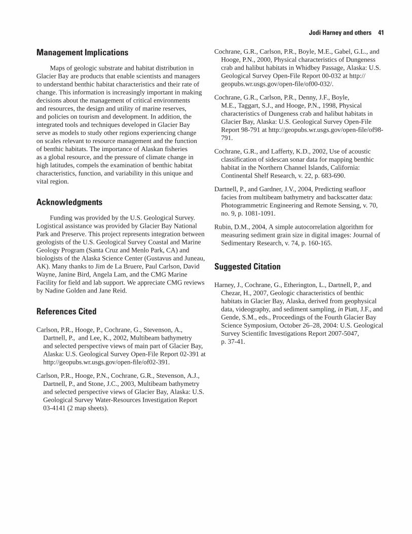
Management Implications
Maps of geologic substrate and habitat distribution in Glacier Bay are products that enable scientists and managers to understand benthic habitat characteristics and their rate of change. This information is increasingly important in making decisions about the management of critical environments and resources, the design and utility of marine reserves, and policies on tourism and development. In addition, the integrated tools and techniques developed in Glacier Bay serve as models to study other regions experiencing change on scales relevant to resource management and the function of benthic habitats. The importance of Alaskan fisheries as a global resource, and the pressure of climate change in high latitudes, compels the examination of benthic habitat characteristics, function, and variability in this unique and vital region.
Acknowledgments
Funding was provided by the U.S. Geological Survey. Logistical assistance was provided by Glacier Bay National Park and Preserve. This project represents integration between geologists of the U.S. Geological Survey Coastal and Marine Geology Program (Santa Cruz and Menlo Park, CA) and biologists of the Alaska Science Center (Gustavus and Juneau, AK). Many thanks to Jim de La Bruere, Paul Carlson, David Wayne, Janine Bird, Angela Lam, and the CMG Marine Facility for field and lab support. We appreciate CMG reviews by Nadine Golden and Jane Reid.
References Cited
Carlson, P.R., Hooge, P., Cochrane, G., Stevenson, A., Dartnell, P., and Lee, K., 2002, Multibeam bathymetry and selected perspective views of main part of Glacier Bay, Alaska: U.S. Geological Survey Open-File Report 02-391 at http://geopubs.wr.usgs.gov/open-file/of02-391.
Carlson, P.R., Hooge, P.N., Cochrane, G.R., Stevenson, A.J., Dartnell, P., and Stone, J.C., 2003, Multibeam bathymetry and selected perspective views of Glacier Bay, Alaska: U.S. Geological Survey Water-Resources Investigation Report 03-4141 (2 map sheets).
Cochrane, G.R., Carlson, P.R., Boyle, M.E., Gabel, G.L., and Hooge, P.N., 2000, Physical characteristics of Dungeness crab and halibut habitats in Whidbey Passage, Alaska: U.S. Geological Survey Open-File Report 00-032 at http://geopubs.wr.usgs.gov/open-file/of00-032/.
Cochrane, G.R., Carlson, P.R., Denny, J.F., Boyle, M.E., Taggart, S.J., and Hooge, P.N., 1998, Physical characteristics of Dungeness crab and halibut habitats in Glacier Bay, Alaska: U.S. Geological Survey Open-File Report 98-791 at http://geopubs.wr.usgs.gov/open-file/of98-791.
Cochrane, G.R., and Lafferty, K.D., 2002, Use of acoustic classification of sidescan sonar data for mapping benthic habitat in the Northern Channel Islands, California: Continental Shelf Research, v. 22, p. 683-690.
Dartnell, P., and Gardner, J.V., 2004, Predicting seafloor facies from multibeam bathymetry and backscatter data: Photogrammetric Engineering and Remote Sensing, v. 70, no. 9, p. 1081-1091.
Rubin, D.M., 2004, A simple autocorrelation algorithm for measuring sediment grain size in digital images: Journal of Sedimentary Research, v. 74, p. 160-165.
Suggested Citation
Harney, J., Cochrane, G., Etherington, L., Dartnell, P., and Chezar, H., 2007, Geologic characteristics of benthic habitats in Glacier Bay, Alaska, derived from geophysical data, videography, and sediment sampling, in Piatt, J.F., and Gende, S.M., eds., Proceedings of the Fourth Glacier Bay Science Symposium, October 26–28, 2004: U.S. Geological Survey Scientific Investigations Report 2007-5047, p. 37-41.
Jodi Harney and others �1
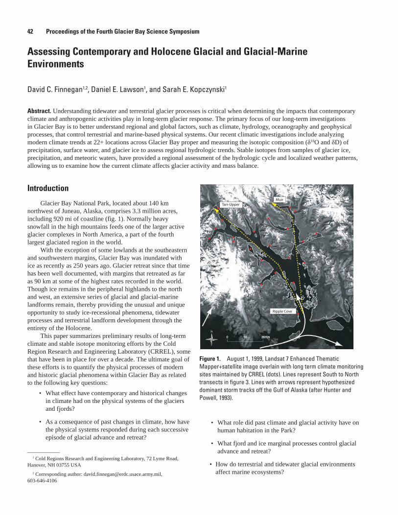
Assessing Contemporary and Holocene Glacial and Glacial-Marine Environments
David C. Finnegan1,2, Daniel E. Lawson1, and Sarah E. Kopczynski1
Abstract. Understanding tidewater and terrestrial glacier processes is critical when determining the impacts that contemporary climate and anthropogenic activities play in long-term glacier response. The primary focus of our long-term investigations in Glacier Bay is to better understand regional and global factors, such as climate, hydrology, oceanography and geophysical processes, that control terrestrial and marine-based physical systems. Our recent climatic investigations include analyzing modern climate trends at 22+ locations across Glacier Bay proper and measuring the isotopic composition (δ18O and δD) of precipitation, surface water, and glacier ice to assess regional hydrologic trends. Stable isotopes from samples of glacier ice, precipitation, and meteoric waters, have provided a regional assessment of the hydrologic cycle and localized weather patterns, allowing us to examine how the current climate affects glacier activity and mass balance.
Tarr-UpperMuir
Ripple Cove
Figure 1. August 1, 1999, Landsat 7 Enhanced Thematic Mapper+satellite image overlain with long term climate monitoring sites maintained by CRREL (dots). Lines represent South to North transects in figure 3. Lines with arrows represent hypothesized dominant storm tracks off the Gulf of Alaska (after Hunter and Powell, 1993).
• What role did past climate and glacial activity have on human habitation in the Park?
• What fjord and ice marginal processes control glacial advance and retreat?
• How do terrestrial and tidewater glacial environments affect marine ecosystems?
Introduction
Glacier Bay National Park, located about 140 km northwest of Juneau, Alaska, comprises 3.3 million acres, including 920 mi of coastline (fig. 1). Normally heavy snowfall in the high mountains feeds one of the larger active glacier complexes in North America, a part of the fourth largest glaciated region in the world.
With the exception of some lowlands at the southeastern and southwestern margins, Glacier Bay was inundated with ice as recently as 250 years ago. Glacier retreat since that time has been well documented, with margins that retreated as far as 90 km at some of the highest rates recorded in the world. Though ice remains in the peripheral highlands to the north and west, an extensive series of glacial and glacial-marine landforms remain, thereby providing the unusual and unique opportunity to study ice-recessional phenomena, tidewater processes and terrestrial landform development through the entirety of the Holocene.
This paper summarizes preliminary results of long-term climate and stable isotope monitoring efforts by the Cold Region Research and Engineering Laboratory (CRREL), some that have been in place for over a decade. The ultimate goal of these efforts is to quantify the physical processes of modern and historic glacial phenomena within Glacier Bay as related to the following key questions:
• What effect have contemporary and historical changes in climate had on the physical systems of the glaciers and fjords?
• As a consequence of past changes in climate, how have the physical systems responded during each successive episode of glacial advance and retreat?
1 Cold Regions Research and Engineering Laboratory, 72 Lyme Road, Hanover, NH 03755 USA
2 Corresponding author: [email protected], 603-646-4106
�2 Proceedings of the Fourth Glacier Bay Science Symposium

Table 1. Summary of precipitation data for climate monitoring sites maintained in Glacier Bay by CRREL.
[in/yr, inch per year; –, incomplete data]
Location Year Total (in/yr)Lower Bay
Ripple Cove – –
Geikie East 2002 47.76
Geikie West 2002 71.1
Johnson’s Cove 2002 53.1
Sandy Cove 2002 59.68
Sebree 2002 77.54
West ArmSundew Cove 2002 76.18
Skidmore 2002 68.32
Tidal 2002 42.15
Queen Inlet1 2002 86
Reid Inlet Entrance 2002 64.36
Reid Glacier 2002 57.08
Tarr Lower 2002 72.65
Tarr Upper 2002 69.88
Johns Hopkins InletTopeka 2002 49.46
Johns Hopkins1 2003 50.73
East ArmAdams East 2002 39.75
Adams West 2002 76.08
Wachusett East 2002 85.75
McBride 2002 94.22
Wachusett West – –
Riggs Glacier 2002 63.88
Muir Glacier 2003 88.83
Upper Muir 2002 55.91GOES near real-time data collection site.
• Is there evidence of significant climate forcing in the sedimentary and dendrochronological record and can changes in climate be related to global changes or regional phenomena?
Methods
The long-term monitoring of contemporary climate in Glacier Bay has been ongoing by CRREL in cooperation with the National Park Service since 1999 (Finnegan and others, 2003; Kopczynski and others, 2003). As of October 2004, there are 24 active climate-sites including two snow water equivalent gauges (these include a full climate site) and two realtime Geostationary Operational Environmental Satellite systems (GOES) that are maintained by CRREL within the main bay of the park (fig. 1). Each of these stations has been located to optimize data collection at approximately the same elevation (sea level) for regional comparisons. Furthermore, the locations of each site were chosen to minimize environmental and visual impact to respect park wilderness resources and ethics.
Each climate site has a minimum configuration of two rain gauges that collect data at 0.01-in. increments; a high-resolution temperature sensor sensitive to tenth of a degree; and a bulk rainwater sampler at each rain gauge for stable isotope analysis. We have collected and analyzed the bulk rainwater samples as well as precipitation (rain, snow) at re-occupied locations for oxygen (δ18O) and hydrogen (δD) stable isotope content over the last 10 years. Glacier ice samples also were obtained from tidewater and terrestrial glaciers throughout the Park. We have been sampling both the basal and englacial ice in systematic sampling grids to develop a better understanding of the sources of precipitation for glaciers and how these may vary across the region.
Results
Climate DataClimate data acquired within Glacier Bay, though
preliminary, is beginning to reveal trends in the local and regional climate systems. A summary of the first consistent long-term climate records to provide a holistic perspective of precipitation within Glacier Bay is shown in table 1. Overall yearly averages at each site are high (>50 in/yr) and our yearly records, indicate that precipitation levels are fairly consistent. Furthermore, the data illustrates patterns and trends which occur along the main bay, East Arm and West Arm.
As an addition to the future of climate monitoring within the park, we are developing and deploying near real-time GOES up-linked climate platforms. The GOES satellite
is a geostationary imaging satellite that is primarily used for weather imaging and observations over the eastern and western continental United States. Included on the GOES platform is a one-way radio communication channel that allows for transmission of approved scientific information. Currently, most CRREL climate stations are revisited during the spring and fall seasons to calibrate instrumentation, download data, collect samples and repair damage that may have been incurred due to wildlife and environmental conditions. By using the GOES transmission system, data are collected at regularly timed intervals (15 minutes) but are transmitted via the GOES system for processing hourly. Once the data are transmitted, the information is decoded at a central receiving station at the Corp of Engineers New England District, quality checked and then sent to a central database server at CRREL.
David C. Finnegan and others ��
Figure 2. Relation between δ18O and δD values for all precipitation and snow samples (1997–2003) collected within Glacier Bay. Samples are shown in comparison to the Global Meteoric Water Line (GMWL) where δ2H=8 δ18O+10‰. Data from Glacier Bay show a reasonable fit to the GMWL.
Figure �. Spatial distribution of δ18O and cumulative precipitation values derived from CRREL climate monitoring sites (up to 2004) for transects running South to North along the West and East Arms of Glacier Bay (see fig. 1 for locations). Precipitation values show an approximate increasing trend from the mouth of Glacier Bay to the head of Muir Inlet and less so towards the head of Tarr Inlet. Likewise, the isotopic values become increasing lighter with distance up each respective inlet, particularly in Muir Inlet.
-20.00
0.00
-20.00
-40.00
-60.00
-80.00
-100.00
-120.00
-140.00
-160.00
-180.00-25.00 -15.00 -10.00 -5.00 0.00
y = 7.9158x + 5.0692R2 = 0.9004
all precip (snow, rain, cum precip)
----GMWL
δ18O
δ2H
δ18O
avg (‰
)
Distance North (km)
Cu
mu
lati
ve P
reci
pit
atio
n (i
nch
es)
Ripple Cove to Muir (Muir Inlet)
Ripple Cove to Tarr-upper (West Arm)
The benefits of installing these sophisticated devices include the near real-time retrieval of weather information and greatly reducing labor and resources needed to maintain a consistent, yet highly accurate accumulation of climate data. By installing the GOES systems throughout the Park, we will also reduce impact on biologically sensitive areas at critical times of the year through reduced number of visitations each season. The remote monitoring systems are capable of being expanded to include new instruments as the need arises and allows for collaboration with other researchers working in the park that likewise may benefit from near real-time data transmission. Furthermore, easy and rapid access to climate data in remote areas of the park through our web-based interface may be especially useful to Park resource managers for planning, to interpreters and naturalists for daily climate information, and to Park Rangers during emergency situations.
IsotopesIt is widely recognized that the δ18O and δD isotopic
compositions of precipitation are influenced by source, temperature, altitude, distance inland along storm tracks, and latitude. In Glacier Bay, our data show a trend consistent to the Global Meteoric Water Line (fig. 2), representing the average relationship between δ18O and δD in meteoric waters throughout the world. Regionally, the changes exhibited in the isotopic composition of precipitation vary. For example, oxygen ratios vary by a significant 6 to 8‰ across the Park. Within the East Arm, the oxygen isotope ratio of precipitation shows seasonal variations ranging from -7 to -14.5‰, whereas in the West Arm they range from -8 to -14.5‰. The isotopic values vary significantly with location. Along north-south transects from the mouth of Glacier Bay (Ripple Cove) to the head of Muir and Tarr Inlets respectively, the δ18O values for cumulative samples of precipitation decrease, becoming more negative with distance. In contrast, annual precipitation totals show an increasing trend toward the head of Muir Inlet, but a slightly erratic, mostly increasing trend into the West Arm. Combined, these trends suggest a predominance of storms tracking from the mouth of Glacier Bay to the head of Muir Inlet, but less effective movement of these storms northwestward into Tarr Inlet, inland of the Fairweather Range.
We also see isotopic differences and trends within glacial ice. Values for glaciers in the East and West Arms differ significantly from one another. These variations reflect differences in the elevation and precipitation sources of the accumulation areas. The eastern systems radiate from icefields in the Takinsha Mountains at elevations ranging from 1,200 to 1,900 m (Equilibrium Line Altitude (ELA) ~750 m), whereas those in the West Arm are fed by snow falling in the Fairweather Range at elevations of over 2,500 to 4,500 m (ELA ~1,000–1,100 m). The orogenic effect or rain shadow created by the Fairweather Range and its elevational control on the tracks of storms entering Glacier Bay appear to exert a strong regional control on the climate of the Park (fig. 3).
�� Proceedings of the Fourth Glacier Bay Science Symposium
Discussion and Conclusions
Understanding the modern glacial environment is essential for reconstructing the glacial history and dynamics throughout the Holocene. It also improves our understanding of the impact that climate change will have on future marine and terrestrial communities and ecosystems. Weather patterns may be highly localized, impacted by the glaciers themselves, and influenced by mountainous topography. Glaciers respond according to their location, amount of precipitation and respective source areas. The length of our records of temperature and precipitation remain too short to assess annual, seasonal and spatial variability in temperature and precipitation, but the data do suggest that trends may be present and related to both the prevailing storm tracks and local topography. The influence of other factors such as El Nino, Pacific Decadal Oscillation (PDO) and Arctic Oscillation are unknown but will be investigated as part of our paleoclimatic research (Lawson and others, this volume).
Trends present in the preliminary bulk rainwater isotopic data lead us to believe that the storm sources are diverse, but there is a regional effect related to primary storm tracks. Storms in the Gulf of Alaska appear to move through Cross Sound and then north out of Icy Strait up the lower Bay and into the East and West Arms. There is some suggestion in the data that the storms may more commonly move into the West Arm.
Expansion of the climate network to higher elevations is essential to understanding the regional variability in climate and to provide data critical to both physical, biological and ecosystem research in the Park. The climatic network is crucial to many types of studies, but a record does not exist within the Park prior to 1999. There remains a need to install additional sensors, including those for wind speed and direction and solar radiation.
Management Implications
Climatic data provide a record of the essential elements that control the physical and biological processes of freshwater, terrestrial and marine ecosystems of the Park. It is critical to establish and maintain long-term monitoring of climatic parameters. The CRREL climatic network is the first step toward meeting this goal. By upgrading the existing sites to satellite transmission and web access, the data will be available in near real time for use by park management, rangers, naturalists, and interpreters as well as researchers. Our extremely limited understanding of the climate in the Park and such basic knowledge as storm tracks and prevailing winds are being met by our climate sites and the associated studies of stable isotopes and other aspects of the hydrologic cycle.
Acknowledgments
This project has been funded in part by the U.S. Army Cold Regions Research and Engineering Lab, the National Park Service, National Science Foundation, Rockefeller Foundation, Arctic Institute Dartmouth College, and private donations. We are extremely grateful to the staff and management of Glacier Bay National Park for their continuing support, assistance and encouragement, including the M/V Nunatak and her Captains and Mates, without which this research could not have been conducted.
References Cited
Finnegan, D.C., Lawson, D.E., Kopczynski, S., and Bigl, S.R., 2003, Long-term studies of tidewater and terrestrial dynamics, glacier hydrology, and Holocene and historic climate activity; Glacier Bay, Southeast Alaska [abs.]: Eos Transactions, American Geophysical Union, Fall Meeting, Suppl., v. 84, no. 46, p. C12A-0874.
Hunter, L.E., and Powell, R.D., 1993, Climatic controls on glacier mass balance in Glacier Bay National Park and Preserve, in, Engstrom, D., ed., Proceedings of the Third Glacier Bay Science Symposium, 1993: U.S. National Park Service.
Kopczynski, S., Bigl, S.R., Lawson, D.C., Finnegan, D.C., 2003, Recent climate trends in Glacier Bay[abs.]:, Eos Transactions, American Geophysical Union, Fall Meeting, Suppl., v. 84, no. 46, p. C12A-0873.
Lawson, D.E., Finnegan, D.F., Kopczynski S.E., and Bigl, S.R., 2007, Early to mid-Holocene glacier fluctuations in Glacier Bay, Alaska, in Piatt, J.F., and Gende, S.M., eds., Proceedings of the Fourth Glacier Bay Science Symposium, 2004, October 26–28, 2004: U.S. Geological Survey Scientific Investigations Report 2007-5047, p. 54-56.
Suggested Citation
Finnegan, D.C., Lawson, D.E., Kopczynski, S.E, 2007, Assessing contemporary and Holocene glacial and glacial-marine environments, in Piatt, J.F., and Gende, S.M., eds., Proceedings of the Fourth Glacier Bay Science Symposium, October 26–28, 2004: U.S. Geological Survey Scientific Investigations Report 2007-5047, p. 42-45.
David C. Finnegan and others �5
High Frequency Climate Signals in Fjord Sediments of Glacier Bay National Park, Alaska
Ellen A. Cowan1,3 and Ross D. Powell2
Abstract. More than 25 years of glacimarine research has provided the background to interpret the fjord sediment record in basins near tidewater glaciers in terms of paleoclimate. Key sedimentary products for interpreting this high frequency record are gravelly-mud beds and black layers that are deposited annually. During the meltwater season deep-water tidal rhythmites are organized in distinctive half-month packages by their thickness. Identification of these time-indicators within the record allows for establishment of a meltwater discharge proxy from tidewater glaciers. In turn, this proxy can be used to test the fluctuation of annual meltwater production with meteorological variables and the Pacific Decadal Oscillation (PDO).
Introduction
Research conducted for over 25 years on the glacimarine sedimentary environment in Glacier Bay National Park and Preserve sets the stage for interpretation of the paleoclimate record in fjord sediment deposits. This topic has recently come to the forefront in the geological community because of the initiation of studies to evaluate the dynamic interplay between climate and tectonics along the Alaskan margin (Gulick and others, 2004). Glacier Bay is of particular interest because of the well-documented history of glacial retreat from the Little Ice Age maximum position, and because of high sediment accumulation rates in basins adjacent to temperate tidewater glaciers (Hunter and others, 1996, Powell and Domack, 2002). This combination has the potential for producing a high-resolution record where days and weeks within the meltwater season can be identified. The purpose of this paper is to summarize our present understanding of the high-resolution record preserved in fjord sediments based on previous work in Glacier Bay and at Hubbard Glacier near Yakutat, Alaska.
Methods
Depositional processes from turbid plumes within baroclinic overflows from meltwater stream discharges within glacial fjords have previously been investigated with CTD casts, suspended sediment sampling, floc camera imaging at anchor stations, and with sediment traps (Cowan and Powell, 1991, Cowan, 1992, Hill and others, 1998). In addition, a tethered submersible has been used to visually investigate tidewater termini (Powell and Domack, 2002). These synoptic sampling techniques provide the link between climate forcing variables and spatial and temporal patterns of fjord
sedimentation determined from sediment cores, grab samples and seismic-reflection profiles (Cai and others, 1997, Seramur and others, 1997). Water column and suspended sediment properties have been measured over time scales of 6 to 12 hours during both spring and neap tides because of variability greater than 7 m in the semi-diurnal tidal range in Glacier Bay. Seasonal variability also is of considerable importance because meltwater from tidewater glaciers contributes the bulk of sediment to the fjord (Hunter and others, 1996). We estimate from our seasonal sampling that the duration of the meltwater season is approximately 4 months, beginning abruptly in May and ending in late August with little or no discharge during winter (Cowan and others, 1999).
Several studies have been conducted by our research group in Glacier Bay using sediment cores up to 4 m-long to document the marine record of tidewater glaciers (Cai and others, 1997, Cowan and others, 1999). In these studies we developed a chronology using 210Pb radioisotopes that compares favorably with bathymetric changes in ice-proximal areas. On September 7–8, 2004, we participated in a cruise onboard the R/V Maurice Ewing that collected data from Muir Inlet with the goal of developing a better understanding of Alaska’s paleoclimate record. Two sediment cores, each about 17 m-long, were collected from basins in upper Muir Inlet (between Wachusett and McBride Inlets). The seasonal indicators and tidal rhythmites described below are important in interpreting the high-resolution climate record preserved in these cores.
Results
Recognizable sedimentary products are a result of forcing variables that reoccur at known time scales (table 1). Of particular interest for interpreting the paleoclimate record are gravelly-mud beds, (diamictons), black layers, and deep-water tidal rhythmites. Sediment transported by a large rainfall event has been documented at McBride Glacier but generally, this process likely occurs episodically (Cowan and others, 1988).
1 Department of Geology, Appalachian State University, Boone, NC 28608
2 Department of Geology and Environmental Geosciences, Northern Illinois University, DeKalb, IL 60115
3 Corresponding author: [email protected], 828-262-2260
�� Proceedings of the Fourth Glacier Bay Science Symposium
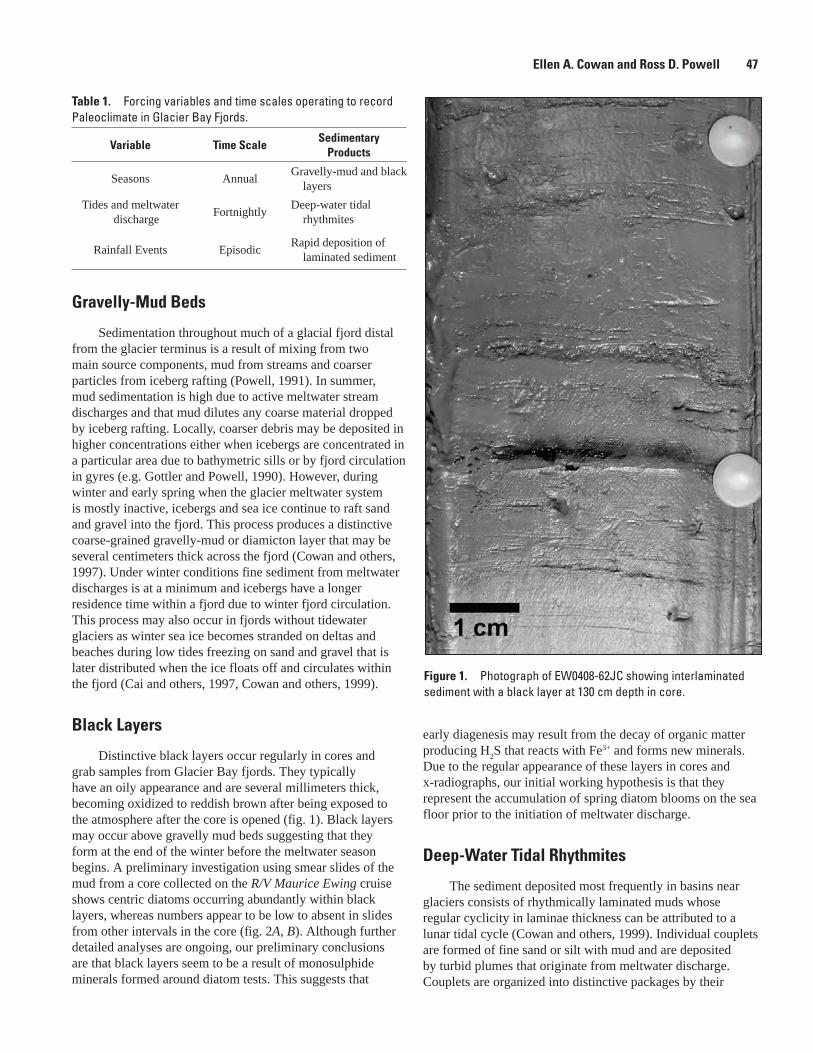
Table 1. Forcing variables and time scales operating to record Paleoclimate in Glacier Bay Fjords.
Variable Time ScaleSedimentary
Products
Seasons AnnualGravelly-mud and black
layers
Tides and meltwater discharge
FortnightlyDeep-water tidal
rhythmites
Rainfall Events EpisodicRapid deposition of
laminated sediment
Figure 1. Photograph of EW0408-62JC showing interlaminated sediment with a black layer at 130 cm depth in core.
Gravelly-Mud Beds
Sedimentation throughout much of a glacial fjord distal from the glacier terminus is a result of mixing from two main source components, mud from streams and coarser particles from iceberg rafting (Powell, 1991). In summer, mud sedimentation is high due to active meltwater stream discharges and that mud dilutes any coarse material dropped by iceberg rafting. Locally, coarser debris may be deposited in higher concentrations either when icebergs are concentrated in a particular area due to bathymetric sills or by fjord circulation in gyres (e.g. Gottler and Powell, 1990). However, during winter and early spring when the glacier meltwater system is mostly inactive, icebergs and sea ice continue to raft sand and gravel into the fjord. This process produces a distinctive coarse-grained gravelly-mud or diamicton layer that may be several centimeters thick across the fjord (Cowan and others, 1997). Under winter conditions fine sediment from meltwater discharges is at a minimum and icebergs have a longer residence time within a fjord due to winter fjord circulation. This process may also occur in fjords without tidewater glaciers as winter sea ice becomes stranded on deltas and beaches during low tides freezing on sand and gravel that is later distributed when the ice floats off and circulates within the fjord (Cai and others, 1997, Cowan and others, 1999).
Black Layers
Distinctive black layers occur regularly in cores and grab samples from Glacier Bay fjords. They typically have an oily appearance and are several millimeters thick, becoming oxidized to reddish brown after being exposed to the atmosphere after the core is opened (fig. 1). Black layers may occur above gravelly mud beds suggesting that they form at the end of the winter before the meltwater season begins. A preliminary investigation using smear slides of the mud from a core collected on the R/V Maurice Ewing cruise shows centric diatoms occurring abundantly within black layers, whereas numbers appear to be low to absent in slides from other intervals in the core (fig. 2A, B). Although further detailed analyses are ongoing, our preliminary conclusions are that black layers seem to be a result of monosulphide minerals formed around diatom tests. This suggests that
early diagenesis may result from the decay of organic matter producing H
2S that reacts with Fe3+ and forms new minerals.
Due to the regular appearance of these layers in cores and x-radiographs, our initial working hypothesis is that they represent the accumulation of spring diatom blooms on the sea floor prior to the initiation of meltwater discharge.
Deep-Water Tidal Rhythmites
The sediment deposited most frequently in basins near glaciers consists of rhythmically laminated muds whose regular cyclicity in laminae thickness can be attributed to a lunar tidal cycle (Cowan and others, 1999). Individual couplets are formed of fine sand or silt with mud and are deposited by turbid plumes that originate from meltwater discharge. Couplets are organized into distinctive packages by their
Ellen A. Cowan and Ross D. Powell �7

Figure 2. A. Smear slide of sediment from a black layer at 35 cm depth in core EW0408-62JC from Muir Inlet. Diatoms occur in abundance only in black layers. Horizontal field of view is 350 microns. B. Smear slide from 130 cm depth in core EW0408-62JC. Early diagenesis appears to form monosulphide minerals. Where decaying of organic matter produces H2S that reacts with Fe3+.
thickness representing one half-month, spring-neap tidal period. Each package is bound by thin couplets with a silt lamina and a very thin mud lamina. Over the duration of the fortnightly tidal cycle, couplets increase in thickness as each mud lamina thickens. These cycles recur as large and small packages downcore, which record alternating successive high- and low-amplitude spring tidal cycles (Cowan and others, 1999). Identification of this organization within the rhythmite record allows the comparison of sediment and meltwater discharge variations over successive two-week periods within a single meltwater season or between annual seasons.
Discussion
The analysis of long sediment cores from Glacier Bay fjords can yield a proxy record of recent glacial meltwater discharge. Gravelly-mud beds and black layers, deposited
annually are key to interpreting this record. Deep-water tidal rhythmites, organized in distinctive one-half-month packages by thickness are a proxy for meltwater discharge from the tidewater terminus. This annually-resolved climate record then can be correlated with local meteorological data to test how meltwater production from tidewater glaciers varies in response to past high frequency climate changes such as the PDO.
Management Implications
Glacier Bay National Park contains a unique paleoclimate record for Southeast Alaska deposited since the end of the Little Ice Age. This record is especially valuable because of the detail with which glacial terminus positions have been mapped over time and because of the documentation of modern glacimarine processes. We recommend that Park management plans include provisions that permit scientists to access this irreplaceable sediment record for future generations.
Acknowledgments
The National Science Foundation provided funding for this work. We appreciate the contributions of many students and colleagues who participated in the field studies of tidewater glaciers.
References Cited
Cai, J., Powell, R.D., Cowan, E.A., Carlson, P.R., 1997, Lithofacies and seismic-reflection interpretation of temperate glacimarine sedimentation in Tarr Inlet, Glacier Bay, Alaska: Marine Geology, v. 143, p. 5-37.
Cowan, E.A., 1992, Meltwater and tidal currents: Controls on circulation of a small glacial fjord: Estuarine Coastal Shelf Science, v. 34, p. 381-392.
Cowan, E.A., Cai, J., Powell, R.D., Clark, J.D., and Pitcher, J.N., 1997, Temperate glacimarine varves: an example from Disenchantment Bay, Southern Alaska: Journal of Sedimentary Research, v. 67, p. 536-549.
Cowan, E.A., and Powell, R.D., 1991, Ice-proximal sediment accumulation rates in a temperate glacial fjord, southeastern Alaska, in Anderson, J.B., and Ashley, G.M., eds., Glacial marine sedimentation; paleoclimatic significance: Geological Society of America, Special Paper 261, p. 61-73.
Cowan, E.A., Powell, R.D., and Smith N.D., 1988, Rainstorm-induced event sedimentation at the tidewater front of a temperate glacier: Geology, v. 16, p. 409-412.
�� Proceedings of the Fourth Glacier Bay Science Symposium
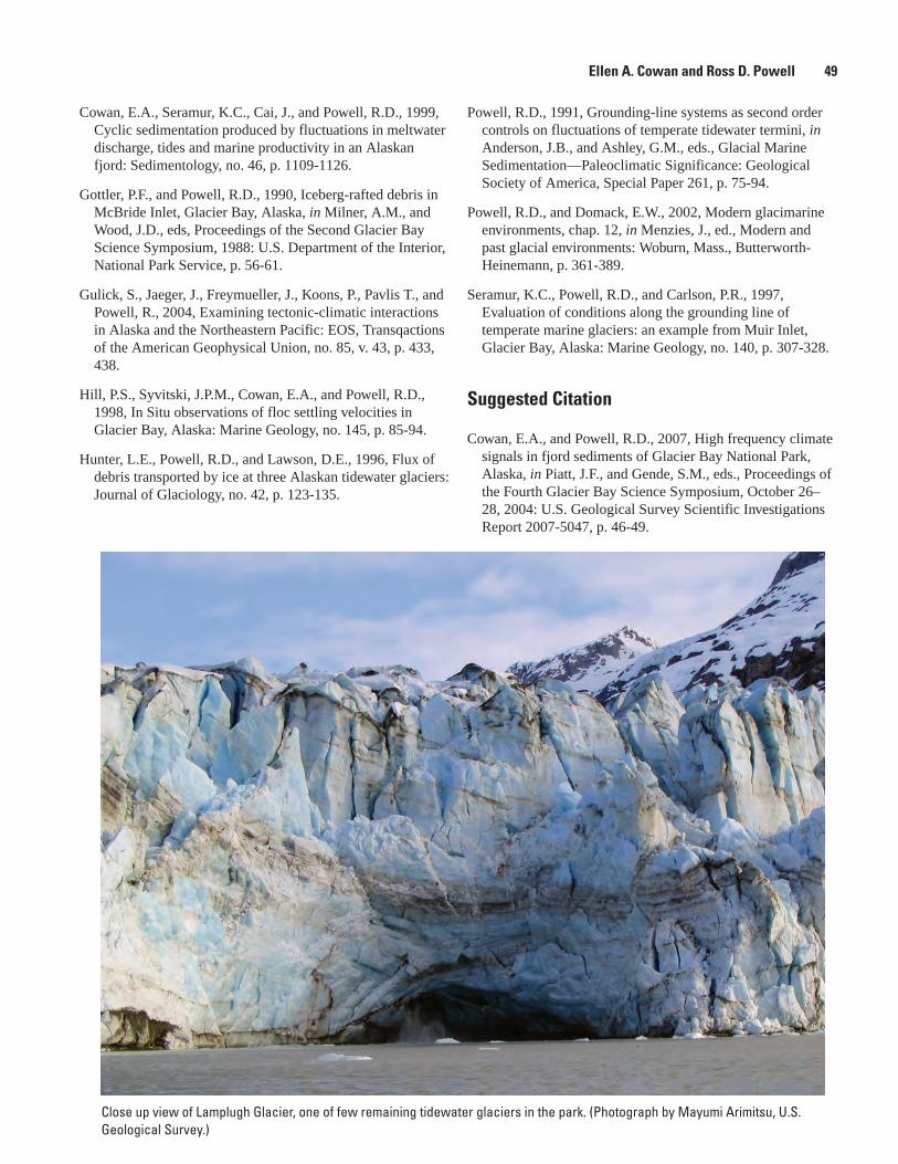
Close up view of Lamplugh Glacier, one of few remaining tidewater glaciers in the park. (Photograph by Mayumi Arimitsu, U.S. Geological Survey.)
Cowan, E.A., Seramur, K.C., Cai, J., and Powell, R.D., 1999, Cyclic sedimentation produced by fluctuations in meltwater discharge, tides and marine productivity in an Alaskan fjord: Sedimentology, no. 46, p. 1109-1126.
Gottler, P.F., and Powell, R.D., 1990, Iceberg-rafted debris in McBride Inlet, Glacier Bay, Alaska, in Milner, A.M., and Wood, J.D., eds, Proceedings of the Second Glacier Bay Science Symposium, 1988: U.S. Department of the Interior, National Park Service, p. 56-61.
Gulick, S., Jaeger, J., Freymueller, J., Koons, P., Pavlis T., and Powell, R., 2004, Examining tectonic-climatic interactions in Alaska and the Northeastern Pacific: EOS, Transqactions of the American Geophysical Union, no. 85, v. 43, p. 433, 438.
Hill, P.S., Syvitski, J.P.M., Cowan, E.A., and Powell, R.D., 1998, In Situ observations of floc settling velocities in Glacier Bay, Alaska: Marine Geology, no. 145, p. 85-94.
Hunter, L.E., Powell, R.D., and Lawson, D.E., 1996, Flux of debris transported by ice at three Alaskan tidewater glaciers: Journal of Glaciology, no. 42, p. 123-135.
Powell, R.D., 1991, Grounding-line systems as second order controls on fluctuations of temperate tidewater termini, in Anderson, J.B., and Ashley, G.M., eds., Glacial Marine Sedimentation—Paleoclimatic Significance: Geological Society of America, Special Paper 261, p. 75-94.
Powell, R.D., and Domack, E.W., 2002, Modern glacimarine environments, chap. 12, in Menzies, J., ed., Modern and past glacial environments: Woburn, Mass., Butterworth-Heinemann, p. 361-389.
Seramur, K.C., Powell, R.D., and Carlson, P.R., 1997, Evaluation of conditions along the grounding line of temperate marine glaciers: an example from Muir Inlet, Glacier Bay, Alaska: Marine Geology, no. 140, p. 307-328.
Suggested Citation
Cowan, E.A., and Powell, R.D., 2007, High frequency climate signals in fjord sediments of Glacier Bay National Park, Alaska, in Piatt, J.F., and Gende, S.M., eds., Proceedings of the Fourth Glacier Bay Science Symposium, October 26–28, 2004: U.S. Geological Survey Scientific Investigations Report 2007-5047, p. 46-49.
Ellen A. Cowan and Ross D. Powell �9
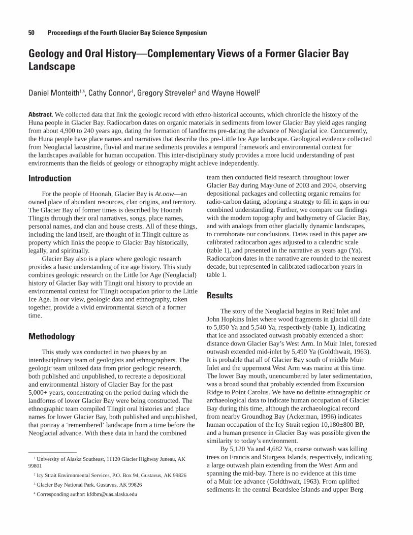
Geology and Oral History—Complementary Views of a Former Glacier Bay Landscape
Daniel Monteith1,4, Cathy Connor1, Gregory Streveler2 and Wayne Howell3
Abstract. We collected data that link the geologic record with ethno-historical accounts, which chronicle the history of the Huna people in Glacier Bay. Radiocarbon dates on organic materials in sediments from lower Glacier Bay yield ages ranging from about 4,900 to 240 years ago, dating the formation of landforms pre-dating the advance of Neoglacial ice. Concurrently, the Huna people have place names and narratives that describe this pre-Little Ice Age landscape. Geological evidence collected from Neoglacial lacustrine, fluvial and marine sediments provides a temporal framework and environmental context for the landscapes available for human occupation. This inter-disciplinary study provides a more lucid understanding of past environments than the fields of geology or ethnography might achieve independently.
1 University of Alaska Southeast, 11120 Glacier Highway Juneau, AK 99801
2 Icy Strait Environmental Services, P.O. Box 94, Gustavus, AK 99826
3 Glacier Bay National Park, Gustavus, AK 99826
4 Corresponding author: [email protected]
Introduction
For the people of Hoonah, Glacier Bay is At.oow—an owned place of abundant resources, clan origins, and territory. The Glacier Bay of former times is described by Hoonah Tlingits through their oral narratives, songs, place names, personal names, and clan and house crests. All of these things, including the land itself, are thought of in Tlingit culture as property which links the people to Glacier Bay historically, legally, and spiritually.
Glacier Bay also is a place where geologic research provides a basic understanding of ice age history. This study combines geologic research on the Little Ice Age (Neoglacial) history of Glacier Bay with Tlingit oral history to provide an environmental context for Tlingit occupation prior to the Little Ice Age. In our view, geologic data and ethnography, taken together, provide a vivid environmental sketch of a former time.
Methodology
This study was conducted in two phases by an interdisciplinary team of geologists and ethnographers. The geologic team utilized data from prior geologic research, both published and unpublished, to recreate a depositional and environmental history of Glacier Bay for the past 5,000+ years, concentrating on the period during which the landforms of lower Glacier Bay were being constructed. The ethnographic team compiled Tlingit oral histories and place names for lower Glacier Bay, both published and unpublished, that portray a ‘remembered’ landscape from a time before the Neoglacial advance. With these data in hand the combined
team then conducted field research throughout lower Glacier Bay during May/June of 2003 and 2004, observing depositional packages and collecting organic remains for radio-carbon dating, adopting a strategy to fill in gaps in our combined understanding. Further, we compare our findings with the modern topography and bathymetry of Glacier Bay, and with analogs from other glacially dynamic landscapes, to corroborate our conclusions. Dates used in this paper are calibrated radiocarbon ages adjusted to a calendric scale (table 1), and presented in the narrative as years ago (Ya). Radiocarbon dates in the narrative are rounded to the nearest decade, but represented in calibrated radiocarbon years in table 1.
Results
The story of the Neoglacial begins in Reid Inlet and John Hopkins Inlet where wood fragments in glacial till date to 5,850 Ya and 5,540 Ya, respectively (table 1), indicating that ice and associated outwash probably extended a short distance down Glacier Bay’s West Arm. In Muir Inlet, forested outwash extended mid-inlet by 5,490 Ya (Goldthwait, 1963). It is probable that all of Glacier Bay south of middle Muir Inlet and the uppermost West Arm was marine at this time. The lower Bay mouth, unencumbered by later sedimentation, was a broad sound that probably extended from Excursion Ridge to Point Carolus. We have no definite ethnographic or archaeological data to indicate human occupation of Glacier Bay during this time, although the archaeological record from nearby Groundhog Bay (Ackerman, 1996) indicates human occupation of the Icy Strait region 10,180±800 BP, and a human presence in Glacier Bay was possible given the similarity to today’s environment.
By 5,120 Ya and 4,682 Ya, coarse outwash was killing trees on Francis and Sturgess Islands, respectively, indicating a large outwash plain extending from the West Arm and spanning the mid-bay. There is no evidence at this time of a Muir ice advance (Goldthwait, 1963). From uplifted sediments in the central Beardslee Islands and upper Berg
50 Proceedings of the Fourth Glacier Bay Science Symposium
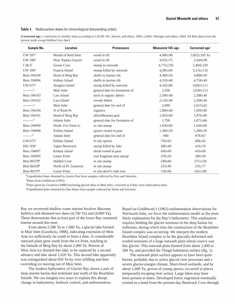
Table 1. Radiocarbon dates (in chronological descending order).
[Corrected age: t conversion to clendric dates according to CALIB 14C, Stuiver, and others, 2004, CalPal, Weiniger and others, 2004. All Beta dates from the present study except Halibut Cove date]
Sample No. Location Provenance Measured 1�C age Corrected age t
UW 5971 Mouth of Reid Inlet wood in till 4,980±90 5,852±105 Ya
UW 5981 Near Topeka Glacier wood in till 4,655±75 5,544±99
I 58-52 Goose Cove stump in outwash 4,775±250 5,494±320
UW 5961 Francis Island stump killed by outwash 4,385±60 5,116±116
Beta 194100 Head of Berg Bay shells in marine silt 4,380±50 4,898±50
Beta 194096 Kidney Island shells in marine silt 4,310±40 4,758±40
UW 6711 Sturgess Island stump killed by outwash 4,165±80 4,692±111
---------3 Muir Inlet general date for formation of 2,500 2,630±112
Beta 194103 Lars Island stick in organic debris 2,300±40 2,398±40
Beta 194102 Lars Island woody debris 2,120±40 2,208±40
---------3 Muir Inlet general date for end of 2,000 2,013±62
Beta 194104 N of Rush Pt. organics 1,860±40 1,920±40
Beta 194101 Head of Berg Bay allochthonous peat 1,910±60 1,870±60
---------3 Adams Inlet general date for formation of 1,700 1,671±66
Beta 194099 North. Fox Farm Is. ex situ stump 1,630±60 1,650±60
Beta 194098 Kidney Island spruce rooted in peat 1,300±50 1,300±50
--------3 Adams Inlet general date for end of 900 878±67
UW-6721 Kidney Island in situ spruce 750±65 696±42
DIC-9391 Upper Beartrack stump killed by lake 380±40 416±70
Beta 194097 Kidney island shrub rooted in peat 430±60 410±60
Beta 194095 Lester Point root fragment near stump 370±50 390±50
Beta 863784 Halibut Cove in situ stump 240±60 275±126
Beta 863284 North of Pt. Gustavus in situ stump 233±40 235±77
Beta 863794 Lester Point in situ devil’s club root 150±60 145±1081Unpublished dates obtained by Austin Post from samples collected by Post and Streveler..2Dates from Goldthwait (1963). 3Dates given by Goodwin (1988) bracketing glacial lakes in Muir Inlet, corrected as if they were radiocarbon dates.4Unpublished dates obtained by Dan Mann from sample collected by Mann and Streveler.
Bay we recovered shallow-water marine bivalves Macoma balthica and obtained two dates (4,760 Ya) and (4,900 Ya). These demonstrate that at least part of the lower Bay remained marine around this time.
From about 2,580 Ya to 1,960 Ya, a glacial lake formed in Muir Inlet (Goodwin, 1988), indicating extension of West Arm ice sufficiently far south to form a dam. A considerable outwash plain grew south from the ice front, reaching to the latitude of Berg Bay by about 2,400 Ya. Retreat of West Arm ice drained this lake, to be replaced by a second advance and lake about 1,620 Ya. This second lake apparently was extinguished about 820 Ya by river infilling and then overriding ice moving out of Muir Inlet.
The modern bathymetry of Glacier Bay shows a pair of deep marine basins that terminate just north of the Beardslee Islands. We can imagine two ways to explain this abrupt change in bathymetry; bedrock control, and sedimentation.
Based on Goldthwait’s (1963) sedimentation observations for Wachusett Inlet, we favor the sedimentation model as the most likely explanation for the Bay’s bathymetry. This explanation requires holding the glacier terminus in the deep basins for millennia, during which time the construction of the Beardslee Island complex was occurring. We interpret the modern Beardslee Island complex to be the glacially deformed and eroded remnants of a large outwash plain whose source was this glacier. This outwash plain formed from about 2,400 to 300 Ya, and provided the Tlingit habitation surface (fig. 1).
The outwash plain surface appears to have been quite barren, probably due to active glacial river processes and a severe glacier-margin climate. Short-lived wetlands, and by about 1,600 Ya, groves of young spruce, occurred in places temporarily escaping river action. Large lakes may have been present at times. Developed forest vegetation eventually existed in a band from the present-day Beartrack Cove through
Daniel Monteith and others 51
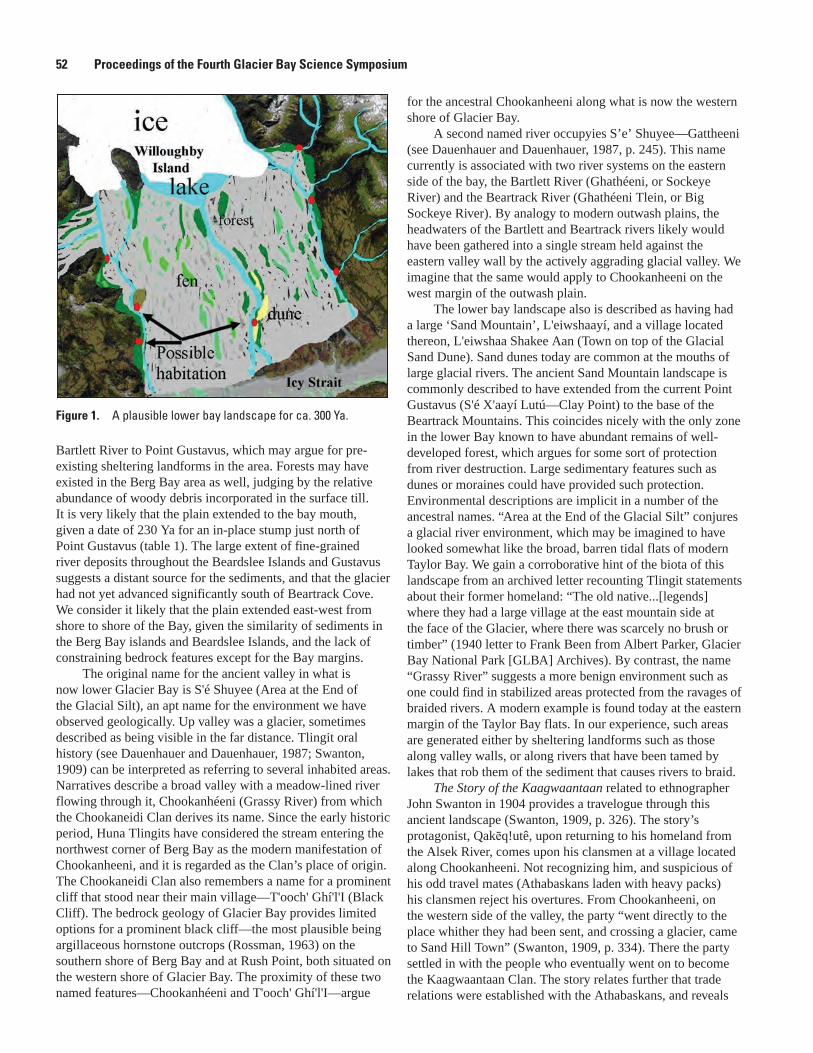
Bartlett River to Point Gustavus, which may argue for pre-existing sheltering landforms in the area. Forests may have existed in the Berg Bay area as well, judging by the relative abundance of woody debris incorporated in the surface till. It is very likely that the plain extended to the bay mouth, given a date of 230 Ya for an in-place stump just north of Point Gustavus (table 1). The large extent of fine-grained river deposits throughout the Beardslee Islands and Gustavus suggests a distant source for the sediments, and that the glacier had not yet advanced significantly south of Beartrack Cove. We consider it likely that the plain extended east-west from shore to shore of the Bay, given the similarity of sediments in the Berg Bay islands and Beardslee Islands, and the lack of constraining bedrock features except for the Bay margins.
The original name for the ancient valley in what is now lower Glacier Bay is S'é Shuyee (Area at the End of the Glacial Silt), an apt name for the environment we have observed geologically. Up valley was a glacier, sometimes described as being visible in the far distance. Tlingit oral history (see Dauenhauer and Dauenhauer, 1987; Swanton, 1909) can be interpreted as referring to several inhabited areas. Narratives describe a broad valley with a meadow-lined river flowing through it, Chookanhéeni (Grassy River) from which the Chookaneidi Clan derives its name. Since the early historic period, Huna Tlingits have considered the stream entering the northwest corner of Berg Bay as the modern manifestation of Chookanheeni, and it is regarded as the Clan’s place of origin. The Chookaneidi Clan also remembers a name for a prominent cliff that stood near their main village—T'ooch' Ghí'l'I (Black Cliff). The bedrock geology of Glacier Bay provides limited options for a prominent black cliff—the most plausible being argillaceous hornstone outcrops (Rossman, 1963) on the southern shore of Berg Bay and at Rush Point, both situated on the western shore of Glacier Bay. The proximity of these two named features—Chookanhéeni and T'ooch' Ghí'l'I—argue
for the ancestral Chookanheeni along what is now the western shore of Glacier Bay.
A second named river occupyies S’e’ Shuyee—Gattheeni (see Dauenhauer and Dauenhauer, 1987, p. 245). This name currently is associated with two river systems on the eastern side of the bay, the Bartlett River (Ghathéeni, or Sockeye River) and the Beartrack River (Ghathéeni Tlein, or Big Sockeye River). By analogy to modern outwash plains, the headwaters of the Bartlett and Beartrack rivers likely would have been gathered into a single stream held against the eastern valley wall by the actively aggrading glacial valley. We imagine that the same would apply to Chookanheeni on the west margin of the outwash plain.
The lower bay landscape also is described as having had a large ‘Sand Mountain’, L'eiwshaayí, and a village located thereon, L'eiwshaa Shakee Aan (Town on top of the Glacial Sand Dune). Sand dunes today are common at the mouths of large glacial rivers. The ancient Sand Mountain landscape is commonly described to have extended from the current Point Gustavus (S'é X'aayí Lutú—Clay Point) to the base of the Beartrack Mountains. This coincides nicely with the only zone in the lower Bay known to have abundant remains of well-developed forest, which argues for some sort of protection from river destruction. Large sedimentary features such as dunes or moraines could have provided such protection. Environmental descriptions are implicit in a number of the ancestral names. “Area at the End of the Glacial Silt” conjures a glacial river environment, which may be imagined to have looked somewhat like the broad, barren tidal flats of modern Taylor Bay. We gain a corroborative hint of the biota of this landscape from an archived letter recounting Tlingit statements about their former homeland: “The old native...[legends] where they had a large village at the east mountain side at the face of the Glacier, where there was scarcely no brush or timber” (1940 letter to Frank Been from Albert Parker, Glacier Bay National Park [GLBA] Archives). By contrast, the name “Grassy River” suggests a more benign environment such as one could find in stabilized areas protected from the ravages of braided rivers. A modern example is found today at the eastern margin of the Taylor Bay flats. In our experience, such areas are generated either by sheltering landforms such as those along valley walls, or along rivers that have been tamed by lakes that rob them of the sediment that causes rivers to braid.
The Story of the Kaagwaantaan related to ethnographer John Swanton in 1904 provides a travelogue through this ancient landscape (Swanton, 1909, p. 326). The story’s protagonist, Qakēq!utê, upon returning to his homeland from the Alsek River, comes upon his clansmen at a village located along Chookanheeni. Not recognizing him, and suspicious of his odd travel mates (Athabaskans laden with heavy packs) his clansmen reject his overtures. From Chookanheeni, on the western side of the valley, the party “went directly to the place whither they had been sent, and crossing a glacier, came to Sand Hill Town” (Swanton, 1909, p. 334). There the party settled in with the people who eventually went on to become the Kaagwaantaan Clan. The story relates further that trade relations were established with the Athabaskans, and reveals
Figure 1. A plausible lower bay landscape for ca. 300 Ya.
52 Proceedings of the Fourth Glacier Bay Science Symposium
something of the location of the glacier, “The Athabaskans on their way down used to be seen when still far back from the coast. One time, as they were coming across the glacier...” (Swanton, 1909, p. 337).
Dates varying from 390 to 150 Ya have been obtained by various investigators for forests in the Bartlett Cove area just prior to the ice advance (table 1). In 1794 AD (210 Ya.), Lt. Whidbey of the Vancouver Expedition mapped the Glacier Bay ice sheet already somewhat back from its maximum extent. The two youngest dates in table 1 from wood living prior to the advance average to 235 Ya, and their 1-sigma positive limits average to 285 Ya. This gives a very tight window (210–235/285 Ya) during which time the glacier would have over-run the Bartlett Cove area, reached its maximum in Icy Strait, and begun to retreat.
Discussion and Conclusions
This interdisciplinary study provides two independent sets of data to reconstruct a past Glacier Bay landscape. Geologic observations of landform composition and environmental conditions conform nicely with Tlingit oral narratives. Radiocarbon dates on organic materials contained within these sediment packages provides a temporal framework for correlating geologic processes with Tlingit oral narratives. Combined, these complimentary data provide a plausible description of pre-Neoglacial human occupation in Glacier Bay, and validate oral history as a viable data set, especially when corroborated with independent data. This study also takes a step toward understanding the terrestrial landscape history and bathymetry of lower Glacier Bay.
Management Implications
This study helps deepen our understanding of the human history of Glacier Bay. It provides an enhanced understanding of Glacier Bay’s geologic history and bathymetry, and information with application to other fields of study such as oceanography. It helps NPS more accurately describe and draw boundaries around the cultural landscapes of lower Glacier Bay—Chookenheeni and L'eiwshaa Shakee Aan—as the agency prepares to nominate them to the National Register of Historic Places. Lastly, and most importantly, the study integrates more fully and richly the Hoonah Tlingit people into the history of their ancestral homeland.
Acknowledgments
The authors thank the Hoonah Indian Association for the use of unpublished place name information, and the Hoonah elders for generously sharing knowledge with us, particularly Lily White and Sam Hanlon, Sr.
References Cited
Ackerman, Robert, 1996, Groundhog Bay site 2, in West, Frederick Hadleigh, ed., American beginnings—the Prehistory and paleoecology of Beringia: Chicago University of Chicago Press, p. 470-478.
Goodwin, R.F., 1988, Holocene glaciolacustrine sedimentation in Muir Inlet and ice advance in Glacier Bay, Alaska, U.S.A: Arctic and Alpine Research, v. 20, no. 1, p. 55-69.
Dauenhauer, Nora Marks, and Dauenhauer, Richard, eds., 1987, Haa Shuka, our ancestors—Tlingit oral narratives, classics of Tlingit oral literature, vol. 1: Seattle, University of Washington Press.
Goldthwait, R.P., 1963, Dating the Little Ice Age in Glacier Bay, Alaska: Intenational Geological Congress, XXI Session, Norden, Norway, 1960, p. 37-46.
Stuiver, M., Reimer, P.J., and Braziunas, T.F., 2001, High-precision radiocarbon age calibration for terrestrial and marine samples: Radiocarbon, v. 40, p. 1127-1151 (CALIB 4.4 Radiocarbon Calibration at http://radiocarbon.pa.qub.ac.uk/calib/).
Swanton, John R., 1909, Tlingit myth and texts: Washington D.C., Bureau of American Ethnology Bulletin 39. p.
Weninger, B., Joris, O., and Danzeglocke, Uwe, 2004, Cologne Radiocarbon Calibration & Paleoclimate Research Package (CalPal_2004_SFCP Calibration Curv, http://www.calpal.de/calpal/authors.htm).
Suggested Citation
Monteith, D., Connor, C., Streveler, G., and Howell, W., 2007, Geology and oral history—Complementary views of a former Glacier Bay landscape, in Piatt, J.F., and Gende, S.M., eds., Proceedings of the Fourth Glacier Bay Science Symposium, October 26–28, 2004: U.S. Geological Survey Scientific Investigations Report 2007-5047, p. 50 – 53.
Daniel Monteith and others 5�
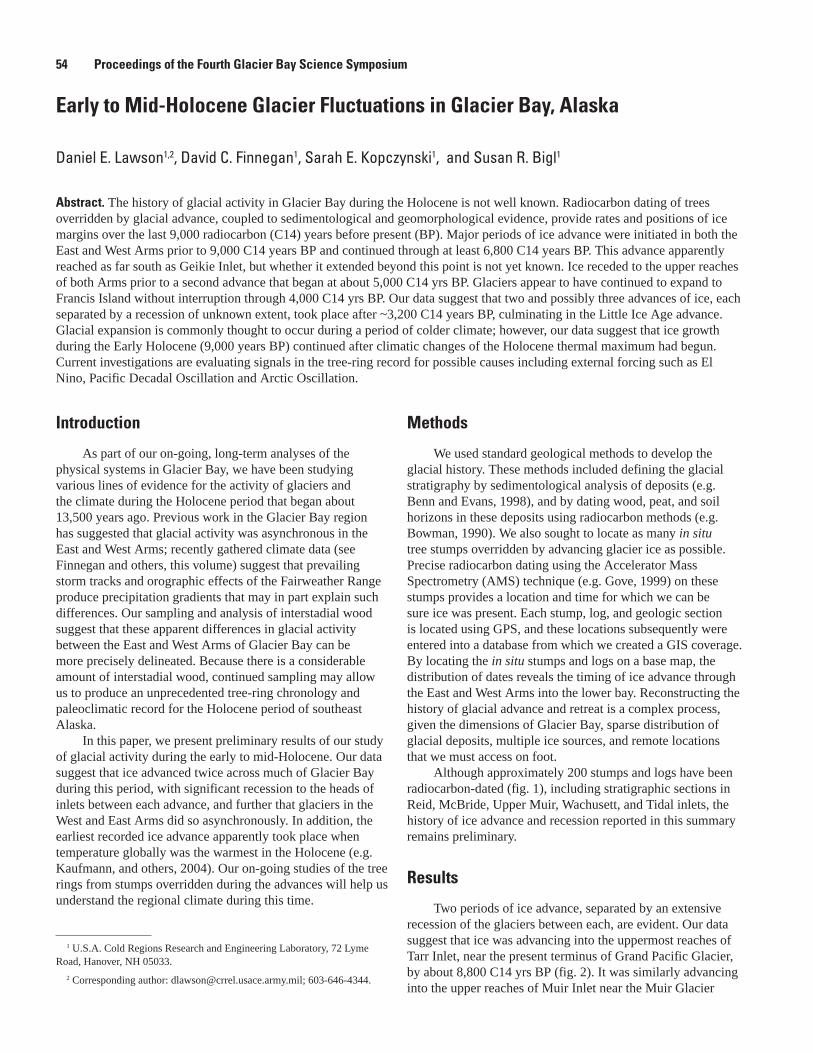
Early to Mid-Holocene Glacier Fluctuations in Glacier Bay, Alaska
Daniel E. Lawson1,2, David C. Finnegan1, Sarah E. Kopczynski1, and Susan R. Bigl1
Abstract. The history of glacial activity in Glacier Bay during the Holocene is not well known. Radiocarbon dating of trees overridden by glacial advance, coupled to sedimentological and geomorphological evidence, provide rates and positions of ice margins over the last 9,000 radiocarbon (C14) years before present (BP). Major periods of ice advance were initiated in both the East and West Arms prior to 9,000 C14 years BP and continued through at least 6,800 C14 years BP. This advance apparently reached as far south as Geikie Inlet, but whether it extended beyond this point is not yet known. Ice receded to the upper reaches of both Arms prior to a second advance that began at about 5,000 C14 yrs BP. Glaciers appear to have continued to expand to Francis Island without interruption through 4,000 C14 yrs BP. Our data suggest that two and possibly three advances of ice, each separated by a recession of unknown extent, took place after ~3,200 C14 years BP, culminating in the Little Ice Age advance. Glacial expansion is commonly thought to occur during a period of colder climate; however, our data suggest that ice growth during the Early Holocene (9,000 years BP) continued after climatic changes of the Holocene thermal maximum had begun. Current investigations are evaluating signals in the tree-ring record for possible causes including external forcing such as El Nino, Pacific Decadal Oscillation and Arctic Oscillation.
Introduction
As part of our on-going, long-term analyses of the physical systems in Glacier Bay, we have been studying various lines of evidence for the activity of glaciers and the climate during the Holocene period that began about 13,500 years ago. Previous work in the Glacier Bay region has suggested that glacial activity was asynchronous in the East and West Arms; recently gathered climate data (see Finnegan and others, this volume) suggest that prevailing storm tracks and orographic effects of the Fairweather Range produce precipitation gradients that may in part explain such differences. Our sampling and analysis of interstadial wood suggest that these apparent differences in glacial activity between the East and West Arms of Glacier Bay can be more precisely delineated. Because there is a considerable amount of interstadial wood, continued sampling may allow us to produce an unprecedented tree-ring chronology and paleoclimatic record for the Holocene period of southeast Alaska.
In this paper, we present preliminary results of our study of glacial activity during the early to mid-Holocene. Our data suggest that ice advanced twice across much of Glacier Bay during this period, with significant recession to the heads of inlets between each advance, and further that glaciers in the West and East Arms did so asynchronously. In addition, the earliest recorded ice advance apparently took place when temperature globally was the warmest in the Holocene (e.g. Kaufmann, and others, 2004). Our on-going studies of the tree rings from stumps overridden during the advances will help us understand the regional climate during this time.
1 U.S.A. Cold Regions Research and Engineering Laboratory, 72 Lyme Road, Hanover, NH 05033.
2 Corresponding author: [email protected]; 603-646-4344.
Methods
We used standard geological methods to develop the glacial history. These methods included defining the glacial stratigraphy by sedimentological analysis of deposits (e.g. Benn and Evans, 1998), and by dating wood, peat, and soil horizons in these deposits using radiocarbon methods (e.g. Bowman, 1990). We also sought to locate as many in situ tree stumps overridden by advancing glacier ice as possible. Precise radiocarbon dating using the Accelerator Mass Spectrometry (AMS) technique (e.g. Gove, 1999) on these stumps provides a location and time for which we can be sure ice was present. Each stump, log, and geologic section is located using GPS, and these locations subsequently were entered into a database from which we created a GIS coverage. By locating the in situ stumps and logs on a base map, the distribution of dates reveals the timing of ice advance through the East and West Arms into the lower bay. Reconstructing the history of glacial advance and retreat is a complex process, given the dimensions of Glacier Bay, sparse distribution of glacial deposits, multiple ice sources, and remote locations that we must access on foot.
Although approximately 200 stumps and logs have been radiocarbon-dated (fig. 1), including stratigraphic sections in Reid, McBride, Upper Muir, Wachusett, and Tidal inlets, the history of ice advance and recession reported in this summary remains preliminary.
Results
Two periods of ice advance, separated by an extensive recession of the glaciers between each, are evident. Our data suggest that ice was advancing into the uppermost reaches of Tarr Inlet, near the present terminus of Grand Pacific Glacier, by about 8,800 C14 yrs BP (fig. 2). It was similarly advancing into the upper reaches of Muir Inlet near the Muir Glacier
5� Proceedings of the Fourth Glacier Bay Science Symposium
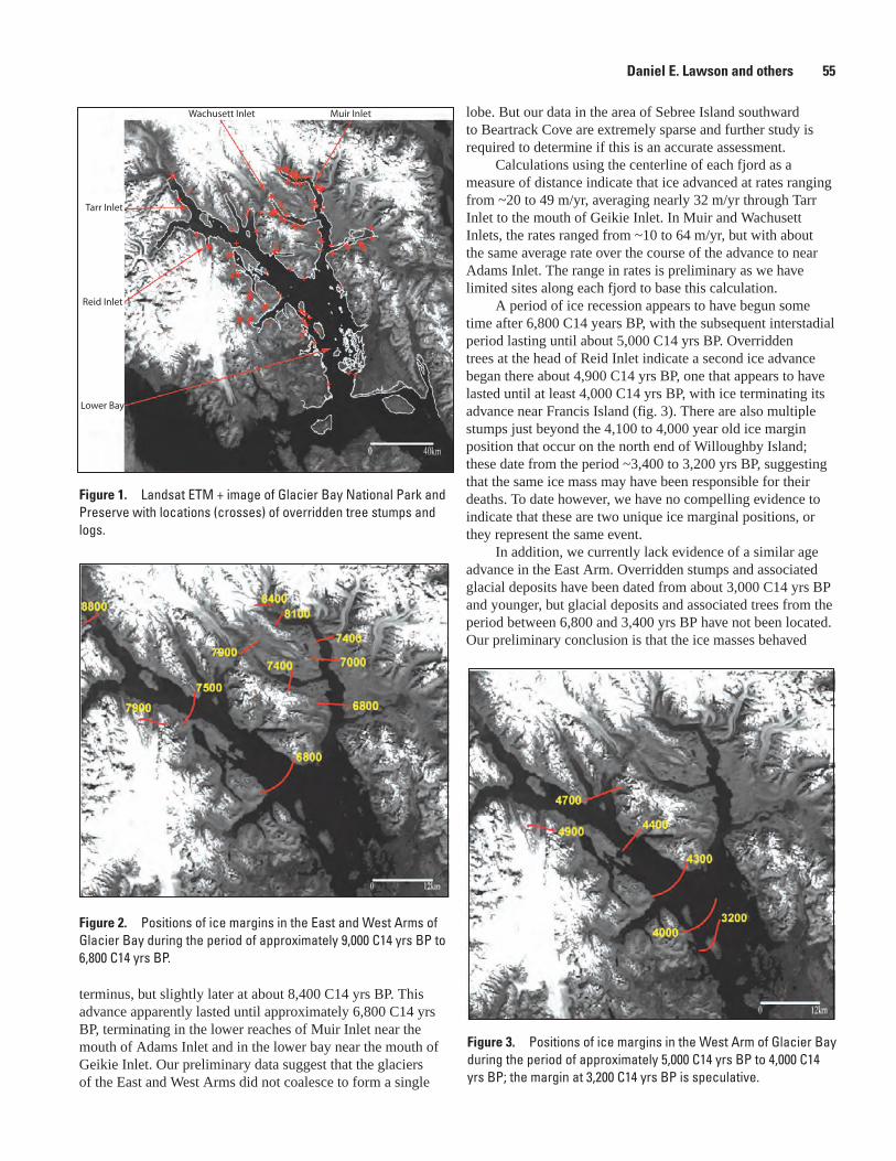
Figure 2. Positions of ice margins in the East and West Arms of Glacier Bay during the period of approximately 9,000 C14 yrs BP to 6,800 C14 yrs BP.
Figure �. Positions of ice margins in the West Arm of Glacier Bay during the period of approximately 5,000 C14 yrs BP to 4,000 C14 yrs BP; the margin at 3,200 C14 yrs BP is speculative.
Figure 1. Landsat ETM + image of Glacier Bay National Park and Preserve with locations (crosses) of overridden tree stumps and logs.
Wachusett Inlet Muir Inlet
Tarr Inlet
Reid Inlet
Lower Bay
terminus, but slightly later at about 8,400 C14 yrs BP. This advance apparently lasted until approximately 6,800 C14 yrs BP, terminating in the lower reaches of Muir Inlet near the mouth of Adams Inlet and in the lower bay near the mouth of Geikie Inlet. Our preliminary data suggest that the glaciers of the East and West Arms did not coalesce to form a single
lobe. But our data in the area of Sebree Island southward to Beartrack Cove are extremely sparse and further study is required to determine if this is an accurate assessment.
Calculations using the centerline of each fjord as a measure of distance indicate that ice advanced at rates ranging from ~20 to 49 m/yr, averaging nearly 32 m/yr through Tarr Inlet to the mouth of Geikie Inlet. In Muir and Wachusett Inlets, the rates ranged from ~10 to 64 m/yr, but with about the same average rate over the course of the advance to near Adams Inlet. The range in rates is preliminary as we have limited sites along each fjord to base this calculation.
A period of ice recession appears to have begun some time after 6,800 C14 years BP, with the subsequent interstadial period lasting until about 5,000 C14 yrs BP. Overridden trees at the head of Reid Inlet indicate a second ice advance began there about 4,900 C14 yrs BP, one that appears to have lasted until at least 4,000 C14 yrs BP, with ice terminating its advance near Francis Island (fig. 3). There are also multiple stumps just beyond the 4,100 to 4,000 year old ice margin position that occur on the north end of Willoughby Island; these date from the period ~3,400 to 3,200 yrs BP, suggesting that the same ice mass may have been responsible for their deaths. To date however, we have no compelling evidence to indicate that these are two unique ice marginal positions, or they represent the same event.
In addition, we currently lack evidence of a similar age advance in the East Arm. Overridden stumps and associated glacial deposits have been dated from about 3,000 C14 yrs BP and younger, but glacial deposits and associated trees from the period between 6,800 and 3,400 yrs BP have not been located. Our preliminary conclusion is that the ice masses behaved
Daniel E. Lawson and others 55
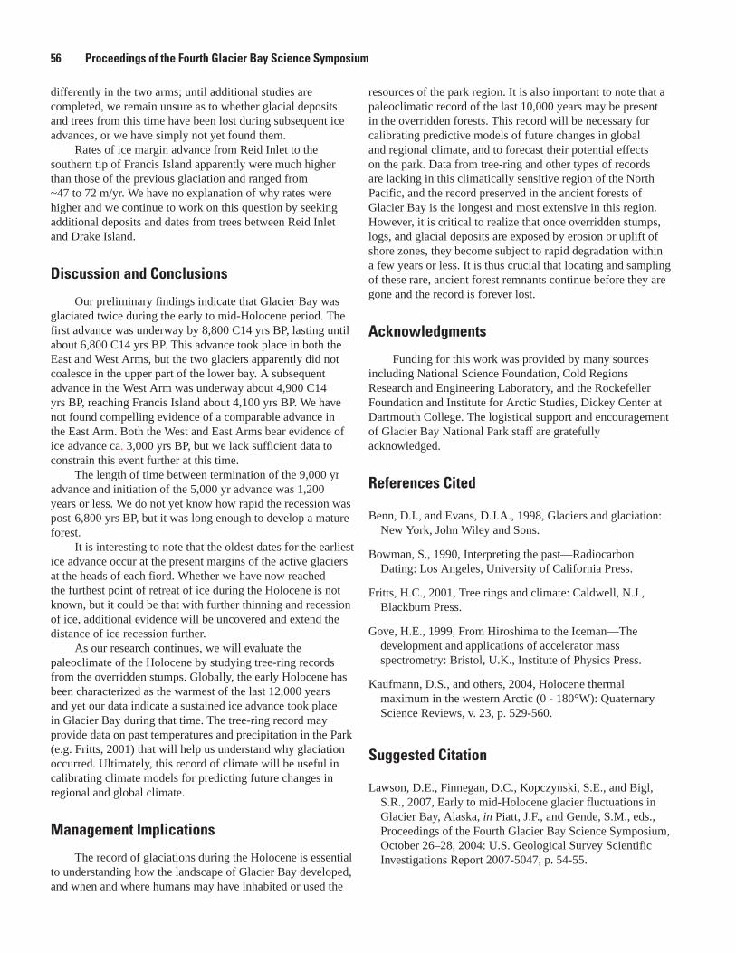
resources of the park region. It is also important to note that a paleoclimatic record of the last 10,000 years may be present in the overridden forests. This record will be necessary for calibrating predictive models of future changes in global and regional climate, and to forecast their potential effects on the park. Data from tree-ring and other types of records are lacking in this climatically sensitive region of the North Pacific, and the record preserved in the ancient forests of Glacier Bay is the longest and most extensive in this region. However, it is critical to realize that once overridden stumps, logs, and glacial deposits are exposed by erosion or uplift of shore zones, they become subject to rapid degradation within a few years or less. It is thus crucial that locating and sampling of these rare, ancient forest remnants continue before they are gone and the record is forever lost.
Acknowledgments
Funding for this work was provided by many sources including National Science Foundation, Cold Regions Research and Engineering Laboratory, and the Rockefeller Foundation and Institute for Arctic Studies, Dickey Center at Dartmouth College. The logistical support and encouragement of Glacier Bay National Park staff are gratefully acknowledged.
References Cited
Benn, D.I., and Evans, D.J.A., 1998, Glaciers and glaciation: New York, John Wiley and Sons.
Bowman, S., 1990, Interpreting the past—Radiocarbon Dating: Los Angeles, University of California Press.
Fritts, H.C., 2001, Tree rings and climate: Caldwell, N.J., Blackburn Press.
Gove, H.E., 1999, From Hiroshima to the Iceman—The development and applications of accelerator mass spectrometry: Bristol, U.K., Institute of Physics Press.
Kaufmann, D.S., and others, 2004, Holocene thermal maximum in the western Arctic (0 - 180°W): Quaternary Science Reviews, v. 23, p. 529-560.
Suggested Citation
Lawson, D.E., Finnegan, D.C., Kopczynski, S.E., and Bigl, S.R., 2007, Early to mid-Holocene glacier fluctuations in Glacier Bay, Alaska, in Piatt, J.F., and Gende, S.M., eds., Proceedings of the Fourth Glacier Bay Science Symposium, October 26–28, 2004: U.S. Geological Survey Scientific Investigations Report 2007-5047, p. 54-55.
differently in the two arms; until additional studies are completed, we remain unsure as to whether glacial deposits and trees from this time have been lost during subsequent ice advances, or we have simply not yet found them.
Rates of ice margin advance from Reid Inlet to the southern tip of Francis Island apparently were much higher than those of the previous glaciation and ranged from ~47 to 72 m/yr. We have no explanation of why rates were higher and we continue to work on this question by seeking additional deposits and dates from trees between Reid Inlet and Drake Island.
Discussion and Conclusions
Our preliminary findings indicate that Glacier Bay was glaciated twice during the early to mid-Holocene period. The first advance was underway by 8,800 C14 yrs BP, lasting until about 6,800 C14 yrs BP. This advance took place in both the East and West Arms, but the two glaciers apparently did not coalesce in the upper part of the lower bay. A subsequent advance in the West Arm was underway about 4,900 C14 yrs BP, reaching Francis Island about 4,100 yrs BP. We have not found compelling evidence of a comparable advance in the East Arm. Both the West and East Arms bear evidence of ice advance ca. 3,000 yrs BP, but we lack sufficient data to constrain this event further at this time.
The length of time between termination of the 9,000 yr advance and initiation of the 5,000 yr advance was 1,200 years or less. We do not yet know how rapid the recession was post-6,800 yrs BP, but it was long enough to develop a mature forest.
It is interesting to note that the oldest dates for the earliest ice advance occur at the present margins of the active glaciers at the heads of each fiord. Whether we have now reached the furthest point of retreat of ice during the Holocene is not known, but it could be that with further thinning and recession of ice, additional evidence will be uncovered and extend the distance of ice recession further.
As our research continues, we will evaluate the paleoclimate of the Holocene by studying tree-ring records from the overridden stumps. Globally, the early Holocene has been characterized as the warmest of the last 12,000 years and yet our data indicate a sustained ice advance took place in Glacier Bay during that time. The tree-ring record may provide data on past temperatures and precipitation in the Park (e.g. Fritts, 2001) that will help us understand why glaciation occurred. Ultimately, this record of climate will be useful in calibrating climate models for predicting future changes in regional and global climate.
Management Implications
The record of glaciations during the Holocene is essential to understanding how the landscape of Glacier Bay developed, and when and where humans may have inhabited or used the
5� Proceedings of the Fourth Glacier Bay Science Symposium
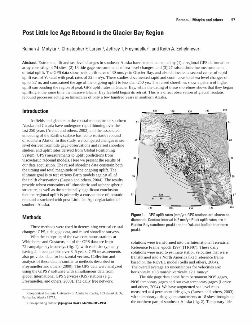
Post Little Ice Age Rebound in the Glacier Bay Region
Roman J. Motyka1,2, Christopher F. Larsen1, Jeffrey T. Freymueller1, and Keith A. Echelmeyer1
Abstract. Extreme uplift and sea level changes in southeast Alaska have been documented by (1) a regional GPS deformation array consisting of 74 sites; (2) 18 tide gage measurements of sea-level changes; and (3) 27 raised shoreline measurements of total uplift. The GPS data show peak uplift rates of 30 mm/ yr in Glacier Bay, and also delineated a second center of rapid uplift east of Yakutat with peak rates of 32 mm/yr. These studies documented rapid and continuous total sea level changes of up to 5.7 m, and constrained the age of the ongoing uplift to less than 250 yrs. The raised shorelines show a pattern of higher uplift surrounding the region of peak GPS uplift rates in Glacier Bay, while the dating of these shorelines shows that they began uplifting at the same time the massive Glacier Bay Icefield began its retreat. This is a direct observation of glacial isostatic rebound processes acting on timescales of only a few hundred years in southern Alaska.
Figure 1. GPS uplift rates (mm/yr). GPS stations are shown as diamonds. Contour interval is 2 mm/yr. Peak uplift rates are in Glacier Bay (southern peak) and the Yakutat Icefield (northern peak).
1 Geophysical Institute, University of Alaska Fairbanks, 903 Koyukuk Dr, Fairbanks, Alaska 99775.
2 Corresponding author: [email protected] [email protected] [email protected] 907-586-1994.uas.alaska.edu 907-586-1994.
Introduction
Icefields and glaciers in the coastal mountains of southern Alaska and Canada have undergone rapid thinning over the last 250 years (Arendt and others, 2002) and the associated unloading of the Earth’s surface has led to isostatic rebound of southern Alaska. In this study, we compared changes in sea level derived from tide gage observations and raised shoreline studies, and uplift rates derived from Global Positioning System (GPS) measurements to uplift predictions from viscoelastic rebound models. Here we present the results of our data acquisition. The raised shoreline data constrain both the timing and total magnitude of the ongoing uplift. The ultimate goal is to test various Earth models against all of the uplift observations (Larsen and others, 2004). The results provide robust constraints of lithospheric and asthenospheric structure, as well as the statistically significant conclusion that the regional uplift is primarily a consequence of isostatic rebound associated with post-Little Ice Age deglaciation of southern Alaska.
Methods
Three methods were used in determining vertical crustal changes: GPS, tide gage data, and raised shoreline surveys.
With the exception of the two continuous stations at Whitehorse and Gustavus, all of the GPS data are from 72 campaign-style surveys (fig. 1), with each site typically having 2–4 occupations over 3–5 years. GPS measurements also provided data for horizontal vectors. Collection and analysis of these data is similar to methods described in Freymueller and others (2000). The GPS data were analyzed using the GIPSY software with simultaneous data from global International GPS Services (IGS) stations (e.g., Freymueller, and others, 2000). The daily free network
solutions were transformed into the International Terrestrial Reference Frame, epoch 1997 (ITRF97). These daily solutions were used to estimate station velocities that were transformed into a North America fixed reference frame based on the REVEL model (Sella and others, 2004). The overall average 1σ uncertainties for velocities are: horizontal= ±0.8 mm/yr, vertical= ±2.1 mm/yr.
The tide gage data come from permanent NOS gages, NOS temporary gages and our own temporary gages (Larsen and others, 2004). We have augmented sea level rates measured at 4 permanent tide gages (Larsen and others, 2003) with temporary tide gage measurements at 18 sites throughout the northern part of southeast Alaska (fig. 2). Temporary tide
Roman J. Motyka and others 57
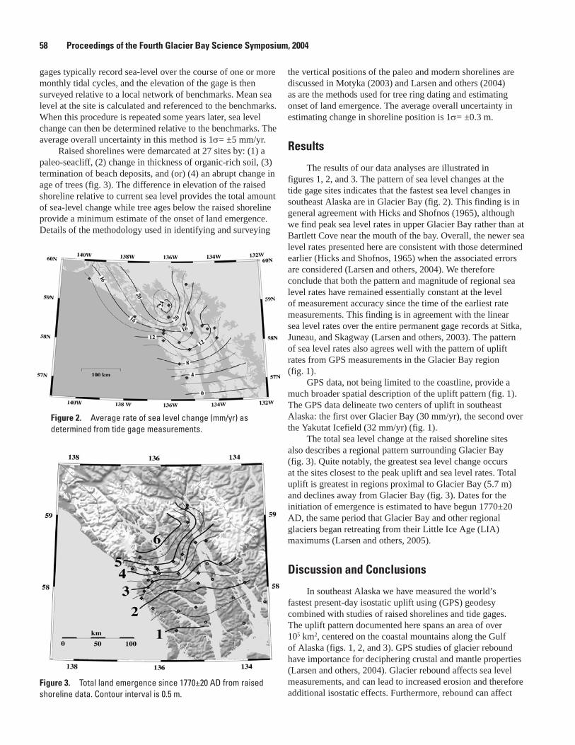
gages typically record sea-level over the course of one or more monthly tidal cycles, and the elevation of the gage is then surveyed relative to a local network of benchmarks. Mean sea level at the site is calculated and referenced to the benchmarks. When this procedure is repeated some years later, sea level change can then be determined relative to the benchmarks. The average overall uncertainty in this method is 1σ= ±5 mm/yr.
Raised shorelines were demarcated at 27 sites by: (1) a paleo-seacliff, (2) change in thickness of organic-rich soil, (3) termination of beach deposits, and (or) (4) an abrupt change in age of trees (fig. 3). The difference in elevation of the raised shoreline relative to current sea level provides the total amount of sea-level change while tree ages below the raised shoreline provide a minimum estimate of the onset of land emergence. Details of the methodology used in identifying and surveying
the vertical positions of the paleo and modern shorelines are discussed in Motyka (2003) and Larsen and others (2004) as are the methods used for tree ring dating and estimating onset of land emergence. The average overall uncertainty in estimating change in shoreline position is 1σ= ±0.3 m.
Results
The results of our data analyses are illustrated in figures 1, 2, and 3. The pattern of sea level changes at the tide gage sites indicates that the fastest sea level changes in southeast Alaska are in Glacier Bay (fig. 2). This finding is in general agreement with Hicks and Shofnos (1965), although we find peak sea level rates in upper Glacier Bay rather than at Bartlett Cove near the mouth of the bay. Overall, the newer sea level rates presented here are consistent with those determined earlier (Hicks and Shofnos, 1965) when the associated errors are considered (Larsen and others, 2004). We therefore conclude that both the pattern and magnitude of regional sea level rates have remained essentially constant at the level of measurement accuracy since the time of the earliest rate measurements. This finding is in agreement with the linear sea level rates over the entire permanent gage records at Sitka, Juneau, and Skagway (Larsen and others, 2003). The pattern of sea level rates also agrees well with the pattern of uplift rates from GPS measurements in the Glacier Bay region (fig. 1).
GPS data, not being limited to the coastline, provide a much broader spatial description of the uplift pattern (fig. 1). The GPS data delineate two centers of uplift in southeast Alaska: the first over Glacier Bay (30 mm/yr), the second over the Yakutat Icefield (32 mm/yr) (fig. 1).
The total sea level change at the raised shoreline sites also describes a regional pattern surrounding Glacier Bay (fig. 3). Quite notably, the greatest sea level change occurs at the sites closest to the peak uplift and sea level rates. Total uplift is greatest in regions proximal to Glacier Bay (5.7 m) and declines away from Glacier Bay (fig. 3). Dates for the initiation of emergence is estimated to have begun 1770±20 AD, the same period that Glacier Bay and other regional glaciers began retreating from their Little Ice Age (LIA) maximums (Larsen and others, 2005).
Discussion and Conclusions
In southeast Alaska we have measured the world’s fastest present-day isostatic uplift using (GPS) geodesy combined with studies of raised shorelines and tide gages. The uplift pattern documented here spans an area of over 105 km2, centered on the coastal mountains along the Gulf of Alaska (figs. 1, 2, and 3). GPS studies of glacier rebound have importance for deciphering crustal and mantle properties (Larsen and others, 2004). Glacier rebound affects sea level measurements, and can lead to increased erosion and therefore additional isostatic effects. Furthermore, rebound can affect
Figure 2. Average rate of sea level change (mm/yr) as determined from tide gage measurements.
Figure �. Total land emergence since 1770±20 AD from raised shoreline data. Contour interval is 0.5 m.
5� Proceedings of the Fourth Glacier Bay Science Symposium, 200�
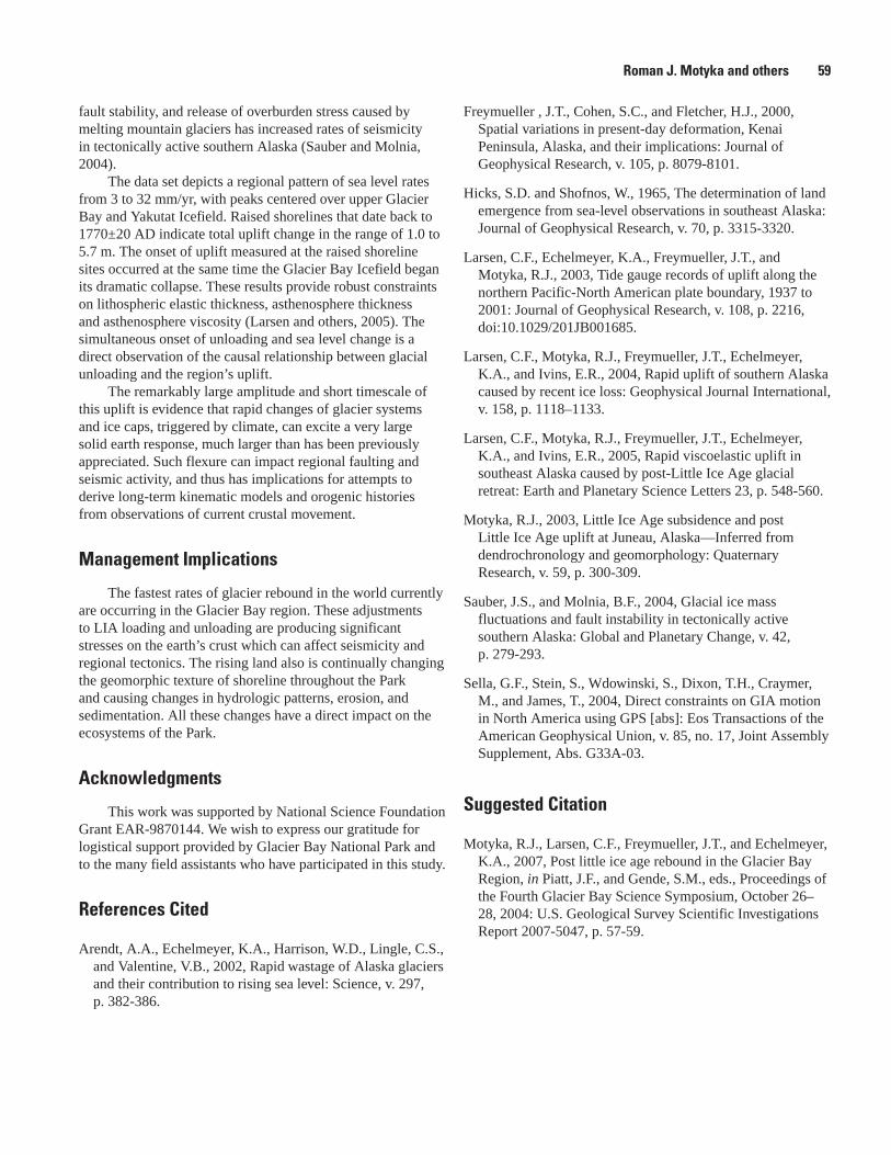
fault stability, and release of overburden stress caused by melting mountain glaciers has increased rates of seismicity in tectonically active southern Alaska (Sauber and Molnia, 2004).
The data set depicts a regional pattern of sea level rates from 3 to 32 mm/yr, with peaks centered over upper Glacier Bay and Yakutat Icefield. Raised shorelines that date back to 1770±20 AD indicate total uplift change in the range of 1.0 to 5.7 m. The onset of uplift measured at the raised shoreline sites occurred at the same time the Glacier Bay Icefield began its dramatic collapse. These results provide robust constraints on lithospheric elastic thickness, asthenosphere thickness and asthenosphere viscosity (Larsen and others, 2005). The simultaneous onset of unloading and sea level change is a direct observation of the causal relationship between glacial unloading and the region’s uplift.
The remarkably large amplitude and short timescale of this uplift is evidence that rapid changes of glacier systems and ice caps, triggered by climate, can excite a very large solid earth response, much larger than has been previously appreciated. Such flexure can impact regional faulting and seismic activity, and thus has implications for attempts to derive long-term kinematic models and orogenic histories from observations of current crustal movement.
Management Implications
The fastest rates of glacier rebound in the world currently are occurring in the Glacier Bay region. These adjustments to LIA loading and unloading are producing significant stresses on the earth’s crust which can affect seismicity and regional tectonics. The rising land also is continually changing the geomorphic texture of shoreline throughout the Park and causing changes in hydrologic patterns, erosion, and sedimentation. All these changes have a direct impact on the ecosystems of the Park.
Acknowledgments
This work was supported by National Science Foundation Grant EAR-9870144. We wish to express our gratitude for logistical support provided by Glacier Bay National Park and to the many field assistants who have participated in this study.
References Cited
Arendt, A.A., Echelmeyer, K.A., Harrison, W.D., Lingle, C.S., and Valentine, V.B., 2002, Rapid wastage of Alaska glaciers and their contribution to rising sea level: Science, v. 297, p. 382-386.
Freymueller , J.T., Cohen, S.C., and Fletcher, H.J., 2000, Spatial variations in present-day deformation, Kenai Peninsula, Alaska, and their implications: Journal of Geophysical Research, v. 105, p. 8079-8101.
Hicks, S.D. and Shofnos, W., 1965, The determination of land emergence from sea-level observations in southeast Alaska: Journal of Geophysical Research, v. 70, p. 3315-3320.
Larsen, C.F., Echelmeyer, K.A., Freymueller, J.T., and Motyka, R.J., 2003, Tide gauge records of uplift along the northern Pacific-North American plate boundary, 1937 to 2001: Journal of Geophysical Research, v. 108, p. 2216, doi:10.1029/201JB001685.
Larsen, C.F., Motyka, R.J., Freymueller, J.T., Echelmeyer, K.A., and Ivins, E.R., 2004, Rapid uplift of southern Alaska caused by recent ice loss: Geophysical Journal International, v. 158, p. 1118–1133.
Larsen, C.F., Motyka, R.J., Freymueller, J.T., Echelmeyer, K.A., and Ivins, E.R., 2005, Rapid viscoelastic uplift in southeast Alaska caused by post-Little Ice Age glacial retreat: Earth and Planetary Science Letters 23, p. 548-560.
Motyka, R.J., 2003, Little Ice Age subsidence and post Little Ice Age uplift at Juneau, Alaska—Inferred from dendrochronology and geomorphology: Quaternary Research, v. 59, p. 300-309.
Sauber, J.S., and Molnia, B.F., 2004, Glacial ice mass fluctuations and fault instability in tectonically active southern Alaska: Global and Planetary Change, v. 42, p. 279-293.
Sella, G.F., Stein, S., Wdowinski, S., Dixon, T.H., Craymer, M., and James, T., 2004, Direct constraints on GIA motion in North America using GPS [abs]: Eos Transactions of the American Geophysical Union, v. 85, no. 17, Joint Assembly Supplement, Abs. G33A-03.
Suggested Citation
Motyka, R.J., Larsen, C.F., Freymueller, J.T., and Echelmeyer, K.A., 2007, Post little ice age rebound in the Glacier Bay Region, in Piatt, J.F., and Gende, S.M., eds., Proceedings of the Fourth Glacier Bay Science Symposium, October 26–28, 2004: U.S. Geological Survey Scientific Investigations Report 2007-5047, p. 57-59.
Roman J. Motyka and others 59
Abstract. Historical photographs, some made as early as the mid-l880s, are being used as a primary component of an integrated effort to characterize the rapid landscape evolution of the Glacier Bay area. Selected historical photographs are analyzed to document former landscape parameters including: glacier extent, thickness, and terminus position; distribution and type of vegetation; wetland location and extent; shoreline characteristics; and sediment characteristics and distribution. In the field, new ‘repeat’ photographs are made at each historical photograph location. The new photographs are analyzed for the same parameters as the originals and the results compared. In addition to the extracted information, the resulting pairs of photograph provide striking visual documentation of the dynamic landscape evolution occurring in the Glacier Bay area.
Introduction
Alaska’s landscapes are among the most dynamic on Earth (Molnia, 2000). They change rapidly in response to active physical processes, such as glaciation, tectonics, seismicity, sedimentation, rapid post-glacial isostatic rebound, and eustatic and relative sea level change (Molnia, 2000). They also are very sensitive indicators of climate change. In Glacier Bay National Park, the most rapidly changing component of the landscape is the glaciers. Their changes effect and often drive all other components of Glacier Bay’s physical and biological environment. A joint U.S. Geological Survey-National Park Service project is studying landscape evolution, glacier change, and vegetative succession in Glacier Bay National Park, specifically in the area that was covered by the complex, multi-tributary, Little-Ice-Age glacier system that filled Glacier Bay through the early 18th century. The primary technique being used is comparison of several hundred pairs of modern and historical photographs, each pair having been made at a unique location. The use of historical photography (‘repeat photography’) to document temporal change at Glacier Bay is not a new concept. As early as 1926, William O. Field was revisiting locations photographed by H.F. Reed in the early 1890s (Field and Brown, 2003). What is unique is the systematic approach being used to obtain maximum spatial and temporal photographic coverage for every fiord in Glacier Bay. Through analysis and interpretation of these photographic pairs, both quantitative and qualitative information is extracted to document the landscape evolution of the Glacier Bay area.
An archeological survey of the Glacier Bay region documented prehistoric habitation of the area dating to at least 9,000 yr B.P. (Ackerman, 1968). Although Tlingit oral histories contain narratives related to the glacier history of
the region (Cruikshank, 2001), none extend back to this early Holocene period of habitation. However, several oral histories describe Xunaa Ka`awu (Huna Tlingit Clans) villages being destroyed by Glacier Bay’s Little Ice Age glacier advance, resulting in the displacement of Xunaa Ka`awu People to areas outside the Bay (Dauenhauer and Dauenhauer, 1987). However, these histories do not provide an absolute chronology of Glacier Bay events, nor contain any visual documentation of glacier extent.
By the late 1870s, when Glacier Bay was seen by Lt. C.E.S. Wood (Wood, 1882) and explored by John Muir (Muir, 1895), glacier retreat had been underway for more than a century. By that time, the ice edge was more than 60 km from its “Little-Ice-Age” maximum position. There is no photographic documentation to provide insights into the glacier’s maximum extent or to document how the first ~130 years of rapid retreat proceeded. However, less than a decade after Muir’s 1879 visit, the first photographs of the Glacier Bay landscape were made. In subsequent years, mapping surveys, early scientific expeditions, geological and glaciological investigations, commercial photographers, and tourists brought cameras to Glacier Bay and began to photograph the landscape. By the end of the 19th century, hundreds of photographs had been made, many of which are still extant. With continuing early-20th century glacier retreat, more inlets began to become exposed, each with its own unique retreating ice tongue or tongues and its own history and timing of ice movement. Historical photographs have been acquired that document these early-20th century changes for every fiord in Glacier Bay.
Our goal is to document the dynamic landscape evolution of the Glacier Bay region. To do this, we: (1) locate and acquire historical photographs; (2) interpret these historical photographs to quantify and visualize the appearance of the landscape at the time they were made; (3) revisit locations from which historical photographs were made and rephotograph the same field of view; and (4) document
Documenting More than a Century of Glacier Bay Landscape Evolution with Historical Photography
Bruce F. Molnia1,3, Ronald D. Karpilo, Jr.2, and Harold S. Pranger2
1 U.S. Geological Survey, Mail Stop 926A, 12201 Sunrise Valley Drive, Reston, VA 20192 USA
2 National Park Service, Geologic Resources Division, 12795 West Alameda Parkway, P.O. Box 25287, Denver, CO 80225-0287 USA
3 Corresponding author: [email protected], 703-648-4120
�0 Proceedings of the Fourth Glacier Bay Science Symposium
changes at each location and provide written and visual products that depict the mechanics and magnitude of the changes that occurred during the intervening period.
Methods
More than 1,200 late-19th-century and early-20th-century, ground- and sea-surface-based photographs have been found that show landscape features in Glacier Bay National Park and Preserve. More than half of these historical photographs depict glacier termini and related features in the geographic area that was covered by Glacier Bay’s Little-Ice-Age glacier system. Nearly all of these historical photographs lack important elements of metadata, most significantly, geographic coordinates of the photo-point from which a photograph was made, but also camera specifics, lens information, film type, exposure data, and date of collection. The earliest of these photographs may predate 1885. Sources of these photographs include national archives, museums, publications, libraries, internet sites, antique dealers, and individuals. Photographs acquired in an analog format (paper) are scanned and converted to a digital format. More than 600 of these photographs have been compiled into a dual mode (digital and analog) database. As possible, supporting metadata are developed for each historical image. Historical photographs included in this study were ‘taken’ by Alfred H. Brooks, Grove K. Gilbert, William O. Field, the International Boundary Commission, Frank LaRoche, John B. Mertie, John C. Reed, Harry F. Reid, Charles W. Wright, Juneau-based commercial photographers Lloyd Winter and E. Percy Pond, and others.
During the 2003 and 2004 field seasons, nearly 100 locations from which historical photographs had been made were identified and revisited. At about 20 locations, cairns built by the original or subsequent photographers, were found and reoccupied. At each site, date, time, latitude and longitude, elevation, and bearing to the center of each photographic target were determined with GPS receiver and compass. Using a paper copy of the appropriate historical photographs as a composition guide, a suite of digital images and color-film photographs were made of the same areas displayed in the historical photograph, often using multiple lenses of different focal length. Many of the historical photographs were made with rotating-lens panoramic or mapping cameras, typically with fields-of-view that exceed those of most modern ‘normal’ or even ‘wide-angle’ lenses. To duplicate these photographs, overlapping sequential photographs were made so that they could be digitally joined as panoramas. Fourteen photo-sites from which the first author photographed Glacier Bay glaciers prior to 1980 also were revisited.
In the laboratory, new images and photographs were compared with corresponding historical photographs to determine differences, and to better understand rates, timing, and mechanics of landscape change and evolution. Particular emphasis was placed on understanding the response of specific glaciers to changing climate and environment.
Results
Comparisons of historical and modern photo-pairs provide great insight into the post-Little-Ice-Age evolution of the Glacier Bay landscape. With respect to glaciers, derived information was useful in documenting: (1) the post-late-1880s timing and magnitude of glacier retreat in East Arm, a trend continuing to the present (figs. 1 and 2); (2) a similar continuous retreat of the glaciers in the Geikie and Hugh Miller Inlet areas of West Arm; (3) early-20th century retreat and subsequent variability of Reid and Lamplugh Glaciers (fig. 3); (4) early-to-late-20th century readvances of Johns Hopkins and Grand Pacific Glaciers; (5) continued late-20th century and early-21st century advance of Johns Hopkins Glacier; (6) late-20th century and early-21st century retreat and thinning of Grand Pacific Glacier; (7) decadal-scale fluctuations of smaller glaciers, such as hanging glaciers in Johns Hopkins Inlet, including Hoonah and Toyatte Glaciers; and (8) transitions from tidewater termini to land-based, stagnant or retreating, debris-covered, glacier termini in a number of locations including Muir, Carroll, and Rendu Glaciers.
Elsewhere in Glacier Bay, the comparisons of historical and modern photo-pairs document: (1) the filling of upper Queen Inlet with more than 100 m of sediment (fig. 4); (2) the rapid erosion of fiord-wall moraines following ice retreat; and (3) the development of outwash and talus features at many locations. Also universally evident is the rapid influx of vegetation and the transformation and progression from essentially bare bedrock to forest.
Annotated photo-pairs are being posted on publicly-accessible websites [such as: The U.S. Geological Survey Photographic Library (http:// libraryphoto.cr.usgs.gov); a National Park Service website depicting animated pairs of historical and modern photographs (http://www2.nature.nps.gov/geology/GLBA/glaciers.htm), and The National Snow and Ice Data Center (NSIDC) Long-Term Change Photographic Pairs Special Collection (http://nsidc.org/data/glacier_photo/special_collection.html)], and provided to National Park Service managers and interpreters. Beginning in 2004, similar studies have been conducted in Kenai Fjords and Denali National Parks.
Bruce F. Molnia and others �1
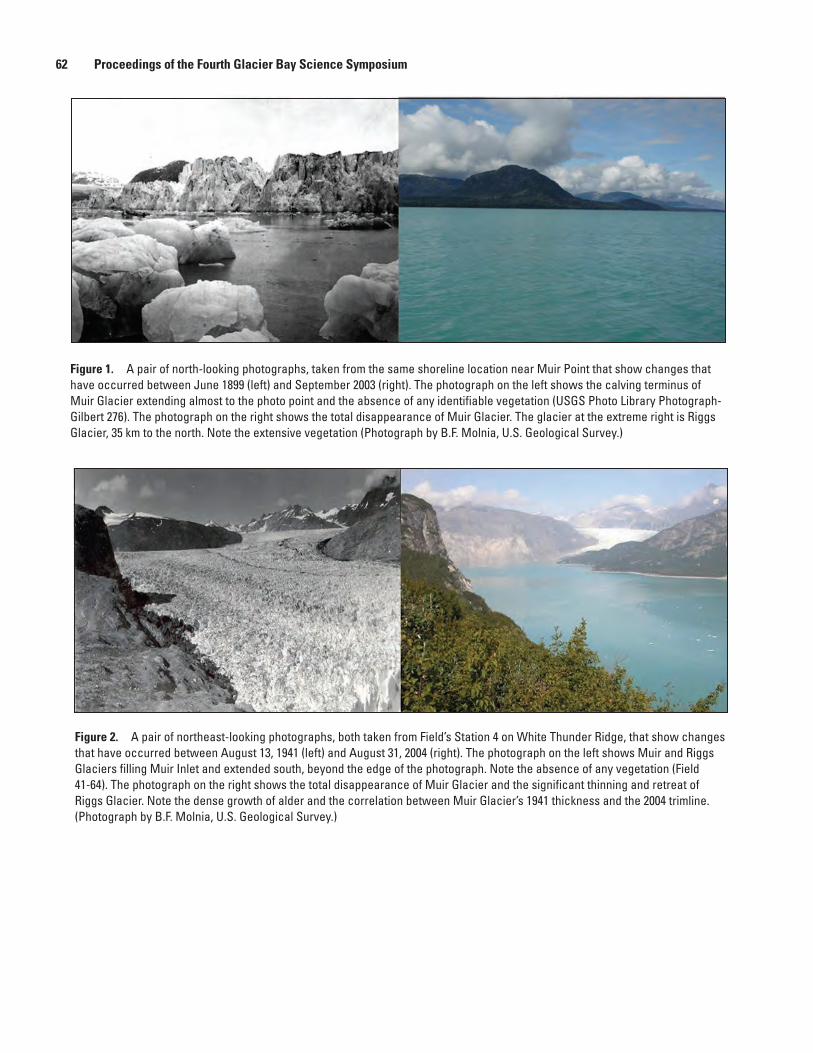
Figure 1. A pair of north-looking photographs, taken from the same shoreline location near Muir Point that show changes that have occurred between June 1899 (left) and September 2003 (right). The photograph on the left shows the calving terminus of Muir Glacier extending almost to the photo point and the absence of any identifiable vegetation (USGS Photo Library Photograph-Gilbert 276). The photograph on the right shows the total disappearance of Muir Glacier. The glacier at the extreme right is Riggs Glacier, 35 km to the north. Note the extensive vegetation (Photograph by B.F. Molnia, U.S. Geological Survey.)
Figure 2. A pair of northeast-looking photographs, both taken from Field’s Station 4 on White Thunder Ridge, that show changes that have occurred between August 13, 1941 (left) and August 31, 2004 (right). The photograph on the left shows Muir and Riggs Glaciers filling Muir Inlet and extended south, beyond the edge of the photograph. Note the absence of any vegetation (Field 41-64). The photograph on the right shows the total disappearance of Muir Glacier and the significant thinning and retreat of Riggs Glacier. Note the dense growth of alder and the correlation between Muir Glacier’s 1941 thickness and the 2004 trimline. (Photograph by B.F. Molnia, U.S. Geological Survey.)
�2 Proceedings of the Fourth Glacier Bay Science Symposium

Figure �. A pair of southwest-looking photographs, both taken from the same location adjacent to Lamplugh Glacier showing the changes that have occurred at the lower end of Lamplugh’s inlet between August 1941 (left) and September 8, 2003 (right). The photograph on the left shows the calving terminus of Lamplugh Glacier extending to within a kilometer of the photo point (Field 430-41). No vegetation is visible. The photograph on the right shows that the terminus of Lamplugh Glacier is ~0.8 km forward of its 1941 position. However, till on the closest bedrock ridge indicates that the glacier had advanced beyond the photo point at some time during the interval between photographs, probably in the late-1960s. Note the developing vegetation. (Photograph by B.F. Molnia, U.S. Geological Survey.)
Figure �. A pair of northwest-looking photographs, both taken from the same location, several hundred meters up an steep alluvial fan located in a side valley on the east side of Queen Inlet showing the changes that have occurred to Carroll Glacier and upper Queen Inlet during the 98 years between August 1906 (left) and June 21, 2004 (right). The photograph on the left shows the calving terminus of Carroll Glacier sitting at the head of Queen Inlet (USGS Photo Library Photograph-Wright 335). No vegetation is visible. The photograph on the right shows that the terminus of Carroll Glacier has changed to a stagnant, debris-covered glacier that has significantly thinned and retreated from its 1906 position. The head of Queen Inlet has been filled by sediment. An examination of early 20th century nautical charts suggests that the sediment fill exceeds 125 m. Note the developing vegetation on the sediment fill. (Photograph by B.F. Molnia, U.S. Geological Survey.).
Bruce F. Molnia and others ��
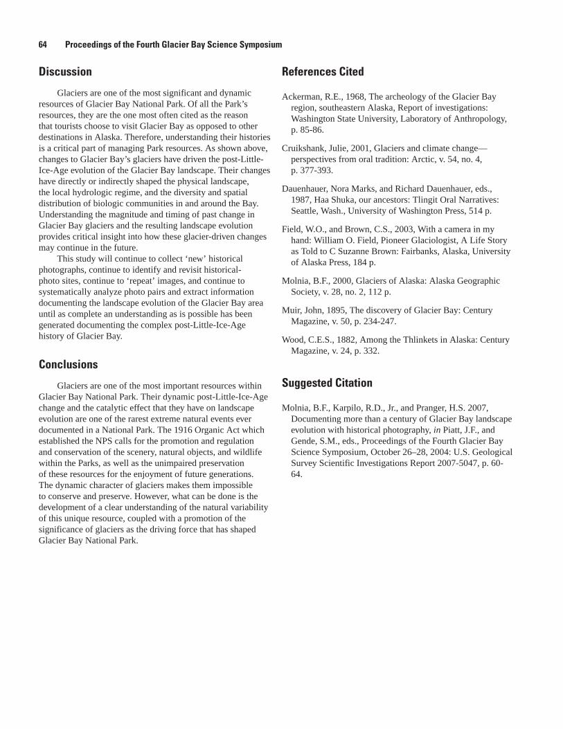
Discussion
Glaciers are one of the most significant and dynamic resources of Glacier Bay National Park. Of all the Park’s resources, they are the one most often cited as the reason that tourists choose to visit Glacier Bay as opposed to other destinations in Alaska. Therefore, understanding their histories is a critical part of managing Park resources. As shown above, changes to Glacier Bay’s glaciers have driven the post-Little-Ice-Age evolution of the Glacier Bay landscape. Their changes have directly or indirectly shaped the physical landscape, the local hydrologic regime, and the diversity and spatial distribution of biologic communities in and around the Bay. Understanding the magnitude and timing of past change in Glacier Bay glaciers and the resulting landscape evolution provides critical insight into how these glacier-driven changes may continue in the future.
This study will continue to collect ‘new’ historical photographs, continue to identify and revisit historical-photo sites, continue to ‘repeat’ images, and continue to systematically analyze photo pairs and extract information documenting the landscape evolution of the Glacier Bay area until as complete an understanding as is possible has been generated documenting the complex post-Little-Ice-Age history of Glacier Bay.
Conclusions
Glaciers are one of the most important resources within Glacier Bay National Park. Their dynamic post-Little-Ice-Age change and the catalytic effect that they have on landscape evolution are one of the rarest extreme natural events ever documented in a National Park. The 1916 Organic Act which established the NPS calls for the promotion and regulation and conservation of the scenery, natural objects, and wildlife within the Parks, as well as the unimpaired preservation of these resources for the enjoyment of future generations. The dynamic character of glaciers makes them impossible to conserve and preserve. However, what can be done is the development of a clear understanding of the natural variability of this unique resource, coupled with a promotion of the significance of glaciers as the driving force that has shaped Glacier Bay National Park.
References Cited
Ackerman, R.E., 1968, The archeology of the Glacier Bay region, southeastern Alaska, Report of investigations: Washington State University, Laboratory of Anthropology, p. 85-86.
Cruikshank, Julie, 2001, Glaciers and climate change—perspectives from oral tradition: Arctic, v. 54, no. 4, p. 377-393.
Dauenhauer, Nora Marks, and Richard Dauenhauer, eds., 1987, Haa Shuka, our ancestors: Tlingit Oral Narratives: Seattle, Wash., University of Washington Press, 514 p.
Field, W.O., and Brown, C.S., 2003, With a camera in my hand: William O. Field, Pioneer Glaciologist, A Life Story as Told to C Suzanne Brown: Fairbanks, Alaska, University of Alaska Press, 184 p.
Molnia, B.F., 2000, Glaciers of Alaska: Alaska Geographic Society, v. 28, no. 2, 112 p.
Muir, John, 1895, The discovery of Glacier Bay: Century Magazine, v. 50, p. 234-247.
Wood, C.E.S., 1882, Among the Thlinkets in Alaska: Century Magazine, v. 24, p. 332.
Suggested Citation
Molnia, B.F., Karpilo, R.D., Jr., and Pranger, H.S. 2007, Documenting more than a century of Glacier Bay landscape evolution with historical photography, in Piatt, J.F., and Gende, S.M., eds., Proceedings of the Fourth Glacier Bay Science Symposium, October 26–28, 2004: U.S. Geological Survey Scientific Investigations Report 2007-5047, p. 60-64.
�� Proceedings of the Fourth Glacier Bay Science Symposium
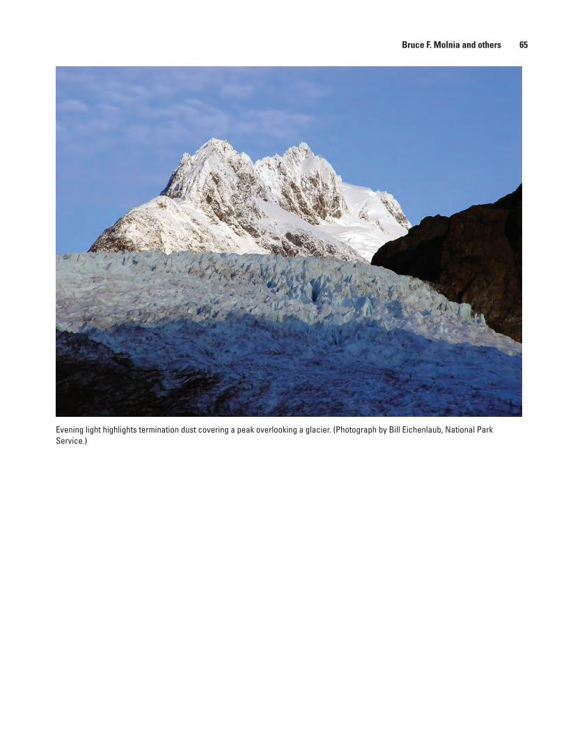
Evening light highlights termination dust covering a peak overlooking a glacier. (Photograph by Bill Eichenlaub, National Park Service.)
Bruce F. Molnia and others �5
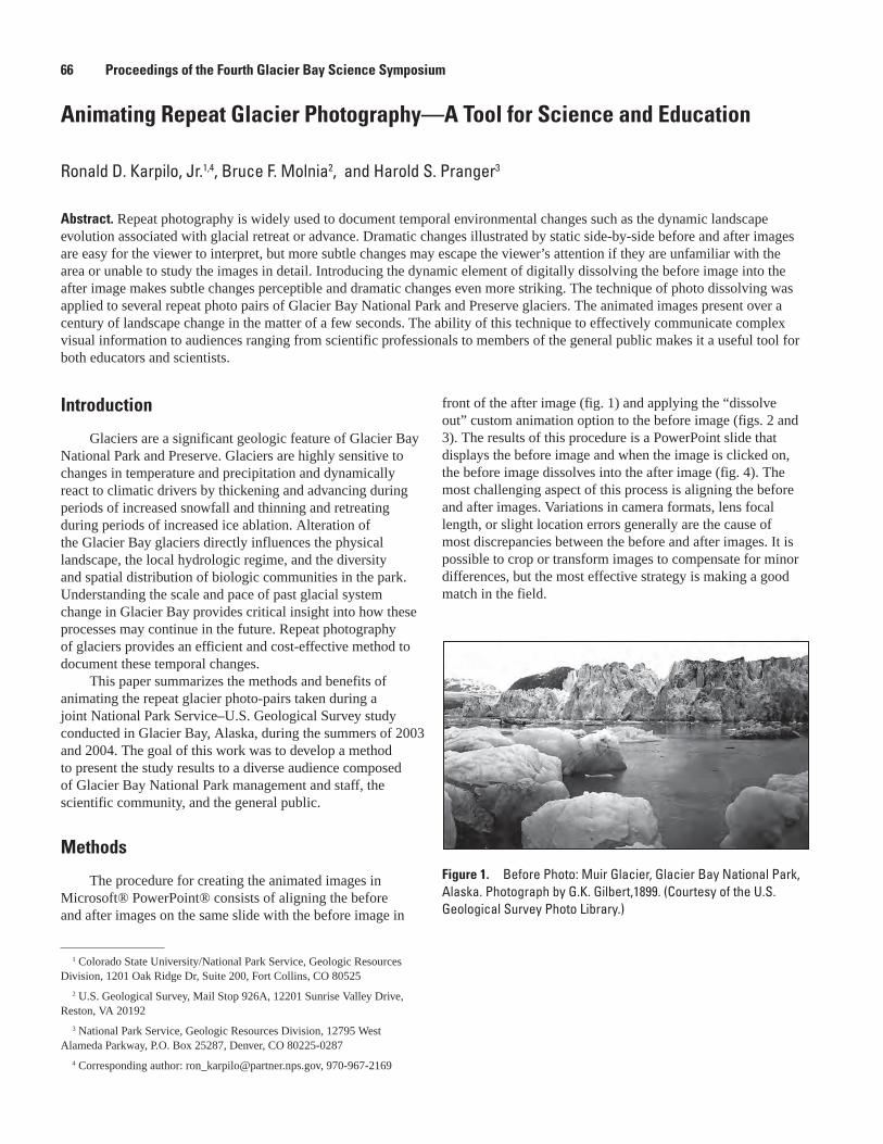
Animating Repeat Glacier Photography—A Tool for Science and Education
Ronald D. Karpilo, Jr.1,4, Bruce F. Molnia2, and Harold S. Pranger3
Abstract. Repeat photography is widely used to document temporal environmental changes such as the dynamic landscape evolution associated with glacial retreat or advance. Dramatic changes illustrated by static side-by-side before and after images are easy for the viewer to interpret, but more subtle changes may escape the viewer’s attention if they are unfamiliar with the area or unable to study the images in detail. Introducing the dynamic element of digitally dissolving the before image into the after image makes subtle changes perceptible and dramatic changes even more striking. The technique of photo dissolving was applied to several repeat photo pairs of Glacier Bay National Park and Preserve glaciers. The animated images present over a century of landscape change in the matter of a few seconds. The ability of this technique to effectively communicate complex visual information to audiences ranging from scientific professionals to members of the general public makes it a useful tool for both educators and scientists.
Figure 1. Before Photo: Muir Glacier, Glacier Bay National Park, Alaska. Photograph by G.K. Gilbert,1899. (Courtesy of the U.S. Geological Survey Photo Library.)
�� Proceedings of the Fourth Glacier Bay Science Symposium
Introduction
Glaciers are a significant geologic feature of Glacier Bay National Park and Preserve. Glaciers are highly sensitive to changes in temperature and precipitation and dynamically react to climatic drivers by thickening and advancing during periods of increased snowfall and thinning and retreating during periods of increased ice ablation. Alteration of the Glacier Bay glaciers directly influences the physical landscape, the local hydrologic regime, and the diversity and spatial distribution of biologic communities in the park. Understanding the scale and pace of past glacial system change in Glacier Bay provides critical insight into how these processes may continue in the future. Repeat photography of glaciers provides an efficient and cost-effective method to document these temporal changes.
This paper summarizes the methods and benefits of animating the repeat glacier photo-pairs taken during a joint National Park Service–U.S. Geological Survey study conducted in Glacier Bay, Alaska, during the summers of 2003 and 2004. The goal of this work was to develop a method to present the study results to a diverse audience composed of Glacier Bay National Park management and staff, the scientific community, and the general public.
Methods
The procedure for creating the animated images in Microsoft® PowerPoint® consists of aligning the before and after images on the same slide with the before image in
1 Colorado State University/National Park Service, Geologic Resources Division, 1201 Oak Ridge Dr, Suite 200, Fort Collins, CO 80525
2 U.S. Geological Survey, Mail Stop 926A, 12201 Sunrise Valley Drive, Reston, VA 20192
3 National Park Service, Geologic Resources Division, 12795 West Alameda Parkway, P.O. Box 25287, Denver, CO 80225-0287
4 Corresponding author: [email protected], 970-967-2169
front of the after image (fig. 1) and applying the “dissolve out” custom animation option to the before image (figs. 2 and 3). The results of this procedure is a PowerPoint slide that displays the before image and when the image is clicked on, the before image dissolves into the after image (fig. 4). The most challenging aspect of this process is aligning the before and after images. Variations in camera formats, lens focal length, or slight location errors generally are the cause of most discrepancies between the before and after images. It is possible to crop or transform images to compensate for minor differences, but the most effective strategy is making a good match in the field.
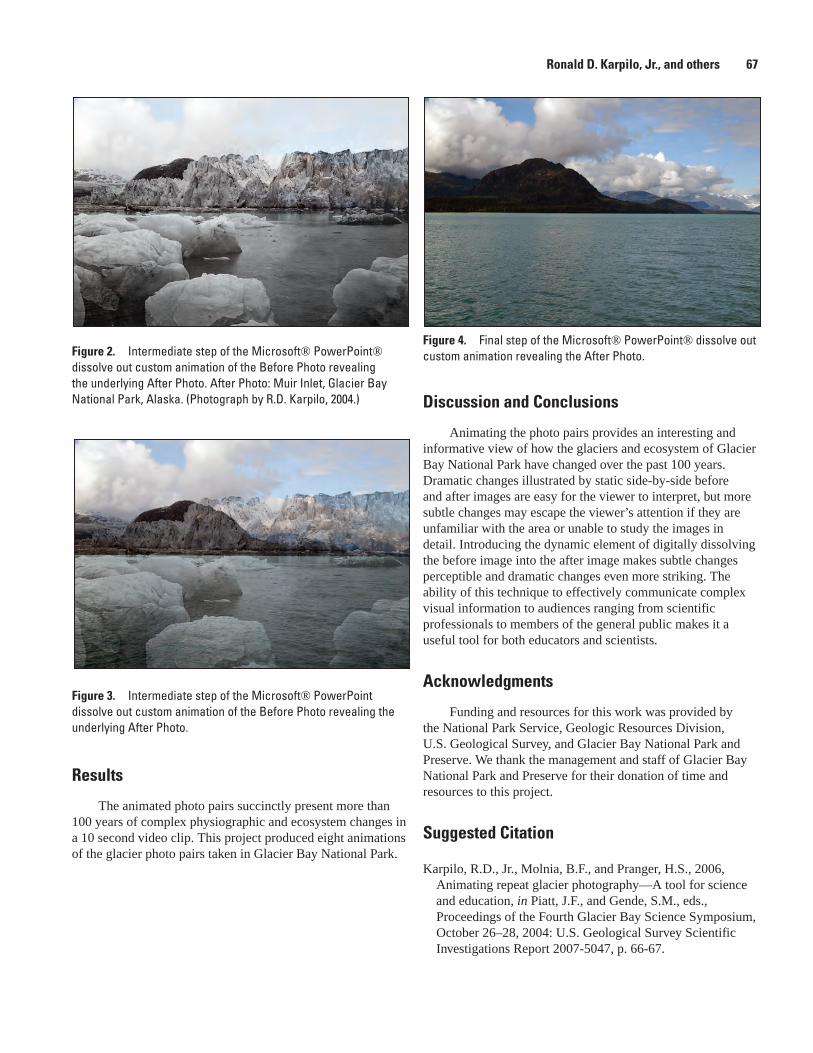
Figure 2. Intermediate step of the Microsoft® PowerPoint® dissolve out custom animation of the Before Photo revealing the underlying After Photo. After Photo: Muir Inlet, Glacier Bay National Park, Alaska. (Photograph by R.D. Karpilo, 2004.)
Figure �. Intermediate step of the Microsoft® PowerPoint dissolve out custom animation of the Before Photo revealing the underlying After Photo.
Figure �. Final step of the Microsoft® PowerPoint® dissolve out custom animation revealing the After Photo.
Ronald D. Karpilo, Jr., and others �7
Results
The animated photo pairs succinctly present more than 100 years of complex physiographic and ecosystem changes in a 10 second video clip. This project produced eight animations of the glacier photo pairs taken in Glacier Bay National Park.
Discussion and Conclusions
Animating the photo pairs provides an interesting and informative view of how the glaciers and ecosystem of Glacier Bay National Park have changed over the past 100 years. Dramatic changes illustrated by static side-by-side before and after images are easy for the viewer to interpret, but more subtle changes may escape the viewer’s attention if they are unfamiliar with the area or unable to study the images in detail. Introducing the dynamic element of digitally dissolving the before image into the after image makes subtle changes perceptible and dramatic changes even more striking. The ability of this technique to effectively communicate complex visual information to audiences ranging from scientific professionals to members of the general public makes it a useful tool for both educators and scientists.
Acknowledgments
Funding and resources for this work was provided by the National Park Service, Geologic Resources Division, U.S. Geological Survey, and Glacier Bay National Park and Preserve. We thank the management and staff of Glacier Bay National Park and Preserve for their donation of time and resources to this project.
Suggested Citation
Karpilo, R.D., Jr., Molnia, B.F., and Pranger, H.S., 2006, Animating repeat glacier photography—A tool for science and education, in Piatt, J.F., and Gende, S.M., eds., Proceedings of the Fourth Glacier Bay Science Symposium, October 26–28, 2004: U.S. Geological Survey Scientific Investigations Report 2007-5047, p. 66-67.

�� Proceedings of the Fourth Glacier Bay Science Symposium
This page is intentionally left blank.
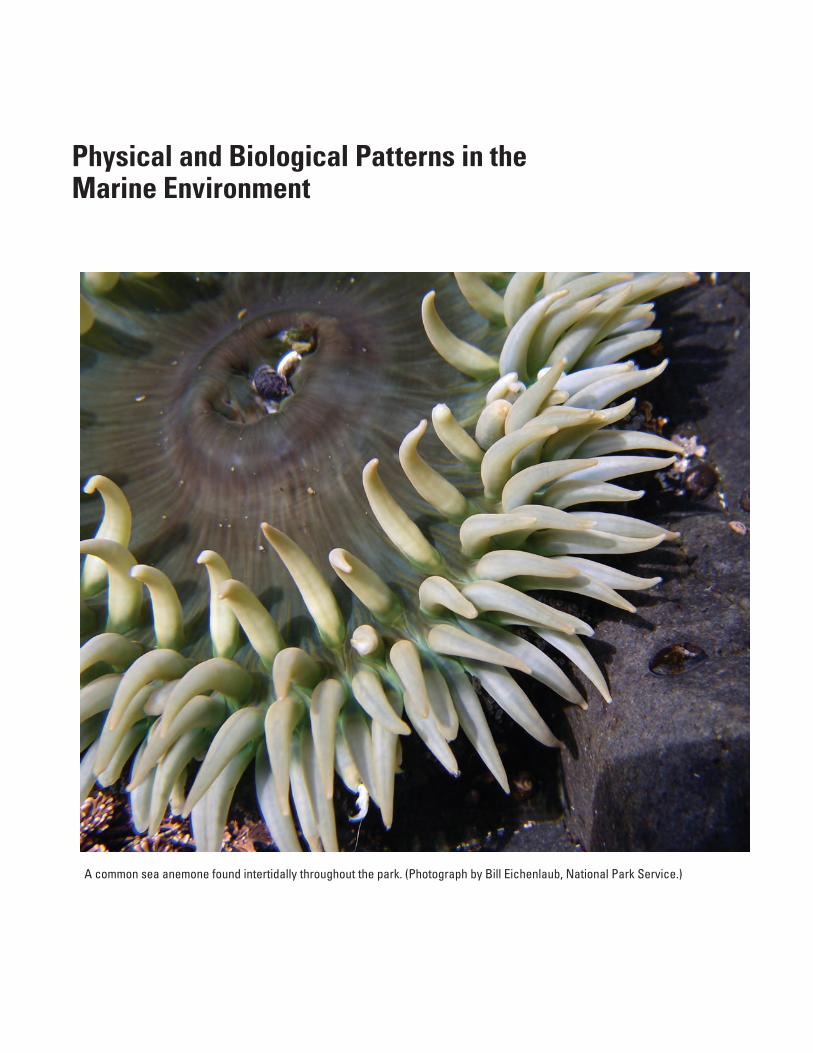
Physical and Biological Patterns in the Marine Environment
A common sea anemone found intertidally throughout the park. (Photograph by Bill Eichenlaub, National Park Service.)

70 Proceedings of the Fourth Glacier Bay Science Symposium, 200�
This page is intentionally left blank.
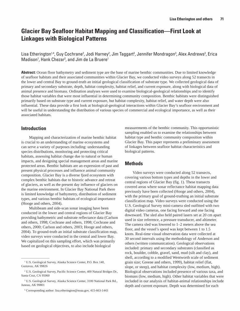
Glacier Bay Seafloor Habitat Mapping and Classification—First Look at Linkages with Biological Patterns
Lisa Etherington1,4, Guy Cochrane2, Jodi Harney2, Jim Taggart3, Jennifer Mondragon3, Alex Andrews3, Erica Madison1, Hank Chezar2, and Jim de La Bruere1
Abstract: Ocean floor bathymetry and sediment type are the base of marine benthic communities. Due to limited knowledge of seafloor habitats and their associated communities within Glacier Bay, we conducted video surveys along 52 transects in the lower and central Bay to ground-truth an initial geological classification of substrate type. We collected geological data of primary and secondary substrate, depth, habitat complexity, habitat relief, and current exposure, along with biological data of animal presence and biomass. Ordination analyses were used to examine biological-geological relationships and to identify those habitat variables that were most influential in determining community composition. Benthic habitats were distinguished primarily based on substrate type and current exposure, but habitat complexity, habitat relief, and water depth were also influential. These data provide a first look at biological-geological interactions within Glacier Bay’s seafloor environment and will be useful in understanding the distribution of various species of commercial and ecological importance, as well as their associated habitats.
Lisa Etherington and others 71
1 U.S. Geological Survey, Alaska Science Center, P.O. Box 140, Gustavus, AK 99826
2 U.S. Geological Survey, Pacific Science Center, 400 Natural Bridges Dr., Santa Cruz, CA 95060
3 U.S. Geological Survey, Alaska Science Center, 3100 National Park Rd., Juneau, AK 99801
4 Corresponding author: [email protected], 415-663-1443
measurements of the benthic community. This opportunistic sampling enabled us to examine the relationships between habitat type and benthic community composition within Glacier Bay. This paper represents a preliminary assessment of linkages between seafloor habitat characteristics and biological patterns.
Methods
Video surveys were conducted along 52 transects, covering various bottom types and depths in the lower and central regions of Glacier Bay (fig. 1). These transects covered areas where sonar reflectance habitat mapping data previously have been collected (Hooge and others, 2004), with the primary goal of ground-truthing an initial substrate classification map. Video surveys were conducted using the U.S. Geological Survey mini-camera sled outfitted with two digital video cameras, one facing forward and one facing downward. The sled also held paired lasers set at 20 cm apart used in size reference, a pressure transducer, and altimeter. The camera sled was lowered to 1–2 meters above the sea floor, and the vessel’s speed was kept between 1 to 1.5 knots. Real-time visual observation data were collected at 30 second intervals using the methodology of Anderson and others (written communication). Geological observations included: primary and secondary substrates (classified as rock, boulder, cobble, gravel, sand, mud (silt and clay), and shell, according to a modified Wentworth scale of sediment grain size; Greene and others, 1999), habitat relief (flat, slope, or steep), and habitat complexity (low, medium, high). Biological observations included presence of various taxa, and biomass (low, medium, high). Other habitat variables that were included in our analysis of habitat-animal relationships include depth and current exposure. Depth was determined for each
Introduction
Mapping and characterization of marine benthic habitat is crucial to an understanding of marine ecosystems and can serve a variety of purposes including: understanding species distributions, monitoring and protecting critical habitats, assessing habitat change due to natural or human impacts, and designing special management areas and marine protected areas. Benthic habitats are an expression of past and present physical processes and influence animal community composition. Glacier Bay is a diverse fjord ecosystem with complex benthic habitats due to historic advance and retreat of glaciers, as well as the present day influence of glaciers on the marine environment. In Glacier Bay National Park there is limited knowledge of bathymetry, distribution of sediment types, and various benthic habitats of ecological importance (Hooge and others, 2004).
Multibeam and side-scan sonar imaging have been conducted in the lower and central regions of Glacier Bay providing bathymetric and substrate reflectance data (Carlson and others, 1998; Cochrane and others, 1998; Cochrane and others, 2000; Carlson and others, 2003; Hooge and others, 2004). To ground-truth an initial substrate classification map, video surveys were conducted in the central and lower Bay. We capitalized on this sampling effort, which was primarily based on geological objectives, to also include biological
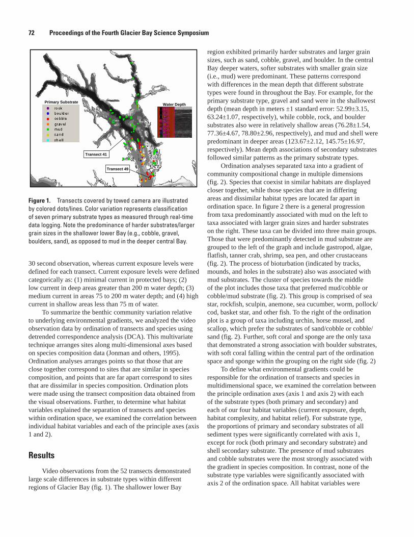
30 second observation, whereas current exposure levels were defined for each transect. Current exposure levels were defined categorically as: (1) minimal current in protected bays; (2) low current in deep areas greater than 200 m water depth; (3) medium current in areas 75 to 200 m water depth; and (4) high current in shallow areas less than 75 m of water.
To summarize the benthic community variation relative to underlying environmental gradients, we analyzed the video observation data by ordination of transects and species using detrended correspondence analysis (DCA). This multivariate technique arranges sites along multi-dimensional axes based on species composition data (Jonman and others, 1995). Ordination analyses arranges points so that those that are close together correspond to sites that are similar in species composition, and points that are far apart correspond to sites that are dissimilar in species composition. Ordination plots were made using the transect composition data obtained from the visual observations. Further, to determine what habitat variables explained the separation of transects and species within ordination space, we examined the correlation between individual habitat variables and each of the principle axes (axis 1 and 2).
Results
Video observations from the 52 transects demonstrated large scale differences in substrate types within different regions of Glacier Bay (fig. 1). The shallower lower Bay
region exhibited primarily harder substrates and larger grain sizes, such as sand, cobble, gravel, and boulder. In the central Bay deeper waters, softer substrates with smaller grain size (i.e., mud) were predominant. These patterns correspond with differences in the mean depth that different substrate types were found in throughout the Bay. For example, for the primary substrate type, gravel and sand were in the shallowest depth (mean depth in meters ±1 standard error: 52.99±3.15, 63.24±1.07, respectively), while cobble, rock, and boulder substrates also were in relatively shallow areas (76.28±1.54, 77.36±4.67, 78.80±2.96, respectively), and mud and shell were predominant in deeper areas (123.67±2.12, 145.75±16.97, respectively). Mean depth associations of secondary substrates followed similar patterns as the primary substrate types.
Ordination analyses separated taxa into a gradient of community compositional change in multiple dimensions (fig. 2). Species that coexist in similar habitats are displayed closer together, while those species that are in differing areas and dissimilar habitat types are located far apart in ordination space. In figure 2 there is a general progression from taxa predominantly associated with mud on the left to taxa associated with larger grain sizes and harder substrates on the right. These taxa can be divided into three main groups. Those that were predominantly detected in mud substrate are grouped to the left of the graph and include gastropod, algae, flatfish, tanner crab, shrimp, sea pen, and other crustaceans (fig. 2). The process of bioturbation (indicated by tracks, mounds, and holes in the substrate) also was associated with mud substrates. The cluster of species towards the middle of the plot includes those taxa that preferred mud/cobble or cobble/mud substrate (fig. 2). This group is comprised of sea star, rockfish, sculpin, anemone, sea cucumber, worm, pollock/cod, basket star, and other fish. To the right of the ordination plot is a group of taxa including urchin, horse mussel, and scallop, which prefer the substrates of sand/cobble or cobble/sand (fig. 2). Further, soft coral and sponge are the only taxa that demonstrated a strong association with boulder substrates, with soft coral falling within the central part of the ordination space and sponge within the grouping on the right side (fig. 2)
To define what environmental gradients could be responsible for the ordination of transects and species in multidimensional space, we examined the correlation between the principle ordination axes (axis 1 and axis 2) with each of the substrate types (both primary and secondary) and each of our four habitat variables (current exposure, depth, habitat complexity, and habitat relief). For substrate type, the proportions of primary and secondary substrates of all sediment types were significantly correlated with axis 1, except for rock (both primary and secondary substrate) and shell secondary substrate. The presence of mud substrates and cobble substrates were the most strongly associated with the gradient in species composition. In contrast, none of the substrate type variables were significantly associated with axis 2 of the ordination space. All habitat variables were
72 Proceedings of the Fourth Glacier Bay Science Symposium
Figure 1. Transects covered by towed camera are illustrated by colored dots/lines. Color variation represents classification of seven primary substrate types as measured through real-time data logging. Note the predominance of harder substrates/larger grain sizes in the shallower lower Bay (e.g., cobble, gravel, boulders, sand), as opposed to mud in the deeper central Bay.
Primary Substrate Water Depth
Transect 41
Transect 49
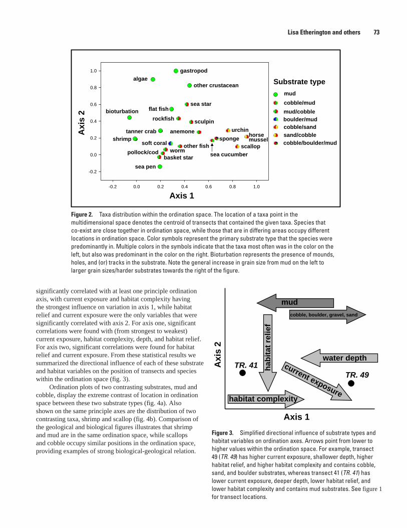
Figure �. Simplified directional influence of substrate types and habitat variables on ordination axes. Arrows point from lower to higher values within the ordination space. For example, transect 49 (TR. 49) has higher current exposure, shallower depth, higher habitat relief, and higher habitat complexity and contains cobble, sand, and boulder substrates, whereas transect 41 (TR. 41) has lower current exposure, deeper depth, lower habitat relief, and lower habitat complexity and contains mud substrates. See figure 1 for transect locations.
Lisa Etherington and others 7�
Axis 1
Axi
s 2
current exposure
habi
tat r
elie
f
water depth
habitat complexity
TR. 41TR. 49
mudcobble, boulder, gravel, sand
Figure 2. Taxa distribution within the ordination space. The location of a taxa point in the multidimensional space denotes the centroid of transects that contained the given taxa. Species that co-exist are close together in ordination space, while those that are in differing areas occupy different locations in ordination space. Color symbols represent the primary substrate type that the species were predominantly in. Multiple colors in the symbols indicate that the taxa most often was in the color on the left, but also was predominant in the color on the right. Bioturbation represents the presence of mounds, holes, and (or) tracks in the substrate. Note the general increase in grain size from mud on the left to larger grain sizes/harder substrates towards the right of the figure.
-0.2 0.0 0.2 0.4 0.6 0.8 1.0
-0.2
0.0
0.2
0.4
0.6
0.8
1.0
mudcobble/mudmud/cobbleboulder/mudcobble/sandsand/cobblecobble/boulder/mud
Substrate type
Axis 1
Axi
s 2
sea pen
shrimp
bioturbation
tanner crab
algae
anemone
other fish
basket starpollock/cod worm
soft coral
flat fish
rockfish sculpin
sea star
other crustacean
scallop
urchinsponge
gastropod
sea cucumber
horse mussel
significantly correlated with at least one principle ordination axis, with current exposure and habitat complexity having the strongest influence on variation in axis 1, while habitat relief and current exposure were the only variables that were significantly correlated with axis 2. For axis one, significant correlations were found with (from strongest to weakest) current exposure, habitat complexity, depth, and habitat relief. For axis two, significant correlations were found for habitat relief and current exposure. From these statistical results we summarized the directional influence of each of these substrate and habitat variables on the position of transects and species within the ordination space (fig. 3).
Ordination plots of two contrasting substrates, mud and cobble, display the extreme contrast of location in ordination space between these two substrate types (fig. 4a). Also shown on the same principle axes are the distribution of two contrasting taxa, shrimp and scallop (fig. 4b). Comparison of the geological and biological figures illustrates that shrimp and mud are in the same ordination space, while scallops and cobble occupy similar positions in the ordination space, providing examples of strong biological-geological relation.
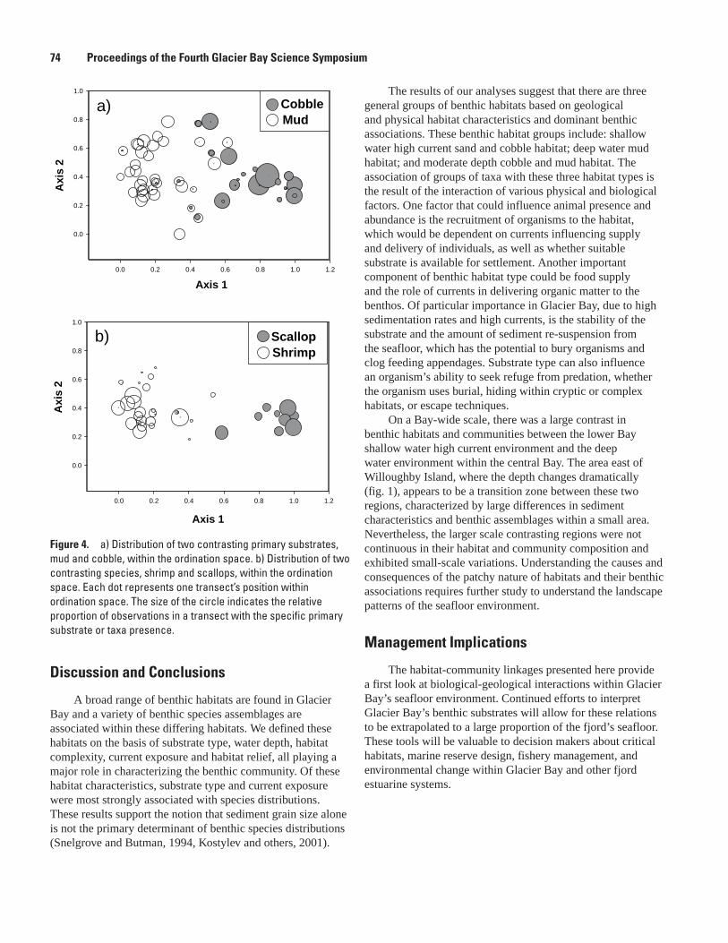
Discussion and Conclusions
A broad range of benthic habitats are found in Glacier Bay and a variety of benthic species assemblages are associated within these differing habitats. We defined these habitats on the basis of substrate type, water depth, habitat complexity, current exposure and habitat relief, all playing a major role in characterizing the benthic community. Of these habitat characteristics, substrate type and current exposure were most strongly associated with species distributions. These results support the notion that sediment grain size alone is not the primary determinant of benthic species distributions (Snelgrove and Butman, 1994, Kostylev and others, 2001).
The results of our analyses suggest that there are three general groups of benthic habitats based on geological and physical habitat characteristics and dominant benthic associations. These benthic habitat groups include: shallow water high current sand and cobble habitat; deep water mud habitat; and moderate depth cobble and mud habitat. The association of groups of taxa with these three habitat types is the result of the interaction of various physical and biological factors. One factor that could influence animal presence and abundance is the recruitment of organisms to the habitat, which would be dependent on currents influencing supply and delivery of individuals, as well as whether suitable substrate is available for settlement. Another important component of benthic habitat type could be food supply and the role of currents in delivering organic matter to the benthos. Of particular importance in Glacier Bay, due to high sedimentation rates and high currents, is the stability of the substrate and the amount of sediment re-suspension from the seafloor, which has the potential to bury organisms and clog feeding appendages. Substrate type can also influence an organism’s ability to seek refuge from predation, whether the organism uses burial, hiding within cryptic or complex habitats, or escape techniques.
On a Bay-wide scale, there was a large contrast in benthic habitats and communities between the lower Bay shallow water high current environment and the deep water environment within the central Bay. The area east of Willoughby Island, where the depth changes dramatically (fig. 1), appears to be a transition zone between these two regions, characterized by large differences in sediment characteristics and benthic assemblages within a small area. Nevertheless, the larger scale contrasting regions were not continuous in their habitat and community composition and exhibited small-scale variations. Understanding the causes and consequences of the patchy nature of habitats and their benthic associations requires further study to understand the landscape patterns of the seafloor environment.
Management Implications
The habitat-community linkages presented here provide a first look at biological-geological interactions within Glacier Bay’s seafloor environment. Continued efforts to interpret Glacier Bay’s benthic substrates will allow for these relations to be extrapolated to a large proportion of the fjord’s seafloor. These tools will be valuable to decision makers about critical habitats, marine reserve design, fishery management, and environmental change within Glacier Bay and other fjord estuarine systems.
7� Proceedings of the Fourth Glacier Bay Science Symposium
Figure �. a) Distribution of two contrasting primary substrates, mud and cobble, within the ordination space. b) Distribution of two contrasting species, shrimp and scallops, within the ordination space. Each dot represents one transect’s position within ordination space. The size of the circle indicates the relative proportion of observations in a transect with the specific primary substrate or taxa presence.
0.0 0.2 0.4 0.6 0.8 1.0 1.2
Axi
s2
0.0
0.2
0.4
0.6
0.8
1.0
Axis 1
CobbleMud
Axi
s2
Axis 1
0.0 0.2 0.4 0.6 0.8 1.0 1.2
0.0
0.2
0.4
0.6
0.8
1.0
ScallopShrimp
b)
a)
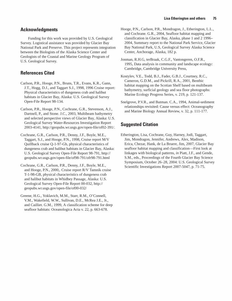
Lisa Etherington and others 75
Acknowledgments
Funding for this work was provided by U.S. Geological Survey. Logistical assistance was provided by Glacier Bay National Park and Preserve. This project represents integration between the Biologists of the Alaska Science Center and Geologists of the Coastal and Marine Geology Program of U.S. Geological Survey.
References Cited
Carlson, P.R., Hooge, P.N., Bruns, T.R., Evans, K.R., Gann, J.T., Hogg, D.J., and Taggart S.J., 1998, 1996 Cruise report: Physical characteristics of dungeness crab and halibut habitats in Glacier Bay, Alaska: U.S. Geological Survey Open-File Report 98-134.
Carlson, P.R., Hooge, P.N., Cochrane, G.R., Stevenson, A.J., Dartnell, P., and Stone. J.C., 2003, Multibeam bathymetry and selected perspective views of Glacier Bay, Alaska: U.S. Geological Survey Water-Resources Investigation Report 2003-4141, http://geopubs.wr.usgs.gov/open-file/of02-391/.
Cochrane, G.R., Carlson, P.R., Denny, J.F., Boyle, M.E., Taggart, S.J., and Hooge, P.N., 1998, Cruise report M/V Quillback cruise Q-1-97-Gb, physical characteristics of dungeness crab and halibut habitats in Glacier Bay, Alaska: U.S. Geological Survey Open-File Report 98-791, http://geopubs.wr.usgs.gov/open-file/of98-791/ofr98-791.html
Cochrane, G.R., Carlson, P.R., Denny, J.F., Boyle, M.E., and Hooge, P.N., 2000,. Cruise report R/V Tamnik cruise T-1-98-GB, physical characteristics of dungeness crab and halibut habitats in Whidbey Passage, Alaska: U.S. Geological Survey Open-File Report 00-032, http://geopubs.wr.usgs.gov/open-file/of00-032/
Greene, H.G., Yoklavich, M.M., Starr, R.M., O’Connell, V.M., Wakefield, W.W., Sullivan, D.E., McRea J.E., Jr., and Cailliet. G.M., 1999, A classification scheme for deep seafloor habitats: Oceanologica Acta v. 22, p. 663-678.
Hooge, P.N., Carlson, P.R., Mondragon, J., Etherington, L.L., and Cochrane. G.R., 2004, Seafloor habitat mapping and classification in Glacier Bay, Alaska, phase 1 and 2 1996–2004, Summary report to the National Park Service, Glacier Bay National Park, U.S, Geological Survey Alaska Science Center, Anchorage, Alaska, 182 p.
Jonman, R.H.G, terBraak, C.G.F., Vantongeren, O.F.R., 1995, Data analysis in community and landscape ecology: Cambridge, Cambridge University Press,
Kostylev, V.E., Todd, B.J., Fader, G.B.J., Courtney, R.C., Cameron, G.D.M., and Pickrill, R.A., 2001, Benthic habitat mapping on the Scotian Shelf based on multibeam bathymetry, surficial geology and sea floor photographs: Marine Ecology Progress Series, v. 219, p. 121-137.
Snelgrove, P.V.R., and Butman. C.A., 1994, Animal-sediment relationships revisited: Cause versus effect: Oceanography and Marine Biology Annual Review, v. 32, p. 111-177.
Suggested Citation
Etherington, Lisa, Cochrane, Guy, Harney, Jodi, Taggart, Jim, Mondragon, Jennifer, Andrews, Alex, Madison, Erica, Chezar, Hank, de La Bruere, Jim, 2007, Glacier Bay seafloor habitat mapping and classification—First look at linkages with biological patterns, in Piatt, J.F., and Gende, S.M., eds., Proceedings of the Fourth Glacier Bay Science Symposium, October 26–28, 2004: U.S. Geological Survey Scientific Investigations Report 2007-5047, p. 71-75.

Physical and Biological Oceanographic Patterns in Glacier Bay
Lisa L. Etherington1,4, Philip N. Hooge2, and Elizabeth R. Hooge3
Abstract. As part of a monitoring program, oceanographic sampling has been conducted at 23 stations within Glacier Bay from 1993-2002. Seasonal patterns of salinity, temperature, stratification, turbidity, and euphotic depth are related to seasonal patterns of modeled freshwater input for southeast Alaska. Spatial patterns of chlorophyll-a abundance vary throughout the season and are influenced by stratification levels and euphotic depth. High levels of freshwater discharge from upper Bay regions promote stratification from spring through fall, while strong tidal currents over shallow sills enhance mixing. Where these processes meet in the central Bay, there are optimal conditions of intermediate stratification, higher light levels, and potential nutrient renewal. These conditions may explain observed high and sustained chlorophyll-a levels, and provide a framework for understanding abundance and distribution of higher trophic levels within Glacier Bay.
Figure 1. Glacier Bay, Alaska, and the oceanographic sampling stations. Stations were grouped into four Regions and were defined as lower Bay (stations 0, 1, 2, 3), central Bay (stations 4, 5, 6, 13, 14, 15), West Arm (stations 7, 8, 9, 10, 11, 12, 21, 22, 23), and East Arm (stations 16, 17, 18, 19, 20).
7� Proceedings of the Fourth Glacier Bay Science Symposium
Gulf of Alaska
CrossSound
Icy Strait
West Arm
East Arm
GlacierBay
GeikieInlet
Tarr Inlet
Muir Inlet
SitakadayNarrows
21
12
11
10
9
8 7
6
22
23
5
4
20
19 18
17
16
1514
13
3
2
1
0
Regionslower Baycentral BayWest ArmEast Arm
0 10 km
Introduction
Oceanographic conditions in high latitude glacially fed estuaries are often complex, due to high rates of freshwater input, dramatic bathymetry (shallow sills and deep basins), and high sedimentation rates. Glacier Bay is a recently (<300 yrs. ago) deglaciated fjord surrounded by mountainous terrain with many sources of freshwater, mainly from glacial discharge (including 12 tidewater glaciers). Glacier Bay’s shallow sills (minimum depth = 25 m) are associated with strong currents and water column mixing, while deep basins (maximum depth = 450 m) exhibit stratification throughout much of the year. Previous work suggests that chlorophyll-a levels are relatively high and sustained through the summer season (Hooge and Hooge, written commun.).
This paper summarizes the results of a program to monitor oceanographic conditions at 23 stations throughout Glacier Bay from 1993–2002 (fig. 1). The objective of the current work was to quantify the seasonal and spatial patterns of physical oceanographic parameters and chlorophyll-a levels within Glacier Bay surface waters.
Methods
Physical and biological oceanographic samples were collected at 23 mid-channel stations spanning the axes of Glacier Bay (fig. 1). Each station was sampled approximately five times per year from 1993–2002. At each station, conductivity-temperature-depth samples were taken from the surface to the bottom of the water column (continuous record to maximum depth of 300 m). From these samples, we measured salinity, temperature, density (σ
t), fluorescence
1 U.S. Geological Survey, Alaska Science Center, P.O. Box 140, Gustavus, AK
2 Denali National Park and Preserve, P.O. Box 9, Denali Park, AK 99755
3 P.O. Box 94, Denali Park, AK 99755
4 Corresponding author: [email protected], 415-663-1443
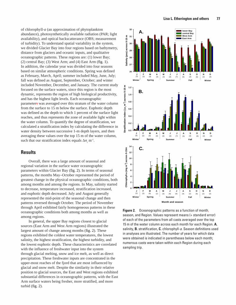
Figure 2. Oceanographic patterns as a function of month, season, and Region. Values represent means (+ standard error) of each of the parameters from all casts averaged over the top 15 m of the water column across each month for each Region. A. salinity, B. stratification, C. chlorophyll-a. Season definitions used in analyses are illustrated. The number of years for which data were obtained is indicated in parentheses below each month; numerous casts were taken within each Region during each sampling trip.
Lisa L. Etherington and others 77
of chlorophyll-a (an approximation of phytoplankton abundance), photosynthetically available radiation (PAR; light availability), and optical backscatterance (OBS; measurement of turbidity). To understand spatial variability in the system, we divided Glacier Bay into four regions based on bathymetry, distance from glaciers and oceanic inputs, and qualitative oceanographic patterns. These regions are: (1) lower Bay; (2) central Bay; (3) West Arm; and (4) East Arm (fig. 1). In addition, the calendar year was divided into four seasons based on similar atmospheric conditions. Spring was defined as February, March, April; summer included May, June, July; fall was defined as August, September, October; and winter included November, December, and January. The current study focused on the surface waters, since this region is the most dynamic, represents the region of high biological productivity, and has the highest light levels. Each oceanographic parameters was averaged over this stratum of the water column from the surface to 15 m below the surface. Euphotic depth was defined as the depth to which 1 percent of the surface light reaches, and thus represents the zone of available light within the water column. To quantify the degree of stratification, we calculated a stratification index by calculating the difference in water density between successive 1-m depth layers, and then averaging these values over the top 15 m of the water column, such that our stratification index equals Δσ
t m-1.
Results
Overall, there was a large amount of seasonal and regional variation in the surface water oceanographic parameters within Glacier Bay (fig. 2). In terms of seasonal patterns, the months May–October represented the period of greatest change in the physical oceanographic conditions, both among months and among the regions. In May, salinity started to decrease, temperature increased, stratification increased, and euphotic depth decreased. July and August generally represented the mid-point of the seasonal change and then patterns reversed through October. The period of November through April exhibited fairly homogeneous patterns in these oceanographic conditions both among months as well as among regions.
In general, the upper Bay regions closest to glacial sources (East Arm and West Arm regions) illustrated the largest amount of change among months (fig. 2). These regions exhibited the coldest water temperatures, the lowest salinity, the highest stratification, the highest turbidity, and the lowest euphotic depth. These characteristics are correlated with the influence of freshwater input into the system through glacial melting, snow and ice melt, as well as direct precipitation. These freshwater inputs are concentrated in the upper-most reaches of the fjord that are most influenced by glacial and snow melt. Despite the similarity in their relative position to glacial sources, the East and West regions exhibited substantial differences in oceanographic patterns, with the East Arm surface waters being fresher, more stratified, and more turbid (fig. 2).
J F M A M J J A S O N D
Salin
ity (p
su) a
cros
s 0-
15 m
26
27
28
29
30
31
32
Spring Summer FallWinter
(3) (2) (4) (3) (3) (3) (7) (5) (3) (6) (2) (3)
Winter
lower Baycentral BayWest ArmEast Arm
A.
J F M A M J J A S O N DStra
tific
atio
n in
dex
( t
m-1
) acr
oss
0-15
m
0.0
0.2
0.4
0.6
0.8
1.0
1.2
Spring Summer Fall WinterWinter
(3) (2) (4) (3) (3) (3) (7) (5) (3) (6) (2) (3)
Month and season
J F M A M J J A S O N D
Chl
orop
hyll-
a (m
g m
-3) a
cros
s 0-
15m
0
2
4
6
8
10
12
14
Spring Summer FallWinter
(2) (2) (5) (2) (3) (4) (6) (4) (2) (6) (2) (2)
Winter
C.
B.
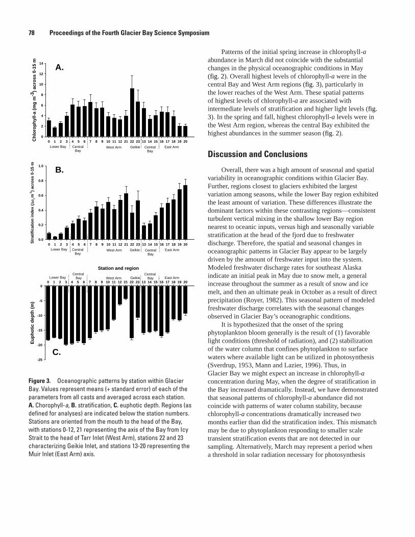
Figure �. Oceanographic patterns by station within Glacier Bay. Values represent means (+ standard error) of each of the parameters from all casts and averaged across each station. A. Chorophyll-a, B. stratification, C. euphotic depth. Regions (as defined for analyses) are indicated below the station numbers. Stations are oriented from the mouth to the head of the Bay, with stations 0-12, 21 representing the axis of the Bay from Icy Strait to the head of Tarr Inlet (West Arm), stations 22 and 23 characterizing Geikie Inlet, and stations 13-20 representing the Muir Inlet (East Arm) axis.
7� Proceedings of the Fourth Glacier Bay Science Symposium
0 1 2 3 4 5 6 7 8 9 10 11 12 21 22 23 13 14 15 16 17 18 19 20Chl
orop
hyll-
a (m
g m
-3) a
cros
s 0-
15 m
0
2
4
6
8
10
12
14
Lower Bay CentralBay
West Arm CentralBay
East ArmGeikie
0 1 2 3 4 5 6 7 8 9 10 11 12 21 22 23 13 14 15 16 17 18 19 20Stra
tific
atio
n in
dex
( t
m-1
) acr
oss
0-15
m
0.0
0.2
0.4
0.6
0.8
1.0
Lower Bay CentralBay
West Arm CentralBay
East ArmGeikie
Station and region
0 1 2 3 4 5 6 7 8 9 10 11 12 21 22 23 13 14 15 16 17 18 19 20
Euph
otic
dep
th (m
)
-25
-20
-15
-10
-5
0
Lower BayCentral
Bay West ArmCentral
Bay East ArmGeikie
C.
A.
B.
Patterns of the initial spring increase in chlorophyll-a abundance in March did not coincide with the substantial changes in the physical oceanographic conditions in May (fig. 2). Overall highest levels of chlorophyll-a were in the central Bay and West Arm regions (fig. 3), particularly in the lower reaches of the West Arm. These spatial patterns of highest levels of chlorophyll-a are associated with intermediate levels of stratification and higher light levels (fig. 3). In the spring and fall, highest chlorophyll-a levels were in the West Arm region, whereas the central Bay exhibited the highest abundances in the summer season (fig. 2).
Discussion and Conclusions
Overall, there was a high amount of seasonal and spatial variability in oceanographic conditions within Glacier Bay. Further, regions closest to glaciers exhibited the largest variation among seasons, while the lower Bay region exhibited the least amount of variation. These differences illustrate the dominant factors within these contrasting regions—consistent turbulent vertical mixing in the shallow lower Bay region nearest to oceanic inputs, versus high and seasonally variable stratification at the head of the fjord due to freshwater discharge. Therefore, the spatial and seasonal changes in oceanographic patterns in Glacier Bay appear to be largely driven by the amount of freshwater input into the system. Modeled freshwater discharge rates for southeast Alaska indicate an initial peak in May due to snow melt, a general increase throughout the summer as a result of snow and ice melt, and then an ultimate peak in October as a result of direct precipitation (Royer, 1982). This seasonal pattern of modeled freshwater discharge correlates with the seasonal changes observed in Glacier Bay’s oceanographic conditions.
It is hypothesized that the onset of the spring phytoplankton bloom generally is the result of (1) favorable light conditions (threshold of radiation), and (2) stabilization of the water column that confines phytoplankton to surface waters where available light can be utilized in photosynthesis (Sverdrup, 1953, Mann and Lazier, 1996). Thus, in Glacier Bay we might expect an increase in chlorophyll-a concentration during May, when the degree of stratification in the Bay increased dramatically. Instead, we have demonstrated that seasonal patterns of chlorophyll-a abundance did not coincide with patterns of water column stability, because chlorophyll-a concentrations dramatically increased two months earlier than did the stratification index. This mismatch may be due to phytoplankton responding to smaller scale transient stratification events that are not detected in our sampling. Alternatively, March may represent a period when a threshold in solar radiation necessary for photosynthesis
Lisa L. Etherington and others 79
is reached. Another study in a high latitude fjord system has demonstrated that incident light (rather than stratification) controls the initiation of the spring bloom (Ziemann and others, 1991).
Glacier Bay is a unique estuarine system with strong competing forces influencing water column stability. High levels of freshwater discharge from glacial melt and rainfall promote stratification, while strong tidal currents over shallow sills enhance vertical mixing. Where stabilizing and mixing forces meet, there are optimal conditions of intermediate stratification, higher light levels (due to decreased sediment concentrations), and potential nutrient renewal. These optimal conditions may explain the relatively high and sustained chlorophyll-a levels within particular regions of Glacier Bay. Further analyses will provide insight into the physical factors most influential in driving the oceanographic patterns detected in Glacier Bay
Management Implications
This summary of the oceanographic conditions within Glacier Bay highlights the utility of a monitoring program to understand the basic seasonal and spatial variability in some of the core physical processes that are influential in determining biological patterns within Glacier Bay. The results of this study emphasize the importance of freshwater input in driving the spatial and seasonal patterns in oceanographic conditions within the Bay, and highlight the role of climate and the terrestrial system in influencing Glacier Bay’s marine environment. Understanding these linkages provides insight into how this marine ecosystem potentially responds to changes in climate regimes. These findings further our understanding of physical-biological coupling in fjord estuaries and provide some probable explanations for the seasonal and regional patterns in higher trophic levels in this highly productive fjord estuarine system.
Acknowledgments
This study was completed with the financial and logistical support of Glacier Bay National Park and Preserve and the U.S. Geological Survey, Alaska Science Center. We would like to thank all those who participated in the sampling cruises throughout the years, particularly Jim de La Bruere, captain of the USGS R/V Alaskan Gyre, and Chohla Dick.
References Cited
Hooge, P.N., and Hooge, E.R., 2002, Fjord oceanographic processes in Glacier Bay, Alaska: U.S. Geological Survey, Alaska Science Center, Anchorage, AK, 142 p.
Mann, K.H., and Lazier, J.R.N., 1996, Dynamics of marine ecosystems: Biological-physical interactions in the oceans, 2nd ed.: Malden, Mass., Blackwell Science, Inc., 394 p.
Royer, T.C., 1982, Coastal freshwater discharge in the Northeast Pacific: Journal of Geophysical Research, v. 87, p. 2017–2021.
Sverdrup, H.U., 1953, On conditions for the vernal blooming of phytoplankton: Journal du Conseil Permanent, International pour l’Exploration de la Mer, v. 18, p. 287–295.
Ziemann, D.A., Conquest, L.D., Olaizola, M., and Bienfang, P.K., 1991. Interannual variability in the spring phytoplankton bloom in Auke Bay, Alaska: Marine Biology, v. 109, p. 321–334.
Suggested Citation
Etherington, L.L., Hooge, P.N., Hooge E.R., 2007, Physical and biological oceanographic patterns in Glacier Bay, in Piatt, J.F., and Gende, S.M., eds., Proceedings of the Fourth Glacier Bay Science Symposium, October 26–28, 2004: U.S. Geological Survey Scientific Investigations Report 2007-5047, p. 76-79.
A Transect of Glacier Bay Ocean Currents Measured by Acoustic Doppler Current Profiler (ADCP)
Edward D. Cokelet1,4, Antonio J. Jenkins2 and Lisa L. Etherington3
Abstract. We present one of the first shipboard acoustic Doppler current profiler (ADCP) transects of ocean current in Glacier Bay and Muir Inlet. The water temperature, salinity, nitrate plus nitrite concentration and chlorophyll fluorescence also were sampled underway at 5 m depth from the research vessel. These data were combined with conductivity-temperature-depth (CTD) sections made a fortnight later to provide a composite data set. The measurements show that the tidal flow accelerates over Glacier Bay’s shallow entrance sill to speeds of 180 cm/s and then slows to a few cm/s in the deeper basin beyond. The near-surface salinity was ~32 psu in Icy Strait and Sitakaday Narrows but freshened up the estuary to ~20 psu in patches, owing to glacial melt water. The nitrate plus nitrite concentration followed a similar pattern with enrichment (~19 μM) in the mixed water over the sill but then depletion (0-2 μM) in Glacier Bay, presumably due to phytoplankton consumption. We postulate that turbulence generated by strong currents over the shallow entrance sill to Glacier Bay mixes deeper, nutrient-rich water into the surface layers and fertilizes the fjord.
�0 Proceedings of the Fourth Glacier Bay Science Symposium
Introduction
In recent years, detailed studies of the water properties and density stratification in Glacier Bay. However, owing to a lack of resources and to the technical challenges of making ocean current measurements, little is known about current speeds in the fjord. Fortunately, at the end of a 23-day fisheries oceanography research cruise in the Gulf of Alaska, National Oceanic and Atmospheric Administration (NOAA) ship Miller Freeman had 15 hours of ship time to spare as she passed the bay’s entrance. Anticipating this we sought permission to enter Glacier Bay on August 8, 2003, and make underway observations.
Methods
The ADCP was an RD Instruments, 150-kHz, narrowband unit running Data Acquisition System (DAS) version 2.48 software. The ship’s heading was provided by a Sperry Mk 37 gyrocompass, and its position by a Northstar differential GPS receiver. DAS 2.48 also used the University of Hawaii’s CODAS User Exit 4 (UE4) to correct the computer’s clock to GPS time. Accurate heading data is vital to measuring currents with the ADCP because at typical research vessel speeds (10-12 kt), each 1° error in ship’s heading leads to a 10 cm/s false across-ship current. Therefore the goal is to reduce heading inaccuracy to 0.1° or less thus
giving 1 cm/s accuracy in ADCP currents. Miller Freeman carried a TSS POS/MV GPS-aided inertial navigation system for this purpose. It provided a heading accuracy of 0.02° throughout most of the cruise. Owing to other factors the current accuracy was probably 1-2 cm/s. The ADCP was set up with an 8 m pulse length and depth-bin thickness. The instrument remained in water track mode. ADCP eastward and northward velocity components were stored as 5-minute-averaged ensembles. The ADCP transducer was mounted on the ship’s centerboard at a nominal depth of 10 m below the waterline. With 4 m specified as blanking distance after ping transmission, the center depth of the first ADCP depth bin was 22 m. The depth range of the ADCP was about 350 m. ADCP data were averaged into 2 km segments along the ship track.
The near-surface temperature and salinity were measured electronically with a Sea-Bird thermosalinograph (TSG) in water pumped from the ship’s sea chest at a depth of 5 m. During the cruise in the Gulf of Alaska, 98 CTD casts were taken. The accurate CTD temperature was subsampled at 5 m and compared to the TSG temperature at the same times. A post-cruise linear regression (r2=0.98) of the two temperature time series gave a correction to the TSG temperature that took into account sensor differences between the two instruments and warming of the water between the sea chest and the TSG. TSG temperature accuracy was estimated to be about 0.1°C. The ship’s CTD salinity was corrected to water bottle samples analyzed with a salinometer. The CTD salinity at 5 m was then compared to the TSG salinity for all CTD casts. Linear regression (r2=0.98) between the two salinity time series gave a correction to the TSG salinity. Its accuracy was about 0.2 psu. The TSG measurements were recorded every 30 seconds on the shipboard Scientific Computer System.
1 National Oceanic and Atmospheric Administration, Pacific Marine Environmental Laboratory, 7600 Sand Point Way NE, Seattle, WA 98115
2 University of Washington, Joint Institute for the Study of the Atmosphere and Ocean, 7600 Sand Point Way NE, Seattle, WA 98115
3 U.S. Geological Survey, Alaska Science Center, Glacier Bay Field Station, P.O. Box 140, Gustavus, AK 99826
4 Corresponding author: [email protected], 206-526-6820
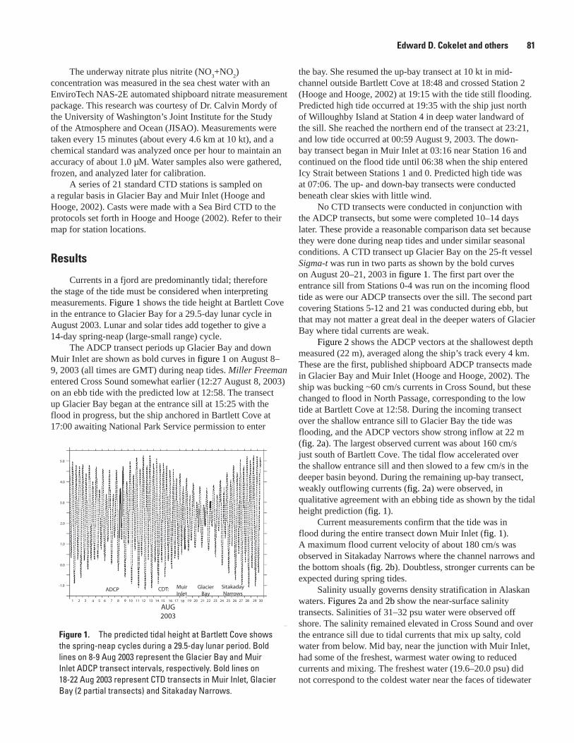
Figure 1. The predicted tidal height at Bartlett Cove shows the spring-neap cycles during a 29.5-day lunar period. Bold lines on 8-9 Aug 2003 represent the Glacier Bay and Muir Inlet ADCP transect intervals, respectively. Bold lines on 18-22 Aug 2003 represent CTD transects in Muir Inlet, Glacier Bay (2 partial transects) and Sitakaday Narrows.
1 2 3 4 5 6 7 8 9 10 11 12 13 14 15 16 17 18 19 20 21 22 23 24 25 26 27 28 29 30
ADCP CDT: MuirInlet
GlacierBay
SitakadayNarrows
-1.0
0.0
1.0
2.0
3.0
4.0
5.0
AUG2003
Edward D. Cokelet and others �1
The underway nitrate plus nitrite (NO3+NO
2)
concentration was measured in the sea chest water with an EnviroTech NAS-2E automated shipboard nitrate measurement package. This research was courtesy of Dr. Calvin Mordy of the University of Washington’s Joint Institute for the Study of the Atmosphere and Ocean (JISAO). Measurements were taken every 15 minutes (about every 4.6 km at 10 kt), and a chemical standard was analyzed once per hour to maintain an accuracy of about 1.0 μM. Water samples also were gathered, frozen, and analyzed later for calibration.
A series of 21 standard CTD stations is sampled on a regular basis in Glacier Bay and Muir Inlet (Hooge and Hooge, 2002). Casts were made with a Sea Bird CTD to the protocols set forth in Hooge and Hooge (2002). Refer to their map for station locations.
Results
Currents in a fjord are predominantly tidal; therefore the stage of the tide must be considered when interpreting measurements. Figure 1 shows the tide height at Bartlett Cove in the entrance to Glacier Bay for a 29.5-day lunar cycle in August 2003. Lunar and solar tides add together to give a 14-day spring-neap (large-small range) cycle.
The ADCP transect periods up Glacier Bay and down Muir Inlet are shown as bold curves in figure 1 on August 8–9, 2003 (all times are GMT) during neap tides. Miller Freeman entered Cross Sound somewhat earlier (12:27 August 8, 2003) on an ebb tide with the predicted low at 12:58. The transect up Glacier Bay began at the entrance sill at 15:25 with the flood in progress, but the ship anchored in Bartlett Cove at 17:00 awaiting National Park Service permission to enter
the bay. She resumed the up-bay transect at 10 kt in mid-channel outside Bartlett Cove at 18:48 and crossed Station 2 (Hooge and Hooge, 2002) at 19:15 with the tide still flooding. Predicted high tide occurred at 19:35 with the ship just north of Willoughby Island at Station 4 in deep water landward of the sill. She reached the northern end of the transect at 23:21, and low tide occurred at 00:59 August 9, 2003. The down-bay transect began in Muir Inlet at 03:16 near Station 16 and continued on the flood tide until 06:38 when the ship entered Icy Strait between Stations 1 and 0. Predicted high tide was at 07:06. The up- and down-bay transects were conducted beneath clear skies with little wind.
No CTD transects were conducted in conjunction with the ADCP transects, but some were completed 10–14 days later. These provide a reasonable comparison data set because they were done during neap tides and under similar seasonal conditions. A CTD transect up Glacier Bay on the 25-ft vessel Sigma-t was run in two parts as shown by the bold curves on August 20–21, 2003 in figure 1. The first part over the entrance sill from Stations 0-4 was run on the incoming flood tide as were our ADCP transects over the sill. The second part covering Stations 5-12 and 21 was conducted during ebb, but that may not matter a great deal in the deeper waters of Glacier Bay where tidal currents are weak.
Figure 2 shows the ADCP vectors at the shallowest depth measured (22 m), averaged along the ship’s track every 4 km. These are the first, published shipboard ADCP transects made in Glacier Bay and Muir Inlet (Hooge and Hooge, 2002). The ship was bucking ~60 cm/s currents in Cross Sound, but these changed to flood in North Passage, corresponding to the low tide at Bartlett Cove at 12:58. During the incoming transect over the shallow entrance sill to Glacier Bay the tide was flooding, and the ADCP vectors show strong inflow at 22 m (fig. 2a). The largest observed current was about 160 cm/s just south of Bartlett Cove. The tidal flow accelerated over the shallow entrance sill and then slowed to a few cm/s in the deeper basin beyond. During the remaining up-bay transect, weakly outflowing currents (fig. 2a) were observed, in qualitative agreement with an ebbing tide as shown by the tidal height prediction (fig. 1).
Current measurements confirm that the tide was in flood during the entire transect down Muir Inlet (fig. 1). A maximum flood current velocity of about 180 cm/s was observed in Sitakaday Narrows where the channel narrows and the bottom shoals (fig. 2b). Doubtless, stronger currents can be expected during spring tides.
Salinity usually governs density stratification in Alaskan waters. Figures 2a and 2b show the near-surface salinity transects. Salinities of 31–32 psu water were observed off shore. The salinity remained elevated in Cross Sound and over the entrance sill due to tidal currents that mix up salty, cold water from below. Mid bay, near the junction with Muir Inlet, had some of the freshest, warmest water owing to reduced currents and mixing. The freshest water (19.6–20.0 psu) did not correspond to the coldest water near the faces of tidewater
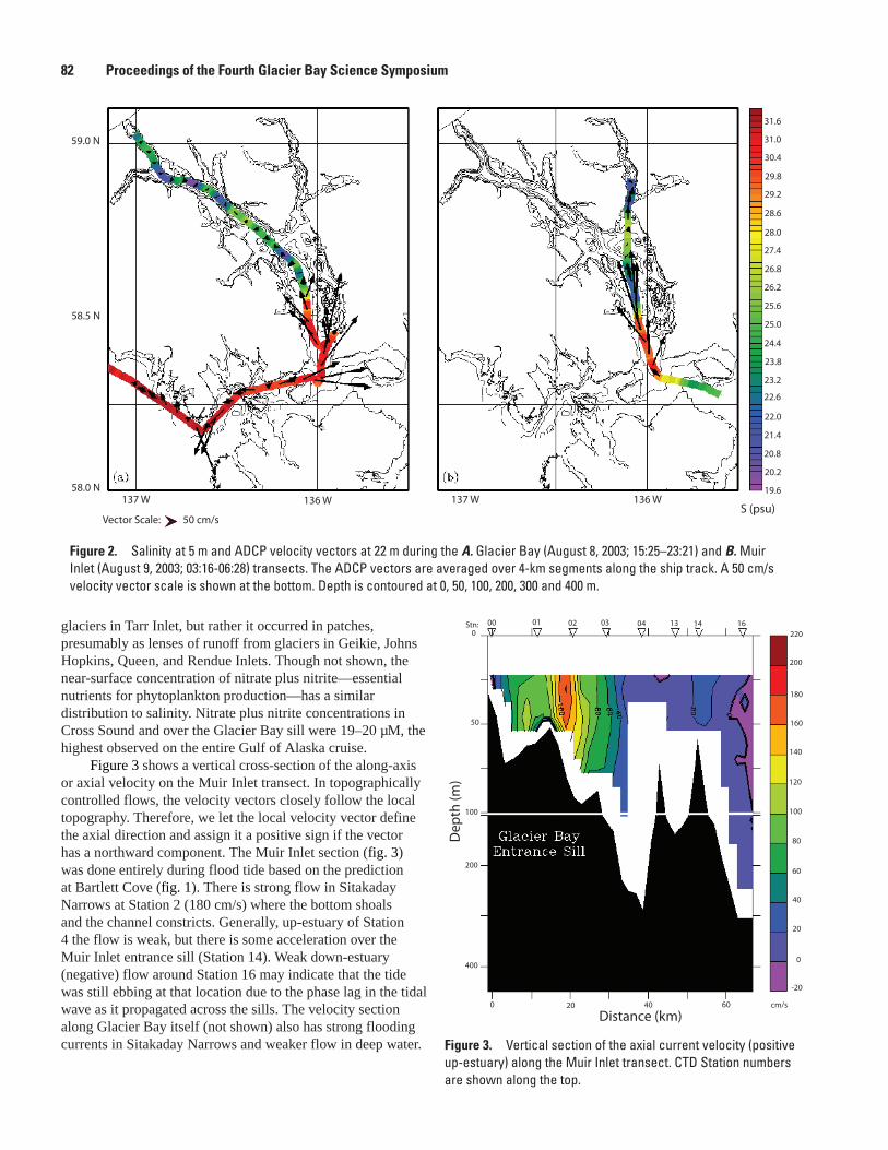
Figure 2. Salinity at 5 m and ADCP velocity vectors at 22 m during the A. Glacier Bay (August 8, 2003; 15:25–23:21) and B. Muir Inlet (August 9, 2003; 03:16-06:28) transects. The ADCP vectors are averaged over 4-km segments along the ship track. A 50 cm/s velocity vector scale is shown at the bottom. Depth is contoured at 0, 50, 100, 200, 300 and 400 m.
Figure �. Vertical section of the axial current velocity (positive up-estuary) along the Muir Inlet transect. CTD Station numbers are shown along the top.
cm/s6040200
400
200
100
50
0Stn: 00 01 02 03 04 13 14 16
220
200
180
160
140
120
100
80
60
40
20
0
-20
Distance (km)
Dep
th (m
)
59.0 N
58.5 N
58.0 N136 W137 W136 W137 W
Vector Scale: 50 cm/sS (psu)
31.6
31.0
30.4
29.8
29.2
28.6
28.0
27.4
26.8
26.2
25.6
25.0
24.4
23.8
23.2
22.6
22.0
21.4
20.8
20.2
19.6
�2 Proceedings of the Fourth Glacier Bay Science Symposium
glaciers in Tarr Inlet, but rather it occurred in patches, presumably as lenses of runoff from glaciers in Geikie, Johns Hopkins, Queen, and Rendue Inlets. Though not shown, the near-surface concentration of nitrate plus nitrite—essential nutrients for phytoplankton production—has a similar distribution to salinity. Nitrate plus nitrite concentrations in Cross Sound and over the Glacier Bay sill were 19–20 μM, the highest observed on the entire Gulf of Alaska cruise.
Figure 3 shows a vertical cross-section of the along-axis or axial velocity on the Muir Inlet transect. In topographically controlled flows, the velocity vectors closely follow the local topography. Therefore, we let the local velocity vector define the axial direction and assign it a positive sign if the vector has a northward component. The Muir Inlet section (fig. 3) was done entirely during flood tide based on the prediction at Bartlett Cove (fig. 1). There is strong flow in Sitakaday Narrows at Station 2 (180 cm/s) where the bottom shoals and the channel constricts. Generally, up-estuary of Station 4 the flow is weak, but there is some acceleration over the Muir Inlet entrance sill (Station 14). Weak down-estuary (negative) flow around Station 16 may indicate that the tide was still ebbing at that location due to the phase lag in the tidal wave as it propagated across the sills. The velocity section along Glacier Bay itself (not shown) also has strong flooding currents in Sitakaday Narrows and weaker flow in deep water.

Figure 4 shows a vertical cross-section of salinity from the CTD sections of August 20–21 (fig. 1). Though a section along the west arm of Glacier Bay and not simultaneous with the velocity section (fig. 3), it is probably similar with salinity stratification up-estuary of the entrance sill and weaker stratification over the sill due to turbulent mixing caused by strong tidal currents. Several isohalines intersect the free surface near Station 0 which indicates a sharp frontal zone there. Salinity (and density) gradients are weak in the deep water. (Salinity inversions in the deep water along the 31.0 psu surface are suspect. The CTD measurements may not have sufficient accuracy in these weak-gradient regions.).
Discussion And Conclusions
Although the data set is preliminary and very short, it represents the first snapshot of tidal currents in Glacier Bay. Our data indicate that strong currents exist over shallow sills and in narrow channels. They also demonstrate the importance of the tidal phase in determining flow direction. On the outgoing transect, fresher water was seen in Icy Strait than over the Glacier Bay sill or in nearby Cross Sound. If this were generally the case, then it would imply that the salty, oceanic water mixed up from depth in Cross Sound is the nutrient-rich source water for Glacier Bay. Therefore, two factors would be at work: Cross Sound would provide a source of deep oceanic water in close proximity to Glacier Bay, and strong tidal currents would mix it up for entry into the bay.
Management Implications
Currents affect a marine ecosystem in four ways: (1) seawater flow combines with freshwater from runoff and glacial melt to determine water properties—basic ecosystem parameters. (2) Currents affect phytoplankton productivity—the base of the oceanic food chain. They can enhance photosynthesis by mixing nutrient-rich water from depth into upper waters where sufficient light is available. However, mixing also can transport phytoplankton below the photic zone and quench primary production. (3) Currents transport larval fish and crustaceans. (4) Currents affect benthic habitat by sediment transport and scour. Understanding the current field will lead to improved ecosystem understanding and better estuarine management.
0 20 40 60 80 100
400
200
100
50
0Stn: 00 01 02 03 04 05 06 07 08 09 10 11 12 21
32.0
31.5
31.0
30.5
30.0
29.5
29.0
28.5
28.0
psu
Distance (km)
Dep
th (m
)
Figure �. Vertical section of salinity along the Glacier Bay transect. CTD Station numbers are shown along the top.
Edward D. Cokelet and others ��
Acknowledgments
We thank the captain and crew of NOAA Ship Miller Freeman, Bill Floering for his hard work and oceanographic expertise on the cruise, Gary Stauffer for obtaining ship time, Calvin Mordy for nutrient measurements, Jeff Napp and Colleen Harpold for chlorophyll analyses, Mary Kralovec for granting permission for Miller Freeman to enter Glacier Bay, Jennifer Mondragon for bathymetric data, Hope Rieden for CTD casts and processing. The Miller Freeman cruise was sponsored by NOAA’s Ocean Carrying Capacity (OCC) and Global Ocean Ecosystem Dynamics (GLOBEC) programs. This is NOAA/PMEL contribution 2912, NOAA Fisheries-Oceanography Coordinated Investigations contribution FOCI-590, and GLOBEC contribution 284.
Suggested Citation
Cokelet, E.D., Jenkins, A.J., and Etherington, L.L., 2007, A transect of Glacier Bay ocean currents measured by acoustic Doppler current profiler (ADCP), in Piatt, J.F., and Gende, S.M., eds., Proceedings of the Fourth Glacier Bay Science Symposium, October 26–28, 2004: U.S. Geological Survey Scientific Investigations Report 2007-5047, p. 80-83.
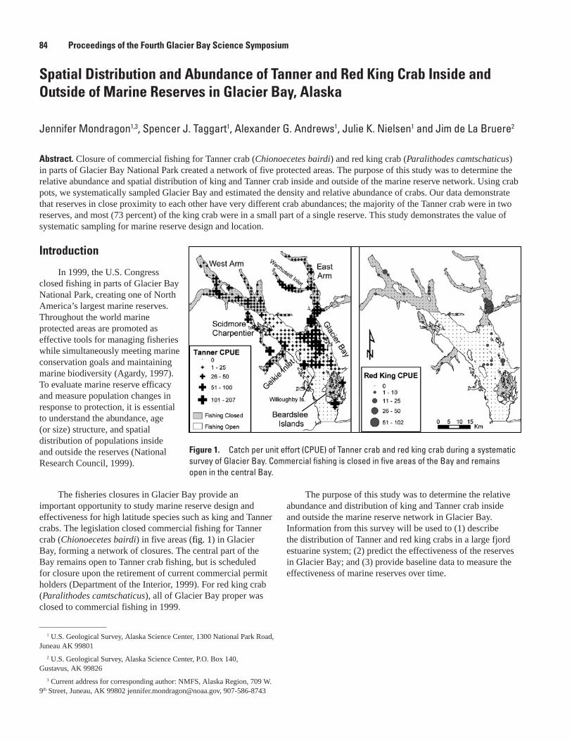
Spatial Distribution and Abundance of Tanner and Red King Crab Inside and Outside of Marine Reserves in Glacier Bay, Alaska
Jennifer Mondragon1,3, Spencer J. Taggart1, Alexander G. Andrews1, Julie K. Nielsen1 and Jim de La Bruere2
Abstract. Closure of commercial fishing for Tanner crab (Chionoecetes bairdi) and red king crab (Paralithodes camtschaticus) in parts of Glacier Bay National Park created a network of five protected areas. The purpose of this study was to determine the relative abundance and spatial distribution of king and Tanner crab inside and outside of the marine reserve network. Using crab pots, we systematically sampled Glacier Bay and estimated the density and relative abundance of crabs. Our data demonstrate that reserves in close proximity to each other have very different crab abundances; the majority of the Tanner crab were in two reserves, and most (73 percent) of the king crab were in a small part of a single reserve. This study demonstrates the value of systematic sampling for marine reserve design and location.
Figure 1. Catch per unit effort (CPUE) of Tanner crab and red king crab during a systematic survey of Glacier Bay. Commercial fishing is closed in five areas of the Bay and remains open in the central Bay.
�� Proceedings of the Fourth Glacier Bay Science Symposium
Introduction
In 1999, the U.S. Congress closed fishing in parts of Glacier Bay National Park, creating one of North America’s largest marine reserves. Throughout the world marine protected areas are promoted as effective tools for managing fisheries while simultaneously meeting marine conservation goals and maintaining marine biodiversity (Agardy, 1997). To evaluate marine reserve efficacy and measure population changes in response to protection, it is essential to understand the abundance, age (or size) structure, and spatial distribution of populations inside and outside the reserves (National Research Council, 1999).
The fisheries closures in Glacier Bay provide an important opportunity to study marine reserve design and effectiveness for high latitude species such as king and Tanner crabs. The legislation closed commercial fishing for Tanner crab (Chionoecetes bairdi) in five areas (fig. 1) in Glacier Bay, forming a network of closures. The central part of the Bay remains open to Tanner crab fishing, but is scheduled for closure upon the retirement of current commercial permit holders (Department of the Interior, 1999). For red king crab (Paralithodes camtschaticus), all of Glacier Bay proper was closed to commercial fishing in 1999.
1 U.S. Geological Survey, Alaska Science Center, 1300 National Park Road, Juneau AK 99801
2 U.S. Geological Survey, Alaska Science Center, P.O. Box 140, Gustavus, AK 99826
3 Current address for corresponding author: NMFS, Alaska Region, 709 W. 9th Street, Juneau, AK 99802 [email protected], 907-586-8743
The purpose of this study was to determine the relative abundance and distribution of king and Tanner crab inside and outside the marine reserve network in Glacier Bay. Information from this survey will be used to (1) describe the distribution of Tanner and red king crabs in a large fjord estuarine system; (2) predict the effectiveness of the reserves in Glacier Bay; and (3) provide baseline data to measure the effectiveness of marine reserves over time.
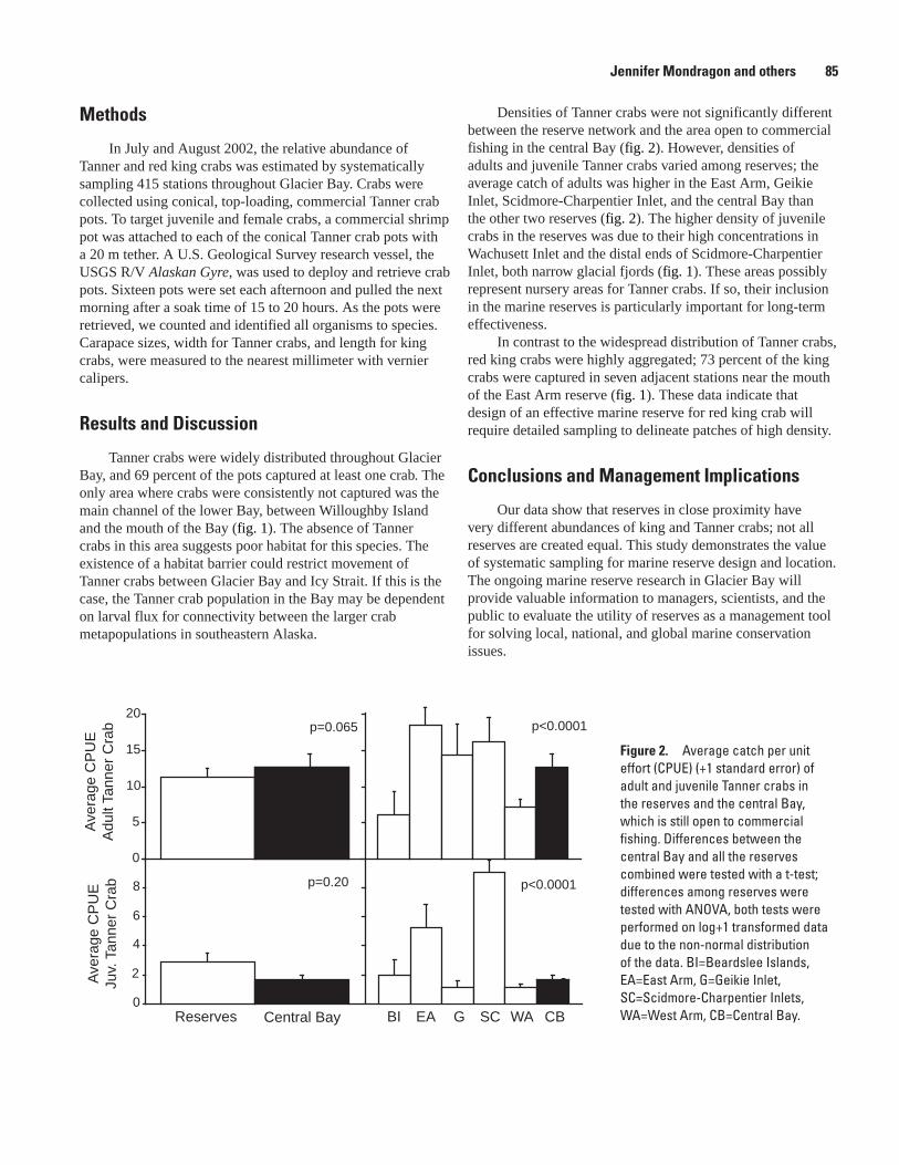
0
5
10
15
20
2
4
6
8
0
Aver
age
CP
UE
Juv.
Tan
ner C
rab
Aver
age
CP
UE
Adu
lt Ta
nner
Cra
b
Reserves Central Bay BI EA G SC WA CB
p=0.065 p<0.0001
p=0.20 p<0.0001
Figure 2. Average catch per unit effort (CPUE) (+1 standard error) of adult and juvenile Tanner crabs in the reserves and the central Bay, which is still open to commercial fishing. Differences between the central Bay and all the reserves combined were tested with a t-test; differences among reserves were tested with ANOVA, both tests were performed on log+1 transformed data due to the non-normal distribution of the data. BI=Beardslee Islands, EA=East Arm, G=Geikie Inlet, SC=Scidmore-Charpentier Inlets, WA=West Arm, CB=Central Bay.
Jennifer Mondragon and others �5
Methods
In July and August 2002, the relative abundance of Tanner and red king crabs was estimated by systematically sampling 415 stations throughout Glacier Bay. Crabs were collected using conical, top-loading, commercial Tanner crab pots. To target juvenile and female crabs, a commercial shrimp pot was attached to each of the conical Tanner crab pots with a 20 m tether. A U.S. Geological Survey research vessel, the USGS R/V Alaskan Gyre, was used to deploy and retrieve crab pots. Sixteen pots were set each afternoon and pulled the next morning after a soak time of 15 to 20 hours. As the pots were retrieved, we counted and identified all organisms to species. Carapace sizes, width for Tanner crabs, and length for king crabs, were measured to the nearest millimeter with vernier calipers.
Results and Discussion
Tanner crabs were widely distributed throughout Glacier Bay, and 69 percent of the pots captured at least one crab. The only area where crabs were consistently not captured was the main channel of the lower Bay, between Willoughby Island and the mouth of the Bay (fig. 1). The absence of Tanner crabs in this area suggests poor habitat for this species. The existence of a habitat barrier could restrict movement of Tanner crabs between Glacier Bay and Icy Strait. If this is the case, the Tanner crab population in the Bay may be dependent on larval flux for connectivity between the larger crab metapopulations in southeastern Alaska.
Densities of Tanner crabs were not significantly different between the reserve network and the area open to commercial fishing in the central Bay (fig. 2). However, densities of adults and juvenile Tanner crabs varied among reserves; the average catch of adults was higher in the East Arm, Geikie Inlet, Scidmore-Charpentier Inlet, and the central Bay than the other two reserves (fig. 2). The higher density of juvenile crabs in the reserves was due to their high concentrations in Wachusett Inlet and the distal ends of Scidmore-Charpentier Inlet, both narrow glacial fjords (fig. 1). These areas possibly represent nursery areas for Tanner crabs. If so, their inclusion in the marine reserves is particularly important for long-term effectiveness.
In contrast to the widespread distribution of Tanner crabs, red king crabs were highly aggregated; 73 percent of the king crabs were captured in seven adjacent stations near the mouth of the East Arm reserve (fig. 1). These data indicate that design of an effective marine reserve for red king crab will require detailed sampling to delineate patches of high density.
Conclusions and Management Implications
Our data show that reserves in close proximity have very different abundances of king and Tanner crabs; not all reserves are created equal. This study demonstrates the value of systematic sampling for marine reserve design and location. The ongoing marine reserve research in Glacier Bay will provide valuable information to managers, scientists, and the public to evaluate the utility of reserves as a management tool for solving local, national, and global marine conservation issues.
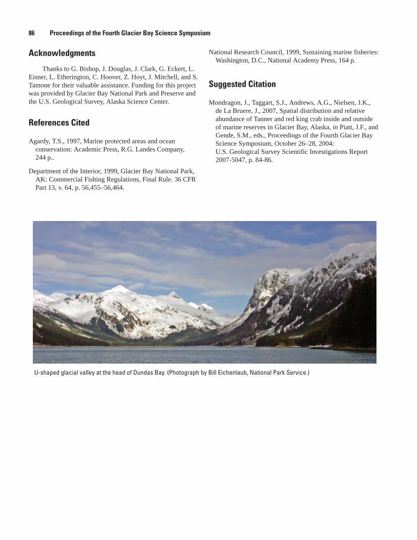
�� Proceedings of the Fourth Glacier Bay Science Symposium
U-shaped glacial valley at the head of Dundas Bay. (Photograph by Bill Eichenlaub, National Park Service.)
Acknowledgments
Thanks to G. Bishop, J. Douglas, J. Clark, G. Eckert, L. Eisner, L. Etherington, C. Hoover, Z. Hoyt, J. Mitchell, and S. Tamone for their valuable assistance. Funding for this project was provided by Glacier Bay National Park and Preserve and the U.S. Geological Survey, Alaska Science Center.
References Cited
Agardy, T.S., 1997, Marine protected areas and ocean conservation: Academic Press, R.G. Landes Company, 244 p..
Department of the Interior, 1999, Glacier Bay National Park, AK: Commercial Fishing Regulations, Final Rule. 36 CFR Part 13, v. 64, p. 56,455–56,464.
National Research Council, 1999, Sustaining marine fisheries: Washington, D.C., National Academy Press, 164 p.
Suggested Citation
Mondragon, J., Taggart, S.J., Andrews, A.G., Nielsen, J.K., de La Bruere, J., 2007, Spatial distribution and relative abundance of Tanner and red king crab inside and outside of marine reserves in Glacier Bay, Alaska, in Piatt, J.F., and Gende, S.M., eds., Proceedings of the Fourth Glacier Bay Science Symposium, October 26–28, 2004: U.S. Geological Survey Scientific Investigations Report 2007-5047, p. 84-86.
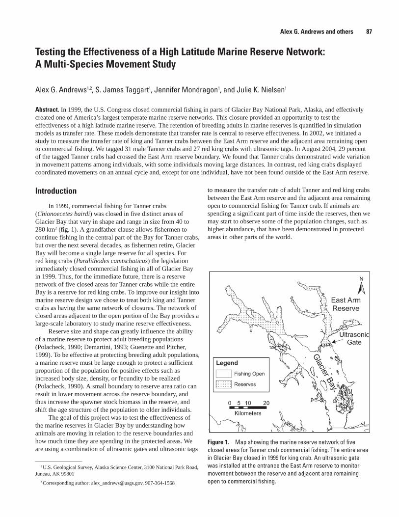
Testing the Effectiveness of a High Latitude Marine Reserve Network: A Multi-Species Movement Study
Alex G. Andrews1,2, S. James Taggart1, Jennifer Mondragon1, and Julie K. Nielsen1
Abstract. In 1999, the U.S. Congress closed commercial fishing in parts of Glacier Bay National Park, Alaska, and effectively created one of America’s largest temperate marine reserve networks. This closure provided an opportunity to test the effectiveness of a high latitude marine reserve. The retention of breeding adults in marine reserves is quantified in simulation models as transfer rate. These models demonstrate that transfer rate is central to reserve effectiveness. In 2002, we initiated a study to measure the transfer rate of king and Tanner crabs between the East Arm reserve and the adjacent area remaining open to commercial fishing. We tagged 31 male Tanner crabs and 27 red king crabs with ultrasonic tags. In August 2004, 29 percent of the tagged Tanner crabs had crossed the East Arm reserve boundary. We found that Tanner crabs demonstrated wide variation in movement patterns among individuals, with some individuals moving large distances. In contrast, red king crabs displayed coordinated movements on an annual cycle and, except for one individual, have not been found outside of the East Arm reserve.
Alex G. Andrews and others �7
1 U.S. Geological Survey, Alaska Science Center, 3100 National Park Road, Juneau, AK 99801
2 Corresponding author: [email protected], 907-364-1568
Introduction
In 1999, commercial fishing for Tanner crabs (Chionoecetes bairdi) was closed in five distinct areas of Glacier Bay that vary in shape and range in size from 40 to 280 km2 (fig. 1). A grandfather clause allows fishermen to continue fishing in the central part of the Bay for Tanner crabs, but over the next several decades, as fishermen retire, Glacier Bay will become a single large reserve for all species. For red king crabs (Paralithodes camtschaticus) the legislation immediately closed commercial fishing in all of Glacier Bay in 1999. Thus, for the immediate future, there is a reserve network of five closed areas for Tanner crabs while the entire Bay is a reserve for red king crabs. To improve our insight into marine reserve design we chose to treat both king and Tanner crabs as having the same network of closures. The network of closed areas adjacent to the open portion of the Bay provides a large-scale laboratory to study marine reserve effectiveness.
Reserve size and shape can greatly influence the ability of a marine reserve to protect adult breeding populations (Polacheck, 1990; Demartini, 1993; Guenette and Pitcher, 1999). To be effective at protecting breeding adult populations, a marine reserve must be large enough to protect a sufficient proportion of the population for positive effects such as increased body size, density, or fecundity to be realized (Polacheck, 1990). A small boundary to reserve area ratio can result in lower movement across the reserve boundary, and thus increase the spawner stock biomass in the reserve, and shift the age structure of the population to older individuals.
The goal of this project was to test the effectiveness of the marine reserves in Glacier Bay by understanding how animals are moving in relation to the reserve boundaries and how much time they are spending in the protected areas. We are using a combination of ultrasonic gates and ultrasonic tags
Figure 1. Map showing the marine reserve network of five closed areas for Tanner crab commercial fishing. The entire area in Glacier Bay closed in 1999 for king crab. An ultrasonic gate was installed at the entrance the East Arm reserve to monitor movement between the reserve and adjacent area remaining open to commercial fishing.
to measure the transfer rate of adult Tanner and red king crabs between the East Arm reserve and the adjacent area remaining open to commercial fishing for Tanner crab. If animals are spending a significant part of time inside the reserves, then we may start to observe some of the population changes, such as higher abundance, that have been demonstrated in protected areas in other parts of the world.
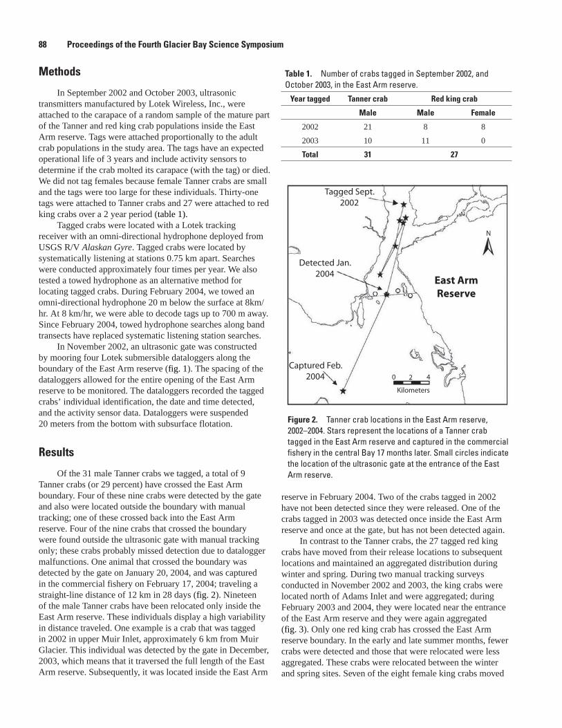
Methods
In September 2002 and October 2003, ultrasonic transmitters manufactured by Lotek Wireless, Inc., were attached to the carapace of a random sample of the mature part of the Tanner and red king crab populations inside the East Arm reserve. Tags were attached proportionally to the adult crab populations in the study area. The tags have an expected operational life of 3 years and include activity sensors to determine if the crab molted its carapace (with the tag) or died. We did not tag females because female Tanner crabs are small and the tags were too large for these individuals. Thirty-one tags were attached to Tanner crabs and 27 were attached to red king crabs over a 2 year period (table 1).
Tagged crabs were located with a Lotek tracking receiver with an omni-directional hydrophone deployed from USGS R/V Alaskan Gyre. Tagged crabs were located by systematically listening at stations 0.75 km apart. Searches were conducted approximately four times per year. We also tested a towed hydrophone as an alternative method for locating tagged crabs. During February 2004, we towed an omni-directional hydrophone 20 m below the surface at 8km/hr. At 8 km/ hr, we were able to decode tags up to 700 m away. Since February 2004, towed hydrophone searches along band transects have replaced systematic listening station searches.
In November 2002, an ultrasonic gate was constructed by mooring four Lotek submersible dataloggers along the boundary of the East Arm reserve (fig. 1). The spacing of the dataloggers allowed for the entire opening of the East Arm reserve to be monitored. The dataloggers recorded the tagged crabs’ individual identification, the date and time detected, and the activity sensor data. Dataloggers were suspended 20 meters from the bottom with subsurface flotation.
Results
Of the 31 male Tanner crabs we tagged, a total of 9 Tanner crabs (or 29 percent) have crossed the East Arm boundary. Four of these nine crabs were detected by the gate and also were located outside the boundary with manual tracking; one of these crossed back into the East Arm reserve. Four of the nine crabs that crossed the boundary were found outside the ultrasonic gate with manual tracking only; these crabs probably missed detection due to datalogger malfunctions. One animal that crossed the boundary was detected by the gate on January 20, 2004, and was captured in the commercial fishery on February 17, 2004; traveling a straight-line distance of 12 km in 28 days (fig. 2). Nineteen of the male Tanner crabs have been relocated only inside the East Arm reserve. These individuals display a high variability in distance traveled. One example is a crab that was tagged in 2002 in upper Muir Inlet, approximately 6 km from Muir Glacier. This individual was detected by the gate in December, 2003, which means that it traversed the full length of the East Arm reserve. Subsequently, it was located inside the East Arm
reserve in February 2004. Two of the crabs tagged in 2002 have not been detected since they were released. One of the crabs tagged in 2003 was detected once inside the East Arm reserve and once at the gate, but has not been detected again.
In contrast to the Tanner crabs, the 27 tagged red king crabs have moved from their release locations to subsequent locations and maintained an aggregated distribution during winter and spring. During two manual tracking surveys conducted in November 2002 and 2003, the king crabs were located north of Adams Inlet and were aggregated; during February 2003 and 2004, they were located near the entrance of the East Arm reserve and they were again aggregated (fig. 3). Only one red king crab has crossed the East Arm reserve boundary. In the early and late summer months, fewer crabs were detected and those that were relocated were less aggregated. These crabs were relocated between the winter and spring sites. Seven of the eight female king crabs moved
Figure 2. Tanner crab locations in the East Arm reserve, 2002–2004. Stars represent the locations of a Tanner crab tagged in the East Arm reserve and captured in the commercial fishery in the central Bay 17 months later. Small circles indicate the location of the ultrasonic gate at the entrance of the East Arm reserve.
�� Proceedings of the Fourth Glacier Bay Science Symposium
Captured Feb.2004
Detected Jan.2004
Tagged Sept.2002
East ArmReserve
Kilometers
0 2 4
N
Table 1. Number of crabs tagged in September 2002, and October 2003, in the East Arm reserve.
Year tagged Tanner crab Red king crab
Male Male Female
2002 21 8 8
2003 10 11 0
Total �1 27

Figure �. East Arm reserve at Adams Inlet displaying the two areas of high seasonal use by red king crab. Large circles highlight areas. Small circles indicate the location of the ultrasonic gate at the entrance of the East Arm reserve.
Alex G. Andrews and others �9
Tracking Trip
Feb 03
Feb 04
Nov 02
Nov 03
East ArmReserve
Kilometers
0 2 4
N
to the entrance of the East Arm reserve and many have been relocated at this location and display no activity (i.e., crab molted it’s carapace or died).
Discussion and Conclusions
The combination of the ultrasonic gate and towed hydrophone searches made it possible to estimate the movements of crabs at a population level. Our data of Tanner crab movement demonstrate that there is large variation in distance and direction traveled among individual crabs. Three of the crabs tagged in 2003 moved to the mouth of the East Arm and were detected by the ultrasonic gate. These data demonstrate that Tanner crabs are able to move considerable distances in a short time and support the hypothesis that crabs not detected since their release in 2002 may have left the East Arm reserve before the ultrasonic gate was functional. Therefore, the number of tagged Tanner crabs detected crossing the boundary may be an underestimate of the actual number that crossed. Tanner crab movements encompassed an area larger than the East Arm reserve; therefore, the East Arm reserve may not adequately protect the Tanner crab population. Further research would be beneficial to address the movements of Tanner crabs in relation to the entrance of Glacier Bay to determine how the Bay as a whole will protect Tanner crabs.
Multi-year relocations of tagged king crabs demonstrate that the crabs migrate seasonally between the area north of Adams Inlet and the entrance of the East Arm reserve. Seven of the eight tagged females presumably molted their tags at the entrance of the East Arm reserve. This suggests that this area may be an important reproductive habitat because female king crabs molt their exoskeletons before mating and extruding eggs. It is inconclusive where the king crabs reside during the summer and whether they maintain an aggregated distribution as they move seasonally between Adams Inlet and the entrance of the East Arm reserve. Coordinated movements of adult king crabs have been previously documented in Auke Bay, Alaska (Stone and others, 1992). Our findings in Glacier Bay may have important management implications in the southeast Alaska fishery. For example, it may be feasible to close relatively small areas to the commercial fishery to protect important aggregations of adult king crabs.
Acknowledgments
Thanks to all the field crews. We especially thank Captain Jim de La Bruere for his expertise in boat handling. Funding for this work was provided by the U.S. Geological Survey, Alaska Science Center and the National Park Science Foundation.
References Cited
Demartini, E.E., 1993, Modeling the potential of fishery reserves for managing Pacific coral reef fishes: Fishery Bulletin, v. 91, p. 414-427.
Guenette, S., and Pitcher, T.J., 1999, An age-structured model showing the benefits of marine reserves in controlling overexploitation: Amsterdam, Fisheries Research, v. 39, p. 295-303.
Polacheck, T., 1990, Year round closed areas as a management tool: Natural Resource Modeling, v. 4, p. 327-354.
Stone, R.P., O’Clair, C.E., and Shirley, T.C., 1992, Seasonal migration and distribution of female red king crabs in a southeast Alaskan estuary: Journal of Crustacean Biology, v. 12, no. 4, p. 546-560.
Suggested Citation
Andrews, A.G., Taggart, S.J., Mondragon, J., Nielsen, J.K., 2007, Testing the effectiveness of a high latitude marine reserve network: a multi-species movement study, in Piatt, J.F., and Gende, S.M., eds., Proceedings of the Fourth Glacier Bay Science Symposium, October 26–28, 2004: U.S. Geological Survey Scientific Investigations Report 2007-5047, p. 87-89.
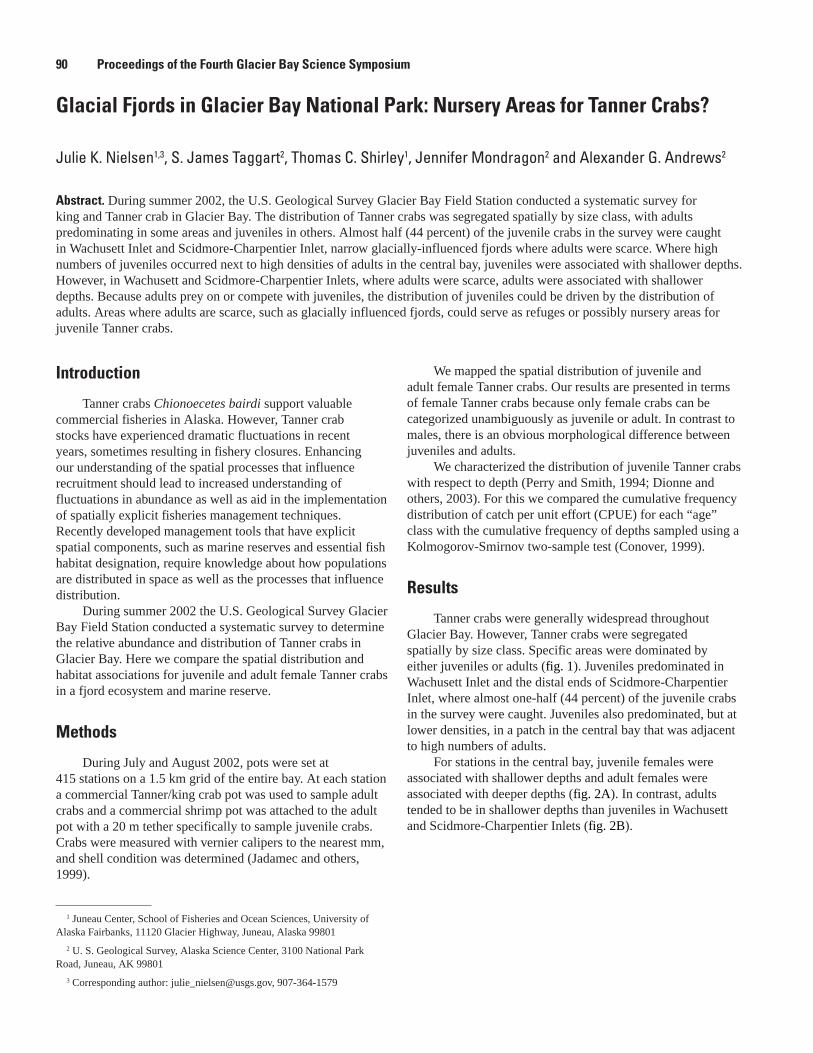
Glacial Fjords in Glacier Bay National Park: Nursery Areas for Tanner Crabs?
Julie K. Nielsen1,3, S. James Taggart2, Thomas C. Shirley1, Jennifer Mondragon2 and Alexander G. Andrews2
Abstract. During summer 2002, the U.S. Geological Survey Glacier Bay Field Station conducted a systematic survey for king and Tanner crab in Glacier Bay. The distribution of Tanner crabs was segregated spatially by size class, with adults predominating in some areas and juveniles in others. Almost half (44 percent) of the juvenile crabs in the survey were caught in Wachusett Inlet and Scidmore-Charpentier Inlet, narrow glacially-influenced fjords where adults were scarce. Where high numbers of juveniles occurred next to high densities of adults in the central bay, juveniles were associated with shallower depths. However, in Wachusett and Scidmore-Charpentier Inlets, where adults were scarce, adults were associated with shallower depths. Because adults prey on or compete with juveniles, the distribution of juveniles could be driven by the distribution of adults. Areas where adults are scarce, such as glacially influenced fjords, could serve as refuges or possibly nursery areas for juvenile Tanner crabs.
90 Proceedings of the Fourth Glacier Bay Science Symposium
Introduction
Tanner crabs Chionoecetes bairdi support valuable commercial fisheries in Alaska. However, Tanner crab stocks have experienced dramatic fluctuations in recent years, sometimes resulting in fishery closures. Enhancing our understanding of the spatial processes that influence recruitment should lead to increased understanding of fluctuations in abundance as well as aid in the implementation of spatially explicit fisheries management techniques. Recently developed management tools that have explicit spatial components, such as marine reserves and essential fish habitat designation, require knowledge about how populations are distributed in space as well as the processes that influence distribution.
During summer 2002 the U.S. Geological Survey Glacier Bay Field Station conducted a systematic survey to determine the relative abundance and distribution of Tanner crabs in Glacier Bay. Here we compare the spatial distribution and habitat associations for juvenile and adult female Tanner crabs in a fjord ecosystem and marine reserve.
Methods
During July and August 2002, pots were set at 415 stations on a 1.5 km grid of the entire bay. At each station a commercial Tanner/king crab pot was used to sample adult crabs and a commercial shrimp pot was attached to the adult pot with a 20 m tether specifically to sample juvenile crabs. Crabs were measured with vernier calipers to the nearest mm, and shell condition was determined (Jadamec and others, 1999).
We mapped the spatial distribution of juvenile and adult female Tanner crabs. Our results are presented in terms of female Tanner crabs because only female crabs can be categorized unambiguously as juvenile or adult. In contrast to males, there is an obvious morphological difference between juveniles and adults.
We characterized the distribution of juvenile Tanner crabs with respect to depth (Perry and Smith, 1994; Dionne and others, 2003). For this we compared the cumulative frequency distribution of catch per unit effort (CPUE) for each “age” class with the cumulative frequency of depths sampled using a Kolmogorov-Smirnov two-sample test (Conover, 1999).
Results
Tanner crabs were generally widespread throughout Glacier Bay. However, Tanner crabs were segregated spatially by size class. Specific areas were dominated by either juveniles or adults (fig. 1). Juveniles predominated in Wachusett Inlet and the distal ends of Scidmore-Charpentier Inlet, where almost one-half (44 percent) of the juvenile crabs in the survey were caught. Juveniles also predominated, but at lower densities, in a patch in the central bay that was adjacent to high numbers of adults.
For stations in the central bay, juvenile females were associated with shallower depths and adult females were associated with deeper depths (fig. 2A). In contrast, adults tended to be in shallower depths than juveniles in Wachusett and Scidmore-Charpentier Inlets (fig. 2B).
1 Juneau Center, School of Fisheries and Ocean Sciences, University of Alaska Fairbanks, 11120 Glacier Highway, Juneau, Alaska 99801
2 U. S. Geological Survey, Alaska Science Center, 3100 National Park Road, Juneau, AK 99801
3 Corresponding author: [email protected], 907-364-1579
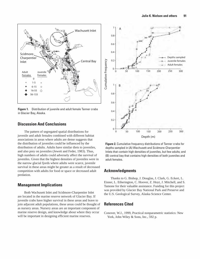
Figure 2. Cumulative frequency distributions of Tanner crabs for depths sampled in (A) Wachusett and Scidmore-Charpentier Inlets that contain high densities of juveniles, but few adults; and (B) central bay that contains high densities of both juveniles and adult females.
Figure 1. Distribution of juvenile and adult female Tanner crabs in Glacier Bay, Alaska.
Julie K. Nielsen and others 91
Wachusett Inlet
Central Bay
Scidmore-CharpentierInlet
AdultFemales
JuvenileFemales
0
1-5
6-15
16-55
56-133
Depth (m)
Cu
mu
lati
ve F
req
uen
cy
B
A
Depths sampled
Juvenile females
Adult females
1
0.8
0.6
0.4
0.2
00 50 100 150 200 250 300
1
0.8
0.6
0.4
0.2
00 50 100 150 200 250 300
Discussion And Conclusions
The pattern of segregated spatial distributions for juvenile and adult females combined with different habitat associations in areas where adults are dense suggests that the distribution of juveniles could be influenced by the distribution of adults. Adults have similar diets to juveniles, and also prey on juveniles (Jewett and Feder, 1983). Thus, high numbers of adults could adversely affect the survival of juveniles. Given that the highest densities of juveniles were in the narrow glacial fjords where adults were scarce, juvenile survival in these areas might be greater as a result of decreased competition with adults for food or space or decreased adult predation.
Management Implications
Both Wachusett Inlet and Scidmore-Charpentier Inlet are located in the marine reserve network of Glacier Bay. If juvenile crabs have higher survival in these areas and leave to join adjacent adult populations, these areas could be thought of as nursery areas. Nursery areas are an important component of marine reserve design, and knowledge about where they occur will be important in designing efficient marine reserves.
Acknowledgments
Thanks to G. Bishop, J. Douglas, J. Clark, G. Eckert, L. Eisner, L. Etherington, C. Hoover, Z. Hoyt, J. Mitchell, and S. Tamone for their valuable assistance. Funding for this project was provided by Glacier Bay National Park and Preserve and the U.S. Geological Survey, Alaska Science Center.
References Cited
Conover, W.J., 1999, Practical nonparametric statistics: New York, John Wiley & Sons, Inc., 592 p.
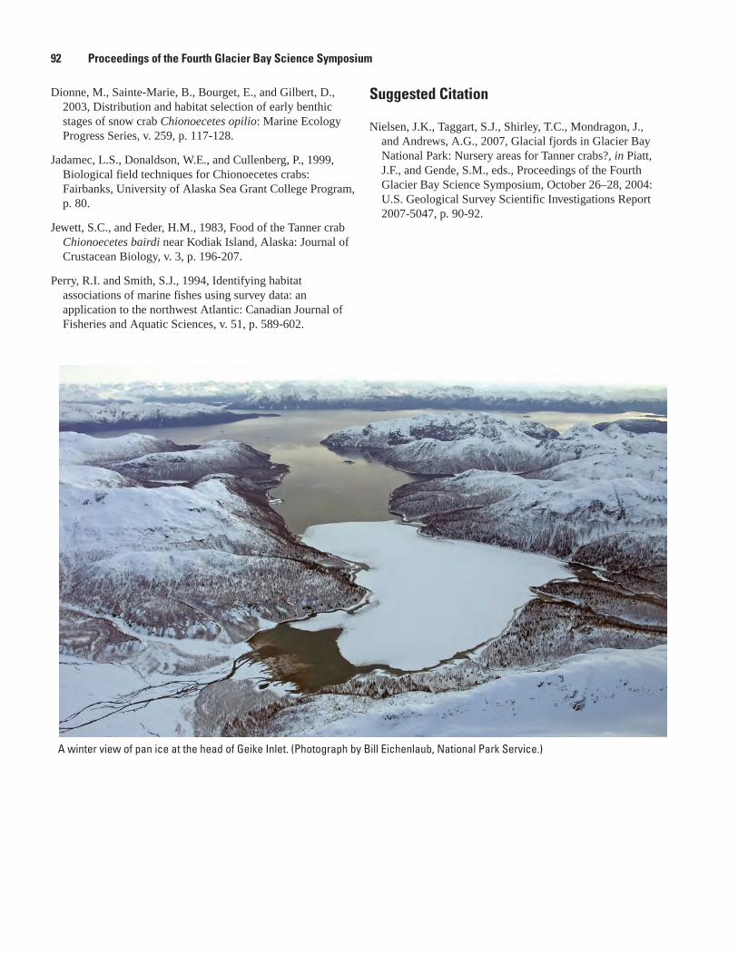
92 Proceedings of the Fourth Glacier Bay Science Symposium
A winter view of pan ice at the head of Geike Inlet. (Photograph by Bill Eichenlaub, National Park Service.)
Dionne, M., Sainte-Marie, B., Bourget, E., and Gilbert, D., 2003, Distribution and habitat selection of early benthic stages of snow crab Chionoecetes opilio: Marine Ecology Progress Series, v. 259, p. 117-128.
Jadamec, L.S., Donaldson, W.E., and Cullenberg, P., 1999, Biological field techniques for Chionoecetes crabs: Fairbanks, University of Alaska Sea Grant College Program, p. 80.
Jewett, S.C., and Feder, H.M., 1983, Food of the Tanner crab Chionoecetes bairdi near Kodiak Island, Alaska: Journal of Crustacean Biology, v. 3, p. 196-207.
Perry, R.I. and Smith, S.J., 1994, Identifying habitat associations of marine fishes using survey data: an application to the northwest Atlantic: Canadian Journal of Fisheries and Aquatic Sciences, v. 51, p. 589-602.
Suggested Citation
Nielsen, J.K., Taggart, S.J., Shirley, T.C., Mondragon, J., and Andrews, A.G., 2007, Glacial fjords in Glacier Bay National Park: Nursery areas for Tanner crabs?, in Piatt, J.F., and Gende, S.M., eds., Proceedings of the Fourth Glacier Bay Science Symposium, October 26–28, 2004: U.S. Geological Survey Scientific Investigations Report 2007-5047, p. 90-92.
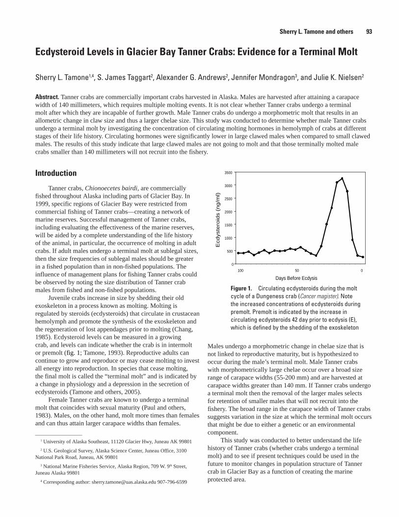
Ecdysteroid Levels in Glacier Bay Tanner Crabs: Evidence for a Terminal Molt
Sherry L. Tamone1,4, S. James Taggart2, Alexander G. Andrews2, Jennifer Mondragon3, and Julie K. Nielsen2
Abstract. Tanner crabs are commercially important crabs harvested in Alaska. Males are harvested after attaining a carapace width of 140 millimeters, which requires multiple molting events. It is not clear whether Tanner crabs undergo a terminal molt after which they are incapable of further growth. Male Tanner crabs do undergo a morphometric molt that results in an allometric change in claw size and thus a larger chelae size. This study was conducted to determine whether male Tanner crabs undergo a terminal molt by investigating the concentration of circulating molting hormones in hemolymph of crabs at different stages of their life history. Circulating hormones were significantly lower in large clawed males when compared to small clawed males. The results of this study indicate that large clawed males are not going to molt and that those terminally molted male crabs smaller than 140 millimeters will not recruit into the fishery.
Figure 1. Circulating ecdysteroids during the molt cycle of a Dungeness crab (Cancer magister). Note the increased concentrations of ecdysteroids during premolt. Premolt is indicated by the increase in circulating ecdysteroids 42 day prior to ecdysis (E), which is defined by the shedding of the exoskeleton
0
500
1000
1500
2000
2500
3000
3500
Days Before Ecdysis
Ecd
yste
roid
s(n
g/m
l)
100 050
Sherry L. Tamone and others 9�
1 University of Alaska Southeast, 11120 Glacier Hwy, Juneau AK 99801
2 U.S. Geological Survey, Alaska Science Center, Juneau Office, 3100 National Park Road, Juneau, AK 99801
3 National Marine Fisheries Service, Alaska Region, 709 W. 9th Street, Juneau Alaska 99801
4 Corresponding author: [email protected] 907-796-6599
Introduction
Tanner crabs, Chionoecetes bairdi, are commercially fished throughout Alaska including parts of Glacier Bay. In 1999, specific regions of Glacier Bay were restricted from commercial fishing of Tanner crabs—creating a network of marine reserves. Successful management of Tanner crabs, including evaluating the effectiveness of the marine reserves, will be aided by a complete understanding of the life history of the animal, in particular, the occurrence of molting in adult crabs. If adult males undergo a terminal molt at sublegal sizes, then the size frequencies of sublegal males should be greater in a fished population than in non-fished populations. The influence of management plans for fishing Tanner crabs could be observed by noting the size distribution of Tanner crab males from fished and non-fished populations.
Juvenile crabs increase in size by shedding their old exoskeleton in a process known as molting. Molting is regulated by steroids (ecdysteroids) that circulate in crustacean hemolymph and promote the synthesis of the exoskeleton and the regeneration of lost appendages prior to molting (Chang, 1985). Ecdysteroid levels can be measured in a growing crab, and levels can indicate whether the crab is in intermolt or premolt (fig. 1; Tamone, 1993). Reproductive adults can continue to grow and reproduce or may cease molting to invest all energy into reproduction. In species that cease molting, the final molt is called the “terminal molt” and is indicated by a change in physiology and a depression in the secretion of ecdysteroids (Tamone and others, 2005).
Female Tanner crabs are known to undergo a terminal molt that coincides with sexual maturity (Paul and others, 1983). Males, on the other hand, molt more times than females and can thus attain larger carapace widths than females.
Males undergo a morphometric change in chelae size that is not linked to reproductive maturity, but is hypothesized to occur during the male’s terminal molt. Male Tanner crabs with morphometrically large chelae occur over a broad size range of carapace widths (55-200 mm) and are harvested at carapace widths greater than 140 mm. If Tanner crabs undergo a terminal molt then the removal of the larger males selects for retention of smaller males that will not recruit into the fishery. The broad range in the carapace width of Tanner crabs suggests variation in the size at which the terminal molt occurs that might be due to either a genetic or an environmental component.
This study was conducted to better understand the life history of Tanner crabs (whether crabs undergo a terminal molt) and to see if present techniques could be used in the future to monitor changes in population structure of Tanner crab in Glacier Bay as a function of creating the marine protected area.
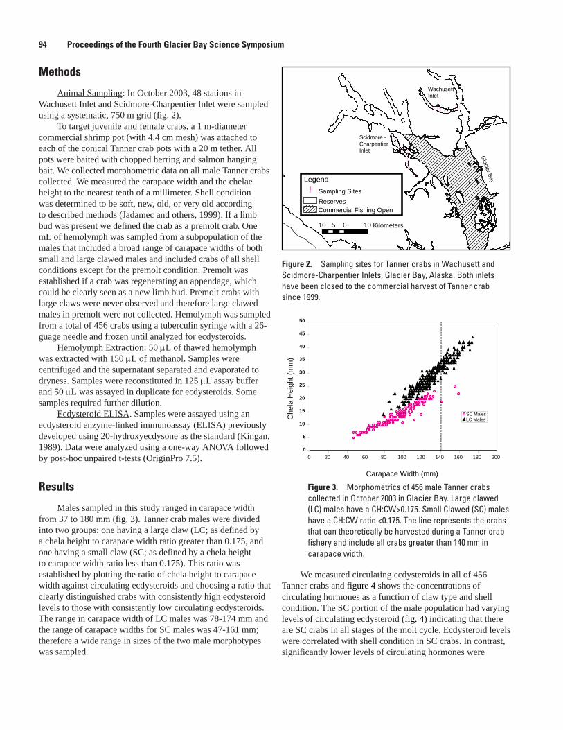
Methods
Animal Sampling: In October 2003, 48 stations in Wachusett Inlet and Scidmore-Charpentier Inlet were sampled using a systematic, 750 m grid (fig. 2).
To target juvenile and female crabs, a 1 m-diameter commercial shrimp pot (with 4.4 cm mesh) was attached to each of the conical Tanner crab pots with a 20 m tether. All pots were baited with chopped herring and salmon hanging bait. We collected morphometric data on all male Tanner crabs collected. We measured the carapace width and the chelae height to the nearest tenth of a millimeter. Shell condition was determined to be soft, new, old, or very old according to described methods (Jadamec and others, 1999). If a limb bud was present we defined the crab as a premolt crab. One mL of hemolymph was sampled from a subpopulation of the males that included a broad range of carapace widths of both small and large clawed males and included crabs of all shell conditions except for the premolt condition. Premolt was established if a crab was regenerating an appendage, which could be clearly seen as a new limb bud. Premolt crabs with large claws were never observed and therefore large clawed males in premolt were not collected. Hemolymph was sampled from a total of 456 crabs using a tuberculin syringe with a 26-guage needle and frozen until analyzed for ecdysteroids.
Hemolymph Extraction: 50 µL of thawed hemolymph was extracted with 150 µL of methanol. Samples were centrifuged and the supernatant separated and evaporated to dryness. Samples were reconstituted in 125 µL assay buffer and 50 µL was assayed in duplicate for ecdysteroids. Some samples required further dilution.
Ecdysteroid ELISA. Samples were assayed using an ecdysteroid enzyme-linked immunoassay (ELISA) previously developed using 20-hydroxyecdysone as the standard (Kingan, 1989). Data were analyzed using a one-way ANOVA followed by post-hoc unpaired t-tests (OriginPro 7.5).
Results
Males sampled in this study ranged in carapace width from 37 to 180 mm (fig. 3). Tanner crab males were divided into two groups: one having a large claw (LC; as defined by a chela height to carapace width ratio greater than 0.175, and one having a small claw (SC; as defined by a chela height to carapace width ratio less than 0.175). This ratio was established by plotting the ratio of chela height to carapace width against circulating ecdysteroids and choosing a ratio that clearly distinguished crabs with consistently high ecdysteroid levels to those with consistently low circulating ecdysteroids. The range in carapace width of LC males was 78-174 mm and the range of carapace widths for SC males was 47-161 mm; therefore a wide range in sizes of the two male morphotypes was sampled.
We measured circulating ecdysteroids in all of 456 Tanner crabs and figure 4 shows the concentrations of circulating hormones as a function of claw type and shell condition. The SC portion of the male population had varying levels of circulating ecdysteroid (fig. 4) indicating that there are SC crabs in all stages of the molt cycle. Ecdysteroid levels were correlated with shell condition in SC crabs. In contrast, significantly lower levels of circulating hormones were
Figure 2. Sampling sites for Tanner crabs in Wachusett and Scidmore-Charpentier Inlets, Glacier Bay, Alaska. Both inlets have been closed to the commercial harvest of Tanner crab since 1999.
Figure �. Morphometrics of 456 male Tanner crabs collected in October 2003 in Glacier Bay. Large clawed (LC) males have a CH:CW>0.175. Small Clawed (SC) males have a CH:CW ratio <0.175. The line represents the crabs that can theoretically be harvested during a Tanner crab fishery and include all crabs greater than 140 mm in carapace width.
!! ! !! !! !! ! ! !
! !! !!
! ! ! !! ! ! ! !
! ! ! !! ! !!
!!
! !! !! !
!!
!!
!!
!! !
! !! !
! !! ! ! ! ! ! ! !
! ! ! ! ! ! ! ! ! ! !! ! ! ! ! ! ! ! ! ! !
! ! ! ! ! ! !!
!
10 0 105
!Legend
Sampling SitesReservesCommercial Fishing Open
Kilometers
Scidmore -CharpentierInlet
WachusettInlet
Glacier Bay
0
5
10
15
20
25
30
35
40
45
50
0 20 40 60 80 100 120 140 160 180 200
Carapace Width (mm)
Che
laH
eigh
t(m
m)
SC MalesLC Males
9� Proceedings of the Fourth Glacier Bay Science Symposium
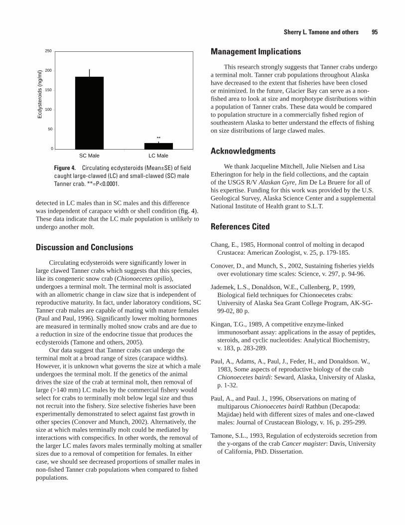
Figure �. Circulating ecdysteroids (Mean±SE) of field caught large-clawed (LC) and small-clawed (SC) male Tanner crab. **=P<0.0001.
0
50
100
150
200
250
SC Male LC Male
Ecd
yste
roid
s(n
g/m
l)
**
Sherry L. Tamone and others 95
detected in LC males than in SC males and this difference was independent of carapace width or shell condition (fig. 4). These data indicate that the LC male population is unlikely to undergo another molt.
Discussion and Conclusions
Circulating ecdysteroids were significantly lower in large clawed Tanner crabs which suggests that this species, like its congeneric snow crab (Chionoecetes opilio), undergoes a terminal molt. The terminal molt is associated with an allometric change in claw size that is independent of reproductive maturity. In fact, under laboratory conditions, SC Tanner crab males are capable of mating with mature females (Paul and Paul, 1996). Significantly lower molting hormones are measured in terminally molted snow crabs and are due to a reduction in size of the endocrine tissue that produces the ecdysteroids (Tamone and others, 2005).
Our data suggest that Tanner crabs can undergo the terminal molt at a broad range of sizes (carapace widths). However, it is unknown what governs the size at which a male undergoes the terminal molt. If the genetics of the animal drives the size of the crab at terminal molt, then removal of large (>140 mm) LC males by the commercial fishery would select for crabs to terminally molt below legal size and thus not recruit into the fishery. Size selective fisheries have been experimentally demonstrated to select against fast growth in other species (Conover and Munch, 2002). Alternatively, the size at which males terminally molt could be mediated by interactions with conspecifics. In other words, the removal of the larger LC males favors males terminally molting at smaller sizes due to a removal of competition for females. In either case, we should see decreased proportions of smaller males in non-fished Tanner crab populations when compared to fished populations.
Management Implications
This research strongly suggests that Tanner crabs undergo a terminal molt. Tanner crab populations throughout Alaska have decreased to the extent that fisheries have been closed or minimized. In the future, Glacier Bay can serve as a non-fished area to look at size and morphotype distributions within a population of Tanner crabs. These data would be compared to population structure in a commercially fished region of southeastern Alaska to better understand the effects of fishing on size distributions of large clawed males.
Acknowledgments
We thank Jacqueline Mitchell, Julie Nielsen and Lisa Etherington for help in the field collections, and the captain of the USGS R/V Alaskan Gyre, Jim De La Bruere for all of his expertise. Funding for this work was provided by the U.S. Geological Survey, Alaska Science Center and a supplemental National Institute of Health grant to S.L.T.
References Cited
Chang, E., 1985, Hormonal control of molting in decapod Crustacea: American Zoologist, v. 25, p. 179-185.
Conover, D., and Munch, S., 2002, Sustaining fisheries yields over evolutionary time scales: Science, v. 297, p. 94-96.
Jademek, L.S., Donaldson, W.E., Cullenberg, P., 1999, Biological field techniques for Chionoecetes crabs: University of Alaska Sea Grant College Program, AK-SG-99-02, 80 p.
Kingan, T.G., 1989, A competitive enzyme-linked immunosorbant assay: applications in the assay of peptides, steroids, and cyclic nucleotides: Analytical Biochemistry, v. 183, p. 283-289.
Paul, A., Adams, A., Paul, J., Feder, H., and Donaldson. W., 1983, Some aspects of reproductive biology of the crab Chionoecetes bairdi: Seward, Alaska, University of Alaska, p. 1-32.
Paul, A., and Paul. J., 1996, Observations on mating of multiparous Chionoecetes bairdi Rathbun (Decapoda: Majidae) held with different sizes of males and one-clawed males: Journal of Crustacean Biology, v. 16, p. 295-299.
Tamone, S.L., 1993, Regulation of ecdysteroids secretion from the y-organs of the crab Cancer magister: Davis, University of California, PhD. Dissertation.
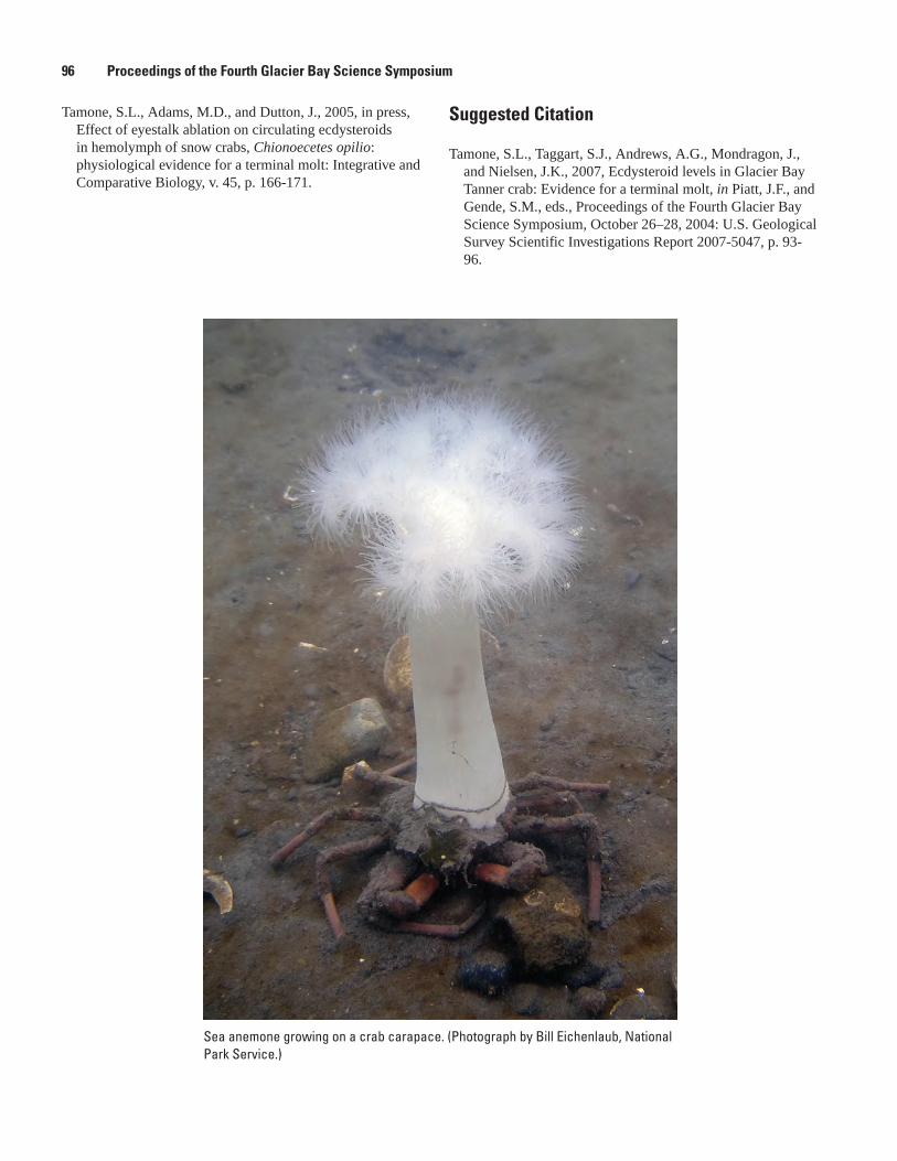
9� Proceedings of the Fourth Glacier Bay Science Symposium
Sea anemone growing on a crab carapace. (Photograph by Bill Eichenlaub, National Park Service.)
Tamone, S.L., Adams, M.D., and Dutton, J., 2005, in press, Effect of eyestalk ablation on circulating ecdysteroids in hemolymph of snow crabs, Chionoecetes opilio: physiological evidence for a terminal molt: Integrative and Comparative Biology, v. 45, p. 166-171.
Suggested Citation
Tamone, S.L., Taggart, S.J., Andrews, A.G., Mondragon, J., and Nielsen, J.K., 2007, Ecdysteroid levels in Glacier Bay Tanner crab: Evidence for a terminal molt, in Piatt, J.F., and Gende, S.M., eds., Proceedings of the Fourth Glacier Bay Science Symposium, October 26–28, 2004: U.S. Geological Survey Scientific Investigations Report 2007-5047, p. 93-96.
Geochemical Signatures as Natural Fingerprints to Aid in Determining Tanner Crab Movement in Glacier Bay National Park, Alaska
Bronwen Wang1,5, Robert R. Seal2, S. James Taggart3, Jennifer Mondragon3, Alex Andrews3, Julie Nielsen3, James G. Crock4, and Gregory A. Wandless2
Introduction
Elemental and isotopic variations in biota arise from differences in local environmental conditions. In some instances, these “geochemical fingerprints” are sufficiently unique to serve as life-history markers. Geochemical fingerprints have been used to distinguished stock and migration patterns for a variety of fish and marine invertebrates (Edmond and others, 1989; Campana and Gagne, 1995; Thorrold and others, 1997; DiBacco and Levin, 2000). Stable isotopic studies have been carried out on a variety of topics related to aquatic and terrestrial ecosystems (Fry and Sherr, 1984, Peterson and Fry, 1987, Fry, 1988, Carmichael and others, 2004). Environmental conditions that may result in unique geochemical signatures include food source, C source (e.g. shelf or oceanic) salinity and temperature differences, and differences in the local geology.
The success of geochemical fingerprinting tools in other studies led us to consider the possibility that such signatures in Tanner crabs may aid in understanding their migration within Glacier Bay. Tanner crab life-history characteristics make them well suited for a geochemical fingerprinting approach. Female Tanner crabs do not molt again after they molt to sexual maturity. Therefore, if a female Tanner crab leaves the area where she molted to maturity (e.g., a nursery area), the geochemical signature in her carapace could be used as
Bronwen Wang and others 97
1 U.S. Geological Survey, Alaska Science Center, 4200 University Dr., Anchorage, AK 99508
2 U.S. Geological Survey, 12201 Sunrise Valley Dr MS 954, Reston, Virginia, 20192
3 U.S. Geological Survey, 3100 National Park Road, Juneau, AK, 99801
4 U.S. Geological Survey, Denver Federal Center MS 973, Denver, CO, 80225
5 Corresponding author: [email protected], 907 786-7110
a marker for the area in which she molted. It is highly likely that males also undergo a terminal molt (Tamone and others, 2007), in which case the technique could be applied to males as well. In addition, isotopic variations in the muscle tissue could serve as an indicator of crab movement and thus could complement the geochemical information from the carapace. For example, if crabs leave the nursery area after molting, the carapace should reflect the signature of the nursery area, while the muscle may reflect both the terminal molt and a more recent environment. Based on the geological and hydrological heterogeneity present in Glacier Bay and the life history of the Tanner crab, there is a reasonable chance geochemical variations imparted to the crab body tissue can be used to determine the area where the terminal molt occurred.
Physical Setting and Methods
Tanner crabs were collected from five sites within Glacier Bay: Scidmore Bay, Charpentier Inlet, Hugh Miller Inlet, Wachusett Inlet, and Bartlett Cove (fig. 1). Sedimentary rock units that include the Point Augusta Formation and surficial deposits dominate the area around Barlett Cove. The geology of the region surrounding Wachusett Inlet, Hugh Miller Inlet, Charpentier Inlet, and Scidmore Bay is a mix of magmatic, metamorphic, and sedimentary rocks and surficial deposits (Dave Brew, U.S. Geological Survey, 2004, unpub. data). Cu and Mo, Ag, and Ag-Cu-Pb mineral occurrences are known in the area surrounding Wachusett Inlet and Cu and Cu-Mo occurrences are known near Scidmore Bay and Charpentier Inlet (Alaska Resource Data file; http://ardf.wr.usgs.gov). Tanner crabs (Chionoecetes bairdi) were collected using herring-baited crab pots in late October 2003.
Crabs were sorted, sexed, measured, and shell condition noted (table 1). Recently molted juvenile crabs were selected from the overall catch and field processed for later elemental
Abstract. The migration of Tanner crabs (Chionoecetes bairdi) with ontogeny is poorly understood but could have important implications for fisheries management. Relatively dense populations of juvenile Tanner crabs have been found in several areas within Glacier Bay; these could be nursery areas from which maturing crabs disperse. Geochemical signatures imparted to the carapace during molt or to the muscle tissue during growth could serve as a natural fingerprint that identifies the area where molting or growth occurred. These signatures may reflect subtle but unique elemental or isotopic compositions that arise from hydrologic, geologic, or nutritional variations in Glacier Bay. For this pilot study, recently molted Tanner crabs were collected from Scidmore Bay, Charpentier Inlet, Hugh Miller Inlet, Wachusett Inlet, and Bartlett Cove. Leg muscle tissue and the entire dorsal carapace were retained for elemental and stable isotopic (C and N) analysis. If geochemical signatures differ among crabs from different sample sites, this signature could aid in understanding Tanner crab migration. Here we present preliminary data and baseline information needed to determine the feasibility of establishing a geochemical signature for use as a natural fingerprint.
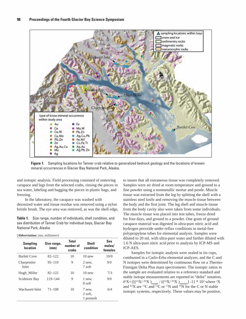
to insure that all extraneous tissue was completely removed. Samples were air dried at room temperature and ground to a fine powder using a nonmetallic mortar and pestle. Muscle tissue was extracted from the leg by splitting the shell with a stainless steel knife and removing the muscle tissue between the body and the first joint. The leg shell and muscle tissue from the body cavity also were taken from some individuals. The muscle tissue was placed into test tubes, freeze dried for four days, and ground to a powder. One gram of ground carapace material was digested in ultra-pure nitric acid and hydrogen peroxide under reflux conditions in metal-free polypropylene tubes for elemental analysis. Samples were diluted to 20 mL with ultra-pure water and further diluted with 1.6 N ultra-pure nitric acid prior to analysis by ICP-MS and ICP-AES.
Samples for isotopic analysis were sealed in tin cups, combusted in a Carlo-Erba elemental analyzer, and the C and N isotopes were determined by continuous flow on a Thermo-Finnigan Delta Plus mass spectrometer. The isotopic ratios in the sample are evaluated relative to a reference standard and stable isotope measurements are reported in “delta” notation; δaX={[((a)X/ (b)X )
sample / (((a)X/ (b)X )
standard] -1} * 103 where aX
and (b)X are 13C and 12C or 15N and 14N for the C or N stable isotopic systems, respectively. These values may be positive,
Table 1. Size range, number of individuals, shell condition, and sex distribution of Tanner Crab for individual bays, Glacier Bay National Park, Alaska.
[Abbreviation: mm, millimeter]
Sampling location
Size range, (mm)
Total number of
crabs
Shellcondition
Sex males/
females
Barlett Cove 82–122 10 10 new 10/0
Charpentier Inlet
95–119 9 2 new,7 soft
9/0
Hugh_Miller 82–122 10 10 new 7/3
Scidmore Bay 119–144 9 1 new,8 soft
9/0
Wachusett Inlet 71–108 10 7 new,2 soft,1 premolt
6/4
and isotopic analysis. Field processing consisted of removing carapace and legs from the selected crabs, rinsing the pieces in sea water, labeling and bagging the pieces in plastic bags, and freezing.
In the laboratory, the carapace was washed with deionized water and tissue residue was removed using a nylon bristle brush. The eye area was removed, as was the shell edge,
Figure 1. Sampling locations for Tanner crab relative to generalized bedrock geology and the locations of known mineral occurrences in Glacier Bay National Park, Alaska.
9� Proceedings of the Fourth Glacier Bay Science Symposium
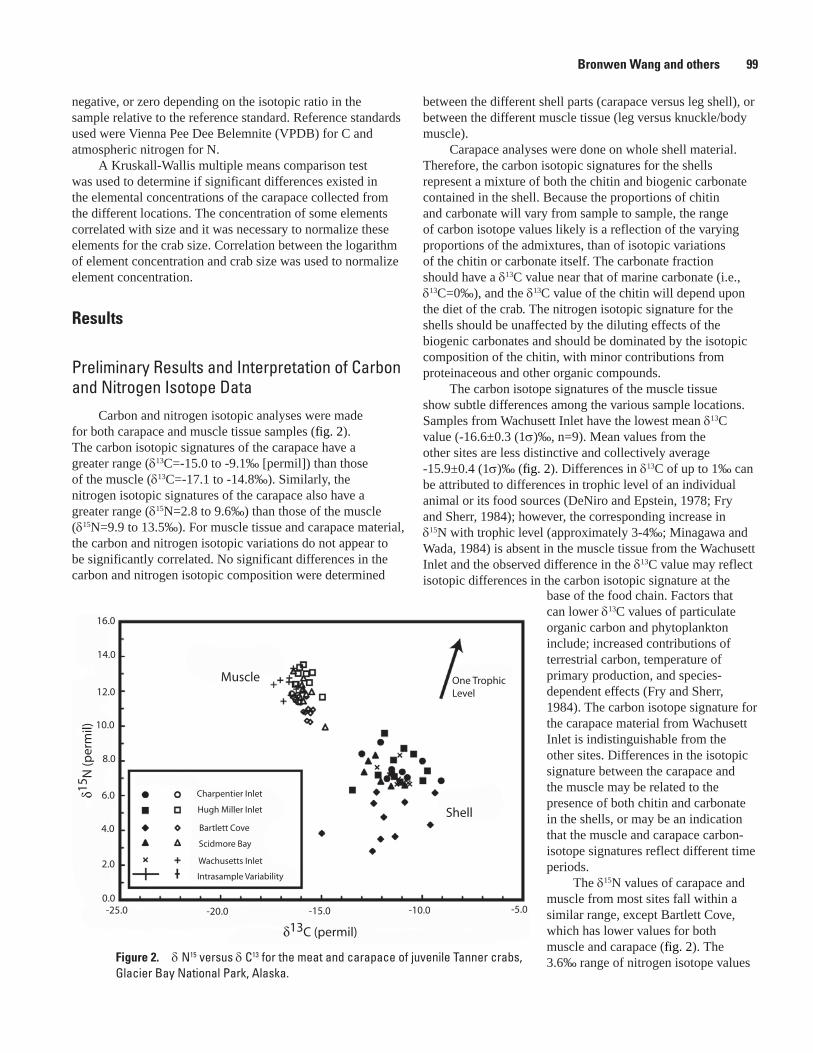
negative, or zero depending on the isotopic ratio in the sample relative to the reference standard. Reference standards used were Vienna Pee Dee Belemnite (VPDB) for C and atmospheric nitrogen for N.
A Kruskall-Wallis multiple means comparison test was used to determine if significant differences existed in the elemental concentrations of the carapace collected from the different locations. The concentration of some elements correlated with size and it was necessary to normalize these elements for the crab size. Correlation between the logarithm of element concentration and crab size was used to normalize element concentration.
Results
Preliminary Results and Interpretation of Carbon and Nitrogen Isotope Data
Carbon and nitrogen isotopic analyses were made for both carapace and muscle tissue samples (fig. 2). The carbon isotopic signatures of the carapace have a greater range (δ13C=-15.0 to -9.1‰ [permil]) than those of the muscle (δ13C=-17.1 to -14.8‰). Similarly, the nitrogen isotopic signatures of the carapace also have a greater range (δ15N=2.8 to 9.6‰) than those of the muscle (δ15N=9.9 to 13.5‰). For muscle tissue and carapace material, the carbon and nitrogen isotopic variations do not appear to be significantly correlated. No significant differences in the carbon and nitrogen isotopic composition were determined
13C (permil)
15N
(per
mil)
16.0
14.0
12.0
10.0
8.0
6.0
4.0
2.0
0.0-25.0 -20.0 -15.0 -10.0 -5.0
Muscle
Shell
One Trophic Level
Charpentier Inlet
Hugh Miller Inlet
Bartlett Cove
Scidmore Bay
Wachusetts Inlet
Intrasample Variability
Figure 2. δ N15 versus δ C13 for the meat and carapace of juvenile Tanner crabs, Glacier Bay National Park, Alaska.
Bronwen Wang and others 99
between the different shell parts (carapace versus leg shell), or between the different muscle tissue (leg versus knuckle/body muscle).
Carapace analyses were done on whole shell material. Therefore, the carbon isotopic signatures for the shells represent a mixture of both the chitin and biogenic carbonate contained in the shell. Because the proportions of chitin and carbonate will vary from sample to sample, the range of carbon isotope values likely is a reflection of the varying proportions of the admixtures, than of isotopic variations of the chitin or carbonate itself. The carbonate fraction should have a δ13C value near that of marine carbonate (i.e., δ13C=0‰), and the δ13C value of the chitin will depend upon the diet of the crab. The nitrogen isotopic signature for the shells should be unaffected by the diluting effects of the biogenic carbonates and should be dominated by the isotopic composition of the chitin, with minor contributions from proteinaceous and other organic compounds.
The carbon isotope signatures of the muscle tissue show subtle differences among the various sample locations. Samples from Wachusett Inlet have the lowest mean δ13C value (-16.6±0.3 (1σ)‰, n=9). Mean values from the other sites are less distinctive and collectively average -15.9±0.4 (1σ)‰ (fig. 2). Differences in δ13C of up to 1‰ can be attributed to differences in trophic level of an individual animal or its food sources (DeNiro and Epstein, 1978; Fry and Sherr, 1984); however, the corresponding increase in δ15N with trophic level (approximately 3-4‰; Minagawa and Wada, 1984) is absent in the muscle tissue from the Wachusett Inlet and the observed difference in the δ13C value may reflect isotopic differences in the carbon isotopic signature at the
base of the food chain. Factors that can lower δ13C values of particulate organic carbon and phytoplankton include; increased contributions of terrestrial carbon, temperature of primary production, and species-dependent effects (Fry and Sherr, 1984). The carbon isotope signature for the carapace material from Wachusett Inlet is indistinguishable from the other sites. Differences in the isotopic signature between the carapace and the muscle may be related to the presence of both chitin and carbonate in the shells, or may be an indication that the muscle and carapace carbon-isotope signatures reflect different time periods.
The δ15N values of carapace and muscle from most sites fall within a similar range, except Bartlett Cove, which has lower values for both muscle and carapace (fig. 2). The 3.6‰ range of nitrogen isotope values
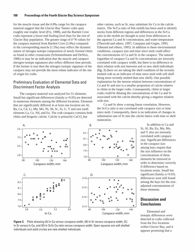
for the muscle tissue and the 6.8‰ range for the carapace material suggest that the Glacier Bay Tanner crabs span roughly one trophic level (Fry, 1988), and the Bartlett Cove crabs represent a lower-end feeding level than for the rest of Glacier Bay population. The greater range of δ15N values for the carapace material from Bartlett Cove (3.4‰) compared to the corresponding muscle (1.5‰) may reflect the dynamic nature of nitrogen isotope composition of newly formed chitin as found in other crustaceans (Schimmelmann and DeNiro, 1986) or may be an indication that the muscle and carapace nitrogen-isotope signatures also reflect different time periods. If the former is true then the nitrogen isotopic signature of the carapace may not provide the most robust indicator of the site of origin for crabs.
Preliminary Evaluation of Elemental Data and Discriminant Factor Analysis
The carapace material was analyzed for 51 elements. Small but significant differences (family α=0.05) are detected in numerous elements among the different locations. Elements that are significantly different in at least one location are Al, Ba, Ca, Cd, Li, Mn, Mo, Ni, Sb, Sc, Sr, U, Y and rare earth elements La, Ce, Nd, and Eu. The crab carapace contains both chitin and biogenic calcite. Calcite is primarily CaCO
3 but
other cations, such as Sr, may substitute for Ca in the calcite matrix. The Sr/Ca ratio of fish otolith has been used to identify stocks from different regions and differences in the Sr/Ca ratio in the otolith are thought to arise from differences in the aqueous Ca and Sr concentration, and water temperature (Thorrold and others, 1997; Campana and Gagne, 1995; Edmond and others, 1995). In addition to these environmental conditions, carapace size and time since molt could affect the concentrations of Ca and Sr in the carapace. The natural logarithm of carapace Ca and Sr concentrations are inversely correlated with carapace width, but there is no difference in their relation with size between soft or new shell individuals (fig. 3) (here we are taking the shell condition of the recently molted crab as an indicator of time since molt with soft shell being more recently molted than new shell). One possible explanation for the inverse relation between concentrations of Ca and Sr and size is a smaller proportion of calcite relative to chitin in the larger crabs. Consequently, chitin in larger crabs could be diluting the concentrations of the Ca and Sr associated with the calcite thereby giving a negative relation with size.
Ca and Sr show a strong linear correlation. However, the Sr/Ca ratio is not correlated with carapace size or time since molt. Consequently, there is no indication of changes in substitution rate of Sr into the calcite lattice with time or shell maturation.
Figure �. Plots showing (A) ln Ca versus carapace width, (B) ln Sr versus carapace width, (C) ln Sr versus ln Ca, and (D) ln Sr/ln Ca ratio versus carapace width. Open squares are soft shelled individuals and solid circles are new shelled individuals.
Carapace width, mm
Carapace width, mm
Carapace width, mm
In Ca
A. B.
C. D.
3.4
3.2
3.0
2.8
80 100 120 140
8.2
8.1
8.0
7.9
7.8
0.16
0.15
0.14
0.1380 100 120 140
8.2
8.1
8.0
7.9
7.8
80 100 120 140
2.8 3.0 3.2 3.4
100 Proceedings of the Fourth Glacier Bay Science Symposium
In addition to Ca and Sr, Al, Ba, Eu, Mn, Mo, and Y also are inversely correlated with carapace size. Significant differences in the carapace size among bays require that the size influence on the concentrations of these elements be removed in order to determine correctly if difference based on locations exists. Small but significant (family α=0.05) differences were still found among the bays for the size-adjusted concentrations of these elements.
Discussion and Conclusions
Elemental and isotopic differences were detected in crabs collected from the five locations within Glacier Bay, and it appears promising that a
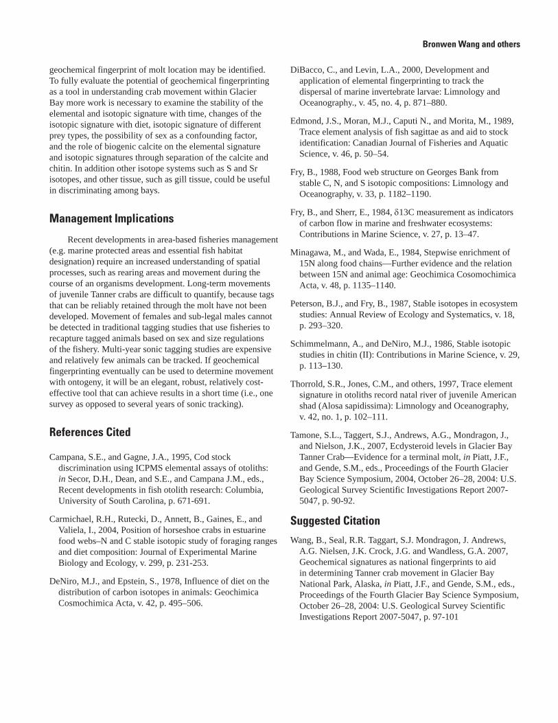
Bronwen Wang and others
geochemical fingerprint of molt location may be identified. To fully evaluate the potential of geochemical fingerprinting as a tool in understanding crab movement within Glacier Bay more work is necessary to examine the stability of the elemental and isotopic signature with time, changes of the isotopic signature with diet, isotopic signature of different prey types, the possibility of sex as a confounding factor, and the role of biogenic calcite on the elemental signature and isotopic signatures through separation of the calcite and chitin. In addition other isotope systems such as S and Sr isotopes, and other tissue, such as gill tissue, could be useful in discriminating among bays.
Management Implications
Recent developments in area-based fisheries management (e.g. marine protected areas and essential fish habitat designation) require an increased understanding of spatial processes, such as rearing areas and movement during the course of an organisms development. Long-term movements of juvenile Tanner crabs are difficult to quantify, because tags that can be reliably retained through the molt have not been developed. Movement of females and sub-legal males cannot be detected in traditional tagging studies that use fisheries to recapture tagged animals based on sex and size regulations of the fishery. Multi-year sonic tagging studies are expensive and relatively few animals can be tracked. If geochemical fingerprinting eventually can be used to determine movement with ontogeny, it will be an elegant, robust, relatively cost-effective tool that can achieve results in a short time (i.e., one survey as opposed to several years of sonic tracking).
References Cited
Campana, S.E., and Gagne, J.A., 1995, Cod stock discrimination using ICPMS elemental assays of otoliths: in Secor, D.H., Dean, and S.E., and Campana J.M., eds., Recent developments in fish otolith research: Columbia, University of South Carolina, p. 671-691.
Carmichael, R.H., Rutecki, D., Annett, B., Gaines, E., and Valiela, I., 2004, Position of horseshoe crabs in estuarine food webs–N and C stable isotopic study of foraging ranges and diet composition: Journal of Experimental Marine Biology and Ecology, v. 299, p. 231-253.
DeNiro, M.J., and Epstein, S., 1978, Influence of diet on the distribution of carbon isotopes in animals: Geochimica Cosmochimica Acta, v. 42, p. 495–506.
DiBacco, C., and Levin, L.A., 2000, Development and application of elemental fingerprinting to track the dispersal of marine invertebrate larvae: Limnology and Oceanography., v. 45, no. 4, p. 871–880.
Edmond, J.S., Moran, M.J., Caputi N., and Morita, M., 1989, Trace element analysis of fish sagittae as and aid to stock identification: Canadian Journal of Fisheries and Aquatic Science, v. 46, p. 50–54.
Fry, B., 1988, Food web structure on Georges Bank from stable C, N, and S isotopic compositions: Limnology and Oceanography, v. 33, p. 1182–1190.
Fry, B., and Sherr, E., 1984, δ13C measurement as indicators of carbon flow in marine and freshwater ecosystems: Contributions in Marine Science, v. 27, p. 13–47.
Minagawa, M., and Wada, E., 1984, Stepwise enrichment of 15N along food chains—Further evidence and the relation between 15N and animal age: Geochimica Cosomochimica Acta, v. 48, p. 1135–1140.
Peterson, B.J., and Fry, B., 1987, Stable isotopes in ecosystem studies: Annual Review of Ecology and Systematics, v. 18, p. 293–320.
Schimmelmann, A., and DeNiro, M.J., 1986, Stable isotopic studies in chitin (II): Contributions in Marine Science, v. 29, p. 113–130.
Thorrold, S.R., Jones, C.M., and others, 1997, Trace element signature in otoliths record natal river of juvenile American shad (Alosa sapidissima): Limnology and Oceanography, v. 42, no. 1, p. 102–111.
Tamone, S.L., Taggert, S.J., Andrews, A.G., Mondragon, J., and Nielson, J.K., 2007, Ecdysteroid levels in Glacier Bay Tanner Crab—Evidence for a terminal molt, in Piatt, J.F., and Gende, S.M., eds., Proceedings of the Fourth Glacier Bay Science Symposium, 2004, October 26–28, 2004: U.S. Geological Survey Scientific Investigations Report 2007-5047, p. 90-92.
Suggested Citation
Wang, B., Seal, R.R. Taggart, S.J. Mondragon, J. Andrews, A.G. Nielsen, J.K. Crock, J.G. and Wandless, G.A. 2007, Geochemical signatures as national fingerprints to aid in determining Tanner crab movement in Glacier Bay National Park, Alaska, in Piatt, J.F., and Gende, S.M., eds., Proceedings of the Fourth Glacier Bay Science Symposium, October 26–28, 2004: U.S. Geological Survey Scientific Investigations Report 2007-5047, p. 97-101
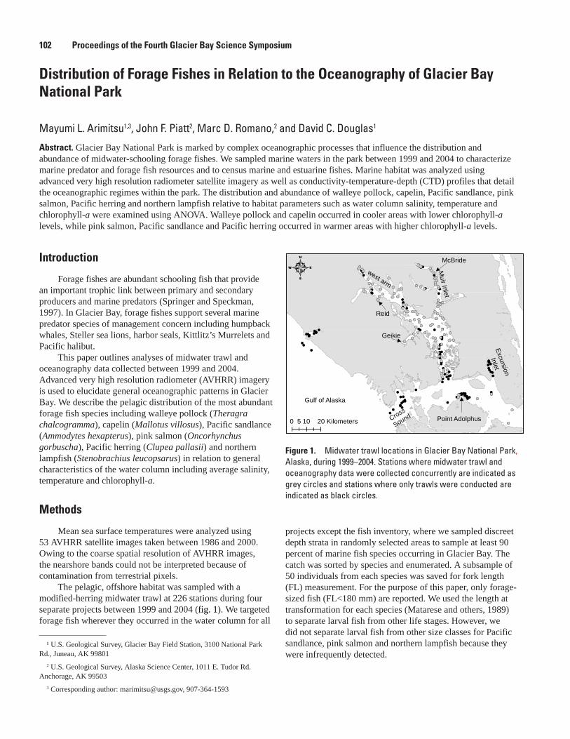
Distribution of Forage Fishes in Relation to the Oceanography of Glacier Bay National Park
Mayumi L. Arimitsu1,3, John F. Piatt2, Marc D. Romano,2 and David C. Douglas1
Abstract. Glacier Bay National Park is marked by complex oceanographic processes that influence the distribution and abundance of midwater-schooling forage fishes. We sampled marine waters in the park between 1999 and 2004 to characterize marine predator and forage fish resources and to census marine and estuarine fishes. Marine habitat was analyzed using advanced very high resolution radiometer satellite imagery as well as conductivity-temperature-depth (CTD) profiles that detail the oceanographic regimes within the park. The distribution and abundance of walleye pollock, capelin, Pacific sandlance, pink salmon, Pacific herring and northern lampfish relative to habitat parameters such as water column salinity, temperature and chlorophyll-a were examined using ANOVA. Walleye pollock and capelin occurred in cooler areas with lower chlorophyll-a levels, while pink salmon, Pacific sandlance and Pacific herring occurred in warmer areas with higher chlorophyll-a levels.
Figure 1. Midwater trawl locations in Glacier Bay National Park, Alaska, during 1999–2004. Stations where midwater trawl and oceanography data were collected concurrently are indicated as grey circles and stations where only trawls were conducted are indicated as black circles.
102 Proceedings of the Fourth Glacier Bay Science Symposium
!!
!!
!!!
!! !
!!!
!!!
!!
!
!
!
!
!!
!
!
!!
!!!
!!!
!!
!!
!!
!
!
!
!!!!
!!
!!
!
!!
!
!
!!!!!
!
!!!!
!!
!
!!!!!
!!!
!!
!
!
!!
!!
!
!
!!
!!
!
!! !!!!
!
!!!!
! !!!
!
!
!
!
!
!! !
! !
!
! !
!
! !
! !
!
!!
!
!!
!
!!!
! !
!
!
!!
! !
!!
!!
! !!
!!
!!!
!!
! !!!
!
!
!
!
!
!
! !!
!! ! !
!
!!
! !!!
!
!!
!!
!
!!
!
!
!
!
!!
!
!
!
!
!!
!
!
!!!!
!!
!
!!
!!
!
!
!
!
!
!
!!
!
!!
!
!
!(!(!(
!(
!(
!(
!(
!(
!(!( !(
!( !(
!(
!( !(
!(
!( !(
!( !(
!(
!(!(
!(
!(!(
!(
!(!(!(
!( !(
!(
!(
!(!(
!(!(
!(!(
!(!(
!( !(!(
!(!(
!(!(!(
!(!(!( !(!(!(
!(
!(
!(
!(
!(
!(
!( !(!(
!(!( !( !(
!(
!(!(
!( !(!(!(
!(
!(!(
!(!(
!(
!(!(
!(
!(
!(
!(
!(!(
!(
!(
!(
!(
!(!(
!(
!(
!(!(!(!(
!(!(
!(
!(!(
!(!(
!(
!(
!(
!(
!(
!(
!(!(
!(
!(!(
!(
!(
4
0 10 205 Kilometers Point AdolphusCross
Sound
Gulf of Alaska
Muir Inlet
west arm
Excursion
Inlet
Reid
McBride
Geikie
Introduction
Forage fishes are abundant schooling fish that provide an important trophic link between primary and secondary producers and marine predators (Springer and Speckman, 1997). In Glacier Bay, forage fishes support several marine predator species of management concern including humpback whales, Steller sea lions, harbor seals, Kittlitz’s Murrelets and Pacific halibut.
This paper outlines analyses of midwater trawl and oceanography data collected between 1999 and 2004. Advanced very high resolution radiometer (AVHRR) imagery is used to elucidate general oceanographic patterns in Glacier Bay. We describe the pelagic distribution of the most abundant forage fish species including walleye pollock (Theragra chalcogramma), capelin (Mallotus villosus), Pacific sandlance (Ammodytes hexapterus), pink salmon (Oncorhynchus gorbuscha), Pacific herring (Clupea pallasii) and northern lampfish (Stenobrachius leucopsarus) in relation to general characteristics of the water column including average salinity, temperature and chlorophyll-a.
Methods
Mean sea surface temperatures were analyzed using 53 AVHRR satellite images taken between 1986 and 2000. Owing to the coarse spatial resolution of AVHRR images, the nearshore bands could not be interpreted because of contamination from terrestrial pixels.
The pelagic, offshore habitat was sampled with a modified-herring midwater trawl at 226 stations during four separate projects between 1999 and 2004 (fig. 1). We targeted forage fish wherever they occurred in the water column for all
projects except the fish inventory, where we sampled discreet depth strata in randomly selected areas to sample at least 90 percent of marine fish species occurring in Glacier Bay. The catch was sorted by species and enumerated. A subsample of 50 individuals from each species was saved for fork length (FL) measurement. For the purpose of this paper, only forage-sized fish (FL<180 mm) are reported. We used the length at transformation for each species (Matarese and others, 1989) to separate larval fish from other life stages. However, we did not separate larval fish from other size classes for Pacific sandlance, pink salmon and northern lampfish because they were infrequently detected.
¹ U.S. Geological Survey, Glacier Bay Field Station, 3100 National Park Rd., Juneau, AK 99801
2 U.S. Geological Survey, Alaska Science Center, 1011 E. Tudor Rd. Anchorage, AK 99503
3 Corresponding author: [email protected], 907-364-1593
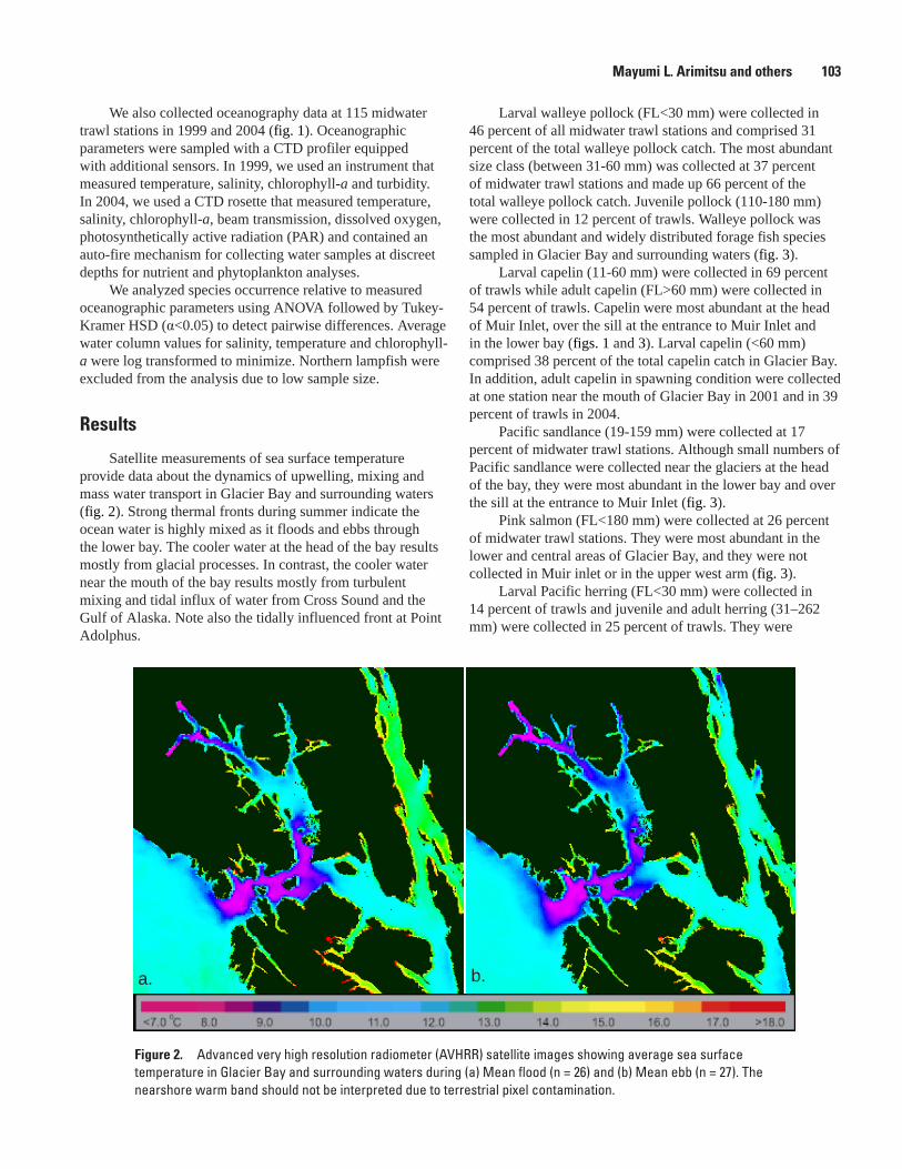
Figure 2. Advanced very high resolution radiometer (AVHRR) satellite images showing average sea surface temperature in Glacier Bay and surrounding waters during (a) Mean flood (n = 26) and (b) Mean ebb (n = 27). The nearshore warm band should not be interpreted due to terrestrial pixel contamination.
Mayumi L. Arimitsu and others 10�
a. b.
We also collected oceanography data at 115 midwater trawl stations in 1999 and 2004 (fig. 1). Oceanographic parameters were sampled with a CTD profiler equipped with additional sensors. In 1999, we used an instrument that measured temperature, salinity, chlorophyll-a and turbidity. In 2004, we used a CTD rosette that measured temperature, salinity, chlorophyll-a, beam transmission, dissolved oxygen, photosynthetically active radiation (PAR) and contained an auto-fire mechanism for collecting water samples at discreet depths for nutrient and phytoplankton analyses.
We analyzed species occurrence relative to measured oceanographic parameters using ANOVA followed by Tukey-Kramer HSD (α<0.05) to detect pairwise differences. Average water column values for salinity, temperature and chlorophyll-a were log transformed to minimize. Northern lampfish were excluded from the analysis due to low sample size.
Results
Satellite measurements of sea surface temperature provide data about the dynamics of upwelling, mixing and mass water transport in Glacier Bay and surrounding waters (fig. 2). Strong thermal fronts during summer indicate the ocean water is highly mixed as it floods and ebbs through the lower bay. The cooler water at the head of the bay results mostly from glacial processes. In contrast, the cooler water near the mouth of the bay results mostly from turbulent mixing and tidal influx of water from Cross Sound and the Gulf of Alaska. Note also the tidally influenced front at Point Adolphus.
Larval walleye pollock (FL<30 mm) were collected in 46 percent of all midwater trawl stations and comprised 31 percent of the total walleye pollock catch. The most abundant size class (between 31-60 mm) was collected at 37 percent of midwater trawl stations and made up 66 percent of the total walleye pollock catch. Juvenile pollock (110-180 mm) were collected in 12 percent of trawls. Walleye pollock was the most abundant and widely distributed forage fish species sampled in Glacier Bay and surrounding waters (fig. 3).
Larval capelin (11-60 mm) were collected in 69 percent of trawls while adult capelin (FL>60 mm) were collected in 54 percent of trawls. Capelin were most abundant at the head of Muir Inlet, over the sill at the entrance to Muir Inlet and in the lower bay (figs. 1 and 3). Larval capelin (<60 mm) comprised 38 percent of the total capelin catch in Glacier Bay. In addition, adult capelin in spawning condition were collected at one station near the mouth of Glacier Bay in 2001 and in 39 percent of trawls in 2004.
Pacific sandlance (19-159 mm) were collected at 17 percent of midwater trawl stations. Although small numbers of Pacific sandlance were collected near the glaciers at the head of the bay, they were most abundant in the lower bay and over the sill at the entrance to Muir Inlet (fig. 3).
Pink salmon (FL<180 mm) were collected at 26 percent of midwater trawl stations. They were most abundant in the lower and central areas of Glacier Bay, and they were not collected in Muir inlet or in the upper west arm (fig. 3).
Larval Pacific herring (FL<30 mm) were collected in 14 percent of trawls and juvenile and adult herring (31–262 mm) were collected in 25 percent of trawls. They were
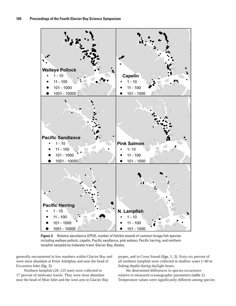
Figure �. Relative abundance (CPUE, number of fish/km towed) of common forage fish species including walleye pollock, capelin, Pacific sandlance, pink salmon, Pacific herring, and northern lampfish sampled by midwater trawl, Glacier Bay, Alaska.
10� Proceedings of the Fourth Glacier Bay Science Symposium
generally encountered in low numbers within Glacier Bay and were most abundant at Point Adolphus and near the head of Excursion Inlet (fig. 3).
Northern lampfish (26–125 mm) were collected in 17 percent of midwater trawls. They were most abundant near the head of Muir Inlet and the west arm in Glacier Bay
proper, and in Cross Sound (figs. 1, 3). Sixty-six percent of all northern lampfish were collected in shallow water (<40 m fishing depth) during daylight hours.
We determined differences in species occurrence relative to measured oceanographic parameters (table 1). Temperature values were significantly different among species
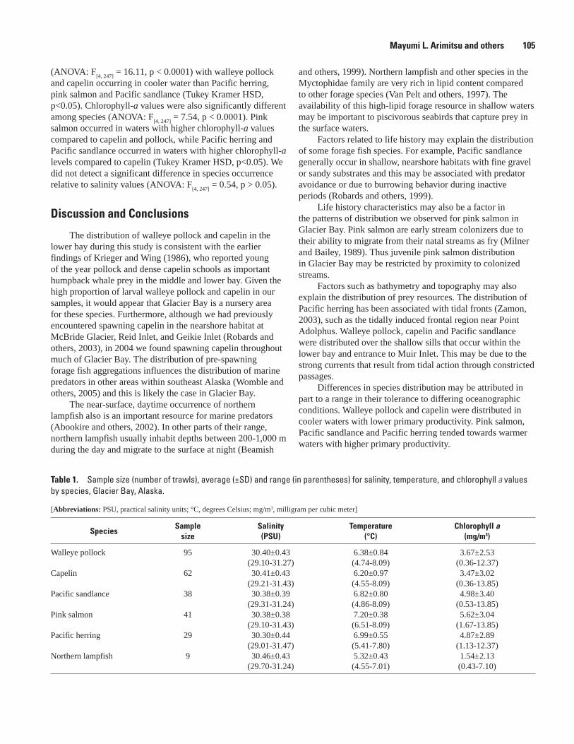
Table 1. Sample size (number of trawls), average (±SD) and range (in parentheses) for salinity, temperature, and chlorophyll a values by species, Glacier Bay, Alaska.
[Abbreviations: PSU, practical salinity units; °C, degrees Celsius; mg/m3, milligram per cubic meter]
SpeciesSample
sizeSalinity(PSU)
Temperature(°C)
Chlorophyll a(mg/m�)
Walleye pollock 95 30.40±0.43(29.10-31.27)
6.38±0.84(4.74-8.09)
3.67±2.53(0.36-12.37)
Capelin 62 30.41±0.43(29.21-31.43)
6.20±0.97(4.55-8.09)
3.47±3.02(0.36-13.85)
Pacific sandlance 38 30.38±0.39(29.31-31.24)
6.82±0.80(4.86-8.09)
4.98±3.40(0.53-13.85)
Pink salmon 41 30.38±0.38(29.10-31.43)
7.20±0.38(6.51-8.09)
5.62±3.04(1.67-13.85)
Pacific herring 29 30.30±0.44(29.01-31.47)
6.99±0.55(5.41-7.80)
4.87±2.89(1.13-12.37)
Northern lampfish 9 30.46±0.43(29.70-31.24)
5.32±0.43(4.55-7.01)
1.54±2.13(0.43-7.10)
Mayumi L. Arimitsu and others 105
(ANOVA: F[4, 247]
= 16.11, p < 0.0001) with walleye pollock and capelin occurring in cooler water than Pacific herring, pink salmon and Pacific sandlance (Tukey Kramer HSD, p<0.05). Chlorophyll-a values were also significantly different among species (ANOVA: F
[4, 247] = 7.54, p < 0.0001). Pink
salmon occurred in waters with higher chlorophyll-a values compared to capelin and pollock, while Pacific herring and Pacific sandlance occurred in waters with higher chlorophyll-a levels compared to capelin (Tukey Kramer HSD, p<0.05). We did not detect a significant difference in species occurrence relative to salinity values (ANOVA: F
[4, 247] = 0.54, p > 0.05).
Discussion and Conclusions
The distribution of walleye pollock and capelin in the lower bay during this study is consistent with the earlier findings of Krieger and Wing (1986), who reported young of the year pollock and dense capelin schools as important humpback whale prey in the middle and lower bay. Given the high proportion of larval walleye pollock and capelin in our samples, it would appear that Glacier Bay is a nursery area for these species. Furthermore, although we had previously encountered spawning capelin in the nearshore habitat at McBride Glacier, Reid Inlet, and Geikie Inlet (Robards and others, 2003), in 2004 we found spawning capelin throughout much of Glacier Bay. The distribution of pre-spawning forage fish aggregations influences the distribution of marine predators in other areas within southeast Alaska (Womble and others, 2005) and this is likely the case in Glacier Bay.
The near-surface, daytime occurrence of northern lampfish also is an important resource for marine predators (Abookire and others, 2002). In other parts of their range, northern lampfish usually inhabit depths between 200-1,000 m during the day and migrate to the surface at night (Beamish
and others, 1999). Northern lampfish and other species in the Myctophidae family are very rich in lipid content compared to other forage species (Van Pelt and others, 1997). The availability of this high-lipid forage resource in shallow waters may be important to piscivorous seabirds that capture prey in the surface waters.
Factors related to life history may explain the distribution of some forage fish species. For example, Pacific sandlance generally occur in shallow, nearshore habitats with fine gravel or sandy substrates and this may be associated with predator avoidance or due to burrowing behavior during inactive periods (Robards and others, 1999).
Life history characteristics may also be a factor in the patterns of distribution we observed for pink salmon in Glacier Bay. Pink salmon are early stream colonizers due to their ability to migrate from their natal streams as fry (Milner and Bailey, 1989). Thus juvenile pink salmon distribution in Glacier Bay may be restricted by proximity to colonized streams.
Factors such as bathymetry and topography may also explain the distribution of prey resources. The distribution of Pacific herring has been associated with tidal fronts (Zamon, 2003), such as the tidally induced frontal region near Point Adolphus. Walleye pollock, capelin and Pacific sandlance were distributed over the shallow sills that occur within the lower bay and entrance to Muir Inlet. This may be due to the strong currents that result from tidal action through constricted passages.
Differences in species distribution may be attributed in part to a range in their tolerance to differing oceanographic conditions. Walleye pollock and capelin were distributed in cooler waters with lower primary productivity. Pink salmon, Pacific sandlance and Pacific herring tended towards warmer waters with higher primary productivity.
10� Proceedings of the Fourth Glacier Bay Science Symposium
Management Implications
Forage fish are key intermediaries between primary and secondary producers and dominant marine predators such as halibut, marine birds, seals, and whales. Therefore, it is useful to understand how they distribute themselves in Glacier Bay because (1) their patterns of distribution and abundance will reflect the underlying modes of productivity, and provide insight into long-term changes in fundamental bio-physical properties of the ecosystem, and (2) their patterns of distribution and abundance may largely explain the patterns of distribution of higher predators, and so act as in indicator by which potential human disturbance of marine predators should be assessed.
Acknowledgments
Funding for this project was provided by National Park Service and U.S. Geological Survey, Alaska Science Center. We thank the crews of R/V Steller and R/V Pandalus, B. Congdon, J. Douglas, G. Drew, J. Driscoll, G. Eckert, L. Eisner, K. Emmerson, K. Juk, N. Hillgruber, N. Naslund, L. Nussman, L. Parker, J. Piatt, S. Scott, S. Speckman, N. Tojo and K. Weersing.
References Cited
Abookire, A.A., Piatt, J.F., and Speckman, S.G., 2002, A nearsurface, daytime occurrence of two mesopelagic fish species (Stenobrachius leucopsarus and Leuroglossus schmidti) in a glacial fjord: Fisheries Bulletin, v. 100, p. 376-380.
Beamish, R.J., Leask, K.D., Ivanov, O.A., Balanov, A.A., Orlov A.M., and Sinclair. B., 1999, The ecology, distribution, and abundance of midwater fishes of the Subarctic Pacific Gyres.:Progress in Oceanography v. 43, p. 399-442.
Krieger, K.J., and Wing. B.L., 1986, Hydroacoustic monitoring of prey to determine humpback whale movements: National Oceanic and Atmospheric Administration Technical Memo, U.S. Department of Commerce, 62 p.
Matarese, A.C., Kendall, A.W., Blood D.M., and Vinter, B.M., 1989, Laboratory guide to early life history stages of northeast pacific fishes: Seattle, Wash., National Marine Fisheries Service, Northwest and Alaska Fisheries Center, 650 p.
Milner, A.M. and Baileym R.G., 1989, Salmonid colonization of new streams in Glacier Bay National Park, Alaska: Aquaculture and Fisheries Management, v 20, p. 179-192.
Robards, M.D., Willson, M.F., Armstrong, R.H., and Piatt, J.F., eds., 1999, Sand Lance: A review of biology and predator relations and annotated bibliography: Portland, Oregon, Research Paper PNW-RP-521, U.S. Department of Agriculture, Forest Service, Pacific Northwest Research Station. 327 p.
Springer, A.M., and Speckman, S.G., 1997, A forage fish is what? Summary of the Symposium, in Forage fishes in marine ecosystems, Proceedings of the International Symposium on the Role of Forage Fishes in Marine Ecosystems: Fairbanks, University of Alaska, Alaska Sea Grant College Program Report No. 97-01, p. 773-805.
Van Pelt, T.I., Piatt, J.F., Lance B.K., and Roby, D.D., 1997, Proximate composition and energy density of some north Pacific forage fishes: Comparative Biochemistry and Physiology, v. 118A, p. 1393-1398.
Womble, J.N., Willson, M.F., Sigler, M.F., Kelly B.P., and VanBlaricom, G.R., 2005, Distribution of Steller sea lions Eumitopias jubatus in relation to spring-spawning fish in SE Alaska: Marine Ecology Progress Series v. 294, p. 271-282.
Zamon, J.E., 2003, Mixed species aggregations feeding upon herring and sandlance school in a nearshore archipelago depend on flooding tidal currents: Marine Ecology Progress Series 261, p. 243-255.
Suggested Citation
Arimitsu, M.L., Piatt, J.F., Romano, M.D., and Douglas, D.C., 2007, Distribution of forage fishes in relation to the oceanography of Glacier Bay, in Piatt, J.F., and Gende, S.M., eds., Proceedings of the Fourth Glacier Bay Science Symposium, October 26–28, 2004: U.S. Geological Survey Scientific Investigations Report 2007-5047, p. 102-106
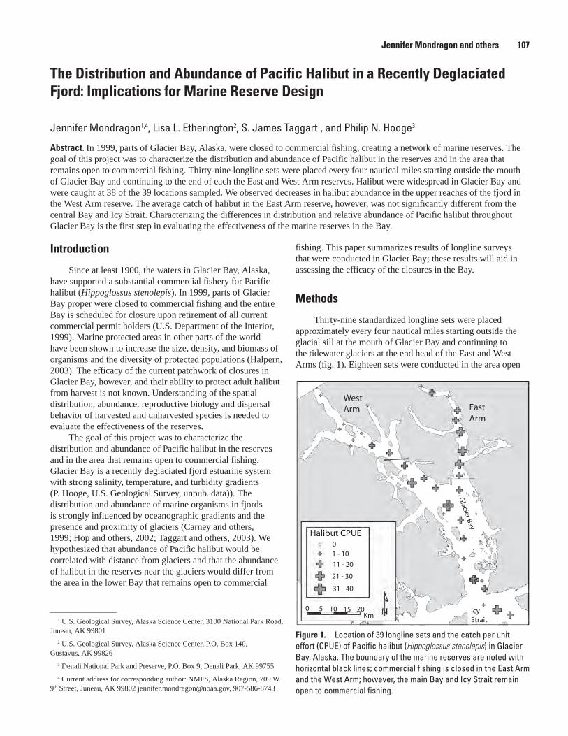
The Distribution and Abundance of Pacific Halibut in a Recently Deglaciated Fjord: Implications for Marine Reserve Design
Jennifer Mondragon1,4, Lisa L. Etherington2, S. James Taggart1, and Philip N. Hooge3
Abstract. In 1999, parts of Glacier Bay, Alaska, were closed to commercial fishing, creating a network of marine reserves. The goal of this project was to characterize the distribution and abundance of Pacific halibut in the reserves and in the area that remains open to commercial fishing. Thirty-nine longline sets were placed every four nautical miles starting outside the mouth of Glacier Bay and continuing to the end of each the East and West Arm reserves. Halibut were widespread in Glacier Bay and were caught at 38 of the 39 locations sampled. We observed decreases in halibut abundance in the upper reaches of the fjord in the West Arm reserve. The average catch of halibut in the East Arm reserve, however, was not significantly different from the central Bay and Icy Strait. Characterizing the differences in distribution and relative abundance of Pacific halibut throughout Glacier Bay is the first step in evaluating the effectiveness of the marine reserves in the Bay.
Figure 1. Location of 39 longline sets and the catch per unit effort (CPUE) of Pacific halibut (Hippoglossus stenolepis) in Glacier Bay, Alaska. The boundary of the marine reserves are noted with horizontal black lines; commercial fishing is closed in the East Arm and the West Arm; however, the main Bay and Icy Strait remain open to commercial fishing.
Jennifer Mondragon and others 107
Halibut CPUE01 - 10
11 - 20
21 - 30
31 - 40
0 5 10 15 20Km
WestArm East
Arm
IcyStrait
Glacier Bay
1 U.S. Geological Survey, Alaska Science Center, 3100 National Park Road, Juneau, AK 99801
2 U.S. Geological Survey, Alaska Science Center, P.O. Box 140, Gustavus, AK 99826
3 Denali National Park and Preserve, P.O. Box 9, Denali Park, AK 99755
4 Current address for corresponding author: NMFS, Alaska Region, 709 W. 9th Street, Juneau, AK 99802 [email protected], 907-586-8743
Introduction
Since at least 1900, the waters in Glacier Bay, Alaska, have supported a substantial commercial fishery for Pacific halibut (Hippoglossus stenolepis). In 1999, parts of Glacier Bay proper were closed to commercial fishing and the entire Bay is scheduled for closure upon retirement of all current commercial permit holders (U.S. Department of the Interior, 1999). Marine protected areas in other parts of the world have been shown to increase the size, density, and biomass of organisms and the diversity of protected populations (Halpern, 2003). The efficacy of the current patchwork of closures in Glacier Bay, however, and their ability to protect adult halibut from harvest is not known. Understanding of the spatial distribution, abundance, reproductive biology and dispersal behavior of harvested and unharvested species is needed to evaluate the effectiveness of the reserves.
The goal of this project was to characterize the distribution and abundance of Pacific halibut in the reserves and in the area that remains open to commercial fishing. Glacier Bay is a recently deglaciated fjord estuarine system with strong salinity, temperature, and turbidity gradients (P. Hooge, U.S. Geological Survey, unpub. data)). The distribution and abundance of marine organisms in fjords is strongly influenced by oceanographic gradients and the presence and proximity of glaciers (Carney and others, 1999; Hop and others, 2002; Taggart and others, 2003). We hypothesized that abundance of Pacific halibut would be correlated with distance from glaciers and that the abundance of halibut in the reserves near the glaciers would differ from the area in the lower Bay that remains open to commercial
fishing. This paper summarizes results of longline surveys that were conducted in Glacier Bay; these results will aid in assessing the efficacy of the closures in the Bay.
Methods
Thirty-nine standardized longline sets were placed approximately every four nautical miles starting outside the glacial sill at the mouth of Glacier Bay and continuing to the tidewater glaciers at the end head of the East and West Arms (fig. 1). Eighteen sets were conducted in the area open
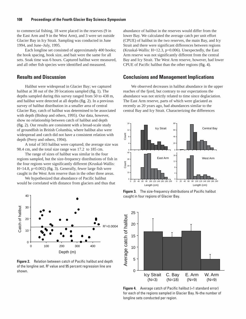
to commercial fishing, 18 were placed in the reserves (9 in the East Arm and 9 in the West Arm), and 3 were set outside Glacier Bay in Icy Strait. Sampling was conducted in June 1994, and June–July, 1995.
Each longline set consisted of approximately 400 hooks; the hook spacing, hook size, and bait were the same for all sets. Soak time was 6 hours. Captured halibut were measured, and all other fish species were identified and measured.
Results and Discussion
Halibut were widespread in Glacier Bay; we captured halibut at 38 out of the 39 locations sampled (fig. 1). The depths sampled during this survey ranged from 50 to 438 m, and halibut were detected at all depths (fig. 2). In a previous survey of halibut distribution in a smaller area of central Glacier Bay, catch of halibut was determined to be associated with depth (Bishop and others, 1995). Our data, however, show no relationship between catch of halibut and depth (fig. 2). Our results are consistent with a broad-scale study of groundfish in British Columbia, where halibut also were widespread and catch did not have a consistent relation with depth (Perry and others, 1994).
A total of 503 halibut were captured; the average size was 98.4 cm, and the total size range was 17.2 to 185 cm.
The range of sizes of halibut was similar in the four regions sampled, but the size-frequency distributions of fish in the four regions were significantly different (Kruskal-Wallis: H=14.8, p=0.002) (fig. 3). Generally, fewer large fish were caught in the West Arm reserve than in the other three areas.
We hypothesized that abundance of Pacific halibut would be correlated with distance from glaciers and thus that
Depth (m)
R2=0.0004
Cat
ch o
f hal
ibut
0
10
20
30
40
0 100 200 300 400
Figure 2. Relation between catch of Pacific halibut and depth of the longline set. R2 value and 95 percent regression line are shown.
Central Bay
0
20
40
60
80
East Arm
0
10
20
30
40
0 20 40 60 80 100 120 140 160 180 200
Icy Strait
0
4
8
12
16
West Arm
0
4
8
12
16
0 20 40 60 80 100 120 140 160 180 200
Length (cm)Length (cm)
Cou
ntC
ount
Figure �. The size-frequency distributions of Pacific halibut caught in four regions of Glacier Bay.
0
5
10
15
20
25
Icy Strait(N=3)
Aver
age
catc
h of
hal
ibut
C. Bay(N=18)
E. Arm(N=9)
W. Arm(N=9)
Figure �. Average catch of Pacific halibut (+1 standard error) for each of the regions sampled in Glacier Bay. N=the number of longline sets conducted per region.
10� Proceedings of the Fourth Glacier Bay Science Symposium
abundance of halibut in the reserves would differ from the lower Bay. We calculated the average catch per unit effort (CPUE) of halibut in the two reserves, the main Bay, and Icy Strait and there were significant differences between regions (Kruskal-Wallis: H=12.3, p=0.006). Unexpectedly, the East Arm reserve was not significantly different from the central Bay and Icy Strait. The West Arm reserve, however, had lower CPUE of Pacific halibut than the other regions (fig. 4).
Conclusions and Management Implications
We observed decreases in halibut abundance in the upper reaches of the fjord, but contrary to our expectations the abundance was not strictly related to time since deglaciation. The East Arm reserve, parts of which were glaciated as recently as 20 years ago, had abundances similar to the central Bay and Icy Strait. Characterizing the differences

Jennifer Mondragon and others 109
in distribution and relative abundance of Pacific halibut throughout Glacier Bay is the first step in evaluating the effectiveness of the marine reserves and allows us to answer the question: Are there animals in the reserve?
Acknowledgments
Glacier Bay National Park and Preserve and the U.S. Geological Survey, Alaska Science Center provided funding for this work. We thank the field crew who assisted in data collection, in particular: J. de La Bruere, G. Bishop, L. Chilton, C. Dezan, E. Hooge, F. Koschmann, and L. Solomon.
References Cited
Bishop, G.H., Hooge, P.N., and Taggart, S.J., 1995, Habitat correlates of Pacific halibut and other groundfish species in Glacier Bay National Park, in D.R. Engstrom, ed., Third Glacier Bay Science Symposium: U.S. National Park Service, Glacier Bay National Park and Preserve, Alaska, p. 215-220
Carney, D., Oliver, J.S., and Armstrong, C., 1999, Sedimentation and composition of wall communities in Alaskan fjords: Polar Biology v. 22, p. 38-49.
Halpern, B.S., 2003, The impact of marine reserves: Do reserves work and does reserve size matter? Ecological Applications, v. 13, p. S117-S137.
Hop, H., Pearson, T., and others, 2002, The marine ecosystem of Kongsfjorden, Svalbard: Polar Research v. 21, no. 1, p. 167-208.
Perry, R.I., Stocker, M., and Fargo, J., 1994, Environmental effects on the distributions of groundfish in Hecate Strait, British Columbia: Canadian Journal of Fisheries and Aquatic Sciences, v. 51, p. 1401-1409.
Taggart, S.J., Hooge, P.N., Mondragon, J., Hooge, E.R., and Andrews, A.G., 2003, Living on the edge: the distribution of Dungeness crab, Cancer magister, in a recently deglaciated fjord: Marine Ecology Progress Series 246, p. 241-252.
U.S. Department of the Interior, 1999, Glacier Bay National Park, Alaska: U.S. Department of the Interior, Commercial Fishing Regulations; Final Rule. 36 CFR Part 13, v. 64, p. 56455-56464.
Suggested Citation
Mondragon J., Etherington, L.E., Taggart, S.J., Hooge, P.N., 2007, The distributin and abundance of Pacific halibut in a recently deglaciated fjord: Implications for marine reserve design, in Piatt, J.F., and Gende, S.M., eds., Proceedings of the Fourth Glacier Bay Science Symposium, October 26–28, 2004: U.S. Geological Survey Scientific Investigations Report 2007-5047, p. 107-109
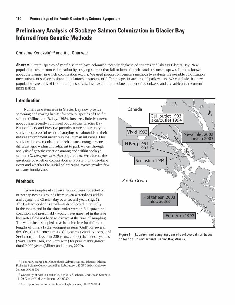
Preliminary Analysis of Sockeye Salmon Colonization in Glacier Bay Inferred from Genetic Methods
Christine Kondzela1,2,3 and A.J. Gharrett2
Abstract. Several species of Pacific salmon have colonized recently deglaciated streams and lakes in Glacier Bay. New populations result from colonization by straying salmon that fail to home to their natal streams to spawn. Little is known about the manner in which colonization occurs. We used population genetics methods to evaluate the possible colonization mechanisms of sockeye salmon populations in streams of different ages in and around park waters. We conclude that new populations are derived from multiple sources, involve an intermediate number of colonizers, and are subject to recurrent immigration.
Figure 1. Location and sampling year of sockeye salmon tissue collections in and around Glacier Bay, Alaska.
110 Proceedings of the Fourth Glacier Bay Science Symposium
U.S.Canada
Pacific Ocean
Ford Arm 1992
Hoktaheen 2003inlet/outlet
Seclusion 1994
N Berg 1991 1992
Vivid 1993
Gull outlet 1993lake/outlet 1994
Neva inlet 2002 beach 2003
N
Introduction
Numerous watersheds in Glacier Bay now provide spawning and rearing habitat for several species of Pacific salmon (Milner and Bailey, 1989); however, little is known about these recently colonized populations. Glacier Bay National Park and Preserve provides a rare opportunity to study the successful result of straying by salmonids in their natural environment under minimal human influence. Our study evaluates colonization mechanisms among streams of different ages within and adjacent to park waters through analysis of genetic variation among and within sockeye salmon (Oncorhynchus nerka) populations. We address the questions of whether colonization is recurrent or a one-time event and whether the initial colonization events involve few or many immigrants.
Methods
Tissue samples of sockeye salmon were collected on or near spawning grounds from seven watersheds within and adjacent to Glacier Bay over several years (fig. 1). The Gull watershed is small—fish collected intertidally in the mouth and in the short outlet were in full spawning condition and presumably would have spawned in the lake had water flow not been restrictive at the time of sampling. The watersheds sampled have been ice-free for different lengths of time: (1) the youngest system (Gull) for several decades, (2) the “medium-aged” systems (Vivid, N. Berg, and Seclusion) for less than 200 years, and (3) the oldest systems (Neva, Hoktaheen, and Ford Arm) for presumably greater than10,000 years (Milner and others, 2000).
1 National Oceanic and Atmospheric Administration Fisheries, Alaska Fisheries Science Center, Auke Bay Laboratory, 11305 Glacier Highway, Juneau, AK 99801
2 University of Alaska Fairbanks, School of Fisheries and Ocean Sciences, 11120 Glacier Highway, Juneau, AK 99801
3 Corresponding author: [email protected], 907-789-6084
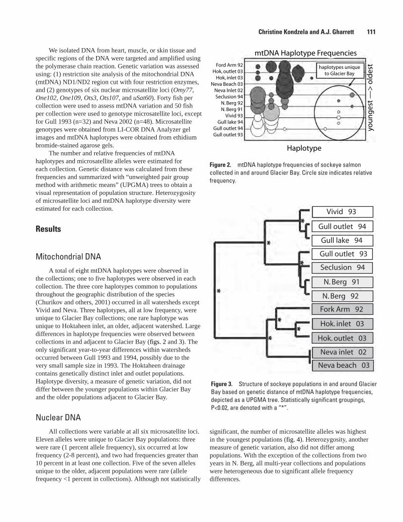
We isolated DNA from heart, muscle, or skin tissue and specific regions of the DNA were targeted and amplified using the polymerase chain reaction. Genetic variation was assessed using: (1) restriction site analysis of the mitochondrial DNA (mtDNA) ND1/ND2 region cut with four restriction enzymes, and (2) genotypes of six nuclear microsatellite loci (Omy77, One102, One109, Ots3, Ots107, and uSat60). Forty fish per collection were used to assess mtDNA variation and 50 fish per collection were used to genotype microsatellite loci, except for Gull 1993 (n=32) and Neva 2002 (n=48). Microsatellite genotypes were obtained from LI-COR DNA Analyzer gel images and mtDNA haplotypes were obtained from ethidium bromide-stained agarose gels.
The number and relative frequencies of mtDNA haplotypes and microsatellite alleles were estimated for each collection. Genetic distance was calculated from these frequencies and summarized with “unweighted pair group method with arithmetic means” (UPGMA) trees to obtain a visual representation of population structure. Heterozygosity of microsatellite loci and mtDNA haplotype diversity were estimated for each collection.
Results
Mitochondrial DNAA total of eight mtDNA haplotypes were observed in
the collections; one to five haplotypes were observed in each collection. The three core haplotypes common to populations throughout the geographic distribution of the species (Churikov and others, 2001) occurred in all watersheds except Vivid and Neva. Three haplotypes, all at low frequency, were unique to Glacier Bay collections; one rare haplotype was unique to Hoktaheen inlet, an older, adjacent watershed. Large differences in haplotype frequencies were observed between collections in and adjacent to Glacier Bay (figs. 2 and 3). The only significant year-to-year differences within watersheds occurred between Gull 1993 and 1994, possibly due to the very small sample size in 1993. The Hoktaheen drainage contains genetically distinct inlet and outlet populations. Haplotype diversity, a measure of genetic variation, did not differ between the younger populations within Glacier Bay and the older populations adjacent to Glacier Bay.
Nuclear DNAAll collections were variable at all six microsatellite loci.
Eleven alleles were unique to Glacier Bay populations: three were rare (1 percent allele frequency), six occurred at low frequency (2-8 percent), and two had frequencies greater than 10 percent in at least one collection. Five of the seven alleles unique to the older, adjacent populations were rare (allele frequency <1 percent in collections). Although not statistically
Haplotype
you
ng
est
—>
old
esthaplotypes unique
to Glacier Bay
Ford Arm 92Hok, outlet 03
Hok, inlet 03Neva Beach 03
Neva Inlet 02Seclusion 94
N. Berg 92N. Berg 91
Vivid 93Gull lake 94
Gull outlet 94Gull outlet 93
mtDNA Haplotype Frequencies
Figure 2. mtDNA haplotype frequencies of sockeye salmon collected in and around Glacier Bay. Circle size indicates relative frequency.
Figure �. Structure of sockeye populations in and around Glacier Bay based on genetic distance of mtDNA haplotype frequencies, depicted as a UPGMA tree. Statistically significant groupings, P<0.02, are denoted with a “*”.
Christine Kondzela and A.J. Gharrett 111
Vivid 93
Gull outlet 94
Gull lake 94
Gull outlet 93
Seclusion 94
N. Berg 91
N. Berg 92
Fork Arm 92
Hok. inlet 03
Hok. outlet 03
Neva inlet 02
Neva beach 03
significant, the number of microsatellite alleles was highest in the youngest populations (fig. 4). Heterozygosity, another measure of genetic variation, also did not differ among populations. With the exception of the collections from two years in N. Berg, all multi-year collections and populations were heterogeneous due to significant allele frequency differences.
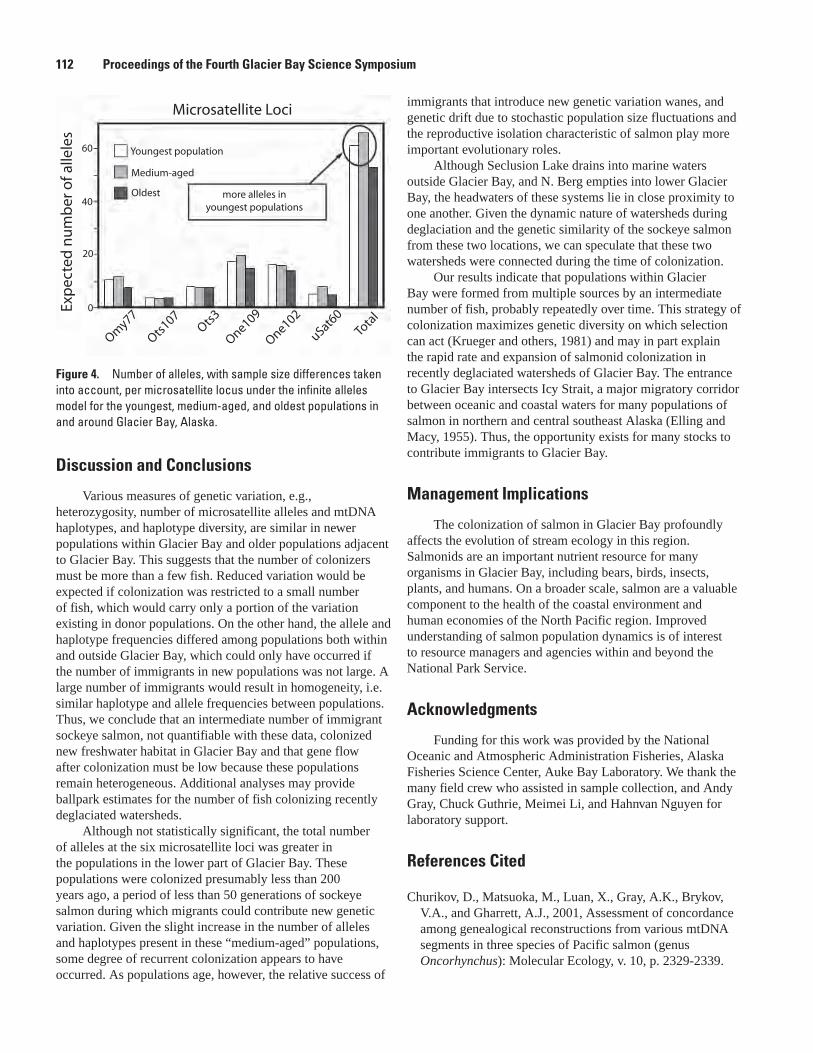
Discussion and Conclusions
Various measures of genetic variation, e.g., heterozygosity, number of microsatellite alleles and mtDNA haplotypes, and haplotype diversity, are similar in newer populations within Glacier Bay and older populations adjacent to Glacier Bay. This suggests that the number of colonizers must be more than a few fish. Reduced variation would be expected if colonization was restricted to a small number of fish, which would carry only a portion of the variation existing in donor populations. On the other hand, the allele and haplotype frequencies differed among populations both within and outside Glacier Bay, which could only have occurred if the number of immigrants in new populations was not large. A large number of immigrants would result in homogeneity, i.e. similar haplotype and allele frequencies between populations. Thus, we conclude that an intermediate number of immigrant sockeye salmon, not quantifiable with these data, colonized new freshwater habitat in Glacier Bay and that gene flow after colonization must be low because these populations remain heterogeneous. Additional analyses may provide ballpark estimates for the number of fish colonizing recently deglaciated watersheds.
Although not statistically significant, the total number of alleles at the six microsatellite loci was greater in the populations in the lower part of Glacier Bay. These populations were colonized presumably less than 200 years ago, a period of less than 50 generations of sockeye salmon during which migrants could contribute new genetic variation. Given the slight increase in the number of alleles and haplotypes present in these “medium-aged” populations, some degree of recurrent colonization appears to have occurred. As populations age, however, the relative success of
Microsatellite Loci
Omy77
Ots107
Ots3
One109
One102
uSat60
Tota
l
60
40
20
0Exp
ecte
d n
um
ber
of a
llele
s
Youngest population
Medium-aged
Oldest more alleles inyoungest populations
Figure �. Number of alleles, with sample size differences taken into account, per microsatellite locus under the infinite alleles model for the youngest, medium-aged, and oldest populations in and around Glacier Bay, Alaska.
112 Proceedings of the Fourth Glacier Bay Science Symposium
immigrants that introduce new genetic variation wanes, and genetic drift due to stochastic population size fluctuations and the reproductive isolation characteristic of salmon play more important evolutionary roles.
Although Seclusion Lake drains into marine waters outside Glacier Bay, and N. Berg empties into lower Glacier Bay, the headwaters of these systems lie in close proximity to one another. Given the dynamic nature of watersheds during deglaciation and the genetic similarity of the sockeye salmon from these two locations, we can speculate that these two watersheds were connected during the time of colonization.
Our results indicate that populations within Glacier Bay were formed from multiple sources by an intermediate number of fish, probably repeatedly over time. This strategy of colonization maximizes genetic diversity on which selection can act (Krueger and others, 1981) and may in part explain the rapid rate and expansion of salmonid colonization in recently deglaciated watersheds of Glacier Bay. The entrance to Glacier Bay intersects Icy Strait, a major migratory corridor between oceanic and coastal waters for many populations of salmon in northern and central southeast Alaska (Elling and Macy, 1955). Thus, the opportunity exists for many stocks to contribute immigrants to Glacier Bay.
Management Implications
The colonization of salmon in Glacier Bay profoundly affects the evolution of stream ecology in this region. Salmonids are an important nutrient resource for many organisms in Glacier Bay, including bears, birds, insects, plants, and humans. On a broader scale, salmon are a valuable component to the health of the coastal environment and human economies of the North Pacific region. Improved understanding of salmon population dynamics is of interest to resource managers and agencies within and beyond the National Park Service.
Acknowledgments
Funding for this work was provided by the National Oceanic and Atmospheric Administration Fisheries, Alaska Fisheries Science Center, Auke Bay Laboratory. We thank the many field crew who assisted in sample collection, and Andy Gray, Chuck Guthrie, Meimei Li, and Hahnvan Nguyen for laboratory support.
References Cited
Churikov, D., Matsuoka, M., Luan, X., Gray, A.K., Brykov, V.A., and Gharrett, A.J., 2001, Assessment of concordance among genealogical reconstructions from various mtDNA segments in three species of Pacific salmon (genus Oncorhynchus): Molecular Ecology, v. 10, p. 2329-2339.
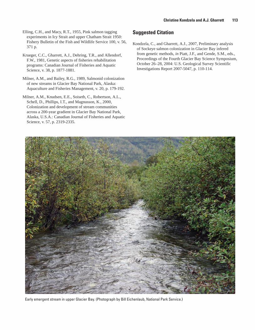
Christine Kondzela and A.J. Gharrett 11�
Elling, C.H., and Macy, R.T., 1955, Pink salmon tagging experiments in Icy Strait and upper Chatham Strait 1950: Fishery Bulletin of the Fish and Wildlife Service 100, v. 56, 371 p.
Krueger, C.C., Gharrett, A.J., Dehring, T.R., and Allendorf, F.W., 1981, Genetic aspects of fisheries rehabilitation programs: Canadian Journal of Fisheries and Aquatic Science, v. 38, p. 1877-1881.
Milner, A.M., and Bailey, R.G., 1989, Salmonid colonization of new streams in Glacier Bay National Park, Alaska: Aquaculture and Fisheries Management, v. 20, p. 179-192.
Milner, A.M., Knudsen, E.E., Soiseth, C., Robertson, A.L., Schell, D., Phillips, I.T., and Magnusson, K., 2000, Colonization and development of stream communities across a 200-year gradient in Glacier Bay National Park, Alaska, U.S.A.: Canadian Journal of Fisheries and Aquatic Science, v. 57, p. 2319-2335.
Early emergent stream in upper Glacier Bay. (Photograph by Bill Eichenlaub, National Park Service.)
Suggested Citation
Kondzela, C., and Gharrett, A.J., 2007, Preliminary analysis of Sockeye salmon colonization in Glacier Bay infered from genetic methods, in Piatt, J.F., and Gende, S.M., eds., Proceedings of the Fourth Glacier Bay Science Symposium, October 26–28, 2004: U.S. Geological Survey Scientific Investigations Report 2007-5047, p. 110-114.

This page is intentionally left blank.
11� Proceedings of the Fourth Glacier Bay Science Symposium
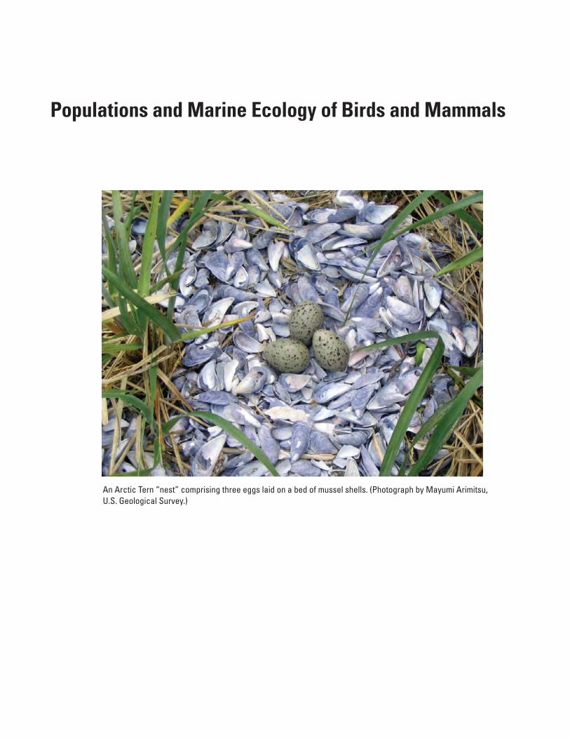
Populations and Marine Ecology of Birds and Mammals
An Arctic Tern “nest” comprising three eggs laid on a bed of mussel shells. (Photograph by Mayumi Arimitsu, U.S. Geological Survey.)

This page is intentionally left blank.
11� Proceedings of the Fourth Glacier Bay Science Symposium, 200�
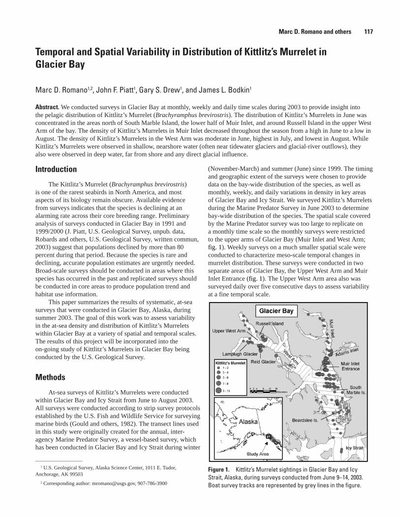
Temporal and Spatial Variability in Distribution of Kittlitz’s Murrelet in Glacier Bay
Marc D. Romano1,2, John F. Piatt1, Gary S. Drew1, and James L. Bodkin1
Abstract. We conducted surveys in Glacier Bay at monthly, weekly and daily time scales during 2003 to provide insight into the pelagic distribution of Kittlitz’s Murrelet (Brachyramphus brevirostris). The distribution of Kittlitz’s Murrelets in June was concentrated in the areas north of South Marble Island, the lower half of Muir Inlet, and around Russell Island in the upper West Arm of the bay. The density of Kittlitz’s Murrelets in Muir Inlet decreased throughout the season from a high in June to a low in August. The density of Kittlitz’s Murrelets in the West Arm was moderate in June, highest in July, and lowest in August. While Kittlitz’s Murrelets were observed in shallow, nearshore water (often near tidewater glaciers and glacial-river outflows), they also were observed in deep water, far from shore and any direct glacial influence.
Figure 1. Kittlitz’s Murrelet sightings in Glacier Bay and Icy Strait, Alaska, during surveys conducted from June 9–14, 2003. Boat survey tracks are represented by grey lines in the figure.
Marc D. Romano and others 117
1 U.S. Geological Survey, Alaska Science Center, 1011 E. Tudor, Anchorage, AK 99503
2 Corresponding author: [email protected], 907-786-3900
Introduction
The Kittlitz’s Murrelet (Brachyramphus brevirostris) is one of the rarest seabirds in North America, and most aspects of its biology remain obscure. Available evidence from surveys indicates that the species is declining at an alarming rate across their core breeding range. Preliminary analysis of surveys conducted in Glacier Bay in 1991 and 1999/2000 (J. Piatt, U.S. Geological Survey, unpub. data, Robards and others, U.S. Geological Survey, written commun, 2003) suggest that populations declined by more than 80 percent during that period. Because the species is rare and declining, accurate population estimates are urgently needed. Broad-scale surveys should be conducted in areas where this species has occurred in the past and replicated surveys should be conducted in core areas to produce population trend and habitat use information.
This paper summarizes the results of systematic, at-sea surveys that were conducted in Glacier Bay, Alaska, during summer 2003. The goal of this work was to assess variability in the at-sea density and distribution of Kittlitz’s Murrelets within Glacier Bay at a variety of spatial and temporal scales. The results of this project will be incorporated into the on-going study of Kittlitz’s Murrelets in Glacier Bay being conducted by the U.S. Geological Survey.
Methods
At-sea surveys of Kittlitz’s Murrelets were conducted within Glacier Bay and Icy Strait from June to August 2003. All surveys were conducted according to strip survey protocols established by the U.S. Fish and Wildlife Service for surveying marine birds (Gould and others, 1982). The transect lines used in this study were originally created for the annual, inter-agency Marine Predator Survey, a vessel-based survey, which has been conducted in Glacier Bay and Icy Strait during winter
(November-March) and summer (June) since 1999. The timing and geographic extent of the surveys were chosen to provide data on the bay-wide distribution of the species, as well as monthly, weekly, and daily variations in density in key areas of Glacier Bay and Icy Strait. We surveyed Kittlitz’s Murrelets during the Marine Predator Survey in June 2003 to determine bay-wide distribution of the species. The spatial scale covered by the Marine Predator survey was too large to replicate on a monthly time scale so the monthly surveys were restricted to the upper arms of Glacier Bay (Muir Inlet and West Arm; fig. 1). Weekly surveys on a much smaller spatial scale were conducted to characterize meso-scale temporal changes in murrelet distribution. These surveys were conducted in two separate areas of Glacier Bay, the Upper West Arm and Muir Inlet Entrance (fig. 1). The Upper West Arm area also was surveyed daily over five consecutive days to assess variability at a fine temporal scale.
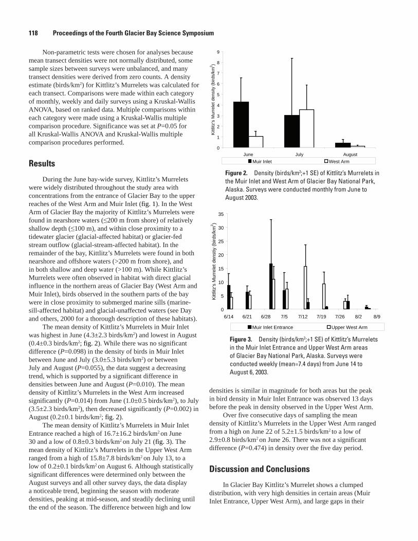
Non-parametric tests were chosen for analyses because mean transect densities were not normally distributed, some sample sizes between surveys were unbalanced, and many transect densities were derived from zero counts. A density estimate (birds/km2) for Kittlitz’s Murrelets was calculated for each transect. Comparisons were made within each category of monthly, weekly and daily surveys using a Kruskal-Wallis ANOVA, based on ranked data. Multiple comparisons within each category were made using a Kruskal-Wallis multiple comparison procedure. Significance was set at P=0.05 for all Kruskal-Wallis ANOVA and Kruskal-Wallis multiple comparison procedures performed.
Results
During the June bay-wide survey, Kittlitz’s Murrelets were widely distributed throughout the study area with concentrations from the entrance of Glacier Bay to the upper reaches of the West Arm and Muir Inlet (fig. 1). In the West Arm of Glacier Bay the majority of Kittlitz’s Murrelets were found in nearshore waters (≤200 m from shore) of relatively shallow depth (≤100 m), and within close proximity to a tidewater glacier (glacial-affected habitat) or glacier-fed stream outflow (glacial-stream-affected habitat). In the remainder of the bay, Kittlitz’s Murrelets were found in both nearshore and offshore waters (>200 m from shore), and in both shallow and deep water (>100 m). While Kittlitz’s Murrelets were often observed in habitat with direct glacial influence in the northern areas of Glacier Bay (West Arm and Muir Inlet), birds observed in the southern parts of the bay were in close proximity to submerged marine sills (marine-sill-affected habitat) and glacial-unaffected waters (see Day and others, 2000 for a thorough description of these habitats).
The mean density of Kittlitz’s Murrelets in Muir Inlet was highest in June (4.3±2.3 birds/km2) and lowest in August (0.4±0.3 birds/km2; fig. 2). While there was no significant difference (P=0.098) in the density of birds in Muir Inlet between June and July (3.0±5.3 birds/km2) or between July and August (P=0.055), the data suggest a decreasing trend, which is supported by a significant difference in densities between June and August (P=0.010). The mean density of Kittlitz’s Murrelets in the West Arm increased significantly (P=0.014) from June (1.0±0.5 birds/km2), to July (3.5±2.3 birds/km2), then decreased significantly (P=0.002) in August (0.2±0.1 birds/km2; fig. 2).
The mean density of Kittlitz’s Murrelets in Muir Inlet Entrance reached a high of 16.7±16.2 birds/km2 on June 30 and a low of 0.8±0.3 birds/km2 on July 21 (fig. 3). The mean density of Kittlitz’s Murrelets in the Upper West Arm ranged from a high of 15.8±7.8 birds/km2 on July 13, to a low of 0.2±0.1 birds/km2 on August 6. Although statistically significant differences were determined only between the August surveys and all other survey days, the data display a noticeable trend, beginning the season with moderate densities, peaking at mid-season, and steadily declining until the end of the season. The difference between high and low
densities is similar in magnitude for both areas but the peak in bird density in Muir Inlet Entrance was observed 13 days before the peak in density observed in the Upper West Arm.
Over five consecutive days of sampling the mean density of Kittlitz’s Murrelets in the Upper West Arm ranged from a high on June 22 of 5.2±1.5 birds/km2 to a low of 2.9±0.8 birds/km2 on June 26. There was not a significant difference (P=0.474) in density over the five day period.
Discussion and Conclusions
In Glacier Bay Kittlitz’s Murrelet shows a clumped distribution, with very high densities in certain areas (Muir Inlet Entrance, Upper West Arm), and large gaps in their
Figure 2. Density (birds/km2;+1 SE) of Kittlitz’s Murrelets in the Muir Inlet and West Arm of Glacier Bay National Park, Alaska. Surveys were conducted monthly from June to August 2003.
Figure �. Density (birds/km2;+1 SE) of Kittlitz’s Murrelets in the Muir Inlet Entrance and Upper West Arm areas of Glacier Bay National Park, Alaska. Surveys were conducted weekly (mean=7.4 days) from June 14 to August 6, 2003.
11� Proceedings of the Fourth Glacier Bay Science Symposium
AK2-0043_fig02_Romano-Temporal.ai
0
1
2
3
4
5
6
7
8
9
June July August
Kitt
litz'
sM
urre
letd
ensi
ty(b
irds/
km2 )
Muir Inlet West Arm
AK2-0043_fig03_Romano-Temporal.ai
0
5
10
15
20
25
30
35
6/14 6/21 6/28 7/5 7/12 7/19 7/26 8/2 8/9
Kitt
litz'
sM
urre
letd
enst
iy(b
irds/
km2 )
Muir Inlet Entrance Upper West Arm
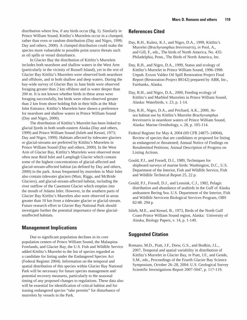
Marc D. Romano and others 119
distribution where few, if any birds occur (fig. 1). Similarly in Prince William Sound, Kittlitz’s Murrelets occur in a clumped, rather than even or random distribution (Day and Nigro, 1999; Day and others, 2000). A clumped distribution could make the species more vulnerable to possible point source threats such as oil spills or vessel disturbance.
In Glacier Bay the distribution of Kittlitz’s Murrelets includes both nearshore and shallow waters in the West Arm (particularly in the vicinity of Russell Island), yet in the rest of Glacier Bay Kittlitz’s Murrelets were observed both nearshore and offshore, and in both shallow and deep waters. During the bay-wide survey of Glacier Bay in June birds were observed foraging greater than 2 km offshore and in water deeper than 200 m. It is not known whether birds in these areas were foraging successfully, but birds were often observed greater than 2 km from shore holding fish in their bills at the Muir Inlet Entrance. Kittlitz’s Murrelets have shown a preference for nearshore and shallow waters in Prince William Sound (Day and Nigro, 2000).
The distribution of Kittlitz’s Murrelet has been linked to glacial fjords in both south-eastern Alaska (Day and others, 1999) and Prince William Sound (Islieb and Kessel, 1973; Day and Nigro, 1999). Habitats affected by tidewater glaciers or glacial-streams are preferred by Kittlitz’s Murrelets in Prince William Sound (Day and others, 2000). In the West Arm of Glacier Bay, Kittlitz’s Murrelets were observed most often near Reid Inlet and Lamplugh Glacier which contain some of the highest concentrations of glacial-affected and glacial-stream-affected habitat (as defined by Day and others, 2000) in the park. Areas frequented by murrelets in Muir Inlet also contain tidewater glaciers (Muir, Riggs, and McBride Glaciers), and glacial-stream-affected habitat, including the river outflow of the Casement Glacier which empties into the mouth of Adams Inlet. However, in the southern parts of Glacier Bay Kittlitz’s Murrelets also were observed in areas greater than 10 km from a tidewater glacier or glacial-stream. Future research effort in Glacier Bay National Park should investigate further the potential importance of these glacial-unaffected habitats.
Management Implications
Due to significant population declines in its core population centers of Prince William Sound, the Malaspina Forelands, and Glacier Bay, the U.S. Fish and Wildlife Service added Kittlitz’s Murrelet to the list of species regarded as a candidate for listing under the Endangered Species Act (Federal Register 2004). Information on the temporal and spatial distribution of this species within Glacier Bay National Park will be necessary for future species management and potential recovery measures, particularly to the seasonal timing of any proposed changes to regulations. These data also will be essential for identification of critical habitat and for issuing endangered species “take permits” for disturbance of murrelets by vessels in the Park.
References Cited
Day, R.H., Kuletz, K.J., and Nigro, D.A., 1999, Kittlitz’s Murrelet (Brachyramphus brevirostris), in Pool, A., and Gill, F., eds., The birds of North America, No. 435: Philadelphia, Penn., The Birds of North America, Inc.
Day, R.H., and Nigro, D.A., 1999, Status and ecology of Kittlitz’s Murrelet in Prince William Sound, 1996-1998: Unpub. Exxon Valdez Oil Spill Restoration Project Final Report (Restoration Project 88142) prepared by ABR, Inc., Fairbanks, Alaska.
Day, R.H., and Nigro, D.A., 2000, Feeding ecology of Kittlitz’s and Marbled Murrelets in Prince William Sound, Alaska: Waterbirds, v. 23, p. 1-14.
Day, R.H., Nigro, D.A., and Prichard, A.K., 2000, At-sea habitat use by Kittlitz’s Murrelet Brachyramphus brevirostris in nearshore waters of Prince William Sound, Alaska: Marine Ornithology, v. 28, p. 105-114.
Federal Register for May 4, 2004 (69 CFR 24875–24904), Review of species that are candidates or proposed for listing as endangered or threatened; Annual Notice of Findings on Resubmitted Petitions; Annual Description of Progress on Listing Actions.
Gould, P.J., and Forsell, D.J., 1989, Techniques for shipboard surveys of marine birds: Washington, D.C., U.S. Department of the Interior, Fish and Wildlife Service, Fish and Wildlife Technical Report 25, 22 p.
Gould, P.J., Forsell, D.J., and Lensink, C.J., 1982, Pelagic distribution and abundance of seabirds in the Gulf of Alaska andeastern Bering Sea. U.S. Department of the Interior, Fish and Wildlife Servicem Biological Services Program, OBS 82/48. 294 p.
Islieb, M.E., and Kessel, B., 1973, Birds of the North Gulf Coast-Prince William Sound region, Alaska: University of Alaska, Biology Papers, v. 14, p. 1-149.
Suggested Citation
Romano, M.D., Piatt, J.F., Drew, G.S., and Bodkin, J.L., 2007, Temporal and spatial variability in distribution of Kittlitz’s Murrelet in Glacier Bay, in Piatt, J.F., and Gende, S.M., eds., Proceedings of the Fourth Glacier Bay Science Symposium, October 26–28, 2004: U.S. Geological Survey Scientific Investigations Report 2007-5047, p. 117-119.
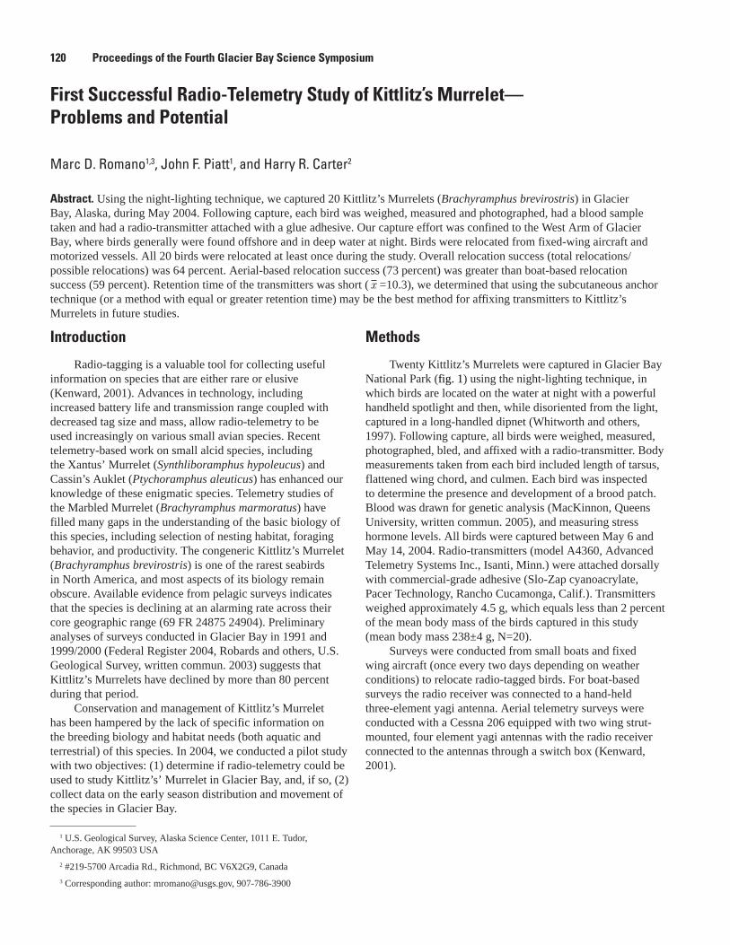
First Successful Radio-Telemetry Study of Kittlitz’s Murrelet—Problems and Potential
Marc D. Romano1,3, John F. Piatt1, and Harry R. Carter2
Abstract. Using the night-lighting technique, we captured 20 Kittlitz’s Murrelets (Brachyramphus brevirostris) in Glacier Bay, Alaska, during May 2004. Following capture, each bird was weighed, measured and photographed, had a blood sample taken and had a radio-transmitter attached with a glue adhesive. Our capture effort was confined to the West Arm of Glacier Bay, where birds generally were found offshore and in deep water at night. Birds were relocated from fixed-wing aircraft and motorized vessels. All 20 birds were relocated at least once during the study. Overall relocation success (total relocations/possible relocations) was 64 percent. Aerial-based relocation success (73 percent) was greater than boat-based relocation success (59 percent). Retention time of the transmitters was short (x =10.3), we determined that using the subcutaneous anchor technique (or a method with equal or greater retention time) may be the best method for affixing transmitters to Kittlitz’s Murrelets in future studies.
120 Proceedings of the Fourth Glacier Bay Science Symposium
Introduction
Radio-tagging is a valuable tool for collecting useful information on species that are either rare or elusive (Kenward, 2001). Advances in technology, including increased battery life and transmission range coupled with decreased tag size and mass, allow radio-telemetry to be used increasingly on various small avian species. Recent telemetry-based work on small alcid species, including the Xantus’ Murrelet (Synthliboramphus hypoleucus) and Cassin’s Auklet (Ptychoramphus aleuticus) has enhanced our knowledge of these enigmatic species. Telemetry studies of the Marbled Murrelet (Brachyramphus marmoratus) have filled many gaps in the understanding of the basic biology of this species, including selection of nesting habitat, foraging behavior, and productivity. The congeneric Kittlitz’s Murrelet (Brachyramphus brevirostris) is one of the rarest seabirds in North America, and most aspects of its biology remain obscure. Available evidence from pelagic surveys indicates that the species is declining at an alarming rate across their core geographic range (69 FR 24875 24904). Preliminary analyses of surveys conducted in Glacier Bay in 1991 and 1999/2000 (Federal Register 2004, Robards and others, U.S. Geological Survey, written commun. 2003) suggests that Kittlitz’s Murrelets have declined by more than 80 percent during that period.
Conservation and management of Kittlitz’s Murrelet has been hampered by the lack of specific information on the breeding biology and habitat needs (both aquatic and terrestrial) of this species. In 2004, we conducted a pilot study with two objectives: (1) determine if radio-telemetry could be used to study Kittlitz’s’ Murrelet in Glacier Bay, and, if so, (2) collect data on the early season distribution and movement of the species in Glacier Bay.
Methods
Twenty Kittlitz’s Murrelets were captured in Glacier Bay National Park (fig. 1) using the night-lighting technique, in which birds are located on the water at night with a powerful handheld spotlight and then, while disoriented from the light, captured in a long-handled dipnet (Whitworth and others, 1997). Following capture, all birds were weighed, measured, photographed, bled, and affixed with a radio-transmitter. Body measurements taken from each bird included length of tarsus, flattened wing chord, and culmen. Each bird was inspected to determine the presence and development of a brood patch. Blood was drawn for genetic analysis (MacKinnon, Queens University, written commun. 2005), and measuring stress hormone levels. All birds were captured between May 6 and May 14, 2004. Radio-transmitters (model A4360, Advanced Telemetry Systems Inc., Isanti, Minn.) were attached dorsally with commercial-grade adhesive (Slo-Zap cyanoacrylate, Pacer Technology, Rancho Cucamonga, Calif.). Transmitters weighed approximately 4.5 g, which equals less than 2 percent of the mean body mass of the birds captured in this study (mean body mass 238±4 g, N=20).
Surveys were conducted from small boats and fixed wing aircraft (once every two days depending on weather conditions) to relocate radio-tagged birds. For boat-based surveys the radio receiver was connected to a hand-held three-element yagi antenna. Aerial telemetry surveys were conducted with a Cessna 206 equipped with two wing strut-mounted, four element yagi antennas with the radio receiver connected to the antennas through a switch box (Kenward, 2001).
1 U.S. Geological Survey, Alaska Science Center, 1011 E. Tudor, Anchorage, AK 99503 USA
2 #219-5700 Arcadia Rd., Richmond, BC V6X2G9, Canada
3 Corresponding author: [email protected], 907-786-3900
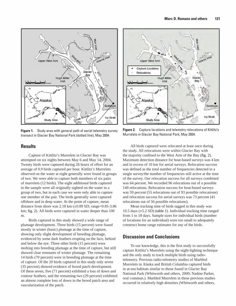
Figure 1. Study area with general path of aerial telemetry survey transect in Glacier Bay National Park (dotted line), May 2004.
Figure 2. Capture locations and telemetry relocations of Kittlitz’s Murrelets in Glacier Bay National Park, May 2004.
Marc D. Romano and others 121
All birds captured were relocated at least once during the study. All relocations were within Glacier Bay with the majority confined to the West Arm of the Bay (fig. 2). Maximum detection distance for boat-based surveys was 4 km and in excess of 10 km for aerial surveys. Relocation success was defined as the total number of frequencies detected in a single survey/the number of frequencies still active at the time of the survey. Our relocation success for all surveys combined was 64 percent. We recorded 96 relocations out of a possible 149 relocations. Relocation success for boat-based surveys was 59 percent (55 relocations out of 93 possible relocations) and relocation success for aerial surveys was 73 percent (41 relocations out of 56 possible relocations).
Mean tracking time of birds tagged in this study was 10.5 days (±5.2 SD) (table 1). Individual tracking time ranged from 1 to 18 days. Sample sizes for individual birds (number of locations for an individual) were too small to adequately construct home range estimates for any of the birds.
Discussion and Conclusions
To our knowledge, this is the first study to successfully capture Kittlitz’s Murrelets using the night-lighting technique and the only study to track multiple birds using radio-telemetry. Previous radio-telemetry studies of Marbled Murrelets in Alaska and British Columbia captured birds in at-sea habitats similar to those found in Glacier Bay National Park (Whitworth and others, 2000; Nadine Parker, oral commun.). Marbled Murrelets in these previous studies occurred in relatively high densities (Whitworth and others,
Results
Capture of Kittlitz’s Murrelets in Glacier Bay was attempted on six nights between May 6 and May 14, 2004. Twenty birds were captured during 26 hours of effort for an average of 0.9 birds captured per hour. Kittlitz’s Murrelets observed on the water at night generally were found in groups of two. We were able to capture both members of six pairs of murrelets (12 birds). The eight additional birds captured in the sample were all originally sighted on the water in a group of two, but in each case we were only able to capture one member of the pair. The birds generally were captured offshore and in deep water. At the point of capture, mean distance from shore was 2.18 km (±0.89 SD; range=0.85-3.86 km; fig. 2). All birds were captured in water deeper than 100 m.
Birds captured in this study showed a wide range of plumage development. Three birds (15 percent) were found mostly in winter (basic) plumage at the time of capture, showing only slight development of breeding plumage, evidenced by some dark feathers erupting on the face, behind and below the eye. Three other birds (15 percent) were molting into breeding plumage at the time of capture, but still showed clear remnants of winter plumage. The remaining 14 birds (70 percent) were in breeding plumage at the time of capture. Of the 20 birds captured in this study only seven (35 percent) showed evidence of brood patch development. Of these seven, five (71 percent) exhibited a loss of down and contour feathers, and the remaining two (29 percent) exhibited an almost complete loss of down in the brood patch area and vascularization of the patch.

122 Proceedings of the Fourth Glacier Bay Science Symposium
2000; Nadine Parker, oral commun.) and a concern prior to attempting this study was whether Kittlitz’s Murrelets occurred in high enough densities in Glacier Bay to enable capture of an adequate sample for a radio-telemetry study. Our capture per unit effort (0.9 captures/hour) was greater than expected and we believe that this capture technique is an efficient and cost-effective method of capturing Kittlitz’s Murrelets in this study area.
Although all birds marked in the study were relocated at least once, overall relocation success for the study (64 percent) was lower than expected, and boat-based relocation success was particularly low. The 4 km maximum detection range of the boat-based surveys may have affected relocation success, particularly in the lower portions of Glacier Bay where the bay is wider and there are more islands to block potential radio signals. In addition, several areas of Glacier Bay are designated non-motorized zones and we were not able to access these areas during our boat-based surveys. Non-motorized zones were accessible for aerial surveys however, and this increase in survey area, coupled with greater maximum detection range, could account for the greater relocation success of aerial surveys. The main benefit of the boat-based survey is that it allows researchers to observe radio-marked individuals to assess behavior (e.g. reaction to radio, foraging behavior, disturbance by vessels, etc.).
The mean tracking time of Kittlitz’s Murrelets in this study was much less compared to radio-telemetry studies of other small alcids (table 1). Several factors can influence the tracking time of a radio-telemetry study including transmitter failure, individuals leaving the study site, and transmitter loss. It is unlikely that transmitter failure is responsible for the low mean tracking time of our study. The ATS model A4360 radio-transmitter has been used in several studies including an intensive multi-year study of Marbled Murrelets in British Columbia (over 500 birds radio-marked). The researchers conducting this study found no evidence of widespread transmitter failure (Nadine Parker and Russell Bradley oral commun.). While it is possible that radio-marked Kittlitz’s Murrelets left the Glacier Bay study area after being captured, aerial telemetry surveys were flown outside of Glacier Bay in Icy Strait and Cross Sound and no frequencies were detected.
For a radio telemetry study to be successful, the method of transmitter attachment must provide adequate transmitter retention time without adversely affecting the behavior of the animal (Newman and others, 1999; Kenward, 2001).
Currently, the most common method of attaching radio-transmitters to small alcids is the subcutaneous anchor technique (Newman and others, 1999; Whitworth and others, 2000; Adams and others, 2004). This technique was developed specifically to improve tracking time of radio-marked birds. Previous studies indicated that adhesive-only attachments are not as durable as the anchor technique (Quinlan and Hughes, 1992; Newman and others, 1999). Mean tracking time of small alcids with transmitters attached using the subcutaneous anchor method are three to six times greater than the tracking time of Kittlitz’s Murrelets with glued-on transmitters in our study (table 1).
If radio telemetry is to be used as a tool to study Kittlitz’s Murrelet then tracking time of individual birds should be greater than that in our study. Generally, home range estimation for individual animals requires a minimum sample size of 30 position locations (Millspaugh and Marzluff, 2001). Our sample size of position locations for any of the marked birds was not large enough (range=1–11 position locations) to estimate home range or make inferences about habitat use and individual movements. Tracking time from this study would need to be increased by a factor of three to obtain enough data to characterize habitat use and home range.
Management Implications
On May 4, 2004, the U.S. Fish and Wildlife Service added Kittlitz’s Murrelet to the list of candidate species for listing as threatened or endangered species (69 FR 24875 24904). Among the likely causes for the recent “significant population declines” in the core range of the species are “habitat loss or degradation, increased adult and juvenile mortality, and low recruitment…” (69 FR 24875 24904). Investigation of these and other potential causes for decline would directly benefit from data collected using radio-telemetry methods. Habitat use and nesting requirements are important needs that will also be essential if a future determination of critical habitat for the species is justified.
References Cited
Adams, J., Takekawa, J.Y., and Carter. H.R., 2004, Foraging distance and home range of Cassin’s Auklets nesting at two colonies in the California Channel Islands: The Condor, v. 106, p. 618-637.
Table 1. Comparison of mean tracking time of small, radio-tagged alcids, from four studies using different attachment methods.
Data source Species Location Attachment method Tracking time
This study Kittlitz’s Murrelet Glacier Bay National Park Glue 10.5 daysAdams and others, 2004 Cassin’s Auklet Channel Islands National Park Subcutaneous Anchor 30.0 daysNewman and others, 1999 Marbled Murrelet Año Nuevo Bay, California Subcutaneous Anchor 45.1 daysWhitworth and others, 2000 Marbled Murrelet Auke Bay, AK Subcutaneous Anchor 67.0 days
Marc D. Romano and others 12�
A Bald Eagle rests atop a small iceberg. (Photograph by Brenda Ballachey, U.S. Geological Survey.)
Federal Register for May 4, 2004 (69 CFR 24875–24904), Review of species that are candidates or proposed for listing as endangered or threatened; Annual Notice of Findings on Resubmitted Petitions; Annual Description of Progress on Listing Actions.
Kenward, R.E., 2001, A manual for wildlife radio tagging: San Diego, Calif., Academic Press.
Millspaugh, J.J., and Marzluff. J.M. 2001. Radio tracking of animal populations: San Diego, Calif., Academic Press.
Newman, S.H., Takekawa, J.Y., Whitworth, D.L., and Burkett, E.E., 1999, Subcutaneous anchor attachment increases retention of radio transmitters on seabirds: Xantus’ and Marbled Murrelets: Journal of Field Ornithology, v. 70, p. 520-534.
Quilan, S.E., and Hughes, J.H., 1992, Techniques for radio tagging of Marbled Murrelets, in Carter, H.R., and Morrison, M.L., eds., Status and conservation of the Marbled Murrelet in North America: Proceedings of the Western Foundation of Vertebrate Zoology, v. 5. p. 117-121.
Whitworth D.L., Nelson, S.K., Newman, S.H., Van Vliet, G.B., and Smith, W.P., 2000, Foraging distances of radio-marked Marbled Murrelets from inland areas in Southeast Alaska: The Condor, v. 102, p. 452-456.
Whitworth D.L., Takekawa, J.Y., Carter, H.R., and McIver, W.R., 1997, A night-lighting technique for at-sea capture of Xantus’ Murrelets: Colonial Waterbirds, v. 20, no. 3, p. 525-531.
Suggested Citation
Romano, M.D., Piatt, J.F., and Carter, H.R., 2007, First successfult radio-telemetry study of Kittlitz’s Murrelet—Problems and potential, in Piatt, J.F., and Gende, S.M., eds., Proceedings of the Fourth Glacier Bay Science Symposium, October 26–28, 2004: U.S. Geological Survey Scientific Investigations Report 2007-5047, p. 120-123.
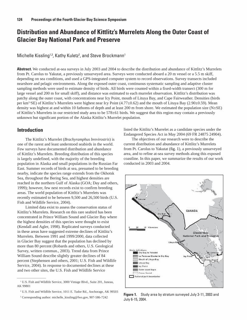
Distribution and Abundance of Kittlitz’s Murrelets Along the Outer Coast of Glacier Bay National Park and Preserve
Michelle Kissling1,3, Kathy Kuletz2, and Steve Brockmann1
Abstract. We conducted at-sea surveys in July 2003 and 2004 to describe the distribution and abundance of Kittlitz’s Murrelets from Pt. Carolus to Yakutat, a previously unsurveyed area. Surveys were conducted aboard a 20 m vessel or a 5.5 m skiff, depending on sea conditions, and used a GPS-integrated computer system to record observations. Survey transects included nearshore and pelagic environments. Along the exposed outer coast, continuous systematic sampling and adaptive cluster sampling methods were used to estimate density of birds. All birds were counted within a fixed-width transect (300 m for large vessel and 200 m for small skiff), and distance was estimated to each murrelet observation. Kittlitz’s distribution was patchy along the outer coast, with concentrations near Icy Point, mouth of Lituya Bay, and Cape Fairweather. Densities (birds per km2±SE) of Kittlitz’s Murrelets were highest near Icy Point (4.77±0.62) and the mouth of Lituya Bay (2.90±0.59). Mean density was highest at and within 10 fathoms of depth and at least 200 m from shore. We estimated the population size (N±SE) of Kittlitz’s Murrelets in our restricted study area to be 578±61 birds. We suggest that this region may contain a previously unknown but significant portion of the Alaska Kittlitz’s Murrelet population.
Figure 1. Study area by stratum surveyed July 3-11, 2003 and July 6-15, 2004.
12� Proceedings of the Fourth Glacier Bay Science Symposium
Introduction
The Kittlitz’s Murrelet (Brachyramphus brevirostris) is one of the rarest and least understood seabirds in the world. Few surveys have documented distribution and abundance of Kittlitz’s Murrelets. Breeding distribution of this species is largely undefined, with the majority of the breeding population in Alaska and small populations in the Russian Far East. Summer records of birds at sea, presumed to be breeding nearby, indicate the species range extends from the Okhotsk Sea, throughout the Bering Sea, and highest densities are reached in the northern Gulf of Alaska (GOA; Day and others, 1999); however, few nest records exist to confirm breeding areas. The world population of Kittltiz’s Murrelets was recently estimated to be between 9,500 and 26,500 birds (U.S. Fish and Wildlife Service, 2004).
Limited data exist to assess the conservation status of Kittlitz’s Murrelets. Research on this rare seabird has been concentrated in Prince William Sound and Glacier Bay where the highest densities of this species were thought to exist (Kendall and Agler, 1998). Replicated surveys conducted in these areas have suggested extreme declines of Kittlitz’s Murrelets. Between 1991 and 1999/2000, data collected in Glacier Bay suggest that the population has declined by more than 80 percent (Robards and others, U.S. Geological Survey, written commun., 2003). Trend data from Prince William Sound describe slightly greater declines of 84 percent (Stephensen and others, 2001; U.S. Fish and Wildlife Service, 2004). In response to documented declines at these and two other sites, the U.S. Fish and Wildlife Service
listed the Kittlitz’s Murrelet as a candidate species under the Endangered Species Act in May 2004 (69 FR 24875 24904).
The objectives of our research were to describe the current distribution and abundance of Kittlitz’s Murrelets from Pt. Carolus to Yakutat (fig. 1), a previously unsurveyed area, and to refine at-sea survey methods along this exposed coastline. In this paper, we summarize the results of our work conducted in 2003 and 2004.
1 U.S. Fish and Wildlife Service, 3000 Vintage Blvd., Suite 201, Juneau, AK 99801
2 U.S. Fish and Wildlife Service, 1011 E. Tudor Rd., Anchorage, AK 99503
3 Corresponding author: [email protected], 907-586-7242
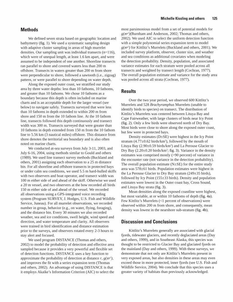
Michelle Kissling and others 125
Methods
We defined seven strata based on geographic location and bathymetry (fig. 1). We used a systematic sampling design with adaptive cluster sampling in areas of high murrelet densities. Our sampling unit was individual transects (n=116), which were of unequal length, at least 1.6 km apart, and were assumed to be independent of one another. Shoreline transects ran parallel to shore and covered waters less than 200 m offshore. Transects in waters greater than 200 m from shore were perpendicular to shore, followed a sawtooth (i.e., zigzag) pattern, or were parallel to shore depending on water depth.
Along the exposed outer coast, we stratified our study area by three water depths: less than 10 fathoms, 10 fathoms, and greater than 10 fathoms. We chose 10 fathoms as a boundary because this depth is often included on marine charts and is an acceptable depth for the larger vessel (see below) to navigate safely. Transects surveyed that were less than 10 fathoms in depth extended to within 200 m from shore and 150 m from the 10 fathom line. At the 10 fathom line, transects followed this depth continuously and transect width was 300 m. Transects surveyed that were greater than 10 fathoms in depth extended from 150 m from the 10 fathom line to 5.56 km (3 nautical miles) offshore. This distance from shore denotes the territorial sea boundary and is also often noted on marine charts.
We conducted at-sea surveys from July 3-11, 2003, and July 6-16, 2004, using methods similar to Gould and others (1989). We used line transect survey methods (Buckland and others, 2001) assigning each observation to a 25 m distance bin. For all shoreline and offshore transects in protected bays or under calm sea conditions, we used 5.5 m hard-hulled skiffs with two observers and boat operator, and transect width was 100 m either side of and ahead of the skiff. Otherwise we used a 20 m vessel, and two observers at the bow recorded all birds 150 m either side of and ahead of the vessel. We recorded all observations using a GPS-integrated voice recording system (Program SURVEY, J. Hodges, U.S. Fish and Wildlife Service, Juneau). For all murrelet observations, we recorded number in group, behavior (e.g., on water, flying, foraging), and the distance bin. Every 30 minutes we also recorded weather, sea and ice conditions, swell height, wind speed and direction, and water temperature and clarity. All observers were trained in bird identification and distance estimation prior to the surveys, and observers rotated every 2-3 hours to stay alert and focused.
We used program DISTANCE (Thomas and others, 2002) to model the probability of detection and effective area sampled because it provides a very powerful and flexible set of detection functions. DISTANCE uses a key function to approximate the probability of detection at distance r, g(πr2), and improves the fit with a series expansion term (Thomas and others, 2002). An advantage of using DISTANCE is that it employs Akaike’s Information Criterion (AIC) to select the
most parsimonious model from a set of potential models for g(πr2)(Burnham and Anderson, 2002; Thomas and others, 2002). We used AIC to select the uniform detection function with a simple polynomial series expansion term to model g(πr2) for Kittlitz’s Murrelets (Buckland and others, 2001). We included survey platform, observer, cluster size, and weather and sea conditions as additional covariates when modeling the detection probability. Density, population, and associated variance estimates for each stratum were pooled across all transects and weighted by transect length (Cochran, 1977). The overall population estimate and variance for the study area was pooled across all strata (Cochran, 1977).
Results
Over the two year period, we observed 600 Kittlitz’s Murrelets and 528 Brachyramphus Murrelets (unable to identify birds to species) on transect. The distribution of Kittlitz’s Murrelets was centered between Lituya Bay and Cape Fairweather, with large clusters of birds near Icy Point (fig. 2). Only a few birds were observed north of Dry Bay. Most birds were close to shore along the exposed outer coast, but few were in protected bays.
Density estimates (D±SE) were highest in the Icy Point stratum (4.77±0.62 birds/km2), followed by the mouth of Lituya Bay (2.90±0.59 birds/km2) and La Perouse Glacier to Dry Bay (2.20±0.20 birds/km2; fig. 3). Variance in the density estimates was comprised mostly (>90 percent) of variance in the encounter rate (not variance in the detection probability). The overall population estimate (N±SE) for the entire study area was 578±61 birds. Population estimates were highest in the La Perouse Glacier to Dry Bay stratum (249±35 birds), followed by Icy Point (155±33 birds). Density and population estimates were lowest in the Outer coast bay, Cross Sound, and Lituya Bay strata (fig. 3).
Mean densities along the exposed coastline were highest, but most variable, at or within 10 fathoms of depth (fig. 4a). Few Kittlitz’s Murrelets (<1 percent of observations) were observed within 200 m from shore, and consequently, mean density was lowest in the nearshore sub-stratum (fig. 4b).
Discussion and Conclusions
Kittlitz’s Murrelets generally are associated with glacial fjords, tidewater glaciers, and recently deglaciated areas (Day and others, 1999), and in Southeast Alaska, this species was thought to be restricted to Glacier Bay and glaciated fjords on the mainland (Day and others, 1999). With these surveys, we demonstrate that not only are Kittlitz’s Murrelets present in very exposed areas, but also densities in these areas may even exceed those in more protected, inner fjords (see U.S. Fish and Wildlife Service, 2004). We conclude that this species uses a greater variety of habitats than previously acknowledged.
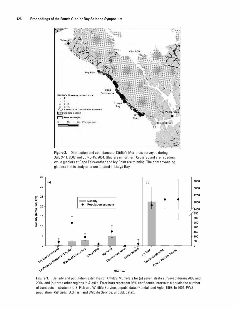
Figure �. Density and population estimates of Kittlitz’s Murrelets for (a) seven strata surveyed during 2003 and 2004, and (b) three other regions in Alaska. Error bars represent 95% confidence intervals: n equals the number of transects in stratum (1U.S. Fish and Wildlife Service, unpubl. data; 2Kendall and Agler 1998. In 2004, PWS population=758 birds [U.S. Fish and Wildlife Service, unpubl. data]).
12� Proceedings of the Fourth Glacier Bay Science Symposium
Figure 2. Distribution and abundance of Kittlitz’s Murrelets surveyed during July 3-11, 2003 and July 6-15, 2004. Glaciers in northern Cross Sound are receding, while glaciers at Cape Fairweather and Icy Point are thinning. The only advancing glaciers in this study area are located in Lituya Bay.
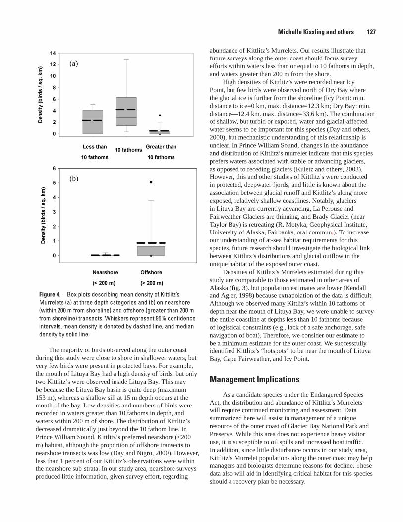
The majority of birds observed along the outer coast during this study were close to shore in shallower waters, but very few birds were present in protected bays. For example, the mouth of Lituya Bay had a high density of birds, but only two Kittlitz’s were observed inside Lituya Bay. This may be because the Lituya Bay basin is quite deep (maximum 153 m), whereas a shallow sill at 15 m depth occurs at the mouth of the bay. Low densities and numbers of birds were recorded in waters greater than 10 fathoms in depth, and waters within 200 m of shore. The distribution of Kittlitz’s decreased dramatically just beyond the 10 fathom line. In Prince William Sound, Kittlitz’s preferred nearshore (<200 m) habitat, although the proportion of offshore transects to nearshore transects was low (Day and Nigro, 2000). However, less than 1 percent of our Kittlitz’s observations were within the nearshore sub-strata. In our study area, nearshore surveys produced little information, given survey effort, regarding
Figure �. Box plots describing mean density of Kittlitz’s Murrelets (a) at three depth categories and (b) on nearshore (within 200 m from shoreline) and offshore (greater than 200 m from shoreline) transects. Whiskers represent 95% confidence intervals, mean density is denoted by dashed line, and median density by solid line.
Michelle Kissling and others 127
abundance of Kittlitz’s Murrelets. Our results illustrate that future surveys along the outer coast should focus survey efforts within waters less than or equal to 10 fathoms in depth, and waters greater than 200 m from the shore.
High densities of Kittlitz’s were recorded near Icy Point, but few birds were observed north of Dry Bay where the glacial ice is further from the shoreline (Icy Point: min. distance to ice=0 km, max. distance=12.3 km; Dry Bay: min. distance—12.4 km, max. distance=33.6 km). The combination of shallow, but turbid or exposed, water and glacial-affected water seems to be important for this species (Day and others, 2000), but mechanistic understanding of this relationship is unclear. In Prince William Sound, changes in the abundance and distribution of Kittlitz’s murrelet indicate that this species prefers waters associated with stable or advancing glaciers, as opposed to receding glaciers (Kuletz and others, 2003). However, this and other studies of Kittlitz’s were conducted in protected, deepwater fjords, and little is known about the association between glacial runoff and Kittlitz’s along more exposed, relatively shallow coastlines. Notably, glaciers in Lituya Bay are currently advancing, La Perouse and Fairweather Glaciers are thinning, and Brady Glacier (near Taylor Bay) is retreating (R. Motyka, Geophysical Institute, University of Alaska, Fairbanks, oral commun.). To increase our understanding of at-sea habitat requirements for this species, future research should investigate the biological link between Kittlitz’s distributions and glacial outflow in the unique habitat of the exposed outer coast.
Densities of Kittlitz’s Murrelets estimated during this study are comparable to those estimated in other areas of Alaska (fig. 3), but population estimates are lower (Kendall and Agler, 1998) because extrapolation of the data is difficult. Although we observed many Kittliz’s within 10 fathoms of depth near the mouth of Lituya Bay, we were unable to survey the entire coastline at depths less than 10 fathoms because of logistical constraints (e.g., lack of a safe anchorage, safe navigation of boat). Therefore, we consider our estimate to be a minimum estimate for the outer coast. We successfully identified Kittlitz’s “hotspots” to be near the mouth of Lituya Bay, Cape Fairweather, and Icy Point.
Management Implications
As a candidate species under the Endangered Species Act, the distribution and abundance of Kittlitz’s Murrelets will require continued monitoring and assessment. Data summarized here will assist in management of a unique resource of the outer coast of Glacier Bay National Park and Preserve. While this area does not experience heavy visitor use, it is susceptible to oil spills and increased boat traffic. In addition, since little disturbance occurs in our study area, Kittlitz’s Murrelet populations along the outer coast may help managers and biologists determine reasons for decline. These data also will aid in identifying critical habitat for this species should a recovery plan be necessary.
Acknowledgments
We are grateful to Liz Labunski, Mary Kralovic, Steve Lewis, Mike Jacobson, Joe Spicianni, Paul Suchanek, and Joe McClung for their assistance in the field. Tammy Davis and Adrianna Rodriguez transcribed all of the data. We thank Jack Hodges and Jeff Bromaghin for statistical support. This project was funded by Glacier Bay National Park and U.S. Fish and Wildlife Service.
References Cited
Buckland, S.T., Anderson, D.R., Burnham, K.P., Laake, J.L., Borchers, D.L., and Thomas, L., 2001, Introduction to distance sampling: Oxford, England, Oxford University Press.
Burnham, K.P., and Anderson, D.R., 2002, Model Selection and Multimodel Inference; a Practical Information-Theoretic Approach: New York, Springer.496 p.
Cochran, W.G., 1977, Sampling techniques: New York, John Wiley and Sons, Inc.
Day, R.H., Kuletz, K.J., and Nigro, D.A., 1999, Kittlitz’s Murrelet (Brachyramphus brevirostris), in Poole, A., and Gill, F., eds., The birds of North America, no. 435: Philadelphia, Penn., The Birds of North America, Inc.,
Day, R.H., and Nigro, D.A., 2000, Feeding ecology of Kittlitz’s and Marbled Murrelets in Prince William Sound, Alaska: Waterbirds, v. 23, p. 1-14.
Day, R.H., Nigro, D.A., and Prichard, A.K., 2000, At-sea habitat use by Kittlitz’s Murrelet Brachyramphus brevirostris in nearshore waters of Prince William Sound, Alaska: Marine Ornithology, v. 28, p. 105-114.
Federal Register for May 4, 2004 (50 CFR 24875 – 24904). Review of species that are candidates or proposed for listing as endangered or threatened; Annual Notice of Findings on Resubmitted Petitions; Annual Description of Progress on Listing Actions.
Gould, P.J., and Forsell, D.J., 1989. Techniques for shipboard surveys of marine birds: Washington, D.C., U.S. Department of the Interior, Fish and Wildlife Service, Fish and Wildlife Technical Report 25, 22 p.
12� Proceedings of the Fourth Glacier Bay Science Symposium
Kendall, S.J., and Agler B.A., 1998, Distribution and abundance of Kittlitz’s Murrelets in Southcentral and Southeastern Alaska: Colonial Waterbirds, v. 21, p. 53-60.
Kuletz, K.J., Stephensen, S.W., Irons, D.B., Labunski, E.A., and Brenneman, K.M., 2003, Changes in distribution and abundance of Kittlitz’s Murrelets (Brachyramphus brevirostris) relative to glacial recession in Prince William Sound, Alaska: Marine Ornithology, v. 31, p. 133-140.
Robards, M., Drew, G., Piatt, J., Anson, J.M., Abookire, A., Bodkin, J., Hooge, P., and Speckman, S., 2003, Ecology of selected marine communities in Glacier Bay—zooplankton, forage fish, seabirds and marine mammals: U.S. Geological Survey final report to the National Park Service, 156 p.
Stephensen, S.W., Irons, D.B., Kendall, S.J., Lance, B.K., and McDonald, L.L., 2001, Marine bird and sea otter population abundance of Prince William Sound, Alaska: Trends following the T/V Exxon Valdez Oil Spill, 1989-2000: Anchorage, Alaska, U.S. Fish and Wildlife Service, Exxon Valdez Oil Spill Restoration Project annual report (Restoration Project 00159).
Thomas, L., Laake, J.L., Strindberg, S., Marques, F.F.C., Buckland, S.T., Borchers, D.L., Anderson, D.R., Burnham, K.P., Hedley, S.L., and Pollard, J.H., 2002, Distance 4.1. Release 1. Research unit for wildlife population assessment: University of St. Andrews, United Kingdom, http://www.ruwpa.st-and.ac.uk/distance.
U.S. Fish and Wildlife Service, 2004, Candidate and listing priority assignment form for Kittlitz’s Murrelet: Anchorage, Alaska, U.S. Fish and Wildlife Service, Migratory Bird Management, 38 p.
Suggested Citation
Kissling, M., Kuletz, K., and Brockmann, S., 2007, Distribution and abundance of Kittlitz’s Murrelets along the outer coast of Glacier Bay National Park and Preserve, in Piatt, J.F., and Gende, S.M., eds., Proceedings of the Fourth Glacier Bay Science Symposium, October 26–28, 2004: U.S. Geological Survey Scientific Investigations Report 2007-5047, p. 124-128.
Population Status and Trends of Marine Birds and Mammals in Glacier Bay National Park
Gary S. Drew1,2, John F. Piatt1, and James Bodkin1
Abstract. By censusing marine birds and mammals at sea it is possible to assess abundance and distribution of entire communities, and monitor population trends of many species simultaneously. We conducted surveys for marine birds and mammals in Glacier Bay, Alaska, during June 1991 and annually from 1999 to 2003. The 1991 surveys were almost exclusively coastal, so only the coastal transects of the more extensive 1999–2003 ship based surveys were used for comparison. To compare data sets, we calculated densities of each species by transect. The mean and standard error were calculated for the most common marine bird and mammal species. Populations of most species showed little change over the past 13 years; however, randomization tests confirmed that there were several exceptions. Kittlitz’s and marbled murrelet populations have declined within the Bay. In contrast, population increases were noted for glaucous-winged gulls, mew gulls, sea otters, and humpback whales. Population changes may be a reflection of ongoing environmental changes in Glacier Bay.
Gary S. Drew and others 129
1 U.S. Geological Survey, Alaska Science Center, 1011 E. Tudor, Anchorage, AK 99503
2 Corresponding author: [email protected], 907-786-3475
Introduction
Assessing the population status and trends for seabirds and marine mammals can be difficult. Many colonial species can be studied at their rookeries, however, at-sea surveys are required to study non-colonial species, several species concurrently, or the status of juveniles or non-breeders (Tasker and others, 1984). At-sea surveys have the added benefit of providing information about the use of different marine habitats by marine birds and mammals. We conducted surveys of seabirds and marine mammals in Glacier Bay, Alaska, in June 1991 and 1999–2003, with the goal of determining the species composition, population trends, and species distributions within the Bay.
Methods
The 1991 surveys were conducted from a small boat. At the time, transect locations were noted on a 1:24,000 chart. We later digitized these transects to facilitate comparisons with later surveys. The 1999–2003 surveys were collected from both small boats and moderate sized (<100 ft) vessels. Bird and mammal sightings were recorded by entering them directly into a real-time computer data-entry system (DLOG; DLOG; Glann Ford Consulting, Portland, OR, ECI) that plots sighting positions continuously using GPS coordinates. Ground speed for vessels was approximately 15-20 km/hr (8-12 knots). Surveys were conducted, with some modifications, according to protocols established by the U.S. Fish and Wildlife Service for marine birds (Gould and others, 1982; Gould and Forsell, 1989). Observers from the Pandalus and
USGS R/V Alaskan Gyre counted and identified to species, swimming birds and mammals within 150 m on either side or 300 m forward of the boat. Because of their lower viewing angles in the small boats, we limited the area of counting and identification to 100 m on both sides and 200 m forward. We counted all flying birds that crossed within transects. Due to the considerably greater coverage of offshore areas on the 1999–2003 surveys we only used data from coastal transects to calculate densities. We used a GIS to determine transect lengths. Multiplying transect width by length yielded the area surveyed. Simply dividing the number of each species sighted by each transect’s area yielded a sample. All transects (samples) were then averaged to provide an population index for each species. Although this index could have the effect of underestimating the 1991 populations (due to lower average transect width), we were confident that by looking at the range of species, we would be able to identify any bias.
Results
We observed 65 species of marine birds and 9 species of marine mammals during the surveys. Forty-two of these species were seen in all years. Maps of five common seabirds and the most common marine mammal suggest that some areas of Glacier Bay are important for multiple species, though; some species have distinctly different distributions (fig. 1). Most species showed a coastal pattern of habitat use; however, Kittlitz’s and marbled murrelets were more pelagic in their distribution than the other “common” species. The majority of species had reasonably consistent patterns of habitat use. Among marine birds we noted the increase in the use of the northern part of Glacier Bay by gulls. Among marine mammals, both sea otters and humpback whales expanded their range in the Bay between 1991 and 2003. Conversely, harbor seals appeared to have declined in the East Arm of the Bay over time.
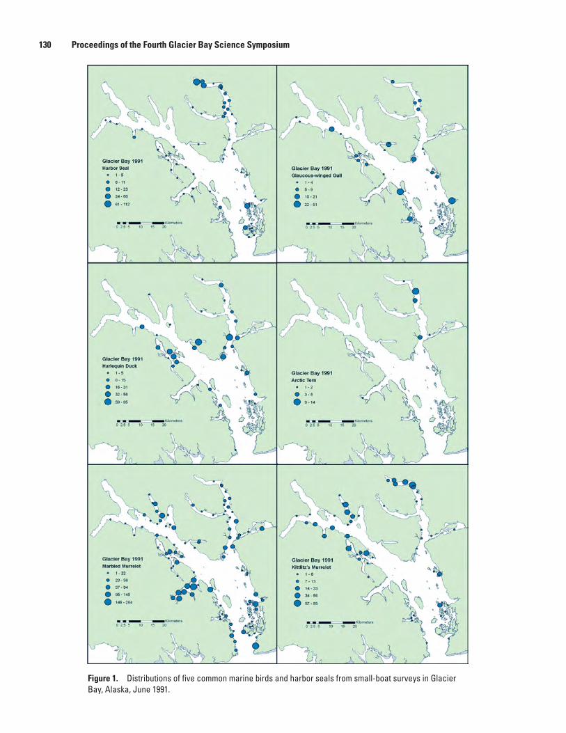
Figure 1. Distributions of five common marine birds and harbor seals from small-boat surveys in Glacier Bay, Alaska, June 1991.
1�0 Proceedings of the Fourth Glacier Bay Science Symposium
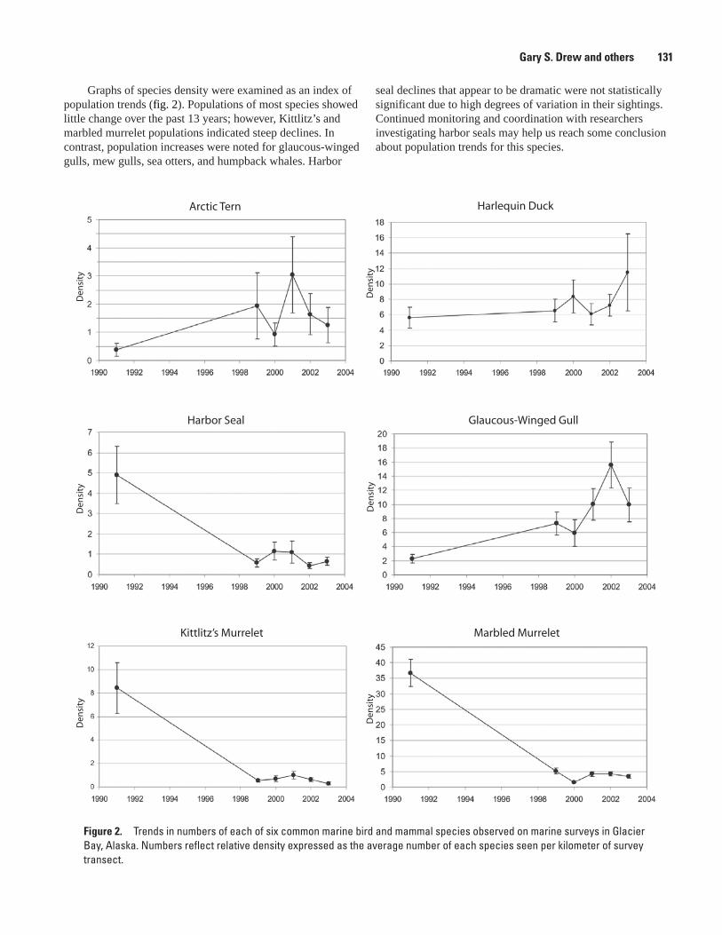
Figure 2. Trends in numbers of each of six common marine bird and mammal species observed on marine surveys in Glacier Bay, Alaska. Numbers reflect relative density expressed as the average number of each species seen per kilometer of survey transect.
Kittlitz’s Murrelet Marbled Murrelet
Harbor Seal Glaucous-Winged Gull
Arctic Tern Harlequin Duck
Den
sity
Den
sity
Den
sity
Den
sity
Den
sity
Den
sity
Gary S. Drew and others 1�1
Graphs of species density were examined as an index of population trends (fig. 2). Populations of most species showed little change over the past 13 years; however, Kittlitz’s and marbled murrelet populations indicated steep declines. In contrast, population increases were noted for glaucous-winged gulls, mew gulls, sea otters, and humpback whales. Harbor
seal declines that appear to be dramatic were not statistically significant due to high degrees of variation in their sightings. Continued monitoring and coordination with researchers investigating harbor seals may help us reach some conclusion about population trends for this species.
1�2 Proceedings of the Fourth Glacier Bay Science Symposium
Discussion and Conclusions
Glacier Bay is home to an abundant and variable set of marine species. The variable marine environments in Glacier Bay appear to be highly productive and provide quality habitats for many species. However, Glacier Bay also is an ecosystem undergoing rapid change. Despite the dramatic pace of habitat change it is difficult to determine species numerical responses particularly for long lived marine species. Our ability to look at marine populations over a 13-year period provided us the data required to detect increases in gulls and decreases in both Kittlitz’s and marbled murrelets. The cause of these population changes may vary among species; however, we suspect that the dramatic changes in Glacier Bay’s glacial-marine habitats and alterations in terrestrial nesting habitats are playing a major role.
Management Implications
The results of our at-sea surveys provided managers with information about population trends for most marine bird and mammal species in the Park. The ability of this annual “snapshot” to identify population trends for a wide diversity of marine birds and mammals at once makes it an efficient tool for monitoring these populations. This is particularly true of the species that cannot be monitored in any other way. At-sea survey methodology is a useful tool for monitoring marine bird and mammal populations, however, continued refinement of survey techniques is necessary to reduce variation and increase power to detect change. Marine bird and mammal populations are undergoing considerable change in Glacier Bay and therefore further research is needed to identify the causes of this change.
Acknowledgments
Funding for this work was provided by the National Park Service and the U.S. Geological Survey. We thank the many field observers who assisted in data collection.
References Cited
Gould, P.J., and Forsell, D.J., 1989, Techniques for shipboard surveys of marine birds: U.S. Fish and Wildlife Technical Report 25, 22 p.
Gould, P.J., Forsell, D.J., and Lensink, C.J., 1982, Pelagic distribution and abundance of seabirds in the Gulf of Alaska and eastern Bering Sea: U.S. Deptartment of the Interior, Fish and Wildlife Service, Biological Services Program, OBS 82/48, 294 p.
Tasker, M.L., Jones, P.H., Dixon, T., and Blake, B.F., 1984, Counting seabirds at sea from ships: a review of methods employed and a suggestion for a standardized approach: Auk, v. 101, p. 567-577.
Suggested Citation
Drew, G.S., Piatt, J.F., and Bodkin, J.L., 2007, Population status and trends of marine birds and mammals in Glacier Bay National Park, in Piatt, J.F., and Gende, S.M., eds., Proceedings of the Fourth Glacier Bay Science Symposium, October 26–28, 2004: U.S. Geological Survey Scientific Investigations Report 2007-5047, p. 129-132.
Perspectives on an Invading Predator—Sea Otters in Glacier Bay
James L. Bodkin1,2, B.E. Ballachey1, G.G. Esslinger1, K.A. Kloecker1, D.H. Monson1, and H.A. Coletti1
Abstract. Since 1995, numbers of sea otters (Enhydra lutris) in Glacier Bay have increased from just a few to nearly 2,400 in 2004. Immigration and reproduction have both contributed to this rapid increase. Abundant populations of benthic invertebrates, including clams, mussels, crabs, and urchins, are providing the prey resources to support this rapid increase. Unutilized habitat remains widely available. In areas of Glacier Bay colonized by sea otters, densities of clams are 3–9 times greater and mean sizes of clams are twice as large than in areas long occupied by sea otters outside Glacier Bay. Further, colonized areas in lower Glacier Bay have greater intertidal urchin and clam densities and biomass compared to areas not colonized. In addition to abundant prey, Glacier Bay has provided refuge from human harvest of sea otters that is not afforded elsewhere, likely contributing to the high rate of population growth.
James L. Bodkin and others 1��
1 U.S. Geological Survey, Alaska Science Center, 1011 E. Tudor, Anchorage, AK 99503.
2 Corresponding author: [email protected], 907-786-3550.
Introduction
During most of the early 20th century, sea otters were absent from large parts or areas of their habitat in the North Pacific. Subsequent expansion into unoccupied habitat by remnant and translocated populations resulted in rapid rates of recovery throughout much of the species’ historic range (Bodkin and others, 1999). This situation afforded an opportunity to evaluate relations between sea otters and the ecosystems they inhabit, providing one of the best-documented examples of top-down forcing on the structure and function of nearshore marine ecosystems in the North Pacific Ocean (Kenyon, 1969; VanBlaricom and Estes, 1988; Riedman and Estes, 1990; Estes and Duggins, 1995). Documented effects of sea otter foraging include declines in the abundance and size of benthic invertebrates and increases in the diversity and complexity of nearshore ecosystems.
By the end of the 20th century recovering sea otter populations in Alaska began to stabilize or decline in some areas. In some cases declines could be attributed to predation (Estes and others, 1998), while other populations equilibrated with available space and prey resources (Bodkin and others, 2000). However, relations between sea otter density, prey density, and immigration remain largely unexplored in Alaska.
Prior to about 1998, sea otters were effectively absent from Glacier Bay. In anticipation of sea otters moving into the area, we initiated studies in 1994 to describe the process of recolonization. Our research included annual surveys of sea otter abundance and distribution, and quantitative descriptions of the nearshore macro-invertebrate populations that existed in Glacier Bay. Our objectives in this summary are to: (1) describe the numerical process of sea otter colonization, (2) compare data on sea otter prey populations in Glacier Bay, between areas initially colonized and those not colonized, and (3) compare prey population densities and sizes in Glacier Bay prior to recolonization with those in Port Althorp, an area near Glacier Bay occupied by sea otters for about 25 years.
Methods
From 1994–2004, surveys of sea otter distribution and relative abundance have been conducted in Cross Sound, Icy Strait, and Glacier Bay. The distribution surveys consist of tracks flown parallel to shore and include all habitat out to the 100 m bathymetric contour. Numbers of animals observed, group sizes, and locations were recorded. We assumed that detection probabilities remained comparable among surveys and therefore our counts provide an index of abundance that is comparable over time.
In 1999, we initiated a second type of survey that was designed to provide estimates of sea otter abundance that were corrected for animals not detected (Bodkin and Udevitz, 1999). Transect selection and sampling was proportional to expected sea otter abundance with most effort taking place over waters from 0–40 m in depth. Intensive searches were periodically conducted within transects to estimate the proportion of sea otters not detected. Counts are adjusted for area not surveyed and detection probabilities less than1.0 to obtain a population size estimate.
Beginning in 1999, we randomly sampled intertidal clam and urchin populations throughout Glacier Bay, and at Port Althorp (Bodkin and others, 2000), where sea otters have been present for at least 20 years (fig. 1). All clam and urchin samples collected were identified, counted, and measured. In addition to the random sites, we sampled a supplementary suite of selected sites within preferred clam habitat (PCH), designated by the presence of abundant clam siphons and shell litter. Beginning in 2001, we sampled subtidal clam and urchin populations at selected sites throughout Glacier Bay and Port Althorp (Bodkin and others, 2002). Sites were selected based on extensive reconnaissance via diving and surface deployed drop cameras and clams and urchins were processed as for intertidal sampling.
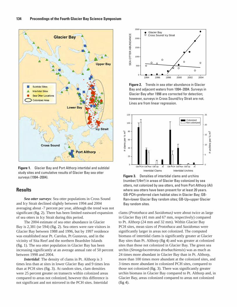
Results
Sea otter surveys: Sea otter populations in Cross Sound and Icy Strait declined slightly between 1994 and 2004 averaging about -7 percent per year, although the trend was not significant (fig. 2). There has been limited eastward expansion of sea otters in Icy Strait during this period.
The 2004 estimate of sea otter abundance in Glacier Bay is 2,381 (se 594) (fig. 2). Sea otters were rare visitors in Glacier Bay between 1988 and 1996, but by 1997 residence was established near Pt. Carolus, Pt Gustavus, and in the vicinity of Sita Reef and the northern Beardslee Islands (fig. 1). The sea otter population in Glacier Bay has been increasing significantly at an average annual rate of 50 percent between 1998 and 2004.
Intertidal: The density of clams in Pt. Althorp is 3 times less than at sites in lower Glacier Bay and 9 times less than at PCH sites (fig. 3). At random sites, clam densities were 25 percent greater on transects within colonized areas compared to areas not colonized, however this difference is not significant and not mirrored in the PCH sites. Intertidal
Figure �. Densities of intertidal clams and urchins (number/1/4m2) in areas of Glacier Bay colonized by sea otters, not colonized by sea otters, and from Port Althorp (AI) where sea otters have been present for at least 20 years. GB-PCH=preferred clam habitat sites in Glacier Bay; GB-Ran=lower Glacier Bay random sites; GB-Up=upper Glacier Bay random sites.
Figure 2. Trends in sea otter abundance in Glacier Bay and adjacent waters from 1994–2004. Surveys in Glacier Bay after 1998 are corrected for detection; however, surveys in Cross Sound/Icy Strait are not. Lines are from linear regression.
1�� Proceedings of the Fourth Glacier Bay Science Symposium
1994 1996 1998 2000 2002 2004
SEA
OTT
ER
AB
UN
DA
NC
E
0
500
1000
1500
2000
2500Glacier BayCross Sound/ Icy Strait
#cl
ams
per¼
m2
0
20
40
60
80
100
120
#ur
chin
spe
r¼m
2
0
5
10
15
20
25
ColonizedNot colonized
GB-PCH GB-Ran GB-Up AlGB-PCH GB-Ran GB-Up Al
Intertidal UrchinsIntertidal ClamsFigure 1. Glacier Bay and Port Althorp intertidal and subtidal study sites and cumulative results of Glacier Bay sea otter surveys (1994–2004).
clams (Protothaca and Saxidomus) were about twice as large in Glacier Bay (41 mm and 67 mm, respectively) compared to Pt. Althorp (24 mm and 32 mm). Within Glacier Bay PCH sites, mean sizes of Protothaca and Saxidomus were significantly larger in areas not colonized. The computed biomass of intertidal clams is significantly greater at Glacier Bay sites than Pt. Althorp (fig 4) and was greater at colonized sites than those not colonized in Glacier Bay. The green sea urchin (Strongylocentrotus droebachiensis) was as much as 24 times more abundant in Glacier Bay than in Pt. Althorp, more than 100 times more abundant at the colonized sites, and 3 times more abundant in colonized PCH sites, compared to those not colonized (fig. 3). There was significantly greater urchin biomass in Glacier Bay compared to Pt. Althorp and, in Glacier Bay, areas colonized compared to areas not colonized (fig 4).
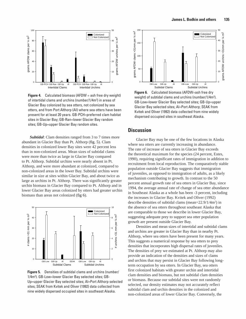
Figure 5. Densities of subtidal clams and urchins (number/1/4m2). GB-Low=lower Glacier Bay selected sites; GB-Up=upper Glacier Bay selected sites; Al=Port Althorp selected sites; SEAK from Kvitek and Oliver (1992) data collected from nine widely dispersed occupied sites in southeast Alaska.
Figure �. Calculated biomass (AFDW=ash free dry weight) of subtidal clams and urchins (number/1/4m2). GB-Low=lower Glacier Bay selected sites; GB-Up=upper Glacier Bay selected sites; Al=Port Althorp; SEAK from Kvitek and Oliver (1992) data collected from nine widely dispersed occupied sites in southeast Alaska.
James L. Bodkin and others 1�5
#cl
ams
>31
mm
per¼
m2
0
10
20
30
40
50
#ur
chin
s>3
1m
mpe
r¼m
2
0
2
4
6
8
10
ColonizedNot Colonized
GB-Low GB-Up AlSEAKGB-Low GB-Up Al
Subtidal Clams Subtidal Urchins
gram
sAF
DW
clam
s>3
1mm
per¼
m2
0
50
100
150
200
gram
sAF
DW
urch
ins
>31m
mpe
r¼m
2
0
10
20
30
40
50
ColonizedNot Colonized
GB-Low GB-Up AlGB-Low GB-Up Al
Subtidal Clams Subtidal Urchins
Figure �. Calculated biomass (AFDW = ash free dry weight) of intertidal clams and urchins (number/1/4m2) in areas of Glacier Bay colonized by sea otters, not colonized by sea otters, and from Port Althorp (AI) where sea otters have been present for at least 20 years. GB-PCH=preferred clam habitat sites in Glacier Bay; GB-Ran=lower Glacier Bay random sites; GB-Up=upper Glacier Bay random sites.
gram
sAF
DW
clam
spe
r¼m
2
0
20
40
60
80
100
gram
sAF
DW
urch
ins
per¼
m2
0
10
20
30
40
50
ColonizedNot Colonized
GB-PCH GB-Ran GB-Up AlGB-PCH GB-Ran GB-Up AlIntertidal UrchinsIntertidal Clams
Subtidal: Clam densities ranged from 3 to 7 times more abundant in Glacier Bay than Pt. Althorp (fig. 5). Clam densities in colonized lower Bay sites were 42 percent less than in non-colonized areas. Mean sizes of subtidal clams were more than twice as large in Glacier Bay compared to Pt. Althorp. Subtidal urchins were nearly absent in Pt. Althorp, and were more abundant at colonized, compared to non-colonized areas in the lower Bay. Subtidal urchins were similar in size at sites within Glacier Bay, and about twice as large as urchins in Pt. Althorp. There was significantly greater urchin biomass in Glacier Bay compared to Pt. Althorp and in lower Glacier Bay areas colonized by otters had greater urchin biomass than areas not colonized (fig 6).
Discussion
Glacier Bay may be one of the few locations in Alaska where sea otters are currently increasing in abundance. The rate of increase of sea otters in Glacier Bay exceeds the theoretical maximum for the species (24 percent, Estes, 1990), requiring significant rates of immigration in addition to recruitment from local reproduction. The comparatively stable population outside Glacier Bay suggests that immigration of juveniles, as opposed to immigration of adults, as a likely mechanism contributing to growth. In contrast to the 50 percent annual growth rate of sea otters in Glacier Bay, since 1994, the average annual rate of change of sea otter abundance in Southeast Alaska as a whole has been -3 percent, including the increases in Glacier Bay. Kvitek and Oliver (1992) describe densities of subtidal clams (mean=22.9/1/4m2) in the absence of sea otters throughout southeast Alaska that are comparable to those we describe in lower Glacier Bay, suggesting adequate prey to support sea otter population growth are present outside Glacier Bay.
Densities and mean sizes of intertidal and subtidal clams and urchins are greater in Glacier Bay than in nearby Pt. Althorp, where sea otters have been present for many years. This suggests a numerical response by sea otters to prey densities that incorporates high dispersal rates of juveniles. The densities of prey we estimated at Pt. Althorp may also provide an indication of the densities and sizes of clams and urchins that may persist in Glacier Bay following long-term occupation by sea otters. In Glacier Bay, sea otters first colonized habitats with greater urchin and intertidal clam densities and biomass, but not subtidal clam densities or biomass. Because our subtidal sites were not randomly selected, our density estimates may not accurately reflect subtidal clam and urchin densities in the colonized and non-colonized areas of lower Glacier Bay. Conversely, the
1�� Proceedings of the Fourth Glacier Bay Science Symposium
intertidal sites were randomly selected and should provide unbiased estimates of prey populations. Thus, at least for the intertidal zone, it appears as though sea otters selected areas for colonization that supported the highest prey populations. Other factors, such as behavior and social organization may play a role in the spatial aspects of colonization.
While abundant prey and space resources support colonizing sea otters in Glacier Bay, similar prey densities in other areas of southeast Alaska are not supporting similar rates of increase. Causes of differences in population growth inside and outside of Glacier Bay not well known, but the lack of a human harvest in Glacier Bay is likely contributing to the rapid colonization process.
Management Implications
The rapid increase in sea otters in Glacier Bay National Park has serious and multifaceted implications to management of marine resources in Glacier Bay. First, predation by sea otters on a variety of invertebrates will have profound effects on the benthic community structure and function of the Glacier Bay ecosystem. Expected consequences include reduced sizes and density of many common and abundant species that currently support other avian, mammalian, fish, and invertebrate consumers. Expected indirect consequences include increases in macroalgae populations, including understory and canopy forming species that support populations of grazing invertebrates and provide habitat for a diverse assemblage of nearshore marine taxa. Managers need to understand the direct and indirect effects of sea otter colonization and predation to properly assign causes of changes observed in nearshore marine resources. Second, sea otters are protected from most disturbances by the Marine Mammal Protection Act, but because they often rest in groups nearshore they may be particularly susceptible to disturbance by Park visitors. And lastly, while there exists a legal harvest of sea otters in Alaska, there has been no reported take from within Glacier Bay. Managers need to recognize the role of Glacier Bay as a refuge, and potentially as a marine reserve as the Bay eventually becomes a source of emigrating sea otters.
Acknowledgments
This work was supported by the U.S. Geological Survey, Alaska Science Center and Glacier Bay National Park and Preserve, National Park Service.
References Cited
Bodkin, J.L., Ballachey, B.E., Cronin, M.A., and Scribner, K.T., 1999, Population demographics and genetic diversity in remnant and re-established populations of sea otters: Conservation Biology, v. 13, no. 6, p. 1278–1385.
Bodkin, J.L., Burdin, A.M., and Ryzanov, D.A., 2000, Age and sex specific mortality and population structure in sea otters: Marine Mammal Science, v. 16, p. 201–219.
Bodkin, J.L., Kloecker, K.A., Esslinger, G.G., Monson, D.H., DeGroot, J.D., and Doherty, J., 2002, Sea otter studies in Glacier Bay National Park and Preserve: U.S. Geological Survey Annual Report 2001.
Bodkin, J.L., and Udevitz, M.S., 1999, An aerial survey method to estimate sea otter abundance, in Garner G.W. and others, eds., Marine mammal survey and assessment methods: Rotterdam, Netherlands, Balkema, p 13–26
Estes, J.A., 1990, Growth and equilibrium in sea otter populations: Journal of Animal Ecology, v. 59, p. 385–401.
Estes, J.A., and Duggins, D.O., 1995, Sea otters and kelp forests in Alaska: generality and variation in a community ecological paradigm: Ecological Monographs, v. 65, no. 1, p. 75–100.
Estes, J.A., Tinker, M.T., Williams, T.M., and Doak, D.F., 1998, Killer whale predation on sea otters linking oceanic and nearshore ecosystems: Science, v. 282, p. 473–476.
Kenyon, K.W., 1969, The sea otter in the eastern Pacific Ocean: North American Fauna v. 68, 352 p.
Kvitek, R.G., and Oliver, J.S., 1992, Influences of sea otters on soft-bottom prey communities in southeast Alaska: Marine Ecology Progress Series 82, p. 103–112.
Riedman, M.L., and Estes, J.A., 1990, The sea otter: behavior, ecology and natural history. Biological Report 90. U.S. Department of the Interior Fish and Wildlife Service, Washington, D.C., USA.
VanBlaricom, G.V., and Estes, J.A., 1988, The community ecology of sea otters: New York, Ecological Studies 65, Springer-Verlag.
Suggested Citation
Bodkin, J.L., Ballachey, B.E., Esslinger, G.G., Kloecker, K.A., Monson, D.H., and Coletti, H.A., 2007, Perspectives on an invading predator—Sea otters in Glacier Bay, in Piatt, J.F., and Gende, S.M., eds., Proceedings of the Fourth Glacier Bay Science Symposium, October 26–28, 2004: U.S. Geological Survey Scientific Investigations Report 2007-5047, p. 133-136
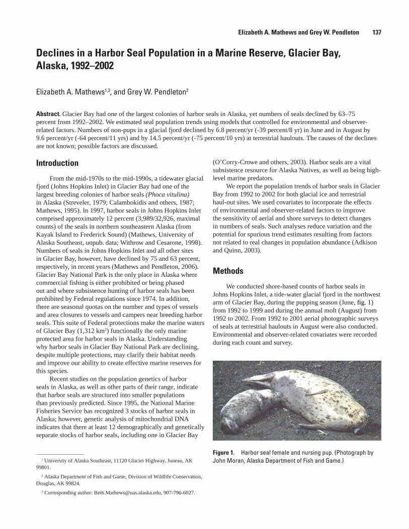
Declines in a Harbor Seal Population in a Marine Reserve, Glacier Bay, Alaska, 1992–2002
Elizabeth A. Mathews1,3, and Grey W. Pendleton2
Abstract. Glacier Bay had one of the largest colonies of harbor seals in Alaska, yet numbers of seals declined by 63–75 percent from 1992–2002. We estimated seal population trends using models that controlled for environmental and observer-related factors. Numbers of non-pups in a glacial fjord declined by 6.8 percent/yr (-39 percent/8 yr) in June and in August by 9.6 percent/yr (-64 percent/11 yrs) and by 14.5 percent/yr (-75 percent/10 yrs) at terrestrial haulouts. The causes of the declines are not known; possible factors are discussed.
Figure 1. Harbor seal female and nursing pup. (Photograph by John Moran, Alaska Department of Fish and Game.)
Elizabeth A. Mathews and Grey W. Pendleton 1�7
1 University of Alaska Southeast, 11120 Glacier Highway, Juneau, AK 99801.
2 Alaska Department of Fish and Game, Division of Wildlife Conservation, Douglas, AK 99824.
3 Corresponding author: [email protected], 907-796-6027.
Introduction
From the mid-1970s to the mid-1990s, a tidewater glacial fjord (Johns Hopkins Inlet) in Glacier Bay had one of the largest breeding colonies of harbor seals (Phoca vitulina) in Alaska (Streveler, 1979; Calambokidis and others, 1987; Mathews, 1995). In 1997, harbor seals in Johns Hopkins Inlet comprised approximately 12 percent (3,989/32,926, maximal counts) of the seals in northern southeastern Alaska (from Kayak Island to Frederick Sound) (Mathews, University of Alaska Southeast, unpub. data; Withrow and Cesarone, 1998). Numbers of seals in Johns Hopkins Inlet and all other sites in Glacier Bay, however, have declined by 75 and 63 percent, respectively, in recent years (Mathews and Pendleton, 2006). Glacier Bay National Park is the only place in Alaska where commercial fishing is either prohibited or being phased out and where subsistence hunting of harbor seals has been prohibited by Federal regulations since 1974. In addition, there are seasonal quotas on the number and types of vessels and area closures to vessels and campers near breeding harbor seals. This suite of Federal protections make the marine waters of Glacier Bay (1,312 km2) functionally the only marine protected area for harbor seals in Alaska. Understanding why harbor seals in Glacier Bay National Park are declining, despite multiple protections, may clarify their habitat needs and improve our ability to create effective marine reserves for this species.
Recent studies on the population genetics of harbor seals in Alaska, as well as other parts of their range, indicate that harbor seals are structured into smaller populations than previously predicted. Since 1995, the National Marine Fisheries Service has recognized 3 stocks of harbor seals in Alaska; however, genetic analysis of mitochondrial DNA indicates that there at least 12 demographically and genetically separate stocks of harbor seals, including one in Glacier Bay
(O’Corry-Crowe and others, 2003). Harbor seals are a vital subsistence resource for Alaska Natives, as well as being high-level marine predators.
We report the population trends of harbor seals in Glacier Bay from 1992 to 2002 for both glacial ice and terrestrial haul-out sites. We used covariates to incorporate the effects of environmental and observer-related factors to improve the sensitivity of aerial and shore surveys to detect changes in numbers of seals. Such analyses reduce variation and the potential for spurious trend estimates resulting from factors not related to real changes in population abundance (Adkison and Quinn, 2003).
Methods
We conducted shore-based counts of harbor seals in Johns Hopkins Inlet, a tide-water glacial fjord in the northwest arm of Glacier Bay, during the pupping season (June, fig. 1) from 1992 to 1999 and during the annual molt (August) from 1992 to 2002. From 1992 to 2001 aerial photographic surveys of seals at terrestrial haulouts in August were also conducted. Environmental and observer-related covariates were recorded during each count and survey.

Aerial and shore-based surveys of seals at haulouts measure only the portion of the population out of the water and available to be counted. We used standardized survey methods and included covariates in trend analyses to reduce the variation caused by changes in the proportion of seals hauled out. If the covariates account for most of this variation, the resulting trend estimates will have small bias (Adkison and Quinn, 2003). Covariates included in both glacial and terrestrial analyses were year, date, and time relative to solar noon. Tide height and time from low tide were incorporated for each terrestrial site. Additional covariates used in the analyses of counts from shore were sky condition, precipitation, within-season observer experience, and long-term experience level. We also included quadratic (non-linear) effects for date and time. Trend was defined as the geometric mean rate of change over the interval of interest (Link and Sauer, 1997).
Results
The minimal population estimate during August surveys in Glacier Bay declined from 6,189 to 2,551 seals from 1992 to 2001 despite increased survey effort. On average, 72 percent (range=62–80 percent, n=9 yr) of all seals were found in tidewater glacial fjords, primarily Johns Hopkins Inlet. In Johns Hopkins Inlet, the number of non-pups declined during June as did counts of all seals during August surveys in this glacial fjord. Similarly, numbers of harbor seals at terrestrial sites surveyed during August declined (table 1). In contrast to the declines in non-pup numbers, there was no significant trend (i.e., 95 percent CI includes 0) in numbers of harbor seal pups in Johns Hopkins Inlet in June (table 1), and the proportion of pups increased by 5.4 percent per year (fig. 2).
Discussion
Between 1992 and 2002 harbor seals counted in Glacier Bay declined at annual rates and magnitudes exceeding any documented harbor seal decline in Alaska with the exception of that at Tugidak Island (Pitcher, 1990). The 14.5 percent/yr
decline in harbor seals at terrestrial haulouts in Glacier Bay from 1992 to 2001 (table 1) exceeds the maximum theoretical and observed annual reproductive rate for harbor seals (12.5 percent) (Olesiuk and others, 1990), indicating that mortality or emigration of more than just young of the year is occurring. The declines in harbor seals in Glacier Bay suggest a localized decline, as they are in contrast to the only other areas within southeastern Alaska where longterm monitoring of harbor seals has occurred. From 1984 to 2001, harbor seal numbers were stable at 21 haulouts in Tenakee Inlet and Peril Strait (north of Sitka), and from 1983 to 1998, seal numbers increased by 7.4 percent/yr at 16 haulouts near Ketchikan (Small and others, 2003).
The potential causes of the observed declines can broadly be categorized as due to (1) redistribution or emigration out of Glacier Bay, (2) decreased reproductive output, or (3) increased mortality. Determining if the cause or causes of the declines in harbor seals in Glacier Bay are part of a natural cycle or due to human factors is an essential first step for preserving this important resource. Potential contributing factors that need to be studied include predation (by killer
0
0.1
0.2
0.3
0.4
0.5
1994 1995 1996 1997 1998 1999
Pup
Prop
ortio
n
Year
Figure 2. Proportion of harbor seal pups in Johns Hopkins Inlet counted in nearby subsections of 100 seals by year (=trend). Each circle represents one count of 100 seals; the line is the trend. The proportion of pups increased significantly by 5.4% per year (95% CI=3.9%-6.8%).
Table 1. Population trend for harbor seals in Johns Hopkins Inlet (JHI), a glacial fjord, and at all other, primarily terrestrial (Terr), haulout sites in Glacier Bay.
[Influential covariates are listed in order of decreasing influence. All trends were significant except that for pups. No covariates met the importance threshold for the terrestrial sites. Abbreviations: trm, time relative to midday (solar noon); longterm exper, number of observer survey seasons; pcp, precipitation]
Year Site Month Seals Annual trend 95 percent CICummulative
change(percent)
Influential covariates
1992-99 JHI June non-pups 6.55 -8.45 to -4.65 -39 date, sky, pcp
1994-99 JHI June pups 3.56 -0.98 to 8.10 19 date, date, sky, pcp
1992-2002 JHI August all -9.56 -10.3 to -8.8 -63 pcp, date, trm, longterm exper
1992-2001 Terr August all -14.46 -17.1 to -11.85 -75 (none)
1�� Proceedings of the Fourth Glacier Bay Science Symposium
Elizabeth A. Mathews and Grey W. Pendleton 1�9
whales, Steller sea lions, and (or) Pacific sleeper sharks, Somniosus pacificus) (Taggart and others, 2005), changes in prey availability or quality, disease, contaminants, and subsistence hunting. Competition with Steller sea lions, whose numbers in Glacier Bay have increased rapidly from the early to late 1990s (Mathews, University of Alaska Southeast, unpub. data), also needs to be examined as a possible factor.
Large changes in the abundance of several marine vertebrates in Glacier Bay indicate that the underlying food web dynamics in Glacier Bay have changed (Mathews and Pendleton, 2006). During approximately the same time as the seal declines, the number of Kittlitz’s (Brachyramphus brevirostris) and Marbled (B. marmoratus) murrelets in Glacier Bay also declined (Robards and others, , U.S. Geological Survey, written commun. 2003); these alcids both use glacial fjords during breeding and feed on some of the same small schooling fish species as harbor seals. In addition to the rapid increase in numbers of Steller sea lions in the last decade, sea otter numbers have increased (Bodkin and others, U.S. Geological Survey, written commun., 2002), as has the number of humpback whales (Megaptera novaeangliae) in Glacier Bay and Icy Strait (Doherty and Gabriele, Glacier Bay National Park, written commun., 2002). Information on Glacier Bay’s marine ecosystem alone may not be adequate for determining the cause or causes of the declines in harbor seals. Seals most likely leave Glacier Bay to forage elsewhere in early fall (Mathews and Kelly, 1996); determining the movements and foraging behavior during fall and winter of seals that breed in Glacier Bay will be necessary for identifying factors outside of the Park that may be contributing to the declines.
Management Implications
Glacier Bay is the largest (1,312 km2), highly protected marine reserve in North America and there are Federal protections specifically for protecting harbor seals during breeding. The effectiveness of Glacier Bay as a defacto reserve for harbor seals may be compromised if there are anthropogenic forces outside of the Park that now limit the population. Determining whether the declines in harbor seals in Glacier Bay National Park are driven by natural ecological cycles and (or) human factors and whether harbor seals in Glacier Bay are part of a local or a more regional decline is necessary for effective management of this important breeding habitat.
References Cited
Adkison, M.D., and Quinn, T.J., II, 2003, Evaluation of the Alaska harbor seal (Phoca vitulina) population survey: a simulation study: Marine Mammal Science, v. 19, no. 4, p. 764–790.
Calambokidis, J., Taylor, B.L., Carter, G.H., Steiger, P.K., Dawson, L.D., and Antrim, S.D., 1987, Distribution and haul-out behavior of harbor seals in Glacier Bay, Alaska: Canadian Journal of Zoology, v. 65, p. 1391–1396.
Link, W.A., and Sauer, J.R., 1997, Estimation of population trajectories from count data: Biometrics, v. 53, p. 488–497.
Mathews, E.A., 1995, Longterm trends in abundance of harbor seals (Phoca vitulina richardsi) and development of monitoring methods in Glacier Bay National Park, Southeast Alaska in Engstrom, D.R. ed., Proceedings of the Third Glacier Bay Science Symposium: Gustavus, Alaska, U.S. National Park Service, Glacier Bay National Park and Preserve, p 254–263.
Mathews, E.A., and Kelly, B.P., 1996, Extreme temporal variation in harbor seal (Phoca vitulina richardsi) numbers in Glacier Bay, a glacial fjord in Southeast Alaska: Marine Mammal Science, v. 12, p. 483–488.
Mathews, E.A., and Pendleton, G.W., 2006, Declining trends in harbor seal (Phoca vitulina) numbers at glacial ice and terrestrial haulouts in Glacier Bay National Park, 1992–2002: Marine Mammal Science, v. 22, no. 1, p. 167–189.
O’Corry-Crowe, G.M., Martien, K.K., and Taylor, B.L., 2003, The analysis of population genetic structure in Alaskan harbor seals, Phoca vitulina, as a framework for the identification of management stocks: La Jolla, Calif., Southwest Fisheries Science Center, National Marine Fisheries Service, National Oceanic and Atmospheric Administration, Adminstrative Report LJ-03-08, 54 p.
Olesiuk, P.F., Bigg, M.A., and Ellis, G.M., 1990, Recent trends in the abundance of harbor seals, Phoca vitulina, in British Columbia: Canadian Journal of Fisheries and Aquatic Sciences, v. 47, p. 992–1003.
Pitcher, K.W., 1990, Major decline in the number of harbor seals (Phoca vitulina) on Tugidak Island, Gulf of Alaska: Marine Mammal Science, v. 6 no. 2, p. 121–134.
Small, R.J., Pendleton, G.W., and Pitcher, K.W., 2003, Trends in abundance of Alaska harbor seals, 1983-2002: Marine Mammal Science, v. 19, p. 344–362.
Streveler, G., 1979, Distribution, population ecology, and impact susceptibility of the harbor seal in Glacier Bay, Alaska: Gustavus, Alaska, Glacier Bay National Park, 49 p.

1�0 Proceedings of the Fourth Glacier Bay Science Symposium
Mount Fairweather and its neighbors, as viewed from the outer coast (west). (Photograph by Bill Eichenlaub, National Park Service.)
Taggart, S.J., Andrews, A.G., Mondragon, J., and Mathews, E.A., 2005 (2005), Co-occurrence of Pacific sleeper sharks Somniosus pacificus and harbor seals Phoca vitulina in Glacier Bay: Alaska Fishery Research Bulletin, v. 11, no. 2, p. 113–117.
Withrow, D.E., and Cesarone, J.C., 1998, Abundance and distribution of harbor seals (Phoca vitulina richardsi) for northern southeast Alaska from Kayak Island to Frederick Sound in 1997, in MMPA and ESA Implementation Program 1997: Alaska Fisheries Science Center, NOAA, AFSC Processed Report 98-10, Annual report to the Office of Protected Resources, NMFS, NOAA, 1335 East-West Highway, Silver Spring, MD 20910. p. 116–123
Suggested Citation
Mathews, E.A., and Pendleton, G.W., 2007, Declines in a harbor seal population in a marine reserve, Glacier Bay, Alaska, 1992–2002, in Piatt, J.F., and Gende, S.M., eds., Proceedings of the Fourth Glacier Bay Science Symposium, October 26–28, 2004: U.S. Geological Survey Scientific Investigations Report 2007-5047, p. 137-140.
Harbor Seal Research in Glacier Bay National Park
Gail M. Blundell1,4, Scott M. Gende2, Jamie N. Womble2,3
Abstract. Harbor seals (n=79) were captured and a subset were fitted with VHF and satellite tags, and dive recorders in 2004 during the first of a multi-year study addressing potential causal factors contributing to their precipitous decline in Glacier Bay. Preliminary analyses suggest that harbor seals generally tend to forage near their haul-outs during the spring and summer; however, during fall and winter some seals made more extensive movements outside of the park.
Gail M. Blundell and others 1�1
1 Harbor Seal Research Program, Alaska Department of Fish and Game, Division of Wildlife Conservation, Douglas, AK 99824-0020
2 National Park Service, Glacier Bay Field Station, Juneau, AK 99801
3 Alaska Fisheries Science Center, Auke Bay Laboratory, Juneau, AK 99801
4 Corresponding author: [email protected], 907-465-4345
Introduction
Glacier Bay National Park has historically supported one of the largest breeding populations of harbor seals (Phoca vitulina richardii) in Alaska. Harbor seals are an important apex predator and the most numerous marine mammal in the park; however, seals have declined by more than 70 percent in the park since 1992 (Mathews and Pendleton, 2006). The magnitude and rate of decline exceed all reported declines of harbor seals in Alaska, with the exception of that at Tugidak Island (Pitcher, 1990), and show no signs of reversal despite the implementation of various management strategies (e.g., reduction in commercial fishing, cessation of subsistence harvest, vessel restrictions). In contrast to the population trend in Glacier Bay, harbor seals in two other areas of southeastern Alaska (near Sitka and Ketchikan) are stable or increasing (Small and others, 2003).
In 2004, a long-term multi-agency study was initiated intended to identify potential causal factors contributing to the decline by collecting data on a diversity of ecological, behavioral, and physiological parameters. As part of the first year of this effort, harbor seals were captured in spring and autumn and fitted with either (1) long-term (5-year) VHF implant transmitters to quantify ‘vital rates’, including survival and reproductive success, (2) external VHF transmitters and Time Depth Recorders (TDRs) to address fine-scale movements, habitat use, foraging ecology, and dive behavior, or (3) Satellite Depth Recorders (SDRs) to assess large-scale movements and winter dive behavior. Here we describe the number of seals captured during 2004 and the type of instruments deployed on a subset of those seals. We also provide preliminary analyses of movements of seals in and outside the park during summer/autumn 2004. Data on a diversity of other parameters that will help provide insight into the causal factors associated with the decline in harbor seal numbers observed in Glacier Bay—data such as survival, diet, health and condition, genetics, available forage, disturbance,
and contaminants—will continue to be collected and analyzed over the next 6 years.
Methods
Harbor seals were captured using multifilament nylon nets at terrestrial (reef) sites, and monofilament nets that are less detectable in glacial silt were used in ice (glacial iceberg) habitat. Biological samples (blood, skin, hair, blubber biopsies) were collected from all captured seals to assess health, condition, contaminants, diet (fatty acid profiles of blubber and stable isotope signatures from blood and hair), disease exposure, immunocompetency, and genetics. VHF transmitters (Telonics IMP 300-L) were surgically implanted under the skin and blubber layer of harbor seals (Lander and others, 2005). VHF implant transmitters were equipped with mortality sensors and, to extend battery life for 5 years, emit a signal only from 10:00 to 14:00 when seals are most likely to be hauled out and more easily located. VHF implant transmitters allow for long-term monitoring of vital rates, such as survival, as individual animals can be monitored via radio tracking for up to five years. To facilitate long-term monitoring, land-based datalogger stations (Advanced Telemetry Systems, R4500S) were established in Johns Hopkins Inlet and near Spider Reef Complex to continuously monitor the presence/absence of radio-tagged seals.
Other seals were fitted with external head-mounted VHF transmitters, which emit a signal continuously. Head-mounted VHF transmitters were deployed to determine foraging locations, behavior, and habitat use of harbor seals within the park. Some seals also received archival Time-Depth Recorders (TDRs; Wildlife Computers, MK-9). TDRs were programmed to record depth, temperature, and light every two seconds. TDRs were shed during the molt and recovered using vessels, floatplanes, and kayaks. Data from TDRs quantify the dive behavior of harbor seals and, coupled with foraging locations, will elucidate fine-scale foraging behavior and identify important foraging habitat.
Foraging areas of harbor seals were determined by conducting real-time VHF-tracking of seals from the R/V Capelin and from aerial surveys. Vessel surveys occurred during 4-day periods every other week from May to July in 2004 (n=25 days). Aerial surveys were conducted every other week to obtain better spatial coverage. During vessel-tracking
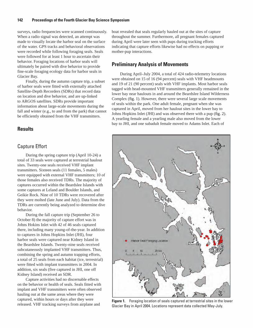
surveys, radio frequencies were scanned continuously. When a radio signal was detected, an attempt was made to visually locate the harbor seal on the surface of the water. GPS tracks and behavioral observations were recorded while following foraging seals. Seals were followed for at least 1 hour to ascertain their behavior. Foraging locations of harbor seals will ultimately be paired with dive behavior to provide fine-scale foraging ecology data for harbor seals in Glacier Bay.
Finally, during the autumn capture trip, a subset of harbor seals were fitted with externally attached Satellite-Depth Recorders (SDRs) that record data on location and dive behavior, and are up-linked to ARGOS satellites. SDRs provide important information about large-scale movements during the fall and winter (e.g., to and from the park) that cannot be efficiently obtained from the VHF transmitters.
Results
Capture EffortDuring the spring capture trip (April 10-24) a
total of 33 seals were captured at terrestrial haulout sites. Twenty-one seals received VHF implant transmitters. Sixteen seals (11 females, 5 males) were equipped with external VHF transmitters; 10 of those females also received TDRs. The majority of captures occurred within the Beardslee Islands with some captures at Leland and Boulder Islands, and Geikie Rock. Nine of 10 TDRs were recovered after they were molted (late June and July). Data from the TDRs are currently being analyzed to determine dive behavior.
During the fall capture trip (September 26 to October 8) the majority of capture effort was in Johns Hokins Inlet with 42 of 46 seals captured there, including many young-of-the-year. In addition to captures in Johns Hopkins Inlet (JHI), four harbor seals were captured near Kidney Island in the Beardslee Islands. Twenty-nine seals received subcutaneously implanted VHF transmitters. Thus, combining the spring and autumn trapping efforts, a total of 25 seals from each habitat (ice, terrestrial) were fitted with implant transmitters in 2004. In addition, six seals (five captured in JHI, one off Kidney Island) received an SDR.
Capture activities had no discernable effects on the behavior or health of seals. Seals fitted with implant and VHF transmitters were often observed hauling out at the same areas where they were captured, within hours or days after they were released. VHF tracking surveys from airplane and
Figure 1. Foraging location of seals captured at terrestrial sites in the lower Glacier Bay in April 2004. Locations represent data collected May-July.
1�2 Proceedings of the Fourth Glacier Bay Science Symposium
boat revealed that seals regularly hauled out at the sites of capture throughout the summer. Furthermore, all pregnant females captured during April were later seen with pups during tracking efforts indicating that capture efforts likewise had no effects on pupping or mother-pup interactions.
Preliminary Analysis of Movements
During April–July 2004, a total of 424 radio-telemetry locations were obtained on 15 of 16 (94 percent) seals with VHF headmounts and 19 of 21 (90 percent) seals with VHF implants. Most harbor seals tagged with head-mounted VHF transmitters generally remained in the lower bay near haulouts in and around the Beardslee Island Wilderness Complex (fig. 1). However, there were several large scale movements of seals within the park. One adult female, pregnant when she was captured in April, moved from her haulout sites in the lower bay to Johns Hopkins Inlet (JHI) and was observed there with a pup (fig. 2). A yearling female and a yearling male also moved from the lower bay to JHI, and one subadult female moved to Adams Inlet. Each of
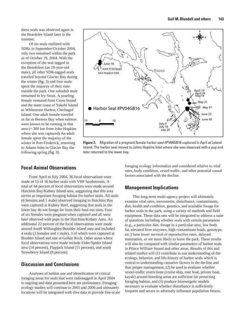
Harbor Seal #PV04GB16
April 19April 29May14
May 21
May 27
June 23
June 30
July 9July 16
July 20
10 0 10
John Hopkins Inlet
June 4 (w/pup)
June 18
Figure 2. Migration of a pregnant female harbor seal #PV04GB16 captured in April at Leland Island. The harbor seal moved to Johns Hopkins Inlet where she was observed with a pup and later returned to the lower bay.
Gail M. Blundell and others 1��
these seals was observed again in the Beardslee Island later in the summer.
Of six seals outfitted with SDRs in September/October 2004, only two remained within the park as of October 18, 2004. With the exception of the seal tagged in the Beardslees (an 18-year-old male), all other SDR-tagged seals traveled beyond Glacier Bay during the winter (fig. 3) and four seals spent the majority of their time outside the park. One subadult male remained in Icy Strait. A yearling female ventured from Cross Sound and the outer coast of Yakobi Island to Whitestone Harbor, Chichagof Island. One adult female traveled as far as Berners Bay when salmon were known to be running in that area (~ 300 km from John Hopkins where she was captured) An adult female spent the majority of the winter in Port Frederick, returning to Adams Inlet in Glacier Bay the following spring (fig. 3).
Focal Animal Observations
From April to July 2004, 36 focal observations were made of 15 of 16 harbor seals with VHF headmounts. A total of 44 percent of focal observations were made around Hutchins Bay/Kidney Island area, suggesting that this area serves as important foraging habitat for harbor seals. All seals (6 females and 1 male) observed foraging in Hutchins Bay were captured at Kidney Reef, suggesting that seals in the lower bay do not forage far from their haul-out sites. Four of six females were pregnant when captured and all were later observed with pups in the Hutchins/Kidney Area. An additional 22 percent of the focal observations were made around South Willoughby/Boulder Island area and included 4 seals (3 females and 1 male), 3 of which were captured at Boulder Island and one at Geikie Rock. Other areas where focal observations were made include Eider/Spider Island area (14 percent), Flapjack Island (11 percent), and south Strawberry Island (8 percent).
Discussion and Conclusions
Analyses of habitat use and identification of critical foraging areas for seals that were radiotagged in April 2004 is ongoing and data presented here are preliminary. Foraging ecology studies will continue in 2005 and 2006 and ultimately locations will be integrated with dive data to provide fine-scale
foraging ecology information and considered relative to vital rates, body condition, vessel traffic, and other potential causal factors associated with the decline.
Management Implications
This long-term multi-agency project will ultimately examine vital rates, movements, disturbance, contaminants, diet, health and condition, genetics, and available forage for harbor seals in the park, using a variety of methods and field equipment. These data sets will be integrated to address a suite of questions including whether seals with certain parameters (e.g., a particular diet, forage in a particular area, low body fat, elevated liver enzymes, high contaminant loads, genotype, etc.) have lower survival or reproductive rates, delayed maturation, or are more likely to leave the park. These results will also be compared with similar parameters of harbor seals in Prince William Sound and other areas. Results of this and related studies will (1) contribute to our understanding of the ecology, behavior, and life-history of harbor seals which is central to understanding causative factors in the decline and thus proper management, (2) be used to evaluate whether vessel-traffic restrictions (cruise ship, tour boat, private boat, kayak) around breeding areas are sufficient for protecting foraging habitat, and (3) produce bioenergetic models necessary to evaluate whether disturbance is sufficiently frequent and severe to adversely influence population fitness.
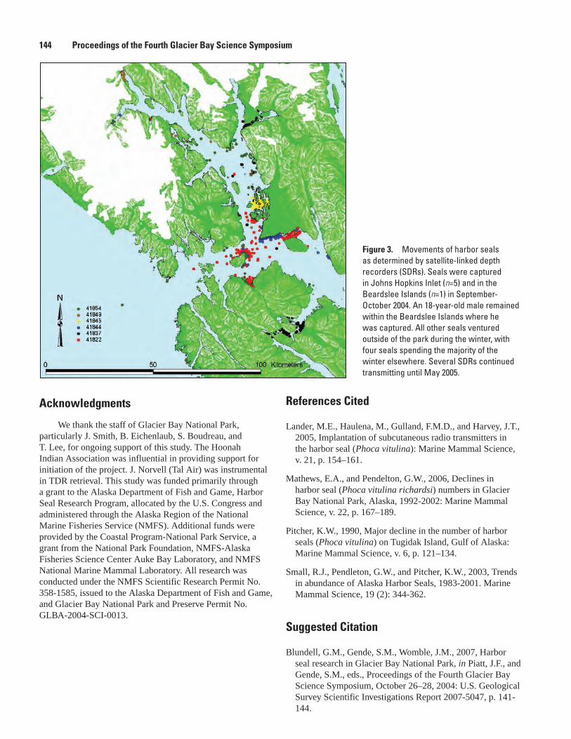
1�� Proceedings of the Fourth Glacier Bay Science Symposium
Acknowledgments
We thank the staff of Glacier Bay National Park, particularly J. Smith, B. Eichenlaub, S. Boudreau, and T. Lee, for ongoing support of this study. The Hoonah Indian Association was influential in providing support for initiation of the project. J. Norvell (Tal Air) was instrumental in TDR retrieval. This study was funded primarily through a grant to the Alaska Department of Fish and Game, Harbor Seal Research Program, allocated by the U.S. Congress and administered through the Alaska Region of the National Marine Fisheries Service (NMFS). Additional funds were provided by the Coastal Program-National Park Service, a grant from the National Park Foundation, NMFS-Alaska Fisheries Science Center Auke Bay Laboratory, and NMFS National Marine Mammal Laboratory. All research was conducted under the NMFS Scientific Research Permit No. 358-1585, issued to the Alaska Department of Fish and Game, and Glacier Bay National Park and Preserve Permit No. GLBA-2004-SCI-0013.
Figure �. Movements of harbor seals as determined by satellite-linked depth recorders (SDRs). Seals were captured in Johns Hopkins Inlet (n=5) and in the Beardslee Islands (n=1) in September-October 2004. An 18-year-old male remained within the Beardslee Islands where he was captured. All other seals ventured outside of the park during the winter, with four seals spending the majority of the winter elsewhere. Several SDRs continued transmitting until May 2005.
References Cited
Lander, M.E., Haulena, M., Gulland, F.M.D., and Harvey, J.T., 2005, Implantation of subcutaneous radio transmitters in the harbor seal (Phoca vitulina): Marine Mammal Science, v. 21, p. 154–161.
Mathews, E.A., and Pendelton, G.W., 2006, Declines in harbor seal (Phoca vitulina richardsi) numbers in Glacier Bay National Park, Alaska, 1992-2002: Marine Mammal Science, v. 22, p. 167–189.
Pitcher, K.W., 1990, Major decline in the number of harbor seals (Phoca vitulina) on Tugidak Island, Gulf of Alaska: Marine Mammal Science, v. 6, p. 121–134.
Small, R.J., Pendleton, G.W., and Pitcher, K.W., 2003, Trends in abundance of Alaska Harbor Seals, 1983-2001. Marine Mammal Science, 19 (2): 344-362.
Suggested Citation
Blundell, G.M., Gende, S.M., Womble, J.M., 2007, Harbor seal research in Glacier Bay National Park, in Piatt, J.F., and Gende, S.M., eds., Proceedings of the Fourth Glacier Bay Science Symposium, October 26–28, 2004: U.S. Geological Survey Scientific Investigations Report 2007-5047, p. 141-144.
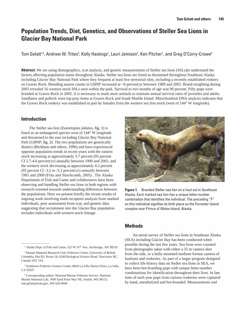
Population Trends, Diet, Genetics, and Observations of Steller Sea Lions in Glacier Bay National Park
Tom Gelatt1,4, Andrew W. Trites2, Kelly Hastings1, Lauri Jemison1, Ken Pitcher1, and Greg O’Corry-Crowe3
Abstract. We are using demographics, scat analysis, and genetic measurements of Steller sea lions (SSLs)to understand the factors affecting population status throughout Alaska. Steller sea lions are listed as threatened throughout Southeast Alaska including Glacier Bay National Park where they frequent at least five terrestrial sites, including a recently established rookery on Graves Rock. Breeding season counts in GBNP increased at ~6 percent/yr between 1989 and 2002. Brand resighting during 2003 revealed 16 western stock SSLs seen within the park. Survival to two months of age was 90 percent. Fifty pups were branded at Graves Rock in 2002. It is necessary to mark more animals to estimate annual survival rates of juveniles and adults. Sandlance and pollock were top prey items at Graves Rock and South Marble Island. Mitochondrial DNA analysis indicates that the Graves Rock rookery was established in part by females from the western sea lion stock (west of 144° W longitude).
Figure 1. Branded Steller sea lion on a haul out in Southeast Alaska. Each marked sea lion has a unique letter-number combination that identifies the individual. The preceding “F” on this individual signifies its birth place as the Forrester Island complex near Prince of Wales Island, Alaska.
Tom Gelatt and others 1�5
1 Alaska Dept. of Fish and Game, 525 W. 67th Ave, Anchorage, AK 99518
2 Marine Mammal Research Unit, Fisheries Center, University of British Columbia, Hut B3, Room 18, 6248 Biological Science Road, Vancouver BC, Canada V6T 1Z4
3 Southwest Fisheries Science Center, 8604 La Jolla Shores Drive, La Jolla, CA 92037
4 Corresponding author: National Marine Fisheries Service, National Marine Mammal Lab, 7600 Sand Point Way NE, Seattle, WA 98115, [email protected], 206-526-4040
Introduction
The Steller sea lion (Eumetopias jubatus, fig. 1) is listed as an endangered species west of 144° W longitude and threatened to the east including Glacier Bay National Park (GBNP; fig. 2). The two populations are genetically distinct (Bickham and others, 1996) and have experienced opposite population trends in recent years with the eastern stock increasing at approximately 3.7 percent (95 percent CI 2.7-4.6 percent/yr) annually between 1990 and 2002, and the western stock decreasing at approximately 4.2 percent (95 percent CI -3.2 to -5.2 percent/yr) annually between 1991 and 2000 (Fritz and Stinchcomb, 2005) . The Alaska Department of Fish and Game and collaborators have been observing and handling Steller sea lions in both regions with research oriented towards understanding differences between the populations. Here we present briefly the recent results of ongoing work involving mark-recapture analysis from marked individuals, prey assessment from scat, and genetic data suggesting that recruitment into the Glacier Bay population includes individuals with western stock lineage.
Methods
An aerial survey of Steller sea lions in Southeast Alaska (SEA) including Glacier Bay has been conducted when possible during the last few years. Sea lions were counted from photographs taken with either a 35 m camera shot from the side, or a belly-mounted medium format camera of haulouts and rookeries. As part of a larger program designed to collect life history data on Steller sea lions in SEA, we have been hot-branding pups with unique letter-number combinations for identification throughout their lives. In late June of each year pups from various rookeries were captured by hand, anesthetized and hot-branded. Measurements and
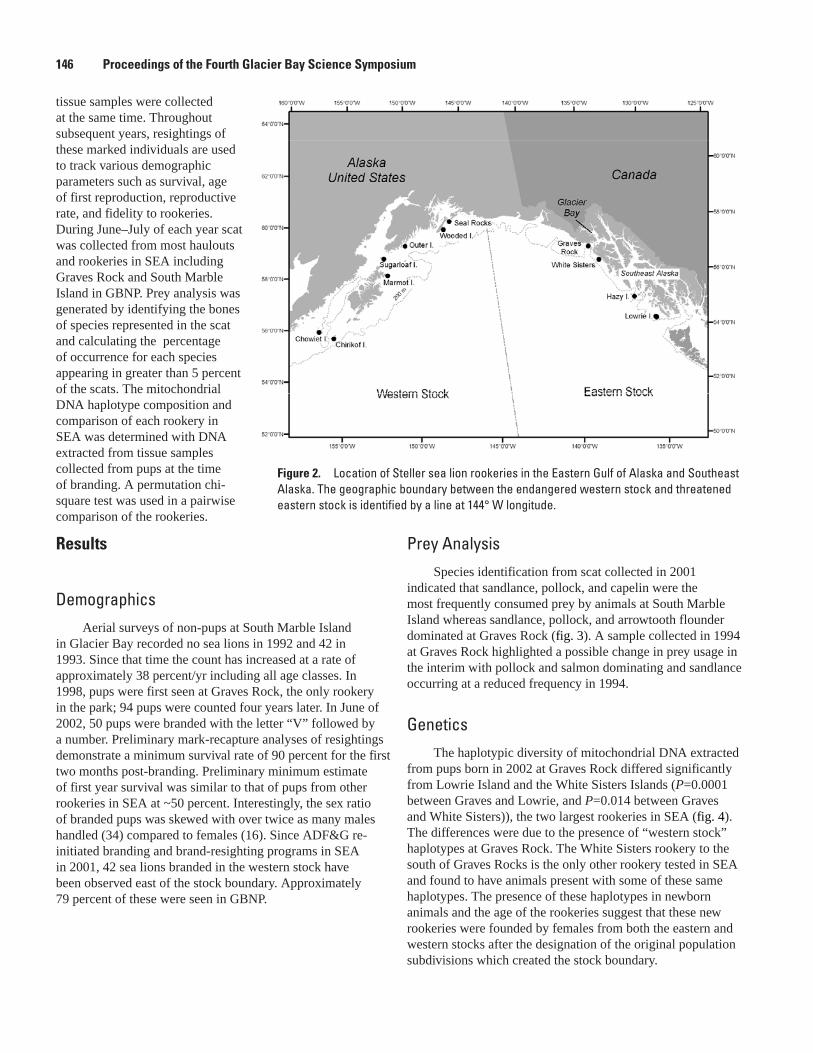
Figure 2. Location of Steller sea lion rookeries in the Eastern Gulf of Alaska and Southeast Alaska. The geographic boundary between the endangered western stock and threatened eastern stock is identified by a line at 144° W longitude.
1�� Proceedings of the Fourth Glacier Bay Science Symposium
tissue samples were collected at the same time. Throughout subsequent years, resightings of these marked individuals are used to track various demographic parameters such as survival, age of first reproduction, reproductive rate, and fidelity to rookeries. During June–July of each year scat was collected from most haulouts and rookeries in SEA including Graves Rock and South Marble Island in GBNP. Prey analysis was generated by identifying the bones of species represented in the scat and calculating the percentage of occurrence for each species appearing in greater than 5 percent of the scats. The mitochondrial DNA haplotype composition and comparison of each rookery in SEA was determined with DNA extracted from tissue samples collected from pups at the time of branding. A permutation chi-square test was used in a pairwise comparison of the rookeries.
Results
DemographicsAerial surveys of non-pups at South Marble Island
in Glacier Bay recorded no sea lions in 1992 and 42 in 1993. Since that time the count has increased at a rate of approximately 38 percent/yr including all age classes. In 1998, pups were first seen at Graves Rock, the only rookery in the park; 94 pups were counted four years later. In June of 2002, 50 pups were branded with the letter “V” followed by a number. Preliminary mark-recapture analyses of resightings demonstrate a minimum survival rate of 90 percent for the first two months post-branding. Preliminary minimum estimate of first year survival was similar to that of pups from other rookeries in SEA at ~50 percent. Interestingly, the sex ratio of branded pups was skewed with over twice as many males handled (34) compared to females (16). Since ADF&G re-initiated branding and brand-resighting programs in SEA in 2001, 42 sea lions branded in the western stock have been observed east of the stock boundary. Approximately 79 percent of these were seen in GBNP.
Prey AnalysisSpecies identification from scat collected in 2001
indicated that sandlance, pollock, and capelin were the most frequently consumed prey by animals at South Marble Island whereas sandlance, pollock, and arrowtooth flounder dominated at Graves Rock (fig. 3). A sample collected in 1994 at Graves Rock highlighted a possible change in prey usage in the interim with pollock and salmon dominating and sandlance occurring at a reduced frequency in 1994.
GeneticsThe haplotypic diversity of mitochondrial DNA extracted
from pups born in 2002 at Graves Rock differed significantly from Lowrie Island and the White Sisters Islands (P=0.0001 between Graves and Lowrie, and P=0.014 between Graves and White Sisters)), the two largest rookeries in SEA (fig. 4). The differences were due to the presence of “western stock” haplotypes at Graves Rock. The White Sisters rookery to the south of Graves Rocks is the only other rookery tested in SEA and found to have animals present with some of these same haplotypes. The presence of these haplotypes in newborn animals and the age of the rookeries suggest that these new rookeries were founded by females from both the eastern and western stocks after the designation of the original population subdivisions which created the stock boundary.
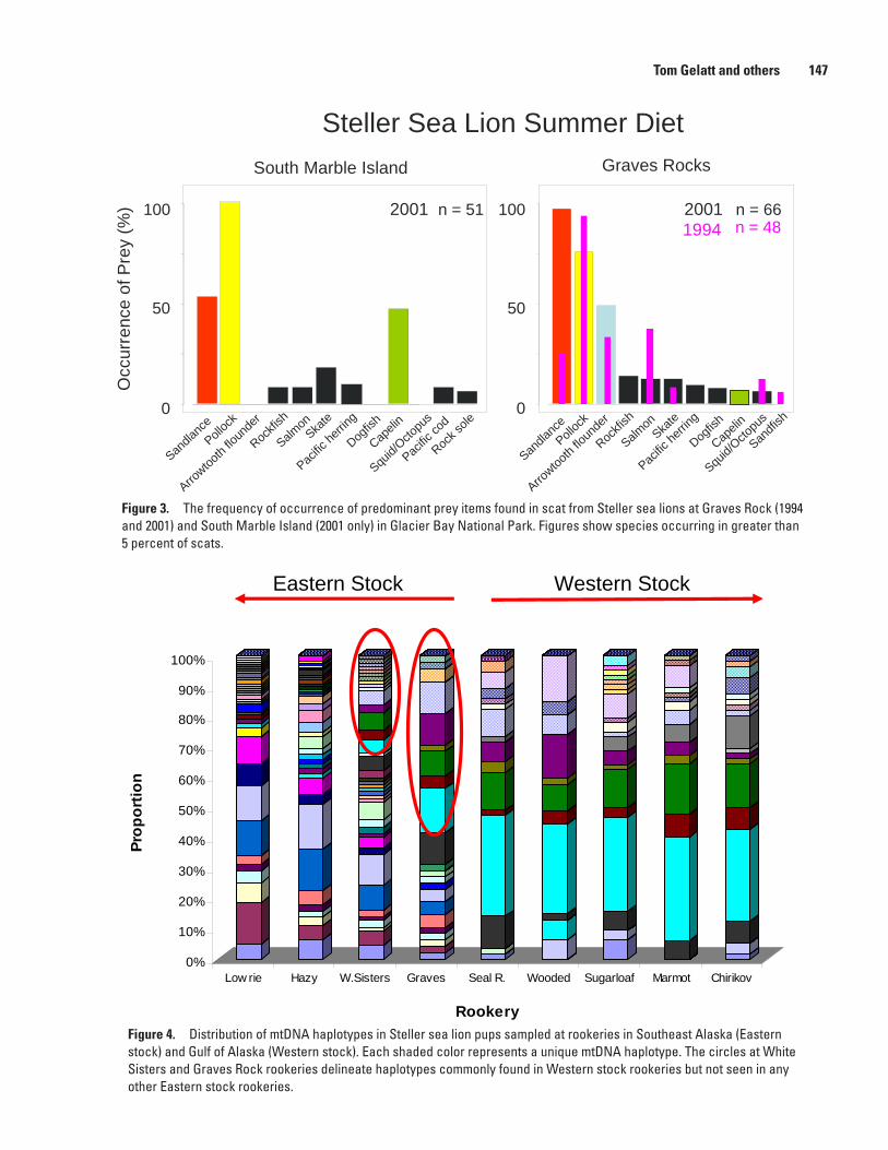
Tom Gelatt and others 1�7
Figure �. The frequency of occurrence of predominant prey items found in scat from Steller sea lions at Graves Rock (1994 and 2001) and South Marble Island (2001 only) in Glacier Bay National Park. Figures show species occurring in greater than 5 percent of scats.
Arrowtoo
thflo
unde
r
Sandla
ncePoll
ock
Rockfi
sh
Salmon
Skate
Pacific
herrin
g
Dogfis
h
Squid/
Octopu
s
Capeli
n
n = 512001
Steller Sea Lion Summer DietSouth Marble Island
n = 66
0
50
100
Graves Rocks
20011994 n = 48
0
50
100
Occ
urr e
nce
ofP
rey
(%)
Arrowtoo
thflo
unde
r
Sandla
ncePoll
ock
Capeli
n
Rockfi
sh
Salmon
Skate
Pacific
herrin
g
Dogfis
h
Squid/
Octopu
s
Pacific
cod
Rock so
le
Sandfi
sh
Figure �. Distribution of mtDNA haplotypes in Steller sea lion pups sampled at rookeries in Southeast Alaska (Eastern stock) and Gulf of Alaska (Western stock). Each shaded color represents a unique mtDNA haplotype. The circles at White Sisters and Graves Rock rookeries delineate haplotypes commonly found in Western stock rookeries but not seen in any other Eastern stock rookeries.
0%
10%
20%
30%
40%
50%
60%
70%
80%
90%
100%
Prop
ortio
n
Low rie Hazy W.Sisters Graves Seal R. Wooded Sugarloaf Marmot Chirikov
Rookery
Eastern Stock Western Stock
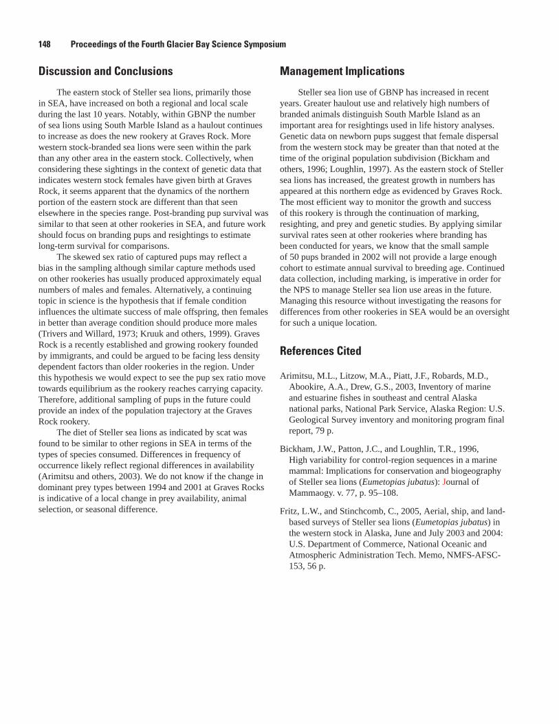
1�� Proceedings of the Fourth Glacier Bay Science Symposium
Discussion and Conclusions
The eastern stock of Steller sea lions, primarily those in SEA, have increased on both a regional and local scale during the last 10 years. Notably, within GBNP the number of sea lions using South Marble Island as a haulout continues to increase as does the new rookery at Graves Rock. More western stock-branded sea lions were seen within the park than any other area in the eastern stock. Collectively, when considering these sightings in the context of genetic data that indicates western stock females have given birth at Graves Rock, it seems apparent that the dynamics of the northern portion of the eastern stock are different than that seen elsewhere in the species range. Post-branding pup survival was similar to that seen at other rookeries in SEA, and future work should focus on branding pups and resightings to estimate long-term survival for comparisons.
The skewed sex ratio of captured pups may reflect a bias in the sampling although similar capture methods used on other rookeries has usually produced approximately equal numbers of males and females. Alternatively, a continuing topic in science is the hypothesis that if female condition influences the ultimate success of male offspring, then females in better than average condition should produce more males (Trivers and Willard, 1973; Kruuk and others, 1999). Graves Rock is a recently established and growing rookery founded by immigrants, and could be argued to be facing less density dependent factors than older rookeries in the region. Under this hypothesis we would expect to see the pup sex ratio move towards equilibrium as the rookery reaches carrying capacity. Therefore, additional sampling of pups in the future could provide an index of the population trajectory at the Graves Rock rookery.
The diet of Steller sea lions as indicated by scat was found to be similar to other regions in SEA in terms of the types of species consumed. Differences in frequency of occurrence likely reflect regional differences in availability (Arimitsu and others, 2003). We do not know if the change in dominant prey types between 1994 and 2001 at Graves Rocks is indicative of a local change in prey availability, animal selection, or seasonal difference.
Management Implications
Steller sea lion use of GBNP has increased in recent years. Greater haulout use and relatively high numbers of branded animals distinguish South Marble Island as an important area for resightings used in life history analyses. Genetic data on newborn pups suggest that female dispersal from the western stock may be greater than that noted at the time of the original population subdivision (Bickham and others, 1996; Loughlin, 1997). As the eastern stock of Steller sea lions has increased, the greatest growth in numbers has appeared at this northern edge as evidenced by Graves Rock. The most efficient way to monitor the growth and success of this rookery is through the continuation of marking, resighting, and prey and genetic studies. By applying similar survival rates seen at other rookeries where branding has been conducted for years, we know that the small sample of 50 pups branded in 2002 will not provide a large enough cohort to estimate annual survival to breeding age. Continued data collection, including marking, is imperative in order for the NPS to manage Steller sea lion use areas in the future. Managing this resource without investigating the reasons for differences from other rookeries in SEA would be an oversight for such a unique location.
References Cited
Arimitsu, M.L., Litzow, M.A., Piatt, J.F., Robards, M.D., Abookire, A.A., Drew, G.S., 2003, Inventory of marine and estuarine fishes in southeast and central Alaska national parks, National Park Service, Alaska Region: U.S. Geological Survey inventory and monitoring program final report, 79 p.
Bickham, J.W., Patton, J.C., and Loughlin, T.R., 1996, High variability for control-region sequences in a marine mammal: Implications for conservation and biogeography of Steller sea lions (Eumetopias jubatus): Journal of Mammaogy. v. 77, p. 95–108.
Fritz, L.W., and Stinchcomb, C., 2005, Aerial, ship, and land-based surveys of Steller sea lions (Eumetopias jubatus) in the western stock in Alaska, June and July 2003 and 2004: U.S. Department of Commerce, National Oceanic and Atmospheric Administration Tech. Memo, NMFS-AFSC-153, 56 p.
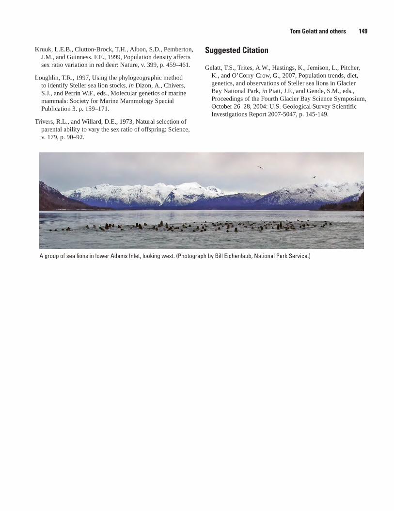
Tom Gelatt and others 1�9
A group of sea lions in lower Adams Inlet, looking west. (Photograph by Bill Eichenlaub, National Park Service.)
Kruuk, L.E.B., Clutton-Brock, T.H., Albon, S.D., Pemberton, J.M., and Guinness. F.E., 1999, Population density affects sex ratio variation in red deer: Nature, v. 399, p. 459–461.
Loughlin, T.R., 1997, Using the phylogeographic method to identify Steller sea lion stocks, in Dizon, A., Chivers, S.J., and Perrin W.F., eds., Molecular genetics of marine mammals: Society for Marine Mammology Special Publication 3. p. 159–171.
Trivers, R.L., and Willard, D.E., 1973, Natural selection of parental ability to vary the sex ratio of offspring: Science, v. 179, p. 90–92.
Suggested Citation
Gelatt, T.S., Trites, A.W., Hastings, K., Jemison, L., Pitcher, K., and O’Corry-Crow, G., 2007, Population trends, diet, genetics, and observations of Steller sea lions in Glacier Bay National Park, in Piatt, J.F., and Gende, S.M., eds., Proceedings of the Fourth Glacier Bay Science Symposium, October 26–28, 2004: U.S. Geological Survey Scientific Investigations Report 2007-5047, p. 145-149.
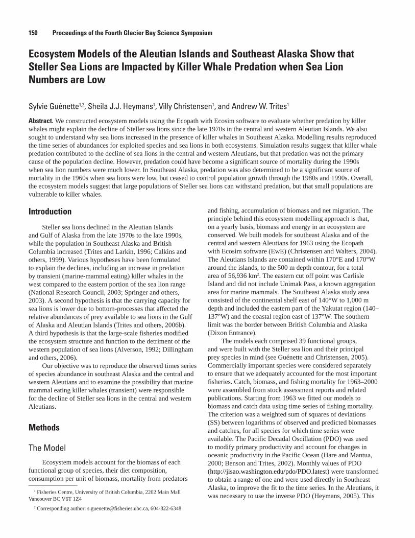
Ecosystem Models of the Aleutian Islands and Southeast Alaska Show that Steller Sea Lions are Impacted by Killer Whale Predation when Sea Lion Numbers are Low
Sylvie Guénette1,2, Sheila J.J. Heymans1, Villy Christensen1, and Andrew W. Trites1
Abstract. We constructed ecosystem models using the Ecopath with Ecosim software to evaluate whether predation by killer whales might explain the decline of Steller sea lions since the late 1970s in the central and western Aleutian Islands. We also sought to understand why sea lions increased in the presence of killer whales in Southeast Alaska. Modelling results reproduced the time series of abundances for exploited species and sea lions in both ecosystems. Simulation results suggest that killer whale predation contributed to the decline of sea lions in the central and western Aleutians, but that predation was not the primary cause of the population decline. However, predation could have become a significant source of mortality during the 1990s when sea lion numbers were much lower. In Southeast Alaska, predation was also determined to be a significant source of mortality in the 1960s when sea lions were low, but ceased to control population growth through the 1980s and 1990s. Overall, the ecosystem models suggest that large populations of Steller sea lions can withstand predation, but that small populations are vulnerable to killer whales.
150 Proceedings of the Fourth Glacier Bay Science Symposium
Introduction
Steller sea lions declined in the Aleutian Islands and Gulf of Alaska from the late 1970s to the late 1990s, while the population in Southeast Alaska and British Columbia increased (Trites and Larkin, 1996; Calkins and others, 1999). Various hypotheses have been formulated to explain the declines, including an increase in predation by transient (marine-mammal eating) killer whales in the west compared to the eastern portion of the sea lion range (National Research Council, 2003; Springer and others, 2003). A second hypothesis is that the carrying capacity for sea lions is lower due to bottom-processes that affected the relative abundances of prey available to sea lions in the Gulf of Alaska and Aleutian Islands (Trites and others, 2006b). A third hypothesis is that the large-scale fisheries modified the ecosystem structure and function to the detriment of the western population of sea lions (Alverson, 1992; Dillingham and others, 2006).
Our objective was to reproduce the observed times series of species abundance in southeast Alaska and the central and western Aleutians and to examine the possibility that marine mammal eating killer whales (transient) were responsible for the decline of Steller sea lions in the central and western Aleutians.
Methods
The ModelEcosystem models account for the biomass of each
functional group of species, their diet composition, consumption per unit of biomass, mortality from predators
and fishing, accumulation of biomass and net migration. The principle behind this ecosystem modelling approach is that, on a yearly basis, biomass and energy in an ecosystem are conserved. We built models for southeast Alaska and of the central and western Aleutians for 1963 using the Ecopath with Ecosim software (EwE) (Christensen and Walters, 2004). The Aleutians Islands are contained within 170°E and 170°W around the islands, to the 500 m depth contour, for a total area of 56,936 km2. The eastern cut off point was Carlisle Island and did not include Unimak Pass, a known aggregation area for marine mammals. The Southeast Alaska study area consisted of the continental shelf east of 140°W to 1,000 m depth and included the eastern part of the Yakutat region (140–137°W) and the coastal region east of 137°W. The southern limit was the border between British Columbia and Alaska (Dixon Entrance).
The models each comprised 39 functional groups, and were built with the Steller sea lion and their principal prey species in mind (see Guénette and Christensen, 2005). Commercially important species were considered separately to ensure that we adequately accounted for the most important fisheries. Catch, biomass, and fishing mortality for 1963–2000 were assembled from stock assessment reports and related publications. Starting from 1963 we fitted our models to biomass and catch data using time series of fishing mortality. The criterion was a weighted sum of squares of deviations (SS) between logarithms of observed and predicted biomasses and catches, for all species for which time series were available. The Pacific Decadal Oscillation (PDO) was used to modify primary productivity and account for changes in oceanic productivity in the Pacific Ocean (Hare and Mantua, 2000; Benson and Trites, 2002). Monthly values of PDO (http://jisao.washington.edu/pdo/PDO.latest) were transformed to obtain a range of one and were used directly in Southeast Alaska, to improve the fit to the time series. In the Aleutians, it was necessary to use the inverse PDO (Heymans, 2005). This
1 Fisheries Centre, University of British Columbia, 2202 Main Mall Vancouver BC V6T 1Z4
2 Corresponding author: [email protected], 604-822-6348
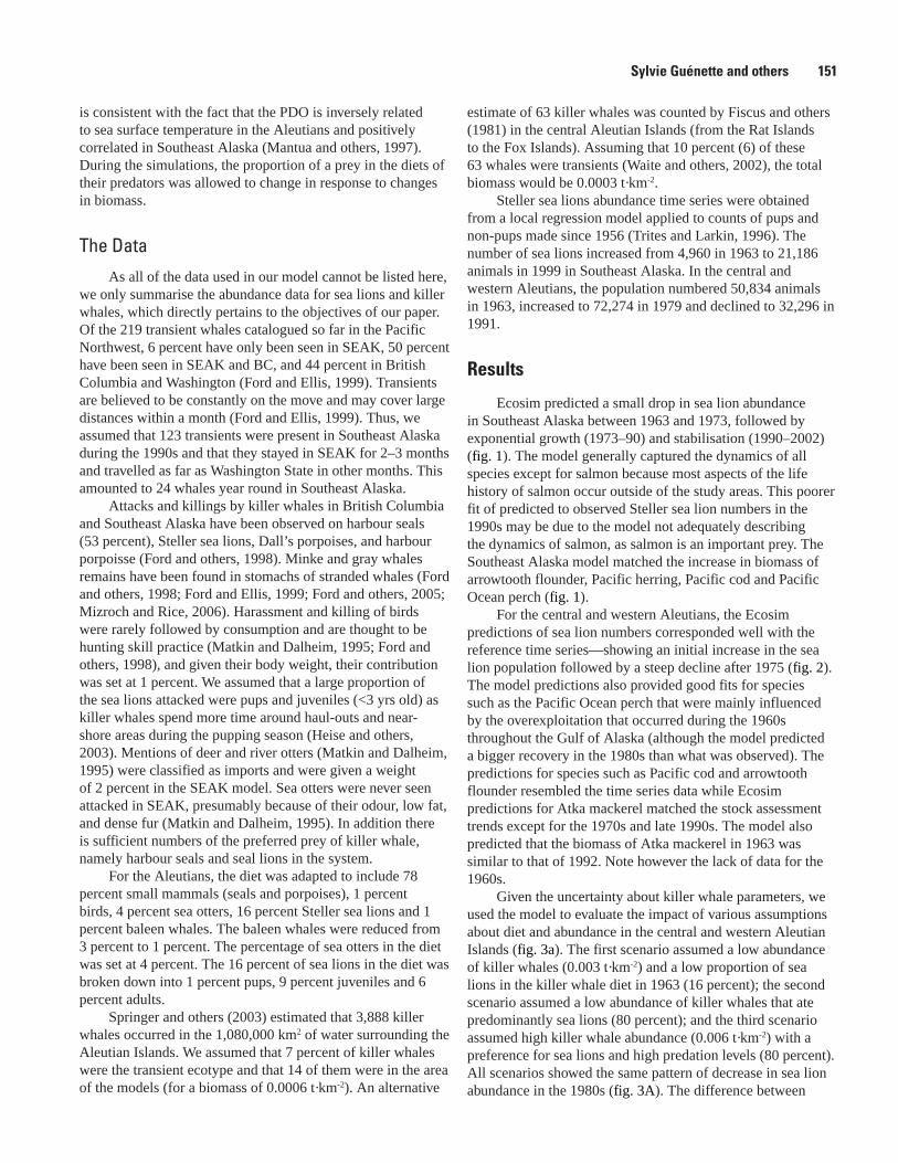
Sylvie Guénette and others 151
is consistent with the fact that the PDO is inversely related to sea surface temperature in the Aleutians and positively correlated in Southeast Alaska (Mantua and others, 1997). During the simulations, the proportion of a prey in the diets of their predators was allowed to change in response to changes in biomass.
The DataAs all of the data used in our model cannot be listed here,
we only summarise the abundance data for sea lions and killer whales, which directly pertains to the objectives of our paper. Of the 219 transient whales catalogued so far in the Pacific Northwest, 6 percent have only been seen in SEAK, 50 percent have been seen in SEAK and BC, and 44 percent in British Columbia and Washington (Ford and Ellis, 1999). Transients are believed to be constantly on the move and may cover large distances within a month (Ford and Ellis, 1999). Thus, we assumed that 123 transients were present in Southeast Alaska during the 1990s and that they stayed in SEAK for 2–3 months and travelled as far as Washington State in other months. This amounted to 24 whales year round in Southeast Alaska.
Attacks and killings by killer whales in British Columbia and Southeast Alaska have been observed on harbour seals (53 percent), Steller sea lions, Dall’s porpoises, and harbour porpoisse (Ford and others, 1998). Minke and gray whales remains have been found in stomachs of stranded whales (Ford and others, 1998; Ford and Ellis, 1999; Ford and others, 2005; Mizroch and Rice, 2006). Harassment and killing of birds were rarely followed by consumption and are thought to be hunting skill practice (Matkin and Dalheim, 1995; Ford and others, 1998), and given their body weight, their contribution was set at 1 percent. We assumed that a large proportion of the sea lions attacked were pups and juveniles (<3 yrs old) as killer whales spend more time around haul-outs and near-shore areas during the pupping season (Heise and others, 2003). Mentions of deer and river otters (Matkin and Dalheim, 1995) were classified as imports and were given a weight of 2 percent in the SEAK model. Sea otters were never seen attacked in SEAK, presumably because of their odour, low fat, and dense fur (Matkin and Dalheim, 1995). In addition there is sufficient numbers of the preferred prey of killer whale, namely harbour seals and seal lions in the system.
For the Aleutians, the diet was adapted to include 78 percent small mammals (seals and porpoises), 1 percent birds, 4 percent sea otters, 16 percent Steller sea lions and 1 percent baleen whales. The baleen whales were reduced from 3 percent to 1 percent. The percentage of sea otters in the diet was set at 4 percent. The 16 percent of sea lions in the diet was broken down into 1 percent pups, 9 percent juveniles and 6 percent adults.
Springer and others (2003) estimated that 3,888 killer whales occurred in the 1,080,000 km2 of water surrounding the Aleutian Islands. We assumed that 7 percent of killer whales were the transient ecotype and that 14 of them were in the area of the models (for a biomass of 0.0006 t·km-2). An alternative
estimate of 63 killer whales was counted by Fiscus and others (1981) in the central Aleutian Islands (from the Rat Islands to the Fox Islands). Assuming that 10 percent (6) of these 63 whales were transients (Waite and others, 2002), the total biomass would be 0.0003 t·km-2.
Steller sea lions abundance time series were obtained from a local regression model applied to counts of pups and non-pups made since 1956 (Trites and Larkin, 1996). The number of sea lions increased from 4,960 in 1963 to 21,186 animals in 1999 in Southeast Alaska. In the central and western Aleutians, the population numbered 50,834 animals in 1963, increased to 72,274 in 1979 and declined to 32,296 in 1991.
Results
Ecosim predicted a small drop in sea lion abundance in Southeast Alaska between 1963 and 1973, followed by exponential growth (1973–90) and stabilisation (1990–2002) (fig. 1). The model generally captured the dynamics of all species except for salmon because most aspects of the life history of salmon occur outside of the study areas. This poorer fit of predicted to observed Steller sea lion numbers in the 1990s may be due to the model not adequately describing the dynamics of salmon, as salmon is an important prey. The Southeast Alaska model matched the increase in biomass of arrowtooth flounder, Pacific herring, Pacific cod and Pacific Ocean perch (fig. 1).
For the central and western Aleutians, the Ecosim predictions of sea lion numbers corresponded well with the reference time series—showing an initial increase in the sea lion population followed by a steep decline after 1975 (fig. 2). The model predictions also provided good fits for species such as the Pacific Ocean perch that were mainly influenced by the overexploitation that occurred during the 1960s throughout the Gulf of Alaska (although the model predicted a bigger recovery in the 1980s than what was observed). The predictions for species such as Pacific cod and arrowtooth flounder resembled the time series data while Ecosim predictions for Atka mackerel matched the stock assessment trends except for the 1970s and late 1990s. The model also predicted that the biomass of Atka mackerel in 1963 was similar to that of 1992. Note however the lack of data for the 1960s.
Given the uncertainty about killer whale parameters, we used the model to evaluate the impact of various assumptions about diet and abundance in the central and western Aleutian Islands (fig. 3a). The first scenario assumed a low abundance of killer whales (0.003 t·km-2) and a low proportion of sea lions in the killer whale diet in 1963 (16 percent); the second scenario assumed a low abundance of killer whales that ate predominantly sea lions (80 percent); and the third scenario assumed high killer whale abundance (0.006 t·km-2) with a preference for sea lions and high predation levels (80 percent). All scenarios showed the same pattern of decrease in sea lion abundance in the 1980s (fig. 3A). The difference between
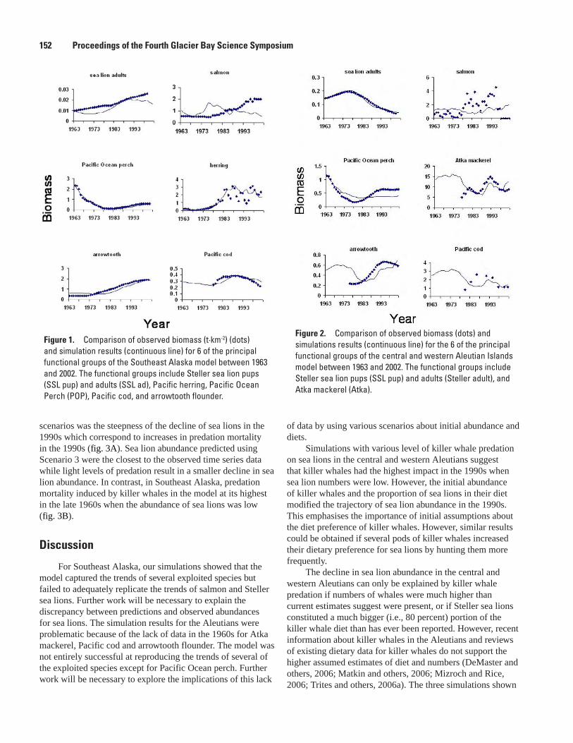
Figure 2. Comparison of observed biomass (dots) and simulations results (continuous line) for the 6 of the principal functional groups of the central and western Aleutian Islands model between 1963 and 2002. The functional groups include Steller sea lion pups (SSL pup) and adults (Steller adult), and Atka mackerel (Atka).
152 Proceedings of the Fourth Glacier Bay Science Symposium
scenarios was the steepness of the decline of sea lions in the 1990s which correspond to increases in predation mortality in the 1990s (fig. 3A). Sea lion abundance predicted using Scenario 3 were the closest to the observed time series data while light levels of predation result in a smaller decline in sea lion abundance. In contrast, in Southeast Alaska, predation mortality induced by killer whales in the model at its highest in the late 1960s when the abundance of sea lions was low (fig. 3B).
Discussion
For Southeast Alaska, our simulations showed that the model captured the trends of several exploited species but failed to adequately replicate the trends of salmon and Steller sea lions. Further work will be necessary to explain the discrepancy between predictions and observed abundances for sea lions. The simulation results for the Aleutians were problematic because of the lack of data in the 1960s for Atka mackerel, Pacific cod and arrowtooth flounder. The model was not entirely successful at reproducing the trends of several of the exploited species except for Pacific Ocean perch. Further work will be necessary to explore the implications of this lack
of data by using various scenarios about initial abundance and diets.
Simulations with various level of killer whale predation on sea lions in the central and western Aleutians suggest that killer whales had the highest impact in the 1990s when sea lion numbers were low. However, the initial abundance of killer whales and the proportion of sea lions in their diet modified the trajectory of sea lion abundance in the 1990s. This emphasises the importance of initial assumptions about the diet preference of killer whales. However, similar results could be obtained if several pods of killer whales increased their dietary preference for sea lions by hunting them more frequently.
The decline in sea lion abundance in the central and western Aleutians can only be explained by killer whale predation if numbers of whales were much higher than current estimates suggest were present, or if Steller sea lions constituted a much bigger (i.e., 80 percent) portion of the killer whale diet than has ever been reported. However, recent information about killer whales in the Aleutians and reviews of existing dietary data for killer whales do not support the higher assumed estimates of diet and numbers (DeMaster and others, 2006; Matkin and others, 2006; Mizroch and Rice, 2006; Trites and others, 2006a). The three simulations shown
Figure 1. Comparison of observed biomass (t·km-2) (dots) and simulation results (continuous line) for 6 of the principal functional groups of the Southeast Alaska model between 1963 and 2002. The functional groups include Steller sea lion pups (SSL pup) and adults (SSL ad), Pacific herring, Pacific Ocean Perch (POP), Pacific cod, and arrowtooth flounder.
Figure �. (A) Comparisons of observed sea lion numbers in the central and western Aleutians (dots) with simulation results (lines) corresponding to three scenarios that considered different combinations of whale numbers and dietary makeup: Scenario 1: low killer whale abundance and low (16 percent) predation on sea lions; Scenario 2. high killer whale abundance and low (28 percent) predation; Scenario 3. high killer whale and high predation (80 percent). and (B) Trajectory of adult sea lion mortality in Southeast Alaska and the central and western Aleutians.
Sylvie Guénette and others 15�
in figure 3a imply that Steller sea lions would have declined during the 1980s in the absence of killer whales (given the small difference between scenarios), and that the most pronounced effect of killer whales would only have occurred when sea lion numbers were low (i.e., during the 1990s).
This modelling exercise is a first step in trying to examine the effect of killer whale predation on sea lions within the framework of an ecosystem model that includes fishing. Further work is needed to delineate the relative impact of fishing, predation, and ocean productivity on the sea lion abundance trends in both ecosystems.
Implications
The ecosystem model built for Southeast Alaska could be modified to address concerns of Glacier Bay National Park. It could be used to compare and rank the various hypotheses
about the trends in harbour seals in Glacier Bay. This would require careful compilation of the catch and abundance of harbour seals throughout its geographical range to give a basis for comparison and to provide some insight into the regional declines of harbour seals.
Acknowledgments
Support was provided by NOAA through the North Pacific Universities Marine Mammal Research Consortium and the North Pacific Marine Science Foundation. This project would not have been possible without the assistance of numerous colleagues in the Alaska Fisheries Centre, Auke Bay Laboratory, Alaska Department of Fish and Game, University of Alaska, Marine Mammal Research Unit (UBC), Glacier Bay National Park, and Department of Fisheries and Oceans of Canada. We thank two reviewers for their helpful comments.
References Cited
Alverson, D.L., 1992, Commercial fisheries and the Steller sea lion (Eumetopias jubatus): the conflict arena: Reviews in Aquatic Sciences, v. 6, p. 203–256.
Benson, A.J., and Trites, A.W., 2002, Ecological effects of regime shifts in the Bering Sea and eastern North Pacific Ocean: Fish and Fisheries, v. 3, p. 95–113.
Calkins, D.G., McAllister, D.C., Pitcher, K.W., and Pendleton, G.W., 1999, Steller sea lion status and trend in Southeast Alaska: 1979-1997: Marine Mammal Science, v. 15, no. 2, p. 462–477.
Christensen, V., and Walters, C.J. 2004. Ecopath with Ecosim: methods, capabilities and limitations: Ecological Modelling, v. 172, p. 109–139.
DeMaster, D.P., Trites, A.W., Clapham, P., Mizroch, S., Wade, P., Small, R.J., and Hoef, J.V., 2006, The sequential megafaunal collapse hypothesis: testing with existing data: Progress in Oceanography.
Dillingham, P.W., Skalski, J.R., and Ryding, K.E., 2006, Fine-scale geographic interactions between Steller sea lion (Eumetopias jubatus) trends and local fisheries. Canadian Journal of Fisheries and Aquatic Sciences, v. 61, p. 107–119.
Fiscus, C.H., Rugh, D.J., and Loughlin, T.R., 1981, Census of northern sea lion (Eumetopias jubatus) in central Aleutian Islands, Alaska, 17 June-15 July 1979, with notes on other marine mammals and birds: U.S. Department of Commerce, NOAA Technical Memorandum, NMFS F/NWC-17. 109 p.
15� Proceedings of the Fourth Glacier Bay Science Symposium
Ford, J.K.B., and Ellis, G.M., 1999, Transients: mammal-hunting killer whales of British Columbia, Washington, and Southeastern Alaska: Seattle, Vancouver, BC, UBC Press, and Seattle, Wash., University of Washington Press, 96 p.
Ford, J.K.B., Ellis, G.M., Matkin, D.R., Balcomb, K.C., Briggs, D., and Morton, A.B., 2005, Killer whale attacks on minke whales: Prey capture and antipredator tactics. Marine Mammal Science, v. 21, p. 603–618.
Ford, J.K.B., Ellis, G., Barrett-Lennard, L., Morton, A., Palm, R.S., and Balcomb, K.C., 1998, Dietary specialization in two sympatric populations of killer whales (Orcinus orca) in coastal British Columbia and adjacent waters: Canadian Journal of Zoology, v. 76, p. 1456–1471.
Guénette, S., and Christensen, V., eds., 2005, Foodweb models and data for studying fisheries and environmental impact on Eastern Pacific ecosystems: Vancouver, BC, Canada, Fisheries Centre, University of British Columbia, v. 13 no. 1, 237 p.
Hare, S.R., and Mantua, N.J., 2000, Empirical evidence for North Pacific regime shifts in 1977 and 1989: Progress in Oceanography, v. 47, p. 103–145.
Heise, K., Barrett-Lennard, L.G., Saulitis, E., Matkin, C., and Bain, D., 2003, Examining the evidence for killer whale predation on Steller sea lions in British Columbia and Alaska, Aquatic Mammals, v. 29, p. 325–334.
Heymans, S., 2005, Ecosystem models of the Western and Central Aleutian Islands in 1963, 1979 and 1991, in Guénette, S., and Christensen, V., eds., Foodweb models and data for studying fisheries and environmental impact on Eastern Pacific ecosystems: Vancouver, BC, Canada, Fisheries Centre, University of British Columbia, v. 13, no. 1, p. 8-82, accessed March 1, 2007 at http://www.fisheries.ubc.ca/publications/reports/report13_1.php.
Mantua, N.J., Hare, S.R., Zhang, Y., Wallace, J.M., and Francis, R.C., 1997, A Pacific interdecadal climate oscillation with impacts on salmon production: Bulletin of the American Meteorological Society, v. 78, p. 1069–1079.
Matkin, C., Barrett-Lennard, L.G., H.Yurk, Ellifrit, D., and Trites, A.W., 2006, Ecotypic variation and predatory behavior of killer whales (Orcinus orca) in the eastern Aleutian Islands, Alaska: Fisheries Bulletin (in press).
Matkin, D.R., and Dalheim, M.E., 1995, Feeding behaviors of killer whales in northern Southeastern Alaska, in Engstrom, D.R., ed., Proceedings of the Third Glacier Bay Science Symposium, 1993: Anchorage, Alaska, National Park Service, p. 246–253.
Mizroch, S.A., and Rice, D.W., 2006, Have North Pacific killer whales switched prey species in response to depletion of the great whale populations? Marine Ecology Progress Series (in press).
National Research Council, 2003, Decline of the Steller sea lion in Alaskan waters: untangling food webs and fishing nets: Washington, D.C., The National Academies Press, 204 p.
Springer, A.M., Estes, J.A., van Vliet, G.B., Williams, T.M., Doak, D.F., Danner, E.M., Forney, K.A., and Pfister, B., 2003, Sequential megafaunal collapse in the North Pacific Ocean: An ongoing legacy of industrial whaling?: Proceedings of the National Academy of Sciences of the United States of America, v. 100, no. 21, p. 12223–12228.
Trites, A.W., and Larkin, P.A., 1996, Changes in the abundance of Steller sea lions (Eumetopias jubatus) in Alaska from 1956 to 1992: how many were there?: Aquatic Mammals, v. 22, p. 153–166.
Trites, A.W., Deecke, V.B., Gregr, E.J., Ford, J.K.B., and Olesiuk, P.F., 2006a, Killer whales, whaling and sequential megafaunal collapse in the North Pacific: a comparative analysis of the dynamics of marine mammals in Alaska and British Columbia following commercial whaling: Marine Mammal Science (in press).
Trites, A.W., Miller, A.J., Maschner, H.D.G., Alexander, M.A., Bograd, S.J., Calder, J.A., Capotondi, A., Coyle, K.O., Lorenzo, E.D., Finney, B.P., Gregr, E.J., Grosch, C.E., Hare, S.R., Hunt, G.L., Jahncke, J., Kachel, N.B., Kim, H.-J., Ladd, C., Mantua, N.J., Marzban, C., Maslowski, W., Mendelssohn, R., Neilson, D.J., Okkonen, S.R., Overland, J.E., Reedy-Maschner, K.L., Royer, T.C., Schwing, F.B., Wang, J.X.L., and Winship, A.J., 2006b, Bottom-up forcing and the decline of Steller sea lions in Alaska: assessing the ocean climate hypothesis: Fisheries Oceanography (in press).
Waite, J.M., Friday, N.A., and Moore, S.E., 2002, Killer whale (Orcinus orca) distribution and abundance in the central and southeastern Bering Sea, July 1999 and June 2000: Marine Mammal Science, v. 18, no. 3, p. 779–786.
Suggested Citation
Guénette, S., Heymans, S.J.J., Christensen, V., and Trites, A.W., 2007, Ecosystem models of the Aleutian Islands and southeast Alaska show that Steller sea lions are impacted by Killer Whale predation when sea lion numbers are low, in Piatt, J.F., and Gende, S.M., eds., Proceedings of the Fourth Glacier Bay Science Symposium, October 26–28, 2004: U.S. Geological Survey Scientific Investigations Report 2007-5047, p. 150–154.
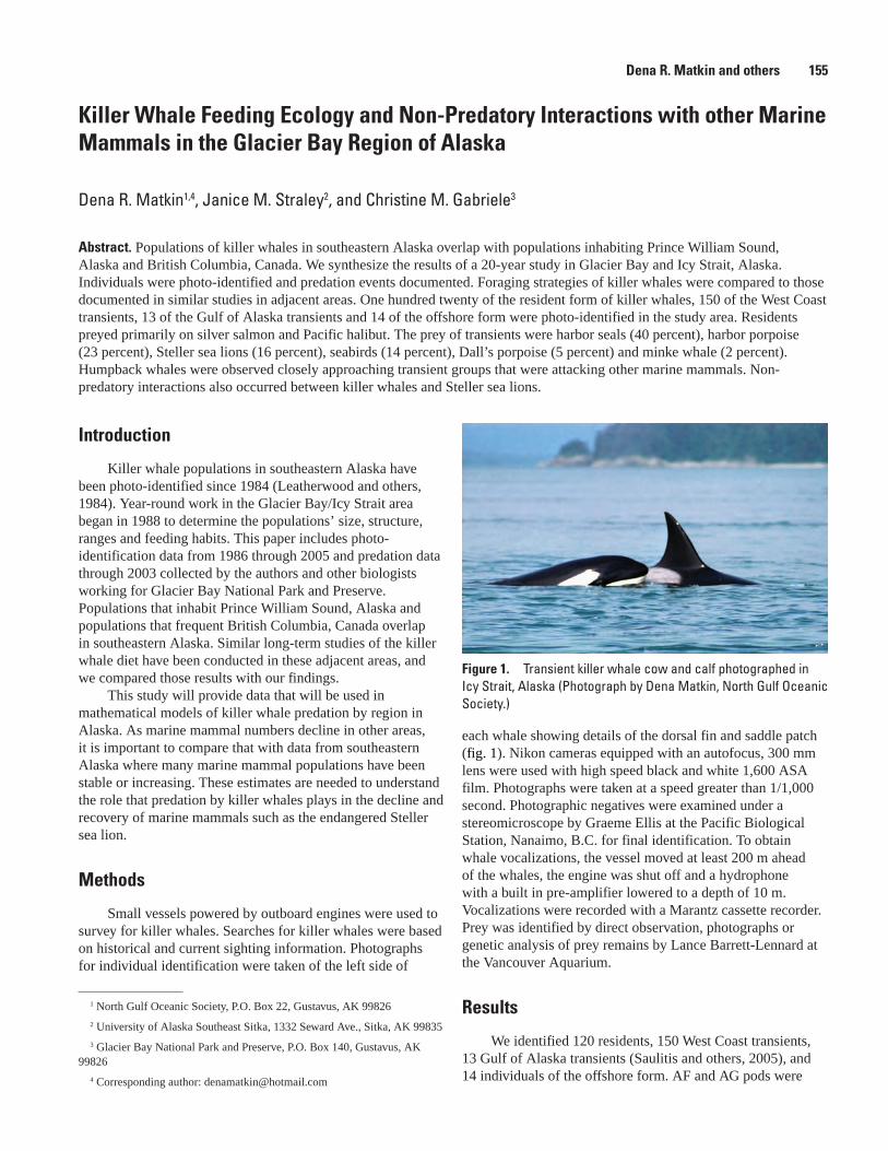
Killer Whale Feeding Ecology and Non-Predatory Interactions with other Marine Mammals in the Glacier Bay Region of Alaska
Dena R. Matkin1,4, Janice M. Straley2, and Christine M. Gabriele3
Abstract. Populations of killer whales in southeastern Alaska overlap with populations inhabiting Prince William Sound, Alaska and British Columbia, Canada. We synthesize the results of a 20-year study in Glacier Bay and Icy Strait, Alaska. Individuals were photo-identified and predation events documented. Foraging strategies of killer whales were compared to those documented in similar studies in adjacent areas. One hundred twenty of the resident form of killer whales, 150 of the West Coast transients, 13 of the Gulf of Alaska transients and 14 of the offshore form were photo-identified in the study area. Residents preyed primarily on silver salmon and Pacific halibut. The prey of transients were harbor seals (40 percent), harbor porpoise (23 percent), Steller sea lions (16 percent), seabirds (14 percent), Dall’s porpoise (5 percent) and minke whale (2 percent). Humpback whales were observed closely approaching transient groups that were attacking other marine mammals. Non-predatory interactions also occurred between killer whales and Steller sea lions.
Figure 1. Transient killer whale cow and calf photographed in Icy Strait, Alaska (Photograph by Dena Matkin, North Gulf Oceanic Society.)
Dena R. Matkin and others 155
1 North Gulf Oceanic Society, P.O. Box 22, Gustavus, AK 99826
2 University of Alaska Southeast Sitka, 1332 Seward Ave., Sitka, AK 99835
3 Glacier Bay National Park and Preserve, P.O. Box 140, Gustavus, AK 99826
4 Corresponding author: [email protected]
Introduction
Killer whale populations in southeastern Alaska have been photo-identified since 1984 (Leatherwood and others, 1984). Year-round work in the Glacier Bay/Icy Strait area began in 1988 to determine the populations’ size, structure, ranges and feeding habits. This paper includes photo-identification data from 1986 through 2005 and predation data through 2003 collected by the authors and other biologists working for Glacier Bay National Park and Preserve. Populations that inhabit Prince William Sound, Alaska and populations that frequent British Columbia, Canada overlap in southeastern Alaska. Similar long-term studies of the killer whale diet have been conducted in these adjacent areas, and we compared those results with our findings.
This study will provide data that will be used in mathematical models of killer whale predation by region in Alaska. As marine mammal numbers decline in other areas, it is important to compare that with data from southeastern Alaska where many marine mammal populations have been stable or increasing. These estimates are needed to understand the role that predation by killer whales plays in the decline and recovery of marine mammals such as the endangered Steller sea lion.
Methods
Small vessels powered by outboard engines were used to survey for killer whales. Searches for killer whales were based on historical and current sighting information. Photographs for individual identification were taken of the left side of
each whale showing details of the dorsal fin and saddle patch (fig. 1). Nikon cameras equipped with an autofocus, 300 mm lens were used with high speed black and white 1,600 ASA film. Photographs were taken at a speed greater than 1/1,000 second. Photographic negatives were examined under a stereomicroscope by Graeme Ellis at the Pacific Biological Station, Nanaimo, B.C. for final identification. To obtain whale vocalizations, the vessel moved at least 200 m ahead of the whales, the engine was shut off and a hydrophone with a built in pre-amplifier lowered to a depth of 10 m. Vocalizations were recorded with a Marantz cassette recorder. Prey was identified by direct observation, photographs or genetic analysis of prey remains by Lance Barrett-Lennard at the Vancouver Aquarium.
Results
We identified 120 residents, 150 West Coast transients, 13 Gulf of Alaska transients (Saulitis and others, 2005), and 14 individuals of the offshore form. AF and AG pods were
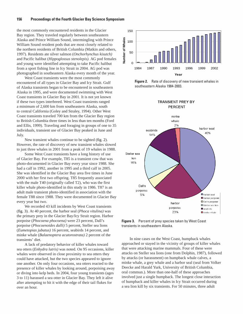
the most commonly encountered residents in the Glacier Bay region. They traveled regularly between southeastern Alaska and Prince William Sound, intermingling with Prince William Sound resident pods that are most closely related to the northern residents of British Columbia (Matkin and others, 1997). Residents ate silver salmon (Onchorhynchus kisutch) and Pacific halibut (Hippoglossus stenolepis). AG pod females and young were identified attempting to take Pacific halibut from a sport fishing line in Icy Strait in 2004. AG pod was photographed in southeastern Alaska every month of the year.
West Coast transients were the most commonly encountered of all types in Glacier Bay and Icy Strait. Gulf of Alaska transients began to be encountered in southeastern Alaska in 1995, and were documented swimming with West Coast transients in Glacier Bay in 2001. It is not yet known if these two types interbreed. West Coast transients ranged a minimum of 2,600 km from southeastern Alaska, south to central California (Goley and Straley, 1994). Other West Coast transients traveled 700 km from the Glacier Bay region to British Columbia three times in less than ten months (Ford and Ellis, 1999). Traveling and foraging in groups of one to 35 individuals, transient use of Glacier Bay peaked in June and July.
New transient whales continue to be sighted (fig. 2). However, the rate of discovery of new transient whales slowed to just three whales in 2001 from a peak of 19 whales in 1988.
Some West Coast transients have a long history of use of Glacier Bay. For example, T85 is a transient cow that was photo-documented in Glacier Bay every year since 1988. She had a calf in 1992, another in 1995 and a third calf in 2005. She was identified in the Glacier Bay area five times in June 2000 with her first two offspring. T85 frequently associated with the male T40 (originally called T2), who was the first killer whale photo-identified in this study in 1986. T87 is an adult male transient photo-identified in association with the female T88 since 1988. They were documented in Glacier Bay every year but two.
We recorded 43 kill incidents by West Coast transients (fig. 3). At 40 percent, the harbor seal (Phoca vitulina) was the primary prey in the Glacier Bay/Icy Strait region. Harbor porpoise (Phocoena phocoena) were 23 percent, Dall’s porpoise (Phocoenoides dalli) 5 percent, Steller sea lions (Eumetopias jubatus) 16 percent, seabirds 14 percent, and minke whale (Balaenoptera acutorostrata) 2 percent of the transients’ diet.
A lack of predatory behavior of killer whales toward sea otters (Enhydra lutris) was noted. On 95 occasions, killer whales were observed in close proximity to sea otters they could have attacked, but the two species appeared to ignore one another. On only four occasions, sea otters reacted to the presence of killer whales by looking around, porpoising away or diving into kelp beds. In 2004, four young transients (ages 3 to 11) harassed a sea otter in Glacier Bay. They left it alive after attempting to hit it with the edge of their tail flukes for over an hour.
In nine cases on the West Coast, humpback whales approached or stayed in the vicinity of groups of killer whales that were attacking marine mammals. Four of these were attacks on Steller sea lions (one from Dolphin, 1987), followed by attacks (or harassment) on humpback whale calves, a minke whale, a grey whale and a harbor seal (seal from Volker Deecke and Harald Yurk, University of British Columbia, oral commun.). More than one-half of these approaches involved just a single humpback. The longest close interaction of humpback and killer whales in Icy Strait occurred during a sea lion kill by six transients. For 50 minutes, three adult
Figure �. Percent of prey species taken by West Coast transients in southeastern Alaska.
Figure 2. Rate of discovery of new transient whales in southeastern Alaska 1984-2003.
0
50
100
150
1984 1987 1990 1993 1996 1999 2002
Year
Num
bero
fWha
les
15� Proceedings of the Fourth Glacier Bay Science Symposium
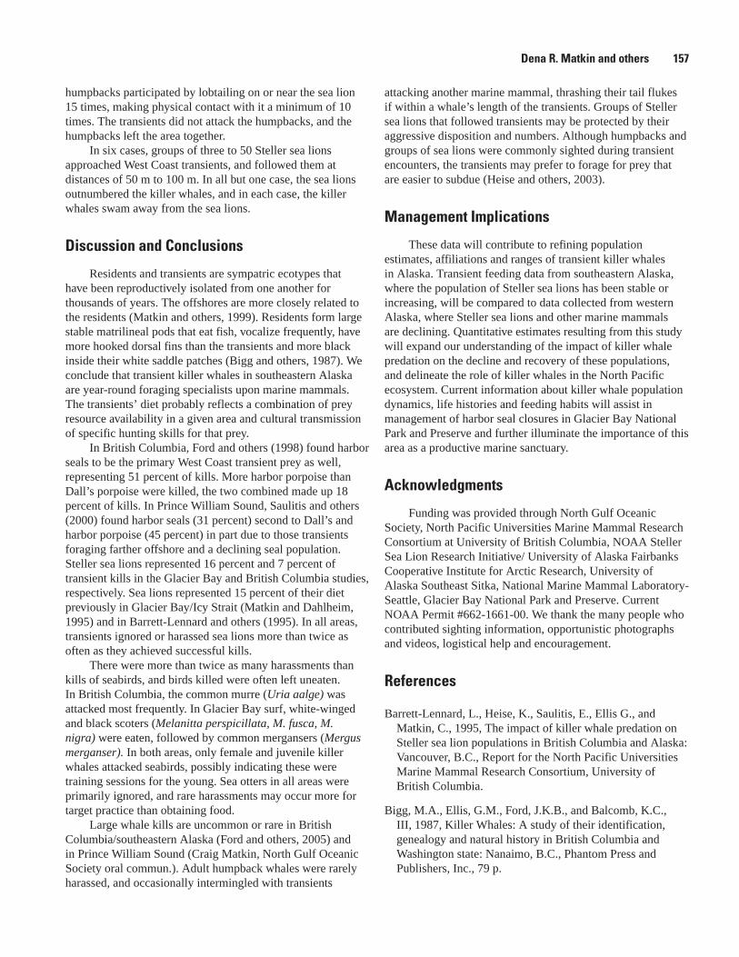
Dena R. Matkin and others 157
humpbacks participated by lobtailing on or near the sea lion 15 times, making physical contact with it a minimum of 10 times. The transients did not attack the humpbacks, and the humpbacks left the area together.
In six cases, groups of three to 50 Steller sea lions approached West Coast transients, and followed them at distances of 50 m to 100 m. In all but one case, the sea lions outnumbered the killer whales, and in each case, the killer whales swam away from the sea lions.
Discussion and Conclusions
Residents and transients are sympatric ecotypes that have been reproductively isolated from one another for thousands of years. The offshores are more closely related to the residents (Matkin and others, 1999). Residents form large stable matrilineal pods that eat fish, vocalize frequently, have more hooked dorsal fins than the transients and more black inside their white saddle patches (Bigg and others, 1987). We conclude that transient killer whales in southeastern Alaska are year-round foraging specialists upon marine mammals. The transients’ diet probably reflects a combination of prey resource availability in a given area and cultural transmission of specific hunting skills for that prey.
In British Columbia, Ford and others (1998) found harbor seals to be the primary West Coast transient prey as well, representing 51 percent of kills. More harbor porpoise than Dall’s porpoise were killed, the two combined made up 18 percent of kills. In Prince William Sound, Saulitis and others (2000) found harbor seals (31 percent) second to Dall’s and harbor porpoise (45 percent) in part due to those transients foraging farther offshore and a declining seal population. Steller sea lions represented 16 percent and 7 percent of transient kills in the Glacier Bay and British Columbia studies, respectively. Sea lions represented 15 percent of their diet previously in Glacier Bay/Icy Strait (Matkin and Dahlheim, 1995) and in Barrett-Lennard and others (1995). In all areas, transients ignored or harassed sea lions more than twice as often as they achieved successful kills.
There were more than twice as many harassments than kills of seabirds, and birds killed were often left uneaten. In British Columbia, the common murre (Uria aalge) was attacked most frequently. In Glacier Bay surf, white-winged and black scoters (Melanitta perspicillata, M. fusca, M. nigra) were eaten, followed by common mergansers (Mergus merganser). In both areas, only female and juvenile killer whales attacked seabirds, possibly indicating these were training sessions for the young. Sea otters in all areas were primarily ignored, and rare harassments may occur more for target practice than obtaining food.
Large whale kills are uncommon or rare in British Columbia/southeastern Alaska (Ford and others, 2005) and in Prince William Sound (Craig Matkin, North Gulf Oceanic Society oral commun.). Adult humpback whales were rarely harassed, and occasionally intermingled with transients
attacking another marine mammal, thrashing their tail flukes if within a whale’s length of the transients. Groups of Steller sea lions that followed transients may be protected by their aggressive disposition and numbers. Although humpbacks and groups of sea lions were commonly sighted during transient encounters, the transients may prefer to forage for prey that are easier to subdue (Heise and others, 2003).
Management Implications
These data will contribute to refining population estimates, affiliations and ranges of transient killer whales in Alaska. Transient feeding data from southeastern Alaska, where the population of Steller sea lions has been stable or increasing, will be compared to data collected from western Alaska, where Steller sea lions and other marine mammals are declining. Quantitative estimates resulting from this study will expand our understanding of the impact of killer whale predation on the decline and recovery of these populations, and delineate the role of killer whales in the North Pacific ecosystem. Current information about killer whale population dynamics, life histories and feeding habits will assist in management of harbor seal closures in Glacier Bay National Park and Preserve and further illuminate the importance of this area as a productive marine sanctuary.
Acknowledgments
Funding was provided through North Gulf Oceanic Society, North Pacific Universities Marine Mammal Research Consortium at University of British Columbia, NOAA Steller Sea Lion Research Initiative/ University of Alaska Fairbanks Cooperative Institute for Arctic Research, University of Alaska Southeast Sitka, National Marine Mammal Laboratory-Seattle, Glacier Bay National Park and Preserve. Current NOAA Permit #662-1661-00. We thank the many people who contributed sighting information, opportunistic photographs and videos, logistical help and encouragement.
References
Barrett-Lennard, L., Heise, K., Saulitis, E., Ellis G., and Matkin, C., 1995, The impact of killer whale predation on Steller sea lion populations in British Columbia and Alaska: Vancouver, B.C., Report for the North Pacific Universities Marine Mammal Research Consortium, University of British Columbia.
Bigg, M.A., Ellis, G.M., Ford, J.K.B., and Balcomb, K.C., III, 1987, Killer Whales: A study of their identification, genealogy and natural history in British Columbia and Washington state: Nanaimo, B.C., Phantom Press and Publishers, Inc., 79 p.
15� Proceedings of the Fourth Glacier Bay Science Symposium
An unnamed stream discharges glacial meltwater into Wachusett Inlet. (Photograph by Bill Eichenlaub, National Park Service.)
Dolphin, W.F., 1987, Observations of humpback whale, Megaptera novaeangliae,—killer whale, Orcinus orca, interactions in Alaska: comparison with terrestrial predator-prey relationships: Canadian Field Naturalist, v. 101, p. 70-75.
Ford, J.K.B. and Ellis, G.M., 1999, Transients: Mammal-hunting killer whales: Vancouver, B.C., UBC Press.
Ford, J.K.B., Ellis, G.M., Matkin, D.R., Balcomb, K.C., Briggs, D., and Morton, A.B., 2005, Killer whale attacks on minke whales: Prey capture and antipredator tactics: Marine Mammal Science, v. 21, no. 4.
Ford, J.K.B., Ellis, G.M., Barrett-Lennard, L.G., Morton, A.B., Palm R.S., and Balcomb, K.C., III. 1998, Dietary specialization in two sympatric populations of killer whales (Orcinus orca) in coastal British Columbia and adjacent waters: Canadian Journal of Zoology, v. 76, p. 1456-1471.
Goley, P.D., and Straley, J.M., 1994, Attack on gray whales (Eschrichtius robustus) in Monterey Bay, California, by killer whales (Orcinus orca) previously identified in Glacier Bay, Alaska: Canadian Journal of Zoology, v. 72, p. 1528-1530.
Heise, K., Barrett-Lennard, L.G., Saulitis, E., Matkin C.O., and Bain, D., 2003, Examining the evidence for killer whale predation on Steller sea lions in British Columbia and Alaska: Aquatic Mammals, v. 29, p. 325-334.
Leatherwood, S., Balcomb, K.C., III, Matkin, C., and Ellis, G., 1984, Killer whales (Orcinus orca) of southern Alaska: Hubbs Sea World Research Institute Technical Report No. 84-175, 59 p.
Matkin, D.R., and Dahlheim, M.E., 1995, Feeding behaviors of killer whales in northern southeastern Alaska, in Engstrom, D.R., Proceedings of the Third Glacier Bay Science Symposium, 1993: Anchorage, Alaska, National Park Service, p. 246-253.
Matkin, C.O., Ellis, G.M., Saulitis, E., Barrett-Lennard, L.G., and Matkin, D.R., 1999, Killer whales of southern Alaska: Homer, Alaska, North Gulf Oceanic Society.
Matkin, C.O., Matkin, D.R., Ellis, G.M., Saulitis E., and McSweeney, D., 1997, Movements of resident killer whales between southeastern Alaska and Prince William Sound, Alaska: Marine Mammal Science, v. 13, no. 3.
Saulitis, E., Matkin, C., Barrett-Lennard, L., Heise K., and Ellis, G., 2000, Foraging strategies of sympatric killer whale (Orcinus orca) populations in Prince William Sound, Alaska: Marine Mammal Science, v. 16, no. 1.
Saulitis, E., Matkin, C.O., and Fay, F.H., 2005, Vocal repertoire and acoustic behavior of the isolated AT1 killer whale subpopulation in Southern Alaska: Canadian Journal of Zoology, v. 83, p. 1015-1029.
Suggested Citation
Matkin, D.R., Straley, J.M. and Gabriele, C.M. 2007, Killer whale feeding ecology and non-predatory interactions with other marine mammals in the Glacier Bay region of Alaska, in Piatt, J.F., and Gende, S.M., eds., Proceedings of the Fourth Glacier Bay Science Symposium, October 26–28, 2004: U.S. Geological Survey Scientific Investigations Report 2007-5047, p. 155-158
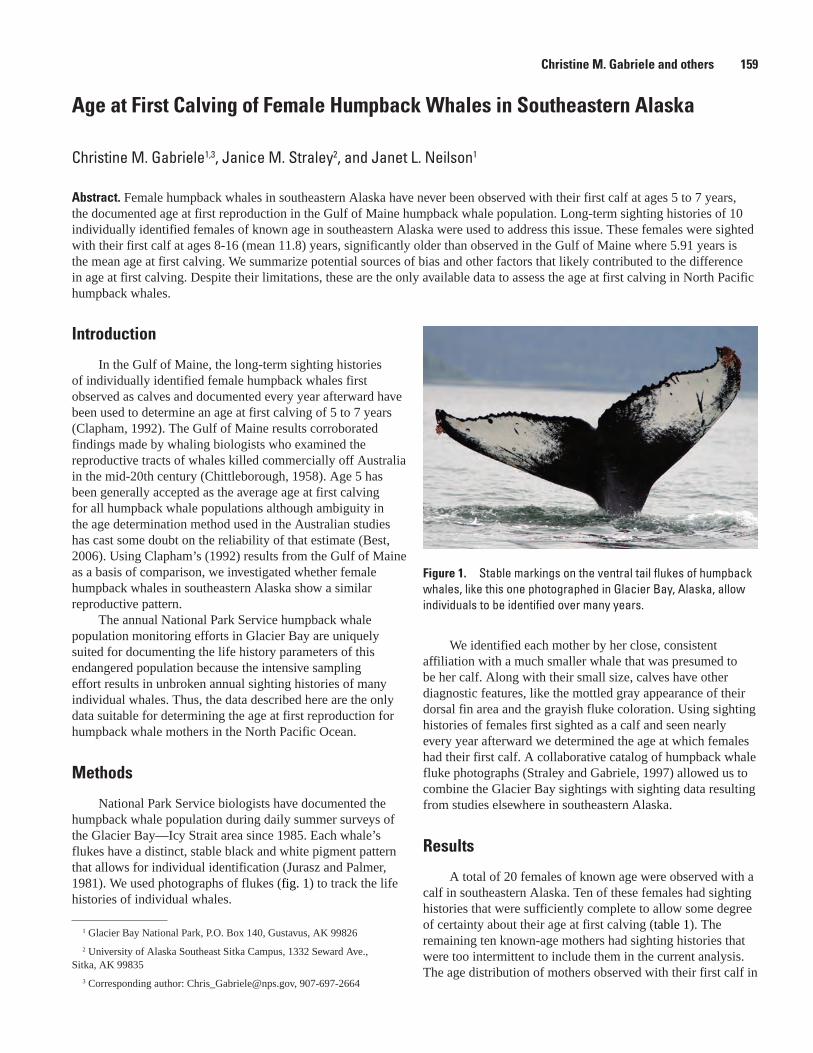
Age at First Calving of Female Humpback Whales in Southeastern Alaska
Christine M. Gabriele1,3, Janice M. Straley2, and Janet L. Neilson1
Abstract. Female humpback whales in southeastern Alaska have never been observed with their first calf at ages 5 to 7 years, the documented age at first reproduction in the Gulf of Maine humpback whale population. Long-term sighting histories of 10 individually identified females of known age in southeastern Alaska were used to address this issue. These females were sighted with their first calf at ages 8-16 (mean 11.8) years, significantly older than observed in the Gulf of Maine where 5.91 years is the mean age at first calving. We summarize potential sources of bias and other factors that likely contributed to the difference in age at first calving. Despite their limitations, these are the only available data to assess the age at first calving in North Pacific humpback whales.
Figure 1. Stable markings on the ventral tail flukes of humpback whales, like this one photographed in Glacier Bay, Alaska, allow individuals to be identified over many years.
Christine M. Gabriele and others 159
1 Glacier Bay National Park, P.O. Box 140, Gustavus, AK 99826
2 University of Alaska Southeast Sitka Campus, 1332 Seward Ave., Sitka, AK 99835
3 Corresponding author: [email protected], 907-697-2664
Introduction
In the Gulf of Maine, the long-term sighting histories of individually identified female humpback whales first observed as calves and documented every year afterward have been used to determine an age at first calving of 5 to 7 years (Clapham, 1992). The Gulf of Maine results corroborated findings made by whaling biologists who examined the reproductive tracts of whales killed commercially off Australia in the mid-20th century (Chittleborough, 1958). Age 5 has been generally accepted as the average age at first calving for all humpback whale populations although ambiguity in the age determination method used in the Australian studies has cast some doubt on the reliability of that estimate (Best, 2006). Using Clapham’s (1992) results from the Gulf of Maine as a basis of comparison, we investigated whether female humpback whales in southeastern Alaska show a similar reproductive pattern.
The annual National Park Service humpback whale population monitoring efforts in Glacier Bay are uniquely suited for documenting the life history parameters of this endangered population because the intensive sampling effort results in unbroken annual sighting histories of many individual whales. Thus, the data described here are the only data suitable for determining the age at first reproduction for humpback whale mothers in the North Pacific Ocean.
Methods
National Park Service biologists have documented the humpback whale population during daily summer surveys of the Glacier Bay—Icy Strait area since 1985. Each whale’s flukes have a distinct, stable black and white pigment pattern that allows for individual identification (Jurasz and Palmer, 1981). We used photographs of flukes (fig. 1) to track the life histories of individual whales.
We identified each mother by her close, consistent affiliation with a much smaller whale that was presumed to be her calf. Along with their small size, calves have other diagnostic features, like the mottled gray appearance of their dorsal fin area and the grayish fluke coloration. Using sighting histories of females first sighted as a calf and seen nearly every year afterward we determined the age at which females had their first calf. A collaborative catalog of humpback whale fluke photographs (Straley and Gabriele, 1997) allowed us to combine the Glacier Bay sightings with sighting data resulting from studies elsewhere in southeastern Alaska.
Results
A total of 20 females of known age were observed with a calf in southeastern Alaska. Ten of these females had sighting histories that were sufficiently complete to allow some degree of certainty about their age at first calving (table 1). The remaining ten known-age mothers had sighting histories that were too intermittent to include them in the current analysis. The age distribution of mothers observed with their first calf in
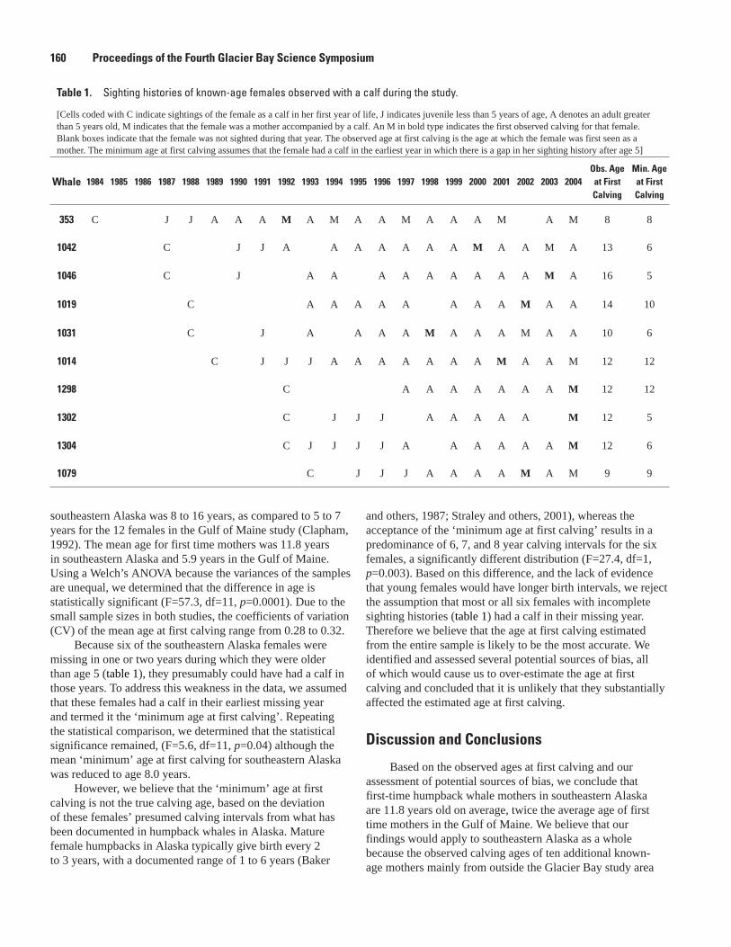
southeastern Alaska was 8 to 16 years, as compared to 5 to 7 years for the 12 females in the Gulf of Maine study (Clapham, 1992). The mean age for first time mothers was 11.8 years in southeastern Alaska and 5.9 years in the Gulf of Maine. Using a Welch’s ANOVA because the variances of the samples are unequal, we determined that the difference in age is statistically significant (F=57.3, df=11, p=0.0001). Due to the small sample sizes in both studies, the coefficients of variation (CV) of the mean age at first calving range from 0.28 to 0.32.
Because six of the southeastern Alaska females were missing in one or two years during which they were older than age 5 (table 1), they presumably could have had a calf in those years. To address this weakness in the data, we assumed that these females had a calf in their earliest missing year and termed it the ‘minimum age at first calving’. Repeating the statistical comparison, we determined that the statistical significance remained, (F=5.6, df=11, p=0.04) although the mean ‘minimum’ age at first calving for southeastern Alaska was reduced to age 8.0 years.
However, we believe that the ‘minimum’ age at first calving is not the true calving age, based on the deviation of these females’ presumed calving intervals from what has been documented in humpback whales in Alaska. Mature female humpbacks in Alaska typically give birth every 2 to 3 years, with a documented range of 1 to 6 years (Baker
and others, 1987; Straley and others, 2001), whereas the acceptance of the ‘minimum age at first calving’ results in a predominance of 6, 7, and 8 year calving intervals for the six females, a significantly different distribution (F=27.4, df=1, p=0.003). Based on this difference, and the lack of evidence that young females would have longer birth intervals, we reject the assumption that most or all six females with incomplete sighting histories (table 1) had a calf in their missing year. Therefore we believe that the age at first calving estimated from the entire sample is likely to be the most accurate. We identified and assessed several potential sources of bias, all of which would cause us to over-estimate the age at first calving and concluded that it is unlikely that they substantially affected the estimated age at first calving.
Discussion and Conclusions
Based on the observed ages at first calving and our assessment of potential sources of bias, we conclude that first-time humpback whale mothers in southeastern Alaska are 11.8 years old on average, twice the average age of first time mothers in the Gulf of Maine. We believe that our findings would apply to southeastern Alaska as a whole because the observed calving ages of ten additional known-age mothers mainly from outside the Glacier Bay study area
Table 1. Sighting histories of known-age females observed with a calf during the study.
[Cells coded with C indicate sightings of the female as a calf in her first year of life, J indicates juvenile less than 5 years of age, A denotes an adult greater than 5 years old, M indicates that the female was a mother accompanied by a calf. An M in bold type indicates the first observed calving for that female. Blank boxes indicate that the female was not sighted during that year. The observed age at first calving is the age at which the female was first seen as a mother. The minimum age at first calving assumes that the female had a calf in the earliest year in which there is a gap in her sighting history after age 5]
Whale 19�� 19�5 19�� 19�7 19�� 19�9 1990 1991 1992 199� 199� 1995 199� 1997 199� 1999 2000 2001 2002 200� 200�Obs. Age at First Calving
Min. Age at First Calving
�5� C J J A A A M A M A A M A A A M A M 8 8
10�2 C J J A A A A A A A M A A M A 13 6
10�� C J A A A A A A A A A M A 16 5
1019 C A A A A A A A A M A A 14 10
10�1 C J A A A A M A A A M A A 10 6
101� C J J J A A A A A A A M A A M 12 12
129� C A A A A A A A M 12 12
1�02 C J J J A A A A A M 12 5
1�0� C J J J J A A A A A A M 12 6
1079 C J J J A A A A M A M 9 9
1�0 Proceedings of the Fourth Glacier Bay Science Symposium
Christine M. Gabriele and others 1�1
with non-continuous sighting histories (that were therefore not included in the present analysis) were consistent with our findings in Glacier Bay and Icy Strait. We suggest four main factors that may account for the differences between the age at first calving in the southeastern Alaska and Gulf of Maine humpback whale populations: (1) the length of each study, (2) prey availability, (3) migration length, and (4) whaling history. Weighing the influence of each of these factors is essential but beyond the scope of this paper. Additional observations of known-age mothers will provide a needed increase in sample size and help solidify the current findings.
Management Implications
Knowledge of the reproductive parameters of endangered populations is essential for predicting population dynamics and recovery (Brandao and others, 2000) and for determining allowable levels of incidental take in commercial fisheries (Angliss and Lodge, 2004). Accurate prediction of population trajectories is especially important for endangered populations because inaccuracies could mislead managers into incorrect assessments regarding population recovery. This study highlights the importance of basing management actions on current life history information about the population that is being assessed, despite the rarity of data on large whale life history traits. While we can only guess at the forces that generated the 11.8 year mean age at first calving and cause it to persist, documenting the variability in this parameter is an important first step.
Acknowledgments
Glacier Bay National Park is truly an important natural laboratory when it comes to the biology of humpback whales and it is much to the credit of the National Park Service (NPS) that important studies like this can be funded and carried out over the long term. Funding for this work was provided by the NPS and the NPS Fee Demonstration Program. We thank Scott Baker, Anjanette Perry, Alex Andrews and the many interns and volunteers who assisted in data collection over the years. The sustained efforts of Bill Eichenlaub, NPS Data Manager extraordinaire have been instrumental in keeping the data accurate and accessible. We appreciate the data collection and processing efforts of the UAS-Sitka whale crew and particularly the fluke-matching expertise of Jen Cedarleaf (UAS-Sitka) to fill in some of the sighting histories reported here. Lisa Etherington (U.S. Geological Survey) and Jim Saracco provided assistance with JMP statistical software that allowed a more thorough analysis of our results. Whale sighting reports provided by many Park employees, concessionaires and visitors were essential in helping us find and document these sometimes elusive females.
References Cited
Angliss, R.P., and Lodge, K.L., 2004, Alaska marine mammal stock assessments 2003: U.S. Department of Commerce NOAA Tech Memo NMFS-AFSC-144, 230 p.
Baker, C.S., Perry A., and Herman, L.M., 1987, Reproductive histories of female humpback whales (Megaptera novaeangliae) in the North Pacific: Marine Ecology Progress Series, v. 41, p. 103-114.
Best, P.B., 2006, A note on the age at sexual maturity of humpback whales. Paper SC/A06/HW5 submitted to the International Whaling Commission workshop on the comprehensive assessment of southern hemisphere humpback whales, Tasmania, 4-7 April 2006, 6 p.
Brandao, A., Butterworth D.S., and Brown, M.R., 2000, Maximum possible humpback whale increase rates as a function of biological parameter values: Report of the International Whaling Commission Scientific Committee, Annex G, p. 192-193.
Chittleborough, R.G., 1958, The breeding cycle of the female humpback whale, Megaptera nodosa (Bonnaterre). Autralian Journal of Marine and Freshwater Research, v. 9, p. 1-18.
Clapham, P.J., 1992, Age at attainment of sexual maturity of humpback whales, Megaptera novaeangliae: Canadian Journal of Zoology, v. 70, p. 1470-1472.
Jurasz, C.M., and Palmer V.P., (1981), Censusing and establishing age composition of humpback whales (Megaptera novaeangliae), employing photodocumentation in Glacier Bay National Monument, Alaska: Sea Search Ltd., Auke Bay, Alaska, Report to the National Park Service, Anchorage, Alaska, 42 p.
Straley, J.M., and Gabriele, C.M., 1997, Humpback whales of southeastern Alaska: a catalog of photographs: Gustavus, Alaska, National Park Service, 107 p.
Straley, J.M., Mizroch, S.A., Gabriele, C.M., Ziegesar, V., Herman, L.M., Craig, A.S., Glockner-Ferrari, D., Baker, C.S., Darling, J., McSweeney, D., Jurasz, C., Cerchio, S., Salden, D., Jacobsen, J.K., and Ellis. G., 2001, Birth intervals and calving rates of central North Pacific humpback whales: Poster presented at the 14th Biennial Conference on the Biology of Marine Mammals, Vancouver, British Columbia. p. 207.
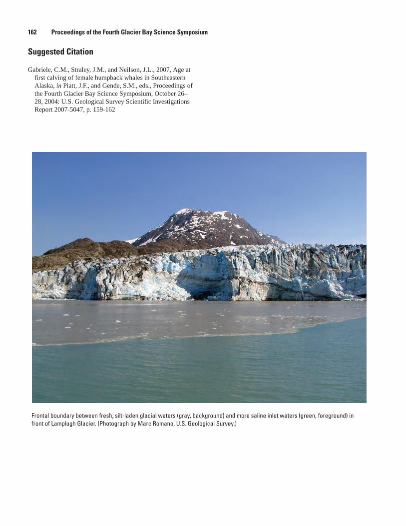
1�2 Proceedings of the Fourth Glacier Bay Science Symposium
Frontal boundary between fresh, silt-laden glacial waters (gray, background) and more saline inlet waters (green, foreground) in front of Lamplugh Glacier. (Photograph by Marc Romano, U.S. Geological Survey.)
Suggested Citation
Gabriele, C.M., Straley, J.M., and Neilson, J.L., 2007, Age at first calving of female humpback whales in Southeastern Alaska, in Piatt, J.F., and Gende, S.M., eds., Proceedings of the Fourth Glacier Bay Science Symposium, October 26–28, 2004: U.S. Geological Survey Scientific Investigations Report 2007-5047, p. 159-162
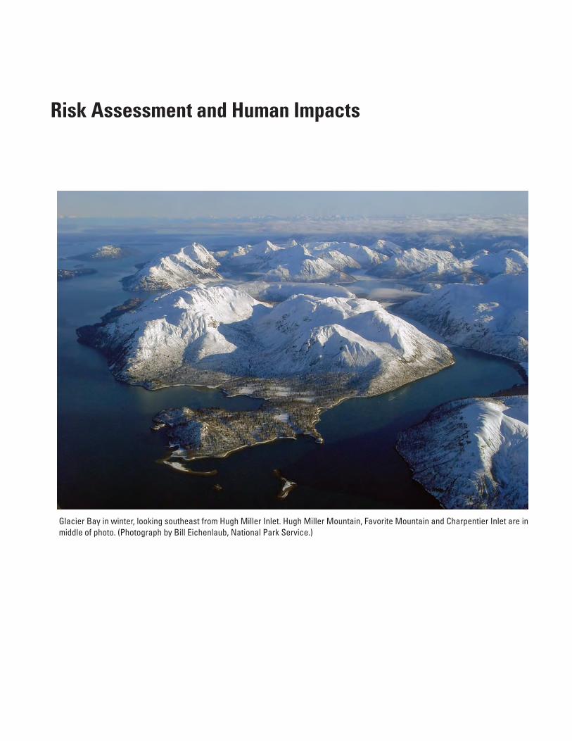
Risk Assessment and Human Impacts
Glacier Bay in winter, looking southeast from Hugh Miller Inlet. Hugh Miller Mountain, Favorite Mountain and Charpentier Inlet are in middle of photo. (Photograph by Bill Eichenlaub, National Park Service.)

This page is intentionally left blank.
1�� Proceedings of the Fourth Glacier Bay Science Symposium, 200�

Landslide-Induced Wave Hazard Assessment—Tidal Inlet, Glacier Bay National Park, Alaska
Gerald F. Wieczorek1,5, Eric L. Geist1, Matthias Jakob2, Sandy L. Zirnheld3, Ellie Boyce3, Roman J. Motyka3, and Patricia Burns4
Abstract. An unstable landslide perched above the northern shore of Tidal Inlet has the potential from seismic or climatic trigger of rapidly moving into Tidal Inlet and generating large, long period impulse waves. Numerical simulations of landslide-generated waves indicate that near the mouth of Tidal Inlet, wave amplitude would be greatest within approximately 40 minutes of the slide entering water. Significant wave activity would continue in the western arm of Glacier Bay for more than several hours, while wave amplitudes would decrease in deeper waters. Severity of impact to vessels in the region depends on the size and speed of the slide and on which part of the wave ships would encounter.
Figure 1. Detached landslide perched above the northern shore of Tidal Inlet, Glacier Bay National Park, Alaska. Photograph taken July 12, 2002.
1 U.S. Geological Survey, Menlo Park, CA 94025
2 BGC Engineering Inc., Vancouver, British Columbia, Canada
3 Geophysical Institute, University of Alaska, Fairbanks, Alaska
4 Alaska Division of Geological & Geophysical Surveys, Fairbanks, Alaska
5 Corresponding author: [email protected], 650-329-5251
Introduction
Glacier Bay National Park is located in a region of high seismicity, which has had four large magnitude (M>7.0) earthquakes during the 20th century (Brew and others, 1995). The 1958 earthquake on the Fairweather fault triggered a 30 million m3 rockslide which generated a 30-m high wave through Lituya Bay sinking two of three fishing boats and killing two persons (Miller, 1960). A large detached rock mass above the northern shore of Tidal Inlet (fig. 1) poses a threat similar to the landslide that occurred at Lituya Bay.
Deglaciation of Tidal Inlet probably proceeded simultaneously with the calving retreat that rapidly depleted ice in both arms of Glacier Bay during the 19th century. Maps by Reid (1896) show that Tidal Inlet was devoid of ice by AD 1890 except for a small remnant glacier at its headwaters. The retreat of glacial ice decreased lateral support for the hillside. Although it is not known exactly when the landslide on the northern shore of Tidal Inlet first moved, the major slide event is evident on photos taken between 1892 and 1919. The general lack of revegetation of landslide features supports minor recent movement of the landslide mass. The objectives of this study are to determine if landslide movement is presently occurring and to estimate wave height and runup from potential landslide impact into Tidal Inlet.
Methods
The main scarp has a fairly uniform range of height, 20-40 m, suggesting that the body of the landslide detached rigidly. Within the main body of the landslide the surface topography is severely disrupted by rotational blocks with
prominent back-facing scarps. In the upper portion of the main body the exposed portions of these blocks are within glacial till, but further downslope bedrock can be seen within the blocks. The thickness of the landslide was estimated to determine the total volume of material that could enter Tidal Inlet. The stability of the landslide was evaluated by examining the features and by measuring movement of established reference points using GPS. However, on the right (west) flank of the landslide, two closely spaced sets of parallel open fissures were found in surficial soils extending downhill from the termination of the main scarp, and pointing downslope towards the toe of the landslide. These fissures appeared relatively fresh within generally weak soils and would not be preserved for more than a year.
Topographic monuments were installed on the Tidal Inlet landslide to assess movement rates. GPS data were collected for durations of at least one hour and collection intervals
Gerald F. Wieczorek and others 1�5
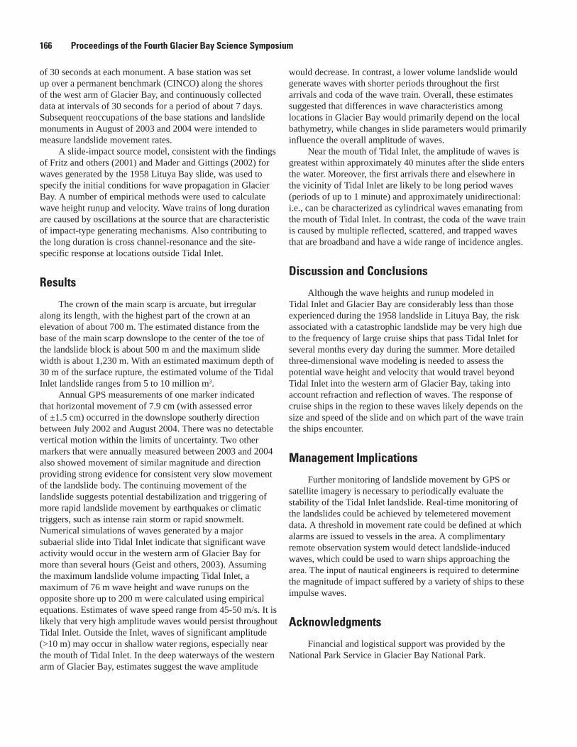
of 30 seconds at each monument. A base station was set up over a permanent benchmark (CINCO) along the shores of the west arm of Glacier Bay, and continuously collected data at intervals of 30 seconds for a period of about 7 days. Subsequent reoccupations of the base stations and landslide monuments in August of 2003 and 2004 were intended to measure landslide movement rates.
A slide-impact source model, consistent with the findings of Fritz and others (2001) and Mader and Gittings (2002) for waves generated by the 1958 Lituya Bay slide, was used to specify the initial conditions for wave propagation in Glacier Bay. A number of empirical methods were used to calculate wave height runup and velocity. Wave trains of long duration are caused by oscillations at the source that are characteristic of impact-type generating mechanisms. Also contributing to the long duration is cross channel-resonance and the site-specific response at locations outside Tidal Inlet.
Results
The crown of the main scarp is arcuate, but irregular along its length, with the highest part of the crown at an elevation of about 700 m. The estimated distance from the base of the main scarp downslope to the center of the toe of the landslide block is about 500 m and the maximum slide width is about 1,230 m. With an estimated maximum depth of 30 m of the surface rupture, the estimated volume of the Tidal Inlet landslide ranges from 5 to 10 million m3.
Annual GPS measurements of one marker indicated that horizontal movement of 7.9 cm (with assessed error of ±1.5 cm) occurred in the downslope southerly direction between July 2002 and August 2004. There was no detectable vertical motion within the limits of uncertainty. Two other markers that were annually measured between 2003 and 2004 also showed movement of similar magnitude and direction providing strong evidence for consistent very slow movement of the landslide body. The continuing movement of the landslide suggests potential destabilization and triggering of more rapid landslide movement by earthquakes or climatic triggers, such as intense rain storm or rapid snowmelt. Numerical simulations of waves generated by a major subaerial slide into Tidal Inlet indicate that significant wave activity would occur in the western arm of Glacier Bay for more than several hours (Geist and others, 2003). Assuming the maximum landslide volume impacting Tidal Inlet, a maximum of 76 m wave height and wave runups on the opposite shore up to 200 m were calculated using empirical equations. Estimates of wave speed range from 45-50 m/s. It is likely that very high amplitude waves would persist throughout Tidal Inlet. Outside the Inlet, waves of significant amplitude (>10 m) may occur in shallow water regions, especially near the mouth of Tidal Inlet. In the deep waterways of the western arm of Glacier Bay, estimates suggest the wave amplitude
would decrease. In contrast, a lower volume landslide would generate waves with shorter periods throughout the first arrivals and coda of the wave train. Overall, these estimates suggested that differences in wave characteristics among locations in Glacier Bay would primarily depend on the local bathymetry, while changes in slide parameters would primarily influence the overall amplitude of waves.
Near the mouth of Tidal Inlet, the amplitude of waves is greatest within approximately 40 minutes after the slide enters the water. Moreover, the first arrivals there and elsewhere in the vicinity of Tidal Inlet are likely to be long period waves (periods of up to 1 minute) and approximately unidirectional: i.e., can be characterized as cylindrical waves emanating from the mouth of Tidal Inlet. In contrast, the coda of the wave train is caused by multiple reflected, scattered, and trapped waves that are broadband and have a wide range of incidence angles.
Discussion and Conclusions
Although the wave heights and runup modeled in Tidal Inlet and Glacier Bay are considerably less than those experienced during the 1958 landslide in Lituya Bay, the risk associated with a catastrophic landslide may be very high due to the frequency of large cruise ships that pass Tidal Inlet for several months every day during the summer. More detailed three-dimensional wave modeling is needed to assess the potential wave height and velocity that would travel beyond Tidal Inlet into the western arm of Glacier Bay, taking into account refraction and reflection of waves. The response of cruise ships in the region to these waves likely depends on the size and speed of the slide and on which part of the wave train the ships encounter.
Management Implications
Further monitoring of landslide movement by GPS or satellite imagery is necessary to periodically evaluate the stability of the Tidal Inlet landslide. Real-time monitoring of the landslides could be achieved by telemetered movement data. A threshold in movement rate could be defined at which alarms are issued to vessels in the area. A complimentary remote observation system would detect landslide-induced waves, which could be used to warn ships approaching the area. The input of nautical engineers is required to determine the magnitude of impact suffered by a variety of ships to these impulse waves.
Acknowledgments
Financial and logistical support was provided by the National Park Service in Glacier Bay National Park.
1�� Proceedings of the Fourth Glacier Bay Science Symposium
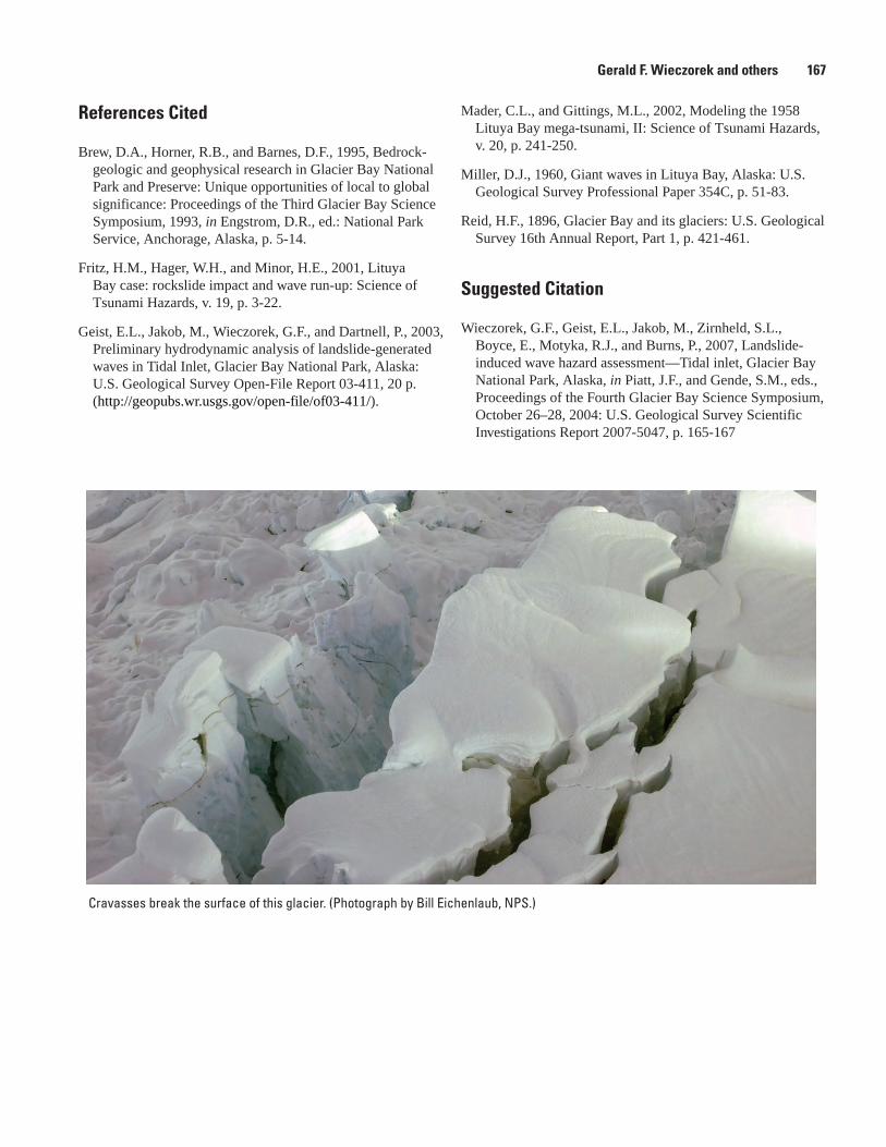
Cravasses break the surface of this glacier. (Photograph by Bill Eichenlaub, NPS.)
References Cited
Brew, D.A., Horner, R.B., and Barnes, D.F., 1995, Bedrock-geologic and geophysical research in Glacier Bay National Park and Preserve: Unique opportunities of local to global significance: Proceedings of the Third Glacier Bay Science Symposium, 1993, in Engstrom, D.R., ed.: National Park Service, Anchorage, Alaska, p. 5-14.
Fritz, H.M., Hager, W.H., and Minor, H.E., 2001, Lituya Bay case: rockslide impact and wave run-up: Science of Tsunami Hazards, v. 19, p. 3-22.
Geist, E.L., Jakob, M., Wieczorek, G.F., and Dartnell, P., 2003, Preliminary hydrodynamic analysis of landslide-generated waves in Tidal Inlet, Glacier Bay National Park, Alaska: U.S. Geological Survey Open-File Report 03-411, 20 p. (http://geopubs.wr.usgs.gov/open-file/of03-411/).
Gerald F. Wieczorek and others 1�7
Mader, C.L., and Gittings, M.L., 2002, Modeling the 1958 Lituya Bay mega-tsunami, II: Science of Tsunami Hazards, v. 20, p. 241-250.
Miller, D.J., 1960, Giant waves in Lituya Bay, Alaska: U.S. Geological Survey Professional Paper 354C, p. 51-83.
Reid, H.F., 1896, Glacier Bay and its glaciers: U.S. Geological Survey 16th Annual Report, Part 1, p. 421-461.
Suggested Citation
Wieczorek, G.F., Geist, E.L., Jakob, M., Zirnheld, S.L., Boyce, E., Motyka, R.J., and Burns, P., 2007, Landslide-induced wave hazard assessment—Tidal inlet, Glacier Bay National Park, Alaska, in Piatt, J.F., and Gende, S.M., eds., Proceedings of the Fourth Glacier Bay Science Symposium, October 26–28, 2004: U.S. Geological Survey Scientific Investigations Report 2007-5047, p. 165-167
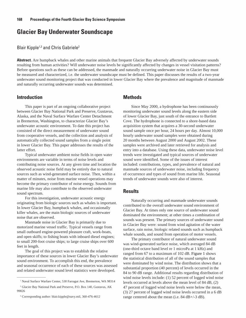
Glacier Bay Underwater Soundscape
Blair Kipple1,3 and Chris Gabriele2
Abstract. Are humpback whales and other marine animals that frequent Glacier Bay adversely affected by underwater sounds resulting from human activities? Will underwater noise levels be significantly affected by changes in vessel visitation patterns? Before questions such as these can be addressed, the manmade and naturally occurring underwater noise in Glacier Bay must be measured and characterized, i.e. the underwater soundscape must be defined. This paper discusses the results of a two-year underwater sound monitoring project that was conducted in lower Glacier Bay where the prevalence and magnitude of manmade and naturally occurring underwater sounds was determined.
Introduction
This paper is part of an ongoing collaborative project between Glacier Bay National Park and Preserve, Gustavus, Alaska, and the Naval Surface Warfare Center Detachment in Bremerton, Washington, to characterize Glacier Bay’s underwater acoustic environment. To date this project has consisted of the direct measurement of underwater sound from cooperative vessels, and the collection and analysis of automatically collected sound samples from a single point in lower Glacier Bay. This paper addresses the results of the latter effort.
Typical underwater ambient noise fields in open water environments are variable in terms of noise levels and contributing noise sources. At any given time and location the observed acoustic noise field may be entirely due to natural sources such as wind-generated surface noise. Then, within a matter of minutes, noise from marine vessel operations may become the primary contributor of noise energy. Sounds from marine life may also contribute to the observed underwater sound spectrum.
For this investigation, underwater acoustic energy originating from biologic sources such as whales is important. In lower Glacier Bay, humpback whales, and occasionally killer whales, are the main biologic sources of underwater noise that are observed.
Manmade noise in Glacier Bay is primarily due to motorized marine vessel traffic. Typical vessels range from small outboard engine-powered pleasure craft, work-boats, and open skiffs; to fishing boats with inboard diesel engines; to small 200-foot cruise ships; to large cruise ships over 600 feet in length.
The goal of this project was to establish the relative importance of these sources in lower Glacier Bay’s underwater sound environment. To accomplish this end, the prevalence and seasonal occurrence of each of these sources was assessed and related underwater sound level statistics were developed.
Methods
Since May 2000, a hydrophone has been continuously monitoring underwater sound levels along the eastern side of lower Glacier Bay, just south of the entrance to Bartlett Cove. The hydrophone is connected to a shore-based data acquisition system that acquires a 30-second underwater sound sample once per hour, 24 hours per day. Almost 10,000 hourly underwater sound samples were obtained during 20 months between August 2000 and August 2002. These samples were archived and later retrieved for analysis and entry into a database. Using these data, underwater noise level trends were investigated and typical sources of underwater sound were identified. Some of the issues of interest included: contributions, types, and prevalence of natural and manmade sources of underwater noise, including frequency of occurrence and types of sound from marine life. Seasonal trends of underwater sounds were also of interest.
Results
Naturally occurring and manmade underwater sounds contributed to the overall underwater sound environment of Glacier Bay. At times only one source of underwater sound dominated the environment; at other times a combination of sounds was present. The primary sources of underwater sound in Glacier Bay were: sound from wind agitation of the water surface, rain noise, biologic related sounds such as humpback whale sounds, and sound from operation of motor vessels.
The primary contributor of natural underwater sound was wind-generated surface noise, which averaged 84 dB (one-third octave band level re 1 microPa at 1 kHz) and ranged from 67 to a maximum of 102 dB. Figure 1 shows the statistical distribution of all of the sound samples that were dominated by wind noise. The distribution shows that a substantial proportion (40 percent) of levels occurred in the 84 to 90 dB range. Additional results regarding distribution of wind noise levels include: (1) 52 percent of logged wind noise levels occurred at levels above the mean level of 84 dB, (2) 47 percent of logged wind noise levels were below the mean, (3) 27 percent of logged wind noise levels occurred in a 6 dB range centered about the mean (i.e. 84 dB+/-3 dB).
1 Naval Surface Warfare Center, 530 Farragut Ave, Bremerton, WA 98314
2 Glacier Bay National Park and Preserve, P.O. Box 140, Gustavus, AK 99826
3 Corresponding author: [email protected], 360-476-4612
1�� Proceedings of the Fourth Glacier Bay Science Symposium

Figure 1. Distribution of underwater sound levels—wind vs. vessels.
Figure 2. Samples per day containing biologic sounds.
0
100
200
300
400
500
600
700
68 72 76 80 84 88 92 96 100
104
108
112
116
120
124
128
dB re 1 microPa (Wind - 1kHz OTO band level) (Vessel - peak OTO band level)
Wind
Vessels
Vessel average = 94
Wind average = 84
Num
ber o
f Occ
uren
ces
0
1
2
3
4
5
6Au
g-00
Sep
-00
Oct
-00
Nov
-00
Dec
-00
Jan-
01
Feb-
01
Mar
-01
Apr-0
1
May
-01
Jun-
01
Jul-0
1
Aug-
01
Sep
-01
Oct
-01
Nov
-01
Dec
-01
Jan-
02
Feb-
02
Mar
-02
Apr-0
2
May
-02
Jun-
02
Jul-0
2
Aug-
02
Other bios (not humpback)Humpback - otherHumpback - song
NO
DAT
A-S
YS
TEM
NO
TO
PE
RAT
ION
AL
NO
TC
OV
ER
ED
NO
TC
OV
ER
ED
NO
TC
OV
ER
ED
NO
TC
OV
ER
ED
ON
LY8
DAY
SO
FAC
OU
STI
CC
OV
ER
AGE
Num
ber o
f Sam
ples
per
“Day
”
Noise due to rainfall was present in an average of 2.1 out of 24 samples per day and was not especially prevalent in winter versus other seasons. Rain noise levels at 16 kHz averaged 91 dB and ranged as high as 110 dB.
Humpback whales were the most common source of biologic sounds. These sounds included various grunts, whoops, and squeaks as well as songs. Killer whale sounds were also observed in a number of samples. Humpback whale sounds were present in more than three times the number of samples as killer whale and other biologic sounds. As shown in figure 2, humpback whale sounds were most common August through November, and 61 percent of all humpback songs were observed in October 2000.
The occurrence of humpback whale sounds correlated well with humpback whale survey data collected by NPS, especially August to September 2000. Months where humpback whale sounds were frequently logged corresponded to periods where NPS personnel observed whales in lower Glacier Bay and also when the 10-knot whale waters speed limit was in effect. Also, particularly in 2000, whale sounds were frequently observed in October and November, after the NPS whale-surveying season concluded.
By far the most prevalent source of identifiable manmade noise in this study was related to operation of motorized marine vessels. The statistical distribution of peak vessel noise levels in figure 1 shows that the average level was 94 dB, 10 dB greater than the average wind noise level. The highest vessel level recorded was 129 dB, but only about 5 percent of the peak vessel noise levels exceeded 110 dB at the hydrophone.
As expected, vessel noise was most common during summer. Figure 3 shows that in summer, about 40 percent of the noise samples were free of vessel noise; however, in winter, October through April, roughly 90 percent contained no vessel noise. In May and September, approximately 60 percent of the samples were free of vessel noise. On average, over the entire survey period, 7.7 out of 24 samples per day contained vessel noise. The rate of vessel noise presence ranged from a low of 1.7 samples per day (out of 24 samples per day) in December 2000 to a high of 16.5 in August 2000.
Vessel sounds were categorized by vessel size: small, up to 50 feet in length; medium, 50 to 200 feet; and large, over 200 feet. Figure 4 shows that medium sized vessels were the most prevalent vessel type, which was true for all times of year. They constituted 68 percent of all vessel types observed. At most, large ships were observed in four samples per day. Noise from small craft was most common from May to August.
On average, large vessels were slightly louder at the hydrophone than medium and small craft. Large vessels averaged 99 dB, while the average noise levels for medium and small vessel were 92 and 97 dB, respectively. The maximum large vessel level was 129 dB. The maximum level for both medium and small vessels was 126 dB.
Vessel noise levels were lower during periods when a 10-knot speed limit was in effect, especially for large and small vessels. In August 2000 and August 2002, average noise levels for large and small vessels were 2 to 4 dB lower during the 10-knot period compared to the 20-knot period. The average 10 and 20-knot medium vessel noise levels were comparable. Maximum vessel levels for a given vessel category were as much as 9 dB lower when the 10-knot speed limit was in effect.
Blair Kipple and Chris Gabriele 1�9
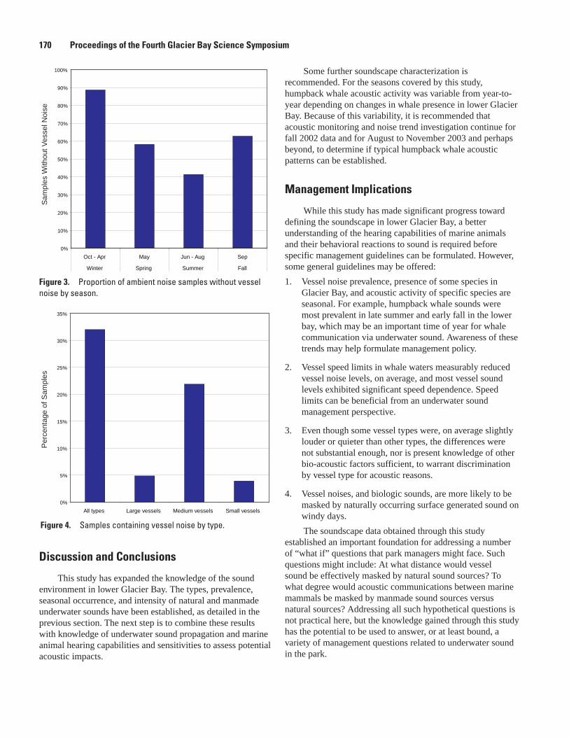
Figure �. Proportion of ambient noise samples without vessel noise by season.
Figure �. Samples containing vessel noise by type.
0%
10%
20%
30%
40%
50%
60%
70%
80%
90%
100%
Oct - Apr May Jun - Aug Sep
Winter Spring Summer Fall
Sam
ples
With
out V
esse
l Noi
se
0%
5%
10%
15%
20%
25%
30%
35%
All types Large vessels Medium vessels Small vessels
Per
cent
age
of S
ampl
es
Discussion and Conclusions
This study has expanded the knowledge of the sound environment in lower Glacier Bay. The types, prevalence, seasonal occurrence, and intensity of natural and manmade underwater sounds have been established, as detailed in the previous section. The next step is to combine these results with knowledge of underwater sound propagation and marine animal hearing capabilities and sensitivities to assess potential acoustic impacts.
Some further soundscape characterization is recommended. For the seasons covered by this study, humpback whale acoustic activity was variable from year-to-year depending on changes in whale presence in lower Glacier Bay. Because of this variability, it is recommended that acoustic monitoring and noise trend investigation continue for fall 2002 data and for August to November 2003 and perhaps beyond, to determine if typical humpback whale acoustic patterns can be established.
Management Implications
While this study has made significant progress toward defining the soundscape in lower Glacier Bay, a better understanding of the hearing capabilities of marine animals and their behavioral reactions to sound is required before specific management guidelines can be formulated. However, some general guidelines may be offered:
Vessel noise prevalence, presence of some species in Glacier Bay, and acoustic activity of specific species are seasonal. For example, humpback whale sounds were most prevalent in late summer and early fall in the lower bay, which may be an important time of year for whale communication via underwater sound. Awareness of these trends may help formulate management policy.
Vessel speed limits in whale waters measurably reduced vessel noise levels, on average, and most vessel sound levels exhibited significant speed dependence. Speed limits can be beneficial from an underwater sound management perspective.
Even though some vessel types were, on average slightly louder or quieter than other types, the differences were not substantial enough, nor is present knowledge of other bio-acoustic factors sufficient, to warrant discrimination by vessel type for acoustic reasons.
Vessel noises, and biologic sounds, are more likely to be masked by naturally occurring surface generated sound on windy days.
The soundscape data obtained through this study established an important foundation for addressing a number of “what if” questions that park managers might face. Such questions might include: At what distance would vessel sound be effectively masked by natural sound sources? To what degree would acoustic communications between marine mammals be masked by manmade sound sources versus natural sources? Addressing all such hypothetical questions is not practical here, but the knowledge gained through this study has the potential to be used to answer, or at least bound, a variety of management questions related to underwater sound in the park.
1.
2.
3.
4.
170 Proceedings of the Fourth Glacier Bay Science Symposium
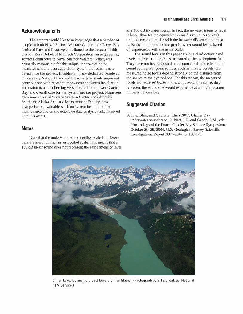
Crillon Lake, looking northeast toward Crillon Glacier. (Photograph by Bill Eichenlaub, National Park Service.)
Acknowledgments
The authors would like to acknowledge that a number of people at both Naval Surface Warfare Center and Glacier Bay National Park and Preserve contributed to the success of this project. Russ Dukek of Mantech Corporation, an engineering services contractor to Naval Surface Warfare Center, was primarily responsible for the unique underwater noise measurement and data acquisition system that continues to be used for the project. In addition, many dedicated people at Glacier Bay National Park and Preserve have made important contributions with regard to measurement system installation and maintenance, collecting vessel scan data in lower Glacier Bay, and overall care for the system and the project. Numerous personnel at Naval Surface Warfare Center, including the Southeast Alaska Acoustic Measurement Facility, have also performed valuable work on system installation and maintenance and on the extensive data analysis tasks involved with this effort.
Notes
Note that the underwater sound decibel scale is different than the more familiar in-air decibel scale. This means that a 100 dB in-air sound does not represent the same intensity level
as a 100 dB in-water sound. In fact, the in-water intensity level is lower than for the equivalent in-air dB value. As a result, until becoming familiar with the in-water dB scale, one must resist the temptation to interpret in-water sound levels based on experiences with the in-air scale.
The sound levels in this paper are one-third octave band levels in dB re 1 microPa as measured at the hydrophone face. They have not been adjusted to account for distance from the sound source. For point sources such as marine vessels, the measured noise levels depend strongly on the distance from the source to the hydrophone. For this reason, the measured levels are received levels, not source levels. In a sense, they represent the sound one would experience at a single location in lower Glacier Bay.
Suggested Citation
Kipple, Blair, and Gabriele. Chris 2007, Glacier Bay underwater soundscape, in Piatt, J.F., and Gende, S.M., eds., Proceedings of the Fourth Glacier Bay Science Symposium, October 26–28, 2004: U.S. Geological Survey Scientific Investigations Report 2007-5047, p. 168-171.
Blair Kipple and Chris Gabriele 171
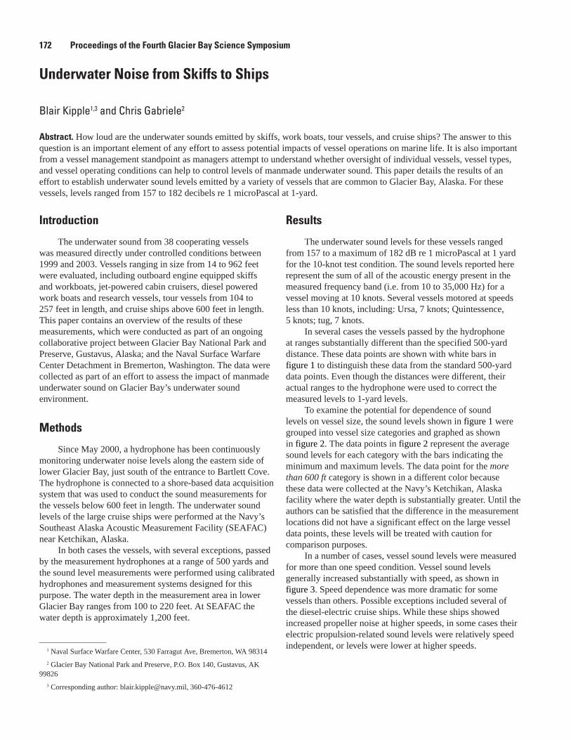
Underwater Noise from Skiffs to Ships
Blair Kipple1,3 and Chris Gabriele2
Abstract. How loud are the underwater sounds emitted by skiffs, work boats, tour vessels, and cruise ships? The answer to this question is an important element of any effort to assess potential impacts of vessel operations on marine life. It is also important from a vessel management standpoint as managers attempt to understand whether oversight of individual vessels, vessel types, and vessel operating conditions can help to control levels of manmade underwater sound. This paper details the results of an effort to establish underwater sound levels emitted by a variety of vessels that are common to Glacier Bay, Alaska. For these vessels, levels ranged from 157 to 182 decibels re 1 microPascal at 1-yard.
Introduction
The underwater sound from 38 cooperating vessels was measured directly under controlled conditions between 1999 and 2003. Vessels ranging in size from 14 to 962 feet were evaluated, including outboard engine equipped skiffs and workboats, jet-powered cabin cruisers, diesel powered work boats and research vessels, tour vessels from 104 to 257 feet in length, and cruise ships above 600 feet in length. This paper contains an overview of the results of these measurements, which were conducted as part of an ongoing collaborative project between Glacier Bay National Park and Preserve, Gustavus, Alaska; and the Naval Surface Warfare Center Detachment in Bremerton, Washington. The data were collected as part of an effort to assess the impact of manmade underwater sound on Glacier Bay’s underwater sound environment.
Methods
Since May 2000, a hydrophone has been continuously monitoring underwater noise levels along the eastern side of lower Glacier Bay, just south of the entrance to Bartlett Cove. The hydrophone is connected to a shore-based data acquisition system that was used to conduct the sound measurements for the vessels below 600 feet in length. The underwater sound levels of the large cruise ships were performed at the Navy’s Southeast Alaska Acoustic Measurement Facility (SEAFAC) near Ketchikan, Alaska.
In both cases the vessels, with several exceptions, passed by the measurement hydrophones at a range of 500 yards and the sound level measurements were performed using calibrated hydrophones and measurement systems designed for this purpose. The water depth in the measurement area in lower Glacier Bay ranges from 100 to 220 feet. At SEAFAC the water depth is approximately 1,200 feet.
1 Naval Surface Warfare Center, 530 Farragut Ave, Bremerton, WA 98314
2 Glacier Bay National Park and Preserve, P.O. Box 140, Gustavus, AK 99826
3 Corresponding author: [email protected], 360-476-4612
Results
The underwater sound levels for these vessels ranged from 157 to a maximum of 182 dB re 1 microPascal at 1 yard for the 10-knot test condition. The sound levels reported here represent the sum of all of the acoustic energy present in the measured frequency band (i.e. from 10 to 35,000 Hz) for a vessel moving at 10 knots. Several vessels motored at speeds less than 10 knots, including: Ursa, 7 knots; Quintessence, 5 knots; tug, 7 knots.
In several cases the vessels passed by the hydrophone at ranges substantially different than the specified 500-yard distance. These data points are shown with white bars in figure 1 to distinguish these data from the standard 500-yard data points. Even though the distances were different, their actual ranges to the hydrophone were used to correct the measured levels to 1-yard levels.
To examine the potential for dependence of sound levels on vessel size, the sound levels shown in figure 1 were grouped into vessel size categories and graphed as shown in figure 2. The data points in figure 2 represent the average sound levels for each category with the bars indicating the minimum and maximum levels. The data point for the more than 600 ft category is shown in a different color because these data were collected at the Navy’s Ketchikan, Alaska facility where the water depth is substantially greater. Until the authors can be satisfied that the difference in the measurement locations did not have a significant effect on the large vessel data points, these levels will be treated with caution for comparison purposes.
In a number of cases, vessel sound levels were measured for more than one speed condition. Vessel sound levels generally increased substantially with speed, as shown in figure 3. Speed dependence was more dramatic for some vessels than others. Possible exceptions included several of the diesel-electric cruise ships. While these ships showed increased propeller noise at higher speeds, in some cases their electric propulsion-related sound levels were relatively speed independent, or levels were lower at higher speeds.
172 Proceedings of the Fourth Glacier Bay Science Symposium

Figure 2. Range of 10-knot sound levels by vessel category.
Figure 1. 10-knot sound level by vessel.
120
130
140
150
160
170
180
190
Urs
a
Gum
boot
Litu
ya
Snip
e
Ogi
ve
Ala
ria
Mus
sel
Sand
Lanc
e
Reb
ound
Are
teA
Cap
elin
Sigm
aT
Are
te
Qui
ntes
senc
e
Talu
s
Sera
c
Taz
Tug/
Bar
ge
Gyr
e
Ala
skan
Gra
ndeu
r
Nun
atak
Stel
ler
Kee
t
Wild
erne
ssEx
plor
er
Spiri
tofA
lask
a
Seab
ird
Sea
Lion
Wild
erne
ssA
dven
ture
r
Wild
erne
ssD
isco
vere
r
York
tow
n
Uni
vers
eEx
plor
er
Stat
enda
m
Nor
weg
ian
Win
d
Vole
ndam
Cry
stal
Har
mon
y
Nor
weg
ian
Sky
Daw
nPr
ince
ss
Cor
alPr
ince
ss
Sou
ndLe
veld
Bre
1m
icro
Pa
at1
yd
20 ft 40 ft100 ft
250 ft
Smaller Larger14 962
140
150
160
170
180
190
Up to 20 ft 20 to 40 ft 40 to 100 ft 100 to 250 ft More than 600 ft
Sou
nd L
evel
- dB
re 1
mic
roP
a at
1 y
ard
Vessel propulsion type and horsepower can also be important factors in the intensity of underwater sound emitted by powered vessels. Figure 4 shows that, for small vessels, underwater sound from propeller-powered craft were generally greater for higher horsepower vessels. It also shows that, for their power rating, the two jet powered vessels were noticeably quieter than their comparably powered propeller-driven counterparts.
Discussion and Conclusions
Under controlled measurement conditions, the 10-knot underwater sound levels ranged from a minimum of 157 to a maximum of 182 dB for the 38 vessels that were evaluated. Sound levels showed an increasing trend with increasing vessel size, with the large cruise ship category as one possible exception—although the authors are treating this data point with caution, as cited above. Most vessel noise levels increased with increasing speed. Also, vessel sound levels showed dependence on propulsion type and horsepower.
Note that the underwater sound decibel scale is different than the more familiar in-air decibel scale. This means that a 100 dB in-air sound does not represent the same intensity level as a 100 dB in-water sound. The in-water intensity level is in fact lower than for the equivalent in-air dB value. As a result,
until becoming familiar with the in-water dB scale, one must resist the temptation to interpret in-water sound levels based on experiences with the in-air scale.
Also, the sound levels reported here are given as 1-yard source levels, which means that the levels have been projected from the distance at which they were measured to the levels that one would measure at 1 yard from the vessel, if it were possible to do so. As a result, the levels that would be expected at reasonable distances from these vessels would be substantially lower than those listed here. For example, at 100 yards they would be expected to be about 40 dB lower than the 1-yard level, and about 53 dB lower at one-quarter mile.
Blair Kipple and Chris Gabriele 17�
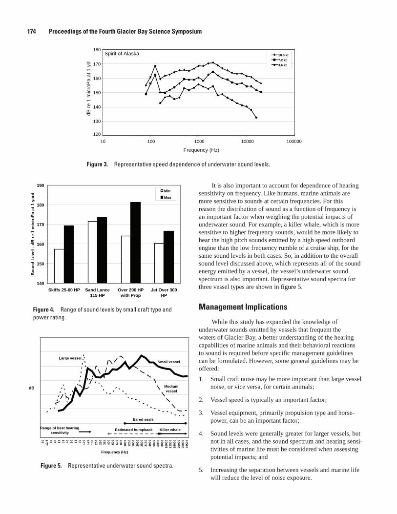
Figure 5. Representative underwater sound spectra.
60
70
80
90
100
110
120
130
1012
.5 16 20 25 31 40 50 63 80 100
125
160
200
250
315
400
500
630
800
1000
1250
1600
2000
2500
3150
4000
5000
6300
8000
1000
012
500
1600
020
000
2500
031
500
Frequency (Hz)
dB
Small vessel
Mediumvessel
Large vessel
Estimated humpback Killer whaleRange of best hearingsensitivity
Eared seals
Figure �. Range of sound levels by small craft type and power rating.
140
150
160
170
180
190
Skiffs 25-60 HP Sand Lance115 HP
Over 200 HPwith Prop
Jet Over 300HP
Soun
dLe
vel-
dBre
1m
icro
Paat
1ya
rd
Min
Max
It is also important to account for dependence of hearing sensitivity on frequency. Like humans, marine animals are more sensitive to sounds at certain frequencies. For this reason the distribution of sound as a function of frequency is an important factor when weighing the potential impacts of underwater sound. For example, a killer whale, which is more sensitive to higher frequency sounds, would be more likely to hear the high pitch sounds emitted by a high speed outboard engine than the low frequency rumble of a cruise ship, for the same sound levels in both cases. So, in addition to the overall sound level discussed above, which represents all of the sound energy emitted by a vessel, the vessel’s underwater sound spectrum is also important. Representative sound spectra for three vessel types are shown in figure 5.
Management Implications
While this study has expanded the knowledge of underwater sounds emitted by vessels that frequent the waters of Glacier Bay, a better understanding of the hearing capabilities of marine animals and their behavioral reactions to sound is required before specific management guidelines can be formulated. However, some general guidelines may be offered:
Small craft noise may be more important than large vessel noise, or vice versa, for certain animals;
Vessel speed is typically an important factor;
Vessel equipment, primarily propulsion type and horse-power, can be an important factor;
Sound levels were generally greater for larger vessels, but not in all cases, and the sound spectrum and hearing sensi-tivities of marine life must be considered when assessing potential impacts; and
Increasing the separation between vessels and marine life will reduce the level of noise exposure.
1.
2.
3.
4.
5.
Figure �. Representative speed dependence of underwater sound levels.
120
130
140
150
160
170
180
10 100 1000 10000 100000
10.5 kt7.2 kt3.6 kt
Spirit of Alaska
dB re
1 m
icro
Pa
at 1
yd
Frequency (Hz)
17� Proceedings of the Fourth Glacier Bay Science Symposium

Acknowledgments
The authors would like to acknowledge the cooperation and contributions to this project from several sources, including Glacier Bay National Park and Preserve personnel, vessel operators, vessel concessionaires, and the cruise ship companies.
Selected References
Kipple, B.M. and Gabriele, C.M., 2004, Glacier Bay Watercraft Noise–Noise Characterization for Tour, Charter, Private, and Government Vessels, Naval Surface Warfare Center Technical Report NSWCCD-71-TR-2004/545.
Kipple, B.M. and Gabriele, C.M., 2003, Glacier Bay Watercraft Noise, Naval Surface Warfare Center Technical Report NSWCCD-71-TR-2003/522.
Kipple, B.M., 2002, Southeast Alaska Cruise Ship Underwater Acoustic Noise, Naval Surface Warfare Center Technical Report NSWCCD-71-TR-2002/574.
Suggested Citation
Kipple, B.M., and Gabriele, C.M., 2007, Underwater noise from skiffs to ships, in Piatt, J.F., and Gende, S.M., eds., Proceedings of the Fourth Glacier Bay Science Symposium, October 26–28, 2004: U.S. Geological Survey Scientific Investigations Report 2007-5047, p. 172-175.
Blair Kipple and Chris Gabriele 175
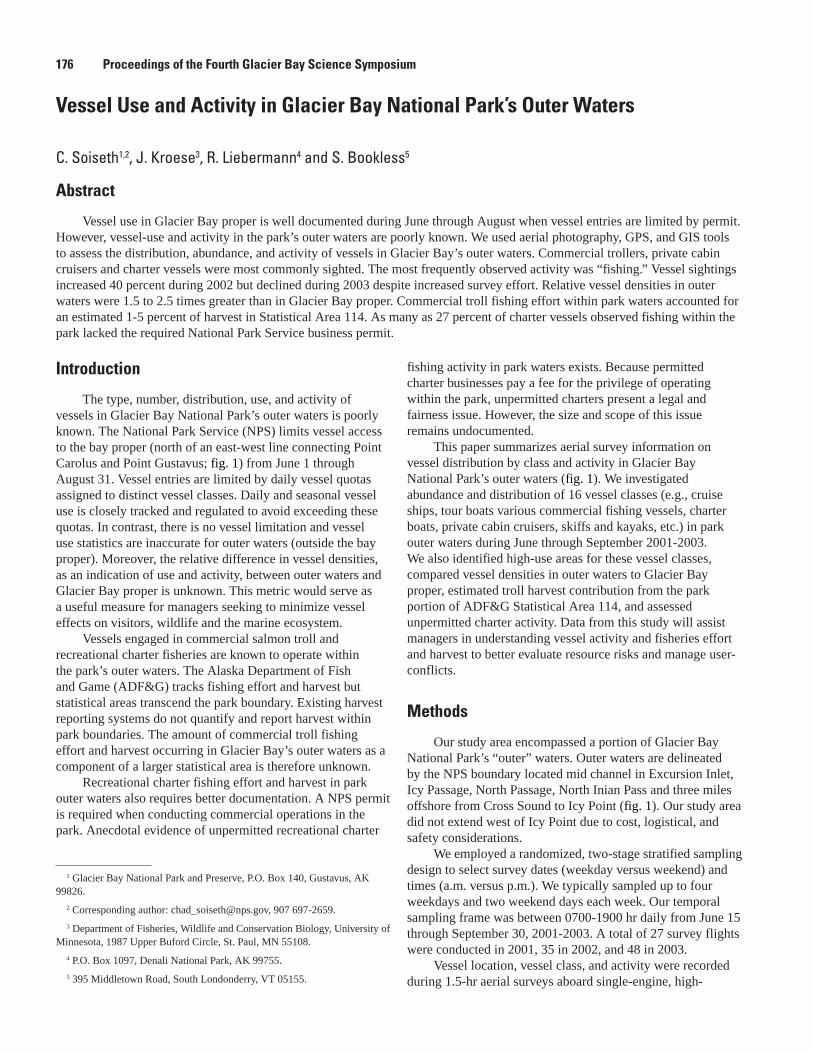
Vessel Use and Activity in Glacier Bay National Park’s Outer Waters
C. Soiseth1,2, J. Kroese3, R. Liebermann4 and S. Bookless5
1 Glacier Bay National Park and Preserve, P.O. Box 140, Gustavus, AK 99826.
2 Corresponding author: [email protected], 907 697-2659.
3 Department of Fisheries, Wildlife and Conservation Biology, University of Minnesota, 1987 Upper Buford Circle, St. Paul, MN 55108.
4 P.O. Box 1097, Denali National Park, AK 99755.
5 395 Middletown Road, South Londonderry, VT 05155.
17� Proceedings of the Fourth Glacier Bay Science Symposium
Abstract
Vessel use in Glacier Bay proper is well documented during June through August when vessel entries are limited by permit. However, vessel-use and activity in the park’s outer waters are poorly known. We used aerial photography, GPS, and GIS tools to assess the distribution, abundance, and activity of vessels in Glacier Bay’s outer waters. Commercial trollers, private cabin cruisers and charter vessels were most commonly sighted. The most frequently observed activity was “fishing.” Vessel sightings increased 40 percent during 2002 but declined during 2003 despite increased survey effort. Relative vessel densities in outer waters were 1.5 to 2.5 times greater than in Glacier Bay proper. Commercial troll fishing effort within park waters accounted for an estimated 1-5 percent of harvest in Statistical Area 114. As many as 27 percent of charter vessels observed fishing within the park lacked the required National Park Service business permit.
fishing activity in park waters exists. Because permitted charter businesses pay a fee for the privilege of operating within the park, unpermitted charters present a legal and fairness issue. However, the size and scope of this issue remains undocumented.
This paper summarizes aerial survey information on vessel distribution by class and activity in Glacier Bay National Park’s outer waters (fig. 1). We investigated abundance and distribution of 16 vessel classes (e.g., cruise ships, tour boats various commercial fishing vessels, charter boats, private cabin cruisers, skiffs and kayaks, etc.) in park outer waters during June through September 2001-2003. We also identified high-use areas for these vessel classes, compared vessel densities in outer waters to Glacier Bay proper, estimated troll harvest contribution from the park portion of ADF&G Statistical Area 114, and assessed unpermitted charter activity. Data from this study will assist managers in understanding vessel activity and fisheries effort and harvest to better evaluate resource risks and manage user-conflicts.
Methods
Our study area encompassed a portion of Glacier Bay National Park’s “outer” waters. Outer waters are delineated by the NPS boundary located mid channel in Excursion Inlet, Icy Passage, North Passage, North Inian Pass and three miles offshore from Cross Sound to Icy Point (fig. 1). Our study area did not extend west of Icy Point due to cost, logistical, and safety considerations.
We employed a randomized, two-stage stratified sampling design to select survey dates (weekday versus weekend) and times (a.m. versus p.m.). We typically sampled up to four weekdays and two weekend days each week. Our temporal sampling frame was between 0700-1900 hr daily from June 15 through September 30, 2001-2003. A total of 27 survey flights were conducted in 2001, 35 in 2002, and 48 in 2003.
Vessel location, vessel class, and activity were recorded during 1.5-hr aerial surveys aboard single-engine, high-
Introduction
The type, number, distribution, use, and activity of vessels in Glacier Bay National Park’s outer waters is poorly known. The National Park Service (NPS) limits vessel access to the bay proper (north of an east-west line connecting Point Carolus and Point Gustavus; fig. 1) from June 1 through August 31. Vessel entries are limited by daily vessel quotas assigned to distinct vessel classes. Daily and seasonal vessel use is closely tracked and regulated to avoid exceeding these quotas. In contrast, there is no vessel limitation and vessel use statistics are inaccurate for outer waters (outside the bay proper). Moreover, the relative difference in vessel densities, as an indication of use and activity, between outer waters and Glacier Bay proper is unknown. This metric would serve as a useful measure for managers seeking to minimize vessel effects on visitors, wildlife and the marine ecosystem.
Vessels engaged in commercial salmon troll and recreational charter fisheries are known to operate within the park’s outer waters. The Alaska Department of Fish and Game (ADF&G) tracks fishing effort and harvest but statistical areas transcend the park boundary. Existing harvest reporting systems do not quantify and report harvest within park boundaries. The amount of commercial troll fishing effort and harvest occurring in Glacier Bay’s outer waters as a component of a larger statistical area is therefore unknown.
Recreational charter fishing effort and harvest in park outer waters also requires better documentation. A NPS permit is required when conducting commercial operations in the park. Anecdotal evidence of unpermitted recreational charter
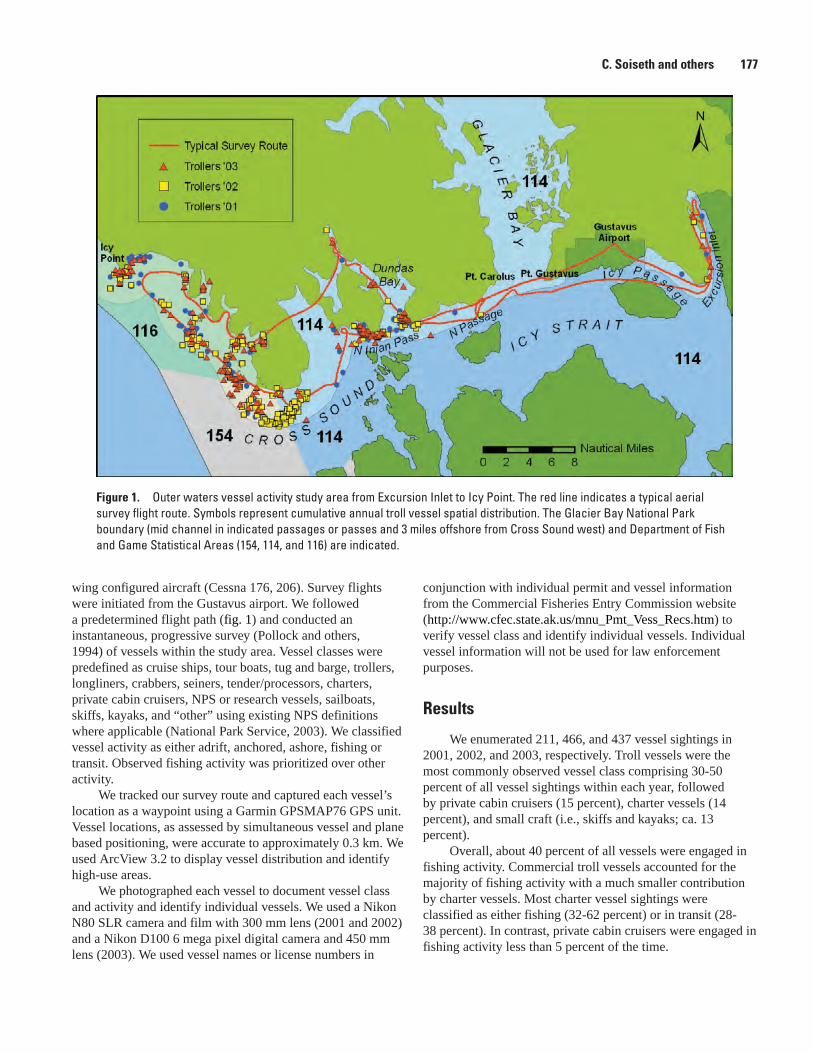
Figure 1. Outer waters vessel activity study area from Excursion Inlet to Icy Point. The red line indicates a typical aerial survey flight route. Symbols represent cumulative annual troll vessel spatial distribution. The Glacier Bay National Park boundary (mid channel in indicated passages or passes and 3 miles offshore from Cross Sound west) and Department of Fish and Game Statistical Areas (154, 114, and 116) are indicated.
C. Soiseth and others 177
wing configured aircraft (Cessna 176, 206). Survey flights were initiated from the Gustavus airport. We followed a predetermined flight path (fig. 1) and conducted an instantaneous, progressive survey (Pollock and others, 1994) of vessels within the study area. Vessel classes were predefined as cruise ships, tour boats, tug and barge, trollers, longliners, crabbers, seiners, tender/processors, charters, private cabin cruisers, NPS or research vessels, sailboats, skiffs, kayaks, and “other” using existing NPS definitions where applicable (National Park Service, 2003). We classified vessel activity as either adrift, anchored, ashore, fishing or transit. Observed fishing activity was prioritized over other activity.
We tracked our survey route and captured each vessel’s location as a waypoint using a Garmin GPSMAP76 GPS unit. Vessel locations, as assessed by simultaneous vessel and plane based positioning, were accurate to approximately 0.3 km. We used ArcView 3.2 to display vessel distribution and identify high-use areas.
We photographed each vessel to document vessel class and activity and identify individual vessels. We used a Nikon N80 SLR camera and film with 300 mm lens (2001 and 2002) and a Nikon D100 6 mega pixel digital camera and 450 mm lens (2003). We used vessel names or license numbers in
conjunction with individual permit and vessel information from the Commercial Fisheries Entry Commission website (http://www.cfec.state.ak.us/mnu_Pmt_Vess_Recs.htm) to verify vessel class and identify individual vessels. Individual vessel information will not be used for law enforcement purposes.
Results
We enumerated 211, 466, and 437 vessel sightings in 2001, 2002, and 2003, respectively. Troll vessels were the most commonly observed vessel class comprising 30-50 percent of all vessel sightings within each year, followed by private cabin cruisers (15 percent), charter vessels (14 percent), and small craft (i.e., skiffs and kayaks; ca. 13 percent).
Overall, about 40 percent of all vessels were engaged in fishing activity. Commercial troll vessels accounted for the majority of fishing activity with a much smaller contribution by charter vessels. Most charter vessel sightings were classified as either fishing (32-62 percent) or in transit (28-38 percent). In contrast, private cabin cruisers were engaged in fishing activity less than 5 percent of the time.
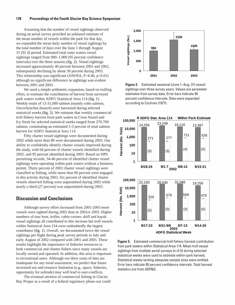
17� Proceedings of the Fourth Glacier Bay Science Symposium
Assuming that the number of vessel sightings observed during an aerial survey provided an unbiased estimate of the mean number of vessels within the park for that day, we expanded the mean daily number of vessel sightings by the total number of days over the June 1 through August 31 (92 d) period. Estimated total outer waters vessel sightings ranged from 900–1,900 (95 percent confidence intervals) over the three seasons (fig. 2). Vessel sightings increased approximately 40 percent between 2001 and 2002, subsequently declining by about 30 percent during 2003. This relationship was significant (ANOVA, F=4.46, p=0.01) although no significant difference in sightings was evident between 2001 and 2003.
We used a simple arithmetic expansion, based on trolling effort, to estimate the contribution of harvest from surveyed park waters within ADFG Statistical Area 114 (fig. 1). Weekly totals of 13-31,000 salmon (mainly coho salmon, Oncorhynchus kisutch) were harvested during selected statistical weeks (fig. 3). We estimate that weekly commercial troll fishery harvest from park waters in Cross Sound and Icy Strait for selected statistical weeks ranged from 270-700 salmon, constituting an estimated 1-5 percent of total salmon harvest for ADFG Statistical Area 114.
Fifty charter vessel sightings were documented during 2002 while more than 80 were documented during 2003. Our ability to confidently identify charter vessels improved during the study, with 64 percent of charter vessels identified during 2002, and 95 percent identified during 2003. Based on NPS permitting records, 34-46 percent of identified charter vessel sightings were operating within park waters without a business permit. Thirty percent of 2002 charter vessel sightings were classified as fishing, while more than 60 percent were engaged in this activity during 2003. Six percent of identified charter vessels observed fishing were unpermitted during 2002 while nearly a third (27 percent) was unpermitted during 2003.
Discussion and Conclusions
Although survey effort increased from 2001-2003 more vessels were sighted during 2002 than in 2001or 2003. Higher numbers of tour boat, troller, cabin cruiser, skiff and kayak vessel sightings all contributed to this increase but troll vessels within Statistical Area 154 were undoubtedly the largest contributor (fig. 1). Overall, we documented twice the vessel sightings per flight during peak survey periods in July and early August of 2002 compared with 2001 and 2003. These results highlight the importance of fisheries resources to both commercial and charter fishers since many vessels are locally owned and operated. In addition, this area is important to recreational users. Although our three years of data are inadequate for any trend assessment, we predict that future increased use and resource limitation (e.g., space, fisheries, opportunity for solitude) may well lead to user-conflicts.
The eventual attrition of commercial fishing in Glacier Bay Proper as a result of a federal regulatory phase-out could
994
1536
1049
0
500
1,000
1,500
2,000
2001 2002 2003
Vess
el s
ight
ings
(No.
).
Figure 2. Estimated seasonal (June 1–Aug. 31) vessel sightings over three survey years. Values are parameter estimates from survey data. Error bars indicate 95 percent confidence intervals. Data were expanded according to Cochran (1977).
2002
23,249 16,110 13,38714,293
271 277711 626
1
10
100
1,000
10,000
100,000
8/18-24 9/1-7 9/8-14 9/15-21
Har
vest
(No.
fish
) .
ADFG Stat. Area 114 Within Park Estimate
(3) (3) (3)(4)
2003
22,193 28,530 31,086 19,259
316 576 569 470
1
10
100
1,000
10,000
100,000
8/17-23 8/31-9/6 9/7-13 9/14-20
ADFG Statistical Week
Har
vest
(No.
fish
) .
(3) (3) (3) (5)
Figure �. Estimated commercial troll fishery harvest contribution from park waters within Statistical Area 114. Mean troll vessel sightings from multiple aerial surveys (n=3-5) during selected statistical weeks were used to estimate within-park harvest. Statistical weeks lacking adequate sample sizes were omitted. Error bars indicate 95 percent confidence intervals. Total harvest statistics are from ADF&G.
C. Soiseth and others 179
result in increased fishing activity in Glacier Bay National Park’s outer waters. As commercial fishing is phased out in Glacier Bay proper over the next 30-40 years, an excess productivity “spillover effect” of large halibut and other commercially or recreationally sought species could further focus fishing effort at the mouth of the Bay (Gasper and others, 2004). In fact, Gasper and others (2004) report that the Gustavus charter fleet currently targets halibut along the terminal moraine near the mouth of Glacier Bay proper.
Next to “fishing,” vessels “in transit” were the next most frequently observed activity. Few vessels, other than cruise ships and tugs and barges, remain in transit through park waters. With the exception of a marine disaster (i.e., collision, grounding, fire, or fuel spill), transit associated impacts would include primarily emissions, noise (above and underwater), and cetacean ship strikes.
Vessel densities in our survey area (5.9-12.4 vessels/1,000 acres) were 1.5–2.5 times greater than in Glacier Bay Proper (4.0-4.9 vessels/1,000 acres) during the June through August visitor use period. NPS vessel entry restrictions for Glacier Bay proper have resulted in more opportunities for boater solitude and recreation within Glacier Bay proper compared with unregulated waters in Cross Sound and Icy Strait. Absent new regulations, this disparity in vessel use and crowding will likely increase as local populations and tourism activities increase throughout Southeast Alaska.
Salmonid distribution is structured both in space and time. Troll vessel distribution is presumably determined by the underlying fish distribution, mediated to some extent, by weather and the number of troll vessels competing for fish within a given area. Our estimated troll harvest contribution from park waters of 1-5 percent is one third or less of the harvest contribution estimate of 15 percent for this area previously provided by Taylor and Perry (1990). However, it is not possible to determine whether the spatial distribution of troll fishing effort has shifted since Taylor and Perry’s time.
Our estimate of 34-46 percent for unpermitted charter vessels may overestimate this activity. Charters are exempt from the NPS permitting requirement when not operating commercially. Thus, for example, charter vessels in Elfin Cove are not required to be permitted when checking recreational Dungeness crab pots in Dundas Bay as long as they are not operating commercially. The estimated 27 percent or less of charter vessel sightings characterized as fishing may actually provide a more accurate estimate of unpermitted charter activity in park waters.
Management Implications
Although a variety of vessels transit and use the park’s outer waters, very little onshore activity was documented. Potential resource impact concerns include fishery effects, the possibility of a marine disaster, and cetacean ship strikes. This study and Gasper and others (2004) indicate that a very small component of Cross Sound and Icy Strait troll and charter
harvest can be attributed to park waters. Tugs and barges were observed infrequently but nevertheless pose a threat because fuel transport vessels can hold up to a million gallons of fuel. Geographic response strategies must be developed for critical resource areas in close proximity to high probability fuel spill areas.
Additionally, the NPS must resolve the legal and fairness issues associated with unpermitted charter vessels. We recommend a two pronged approach of education and enforcement. The NPS must inform all charter businesses of the permitting requirement and facilitate the permitting process. A more visible NPS presence in outer waters could reduce illegal charter activity provided that the consequences of unpermitted operation are prohibitive, and, the detection probability of unpermitted charter operators is high.
Our work establishes a baseline for vessel distribution and activity in Glacier Bay’s outside waters. We hope future managers grappling with increased use, resource limitations, and/or user-conflicts will learn from and build on our approach.
Acknowledgments
Bill Eichenlaub, Bill Thompson, and Brian Lynch provided technical assistance to this project. Thanks to the National Park Service survey technicians Jennifer Hamblen, Kathy Smikrud and Steve Gray. Special thanks to pilots Mike Sharp, Chuck Schroth, Mike Loverink, Larry Hazen and Steve Wilson for keeping us safe! This project (PMIS #35700) was funded in part by the National Park Service Natural Resources Preservation Program.
References Cited
Gasper, J.R., Gallucci, V.F., Miller, M.M., Soiseth, C., Johnson, D., and Swanson, J., 2004, Sport fishery information for managing Glacier Bay National Park and Preserve vol. 1: Catch, harvest and effort for the Gustavus and Elfin Cove sport fishery in the Cross Sound and Icy Strait region of northern Southeast Alaska during 2003: Seattle, Wash., National Park Service, Pacific West Region, University of Washington, Technical Report NPS/PWRUW/NRTR-2005-01.
National Park Service, 2003, Vessel quotas and operating requirements in Glacier Bay National Park and Preserve. United States Department of the Interior, National Park Service, Alaska Region. Final Environmental Impact Statement.
Pollock, K.H., Jones, C.M., and Brown, T.L., 1994, Angler survey methods and their applications in fisheries management: Bethesda, Md., American Fisheries Society Special Publication 25.
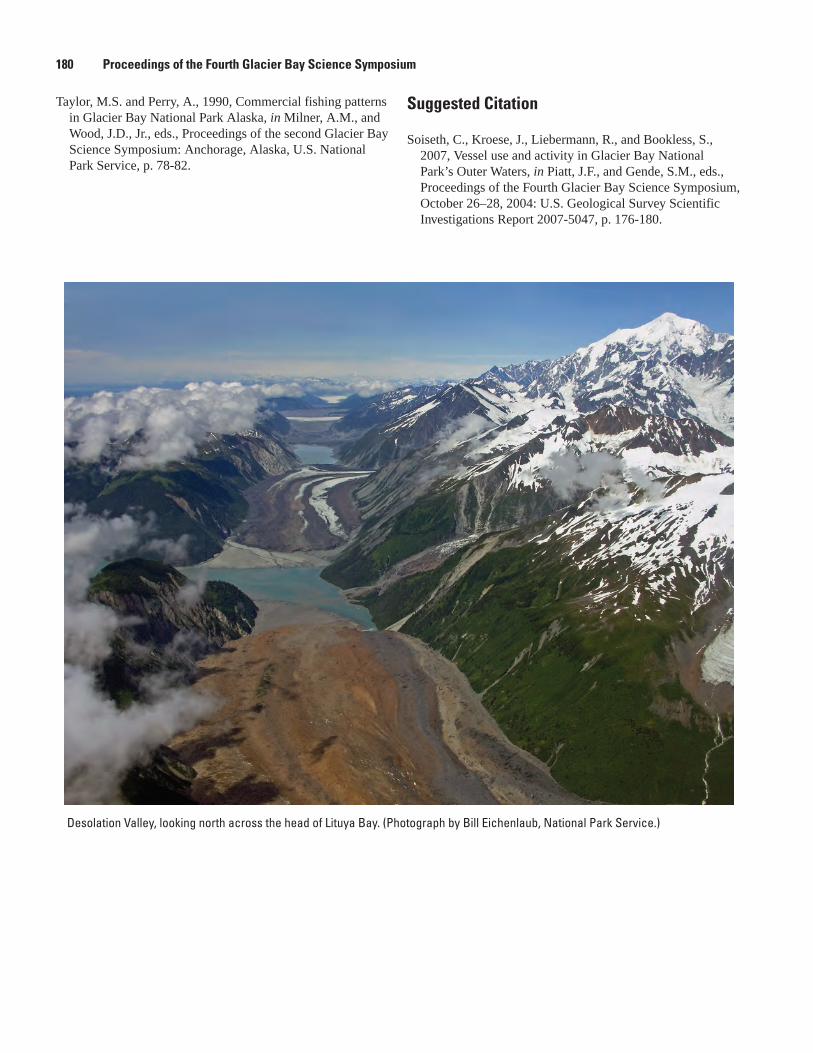
1�0 Proceedings of the Fourth Glacier Bay Science Symposium
Desolation Valley, looking north across the head of Lituya Bay. (Photograph by Bill Eichenlaub, National Park Service.)
Taylor, M.S. and Perry, A., 1990, Commercial fishing patterns in Glacier Bay National Park Alaska, in Milner, A.M., and Wood, J.D., Jr., eds., Proceedings of the second Glacier Bay Science Symposium: Anchorage, Alaska, U.S. National Park Service, p. 78-82.
Suggested Citation
Soiseth, C., Kroese, J., Liebermann, R., and Bookless, S., 2007, Vessel use and activity in Glacier Bay National Park’s Outer Waters, in Piatt, J.F., and Gende, S.M., eds., Proceedings of the Fourth Glacier Bay Science Symposium, October 26–28, 2004: U.S. Geological Survey Scientific Investigations Report 2007-5047, p. 176-180.
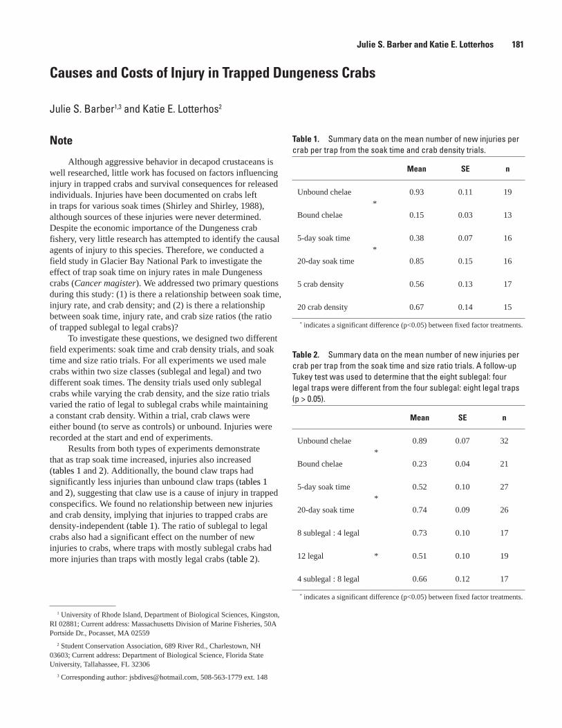
Causes and Costs of Injury in Trapped Dungeness Crabs
Julie S. Barber1,3 and Katie E. Lotterhos2
Note
Although aggressive behavior in decapod crustaceans is well researched, little work has focused on factors influencing injury in trapped crabs and survival consequences for released individuals. Injuries have been documented on crabs left in traps for various soak times (Shirley and Shirley, 1988), although sources of these injuries were never determined. Despite the economic importance of the Dungeness crab fishery, very little research has attempted to identify the causal agents of injury to this species. Therefore, we conducted a field study in Glacier Bay National Park to investigate the effect of trap soak time on injury rates in male Dungeness crabs (Cancer magister). We addressed two primary questions during this study: (1) is there a relationship between soak time, injury rate, and crab density; and (2) is there a relationship between soak time, injury rate, and crab size ratios (the ratio of trapped sublegal to legal crabs)?
To investigate these questions, we designed two different field experiments: soak time and crab density trials, and soak time and size ratio trials. For all experiments we used male crabs within two size classes (sublegal and legal) and two different soak times. The density trials used only sublegal crabs while varying the crab density, and the size ratio trials varied the ratio of legal to sublegal crabs while maintaining a constant crab density. Within a trial, crab claws were either bound (to serve as controls) or unbound. Injuries were recorded at the start and end of experiments.
Results from both types of experiments demonstrate that as trap soak time increased, injuries also increased (tables 1 and 2). Additionally, the bound claw traps had significantly less injuries than unbound claw traps (tables 1 and 2), suggesting that claw use is a cause of injury in trapped conspecifics. We found no relationship between new injuries and crab density, implying that injuries to trapped crabs are density-independent (table 1). The ratio of sublegal to legal crabs also had a significant effect on the number of new injuries to crabs, where traps with mostly sublegal crabs had more injuries than traps with mostly legal crabs (table 2).
Table 1. Summary data on the mean number of new injuries per crab per trap from the soak time and crab density trials.
Mean SE n
Unbound chelae *
0.93 0.11 19
Bound chelae 0.15 0.03 13
5-day soak time *
0.38 0.07 16
20-day soak time 0.85 0.15 16
5 crab density 0.56 0.13 17
20 crab density 0.67 0.14 15
* indicates a significant difference (p<0.05) between fixed factor treatments.
Table 2. Summary data on the mean number of new injuries per crab per trap from the soak time and size ratio trials. A follow-up Tukey test was used to determine that the eight sublegal: four legal traps were different from the four sublegal: eight legal traps (p > 0.05).
Mean SE n
Unbound chelae*
0.89 0.07 32
Bound chelae 0.23 0.04 21
5-day soak time*
0.52 0.10 27
20-day soak time 0.74 0.09 26
8 sublegal : 4 legal
*
0.73 0.10 17
12 legal 0.51 0.10 19
4 sublegal : 8 legal 0.66 0.12 17
* indicates a significant difference (p<0.05) between fixed factor treatments.
Julie S. Barber and Katie E. Lotterhos 1�1
1 University of Rhode Island, Department of Biological Sciences, Kingston, RI 02881; Current address: Massachusetts Division of Marine Fisheries, 50A Portside Dr., Pocasset, MA 02559
2 Student Conservation Association, 689 River Rd., Charlestown, NH 03603; Current address: Department of Biological Science, Florida State University, Tallahassee, FL 32306
3 Corresponding author: [email protected], 508-563-1779 ext. 148
Observations from video footage of traps suggest that new injuries are caused by an increase in agonistic interactions with increasing soak time, and that these injuries are unlikely to have been caused by cannibalism or competition over space (Barber, 2004). Qualitative investigations revealed that sublegal crabs appeared to be more aggressive than legal crabs when trapped with many conspecifics of similar size, and legal crabs may be more tolerant when trapped with similarly-sized crabs. This observation could also explain the increased number of injuries in traps containing high numbers of sublegal crabs. Our results also established that injuries to trapped Dungeness crabs are density-independent. Perhaps when crab density is high, the rate of agonistic interactions is low, suggesting that the crabs could be altering their behavior in accordance to changes in soak time or crab density.
Sublegal crabs are of particular concern to managers of the Dungeness crab fishery because these crabs will be released upon retrieval of the trap. It is possible that released injured crabs will exhibit a lower success rate in finding and defending mates, decreased foraging ability, and a lower survival rate than intact crabs, although these suggestions are based upon known effects of injury on other decapod crustacean species (Juanes and Smith, 1995). The consequences of injuries on the fitness of Dungeness crabs remain largely unknown (Juanes and Smith, 1995; Barber, 2004).
Recreational crabbers in Glacier Bay National Park, and presumably recreational crabbers in other areas within the range of the Dungeness crab, are known to leave their traps fishing for extended periods of time (>10 days). Commercial crabbers, on the other hand, normally soak their traps for much shorter durations (2-5 days) (J. Barber, personal observation). This information suggests that the recreational fishery may have a disproportionate impact on the number of injuries sustained by trapped crabs. Indeed, crabs in recreationally-fished areas within Glacier Bay appear to have more injuries than areas that are closed to crabbing (J. Barber, personal observation).
The results from this study suggest a need to monitor and regulate trap soak time in an effort to decrease injury to crabs. Future research should investigate methods to minimize injuries to crabs in traps and consider ways to educate recreational crabbers about the potential consequences of their fishing practices.
Acknowledgments
Support for this project was provided by the National Park Service and the PADI Project AWARE Foundation. We would especially like to thank the Alaska Department of Fish and Game, the NOAA Auke Bay Laboratory, Dr. Stanley Cobb, Dr. Thomas Shirley, James Dimond, Chad Soiseth, and countless field volunteers.
References Cited
Barber, J., 2004, Factors influencing injury of trapped Dungeness crabs and survival consequences for released males: Kingston, RI, University of Rhode Island, M.S. thesis.
Juanes, F., and Smith, L.D., 1995, The ecological consequences of limb damage and loss in decapod crustaceans: a review and prospectus: Journal of Experimental Marine Biology, v. 193, p. 197-223.
Shirley, S.M., and Shirley, T.C., 1988, Appendage injury in Dungeness crabs (Cancer magister) in southeastern Alaska: Fisheries Bulletin v. 86, p. 156-160.
Suggested Citation
Barber, J., and Lotterhos, K.E., 2007, Causes and costs of injury in trapped Dungeness crabs, in Piatt, J.F., and Gende, S.M., eds., Proceedings of the Fourth Glacier Bay Science Symposium, October 26–28, 2004: U.S. Geological Survey Scientific Investigations Report 2007-5047, p. 181-182.
1�2 Proceedings of the Fourth Glacier Bay Science Symposium
The Diffusion of Fishery Information in a Charter Boat Fishery—Guide-Client Interactions in Gustavus, Alaska
Jason R. Gasper1,2,4, Marc L. Miller2, Vincent F. Gallucci2, and Chad Soiseth3
Abstract. Charter sport fisheries present a situation where management information and regulations are disseminated from management agencies to charter guides who are expected to pass it on to their clients. This paper explores educative interactions that took place between guides and their clients in a charter boat fishery in Gustavus, Alaska. Guide-client interactions were framed in the context of power as described by Michele Foucault. Applying this framework to a tourist setting suggests that guides have power to control what clients see on a trip and the types of information disseminated; whereas, clients have the power to reject or accept a guide’s activities. This interaction was observed between charter guides and clients. Charter guides encouraged clients to release halibut larger than 100 pounds and encouraged them to reduce the number of pounds harvested. Moreover, guides used a client’s willingness to learn and their position of power when diffusing their conservation viewpoints. These findings suggest that guides have significant control over their clients behavior, the types of information disseminated, and that charter-guide client interactions follow a Foucauldian framework.
Jason R. Gasper and others 1��
1 University of Alaska Fairbanks School of Fisheries, 11120 Glacier Hwy. Juneau, AK 99801
2 University of Washington School of Marine Affairs, 3207 Brooklyn Ave. N.E. Seattle, WA 98105
3 National Park Service, Glacier Bay National Park, P.O. Box 180 Gustavus, AK 99826
4 Corresponding author: National Marine Fisheries Service, Alaska Region, P.O. Box 21668, Juneau, Alaska 99802-1668, [email protected], 907-586-7237
Power is not a system of domination by one group over another. Power is the result of successive interactions occurring between two groups. Power modifies discourse between two parties (Foucault, 1978; Gordon, 1980);
Power is a fluid force between groups that is always in a state of flux;
Power and knowledge are wedded and cannot be separated when analytically explaining the influences of power on group interactions.
Foucault’s designation of these three elements suggest that power explains most human affairs, power and knowledge are wedded, and power can be analytically studied. In this sense, Foucault assigned himself the role of a political scientist. This paper focuses on Foucault’s concept of power and knowledge in a political science framework and is not concerned with his postmodernist thesis.
A dynamic power relationship that follows Foucault’s framework is maintained between charter guides and clients as each group rejects or accepts imposed activities or inducements. Clients have monetary power over a guide’s activities. Conversely, a charter guide’s power lies in his or her ability to construct and manage a client’s experience and expectations. Charter guides modify their clients behavior using a variety of methods such as marketing, determining the nature of fishing activities (location and species), interpreting regulations, disseminating knowledge and advice (e.g., recommending local businesses), and acting as a culture broker between clients and locals.
This study explores the use of power by guides and educative processes that influence guide-client relationships. Guide-client interactions are discussed in context with releasing large halibut, educational interests held by charter guides and clients, and displays of power.
1.
2.
3.
Introduction
Charter sport fisheries are unique in that management information is often not directly distributed to the angler (charter client) from management agencies. Instead, information is distributed through a mediating party: the charter guide. Thus, communication between management agencies and charter clients is dependent upon a guide’s ability to disseminate accurate information and educate his or her clients about local resources.
Clients expect a guide to provide information and interpretation of the local environment and aide their participation in activities (Cohen, 1985). Charter guides are hired by clients for their expertise about a potentially dangerous environment and to lead them to their bounty (Cohen, 1985). Thus, a guide’s expertise gives them a substantial amount of power over client behavior.
Charter Guide–Client Power
Interactions of power between guides and clients follow a framework described by Michele Foucault (Miller and Auyong, 1991). Foucault’s power framework contains three elements (Foucault, 1978; Cheong and Miller, 2000):
Charter guides were asked similar questions as the clients. Charter guides were questioned about their interest in teaching clients about conservation and fishing, their interest in encouraging clients to release large halibut, and reasons they cite while encouraging clients to release large halibut. A charter guide’s desire to educate his or her clients was assessed using the following questions: (1) how much emphasis do you place on teaching your clients to fish (9 point scale was used for rating); (2) do you encourage clients to release large halibut; (3) when encouraging clients to release large halibut, do you cite biological reasons (yes or no), logistical reasons (yes or no), or consumptive reasons (yes or no).
Ethnographic Participant ObservationEthnographic Participant Observation (EPO) techniques
consisted of interviews and observations structured to assess the following variants of Foucauldian power: power through surveillance, education, and advice; and, clandestine, and peripheral forms of power. These forms of power will be described in the results and discussion section.
Results And Discussion
Social Survey Research
Response RateA total of 173 clients were randomly sampled between
thirteen charter guides. Samplers evenly sampled clients among the thirteen charter guides. Less than 5 percent of contacted clients refused a survey and 14 percent of interviewed clients did not complete or return their survey. Non-respondent analysis was not conducted due to the small number of refusals and a demographically homogenous respondent group. Moreover, the random experimental design allowed all clients to have an equal chance of selection.
A census was completed for 13 charter guides who operated, on average, two or more times a week from the Gustavus Dock. All charter guides operating 2 or more days a week participated in the survey.
Survey ResultsClients generally acknowledged the requests made
by charter guides to release large halibut. The majority (70 percent) of charter clients indicated that they were encouraged to release large halibut. Similarly, most (92 percent) charter guides indicated they encouraged clients to release large halibut. A significant positive relationship was observed between charter guides who encouraged clients to release large halibut and clients indicating they were encouraged (Cramer’s V=0.348; p=<0.001). Significant relationships were also observed between guides who cited biological reasons
Methods
Study SettingThe Glacier Bay/Icy Strait Region (GBISR), located
in Northern Southeast, Alaska, is a world class sportfishing destination. Anglers travel from around the world to pursue halibut (Hippoglossus stenolepis) and salmon (Oncorhynchus spp.) during spring and summer months (May–September). A variety of sportfishing charter companies and lodges operate in GBISR. Most charter companies in GBISR are based in one of the following communities: Elfin Cove, Gustavus, Hoonah, or Juneau. This study is focused on Gustavus and does not represent other communities in the region.
Charter boats based in Gustavus operate from a single dock (Gustavus Dock) that can moor up to 10 charter boats simultaneously. Most charter guides operate day trips that offer 8 to 12 hours of fishing for anglers staying at local lodges. Anglers staying at a lodge often book two or more consecutive days of charter fishing; however, a small number of single day charters are taken.
Research MethodsData for this study were collected using two research
approaches: social survey research (Patton, 1998) and Ethnographic Participant Observation (EPO). Social survey research was used to assess demographic questions and questions regarding education. Onsite EPO questions assessed the types of power used by charter guides and clients.
Social Survey ResearchSurvey questions were posed to charter guides operating
from the Gustavus Dock two or more days a week and among randomly selected clients. Question format was modified from examples given in Patton (1998) and distributed to respondents in booklet form. Survey questions for charter guides and clients were embedded in larger questionnaires that took approximately 7-8 minutes to complete. Responses for both clients and guides were broken into multi-day (>1 day of charter fishing) and single day charter responses. This paper will only focus on multi-day fishing trips.
Charter clients were questioned about their interest in receiving fishing instruction, if their guide disseminated information regarding the release of large halibut (>100 lbs), and if they released a large halibut. Client attitudes were assessed using the following three questions: (1) how important is it for you to have your guide teach fishing techniques for halibut (9 point scale was used for rating); (2) did your guide encourage you to release large halibut (yes or no); (3) if your guide encouraged you to release large halibut, did he or she cite biological reasons (yes or no), consumptive reasons (yes or no), or logistical reasons (yes or no); (4) if you caught a large halibut, did you release it?
1�� Proceedings of the Fourth Glacier Bay Science Symposium

for releasing large halibut and clients who indicated that their guide cited biology as a reason for releasing large halibut (Cramer’s V=0.308; p=0.001). Most clients (90 percent) responded that their guide cited biological reasons. Guides also appeared to influence the number of clients who released large halibut: out of the 77 clients who released large halibut, 53 percent of them indicated that their guide encouraged the practice.
Relationships were observed between a charter guide’s interest in educating clients, a client’s desire to learn, and clients who indicated they were encouraged to release large halibut. Clients were more likely to indicate they were encouraged to release large halibut if their guide placed a high importance on teaching conservation ( t r= =0 355 0 131. , . ) or fishing technique ( t r= =0 565 0 01. , . ). Furthermore, a guide’s influence was mediated by a client’s desire to be taught fishing technique. Fishing technique refers to the methodology used to catch and land halibut. The greater a clients desire to be taught fishing technique, the more likely it was that their guides encouraged them to release large halibut ( t r= =0 55 0 02. , . ).
Survey DiscussionThe use of pressure placed on clients by charter guides
and rapport developed between charter guides and their clients may have influenced the number of large halibut released. This was evident by statistically significant associations between guides who encouraged the release of large halibut and clients who understood a guide’s message. This suggests that the behavior of many clients were influenced by their charter guide. It is possible that client attitude towards large halibut was influenced by several exogenous factors: locals in Gustavus; fishing peers previously exposed to the Gustavus fishing social world; and, personal experience. External sources of influences are impossible to eliminate; however, clients probably did not learn about the release of large halibut from management documents or marketing sources. The authors are not aware of any management documents that contain information advocating the release of large halibut and marketing for Alaskan sport fishing trips are often focused on the harvest of large halibut.
The flow of power between charter guides and clients was fluid as indicated by a guide’s influence being mediated by a client’s level of interest. This was evident by statistically significant relationships between a client’s desire to be taught fishing technique, a guides desire to teach, and a client’s response concerning the release of large halibut. These results are consistent with education-orientated literature that suggests that the perceived “fruitfulness” of an educational activity is an important learning factor (Weiner, 1980; Hill, 1997). For example, ideas would be easily exchanged between a guide that is interested in teaching and an educationally engaged client. Conversely, a less interactive and less communicative guide would perhaps not pique client interests and an uninterested client would not pay attention to a guide’s instruction.
Jason R. Gasper and others 1�5
Epo Research
SurveillanceOpposing groups observe each other to acquire
knowledge about the status and attributes associated with the other group (Gordon, 1980, p. 104). Charter guides were observed placing judgments on client behavior and clients were observed placing judgments on charter guide behavior. This discourse provided a baseline that each group used to construct assumptions concerning how the other would react when exposed to different scenarios. For example, a charter guide used surveillance to determine a strategy that would most effectively encourage a client to release halibut. Surveillance is exemplified in the following statement made by a charter guide when a client decided to keep a large (150 lbs) halibut
“This is the part where they [the client] realize how much fish they have and try and figure out what they are going to do with it.”
The charter guide’s statement reflected a conversation the clients were having out of hearing range of the charter guide. The clients indicated that when they kept the fish they did not realize how many pounds of meat they had.
Charter guides also used prior knowledge gathered from surveillance to label a client’s behavior. Labeling clients was a tactic used by guides to reduce the catch of large halibut. For example, clients who harvested large amounts of fish were often labeled “meathounds.” These labels were developed and shared between charter guides without the client’s knowledge. Guides informed these clients about the taste of larger fish and logistical issues before presenting biological arguments.
EducationClients generally rely on charter guides for fishing and
fishery information such as the types and sizes of fish to eat, biological information, environmental information, and information concerning ritualistic objects associated with fishing (i.e., rods, reels, boats, lures, etc.). Clients unfamiliar with the Gustavus fishery possessed limited information regarding the application of fishing related objects or specific biological issues. Clients expect a guide to be a source of accurate and honest information (Cohen, 1985). This was particularly true in situations were information is difficult to understand or changes rapidly. For example, regulatory information often changes annually and can be tedious to understand in a foreign environment. Thus, many clients rely on guides to inform and educate them about regulations as reflected in the following statements:
Interviewer: “Do your clients ever look at the regulation book?”
Guide: [laughing] “NO! They believe whatever we tell them”
influence client behavior (Cohen, 1985). For example, guides could take clients to less productive fishing grounds to curtail harvest:
“Yesterday they [clients] caught a limit of large halibut. So today I took them to the chicken ranch”
The chicken ranch refers to a place where small halibut are caught. This guide was attempting to curtail the size of halibut caught and the total pounds of harvested halibut.
PeripheralGroup pressure is important when considering the power
relationship between charter guides and their clients. People who have prior relationships or joint interests often influence each others actions (Masclet, 2003). Group pressure is also not unique to people with social ties, it can occur between strangers united around a central cause (e.g., sportfishing). Guides did not always actively exhert pressure; rather, disagreements among clients on whether large halibut should be released or not were often facilitated through group pressure. On some occasions a client was ostracized through disapproval:
Guide: client’s “will raz each other about it [releasing large halibut]… one group member insisted on keeping a big one and all the others really gave him a hard time about it, group pressure took over”
Conclusion
Interactions of power between charter guides and clients can influence attempts by fishery managers and other organizations to distribute conservation, regulatory, and safety information. Furthermore, these findings suggest that dissemination of conservation and management information should focus on charter guides while acknowledging client needs.
References Cited
Cohen, E., 1985, The tourist guide: the origins, structure and dynamics of a role: Annals of Tourism Research, v. 12, p. 5-29.
Cheong, S., and Miller, M.L., 2000, Power and tourism: a Foucauldian observation: Annals of Tourism Research, v. 27, p. 371-390.
Foucault, M., 1978, The history of sexuality—an introduction: Vintage Books, New York.
Fine, E., and Speer, J., 1985, “Tour Guide Performances as Site Sacralization”: Annals of Tourism Research, v. 12, p. 73-95.
Clients routinely asked guides about halibut regulations such as bag limits and minimum and maximum size restrictions. Most guides issued information about large halibut being females with high fecundity and are thus, important for the population. One guide even held a quick orientation before embarking on a trip:
I give an orientation the day before or day of the trip… it comes out there [releasing large halibut]. I talk to them about the spawners and consumptive concerns.
AdviceGuides are analogous to travel agents because, like travel
agents, they are often the first or second point of contact for clients planning a trip, are viewed as locals who can provide information, are often perceived as experts, and may provide a sense of security in a foreign environment (Cohen, 1985). One aspect of power for guides lies in their ability “to create or limit opportunities for tourists” (Cheong and Miller, 2000). Clients often legitimize a guide’s trip plan because they are expected to be competent and knowledgeable about a destination or environment (i.e., fishing spots) (Johnson and Griffith, 1995).
Gustavus charter guides commonly issued consumptive and conservation advice concerning the amount of halibut clients harvested and the type of fishing clients are engaged in:
“Tomorrow we should probably go after salmon because you already have quite a bit of halibut”
Guides also issued advice about local businesses:
“You should have {local business name} do it, those little jobbers [personal vacuum packers] just do not do it. Besides, you won’t need to deal with it [in reference to packing fish].”
ClandestineGuides often choose what clients see during a fishing trip
or tour. (Schmidt 1979, p. 458-459; Cheong and Miller 2000) and focus a client’s attention on objects worthy of attention (Cohen, 1985; Fine and Speer, 1985; Cheong and Miller, 2000). Cohen (1985, p. 14) suggested that guides have control over what tourists do not see by selecting objects of interest in “accordance with his personal preferences and taste” or “the assumed interests of his party”. This places a guide in a position of power that allows the manipulation of client behavior in a clandestine fashion.
Two forms of clandestine power were identified in this study: interpretation and fabrication. Interpretation occurs when guides socialize clients to their agenda by disseminating inaccurate information (Nettekoven 1979, p. 142; Cohen, 1985, p. 15; Cheong and Miller, 2000, p. 384). A guide encouraging the release of large halibut to increase stock size is an example of clandestine interpretation. Fabrication consists of inventions or deceptions made by guides to
1�� Proceedings of the Fourth Glacier Bay Science Symposium

Gordon, C., 1980, Power and knowledge: selected interviews and other writings 1972-1977: New York, Pantheon Books, 271 p.
Hill, L.M., 1997, Just tell them the rule: learning to teach elementary mathematics: Journal of Teacher Education, v. 48, no. 3, p. 211-223.
Johnson, J.C., and Griffith, D.C., 1995, Promoting sportfish development in Puerto Rico: travel agents perception of the Caribbean: Human Organization, v. 54, no. 3, p. 295-303.
Masclet, D., 2003, Ostracism in work teams: a public good experiment: International Journal of Manpower, v. 24, no. 7, p. 867-887.
Miller, M.L., and Auyong, J., 1991, Coastal zone tourism: a potent force affecting environment and society: Marine Policy, p. 75-79.
Jason R. Gasper and others 1�7
View from above Icy Point looking northeasterly across the southern Fairweather Range and Brady Glacier. (Photograph by Bill Eichenlaub, National Park Service.)
Nettekoven, L., 1979, Mechanisms of intercultural interaction, in Kadt, E., Tourism: passport to development: New York, Oxford University Presss, p. 135-145.
Patton, M.L., 1998, Questionnaire research: a practical guide: Pyrczak Publishing, California. 137 p.
Schmidt C.J., 1997, The guided tour: insulated adventure: Urban Life, v. 7, no. 4, p. 441-467.
Weiner, B., 1980, Human motivation: Holt, Rinehart, and Winston. California.
Suggested Citation
Gasper, J.R., Miller, M.L., Gallucci, V.F., Soiseth, C., 2007, The diffusion of fishery information in a charter boat fishery—Guide-client interactions in Gustavus, Alaska, in Piatt, J.F., and Gende, S.M., eds., Proceedings of the Fourth Glacier Bay Science Symposium, October 26–28, 2004: U.S. Geological Survey Scientific Investigations Report 2007-5047, p. 183-187.

Simulating the Effects of Predation and Egg-harvest at a Gull Colony
Stephani Zador1,3 and John F. Piatt2
Abstract
We developed an individual-based simulation model to explore the effects of harvesting eggs from a glaucous-winged gull (Larus glaucescens) colony that also experiences egg loss from avian predators. The model has direct application to Glacier Bay National Park, where resource managers are interested in the potential effects of traditional harvesting of gull eggs at colonies within the park. This model simulates the sequence of egg laying, relaying, and incubation to hatching for individual nests and calculates hatching success, incubation length, and total eggs laid in all nests during the simulation. Stochasticity is incorporated in the distribution of nest lay dates, predation rates, and nests attacked during predation and harvest events. We used maximum likelihood to estimate parameters by fitting the model to data collected at South Marble Island in 1999 and 2000. We then simulated harvests and analyzed model predictions. Model outputs suggest that harvesting early, at one time, and from no more than 20 percent of the colony provides a constant harvest with the least impact to gulls.
Introduction
Glaucous-winged gulls (Larus glaucescens) are common along the west coast of North America from Washington to the Alaska Peninsula (Verbeek, 1993). Their average clutch size is 3 eggs, and females lay at 2-day intervals until clutches are complete and incubation begins. The loss of all eggs in a nest prior to clutch completion may result in protracted laying, in which case females continue to lay at 2-day intervals until their clutch is complete. Replacing a clutch lost after the onset of incubation requires 12-13 days to resume follicle growth and lay the first egg of the replacement clutch.
Replacement-laying is common in ground-nesting gulls, which have evolved to replace eggs lost to factors such as floods and predators (Brown and Morris, 1996). Common predators of glaucous-winged gull eggs include conspecifics (Verbeek 1988; Good and others, 2000), common ravens (Corvus corax) (Patten Jr., 1974) American crows (Corvus brachyrhynchos) (Verbeek, 1988) bald eagles (Haliaeetus leucocephalus) (Thompson, 1989; Good and others, 2000) and humans (Vermeer and others, 1991). Egg predation by
1�� Proceedings of the Fourth Glacier Bay Science Symposium
one predator species, such as humans or bald eagles, can also facilitate predation by conspecifics (Hand 1980; Good and others, 2000).
On South Marble Island in Glacier Bay, Alaska, glaucous-winged gull eggs are commonly preyed upon by bald eagles and were traditionally harvested by Huna Tlingit peoples. Little harvesting has been permitted legally in recent decades within Glacier Bay National Park (Hunn and others, 2002). However, the collection of eggs has retained importance as part of the Huna cultural heritage. The goal of this study was to find a balance among the competing interests of gulls, eagles, and people, such as the Huna and the resource managers.
Data collected by Zador (2001) during 2 years at South Marble Island were used to parameterize an individual-based simulation model that predicts hatching success at a gull colony subject to egg loss through predation and harvesting. The model can be used to manipulate the extent and intensity of egg loss in ways that are not possible in the field. Specifically, it can be used to test the effects of variation in timing and intensity of harvest rates given the natural variability in background predation rates.
Methods
An individual-based model was developed that simulates the changes in gull nest contents from pre-laying to hatching. As the simulation proceeds, the status of each nest is updated daily as eggs are laid, lost, replaced, and hatched. The model outputs hatching success (the percent of nests that produce ≥1 chick), the number of eggs laid, the number of eggs harvested, and the length of the simulation (a proxy for the length of the incubation period). The form of the rules on which the simulations were based were determined from field observations at South Marble Island in 1999 and 2000 (Zador, 2001) and glaucous-winged gull biology (Verbeek, 1993). We used maximum likelihood and the field data to estimate parameter values for the distribution of lay dates, the distribution of predation rates, and the probability of replacing eggs in 1999 and 2000. Final clutch sizes (defined as the number of eggs in the nest when incubation begins) are determined by the proportions that were observed in the field. Each simulation run uses parameter values from one of
1 School of Aquatic and Fisheries Sciences, University of Washington, Box 355020, Seattle, WA 98195
2 U.S. Geological Survey, Alaska Science Center, 1011 E. Tudor, Anchorage, AK 99503
3 Corresponding author: [email protected], 206-221-6904
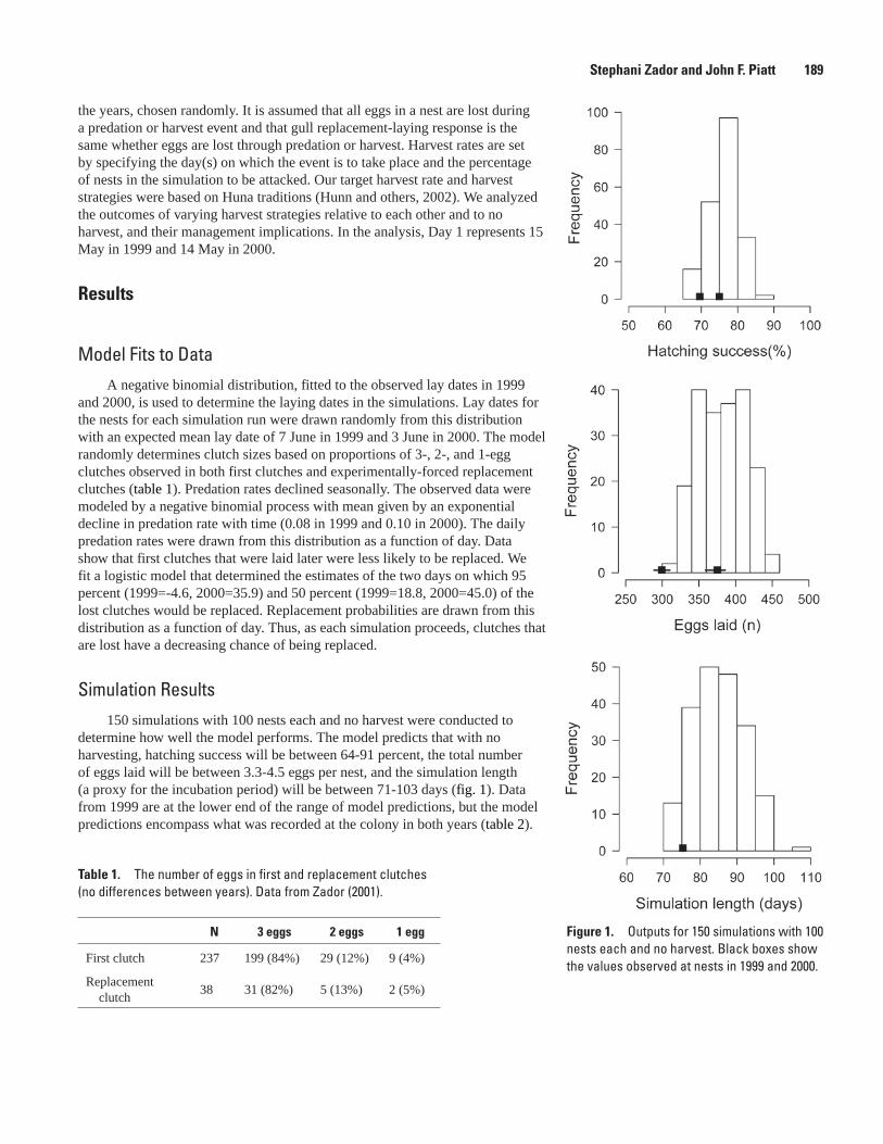
Table 1. The number of eggs in first and replacement clutches (no differences between years). Data from Zador (2001).
N � eggs 2 eggs 1 egg
First clutch 237 199 (84%) 29 (12%) 9 (4%)
Replacement clutch
38 31 (82%) 5 (13%) 2 (5%)
Figure 1. Outputs for 150 simulations with 100 nests each and no harvest. Black boxes show the values observed at nests in 1999 and 2000.
Stephani Zador and John F. Piatt 1�9
the years, chosen randomly. It is assumed that all eggs in a nest are lost during a predation or harvest event and that gull replacement-laying response is the same whether eggs are lost through predation or harvest. Harvest rates are set by specifying the day(s) on which the event is to take place and the percentage of nests in the simulation to be attacked. Our target harvest rate and harvest strategies were based on Huna traditions (Hunn and others, 2002). We analyzed the outcomes of varying harvest strategies relative to each other and to no harvest, and their management implications. In the analysis, Day 1 represents 15 May in 1999 and 14 May in 2000.
Results
Model Fits to DataA negative binomial distribution, fitted to the observed lay dates in 1999
and 2000, is used to determine the laying dates in the simulations. Lay dates for the nests for each simulation run were drawn randomly from this distribution with an expected mean lay date of 7 June in 1999 and 3 June in 2000. The model randomly determines clutch sizes based on proportions of 3-, 2-, and 1-egg clutches observed in both first clutches and experimentally-forced replacement clutches (table 1). Predation rates declined seasonally. The observed data were modeled by a negative binomial process with mean given by an exponential decline in predation rate with time (0.08 in 1999 and 0.10 in 2000). The daily predation rates were drawn from this distribution as a function of day. Data show that first clutches that were laid later were less likely to be replaced. We fit a logistic model that determined the estimates of the two days on which 95 percent (1999=-4.6, 2000=35.9) and 50 percent (1999=18.8, 2000=45.0) of the lost clutches would be replaced. Replacement probabilities are drawn from this distribution as a function of day. Thus, as each simulation proceeds, clutches that are lost have a decreasing chance of being replaced.
Simulation Results150 simulations with 100 nests each and no harvest were conducted to
determine how well the model performs. The model predicts that with no harvesting, hatching success will be between 64-91 percent, the total number of eggs laid will be between 3.3-4.5 eggs per nest, and the simulation length (a proxy for the incubation period) will be between 71-103 days (fig. 1). Data from 1999 are at the lower end of the range of model predictions, but the model predictions encompass what was recorded at the colony in both years (table 2).
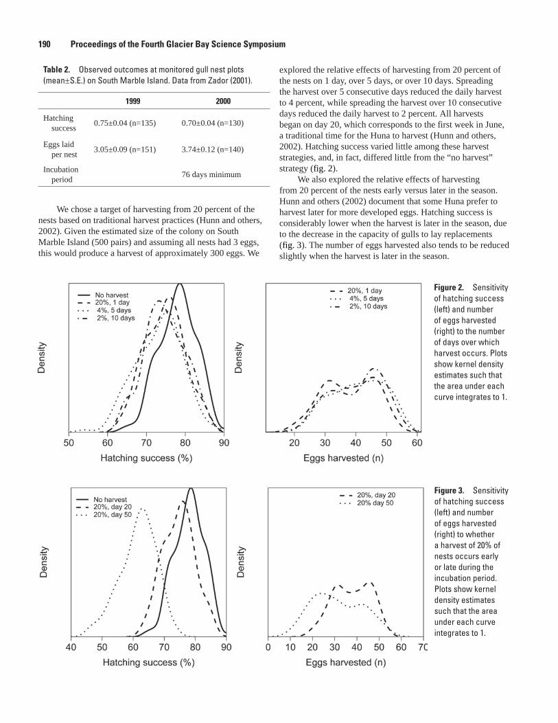
Figure �. Sensitivity of hatching success (left) and number of eggs harvested (right) to whether a harvest of 20% of nests occurs early or late during the incubation period. Plots show kernel density estimates such that the area under each curve integrates to 1.
Figure 2. Sensitivity of hatching success (left) and number of eggs harvested (right) to the number of days over which harvest occurs. Plots show kernel density estimates such that the area under each curve integrates to 1.
190 Proceedings of the Fourth Glacier Bay Science Symposium
We chose a target of harvesting from 20 percent of the nests based on traditional harvest practices (Hunn and others, 2002). Given the estimated size of the colony on South Marble Island (500 pairs) and assuming all nests had 3 eggs, this would produce a harvest of approximately 300 eggs. We
explored the relative effects of harvesting from 20 percent of the nests on 1 day, over 5 days, or over 10 days. Spreading the harvest over 5 consecutive days reduced the daily harvest to 4 percent, while spreading the harvest over 10 consecutive days reduced the daily harvest to 2 percent. All harvests began on day 20, which corresponds to the first week in June, a traditional time for the Huna to harvest (Hunn and others, 2002). Hatching success varied little among these harvest strategies, and, in fact, differed little from the “no harvest” strategy (fig. 2).
We also explored the relative effects of harvesting from 20 percent of the nests early versus later in the season. Hunn and others (2002) document that some Huna prefer to harvest later for more developed eggs. Hatching success is considerably lower when the harvest is later in the season, due to the decrease in the capacity of gulls to lay replacements (fig. 3). The number of eggs harvested also tends to be reduced slightly when the harvest is later in the season.
Table 2. Observed outcomes at monitored gull nest plots (mean±S.E.) on South Marble Island. Data from Zador (2001).
1999 2000
Hatching success
0.75±0.04 (n=135) 0.70±0.04 (n=130)
Eggs laid per nest
3.05±0.09 (n=151) 3.74±0.12 (n=140)
Incubation period
76 days minimum
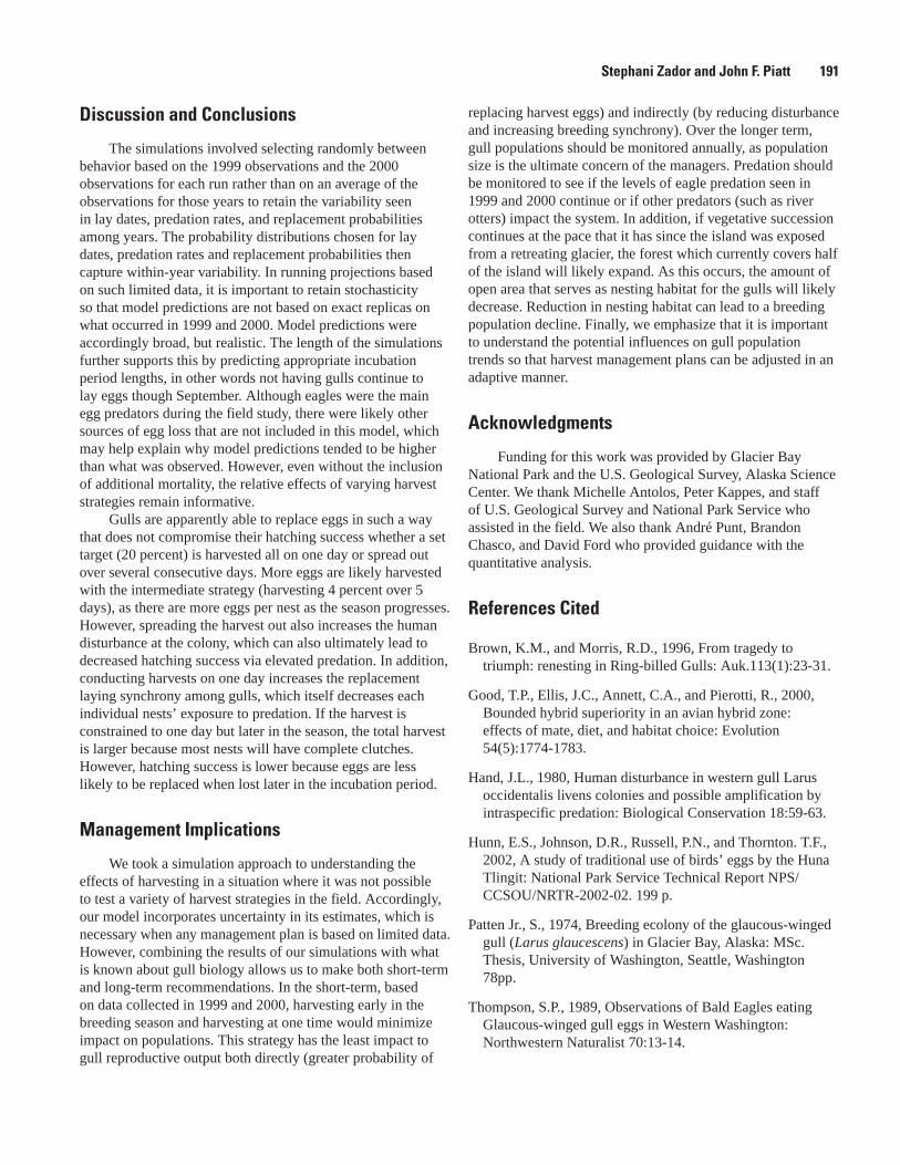
Stephani Zador and John F. Piatt 191
Discussion and Conclusions
The simulations involved selecting randomly between behavior based on the 1999 observations and the 2000 observations for each run rather than on an average of the observations for those years to retain the variability seen in lay dates, predation rates, and replacement probabilities among years. The probability distributions chosen for lay dates, predation rates and replacement probabilities then capture within-year variability. In running projections based on such limited data, it is important to retain stochasticity so that model predictions are not based on exact replicas on what occurred in 1999 and 2000. Model predictions were accordingly broad, but realistic. The length of the simulations further supports this by predicting appropriate incubation period lengths, in other words not having gulls continue to lay eggs though September. Although eagles were the main egg predators during the field study, there were likely other sources of egg loss that are not included in this model, which may help explain why model predictions tended to be higher than what was observed. However, even without the inclusion of additional mortality, the relative effects of varying harvest strategies remain informative.
Gulls are apparently able to replace eggs in such a way that does not compromise their hatching success whether a set target (20 percent) is harvested all on one day or spread out over several consecutive days. More eggs are likely harvested with the intermediate strategy (harvesting 4 percent over 5 days), as there are more eggs per nest as the season progresses. However, spreading the harvest out also increases the human disturbance at the colony, which can also ultimately lead to decreased hatching success via elevated predation. In addition, conducting harvests on one day increases the replacement laying synchrony among gulls, which itself decreases each individual nests’ exposure to predation. If the harvest is constrained to one day but later in the season, the total harvest is larger because most nests will have complete clutches. However, hatching success is lower because eggs are less likely to be replaced when lost later in the incubation period.
Management Implications
We took a simulation approach to understanding the effects of harvesting in a situation where it was not possible to test a variety of harvest strategies in the field. Accordingly, our model incorporates uncertainty in its estimates, which is necessary when any management plan is based on limited data. However, combining the results of our simulations with what is known about gull biology allows us to make both short-term and long-term recommendations. In the short-term, based on data collected in 1999 and 2000, harvesting early in the breeding season and harvesting at one time would minimize impact on populations. This strategy has the least impact to gull reproductive output both directly (greater probability of
replacing harvest eggs) and indirectly (by reducing disturbance and increasing breeding synchrony). Over the longer term, gull populations should be monitored annually, as population size is the ultimate concern of the managers. Predation should be monitored to see if the levels of eagle predation seen in 1999 and 2000 continue or if other predators (such as river otters) impact the system. In addition, if vegetative succession continues at the pace that it has since the island was exposed from a retreating glacier, the forest which currently covers half of the island will likely expand. As this occurs, the amount of open area that serves as nesting habitat for the gulls will likely decrease. Reduction in nesting habitat can lead to a breeding population decline. Finally, we emphasize that it is important to understand the potential influences on gull population trends so that harvest management plans can be adjusted in an adaptive manner.
Acknowledgments
Funding for this work was provided by Glacier Bay National Park and the U.S. Geological Survey, Alaska Science Center. We thank Michelle Antolos, Peter Kappes, and staff of U.S. Geological Survey and National Park Service who assisted in the field. We also thank André Punt, Brandon Chasco, and David Ford who provided guidance with the quantitative analysis.
References Cited
Brown, K.M., and Morris, R.D., 1996, From tragedy to triumph: renesting in Ring-billed Gulls: Auk.113(1):23-31.
Good, T.P., Ellis, J.C., Annett, C.A., and Pierotti, R., 2000, Bounded hybrid superiority in an avian hybrid zone: effects of mate, diet, and habitat choice: Evolution 54(5):1774-1783.
Hand, J.L., 1980, Human disturbance in western gull Larus occidentalis livens colonies and possible amplification by intraspecific predation: Biological Conservation 18:59-63.
Hunn, E.S., Johnson, D.R., Russell, P.N., and Thornton. T.F., 2002, A study of traditional use of birds’ eggs by the Huna Tlingit: National Park Service Technical Report NPS/CCSOU/NRTR-2002-02. 199 p.
Patten Jr., S., 1974, Breeding ecolony of the glaucous-winged gull (Larus glaucescens) in Glacier Bay, Alaska: MSc. Thesis, University of Washington, Seattle, Washington 78pp.
Thompson, S.P., 1989, Observations of Bald Eagles eating Glaucous-winged gull eggs in Western Washington: Northwestern Naturalist 70:13-14.
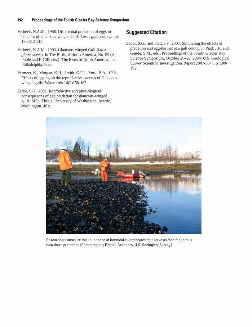
192 Proceedings of the Fourth Glacier Bay Science Symposium
Researchers measure the abundance of intertidal invertebrates that serve as food for various nearshore predators. (Photograph by Brenda Ballachey, U.S. Geological Survey.)
Verbeek, N.A.M., 1988, Differential predation of eggs in clutches of Glaucous-winged Gulls Larus glaucescens: Ibis 130:512-518.
Verbeek, N.A.M., 1993, Glaucous-winged Gull (Larus glaucescens). In The Birds of North America, No. 59 (A. Poole and F. Gill, eds.): The Birds of North America, Inc., Philadelphia, Penn.
Vermeer, K., Morgan, K.H., Smith, G.E.J., York. B.A., 1991, Effects of egging on the reproductive success of Glaucous-winged gulls: Waterbirds 14(2)158-165.
Zador, S.G., 2001, Reproductive and physiological consequences of egg predation for glaucous-winged gulls: MSc. Thesis, University of Washington, Seattle, Washington, 46 p.
Suggested Citation
Zador, S.G., and Piatt, J.F., 2007, Simulating the effects of predation and egg-harvest at a gull colony, in Piatt, J.F., and Gende, S.M., eds., Proceedings of the Fourth Glacier Bay Science Symposium, October 26–28, 2004: U.S. Geological Survey Scientific Investigations Report 2007-5047, p. 188-192.
Huna Tlingit Gull Egg Harvests in Glacier Bay National Park
Eugene S. Hunn1,5, Darryll R. Johnson2, Priscilla N. Russell3, Thomas F. Thornton4
Abstract. We report the results of an ethnographic study of the cultural significance and traditional practice of Glaucous-winged Gull egg harvests by the Huna Tlingit people of Hoonah, Alaska, with particular reference to Glacier Bay National Park. The study involved semi-structured interviews with 48 Huna individuals knowledgeable about such harvests. Huna gull egg harvests were a seasonal family activity supportive of important social and cultural values. Most Huna today resent the fact that they are no longer able to harvest eggs at the Marble Islands within Glacier Bay, a favored site. Huna gull egg harvests were also guided by a set of traditional rules which likely served to conserve the resource, e.g., take eggs only from nests with incomplete clutches.
Eugene S. Hunn and others 19�
1 Department of Anthropology, University of Washington, Seattle, WA 98195-3100
2 Cooperative Ecosystem Studies Unit, School of Forestry, University of Washington, Seattle, WA 98195
3 4550 West 57th St., Apt 1A-2, Chicago, Illinois 60629
4 Department of Anthropology, St. Lawrence University, Canton, NY 13617, [email protected]
5 Corresponding author: [email protected], 206-543-5240
Introduction
There is a vigorous debate in academic and management circles with regard to the question of whether indigenous peoples conserve their natural resources. Proponents argue that indigenous communities are more deeply attached to their homelands than are other stake holders in the locality, such as recent settlers and transient resource users. Indigenous communities with deep roots in local landscapes typically develop detailed knowledge and deep appreciation of local natural environments by virtue of their dependence on local resources for their livelihood. Such knowledge and understanding is prerequisite to careful management of local resources for long-term sustainability.
Skeptics question whether indigenous communities are in fact so stable, whether instead human history involves a succession of environmental crises and violent population shifts more like modern human history. They further question whether humans are by nature capable of sacrificing short-term selfish gains in the interests of a collective concern to protect long-term stable relationships between the community and its natural environment. The impact of new technologies on the sustainability of harvests is also at issue. Our Huna gull egg harvest study provides one example that should help clarify these contentious issues.
Methods
Our team was brought in at the joint request of the Glacier Bay National Park administration and the Hoonah Indian Association to document the history and contemporary
significance of gull egg harvests by Huna people. Wayne Howell of the Glacier Bay National Park Service administration introduced our team at an open meeting at Hoonah and we developed a procedure acceptable to both the Park Service and the Huna community. We would seek to interview all knowledgeable Huna willing and able to speak for the record. We subsequently completed 48 interviews. These were tape recorded and transcribed. The interviews focused on the significance of gull egg harvests and how such harvests were conducted, based on the personal recollections of the interviewees. A detailed analysis of the results were first circulated in draft form to Glacier Bay National Park personnel and Huna community representatives, modified in response to comments received, then published (Hunn and others, 2004).
Results
First, our review of the archaeological, linguistic, and historical evidence strongly supports the view that the Huna Tlingit people are the direct descendents of Native communities in continuous occupation of the Icy Straits and Glacier Bay region for 6,000 to 10,000 years. The ethnographic record demonstrates further that the local community has inherited an extensive body of Traditional Environmental Knowledge (TEK)—detailed, empirically and experientially grounded knowledge of local plants, animals, and places—that informs their occupation and use of the local landscape and its natural resources. We demonstrate furthermore a specific linkage between local knowledge of gull breeding biology and behavior and resource harvest practices based in that knowledge that may represent an instance of indigenous conservation.
Our Huna Tlingit consultants describe the traditional seasonal harvest of glaucous-winged gull eggs as of particular cultural significance because it marked a key transition in their annual cycle of travels and harvests. Seagull eggs were available for harvest for but a few weeks at the first of June
and this was the occasion for family outings to the gull colonies, most notably those on the Marble Islands in Glacier Bay, where the sheltered waters allowed even young children to participate and learn the basics of Tlingit resource harvest etiquette.
Our most striking finding was that nearly all knowledgeable Huna—we interviewed 48 Huna residents with some knowledge of the traditional practice of gull egg harvests—referred to traditional rules governing these harvests. A substantial majority (24 of 39 consultants, 64 percent of those specifying a rule) agreed that they had been taught to carefully note the number of eggs in each nest and to harvest the eggs only if one or two had been laid but to leave the nest undisturbed if there were three eggs present. There was some disagreement as to the precise rule, with some stressing the need to leave one egg in the nest. Though one respondent described a more radical strategy involving destroying the eggs in full nests, then returning later to harvest fresh eggs laid to replace those that had been destroyed, several elderly consultants vigorously denied that such a practice was ever sanctioned.
Discussion
Initially we did not appreciate the significance of these cultural rules, but on further investigation learned that the glaucous-winged gull (Larus glaucescens), the primary target of these harvests, is an “indeterminate nester,” that is, females are “programmed” to lay a clutch of a particular size—in this case, the modal clutch size is three eggs—laying a single egg approximately every second day, continuing to lay until the target clutch size is achieved. When a full clutch is present in the nest, the female begins to incubate and her hormonal system shuts off egg production. However, if eggs are removed from the nest before the clutch is complete, she will continue to lay.
In short, the Huna community had devised a traditional resource management system, transmitted from generation to generation by explicit instruction of the young during the harvest itself and enforced by public opinion, that was very likely designed to sustain a culturally significant harvest of a potentially vulnerable natural resource. Furthermore, this resource management strategy was informed by careful empirical observation of gull breeding habits.
After a preliminary review of our findings by Glacier Park staff, the Park contracted with U.S. Geological Survey to support a biology student (Stephani Zador) and to conduct a detailed study of the Marble Island glaucous-winged gull colonies in Glacier Bay. Zador’s research (Zador, 2001; Zador and Piatt, 2002; Zador and others, 2006) raised a number of questions with regard to the long-term sustainability of the traditional Huna Tlingit practice. Firstly, it is obvious that the size and distribution of glaucous-winged gull nesting colonies in the Glacier Bay region is highly dynamic, regardless of the intensity of indigenous harvests. Several colonies
noted as being of significance to the Huna historically no longer support nesting gulls, while new colonies have been established far up Glacier Bay in areas more recently freed from the retreating glaciers. These changes are due in large part to vegetational succession subsequent to glacial retreat. A second dynamic factor is predation by bald eagles. According to Zador, eagle predation is now the most significant contributing natural factor in the destruction of eggs and chicks at the Marble Island colonies. Finally, Zador notes that the traditional harvest strategy might nevertheless negatively impact gull nesting success by introducing additional stresses on breeding females through colony disturbance and the energetic demands of producing extra eggs.
Management Implications
Evidence to assess the impact of a given harvest practice over the long haul is rarely available. Thus, if subsistence egg harvests by Huna in Glacier Bay were to be legalized, there would remain considerable uncertainty with respect to the sustainability and appropriate scale of such harvests. The Glacier Bay National Park administration is in a difficult position; on the one hand charged to protect for all Americans Glacier Bay as a premier “wilderness” park, while on the other hand, recognizing that Huna Tlingit people have a legitimate interest in managing resources that constitute the material and symbolic foundation of their community.
Park staff has worked with the Huna community since the completion of our study to help arrange the harvest of gull eggs at a small colony outside of the Park at Middle Pass Rock in Icy Straits, which has allowed elders and young people from the community to experience this traditional subsistence practice without fear of arrest for the first time in decades. However, the Middle Pass Rock colony is subject to stronger currents and wave action than is the case at the Marble Islands and thus is not safe for younger children. If the legal obstacles to the resumption of Huna Tlingit harvests in Glacier Bay can be resolved, the administrative details of a truly cooperative management effort will still need to be hammered out, in the face of stiff opposition by those committed to the notion of parks as “wilderness,” on the one hand, and by indigenous activists on the other who reject as illegitimate any federal presence in their traditional homeland.
Acknowledgments
Don Calloway, Wayne Howell, and Mary Beth Moss of the National Park Service provided helpful reviews. Wayne Howell guided and assisted in coordinating the project in Hoonah. Stephani Zador provided guidance with regard to research articles on gull biology. The authors gratefully acknowledge the contributions of the Huna people to this report. The conclusions reported here do not necessarily reflect the views and policies of the NPS.
19� Proceedings of the Fourth Glacier Bay Science Symposium
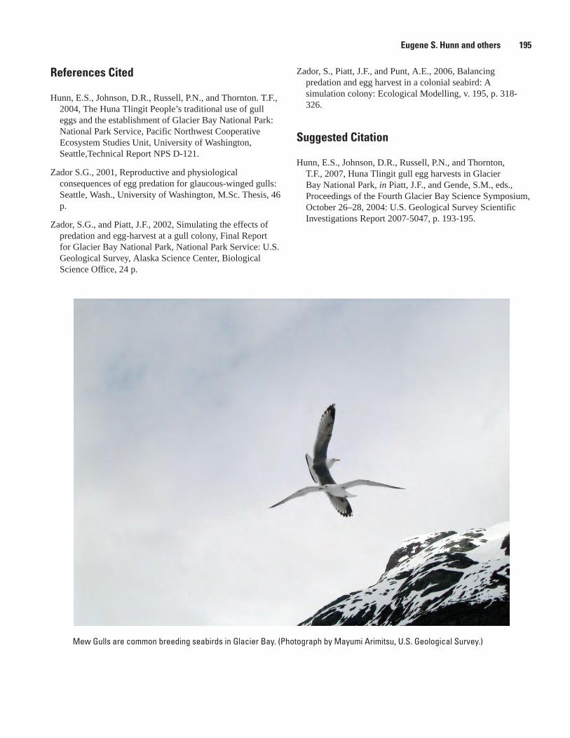
Eugene S. Hunn and others 195
Mew Gulls are common breeding seabirds in Glacier Bay. (Photograph by Mayumi Arimitsu, U.S. Geological Survey.)
References Cited
Hunn, E.S., Johnson, D.R., Russell, P.N., and Thornton. T.F., 2004, The Huna Tlingit People’s traditional use of gull eggs and the establishment of Glacier Bay National Park: National Park Service, Pacific Northwest Cooperative Ecosystem Studies Unit, University of Washington, Seattle,Technical Report NPS D-121.
Zador S.G., 2001, Reproductive and physiological consequences of egg predation for glaucous-winged gulls: Seattle, Wash., University of Washington, M.Sc. Thesis, 46 p.
Zador, S.G., and Piatt, J.F., 2002, Simulating the effects of predation and egg-harvest at a gull colony, Final Report for Glacier Bay National Park, National Park Service: U.S. Geological Survey, Alaska Science Center, Biological Science Office, 24 p.
Zador, S., Piatt, J.F., and Punt, A.E., 2006, Balancing predation and egg harvest in a colonial seabird: A simulation colony: Ecological Modelling, v. 195, p. 318-326.
Suggested Citation
Hunn, E.S., Johnson, D.R., Russell, P.N., and Thornton, T.F., 2007, Huna Tlingit gull egg harvests in Glacier Bay National Park, in Piatt, J.F., and Gende, S.M., eds., Proceedings of the Fourth Glacier Bay Science Symposium, October 26–28, 2004: U.S. Geological Survey Scientific Investigations Report 2007-5047, p. 193-195.
Ground-Nesting Marine Bird Distribution and Potential for Human Impacts in Glacier Bay
Mayumi L. Arimitsu1,3, Marc D. Romano2 and John F. Piatt2
Abstract. With the exception of a few large colonies, the distribution and abundance of ground-nesting marine birds in Glacier Bay National Park is largely unknown. There is growing concern about the potential impact of human activities to breeding birds as visitor use increases in back-country areas of the park. We surveyed the shoreline of Glacier Bay proper to locate ground-nesting marine birds and their nesting areas during the 2003 and 2004 breeding seasons. We determined the nesting distribution of the four most common ground-nesting marine bird species: Arctic Tern, Black Oystercatcher, Mew Gull and Glaucous-winged Gull. We also recorded observations of less abundant species that we encountered including Herring Gull, Semipalmated Plover, Spotted Sandpiper and Parasitic Jaeger. This project comprises the first complete, bay-wide, nesting distribution survey of ground-nesting marine birds in Glacier Bay. This information provides valuable baseline data that may be used to assess potential impacts of human disturbance and to track changes in nesting bird distribution and populations over time.
19� Proceedings of the Fourth Glacier Bay Science Symposium
Introduction
Glacier Bay National Park and Preserve contains a diverse assemblage of marine birds that use the area for nesting, foraging and molting. The abundance and diversity of marine bird species in Glacier Bay is unmatched in the region, due in part to the geomorphic and successional characteristics that result in a wide array of habitat types (Robards and others, 2003). The opportunity for proactive management of these species is unique in Glacier Bay National Park because much of the suitable marine bird nesting habitat occurs in areas designated as wilderness.
Ground-nesting marine birds are vulnerable to human disturbance wherever visitors can access nest sites during the breeding season. Human disturbance of nest sites can be significant because intense parental care is required for egg and hatchling survival, and repeated disturbance can result in reduced productivity (Leseberg and others, 2000). Temporary nest desertion by breeding birds in disturbed areas can lead to increased predation on eggs and hatchlings by conspecifics or other predators (Bolduc and Guillemette, 2003). Human disturbance of ground-nesting birds may also affect incubation time and adult foraging success, which in turn can alter breeding success (Verhulst and others, 2001). Furthermore, human activity can potentially cause colony failure when disturbance prevents the initiation of nesting (Hatch, 2002).
There is management concern about the susceptibility of breeding birds to disturbance from human activities, but little historical data has been collected on the distribution of ground-nesting marine birds in Glacier Bay. This report summarizes results obtained during two years of a three-year
study to determine the distribution of ground-nesting marine birds in Glacier Bay, and the potential for human disturbance of those nesting birds.
Methods
We determined the nesting distribution of the four most common ground-nesting bird species in Glacier Bay: Arctic Tern (Sterna paradisaea), Black Oystercatcher (Haematopus bachmani), Mew Gull (Larus canus) and Glaucous-winged Gull (Larus glaucescens). We also recorded observations of other ground nesting bird species that we encountered including Herring Gull (Larus argentatus), Semipalmated Plover (Chardrius semipalmatus), Spotted Sandpiper (Actitis mucularia) and Parasitic Jaeger (Sterorarius parasiticus).
We surveyed for ground-nesting marine birds and their associated nests between June 4 and July 15, 2003 and between May 17 and July 1, 2004. Using National Park Service data that details visitor-use between 1996 and 2002, we determined which coastal areas receive high use by kayakers and campers (fig. 1). We defined “high-use” as sites that received 30 or more overnight visits during the seven years covered by the data set. All areas classed as high-use were surveyed by observers walking the length of the particular coastal segment in order to map nest locations. In areas considered low-use (defined as an area that received fewer than 30 overnight visits) we surveyed the shoreline from a distance of 3-15 m using a skiff in motorized waters, or a kayak in non-motorized waters. When potential nesting behavior was observed (concentrations of birds on shore, defensive behavior by one or more birds, or the presence of paired birds) we landed the vessel and walked the length of the beach. At all survey locations we recorded site and nest positions using hand held GPS units, nest contents (eggs, chicks), adult behavior, general habitat characteristics and evidence of human disturbance. High and low-use areas that had concentrations of nesting birds in 2003 were resurveyed in 2004.
1 U.S. Geological Survey, Alaska Science Center, 3100 National Park Rd, Juneau, AK 99801
2 U.S. Geological Survey, Alaska Science Center, 1011 E. Tudor Rd., Anchorage, AK 99503
3 Corresponding author: [email protected], 907-364-1593
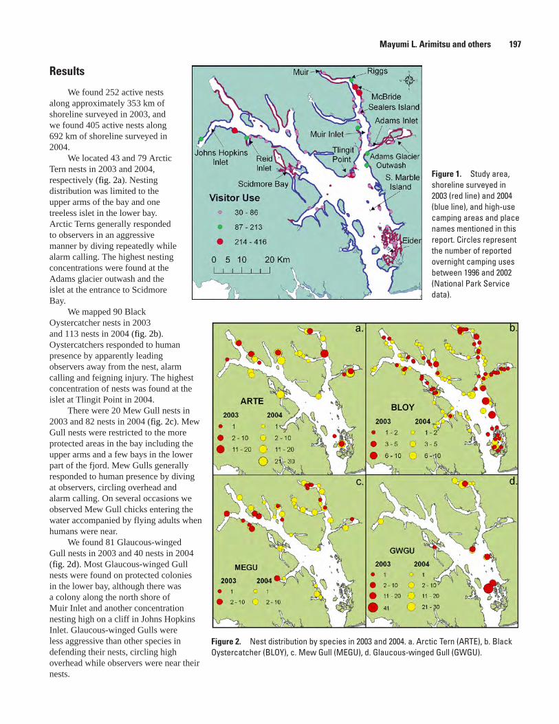
Figure 1. Study area, shoreline surveyed in 2003 (red line) and 2004 (blue line), and high-use camping areas and place names mentioned in this report. Circles represent the number of reported overnight camping uses between 1996 and 2002 (National Park Service data).
Mayumi L. Arimitsu and others 197
Results
We found 252 active nests along approximately 353 km of shoreline surveyed in 2003, and we found 405 active nests along 692 km of shoreline surveyed in 2004.
We located 43 and 79 Arctic Tern nests in 2003 and 2004, respectively (fig. 2a). Nesting distribution was limited to the upper arms of the bay and one treeless islet in the lower bay. Arctic Terns generally responded to observers in an aggressive manner by diving repeatedly while alarm calling. The highest nesting concentrations were found at the Adams glacier outwash and the islet at the entrance to Scidmore Bay.
We mapped 90 Black Oystercatcher nests in 2003
Figure 2. Nest distribution by species in 2003 and 2004. a. Arctic Tern (ARTE), b. Black Oystercatcher (BLOY), c. Mew Gull (MEGU), d. Glaucous-winged Gull (GWGU).
and 113 nests in 2004 (fig. 2b). Oystercatchers responded to human presence by apparently leading observers away from the nest, alarm calling and feigning injury. The highest concentration of nests was found at the islet at Tlingit Point in 2004.
There were 20 Mew Gull nests in 2003 and 82 nests in 2004 (fig. 2c). Mew Gull nests were restricted to the more protected areas in the bay including the upper arms and a few bays in the lower part of the fjord. Mew Gulls generally responded to human presence by diving at observers, circling overhead and alarm calling. On several occasions we observed Mew Gull chicks entering the water accompanied by flying adults when humans were near.
We found 81 Glaucous-winged Gull nests in 2003 and 40 nests in 2004 (fig. 2d). Most Glaucous-winged Gull nests were found on protected colonies in the lower bay, although there was a colony along the north shore of Muir Inlet and another concentration nesting high on a cliff in Johns Hopkins Inlet. Glaucous-winged Gulls were less aggressive than other species in defending their nests, circling high overhead while observers were near their nests.

Figure �. Nest distribution by species in 2003 and 2004. a. Herring Gull (HEGU), b. Semipalmated Plover (SEPL), c. Spotted Sandpiper (SPSA), d. Parasitic Jaeger (PAJA).
19� Proceedings of the Fourth Glacier Bay Science Symposium
In addition to nests of the more abundant species, we also located nests of several other species. We located 18 Herring Gull nests in 2004 (fig. 3a), 13 and 23 Semipalmated Plover nests in 2003 and 2004, respectively (fig. 3b), two Spotted Sandpiper nests in 2003 and 6 nests in 2004 (fig. 3c), one Parasitic Jaeger nest in 2003 and one nest in 2004 (fig. 3d). Herring Gull distribution was limited to the head of the east arm and Johns Hopkins Inlet. Semipalmated Plovers were found on flat sand and gravel shorelines, where they nested near low vegetation. Spotted Sandpipers were usually found within the terrestrial vegetation near the edge of the beach. Parasitic Jaegers laid eggs on bare ground and we noted the presence of pairs flying north of Adams Inlet and near Reid Glacier (fig. 3d).
We surveyed three high-use areas with potential for human disturbance including the north spit at McBride glacier, the west entrance to Reid Inlet and Sealers Island (table 1). During our survey in 2003, Arctic Terns were absent from Reid and McBride inlets. However, in 2004, we found 14 Arctic Tern nests at Reid Inlet between 27 May and 6 June, and 3 Arctic Tern nests on the north spit at McBride Glacier on May 28. By June 26 all Arctic Tern nests at the entrance to Reid Inlet had disappeared. One of those nests was trampled by a visitor on June 20, and this was the only observation of direct human impact on beach-nesting birds during our surveys. We also found 16 Arctic Tern, 1 Glaucous-winged Gull, 1 Mew Gull and 2 Black Oystercatcher nests at Sealers Island on 15 June, 2003. We revisited Sealers Island in 2004 and found 3 Mew Gull, 1 Glaucous-winged Gull and 4 Black Oystercatcher nests. In 2004, we also observed 8-10 defensive Arctic Terns flying and there were recently predated Arctic Tern egg shells near a Northwestern Crow nesting area in the center of Sealers Island.
We also found high concentrations of ground-nesting marine birds at low-use areas including the shoreline between Riggs and Muir glaciers, the islet at Tlingit Point, the islet at the entrance to Scidmore Bay, Adams glacier outwash and the islet northwest of Eider Island (table 1). The north shore between Riggs and Muir glaciers had more nests than any other unprotected area in the bay. The large outwash on the southwest shore of Adam’s Inlet and the unnamed islet northwest of Eider Island are notable because of their Arctic Tern aggregations; in 2004 there were approximately 500 and 300 adult Arctic Terns flying over these areas, respectively.
Discussion and Conclusions
The preferred nesting habitat for Arctic Terns, cobble outwash areas and rocky outcrops on small islands (Hatch, 2002), is found mostly up-bay in early successional habitats. Their aggressive behavior when humans approach may make their nesting areas less vulnerable to human disturbance, however, individual Arctic Tern nests are inconspicuous and therefore are more likely to be trampled.
Black Oystercatchers prefer to nest on gravel beaches with low-sloping substrates and usually nest near the high tide line (Andres and Falxa, 1995). Oystercatcher nests may be particularly susceptible to disturbance because kayakers tend to use the same beaches for camping. Nests are made of gravel and may be trampled when boats are hauled above the high tide line.
Mew Gulls prefer nesting in areas with little or no vegetation and on gravel banks or beaches, often near freshwater streams (Moskoff and Bevier, 2002). Mew Gull chicks may be susceptible to human disturbance because they usually entered the water when humans approached them.

Table 1. Nesting areas with highest potential for human disturbance, human use patterns between 1996 and 2002 (high is ≥ 30 camping uses and low is < 30 camping uses), total nest count and species observed. Nest count represents the greatest number of nests found in one year including all species at each location. Species are listed in order of abundance and abbreviations are as follows: Arctic Tern (ARTE), Black Oystercatcher (BLOY), Glaucous-winged Gull (GWGU), Mew Gull (MEGU), Herring Gull (HEGU), Semipalmated Plover (SEPL), Spotted Sandpiper (SPSA) and Parasitic Jaeger (PAJA).
Site Name Visitor Use Nest Count Species
Entrance to Reid High 16 ARTE, BLOY, SEPL
N. spit at McBride High 12 BLOY, SEPL, ARTE, MEGU
Sealers Island High 20 ARTE, BLOY, MEGU, GWGU
North shore Muir Inlet Low 68GWGU, HEGU, MEGU, BLOY,ARTE, SEPL, PAJA
Islet at Tlingit Point Low 21 BLOY, ARTE, GWGU, MEGU
Islet at entrance to Scidmore Bay Low 29 ARTE, MEGU, BLOY
Adams Glacier outwash Low 16 ARTE, BLOY, SEPL, PAJA, MEGU
Islet NW of Eider Island Low 17 ARTE, BLOY
Mayumi L. Arimitsu and others 199
In 1999, 285 Glaucous-winged Gull nests were counted on South Marble Island (Zador and Piatt, 1999), which is currently the largest Glaucous-winged Gull colony in the bay. Although Glaucous-winged Gulls are known to use a wide variety of habitat types for nesting (Verbeek, 1993), in Glacier Bay we found them nesting in areas with low vegetation or on rocky cliffs. Glaucous-winged Gulls place their eggs in conspicuous nest bowls and therefore trampling of nests by humans is less likely than for other ground-nesting bird species.
Hybridization between Herring Gulls and Glaucous-winged Gulls, which commonly occurs in areas where their breeding ranges overlap (Grant, 1986), was documented at North Marble Island by Patten and Weisbrod (1974). We observed signs of hybridization including copulation between a Herring Gull and a Glaucous-winged Gull, an individual from each species attending the same nest and several adults with characteristics intermediate of the two species at the mixed gull colony on the north shore of Muir Inlet.
Semipalmated Plovers, Spotted Sandpipers and Parasitic Jaegers are solitary nesters and have well camouflaged nests. The resolution of our surveys was too coarse to locate the majority of nests for these cryptic species, and our results therefore represent a minimum estimate of pairs and nests for these species.
Although we found unprotected nesting bird concentrations to be generally low in most areas, we found potential for disturbance to nesting birds at high-use areas including the north spit at McBride Glacier, the entrance to Reid Inlet and Sealers Island. These areas have historically supported nesting colonies of Arctic Terns (Wik, 1968; Greg Streveler, pers. comm.) and owing to their close proximity to tidewater glaciers, they are among the most heavily used areas by visitors in the bay.
There was also higher nesting activity in several low-use areas including the north shore of Muir Inlet between Riggs and Muir Glaciers, the islet at Tlingit Point, the islet at the entrance to Scidmore Bay, the Adams glacier outwash and an unnamed islet northwest of Eider Island. The nesting areas on the mainland, including the north shore of Muir Inlet and Adams glacier outwash, may be less susceptible to human disturbance because nesting activity was dispersed over a large area. In contrast, colonies on the smaller islets may be more susceptible to human disturbance because nesting was concentrated over a smaller area.
Management Implications
Most of the largest seabird nesting areas in Glacier Bay are closed to human use and are therefore largely protected from disturbance by park visitors. Nonetheless, there are areas where significant concentrations of nesting birds gather to breed and human disturbance could affect these breeding activities. Short of closing these areas to visitors, perhaps the simplest way to minimize disturbance to nesting birds is to educate visitors about where they may encounter nesting birds, how to identify nests and nesting bird behavior, and how they should respond when they encroach upon nest sites. This could be accomplished during the mandatory camper/boater orientation and reinforced in the annual regulations publication which is distributed to all visitors.
Baseline data that we have gathered on the distribution and abundance of ground-nesting birds in the park can be used for monitoring changes in breeding bird abundance and distribution over time, whether those changes are due to human disturbance of natural factors (for example, climate change or succession). This project provides a foundation to design and implement a management program that will minimize human disturbance to breeding birds in Glacier Bay.
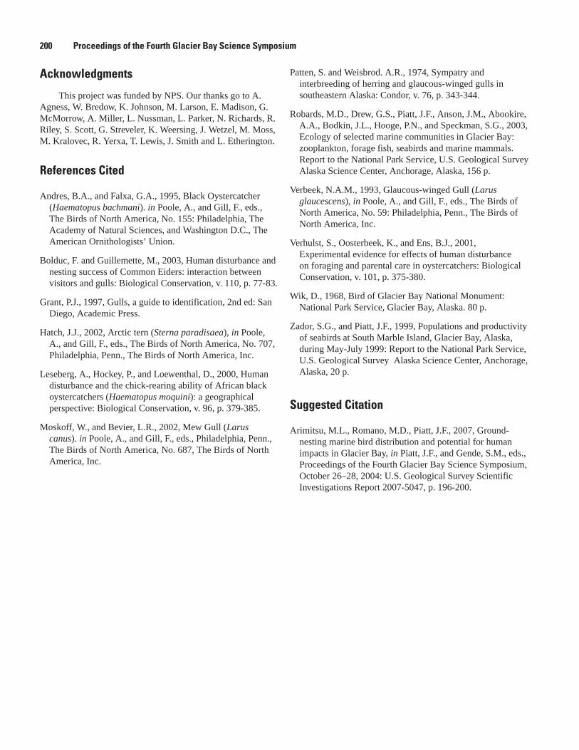
200 Proceedings of the Fourth Glacier Bay Science Symposium
Acknowledgments
This project was funded by NPS. Our thanks go to A. Agness, W. Bredow, K. Johnson, M. Larson, E. Madison, G. McMorrow, A. Miller, L. Nussman, L. Parker, N. Richards, R. Riley, S. Scott, G. Streveler, K. Weersing, J. Wetzel, M. Moss, M. Kralovec, R. Yerxa, T. Lewis, J. Smith and L. Etherington.
References Cited
Andres, B.A., and Falxa, G.A., 1995, Black Oystercatcher (Haematopus bachmani). in Poole, A., and Gill, F., eds., The Birds of North America, No. 155: Philadelphia, The Academy of Natural Sciences, and Washington D.C., The American Ornithologists’ Union.
Bolduc, F. and Guillemette, M., 2003, Human disturbance and nesting success of Common Eiders: interaction between visitors and gulls: Biological Conservation, v. 110, p. 77-83.
Grant, P.J., 1997, Gulls, a guide to identification, 2nd ed: San Diego, Academic Press.
Hatch, J.J., 2002, Arctic tern (Sterna paradisaea), in Poole, A., and Gill, F., eds., The Birds of North America, No. 707, Philadelphia, Penn., The Birds of North America, Inc.
Leseberg, A., Hockey, P., and Loewenthal, D., 2000, Human disturbance and the chick-rearing ability of African black oystercatchers (Haematopus moquini): a geographical perspective: Biological Conservation, v. 96, p. 379-385.
Moskoff, W., and Bevier, L.R., 2002, Mew Gull (Larus canus). in Poole, A., and Gill, F., eds., Philadelphia, Penn., The Birds of North America, No. 687, The Birds of North America, Inc.
Patten, S. and Weisbrod. A.R., 1974, Sympatry and interbreeding of herring and glaucous-winged gulls in southeastern Alaska: Condor, v. 76, p. 343-344.
Robards, M.D., Drew, G.S., Piatt, J.F., Anson, J.M., Abookire, A.A., Bodkin, J.L., Hooge, P.N., and Speckman, S.G., 2003, Ecology of selected marine communities in Glacier Bay: zooplankton, forage fish, seabirds and marine mammals. Report to the National Park Service, U.S. Geological Survey Alaska Science Center, Anchorage, Alaska, 156 p.
Verbeek, N.A.M., 1993, Glaucous-winged Gull (Larus glaucescens), in Poole, A., and Gill, F., eds., The Birds of North America, No. 59: Philadelphia, Penn., The Birds of North America, Inc.
Verhulst, S., Oosterbeek, K., and Ens, B.J., 2001, Experimental evidence for effects of human disturbance on foraging and parental care in oystercatchers: Biological Conservation, v. 101, p. 375-380.
Wik, D., 1968, Bird of Glacier Bay National Monument: National Park Service, Glacier Bay, Alaska. 80 p.
Zador, S.G., and Piatt, J.F., 1999, Populations and productivity of seabirds at South Marble Island, Glacier Bay, Alaska, during May-July 1999: Report to the National Park Service, U.S. Geological Survey Alaska Science Center, Anchorage, Alaska, 20 p.
Suggested Citation
Arimitsu, M.L., Romano, M.D., Piatt, J.F., 2007, Ground-nesting marine bird distribution and potential for human impacts in Glacier Bay, in Piatt, J.F., and Gende, S.M., eds., Proceedings of the Fourth Glacier Bay Science Symposium, October 26–28, 2004: U.S. Geological Survey Scientific Investigations Report 2007-5047, p. 196-200.

Bear-Human Conflict Risk Assessment at Glacier Bay National Park and Preserve
Tom Smith1,4, Terry D. Debruyn2, Tania Lewis3, Rusty Yerxa3, and Steven T. Partridge1
Abstract. We used historical data, extensive site surveys, and artificial neural network models to estimate the relative probability of bear (Ursus arctos, U. americanus) use of habitats and bear-human conflict at kayaker campsites within Glacier Bay National Park and Preserve, Alaska. We created a database for the input, organization and analysis of 70 years of bear sightings and conflicts data. Geographic information system (GIS) was used to analyze temporal-spatial patterns of both bear and camper use of the area. We visited 162 campsites throughout the bay and recorded a suite of variables deemed relevant to bear habitat quality and bear-human conflict potential. Artificial neural network models are being used to predict bear use and bear-human conflict. Results from this work will assist park managers in minimizing bear-human conflict and bear displacement from important habitats by camper activity.
Tom Smith and others 201
1 U.S. Geological Survey, Alaska Science Center, 1011 E. Tudor, Anchorage, AK 99503
2 National Park Service, Alaska Support Office, 240 West 5th Avenue, Anchorage, AK 99501
3 National Park Service, Glacier Bay National Park and Preserve, P.O. Box 140, Gustavus, AK 99826
4 Corresponding author: [email protected]
Introduction
Sea kayaking is the predominant recreational activity in Glacier Bay’s extensive marine backcountry. Kayakers frequently camp several nights, camping within the narrow strip of land between the ocean and steep-walled mountains. Both brown and American black bears seasonally occupy these same coastal areas. Beaches not only provide bears with unrestricted movement corridors, but also important foraging opportunities. Seaside habitats are among the earliest to provide bears with new plant growth as well as access to intertidal areas that host a variety of marine forage items. Consequently, the potential for bear-human interaction at Glacier Bay’s campsites is higher than for other areas of the backcountry. It is also more likely that human activity in these areas will displace bears from important forage resources, or interfere with their movements.
Study Area
Glacier Bay National Park and Preserve (GLBA) is located in southeast Alaska at the northernmost end of the Alexander Archipelago. Glacier Bay extends northward from Icy Strait more than 96 km (60 mi). Plant communities reflect its history of glacial recession, with boreal rain forests giving way to scrublands which, in turn, fade until only bare rock meets the glacial interface. GLBA is a vast maritime wilderness encompassing 1.3 million hectares of tidewater glaciers, timbered islands, winding fjords and a unique
assemblage of marine and terrestrial life. Mountains in the park rise from the ocean to >4,600 m (15,000 ft), with rock, ice and barren terrain comprising the largest component of the terrestrial ecosystem. Consequently, some of the most productive terrestrial habitat lies within the narrow belt of terrain alongside beaches. This research estimated the potential risk of bear conflict and bear displacement at campsites within Glacier Bay proper. Bear-human interactions also occur in the park’s interior, along the Outer Coast, and at Dry Bay, but these areas are not discussed here.
Methods
Initially we constructed an accurate history of bear activity and conflict at Glacier Bay before attempting to devise research that would provide insight regarding bear-human conflict. Glacier Bay National Park staff have carefully documented instances of bear-human conflict (approximately 300 incidents from 1960-2004), bear sightings (>3,700 sightings from 1932 to 2004), and backcountry campsite use (>8,000 records from 1996 to 2004). We then created a computer database into which these records were entered.
This database of ‘bear sightings and incidents’ guides the process of data entry (fig. 1), visually presents the distribution of sightings and incidents that have occurred in the bay, and enables users to query for specific information by providing key words. We also used geographic information system (GIS) software to perform spatial analyses of camper and bear use of the bay. This information, in turn, was used to create a temporal-spatial profile of bear and human activity and conflict in the back country.
To assess the potential for bear-human interaction at campsites, this research built upon the work of Herrero and others (1986) and MacHutchon and Wellwood (2002). The assumption underlying these previous research efforts was that bears are not randomly distributed across the terrain; but rather that the temporal-spatial pattern of bear activity is largely a
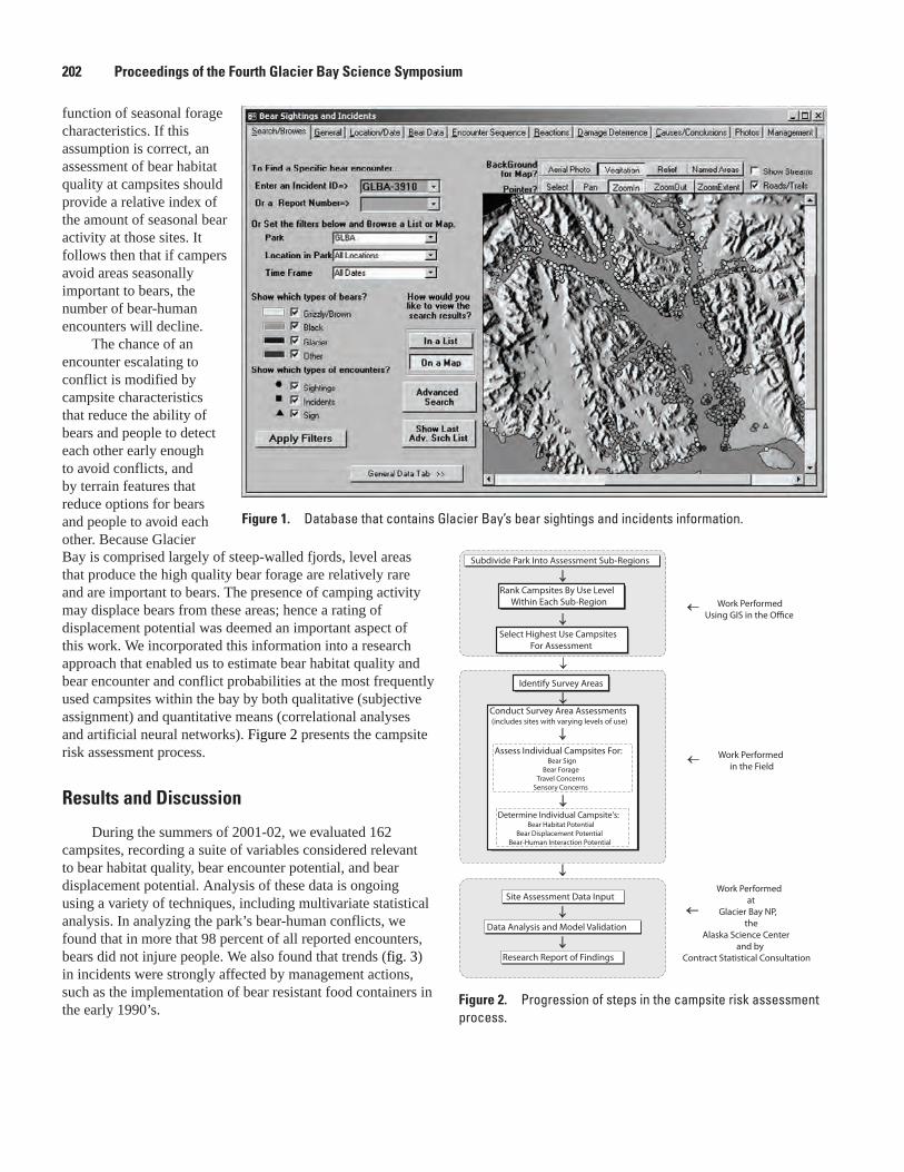
Subdivide Park Into Assessment Sub-Regions
Data Analysis and Model Validation
Research Report of Findings
Site Assessment Data Input
Select Highest Use Campsites For Assessment
Work PerformedUsing GIS in the Office
Work Performed in the Field
Work Performedat
Glacier Bay NP,the
Alaska Science Centerand by
Contract Statistical Consultation
Identify Survey Areas
Conduct Survey Area Assessments(includes sites with varying levels of use)
Assess Individual Campsites For:Bear Sign
Bear Forage Travel Concerns
Sensory Concerns
Determine Individual Campsite's:Bear Habitat Potential
Bear Displacement PotentialBear-Human Interaction Potential
Rank Campsites By Use LevelWithin Each Sub-Region
Figure 2. Progression of steps in the campsite risk assessment process.
202 Proceedings of the Fourth Glacier Bay Science Symposium
function of seasonal forage characteristics. If this assumption is correct, an assessment of bear habitat quality at campsites should provide a relative index of the amount of seasonal bear activity at those sites. It follows then that if campers avoid areas seasonally important to bears, the number of bear-human encounters will decline.
The chance of an encounter escalating to conflict is modified by campsite characteristics that reduce the ability of bears and people to detect each other early enough to avoid conflicts, and by terrain features that reduce options for bears and people to avoid each other. Because Glacier Bay is comprised largely of steep-walled fjords, level areas that produce the high quality bear forage are relatively rare and are important to bears. The presence of camping activity may displace bears from these areas; hence a rating of displacement potential was deemed an important aspect of this work. We incorporated this information into a research approach that enabled us to estimate bear habitat quality and bear encounter and conflict probabilities at the most frequently used campsites within the bay by both qualitative (subjective assignment) and quantitative means (correlational analyses and artificial neural networks). Figure 2 presents the campsite risk assessment process.
Results and Discussion
During the summers of 2001-02, we evaluated 162 campsites, recording a suite of variables considered relevant to bear habitat quality, bear encounter potential, and bear displacement potential. Analysis of these data is ongoing using a variety of techniques, including multivariate statistical analysis. In analyzing the park’s bear-human conflicts, we found that in more that 98 percent of all reported encounters, bears did not injure people. We also found that trends (fig. 3) in incidents were strongly affected by management actions, such as the implementation of bear resistant food containers in the early 1990’s.
Figure 1. Database that contains Glacier Bay’s bear sightings and incidents information.

Figure �. Trends in bear-human conflict at Glacier Bay National Park and Preserve, 1959-2002. Bear proof containers were introduced in 1994.
Nu
mb
er o
f In
cid
ents
Year
0
5
10
15
20
25
30
35
19591969
19741978
19801982
19841986
19881990
19921994
19961998
20002002
1 1 1 1 12
4 43
5
10
1314
8 8
13
15
12
16
21
32
4
9
5
9
12
15
21 21
12
15
Tom Smith and others 20�
Although black bear sightings (2,100) outnumbered brown bear sightings (1,300) nearly 2 to 1, black and brown bears were nearly equally involved in conflicts with people (56 percent vs. 44 percent). Eighty-five percent of bear conflicts occurred between 6 a.m. and 6 p.m. and human foods were a factor in bear conflict nearly half the time (42 percent). We also found that single campers were disproportionately more involved in bear conflicts than camps with 2 or more people. Our assessment of information supplied by persons involved in bear conflicts suggests that people were responsible for precipitating conflicts twice as often as were the bears.
Park policies and practices must be based on the best possible information to effectively manage people and bears. This project provides managers with a bear sightings and encounter database which will not only provide a historical perspective regarding bear activity and bear-human conflict, but also a framework for future data collection, input, and analysis. Campsite risk assessment determines which site variables most influence bear-human encounter and conflict rates, and provides input for bear management policy. Statistical analysis is providing insight regarding the roles both biotic and abiotic factors play in bear-human encounter rates and conflicts.
Management Implications
Although analysis is ongoing, results from this work will be valuable for park managers to better understand the seasonal importance of various habitats to bears within Glacier Bay. Additionally, an understanding of the relative roles played by specific site characteristics in determining both habitat quality and bear-conflict potential is important for managing human activity.
Acknowledgments
Funding for this work was provided by the US National Park Service and the U.S. Geological Survey, Alaska Science Center. Mary Beth Moss, former Resource Management Chief at GLBA, was instrumental in providing support for this project. We also thank all field crew members who assisted in data collection including Nat Drumheller, Nikki Koehler,
Randy Ramey, and Mia Grifalconi. We also acknowledge Phoebe Vanselow and Marylou Blakeslee who assisted with data collection. Bill Eichenlaub was extremely helpful with database design and consultation. The expert skill of skippers Justin Smith and Jim Luthy are also gratefully acknowledged.
References Cited
Herrero, S., McCrory W., and Pelchat, B., 1986, Using grizzly bear habitat evaluations to locate trails and campsites in Kananaskis Provincial Park: International Conference on Bear Research and Management, v. 6, p. 187-193.
MacHutchon, A.G., and Wellwood, D.W., 2002, Assessing the risk of bear human interaction at river campsites: Ursus, v. 13, p. 293-298.
Suggested Citation
Smith, T.S., DeBruyn, T.D., Lewis, T., Yerxa, R., and Partridge, S.T., 2007, Bear-human conflict risk assessment at Glacier Bay National Park and Preserve, in Piatt, J.F., and Gende, S.M., eds., Proceedings of the Fourth Glacier Bay Science Symposium, October 26–28, 2004: U.S. Geological Survey Scientific Investigations Report 2007-5047, p. 201-203.
Humpback Whale Entanglement in Fishing Gear in Northern Southeastern Alaska
Janet L. Neilson1,2,4, Christine M. Gabriele1, and Janice M. Straley3
Abstract
The prevalence of non-lethal entanglements of humpback whales in fishing gear in northern southeastern Alaska (SEAK) was quantified using a scar-based method. The percentage of whales assessed to have been entangled ranged from 52 percent (minimal estimate) to 71percent (conditional estimate) to 78 percent (maximal estimate). The conditional estimate is recommended because it is based solely on whales with unambiguous scars. Eight percent of the whales in Glacier Bay/Icy Strait acquired new entanglement scars between years, although the sample size was small. Calves were less likely to have entanglement scars than older whales and males may be at higher risk than females. The percentage of whales with entanglement scarring is comparable to the Gulf of Maine where entanglement is a substantial management concern. Consequently, SEAK humpback whale-fisheries interactions may warrant a similar level of scrutiny.
20� Proceedings of the Fourth Glacier Bay Science Symposium
Introduction
From 1997 through 2004, 52 humpback whales (Megaptera novaeangliae) were reported entangled in fishing nets and/or lines in Alaska (or were reported elsewhere and were confirmed to be entangled in Alaskan fishing gear.) Seventy-seven percent of the reports involved SEAK humpback whales (unpublished data, National Marine Fisheries Service (NMFS) Alaska Regional Office). Wounds resulting from entanglements can often be seen on the posterior caudal peduncle (the narrowing of the body at the insertion point of the flukes). These wounds can remain visible as unique scarring patterns years after the entanglement incident.
Robbins and Mattila (2001) examined whales’ caudal peduncles for entanglement-related scarring and concluded that 48–65 percent of the humpback whales photographed annually between 1997 and 2002 in the Gulf of Maine had been entangled. Until now there have been no systematic efforts to quantify the prevalence of humpback whale entanglement in Alaska. Managers in southeastern Alaska have had to rely on eyewitness reports as the only estimate of the magnitude of the problem, but not all entangled whales are found or reported. In 2001, NMFS acknowledged the pressing need for a detailed assessment of humpback whale entanglement in Alaska.
The objectives of this study were to (1) estimate the percentage of humpback whales in northern SEAK that have been non-lethally entangled based on caudal peduncle scars,
1 Glacier Bay National Park & Preserve, P.O. Box 140, Gustavus, AK 99826
2 University of Alaska Fairbanks, School of Fisheries & Ocean Sciences, Fairbanks, AK 99775
3 University of Alaska Southeast, 1332 Seward Avenue, Sitka, AK 99835
4 Corresponding author: [email protected], 907 697-2658
(2) analyze the entanglement scar data in conjunction with existing long-term humpback whale demographic data to identify any particularly vulnerable segments of the humpback whale population and (3) describe the distribution of scarred humpback whales in relation to the distribution and amount of commercial fishing in the study area. This paper focuses on objectives 1 and 2 only.
Methods
We conducted 1,139 hours of vessel-based surveys for humpback whales in northern SEAK between May 2003 and November 2004. We approached the whales in outboard-driven motorboats 4–6.5 m in length and took high resolution photographs of each whale’s caudal peduncle by operating the boat parallel and slightly forward of each whale as it dove. In order to reduce observer bias towards scarred whales, we collected caudal peduncle photographs from all suitably positioned whales. Whales were identified based on the pigmentation and morphology of the ventral surface of their tail flukes and dorsal fin.
We used a photographic coding technique developed and ground-truthed in the Gulf of Maine by Robbins and Mattila (2001) to assess the likelihood that a whale had been entangled in the past. We divided each whale’s caudal peduncle into six areas, coded these areas for signs of entanglement-related scarring (table 1) and assigned an overall entanglement status code (table 2) to whales with adequate photographic coverage.

Table 1. Summary of scar code descriptions (after Robbins and Mattila, 2001).
Code Scar Code Description
S0 No visible marks
S1Non-linear marks or apparently randomly oriented linear
marks
S2Linear marks or wide areas lacking pigmentation, which
did not appear to wrap around the feature
S3Linear or wide scars which appeared to wrap around the
feature
S4At least one visible linear notch or indentation (generally
on the dorsal or ventral peduncle)
S5 Extensive tissue damage and deformation of the feature
SXFeature could not be coded due to lack of photographic
coverage or inadequate photo quality
Table 2. Summary of entanglement status codes (after Rob-bins and Mattila, 2001).
CodeLikelihood of Past
EntanglementEntanglement Status Code
E0 NONENo evidence of entanglement (no
marks present)
E1 LOW
Marks were observed, but did not suggest a previous en-tanglement. Scar codes did not generally exceed S2 in any documented region
E2 AMBIGUOUS
Entanglement-like elements were present, but there was no consis-tent pattern. At least one region was generally assigned a scar code of S3 or higher
E3 HIGH
Marks appeared to be entangle-ment-related and minor tissue damage was evident. At least two regions were generally assigned scar codes of S3 or higher
E4 HIGH
Marks appeared to be entangle-ment-related and major tissue damage was evident. At least two regions were assigned scar codes of S3 or higher. At least one region was coded as S5
Janet L. Neilson and others 205
Three methods were used to estimate the percentage of whales that had been non-lethally entangled:
Minimal Entanglement Scarring Percentage =E E
E E E3 4
0 1 2∑ + ∑
+ + + EE E3 4∑ + ∑∑∑∑
Conditional Entanglement Scarring Percentage =E E
E E3 4
0 1∑ + ∑
+ ++ ∑ + ∑∑∑ E E3 4
Maximal Entanglement Scarring Percentage =E E E
E E2 3 4
0 1∑ + − ∑∑
+ ++ ∑ + + ∑∑∑∑ E E E2 3 4
where:
E0, E1, E2, E3 and E4=the number of whales assigned entan-glement status codes E0, E1, E2, E3 and E4, respectively.
Two-tailed Fisher’s exact tests of independence (Zar, 1999) were used to test for significant differences between percentages.
Individual whales with adequate photographs in both years were used to estimate the annual rate of entanglement scar acquisition between 2003 and 2004. The whale’s caudal peduncle photographs from both years were compared and assessed to estimate the amount of new entanglement-related scarring occurring between 2003 and 2004. This rate was calculated by dividing the number of whales in 2004 with an increase in entanglement scarring by the total number of individuals with adequate photographic coverage in both years.
Results
We photographed the caudal peduncle of 303 humpback whales and assigned entanglement status codes to 180 unique individuals. The photographic coverage and/or quality of 123 whales was insufficient to assign codes (i.e., photographs were too distant, blurry and/or were taken at a poor angle).
The percentage of whales assessed to have been entangled ranged from 52 percent (95 percent CI: 45 percent, 60 percent) (minimal estimate) to 71 percent (95 percent CI: 62 percent, 78 percent) (conditional estimate) to 78 percent (95 percent CI: 72 percent, 84 percent) (maximal estimate). The conditional estimate is recommended because it is based solely on unambiguous scars. Eight percent (95 percent CI: 1 percent, 25 percent) of the whales in Glacier Bay/Icy Strait acquired new entanglement scars between 2003 and 2004.
The whales with adequate quality photographs consisted of 62 females, 33 males and 85 whales of unknown sex. The minimal scarring percentage of males (82 percent) was higher than that of females (55 percent) and the difference was significant (P=0.013). However, males and females did not have significantly different conditional scarring percentages (males 87 percent, females 72 percent) (P=0.165) or maximal scarring percentages (males 88 percent, females 79 percent) (P=0.402).
20� Proceedings of the Fourth Glacier Bay Science Symposium
The whales with adequate quality photographs consisted of 12 calves (i.e., whales less than one year old) and 168 older whales. The minimal scarring percentage of calves (17 percent) was lower than that of older whales (55 percent) and the difference was significant (P=0.015). In addition, the conditional scarring percentage of calves (29 percent) was lower than that of older whales (73 percent) and the difference was significant (P=0.023). However, calves and older whales did not have significantly different maximal scarring percentages (calves 58 percent, older whales 80 percent) (P=0.137).
Discussion and Conclusions
The minimal, conditional and maximal entanglement scarring percentages indicate that the majority (52–78 percent) of the humpback whales in northern SEAK have been entangled at some point in their lives. Most apparently shed the gear on their own, unless whales are being disentangled by humans much more often than is reported. The conditional estimate (71 percent) is recommended because it is based solely on whales with unambiguous scars. The estimate of the annual rate of entanglement scar acquisition (8 percent) is highly uncertain due to the small sample size of whales with adequate photographs in both years. Similar rates of annual entanglement scar acquisition were found in the Gulf of Maine from 1997 through 2002 (8–25 percent) (Robbins and Mattila 2004).
These results indicate that entanglements are much more common in northern SEAK than previously thought based on reports of entangled whales. Nevertheless, a scar-based approach is expected to underestimate the true frequency of entanglement because it cannot account for (1) whales that died before they could be detected, (2) entanglements that did not involve the caudal peduncle and (3) entanglement injuries that were so old or faint that they had healed beyond recognition. In addition, whales that were entangled once were coded the same as whales that were entangled multiple times.
The minimal estimates indicate that male humpback whales may be more likely to become non-lethally entangled than female humpback whales. It is unknown why males would have a higher minimal entanglement percentage than females. The fact that males’ and females’ maximal and conditional scarring percentages were not significantly different indicates that the difference in minimal scarring percentages is attributable to differences in the number of whales of each sex with an ambiguous entanglement history.
The minimal and conditional estimates suggest that calves are less likely to become non-lethally entangled than older whales. A lower incidence of scarring in calves is expected because calves had less time to accumulate entanglement scarring than adults. However, the minimal scarring percentage of calves in northern SEAK (17 precent)
was higher than in the Gulf of Maine, where only 9 percent of calves were assessed to have been entangled (Robbins and Mattila, 2001), but this is not a significant difference. Continued sampling of calves in SEAK would elucidate if the scarring percentages found during this study are typical.
Management Implications
From a management perspective, data on the rate of serious injury and mortality due to entanglements would be most useful but are difficult, if not impossible, to obtain. Scarring data cannot be used to estimate the lethal entanglement rate. Managers also need to know the effects of non-lethal entanglements on humpback whale fitness. For instance, female humpback whales in the Gulf of Maine that survived being entangled were less likely to be lactating than females that had not been entangled, suggesting that non-lethal entanglements may have an impact on reproductive success (Robbins and Mattila, 2001).
While the specific circumstances that led to most past entanglements will never be known, a description of the current distribution of commercial, subsistence and sport fishing gear in SEAK which overlaps with areas of high whale numbers seasonally would increase managers’ understanding of sources of current potential threats to this population on a regional scale and could help inform management actions aimed at preventing entanglements. This approach would entail identifying areas where humpback whales regularly concentrate in SEAK and examining how these areas overlap with fishing “hotspots” to identify areas that may warrant monitoring and/or special protection. Prevention is the key and may mean that some gear modifications are needed. Disentangling whales from fishing gear is a last resort that requires proper training and NMFS authorization.
Humpback whale-fisheries interactions in northern SEAK may warrant a similar level of management scrutiny as the Gulf of Maine where entanglement has been identified as a substantial management concern, based on similarities in the amount of non-lethal entanglement scarring between the two populations.
Acknowledgments
Funding for this study was provided by the Alaska Sea Grant College Program, the National Marine Fisheries Service and Glacier Bay National Park and Preserve. Data collection was conducted under NMFS Scientific Research Permits #945-1499-00 and #473-1433. We thank Jooke Robbins (Center for Coastal Studies), Sue Hills (University of Alaska Fairbanks), Kaja Brix and Mary Sternfeld (National Marine Fisheries Service), Jen Cedarleaf (University of Alaska Southeast) and Betsy Wilson for their help with this study.
References Cited
Robbins, J., and Mattila, D.K., 2001, Monitoring entanglements of humpback whales (Megaptera novaeangliae) in the Gulf of Maine on the basis of caudal peduncle scarring. Unpub. report to the 53rd Scientific Committee Meeting of the International Whaling Commission. Hammersmith, London. Document # SC/53/NAH25. 12 p.
Robbins, J., and Mattila, D., 2004. Estimating humpback whale (Megaptera novaeangliae) entanglement rates on the basis of scar evidence: Report to the Northeast Fisheries Science Center, National Marine Fisheries Service. Order number 43EANF030121. 21 p.
Zar, J.H., 1999, Biostatistical analysis. 4th ed., Upper Saddle River, NJ, Prentice Hall.
Suggested Citation
Neilson, J.L., Gabriele, C.M., Straley, J.M., 2007, Humpback whale entanglement in fishing gear in northern southeastern Alaska, in Piatt, J.F., and Gende, S.M., eds., Proceedings of the Fourth Glacier Bay Science Symposium, October 26–28, 2004: U.S. Geological Survey Scientific Investigations Report 2007-5047, p. 204-207.
Janet L. Neilson and others 207
Distribution and Numbers of Back Country Visitors in Glacier Bay National Park 199�–200�
Mary L. Kralovec1,4, Allison H. Banks2,4, and Hank Lentfer3
Abstract. Most backcountry visitors to Glacier Bay National Park travel by motorized vessel or sea kayak. In the 1990s, we observed a noticeable increase in the number of visitors who chose to experience the backcountry using non-motorized methods. In 1996, we began monitoring the amount and distribution of private motor vessels, private and commercially guided sea kayakers, and backcountry campers using a voluntary survey. Popular destinations, peak travel periods, frequently used campsites and travel routes, anchorages, party size and lengths of stay were identified using a voluntary survey. Visitor use increased in 1995 and slowly declined until 2003. Highest use occurred during June, July and August of each year. Almost all the shoreline of Glacier Bay was used for camping at some point. Areas receiving concentrated use included McBride and Lamplugh Glaciers, Adams, Johns Hopkins, Reid and Hugh Miller Inlets, Ptarmigan Creek, and the Beardslee Islands. Motorized vessels traveled into most areas of the Bay and anchored in popular spots such as Reid Inlet, North Sandy Cove, and Berg Bay.
Introduction
Most of the Glacier Bay National Park backcountry beyond the marine shoreline is rarely visited due to difficult terrain. No surface road connection to the rest of Alaska or Canada currently exists making Glacier Bay accessible only by motorized vessel, sea kayak, floatplane, rowing or sailing craft, or foot. The majority of visitors reach Glacier Bay on large cruise ships and do not actually set foot on the ground of the park. They spend one day touring and viewing several active tidewater glaciers of the park’s West Arm as part of a longer cruise. A daily tour vessel is provided by the Glacier Bay Lodge concession. The day tour vessel also provides a drop-off and pick-up service at 3-4 designated points within Glacier Bay for kayakers and hikers.
To protect park resources and provide a diversity of opportunity for visitors, motorized vessel use in Glacier Bay is limited from May through early September using a system of daily and seasonal quotas. In addition, Hugh Miller, Adams, Muir, Wachusett Inlets and the Beardslee Islands are seasonally closed to motorized vessel entry. Johns Hopkins Inlet is also seasonally closed to motorized vessels to protect breeding harbor seals. In 1998 and 1999, a backcountry use limit of no more than 2,200 and 1,870 backcountry visitors, respectively, was initiated for the Glacier Bay backcountry. At that time, all backcountry visitors were required to register and obtain a permit at the Visitor Information Station (VIS)
located in Bartlett Cove. Backcountry use limits were initiated to control the overall increasing number of backcountry visitors until a comprehensive backcountry management plan could be developed. In 2004, the use limit was lifted, although entry registration at the VIS is still required.
In 1996, a voluntary backcountry visitor and motorized vessel survey was initiated in order to document the distribution and number of private and commercially guided backcountry visitors and private motorized vessels using Glacier Bay from May through September. This paper summarizes data gathered from voluntary surveys collected from 1996 through 2003 and data collected from the backcountry permit program. The information will inform the ongoing Backcountry Management Plan process, identify trends in use, areas of potential user group conflict and resource impacts, and help focus management attention where it is most needed.
Methods
All visitors entering Glacier Bay by motor vessel and/or kayaks are required to register at the VIS and receive orientation materials. Because all users must pass through the VIS, it is an effective location to track visitor use and distribute surveys. Surveys are also available on the camper drop/off vessel and interpretive rangers ask campers using the service to complete the form.
Backcountry UseBackcountry use was tracked and summarized through
the backcountry permit database. Each permit issued to a camping group or vessel was entered into an Access database at the VIS. This allows summary of backcountry use on a daily, monthly, or yearly basis. As the permit database
1 National Park Service, Organ Pipe Cactus National Monument, 10 Organ Pipe Drive, Ajo, AZ 85321
2 National Park Service, Glacier Bay National Park and Preserve, P.O. Box 140, Gustavus, AK 99826
3 P.O. Box 162, Gustavus, AK 99826.
4 Corresponding authors: [email protected], 520-387-7661, [email protected], 907-697-2611
20� Proceedings of the Fourth Glacier Bay Science Symposium
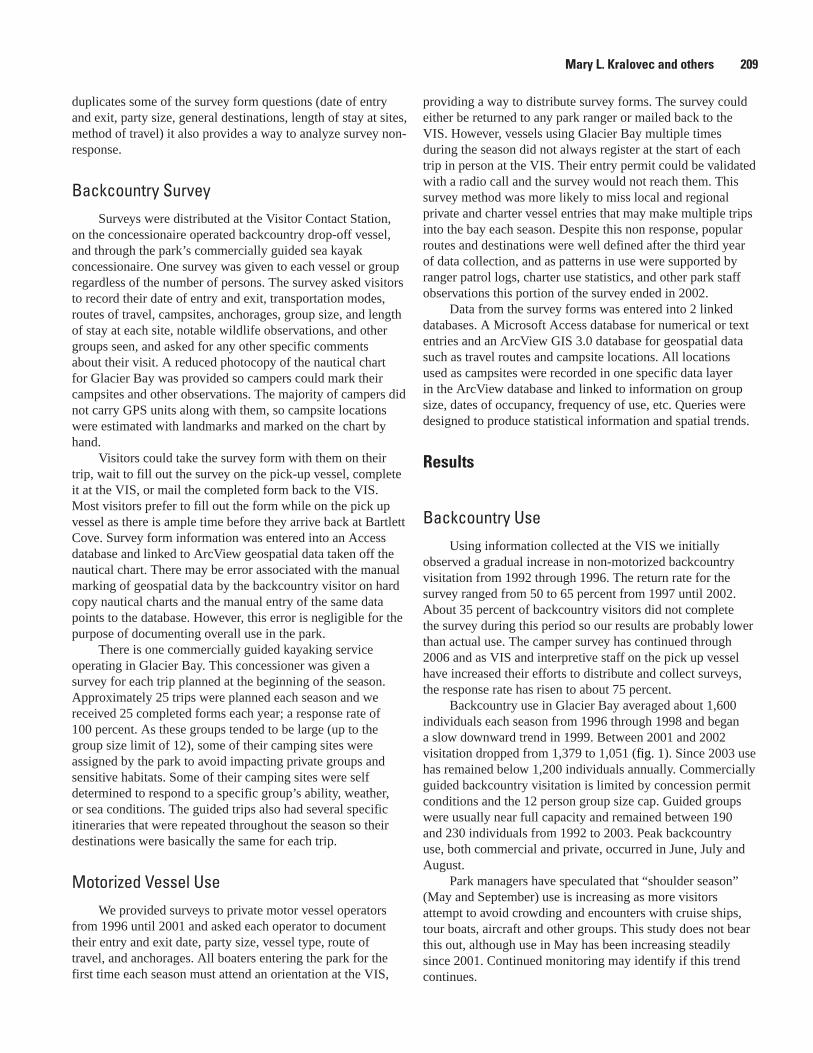
duplicates some of the survey form questions (date of entry and exit, party size, general destinations, length of stay at sites, method of travel) it also provides a way to analyze survey non-response.
Backcountry SurveySurveys were distributed at the Visitor Contact Station,
on the concessionaire operated backcountry drop-off vessel, and through the park’s commercially guided sea kayak concessionaire. One survey was given to each vessel or group regardless of the number of persons. The survey asked visitors to record their date of entry and exit, transportation modes, routes of travel, campsites, anchorages, group size, and length of stay at each site, notable wildlife observations, and other groups seen, and asked for any other specific comments about their visit. A reduced photocopy of the nautical chart for Glacier Bay was provided so campers could mark their campsites and other observations. The majority of campers did not carry GPS units along with them, so campsite locations were estimated with landmarks and marked on the chart by hand.
Visitors could take the survey form with them on their trip, wait to fill out the survey on the pick-up vessel, complete it at the VIS, or mail the completed form back to the VIS. Most visitors prefer to fill out the form while on the pick up vessel as there is ample time before they arrive back at Bartlett Cove. Survey form information was entered into an Access database and linked to ArcView geospatial data taken off the nautical chart. There may be error associated with the manual marking of geospatial data by the backcountry visitor on hard copy nautical charts and the manual entry of the same data points to the database. However, this error is negligible for the purpose of documenting overall use in the park.
There is one commercially guided kayaking service operating in Glacier Bay. This concessioner was given a survey for each trip planned at the beginning of the season. Approximately 25 trips were planned each season and we received 25 completed forms each year; a response rate of 100 percent. As these groups tended to be large (up to the group size limit of 12), some of their camping sites were assigned by the park to avoid impacting private groups and sensitive habitats. Some of their camping sites were self determined to respond to a specific group’s ability, weather, or sea conditions. The guided trips also had several specific itineraries that were repeated throughout the season so their destinations were basically the same for each trip.
Motorized Vessel UseWe provided surveys to private motor vessel operators
from 1996 until 2001 and asked each operator to document their entry and exit date, party size, vessel type, route of travel, and anchorages. All boaters entering the park for the first time each season must attend an orientation at the VIS,
providing a way to distribute survey forms. The survey could either be returned to any park ranger or mailed back to the VIS. However, vessels using Glacier Bay multiple times during the season did not always register at the start of each trip in person at the VIS. Their entry permit could be validated with a radio call and the survey would not reach them. This survey method was more likely to miss local and regional private and charter vessel entries that may make multiple trips into the bay each season. Despite this non response, popular routes and destinations were well defined after the third year of data collection, and as patterns in use were supported by ranger patrol logs, charter use statistics, and other park staff observations this portion of the survey ended in 2002.
Data from the survey forms was entered into 2 linked databases. A Microsoft Access database for numerical or text entries and an ArcView GIS 3.0 database for geospatial data such as travel routes and campsite locations. All locations used as campsites were recorded in one specific data layer in the ArcView database and linked to information on group size, dates of occupancy, frequency of use, etc. Queries were designed to produce statistical information and spatial trends.
Results
Backcountry UseUsing information collected at the VIS we initially
observed a gradual increase in non-motorized backcountry visitation from 1992 through 1996. The return rate for the survey ranged from 50 to 65 percent from 1997 until 2002. About 35 percent of backcountry visitors did not complete the survey during this period so our results are probably lower than actual use. The camper survey has continued through 2006 and as VIS and interpretive staff on the pick up vessel have increased their efforts to distribute and collect surveys, the response rate has risen to about 75 percent.
Backcountry use in Glacier Bay averaged about 1,600 individuals each season from 1996 through 1998 and began a slow downward trend in 1999. Between 2001 and 2002 visitation dropped from 1,379 to 1,051 (fig. 1). Since 2003 use has remained below 1,200 individuals annually. Commercially guided backcountry visitation is limited by concession permit conditions and the 12 person group size cap. Guided groups were usually near full capacity and remained between 190 and 230 individuals from 1992 to 2003. Peak backcountry use, both commercial and private, occurred in June, July and August.
Park managers have speculated that “shoulder season” (May and September) use is increasing as more visitors attempt to avoid crowding and encounters with cruise ships, tour boats, aircraft and other groups. This study does not bear this out, although use in May has been increasing steadily since 2001. Continued monitoring may identify if this trend continues.
Mary L. Kralovec and others 209
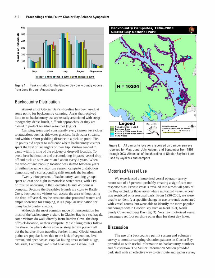
Figure 2. All campsite locations recorded on camper surveys received for May, June, July, August, and September from 1996 through 2003. Almost all of the shoreline of Glacier Bay has been used by kayakers and campers.
Backcountry DistributionAlmost all of Glacier Bay’s shoreline has been used, at
some point, for backcountry camping. Areas that received little or no backcountry use are usually associated with steep topography, dense brush, difficult approaches, or they are closed to protect sensitive resources (fig. 2).
Camping areas used consistently every season were close to attractions such as tidewater glaciers, fresh water streams, and within a short paddling distance to a pick-up point. Pick-up points did appear to influence where backcountry visitors spent the first or last nights of their trip. Visitors tended to camp within 1 mile of the pick-up or drop-off location. To avoid bear habituation and accumulating impacts, vessel drop-off and pick-up sites are rotated about every 2 years. When the drop-off and pick-up location was shifted between years or within the same visitor use season, campsite distribution demonstrated a corresponding shift towards the location.
Twenty-nine percent of backcountry camping groups spent at least one night in motorless water areas, with 11% of this use occurring in the Beardslee Island Wilderness complex. Because the Beardslee Islands are close to Bartlett Cove, backcountry visitors can access the area without using the drop-off vessel. As the area contains protected waters and ample shoreline for camping, it is a popular destination for many backcountry visitors.
Although the most common mode of transportation for most of the backcountry visitors in Glacier Bay is a sea kayak, some visitors do walk directly from Bartlett Cove, the drop-off/pick-location, or their campsite. Most hiking routes follow the shoreline where dense alder or steep terrain prevent all but the hardiest from traveling further inland. Glacial outwash plains are popular hikes due to the lack of vegetation, level terrain, and open vistas. Popular hiking areas include Riggs, McBride, Lamplugh and Reid Glaciers, and Geikie Inlet.
Motorized Vessel UseWe experienced a motorized vessel operator survey
return rate of 16 percent; probably creating a significant non-response bias. Private vessels traveled into almost all parts of the Bay excluding those areas where motorized vessel access was restricted on a seasonal basis. From 1996-2001, we were unable to identify a specific change in use or trends associated with vessel routes, but were able to identify the more popular anchorages within Glacier Bay such as Reid Inlet, North Sandy Cove, and Berg Bay (fig. 3). Very few motorized vessel passengers set foot on shore other than for short day hikes.
Discussion
The use of a backcountry permit system and voluntary survey to monitor camping visitation patterns in Glacier Bay provided us with useful information on backcountry numbers and distribution. The Visitor Information Station provided park staff with an effective way to distribute and gather survey
Figure 1. Peak visitation for the Glacier Bay backcountry occurs from June through August each year.
210 Proceedings of the Fourth Glacier Bay Science Symposium
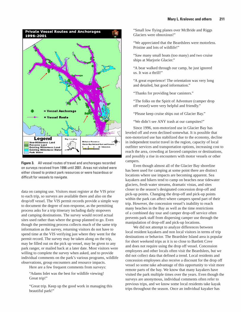
Figure �. All vessel routes of travel and anchorages recorded on surveys received from 1996 until 2001. Areas not visited were either closed to protect park resources or were hazardous or difficult for vessels to navigate.
data on camping use. Visitors must register at the VIS prior to each trip, so surveys are available there and also on the drop/off vessel. The VIS permit records provide a simple way to document the degree of non-response, as the permitting process asks for a trip itinerary including daily stopovers and camping destinations. The survey would record actual sites used rather than where the group planned to go. Even though the permitting process collects much of the same trip information as the survey, returning visitors do not have to spend time at the VIS verifying just where they went for the permit record. The survey may be taken along on the trip, may be filled out on the pick up vessel, may be given to any park ranger, or mailed back at a later date. Most visitors were willing to complete the survey when asked, and to provide individual comments on the park’s various programs, wildlife observations, group encounters and resource impacts.
Here are a few frequent comments from surveys:
“Adams Inlet was the best for wildlife viewing! Great trip!”
“Great trip. Keep up the good work in managing this beautiful park!”
“Small low flying planes over McBride and Riggs Glaciers were obnoxious!”
“We appreciated that the Beardslees were motorless. Pristine and lots of wildlife!”
“Saw many small boats (too many) and two cruise ships at Marjorie Glacier.”
“A bear walked through our camp, he just ignored us. It was a thrill!”
“A great experience! The orientation was very long and detailed, but good information.”
“Thanks for providing bear canisters.”
“The folks on the Spirit of Adventure (camper drop off vessel) were very helpful and friendly.”
“Please keep cruise ships out of Glacier Bay.”
“We didn’t see ANY trash at our campsites!”
Since 1996, non-motorized use in Glacier Bay has leveled off and even declined somewhat. It is possible that non-motorized use has stabilized due to the economy, decline in independent tourist travel in the region, capacity of local outfitter services and transportation options, increasing cost to reach the area, crowding at favored campsites or destinations, and possibly a rise in encounters with motor vessels or other campers.
Even though almost all of the Glacier Bay shoreline has been used for camping at some point there are distinct locations where use impacts are becoming apparent. Sea kayakers and hikers tend to camp on beaches near tidewater glaciers, fresh water streams, dramatic vistas, and sites closer to the season’s designated concession drop-off and pick-up points. Changing the drop-off and pick-up points within the park can affect where campers spend part of their trip. However, the concession vessel’s inability to reach many beaches in the Bay as well as the time restrictions of a combined day tour and camper drop-off service often prevents park staff from dispersing camper use through the manipulation of drop-off and pick-up locations.
We did not attempt to analyze differences between local resident kayakers and non local visitors in terms of trip destinations or behavior. The Beardslee Island area is popular for short weekend trips as it is so close to Bartlett Cove and does not require using the drop off vessel. Concession employees and other locals often visit the Beardslees, but we did not collect data that defined a trend. Local residents and concession employees also receive a discount for the drop off vessel so some take advantage of this opportunity to visit more remote parts of the bay. We know that many kayakers have visited the park multiple times over the years. Even though the surveys are anonymous, individual comments often refer to previous trips, and we know some local residents take kayak trips throughout the season. Once an individual kayaker has
Mary L. Kralovec and others 211
received an orientation for the season they are not required to complete it again. A new permit is issued to them for each trip and a new survey given out, but the VIS staff can determine a repeat visitor using the permit database. Using the permit database we could analyze the percentage of repeat visits and probably determine a trend in destinations.
It does not seem apparent that motor vessel visitation is shifting to the shoulder seasons of May and September even though there is less vessel traffic, fewer aircraft overflights, and less chance of seeing or hearing other people at these times. While use in May has increased slightly, the trend is not clear. Long term monitoring of backcountry use may provide a better indication of this use.
Comments from the backcountry survey frequently include concerns about the number of motor vessels seen and heard, including cruise ships, the amount of low flying aircraft noise, and the number of people encountered in what is considered to be a pristine wilderness. Many kayakers appreciate the five areas where motor vessels are excluded during May 15 through September 30 and comment that they would like the motor restrictions expanded. Occasionally we received a comment asking for increased drop off and pick up vessel services so more remote parts of the bay could be reached during shorter trips.
A voluntary survey distributed from the VIS probably does not reach a significant portion of private vessel operators especially those visiting the bay multiple times per season. Once a particular vessel crew has received an orientation at the VIS for the season and their permits issued, they may call in their arrivals and departures from Glacier Bay by radio. Many vessels apply for and receive entry permits while underway for other ports, so making surveys available on websites or email would not necessarily reach them. We realized a significant number of vessels would not have access to the survey forms even if the surveys were sent out by mail with permits, and as motor vessel use patterns were fairly well defined early in the survey and backed up by other observations, this portion of the project was discontinued. The vessel entry permitting process asks for destination information, ranger patrol logs and other staff field logs also provide corroborative observations on vessel use in the bay. Based on the survey data we did collect in conjunction with other observations, private motor vessel traffic patterns in the park have remained fairly consistent over the past 10 years. Because the number of vessels entering Glacier Bay on a daily basis is currently restricted and the length of their stay limited, vessel numbers will likely remain un-changed for the near future. Vessel distribution, routes, and anchorages will also likely remain consistent due to terrain, popular viewing locations, and resource protection actions.
Boaters commented fairly often about the complicated permit procedure, the number of regulations and limited opportunities to visit the bay, both on surveys and directly to VIS staff. The boater permit database maintained at the VIS could determine if these comments were received from local, regional, or repeat visiting vessels, or single visit vessels
traveling long distances to reach the park. First time motor vessel visitors often commented to the VIS staff that the orientation materials received were thorough and helpful.
Management Implications
This survey has provided essential information on Glacier Bay National Park backcountry visitor and vessel use and distribution patterns. Park staff are now able to identify areas that presently show impacts from human use as well as the type, intensity, and persistence of damage associated with this use. Impacted as well as pristine sites can be monitored over time to determine if limits to use or restoration will be needed to protect them. Survey results can also be used to identify areas where sensitive wildlife such as ground-nesting birds, bears, wolves, and molting waterfowl may be impacted by human activity. The campsite data has focused attention on where and why humans are more likely to encounter bears and has helped us clarify our visitor safety messages. Conflicts between user groups or activities may be addressed before they actually occur.
Survey results also demonstrated how the camper drop off and pick up points affects kayaker destinations and corresponding camp distribution in Glacier Bay. Changes in the vessel service will affect the park’s ability to manage camper impacts over time. If the drop off service is discontinued or reduced or the vessel is unable to land at many beaches, the Beardless Islands area could see an increase in use and a corresponding increase in long term impacts to wildlife and beaches.
The survey did not attempt to analyze why visitors did not come to Glacier Bay. The survey only reflects the use of people who were able to reach the park and were prepared for undeveloped wilderness conditions of the backcountry. There are no plans to provide additional facilities in the backcountry such as maintained trails, vehicle access or cabins.
Permit records kept by the VIS will probably be a more efficient way to gather motor vessel use data, as vessels are required to contact the VIS at least by radio when they arrive and depart. Camper permit information collected by the VIS will also provide much of the data gathered by the survey, but may not detect subtle trends in campsite use, user group conflicts, or site impacts over time. In the future the survey can be modified or repeated on a bi-annual basis as management needs change.
Suggested Citation
Kralovec, M.L., Banks, A.L., and Lentfer, H., 2007, Distribution and number of backcountry visitors in Glacier Bay National Park 1996-2003, in Piatt, J.F., and Gende, S.M., eds., Proceedings of the Fourth Glacier Bay Science Symposium, October 26–28, 2004: U.S. Geological Survey Scientific Investigations Report 2007-5047, p. 204-207.
212 Proceedings of the Fourth Glacier Bay Science Symposium
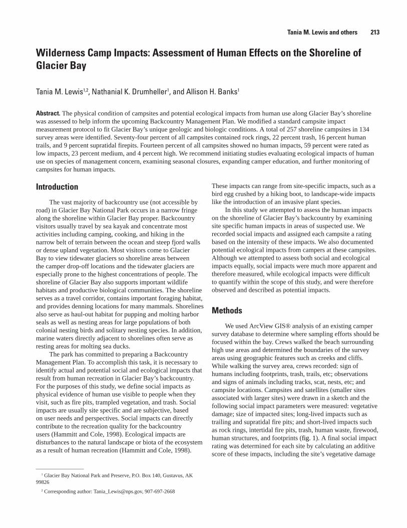
Wilderness Camp Impacts: Assessment of Human Effects on the Shoreline of Glacier Bay
Tania M. Lewis1,2, Nathanial K. Drumheller1, and Allison H. Banks1
Abstract. The physical condition of campsites and potential ecological impacts from human use along Glacier Bay’s shoreline was assessed to help inform the upcoming Backcountry Management Plan. We modified a standard campsite impact measurement protocol to fit Glacier Bay’s unique geologic and biologic conditions. A total of 257 shoreline campsites in 134 survey areas were identified. Seventy-four percent of all campsites contained rock rings, 22 percent trash, 16 percent human trails, and 9 percent supratidal firepits. Fourteen percent of all campsites showed no human impacts, 59 percent were rated as low impacts, 23 percent medium, and 4 percent high. We recommend initiating studies evaluating ecological impacts of human use on species of management concern, examining seasonal closures, expanding camper education, and further monitoring of campsites for human impacts.
1 Glacier Bay National Park and Preserve, P.O. Box 140, Gustavus, AK 99826
2 Corresponding author: [email protected], 907-697-2668
Introduction
The vast majority of backcountry use (not accessible by road) in Glacier Bay National Park occurs in a narrow fringe along the shoreline within Glacier Bay proper. Backcountry visitors usually travel by sea kayak and concentrate most activities including camping, cooking, and hiking in the narrow belt of terrain between the ocean and steep fjord walls or dense upland vegetation. Most visitors come to Glacier Bay to view tidewater glaciers so shoreline areas between the camper drop-off locations and the tidewater glaciers are especially prone to the highest concentrations of people. The shoreline of Glacier Bay also supports important wildlife habitats and productive biological communities. The shoreline serves as a travel corridor, contains important foraging habitat, and provides denning locations for many mammals. Shorelines also serve as haul-out habitat for pupping and molting harbor seals as well as nesting areas for large populations of both colonial nesting birds and solitary nesting species. In addition, marine waters directly adjacent to shorelines often serve as resting areas for molting sea ducks.
The park has committed to preparing a Backcountry Management Plan. To accomplish this task, it is necessary to identify actual and potential social and ecological impacts that result from human recreation in Glacier Bay’s backcountry. For the purposes of this study, we define social impacts as physical evidence of human use visible to people when they visit, such as fire pits, trampled vegetation, and trash. Social impacts are usually site specific and are subjective, based on user needs and perspectives. Social impacts can directly contribute to the recreation quality for the backcountry users (Hammitt and Cole, 1998). Ecological impacts are disturbances to the natural landscape or biota of the ecosystem as a result of human recreation (Hammitt and Cole, 1998).
These impacts can range from site-specific impacts, such as a bird egg crushed by a hiking boot, to landscape-wide impacts like the introduction of an invasive plant species.
In this study we attempted to assess the human impacts on the shoreline of Glacier Bay’s backcountry by examining site specific human impacts in areas of suspected use. We recorded social impacts and assigned each campsite a rating based on the intensity of these impacts. We also documented potential ecological impacts from campers at these campsites. Although we attempted to assess both social and ecological impacts equally, social impacts were much more apparent and therefore measured, while ecological impacts were difficult to quantify within the scope of this study, and were therefore observed and described as potential impacts.
Methods
We used ArcView GIS® analysis of an existing camper survey database to determine where sampling efforts should be focused within the bay. Crews walked the beach surrounding high use areas and determined the boundaries of the survey areas using geographic features such as creeks and cliffs. While walking the survey area, crews recorded: sign of humans including footprints, trash, trails, etc; observations and signs of animals including tracks, scat, nests, etc; and campsite locations. Campsites and satellites (smaller sites associated with larger sites) were drawn in a sketch and the following social impact parameters were measured: vegetative damage; size of impacted sites; long-lived impacts such as trailing and supratidal fire pits; and short-lived impacts such as rock rings, intertidal fire pits, trash, human waste, firewood, human structures, and footprints (fig. 1). A final social impact rating was determined for each site by calculating an additive score of these impacts, including the site’s vegetative damage
Tania M. Lewis and others 21�
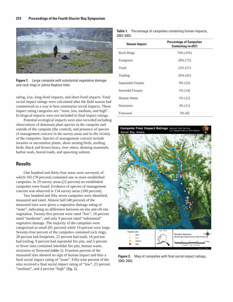
rating, size, long-lived impacts, and short-lived impacts. Final social impact ratings were calculated after the field season had commenced as a way to best summarize social impacts. These impact rating categories are: “none, low, medium, and high”. Ecological impacts were not included in final impact ratings.
Potential ecological impacts were also recorded including observations of dominant plant species in the campsite and outside of the campsite (the control), and presence of species of management concern in the survey areas and in the vicinity of the campsites. Species of management concern include invasive or uncommon plants, shore nesting birds, molting birds, black and brown bears, river otters, denning mammals, harbor seals, boreal toads, and spawning salmon.
Results
One hundred and thirty-four areas were surveyed, of which 105 (78 percent) contained one or more established campsites. In 29 survey areas (22 percent) no established campsites were found. Evidence of species of management concern was observed in 134 survey areas (100 percent).
Two hundred and fifty seven campsites were identified, measured and rated. Almost half (48 percent) of the measured sites were given a vegetative damage rating of “none”, indicating no difference between on-site and off-site vegetation. Twenty-five percent were rated “low”, 18 percent rated “moderate”, and only 9 percent rated “substantial” vegetative damage. The majority of the campsites were categorized as small (81 percent) while 19 percent were large. Seventy-four percent of the campsites contained rock rings, 28 percent had footprints, 22 percent had trash, 16 percent had trailing, 9 percent had supratidal fire pits, and 5 percent or fewer sites contained intertidal fire pits, human waste, structures or firewood (table 1). Fourteen percent of the measured sites showed no sign of human impact and thus a final social impact rating of “none”. Fifty-nine percent of the sites received a final social impact rating of “low”, 23 percent “medium”, and 4 percent “high” (fig. 2).
Table 1. Percentage of campsites containing human impacts, 2002-2003.
Human ImpactPercentage of Campsites
Containing (n=257)
Rock Rings 74% (191)
Footprints 28% (72)
Trash 22% (57)
Trailing 16% (41)
Supratidal Firepits 9% (22)
Intertidal Firepits 5% (14)
Human Waste 5% (12)
Structures 4% (11)
Firewood 3% (8)
Figure 2. Map of campsites with final social impact ratings, 2002-2003.
Figure 1. Large campsite with substantial vegetative damage and rock rings in Johns Hopkins Inlet.
21� Proceedings of the Fourth Glacier Bay Symposium
Discussion and Conclusions
Social ImpactsThe locations of campsites with medium and high
final social impact ratings were generally (1) near tidewater glaciers, (2) near camper drop-off locations, (3) along popular travel routes, often between camper drop-off locations and glaciers, and/or (4) in areas of steep terrain that concentrate camping.
Glacier Bay National Park requires a backcountry orientation to all campers in which they are encouraged to leave no trace of camping, and specifically asked to build fires only in the intertidal zone. Despite these requirements most campsites were found contain rock rings and many had trash and supratidal firepits. Rock rings were much more common in the northern portions of the bay than the southern, probably due to higher use and rockier ground substrates that make tent stakes difficult to use. Most trash appeared to be items left unintentionally, but occasionally we found trash that appeared purposefully left in fire pits.
Overall the social impacts on the shoreline of Glacier Bay appear minimal. Approximately 2,000 people camp in the backcountry every year, and because there are no established campsites, campers generally spread out along the shoreline as they find their own places to camp. Campsite locations also continually change over time in Glacier Bay. The land is rising approximately 2.5 cm per year from glacial rebound so the shoreline is in a constant state of renewal. Campsites that were once in beach meadows are now covered with bushes, while areas still submerged by high tides will be soon be dry meadows suitable for camping. Plant succession processes in recently deglaciated areas also cover up vegetative damage from camping. Another contributing factor in the low level of social impacts observed is the way in which people camp in Glacier Bay. Campers are taught during their orientation to cook and eat in the intertidal zone where the next high tide will wash away food remains and smells. This greatly reduces time spent above the intertidal zone, and the overall footprint of the campsite tends to be smaller than if it included both eating and sleeping areas.
Potential Ecological ImpactsGiven the scope of this project we did not attempt
to make any conclusions about the number of species or individuals that are impacted by campers. However we did observe several potential ecological impacts in specific locations. For example, we observed an invasive species of dandelion (Taraxacum spp.) in many parts of the bay and uncommon orchid species (Platanthera and Cypripedium spp.) near several camping areas.
We observed thirteen species of birds nesting on the ground in the vicinity of camping areas and rafts of flightless birds in molt near the shore of many camping areas in the
Tania M. Lewis and others 215
latter part of the summer. Nesting success and survivorship of these birds may be affected due to trampling or disturbance.
We observed signs of bear, river otter, wolf, coyote, mink and wolverine in camping areas. We saw denning marmots in three camping areas, but found no active dens of any other species. We found potential for disturbance of harbor seals from campers on Leland Island, in McBride Inlet, and in the Beardslee Islands. Harbor seals are of special management concern because their numbers have declined drastically since 1992 and because harbor seals often leave their haulouts in the presence of humans.
Finally, we observed boreal toads in several camping areas. Boreal toads and other amphibians are declining in the region and throughout the world although it is unlikely that campers contribute to this decline. We saw spawning salmon in 11 camping areas. Not only are spawning salmon sensitive to disturbance by people walking in the stream bed, but these areas also attract many species of birds and mammals and thus represent a valuable food resource to be protected.
Management Implications
Social and ecological impacts along the shoreline of Glacier Bay may be minimized by, 1) initiating further studies on distribution, abundance, and human disturbance of species of management concern, 2) considering changes to seasonal human use closures to further protect species of concern, 3) expanding current camper education, including the results of this study, and 4) monitoring long-term camper impacts at a random selection of campsites of varying human use.
Acknowledgments
Many thanks to Greg Streveler, Paul Twardock, Nikki Koehler, Bonnie Harris, Judy Brakel, Rusty Yerxa, Bill Eichenlaub, Justin Smith, Randy Ramey, Steve Partridge, Mia Grifalconi, Phoebe Vanselow, Marylou Blakeslee, Ken Grant, Joe Tiblis, and anonymous reviewers.
References Cited
Hammitt, W.E. and Cole, D.N., 1998, Wildland Recreation, Ecology and Management, 2nd ed.,: New York, John Wiley & Sons, Inc.
Suggested Citation
Lewis, T.M., Drumheller, N.K., and Banks, A.H., 2007, Wilderness camp impacts: Assessment of human effects on the shoreline of Glacier Bay, in Piatt, J.F., and Gende, S.M., eds., Proceedings of the Fourth Glacier Bay Science Symposium, October 26–28, 2004: U.S. Geological Survey Scientific Investigations Report 2007-5047, p. 208-212.

This page is intentionally left blank.
21� Proceedings of the Fourth Glacier Bay Symposium
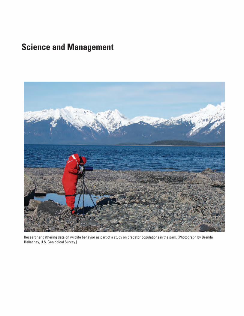
Science and Management
Researcher gathering data on wildlife behavior as part of a study on predator populations in the park. (Photograph by Brenda Ballachey, U.S. Geological Survey.)

21� Proceedings of the Fourth Glacier Bay Science Symposium
This page is intentionally left blank.
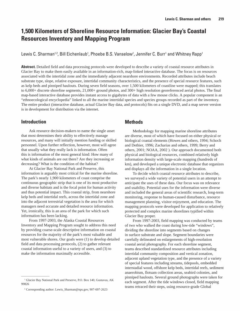
1,500 Kilometers of Shoreline Resource Information: Glacier Bay’s Coastal Resources Inventory and Mapping Program
Lewis C. Sharman1,2, Bill Eichenlaub1, Phoebe B.S. Vanselow1, Jennifer C. Burr1 and Whitney Rapp1
Abstract. Detailed field and data processing protocols were developed to describe a variety of coastal resource attributes in Glacier Bay to make them easily available in an information-rich, map-linked interactive database. The focus is on resources associated with the intertidal zone and the immediately adjacent nearshore environments. Recorded attributes include beach substrate type, slope, relative exposure, intertidal community characteristics, and the presence of special resource features, such as kelp beds and pinniped haulouts. During seven field seasons, over 1,500 kilometers of coastline were mapped; this translates to 6,000+ discrete shoreline segments, 21,000+ ground photos, and 300+ high resolution georeferenced aerial photos. The final map-based interactive database provides instant access to gigabytes of data with a few mouse clicks. A popular component is an “ethnoecological encyclopedia” linked to all the marine intertidal species and species groups recorded as part of the inventory. The entire product (interactive database, actual Glacier Bay data, and protocols) fits on a single DVD, and a map server version is in development for distribution via the internet.
1 Glacier Bay National Park and Preserve, P.O. Box 140, Gustavus, AK 99826
2 Corresponding author: [email protected], 907-697-2623
Introduction
Ask resource decision-makers to name the single asset that most determines their ability to effectively manage resources, and many will initially mention funding or skilled personnel. Upon further reflection, however, most will agree that usually what they really lack is information. Often this is information of the most general kind: How many of what kinds of animals are out there? Are they increasing or decreasing? What is the condition of the habitat?
At Glacier Bay National Park and Preserve, this information is arguably most critical for the marine shoreline. The park’s nearly 1,900 kilometers of coast comprise the continuous geographic strip that is one of its most productive and diverse habitats and is the focal point for human activity and thus potential impact. This coastal strip, from nearshore kelp beds and intertidal reefs, across the intertidal zone and into the adjacent terrestrial vegetation is the area for which managers need accurate and detailed resource information. Yet, ironically, this is an area of the park for which such information has been lacking.
From 1997-2003, the Alaska Coastal Resources Inventory and Mapping Program sought to address this need by providing coarse-scale descriptive information on coastal resources for the majority of the park’s most valuable and most vulnerable shores. Our goals were (1) to develop detailed field and data processing protocols, (2) to gather relevant coastal information useful to a variety of users, and (3) to make the information maximally accessible.
Methods
Methodology for mapping marine shoreline attributes are diverse, most of which have focused on either physical or biological coastal elements (Howes and others, 1994; Schoch and Dethier, 1996; Zacharias and others, 1999; Berry and others, 2001; NOAA, 2002 ). Our approach documented both physical and biological resources, combined relatively high information density with large-scale mapping (hundreds of km), and developed a unique electronic database that organizes and displays all the information in a single location.
To decide which coastal resource attributes to describe, we surveyed a wide variety of potential users in an attempt to anticipate the uses of these data. Our focus was on relevance and usability. Potential uses for the information were diverse and included the general areas of scientific research, long-term monitoring, response to human-caused disturbance, resource management planning, visitor enjoyment, and education. The mapping protocols were developed for application to relatively protected and complex marine shorelines typified within Glacier Bay proper.
From 1997-2003, field mapping was conducted by teams of two who walked the coast during low-tide “windows”, dividing the shoreline into segments based on changes in surface substrate and slope. Segment boundaries were carefully delineated on enlargements of high-resolution coastal aerial photography. For each shoreline segment, teams described standardized resource attributes including intertidal community composition and vertical zonation, adjacent upland vegetation type, and the presence of a variety of special features including streams, tidepools, embedded interstadial wood, offshore kelp beds, intertidal reefs, sediment anaerobism, flotsam collection areas, seabird colonies, and pinniped haulouts. Several ground photographs were taken for each segment. After the tide windows closed, field mapping teams retraced their steps, using resource-grade Global
Lewis C. Sharman and others 219
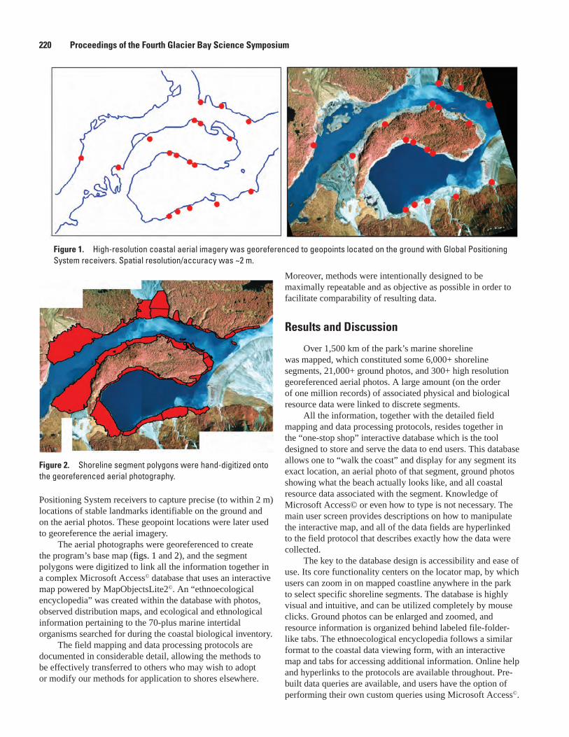
Figure 2. Shoreline segment polygons were hand-digitized onto the georeferenced aerial photography.
Figure 1. High-resolution coastal aerial imagery was georeferenced to geopoints located on the ground with Global Positioning System receivers. Spatial resolution/accuracy was ~2 m.
Positioning System receivers to capture precise (to within 2 m) locations of stable landmarks identifiable on the ground and on the aerial photos. These geopoint locations were later used to georeference the aerial imagery.
The aerial photographs were georeferenced to create the program’s base map (figs. 1 and 2), and the segment polygons were digitized to link all the information together in a complex Microsoft Access© database that uses an interactive map powered by MapObjectsLite2©. An “ethnoecological encyclopedia” was created within the database with photos, observed distribution maps, and ecological and ethnological information pertaining to the 70-plus marine intertidal organisms searched for during the coastal biological inventory.
The field mapping and data processing protocols are documented in considerable detail, allowing the methods to be effectively transferred to others who may wish to adopt or modify our methods for application to shores elsewhere.
Moreover, methods were intentionally designed to be maximally repeatable and as objective as possible in order to facilitate comparability of resulting data.
Results and Discussion
Over 1,500 km of the park’s marine shoreline was mapped, which constituted some 6,000+ shoreline segments, 21,000+ ground photos, and 300+ high resolution georeferenced aerial photos. A large amount (on the order of one million records) of associated physical and biological resource data were linked to discrete segments.
All the information, together with the detailed field mapping and data processing protocols, resides together in the “one-stop shop” interactive database which is the tool designed to store and serve the data to end users. This database allows one to “walk the coast” and display for any segment its exact location, an aerial photo of that segment, ground photos showing what the beach actually looks like, and all coastal resource data associated with the segment. Knowledge of Microsoft Access© or even how to type is not necessary. The main user screen provides descriptions on how to manipulate the interactive map, and all of the data fields are hyperlinked to the field protocol that describes exactly how the data were collected.
The key to the database design is accessibility and ease of use. Its core functionality centers on the locator map, by which users can zoom in on mapped coastline anywhere in the park to select specific shoreline segments. The database is highly visual and intuitive, and can be utilized completely by mouse clicks. Ground photos can be enlarged and zoomed, and resource information is organized behind labeled file-folder-like tabs. The ethnoecological encyclopedia follows a similar format to the coastal data viewing form, with an interactive map and tabs for accessing additional information. Online help and hyperlinks to the protocols are available throughout. Pre-built data queries are available, and users have the option of performing their own custom queries using Microsoft Access©.
220 Proceedings of the Fourth Glacier Bay Science Symposium
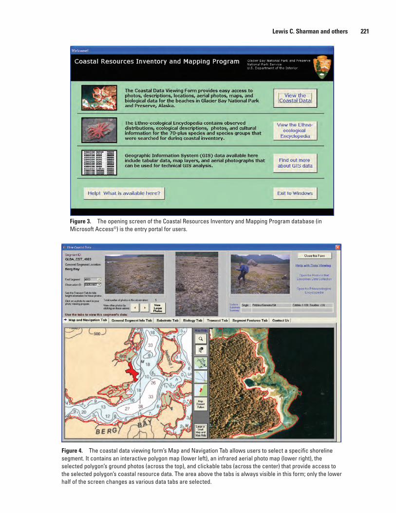
Figure �. The opening screen of the Coastal Resources Inventory and Mapping Program database (in Microsoft Access©) is the entry portal for users.
Figure �. The coastal data viewing form’s Map and Navigation Tab allows users to select a specific shoreline segment. It contains an interactive polygon map (lower left), an infrared aerial photo map (lower right), the selected polygon’s ground photos (across the top), and clickable tabs (across the center) that provide access to the selected polygon’s coastal resource data. The area above the tabs is always visible in this form; only the lower half of the screen changes as various data tabs are selected.
Lewis C. Sharman and others 221

Figure 5. The coastal data viewing form’s Transect Tab contains simple graphs summarizing complex vertical zonation data. Links to sections of the help document pertaining directly to this tab are present in the top right corner and above the left graph.
Figure �. The ethnoecological encyclopedia contains detailed information about the 70-plus species or species groups searched for during the coastal inventory. Clickable tabs across the top of the screen provide access to physical, ecological, and ethnological information about the organism. Photos of the organism (upper left) and an interactive observed distribution map (lower left) are always visible.
222 Proceedings of the Fourth Glacier Bay Science Symposium
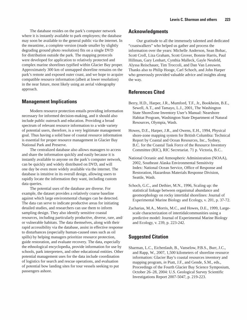
The database resides on the park’s computer network where it is instantly available to park employees; the database may soon be available to the general public via the internet. In the meantime, a complete version (made smaller by slightly degrading ground photo resolution) fits on a single DVD for distribution outside the park. The mapping protocols were developed for application to relatively protected and complex marine shorelines typified within Glacier Bay proper. Approximately 300 km of unmapped shoreline remains on the park’s remote and exposed outer coast, and we hope to acquire compatible resource information (albeit at lower resolution) in the near future, most likely using an aerial videography approach.
Management Implications
Modern resource protection entails providing information necessary for informed decision-making, and it should also include public outreach and education. Providing a broad spectrum of relevant resource information to a wide variety of potential users, therefore, is a very legitimate management goal. Thus having a solid base of coastal resource information is essential for proper resource management in Glacier Bay National Park and Preserve.
The centralized database also allows managers to access and share the information quickly and easily because it is instantly available to anyone on the park’s computer network, can be quickly and widely distributed on DVD, and will one day be even more widely available via the internet. The database is intuitive in its overall design, allowing users to rapidly locate the information they want, including custom data queries.
The potential uses of the database are diverse. For example, the dataset provides a relatively coarse baseline against which large environmental changes can be detected. The data can serve to indicate productive areas for initiating detailed studies, and researchers can use them to inform sampling design. They also identify sensitive coastal resources, including particularly productive, diverse, rare, and/or vulnerable habitats. The data themselves, along with their rapid accessibility via the database, assist in effective response to disturbances (especially human-caused ones such as oil spills) by helping managers prioritize resource protection, guide restoration, and evaluate recovery. The data, especially the ethnological encyclopedia, provide information for use by schools, park interpreters, and other educational entities. Other potential management uses for the data include coordination of logistics for search and rescue operations, and evaluation of potential bow landing sites for tour vessels seeking to put passengers ashore.
Acknowledgments
Our gratitude to all the immensely talented and dedicated “coastwalkers” who helped us gather and process the information over the years: Michelle Anderson, Sean Bohac, Scott Croll, Liza Graham, Scott Grover, Bonnie Harris, Paul Hillman, Gary Lenhart, Cynthia Malleck, Gayle Neufeld, Alyssa Reischauer, Tim Troccoli, and Dan Van Leeuwen. Thanks also to Philip Hooge, Carl Schoch, and John Harper who generously provided valuable advice and insights along the way.
References Cited
Berry, H.D., Harper, J.R., Mumford, T.F., Jr., Bookheim, B.E., Sewell, A.T., and Tamayo, L.J., 2001, The Washington State ShoreZone Inventory User’s Manual: Nearshore Habitat Program, Washington State Department of Natural Resources, Olympia, Wash.
Howes, D.E., Harper, J.R., and Owens, E.H., 1994, Physical shore-zone mapping system for British Columbia: Technical Report by Coastal and Ocean Resources, Inc., Sydney, B.C. for the Coastal Task Force of the Resource Inventory Committee (RIC), RIC Secretariat. 71 p. Victoria, B.C..
National Oceanic and Atmospheric Administration (NOAA), 2002, Southeast Alaska Environmental Sensitivity Index: National Ocean Service, Office of Response and Restoration, Hazardous Materials Response Division, Seattle, Wash.
Schoch, G.C., and Dethier, M.N., 1996, Scaling up: the statistical linkage between organismal abundance and geomorphology on rocky intertidal shorelines: Journal of Experimental Marine Biology and Ecology, v. 201, p. 37-72.
Zacharias, M.A., Morris, M.C., and Howes, D.E., 1999, Large-scale characterization of intertidalcommunities using a predictive model: Journal of Experimental Marine Biology and Ecology, v. 239, p. 223-242.
Suggested Citation
Sharman, L.C., Eichenlaub, B., Vanselow, P.B.S., Burr, J.C., and Rapp, W., 2007, 1,500 kilometers of shoreline resource information: Glacier Bay’s coastal resources inventory and mapping program, in Piatt, J.F., and Gende, S.M., eds., Proceedings of the Fourth Glacier Bay Science Symposium, October 26–28, 2004: U.S. Geological Survey Scientific Investigations Report 2007-5047, p. 219-223.
Lewis C. Sharman and others 22�
Conceptual Ecosystem Models for Glacier Bay National Park and Preserve
Christopher L. Fastie1,3 and Chiska C. Derr2
Abstract. As part of a nationwide effort, the National Park Service is developing an inventory and monitoring program for the three national park units in southeast Alaska. To guide the selection of vital signs to be monitored in each park, we are developing conceptual models of park ecosystem components and the global, regional, and local processes affecting those components. Conceptual models of terrestrial, freshwater, and marine ecosystem components incorporate biotic and abiotic processes and include human influences. A common theme among the models is the environmental change (ecological succession) that occurs following natural or anthropogenic disturbance (e.g., glacial retreat, floods, timber or wildlife harvest, global warming).
Introduction
The Southeast Alaska Park Network (SEAN, including Glacier Bay National Park and Preserve, Klondike Gold Rush National Historical Park, and Sitka National Historical Park) is part of a national initiative to establish a long-term and integrated natural resource monitoring program for the National Park Service. Parks were grouped into 32 networks based on geographic proximity and ecological similarities. In 2003 SEAN began the process of planning a long-term natural resources monitoring program (Derr and others, 2004). Central to this program is the identification of vital signs (indicators of park health to be monitored). As part of the vital signs selection process, conceptual ecosystem models of parks within each network are developed.
The Habitats and Environments of Glacier Bay
We have adopted an image of three overlapping ovals to represent the contact, overlap, and interaction among three ecosystem components (marine, freshwater, and terrestrial) and the habitats within them (fig. 1). A key feature of this conceptualization is that biotic and abiotic processes and population and community interactions in habitats within each type of ecosystem component may be dependent upon processes operating in other ecosystem components. Certain habitats are the products of interaction among two or more ecosystem components (the overlaps in fig. 1), but all habitats have some interactions with all three ecosystem components.
Landscape Drivers of Change
We have identified four broad categories of factors that influence the current environmental conditions in Southeast Alaska, and that are most likely to drive future changes within the ecosystem components (fig. 2). These four landscape drivers of change are climate, landform, ocean processes, and human activity.
Climate. The regional climate has a controlling affect on the landscape of Southeast Alaska. Climate supports the highly productive coastal rainforest, suppliess snowfall to feed alpine glaciers, creates myriad wetland and freshwater ecosystems, and influences marine processes.
Geography, geology and landforms. The geography, geology and landforms of the coastal region largely determine how the regional climate interacts with the land or water to shape a particular ecosystem. The dramatic coastal mountains and islands of the Alexander Archipelago dominate the landscape and create a spatially complex system of marine environments.
Ocean processes. Oceanic patterns and processes support productive and diverse marine ecosystems and strongly influence the weather, biochemistry, and biota of freshwater and terrestrial systems.
Human activity. Human activity (past and present, near and far) has affected all ecosystem components in Southeast Alaska, and has great potential to drive future changes in those components. For example, human effects on Earth’s atmosphere, and the unpredictable risk of resulting climate changes may provide the most serious future concern.
1.
2.
3.
4.
1 Biology Department, Middlebury College, Middlebury, Vermont 05753
2 Southeast Alaska Park Network Inventory & Monitoring Coordinator, National Park Service, 3100 National Park Road, Juneau, Alaska 99801
3 Corresponding author: [email protected]
22� Proceedings of the Fourth Glacier Bay Science Symposium
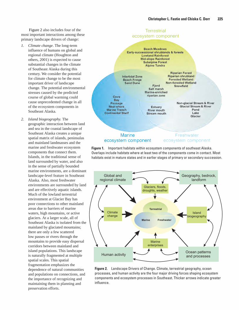
Figure 1. Important habitats within ecosystem components of southeast Alaska. Overlaps include habitats where at least two of the components come in contact. Most habitats exist in mature states and in earlier stages of primary or secondary succession.
Figure 2. Landscape Drivers of Change. Climate, terrestrial geography, ocean processes, and human activity are the four major driving forces shaping ecosystem components and ecosystem processes in Southeast. Thicker arrows indicate greater influence.
Figure 2 also includes four of the most important interactions among these primary landscape drivers of change:
Climate change. The long-term influence of humans on global and regional climate (Houghton and others, 2001) is expected to cause substantial changes in the climate of Southeast Alaska during this century. We consider the potential for climate change to be the most important driver of landscape change. The potential environmental stresses caused by the predicted course of global warming could cause unprecedented change in all of the ecosystem components in Southeast Alaska.
Island biogeography. The geographic interaction between land and sea in the coastal landscape of Southeast Alaska creates a unique spatial matrix of islands, peninsulas and mainland landmasses and the marine and freshwater ecosystem components that connect them. Islands, in the traditional sense of land surrounded by water, and also in the sense of partially bounded marine environments, are a dominant landscape-level feature in Southeast Alaska. Also, most freshwater environments are surrounded by land and are effectively aquatic islands. Much of the lowland terrestrial environment at Glacier Bay has poor connections to other mainland areas due to barriers of marine waters, high mountains, or active glaciers. At a larger scale, all of Southeast Alaska is isolated from the mainland by glaciated mountains; there are only a few scattered low passes or rivers through the mountains to provide easy dispersal corridors between mainland and island populations. This landscape is naturally fragmented at multiple spatial scales. This spatial fragmentation emphasizes the dependence of natural communities and populations on connections, and the importance of recognizing and maintaining them in planning and preservation efforts.
1.
2.
Christopher L. Fastie and Chiska C. Derr 225
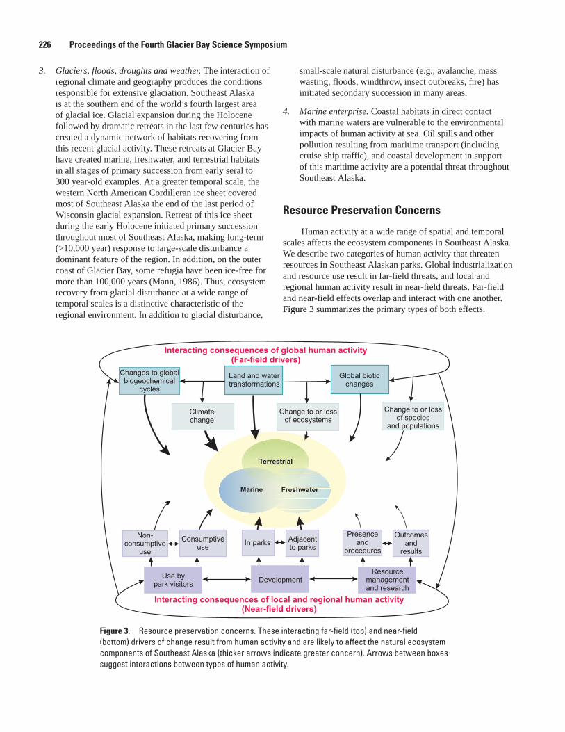
Figure �. Resource preservation concerns. These interacting far-field (top) and near-field (bottom) drivers of change result from human activity and are likely to affect the natural ecosystem components of Southeast Alaska (thicker arrows indicate greater concern). Arrows between boxes suggest interactions between types of human activity.
Glaciers, floods, droughts and weather. The interaction of regional climate and geography produces the conditions responsible for extensive glaciation. Southeast Alaska is at the southern end of the world’s fourth largest area of glacial ice. Glacial expansion during the Holocene followed by dramatic retreats in the last few centuries has created a dynamic network of habitats recovering from this recent glacial activity. These retreats at Glacier Bay have created marine, freshwater, and terrestrial habitats in all stages of primary succession from early seral to 300 year-old examples. At a greater temporal scale, the western North American Cordilleran ice sheet covered most of Southeast Alaska the end of the last period of Wisconsin glacial expansion. Retreat of this ice sheet during the early Holocene initiated primary succession throughout most of Southeast Alaska, making long-term (>10,000 year) response to large-scale disturbance a dominant feature of the region. In addition, on the outer coast of Glacier Bay, some refugia have been ice-free for more than 100,000 years (Mann, 1986). Thus, ecosystem recovery from glacial disturbance at a wide range of temporal scales is a distinctive characteristic of the regional environment. In addition to glacial disturbance,
3. small-scale natural disturbance (e.g., avalanche, mass wasting, floods, windthrow, insect outbreaks, fire) has initiated secondary succession in many areas.
Marine enterprise. Coastal habitats in direct contact with marine waters are vulnerable to the environmental impacts of human activity at sea. Oil spills and other pollution resulting from maritime transport (including cruise ship traffic), and coastal development in support of this maritime activity are a potential threat throughout Southeast Alaska.
Resource Preservation Concerns
Human activity at a wide range of spatial and temporal scales affects the ecosystem components in Southeast Alaska. We describe two categories of human activity that threaten resources in Southeast Alaskan parks. Global industrialization and resource use result in far-field threats, and local and regional human activity result in near-field threats. Far-field and near-field effects overlap and interact with one another. Figure 3 summarizes the primary types of both effects.
4.
22� Proceedings of the Fourth Glacier Bay Science Symposium
Many habitats in Southeast Alaska are as wild and pristine as any on Earth. However, human enterprise around the world has caused changes which affect every place on Earth (Vitousek and others, 1997). Thus the relatively natural environments of Southeast Alaska operate within a global system of physical and biological drivers that have been altered by human activity. Human activities have transformed much of the earth’s surface, altered its biogeochemical processes, and eliminated or redistributed species and populations (fig. 3). Three important consequences of these changes are climate change, loss of ecosystem processes and habitats, and loss of species, populations and communities.
Land transformation around the world has altered global biogeochemical cycles by transferring large quantities of carbon from fossil fuels and biomass into the atmosphere, and by fixing non-reactive atmospheric nitrogen (N
2) into reactive
compounds (e.g., nitrous oxide, nitric oxide, ammonia) that contribute to the greenhouse effect or alter plant nutrient status. The effects of carbon- and nitrogen-based greenhouse gases have already contributed to global climate change (Houghton and others, 2001), and continued changes threaten to alter natural competitive balances in plant and animal communities and initiate new disturbance regimes.
At the bioregional scale, there are several types of human activity that have the potential to negatively impact park natural resources. Three categories of local or regional human activity which are most likely to affect natural and cultural resources in SEAN parks are park visitation, development in and near parks, and resource management and research activities (fig. 3). The most threatening set of environmental effects is associated with development. Development within parks or near parks could result in toxic contamination of land or water and possible trophic accumulation in food webs, changes in natural populations of animals or plants, and the establishment and spread of invasive introduced species, among other changes
Consumption of natural resources by park visitors can lead to over-harvest of plants or animals, waste and refuse in parks, hardening of sites, and the introduction of new species to park habitats. The most important potential environmental effect of these stressors is disturbance of wildlife and the subsequent changes in populations of animals or plants. Other important effects include the establishment and spread of invasive species and altered successional pathways. Non-consumptive uses such as noise, crowding, or refuse left by park visitors in formerly pristine areas can be an aesthetic concern for other visitors.
Although less threatening than other concerns, resource management or research activity administered by parks, other agencies, or individual researchers has the potential to influence natural environments. The research activity and the
specific procedures used may be invasive and result in changes within populations and communities of plants or animals and alterations to successional pathways. Action taken based on the findings of research programs can also lead to population changes and novel successional pathways.
Summary
The SEAN conceptual ecosystem models are a tool to simplify and describe the physical and biological processes and interactions occurring within the parks, and will ultimately aid in identifying network vital signs. Southeast Alaska is influenced by climate, geography, geology and landforms, ocean processes and human activity. These influences overlap at different spatial and temporal scales. Understanding ecosystem component interactions can help focus research questions and aid in management decisions.
References Cited
Derr, C.C., Rapp, W.S., and Eichenlaub, W.M., 2004, Monitoring of vital ecosystem components in the Southeast Alaska Park Network: Glacier Bay Science Symposium, Juneau, Alaska. Poster.
Houghton, J.T., Ding, Y., Griggs, D.J., Noguer, M., v. d. Linden, P.J., and Xiaosu, D., 2001, Climate change 2001: The scientific basis, contribution of Working Goup I to the third assessment report of the intergovernmental panel on climate change: Cambridge University Press, UK.
Mann, D.H., 1986, Wisconsin and Holocene glaciation of southeast Alaska, in Hamilton, T.D., Reed, K.M., and Thorson, R.M., eds., Glaciation in Alaska: Alaska Geological Society, Anchorage, Alaska, p. 237-265.
Vitousek, P.M., Mooney, H.A., Lubchenko, J., and Melillo, J.M., 1997, Human domination of Earth’s ecosystems: Science, v. 277, p. 494-499.
Suggested Citation
Fastie, C.L., and Derr, C.C., 2007, Conceptual Ecosystem Models for Glacier Bay National Park and Preserve, in Piatt, J.F., and Gende, S.M., eds., Proceedings of the Fourth Glacier Bay Science Symposium, October 26–28, 2004: U.S. Geological Survey Scientific Investigations Report 2007-5047, p. 224-227.
Christopher L. Fastie and Chiska C. Derr 227
Toward an Integrated Science Plan for Glacier Bay National Park and Preserve: Results from a Workshop, 200�
J.L. Bodkin1 and S. L. Boudreau2
Introduction
In October 2004, Glacier Bay National Park and Preserve and the U.S. Geological Survey’s Alaska Science Center invited 34 scientists from a wide array of backgrounds to a one and one-half day workshop to aid in developing a long-term Integrated Science Plan (ISP) for Glacier Bay. The goal of the ISP is to identify the research, inventory, and monitoring necessary as a foundation for understanding resource threats and to enable informed management decisions and actions. The guest scientists convened in three groups based on individual areas of expertise in terrestrial, freshwater, or marine ecosystems. Each group was asked to respond to the following questions:
Which physical and biological processes are important in modifying habitats and influencing the abundance and structure of populations and communities representing the marine, freshwater, and terrestrial ecosystems in Glacier Bay?
Which of these processes provide the most accurate, sensitive, and efficient measurements to detect changes in environments, populations, and communities representing marine, freshwater, and terrestrial ecosystems in Glacier Bay?
Which key species would provide the most accurate, sensitive, and efficient measurements to detect changes in environments, populations (biomass, abundance, and distribution), and communities representing the marine, freshwater, and terrestrial ecosystems in Glacier Bay?
What are the important processes or taxa that provide linkages among the different ecosystems?
Terrestrial Ecosystem
The terrestrial ecosystem group identified and grouped physical and biological processes that are active in the terrestrial environment. The team noted that the manifestations of four processes—the tectonic regime, climate, human influences, and glaciers—define Glacier Bay National Park and Preserve (Glacier Bay) and make it unique.
1.
2.
3.
4.
Key Processes
• Tectonic regime
• Climate (long term)/weather (immediate, time-related)
• Anthropogenic
• Glacial change
Key Drivers, Resulting from Key Processes• Glaciers, glacial change
• Community succession (colonization, immigration, emigration, extinction etc.)
• Biogeochemical cycling
Other Important Processes• Human harvest
• Herbivory/Predation/Disease/Pest Eruptions
• Insect infestation
• Soil development, structure
• Paludification
• Post-glacial rebound
• Mass wasting events/erosion/sedimentation
• Blow down, windthrow
• Wildfires
• Bedrock geology
• Genetic drift/evolution
• Flooding, storm surges
Key Species
• Spruce
• Alder
• Sphagnum
• Moose
• Bear
• Eagles (or a more common predator, e.g. seaducks or gulls)
1 U.S. Geological Survey, Alaska Science Center, 1011 E. Tudor Rd. Anchorage, AK 99503 [email protected] 907.786.3550
2 National Park Service, Glacier Bay National Park and Preserve, P.O. Box 140, Gustavus, AK 99826 [email protected] 907.697.2640
22� Proceedings of the Fourth Glacier Bay Science Symposium
Key Species—Continued
• Seed dispersers—These include bear, some land birds, and several small mammals.
• Western toad (essentially the park’s only amphibian)
• Beaver
Ecosystem Linkages
Physical Processes that Affect and Link all Ecosystems.
Examples include climate/weather (including rain and wind), tectonic forces, and gravity.
Linkages that Flow from High to Low Altitude or from the Terrestrial Ecosystem to Others.
These linkages include animals and plants, both vascular and non-vascular, which live in the terrestrial ecosystem, die, break down, and then send nutrients through the ecosystems. Another is the physical effect of large woody debris from the terrestrial ecosystem that falls into riparian streams, and affects and links the terrestrial ecosystem with the freshwater ecosystem. Glaciers are another example of a link among all the ecosystems; they originate in the terrestrial ecosystem and provide water for the terrestrial hydrosphere, which travels to the ocean. They also provide sediment that is transported throughout the environment.
Linkages from the Marine or Freshwater Ecosystem that Affect the Terrestrial Ecosystem.
This type of linkage in Glacier Bay is the fjord-tidewater system, which affects the behavior of tidewater glaciers. Similarly, alluvial and lacustrine processes leave surfaces behind that affect vegetative communities. A storm event, where wave energy hits the land at the peri-marine zone, is an example of marine events that affect the freshwater and terrestrial ecosystems. Isostatic rebound in Glacier Bay is another example as it creates former marine surfaces that are now terrestrial surfaces and the host for terrestrial communities. (Note that the reverse process occurs too, where formerly terrestrial surfaces and communities are now marine surfaces.)
Species that Move Back and Forth or Cycle Among the Ecosystems.
These include but are not limited to salmon, ravens, humans, marine birds, insects, eagles, river otters and beavers. In general, these linkages follow a path from sea to land, and the terrestrial environment serves as the ‘nursery’ or incubator. Seeds are another linkage that cycles among the ecosystems.
Freshwater Ecosystem
Key Processes
• Climate—solar radiation, precipitation (rain, snow), temperature, wind, altitudinal effects
• Glaciers and glacial change
• Tectonic processes/uplift/mountain building
• Land cover change—vegetation and geomorphology changes
• Air quality
• Anthropogenic influences
Specific Freshwater Processes, Variables as Surrogates of Processes, and Indicators of Community Structure and Function
• Flow/Discharge
• Sediment deposition, erosion, suspension
• Source of water input to freshwater system (glacial, precipitation, groundwater)
• Water temperature
• Nutrients—Total Organic Carbon (TOC), Dissolved Organic Carbon (DOC), nitrogen, phosphorus, benthic and free carbon
• pH/alkalinity
• Channel morphology changes
• Change in lake association with stream (older streams “lose” their lakes)
• Coarse woody debris recruitment and abundance
• Canopy closure/density
• Hyporheic and groundwater processes
• Primary productivity/chlorophyll-a
• Organisms—presence/ absence/ relative abundance of fish and amphibians, diatoms (lake environments), benthic species productivity and richness
J.L. Bodkin and S.L. Boudreau 229

Key Species
• Benthic invertebrate abundance and diversity
• Diatoms (an important and sensitive indicator of freshwater lake ecosystem health)
• Presence/absence and relative abundance of resident or anadromous fish
• Presence/absence of amphibians
Specific Physical and Biological Metrics:• Stream stage
• Turbidity
• Water temperature
• pH
• Chlorophyll-a
• Nitrogen, phosphorus, TOC, DOC quality (SUVA value), benthic organic carbon, free carbon
• Diatoms (essential taxa for lakes)
• Benthic organisms—biovolume Orders Ephermeropters (mayflies), Plecoptera (stoneflies) and Trichoptera (caddisflies) richness sensitive for water quality
• Aerial imagery—channel morphology changes, lake presence/size, wetland presence/size, coarse woody debris (size and density), canopy density/closure (affects light, temperature, litter input)
• Fish presence/absence (minnow traps in streams)
• Amphibian presence/absence (important wetland taxa)
Important Tools to Study Important Freshwater Processes Could Include Remote Sensing (e.g. Aerial Imaging and Watershed Specific Study) Based on the Following Criteria:
• Of different scales, gradient, and levels of complexity (stream order)
• Lakes present and absent
• Active glacial input present or absent
• Ice remnants present and absent
• Within the bay proper and on the outer coast
• In various successional stages and pathways (e.g., N-S, and E-W, which may illustrate succession pathway with alder and without)
• Where baseline data and/or a significant body of research exists
Key Linkages
Physical Processes that Affect and Link all Ecosystems
• Climate/weather solar radiation, precipitation (rain, snow), temperature, wind, altitudinal effects
• Tectonic forces (uplift and mountain building)
• Glacier change
Terrestrial to Freshwater
• Land cover changes—especially percent cover in alder, wetlands/peat
• Drainage
• Surficial geology/soils
Freshwater to Marine
• Effects of freshwater input on the marine environment, including the delivery of carbon and nutrients, and temperature and salinity change. Note that effects would differ for subglacial streams (direct glacial to marine) than for freshwater entering the marine environment at a non-tidewater glacier setting.
• Movement of sediment/material from the watershed to the marine environment
• Successional changes of nitrogen contributions (and attendant productivity) to the marine system; with different successional stages (time) and pathways (e.g., alder, no alder).
Marine to Freshwater
• Marine-derived nutrients coming from the marine environment to the freshwater and terrestrial environment
• Contribution of chloride to the freshwater and terrestrial environments due to sea spray
• Evaporation, condensation, precipitation
Freshwater to Terrestrial
• Marine-derived nutrients
• Aquatic insects
2�0 Proceedings of the Fourth Glacier Bay Science Symposium
Marine To Terrestrial
• Marine-derived nutrients
• Birds, mammals (vectors and pathways)
Marine Ecosystem
Key Processes
• Glacial Dynamics—e.g., ice velocity, calving, melting by seawater, mass balance, debris concentrations
• Stream Dynamics—e.g., submarine glacial discharges and upwelling, deltaic discharges
• Sediment Dynamics—e.g., fluxes, settling velocities, dispersal patterns, fjord floor re-sedimentation processes, mass wasting
• Ocean Dynamics—e.g., stratification, vertical mixing and baroclinic flows, salinity, temperature and current velocities, replenishment and water-column turnover, turbidity, wave climate, tides, hydrology
• Base Level Dynamics—e.g., tectonics, earthquakes, isostasy, eustasy, bathymetry
• Atmospheric Dynamics—e.g., wind, precipitation (rain, snow), temperature, solar radiation
• Climate Dynamics—e.g., cyclical change, non-cyclicalyclical change, non-cyclical change (Pacific Decadal Oscillation)
• Sound Dynamics—e.g., propagation of natural (wind, precipitation) and man-made (vessels, aircraft) underwater sounds
Production Processes
• Photosynthesis
• Hydrology
• Nutrients
• Trophic transfer
• Melt water
• Population dynamics
• Recruitment
• Defecation
• Decomposition/Nutrient cycling
• Oceanography
• Mixing
Key Processes, Species and Metrics
The marine ecosystem group recognized three fairly distinct habitats with common and distinctive processes, species, and metrics to be considered in science planning.
Intertidal and Nearshore (20-�0 Meters Water Depth) Habitats
Physical• Water Chemistry
• Temperature
• Salinity
• Icebergs
• Ice freezing
• Ice freezing, pan ice and icebergs
• Solar radiation
• Turbidity (to determine light regime, visual predators, mechanical fouling/clogging)
• Wind
Biological• Kelps and sea grasses (freshwater and tidal, subtidal,
and intertidal)
• Zooplankton
• Exposure (expressed and wave energy)
• Detailed substrate character
• Filter feeders (barnacles, mussels, clams)
• Pan ice (and bergs)
• Snails
• Urchins
• Sea stars (predatory influence)
• Shorebirds (oystercatchers)
• Seabirds (gulls)
• Predatory fishes (rockfish, lingcod, halibut)
• Forage fishes (gunnels, capelin, hooligan, sand lance, juvenile pollock)
• Marine mammals (whales, sea otters, pinnipeds)
• Sea ducks (scoters, Barrows goldeneye)
J.L. Bodkin and S.L. Boudreau 2�1
Transportation Processes
• Passive transport
• Active transport
• Migration
• Currents
• Dispersal
• Patch dynamics
• Atmospheric forcing
• Exotic species introduction
• Behavior
Species Interaction Processes
• Predation
• Fishing
• Grazing
• Facilitation
• Parasitism
• Bioturbation
• Selection
• Succession
• Human subsistence
• Decomposition
• Food chain
• Disease
• Competition
• Mutualism
Human Influence Processes
• Man-made objects
• Contaminants
• Disturbance
• Sound
• Subsistence/removal
• Exotic species introduction
• Habitat change
• Harvest selection
Pelagic Habitat (Water Column Greater than �0 Meters Water Depth)
Physical• Bathymetry
• Icebergs (harbor seal pupping)
• Wind
• Solar radiation
• Ice face dynamics (vertical mixing and baroclinic flows)
• Temperature
• Salinity
• Turbidity (light levels)
• Hydrography (transportation, productivity)
• Currents
• Water chemistry (contaminants, water quality, nutrients)
Biological• Forage fishes (food source, lantern fish)
• Phytoplankton (as a standing crop)
• Zooplankton (krill, copepods)
• Seabirds (murrelets, cormorants, kittiwakes, -site specific)
• Marine mammals (whales, seal lions, harbor seals, sea otters)
• Predatory fishes (salmon, halibut, pollock, sleeper sharks)
• Jellyfish
• Puffins (rare bird in the park)
• Water chemistry (contaminants, water quality, nutrients)
Benthic Habitat (Fjord Floor Greater than �0 Meters Water Depth)
Physical• Replenishment (water cycle in the 3D)
• Substrate (fine- vs. coarse-grained determines species)
• Currents (lower bay different from upper bay and from east and west arms)
2�2 Proceedings of the Fourth Glacier Bay Science Symposium

Benthic Habitat (Fjord Floor Greater than �0 Meters Water Depth)—Continued
Physical—Continued• Salinity
• Depth
• Sediment chemistry
• Water chemistry (contaminants, water quality, nutrients)
• Surface-to-benthic coupling (moves detritus, phytoplankton to benthic community)
• Iceberg scouring (disturbance and recolonization)
• Sedimentation rates (controls habitat)
• Bioturbation (substrate)
Biological• Predatory fish (halibut, lingcod, rockfish, black- and
gray cod, sculpins, sharks, rays/skates)
• Soft coral and sponges
• Sea whips
• Horse mussels, scallops (influencing substrate structure)
• Echinoderms (different species depending on location in Bay )
• Shrimp
• Crabs
• Gastropods
• Water chemistry (contaminants, water quality, nutrients)
Key Linkages Among Habitats
• Continuous oceanographic moorings, in various and multiple locations. This would provide information on sediment, temperature, salinity, currents, PAR, chlorophyll, dissolved oxygen, nutrients, sound, and turbidity.
• Continuous real-time weather stations, in various and multiple locations (one within the east and west arm, at a minimum), to gather information on wind speed, precipitation, solar radiation, and temperature.
• Glacier monitoring to understand iceberg production, freshwater and sediment loads into/out of the system and mass balance.
Key Linkages Among Habitats—Continued
• Stream flow discharge monitoring.
• Colonization, as a way to help detect new processes that may not yet exist (design research, monitoring, and inventory programs to detect new things, as well as those that currently exist).
• Gene flow
Integration Across Ecosystems
All groups joined to integrate ideas on the research and monitoring needed to detect and understand change across ecosystems in Glacier Bay. This research, monitoring, and inventory process is the heart of the ISP, which is needed to assist the NPS in identifying resource threats and guiding management decisions.
Three dominant physical processes that link the ecosystems were widely recognized both within and among ecosystems; climate (weather), tectonics and glaciers. Other common linkages include transport and cycling of water, sediment, nutrients, and biota; the presence, abundance and actions of humans, the composition, abundance and distribution of species; and disturbance events, both natural and human induced.
An Integrated Science Framework
Toward developing a generalized approach to understanding and detecting change in Glacier Bay, a list of relevant research topics pertaining to one or more of the ecosystems was developed. Those research topics were then organized and subsequently categorized as Physical, Biological, or Human Processes. Within each of these generalized processes more specific areas of research were identified that bridged each ecosystem:
Physical Processes• Climate/weather
• Glaciology
• Tectonics
• Hydrology
• Sedimentology
• Chemistry
• Transport of matter, nutrients, and energy
J.L. Bodkin and S.L. Boudreau 2��
Biological Processes• Ecosystem and community organization
• Productivity
• Trophic dynamics
• Succession
• Transport of productivity
Human Processes• Disturbance
• Contaminants
• Removals
• Invasive species
Once the list of key research processes and topics were developed, a list of general questions was formulated in an attempt to capture the important concepts and processes that were widely regarded by the contributing scientists as fundamental to advancing our understanding of the structure and function of Glacier Bay. The questions are framed to be conceptually, organizationally, and taxonomically broad and to embrace those factors that were widely regarded as important in detecting and understanding change within and among the terrestrial, freshwater, and marine ecosystems that comprise Glacier Bay. Clearly, these questions do not provide detail or specific recommendations, but rather they provide a foundation upon which an integrated science plan can be built. Recommendations related to specific metrics or species can be found in the complete workshop report (Glacier Bay NPP, Gustavus AK, electronic link)
Ecosystem Questions
• How do climate change and weather affect physical and biological processes in Glacier Bay?
• What are the consequences of glacial retreat and advance on environments and ecosystems in Glacier Bay?
• How is variation in the transport of matter, nutrients, and energy reflected in variation in productivity in Glacier Bay ecosystems?
• How is variation in biological productivity transferred within and among the marine, freshwater, and terrestrial ecosystems in Glacier Bay?
• What are the human influences that are likely to affect the integrity, stability, beauty, and capacity for self-renewal of Glacier Bay?
Acknowledgments
The following scientists participated in the workshop: R. Carstensen, T. Chapin, G. Davis, C. Derr, G. Eckert, R. Edwards, D. Engstrom, L. Etherington, C. Fastie, C. Gabriele, S. Gende, K. Grant, S. Guenette, D. Hill, W. Howell, C. Kondzela, M. Kralovec, D. Lawson, S. Milner, R. Motyka, E. Neil, J. Piatt, R. Powell, E. Rexstad, L. Sharman, C. Soiseth, P. Spencer, G. Streveler, J. Taggart, K. White, R. Winfrey, and G. York.
Suggested Citation
Bodkin, J.L.. and Boudreau, S.L, 2007, Toward an integrated science plan for Glacier Bay National Park and Preserve: Results from a Workshop, 2004, in Piatt, J.F., and Gende, S.M., eds., Proceedings of the Fourth Glacier Bay Science Symposium, October 26–28, 2004: U.S. Geological Survey Scientific Investigations Report 2007-5047, p. 217-218.
2�� Proceedings of the Fourth Glacier Bay Science Symposium
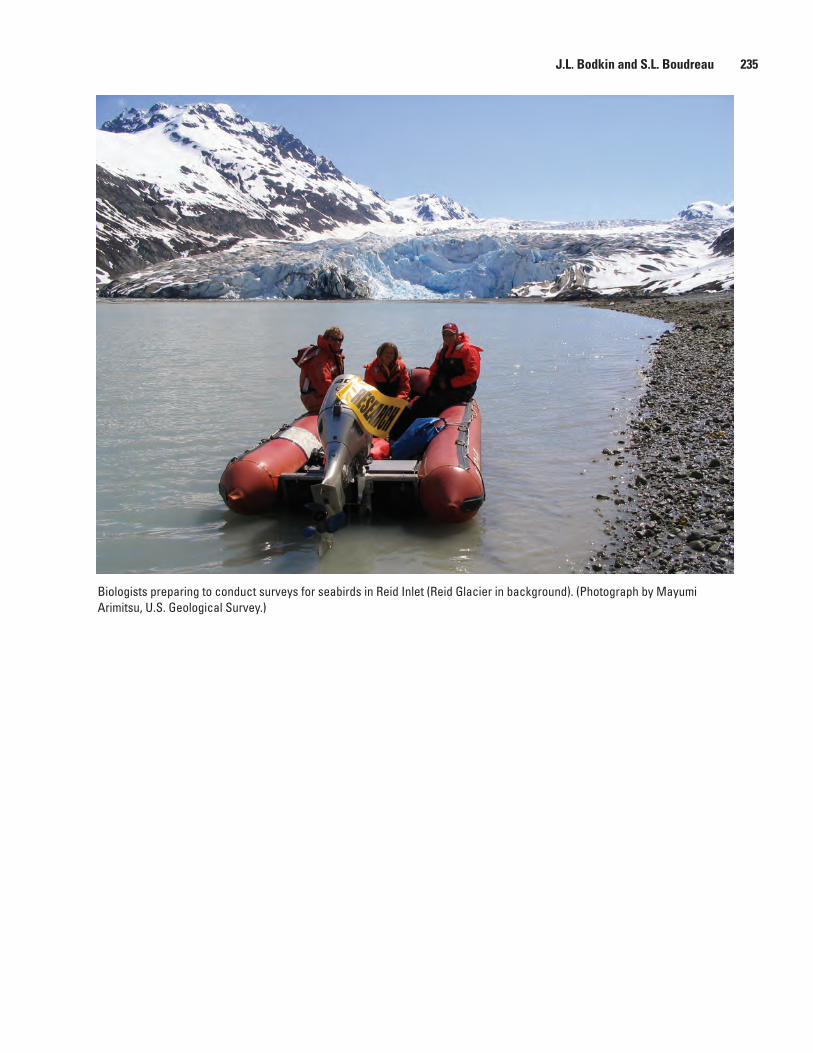
Biologists preparing to conduct surveys for seabirds in Reid Inlet (Reid Glacier in background). (Photograph by Mayumi Arimitsu, U.S. Geological Survey.)
J.L. Bodkin and S.L. Boudreau 2�5
Peripheral Vision as an Adjunct to Rigor
Greg Streveler1
Over recent decades at Glacier Bay, there has been increasing emphasis on rigor in the selection and implementation of studies. I do not presume to argue against the value of statistical validity and reproducibility; however, few things in this world are entirely beneficial. I will suggest that several characteristics of modern research as practiced at Glacier Bay have problematic consequences. Here are those characteristics.
• Rigor requires focus. Pursuit of enough, and good enough data encourages narrowing the scope of the research question.
• Rigor costs time and money. In-house funding has been lavish of late, but that is coming to an end. Independent research has almost died on the vine.
• Modern techniques often reduce the interaction between researcher and environment. Today one sees a lot of quick trips up the bay, monitoring of electronic signals in the wheelhouse, and long hours of data reduction in the office.
• Many important subjects resist rigorous treatment. We will know a lot about campsite vegetation, but god help wolverines...
Taken in sum, these characteristics result in deep but narrow views of the world. If we analogize the Glacier Bay ecosystem to a broad-band spectrogram, modern research brightly illuminates a small number of spectral bands at the cost of leaving large segments of the spectrogram in darkness.
Happily, this problem can be at least partially mitigated with little or no loss to the core value of research. Here are some thoughts on a strategy for illuminating the gaps between studies, mostly stolen from others, that may merit consideration.
• Encourage investigators to keep and report on phe-nomena outside their study objectives but within their expertise. In the highly professional U.S. Geological Survey paper (1963) by Darwin Rossman (the last non-helicoptered geologist according to Dave Brew) are several pages giving his observations on wildlife, remnants of human endeavor and hiking conditions that have increasing value with time.
1Icy Strait Environmental Services, Box 94, Gustavus, Alaska 99826 [email protected] 907 697-2287.
• Create a conducive environment for interdisciplinary work and for linking complementary studies. In 1965, Dick Goldthwait assembled a team of geologists and biologists to look at Muir Inlet from a number of stand-points. The resulting publication (1966) provides the best paradigm for multidisciplinary work in the park that I know of.
• Encourage long-term research. It generates seasoned observers capable of making many sorts of observa-tions in a contextual fashion.
• Encourage the National Park Service and U.S. Geo-logical Survey field staff to keep personal journals of observations. The former seasonal ranger, Ole Wik, not only kept a journal but on his own time researched the old literature on birds of the area and then wrote “The Birds of Glacier Bay National Monument” (1967). This remains the only work other than checklists that covers the entire gamut of bird observations in the park.
• Allow for backcountry sabbaticals. This holds much promise as a tool for re-linking National Park Service staff to the area they are managing, and for produc-ing observations on potential “mine canaries” that we might be overlooking.
• Develop a system for guiding, accumulating and reporting ancillary observations. This need overarches all the above; without it, they will probably remain just notes buried in notebooks or files.
These ideas in sum approach what I mean by peripheral vision, but there is a final, more elusive element that one senses in the joy we all feel when listening to one another’s results: the investment of heart—dare I say love of place—that always arises when any group I’ve ever been in talks about Glacier Bay. This feeling can unite Tlingit resident with Caucasian fisherman with researchers with park managers with tourists. This is the deep ecology of place, which allows us all to sense what we cannot measure, and which leads us to give back to Glacier Bay what it has so unstintingly given us. Anything that increases this is a good thing.
2�� Proceedings of the Fourth Glacier Bay Science Symposium
References
Goldthwait, R.P., ed. 1966, Soil Development and Ecological Succession in a Deglaciated Area of Muir Inlet, Southeast Alaska: Institute of Polar Studies Report # 20, Ohio State University, Columbus Ohio. 166p.
Rossman, D.L., 1963, Geology of the Eastern Part of the Mount Fairweather Quadrangle, Glacier Bay, Alaska: U.S. Geological Survey Bulletin 1121-K. 57 p.
Wik, Dennis (Ole), 1967, Birds of Glacier Bay National Monument: National Park Service, Juneau, Alaska. 80 p.
Suggested Citation
Streveler, G., 2007, Peripheral vision as an adjunct to rigor, in Piatt, J.F., and Gende, S.M., eds., Proceedings of the Fourth Glacier Bay Science Symposium, October 26–28, 2004: U.S. Geological Survey Scientific Investigations Report 2007-5047, p. 236-238.
Greg Streveler 2�7

This page is intentionally left blank.
2�� Proceedings of the Fourth Glacier Bay Science Symposium
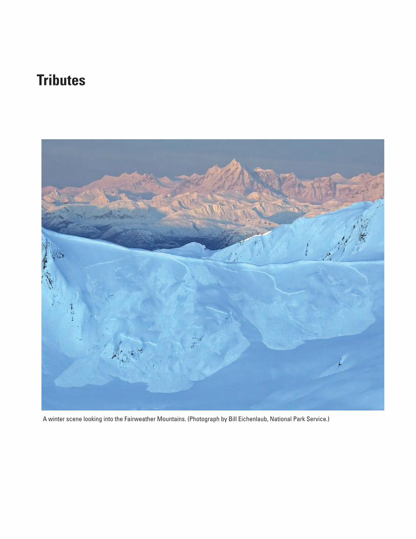
Tributes
A winter scene looking into the Fairweather Mountains. (Photograph by Bill Eichenlaub, National Park Service.)

This page is intentionally left blank.
2�0 Proceedings of the Fourth Glacier Bay Science Symposium
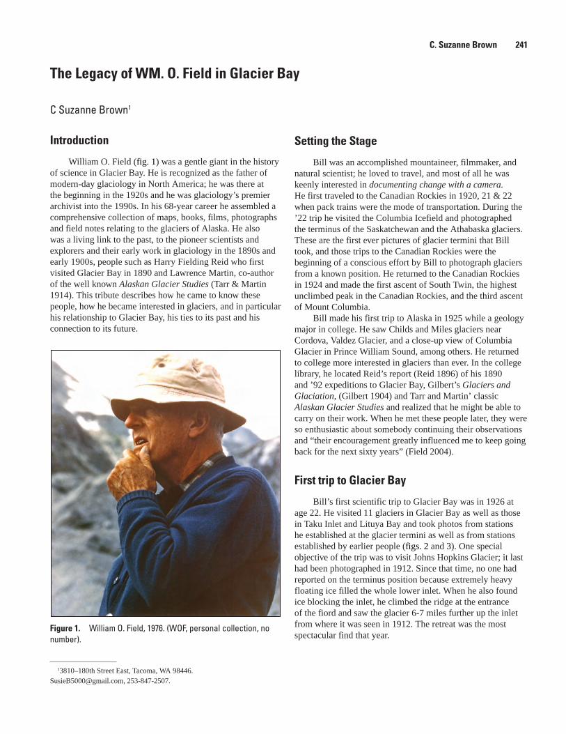
The Legacy of WM. O. Field in Glacier Bay
C Suzanne Brown1
Introduction
William O. Field (fig. 1) was a gentle giant in the history of science in Glacier Bay. He is recognized as the father of modern-day glaciology in North America; he was there at the beginning in the 1920s and he was glaciology’s premier archivist into the 1990s. In his 68-year career he assembled a comprehensive collection of maps, books, films, photographs and field notes relating to the glaciers of Alaska. He also was a living link to the past, to the pioneer scientists and explorers and their early work in glaciology in the 1890s and early 1900s, people such as Harry Fielding Reid who first visited Glacier Bay in 1890 and Lawrence Martin, co-author of the well known Alaskan Glacier Studies (Tarr & Martin 1914). This tribute describes how he came to know these people, how he became interested in glaciers, and in particular his relationship to Glacier Bay, his ties to its past and his connection to its future.
Figure 1. William O. Field, 1976. (WOF, personal collection, no number).
C. Suzanne Brown 2�1
13810–180th Street East, Tacoma, WA 98446. [email protected], 253-847-2507.
Setting the Stage
Bill was an accomplished mountaineer, filmmaker, and natural scientist; he loved to travel, and most of all he was keenly interested in documenting change with a camera. He first traveled to the Canadian Rockies in 1920, 21 & 22 when pack trains were the mode of transportation. During the ’22 trip he visited the Columbia Icefield and photographed the terminus of the Saskatchewan and the Athabaska glaciers. These are the first ever pictures of glacier termini that Bill took, and those trips to the Canadian Rockies were the beginning of a conscious effort by Bill to photograph glaciers from a known position. He returned to the Canadian Rockies in 1924 and made the first ascent of South Twin, the highest unclimbed peak in the Canadian Rockies, and the third ascent of Mount Columbia.
Bill made his first trip to Alaska in 1925 while a geology major in college. He saw Childs and Miles glaciers near Cordova, Valdez Glacier, and a close-up view of Columbia Glacier in Prince William Sound, among others. He returned to college more interested in glaciers than ever. In the college library, he located Reid’s report (Reid 1896) of his 1890 and ’92 expeditions to Glacier Bay, Gilbert’s Glaciers and Glaciation, (Gilbert 1904) and Tarr and Martin’ classic Alaskan Glacier Studies and realized that he might be able to carry on their work. When he met these people later, they were so enthusiastic about somebody continuing their observations and “their encouragement greatly influenced me to keep going back for the next sixty years” (Field 2004).
First trip to Glacier Bay
Bill’s first scientific trip to Glacier Bay was in 1926 at age 22. He visited 11 glaciers in Glacier Bay as well as those in Taku Inlet and Lituya Bay and took photos from stations he established at the glacier termini as well as from stations established by earlier people (figs. 2 and 3). One special objective of the trip was to visit Johns Hopkins Glacier; it last had been photographed in 1912. Since that time, no one had reported on the terminus position because extremely heavy floating ice filled the whole lower inlet. When he also found ice blocking the inlet, he climbed the ridge at the entrance of the fiord and saw the glacier 6-7 miles further up the inlet from where it was seen in 1912. The retreat was the most spectacular find that year.
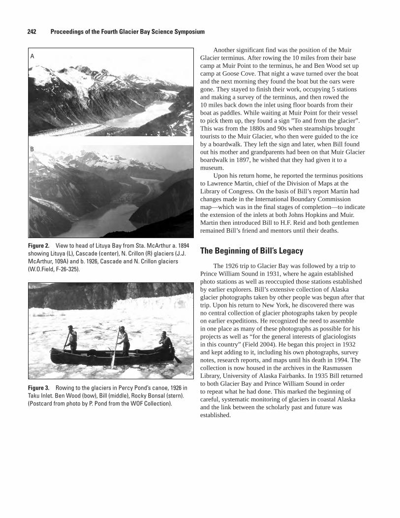
Figure �. Rowing to the glaciers in Percy Pond’s canoe, 1926 in Taku Inlet. Ben Wood (bow), Bill (middle), Rocky Bonsal (stern). (Postcard from photo by P. Pond from the WOF Collection).
Figure 2. View to head of Lituya Bay from Sta. McArthur a. 1894 showing Lituya (L), Cascade (center), N. Crillon (R) glaciers (J.J. McArthur, 109A) and b. 1926, Cascade and N. Crillon glaciers (W.O.Field, F-26-325).
2�2 Proceedings of the Fourth Glacier Bay Science Symposium
A
B
Another significant find was the position of the Muir Glacier terminus. After rowing the 10 miles from their base camp at Muir Point to the terminus, he and Ben Wood set up camp at Goose Cove. That night a wave turned over the boat and the next morning they found the boat but the oars were gone. They stayed to finish their work, occupying 5 stations and making a survey of the terminus, and then rowed the 10 miles back down the inlet using floor boards from their boat as paddles. While waiting at Muir Point for their vessel to pick them up, they found a sign ”To and from the glacier”. This was from the 1880s and 90s when steamships brought tourists to the Muir Glacier, who then were guided to the ice by a boardwalk. They left the sign and later, when Bill found out his mother and grandparents had been on that Muir Glacier boardwalk in 1897, he wished that they had given it to a museum.
Upon his return home, he reported the terminus positions to Lawrence Martin, chief of the Division of Maps at the Library of Congress. On the basis of Bill’s report Martin had changes made in the International Boundary Commission map—which was in the final stages of completion—to indicate the extension of the inlets at both Johns Hopkins and Muir. Martin then introduced Bill to H.F. Reid and both gentlemen remained Bill’s friend and mentors until their deaths.
The Beginning of Bill’s Legacy
The 1926 trip to Glacier Bay was followed by a trip to Prince William Sound in 1931, where he again established photo stations as well as reoccupied those stations established by earlier explorers. Bill’s extensive collection of Alaska glacier photographs taken by other people was begun after that trip. Upon his return to New York, he discovered there was no central collection of glacier photographs taken by people on earlier expeditions. He recognized the need to assemble in one place as many of these photographs as possible for his projects as well as “for the general interests of glaciologists in this country” (Field 2004). He began this project in 1932 and kept adding to it, including his own photographs, survey notes, research reports, and maps until his death in 1994. The collection is now housed in the archives in the Rasmussen Library, University of Alaska Fairbanks. In 1935 Bill returned to both Glacier Bay and Prince William Sound in order to repeat what he had done. This marked the beginning of careful, systematic monitoring of glaciers in coastal Alaska and the link between the scholarly past and future was established.
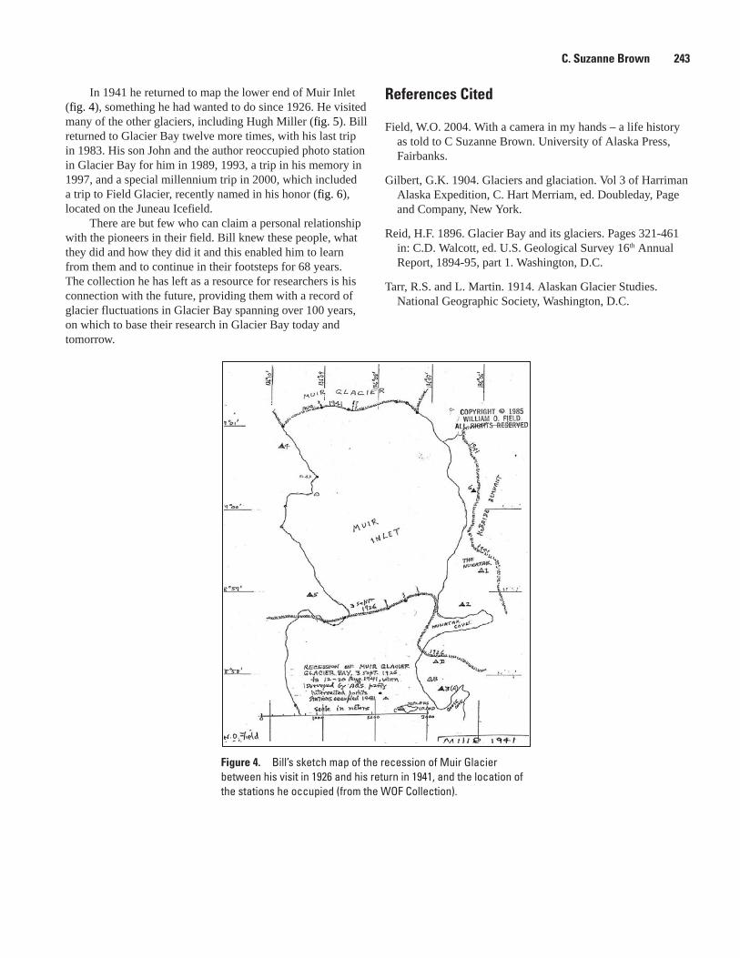
C. Suzanne Brown 2��
Figure �. Bill’s sketch map of the recession of Muir Glacier between his visit in 1926 and his return in 1941, and the location of the stations he occupied (from the WOF Collection).
In 1941 he returned to map the lower end of Muir Inlet (fig. 4), something he had wanted to do since 1926. He visited many of the other glaciers, including Hugh Miller (fig. 5). Bill returned to Glacier Bay twelve more times, with his last trip in 1983. His son John and the author reoccupied photo station in Glacier Bay for him in 1989, 1993, a trip in his memory in 1997, and a special millennium trip in 2000, which included a trip to Field Glacier, recently named in his honor (fig. 6), located on the Juneau Icefield.
There are but few who can claim a personal relationship with the pioneers in their field. Bill knew these people, what they did and how they did it and this enabled him to learn from them and to continue in their footsteps for 68 years. The collection he has left as a resource for researchers is his connection with the future, providing them with a record of glacier fluctuations in Glacier Bay spanning over 100 years, on which to base their research in Glacier Bay today and tomorrow.
References Cited
Field, W.O. 2004. With a camera in my hands – a life history as told to C Suzanne Brown. University of Alaska Press, Fairbanks.
Gilbert, G.K. 1904. Glaciers and glaciation. Vol 3 of Harriman Alaska Expedition, C. Hart Merriam, ed. Doubleday, Page and Company, New York.
Reid, H.F. 1896. Glacier Bay and its glaciers. Pages 321-461 in: C.D. Walcott, ed. U.S. Geological Survey 16th Annual Report, 1894-95, part 1. Washington, D.C.
Tarr, R.S. and L. Martin. 1914. Alaskan Glacier Studies. National Geographic Society, Washington, D.C.
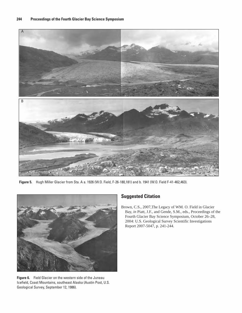
2�� Proceedings of the Fourth Glacier Bay Science Symposium
Figure �. Field Glacier on the western side of the Juneau Icefield, Coast Mountains, southeast Alaska (Austin Post, U.S. Geological Survey, September 12, 1986).
Suggested Citation
Brown, C.S., 2007,The Legacy of WM. O. Field in Glacier Bay, in Piatt, J.F., and Gende, S.M., eds., Proceedings of the Fourth Glacier Bay Science Symposium, October 26–28, 2004: U.S. Geological Survey Scientific Investigations Report 2007-5047, p. 241-244.
Figure 5. Hugh Miller Glacier from Sta. A a. 1926 (W.O. Field, F-26-180,181) and b. 1941 (W.O. Field F-41-462,463).
A
B
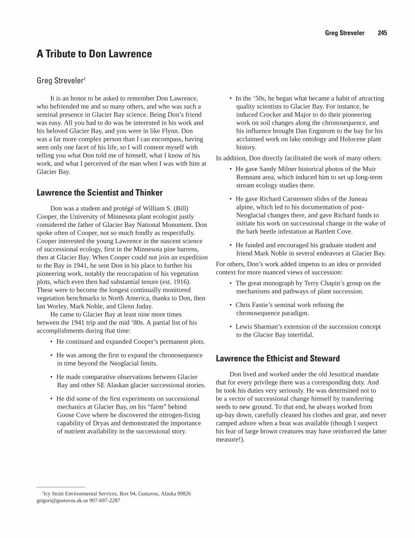
A Tribute to Don Lawrence
Greg Streveler1
It is an honor to be asked to remember Don Lawrence, who befriended me and so many others, and who was such a seminal presence in Glacier Bay science. Being Don’s friend was easy. All you had to do was be interested in his work and his beloved Glacier Bay, and you were in like Flynn. Don was a far more complex person than I can encompass, having seen only one facet of his life, so I will content myself with telling you what Don told me of himself, what I know of his work, and what I perceived of the man when I was with him at Glacier Bay.
Lawrence the Scientist and Thinker
Don was a student and protégé of William S. (Bill) Cooper, the University of Minnesota plant ecologist justly considered the father of Glacier Bay National Monument. Don spoke often of Cooper, not so much fondly as respectfully. Cooper interested the young Lawrence in the nascent science of successional ecology, first in the Minnesota pine barrens, then at Glacier Bay. When Cooper could not join an expedition to the Bay in 1941, he sent Don in his place to further his pioneering work, notably the reoccupation of his vegetation plots, which even then had substantial tenure (est. 1916). These were to become the longest continually monitored vegetation benchmarks in North America, thanks to Don, then Ian Worley, Mark Noble, and Glenn Juday.
He came to Glacier Bay at least nine more times between the 1941 trip and the mid ‘80s. A partial list of his accomplishments during that time:
• He continued and expanded Cooper’s permanent plots.
• He was among the first to expand the chronosequence in time beyond the Neoglacial limits.
• He made comparative observations between Glacier Bay and other SE Alaskan glacier successional stories.
• He did some of the first experiments on successional mechanics at Glacier Bay, on his “farm” behind Goose Cove where he discovered the nitrogen-fixing capability of Dryas and demonstrated the importance of nutrient availability in the successional story.
Greg Streveler 2�5
1Icy Strait Environmental Services, Box 94, Gustavus, Alaska 99826 [email protected] 907-697-2287
• In the ‘50s, he began what became a habit of attracting quality scientists to Glacier Bay. For instance, he induced Crocker and Major to do their pioneering work on soil changes along the chronosequence, and his influence brought Dan Engstrom to the bay for his acclaimed work on lake ontology and Holocene plant history.
In addition, Don directly facilitated the work of many others:
• He gave Sandy Milner historical photos of the Muir Remnant area, which induced him to set up long-term stream ecology studies there.
• He gave Richard Carstensen slides of the Juneau alpine, which led to his documentation of post-Neoglacial changes there, and gave Richard funds to initiate his work on successional change in the wake of the bark beetle infestation at Bartlett Cove.
• He funded and encouraged his graduate student and friend Mark Noble in several endeavors at Glacier Bay.
For others, Don’s work added impetus to an idea or provided context for more nuanced views of succession:
• The great monograph by Terry Chapin’s group on the mechanisms and pathways of plant succession.
• Chris Fastie’s seminal work refining the chronosequence paradigm.
• Lewis Sharman’s extension of the succession concept to the Glacier Bay intertidal.
Lawrence the Ethicist and Steward
Don lived and worked under the old Jesuitical mandate that for every privilege there was a corresponding duty. And he took his duties very seriously. He was determined not to be a vector of successional change himself by transferring seeds to new ground. To that end, he always worked from up-bay down, carefully cleaned his clothes and gear, and never camped ashore when a boat was available (though I suspect his fear of large brown creatures may have reinforced the latter measure!).
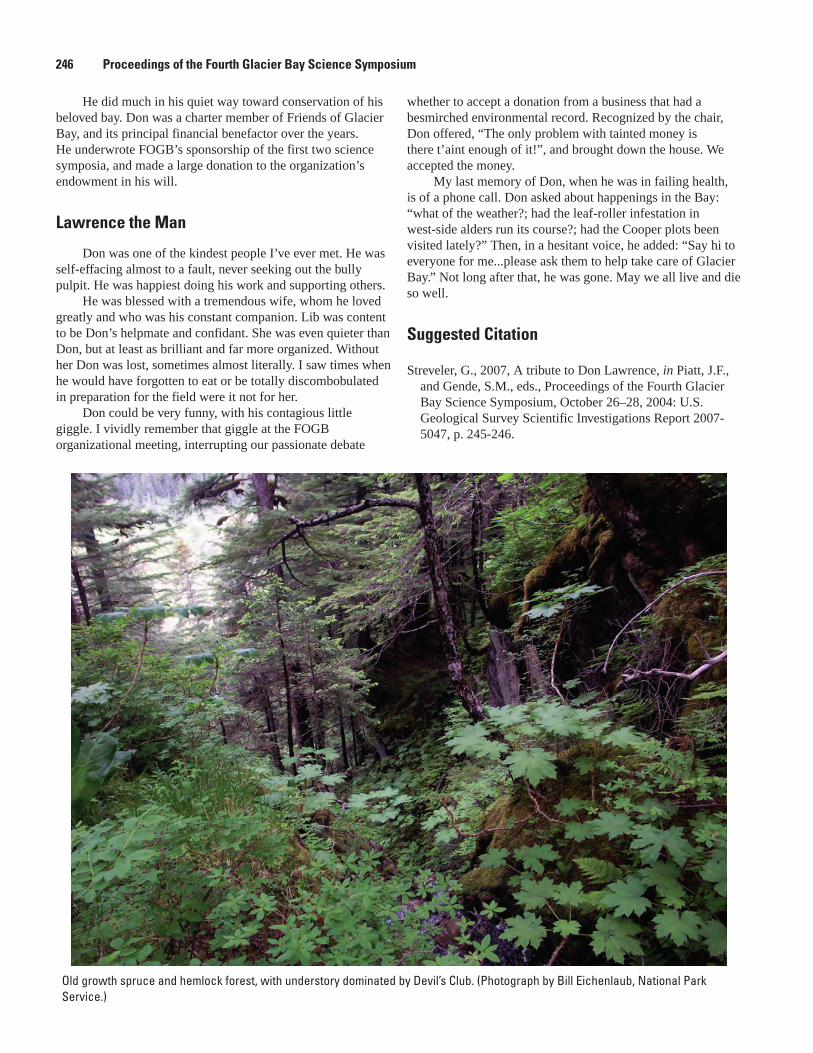
2�� Proceedings of the Fourth Glacier Bay Science Symposium
He did much in his quiet way toward conservation of his beloved bay. Don was a charter member of Friends of Glacier Bay, and its principal financial benefactor over the years. He underwrote FOGB’s sponsorship of the first two science symposia, and made a large donation to the organization’s endowment in his will.
Lawrence the Man
Don was one of the kindest people I’ve ever met. He was self-effacing almost to a fault, never seeking out the bully pulpit. He was happiest doing his work and supporting others.
He was blessed with a tremendous wife, whom he loved greatly and who was his constant companion. Lib was content to be Don’s helpmate and confidant. She was even quieter than Don, but at least as brilliant and far more organized. Without her Don was lost, sometimes almost literally. I saw times when he would have forgotten to eat or be totally discombobulated in preparation for the field were it not for her.
Don could be very funny, with his contagious little giggle. I vividly remember that giggle at the FOGB organizational meeting, interrupting our passionate debate
Old growth spruce and hemlock forest, with understory dominated by Devil’s Club. (Photograph by Bill Eichenlaub, National Park Service.)
whether to accept a donation from a business that had a besmirched environmental record. Recognized by the chair, Don offered, “The only problem with tainted money is there t’aint enough of it!”, and brought down the house. We accepted the money.
My last memory of Don, when he was in failing health, is of a phone call. Don asked about happenings in the Bay: “what of the weather?; had the leaf-roller infestation in west-side alders run its course?; had the Cooper plots been visited lately?” Then, in a hesitant voice, he added: “Say hi to everyone for me...please ask them to help take care of Glacier Bay.” Not long after that, he was gone. May we all live and die so well.
Suggested Citation
Streveler, G., 2007, A tribute to Don Lawrence, in Piatt, J.F., and Gende, S.M., eds., Proceedings of the Fourth Glacier Bay Science Symposium, October 26–28, 2004: U.S. Geological Survey Scientific Investigations Report 2007-5047, p. 245-246.

For more information concerning the research in this report, contact the Director, Alaska Science Center U.S. Geological Survey, 4230 University Dr., Suite 201 Anchorage, AK 99508-4650 http://alaska.usgs.gov

Proceedings of the Fourth Glacier Bay Science Symposium
Piatt and GendeSIR 2007–5047
Printed on recycled paper