Astronomy & Astrophysics manuscript no. helicity c© ESO 2011March 17, 2011

Probing magnetic helicity with synchrotron radiation and Faradayrotation

N. Oppermann, H. Junklewitz, G. Robbers, and T.A. Enßlin

Max Planck Institute for Astrophysics, Karl-Schwarzschild-Str. 1, 85741 Garching, Germanye-mail: niels@mpa-garching.mpg.de

Received 06 Aug. 2010 / Accepted 01 Feb. 2011

ABSTRACT

We present a first application of the recently proposed LITMUS test for magnetic helicity, as well as a thorough study of its applicabilityunder different circumstances. In order to apply this test to the galactic magnetic field, the newly developed critical filter formalismis used to produce an all-sky map of the Faraday depth. The test does not detect helicity in the galactic magnetic field. To understandthe significance of this finding, we made an applicability study, showing that a definite conclusion about the absence of magnetichelicity in the galactic field has not yet been reached. This study is conducted by applying the test to simulated observational data.We consider simulations in a flat sky approximation and all-sky simulations, both with assumptions of constant electron densities andrealistic distributions of thermal and cosmic ray electrons. Our results suggest that the LITMUS test does indeed perform very well incases where constant electron densities can be assumed, both in the flat-sky limit and in the galactic setting. Non-trivial distributionsof thermal and cosmic ray electrons, however, may complicate the scenario to the point where helicity in the magnetic field can escapedetection.

Key words. ISM: magnetic fields - Galaxies: magnetic fields - Methods: data analysis

1. Introduction

Helicity is of utmost interest in the study of astrophysical mag-netism. Mean field theories for turbulent dynamos operatingin the galactic interstellar medium have been successful in ex-plaining how the observed magnetic field strengths are main-tained (e.g. Subramanian 2002). These theories predict that he-licity is present on small scales in interstellar magnetic fields.Observationally detecting or excluding helicity in these fieldswould therefore either strongly suggest that these theories arevalid or indicate that there are some flaws in them.

However, since helicity is a quantity that describes the three-dimensional structure of a magnetic field and most observationtechniques produce at best two-dimensional images leading toan informational deficit, it has thus far largely eluded observers.Previous work on the detection of magnetic helicity in astro-physical contexts has focused mainly on either magnetic fieldsof specific objects, such as the Sun (see e.g. Zhang 2010, andreferences therein) or astrophysical jets (cf. e.g. Enßlin 2003;Gabuzda et al. 2004), or cosmological primordial magnetic fields(e.g. Kahniashvili & Ratra 2005; Kahniashvili et al. 2005). Twoexceptions are the work by Volegova & Stepanov (2010), inwhich the use of Faraday rotation and synchrotron radiation fordetecting magnetic helicity was suggested for the first time, andthe work of Kahniashvili & Vachaspati (2006), in which the useof charged ultra high energy cosmic rays of known sources issuggested for probing the three-dimensional structure of mag-netic fields through which they pass. However, the sources ofultra high energy cosmic rays are not known yet and the appli-cability of this test is therefore limited.

The LITMUS (Local Inference Test for Magnetic fieldswhich Uncovers heliceS) procedure for the detection of mag-netic helicity suggested by Junklewitz & Enßlin (2010) probesthe local current helicity density B · j, which for an ideally con-

ducting plasma becomes

B · j ∝ B · (∇ × B) . (1)

Here, the magnetic field is denoted by B and the electric cur-rent density by j. The test uses measurements of the Faradaydepth and of the polarization direction of synchrotron radiationto probe the magnetic field components along the line of sightand perpendicular to it, respectively. Its simple geometrical mo-tivation should make it applicable in a general setting, providedthese quantities can be measured. The results depend only onthe properties of the magnetic field along a line of sight and aretherefore purely local in the two-dimensional sky projection. Ouraim is to test this idea on observational as well as on simulateddata, thereby determining the conditions under which the testwill yield useful results.

This paper is organized as follows. In Sect. 2, the basic equa-tions used in the LITMUS test are reviewed. They are appliedto observational data describing the galactic magnetic field inSect. 3, with special emphasis on a sophisticated reconstructionof the Faraday depth, described in Sect. 3.2. Section 4 is de-voted to a thorough general assessment of the test’s reliability.To this end it is applied to simulated observations of increasingcomplexity. Section 4.1 describes the application in a flat skyapproximation, whereas Sect. 4.2 examines all-sky simulations,finally arriving at complete simulations of the galactic setting inSect. 4.2.2, where realistic electron distributions are added. Wediscuss our results and conclude in Sect. 5.

2. The helicity test

For a thorough introduction into the ideas behind the LITMUStest, the reader is referred to Junklewitz & Enßlin (2010). Here,we only summarize the resulting equations.

arX

iv:1

008.

1246

v3 [

astr

o-ph

.IM

] 1

6 M

ar 2

011

2 N. Oppermann et al.: Probing Magnetic Helicity

On the one hand side, synchrotron emission produced bycosmic ray electrons is used to probe the magnetic field com-ponent perpendicular to the line of sight. Its polarization is de-scribed by the complex field

P = Q + iU = |P| e2iχ, (2)

where Q and U are the usual Stokes parameters quantifying thelinearly polarized components of the radiation with respect tosome orthogonal coordinate system and χ is the polarization an-gle with respect to the first coordinate direction. On the otherhand, the Faraday depth

φ ∝

∫LOS

neB · dl (3)

is used to probe the magnetic field component parallel to the lineof sight (LOS).

A helical magnetic field will lead to a gradient of the Faradaydepth that is parallel to the polarization direction of the syn-chrotron emission, as was argued in Junklewitz & Enßlin (2010).In order to compare the directions of the two quantities, this gra-dient is also formulated as a complex field

G =((∇φ)x + i (∇φ)y

)2= |G| e2iα, (4)

with

α = arctan( (∇φ)y

(∇φ)x

), (5)

where the indices x and y denote its components with respect tothe coordinates used. The helicity test that is performed in thiswork consists simply of multiplying G with the complex conju-gate of the polarization P∗. If the two angles χ and α differ by amultiple of π (i.e. the gradient and the polarization direction areparallel), the product will be real and positive. If they differ byan odd multiple of π/2 (i.e. the two directions are perpendicu-lar), it will be real and negative. Any orientation in between willproduce varying real and imaginary parts in the product. Thus,observational directions along which a magnetic field is helicalare indicated by a positive real part and a vanishing imaginarypart of the product. Averaging over all observational directionswill give an indication of the global helicity of the field.

It was furthermore shown by Junklewitz & Enßlin (2010)that the ensemble average of this product over all magnetic fieldrealizations given a magnetic correlation tensor (and therefore ahelicity power spectrum) is a measure for the squared integratedspectral current helicity density

〈GP∗〉B ∝(∫ ∞

0dkεH(k)

k

)2

, (6)

with large scales weighted more strongly than small scales.

3. Application to galactic observations

In this section, we try to answer the question whether the mag-netic field of the Milky Way is helical by applying the LITMUStest to the available observational data. Since the magnetic fieldis localized in a region that surrounds the observer, all relevantquantities will be given as fields on the sphere S2, i.e. as func-tions of the observational direction, specified by two angles ϑand ϕ, which are taken to represent the standard spherical polarcoordinates in a galactic coordinate system.

3.1. Observational data

For the synchrotron emission, we use the data gathered by theWMAP satellite after seven years of observations1, described inPage et al. (2007). Since the foreground synchrotron emissionis most intense at low frequencies, we use the measurement inthe K-Band, which is centered at a frequency of ν = 23 GHz.Furthermore, we assume that the detected polarized intensity issolely due to galactic synchrotron emission. Thus, the StokesQ and U parameter maps (defined with respect to the sphericalpolar coordinate directions eϑ and eϕ in the galactic coordinatesystem) can be simply combined according to Eq. (2) to give thecomplex quantity P whose argument is twice the rotation angleof the plane of polarization with respect to the eϑ-direction

χ(ϑ, ϕ) =12

arctan(

Im(P(ϑ, ϕ))Re(P(ϑ, ϕ))

)(7)

(cf. Junklewitz & Enßlin 2010).There are several depolarizing effects that have to be con-

sidered when dealing with polarization data. Faraday depo-larization, which is important only at low frequencies due tothe proportionality of the Faraday rotation angle to the squareof the wavelength, can be safely neglected in the K-Band.Depolarization effects due to different magnetic field orienta-tions along the line of sight are certainly present. However,they are present as well in the numerical test cases presentedin Sect. 4, which yield good results. Additionally, depolarizationdue to the finite beam-size of the WMAP satellite and the finitepixel size of the polarization maps used in this study can playa role. The only way to limit this effect is to use higher resolu-tion maps, ultimately necessitating the use of Planck data in thefuture.

In order to construct a map of the Faraday depth, we usethe catalog of rotation measurements provided by Taylor et al.(2009)2. These provide an observational estimate of the Faradaydepth for certain directions in the sky where polarized radiopoint-sources could be observed. Since the catalog encompassesa large number (37 543) of point-sources, it paints a rather clearpicture of the structure of the Faraday depth. However, Earth’sshadow prevents observations in a considerably large regionwithin the southern hemisphere.

3.2. Reconstructing the Faraday depth map

The reconstruction is conducted according to the critical filtermethod first presented in Enßlin & Frommert (2010). A moreelegant derivation of the same filter can be found in Enßlin &Weig (2010). Since this formalism takes into account availableinformation on the statistical properties of the signal in the formof the power spectrum, it is able to interpolate into regions whereno direct information on the signal is provided by the data, suchas the shadow of Earth in this case. Furthermore, it takes intoaccount the available information on the uncertainty of the mea-surements. All in all it is expected to lead to a reconstructed mapof the Faraday depth that is much closer to reality than e.g. amap in which the data were simply smoothed to cover the sphere.Small-scale features that are lost in such a smoothing process arefor example reproduced by the critical filter algorithm.

1 The data are available from NASA’s Legacy Archive for MicrowaveBackground Data Analysis at http://lambda.gsfc.nasa.gov.

2 The catalog is available athttp://www.ucalgary.ca/ras/rmcatatlogue.

N. Oppermann et al.: Probing Magnetic Helicity 3

0

20

40

60

80

100

120

140

160

0 0.5 1 1.5 2 2.5 3

p(ϑ

)

ϑ

Fig. 1. Vertical galactic profile p(ϑ) of the Faraday depth.

3.2.1. Data model

The field that is to be reconstructed here is the sky-map of theFaraday depth. In order to apply the critical filter formula, thesignal should be an isotropic Gaussian field. Since the Faradaydepth clearly is larger along directions passing through the galac-tic plane, the condition of isotropy is not satisfied. Therefore, avertical profile is calculated by binning the observations into in-tervals [ϑi, ϑi + ∆ϑ), calculating the root mean square rotationmeasure value for each bin and smoothing the resulting valuesto obtain a smooth function p(ϑ). The result is shown in Fig. 1.This profile is used to approximatively correct the anisotropiesinduced by the galactic structure and the resulting signal field

s(ϑ, ϕ) =φ(ϑ, ϕ)

p(ϑ)(8)

is assumed to be isotropic and Gaussian with a covariance ma-trix S . The Gaussian covariance matrix is determined solely bythe angular power spectrum coefficients Cl, the reconstruction ofwhich is part of the problem at hand.

The data d, i.e. the rotation measure values in the catalog,are taken to arise from the signal s by multiplication with a re-sponse matrix R, which consists of a part encoding the specificdirections in which the signal field is probed in order to pro-duce the measurements and another part that is a simple multi-plication with the vertical profile p(ϑ). Additionally, a Gaussiannoise component n is assumed with a covariance matrix N =diag(σ2

1, σ22, . . . ), where σi is the one sigma error bar for the ith

measurement in the catalog. Thus, the data are given by3

d = Rs + n = Rps + n. (9)

Recent discussions in the literature (see e.g. Stil et al. 2011) haveshown, however, that the error estimates as quoted in the cat-alog are probably too low. In addition, any contribution to themeasured data from intrinsic Faraday rotation within the sourceswill further increase the error budget since the signal field in thiscontext is only the contribution of the Milky Way. We thereforeadapt the error bars of Taylor et al. (2009) according to the for-mula

σ(corrected) =

√( fσσ)2 +

(σ(int))2

, (10)

3 The discretized version used in the implementations is di =∑j Ri j s j + ni =

∑j Ri j p j s j + ni, where the index j determines a pixel

on the sphere, so that s j = s(ϑ j, ϕ j) and p j = p(ϑ j).

respectively. Here, the factor fσ accounts for the general under-estimation of the errors in the catalog of Taylor et al. (2009),whereas the additive constant σ(int) represents the average con-tribution of the sources’ intrinsic Faraday rotation. As numeri-cal values, we use fσ = 1.22, which was found by Stil et al.(2011) by comparing the data of Taylor et al. (2009) and Maoet al. (2010) on sources that are contained in both catalogs, andσ(int) = 6.6 m−2, which corresponds to the upper end of the num-bers found by Schnitzeler (2010). Since the error contributionfrom the internal Faraday rotation is not correlated with the mea-surement error, the two contributions add up quadratically in thenoise covariance matrix.

3.2.2. Reconstruction method

For signal and noise fields with a Gaussian prior probability dis-tribution, the posterior probability distribution of the signal fieldis again a Gaussian, i.e. it is of the form P(s|d,Cl) = G(s−m,D),where a multivariate Gaussian probability distribution with co-variance matrix X is denoted by

G(x, X) =1

|2πX|1/2exp

(−

12

x†X−1x), (11)

where the † symbol denotes a transposed and complex con-jugated quantity. In order to reconstruct the mean signal fieldm = 〈s〉, where the brackets denote the posterior mean, it is alsonecessary to reconstruct the angular power spectrum Cl. To doso, the critical filter formulas

m = D j (12)

andCl =

12l + 1

tr((

mm† + D)

S l

)(13)

are iterated, starting with some initial guess for the power spec-trum. Here, the signal covariance matrix is expanded as S =∑

l ClS l, where S l is the projection onto the spherical harmoniccomponents with index l. Furthermore, D is the posterior covari-ance matrix,

D =(S −1 + R†N−1R

)−1, (14)

and j is the information source term,

j = R†N−1d. (15)

Since the critical filter is on the brink of exhibiting a per-ception threshold (cf. Enßlin & Frommert 2010) and it is gen-erally more desirable to overestimate a power spectrum enter-ing a filter than to underestimate it, the coefficients Cl are sub-jected to a procedure in which the value of Cl is replaced bymax {Cl−1,Cl,Cl+1} after each iteration step. The advantage ofoverestimating the power spectrum can be seen by consideringthe limit of Cl → ∞ in Eq. (12) and (14). For high values of Cl,the first term in Eq. (14) can be neglected and Eq. (12) becomes

mCl→∞ = s + R−1n. (16)

Thus, by overestimating the power spectrum the importance ofits exact shape is diminished and the reconstruction will insteadfollow the information given directly by the data more closely.Considering an extreme underestimation of the power spectrum,Cl → 0, on the other hand, would lead to

mCl→0 = 0, (17)

suppressing the information given by the data.

4 N. Oppermann et al.: Probing Magnetic Helicity

(a)

�5 5

(c)

0.1 1.2

(b)

�500 500

(d)

1 150

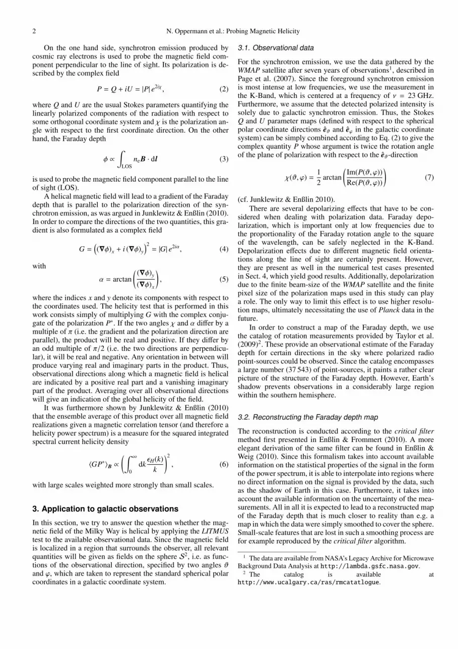
Fig. 2. Results of the reconstruction of the signal field and Faraday depth. The left column shows the posterior mean of the signalfield m (panel (a)) and its one-sigma uncertainty

√D (panel (c)). The right column shows the resulting map of the Faraday depth

pm (panel(b)) and the corresponding one-sigma uncertainty√

p2D (panel (d)) in m−2.

1e-05

0.0001

0.001

0.01

0.1

1

1 10 100

Cl

l

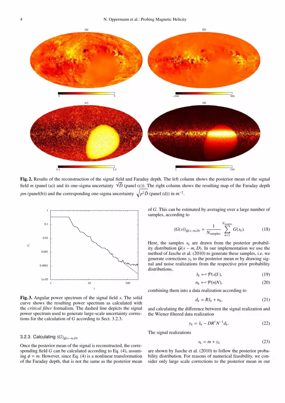
Fig. 3. Angular power spectrum of the signal field s. The solidcurve shows the resulting power spectrum as calculated withthe critical filter formalism. The dashed line depicts the signalpower spectrum used to generate large-scale uncertainty correc-tions for the calculation of G according to Sect. 3.2.3.

3.2.3. Calculating 〈G〉G(s−m,D)

Once the posterior mean of the signal is reconstructed, the corre-sponding field G can be calculated according to Eq. (4), assum-ing φ = m. However, since Eq. (4) is a nonlinear transformationof the Faraday depth, that is not the same as the posterior mean

of G. This can be estimated by averaging over a large number ofsamples, according to

〈G(s)〉G(s−m,D) ≈1

Nsamples

Nsamples∑k=1

G(sk). (18)

Here, the samples sk are drawn from the posterior probabil-ity distribution G(s − m,D). In our implementation we use themethod of Jasche et al. (2010) to generate these samples, i.e. wegenerate corrections yk to the posterior mean m by drawing sig-nal and noise realizations from the respective prior probabilitydistributions,

sk ←↩ P(s|S ), (19)

nk ←↩ P(n|N), (20)

combining them into a data realization according to

dk = Rsk + nk, (21)

and calculating the difference between the signal realization andthe Wiener filtered data realization

yk = sk − DR†N−1dk. (22)

The signal realizations

sk = m + yk (23)

are shown by Jasche et al. (2010) to follow the posterior proba-bility distribution. For reasons of numerical feasibility, we con-sider only large scale corrections to the posterior mean in our

N. Oppermann et al.: Probing Magnetic Helicity 5

(a)

0.01 1000.00

(b)

0.01 1000.00

(c)

0.1 1000.0

(d)

�1 1

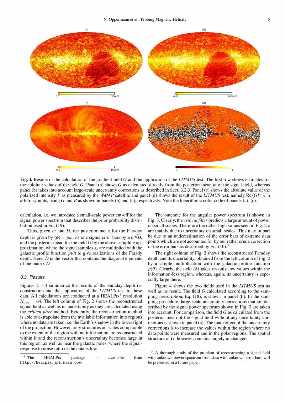
Fig. 4. Results of the calculation of the gradient field G and the application of the LITMUS test. The first row shows estimates forthe ablolute values of the field G. Panel (a) shows G as calculated directly from the posterior mean m of the signal field, whereaspanel (b) takes into account large-scale uncertainty corrections as described in Sect. 3.2.3. Panel (c) shows the absolute value of thepolarized intensity P as measured by the WMAP satellite and panel (d) shows the result of the LITMUS test, namely Re (GP∗), inarbitrary units, using G and P as shown in panels (b) and (c), respectively. Note the logarithmic color code of panels (a)–(c).

calculation, i.e. we introduce a small-scale power cut-off for thesignal power spectrum that describes the prior probability distri-bution used in Eq. (19).

Thus, given m and D, the posterior mean for the Faradaydepth is given by 〈φ〉 = pm, its one sigma error bars by ±p

√D,

and the posterior mean for the field G by the above sampling ap-proximation, where the signal samples sk are multiplied with thegalactic profile function p(θ) to give realizations of the Faradydepth. Here, D is the vector that contains the diagonal elementsof the matrix D.

3.3. Results

Figures 2 – 4 summarize the results of the Faraday depth re-construction and the application of the LITMUS test to thesedata. All calculations are conducted at a HEALPix4 resolutionNside = 64. The left column of Fig. 2 shows the reconstructedsignal field as well as its uncertainty as they are calculated usingthe critical filter method. Evidently, the reconstruction methodis able to extrapolate from the available information into regionswhere no data are taken, i.e. the Earth’s shadow in the lower rightof the projection. However, only structures on scales comparableto the extent of the region without information are reconstructedwithin it and the reconstruction’s uncertainty becomes large inthis region, as well as near the galactic poles, where the signal-response to noise ratio of the data is low.

4 The HEALPix package is available fromhttp://healpix.jpl.nasa.gov.

The outcome for the angular power spectrum is shown inFig. 3. Clearly, the critical filter predicts a large amount of poweron small scales. Therefore the rather high values seen in Fig. 2.care mainly due to uncertainty on small scales. This may in partbe due to an underestimation of the error bars of extreme datapoints which are not accounted for by our rather crude correctionof the error bars as described by Eq. (10).5

The right column of Fig. 2 shows the reconstructed Faradaydepth and its uncertainty, obtained from the left column of Fig. 2by a simple multiplication with the galactic profile functionp(ϑ). Clearly, the field 〈φ〉 takes on only low values within theinformation-less region, whereas, again, its uncertainty is espe-cially large there.

Figure 4 shows the two fields used in the LITMUS test aswell as its result. The field G calculated according to the sam-pling prescription, Eq. (18), is shown in panel (b). In the sam-pling procedure, large-scale uncertainty corrections that are de-scribed by the signal power spectrum shown in Fig. 3 are takeninto account. For comparison, the field G as calculated from theposterior mean of the signal field without any uncertainty cor-rections is shown in panel (a). The main effect of the uncertaintycorrections is to increase the values within the region where nodata points were measured and in the polar regions. The spatialstructure of G, however, remains largely unchanged.

5 A thorough study of the problem of reconstructing a signal fieldwith unknown power spectrum from data with unknown error bars willbe presented in a future paper.

6 N. Oppermann et al.: Probing Magnetic Helicity

-1

-0.8

-0.6

-0.4

-0.2

0

0.2

0.4

-3 -2 -1 0 1 2 3

Re〈G

P∗〉 S

2

β

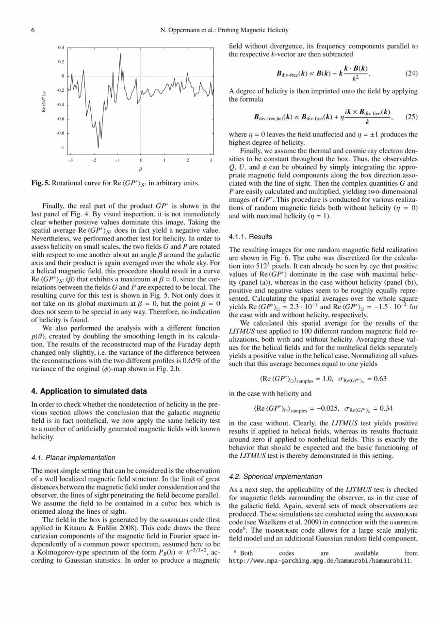
Fig. 5. Rotational curve for Re 〈GP∗〉S2 in arbitrary units.

Finally, the real part of the product GP∗ is shown in thelast panel of Fig. 4. By visual inspection, it is not immediatelyclear whether positive values dominate this image. Taking thespatial average Re 〈GP∗〉S2 does in fact yield a negative value.Nevertheless, we performed another test for helicity. In order toassess helicity on small scales, the two fields G and P are rotatedwith respect to one another about an angle β around the galacticaxis and their product is again averaged over the whole sky. Fora helical magnetic field, this procedure should result in a curveRe 〈GP∗〉S2 (β) that exhibits a maximum at β = 0, since the cor-relations between the fields G and P are expected to be local. Theresulting curve for this test is shown in Fig. 5. Not only does itnot take on its global maximum at β = 0, but the point β = 0does not seem to be special in any way. Therefore, no indicationof helicity is found.

We also performed the analysis with a different functionp(ϑ), created by doubling the smoothing length in its calcula-tion. The results of the reconstructed map of the Faraday depthchanged only slightly, i.e. the variance of the difference betweenthe reconstructions with the two different profiles is 0.65% of thevariance of the original 〈φ〉-map shown in Fig. 2.b.

4. Application to simulated data

In order to check whether the nondetection of helicity in the pre-vious section allows the conclusion that the galactic magneticfield is in fact nonhelical, we now apply the same helicity testto a number of artificially generated magnetic fields with knownhelicity.

4.1. Planar implementation

The most simple setting that can be considered is the observationof a well localized magnetic field structure. In the limit of greatdistances between the magnetic field under consideration and theobserver, the lines of sight penetrating the field become parallel.We assume the field to be contained in a cubic box which isoriented along the lines of sight.

The field in the box is generated by the garfields code (firstapplied in Kitaura & Enßlin 2008). This code draws the threecartesian components of the magnetic field in Fourier space in-dependently of a common power spectrum, assumed here to bea Kolmogorov-type spectrum of the form PB(k) ∝ k−5/3−2, ac-cording to Gaussian statistics. In order to produce a magnetic

field without divergence, its frequency components parallel tothe respective k-vector are then subtracted

Bdiv-free(k) ∝ B(k) − kk · B(k)

k2 . (24)

A degree of helicity is then imprinted onto the field by applyingthe formula

Bdiv-free,hel(k) ∝ Bdiv-free(k) + ηik × Bdiv-free(k)

k, (25)

where η = 0 leaves the field unaffected and η = ±1 produces thehighest degree of helicity.

Finally, we assume the thermal and cosmic ray electron den-sities to be constant throughout the box. Thus, the observablesQ, U, and φ can be obtained by simply integrating the appro-priate magnetic field components along the box direction asso-ciated with the line of sight. Then the complex quantities G andP are easily calculated and multiplied, yielding two-dimensionalimages of GP∗. This procedure is conducted for various realiza-tions of random magnetic fields both without helicity (η = 0)and with maximal helicity (η = 1).

4.1.1. Results

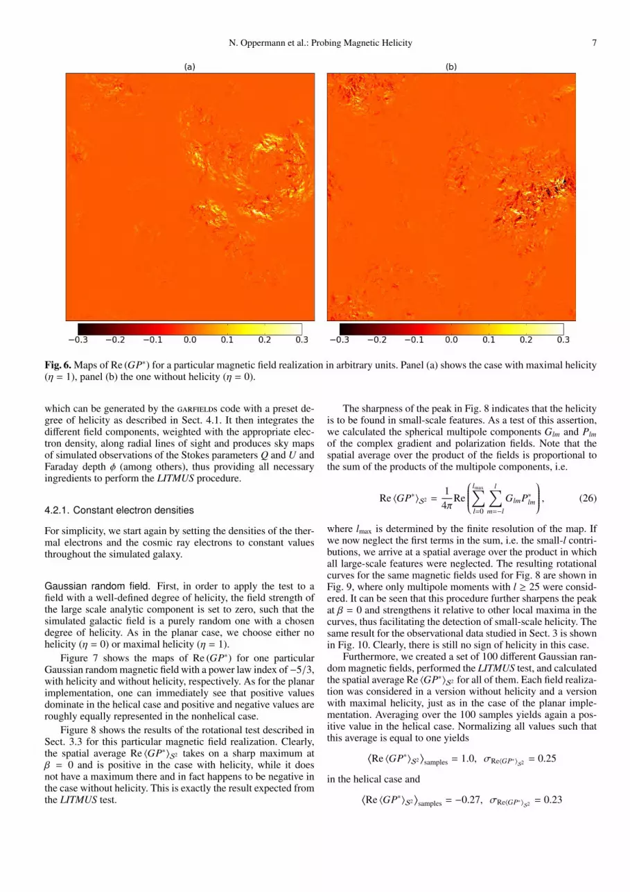
The resulting images for one random magnetic field realizationare shown in Fig. 6. The cube was discretized for the calcula-tion into 5123 pixels. It can already be seen by eye that positivevalues of Re (GP∗) dominate in the case with maximal helic-ity (panel (a)), whereas in the case without helicity (panel (b)),positive and negative values seem to be roughly equally repre-sented. Calculating the spatial averages over the whole squareyields Re 〈GP∗〉� = 2.3 · 10−3 and Re 〈GP∗〉� = −1.5 · 10−4 forthe case with and without helicity, respectively.

We calculated this spatial average for the results of theLITMUS test applied to 100 different random magnetic field re-alizations, both with and without helicity. Averaging these val-ues for the helical fields and for the nonhelical fields separatelyyields a positive value in the helical case. Normalizing all valuessuch that this average becomes equal to one yields

〈Re 〈GP∗〉�〉samples = 1.0, σRe〈GP∗〉� = 0.63

in the case with helicity and

〈Re 〈GP∗〉�〉samples = −0.025, σRe〈GP∗〉� = 0.34

in the case without. Clearly, the LITMUS test yields positiveresults if applied to helical fields, whereas its results fluctuatearound zero if applied to nonhelical fields. This is exactly thebehavior that should be expected and the basic functioning ofthe LITMUS test is thereby demonstrated in this setting.

4.2. Spherical implementation

As a next step, the applicability of the LITMUS test is checkedfor magnetic fields surrounding the observer, as in the case ofthe galactic field. Again, several sets of mock observations areproduced. These simulations are conducted using the hammurabicode (see Waelkens et al. 2009) in connection with the garfieldscode6. The hammurabi code allows for a large scale analyticfield model and an additional Gaussian random field component,

6 Both codes are available fromhttp://www.mpa-garching.mpg.de/hammurabi/hammurabi11.

N. Oppermann et al.: Probing Magnetic Helicity 7

Fig. 6. Maps of Re (GP∗) for a particular magnetic field realization in arbitrary units. Panel (a) shows the case with maximal helicity(η = 1), panel (b) the one without helicity (η = 0).

which can be generated by the garfields code with a preset de-gree of helicity as described in Sect. 4.1. It then integrates thedifferent field components, weighted with the appropriate elec-tron density, along radial lines of sight and produces sky mapsof simulated observations of the Stokes parameters Q and U andFaraday depth φ (among others), thus providing all necessaryingredients to perform the LITMUS procedure.

4.2.1. Constant electron densities

For simplicity, we start again by setting the densities of the ther-mal electrons and the cosmic ray electrons to constant valuesthroughout the simulated galaxy.

Gaussian random field. First, in order to apply the test to afield with a well-defined degree of helicity, the field strength ofthe large scale analytic component is set to zero, such that thesimulated galactic field is a purely random one with a chosendegree of helicity. As in the planar case, we choose either nohelicity (η = 0) or maximal helicity (η = 1).

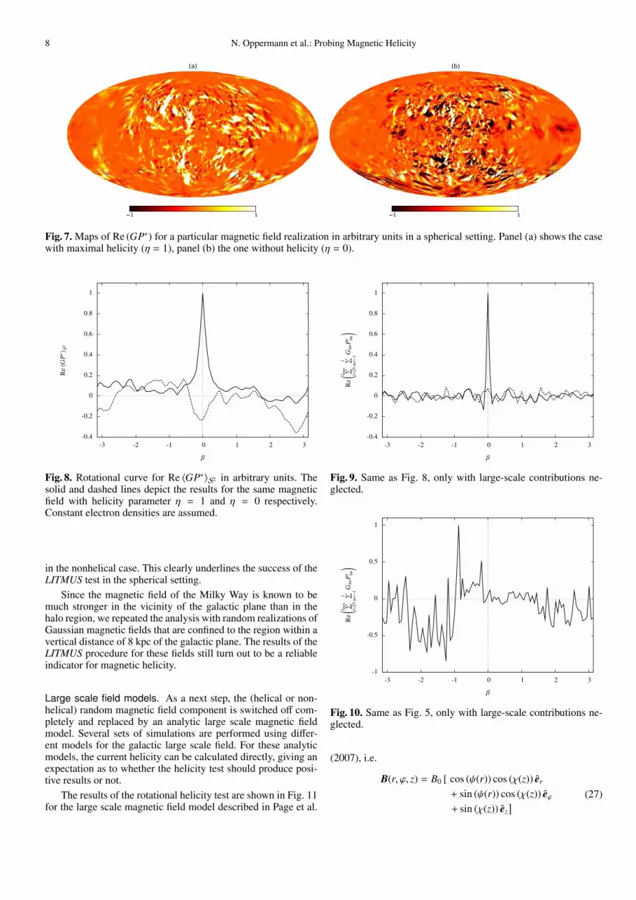
Figure 7 shows the maps of Re (GP∗) for one particularGaussian random magnetic field with a power law index of −5/3,with helicity and without helicity, respectively. As for the planarimplementation, one can immediately see that positive valuesdominate in the helical case and positive and negative values areroughly equally represented in the nonhelical case.

Figure 8 shows the results of the rotational test described inSect. 3.3 for this particular magnetic field realization. Clearly,the spatial average Re 〈GP∗〉S2 takes on a sharp maximum atβ = 0 and is positive in the case with helicity, while it doesnot have a maximum there and in fact happens to be negative inthe case without helicity. This is exactly the result expected fromthe LITMUS test.

The sharpness of the peak in Fig. 8 indicates that the helicityis to be found in small-scale features. As a test of this assertion,we calculated the spherical multipole components Glm and Plmof the complex gradient and polarization fields. Note that thespatial average over the product of the fields is proportional tothe sum of the products of the multipole components, i.e.

Re 〈GP∗〉S2 =1

4πRe

lmax∑l=0

l∑m=−l

GlmP∗lm

, (26)

where lmax is determined by the finite resolution of the map. Ifwe now neglect the first terms in the sum, i.e. the small-l contri-butions, we arrive at a spatial average over the product in whichall large-scale features were neglected. The resulting rotationalcurves for the same magnetic fields used for Fig. 8 are shown inFig. 9, where only multipole moments with l ≥ 25 were consid-ered. It can be seen that this procedure further sharpens the peakat β = 0 and strengthens it relative to other local maxima in thecurves, thus facilitating the detection of small-scale helicity. Thesame result for the observational data studied in Sect. 3 is shownin Fig. 10. Clearly, there is still no sign of helicity in this case.

Furthermore, we created a set of 100 different Gaussian ran-dom magnetic fields, performed the LITMUS test, and calculatedthe spatial average Re 〈GP∗〉S2 for all of them. Each field realiza-tion was considered in a version without helicity and a versionwith maximal helicity, just as in the case of the planar imple-mentation. Averaging over the 100 samples yields again a pos-itive value in the helical case. Normalizing all values such thatthis average is equal to one yields⟨

Re 〈GP∗〉S2⟩

samples = 1.0, σRe〈GP∗〉S2 = 0.25

in the helical case and⟨Re 〈GP∗〉S2

⟩samples = −0.27, σRe〈GP∗〉

S2 = 0.23

8 N. Oppermann et al.: Probing Magnetic Helicity

(a)

�1 1

(b)

�1 1

Fig. 7. Maps of Re (GP∗) for a particular magnetic field realization in arbitrary units in a spherical setting. Panel (a) shows the casewith maximal helicity (η = 1), panel (b) the one without helicity (η = 0).

-0.4

-0.2

0

0.2

0.4

0.6

0.8

1

-3 -2 -1 0 1 2 3

Re〈G

P∗〉 S

2

β

Fig. 8. Rotational curve for Re 〈GP∗〉S2 in arbitrary units. Thesolid and dashed lines depict the results for the same magneticfield with helicity parameter η = 1 and η = 0 respectively.Constant electron densities are assumed.

in the nonhelical case. This clearly underlines the success of theLITMUS test in the spherical setting.

Since the magnetic field of the Milky Way is known to bemuch stronger in the vicinity of the galactic plane than in thehalo region, we repeated the analysis with random realizations ofGaussian magnetic fields that are confined to the region within avertical distance of 8 kpc of the galactic plane. The results of theLITMUS procedure for these fields still turn out to be a reliableindicator for magnetic helicity.

Large scale field models. As a next step, the (helical or non-helical) random magnetic field component is switched off com-pletely and replaced by an analytic large scale magnetic fieldmodel. Several sets of simulations are performed using differ-ent models for the galactic large scale field. For these analyticmodels, the current helicity can be calculated directly, giving anexpectation as to whether the helicity test should produce posi-tive results or not.

The results of the rotational helicity test are shown in Fig. 11for the large scale magnetic field model described in Page et al.

-0.4

-0.2

0

0.2

0.4

0.6

0.8

1

-3 -2 -1 0 1 2 3

Re( l m

ax ∑ l=25

l ∑ m=−

lGlm

P∗ lm

)

β

Fig. 9. Same as Fig. 8, only with large-scale contributions ne-glected.

-1

-0.5

0

0.5

1

-3 -2 -1 0 1 2 3

Re( l m

ax ∑ l=25

l ∑ m=−

lGlm

P∗ lm

)

β

Fig. 10. Same as Fig. 5, only with large-scale contributions ne-glected.

(2007), i.e.

B(r, ϕ, z) = B0 [ cos (ψ(r)) cos (χ(z)) er

+ sin (ψ(r)) cos (χ(z)) eϕ+ sin (χ(z)) ez

] (27)

N. Oppermann et al.: Probing Magnetic Helicity 9

0.2

0.4

0.6

0.8

1

-3 -2 -1 0 1 2 3

Re〈G

P∗〉 S

2

β

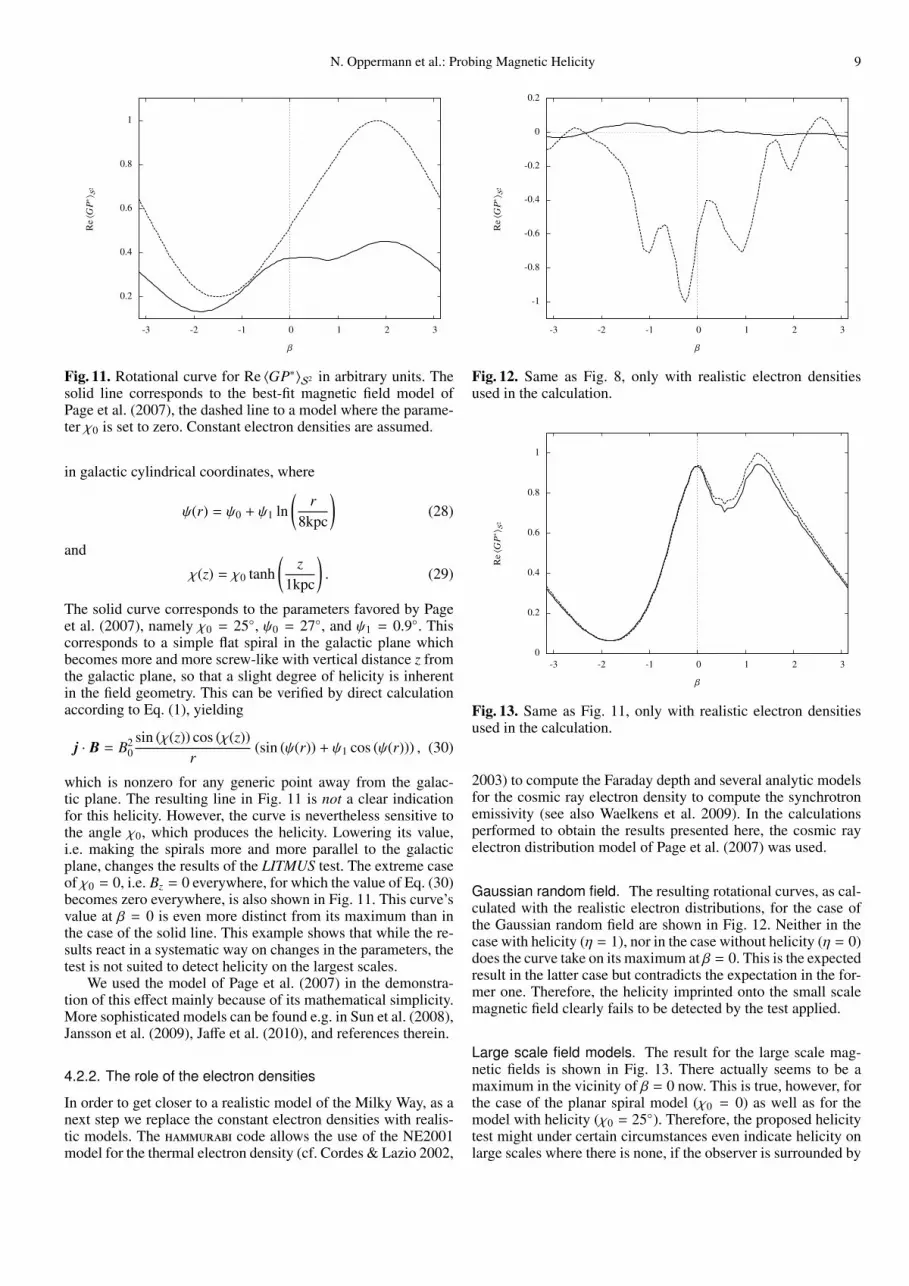
Fig. 11. Rotational curve for Re 〈GP∗〉S2 in arbitrary units. Thesolid line corresponds to the best-fit magnetic field model ofPage et al. (2007), the dashed line to a model where the parame-ter χ0 is set to zero. Constant electron densities are assumed.

in galactic cylindrical coordinates, where

ψ(r) = ψ0 + ψ1 ln(

r8kpc

)(28)

and

χ(z) = χ0 tanh(

z1kpc

). (29)

The solid curve corresponds to the parameters favored by Pageet al. (2007), namely χ0 = 25◦, ψ0 = 27◦, and ψ1 = 0.9◦. Thiscorresponds to a simple flat spiral in the galactic plane whichbecomes more and more screw-like with vertical distance z fromthe galactic plane, so that a slight degree of helicity is inherentin the field geometry. This can be verified by direct calculationaccording to Eq. (1), yielding

j · B = B20

sin (χ(z)) cos (χ(z))r

(sin (ψ(r)) + ψ1 cos (ψ(r))) , (30)

which is nonzero for any generic point away from the galac-tic plane. The resulting line in Fig. 11 is not a clear indicationfor this helicity. However, the curve is nevertheless sensitive tothe angle χ0, which produces the helicity. Lowering its value,i.e. making the spirals more and more parallel to the galacticplane, changes the results of the LITMUS test. The extreme caseof χ0 = 0, i.e. Bz = 0 everywhere, for which the value of Eq. (30)becomes zero everywhere, is also shown in Fig. 11. This curve’svalue at β = 0 is even more distinct from its maximum than inthe case of the solid line. This example shows that while the re-sults react in a systematic way on changes in the parameters, thetest is not suited to detect helicity on the largest scales.

We used the model of Page et al. (2007) in the demonstra-tion of this effect mainly because of its mathematical simplicity.More sophisticated models can be found e.g. in Sun et al. (2008),Jansson et al. (2009), Jaffe et al. (2010), and references therein.

4.2.2. The role of the electron densities

In order to get closer to a realistic model of the Milky Way, as anext step we replace the constant electron densities with realis-tic models. The hammurabi code allows the use of the NE2001model for the thermal electron density (cf. Cordes & Lazio 2002,

-1

-0.8

-0.6

-0.4

-0.2

0

0.2

-3 -2 -1 0 1 2 3

Re〈G

P∗〉 S

2

β

Fig. 12. Same as Fig. 8, only with realistic electron densitiesused in the calculation.

0

0.2

0.4

0.6

0.8

1

-3 -2 -1 0 1 2 3

Re〈G

P∗〉 S

2

β

Fig. 13. Same as Fig. 11, only with realistic electron densitiesused in the calculation.

2003) to compute the Faraday depth and several analytic modelsfor the cosmic ray electron density to compute the synchrotronemissivity (see also Waelkens et al. 2009). In the calculationsperformed to obtain the results presented here, the cosmic rayelectron distribution model of Page et al. (2007) was used.

Gaussian random field. The resulting rotational curves, as cal-culated with the realistic electron distributions, for the case ofthe Gaussian random field are shown in Fig. 12. Neither in thecase with helicity (η = 1), nor in the case without helicity (η = 0)does the curve take on its maximum at β = 0. This is the expectedresult in the latter case but contradicts the expectation in the for-mer one. Therefore, the helicity imprinted onto the small scalemagnetic field clearly fails to be detected by the test applied.

Large scale field models. The result for the large scale mag-netic fields is shown in Fig. 13. There actually seems to be amaximum in the vicinity of β = 0 now. This is true, however, forthe case of the planar spiral model (χ0 = 0) as well as for themodel with helicity (χ0 = 25◦). Therefore, the proposed helicitytest might under certain circumstances even indicate helicity onlarge scales where there is none, if the observer is surrounded by

10 N. Oppermann et al.: Probing Magnetic Helicity

the field. Other magnetic field models with planar spirals, suchas the bisymmetric (i.e. B(r, ϕ, z) = −B(r, ϕ + π, z)) spiral modelof Stanev (1997) lead to similar results.

5. Discussion and conclusion

The present work presents the first application of the LITMUStest for magnetic helicity proposed by Junklewitz & Enßlin(2010) to actual data. The application of the test involves thor-oughly reconstructing a map of the Faraday depth distribution,calculating its transformed gradient field G, creating a map ofGP∗, averaging over this map, shifting the two fields with respectto each other to see whether any signal vanishes, and filteringout large-scale contributions for a better detection of small-scalehelicity. This procedure, applied to observations of the Faradaydepth and polarization properties of the synchrotron radiationwithin our own galaxy in Sect. 3, does not show any signs ofhelicity in the Milky Way’s magnetic field.

In order to assess the significance of this, the applicability ofthe test was probed in different artificial settings. The complex-ity of these settings was increased bit by bit to find out underwhat circumstances exactly the LITMUS test yields reliable re-sults. It was found that meaningful results can be achieved ifthe electron densities do not vary on the scales of the magneticfield, both in the regime of magnetic field structures whose dis-tance from the observer is much greater than their extension, asshown in Sect. 4.1, and in the regime of magnetic fields sur-rounding the observer, as shown in Sect. 4.2.1. We showed thatthe performance of the LITMUS test with regard to small-scalehelicity is further improved by dropping the first few terms inEq. (26). However, indications of helicity on large scales are un-reliable, as shown in Sect. 4.2.1. Furthermore, it was demon-strated in Sect. 4.2.2 that any non-trivial electron density maydistort the outcome of the test to a point where even small-scalehelical structures fail to be detected. This is not too surprisingsince e.g. a variation in the thermal electron density will intro-duce a gradient in the Faraday depth that is not caused by themagnetic field structure. Therefore the nondetection of helicityfor the galactic magnetic field does not necessarily mean that thefield is nonhelical on small scales. It may be the case that small-scale fluctuations of the electron density introduce effects in theobservational data that prevent the detection of helicity.

So, as a natural next step, the hunt for helicity in astrophysi-cal magnetic fields should focus on a region that is small and/orhomogeneus enough for the assumption of constant electrondensities to hold at least approximatively. Although our workhas shown that the helicity test that we studied is not suitablefor all astrophysical settings, we are confident that it may nev-ertheless yield useful results if applied in a setting with constantelectron densities.

As a side effect of this paper, it was demonstrated in Sect. 3.2that the method proposed by Enßlin & Frommert (2010) to re-construct a Gaussian signal with unknown power spectrum isvery well suited for practical application.

Acknowledgements. The authors would like to thank Cornelius Weig for helpwith an efficient planar implementation of the LITMUS test. Some of the resultsin this paper have been derived using the HEALPix (Gorski et al. 2005) pack-age. We acknowledge the use of the Legacy Archive for Microwave BackgroundData Analysis (LAMBDA). Support for LAMBDA is provided by the NASAOffice of Space Science. Most computations were performed using the Sagesoftware package (Sage 2010). This research was performed in the frameworkof the DFG Forschergruppe 1254 “Magnetisation of Interstellar and IntergalacticMedia: The Prospects of Low-Frequency Radio Observations”. The idea for thiswork emerged from the very stimulating discussion with Rodion Stepanov dur-

ing his visit to Germany, which was supported by the DFG–RFBR grant 08-02-92881. We thank the anonymous referee for constructive comments.

ReferencesCordes, J. M. & Lazio, T. J. W., NE2001.I. A New Model for the Galactic

Distribution of Free Electrons and its Fluctuations, ArXiv Astrophysics e-prints (Jul. 2002), arXiv:astro-ph/0207156

Cordes, J. M. & Lazio, T. J. W., NE2001. II. Using Radio Propagation Datato Construct a Model for the Galactic Distribution of Free Electrons, ArXivAstrophysics e-prints (Jan. 2003), arXiv:astro-ph/0301598

Enßlin, T. & Frommert, M., Reconstruction of signals with unknown spectrain information field theory with parameter uncertainty, ArXiv e-prints (Feb.2010), arXiv:1002.2928 [astro-ph.IM]

Enßlin, T. A., Does circular polarisation reveal the rotation of quasar engines?,A&A 401 (Apr. 2003) 499–504,, arXiv:astro-ph/0212387

Enßlin, T. A. & Weig, C., Inference with minimal Gibbs free energy in in-formation field theory, Phys. Rev. E 82 no. 5, (Nov. 2010) 051112–+,,arXiv:1004.2868 [astro-ph.IM]

Gabuzda, D. C., Murray, E., & Cronin, P., Helical magnetic fields associatedwith the relativistic jets of four BL Lac objects, MNRAS 351 (Jul. 2004)L89–L93,, arXiv:astro-ph/0405394

Gorski, K. M., Hivon, E., Banday, A. J., et al., HEALPix: A Framework forHigh-Resolution Discretization and Fast Analysis of Data Distributed on theSphere, ApJ 622 (Apr. 2005) 759–771,, arXiv:astro-ph/0409513

Jaffe, T. R., Leahy, J. P., Banday, A. J., et al., Modelling the Galactic magneticfield on the plane in two dimensions, MNRAS 401 (Jan. 2010) 1013–1028,,arXiv:0907.3994 [astro-ph.GA]

Jansson, R., Farrar, G. R., Waelkens, A. H., & Enßlin, T. A., Constraining modelsof the large scale Galactic magnetic field with WMAP5 polarization data andextragalactic rotation measure sources, J. Cosmology Astropart. Phys. 7 (Jul.2009) 21–+,, arXiv:0905.2228 [astro-ph.GA]

Jasche, J., Kitaura, F. S., Wandelt, B. D., & Enßlin, T. A., Bayesian power-spectrum inference for large-scale structure data, MNRAS 406 (Jul. 2010)60–85,, arXiv:0911.2493 [astro-ph.CO]

Junklewitz, H. & Enßlin, T. A., Imprints of magnetic power and helic-ity spectra on radio polarimetry statistics, ArXiv e-prints (Aug. 2010),arXiv:1008.1243 [astro-ph.IM]

Kahniashvili, T., Gogoberidze, G., & Ratra, B., Polarized CosmologicalGravitational Waves from Primordial Helical Turbulence, Physical ReviewLetters 95 no. 15, (Oct. 2005) 151301–+,, arXiv:astro-ph/0505628

Kahniashvili, T. & Ratra, B., Effects of cosmological magnetic helicity on thecosmic microwave background, Phys. Rev. D 71 no. 10, (May 2005) 103006–+,, arXiv:astro-ph/0503709

Kahniashvili, T. & Vachaspati, T., Detection of magnetic helicity,Phys. Rev. D 73 no. 6, (Mar. 2006) 063507–+,, arXiv:astro-ph/0511373

Kitaura, F. S. & Enßlin, T. A., Bayesian reconstruction of the cosmological large-scale structure: methodology, inverse algorithms and numerical optimization,MNRAS 389 (Sep. 2008) 497–544,, arXiv:0705.0429

Mao, S. A., Gaensler, B. M., Haverkorn, M., et al., A Survey of ExtragalacticFaraday Rotation at High Galactic Latitude: The Vertical Magnetic Field ofthe Milky Way Toward the Galactic Poles, ApJ 714 (May 2010) 1170–1186,,arXiv:1003.4519 [astro-ph.GA]

Page, L., Hinshaw, G., Komatsu, E., et al., Three-Year Wilkinson MicrowaveAnisotropy Probe (WMAP) Observations: Polarization Analysis, ApJS 170(Jun. 2007) 335–376,, arXiv:astro-ph/0603450

Sage. 2010, SAGE Mathematical Software, Version 4.3.3.,http://www.sagemath.org

Schnitzeler, D. H. F. M., The latitude dependence of the rotation mea-sures of NVSS sources, MNRAS(Oct. 2010) L160+,, arXiv:1011.0737[astro-ph.GA]

Stanev, T., Ultra–High-Energy Cosmic Rays and the Large-ScaleStructure of the Galactic Magnetic Field, ApJ 479 (Apr. 1997) 290–+,,arXiv:astro-ph/9607086

Stil, J. M., Taylor, A. R., & Sunstrum, C., Structure in the Rotation Measure Sky,ApJ 726 (Jan. 2011) 4–+,, arXiv:1010.5299 [astro-ph.GA]

Subramanian, K., Magnetic helicity in galactic dynamos., Bulletinof the Astronomical Society of India 30 (Dec. 2002) 715–721,,arXiv:astro-ph/0204450

Sun, X. H., Reich, W., Waelkens, A., & Enßlin, T. A., Radio observational con-straints on Galactic 3D-emission models, A&A 477 (Jan. 2008) 573–592,,arXiv:0711.1572

Taylor, A. R., Stil, J. M., & Sunstrum, C., A Rotation Measure Image of the Sky,ApJ 702 (Sep. 2009) 1230–1236,

Volegova, A. A. & Stepanov, R. A., Helicity detection of astrophysical mag-netic fields from radio emission statistics, Soviet Journal of Experimental

N. Oppermann et al.: Probing Magnetic Helicity 11

and Theoretical Physics Letters 90 (Jan. 2010) 637–641,, arXiv:1001.2857[astro-ph.IM]

Waelkens, A., Jaffe, T., Reinecke, M., Kitaura, F. S., & Enßlin, T. A., Simulatingpolarized Galactic synchrotron emission at all frequencies. The Hammurabicode, A&A 495 (Feb. 2009) 697–706,, arXiv:0807.2262

Zhang, H., Helicity of solar magnetic field from observations, in IAUSymposium, Vol. 264, IAU Symposium, ed. A. G. Kosovichev, A. H. Andrei,& J.-P. Roelot. 2010, 181–190