RESEARCH ARTICLE

Prediction of water quality index in constructed wetlands usingsupport vector machine

Reza Mohammadpour & Syafiq Shaharuddin & Chun Kiat Chang &

Nor Azazi Zakaria & Aminuddin Ab Ghani & Ngai Weng Chan

Received: 8 July 2014 /Accepted: 2 November 2014 /Published online: 19 November 2014# Springer-Verlag Berlin Heidelberg 2014

Abstract Poor water quality is a serious problem in the worldwhich threatens human health, ecosystems, and plant/animallife. Prediction of surface water quality is a main concern inwater resource and environmental systems. In this research,the support vector machine and two methods of artificialneural networks (ANNs), namely feed forward back propaga-tion (FFBP) and radial basis function (RBF), were used topredict the water quality index (WQI) in a free constructedwetland. Seventeen points of the wetland were monitoredtwice a month over a period of 14 months, and an extensivedataset was collected for 11 water quality variables. A detailedcomparison of the overall performance showed that predictionof the support vector machine (SVM) model with coefficientof correlation (R2)=0.9984 and mean absolute error (MAE)=0.0052 was either better or comparable with neural networks.This research highlights that the SVM and FFBP can besuccessfully employed for the prediction of water quality ina free surface constructed wetland environment. Thesemethods simplify the calculation of the WQI and reducesubstantial efforts and time by optimizing the computations.

Keywords Support vector machine . Constructedwetland .

Water quality index . Neural networks . Surface water

Introduction

Municipal and industrial wastewaters from human activitiesare the major factors that contribute to the deterioration ofwater quality in urban areas. Water quality (WQ) can be usedto assess the water properties in reference to human health andnatural quality effects. The poor quality of surface wateris a serious problem in the world which threatens hu-man health, ecosystems, and plant/animal life.Consequently, water quality analysis has become a mainconcern in water resource and environmental systems(Espejo et al. 2012; Vanlandeghem et al. 2012; Zhanget al. 2013a, b; Wang et al. 2012). In terms of environ-mental and ecological problems, the number of waterquality parameters is quite extensive. Hence, a robustmathematical technique is required to combine the phys-icochemical characterization of water into a single var-iable which describes the water quality. A water qualityindex (WQI) is a single number which uses a set ofphysicochemical water parameters to express the qualityof water at a certain place and time.

In 1974, the Department of Environment of Malaysia(DoE) recommended the WQI parameter for categorizingand estimating water quality. Based on this parameter, thewater quality was classified into five different classes accord-ing to the water’s suitability for various uses such as watersupplies, irrigation, and fish culture. The conventional methodsuggested by DoE requires lengthy transformations to esti-mate subindices. In addition, the subindices required the in-clusion of different equations, which need lengthy effort andtime to calculate the final WQI. Therefore, estimation ofsuch a WQI is cumbersome and can lead to occasionalmistakes. However, the support vector machine (SVM)and artificial neural networks (ANNs) can be suggestedas alternatives for estimation of WQI, as both employthe raw data instead of subindices.

Responsible editor: Michael Matthies

R. Mohammadpour (*) : S. Shaharuddin :C. K. Chang :N. A. Zakaria :A. A. Ghani :N. W. ChanRiver Engineering and Urban Drainage Research Centre (REDAC),Universiti Sains Malaysia, Engineering Campus, Seri Ampangan,14300 Nibong Tebal, Penang, Malaysiae-mail: reza564@gmail.com

Environ Sci Pollut Res (2015) 22:6208–6219DOI 10.1007/s11356-014-3806-7

The performance of free surface wetlands to enhance waterquality and reduce a wide range of wastewater was reported inseveral studies (Zedler and Kercher 2005; Vymazal 2011;Zhang et al. 2012; Wang et al. 2012; Shih et al. 2013;Mohammadpour et al. 2014). Wetlands have high ability toabsorb and reduce agriculture and municipal wastewater andcan also highly decrease various nutrients (Mitsch andGosselink 2007; Kadlec and Wallace 2008). To remove pol-lutants and nutrients associated with fine particulates, severalprocesses occur in the constructed wetlands such as settling,filtration, absorption, and biological uptake (Guardo 1999).Generally, three parts can be recognized in the free surfacewetlands such as inlet, macrophyte, and open water area(Zakaria et al. 2003). The macrophyte area (wetland plants)has a high effect on the wetland ecosystem and water quality(Brix 1997; Kadlec and Wallace 2008). Since the number ofvariables which affect water quality is too high, the SVM canbe proposed as a robust technique for prediction of waterquality in a free constructed wetland environment.

Recently, soft computing techniques such as SVM, geneticprogramming (GP), and ANNs have been successfullyemployed to solve the problems related to engineering(Mohammadpour et al. 2011; Tabari et al. 2012; KakaeiLafdani et al. 2013; Mohammadpour et al. 2013b; Ghaniand Azamathulla 2014; He et al. 2014). The SVM is proposedas a leading technique which can be used for regression andclassification purposes (Noori et al. 2011; Singh et al. 2011a,b). The SVM has high ability for generalization and is lessprone to overfitting. Furthermore, it simultaneously mini-mizes the estimation of error and model dimensions (Singhet al. 2011a, b; Li et al. 2013). Sivapragasam and Muttil(2005) applied the SVM for prediction of water level in riversby extension of rating curves. Khan and Coulibaly (2006)recommended the SVM as the appropriate tool to fore-cast lake water levels and obtained quite acceptableresults. Singh et al. (2011a, b) employed the SVM forclassification and regression of water quality. The SVMwas applied as a classification tool for some studiesrelated to wetlands (Dronova et al. 2012; Betbederet al. 2013; Zhang and Xie 2013). Sadeghi et al.(2012) predicted the distribution pattern of Azollafiliculoides (Lam.) in wetlands using the SVM.

The ANNs have been recommended as an effective tool forthe prediction of water pollution and water quality in thewetlands (Schmid and Koskiaho 2006; Wang et al. 2012;Dong et al. 2012; Dadaser-Celik and Cengiz 2013; Li et al.2013; Song et al. 2013). The ANNs were employed to modelthe constructed wetlands in different fields (Tomenko et al.2007; Singh et al. 2011a, b; Zhang et al. 2013a, b). The ANNsare a useful technique that was used to speed up the calcula-tion of water quality index in rivers (Khuan et al. 2002; Juahiret al. 2004; Gazzaz et al. 2012). Mohammadpour et al.(2013a) examined two kinds of ANNs, feed forward back

propagation (FFBP) and radial basis function (RBF), for theprediction of time variation of local scour in rivers. Nouraniet al. (2013) applied the FFBP network to determine thequality of treated water. Diamantopoulou et al. (2005) usedthe neural networks to predict water quality in a river inGreece. Khalil et al. (2011) estimated water quality character-istics at ungauged sites using ANN and ensemble ANN(EANN). The results showed that the EANN provides betterprediction than the ANN.

In this research, both SVM and ANNs were used asrobust techniques for rapid and direct prediction of theWQI in the constructed wetlands which can be used asanother alternative for some long-lasting conventionalmethods. Seventeen points in the wetland were moni-tored twice a month over a period of 14 months and anextensive dataset was collected for 11 water qualityvariables. A sensitivity analysis was conducted to findmore significant variables on WQI. Finally, the SVMresult was compared with two models of neural net-works, namely the FFBP and RBF.

Materials and methods

Study area

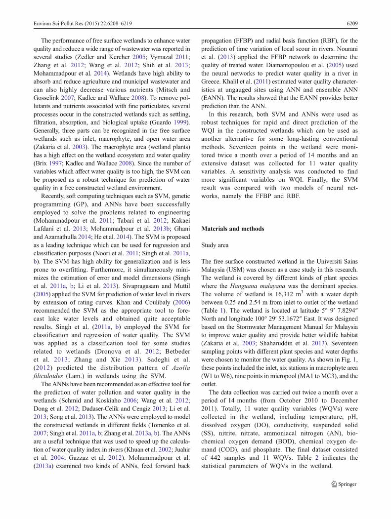
The free surface constructed wetland in the Universiti SainsMalaysia (USM) was chosen as a case study in this research.The wetland is covered by different kinds of plant specieswhere the Hanguana malayana was the dominant species.The volume of wetland is 16,312 m3 with a water depthbetween 0.25 and 2.54 m from inlet to outlet of the wetland(Table 1). The wetland is located at latitude 5° 9′ 7.8294″North and longitude 100° 29′ 53.1672″ East. It was designedbased on the Stormwater Management Manual for Malaysiato improve water quality and provide better wildlife habitat(Zakaria et al. 2003; Shaharuddin et al. 2013). Seventeensampling points with different plant species and water depthswere chosen to monitor the water quality. As shown in Fig. 1,these points included the inlet, six stations in macrophyte area(W1 toW6), nine points in micropool (MA1 toMC3), and theoutlet.

The data collection was carried out twice a month over aperiod of 14 months (from October 2010 to December2011). Totally, 11 water quality variables (WQVs) werecollected in the wetland, including temperature, pH,dissolved oxygen (DO), conductivity, suspended solid(SS), nitrite, nitrate, ammoniacal nitrogen (AN), bio-chemical oxygen demand (BOD), chemical oxygen de-mand (COD), and phosphate. The final dataset consistedof 442 samples and 11 WQVs. Table 2 indicates thestatistical parameters of WQVs in the wetland.

Environ Sci Pollut Res (2015) 22:6208–6219 6209

The local water quality index

To determine the WQI, six physicochemical parameterswere proposed by Department of Environment (DoE2005), namely DO, BOD, COD, AN, SS, and pH. TheWQI was recognized as a unitless variable with a valuefrom 0 to 100, where a high value of WQI representshigh water quality. As shown in Table 2, the mentioned

WQVs should be converted into nondimensional vari-ables using subindex functions (SI). Finally, the WQIcan be estimated using the following equation (DoE2005; Khuan et al. 2002):

WQI ¼ 0:22SIDO þ 0:19SIBOD þ 0:16SICOD

þ 0:15SIAN þ 0:16SISS þ 0:12SIpH ð1Þ

Table 1 Plant species and the water depth in the USM wetland

Site Wetland plant species Water depth (m)

Wetland 1 Dominant: Hanguana malayana, Lepironia articulata 0.25–0.3

Wetland 2 Dominant: Hanguana malayana, Typha angustifoliaLess dominant: Scirpus grossus

0.27–0.32

Wetland 3 Dominant: Lepironia articulata, Eleocharis variegataLess dominant: Eriocaulon longifolium

0.51–0.62

Wetland 4 Dominant: Hanguana malayana, Lepironia articulata,Eleocharis variegata

0.47–0.54

Wetland 5 Dominant: Lepironia articulata 0.51–0.64

Wetland 6 Dominant: Lepironia articulataLess dominant: Typha angustifolia

0.31–0.54

Micropool (MA, MB, and MC) Without plant 2.48–2.54

Fig. 1 Seventeen sample points in the constructed wetland of USM

6210 Environ Sci Pollut Res (2015) 22:6208–6219

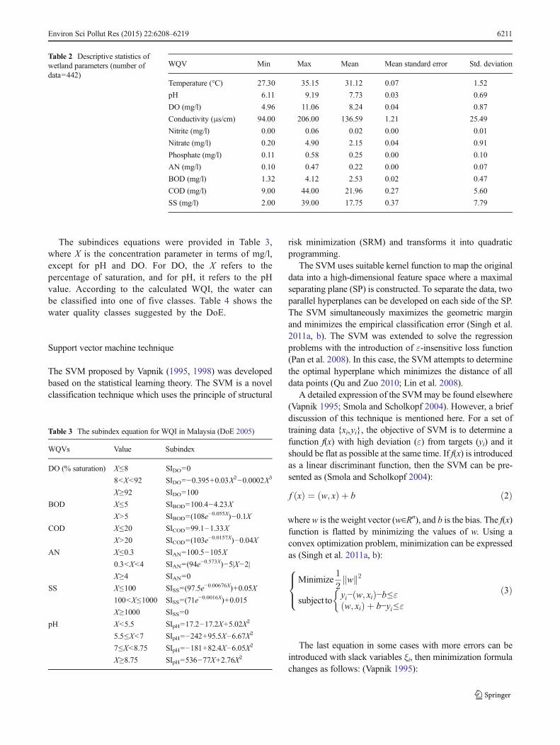
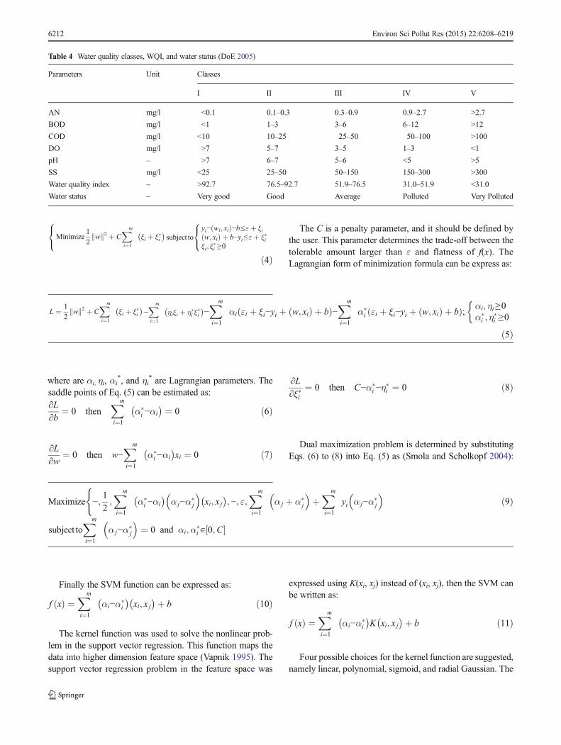
The subindices equations were provided in Table 3,where X is the concentration parameter in terms of mg/l,except for pH and DO. For DO, the X refers to thepercentage of saturation, and for pH, it refers to the pHvalue. According to the calculated WQI, the water canbe classified into one of five classes. Table 4 shows thewater quality classes suggested by the DoE.

Support vector machine technique

The SVM proposed by Vapnik (1995, 1998) was developedbased on the statistical learning theory. The SVM is a novelclassification technique which uses the principle of structural

risk minimization (SRM) and transforms it into quadraticprogramming.

The SVM uses suitable kernel function to map the originaldata into a high-dimensional feature space where a maximalseparating plane (SP) is constructed. To separate the data, twoparallel hyperplanes can be developed on each side of the SP.The SVM simultaneously maximizes the geometric marginand minimizes the empirical classification error (Singh et al.2011a, b). The SVM was extended to solve the regressionproblems with the introduction of ε-insensitive loss function(Pan et al. 2008). In this case, the SVM attempts to determinethe optimal hyperplane which minimizes the distance of alldata points (Qu and Zuo 2010; Lin et al. 2008).

A detailed expression of the SVMmay be found elsewhere(Vapnik 1995; Smola and Scholkopf 2004). However, a briefdiscussion of this technique is mentioned here. For a set oftraining data {xi,yi}, the objective of SVM is to determine afunction f(x) with high deviation (ε) from targets (yi) and itshould be flat as possible at the same time. If f(x) is introducedas a linear discriminant function, then the SVM can be pre-sented as (Smola and Scholkopf 2004):

f xð Þ ¼ w; xð Þ þ b ð2Þ

wherew is the weight vector (w∈Rn), and b is the bias. The f(x)function is flatted by minimizing the values of w. Using aconvex optimization problem, minimization can be expressedas (Singh et al. 2011a, b):

Minimize1

2wk k2

subject toyi− w; xið Þ−b≤εw; xið Þ þ b−yi≤ε

�8><>: ð3Þ

The last equation in some cases with more errors can beintroduced with slack variables ξi, then minimization formulachanges as follows: (Vapnik 1995):

Table 2 Descriptive statistics ofwetland parameters (number ofdata=442)

WQV Min Max Mean Mean standard error Std. deviation

Temperature (°C) 27.30 35.15 31.12 0.07 1.52

pH 6.11 9.19 7.73 0.03 0.69

DO (mg/l) 4.96 11.06 8.24 0.04 0.87

Conductivity (μs/cm) 94.00 206.00 136.59 1.21 25.49

Nitrite (mg/l) 0.00 0.06 0.02 0.00 0.01

Nitrate (mg/l) 0.20 4.90 2.15 0.04 0.91

Phosphate (mg/l) 0.11 0.58 0.25 0.00 0.10

AN (mg/l) 0.10 0.47 0.22 0.00 0.07

BOD (mg/l) 1.32 4.12 2.53 0.02 0.47

COD (mg/l) 9.00 44.00 21.96 0.27 5.60

SS (mg/l) 2.00 39.00 17.75 0.37 7.79

Table 3 The subindex equation for WQI in Malaysia (DoE 2005)

WQVs Value Subindex

DO (% saturation) X≤8 SIDO=0

8<X<92 SIDO=−0.395+0.03X2−0.0002X3

X≥92 SIDO=100

BOD X≤5 SIBOD=100.4−4.23XX>5 SIBOD=(108e

−0.055X)−0.1XCOD X≤20 SICOD=99.1−1.33X

X>20 SICOD=(103e−0.0157X)−0.04X

AN X≤0.3 SIAN=100.5−105X0.3<X<4 SIAN=(94e

−0.573X)−5|X−2|X≥4 SIAN=0

SS X≤100 SISS=(97.5e−0.00676X)+0.05X

100<X≤1000 SISS=(71e−0.0016X)+0.015

X≥1000 SISS=0

pH X<5.5 SIpH=17.2−17.2X+5.02X2

5.5≤X<7 SIpH=−242+95.5X−6.67X2

7≤X<8.75 SIpH=−181+82.4X−6.05X2

X≥8.75 SIpH=536−77X+2.76X2

Environ Sci Pollut Res (2015) 22:6208–6219 6211

Minimize1

2wk k2 þ C

Xi¼1

m

ξi þ ξ�i� �

subject toyi− wi; xið Þ−b≤εþ ξiw; xið Þ þ b−yi≤εþ ξ�iξi; ξ

�i ≥0

8<:

8<:

ð4Þ

The C is a penalty parameter, and it should be defined bythe user. This parameter determines the trade-off between thetolerable amount larger than ε and flatness of f(x). TheLagrangian form of minimization formula can be express as:

L ¼ 1

2wk k2 þ C

Xi¼1

m

ξi þ ξ�i� �

−Xi¼1

m

ηiξi þ η�i ξ�i

� �−Xi¼1

m

αi εi þ ξi−yi þ w; xið Þ þ bð Þ−Xi¼1

m

α�i εi þ ξi−yi þ w; xið Þ þ bð Þ; αi; ηi≥0

α�i ; η

�i ≥0

�

ð5Þ

where are αi, ηi, αi*, and ηi

* are Lagrangian parameters. Thesaddle points of Eq. (5) can be estimated as:∂L∂b

¼ 0 thenXi¼1

m

α�i −αi

� � ¼ 0 ð6Þ

∂L∂w

¼ 0 then w−Xi¼1

m

α�i −αi

� �xi ¼ 0 ð7Þ

∂L∂ξ�i

¼ 0 then C−α�i −η

�i ¼ 0 ð8Þ

Dual maximization problem is determined by substitutingEqs. (6) to (8) into Eq. (5) as (Smola and Scholkopf 2004):

Maximize −;1

2;Xi¼1

m

α�i −αi

� �α j−α�

j

� �xi; x j� �

;−; ε;Xi¼1

m

α j þ α�j

� �þXi¼1

m

yi α j−α�j

� �(

subject toXi¼1

m

α j−α�j

� �¼ 0 and αi;α

�i ∈ 0;C½ �

ð9Þ

Finally the SVM function can be expressed as:

f xð Þ ¼Xi¼1

m

αi−α�i

� �xi; x j� �þ b ð10Þ

The kernel function was used to solve the nonlinear prob-lem in the support vector regression. This function maps thedata into higher dimension feature space (Vapnik 1995). Thesupport vector regression problem in the feature space was

expressed using K(xi, xj) instead of (xi, xj), then the SVM canbe written as:

f xð Þ ¼Xi¼1

m

αi−α�i

� �K xi; x j� �þ b ð11Þ

Four possible choices for the kernel function are suggested,namely linear, polynomial, sigmoid, and radial Gaussian. The

Table 4 Water quality classes, WQI, and water status (DoE 2005)

Parameters Unit Classes

I II III IV V

AN mg/l <0.1 0.1–0.3 0.3–0.9 0.9–2.7 >2.7

BOD mg/l <1 1–3 3–6 6–12 >12

COD mg/l <10 10–25 25–50 50–100 >100

DO mg/l >7 5–7 3–5 1–3 <1

pH – >7 6–7 5–6 <5 >5

SS mg/l <25 25–50 50–150 150–300 >300

Water quality index – >92.7 76.5–92.7 51.9–76.5 31.0–51.9 <31.0

Water status – Very good Good Average Polluted Very Polluted

6212 Environ Sci Pollut Res (2015) 22:6208–6219

most common kernel functions are polynomial and Gaussianor RBF which were expressed as:

K xi; x j� � ¼ 1þ xi:x j

� �pPolynomialkernel function ð12Þ

K xi; x j� � ¼ exp −γ xi:x j

�� ��2� �Gaussiankernel function ð13Þ

where p and γ are adjustable kernel parameters. The per-formance of SVM depends on the combination of severalparameters, such as the type of kernel function and its adjust-able parameters, penalty parameter, C, and ε-insensitive lossfunction. The selection of kernel function depends on thedistribution of the data and generally can be selected throughthe trial and error approach (Widodo and Yang 2007). Sincethe RBF is employed in most of the applications (Xie et al.2008), then in this study, the RBF (Gaussian kernel function)was chosen as kernel function for the prediction of WQI.

The γ is the most important parameter for the RBF kernelfunction. The amplitude of the kernel can be controlled by thisparameter, and it can lead to overfitting and underfitting inprediction. The best value of γ can be found by trial and error(Noori et al. 2011). The C is a regularization parameter thatcontrols the trade-off between maximizing the margin andminimizing the training error. For a low value of C, insuffi-cient fitting will be placed on the training data, while thealgorithm will overfit for too large of C (Wang et al. 2007).A well-performing and robust regression model is dependenton a proper choice of C in combination with ε (Ustun et al.2005). A range of 0.001–20,000 was chosen for the C param-eter to investigate the optimal value (Fig. 3). Furthermore,since the exact contribution of the noise in the training set isusually unknown, the εwas optimized in the range of 0.00001and 0.1 (Ustun et al. 2005). To achieve a good combination ofthe two variables (C and ε), an internal cross-validation wasperformed during the construction of the SVM model. In thisstudy, the SVM-base classification was performed using

Library for Support Vector Machines (LIBSVM) inMATLAB (Chang and Lin 2011).

Artificial neural network methods

ANNs are a computational process which attempts to repre-sent and compute a mapping from multivariate dataset asinputs to another as outputs. A neuron is the smallest part ofthe neural network; these artificial neurons are arranged in thestructure like a network. In this study, two models of neuralnetworks, FFBP and RBF, were presented and a brief descrip-tion of these methods are given here.

Feed forward back propagation neural network

The network consists of a set of neurons in three, inputs,hidden, and output, layers to approximate a multivariant func-tion f(x). The number of neurons in hidden layers can bedetected by trial and error. The learning procedure includesthe best weight vector to achieve the best approximation off(x). Firstly, a set of input data (x1,x2,…xR) is fed to the inputlayer, and the output of each neuron can be determined fromthe following relation:

n ¼X

wi jxi þ bi

ð14Þ

where n is the neuron output, wij is the weight of the connec-tion between the jth neuron in the present layer and ith neuronin the previous layer, xi is the neuron value in the previouslayer, and bi is the bias. The sigmoid function can be used as atransfer function to generate the output of each neuron (Bateniet al. 2007) given by:

yi ¼1

1þ e−C1

Xwi jxiþbi

� � ;C1 > 0 ð15Þ

Fig. 2 Variation of gamma values in terms of RMSE in the SVM model

Table 5 Sensitivityanalysis using ANNs All variable without Ratio Rank

pH 1.226 1

COD 1.081 2

DO 1.048 3

AN 1.044 4

SS 1.020 5

BOD 1.019 6

Phosphate 1.000 7

Nitrate 1.000 8

Conductivity 0.999 9

Nitrite 0.998 10

Temperature 0.997 11

Environ Sci Pollut Res (2015) 22:6208–6219 6213

The network error calculation uses a comparison betweenthe target value and the obtained results, while the backpropagation algorithm corrects the weight between neurons.The back propagation (BP) method is a descent algorithm,which tries to minimize the error at each iteration. The net-work weights are set by the algorithm such that the networkerror decreases along a descent direction (gradient descent).Generally, two parameters, called momentum factor (MF) andlearning rate (LR), are used to control the weight adjustmentin the descent direction.

Radial basis function neural network

The RBF network is a general regression tool for approximatefunction that uses a radial basis function as activation func-tion. In this study, the Softmax transfer function is used toestimate the ∅ value at each node.

ϕ j xð Þ ¼exp −

x−μ j

�� ��22σ2

j

!

Xexp −

x−μ j

�� ��22σ2

j

! ð16Þ

where x is the input dataset, μj is the center of the radial basisfunction for the jth hidden node, σj is a radius of the radialbasis function for the jth hidden node, and ‖x−μj‖2 is theEuclidean norm. The linear interconnectedness between net-work outputs and hidden nodes can be explained by thefollowing equation:

yk ¼X

wk jϕ j xð Þ ð17Þ

where yk is the kth component of the output layer, andwkj is theweight between the jth hidden node and kth node of the outputlayer.

In this study, the collected dataset was normalized withinthe range of 0.1–0.9. Three common statistical measures,namely the coefficient of correlation (R2), root mean squareerror (RMSE), and mean absolute error (MAE), were used tovalidate the provided results.

Results and discussion

Determining the main water quality variables

To determine the main WQVs in the prediction of the WQI, asensitivity analysis was carried out using ANN. The sensitiv-ity analysis was conducted using the FFBP network with onehidden layer. The number of neurons in the input layer was

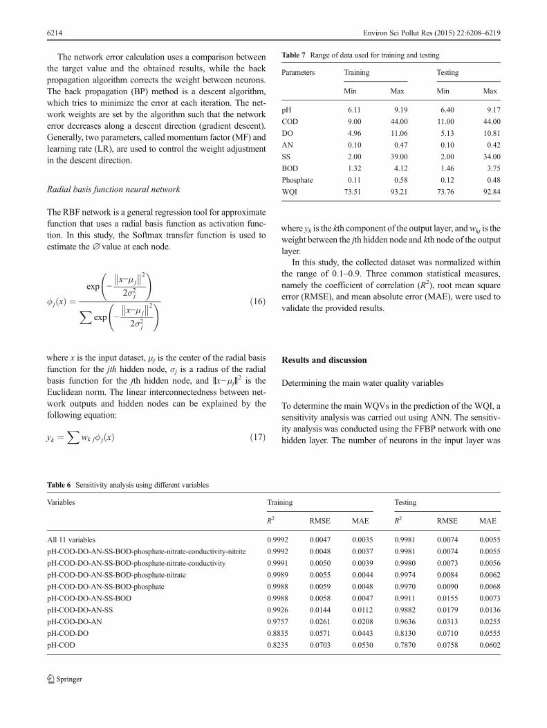
Table 6 Sensitivity analysis using different variables

Variables Training Testing

R2 RMSE MAE R2 RMSE MAE

All 11 variables 0.9992 0.0047 0.0035 0.9981 0.0074 0.0055

pH-COD-DO-AN-SS-BOD-phosphate-nitrate-conductivity-nitrite 0.9992 0.0048 0.0037 0.9981 0.0074 0.0055

pH-COD-DO-AN-SS-BOD-phosphate-nitrate-conductivity 0.9991 0.0050 0.0039 0.9980 0.0073 0.0056

pH-COD-DO-AN-SS-BOD-phosphate-nitrate 0.9989 0.0055 0.0044 0.9974 0.0084 0.0062

pH-COD-DO-AN-SS-BOD-phosphate 0.9988 0.0059 0.0048 0.9970 0.0090 0.0068

pH-COD-DO-AN-SS-BOD 0.9988 0.0058 0.0047 0.9911 0.0155 0.0073

pH-COD-DO-AN-SS 0.9926 0.0144 0.0112 0.9882 0.0179 0.0136

pH-COD-DO-AN 0.9757 0.0261 0.0208 0.9636 0.0313 0.0255

pH-COD-DO 0.8835 0.0571 0.0443 0.8130 0.0710 0.0555

pH-COD 0.8235 0.0703 0.0530 0.7870 0.0758 0.0602

Table 7 Range of data used for training and testing

Parameters Training Testing

Min Max Min Max

pH 6.11 9.19 6.40 9.17

COD 9.00 44.00 11.00 44.00

DO 4.96 11.06 5.13 10.81

AN 0.10 0.47 0.10 0.42

SS 2.00 39.00 2.00 34.00

BOD 1.32 4.12 1.46 3.75

Phosphate 0.11 0.58 0.12 0.48

WQI 73.51 93.21 73.76 92.84

6214 Environ Sci Pollut Res (2015) 22:6208–6219

determined based on the number of WQVs as input to ANN.In the output, a layer with one neuron was chosen for WQI.The leave-one-out technique was employed to assess theeffect of each variable on the WQI. By removing one variablein the input at each time, two indicators were determined,namely the ratio of ANN error and its rank (Ha andStenstrom 2003). The ratio of ANN error was found byremoving an individual variable to the error obtained usingall variables. The high value for this ratio can be interpreted ashigh significance of individual variable and vice versa. Theresult of this analysis is shown in Table 5. Generally, in theenvironmental works, the simple equations with a few vari-ables are more practical and useful in comparison with com-plex equations. Therefore, another sensitivity analysis wasconducted to simplify the classification and reduce the numberof variables onWQI. Table 6 compares the ANNmodels withone of the independent variables removed in each case. Asshown in this table, pH, COD, DO, AN, and SS are significant

variables, with a high performance of ANNs (R2=0.9882,RMSE=0.0179, and MAE=0.0136). The performance ofANNs decreases with removal of one of these variables inthe next rows. Therefore, these variables were chosen todevelop the SVM, FFBP, and ANNs-RBF models. It wasobserved that removing more variables such as BOD, phos-phate, nitrate, nitrite, and conductivity has no considerablyeffect on the performance of ANNs. In light of these findings,the pH with the highest rank in the sensitive analysis can beconsidered as a main parameter (Table 5), while it is ranked asthe sixth variable in the conventional WQI equation (Eq. 1).This equation is recommended for estimation of WQI in therivers, and the difference between ranking of pH in Eq. 1 andthe present study can be due to the discharge at the pointsource and nonpoint pollution to rivers. However, the selectedwetland is discharged just by nonpoint source pollution due tostorm water. Same ranking results were observed by Gazzazet al. (2012). This point may be considered for re-

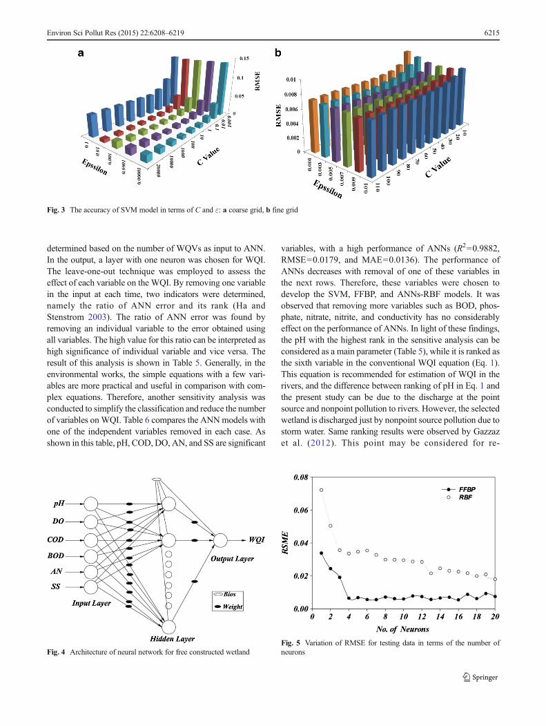
Fig. 3 The accuracy of SVM model in terms of C and ε: a coarse grid, b fine grid

Fig. 4 Architecture of neural network for free constructed wetlandFig. 5 Variation of RMSE for testing data in terms of the number ofneurons

Environ Sci Pollut Res (2015) 22:6208–6219 6215

establishment of a new equation for WQI in the wetlands andother water resource with nonpoint pollution discharge.

The SVM result

Based on the provided result by sensitivity analysis, all 11water quality variables can be reduced to just six significantvariables including pH, COD, DO, AN, SS, and BOD. In thepresent study, the selected dataset (442 samples×6 variables)was randomly divided into training dataset (354 samples×7variables) and testing subsets dataset (88 samples×7 vari-ables). Thus, the training and validation (testing) dataset werecomprised of 80 and 20 % of samples, respectively. Table 7summarizes the range of training and testing dataset.

The SVM models with different values of γ were devel-oped to determine the best value for this parameter. TheRMSE was chosen to assess the accuracy of SVM models.Figure 2 indicates that the minimum error was obtained for γ=0.9, and this value was chosen to determineC and ε in the nextsteps. Furthermore, a tenfold cross-validation and grid searchalgorithmwere employed to find the optimal values ofC and ε(Hsu et al. 2003).

In tenfold cross-validation, the collected data were random-ly divided into ten equal groups, where eight groups were usedfor training, and the rest of the groups were employed forvalidation. The grid search algorithm takes different samples

from the space of the independent variables. In each step, theprediction of the model was compared with the best valueprovided from the previous iterations. If the newly foundvalues were better than the previous one, the new values wereused. The grid search algorithm is an unguided technique, andit was developed based on trial and error (Hsu et al. 2003;Noori et al. 2011). A two-step grid search with cross-validation was employed to solve this problem and determinethe tune values of C and ε (Chen and Yu 2007). In the firststep, a coarse grid search was applied to determine the bestregion of demanded parameters. In the next step, a finer gridsearch was employed to recognize the optimal combination ofparameters. In Fig. 3, the accuracy of SVM was assessedregarding C and ε values. Through a coarse grid search(Fig. 3a), the optimum values of C and ε were determined

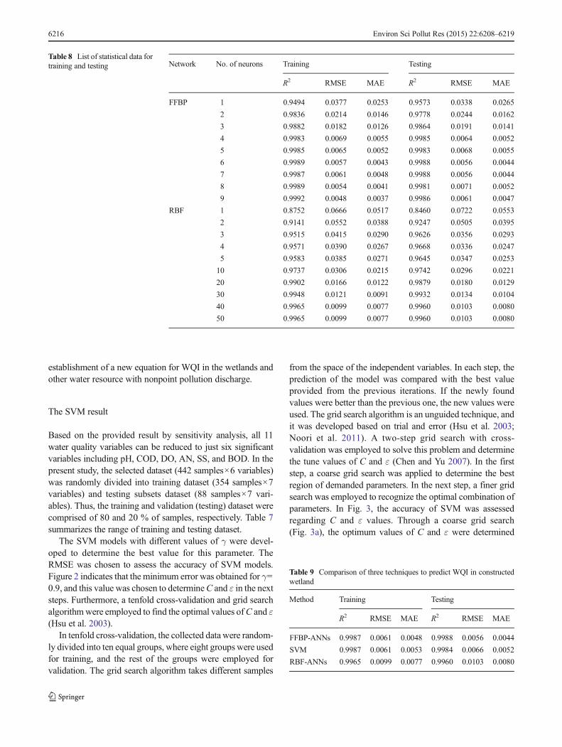
Table 8 List of statistical data fortraining and testing Network No. of neurons Training Testing

R2 RMSE MAE R2 RMSE MAE

FFBP 1 0.9494 0.0377 0.0253 0.9573 0.0338 0.0265

2 0.9836 0.0214 0.0146 0.9778 0.0244 0.0162

3 0.9882 0.0182 0.0126 0.9864 0.0191 0.0141

4 0.9983 0.0069 0.0055 0.9985 0.0064 0.0052

5 0.9985 0.0065 0.0052 0.9983 0.0068 0.0055

6 0.9989 0.0057 0.0043 0.9988 0.0056 0.0044

7 0.9987 0.0061 0.0048 0.9988 0.0056 0.0044

8 0.9989 0.0054 0.0041 0.9981 0.0071 0.0052

9 0.9992 0.0048 0.0037 0.9986 0.0061 0.0047

RBF 1 0.8752 0.0666 0.0517 0.8460 0.0722 0.0553

2 0.9141 0.0552 0.0388 0.9247 0.0505 0.0395

3 0.9515 0.0415 0.0290 0.9626 0.0356 0.0293

4 0.9571 0.0390 0.0267 0.9668 0.0336 0.0247

5 0.9583 0.0385 0.0271 0.9645 0.0347 0.0253

10 0.9737 0.0306 0.0215 0.9742 0.0296 0.0221

20 0.9902 0.0166 0.0122 0.9879 0.0180 0.0129

30 0.9948 0.0121 0.0091 0.9932 0.0134 0.0104

40 0.9965 0.0099 0.0077 0.9960 0.0103 0.0080

50 0.9965 0.0099 0.0077 0.9960 0.0103 0.0080

Table 9 Comparison of three techniques to predict WQI in constructedwetland

Method Training Testing

R2 RMSE MAE R2 RMSE MAE

FFBP-ANNs 0.9987 0.0061 0.0048 0.9988 0.0056 0.0044

SVM 0.9987 0.0061 0.0053 0.9984 0.0066 0.0052

RBF-ANNs 0.9965 0.0099 0.0077 0.9960 0.0103 0.0080

6216 Environ Sci Pollut Res (2015) 22:6208–6219

over a space of 10–100 and 0.0001–0.01, respectively. Finally,the best value of C and ε was found equal to 57 and 0.007through the fine grid search (Fig. 3b).

The neural network results

The ANN model was developed using the same datasetemployed for the SVM. Figure 4 indicates the architectureof FFBPwith six neurons in the input layer forWQVs and oneneuron in the output layer for WQI. Two types of ANNs,FFBP and RBF, were developed to investigate the best net-work for the reliable prediction of WQI. Based on trial anderror, the FFBP network with 2000 epochs and the RBFnetwork with the spread constant of 1.1 provided better resultsin comparison to the other networks.

Since the ANNs are sensitive to the number of neurons inthe hidden layer and these neurons were unknown in the firststep, then the ANNs were developed with different numbersof neurons in the hidden layer. The RMSE was employed toassess overfitting of network (low training error but high testerror). As shown in Fig. 5, the RMSE decreased dramaticallywith increasing number of neurons in the hidden layer, espe-cially in the FFBPmethod. An overfitting was observed in theFFBP networks when the number of neurons was more than16. The performance of both FFBP and RBF with differentneurons in the hidden layer is indicated in Table 8.

The testing data was assessed to find the optimum numberof neurons. The best performance for FFBP and RBF wasprovided for networks with six and 40 neurons in the hiddenlayer. For testing data, the FFBP with R2=0.9988, RMSE=0.0056, and MAE=0.0044 predicts the WQI with high accu-racy. As shown in this table, the accuracy of RBF (R2=0.9960,RMSE=0.0103, and MAE=0.0080) is a little lower than theFFBP method.

Comparison between SVM and ANNs

In Table 9, the performance of the SVM was compared withboth the FFBP and RBF models. The SVM with R2=0.9984,RMSE=0.0066, and MAE=0.0052 forecasts the WQI in thewetland better than the RBF (R2=0.9960, RMSE=0.0103,and MAE=0.0080). Furthermore, statistical parameters andscatter plot (Fig. 6) show that the prediction of SVM iscomparable with FFBP with R2=0.9988, RMSE=0.0056,and MAE=0.0044.

In light of this research, it can be concluded that to predictthe WQI in free surface constructed wetland environment,both the SVM and FFBP propose some advantages over theconventional method. The method recommended by DoE(2005) employs six subindices parameters, which need moreeffort and a long time to convert the six raw data (DO, BOD,COD, AN, SS, and pH) into its subindices (Table 3).Furthermore, instead of using the original parameters, allcalculations are based on the subindices (Eq. 1) which areobtained from rating curves. In contrast, both the SVM andFFBP approaches use the raw WQVs for training and testingrather than the subindices which led to a direct prediction ofthe WQI. Therefore, the SVM and FFBP methods are moredirect, rapid, and convenient techniques than the conventionalmethod.

Accordingly, this research highlights that the SVM andFFBP can be used as valuable methods for the prediction ofwater quality in the constructed wetland as they simplify thecalculation of the WQI and reduce substantial efforts and timeby optimizing the computations. These approaches can becommonly used for any aquatic system in the world. Thisresearch should encourage the managers and authorities to usethe SVM and FFBP methods as more direct and highlyreliable alternatives to predict water quality in wetlands andother water bodies.

Conclusions

In this study, the SVM and two methods of ANNs, namelyFFBP and RBF, were employed to investigate the WQI in thefree surface constructed wetland. Seventeen points of thewetland were monitored twice a month over a period of14months, and an extensive dataset was collected for 11 waterquality variables. A sensitivity analysis was carried out usingANN and six significant variables that included pH, COD,DO, AN, SS, and BOD to develop the SVM, FFBP, andANNs-RBF models. The results illustrate that the SVM tech-nique was able to successfully predict the WQI with highaccuracy. The high value of the coefficient of correlation(R2=0.9984) and low error (MAE=0.0052) indicated thatthe SVM model provides better prediction compared to theFig. 6 Comparison between predicted and observed WQI

Environ Sci Pollut Res (2015) 22:6208–6219 6217

RBF network with R2 = 0.9960 and MAE=0.0080.Furthermore, the result provided by SVM was comparablewith that of the FFBP network (R2=0.9988 and MAE=0.0044). This research highlights that the SVM and FFBPcan be successfully used as valuable methods for the predic-tion of water quality in the wetlands. These methods simplifythe calculation of the WQI and decrease the substantial effortsand time by optimizing the computations. The mentionedapproaches can be commonly used as more direct and highlyreliable techniques to predict water quality at any aquaticsystem worldwide.

Acknowledgments The authors would like to acknowledge the finan-cial assistance from the Ministry of Education under the Long TermResearch Grant (LRGS) No. 203/PKT/672004 entitled “Urban WaterCycle Processes, Management and Societal Interactions: Crossing fromCrisis to Sustainability.” This study is funded under a subproject entitled“Sustainable Wetland Design Protocol for Water Quality Improvement”(Grant number: 203/PKT/6724002).

References

Bateni SM, Borghei SM, Jeng DS (2007) Neural network and neuro-fuzzy assessments for scour depth around bridge piers. Eng ApplArtif Intell 20:401–414

Betbeder J, Rapinel S, Corpetti T, Pottier E, Corgne S & Hubert-Moy L(2013) Multi-temporal classification of TerraSAR-X data for wet-land vegetation mapping. Proc SPIE Int Soc Opt Eng

Brix H (1997) Do macrophytes play a role in constructed treatmentwetlands? Water Sci Technol 35:11–17

Chang C-C, Lin C-J (2011) LIBSVM: a library for support vectormachines. ACM Trans Intell Syst Technol 2:27

Chen S-T, Yu P-S (2007) Real-time probabilistic forecasting of floodstages. J Hydrol 340:63–77

Dadaser-Celik F, Cengiz E (2013) A neural network model for simulationof water levels at the Sultan Marshes wetland in Turkey. Wetl EcolManag 21:297–306

Department of Environment. Malaysia Environmental Quality Report(2005) Department of Environment, Ministry of Natural Resourcesand Environment, Petaling Jaya, Malaysia

Diamantopoulou MJ, Antonopoulos VZ, Papamichail DM (2005) Theuse of a neural network technique for the prediction of water qualityparameters of Axios River in Northern Greece. J Oper Res,Springer-Verlag, 115–125

Dong Y, Scholz M, Harrington R (2012) Statistical modeling of contam-inants removal in mature integrated constructed wetland sediments.J Environ Eng (United States) 138:1009–1017

Dronova I, Gong P, Clinton NE, Wang L, Fu W, Qi S, Liu Y (2012)Landscape analysis of wetland plant functional types: the effects ofimage segmentation scale, vegetation classes and classificationmethods. Remote Sens Environ 127:357–369

Espejo L, Kretschmer N, Oyarzún J, Meza F, Núñez J, Maturana H, SotoG, Oyarzo P, Garrido M, Suckel F, Amezaga J, Oyarzún R (2012)Application of water quality indices and analysis of the surfacewater quality monitoring network in semiarid North-Central Chile.Environ Monit Assess 184:5571–5588

Gazzaz NM, Yusoff MK, Aris AZ, Juahir H, Ramli MF (2012) Artificialneural network modeling of the water quality index for Kinta River(Malaysia) using water quality variables as predictors. Mar PollutBull 64:2409–2420

Ghani AA, Azamathulla HM (2014) Development of GEP-based func-tional relationship for sediment transport in tropical rivers. NeuralComput & Applic 24:271–276

GuardoM (1999) Hydrologic balance for a subtropical treatment wetlandconstructed for nutrient removal. Ecol Eng 12:315–337

Ha H, StenstromMK (2003) Identification of land use with water qualitydata in stormwater using a neural network.Water Res 37:4222–4230

He Z, Wen X, Liu H, Du J (2014) A comparative study of artificial neuralnetwork, adaptive neuro fuzzy inference system and support vectormachine for forecasting river flow in the semiarid mountain region. JHydrol 509:379–386

Hsu CW, Chang CC, Lin CJ (2003) A practical guide to support vectorclassification. <http://www.csie.ntu.edu.tw/~cjlin/papers/guide/guide.pdf>

Juahir H, Zain SM, Toriman ME, Mokhtar M, Man HC (2004)Application of artificial neural network models for predicting waterquality index. J KejuruteraanAwam 16:42–55

Kadlec RH,Wallace SD (2008) Treatment wetlands, 2nd edn. CRC, BocaRaton

Kakaei Lafdani E, Moghaddam Nia A, Ahmadi A (2013) Dailysuspended sediment load prediction using artificial neural networksand support vector machines. J Hydrol 478:50–62

Khalil B, Ouarda TBMJ, St-Hilaire A (2011) Estimation of water qualitycharacteristics at ungauged sites using artificial neural networks andcanonical correlation analysis. J Hydrol 405:277–287

Khan MS, Coulibaly P (2006) Application of support vector machine inlake water level prediction. J Hydrol Eng 11:199–205

Khuan LY, Hamzah N, Jailani R (2002) Prediction of water quality index(WQI) based on artificial neural network (ANN). In: Proceedings ofthe student conference on research and development, Shah Alam,Malaysia

LiW, Cui L, Zhang Y, Zhang M, Zhao X & Wang Y (2013) Statisticalmodeling of phosphorus removal in horizontal subsurface construct-ed wetland. Wetlands, 1–11

Lin S-W, Lee Z-J, Chen S-C, Tseng T-Y (2008) Parameter determinationof support vector machine and feature selection using simulatedannealing approach. Appl Soft Comput 8:1505–1512

Mitsch WJ, Gosselink JG (2007) Wetlands, 4th edn. Wiley, New YorkMohammadpour R, Ghani AA, Azamathulla HM (2013a) Prediction of

equilibrium scours time around long abutments. Proc Inst Civ EngWater Manag 166(7):394–401

Mohammadpour R, Ab. Ghani A & Azamathulla HM (2011) Estimatingtime to equilibrium scour at long abutment by using genetic pro-gramming. 3rd International conference on managing rivers in the21st century, rivers 2011, 6th–9th December, Penang, Malaysia

Mohammadpour R, Ghani AA, Azamathulla HM (2013b) Estimation ofdimension and time variation of local scour at short abutment. Int JRivers Basin Manag 11:121–135

Mohammadpour R, Shaharuddin S, Chang CK, Zakaria NA, Ghani AA(2014) Spatial pattern analysis for water quality in free surfaceconstructed wetland. Water Sci and Technol 70:1161–1167

Noori R, Karbassi AR, Moghaddamnia A, Han D, Zokaei-Ashtiani MH,Farokhnia A, Gousheh MG (2011) Assessment of input variablesdetermination on the SVM model performance using PCA, gammatest, and forward selection techniques for monthly stream flowprediction. J Hydrol 401:177–189

Nourani V, Rezapour Khanghah T & Sayyadi M (2013) Application ofthe artificial neural network to monitor the quality of treated water.Int J Manag Inf Technol, 3

Pan Y, Jiang J, Wang R, Cao H (2008) Advantages of supportvector machine in QSPR studies for predicting auto-ignitiontemperatures of organic compounds. Chemom Intell Lab Syst92:169–178

Qu J, Zuo MJ (2010) Support vector machine based data processingalgorithm for wear degree classification of slurry pump systems.Measurement 43:781–791

6218 Environ Sci Pollut Res (2015) 22:6208–6219

Sadeghi R, Zarkami R, Sabetraftar K, Van Damme P (2012) Use ofsupport vector machines (SVMs) to predict distribution of an inva-sive water fern Azolla filiculoides (Lam.) in Anzali wetland, south-ern Caspian Sea, Iran. Ecol Model 244:117–126

Schmid BH, Koskiaho J (2006) Artificial neural network modeling ofdissolved oxygen in a wetland pond: the case of Hovi, Finland. JHydrol Eng 11:188–192

Shaharuddin S, Zakaria NA, Ghani AA, Chang CK (2013) Performanceevaluation of constructed wetland in Malaysia for water securityenhancement. Proceedings of 2013 IAHRWorld Congress, China

Shih SS, Kuo PH, Fang WT, Lepage BA (2013) A correction coefficientfor pollutant removal in free water surface wetlands using first-ordermodeling. Ecol Eng 61:200–206

Singh KP, Basant N, Gupta S (2011a) Support vector machines in waterquality management. Anal Chim Acta 703:152–162

Singh G, Kandasamy J, Shon HK, Chob J (2011b) Measuring treatmenteffectiveness of urban wetland using hybrid water quality—artificialneural network (ANN) model. Desalin Water Treat 32:284–290

Sivapragasam C, Muttil N (2005) Discharge rating curve extension—anew approach. Water Resour Manag 19:505–520

Smola A, Scholkopf B (2004) A tutorial on support vector regression.Stat Comput 14:199–222

Song K, Park YS, Zheng F, Kang H (2013) The application of artificialneural network (ANN) model to the simulation of denitrificationrates in mesocosm-scale wetlands. Ecol Inform 16:10–16

Tabari H, Kisi O, Ezani A, Hosseinzadeh Talaee P (2012) SVM, ANFIS,regression and climate based models for reference evapotranspira-tion modeling using limited climatic data in a semi-arid highlandenvironment. J Hydrol 444–445:78–89

Tomenko V, Ahmed S, Popov V (2007) Modelling constructed wetlandtreatment system performance. Ecol Model 205:355–364

Ustun B, Melssen WJ, Oudenhuijzen M, Buydens LMC (2005)Determination of optimal support vector regression parameters bygenetic algorithms and simplex optimization. Anal Chim Acta 544:292–305

Vanlandeghem MM, Meyer MD, Cox SB, Sharma B, Patiño R (2012)Spatial and temporal patterns of surface water quality and

ichthyotoxicity in urban and rural river basins in Texas. Water Res46:6638–6651

Vapnik VN (1995) The nature of statistical learning theory. Springer, NewYork

Vapnik VN (1998) Statistical learning theory. Wiley, New YorkVymazal J (2011) Enhancing ecosystem services on the landscape with

created, constructed and restored wetlands. Ecol Eng 37:1–5Wang J, Du H, Liu H, Yao X, Hu Z, Fan B (2007) Prediction of surface

tension for common compounds based on novel methods usingheuristic method and support vector machine. Talanta 73:147–156

Wang L, Li X, Cui W (2012) Fuzzy neural networks enhanced evaluation ofwetland surface water quality. Int J Comput Appl Technol 44:235–240

Widodo A, Yang BS (2007) Application of nonlinear feature extractionand support vector machines for fault diagnosis of induction motors.Expert Syst Appl 33:241–250

Xie X, Liu WT, Tang B (2008) Spacebased estimation of moisturetransport in marine atmosphere using support vector regression.Remote Sens Environ 112:1846–1855

Zakaria NA, Ghani AA, Abdullah R, Mohd Sidek L, Ainan A (2003)Bio-ecological drainage system (BIOECODS) for water quantityand quality control. Int J Rivers Basin Manag 1:237–251

Zedler JB, Kercher S (2005) Wetland resources: status, trends, ecosystemservices, and restorability. Annu Rev Environ Resour 30:39–74

Zhang C & Xie Z (2013) Object-based vegetation mapping in theKissimmee River watershed using HyMap data and machine learn-ing techniques. Wetlands, 1–12

Zhang T, Xu D, He F, Zhang Y, Wu Z (2012) Application of constructedwetland for water pollution control in China during 1990–2010.Ecol Eng 47:189–197

Zhang H, Sun L, Sun T, Li H, Luo Q (2013a) Spatial distribution andseasonal variation of polycyclic aromatic hydrocarbons (PAHs)contaminations in surface water from the Hun River, NortheastChina. Environ Monit Assess 185:1451–1462

Zhang Y, Cui L, Li W, Zhang M, Zhao X, Wang Y (2013b) Modelingphosphorus removal in horizontal subsurface constructed wetlandbased on principal component analysis. Nongye GongchengXuebao Trans Chin Soc Agric Eng 29:200–207

Environ Sci Pollut Res (2015) 22:6208–6219 6219