Pooling Problem: Alternate Formulations and Solution Methods

Les Cahiers du GERAD ISSN: 0711–2440

Pooling Problem: AlternateFormulations and Solution Methods

C. Audet, J. BrimbergP. Hansen, S. Le DigabelN. Mladenovic

G-2000-23

May 2000Revised: July 2002

Les textes publies dans la serie des rapports de recherche HEC n’engagent que la responsabilite de leursauteurs. La publication de ces rapports de recherche beneficie d’une subvention du Fonds F.C.A.R.

Pooling Problem: Alternate Formulations and

Solution Methods

Charles Audet

Ecole Polytechnique de MontrealC.P. 6079, Succ. Centre-ville

Montreal (Quebec) Canada H3C [email protected]

Jack BrimbergSchool of Business AdministrationUniversity of Prince Edward Island

Charlottetown (PEI) Canada C1A [email protected]

Pierre [email protected]

Sebastien Le [email protected]

Nenad [email protected]

GERAD and Ecole des Hautes Etudes Commerciales3000, chemin de la Cote-Sainte-Catherine

Montreal (Quebec) Canada H3T 2A7

May, 2000Revised: July, 2002

Les Cahiers du GERAD

G–2000–23

Copyright c© 2002 GERAD

Abstract

The pooling problem, which is fundamental to the petroleum industry, describes asituation where products possessing different attribute qualities are mixed in a seriesof pools in such a way that the attribute qualities of the blended products of the endpools must satisfy given requirements. It is well known that the pooling problem canbe modeled through bilinear and nonconvex quadratic programming. In this paper, weinvestigate how best to apply a new branch-and-cut quadratic programming algorithmto solve the pooling problem. To this effect, we consider two standard models: oneis based primarily on flow variables, and the other relies on the proportion of flowsentering pools. A hybrid of these two models is proposed for general pooling problems.Comparison of the computational properties of flow and proportion models is madeon several problem instances taken from the literature. Moreover, a simple alternatingprocedure and a variable neighborhood search heuristic are developed to solve large in-stances, and compared with the well-known method of successive linear programming.Solution of difficult test problems from the literature is substantially accelerated, andlarger ones are solved exactly or approximately.

Key words: Pooling Problem, Bilinear Programming, Branch-and-cut, Heuristics,Variable Neighborhood Search.

Resume

Le probleme de melange multi-echelons (pooling problem) qui est fondamental pourl’industrie petroliere, decrit une situation dans laquelle des produits ayant des qualitesdifferentes pour divers attributs sont melanges dans une serie de reservoirs de sorte queles qualites des attributs des produits melanges dans les reservoirs finaux satisfassentdes conditions donnees. Il est bien connu que le probleme de melange avec etapesintermediaires peut etre modelise sous la forme d’un programme bilineaire. Dans cetarticle nous etudions deux modeles standards : le premier est base principalement surdes flots et le second sur la proportion des flots entrants dans les reservoirs. Un hy-bride de ces deux modeles est propose pour le probleme de melange multi-echelonsgeneralise. Une comparaison des proprietes de calcul des modeles de flot et de pro-portion est faite sur la base de plusieurs exemples de la litterature, resolus par unalgorithme de branchement et coupes. Une procedure alternante simple et une heuris-tique de recherche a voisinage variable sont developpes pour la resolution d’exemplesde grande taille et comparees avec la methode bien connue d’approximations lineairesrecursives. La resolution de problemes tests difficiles de la litterature est substancielle-ment acceleree, et de plus grands problemes sont resolus exactement ou approxima-tivement.

Mots-cles : melange multi-echelons, programme bilineaire, branchement et coupes,heuristique, recherche a voisinage variable.

Acknowledgments: The authors would like to thank Ultramar Canada and LucMasse for funding this project. Work of the first author was supported by NSERC(Natural Sciences and Engineering Research Council) fellowship PDF-207432-1998 andby CRPC (Center for Research on Parallel Computation). Work of the second authorwas supported by NSERC grant #OGP205041. Work of the third author was sup-ported by FCAR (Fonds pour la Formation des Chercheurs et l’Aide a la Recherche)grant #95ER1048, and NSERC grant #GP0105574.

Les Cahiers du GERAD G–2000–23 – Revised 1

1 Introduction

The classical blending problem arises in refinery processes when feeds possessing differentattribute qualities, such as sulfur composition, density or octane number, are mixed directlytogether into final products. A generalization known as the pooling problem is used tomodel many actual systems which have intermediate mixing (or pooling) tanks in theblending process. The latter problem may be stated in a general way as follows. Given theavailabilities of a number of feeds, what quantities should be mixed in intermediate poolsin order to meet the demands of various final blends whose attribute qualities must meetknown requirements? There are usually several ways of satisfying the requirements, eachway having its cost. The question to be answered consists in identifying that one whichmaximizes the difference between the revenue generated by selling the final blends and thecost of purchasing the feeds. The need for blending occurs, for example, when there arefewer pooling tanks available than feeds or final products, or simply when the requirementsof a demand product are not met by any single feed. The classical blending problem maybe formulated as a linear program, whereas the pooling problem has nonlinear terms andmay be formulated as a bilinear program (BLP), which is a particular case of a nonconvexquadratic program with nonconvex constraints (QP).

In this paper, we investigate how best to solve the pooling problem with a recentalgorithm for QP (Audet et al. 2000a). The results clearly show that the type of modelformulation chosen and initial heuristic used may significantly affect the performance ofthe exact method.

The general bilinear programming (BLP) problem is usually formulated by dividing aset of variables into two subsets: linear and nonlinear variables (see for example Baker andLasdon, 1985). The nonlinear variables may be further divided into two disjoint subsets,called non complicating and complicating, respectively. This partition is based on thesimple fact that it is always possible to get a linear program when the variables from eithersubset are fixed. It may be found by solving the minimal transversal of the corresponding(unweighted) co-occurrence graph (Hansen and Jaumard, 1992), where vertices representvariables and edges represent bilinear terms either in the objective function or in theconstraint set.

In order to formulate the BLP problem, which will be referred to in later sections, weintroduce the following notation:

n - number of variablesm - number of constraintsn1 - number of linear variablesn2 - number of nonlinear non-complicating variablesn3 - number of nonlinear complicating variables (n = n1 + n2 + n3)m1 - number of linear constraintsm2 - number of nonlinear constraints (m = m1 + m2)x = (x1, . . . , xn1

)T - linear variables


y = (y1, . . . , yn2)T - nonlinear non-complicating variables

z = (z1, . . . , zn3)T - nonlinear complicating variables

cx, cy, cz - constant vectors from Rn1 , Rn2 and Rn3 , respectivelyC - n2 × n3 matrix (if cij 6= 0, then bilinear term yizj exists in the objective function)b = (b1, . . . , bm)T - constants on the right-hand side of constraintsgi,x, gi,y, gi,z - constant vectors from Rn1 , Rn2 and Rn3 , respectively, i = 1, .., mGi - n2 × n3 matrix, (i = m1 + 1, . . . , m).

The general BLP problem may then be represented as

max f(x, y, z) = cTx x + cT

y y + cTz z + yT Cz

s.t.

gi(x, y, z) = gTi,xx + gT

i,yy + gTi,zz ≤ bi, i = 1, . . . ,m1

gi(x, y, z) = gTi,xx + gT

i,yy + gTi,zz + yT Giz ≤ bi, i = m1 + 1, . . . ,m

BLP is a strongly NP-hard problem since it subsumes the strongly NP-hard linearmaxmin problem (Hansen et al. 1992). Moreover, simply finding a feasible solution isNP-hard as the constraint set generalizes the NP-hard linear complementarity problem(Chung, 1989). The objective function is neither convex nor concave, and the feasibleregion is not convex and may even be disconnected.

The nonlinear structure of the pooling problem was first pointed out in the famous smallexample by Haverly (1978). In order to illustrate the potential difficulty of the problem,a two step iterative algorithm was presented. It consists in estimating and fixing theattribute qualities of the intermediate pools, then solving the resulting linear program. Ifthe resulting qualities coincide with the estimated ones, stop; otherwise update the valuesand reiterate the steps. It is shown by Haverly (1978) that this process may not lead to aglobal optimum.

Refinery modeling produces large sparse linear programs containing small bilinear sub-problems. Successive Linear Programming (SLP) algorithms were designed for this typeof problem. Such algorithms solve nonlinear optimization problems through a sequence oflinear programs. The idea of the method consists in replacing bilinear terms by first-orderTaylor expansions in order to obtain a direction in which to move. A step (of boundedlength for convergence reasons) is taken in that direction, and the process is reiterated. Thefirst paper on SLP was that of Griffith and Stewart (1961) of Shell Oil, who referred to themethod as Mathematical Approximation Programming (later usage replaced that name bySLP). Other SLP algorithms are detailed in Palacios-Gomez, Lasdon and Engquist (1982)and Zhang, Kim and Lasdon (1985) and applications at Exxon are discussed in Baker andLasdon (1985). Lasdon and Joffe (1990) show that the method implemented in commercialpackages called Distributive Recursion is equivalent to SLP through a change of variables.A method using Benders’ decomposition is detailed in Floudas and Aggarwal (1990). Asin the previous methods, this procedure does not guarantee identification of the globaloptimum. Floudas and Visweswaran (1993a) propose a decomposition-based global opti-mization algorithm (GOP), improved in Floudas and Visweswaran (1993b and 1996) and


proven to achieve a global ǫ-optimum. Androulakis et al. (1996) discuss a distributed im-plementation of the algorithm and present computational results for randomly generatedpooling problems with up to five pools, four blends, twelve feeds and thirty attributes.Analysing continuous branch-and-bound algorithms, Dur and Horst (1997) show that theduality gap goes to zero for some general non-convex optimization problems that includethe pooling problem.

Lodwick (1992) discusses pre-optimization and post-optimization analyses of the bilin-ear programming model. This work allows identification of some constraints that will betight and others that will be redundant at optimality. Foulds, Haugland and Jornsten(1992) apply Al-Khayyal and Falk’s (1983) branch and bound algorithm for bilinear pro-gramming to the pooling problem. This method finds in finite time a solution as closeas desired to a globally optimal solution. The general idea consists in replacing each bi-linear term by a linear variable, and to add linear constraints in order to force the linearvariable to be equal to the bilinear term. This is done by taking the convex and concaveenvelopes of the bilinear function g : IR2 → IR, g(x, y) 7→ xy over an hyper-rectangle. Thebranching rule of the algorithm then splits the hyper-rectangle in its middle and recur-sively explores the two parts. The method is extremely sensitive to the bounds on thevariables. Computational time increases rapidly with the number of variables that arenot at one of their bounds at optimality. Audet et al. (2000a) strengthen several aspectsof Al-Khayyal and Falk’s (1983) algorithm (the improvements will be discussed later inthe paper when computational results are presented). This algorithm is also based on theReformulation-Linearization Techniques of Sherali and Tuncbilek (1992), (1997a), (1997b).

Ben-Tal et al. (1994) use the proportion model (detailed in subsection 2.2 below) tosolve the pooling problem. The variables are partitioned into two groups: q and (x, y).The bilinear program can then be written

maxq∈Q

max(x,y)∈P (q)

f(q, x, y),

where Q is a simplex, P (q) is a set that depends on q, and f is a bilinear function. Bytaking the dual of the second parameterized program, the bilinear problem can be rewritteninto an equivalent semi-infinite linear program, in which the constraints must be satisfiedfor all the proportion vectors q of the simplex Q. This problem is relaxed by taking onlythe constraints corresponding to the vertices of Q. These steps are integrated into a branchand bound algorithm that partitions Q into smaller sets until the duality gap is null.

Grossmann and Quesada (1995) study a more sophisticated modelization for generalprocess networks (such as splitters, mixers and linear process units that involve multicom-ponent streams), with two different formulations, based on components compositions andtotal flows. They use a reformulation-linearization technique (Alameddine and Sherali,1992) to obtain a valid lower bound given by a LP-relaxation. This reformulation is thenused within a spatial branch-and-bound algorithm.


Amos, Ronnqvist and Gill (1997) use cumulative functions describing the distillationyield to model the pooling problem through a nonlinear constrained least-square problem.Promising results are shown on examples derived from the New Zealand Refining Company.

Adhya et al.(1999), after an exhaustive literature review, obtain tighter lower boundswith their Lagrangian approach, because of the original choice of the relaxed constraints,which is not made in order to obtain easier to solve subproblems (in fact, after reformu-lation, they have a mixed-integer problem). They test their algorithm with the globaloptimization software BARON (Sahinidis, 1996), on several problems from the literatureand on four new difficult instances.

This paper is divided into three parts. In the next section, we analyze two differentways of modeling the pooling problem into bilinear programming problems. The variablesare either partitioned into flow and attribute variables (as suggested in Haverly (1978),and made more formal in Foulds et al. (1992)) or into flow and proportion variables (asin Ben-Tal et al., 1994). A combination of these two, called the hybrid model, is alsopresented for the generalized pooling problem. The type of formulation is seen to affectthe number of nonlinear variables obtained in the model. The second part of the paperapplies a recent branch-and-cut algorithm (Audet et al., 2000a) to the flow and proportionmodels of several problem instances taken from the literature. The results suggest thatthe proportion formulation is preferable for this algorithm. The computational resultsalso demonstrate that good heuristics are needed to obtain starting solutions for exactmethods and/or to solve larger problem instances approximately. The last part of thepaper introduces a new variable neighborhood search heuristic (VNS) and compares thismethod to the successive linear programming method and the Alternate procedure. VNSis seen to outperform the existing heuristics on the same set of problem instances from theliterature as well as on large randomly-generated problem sets.

2 Model formulation

The classical blending problem determines the optimal way of mixing feeds directly intoblends. The basic structure of the pooling problem is similar except for one set of additionalintermediate pools where the feeds are mixed prior to being directed to the final blends.Therefore, there are three types of pools: source pools, having a single purchased feed asinput, intermediate pools with multiple inputs and outputs, and final pools having a singlefinal blend as output. The objective function is derived through the input of the sourcepools and the output of the final pools.

It is assumed that the intermediate pools receive flow from at least two feeds, and areconnected to at least two blends. The motivation behind these conditions is that if eitheris not satisfied, the intermediate pool can be eliminated by merging it to the feed or theblend, thus trivially simplifying the model. Let Fi, Pj and Bk denote feed i, pool j andblend k, respectively. The following parameters are introduced:


nF , nP , nB , nA number of feeds, intermediate pools, blends and attribute qualitiesX the set of indices {(i, k) : there is an arc from Fi to Bk}W the set of indices {(i, j) : there is an arc from Fi to Pj}Y the set of indices {(j, k) : there is an arc from Pj to Bk}

pFi , pB

k prices of feed i and blend k for i = 1, 2, . . . nF and k = 1, 2, . . . nB

ℓFi , uF

i lower and upper bounds on the availability of feed i for i = 1, 2, . . . nF

ℓBk , uB

k lower and upper bounds on the demand of blend k for k = 1, 2, . . . nB

ℓFBik , uFB

ik lower and upper bounds on the capacity of arc (i, k) ∈ XℓPj , uP

j lower and upper bounds on the capacity of pool j for j = 1, 2, . . . nP

ℓFPij , uFP

ij lower and upper bounds on the capacity of arc (i, j) ∈ W

ℓPBjk , uPB

jk lower and upper bounds on the capacity of arc (j, k) ∈ Y

sai attribute quality a of feed i for a = 1, 2, . . . nA and i = 1, 2, . . . nF

ℓak, ua

k lower and upper bounds on the requirements of attribute quality aof blend k for for a = 1, 2, . . . nA and k = 1, 2, . . . nB

Throughout the paper, the following notation concerning sets of pairs of indices such asX is used. For a given first element i of a pair of indices, X(i) is defined to be the set

of forward indices {k : (i, k) ∈ X} and for a given second element k, X−1(k) is the set of

backward indices {i : (i, k) ∈ X}. The set of forward and backward indices of elements ofW and Y are defined in a similar fashion. The flow conservation property allows reductionof the number of variables. In order to do so, at each intermediate pool, the flow of oneof the entering feeds is deduced by the difference of the total exiting blend and the sumof the other entering feeds. An additional index parameter that identifies which enteringfeed is deduced from the others is required; we denote by

i(j) the smallest index of W−1(j) for j = 1, 2, . . . nP .

When different products are mixed together, it is assumed that the attribute qualitiesblend linearly: the attribute quality of the pool or blend is the weighted sum of the enteringstreams, where each weight is the volume proportion of the corresponding entering streamover the total volume. In what follows, we assume that all attribute qualities blend inthis manner. DeWitt et al. (1989) present more precise models for octane and distillationblending. However, due to their complexity (they contain logarithms or fourth order terms)these models are not considered in this paper.

The flow variables are given by:

xik flow from Fi to Bk on the arc (i, k) ∈ Xwij flow from Fi to Pj on the arc (i, j) ∈ Wyjk flow from Pj to Bk on the arc (j, k) ∈ Y .

We present two bilinear formulations of the pooling problem that differ in the representationof the flow from the feeds to the intermediate pools. To our best knowledge, these are thefirst complete formulation of the pooling problem which provide for automated constructionof the model and comparison of the computational aspects of the two forms.


2.1 Flow Model of the Pooling Problem

In this subsection, we develop a bilinear programming model of the pooling problem basedon the primary flow variables. For each arc (i, j) in W , the flow originating from feed i topool j is denoted by the variable wij , except when i is the index i(j). Recall that i(j) ∈ W−1

(j)

is defined to be the smallest index of the input feed connected to the intermediate poolPj . The flow conservation property ensures that the flow on the arc (i(j), j) of W is thedifference between the total flow exiting Pj and the flows on the other arcs entering Pj :

wi(j)j =∑

k∈Y(j)

yjk −∑

i∈W−1(j)

:

i6=i(j)

wij .

Thus, the variable wi(j)j is not required in the model.

For each attribute quality a ∈ {1, 2, . . . , nA}, a variable taj is introduced to representthe attribute quality of the intermediate pool Pj . Assuming that the attribute qualitiesblend linearly, we obtain that

taj =

sai(j)

(

∑

k∈Y(j)

yjk −∑

i∈W−1(j)

:

i6=i(j)

wij

)

+∑

i∈W−1(j)

:

i6=i(j)

sai wij

∑

k∈Y(j)

yjk

.

This equation simplifies to the bilinear constraint∑

k∈Y(j)

(sai(j) − taj )yjk −

∑

i∈W−1(j)

:

i6=i(j)

(sai(j) − sa

i )wij = 0.

The attribute quality a = 1, 2, . . . , nA of blend k = 1, 2, . . . , nB may be calculated as theratio:

∑

i∈X−1(k)

sai xik +

∑

j∈Y−1(k)

taj yjk

∑

i∈X−1(k)

xik +∑

j∈Y−1(k)

yjk

.

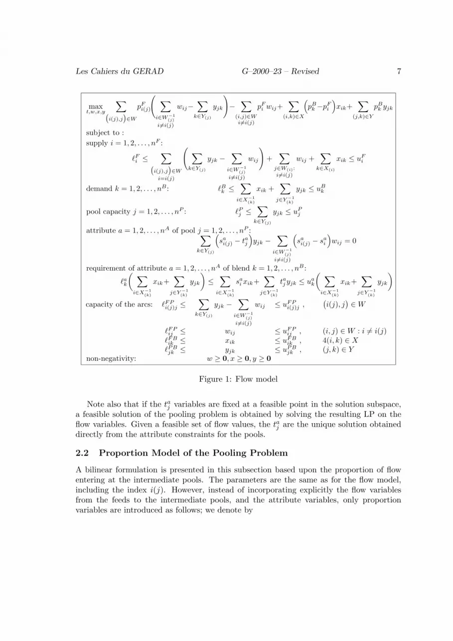
The flow bilinear programming formulation which maximizes the net profit of the pool-ing is shown in Figure 1.

Observe in the flow formulation that the objective function and all constraints arelinear except for those constraints dealing with the attribute qualities of pools and finalblends. The bilinear variables are divided into two sets: {taj} and {yjk}, giving a total of

nAnP + |Y | nonlinear variables. Furthermore there are as many as nA(nP + 2nB) bilinearconstraints.


maxt,w,x,y

∑

(

i(j),j)

∈W

pFi(j)

(

∑

i∈W−1(j)

i6=i(j)

wij−∑

k∈Y(j)

yjk

)

−∑

(i,j)∈Wi6=i(j)

pFi wij+

∑

(i,k)∈X

(

pBk −pF

i

)

xik+∑

(j,k)∈Y

pBk yjk

subject to :

supply i = 1, 2, . . . , nF :

ℓFi ≤

∑

(

i(j),j)

∈W

i=i(j)

(

∑

k∈Y(j)

yjk −∑

i∈W−1(j)

i6=i(j)

wij

)

+∑

j∈W(i):

i6=i(j)

wij +∑

k∈X(i)

xik ≤ uFi

demand k = 1, 2, . . . , nB : ℓBk ≤

∑

i∈X−1(k)

xik +∑

j∈Y−1(k)

yjk ≤ uBk

pool capacity j = 1, 2, . . . , nP : ℓPj ≤

∑

k∈Y(j)

yjk ≤ uPj

attribute a = 1, 2, . . . , nA of pool j = 1, 2, . . . , nP :∑

k∈Y(j)

(

sai(j) − taj

)

yjk −∑

i∈W−1(j)

i6=i(j)

(

sai(j) − sa

i

)

wij = 0

requirement of attribute a = 1, 2, . . . , nA of blend k = 1, 2, . . . , nB :

ℓak

(

∑

i∈X−1(k)

xik+∑

j∈Y−1(k)

yjk

)

≤∑

i∈X−1(k)

sai xik+

∑

j∈Y−1(k)

taj yjk ≤ uak

(

∑

i∈X−1(k)

xik+∑

j∈Y−1(k)

yjk

)

capacity of the arcs: ℓFPi(j)j ≤

∑

k∈Y(j)

yjk −∑

i∈W−1(j)

i6=i(j)

wij ≤ uFPi(j)j ,

(

i(j), j)

∈ W

ℓFPij ≤ wij ≤ uFP

ij , (i, j) ∈ W : i 6= i(j)ℓFBik ≤ xik ≤ uFB

ik , 4(i, k) ∈ XℓPBjk ≤ yjk ≤ uPB

jk , (j, k) ∈ Ynon-negativity: w ≥ 0, x ≥ 0, y ≥ 0

Figure 1: Flow model

Note also that if the taj variables are fixed at a feasible point in the solution subspace,a feasible solution of the pooling problem is obtained by solving the resulting LP on theflow variables. Given a feasible set of flow values, the taj are the unique solution obtaineddirectly from the attribute constraints for the pools.

2.2 Proportion Model of the Pooling Problem

A bilinear formulation is presented in this subsection based upon the proportion of flowentering at the intermediate pools. The parameters are the same as for the flow model,including the index i(j). However, instead of incorporating explicitly the flow variablesfrom the feeds to the intermediate pools, and the attribute variables, only proportionvariables are introduced as follows; we denote by


qij the proportion of the total flow into Pj from Fi along the arc (i, j) ∈ W , for all i 6= i(j).

The proportion variables allow computation of the flow on the arc (i, j) ∈ W , i 6= i(j),as:

wij = qij

∑

k∈Y(j)

yjk.

The flow on the arc (i(j), j) ∈ W is:

wi(j)j =

(

1 −∑

h∈W−1(j)

:

h6=i(j)

qhj

)

∑

k∈Y(j)

yjk.

The total flow leaving Fi, i = 1, 2, . . . nF , is given by:

∑

k∈X(i)

xik +∑

j∈W(i):

i6=i(j)

qij

∑

k∈Y(j)

yjk +∑

j∈W(i):

i=i(j)

(

1 −∑

h∈W−1(j)

:

h6=i(j)

qhj

)

∑

k∈Y(j)

yjk.

The attribute a = 1, 2, . . . , nA of intermediate pool j = 1, 2, . . . , nP is:

∑

i∈W−1(j)

:

i6=i(j)

sai qij + sa

i(j)

(

1 −∑

i∈W−1(j)

:

i6=i(j)

qij

)

= sai(j) +

∑

i∈W−1(j)

:

i6=i(j)

(

sai − sa

i(j)

)

qij .

The attribute quality a = 1, 2, . . . , nA of blend k = 1, 2, . . . , nB is:

∑

i∈X−1(k)

sai xik +

∑

j∈Y−1(k)

(

sai(j) +

∑

i∈W−1(j)

:

i6=i(j)

(sai − sa

i(j))qij

)

yjk

∑

i∈X−1(k)

xik +∑

j∈Y−1(k)

yjk

.

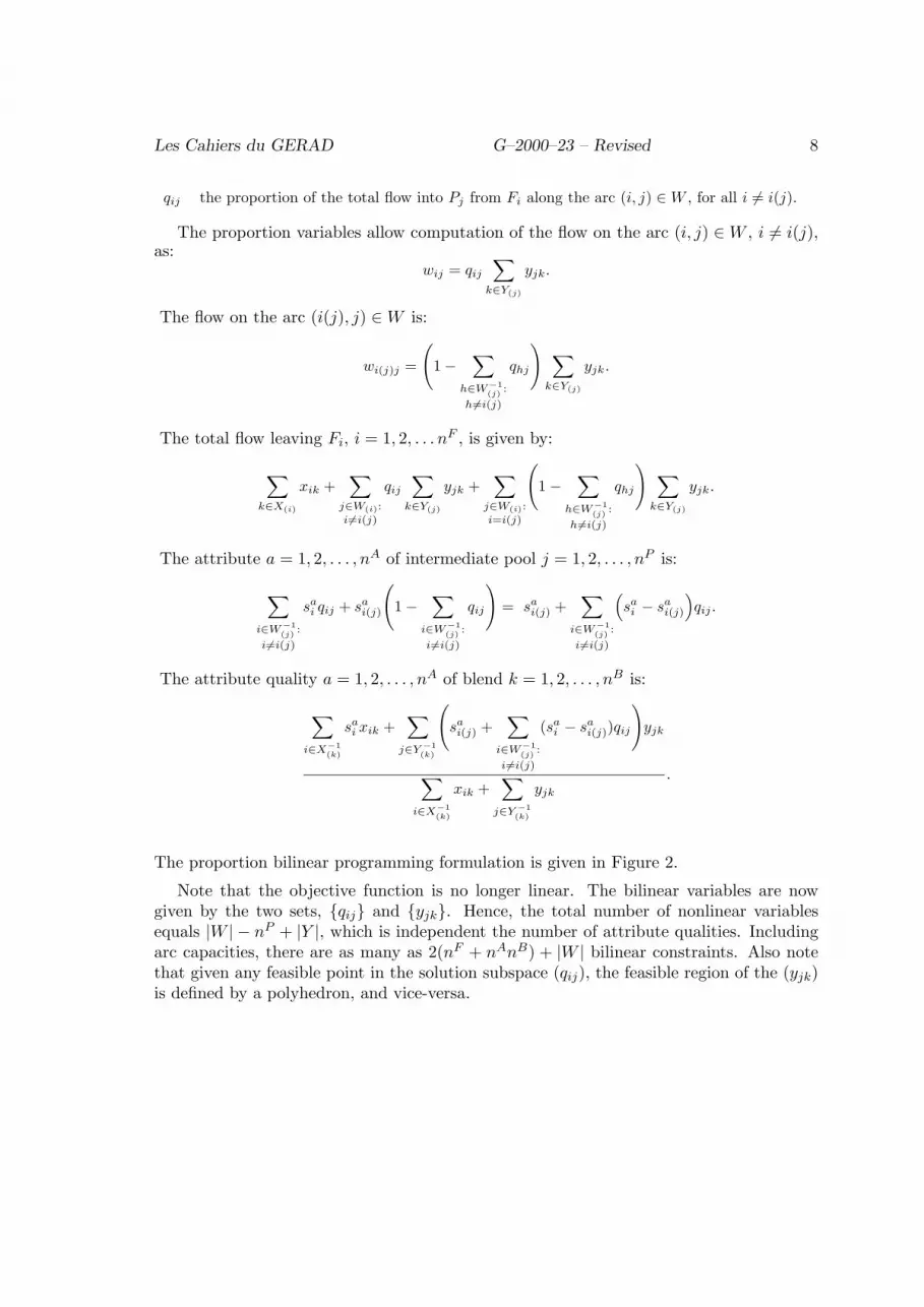
The proportion bilinear programming formulation is given in Figure 2.

Note that the objective function is no longer linear. The bilinear variables are nowgiven by the two sets, {qij} and {yjk}. Hence, the total number of nonlinear variablesequals |W | − nP + |Y |, which is independent the number of attribute qualities. Includingarc capacities, there are as many as 2(nF + nAnB) + |W | bilinear constraints. Also notethat given any feasible point in the solution subspace (qij), the feasible region of the (yjk)is defined by a polyhedron, and vice-versa.


maxx,y,q

∑

(

i(j),j)

∈W

pFi(j)

(

∑

h∈W−1(j)

h6=i(j)

qhj − 1

)

∑

k∈Y(j)

yjk −∑

(i,j)∈W :i6=i(j)

pFi qij

∑

k∈Y(j)

yjk

+∑

(i,k)∈X

(

pBk − pF

i

)

xik +∑

(j,k)∈Y

pBk yjk

subject to :

supply i = 1, 2, . . . , nF :

ℓFi ≤

∑

(

i(j),j)

∈W

i=i(j)

(

1−∑

h∈W−1(j)

h6=i(j)

qhj

)

∑

k∈Y(j)

yjk +∑

j∈W(i)

i6=i(j)

qij

∑

k∈Y(j)

yjk +∑

k∈X(i)

xik ≤ uFi

demand k = 1, 2, . . . , nB : ℓBk ≤

∑

i∈X−1(k)

xik +∑

j∈Y−1(k)

yjk ≤ uBk

pool capacity j = 1, 2, . . . , nP : ℓPj ≤

∑

k∈Y(j)

yjk ≤ uPj

requirement of attribute a = 1, 2, . . . , nA of blend k = 1, 2, . . . , nB :

ℓak

(

∑

i∈X−1(k)

xik +∑

j∈Y−1(k)

yjk

)

≤∑

i∈X−1(k)

sai xik +

∑

j∈Y−1(k)

(

sai(j) +

∑

i∈W−1(j)

i6=i(j)

(sai − sa

i(j))qij

)

yjk

≤ uak

(

∑

i∈X−1(k)

xik +∑

j∈Y−1(k)

yjk

)

capacity of the arcs: ℓFPi(j)j ≤

(

1 −∑

h∈W−1(j)

h6=i(j)

qhj

)

∑

k∈Y(j)

yjk ≤ uFPi(j)j ,

(

i(j), j)

∈ W

ℓFPij ≤ qij

∑

k∈Y(j)

yjk ≤ uFPij , (i, j) ∈ W : i 6= i(j)

ℓFBik ≤ xik ≤ uFB

ik , (i, k) ∈ XℓPBjk ≤ yjk ≤ uPB

jk , (j, k) ∈ Y

non-negativity and proportion j = 1, 2, . . . , nP : x ≥ 0, y ≥ 0, q ≥ 0,∑

h∈W−1(j)

h6=i(j)

qhj ≤ 1

Figure 2: Proportion model


2.3 Comparison of the Flow and Proportion Models

For comparison purposes, the following ten examples are taken from the literature: Haver-ly’s (1978) pooling problem (referred to as H1), Ben Tal et al.’s (1994) fourth and fifthpooling problems (BT4, BT5), Rehfeldt and Tisljar’s (1997) first and second problems(RT1, RT2), Foulds et al.’s (1992) second problem (F2) and the four examples proposedin Adhya et al.(1999), referred to as AST1,2,3 and 4. For brevity, only RT2 is shown indetail in the Appendix. The data describing all examples considered in the paper can befound at www.gerad.ca/Charles.Audet.

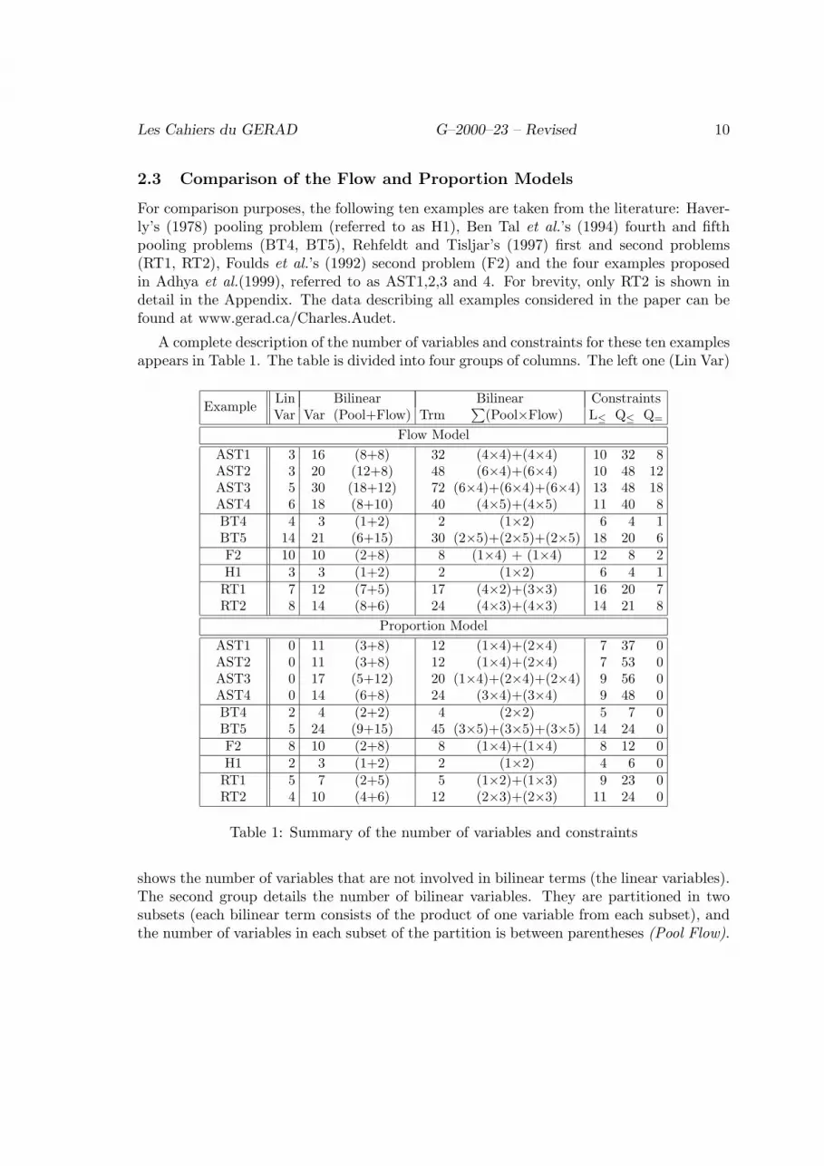
A complete description of the number of variables and constraints for these ten examplesappears in Table 1. The table is divided into four groups of columns. The left one (Lin Var)

ExampleLin Bilinear Bilinear ConstraintsVar Var (Pool+Flow) Trm

∑

(Pool×Flow) L≤ Q≤ Q=

Flow Model

AST1 3 16 (8+8) 32 (4×4)+(4×4) 10 32 8AST2 3 20 (12+8) 48 (6×4)+(6×4) 10 48 12AST3 5 30 (18+12) 72 (6×4)+(6×4)+(6×4) 13 48 18AST4 6 18 (8+10) 40 (4×5)+(4×5) 11 40 8BT4 4 3 (1+2) 2 (1×2) 6 4 1BT5 14 21 (6+15) 30 (2×5)+(2×5)+(2×5) 18 20 6F2 10 10 (2+8) 8 (1×4) + (1×4) 12 8 2H1 3 3 (1+2) 2 (1×2) 6 4 1RT1 7 12 (7+5) 17 (4×2)+(3×3) 16 20 7RT2 8 14 (8+6) 24 (4×3)+(4×3) 14 21 8

Proportion Model

AST1 0 11 (3+8) 12 (1×4)+(2×4) 7 37 0AST2 0 11 (3+8) 12 (1×4)+(2×4) 7 53 0AST3 0 17 (5+12) 20 (1×4)+(2×4)+(2×4) 9 56 0AST4 0 14 (6+8) 24 (3×4)+(3×4) 9 48 0BT4 2 4 (2+2) 4 (2×2) 5 7 0BT5 5 24 (9+15) 45 (3×5)+(3×5)+(3×5) 14 24 0F2 8 10 (2+8) 8 (1×4)+(1×4) 8 12 0H1 2 3 (1+2) 2 (1×2) 4 6 0RT1 5 7 (2+5) 5 (1×2)+(1×3) 9 23 0RT2 4 10 (4+6) 12 (2×3)+(2×3) 11 24 0

Table 1: Summary of the number of variables and constraints

shows the number of variables that are not involved in bilinear terms (the linear variables).The second group details the number of bilinear variables. They are partitioned in twosubsets (each bilinear term consists of the product of one variable from each subset), andthe number of variables in each subset of the partition is between parentheses (Pool Flow).


Flow is the number of flow variables, and Pool is the number of attribute or proportionvariables (depending on the model used). These numbers are decomposed in the next groupto explain the total number of bilinear terms (Trm) introduced by the intermediate pools.For example, the flow model of RT2 has four attributes and three exiting feeds, at eachpool, P1 and P2. The number of bilinear terms is the number of cross-product elements of{t11, t

21, t

31, t

41}×{y11, y12, y13} and {t12, t

22, t

32, t

42}×{y21, y22, y23}; therefore, there are a total

of 4× 3 + 4× 3 = 24 bilinear terms. The last group of columns gives the number of linearinequalities L≤, quadratic inequalities Q≤, and quadratic equalities Q= in the constraintset of each problem.

The difficulty of the bilinear programming problem can be roughly estimated by thenumber of bilinear variables, terms and constraints. The advantage of the flow modeloccurs when there are few attributes. The number of complicating variables (the taj ) willthen be small. When the number of attributes increases, the advantage of the proportionmodel becomes apparent since the number of bilinear variables and terms stays the same.These numbers are determined by the number of entering and exiting flows at the inter-mediate pools. (For total number of bilinear variables, the turnover between the flow andproportional models occurs when nA = |W |/nP −1, that is, the average number of enteringarcs at the intermediate pools less one.) Referring to Table 1, we see that the proportionmodels of Examples RT1 and RT2 are considerably smaller than the corresponding flowmodels. At first glance, the flow model appears to be simpler than the proportion in BT5.We will see in the next section when these problems are solved exactly that this is not thecase. The number of bilinear constraints is also an important factor.

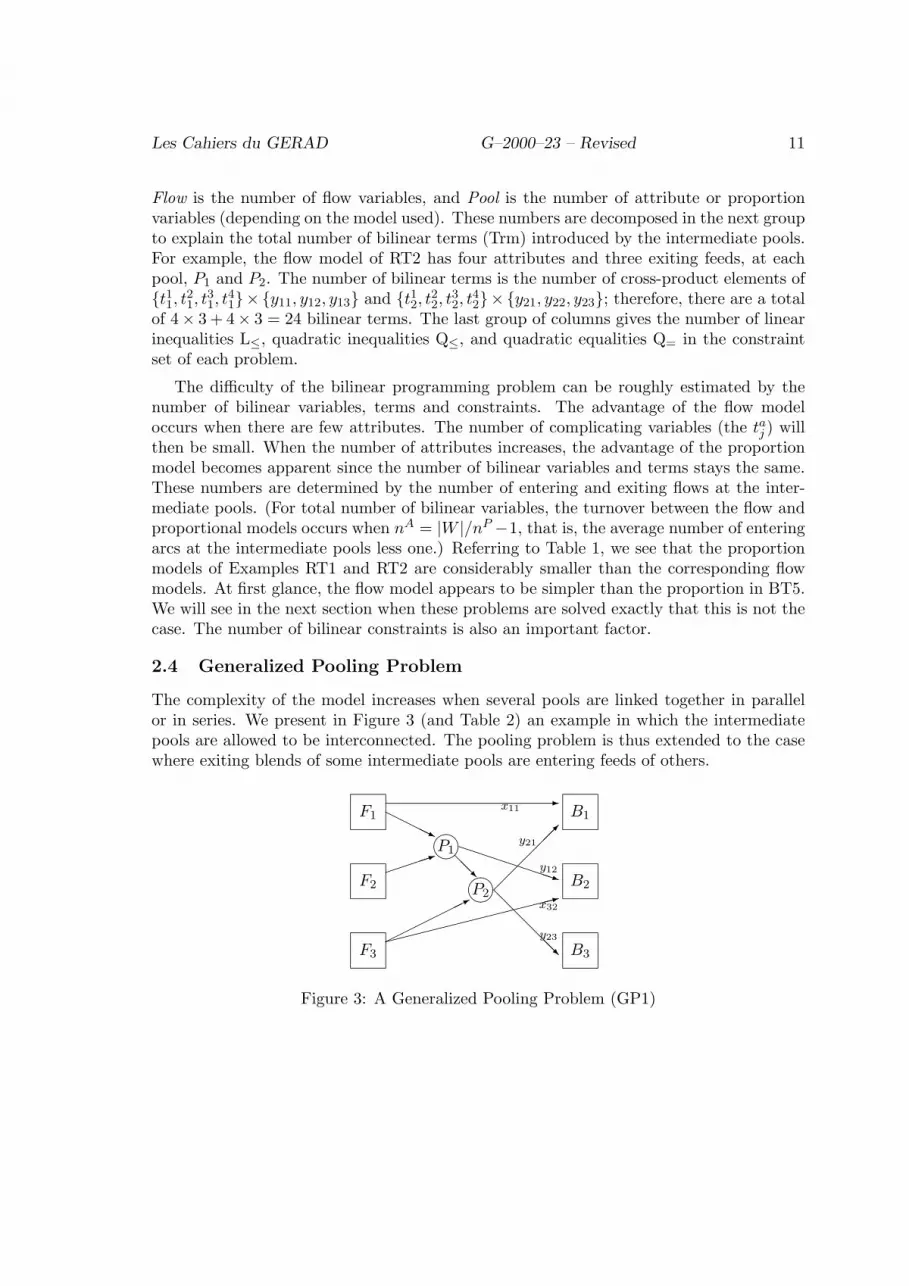
2.4 Generalized Pooling Problem

The complexity of the model increases when several pools are linked together in parallelor in series. We present in Figure 3 (and Table 2) an example in which the intermediatepools are allowed to be interconnected. The pooling problem is thus extended to the casewhere exiting blends of some intermediate pools are entering feeds of others.

F1

F2

F3

±°²¯P1

±°²¯P2

B1

B2

B3

x11

y21

y12

x32

y23

-HHHHj

³³³³1

©©©©©©*

»»»»»»»»»»»»:

PPPPPPPq@@R

¡¡

¡¡¡µ

@@

@@@R

Figure 3: A Generalized Pooling Problem (GP1)


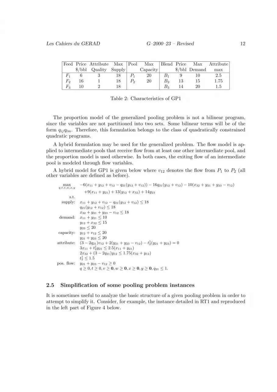
Feed Price Attribute Max Pool Max Blend Price Max Attribute$/bbl Quality Supply Capacity $/bbl Demand max

F1 6 3 18 P1 20 B1 9 10 2.5F2 16 1 18 P2 20 B2 13 15 1.75F3 10 2 18 B3 14 20 1.5

Table 2: Characteristics of GP1

The proportion model of the generalized pooling problem is not a bilinear program,since the variables are not partitioned into two sets. Some bilinear terms will be of theform qijqlm. Therefore, this formulation belongs to the class of quadratically constrainedquadratic programs.

A hybrid formulation may be used for the generalized problem. The flow model is ap-plied to intermediate pools that receive flow from at least one other intermediate pool, andthe proportion model is used otherwise. In both cases, the exiting flow of an intermediatepool is modeled through flow variables.

A hybrid model for GP1 is given below where v12 denotes the flow from P1 to P2 (allother variables are defined as before).

maxq,t,v,w,x,y

−6(x11 + y12 + v12 − q21(y12 + v12)) − 16q21(y12 + v12) − 10(x32 + y21 + y23 − v12)

+9(x11 + y21) + 13(y12 + x32) + 14y23

s.t.supply: x11 + y12 + v12 − q21(y12 + v12) ≤ 18

q21(y12 + v12) ≤ 18x32 + y21 + y23 − v12 ≤ 18

demand: x11 + y21 ≤ 10y12 + x32 ≤ 15y23 ≤ 20

capacity: y12 + v12 ≤ 20y21 + y23 ≤ 20

attribute: (3 − 2q21)v12 + 2(y21 + y23 − v12) − t12(y21 + y23) = 03x11 + t12y21 ≤ 2.5(x11 + y21)2x32 + (3 − 2q21)y12 ≤ 1.75(x32 + y12)t12 ≤ 1.5

pos. flow: y21 + y23 − v12 ≥ 0q ≥ 0, t ≥ 0, v ≥ 0, w ≥ 0, x ≥ 0, y ≥ 0, q21 ≤ 1.

2.5 Simplification of some pooling problem instances

It is sometimes useful to analyze the basic structure of a given pooling problem in order toattempt to simplify it. Consider, for example, the instance detailed in RT1 and reproducedin the left part of Figure 4 below.


F1

F2

F3

±°²¯P1

±°²¯P2

B1

B2

B3

x12

x13

x21

x31

x33

y21

y12

y22

y13

y23

PPPPPPPPPPPPq

HHHHHHj

ZZ

ZZ

ZZ

ZZ

ZZ

ZZ~

³³³³³³³³³³³³1

PPPPPPq

¡¡

¡¡

¡µ

½½

½½

½½

½½

½½

½½>

³³³³³³1

-

XXXXXz@@

@@

@R¶

¶¶

¶¶

¶¶7

³³³³³1

HHHHHj

F1

F2

F3

±°²¯P2

B1

B2

B3

x12

x13

x21

x31

x33

x32

y22

y23

PPPPPPPPPPPPq

ZZ

ZZ

ZZ

ZZ

ZZ

ZZ~

³³³³³³³³³³³³1

PPPPPPq³³³³³³³³³³³³1

½½

½½

½½

½½

½½

½½>

³³³³³³1

-

³³³³³1

HHHHHj

Figure 4: Simplification of Rehfeldt and Tisljar’s first pooling problem (RT1)

A closer look at the definition of the problem allows considerable simplifications. Ob-serve that the flows x21, x31 and y21 entering blend B1 originate solely from the two feedsF2 and F3. A positive flow y21 of any feasible solution could be transferred to the un-constrained flows x21 and x31 without affecting feasibility, or objective function value.Therefore, we can assume without any loss of generality that the flow variable y21 is fixedto zero.

Similarly, by considering the flows y13, x13 and x33, we can deduce that y13 can befixed to zero. This observation has important consequences: the pool P1 has thereforea unique exiting flow y12, and thus that pool can be combined with the final pool B2.The flow from F3 to B2 is bounded above by the capacity of pool P1. This constraint ishowever redundant, since the maximum demand of B2 is less than that capacity. Thesesimplifications are illustrated on the right part of Figure 4 and they lead to new ones.Indeed, consider the flow from the feed F3 to the intermediate pool P2: it can be transferredto x32 and x33 without altering feasibility or objective function value, thus allowing fixing itto zero. It follows that the intermediate pool P2 can be combined with F2 as the capacity ofpool P2 is greater than the availability of feed F2. Therefore, this example can be reducedto an equivalent blending problem since all intermediate pools may be eliminated. Thus,Rehfeldt and Tilsjar’s (1997) first pooling problem can be solved by linear programming!

The instances F3, F4 and F5 of Foulds et al. (1992) can also be simplified. In fact, thelinear structure describing these instances allows an analytical solution. We will show howto solve F3; F4 and F5 can be treated similarly. In that instance, the single attribute valueand cost of the 11 feeds are s1

i = 9+i10 and pF

i = 21 − i for i = 1, 2, ..., 11. The capacities ofthe arcs and pools are unlimited. Each of the 16 blends has a maximal demand of 1. Theirprice and maximal attribute values are pB

k = 41−k2 and u1

k = 1 + .05k for k = 1, 2, ..., 16.

A consequence of this linear structure is that the cost of producing a unit amountof a blend with fixed attribute α ∈ [1, 2] comprises a constant purchase cost, 30 − 10α,independent of which feeds are blended together. Therefore, a strategy to get the optimal


solution is to simply direct 9.2 units of feed F1 into pool P1 and 6.8 units of F11 intoP8, then blend 2 − u1

k units of P1 together with u1k − 1 units of P8 into blend Bk, for

k = 1, 2, ..., 16. This optimal solution is displayed in Figure 5.

s1

ipFi

B1

Bk

...

...

B16

F11 ¹¸º·P8

¹¸º·P1

2−u1

k

u1

k−1

HHHHHj

³³³³³1¶

¶¶

¶¶

¶¶7

QQ

QQQs

©©©©©*

SS

SS

SSSw

-

-10 2

20 1 F1

1+0.05k41−k2

12.5 1.8

20 1.05

u1

kpB

k

.95

.05

.2

.8

6.8

9.2

Figure 5: Simplification of F3, F4 and F5

3 Computational Results for Exact Solution

Since the objective function and feasible region are nonconvex, the pooling problem requiresa global optimization approach. Methods using local searches along descent directions, suchas successive linear programming (SLP), are only guaranteed to find a local optimum, thequality of which is unknown.

The pooling examples described in the preceding section are solved to global optimalityusing a recent branch-and-cut algorithm by Audet et al. (2000a) for the general class ofnonconvex quadratically constrained quadratic programs. Their method is inspired by Al-Khayyal and Falk’s (1983) branch and bound algorithm for bilinear programming and theReformulation-Linearization Techniques of Sherali and Tuncbilek (1992), (1997a), (1997b).The improvement to these methods are: (i) selection of the branching value: splitting ofthe hyper-rectangle is done in a way that minimizes the resulting potential error, and thusnot necessarily in its middle; (ii) approximation of bilinear terms: instead of systematicallyadding all linear inequalities defining the convex and concave envelopes, only those violatedare added to the model thus keeping the linear program size from growing too fast; (iii)introduction of a new class of cuts: cuts derived from under-approximation of the convexparaboloid are used to force linear variables to approach the corresponding bilinear term;(iv) the proposed algorithm is of the branch and cut type: cuts introduced at any node ofthe exploration tree are valid at all other nodes.


Example [ref] nF nP nB nA solution

AST1 [1] 5 2 4 4 549.803AST2 [1] 5 2 4 6 549.803AST3 [1] 8 3 4 6 561.048AST4 [1] 8 2 5 4 877.649

BT4 [11] 4 1 2 1 45BT5 [11] 5 3 5 2 350

F2 [20] 6 2 4 1 110

H1 [27] 3 1 2 1 40H2 [27] 3 1 2 1 60H3 [27] 3 1 2 1 75

RT1 [32] 3 2 3 4 4136.22RT2 [32] 3 2 3 4 4391.83

GP1 3 2 3 1 60.5

Table 3: Instances characteristics

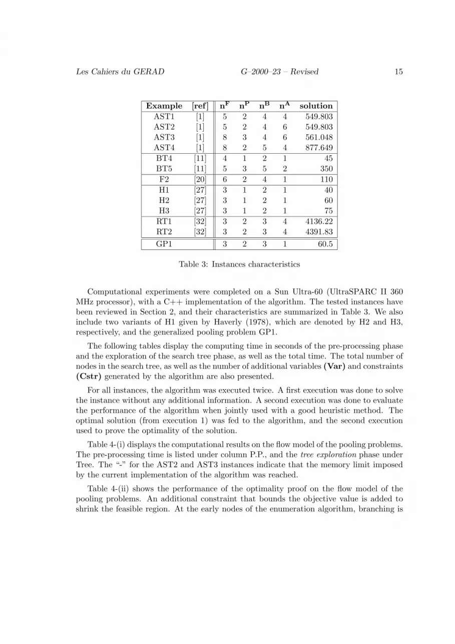
Computational experiments were completed on a Sun Ultra-60 (UltraSPARC II 360MHz processor), with a C++ implementation of the algorithm. The tested instances havebeen reviewed in Section 2, and their characteristics are summarized in Table 3. We alsoinclude two variants of H1 given by Haverly (1978), which are denoted by H2 and H3,respectively, and the generalized pooling problem GP1.

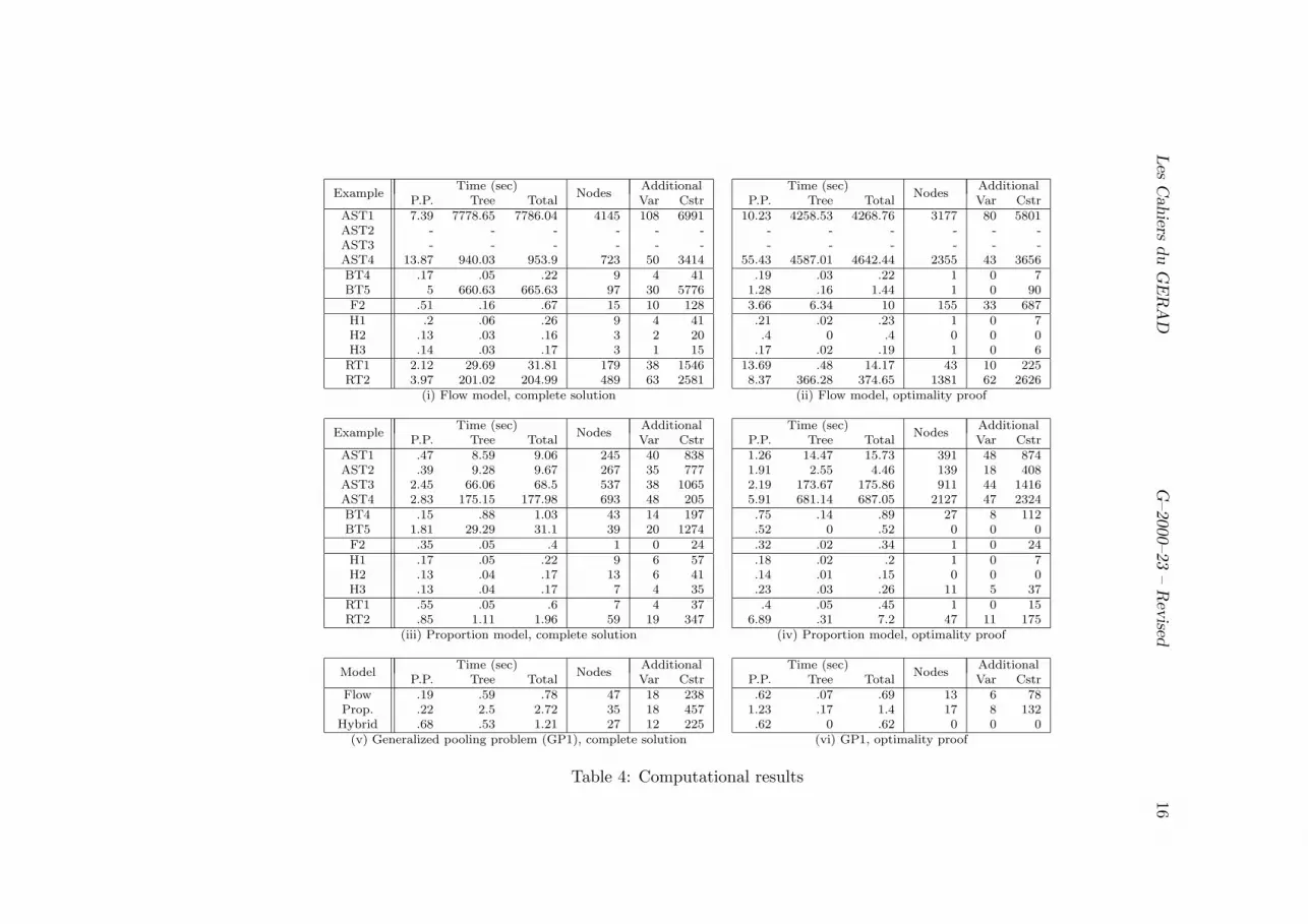
The following tables display the computing time in seconds of the pre-processing phaseand the exploration of the search tree phase, as well as the total time. The total number ofnodes in the search tree, as well as the number of additional variables (Var) and constraints(Cstr) generated by the algorithm are also presented.

For all instances, the algorithm was executed twice. A first execution was done to solvethe instance without any additional information. A second execution was done to evaluatethe performance of the algorithm when jointly used with a good heuristic method. Theoptimal solution (from execution 1) was fed to the algorithm, and the second executionused to prove the optimality of the solution.

Table 4-(i) displays the computational results on the flow model of the pooling problems.The pre-processing time is listed under column P.P., and the tree exploration phase underTree. The “-” for the AST2 and AST3 instances indicate that the memory limit imposedby the current implementation of the algorithm was reached.

Table 4-(ii) shows the performance of the optimality proof on the flow model of thepooling problems. An additional constraint that bounds the objective value is added toshrink the feasible region. At the early nodes of the enumeration algorithm, branching is

Les

Cahie

rs

du

GE

RA

DG

–2000–23

–R

evis

ed

16

ExampleTime (sec)

NodesAdditional

P.P. Tree Total Var CstrAST1 7.39 7778.65 7786.04 4145 108 6991AST2 - - - - - -AST3 - - - - - -AST4 13.87 940.03 953.9 723 50 3414BT4 .17 .05 .22 9 4 41BT5 5 660.63 665.63 97 30 5776F2 .51 .16 .67 15 10 128H1 .2 .06 .26 9 4 41H2 .13 .03 .16 3 2 20H3 .14 .03 .17 3 1 15RT1 2.12 29.69 31.81 179 38 1546RT2 3.97 201.02 204.99 489 63 2581

(i) Flow model, complete solution

ExampleTime (sec)

NodesAdditional

P.P. Tree Total Var CstrAST1 .47 8.59 9.06 245 40 838AST2 .39 9.28 9.67 267 35 777AST3 2.45 66.06 68.5 537 38 1065AST4 2.83 175.15 177.98 693 48 205BT4 .15 .88 1.03 43 14 197BT5 1.81 29.29 31.1 39 20 1274F2 .35 .05 .4 1 0 24H1 .17 .05 .22 9 6 57H2 .13 .04 .17 13 6 41H3 .13 .04 .17 7 4 35RT1 .55 .05 .6 7 4 37RT2 .85 1.11 1.96 59 19 347

(iii) Proportion model, complete solution

ModelTime (sec)

NodesAdditional

P.P. Tree Total Var CstrFlow .19 .59 .78 47 18 238Prop. .22 2.5 2.72 35 18 457Hybrid .68 .53 1.21 27 12 225

(v) Generalized pooling problem (GP1), complete solution

Time (sec)Nodes

AdditionalP.P. Tree Total Var Cstr

10.23 4258.53 4268.76 3177 80 5801- - - - - -- - - - - -

55.43 4587.01 4642.44 2355 43 3656.19 .03 .22 1 0 7

1.28 .16 1.44 1 0 903.66 6.34 10 155 33 687.21 .02 .23 1 0 7.4 0 .4 0 0 0

.17 .02 .19 1 0 613.69 .48 14.17 43 10 2258.37 366.28 374.65 1381 62 2626

(ii) Flow model, optimality proof

Time (sec)Nodes

AdditionalP.P. Tree Total Var Cstr1.26 14.47 15.73 391 48 8741.91 2.55 4.46 139 18 4082.19 173.67 175.86 911 44 14165.91 681.14 687.05 2127 47 2324.75 .14 .89 27 8 112.52 0 .52 0 0 0.32 .02 .34 1 0 24.18 .02 .2 1 0 7.14 .01 .15 0 0 0.23 .03 .26 11 5 37.4 .05 .45 1 0 15

6.89 .31 7.2 47 11 175(iv) Proportion model, optimality proof

Time (sec)Nodes

AdditionalP.P. Tree Total Var Cstr.62 .07 .69 13 6 78

1.23 .17 1.4 17 8 132.62 0 .62 0 0 0

(vi) GP1, optimality proof

Table 4: Computational results


done on the incumbent variables involved in quadratic terms that are not at either theirlower or upper bound. This allows a more precise linearization near the incumbent solution.Computational times remain comparable for the small instances, but drop significantly forthe larger problems, except for AST4 where proving optimality is more expensive thansearching from scratch. This seems to justify the joint use of a heuristic to obtain a goodincumbent solution.

Results of the algorithm on the proportion model of the pooling problem are displayedin Table 4-(iii). For the larger instances, the proportion model is significantly easier tosolve than the flow model, even for BT5 where this model has a greater number of bilinearvariables and terms than the former one. Note, however, that the proportion model of BT5has fewer bilinear constraints than the flow model (11 versus 16). The significant differencein computation times in Tables 4-(i) and 4-(iii) suggests that care should be taken initiallyto choose the right model.

Optimality proof performance on the proportion model of the pooling problems appearsin Table 4-(iv). Again, the proportion model seems easier to solve than the flow model.Moreover, the time required for the optimality proof is less or comparable to the time ofsolving the original problem, except for the problems AST and for Example RT2 wherethe computational time increased. As for the remaining examples, the pre-processing timeincreased, but the tree exploration phase decreased. This is explained by the addition ofthe non-linear constraint to bound the feasible region. The feasible region becomes smalland hard to approximate by outer-approximations.

Tables 4-(v) and 4-(vi) display computing times for solving the three equivalent formu-lations of the generalized pooling problem presented in Example GP1. Contrary to thestandard pooling problem, the proportion model of the generalized problem appears to beharder to solve than the flow model. The addition of the variable q22 that represents theproduct of two proportion variables adds a level of complexity to the outer-approximationscheme. It seems that the hybrid model is the easiest one to solve. The proportion variablesallow elimination of the attribute variable of pool P1 without adding complexity.

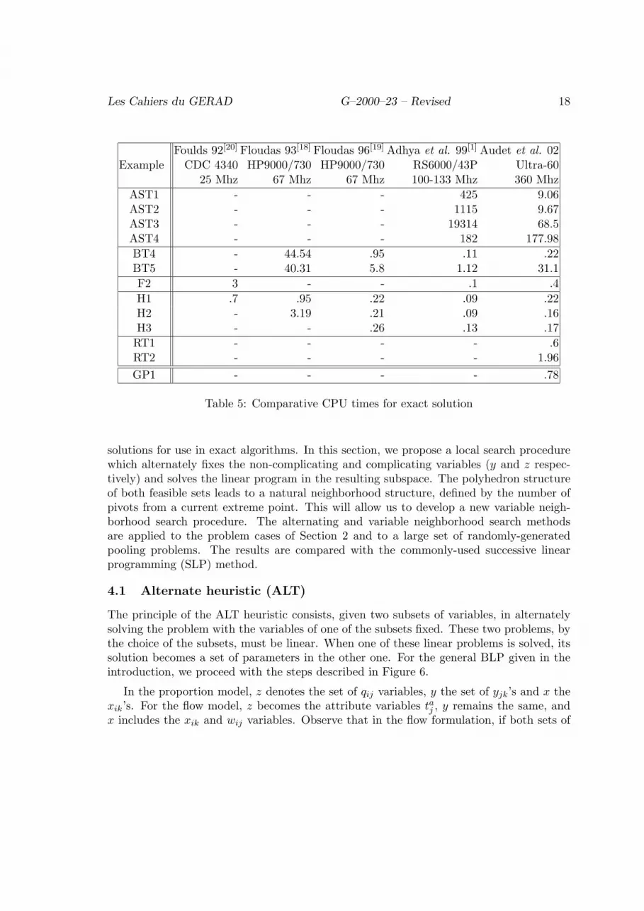
Table 5 shows a computational results comparison, similar to that of Adhya et al.(1999). For the easier problems, i.e. BT4, BT5, F2, H1, H2 and H3, the state-of-the-artalgorithm of Adhya et al. (1999) takes less computer time than the algorithm of Audet etal. (2000a) ; however for the three difficult instances AST1, AST2 and AST3, the CPUtimes of this last algorithm are 46 to 282 times (or 17 to 104 times, taking into accountthe relative CPU speeds) less than those of Adhya et al. (1999). So use of the proportionmodel and Audet et al. (2000a) algorithm appears to notably advance the state-of-the-art.

4 Heuristic Methods

As inferred in the preceding section, heuristic approaches to the pooling problem are re-quired to (i) obtain good solutions for larger problem instances, and (ii) obtain good initial


ExampleFoulds 92[20] Floudas 93[18] Floudas 96[19] Adhya et al. 99[1] Audet et al. 02

CDC 4340 HP9000/730 HP9000/730 RS6000/43P Ultra-6025 Mhz 67 Mhz 67 Mhz 100-133 Mhz 360 Mhz

AST1 - - - 425 9.06AST2 - - - 1115 9.67AST3 - - - 19314 68.5AST4 - - - 182 177.98

BT4 - 44.54 .95 .11 .22BT5 - 40.31 5.8 1.12 31.1

F2 3 - - .1 .4

H1 .7 .95 .22 .09 .22H2 - 3.19 .21 .09 .16H3 - - .26 .13 .17

RT1 - - - - .6RT2 - - - - 1.96

GP1 - - - - .78

Table 5: Comparative CPU times for exact solution

solutions for use in exact algorithms. In this section, we propose a local search procedurewhich alternately fixes the non-complicating and complicating variables (y and z respec-tively) and solves the linear program in the resulting subspace. The polyhedron structureof both feasible sets leads to a natural neighborhood structure, defined by the number ofpivots from a current extreme point. This will allow us to develop a new variable neigh-borhood search procedure. The alternating and variable neighborhood search methodsare applied to the problem cases of Section 2 and to a large set of randomly-generatedpooling problems. The results are compared with the commonly-used successive linearprogramming (SLP) method.

4.1 Alternate heuristic (ALT)

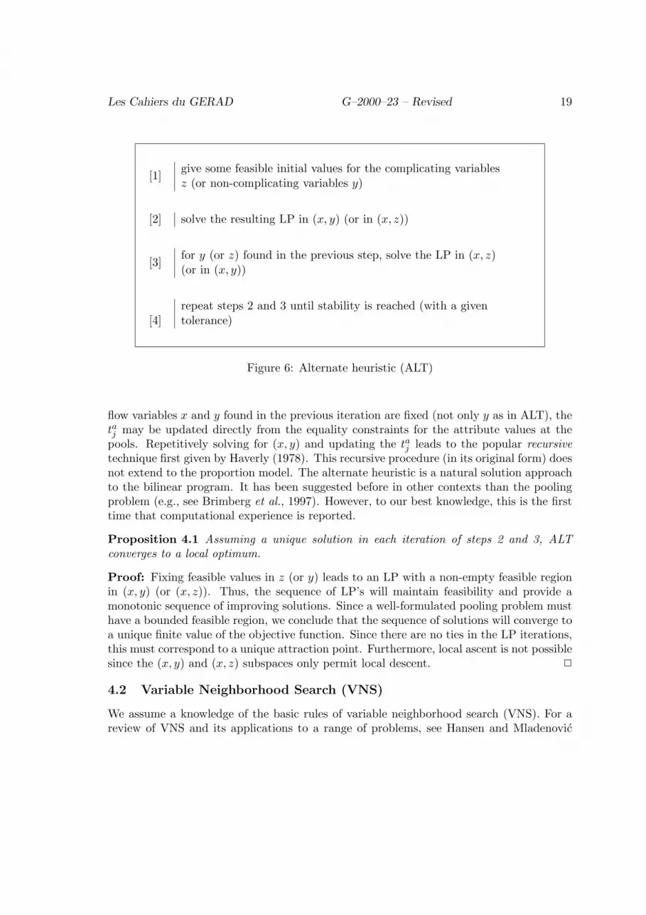
The principle of the ALT heuristic consists, given two subsets of variables, in alternatelysolving the problem with the variables of one of the subsets fixed. These two problems, bythe choice of the subsets, must be linear. When one of these linear problems is solved, itssolution becomes a set of parameters in the other one. For the general BLP given in theintroduction, we proceed with the steps described in Figure 6.

In the proportion model, z denotes the set of qij variables, y the set of yjk’s and x thexik’s. For the flow model, z becomes the attribute variables taj , y remains the same, andx includes the xik and wij variables. Observe that in the flow formulation, if both sets of


[1]give some feasible initial values for the complicating variablesz (or non-complicating variables y)

[2] solve the resulting LP in (x, y) (or in (x, z))

[3]for y (or z) found in the previous step, solve the LP in (x, z)(or in (x, y))

[4]repeat steps 2 and 3 until stability is reached (with a giventolerance)

Figure 6: Alternate heuristic (ALT)

flow variables x and y found in the previous iteration are fixed (not only y as in ALT), thetaj may be updated directly from the equality constraints for the attribute values at thepools. Repetitively solving for (x, y) and updating the taj leads to the popular recursivetechnique first given by Haverly (1978). This recursive procedure (in its original form) doesnot extend to the proportion model. The alternate heuristic is a natural solution approachto the bilinear program. It has been suggested before in other contexts than the poolingproblem (e.g., see Brimberg et al., 1997). However, to our best knowledge, this is the firsttime that computational experience is reported.

Proposition 4.1 Assuming a unique solution in each iteration of steps 2 and 3, ALTconverges to a local optimum.

Proof: Fixing feasible values in z (or y) leads to an LP with a non-empty feasible regionin (x, y) (or (x, z)). Thus, the sequence of LP’s will maintain feasibility and provide amonotonic sequence of improving solutions. Since a well-formulated pooling problem musthave a bounded feasible region, we conclude that the sequence of solutions will converge toa unique finite value of the objective function. Since there are no ties in the LP iterations,this must correspond to a unique attraction point. Furthermore, local ascent is not possiblesince the (x, y) and (x, z) subspaces only permit local descent. 2

4.2 Variable Neighborhood Search (VNS)

We assume a knowledge of the basic rules of variable neighborhood search (VNS). For areview of VNS and its applications to a range of problems, see Hansen and Mladenovic


(1997 and 1999). In a nutshell, the variable neighborhood search consists in repeating thefollowing two steps : (i) perturb the current solution within a neighborhood of length k(initially set to 1); (ii) from this perturbed point, find a new point with a local search. Ifthis new local optimum is better, it becomes the new current point, and the k parameteris set again to 1; else the original current point is kept and the k parameter is increased,for a bigger perturbation in step (i).

Let s =(x′, y′, z′) be a feasible solution obtained by ALT. It follows that (x′, y′) and(x′, z′) are extreme points of a polyhedron in the respective subspaces. Let us denote thesetwo polyhedrons by P1(s) and P2(s). The first neighborhood N1(s) is represented by theunion of all feasible extreme points adjacent to either (x′, y′) (in P1(s)) or (x′, z′) (in P2(s)).Thus, the cardinality of N1(s) is less than or equal to 2n1 + n2 + n3, since the numberof adjacent points in a polyhedron cannot be larger than the dimension of the space.The equality occurs when the LP problems are not degenerate (in both (x, y) and (x, z)subspaces). N2(s) would then be the set of adjacent extreme points on P1(s) or P2(s)obtained by changing exactly two elements in the respective bases; N3(s) exactly threeelements; and so on. It is easy to see that the cardinality of Nk(s) increases exponentiallywith k.

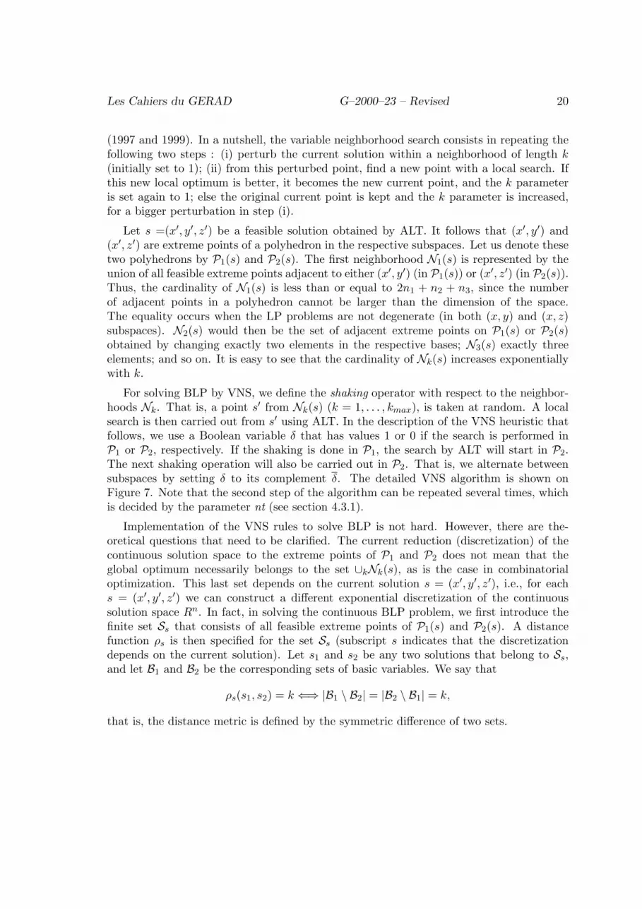
For solving BLP by VNS, we define the shaking operator with respect to the neighbor-hoods Nk. That is, a point s′ from Nk(s) (k = 1, . . . , kmax), is taken at random. A localsearch is then carried out from s′ using ALT. In the description of the VNS heuristic thatfollows, we use a Boolean variable δ that has values 1 or 0 if the search is performed inP1 or P2, respectively. If the shaking is done in P1, the search by ALT will start in P2.The next shaking operation will also be carried out in P2. That is, we alternate betweensubspaces by setting δ to its complement δ. The detailed VNS algorithm is shown onFigure 7. Note that the second step of the algorithm can be repeated several times, whichis decided by the parameter nt (see section 4.3.1).

Implementation of the VNS rules to solve BLP is not hard. However, there are the-oretical questions that need to be clarified. The current reduction (discretization) of thecontinuous solution space to the extreme points of P1 and P2 does not mean that theglobal optimum necessarily belongs to the set ∪kNk(s), as is the case in combinatorialoptimization. This last set depends on the current solution s = (x′, y′, z′), i.e., for eachs = (x′, y′, z′) we can construct a different exponential discretization of the continuoussolution space Rn. In fact, in solving the continuous BLP problem, we first introduce thefinite set Ss that consists of all feasible extreme points of P1(s) and P2(s). A distancefunction ρs is then specified for the set Ss (subscript s indicates that the discretizationdepends on the current solution). Let s1 and s2 be any two solutions that belong to Ss,and let B1 and B2 be the corresponding sets of basic variables. We say that

ρs(s1, s2) = k ⇐⇒ |B1 \ B2| = |B2 \ B1| = k,

that is, the distance metric is defined by the symmetric difference of two sets.


[1] Initialization

find an initial feasible solution schoose a stopping condition ntit ← 1

[2] While it ≤ nt

k ← 1While k ≤ kmax

[i] Shakingget s′ from Nk(s) at random using current value of δ

[ii] Local search

δ ← δuse ALT with s′ as initial solution to obtain local

optimum s′′

[iii] Move or notif s′′ better than s

move to s′′ (s ← s′′)k ← 1update the neighborhoods Nk(s) for the new

current solution (i.e., update the simplextable, or polyhedron, where s” is found)

else k ← k + 1it ← it + 1

Figure 7: VNS algorithm

4.3 Computer Results

Three heuristic methods were tested: an efficient version of SLP (noted as SLPR inPalacios-Gomez et al., 1982), and the alternate and VNS procedures given above. Allthree heuristics were coded in C++ and run on the Ultra-60 station as before. Recall thatfinding a feasible initial solution (a requirement for all three heuristics) is in itself a verydifficult problem. For example, in RT2, 10,000 sets of proportion values were generated atrandom, and not one feasible solution was found by ALT. The following “tricks” were usedto significantly improve the rate of success:

(i) since the solutions of the LPs typically have many zero-valued variables, set everyvariable in z (or y) to zero with probability .5; if the variable is decided to be non-zero, set its value randomly;


(ii) for some problem instances, we observe that it is better to start with random valuesof z, while for others, a feasible solution is easier to find if the variables from y arefixed at random. Therefore, we choose to start with y or z with probability 0.5.

The above procedure allowed us to obtain about 25% feasible solutions in RT2. The choiceof the set of variables to be fixed has in general no important incidence on the efficiencyof this method, except for the AST problems under the flow formulation: no feasible pointwas generated when the set of smallest cardinality was chosen.

In order to improve the quality of the solutions, multistart versions of SLP and ALT(referred to as MSLP and MALT, respectively) were used. The rule above was taken forthe starting values of MALT. The starting procedure suggested in Palacios-Gomez et al.(1982) was applied in MSLP. If the starting solution was found to be infeasible, iterationsof ALT were allowed to continue until a feasible point was found. The best solution fromMALT was taken as the initial solution for VNS. In Tables 6 and 7, a “-” means that theMSLP method could not find a solution or that the memory limit was reached for the exactalgorithm.

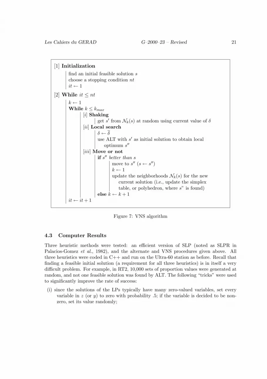
4.3.1 Pooling problems from the literature We first tested the heuristics on theproblem instances discussed in Section 2 and 3, and for which exact solutions were alreadyfound. The results are summarized in Table 6 for flow and proportion models. In thistable, we give the parameters used for the 3 methods MSLP, MALT and VNS. They are:

nsp number of starting points for the MSLP and MALT algorithmskmax VNS parameter, maximum length of the neighborhoodnt VNS parameter, number of repetitions of VNS’s phase 2

(see the algorithm on Figure 7).

Because the proportion formulation of GP1 is not a bilinear problem, only the resolutionwith flow formulation is made.

Given that the initial solution of VNS is the best solution of MALT, the CPU timesgiven for the VNS include the time of MALT. If no improvement can be made by the VNS,the kmax and nt parameters are set to zero, and the times for MALT and VNS are thesame.

Table 6 shows that there is not a significant difference between the flow and proportionformulations (except for AST3 and F2). We note that MALT gives the optimal solutionfor five instances, MSLP in only three instances, and VNS obtained the exact solution inall cases except the AST problems. This is caused by the degeneracy in the AST problems,which does not allow efficient shaking. Note that any improvements by VNS to MALTwere obtained very quickly.


ExampleParameters Solution CPU time (s) Error (%)nsp kmax nt Exact MSLP MALT VNS MSLP MALT VNS MSLP MALT VNS

Flow Model

AST1 1000 10 1 549.803 276.661 532.901 545.27 2.20 2.45 2.81 49.68 3.07 .82AST2 1500 10 1 549.803 284.186 535.617 543.909 9.18 5.21 5.68 48.31 2.58 1.07AST3 1000 10 1 561.048 255.846 397.441 412.145 18.71 4.96 5.34 54.35 29.09 26.47AST4 230 0 0 877.649 - 876.206 876.206 .82 .77 1.01 - .16 .16

BT4 5 0 0 45 39.6970 45 45 .01 .01 .01 11.78 0 0BT5 10 15 2 350 327.016 324.077 350 .03 .09 1.11 6.57 7.41 0

F2 120 10 1 110 100 107.869 110 .07 .44 .57 9.09 1.94 0

H1 5 0 0 40 40 40 40 .02 .01 .01 0 0 0H2 5 0 0 60 60 60 60 .02 .01 .01 0 0 0H3 5 3 1 75 60.7332 70 75 .02 .01 .03 19.02 6.67 0

RT1 5 0 0 4136.22 126.913 4136.22 4136.22 1.34 .04 .04 96.93 0 0RT2 5 5 1 4391.83 - 4330.78 4391.83 .04 .47 .60 - 1.39 0

GP1 50 5 1 60.5 28.732 35 46 .01 .04 .08 52.51 42.15 23.97

Proportion Model

AST1 1000 10 1 549.803 544.307 532.901 533.783 1.14 2.38 2.61 1 3.07 2.91AST2 1500 10 1 549.803 548.407 535.617 542.54 3.04 4.97. 5.37 .25 2.58 1.32AST3 1000 10 1 561.048 551.081 397.441 558.835 4.98 4.98 5.93 1.68 29.09 .3AST4 230 0 0 877.649 - 876.206 876.206 1.19 1.21 1.55 - .16 .16

BT4 5 0 0 45 39.7019 45 45 .01 .02 .02 11.77 0 0BT5 10 15 2 350 292.532 323.12 350 .12 .16 1.53 16.42 7.68 0

F2 120 0 0 110 110 110 110 .15 .49 .49 0 0 0

H1 5 0 0 40 40 40 40 .02 .01 .01 0 0 0H2 5 0 0 60 60 60 60 .02 .01 .01 0 0 0H3 5 3 1 75 69.9934 70 75 .02 .01 .02 6.68 6.67 0

RT1 5 0 0 4136.22 3061.03 4136.22 4136.22 .07 .03 .03 25.99 0 0RT2 5 5 1 4391.83 4391.02 4330.77 4391.82 .04 .58 .72 .02 1.39 0

Table 6: Pooling test problems from the literature

4.3.2 Randomly generated pooling problems We generated 19 problems with thefollowing predetermined characteristics:

number of feeds nF varies from 6 to 12number of pools nP varies from 3 to 10number of blends nB varies from 4 to 11number of attributes nA varies from 3 to 30.

All other input parameters of the model are generated at random within intervals derivedfrom feasibility requirements. For comparison purposes, the data describing these examplescan be found at www.gerad.ca/Charles.Audet.

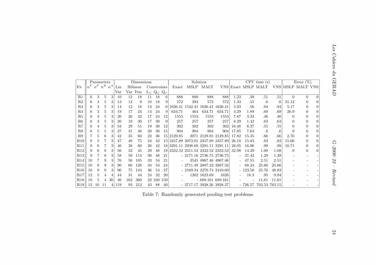
Computer results for the random pooling problems are summarized in Table 7. Theflow formulation is used here, and we use the same following parameters for all the in-stances: nsp = 100, kmax = 100 and nt = 1.

Les

Cahie

rs

du

GE

RA

DG

–2000–23

–R

evis

ed

24

ExParameters Dimensions Solution CPU time (s) Error (%)

nF nP nB nA Lin Bilinear Constraints Exact MSLP MALT VNS Exact MSLP MALT VNS MSLP MALT VNSVar Var Trm L≤ Q≤ Q=

R1 6 3 5 3 10 12 18 11 18 6 888 888 888 888 1.23 .39 .51 .51 0 0 0R2 6 3 5 3 13 12 9 10 18 9 572 394 572 572 1.33 .55 .6 .6 31.12 0 0R3 6 3 5 3 14 12 18 13 24 6 1626.41 1542.41 1626.41 1626.41 5.03 .56 .94 .94 5.17 0 0R4 6 3 5 3 19 17 24 14 24 9 634.71 464 634.71 634.71 4.29 1.89 .69 .69 26.9 0 0R5 6 3 5 3 20 26 42 17 24 12 1553 1553 1553 1553 7.87 3.32 .46 .46 0 0 0R6 6 3 5 3 20 19 30 17 30 9 257 257 257 257 8.29 1.42 .63 .63 0 0 0R7 6 4 5 3 34 29 51 19 30 12 302 302 302 302 16.48 6.37 .55 .55 0 0 0R8 6 5 5 3 27 31 48 20 30 15 904 904 904 904 17.05 7.63 .6 .6 0 0 0R9 7 5 6 3 42 35 60 23 36 15 2129.85 2071 2129.85 2129.85 17.82 15.35 .66 .66 2.76 0 0R10 8 5 7 3 47 40 75 24 42 15 2457.89 2073.01 2457.89 2457.89 26.18 15.83 .83 .83 15.66 0 0R11 8 6 7 3 46 38 60 26 42 18 3291.11 2938.69 3291.11 3291.11 28.05 16.96 .99 .99 10.71 0 0R12 9 6 8 3 56 33 45 29 48 18 2332.52 2311.52 2332.52 2332.52 32.98 14.39 1.08 1.08 .9 0 0R13 9 7 8 3 58 59 114 30 48 21 - 2171.16 2736.75 2736.75 - 37.42 1.29 1.29 - - -R14 10 7 9 3 76 56 105 33 54 21 - 3545 4967.46 4967.46 - 47.55 2.51 2.51 - - -R15 10 8 9 3 90 66 126 34 54 24 - 2711.49 2887.32 2887.32 - 68.24 25.66 25.66 - - -R16 10 9 9 3 96 75 144 36 54 27 - 2169.34 2276.74 2410.69 - 123.58 25.76 48.83 - - -R17 12 5 4 4 44 31 44 24 32 20 - 1262 1623.69 1626 - 16.3 .95 9.94 - - -R18 10 5 4 30 46 162 360 22 240 150 - - 689.161 689.161 - - 11.61 11.61 - - -R19 12 10 11 4 119 93 212 43 88 40 - 3717.17 3928.26 3928.37 - 726.57 703.53 763.15 - - -

Table 7: Randomly generated pooling test problems


Observe that (i) VNS always gives the best results, (ii) MALT and VNS outperformMSLP in all cases, (iii) the improvements made by VNS are obtained in small amountsof additional computing time over that of MALT, (iv) the exact algorithm solves largerinstances than done previously, in very moderate time, and (v) the largest instances (R13and above) could not be solved by the current version of the exact algorithm, due tomemory limitation.

5 Discussion

Three general bilinear programming formulations of the pooling problem are developed:these represent the flow and proportion models, and a new hybrid model which may beused when intermediate pools are configured in series as well as in parallel. Using sampleproblems from the literature, a key observation is made that the type of formulation chosencan significantly impact the complexity of the model, and as a result, the computationaleffort required to solve it.

A recently developed branch and cut algorithm is tested on the sample problems. Theresults show the computational time increases rapidly with the number of bilinear variablesand constraints. Furthermore, using a good heuristic in conjunction with the exact proce-dure is demonstrated to substantially reduce this time. Also observe that a combinationof branch-and-cut and of best model formulation can yield much better computation timesthan those of state-of-the-art algorithms.

Two new heuristic procedures are proposed. The first, a simple iterative scheme appliedto two LPs, differs from previous recursive methods by identifying a set of linear variablesand including them in both LPs. As a local search, the new alternating procedure (ALT)is seen to perform as well or better than the well-studied method of successive linear pro-gramming (SLP) on a set of randomly-generated pooling problems. Furthermore, ALTautomatically produces a sequence of feasible solutions once an initial feasible solution isfound without any need for step-size adjustments. Some heuristic rules are also providedwhich appear to work well in generating initial feasible solutions. The second heuristic pro-cedure performs a variable neighborhood search (VNS) on a set of extreme points identifiedat any current solution. The shaking operation chooses a random point at progressivelyfurther pivots from the current solution. A local search using ALT is then carried out atthe random point. Our preliminary results suggest that VNS will improve the quality ofsolutions obtained by multistart versions of SLP and ALT, particularly for larger probleminstances, within a modest increase in computing time.

Reformulation is a powerful tool of mathematical programming. In Audet et al. 1997 itwas used to study relationships between structured global optimization problems and al-gorithms, revealing embeddings of algorithms one into the other, and unifying them. Here,its effect on computational performance is investigated for the pooling problem. Otherstructured global optimization problems can be studied in the same way. For instance, this


approach led to determination of the octagon with unit diameter and largest area (Audetet al. 2002) and to the first exact algorithm for fractional goal programming (Audet et al.2000b). Several other such problems will be investigated in future work.

Appendix

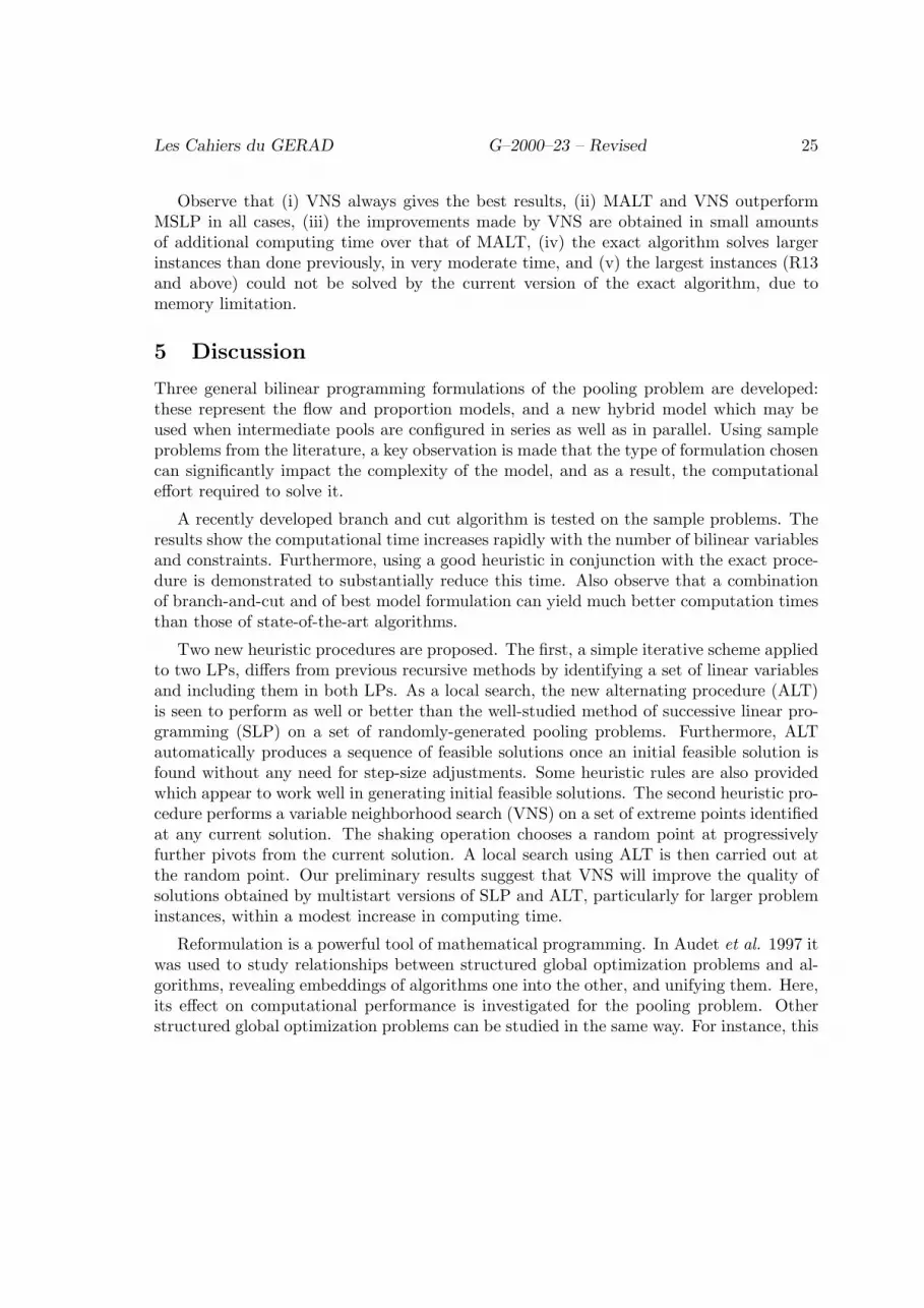
The following figure and table summarize the second pooling problem in Rehfeldt andTisljar (1997).

F1

F2

F3

¹¸º·P1

¹¸º·P2

B1

B2

B3

x21

y11 x31

y21

x12

y12

y22

y13

y23

x23

PPPPPPPPPPPPPPPPPPq

HHHHHHj

JJ

JJ

JJ

JJJ

©©©©©©©©©©©© -

³³³³³³1

PPPPPPqHHHHHHHHHHHH -

¶¶

¶¶

¶¶

¶¶7

½½

½½

½½

½½

½½

½½

½½

½½

½½>

©©©©©©*

©©©©©©©©©*

PPPPPPPPPq

@@

@@

@@

@@@R

¡¡

¡¡

¡¡

¡¡¡µ

³³³³³³³³³1

HHHHHHHHHj

Figure 8: Rehfeldt and Tisljar’s second pooling problem

Feed Price supply Pool capacity Blend Price Demand Arc ×102bblDM/bbl ×102bbl ×102bbl DM/bbl min ×102bbl max

F1 49.2 60.9756 P1 12.5 B1 190 5 x12 7.5F2 62.0 161.29 P2 17.5 B2 230 5 x31 7.5F3 300.0 5 B3 150 5

Attribute Minimum MaximumFeed DEN BNZ ROZ MOZ Blend DEN ROZ MOZ DEN BNZF1 .82 3 99.2 90.5 B1 .74 95 85 .79 -F2 .62 0 87.9 83.5 B2 .74 96 88 .79 .9F3 .75 0 114 98.7 B3 .74 91 - .79 -

Table 8: Characteristics

Since each feed may enter each intermediate pool, and each intermediate pool is con-nected to each final blend, we may assume without any loss of generality that the flow inthe largest pool is greater than or equal to that of the smallest. This additional constraintreduces significantly the feasible region.


References[1] ADHYA N., SAHINIDIS N.V. and TAWARMALANI M. (1999), “A Lagrangian Approach to the

Pooling Problem,” Industrial & Engineering Chemistry Research 38, 1956–1972.

[2] AL-KHAYYAL F.A. and FALK J.E.(1983), “Jointly Constrained Biconvex Programming,” Mathe-

matics of Operations Research 8 (2), 273–286.

[3] ALAMEDDINE A. and SHERALI H.D. (1992), “A new reformulation-linearization technique forbilinear programming problems,” Journal of Global optimization 2, 379–410.

[4] AMOS F., RONNQVIST and GILL G.(1997), “Modeling the Pooling Problem at the New ZealandRefining Company,” Journal of the Operational Research Society 48, 767–778.

[5] ANDROULAKIS I.P., FLOUDAS C.A. and VISWESWARAN V.(1996), “Distributed Decomposition-Based Approaches,” in C.A. Floudas and P.M. Pardalos (eds.) State of the Art in Global Optimization:

Computational Methods and Applications, Kluwer Academics Publishers, Dordrecht.

[6] AUDET C., HANSEN P., JAUMARD B. and SAVARD G.(1997), “Links between the Linear Bileveland Mixed 0 − 1 Programming Problem,” Journal of Optimization Theory and Applications 93(2),273–300.

[7] AUDET C., HANSEN P., JAUMARD B. and SAVARD G. (2000a), “A Branch and Cut Algorithm forNonconvex Quadratically Constrained Quadratic Programming,” Mathematical Programming 87(1),131–152.

[8] AUDET C., CARRIZOSA E. and HANSEN P. (2000b), “An Exact Method for Fractional GoalProgramming,” Les Cahiers du Gerad G-2000-64.

[9] AUDET C., HANSEN P., MESSINE F. and XIONG J. (2002), “The Largest Small Octagon,” Journal

of Combinatorial Theory, series A 98(1),46–59.

[10] BAKER T.E. and LASDON L.S.(1985), “Successive Linear Programming at Exxon,” Management

Science 31 (3), 264–274.

[11] BEN-TAL A., EIGER G. and GERSHOVITZ V.(1994), “Global Minimization by Reducing the Du-ality Gap,” Mathematical Programming 63, 193–212.

[12] BRIMBERG J., ORON G. and MEHREZ A.(1997). “An Operational Model for Utilizing WaterSources of Varying Qualities in an Agricultural Enterprise”, Geography Research Forum 17, 67–77.

[13] CHUNG S.J.(1989), “NP-Completeness of the Linear Complementarity Problem,” Journal of Opti-

mization Theory and Applications 60 (3), 393–399.

[14] DEWITT C.W., LASDON L.S., BRENNER D.A. and MELHEM S.A.(1989), “OMEGA: An ImprovedGasoline Blending System for Texaco,” Interfaces 19, 85–101.

[15] DUR M. and HORST R.(1997), “Lagrange Duality and Partitioning Techniques in Nonconvex GlobalOptimization,” Journal of Optimization Theory and Applications 95 (2), 347–369.

[16] FLOUDAS C.A. and AGGARWAL A.(1990), “A Decomposition Strategy for Global Optimum Searchin the Pooling Problem,” ORSA Journal on Computing 2 (3), 225–235.

[17] FLOUDAS C.A. and VISWESWARAN V.(1993a), “A Primal-Relaxed Dual Global OptimizationApproach,” Journal of Optimization Theory and Applications, 78(2), 187–225.

[18] FLOUDAS C.A. and VISWESWARAN V.(1993b), “New Properties and Computational Improvementof the GOP Algorithm For Problems With Quadratic Objective Function and Constraints,” Journal

of Global optimization 3, 439–462.

[19] FLOUDAS C.A. and VISWESWARAN V.(1996), “New Formulations and Branching Strategies forthe GOP Algorithm,” in I.E. Grossmann (ed.) Global Optimization in Engineering Design, KluwerAcademics Publishers, Dordrecht.

[20] FOULDS L.R, HAUGLAND D. and JORNSTEN K.(1992), “A Bilinear Approach to the PoolingProblem,” Optimization 24, 165–180.


[21] GRIFFITH R.E. and STEWART R.A.(1961), “A Nonlinear Programming Technique for the Opti-mization of Continuous Processing Systems,” Management Science 7, 379–392.

[22] GROSSMANN I.E. and QUESADA I.(1995), “Global Optimization of Bilinear Process Networks withMulticomponents Flows,” Computers & Chemical Engineering 19(12), 1219–1242.

[23] HANSEN P. and JAUMARD B.(1992), “Reduction of Indefinite Quadratic Programs to BilinearPrograms,” Journal of Global optimization 2, 41–60.

[24] HANSEN P., JAUMARD B. and SAVARD G.(1992), “New Branch-and-Bound Rules for LinearBilevel Programming,” SIAM Journal on Scientific and Statistical Computing 13, 1194–1217.

[25] HANSEN P. and MLADENOVIC N. (1997). Variable Neighborhood Search. Computers and Opera-

tions Research 24, 1097-1100.

[26] HANSEN, P. and. MLADENOVIC, N.. (1999). An Introduction to Variable Neighborhood Search. InS. Voss et al. (eds.), Metaheuristics, Advances and Trends in Local Search Paradigms for Optimization,pp.433–458, Kluwer, Dordrecht.

[27] HAVERLY C.A.(1978), “Studies of the Behaviour of Recursion for the Pooling Problem,” ACM

SIGMAP Bulletin 25, 19–28.

[28] LASDON L. and JOFFE B.(1990), “The Relationship between Distributive Recursion and SuccessiveLinear Programming in Refining Production Planning Models,” NPRA Computer Conference Seattle,Washington.

[29] LASDON L., WAREN A., SARKAR S. and PALACIOS-GOMEZ F.(1979), “Solving the PoolingProblem Using Generalized Reduced Gradient and Successive Linear Programming Algorithms,” ACM

Sigmap Bulletin 27, 9–25.

[30] LODWICK W.A.(1992), “Preprocessing Nonlinear Functional Constraints with Applications to thePooling Problem ,” ORSA Journal on Computing 4 (2), 119-131.

[31] PALACIOS-GOMEZ F., LASDON L.S. and ENGQUIST M.(1982), “Nonlinear Optimization by Suc-cessive Linear Programming,” Management Science 28 (10), 1106–1120.

[32] REHFELDT AND TISLJAR (1997). Private communication.

[33] SAHINIDIS N.V. (1996), “BARON: A General Purpose Global Optimization Software Package,”Journal of Global Optimization 8, 201–205.

[34] SHERALI H.D. and TUNCBILEK C.H.(1992), “A Global Optimization Algorithm for PolynomialProgramming Using a Reformulation-Linearization Technique,” Journal of Global Optimization 2,101–112.

[35] SHERALI H.D. and TUNCBILEK C.H.(1997a), “Comparison of Two Reformulation-LinearizationTechnique Based Linear Programming Relaxations for Polynomial Programming Problems,” Journal

of Global Optimization 10, 381–390.

[36] SHERALI H.D. and TUNCBILEK C.H.(1997b), “New Reformulation Linearization/ConvexificationRelaxations for Univariate and Multivariate Polynomial Programming Problems,” Operations Re-

search Letters 21, 1–9.

[37] ZHANG J, KIM N.H. and LASDON L.S.(1985), “An Improved Successive Linear Programming Al-

gorithm,” Management Science 31 (10), 1312–1331.

Documents

Pooling Problem: Alternate Formulations and Solution Methods