Plant communities of field boundaries in Finnish farmland

121

A G R I C U L T U R A L A N D F O O D S C I E N C E I N F I N L A N D

Vol. 11 (2002): 121–135.

© Agricultural and Food Science in FinlandManuscript received February 2002


Vol. 11 (2002): 121–135.

Plant communities of field boundariesin Finnish farmland

Sanna TarmiMTT Agrifood Research Finland, Environmental Management, FIN-31600 Jokioinen, Finland. Current address: Depart-

ment of Applied Biology, PO Box 27, FIN-00014 University of Helsinki, Finland, e-mail: [email protected]

Hannu TuuriMTT Agrifood Research Finland, Data and Information Services, FIN-31600 Jokioinen, Finland

Juha HeleniusDepartment of Applied Biology, PO Box 27, FIN-00014 University of Helsinki, Finland

To determine the importance of field boundary habitats for farmland biodiversity, we surveyed a totalof 193 boundaries from four climatically and agriculturally dissimilar regions in Finland. We meas-ured the current plant species richness and composition of the boundaries, and, based on the differ-ences in vegetation characteristics, we describe six boundary types.

The observed plant species were mainly indicators of fresh to wet soils and moderate to rich min-eral nitrogen content. The most frequent species were tall, perennial monocots and dicots indicatingthe high productivity of the vegetation. Moreover, herbicide-tolerant species were common. No spe-cies rare for Finland were found. In animal husbandry regions, the most frequent species were sowngrassland species and typical grassland weeds. In cereal production regions, fast-spreading root weedstolerant of herbicides were the most frequent. Mean species richness was highest in the cluster Ca-lamagrostis-Phalaris (24 species (s) / boundary (b)), which we considered as representative of moistsites with some disturbance by agricultural practices. Most species-poor were the clusters Elymus-Anthriscus (14 s/b) and Elymus-Cirsium (16 s/b), both found predominantly in cereal productionregions in southern Finland.

Our results suggest that the biodiversity value of boundaries is lowest in the most intensive cerealproduction areas and highest in areas of mixed farming.

Key words: plant communities, correspondence analysis, boundaries, diversity, species richness

Introduction

Intensified agricultural land use has drastical-ly reduced semi-natural habitats. Traditional

pastures and a variety of natural meadow typeshave almost disappeared (Alanen 1997). More-over, the amount of field boundaries has beenconsiderably reduced (Ruuska and Helenius1996, Hietala-Koivu 1999). In particular, sub-

mailto:[email protected]

122


Tarmi, S. et al. Plant communities of field boundaries

surface draining of fields to increase the cul-tivated area has decreased boundary areas, acommon phenomenon in many European coun-tries since the 1950s. In Finland, the area offields with subsurface drainage increased from5.1% (of a total field area of 2 292 000 ha) in1945 (Hilli 1949) to 53% (2 501 000 ha) in1998 (Information Centre of the Ministry ofAgriculture and Forestry 1999). Subsurfacedrainage is more common in cereal productionregions in southern parts of Finland, where upto 91% of the parcel ditches have been re-moved during the last four decades (Hietala-Koivu 1999). Besides the decrease in the totalboundary area, the remaining boundaries havebeen exposed to herbicide drift from cropspraying and fertiliser misplacement or run-off from cultivated fields, both of which sim-plify plant community structure and decreasespecies richness (Marrs et al. 1991, Kleijn andSnoeijing 1997, Hansson and Fogelfors 1998).Higher plant species diversity increases thetemporal s tabi l i ty of plant communit ies(Tilman et al. 1996). More diverse plant com-munities may also utilise soil mineral nitro-gen more efficiently than a species-poor eco-system (Tilman et al. 1996). Diverse plantcommunities are important also for hetero-trophs exploiting these habitats. Siemann(1998) demonstrated that plant species diver-sity and productivity increased diversity alsoat higher trophic levels.

The decreased area and harmful impacts ofagricultural practices on remaining boundaryhabitats have been a common phenomena inWestern Europe during the last century. Despitethis, the importance of these habitats for wild-life of the agricultural environment has beenshown in many studies. Boundaries enhance ar-thropod diversity, including the natural enemiesof crop pests (Dennis and Fry 1992, Canters andTamis 1999, Pfiffner and Luka 2000). They in-crease overall carabid densities (Fournier andLoreau 1999) in cultivated areas and provideoverwintering habitats for e.g. spiders (Bayramand Luff 1993). Flowering plants are a food re-source for pollinators (Lagerlöf et al. 1992,

Bäckman and Tiainen 2002). Field boundariesalso provide important links among favourablehabitat patches for butterfly species (Dover etal. 1992, Sparks and Parish 1995), and the vari-ous boundary types support a diverse butterflyfauna (Saarinen et al. 1998). Boundaries provideimportant feeding and nesting habitats for game-birds (e.g. Aebischer et al. 1994, Tiainen andPakkala 2000). As a consequence of intensifiedland use, the decline in numbers of grey par-tridge, as well as several other farmland birdspecies, has been reported in Finland (Väisänen1999).

In this research, we tried to estimate the bi-odiversity value of Finnish field boundaries bysurveying plant assemblages. Our specific ob-jectives were: 1) to describe plant species di-versity and composition in Finnish field bound-aries, 2) to identify boundary plant communi-ties based on species composition, and 3) to de-scribe the factors determining these types onthe basis of the ecological requirements of theplant species. In addition, our objective wasto estimate the value of boundary plant com-munities as secondary habitats for meadowplant species. The importance of current bound-ary plant communities for animals is also dis-cussed.

We know only one earlier study on Finnishfield boundary vegetation, which focused on thespecies’ value as silage for cattle, rather than onthe biodiversity aspect (Hilli 1949).

This study was made just before managementmeasures of the 1st Finnish agri-environmentalscheme required by EU regulations were applied.One target of the agri-environmental scheme isto maintain biodiversity and landscape in agri-cultural environment. In the basic scheme, man-agement agreement includes the widening ofboundaries along waterways to one (main ditch-es) or three (stream, river, lake) meters wide.Boundaries should not be fertilized or treatedwith pesticides. Mowing is mentioned as a use-ful management for wildlife, but it is not oblig-atory treatment (Ministry of Agriculture andForestry 2000).

123


Vol. 11 (2002): 121–135.

Material and methods

Botanical studies of field boundaries were in-cluded in a broad nationwide MYTVAS -projecton Monitoring the Impacts of the Agri-Environ-mental Support Scheme in 1995–1999. Thisproject was carried out in four watershed regions,which are representative of agricultural regionsin Finland. Lepsämänjoki, about 30 km N ofHelsinki, and Yläneenjoki, about 50 km NE ofTurku, are predominantly cereal production re-gions. Lestijoki, about 60 km SE of Kokkola, isa region of animal husbandry and mixed farm-ing, and Taipaleenjoki, about 20 km W of Joen-suu, is a typical animal husbandry region of smallfarms and fine-grained landscape structure. Theco-ordinates of the regions are Lepsämänjoki60°20’ N, 60°27’ N, 24°37’ E, 24°49’ E, Yläneen-joki 60°47’ N to 60°56’ N and 22°25’ E to 22°40’E, Lestijoki 63°39’ N, 63°50’ N, 24°09’ E, 24°25’E and Taipaleenjoki 62°36’ N, 62°38’ N, 29°10’E, 29°20’ E.

The most common soil types in Lepsämän-joki are sandy clay (in 55% of the boundaries),fine sand (26%), and clay (16%); in Yläneen-joki fine sand (61%) and sandy clay (31%); inLestijoki fine sand (91%), and in Taipaleenjokifine sand (59%), mull (19%) and silt (13%) (Tar-mi and Helenius, unpublished data). The aver-age thermal growing season in Yläneenjoki andLepsämänjoki is 170 days, in Taipaleenjoki 155days, and in Lestijoki 150 days (Alalammi 1987).Average annual precipitation is 582, 619, 612 and544 mm, respectively.

Our fieldwork period was from the beginningof July to mid-August 1995. To facilitate siteselection in the field, we made a preliminarychoice of boundaries from aerial photographs(scale 1:20000). Subsequently we refined thechoice using the following criteria. (1) Locationnext to a waterway such as a main ditch, river orlake. (2) No or only a few trees and shrubspresent (because these might affect the speciescomposition in the herbaceous layer). (3) Noforest edge next to a site because of the possibleshading effects and the dispersal of forest field

layer species. Only sites matching these criteriawere included.

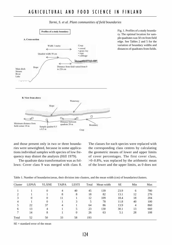
We studied 193 boundaries in all (50 inYläneenjoki, 52 in Lepsämänjoki, 58 in Lesti-joki and 33 in Taipaleenjoki). The boundary wasdetermined as a zone from a field edge to thebeginning of a slope. All plant species weremeasured in one to five 0.25 m2 quadrates (0.5m x 0.5 m) in each boundary (Fig. 1). The dis-tance of a quadrate to the field was measured asthe distance from the field edge to the nearest,parallel side of the quadrate. We aimed at a quad-rate distance of 50 cm from the field edge, butin practice these varied from zero to over twometres depending on the variation in boundarywidths. When the boundary width was less than50 cm, less than five quadrates were studied.When the boundary width was less than onemetre, quadrate distance from the field was lessthan aimed 50 cm. In cases of over one metrethe distance from the field was more than 50 cm.The width of a boundary was measured in allfive quadrate sites to calculate the mean widthbased on five values. The minimum distance ofthe first sample quadrate from one end of aboundary was 10 metres and the distance be-tween quadrates 20 metres.

We used Oksanen’s nine class scale (1981),1 – ≤0.8%, 2 – ≤1.6%, 3 – ≤3.1%, 4 – ≤6.3%, 5– ≤12.5%, 6 – ≤25%, 7 – ≤50%, 8 – ≤75%, 9 –≤100%, in estimating plant species’ coverage.Because our field work schedule was tight, fieldworkers identified sterile or difficult grasses onlyto genus level. In species nomenclature, we fol-low Hämet-Ahti et al. (1986). To describe theecological characters of the species, we appliedEllenberg et al. (1991) indicator values.

In the original data, we determined the covervalues of the species in each 0.25 m2 samplequadrate using a nine-class scale. For the statis-tical analyses, we combined the quadrate datato calculate the mean cover of each species in aboundary. Boundaries with only two quadrateswere made passive in the correspondence anal-ysis (CA), but were included in classification.Species which were present only in one bounda-ry were dropped from the CA (listed in App. 1)

124



Fig. 1. Profiles of a study bounda-ry. The optimal location for sam-ple quadrates was 50 cm from fieldedge. See Tables 2 and 5 for thevariation of boundary widths anddistances of quadrates from fields.

and those present only in two or three bounda-ries were unweighted, because in some applica-tions individual samples with species of low fre-quency may distort the analysis (Hill 1979).

The quadrate data transformation was as fol-lows: Cover class 9 was merged with class 8.

The classes for each species were replaced withthe corresponding class centres by calculatingthe geometric means of lower and upper limitsof cover percentages. The first cover class,>0–0.8%, was replaced by the arithmetic meanof the lower and the upper limits, as 0 does not

Table 1. Number of boundaries/areas, their division into clusters, and the mean width (cm) of boundaries/clusters.

Cluster LEPSÄ YLÄNE TAIPA LESTI Total Mean width SE Min Max

1 1 0 4 40 45 139 23.9 6 7802 1 1 8 8 18 82 13.1 12 2763 0 0 11 1 12 109 18.4 18 2044 1 0 1 3 5 78 11.8 40 1005 22 37 4 1 64 86 13.9 4 8606 13 4 1 5 23 130 30.1 13 6607 14 8 1 0 26 63 5.1 28 108

Total 52 50 33 58 193

SE = standard error of the mean

Crop:• cereal• grass ley• rape• cabbage

125


Vol. 11 (2002): 121–135.

allow computing a geometric mean. A mean cov-er percentage per species was then obtained asan arithmetic mean of the quadrates. Finally,these cover percentages were replaced with thecorresponding value from the original scale(classes from 1 to 8). These new values approx-imate the cover percentages of species (Oksanen1981).

We used ordination technique to reveal themajor variation in the species abundance data ofboundaries. CA was performed with the programCanoco™ (ter Braak 1987). By CA it may bepossible to detect whether unknown environmen-tal variables determine the species occurrencesin the data set (Jongman et al. 1995). The ordi-nation diagram presented the similarity or dis-similarity of the species compositions of the testboundaries. Based on the scores of the first fouraxes of ordination, the boundaries were groupedinto clusters by Ward’s method (see Jongman etal. 1995). Cluster analysis was performed usingthe SAS™ Statistical package’s CLUSTER andTREE procedures.

The mean species richness was measured foreach cluster using only boundaries with an equalsample size of five quadrate samples to allowfor the asymptotic dependence of the speciesnumber on the sample size. Because clusteringis a subjective method, i.e. one may decide thenumber of groups to be left after fusion, we foundit inappropriate to make any statistical test forspecies richness between clusters. However, wefound it important to check whether the distancefrom the field could, at least partially, be one ofthe factors affecting the species richness in thesedata. To test the effect of distance from the fieldedge on plant species richness, we dividedboundaries into three classes: 1) the mean dis-tance of the quadrates from field edge 0–19 cm(n = 60), 2) distance 20–39 cm (n = 36), and 3)distance > 40 cm (n = 50). To test the differenc-es between classes we used ANOVA, which wasperformed with SYSTAT™ (SPSS™ Inc. 1997).The normality of variables in ANOVA waschecked from the normal probability plots ofresiduals. The homogeneity of variables was test-ed with Cochran’s test.

Results

The results of the CA ordination indicated dis-similarities in boundary vegetation between theregions. The studied regions formed three groupsof plots in the first two axes in CA ordination(Fig. 2). Southern regions were plotted as onecloud of plots, whereas Lestijoki and Taipaleen-joki formed their own groups, from whichTaipaleenjoki sites were plotted in a more scat-tered way. Points in the first two groups werearranged in relation to the first axis, while theTaipaleenjoki sites were scattered in relation tothe second axis (Fig. 2).

Based on the scores of the first four axes ofordination, we classified the boundaries by us-ing Ward’s clustering method. We found sevenclusters to represent a reasonable level of ag-

Fig. 2. Ordination diagram of correspondence analysis ofthe studied field boundaries based on their plant speciescomposition. Different symbols represent the four studyareas. For axis 1 eigenvalue = 0.424, percentage varianceof species data 10.6, and for axis 2 eigenvalue = 0.224,percentage variance of species data 5.6.

126



glomeration even though cluster 4 (C4) includ-ed only five boundaries at this level (Table 1,Fig. 3). Boundaries in C4 were interpreted as out-liers and were not considered as representativeboundary group. In the next level of fusion C4would have been merged with cluster 2 (C2). Asin CA results, groups that were formed by clus-tering also indicated that some local environmen-tal factors may determine the vegetation com-position of boundaries. Cluster 1 (C1) includedmainly Lestijoki sites and cluster 3 (C3) mainlyTaipaleenjoki sites (Fig. 3, Table 1). Cluster 2(C2) represents mainly sites from Taipaleenjokiand Lestijoki whereas clusters 5 (C5) and 7 (C7)represent mainly sites from Lepsämänjoki andYläneenjoki. Cluster 6 (C6) is the most inde-pendent of any particular region and includesseveral sites from southern regions and Lesti-joki.

Each cluster was described as a group ofboundaries that had the most similar plant spe-cies compositions (Figs. 3 and 4). Because wehave mainly genus data on monocot (grassy)species, we use the preliminary results of laterstudies in these regions to introduce the exactspecies. Unidentified species belonged most of-ten to the genera Poa, Festuca, Agrostis, Ca-lamagrostis and Carex (App. 1). According tothe later studies on these regions (Tarmi andHelenius, unpublished results from 1997–1999),Poa turned out to be mostly P. pratensis, Festu-ca F. pratensis or F. rubra, and Agrostis A. cap-illaris, A. gigantea or A. stolonifera. Calama-grostis was most often C. canescens, C. arundi-nacea, C. epigejos or C. purpurea. Carex wasidentified as C. acuta, C. canescens, C. nigra,C. ovalis or C. vesicaria species.

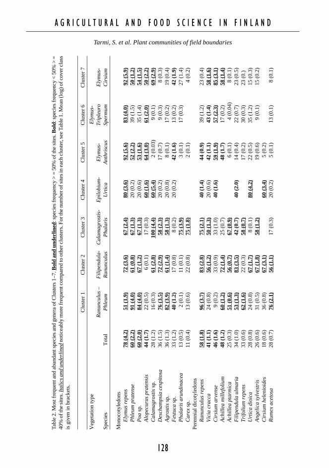
Each cluster was named by the characteris-tic species (Table 2) and were described as fol-lows:

C1 – Ranunculus-Phleum: Grasses such as Ph-leum pratense, Poa sp., Agrostis sp., and Fes-tuca sp. were common. The perennial herbsRanunculus repens, Rumex acetosa, Trifoliumrepens, Achillea millefolium, and Leontodonautumnalis were abundant. Annual specieswere rarely found.

C2 – Filipendula-Ranunculus: In this cluster,none of the species attained absolute domi-nance compared to each other, but many spe-cies occurred with moderate frequency. It wascharacterised by tall herbs favouring moistsites such as Filipendula ulmaria, Angelicasylvestris, Cirsium helenioides and Calama-grostis sp.. Moreover, species of nutrient richsites such as Urtica dioica, Epilobium angus-tifolium and Galeopsis sp. were common.

C3 – Calamagrostis-Phalaris: Tall grasses Ca-lamagrostis sp. and Phalaris arundinaceawere characteristic of the cluster. Perennialspecies indicating moist or wet sites – Carexsp., Achillea ptarmica, Angelica sylvestris,Lysimachia sp., Polygonum amhibium, Peu-cedanum palustre, Lactuca sibirica – were

Fig. 3. Ordination diagram of correspondence analysis. Eachplot represents one field boundary. Based on their speciescomposition, boundaries are grouped into seven clustersfrom a cluster analysis (Ward’s method). For axis 1 eigen-value = 0.424, percentage variance of species data 10.6,and for axis 2 eigenvalue = 0.224, percentage variance ofspecies data 5.6. Each symbol represents one cluster.

127


Vol. 11 (2002): 121–135.

frequent, as well as some annuals such asPolygonum hydropiper, Stellaria media andGalium uliginosum.

C4 – Epilobium-Urtica: Most frequent specieswere Elymus repens, Epilobium angustifo-lium and Urtica dioica.

C5 – Elymus-Anthriscus: Elymus repens was ahighly dominant species. Other frequent spe-cies were mostly grasses, such as Phleumpratense, Poa sp., Alopecurus pratensis andruderal herbs like Cirsium arvense, Anthris-cus sylvestris. A characteristic species for

only this cluster, even if not very frequent,was Aegopodium podagraria.

C6 – Elymus-Tripleurospermum: Elymus repensand Alopecurus pratensis were the most fre-quent grasses. Annual herbs such as Galeop-sis sp., Stellaria media, Tripleurospermum in-odorum, and Polygonum aviculare were char-acteristic of this cluster.

C7 – Elymus-Cirsium: The most frequent spe-cies were Elymus repens, Calamagrostis sp.,Cirsium arvense, Equisetum arvense, Lathy-rus pratensis, Tussilago farfara, Vicia crac-ca and Achillea millefolium.

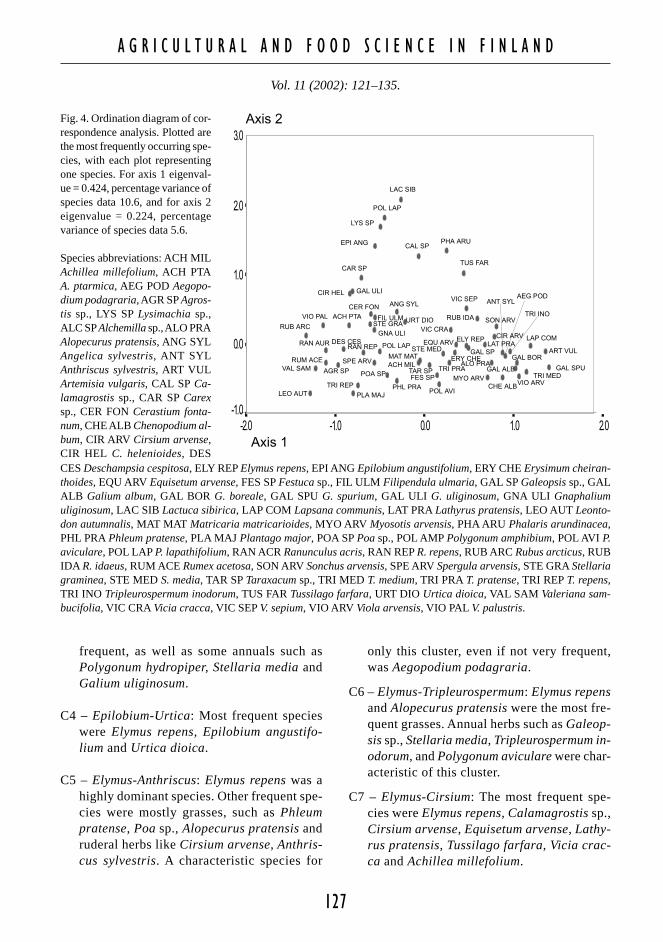
Fig. 4. Ordination diagram of cor-respondence analysis. Plotted arethe most frequently occurring spe-cies, with each plot representingone species. For axis 1 eigenval-ue = 0.424, percentage variance ofspecies data 10.6, and for axis 2eigenvalue = 0.224, percentagevariance of species data 5.6.

Species abbreviations: ACH MILAchillea millefolium, ACH PTAA. ptarmica, AEG POD Aegopo-dium podagraria, AGR SP Agros-tis sp., LYS SP Lysimachia sp.,ALC SP Alchemilla sp., ALO PRAAlopecurus pratensis, ANG SYLAngelica sylvestris, ANT SYLAnthriscus sylvestris, ART VULArtemisia vulgaris, CAL SP Ca-lamagrostis sp., CAR SP Carexsp., CER FON Cerastium fonta-num, CHE ALB Chenopodium al-bum, CIR ARV Cirsium arvense,CIR HEL C. helenioides, DESCES Deschampsia cespitosa, ELY REP Elymus repens, EPI ANG Epilobium angustifolium, ERY CHE Erysimum cheiran-thoides, EQU ARV Equisetum arvense, FES SP Festuca sp., FIL ULM Filipendula ulmaria, GAL SP Galeopsis sp., GALALB Galium album, GAL BOR G. boreale, GAL SPU G. spurium, GAL ULI G. uliginosum, GNA ULI Gnaphaliumuliginosum, LAC SIB Lactuca sibirica, LAP COM Lapsana communis, LAT PRA Lathyrus pratensis, LEO AUT Leonto-don autumnalis, MAT MAT Matricaria matricarioides, MYO ARV Myosotis arvensis, PHA ARU Phalaris arundinacea,PHL PRA Phleum pratense, PLA MAJ Plantago major, POA SP Poa sp., POL AMP Polygonum amphibium, POL AVI P.aviculare, POL LAP P. lapathifolium, RAN ACR Ranunculus acris, RAN REP R. repens, RUB ARC Rubus arcticus, RUBIDA R. idaeus, RUM ACE Rumex acetosa, SON ARV Sonchus arvensis, SPE ARV Spergula arvensis, STE GRA Stellariagraminea, STE MED S. media, TAR SP Taraxacum sp., TRI MED T. medium, TRI PRA T. pratense, TRI REP T. repens,TRI INO Tripleurospermum inodorum, TUS FAR Tussilago farfara, URT DIO Urtica dioica, VAL SAM Valeriana sam-bucifolia, VIC CRA Vicia cracca, VIC SEP V. sepium, VIO ARV Viola arvensis, VIO PAL V. palustris.

128



Tabl

e 2.

Mos

t fre

quen

t and

abu

ndan

t spe

cies

and

gen

era

of C

lust

ers

1–7.

Bol

d an

d un

derl

ined

: spe

cies

freq

uenc

y >

= 50

% o

f the

site

s. B

old:

spe

cies

freq

uenc

y <

50%

> =

40%

of t

he s

ites.

Ital

ics

and

unde

rlin

ed n

otic

eabl

y m

ore

freq

uent

com

pare

d to

oth

er c

lust

ers.

For

the

num

ber o

f site

s in

eac

h cl

uste

r, se

e Ta

ble

1. M

ean

(log

) of c

over

cla

ssis

giv

en in

bra

cket

s.

Clu

ster

1C

lust

er 2

Clu

ster

3C

lust

er 4

Clu

ster

5C

lust

er 6

Clu

ster

7

Veg

etat

ion

type

Ely

mus

-R

anun

culu

s –

Fil

ipen

dula

-C

alam

agro

stis

-E

pilo

bium

-E

lym

us-

Tri

pleu

roE

lym

us-

Spec

ies

Tot

alP

hleu

mR

anun

culu

sP

hala

ris

Urt

ica

Ant

hris

cus

Sper

mum

Cir

sium

Mon

ocot

yled

ons

Ely

mus

rep

ens

78 (

4.2)

51 (

1.9)

72 (

3.6)

67 (

2.4)

80 (

3.6)

92 (

5.6)

83 (

4.0)

92 (

5.9)

Phl

eum

pra

tens

e60

(2.

2)91

(4.

0)61

(0.

8)67

(1.

3)20

(0.

2)52

(2.

2)39

(1.

5)50

(1.

2)P

oa s

p.60

(2.

0)84

(4.

0)67

(1.

2)67

(1.

3)20

(0.

6)53

(1.

6)35

(1.

4)54

(1.

5)A

lope

curu

s pr

aten

sis

44 (

1.7)

22 (

0.5)

6 (0

.1)

17 (

0.3)

60 (

1.6)

64 (

3.0)

61 (

2.0)

50 (

2.2)

Cal

amag

rost

is s

p.28

(1.

2)16

(0.

3)61

(2.

8)10

0 (4

.4)

60 (

5.4)

2 (0

.03)

9 (0

.1)

69 (

2.9)

Des

cham

psia

ces

pito

sa36

(1.

5)76

(3.

5)72

(2.

9)58

(2.

3)20

(0.

2)17

(0.

7)9

(0.3

)8

(0.3

)A

gros

tis

sp.

36 (

1.3)

82 (

3.9)

61 (

1.4)

58 (

1.3)

20 (

0.8)

8 (0

.1)

17 (

0.2)

19 (

0.4)

Fes

tuca

sp.

33 (

1.2)

40 (

1.2)

17 (

0.8)

8 (0

.2)

20 (

0.2)

42 (

1.6)

13 (

0.2)

42 (

1.9)

Pha

lari

s ar

undi

nace

a13

(0.

5)2

(0.1

)11

(0.

1)75

(3.

9)3

(0.1

)17

(0.

3)27

(1.

4)C

arex

sp.

11 (

0.4)

13 (

0.6)

22 (

0.8)

75 (

1.8)

2 (0

.1)

4 (0

.2)

Pere

nnia

l dic

otyl

edon

sR

anun

culu

s re

pens

58 (

1.8)

96 (

3.7)

83 (

2.8)

75 (

2.1)

40 (

1.4)

44 (

0.9)

39 (

1.2)

23 (

0.4)

Vic

ia c

racc

a41

(1.

1)24

(0.

8)56

(1.

2)50

(1.

3)20

(0.

6)42

(1.

1)43

(1.

4)58

(1.

6)C

irsi

um a

rven

se46

(1.

6)9

(0.2

)33

(0.

9)33

(1.

0)40

(1.

6)59

(1.

9)57

(2.

3)85

(3.

1)A

chil

lea

mil

lefo

lium

48 (

1.2)

60 (

1.2)

72 (

1.4)

25 (

0.7)

48 (

1.7)

17 (

0.2)

58 (

1.4)

Ach

ille

a pt

arm

ica

25 (

0.3)

51 (

0.6)

56 (

0.7)

67 (

0.9)

6 (0

.1)

4 (0

.04)

8 (0

.1)

Fil

ipen

dula

ulm

aria

34 (

1.0)

53 (

1.3)

83 (

3.5)

42 (

0.7)

40 (

2.0)

14 (

0.4)

22 (

0.7)

23 (

0.5)

Tri

foli

um r

epen

s33

(0.

6)62

(1.

6)22

(0.

3)58

(0.

7)17

(0.

2)30

(0.

3)23

(0.

)U

rtic

a di

oica

28 (

0.8)

24 (

0.8)

67 (

1.7)

8 (0

.1)

80 (

4.2)

22 (

0.5)

35 (

1.2)

15 (

0.3)

Ang

elic

a sy

lves

tris

26 (

0.6)

31 (

0.5)

67 (

1.8)

58 (

1.2)

19 (

0.6)

9 (0

.1)

15 (

0.2)

Cir

sium

hel

enio

ides

18 (

0.6)

36 (

0.8)

67 (

3.1)

60 (

3.4)

5 (0

.2)

Rum

ex a

ceto

sa28

(0.

7)76

(2.

1)56

(1.

1)17

(0.

3)20

(0.

2)5

(0.1

)13

(0.

1)8

(0.1

)

129


Vol. 11 (2002): 121–135.

Epi

lobi

um a

ngus

tifo

lium

12 (

0.5)

9 (0

.2)

61 (

2.6)

17 (

0.7)

80 (

4.6)

2 (0

.1)

9 (0

.1)

Equ

iset

um a

rven

se38

(0.

9)33

(0.

7)33

(0.

8)17

(0.

2)41

(1.

0)30

(0.

8)69

(1.

4)A

nthr

iscu

s sy

lves

tris

35 (

1.0)

4 (0

.1)

33 (

0.8)

17 (

0.2)

63 (

2.1)

26 (

1.0)

42 (

0.7)

Lat

hyru

s pr

aten

sis

33 (

0.9)

9 (0

.1)

28 (

0.6)

33 (

0.4)

20 (

0.2)

44 (

1.3)

22 (

0.4)

62 (

2.2)

Tus

sila

go fa

rfar

a17

(0.

6)2

(0.0

2)17

(0.

7)42

(1.

8)20

(0.

4)9

(0.2

)4

(0.2

)58

(2.

1)T

arax

acum

sp.

37 (

0.9)

36 (

0.7)

39 (

0.6)

33 (

0.3)

20 (

0.8)

47 (

1.2)

4 (0

.04)

50 (

1.5)

Leo

ntod

on a

utum

nali

s17

(0.

4)58

(1.

6)17

(0.

2)8

(0.1

)2

(0.1

)4

(0.0

4)L

ysim

achi

a sp

.8

(0.2

)4

(0.1

)28

(0.

9)50

(1.

7)4

(0.0

4)4

(0.1

)P

olyg

onum

am

phib

ium

7 (0

.2)

4 (0

.1)

17 (

0.6)

50 (

1.4)

2 (0

.02)

9 (0

.22)

Peu

ceda

num

pal

ustr

e4

(0.1

)50

(0.

8)2

(0.0

2)R

anun

culu

s ac

ris

16 (

0.3)

33 (

0.9)

44 (

0.7)

17 (

0.3)

40 (

0.8)

3 (0

.1)

9 (0

.13)

Sonc

hus

arve

nsis

22 (

0.5)

2 (0

.02)

17 (

0.6)

25 (

0.4)

40 (

0.4)

17 (

0.3)

43 (

1.4)

46 (

1.1)

Aeg

opod

ium

pod

agra

ria

16 (

0.7)

4 (0

.1)

6 (0

.3)

31 (

1.5)

17 (

0.5)

15 (

0.5)

Art

emis

ia v

ulga

ris

7 (0

.3)

6 (0

.1)

3 (0

.1)

39 (

2.0)

4 (0

.1)

Lac

tuca

sib

iric

a5

(0.1

)2

(0.1

)17

(0.

3)42

(1.

1)4

(0.1

)A

nnua

l dic

otyl

edon

sG

aleo

psis

sp.

45 (

0.8)

22 (

0.3)

56 (

1.00

)25

(0.

3)20

(0.

2)47

(1.

0)87

(2.

0)50

(0.

6)St

ella

ria

med

ia45

(0.

7)36

(0.

5)28

(0.

6)67

(0.

7)20

(0.

2)42

(0.

5)83

(2.

3)42

(0.

6)Tr

iple

uros

perm

um in

odor

um31

(0.

8)9

(0.1

)17

(0.

2)42

(0.

4)20

(0.

2)22

(0.

6)83

(2.

8)50

(1.

4)G

aliu

m u

ligi

nosu

m13

(0.

2)18

(0.

3)39

(0.

4)58

(0.

7)2

(0.0

2)4

(0.0

4)4

(0.0

4)P

olyg

onum

avi

cula

re17

(0.

2)18

(0.

3)11

(0.

1)8

(0.1

)6

(0.1

)57

(0.

8)15

(0.

2)L

apsa

na c

omm

unis

15 (

0.2)

11 (

0.2)

13 (

0.2)

43 (

0.8)

31 (

0.5)

Che

nopo

dium

alb

um12

(0.

2)7

(0.1

)11

(0.

1)9

(0.1

)43

(0.

7)12

(0.

2)E

rysi

mum

che

iran

thoi

des

9 (0

.1)

4 (0

.04)

11 (

0.1)

3 (0

.03)

35 (

0.4)

15 (

0.2)

Fal

lopi

a co

nvol

vulu

s7

(0.1

)3

(0.0

3)35

(0.

6)12

(0.

1)G

aliu

m b

orea

le15

(0.

4)4

(0.1

)6

(0.1

)19

(0.

7)35

(1.

0)19

(0.

5)G

aliu

m s

puri

um7

(0.1

)2

(0.0

2)3

(0.0

3)30

(0.

6)12

(0.

3)P

olyg

onum

hyd

ropi

per

6 (0

.1)

2 (0

.02)

11 (

0.2)

42 (

0.4)

20 (

0.2)

2 (0

.02)

9 (0

.2)

Gna

phal

ium

uli

gino

sum

13 (

0.2)

16 (

0.2)

22 (

0.4)

33 (

0.3)

3 (0

.03)

26 (

0.7)

12 (

0.1)

Myo

soti

s ar

vens

is12

(0.

2)7

(0.1

)8

(0.1

)20

(0.

2)9

(0.1

)35

(0.

5)15

(0.

2)Sp

ergu

la a

rven

sis

11 (

0.2)

16 (

0.2)

11 (

0.2)

17 (

0.2)

3 (0

.03)

30 (

0.7)

4 (0

.04)

Vio

la a

rven

sis

9 (0

.1)

2 (0

.02)

6 (0

.1)

8 (0

.1)

30 (

0.4)

15 (

0.2)

130



The mean species richness was highest inthe Calamagrostis-Phalaris type (Table 3)whereas Elymus-Anthriscus and Elymus-Cirsi-um types were the most species-poor among alltypes. When the effect of distance from the fieldon species richness was tested, no statisticallysignificant differences between the three class-es (ANOVA, df = 2, f = 1.23, P = 0.29) wasfound. The mean species richness next to fieldedges with crops was 16.12 ± 0.87 (mean ± SE),at 20–39 cm distance from the field edge 17.14± 1.12, and at 40 cm or more from the edge18.14± 0.95.

The mean widths of the boundaries werehighest in C1 and in C6 (Table 1). The narrow-est boundaries, slightly over half metre in width,were in C7. The total number of plant speciesidentified in the boundaries was 140. Thisnumber does not include plants identified onlyto genus level, except the Taraxacum genus.

After the data modifications that precededstatistical analyses, 100 identified species wereincluded in CA and cluster analysis. The eco-logical requirements of these species were de-scribed based on Ellenberg et al. (1991) classi-fication. However, some species’ ecological re-quirements are not fully understood, so that theoccurrence of 87 species in relation to soil mois-ture and 80 species in relation to soil nitrogenwere included for further description.

In this study, none of the examined species

indicated dry soil conditions, but 12% of thespecies indicated soil conditions between dry andfresh. More than half of the species (52%) indi-cated moderately fresh conditions, 25% indicat-ed moist or nearly wet soils, and 11 % indicatedwet soils. For mineral nitrogen, 17% of the spe-cies indicated poor soils and the largest group,45% of the species, indicated intermediate soils.Nitrogen-rich soils were indicated by 17% ofspecies and 16% (13 species) were nitrogen in-dicators.

Discussion

Plant species observed during the survey weremainly species indicating fresh to wet soil mois-ture conditions and moderate to rich mineral ni-trogen content in the soil. The most frequentspecies were tall, perennial monocots and dicotsindicating high productivity in the boundaries.Moreover, many of the observed species areknown to tolerate herbicides, which has proba-bly enhanced their abundance in boundaries ex-posed to herbicide drift from crop sprayings, orfrom direct sprayings that were permitted until1994. As with the results of Kleijn et al. (1998)study of boundaries elsewhere in Europe, weobserved no rare plant species. Species listed by

Table 3. Plant species richness per 1.25 m2 (five 0.25 m2 quadrates) and distance (cm) of quadrates from thefield edge in each cluster.

Species Distancerichness from field

Cluster N Mean SE Min Max Mean SE Min Max

1 37 19 5.4 6 28 28 2.9 0 502 12 20 8.2 10 35 40 17.4 0 2263 9 24 8.3 12 36 38 5.7 0 504 3 13 3.6 8 15 43 1.8 40 465 48 14 5.1 2 24 21 3.2 0 806 19 19 5.6 11 35 29 6.1 0 897 19 16 5.6 7 23 19 3.9 0 50

N = number of boundaries, SE = standard error of the mean

131


Vol. 11 (2002): 121–135.

Hilli (1949) as the most abundant were similarto those in our study except Leucanthemum vul-gare. It used to be a common grassland weedspecies, but has declined due to gradual chang-es in cultivation methods (Raatikainen 1991). Inthis study it was found only once.

Lestijoki and Taipaleenjoki are dairy produc-tion regions (Granlund et al. 2000) and more thanhalf of the cultivated area in the crop rotation isgrassland (Grönroos et al. 1998) for grazing andsilage. These are not ploughed annually but atintervals of three to five years. Compared to ce-real production herbicides are rarely used. Ac-cording to our field observations, especially onthe pastures, grassland fields often reach in tothe boundary area or, on gently sloping river-banks, even to the shoreline. This means that theborder between the original boundary and culti-vated grassland is unclear, or in extreme situa-tions there is no original boundary but only leygrassland. Boundaries highly similar in speciesto ley grassland were mainly grouped into theC1, Ranunculus-Phleum type, even if their rela-tive abundance of species was different. Themost commonly cultivated species such as Ph-leum pratense and Festuca pratensis as well asmany species that are considered typical grass-land weeds in leys, were frequent. Especially Le-ontodon autumnalis is common in boundariesand in old leys, where the coverage of sowngrasses has decreased (Raatikainen 1991). ForC2, the Calamagrostis Phalaris type, severalspecies favouring nitrogen and moist soils werecharacteristic. Of the boundaries studied, C2 rep-resents probably the most fertile sites. In C2 thedominant species indicate moist or wet soil con-ditions. Moisture conditions may explain thehigh species richness in this group. These bound-aries were probably left in a natural state andwere not affected by cultivation practices, as thespecies composition would indicate. This is be-cause seasonally wet habitats are impossible ornot profitable to cultivate. Thereby these bound-aries seem to belong to the least disturbed habi-tat type among the groups. Lactuca sibirica, typ-ically a species of river and stream shores in Eand N Finland, is more frequent in this than in

the other clusters. C2 and C3 have the highestspecies diversity of all the groups. This may bepartly explained by crop rotation, which is com-mon in the Lestijoki and Taipaleenjoki regions.Crop rotation has been shown to be an impor-tant factor for boundary species composition(Kleijn and Verbeek 2000). In Taipaleenjoki, thelandscape is also more fine-grained, and agri-culture is less intensive than in the other regions,which may have contributed to the higher spe-cies richness in C2, the Calamagrostis-Phalarisgroup.

Clusters C5, Elymus-Anthriscus, C6, Elymus-Tripleurospermum, and C7 Elymus-Cirsium, rep-resent southern regions. There more than half thefield area is under spring cereal production year-ly, which means ploughing, tilling and the useof herbicides are annual practices. In these fair-ly similar clusters, species tolerant of herbicidesand/or capable of spreading fast by rhizomes orseeds to bare soil gaps were the most common.Elymus repens and Cirsium arvense were fre-quent everywhere, most of all in C7. These mostfrequent species indicate fresh soil moisture con-ditions. Of all six representative clusters C5 wasthe poorest in species. Only a few species, mainlyruderals, constituted the main part of the vege-tation in C5. However, the mean number of spe-cies was clearly higher even in this species poorgroup compared with a study on Dutch bounda-ries (Kleijn 1997). Even though the samplingareas in the Dutch study were larger than ours(4 m2), the highest mean number of speciesamong groups was 11.8. Aegopodium podagrariawas the characteristic species of C5. It is nativeto southern Finland and easily invades new sitesusing rhizomes. C7 is close to C5, but the high-er numbers of frequently encountered speciesindicate a slightly more heterogeneous vegeta-tion structure. However, the frequency and abun-dance of Elymus repens was very high in bothgroups. C6 differs from others by the frequentoccurrences of annual species, which is indica-tive of recent disturbance destroying permanentvegetation cover. This was probably caused byrecent mechanical disturbance during cultiva-tion. Also, heavy rains in summer 1995, just be-

132



fore our fieldwork started, may have caused soildisturbance. In several boundaries we observedgaps caused by erosion without permanent veg-etation cover. Exceptional weather conditionsmay have enhanced the amount of annuals in1995 compared to more typical summers. Thissuggests that temporal aspects such as the stageof vegetation succession, should also be consid-ered in boundary classification.

According to this study, the sample quadratedistance from the field was not a significant fac-tor for species richness. However, boundarywidth has been shown to be significant for over-all species diversity in boundary habitats (Ma etal. 2002). Cultivation practices affect boundaryvegetation with different intensity depending onthe distance from the field. As a result, variablevegetation zones have developed in the bounda-ry, which increases species diversity in the wholeboundary community (Ma et al. 2002).

On the basis of our study, the effects of farm-ing practices on species composition seem ob-vious. However, also indirect factors should beconsidered. The current division between cropand dairy production along Finland’s north-southgradient is partly a consequence of the country’sclimatic conditions, which allows profitable cropproduction only in southern parts of Finland.Another explanatory factor is the agriculturalpolicy of the 70s, which also supported this re-gional specialisation of farms into crop or dairyproduction. In the past few years an increase inorganic production has favoured mixed farmingalso in the south because of the need for animalmanure for organic crop production. Mixed farm-ing could enhance the diversity of boundarytypes at farm level, which was reported as beingimportant in e.g. providing food for granivorousbirds (Wilson et al. 1999).

In our results, many of the boundaries werespecies-poor and dominated by grasses. At aboundary level they have low diversity value butat a landscape level they may increase the inter-boundary diversity among boundaries with dis-similar species compositions (Le Coeur et al.1997). Tussocks forming grasses are importantoverwintering sites for spiders and ground bee-

tles, some of them being also beneficial to pestpredators (Bayram and Luff 1993, Dennis et al.1994). Among grasses of this growth form Agros-tis and Poa species and Deschampsia cespitosawere common in the studied boundaries. We didnot measure the flowering intensity of plants,which prevents us from estimating the exact im-portance of species as sources of nectar. How-ever, it is known that many frequently foundspecies such as Cirsium arvense and Epilobiumangustifolium are important nectar flowers forbutterflies (Kuussaari et al. 2001) and for bum-blebees (Bäckman and Tiainen 2002). Moreover,such species as Urtica dioica, Festuca sp. andPoa sp. are important host plants for butterflylarvae (Silfverberg 1996).

Many common weed species were observedfrequently in the boundaries and farmers oftenregard boundaries as a source of weeds and thusbasically harmful. However, weeds have beenreported as spreading only short distances into afield (Marshall 1989, Marshall and Arnold 1995,Wilson and Aebischer 1995). When weeds, es-pecially fast spreading clonal weeds such as Ely-mus repens and Cirsium arvense, dominate theboundary community, management is needed todiminish their abundance. Cutting and remov-ing should thus be applied in order to reduce notonly weeds but also nutrient and litter accumu-lation in boundaries. If nutrients are not dimin-ished by biomass removal, boundaries buffernutrient leaching to surface waters for only ashort time. Moreover, increased mineral nitro-gen results in higher productivity and litter ac-cumulation, which may decrease the species di-versity by preventing seedlings from becomingestablished (Foster and Gross 1998). Kleijn(1996) also stressed the importance of cuttingand removing to avoid nutrient accumulation,because boundary species are able to capturenutrients from a field. If weeds are a seriousproblem in a boundary, re-establishment by sow-ing could be an option. Biodiversity values re-mains low if only grassy species are sown. How-ever, species such as Dactylis glomerata havebeen demonstrated to be effective in suppress-ing invasions of Elymus repens (Marshall 1990).

133


Vol. 11 (2002): 121–135.

Ideally local seed mixtures of wild plants couldbe used to enhance species richness, but this maybe difficult in practice. Sown species may be toosensitive to herbicides, so that one accidentalherbicide drift may destroy the vegetation. Suchspecies may also not have the ability to survivein nutrient rich, disturbed habitats such as bound-aries most often are.

Agricultural practices are important for de-termining plant communities in boundaries.These habitats are exposed to herbicides, ferti-lisers, ploughing, and sometimes even used asgrassland. The intensity of different disturbancefactors and the species’ response to them large-ly determines the species composition. Variationin species compositions was found mainly be-tween regions, therefore regionally focused stud-ies are needed to gain a better understandingabout local factors. This study provides a basisfor further planning of more analytical studiesof field boundary plant communities, and ani-mals dependent on the vegetation.

Kleijn et al. (2001) made evident the insuffi-

ciency of current agri-environment schemes toprotect biodiversity in the Netherlands, whereagriculture is extremely intensive comparing toFinland. Nevertheless, we found species poorboundaries especially in southern areas, whichmay need additional management as mowingwith biomass removal or cattle grazing to im-prove species diversity. However, these practis-es are difficult to carry out in boundaries usual-ly not more than three meters wide.

Acknowledgements. We are grateful to Virpi Aalto, ErkkiAlho, Mira Heiskanen, Teppo Häyhä, Eija Lintula, AnneNissinen, Aki Sinkkonen and Pekka Ylhäinen, who collectedthe data in the field. We also want to thank Jan-Peter Bäck-man, Maohua Ma, Laura Seppänen, Iryna Herzon, K.V.Sykora and anonymous referees for useful comments onthe manuscript. The data were collected in the project ‘Mon-itoring the impacts of Agri-Environmental SupportSchemes’ (MYTVAS) financed by the Ministry of Agricul-ture and Forestry. This study was also financed by the Finn-ish Cultural Foundation and the Agricultural Research Foun-dation of August Johannes and Aino Tiura. Marcus Walshkindly checked the English.

References

Aebischer, N.J., Blake, K.A. & Boatman, N.D. 1994. Fieldmargins as habitats for game. In: Boatman, N.D.(ed.). Field margins: Integrating agriculture and con-servation. BCPC Monograph 58: 95–104.

Alalammi, P. 1987. Suomen kartasto. Ilmasto. Vihko 131.Maanmittaushallitus, Helsinki. 31 p.

Alanen, A. 1997. Maaseudun mansikkapaikat – muisto-jako vain? Luonnon Tutkija 5: 197–208.

Bäckman, J.P.C. & Tiainen, J. 2002. Habitat quality offield margins in a Finnish farmland area for bumble-bees (Hymenoptera: Bombus and Psithyrus). Agri-culture, Ecosystems & Environment 89: 53–68.

Bayram, A. & Luff, M.L. 1993. Winter abundance and di-versity of lycosids (Lycosidae, Araneae) and otherspiders in grass tussocks in a field margin. Pedobio-logia 37: 357–364.

Canters, K.J. & Tamis, W.L.M. 1999. Arthropods in grassyfield margins in the Wieringermeer Scope, popula-tion development and possible consequences forfarm practice. Landscape and Urban Planning 46:63–69.

Dennis, P. & Fry, G.L.A. 1992. Field margins: can theyenhance natural enemy population densities and

general arthropod diversity on farmland. Agriculture,Ecosystems and Environment 40: 95–115.

Dennis, P., Thomas, M.B. & Sotherton, N.W. 1994. Struc-tural features of field boundaries which influence theoverwintering densities of beneficial arthropod pred-ators. Journal of Applied Ecology 31: 361–370.

Dover, J.W., Clarke, S.A. & Rew, L. 1992. Habitats andmovement patterns of satyrid butterflies (Lepidoptera:Satyridae) on arable farmland. Entomologist’s Ga-zette 43: 29–44.

Ellenberg, H., Weber, H.E., Düll, R., Wirth, V., Werner,W. & Paulißen, D. 1991. Zeigerwerte von Pflanzenin Mitteleuropa. Scripta Geobotanica 18: 1–248.

Foster, B.L. & Gross, K.L. 1998. Species richness in asuccessional grassland: effects of nitrogen enrich-ment and plant litter. Ecology 78: 2593–2602.

Fournier, E. & Loreau, M. 1999. Effects of newly plantedhedges on ground-beetle diversity (Coleoptera, Cara-bidae) in an agricultural landscape. Ecography 22:87–97.

Granlund, K., Rekolainen, S., Grönroos, J., Nikander, A.& Laine, Y. 2000. Estimation of the impact of fertili-sation rate on nitrate leaching in Finland using a

134



mathematical simulation model. Agriculture, Ecosys-tem and Environment 80: 1–13.

Grönroos, J., Rekolainen, S., Palva, R., Granlund, K.,Bärlund, I., Nikander, A. & Laine, Y. 1998. Maataloudenympäristötuki. Toimenpiteiden toteutuminen ja vaiku-tukset v. 1995–1997. Suomen ympäristö 239. 77 p.

Hansson, M. & Fogelfors, H. 1998. Management of per-manent set-aside on arable land in Sweden. Journalof Applied Ecology 35: 758–771.

Hämet-Ahti, L., Suominen, J., Ulvinen, T., Uotila, P. &Vuokko, S. (eds.). 1986. Retkeilykasvio. SuomenLuonnonsuojelun Tuki, Helsinki. 598 p.

Hietala-Koivu, R. 1999. Agricultural landscape change:a case study in Yläne, southwest Finland. Landscapeand Urban Planning 46: 103–108.

Hill, M.O. 1979. DECORANA: a FORTRAN program fordetrended correspondence analysis and reciprocalaveraging. Section of Ecology and Systematics, Cor-nell University, Ithaca, New York. 52 p.

Hilli, A. 1949. Piennarkasvustojen maataloudellisestamerkityksestä. Suomen Maataloustieteellisen Seuranjulkaisuja 70. 62 p.

Information Centre of the Ministry of Agriculture and For-estry 1999. Yearbook of Farm Statistics. Agriculture,forestry and fishery 12. Helsinki: Hakapaino Oy.262 p.

Jongman, R.H.G., ter Braak, C.J.F. & van Tongeren,O.F.R. 1995. Data analysis in community and land-scape ecology. 2nd ed. Cambridge University Press.299 p.

Kleijn, D. 1996. The use of nutrient resources from ara-ble fields by plants in field boundaries. Journal ofApplied Ecology 33: 1433-1440

Kleijn, D. 1997. Species richness and weed abundancein the vegetation of arable field boundaries. PhD the-sis. Wageningen Agricultural University, Wageningen.177 p.

Kleijn, D., Berendse, F., Smit, R. & Gilissen, N. 2001.Agri-environment schemes do not effectively protectbiodiversity in Dutch agricultural landscapes. Nature413: 723-725.

Kleijn, D., Joenje, W., Le Coeur, D. & Marshall, E.J.P.1998. Similarities in vegetation development of new-ly established herbaceous strips along contrastingEuropean field boundaries. Agriculture, Ecosystemsand Environment 68: 13–26.

Kleijn, D. & Snoeijing, I.J. 1997. Field boundary vegeta-tion and the effects of agrochemical drift: botanicalchange caused by low levels of herbicide and ferti-lizer. Journal of Applied Ecology 34: 1413–1425.

Kleijn, D. & Verbeek, M. 2000. Factors affecting the spe-cies compostition of arable field boundary vegeta-tion. Journal of Applied Ecology 37: 256–266.

Kuussaari, M., Heliölä, J., Salminen, J. & Niininen, I.2001. Maatalousympäristön päiväperhosseurannanvuoden 2000 tulokset. (Results of the butterfly mon-itoring scheme in Finnish agricultural landscapes forthe year 2000). Babtria 26: 69–79.

Lagerlöf, J., Stark, J. & Svensson, B. 1992. Margins ofagricultural fields as habitats for pollinating insects.Agriculture, Ecosystems and Environment 40: 117–124.

Le Coeur, D., Baudry, J. & Burel, F. 1997. Field marginsplant assemblages: variation partitioning betweenlocal and landscape factors. Landscape and UrbanPlanning 37: 57–71.

Ma, M., Tarmi, S. & Helenius, J. 2002. Revisited spe-cies-area relationship in a semi-natural habitat: flo-ral richness in agricultural buffer zones. Agriculture,Ecosystems & Environment 89: 137–148.

Marrs, R.H., Gough, M.W. & Griffiths, M. 1991. Soil chem-istry and leaching losses of nutrients from semi-nat-ural grassland and arable soils on three contrastingparent materials. Biological Conservation 57: 257–271.

Marshall, E.J.P. 1989. Distribution patterns of plants as-sociated with arable field edges. Journal of AppliedEcology 26: 247–257.

Marshall, E.J.P. 1990. Interference between sown grass-es and the growth of rhizome of Elymus repens(couch grass). Agriculture, Ecosystems and Environ-ment 33: 11–22.

Marshall, E.J.P. & Arnold, G.M. 1995. Factors affectingfield weed and field margin flora on a farm in Essex,UK. Landscape and Urban Planning 31: 205–216.

Ministry of Agriculture and Forestry 2000. Ympäristötuki-opas. 28 p.

Oksanen, J. 1981. Reindeer lichen (Cladina) vegetationof rock outcrops on a coast – inland transect in SouthFinland. Annales Botanici Fennici 18: 133–154.

Pfiffner, L. & Luka, H. 2000. Overwintering of arthropodsin soils of arable fields and adjacent semi-naturalhabitats. Agriculture, Ecosystems and Environment78: 215–22

Raatikainen, M. 1991. Rikkakasvikuvasto. Kasvinsuoje-luseuran julkaisuja 82. Kasvinsuojeluseura ry.136 p.

Ruuska, R. & Helenius, J. 1996. GIS analysis of changein an agricultural landscape in Central Finland. Agri-cultural and Food Science in Finland 5:567–576.

Saarinen, K., Marttila, O. & Jantunen, J. 1998. Speciesrichness and distribution of butterflies (Lepidoptera:Hesperioidea, Papilionoidea) in an agricultural envi-ronment in SE Finland. Entomologica Fennica 9: 9–18.

Siemann, E. 1998. Experimental tests of effects of plantproductivity and diversity on grassland arthropod di-versity. Ecology 79: 2057–2070

Silfverberg, H. 1996. Niittyjemme eläimiä värikuvina. 3rded. Porvoo: WSOY. 177 p.

Sparks, T.H. & Parish, T. 1995. Factors affecting the abun-dance of butterflies in field boundaries in swaveseyfens, Cambridgeshire, UK. Biological conservation73: 221–227.

SPSS™ Inc 1997. SYSTAT for Windows Version 7.ter Braak, C.J.F. 1987. CANOCO – a FORTRAN program

for canonical community ordination by partial detrend-ed canonical correspondence analysis, principal com-ponents analysis and redundancy analysis (version2.1). Agricultural Mathematics Group, Wageningen.95 p.

Tiainen, J. & Pakkala, T. 2000. Maatalousympäristön lin-nuston muutokset ja seuranta Suomessa. In: Linnut-vuosikirja. p. 98–105.

135


Vol. 11 (2002): 121–135.

Tilman, D., Wedin, D. & Knops, J. 1996. Productivity andsustainability influenced by biodiversity in grasslandecosystems. Nature 379: 718–720.

Väisänen, R.A. 1999. Jyrkimmin taantuneet yleisetmaalinnut. Linnut 34: 6–8.

Wilson, J.D., Morris, A.J., Arroyo, B.E., Clark, S.C. & Brad-bury, R.B. 1999. A review of the abundance and di-versity of invertebrate and plant foods of granivorous

birds in northern Europe in relation to agriculturalchange. Agriculture, Ecosystems and Environment75: 13–30.

Wilson, P.J. & Aebischer, N.J. 1995. The distribution ofdicotyledonous arable weeds in relation to distancefrom the field edge. Journal of Applied Ecology 32:295–310.

SELOSTUSPellon pientareiden kasviyhteisöt Suomessa

Sanna Tarmi, Hannu Tuuri ja Juha HeleniusHelsingin yliopisto ja MTT (Maa- ja elintarviketalouden tutkimuskeskus)

Pientareiden kasviyhteisöjen lajiston selvittämiseksitutkimme kaikkiaan 193 piennarta, jotka sijaitsivattuotantosuunniltaan ja ilmastoltaan erilaisilla alueil-la Suomessa. Pientareet ryhmiteltiin kasvillisuuten-sa perusteella kuuteen kasvillisuustyyppiin.

Pientareiden kasvilajit olivat enimmäkseen tuo-reilta tai sitä kosteammilta kasvupaikoilta. Lisäksikasvit olivat typen suosijoita, jotka viihtyvät parhai-ten kohtalaisesti tai sitä runsaammin mineraalityppeäsisältävillä kasvupaikoilla. Yleisimmät lajit olivatkorkeakasvuisia, monivuotisia yksi- ja kaksisirkkai-sia, jotka tuottavat biomassaa runsaasti. Myös rikka-kasvien torjunta-aineita sietävät lajit olivat yleisiä.Suomessa harvinaisia kasvilajeja ei pientareilta ha-vaittu. Tuotantomuotojen alueelliset erot näkyivätkasviyhteisöissä. Karjatalousvaltaisilla alueilla ylei-simmät lajit olivat kylvettäviä nurmilajeja ja nurmi-en rikkakasveja. Viljanviljelyalueilla herbisidejä sie-tävät ja nopeasti leviävät juuririkkakasvit olivat ylei-

simpiä. Lajimäärä oli suurin Calamagrostis-Phalaristyypissä (24 lajia /piennar), jonka tulkitsimme ole-van kostea ja luonnontilainen kasvupaikka. Pienim-mät lajimäärät olivat Elymus-Anthriscus (14 lajia/piennar) ja Elymus-Cirsium tyypeillä, joita löytyi eni-ten viljanviljelyyn keskittyneiltä eteläisiltä alueilta.

Tulosten perusteella viljelytoimilla on suuri mer-kitys pientareiden kasviyhteisöjen lajikoostumukseen.Nurmen kuuluminen viljelykiertoon, muokkauksentehokkuus ja rikkakasvien torjunta-aineiden käyttöovat ilmeisesti tärkeitä kasvillisuuteen vaikuttaviatekijöitä. Aiemman maatalouspolitiikan seurauksenaviljanviljely on keskittynyt eteläisille ja karjataloustaas pohjoisemmille maatalousalueille, mikä on epä-suorasti vaikuttanut alueelliseen piennarkasvillisuu-teen. Jatkotutkimuksissa on tarpeen selvittää, mitenpientareet eroavat alueiden sisällä toisistaan ja mit-kä paikalliset tekijät eroja aiheuttavat.

136


Appendix 1. List of species found in boundaries.

Abbreviation Species Abbreviation Species

I ACH MIL Achillea millefolium L. O Leucanthemum vulgare Lam.I ACH PTA A. ptarmica L. I Linaria vulgaris Mill.I AEG POD Aegopodium podagraria L. I Lolium perenne L.I Agrostis capillaris L. O Luzula pallescens SwartzO A. gigantea Roth O L. sudetica (Willd.) DC.O A. stolonifera I LEO AUT Leontodon autumnalis L.I AGR SP Agrostis sp. L. I LYS SP Lysimachia sp. L.I ALC SP Alchemilla sp. L. O Maianthemum bifolium (L.) F.W. SchmidtI Alopecurus geniculatus L. I MAT MAT Matricaria matricarioides (Less.) PorterI ALO PRA A. pratensis L. I Mentha arvensis L.I ANG SYL Angelica sylvestris L. I MYO ARV Myosotis arvensis (L.) HillO Anthoxanthum odoratum L. O Nardus stricta L.I ANT SYL Anthriscus sylvestris (L.) Hoffm. O Odontites vulgaris MoenchO Arctium tomentosum Miller I Peucedanum palustre (L.) MoenchI ART VUL Artemisia vulgaris L. I PHA ARU Phalaris arundinacea L.O Atriplex patula L. I PHL PRA Phleum pratense L.I Barbarea vulgaris R.Br. I Phragmites australis (Cav.) Trin. ex

Steud.I Betula sp. L. O Pimpinella saxifraga L.I Bidens tripartita L. I PLA MAJ Plantago major L.I CAL SP Calamagrostis sp. Adans. I POA SP Poa sp. L.I C. rotundifolia L. I POL AMP Polygonum amphibium L.O Caltha palustris L. I POL AVI P. aviculare L.O Campanula glomerata L. I P. hydropiper L.O C. patula L. I POL LAP P. lapathifolium L.I Capsella bursa-pastoris (L.) Medik. I Potentilla anserina L.I CAR SP Carex sp. L. O P. erectaI Cerastium arvense L. I P. norvegica L.I CER FON C. fontanum Baumg. I RAN ACR Ranunculus acris L.I CHE ALB Chenopodium album L. I RAN REP R. repens L.I C. suecicum Murr O Rhinanthus serotinus (Schönh.) ObornyO Cicuta virosa L. I Rorippa palustris (L.) BesserI CIR ARV Cirsium arvense Mill. O Rosa majalis J. HerrmannI CIR HEL C. helenioides (L.) Hill I Rosa sp. L.O Convallaria majalis L. I RUB ARC Rubus arcticus L.I Cuscuta europaea L. I RUB IDA R. idaeus L.I Dactylis glomerata L. I RUM ACE Rumex acetosa L.I DES CES Deschampsia cespitosa (L.) P.Beauv. I R. acetosella L.O Eleocharis mamillata (H. lindb.) H. I R. longifolius DC.

Lind. ex DörflerI Elymus caninus (L.) L. O Sagina procumbens L.I ELY REP E. repens (L.) Gould I Salix sp. L.I Epilobium adenocaulon Hausskn. I Scirpus sylvaticus L.I EPI ANG E. angustifolium L. O Scleranthus annuus L.I E. palustre L. O Scrophularia nodosa L.I EQU ARV Equisetum arvense L. O Solidago virgaurea L.I E. fluviatile L. I SON ARV Sonchus arvensis L.I E. palustre L. I S. asper (L.) HillI E. sylvaticum L. I SPE ARV Spergula arvensis L.O Eriophorum angustifolium Honckeny O Stachys palustris L.I ERY CHE Erysimum cheiranthoides L. I STE GRA Stellaria graminea L.I Euphorbia helioscopia L. I STE MED S. media (L.) Vill.

137


Appendix 1. List of species found in boundaries.

Abbreviation Species Abbreviation Species

I Euphrasia stricta D. Wolff ex O Succisa pratensis MoenchJ.F.Lehm.

I Fallopia convolvulus (L.) Á. Löve I Tanacetum vulgare L.I FES SP Festuca sp.L. I TAR SP Taraxacum sp. WeberI FIL ULM Filipendula ulmaria (L.) Maxim. I Thalictrum flavum L.I Fumaria officinalis L. O Thelypteris phegopteris (L.) SlossonI GAL SP Galeopsis sp. L. O Thlaspi arvense L.I GAL ALB Galium album Mill. I Trifolium hybridum L.I GAL BOR G. boreale L. I TRI MED T. medium L.I G. palustre L. I TRI PRA T. pratense L.I GAL SPU G. spurium L. I TRI REP T. repens L.I GAL ULI G. uliginosum L. I TRI INO Tripleurospermum inodorum Sch. Bip.O Geranium sylvaticum L. I TUS FAR Tussilago farfara L.O Glechoma hederacea L. I URT DIO Urtica dioica L.O Glyceria fluitans (L.) R. Br. O U. urens L.I GNA ULI Gnaphalium uliginosum L. O Vaccinium myrtillus L.I Hierochloë hirta (Schrank) Borbás I VAL SAM Valeriana sambucifolia J.C. MikanI Hypericum maculatum Crantz O Valeriana sp.I Juncus bufonius L. I Veronica chamaedrys L.O J. effusus L. I V. officinalis L.I J. filiformis L. O V. serpyllifolia L.I LAC SIB Lactuca sibirica (L.) Maxim. O V. spicata L.I Lamium hybridum Vill. O Veronica sp. L.O Lamium sp. L. I VIC CRA Vicia cracca L.I L. purpureum L. I VIC SEP V. sepium L.I LAP COM Lapsana communis L. I VIO ARV Viola arvensis MurrayI LAT PRA Lathyrus pratensis L. O V. caninaO Lemna minor L. I VIO PAL V. palustris L.

Species marked with (I) were included in and species marked with (O) were omitted or made passive in correspondenceanalysis. The 60 most frequent species (with abbreviations) are plotted in Fig. 3.

Documents

Plant communities of field boundaries in Finnish farmland