Embed Size (px)
Citation preview
Pitch Period Segmentation and Spectral Representationof Speech Signals
by
John Joseph Rusnak, Junior
S.B. Massachusetts Institute of Technology(1997)
Submitted to the Department ofElectrical Engineering and Computer Science
in partial fulfillment of the requirements for the degree of
Master of Engineering in Electrical Engineering and Computer Science
at the
Massachusetts Institute of Technology
September 9, 1998
Copyright 1998 John Joseph Rusnak, Junior. All rights reserved.
The author hereby grants to M.I.T. permission to reproduce anddistribute publicly paper and electronic copies of this thesis
and to grant others the right to do so.14 "1
AuthorJohn Jose Rusnak, Junior
Department lectrical Engineering an C9 ijuter Science/ I ) - ,
Certified by
Accepted by
Wrofissor David Hudso , aelinh-Tesis pervisor
rofessor Arthur Cla e thChairman of the Department Committee on Graduate Theses
Pitch Period Segmentation and Spectral Representation of Speech Signals
Pitch Period Segmentation and Spectral Representationof Speech Signals
by
John Joseph Rusnak, Junior
Submitted to the Department ofElectrical Engineering and Computer Science
in partial fulfillment of the requirements for the degree ofMaster of Engineering in Electrical Engineering and Computer Science
at theMassachusetts Institute of Technology
@ 1998 John Joseph Rusnak, Junior. All rights reserved.
Abstract
Pitch estimation is a well studied problem in speech processing research. A powerful
technique to aid in estimation is the segmentation of speech into pitch periods. A signal
processing algorithm is proposed which will utilize the phase component to determine
where pitch periods start and finish.
With the proposed algorithm we can analyze the spectral composition of speech segments
while synchronizing on pitch periods. Pitch-synchronous speech spectrograms can then
be produced. When compared with fixed-window-size spectrograms, these new
spectrograms display significantly less pitch harmonics. Therefore format information is
more easily observed in pitch-synchronous spectrograms.
2
John J. Rusnak, Jr.
Pitch Period Segmentation and Spectral Representation of Speech Signals
Acknowledgements
I would like to thank my thesis supervisor Professor and Lincoln Laboratories Assistant
Director David H. Staelin for taking much time to work with me and provide guidance
during this research project. I also greatly appreciate the help I received from doctoral
candidate Carlos R. Cabrera Mercader. With his aid and experience he helped me stay on
track during the course of the project.
I also wish to thank my academic advisor Vice President and Professor James D. Bruce
for always taking time to help me plan my career goals. Also much appreciation to my
teaching supervisors Prof. Jung-Hoon Chun, Prof. Stephen A Ward, and most recently
Chairman of the Institute Alexander V. d'Arbeloff for entrusting me to teach the many
students in their respective courses.
I also give a great deal of thanks and appreciation to my family and also to two of my
peers Christopher G. Rodarte and James M. Wahl.
3
John J. Rusnak, Jr.
Pitch Period Segmentation and Spectral Representation of Speech Signals John J. Rusnak, Jr.
Table of Contents
ABSTRACT ............................................................................................................................................ 2
ACK NOW LEDG EM ENTS....................................................................................................................3
TABLE O F CO NTENTS........................................................................................................................4
LIST O F FIGURES................................................................................................................................6
1. BACK G ROUND ............................................................................................................................. 9
1.1. PHYSIOLOGICAL DESCRIPTION OF SPEECH ................................................................................ 91.2. ACQUIRED DATA...................................................................................................................... 10
1.3. TYPES OF SPEECH VOICING W INDOW S ...................................................................................... 111.3.1. Voiced ............................................................................................................................. 111.3.2. Unvoiced ......................................................................................................................... 121.3.3. Silence ............................................................................................................................. 121.3.4. Transition ........................................................................................................................ 13
2. G LOTTAL PULSE ....................................................................................................................... 14
2.1. SIGNIFICANCE OF THE GLOTTAL PULSE .................................................................................... 14
2.2. M EASURING W IDTHS OF GLOTTAL PULSES............................................................................... 15
2.3. VARIATIONS ON LOCATING THE BEGIN AND END POINTS OF GLOTTAL PULSES........................... 16
2.4. ANALYSIS OF GLOTTAL W IDTH DATA ...................................................................................... 19
3. PITCH SEGM ENTATION ........................................................................................................... 21
3.1. PITCH DETERMINATION VERSUS PITCH SEGMENTATION .......................................................... 21
3.2. PITCH SEGMENTATION ALGORITHM ....................................................................................... 22
3.2.1. Silence Detection ............................................................................................................. 233.2.2. Voicing Detection ............................................................................................................ 233.2.3. Pitch Period Estimation ................................................................................................ 243.2.4. Determining Begin and End Points for Each Period ..................................................... 25
3.3. ERRORS OBSERVED IN PITCH SEGMENTATION ......................................................................... 27
3.3.1. Voicing Determination Errors...................................................................................... 283.3.2. Gross Pitch Determination Errors.................................................................................. 29
3.3.2.1. Higher Harmonic Errors ......................................................................................................... 293.3.2.2. Sub-Harmonic Errors ............................................................................................................. 303.3.2.3. Non-Harmonic Errors............................................................................................................. 31
3.4. FINE PITCH DETERMINATION ERRORS ....................................................................................... 32
3.5. BIASING THE SEGMENTATION ALGORITHM ............................................................................. 33
4. SPECTRO G RA M S....................................................................................................................... 36
4.1. LIMITATIONS OF W AVEFORM ANALYSIS ................................................................................... 36
4.2. TYPES OF SPECTROGRAM DISPLAYS.......................................................................................... 36
4.3. FORMANTS AND PITCH ............................................................................................................ 38
4.4. NON-PITCH-SYNCHRONOUS FIXED-WINDOW-SIZE SPECTROGRAMS ......................................... 39
4.5. PITCH-SYNCHRONOUS SPECTROGRAMS..................................................................................... 39
4.5.1. Pitch Period Operator M odule (PPOM )......................................................................... 394.5.2. Cascading Pitch Period Operator M odules .................................................................. 41
4.6. COMPARISON OF FIXED-WINDOW-SIZE AND PITCH-SYNCHRONOUS SPECTROGRAMS .................. 42
4.7. A NOTE ON REPRODUCING PITCH-SYNCHRONOUS SPECTROGRAMS......................................... 48
4
Pitch Period Segmentation and Spectral Representation of Speech Signals John J. Rusnak, Jr.
5. CO NCLUSIO NS...........................................................................................................................49
Al. APPENDIX 1 - ADDITIONAL SPECTROGRAM COMPARISONS.................50
A1.1. COMPARISONS OF FIXED-WINDOW-SIZE AND PITCH-SYNCHRONOUS SPECTROGRAMS............. 50
A].1.] . Subject DHS - M ale Speaker ........................................................................................ 50A1.1.2. Subject ES - M ale Speaker ............................................................................................ 53A1.1.3. Subject CHL - Female Speaker...................................................................................... 56A1.1.4. Subject LCK - Female Speaker......................................................................................... 59
A 1.2. W AVEFORMS USED FOR SPECTROGRAM COMPARISONS ...................................................... 62
A2. APPENDIX 2 - SOURCE CODE .......................................................................................... 66
A2. 1. GLOTTAL PULSE SOURCE CODE ......................................................................................... 66
A2.1.1. loop.m (script ffile)............................................................................................................ 66A2.1.2. width.m ............................................................................................................................ 66A2.1.3. gaussian.m....................................................................................................................... 68A2.1.4. gwidth.m.......................................................................................................................... 68
A2.2. PITCH PERIOD SEGMENTATION SOURCE CODE ....................................................................... 69
A2.2.1. estimatepitch.m (no biasing)........................................................................................ 69A2.2.2. estimatepitch.m (with bias to find peak)....................................................................... 70A2.2.3. idx ed ge.m ...................................................................................................................... 72A2.2.4. idx_max.m ....................................................................................................................... 72A2.2.5. nsegment _speech.m.......................................................................................................... 73
A2.3. SPECTROGRAM SOURCE CODE ............................................................................................ 76
A2.3.1. matlabspec.m................................................................................................................... 76A2.3.2. newspec.m ....................................................................................................................... 77
A2.3.3. iterate.m .......................................................................................................................... 77A2.3.4. IndexToFreq.m ................................................................................................................ 79A2.3.5. IndexToFreq2.m .............................................................................................................. 79
A2.4. PIXEL-BASED FILTERS SOURCE CODE ................................................................................ 80
A2.4.1. ave3.m ............................................................................................................................. 80A2.4.2. ave5.m ............................................................................................................................. 80A2.4.3. max3.m ............................................................................................................................ 81A2.4.4. max5.m ............................................................................................................................ 82A2.4.5. triangle3..m ...................................................................................................................... 82A2.4.6. triangle5.m ...................................................................................................................... 83
A2.5. UTILITIES SOURCE CODE ................................................................................................... 84
A2.5.1. ls2matrix.m...................................................................................................................... 84A2.5.2. lspeech.m......................................................................................................................... 85A2.5.3. fftmag.m .......................................................................................................................... 85A2.5.4. nozerro.m ........................................................................................................................ 85A2.5.5. plotxy.m........................................................................................................................... 85A2.5.6. plotxyc.m ......................................................................................................................... 86A2.5.7. reverse.m......................................................................................................................... 86
REFERENCES ..................................................................................................................................... 87
5
Pitch Period Segmentation and Spectral Representation of Speech Signals
List of Figures
FIGURE 1 AN INCOMPLETE LIST OF VOICED AND UNVOICED PHOENIMS FROM THE IPA. 10
FIGURE 2 RECORDED DATA TYPES. 1IFIGURE 3 SAMPLE VOICED SPEECH WINDOW. I
FIGURE 4 SAMPLE UNVOICED SPEECH WINDOW. 12
FIGURE 5 SAMPLE SILENT SPEECH WINDOW. 12
FIGURE 6 SAMPLE UNVOICED TO VOICED TRANSITION WINDOW. 13
FIGURE 7 SAMPLE VOICED SPEECH SEGMENT WITH FOUR GLOTTAL PULSES. 14
FIGURE 8 BLOCK DIAGRAM OF THE GLOTTAL WIDTH CALCULATOR. 15
FIGURE 9 INCREMENTAL SEARCH FOR LOCAL MINIMA (Top). A CORRECT IDENTIFICATION OF LOCAL
MINIMA (BOTTOM). 16
FIGURE 10 INCREMENTAL SEARCH FOR LOCAL MINIMA ON NOISY DATA (Top). AN INCORRECT
IDENTIFICATION OF LOCAL MINIMA (X'S) WHICH RESULTS IN AN INCORRECT COMPUTATION
OF HALF-AMPLITUDE WIDTH (ASTERISKS) (BOTTOM). 17FIGURE 11 ILLUSTRATION OF ±2 MS WINDOWS ABOUT TWO GLOTTAL PEAKS (Top). RESULTS OF THE
SEARCH FOR ABSOLUTE MINIMA IN EACH WINDOW (X'S) WITH CORRESPONDING COMPUTATION
OF HALF-AMPLITUDE WIDTHS (ASTERISKS) (BOTTOM). 18
FIGURE 12 MEASUREMENTS OF GLOTTAL WIDTHS AVERAGED OVER ALL VOICED PHOENIMS. UNITS FOR
ALL MEASUREMENTS ARE SAMPLES TAKEN AT 48 KHz. 19
FIGURE 13 BLOCK DIAGRAM OF THE PITCH PERIOD SEGMENTATION ALGORITHM [CABRERA, 1998]. 22
FIGURE 14 SAMPLE SPECTRUM WITH PEAKS MARKED. 23
FIGURE 15 EXAMPLE OF AN ACCURATELY SEGMENTED WINDOW OF VOICED SPEECH. 26
FIGURE 16 EXAMPLE OF AN ACCURATELY SEGMENTED WINDOW OF UNVOICED SPEECH USING THE QUASI-
PITCH PERIOD LENGTH. 27
FIGURE 17 HIERARCHY OF PITCH DETERMINATION ERRORS AFTER RABINER WITH MODIFICATIONS BY
HESS. 28
FIGURE 18 EXAMPLE OF A VOICING DETERMINATION ERROR WHICH INCORRECTLY IDENTIFIES VOICED
SPEECH AS UNVOICED SPEECH. 29
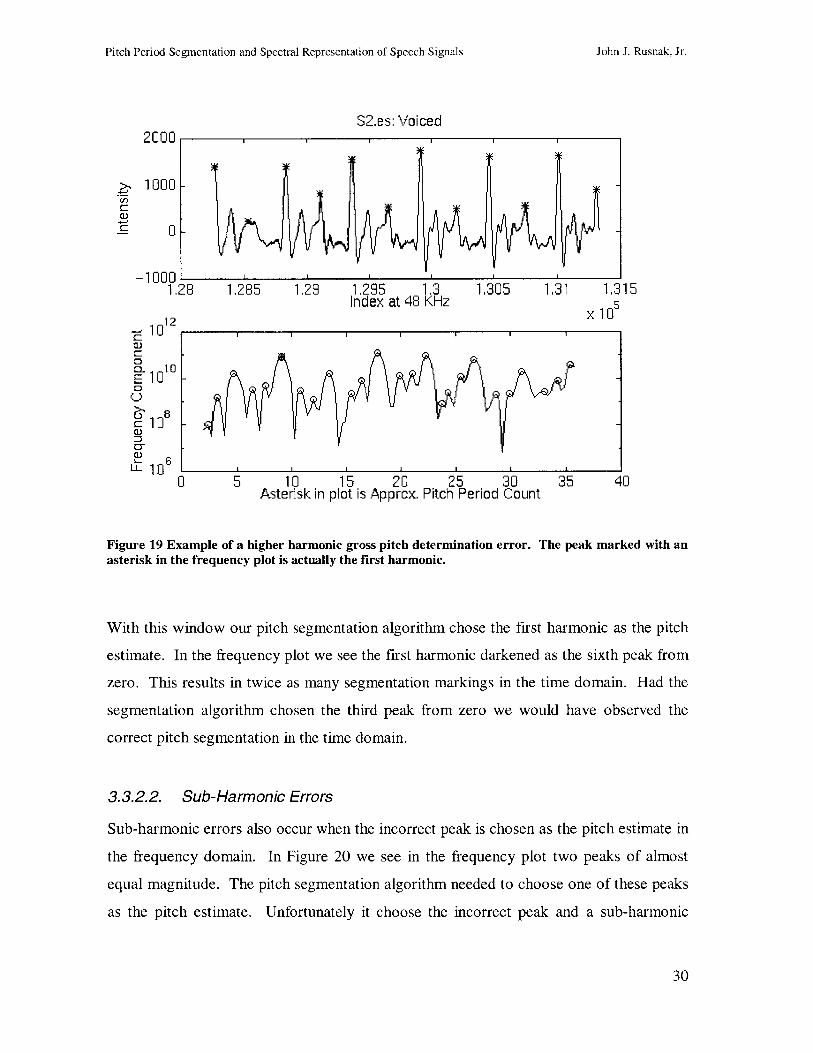
FIGURE 19 EXAMPLE OF A HIGHER HARMONIC GROSS PITCH DETERMINATION ERROR. THE PEAK MARKED
WITH AN ASTERISK IN THE FREQUENCY PLOT IS ACTUALLY THE FIRST HARMONIC. 30
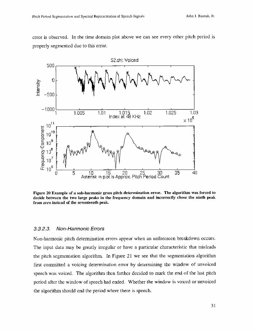
FIGURE 20 EXAMPLE OF A SUB-HARMONIC GROSS PITCH DETERMINATION ERROR. THE ALGORITHM WAS
FORCED TO DECIDE BETWEEN THE TWO LARGE PEAKS IN THE FREQUENCY DOMAIN AND
INCORRECTLY CHOSE THE NINTH PEAK FROM ZERO INSTEAD OF THE SEVENTEENTH PEAK. 31
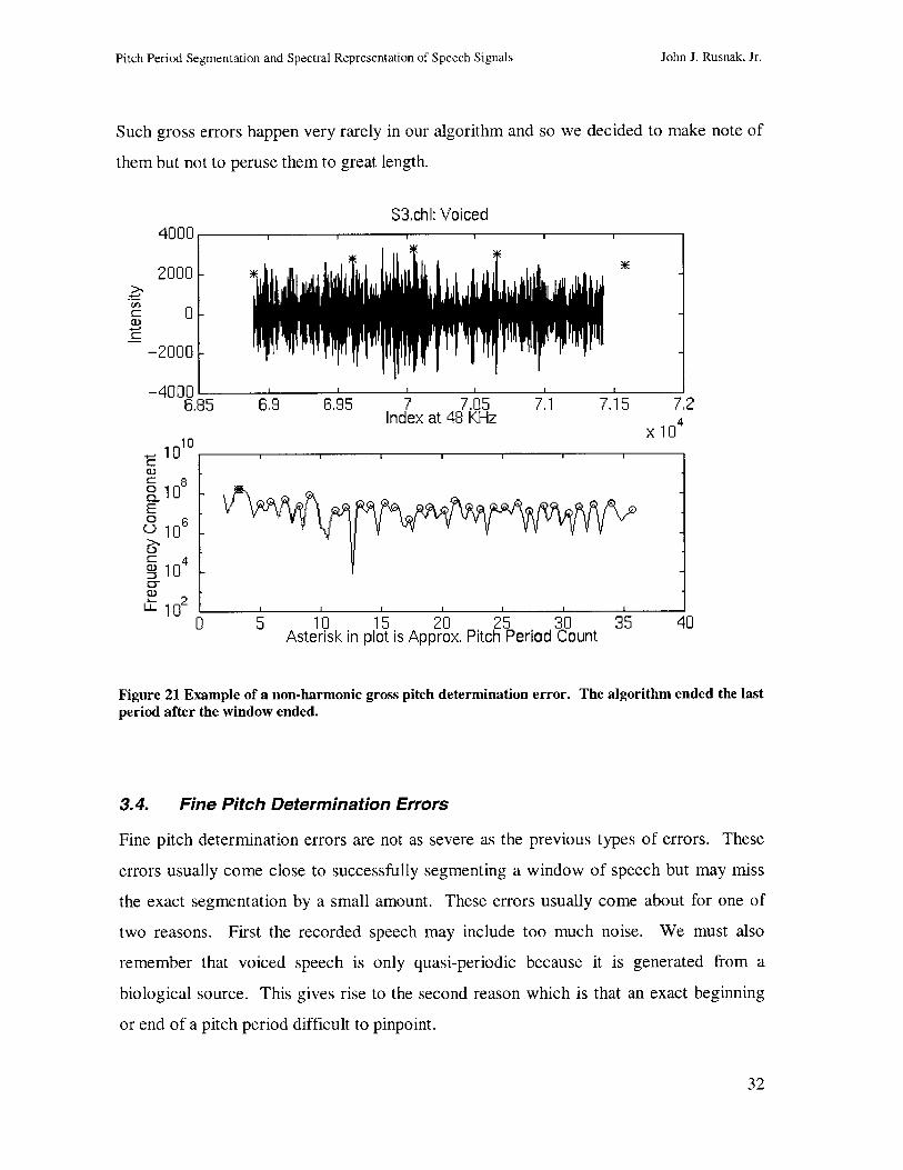
FIGURE 21 EXAMPLE OF A NON-HARMONIC GROSS PITCH DETERMINATION ERROR. THE ALGORITHM
ENDED THE LAST PERIOD AFTER THE WINDOW ENDED. 32
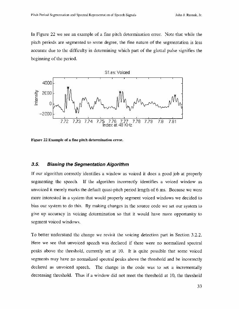
FIGURE 22 EXAMPLE OF A FINE PITCH DETERMINATION ERROR. 33
FIGURE 23 THE CORRECT SEGMENTATION A VOICED WINDOW OF SPEECH USING THE BIASED ALGORITHM.
COMPARE TO THE INCORRECT SEGMENTATION OF THE SAME VOICED WINDOW IN FIGURE 18. _ 35
FIGURE 24 EXAMPLE OF A WAVEFORM OSCILLOGRAM OF THE WORD "PHONETICIAN" [FILIPSSON, 1998]. - 36
FIGURE 25 EXAMPLE OF A WATERFALL SPECTROGRAM FOR THE WORD "PHONETICIAN" [FILIPSSON, 1998]. 37
FIGURE 26 EXAMPLE OF A GRAY SCALE SPECTROGRAM OF THE WORD "PHONETICIAN" [FILIPSSON, 1998]. 38
FIGURE 27 DETAIL OF A PITCH PERIOD OPERATOR MODULE (PPOM). 40
FIGURE 28 BLOCK DIAGRAM OF THE PITCH-SYNCHRONOUS SPECTROGRAM ALGORITHM. ITERATION 0
REPRESENTS A PREVIEW OF THE PITCH PERIOD DATA. THIS PREVIEW IS USED IN ITERATION 1TO INSURE THE INTERPOLATION PORTION OF THE SPECTROGRAM GENERATION WILL WORK FOR
ALL SPEAKERS REGARDLESS OF PITCH PERIOD LENGTH. 41
FIGURE 29 WAVEFORM OF A MALE SPEAKER PRONOUNCING /A/ STARTING AT LOW PITCH AND INCREASING
TO HIGH PITCH. 42
FIGURE 30 COMPARISON OF FIXED-WINDOW (LEFT) AND PITCH-SYNCHRONOUS (RIGHT) SPECTROGRAMS
FOR THE WAVEFORM IN FIGURE 29. 43
6
John J. Rusnak, Jr.
Pitch Period Segmentation and Spectral Representation of Speech Signals
FIGURE 31 WAVEFORM OSCILLOGRAM OF A FEMALE SPEAKER PRONOUNCING / 0 / STARTING AT LOW
PITCH AND INCREASING TO HIGH PITCH. 43
FIGURE 32 COMPARISON OF FIXED-WINDOW (LEFT) AND PITCH-SYNCHRONOUS (RIGHT) SPECTROGRAMS
FOR THE WAVEFORM IN FIGURE 31. 44
FIGURE 33 WAVEFORM OF A MALE SPEAKER PRONOUNCING A PHONETICALLY BALANCED SENTENCE. 44
FIGURE 34 COMPARISON OF FIXED-WINDOW (LEFT) AND PITCH-SYNCHRONOUS (RIGHT) SPECTROGRAMS
FOR THE SENTENCE IN FIGURE 33. 45
FIGURE 35 DETAIL VIEWS OF THE SENTENCE IN FIGURE 33 FROM 0.3 SECONDS TO 1.2 SECONDS (LEFT)
AND 1.2 SECONDS TO 2.4 SECONDS (RIGHT). 45
FIGURE 36 COMPARISON OF FIXED-WINDOW (LEFT) AND PITCH-SYNCHRONOUS (RIGHT) SPECTROGRAMS
FOR THE DETAIL VIEW IN FIGURE 35 FROM 0.3 SECONDS TO 1.2 SECONDS. 46FIGURE 37 COMPARISON OF FIXED-WINDOW (LEFT) AND PITCH-SYNCHRONOUS (RIGHT) SPECTROGRAMS
FOR THE DETAIL VIEW IN FIGURE 35 FROM 1.2 SECONDS TO 2.4 SECONDS. 46
FIGURE 38 LARGER VERSION OF THE FIXED-WINDOW SPECTROGRAM IN FIGURE 36. 47
FIGURE 39 LARGER VERSION OF THE PITCH-SYNCHRONOUS SPECTROGRAM IN FIGURE 36. 47
FIGURE 40 SPECTROGRAMS OF MALE SPEAKER DHS PRONOUNCING THE PHONEME /A/, FIXED-WINDOW-
SIZE (LEFT) AND PITCH-SYNCHRONOUS (RIGHT). .50
FIGURE 41 SPECTROGRAMS OF MALE SPEAKER DHS PRONOUNCING THE PHONEME /E/, FIXED-WINDOW-
SIZE (LEFT) AND PITCH-SYNCHRONOUS (RIGHT). .51
FIGURE 42 SPECTROGRAMS OF MALE SPEAKER DHS PRONOUNCING THE PHONEME /1/, FIXED-WINDOW-
SIZE (LEFT) AND PITCH-SYNCHRONOUS (RIGHT). .51
FIGURE 43 SPECTROGRAMS OF MALE SPEAKER DHS PRONOUNCING THE PHONEME /0/, FIXED-WINDOW-
SIZE (LEFT) AND PITCH-SYNCHRONOUS (RIGHT). _52
FIGURE 44 SPECTROGRAMS OF MALE SPEAKER DHS PRONOUNCING THE PHONEME /U/, FIXED-WINDOW-
SIZE (LEFT) AND PITCH-SYNCHRONOUS (RIGHT). _52
FIGURE 45 SPECTROGRAMS OF MALE SPEAKER ES PRONOUNCING THE PHONEME /A/, FIXED-WINDOW-
SIZE (LEFT) AND PITCH-SYNCHRONOUS (RIGHT). . 53FIGURE 46 SPECTROGRAMS OF MALE SPEAKER ES PRONOUNCING THE PHONEME /E/, FIXED-WINDOW-
SIZE (LEFT) AND PITCH-SYNCHRONOUS (RIGHT). _ 53
FIGURE 47 SPECTROGRAMS OF MALE SPEAKER ES PRONOUNCING THE PHONEME /I/, FIXED-WINDOW-
SIZE (LEFT) AND PITCH-SYNCHRONOUS (RIGHT). _54
FIGURE 48 SPECTROGRAMS OF MALE SPEAKER ES PRONOUNCING THE PHONEME /0/, FIXED-WINDOW-
SIZE (LEFT) AND PITCH-SYNCHRONOUS (RIGHT). _54
FIGURE 49 SPECTROGRAMS OF MALE SPEAKER ES PRONOUNCING THE PHONEME /U/, FIXED-WINDOW-
SIZE (LEFT) AND PITCH-SYNCHRONOUS (RIGHT). _55
FIGURE 50 SPECTROGRAMS OF FEMALE SPEAKER CHL PRONOUNCING THE PHONEME /A/, FIXED-WINDOW-
SIZE (LEFT) AND PITCH-SYNCHRONOUS (RIGHT). _56
FIGURE 51 SPECTROGRAMS OF FEMALE SPEAKER CHL PRONOUNCING THE PHONEME /E/, FIXED-WINDOW-
SIZE (LEFT) AND PITCH-SYNCHRONOUS (RIGHT). _56
FIGURE 52 SPECTROGRAMS OF FEMALE SPEAKER CHL PRONOUNCING THE PHONEME /1/, FIXED-WINDOW-
SIZE (LEFT) AND PITCH-SYNCHRONOUS (RIGHT). _ 57FIGURE 53 SPECTROGRAMS OF FEMALE SPEAKER CHL PRONOUNCING THE PHONEME /0/, FIXED-WINDOW-
SIZE (LEFT) AND PITCH-SYNCHRONOUS (RIGHT). _ 57FIGURE 54 SPECTROGRAMS OF FEMALE SPEAKER CHL PRONOUNCING THE PHONEME /U/, FIXED-WINDOW-
SIZE (LEFT) AND PITCH-SYNCHRONOUS (RIGHT). _58
FIGURE 55 SPECTROGRAMS OF FEMALE SPEAKER LCK PRONOUNCING THE PHONEME /A/, FIXED-WINDOW-
SIZE (LEFT) AND PITCH-SYNCHRONOUS (RIGHT). _59
FIGURE 56 SPECTROGRAMS OF FEMALE SPEAKER LCK PRONOUNCING THE PHONEME /E/, FIXED-WINDOW-
SIZE (LEFT) AND PITCH-SYNCHRONOUS (RIGHT). _59
FIGURE 57 SPECTROGRAMS OF FEMALE SPEAKER LCK PRONOUNCING THE PHONEME /1/, FIXED-WINDOW-
SIZE (LEFT) AND PITCH-SYNCHRONOUS (RIGHT). .60
FIGURE 58 SPECTROGRAMS OF FEMALE SPEAKER LCK PRONOUNCING THE PHONEME /0/, FIXED-WINDOW-
SIZE (LEFT) AND PITCH-SYNCHRONOUS (RIGHT). _60
7
John J. Rusnak, Jr.
Pitch Period Segmentation and Spectral Representation of Speech Signals
FIGURE 59 SPECTROGRAMS OF FEMALE SPEAKER LCK PRONOUNCING THE PHONEME /U/, FIXED-WINDOW-
SIZE (LEFT) AND PITCH-SYNCHRONOUS (RIGHT). .61
FIGURE 60 WAVEFORMS OF /A/, /E/, /I/, /0/, AND /U/ RESPECTIVELY FOR MALE SPEAKER DHS. 62
FIGURE 61 WAVEFORMS OF /A/, /E/, /I/, /0/, AND /U/ RESPECTIVELY FOR MALE SPEAKER ES. 63
FIGURE 62 WAVEFORMS OF /A/, /E/, /1/, /0/, AND /U/ RESPECTIVELY FOR FEMALE SPEAKER CHL. 64
FIGURE 63 WAVEFORMS OF /A/, /E/, /1/, /0/, AND /U/ RESPECTIVELY FOR FEMALE SPEAKER LCK. 65
8
John J. Rusnak, Jr.

Pitch Period Segmentation and Spectral Representation of Speech Signals
1. Background
1.1. Physiological Description of Speech
The human vocal tract includes the pathway starting at the lungs and ending at the lips of
the speaker. To produce sound, air is forced from the lungs through the trachea. At the
top of the trachea is the larynx which houses the vocal cords. Air passing through the
larynx causes the vocal cords to vibrate and excite the pharynx or voice box. This speech
production system produces basic linguistic units of sound called a phonemes. Because
each phoneme is unique, a speaker can piece phonemes together to form clear words and
understandable speech.
The slit between the vocal cords is called the glottis. If the glottis is wide when air passes
through it unvoiced sounds are produced. Unvoiced sounds have one of several air
characteristics. Fricative phonemes such as /s/ and /f/ are produced if a large flow of air
passes through a constricted vocal tract. If a brief amount of air, followed by building
pressure ends in total closure along the tract, then stop-consonant phonemes such as /p/
and /t/ are produced when the pressure is released.
If the vocal cords are allowed to vibrate, then the glottis changes in width periodically
and voiced sound is produced. As air passes through the vocal tract resonant modes of
vibration, or formants, give character to the sound. Articulators which include the lips,
tongue, and velum, also characterize the sound.
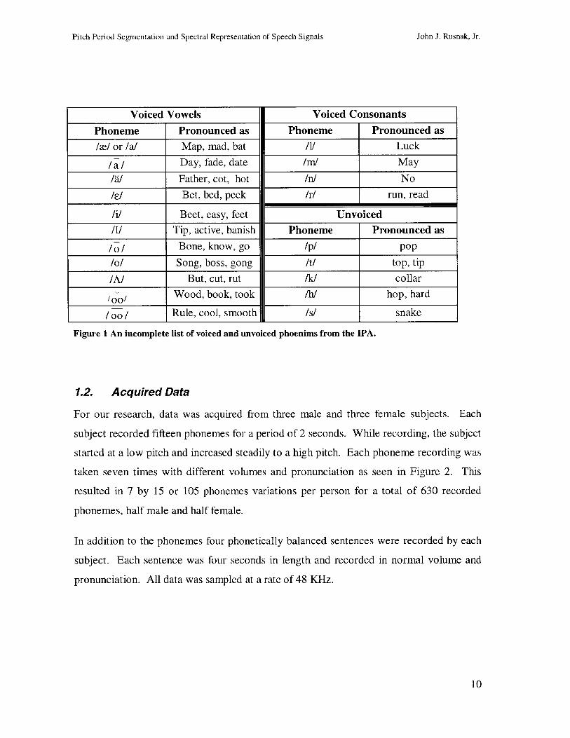
An incomplete list of phonemes, both voiced and unvoiced from the International
Phonetic Alphabet (IPA), is included in Figure 1.
9
John J. Rusnak, Jr.
Pitch Period Segmentation and Spectral Representation of Speech Signals
Voiced Vowels Voiced Consonants
Phoneme Pronounced as Phoneme Pronounced as
// or /a/ Map, mad, bat /l/ Luck
Day, fade, date /m/ May
/s/ Father, cot, hot /n/ No
/e/ Bet, bed, peck /r/ run, read
/i/ Beet, easy, feet Unvoiced/I Tip, active, banish Phoneme Pronounced as
Bone, know, go /p/ pop/o/ Song, boss, gong /t/ top, tip
/A/ But, cut, rut /k/ collar
'00' Wood, book, took /h/ hop, hard
/oo/ Rule, cool, smooth /s/ snake
Figure 1 An incomplete list of voiced and unvoiced phoenims from the IPA.
1.2. Acquired Data
For our research, data was acquired from three male and three female subjects. Each
subject recorded fifteen phonemes for a period of 2 seconds. While recording, the subject
started at a low pitch and increased steadily to a high pitch. Each phoneme recording was
taken seven times with different volumes and pronunciation as seen in Figure 2. This
resulted in 7 by 15 or 105 phonemes variations per person for a total of 630 recorded
phonemes, half male and half female.
In addition to the phonemes four phonetically balanced sentences were recorded by each
subject. Each sentence was four seconds in length and recorded in normal volume and
pronunciation. All data was sampled at a rate of 48 KHz.
10
John J. Rusnak, Jr.
Pitch Period Segmentation and Spectral Representation of Speech Signals
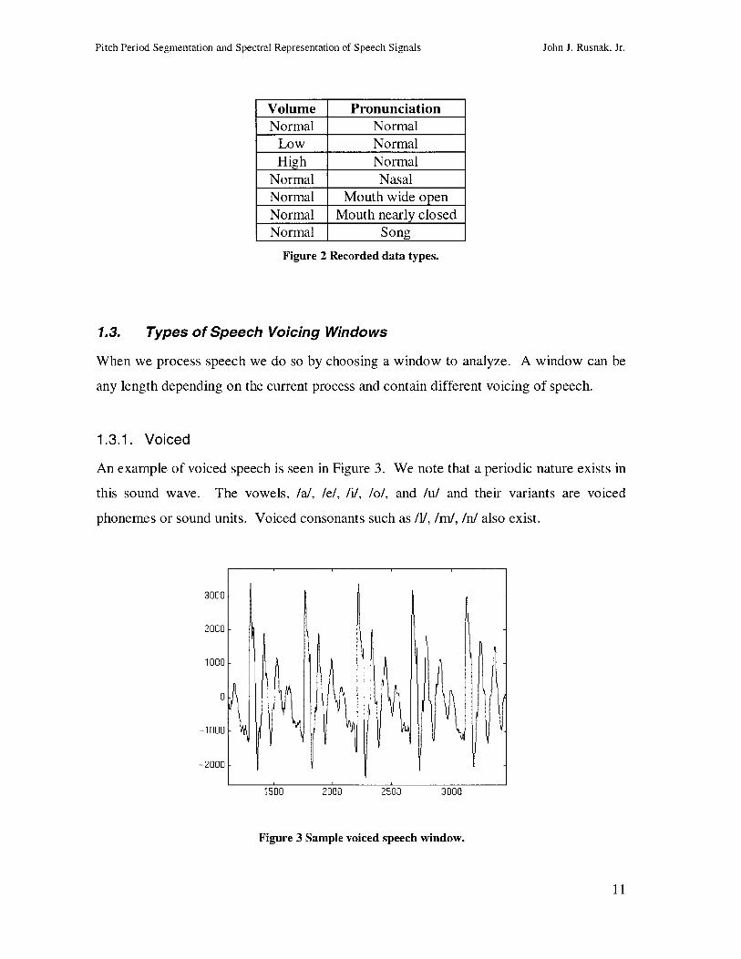
Volume PronunciationNormal Normal
Low NormalHigh Normal
Normal NasalNormal Mouth wide open
Normal Mouth nearly closedNormal Song
Figure 2 Recorded data types.
1.3. Types of Speech Voicing Windows
When we process speech we do so by choosing a window to analyze. A window can be
any length depending on the current process and contain different voicing of speech.
1.3.1. Voiced
An example of voiced speech is seen in Figure 3. We note that a periodic nature exists in
this sound wave. The vowels, /a/, /e/, /i/, /o/, and /u/ and their variants are voiced
phonemes or sound units. Voiced consonants such as /1/, /m/, /n/ also exist.
1500 2000 2500 3000
Figure 3 Sample voiced speech window.
11
John J. Rusnak, Jr.
Pitch Period Segmentation and Spectral Representation of Speech Signals
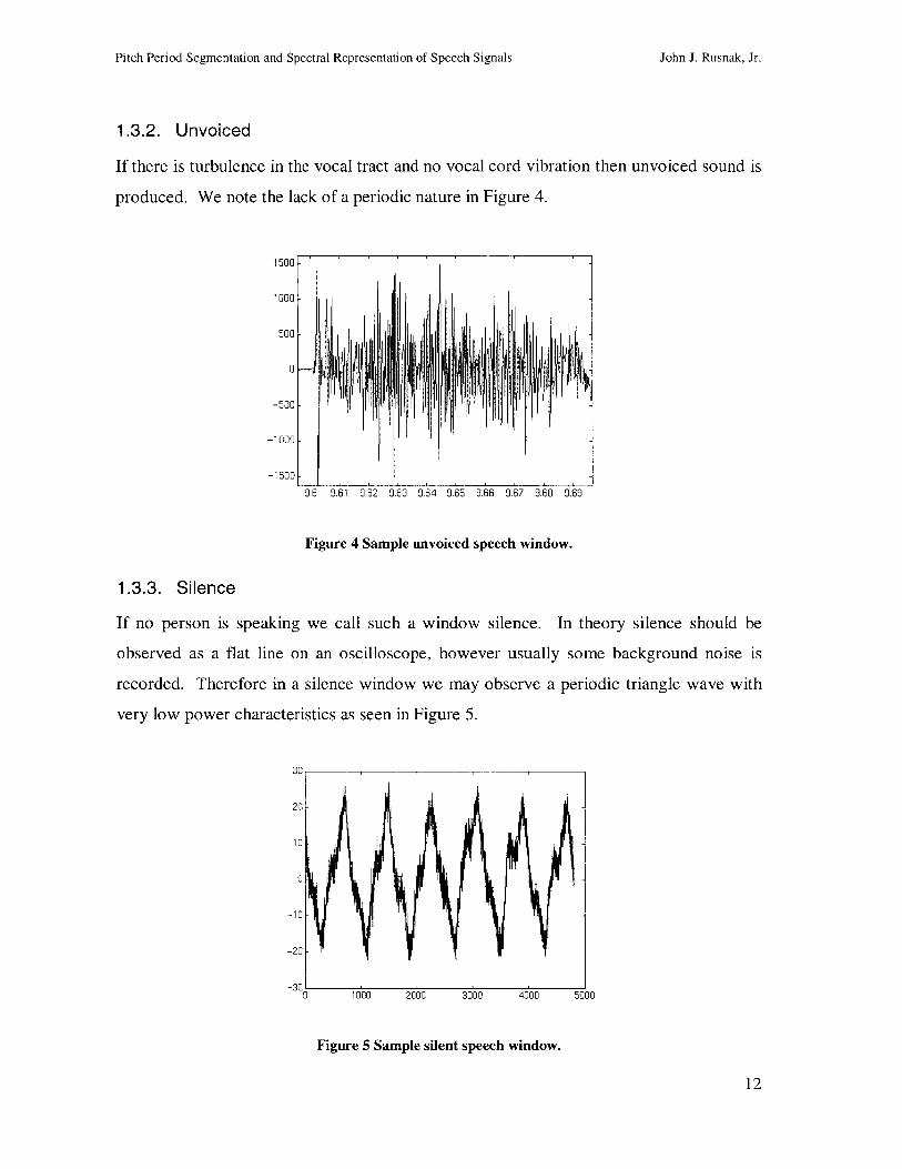
1.3.2. Unvoiced
If there is turbulence in the vocal tract and no vocal cord vibration then unvoiced sound is
produced. We note the lack of a periodic nature in Figure 4.
1500
1000
500
0
-500
-1000
-1500 -
9.6 9.61 9.62 9.63 9.64 9.65 9.66 9.67 9.68 9.69
Figure 4 Sample unvoiced speech window.
1.3.3. Silence
If no person is speaking we call such a window silence. In theory silence should be
observed as a flat line on an oscilloscope, however usually some background noise is
recorded. Therefore in a silence window we may observe a periodic triangle wave with
very low power characteristics as seen in Figure 5.
30
20
10
0
-10
-20
-30-
Figure 5 Sample silent speech window.
12
John J. Rusnak, Jr.
Pitch Period Segmentation and Spectral Representation of Speech Signals
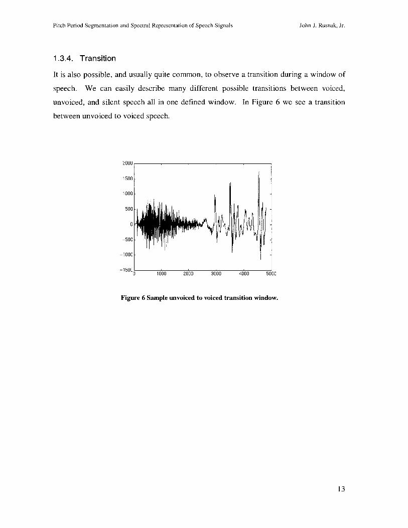
1.3.4. Transition
It is also possible, and usually quite common, to observe a transition during a window of
speech. We can easily describe many different possible transitions between voiced,
unvoiced, and silent speech all in one defined window. In Figure 6 we see a transition
between unvoiced to voiced speech.
2000 -
1500 -
1000 -
500
0
-500
I I .L I.
-1000k
0 1000 2000 3000 4000 5000
Figure 6 Sample unvoiced to voiced transition window.
13
John J. Rusnak, Jr.
.I
II..
'7 '-I111 ||1
Pitch Period Segmentation and Spectral Representation of Speech Signals
2. Glottal Pulse
2.1. Significance of the Glottal Pulse
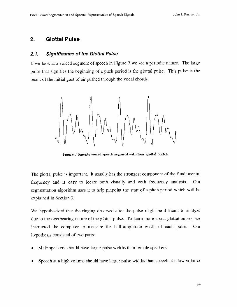
If we look at a voiced segment of speech in Figure 7 we see a periodic nature. The large
pulse that signifies the beginning of a pitch period is the glottal pulse. This pulse is the
result of the initial gust of air pushed through the vocal chords.
Figure 7 Sample voiced speech segment with four glottal pulses.
The glottal pulse is important. It usually has the strongest component of the fundamental
frequency and is easy to locate both visually and with frequency analysis. Our
segmentation algorithm uses it to help pinpoint the start of a pitch period which will be
explained in Section 3.
We hypothesized that the ringing observed after the pulse might be difficult to analyze
due to the overbearing nature of the glottal pulse. To learn more about glottal pulses, we
instructed the computer to measure the half-amplitude width of each pulse. Our
hypothesis consisted of two parts:
" Male speakers should have larger pulse widths than female speakers
* Speech at a high volume should have larger pulse widths than speech at a low volume
14
John J. Rusnak, Jr.
Pitch Period Segmentation and Spectral Representation of Speech Signals
If this hypothesis was true we could create an adaptive pitch determination algorithm
based on sex and volume.
2.2.
The
data
Measuring Widths of Glottal Pulses
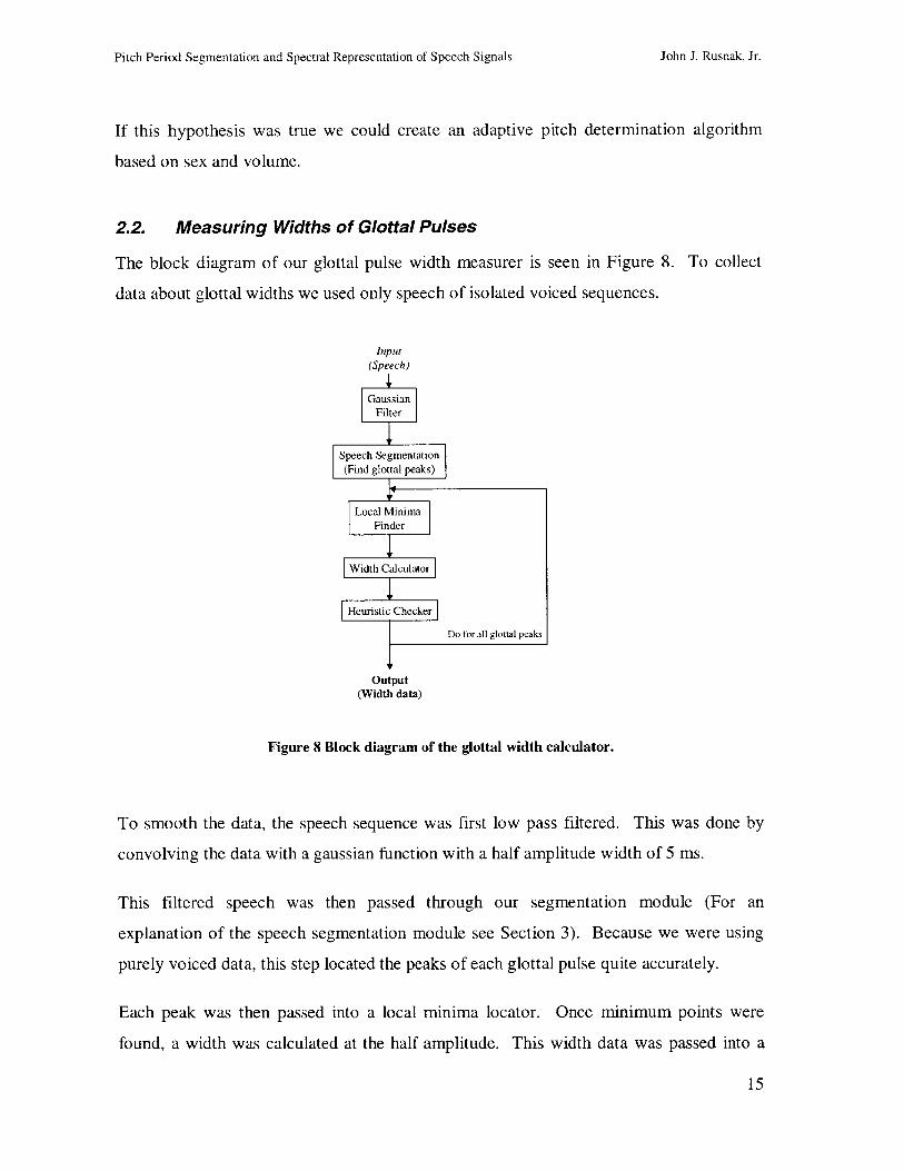
block diagram of our glottal pulse width measurer is seen in Figure 8. To collect
about glottal widths we used only speech of isolated voiced sequences.
Input(Speech)
Output(Width data)
Figure 8 Block diagram of the glottal width calculator.
To smooth the data, the speech sequence was first low pass filtered. This was done by
convolving the data with a gaussian function with a half amplitude width of 5 ms.
This filtered speech was then passed through our segmentation module (For an
explanation of the speech segmentation module see Section 3). Because we were using
purely voiced data, this step located the peaks of each glottal pulse quite accurately.
Each peak was then passed into a local minima locator. Once minimum points were
found, a width was calculated at the half amplitude. This width data was passed into a
15
John J. Rusnak, Jr.
Pitch Period Segmentation and Spectral Representation of Speech Signals John J. Rusnak, Jr.
heuristic checker for final verification. Finally, an average width was computed for each
speech sequence based on the widths for each glottal pulse.
2.3. Variations on Locating the Begin and End Points of Glottal Pulses
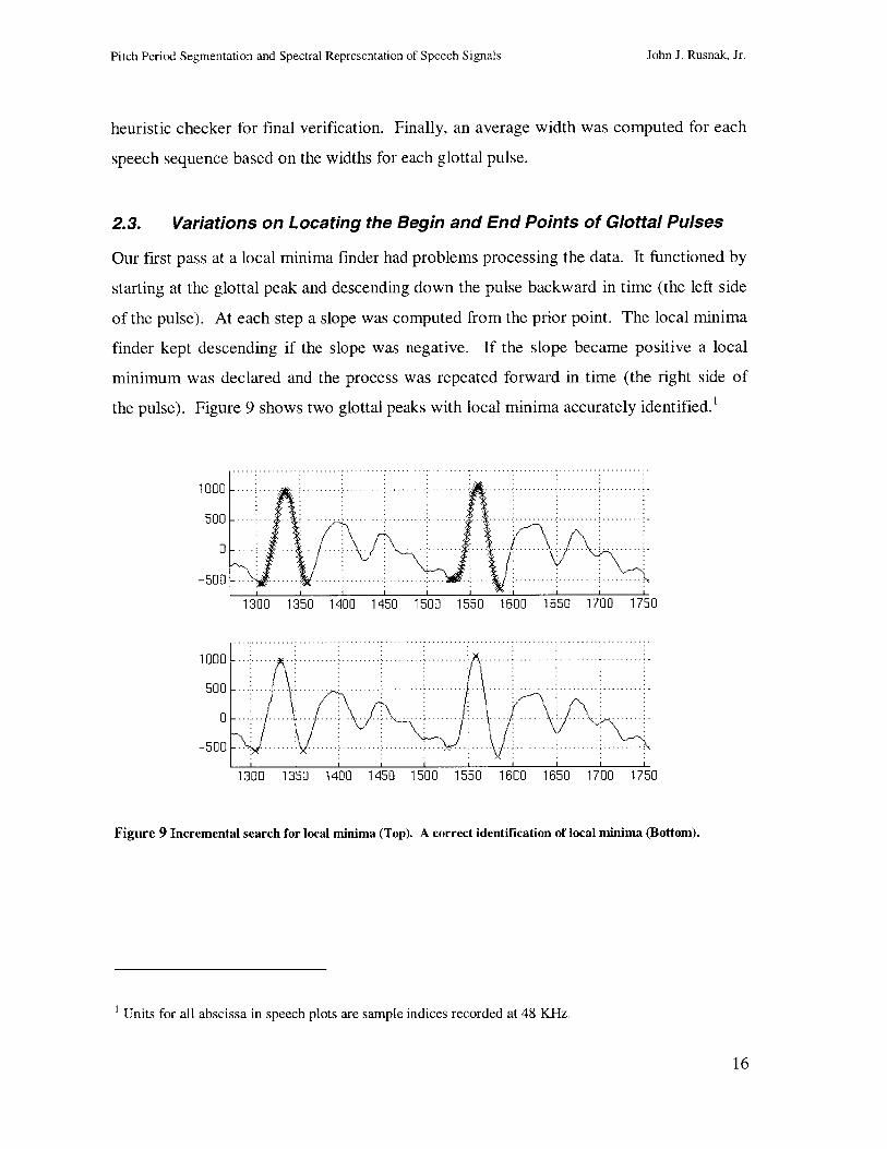
Our first pass at a local minima finder had problems processing the data. It functioned by
starting at the glottal peak and descending down the pulse backward in time (the left side
of the pulse). At each step a slope was computed from the prior point. The local minima
finder kept descending if the slope was negative. If the slope became positive a local
minimum was declared and the process was repeated forward in time (the right side of
the pulse). Figure 9 shows two glottal peaks with local minima accurately identified.'
500 ..--- -- - -
0 -.. --. --.. -.-.--. -
-500 - - -- --- -
1300 1350 1400 1450 1500 1550 1600 1650 1700 1750
0 .... .... .. .... ............... ...... ....150 0 -. .-- - - - - - -.-.--.-
1300 1350 1400 1450 1500 1550 1600 1650 1700 1750
Figure 9 Incremental search for local minima (Top). A correct identification of local minima (Bottom).
Units for all abscissa in speech plots are sample indices recorded at 48 KHz.
16
Pitch Period Segmentation and Spectral Representation of Speech Signals
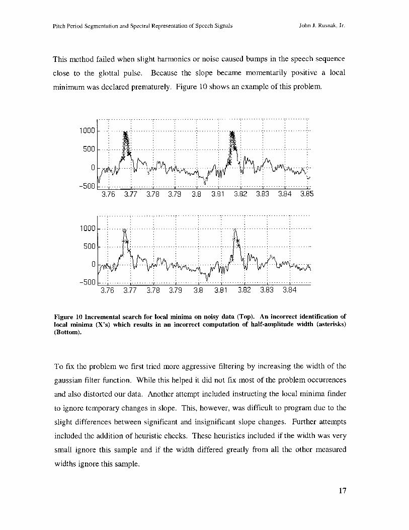
This method failed when slight harmonics or noise caused bumps in the speech sequence
close to the glottal pulse. Because the slope became momentarily positive a local
minimum was declared prematurely. Figure 10 shows an example of this problem.
100 ....................... ............
0 X : .A i O-J'>'MA jr fx- ..... X : I 1j A . .. J.t -... -
-500
1000
500
0
-500
3.76 3.77 3.78 3.79 3.8 3.81 3.82 3.83 3.84 3.85
3.76 3.77 3.78 3.79 3.8 3.81 3.82 3.83 3.84
Figure 10 Incremental search for local minima on noisy data (Top). An incorrect identification oflocal minima (X's) which results in an incorrect computation of half-amplitude width (asterisks)(Bottom).
To fix the problem we first tried more aggressive filtering by increasing the width of the
gaussian filter function. While this helped it did not fix most of the problem occurrences
and also distorted our data. Another attempt included instructing the local minima finder
to ignore temporary changes in slope. This, however, was difficult to program due to the
slight differences between significant and insignificant slope changes. Further attempts
included the addition of heuristic checks. These heuristics included if the width was very
small ignore this sample and if the width differed greatly from all the other measured
widths ignore this sample.
17
John J. Rusnak, Jr.
...... ............. ... .... .. ... .... .....
........... ........ ........ ........
........ ..... ........ ........ .........
Pitch Period Segmentation and Spectral Representation of Speech Signals
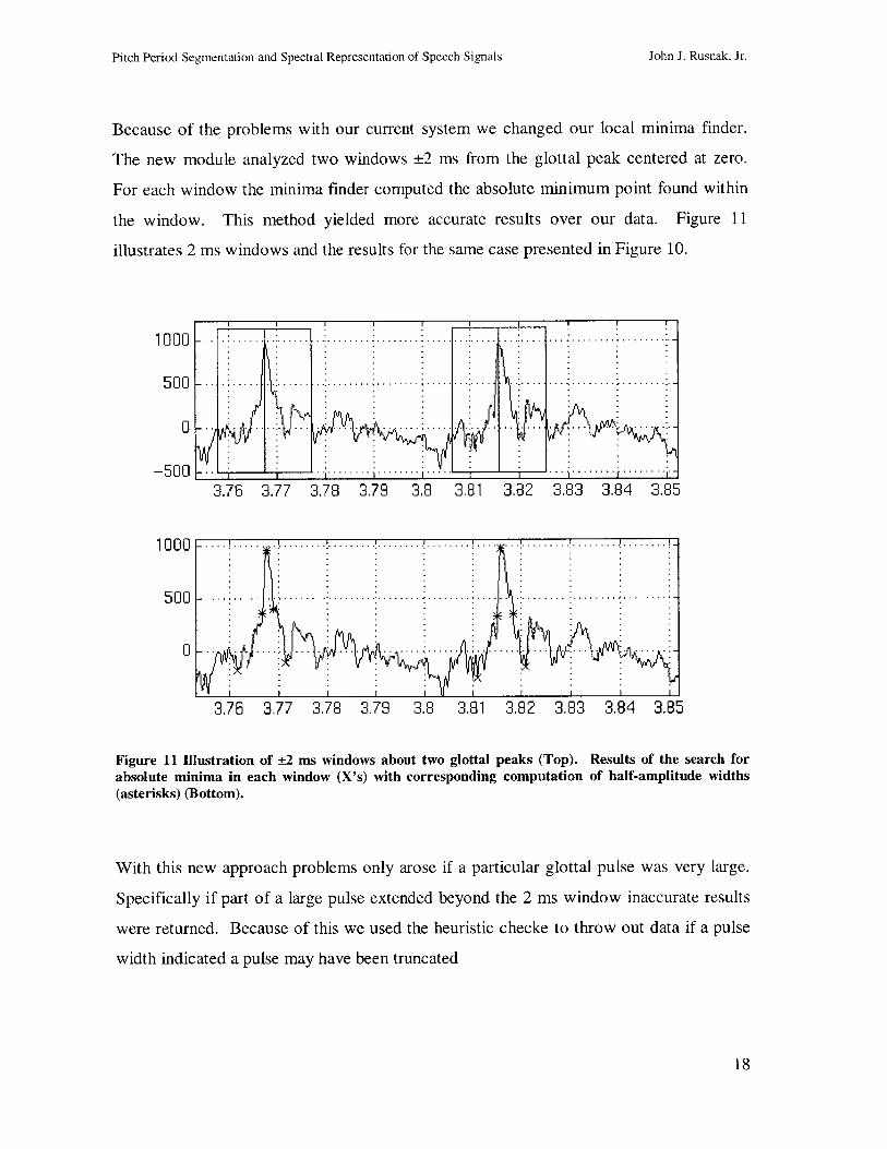
Because of the problems with our current system we changed our local minima finder.
The new module analyzed two windows ±2 ms from the glottal peak centered at zero.
For each window the minima finder computed the absolute minimum point found within
the window. This method yielded more accurate results over our data. Figure 11
illustrates 2 ms windows and the results for the same case presented in Figure 10.
1000
500
0
1000.
500
0
/ ~JVw ........ IL ____
3.76 3.77 3.78 3.79 3.8 3.81 3.82 3.83 3.84 3.85
..I . . . . . ... . . .p I N6
3.76 3.77 3.78 3.79 3.8 3.81 3.82 3.83 3.84 3.85
Figure 11 Illustration of ±2 ms windows about two glottal peaks (Top). Results of the search forabsolute minima in each window (X's) with corresponding computation of half-amplitude widths(asterisks) (Bottom).
With this new approach problems only arose if a particular glottal pulse was very large.
Specifically if part of a large pulse extended beyond the 2 ms window inaccurate results
were returned. Because of this we used the heuristic checke to throw out data if a pulse
width indicated a pulse may have been truncated
18
..... . . . . ......I
John J. Rusnak, Jr.
Pitch Period Segmentation and Spectral Representation of Speech Signals
2.4. Analysis of Glottal Width Data
Our initial hypothesis involving glottal width was male speakers should have larger
widths than female speakers and speech at high volume should have larger pulse widths
than speech at low volume. If this hypothesis was true we could create an adaptive pitch
determination algorithm based on sex and volume.
It was observed that in most cases the hypothesis on widths versus sex and volume was
not only false but did not show a simple trend.
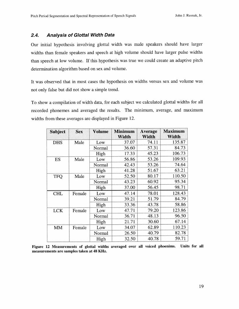
To show a compilation of width data, for each subject we calculated glottal widths for all
recorded phonemes and averaged the results. The minimum, average, and maximum
widths from these averages are displayed in Figure 12.
Subject Sex Volume Minimum Average MaximumWidth Width 1,Width
DHS Male Low 37.07 74.11 135.87Normal 36.60 57.31 84.73
High 17.33 45.23 106.73ES Male Low 56.86 53.26 109.93
Normal 42.43 53.26 74.64
High 41.28 51.67 63.21TFQ Male Low 52.50 80.17 110.50
Normal 43.23 60.92 95.34High 37.00 56.45 98.71
CHL Female Low 47.14 78.01 128.43Normal 39.21 51.79 84.79
High 33.36 43.78 58.86LCK Female Low 47.71 79.20 123.86
Normal 36.71 48.13 96.50
------- _ _ High 21.71 30.60 67.14MM Female Low 34.07 62.89 110.23
Normal 26.50 40.79 82.78High 32.50 40.78 59.71
Figure 12 Measurements of glottal widths averaged over all voiced phoenims. Units for allmeasurements are samples taken at 48 KHz.
19
John J. Rusnak, Jr.
Pitch Period Segmentation and Spectral Representation of Speech Signals
By examining Figure 12 we can see that not only did our hypothesis fail, but the lack of a
clear trend suggests that a more complicated model is needed. Library research brought
up several important considerations that should be incorporated into such a model. It is
possible that because the glottis does not always close for each phoneme our hypothesis
will fail. Chuang and Hanson reported that "males tend to have a more complete glottal
closure than females" [Chuang, Hanson, 1996]. Hanson also focused research on
situations when males and females have different glottal closures during the
pronunciation of different phonemes and found the system to be much more complicated
then our original hypothesis [Hanson, 1997].
When the complexity of glottal width versus sex and volume was realized both
experimentally and by outside research, we decided to abandon the idea of an adaptive
system based on glottal width and take a new approach to analyze the speech.
20
John J. Rusnak, Jr.
Pitch Period Segmentation and Spectral Representation of Speech Signals
3. Pitch Segmentation
While the theory of pitch determination and pitch segmentation are related, they are
different processes and have different types of output. Pitch, simply put, is the perceived
tone level heard by a listener. If a high pitch is heard then the vocal chords are vibrating
quickly. Similarly, if a low pitch is heard then the vocal chords are vibrating slowly.
Because the vocal chords have to vibrate to create a pitch, only voiced phonemes can
have a pitch.
3.1. Pitch Determination Versus Pitch Segmentation
If a system determines the pitch for a window of speech, the output of such a system will
be a frequency in Hertz. This number can also be inverted to determine the length of a
pitch period. So a pitch determination system will output a numeric result to characterize
the pitch of a window of speech.
Unless the speech to be analyzed is produced by a machine, speech will not be exactly
periodic. This means a single voiced phoneme produced by a biological source will not
maintain a fixed pitch for a large window. Thus we cannot say that a large window of
speech has an overall pitch or pitch period. In the literature we see the term quasi-
periodic to describe the nature of voiced speech. This means while the waveform of a
naturally produced phoneme has periodic features it is not exactly periodic.
It is useful when analyzing a speech waveform to be able to mark where a pitch period
begins and ends. Because speech is quasi-periodic we cannot simply take our measure of
the pitch period, T, and place markers on the waveform at T, 2T, 3T,..., nT. Such a
placement of pitch period begin and end markers would only work if the source was
artificially produced. To properly mark these points a pitch segmentation system must be
used. Thus a pitch segmentation system will output the location of markers that signify
the start and end of each pitch period in a window of speech.
We need to consider the question of once isolated, where a pitch period actually begins
and ends. Hess suggests one of two places. If we have a window containing many
21
John J. Rusnak, Jr.
Pitch Period Segmentation and Spectral Representation of Speech Signals
voiced pitch periods in succession, a pitch period is defined to begin at the peak of the
glottal pulse and defined to end at the peak of the next successive glottal pulse. We can
also define that the pitch period begins at the base of the glottal pulse and define the end
to be the base of the next successive glottal pulse [Hess, 1983].
In actuality we can freely convert between the two methods. In this thesis we explain
how to find the base of a glottal pulse given the peak in the latter half of Section 2.3. The
key is to note that in pitch segmentation we need to determine if the window is voiced
and then locate the glottal pulses.
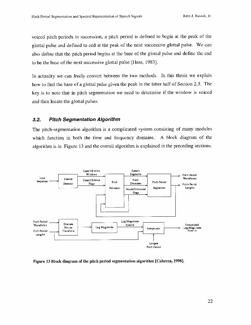
3.2. Pitch Segmentation Algorithm
The pitch-segmentation algorithm is a complicated system consisting of many modules
which function in both the time and frequency domains. A block diagram of the
algorithm is in Figure 13 and the overall algorithm is explained in the preceding sections.
Speech/SiLence Speech
InputSequence
Pitch-PeLiodWaveforms
Pitch-PeiodLengths
Pitch-PeriodWaveforms
Pitch-PeriodLengths
InterpolatedLog-Magnitrde
Spectra
LongestPitch-Peiiod
Figure 13 Block diagram of the pitch period segmentation algorithm [Cabrera, 1998].
22
John J. Rusnak, Jr.
Pitch Period Segmentation and Spectral Representation of Speech Signals
3.2.1. Silence Detection
The first task of the algorithm is to acquire a window of speech suitable to segment. The
algorithm incrementally examines fixed size windows 16 ms in length. We call these 16
ms windows sub-windows. The RMS power is computed for each sub-window to
determine if it contains silence or speech. If speech is detected the next sub-window is
analyzed. This analysis continues until a silence sub-window is reached or a total time of
two times our projected maximum pitch period length, which is 2 times 25 ms, has been
analyzed. When one of these two cases has been reached the group of non-silence sub-
windows are grouped together as one window for the next sub-module.
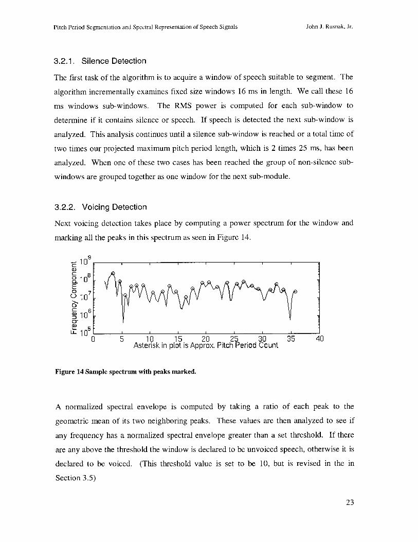
3.2.2. Voicing Detection
Next voicing detection takes place by computing a power spectrum for the window and
marking all the peaks in this spectrum as seen in Figure 14.
109
S8O_10E
7C10
- 6Z 10
0
0 5 10 15 20 25 30 35 40Asterisk in plot is Approx. Pitch Period Count
Figure 14 Sample spectrum with peaks marked.
A normalized spectral envelope is computed by taking a ratio of each peak to the
geometric mean of its two neighboring peaks. These values are then analyzed to see if
any frequency has a normalized spectral envelope greater than a set threshold. If there
are any above the threshold the window is declared to be unvoiced speech, otherwise it is
declared to be voiced. (This threshold value is set to be 10, but is revised in the in
Section 3.5)
23
John J. Rusnak, Jr.
Pitch Period Segmentation and Spectral Representation of Speech Signals
3.2.3. Pitch Period Estimation
If the window contains voiced speech a primary pitch estimate is obtained using several
heuristics. First a count of the normalized spectral peaks above the threshold are
computed. If there are not at least five normalized peaks above the threshold the lowest
frequency in this group simply becomes the primary pitch estimate. If there are at least
five normalized peaks above the threshold the algorithm then determines the maximum
normalized peak from the set of frequencies which are below the lowest frequency which
meets the threshold condition. If this maximum peak exists and is also greater than five
and also occurs at a frequency which falls within 20% of half the lowest frequency at
which the normalized spectrum is greater than the threshold, then the lower of the two
frequencies becomes the primary pitch estimate. If this condition fails the higher of the
two frequencies becomes the primary pitch period estimate.
A secondary pitch estimate may also be computed if the current and previous speech
windows are not separated by silence and were both declared as voiced. By doing this
the algorithm keeps a memory of the pitch of the previous window. Because speech
typically changes pitch gradually there should not be any major change in pitch between
two neighboring voiced windows. The mean and standard deviation of the pitch period
lengths of the previous window are examined. If the standard deviation is below 10% of
the mean and the mean is less than the set maximum pitch period (25 ms) then the mean
pitch period length for the previous window becomes the secondary pitch period estimate
for the current window.
Now with a primary and possibly a secondary pitch period estimate a final pitch estimate
is computed. If there is only a primary estimate it becomes the final estimate. If both
estimates exist a ratio of the primary and the secondary estimates is computed. If the
ratio is less than 1.3 and greater than 0.7 the primary estimate is used. If the previous
condition fails then the secondary estimate is used. These two threshold numbers are set
so as to not accept any drastic change in pitch from the previous window as the new pitch
estimate.
24
John J. Rusnak, Jr.
Pitch Period Segmentation and Spectral Representation of Speech Signals
All the above will take place only if the analyzed window contains voiced speech. If it
contains unvoiced speech then a default pitch period length of 6 ms is declared. We need
to point out that unvoiced speech has no pitch and so it has no pitch period length.
However for purposes of segmentation keeping some type of constant marking
throughout unvoiced speech will be useful later on. Therefore our default pitch is
misnamed and is actually an unvoiced speech fixed length marking system or quasi-pitch
period length. For simplicity we will call it the pitch period length of unvoiced speech.
3.2.4. Determining Begin and End Points for Each Period
A basic time interval needs to be set to segment the speech. If the current window is
bordered by silence on both sides, the algorithm finds the maximum peak in time of the
speech waveform starting at the beginning of the window and ending at the maximum
predicted pitch period length (25 ms). If the window is not bordered by silence on both
sides, the algorithm finds the maximum peak in time starting at 70% of the pitch period
estimate ahead of the last located peak and ending at 130% of the pitch period estimate
ahead of the last located peak. We let smax and tmax be the value and time index of
these maxima respectively.
Next the algorithm finds the maximum value of the speech waveform in the interval
lasting 50% of the estimated pitch period ending at tmax. We let s_min be this value.
Now using a marking cursor which starts at t_max, we look back in time to find all the
peaks above a set slope (50% of [s-max - s-min] divided by the estimated pitch period
length) which passes through the current peak and is also contained in an interval of time
30% of the pitch estimate and ends at tmax. The last located peak is saved as t-p.
To find the start of the pitch period we first check to see what type of speech the
neighboring windows contain. If the current and previous speech windows are separated
by silence and the current pitch period is the first period in the window then the start of
the current pitch period is the maximum of the zero crossing preceding t-p and the start
25
John J. Rusnak, Jr.
Pitch Period Segmentation and Spectral Representation of Speech Signals
of the current speech segment. If the algorithm can find no zero crossing then the start of
the current pitch period is the start of the speech window.
If the current and previous speech windows are adjacent and there is a zero crossing
between tp and the start of the previous pitch period then the start of the current pitch
period is the is the minimum of the zero crossing preceding tp and the start of the
previous pitch period plus the maximum pitch period length. If there is no zero crossing
between tp and the start of the previous pitch period, the start of the current pitch
period is the start of the previous pitch period plus the estimated pitch period.
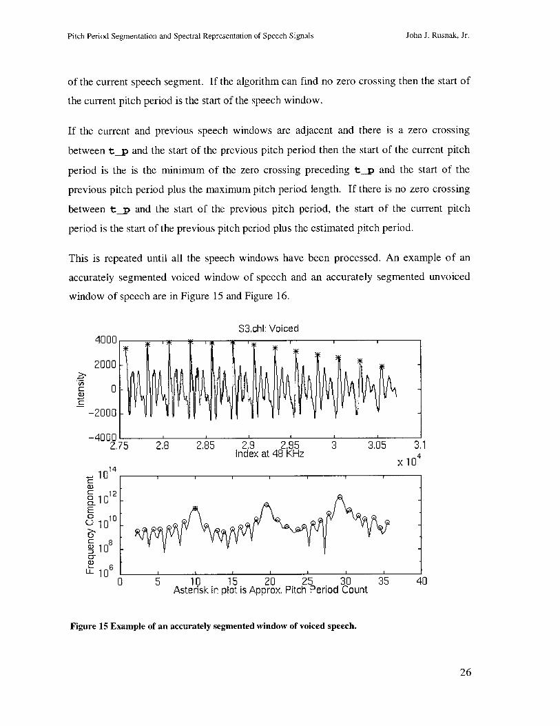
This is repeated until all the speech windows have been processed. An example of an
accurately segmented voiced window of speech and an accurately segmented unvoiced
window of speech are in Figure 15 and Figure 16.
4000
2000
0
-2000
-4000 12.75
-
0
E0
(-)
1014
1012
1010
108
1n6
S3.chl: Voiced
2.8 2.85 2.8 2.85 3 3.05Index at 48 KHz
0 5 10 15 20 25 30Asterisk in plot is Approx. Pitch Period Count
3,1
x 104
35 40
Figure 15 Example of an accurately segmented window of voiced speech.
26
John J. Rusnak, Jr.
Pitch Period Segmentation and Spectral Representation of Speech Signals
S1.chl: Unvoiced
4.7 4.75 4.8 4.85 4.8 4.85Index at 48 KHz
5 10 15 20 25 30Asterisk in plot is Approx. Pitch Period Count
5
x10
35 40
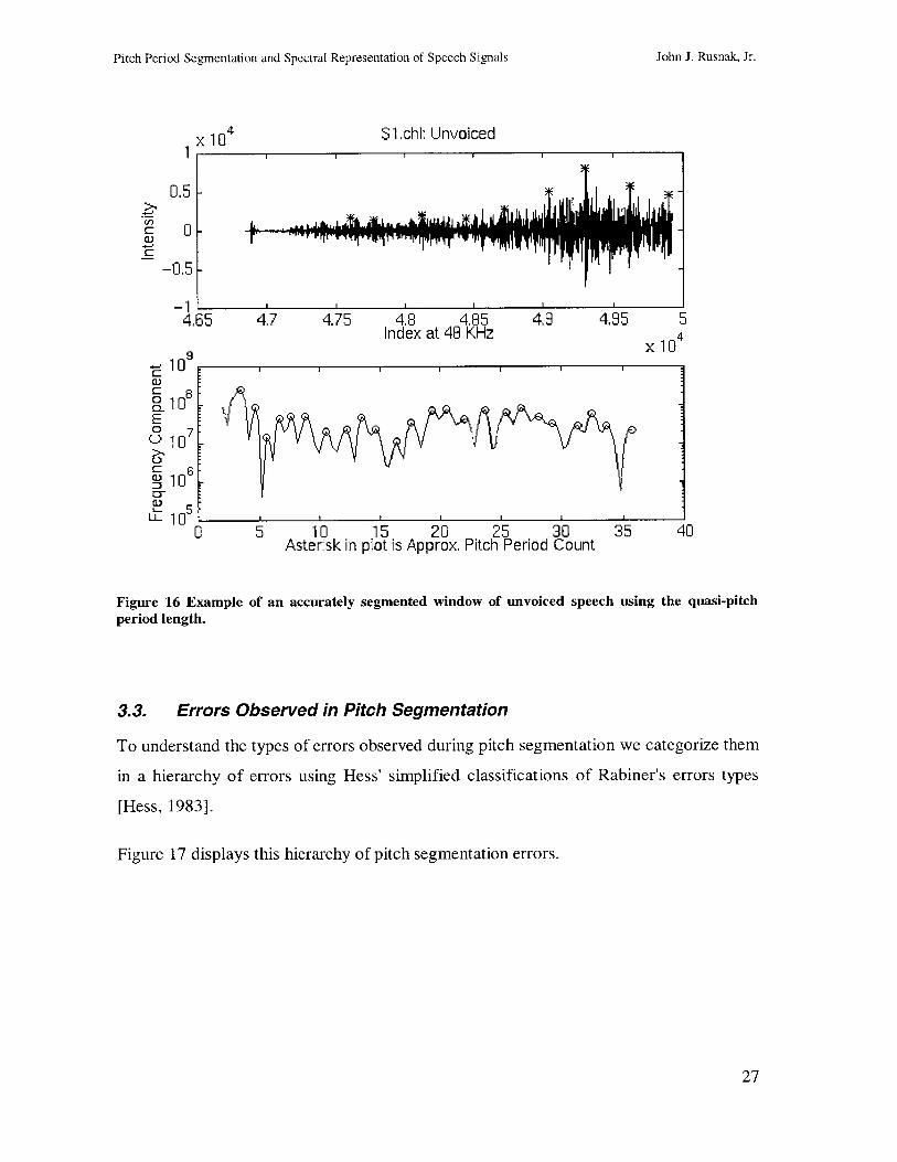
Figure 16 Exampleperiod length.
of an accurately segmented window of unvoiced speech using the quasi-pitch
3.3. Errors Observed in Pitch Segmentation
To understand the types of errors observed during pitch segmentation we categorize them
in a hierarchy of errors using Hess' simplified classifications of Rabiner's errors types
[Hess, 1983].
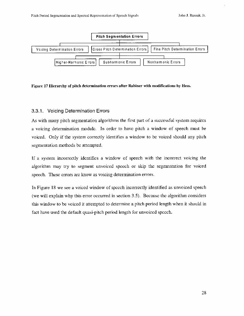
Figure 17 displays this hierarchy of pitch segmentation errors.
27
x1
0.5k
Ol-
-0.51-
l~TW1.1 ii T1 II If
I _ I I I - _ _ I _ _ _ - I
5-11
4.6
10
10
10
10 6
E0
U_
105L0
John J. Rusnak, Jr.
r
Pitch Period Segmentation and Spectral Representation of Speech Signals
Pitch Segmentation Errors
Voicing Determination Errors Gross Pitch Determination Errors Fine Pitch Determination Errors
Higher-Harmonic Errors Subharmonic Errors Nonharmonic Errors
Figure 17 Hierarchy of pitch determination errors after Rabiner with modifications by Hess.
3.3.1. Voicing Determination Errors
As with many pitch segmentation algorithms the first part of a successful system requires
a voicing determination module. In order to have pitch a window of speech must be
voiced. Only if the system correctly identifies a window to be voiced should any pitch
segmentation methods be attempted.
If a system incorrectly identifies a window of speech with the incorrect voicing the
algorithm may try to segment unvoiced speech or skip the segmentation for voiced
speech. These errors are know as voicing determination errors.
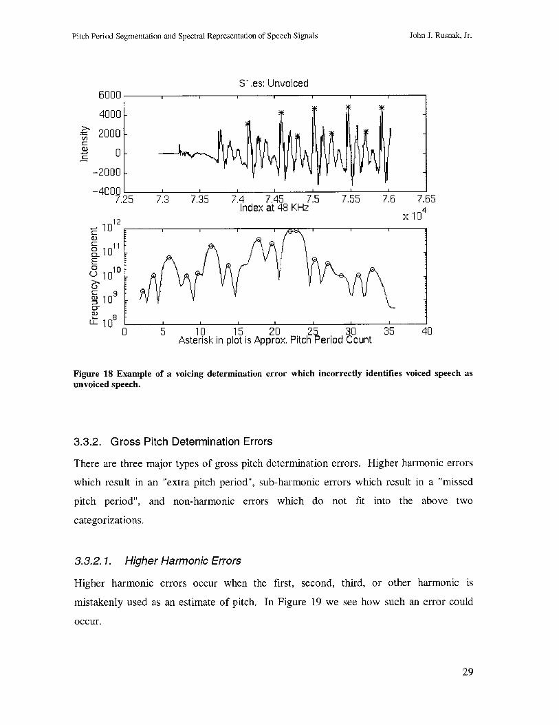
In Figure 18 we see a voiced window of speech incorrectly identified as unvoiced speech
(we will explain why this error occurred in section 3.5). Because the algorithm considers
this window to be voiced it attempted to determine a pitch period length when it should in
fact have used the default quasi-pitch period length for unvoiced speech.
28
John J. Rusnak, Jr.
Pitch Period Segmentation and Spectral Representation of Speech Signals
S1.es: Unvoiced6000
4000-
2000 -
0
-2000 -
-40007.25 7.55 7.6 7.65
x10
5 10 15 20 25 30Asterisk in plot is Approx. Pitch Period Count
35 40
Figure 18 Exampleunvoiced speech.
of a voicing determination error which incorrectly identifies voiced speech as
3.3.2. Gross Pitch Determination Errors
There are three major types of gross pitch determination errors. Higher harmonic errors
which result in an "extra pitch period", sub-harmonic errors which result in a "missed
pitch period", and non-harmonic errors which do not fit into the above two
categorizations.
3.3.2.1. Higher Harmonic Errors
Higher harmonic errors occur when the first, second, third, or other harmonic is
mistakenly used as an estimate of pitch. In Figure 19 we see how such an error could
occur.
29
a,
7.3 7.35 7.4 7.45 7.5Index at 48 KHz
10 2
S 11n 10E
D 100 10
- 1010
(0L8
0
John J. Rusnak, Jr.
I I I
Pitch Period Segmentation and Spectral Representation of Speech Signals
S2.es: Voiced2000
1000-
0 k
-100011.28 1.285 1.29 1.295 1.3 1.305 1.31
Index at 48 KHz1.315
x 10
0 5 10 15 20 25 30Asterisk in plot is Approx. Pitch Period Count
Figure 19 Example of a higher harmonic gross pitch determination error. The peakasterisk in the frequency plot is actually the first harmonic.
marked with an
With this window our pitch segmentation algorithm chose the first harmonic as the pitch
estimate. In the frequency plot we see the first harmonic darkened as the sixth peak from
zero. This results in twice as many segmentation markings in the time domain. Had the
segmentation algorithm chosen the third peak from zero we would have observed the
correct pitch segmentation in the time domain.
3.3.2.2. Sub-Harmonic Errors
Sub-harmonic errors also occur when the incorrect peak is chosen as the pitch estimate in
the frequency domain. In Figure 20 we see in the frequency plot two peaks of almost
equal magnitude. The pitch segmentation algorithm needed to choose one of these peaks
as the pitch estimate. Unfortunately it choose the incorrect peak and a sub-harmonic
30
U)
w
- 102CD
E 100010E 100
1. n
I I I I I I I
I I I I I I I
35 40
I I I I I I
John J. Rusnak, Jr.
Pitch Period Segmentation and Spectral Representation of Speech Signals
error is observed. In the time domain plot above we can see every other pitch period is
properly segmented due to this error.
S2.chl: Voiced500 W , I I I I
4-j
C,)
w
0
-500
-10001
10(D 100 10
E0 10
S106
0
1.005 1.01 1.015 1.02 1,025Index at 48 KHz
1.03
x10
5 10 15 20 25 30 35 40Asterisk in plot is Approx. Pitch Period Count
Figure 20 Example of a sub-harmonic gross pitch determination error. The algorithm was forced todecide between the two large peaks in the frequency domain and incorrectly chose the ninth peakfrom zero instead of the seventeenth peak.
3.3.2.3. Non-Harmonic Errors
Non-harmonic pitch determination errors appear when an unforeseen breakdown occurs.
The input data may be greatly irregular or have a particular characteristic that misleads
the pitch segmentation algorithm. In Figure 21 we see that the segmentation algorithm
first committed a voicing determination error by determining the window of unvoiced
speech was voiced. The algorithm then further decided to mark the end of the last pitch
period after the window of speech had ended. Whether the window is voiced or unvoiced
the algorithm should end the period where there is speech.
31
John J. Rusnak, Jr.
Pitch Period Segmentation and Spectral Representation of Speech Signals
Such gross errors happen very rarely in our algorithm and so we decided to make note of
them but not to peruse them to great length.
4000
2000|-
0
S3.chl: Voiced
-20001-
600016.85 6.9 6.95 7 7.05 7.1 7.15
Index at 48 KHz7.2
x10410
610
10 20 5 10 15 20 25 30 35 40
Asterisk in plot is Approx. Pitch Period Count
Figure 21 Example of a non-harmonic gross pitch determination error. The algorithm ended the lastperiod after the window ended.
3.4. Fine Pitch Determination Errors
Fine pitch determination errors are not as severe as the previous types of errors. These
errors usually come close to successfully segmenting a window of speech but may miss
the exact segmentation by a small amount. These errors usually come about for one of
two reasons. First the recorded speech may include too much noise. We must also
remember that voiced speech is only quasi-periodic because it is generated from a
biological source. This gives rise to the second reason which is that an exact beginning
or end of a pitch period difficult to pinpoint.
32
4-,
U.,4
-J
)KE
0
E0
U
. .
John J. Rusnak, Jr.
Pitch Period Segmentation and Spectral Representation of Speech Signals
In Figure 22 we see an example of a fine pitch determination error. Note that while the
pitch periods are segmented to some degree, the fine nature of the segmentation is less
accurate due to the difficulty in determining which part of the glottal pulse signifies the
beginning of the period.
Sl.es: Voiced
4000-
2000 -
0~ 0
-2000I I I I I I I I I I
7.72 7.73 7.74 7.75 7.76 7.77 7.78 7.78 7.8 7.81Index at 48 KHz
Figure 22 Example of a fine pitch determination error.
3.5. Biasing the Segmentation Algorithm
If our algorithm correctly identifies a window as voiced it does a good job at properly
segmenting the speech. If the algorithm incorrectly identifies a voiced window as
unvoiced it merely marks the default quasi-pitch period length of 6 ms. Because we were
more interested in a system that would properly segment voiced windows we decided to
bias our system to do this. By making changes in the source code we set our system to
give up accuracy in voicing determination so that it would have more opportunity to
segment voiced windows.
To better understand the change we revisit the voicing detection part in Section 3.2.2.
Here we see that unvoiced speech was declared if there were no normalized spectral
peaks above the threshold, currently set at 10. It is quite possible that some voiced
segments may have no normalized spectral peaks above the threshold and be incorrectly
declared as unvoiced speech. The change in the code was to set a incrementally
decreasing threshold. Thus if a window did not meet the threshold at 10, the threshold
33
John J. Rusnak, Jr.
Pitch Period Segmentation and Spectral Representation of Speech Signals John J. Rusnak, Jr.
was lowered to 8. Then the threshold test was applied again. If the window could now
be declared as voiced the algorithm continued as normal. If the test for voiced speech
failed yet again, the threshold was then lowered to 6 and the test was reapplied. Only if
the test failed at a threshold of 6 would the window be declared as unvoiced speech.
This change had several effects. First many unvoiced windows were not being declared
as voiced windows. At first, this might seem to be a terrible flaw. However we
previously designed the system to use a default quasi-pitch period length for unvoiced
windows simply to keep some marking during the unvoiced speech. We still have this
marking effect though now our quasi-pitch period length may vary from unvoiced
window to unvoiced window. Even so, it is not our goal to have a quality voicing
detection module, out interest is in segmenting voiced speech and the creation of pitch-
synchronous spectrograms which are explained in Section 4.5.
Second, those voiced windows that did not meet the original strict threshold condition
can now still be segmented if they pass one of the other lower threshold conditions. This
allows such windows to be properly segmented instead of incorrectly being marked as
unvoiced windows.
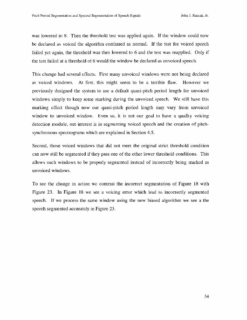
To see the change in action we contrast the incorrect segmentation of Figure 18 with
Figure 23. In Figure 18 we see a voicing error which lead to incorrectly segmented
speech. If we process the same window using the new biased algorithm we see a the
speech segmented accurately in Figure 23.
34
Pitch Period Segmentation and Spectral Representation of Speech Signals
6000
4000-
2000 -
0 -
-2000
-4000 -7.25
10
1110
1010
10
100
0-
0-
E0U)
5-
S1es: Voiced
7.3 7.35 7.4 7.45 7.5Index at 48 KHz
7.55 7.6 7.65
x10
5 10 15 20 25 30Asterisk in plot is Approx. Pitch Period Count
35 40
Figure 23 The correct segmentation a voiced window of speech using the biased algorithm. Compareto the incorrect segmentation of the same voiced window in Figure 18.
Overall we sacrificed accuracy in voicing detection for an increased probability that all
voiced windows will be segmented properly. The trade-off allowed higher quality pitch-
synchronous spectrograms to be produced.
35
V)
John J. Rusnak, Jr.
Pitch Period Segmentation and Spectral Representation of Speech Signals
4. Spectrograms
4.1. Limitations of Waveform Analysis
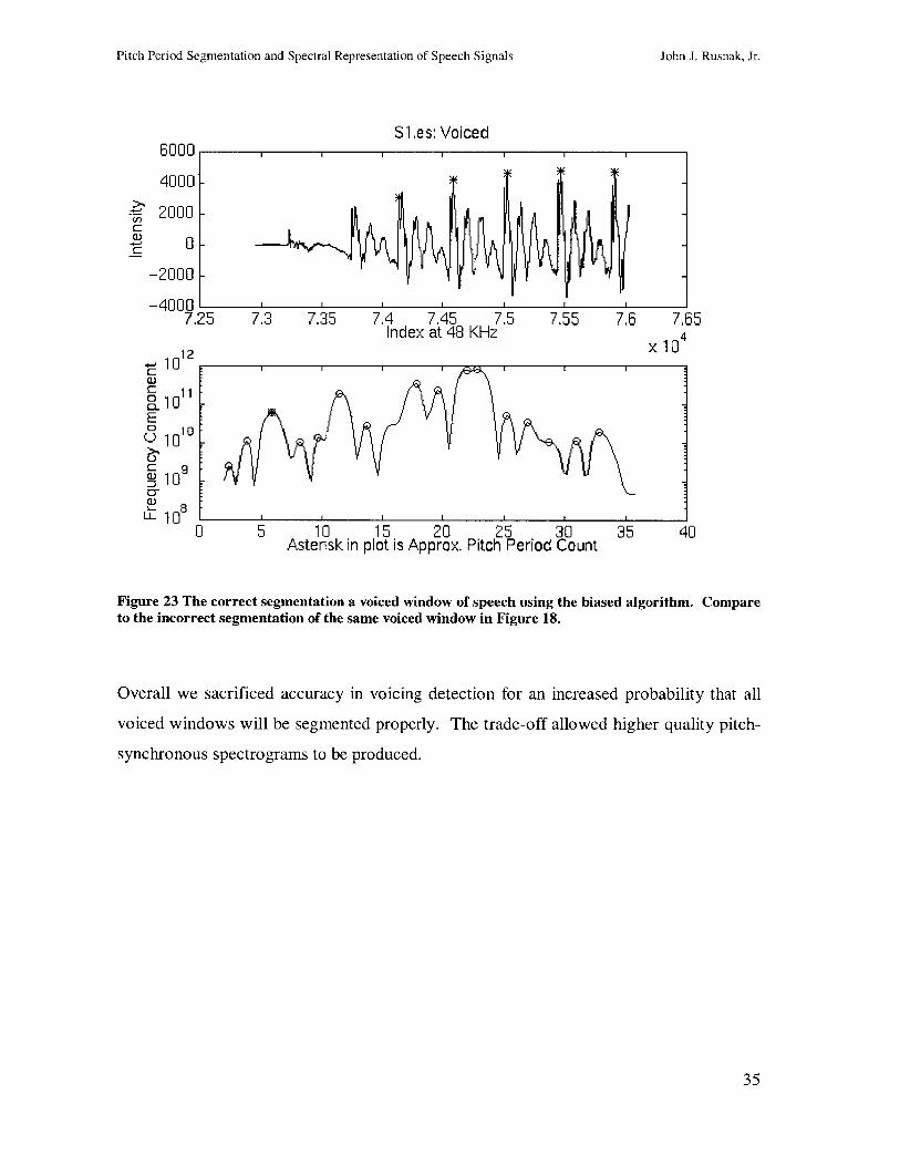
A speech waveform is only one way to visually display spoken speech. When a person
speaks into a microphone, variations in pressure are converted into proportional changes
in voltage. We can display these changes in voltage on a waveform plot with time as the
abscissa and voltage as the ordinate as seen in Figure 24. Such a plot is called a
oscillogram and allows us to learn things such as changes in voicing and periods of
silence that exist in the recorded speech.
210 0.2 0tO. 3 UCu 0 5 10 .0 F 'ho
Figure 24 Example of a waveform oscillogram of the word "phonetician" [Filipsson, 1998].
Because speech characteristics can vary greatly between different speakers it is difficult
to detect individual phonemes from waveform analysis. It is useful to have other display
techniques that are invariant to personal speaker traits and instead can help detect
phoneme information. To fit this need we can use a speech spectrogram.
4.2. Types of Spectrogram Displays
A speech spectrogram is a three-dimensional plot of the recorded speech. The three axes
are time, frequency, and intensity. To produce a spectrogram we compute the spectrum
of several successive windows of continuous speech. In Figure 14 we see a two-
dimensional spectrum of a speech window. We can think of a spectrogram as the
successive displays of speech spectra in time. With this third dimension of time a three-
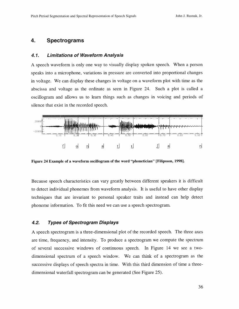
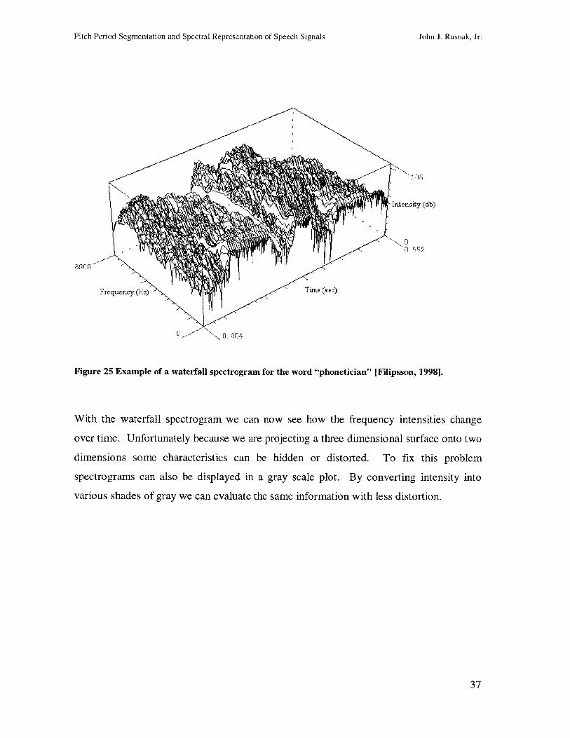
dimensional waterfall spectrogram can be generated (See Figure 25).
36
John J. Rusnak, Jr.
Pitch Period Segmentation and Spectral Representation of Speech Signals
8000'
Frequency (Hz) Time (sec)
Figure 25 Example of a waterfall spectrogram for the word "phonetician" [Filipsson, 1998].
With the waterfall spectrogram we can now see how the frequency intensities change
over time. Unfortunately because we are projecting a three dimensional surface onto two
dimensions some characteristics can be hidden or distorted. To fix this problem
spectrograms can also be displayed in a gray scale plot. By converting intensity into
various shades of gray we can evaluate the same information with less distortion.
37
John J. Rusnak, Jr.
Pitch Period Segmentation and Spectral Representation of Speech Signals
400~/~2000 ~- VI--
010. 02 I 0.4 1 0.5 1 0.6 0 .7 0.0 0.113
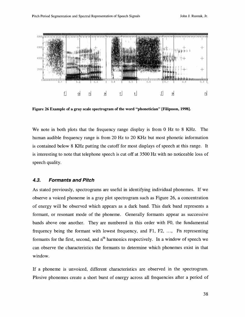
Figure 26 Example of a gray scale spectrogram of the word "phonetician" [Filipsson, 1998].
We note in both plots that the frequency range display is from 0 Hz to 8 KHz. The
human audible frequency range is from 20 Hz to 20 KHz but most phonetic information
is contained below 8 KHz putting the cutoff for most displays of speech at this range. It
is interesting to note that telephone speech is cut off at 3500 Hz with no noticeable loss of
speech quality.
4.3. Formants and Pitch
As stated previously, spectrograms are useful in identifying individual phonemes. If we
observe a voiced phoneme in a gray plot spectrogram such as Figure 26, a concentration
of energy will be observed which appears as a dark band. This dark band represents a
formant, or resonant mode of the phoneme. Generally formants appear as successive
bands above one another. They are numbered in this order with FO, the fundamental
frequency being the formant with lowest frequency, and Fl, F2, ... , Fn representing
formants for the first, second, and nth harmonics respectively. In a window of speech we
can observe the characteristics the formants to determine which phonemes exist in that
window.
If a phoneme is unvoiced, different characteristics are observed in the spectrogram.
Plosive phonemes create a short burst of energy across all frequencies after a period of
38
John J. Rusnak, Jr.
Pitch Period Segmentation and Spectral Representation of Speech Signals
silence. Aspirate and fricative phonemes display a constant blur of energy across both
axes. Unvoiced phonemes do not have formants nor do they have any pitch.
4.4. Non-Pitch-Synchronous Fixed- Window-Size Spectrograms
When we produce Fourier transforms for a spectrogram we need to choose a window size
in time. For example the spectrogram for two seconds of speech might employ 960
samples (at 48 kHz) in each window of 0.02 seconds. Instead of computing the transform
for time indices of every 0.02 seconds, an overlap is also included of .01 seconds. So
transforms are computed for time indices 0 to 0.02, 0.01 to 0.03, 0.02 to 0.04, and so on.
With this method we note several things. Each speech sequence of the same length will
have the same number of windows for which the Fourier transform was computed. The
windows are all of the same length and chosen in succession one after another, including
an overlap which is usually half the window length. In Section 4.5 we compare the
display of this standard spectrogram algorithm with those of different algorithms.
4.5. Pitch-Synchronous Spectrograms
Our spectrogram algorithm uses one complete pitch period as the window size to
compute spectrograms. This means that for each successive pitch period in a sentence,
the Fourier transform is computed. These spectra are then concatenated with one another
to produce the spectrogram. Each vertical sliver of the spectrogram represents the
spectrum of one complete pitch period.
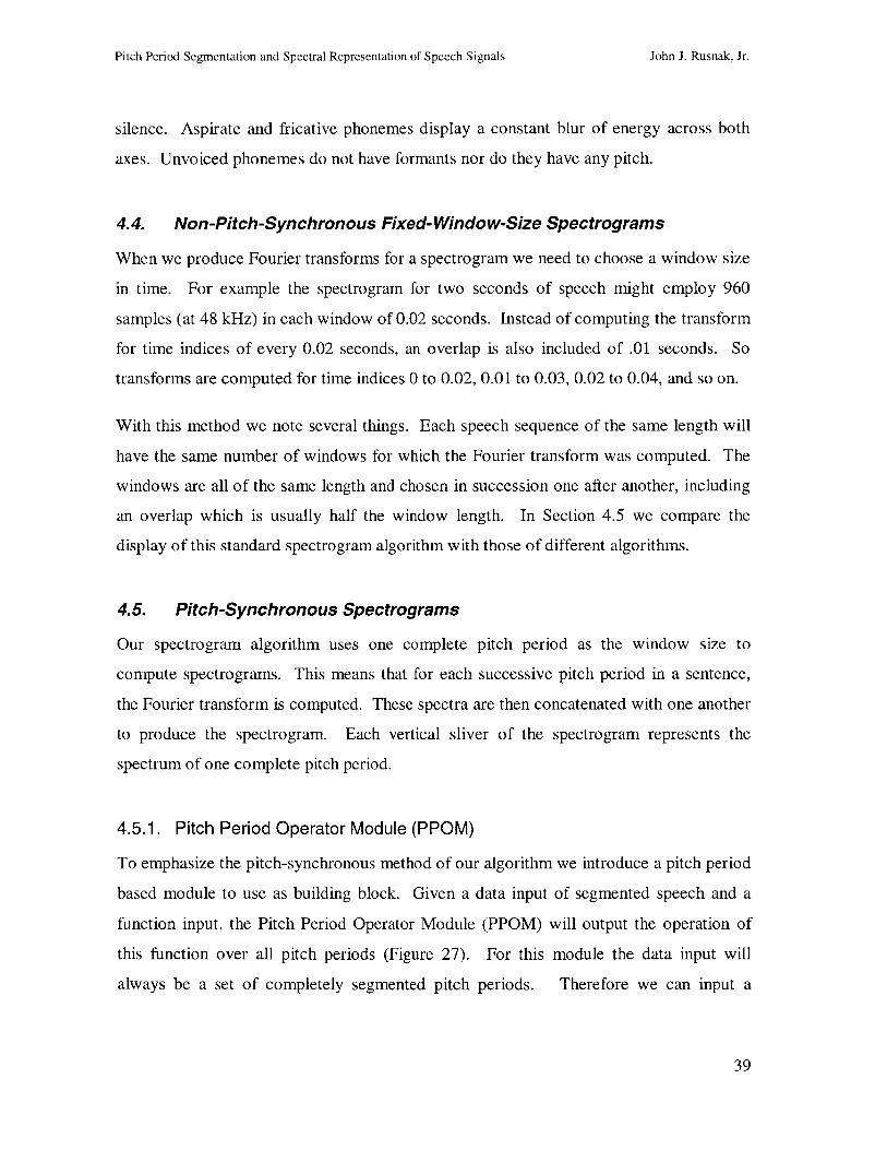
4.5.1. Pitch Period Operator Module (PPOM)
To emphasize the pitch-synchronous method of our algorithm we introduce a pitch period
based module to use as building block. Given a data input of segmented speech and a
function input, the Pitch Period Operator Module (PPOM) will output the operation of
this function over all pitch periods (Figure 27). For this module the data input will
always be a set of completely segmented pitch periods. Therefore we can input a
39
John J. Rusnak, Jr.
Pitch Period Segmentation and Spectral Representation of Speech Signals
segmented speech window with n pitch periods to this module and expect the output to be
some function applied to each of these n pitch periods.
Pitch segmented Function:speech:
FP0, P, ... , PF
Pitch PeriodOperator Module
F(P0), F(Pj), ...,9 F(P.)
Figure 27 Detail of a Pitch Period Operator Module (PPOM).
We can use the PPOM to produce a spectrogram synchronized on successive and
complete pitch periods. The obvious problem is that in general no two pitch periods have
the same length, while generating a spectrogram requires each transform of Fourier data
to have equal length. To avoid this problem we interpolate the transform of each pitch
period to insure each has the same length for the display output.
An important question is how to interpolate the transforms. One method is to set some
arbitrary length and linearly interpolate each pitch period so that all periods have the
same length. This is the simplest method but will create problems on several fronts. First
we need to determine this arbitrary length. Previously we discussed the many individual
characteristics of a speaker's speech patterns. There may be some difficulty in setting a
length that will work for all speakers. Second, if for some reason one pitch period is
longer than our arbitrarily set length our algorithm will fail. Thirdly if we counteract this
potential problem by setting an overly conservative length for interpolation, our data will
become distorted if our input is comprised of only small pitch periods.
40
John J. Rusnak, Jr.
Pitch Period Segmentation and Spectral Representation of Speech Signals
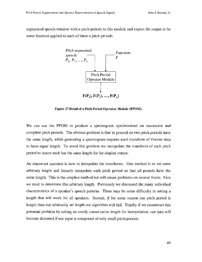
4.5.2. Cascading Pitch Period Operator Modules
To avoid these problems we preview our pitch period input data during a stage called
Iteration 0 (Figure 28). Iteration 0 uses a PPOM to calculate the length of the FFT of
each period. The maximum length is then found and with this insight a second PPOM in
Iteration 1 calculates the FFT of each period and interpolates at an appropriate grain for
the given input. By adding a preview of the data in Iteration 0 we insure our algorithm
will be universal for all speakers, and will not distort our data.
Speech Input
Speech Iteration 0Segmentation t--------------------------------------
F=length(FFT(P))
Pitch PeriodOperator Module
Maximum LengthCalculator Iteration 1
F=fft(Pmaxlength)
Pitch PeriodOperator Module
Spectrogram Output
Figure 28 Block diagram of the pitch-synchronous spectrogram algorithm. Iteration 0 represents apreview of the pitch period data. This preview is used in Iteration 1 to insure the interpolationportion of the spectrogram generation will work for all speakers regardless of pitch period length.
41
John J. Rusnak, Jr.
Pitch Period Segmentation and Spectral Representation of Speech Signals
4.6. Comparison of Fixed-Window-Size and Pitch-SynchronousSpectrograms
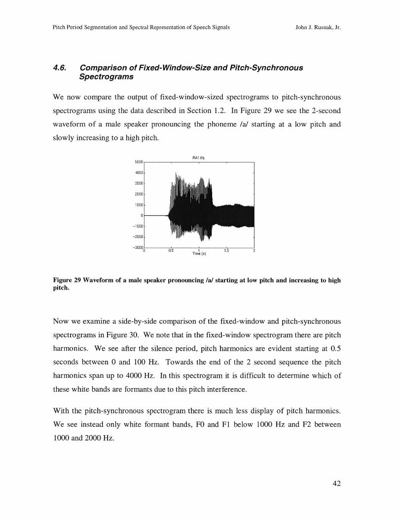
We now compare the output of fixed-window-sized spectrograms to pitch-synchronous
spectrograms using the data described in Section 1.2. In Figure 29 we see the 2-second
waveform of a male speaker pronouncing the phoneme /a/ starting at a low pitch and
slowly increasing to a high pitch.
RAl1tq5000
4000-
3000 -
2000
1000 -
0
-1000
-2000
-3000U
Time (s)
Figure 29 Waveform of a male speaker pronouncing /a/ starting at low pitch and increasing to highpitch.
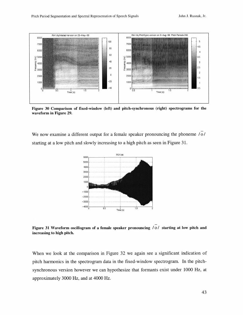
Now we examine a side-by-side comparison of the fixed-window and pitch-synchronous
spectrograms in Figure 30. We note that in the fixed-window spectrogram there are pitch
harmonics. We see after the silence period, pitch harmonics are evident starting at 0.5
seconds between 0 and 100 Hz. Towards the end of the 2 second sequence the pitch
harmonics span up to 4000 Hz. In this spectrogram it is difficult to determine which of
these white bands are formants due to this pitch interference.
With the pitch-synchronous spectrogram there is much less display of pitch harmonics.
We see instead only white formant bands, FO and F1 below 1000 Hz and F2 between
1000 and 2000 Hz.
42
John J. Rusnak, Jr.
Pitch Period Segmentation and Spectral Representation of Speech Signals
RA1.tfqMatlab Version on 26-May-98 RAl.tfq PitchSync version on 9-Aug-98 Pitch Periods:280
100 5
+p,. +.47000 44.580
60004
603.5
20 1 :000 254000 2.5
2023000
0 2000 --
-20 1000
-40 0 0.5
Time (s)Time (s)
Figure 30 Comparison of fixed-windowwaveform in Figure 29.
(left) and pitch-synchronous (right) spectrograms for the
We now examine a different output for a female speaker pronouncing the phoneme / o /
starting at a low pitch and slowly increasing to a high pitch as seen in Figure 31.
RO1lIck6000
500 0 ----- --- -.-.-
4 0 0 0 -. -.. . . . -- --....-. .--.. .-..--...-.. . -
3 0 0 0 --.. . -.. .-- .. ----------.... ..
2 0 0 0 -.. .. . -. ... .--. .. ....-- ... .
1000 -- .. .--
0
- 100 0 -.. --- --.. .. ... .. ...
- 2 0 0 0 -........... ... . ...... .....
- 3 00 0 -. -.. .... ... -.. . -.. . -.. -.. .-..--... .--.
-40000 0.5 Time (s) 1.2
Figure 31 Waveform oscillogram of aincreasing to high pitch.
female speaker pronouncing / o / starting at low pitch and
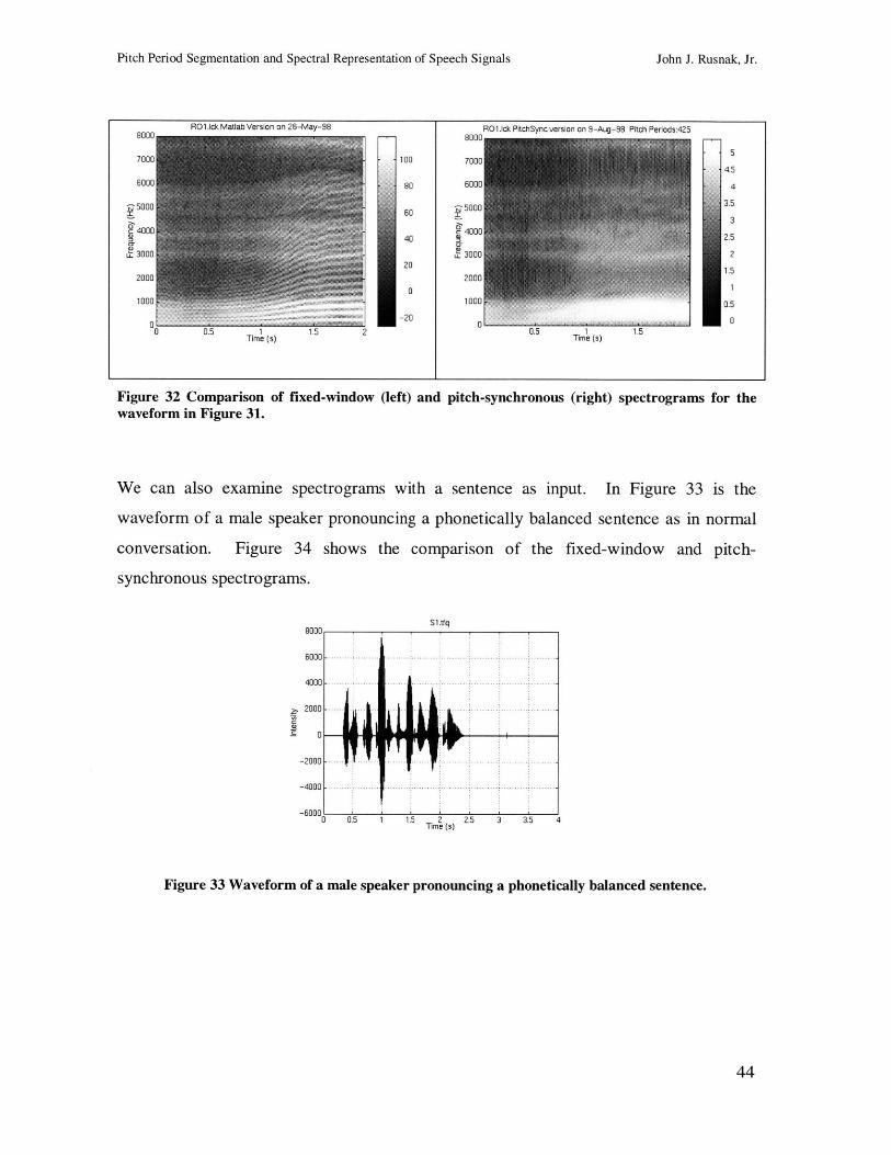
When we look at the comparison in Figure 32 we again see a significant indication of
pitch harmonics in the spectrogram data in the fixed-window spectrogram. In the pitch-
synchronous version however we can hypothesize that formants exist under 1000 Hz, at
approximately 3000 Hz, and at 4000 Hz.
43
5000
4000
u- 3000
John J. Rusnak, Jr.
Pitch Period Segmentation and Spectral Representation of Speech Signals
Figure 32 Comparison of fixed-windowwaveform in Figure 31.
John J. Rusnak, Jr.
We can also examine spectrograms with a sentence as input. In Figure 33 is the
waveform of a male speaker pronouncing a phonetically balanced sentence as in normal
conversation. Figure 34 shows the comparison of the fixed-window and pitch-
synchronous spectrograms.
S .tfq2000
6000 - -...--..
4000
-6000-0 0.5 1 1.5 2 2.5 3 35 4
Fime (3)
Figure 33 Waveform of a male speaker pronouncing a phonetically balanced sentence.
44
RO1ick Matlab Version on 26-May-98 RO1lck PitchSync version on 9-Aug-98 Pitch Periods:425
57000 100 7000
4.5
6000 80 6000 . 4
5000 60 50003.3
4000 c400025'20 _
2000 2000
01000 -01000 0.5
Time (s)Time (s)
(left) and pitch-synchronous (right) spectrograms for the
Pitch Period Segmentation and Spectral Representation of Speech Signals
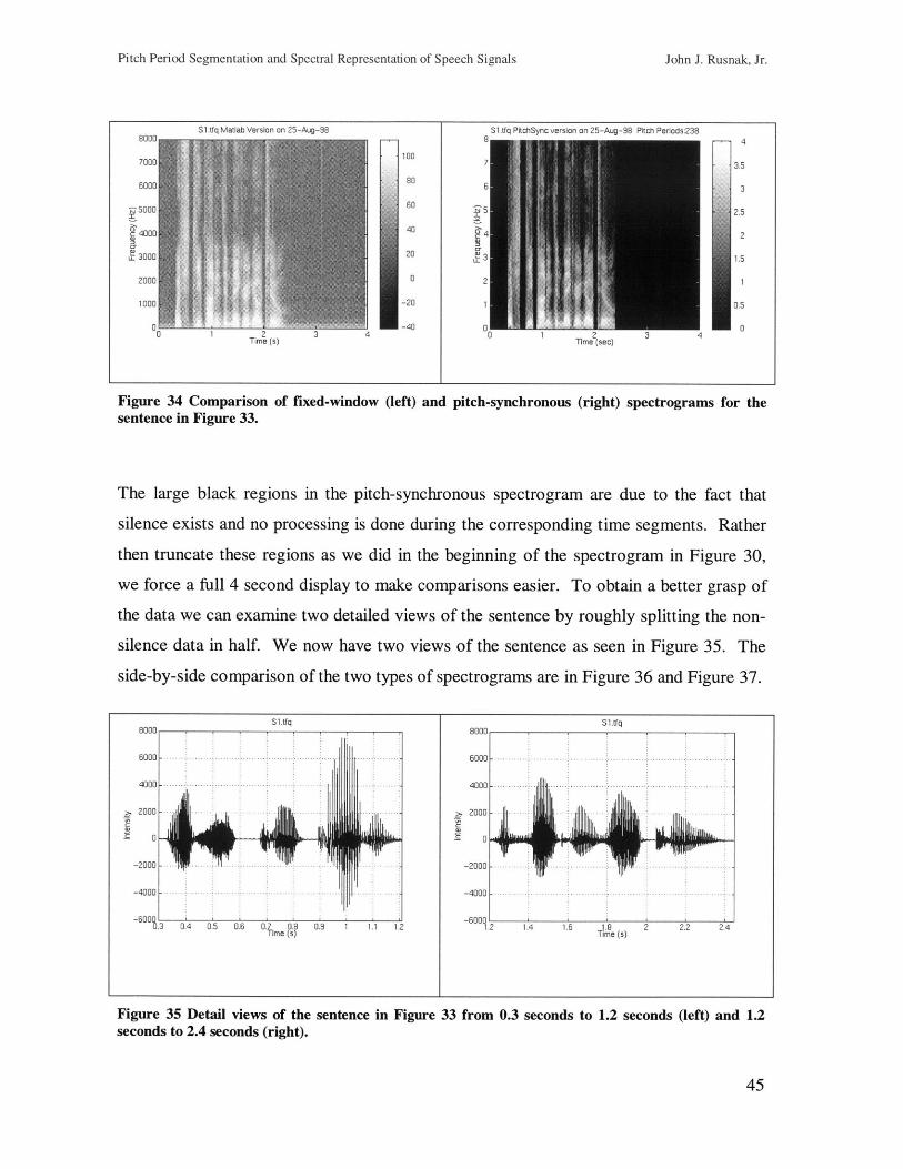
Figure 34 Comparison ofsentence in Figure 33.
fixed-window (left) and pitch-synchronous (right) spectrograms for the
The large black regions in the pitch-synchronous spectrogram are due to the fact that
silence exists and no processing is done during the corresponding time segments. Rather
then truncate these regions as we did in the beginning of the spectrogram in Figure 30,
we force a full 4 second display to make comparisons easier. To obtain a better grasp of
the data we can examine two detailed views of the sentence by roughly splitting the non-
silence data in half. We now have two views of the sentence as seen in Figure 35. The
side-by-side comparison of the two types of spectrograms are in Figure 36 and Figure 37.
9000 S1.tfq6000
2000 - --.-
0
-2000 - -.-
-4000
-600010.3 0.4 0.5 0.6 0.7 0.6 0.9 1 1.1 1.2
Time (s)
Figure 35 Detail views of the sentence in Figure 33 from 0.3 seconds to 1.2 seconds (left) and 1.2seconds to 2.4 seconds (right).
45
8000 S.tfq Matiab Version on 25-Aug-98 8 S.tfq PitchSync version on 25-Aug-98 Pitch Periods:238
7000 7 3.5
6000 806 3
r 5000 6052.5
4044000 42
20 2L3000 2031.5
2000 0 2
-201000 -20T1m0.5
0- --40 0 0
S1.tfq
1.6 1.6 2Time (s)
John J. Rusnak, Jr.
Time (s) I Time'(sec)
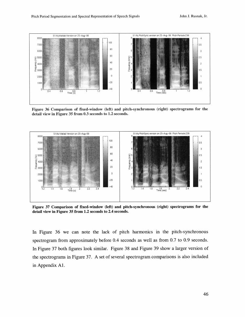
Pitch Period Segmentation and Spectral Representation of Speech Signals
Figure 36 Comparison of fixed-window (left) and pitch-synchronous (right) spectrograms for thedetail view in Figure 35 from 0.3 seconds to 1.2 seconds.
Figure 37 Comparison of fixed-window (left) and pitch-synchronous (right) spectrograms for thedetail view in Figure 35 from 1.2 seconds to 2.4 seconds.
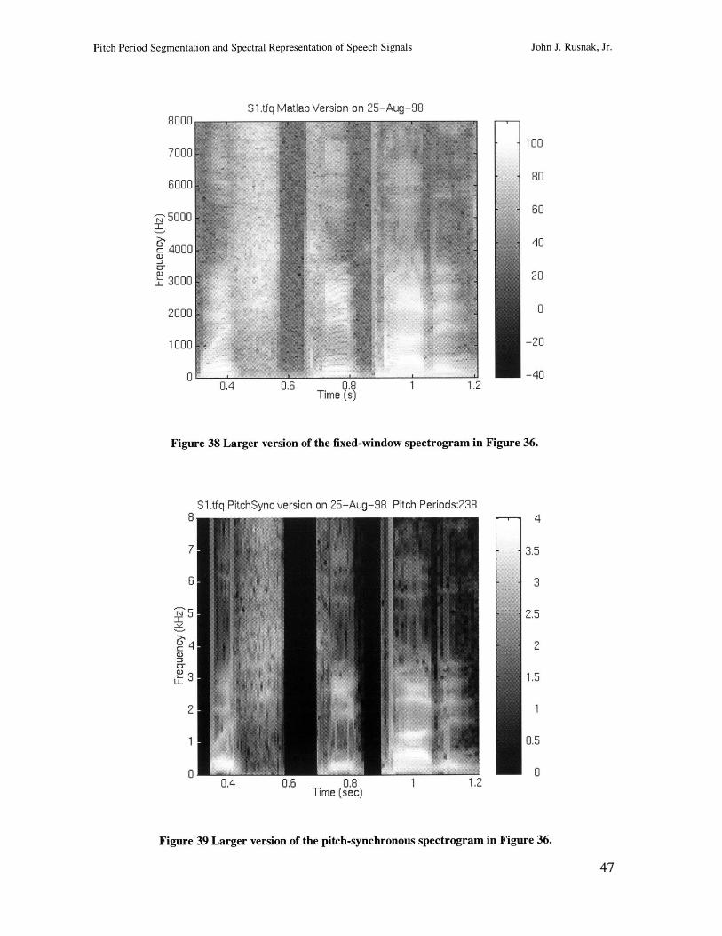
In Figure 36 we can note the lack of pitch harmonics in the pitch-synchronous
spectrogram from approximately before 0.4 seconds as well as from 0.7 to 0.9 seconds.
In Figure 37 both figures look similar. Figure 38 and Figure 39 show a larger version of
the spectrograms in Figure 37. A set of several spectrogram comparisons is also included
in Appendix Al.
46
I
John J. Rusnak, Jr.
Pitch Period Segmentation and Spectral Representation of Speech Signals
S1.tfq Matlab Version on 25-Aug-98
-]8000
7000
6000
N5000
4000
LL 3000
2000
1000
0
100
80
60
40
20
0
-20
-40
Figure 38 Larger version of the fixed-window spectrogram in Figure 36.
S1.tfq PitchSync version on 25-Aug-98 Pitch Periods:238
71
U.4 U.b U.8Time (sec)
Figure 39 Larger version of the pitch-synchronous spectrogram in Figure 36.
47
0.4 0.6 0.8 1 1.2Time (s)
8
7
6
N5
4
3
2
1
0
4
3.5
3
2.5
2
1.5
1
0.5
0
John J. Rusnak, Jr.
Pitch Period Segmentation and Spectral Representation of Speech Signals
4.7. A Note on Reproducing Pitch-Synchronous Spectrograms
In order to independently build a pitch-synchronous spectrogram system one should base
their system around some type of PPOM module. The nature of synchronizing on
individual pitch periods is built into this module. A PPOM should be based on a pitch
segmentation algorithm. There are many such algorithms available in the literature and
one is presented in Section 3.2.
Once the PPOM is built one merely needs to connect one or more PPOM modules
together cascading their input. The system is primed with a speech waveform and input
parameters that will yield an output of a pitch-synchronous spectrogram with desired
properties of the system builder. Source code is included in Appendix A2 of components
used produce the output in this thesis.
48
John J. Rusnak, Jr.
Pitch Period Segmentation and Spectral Representation of Speech Signals
5. Conclusions
In conclusion, this thesis focused on only a small subset of current speech research. We
presented a speech segmentation algorithm. While many algorithms in the literature have
focused on determining an approximate pitch for a window of speech, few have produced
an algorithm that can approximate the start and end points of each pitch period.
We explained that by modifying a small portion of the segmentation algorithm we can
bias the voicing detection module. With this bias we create a trade off where we loose
some accuracy in voicing detection but now allow almost all windows of voiced speech
to be properly segmented. Because our requirements included marking a quasi-pitch
period length for unvoiced speech this was a useful trade-off to make.
We used our pitch-segmentation algorithm as one of the modules in a new algorithm to
create pitch-synchronous spectrograms. An issue for all spectrograms is to choose the
window size to display the relationship between time, frequency, and intensity. Our
pitch-synchronous spectrogram algorithm adapts the window size to each speech sample
to insure that the window size is synchronized on the length of each pitch period. It does
this by taking a preview of the data and then interpolating some of the pitch periods to
insure that we meet the need to have each window be a set length. The end result is a
pitch-synchronous spectrogram that allows for easier identification of format information.
49
John J. Rusnak, Jr.
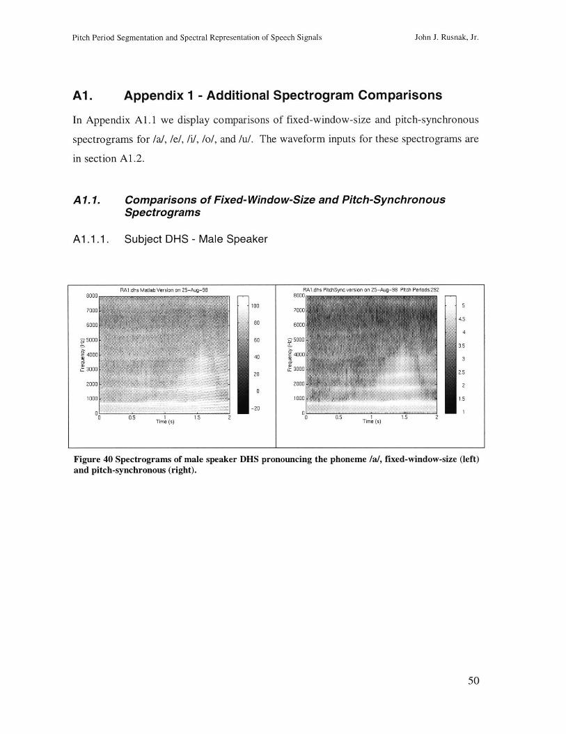
Pitch Period Segmentation and Spectral Representation of Speech Signals
Al. Appendix 1 - Additional Spectrogram Comparisons
In Appendix Al.1 we display comparisons of fixed-window-size and pitch-synchronous
spectrograms for /a/, /e/, /i/, /o/, and /u/. The waveform inputs for these spectrograms are
in section A1.2.
A1.1. Comparisons of Fixed-Window-Size and Pitch-SynchronousSpectrograms
A1.1.1. Subject DHS - Male Speaker
RAl dhs Matlab Version on 25-Aug-98 RAl.dhs PitchSync version on 25-Aug-98 Pitch Periods:292
700010
6000 80 6000 4.5
45000 80 5000 3
L 3000 L 300020 V 2.5
2000- 2000 20
1000 1000 lp 1.5
3 20 00 0.5 Tie1s 1.5 20 0.5 Tie1 s 1.5 200 05 Time (s) 20Time (s)
Figure 40 Spectrograms of male speaker DHS pronouncing the phoneme /a/, fixed-window-size (left)and pitch-synchronous (right).
50
John J. Rusnak, Jr.
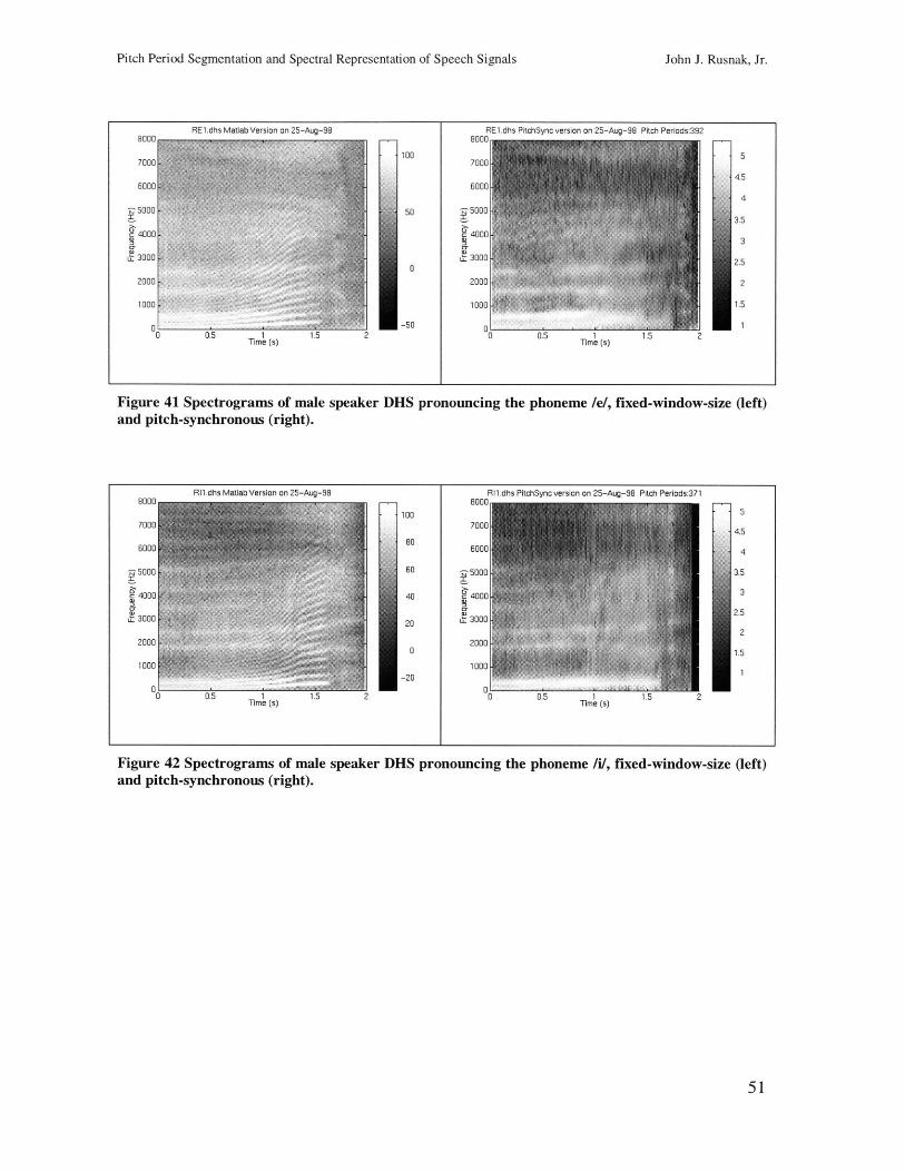
Pitch Period Segmentation and Spectral Representation of Speech Signals
-5001
400
u 300
John J. Rusnak, Jr.
RE1 .dhs Matlab Version on 25-Aug-98 RE1.dhs PitchSync version on 25-Aug-98 Pitch Periods:3928000
100 57000
4.56000
I450 50003.5
400033
3000 2.5
2000 " 2
, i-501000m
15
0 0.5 1Time (s)
Figure 41 Spectrograms of male speaker DHS pronouncing the phoneme /e/, fixed-window-size (left)and pitch-synchronous (right).
8000
7000
Rll.dhs Matlab Version on 25-Aug-98 RIl.dhs PitchSync version on 25-Aug-98 Pitch Periods:371
10080
40 c70004
3
2.520 L3000
20, 2
-20 20001
1000-20
0 ... ... ... ...0.5 1
Time (s)1b
1.5
Figure 42 Spectrograms of maleand pitch-synchronous (right).
speaker DHS pronouncing the phoneme /i/, fixed-window-size (left)
51
I
01M nTime (s)
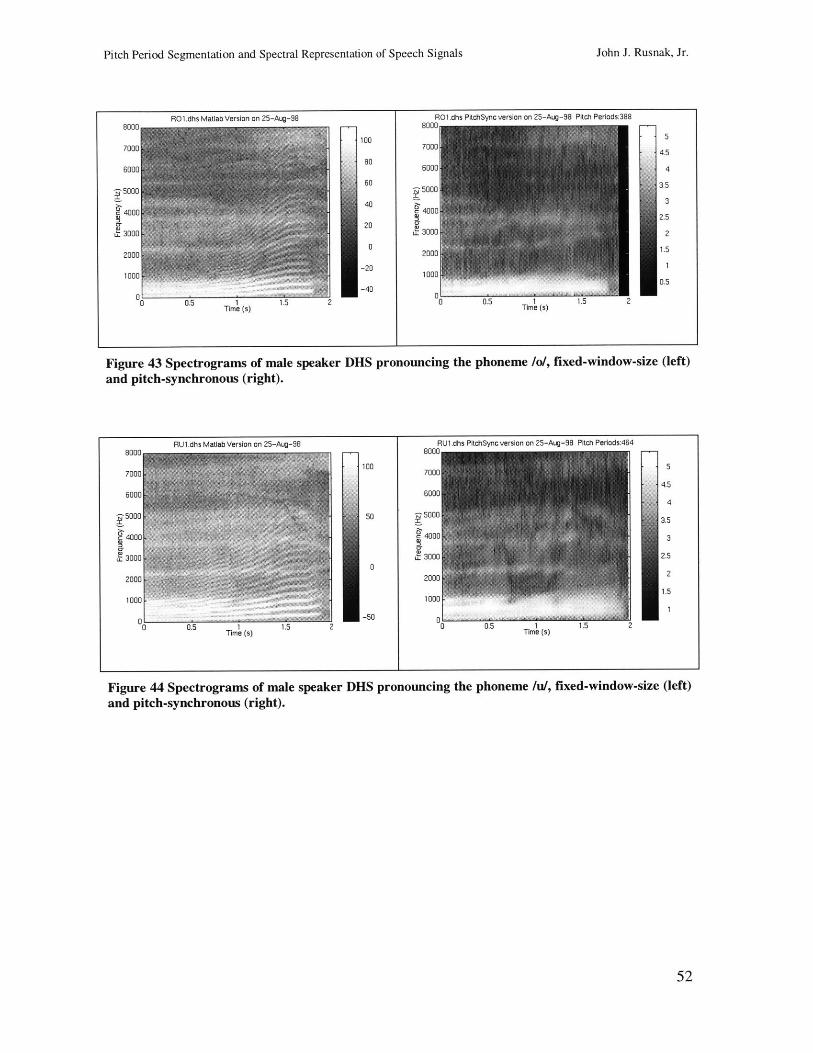
Pitch Period Segmentation and Spectral Representation of Speech Signals
RO1.dhs Matlab Version on 25-Aug-98
5001
400
t 300
Time (s)
RO1.dhs PitchSync version on 25-Aug-98 Pitch Periods:3888000
5
4.5
4
3.5
3
2.5
2
1.5
0.5
F
1.5 20 0.5 1Time (s)
Figure 43 Spectrograms of male speaker DHS pronouncing the phoneme /o/, fixed-window-size (left)and pitch-synchronous (right).
RUl.dhs Matlab Version on 25-Aug-98 RUl.dhs PitchSync version on 25-Aug-98 Pitch Periods:4648000 8000
100 57000 ++.(lm*s7000
6000 + + +++ .. 6000
5000 J . 50 5003.5
4000 4000 3
S3000 3000 2.5
022000. 200D
1.51000 1000
0. 0.5 1 15 1 -00 0 10.5 1 1.5 2Time (s) Time (s)
100
80
60
40
20
0
-20
-40
Figure 44 Spectrograms of male speaker DHS pronouncing the phoneme /u/,and pitch-synchronous (right).
fixed-window-size (left)
52
John J. Rusnak, Jr.
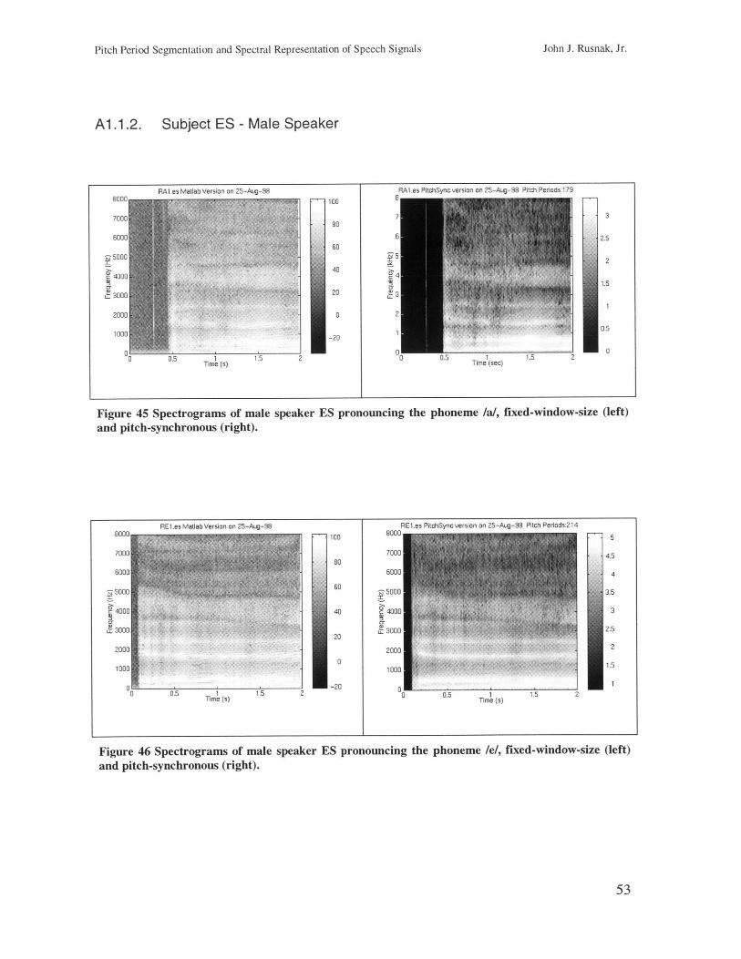
Pitch Period Segmentation and Spectral Representation of Speech Signals John J. Rusnak, Jr.
A1.1.2. Subject ES - Male Speaker
RA1.es Matlab Version on 25-Aug-98 RA1.es PitchSync version on 25-Aug-98 Pitch Periods:1798000 --- |10087000 7 3
80
6000 6 2.560
5000 5 2
20 240
4000 +.4 9 9 1.5
0.5
30003
1000 20 0-20
0 00 0.5 1 1.5 20 0.5 1 1.5 2
Time (s) Time (sec)
Figure 45 Spectrograms of male speaker ES pronouncing the phoneme /a/, fixed-window-size (left)and pitch-synchronous (right).
RE1.es Matab Version on 25-Aug-98
Time (s)
Figure 46 Spectrograms of maleand pitch-synchronous (right).
REl es PitchSync version on 25-Aug-98 Pitch Periods 214
100 8000 5
7000 4.5
6000 4
20
5000 3.5
40 4000 3
0 1.52 000 412
20
100 1.51000
-20 n11.5 20.5 1
Time (s)
speaker ES pronouncing the phoneme /e/, fixed-window-size (left)
53
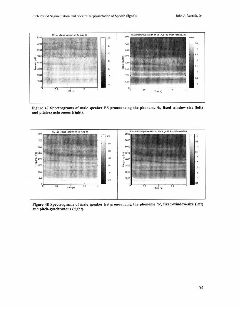
Pitch Period Segmentation and Spectral Representation of Speech Signals
Figure 47 Spectrograms of male speaker ES pronouncing the phoneme /i/, fixed-window-size (left)and pitch-synchronous (right).
RO1.es Matlab Version on 25-Aug-98 RO1.es PitchSync version on 25-Aug-98 Pitch Periods:209F., 1008000
100 5,5
807000 4.580
6000 4
lit50003. 404
k4000
20 2 30002
t 0 20001.
-20 1000 05
0.5 1 1.5 2 0 0.5 1 1.5 2Time (s) Time (s)
Figure 48 Spectrograms of maleand pitch-synchronous (right).
speaker ES pronouncing the phoneme /o/, fixed-window-size (left)
54
7
2000
1000
00
I
John J. Rusnak, Jr.
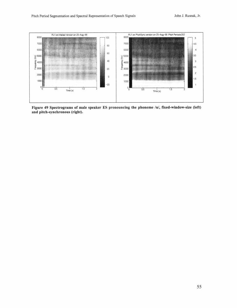
Pitch Period Segmentation and Spectral Representation of Speech Signals
RU1 es Malab Version on 25-Aug-98 RULes PitchSync version on 25-Aug-98 Pitch Periods:202100 8000 5
7000 4.580
6000 4Ijt60
605000 3.5
4000 .3
2.520 u 3000 2
20 2000
1.51000
-20 1
In 0 ̂
Figure 49 Spectrograms of maleand pitch-synchronous (right).
speaker ES pronouncing the phoneme /u/, fixed-window-size (left)
55
5001
400
ut 3001
John J. Rusnak, Jr.
Time (s) 0.5 1Time (s)
1.5 2
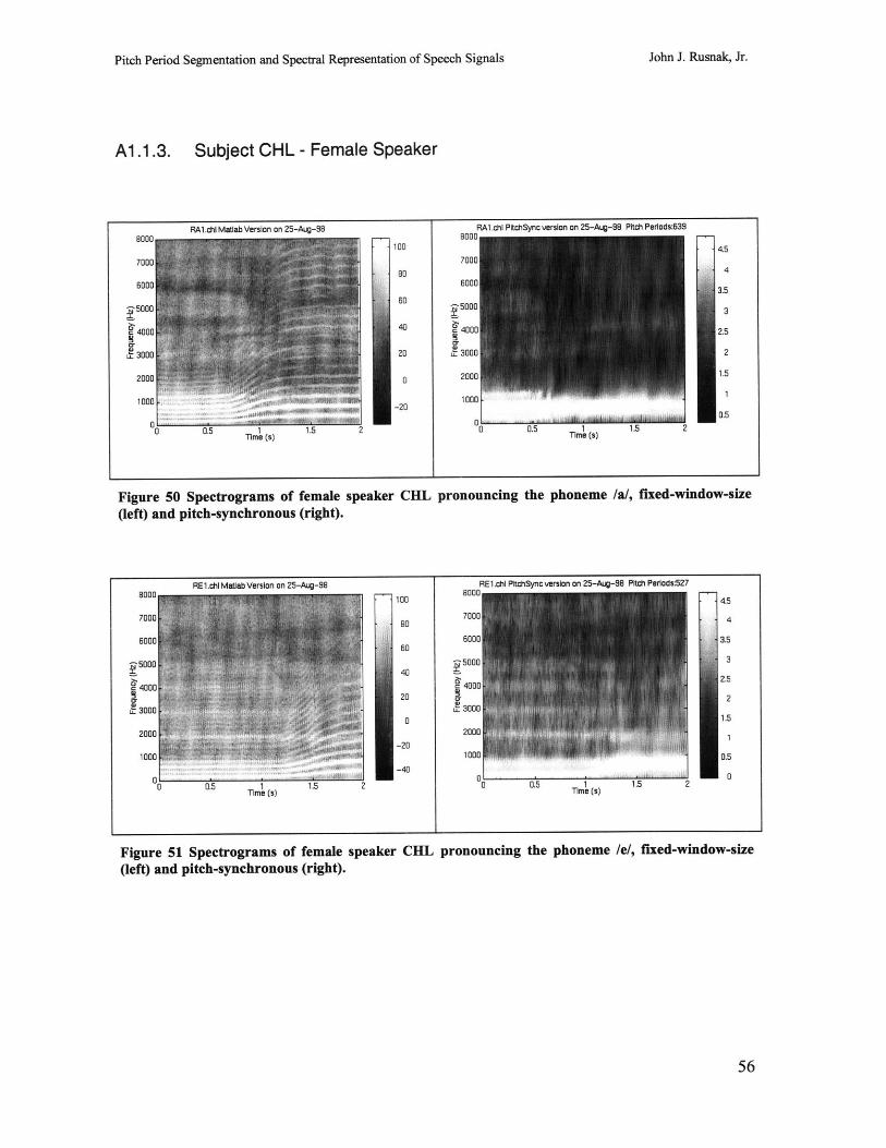
Pitch Period Segmentation and Spectral Representation of Speech Signals
Al .1.3. Subject CHL - Female Speaker
Figure 50 Spectrograms of female speaker CHL pronouncing the phoneme(left) and pitch-synchronous (right).
/a/, fixed-window-size
Figure 51 Spectrograms of female speaker CHIL pronouncing the phoneme /e/, fixed-window-size(left) and pitch-synchronous (right).
56
RAl.chi Matlab Version on 25-Aug-98 RAl.chi PitchSync version on 25-Aug-98 Pitch Periods:6398000 8000
100 4.5
7000 7000
80 4
6000 60003. 3.5
5000 605000 340
4000 44000 2.5
S300 20 L 3000 2
20.(0 15m.5
Time (s) mre (s)
John J. Rusnak, Jr.
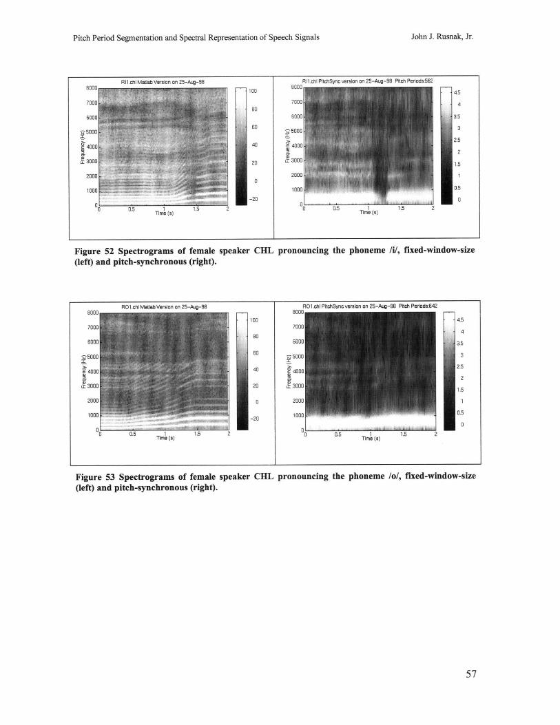
Pitch Period Segmentation and Spectral Representation of Speech Signals
Figure 52 Spectrograms of female speaker CHL pronouncing the phoneme /i/, fixed-window-size(left) and pitch-synchronous (right).
Figure 53 Spectrograms of female speaker CHL pronouncing the phoneme /o/, fixed-window-size(left) and pitch-synchronous (right).
57
71
I 7I I
John J. Rusnak, Jr.
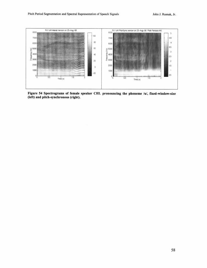
Pitch Period Segmentation and Spectral Representation of Speech Signals
500
400
L 300
John J. Rusnak, Jr.
RU1.chlI Matiab Version on 25-Aug-98 RU1.chi PitchSync version on 25-Aug-8 Pltch Periods:4408000 5
10004.5
804
3.560 -5000
F 3
40 40002.5
20 2
2000 1.5
-0
- -20
pi.
0.5 1Time (s)
1.5 2
Figure 54 Spectrograms of female speaker CHL(left) and pitch-synchronous (right).
pronouncing the phoneme /u/, fixed-window-size
58
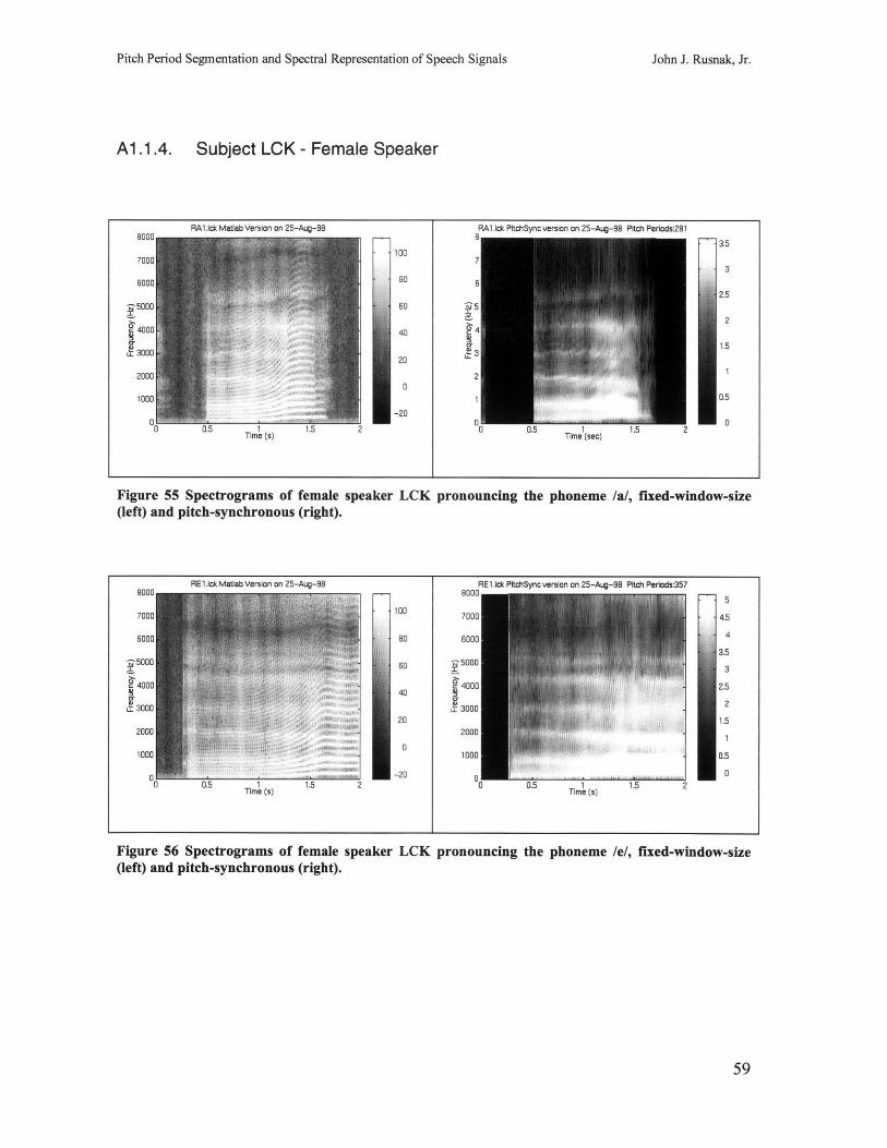
Pitch Period Segmentation and Spectral Representation of Speech Signals John J. Rusnak, Jr.
A1.1.4. Subject LCK - Female Speaker
400(
Lr 300C
RA1lck Matlab Version on 25-Aug-98 RA1lck PitchSync version on 25-Aig-98 Pitch Periods:281
3.5100
30
2
20
22
40
1 0.5
Figure 55 Spectrograms of female speaker LCK pronouncing the phoneme(left) and pitch-synchronous (right).
500[
400[
' 300C
/a/, fixed-window-size
RElick Matlab Version on 25-Ai.~-90 RElick PltctiSync version on 25-Ai.~-88 Pitch Perlods:357RE1.ck PitchSync version on 25-Aug-98 Pitch Periods:357
8000
100 7000 4.5
80 6000
3.5
60 5000
4000 2.5
2 2L30002
20 1.52000
01000 0.5
-20 00 0.5 1 1.5 2
Time (s)
Figure 56 Spectrograms of female speaker LCK(left) and pitch-synchronous (right).
pronouncing the phoneme /e/, fixed-window-size
59
I
RE1.lck Matlab Version on 25-Aug-98
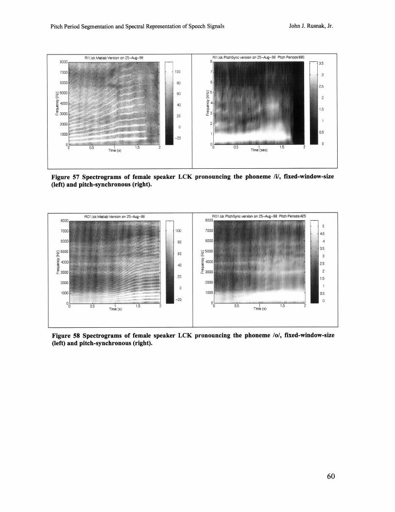
Pitch Period Segmentation and Spectral Representation of Speech Signals
5001
400
L' 3001
John J. Rusnak, Jr.
R Il.ck Matab Version on 25-Aug-98 RIl.ck PitchSync version on 25-Aug-98 Pitch Perlods:8803.5
100 73
2.5
60 52
4
rrS 1.5L- 320-
21
-20
0
I~ 0n~~i
Time (sec)Time (s)
Figure 57 Spectrograms of female(left) and pitch-synchronous (right).
speaker LCK pronouncing the phoneme /i/, fixed-window-size
Figure 58 Spectrograms of female speaker LCK pronouncing the phoneme /o/, fixed-window-size(left) and pitch-synchronous (right).
60
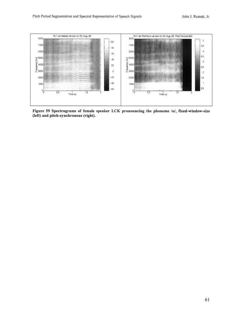
Pitch Period Segmentation and Spectral Representation of Speech Signals John J. Rusnak, Jr.
RU1lck Matlab Version on 25-Aug-98 RU1.lck PitchSync version on 25-Aug-98 Pitch Periods:3638000 100 8000 510005
07000 4.580
6000 66000 460
5000 5000B3.5Y o tl l tu::il '.Ii i ll 5003
c4000 20- 40002.5
3000 0 LL 3000 2
2000 -20 2000 1.5
1000 1000
-60 0.5
0.5 1 1.5T1me (s)0 0.5 1
Time (s)1.5
Figure 59 Spectrograms of female speaker LCK(left) and pitch-synchronous (right).
pronouncing the phoneme /u/, fixed-window-size
61
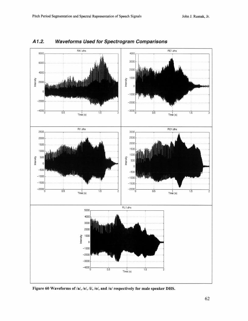
Pitch Period Segmentation and Spectral Representation of Speech Signals
A1.2. Waveforms Used for Spectrogram Comparisons
RA1.dhs8000
6 0 0 0 -.. .. . . -... . -. . . . . . . - . .. ..
0
- 2 0 0 0 -.. .. . -.. . . .. . - . . . . . -. - . . . . - -..--..-.- .
-40000.5 1
Time (s)1.5 2
Rll dhs2500
2 0 0 0 - -. -. . . . . . .. . . . . . . . . . . .. . . . . . .. . . . . . .
15 0 0 - -. -. -.. . --..-..-..-.
1000 -.... ...
500 - ...
0
-500 ...
-1000 - - - -
-200 0.5 T 1 s 1.5 2
RE1.dhs
-1000
-2000
-30000 0.5
Time (s)
RO1.dhs3000
2 5 0 0 -... . -. . -.. . . . . . . . . . . ... . -- . . . . . .. . . . ...
2 0 0 0 -.. . . . . . . . . -. --...-.--...--
1500 . . . . .. . ..
1000 -....
500.. .
0
-500 ....
-1000
-200 0 .5 Ti1 s 1.5 2
RU1.dhs
C
5000
4 0 0 0 -.. .. . - -.. .. . - . .. -. .. -. . . . . -... . -. . .. . .
3 0 0 0 -. .... .- . -..... .- ...- .. -.. -..- ..- ..-
2000 -.-.-.-
1000-- - -
0
-1000-
-2000 - .... -....-.
-3000 ---
0 0.5 1 1.5 2Time (s)
0 1.5 2
Figure 60 Waveforms of /a/, /e/, /i/, /o/, and /u/ respectively for male speaker DHS.
62
John J. Rusnak, Jr.
&
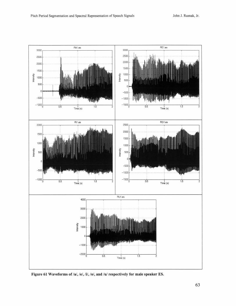
Pitch Period Segmentation and Spectral Representation of Speech Signals
RE1.es3000
2500 - . - - - - - - - - -
2 0 0 0 - - -- -- - - - -- -----... ... .... .... ....
1500
1000-
500
0
-500
-10001
-10 0 0.5 1 1.5 2Time (s)
RO1.es
2000
1500
1000
500
-500 --1
-100 0 .. . .. .. .... ........ .... ..
-150010 0.51
Time (s)
RU1.es
Figure 61 Waveforms of /a/, /e/, /i/, /o/, and /u/ respectively for male speaker ES.
63
RA1.es
Ril.es2000
1 0 .. .0.. . . 5 1 . 1.5.. .. .2..
Time(s)
1000
1.5 2
I
2500.
John J. Rusnak, Jr.
21C.E;
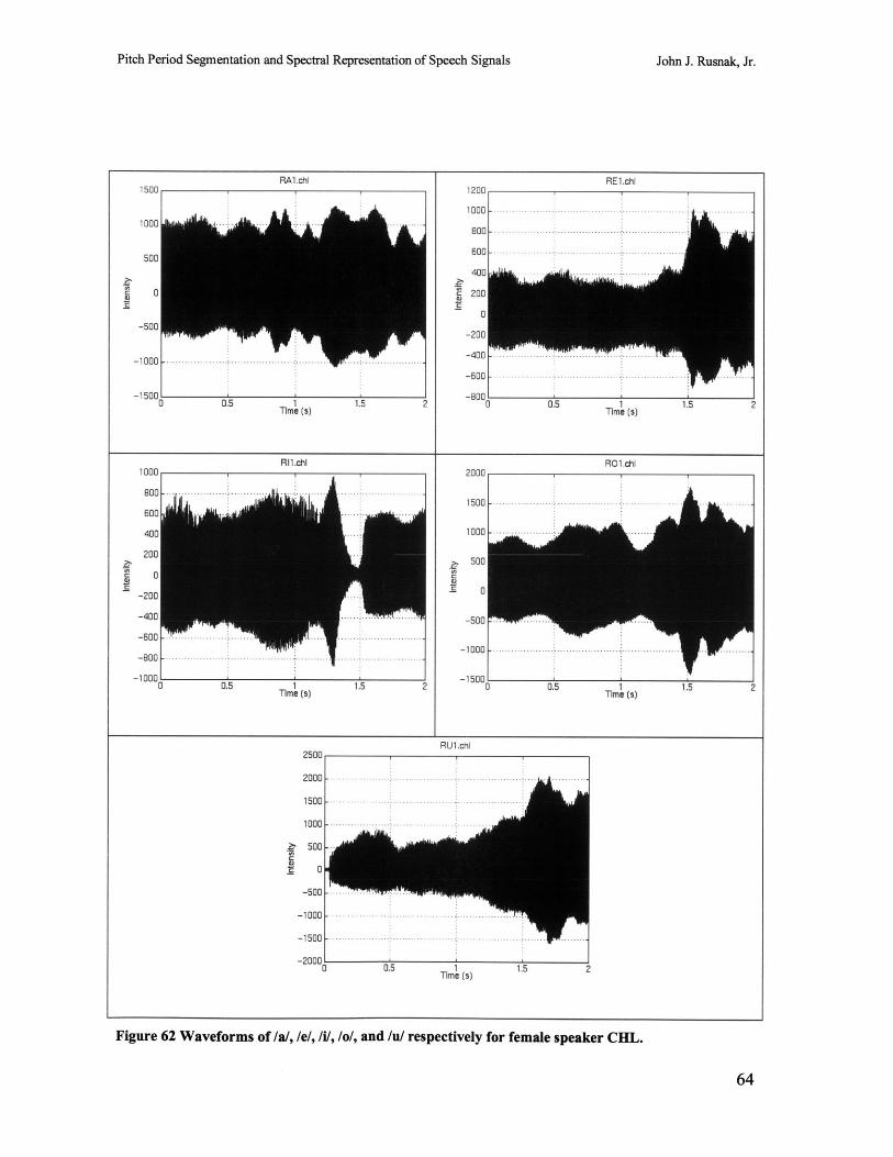
Pitch Period Segmentation and Spectral Representation of Speech Signals
RA1.chl1500
1000 -.. -. . -...
500
0
-500
-100
-10 0 0.5 1 1.5 2Time (s)
RI1.chl1000.
200
0
-200
-400
-600 --
-800 ......... . ...............
-10000 0.5 1
Time (s)1.5 2
RE1.chi
0 0.5 1 1.5Time (s)
RO1.chl2000
1 5 0 0 -- - . . . . . .:. . . . . . . . . . . . . . . . . . - . . . .....
1000 -. . . . . . . . .. .. ...
0
-500 -... -...
-100
10 0.5 1 1.5 2Time (s)
RUl.chl
Figure 62 Waveforms of /a/, /e/, /i/, /o/, and /u/ respectively for female speaker CHL.
64
2
2 0 0 0 -.. . . . .. . . . .. -. .. -. . . . . . . . . . -.. -. -..-
1 5 0 0 -. . - -.. .. . . - ...... ...- ..- ..-.-
10 0 0 -... -... . -.. . . . . . . . .
500
0
-500 - ... -
- 10 00 -.. .. . -.. . . .. . . . - .
- 1 5 0 0 -. -.. . . . . . . . -.. . .. . . - . - - . . . . . .. . .. . . . .
-2000 5 -0 .5 12
John J. Rusnak, Jr.
-
2500n
b
Time (s)
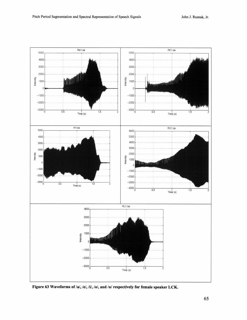
Pitch Period Segmentation and Spectral Representation of Speech Signals John J. Rusnak, Jr.
RA1.lck RE1lck5000 5000
4000 -- 40
3 00 0. . . . .-. --. .. - -. ..-. ..-. . .-- 3-
2000 -.-. -.--.-.-.-.-.-.2000.-
C 1000 - - - 1000 - -
0 0
-1000 - - - -.-.-.-.-.- -1000 - - .-
-2000 - -.-. - -2000 -
-3000 -30000 0.5 11520. .
Time (s) Time (s)
Rillck RO1lck500n60
500
4000 .. 5000
3000
20001000 ....
2 1000
0-1000 -100.
-1000
-2000 -2000
--3000 -3000m0 0.5 1 1.5 2Time (s)
05 1 1.5 2Time (s)
RU1lick4000
3000 - -... ..
2000
-1000
- 2 0 00 -... -. . . --.. -.. . . . . -. .... ..
o as5 1.5 2Time (s)
Figure 63 Waveforms of /a/, /e/, /i/, /o/, and /u/ respectively for female speaker LCK.
65
-.....-- -. ..- --. . -.. . .....
.................. ...... ... . - -.. . -.. . -... -.
-. ......- -. ...-. .....-. .
Pitch Period Segmentation and Spectral Representation of Speech Signals
A2. Appendix 2 - Source Code
These source code files are Matlab functions. Matlab is a matrix processing software
package Copyright 1984-98 by The MathWorks, Inc.
A2. 1. Glottal Pulse Source Code
A2.1.1. loop.m (script file)
% Author: John J. Rusnak, Jr, 1998
fi=1;clear Answer;%header=['Mean' 'STD' 'min' 'Max' 'Samples' 'Rejected Samples']
% Gaussian LPF try 5 and 7% gauss=gaussian(l/.08,0,5);gauss=gaussian(1,240,5);
Answer= [];while fi<=length(files)file=deblank(files(fi,:))s=lspeech(file,2);
% SampleIndex=(1:length(s))';
s=conv(gauss,s);
[p,nsil] = nsegment-speech(s);[Width,problem] =width(s,p,0);
% hist(Width);title(file);print;
% WidthNZ=nozerro(Width);answer=[mean(Width) std(Width) min(Width) max(Width) length(Width) (length(p)-length(Width)) problem]Answer= [Answer; answer];fi=fi+l;
end
A2.1.2. width.m
function [Width,problem] = width(s,p,glevel)
% Returns the widths of glottal pulses by finding local minima points.
% [Width,problem) = width(s,p,glevel)% Width = vector of widths% problem = count of the widths thrown out due to heuristic methods. If% this number is high consider ignoring the data set.% s = sound sequence or sentence% p = list of glottal peaks% glevel can be O=no outputs, 1=widths marked
% Author: John J. Rusnak, Jr, 1998
66
John J. Rusnak, Jr.
Pitch Period Segmentation and Spectral Representation of Speech Signals
%window size on +/- the peak in samplesproblem=0;size=2*48;
if glevel>0hold on; plot(s);grid on
end
i=0;
%For each glottal pulse do...
while i< length(p)i=i+l;
%Peak=[indicies or time of peak, value]Peak=[p(i) ,s(p(i))];if glevel >0 plot(Peak(1),Peak(2),'m*'); end
% get window
WindowStart=p(i)-size;if WindowStart<=0 WindowStart=l; endWindowEnd =p(i)+size;if WindowEnd>length(s) WindowEnd=length(s); end
LeftWindow =[(WindowStart:Peak(1))' (s(WindowStart:Peak(1)))1;RightWindow=((Peak(l)+l:WindowEnd)' (s(Peak(1)+1:WindowEnd))];
Window=[LeftWindow;RightWindowl;% also works Window=[(WindowStart:WindowEnd)' (s(WindowStart:WindowEnd))]
[LeftMinVal,LeftMinIndex]=min(LeftWindow(:,2));LeftMin=LeftWindow(LeftMinIndex);
[RightMinVal,RightMinIndex]=min(RightWindow(:,2));RightMin=RightWindow(RightMinIndex);
if glevel>0plot(LeftMin,LeftMinVal,'gx')plot(RightMin,RightMinVal, 'rx')
end
GlottalStart=[LeftMin LeftMinVal];GlottalEnd =[RightMin,RightMinVal];
% Left with GlottalStart, GlottalEnd, and Peak, all 1x2
GlottalBase=(GlottalStart(2)+GlottalEnd(2))/2;GlottalHA=(Peak(2)+GlottalBase)/2;
Plindex=length(LeftWindow);while (GlottalHA < LeftWindow(Plindex,2))&(Plindex>l)
Plindex=Plindex-1;end
P2index=l;while (GlottalHA < RightWindow(P2index,2))&(P2index<length(RightWindow))
P2index=P2index+l;end
67
John J. Rusnak, Jr.
Pitch Period Segmentation and Spectral Representation of Speech Signals
P1=LeftWindow(Plindex,:);P2=RightWindow(P2index,:);
if glevel>0plotxym(P1, g*')plotxym(P2, 'r*')
end
Width(i)=P2(1)-P1(l);
% check=checker(Width(i),GlottalStart,GlottalEnd,Peak);% if check==1% Width(i)=0;% end
%if Width(i)>90 keyboard;end%keyboard
if (Plindex==1) |(P2index==length (RightWindow)) problem=problem+1; end
end
problem;
A2.1.3. gaussian.m
function gauss=gaussian(c,m,sigma);
% Utility to create a gaussian function using the input paramaters c, m, and% sigma.
% gauss=gaussian(c,m,sigma);
% Author: John J. Rusnak, Jr, 1998
%c=1;%m=240;%sigma=5/2;%sigma=10;%t=(-24: .1:24);t=(0:1:480);
gauss=c*(exp(-(t-m).^2/(2*sigma.^2)))/(sqrt(2*pi*sigma.^2));plot(t,gauss)
A2.1.4. gwidth.m
function gw = gwidth(gauss,glevel)
% Utility to find width of gaussian from the half amplitude
% gw = gwidth(gauss,glevel)% gw = gaussian width at half amplitude% gauss = gaussian% glevel can be 0=no output 1=half amplitude marked
% Author: John J. Rusnak, Jr, 1998
HA=max(gauss)/2;
68
John J. Rusnak, Jr.
Pitch Period Segmentation and Spectral Representation of Speech Signals
HAIndex=find (gauss>=HA);
pl=HAIndex(l);p2=HAIndex(length(HAIndex));
gw=p2-p1;
if glevel==1plot (gauss)hold onplot(p1,gauss(p1), 'gx')plot(p2,gauss(p2),'rx')
end
A2.2. Pitch Period Segmentation Source Code
A2.2.1. estimatepitch.m (no biasing)
function [pest, voiced] = estimatepitch(ss,PMIN,PMAX)
% Usage: [pest, voiced] = estimate-pitch(ss,PMIN,PMAX)
% Estimate pitch of a voiced speech sequence. Not biased to find a pitch by% lowering accuracy in voicing detection. - JJR
% ss speech sequence % JJR% P_MIN minimum pitch% P_MAX maximum pitch% voiced = 1 if a pitch estimate is found; 0 otherwise.% pest pitch estimate if voiced = 1; pest = -1 otherwise.
% Author: Carlos R. Cabrera Mercader, 1997% Edited: John J. Rusnak, Jr, 1998
Ip=[]; %JJRglobal f;
ls = length(ss);lR = 2^ceil(log(ls)/log(2) + 1);I_min = ceil(lR/PMAX);I_max = fix(lR/PMIN);
% compute power spectrumR = fft(ss,lR);R = R.*conj(R);
% find the fundamental frequencyfor I=Imin:Imax,
if R(I) > max(R(I-1),R(I+1)),Ip = [Ip; I]; % find frequencies where there are peaks
endend
P = Ip;for i=1:length(Ip),
if i == 1,P(i) = R(Ip(i))/R(Ip(i+1));
elseif i == length(Ip),
P(i) = R(Ip(i))/R(Ip(i-1));else
69
John J. Rusnak, Jr.
Pitch Period Segmentation and Spectral Representation of Speech Signals
P(i) = R(Ip(i))/sqrt(R(Ip(i-1))*R(Ip(i+1)));end
endi = min(find(P > 10)); % found nothing at 10, 10 to 7I_est = Ip(i); % pick the first peak indexif sum(P > 10) > 4 & i > 1, % 10 to 7
j = min(find(P(1:i-1) == max(P(1:i-l))));if P(j) > 5 & Iest/Ip(j) < 2.2 & Iest/Ip(j) > 1.8,I_est = Ip(j);
endend
if isempty(I-est),title([setstr(f) ' Unvoiced'])voiced = 0;p_est = -1;
elsetitle([setstr(f) ': Voiced'])voiced = 1;p_est = 1R/I_est;
end
%%subplot(2,1,2),semilogy([I-min:I_max],R(IImin:I-max),'-',IR,R(IR),'o')subplot(2,1,2),semilogy([Imin:I-max],R(I_min:I-max),'w-')%%subplot(2,1,1),plot(Ip,P,'*')%%subplot(2,1,1),hist(P,[1 2 3 4 5 10 201)%%OLD subplot(2,1,2),semilogy([Imin:I-max],R(I min:I max),'-',Ip,R(Ip),'o',I-est,R(Iest),'*')
subplot(2,1,2),semilogy([ Imin:I-max]*1 /lR,R(I_min:I_max), 'w-
',Ip*ls/lR,R(Ip),'wo',I-est*ls/lR,R(I-est), 'w*')
xlabel('Asterisk in plot is Approx. Pitch Period Count')ylabel('Frequency Component')
%keyboard
A2.2.2. estimate-pitch.m (with bias to find peak)
function [pest, voiced] = estimate-pitch(ss,PMIN,PMAX)
% Usage: [pest, voiced] = estimate-pitch(ss,PMIN,PMAX)
% Estimate pitch of a voiced speech sequence% Edited to bias the algorithm to find a pitch by lowering accuracy in% voicing detection. - JJR
% ss speech sequence % JJR% PMIN minimum pitch% PMAX maximum pitch% voiced = 1 if a pitch estimate is found; 0 otherwise.% p-est pitch estimate if voiced = 1; pest = -1 otherwise.
% Author: Carlos R. Cabrera Mercader, 1997% Edited: John J. Rusnak, Jr, 1998
Ip=[]; %JJRglobal f
ls = length(ss);
70
John J. Rusnak, Jr.
Pitch Period Segmentation and Spectral Representation of Speech Signals
1R = 2^ceil(log(ls)/log(2) + 1);I_min = ceil(lR/PMAX);I_max = fix(lR/PMIN);
% compute power spectrumR = fft(ss,lR);R = R.*conj(R);
% find the fundamental frequencyfor I=Imin:I max,
if R(I) > max(R(I-1),R(I+1)),Ip = [Ip; I]; % find frequencies where there are peaks
endend
P = Ip;for i=1:length(Ip),
if i == 1,P(i) = R(Ip(i))/R(Ip(i+l));
elseif i == length(Ip),P(i) = R(Ip(i))/R(Ip(i-1));
elseP(i) = R(Ip(i))/sqrt(R(Ip(i-1))*R(Ip(i+l)));
endend
%% JJR Start
I_est=[];threshold=10+2;while (isempty(Iest)==1 & threshold>4)
threshold=threshold-2;
% JJR: Bias the algorithm to find a ptich by lowering accuracy in voicing
% determinationi = min(find(P > threshold));% i = min(find(P > 10)); % found nothing at 10, 10 to 7
I_est = Ip(i); % pick the first peak index% if sum(P > 10) > 4 & i > 1, % 10 to 7
if sum(P > threshold) > 4 & i > 1, % 10 to 7
j = min(find(P(1:i-1) == max(P(1:i-1))));
if P(j) > 5 & Iest/Ip(j) < 2.2 & I-est/Ip(j) > 1.8,
I_est = Ip(j);end
end
end
if isempty(I-est),title([setstr(f) ': Unvoiced'])voiced = 0;p_est = -1;
elsetitle([setstr(f) ': Voiced'])voiced = 1;p_est = lR/Iest;if p-est < 80title([setstr(f) ': Unvoiced'])voiced = 0;p-est = -1;
end
71
John J. Rusnak, Jr.
Pitch Period Segmentation and Spectral Representation of Speech Signals
end
% Various Output Methods:
%%subplot(2,1,2),semilogy([I-min:I_max],R(I-min:I-max),'-',IR,R(IR),'o')
subplot (2 ,1,2 ) ,semilogy ( [ Imin: I-max] , R( Imin: I-max) , 'w- ')%%subplot(2,1,1),plot(Ip,P,*)%%subplot (2, 1, 1), hist (P, [1 2 3 4 5 10 20])%%OLD subplot(2,1,2),semilogy ([Imin:I-max],R(Imin:I_max),'-',Ip,R(Ip),'o',I-est,R(I-est),'*')
subplot(2,1,2),semilogy([I-min:I_max]*ls/lR,R(I_min:I_max),'w-',Ip*ls/lR,R(Ip),'wo',I_est*ls/lR,R(Iest),'w*')
xlabel('Asterisk in plot is Approx. Pitch Period Count')ylabel ('Frequency Component')
% keyboard%% JJR End
A2.2.3. idx-edge.m
function iedge = idx-edge(pest,i-max)
% Usage: i-edge = idx-edge(pest,i_max)
% Find index of "leading edge" of a pitch period
% p-est pitch estimate% imax index of maximum value
% Author: Carlos R Cabrera Mercader, 1997
global s
back-edge = round(0.3*p-est);back_min = round(0.5*p-est);
i low = max( [1 i-max-back-edge]);s_min = min(s(max([1 imax-back min]):i max));slope = 0.5*(s(i-max) - s-min)/p-est;i_cand = i_max;
while -isempty(i-cand),while (i-cand > ilow) & (s(i-cand) <= s(max([1 i-cand-1]))),
i_cand = i_cand - 1;endi_edge = icand;i-high = i-cand;while (s(max([l i-high-1])) - max([1 i-high-1])*slope > s(i-edge)
slope*iedge) & (i-high > ijlow) & (s(i-high) >= s(max([1 i-high-1]))),i-high = ihigh - 1;
endi_cand = i_low - 1 + max(find(s(ilow:i-high) - [ilow:i-high]'*slope >
s(iedge) - slope*iedge));end
A2.2.4. idxmax.m
function im = idxmax(iliu);
72
John J. Rusnak, Jr.
Pitch Period Segmentation and Spectral Representation of Speech Signals
% Usage: im = idx_max(il,iu);
% Find the index of the maximum value of s in the interval [il,iu].
% If the maximum value ocurrs at either boundary, then the index of
% the corresponding peak outside [il,iu] is found.
% s data sequence% ls length(s)% il lower boundary% iu upper boundary% im index of maximum value
% Author: Carlos R Cabrera Mercader, 1997
global s ls
im = il - 1 + min(find(s(il:iu) == max(s(il:iu))));if im == iu,while s(im) < s(min([ls im+1])),
im = im + 1;end
elseif im == il,while s(im) < s(max([1 im-1])),
im = im - 1;end
end
A2.2.5. nsegmentspeech.m
function [p,nsil] = nsegment-speech(s)
% Usage: [p,nsil] = nsegmentspeech(s)
% Segment a speech sequence into pitch periods
% s speech sequence% p starting points of pitch periods% nsil boundaries of non-silence segments
% Author: Carlos R. Cabrera Mercader, 1997% Edited: John J. Rusnak, Jr, 1998
global s ls
%% 48 time units is 1 msec
PTH = 1000; % power thresholdLPTH = 0.7; % lower pitch thresholdUPTH = 1.3; % upper pitch threshold
LW = 768; % length of silence detection window (16 msec)
P_MIN = 67; % minimum pitch (1.4 msec)P_MAX = 1200; % maximum pitch (25 msec)P_DEF = 288; % default pitch (6 msec)
73
John J. Rusnak, Jr.
Pitch Period Segmentation and Spectral Representation of Speech Signals
ls = length(s);
i = 1;sil = 1; % silencenp = 0; % number of pitch periods;start = 1; % start non-silence segment
prev_p_est = 0; % initial pitch estimate
nsil = [];
%% i*length of silence detection window <= length of sound%% index is i, go through entire sound sample to find silence periods%% a:b = a to b step 1
%% while not reach the end of soundwhile i*LW <= is,
% mean-square value of entire windowpow = mean(s((i-l)*LW+l:i*LW).^2);
% if mean square value is greater than power threshold (constant) then% we have NON-SILENCE...if pow > PTH,
% if there was silence previous to this ...if sil,
sil = 0;% istart is sample where non-silence startsi_start = (i-l)*LW+l;% nsil is a vector that grows, it will contain all the boundary% points where non silence startsnsil = [nsil istart];
end
%% take a window that is found to be non-silence and plot it%% subplot(2,1,1),plot(i-start:i*LW,s(i-start:i*LW),'y')%% pause(.2)
1sp = i*LW - istart + 1; % length of non-silence portion
% Now find where non-silence ends...% if the non-silence segment is >= 2* max pitch (2400 samp)% or (the next window will be too big for is% and we are starting a silence segment)if (lsp >= 2*P_ -MAX) | (((i+l)*LW > ls) & -start),
% then find the "end" of the segment to be analyzed
ithigh = min([istart+2*PMAX-1 is]);% estimate the pitch/voice from istart to i-high[p-est,voiced] = estimatepitch(s(i-start:ihigh),PMIN,PMAX);
% if determined not voiced, select defult pitchif -voiced,p_est = PDEF;
elseif prev-p-est -= 0,if p-est/prev_p_est > UPTH I p-est/prev-p-est < LPTH,p-est = prev_p_est;
endend
74
John J. Rusnak, Jr.
Pitch Period Segmentation and Spectral Representation of Speech Signals
if start,start = 0;ihigh = i.start - 1 + PMAX;i_smax = idx-max(i-start,ihigh);np = np + 1;p(np) = idx-edge(p-est,i-smax);
end
n1 = np;
while p(np) + p-est < i*LW,i_low p(np) + round(LPTH*p-est);i_high = min([ls p(np)+round(UPTH*pest)]);i_smax = idx max(ijlow,i-high);np = np + 1;p(np) = idx-edge(pest,ismax);
end
i_start = p(np) + 1;n2 = np;
subplot(2,1,1)hold onplot(p(nl:n2),s(p(nl:n2)),'*m')
%% hold off
if voiced,prev-p-est = mean(diff(p(nl:n2)));if std(diff(p(n1:n2)))/prev_p_est > 0.1,
prev-p-est = 0;end
end%% keyboard
end
% if pow is < PTH we are dealing with SILENCEelse
% if there was no silence previous to this, then the non-silence period% has ended. Mark this spot in the nsil vector.if -sil,
%% subplot(2,1,1),plot(i-start:i*LW,s(istart:i*LW),'y')%% pause(.2)sil = 1;nsil = [nsil (i-l)*LW];
if start,i-high = (i-1)*LW;[p-est,voiced] = estimate-pitch(s(istart:ihigh),PMIN,PMAX);
% same unvoiced pitch estimate as aboveif -voiced,
p_est = P_DEF;elseif prev-p_est ~ 0,
if p-est/prev_p-est > UPTH I p-est/prev-p-est < LPTH,p-est = prev_p-est;
endend
i_smax = idx-max(istart,ihigh);
75
John J. Rusnak, Jr.
Pitch Period Segmentation and Spectral Representation of Speech Signals
np = np + 1;p(np) = idx-edge(p-est,i_smax);
end
start = 1;prev-p_est = 0;n1 = np;
while p(np) + p-est < (i-l)*LW,i_low p(np) + round(LPTH*pest);i_high min([ls p(np)+round(UPTH*p-est)]);i_smax idx max(ijlow,i_high);np = np + 1;
p(np) = idx-edge(pest,i_smax);end
n2 = np;
%% subplot(2,1,1)%% hold on%% plot(p(n1:n2),s(p(nl:n2)),'*m')%% hold off%% keyboard
end
endi i + 1;
end
if -sil,nsil = [nsil (i-l)*LW];
end
clear global ls s
A2.3. Spectrogram Source Code
A2.3.1. matlabspec.m
function matlabspec(s)
% Generate a spectrogram using the matlab fixed window size method
% matlabspec(s)% s = sound sequence or sentence
% Author: John J. Rusnak, Jr, 1998
global f
[b,freq,t]=specgram(s,20*48,48000,20*48,10*48);
colormap (1-bone)imagesc(t,reverse(freq),20*loglO(abs(b)))axis([0 length(s)/48000 0 8000])% normalized... imagesc(t, (max(freq)-freq)/max(freq)*100,20*-logl0(abs(b)))colorbarxlabel('Time (s)');ylabel('Frequency (Hz)')title([setstr(f) ' Matlab Version on ' setstr(date)])
76
John J. Rusnak, Jr.
Pitch Period Segmentation and Spectral Representation of Speech Signals
% To save output... print(setstr(['mat' f '.ps']))
A2.3.2. newspec.m
function newspec(s)
% Generate a spectrogram using the pitch-synchronous method.
% newspec(s)% s = sound sequence or sentence
% Author: John J. Rusnak, Jr, 1998
tic
global f
[p,nsil] =nsegment-speech(s);
clear lengths maxlength output FVecmaxlength
% Oth iteration% Find the maximum lengthlengths=iterate(s,p,0,0,-1);
maxjlength=max ( lengths);FVecmaxlength=IndexToFreq2 (maxjlength, 8000);
% 1st iteration% interpolate so each magnitude vector has the same lengthoutput=iterate (s,p, 0,1, FVecjmaxjlength);
clfcolormap (1-bone)%imagesc(p/48000, (1:length(output))*(48000/length(output)),output)imagesc(p/48000, (8000:-1:1),output)
colorbarxlabel('Time (s)');ylabel('Frequency (Hz)')% To measure processing time ...title([setstr(f)mat2str(round(toc))])
title([setstr(f) ' PitchSync version on ' setstr(date) ' Pnum2str(length(p))])
%brighten( .1)%brighten(-.1)
% To save output... print(setstr(['new' f '.ps']))
Time:'
tch Periods:'
A2.3.3. iterate.m
function [output] = iterate (s,p,glevel, iteration, FVec max length)
% This fucntion represents the PPOMs (Pitch-Period Operating Modules). It% is called from newspec.
% [output] = setup(s,p,glevel, iteration,FVec max length)% s = sound sequence or sentence% p = list of glottal peaks
77
John J. Rusnak, Jr.
Pitch Period Segmentation and Spectral Representation of Speech Signals
% glevel can be 0=no graphs, 1=widths marked% iteration can be 0=lengths, 1=data% FVecmaxlength = max length calculated from Oth iteration
% Author: John J. Rusnak, Jr, 1998
% window size from +/- the peak in samplessize=2*48;i=0;
if iteration==0'Iteration 0'
elseif iteration==1'Iteration 1'
end
while i< length(p)-l
i=i+l;length(p)-i% could make i an input variable to select wich period to analyze
% Peak=[indicies or time of peak, value]Peak1=[p(i),s(p(i))];Peak2=[p(i+l),s(p(i+l))];if glevel >0plotxym(Peakl,'rx');plotxym(Peak2,'rx');
end
% mark the window to be analyzed
BeginWindowIndex=Peakl(1)-size;if BeginWindowIndex<=0 BeginWindowIndex=l; end
EndWindowIndex =Peak2(1)-size;if EndWindowIndex>length(s) EndWindowIndex=length(s)elseif EndWindowIndex<=0 EndWindowIndex='Problem!';end
BeginWindow =[(BeginWindowIndex:Peakl(1))'(s(BeginWindowIndex:Peakl(l)))];
EndWindow=[(EndWindowIndex:Peak2(1))'(s(EndWindowIndex:Peak2(1)))];
[BeginMinVal,BeginMinIndex]=min(BeginWindow(:,2));BeginMin=BeginWindow(BeginMinIndex);
[EndMinVal,EndMinIndex]=min(EndWindow( : ,2));EndMin=EndWindow(EndMinIndex);
PeriodBegin=[BegiriMin BeginMinVal];PeriodEnd =[EndMin,EndMinVal];
if glevel>0clf;hold on; plot(s);grid onplotxy(PeriodBegin)plotxy(PeriodEnd)
end
% Isolate a period
78
John J. Rusnak, Jr.
Pitch Period Segmentation and Spectral Representation of Speech Signals
PeriodA=[(PeriodBegin(l):PeriodEnd(1))'s((PeriodBegin(l):PeriodEnd(l)))];
MagPeriodA=fftmag(PeriodA(:,2));
if iteration==0output=[output length(MagPeriodA)];
elseif iteration==1% limit to 8KhzFVec=IndexToFreq(length(MagPeriodA),8000);MagPeriodACut=MagPeriodA(1:length(FVec));
yi = interpl(FVec,MagPeriodACut,FVecmaxlength,'linear');%yi = spline(FVec,MagPeriodACut,FVecmaxlength)';
output=[output yi];end
end
A2.3.4. IndexToFreq.m
function FVec=IndexToFreq(len,Fcutoff);
% Given a period length and a cutoff frequency calculate a frequency vector% for interpolation use using a ceiling method.% Also see IndexToFreq2
% FVec=IndexToFreq(len,Fcutoff)% len = length of Period% Fcutoff = cutoff frequency (8000Hz)% FVec = frequency vector
% Author: John J. Rusnak, Jr, 1998
deltaF=48000/len;N = ceil(Fcutoff/deltaF);FVec=deltaF*[0:N];
A2.3.5. IndexToFreq2.m
function IndexToFreq2(len,Fcutoff);
% Given a period length and a cutoff frequency calculate a frequency vector% for interpolation use using a floor method.% Also see IndexToFreq
% FVec=IndexToFreq(len,Fcutoff)% len = length of Period% Fcutoff = cutoff frequency (8000Hz)% FVec = frequency vector
% Author: John J. Rusnak, Jr, 1998
deltaF=48000/len;N = floor(Fcutoff/deltaF);FVec=deltaF*[0:N];
79
John J. Rusnak, Jr.
Pitch Period Segmentation and Spectral Representation of Speech Signals
A2.4. Pixel-Based Filters Source Code
A2.4.1. ave3.m
function out = ave3(in)
% Bitwise filter for a matrix% Linear% Over each column, examine three neighboring points, select the average of% these three points to hold the middle position in the output matrix. Do% for each column in matrix. Endpoints treated specially.
% out = ave3(in)
% Author: John J. Rusnak, Jr, 1998
[ rows,cols] = size(in);
colindex=1;
while colindex <cols+ldata = in(:,colindex);
newdata(l)=data(l);newdata(length(data))=data(length(data));
rowindex=2;
while rowindex <rowspl=data(rowindex-1);p2=data(rowindex);p3=data(rowindex+1);newdata (rowindex) =mean(
rowindex=rowindex+1;end
out(:,colindex)=newdata';clear newdatacolindex=colindex+1;
end
A2.4.2. ave5.m
[p1 p2 p3]);
function out = ave5(in)
% Bitwise filter for a matrix% Linear% Over each column, examine five neighboring points, select the average of% these five points to hold the middle position in the output matrix. Do% for each column in matrix. Endpoints treated specially.
% out = ave5(in)
% Author: John J. Rusnak, Jr, 1998
[ rows,cols] = size(in);
80
John J. Rusnak, Jr.
Pitch Period Segmentation and Spectral Representation of Speech Signals
colindex=1;
while colindex <cols+ldata = in(:,colindex);
newdata(l)=data(l);newdata(2)=data(2);
newdata(length(data)-l)=data(length(data)-l);newdata(length(data))=data(length(data));
rowindex=3;
while rowindex <rows-ipl=data(rowindex-2);p2=data(rowindex-1);p3=data(rowindex);p4=data(rowindex+1);p5=data(rowindex+2);
newdata(rowindex)=mean([pl p2 p3 p4 p5]);
rowindex=rowindex+1;end
out(:,colindex)=newdata';clear newdatacolindex=colindex+1;
end
A2.4.3. max3.m
function out = max3(in)
% Bitwise filter for a matrix% Nonlinear% Over each column, examine three neighboring points, select the maximum of% these three points to hold the middle position in the output matrix. Do% for each column in matrix. Endpoints treated specially.
% out = max3(in)
% Author: John J. Rusnak, Jr, 1998
[rows,cols] = size(in);
colindex=1;
while colindex <cols+ldata = in(:,colindex);
newdata(l)=data(l);newdata(length(data))=data(length(data));
rowindex=2;
while rowindex <rowspl=data(rowindex-1);p2=data(rowindex);p3=data(rowindex+l);
81
John J. Rusnak, Jr.
Pitch Period Segmentation and Spectral Representation of Speech Signals
newdata(rowindex)=max( [p1 p2 p3]);
rowindex=rowindex+1;end
out(:,colindex)=newdata';clear newdatacolindex=colindex+1;
end
A2.4.4. max5.m
function out = max5(in)
% Bitwise filter for a matrix% Nonlinear% Over each column, examine five neighboring points, select the maximum of% these five points to hold the middle position in the output matrix. Do% for each column in matrix. Endpoints treated specially.
% out = max5(in)
% Author: John J. Rusnak, Jr, 1998
[rows,cols] = size(in);
colindex=1;
while colindex <cols+ldata = in(:,colindex);
newdata(1)=data(1);newdata(2)=data(2);
newdata(length(data)-1)=data(length(data)-1);newdata(length(data))=data(length(data));
rowindex=3;
while rowindex <rows-1pl=data(rowindex-2);p2=data(rowindex-1);p3=data(rowindex);p4=data(rowindex+l);p5=data(rowindex+2);
newdata(rowindex)=max([pl p2 p3 p4 p5]);
rowindex=rowindex+1;end
out(:,colindex)=newdata';clear newdatacolindex=colindex+1;
end
A2.4.5. triangle3.m
function out = triangle3(in)
% Bitwise filter for a matrix
82
John J. Rusnak, Jr.
Pitch Period Segmentation and Spectral Representation of Speech Signals
% Linear% Over each column, examine three neighboring points, select the weighted% average of these three points (xl x2 x1) to hold the middle position in the% output matrix. Do for each column in matrix. Endpoints treated specially.
% out = triangle3(in)
% Author: John J. Rusnak, Jr, 1998
[ rows,cols] = size(in);
colindex=1;
while colindex <cols+ldata = in(:,colindex);
newdata(l)=data(l);newdata(length(data))=data(length(data));
rowindex=2;
while rowindex <rowspl=data(rowindex-1);p2=data(rowindex);p3=data(rowindex+l);newdata(rowindex)=mean([p1 2*p2 p3]);
rowindex=rowindex+1;end
out(:,colindex)=newdata';clear newdatacolindex=colindex+1;
end
A2.4.6. triangle5.m
function out = triangle5(in)
% Bitwise filter for a matrix% Linear% Over each column, examine five neighboring points, select the weighted% average of these five points (xl x2 x3 x2 x1) to hold the middle position% in the output matrix. Do for each column in matrix. Endpoints treated% specially.
% out = triangle5(in)
% Author: John J. Rusnak, Jr, 1998
[ rows,cols] = size(in);
colindex=1;
while colindex <cols+ldata = in(:,colindex);
newdata(l)=data(l);newdata(2)=data(2);
newdata(length(data)-l)=data(length(data)-1);
83
John J. Rusnak, Jr.
Pitch Period Segmentation and Spectral Representation of Speech Signals
newdata(length(data))=data(length(data));
rowindex=3;
while rowindex <rows-ipl=data(rowindex-2);p2=data(rowindex-1);p3=data(rowindex);p4=data(rowindex+l);p5=data(rowindex+2);
newdata(rowindex)=mean( [p1 2*p2 3*p3 2*p4 p5]);
rowindex=rowindex+1;end
out(:,colindex)=newdata';clear newdatacolindex=colindex+1;
end
A2.5. Utilities Source Code
A2.5.1. Is2matrix.m
function matrix=ls2matrix(lspath);
% Generate a matrix of file names given a path. This function overcomes the
% problem of indixing a matrix of string names inherit in Matlab.
% matrix = ls2matrix(lspath)% matrix = matrix of easily indexed file names% lspath = target path where file are located
% Author: John J. Rusnak, Jr, 1998
% matrix=ls2matrix(1spath)% Use matrix(n,:) to pull out file n
cd(1spath)filesa=real(ls);%or filesa=real(ls(lspath))
cr=findstr(filesa,10);
clear files;i=1;prev=1;
files=[];
while i<=length(cr);processed=setstr(filesa(prev:cr(i)-1));files=str2mat(files, str2mat(processed));prev=cr ( i) +1;i=i+1;
end
84
John J. Rusnak, Jr.
Pitch Period Segmentation and Spectral Representation of Speech Signals
matrix=files(2:length(cr)+1,:);
%'File count'%length(files)
A2.5.2. Ispeech.m
function varname = lspeech(filename,length)
% Usage: varname = lspeech(filename,length)
% length duration in seconds
% Author: Carlos R. Cabrera Mercader, 1997
fp = fopen(filename,'r');[varname, count] = fread(fp,48000*length, 'short');fprintf (1, '%d elements read successfully.\n',count);
fclose(fp);end
A2.5.3. fftmag.m
function [R] = fftmag(data)
% compute power spectrumls = length(data);%lR = 2^ceil(log(ls)/log(2) + 1);Rc = fft(data);R = loglO(abs(Rc)); %R = Rc.*conj(Rc); Magnitude
A2.5.4. nozerro.m
function output=nozerro(input)
% Remove all zero entries in a vector
% output=nozerro(input)% input = vector contaning some zeros intermixed with other data% output = new vector containing just data
% Author: John J. Rusnak, Jr, 1998
i=0;
while i <length(input)i=i+1;if input(i)-=Ooutput=[output input(i)];endend
A2.5.5. plotxy.m
function plotxy(matrix)
% Quick utility to generate an XY plot for a Nx2 matrix% Can easily be combined with plotxyc.
% plotxy(matrix)
85
John J. Rusnak, Jr.
Pitch Period Segmentation and Spectral Representation of Speech Signals
% Author: John J. Rusnak, Jr, 1998
plot(matrix(:,1),matrix(:,2))
A2.5.6. plotxyc.m
function plotxyc (matrix, color)
% Quick utility to generate an XY plot for a Nx2 matrix using color% Can easily be combined with plotxy.
% plotxyc (matrix, color)
% Author: John J. Rusnak, Jr, 1998
plot(matrix(:,1),matrix(:,2),color)
A2.5.7. reverse.m
function out=reverse(in)
% Utility to reverse the order of the elements a nxl matrix.
% out = reverse(in)
% Author: John J. Rusnak, Jr, 1998
lin=length(in);i=0;
while i<linout(i+l)=in(lin-i);
i=i+1;end
out=out';
86
John J. Rusnak, Jr.
Pitch Period Segmentation and Spectral Representation of Speech Signals
References
[Arnfield, 1998] Arnfield, Simon, Speech Visualization Tutorial, Cognitive PsychologyResearch Group, Leeds University, <http://www.psyc.leeds.ac.uk/research/cogn/speechlab/tutorial/>, 1998.
[Britannica, Speech, 1998] Speech: Table of Contents, Britannica Online<http://www.eb.com>, 1998.
[Cabrera, 1998] Cabrera Mercader, Carlos R., Ph.D. Candidate, Research Laboratory ofElectronics, Massachusetts Institute of Technology, 1998.
[Carmell, et al., 1998] Carmell Tim, et al., Spectrogram Reading , Center for SpokenLanguage Understanding, Oregon Graduate Institute of Science and Technology,<http://www.cse.ogi.edu/CSLU/cse551/>, 1998.
[Chuang, Hanson, 1996] Chuang, Erika S., and Hanson, Helen M. "GlottalCharacteristics of Male Speakers: Acoustic Correlates and Comparison with FemaleData", Journal of the Acoustical Society ofAmerica, Vol 100, No 4, Pt 2, October 1996.
[Filipsson, 1998] Marcus Filipsson, Deptment of Linguistics and Phonetics, LundUniversity, Sweden, 1998.
[Flanagan, 1972] Flanagan, James, Speech Analysis: Synthesis, and Perception,Springer-Verlag, 1972.
[Furui, 1989] Furui, Sadaoki, Digital Speech Processing, Synthesis, and Recognition,Marcel Dekker, 1989.
[Hanson, 1997] Hanson, Helen, "Glottal Characteristics of Female Speakers: AcousticCorrelates", Journal of the Acoustical Society ofAmerica, Vol 101, No 1, January 1997.
[Hess, 1983] Hess, Wolfgang, Pitch Determination of Speech Signals: Algorithms andDevices, Springer-Verlag, 1983.
[Liu, 1995] Liu, Sharlene Anne, Landmark Detection for Distinctive Feature-BasedSpeech Recognition, Massachusetts Institute of Technology Ph.D. Thesis, 1995.
[Quackenbush, Barnwell, Clements, 1988] Quackenbush, Schuyler, and Barnwell,Thomas, and Clements, Mark, Objective Measures of Speech Quality, Prentice Hall,1988.
87
John J. Rusnak, Jr.
Pitch Period Segmentation and Spectral Representation of Speech Signals
[Rabiner, Gold, 1975] Rabiner, Lawrence, and Gold, Bernard, Theory and Application ofDigital Signal Processing, Chapter 12: Applications of Digital Signal Processing toSpeech, pp 658-708, Prentice Hall, 1975.
[Ramachandran, Mammone, 1995] Ramachandran, Ravi, and Mammone, Richard, ed.,Modern Methods of Speech Processing, Kluwer Academic, 1995.
[Saito, Nakata, 1985] Saito, Shuzo, and Nakata, Kazuo, Fundamentals of Speech SignalProcessing, Academic Press, 1985.
88
John J. Rusnak, Jr.


