Embed Size (px)
Citation preview

arX
iv:h
ep-p
h/04
1036
4 v1
27
Oct
200
4hep-ph/0410364
Physics Interplay of the LHC and the ILC
The LHC / LC Study Group
Editors:
G. WEIGLEIN1 , T. BARKLOW2 , E. BOOS3 , A. DE ROECK4 , K. DESCH5 , F. GIANOTTI4 ,R. GODBOLE6 , J.F. GUNION7 , H.E. HABER8 , S. HEINEMEYER4 , J.L. HEWETT2 ,
K. KAWAGOE9 , K. MONIG10 , M.M. NOJIRI11 , G. POLESELLO12,4 , F. RICHARD13 ,S. RIEMANN10 , W.J. STIRLING1
Working group members who have contributed to this report:
A.G. AKEROYD14 , B.C. ALLANACH15 , D. ASNER16 , S. ASZTALOS17 , H. BAER18 ,T. BARKLOW2 , M. BATTAGLIA19 , U. BAUR20 , P. BECHTLE5 , G. BELANGER21 ,A. BELYAEV18 , E.L. BERGER22 , T. BINOTH23 , G.A. BLAIR24 , S. BOOGERT25 ,
E. BOOS3 , F. BOUDJEMA21 , D. BOURILKOV26 , W. BUCHMULLER27 V. BUNICHEV3 ,G. CERMINARA28 , M. CHIORBOLI29 , H. DAVOUDIASL30 , S. DAWSON31 , A. DE
ROECK4 , S. DE CURTIS32 , F. DEPPISCH23 , K. DESCH5 , M.A. DIAZ33 , M. DITTMAR34 ,A. DJOUADI35 , D. DOMINICI32 , U. ELLWANGER36 , J.L. FENG37 , F. GIANOTTI4 ,I.F. GINZBURG38 , A. GIOLO-NICOLLERAT34 , B.K. GJELSTEN39 , R. GODBOLE6 ,S. GODFREY40 , D. GRELLSCHEID41 , J. GRONBERG17 , E. GROSS42 , J. GUASCH43 ,J.F. GUNION7 , H.E. HABER8 , K. HAMAGUCHI27 T. HAN44 , S. HEINEMEYER4 ,
J.L. HEWETT2 , J. HISANO45 , W. HOLLIK46 , C. HUGONIE47 , T. HURTH4,2 , J. JIANG22 ,A. JUSTE48 , J. KALINOWSKI49 , K. KAWAGOE9 , W. KILIAN27 , R. KINNUNEN50 ,
S. KRAML4,51 , M. KRAWCZYK49 , A. KROKHOTINE52 , T. KRUPOVNICKAS18 ,R. LAFAYE53 , S. LEHTI50 , H.E. LOGAN44 , E. LYTKEN54 , V. MARTIN55 ,
H.-U. MARTYN56 , D.J. MILLER55,57 , K. MONIG10 , S. MORETTI58 , F. MOORTGAT4 ,G. MOORTGAT-PICK1,4 , M. MUHLLEITNER43 , P. NIEZURAWSKI59 ,
A. NIKITENKO60,52 , M.M. NOJIRI11 , L.H. ORR61 , P. OSLAND62 , A.F. OSORIO63 ,H. PAS23 , T. PLEHN4 , G. POLESELLO12,4 , W. POROD64,47 , A. PUKHOV3 ,
F. QUEVEDO15 , D. RAINWATER61 , M. RATZ27 , A. REDELBACH23 , L. REINA18 ,F. RICHARD13 , S. RIEMANN10 , T. RIZZO2 , R. RUCKL23 , H.J. SCHREIBER10 ,
M. SCHUMACHER41 , A. SHERSTNEV3 , S. SLABOSPITSKY65 , J. SOLA66,67 ,A. SOPCZAK68 , M. SPIRA43 , M. SPIROPULU4 , W.J. STIRLING1 , Z. SULLIVAN48 ,
M. SZLEPER69 , T.M.P. TAIT48 , X. TATA70 , D.R. TOVEY71 , A. TRICOMI29 ,M. VELASCO69 , D. WACKEROTH20 , C.E.M. WAGNER22,72 , G. WEIGLEIN1 ,S. WEINZIERL73 , P. WIENEMANN27 , T. YANAGIDA74,75 , A.F. ZARNECKI59 ,
D. ZERWAS13 , P.M. ZERWAS27 , L. ZIVKOVIC42
1Institute for Particle Physics Phenomenology, University of Durham,Durham DH1 3LE, UK
2Stanford Linear Accelerator Center, Menlo Park, CA 94025, USA,3Skobeltsyn Institute of Nuclear Physics, Moscow State University,
119992 Moscow, Russia4CERN, CH-1211 Geneva 23, Switzerland
5Universitat Hamburg, Institut fur Experimentalphysik, Luruper Chaussee,D-22761 Hamburg, Germany
6Centre for Theoretical Studies, Indian Institute of Science, Bangalore, 560012, India7Davis Institute for HEP, Univ. of California, Davis, CA 95616, USA
8Santa Cruz Institute for Particle Physics, UCSC, Santa Cruz CA 95064, USA9Kobe University, Japan
10DESY, Deutsches Elektronen-Synchrotron, D-15738 Zeuthen, Germany11YITP, Kyoto University, Japan
12INFN, Sezione di Pavia, Via Bassi 6, Pavia 27100, Italy13LAL-Orsay, France
14KEK Theory Group, Tsukuba, Japan 305-080115DAMTP, CMS, Wilberforce Road, Cambridge CB3 0WA, UK
16University of Pittsburgh, Pittsburgh, Pennsylvania, USA17LLNL, Livermore, Livermore, California, USA
18Physics Department, Florida State University, Tallahassee, FL 32306, USA19Univ. of California, Berkeley, USA
20Physics Department, State University of New York, Buffalo, NY 14260, USA21LAPTH, 9 Chemin de Bellevue, BP 110, F-74941 Annecy-Le-Vieux, France
22HEP Division, Argonne National Laboratory, Argonne, IL 6043923Institut fur Theoretische Physik und Astrophysik, Universitat Wurzburg, D-97074
Wurzburg, Germany24Royal Holloway University of London, Egham, Surrey. TW20 0EX, UK
25University College, London, UK26University of Florida, Gainesville, FL 32611, USA
27DESY, Notkestraße 85, D-22603 Hamburg, Germany28University of Torino and INFN, Torino, Italy
29Universita di Catania and INFN, Via S. Sofia 64, I-95123 Catania, Italy30School of Natural Sciences, Inst. for Advanced Study, Princeton, NJ 08540, USA31Physics Department, Brookhaven National Laboratory, Upton, NY 11973, USA
32Dept. of Physics, University of Florence, and INFN, Florence, Italy33Departamento de Fısica, Universidad Catolica de Chile, Santiago, Chile34Institute for Particle Physics, ETH Zurich, CH-8093 Zurich, Switzerland
35LPMT, Universite de Montpellier II, F-34095 Montpellier Cedex 5, France36Laboratoire de Physique Theorique, Universite de Paris XI,
F-91405 Orsay Cedex, France37Department of Physics and Astronomy, University of California,
Irvine, CA 92697, USA38Sobolev Institute of Mathematics, SB RAS, 630090 Novosibirsk, Russia
39Department of Physics, University of Oslo, P.O. Box 1048 Blindern, N-0316 Oslo,Norway
40Ottawa-Carleton Institute for Physics, Dept. of Physics, Carleton University,
2

Ottawa K1S 5B6 Canada41Physikalisches Institut, Universitat Bonn, Germany
42Weizmann Inst. of Science, Dept. of Particle Physics, Rehovot 76100, Israel43Theory Group LTP, Paul Scherrer Institut, CH-5232 Villigen PSI, Switzerland
44Dept. of Physics, Univ. of Wisconsin, Madison, WI 5370645ICRR, Tokyo University, Japan
46Max-Planck-Institut fur Physik, Fohringer Ring 6, D-80805 Munchen, Germany47Instituto de Fısica Corpuscular, E-46071 Valencia, Spain
48Theoretical Physics Department, Fermi National Accelerator Laboratory, Batavia,IL, 60510-0500
49Institute of Theoretical Physics, Warsaw University, Warsaw, Poland50Helsinki Institute of Physics, Helsinki, Finland
51Inst. f. Hochenergiephysik, Osterr. Akademie d. Wissenschaften, Wien, Austria52ITEP, Moscow, Russia
53LAPP-Annecy, F-74941 Annecy-Le-Vieux, France54Kobenhavns Univ., Mathematics Inst., Universitetsparken 5,
DK-2100 Copenhagen O, Denmark55School of Physics, The University of Edinburgh, Edinburgh, UK
56I. Physik. Institut, RWTH Aachen, D-52074 Aachen, Germany57Department of Physics and Astronomy, University of Glasgow, Glasgow, UK
58School of Physics & Astronomy, University of Southampton,Southampton SO17 1BJ, UK
59Inst. of Experimental Physics, Warsaw University, Warsaw, Poland60Imperial College, London, UK
61University of Rochester, Rochester, NY 14627, USA62Department of Physics, University of Bergen, N-5007 Bergen, Norway
63University of Manchester, UK64Institut fur Theoretische Physik, Universitat Zurich,
CH-8057 Zurich, Switzerland65Institute for High Energy Physics, Protvino, Moscow Region, Russia
66Departament d’Estructura i Constituents de la Materia, Universitat de Barcelona,E-08028, Barcelona, Catalonia, Spain
67C.E.R. for Astrophysics, Particle Physics and Cosmology, Univ. de Barcelona,E-08028, Barcelona, Catalonia, Spain
68Lancaster University, UK69Dept. of Physics, Northwestern University, Evanston, IL, USA
70Dept. of Physics and Astronomy, University of Hawaii, Honolulu, HI 96822, USA71Department of Physics and Astronomy, University of Sheffield,
Hounsfield Road, Sheffield S3 7RH, UK72Enrico Fermi Institute and Department of Physics, University of Chicago, Chicago,
IL 60637, USA73Institut fur Physik, Universitat Mainz, D-55099 Mainz, Germany
74Department of Physics, University of Tokyo, Tokyo 113-0033, Japan75Research Center for the Early Universe, University of Tokyo, Japan
3
ANL-HEP-PR-04-108, CERN-PH-TH/2004-214, DCPT/04/134, DESY 04-206,IFIC/04-59, IISc/CHEP/13/04, IPPP/04/67, SLAC-PUB-10764, UB-ECM-PF-04/31,UCD-04-28, UCI-TR-2004-37
AbstractPhysics at the Large Hadron Collider (LHC) and the Interna-tional e+e− Linear Collider (ILC) will be complementary in manyrespects, as has been demonstrated at previous generations ofhadron and lepton colliders. This report addresses the possi-ble interplay between the LHC and ILC in testing the StandardModel and in discovering and determining the origin of newphysics. Mutual benefits for the physics programme at both ma-chines can occur both at the level of a combined interpretationof Hadron Collider and Linear Collider data and at the level ofcombined analyses of the data, where results obtained at onemachine can directly influence the way analyses are carried outat the other machine. Topics under study comprise the physicsof weak and strong electroweak symmetry breaking, supersym-metric models, new gauge theories, models with extra dimen-sions, and electroweak and QCD precision physics. The sta-tus of the work that has been carried out within the LHC / LCStudy Group so far is summarised in this report. Possible topicsfor future studies are outlined.
4
Contents
Executive Summary 1
1 Introduction and Overview 51.1 Introduction . . . . . . . . . . . . . . . . . . . . . . . . . . . . . . . . . . 5
1.1.1 The role of LHC and LC in revealing the nature of matter, space and time 51.1.2 Objectives of the study . . . . . . . . . . . . . . . . . . . . . . . . 8
1.2 Overview of the LHC / LC Study . . . . . . . . . . . . . . . . . . . . . . 101.2.1 Electroweak symmetry breaking . . . . . . . . . . . . . . . . . . 101.2.2 Supersymmetric models . . . . . . . . . . . . . . . . . . . . . . . 171.2.3 Gauge theories and precision physics . . . . . . . . . . . . . . . 201.2.4 Models with extra dimensions . . . . . . . . . . . . . . . . . . . 221.2.5 The nature of Dark Matter . . . . . . . . . . . . . . . . . . . . . . 23
2 Experimental Aspects of the LHC and LC 312.1 The interaction rate and the environment . . . . . . . . . . . . . . . . . 322.2 Physics cross-sections and backgrounds . . . . . . . . . . . . . . . . . . 332.3 The detector performance requirements . . . . . . . . . . . . . . . . . . 342.4 Summary of physics capabilities . . . . . . . . . . . . . . . . . . . . . . 36
3 Higgs Physics and Electroweak Symmetry Breaking 413.1 Higgs coupling measurements and flavour-independent Higgs searches 44
3.1.1 Model independent determination of the top Yukawa coupling from LHC and LC 463.1.2 Associated tth production at the LC and LHC . . . . . . . . . . 513.1.3 Determining the parameters of the Higgs boson potential . . . 653.1.4 Higgs boson decay into jets . . . . . . . . . . . . . . . . . . . . . 71
3.2 Determination of CP properties of Higgs bosons . . . . . . . . . . . . . 763.2.1 CP studies of the Higgs sector . . . . . . . . . . . . . . . . . . . 77
3.3 SUSY Higgs physics . . . . . . . . . . . . . . . . . . . . . . . . . . . . . 813.3.1 Consistency tests and parameter extraction from the combination of LHC and LC results 823.3.2 Importance of the χ0
1 mass measurement for the A0, H0 → χ02χ
02 mass reconstruction 92
3.3.3 The neutral MSSM Higgs bosons in the intense-coupling regime 973.3.4 Estimating the precision of a tanβ determination with H/A→ τ+τ− in CMS and τ+τ− fusion3.3.5 LHC and LC determinations of tan β . . . . . . . . . . . . . . . 108
3.4 Higgs sector in non-minimal models . . . . . . . . . . . . . . . . . . . . 1133.4.1 NMSSM Higgs discovery at the LHC . . . . . . . . . . . . . . . 1143.4.2 An interesting NMSSM scenario at the LHC and LC . . . . . . . 1243.4.3 Identifying an SM-like Higgs particle at future colliders . . . . 1333.4.4 Synergy of LHC, LC and PLC in testing the 2HDM (II) . . . . . 1353.4.5 Enhanced h0 → γγ decays in fermiophobic Higgs models at the LHC and LC135
5
3.4.6 Visible signals of an ’invisible’ SUSY Higgs at the LHC . . . . . 1393.5 A light Higgs in scenarios with extra dimensions . . . . . . . . . . . . 144
3.5.1 On the complementarity of Higgs and radion searches at LHC and LC1453.5.2 Radions at a photon collider . . . . . . . . . . . . . . . . . . . . . 1523.5.3 Further scenarios . . . . . . . . . . . . . . . . . . . . . . . . . . . 1553.5.4 Conclusions . . . . . . . . . . . . . . . . . . . . . . . . . . . . . . 156
3.6 Phenomenology of the Littlest Higgs model . . . . . . . . . . . . . . . . 1563.6.1 The Little Higgs at the LHC . . . . . . . . . . . . . . . . . . . . . 1583.6.2 The Little Higgs at a Linear Collider . . . . . . . . . . . . . . . . 160
3.7 Exotic scenarios . . . . . . . . . . . . . . . . . . . . . . . . . . . . . . . . 1633.7.1 The CP-conserving MSSM in the decoupling limit . . . . . . . . 1643.7.2 The CP-conserving 2HDM with the only light Higgs boson being pseudoscalar – a3.7.3 Maximally-mixed and “Continuum” Higgs models . . . . . . . 1663.7.4 Higgsless models . . . . . . . . . . . . . . . . . . . . . . . . . . . 168
4 Strong Electroweak Symmetry Breaking 1874.1 Introduction . . . . . . . . . . . . . . . . . . . . . . . . . . . . . . . . . . 1874.2 Low-energy effective theory . . . . . . . . . . . . . . . . . . . . . . . . . 1894.3 Beyond the threshold . . . . . . . . . . . . . . . . . . . . . . . . . . . . . 1904.4 Processes at the LHC and the LC . . . . . . . . . . . . . . . . . . . . . . 191
4.4.1 Vector-boson scattering at the LHC . . . . . . . . . . . . . . . . . 1914.4.2 Vector-boson scattering at the Linear Collider . . . . . . . . . . 1924.4.3 Three-boson production . . . . . . . . . . . . . . . . . . . . . . . 1934.4.4 Rescattering . . . . . . . . . . . . . . . . . . . . . . . . . . . . . . 194
4.5 Results . . . . . . . . . . . . . . . . . . . . . . . . . . . . . . . . . . . . . 1944.5.1 Approximations . . . . . . . . . . . . . . . . . . . . . . . . . . . 1944.5.2 Existing results . . . . . . . . . . . . . . . . . . . . . . . . . . . . 1964.5.3 Ongoing studies . . . . . . . . . . . . . . . . . . . . . . . . . . . 197
4.6 Scenarios where the LHC sees resonances . . . . . . . . . . . . . . . . . 1994.7 Conclusions . . . . . . . . . . . . . . . . . . . . . . . . . . . . . . . . . . 201
5 Supersymmetric Models 2075.1 Measurement of supersymmetric particle masses, mixings and couplings at LHC and LC207
5.1.1 The SPS 1a benchmark scenario . . . . . . . . . . . . . . . . . . 2085.1.2 A detailed analysis of the measurement of SUSY masses with the ATLAS detector5.1.3 Squark and gluino reconstruction with CMS at LHC . . . . . . 2355.1.4 Measurement of sparticle masses in mSUGRA scenario SPS 1a at a Linear Collider5.1.5 Sparticle mass measurements from LHC analyses and combination with LC results5.1.6 Susy parameter determination in combined analyses at LHC/LC2565.1.7 Determination of stop and sbottom sector by LHC and LC . . . 272
5.2 Global fits in the MSSM . . . . . . . . . . . . . . . . . . . . . . . . . . . 2755.2.1 SFITTER: SUSY parameter analysis at LHC and LC . . . . . . . 2755.2.2 Fittino: A global fit of the MSSM parameters . . . . . . . . . . . 282
5.3 SUSY and Dark Matter . . . . . . . . . . . . . . . . . . . . . . . . . . . . 2885.3.1 Reach of LHC and LC in Dark Matter allowed regions of the mSUGRA model2885.3.2 Impact of the LHC and LC on the accuracy of the predicted Dark Matter relic density
5.4 Further SUSY scenarios . . . . . . . . . . . . . . . . . . . . . . . . . . . . 299
5.4.1 Non-decoupling effect in sfermion-chargino/neutralino couplings 2995.4.2 Correlations of flavour and collider physics within supersymmetry3065.4.3 Supersymmetric lepton flavour violation at LHC and LC . . . 3105.4.4 Detection difficulties for MSSM and other SUSY models for special boundary conditions320
5.5 Determination of mSUGRA parameters and discrimination between SUSY breaking scenarios3255.5.1 Complementarity of LHC and Linear Collider measurements of slepton and lighter neutralino5.5.2 Discriminating SUSY breaking scenarios . . . . . . . . . . . . . 3295.5.3 Gravitino and goldstino at colliders . . . . . . . . . . . . . . . . 3315.5.4 Reconstructing supersymmetric theories by coherent LHC / LC analyses339
6 Electroweak and QCD Precision Physics 3696.1 Top physics . . . . . . . . . . . . . . . . . . . . . . . . . . . . . . . . . . 369
6.1.1 Top-quark production . . . . . . . . . . . . . . . . . . . . . . . . 3696.1.2 Spin correlations in top production and decays . . . . . . . . . . 3726.1.3 Anomalous couplings . . . . . . . . . . . . . . . . . . . . . . . . 3756.1.4 FCNC in top quark physics . . . . . . . . . . . . . . . . . . . . . 377
6.2 Electroweak precision physics . . . . . . . . . . . . . . . . . . . . . . . 3806.2.1 Electroweak precision measurements at the LHC and the LC . . 3806.2.2 Constraints on the parameters of the scalar top sector . . . . . . 3816.2.3 Constraints on the parameters of the MSSM Higgs boson sector 3836.2.4 Triple gauge boson couplings . . . . . . . . . . . . . . . . . . . . 3846.2.5 Conclusions . . . . . . . . . . . . . . . . . . . . . . . . . . . . . . 387
6.3 QCD studies . . . . . . . . . . . . . . . . . . . . . . . . . . . . . . . . . . 3876.3.1 Measurements of αS . . . . . . . . . . . . . . . . . . . . . . . . . 3896.3.2 BFKL physics . . . . . . . . . . . . . . . . . . . . . . . . . . . . . 3916.3.3 Improving the H → γγ background prediction by using combined collider data397
7 New Gauge Theories 4097.1 Scenarios with extra gauge bosons . . . . . . . . . . . . . . . . . . . . . 409
7.1.1 Sensitivity to new physics models . . . . . . . . . . . . . . . . . 4107.2 Z′ studies at the LHC . . . . . . . . . . . . . . . . . . . . . . . . . . . . . 412
7.2.1 Z′mass reaches at the LHC . . . . . . . . . . . . . . . . . . . . . 4127.2.2 Distinction of models at the LHC . . . . . . . . . . . . . . . . . . 4137.2.3 Summary: Z′ search at the LHC . . . . . . . . . . . . . . . . . . . 414
7.3 Z′ studies at the LC . . . . . . . . . . . . . . . . . . . . . . . . . . . . . . 4147.3.1 Z′ mass reaches at the LC . . . . . . . . . . . . . . . . . . . . . . 4147.3.2 Distinction of models with the LC . . . . . . . . . . . . . . . . . 4157.3.3 Z′ search at GigaZ . . . . . . . . . . . . . . . . . . . . . . . . . . 417
7.4 Z′ in Little Higgs models . . . . . . . . . . . . . . . . . . . . . . . . . . . 4187.4.1 Studies at LC . . . . . . . . . . . . . . . . . . . . . . . . . . . . . 4187.4.2 Studies at LHC . . . . . . . . . . . . . . . . . . . . . . . . . . . . 419
7.5 Charged new gauge bosons . . . . . . . . . . . . . . . . . . . . . . . . . 4207.6 Z′ from a Kaluza-Klein excitation . . . . . . . . . . . . . . . . . . . . . . 421
7.6.1 Discovery reach for a Z′ from a Kaluza-Klein excitation . . . . . 4217.6.2 Distinguishing a ’conventional’ and KK Z′ . . . . . . . . . . . . 423
7.7 Summary . . . . . . . . . . . . . . . . . . . . . . . . . . . . . . . . . . . . 425
8 Models with Extra Dimensions 4318.1 Large extra dimensions . . . . . . . . . . . . . . . . . . . . . . . . . . . . 431
8.1.1 Indirect effects: graviton exchange . . . . . . . . . . . . . . . . . 4328.1.2 Direct production: graviton emission . . . . . . . . . . . . . . . 4378.1.3 Graviscalar effects in Higgs production . . . . . . . . . . . . . . 4398.1.4 Determination of the model parameters . . . . . . . . . . . . . . 445
8.2 TeV−1 extra dimensions . . . . . . . . . . . . . . . . . . . . . . . . . . . 4488.2.1 Gauge fields in the bulk . . . . . . . . . . . . . . . . . . . . . . . 4498.2.2 Universal extra dimensions . . . . . . . . . . . . . . . . . . . . . 456
8.3 Warped extra dimensions . . . . . . . . . . . . . . . . . . . . . . . . . . 4578.3.1 Conventional RS model . . . . . . . . . . . . . . . . . . . . . . . 4588.3.2 Extensions of the RS model . . . . . . . . . . . . . . . . . . . . . 4598.3.3 Conclusions . . . . . . . . . . . . . . . . . . . . . . . . . . . . . . 463
9 Conclusions and Outlook 471
8
Executive Summary
The present level of understanding of the fundamental interactions of nature and ofthe structure of matter, space and time will enormously be boosted by the experi-ments under construction at the Large Hadron Collider (LHC) [1] and those plannedfor the International Linear Collider (ILC) [2]. The LHC, which will collide protonswith protons, is currently under construction and is scheduled to go into operationin 2007. The ILC, which will bring the electron to collision with its antiparticle, thepositron, has been agreed in a world-wide consensus to be the next large experimen-tal facility in high-energy physics. The concept of the ILC has been proved to betechnologically feasible and mature, allowing a timely realisation leading to a start ofdata taking by the middle of the next decade.
One of the fundamental questions that the LHC and the ILC will most likely answeris what gives particles the property of mass. Furthermore, the results of the LHC andILC are expected to be decisive in the quest for the ultimate unification of forces. Thiswill provide insight, for instance, about the possible extension of space and time bynew supersymmetric coordinates. The LHC and ILC could reveal the nature of DarkMatter, which forms a large but as yet undisclosed part of all the matter occurring inthe Universe, and could advance our understanding of the origin of the dominance ofmatter over antimatter in the Universe. At the energy scales probed at the LHC andthe ILC new space–time dimensions might manifest themselves. Thus, results fromLHC and ILC could dramatically change our current picture of the structure of spaceand time.
The way the LHC and ILC will probe the above-mentioned questions will be verydifferent, as a consequence of the distinct experimental conditions of the two ma-chines. The LHC, due to its high collision energy, in particular has a large massreach for direct discoveries. Striking features of the ILC are its clean experimentalenvironment, polarised beams, and known collision energy, enabling precision mea-surements and therefore detailed studies of directly accessible new particles as wellas a high sensitivity to indirect effects of new physics. The need for instruments thatare optimised in different ways is typical for all branches of natural sciences, for ex-ample earth- and space-based telescopes in astronomy. The results obtained at theLHC and ILC will complement and supplement each other in many ways. Both ofthem will be necessary in order to disentangle the underlying structure of the newphysics that lies ahead of us. The synergy between the LHC and ILC will likely bevery similar to that demonstrated at previous generations of electron–positron andproton–(anti-)proton colliders running concurrently, where the interplay between thetwo kinds of machines has proved to be highly successful. There are many exam-ples in the past where a new particle has been discovered at one machine, and itsproperties have been studied in detail with measurements at the other. Similarly, ex-perimental results obtained at one machine have often given rise to predictions thathave led the searches at the other machine, resulting in ground-breaking discoveries.
1
The synergy from the interplay of the LHC and ILC can occur in different ways.The combined interpretation of the LHC and ILC data will lead to a much clearerpicture of the underlying physics than the results of both colliders taken separately.Furthermore, in combined analyses of the data during concurrent running of bothmachines the results obtained at one machine can directly influence the way analysesare carried out at the other machine, leading to optimised experimental strategies anddedicated searches.
An important example is the physics of the Higgs boson, which, if it exists, willbe the key to understanding the mechanism of generating masses of the elementaryparticles. The combination of the highly precise measurements possible at the ILCand the large mass and high-energy coverage of the LHC will be crucial to completelydecipher the properties of the Higgs boson (or several Higgs bosons) and thus todisentangle the mechanism of mass generation. The discovery of particles predictedby supersymmetric theories would be a breakthrough in our understanding of matter,space and time. It is likely in this case that the LHC and the ILC will be able to accessdifferent parts of the spectrum of supersymmetric particles. Using results from theILC as input for analyses at the LHC will significantly improve and extend the scopeof the measurements carried out at the LHC. The information from both the LHCand ILC will be crucial in order to reliably determine the underlying structure of thesupersymmetric theory, which should open the path to the ultimate unification offorces and give access to the structure of nature at scales far beyond the energy reachof any foreseeable future accelerator. Another possible extension of the currentlyknown spectrum of elementary particles are heavier copies of the W and Z bosons,the mediators of the weak interaction. The LHC has good prospects for discoveringheavy states of this kind, while the ILC has sensitivity exceeding the direct searchreach of the LHC through virtual effects of the new particles. If the mass of the heavystate is known from the LHC, its properties can be determined with high precisionat the ILC. A detailed study of the properties of these heavy states will be of utmostimportance, since they could arise from very different underlying physics scenarios,among them the existence of so far undetected extra dimensions of space. Thus, theintricate interplay between the LHC and ILC during concurrent running of the twomachines will allow to make optimal use of the capabilities of both machines.
The present report contains the results obtained within the LHC / LC Study Groupsince this working group formed in spring 2002 as a collaborative effort of the hadroncollider and linear collider experimental communities and theorists. The aim of thereport is to summarise the present status and to guide the way towards further stud-ies. Many different scenarios have been investigated, and significant synergistic ef-fects benefiting the two collider programmes have been demonstrated. For scenar-ios where detailed experimental simulations of the possible measurements and theachievable accuracies are available both for the LHC and ILC, the LHC / ILC in-terplay has been investigated in a quantitative manner. In other scenarios the moststriking synergy effects arising from the LHC / ILC interplay have been discussed ina qualitative way. These studies can be supplemented with more detailed analysesin the future, when further experimental simulations from the LHC and ILC physicsgroups are available.
2
Bibliography
[1] ATLAS Coll., Technical Design Report, CERN/LHCC/99-15 (1999);CMS Coll., Technical Proposal, CERN/LHCC/94-38 (1994);J. G. Branson, D. Denegri, I. Hinchliffe, F. Gianotti, F. E. Paige and P. Sphicas[ATLAS and CMS Collaborations], Eur. Phys. J. directC 4 (2002) N1;
[2] J. A. Aguilar-Saavedra et al. [ECFA/DESY LC Physics Working Group Collabo-ration], arXiv:hep-ph/0106315;T. Abe et al. [American Linear Collider Working Group Collaboration], in Proc.of Snowmass 2001, ed. N. Graf, arXiv:hep-ex/0106055;K. Abe et al. [ACFA Linear Collider Working Group Coll.], arXiv:hep-ph/0109166; see: lcdev.kek.jp/RMdraft/ .
3

Bibliography
4
1 Introduction and Overview
1.1 Introduction
1.1.1 The role of LHC and LC in revealing the nature of matter,space and time
The goal of elementary particle physics is to reveal the innermost building blocks ofmatter and to understand the fundamental forces acting between them. The physicsof elementary particles and their interactions played a key role in the evolution ofthe Universe from the Big Bang to its present appearance in terms of galaxies, stars,black holes, chemical elements and biological systems. Research in elementary parti-cle physics thus addresses some of the most elementary human questions: what arewe made of, what is the origin and what is the fate of the Universe?
The past century was characterised by an enormous progress towards an under-standing of the innermost secrets of the Universe, which became possible througha cross-fertilisation of breakthroughs on the experimental and theoretical side. Theresults obtained in particle physics have revealed a complex microphysical world,which however seems to obey surprisingly simple mathematical descriptions, gov-erned by symmetry principles. We now believe that there are four fundamental forcesin nature, the strong, electromagnetic, weak and gravitational forces. The seeminglydisparate electromagnetic and weak interactions have been found to emerge from theunified electroweak interaction. We have been able to formulate a quantum theoryof elementary particles based on the strong and electroweak interactions, which willstand as one of the lasting achievements of the twentieth century. The quantum na-ture of the interactions means in particular that they arise from the interchange ofparticles, namely the massless photon, massive W and Z bosons for the electroweakinteraction, and the massless gluon for the strong interaction.
According to our current understanding there seem to be indications pointing to-wards a unification of the strong and electroweak forces, and it appears to be con-ceivable that also gravity, with the graviton as mediator of the interaction, may beincorporated into a unified framework. We know, however, that our picture of theobserved forces and particles — the known particles comprise the constituents ofmatter, the quarks and leptons, and the mediators of the interactions — is incom-plete. There needs to be another ingredient, being related to the origin of mass andthe breaking of the symmetry governing the electroweak interaction. Its effects willmanifest itself at the energy scales that can be probed at the next generation of collid-ers. The favourite candidate for this ingredient is the Higgs field, a scalar field thatspreads out in all space. Its field quantum is the Higgs particle. If no fundamentalHiggs boson exists in nature, electroweak symmetry breaking can occur, for instance,via a new kind of strong interaction.
The Higgs boson is the last missing ingredient of the “Standard Model” (SM) of
5
1 Introduction and Overview
particle physics, which was proposed more than three decades ago. The SM has pro-vided an extremely successful description of the phenomena of the electroweak andstrong interaction, having passed hundreds of experimental tests at high precision.The direct search for the Higgs boson has excluded a SM Higgs boson with a massbelow about 114 GeV [1], which is about 120 times the mass of the proton. The pre-cision tests of the SM, based on the interplay of experimental information obtainedat different accelerators, allow one to set an indirect upper bound for a SM Higgs ofabout 250 GeV [2].
However, even if a SM-like Higgs boson is found, the SM cannot be the ultimatetheory, which is obvious already from the fact that it does not contain gravity. Thereare indications that new physics beyond the SM should manifest itself below an en-ergy scale of about 1 TeV (≡ 103 GeV). A particular shortcoming of the SM is itsinstability against the huge hierarchy of vastly different scales relevant in particlephysics. We know of at least two such scales, the electroweak scale at a few hundredGeV and the Planck scale at about 1019 GeV, where the strengths of gravity and theother interactions become comparable. The Higgs-, W - and Z-boson masses are allunstable to quantum fluctuations and would naturally be pushed to the Planck scalewithout the onset of new physics at the scale of few hundred GeV.
There are also direct experimental indications for physics beyond the SM. While inthe SM the neutrinos are assumed to be massless, there is now overwhelming exper-imental evidence that the neutrinos possess non-zero (but very small) masses [3]. Aneutrino mass scale in agreement with the experimental observations emerges natu-rally if there is new physics at a scale of about 1016 GeV. We furthermore know that“ordinary” matter, i.e. quarks and leptons, contributes only a small fraction of thematter density of the Universe [4]. There is clear evidence, in particular, for a differ-ent kind of “cold Dark Matter”, for which the SM does not offer an explanation. Theknown properties of Dark Matter could arise in particular if new weakly interactingmassive particles exist, which requires an extension of the SM.
A very attractive possibility of new physics that stabilises the hierarchy betweenthe electroweak and the Planck scale is supersymmetry (SUSY), i.e. the extension ofspace and time by new supersymmetric coordinates. Supersymmetric models predictthe existence of partner particles with the same properties as the SM particles exceptthat their “spin”, i.e. their internal angular momentum, differs by half a unit. Otherideas to solve the hierarchy problem postulate extra spatial dimensions beyond thethree that we observe in our every-day life, or new particles at the several TeV scale.
Supersymmetric theories allow the unification of the strong, electromagnetic andweak interactions at a scale of about 1016 GeV. In such a “grand unified theory”, thestrong, electromagnetic and weak interactions can be understood as being just threedifferent manifestations of a single fundamental interaction. (In contrast, in the ab-sence of supersymmetry, the three interactions fail to unify in the SM.) It should benoted that the possible scale of grand unification is approximately the same as theone that would give rise to neutrino masses consistent with the experimental obser-vations. In the minimal supersymmetric extension of the SM the lightest SUSY parti-cle (LSP) is stable. The LSP has emerged as our best candidate for cold Dark Matterin the Universe.
The current understanding of the innermost structure of the Universe will be boosted
6
1.1 Introduction
by a wealth of new experimental information which we expect to obtain in the nearfuture within a coherent programme of very different experimental approaches. Theyrange from astrophysical observations, physics with particles from cosmic rays, neu-trino physics (from space, the atmosphere, from reactors and accelerators), precisionexperiments with low-energy high-intensity particle beams to experiments with col-liding beams at the highest energies. The latter play a central role because new fun-damental particles can be discovered and studied under controllable experimentalconditions and a multitude of observables is accessible in one experiment.
While the discovery of new particles often requires access to the highest possibleenergies, disentangling the underlying structure calls for highest possible precisionof the measurements. Quantum corrections are influenced by the whole structure ofthe model. Thus, the fingerprints of new physics often only manifest themselves intiny deviations. These two requirements — high energy and high precision — can-not normally be obtained within the same experimental approach. While in hadroncollisions (collisions of protons with protons or protons with antiprotons) it is tech-nically feasible to reach the highest centre-of-mass energies, in lepton collisions (inparticular collisions of the electron and its antiparticle, the positron) the highest pre-cision of measurements can be achieved. This complementarity has often led to aconcurrent operation of hadron and lepton colliders in the past and has undoubtedlycreated a high degree of synergy of the physics programmes of the two colliders. Asan example, the Z boson, a mediator of the weak interactions, has been discoveredat a proton–antiproton collider, i.e. by colliding strongly interacting particles. Its de-tailed properties, on the other hand, have only been measured with high precisionat electron–positron colliders. These measurements were crucial for establishing theSM. Contrarily, the gluon, the mediator of the strong interactions, has been discov-ered at an electron–positron collider rather than at a proton collider where the stronginteraction dominates.
Within the last decade, the results obtained at the electron–positron colliders LEPand SLC had a significant impact on the physics programme of the Tevatron proton–antiproton collider and vice versa. The electroweak precision measurements at LEPand SLC gave rise to an indirect prediction of the top-quark mass. The top quarkwas subsequently discovered at the Tevatron with a mass in agreement with the in-direct prediction. The measurement of the top-quark mass at the Tevatron, on theother hand, was crucial for deriving indirect constraints from LEP/SLC data on theHiggs-boson mass in the SM, while experimental bounds from the direct search wereestablished at LEP. The experimental results obtained at LEP have been importantfor the physics programme of the currently ongoing Run II of the Tevatron. Thereare further examples of this type of synergy between different colliders in the recentpast. Following an observed excess of events with high momentum squared at HERAin 1997, and their possible interpretation as leptoquark production, dedicated lepto-quark searches at the concurrently running Tevatron were subsequently carried out.These Tevatron searches provided strong constraints on the leptoquark model, infor-mation that was in turn fed back to the HERA analyses. The most recent exampleof the interplay of lepton and hadron colliders is the discovery of the state X(3872)at BELLE [5], which gave rise to a dedicated search at the Tevatron, leading to anindependent confirmation of the new state [6, 7].
The enormous advance of accelerator science over the last decades has put us in
7
1 Introduction and Overview
a situation where both the next generation of hadron and electron–positron collidersare technologically feasible and mature. The Large Hadron Collider (LHC) [8] is un-der construction at CERN and is scheduled to start taking data in 2007. It will collideprotons with an energy of 14 TeV. Since the proton is a composite particle, the actual“hard” scattering process takes place between quarks and gluons at a fraction of thetotal energy.
The Linear Collider (LC)1 will bring the electron and the positron to collision withan energy of up to approximately 1 TeV and high luminosity [9]. The LC has beenagreed in a world-wide consensus to be the next large experimental facility in high-energy physics. Designs for this machine have been developed in a world-wide effort,and it has been demonstrated that a LC can be built and reliably operated. The tech-nology for the accelerating cavities has recently been chosen, and the development ofan internationally federated design has been endorsed [10].
Ground-breaking discoveries are expected at the LHC and LC. The informationobtained from these machines will be indispensable, in particular, for decipheringthe mechanism giving rise to the breaking of the electroweak symmetry, and thusestablishing the origin of the masses of particles. Furthermore it is very likely thatwe will be able to determine the new physics responsible for stabilising the hierarchybetween the electroweak and the Planck scale, which may eventually lead us to anunderstanding of the ultimate unification of forces. We expect new insights into thephysics of flavour and into the origin for the violation of the charge conjugation andparity (CP) symmetry. This could lead to a more fundamental understanding of theobserved matter–antimatter asymmetry in the Universe.
Thus, the physics case is well established for both the LHC and the LC. While thephysics programme at each of the machines individually is very rich, further impor-tant synergistic effects can be expected from an intimate interplay of the results fromthe two accelerators, in particular during concurrent running. This will lead to mu-tual benefits for the physics programme of both machines. In this way the physicsreturn for the investment made in both machines will be maximised.
1.1.2 Objectives of the study
The goal of the studies contained in this document is to delineate through detailedexamples the complementarity of the LHC and LC programs and the enormous syn-ergy that will result if the two machines have a very substantial overlap of concurrentoperation.
One of the great assets of the LHC is its large mass reach for direct discoveries,which extends up to typically ∼6–7 TeV for singly-produced particles with QCD-likecouplings (e.g. excited quarks) and ∼2–3 TeV for pair-produced strongly interactingparticles. The reach for singly produced electroweak resonances (e.g. a heavy partnerof the Z boson) is about 5 TeV. The hadronic environment at the LHC, on the otherhand, will be experimentally challenging. Kinematic reconstructions are normally re-stricted to the transverse direction. Since the initial-state particles carry colour charge,QCD cross sections at the LHC are huge, giving rise to backgrounds which are manyorders of magnitude larger than important signal processes of electroweak nature.
1The shorthands LC and ILC are used synonymously in this report.
8
1.1 Introduction
Furthermore, operation at high luminosity entails an experimentally difficult envi-ronment such as pile-up events.
The envisaged LC in the energy range of ∼0.5–1 TeV provides a much cleaner ex-perimental environment that is well suited for high-precision physics. It has a well-defined initial state which can be prepared to enhance or suppress certain processeswith the help of beam polarisation. The better knowledge of the momenta of theinteracting particles gives rise to kinematic constraints which allow reconstructionof the final state in detail. The signal–to–background ratios at the LC are in generalmuch better than at the LHC. Direct discoveries at the LC are possible up to the kine-matic limit of the available energy. In many cases the indirect sensitivity to effectsof new physics via precision measurements greatly exceeds the kinematic limit, typi-cally reaching up to 10 TeV.
While the complementarity between the LHC and LC is qualitatively obvious, morequantitative analyses of the possible interplay between the LHC and LC have beenlacking until recently. They require detailed case studies, involving input about var-ious experimental aspects at both the LHC and LC. In order to achieve this, a closecollaboration is necessary between experimentalists from the LHC and LC and theo-rists.
The LHC / LC Study Group has formed as a collaborative effort of the hadron col-lider and linear collider communities. This world-wide working group investigateshow analyses carried out at the LHC could profit from results obtained at the LC andvice versa. In order to be able to carry out analyses of this kind, it is necessary toassess in detail the capabilities of the LHC and LC in different scenarios of physicswithin and beyond the Standard Model. Based on these results, the LHC / LC StudyGroup investigates the possible synergy of a concurrent running of the LHC and LC.This synergy can arise from a simultaneous interpretation of LHC and LC data, lead-ing to a clearer physics picture. Furthermore, results from one collider can be directlyfed into the analyses of the other collider, so that experimental strategies making useof input from both colliders can be established. The LC results can in this contextdirectly influence the running strategy at the LHC. In particular, the LC could predictproperties of new particles, leading to a dedicated search at the LHC. This could in-volve the implementation of optimised selection criteria or modifications of the trig-ger algorithms. LC results could also guide decisions on required running time andsharpen the goals for a subsequent phase of LHC running.
In general, the untriggered operation of the LC has the potential to reveal newphysics that gives rise to signatures that do not pass the LHC triggers. Such a sit-uation occurred in the past, for instance, at ISR where the discovery of the J/ψ atthe electron–positron collider SPEAR (and independently at AGS) lead to a modifica-tion of the trigger, and the signal could subsequently be confirmed at ISR. In the TeVregime one cannot exclude the possibility that unexpected new physics manifests it-self in events which will not be selected by the very general trigger strategies adoptedby the LHC experiments. Insight from the LC could help in such a case to optimisethe search strategy at the LHC.
While the LHC is scheduled to take first data in 2007, the LC could go into oper-ation in about the middle of the next decade. This would allow a substantial periodof overlapping running of both machines, since it seems reasonable to expect thatthe LHC (including upgrades) will run for about 15 years (similarly to the case of
9
1 Introduction and Overview
the Tevatron, whose physics programme started more than 20 years ago). Duringsimultaneous running of both machines there is obviously the highest flexibility foradapting analyses carried out at one machine according to the results obtained at theother machine.
The results obtained in the framework of the LHC / LC Study Group are docu-mented in this first working group report. The report should be viewed as a first stepthat summarises the present status and guides the way towards further studies. Manydifferent scenarios were investigated, and important synergistic effects have been es-tablished. Topics under study comprise the physics of weak and strong electroweaksymmetry breaking, electroweak and QCD precision physics, the phenomenology ofsupersymmetric models, new gauge theories and models with extra dimensions. Forscenarios where detailed experimental simulations of the possible measurements andthe achievable accuracies are available both for the LHC and LC, the LHC / LC inter-play could be investigated in a quantitative manner. In other scenarios the assessmentof the current situation has revealed the need for further experimental simulations atthe LHC and LC as input for studying the interplay between the two machines. Thus,the present work of the LHC and LC physics groups will serve as an important inputfor future LHC / LC analyses.
1.2 Overview of the LHC / LC Study
In the following, a brief overview of the results obtained in this working group reportis given.
1.2.1 Electroweak symmetry breaking
Revealing the mechanism of electroweak symmetry breaking will be the central issuefor the LHC and LC. Within the SM, the mass of the Higgs boson is a free parame-ter. The comparison of the SM predictions with the electroweak precision data pointtowards a light Higgs boson with mh
<∼ 250 GeV [2]. In the Minimal Supersymmet-ric extension of the Standard Model (MSSM) the mass of the lightest CP-even Higgsboson can be directly predicted from the other parameters of the model, yielding anupper bound of mh
<∼ 140 GeV [11]. The MSSM predicts four other fundamentalHiggs bosons, H , A and H±. The Higgs sectors of the SM and the MSSM are the mostcommonly studied realisations of electroweak symmetry breaking.
However, the electroweak precision data do not exclude the possibility of a Higgssector with unconventional properties. In particular, new physics contributions toelectroweak precision observables can in principle compensate the effects of a heavyHiggs boson, mimicking in this way the contribution from a light SM-like Higgs bo-son. While a light Higgs boson is also required in extensions of the MSSM, the prop-erties of such a light Higgs boson (and also the other states in the Higgs sector) cansignificantly differ from the MSSM.
Furthermore, the possibility that no fundamental Higgs particle exists has to be in-vestigated. This necessitates, in particular, the study of scenarios where electroweaksymmetry breaking occurs as a consequence of a new strong interaction.
10
1.2 Overview of the LHC / LC Study
In the following, four different scenarios of electroweak symmetry breaking will bediscussed and the impact of the LHC / LC interplay will be highlighted.
1.2.1.1 Scenarios with a light SM-like or MSSM-like Higgs bo son
If a state resembling a Higgs boson is detected, it is crucial to experimentally test itsnature as a Higgs boson. To this end the couplings of the new state to as many parti-cles as possible must be precisely determined, which requires observation of the can-didate Higgs boson in several different production and decay channels. Furthermorethe spin and the other CP-properties of the new state need to be measured, and itmust be clarified whether there is more than one Higgs state. The LHC will be able toaddress some of these questions, but in order to make further progress a comprehen-sive programme of precision Higgs measurements at the LC will be necessary. Thesignificance of the precision Higgs programme is particularly evident from the factthat many extended Higgs theories over a wide part of their parameter space have alightest Higgs scalar with nearly identical properties to those of the SM Higgs boson.In this so-called decoupling limit additional states of the Higgs sector are heavy andmay be difficult to detect both at the LHC and LC. Thus, precision measurements arecrucial in order to distinguish the SM Higgs sector from a more complicated scalarsector. In this way the verification of small deviations from the SM may be the pathto decipher the physics of electroweak symmetry breaking.
While the LC will provide a wealth of precise experimental information on a lightHiggs boson, the LHC may be able to detect heavy Higgs bosons which lie outsidethe kinematic reach of the LC (it is also possible, however, that the LC will detecta heavy Higgs boson that is not experimentally observable at the LHC due to over-whelming backgrounds). Even in the case where only one scalar state is accessible atboth colliders important synergistic effects arise from the interplay of LHC and LC.This has been demonstrated for the example of the Yukawa coupling of the Higgsboson to a pair of top quarks. At a 500 GeV LC the tth coupling can only be measuredwith limited precision for a light Higgs boson h. The LHC will provide a measure-ment of the tth production cross section times the decay branching ratio (for h → bbor h→ W+W−). The LC, on the other hand, will perform precision measurements ofthe decay branching ratios. Combining LHC and LC information will thus allow oneto extract the top Yukawa coupling. A similar situation occurs for the determinationof the Higgs-boson self-coupling, which is a crucial ingredient for the reconstruc-tion of the Higgs potential. The measurement of the Higgs self-coupling at the LHCwill require precise experimental information on the top Yukawa coupling, the hWWcoupling and the total Higgs width, which will be available with the help of the LC.An important synergy between LHC and LC results would even exist if nature hadchosen the (very unlikely) scenario of just a SM-type Higgs boson and no other newphysics up to a very high scale. The precision measurements at the LC of the Higgs-boson properties as well as of electroweak precision observables, the top sector, etc.(see Sec. 1.2.3.1), together with the exclusion bounds from the direct searches at theLHC would be crucial to verify that the observed particles are sufficient for a consis-tent description of the experimental results.
The LHC and LC can successfully work together in determining the CP proper-ties of the Higgs bosons. In an extended Higgs-sector with CP-violation there is a
11
1 Introduction and Overview
non-trivial mixing between all neutral Higgs states. Different measurements at theLHC and the LC (both for the electron–positron and the photon–photon collider op-tion) have sensitivity to different coupling parameters. In the decoupling limit, thelightest Higgs boson is an almost pure CP-even state, while the heavier Higgs statesmay contain large CP-even and CP-odd components. Also in this case, high-precisionmeasurements of the properties of the light Higgs boson at the LC may reveal smalldeviations from the SM case, while the heavy Higgs bosons might only be accessi-ble at the LHC. In many scenarios, for instance the MSSM, CP-violating effects areinduced via loop corrections. The CP properties therefore depend on the particlespectrum. The interplay of precision measurements in the Higgs sector from the LCand information on, the SUSY spectrum from the LHC can therefore be importantfor revealing the CP structure. As an example, if CP-violating effects in the Higgssector in a SUSY scenario are established at the LC, one would expect CP-violatingcouplings in the scalar top and bottom sector. The experimental strategy at the LHCcould therefore focus on the CP properties of scalar tops and bottoms.
In supersymmetric theories Higgs boson masses can directly be predicted fromother parameters of the model, leading, for instance, to the upper bound of mh
<∼140 GeV [11] for the mass of the lightest CP-even Higgs boson of the MSSM. A pre-cise determination of the Higgs masses and couplings therefore gives important in-formation about the parameter space of the model. If at the LHC the h → γγ decaymode is accessible, the LHC will be able to perform a first precision measurementin the Higgs sector by determining the Higgs-boson mass with an accuracy of about∆mexp
h ≈ 200 MeV [8]. As a consequence of large radiative corrections from the topand scalar top sector of supersymmetric theories, the prediction for mh sensitivelydepends on the precise value of the top-quark mass. For the lightest CP-even Higgs-bosons of the MSSM, an experimental error of 1 GeV in mt translates into a theoryuncertainty in the prediction of mh of also about 1 GeV. As a consequence, the exper-imental accuracy of the top-mass measurement achievable at the LHC, ∆mLHC
t ≈ 1–2 GeV [12], will not be sufficient to exploit the high precision of the LHC measurementof mh. Thus, in order to match the experimental precision of mh at the LHC with theaccuracy of the theoretical prediction, the precise measurement of the top-quark massat the LC, ∆mLC
t<∼ 0.1 GeV [13], will be mandatory.
If the uncertainty in the predictions for observables in the Higgs sector arising fromthe experimental error of the top-quark mass is under control (and the theoretical pre-dictions are sophisticated enough so that uncertainties from unknown higher-ordercorrections are sufficiently small), one can make use of precision measurements in theHiggs sector to obtain constraints on the masses and couplings of the SUSY particlesthat enter in the radiative corrections to the Higgs sector observables. The results canbe compared with the direct information on the SUSY spectrum. In general, the LHCand LC are sensitive to different aspects of the SUSY spectrum, and both machineswill provide crucial input data for the theoretical interpretation of the precision Higgsprogramme. In a scenario where the LHC and LC only detect one light Higgs boson,precision measurements of its properties at the LC allow to set indirect limits on themass scale of the heavy Higgs bosons, provided that combined information from theLHC and LC on the SUSY spectrum is available. If the heavy Higgs bosons are di-rectly accessible at the LHC, the combination of the information on the heavy Higgsstates at the LHC with the LC measurements of the mass and branching ratios of
12
1.2 Overview of the LHC / LC Study
the light Higgs will allow one to obtain information on the scalar quark sector of thetheory. In particular it was demonstrated that the trilinear coupling At of the Higgsbosons to the scalar top quarks can be determined in this way.
A promising possibility for the detection of heavy Higgs states at the LHC is fromthe decay of heavy Higgs bosons into SUSY particles, for instance a pair of next-to-lightest neutralinos. The next-to-lightest neutralino will decay into leptons andthe lightest neutralino, which will escape undetected in most SUSY scenarios. Forthis case it was demonstrated that the reconstruction of the mass of the heavy Higgsbosons at the LHC requires as input the precision measurement of the mass of thelightest neutralino at the LC.
A fundamental parameter in models with two Higgs doublets (e.g., the MSSM) istan β, the ratio of the vacuum expectation values of the two Higgs doublets. It notonly governs the Higgs sector, but is also important in many other sectors of the the-ory. A precise experimental determination of this parameter will be difficult, and itseems very unlikely that it will be possible to extract tanβ from a single observable.Instead, a variety of measurements at the LHC and LC will be needed to reliably de-termine tan β. The measurements involve observables in the Higgs sector, the gaug-ino sector and the scalar tau sector as well as information on the SUSY spectrum.
1.2.1.2 Higgs sector with non-standard properties
While the most studied Higgs boson models are the SM and the MSSM, more exoticrealisations of the Higgs sector cannot be ruled out. Thus, it is important to explorethe extent to which search strategies need to be altered in such a case.
A possible scenario giving rise to non-standard properties of the Higgs sector isthe presence of large extra dimensions, motivated for instance by a “fine-tuning” and“little hierarchy” problem of the MSSM. A popular class of such models comprisethose in which some or all of the SM particles live on 3-branes in the extra dimen-sions. Such models inevitably require the existence of a radion (the quantum degreeassociated with fluctuations of the distance between the three branes or the size of theextra dimension(s)).
The radion has the same quantum numbers as the Higgs boson and in generalthe two will mix. Since the radion has couplings that are very different from thoseof the SM Higgs boson, the two physical eigenstates will have unusual propertiescorresponding to a mixture of the Higgs and radion properties; the prospects fordetecting them at the LHC and LC must be carefully analysed. One finds that thereare significant portions of the parameter space for which it will not be possible toobserve the Higgs-like h state at the LHC. For most of this region, the radion-like φstate will be observable in the process gg → φ→ ZZ∗ → 4ℓ, leading thus to a situationwhere one scalar will be detected at the LHC. Disentangling the nature of this scalarstate will be a very important but experimentally challenging task.
For instance, if the LHC observes a scalar state with a non-SM-like production ordecay rate, it will be unclear from LHC data alone whether this is due to mixingwith a radion from extra dimensions or due to the presence of an extended Higgssector, such as that predicted by the MSSM or its most attractive extension, the Next-to-Minimal Supersymmetric Model (NMSSM), which has two more neutral Higgsbosons. The difficulty in interpreting the LHC experiments would also be severe
13

1 Introduction and Overview
if an intermediate-mass scalar, with a mass above the SM bound from electroweakprecision tests (e.g. m ∼ 400 GeV), is observed alone. It will then be very challeng-ing to determine whether the observed particle is the radion (with the Higgs particleleft undetected), a heavy Higgs boson within a multi-doublet Higgs sector (with ad-ditional contributions to precision electroweak observables that compensate for thenon-standard properties of the observed scalar) or something else.
In the above scenarios, the LC can observe both the Higgs boson and the radion,and covers most of the parameter space where detection of either state at the LHCis difficult. The Higgs–radion mixing effect would give rise to the same shift in theHiggs couplings ghWW , ghZZ and ghff . Thus, ratios of couplings would remain un-perturbed and correspond to those expected in the SM. Since the LHC will measuremostly ratios of couplings, the Higgs–radion mixing could easily be missed. The LC,on the other hand, has the capability to measure the absolute values of the couplingsto fermions and gauge bosons with high precision. Furthermore, an accurate deter-mination of the total Higgs width will be possible at the LC. These capabilities arecrucial in the described scenario, since there would be enough measurements andsufficient accuracy to experimentally establish the Higgs–radion mixing effects. Ithas been demonstrated in a detailed analysis that the parameter regions for which theHiggs significance is below 5σ at the LHC are covered by the regions where precisionmeasurements of Higgs couplings at the LC establish the Higgs–radion mixing effect.The LHC, on the other hand, will easily observe the distinctive signature of Kaluza–Klein graviton excitation production in these scenarios over a substantial range of theradion vacuum expectation value, Λφ.
A case where the LHC detects a heavy (500 GeV–1 TeV) SM-like Higgs bosonrather than a light CP-even Higgs boson as apparently needed to satisfy precisionelectroweak constraints can also occur in a general two-Higgs-doublet model. Thesource of the extra contributions mimicking the effect of a light Higgs boson in theelectroweak precision tests may remain obscure in this case. The significant improve-ment in the accuracy of the electroweak precision observables obtainable at the LCrunning in the GigaZ mode and at the WW threshold will be crucial to narrow downthe possible scenarios.
If nature has chosen a scenario far from the decoupling limit, even in the case of theMSSM, electroweak symmetry breaking dynamics produces no state that closely re-sembles the SM Higgs boson. Within the MSSM a situation is possible where the neu-tral Higgs bosons are almost mass-degenerate and tanβ is large. In this case, detec-tion of the individual Higgs boson peaks is very challenging at the LHC, whereas thedifferent Higgs boson signals can more easily be separated at the LC. The measuredcharacteristics at the LC will then allow to determine further Higgs-boson propertiesat the LHC.
Another situation which was investigated in this report is the case of a fermiopho-bic Higgs boson (hf ) decaying to two photons with a larger branching ratio than inthe SM. In this case the standard Higgs production mechanisms are very much sup-pressed for moderate to large tan β, both at the LC and the LHC. It has been shownthat the search for pp → H±hf should substantially benefit from a previous signal ata LC in the channel e+e− → Ahf , and would provide important confirmation of anyLC signal for hf .
There are many other scenarios where Higgs detection at the LHC can be difficult,
14
1.2 Overview of the LHC / LC Study
or the Higgs signal, while visible, would be hard to interpret. If no clear Higgs signalhas been established at the LHC, it will be crucial to investigate with the possibilitiesof the LC whether the Higgs boson has not been missed at the LHC because of itsnon-standard properties. This will be even more the case if the gauge sector doesn’tshow indications of strong electroweak symmetry breaking dynamics. The informa-tion obtained from the LC can therefore be crucial for understanding the physics ofmass generation and for guiding the future experimental programme in high-energyphysics. The particular power of the LC is its ability to look for e+e− → ZH in theinclusive e+e− → ZX missing-mass, MX , distribution recoiling against the Z boson.Even if the Higgs boson decays completely invisibly or different Higgs signals over-lap in a complicated way, the recoil mass distribution will reveal the Higgs bosonmass spectrum of the model.
An example studied in this context is a scenario where the Higgs boson decays pri-marily into hadronic jets, possibly without definite flavor content. Such a situationcould be realised for instance in the MSSM if the scalar bottom quark turns out to bevery light. A light Higgs boson decaying into jets, undetected at the LHC, could thuslead one to conclude erroneously that the Higgs sector has a more exotic structurethan in the MSSM. Such a state could be discovered at the LC and its properties mea-sured with high accuracy. The LHC, on the other hand, should be able to produce,discover, and study in great detail possible new physics at the weak scale (the super-partners in the SUSY example). In order to truly understand electroweak symmetrybreaking and the solution of the hierarchy problem, the synergy of the LHC and theLC is crucial. As a further possibility, one might produce superpartners at the LHCthat decay through light Higgs bosons as intermediate states into jets and not realisethe identity of the intermediate states. In such a situation, it might even be impossibleto identify the parent superparticles, despite their having rather ordinary propertiesfrom the point of view of the MSSM. The analysis and understanding of data fromconcurrent operation of the LHC and LC would very likely prove crucial.
New Higgs boson decay modes can also open up in extensions of the MSSM, forinstance the NMSSM. A case in which Higgs detection may be difficult occurs if thereis a light (CP-even) Higgs boson which dominantly decays into two light CP-oddHiggs bosons, h→ aa. Confirmation of the nature of a possible LHC signal at the LCwould be vital. For example, the WW → h → aa signal, as well as the usual e+e− →Zh→ Zaa signal, will be highly visible at the LC due to its cleaner environment andhigh luminosity. The LC will furthermore be able to measure important properties ofthe CP-odd scalar.
Another challenging NMSSM scenario is a singlet dominated light Higgs. Whilethis state has reasonably large production cross sections at the LHC, it would be diffi-cult to detect as it mainly decays hadronically. Such a state could be discovered at theLC. From the measurement of its properties, the masses of the heavier Higgs bosonscould be predicted, guiding in this way the searches at the LHC. For a very heavy sin-glet dominated Higgs state, on the other hand, the kinematic reach of the LHC willbe crucial in order to verify that a non-minimal Higgs sector is realised. Thus, inputfrom both the LHC and the LC will be needed in order to provide complete coverageover the NMSSM parameter space.
Another very difficult scenario for Higgs boson detection would be the case of a“continuum” Higgs model, i.e. a large number of doublet and/or singlet fields with
15
1 Introduction and Overview
complicated self interactions. This could result in a very significant diminution of allthe standard LHC signals. The missing-mass signal from the LC will be crucial in thiscase to guide the search strategy at the LHC. In all cases with Higgs properties suchthat the Higgs boson remains undetected at the LHC, experimental information fromthe LC will be crucial in order to identify the phenomenology responsible for makingthe Higgs boson “invisible” at the LHC.
1.2.1.3 The Little Higgs scenario
New approaches to electroweak symmetry breaking dynamics have led to pheno-menologies that may be quite different from the conventional expectations of weaklycoupled multi-Higgs models.
Little Higgs models revive an old idea to keep the Higgs boson naturally light: theymake the Higgs particle a pseudo-Nambu-Goldstone boson of a broken global sym-metry. The new ingredient of little Higgs models is that they are constructed in sucha way that at least two interactions are needed to explicitly break all of the globalsymmetries that protect the Higgs mass. Consequently, the dangerous quadratic di-vergences in the Higgs mass are forbidden at one-loop order. In this way a cutoffscale Λ ≈ 10 TeV could be naturally accommodated, solving the “little hierarchy”problem.
The phenomenology of Little Higgs models is normally very rich, giving rise tonew weakly coupled fermions, gauge bosons and scalars at the TeV scale. The LHChas good prospects in such a scenario to discover new heavy gauge bosons and thevector-like partner of the top quark. The LC has a high sensitivity to deviations in theprecision electroweak observables and in the triple gauge boson couplings, and toloop effects of the new heavy particles on the Higgs boson coupling to photon pairs.Therefore, both the LHC direct observations and the LC indirect measurements willbe important to clarify the underlying new physics. If only part of the new statesare detectable at the LHC, the high-precision measurements at the LC may allow toset indirect constraints on the masses of new states, indicating in this way a possi-ble route for upgrades in luminosity or even energy for a subsequent phase of LHCrunning.
1.2.1.4 No Higgs scenarios
If no light Higgs boson exists, quasi-elastic scattering processes of W and Z bosonsat high energies provide a direct probe of the dynamics of electroweak symmetrybreaking. The amplitudes can be measured in 6-fermion processes both at the LHCand the LC. The two colliders are sensitive to different scattering channels and yieldcomplementary information.
The combination of LHC and LC data will considerably increase the LHC resolvingpower. In the low-energy range it will be possible to measure anomalous triple gaugecouplings down to the natural value of 1/16π2. The high-energy region where reso-nances may appear can be accessed at the LHC only. The LC, on the other hand, hasan indirect sensitivity to the effects of heavy resonances even in excess of the directsearch reach of the LHC. Detailed measurements of cross sections and angular distri-butions at the LC will be crucial for making full use of the LHC data. In particular,
16
1.2 Overview of the LHC / LC Study
the direct sensitivity of the LHC to resonances in the range above 1 TeV can be fullyexploited if LC data on the cross section rise in the region below 1 TeV are available.In this case the LHC measures the mass of the new resonances and the LC measurestheir couplings. Furthermore, the electroweak precision measurements (in particularfrom GigaZ running) at the LC will be crucial to resolve the conspiracy that mimicsa light Higgs in the electroweak precision tests. Thus, a thorough understanding ofthe data of the LC and the LHC combined will be essential for disentangling the newstates and identifying the underlying physics.
Besides the mechanism of strong electroweak symmetry breaking, recently Higgs-less models have been proposed in the context of higher-dimensional theories. Insuch a scenario boundary conditions on a brane in a warped 5th dimension are re-sponsible for electroweak symmetry breaking. The unitarity of WW scattering ismaintained so long as the KK excitations of the W and Z are not much above theTeV scale and therefore accessible to direct production at the LHC. Experimental in-formation from the LC, in particular electroweak precision measurements, will beimportant in this case in order to correctly identify the underlying physics scenario.
1.2.2 Supersymmetric models
Experimental information on the masses and couplings of the largest possible setof supersymmetric particles is the most important input to the reconstruction of asupersymmetric theory, in particular of the SUSY breaking mechanism. The lightestsupersymmetric particle (LSP) is an attractive candidate for cold Dark Matter in theUniverse. A precise knowledge about the SUSY spectrum and the properties of theSUSY particles will be indispensable in order to predict the Dark Matter relic densityarising from the LSP (see Sec. 1.2.5 below).
The production of supersymmetric particles at the LHC will be dominated by theproduction of coloured particles, i.e. gluinos and squarks. Searches for the signatureof jets and missing energy at the LHC will cover gluino and squark masses of upto 2–3 TeV [8]. The main handle to detect uncoloured particles will be from cascadedecays of heavy gluinos and squarks, since in most SUSY scenarios the uncolouredparticles are lighter than the coloured ones. An example of a possible decay chain isg → qq → qqχ0
2 → qqτ τ → qqττ χ01, where χ0
1 is assumed to be the LSP. Thus, fairlylong decay chains giving rise to the production of several supersymmetric particlesin the same event and leading to rather complicated final states can be expected tobe a typical feature of SUSY production at the LHC. In fact, the main background formeasuring SUSY processes at the LHC will be SUSY itself.
The LC, on the other hand, has good prospects for the production of the light un-coloured particles. The clean signatures and small backgrounds at the LC as well asthe possibility to adjust the energy of the collider to the thresholds at which SUSYparticles are produced will allow a precise determination of the mass and spin ofsupersymmetric particles and of mixing angles and complex phases [9].
In order to establish SUSY experimentally, it will be necessary to demonstrate thatevery particle has a superpartner, that their spins differ by 1/2, that their gauge quan-tum numbers are the same, that their couplings are identical and that certain massrelations hold. This will require a large amount of experimental information, in par-ticular precise measurements of masses, branching ratios, cross sections, angular dis-
17

1 Introduction and Overview
tributions, etc. A precise knowledge of as many SUSY parameters as possible will benecessary to disentangle the underlying pattern of SUSY breaking. In order to carryout this physics programme, experimental information from both the LHC and theLC will be crucial.
1.2.2.1 Measurement of supersymmetric particle masses, mi xings andcouplings at LHC and LC
As mentioned above, at the LHC the dominant production mechanism is pair pro-duction of gluinos or squarks and associated production of a gluino and a squark.For these processes, SUSY particle masses have to be determined from the recon-struction of long decay chains which end in the production of the LSP. The invariantmass distributions of the observed decay products exhibit thresholds and end-pointstructures. The kinematic structures can in turn be expressed as a function of themasses of the involved supersymmetric particles. The LHC is sensitive in this waymainly to mass differences, resulting in a strong correlation between the extracted par-ticle masses. In particular, the LSP mass is only weakly constrained. This uncertaintypropagates into the experimental errors of the heavier SUSY particle masses.
At the LC, the colour–neutral part of the SUSY particle spectrum can be recon-structed with high precision if it is kinematically accessible. It has been demonstratedthat experimental information on properties of colour–neutral particles from the LCcan significantly improve the analysis of cascade decays at the LHC. In particular, theprecise measurement of the LSP mass at the LC eliminates a large source of uncer-tainty in the LHC analyses. This leads to a substantial improvement in the accuracyof the reconstructed masses of the particles in the decay chain.
In general LC input will help to significantly reduce the model dependence of theLHC analyses. Intermediate states that appear in the decay chains detected at theLHC can be produced directly and individually at the LC. Since their spin and otherproperties can be precisely determined at the LC, it will be possible to unambiguouslyidentify the nature of these states as part of the SUSY spectrum. In this way it willbe possible to verify the kind of decay chain observed at the LHC. The importance ofthis has been demonstrated, for instance, in a scenario with sizable flavour-changingdecays of the squarks. Once the particles in the lower parts of the decay cascades havebeen clearly identified, one can include the MSSM predictions for their branchingratios into a constrained fit. This will be helpful in order to determine the couplingsof particles higher up in the decay chain.
Most of the studies of the LHC / LC interplay in the reconstruction of SUSY par-ticle masses carried out so far have been done for one particular MSSM benchmarkscenario, the SPS 1a benchmark point [15], since only for this benchmark point de-tailed experimental simulations are available both for the LHC and LC. As an exam-ple, the scalar top and bottom mixing angles can be extracted from the reconstructedscalar bottom masses from cascade decays and the measurement of ratios of branch-ing ratios at the LHC in the SPS 1a scenario, provided that precise information on theparameters in the neutralino and chargino mass matrices is available from the LC.
A detailed study of important synergistic effects between LHC and LC has beencarried out in the gaugino sector within the SPS 1a scenario. In this analysis themeasurements of the masses of the two lightest neutralinos, the lighter chargino, the
18
1.2 Overview of the LHC / LC Study
selectrons and the sneutrino at the LC were used to predict the properties of the heav-ier neutralinos. It was demonstrated that this input makes it possible to identify theheaviest neutralino at the LHC and to measure its mass with high precision. Feedingthis information back into the LC analysis significantly improves the determinationof the fundamental SUSY parameters from the neutralino and chargino sector at theLC.
The described analysis is a typical example of LHC / LC synergy. If a statisticallynot very pronounced (or even marginal) signal is detected at the LHC, input fromthe LC can be crucial in order to identify its nature. In fact, the mere existence of aLC prediction as input for the LHC searches increases the statistical sensitivity of theLHC analysis. This happens since a specific hypothesis is tested, rather than perform-ing a search over a wide parameter space. In the latter case, a small excess somewherein the parameter space is statistically much less significant, since one has to take intoaccount that a statistical fluctuation is more likely to occur in the simultaneous test ofmany mass hypotheses. On the other hand, if the LHC does not see a signal which ispredicted within the MSSM from LC input, this would be an important hint that theobserved particles cannot be consistently described within the minimal model.
Beyond the enhancement of the statistical sensitivity, predictions based on LC in-put can also give important guidance for dedicated searches at the LHC. This couldlead to an LHC analysis with optimised cuts or even improved triggers. LC inputmight also play an important role in the decision for upgrades at later stages of LHCrunning. For instance, the prediction of states being produced at the LHC with verysmall rate could lead to a call for an LHC upgrade with higher luminosity.
In order to establish SUSY experimentally and to determine the SUSY-breaking pat-terns, it is necessary to accurately measure as many Lagrangian parameters as possi-ble. Since most observables depend on a variety of parameters, one will have to per-form a global fit of the SUSY model to a large number of experimental observables.As the measurements at the LHC and the LC in general probe different sectors of theMSSM Lagrangian, the combination of LHC and LC data will be crucial in order toobtain comprehensive information on the underlying structure of the model. For thestudied cases, it has been demonstrated that only the combination of measurementsof both the LHC and the LC offers a complete picture of the MSSM model parametersin a reasonably model independent framework. In fact, it turned out that attempts tofit only individual sectors of the theory are unsuccessful, and a converging fit is onlyobtained from the combination of LHC and LC data.
As mentioned above, most of the studies of the LHC / LC interplay in the recon-struction of SUSY particle masses carried out so far have been done for the SPS 1abenchmark scenario [15]. The SPS 1a benchmark point is a favourable scenario bothfor the LHC and LC. The interplay between the LHC and LC could be qualitativelyrather different in different regions of the MSSM parameter space. It seems plausiblethat synergistic effects from the LHC / LC interplay will be even more important inparameter regions which are more challenging for both colliders. In order to allow aquantitative assessment of the LHC / LC interplay also for other parameter regions,more experimental simulations for the LHC and LC are required.
19
1 Introduction and Overview
1.2.2.2 Distinction between different SUSY-breaking scen arios andextrapolation to physics at high scales
The importance of a precise knowledge of the fundamental SUSY parameters for dis-criminating between different SUSY-breaking scenarios has been demonstrated forseveral examples. In general, a per-cent level accuracy appears to be mandatory inorder to have a suitable sensitivity to discriminate between different scenarios. Thiswill require detailed experimental information from both the LHC and LC.
The interplay between the LHC and LC is also important for the determination ofthe nature of the lightest and next-to-lightest SUSY particle (LSP and NLSP). In a sce-nario where the long-lived NLSP is a charged slepton, methods have been establishedto discover a massive gravitino, and thereby supergravity, at the LHC and LC. It iscrucial to verify supergravity predictions for the NLSP lifetime as well as angular andenergy distributions in 3-body NLSP decays. With the gravitino mass inferred fromkinematics, the measurement of the NLSP lifetime will test an unequivocal predic-tion of supergravity. It has been demonstrated that the characteristic couplings of thegravitino, or goldstino, can be tested even for very small masses.
Combining the experimental results from the LHC and LC, stable extrapolationscan be performed from the electroweak scale to the grand unification scale, providedthat the low-energy spectrum can be fully reconstructed. This has been done bystudying the evolution of the three gauge couplings and of the soft supersymmetrybreaking parameters, which approach universal values at the GUT scale in minimalsupergravity scenarios. For the example of the SPS 1a benchmark point it has beenshown that from LHC data alone no reliable extrapolation to the GUT scale can beperformed. The coherent analyses based on combined information from the LHC andLC, in which the measurements of SUSY particle properties at the LHC and LC mu-tually improve each other, result in a comprehensive and detailed picture of the su-persymmetric particle system. In particular, the gaugino sector and the non-colouredscalar sector are under excellent control.
Though minimal supergravity has been chosen as a specific example, the method-ology can equally well be applied to more general supersymmetric theories. High-precision high-energy experiments at the LHC and LC, providing accuracies at thelevel of per-cent to per-mille, allow a thorough analysis of the mechanism of super-symmetry breaking and give access to the structure of nature at scales where gravityis linked with particle physics.
1.2.3 Gauge theories and precision physics
1.2.3.1 Standard Model gauge sector
A detailed analysis of the properties in the gauge sector is important for determin-ing the structure of the underlying physics and for distinguishing between differentmodels. Examples of extensions of the SM that however have the same gauge sectoras the SM are the MSSM or more general two-Higgs-doublet models.
Models possessing the same gauge sector can be distinguished via quantum correc-tions that are influenced by the whole structure of the model. The LC provides pre-cision data obtained from running at the tt threshold, from fermion pair productionat high energies, from measurements in the Higgs sector, etc. Furthermore, running
20

1.2 Overview of the LHC / LC Study
the LC in the GigaZ mode yields extremely precise information on the effective weakmixing angle, the total Z-boson width, the Z partial widths and the mass of theW bo-son (the latter from running at the WW threshold). Comparing these measurementswith the predictions of different models provides a very sensitive test of the theory, inthe same way as many alternatives to the SM have been found to be in conflict withthe electroweak precision data in the past. In this way, the electroweak precision testscan give access to effects of heavy particles which are beyond the direct reach of theLHC and the LC. However, in order to fully exploit the sensitivity to new physics,as much information as possible is necessary about the part of the spectrum that isdirectly accessible experimentally. This will most likely require measurements fromboth the LHC and the LC.
Interesting LHC / LC synergy can also be expected in the determination of theself-couplings of the gauge bosons. The couplings among the gauge bosons can bemeasured at both colliders independently. Therefore the combination of the uncorre-lated LHC and LC measurements may lead to a significantly higher accuracy than theindividual measurements. Deviations from the prediction of a SM-like gauge sectorcould reveal the existence of new (and so far unknown) high mass scales.
The physics of the top quark plays an important role as a possible window to newphysics. The top quark is the heaviest elementary particle found so far. Since it de-cays much faster than the typical time for formation of top hadrons, it provides aclean source of fundamental information. Accurate measurements of the top quarkproperties, such as its mass, couplings, in particular the couplings to gauge bosonsand Higgs fields, and branching ratios of rare decay modes, probe possible devia-tions from the SM predictions in a sensitive way. Since there are many possibilities ofanomalous couplings of the top quark to gauge bosons, one will greatly benefit fromthe combined results of the LHC and LC. The analysis of spin correlations betweenproduction and decay of the top quarks is of particular interest in this context. Forexample, the top-quark pair production at the LHC involves the strong coupling ofgluons to the top quark. In order to probe deviations from the SM structure for thiscoupling via spin correlations one needs to take into account the information on theWtb coupling structure which occurs in the top-quark decay. The latter can be ac-curately measured at the LC. Such an information from the LC could also be usefulfor measuring the b-quark structure function via single top-quark production at theLHC.
An interesting interplay between the LHC and LC can also occur in QCD analy-ses. For instance, the clean experimental environment at the LC will allow importantmeasurements relevant for determining fragmentation functions. This informationcan lead to an improvement of the understanding of two-photon events at the LHC.
1.2.3.2 New gauge theories
Many kinds of extensions of the SM lead to an enlarged gauge-boson sector. Deter-mining the nature of the new gauge bosons will require a variety of detailed experi-mental results that can be provided by the interplay of the LHC and LC. The LHC hasa large mass reach for direct detection of new gauge bosons, while the LC has a largeindirect reach arising from virtual effects of the new states that result in deviationsfrom the SM predictions. The indirect search reach of the LC is substantially larger
21
1 Introduction and Overview
than the direct discovery reach achievable at the LHC.The LC is sensitive toZ–Z ′ interference effects through the fermion pair-production
process, e+e− → f f , running at its highest energy. If the mass of the Z ′ is knownfrom the LHC, the LC information on the ratio of the Z ′f f couplings and the Z ′ masscan be used to determine the Z ′ couplings with high precision. Furthermore, themeasurements of the electroweak precision observables in the GigaZ mode of the LCyield important information for distinguishing different models of new physics. Thisinput can be helpful for optimising the search strategies at the LHC.
Careful analyses are required to distinguish a Z ′ from other possible manifesta-tions of new physics, which can have a somewhat similar phenomenology, but acompletely different physical origin. An example is the study of the lightest Kaluza–Klein (KK) excitations of the SM electroweak gauge bosons, which arise in modelswith large extra dimensions. Little Higgs models provide a class of models with anextended gauge sector. Detailed experimental information is necessary in order todetermine the structure of Little Higgs models from the properties of the observednew particle states. In all these cases, combined information from the LHC and LCcan be crucial.
1.2.4 Models with extra dimensions
Collider signatures for the presence of extra spatial dimensions are wide and varied,depending on the geometry of the additional dimensions. The basic signal is theobservation of a KK tower of states corresponding to a particle propagating in thehigher dimensional space-time. The measurement of the properties of the KK statesdetermines the size and geometry of the extra dimensions.
In the scenario of large extra dimensions, where gravity alone can propagate in thebulk, the indirect effects and direct production of KK gravitons are both available atthe LHC and at the LC. For the indirect effects of KK gravitons, the search reach of theLC exceeds that of the LHC for an LC centre of mass energy of
√s >∼ 800 GeV. Mea-
surement of the moments of the resulting angular distributions at the LC can identifythe spin-2 nature of the graviton exchange. If positron polarisation is available, thenazimuthal asymmetries can extend the search for graviton exchange by a factor oftwo, probing fundamental scales of gravity up to 21 TeV for
√s = 1 TeV with 500
fb−1 of integrated luminosity. In the case of direct KK graviton production, the LHCand LC have comparable search reaches. However, the LHC is hampered by theo-retical ambiguities due to a break-down of the effective theory when the parton-levelcentre of mass energy exceeds the fundamental scale of gravity. Measurements ofdirect graviton production at two different centre of mass energies at the LC can de-termine the number of extra dimensions, and the absolute normalisation of the crosssection can determine the fundamental scale. Simultaneous determination of all themodel parameters has been examined in a quantitative fashion with the result thatdata from the LC and LHC analysed together substantially improves the accuracy ofthis determination over the LHC data taken alone.
Standard Model fields are allowed to propagate in extra dimensions with size lessthan TeV−1. Signatures for the KK states of the SM gauge fields mimic those for newheavy gauge bosons in extended gauge theories. The LHC may discover electroweakgauge KK states via direct production in the mass range Mc ≃ 4–6 TeV (lower masses
22

1.2 Overview of the LHC / LC Study
are excluded by LEP/SLC data), while indirect detection at the LC is possible forMc
<∼ 20 TeV for√s = 1 TeV. Indirect detection of electroweak gauge KK states is also
possible at the LHC for Mc<∼ 12 TeV via a detailed study of the shape of the Drell-Yan
lepton-pair invariant mass distribution. If discovered, the determination of the massof the first gauge KK excitation at the LHC, together with indirect effects at the LCcan be used to distinguish the production of a KK gauge state from a new gauge fieldin extended gauge sectors.
The possibility of universal extra dimensions, where all SM fields are in the bulk,can be mistaken for the production of supersymmetric states, since the KK spectrumand phenomenology resembles that of supersymmetry. In fact, the lightest KK stateis a Dark Matter candidate. In this case, threshold production of the new (s)particle atthe LC can easily determine its spin and distinguish universal extra dimensions fromsupersymmetry. Spin determination analyses are on-going for the LHC.
Lastly, the presence of warped extra dimensions results in the resonance produc-tion of spin-2 gravitons. This produces a spectacular signature at the LHC for the con-ventional construction of the Randall-Sundrum model. However, extensions to thismodel, such as the embedding in a higher-dimensional manifold, or the inclusion ofkinetic brane terms, may result in reduced coupling strengths and extremely narrow-width graviton KK states. Narrow resonances of this kind, in particular if they areclosely spaced, may be difficult to disentangle in a general search at the LHC. Thiscan be the case even for very light KK states. Radiative return at the LC may pinpointthe existence of these states, which can then be confirmed by a dedicated search atthe LHC.
1.2.5 The nature of Dark Matter
The properties of Dark Matter as understood today imply that it should be stable,cold, and non-baryonic. This behaviour is not compatible with the particles and in-teractions of the SM. Thus, the existence of Dark Matter, which is strongly impliedfrom cosmological observations, is unambiguous evidence for new physics.
It seems suggestive that the physics giving rise to Dark Matter is related to theweak scale, possibly closely tied to the origin of electroweak symmetry breaking.Thus, there is an intriguing possibility at the LHC and LC that Dark Matter particleswill be produced in the laboratory.
Several of the new physics scenarios discussed above provide possible Dark Mattercandidates that give rise to an acceptable relic density. Supersymmetry offers the LSPas a very attractive candidate. In many scenarios the lightest neutralino is the LSP. Thecosmological implications of a stable neutralino have been very thoroughly studied inthe literature for many years, and it has been shown that the constraints on the SUSYparameter space from cosmology, direct particle searches, electroweak precision testsand flavour physics can be simultaneously satisfied. Besides a neutralino LSP, othermanifestations of Dark Matter can occur in SUSY, such as the gravitino. Possibleexplanations for Dark Matter have also emerged from models with extra dimensions,for instance ‘Kaluza–Klein Dark Matter’, ‘warped Dark Matter’ or ‘branons’ (see e.g.Ref. [24] for a recent review).
The collider signatures in different kinds of Dark Matter scenarios can be rathersimilar, giving rise, for instance, to jets and missing energy at the LHC. Measure-
23
1 Introduction and Overview
ments at both the LHC and the LC will be crucial in order to identify the underlyingphysics [25–28]. In particular it will be important to determine the quantum numbers,the spin and the interactions of the possible Dark Matter candidate. Precise measure-ments of the properties of this particle are indispensable as input for predicting thecold Dark Matter density, which is a decisive test of the hypothesis that a particularphysics scenario is in fact the origin of cold Dark Matter in the Universe. Studying de-cays of heavier particles into the Dark Matter particle can provide a unique windowto processes that happened in the early Universe.
Thus, it is of utmost importance to obtain precise and comprehensive experimentalinformation on the Dark Matter candidate and its annihilation channels in a model-independent way. This experimental requirement is analogous to the experimentalinformation necessary to disentangle the mechanism of electroweak symmetry break-ing and, within supersymmetric models, the SUSY breaking mechanism.
If the physics responsible for Dark Matter in the Universe is accessible at the nextgeneration of colliders, a major goal of these colliders will be to predict the DarkMatter density at the same level of accuracy as it can be measured experimentally.The WMAP results [29] have led to a measurement of the Dark Matter content atthe 10% level. This precision will further improve with the Planck satellite mission,scheduled for 2007, which aims at a 2% measurement [30].
The impact of the LHC and LC for the precision of the predicted Dark Matter den-sity has mainly been studied for SUSY scenarios so far. For the SPS 1a benchmarkpoint, which as mentioned above is a favourable scenario both for the LHC and LC,the prediction of the Dark Matter density has been studied based on the experimentalprecision achievable at the LHC. Under the theoretical assumption that the minimalsupergravity (mSUGRA) scenario is realised in nature, an accuracy of about 3% canbe achieved for the full LHC-design integrated luminosity [25,28]. A similar accuracycan be reached at the LC for the SPS 1a point without the mSUGRA assumption (anda significantly higher accuracy if mSUGRA is assumed). The prospects at the LHCappear to be much worse for less favourable scenarios [28]. Possible experimentalstrategies for these scenarios are currently assessed in detailed studies.
Precision measurements of the properties of the LSP at the LC in a model-indepen-dent way, in particular of its mass, its couplings and its annihilation channels, willbe crucial for a precise prediction of the relic density that can be compared with theresults from observational cosmology. Even in the experimentally challenging co-annihilation scenario, a reliable prediction of the Dark Matter density can be obtainedat the LC, based on a model-independent determination of the mass of the LSP andthe lightest slepton [26]. An additional critical input from the LC is the precise mea-surement of the top-quark mass. The dependence of the relic density prediction onthe precise value ofmt can be very pronounced if a particular SUSY-breaking scenariois assumed, since in this case the top-quark mass enters via the renormalisation grouprunning from the high scale to the low-energy parameters.
In the case where rapid annihilation occurs through resonant Higgs-boson exchange,the LC measurement of the LSP mass and combined LHC and LC information onthe Higgs-boson properties and the heavier neutralinos could be used to reconstructthe relevant SUSY parameters for predicting the Dark Matter density [31]. In themSUGRA region where the LSP has a significant Higgsino fraction (focus point re-gion), precise measurements of the neutralino masses and of tan β will be crucial.
24

1.2 Overview of the LHC / LC Study
While this scenario may be problematic for the LHC because of its very heavy sfermions,the LC sensitivity to the neutralino sector leads to a coverage up to very large valuesof the common scalar mass parameter in the WMAP-allowed region of the mSUGRAparameter space [32].
Thus, the combined information from LHC and LC can be crucial in order to dis-entangle possible collider signatures of Dark Matter and to precisely determine itsorigin. This could be a breakthrough in the quest to identify the fundamental compo-sition of the Universe.
25

1 Introduction and Overview
26
Bibliography
[1] R. Barate et al. [ALEPH, DELPHI, L3, OPAL Collaborations and LEP Work-ing Group for Higgs boson searches], Phys. Lett. B 565 (2003) 61 [arXiv:hep-ex/0306033].
[2] P. Renton, talk given at the 32nd International Conference onHigh Energy Physics (ICHEP04), Beijing, China, August 2004, seehttp://lepewwg.web.cern.ch/LEPEWWG .
[3] D. L. Wark, Nucl. Phys. Proc. Suppl. 117 (2003) 164 and references therein.
[4] M. Kamionkowski, Nucl. Phys. Proc. Suppl. 117 (2003) 335 and referencestherein.
[5] S. K. Choi et al. [Belle Collaboration], Phys. Rev. Lett. 91 (2003) 262001 [arXiv:hep-ex/0309032].
[6] D. Acosta et al. [CDF II Collaboration], arXiv:hep-ex/0312021.
[7] J. Stark [D0 Collaboration], arXiv:hep-ex/0407002.
[8] J. G. Branson, D. Denegri, I. Hinchliffe, F. Gianotti, F. E. Paige and P. Sphicas[ATLAS and CMS Collaborations], Eur. Phys. J. directC 4 (2002) N1;ATLAS Coll., Technical Design Report, CERN/LHCC/99-15 (1999);CMS Coll., Technical Proposal, CERN/LHCC/94-38 (1994).
[9] J. A. Aguilar-Saavedra et al. [ECFA/DESY LC Physics Working Group Collabo-ration], arXiv:hep-ph/0106315;T. Abe et al. [American Linear Collider Working Group Collaboration], in Proc.of Snowmass 2001, ed. N. Graf, arXiv:hep-ex/0106055;K. Abe et al. [ACFA Linear Collider Working Group Coll.], arXiv:hep-ph/0109166; see: lcdev.kek.jp/RMdraft/ .
[10] J.-E. Augustin et al. [International Technology Recommendation Panel], seehttp://www.interactions.org/linearcollider ;J. Dorfan, talk given at the 32nd International Conference on High EnergyPhysics (ICHEP04), Beijing, China, August 2004.
[11] S. Heinemeyer, W. Hollik and G. Weiglein, Eur. Phys. J. C 9 (1999) 343 [arXiv:hep-ph/9812472];G. Degrassi, S. Heinemeyer, W. Hollik, P. Slavich and G. Weiglein, Eur. Phys. J.C 28 (2003) 133 [arXiv:hep-ph/0212020];B. C. Allanach, A. Djouadi, J. L. Kneur, W. Porod and P. Slavich, arXiv:hep-ph/0406166.
27
Bibliography
[12] M. Beneke et al., arXiv:hep-ph/0003033, in: Standard Model Physics (and more)at the LHC, eds. G. Altarelli and M. Mangano, CERN, Geneva, 1999 [CERN-2000-004].
[13] A. H. Hoang et al., Eur. Phys. J. directC 2 (2000) 3 [arXiv:hep-ph/0001286];M. Martinez and R. Miquel, Eur. Phys. J. C 27 (2003) 49 [arXiv:hep-ph/0207315].
[14] K. Desch, J. Kalinowski, G. Moortgat-Pick, M.M. Nojiri and G. Polesello,[arXiv:hep-ph/0312069].
[15] B. Allanach et al., Eur. Phys. Jour. C 25 (2002) 113 [arXiv:hep-ph/0202233].
[16] J. Hisano, K. Kawagoe, R. Kitano and M. M. Nojiri, Phys. Rev. D 66 (2002) 115004[arXiv:hep-ph/0204078];J. Hisano, K. Kawagoe and M. M. Nojiri, Phys. Rev. D 68 (2003) 035007[arXiv:hep-ph/0304214].
[17] S. Heinemeyer, W. Hollik and G. Weiglein, JHEP 0006 (2000) 009 [arXiv:hep-ph/9909540].
[18] S. Heinemeyer, S. Kraml, W. Porod and G. Weiglein, JHEP 0309 (2003) 075[arXiv:hep-ph/0306181].
[19] M. Battaglia, S. De Curtis, A. De Roeck, D. Dominici and J. F. Gunion, Phys. Lett.B 568, 92 (2003) [arXiv:hep-ph/0304245].
[20] S. Riemann, arXiv:hep-ph/9710564;T. G. Rizzo, Phys. Rev. D 55 (1997) 5483 [arXiv:hep-ph/9612304].
[21] F. Richard, arXiv:hep-ph/0303107.
[22] T. G. Rizzo, JHEP 0306 (2003) 021 [arXiv:hep-ph/0305077];H. Davoudiasl, J. L. Hewett and T. G. Rizzo, JHEP 0308 (2003) 034 [arXiv:hep-ph/0305086];
[23] T. Han, H. E. Logan, B. McElrath and L. T. Wang, Phys. Rev. D 67 (2003) 095004[arXiv:hep-ph/0301040].
[24] G. Bertone, D. Hooper and J. Silk, arXiv:hep-ph/0404175.
[25] G. Polesello and D. R. Tovey, JHEP 0405 (2004) 071 [arXiv:hep-ph/0403047].
[26] P. Bambade, M. Berggren, F. Richard and Z. Zhang, arXiv:hep-ph/0406010.
[27] M. Battaglia, I. Hinchliffe and D. Tovey, arXiv:hep-ph/0406147.
[28] P. Janot [CMS Collaboration], arXiv:hep-ph/0406275.
[29] C. L. Bennett et al., Astrophys. J. Suppl. 148 (2003) 1 [arXiv:astro-ph/0302207];D. N. Spergel et al. [WMAP Collaboration], Astrophys. J. Suppl. 148 (2003) 175[arXiv:astro-ph/0302209].
[30] see astro.estec.esa.nl/Planck .
28

Bibliography
[31] B. C. Allanach, G. Belanger, F. Boudjema and A. Pukhov, arXiv:hep-ph/0410091.
[32] H. Baer, A. Belyaev, T. Krupovnickas and X. Tata, JHEP 0402 (2004) 007[arXiv:hep-ph/0311351].
29

Bibliography
30
2 Experimental Aspects of the LHC and LC
K. Desch and F. Gianotti
The main experimental aspects of the operation at the LHC and at a 0.5-1 TeV Lin-ear Collider are summarized in this Section. Emphasis is given to the comparisonbetween the two machines and their environments leading to complementary exper-imental approaches to explore the new physics at the TeV scale.
The LHC and LC have, to some extent, similar features as previous hadron andelectron colliders. At the same time, they are much more powerful engines than theirpredecessors in terms of energy and luminosity, which implies more difficult experi-mental environments than in the past and more challenging detectors.
The main asset of the LHC is its high mass reach for direct discovery, which ex-tends up to typically ∼6-7 TeV for singly-produced particles. The high luminosityand the excellent expected performance of the experiments, in particular their triggercapabilities, will allow a very large fraction of New Physics signatures to be covered.In most cases, the backgrounds to New Physics processes will be measured by us-ing the data itself. In particular, processes like e.g. W, Z, and top production willoffer high-statistics data samples to calibrate the detector and understand standardphysics (e.g. structure functions, higher-order QCD corrections). In addition, it hasbeen shown [1–3] that several precise measurements of the new particles will be pos-sible, which should provide first constraints on the underlying New Physics.
The main asset of the LC is two-fold: first, within the kinematically accessible rangedetermined by the center-of-mass energy, new particles can be directly produced andtheir properties can be studied in great detail. In particular new particles can bealso dicovered if their cross sections are fairly low or if their decays are complicated,e.g. purely hadronic. Second, high-precision measurements exhibit sensitivity to newphenomena at scales far above the center-of-mass energy due to virtual effects. Highprecision, like at previous e+e− machines, can be achieved thanks to the well knowninitial momenta, which allows complete reconstruction of the final states with highefficiency and resolution, and to the absence of event pile-up (see Section 2.1). Incontrast to LEP a precise determination of the beamstrahlung spectrum is required asdiscussed below. Both beams can be polarized longitudinally offering the possibilityto disentangle the helicity structure of SM and New Physics processes. The center-of-mass energy is tunable allowing for precise mass and quantum number measure-ments from threshold scans. Optional high-luminosity running at the Z resonance(“Giga-Z”) and at the W+W− threshold, as well as e−e−, γγ, and γe− collision modes,offer additional flexibility.
These very different experimental conditions and capabilities of LHC and LC to-gether allow for the discovery and structural understanding of the new phenomena atthe TeV energy scale and may even open up windows to physics of Grand Unificationof forces and Quantum Gravity.
The main experimental features of the LHC and a LC are discussed and compared
31

2 Experimental Aspects of the LHC and LC
briefly below. More details can be found in Refs. [1–6].
2.1 The interaction rate and the environment
The total inelastic proton-proton cross-section is about 80 mb at√s = 14 TeV, therefore
the event rate at the LHC is expected to be 109 interactions per second when runningat design luminosity (1034 cm−2 s−1). Since the bunch spacing is 25 ns, on average∼25soft interactions (minimum-bias events) are expected to be produced at each bunchcrossing. This “pile-up” gives rise to e.g. ∼800 charged particles per crossing insidethe detector region used for tracking (|η| < 2.5).
The need of minimizing the impact of this huge pile-up on the physics performancehas had a major impact on the technological choices for and the design of ATLAS andCMS [2, 3], leading to three main requirements:
• Fast detector response (typically 25-50 ns), in order to integrate over two bunch-crossings at most and therefore to minimize the number of piled-up minimum-bias events. This implies novel-technology readout electronics.
• Fine detector granularity, in order to minimize the probability that pile-up parti-cles hit the same detector element as an interesting object (e.g. a photon comingfrom a H → γγ decay). This implies a large number of readout channels, andtherefore a challenging detector operation (e.g. in terms of calibration and mon-itoring).
• High radiation resistance. The detectors are exposed to an intense flux of par-ticles produced by the pp collisions at each bunch-crossing, which has to beintegrated over at least ten years of operation. For instance, in ten years the for-ward calorimeters will absorb neutron fluences of up to 1017 neutrons/cm2 anddoses of up to 107 Gy.
In spite of these detector features, pile-up is expected to have some residual impacton the physics performance [2, 3]. For example, in the calorimeters pile-up fluctua-tions contribute an additional (noise) term to the energy resolution. The pile-up noiseinside the volume of electromagnetic calorimeter needed to contain an electromag-netic shower has a typical r.m.s. of ET ≃ 250 MeV, giving a contribution of ∼2.5%(∼ 0.25%) to the energy resolution of electrons and photons of ET = 10 (100) GeV.The pile-up noise inside a calorimeter cone of size ∆R = 0.4 has an r.m.s. of ET ≃7 GeV, giving a contribution of 7% (2%) to the energy resolution of jets with ET =100(300) GeV.
In summary, the large pile-up renders the operation at the LHC more challengingthan at previous hadron colliders, and the experimental environment more dirty, andrepresents a high price to be payed for the huge machine luminosity.
Another challenging issue at the LHC is the trigger. Since the interaction rate is109 events/s (dominated by minimum-bias and QCD interactions, see Section 2.2),whereas the maximum affordable rate-to-storage is of the order of 100 Hz, a powerfuland highly-selective trigger system, providing a rate reduction of 107 while preserv-ing a high efficiency for the interesting physics processes, is needed. The ATLAS and
32
2.2 Physics cross-sections and backgrounds
CMS trigger will be based on a multi-level selection, where the first-level trigger isprovided by fast hardware signals from the calorimeters and the muon spectrome-ters, and the higher-level triggers by software algorithms using the information fromall sub-detectors.
The situation is much simpler at a LC, in spite of a even higher peak luminositythan at the LHC, in the range 2-6×1034 cm−2 s−1 depending on the exact center-of-mass energy. The average bunch-crossing rate will be 15-30 kHz (with bunch trainswhose structure depends on the chosen technology) and the interaction rate will bedominated by γγ interactions (∼0.1 events per crossing). Because of such a low rate,the experiment can be run in continual “triggerless” mode, so that the acceptancefor physics is maximized, allowing for an unbiased search for new phenomena. Inthis scenario the LC detector [4] will have no hardware level-one trigger, but only asoftware-based relatively loose selection.
Beam-related backgrounds, although smaller than the LHC pile-up, are much moresevere than at previous e+e− colliders because of the high luminosity. The mainsource of beam-related backgrounds are beam-beam interactions. The high chargedensity of the colliding beams produces intense emission of beamstrahlung photons(about 6·1010 photons per crossing when running at
√s ≃ 500 GeV, carrying a total en-
ergy of about 3·1011 GeV). These photons, although they disappear in the beam pipe,have two main effects. First, they broaden the energy spectrum of the colliding beamstowards lower energies, with typically 85-90% of the luminosity being produced atenergies higher than 95% of the nominal center-of-mass energy. The energy loss dueto beamstrahlung is roughly of the same size as initial state radiation. Second, beam-strahlung photons give rise to secondary particles, among which particularly danger-ous are e+e− pairs from photon conversions in the interaction region. If a sufficientlyhigh magnetic field (3-4 T) is used in the detector, as it is indeed planned (see below),most of these pairs are confined inside a cylinder of radius < 3 cm around the beamline, thereby affecting mainly the first layer of the vertex detector. However, thesepairs tend to move longitudinally in z towards the machine quadrupoles, where theycreate a large number of secondaries. The latter are potentially a harmful source ofbackground for the detectors, which must be shielded with suitable masks [4].
2.2 Physics cross-sections and backgrounds
In addition to the backgrounds and challenges related to the environment discussedin the previous Section, other sources of (physics) backgrounds need to be considered.
At the LHC, the physics cross-sections are dominated by QCD jet production, whichis many orders of magnitude larger than the production of the most interesting physicschannels. The latter are usually characterized by electroweak cross-sections, or areexpected to yield low rates because they involve new massive particles.
Figure 2.1 shows the production cross-sections for several representative processesat hadron colliders, as a function of the center-of-mass energy (left panel). It can beseen, for instance, that at the LHC energies the cross-section for jets with pT > 100 GeVis five orders of magnitude larger than the cross-section for a Higgs boson of mass150 GeV. As a consequence, there is no hope to detect a Higgs boson (or a W , or a Zboson) in the fully-hadronic decay modes (unless it is produced in association with
33
2 Experimental Aspects of the LHC and LC
something else), since such final states are swamped by the much higher, and to alarge extent irreducible, jet background (hereafter referred to as “QCD background”).Decays into leptons and photons have to be used instead, and since they usually havesmaller branching ratios than decays into quarks, a good part of the a-priori large pro-duction cross-section is de facto not used at the LHC.
Small signal-to-background ratios, due to the large QCD cross-sections comparedto electroweak cross-sections, are a general feature of hadron colliders. However,the situation deteriorates with increasing center-of-mass energy, because the small-xregion of the proton structure functions, where the gluon distribution has a huge en-hancement, becomes more and more accessible. At the LHC, which is essentially agluon-gluon collider, the large contribution of gluon-gluon and gluon-quark interac-tions enhances tremendously the QCD cross-sections compared to the (qq-dominated)electroweak cross-sections. This renders the signal-to-background ratio smaller thane.g. at the Tevatron. As an example, the ratio (e/jet) between the inclusive rate ofelectrons (coming e.g. from W and Z decays) and the inclusive rate of jets withpT > 20 GeV is e/jet ≃ 10−3 at the Tevatron and ≃ 10−5 at the LHC. This impliesthat the particle identification capabilities of the LHC detectors must be two ordersof magnitude better than those of the Tevatron experiments.
Signal-to-background ratios are much more favorable at e+e− colliders, as shownin the right panel of Fig. 2.1. For instance, in the case of a light Higgs boson ofmass ∼120 GeV, the signal production cross-section is only two orders of magnitudesmaller than that of the backgrounds (e.g. WW and qq production), which in additionare to a large extent reducible. With high luminosity, many physics scenarios can beexplored in a few years of operation. For some physics processes, relatively low sig-nal rates call for very high integrated luminosity, and therefore require several yearsof operation in order to achieve high accuracy in the precision measurements.
2.3 The detector performance requirements
Numerous detector performance requirements emerge from the above considerationsand from the physics goals of the two machines [2–6]. The main issues are listedbelow:
• Measurements of leptons and jets over unprecedented dynamic ranges, extend-ing from a few GeV up to several hundreds GeV (LC) or up to a few TeV (LHC).This is needed in order to detect light particles, like the soft leptons produced inB-hadron decays, as well as the very energetic objects which may be producedin the decay of new massive particles.
• Detector hermeticity. At both machines, full coverage in φ and coverage downto∼ 1 from the beam axis in θ are needed mainly for a reliable measurement ofthe event missing (transverse) energy, a signature of the production of weakly-interacting particles which are expected in many New Physics processes (e.g.SUSY, Higgs production through WW -fusion at a LC, etc.). At the LHC, calori-metric coverage over the above-mentioned angular range is also needed to de-tect the forward jets produced in association with a Higgs boson in the WW -fusion process.
34
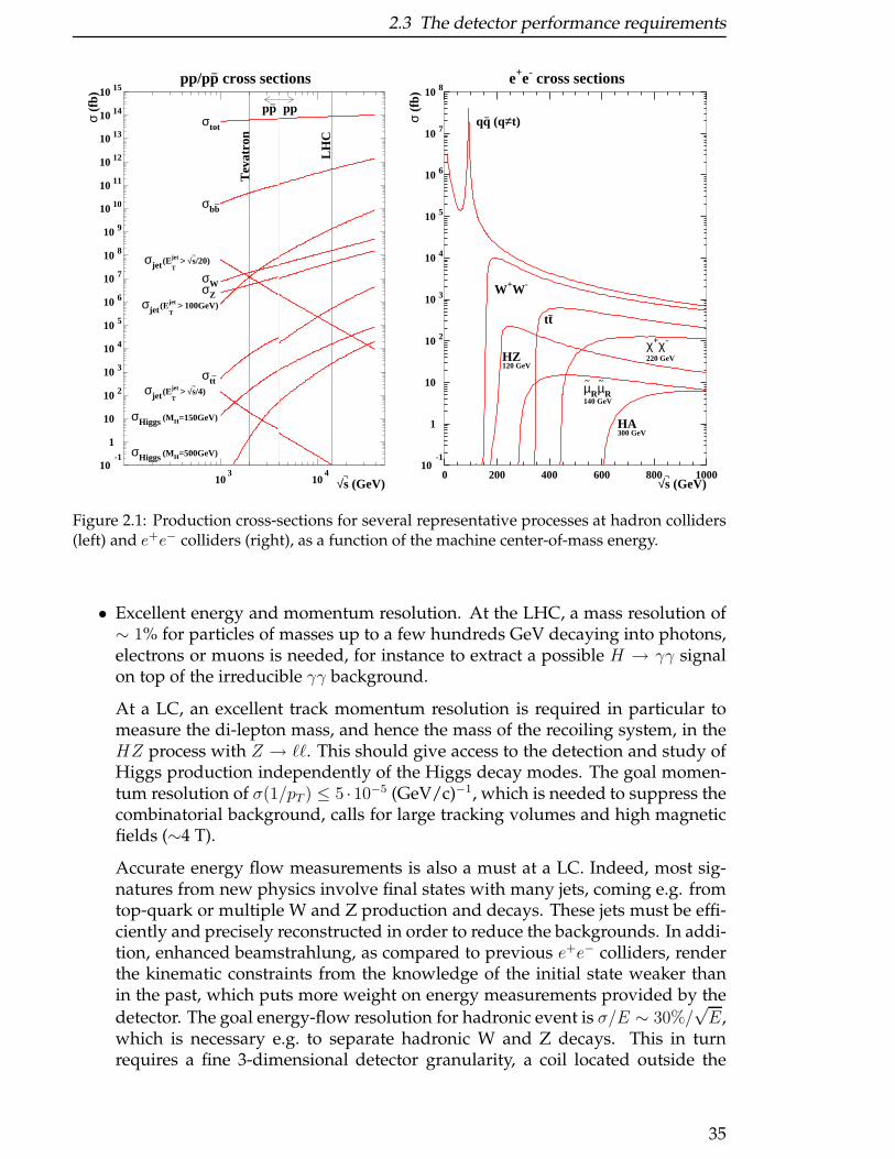
2.3 The detector performance requirements
pp/pp_ cross sections
√s¬ (GeV)
σ (f
b)
σtot
σbb_
σjet(ET
jet > √s¬/20)
σWσZσjet(E
T
jet > 100GeV)
σtt_
σjet(ET
jet > √s¬/4)
σHiggs (MH=150GeV)
σHiggs (MH=500GeV)
pp_
pp
Tev
atro
n
LH
C
10-1
1
10
10 2
10 3
10 4
10 5
10 6
10 7
10 8
10 9
10 10
10 11
10 12
10 13
10 14
10 15
103
104
e+e- cross sections
√s¬ (GeV)
σ (f
b)
qq_ (q≠t)
W+W-
HZ120 GeV
tt_
χ+χ-
220 GeV
µ~
Rµ~
R140 GeV
HA300 GeV
10-1
1
10
10 2
10 3
10 4
10 5
10 6
10 7
10 8
0 200 400 600 800 1000
Figure 2.1: Production cross-sections for several representative processes at hadron colliders(left) and e+e− colliders (right), as a function of the machine center-of-mass energy.
• Excellent energy and momentum resolution. At the LHC, a mass resolution of∼ 1% for particles of masses up to a few hundreds GeV decaying into photons,electrons or muons is needed, for instance to extract a possible H → γγ signalon top of the irreducible γγ background.
At a LC, an excellent track momentum resolution is required in particular tomeasure the di-lepton mass, and hence the mass of the recoiling system, in theHZ process with Z → ℓℓ. This should give access to the detection and study ofHiggs production independently of the Higgs decay modes. The goal momen-tum resolution of σ(1/pT ) ≤ 5 ·10−5 (GeV/c)−1, which is needed to suppress thecombinatorial background, calls for large tracking volumes and high magneticfields (∼4 T).
Accurate energy flow measurements is also a must at a LC. Indeed, most sig-natures from new physics involve final states with many jets, coming e.g. fromtop-quark or multiple W and Z production and decays. These jets must be effi-ciently and precisely reconstructed in order to reduce the backgrounds. In addi-tion, enhanced beamstrahlung, as compared to previous e+e− colliders, renderthe kinematic constraints from the knowledge of the initial state weaker thanin the past, which puts more weight on energy measurements provided by the
detector. The goal energy-flow resolution for hadronic event is σ/E ∼ 30%/√E,
which is necessary e.g. to separate hadronic W and Z decays. This in turnrequires a fine 3-dimensional detector granularity, a coil located outside the
35
2 Experimental Aspects of the LHC and LC
calorimetry in order to minimize the amount of upstream material, and excel-lent detector energy resolution and particle identification capabilities.
• Particle identification. Several stringent requirements on the identification ofelectrons, photons, b-jets, taus, etc. must be satisfied at the LHC in order toreject the huge QCD backgrounds. As an example, excellent electron/jet andphoton/jet separation capabilities are needed. Jets faking photons must be re-jected by a factor of ∼ 103, for a photon efficiency of ∼80%, in order to observea possible H → γγ signal on top of the background. As already mentioned,an unprecedented suppression factor against jets faking electrons of 105− 106 isneeded to extract an inclusive clean electron signal.
At a LC, one of the strongest particle identification requirements is flavor-taggingcapabilities (vertexing), since several channels from New Physics (e.g. SUSY)involve b-quarks or τ -leptons. Moreover, a detailed study of the Higgs sector,which requires the individual measurements of the Higgs decay branching ra-tios into bb, cc, gg, ττ , is only possible with an excellent vertex detector, and aninnermost layer as close as possible to the beam pipe (≤ 2 cm). The goal perfor-mance is to achieve an impact parameter resolution of about 5 µm in both z andRφ.
• At the LC, precision cross section measurements require an excellent luminos-ity measurement (10−4), which has to be matched by equally precise theoreticalpredictions. Luminosity measurement requires fast and highly granular for-ward calorimetry down to angles of approximately 5 mrad. Beam polarizationhas to be determined to a precision of at least 0.5%. A quasi-continuous moni-toring of the differential luminosity spectrum is also necessary.
2.4 Summary of physics capabilities
A detailed discussion of the physics goals of both machines and of their interplay isthe subject of the next Sections of this document.
Here only a few general (and fairly gross) conclusions are given:
• The LHC has the highest mass reach for the direct discovery of new particles.This reach extends up to masses of ∼5-6 TeV for singly-produced electroweakparticles (e.g. possible new gauge bosons W ′ and Z ′), up to ∼7 TeV for singly-produced strongly-interacting particles (e.g. possible excited quarks), and up to∼ 3 TeV for pair-produced SUSY particles with strong interactions.
The direct mass reach of a LC is much more modest, being limited by the avail-able center-of-mass energy to less than 1 TeV for the case considered in this doc-ument. However, due to the cleaner environment, also direct signals of particleswhich are produced with low cross sections or which only decay into hadronsor which leave only a small amount of visible energy in the detector can bediscovered.
• A Linear Collider has an indirect discovery sensitivity to New Physics, throughprecise measurements of known processes (e.g. two-fermion production) and
36

2.4 Summary of physics capabilities
the detection of permil-level deviations from the Standard Model expectation,which extends up to energies of ∼10 TeV. Therefore a 1 TeV LC should be ableto probe New Physics lying at energy scales much higher than the machine
√s
through the measurements of the low-energy (quantum-level) tails of the theory.
Because precise measurements are more difficult at hadron colliders for the rea-sons mentioned above, the LHC indirect sensitivity to New Physics is moremodest, except for some strongly-interacting scenarios (like Compositeness)which are expected to manifest themselves through anomalous contributionsto di-jet production.
• Precision measurements are the strongest asset of a LC. In general, all particlesand processes which are kinematically accessible and produced can be mea-sured with typical precisions ranging from the permil to the percent level, ir-respective of the precise physics scenario. Such a precision allows for the ex-ploration of quantum-level effects and yields the possibility to extrapolate theobservations to energy scales far above the center-of-mass energy in a model-independent way. Ultimately, GUT or Planck scale physics could be probed.
Several precise measurements should also be possible at the LHC, thanks mainlyto the large available event statistics. As an example, if SUSY exists the LHCexperiments should be able to perform several measurements of the sparticlemasses, and therefore to constrain the fundamental parameters of the underly-ing theory to∼ 10% or better (at least in minimal models). Therefore, in additionto being a very powerful and motivated discovery machine, the LHC shouldalso provide a first and possibly quite deep exploration of the structure of NewPhysics. There are however two main limitations. First, in general the extentand the precision of the measurements are poorer than at a LC. For instance,the LHC can only measure some of the Higgs couplings, and with an accuracy(10 − 20%) which is not competitive with that of a LC (∼ 1%). Second, a com-plete, model-independent and conclusive study of the new theory is a priori notgranted and looks difficult in most cases.
These features give rise to a nice complementarity between the two machines, andlead to synergy effects which are discussed in more detail in the rest of this document.
37

2 Experimental Aspects of the LHC and LC
38
Bibliography
[1] J. G. Branson, D. Denegri, I. Hinchliffe, F. Gianotti, F. E. Paige and P. Sphicas[ATLAS and CMS Collaborations], Eur. Phys. J. directC 4 (2002) N1.
[2] ATLAS Collaboration, Technical Design Report, Vol. II, CERN/LHCC/99-15(1999).
[3] CMS Collaboration, Technical Proposal, report CERN/LHCC/94-38 (1994).
[4] J.A. Aguilar-Saavedra et al. [ECFA/DESY LC Physics Working Groups], “TESLATechnical Design Report Part III: Physics at an e+e− Linear Collider”,hep-ph/0106315.
[5] T. Abe et al. [American Linear Collider Working Group], “Linear collider physicsresource book for Snowmass 2001”, hep-ex/0106055 (part 1), hep-ex/0106056(part 2), hep-ex/0106057 (part 3), and hep-ex/0106058 (2001), SLAC-R-570.
[6] K. Abe et al. [ACFA Linear Collider Working Group], “Particle physics experi-ments at JLC”, hep-ph/0109166.
39

Bibliography
40
3 Higgs Physics and Electroweak SymmetryBreaking
Editors: A. De Roeck, H.E. Haber, R. Godbole, J. Gunion, G. Weiglein
The search for the fundamental dynamics that is responsible for electroweak sym-metry breaking is the central challenge for particle physics today. This dynamics,whose fundamental origin is as yet unknown, is ultimately responsible for the gen-eration of the masses of the quarks, charged leptons and the massive gauge bosons.Two broad classes of electroweak symmetry breaking mechanisms have been pur-sued theoretically. In one class of theories, electroweak symmetry breaking dynam-ics is weakly-coupled, and in the second class of theories the dynamics is strongly-coupled.
The electroweak symmetry breaking dynamics that is employed by the StandardModel is governed by a self-interacting complex doublet of scalar fields [1]. TheHiggs potential is chosen so that the neutral component of the scalar doublet acquiresa vacuum expectation value, v = 246 GeV, which sets the mass scale of electroweaksymmetry breaking. Consequently, three massless Goldstone bosons are generatedwhich provide the longitudinal degrees of freedom for the W± and Z0, while thefourth scalar degree of freedom that remains in the physical spectrum is the CP-evenneutral Higgs boson. It is further assumed in the Standard Model that the scalar dou-blet also couples to fermions via the Yukawa interactions. After electroweak sym-metry breaking, these interactions are responsible for the generation of quark andcharged lepton masses. The couplings of the Higgs boson to the Standard Modelparticles is then fixed (and proportional to the corresponding particle mass). How-ever the Higgs mass is proportional to the strength of the Higgs self-coupling, and istherefore not (directly) fixed by present day observations.
Although the Higgs boson has not been directly observed, its virtual effects (pri-marily via its contributions to the W± and Z boson vacuum polarization) can influ-ence electroweak observables. Consequently, one can obtain constraints on the Higgsboson mass (mh) through a global Standard Model fit to the electroweak data. Theresults of the LEP Electroweak Working Group analysis yield [2]: mh = 114+69
−45 GeV,and provides a one-sided 95% CL upper limit of mh < 260 GeV. These results reflectthe logarithmic sensitivity to the Higgs mass via the virtual Higgs loop contributionsto the various electroweak observables. The 95% CL upper limit is consistent withthe direct searches at LEP [3] that show no conclusive evidence for the Higgs boson,and imply that mh > 114.4 GeV at 95% CL. This range of Higgs masses is consistentwith a weakly-coupled Higgs scalar that is the result of the Standard Model scalardynamics.
In the weakly-coupled approach to electroweak symmetry breaking, the StandardModel is very likely embedded in a supersymmetric theory [4] in order to stabilize thelarge energy gap between the electroweak and the Planck scales in a natural way [5].
41
3 Higgs Physics and Electroweak Symmetry Breaking
These theories predict a spectrum of Higgs scalars [6], with an expected mass of thelightest CP-even Higgs boson below 200 GeV [7] (less than 135 GeV in the simplestsupersymmetric models [8]), and a spectrum of additional neutral and charged Higgsbosons with masses up to of order 1 TeV. Moreover, over a significant fraction of thesupersymmetric parameter space, the properties of the lightest Higgs scalar closelyresemble those of the Standard Model (SM) Higgs boson.
An alternative approach to weakly-coupled scalar dynamics posits that electroweaksymmetry breaking is driven by the dynamics of a new strongly-interacting sector ofparticles [9]. Initial models of this kind introduced QCD-like strong interactions nearthe TeV-scale [10], with numerous variations subsequently explored. More recently,so-called “little Higgs models” have been proposed in which the scale of the newstrong interactions is pushed up above 10 TeV [11], and the lightest Higgs scalar re-sembles the weakly-coupled SM Higgs boson. These models typically contain addi-tional particles, such as new gauge bosons and vector-like fermions, which populatethe TeV mass region. In a more speculative direction, a new approach to electroweaksymmetry breaking has been explored in which extra space dimensions beyond theusual 3 + 1 dimensional spacetime are introduced [12] with characteristic sizes oforder (TeV)−1. In scenarios of this type, it is possible to devise a mechanism forelectroweak symmetry breaking that is inherently extra-dimensional [13]. In suchmodels, the resulting phenomenology can be significantly different [14] from thedominant paradigm of the weakly-coupled electroweak symmetry breaking sector.Typically, the spectrum of the TeV-scale will look quite different from the standardweak-coupling approaches. Kaluza-Klein excitations of the Standard Model particlescan play a significant role in the resulting phenomenology. In some cases, the lightHiggs boson is completely absent from the low-energy spectrum, in so-called higgs-less models of electroweak symmetry breaking [15].
Although there is as yet no direct evidence for the origin of electroweak symmetrybreaking dynamics, present data can be used to discriminate among the different ap-proaches. As noted above, the precision electroweak data, accumulated in the pastdecade at LEP, SLC, the Tevatron and elsewhere, seem to be consistent with the Stan-dard Model (or its supersymmetric extension), with a weakly-coupled Higgs bosonwhose mass lies roughly between 100 and 250 GeV [2]. Moreover, the contribution ofnew physics, which can enter through W± and Z boson vacuum polarization correc-tions [16], is severely constrained. This fact has already served to rule out nearly allof the initially proposed models of strongly-coupled electroweak symmetry breakingdynamics, and provides strong constraints on any alternative to the Standard Modeland its supersymmetric extensions.
It is still possible that the Tevatron will yield the first hints of a SM-like Higgs bo-son prior to the start of the LHC. However, the most likely scenario is one where theLHC provides the definitive initial discovery of the physics of the electroweak sym-metry breaking sector [17]. This will be either in the form of a candidate Higgs boson,or evidence that the electroweak symmetry breaking dynamics is driven by somemechanism that does not involve scalar fields in a fundamental way. Any programof Higgs physics at future colliders must address a number of important questions.First, does the SM Higgs boson (or a Higgs scalar with similar properties) exist? Ifyes, how many physical Higgs states are associated with the scalar sector? Moreover,how can one prove that a newly discovered scalar is a Higgs boson? To answer these
42

questions, one must observe the Higgs boson in more than one production and decaychannel, and map out its properties in detail. One must verify that the spin of thecandidate Higgs boson is consistent with spin-zero. It is essential to measure a vari-ety of Higgs couplings and demonstrate that these do indeed scale in proportion tothe corresponding masses. The LHC will be able to address some of these questionswith a program of Higgs measurements that can determine the Higgs couplings tothe top-quark, tau-lepton, W and Z to an accuracy in the range 10–30%, assuming anintegrated luminosity of 300 fb−1 [18]. Note, however, that LHC measurements onlyweakly constrain the Higgs coupling to bb, even though the latter is the dominantHiggs decay channel for Higgs masses below 135 GeV.
To make further progress requires a comprehensive program of precision Higgsmeasurements. Such measurements with typical accuracies in some channels ap-proaching the 1% level, are necessary to fully decipher the dynamics responsible forelectroweak symmetry breaking. Such a program can only be achieved at the LC.The significance of the precision Higgs program is especially evident in the so-calleddecoupling limit [19], in which the properties of the lightest Higgs scalar are nearlyidentical to those of the SM Higgs boson. This limiting case arises in many extendedHiggs theories over a significant fraction of the parameter space. Moreover, addi-tional scalars of the Higgs sector are heavy in the decoupling limit and may not beso easily discovered at the next generation of colliders. Thus precision measurementsthat can distinguish the SM Higgs sector from a more complicated scalar sector areespecially important if only one scalar state is discovered. In particular, small devi-ations from the Standard Model encode the physics of electroweak symmetry break-ing, as well as being sensitive to new physics that lies beyond the Standard Model.
Additional information is required in order to fully probe the underlying scalar dy-namics responsible for electroweak symmetry breaking. Ideally, one aims to recon-struct the Higgs potential and directly demonstrate the mechanism of electroweaksymmetry breaking. This requires precision measurements of Higgs self-couplings,which may only be possible at a very high energy LC. One would like to knowwhether there are CP-violating phenomena associated with the Higgs sector. Nearthe decoupling limit, the couplings of the lightest Higgs boson are CP-conservingto a very good approximation, whereas CP-violating couplings among the heavierHiggs states can be unsuppressed. The former certainly requires the precision Higgsprogram of the LC, whereas the latter may depend on the LHC if the heavier Higgsbosons are too massive to be produced at the LC.
If the Higgs sector is weakly-coupled, one would be very interested in testing theconsistency with the constraints of supersymmetry. In this case, knowledge of thespectrum of supersymmetric particles is especially significant for the precision Higgsprogram. The supersymmetric particle spectrum enters in a crucial way in the ra-diative corrections to Higgs masses and couplings. The LHC and LC are sensitive todifferent aspects of the supersymmetric spectrum, and both machines will providecrucial input data for the theoretical interpretation of the precision Higgs program.
If nature chooses a scenario far from the decoupling limit, then electroweak sym-metry breaking dynamics produces no state that closely resembles the SM Higgs bo-son. In this case, it is likely that there will exist many new light states (below a TeV
43
3 Higgs Physics and Electroweak Symmetry Breaking
in mass) with a rich phenomenology.1 In particular, new approaches to electroweaksymmetry breaking dynamics have led to phenomenologies that may be quite differ-ent from the conventional expectations of weakly coupled multi-Higgs models (withor without supersymmetry). It will be essential to formulate strategies for using pre-cision Higgs studies at future colliders to distinguish among the many possibilities.
This chapter describes a number of studies that exploit the complementarity of theLHC and LC for exploring the origin of electroweak symmetry breaking. Section 3.1focuses on precision studies of the lightest CP-even Higgs boson, with the motiva-tion of determining how close its properties are to that of the SM Higgs boson. Sec-tion 3.2 studies the CP-properties of the Higgs bosons. Section 3.3 focuses on Higgsphysics in the minimal supersymmetric extension of the Standard Model (MSSM),while section 3.4 examines non-minimal approaches (both supersymmetric and non-supersymmetric) to the extended Higgs sector. In section 3.5, Higgs physics in thecontext of extra-dimensional models are studied, and in section 3.6, the consequencesof the so-called littlest Higgs model is explored. Finally, a number of miscellaneoustopics are treated in section 3.7.
3.1 Higgs coupling measurements andflavour-independent Higgs searches
In this section, we examine how complementary measurements from the LHC andthe LC can contribute to the precision Higgs program at future colliders. Here weshall assume that the lightest CP-even Higgs boson of the scalar spectrum has a massin the range of 100 to 200 GeV. This assumption is consistent with the standard in-terpretation of the LEP Higgs search and the implications of the global fit to the pre-cision electroweak data based on the Standard Model (SM). The former implies thatmh > 114.4 GeV at 95% CL [3] (in the context of the MSSM, this limit is somewhatweaker, mh > 91.0 GeV at 95% CL [20]), whereas the latter implies that mh < 260 GeVat 95% CL [2].
The LHC will provide the first opportunity for precision Higgs measurements. Forexample, using methods developed in refs. [21–23], the Higgs couplings to the top-quark, tau-lepton, W and Z can be determined at the LHC to an accuracy in therange 10–30%, assuming an integrated luminosity of 300 fb−1 [18]. At the LC, theexpectations for precision Higgs measurements are well documented [24]. Signifi-cant improvements can be obtained in many channels, approaching accuracies in therange of a few percent or better in a number of cases.
However, there are two important Higgs observables for which the expected accu-racy of the LC running at
√s = 500 GeV is not particularly impressive. These are the
Higgs-top Yukawa coupling and the triple Higgs self-coupling. At the LC, the Higgs-top Yukawa coupling is obtained via measurements of e+e− → tth production and thedetermination of the triple Higgs coupling requires the observation of e+e− → Zhhand/or e+e− → ννW ∗W ∗ → ννhh production. At
√s = 500 GeV, the cross-sections
1The possibility that no light states exist below 1 TeV seems remote given the standard interpretationof the precision electroweak data. Nevertheless, such possibilities cannot yet be excluded withcomplete certainty.
44
3.1 Higgs coupling measurements and flavour-independent Higgs searches
for these processes are quite small (due primarily to the phase space suppression ofthe three and four body final states); consequently, the LC alone can only make crudemeasurements of these Higgs observables, (assuming sufficient luminosity). It is herewhere the LHC can play a strong complementary role. Given the large LHC energyand luminosity, the main challenge for the LHC is to suppress backgrounds efficientlyenough in order to produce a Higgs signal of significance from which the Higgs-topYukawa coupling and the triple Higgs coupling can be extracted.
In this section, we present two studies of the determination of the Higgs-top quarkYukawa coupling. In the contribution of K. Desch and M. Schumacher, an experi-mental method is proposed to determine the Higgs-top quark Yukawa couplings ina model-independent way at the LHC and LC. By combining the results of the mea-surements at both colliders, the most accurate determination of this coupling can beachieved. The contribution of S. Dawson et al. focuses on the theoretical uncertain-ties due to higher order QCD corrections that arise in the computation of the crosssection for tth associated production at the LHC and LC. The detection of a numberof different Higgs decay channels is considered (including bb, W+W−, γγ and τ+τ−).Finally, a brief discussion of the Higgs-top Yukawa coupling determination in theMSSM is given. In the latter case, new channels enter if the non-minimal Higgs statesof the MSSM (H , A and H±) are not too heavy. The complementarity of the LHCand LC for measuring the tth coupling becomes less compelling once higher energiesare available for the LC. For example, for the LC with
√s = 800–1000 GeV and an
integrated luminosity of 1 ab−1, the Higgs-top-quark Yukawa coupling could be de-termined with an accuracy that is significantly more precise than the correspondingtth coupling determination at the LHC.
We also present one study that contrasts the capabilities of the LHC and LC in themeasurement of the triple-Higgs coupling. Ultimately, this is the first step required ina program to experimentally determine the parameters of the Higgs boson potential.Center-of-mass energies at the LC ranging from 500 GeV to 1 TeV were considered.In fact, the lower center-of-mass energy provided the more accurate measurement ofthe triple-Higgs coupling for Higgs masses below about 140 GeV. The prospects fora significant LHC measurement in this mass range are poor. For Higgs masses in therange of 150–200 GeV, the relevant Higgs cross-sections at the LC are becoming toosmall to allow for a useful measurement, whereas LHC data can yield the more accu-rate determination of the triple-Higgs coupling. However, the latter can be reliablyaccomplished only with the input of other precision Higgs properties obtained frommeasurements at the LC. Nevertheless, the initial accuracies for the triple-Higgs cou-plings (formh < 200 GeV) will be crude at best, and higher energy and/or luminositycolliders will be needed to make significant improvements.
Most of the above discussion assumes a pattern of Higgs boson partial widths thatis close to the Standard Model expectations. However, if this assumption provesfalse, the Higgs search strategies (for both discovery and precision measurements)will have to be reconsidered. For example, flavor-independent techniques can be crit-ical for Higgs searches if the theory of the Higgs sector deviates from Standard Modelexpectations. In the contribution of E.L. Berger, T.M.P. Tait and C.E.M. Wagner, thephenomenology of a Higgs boson that decays predominantly into jets of hadrons withno significant b-quark flavor content is examined. This condition may be realized, forinstance, in supersymmetric models in which a light bottom squark is present in the
45
3 Higgs Physics and Electroweak Symmetry Breaking
spectrum and in models in which the dominant Higgs decay is into a pair of of lightCP-odd scalars. Berger et al. emphasize that in these scenarios, the viability of thestandard Higgs discovery channels at the LHC (say, formh = 120 GeV) is significantlydegraded. In contrast, the Higgs discovery potential and precision Higgs measure-ments at the LC are generally much less sensitive to assumptions about the specificpattern of Higgs partial widths. In particular, the Higgs boson can be observed (andits mass determined) independently of its final state decays in hZ production via themissing mass recoiling against the Z.
In probing the physics of the Higgs sector, it is essential to elucidate the natureof the TeV-scale physics associated with the mechanism of electroweak symmetrybreaking. The well known naturalness arguments associated with understanding theorigin of the electroweak scale make plausible the existence of new TeV-scale physicsbeyond the Standard Model. In nearly all models considered, the LHC, with its enor-mous energy and luminosity, is ideally suited to discover the new TeV-scale phenom-ena, and provide the initial opportunity for probing the underlying new dynamics.Thus, even if the observation of Higgs bosons at the LHC is problematical or ambigu-ous, one anticipates a rich phenomenology of TeV-scale physics that is accessible tothe LHC. At the LC, the success of the Higgs program for mh <∼ 200 GeV is guaran-teed, independently of the details of the Higgs model. This illustrates another way inwhich the complementarity of the LHC and the LC can be essential for providing abroad understanding of the physics of electroweak symmetry breaking.
3.1.1 Model independent determination of the top Yukawacoupling from LHC and LC
K. Desch and M. Schumacher
3.1.1.1 Motivation
The Yukawa coupling of the Higgs boson to the heaviest quark, the top quark, is ofgreat interest for the study of the nature of electroweak symmetry breaking and thegeneration of masses. While the Yukawa couplings to bottom and charm quarks andto tau leptons and muons are in principle accessible through the Higgs boson decaybranching ratios, the Higgs boson decay into top quark pairs is kinematically forbid-den for light Higgs bosons as they are favoured by theory and electroweak precisiondata. The only Standard Model process that probes the top Yukawa coupling at treelevel is the associated production of a tt pair with a Higgs boson. This process occursat the LHC (mainly gg→ttH0) as well as at the LC ( e+e−→ttH0). In the latter casethe cross section is only significant at centre–of–mass energies in excess of 800 GeV.At the LHC, the final states that have been investigated so far are ttbb [25–28] andttW+W− [29, 30], the ttτ+τ− final state is under study [31, 32]. At tree level, theirproduction rates are proportional to g2
ttH BR(H0 → bb) and g2ttH BR(H0 → W+W−),
respectively. The absolute values of BR(H0 → bb) and BR(H0 → W+W−) can bemeasured accurately in a model independent way at the LC from the correspondingdecay branching ratios [33]. These can be measured already at a first phase of the LC(√s between 350 and 500 GeV). Thus, the combination of the measurements of both
46
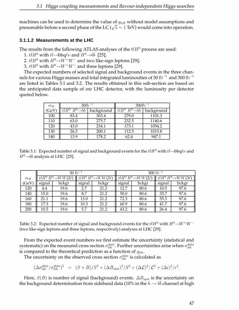
3.1 Higgs coupling measurements and flavour-independent Higgs searches
machines can be used to determine the value of gttH without model assumptions andpresumable before a second phase of the LC (
√s ∼ 1 TeV) would come into operation.
3.1.1.2 Measurements at the LHC
The results from the following ATLAS analyses of the ttH0 process are used:1. ttH0 with tt→bbqℓν and H0→bb [25];2. ttH0 with H0→W+W− and two like-sign leptons [29];3. ttH0 with H0→W+W− and three leptons [29].The expected numbers of selected signal and background events in the three chan-
nels for various Higgs masses and total integrated luminosities of 30 fb−1 and 300 fb−1
are listed in Tables 3.1 and 3.2. The results obtained in this sub-section are based onthe anticipated data sample of one LHC detector, with the luminosity per detectorquoted below.
mH 30fb−1 300fb−1
(GeV) ttH0 H0→bb background ttH0 H0→bb background100 83.4 303.4 279.0 1101.3110 63.0 275.7 232.5 1140.6120 43.0 234.1 173.1 1054.2130 26.5 200.1 112.5 1015.8140 13.9 178.2 62.4 947.1
Table 3.1: Expected number of signal and background events for the ttH0 with tt→bbqℓν andH0→bb analysis at LHC [25].
30 fb−1 300 fb−1
mH ttH0H0→WW (2ℓ) ttH0H0→WW (3ℓ) ttH0H0→WW (2ℓ) ttH0H0→WW (3ℓ)(GeV) signal bckgr signal bckgr signal bckgr signal bckgr
120 4.4 19.6 2.7 21.2 12.7 80.6 10.5 97.6140 15.0 19.6 8.7 21.2 50.0 80.6 33.7 97.6160 21.1 19.6 13.0 21.2 72.3 80.6 55.3 97.6180 17.3 19.6 10.3 21.2 60.9 80.6 41.7 97.6200 10.5 19.6 5.7 21.2 43.2 80.6 26.4 97.6
Table 3.2: Expected number of signal and background events for the ttH0 with H0→W+W−
(two like-sign leptons and three leptons, respectively) analyses at LHC [29].
From the expected event numbers we first estimate the uncertainty (statistical andsystematic) on the measured cross section σdatatth . Further uncertainties arise when σdatatth
is compared to the theoretical prediction as a function of gtth.The uncertainty on the observed cross section σdatatth is calculated as
(∆σdatatth /σdatatth )2 = (S +B)/S2 + (∆Bsyst)2/S2 + (∆L)2/L2 + (∆ǫ)2/ǫ2.
Here, S(B) is number of signal (background) events. ∆Bsyst is the uncertainty onthe background determination from sideband data (10% in the h→ bb channel at high
47
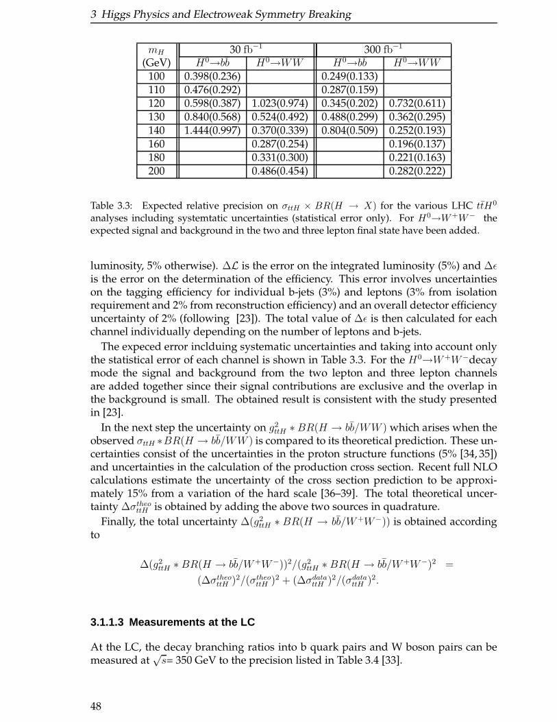
3 Higgs Physics and Electroweak Symmetry Breaking
mH 30 fb−1 300 fb−1
(GeV) H0→bb H0→WW H0→bb H0→WW100 0.398(0.236) 0.249(0.133)110 0.476(0.292) 0.287(0.159)120 0.598(0.387) 1.023(0.974) 0.345(0.202) 0.732(0.611)130 0.840(0.568) 0.524(0.492) 0.488(0.299) 0.362(0.295)140 1.444(0.997) 0.370(0.339) 0.804(0.509) 0.252(0.193)160 0.287(0.254) 0.196(0.137)180 0.331(0.300) 0.221(0.163)200 0.486(0.454) 0.282(0.222)
Table 3.3: Expected relative precision on σttH × BR(H → X) for the various LHC ttH0
analyses including systemtatic uncertainties (statistical error only). For H0→W+W− theexpected signal and background in the two and three lepton final state have been added.
luminosity, 5% otherwise). ∆L is the error on the integrated luminosity (5%) and ∆ǫis the error on the determination of the efficiency. This error involves uncertaintieson the tagging efficiency for individual b-jets (3%) and leptons (3% from isolationrequirement and 2% from reconstruction efficiency) and an overall detector efficiencyuncertainty of 2% (following [23]). The total value of ∆ǫ is then calculated for eachchannel individually depending on the number of leptons and b-jets.
The expeced error inclduing systematic uncertainties and taking into account onlythe statistical error of each channel is shown in Table 3.3. For the H0→W+W−decaymode the signal and background from the two lepton and three lepton channelsare added together since their signal contributions are exclusive and the overlap inthe background is small. The obtained result is consistent with the study presentedin [23].
In the next step the uncertainty on g2ttH ∗BR(H → bb/WW ) which arises when the
observed σttH ∗BR(H → bb/WW ) is compared to its theoretical prediction. These un-certainties consist of the uncertainties in the proton structure functions (5% [34, 35])and uncertainties in the calculation of the production cross section. Recent full NLOcalculations estimate the uncertainty of the cross section prediction to be approxi-mately 15% from a variation of the hard scale [36–39]. The total theoretical uncer-tainty ∆σtheottH is obtained by adding the above two sources in quadrature.
Finally, the total uncertainty ∆(g2ttH ∗ BR(H → bb/W+W−)) is obtained according
to
∆(g2ttH ∗BR(H → bb/W+W−))2/(g2
ttH ∗BR(H → bb/W+W−)2 =
(∆σtheottH )2/(σtheottH )2 + (∆σdatattH )2/(σdatattH )2.
3.1.1.3 Measurements at the LC
At the LC, the decay branching ratios into b quark pairs and W boson pairs can bemeasured at
√s= 350 GeV to the precision listed in Table 3.4 [33].
48
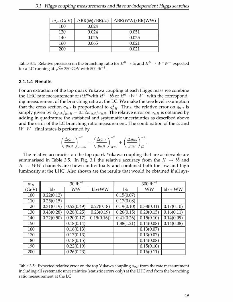
3.1 Higgs coupling measurements and flavour-independent Higgs searches
mH (GeV) ∆BR(bb)/BR(bb) ∆BR(WW)/BR(WW)100 0.024120 0.024 0.051140 0.026 0.025160 0.065 0.021200 0.021
Table 3.4: Relative precision on the branching ratio for H0 → bb and H0 →W+W− expectedfor a LC running at
√s= 350 GeV with 500 fb−1.
3.1.1.4 Results
For an extraction of the top quark Yukawa coupling at each Higgs mass we combinethe LHC rate measurement of ttH0with H0→bb or H0→W+W− with the correspond-ing measurement of the branching ratio at the LC. We make the tree level assumptionthat the cross section σttH is proportional to g2
ttH . Thus, the relative error on gttH issimply given by ∆gtth/gttH = 0.5∆σttH/σttH . The relative error on σttH is obtained byadding in quadrature the statistical and systematic uncertainties as described aboveand the error of the LC branching ratio measurement. The combination of the bb andW+W− final states is performed by
(∆gtthgttH
)−2
comb.
=
(∆gtthgttH
)−2
WW
+
(∆gtthgttH
)−2
bb
.
The relative accuracies on the top quark Yukawa coupling that are achievable aresummarised in Table 3.5. In Fig. 3.1 the relative accuracy from the H → bb andH → WW channels are shown individually and combined both for low and highluminosity at the LHC. Also shown are the results that would be obtained if all sys-
mH 30 fb−1 300 fb−1
(GeV) bb WW bb+WW bb WW bb + WW100 0.22(0.12) 0.15(0.07)110 0.25(0.15) 0.17(0.08)120 0.31(0.19) 0.52(0.49) 0.27(0.18) 0.19(0.10) 0.38(0.31) 0.17(0.10)130 0.43(0.28) 0.28(0.25) 0.23(0.19) 0.26(0.15) 0.20(0.15) 0.16(0.11)140 0.72(0.50) 0.20(0.17) 0.19(0.16)) 0.41(0.26) 0.15(0.10) 0.14(0.09)150 0.18(0.14) 1.88(1.21) 0.14(0.08) 0.14(0.08)160 0.16(0.13) 0.13(0.07)170 0.17(0.13) 0.13(0.07)180 0.18(0.15) 0.14(0.08)190 0.22(0.19) 0.15(0.10)200 0.26(0.23) 0.16(0.11)
Table 3.5: Expected relative error on the top Yukawa coupling gttH from the rate measurementincluding all systematic uncertainties (statistic errors only) at the LHC and from the branchingratio measurement at the LC.
49
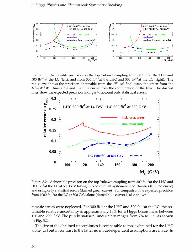
3 Higgs Physics and Electroweak Symmetry Breaking
MH (GeV)
rela
tive
err
or o
n g tt
H
LHC 30 fb-1 at 14 TeV+LC 500 fb-1 at 500 GeV
H → bb H → WWcombinedcombined (stat. error only)
0
0.1
0.2
0.3
0.4
0.5
0.6
100 120 140 160 180 200MH (GeV)
rela
tive
err
or o
n g tt
H
LHC 300 fb-1 at 14 TeV+ LC 500 fb-1 at 500 GeV
H → bb H → WWcombinedcombined (stat. error only)
0
0.1
0.2
0.3
0.4
0.5
0.6
100 120 140 160 180 200
Figure 3.1: Achievable precision on the top Yukawa coupling from 30 fb−1at the LHC and500 fb−1at the LC (left), and from 300 fb−1at the LHC and 500 fb−1at the LC (right). Thered curve shows the precision obtainable from the H0→bb final state, the green from theH0→W+W− final state and the blue curve from the combination of the two. The dashedlines show the expected precision taking into account only statistical errors.
MH (GeV)
rela
tive
err
or o
n g tt
H
LHC 300 fb-1 at 14 TeV + LC 500 fb-1 at 500 GeV
incl. syst. error
stat. error only
LC 1000 fb-1 at 800 GeV
0
0.05
0.1
0.15
0.2
0.25
0.3
100 120 140 160 180 200
Figure 3.2: Achievable precision on the top Yukawa coupling from 300 fb−1at the LHC and500 fb−1at the LC at 500 GeV taking into account all systematic uncertainties (full red curve)and using only statistical errors (dashed green curve) . For comparison the expected precisionfrom 1000 fb−1at the LC at 800 GeV alone (dotted blue curve) is also shown.
tematic errors were neglected. For 300 fb−1at the LHC and 500 fb−1at the LC, the ob-tainable relative uncertainty is approximately 15% for a Higgs boson mass between120 and 200 GeV. The purely statisical uncertainty ranges from 7% to 11% as shownin Fig. 3.2.
The size of the obtained uncertainties is comparable to those obtained for the LHCalone [23] but in contrast to the latter no model-dependent assumptions are made. In
50
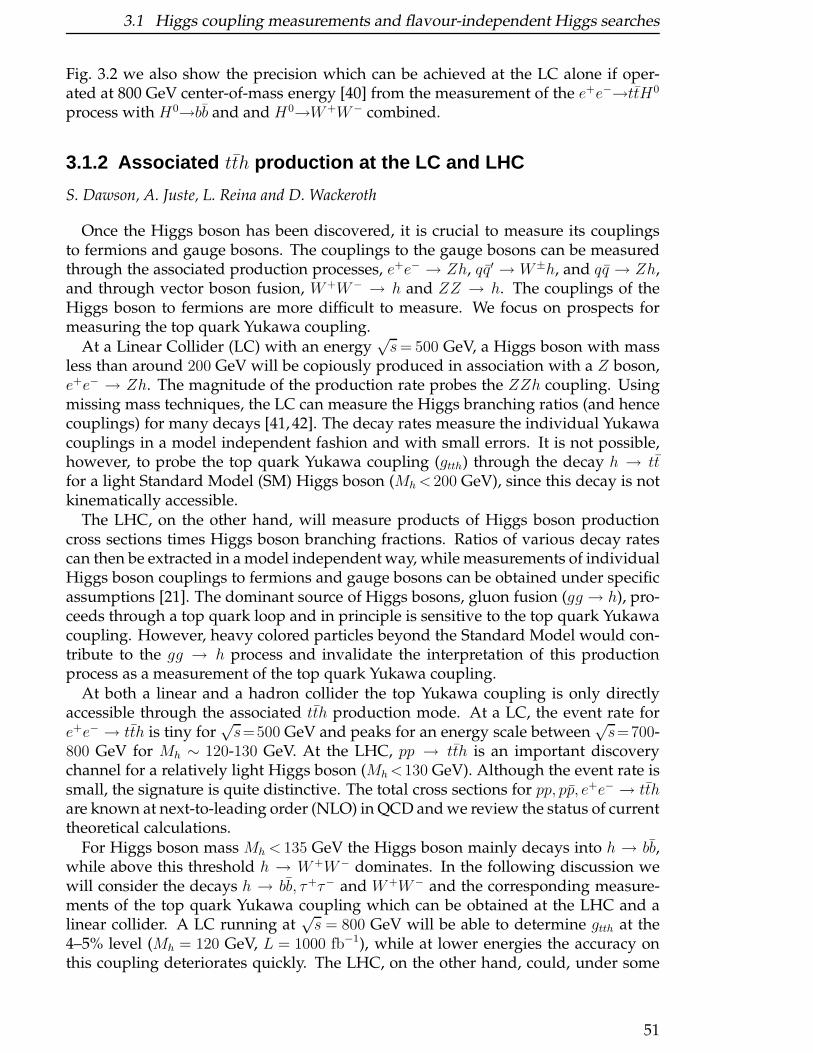
3.1 Higgs coupling measurements and flavour-independent Higgs searches
Fig. 3.2 we also show the precision which can be achieved at the LC alone if oper-ated at 800 GeV center-of-mass energy [40] from the measurement of the e+e−→ttH0
process with H0→bb and and H0→W+W− combined.
3.1.2 Associated tth production at the LC and LHC
S. Dawson, A. Juste, L. Reina and D. Wackeroth
Once the Higgs boson has been discovered, it is crucial to measure its couplingsto fermions and gauge bosons. The couplings to the gauge bosons can be measuredthrough the associated production processes, e+e− → Zh, qq′ → W±h, and qq → Zh,and through vector boson fusion, W+W− → h and ZZ → h. The couplings of theHiggs boson to fermions are more difficult to measure. We focus on prospects formeasuring the top quark Yukawa coupling.
At a Linear Collider (LC) with an energy√s= 500 GeV, a Higgs boson with mass
less than around 200 GeV will be copiously produced in association with a Z boson,e+e− → Zh. The magnitude of the production rate probes the ZZh coupling. Usingmissing mass techniques, the LC can measure the Higgs branching ratios (and hencecouplings) for many decays [41, 42]. The decay rates measure the individual Yukawacouplings in a model independent fashion and with small errors. It is not possible,however, to probe the top quark Yukawa coupling (gtth) through the decay h → ttfor a light Standard Model (SM) Higgs boson (Mh< 200 GeV), since this decay is notkinematically accessible.
The LHC, on the other hand, will measure products of Higgs boson productioncross sections times Higgs boson branching fractions. Ratios of various decay ratescan then be extracted in a model independent way, while measurements of individualHiggs boson couplings to fermions and gauge bosons can be obtained under specificassumptions [21]. The dominant source of Higgs bosons, gluon fusion (gg → h), pro-ceeds through a top quark loop and in principle is sensitive to the top quark Yukawacoupling. However, heavy colored particles beyond the Standard Model would con-tribute to the gg → h process and invalidate the interpretation of this productionprocess as a measurement of the top quark Yukawa coupling.
At both a linear and a hadron collider the top Yukawa coupling is only directlyaccessible through the associated tth production mode. At a LC, the event rate fore+e− → tth is tiny for
√s=500 GeV and peaks for an energy scale between
√s=700-
800 GeV for Mh ∼ 120-130 GeV. At the LHC, pp → tth is an important discoverychannel for a relatively light Higgs boson (Mh<130 GeV). Although the event rate issmall, the signature is quite distinctive. The total cross sections for pp, pp, e+e− → tthare known at next-to-leading order (NLO) in QCD and we review the status of currenttheoretical calculations.
For Higgs boson mass Mh < 135 GeV the Higgs boson mainly decays into h → bb,while above this threshold h → W+W− dominates. In the following discussion wewill consider the decays h → bb, τ+τ− and W+W− and the corresponding measure-ments of the top quark Yukawa coupling which can be obtained at the LHC and alinear collider. A LC running at
√s = 800 GeV will be able to determine gtth at the
4–5% level (Mh = 120 GeV, L = 1000 fb−1), while at lower energies the accuracy onthis coupling deteriorates quickly. The LHC, on the other hand, could, under some
51
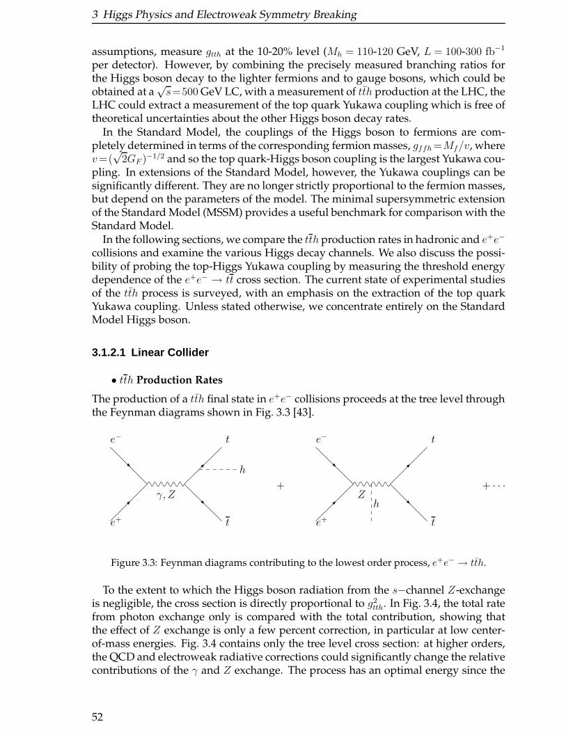
3 Higgs Physics and Electroweak Symmetry Breaking
assumptions, measure gtth at the 10-20% level (Mh = 110-120 GeV, L = 100-300 fb−1
per detector). However, by combining the precisely measured branching ratios forthe Higgs boson decay to the lighter fermions and to gauge bosons, which could beobtained at a
√s=500 GeV LC, with a measurement of tth production at the LHC, the
LHC could extract a measurement of the top quark Yukawa coupling which is free oftheoretical uncertainties about the other Higgs boson decay rates.
In the Standard Model, the couplings of the Higgs boson to fermions are com-pletely determined in terms of the corresponding fermion masses, gffh=Mf/v, wherev=(√
2GF )−1/2 and so the top quark-Higgs boson coupling is the largest Yukawa cou-pling. In extensions of the Standard Model, however, the Yukawa couplings can besignificantly different. They are no longer strictly proportional to the fermion masses,but depend on the parameters of the model. The minimal supersymmetric extensionof the Standard Model (MSSM) provides a useful benchmark for comparison with theStandard Model.
In the following sections, we compare the tth production rates in hadronic and e+e−
collisions and examine the various Higgs decay channels. We also discuss the possi-bility of probing the top-Higgs Yukawa coupling by measuring the threshold energydependence of the e+e− → tt cross section. The current state of experimental studiesof the tth process is surveyed, with an emphasis on the extraction of the top quarkYukawa coupling. Unless stated otherwise, we concentrate entirely on the StandardModel Higgs boson.
3.1.2.1 Linear Collider
• tth Production Rates
The production of a tth final state in e+e− collisions proceeds at the tree level throughthe Feynman diagrams shown in Fig. 3.3 [43].
+γ, Z
e−
e+
h
t
t
+ · · ·Z
e−
e+
h
t
t
Figure 3.3: Feynman diagrams contributing to the lowest order process, e+e− → tth.
To the extent to which the Higgs boson radiation from the s−channel Z-exchangeis negligible, the cross section is directly proportional to g2
tth. In Fig. 3.4, the total ratefrom photon exchange only is compared with the total contribution, showing thatthe effect of Z exchange is only a few percent correction, in particular at low center-of-mass energies. Fig. 3.4 contains only the tree level cross section: at higher orders,the QCD and electroweak radiative corrections could significantly change the relativecontributions of the γ and Z exchange. The process has an optimal energy since the
52

3.1 Higgs coupling measurements and flavour-independent Higgs searches
80.0 120.0 160.0 200.0 240.0Mh (GeV)
10−2
10−1
100
101
σ (f
b)
γ onlyComplete
√s=1 TeV
√s=500 GeV
Figure 3.4: Lowest order cross section for e+e− → tth at√s= 500 GeV and
√s= 1 TeV. The
curve labeled complete includes both γ and Z exchange, along with bremsstrahlung from theZ boson [44].
rate peaks around√s∼700-800 GeV (σtth≃2.5 fb for Mh∼120 GeV). At
√s=500 GeV
and for Mh∼120 GeV, the cross section is of order 0.5 fb.
QED corrections due to initial state radiation effects (bremsstrahlung and beam-trahlung, the former being dominant) significantly distort the tth lineshape. Themain effect is to shift the maximum of the cross section towards higher
√s. As a
result, the cross section at√s=500 GeV is reduced by a factor ≃2, i.e. σtth ≃0.2 fb for
Mh ∼ 120 GeV [45, 46].
The first order QCD corrections to this process, which turn out to be important nearthe tt threshold, have been computed including only γ exchange in Ref. [44] and withthe complete γ and Z contributions in Ref. [47]. The QCD corrected rate, as a functionof Mh and for different center-of-mass energies, is compared to the uncorrected onein Fig. 3.5. At
√s = 500 GeV, the corrections are large and positive, with a strong
dependence on Mh (KNLO ≃ 1.5, for µ=√s and Mh = 120 GeV). At
√s= 1 TeV, they
are small and negative (KNLO ≃ 0.9, for µ=√s), and essentially independent of Mh.
The only scale dependence at NLO is the running of the strong coupling constant,αs(µ). Changing the scale parameter by a factor of 2 induces roughly a 10% change inσNLO, indicating that higher order QCD corrections may be important to match theexperimental precision of a high energy LC.
The electroweak corrections to e+e− → tth are also important and have been com-puted by three groups [48–50]. At
√s = 500 GeV, the QCD corrections are signifi-
cantly larger than the electroweak corrections, while at√s = 1 TeV, the electroweak
corrections are roughly the same size as the QCD corrections but opposite in sign, asshown in Fig. 3.6.
53
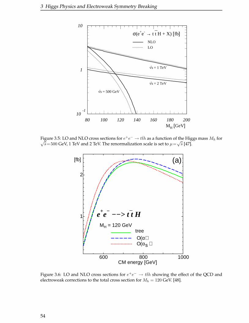
3 Higgs Physics and Electroweak Symmetry Breaking
10-1
1
10
80 100 120 140 160 180 200
σ(e+e- → t t H + X) [fb]¯
MH [GeV]
√s = 1 TeV
√s = 2 TeV
√s = 500 GeV
NLO
LO
Figure 3.5: LO and NLO cross sections for e+e− → tth as a function of the Higgs mass Mh for√s=500 GeV, 1 TeV and 2 TeV. The renormalization scale is set to µ=
√s [47].
600 800 1000
1
2
[fb]
CM energy [GeV]
e+e− −−> t t HMH = 120 GeV
treeΟ(α)Ο(α )s
_
(a)
Figure 3.6: LO and NLO cross sections for e+e− → tth showing the effect of the QCD andelectroweak corrections to the total cross section for Mh = 120 GeV. [48].
54
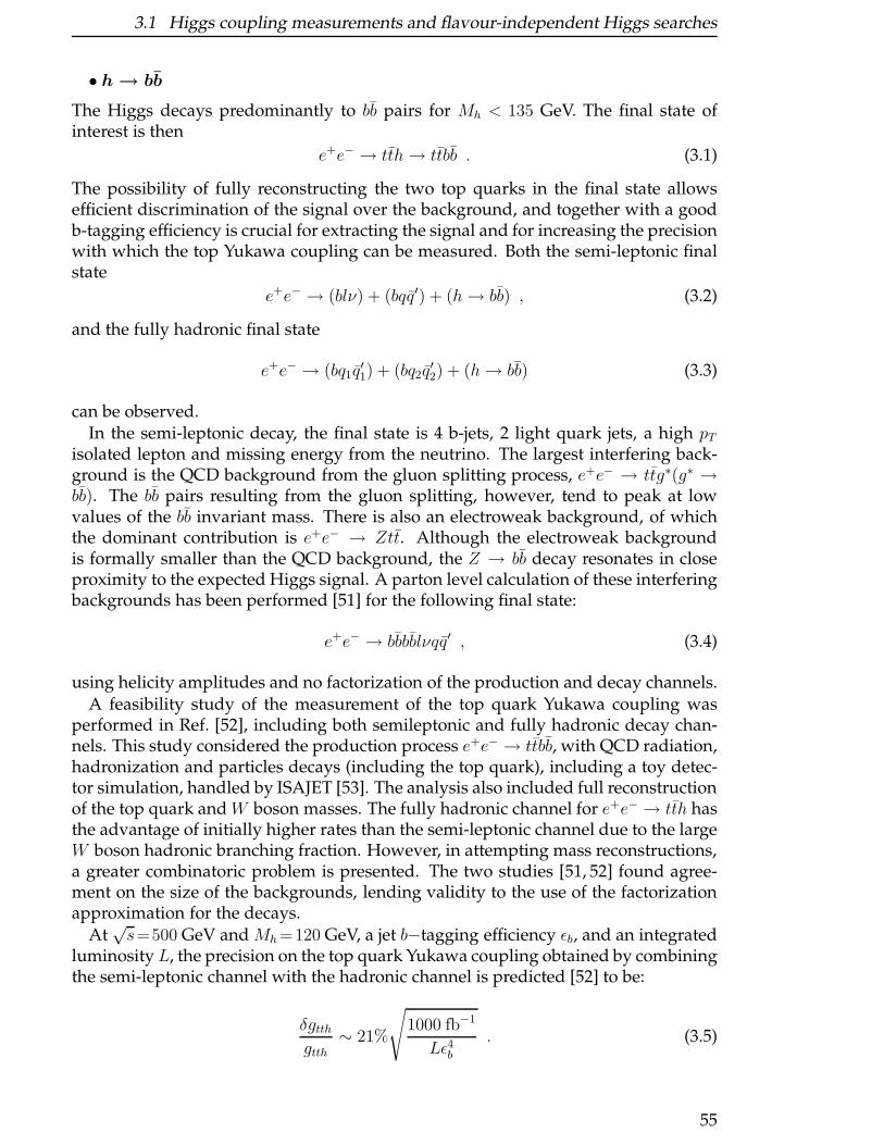
3.1 Higgs coupling measurements and flavour-independent Higgs searches
• h → bb
The Higgs decays predominantly to bb pairs for Mh < 135 GeV. The final state ofinterest is then
e+e− → tth→ ttbb . (3.1)
The possibility of fully reconstructing the two top quarks in the final state allowsefficient discrimination of the signal over the background, and together with a goodb-tagging efficiency is crucial for extracting the signal and for increasing the precisionwith which the top Yukawa coupling can be measured. Both the semi-leptonic finalstate
e+e− → (blν) + (bqq′) + (h→ bb) , (3.2)
and the fully hadronic final state
e+e− → (bq1q′1) + (bq2q
′2) + (h→ bb) (3.3)
can be observed.In the semi-leptonic decay, the final state is 4 b-jets, 2 light quark jets, a high pT
isolated lepton and missing energy from the neutrino. The largest interfering back-ground is the QCD background from the gluon splitting process, e+e− → ttg∗(g∗ →bb). The bb pairs resulting from the gluon splitting, however, tend to peak at lowvalues of the bb invariant mass. There is also an electroweak background, of whichthe dominant contribution is e+e− → Ztt. Although the electroweak backgroundis formally smaller than the QCD background, the Z → bb decay resonates in closeproximity to the expected Higgs signal. A parton level calculation of these interferingbackgrounds has been performed [51] for the following final state:
e+e− → bbbblνqq′ , (3.4)
using helicity amplitudes and no factorization of the production and decay channels.A feasibility study of the measurement of the top quark Yukawa coupling was
performed in Ref. [52], including both semileptonic and fully hadronic decay chan-nels. This study considered the production process e+e− → ttbb, with QCD radiation,hadronization and particles decays (including the top quark), including a toy detec-tor simulation, handled by ISAJET [53]. The analysis also included full reconstructionof the top quark and W boson masses. The fully hadronic channel for e+e− → tth hasthe advantage of initially higher rates than the semi-leptonic channel due to the largeW boson hadronic branching fraction. However, in attempting mass reconstructions,a greater combinatoric problem is presented. The two studies [51, 52] found agree-ment on the size of the backgrounds, lending validity to the use of the factorizationapproximation for the decays.
At√s=500 GeV and Mh=120 GeV, a jet b−tagging efficiency ǫb, and an integrated
luminosity L, the precision on the top quark Yukawa coupling obtained by combiningthe semi-leptonic channel with the hadronic channel is predicted [52] to be:
δgtthgtth
∼ 21%
√1000 fb−1
Lǫ4b. (3.5)
55
3 Higgs Physics and Electroweak Symmetry Breaking
For Mh=130 GeV, the precision declines to
δgtthgtth
∼ 44%
√1000 fb−1
Lǫ4b, (3.6)
primarily due to the suppression of the rate for the heavier Higgs mass.A more detailed preliminary study was performed for
√s = 500 GeV and L =
1000 fb−1, assumingMh=120 GeV, and considering so far only the semileptonic chan-nel [46]. The analysis included both reducible and irreducible backgrounds, realisticdetector effects, and reconstruction efficiencies. The main sources of efficiency lossare from limitations of the jet-clustering algorithm and b-tagging performances in ahigh jet multiplicity environment. Signal and backgrounds are discriminated by mak-ing use of a combination of highly efficient preselections and multivariate techniquesinvolving Neural Networks. Because of the large backgrounds, it is crucial that theyare well modeled both in normalization and shape. A conservative estimate of 5% inthe overall background normalization was included. The estimated total uncertaintyin the top quark Yukawa coupling is approximately 33%. From the optimization ofthis analysis (improved b-tagging performance, dedicated τ selections, extensive useof kinematical information), together with the combination with the hadronic channeland using NLO K-factors, an ultimate accuracy of ≤ 20% is expected. The increasedsignal rate and reduced non-interfering backgrounds at higher
√s allow for a more
precise measurement of the top quark Yukawa coupling.A feasibility study [45], comparable in level of sophistication to the previous one,
but considering both semileptonic and hadronic decay channels at√s=800 GeV and
for Mh = 120 GeV, has been performed. Assuming L= 1000 fb−1, the estimated totaluncertainty in the top-Higgs Yukawa coupling is:
δgtthgtth
∼ 5.5% . (3.7)
Including only the statistical error, the precision becomes 4.2%.
• h → WW ∗
Within the SM and forMh≃135 GeV, the branching ratio for h→WW ∗ is comparablein size with that for h → bb. For larger Higgs masses, h → WW ∗ becomes the domi-nant decay mode. Therefore, it is important to explore the potential of this channel tofurther increase the sensitivity to the top-Higgs decay Yukawa coupling up to highervalues of Mh.
The process under consideration contains 4 W bosons and 2 b-jets in the final state:
e+e− → tth→W+bW−bWW ∗. (3.8)
The final state is fully determined by the W boson decay modes, thus offering awide variety of experimental signatures:
fully hadronic (10 jets) : BR ≃ 20.8% ;
semileptonic (1 lepton + 8 jets) : BR ≃ 40.0% ;
56
3.1 Higgs coupling measurements and flavour-independent Higgs searches
2 opposite− sign leptons + 6 jets : BR ≃ 19.3% ;
2 same− sign leptons + 6 jets : BR ≃ 9.6% ;
3 leptons + 4 jets : BR ≃ 9.3% ;
4 leptons + 2 jets : BR ≃ 1.0% .
A feasibility study has been performed for√s= 800 GeV in the “2 same-sign lep-
tons+jets” final state [40]. This channel is expected to have low backgrounds andtherefore a relatively simple topological selection appears to be sufficient. A 5% sys-tematic uncertainty in the overall background normalization has been included. As-suming L= 1000 fb−1, the estimated total uncertainty in the top-Higgs Yukawa cou-pling is found to be ≃ 15% for 140≤Mh≤180 GeV.
In terms of statistics, the semileptonic channel is the most promising one, althoughthe backgrounds are expected to be much larger that for the “2 same-sign leptons+jets”one. This process could be analyzed with a similar strategy to the one applied to thesemileptonic channel in e+e− → tth(h → bb). Indeed, the increased jet multiplicityin the final state makes it more challenging. Preliminary studies [54, 55] indicate asignificant improvement in the total uncertainty on gtth by combining it with the “2same-sign leptons+jets” channel.
Finally, the results of Refs. [54, 55] suggest that the combination of the h → bb andh→ WW ∗ decay channels could yield an ultimate uncertainty of
δgtthgtth≤15% (3.9)
for Mh≤200 GeV, assuming√s=800 GeV and L=1000 fb−1.
• tt Threshold Scan
The total cross section for e+e− → tt as a function of center-of-mass energy is quitesensitive to the top quark mass, mt, [56]. It is also sensitive to a lesser degree to thestrong coupling constant αs, the total top quark decay width, Γt, and the top quarkYukawa coupling, gtth. By measuring the threshold energy dependence of the for-ward backward asymmetry and the position of the peak of the top quark momentumdistribution, additional sensitivity to Γt and gtth can be obtained [57,58], although thesensitivity to the top quark Yukawa coupling is quite small in all observables.
The total e+e− → tt cross section at threshold has been calculated including someof the next-to-next-to-leading logarithms, [59]. The complete set of next-to-next-to-leading logarithmic contributions is not yet complete, but the large size of the cor-rections relative to the next-to-leading logarithmic terms [60] suggests that the un-certainty on the cross section measurement will be slightly larger than previouslyestimated, δσtt/σtt ∼ ±6%.
In Ref. [58] an experimental study of the precision on gtth has been performed whichwe will summarize in the following. The study assumes an integrated luminosity of300 fb−1 and Mh = 120 GeV. Theoretical predictions are based on the TOPPIK pro-gram [61]. By fixing all variables except gtth and assuming a 3% systematic uncer-tainty on the total cross section, a measurement of
δgtthgtth
= +0.18−0.25 (3.10)
57
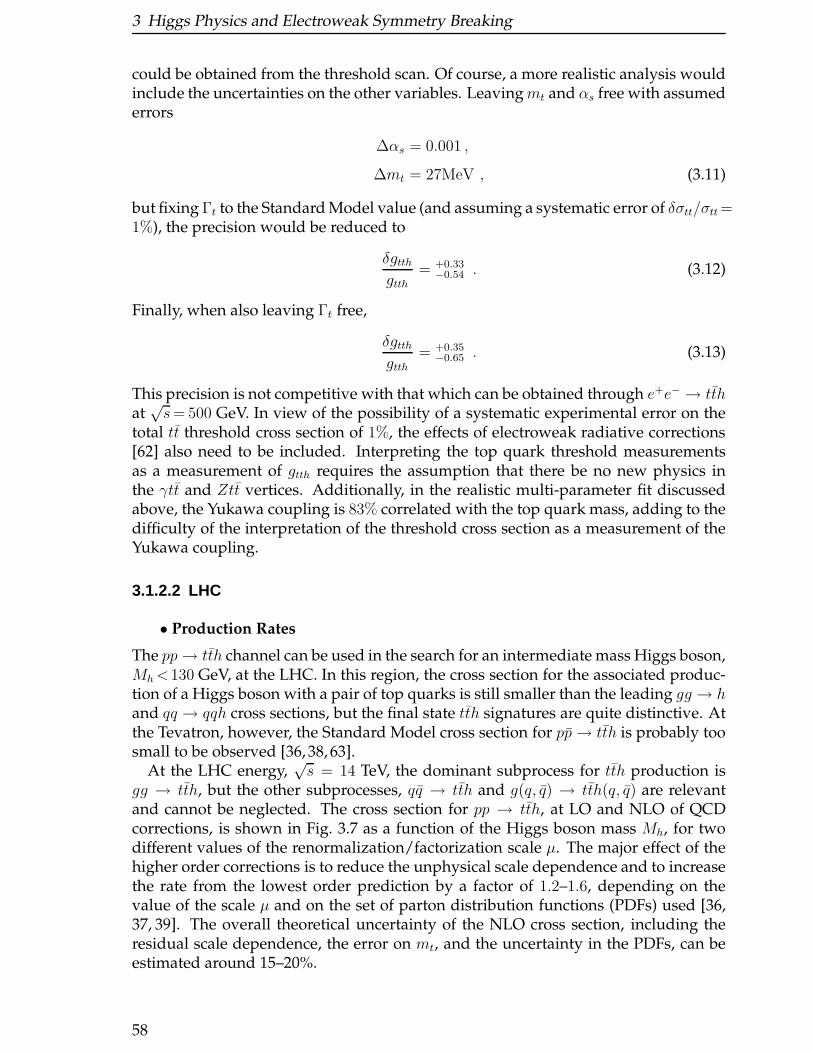
3 Higgs Physics and Electroweak Symmetry Breaking
could be obtained from the threshold scan. Of course, a more realistic analysis wouldinclude the uncertainties on the other variables. Leavingmt and αs free with assumederrors
∆αs = 0.001 ,
∆mt = 27MeV , (3.11)
but fixing Γt to the Standard Model value (and assuming a systematic error of δσtt/σtt=1%), the precision would be reduced to
δgtthgtth
= +0.33−0.54 . (3.12)
Finally, when also leaving Γt free,
δgtthgtth
= +0.35−0.65 . (3.13)
This precision is not competitive with that which can be obtained through e+e− → tthat√s= 500 GeV. In view of the possibility of a systematic experimental error on the
total tt threshold cross section of 1%, the effects of electroweak radiative corrections[62] also need to be included. Interpreting the top quark threshold measurementsas a measurement of gtth requires the assumption that there be no new physics inthe γtt and Ztt vertices. Additionally, in the realistic multi-parameter fit discussedabove, the Yukawa coupling is 83% correlated with the top quark mass, adding to thedifficulty of the interpretation of the threshold cross section as a measurement of theYukawa coupling.
3.1.2.2 LHC
• Production Rates
The pp→ tth channel can be used in the search for an intermediate mass Higgs boson,Mh<130 GeV, at the LHC. In this region, the cross section for the associated produc-tion of a Higgs boson with a pair of top quarks is still smaller than the leading gg → hand qq → qqh cross sections, but the final state tth signatures are quite distinctive. Atthe Tevatron, however, the Standard Model cross section for pp→ tth is probably toosmall to be observed [36, 38, 63].
At the LHC energy,√s = 14 TeV, the dominant subprocess for tth production is
gg → tth, but the other subprocesses, qq → tth and g(q, q) → tth(q, q) are relevantand cannot be neglected. The cross section for pp → tth, at LO and NLO of QCDcorrections, is shown in Fig. 3.7 as a function of the Higgs boson mass Mh, for twodifferent values of the renormalization/factorization scale µ. The major effect of thehigher order corrections is to reduce the unphysical scale dependence and to increasethe rate from the lowest order prediction by a factor of 1.2–1.6, depending on thevalue of the scale µ and on the set of parton distribution functions (PDFs) used [36,37, 39]. The overall theoretical uncertainty of the NLO cross section, including theresidual scale dependence, the error on mt, and the uncertainty in the PDFs, can beestimated around 15–20%.
58
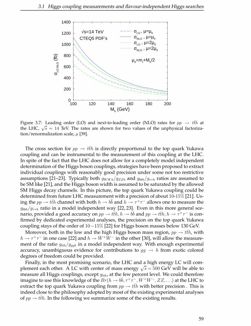
3.1 Higgs coupling measurements and flavour-independent Higgs searches
100 120 140 160 180 200Mh (GeV)
0
200
400
600
800
1000
1200
1400
σ LO,N
LO (
fb)
σLO , µ=µ0
σNLO , µ=µ0
σLO , µ=2µ0
σNLO , µ=2µ0
√s=14 TeV
µ0=mt+Mh/2
CTEQ5 PDF’s
Figure 3.7: Leading order (LO) and next-to-leading order (NLO) rates for pp → tth atthe LHC,
√s = 14 TeV. The rates are shown for two values of the unphysical factoriza-
tion/renormalization scale, µ [39].
The cross section for pp → tth is directly proportional to the top quark Yukawacoupling and can be instrumental to the measurement of this coupling at the LHC.In spite of the fact that the LHC does not allow for a completely model independentdetermination of the Higgs boson couplings, strategies have been proposed to extractindividual couplings with reasonably good precision under some not too restrictiveassumptions [21–23]. Typically both gWWh/gZZh and gbbh/gττh ratios are assumed tobe SM like [21], and the Higgs boson width is assumed to be saturated by the allowedSM Higgs decay channels. In this picture, the top quark Yukawa coupling could bedetermined from future LHC measurement with a precision of about 10-15% [21]. Us-ing the pp → tth channel with both h → bb and h → τ+τ− allows one to measure thegbbh/gττh ratio in a model independent way [22, 23]. Even in this more general sce-nario, provided a good accuracy on pp → tth, h→ bb and pp → tth, h→ τ+τ− is con-firmed by dedicated experimental analyses, the precision on the top quark Yukawacoupling stays of the order of 10−15% [22] for Higgs boson masses below 130 GeV.
Moreover, both in the low and the high Higgs boson mass region, pp → tth, withh→ τ+τ− in one case [22] and h→ W+W− in the other [30], will allow the measure-ment of the ratio gtth/gggh in a model independent way. With enough experimentalaccuracy, unambiguous evidence for contributions to gg → h from exotic coloreddegrees of freedom could be provided.
Finally, in the most promising scenario, the LHC and a high energy LC will com-plement each other. A LC with center of mass energy
√s= 500 GeV will be able to
measure all Higgs couplings, except gtth, at the few percent level. We could thereforeimagine to use this knowledge of the Br(h→ bb, τ+τ−,W+W−, ZZ, . . .) at the LHC toextract the top quark Yukawa coupling from pp → tth with better precision . This isindeed close to the philosophy adopted by most of the existing experimental analysesof pp→ tth. In the following we summarize some of the existing results.
59
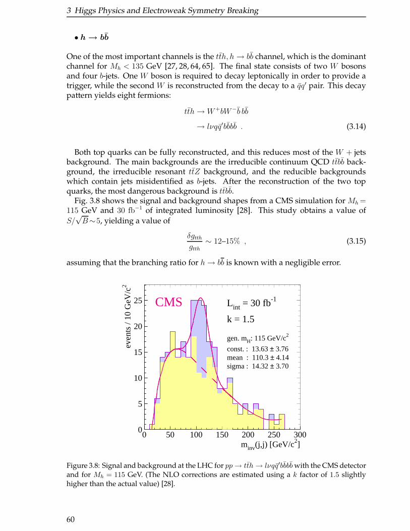
3 Higgs Physics and Electroweak Symmetry Breaking
• h → bb
One of the most important channels is the tth, h→ bb channel, which is the dominantchannel for Mh < 135 GeV [27, 28, 64, 65]. The final state consists of two W bosonsand four b-jets. One W boson is required to decay leptonically in order to provide atrigger, while the second W is reconstructed from the decay to a qq′ pair. This decaypattern yields eight fermions:
tth→W+bW−b bb
→ lνqq′bbbb . (3.14)
Both top quarks can be fully reconstructed, and this reduces most of the W + jetsbackground. The main backgrounds are the irreducible continuum QCD ttbb back-ground, the irreducible resonant ttZ background, and the reducible backgroundswhich contain jets misidentified as b-jets. After the reconstruction of the two topquarks, the most dangerous background is ttbb.
Fig. 3.8 shows the signal and background shapes from a CMS simulation for Mh=115 GeV and 30 fb−1 of integrated luminosity [28]. This study obtains a value of
S/√B∼5, yielding a value of
δgtthgtth
∼ 12–15% , (3.15)
assuming that the branching ratio for h→ bb is known with a negligible error.
0
5
10
15
20
25
0 50 100 150 200 250 300minv(j,j) [GeV/c2]
even
ts /
10 G
eV/c2
CMS L int = 30 fb-1
k = 1.5
gen. mH: 115 GeV/c2
const. : 13.63 ± 3.76mean : 110.3 ± 4.14sigma : 14.32 ± 3.70
Figure 3.8: Signal and background at the LHC for pp→ tth→ lνqq′bbbbwith the CMS detectorand for Mh = 115 GeV. (The NLO corrections are estimated using a k factor of 1.5 slightlyhigher than the actual value) [28].
60

3.1 Higgs coupling measurements and flavour-independent Higgs searches
Results for the h→ bb channel have also been obtained by the ATLAS collaboration[25,65]. The ATLAS analysis assumes a full reconstruction of the final state in order toeliminate combinatoric backgrounds. Assuming aK factor of 1.0 and a Higgs mass of
Mh = 115 GeV, ATLAS finds a value of S/√B = 2.4 with 30 fb−1 [25]. After adjusting
for the different assumptions about efficiencies and the different cross sections (due todiffering choices of the scale factors and PDFs), the ATLAS and CMS analyses are inagreement for the signal and the reducible background. The CMS analysis, however,finds a significantly smaller reducible ttbb background than does the ATLAS study.
• h → γγ
Because of the small rate, the h→ γγ channel is useful only at high luminosity [27,65].
• h → τ+τ−
For Mh< 130–135 GeV, the decay h → τ+τ− is useful as part of a general strategy todetermine Higgs boson couplings with very few theoretical assumptions [22, 23]. Itoffers the possibility of determining in a completely model independent way the ratiogbbh/gττh by measuring the ratio of pp → tth, h → bb to pp → tth, h → τ+τ−. Com-bining pp → tth, gg → h, and qq → qqh channels, it also allows a model independentdetermination of the gtth/gggh ratio.
First studies assumed that one of the top quarks decays leptonically, while the otherdecays hadronically [22] . The parton level signature is bblνqq′τ+τ−, which has the ir-reducible background ttτ+τ−, where the τ pair originates from a Z boson or a photon.The other backgrounds are much smaller. Ref. [22] considered only the τ decays to1 or 3 charged pions and found that with 100 fb−1 an accuracy of about 20% on δσ/σcould be obtained for Mh < 120 GeV, declining to 50% for Mh = 140 GeV. For largerHiggs masses the rate becomes too small for this decay channel to be observed.
• h → W +W −
For Mh > 135 GeV, the dominant decay mode is h → WW ∗ and the process pp →tth, h→ WW ∗ can be observed despite the low signal and the lack of a reconstructedmass peak. By measuring the ratio of
σ(pp→ tth, h→ bb)
σ(pp→ tth, h→WW ∗)(3.16)
a measurement of gbbh/gWWh can be made in which many of the systematic uncertain-ties cancel [30]. Combining pp → tth, h → WW ∗ with gg → h, h → WW ∗, the ratiogtth/gggh can be measured in a model independent way [22, 23].
The process pp → tth, h → W+W− gives the final state W+W−W+W−bb. Thedecays can then be classified according to the number of leptonic W decays [29].Ref. [30] performs a parton model study where the background is reduced by re-quiring both b decays be tagged with an efficiency ǫb = 0.6. The reconstruction of thetop quarks is not required and pT > 20 GeV for one trigger lepton is required. With
61
3 Higgs Physics and Electroweak Symmetry Breaking
120 140 160 180 200 220 240
mh
0
5
10
15
20
25
30
35
40
45
50
y t/y
t
LHC, 300 fb-1
@ High Luminosity
2
3
2 +3
Figure 3.9: Measurement of the top quark Yukawa coupling at the LHC in the tth , h →W+W− channel [30].
300 fb−1 of data, one can achieve an accuracy of
δgtthgtth
∼ 16% , 8% , 12% (3.17)
for Mh=130, 160 and 190 GeV respectively, as illustrated in Fig. 3.9 [30]. The ATLAScollaboration [29] has found that in the most favorable case, Mh = 160 GeV, the crosssection for pp → tth, h → WW ∗, can be measured with δσ/σ ∼ 26 % (15%) accuracywith a luminosity of 30 fb−1 (300 fb−1) by combining several final states.
The tth, h → bb and tth, h → W+W− channels can be combined to get a measure-ment of the relative decay widths Γ(h→ bb)/Γ(h→W+W−) with a 50−60% accuracyassuming a luminosity of 300 fb−1 for Mh <∼ 140 GeV. [23] This measurement is freeof theoretical assumptions. With further assumptions about the h → W+W− width,a value for the hbb coupling can be extracted from this channel [23].
3.1.2.3 SUSY Higgs Sector
There are two important differences between the Higgs sector in the Standard Modeland in a supersymmetric model. First, there are 5 Higgs bosons, A, h,H,H±, in theminimal SUSY model, so there are more associated top quark-Higgs boson processes:
e+e−, pp→ tth , ttH , ttA ,
e+e−, pp→ tbH− + btH+ . (3.18)
At a linear collider, the additional Higgs bosons give important new contributions, forexample, e+e− → AH,A → tt. Secondly, the Higgs boson couplings to the fermionsare changed from those of the Standard Model, and depend on the parameters of themodel, typically tanβ.
62
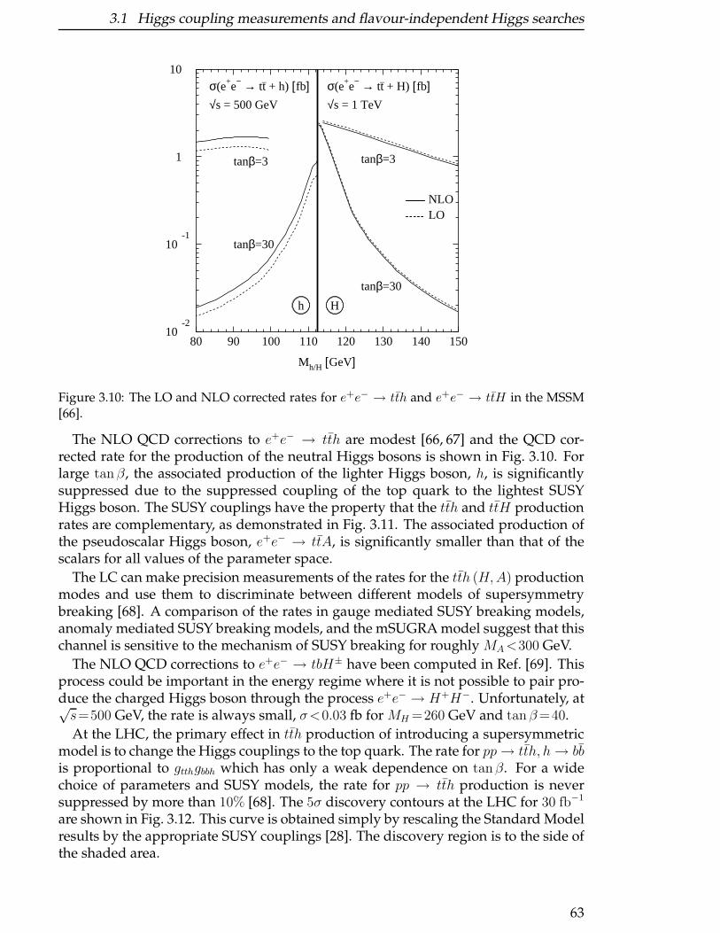
3.1 Higgs coupling measurements and flavour-independent Higgs searches
σ(e+e− → tt_ + h) [fb]
√s = 500 GeV
σ(e+e− → tt_ + H) [fb]
√s = 1 TeV
NLOLO
tanβ=3
tanβ=30
tanβ=3
tanβ=30
h H
Mh/H [GeV]
10-2
10-1
1
10
80 90 100 110 120 130 140 150
Figure 3.10: The LO and NLO corrected rates for e+e− → tth and e+e− → ttH in the MSSM[66].
The NLO QCD corrections to e+e− → tth are modest [66, 67] and the QCD cor-rected rate for the production of the neutral Higgs bosons is shown in Fig. 3.10. Forlarge tanβ, the associated production of the lighter Higgs boson, h, is significantlysuppressed due to the suppressed coupling of the top quark to the lightest SUSYHiggs boson. The SUSY couplings have the property that the tth and ttH productionrates are complementary, as demonstrated in Fig. 3.11. The associated production ofthe pseudoscalar Higgs boson, e+e− → ttA, is significantly smaller than that of thescalars for all values of the parameter space.
The LC can make precision measurements of the rates for the tth (H,A) productionmodes and use them to discriminate between different models of supersymmetrybreaking [68]. A comparison of the rates in gauge mediated SUSY breaking models,anomaly mediated SUSY breaking models, and the mSUGRA model suggest that thischannel is sensitive to the mechanism of SUSY breaking for roughly MA<300 GeV.
The NLO QCD corrections to e+e− → tbH± have been computed in Ref. [69]. Thisprocess could be important in the energy regime where it is not possible to pair pro-duce the charged Higgs boson through the process e+e− → H+H−. Unfortunately, at√s=500 GeV, the rate is always small, σ<0.03 fb for MH =260 GeV and tan β=40.
At the LHC, the primary effect in tth production of introducing a supersymmetricmodel is to change the Higgs couplings to the top quark. The rate for pp→ tth, h→ bbis proportional to gtthgbbh which has only a weak dependence on tanβ. For a widechoice of parameters and SUSY models, the rate for pp → tth production is neversuppressed by more than 10% [68]. The 5σ discovery contours at the LHC for 30 fb−1
are shown in Fig. 3.12. This curve is obtained simply by rescaling the Standard Modelresults by the appropriate SUSY couplings [28]. The discovery region is to the side ofthe shaded area.
63
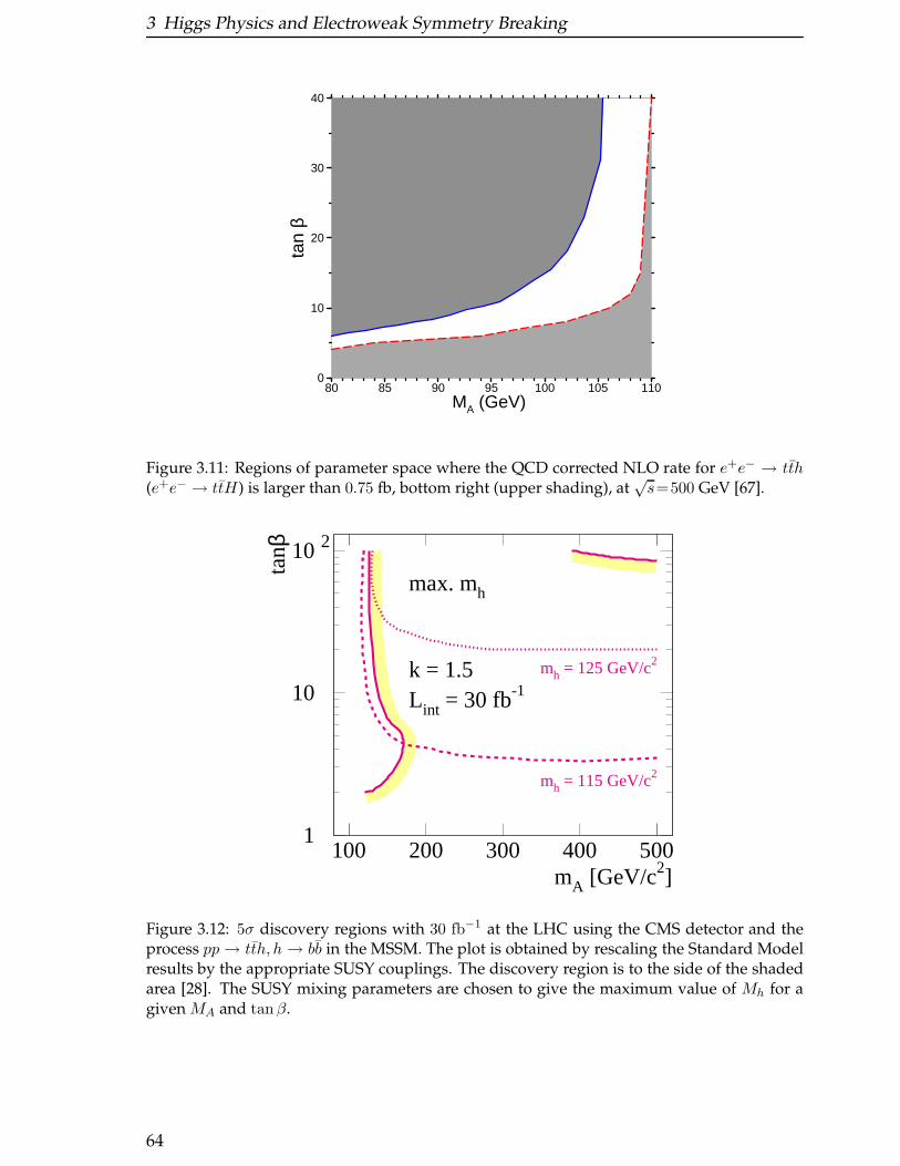
3 Higgs Physics and Electroweak Symmetry Breaking
80 85 90 95 100 105 110MA (GeV)
0
10
20
30
40
tan
β
Figure 3.11: Regions of parameter space where the QCD corrected NLO rate for e+e− → tth(e+e− → ttH) is larger than 0.75 fb, bottom right (upper shading), at
√s=500 GeV [67].
1
10
10 2
100 200 300 400 500mA [GeV/c2]
tanβ
max. mh
k = 1.5L int = 30 fb-1
mh = 115 GeV/c2
mh = 125 GeV/c2
Figure 3.12: 5σ discovery regions with 30 fb−1 at the LHC using the CMS detector and theprocess pp → tth, h → bb in the MSSM. The plot is obtained by rescaling the Standard Modelresults by the appropriate SUSY couplings. The discovery region is to the side of the shadedarea [28]. The SUSY mixing parameters are chosen to give the maximum value of Mh for agiven MA and tan β.
64
3.1 Higgs coupling measurements and flavour-independent Higgs searches
3.1.2.4 Conclusion
The associated production of a Higgs boson with a pair of tt quarks will be the onlyway of directly measuring the top quark Yukawa coupling at both a high energy LCand the LHC. An e+e− collider with
√s=500 GeV can make a preliminary measure-
ment of the top quark Yukawa coupling. However, the small rate at√s = 500 GeV
implies that a precision measurement will require a higher energy. At√s = 800-
1000 GeV, the top quark Yukawa coupling will be determined with a 4-5% precision.The LHC measures the product of the production cross section multiplied by the
Higgs branching ratios and will be instrumental in obtaining a first set of measure-ments of ratios of Higgs coupling constants. In order to extract the top quark Yukawacoupling, it is typically assumed that the Higgs decays with Standard Model branch-ing ratios. With this assumption, the LHC will obtain absolute couplings in somechannels. This assumption could be removed with precision measurements of theHiggs branching ratios at a Linear Collider.
3.1.3 Determining the parameters of the Higgs boson potenti al
U. Baur, T. Plehn and D. Rainwater
The LHC is widely regarded as capable of directly observing the agent responsiblefor electroweak symmetry breaking and fermion mass generation. This is generallybelieved to be a light Higgs boson [2]. The LHC will easily find a light SM Higgsboson with very moderate luminosity [70, 71] and have significant capability to de-termine many of its properties, such as its decay modes and couplings [21, 22, 28, 30,71, 72]. An e+e− linear collider could significantly improve these preliminary mea-surements, in some cases by an order of magnitude in precision [33].
Starting from the requirement that the Higgs boson has to restore unitarity of weakboson scattering at high energies in the SM [73], perhaps the most important measure-ment after the Higgs boson discovery is of the Higgs potential itself, which requiresmeasurement of the Higgs boson self-couplings. These can be probed directly only bymultiple Higgs boson production. Several studies of Higgs boson pair production ine+e− collisions have been conducted over the past few years [74–76], deriving quan-titative sensitivity limits for the trilinear Higgs self-coupling for several proposedlinear colliders for mH ≤ 140 GeV. The potential of hadron colliders has been exam-ined only recently [77–79], investigating Higgs pair production via gluon fusion andvarious subsequent decays. They established that future hadron machines can probethe Higgs potential over a wide range of Higgs mass.
To show the complementarity of hadron and lepton colliders we add to the existingliterature by looking at Higgs boson pair production for mH ≤ 140 GeV at hadroncolliders, and estimate the prospects for probing the Higgs boson self-coupling at alinear collider if mH ≥ 150 GeV. Using this input we determine how well the Higgspotential could be reconstructed. We closely follow our argument in Ref. [80].
The trilinear and quartic Higgs boson couplings λ and λ are defined through thepotential
V (ηH) =1
2m2H η
2H + λ v η3
H +1
4λ η4
H , (3.19)
65
3 Higgs Physics and Electroweak Symmetry Breaking
where ηH is the physical Higgs field. In the SM, λ = λ = λSM = m2H/(2v
2). Re-
garding the SM as an effective theory, the Higgs self-couplings λ and λ are per se free
parameters. S-matrix unitarity constrains λ to λ ≤ 8π/3 [73]. Since future collider ex-
periments likely cannot probe λ, we focus on the trilinear coupling λ in the following.
3.1.3.1 A low mass Higgs boson ( mH ≤ 140 GeV)
• LHC/SLHC
At LHC energies, inclusive Higgs boson pair production is dominated by gluon fu-sion, although weak boson fusion production and weak boson or top quark pair as-sociated production are also possible. Since Higgs pair production is already ratelimited, we consider only the gluon fusion process in the following.
For mH < 140 GeV, the dominant decay mode of the SM Higgs boson is H →bb. Unfortunately, the 4b channel (both Higgs bosons decaying to bb) is completelyoverwhelmed by the enormous QCD background, which is larger by more than twoorders of magnitude. For completeness, we performed a calculation of the signaland background, including the effects of NLO-QCD corrections to the signal via amultiplicative factor. After including kinematic cuts and realistic efficiency factors forthe b jets, a χ2 test on themvis distribution formH = 120 GeV we obtained meaningless1σ bounds of −6.8 < ∆λHHH < 10.1, where ∆λHHH = λ/λSM − 1.
A more advantageous S/B is conceivable if one of the Higgs bosons in gg → HHdecays into a τ pair. In this case, the main contributions to the background arisefrom continuum bbτ+τ− and tt production. The τ -pair invariant mass can be re-constructed with fairly good resolution. We considered the leptonic-hadronic decaychannel of the τ pair, to satisfy detector trigger requirements. Unfortunately, no limitcan be extracted for the LHC. Even for a luminosity-upgraded LHC (SLHC) achiev-ing 3000 fb−1, we expect a possible 1σ limit extraction of only −1.6 < ∆λHHH < 3.1,too weak to be useful. We find even worse results for the final state bbµ+µ−: whilebackground rejection is much better, this channel suffers from simple lack of signalrate due to the extremely small Higgs boson branching ratio to muon pairs - we couldexpect only about 2 events at the SLHC.
The best strategy appears to be to consider the rare decay of one Higgs boson to aphoton pair, while allowing the other to decay to its dominant channel, bb [79]. Thebackground consists of QCD bbγγ production and numerous similar QCD processeswhere one or more of the b jets or photons is a fake from charm or light jets. Wealso must include contributions from single Higgs boson production in associationwith photons and jets, as well as double parton scattering and fakes from multipleinteractions. The latter are of little concern at the LHC, so we may employ a singleb-tag strategy: for ǫb = 50%, this retains three times the number of signal events asdouble b-tagging. However, multiple interactions is a serious problem at an SLHC,which we bring under control with double b-tagging.
We impose kinematic cuts to enhance the signal relative to background, and useconservative estimates for the efficiency to identify the final state, ǫγ = 80% and ǫb =50%, as well as the more pessimistic probabilities from ATLAS for charm and lightjets to fake the signal final state: Pc→b = 1/13, Pj→b = 1/140(1/23) and Pj→γ = 1/1600for the LHC(SLHC). Under these conditions we expect to observe about 6(21) signal
66
3.1 Higgs coupling measurements and flavour-independent Higgs searches
events at the LHC(SLHC), on a background of 14(25) events. The S/B ratio is quiterespectable, but the statistics are low at the LHC. A χ2-test yields limits of −1.1 <∆λHHH < 1.9 for 600 fb−1 at the LHC, and −0.66 < ∆λHHH < 0.82 for 6000 fb−1 atthe SLHC. These limits improve by about 15% if the more optimistic ATLAS estimateof Pj→γ = 1/2500 can be achieved. Another promising approach is to subtract thebackgrounds after measuring them in other kinematic regions, a technique alreadyused by CDF. In this case, the expected limits improve to −0.74(0.46) < ∆λHHH <0.94(0.52) at the LHC(SLHC).
• LC
We now turn our attention to Higgs boson pair production in e+e− collisions. A de-tailed study of how well the Higgs boson self-coupling for mH = 120 GeV could bemeasured in e+e− → ZHH at
√s = 500 GeV can be found in Ref. [76].
Associated ZHH production followed by HH → b+jets is the dominant sourceof HH events in the SM if mH ≤ 140 GeV. The main backgrounds in this channelare tt and W+W− production. These are efficiently suppressed by performing a NNanalysis. Such an analysis, including a detailed detector simulation, was presentedin Ref. [76] for mH = 120 GeV and
√s = 500 GeV. It concluded that λ could be de-
termined with a precision of about 23% if an integrated luminosity of 1 ab−1 couldbe achieved. The limits achievable at hadron colliders for mH = 120 GeV are signifi-cantly weaker.
Since the ZHH cross section and its sensitivity to λ decrease with increasing col-lider energy, a linear collider operating at 500 GeV offers the best chance for a pre-cise measurement of λ for mH ≤ 140 GeV; the bounds we obtain for
√s = 500 GeV
are up to a factor 1.4 (1.9) more stringent than those achievable for√s = 800 GeV
(√s = 1 TeV). The advantage of operating at 500 GeV gradually disappears with in-
creasing Higgs boson mass, due to the reduced phase space. The sensitivity limitsachievable weaken by a factor 1.8 (1.2) for
√s = 500 GeV (
√s = 1 TeV) if mH in-
creases from 120 GeV to 140 GeV; for mH = 140 GeV one will not be able to probe λwith a precision of better than 50% for unpolarized beams. If both the electron andpositron beams could be polarized, the bounds derived here improve by a factor 1.3,assuming 80% polarization for the electron beam and 60% for the positron beam, andthe same integrated luminosity as for unpolarized beams.
We conclude that a 0.5–1 TeV linear collider offers a significantly better chance toprobe λ for the mass range from 120 GeV to 140 GeV, although an upgraded LHCcould provide convincing proof of spontaneous symmetry breaking.
3.1.3.2 A heavier Higgs boson ( mH ≥ 140 GeV)
For mH ≥ 140 GeV, the principal Higgs boson decay is to W pairs. This completelychanges the phenomenology of Higgs pair production.
• LHC/SLHC
We have previously examined this mass range for the LHC [78]. Due to the hugeQCD backgrounds in multijet final states, we can use only multiplepton subsamples,where two same-signW bosons decay leptonically and the other two give four jets, orwhere three W ’s decay leptonically and the events have only two extra jets. Summa-
67
3 Higgs Physics and Electroweak Symmetry Breaking
rizing our previous results, the LHC could give 1σ constraints of −0.4 < ∆λHHH <1.9 [78,81] for mH = 180 GeV. This is sufficient to exclude the case of no self-couplingto slightly better than 95% c.l. for 150 <∼ mH <∼ 200 GeV, proving the existence ofspontaneous symmetry breaking, and is a fortuitous effect of the destructive inter-ference of the two diagrams in the gluon fusion process. An SLHC could insteadmake a 20 − 30% measurement (95% CL) of the self-coupling over the mass range160 < mH < 180 GeV.
• LC
If mH > 140 GeV, the channels yielding the largest event rates are e+e− → ZHHwith Z → jj and HH → 8 jets or ℓν + 6 jets. Final states of similar structure andcomplexity are encountered in ttH production. The main background processes con-tributing both to e+e− → ZHH and e+e− → ttH are WW+ jets, tt+jets and QCDmultijet production. Instead of using a NN analysis, we investigate how the sensi-tivity bounds for λ depend on the signal efficiencies and the signal to backgroundratio. We then explore the prospects for determining the Higgs boson self-couplingin ZHH production for mH > 140 GeV using some rough guidelines.
Since the number of signal events is small, we combine the ℓν + 8 jet and 10 jetfinal states and use the total cross section to derive sensitivity limits. For the likelycase that efficiencies and S/B are similar to the values obtained in the ttH analysis, afirst-generation LC could obtain only very loose bounds on λHHH . Using the valuesquoted in Ref. [80], one finds −4.1 < ∆λHHH < 1.0 at the 1σ level for mH = 180 GeV,√s = 1 TeV and 1 ab−1. The achievable limits improve by about a factor 1.3 for
electron and positron beam polarizations of 80% and 60%, respectively, and if thesame integrated luminosity as in the unpolarized case could be reached. We reachsimilar conclusions for mH = 160 GeV and
√s = 800 GeV. For mH < 160 GeV and
mH > 180 GeV, fewer than 5 signal events would be seen if efficiencies are smallerthan 0.5, disallowing bounds to be placed on λHHH .
At higher collision energies, one should consider e+e− → ννHH production, whichdominates over ZHH above about
√s = 1 − 1.5 TeV, depending on the Higgs mass.
We do not address this channel here, as it is under investigation elsewhere [82].
3.1.3.3 Reconstructing the Higgs Potential
The results presented above can be used to compare the capabilities of future lep-ton and hadron colliders to reconstruct the Higgs potential. In order to translatebounds on ∆λHHH into constraints on the Higgs potential which can be graphicallydisplayed, it is convenient to consider the scaled Higgs potential
2
v2m2H
V (x) = x2 + λHHHx3 +
1
4λ4Hx
4 , (3.20)
where x = ηH/v and λ4H = λ/λSM is the four Higgs boson self-coupling normalizedto the SM value, ηH is the physical Higgs field, and v is the vacuum expectation value.
In the following we assume λ4H = 1.It should be noted that the scaled Higgs potential of Eq. (3.20) is valid only in the
vicinity of x = 0. The presence of a non-SM HHH coupling requires higher di-
mensional terms in an effective Lagrangian which would modify λ4H and also create
68

3.1 Higgs coupling measurements and flavour-independent Higgs searches
terms proportional to xn with n > 4. These terms are ignored in Eq. (3.20). Eq. (3.20)
with λ4H = 1 thus represents a good approximation to the true scaled Higgs potentialonly if the contributions of terms proportional to xn, n ≥ 4, are much smaller thanthat of the x3 term. This is guaranteed for sufficiently small values of x. We restrict therange of x for which we show the scaled Higgs potential to |x| ≤ 0.2. Provided thatthe coefficients of the xn, n ≥ 4, terms are not much larger than λHHH , this guaranteesthat Eq. (3.20) is indeed a good approximation of the true Higgs potential.
In Fig. 3.13 we show how well the scaled Higgs potential could be reconstructed for
Figure 3.13: Constraints on the scaled Higgs potential for a) mH = 120 GeV and b) 180 GeV.The allowed region is between the two lines of equal texture. The solid line represents theSM Higgs potential, and the long-dashed line shows the result for a vanishing Higgs bosonself-coupling.
69
3 Higgs Physics and Electroweak Symmetry Breaking
a Higgs boson of mass mH = 120 GeV and mH = 180 GeV. Hadron colliders indeedhave only very limited capabilities to probe λ if mH ≤ 140 GeV, although with suffi-cient luminosity they can provide proof of spontaneous symmetry breaking. The bestchannel appears to be the semi-rare decay to bbγγ final states. This channel shouldnow be studied with full detector simulation. In contrast, a 500 GeV linear colliderwith an integrated luminosity of 1 ab−1 could measure ∆λHHH with a precision ofabout 20% [76], reconstructing the Higgs potential fairly accurately. We draw similarconclusions for other Higgs boson masses in the range 120 GeV < mH < 140 GeV. Thelimits achievable for ∆λHHH both at lepton and hadron colliders gradually weakenby about a factor 2 if mH is increased from 120 GeV to 140 GeV.
If the Higgs boson decays predominantly into a pair of W -bosons, i.e. if mH ≥150 GeV, a completely different picture emerges. While LHC experiments will onlybe able to put mild constraints on V (x), a luminosity upgrade of the LHC will makeit possible to reconstruct the Higgs potential quite precisely for this mH range. Ofcourse, to control systematic uncertainties associated with knowledge of the Higgsbranching ratios and top Yukawa coupling, ideally one would have precision inputfrom a linear collider. Thus, having both collider data sets at hand would greatlyincrease our understanding of the Higgs potential in this mass region.
At a linear collider with a center of mass energy in the 0.8—1 TeV range and an in-tegrated luminosity of 1 ab−1, the number of Higgs boson pair events is very limited.The dominant WW+ jets and tt + jets backgrounds are several orders of magnitudelarger than the signal. As a result, it will be difficult to constrain the Higgs potentialusing linear collider data if mH ≥ 150 GeV. This point is illustrated in Fig. 3.13b as-suming the efficiencies and the signal to background ratios to be equal to Ref. [45] fore+e− → ttH . We obtain results similar to those shown in Fig. 3.13 for mH = 160 GeV.
It should be noted that the prospects to determine the Higgs boson self-couplingand to reconstruct the Higgs potential at an e+e− collider for a Higgs boson with masslarger than 150 GeV improve dramatically at larger energies.
3.1.3.4 Conclusions
Our results show that hadron colliders and e+e− linear colliders with√s ≤ 1 TeV
are complementary: for mH ≤ 140 GeV, linear colliders offer significantly betterprospects in measuring the Higgs boson self-coupling, λ; for a Higgs boson in therangemH ≥ 150 GeV, the opposite is true. However, to actually perform a meaningfulmeasurement at a hadron collider would demand precision Higgs boson propertiesinput for the top quark Yukawa coupling, the HWW coupling, and the total Higgsboson decay width.
While the LHC can obtain meaningful information on the Higgs total width [23,81],this is at best at the 15% level for mH ≥ 160 GeV, and about a factor of 2 worse in thelower mass region. For individual couplings, the LHC would measure the HWWcoupling to about 10(25)% in the upper(lower) mass region, and the top Yukawa cou-pling at about the 25−30% level. These values constitute large enough systematics toseriously complicate LHC HH measurements. A LC is vastly superior for the HWWcoupling and total Higgs width, with a precision at the few percent level. For thetop Yukawa coupling, a LC with center of mass energy up to 1 TeV is superior in thelowermH region, where it can improve the precision to about 15% (see Sec. 2.1.2). It is
70
3.1 Higgs coupling measurements and flavour-independent Higgs searches
possibly competitive closer to the WW threshold, although the status of these studiesis still not fully mature. A laudable goal would be to remove many of the systematicuncertainty assumptions both LHC and LC studies currently make, to provide moreaccurate estimates of the ultimate precision achievable, as it would greatly affect theinterpretation of LHC results.
3.1.4 Higgs boson decay into jets
E.L. Berger, T.M.P. Tait, C.E.M. Wagner
3.1.4.1 Introduction
Current strategies for the discovery and measurement of the properties the neutralscalar Higgs particle h with mh < 135 GeV rely heavily on the presumption that theprincipal branching fractions are close to those predicted in the standard model (SM)or in the usual minimal supersymmetric standard model (MSSM). For masses in thisrange, the decay width of the SM Higgs boson is dominated by its decay into a pairof bottom quarks, bb. Since the SM bottom-quark Yukawa coupling is small, theseassumptions are not warranted in the presence of non-standard light particles withorder one couplings to the Higgs boson. Searches can become particularly difficultat hadron colliders if the Higgs boson decays predominantly into these new particlesand if these particles decay mainly into jets, with no significant bottom or charm fla-vor content. Ref. [83] shows explicitly that this situation can arise in the MSSM in the
presence of light bottom squarks (b’s), with mass smaller than about 10 GeV. In this
case, b is the lightest supersymmetric particle (LSP). The bottom squarks are assumedto decay primarily into a pair of light quarks via an R-parity-violating interaction.The main results of our study, however, are applicable to a general class of models inwhich the main modification to the Higgs boson branching ratios is induced by theappearance of an additional decay mode into hadron jets.
The possibility that the Higgs boson decays with substantial branching ratio intojets is not unique to the light bottom squark scenario. It results also in models inwhich there is a light CP-odd scalar in the spectrum whose mass is less than 2mb.The Higgs boson then can decay into a pair of these scalars (and in general, owingto the smallness of the bottom Yukawa coupling, it will unless the coupling to theCP-odd scalars is very small). This possibility was discussed in Ref. [84] in a modelin which the CP-odd scalar behaves like an axion. It may arise also in general two-Higgs-doublet models, and even in the MSSM with explicit CP-violation [85]. Quitegenerally, if the mass of the CP-odd scalar is above a few GeV, but below twice thebottom quark mass, the CP-odd scalar decay into jets will overwhelm the decay intotwo photons. The Higgs boson would then decay in a way that resembles the resultsin the light bottom squark scenario, namely, it will decay predominantly into twoscalars that subsequently decay into jets. The exact phenomenology of the light CP-odd scalar scenario will be different from that of the light bottom squark scenario,and it should be analyzed in more detail. For instance, one should determine thevalues of the branching ratio of the CP-odd scalar into two photons that would permitobservation of the Higgs boson in the photon plus jet channel. For the aims of this
71
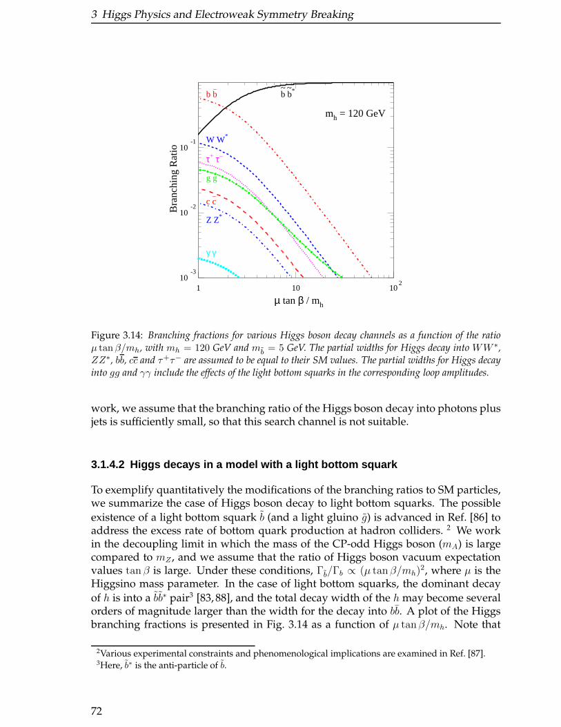
3 Higgs Physics and Electroweak Symmetry Breaking
10-3
10-2
10-1
1 10 102
b b*b b–
W W*
Z Z*
τ+ τ–
g g
c c–
γ γ
mh = 120 GeV
µ tan β / mh
Bra
nchi
ng R
atio
~ ~
Figure 3.14: Branching fractions for various Higgs boson decay channels as a function of the ratioµ tan β/mh, with mh = 120 GeV and mb = 5 GeV. The partial widths for Higgs decay into WW ∗,ZZ∗, bb, cc and τ+τ− are assumed to be equal to their SM values. The partial widths for Higgs decayinto gg and γγ include the effects of the light bottom squarks in the corresponding loop amplitudes.
work, we assume that the branching ratio of the Higgs boson decay into photons plusjets is sufficiently small, so that this search channel is not suitable.
3.1.4.2 Higgs decays in a model with a light bottom squark
To exemplify quantitatively the modifications of the branching ratios to SM particles,we summarize the case of Higgs boson decay to light bottom squarks. The possible
existence of a light bottom squark b (and a light gluino g) is advanced in Ref. [86] toaddress the excess rate of bottom quark production at hadron colliders. 2 We workin the decoupling limit in which the mass of the CP-odd Higgs boson (mA) is largecompared to mZ , and we assume that the ratio of Higgs boson vacuum expectationvalues tan β is large. Under these conditions, Γb/Γb ∝ (µ tanβ/mh)
2, where µ is theHiggsino mass parameter. In the case of light bottom squarks, the dominant decay
of h is into a bb∗ pair3 [83, 88], and the total decay width of the h may become severalorders of magnitude larger than the width for the decay into bb. A plot of the Higgsbranching fractions is presented in Fig. 3.14 as a function of µ tanβ/mh. Note that
2Various experimental constraints and phenomenological implications are examined in Ref. [87].3Here, b∗ is the anti-particle of b.
72
3.1 Higgs coupling measurements and flavour-independent Higgs searches
the partial Higgs widths into SM decay modes (excluding the gg and γγ modes4) areassumed to be given by their SM values (in particular, we assume that radiative cor-rections to these widths due to supersymmetric particle exchanges are negligible).Consequently, the Higgs branching fractions into SM decay channels are reduced
from their SM values by a factor proportional to tan−2 β once the bb∗ decay mode
is dominant. At mh = 120 GeV, the bb and bb∗ branching fractions cross each other forµ tanβ/mh ≃ 1.9, where each of the branching fractions is about 0.4.
3.1.4.3 Higgs boson decay to jets at the LHC
Having demonstrated the feasibility of the scenario under study, we concentrate onsearches for such a Higgs boson. At the Large Hadron Collider (LHC), a SM-likeHiggs boson of mass less than ∼ 135 GeV is expected to be discovered through avariety of production processes and decay modes [17,65,89]. These standard searcheslook for Higgs boson decays into SM particles. As indicated in Fig. 3.14, the presenceof an additional, dominant decay mode into hadron jets may suppress the branchingratios of these decay modes by a factor of order of ten to several hundred, dependingon the coupling of the Higgs boson to the new particles. This reduction raises seriousquestions as to the capability of experiments at the LHC to discover the Higgs boson.The more standard decays are suppressed, and the principal decay mode into jetssuffers from enormous QCD backgrounds.
At the LHC, it is difficult to obtain information about the Higgs boson couplings ina model-independent way because it is impossible to observe all possible decays in asingle production mode. One must be content with measurements of cross sectionstimes branching ratios and cannot make definitive statements about the couplingsthemselves. In Fig. 3.15, for mh = 120 GeV, we show the accuracies that we expectcould be achieved at the LHC (assuming a total integrated luminosity of 100 fb−1)for measurements of the rates (cross sections times branching ratios) of gluon fusioninto a Higgs boson followed by h → γγ, WW ∗, and ZZ∗, and for weak boson fusioninto a Higgs boson followed by the decays h→ WW ∗ and h→ τ+τ−. The accuraciesare shown as a function of the ratio of the jet-jet and the bb widths. By presentingthe plot in this way, the results are more general than the specific supersymmetricmodel discussed above, and apply to any model of new physics in which the Higgscouplings to light quarks and gluons are modified. In particular, the jet-jet width is
the sum of the partial widths for decay into the new hadron channel (bb∗ in the su-persymmetry example given above), plus bb, cc, and gg. The Higgs cross-sections5
and partial Higgs widths into SM decay modes are assumed to be given by their SMvalues (that is, radiative corrections to these widths due to supersymmetric particleexchanges are neglected.) In the SM, Γ(h → jets)/Γ(h→ bb) = 1.12, primarily due tothe WW ∗ (where the W ∗ decays hadronically), gg and cc Higgs decay modes.6 Therelative uncertainties contain statistical effects,
√S +B/S, where we use estimates of
4The partial Higgs widths into gg and γγ (these decay modes are absent at tree-level and only arise atthe loop level) include the effects of the light bottom squarks in the corresponding loop amplitudes.
5Details on the Higgs cross-sections used in this analysis can be found in in Ref. [83].6Note that the left-most edge of the plot in Fig. 3.15, i.e. Γ(h→ jets)/Γ(h→ bb) = 1, would correspond
to a case in which the Higgs decay to bottom quarks is the only hadronic decay mode of the Higgsboson.
73

3 Higgs Physics and Electroweak Symmetry Breaking
0.1
0.2
0.3
0.4
0.5
0.6
0.70.80.9
1 1.2 1.4 1.6 1.8 2 2.2 2.4 2.6 2.8 3
mh = 120 GeV100 fb-1
σgg x BR(γγ)
σgg x BR(ZZ)
σgg x BR(WW)σWW x BR(WW)
σWW x BR(τ+τ-)
σtth x BR(bb)
Γ(h → j j) / ΓSM(h → b b)
Rel
ativ
e U
ncer
tain
ty
Figure 3.15: Expected accuracy in LHC measurements of the product of production cross sections andbranching ratios for the WW , ZZ , bb, γγ, and τ+τ− decay modes of a Higgs boson with mass 120GeV as a function of the ratio of the jet-jet and the bb widths. The horizontal dotted line at 0.2 indicatesthe 5σ discovery reach under the assumption B ≫ S. The partial widths for Higgs decay into WW ∗,ZZ∗, bb, cc, gg, γγ, and τ+τ− and the production cross sections are assumed to be equal to their SMvalues.
the backgrounds and SM signal rates presented in Refs. [90] and [21]. The productionthrough weak boson fusion followed by decay into W bosons is based on leptonic Wdecays into one electron and one muon, and includes a presumed systematic uncer-tainty of 30%.
For values of the branching ratio BR(h→ jets) larger than two to five times that intobottom quarks, the large QCD jet backgrounds will make observation of the h verydifficult in Tevatron and LHC experiments. In the particular example of light bottomsquarks, however, experiments at these colliders may see evidence of low-energysupersymmetry and/or the heavy SUSY Higgs bosons (note, however, the standard
missing-energy signature of conventional SUSY is compromised if a charged b is theLSP).
3.1.4.4 Higgs boson decay to jets at the LC
We now consider a Higgs boson decaying into jets at a high energy e+e− linear col-lider. For a light Higgs boson the dominant production process is e+e− → Z0h via anintermediate Z0 [91]. Once the Z0 is identified, the Higgs boson is discovered, inde-pendent of the Higgs boson decay modes, as a clean enhancement in the distributionof mass recoiling from the Z0 [91], and the mass of the Higgs boson can be measured.
74

3.1 Higgs coupling measurements and flavour-independent Higgs searches
10-2
10-1
1
1 10 102
103
√s–
Lmh
= 500 GeV
= 500 fb-1
= 120 GeV
Γ(h→jj) / ΓSM(h→bb–)
Γh
BR(bb–)
ghWW(bb–)
ghWW(jj)
ghZZ
BR(jj)
Rel
ativ
e U
ncer
tain
ty
Figure 3.16: Expected accuracy in the measurements of the bb and jet-jet branching fractions, the hZZand hWW coupling strengths, and the total width of the Higgs boson, as a function of the ratio of thejet-jet and the bb widths. The Higgs boson partial widths to bb, cc, gg, ZZ∗, and WW ∗ are taken to beequal to their SM values.
The backgrounds from the W fusion and Z0 fusion processes are small. Because theZh cross section depends on the hZZ coupling strength, observation of the Higgsboson determines this coupling with an expected accuracy of ∼ 1.2% [91] and can es-tablish the Higgs boson as the principal scalar responsible for electroweak symmetrybreaking. These statements remain valid if the Higgs boson decays primarily into apair of jets since the method does not depend on the Higgs boson decay products.
In the weak boson fusion process, the jet-jet Higgs boson decay channel can also beused to determine the hWW coupling at large µ tanβ/mh with significantly greateranticipated accuracy than from the bb channel 7. In Fig. 3.16, we show the accuraciesthat we expect could be achieved in the measurements of the bb branching fraction,the hZZ and hWW coupling strengths, and the total width of the Higgs boson, all asa function of the ratio of the jet-jet and the bb widths. We distinguish the accuracies tobe expected for the hWW coupling strength depending upon whether the bb or jet-jet
7To obtain the uncertainty on the branching fraction into a pair of jets, we must first estimate thenumber of signal and background events in the jet-jet channel. We begin with the numbers pre-sented in Ref. [42] of simulated signal and background events for h→ bb in the process e+e− → Zh.We remove the b-tag requirement, increasing both signal and background by (1/0.75)2. The signalsample is then multiplied by (1/0.69), the inverse of the SM bb branching fraction, and by the jet-jetbranching fraction in our model. Since the primary background arises from Z decay, the back-ground is increased by 1/Rb ≃ 1/0.21, where Rb is the measured fraction of the hadronic width ofthe Z into bb.
75
3 Higgs Physics and Electroweak Symmetry Breaking
decay mode of the Higgs boson is used. In this plot, the jet-jet width includes the
partial widths into the new non-standard particles (bb∗ in the MSSM example), plusgg, bb and cc (the partial Higgs widths for the latter three channels are fixed to theirSM values).
Because they rely principally on the production process e+e− → hZ0, experimentsat proposed e+e− linear colliders remain fully viable for direct observation of the hand measurement of its mass and some of its branching fractions [83]. The possibil-ity of measuring the Higgs boson width, however, is diminished owing to the largesuppression of the decay branching ratio into the weak gauge bosons. If the width ex-ceeds about 2 GeV, a direct measurement should be possible from the invariant massdistribution in the jet-jet channel.
3.1.4.5 Conclusions
In the scenario considered here, the Higgs boson decays to a large extent into hadronicjets, possibly without definite flavor content. Measurements of various properties ofthe Higgs boson, such as its full width and branching fractions, may therefore requirea substantial improvement in the experimental jet-jet invariant mass resolution and amore thorough understanding of backgrounds in the jet-jet channel. Full event andreconstruction studies done for the SM decay h → gg (where the SM branching frac-tion is ∼ 5% for mh = 120 GeV) should be pursued further to establish the extent towhich properties of the Higgs boson can be determined solely from the jet-jet mode.
The existence of a light Higgs boson, observable at the LHC, is often considered thehallmark of the minimal supersymmetric standard model. A light Higgs boson de-caying into bottom squarks, undetected at the LHC could thus lead one to concludeerroneously that the underlying effective theory is more exotic than the minimal su-persymmetric extension. On the other hand, a Higgs boson that decays into jets canbe studied quite well at a linear collider (LC), a point that emphasizes the complemen-tary nature of the LHC and a LC in this scenario. The LHC, with enormous energyand luminosity should be able to produce, discover, and study in great detail possiblenew physics at the weak scale (the super-partners in the supersymmetry example).The LC can discover and study the Higgs boson. In order to truly understand elec-troweak symmetry breaking and the solution of the hierarchy problem, both aspectsare crucial. As a further possibility, one might produce super-partners at the LHCthat decay ‘through’ light Higgs bosons into jets and not realize what the intermedi-ate state is. In a situation such as this one, it might even be impossible to identifythe parent super-particles, despite their having properties rather ordinary from thepoint of view of the MSSM. The analysis and understanding of data from concurrentoperation of the LHC and a LC may prove crucial.
3.2 Determination of CP properties of Higgs bosons
In this section we briefly summarise the information on determination of CP proper-ties of Higgs bosons at different colliders and identify areas of investigations to studythe issue of LHC-LC synergy.
76
3.2 Determination of CP properties of Higgs bosons
3.2.1 CP studies of the Higgs sector
R.M. Godbole, S. Kraml, M. Krawczyk, D.J. Miller, P. Niezurawski and A.F. Zarnecki
3.2.1.1 Introduction
Studies of the CP properties of the Higgs sector, which will involve establishing theCP eigenvalue(s) for the Higgs state(s) if CP is conserved, and measuring the mixingbetween the CP-even and CP-odd states if it is not, will certainly be part of the physicsstudies at future colliders [33,92,93]. CP violation in the Higgs sector [94], possible inmulti-Higgs models, is indeed an interesting option to generate CP violation beyondthat of the SM, possibly helping to explain the observed Baryon Asymmetry of theUniverse [95].
In order to identify the CP nature of a Higgs boson, one must probe the structureof its couplings to known particles, in either its production or decay. At tree level, thecouplings of a neutral Higgs boson φ, which may or may not be a CP eigenstate,8 tofermions and vector bosons can be written as
f fφ : − f(vf + iafγ5)fgmf
2mW
, V V φ : cVgm2
V
mW
gµν (3.21)
where g is the usual electroweak coupling constant; vf , af give the Yukawa couplingstrength relative to that of a SM Higgs boson, and cV (V = W, Z) are the correspond-ing relative couplings to gauge bosons. In the SM, for a CP-even Higgs vf = cV = 1and af = 0. A purely CP-odd Higgs boson has vf = cV = 0 and af 6= 0, with themagnitude of af depending on the model. In CP-violating models, vf , af and cV mayall be non-zero at tree level. In particular, in the case of a general 2HDM or the MSSMwith CP violation, there are three neutral Higgs bosons φi, i = 1, 2, 3, which mixwith each other and share out between them the couplings to the Z, W and fermions;various sum rules are given in [96–98]. Due to this fact, limits on the MSSM (and2HDM) Higgs sector implied by LEP data are strongly affected by the presence of CPviolation [85, 97, 99].
In most formulations of CP-violating Higgs sectors [85, 98, 100–103] the amount ofCP mixing is small, being generated at the loop level, with only one of the couplingsto gauge bosons or fermions sizable. In most cases, the predicted CP mixing is also afunction of the CP-conserving parameters of the model, along with the CP-violatingphases.9 Thus observation and measurement of this mixing at the LC may give pre-dictions for LHC physics; for instance for sparticle phenomenology in the MSSM.Moreover, experiments at different colliders have different sensitivities to the variouscouplings of eq. 3.21. Hence a combination of LHC, LC and photon collider (PLC)measurements of both CP-even and CP-odd variables may be necessary to completelydetermine the coupling structure of the Higgs sector. These are two ways in whichthe high potential of LHC-LC synergy for CP studies can be realized.
8For CP eigenstates, a pure scalar will be denoted by H and a pure pseudoscalar by A. Otherwise weuse the generic notation φ.
9For the MSSM with explicit CP violation, computational tools for the Higgs sector are available[104, 105].
77
3 Higgs Physics and Electroweak Symmetry Breaking
In what follows, we give an overview of the LHC, LC, and PLC potentials for CPstudies in the Higgs sector. An example of the LHC-LC synergy is presented as well.
3.2.1.2 CP Studies at the LHC
There are several ways to study the CP nature of a Higgs boson at the LHC. In theresonant s-channel process gg → φ → f f , the scalar or pseudoscalar nature of theYukawa coupling gives rise to f f spin-spin correlations in the production plane [106].A more recent study [107] looks at this process in the context of a general 2HDM.
In the process gg → ttφ, the large top-quark mass enhances the v2 − a2 contri-bution, allowing a determination of the CP-odd and CP-even components of a lightHiggs Boson [108, 109]. While this method should provide a good test for verifyinga pure scalar or pseudoscalar, examination of a mixed CP state would be far morechallenging, requiring 600 fb−1 to distinguish an equal CP-even/CP-odd mixture at∼ 1.5 σ [108].
Higgs decay into two real bosons, φ→ ZZ, with Z → l+l−, [110,111] can be used torule out a pseudoscalar state by examining the azimuthal or polar angle distributionsbetween the decay lepton pairs. Below the threshold, φ → Z∗Z, extra information isprovided by the threshold behavior of the virtual Z boson invariant mass spectrum.This way, one could rule out a pure 0− state at > 5σ with 100 fb−1 in the SM. Anextension of these studies to scalar-pseudoscalar mixing is under progress.
In weak boson fusion, the Higgs boson is produced in association with two tag-ging jets, qq → W+W−qq → φqq. As with the decay to ZZ, the scalar and pseu-doscalar couplings lead to very different azimuthal distributions between the twotagging jets [112]. A similar idea may be employed in φ + 2jets production [113] ingluon fusion. Higher order corrections [114] may, however, reduce this correlationeffect strongly.
Another approach uses the exclusive (inclusive) double diffractive process pp →p + φ + p (pp → X + φ + Y ) [115–117] with large rapidity gaps between the φ andthe (dissociated) protons. The azimuthal angular distribution between the taggedforward protons or the transverse energy flows in the fragmentation regions reflectthe CP of the φ and can be used to probe CP mixing. This process is particularlypromising for the regionmφ < 60 GeV, in which a Higgs signal may have been missedat LEP due to CP violation.
3.2.1.3 CP Studies at an e+e− Linear Collider
In e+e− collisions, the main production mechanisms of neutral Higgs bosons φ are (a)Higgsstrahlung e+e− → Zφ, (b) WW fusion e+e− → φ νν, (c) pair production e+e− →φi φj (i 6= j) and (d) associated production with heavy fermions, e+e− → f fφ. Studiesof CP at the Linear Collider aim at extracting the relevant couplings mentioned ineq. 3.21. Recall that a pure pseudoscalar of the 2HDM or MSSM does not coupleto vector bosons at tree level. The observation of all three φi (i = 1, 2, 3) in a givenprocess, e.g. e+e− → Zφ1,2,3, therefore represents evidence of CP violation [118–120].
In the Higgsstrahlung process, if φ is a pure scalar the Z boson is produced in astate of longitudinal polarization at high energies [121,122]. For a pure pseudoscalar,the process proceeds via loops and the Z boson in the final state is transversally po-
78
3.2 Determination of CP properties of Higgs bosons
larized. The angular distribution of e+e− → ZH is thus ∝ sin2 θZ , where θZ is theproduction angle of the Z boson w.r.t. to the beam axis in the lab frame, while thatof e+e− → ZA is ∝ (1 + cos2 θZ). A forward-backward asymmetry would be a clearsignal of CP violation. Furthermore, angular correlations of the Z → f f decay can beused to test the JPC quantum numbers of the Higgs boson(s). Measurements of thethreshold excitation curve can give useful additional information [123, 124]. A studyin [33] parametrized the effect of CP violation by adding a small ZZA coupling withstrength η to the SM matrix element,M =MZH + iηMZA, and showed that η can bemeasured to an accuracy of 0.032 with 500 fb−1.
Angular correlations of Higgs decays can also be used to determine the CP natureof the Higgs boson(s), independent of the production process; see [125–127] and ref-erences therein. The most promising channels are φ→ τ+τ− (mφ < 2mW ) and φ→ tt(mφ > 2mt) which in contrast to decays into WW or ZZ allow equal sensitivity to theCP-even and CP-odd components of φ.
A detailed simulation of e+e− → ZH followed by H → τ+τ− and τ± → ρ±ντ (ντ )[128–130] showed that CP of a 120 GeV SM-like Higgs boson can be measured to≥ 95% C.L. at a 500 GeV e+e− LC with 500 fb−1 of luminosity. In case of CP violation,the mixing angle between the scalar and pseudoscalar states may be determined toabout 6 degrees [131], the limiting factor being statistics.
3.2.1.4 CP Studies at a Photon Collider
A unique feature of a PLC is that two photons can form a Jz = 0 state with both evenand odd CP. As a result a PLC has a similar level of sensitivity for both the CP-oddand CP-even components of a CP-mixed state:
CP−even :ǫ1 · ǫ2 = −(1+λ1λ2)/2, CP−odd :[ǫ1× ǫ2] · kγ = ωγiλ1(1+λ1λ2)/2, (3.22)
ωi and λi denoting the energies and helicities of the two photons respectively; thehelicity of the system is equal to λ1− λ2. This contrasts the e+e− case, where it is easyto discriminate between CP-even and CP-odd particles but may be difficult to detectsmall CP-violation effects for a dominantly CP-even Higgs boson [132]. For the PLC,one can form three polarization asymmetries in terms of helicity amplitudes whichgive a clear measure of CP mixing [133]. In addition, one can use information on thedecay products of WW , ZZ, tt or bb coming from the Higgs decay. Furthermore, withcircular beam polarization almost mass degenerate (CP-odd) A and (CP-even) H ofthe MSSM may be separated [134–136].
A measurement of the spin and parity of the Higgs boson may also be performedusing the angular distributions of the final-state fermions from the Z boson decay,which encode the helicities of Z’s. A detailed study was performed for above andbelow the ZZ threshold in [110]. A realistic simulation based on this analysis wasmade recently in [137].
The same interference effects as mentioned above can be used in the process γγ →φ → tt [138, 139] to determine the ttφ and γγφ couplings for a φ with indefinite CPparity.
79

3 Higgs Physics and Electroweak Symmetry Breaking
3.2.1.5 Example of LHC-LC synergy
As an example of the LHC-LC synergy, we consider the SM-like, type II 2HDM withCP-violation [137, 140]. We study production of φ2 in the mass range 200 to 350 GeV,decaying to V V , V = W/Z, at the LHC, LC and PLC. In particular, we investigate theinterplay of different experiments for the determination of tan β and mixing angleΦHA.
Figure 3.17 shows the expected rates for φ2 with mφ2 = 250 GeV relative to the SMones, as a function of tanβ and ΦHA. For a SM Higgs boson, the expected precisionon σ × BR(H → V V ) is ∼ 15% at the LHC [141, 142] and better than 10% at LC andPLC [143, 144]. A PLC will allow to measure Γγγ with a precision of 3–8% and thephase of the φ→ γγ amplitude, Φγγ , to 40− 120 mrad [144].
Figure 3.18 shows the 1 σ bands for determination of tanβ and ΦHA, at the LHC,LC and PLC for a particular choice of parameters : tan β = 0.7 and ΦHA = −0.2.The chosen point is indicated by a star. For the PLC, information from Γγγ and Φγγ
is included. As can be seen, an accurate determination of both parameters requirescombination of data from all three colliders.
Figure 3.17: σ× BR for φ2 → V V with V = W/Z , relative to the SM expectation for the samefor a mass of 250 GeV, as a function of tan β and ΦHA for LHC, LC and PLC.
3.2.1.6 Summary
The LHC, an e+e− LC, and a LC in the photon collider option (PLC) will be able toprovide nontrivial information on the CP quantum numbers of the Higgs boson(s).We have summarized the potentials of the different colliders in this document anddiscussed the possible LHC-LC synergy.
In the MSSM, for instance, the size of CP-violating effects in the Higgs sector de-pends in part on the sparticle spectrum. Observation and measurement of Higgs-sector CP mixing at the LC can hence give predictions for phenomenology at the LHCin the CP-conserving sector, thus providing a high potential of LHC-LC synergy. Adetailed study of this issue is, however, still missing.
Moreover, experiments at different colliders have different sensitivities to the vari-ous couplings of eq. 3.21. Hence a combination of LHC and LC/PLC measurements
80
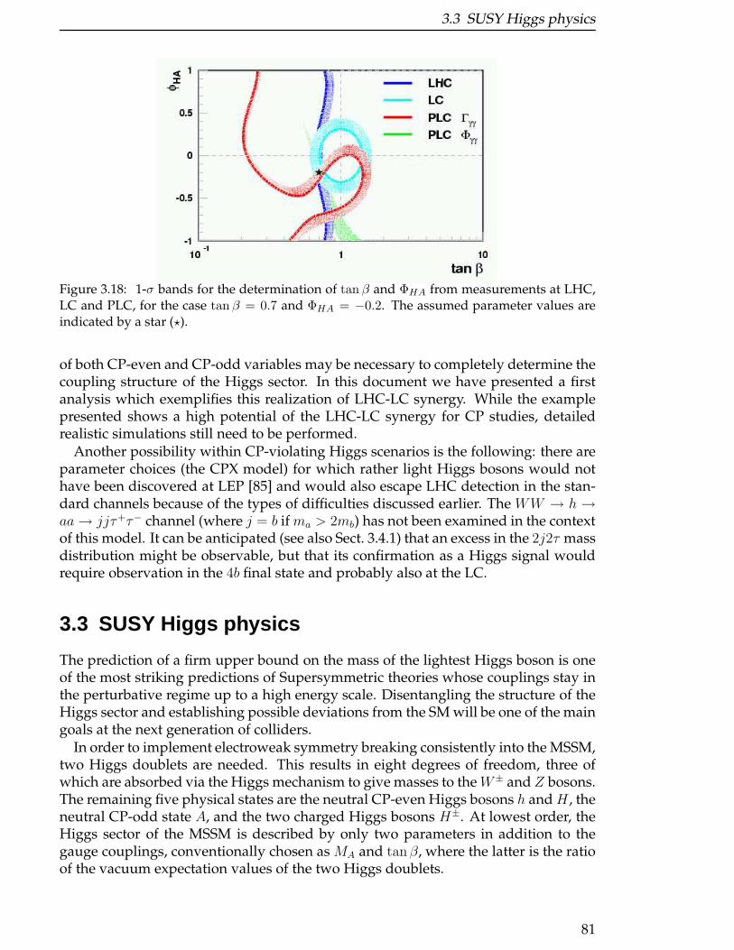
3.3 SUSY Higgs physics
Figure 3.18: 1-σ bands for the determination of tan β and ΦHA from measurements at LHC,LC and PLC, for the case tan β = 0.7 and ΦHA = −0.2. The assumed parameter values areindicated by a star (⋆).
of both CP-even and CP-odd variables may be necessary to completely determine thecoupling structure of the Higgs sector. In this document we have presented a firstanalysis which exemplifies this realization of LHC-LC synergy. While the examplepresented shows a high potential of the LHC-LC synergy for CP studies, detailedrealistic simulations still need to be performed.
Another possibility within CP-violating Higgs scenarios is the following: there areparameter choices (the CPX model) for which rather light Higgs bosons would nothave been discovered at LEP [85] and would also escape LHC detection in the stan-dard channels because of the types of difficulties discussed earlier. The WW → h →aa→ jjτ+τ− channel (where j = b if ma > 2mb) has not been examined in the contextof this model. It can be anticipated (see also Sect. 3.4.1) that an excess in the 2j2τ massdistribution might be observable, but that its confirmation as a Higgs signal wouldrequire observation in the 4b final state and probably also at the LC.
3.3 SUSY Higgs physics
The prediction of a firm upper bound on the mass of the lightest Higgs boson is oneof the most striking predictions of Supersymmetric theories whose couplings stay inthe perturbative regime up to a high energy scale. Disentangling the structure of theHiggs sector and establishing possible deviations from the SM will be one of the maingoals at the next generation of colliders.
In order to implement electroweak symmetry breaking consistently into the MSSM,two Higgs doublets are needed. This results in eight degrees of freedom, three ofwhich are absorbed via the Higgs mechanism to give masses to theW± and Z bosons.The remaining five physical states are the neutral CP-even Higgs bosons h and H , theneutral CP-odd state A, and the two charged Higgs bosons H±. At lowest order, theHiggs sector of the MSSM is described by only two parameters in addition to thegauge couplings, conventionally chosen as MA and tanβ, where the latter is the ratioof the vacuum expectation values of the two Higgs doublets.
81
3 Higgs Physics and Electroweak Symmetry Breaking
The tree-level upper bound on the mass of the lightest CP-even Higgs boson, mh <MZ in the MSSM, arising from the gauge structure of the theory, receives large ra-diative corrections from the Yukawa sector of the theory. Taking corrections up totwo-loop order into account, it is shifted by about 50% [8]. As a consequence, loopeffects, in particular from the top and scalar top sector and for large values of tan βalso from the bottom and scalar bottom sector, are very important for SUSY Higgsphenomenology.
While the Higgs sector of the MSSM is CP-conserving at tree level, CP-violatingeffects can enter via loop corrections. The Higgs sector in extensions of the MSSMcontains further matter structure, for instance additional Higgs singlets.
The LC will provide precision measurements of the properties of all Higgs bosonsthat are within its kinematic reach. Provided that a Higgs boson couples to the Z bo-son, the LC will observe it independently of its decay characteristics. At the LHC,on the other hand, Higgs boson detection can occur in various channels. In manycases complementary information from more than one channel will be accessible atthe LHC. In particular, the LHC has a high potential for detecting heavy Higgs stateswhich might be beyond the kinematic reach of the LC.
In the following, the possible interplay between LHC and LC results in SUSY Higgsphysics is investigated for several examples. In Section 3.3.1 first a scenario is anal-ysed where the LHC can detect the heavy Higgs states of the MSSM, while the LCprovides precise information on the branching ratios of the light Higgs boson. Thisallows to perform a sensitive consistency test of the MSSM and to obtain indirect in-formation on the mixing in the scalar top sector. Furthermore a scenario where LHCand LC only detect one light Higgs boson is investigated and it is demonstrated howconstraints on MA can be derived from combined LHC and LC data. In Section 3.3.2the decay of the heavy Higgs bosons H and A into a pair of neutralinos is studiedat the LHC. This decay can be used to determine MA, provided that a precise mea-surement of the mass of the lightest neutralino from the LC is available. Section 3.3.3investigates the situation where the neutral Higgs bosons are almost mass-degenerateand tan β is large. In this case detection of the individual Higgs boson peaks is verychallenging at the LHC, while the different Higgs boson signals can more easily beseparated at the LC. The measured characteristics at the LC will then allow to de-termine further Higgs-boson properties at the LHC. In Sections 3.3.4 and 3.3.5 thedetermination of tanβ from combined LHC and LC information (including also LCrunning in the γγ mode) is investigated.
3.3.1 Consistency tests and parameter extraction from thecombination of LHC and LC results
K. Desch, E. Gross, S. Heinemeyer, G. Weiglein and L. Zivkovic
The interplay of prospective experimental information from both the LHC and the LC in the
investigation of the MSSM Higgs sector is analyzed in the SPS 1a and SPS 1b benchmark sce-
narios. Combining LHC information on the heavy Higgs states of the MSSM with precise
measurements of the mass and branching ratios of the lightest CP-even Higgs boson at the
LC provides a sensitive consistency test of the MSSM. This allows to set bounds on the tri-
linear coupling At. In a scenario where LHC and LC only detect one light Higgs boson, the
82
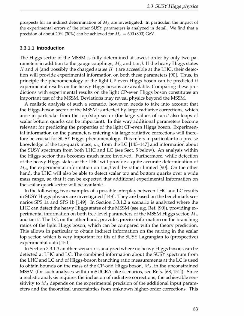
3.3 SUSY Higgs physics
prospects for an indirect determination of MA are investigated. In particular, the impact of
the experimental errors of the other SUSY parameters is analyzed in detail. We find that a
precision of about 20% (30%) can be achieved for MA = 600 (800) GeV.
3.3.1.1 Introduction
The Higgs sector of the MSSM is fully determined at lowest order by only two pa-rameters in addition to the gauge couplings, MA and tanβ. If the heavy Higgs statesH and A (and possibly the charged states H±) are accessible at the LHC, their detec-tion will provide experimental information on both these parameters [90]. Thus, inprinciple the phenomenology of the light CP-even Higgs boson can be predicted ifexperimental results on the heavy Higgs bosons are available. Comparing these pre-dictions with experimental results on the light CP-even Higgs boson constitutes animportant test of the MSSM. Deviations may reveal physics beyond the MSSM.
A realistic analysis of such a scenario, however, needs to take into account thatthe Higgs-boson sector of the MSSM is affected by large radiative corrections, whicharise in particular from the top/stop sector (for large values of tan β also loops ofscalar bottom quarks can be important). In this way additional parameters becomerelevant for predicting the properties of the light CP-even Higgs boson. Experimen-tal information on the parameters entering via large radiative corrections will there-fore be crucial for SUSY Higgs phenomenology. This refers in particular to a preciseknowledge of the top-quark mass, mt, from the LC [145–147] and information aboutthe SUSY spectrum from both LHC and LC (see Sect. 5 below). An analysis withinthe Higgs sector thus becomes much more involved. Furthermore, while detectionof the heavy Higgs states at the LHC will provide a quite accurate determination ofMA, the experimental information on tan β will be rather limited [90]. On the otherhand, the LHC will also be able to detect scalar top and bottom quarks over a widemass range, so that it can be expected that additional experimental information onthe scalar quark sector will be available.
In the following, two examples of a possible interplay between LHC and LC resultsin SUSY Higgs physics are investigated [148]. They are based on the benchmark sce-narios SPS 1a and SPS 1b [149]. In Section 3.3.1.2 a scenario is analyzed where theLHC can detect the heavy Higgs states of the MSSM (see e.g. Ref. [90]), providing ex-perimental information on both tree-level parameters of the MSSM Higgs sector, MA
and tan β. The LC, on the other hand, provides precise information on the branchingratios of the light Higgs boson, which can be compared with the theory prediction.This allows in particular to obtain indirect information on the mixing in the scalartop sector, which is very important for fits of the SUSY Lagrangian to (prospective)experimental data [150].
In Section 3.3.1.3 another scenario is analyzed where no heavy Higgs bosons can bedetected at LHC and LC. The combined information about the SUSY spectrum fromthe LHC and LC and of Higgs-boson branching ratio measurements at the LC is usedto obtain bounds on the mass of the CP-odd Higgs boson, MA, in the unconstrainedMSSM (for such analyses within mSUGRA-like scenarios, see Refs. [68, 151]). Sincea realistic analysis requires the inclusion of radiative corrections, the achievable sen-sitivity to MA depends on the experimental precision of the additional input param-eters and the theoretical uncertainties from unknown higher-order corrections. This
83

3 Higgs Physics and Electroweak Symmetry Breaking
means in particular that observed deviations in the properties of the light CP-evenHiggs boson compared to the SM case cannot be attributed to the single parameterMA. We analyze in detail the impact of the experimental and theory errors on theprecision of the MA determination. Our analysis considerably differs from existingstudies of Higgs boson branching ratios in the literature [152]. In these previous anal-yses, all parameters except for the one under investigation (i.e. MA) have been keptfixed and the effect of an assumed deviation between the MSSM and the SM hassolely been attributed to this single free parameter. This would correspond to a situa-tion with a complete knowledge of all SUSY parameters without any experimental ortheoretical uncertainty, which obviously leads to an unrealistic enhancement of thesensitivity to the investigated parameter.
3.3.1.2 Scenario where LHC information on heavy Higgs state s is available
In this section we analyze a scenario where experimental results at the LHC are usedas input for confronting the predictions for the branching ratios of the light CP-evenHiggs boson with precision measurements at the LC. We consider the SPS 1b bench-mark scenario [149], which is a ‘typical’ mSUGRA scenario with a relatively largevalue of tan β. In particular, this scenario yields an MA value of about 550 GeV,tanβ = 30, and stop and sbottom masses in the range of 600–800 GeV. More detailsabout the mass spectrum can be found in Ref. [149].
We assume the following experimental information from the LHC and the LC:
• ∆MA = 10%This prospective accuracy on MA is rather conservative. The assumption aboutthe experimental accuracy on MA is not crucial in the context of our analysis,however, since for MA ≫ MZ the phenomenology of the light CP-even Higgsboson depends only weakly on MA.
• tanβ > 15The observation of heavy Higgs states at the LHC in channels like bbH/A,H/A→τ+τ−, µ+µ− will be possible in the MSSM if tan β is relatively large [90]. Anattempted determination of tanβ from the comparison of the measured crosssection with the theoretical prediction will suffer from sizable QCD uncertain-ties, from the experimental errors of the SUSY parameters entering the theoret-ical prediction, and from the experimental error of the measured cross section.Nevertheless, the detection of heavy Higgs states at the LHC will at least allowto establish a lower bound on tanβ. On the other hand, if tanβ <∼ 10 the LCwill provide a precise determination from measurements in the chargino andneutralino sector. Thus, assuming a lower bound of tanβ > 15 seems to bereasonable in the scenario we are analyzing.
• ∆mt,∆mb = 5%We assume that the LHC will measure the masses of the scalar top and bottomquarks with 5% accuracy. This could be possible if precise measurements ofparameters in the neutralino and chargino sector are available from the LC, seeSec. 5.1 below. On the other hand, the measurements at the LHC (combinedwith LC input) will only loosely constrain the mixing angles in the scalar top
84
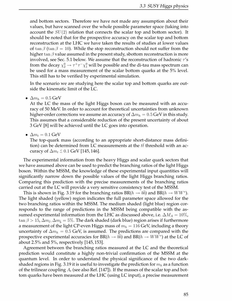
3.3 SUSY Higgs physics
and bottom sectors. Therefore we have not made any assumption about theirvalues, but have scanned over the whole possible parameter space (taking intoaccount the SU(2) relation that connects the scalar top and bottom sector). Itshould be noted that for the prospective accuracy on the scalar top and bottomreconstruction at the LHC we have taken the results of studies at lower valuesof tan β (tanβ = 10). While the stop reconstruction should not suffer from thehigher tanβ value assumed in the present study, sbottom reconstruction is moreinvolved, see Sec. 5.1 below. We assume that the reconstruction of hadronic τ ’sfrom the decay χ0
2 → τ+τ−χ01 will be possible and the di-tau mass spectrum can
be used for a mass measurement of the scalar bottom quarks at the 5% level.This still has to be verified by experimental simulation.
In the scenario we are studying here the scalar top and bottom quarks are out-side the kinematic limit of the LC.
• ∆mh = 0.5 GeVAt the LC the mass of the light Higgs boson can be measured with an accu-racy of 50 MeV. In order to account for theoretical uncertainties from unknownhigher-order corrections we assume an accuracy of ∆mh = 0.5 GeV in this study.This assumes that a considerable reduction of the present uncertainty of about3 GeV [8] will be achieved until the LC goes into operation.
• ∆mt = 0.1 GeVThe top-quark mass (according to an appropriate short-distance mass defini-tion) can be determined from LC measurements at the tt threshold with an ac-curacy of ∆mt
<∼ 0.1 GeV [145, 146].
The experimental information from the heavy Higgs and scalar quark sectors thatwe have assumed above can be used to predict the branching ratios of the light Higgsboson. Within the MSSM, the knowledge of these experimental input quantities willsignificantly narrow down the possible values of the light Higgs branching ratios.Comparing this prediction with the precise measurements of the branching ratioscarried out at the LC will provide a very sensitive consistency test of the MSSM.
This is shown in Fig. 3.19 for the branching ratios BR(h → bb) and BR(h → WW ∗).The light shaded (yellow) region indicates the full parameter space allowed for thetwo branching ratios within the MSSM. The medium shaded (light blue) region cor-responds to the range of predictions in the MSSM being compatible with the as-sumed experimental information from the LHC as discussed above, i.e. ∆MA = 10%,tan β > 15, ∆mt,∆mb = 5%. The dark shaded (dark blue) region arises if furthermorea measurement of the light CP-even Higgs mass of mh = 116 GeV, including a theoryuncertainty of ∆mh = 0.5 GeV, is assumed. The predictions are compared with theprospective experimental accuracies for BR(h → bb) and BR(h → WW ∗) at the LC ofabout 2.5% and 5%, respectively [145, 153].
Agreement between the branching ratios measured at the LC and the theoreticalprediction would constitute a highly non-trivial confirmation of the MSSM at thequantum level. In order to understand the physical significance of the two dark-shaded regions in Fig. 3.19 it is useful to investigate the prediction formh as a functionof the trilinear couplingAt (see also Ref. [147]). If the masses of the scalar top and bot-tom quarks have been measured at the LHC (using LC input), a precise measurement
85
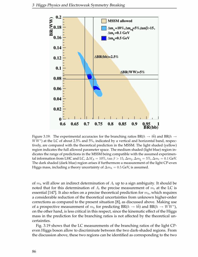
3 Higgs Physics and Electroweak Symmetry Breaking
Figure 3.19: The experimental accuracies for the branching ratios BR(h → bb) and BR(h →WW ∗) at the LC of about 2.5% and 5%, indicated by a vertical and horizontal band, respec-tively, are compared with the theoretical prediction in the MSSM. The light shaded (yellow)region indicates the full allowed parameter space. The medium shaded (light blue) region in-dicates the range of predictions in the MSSM being compatible with the assumed experimen-tal information from LHC and LC, ∆MA = 10%, tan β > 15, ∆mt,∆mb = 5%, ∆mt = 0.1 GeV.The dark shaded (dark blue) region arises if furthermore a measurement of the light CP-evenHiggs mass, including a theory uncertainty of ∆mh = 0.5 GeV, is assumed.
of mh will allow an indirect determination of At up to a sign ambiguity. It should benoted that for this determination of At the precise measurement of mt at the LC isessential [147]. It also relies on a precise theoretical prediction for mh, which requiresa considerable reduction of the theoretical uncertainties from unknown higher-ordercorrections as compared to the present situation [8], as discussed above. Making useof a prospective measurement of mh for predicting BR(h → bb) and BR(h → WW ∗),on the other hand, is less critical in this respect, since the kinematic effect of the Higgsmass in the prediction for the branching ratios is not affected by the theoretical un-certainties.
Fig. 3.19 shows that the LC measurements of the branching ratios of the light CP-even Higgs boson allow to discriminate between the two dark-shaded regions. Fromthe discussion above, these two regions can be identified as corresponding to the two
86
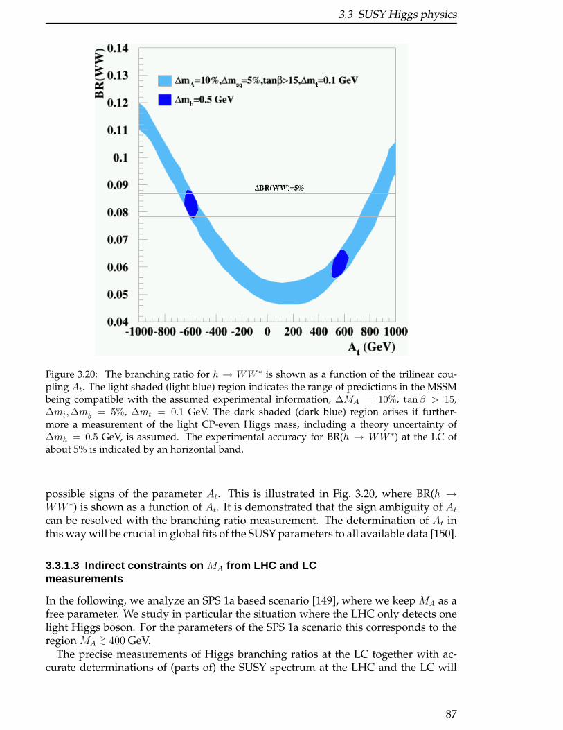
3.3 SUSY Higgs physics
Figure 3.20: The branching ratio for h → WW ∗ is shown as a function of the trilinear cou-pling At. The light shaded (light blue) region indicates the range of predictions in the MSSMbeing compatible with the assumed experimental information, ∆MA = 10%, tan β > 15,∆mt,∆mb = 5%, ∆mt = 0.1 GeV. The dark shaded (dark blue) region arises if further-more a measurement of the light CP-even Higgs mass, including a theory uncertainty of∆mh = 0.5 GeV, is assumed. The experimental accuracy for BR(h → WW ∗) at the LC ofabout 5% is indicated by an horizontal band.
possible signs of the parameter At. This is illustrated in Fig. 3.20, where BR(h →WW ∗) is shown as a function of At. It is demonstrated that the sign ambiguity of Atcan be resolved with the branching ratio measurement. The determination of At inthis way will be crucial in global fits of the SUSY parameters to all available data [150].
3.3.1.3 Indirect constraints on MA from LHC and LCmeasurements
In the following, we analyze an SPS 1a based scenario [149], where we keep MA as afree parameter. We study in particular the situation where the LHC only detects onelight Higgs boson. For the parameters of the SPS 1a scenario this corresponds to theregion MA
>∼ 400 GeV.The precise measurements of Higgs branching ratios at the LC together with ac-
curate determinations of (parts of) the SUSY spectrum at the LHC and the LC will
87
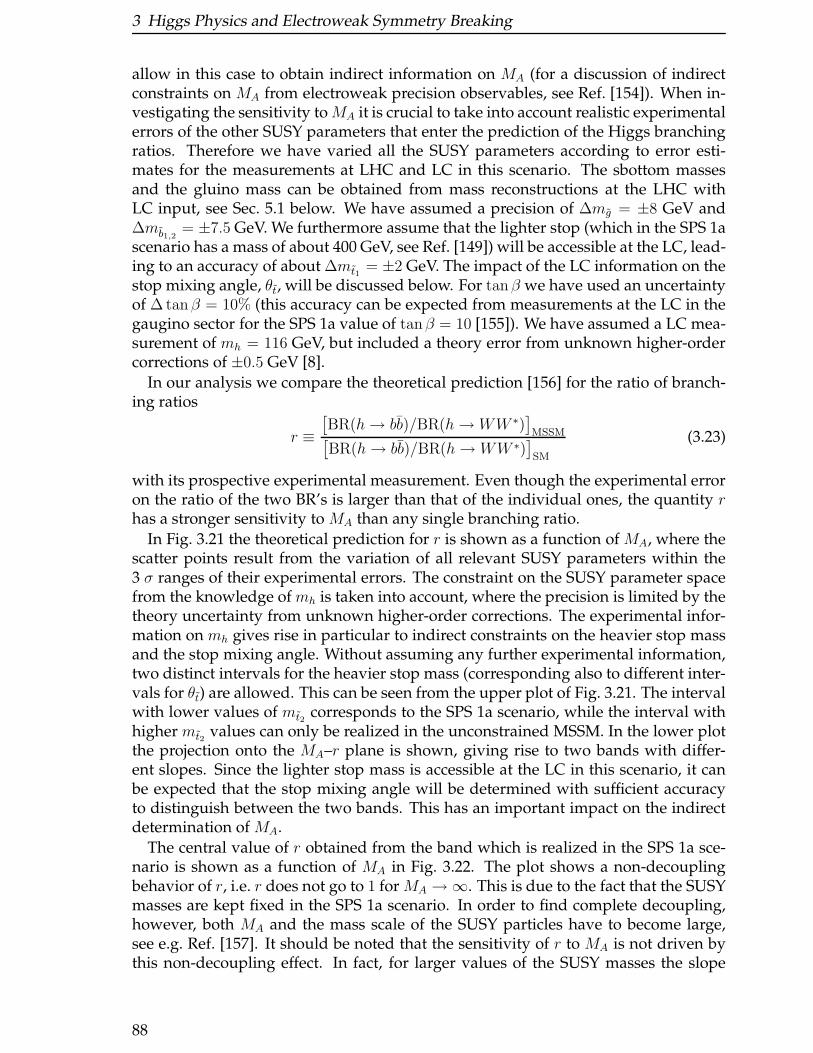
3 Higgs Physics and Electroweak Symmetry Breaking
allow in this case to obtain indirect information on MA (for a discussion of indirectconstraints on MA from electroweak precision observables, see Ref. [154]). When in-vestigating the sensitivity toMA it is crucial to take into account realistic experimentalerrors of the other SUSY parameters that enter the prediction of the Higgs branchingratios. Therefore we have varied all the SUSY parameters according to error esti-mates for the measurements at LHC and LC in this scenario. The sbottom massesand the gluino mass can be obtained from mass reconstructions at the LHC withLC input, see Sec. 5.1 below. We have assumed a precision of ∆mg = ±8 GeV and∆mb1,2
= ±7.5 GeV. We furthermore assume that the lighter stop (which in the SPS 1ascenario has a mass of about 400 GeV, see Ref. [149]) will be accessible at the LC, lead-ing to an accuracy of about ∆mt1 = ±2 GeV. The impact of the LC information on thestop mixing angle, θt, will be discussed below. For tanβ we have used an uncertaintyof ∆ tanβ = 10% (this accuracy can be expected from measurements at the LC in thegaugino sector for the SPS 1a value of tanβ = 10 [155]). We have assumed a LC mea-surement of mh = 116 GeV, but included a theory error from unknown higher-ordercorrections of ±0.5 GeV [8].
In our analysis we compare the theoretical prediction [156] for the ratio of branch-ing ratios
r ≡[BR(h→ bb)/BR(h→WW ∗)
]MSSM[
BR(h→ bb)/BR(h→ WW ∗)]SM
(3.23)
with its prospective experimental measurement. Even though the experimental erroron the ratio of the two BR’s is larger than that of the individual ones, the quantity rhas a stronger sensitivity to MA than any single branching ratio.
In Fig. 3.21 the theoretical prediction for r is shown as a function of MA, where thescatter points result from the variation of all relevant SUSY parameters within the3 σ ranges of their experimental errors. The constraint on the SUSY parameter spacefrom the knowledge of mh is taken into account, where the precision is limited by thetheory uncertainty from unknown higher-order corrections. The experimental infor-mation on mh gives rise in particular to indirect constraints on the heavier stop massand the stop mixing angle. Without assuming any further experimental information,two distinct intervals for the heavier stop mass (corresponding also to different inter-vals for θt) are allowed. This can be seen from the upper plot of Fig. 3.21. The intervalwith lower values of mt2 corresponds to the SPS 1a scenario, while the interval withhigher mt2 values can only be realized in the unconstrained MSSM. In the lower plotthe projection onto the MA–r plane is shown, giving rise to two bands with differ-ent slopes. Since the lighter stop mass is accessible at the LC in this scenario, it canbe expected that the stop mixing angle will be determined with sufficient accuracyto distinguish between the two bands. This has an important impact on the indirectdetermination of MA.
The central value of r obtained from the band which is realized in the SPS 1a sce-nario is shown as a function of MA in Fig. 3.22. The plot shows a non-decouplingbehavior of r, i.e. r does not go to 1 for MA →∞. This is due to the fact that the SUSYmasses are kept fixed in the SPS 1a scenario. In order to find complete decoupling,however, both MA and the mass scale of the SUSY particles have to become large,see e.g. Ref. [157]. It should be noted that the sensitivity of r to MA is not driven bythis non-decoupling effect. In fact, for larger values of the SUSY masses the slope
88
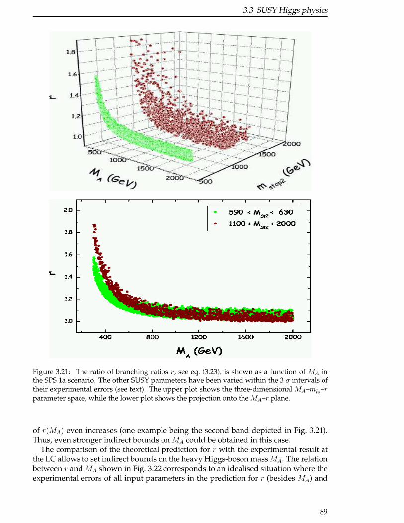
3.3 SUSY Higgs physics
Figure 3.21: The ratio of branching ratios r, see eq. (3.23), is shown as a function of MA inthe SPS 1a scenario. The other SUSY parameters have been varied within the 3 σ intervals oftheir experimental errors (see text). The upper plot shows the three-dimensional MA–mt2
–rparameter space, while the lower plot shows the projection onto the MA–r plane.
of r(MA) even increases (one example being the second band depicted in Fig. 3.21).Thus, even stronger indirect bounds on MA could be obtained in this case.
The comparison of the theoretical prediction for r with the experimental result atthe LC allows to set indirect bounds on the heavy Higgs-boson massMA. The relationbetween r and MA shown in Fig. 3.22 corresponds to an idealised situation where theexperimental errors of all input parameters in the prediction for r (besides MA) and
89
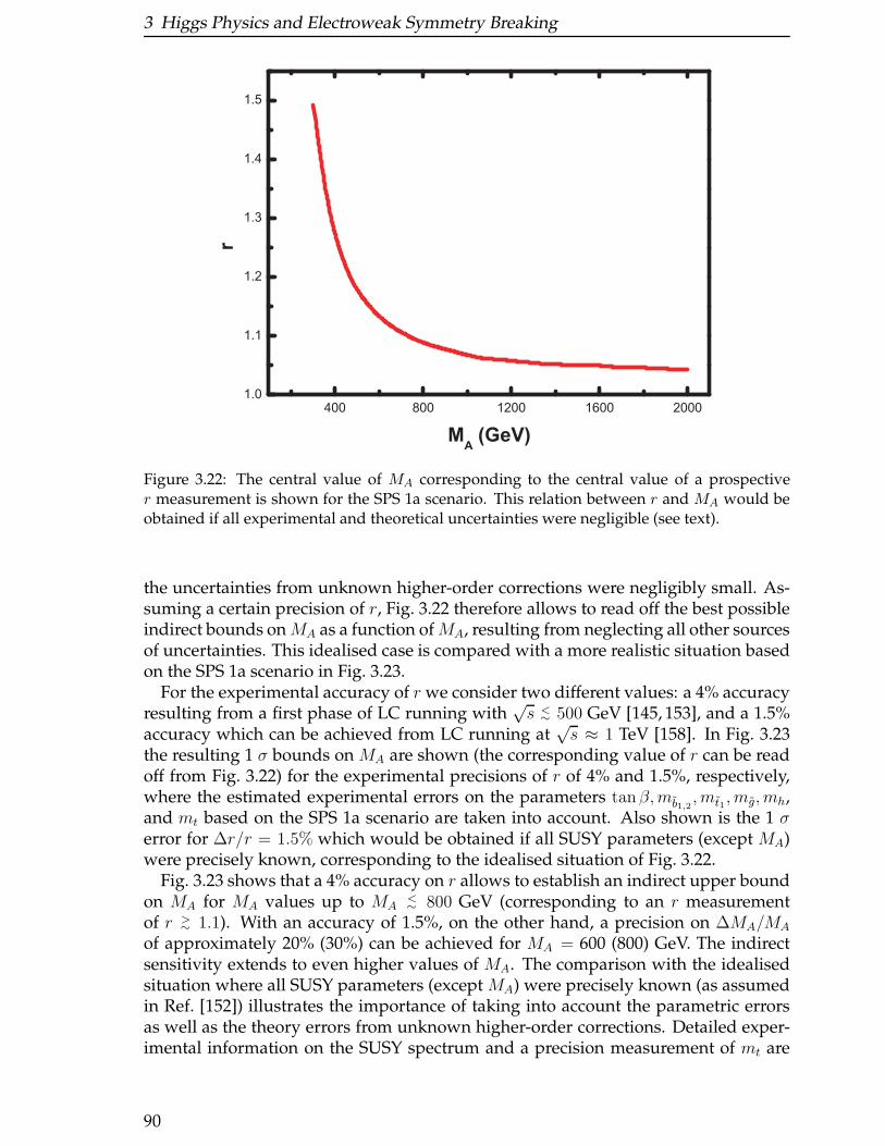
3 Higgs Physics and Electroweak Symmetry Breaking
Figure 3.22: The central value of MA corresponding to the central value of a prospectiver measurement is shown for the SPS 1a scenario. This relation between r and MA would beobtained if all experimental and theoretical uncertainties were negligible (see text).
the uncertainties from unknown higher-order corrections were negligibly small. As-suming a certain precision of r, Fig. 3.22 therefore allows to read off the best possibleindirect bounds onMA as a function ofMA, resulting from neglecting all other sourcesof uncertainties. This idealised case is compared with a more realistic situation basedon the SPS 1a scenario in Fig. 3.23.
For the experimental accuracy of r we consider two different values: a 4% accuracyresulting from a first phase of LC running with
√s <∼ 500 GeV [145, 153], and a 1.5%
accuracy which can be achieved from LC running at√s ≈ 1 TeV [158]. In Fig. 3.23
the resulting 1 σ bounds on MA are shown (the corresponding value of r can be readoff from Fig. 3.22) for the experimental precisions of r of 4% and 1.5%, respectively,where the estimated experimental errors on the parameters tanβ,mb1,2
, mt1 , mg, mh,and mt based on the SPS 1a scenario are taken into account. Also shown is the 1 σerror for ∆r/r = 1.5% which would be obtained if all SUSY parameters (except MA)were precisely known, corresponding to the idealised situation of Fig. 3.22.
Fig. 3.23 shows that a 4% accuracy on r allows to establish an indirect upper boundon MA for MA values up to MA
<∼ 800 GeV (corresponding to an r measurementof r >∼ 1.1). With an accuracy of 1.5%, on the other hand, a precision on ∆MA/MA
of approximately 20% (30%) can be achieved for MA = 600 (800) GeV. The indirectsensitivity extends to even higher values of MA. The comparison with the idealisedsituation where all SUSY parameters (except MA) were precisely known (as assumedin Ref. [152]) illustrates the importance of taking into account the parametric errorsas well as the theory errors from unknown higher-order corrections. Detailed exper-imental information on the SUSY spectrum and a precision measurement of mt are
90
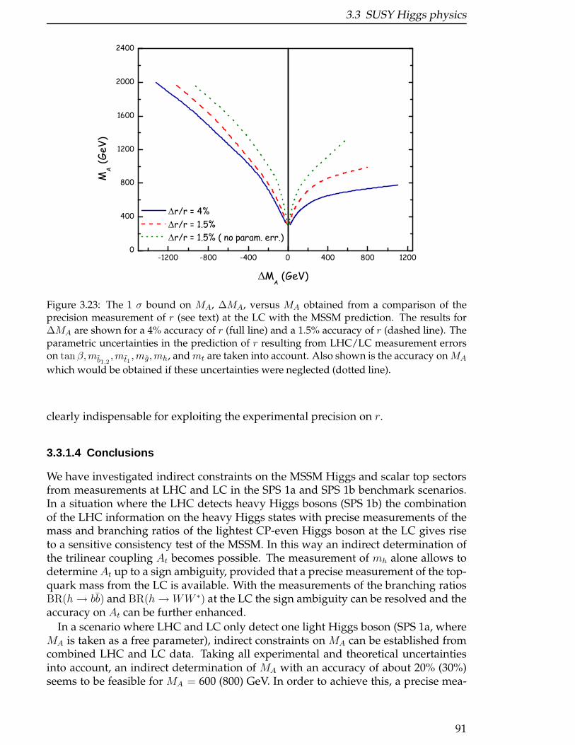
3.3 SUSY Higgs physics
Figure 3.23: The 1 σ bound on MA, ∆MA, versus MA obtained from a comparison of theprecision measurement of r (see text) at the LC with the MSSM prediction. The results for∆MA are shown for a 4% accuracy of r (full line) and a 1.5% accuracy of r (dashed line). Theparametric uncertainties in the prediction of r resulting from LHC/LC measurement errorson tan β,mb1,2
,mt1,mg,mh, andmt are taken into account. Also shown is the accuracy onMA
which would be obtained if these uncertainties were neglected (dotted line).
clearly indispensable for exploiting the experimental precision on r.
3.3.1.4 Conclusions
We have investigated indirect constraints on the MSSM Higgs and scalar top sectorsfrom measurements at LHC and LC in the SPS 1a and SPS 1b benchmark scenarios.In a situation where the LHC detects heavy Higgs bosons (SPS 1b) the combinationof the LHC information on the heavy Higgs states with precise measurements of themass and branching ratios of the lightest CP-even Higgs boson at the LC gives riseto a sensitive consistency test of the MSSM. In this way an indirect determination ofthe trilinear coupling At becomes possible. The measurement of mh alone allows todetermine At up to a sign ambiguity, provided that a precise measurement of the top-quark mass from the LC is available. With the measurements of the branching ratiosBR(h→ bb) and BR(h→WW ∗) at the LC the sign ambiguity can be resolved and theaccuracy on At can be further enhanced.
In a scenario where LHC and LC only detect one light Higgs boson (SPS 1a, whereMA is taken as a free parameter), indirect constraints on MA can be established fromcombined LHC and LC data. Taking all experimental and theoretical uncertaintiesinto account, an indirect determination of MA with an accuracy of about 20% (30%)seems to be feasible for MA = 600 (800) GeV. In order to achieve this, a precise mea-
91

3 Higgs Physics and Electroweak Symmetry Breaking
surement of the branching ratios BR(h → bb) and BR(h → WW ∗) at the LC andinformation on the parameters of the scalar top and bottom sector from combinedLHC / LC analyses will be crucial.
3.3.2 Importance of the χ01 mass measurement for the
A0, H0 → χ02χ
02 mass reconstruction
F. Moortgat
Supersymmetric decay modes of the heavy MSSM Higgs bosons can be used to discover these
particles in the difficult low and intermediate tan β region of the MSSM parameter space. In
particular, the A0,H0 → χ02χ
02 decay can lead to a cleanly observable 4ℓ + EmissT final state,
provided neutralinos and sleptons are sufficiently light. In this contribution we investigate
the importance of a precise measurement of the χ01 mass at a future LC for the Higgs mass
reconstruction in this channel at the LHC. We argue that the best way to determine the mass of
theA0,H0 bosons is to fit the 4-lepton invariant massm4l, which is an estimator for the Higgs
mass, to the Monte Carlo distribution. However, the m4l estimator depends also strongly on
the mass of the lightest neutralino χ01. Therefore, an accurate measurement of the χ0
1 mass
with a precision better than about 1% would be needed for an optimal measurement of mA
through the neutralino channel at the LHC.
3.3.2.1 Introduction
In the MSSM, the couplings of the heavier neutral A0 and H0 bosons to down-typefermions are enhanced at high tan β:
gA0bb ∼ mb tanβ gH0bb ∼ mbcosα
cos β(3.24)
at the expense of the couplings to up-type fermions. This results in an important pro-duction mechanism for H0 and A0 Higgs bosons in association with bb pairs at theLHC: gg → H0, A0bb. For the same reasons, the dominant decay modes of the heavyneutral Higgs bosons are H0, A0 → bb and H0, A0 → ττ . The bb channel has largedifficulties to overcome the experimental trigger thresholds at the LHC and thereforedoes not show much potential; the H0, A0 → ττ mode on the other hand, where boththe hadronic and leptonic τ decaus can be exploited, allows to discover the heavyneutral Higgs bosons over a large part of the parameter space, notably for high andintermediate values of tan β. Also the H0, A0 → µµ channel shows some interestingpotential, in spite of the very small braching ratio of Higgs into muonsO(10−4), sincemuons are objects that can be experimentally measured with high precision and effi-ciency.
In spite of the good coverage of the large tan β region, the low and intermediate tan βdomain remains largely inaccessible for the previously mentioned channels, and newchannels need to be found. Apart from the Higgs couplings to fermions (3.24), alsosome of the Higgs couplings to gauge bosons might be exploited:
gH0V V ∼ cos(β − α) gH0A0Z0 ∼ sin(β − α)
92
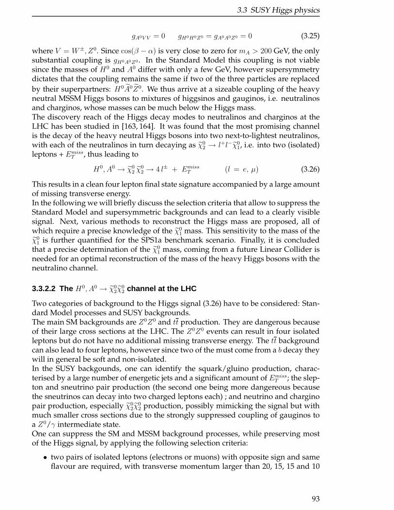
3.3 SUSY Higgs physics
gA0V V = 0 gH0H0Z0 = gA0A0Z0 = 0 (3.25)
where V = W±, Z0. Since cos(β − α) is very close to zero for mA > 200 GeV, the onlysubstantial coupling is gH0A0Z0 . In the Standard Model this coupling is not viablesince the masses of H0 and A0 differ with only a few GeV, however supersymmetrydictates that the coupling remains the same if two of the three particles are replaced
by their superpartners: H0A0Z0. We thus arrive at a sizeable coupling of the heavyneutral MSSM Higgs bosons to mixtures of higgsinos and gauginos, i.e. neutralinosand charginos, whose masses can be much below the Higgs mass.The discovery reach of the Higgs decay modes to neutralinos and charginos at theLHC has been studied in [163, 164]. It was found that the most promising channelis the decay of the heavy neutral Higgs bosons into two next-to-lightest neutralinos,with each of the neutralinos in turn decaying as χ0
2 → l+l−χ01, i.e. into two (isolated)
leptons + EmissT , thus leading to
H0, A0 → χ02 χ
02 → 4 l± + Emiss
T (l = e, µ) (3.26)
This results in a clean four lepton final state signature accompanied by a large amountof missing transverse energy.In the following we will briefly discuss the selection criteria that allow to suppress theStandard Model and supersymmetric backgrounds and can lead to a clearly visiblesignal. Next, various methods to reconstruct the Higgs mass are proposed, all ofwhich require a precise knowledge of the χ0
1 mass. This sensitivity to the mass of theχ0
1 is further quantified for the SPS1a benchmark scenario. Finally, it is concludedthat a precise determination of the χ0
1 mass, coming from a future Linear Collider isneeded for an optimal reconstruction of the mass of the heavy Higgs bosons with theneutralino channel.
3.3.2.2 The H0, A0 → χ02χ
02 channel at the LHC
Two categories of background to the Higgs signal (3.26) have to be considered: Stan-dard Model processes and SUSY backgrounds.The main SM backgrounds are Z0Z0 and tt production. They are dangerous becauseof their large cross sections at the LHC. The Z0Z0 events can result in four isolatedleptons but do not have no additional missing transverse energy. The tt backgroundcan also lead to four leptons, however since two of the must come from a b decay theywill in general be soft and non-isolated.In the SUSY backgounds, one can identify the squark/gluino production, charac-terised by a large number of energetic jets and a significant amount of Emiss
T ; the slep-ton and sneutrino pair production (the second one being more dangereous becausethe sneutrinos can decay into two charged leptons each) ; and neutrino and charginopair production, especially χ0
2χ02 production, possibly mimicking the signal but with
much smaller cross sections due to the strongly suppressed coupling of gauginos toa Z0/γ intermediate state.One can suppress the SM and MSSM background processes, while preserving mostof the Higgs signal, by applying the following selection criteria:
• two pairs of isolated leptons (electrons or muons) with opposite sign and sameflavour are required, with transverse momentum larger than 20, 15, 15 and 10
93

3 Higgs Physics and Electroweak Symmetry Breaking
0
10
20
30
40
50
60
70
80
90
0 50 100 150 200 250 300 350 400
4-lepton effective mass (GeV)
Eve
nts
/ 1
5 G
eV
Figure 3.24: Four lepton invariant mass for signal versus background (SM + SUSY) for theSPS1a scenario wheremA = 393 GeV and tan β = 10 (for an integrated luminosity of 100 fb−1).
GeV resepctively and within |η| < 2.4. The isolation criterion demands thatthere are no charged particles with pT > 1.5 GeV in a cone of radius ∆R =√
(∆φ)2 + (∆η)2 = 0.3 rad around each lepton track, and that the sum of thetransverse energy in the deposited in the electromagnetic calorimeter between∆R = 0.05 and ∆R = 0.3 rad is smaller than 3 GeV.
• a Z0-veto is imposed, i.e. all dilepton pairs of opposite sign and same flavourthat have an invariant mass in the range mZ0 ± 10 GeV are rejected.
• events must have a missing transverse energy in the interval 20 GeV < EmissT
< 150 GeV. The lower limit suppresses the Z0Z0 events while the upper limitreduces the squark/gluino background.
• if needed, one can apply ceilings to the jet multiplicity and the transverse energyof the jets to further suppress squark and gluino events if these particles wouldbe light (and therefore copiously produced).
• further optimization can be done by introducing upper limits to the transversemomentum of the leptons and the four lepton invariant mass, however theydepend on the specific MSSM scenario.
After such a selection procedure, a clear signal remains visible on top of the (mainlySUSY) backgrounds, as can be seen in Figure 3.24 for the SPS1a benchmark scenario[165] where mA = 393 GeV and tan β = 10, M1 = 100 GeV, M2 = 192 GeV, µ = 352 GeV,mlL
= 202 GeV, m ˜lR= 142 GeV, mqL = 540 GeV, mqR = 520 GeV, mg = 595 GeV.
3.3.2.3 Higgs mass reconstruction with the H0, A0 → χ02χ
02 channel
In order to reconstruct the mass of the H0, A0 Higgs boson we can exploit an inter-esting kinematical property of the disintegration process. The decay of the next-to-
94
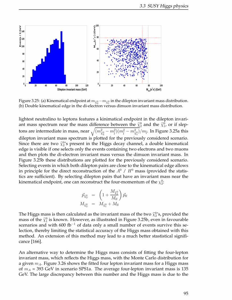
3.3 SUSY Higgs physics
0
20
40
60
80
100
120
140
0 20 40 60 80 100 120
Dilepton invariant mass (GeV)
Eve
nts
/ 3
Ge
V
0
20
40
60
80
100
0 20 40 60 80 100
Minv (e+e-) (GeV)M
inv(µ
+µ
- ) (
Ge
V)
Figure 3.25: (a) Kinematical endpoint atmχ02−mχ0
1in the dilepton invariant mass distribution.
(b) Double kinematical edge in the di-electron versus dimuon invariant mass distribution.
lightest neutralino to leptons features a kinimatical endpoint in the dilepton invari-ant mass spectrum near the mass difference between the χ0
2 and the χ01, or if slep-
tons are intermediate in mass, near√
(m2χ0
2−m2
l)(m2
l−m2
χ01)/ml. In Figure 3.25a this
dilepton invariant mass spectrum is plotted for the previously considered scenario.Since there are two χ0
2’s present in the Higgs decay channel, a double kinematicaledge is visible if one selects only the events containing two electrons and two muonsand then plots the di-electron invariant mass versus the dimuon invariant mass. InFigure 3.25b these distributions are plotted for the previously considered scenario.Selecting events in which both dilepton pairs are close to the kinematical edge allowsin principle for the direct reconstruction of the A0 / H0 mass (provided the statis-tics are sufficient). By selecting dilepton pairs that have an invariant mass near thekinematical endpoint, one can reconstruct the four-momentum of the χ0
2:
~pχ02
=
(1 +
Mχ01
Mll
)~pll
Mχ02
= Mχ01+Mll
The Higgs mass is then calculated as the invariant mass of the two χ02’s, provided the
mass of the χ01 is known. However, as illustrated in Figure 3.25b, even in favourable
scenarios and with 600 fb−1 of data only a small number of events survive this se-lection, thereby limiting the statistical accuracy of the Higgs mass obtained with thismethod. An extension of this method may lead to a much better stastistical signifi-cance [166].
An alternative way to determine the Higgs mass consists of fitting the four-leptoninvariant mass, which reflects the Higgs mass, with the Monte Carlo distribution fora given mA. Figure 3.26 shows the fitted four lepton invariant mass for a Higgs massof mA = 393 GeV in scenario SPS1a. The average four-lepton invariant mass is 135GeV. The large discrepancy between this number and the Higgs mass is due to the
95

3 Higgs Physics and Electroweak Symmetry Breaking
0
25
50
75
100
125
150
175
200
0 50 100 150 200 250 300 350 400
4-lepton invariant mass (GeV)
Even
ts / 1
5 GeV
600 fb−1
A0, H0 → χ02χ
02 → 4ℓ+ Emiss
T
Figure 3.26: Fit of the 4-lepton invariant mass to the Monte Carlo distribution for scenarioSPS1a, for a total integrated luminosity of 600 fb−1.
escaping χ01 particles.
The four lepton invariant mass distribution is only mildly sensitive to the mass ofthe A0 boson (the mass of the H0 boson is typically a few GeV’s higher). A shift ofmA by 10 (20) GeV leads to a shift of 〈Mllll〉 by 4 (8) GeV. This behaviour is illustratedin Figure 3.27a where the four lepton invariant mass distributions are shown for mA
= 373, 393 and 413 GeV.Because of the two χ0
1’s escape during the decay of the Higgs boson., the Mllll distri-bution is also sensitive to the mass of the χ0
1. A shift of mχ01
by 5 (10) GeV leads to ashift of 〈Mllll〉 by 5 (15) GeV. Figure 3.27b illustrates this dependency by showing thefour lepton invariant mass for three values of mχ0
1= 90, 100 and 110 GeV.
Since the Mllll distribution is sensitive to both mA and mχ01, the mass of the χ0
1 needsto be known with good precision in order to suppress this source of error in the de-termination of the Higgs mass. Assuming an ultimate LHC integrated luminosity of600 fb−1, the statistical error on Mllll in the above scenario is ∼1%. This can lead to aprecision on mA of about 3%, provided the mass of the χ0
1 can be determined to betterthan 1%.
3.3.2.4 Conclusion
Supersymmetric decay modes of the heavy MSSM Higgs bosons offer interesting pos-sibilities to discover these particles in the low and intermedate tan β region of theMSSM parameter space. In particular, the A0, H0 → χ0
2χ02 decay can lead to a cleanly
observable 4ℓ + EmissT final state, provided neutralinos and sleptons are sufficiently
light. In this contribution we have investigated the importance of a precise measure-ment of the χ0
1 mass at a future LC for the Higgs mass reconstruction in this channelat the LHC. Probably the best way to determine the mass of the A,H bosons is to
96
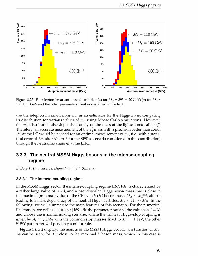
3.3 SUSY Higgs physics
0
25
50
75
100
125
150
175
200
0 50 100 150 200 250 300 350 400
4-lepton invariant mass (GeV)
Eve
nts
/ 15
GeV
600 fb−1
← mA = 373 GeV
← mA = 393 GeV
← mA = 413 GeV
0
25
50
75
100
125
150
175
200
0 50 100 150 200 250 300 350 400
4-lepton invariant mass (GeV)
Eve
nts
/ 15
GeV
600 fb−1
← M1 = 110 GeV
←M1 = 100 GeV
←M1 = 90 GeV
Figure 3.27: Four lepton invariant mass distribition (a) for MA = 393 ± 20 GeV; (b) for M1 =100 ± 10 GeV and the other parameters fixed as described in the text.
use the 4-lepton invariant mass m4l as an estimator for the Higgs mass, comparingits distribution for various values of mA using Monte Carlo simulations. However,the m4l distribution also depends strongly on the mass of the lightest neutralino χ0
1.Therefore, an accurate measurement of the χ0
1 mass with a precision better than about1% at the LC would be needed for an optimal measurement of mA (i.e. with a statis-tical error of 3% after 600 fb−1 for the SPS1a scenario considered in this contribution)through the neutralino channel at the LHC.
3.3.3 The neutral MSSM Higgs bosons in the intense-couplingregime
E. Boos V. Bunichev, A. Djouadi and H.J. Schreiber
3.3.3.1 The intense-coupling regime
In the MSSM Higgs sector, the intense-coupling regime [167, 168] is characterized bya rather large value of tan β, and a pseudoscalar Higgs boson mass that is close tothe maximal (minimal) value of the CP-even h (H) boson mass, MA ∼ Mmax
h , almostleading to a mass degeneracy of the neutral Higgs particles, Mh ∼ MA ∼ MH . In thefollowing, we will summarize the main features of this scenario. For the numericalillustration, we will use HDECAY[169], fix the parameter tan β to the value tanβ = 30and choose the maximal mixing scenario, where the trilinear Higgs–stop coupling isgiven by At ≃
√6MS with the common stop masses fixed to MS = 1 TeV; the other
SUSY parameter will play only a minor role.
Figure 1 (left) displays the masses of the MSSM Higgs bosons as a function of MA.As can be seen, for MA close to the maximal h boson mass, which in this case is
97
3 Higgs Physics and Electroweak Symmetry Breaking
Mmaxh ≃ 130 GeV, the mass differences MA −Mh and MH −MA are less than about
5 GeV. The H± boson mass, given by M2H± ∼ M2
A + M2W , is larger : in the range
MA <∼ 140 GeV, one has MH± <∼ 160 GeV, implying that charged Higgs bosons canalways be produced in top-quark decays, t → H+b. The couplings of the CP-evenHiggs bosons to fermions and gauge bosons normalized to the SM Higgs boson cou-plings are also shown in Fig. 1 (right). For small MA values, the H boson has almostSM couplings, while the couplings of the h boson to W,Z, t (b) are suppressed (en-hanced); for large MA values the roles of h and H are interchanged. For mediumvalues, MA ∼ Mmax
h , the couplings of both h and H to gauge bosons V = W,Z andtop quarks are suppressed, while the couplings to b quarks are strongly enhanced.The normalized couplings of the CP-even Higgs particle are simply gAV V = 0 andgAbb = 1/gAtt = tanβ = 30.
These couplings determine the branching ratios of the Higgs particle, which areshown in Fig. 2. Because the enhanced couplings, the three Higgs particle branchingratios to bb and τ+τ− are the dominant ones, with values ∼ 90% and ∼ 10% respec-tively. The decays H → WW ∗ do not exceed the level of 10%, even for small MA val-ues [whereH is almost SM-like] and in most of theMA range the decaysH, h→ WW ∗
are suppressed to the level where they are not useful. The decays into ZZ∗ are one or-der of magnitude smaller and the decays into γγ are very strongly suppressed for thethree Higgsses and cannot be used anymore. Finally, note that the branching ratiosfor the decays into muons, Φ→ µ+µ−, are constant in the entire MA range exhibited,at the level of 3× 10⁻⁴.
Summing up the partial widths for all decays, the total decay widths of the threeHiggs particles are shown in the left-hand side of Fig. 3. As can be seen, for MA ∼ 130GeV, they are at the level of 1–2 GeV, i.e. two orders of magnitude larger than thewidth of the SM Higgs boson for this value of tan β [the total width increases astan2 β]. The right-hand side of the figure shows the mass bands MΦ ± ΓΦ and, as canbe seen, for the above value of MA, the three Higgs boson masses are overlapping.
3.3.3.2 Discrimination of the three Higgs bosons at the LHC
The most difficult problem we must face in the intense-coupling regime, is to resolvebetween the three peaks of the neutral Higgs bosons when their masses are close toone another. The only decays with large branching ratios on which we can rely arethe bb and τ+τ− modes. At the LHC, the former has too large QCD background to beuseful, while for the latter channel [which has been shown to be viable for discovery]the expected experimental resolution on the invariant mass of the τ+τ− system is ofthe order of 10 to 20 GeV, and thus clearly too large. One would then simply observea relatively wide resonance corresponding to A and h and/or H production. Sincethe branching ratios of the decays into γγ and ZZ∗ → 4ℓ are too small, a way out is touse the Higgs decays into muon pairs: although the branchings ratio is rather small,BR(Φ → µ+µ−) ∼ 3.3 × 10⁻⁴, the resolution is expected to be as good as 1 GeV, i.e.comparable to the total width, for MΦ ∼ 130 GeV.
Because of the strong enhancement of the Higgs couplings to bottom quarks, the
98
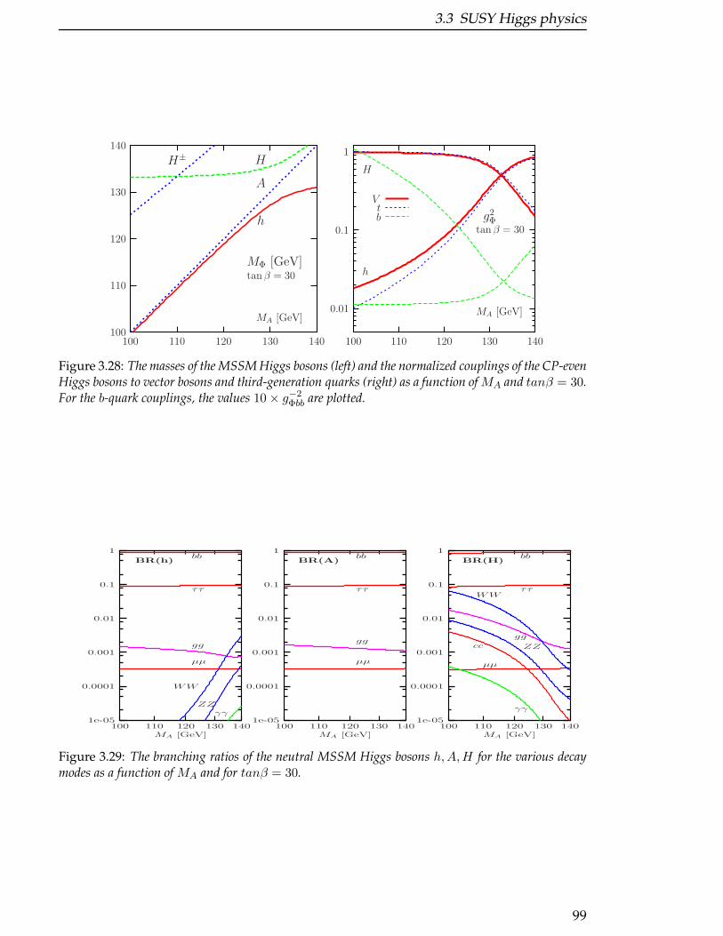
3.3 SUSY Higgs physics
HH±
A
h
MA [GeV]
tanβ = 30
MΦ [GeV]
140130120110100
140
130
120
110
100
btV
MA [GeV]
h
H
tan β = 30g2
Φ
140130120110100
1
0.1
0.01
Figure 3.28: The masses of the MSSM Higgs bosons (left) and the normalized couplings of the CP-evenHiggs bosons to vector bosons and third-generation quarks (right) as a function ofMA and tanβ = 30.For the b-quark couplings, the values 10× g−2
Φbb are plotted.
γγZZ
WW
µµ
gg
ττ
bbBR(h)
MA [GeV]140130120110100
1
0.1
0.01
0.001
0.0001
1e-05
µµ
gg
ττ
bbBR(A)
MA [GeV]140130120110100
1
0.1
0.01
0.001
0.0001
1e-05
γγ
ZZ
WW
µµ
cc
gg
ττ
bbBR(H)
MA [GeV]140130120110100
1
0.1
0.01
0.001
0.0001
1e-05
Figure 3.29: The branching ratios of the neutral MSSM Higgs bosons h,A,H for the various decaymodes as a function of MA and for tanβ = 30.
99
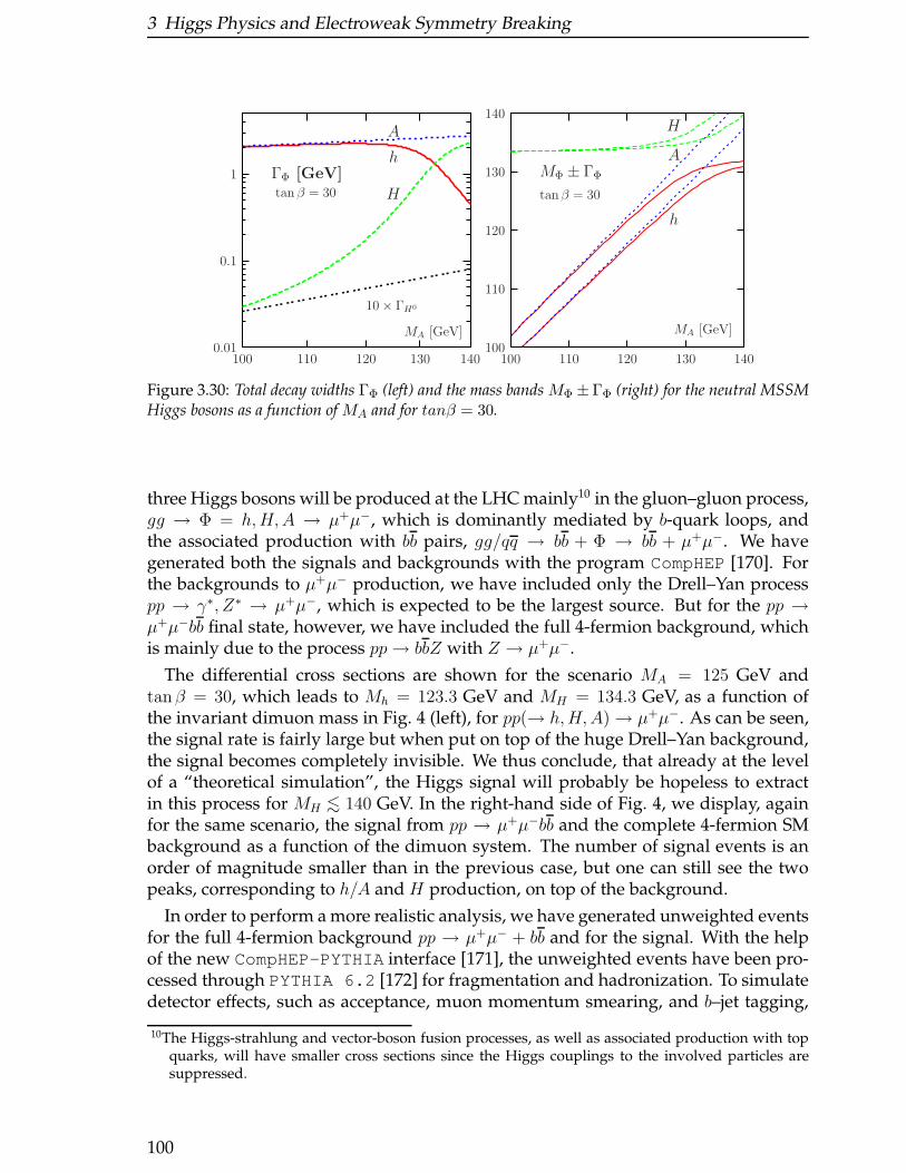
3 Higgs Physics and Electroweak Symmetry Breaking
10× ΓH0
H
h
A
MA [GeV]
tan β = 30
ΓΦ [GeV]
140130120110100
1
0.1
0.01
H
A
h
MA [GeV]
tanβ = 30
MΦ ± ΓΦ
140130120110100
140
130
120
110
100
Figure 3.30: Total decay widths ΓΦ (left) and the mass bands MΦ ± ΓΦ (right) for the neutral MSSMHiggs bosons as a function of MA and for tanβ = 30.
three Higgs bosons will be produced at the LHC mainly10 in the gluon–gluon process,gg → Φ = h,H,A → µ+µ−, which is dominantly mediated by b-quark loops, andthe associated production with bb pairs, gg/qq → bb + Φ → bb + µ+µ−. We havegenerated both the signals and backgrounds with the program CompHEP[170]. Forthe backgrounds to µ+µ− production, we have included only the Drell–Yan processpp → γ∗, Z∗ → µ+µ−, which is expected to be the largest source. But for the pp →µ+µ−bb final state, however, we have included the full 4-fermion background, whichis mainly due to the process pp→ bbZ with Z → µ+µ−.
The differential cross sections are shown for the scenario MA = 125 GeV andtanβ = 30, which leads to Mh = 123.3 GeV and MH = 134.3 GeV, as a function ofthe invariant dimuon mass in Fig. 4 (left), for pp(→ h,H,A)→ µ+µ−. As can be seen,the signal rate is fairly large but when put on top of the huge Drell–Yan background,the signal becomes completely invisible. We thus conclude, that already at the levelof a “theoretical simulation”, the Higgs signal will probably be hopeless to extractin this process for MH <∼ 140 GeV. In the right-hand side of Fig. 4, we display, againfor the same scenario, the signal from pp → µ+µ−bb and the complete 4-fermion SMbackground as a function of the dimuon system. The number of signal events is anorder of magnitude smaller than in the previous case, but one can still see the twopeaks, corresponding to h/A and H production, on top of the background.
In order to perform a more realistic analysis, we have generated unweighted eventsfor the full 4-fermion background pp → µ+µ− + bb and for the signal. With the helpof the new CompHEP-PYTHIAinterface [171], the unweighted events have been pro-cessed through PYTHIA 6.2 [172] for fragmentation and hadronization. To simulatedetector effects, such as acceptance, muon momentum smearing, and b–jet tagging,
10The Higgs-strahlung and vector-boson fusion processes, as well as associated production with topquarks, will have smaller cross sections since the Higgs couplings to the involved particles aresuppressed.
100
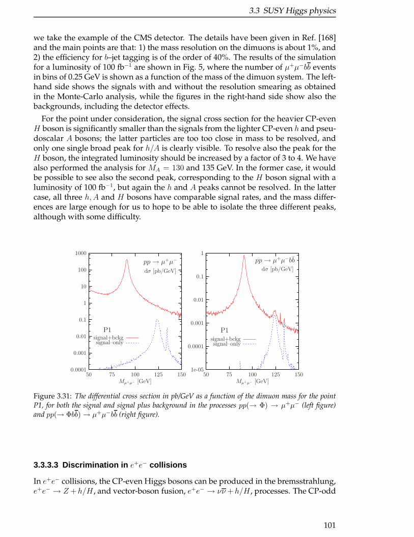
3.3 SUSY Higgs physics
we take the example of the CMS detector. The details have been given in Ref. [168]and the main points are that: 1) the mass resolution on the dimuons is about 1%, and2) the efficiency for b–jet tagging is of the order of 40%. The results of the simulationfor a luminosity of 100 fb−1 are shown in Fig. 5, where the number of µ+µ−bb eventsin bins of 0.25 GeV is shown as a function of the mass of the dimuon system. The left-hand side shows the signals with and without the resolution smearing as obtainedin the Monte-Carlo analysis, while the figures in the right-hand side show also thebackgrounds, including the detector effects.
For the point under consideration, the signal cross section for the heavier CP-evenH boson is significantly smaller than the signals from the lighter CP-even h and pseu-doscalar A bosons; the latter particles are too too close in mass to be resolved, andonly one single broad peak for h/A is clearly visible. To resolve also the peak for theH boson, the integrated luminosity should be increased by a factor of 3 to 4. We havealso performed the analysis for MA = 130 and 135 GeV. In the former case, it wouldbe possible to see also the second peak, corresponding to the H boson signal with aluminosity of 100 fb−1, but again the h and A peaks cannot be resolved. In the lattercase, all three h,A and H bosons have comparable signal rates, and the mass differ-ences are large enough for us to hope to be able to isolate the three different peaks,although with some difficulty.
signal–onlysignal+bckg
P1
dσ [pb/GeV]
pp→ µ+µ−
Mµ+µ− [GeV]1501251007550
1000
100
10
1
0.1
0.01
0.001
0.0001
signal–onlysignal+bckg
P1
dσ [pb/GeV]
pp→ µ+µ−bb
Mµ+µ− [GeV]1501251007550
1
0.1
0.01
0.001
0.0001
1e-05
Figure 3.31: The differential cross section in pb/GeV as a function of the dimuon mass for the pointP1, for both the signal and signal plus background in the processes pp(→ Φ) → µ+µ− (left figure)and pp(→ Φbb)→ µ+µ−bb (right figure).
3.3.3.3 Discrimination in e+e− collisions
In e+e− collisions, the CP-even Higgs bosons can be produced in the bremsstrahlung,e+e− → Z+h/H , and vector-boson fusion, e+e− → νν+h/H , processes. The CP-odd
101
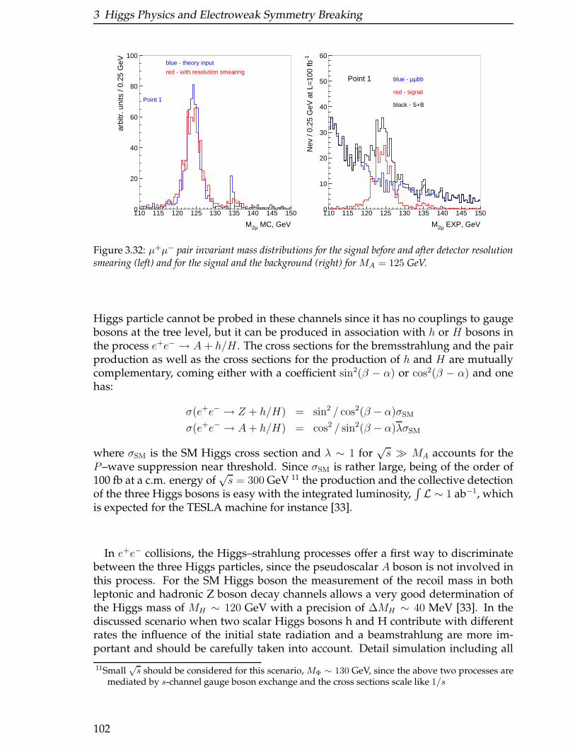
3 Higgs Physics and Electroweak Symmetry Breaking
0
20
40
60
80
100
110 115 120 125 130 135 140 145 150
M2µ MC, GeV
arbi
tr. u
nits
/ 0.
25 G
eV blue - theory input
red - with resolution smearing
Point 1
0
10
20
30
40
50
60
110 115 120 125 130 135 140 145 150
M2µ EXP, GeV
Nev
/ 0.
25 G
eV a
t L=
100
fb-1
blue - µµbb
red - signal
black - S+B
Point 1
Figure 3.32: µ+µ− pair invariant mass distributions for the signal before and after detector resolutionsmearing (left) and for the signal and the background (right) for MA = 125 GeV.
Higgs particle cannot be probed in these channels since it has no couplings to gaugebosons at the tree level, but it can be produced in association with h or H bosons inthe process e+e− → A + h/H . The cross sections for the bremsstrahlung and the pairproduction as well as the cross sections for the production of h and H are mutuallycomplementary, coming either with a coefficient sin2(β − α) or cos2(β − α) and onehas:
σ(e+e− → Z + h/H) = sin2 / cos2(β − α)σSM
σ(e+e− → A+ h/H) = cos2 / sin2(β − α)λσSM
where σSM is the SM Higgs cross section and λ ∼ 1 for√s ≫ MA accounts for the
P–wave suppression near threshold. Since σSM is rather large, being of the order of100 fb at a c.m. energy of
√s = 300 GeV 11 the production and the collective detection
of the three Higgs bosons is easy with the integrated luminosity,∫L ∼ 1 ab−1, which
is expected for the TESLA machine for instance [33].
In e+e− collisions, the Higgs–strahlung processes offer a first way to discriminatebetween the three Higgs particles, since the pseudoscalar A boson is not involved inthis process. For the SM Higgs boson the measurement of the recoil mass in bothleptonic and hadronic Z boson decay channels allows a very good determination ofthe Higgs mass of MH ∼ 120 GeV with a precision of ∆MH ∼ 40 MeV [33]. In thediscussed scenario when two scalar Higgs bosons h and H contribute with differentrates the influence of the initial state radiation and a beamstrahlung are more im-portant and should be carefully taken into account. Detail simulation including all
11Small√s should be considered for this scenario, MΦ ∼ 130 GeV, since the above two processes are
mediated by s-channel gauge boson exchange and the cross sections scale like 1/s
102
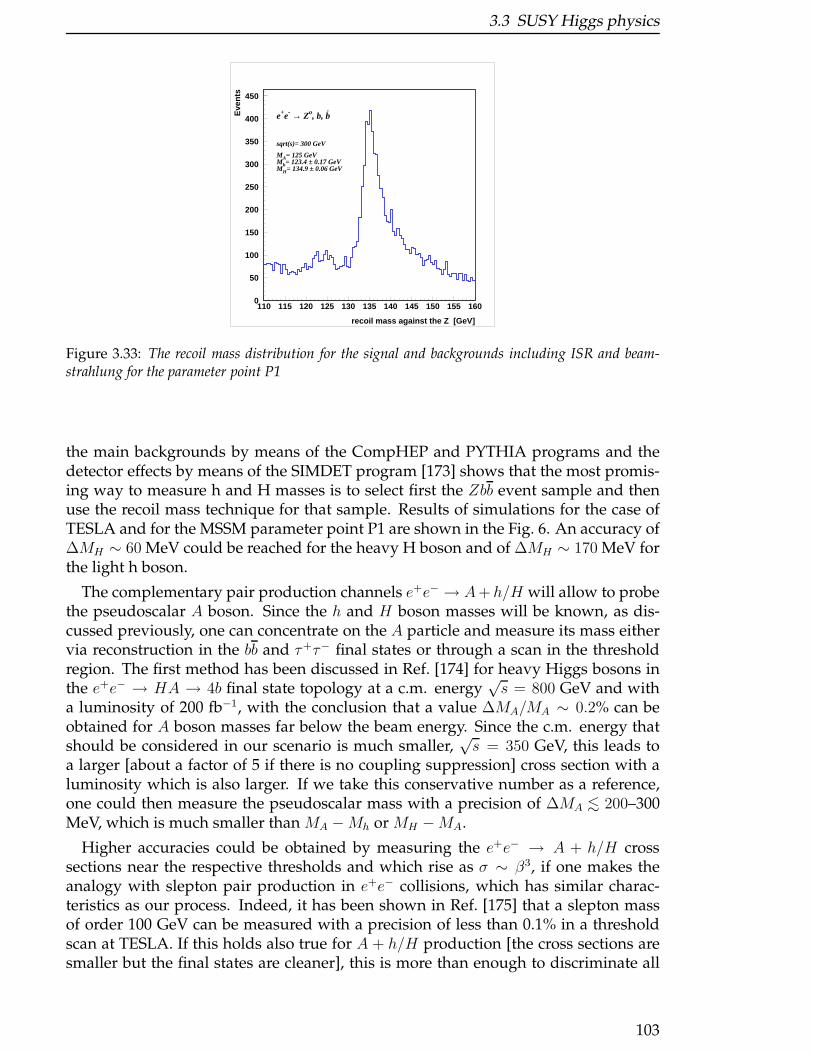
3.3 SUSY Higgs physics
0
50
100
150
200
250
300
350
400
450
110 115 120 125 130 135 140 145 150 155 160
e+e- → Zo, b, b-
sqrt(s)= 300 GeV
MA= 125 GeVMh= 123.4 ± 0.17 GeVMH= 134.9 ± 0.06 GeV
recoil mass against the Z [GeV]
Eve
nts
Figure 3.33: The recoil mass distribution for the signal and backgrounds including ISR and beam-strahlung for the parameter point P1
the main backgrounds by means of the CompHEP and PYTHIA programs and thedetector effects by means of the SIMDET program [173] shows that the most promis-ing way to measure h and H masses is to select first the Zbb event sample and thenuse the recoil mass technique for that sample. Results of simulations for the case ofTESLA and for the MSSM parameter point P1 are shown in the Fig. 6. An accuracy of∆MH ∼ 60 MeV could be reached for the heavy H boson and of ∆MH ∼ 170 MeV forthe light h boson.
The complementary pair production channels e+e− → A+ h/H will allow to probethe pseudoscalar A boson. Since the h and H boson masses will be known, as dis-cussed previously, one can concentrate on the A particle and measure its mass eithervia reconstruction in the bb and τ+τ− final states or through a scan in the thresholdregion. The first method has been discussed in Ref. [174] for heavy Higgs bosons inthe e+e− → HA → 4b final state topology at a c.m. energy
√s = 800 GeV and with
a luminosity of 200 fb−1, with the conclusion that a value ∆MA/MA ∼ 0.2% can beobtained for A boson masses far below the beam energy. Since the c.m. energy thatshould be considered in our scenario is much smaller,
√s = 350 GeV, this leads to
a larger [about a factor of 5 if there is no coupling suppression] cross section with aluminosity which is also larger. If we take this conservative number as a reference,one could then measure the pseudoscalar mass with a precision of ∆MA <∼ 200–300MeV, which is much smaller than MA −Mh or MH −MA.
Higher accuracies could be obtained by measuring the e+e− → A + h/H crosssections near the respective thresholds and which rise as σ ∼ β3, if one makes theanalogy with slepton pair production in e+e− collisions, which has similar charac-teristics as our process. Indeed, it has been shown in Ref. [175] that a slepton massof order 100 GeV can be measured with a precision of less than 0.1% in a thresholdscan at TESLA. If this holds also true for A + h/H production [the cross sections aresmaller but the final states are cleaner], this is more than enough to discriminate all
103
3 Higgs Physics and Electroweak Symmetry Breaking
Higgs bosons in our scenario.
The results quoted here are from an extrapolation of SM–like searches where onlyone isolated Higgs boson is produced. A dedicated analysis, including a detectorsimulation, of the intense coupling regime in e+e− collisions and the prospect formeasuring the A Higgs boson mass is needed. [176].
3.3.3.4 LHC and LC interplay
Once Higgs boson masses will be measured at a e+e− LC one can study a problem of acomplete parameter measurement for the corresponding MSSM parameter point. Inthis sense one can use the measured masses and extracted branching ratios BR(Φ →bb) at the linear collider to measure glue − glue − Higgs couplings, branching ratiosBR(Φ → µ+µ−) and b − b −Higgs couplings via the discussed processes pp(→ Φ) →µ+µ− and pp(→ Φbb) → µ+µ−bb at the LHC. Obviosly this can not be done at LCalone.
3.3.3.5 Conclusions
We have shown that in the intense-coupling regime, i.e. when the h,H and A MSSMbosons have masses too close to the critical point Mmax
h and when the value of tan βis large, the detection of the individual Higgs boson peaks is very challenging at theLHC. It is only in the associated Higgs production mechanism with bb pairs, with atleast one tagged b-jet, and with Higgs particles decaying into the clean muon-pairfinal states, that there is a chance of observing the three signals and resolve betweenthem. This would be possible only if the Higgs mass differences are larger than about5 GeV.
In e+e− collisions, thanks to the clean environment and the complementarity of theproduction channels, one expects the three Higgs bosons to be more easily separated.The Higgs–strahlung processes allow from the very beginning to probe the h and Hbosons and to measure their masses by studying the recoiling Z boson. The associatedCP-even and CP-odd Higgs production would then allow to probe the pseudoscalarA boson, either in the direct reconstruction of its final decay products or via a thresh-old scan. The measured characteristics at the LC allow then to measure several others,like glue-glue-Higgs couplings and BR(Φ→ µ+µ−) at the LHC. From the other hand,in case if the Higgs masses will be not possible to resolve completely at the LHC theinformation on a overall peak position from the LHC will help to make more properchoice of the energy at LC.
3.3.4 Estimating the precision of a tanβ determination withH/A→ τ+τ− in CMS and τ+τ− fusion at a high-energyphoton collider
R. Kinnunen, S. Lehti, F. Moortgat, M. Muhlleitner A. Nikitenko and M. Spira
104
3.3 SUSY Higgs physics
3.3.4.1 The uncertainty of the tan β measurement with H/A → τ+τ− in CMS
If Higgs bosons will be discovered at the LHC, the determination of their propertieswill be of high relevance in order to unravel the underlying model. In the minimalsupersymmetric extension (MSSM) of the Standard Model (SM) as well as a generaltype-II Two-Higgs-Doublet-Model one of the most important parameters is tan β, theratio of the two vacuum expectation values v1,2. In this work the accuracy of thetanβ measurement is estimated in the H/A → τ+τ− decay channels by investigat-ing the final states eµ, ℓℓ (ℓℓ = eµ, ee, µµ) [177], lepton+jet [178] and two-jets [179].The associated Higgs boson production cross section gg → bbH/A is approximatelyproportional to tan2 β at large tanβ. Due to this feature the uncertainty of the tanβmeasurement is only half of the uncertainty of the rate measurement. However, dueto the presence of potentially large radiative corrections [180] the extracted value hasto be considered as an effective parameter tanβeff . The determination of the funda-mental tan β value requires knowledge of the model behind.
The event rates of H/A → τ+τ− decay channels are studied in Refs. [177, 179].The CMS trigger efficiencies and thresholds [181] are taken into account. Event se-lections to suppress the backgrounds include lepton isolation, τ jet identification, τtagging with impact parameter, b tagging and jet veto. The effective τ+τ− mass isreconstructed assuming that the neutrinos are emitted collinear with the measuredtau decay products. The signal events were simulated with the following values ofMSSM SUSY parameters: M2 = 200 GeV/c2, µ = 300 GeV/c2, Mg = 800 GeV/c2, Mq,ℓ
= 1 TeV/c2 and At is set to 2450 GeV/c2. The top mass is set to 175 GeV/c2 and Higgsboson decays to SUSY particles are allowed. We have not included the uncertaintiesrelated to the MSSM parameters, but kept them fixed at our chosen values. The uncer-tainty of the background estimation as well as the uncertainty of the signal selectionefficiency have not yet been taken into account in this study. We expect, however,that the background uncertainty and uncertainty of the signal selection will be of theorder of 5%. The statistical errors from different τ+τ− final states are combined usingthe standard weighted least-squares procedure described in [182].
In addition to event rates, the accuracy of the tanβ measurement depends on thesystematic uncertainty from the luminosity measurement and on the theoretical un-certainty of the cross section calculation. A 5% uncertainty of the luminosity mea-surement was taken. The theoretical accuracy of the cross section depends on thetransverse momentum range of the two spectator quarks and reduces to 10-15% with
the requirement of pb,bT>∼ 20 GeV/c [183, 184]. However, since the associated b jets
are very soft, reconstructing and b tagging them is difficult. In order to minimizethe total measurement error, only one b jet is assumed to be b tagged and a theoret-ical uncertainty of about 20% is adopted accordingly [183, 185]. The branching ratioBR(H/A → ττ) is approximately constant at large tanβ, and the uncertainty of thebranching ratio due to the SM input parameters is about 3%.
Since the value of the cross section depends on the Higgs boson mass, the uncer-tainty of the mass measurement leads to an uncertainty in the signal rate. The Higgsmass is measured using the different final states, and the cross section uncertaintiesdue to mass measurement errors are combined. The mass resolution is almost con-stant as a function of MA, ∼ 24% for the leptonic final states, ∼ 17% for the lepton+jetfinal state and ∼ 12% for the hadronic final state [177]. The uncertainty of the mass
105
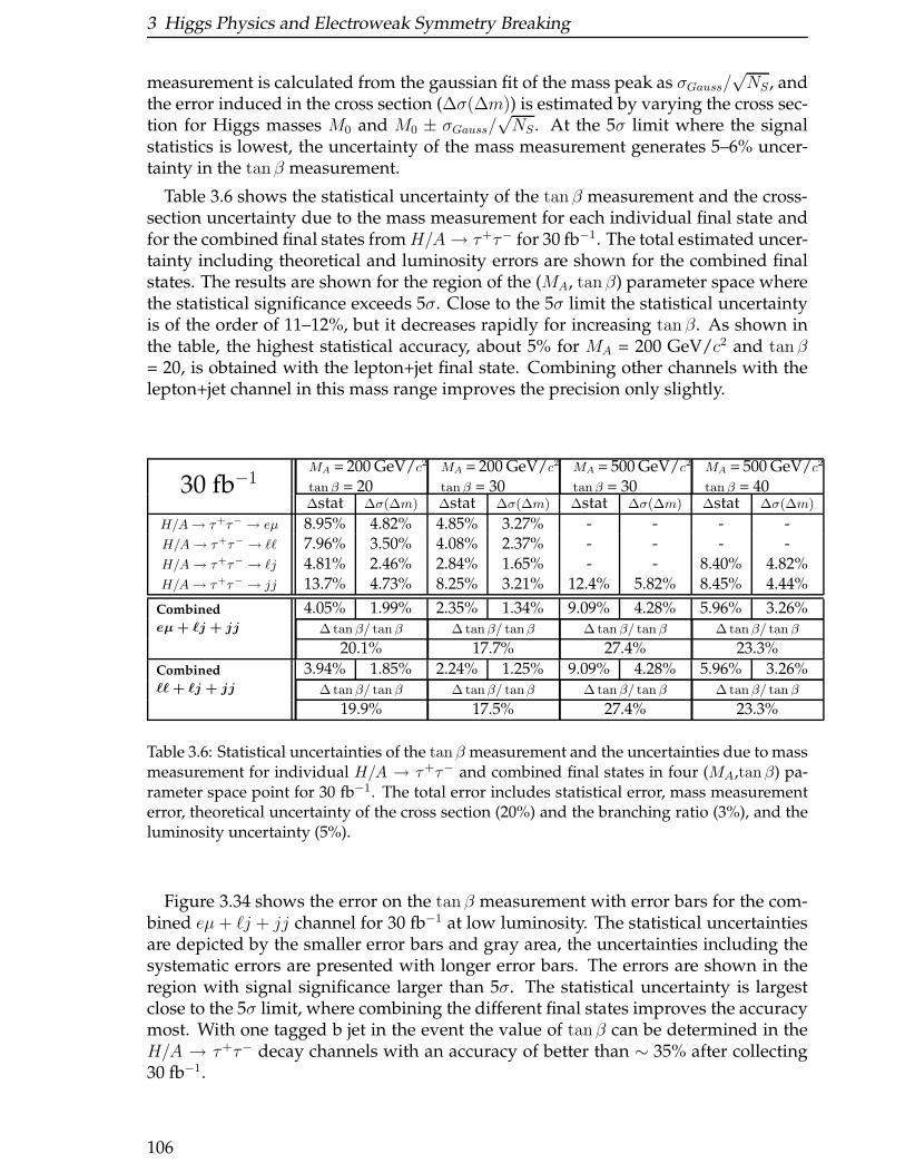
3 Higgs Physics and Electroweak Symmetry Breaking
measurement is calculated from the gaussian fit of the mass peak as σGauss/√NS , and
the error induced in the cross section (∆σ(∆m)) is estimated by varying the cross sec-tion for Higgs masses M0 and M0 ± σGauss/
√NS . At the 5σ limit where the signal
statistics is lowest, the uncertainty of the mass measurement generates 5–6% uncer-tainty in the tanβ measurement.
Table 3.6 shows the statistical uncertainty of the tan β measurement and the cross-section uncertainty due to the mass measurement for each individual final state andfor the combined final states fromH/A→ τ+τ− for 30 fb−1. The total estimated uncer-tainty including theoretical and luminosity errors are shown for the combined finalstates. The results are shown for the region of the (MA, tan β) parameter space wherethe statistical significance exceeds 5σ. Close to the 5σ limit the statistical uncertaintyis of the order of 11–12%, but it decreases rapidly for increasing tan β. As shown inthe table, the highest statistical accuracy, about 5% for MA = 200 GeV/c2 and tan β= 20, is obtained with the lepton+jet final state. Combining other channels with thelepton+jet channel in this mass range improves the precision only slightly.
30 fb−1MA = 200 GeV/c2
tan β = 20MA = 200 GeV/c2
tan β = 30MA = 500 GeV/c2
tanβ = 30MA = 500 GeV/c2
tan β = 40∆stat ∆σ(∆m) ∆stat ∆σ(∆m) ∆stat ∆σ(∆m) ∆stat ∆σ(∆m)
H/A → τ+τ−→ eµ 8.95% 4.82% 4.85% 3.27% - - - -
H/A → τ+τ−→ ℓℓ 7.96% 3.50% 4.08% 2.37% - - - -
H/A → τ+τ−→ ℓj 4.81% 2.46% 2.84% 1.65% - - 8.40% 4.82%
H/A → τ+τ−→ jj 13.7% 4.73% 8.25% 3.21% 12.4% 5.82% 8.45% 4.44%
Combined
eµ + ℓj + jj
4.05% 1.99% 2.35% 1.34% 9.09% 4.28% 5.96% 3.26%∆ tan β/ tan β ∆ tanβ/ tanβ ∆ tan β/ tan β ∆ tan β/ tan β
20.1% 17.7% 27.4% 23.3%
Combined
ℓℓ + ℓj + jj
3.94% 1.85% 2.24% 1.25% 9.09% 4.28% 5.96% 3.26%∆ tan β/ tan β ∆ tanβ/ tanβ ∆ tan β/ tan β ∆ tan β/ tan β
19.9% 17.5% 27.4% 23.3%
Table 3.6: Statistical uncertainties of the tan β measurement and the uncertainties due to massmeasurement for individual H/A → τ+τ− and combined final states in four (MA,tan β) pa-rameter space point for 30 fb−1. The total error includes statistical error, mass measurementerror, theoretical uncertainty of the cross section (20%) and the branching ratio (3%), and theluminosity uncertainty (5%).
Figure 3.34 shows the error on the tan β measurement with error bars for the com-bined eµ + ℓj + jj channel for 30 fb−1 at low luminosity. The statistical uncertaintiesare depicted by the smaller error bars and gray area, the uncertainties including thesystematic errors are presented with longer error bars. The errors are shown in theregion with signal significance larger than 5σ. The statistical uncertainty is largestclose to the 5σ limit, where combining the different final states improves the accuracymost. With one tagged b jet in the event the value of tanβ can be determined in theH/A → τ+τ− decay channels with an accuracy of better than ∼ 35% after collecting30 fb−1.
106
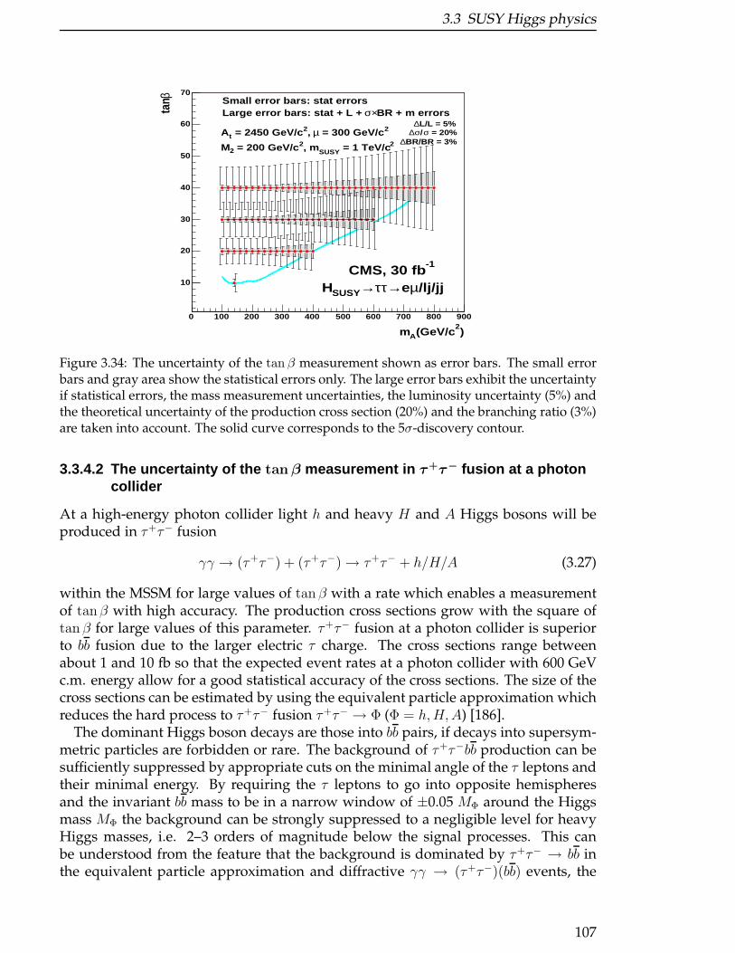
3.3 SUSY Higgs physics
)2
(GeV/cAm
0 100 200 300 400 500 600 700 800 900
βta
n
10
20
30
40
50
60
70
-1CMS, 30 fb
/lj/jjµe→ττ→SUSYH
Small error bars: stat errorsBR + m errors×σLarge error bars: stat + L +
2 = 300 GeV/cµ, 2 = 2450 GeV/ctA2 = 1 TeV/cSUSY, m2 = 200 GeV/c2M
L/L = 5%∆ = 20%σ/σ∆
BR/BR = 3%∆
Figure 3.34: The uncertainty of the tan β measurement shown as error bars. The small errorbars and gray area show the statistical errors only. The large error bars exhibit the uncertaintyif statistical errors, the mass measurement uncertainties, the luminosity uncertainty (5%) andthe theoretical uncertainty of the production cross section (20%) and the branching ratio (3%)are taken into account. The solid curve corresponds to the 5σ-discovery contour.
3.3.4.2 The uncertainty of the tan β measurement in τ+τ− fusion at a photoncollider
At a high-energy photon collider light h and heavy H and A Higgs bosons will beproduced in τ+τ− fusion
γγ → (τ+τ−) + (τ+τ−)→ τ+τ− + h/H/A (3.27)
within the MSSM for large values of tan β with a rate which enables a measurementof tanβ with high accuracy. The production cross sections grow with the square oftan β for large values of this parameter. τ+τ− fusion at a photon collider is superiorto bb fusion due to the larger electric τ charge. The cross sections range betweenabout 1 and 10 fb so that the expected event rates at a photon collider with 600 GeVc.m. energy allow for a good statistical accuracy of the cross sections. The size of thecross sections can be estimated by using the equivalent particle approximation whichreduces the hard process to τ+τ− fusion τ+τ− → Φ (Φ = h,H,A) [186].
The dominant Higgs boson decays are those into bb pairs, if decays into supersym-metric particles are forbidden or rare. The background of τ+τ−bb production can besufficiently suppressed by appropriate cuts on the minimal angle of the τ leptons andtheir minimal energy. By requiring the τ leptons to go into opposite hemispheresand the invariant bb mass to be in a narrow window of ±0.05 MΦ around the Higgsmass MΦ the background can be strongly suppressed to a negligible level for heavyHiggs masses, i.e. 2–3 orders of magnitude below the signal processes. This canbe understood from the feature that the background is dominated by τ+τ− → bb inthe equivalent particle approximation and diffractive γγ → (τ+τ−)(bb) events, the
107
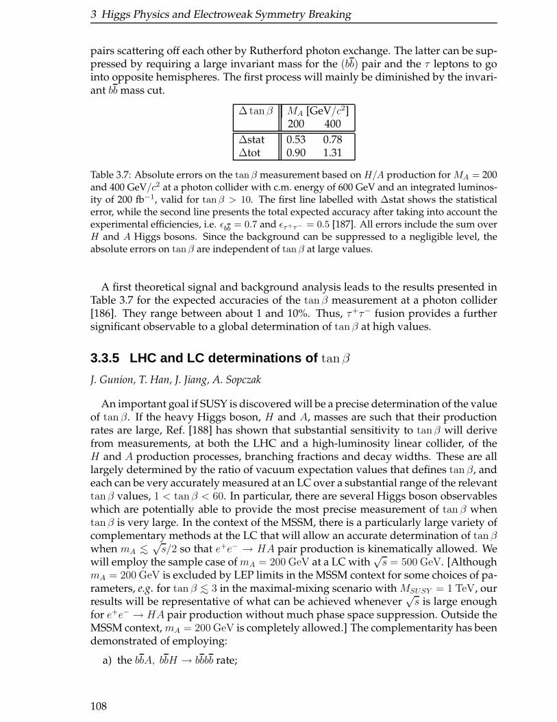
3 Higgs Physics and Electroweak Symmetry Breaking
pairs scattering off each other by Rutherford photon exchange. The latter can be sup-pressed by requiring a large invariant mass for the (bb) pair and the τ leptons to gointo opposite hemispheres. The first process will mainly be diminished by the invari-ant bb mass cut.
∆ tanβ MA [GeV/c2]200 400
∆stat 0.53 0.78∆tot 0.90 1.31
Table 3.7: Absolute errors on the tan β measurement based on H/A production for MA = 200and 400 GeV/c2 at a photon collider with c.m. energy of 600 GeV and an integrated luminos-ity of 200 fb−1, valid for tan β > 10. The first line labelled with ∆stat shows the statisticalerror, while the second line presents the total expected accuracy after taking into account theexperimental efficiencies, i.e. ǫbb = 0.7 and ǫτ+τ− = 0.5 [187]. All errors include the sum overH and A Higgs bosons. Since the background can be suppressed to a negligible level, theabsolute errors on tan β are independent of tan β at large values.
A first theoretical signal and background analysis leads to the results presented inTable 3.7 for the expected accuracies of the tan β measurement at a photon collider[186]. They range between about 1 and 10%. Thus, τ+τ− fusion provides a furthersignificant observable to a global determination of tanβ at high values.
3.3.5 LHC and LC determinations of tanβ
J. Gunion, T. Han, J. Jiang, A. Sopczak
An important goal if SUSY is discovered will be a precise determination of the valueof tan β. If the heavy Higgs boson, H and A, masses are such that their productionrates are large, Ref. [188] has shown that substantial sensitivity to tanβ will derivefrom measurements, at both the LHC and a high-luminosity linear collider, of theH and A production processes, branching fractions and decay widths. These are alllargely determined by the ratio of vacuum expectation values that defines tan β, andeach can be very accurately measured at an LC over a substantial range of the relevanttanβ values, 1 < tan β < 60. In particular, there are several Higgs boson observableswhich are potentially able to provide the most precise measurement of tan β whentanβ is very large. In the context of the MSSM, there is a particularly large variety ofcomplementary methods at the LC that will allow an accurate determination of tan βwhen mA <∼
√s/2 so that e+e− → HA pair production is kinematically allowed. We
will employ the sample case of mA = 200 GeV at a LC with√s = 500 GeV. [Although
mA = 200 GeV is excluded by LEP limits in the MSSM context for some choices of pa-rameters, e.g. for tan β <∼ 3 in the maximal-mixing scenario with MSUSY = 1 TeV, ourresults will be representative of what can be achieved whenever
√s is large enough
for e+e− → HA pair production without much phase space suppression. Outside theMSSM context, mA = 200 GeV is completely allowed.] The complementarity has beendemonstrated of employing:
a) the bbA, bbH → bbbb rate;
108
3.3 SUSY Higgs physics
b) the HA→ bbbb rate;
c) a measurement of the average H,A total width in HA production;
d) the H+H− → tb tb rate; and
e) the total H± width measured in H+H− → tb tb production.
By combining the tanβ errors from all these processes in quadrature, we obtain thenet statistical errors on tanβ shown in Fig. 3.35 by the lines [solid for SUSY scenario(I) and dashed for SUSY scenario (II)], assuming a multi-year integrated luminosityof L = 2000 fb−1. The scenarios are defined as:
(I) mA = 200 GeV, mg = 1 TeV, µ = M2 = 250 GeV,mtL
= mbL= mtR
= mbR≡ mt = 1 TeV,
Aτ = Ab = 0, At = µ/ tanβ +√
6mt (maximal mixing);
(II) mA = 200 GeV, mg = 350 GeV, µ = 272 GeV, M2 = 120 GeV,mtL
= mbL= 356 GeV, mtR
= 273 GeV, mbR= 400 GeV,
Aτ = 0, Ab = −672 GeV, At = −369 GeV.
We see that, independent of the scenario, the Higgs sector will provide an excellentdetermination of tanβ at small and large tan β values, leading to an error on tanβof 10% or better, provided systematic errors can be kept below the statistical level. IfSUSY decays of theH,A,H± are significant [SUSY scenario (II)], the tan β error will besmaller than 13% even in the more difficult moderate tanβ range. However, if SUSYdecays are not significant [SUSY scenario (I)] there is a limited range of moderate tanβfor which the error on tan β would be large, reaching about 50%. In general, it will beimportant to establish the light SUSY particle spectrum (using a combination of LHCand LC data) in order to avoid systematic errors in the tan β determination derivingfrom the influence of non-Higgs model parameters upon predictions for Higgs decaysand production rates.
Regardless of the relative magnitude of the LHC versus LC tanβ errors, the cleanLC environment will provide an important and independent measurement that willcomplement any LHC determination of tan β. Different uncertainties will be asso-ciated with the determination of tanβ at a hadron and an e+e− collider because ofthe different backgrounds. Further, the LHC and LC measurements of tanβ will behighly complementary in that the experimental and theoretical systematic errors in-volved will be very different.
Combining all the different LC measurements as above does not fully account forthe fact that the “effective” tan β value being measured in each process is only thesame at tree-level. The tan β values measured via the H → bb Yukawa coupling, theA → bb Yukawa coupling and the H+ → tb Yukawa coupling could all be influenceddifferently by the MSSM one-loop corrections. For some choices of MSSM parame-ters, the impact of MSSM radiative corrections on interpreting these measurementscan be substantial [197]. However, if the masses of the SUSY particles are known,so that the important MSSM parameters entering these radiative corrections (otherthan tan β) are fairly well determined, then a uniform convention for the definition oftan β can be adopted and, in general, an excellent determination of tan β (with accu-racy similar to that obtained via our tree-level procedures) will be possible using thelinear collider observables considered here. Even for special SUSY parameter choices
109
3 Higgs Physics and Electroweak Symmetry Breaking
such that one of the Yukawa couplings happens to be significantly suppressed, theobservables a)-e) would provide an excellent opportunity for pinning down all theYukawa couplings and checking the consistency of the MSSM model.
To illustrate the relation between the other MSSM model parameters and the sys-tematic errors in the tan β determination, we give one example. For tan β = 5,mA = mH = 200 GeV, M2 large enough that there are no SUSY decays of the Hand A, At = Ab = 0 and m0 = 1 TeV for the 1st and 2nd generations, one finds
BR(H → bb) = 0.61 and BR(A→ bb) = 0.87 for mt = mb = 500 GeV,
BR(H → bb) = 0.69 and BR(A→ bb) = 0.88 for mt = mb = 1000 GeV.(3.28)
The resulting HA → bbbb rate differs by about 14% between the two scenarios. Thebottom and stop masses would need to be known to within about 150 GeV in orderto bring the systematic uncertainty from this source below the roughly 5% statisticaluncertainty shown in Fig. 3.35. Dependence on the stop and sbottom sector mixingangles, the gluino mass and so forth are non-negligible as well. The precision of SMparameters, in particular mt and mb (the latter enters directly into the bb couplingstrength of the H and A) will also contribute to the systematic uncertainty. Of course,because tanβ is not a directly measurable quantity, other techniques for determiningtanβ suffer from similar systematics issues.
Finally, it is important to note that the LC techniques employed for the tan β de-termination discussed above can also be employed in the case of other Higgs sec-tor models. For example, in the general (non-SUSY) 2HDM, if the only non-SM-likeHiggs boson with mass below
√s is the A [198], then a good determination of tan β
will be possible at high tanβ from the bbA→ bbbb production rate. Similarly, in mod-els with more than two Higgs doublet and/or triplet representations, the Yukawacouplings of the Higgs bosons, and, therefore, the analogues of the 2HDM parametertanβ, will probably be accurately determined through Higgs production observablesin e+e− collisions.
Now, we will compare the LC results summarized in Fig. 3.35 [188] to the tan βaccuracies that can be achieved at the LHC based on H,A,H± production and decayprocesses. First note that there is a wedge-shaped window of moderate tanβ andmA >∼ 200 GeV for which the A, H and H± are all unobservable (see, for example,Refs. [189–191]). In this wedge, the only Higgs boson that is detectable at the LHC isthe light SM-like Higgs boson, h. Precision measurements of the properties of the htypically only provide weak sensitivity to tanβ, and will not be considered here. Thelower tan β bound of this moderate-tan β wedge is defined by the LEP-2 limits [192],which are at tanβ ∼ 3 for mA ∼ 200 GeV, falling to tan β ∼ 2.5 for mA >∼ 250 GeV,assuming the maximal mixing scenario [see SUSY scenario (I) defined earlier]. Theupper tan β limit of the wedge is at tan β ∼ 7 for mA ∼ 200 GeV rising to tan β ∼15 at mA ∼ 500 GeV. For either smaller or larger tan β values, the heavy MSSMHiggs bosons can be detected and their production rates and properties will providesensitivity to tan β.
We will now summarize the results currently available regarding the determinationof tan β at the LHC using Higgs measurements (outside the wedge region) assuminga luminosity of L = 300 fb−1. The methods employed are those proposed in [193] asreanalyzed from a more experimental perspective by the ATLAS and/or CMS collab-
110
3.3 SUSY Higgs physics
orations. The reactions that have been studied at the LHC are the following.
1. gg → H → ZZ → 4ℓ [190].
The best accuracy that can be achieved at low tanβ is obtained from the H →ZZ → 4ℓ rate. One finds ∆ tan β/ tanβ = ±0.1 at tanβ = 1 rising to > ±0.3by tanβ = 1.5 for the sample choice of mH = 300 GeV. For mH < 2mZ , tanβcannot be measured via this process. (Of course, in the MSSM maximal mixingscenario, such low values of tan β are unlikely in light of LEP-2 limits on mh.)
2. gg → H + gg → A→ τ+τ−, µ+µ− and gg → bbH + bbA→ bbτ+τ−, bbµ+µ− [190].
At high tan β and taking mA = 150 GeV, Fig. 19-86 of [190] shows that thegg → H → τ+τ−, gg → A→ τ+τ−, and gg → bbA + bbH → bbτ+τ− rates can, incombination, be used to determine tan β with an accuracy of ±0.15 at tanβ = 5,improving to ±0.06 at tanβ = 40. The corresponding rates with H,A → µ+µ−
yield a somewhat better determination at higher tan β: ±0.12 at tanβ = 10 and±0.05 at tan β = 40.
Interpolating, using Figs. 19-86 and 19-87 from [190], we estimate that at mA ∼200 GeV (our choice for this study) the error on tan β based on these rates wouldbe smaller than ±0.1 for tan β >∼ 13, asymptoting to ±0.05 at large tanβ.
The importance of including the gg → H , gg → A as well as the gg → bbH +gg → bbA processes in order to obtain observable signals for tanβ values aslow as 10 in the µ+µ− channels is apparent from [194]. For L = 300 fb−1 andmA = 200 GeV, they find that the bbµ+µ− final states can only be isolated fortan β > 30 whereas the inclusive µ+µ− final state from all production processesbecomes detectable once tanβ > 10.
3. gg → tbH− + tbH+ with H± → τ±ν [195].
The tbH± → tbτν rate gives a fractional tan β uncertainty, ∆ tanβ/ tanβ, rang-ing from ±0.074 at tan β = 20 to ±0.054 at tanβ = 50.
The above error estimates are purely statistical. All three techniques will have sys-tematic errors deriving from imprecise knowledge of the gluon distribution functionand QCD corrections. Background uncertainties might also enter, although not atthe highest tan β values for the tan β-enhanced processes that have very high rates.Additional systematic error will, as in the LC case, derive from the need to have pre-cise measurements of SUSY masses and mixing angles in order to precisely relate thebb Yukawa couplings of the H and A to the tan β parameter. Finally, in the case oftechniques [1.] and (for tanβ < 20 − 30) [2.], the tan β sensitivity is largely due tothe loop-induced gg → A and gg → H production processes. Interpreting gg-inducedrates in terms of tanβ requires significant knowledge of the particles, including SUSYparticles, that go into the loops responsible for the gg → H and gg → A couplings.
Sensitivity to tan β deriving from direct measurements of the decay widths hasnot been studied by the LHC experiments. One can expect excellent tanβ statisticalaccuracy at the higher tan β values for which the gg → bbµ+µ− signal for the H and Ais detectable. Further, the direct width measurement would avoid systematic errorsderiving from uncertainties in the gluon distribution function or the gg → H,A loop-induced couplings.
111
3 Higgs Physics and Electroweak Symmetry Breaking
We now discuss the interplay between the LHC errors and the LC errors for tan β,assuming mA = 200 GeV. This discussion is based upon statistical errors only. Asalready noted, to keep systematic errors at a level below the statistical errors will re-quire substantial input on other model parameters (e.g. sparticle masses and mixingsin the MSSM context) from both the LHC and the LC. First, consider tanβ ≤ 10. Assummarized above, the LHC error on tan β is ±0.12 at tan β ∼ 10 and at tan β ∼ 1,and the error becomes very large for 1.5 <∼ tan β <∼ 5. Meanwhile, the LC errorfrom Fig. 3.35 ranges from roughly ±0.03 to ±0.05 for 2 <∼ tanβ <∼ 5 rising to about±0.1 at tanβ ∼ 10 [in the less favorable SUSY scenario (I)]. Therefore, for tanβ <∼ 10the LC provides the best determination of tan β using Higgs observables related totheir Yukawa couplings. (In the MSSM context, other non-Higgs LHC measure-ments would allow a good tanβ determination at low to moderate tanβ based onother kinds of couplings.) In the middle range of tanβ (roughly 13 < tan β < 30 atmA ∼ 200 GeV), the heavy Higgs determination of tanβ at the LHC might be superiorto that obtained at the LC. This depends upon the SUSY scenario: if the heavy Higgsbosons can decay to SUSY particles, the LC will give tanβ errors that are quite similarto those obtained at the LHC; if the heavy Higgs bosons do not have substantial SUSYdecays, then the expected LC tan β errors are substantially larger than those predictedfor the LHC. At large tanβ, the LC measurement of the heavy Higgs couplings andthe resulting tan β determination at the LC is numerically only slightly more accuratethan that obtained at the LHC. For example, both are of order±0.05 at tan β = 40. (Atthis level of statistical error, the ability to reduce the systematic error by combinedLC and LHC systematic studies will be particularly important.) The statistical errorcomparisons are summarized in Table 3.8. It is possible that the net LHC tanβ er-ror would be somewhat smaller than the LC error for tanβ >∼ 40 if both ATLAS andCMS can each accumulate L = 300 fb−1 of luminosity; combining the two data setswould presumably roughly double the statistics and decrease errors by a factor of or-der 1/
√2. Inclusion of the direct width measurement at the LHC would also decrease
the error. In any case, a very small statistical error on tan β will be achievable for alltanβ by combining the results from the LC with those from the LHC.
Table 3.8: A comparison of fractional statistical errors, ∆ tan β/ tan β, achievable for L =2000 fb−1 at the LC with those expected at the LHC for L = 300 fb−1, assumingmA = 200 GeVin the MSSM. LC results are given for both SUSY scenarios (I) and (II), where Higgs bosondecays to SUSY particles are disallowed, respectively allowed. LHC results are estimated byroughly combining the determinations of tan β based on H,A production from [190] withthose using H± production from [195], both of which assume the standard MSSM maximalmixing scenario. All entries are approximate.
tan β range LHC LC (case I) LC (case II)1 0.12 0.15 0.1
1.5–5 very large 0.03–0.05 0.03–0.0510 0.12 0.1 0.05
13–30 0.05 0.6–0.1 0.05–0.140–60 0.05–0.03 0.05–0.025 0.05–0.025
Finally, we wish to emphasize that the above LHC versus LC comparisons havebeen made based only on H,A,H± processes and for the particular choice of mA =
112
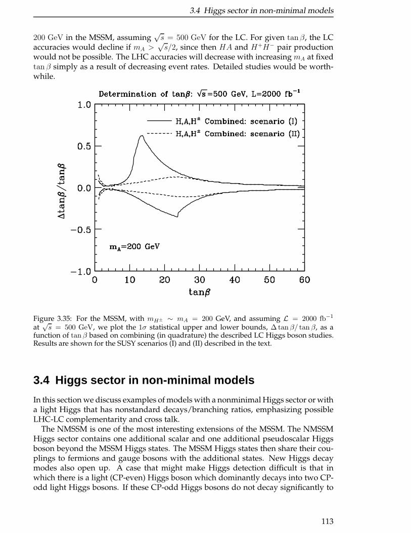
3.4 Higgs sector in non-minimal models
200 GeV in the MSSM, assuming√s = 500 GeV for the LC. For given tanβ, the LC
accuracies would decline if mA >√s/2, since then HA and H+H− pair production
would not be possible. The LHC accuracies will decrease with increasing mA at fixedtan β simply as a result of decreasing event rates. Detailed studies would be worth-while.
Figure 3.35: For the MSSM, with mH± ∼ mA = 200 GeV, and assuming L = 2000 fb−1
at√s = 500 GeV, we plot the 1σ statistical upper and lower bounds, ∆ tan β/ tan β, as a
function of tan β based on combining (in quadrature) the described LC Higgs boson studies.Results are shown for the SUSY scenarios (I) and (II) described in the text.
3.4 Higgs sector in non-minimal models
In this section we discuss examples of models with a nonminimal Higgs sector or witha light Higgs that has nonstandard decays/branching ratios, emphasizing possibleLHC-LC complementarity and cross talk.
The NMSSM is one of the most interesting extensions of the MSSM. The NMSSMHiggs sector contains one additional scalar and one additional pseudoscalar Higgsboson beyond the MSSM Higgs states. The MSSM Higgs states then share their cou-plings to fermions and gauge bosons with the additional states. New Higgs decaymodes also open up. A case that might make Higgs detection difficult is that inwhich there is a light (CP-even) Higgs boson which dominantly decays into two CP-odd light Higgs bosons. If these CP-odd Higgs bosons do not decay significantly to
113
3 Higgs Physics and Electroweak Symmetry Breaking
supersymmetric modes, it is shown that the NMSSM Higgs discovery is close to be-ing guaranteed even in this case if the usually considered LHC detection modes aresupplemented by the WW → h → aa mode, with aa → bbτ+τ−. The resulting signalwould be the only LHC signal for Higgs bosons. Confirmation of the nature of thesignal at the LC would be vital. It is shown that the WW → h→ aa signal, as well asthe usual e+e− → Zh→ Zaa signal, will be highly visible at the LC due to its cleanerenvironment and high luminosity. Further, the LC will be able to observe both theaa → τ+τ− → bb and the aa → bbbb final states, thus allowing a definitive check thatthe ratio BR(a→ τ+τ−)/BR(a→ bb) is that expected for a CP-odd scalar.
Next we discuss the very interesting scenario that at the Tevatron, LHC and e+e−
Linear Collider only one light Higgs boson will be found, with properties as expectedin the Standard Model. It is possible to realize this SM-like scenario in a Two-Higgs-Doublet Model both with and without decoupling. It is shown how precise measure-ments of the Higgs boson coupling to gluons at the LHC and to photons at a PhotonCollider can allow one to determine which scenario is realized in nature.
After this is discussed the case of a fermiophobic Higgs boson (hf ) decaying totwo photons with a larger branching ratio than in the SM. In this case the standardproduction mechanisms are very suppressed for moderate to large tanβ, both at theLC and the LHC. It is shown here that the search for pp→ H±hf should substantiallybenefit from a previous signal at a LC in the channel e+e− → A0hf , and would provideimportant confirmation of any LC signal for hf .
Should a light Higgs have substantial branching ratio in ’invisible’ channels, asmay well happen for a supersymmetric Higgs with mass less than ∼ 130 GeV andnonuniversal gaugino masses at the high scale, its search at the LHC in the standardchannels may get compromised. Such a Higgs can be seen at an LC with ease, allow-ing even a measurement of its ’invisible’ branching ratio. Signals at the LHC whichcan be searched for, so as confirm the lack of signal at LHC in the usual channel dueto these effects are discussed.
3.4.1 NMSSM Higgs discovery at the LHC
U. Ellwanger, J.F. Gunion, C. Hugonie and S. Moretti
One of the most attractive supersymmetric models is the Next to Minimal Super-symmetric Standard Model (NMSSM) (see [199, 201] and references therein) which
extends the MSSM by the introduction of just one singlet superfield, S. When the
scalar component of S acquires a TeV scale vacuum expectation value (a very natural
result in the context of the model), the superpotential term SHuHd generates an effec-
tive µHuHd interaction for the Higgs doublet superfields. Such a term is essential foracceptable phenomenology. No other SUSY model generates this crucial componentof the superpotential in as natural a fashion. Thus, the phenomenological implica-tions of the NMSSM at future accelerators should be considered very seriously. Oneaspect of this is the fact that the h,H,A,H± Higgs sector of the MSSM is extendedso that there are three CP-even Higgs bosons (h1,2,3, mh1 < mh2 < mh3), two CP-oddHiggs bosons (a1,2, ma1 < ma2) (we assume that CP is not violated in the Higgs sector)and a charged Higgs pair (h±). An important question is then the extent to which the
114
3.4 Higgs sector in non-minimal models
no-lose theorem for MSSM Higgs boson discovery at the LHC (after LEP constraints)is retained when going to the NMSSM; i.e. is the LHC guaranteed to find at least oneof the h1,2,3, a1,2, h±? The first exploration of this issue appeared in [200], with theconclusion that for substantial portions of parameter space the LHC would be unableto detect any of the NMSSM Higgs bosons. Since then, there have been improve-ments in many of the detection modes and the addition of new one. These will besummarized below and the implications reviewed. However, these improvementsand additions do not address the possibly important h → aa type decays that couldsuppress all other types of signals [84, 200].
One of the key ingredients in the no-lose theorem for MSSM Higgs boson discoveryis the fact that relations among the Higgs boson masses are such that decays of theSM-like Higgs boson to AA are only possible if mA is quite small, a region that isruled out by LEP by virtue of the fact that Z → hA pair production was not detecteddespite the fact that the relevant coupling is large for small mA. In the NMSSM, thelighter Higgs bosons, h1 or h2, can be SM-like (in particular being the only Higgs withsubstantial WW/ZZ coupling) without the a1 necessarily being heavy. In addition,this situation is not excluded by LEP searches for e+e− → Z∗ → h1,2a1 since, in theNMSSM, the a1 can have small Zh2a1 (Zh1a1) coupling when h1 (h2) is SM-like. [Inaddition, sum rules require that the Zh1a1 (Zh2a1) coupling is small when the h1WW(h2WW ) couplings are large.] As a result, NMSSM parameters that are not excludedby current data can be chosen so that the h1,2 masses are moderate in size (∼ 100 −130 GeV) and the h1 → a1a1 or h2 → a1a1 decays are dominant. Dominance of suchdecays falls outside the scope of the usual detection modes for the SM-like MSSM hon which the MSSM no-lose LHC theorem largely relies.
In Ref. [201], a partial no-lose theorem for NMSSM Higgs boson discovery at theLHC was established. In particular, it was shown that the LHC would be able to de-tect at least one of the Higgs bosons (typically, one of the lighter CP-even Higgs states)throughout the full parameter space of the model, excluding only those parameterchoices for which there is sensitivity to the model-dependent decays of Higgs bosonsto other Higgs bosons and/or superparticles. Here, we will address the question ofwhether or not this no-lose theorem can be extended to those regions of NMSSMparameter space for which Higgs bosons can decay to other Higgs bosons. We findthat the parameter choices such that the “standard” discovery modes fail would allowHiggs boson discovery if detection of h → aa decays is possible. (When used gener-ically, the symbol h will now refer to h = h1, h2 or h3 and the symbol a will refer toa = a1 or a2). Detection of h → aa will be difficult since each a will decay primarilyto bb (or 2 jets if ma < 2mb), τ
+τ−, and, possibly, χ01χ
01, yielding final states that will
typically have large backgrounds at the LHC.In [201] we scanned the parameter space, removing parameter choices ruled out by
constraints from LEP on Higgs boson production, e+e− → Zh or e+e− → ha [202],and eliminating parameter choices for which one Higgs boson can decay to two otherHiggs bosons or a vector boson plus a Higgs boson. For the surviving regions of pa-
rameter space, we estimated the statistical significances (NSD = S/√B) for all Higgs
boson detection modes so far studied at the LHC [203]. These are (with ℓ = e, µ)1) gg → h/a→ γγ;2) associated Wh/a or tth/a production with γγℓ± in the final state;3) associated tth/a production with h/a→ bb;
115
3 Higgs Physics and Electroweak Symmetry Breaking
4) associated bbh/a production with h/a→ τ+τ−;5) gg → h→ ZZ(∗) → 4 leptons;6) gg → h→WW (∗) → ℓ+ℓ−νν;7) WW → h→ τ+τ−;8) WW → h→ WW (∗).
For an integrated luminosity of 300 fb−1 at the LHC, all the surviving points yieldedNSD > 10 after combining all modes, including the W -fusion modes. Thus, NMSSMHiggs boson discovery by just one detector with L = 300 fb−1 is essentially guaran-teed for those portions of parameter space for which Higgs boson decays to otherHiggs bosons or supersymmetric particles are kinematically forbidden.
In this work, we investigate the complementary part of the parameter space, whereat least one Higgs boson decays to other Higgs bosons. To be more precise, we requireat least one of the following decay modes to be kinematically allowed:
i) h→ h′h′ , ii) h→ aa , iii) h→ h±h∓ , iv) h→ aZ ,
v) h→ h±W∓ , vi) a′ → ha , vii) a→ hZ , viii) a→ h±W∓ . (3.29)
After searching those regions of parameter space for which one or more of the decaysi) − viii) is allowed, we found that the only subregions for which discovery of aHiggs boson in modes 1) – 8) was not possible correspond to NMSSM parameterchoices for which (a) there is a light CP-even Higgs boson with substantial doubletcontent that decays mainly to two still lighter CP-odd Higgs states, h→ aa, and (b) allthe other Higgs states are either dominantly singlet-like, implying highly suppressedproduction rates, or relatively heavy, decaying to tt, to one of the “difficult” modesi)− viii) or to a pair of sparticles. In such cases, the best opportunity for detecting atleast one of the NMSSM Higgs bosons is to employWW → h production and developtechniques for extracting a signal for the h → aa final state. We have performed adetailed simulation of the aa → bbτ+τ− final state and find that its detection may bepossible after accumulating 300 fb−1 in both the ATLAS and CMS detectors. Further,we show that the WW → h→ aa signal is extremely robust at an LC.
We consider the simplest version of the NMSSM [199], where the term µH1H2 in the
superpotential of the MSSM is replaced by (we use the notation A for the superfieldand A for its scalar component field)
λH1H2S +κ
3S3 , (3.30)
so that the superpotential is scale invariant. We make no assumption on “universal”soft terms. Hence, the five soft supersymmetry breaking terms
m2H1H2
1 + m2H2H2
2 + m2SS
2 + λAλH1H2S +κ
3AκS
3 (3.31)
are considered as independent. The masses and/or couplings of sparticles will besuch that their contributions to the loop diagrams inducing Higgs boson productionby gluon fusion and Higgs boson decay into γγ are negligible. In the gaugino sector,we chose M2 = 1 TeV (at low scales). Assuming universal gaugino masses at thecoupling constant unification scale, this yields M1 ∼ 500 GeV and M3 ∼ 3 TeV. Inthe squark sector, as particularly relevant for the top squarks which appear in the
116
3.4 Higgs sector in non-minimal models
radiative corrections to the Higgs potential, we chose the soft masses mQ = mT ≡Msusy = 1 TeV, and varied the stop mixing parameter
Xt ≡ 2A2t
M2susy +m2
t
(1− A2
t
12(M2susy +m2
t )
). (3.32)
As in the MSSM, the value Xt =√
6 – so called maximal mixing – maximizes the ra-diative corrections to the Higgs boson masses, and we found that it leads to the mostchallenging points in the parameter space of the NMSSM. We adopt the conventionλ, κ > 0, in which tanβ can have either sign. We require |µeff | > 100 GeV; otherwisea light chargino would have been detected at LEP. The only possibly light SUSY par-ticle will be the χ0
1. A light χ01 is a frequent characteristic of parameter choices that
yield a light a1.We have performed a numerical scan over the free parameters. For each point, we
computed the masses and mixings of the CP-even and CP-odd Higgs bosons, hi (i =1, 2, 3) and aj (j = 1, 2), taking into account radiative corrections up to the dominanttwo loop terms, as described in [204]. We eliminated parameter choices excluded byLEP constraints [202] on e+e− → Zhi and e+e− → hiaj. The latter provides an upperbound on the Zhiaj reduced coupling, R′
ij , as a function of mhi+ maj
for mhi≃ maj
.Finally, we calculated mh± and required mh± > 155 GeV, so that t → h±b would notbe seen.
In order to probe the complementary part of the parameter space as compared tothe scanning of Ref. [201], we required that at least one of the decay modes i)− viii)is allowed. For each Higgs state, we calculated all branching ratios including thosefor modes i)− viii), using an adapted version of the FORTRAN code HDECAY [265].We then estimated the expected statistical significances at the LHC in all Higgs bosondetection modes 1) – 8) by rescaling results for the SM Higgs boson and/or the MSSMh,H and/or A. The rescaling factors are determined by Ri, ti and bi = τi, the ratios ofthe V V hi, tthi and bbhi, τ
+τ−hi couplings, respectively, to those of a SM Higgs boson.Of course |Ri| < 1, but ti and bi can be larger, smaller or even differ in sign withrespect to the SM. For the CP-odd Higgs bosons, R′
i = 0 at tree-level; t′j and b′j are the
ratios of the iγ5 couplings for tt and bb, respectively, relative to SM-like strength. Adetailed discussion of the procedures for rescaling SM and MSSM simulation resultsfor the statistical significances in channels 1) – 8) will appear elsewhere.
In our set of randomly scanned points, we selected those for which all the statisticalsignificances in modes 1) – 8) are below 5σ. We obtained a lot of points, all withsimilar characteristics. Namely, in the Higgs spectrum, we always have a very SM-like CP-even Higgs boson with a mass between 115 and 135 GeV (i.e. above the LEPlimit), which can be either h1 or h2, with a reduced coupling to the gauge bosons R1 ≃1 orR2 ≃ 1, respectively. This state decays dominantly to a pair of (very) light CP-oddstates, a1a1, with ma1 between 5 and 65 GeV. The singlet component of a1 cannot bedominant if we are to have a large h1 → a1a1 or h2 → a1a1 branching ratio when theh1 or h2, respectively, is the SM-like Higgs boson. Further, when the h1 or h2 is verySM-like, one has small Zh1a1 or Zh2a1 coupling, respectively, so that e+e− → h1a1 ore+e− → h2a1 associated production places no constraint on the light CP-odd state atLEP. We have selected six difficult benchmark points, displayed in Table 3.9. Theseare such that a1 → χ0
1χ01 decays are negligible or forbidden. (Techniques for cases such
117
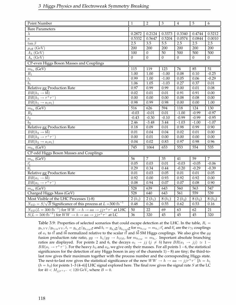
3 Higgs Physics and Electroweak Symmetry Breaking
Point Number 1 2 3 4 5 6
Bare Parametersλ 0.2872 0.2124 0.3373 0.3340 0.4744 0.5212κ 0.5332 0.5647 0.5204 0.0574 0.0844 0.0010tanβ 2.5 3.5 5.5 2.5 2.5 2.5µeff (GeV) 200 200 200 200 200 200Aλ (GeV) 100 0 50 500 500 500Aκ (GeV) 0 0 0 0 0 0
CP-even Higgs Boson Masses and Couplings
mh1(GeV) 115 119 123 76 85 51
R1 1.00 1.00 -1.00 0.08 0.10 -0.25t1 0.99 1.00 -1.00 0.05 0.06 -0.29b1 1.06 1.05 -1.03 0.27 0.37 0.01Relative gg Production Rate 0.97 0.99 0.99 0.00 0.01 0.08
BR(h1 → bb) 0.02 0.01 0.01 0.91 0.91 0.00BR(h1 → τ+τ−) 0.00 0.00 0.00 0.08 0.08 0.00BR(h1 → a1a1) 0.98 0.99 0.98 0.00 0.00 1.00
mh2(GeV) 516 626 594 118 124 130
R2 -0.03 -0.01 0.01 -1.00 -0.99 -0.97t2 -0.43 -0.30 -0.10 -0.99 -0.99 -0.95b2 2.46 -3.48 3.44 -1.03 -1.00 -1.07Relative gg Production Rate 0.18 0.09 0.01 0.98 0.99 0.90
BR(h2 → bb) 0.01 0.04 0.04 0.02 0.01 0.00BR(h2 → τ+τ−) 0.00 0.01 0.00 0.00 0.00 0.00BR(h2 → a1a1) 0.04 0.02 0.83 0.97 0.98 0.96
mh3(GeV) 745 1064 653 553 554 535
CP-odd Higgs Boson Masses and Couplings
ma1(GeV) 56 7 35 41 59 7
t′1 0.05 0.03 0.01 -0.03 -0.05 -0.06b′1 0.29 0.34 0.44 -0.20 -0.29 -0.39Relative gg Production Rate 0.01 0.03 0.05 0.01 0.01 0.05
BR(a1 → bb) 0.92 0.00 0.93 0.92 0.92 0.00BR(a1 → τ+τ−) 0.08 0.94 0.07 0.07 0.08 0.90
ma2(GeV) 528 639 643 560 563 547
Charged Higgs Mass (GeV) 528 640 643 561 559 539
Most Visible of the LHC Processes 1)-8) 2 (h1) 2 (h1) 8 (h1) 2 (h2) 8 (h2) 8 (h2)
NSD = S/√B Significance of this process at L =300 fb−1 0.48 0.26 0.55 0.62 0.53 0.16
NSD(L = 300 fb−1) for WW → h→ aa→ jjτ+τ− at LHC 50 22 69 63 62 21
S(L = 500 fb−1) for WW → h→ aa→ jjτ+τ− at LC 36 320 45 45 45 320
Table 3.9: Properties of selected scenarios that could escape detection at the LHC. In the table, Ri =ghiV V /ghSMV V , ti = ghitt/ghSM tt and bi = ghibb
/ghSMbb formhSM= mhi
; t′1 and b′1 are the iγ5 couplings
of a1 to tt and bb normalized relative to the scalar tt and bb SM Higgs couplings. We also give the ggfusion production rate ratio, gg → hi/gg → hSM , for mhSM
= mhi. Important absolute branching
ratios are displayed. For points 2 and 6, the decays a1 → jj (j 6= b) have BR(a1 → jj) ≃ 1 −BR(a1 → τ+τ−). For the heavy h3 and a2, we give only their masses. For all points 1 – 6, the statisticalsignificances for the detection of any Higgs boson in any of the channels 1) – 8) are tiny; the third-to-last row gives their maximum together with the process number and the corresponding Higgs state.The next-to-last row gives the statistical significance of the new WW → h → aa → jjτ+τ− [h = h1
(h = h2) for points 1–3 (4–6)] LHC signal explored here. The final row gives the signal rate S at the LCfor 40 < Mjjτ+τ− < 120 GeV, where B = 0.
118
3.4 Higgs sector in non-minimal models
that χ01χ
01 decay modes are important are under development.) For points 1 – 3, h1 is
the SM-like CP-even state, while for points 4 – 6 it is h2. We have selected the pointsso that there is some variation in the h1,2 and a1 masses. The main characteristics ofthe benchmark points are displayed in Table 3.9. Note the large BR(h→ a1a1) of theSM-like h (h = h1 for points 1 – 3 and h = h2 for points 4 –6). For points 4 – 6, withmh1 < 100 GeV, the h1 is mainly singlet. As a result, the Zh1a1 coupling is very small,implying no LEP constraints on the h1 and a1 from e+e− → h1a1 production.
We note that in the case of the points 1 – 3, the h2 would not be detectable eitherat the LHC or the LC. For points 4 – 6, the h1, though light, is singlet in nature andwould not be detectable. Further, the h3 or a2 will only be detectable for points 1 –6 if a super high energy LC is eventually built so that e+e− → Z → h3a2 is possible.Thus, we will focus on searching for the SM-like h1 (h2) for points 1 – 3 (4 – 6) usingthe dominant h1(h2)→ a1a1 decay mode.
In the case of points 2 and 6, the a1 → τ+τ− decays are dominant. The final state ofinterest will be jjτ+τ−, where the jj actually comes primarily from a1a1 → τ+τ−τ+τ−
followed by jet decays of two of the τ ’s: τ+τ− → jj + ν ′s. (The contribution from di-rect a1 → jj decays to the jjτ+τ− final state is relatively small for points 2 and 6.)In what follows, when we speak of τ+τ−, we refer to those τ ’s that are seen in theτ+τ− → ℓ+ℓ− + ν ′s final state (ℓ = e, µ). For points 1 and 3 – 5 BR(a1 → bb) is sub-stantial. The relevant final state is bbτ+τ−. Nonetheless, we begin with a study of thebackgrounds and signals without requiring b-tagging. With our latest cuts, we willsee that b-tagging is not necessary to overcome the apriori large Drell-Yan τ+τ−+jetsbackground. It is eliminated by stringent cuts for finding the highly energetic for-ward / backward jets characteristic of the WW the fusion process. As a result, wewill find good signals for all 6 of our points.
In principle, one could explore final states other than bbτ+τ− (or jjτ+τ− for points2 and 6). However, all other channels will be much more problematical at the LHC.A 4b-signal would be burdened by a large QCD background even after implementingb-tagging. A 4j-signal would be completely swamped by QCD background. Mean-while, the 4τ -channel (by which we mean that all decay leptonically) would not allowone to reconstruct the h1, h2 resonances.
In the case of the 2b2τ (or 2j2τ ) signature, we identify the τ ’s through their leptonicdecays to electrons and muons. Thus, they will yield some amount of missing (trans-verse) momentum, pTmiss. This missing transverse momentum can be projected ontothe visible e, µ-momenta in an attempt to reconstruct the parent τ -direction.Results for the LHC
Let us now focus on the WW → h → aa channel that we believe provides thebest hope for Higgs detection in these difficult NMSSM cases. (We reemphasize thatthe h1 [cases 1 – 3] or h2 [cases 4 – 6] has nearly full SM strength coupling to WW .)The bbτ+τ− (or 2jτ+τ−, for points 2 and 6) final state of relevance is complex andsubject to large backgrounds, and the a1 masses of interest are very modest in size.In order to extract the WW fusion 2j2τ NMSSM Higgs boson signature, it is crucialto strongly exploit forward and backward jet tagging on the light quarks emergingafter the double W -strahlung preceding WW -fusion. We also require two additionalcentral jets (from one of the a’s) and two opposite sign central leptons (ℓ = e, µ)coming from the the τ+τ− emerging from the decay of the other a. By imposingstringent forward / backward jet tagging cuts, we remove the otherwise very large
119
3 Higgs Physics and Electroweak Symmetry Breaking
background from Drell-Yan τ+τ− + jets production. In the end, the most importantbackground is due to tt production and decay via the purely SM process, gg → tt →bbW+W− → bbτ+τ− + pTmiss, in association with forward and backward jet radiation.
We have employed numerical simulations based on a version of HERWIG v6.4 [205–207] modified to allow for appropriate NMSSM couplings and decay rates. Calorime-ter emulation was performed using the GETJETcode [208]. Since the a1 will not havebeen detected previously, we must assume a value for ma1 . In practice, it will be nec-essary to repeat the analysis for densely spacedma1 values and look for thema1 choicethat produces the best signal. We look among the central jets for the combination withinvariant mass Mjj closest to ma1 . In the top plot of Fig. 3.36, we show the Mjjτ+τ−
invariant mass distribution obtained after cuts, but before b-tagging or inclusion of Kfactors — the plot presented assumes that we have hit on the correct ma1 choice.
The selection strategy adopted is a more refined (as regards forward / backward jettagging) version of that summarized in [209]. It is clearly efficient in reconstructingthe h1 (for points 1–3) and h2 (for points 4–6) masses from the jjτ+τ− system, asone can appreciate by noting the peaks appearing in the LHC plot of Fig. 3.36 atMjjτ+τ− ≈ 100 GeV. In contrast, the heavy Higgs resonances at mh2 for points 1–3and the rather light resonances at mh1 for points 4–6 (recall Table 3.9) do not appear,the former mainly because of the very poor production rates and the latter due tothe fact that either the h1 → a1a1 decay mode is not open (points 4, 5) or – if it is –the b-quarks and e/µ-leptons eventually emerging from the a1 decays are too soft topass the acceptance cuts (point 6, for which ma1 = 7 GeV and mh1 = 51 GeV). For allsix NMSSM setups, the Higgs resonance produces a bump below the end of the lowmass tail of the tt background (see the insert in the top frame of Fig. 3.36). Note howsmall the DY τ+τ− background is after strong forward / backward jet tagging. Sincethe main surviving background is from tt production, b tagging is not helpful. Forpoints 2 and 6, for which the signal has no b’is in the final state, anti-b-tagging mightbe useful, but has not been considered here.
To estimate S/√B, we assume L = 300 fb−1, a K factor of 1.1 for the WW fusion
signal and K factors of 1, 1 and 1.6 for the DY τ+τ−, ZZ production and tt back-grounds, respectively. (These K factors are not included in the plot of Fig. 3.36.) Wesum events over the region 40 ≤ Mjjτ+τ− ≤ 150 GeV. (Had we only included masses
below 130 GeV, we would have had no tt background, and the S/√B values would
be enormous. However, we are concerned that this absence of tt background below130 GeV might be a reflection of limited Monte Carlo statistics. As a result we havetaken the more conservative approach of at least including the first few bins for whichour Monte Carlo does predict some tt background.)
For points 1, 2, 3, 4, 5 and 6, we obtain signal rates of about S = 1636, 702, 2235,2041, 2013, and 683, respectively. The tt+jets background rate is Btt ∼ 795. The ZZbackground rate is BZZ ∼ 6. The DY τ+τ− background rate is negligible. (We arecontinuing to increase our statistics to get a fully reliable estimate.) The resulting
NSD = S/√B values for points 1-6 are 50, 22, 69, 63, 62, and 21, respectively. The
smaller values for points 2 and 6 are simply a reflection of the difficulty of isolatingand reconstructing the two jets coming from the decay of a very light a1. Overall,these preliminary results are very encouraging and suggest that a no-lose theoremfor NMSSM Higgs detection at the LHC is close at hand.The LC scenario
120
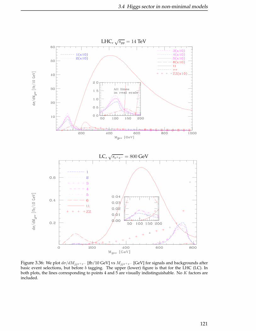
3.4 Higgs sector in non-minimal models
LHC,√spp = 14 TeV
LC,√se+e− = 800 GeV
Figure 3.36: We plot dσ/dMjjτ+τ− [fb/10 GeV] vs Mjjτ+τ− [GeV] for signals and backgrounds afterbasic event selections, but before b tagging. The upper (lower) figure is that for the LHC (LC). Inboth plots, the lines corresponding to points 4 and 5 are visually indistinguishable. No K factors areincluded.
121
3 Higgs Physics and Electroweak Symmetry Breaking
While further examination of and refinements in the LHC analysis may ultimatelylead us to have full confidence in the viability of the NMSSM Higgs boson signalsdiscussed above, an enhancement at low Mbbτ+τ− of the type shown (for some choiceof ma1) will nonetheless be the only evidence on which a claim of LHC observationof Higgs bosons can be based. Ultimately, a means of confirmation and further studywill be critical. Thus, it is important to summarize the prospects at the LC, with en-ergy up to 800 GeV, in the context of the difficult scenarios 1 — 6 of Table 3.9 discussedhere. In the following, h = h1 for points 1–3 and h = h2 for points 4–6 in Table 3.9.
Because the ZZh coupling is nearly full strength in all cases, and because the hmass is of order 100 GeV, discovery of the h will be very straightforward via e+e− →Zh using the e+e− → ZX reconstructed MX technique which is independent of the“unexpected” complexity of the h decay to a1a1. This will immediately provide adirect measurement of the ZZh coupling with very small error [210]. This approach iscompletely independent of the final state decay mode(s) and will thus work for all thepoints 1 – 6, including, in particular, points 2 and 6 for which the final state does notcontain b’s. The next stage will be to look at rates for the various h decay final states,F , and extract BR(h → F ) = σ(e+e− → Zh → ZF )/σ(e+e− → Zh). For the NMSSMpoints 1 and 3 – 5, the main channels would be F = bbbb, F = bbτ+τ− and F =τ+τ−τ+τ−. For points 2 and 6, the relevant final states are F = 4j, jjτ+τ−, τ+τ−τ+τ−.At the LC, a fairly accurate determination of BR(h→ F ) should be possible for bothsets of the three final states F . This information would allow us to determineBR(h→a1a1) independently.
Here, we consider the equally (or perhaps more) useful vector-vector fusion modethat will be active at a LC. At 800 GeV or above, it is the dominant Higgs bosonproduction channel for CP-even Higgs bosons in the intermediate mass range. Con-trary to the case of the LHC though, the dominant contribution (from WW fusion)does not allow for forward and backward particle tagging, as the incoming electronand positron convert into (anti)neutrinos, which escape detection. Although the ZZfusion contribution would allow tagging of forward/backward e− and e+, the crosssection is a factor of 10 smaller (see Fig. 4 of Ref. [210]) in comparison. At the LC theZZ background plays a fairly significant role. It has been simulated in our HERWIGand (LC-adjusted) GETJETnumerical analysis.
At a LC, the optimal signature will thus be different than at the LHC and a differentset of selection criteria are needed (see [209] for details). We have chosen selection cri-teria that retain both the WW and the ZZ fusion Higgs boson production processes.Basic requirements include the presence of at least two central jets — we look amongthe central jets for the combination with invariant mass Mjj closest to ma1 . We alsorequire two oppositely charged central leptons (ℓ = e, µ). After ensuring that theseare not back-to-back, we resolve the pTmiss along their directions and reconstruct theinvariant mass Mτ+τ− . Finally, we note that we have included Initial State Radia-tion (ISR) and beam-strahlung effects, as predicted using the HERWIGdefault. Thesetend to introduce an additional unresolvable missing longitudinal momentum, al-though to a much smaller extent than do the Parton Distribution Functions (PDFs)in hadron-hadron scattering at the LHC. Further discussion of the details of the cutsand simulation will be presented elsewhere.
At the LC, the jjτ+τ− background is again very small. As a result, we do not needto employ b tagging — it is sufficient to simply require two non-forward / backward
122
3.4 Higgs sector in non-minimal models
jets; these happen to be b’s for points 1 and 3 – 5 and light quark jets for points 2 and6.
The bottom plot of Fig. 3.36 gives the resultingMjjτ+τ− invariant mass distributionsfor the signal and several backgrounds. We note that it is not fruitful to place cuts onthe invariant masses Mjj and Mτ+τ− that exclude Mjj,Mτ+τ− ∼ mZ in an attempt toreduce the ZZ background. This is because the SM-like h mass is typically of order115 GeV, i.e. not so far from mZ , and the experimental resolutions in the two massesMjj and Mτ+τ− are poor, either because of the large number of hadronic tracks or themissing longitudinal momenta of the (anti) neutrinos, respectively.
From Fig. 3.36, we see that the Mjjτ+τ− distribution reconstructed at the LC dis-plays resonance mass peaks (again centered at 100 GeV) for the SM-like h1 (points 1– 3) or h2 (points 4 – 6) that are very clearly visible above both the tt and ZZ back-grounds, particularly for the case of points 2 and 6 (see insert in the bottom frameof Fig. 3.36). Assuming L = 500 fb−1, the points 1,3,4,5 yield 36,45,45,45 events inthe 40 ≤ Mjjτ+τ− ≤ 120 GeV interval where the background is essentially zero. Thiswould constitute a convincing signal given the very small size predicted for the back-ground. For points 2 and 6, we get about 320 events over this same background-freemass interval. The much larger signal for these points is mainly due to two reasons.Firstly, the overall BR(h1/h2 → a1a1 → 2j2ℓ) is largest in these cases, as followsfrom the branching ratios in Table 3.9 and simple combinatorics. Secondly, there isa kinematic difference related to the much smaller ma1 in cases 2 and 6 that we nowdiscuss. Notice that, although assigning the entire missing transverse momentum tothe τ -lepton system may seem not entirely appropriate (given the forward/backward(anti)neutrinos from the incoming electrons and positrons in WW fusion), this doesnot hamper the ability to reconstruct the Higgs mass peaks. However, there will bea proportion of the signal events that tend to reproduce the overall
√se+e− value in
the Mjjτ+τ− distribution. The effect is more pronounced for points 1 and 3–5, whichis where the a1 mass is larger (see Table 3.9) so that most of the hadronic tracks com-posing the emerging jets easily enter the detector region. For points 2 and 6, wherema1 is below 10 GeV, this may often not be true and it appears that the consequenteffect of these hadrons escaping detection is that of counterbalancing the pTmiss con-tributions related to the neutrinos left behind in WW fusion reactions. For the caseof the ZZ noise, in the limit of full coverage and perfect resolution of the detector,one would have Mjjτ+τ− ≡
√se+e− , which explains the concentration of events with
Mjjτ+τ− around 800 GeV. (The “tails” beyond√se+e− are due to the smearing of the
visible tracks in our Monte Carlo analysis.)
In summary, we have obtained a statistically very significant LHC signal in thejjτ+τ− final state of WW fusion for cases in which the NMSSM parameters are suchthat the most SM-like of the CP-even Higgs bosons, h, is relatively light and decaysprimarily to a pair of CP-odd Higgs states, h → aa with a → bb, τ+τ− if ma > 2mb ora → jj, τ+τ− if ma < 2mb. The statistical significances are (at least) of order 50 to 70for points withma > 2mb and of order 20 for points withma < 2mb. These high signif-icances were obtained by imposing stringent cuts requiring highly energetic forward/ backward jets in order to isolate the WW fusion signal process from backgroundssuch as DY τ+τ− pair production. Still, this signal will be the only evidence for Higgsbosons at the LHC. The LC will be absolutely essential in order to confirm that theenhancement seen at the LHC really does correspond to a Higgs boson. At the LC,
123
3 Higgs Physics and Electroweak Symmetry Breaking
discovery of a light SM-like h is guaranteed to be possible in the Zh final state usingthe recoil mass technique. Further, we have seen that WW,ZZ fusion production ofthe h will also produce a viable signal in the jjτ+τ− final state (and perhaps in the 4jand τ+τ−τ+τ− final states as well, although we have not examined these [211]); forsome parameter choices the jj will be a bb pair as can be determined by b-tagging.Finally, we have yet to explore the cases in which the a1 → χ0
1χ01 decay has a large
branching ratio. Detecting a Higgs signal in such cases will require a rather differentprocedure. Work on the WW → h→ invisible signal is in progress [211].
As we have stressed, for parameter space points of the type we have discussedhere, detection of any of the other MSSM Higgs bosons is likely to be impossible atthe LHC and is likely to require an LC with
√se+e− above the relevant thresholds
for h′a′ production, where h′ and a′ are heavy CP-even and CP-odd Higgs bosons,respectively.
Although results for the LHC indicate that Higgs boson discovery will be possiblefor the type of situations we have considered, it is clearly important to refine andimprove the techniques for extracting a signal. This will almost certainly be possibleonce data is in hand and the tt background can be more completely modeled.
Clearly, if SUSY is discovered and WW → WW scattering is found to be perturba-tive at WW energies of 1 TeV (and higher), and yet no Higgs bosons are detected inthe standard MSSM modes, a careful search for the signal we have considered shouldhave a high priority.
Finally, we should remark that the h → aa search channel considered here in theNMSSM framework is also highly relevant for a general two-Higgs-doublet model,2HDM. It is really quite possible that the most SM-like CP-even Higgs boson of a2HDM will decay primarily to two CP-odd states. This is possible even if the CP-even state is quite heavy, unlike the NMSSM cases considered here. If CP violation isintroduced in the Higgs sector, either at tree-level or as a result of one-loop corrections(as, for example, is possible in the MSSM), h→ h′h′′ decays will generally be present.The critical signal will be the same as that considered here.
3.4.2 An interesting NMSSM scenario at the LHC and LC
D.J. Miller and S. Moretti
3.4.2.1 Introduction
The Next-to-Minimal Supersymmetric Standard Model (NMSSM) provides an ele-gant solution to the µ problem of the MSSM by introducing an extra complex scalarHiggs superfield. The extra fields have no gauge couplings and are principally onlymanifest through their mixing with the other states. This leads to scenarios whereHiggs boson couplings are reduced in comparison to the MSSM, presenting a chal-lenge to the next generation of colliders. In this contribution, we will examine thephenomenology of one of these scenarios at the LHC and a future e+e− Linear Col-lider and demonstrate a synergy between the two machines.
The NMSSM has already been discussed in Section 3.4.1 of this study, in the con-text of establishing a “no-lose” theorem for the discovery of at least one Higgs boson
124
3.4 Higgs sector in non-minimal models
at the next generation of colliders (see also Ref. [212]). It was seen that for some ex-ceptional NMSSM parameter choices the discovery of any Higgs boson at all will bedifficult at the LHC, but for the majority of choices at least one Higgs boson will bediscovered. Here we adopt a different philosophy and examine a “typical” NMSSMscenario point. While not representative of scenarios over the entire range of param-eters, the chosen scenario is certainly not unusual and a wide range of parameterchoices will result in similar phenomenology, differing only in numerical detail andnot in general structure. This scenario therefore presents an interesting illustrativepicture of the Higgs sector that might be waiting for us at the next generation of col-liders.
3.4.2.2 The Model
The NMSSM has the same field content as the minimal model augmented by an ad-
ditional neutral singlet superfield S. Its superpotential is given by
W = uc huQHu − dc hdQHd − ec heLHd + λS(HuHd) +1
3κS3, (3.33)
where Hu and Hd are the usual Higgs doublet superfields with HuHd ≡ H+u H
−d −
H0uH
0d . Q and L represent left handed quark and lepton weak isospin doublets respec-
tively, while uc, dc and ec are the right handed quark and lepton fields; hu, hd and he
are matrices of Yukawa couplings where family indices have been suppressed. The
usual µ-term of the MSSM, µHuHd, has been replaced by a term coupling the new
singlet field to the usual Higgs doublets, λSHuHd. When the new singlet field gainsa vacuum expectation value (VEV), an effective µ-term is generated with an effec-tive Higgs-higgsino mass parameter given by µeff = λ〈S〉. (We adopt the notationthat the superfields are denoted by expressions with a “hat”, while their scalar com-ponents are denoted by the same expression without the hat.) The superpotentialresulting from this substitution (not yet Eq.(3.33)) contains an extra symmetry — aU(1) “Peccei-Quinn” (PQ) symmetry [213], which will be broken during electroweaksymmetry breaking. As is the case when any global symmetry is dynamically broken,this results in a massless Nambu-Goldstone boson which is in this instance a pseu-doscalar Higgs state. Since this Higgs state has not been observed in experiment wehave only two possibilities: we must either break the Peccei-Quinn symmetry explic-itly, giving the pseudoscalar a mass and putting it out of the kinematical reach of pastexperiments, or we must decouple it from the other particles by setting λ ≪ 1. Herewe adopt the former possibility12 and introduce an explicit Peccei-Quinn symmetry
breaking term 13κS3. This results in the superpotential given in Eq.(3.33). We will not
elaborate on the formal details of the model here except to elucidate our parameterchoice — for a more detailed examination of the model see Ref. [215] and referencestherein.
At tree level, the NMSSM Higgs sector has seven parameters: the Higgs couplingsfrom the superpotential, λ and κ; their two associated soft supersymmetry breakingparameters, Aλ and Aκ ; and the VEVs of the three neutral Higgs fields, which were-express as two ratios of VEVs, tan β = 〈H0
u〉/〈H0d〉 and tanβs =
√2〈S〉/v, and the
12For a description of the decoupled case, see Ref. [214].
125
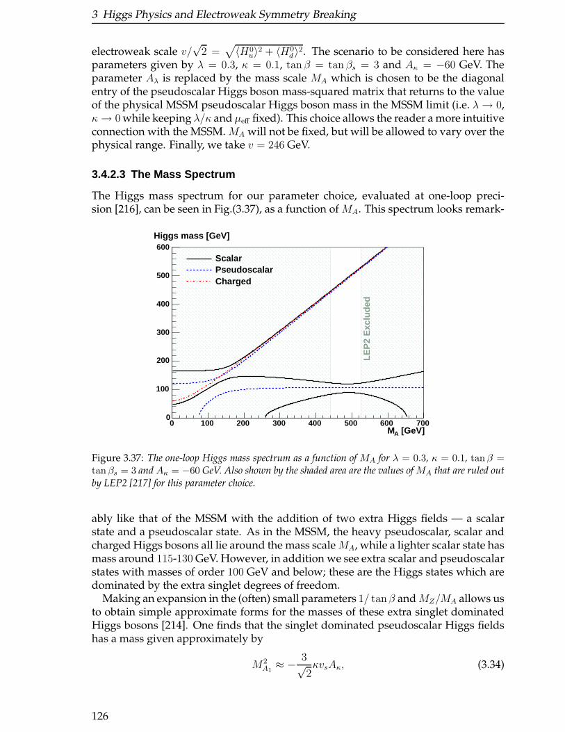
3 Higgs Physics and Electroweak Symmetry Breaking
electroweak scale v/√
2 =√〈H0
u〉2 + 〈H0d〉2. The scenario to be considered here has
parameters given by λ = 0.3, κ = 0.1, tanβ = tan βs = 3 and Aκ = −60 GeV. Theparameter Aλ is replaced by the mass scale MA which is chosen to be the diagonalentry of the pseudoscalar Higgs boson mass-squared matrix that returns to the valueof the physical MSSM pseudoscalar Higgs boson mass in the MSSM limit (i.e. λ→ 0,κ→ 0 while keeping λ/κ and µeff fixed). This choice allows the reader a more intuitiveconnection with the MSSM. MA will not be fixed, but will be allowed to vary over thephysical range. Finally, we take v = 246 GeV.
3.4.2.3 The Mass Spectrum
The Higgs mass spectrum for our parameter choice, evaluated at one-loop preci-sion [216], can be seen in Fig.(3.37), as a function of MA. This spectrum looks remark-
0 100 200 300 400 500 600 7000
100
200
300
400
500
600
[GeV]AM
Higgs mass [GeV]
ScalarPseudoscalarCharged
LEP
2 E
xclu
ded
Figure 3.37: The one-loop Higgs mass spectrum as a function of MA for λ = 0.3, κ = 0.1, tan β =tan βs = 3 and Aκ = −60 GeV. Also shown by the shaded area are the values of MA that are ruled outby LEP2 [217] for this parameter choice.
ably like that of the MSSM with the addition of two extra Higgs fields — a scalarstate and a pseudoscalar state. As in the MSSM, the heavy pseudoscalar, scalar andcharged Higgs bosons all lie around the mass scaleMA, while a lighter scalar state hasmass around 115-130 GeV. However, in addition we see extra scalar and pseudoscalarstates with masses of order 100 GeV and below; these are the Higgs states which aredominated by the extra singlet degrees of freedom.
Making an expansion in the (often) small parameters 1/ tanβ andMZ/MA allows usto obtain simple approximate forms for the masses of these extra singlet dominatedHiggs bosons [214]. One finds that the singlet dominated pseudoscalar Higgs fieldshas a mass given approximately by
M2A1≈ − 3√
2κvsAκ, (3.34)
126
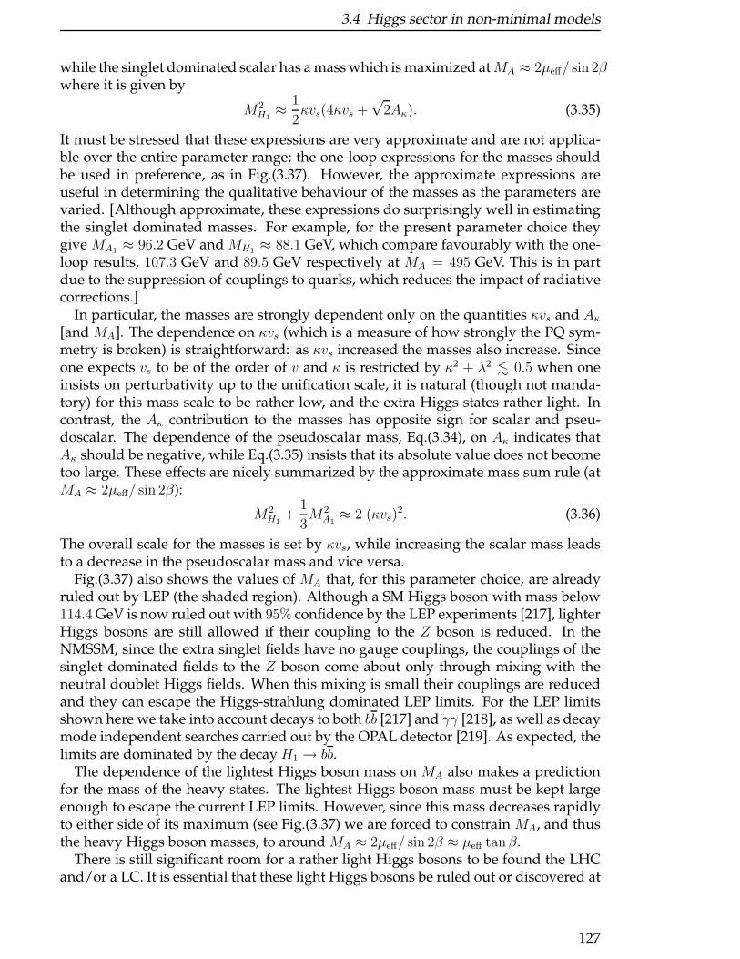
3.4 Higgs sector in non-minimal models
while the singlet dominated scalar has a mass which is maximized atMA ≈ 2µeff/ sin 2βwhere it is given by
M2H1≈ 1
2κvs(4κvs +
√2Aκ). (3.35)
It must be stressed that these expressions are very approximate and are not applica-ble over the entire parameter range; the one-loop expressions for the masses shouldbe used in preference, as in Fig.(3.37). However, the approximate expressions areuseful in determining the qualitative behaviour of the masses as the parameters arevaried. [Although approximate, these expressions do surprisingly well in estimatingthe singlet dominated masses. For example, for the present parameter choice theygive MA1 ≈ 96.2 GeV and MH1 ≈ 88.1 GeV, which compare favourably with the one-loop results, 107.3 GeV and 89.5 GeV respectively at MA = 495 GeV. This is in partdue to the suppression of couplings to quarks, which reduces the impact of radiativecorrections.]
In particular, the masses are strongly dependent only on the quantities κvs and Aκ[and MA]. The dependence on κvs (which is a measure of how strongly the PQ sym-metry is broken) is straightforward: as κvs increased the masses also increase. Sinceone expects vs to be of the order of v and κ is restricted by κ2 + λ2 . 0.5 when oneinsists on perturbativity up to the unification scale, it is natural (though not manda-tory) for this mass scale to be rather low, and the extra Higgs states rather light. Incontrast, the Aκ contribution to the masses has opposite sign for scalar and pseu-doscalar. The dependence of the pseudoscalar mass, Eq.(3.34), on Aκ indicates thatAκ should be negative, while Eq.(3.35) insists that its absolute value does not becometoo large. These effects are nicely summarized by the approximate mass sum rule (atMA ≈ 2µeff/ sin 2β):
M2H1
+1
3M2
A1≈ 2 (κvs)
2. (3.36)
The overall scale for the masses is set by κvs, while increasing the scalar mass leadsto a decrease in the pseudoscalar mass and vice versa.
Fig.(3.37) also shows the values of MA that, for this parameter choice, are alreadyruled out by LEP (the shaded region). Although a SM Higgs boson with mass below114.4 GeV is now ruled out with 95% confidence by the LEP experiments [217], lighterHiggs bosons are still allowed if their coupling to the Z boson is reduced. In theNMSSM, since the extra singlet fields have no gauge couplings, the couplings of thesinglet dominated fields to the Z boson come about only through mixing with theneutral doublet Higgs fields. When this mixing is small their couplings are reducedand they can escape the Higgs-strahlung dominated LEP limits. For the LEP limitsshown here we take into account decays to both bb [217] and γγ [218], as well as decaymode independent searches carried out by the OPAL detector [219]. As expected, thelimits are dominated by the decay H1 → bb.
The dependence of the lightest Higgs boson mass on MA also makes a predictionfor the mass of the heavy states. The lightest Higgs boson mass must be kept largeenough to escape the current LEP limits. However, since this mass decreases rapidlyto either side of its maximum (see Fig.(3.37) we are forced to constrain MA, and thusthe heavy Higgs boson masses, to around MA ≈ 2µeff/ sin 2β ≈ µeff tanβ.
There is still significant room for a rather light Higgs bosons to be found the LHCand/or a LC. It is essential that these light Higgs bosons be ruled out or discovered at
127
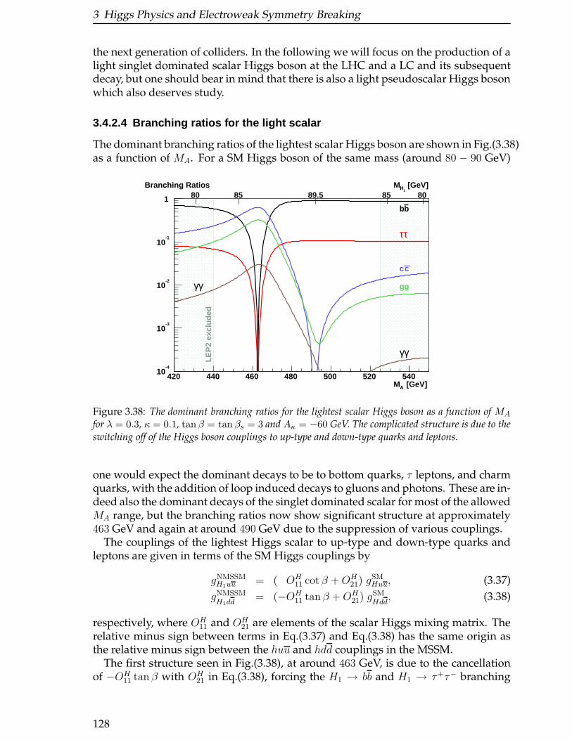
3 Higgs Physics and Electroweak Symmetry Breaking
the next generation of colliders. In the following we will focus on the production of alight singlet dominated scalar Higgs boson at the LHC and a LC and its subsequentdecay, but one should bear in mind that there is also a light pseudoscalar Higgs bosonwhich also deserves study.
3.4.2.4 Branching ratios for the light scalar
The dominant branching ratios of the lightest scalar Higgs boson are shown in Fig.(3.38)as a function of MA. For a SM Higgs boson of the same mass (around 80 − 90 GeV)
420 440 460 480 500 520 54010
-4
10-3
10-2
10-1
1 80 85 89.5 85 80
LEP
2 ex
clud
ed
[GeV]AM
[GeV]1HMBranching Ratios
bb
ττ
cc
ggγγ
γγ
Figure 3.38: The dominant branching ratios for the lightest scalar Higgs boson as a function of MA
for λ = 0.3, κ = 0.1, tan β = tanβs = 3 and Aκ = −60 GeV. The complicated structure is due to theswitching off of the Higgs boson couplings to up-type and down-type quarks and leptons.
one would expect the dominant decays to be to bottom quarks, τ leptons, and charmquarks, with the addition of loop induced decays to gluons and photons. These are in-deed also the dominant decays of the singlet dominated scalar for most of the allowedMA range, but the branching ratios now show significant structure at approximately463 GeV and again at around 490 GeV due to the suppression of various couplings.
The couplings of the lightest Higgs scalar to up-type and down-type quarks andleptons are given in terms of the SM Higgs couplings by
gNMSSMH1uu = ( OH
11 cot β +OH21) g
SMHuu, (3.37)
gNMSSMH1dd
= (−OH11 tan β +OH
21) gSMHdd
, (3.38)
respectively, where OH11 and OH
21 are elements of the scalar Higgs mixing matrix. Therelative minus sign between terms in Eq.(3.37) and Eq.(3.38) has the same origin asthe relative minus sign between the huu and hdd couplings in the MSSM.
The first structure seen in Fig.(3.38), at around 463 GeV, is due to the cancellationof −OH
11 tan β with OH21 in Eq.(3.38), forcing the H1 → bb and H1 → τ+τ− branching
128

3.4 Higgs sector in non-minimal models
ratios to vanish. As MA is increased, OH21 passes smoothly through zero, eventually
canceling with OH11 cot β in Eq.(3.37). This provides the structure at around 490 GeV
where the H1 → cc branching ratio vanishes.The decays to gg and γγ are mediated by loop diagrams giving a more complex
behaviour. H1 → gg is dominated by top and stop loops and consequently showsa marked decrease as the H1tt coupling switches off; although the top-loop contri-bution will pass through zero here, stop loops and bottom (s)quark loops preventthe branching ratio from vanishing. In addition to top and bottom (s)quark loopsthe γγ branching ratio is mediated by virtual W bosons, charged Higgs bosons andcharginos. The dominant effect is from the W bosons and the top loops and so we seea broad suppression over the range where these couplings vanish.
3.4.2.5 LHC Production
Cross-sections for the production of the lightest scalar Higgs boson in various chan-nels at the LHC are shown in Fig.(3.39). The total production cross-section is domi-
420 440 460 480 500 520 54010
-3
10-2
10-1
1
10
80 85 89.5 85 80
LEP
2 E
xclu
ded
[GeV]AM
[GeV]1HM [pb]
1Hσ
1 H→gg
1 H→V V
1 WH→W
1 ZH→Z
bb1 H→gg tt1 H→gg
totσ
Figure 3.39: Production cross-sections for the lightest scalar Higgs boson at the LHC, as a function ofMA for λ = 0.3, κ = 0.1, tan β = tanβs = 3 and Aκ = −60 GeV.
nated by gluon-gluon fusion, and is sizable over the entire range. Other significantproduction channels are vector boson fusion (V V → H1), Higgs-strahlung (W →WH1 and Z → ZH1) and associated production together with top and bottom quarks(gg → H1tt and gg → H1bb respectively). As we saw for the branching ratios we againsee structures which are associated with the couplings of the Higgs boson to variousparticles passing through zero. However, in contrast to the earlier discussion, thereare now three, rather than two, significant values ofMA where structure appears. Thecoupling of the Higgs boson to a vector boson V = W, Z with respect to the SM isgiven by
gNMSSMH1V V
= OH21 g
SMH1V V
, (3.39)
129

3 Higgs Physics and Electroweak Symmetry Breaking
where OH21 is the same element appearing in Eqs.(3.37–3.38), so when this mixing el-
ement vanishes the vector boson fusion and Higgs-strahlung cross-sections will dis-appear. This MA point is very close to the point where the H1tt couplings vanishbecause the first term on the right-hand-side of Eq.(3.37) is suppressed by 1/ tanβ.
For the lower values of MA, where the Higgs decay to bb is suppressed, this Higgsboson may be visible via its decay to γγ (with a branching ratio & 0.1% for MA .
480 GeV). However, as the γγ branching ratio is turned off at higher MA, seeing thisHiggs boson will become much more challenging. Although the cross-section re-mains relatively large, the Higgs boson almost always decays hadronically and thesignal has a very large QCD background. The only significant non-hadronic decay isthe Higgs decay to τ -pairs with a branching fraction of approximately 10%, but thisalso has large SM backgrounds.
The chosen scenario is extremely challenging for the LHC, but it is by no means a“worst-case scenario”. For example, increasing the value of tan β would increase theseparation between the b-quark and vector boson switch-off points, moving the MA
range with an enhanced H1 → γγ branching ratio out of the allowed region. Alter-natively, increasing the value of κvs slightly would lead to a light Higgs boson sittingright on top of the Z-peak, making it very difficult to disentangle from the SM back-grounds. If the value of κvs is significantly larger (and |Aκ| not too large), the singletdominated scalar would be heavy enough to decay to a vector boson pair, makingits detection much easier. However, if the value of MA is such that the coupling ofEq.(3.39) vanishes, these golden channels would be lost.
3.4.2.6 LC Production
The vanishing of the HV V couplings in the region of interest is particularly signif-icant for a LC since the most promising production mechanisms are vector bosonfusion, e.g. e+e− → W+W−νν → H1νν, and Higgs-strahlung, e+e− → Z∗ → ZH1.The cross-sections for these processes at a
√s = 500 GeV LC are plotted in Fig.(3.40)
for our parameter choice, as a function of MA, and show the distinctive vanishing ofthe H1V V coupling. Nevertheless, the lightest scalar Higgs boson would be seen bythese channels for all of the MA range except for a small window around 490 GeV. Incontrast to the LHC, for most of the the observable region decays to bb and/or τ+τ−
could be easily used due the LC’s relatively background free environment. For MA
values where the bottom and τ couplings vanish, the decays to γγ and charm may beused instead.
It is difficult to see what production mechanism could be used to close the remain-ing window around the critical point where the HV V couplings vanish. Higgs pro-duction in association with a top quark pair, e+e− → H1tt, is vanishingly small herebecause of the proximity of the H1V V and H1tt “turning-off” points (they will moveeven closer as tanβ is increased). The production in association with bottom quarks isshown in Fig.(3.40), multiplied by a factor of 104 to be visible on the same scale. Gen-erally, this production process has three contributing sub-processes: Higgs-strahlung,e+e− → ZH1, followed by the Z decay to a bottom quark pair; Higgs pair production,e+e− → H1Ai (i = 1, 2) followed by the pseudoscalar decaying to bottom quarks;and bottom quark pair production, e+e− → bb followed by the radiation of H1 off a
130
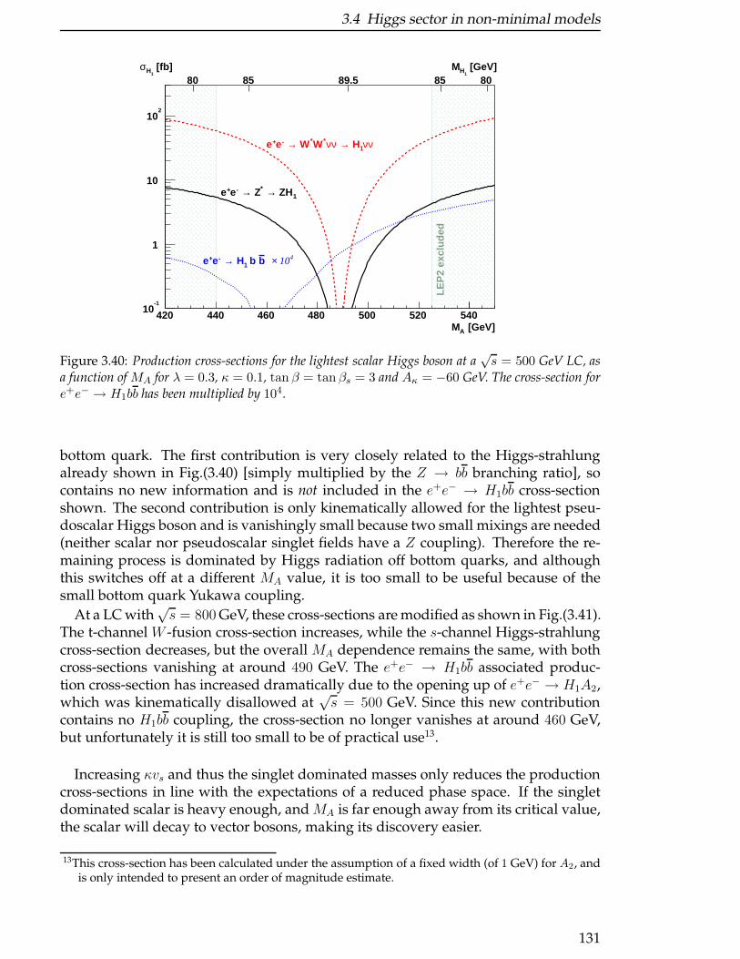
3.4 Higgs sector in non-minimal models
420 440 460 480 500 520 54010
-1
1
10
102
80 85 89.5 85 80
[GeV]AM
[GeV]1HM [fb]
1Hσ
1 ZH→ * Z→ -e+e
b b 1 H→ -e+e
LEP
2 ex
clud
ed
νν1 H→ νν*W* W→ -e+e
4 10×
Figure 3.40: Production cross-sections for the lightest scalar Higgs boson at a√s = 500 GeV LC, as
a function of MA for λ = 0.3, κ = 0.1, tan β = tan βs = 3 and Aκ = −60 GeV. The cross-section fore+e− → H1bb has been multiplied by 104.
bottom quark. The first contribution is very closely related to the Higgs-strahlungalready shown in Fig.(3.40) [simply multiplied by the Z → bb branching ratio], socontains no new information and is not included in the e+e− → H1bb cross-sectionshown. The second contribution is only kinematically allowed for the lightest pseu-doscalar Higgs boson and is vanishingly small because two small mixings are needed(neither scalar nor pseudoscalar singlet fields have a Z coupling). Therefore the re-maining process is dominated by Higgs radiation off bottom quarks, and althoughthis switches off at a different MA value, it is too small to be useful because of thesmall bottom quark Yukawa coupling.
At a LC with√s = 800 GeV, these cross-sections are modified as shown in Fig.(3.41).
The t-channel W -fusion cross-section increases, while the s-channel Higgs-strahlungcross-section decreases, but the overall MA dependence remains the same, with bothcross-sections vanishing at around 490 GeV. The e+e− → H1bb associated produc-tion cross-section has increased dramatically due to the opening up of e+e− → H1A2,which was kinematically disallowed at
√s = 500 GeV. Since this new contribution
contains no H1bb coupling, the cross-section no longer vanishes at around 460 GeV,but unfortunately it is still too small to be of practical use13.
Increasing κvs and thus the singlet dominated masses only reduces the productioncross-sections in line with the expectations of a reduced phase space. If the singletdominated scalar is heavy enough, and MA is far enough away from its critical value,the scalar will decay to vector bosons, making its discovery easier.
13This cross-section has been calculated under the assumption of a fixed width (of 1 GeV) for A2, andis only intended to present an order of magnitude estimate.
131
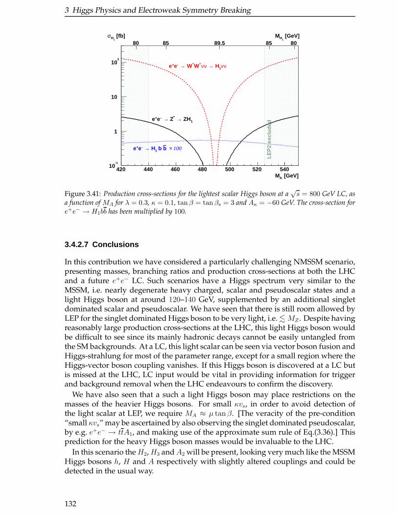
3 Higgs Physics and Electroweak Symmetry Breaking
420 440 460 480 500 520 54010
-1
1
10
102
80 85 89.5 85 80
[GeV]AM
[GeV]1HM [fb]
1Hσ
1 ZH→ * Z→ -e+e
b b 1 H→ -e+e
LEP
2 ex
clud
ed
νν1 H→ νν*W* W→ -e+e
100×
Figure 3.41: Production cross-sections for the lightest scalar Higgs boson at a√s = 800 GeV LC, as
a function of MA for λ = 0.3, κ = 0.1, tan β = tanβs = 3 and Aκ = −60 GeV. The cross-section fore+e− → H1bb has been multiplied by 100.
3.4.2.7 Conclusions
In this contribution we have considered a particularly challenging NMSSM scenario,presenting masses, branching ratios and production cross-sections at both the LHCand a future e+e− LC. Such scenarios have a Higgs spectrum very similar to theMSSM, i.e. nearly degenerate heavy charged, scalar and pseudoscalar states and alight Higgs boson at around 120–140 GeV, supplemented by an additional singletdominated scalar and pseudoscalar. We have seen that there is still room allowed byLEP for the singlet dominated Higgs boson to be very light, i.e. . MZ . Despite havingreasonably large production cross-sections at the LHC, this light Higgs boson wouldbe difficult to see since its mainly hadronic decays cannot be easily untangled fromthe SM backgrounds. At a LC, this light scalar can be seen via vector boson fusion andHiggs-strahlung for most of the parameter range, except for a small region where theHiggs-vector boson coupling vanishes. If this Higgs boson is discovered at a LC butis missed at the LHC, LC input would be vital in providing information for triggerand background removal when the LHC endeavours to confirm the discovery.
We have also seen that a such a light Higgs boson may place restrictions on themasses of the heavier Higgs bosons. For small κvs, in order to avoid detection ofthe light scalar at LEP, we require MA ≈ µ tanβ. [The veracity of the pre-condition“small κvs” may be ascertained by also observing the singlet dominated pseudoscalar,by e.g. e+e− → ttA1, and making use of the approximate sum rule of Eq.(3.36).] Thisprediction for the heavy Higgs boson masses would be invaluable to the LHC.
In this scenario theH2,H3 andA2 will be present, looking very much like the MSSMHiggs bosons h, H and A respectively with slightly altered couplings and could bedetected in the usual way.
132
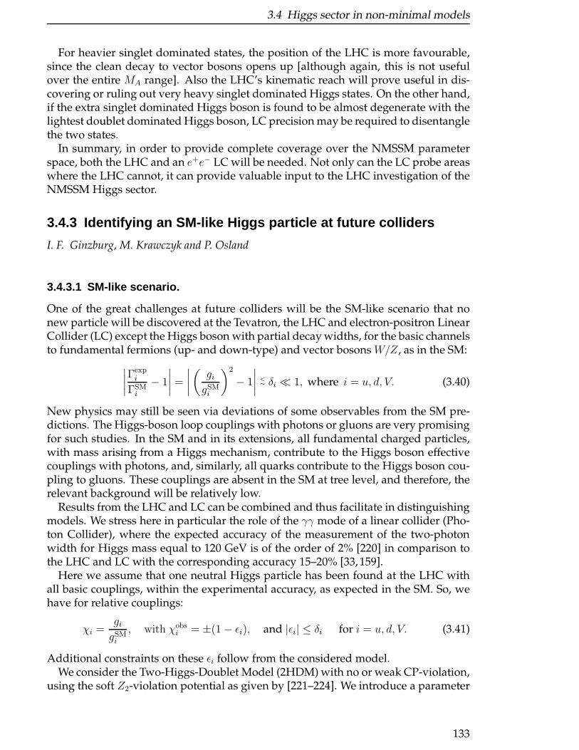
3.4 Higgs sector in non-minimal models
For heavier singlet dominated states, the position of the LHC is more favourable,since the clean decay to vector bosons opens up [although again, this is not usefulover the entire MA range]. Also the LHC’s kinematic reach will prove useful in dis-covering or ruling out very heavy singlet dominated Higgs states. On the other hand,if the extra singlet dominated Higgs boson is found to be almost degenerate with thelightest doublet dominated Higgs boson, LC precision may be required to disentanglethe two states.
In summary, in order to provide complete coverage over the NMSSM parameterspace, both the LHC and an e+e− LC will be needed. Not only can the LC probe areaswhere the LHC cannot, it can provide valuable input to the LHC investigation of theNMSSM Higgs sector.
3.4.3 Identifying an SM-like Higgs particle at future colli ders
I. F. Ginzburg, M. Krawczyk and P. Osland
3.4.3.1 SM-like scenario.
One of the great challenges at future colliders will be the SM-like scenario that nonew particle will be discovered at the Tevatron, the LHC and electron-positron LinearCollider (LC) except the Higgs boson with partial decay widths, for the basic channelsto fundamental fermions (up- and down-type) and vector bosons W/Z, as in the SM:
∣∣∣∣Γexpi
ΓSMi
− 1
∣∣∣∣ =
∣∣∣∣(gigSMi
)2
− 1
∣∣∣∣<∼ δi ≪ 1, where i = u, d, V. (3.40)
New physics may still be seen via deviations of some observables from the SM pre-dictions. The Higgs-boson loop couplings with photons or gluons are very promisingfor such studies. In the SM and in its extensions, all fundamental charged particles,with mass arising from a Higgs mechanism, contribute to the Higgs boson effectivecouplings with photons, and, similarly, all quarks contribute to the Higgs boson cou-pling to gluons. These couplings are absent in the SM at tree level, and therefore, therelevant background will be relatively low.
Results from the LHC and LC can be combined and thus facilitate in distinguishingmodels. We stress here in particular the role of the γγ mode of a linear collider (Pho-ton Collider), where the expected accuracy of the measurement of the two-photonwidth for Higgs mass equal to 120 GeV is of the order of 2% [220] in comparison tothe LHC and LC with the corresponding accuracy 15–20% [33, 159].
Here we assume that one neutral Higgs particle has been found at the LHC withall basic couplings, within the experimental accuracy, as expected in the SM. So, wehave for relative couplings:
χi =gigSMi
, with χobsi = ±(1− ǫi), and |ǫi| ≤ δi for i = u, d, V. (3.41)
Additional constraints on these ǫi follow from the considered model.We consider the Two-Higgs-Doublet Model (2HDM) with no or weak CP-violation,
using the soft Z2-violation potential as given by [221–224]. We introduce a parameter
133

3 Higgs Physics and Electroweak Symmetry Breaking
µ via the real part of the coefficient of the bilinear mixing term ℜ(m212) = 2µ2v1v2/v
2
[224]. For µ2 ≫ |λi|v2 the SM-like scenario with decoupling is realized. The SM-like scenario can also be realized for µ < v with non-decoupling, in particular forMH± ≈MH ≈ 700 GeV, MA ≈ 600 GeV and Mh=120 GeV, µ < 0.3MH±, with λi withinperturbativity and even unitarity constraints. The Yukawa interactions are of Type IIwith the basic couplings constrained by (χu+χd)χV = 1+χuχd (pattern relation [224]),valid for each neutral Higgs boson, even in the general CP-violating case.
The SM-like scenario corresponds to the observation of either h or H . We distin-guish solutions A and B (see ref. [224] and table 3.10) for the realization of an SM-likescenario for the observed Higgs particle with mass 110 to 250 GeV. In solutions A allbasic (relative) couplings are close to 1 or all are close to −1. Note that only solutionAh+ is realized in the decoupling limit. In solutions B, one basic coupling, χu or χd,has opposite sign to the other two, and obviously one expects here larger deviationsfrom the SM than for solutions A. One can see that the decay width h(H)Zγ is lesssensitive to the discussed effects of 2HDM than the h(H)γγ one.14
solution basic couplings |χgg|2 |χγγ|2 |χZγ|2Ah±/AH−
χV ≈ χd ≈ χu ≈ ±1 1.00 0.90 0.96Bh±d/BH−d χV ≈ −χd ≈ χu ≈ ±1 1.28 0.87 0.96
Bh±u χV ≈ χd ≈ −χu ≈ ±1 1.28 2.28 1.21
Table 3.10: SM-like realizations in the 2HDM II [224], together with ratios of partial widths to theirSM values for Mh(H) ≈ 120 GeV for the case |χi| = 1, MH± =700 GeV and µ . 0.3MH± .
3.4.3.2 The two-gluon decay width.
The two-gluon width will be measured at the LHC. This quantity is for solutions Apractically equal to the SM prediction (see table 1).
In the SM the contributions of t and b quarks partly cancel, while for solutions Bthey add, giving larger deviations from the SM predictions. In Fig. 1 (left) the solidcurve corresponds to the case χu = −χd = ±1 for all solutions B. The shaded bandsreflecting 1 σ experimental uncertainties correspond to the Bh+u case only.
120 140 160 180 200 220 2400.8
0.9
1
1.1
1.2
1.3
1.4
120 140 160 180 200 220 2400.8
0.85
0.9
0.95
1
1.05
1.1
Figure 3.42: Ratios of the Higgs boson decay widths in the SM-like 2HDM II and the SM as functionsof Mh,H for solutions B and A for MH±=700 GeV and µ . 0.3M±
H .
14The process eγ → eh(H) with large transverse momentum of the scattered electron, has a sensitivityfrom the h(H)Zγ vertex, with Z far from the mass shell, similar to that of h(H)→ γγ [225].
134
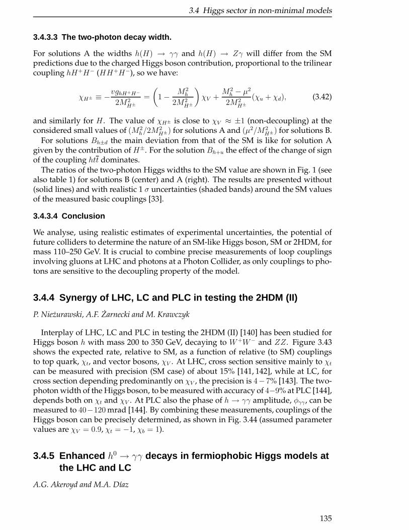
3.4 Higgs sector in non-minimal models
3.4.3.3 The two-photon decay width.
For solutions A the widths h(H) → γγ and h(H) → Zγ will differ from the SMpredictions due to the charged Higgs boson contribution, proportional to the trilinearcoupling hH+H− (HH+H−), so we have:
χH± ≡ −vghH+H−
2M2H±
=
(1− M2
h
2M2H±
)χV +
M2h − µ2
2M2H±
(χu + χd), (3.42)
and similarly for H . The value of χH± is close to χV ≈ ±1 (non-decoupling) at theconsidered small values of (M2
h/2M2H±) for solutions A and (µ2/M2
H±) for solutions B.For solutions Bh±d the main deviation from that of the SM is like for solution A
given by the contribution of H±. For the solution Bh+u the effect of the change of signof the coupling htt dominates.
The ratios of the two-photon Higgs widths to the SM value are shown in Fig. 1 (seealso table 1) for solutions B (center) and A (right). The results are presented without(solid lines) and with realistic 1 σ uncertainties (shaded bands) around the SM valuesof the measured basic couplings [33].
3.4.3.4 Conclusion
We analyse, using realistic estimates of experimental uncertainties, the potential offuture colliders to determine the nature of an SM-like Higgs boson, SM or 2HDM, formass 110–250 GeV. It is crucial to combine precise measurements of loop couplingsinvolving gluons at LHC and photons at a Photon Collider, as only couplings to pho-tons are sensitive to the decoupling property of the model.
3.4.4 Synergy of LHC, LC and PLC in testing the 2HDM (II)
P. Niezurawski, A.F. Zarnecki and M. Krawczyk
Interplay of LHC, LC and PLC in testing the 2HDM (II) [140] has been studied forHiggs boson h with mass 200 to 350 GeV, decaying to W+W− and ZZ. Figure 3.43shows the expected rate, relative to SM, as a function of relative (to SM) couplingsto top quark, χt, and vector bosons, χV . At LHC, cross section sensitive mainly to χtcan be measured with precision (SM case) of about 15% [141, 142], while at LC, forcross section depending predominantly on χV , the precision is 4−7% [143]. The two-photon width of the Higgs boson, to be measured with accuracy of 4−9% at PLC [144],depends both on χt and χV . At PLC also the phase of h → γγ amplitude, φγγ , can bemeasured to 40−120 mrad [144]. By combining these measurements, couplings of theHiggs boson can be precisely determined, as shown in Fig. 3.44 (assumed parametervalues are χV = 0.9, χt = −1, χb = 1).
3.4.5 Enhanced h0 → γγ decays in fermiophobic Higgs models atthe LHC and LC
A.G. Akeroyd and M.A. Dıaz
135
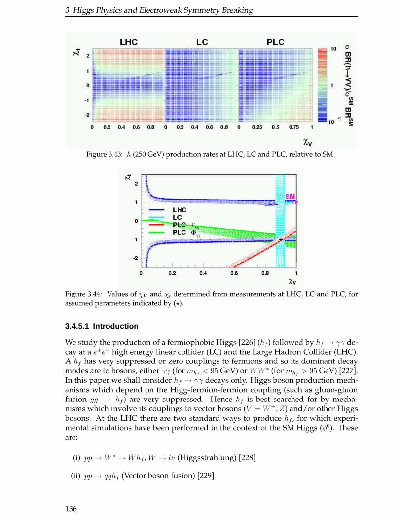
3 Higgs Physics and Electroweak Symmetry Breaking
Figure 3.43: h (250 GeV) production rates at LHC, LC and PLC, relative to SM.
Figure 3.44: Values of χV and χt determined from measurements at LHC, LC and PLC, forassumed parameters indicated by (⋆).
3.4.5.1 Introduction
We study the production of a fermiophobic Higgs [226] (hf ) followed by hf → γγ de-cay at a e+e− high energy linear collider (LC) and the Large Hadron Collider (LHC).A hf has very suppressed or zero couplings to fermions and so its dominant decaymodes are to bosons, either γγ (for mhf
< 95 GeV) or WW ∗ (for mhf> 95 GeV) [227].
In this paper we shall consider hf → γγ decays only. Higgs boson production mech-anisms which depend on the Higg-fermion-fermion coupling (such as gluon-gluonfusion gg → hf ) are very suppressed. Hence hf is best searched for by mecha-nisms which involve its couplings to vector bosons (V = W±, Z) and/or other Higgsbosons. At the LHC there are two standard ways to produce hf , for which experi-mental simulations have been performed in the context of the SM Higgs (φ0). Theseare:
(i) pp→ W ∗ → Whf , W → lν (Higgsstrahlung) [228]
(ii) pp→ qqhf (Vector boson fusion) [229]
136
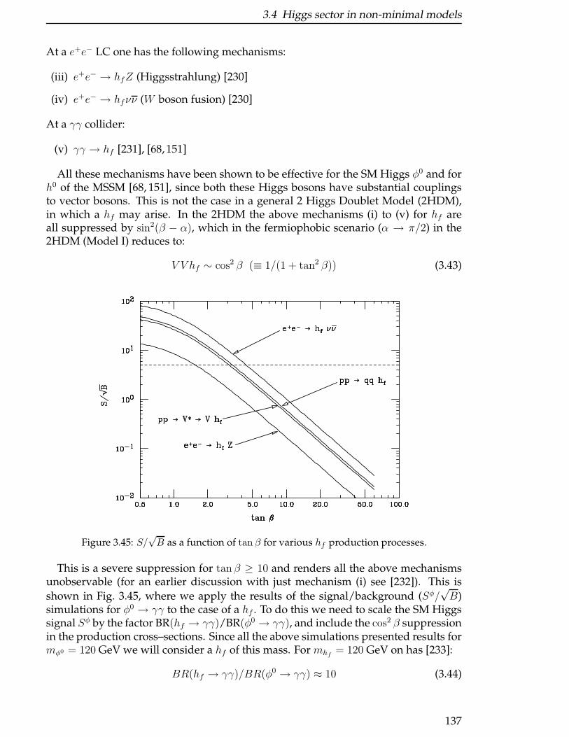
3.4 Higgs sector in non-minimal models
At a e+e− LC one has the following mechanisms:
(iii) e+e− → hfZ (Higgsstrahlung) [230]
(iv) e+e− → hfνν (W boson fusion) [230]
At a γγ collider:
(v) γγ → hf [231], [68, 151]
All these mechanisms have been shown to be effective for the SM Higgs φ0 and forh0 of the MSSM [68, 151], since both these Higgs bosons have substantial couplingsto vector bosons. This is not the case in a general 2 Higgs Doublet Model (2HDM),in which a hf may arise. In the 2HDM the above mechanisms (i) to (v) for hf areall suppressed by sin2(β − α), which in the fermiophobic scenario (α → π/2) in the2HDM (Model I) reduces to:
V V hf ∼ cos2 β (≡ 1/(1 + tan2 β)) (3.43)
Figure 3.45: S/√B as a function of tan β for various hf production processes.
This is a severe suppression for tan β ≥ 10 and renders all the above mechanismsunobservable (for an earlier discussion with just mechanism (i) see [232]). This is
shown in Fig. 3.45, where we apply the results of the signal/background (Sφ/√B)
simulations for φ0 → γγ to the case of a hf . To do this we need to scale the SM Higgssignal Sφ by the factor BR(hf → γγ)/BR(φ0 → γγ), and include the cos2 β suppressionin the production cross–sections. Since all the above simulations presented results formφ0 = 120 GeV we will consider a hf of this mass. For mhf
= 120 GeV on has [233]:
BR(hf → γγ)/BR(φ0 → γγ) ≈ 10 (3.44)
137
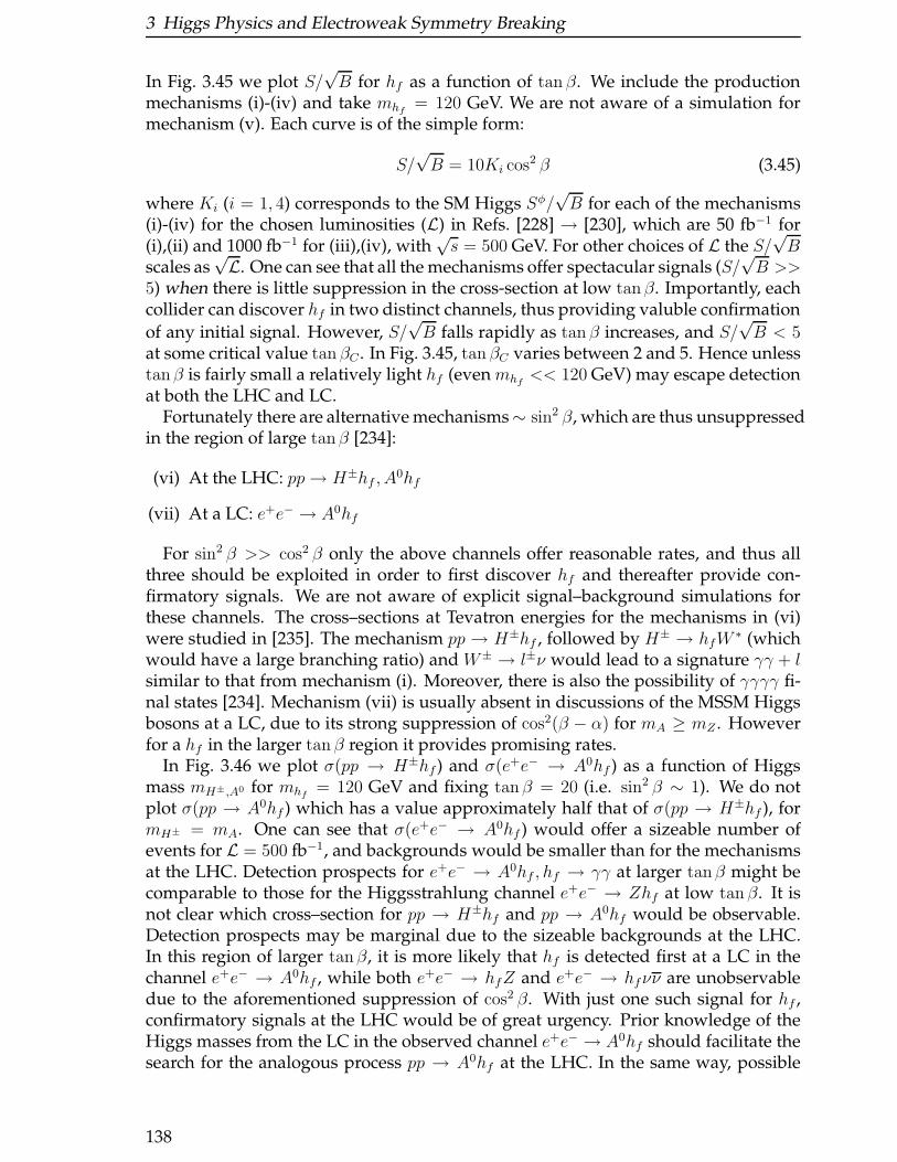
3 Higgs Physics and Electroweak Symmetry Breaking
In Fig. 3.45 we plot S/√B for hf as a function of tan β. We include the production
mechanisms (i)-(iv) and take mhf= 120 GeV. We are not aware of a simulation for
mechanism (v). Each curve is of the simple form:
S/√B = 10Ki cos2 β (3.45)
where Ki (i = 1, 4) corresponds to the SM Higgs Sφ/√B for each of the mechanisms
(i)-(iv) for the chosen luminosities (L) in Refs. [228] → [230], which are 50 fb−1 for(i),(ii) and 1000 fb−1 for (iii),(iv), with
√s = 500 GeV. For other choices of L the S/
√B
scales as√L. One can see that all the mechanisms offer spectacular signals (S/
√B >>
5) when there is little suppression in the cross-section at low tanβ. Importantly, eachcollider can discover hf in two distinct channels, thus providing valuble confirmation
of any initial signal. However, S/√B falls rapidly as tan β increases, and S/
√B < 5
at some critical value tan βC . In Fig. 3.45, tan βC varies between 2 and 5. Hence unlesstanβ is fairly small a relatively light hf (even mhf
<< 120 GeV) may escape detectionat both the LHC and LC.
Fortunately there are alternative mechanisms∼ sin2 β, which are thus unsuppressedin the region of large tanβ [234]:
(vi) At the LHC: pp→ H±hf , A0hf
(vii) At a LC: e+e− → A0hf
For sin2 β >> cos2 β only the above channels offer reasonable rates, and thus allthree should be exploited in order to first discover hf and thereafter provide con-firmatory signals. We are not aware of explicit signal–background simulations forthese channels. The cross–sections at Tevatron energies for the mechanisms in (vi)were studied in [235]. The mechanism pp → H±hf , followed by H± → hfW
∗ (whichwould have a large branching ratio) and W± → l±ν would lead to a signature γγ + lsimilar to that from mechanism (i). Moreover, there is also the possibility of γγγγ fi-nal states [234]. Mechanism (vii) is usually absent in discussions of the MSSM Higgsbosons at a LC, due to its strong suppression of cos2(β − α) for mA ≥ mZ . Howeverfor a hf in the larger tan β region it provides promising rates.
In Fig. 3.46 we plot σ(pp → H±hf ) and σ(e+e− → A0hf ) as a function of Higgsmass mH±,A0 for mhf
= 120 GeV and fixing tanβ = 20 (i.e. sin2 β ∼ 1). We do notplot σ(pp → A0hf ) which has a value approximately half that of σ(pp → H±hf ), formH± = mA. One can see that σ(e+e− → A0hf ) would offer a sizeable number ofevents for L = 500 fb−1, and backgrounds would be smaller than for the mechanismsat the LHC. Detection prospects for e+e− → A0hf , hf → γγ at larger tanβ might becomparable to those for the Higgsstrahlung channel e+e− → Zhf at low tan β. It isnot clear which cross–section for pp → H±hf and pp → A0hf would be observable.Detection prospects may be marginal due to the sizeable backgrounds at the LHC.In this region of larger tanβ, it is more likely that hf is detected first at a LC in thechannel e+e− → A0hf , while both e+e− → hfZ and e+e− → hfνν are unobservabledue to the aforementioned suppression of cos2 β. With just one such signal for hf ,confirmatory signals at the LHC would be of great urgency. Prior knowledge of theHiggs masses from the LC in the observed channel e+e− → A0hf should facilitate thesearch for the analogous process pp → A0hf at the LHC. In the same way, possible
138
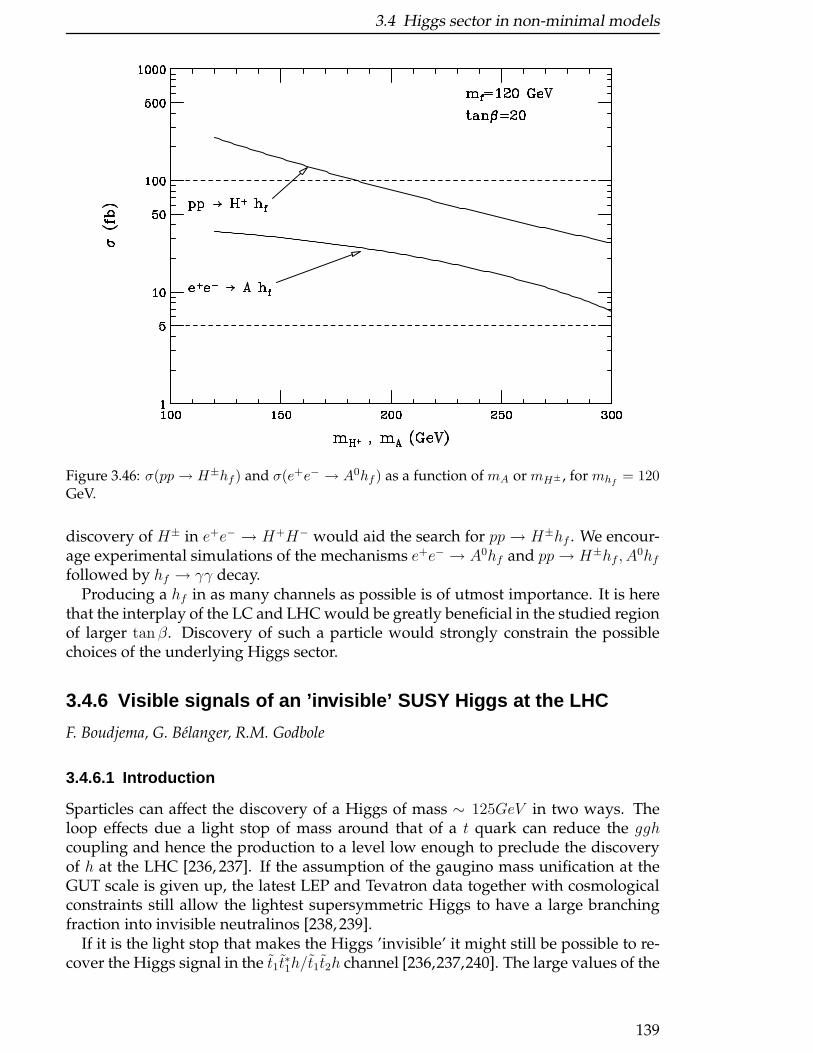
3.4 Higgs sector in non-minimal models
Figure 3.46: σ(pp → H±hf ) and σ(e+e− → A0hf ) as a function of mA or mH± , for mhf= 120
GeV.
discovery of H± in e+e− → H+H− would aid the search for pp → H±hf . We encour-age experimental simulations of the mechanisms e+e− → A0hf and pp→ H±hf , A
0hffollowed by hf → γγ decay.
Producing a hf in as many channels as possible is of utmost importance. It is herethat the interplay of the LC and LHC would be greatly beneficial in the studied regionof larger tan β. Discovery of such a particle would strongly constrain the possiblechoices of the underlying Higgs sector.
3.4.6 Visible signals of an ’invisible’ SUSY Higgs at the LHC
F. Boudjema, G. Belanger, R.M. Godbole
3.4.6.1 Introduction
Sparticles can affect the discovery of a Higgs of mass ∼ 125GeV in two ways. Theloop effects due a light stop of mass around that of a t quark can reduce the gghcoupling and hence the production to a level low enough to preclude the discoveryof h at the LHC [236, 237]. If the assumption of the gaugino mass unification at theGUT scale is given up, the latest LEP and Tevatron data together with cosmologicalconstraints still allow the lightest supersymmetric Higgs to have a large branchingfraction into invisible neutralinos [238, 239].
If it is the light stop that makes the Higgs ’invisible’ it might still be possible to re-cover the Higgs signal in the t1t
∗1h/t1t2h channel [236,237,240]. The large values of the
139
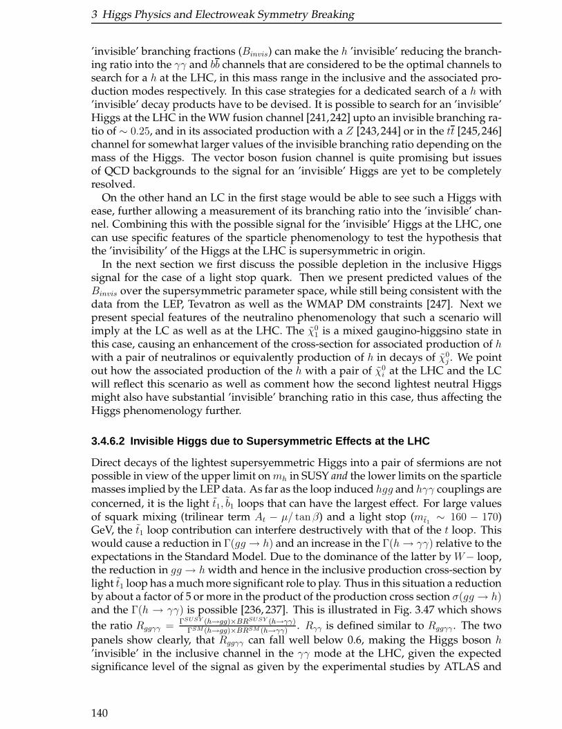
3 Higgs Physics and Electroweak Symmetry Breaking
’invisible’ branching fractions (Binvis) can make the h ’invisible’ reducing the branch-ing ratio into the γγ and bb channels that are considered to be the optimal channels tosearch for a h at the LHC, in this mass range in the inclusive and the associated pro-duction modes respectively. In this case strategies for a dedicated search of a h with’invisible’ decay products have to be devised. It is possible to search for an ’invisible’Higgs at the LHC in the WW fusion channel [241,242] upto an invisible branching ra-tio of ∼ 0.25, and in its associated production with a Z [243,244] or in the tt [245,246]channel for somewhat larger values of the invisible branching ratio depending on themass of the Higgs. The vector boson fusion channel is quite promising but issuesof QCD backgrounds to the signal for an ’invisible’ Higgs are yet to be completelyresolved.
On the other hand an LC in the first stage would be able to see such a Higgs withease, further allowing a measurement of its branching ratio into the ’invisible’ chan-nel. Combining this with the possible signal for the ’invisible’ Higgs at the LHC, onecan use specific features of the sparticle phenomenology to test the hypothesis thatthe ’invisibility’ of the Higgs at the LHC is supersymmetric in origin.
In the next section we first discuss the possible depletion in the inclusive Higgssignal for the case of a light stop quark. Then we present predicted values of theBinvis over the supersymmetric parameter space, while still being consistent with thedata from the LEP, Tevatron as well as the WMAP DM constraints [247]. Next wepresent special features of the neutralino phenomenology that such a scenario willimply at the LC as well as at the LHC. The χ0
1 is a mixed gaugino-higgsino state inthis case, causing an enhancement of the cross-section for associated production of hwith a pair of neutralinos or equivalently production of h in decays of χ0
j . We pointout how the associated production of the h with a pair of χ0
i at the LHC and the LCwill reflect this scenario as well as comment how the second lightest neutral Higgsmight also have substantial ’invisible’ branching ratio in this case, thus affecting theHiggs phenomenology further.
3.4.6.2 Invisible Higgs due to Supersymmetric Effects at th e LHC
Direct decays of the lightest supersyemmetric Higgs into a pair of sfermions are notpossible in view of the upper limit onmh in SUSY and the lower limits on the sparticlemasses implied by the LEP data. As far as the loop induced hgg and hγγ couplings are
concerned, it is the light t1, b1 loops that can have the largest effect. For large valuesof squark mixing (trilinear term At − µ/ tanβ) and a light stop (mt1 ∼ 160 − 170)GeV, the t1 loop contribution can interfere destructively with that of the t loop. Thiswould cause a reduction in Γ(gg → h) and an increase in the Γ(h→ γγ) relative to theexpectations in the Standard Model. Due to the dominance of the latter by W− loop,the reduction in gg → h width and hence in the inclusive production cross-section bylight t1 loop has a much more significant role to play. Thus in this situation a reductionby about a factor of 5 or more in the product of the production cross section σ(gg → h)and the Γ(h → γγ) is possible [236, 237]. This is illustrated in Fig. 3.47 which shows
the ratio Rggγγ = ΓSUSY (h→gg)×BRSUSY (h→γγ)ΓSM (h→gg)×BRSM (h→γγ)
. Rγγ is defined similar to Rggγγ . The two
panels show clearly, that Rggγγ can fall well below 0.6, making the Higgs boson h’invisible’ in the inclusive channel in the γγ mode at the LHC, given the expectedsignificance level of the signal as given by the experimental studies by ATLAS and
140
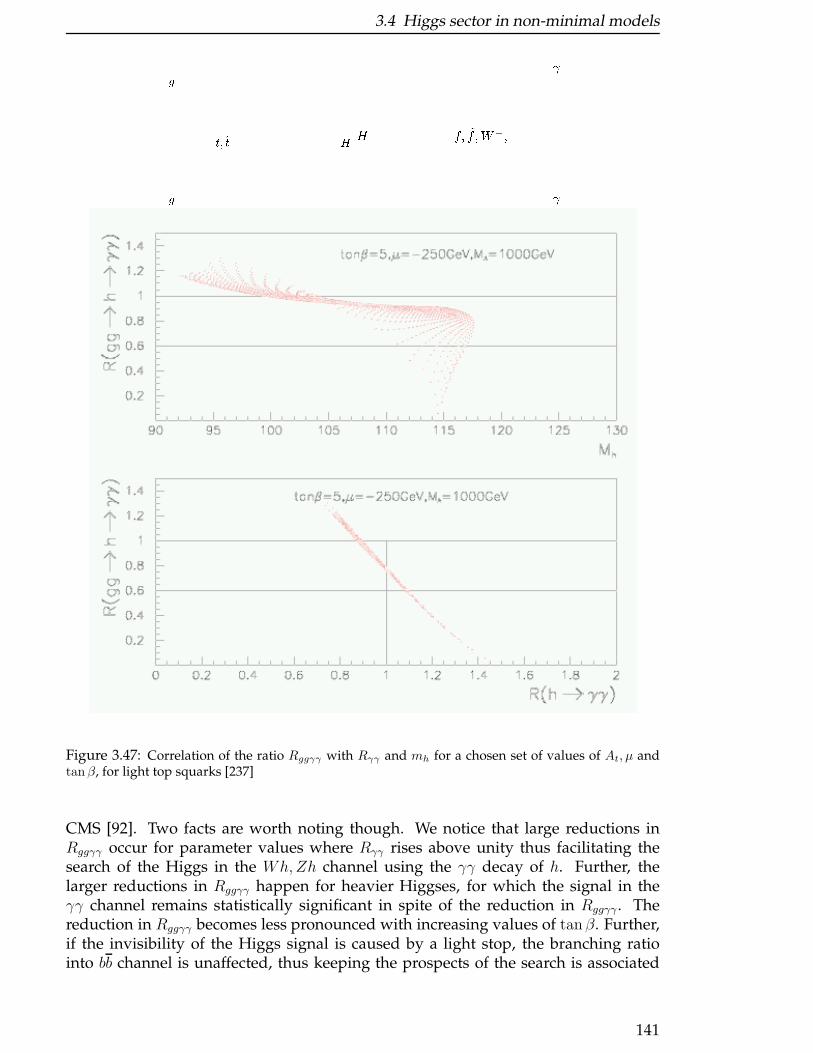
3.4 Higgs sector in non-minimal models
t; ~tgg Hf; ~f;W+;H
Figure 3.47: Correlation of the ratio Rggγγ with Rγγ and mh for a chosen set of values of At, µ andtanβ, for light top squarks [237]
CMS [92]. Two facts are worth noting though. We notice that large reductions inRggγγ occur for parameter values where Rγγ rises above unity thus facilitating thesearch of the Higgs in the Wh,Zh channel using the γγ decay of h. Further, thelarger reductions in Rggγγ happen for heavier Higgses, for which the signal in theγγ channel remains statistically significant in spite of the reduction in Rggγγ . Thereduction in Rggγγ becomes less pronounced with increasing values of tan β. Further,if the invisibility of the Higgs signal is caused by a light stop, the branching ratiointo bb channel is unaffected, thus keeping the prospects of the search is associated
141
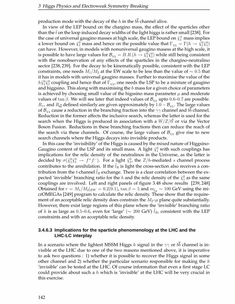
3 Higgs Physics and Electroweak Symmetry Breaking
production mode with the decay of the h in the bb channel alive.In view of the LEP bound on the chargino mass, the effect of the sparticles other
than the t on the loop induced decay widths of the light higgs is rather small [238]. Forthe case of universal gaugino masses at high scale, the LEP bound on χ±
1 mass impliesa lower bound on χ0
1 mass and hence on the possible value that Γχχ = Γ(h → χ01χ
01)
can have. However, in models with nonuniversal gaugino masess at the high scale, itis possible to have large values for Bχχ = B.R.(h→ χ0
1χ01) while still being consistent
with the nonobservation of any effects of the sparticles in the chargino-neutralinosector [238, 239]. For the decay to be kinematically possible, consistent with the LEPconstraints, one needs M1/M2 at the EW scale to be less than the value of ∼ 0.5 thatit has in models with universal gaugino masses. Further to maximise the value of thehχ0
1χ01 coupling and hence that of Γχχ, one needs the LSP to be a mixture of gaugino
and higgsino. This along with maximising the hmass for a given choice of parametersis achieved by choosing small value of the higssino mass parameter µ and moderatevalues of tan β. We will see later that indeed values of Bχχ upto 0.6–0.7 are possible.Rγγ and Rbb defined similarly are given approximately by 1.0−Bχχ. The large valuesof Bχχ cause a reduction in the branching fraction into the γγ channel and bb channel.Reduction in the former affects the inclusive search, whereas the latter is used for thesearch when the Higgs is produced in association with a W/Z/tt or via the VectorBoson Fusion. Reductions in these branching fractions then can reduce the reach ofthe search via these channels. Of course, the large values of Bχχ give rise to newsearch channels where the Higgs decays into invisible products.
In this case the ’invisibility’ of the Higgs is caused by the mixed nature of Higgsino-Gaugino content of the LSP and its small mass. A light χ0
1 with such couplings hasimplications for the relic density of the neutralinos in the Universe, as the latter isdecided by σ(χ0
1χ01 → f+f−). For a light χ0
1, the Z/h-mediated s channel process
contributes to the annihilation. If the lR is light the cross-section also receives a con-
tribution from the t-channel lR exchange. There is a clear correlation between the ex-pected ‘invisible’ branching ratio for the h and the relic density of the χ0
1 as the samecouplings are involved. Left and right panels of figure 3.48 show results [239, 248]Obtained for r = M1/M2|EW = 0.2(0.1), tanβ = 5 and mlR
∼ 100 GeV using the mi-crOMEGAs [249] program to calculate the relic density. These show that the require-ment of an acceptable relic density does constrain the M2–µ plane quite substantially.However, there exist large regions of this plane where the ‘invisible’ branching ratio
of h is as large as 0.5–0.6, even for ‘large’ (∼ 200 GeV) lR, consistent with the LEPconstraints and with an acceptable relic density.
3.4.6.3 Implications for the sparticle phenomenology at th e LHC and theLHC-LC interplay
In a scenario where the lightest MSSM Higgs h signal in the γγ or bb channel is in-visible at the LHC due to one of the two reasons mentioned above, it is imperativeto ask two questions : 1) whether it is possible to recover the Higgs signal in someother channel and 2) whether the particular scenario responsible for making the h’invisible’ can be tested at the LHC. Of course information that even a first stage LCcould provide about such a h which is ’invisible’ at the LHC will be very crucial inthis exercise.
142
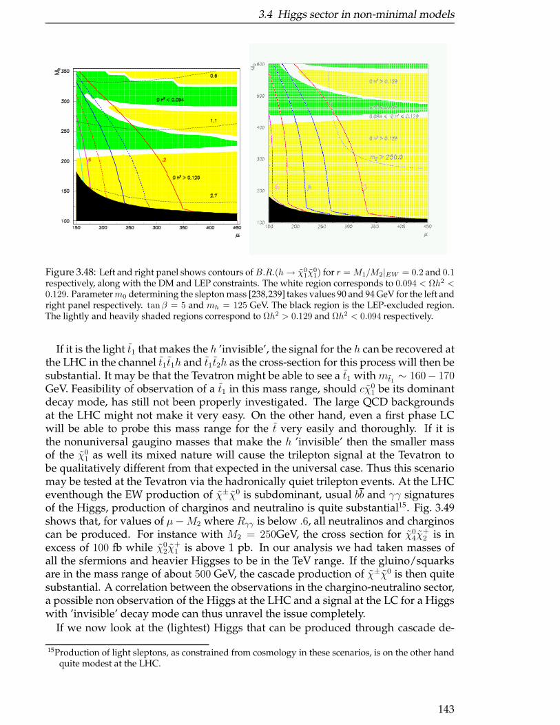
3.4 Higgs sector in non-minimal models
Figure 3.48: Left and right panel shows contours ofB.R.(h→ χ01χ
01) for r = M1/M2|EW = 0.2 and 0.1
respectively, along with the DM and LEP constraints. The white region corresponds to 0.094 < Ωh2 <0.129. Parameterm0 determining the slepton mass [238,239] takes values 90 and 94 GeV for the left andright panel respectively. tanβ = 5 and mh = 125 GeV. The black region is the LEP-excluded region.The lightly and heavily shaded regions correspond to Ωh2 > 0.129 and Ωh2 < 0.094 respectively.
If it is the light t1 that makes the h ’invisible’, the signal for the h can be recovered atthe LHC in the channel t1t1h and t1t2h as the cross-section for this process will then besubstantial. It may be that the Tevatron might be able to see a t1 with mt1 ∼ 160− 170GeV. Feasibility of observation of a t1 in this mass range, should cχ0
1 be its dominantdecay mode, has still not been properly investigated. The large QCD backgroundsat the LHC might not make it very easy. On the other hand, even a first phase LCwill be able to probe this mass range for the t very easily and thoroughly. If it isthe nonuniversal gaugino masses that make the h ’invisible’ then the smaller massof the χ0
1 as well its mixed nature will cause the trilepton signal at the Tevatron tobe qualitatively different from that expected in the universal case. Thus this scenariomay be tested at the Tevatron via the hadronically quiet trilepton events. At the LHCeventhough the EW production of χ±χ0 is subdominant, usual bb and γγ signaturesof the Higgs, production of charginos and neutralino is quite substantial15. Fig. 3.49shows that, for values of µ−M2 where Rγγ is below .6, all neutralinos and charginoscan be produced. For instance with M2 = 250GeV, the cross section for χ0
4χ+2 is in
excess of 100 fb while χ02χ
+1 is above 1 pb. In our analysis we had taken masses of
all the sfermions and heavier Higgses to be in the TeV range. If the gluino/squarksare in the mass range of about 500 GeV, the cascade production of χ±χ0 is then quitesubstantial. A correlation between the observations in the chargino-neutralino sector,a possible non observation of the Higgs at the LHC and a signal at the LC for a Higgswith ’invisible’ decay mode can thus unravel the issue completely.
If we now look at the (lightest) Higgs that can be produced through cascade de-
15Production of light sleptons, as constrained from cosmology in these scenarios, is on the other handquite modest at the LHC.
143

3 Higgs Physics and Electroweak Symmetry Breaking
Figure 3.49: Associated Production of chargino and neutralino at the LHC at LO for M2 = M1/10 a)
as a function of µ for M2 = 250GeV. b) as a function of M2 for µ = 150GeV .
cays in these processes, one sees from Fig. 3.50 that, through essentially χ03 decays,
associated Higgs cross sections of about 30fb are possible. Nonetheless, again, it is inthese regions with highest yield that the Higgs has a large branching ratio into invis-ible and would be difficult to track. The h search in neutralino decays at the LHC, inthis scenario is being investigated and should certainly provide clean examples of thepossible LHC-LC interplay.
The implications of this scenario for the SUSY phenomenology at LC have beenrecently investigated [250]. It has been shown there that, for the region of small val-ues of µ where the Higgs can become ’invisible’ for nonuniversal gaugino masses,for the range of nonuniversality parameter 0.03 – 0.5 (the universal case) and tan βvalues from 10–50, the production cross-section will be at an observable level (> 1fbat a 500 GeV LC) for at least one of the sparticle pairs from among χ+χ−, χ0
1χ03, χ
01χ
02.
For smaller values of m0, even the slepton signal will be large and observable. In thiscase even the χ+
1 χ−1 γ production cross-section will be appeciable. Thus not only can
an LC see an ’invisible’ Higgs easily, but it should be able to see the sparticles, thustesting whether SUSY is responsible for the nonobservation of the light Higgs at theLHC. Further, measurements of the invisible decay width at the LC, can provide use-ful pointers for the sfermion and neutralino/chargino phenomenology at the LHC.Implications for this scenario for lower masses of the Pseudoscalar Higgs have yet tobe investigated fully.
3.5 A light Higgs in scenarios with extra dimensions
In this section we discuss the detectability of a light Higgs at the LHC, and the cor-responding complementarity of a LC, for scenarios beyond the SM based on extradimensions. Models with 3-branes in extra dimensions typically imply the existenceof a radion, φ, that can mix with the Higgs, h, thereby modifying the Higgs propertiesand the prospects for its detectability at the LHC. The presence of the φ will affect the
144
3.5 A light Higgs in scenarios with extra dimensions
Figure 3.50: Higgs yield through charginos and neutralinos decays as a function of µ, M2 = 250GeV,
tanβ = 5, maximal mixing and M1 = M2/10. The subscript for the parentheses ( )j indicates the
parent neutralino or chargino.
scope of the LHC searches. Detection of both the φ and the h might be possible. Wereport on a study on the complementarity of the observation of gg → h, with h→ γγor h → Z0Z0∗ → 4 ℓ, and gg → φ → Z0Z0(∗) → 4 ℓ at the LHC in the context of theRandall-Sundrum model. The potential for determining the nature of the detectedscalar(s) at the LHC and at an e+e− linear collider is discussed, both separately andin combination. Also the virtues of measurements from a low energy photon colliderare discussed.
3.5.1 On the complementarity of Higgs and radion searches atLHC and LC
M.Battaglia, S. De Curtis, A. De Roeck, D. Dominici, J.F. Gunion
3.5.1.1 Introduction
One particularly attractive extra-dimensional model is that proposed by Randall andSundrum (RS) [251], in which there are two 3+1 dimensional branes separated in a 5thdimension. A central prediction of this theory is the existence of the radion, a gravis-calar which corresponds to fluctuations in the size of the extra dimension. Detectionand study of the radion will be central to the experimental probe of the RS and re-lated scenarios with extra dimensions. There is already an extensive literature on thephenomenology of the radion, both in the absence of Higgs-radion mixing [252–256]and in the presence of such a mixing [257–263].
In this section we discuss the complementarity of the search for the Higgs bosonand the radion at the LHC. As the Higgs-radion mixing may suppress the main dis-
145
3 Higgs Physics and Electroweak Symmetry Breaking
covery process gg → H → γγ for a light Higgs boson, we study the extent to whichthe appearance of a gg → φ → Z0Z0(∗) → 4 ℓ signal ensures that LHC experimentswill observe at least one of the two scalars over the full parameter phase space. Theadditional information, which could be extracted from a TeV-class e+e− linear collider(LC), is also considered. More details on the theoretical framework are given in [264]
3.5.1.2 Radion and Higgs Boson Search Complementarity
Here we address two issues. The first is whether there is a complementarity betweenthe Higgs observability, mostly through gg → h → γγ, and the gg → φ → Z0Z0(∗) →4 ℓ reaction, thus offering the LHC the discovery of at least one of the two particlesover the full parameter space. The second, and related, issue,discussed in the nextsection, concerns the strategies available to understand the nature of the discoveredparticle.
The couplings of the h and φ to Z0Z0, W+W− and ff are given relative to those ofthe SM Higgs boson, denoted by H , by:
ghWW
gHWW=ghZZgHZZ
=ghffgHff
= d+ γb ,gφWW
gHWW=gφZZgHZZ
=gφffgHff
= c+ γa . (3.46)
with γ ≡ v/Λφ and a, b, c, d, are functions of the mixing angle defined e.g. in [264].Couplings of the h and φ to γγ and gg receive contributions not only from the usualloop diagrams but also from trace-anomaly couplings to γγ and gg. Thus, these cou-plings are not simply directly proportional to those of the SM H . Of course, in thelimit of ξ = 0, the h has the same properties as the SM Higgs boson.
The effects of the mixing of the radion with the Higgs boson have been studied [263]by introducing the relevant terms in the HDECAY program [265], which computes theHiggs couplings, including higher order QCD corrections. Couplings and widths forthe radion have also been implemented.
Results have been obtained by comparing the product of production and decayrates for the h and φ to those expected for a light SM H . The LHC sensitivity has beenextracted by rescaling the results for Higgs observability, obtained assuming SM cou-plings. We define Higgs observability as a > 5 σ excess over the SM backgroundfor the combination of the inclusive channels: gg → h → γγ; tth, with h → bb andgg → h→ Z0Z0(∗) → 4ℓ, after rescaling the SM Higgs results. We define φ observabil-ity as a > 5 σ signal in the gg → φ→ Z0Z0(∗) → 4ℓ channel only. We study the resultsas a function of four parameters: the Higgs mass Mh, the radion mass Mφ, the scaleΛφ and the mixing parameter ξ.
Due to the suppression, from radion mixing, of the loop-induced effective cou-plings of the h (relative to the SM H) to gluon and photon pairs, the key processgg → h → γγ may fail to provide a significant excess over the γγ background at theLHC. Other modes that depend on the gg fusion production process are suppressedtoo. For Mφ > Mh, this suppression is very substantial for large, negative values of ξ.This region of significant suppression becomes wider at large values of Mφ and Λφ. Incontrast, forMφ < Mh, the gg → h→ γγ rate is generally only suppressed when ξ > 0.All this is shown, in a quantitative way, by the contours in Figures 3.51, 3.52 and 3.53.In all these figures, the outermost, hourglass shaped contours define the theoreticallyallowed region. As shown in Figure 3.51, three main regions of non-detectability may
146
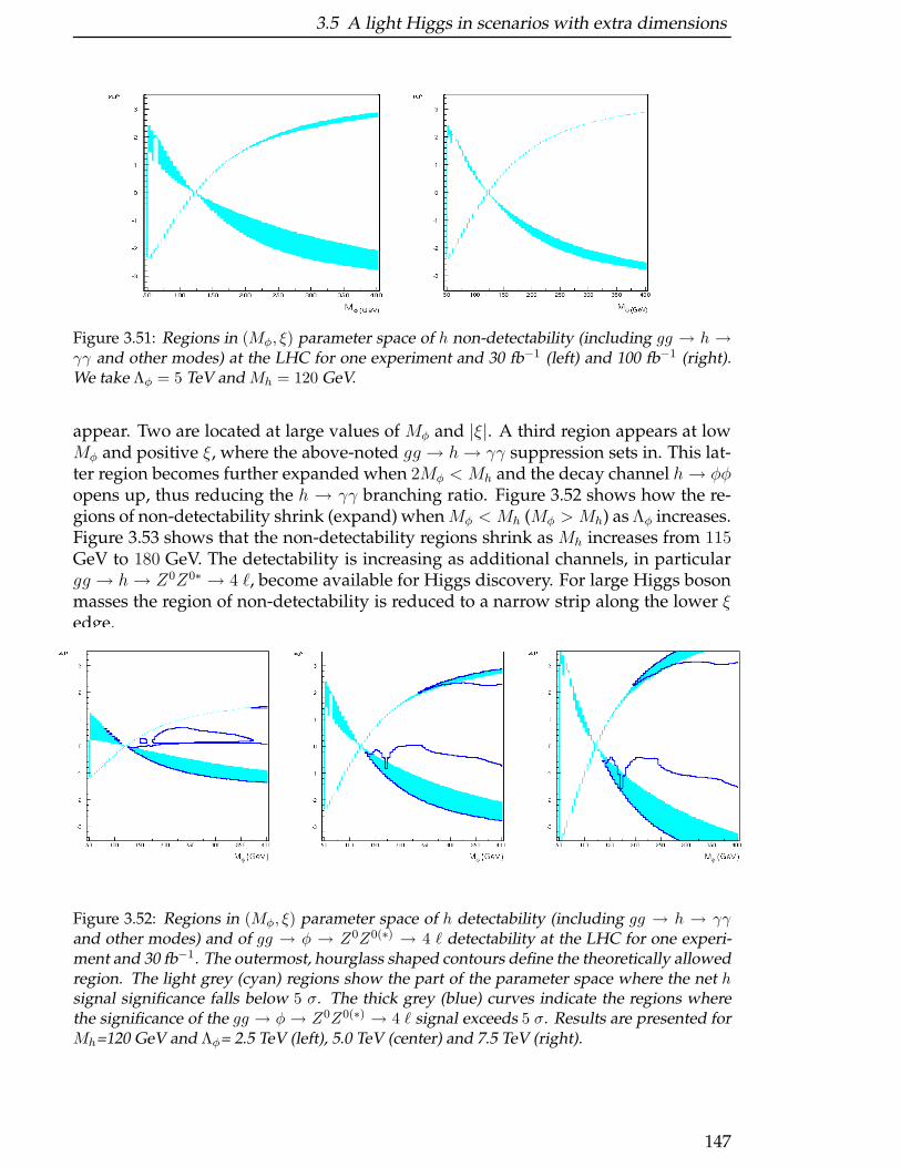
3.5 A light Higgs in scenarios with extra dimensions
Figure 3.51: Regions in (Mφ, ξ) parameter space of h non-detectability (including gg → h →γγ and other modes) at the LHC for one experiment and 30 fb−1 (left) and 100 fb−1 (right).We take Λφ = 5 TeV and Mh = 120 GeV.
appear. Two are located at large values of Mφ and |ξ|. A third region appears at lowMφ and positive ξ, where the above-noted gg → h→ γγ suppression sets in. This lat-ter region becomes further expanded when 2Mφ < Mh and the decay channel h→ φφopens up, thus reducing the h → γγ branching ratio. Figure 3.52 shows how the re-gions of non-detectability shrink (expand) whenMφ < Mh (Mφ > Mh) as Λφ increases.Figure 3.53 shows that the non-detectability regions shrink as Mh increases from 115GeV to 180 GeV. The detectability is increasing as additional channels, in particulargg → h→ Z0Z0∗ → 4 ℓ, become available for Higgs discovery. For large Higgs bosonmasses the region of non-detectability is reduced to a narrow strip along the lower ξedge.
Figure 3.52: Regions in (Mφ, ξ) parameter space of h detectability (including gg → h → γγand other modes) and of gg → φ → Z0Z0(∗) → 4 ℓ detectability at the LHC for one experi-ment and 30 fb−1. The outermost, hourglass shaped contours define the theoretically allowedregion. The light grey (cyan) regions show the part of the parameter space where the net hsignal significance falls below 5 σ. The thick grey (blue) curves indicate the regions wherethe significance of the gg → φ → Z0Z0(∗) → 4 ℓ signal exceeds 5 σ. Results are presented forMh=120 GeV and Λφ= 2.5 TeV (left), 5.0 TeV (center) and 7.5 TeV (right).
147
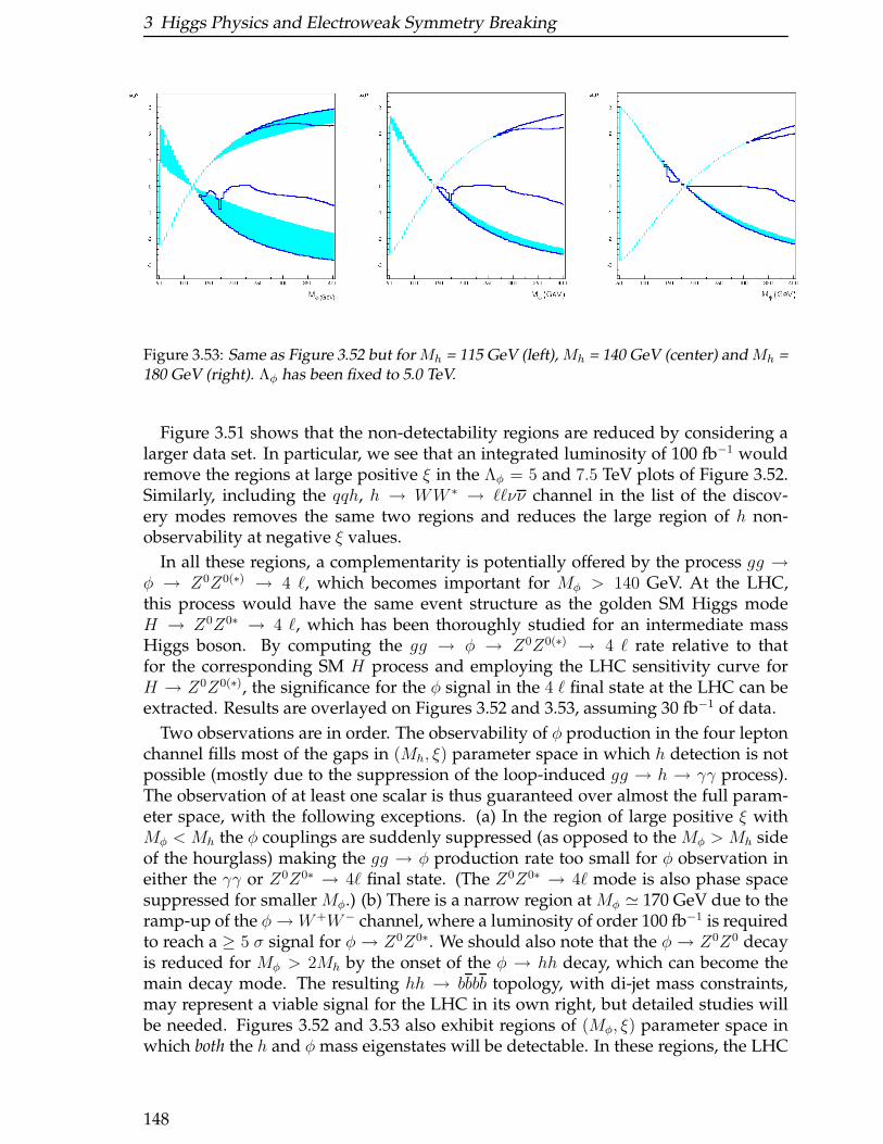
3 Higgs Physics and Electroweak Symmetry Breaking
Figure 3.53: Same as Figure 3.52 but for Mh = 115 GeV (left), Mh = 140 GeV (center) and Mh =180 GeV (right). Λφ has been fixed to 5.0 TeV.
Figure 3.51 shows that the non-detectability regions are reduced by considering alarger data set. In particular, we see that an integrated luminosity of 100 fb−1 wouldremove the regions at large positive ξ in the Λφ = 5 and 7.5 TeV plots of Figure 3.52.Similarly, including the qqh, h → WW ∗ → ℓℓνν channel in the list of the discov-ery modes removes the same two regions and reduces the large region of h non-observability at negative ξ values.
In all these regions, a complementarity is potentially offered by the process gg →φ → Z0Z0(∗) → 4 ℓ, which becomes important for Mφ > 140 GeV. At the LHC,this process would have the same event structure as the golden SM Higgs modeH → Z0Z0∗ → 4 ℓ, which has been thoroughly studied for an intermediate massHiggs boson. By computing the gg → φ → Z0Z0(∗) → 4 ℓ rate relative to thatfor the corresponding SM H process and employing the LHC sensitivity curve forH → Z0Z0(∗), the significance for the φ signal in the 4 ℓ final state at the LHC can beextracted. Results are overlayed on Figures 3.52 and 3.53, assuming 30 fb−1 of data.
Two observations are in order. The observability of φ production in the four leptonchannel fills most of the gaps in (Mh, ξ) parameter space in which h detection is notpossible (mostly due to the suppression of the loop-induced gg → h → γγ process).The observation of at least one scalar is thus guaranteed over almost the full param-eter space, with the following exceptions. (a) In the region of large positive ξ withMφ < Mh the φ couplings are suddenly suppressed (as opposed to the Mφ > Mh sideof the hourglass) making the gg → φ production rate too small for φ observation ineither the γγ or Z0Z0∗ → 4ℓ final state. (The Z0Z0∗ → 4ℓ mode is also phase spacesuppressed for smaller Mφ.) (b) There is a narrow region at Mφ ≃ 170 GeV due to theramp-up of the φ→W+W− channel, where a luminosity of order 100 fb−1 is requiredto reach a ≥ 5 σ signal for φ → Z0Z0∗. We should also note that the φ → Z0Z0 decayis reduced for Mφ > 2Mh by the onset of the φ → hh decay, which can become themain decay mode. The resulting hh → bbbb topology, with di-jet mass constraints,may represent a viable signal for the LHC in its own right, but detailed studies willbe needed. Figures 3.52 and 3.53 also exhibit regions of (Mφ, ξ) parameter space inwhich both the h and φ mass eigenstates will be detectable. In these regions, the LHC
148
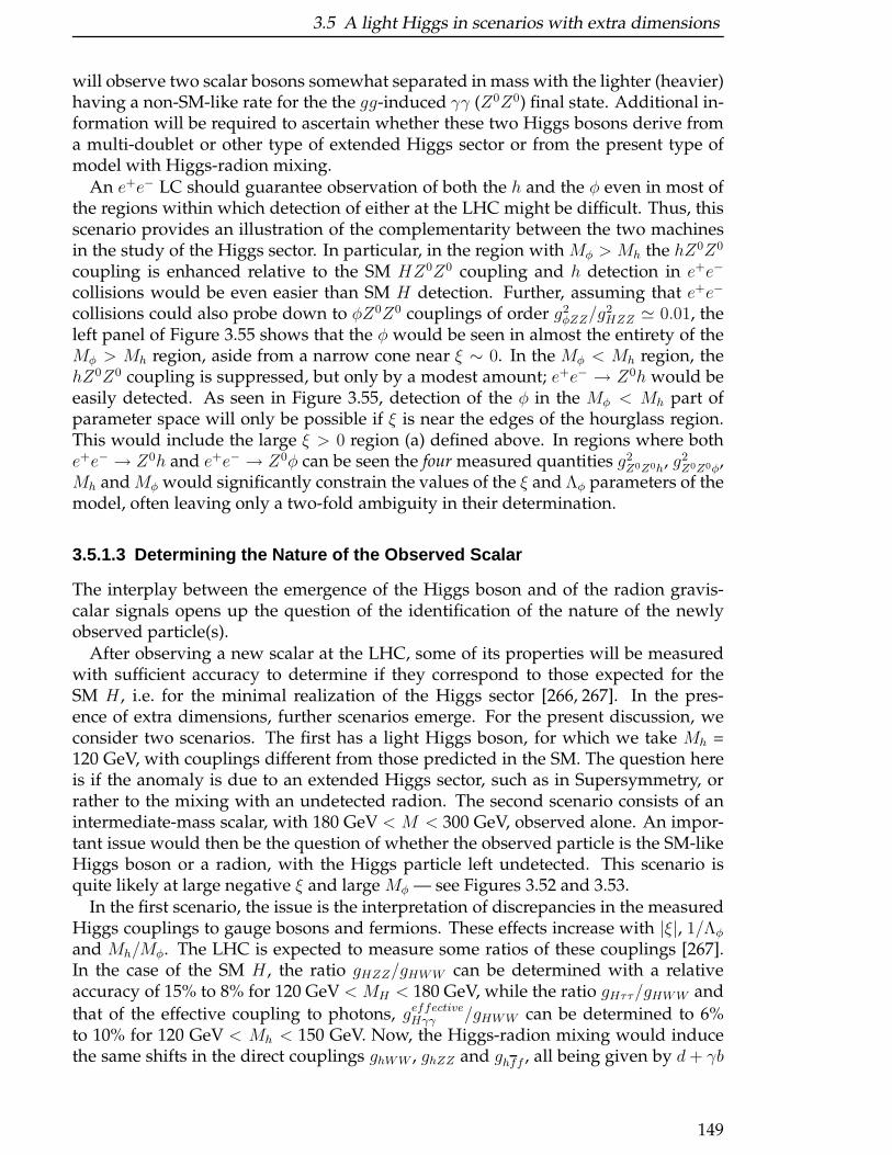
3.5 A light Higgs in scenarios with extra dimensions
will observe two scalar bosons somewhat separated in mass with the lighter (heavier)having a non-SM-like rate for the the gg-induced γγ (Z0Z0) final state. Additional in-formation will be required to ascertain whether these two Higgs bosons derive froma multi-doublet or other type of extended Higgs sector or from the present type ofmodel with Higgs-radion mixing.
An e+e− LC should guarantee observation of both the h and the φ even in most ofthe regions within which detection of either at the LHC might be difficult. Thus, thisscenario provides an illustration of the complementarity between the two machinesin the study of the Higgs sector. In particular, in the region with Mφ > Mh the hZ0Z0
coupling is enhanced relative to the SM HZ0Z0 coupling and h detection in e+e−
collisions would be even easier than SM H detection. Further, assuming that e+e−
collisions could also probe down to φZ0Z0 couplings of order g2φZZ/g
2HZZ ≃ 0.01, the
left panel of Figure 3.55 shows that the φ would be seen in almost the entirety of theMφ > Mh region, aside from a narrow cone near ξ ∼ 0. In the Mφ < Mh region, thehZ0Z0 coupling is suppressed, but only by a modest amount; e+e− → Z0h would beeasily detected. As seen in Figure 3.55, detection of the φ in the Mφ < Mh part ofparameter space will only be possible if ξ is near the edges of the hourglass region.This would include the large ξ > 0 region (a) defined above. In regions where bothe+e− → Z0h and e+e− → Z0φ can be seen the four measured quantities g2
Z0Z0h, g2Z0Z0φ,
Mh and Mφ would significantly constrain the values of the ξ and Λφ parameters of themodel, often leaving only a two-fold ambiguity in their determination.
3.5.1.3 Determining the Nature of the Observed Scalar
The interplay between the emergence of the Higgs boson and of the radion gravis-calar signals opens up the question of the identification of the nature of the newlyobserved particle(s).
After observing a new scalar at the LHC, some of its properties will be measuredwith sufficient accuracy to determine if they correspond to those expected for theSM H , i.e. for the minimal realization of the Higgs sector [266, 267]. In the pres-ence of extra dimensions, further scenarios emerge. For the present discussion, weconsider two scenarios. The first has a light Higgs boson, for which we take Mh =120 GeV, with couplings different from those predicted in the SM. The question hereis if the anomaly is due to an extended Higgs sector, such as in Supersymmetry, orrather to the mixing with an undetected radion. The second scenario consists of anintermediate-mass scalar, with 180 GeV < M < 300 GeV, observed alone. An impor-tant issue would then be the question of whether the observed particle is the SM-likeHiggs boson or a radion, with the Higgs particle left undetected. This scenario isquite likely at large negative ξ and large Mφ — see Figures 3.52 and 3.53.
In the first scenario, the issue is the interpretation of discrepancies in the measuredHiggs couplings to gauge bosons and fermions. These effects increase with |ξ|, 1/Λφ
and Mh/Mφ. The LHC is expected to measure some ratios of these couplings [267].In the case of the SM H , the ratio gHZZ/gHWW can be determined with a relativeaccuracy of 15% to 8% for 120 GeV < MH < 180 GeV, while the ratio gHττ/gHWW and
that of the effective coupling to photons, geffectiveHγγ /gHWW can be determined to 6%to 10% for 120 GeV < Mh < 150 GeV. Now, the Higgs-radion mixing would inducethe same shifts in the direct couplings ghWW , ghZZ and ghff , all being given by d+ γb
149
3 Higgs Physics and Electroweak Symmetry Breaking
times the corresponding H couplings — see Eq. (3.46). Although this factor dependson the Λφ, Mφ and ξ parameters, ratios of couplings would remain unperturbed andcorrespond to those expected in the SM. Since the LHC measures mostly ratios ofcouplings, the presence of Higgs-radion mixing could easily be missed. One window
of sensitivity to the mixing would be offered by the combination geffectivehγγ /ghWW . Butthe mixing effects are expected to be limited to relative variation of ±5% w.r.t. theSM predictions. Hence, the LHC anticipated accuracy corresponds to deviations ofone unit of σ, or less, except for a small region at Λφ ≃ 1 TeV. Larger deviations areexpected for the absolute rates [263], especially for the gg → h → γγ channel whichcan be dramatically enhanced or suppressed relative to the gg → H → γγ predictionfor larger ξ values due to the large changes in the gg → h coupling relative to thegg → H coupling. Of course, to detect these deviations it is necessary to controlsystematic uncertainties for the absolute γγ rate. All the above remarks would alsoapply to distinguishing between the light Higgs of supersymmetry, which would beSM-like assuming an approximate decoupling limit, and the h of the Higgs-radionscenario. In a non-decoupling two-doublet model, the light Higgs couplings to up-type and down-type fermions can be modified differently with respect to those of theSM H , and LHC measurements of coupling ratios would detect this difference.
A TeV-class LC has the capability of measuring the absolute coupling strengths to allfermions separately. For the SM H , accuracies of order 1%-5% for the couplings areachieved. Further, a determination of the total H width to 4% - 6% accuracy is pos-sible. These capabilities are important for the scenario we propose since there wouldbe enough measurements and sufficient accuracy to detect Higgs-radion mixing formoderate to large ξ values [268]. This is shown in Figure 3.54 by the additional con-tours, which indicate the regions where the discrepancy with the SM predictions forthe Higgs couplings to pairs of b quarks and W bosons exceeds 2.5 σ.
It is worth emphasizing that one of the basic predictions of the model is that theW+W−, Z0Z0 and ff couplings of the h should all be changed by exactly the samefactor. The above discussion shows that it will be possible to check this at a basic levelat the LHC (in that ratios of branching ratios should be the same as in the SM) andwith some precision at the LC.
We note that the combination of the direct observation of φ → Z0Z0∗ at the LHCand the precision measurements of the Higgs properties at a e+e− LC will extendour ability to distinguish between the Higgs-radion mixing scenario and the SM Hscenario to a large portion of the regions where at the LHC only the h or only the φ isdetected and determining that the observed boson is not the SMH is difficult. Finally,we reemphasize the fact that h will be detected in e+e− → Z0h throughout the entire(Mφ, ξ) parameter space and that e+e− → Z0φ can be detected in all but the regionexemplified, for Mh = 120 GeV and Λφ = 5 TeV, in the left panel of Figure 3.55. This,in particular, guarantees the observability of the φ in the low Mφ, large ξ > 0 regionthat is most difficult for the LHC.
If, at the LHC, an intermediate mass scalar is observed alone, its non-SM-like na-ture can, in some cases, be determined through measurement of its production yieldand its couplings. In particular, in the region at large, negative ξ values where φproduction is visible whereas h production is not, the yield of Z0Z0 → 4 ℓ from φdecay can differ by a factor of 2 or more from that expected for a SM H (dependingupon the value of Mφ — see Figure 13 of Ref. [263]). For Mφ < 2 Mh the devia-
150
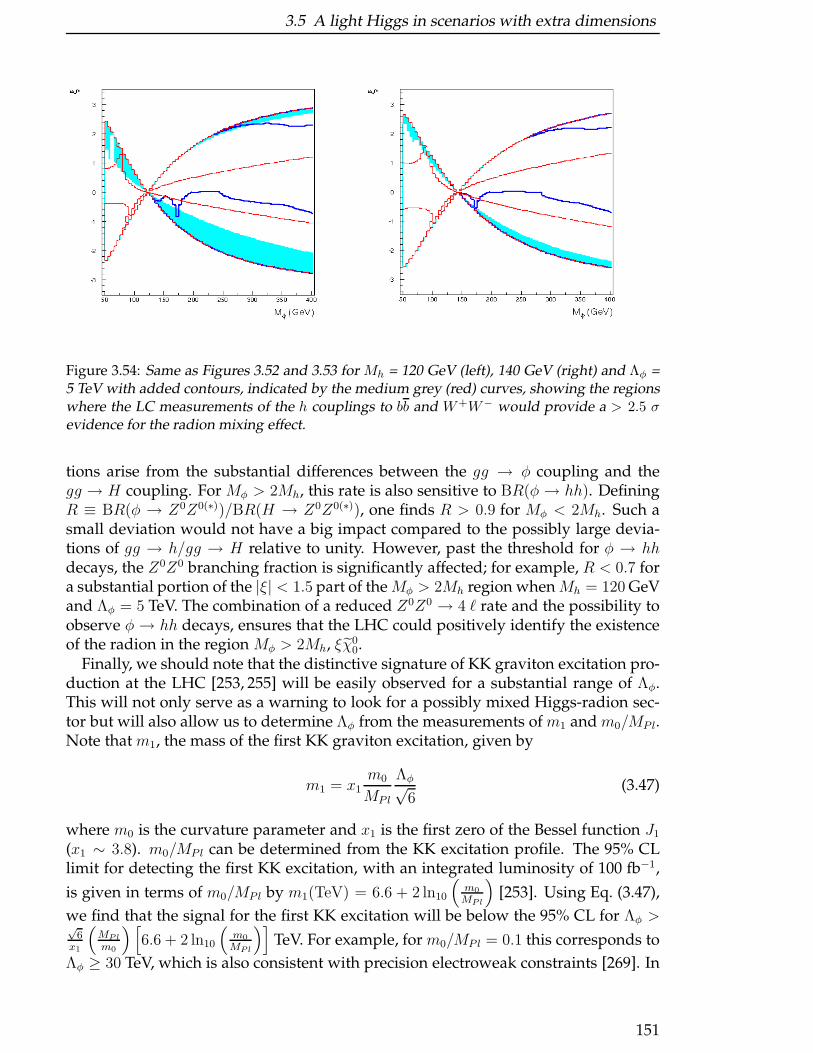
3.5 A light Higgs in scenarios with extra dimensions
Figure 3.54: Same as Figures 3.52 and 3.53 for Mh = 120 GeV (left), 140 GeV (right) and Λφ =5 TeV with added contours, indicated by the medium grey (red) curves, showing the regionswhere the LC measurements of the h couplings to bb and W+W− would provide a > 2.5 σevidence for the radion mixing effect.
tions arise from the substantial differences between the gg → φ coupling and thegg → H coupling. For Mφ > 2Mh, this rate is also sensitive to BR(φ → hh). DefiningR ≡ BR(φ → Z0Z0(∗))/BR(H → Z0Z0(∗)), one finds R > 0.9 for Mφ < 2Mh. Such asmall deviation would not have a big impact compared to the possibly large devia-tions of gg → h/gg → H relative to unity. However, past the threshold for φ → hhdecays, the Z0Z0 branching fraction is significantly affected; for example, R < 0.7 fora substantial portion of the |ξ| < 1.5 part of theMφ > 2Mh region whenMh = 120 GeVand Λφ = 5 TeV. The combination of a reduced Z0Z0 → 4 ℓ rate and the possibility toobserve φ → hh decays, ensures that the LHC could positively identify the existenceof the radion in the region Mφ > 2Mh, ξχ0
0.Finally, we should note that the distinctive signature of KK graviton excitation pro-
duction at the LHC [253, 255] will be easily observed for a substantial range of Λφ.This will not only serve as a warning to look for a possibly mixed Higgs-radion sec-tor but will also allow us to determine Λφ from the measurements of m1 and m0/MP l.Note that m1, the mass of the first KK graviton excitation, given by
m1 = x1m0
MP l
Λφ√6
(3.47)
where m0 is the curvature parameter and x1 is the first zero of the Bessel function J1
(x1 ∼ 3.8). m0/MP l can be determined from the KK excitation profile. The 95% CLlimit for detecting the first KK excitation, with an integrated luminosity of 100 fb−1,
is given in terms of m0/MP l by m1(TeV) = 6.6 + 2 ln10
(m0
MPl
)[253]. Using Eq. (3.47),
we find that the signal for the first KK excitation will be below the 95% CL for Λφ >√6
x1
(MPl
m0
) [6.6 + 2 ln10
(m0
MPl
)]TeV. For example, for m0/MP l = 0.1 this corresponds to
Λφ ≥ 30 TeV, which is also consistent with precision electroweak constraints [269]. In
151
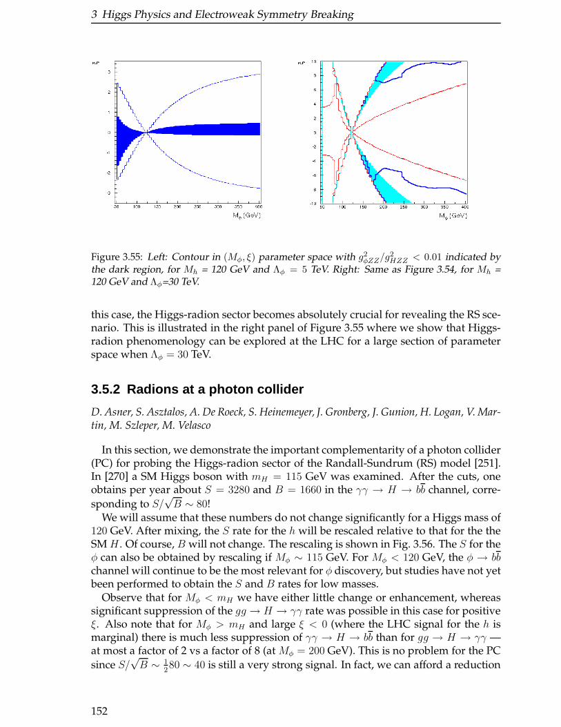
3 Higgs Physics and Electroweak Symmetry Breaking
Figure 3.55: Left: Contour in (Mφ, ξ) parameter space with g2φZZ/g
2HZZ < 0.01 indicated by
the dark region, for Mh = 120 GeV and Λφ = 5 TeV. Right: Same as Figure 3.54, for Mh =120 GeV and Λφ=30 TeV.
this case, the Higgs-radion sector becomes absolutely crucial for revealing the RS sce-nario. This is illustrated in the right panel of Figure 3.55 where we show that Higgs-radion phenomenology can be explored at the LHC for a large section of parameterspace when Λφ = 30 TeV.
3.5.2 Radions at a photon collider
D. Asner, S. Asztalos, A. De Roeck, S. Heinemeyer, J. Gronberg, J. Gunion, H. Logan, V. Mar-tin, M. Szleper, M. Velasco
In this section, we demonstrate the important complementarity of a photon collider(PC) for probing the Higgs-radion sector of the Randall-Sundrum (RS) model [251].In [270] a SM Higgs boson with mH = 115 GeV was examined. After the cuts, oneobtains per year about S = 3280 and B = 1660 in the γγ → H → bb channel, corre-
sponding to S/√B ∼ 80!
We will assume that these numbers do not change significantly for a Higgs mass of120 GeV. After mixing, the S rate for the h will be rescaled relative to that for the theSM H . Of course, B will not change. The rescaling is shown in Fig. 3.56. The S for theφ can also be obtained by rescaling if Mφ ∼ 115 GeV. For Mφ < 120 GeV, the φ → bbchannel will continue to be the most relevant for φ discovery, but studies have not yetbeen performed to obtain the S and B rates for low masses.
Observe that for Mφ < mH we have either little change or enhancement, whereassignificant suppression of the gg → H → γγ rate was possible in this case for positiveξ. Also note that for Mφ > mH and large ξ < 0 (where the LHC signal for the h ismarginal) there is much less suppression of γγ → H → bb than for gg → H → γγ —at most a factor of 2 vs a factor of 8 (at Mφ = 200 GeV). This is no problem for the PC
since S/√B ∼ 1
280 ∼ 40 is still a very strong signal. In fact, we can afford a reduction
152
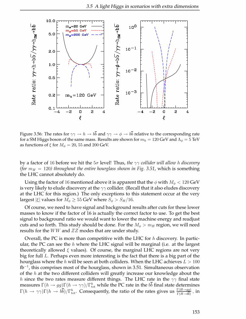
3.5 A light Higgs in scenarios with extra dimensions
Figure 3.56: The rates for γγ → h → bb and γγ → φ → bb relative to the corresponding ratefor a SM Higgs boson of the same mass. Results are shown formh = 120 GeV and Λφ = 5 TeVas functions of ξ for Mφ = 20, 55 and 200 GeV.
by a factor of 16 before we hit the 5σ level! Thus, the γγ collider will allow h discovery(for mH = 120) throughout the entire hourglass shown in Fig. 3.51, which is somethingthe LHC cannot absolutely do.
Using the factor of 16 mentioned above it is apparent that the φwith Mφ < 120 GeVis very likely to elude discovery at the γγ collider. (Recall that it also eludes discoveryat the LHC for this region.) The only exceptions to this statement occur at the verylargest |ξ| values for Mφ ≥ 55 GeV where Sφ > SH/16.
Of course, we need to have signal and background results after cuts for these lowermasses to know if the factor of 16 is actually the correct factor to use. To get the bestsignal to background ratio we would want to lower the machine energy and readjustcuts and so forth. This study should be done. For the Mφ > mH region, we will needresults for the WW and ZZ modes that are under study.
Overall, the PC is more than competitive with the LHC for h discovery. In partic-ular, the PC can see the h where the LHC signal will be marginal (i.e. at the largesttheoretically allowed ξ values). Of course, the marginal LHC regions are not verybig for full L. Perhaps even more interesting is the fact that there is a big part of thehourglass where the h will be seen at both colliders. When the LHC achieves L > 100fb−1, this comprises most of the hourglass, shown in 3.51. Simultaneous observationof the h at the two different colliders will greatly increase our knowledge about theh since the two rates measure different things. The LHC rate in the γγ final statemeasures Γ(h → gg)Γ(h→ γγ)/Γhtot while the PC rate in the bb final state determines
Γ(h → γγ)Γ(h → bb)/Γhtot. Consequently, the ratio of the rates gives us Γ(H→gg)
Γ(H→bb), in
153
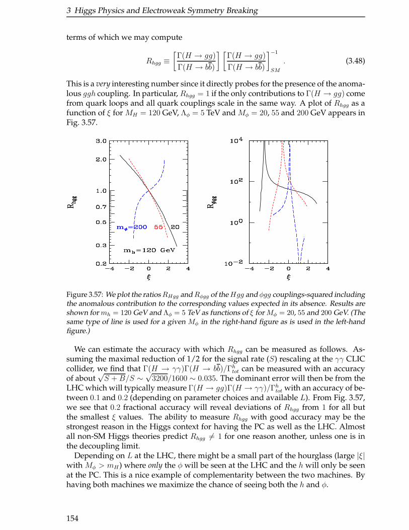
3 Higgs Physics and Electroweak Symmetry Breaking
terms of which we may compute
Rhgg ≡[Γ(H → gg)
Γ(H → bb)
] [Γ(H → gg)
Γ(H → bb)
]−1
SM
. (3.48)
This is a very interesting number since it directly probes for the presence of the anoma-lous ggh coupling. In particular, Rhgg = 1 if the only contributions to Γ(H → gg) comefrom quark loops and all quark couplings scale in the same way. A plot of Rhgg as afunction of ξ for MH = 120 GeV, Λφ = 5 TeV and Mφ = 20, 55 and 200 GeV appears inFig. 3.57.
Figure 3.57: We plot the ratiosRHgg andRφgg of theHgg and φgg couplings-squared includingthe anomalous contribution to the corresponding values expected in its absence. Results areshown for mh = 120 GeV and Λφ = 5 TeV as functions of ξ for Mφ = 20, 55 and 200 GeV. (Thesame type of line is used for a given Mφ in the right-hand figure as is used in the left-handfigure.)
We can estimate the accuracy with which Rhgg can be measured as follows. As-suming the maximal reduction of 1/2 for the signal rate (S) rescaling at the γγ CLICcollider, we find that Γ(H → γγ)Γ(H → bb)/Γhtot can be measured with an accuracyof about
√S +B/S ∼
√3200/1600 ∼ 0.035. The dominant error will then be from the
LHC which will typically measure Γ(H → gg)Γ(H → γγ)/Γhtot with an accuracy of be-tween 0.1 and 0.2 (depending on parameter choices and available L). From Fig. 3.57,we see that 0.2 fractional accuracy will reveal deviations of Rhgg from 1 for all butthe smallest ξ values. The ability to measure Rhgg with good accuracy may be thestrongest reason in the Higgs context for having the PC as well as the LHC. Almostall non-SM Higgs theories predict Rhgg 6= 1 for one reason another, unless one is inthe decoupling limit.
Depending on L at the LHC, there might be a small part of the hourglass (large |ξ|with Mφ > mH ) where only the φ will be seen at the LHC and the h will only be seenat the PC. This is a nice example of complementarity between the two machines. Byhaving both machines we maximize the chance of seeing both the h and φ.
154
3.5 A light Higgs in scenarios with extra dimensions
As regards the φ, we have already noted from Fig. 3.56 that the bb final state rate(relevant for the Mφ = 20 and 55 GeV cases) will only be detectable in the lattercase (more generally for 55 GeV< Mφ < 2mW ), and then only if |ξ| is as large astheoretically allowed. If γγ → φ → bb can be observed, Fig. 3.57 shows that a largedeviation for Rφgg relative to the value predicted for a SM H of the same mass istypical (but not guaranteed). For Mφ > 2mW , BR(φ → bb) will be very small anddetection of γγ → φ → bb will not be possible. We are currently studying γγ → φ →WW,ZZ final states in order to assess possibilities at larger Mφ.
Overall, there is a strong case for the PC in the RS model context, especially if aHiggs boson is seen at the LHC that has non-SM-like rates and other properties.
3.5.3 Further scenarios
J. Gunion
3.5.3.1 Beyond Higgs-radion mixing
Motivations for going beyond the simple RS model are easily found. The one thatwill most obviously have an influence on Higgs-radion mixing physics is the fact thatin the strict RS model the radion is massless, which is to say that the distance betweenthe branes is not stable. The above studies simply introduce a mass for the radion byhand. Several explicit mechanisms for giving mass to the radion have been discussed.One example is the Goldberger-Wise mechanism [275] that relies on introducing anadditional scalar field that propagates in the bulk. However, in the approach of [275]the scalar field potential employed does not yield an exact solution to the Einsteinequations. The result is brane curvature, which might impact Higgs phenomenology.Possible impacts have not been worked out.
In a more recent approach [276], the additional scalar field is introduced in thebulk with a vacuum profile chosen so that the RS metric (with no curvature) is anexact solution of the Einstein equations while at the same time the radion becomesmassive. However, there are inevitable consequences for the Higgs sector. One findsthat the quantum fluctuations of this additional bulk scalar field (which include thefull tower of KK excitation fluctuations) will all mix with the Higgs and radion. Thephenomenology of the extended Higgs-radion-KK excitation mixing matrix has notbeen worked out. But, it is sure to lead to additional freedom in the phenomenologyof the Higgs-radion sector that could possibly pose further challenges for experimen-tal study and an even greater need for having both the LHC and LC available for thisstudy.
3.5.3.2 Universal extra dimension models
In the universal extra dimension models, all particles propagate in the extra dimen-sion(s). There has been relatively little discussion of impacts on Higgs physics in thecontext of these models. Perhaps the most important observation made to date isthat the Higgs mass can be quite large without conflicting with precision electroweakconstraints if the extra dimension is as large as allowed by other constraints [277]. If
155
3 Higgs Physics and Electroweak Symmetry Breaking
the Higgs mass is near the upper limit of about 800 GeV, only the LHC will be able todetect it if the LC energy is restricted to
√s <
∼ 1 TeV.Contributions of various KK excitation modes to one-loop induced Higgs cou-
plings (e.g. the hγγ coupling) will generally be measurable [278]. The complexityof understanding how to relate precision Higgs measurements to the full KK struc-ture will surely require both the LHC and the LC — probably the LHC will be neededto probe the KK excitations while the LC will most clearly reveal deviations from SMexpectations for the couplings most strongly influenced by the KK modes.
3.5.4 Conclusions
In summary, for almost the entire region of the parameter phase space where thesuppression of the Higgs signal yield causes the overall signal significance at the LHCto drop below 5 σ, the radion eigenstate φ can be observed in the gg → φ→ Z0Z0(∗) →4 ℓ process instead. An e+e− linear collider or a low energy PC linear collider wouldeffectively complement the LHC both for the Higgs observability, including the mostdifficult region at low Mφ and positive ξ values, and for the detection of the radionmixing effects, through the precision measurements of the Higgs particle couplingsto various types of particle pairs.
Finally, we note that the Higgs-radion sector is not the only means for probing theRandall-Sundrum type of model. The scenarios considered here will also yield thedistinctive signature of KK graviton excitation production at the LHC [255]. Thiseasily observed signal will serve as a warning to look for a possibly mixed Higgs-radion sector and allow to fix Λφ.
3.6 Phenomenology of the Littlest Higgs model
H.E. Logan
The little Higgs idea is a new way to solve the little hierarchy problem by protecting the Higgs
mass from quadratically divergent one-loop corrections. We consider here the phenomenol-
ogy of one particular realization of the little Higgs idea, the “Littlest Higgs” model. The Large
Hadron Collider should be able to discover and measure some properties of the new heavy
gauge bosons, heavy vector-like partner of the top quark, and heavy scalars, which have
masses typically on the order of one to a few TeV. The linear collider should be sensitive to
deviations in the precision electroweak observables and in the triple gauge boson couplings,
and to loop effects of the new heavy particles on the Higgs boson coupling to photon pairs.
The Standard Model (SM) of the strong and electroweak interactions has passedstringent tests up to the highest energies accessible today. The precision electroweakdata [279] point to the existence of a light Higgs boson in the SM, with massmH <∼ 200GeV. The Standard Model with such a light Higgs boson can be viewed as an effectivetheory valid up to a much higher energy scale Λ, possibly all the way up to the Planckscale. In particular, the precision electroweak data exclude the presence of dimension-six operators arising from strongly coupled new physics below a scale Λ of order 10TeV [280]; if new physics is to appear below this scale, it must be weakly coupled.
156
3.6 Phenomenology of the Littlest Higgs model
However, without protection by a symmetry, the Higgs mass is quadratically sensi-tive to the cutoff scale Λ via quantum corrections, rendering the theory with mH ≪ Λrather unnatural. For example, for Λ = 10 TeV, the “bare” Higgs mass-squared pa-rameter must be tuned against the quadratically divergent radiative corrections at the1% level. This gap between the electroweak scale mH and the cutoff scale Λ is calledthe “little hierarchy”.
Little Higgs models [281–288] revive an old idea to keep the Higgs boson natu-rally light: they make the Higgs particle a pseudo-Nambu-Goldstone boson [289] ofa broken global symmetry. The new ingredient of little Higgs models is that they areconstructed in such a way that at least two interactions are needed to explicitly breakall of the global symmetry that protects the Higgs mass. This forbids quadratic diver-gences in the Higgs mass at one-loop; the Higgs mass is then smaller than the cutoffscale Λ by two loop factors, making the cutoff scale Λ ∼ 10 TeV natural and solvingthe little hierarchy problem.
From the bottom-up point of view, in little Higgs models the most important quadraticdivergences in the Higgs mass due to the top quark, gauge boson, and Higgs bosonloops are canceled by loops of new weakly-coupled fermions, gauge bosons, andscalars with masses around a TeV. In contrast to supersymmetry, the cancellationsin little Higgs models occur between loops of particles with the same statistics. Elec-troweak symmetry breaking is triggered by a Coleman-Weinberg [290] potential, gen-erated by integrating out the heavy degrees of freedom, which also gives the Higgsboson a mass at the electroweak scale.
The “Littlest Higgs” model [283], which we focus on here, is a minimal model ofthis type. It consists of a nonlinear sigma model with a global SU(5) symmetry whichis broken down to SO(5) by a vacuum condensate f ∼ Λ/4π ∼ TeV. The gauged sub-group [SU(2)×U(1)]2 is broken at the same time to its diagonal subgroup SU(2)×U(1),identified as the SM electroweak gauge group. The breaking of the global symmetryleads to 14 Goldstone bosons, four of which are eaten by the broken gauge generators,leading to four massive vector bosons: an SU(2) triplet ZH , W±
H , and a U(1) boson AH .The ten remaining uneaten Goldstone bosons transform under the SM gauge groupas a doublet h (which becomes the SM Higgs doublet) and a triplet φ (which gets amass of order f ). A vector-like pair of colored Weyl fermions is also needed to cancelthe divergence from the top quark loop, leading to a new heavy vector-like quarkwith charge +2/3.
The particle content and interactions are laid out in detail in Ref. [291]. Here wesummarize the features important for the collider phenomenology. The Littlest Higgsmodel contains six new free parameters, which can be chosen as follows:
1) tan θ = s/c = g1/g2, where g1,2 are the couplings of the two SU(2) gauge groups,with g−2 = g−2
1 + g−22 .
2) tan θ′ = s′/c′ = g′1/g′2, where g′1,2 are the couplings of the two U(1) gauge groups,
with g′−2 = g′−21 + g′−2
2 .3) f , the symmetry breaking scale, O(TeV).4) v′, the vacuum expectation value (vev) of the triplet φ; v′ < v2/4f .5) MH , the SM-like Higgs boson mass.6) MT , the top-partner mass (together with mt and f , this fixes the top-partner
couplings up to a two-fold ambiguity).In what follows we describe the prospects for little Higgs studies at the LHC and
157
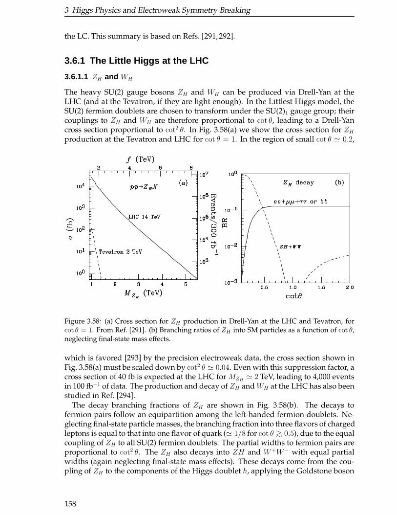
3 Higgs Physics and Electroweak Symmetry Breaking
the LC. This summary is based on Refs. [291, 292].
3.6.1 The Little Higgs at the LHC
3.6.1.1 ZH and WH
The heavy SU(2) gauge bosons ZH and WH can be produced via Drell-Yan at theLHC (and at the Tevatron, if they are light enough). In the Littlest Higgs model, theSU(2) fermion doublets are chosen to transform under the SU(2)1 gauge group; theircouplings to ZH and WH are therefore proportional to cot θ, leading to a Drell-Yancross section proportional to cot2 θ. In Fig. 3.58(a) we show the cross section for ZHproduction at the Tevatron and LHC for cot θ = 1. In the region of small cot θ ≃ 0.2,
Figure 3.58: (a) Cross section for ZH production in Drell-Yan at the LHC and Tevatron, forcot θ = 1. From Ref. [291]. (b) Branching ratios of ZH into SM particles as a function of cot θ,neglecting final-state mass effects.
which is favored [293] by the precision electroweak data, the cross section shown inFig. 3.58(a) must be scaled down by cot2 θ ≃ 0.04. Even with this suppression factor, across section of 40 fb is expected at the LHC for MZH
≃ 2 TeV, leading to 4,000 eventsin 100 fb−1 of data. The production and decay of ZH andWH at the LHC has also beenstudied in Ref. [294].
The decay branching fractions of ZH are shown in Fig. 3.58(b). The decays tofermion pairs follow an equipartition among the left-handed fermion doublets. Ne-glecting final-state particle masses, the branching fraction into three flavors of chargedleptons is equal to that into one flavor of quark (≃ 1/8 for cot θ >∼ 0.5), due to the equalcoupling of ZH to all SU(2) fermion doublets. The partial widths to fermion pairs areproportional to cot2 θ. The ZH also decays into ZH and W+W− with equal partialwidths (again neglecting final-state mass effects). These decays come from the cou-pling of ZH to the components of the Higgs doublet h, applying the Goldstone boson
158

3.6 Phenomenology of the Littlest Higgs model
equivalence theorem for the Goldstone modes eaten by the Z and W bosons. Thepartial widths to ZH and W+W− are proportional to cot2 2θ. The total width of ZHdepends on cot θ; for cot θ ∼ 0.2 the ZH width is about 1% of the ZH mass.
The different dependence of the bosonic and fermionic ZH decay modes on cot θoffers a method to distinguish the Littlest Higgs model from a “big Higgs” modelwith the same gauge group in which the Higgs doublet transforms under only one ofthe SU(2) groups [294], in which case the ZH and W+W− partial widths would alsobe proportional to cot2 θ.
The W±H couplings to fermion doublets are larger by a factor of
√2 than the ZH
couplings; this together with the parton distribution of the proton leads to a W±H
cross section at the LHC about 1.5 times that of ZH [294]. As for the WH decays, thebranching fraction into three lepton flavors is equal to that into one generation ofquarks (≃ 1/4 for cot θ >∼ 0.5). At low cot θ, W±
H decays predominantly into W±H andW±Z with partial widths proportional to cot2 2θ.
The general features of the production and decay of ZH and WH should extendto other little Higgs models in which the SM SU(2) gauge group comes from the di-agonal breaking of two SU(2) groups; this is true, e.g., for the model in Ref. [284].The decays to ZH , WH will however be modified in this model since it contains twoHiggs doublets.
3.6.1.2 AH
The heavy U(1) gauge boson is the lightest new particle in the Littlest Higgs model.Its couplings to fermions are more model dependent than those of the heavy SU(2)gauge bosons, since they depend on the U(1) charges of the fermions (see Ref. [291]for details). Even the presence of AH is somewhat model-dependent, since one canremove this particle from the Littlest Higgs model by gauging only one U(1) group(hypercharge) without adding a significant amount of fine-tuning [293]. Neverthe-less, we show in Fig. 3.59 the cross section and branching ratios ofAH for the simplestanomaly-free choice of fermion U(1) charges given in Ref. [291].
3.6.1.3 T
The heavy top-partner T can be pair produced via QCD interactions with a cross sec-tion that depends only on the T mass. However, this production mode is suppressedby phase space due to the typically high mass of the T . The single T productionmode, W+b → T , is dominant at the LHC for MT above about a TeV. The cross sec-tion for single T production depends on the W+bT coupling, which in turn dependson the amount of mixing between T and the left-handed top quark. This coupling isfixed in terms of MT and f , up to a two-fold ambiguity for MT/f above its minimumvalue of 2mt/v. The cross sections are shown in Fig. 3.60. The top-partner T decaysinto tH , tZ and bW with branching fractions of 1/4, 1/4, and 1/2, respectively. Thesedecays come from the coupling of T to the Higgs doublet h and the 3rd generationquark doublet, applying the Goldstone boson equivalence theorem for the Goldstonemodes eaten by the Z and W bosons.
The structure of the top sector in many of the other little Higgs models in theliterature is quite similar to the Littlest Higgs model, so these general features of
159
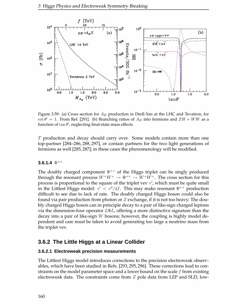
3 Higgs Physics and Electroweak Symmetry Breaking
Figure 3.59: (a) Cross section for AH production in Drell-Yan at the LHC and Tevatron, forcot θ′ = 1. From Ref. [291]. (b) Branching ratios of AH into fermions and ZH + WW as afunction of tan θ′, neglecting final-state mass effects.
T production and decay should carry over. Some models contain more than onetop-partner [284–286, 288, 297], or contain partners for the two light generations offermions as well [285, 287]; in these cases the phenomenology will be modified.
3.6.1.4 Φ++
The doubly charged component Φ++ of the Higgs triplet can be singly producedthrough the resonant process W+W+ → Φ++ → W+W+. The cross section for thisprocess is proportional to the square of the triplet vev v′, which must be quite smallin the Littlest Higgs model: v′ < v2/4f . This may make resonant Φ++ productiondifficult to see due to lack of rate. The doubly charged Higgs boson could also befound via pair production from photon or Z exchange, if it is not too heavy. The dou-bly charged Higgs boson can in principle decay to a pair of like-sign charged leptonsvia the dimension-four operator LΦL, offering a more distinctive signature than thedecay into a pair of like-sign W bosons; however, the coupling is highly model de-pendent and care must be taken to avoid generating too large a neutrino mass fromthe triplet vev.
3.6.2 The Little Higgs at a Linear Collider
3.6.2.1 Electroweak precision measurements
The Littlest Higgs model introduces corrections to the precision electroweak observ-ables, which have been studied in Refs. [293, 295, 296]. These corrections lead to con-straints on the model parameter space and a lower bound on the scale f from existingelectroweak data. The constraints come from Z pole data from LEP and SLD, low-
160
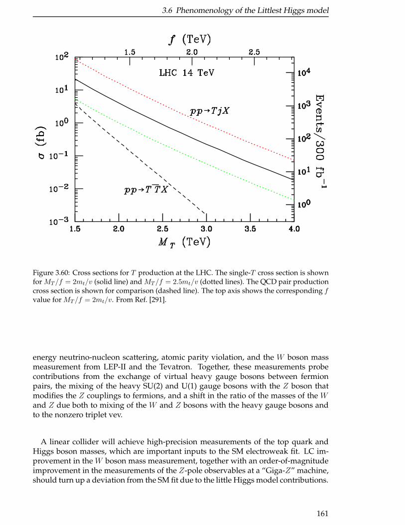
3.6 Phenomenology of the Littlest Higgs model
Figure 3.60: Cross sections for T production at the LHC. The single-T cross section is shownfor MT /f = 2mt/v (solid line) and MT /f = 2.5mt/v (dotted lines). The QCD pair productioncross section is shown for comparison (dashed line). The top axis shows the corresponding fvalue for MT /f = 2mt/v. From Ref. [291].
energy neutrino-nucleon scattering, atomic parity violation, and the W boson massmeasurement from LEP-II and the Tevatron. Together, these measurements probecontributions from the exchange of virtual heavy gauge bosons between fermionpairs, the mixing of the heavy SU(2) and U(1) gauge bosons with the Z boson thatmodifies the Z couplings to fermions, and a shift in the ratio of the masses of the Wand Z due both to mixing of the W and Z bosons with the heavy gauge bosons andto the nonzero triplet vev.
A linear collider will achieve high-precision measurements of the top quark andHiggs boson masses, which are important inputs to the SM electroweak fit. LC im-provement in the W boson mass measurement, together with an order-of-magnitudeimprovement in the measurements of the Z-pole observables at a “Giga-Z” machine,should turn up a deviation from the SM fit due to the little Higgs model contributions.
161
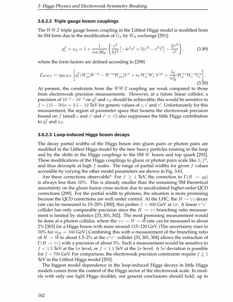
3 Higgs Physics and Electroweak Symmetry Breaking
3.6.2.2 Triple gauge boson couplings
The WWZ triple gauge boson coupling in the Littlest Higgs model is modified fromits SM form due to the modification of GF by WH exchange [291]:
gZ1 = κZ = 1 +1
cos 2θW
v2
8f 2
[−4c2s2 + 5(c′2 − s′2)2
]− 2v′2
v2
, (3.49)
where the form-factors are defined according to [298]
LWWV = igWWV
[gV1 (W+
µνW−µ −W+µW−
µν)Vν + κVW
+µ W
−ν V
µν +λVm2W
W+νµ W−ρ
ν V µρ
].
(3.50)At present, the constraints from the WWZ coupling are weak compared to thosefrom electroweak precision measurements. However, at a future linear collider, aprecision of 10−3−10−4 on gZ1 and κZ should be achievable; this would be sensitive tof ∼ (15− 50)v ∼ 3.5− 12 TeV for generic values of c, c′ and v′. Unfortunately for thismeasurement, the region of parameter space that loosens the electroweak precisionbound on f (small c and v′ and c′ ≃ s′) also suppresses the little Higgs contributionto gZ1 and κZ .
3.6.2.3 Loop-induced Higgs boson decays
The decay partial widths of the Higgs boson into gluon pairs or photon pairs aremodified in the Littlest Higgs model by the new heavy particles running in the loopand by the shifts in the Higgs couplings to the SM W boson and top quark [292].These modifications of the Higgs couplings to gluon or photon pairs scale like 1/f 2,and thus decouple at high f scales. The range of partial widths for given f valuesaccessible by varying the other model parameters are shown in Fig. 3.61.
Are these corrections observable? For f ≥ 1 TeV, the correction to Γ(H → gg)is always less than 10%. This is already smaller than the remaining SM theoreticaluncertainty on the gluon fusion cross section due to uncalculated higher-order QCDcorrections [299]. For the partial width to photons, the situation is more promisingbecause the QCD corrections are well under control. At the LHC, the H → γγ decayrate can be measured to 15–20% [300]; this probes f < 600 GeV at 1σ. A linear e+e−
collider has only comparable precision since the H → γγ branching ratio measure-ment is limited by statistics [33, 301, 302]. The most promising measurement wouldbe done at a photon collider, where the γγ → H → bb rate can be measured to about2% [303] for a Higgs boson with mass around 115–120 GeV. (The uncertainty rises to10% for mH = 160 GeV.) Combining this with a measurement of the branching ratioof H → bb to about 1.5–2% at the e+e− collider [33, 301, 304] allows the extraction ofΓ(H → γγ) with a precision of about 3%. Such a measurement would be sensitive tof < 1.5 TeV at the 1σ level, or f < 1.1 TeV at the 2σ level. A 5σ deviation is possiblefor f < 700 GeV. For comparison, the electroweak precision constraints require f >∼ 1TeV in the Littlest Higgs model [293].
The biggest model dependence in the loop-induced Higgs decays in little Higgsmodels comes from the content of the Higgs sector at the electroweak scale. In mod-els with only one light Higgs doublet, our general conclusions should hold, up to
162
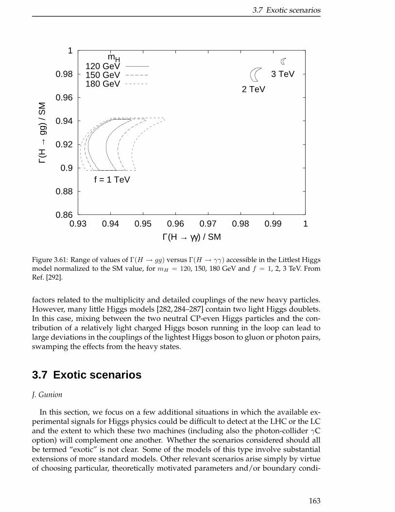
3.7 Exotic scenarios
0.86
0.88
0.9
0.92
0.94
0.96
0.98
1
0.93 0.94 0.95 0.96 0.97 0.98 0.99 1
Γ(H
→ g
g) /
SM
Γ(H → γγ) / SM
f = 1 TeV
2 TeV
3 TeV
mH120 GeV150 GeV180 GeV
Figure 3.61: Range of values of Γ(H → gg) versus Γ(H → γγ) accessible in the Littlest Higgsmodel normalized to the SM value, for mH = 120, 150, 180 GeV and f = 1, 2, 3 TeV. FromRef. [292].
factors related to the multiplicity and detailed couplings of the new heavy particles.However, many little Higgs models [282, 284–287] contain two light Higgs doublets.In this case, mixing between the two neutral CP-even Higgs particles and the con-tribution of a relatively light charged Higgs boson running in the loop can lead tolarge deviations in the couplings of the lightest Higgs boson to gluon or photon pairs,swamping the effects from the heavy states.
3.7 Exotic scenarios
J. Gunion
In this section, we focus on a few additional situations in which the available ex-perimental signals for Higgs physics could be difficult to detect at the LHC or the LCand the extent to which these two machines (including also the photon-collider γCoption) will complement one another. Whether the scenarios considered should allbe termed “exotic” is not clear. Some of the models of this type involve substantialextensions of more standard models. Other relevant scenarios arise simply by virtueof choosing particular, theoretically motivated parameters and/or boundary condi-
163
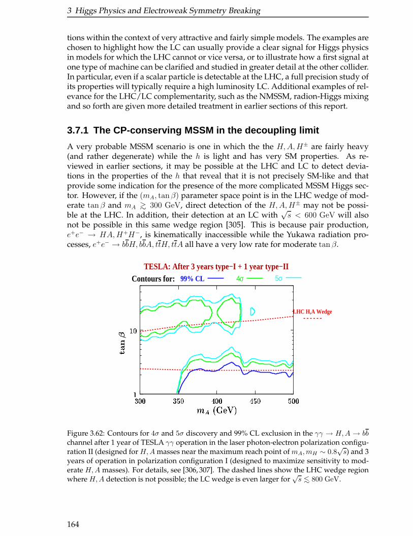
3 Higgs Physics and Electroweak Symmetry Breaking
tions within the context of very attractive and fairly simple models. The examples arechosen to highlight how the LC can usually provide a clear signal for Higgs physicsin models for which the LHC cannot or vice versa, or to illustrate how a first signal atone type of machine can be clarified and studied in greater detail at the other collider.In particular, even if a scalar particle is detectable at the LHC, a full precision study ofits properties will typically require a high luminosity LC. Additional examples of rel-evance for the LHC/LC complementarity, such as the NMSSM, radion-Higgs mixingand so forth are given more detailed treatment in earlier sections of this report.
3.7.1 The CP-conserving MSSM in the decoupling limit
A very probable MSSM scenario is one in which the the H,A,H± are fairly heavy(and rather degenerate) while the h is light and has very SM properties. As re-viewed in earlier sections, it may be possible at the LHC and LC to detect devia-tions in the properties of the h that reveal that it is not precisely SM-like and thatprovide some indication for the presence of the more complicated MSSM Higgs sec-tor. However, if the (mA, tanβ) parameter space point is in the LHC wedge of mod-erate tan β and mA >∼ 300 GeV, direct detection of the H,A,H± may not be possi-ble at the LHC. In addition, their detection at an LC with
√s < 600 GeV will also
not be possible in this same wedge region [305]. This is because pair production,e+e− → HA,H+H−, is kinematically inaccessible while the Yukawa radiation pro-cesses, e+e− → bbH, bbA, ttH, ttA all have a very low rate for moderate tan β.
Contours for:
LHC H,A Wedge
TESLA: After 3 years type−I + 1 year type−II5σ99% CL 4σ
110300 350 400 450 500mA (GeV)
tan
Figure 3.62: Contours for 4σ and 5σ discovery and 99% CL exclusion in the γγ → H,A → bbchannel after 1 year of TESLA γγ operation in the laser photon-electron polarization configu-ration II (designed for H,A masses near the maximum reach point of mA,mH ∼ 0.8
√s) and 3
years of operation in polarization configuration I (designed to maximize sensitivity to mod-erate H,A masses). For details, see [306, 307]. The dashed lines show the LHC wedge regionwhere H,A detection is not possible; the LC wedge is even larger for
√s <∼ 800 GeV.
164
3.7 Exotic scenarios
However, there are options at the LC that would allow H , A and H± detection.First, the LC energy will eventually be upgraded to>∼ 1 TeV, allowingHA andH+H−
pair production up to masses >∼ 500 GeV. Second, it has been shown [306, 307] (seealso [134, 135]) that the photon-collider (γC) option at a
√s = 600 GeV LC has an
excellent chance of allowing direct discovery of the H and A for masses up to about500 GeV in the channel γγ → H,A → bb. A plot from [307] is presented in Fig. 3.62.This plot shows that after 4 years of operation of a TESLA-based γC it would be pos-sible to detect the H,A signal precisely in the wedge of (mA, tanβ) parameter spacewhere their detection would not be possible at either the LHC or LC. The only regionwithin the wedge for which the bb final state signal is weak is the part of the wedgewith the lowest tanβ values. Here, the tt decays of the H and A become importantand the tt final state would be likely to provide a strong signal. This channel has notyet been studied in detail.
3.7.2 The CP-conserving 2HDM with the only light Higgs bosonbeing pseudoscalar – a special non-decoupling limit
The easiest way to satisfy precision electroweak constraints in the two-Higgs-doubletmodel (2HDM) context is if the Higgs potential parameters are chosen so that the de-coupling limit applies. In the decoupling limit, the lightest CP-even Higgs boson, theh, is SM-like by virtue of all the other Higgs bosons (the H,A,H±) being heavy. How-ever, this is not the only way to achieve consistency with the precision electroweakdata. As shown in [308,309] (see also [310]), it is possible to choose 2HDM parametersin such a way that the only light Higgs boson is the A, all the other Higgs bosons (h,H and H±) having masses of order a TeV. The h in this kind of model will be SM-likeand will give sizable ∆T < 0 and ∆S > 0 contributions that would lead to incon-sistency with the precision constraints. However, for parameters such that there is asmall non-zero mH± − mH > 0 mass difference (an isospin splitting) there will be alarge ∆T > 0 that will more than compensate the large ∆T < 0 contribution from theheavy h. This is easily understood algebraically. When the A is relatively light whilethe h is heavy and SM-like, one finds
∆ρ =α
16πm2W c
2W
c2Ws2W
m2H± −m2
H0
2− 3m2
W
[log
m2h0
m2W
+1
6+
1
s2W
logm2W
m2Z
]
The large negative contribution from the heavy SM-like h arising from the 2nd termin brackets is compensated by an even larger positive contribution from the first termproportional to (mH±−mH)(mH± +mH). The resulting predictions of the 2HDM givepostive shifts of O(0.1) to both S and T (assuming U = 0). In this scenario, the LHCwould discover a ∼ 500 GeV − 1 TeV SM-like h (for example, in the h → ZZ → 4ℓchannel) instead of a light CP-even Higgs boson (with SM-like WW,ZZ couplings) asapparently needed to satisfy precision electroweak constraints. The current precisionelectroweak constraints would then imply that additional contributions to S and/orT are required, but their source and nature would be obscure. For example, instead ofthe 2HDM scenario considered here, the negative ∆T and positive ∆S from the heavySM-like h could equally well be compensated by new physics yielding a sizable ∆S <0 contribution with small ∆T (that would yield a net S, T prediction in the lower left
165
3 Higgs Physics and Electroweak Symmetry Breaking
corner of the ellipse) or new physics giving ∆T > 0 and ∆S < 0 contributions (thatwould return the net S, T prediction to near the center of the ellipse).
Clarification of the situation would be difficult. In the 2HDM scenario being con-sidered, and assuming a moderate tanβ value, the A would not be directly detectableat either the LHC or the LC — it falls into the wedge region described in the previoussubsection. The h→ AA decay, if allowed kinematically, would typically have a rea-sonable branching ratio despite the presence of the on-shell ZZ,WW decay modes.Its detection would be very important to unraveling the situation. Of course, the(S, T ) prediction remains within the 90% CL ellipse even if mA is as large as 500 GeV,for which h → AA decays would be forbidden and direct detection of the A (as wellas of the H± and H) in e+e− collisions would require a much higher energy LC. A γCmight play a crucial role. Detection of the A in the γγ → A→ bb channel would gen-erally be possible for mA <∼ 0.8
√s, i.e. for mA <∼ 800 GeV for
√s <∼ 1 TeV. See [306]
for details.Considerable clarification would result from a Giga-Z run at the future LC (com-
bined with a WW threshold scan sufficient to obtain ∆mW = 7MeV ). Given the LHCmeasurement of mh, one could determine with considerable accuracy the additional∆T and/or ∆S from the additional new physics with a (correlated) 1σ error of orderδ∆T ∼ δ∆S ∼ ±0.05. Some scenarios would be excluded, but many possibilitieswould remain, since one could not be sure that the observed deviation was the resultof the presence of undetected Higgs bosons or some of the other types of new physicsdiscussed in earlier sections of this report.
3.7.3 Maximally-mixed and “Continuum” Higgs models
We first describe the general type of model we wish to consider in this section andsome of the related experimental considerations. We then use the continuum Higgsmodel as a particular example.
In unconstrained CP-conserving two-doublet models away from the decouplinglimit, the scalars can mix strongly with one another and have similar masses andmany couplings possibilities. In CP-conserving models with more than two-doubletsand/or doublets plus one or more complex singlets there will be mixing among thepseudoscalars as well as among the scalars. In CP-violating Higgs sectors (includingthe MSSM two-doublet Higgs sector with CP-violation from loop corrections), themixing possibilities will be even greater. Such mixing typically results in a sharingof the WW/ZZ coupling among the CP-even (or all the CP-mixed) Higgs bosons,thereby substantially reducing key high-mass-resolution LHC signals such as gg →h → ZZ(∗) → 4ℓ and especially gg → h → γγ. At the same time, the Higgs bosonscan have masses that differ by an amount of order the experimental resolution inother critical channels that do not rely on the WW/ZZ coupling, such as gg → tthwith h → bb or h→ τ+τ−. Such reduced and overlapping signals will be much moredifficult to separate from background than in the SM Higgs case. In addition, heavierHiggs bosons can decay to lighter ones, further complicating the search possibilities.
Even in the absence of h decays to other Higgs bosons, the WW → h → τ+τ−
detection channel will take a “double-hit”. First, the production rate for each hwouldbe suppressed due to reduced WWh coupling. Second, the poor mass resolution inthe final state would mean that signals for several different h’s (separated in mass by,
166

3.7 Exotic scenarios
say, 10 GeV) will overlap and make peak detection impossible. Instead, one must tryto determine the presence of a broad excess in the Mττ distribution.
Because of these possibilities, it is often fairly easy to find model parameters suchthat the LHC will have difficulty detecting the Higgs boson signals. The power ofthe LC is its ability to look for e+e− → Zh in the inclusive e+e− → ZX missing-mass channel approach by simply looking for a bump in the reconstructed MX . Evenif the signals from different Higgs bosons overlap somewhat and their strength ismaximally shared, the excess in the MX distribution will be apparent at the LC. And,of course, the inclusive MX peak or broad excess is independent of how the Higgsbosons decay.
Another general point is that even if the LHC does not find a direct signal for a setof relatively light but strongly mixed and overlapping Higgs bosons we will knowthat they (or some alternative source of electroweak symmetry breaking) are presentbelow the TeV scale by virtue of the fact that WW → WW scattering measurementswill be consistent with perturbative expectations.
We now very briefly review a particular model in which the above considerationshave been shown to be relevant. This model [311] was explicitly constructed as aworst case scenario for Higgs detection. The idea is to imagine a large number ofdoublet and/or singlet Higgs fields with complicated self interactions. In general,the Higgs sector could be CP-violating. The worst case arises if these many Higgsbosons are spaced in mass at intervals slightly less than the mass resolution in Mbb,Mτ+τ− and MX . They will mix with one another and the heavier ones will decay tothe lighter ones. In general, they will share the WW/ZZ coupling strength. Usingcontinuum limit notation, the only constraints are
∫dmhK(mh) = 1 ,
∫dmhK(mh)g
2ZZhm
2h<∼ (200 GeV)2 (3.51)
where g2ZZh = K(mh)g
2ZZhSM
. The latter constraint relies on either assuming that theseHiggs bosons are entirely responsible for explaining the precision electroweak data(a constraint that can be avoided if there is substantial isospin splitting between thecharged Higgs and scalar Higgs of the model) or if one demands perturbativity of themodel up to the Planck scale.
The result is very substantial diminution of all the standard LHC signals. In par-ticular, the high resolution gg → h → γγ and gg → h → ZZ → 4ℓ final states havevery low production rate for any one of the h’s due to the sharing of the WW/ZZcoupling-squared. Other channels with more limited resolution will not exhibit sep-arated mass peaks. There will only be a spread out signal that must be detected as abroad excess in some type of mass distribution such as Mbb or Mτ+τ− or Mbbτ+τ− (thelatter being relevant for heavier Higgs bosons that decay to a pair of lighter Higgsbosons). The recent study of [312], which claims that a signal can be seen in theWW →
∑i hi → WW → 2ℓ2ν channel, neglects the possibility of Higgs decays
to much lighter Higgs bosons (that have very weak WW/ZZ coupling and do notcontribute to the above sum rules). Allowing for this possibility, it would seem im-possible to guarantee an observable LHC signal for the continuum Higgs scenario.
As discussed in [311], the broad MX excess in the e+e− → ZX channel that wouldarise in this model will be detectable with enough (L >∼ 100 ÷ 200 fb−1) integratedluminosity at the LC. Further, with L ∼ 500 fb−1 it will be possible to determine
167
3 Higgs Physics and Electroweak Symmetry Breaking
the extent of the excess in bins with size of order 10 GeV as well as to examine thedominant final states in each such bin.
3.7.4 Higgsless models
We simply mention the recently proposed Higgsless model [313] in which boundaryconditions on a brane in a warped 5th dimension are responsible for electroweaksymmetry breaking. The unitarity of WW scattering is maintained so long as the KKexcitations of the W and Z are not much above the TeV scale and therefore accessibleto direct production at the LHC. These higher KK excitations also work together insuch a way as to avoid tree-level violation of the ρ = 1 constraint and to make only asmall contribution to the S parameter.
The exact nature of the LHC signals for the W and Z excitations has not beenworked out. However, it is clear that understanding what is happening in WW scat-tering and electroweak symmetry breaking will require detecting all the relevant ex-citations and determining details of their couplings to one another. This will be achallenging task.
An LC (with√s <∼ 1 TeV) might have some difficulty studying all the relevant
KK excitations. Thus, this is a case in which the LHC might be superior for under-standing electroweak symmetry breaking. Still, the LC measurements of the MX dis-tribution would be very revealing in that no excess (at masses below a few hundredGeV) would be observed and one could then be more certain that the KK resonancesobserved at the LHC were indeed the entire story.
168

Bibliography
[1] J.F. Gunion, H.E. Haber, G. Kane and S. Dawson, The Higgs Hunter’s Guide(Perseus Publishing, Cambridge, MA, 1990).
[2] D. Abbaneo et al. [LEP Electroweak Working Group] and N. de Groot et al.[SLD Electroweak and Heavy Flavor Groups], hep-ex/0312023 (December 2003),and additional updates at http://lepewwg.web.cern.ch/LEPEWWG/ ; seealso P. Renton, talk given at the 32nd International Conference on High EnergyPhysics (ICHEP04), Beijing, China, August 2004.
[3] R. Barate et al. [ALEPH, DELPHI, L3 and OPAL Collaborations, and the LEPworking group for Higgs boson searches, Phys. Lett. B565 (2003) 61 [hep-ex/0306033].
[4] H.P. Nilles, Phys. Rep. 110 (1984) 1; H.E. Haber and G.L. Kane, Phys. Rep. 117(1985) 75; S.P. Martin, hep-ph/9709356;
[5] For a review, see e.g., L. Susskind, Phys. Rep. 104 (1984) 181.
[6] K. Inoue, A. Kakuto, H. Komatsu, and S. Takeshita, Prog. Theor. Phys. 68 (1982)927 [E: 70 (1983) 330]; 71 (1984) 413; R. Flores and M. Sher, Ann. Phys. (NY) 148(1983) 95; J.F. Gunion and H.E. Haber, Nucl. Phys. B272 (1986) 1 [E: B402 (1993)567].
[7] J.R. Espinosa and M. Quiros, Phys. Rev. Lett. 81 (1998) 516 [hep-ph/9804235].
[8] G. Degrassi, S. Heinemeyer, W. Hollik, P. Slavich and G. Weiglein, Eur. Phys. J.C28, 133 (2003) [hep-ph/0212020].
[9] For a comprehensive review, see C.T. Hill and E.H. Simmons, Phys. Rep. 381(2003) 235 [E: 390 (2004) 553] [hep-ph/0203079].
[10] E. Farhi and L. Susskind, Phys. Rep.74 (1981) 277; R.K. Kaul, Rev. Mod. Phys. 55(1983) 449.
[11] For a brief review, see M. Schmaltz, Nucl. Phys. Proc. Suppl. 117 (2003) 40 [hep-ph/0210415].
[12] N. Arkani-Hamed, S. Dimopoulos and G.R. Dvali, Phys. Lett. B429 (1998) 263;L. Randall and R. Sundrum, Phys. Rev. Lett. 83 (1999) 3370. For a recent review,see V.A. Rubakov, Phys. Usp. 44 (2001) 871.
[13] M. Quiros, “New ideas in symmetry breaking,” hep-ph/0302189.
169
Bibliography
[14] G.F. Giudice, R. Rattazzi and J.D. Wells, Nucl. Phys. B595 (2001) 250 [hep-ph/0002178]; F.J. Petriello, JHEP 0205 (2002) 003 [hep-ph/0204067]; A. Datta,K. Huitu, J. Laamanen and B. Mukhopadhyaya, hep-ph/0404056.
[15] C. Csaki, C. Grojean, L. Pilo and J. Terning, Phys. Rev. Lett. 92 (2004) 101802 [hep-ph/0308038]; Y. Nomura, JHEP 0311 (2003) 050 [hep-ph/0309189]; H. Davoudi-asl, J.L. Hewett, B. Lillie and T.G. Rizzo, JHEP 0405 (2004) 015 [hep-ph/0403300].
[16] M.E. Peskin and T. Takeuchi, Phys. Rev. Lett. 65 (1990) 964, Phys. Rev. D46 (1992)381.
[17] M. Carena and H.E. Haber, Prog. Part. Nucl. Phys. 50 (2003) 63 [hep-ph/0208209].
[18] M. Duhrssen, S. Heinemeyer, H. Logan, D. Rainwater, G. Weiglein and D. Zep-penfeld, arXiv:hep-ph/0406323.
[19] H.E. Haber and Y. Nir, Nucl. Phys. B335 (1990) 363; J.F. Gunion and H.E. Haber,Phys. Rev. D67 (2003) 075019 [hep-ph/0207010].
[20] ALEPH, DELPHI, L3 and OPAL Collaborations, The LEP Working Group forHiggs Boson Searches, LHWG Note 2001-04 (July 2001) [hep-ex/0107030].
[21] D. Zeppenfeld, R. Kinnunen, A. Nikitenko and E. Richter-Was, Phys. Rev. D62(2000) 013009 [hep-ph/0002036]; D. Zeppenfeld, “Higgs Couplings at the LHC,”in Proceedings of the APS/DPF/DPB Summer Study on the Future of Particle Physics(Snowmass 2001), edited by R. Davidson and C. Quigg, SNOWMASS-2001-P123[hep-ph/0203123].
[22] A. Belyaev and L. Reina, JHEP 0208 (2002) 041 [hep-ph/0205270].
[23] M. Duhrssen, “Prospects for the measurement of Higgs boson coupling param-eters in the mass range from 110–190 Gev/c2,” ATL/PHYS-2003-030.
[24] See, e.g. J.F. Gunion, H.E. Haber and R. Van Kooten, “ Higgs Physics at the LinearCollider,” SCIPP-02-37 and UCD-02-18 [hep-ph/0301023], to appear in LinearCollider Physics in the New Millennium, edited by K. Fujii, D. Miller and A. Soniand references contained therein.
[25] J. Cammin, M. Schumacher, “THE ATLAS discovery potential for the channeltth0, h0 → bb”, ATL-PHYS-2003-024.
[26] J. Dai, J.F. Gunion and R. Vega, Phys. Rev. Lett. 71 (1993) 2699.
[27] M. Beneke et. al., “Top Quark Physics,” hep-ph/0003033.
[28] V. Drollinger, Th. Muller and D. Denegri, CMS Note 2001/054 [hep-ph/0111312].
[29] J. Leveque et al., “Search for the Standard Model Higgs boson in the channel tth0,h0 →WW channel”, ATL-PHYS-2002-19.
[30] F. Maltoni, D. Rainwater, and S. Willenbrock, Phys. Rev. D66 (2002) 034033 [hep-ph/0202205].
170
Bibliography
[31] L. Zivkovic and E. Gross, ATLAS Higgs working group (February, 19 2001).
[32] A. Ito, ATLAS Higgs working group (April, 10 2003).
[33] J.A. Aguilar-Saavedra et al. [ECFA/DESY LC Physics Working Group Collab-oration], “TESLA Technical Design Report Part III: Physics at an e+e− LinearCollider,” arXiv:hep-ph/0106315.
[34] D. Bourilkov, this report and references therein.
[35] A. Djouadi and S. Ferrag, Phys. Lett. B586 (2004) 345 [hep-ph/0310209].
[36] W. Beenakker, S. Dittmaier, M. Kramer, B. Plumper, M. Spira and P.M. Zerwas,Phys. Rev. Lett. 87 (2001) 201805 [hep-ph/0107081].
[37] W. Beenakker, S. Dittmaier, M. Kramer,B. Plumper, M. Spira and P. M. Zerwas,Nucl. Phys. B653 (2003) 151 [hep-ph/0211352].
[38] L. Reina and S. Dawson, Phys. Rev. Lett. 87 (2001) 201804 [hep-ph/0107101];L. Reina, S. Dawson and D. Wackeroth, Phys. Rev. D65 (2002) 053017 [hep-ph/0109066].
[39] S. Dawson, L.H. Orr, L. Reina, and D. Wackeroth, Phys. Rev. D67 (2003) 071503[hep-ph/0211438]; S. Dawson, C. Jackson, L.H. Orr, L. Reina and D. Wackeroth,Phys. Rev. D68 (2003) 034022 [hep-ph/0305087].
[40] A. Gay, results presented at the 2nd ECFA/DESY Workshop, Saint Malo, France,12-15 April 2002, http://www.desy.de/˜desch/higgs/stmalo/gay.ps.
[41] M. Battaglia and K. Desch, in Physics and experiments with future linear e+e− collid-ers, Proceedings of the 5th International Linear Collider Workshop, Batavia, IL,USA, 2000, edited by A. Para and H.E. Fisk (American Institute of Physics, NewYork, 2001), pp. 163–182 [hep-ph/0101165].
[42] C.T. Potter, J.E. Brau and M. Iwasaki, “Standard Model Higgs Boson BranchingRatio Measurements at a Linear Collider,” in Proceedings of the APS/DPF/DPBSummer Study on the Future of Particle Physics (Snowmass 2001), edited byR. Davidson and C. Quigg, SNOWMASS-2001-P118; and “Standard ModelHiggs boson branching ratio measurements at a linear collider,” to appear inthe Proceedings of the International Workshop on Linear Colliders, Workshop onPhysics and Experiments with Future Electron-Positron Linear Colliders, 26–30 Au-gust, 2002, Jeju Island, Korea.
[43] K.J.F. Gaemers and G.J. Gounaris, Phys. Lett. B77 (1978) 379; A. Djouadi, J. Kali-nowski and P.M. Zerwas, Z. Phys. C54 (1992) 255.
[44] S. Dawson and L. Reina, Phys. Rev. D59 (1999) 054012 [hep-ph/9808443].
[45] A. Juste and G. Merino, hep-ph/9910301.
[46] A. Juste, results presented at Chicago linear collider workshop, January, 2002,http://www.pas.rochester.edu/˜orr/justelc.pdf.
171
Bibliography
[47] S. Dittmaier, M. Kramer, Y. Liao, M. Spira, and P.M. Zerwas, Phys. Lett. B441(1998) 383 [hep-ph/9808433].
[48] G. Belanger, preliminary results of the GRACE collaboration presented atLoopfest II, May 14, 2003; G. Belanger, F. Boudjema, J. Fujimoto, T. Ishikawa,T. Kaneko, K. Kato, Y. Shimizu, and Y. Yasui, Phy. Lett. B571 (2003) 163 [hep-ph/0307029].
[49] Y. Yu, M. Wen-Gan, C. Hui, Z. Ren-You, S. Y-Bin, and H. Hong-Sheng, Phys.Lett. B51 (2003) 85, hep-ph/0306036.
[50] A. Denner, S. Dittmaier, M. Roth and M. Weber, Phys. Lett. B 575 (2003) 290[arXiv:hep-ph/0307193]; Nucl. Phys. B 680 (2004) 85 [arXiv:hep-ph/0309274].
[51] S. Moretti, 2nd ECFA/DESY Study, hep-ph/9911501, Phys. Lett. B452 (1999) 338[hep-ph/9902214].
[52] H. Baer, S. Dawson, and L. Reina, Phys. Rev. D61 (2000) 013002 [hep-ph/9906419].
[53] H. Baer, F.E. Paige, S.D. Protopopescu and X. Tata, hep-ph/0001086.
[54] A. Gay, results presented at the 3rd ECFA/DESY Workshop, Prague, CzechRepublic, 15-18 November 2002,http://ireswww.in2p3.fr/ires/recherche/capteurs/ed/prague/prague ag.html.
[55] A. Gay, results presented at the 4th ECFA DESY Workshop, Am-sterdam, Netherlands, 1-4 April 2003, http://www.nikhef.nl/ecfa-desy/ECspecific/Program/Presentations/April-2/Par-1/1A/gay-a.ps.
[56] Y. Sumino, K. Fujii, K. Hagiwara, H. Murayama, and C. Ng, Phys. Rev. D47(1993) 56; A. Hoang and T. Teubner, Phys. Rev. D60 (1999) 114027 [hep-ph/9904468].
[57] K. Fujii, T. Matsui and Y. Sumino, Phys. Rev. D50 (1994) 4341.
[58] M. Martinez and R. Miquel, Eur. Phys. J. C27 (2003) 49 [hep-ph/0207315].
[59] A.H. Hoang et al., Eur. Phys. J. C2 (2000) 3 [hep-ph/0001286].
[60] A.H. Hoang, A.V. Manohar, I.W. Stewart and T. Teubner, Phys. Rev. D65 (2002)014014 [hep-ph/0107144].
[61] R. Harlander, M. Jezabek, J.H. Kuhn and T. Teubner, Phys. Lett. B346 (1995) 137[hep-ph/9411395]; M. Jezabek and T. Teubner, Z. Phys. C59 (1993) 669; M. Jez-abek and J.H. Kuhn, Phys. Lett. B316 (1993) 360; M. Jezabek, J.H. Kuhn andT. Teubner, Z. Phys. C56 (1992) 653.
[62] B. Grzadkowski, J.H. Kuhn, P. Krawczyk, and R. Stuart, Nucl. Phys. B282 (1987)18; R. Guth and J.H. Kuhn, Nucl. Phys. B368 (1992) 38.
[63] J. Goldstein, C. S. Hill, J. Incandela, S. Parke, and D. Stuart, Phys. Rev. Lett. 86(2001) 1694 [hep-ph/0006311].
172
Bibliography
[64] E. Richter-Was and M. Sapinski, Acta Phys. Polon. B30 (1999) 1001.
[65] ATLAS Collaboration, Technical Design Report, Vol. II, CERN/LHCC/99-15(1999).
[66] S. Dittmaier, M. Kramer, Y. Liao, M. Spira and P.M. Zerwas, Phys. Lett. B478(2000) 247 [hep-ph/0002035].
[67] S. Dawson and L. Reina, Phys. Rev. D60 (1999) 015003 [hep-ph/9812488].
[68] A. Dedes, S. Heinemeyer, S. Su and G. Weiglein, Nucl. Phys. B 674 (2003) 271,arXiv:hep-ph/0302174.
[69] B. Kniehl, F. Madricardo and M. Steinhauser, Phys. Rev. D66 (2002) 054016 [hep-ph/0205312].
[70] M. Dittmar and H.K. Dreiner, Phys. Rev. D55 (1997) 167 [hep-ph/9608317];D. Rainwater and D. Zeppenfeld, Phys. Rev. D60 (1999) 113004 [Erratum: D61(2000) 099901] [hep-ph/9906218]; N. Kauer, T. Plehn, D. Rainwater and D. Zep-penfeld, Phys. Lett. B503 (2001) 113 [hep-ph/0012351].
[71] D. Rainwater, D. Zeppenfeld and K. Hagiwara, Phys. Rev. D59 (1999) 014037[hep-ph/9808468]; T. Plehn, D. Rainwater and D. Zeppenfeld, Phys. Lett. B454(1999) 297 [hep-ph/9902434]; Phys. Rev. D61 (2000) 093005 [hep-ph/9911385].
[72] D. Rainwater, Phys. Lett. B503 (2001) 320 [hep-ph/0004119]; V. Drollinger,T. Muller and D. Denegri, hep-ph/0201249.
[73] B.W. Lee, C. Quigg and H.B. Thacker, Phys. Rev. Lett. 38 (1977) 883; Phys. Rev.D16 (1977) 1519.
[74] M. Battaglia, E. Boos and W.M. Yao, hep-ph/0111276.
[75] A. Djouadi, W. Kilian, M. Muhlleitner and P.M. Zerwas, Eur. Phys. J. C10 (1999)27; D.J. Miller and S. Moretti, Eur. Phys. J. C13 (2000) 459.
[76] C. Castanier, P. Gay, P. Lutz and J. Orloff, hep-ex/0101028.
[77] F. Gianotti et al., hep-ph/0204087.
[78] U. Baur, T. Plehn and D. Rainwater, Phys. Rev. Lett. 89 (2000) 151801; Phys. Rev.D67 (2003) 033003.
[79] U. Baur, T. Plehn and D. Rainwater, Phys. Rev. D 69, 053004 (2004).
[80] U. Baur, T. Plehn and D. Rainwater, Phys. Rev. D68 (2003) 033001 [hep-ph/0304015].
[81] K. A. Assamagan et al. [Higgs Working Group Collaboration], arXiv:hep-ph/0406152.
[82] M. Battaglia and A. DeRoeck, in preparation.
173
Bibliography
[83] E.L. Berger, C.W. Chiang, J. Jiang, T.M.P. Tait and C.E.M. Wagner, Phys. Rev. D66(2002) 095001 [hep-ph/0205342].
[84] B.A. Dobrescu, G. Landsberg and K.T. Matchev, Phys. Rev. D63 (2001) 075003[hep-ph/0005308].
[85] M. Carena, J.R. Ellis, S. Mrenna, A. Pilaftsis and C.E.M. Wagner, Nucl. Phys. B659(2003) 145 [hep-ph/0211467].
[86] E.L. Berger, B.W. Harris, D.E. Kaplan, Z. Sullivan, T.M.P. Tait and C.E.M. Wagner,Phys. Rev. Lett. 86 (2001) 4231 [hep-ph/0012001].
[87] E.L. Berger, Int. J. Mod. Phys. A18 (2003) 1263 [hep-ph/0201229]; E.L. Berger,hep-ph/0209374.
[88] M. Carena, S. Heinemeyer, C.E.M. Wagner and G. Weiglein, Phys. Rev. Lett. 86(2001) 4463 [hep-ph/0008023].
[89] CMS Collaboration, Technical Proposal, report CERN/LHCC/94-38 (1994).
[90] D. Cavalli et al., “The Higgs working group: Summary report”, to appear in theproceedings of Workshop on Physics at TeV Colliders, Les Houches, France, 21May—1 June 2001, hep-ph/0203056.
[91] T. Abe et al. [American Linear Collider Working Group], “Linear Collider PhysicsResource Book for Snowmass 2001,” SLAC-R-570; TESLA Technical Design Re-port, Ed. by R. Heuer, D. Miller, F. Richard, A. Wagner, and P.M. Zerwas,www.desy.de/˜lcnotes/tdr.
[92] R. Kinnunen, “Higgs physics at the LHC,” in: Proceedings of the 10th InternationalConference on Supersymmetry and Unification of Fundamental Interactions (SUSY02),Eds. P. Nath, P. M. Zerwas, and C. Grosche, DESY, Hamburg, Germany, 2002.
[93] B. Badelek et al. [ECFA/DESY Photon Collider Working Group Collaboration],“TESLA Technical Design Report, Part VI, Chapter 1: Photon collider at TESLA,”arXiv:hep-ex/0108012; Proc. of Int. Workshop on High Photon Colliders Nucl.Instrum. Meth. A 472 (2001)
[94] S. Weinberg, Phys. Rev. Lett. 37 (1976) 657.
[95] For a review, see e.g. M. Dine and A. Kusenko, arXiv:hep-ph/0303065.
[96] J. F. Gunion, H. E. Haber and J. Wudka, Phys. Rev. D 43 (1991) 904.
[97] J. F. Gunion, B. Grzadkowski, H. E. Haber and J. Kalinowski, Phys. Rev. Lett. 79(1997) 982 [arXiv:hep-ph/9704410].
[98] I. F. Ginzburg, M. Krawczyk and P. Osland, arXiv:hep-ph/0211371.
[99] OPAL Collaboration, OPAL Physics Note PN524 (2003).
[100] M. N. Dubinin and A. V. Semenov, Eur. Phys. J. C 28, 223 (2003) [arXiv:hep-ph/0206205].
174
Bibliography
[101] A. Dedes and S. Moretti, Phys. Rev. Lett. 84 (2000) 22 [arXiv:hep-ph/9908516];Nucl. Phys. B 576 (2000) 29 [arXiv:hep-ph/9909418].
[102] A. Pilaftsis and C. E. Wagner, Nucl. Phys. B 553, 3 (1999) [arXiv:hep-ph/9902371].
[103] S. Y. Choi, M. Drees and J. S. Lee, Phys. Lett. B 481, 57 (2000) [arXiv:hep-ph/0002287].
[104] S. Heinemeyer, Eur. Phys. J. C 22, 521 (2001) [arXiv:hep-ph/0108059].
[105] J. S. Lee, A. Pilaftsis, M. Carena, S. Y. Choi, M. Drees, J. Ellis and C. E. Wagner,[arXiv:hep-ph/0307377].
[106] W. Bernreuther, M. Flesch and P. Haberl, Phys. Rev. D 58 (1998) 114031[arXiv:hep-ph/9709284]; W. Bernreuther, A. Brandenburg and M. Flesch,arXiv:hep-ph/9812387.
[107] W. Khater and P. Osland, Nucl. Phys. B 661, 209 (2003) [arXiv:hep-ph/0302004].
[108] J. F. Gunion and X. G. He, Phys. Rev. Lett. 76 (1996) 4468 [arXiv:hep-ph/9602226].
[109] B. Field, Phys. Rev. D 66 (2002) 114007 [arXiv:hep-ph/0208262].
[110] S. Y. Choi, D. J. Miller, M. M. Muhlleitner and P. M. Zerwas, Phys. Lett. B 553(2003) 61 [arXiv:hep-ph/0210077].
[111] C. P. Buszello, I. Fleck, P. Marquard and J. J. van der Bij, Eur. Phys. J. C 32 (2004)209 [arXiv:hep-ph/0212396].
[112] T. Plehn, D. Rainwater and D. Zeppenfeld, Phys. Rev. Lett. 88 (2002) 051801[arXiv:hep-ph/0105325].
[113] V. Del Duca, W. Kilgore, C. Oleari, C. R. Schmidt and D. Zeppenfeld,[arXiv:hep-ph/0109147].
[114] K. Odagiri, JHEP 0303, 009 (2003) [arXiv:hep-ph/0212215].
[115] V. A. Khoze, A. D. Martin and M. G. Ryskin, Eur. Phys. J. C 23 (2002) 311[arXiv:hep-ph/0111078].
[116] B. E. Cox, J. R. Forshaw, J. S. Lee, J. Monk and A. Pilaftsis, Phys. Rev. D 68 (2003)075004 [arXiv:hep-ph/0303206].
[117] V. A. Khoze, A. D. Martin and M. G. Ryskin, arXiv:hep-ph/0401078.
[118] A. Mendez and A. Pomarol, Phys. Lett. B 272 (1991) 313.
[119] B. Grzadkowski, J. F. Gunion and J. Kalinowski, Phys. Rev. D 60 (1999) 075011[arXiv:hep-ph/9902308].
[120] A. G. Akeroyd and A. Arhrib, Phys. Rev. D 64 (2001) 095018 [arXiv:hep-ph/0107040].
175
Bibliography
[121] V. D. Barger, K. m. Cheung, A. Djouadi, B. A. Kniehl and P. M. Zerwas, Phys.Rev. D 49 (1994) 79 [arXiv:hep-ph/9306270].
[122] K. Hagiwara and M. L. Stong, Z. Phys. C 62 (1994) 99 [arXiv:hep-ph/9309248].
[123] D. J. Miller, S. Y. Choi, B. Eberle, M. M. Muhlleitner and P. M. Zerwas, Phys.Lett. B 505 (2001) 149 [arXiv:hep-ph/0102023].
[124] M. T. Dova, P. Garcia-Abia and W. Lohmann, arXiv:hep-ph/0302113.
[125] M. Kramer, J. H. Kuhn, M. L. Stong and P. M. Zerwas, Z. Phys. C 64 (1994) 21[arXiv:hep-ph/9404280].
[126] B. Grzadkowski and J. F. Gunion, Phys. Lett. B 350 (1995) 218 [arXiv:hep-ph/9501339].
[127] J. F. Gunion, B. Grzadkowski and X. G. He, Phys. Rev. Lett. 77 (1996) 5172[arXiv:hep-ph/9605326].
[128] G. R. Bower, T. Pierzchala, Z. Was and M. Worek, Phys. Lett. B 543 (2002) 227[arXiv:hep-ph/0204292].
[129] K. Desch, Z. Was and M. Worek, Eur. Phys. J. C 29 (2003) 491 [arXiv:hep-ph/0302046].
[130] M. Worek, Acta Phys. Polon. B 34 (2003) 4549 [arXiv:hep-ph/0305082].
[131] K. Desch, A. Imhof, Z. Was and M. Worek, arXiv:hep-ph/0307331.
[132] K. Hagiwara, Nucl. Instrum. Meth. A 472 (2001) 12 [arXiv:hep-ph/0011360].
[133] B. Grzadkowski and J. F. Gunion, Phys. Lett. B 294 (1992) 361 [arXiv:hep-ph/9206262].
[134] M. M. Muhlleitner, M. Kramer, M. Spira and P. M. Zerwas, Phys. Lett. B 508,311 (2001) [arXiv:hep-ph/0101083].
[135] P. Niezurawski, A. F. Zarnecki and M. Krawczyk, arXiv:hep-ph/0307180.
[136] E. Asakawa, J. i. Kamoshita, A. Sugamoto and I. Watanabe, Eur. Phys. J. C 14(2000) 335 [arXiv:hep-ph/9912373].
[137] P. Niezurawski, A. F. Zarnecki and M. Krawczyk, arXiv:hep-ph/0307175;arXiv:hep-ph/0403138;
[138] E. Asakawa, S. Y. Choi, K. Hagiwara and J. S. Lee, Phys. Rev. D 62 (2000) 115005[arXiv:hep-ph/0005313].
[139] R. M. Godbole, S. D. Rindani and R. K. Singh, Phys. Rev. D 67 (2003) 095009[arXiv:hep-ph/0211136].
[140] I. F. Ginzburg, M. Krawczyk and P. Osland, Nucl. Instrum. Meth. A472:149, 2001[arXiv:hep-ph/0101229]; arXiv:hep-ph/0101331; arXiv:hep-ph/0101208.
176
Bibliography
[141] D. Bomestar, D. Denegri, R. Kinnunen, A. Nikitenko, FIZIKA B 4 (1995) 3, 273-286; CMS TN/95-018.
[142] R. Kinnunen, CMS CR-2002/020.
[143] N.Meyer, LC-PHSM-2003-066.
[144] P.Niezurawski, A.F.Zarnecki, M.Krawczyk, JHEP 0211 (2002) 034 [arXiv:hep-ph/0207294]
[145] J. A. Aguilar-Saavedra et al. [ECFA/DESY LC Physics Working Group Collabo-ration], arXiv:hep-ph/0106315;T. Abe et al. [American Linear Collider Working Group Collaboration], in Proc.of Snowmass 2001, ed. N. Graf, arXiv:hep-ex/0106055;K. Abe et al. [ACFA Linear Collider Working Group Coll.], arXiv:hep-ph/0109166; see: lcdev.kek.jp/RMdraft/ .
[146] A. Hoang et al., Eur. Phys. J. C 3 (2000) 1, arXiv:hep-ph/0001286.
[147] S. Heinemeyer, S. Kraml, W. Porod and G. Weiglein, JHEP 0309 (2003) 075,arXiv:hep-ph/0306181.
[148] K. Desch, E. Gross, S. Heinemeyer, G. Weiglein and L. Zivkovic, arXiv:hep-ph/0406322.
[149] B. C. Allanach et al., Eur. Phys. J. C 25 (2002) 113, arXiv:hep-ph/0202233, see:www.ippp.dur.ac.uk/ ∼georg/sps .
[150] R. Lafaye, T. Plehn and D. Zerwas, arXiv:hep-ph/0404282;P. Wienemann, talk given at the LCWS Paris, April 2004, see:agenda.cern.ch/fullAgenda.php?ida=a04172#s15 .
[151] J. R. Ellis, S. Heinemeyer, K. A. Olive and G. Weiglein, JHEP 0301 (2003) 006,arXiv:hep-ph/0211206.
[152] J. Guasch, W. Hollik and S. Penaranda, Phys. Lett. B 515 (2001) 367, arXiv:hep-ph/0106027;M. Carena, H. Haber, H. Logan and S. Mrenna, Phys. Rev. D 65 (2002) 055005, E:ibid D 65 (2002) 099902, arXiv:hep-ph/0106116;D. Asner et al., Eur. Phys. J. C 28 (2003) 27, arXiv:hep-ex/0111056.
[153] J.-C. Brient, LC-PHSM-2004-002, see: www-flc.desy.de/lcnotes .
[154] J. Erler, S. Heinemeyer, W. Hollik, G. Weiglein and P.M. Zerwas, Phys. Lett. B486 (2000) 125, arXiv:hep-ph/0005024;J. Erler and S. Heinemeyer, in Proc. of the 5th International Symposium on RadiativeCorrections (RADCOR 2000) ed. Howard E. Haber, arXiv:hep-ph/0102083.
[155] K. Desch, J. Kalinowski, G. Moortgat-Pick, M. M. Nojiri and G. Polesello, JHEP0402 (2004) 035, arXiv:hep-ph/0312069.
177
Bibliography
[156] S. Heinemeyer, W. Hollik and G. Weiglein, Eur. Phys. J. C 16 (2000)139, arXiv:hep-ph/0003022; Comp. Phys. Comm. 124 (2000) 76, arXiv:hep-ph/9812320, see: www.feynhiggs.de .
[157] H. E. Haber, M. J. Herrero, H. E. Logan, S. Penaranda, S. Rigolin and D. Temes,Phys. Rev. D 63 (2001) 055004, arXiv:hep-ph/0007006.
[158] T. L. Barklow, arXiv:hep-ph/0312268.
[159] CMS Coll., Technical Proposal, report CERN/LHCC/94-38 (1994); ATLASColl., Technical Design Report, CERN/LHCC/99-15 (1999).
[160] J. A. Aguilar-Saavedra et al. [ECFA/DESY LC Physics Working Group Collab-oration], TESLA Technical Design Report Part III: Physics at an e+e- Linear Col-lider, hep-ph/0106315.
[161] For a review on the MSSM, see S. Martin, “A supersymmetry primer”, hep-ph/9709356.
[162] For a review on the Higgs sector of the MSSM, see J.F. Gunion, H.E. Haber,G.L. Kane and S. Dawson, “The Higgs Hunter’s Guide”, Addison–Wesley, Read-ing 1990.
[163] F. Moortgat, S. Abdullin and D. Denegri, hep-ph/0112046.
[164] M. Bisset, F. Moortgat, S. Moretti, hep-ph/0303093, Eur.Phys.J.C 30, 419-434(2003).
[165] G. Weiglein et al., in Proc. of the APS/DPF/DPB Summer Study on the Future ofParticle Physics (Snowmass 2001) ed. N. Graf, hep-ph/0202233, Eur. Phys. J.C 25,113 (2002).
[166] F. Moortgat, M. Nojiri and W. Porod, private discussions during the 2003 LesHouches Workshop on Physics with TeV Colliders; M. Nojiri, G. Polesello andD. Tovey, hep-ph/0312317.
[167] E. Boos, A. Djouadi, M. Muhlleitner and A. Vologdin, Phys. Rev. D66 (2002)055004.
[168] E. Boos, A. Djouadi and A. Nikitenko, Phys. Lett. B 578 (2004) 384
[169] A. Djouadi, J. Kalinowski and M. Spira, Comput. Phys. Commun. 108 (1998) 56.
[170] A. Pukhov et al., Report INP-MSU 98-41/542, hep-ph/9908288.
[171] A.S. Belyaev et al., hep-ph/0101232.
[172] T. Sjostrand, L. Lonnblad and S. Mrenna, hep-ph/0108264.
[173] M. Pohl and H. J. Schreiber, hep-ex/0206009.
[174] A. Andreazza and C. Troncon, Report DESY–123–E, p. 417.
178
Bibliography
[175] G. Blair and H.U. Martyn, Note LC–TH-2000–023 and hep-ph/0002290.
[176] E. Boos, V. Bounichev, A. Djouadi and J. Schreiber, in preparation.
[177] S. Lehti, Prospects for the Detection of the MSSM Higgs Bosons Decaying intoTau Leptons in the CMS Detector, Dissertation, University of Helsinki, Report Seriesin Physics, HU-P-D93 (2001); S. Lehti, Study of gg → bbHSUSY , HSUSY → ττ →ℓℓ+X , CMS NOTE 2002/035.
[178] R. Kinnunen and A. Nikitenko, CMS NOTE 1997/106.
[179] R. Kinnunen and A. Nikitenko, CMS NOTE 2003/006.
[180] M. Carena and H. Haber, Prog. Part. Nucl. Phys. 50 (2003) 63 and referencestherein.
[181] CMS Collaboration, CERN/LHCC 2002-26, CMS TDR 6.2.
[182] K. Hagiwara et. al., Phys. Rev. D66 (2002) 010001.
[183] S. Dittmaier, M. Spira, and M. Kramer, hep-ph/0309204.
[184] S. Dawson, C. Jackson, L. Reina and D. Wackeroth, hep-ph/0311067.
[185] J. Campbell, R. K. Ellis, F. Maltoni and S. Willenbrock, Phys. Rev. D67 (2003)093005.
[186] S.Y. Choi, J. Kalinowski, J.S. Lee, M. Muhlleitner, M. Spira and P.M. Zerwas,arXiv:hep-ph/0404119 and arXiv:hep-ph/0407048.
[187] K. Desch, private communication.
[188] J. Gunion, T. Han, J. Jiang, A. Sopczak, Phys. Lett. B 565, 42 (2003).
[189] CMS Collaboration, Technical Proposal, CERN/LHCC/94–38 (1994).
[190] ATLAS Collaboration, ATLAS Detector and Physics Performance: TechnicalDesign Report, CERN/LHCC/99–14 and 99–15 (1999).
[191] F. Gianotti et al., arXiv:hep-ph/0204087.
[192] LEP Higgs Working Group, July 2002.
[193] J.F. Gunion, L. Poggioli, R. Van Kooten, C. Kao and P. Rowson, arXiv:hep-ph/9703330.
[194] S. Dawson, D. Dicus and C. Kao, Phys. Lett. B 545, 132 (2002).
[195] K.A. Assamagan, Y. Coadou and A. Deandrea, Eur. Phys. J. direct C 4, 9 (2002).
[196] A. Djouadi, J. Kalinowski and M. Spira, Comput. Phys. Commun. 108, 56 (1998).
[197] M. Carena, S. Mrenna and C.E. Wagner, Phys. Rev. D 60, 075010 (1999).
179
Bibliography
[198] P. Chankowski, T. Farris, B. Grzadkowski, J.F. Gunion, J. Kalinowski andM. Krawczyk, Phys. Lett. B 496, 195 (2000).
[199] J. R. Ellis, J. F. Gunion, H. E. Haber, L. Roszkowski and F. Zwirner, Phys. Rev. D39 (1989) 844.
[200] J. F. Gunion, H. E. Haber and T. Moroi, eConf C960625, LTH095 (1996)[arXiv:hep-ph/9610337].
[201] U. Ellwanger, J. F. Gunion and C. Hugonie, arXiv:hep-ph/0111179.
[202] LEP Higgs Working Group, Notes 2002/01 (Zh) and 2001/04 (ha).
[203] CMS Collaboration, “Expected Observability of Standard Model Higgs in CMSwith 100 fb−1”, CMS NOTE 1997/057. ATLAS Collaboration, “Detector andPhysics Performance Technical Design Report Vol. II (1999)”, CERN/LHCC/99-15 p. 675–811. D. Zeppenfeld, R. Kinnunen, A. Nikitenko and E. Richter-Was,Phys. Rev. D 62 (2000) 013009.D. Zeppenfeld, in Proc. of the APS/DPF/DPB Sum-mer Study on the Future of Particle Physics (Snowmass 2001) ed. N. Graf, eConfC010630, P123 (2001).
[204] U. Ellwanger and C. Hugonie, Eur. Phys. J. C 25 (2002) 297.
[205] S. Moretti, K. Odagiri, P. Richardson, M. H. Seymour and B. R. Webber, JHEP0204 (2002) 028 [arXiv:hep-ph/0204123].
[206] G. Corcella et al., arXiv:hep-ph/0201201.
[207] G. Corcella et al., JHEP 0101 (2001) 010 [arXiv:hep-ph/0011363].
[208] S. Moretti, private program.
[209] U. Ellwanger, J. F. Gunion, C. Hugonie and S. Moretti, “Towards a no-lose the-orem for NMSSM Higgs discovery at the LHC,” arXiv:hep-ph/0305109.
[210] See, for example, the summary of J. F. Gunion, H. E. Haber and R. Van Kooten,“Higgs physics at the linear collider,” arXiv:hep-ph/0301023.
[211] U. Ellwanger, J.F. Gunion, C. Hugonie and S. Moretti, in progress.
[212] U. Ellwanger, J. F. Gunion, C. Hugonie and S. Moretti, arXiv:hep-ph/0305109,and this report.
[213] R. D. Peccei and H. R. Quinn, Phys. Rev. Lett. 38 (1977) 1440; Phys. Rev. D 16(1977) 1791.
[214] D. J. Miller and R. Nevzorov, arXiv:hep-ph/0309143.
[215] D. J. Miller, R. Nevzorov and P. M. Zerwas, arXiv:hep-ph/0304049.
[216] P. A. Kovalenko, R. B. Nevzorov and K. A. Ter-Martirosian, Phys. Atom. Nucl.61 (1998) 812 [Yad. Fiz. 61 (1998) 898].
180

Bibliography
[217] R. Barate et al., Phys. Lett. B 565 (2003) 61 [arXiv:hep-ex/0306033]; [LEP HiggsWorking Group for Higgs boson searches Collaboration], arXiv:hep-ex/0107029.
[218] Searches for Higgs Bosons Decaying into Photons: Combined Results from theLEP Experiments LHWG Note/2002-02, 12 July ’02
[219] G. Abbiendi et al. [OPAL Collaboration], Eur. Phys. J. C 27 (2003) 311 [arXiv:hep-ex/0206022].
[220] G. Jikia and S. Soldner-Rembold, Nucl. Phys. Proc. Suppl. 82 (2000) 373[arXiv:hep-ph/9910366]; M. Melles, W. J. Stirling and V. A. Khoze, Phys. Rev.D 61 (2000) 054015 [arXiv:hep-ph/9907238]; P. Niezurawski, A. F. Zarnecki andM. Krawczyk, hep-ph/0307183.
[221] J. L. Diaz-Cruz and A. Mendez, Nucl. Phys. B380 (1992) 39,J. L. Diaz-Cruz and G. Lopez Castro, Phys. Lett. B301 (1993) 405.
[222] H. E. Haber, hep-ph/9501320; J. F. Gunion and H. E. Haber, Phys. Rev. D 67,075019 (2003) [hep-ph/0207010].
[223] G. C. Branco, L. Lavoura, J. P. Silva, “CP Violation” (Oxford Univ. Press, 1999)
[224] I. F. Ginzburg, M. Krawczyk and P. Osland, Linear Collider Note LC-TH-2001-026, in 2nd ECFA/DESY Study 1998–2001, 1705 [hep-ph/0101208]; Nucl. Instrum.Meth. A472 (2001) 149 [hep-ph/0101229]; hep-ph/0101331.
[225] I.F. Ginzburg, M.V. Vychugin. Phys. At. Nucl. 66 (2003) 5, [hep-ph/0201117]
[226] T. J. Weiler, UH-511-644-88 Proceedings of the 8th Vanderbilt Int. Conf. on HighEnergy Physics, Nashville, TN, Oct 8-10, 1987; Edited by J. Brau and R. Pan-vini (World Scientific, Singapore, 1988), p219; V. D. Barger, N. G. Deshpande,J. L. Hewett and T. G. Rizzo, arXiv:hep-ph/9211234. H. Pois, T. J. Weiler andT. C. Yuan, Phys. Rev. D 47 (1993) 3886; A. G. Akeroyd, Phys. Lett. B 368 (1996)89; L. Brucher and R. Santos, Eur. Phys. J. C 12, 87 (2000).
[227] A. Stange, W. J. Marciano and S. Willenbrock, Phys. Rev. D 49 (1994) 1354;M. A. Diaz and T. J. Weiler, arXiv:hep-ph/9401259.
[228] M. Dubinin, V. Ilyin and V. Savrin, CMS note 1997/101
[229] D. Rainwater and D. Zeppenfeld, JHEP 9712 (1997) 005
[230] E. Boos, J. C. Brient, D. W. Reid, H. J. Schreiber and R. Shanidze, Eur. Phys. J. C19 (2001) 455
[231] D. Asner, B. Grzadkowski, arXiv:hep-ph/0208219; D. Asner et al., arXiv:hep-ex/0111056.
[232] A. G. Akeroyd, J. Phys. G 24 (1998) 1983
[233] S. Mrenna and J. Wells, Phys. Rev. D 63 (2001) 015006
[234] A. G. Akeroyd, M. A. Diaz and F. J. Pacheco, arXiv:hep-ph/0312231.
181

Bibliography
[235] A. G. Akeroyd and M. A. Diaz, arXiv:hep-ph/0301203.
[236] A. Djouadi, Phys. Lett. B 435, 101 (1998) [arXiv:hep-ph/9806315].
[237] G. Belanger, F. Boudjema and K. Sridhar, Nucl. Phys. B 568, 3 (2000) [arXiv:hep-ph/9904348].
[238] G. Belanger, F. Boudjema, F. Donato, R. Godbole and S. Rosier-Lees, Nucl. Phys.B 581, 3 (2000) [arXiv:hep-ph/0002039].
[239] G. Belanger, F. Boudjema, A. Cottrant, R. M. Godbole and A. Semenov, Phys.Lett. B 519, 93 (2001) [arXiv:hep-ph/0106275].
[240] A. Djouadi, J. L. Kneur and G. Moultaka, PM-99-57 Prepared for 5th Workshop ofthe 2nd ECFA - DESY Study on Physics and Detectors for a Linear Electron - PositronCollider, Obernai, France, 16-19 Oct 1999 arXiv:hep-ph/9910269.
[241] O. J. Eboli and D. Zeppenfeld, Phys. Lett. B 495, 147 (2000) [arXiv:hep-ph/0009158].
[242] B. Di Girolamo, A. Nikitenko, L. Neukermans, K. Mazumdar and D. Zeppen-feld, Prepared for Workshop on Physics at TeV Colliders, Les Houches, France, 21 May- 1 Jun 2001, L. Neukermans and B. Di Girolamo, ATL-COM-PHYS-2002-039.
[243] R. M. Godbole, M. Guchait, K. Mazumdar, S. Moretti and D. P. Roy, Phys. Lett.B 571, 184 (2003) [arXiv:hep-ph/0304137].
[244] P. Gagnon, Presentation at the ATLAS Higgs WG meeting, December 2002,http://agenda.cern.ch/fullAgenda.php?ida=a022046 , ATLAS noteATL-COM-PHYS-2003-011.
[245] J. F. Gunion, Phys. Rev. Lett. 72, 199 (1994) [arXiv:hep-ph/9309216].
[246] B. P. Kersevan, M. Malawski and E. Richter-Was, arXiv:hep-ph/0207014.
[247] C. L. Bennett et al., Astrophys. J. Suppl. 148, 1 (2003) [arXiv:astro-ph/0302207].
[248] F. Boudjema, G. Belanger and R. M. Godbole, arXiv:hep-ph/0206311.
[249] G. Belanger, F. Boudjema, A. Pukhov and A. Semenov, Comput. Phys. Com-mun. 149, 103 (2002) [arXiv:hep-ph/0112278].
[250] G. Belanger, F. Boudjema, A. Cottrant, A. Pukhov and S. Rosier-Lees, arXiv:hep-ph/0310037.
[251] L. Randall, R. Sundrum, Phys. Rev. Lett. 83 (1999) 3370, [arXiv:hep-ph/9905221];L. Randall, R. Sundrum, Phys. Rev. Lett. 83 (1999) 4690, [arXiv:hep-th/9906064].
[252] S. B. Bae, P. Ko, H. S. Lee and J. Lee, Phys. Lett. B 487 (2000) 299 [arXiv:hep-ph/0002224].
182
Bibliography
[253] H. Davoudiasl, J. L. Hewett and T. G. Rizzo, Phys. Rev. Lett. 84 (2000) 2080[arXiv:hep-ph/9909255].
[254] K. Cheung, Phys. Rev. D 63 (2001) 056007 [arXiv:hep-ph/0009232].
[255] H. Davoudiasl, J. L. Hewett and T. G. Rizzo, Phys. Rev. D 63 (2001) 075004[arXiv:hep-ph/0006041].
[256] S. C. Park, H. S. Song and J. Song, Phys. Rev. D 63 (2001) 077701 [arXiv:hep-ph/0009245].
[257] G. Giudice, R. Rattazzi, J. Wells, Nucl. Phys. B 595 (2001) 250 [arXiv:hep-ph/0002178].
[258] C. Csaki, M.L. Graesser, G.D. Kribs, Phys. Rev. D 63 (2001) 065002-1 [arXiv:hep-th/0008151].
[259] T. Han, G. D. Kribs and B. McElrath, Phys. Rev. D 64 (2001) 076003 [arXiv:hep-ph/0104074].
[260] M. Chaichian, A. Datta, K. Huitu and Z. h. Yu, Phys. Lett. B 524 (2002) 161[arXiv:hep-ph/0110035].
[261] G. Azuelos, D. Cavalli, H. Przysiezniak and L. Vacavant, Eur. Phys. J. direct C4 (2002) 16.
[262] J. L. Hewett and T. G. Rizzo, arXiv:hep-ph/0202155.
[263] D. Dominici, B. Grzadkowski, J. F. Gunion and M. Toharia, arXiv:hep-ph/0206192.
[264] M. Battaglia, S. De Curtis, A. De Roeck, D. Dominici, J.F. Gunion, hep-ph/0304245.
[265] A. Djouadi, J. Kalinowski and M. Spira, Comput. Phys. Commun. 108 (1998) 56,[arXiv:hep-ph/9704448].
[266] D. Zeppenfeld, R. Kinnunen, A. Nikitenko and E. Richter-Was, Phys. Rev. D 62(2000) 013009, [arXiv:hep-ph/0002036].
[267] D. Zeppenfeld, Int. J. Mod. Phys. A 16S1B (2001) 831.
[268] T. G. Rizzo, arXiv:hep-ph/0209076.
[269] J.F. Gunion, M. Toharia and J. Wells, in preparation.
[270] D. Asner et al., Eur. Phys. J. C 28 (2003) 27 [arXiv:hep-ex/0111056].
[271] N. Arkani-Hamed, S. Dimopoulos and G. R. Dvali, Phys. Lett. B 429, 263 (1998);I. Antoniadis, N. Arkani-Hamed, S. Dimopoulos and G. R. Dvali, Phys. Lett. B436, 257 (1998); N. Arkani-Hamed, S. Dimopoulos and J. March-Russell, Phys.Rev. D 63, 064020 (2001).
183
Bibliography
[272] A. Aranda, J.L. Dıaz-Cruz, C. Balazs, [arXiv:hep-ph/0212133].
[273] M. Masip and A. Pomarol, Phys. Rev. D 60, 096005 (1999).
[274] R. W. Assmann et al., SLAC-REPRINT-2000-096
[275] W. D. Goldberger and M. B. Wise, Phys. Rev. Lett. 83 (1999) 4922 [arXiv:hep-ph/9907447].
[276] B. Grzadkowski and J. F. Gunion, Phys. Rev. D 68 (2003) 055002 [arXiv:hep-ph/0304241].
[277] T. Appelquist and H. U. Yee, Phys. Rev. D 67 (2003) 055002 [arXiv:hep-ph/0211023].
[278] F. J. Petriello, JHEP 0205 (2002) 003 [arXiv:hep-ph/0204067].
[279] K. Hagiwara et al. [Particle Data Group Collaboration], Phys. Rev. D 66 (2002)010001.
[280] R. Barbieri and A. Strumia, Phys. Lett. B 462 (1999) 144 [arXiv:hep-ph/9905281];arXiv:hep-ph/0007265.
[281] N. Arkani-Hamed, A. G. Cohen and H. Georgi, Phys. Lett. B 513 (2001) 232[arXiv:hep-ph/0105239].
[282] N. Arkani-Hamed, A. G. Cohen, E. Katz, A. E. Nelson, T. Gregoire andJ. G. Wacker, JHEP 0208 (2002) 021 [arXiv:hep-ph/0206020].
[283] N. Arkani-Hamed, A. G. Cohen, E. Katz and A. E. Nelson, JHEP 0207 (2002)034 [arXiv:hep-ph/0206021].
[284] I. Low, W. Skiba and D. Smith, Phys. Rev. D 66 (2002) 072001 [arXiv:hep-ph/0207243].
[285] D. E. Kaplan and M. Schmaltz, arXiv:hep-ph/0302049.
[286] S. Chang and J. G. Wacker, arXiv:hep-ph/0303001.
[287] W. Skiba and J. Terning, arXiv:hep-ph/0305302.
[288] S. Chang, arXiv:hep-ph/0306034.
[289] S. Dimopoulos and J. Preskill, Nucl. Phys. B 199 (1982) 206; D. B. Kaplan andH. Georgi, Phys. Lett. B 136 (1984) 183; D. B. Kaplan, H. Georgi and S. Dimopou-los, Phys. Lett. B 136 (1984) 187; H. Georgi, D. B. Kaplan and P. Galison, Phys.Lett. B 143 (1984) 152; H. Georgi and D. B. Kaplan, Phys. Lett. B 145 (1984) 216;T. Banks, Nucl. Phys. B 243 (1984) 125; M. J. Dugan, H. Georgi and D. B. Kaplan,Nucl. Phys. B 254 (1985) 299.
[290] S. R. Coleman and E. Weinberg, Phys. Rev. D 7 (1973) 1888.
[291] T. Han, H. E. Logan, B. McElrath and L. T. Wang, Phys. Rev. D 67 (2003) 095004[arXiv:hep-ph/0301040].
184
Bibliography
[292] T. Han, H. E. Logan, B. McElrath and L. T. Wang, Phys. Lett. B 563 (2003) 191[arXiv:hep-ph/0302188].
[293] C. Csaki, J. Hubisz, G. D. Kribs, P. Meade and J. Terning, Phys. Rev. D 68 (2003)035009 [arXiv:hep-ph/0303236].
[294] G. Burdman, M. Perelstein and A. Pierce, Phys. Rev. Lett. 90 (2003) 241802[arXiv:hep-ph/0212228].
[295] C. Csaki, J. Hubisz, G. D. Kribs, P. Meade and J. Terning, Phys. Rev. D 67 (2003)115002 [arXiv:hep-ph/0211124].
[296] J. L. Hewett, F. J. Petriello and T. G. Rizzo, arXiv:hep-ph/0211218.
[297] A. E. Nelson, arXiv:hep-ph/0304036.
[298] K. Hagiwara, R. D. Peccei, D. Zeppenfeld and K. Hikasa, Nucl. Phys. B 282(1987) 253.
[299] R. V. Harlander and W. Kilgore, Phys. Rev. Lett. 88 (2002) 201801 [arXiv:hep-ph/0201206]; C. Anastasiou and K. Melnikov, Nucl. Phys. B 646 (2002) 220[arXiv:hep-ph/0207004].
[300] D. Zeppenfeld, in Proc. of the APS/DPF/DPB Summer Study on the Future of Parti-cle Physics (Snowmass 2001) ed. N. Graf, eConf C010630 (2001) P123 [arXiv:hep-ph/0203123]; D. Zeppenfeld, R. Kinnunen, A. Nikitenko and E. Richter-Was,Phys. Rev. D 62 (2000) 013009 [arXiv:hep-ph/0002036]; A. Belyaev and L. Reina,JHEP 0208 (2002) 041 [arXiv:hep-ph/0205270].
[301] T. Abe et al. [American Linear Collider Working Group Collaboration], “Linearcollider physics resource book for Snowmass 2001. 2: Higgs and supersymme-try studies,” in Proc. of the APS/DPF/DPB Summer Study on the Future of ParticlePhysics (Snowmass 2001) ed. N. Graf, arXiv:hep-ex/0106056.
[302] E. Boos, J. C. Brient, D. W. Reid, H. J. Schreiber and R. Shanidze, Eur. Phys. J. C19 (2001) 455 [arXiv:hep-ph/0011366].
[303] G. Jikia and S. Soldner-Rembold, Nucl. Phys. Proc. Suppl. 82 (2000) 373[arXiv:hep-ph/9910366]; Nucl. Instrum. Meth. A 472 (2001) 133 [arXiv:hep-ex/0101056]; M. M. Velasco et al., in Proc. of the APS/DPF/DPB Summer Studyon the Future of Particle Physics (Snowmass 2001) ed. N. Graf, eConf C010630(2001) E3005 [arXiv:hep-ex/0111055]; D. Asner et al., Eur. Phys. J. C 28 (2003)27 [arXiv:hep-ex/0111056].
[304] K. Abe et al. [ACFA Linear Collider Working Group Collaboration], “Particlephysics experiments at JLC,” arXiv:hep-ph/0109166.
[305] B. Grzadkowski, J. F. Gunion and J. Kalinowski, Phys. Lett. B 480, 287 (2000)[arXiv:hep-ph/0001093].
[306] D. M. Asner, J. B. Gronberg and J. F. Gunion, Phys. Rev. D 67, 035009 (2003)[arXiv:hep-ph/0110320].
185
Bibliography
[307] D. Asner et al., arXiv:hep-ph/0308103.
[308] P. Chankowski, T. Farris, B. Grzadkowski, J. F. Gunion, J. Kalinowski andM. Krawczyk, Phys. Lett. B 496, 195 (2000) [arXiv:hep-ph/0009271].
[309] J. F. Gunion, arXiv:hep-ph/0012199; and in Proc. of the APS/DPF/DPB Sum-mer Study on the Future of Particle Physics (Snowmass 2001) ed. N. Graf, eConfC010630, P116 (2001) [arXiv:hep-ph/0110362].
[310] J. F. Gunion and H. E. Haber, Phys. Rev. D 67, 075019 (2003) [arXiv:hep-ph/0207010].
[311] J. R. Espinosa and J. F. Gunion, Phys. Rev. Lett. 82, 1084 (1999) [arXiv:hep-ph/9807275].
[312] A. Alves, O. Eboli, T. Plehn and D. Rainwater, arXiv:hep-ph/0309042.
[313] C. Csaki, C. Grojean, L. Pilo and J. Terning, arXiv:hep-ph/0308038; G. Caccia-paglia, C, Csaki, C. Grojean, J. Terning, arXiv: hep-ph/0401160; C. Csaki, C.Grojean, J. Hubisz, Y. Shirman, J. Terning, arXiv: hep-ph/0310355.
186
4 Strong Electroweak Symmetry Breaking
Editors: T. Barklow, K. Monig
T. Barklow, S. Boogert, G. Cerminara, W. Kilian, A. Krokhotine, K. Monig, A.F. Osorio
If no light Higgs boson exists, quasi-elastic scattering processes of W and Z bosons at highenergies provide a direct probe of the dynamics of EWSB. The amplitudes can be measuredin 6-fermion processes both at LHC and at the LC. The two colliders are sensitive to differentscattering channels and yield complementary information. Notably, detailed measurementsof cross sections and angular distributions at the LC will be crucial for making full use of theLHC data. The high-energy region where resonances may appear can be accessed at LHConly. A thorough understanding of the sub-TeV data of the LC and the LHC combined willbe essential for disentangling such new states.
This note collects basic facts about the phenomenology of vector boson scattering processes
at LHC and the LC and summarises representative physics studies that have been finished or
are under way.
4.1 Introduction
The experimental data which were obtained in recent years have established thevalidity of the description of electroweak interactions by a spontaneously brokengauge theory. The masses of fermions and electroweak gauge bosons are generatedby the Higgs mechanism [1], which involves the condensation of a scalar multipletwith non-vanishing hypercharge and weak isospin quantum numbers. This includesthe Goldstone bosons associated with the spontaneous breaking of the electroweakSU(2)L×U(1)Y symmetry, which are identified with the longitudinal degrees of free-dom of the massive W and Z gauge bosons.
The Standard Model (SM) [2] is the simplest theory of electroweak interaction thatis complete in the sense that its predictions can be extrapolated up to energies farbeyond the electroweak scale,
v = (√
2GF )−1/2 = 246 GeV, (4.1)
where GF is the Fermi constant. The Higgs mechanism identifies v with the vacuumexpectation value of the Higgs field. In the SM, fluctuations around this expectationvalue are associated with a scalar particle, the Higgs boson. This hypothesis is con-sistent with the electroweak precision data [3].
Nevertheless, the absence of a light Higgs boson is a logical possibility, supportedby the fact that the Higgs has not been observed at LEP. Actually, the best fit of theSM to the data predicts its mass to be below 100 GeV, which is already excluded bydirect searches [4].
If no Higgs boson exists, the Higgs mechanism is still valid formally, but the elec-troweak symmetry cannot be linearly realized on the multiplet of Goldstone bosons.
187
4 Strong Electroweak Symmetry Breaking
As a consequence, the model is non-renormalisable, and scattering amplitudes ofGoldstone bosons are unbounded at high energies. The predictivity of extrapolationsis limited to energies below the scale
Λ = 4πv = 3.1 TeV, (4.2)
where the tree-level amplitudes saturate perturbative unitarity. This scale provides acutoff to the low-energy effective theory. Higher-dimensional operators are expectedto contribute corrections of order v2/Λ2 = 1/(4π)2 to low-energy observables andcould mimic the existence of a light Higgs boson.
In fact, the lowest threshold where without the Higgs boson a tree-level scatteringamplitude would violate unitarity (if naively extrapolated) is already at 1.2 TeV [5].Thus, new experiments which probe amplitudes in the TeV range with sufficient pre-cision will observe dynamics which cannot be inferred from our present knowledgeabout electroweak interactions. While Goldstone bosons by themselves are unphys-ical degrees of freedom, their identification with the longitudinal components of Wand Z bosons makes this new dynamics observable in the scattering amplitudes ofvector bosons:
WLWL →WLWL, WLWL → ZLZL, . . . (4.3)
In this no-Higgs scenario, it is not clear what physics we can expect in the TeVrange. The simplest model of strong electroweak symmetry breaking is minimal tech-nicolour [6], where the paradigm of QCD is transferred to electroweak interactions,assuming the existence of technifermions which are confined at the scale Λ. In thismodel, a strong vector resonance (the technirho) is predicted in WW scattering, anal-ogous to pion scattering in the GeV range. However, technicolour does not accountfor fermion masses and thus must be extended by additional interactions, and it doesnot predict the correct sign and magnitude of the shifts in the low-energy precisionobservables. More realistic models involve more complicated spectra and scale pat-terns and differ in their statements about TeV-scale phenomenology [7].
The LHC and the Linear Collider both have the capabilities to shed light onto thisnew sector of high-energy physics by measurements of the vector boson scatteringamplitudes (4.3). The two facilities are complementary in several respects. Clearly,the LHC with its c.m. energy of 14 TeV is able in principle to collect data beyond theunitarity saturation threshold. However, the fast falloff of the relevant cross sectionlimits its actual reach for the processes we are considering here, and the signals arecontaminated by a large background of SM processes. Backgrounds are much lesssevere at an e+e− collider. There, the machine itself limits the energy reach, but thehigh luminosity anticipated for a Linear Collider makes it more than comparable insensitivity in the range below 1 TeV, where the new strong interactions determine theprecise pattern of the rise of vector boson scattering amplitudes with energy.
At present, no theoretical or experimental analysis is available that compares andcombines the capabilities of both machines in the context of strongly interacting Wand Z bosons. This will be a goal of the ongoing LHC/LC workshop. The purposeof this note is to review the theoretical and phenomenological background, to discussthe principal properties of the relevant processes at both colliders, and to summarisethe studies that have been completed or are under way, on a common basis.
188
4.2 Low-energy effective theory
4.2 Low-energy effective theory
Below the cutoff Λ there is a generic effective-theory description of electroweak inter-actions that relies only on the established facts about symmetries [8]. The electroweakGoldstone bosons wa (a = 1, 2, 3) are used for the parameterisation of a unitary 2× 2matrix Σ,
Σ(x) = exp
(− ivwa(x) τa
), (4.4)
where τa are the Pauli matrices. The Σ field is normalised to unit vacuum expectationvalue,
〈Σ〉 = 1, (4.5)
and serves as the Higgs field in the electroweak effective Lagrangian,
L = −12tr [WµνW
µν ]− 12tr [BµνB
µν ]− v2
4tr [VµV
µ] + ∆ρ v2
8tr [TVµ] tr [TV µ]
+ Lfermion + Lgauge−fixing + Lghost.(4.6)
The additional building blocks of this Lagrangian are the left- and right-handed fermions,the weak and hypercharge gauge bosons W a (a = 1, 2, 3) and B with
Wµ = W aµτa
2, Bµ = Bµ
τ3
2, (4.7)
and the corresponding field strengths Wµν and Bµν . The derived fields Vµ and T aregiven by
Vµ = Σ(DµΣ)† = −igWµ + ig′Bµ + . . . and T = Στ 3Σ† = τ 3 + . . . , (4.8)
where Dµ is the gauge-covariant derivative. In physical terms, Vµ represents the lon-gitudinal gauge bosons which are identified with the Goldstone bosons in observablescattering amplitudes. The omitted terms involve Goldstone fields and their deriva-tives. These vanish in the unitary gauge, where Fadeev-Popov ghost and Goldstonefields are set to zero and the Σ field is set to unity.
From the structure of the generic Lagrangian (4.6) one can infer the leading termproportional to E2/v2 in the rise of the longitudinal vector boson scattering ampli-tudes. This is called the Low-Energy Theorem (LET) [9]. Transversal gauge bosonsprovide contributions that are constant in energy and suppressed by the gauge cou-plings, but enhanced by the larger number of degrees of freedom. For ∆ρ = 0, theLET is given by
A(W−LW
−L →W−
LW−L ) = − s
v2(4.9)
A(W+LW
−L →W+
LW−L ) = − u
v2(4.10)
A(W+LW
−L → ZLZL) =
s
v2(4.11)
A(ZLZL → ZLZL) = 0 (4.12)
Subleading corrections (proportional to E4/v4) are parameterised by the additionaloperators L1 to L11 [8]:
L1 = α1gg′ tr[ΣBµνΣ
†Wµν]
(4.13)
189
4 Strong Electroweak Symmetry Breaking
L2 = iα2g′ tr[ΣBµνΣ
†[V µ, V ν ]]
(4.14)
L3 = iα3g tr [Wµν [Vµ, V ν ]] (4.15)
L4 = α4(tr [VµVν ])2 (4.16)
L5 = α5(tr [VµVµ])2 (4.17)
L6 = α6 tr [VµVν ] tr [TV µ] tr [TV ν ] (4.18)
L7 = α7 tr [VµVµ] tr [TVν ] tr [TV ν ] (4.19)
L8 = 14α8g
2(tr [TWµν ])2 (4.20)
L9 = i2α9g tr [TWµν ] tr [T [V µ, V ν ]] (4.21)
L10 = 12α10(tr [TVµ] tr [TVν])
2 (4.22)
L11 = α11gǫµνρλ tr [TVµ] tr [VνWρλ] (4.23)
In this list, we have omitted terms which involve fermions or violate CP invariance.Although in the Higgs-less scenario the point αi ≡ 0 has no special properties, the
couplings α1 to α11 are often referred to as anomalous couplings. Their values are ex-pected to be of the order v2/Λ2 = 1/16π2 or larger [10]. Two of them (α1 and α8)have been constrained at LEP1. Together with ∆ρ in (4.6), they are equivalent tothe set of electroweak precision observables S, T, U [11]. Four additional parame-ters (α2,3,9,11) modify the interactions of one transversal with two longitudinal gaugebosons and thus are equivalent to the triple-gauge couplings κγ , κZ , g
Z1 , g
Z5 [12]. In a
strong-interaction scenario, these parameters are given by the leading Taylor coeffi-cients of the W/Z form factors. Finally, the parameters α4,5,6,7,10 describe independentdeviations in the four-point interactions of longitudinal gauge bosons and thus de-termine the quasielastic W and Z scattering amplitudes.
4.3 Beyond the threshold
As stated in the Introduction, the extrapolated tree-level scattering amplitudes ofGoldstone bosons violate unitarity in the high-energy range above 1.2 TeV. Depend-ing on the actual values of the αi parameters, the limits may be lower or higher. In anycase, the low-energy effective theory does not predict scattering amplitudes beyonda certain threshold.
Given the fact that even in the well-known QCD case strong interactions are poorlyunderstood, we have no calculational methods which would provide us with reliablequantitative predictions in that range. Therefore, phenomenological models are usedto give results that are at least internally consistent. By comparing different modelsthe resolving power of an experiment in a certain energy range can be estimated. Ifno new degrees of freedom are introduced, unitarity in the 2→ 2 scattering channelsof Goldstone bosons is a necessary requirement. Therefore, models are often basedon the unitarisation of extrapolated scattering amplitudes.
Since low-energy pion scattering (QCD) exhibits resonances in several channels, itis reasonable to expect similar effects for new strong interactions in the electroweaksector. This is implemented by the Pade unitarisation model [13], which is based onthe assumption that each scattering channel is dominated by a single resonance (ordip) in the cross section. By contrast, the K-matrix model [14] exhibits saturation
190
4.4 Processes at the LHC and the LC
of the Goldstone boson scattering amplitudes without resonances. Alternatives andrefinements of these scenarios are also considered in the studies mentioned below.
It should be stressed that such models serve as test cases for sensitivity estimates ina region where otherwise no prediction would be possible. Once real data are avail-able, signals of new strong interactions will be extracted from data without model as-sumptions. Apart from effects in Goldstone scattering, models of strong electroweaksymmetry breaking typically predict additional new particles with properties that canbe studied in various ways [7]. However, since no particular model is preferred (suchas the MSSM in the weakly-interacting case), this is not easily taken into account in ageneric analysis. In the studies discussed in the present paper, no degrees of freedombeyond the known particles are included.
4.4 Processes at the LHC and the LC
Since vector bosons are unstable particles, they are accessible only by their couplingsto fermion pairs and photons. Thus, at tree level, a process, which depends onmassive four-boson interaction amplitudes, typically involves the production of sixfermions in the final state. There are two cases:
1. Vector boson scattering:
ff → ff + V ∗V ∗ → ff + V V → 6f (4.24)
2. Three-boson production:
ff → V ∗ → V V V → 6f (4.25)
Furthermore, at one-loop order, four-boson interactions modify the imaginary part ofvector boson pair production (rescattering):
ff → V ∗ → V ∗V ∗ → V V → 4f (4.26)
In the analysis of the processes listed above, we can make use of the generic prop-erties of Goldstone-boson scattering amplitudes. Since the relative impact of theanomalous couplings rises with the energy of the 2→ 2 scattering, the strongest effectoccurs at large pair invariant masses of the vector bosons. Using angular correlationsof the decay fermions, one can enhance the fraction of longitudinally polarised vectorbosons in the event sample. Finally, forward scattering of vector bosons is dominatedby transversal vector boson exchange which does not involve the symmetry-breakingsector, hence large-angle scattering is most sensitive to anomalous four-boson inter-actions.
4.4.1 Vector-boson scattering at the LHC
At the LHC, four channels of vector boson scattering (4.24) are accessible:
pp→ jj +W+W− (4.27)
191
4 Strong Electroweak Symmetry Breaking
pp→ jj +W±W± (4.28)
pp→ jj + ZZ (4.29)
pp→ jj +W±Z (4.30)
In each case, detection is easiest for leptonic decays of the vector boson. Obviously,ZZ → ℓ+ℓ−ℓ+ℓ− is the golden channel since the vector boson pair can be completelyreconstructed from the final state. In the leptonic W decay W → ℓν, the neutrinoprohibits an unambiguous determination of the invariant mass of the vector bosonpair. Semileptonic modes (one vector boson decays hadronically, one leptonically)are more difficult due to the QCD background, but have a larger branching ratio.Finally, in the fully hadronic modes the QCD background is a major problem.
A necessary ingredient for background reduction is the tagging of the two extrajets in (4.27–4.30), which are found in the forward region. This is due to the fact thatat high energies, where the W and Z masses can be neglected, they are emitted fromquarks essentially on-shell by the splitting processes q → qZ and q → q′W which arepeaked in the collinear region. Generically, the forward jets retain a large fraction ofthe original parton energy, while the transverse momentum is of the order MW/2.
Since there are five independent anomalous couplings which affect the four-bosoninteractions at subleading order, one would need at least five measurements for theirdetermination. At the LHC, this cannot be done using cross sections alone, since inthe subprocesses
W+W−/ZZ →W+W− and W+W−/ZZ → ZZ (4.31)
the initial state cannot be traced.An obvious advantage of the LHC is the accessibility of the high-energy range be-
yond 1 TeV. For a rough estimate, one can regard vector boson scattering as the resultof the splittings p → q and q → W/Z, which allows for an effective subprocess en-ergy up to about 2 TeV. Whether this range can actually be exploited depends onthe presence of resonances. As a guideline, one can take the searches for the Higgsboson in the high-mass region, which for MH = 1 TeV is merely a broad resonancein vector boson scattering. While narrow resonances are likely to be observed, themeasurement of a structureless scattering amplitude becomes difficult in this range.
4.4.2 Vector-boson scattering at the Linear Collider
At an e+e− collider, the relevant processes are
e+e− → ννW+W− and (4.32)
e+e− → ννZZ, (4.33)
which contain the subprocesses
W+W− → W+W− and W+W− → ZZ, (4.34)
respectively. The signatures are characterised by a large missing invariant mass dueto the two neutrinos. The W and Z final states can be detected and measured in all
192
4.4 Processes at the LHC and the LC
decay channels (except Z → νν), hence no reduction due to low branching ratiosapplies.
The difficult backgrounds are
e+e− → e±νW∓Z and e+e− → e+e−W+W−, (4.35)
which are induced by photons and thus have a cross section enhanced by large log-arithms ln s/m2
e. Clearly, in the hadronic modes the separation of W and Z is impor-tant both for disentangling the signals and for reducing the background. To achievethis, the jet pair invariant mass resolution has to be better than the mass differenceMZ −MW . Furthermore, it is essential to detect and veto forward-going electrons.
For the Linear Collider designs which are currently considered, the energy is ini-tially limited to about 1 TeV. There is no particular reason to expect a resonance struc-ture in that range (with the possible exception of a physical Higgs boson). However, aprecise analysis of the rise of the scattering processes in the sub-threshold region willsignificantly add to any information on the high-energy region obtainable at LHC.
By measuring the cross sections of the two processes mentioned above, two linearcombinations of the five parameters α4,5,6,7,10 can be determined. To further separatetheir contributions, one can exploit angular distributions or investigate additionalscattering processes. These are
e+e− → e±νW∓Z, (4.36)
e+e− → e+e−W+W−, (4.37)
e+e− → e+e−ZZ, (4.38)
which have the subprocesses
W∓Z →W∓Z, ZZ →W+W−, and ZZ → ZZ, (4.39)
respectively. To reduce the large contribution of photon-induced irreducible back-ground for the first two cases, the electron(s) in the final state have to be observedaway from the very forward region. Unfortunately, the eeZ coupling is small, sothat ZZ-induced processes have a cross section an order of magnitude smaller thanWW -induced ones.
Finally, the process
e−e− → ννW−W− (4.40)
reveals an additional channel of WW scattering, which requires running the machinein e−e− mode.
For all W -induced processes, the signal can be further enhanced by a factor of upto four if the initial beams are polarised.
4.4.3 Three-boson production
While the vector-boson scattering processes discussed above have a cross section thatlogarithmically increases with energy, the cross section of three-boson productionprocesses falls off like 1/s. This limits their usefulness to subprocess energies in thelower range where the cross section of the fusion processes is still small.
193
4 Strong Electroweak Symmetry Breaking
At the LHC, four channels are present:
pp→ qq → W+W−W±, W+W−Z, W±ZZ, ZZZ, (4.41)
where the latter channel is additionally suppressed, cf. (4.12). At the Linear Colliderthere are only two processes,
e+e− →W+W−Z, ZZZ. (4.42)
Note that the Higgs-strahlung mode of Higgs boson production with H → W+W−
or H → ZZ decay is a special case of this, where a low-lying resonance (the Higgsboson) is present in the spectrum.
4.4.4 Rescattering
The processe+e− →W+W− → 4f (4.43)
can be investigated with great precision at a Linear Collider. Therefore, it is con-ceivable to extract the imaginary part of the amplitude, which is the result of therescattering W+W− → W+W−. To leading order, this imaginary part can be derivedfrom (4.9), while at subleading order anomalous contributions come into play. In thisprocess, WW rescattering takes place at the full collider energy.
It should be noted that the real part of the WW pair production amplitude is alsoa sensitive probe of a strongly-interacting symmetry breaking sector. By making fulluse of polarisation and angular distributions at a Linear Collider, the real and imagi-nary parts of all individual form factors can be disentangled [15], which in the presentcontext amounts to a precise measurement of the parameters α2,3,9,11. Together withresults on vector boson pair production at the LHC, these data have to be taken as aninput for the analysis of vector boson scattering both at LHC and at the LC. This isimportant since the parameters α3,9,11 also affect the quartic vector boson couplingsand therefore must be known if an unambiguous determination of all independentparameters in the low-energy effective Lagrangian is intended.
4.5 Results
4.5.1 Approximations
Several studies have been done in the past, both for the LC and the LHC. Since vector-boson scattering is embedded in complicated six-fermion processes where for a givenfinal state thousands of Feynman graphs contribute, approximations which simplifythe problem are welcome. Many of the studies listed below use one or more of thefollowing:
1. Equivalence Theorem (ET) [16]. The scattering of longitudinal vector bosons isreplaced by the scattering of Goldstone bosons. This is important for the imple-mentation of unitarisation models in the high-energy region, and it is justifiedsince parametrically the corrections (partly due to transversal gauge bosons)
194
4.5 Results
are suppressed by factors of M2W/s and g2. However, this suppression is typi-
cally overcome by the multiplicity of transversal polarisation directions and thelarger structure functions of transversal gauge bosons.
2. Effective W approximation (EWA) [17]. The process is separated into the split-ting of the initial fermions into vector bosons and the subsequent scattering, i.e.
f → f ′ + V and V V → V V. (4.44)
This approach introduces parton distribution functions for the W and Z vectorbosons, which differ for longitudinal and for transversal polarisation. It allowsus to estimate event rates when the ET is used for evaluating the amplitudes.The EWA is formally valid up to corrections of order M2
W/s and g2, where sis the invariant mass squared of the W pair, and g is the weak coupling. Un-fortunately, neither MW nor g are small enough for this approximation to bequantitatively reliable in realistic applications. This is mainly due to the largenumber of numerically important Feynman diagrams which are neglected inthis approach. Another problem with the EWA is the transverse momentum ofthe W pair which is set to zero. This kinematic variable is essential for back-ground reduction.
3. Narrow-width approximation for the vector bosons in the final state. The pro-cess is separated into the on-shell production of vector bosons and their decay,i.e.
ff → ffV V and V → ff. (4.45)
This approximation is justified since non-resonant electroweak six-fermion con-tributions are typically very small in the kinematical range of interest. Since theangular correlations of fermions are important, polarisation information shouldbe carried through. However, for technical reasons this information is often dis-carded. For a realistic simulation, the V mass (W or Z) must be smeared byhand, which introduces an arbitrariness in the results.
4. Leading-order approximation. In fact, complete next-to-leading order (NLO)results, which will be needed for precision studies of real data, are not availablefor any of the processes we are discussing here. Only for on-shell W scatteringthe NLO corrections (O(g2/16π2)) are known [18]. However, these results haveto be embedded in the narrow-width and effective W approximations, whereother O(g2) contributions are neglected. The only effect that can easily be in-cluded is the leading-logarithmic scale dependence of the anomalous couplings,which is proportional to v2/Λ2 = 1/16π2, not suppressed by g2.
While these approximations are quite useful for studying the overall properties ofthe processes under consideration and for developing experimental strategies, fordetailed numerical comparisons and, in particular, for the analysis of real data theyare insufficient. The use of complete calculations in Monte-Carlo generators has onlybegun, and on the experimental side the inclusion of detector effects is essential aswell. Since many of the studies lack this level of sophistication, numerical resultsshould be compared or combined with care.
195
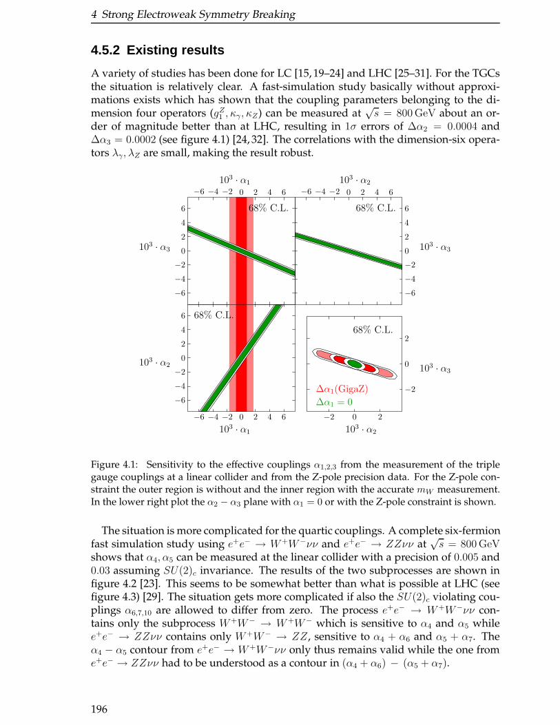
4 Strong Electroweak Symmetry Breaking
4.5.2 Existing results
A variety of studies has been done for LC [15, 19–24] and LHC [25–31]. For the TGCsthe situation is relatively clear. A fast-simulation study basically without approxi-mations exists which has shown that the coupling parameters belonging to the di-mension four operators (gZ1 , κγ, κZ) can be measured at
√s = 800 GeV about an or-
der of magnitude better than at LHC, resulting in 1σ errors of ∆α2 = 0.0004 and∆α3 = 0.0002 (see figure 4.1) [24, 32]. The correlations with the dimension-six opera-tors λγ, λZ are small, making the result robust.
−6 −4 −2 0 2 4 6
−6
−4
−2
0
2
4
6 68% C.L.
103 · α1
103 · α3
−6 −4 −2 0 2 4 6
−6
−4
−2
0
2
4
668% C.L.
103 · α3
103 · α2
−6 −4 −2 0 2 4 6
−6
−4
−2
0
2
4
6 68% C.L.
103 · α1
103 · α2
−2 0 2
−2
0
268% C.L.
∆α1(GigaZ)
∆α1 = 0
103 · α2
103 · α3
Figure 4.1: Sensitivity to the effective couplings α1,2,3 from the measurement of the triplegauge couplings at a linear collider and from the Z-pole precision data. For the Z-pole con-straint the outer region is without and the inner region with the accurate mW measurement.In the lower right plot the α2 − α3 plane with α1 = 0 or with the Z-pole constraint is shown.
The situation is more complicated for the quartic couplings. A complete six-fermionfast simulation study using e+e− → W+W−νν and e+e− → ZZνν at
√s = 800 GeV
shows that α4, α5 can be measured at the linear collider with a precision of 0.005 and0.03 assuming SU(2)c invariance. The results of the two subprocesses are shown infigure 4.2 [23]. This seems to be somewhat better than what is possible at LHC (seefigure 4.3) [29]. The situation gets more complicated if also the SU(2)c violating cou-plings α6,7,10 are allowed to differ from zero. The process e+e− → W+W−νν con-tains only the subprocess W+W− → W+W− which is sensitive to α4 and α5 whilee+e− → ZZνν contains only W+W− → ZZ, sensitive to α4 + α6 and α5 + α7. Theα4 − α5 contour from e+e− → W+W−νν only thus remains valid while the one frome+e− → ZZνν had to be understood as a contour in (α4 + α6) − (α5 + α7).
196
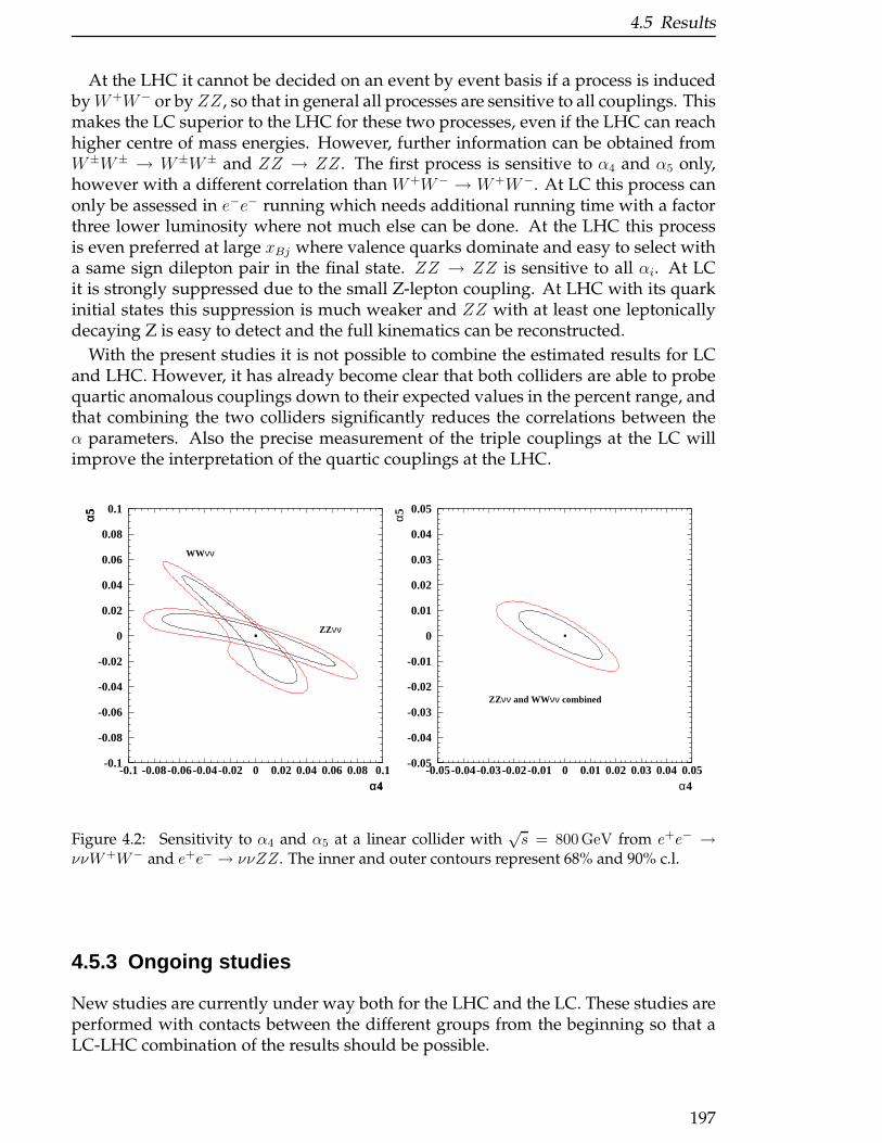
4.5 Results
At the LHC it cannot be decided on an event by event basis if a process is inducedbyW+W− or by ZZ, so that in general all processes are sensitive to all couplings. Thismakes the LC superior to the LHC for these two processes, even if the LHC can reachhigher centre of mass energies. However, further information can be obtained fromW±W± → W±W± and ZZ → ZZ. The first process is sensitive to α4 and α5 only,however with a different correlation than W+W− → W+W−. At LC this process canonly be assessed in e−e− running which needs additional running time with a factorthree lower luminosity where not much else can be done. At the LHC this processis even preferred at large xBj where valence quarks dominate and easy to select witha same sign dilepton pair in the final state. ZZ → ZZ is sensitive to all αi. At LCit is strongly suppressed due to the small Z-lepton coupling. At LHC with its quarkinitial states this suppression is much weaker and ZZ with at least one leptonicallydecaying Z is easy to detect and the full kinematics can be reconstructed.
With the present studies it is not possible to combine the estimated results for LCand LHC. However, it has already become clear that both colliders are able to probequartic anomalous couplings down to their expected values in the percent range, andthat combining the two colliders significantly reduces the correlations between theα parameters. Also the precise measurement of the triple couplings at the LC willimprove the interpretation of the quartic couplings at the LHC.
-0.1
-0.08
-0.06
-0.04
-0.02
0
0.02
0.04
0.06
0.08
0.1
-0.1 -0.08-0.06-0.04-0.02 0 0.02 0.04 0.06 0.08 0.1α4
α5
α4
α5
ZZνν
WWνν
-0.05
-0.04
-0.03
-0.02
-0.01
0
0.01
0.02
0.03
0.04
0.05
-0.05-0.04-0.03-0.02-0.01 0 0.01 0.02 0.03 0.04 0.05α4
α5
ZZνν and WWνν combined
Figure 4.2: Sensitivity to α4 and α5 at a linear collider with√s = 800GeV from e+e− →
ννW+W− and e+e− → ννZZ. The inner and outer contours represent 68% and 90% c.l.
4.5.3 Ongoing studies
New studies are currently under way both for the LHC and the LC. These studies areperformed with contacts between the different groups from the beginning so that aLC-LHC combination of the results should be possible.
197
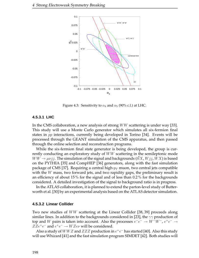
4 Strong Electroweak Symmetry Breaking
α4
α5
W+W+, W–W–
W+Z, W–Z
combined limit
W+W–
ZZ
-0.1
-0.075
-0.05
-0.025
0
0.025
0.05
0.075
0.1
-0.1 -0.075 -0.05 -0.025 0 0.025 0.05 0.075 0.1
Figure 4.3: Sensitivity to α4 and α5 (90% c.l.) at LHC.
4.5.3.1 LHC
In the CMS collaboration, a new analysis of strong WW scattering is under way [33].This study will use a Monte Carlo generator which simulates all six-fermion finalstates in pp interactions, currently being developed in Torino [34]. Events will beprocessed through the GEANT simulation of the CMS apparatus, and then passedthrough the online selection and reconstruction programs.
While the six-fermion final state generator is being developed, the group is cur-rently conducting an exploratory study of WW scattering in the semileptonic modeWW → µνjj. The simulation of the signal and backgrounds (ttX ,Wjj,WX) is basedon the PYTHIA [35] and CompHEP [36] generators, along with the fast simulationpackage of CMS [37]. Requiring a central high-pT muon, two central jets compatiblewith the W mass, two forward jets, and two rapidity gaps, the preliminary result isan efficiency of about 15 % for the signal and of less than 0.2 % for the backgroundsconsidered. A detailed investigation of the signal to background ratio is in progress.
In the ATLAS collaboration, it is planned to extend the parton-level study of Butter-worth et al. [30] by an experimental analysis based on the ATLAS detector simulation.
4.5.3.2 Linear Collider
Two new studies of WW scattering at the Linear Collider [38, 39] proceeds alongsimilar lines. In addition to the backgrounds considered in [23], the γγ production oftop and W pairs is taken into account. Also the processes e−e− → W−W−, e+e− →ZZe+e− and e+e− →WZeν will be considered.
Also a study ofWWZ andZZZ production in e+e− has started [40]. Also this studywill use Whizard [41] and the fast simulation program SIMDET [42]. Both studies will
198

4.6 Scenarios where the LHC sees resonances
be combined in a common fit for α4,5,6,7,10.
4.6 Scenarios where the LHC sees resonances
A LC can help interpret resonances that are seen in vector-boson scattering at theLHC. The LHC should be able to detect directly scalar and vector resonances withmasses up to about 2 TeV [30]. Vector resonances with masses in this range induceanomalous values for α2 and α3 which can readily be measured at a 500 GeV LC [43].In analogy with the pair-production of charged pions in e+e− annihilation near the ρresonance, a form factor FT can be used to describe the effects of vector resonances onthe pair production of longitudinally polarised W bosons in e+e− annihilation. Thereal part of FT − 1 is proportional to α2 + α3, and is related well below threshold tothe masses of the vector resonances by [44]
FT = 1 + s∑
k
akM2
k
, (4.46)
where√s is the e+e− centre of mass energy, Mk are the masses of the vector reso-
nances ordered by M1 < M2 < ..., and ak are their relative weights with∑ak = 1. In
ordinary QCD with vector meson dominance, a1 ≈ 1.A 500 GeV LC could measure the mass of a 1 TeV (1.5 TeV) vector resonance with
an accuracy of ,GeV (27 GeV) by measuring α2 + α3 under the assumption a1 = 1. Ameasurement of α2 + α3 which was consistent with the mass of the LHC resonancewould provide evidence for spin-1. By measuring both the real and imaginary partsof FT a 500 GeV LC would also provide a measurement of the vector resonance widthΓ1 with an error of 19 GeV (90 GeV) for a 1 TeV (1.5 TeV) vector resonance.
It is also possible to drop the assumption a1 = 1 and measure a1 directly. Measure-ments of the real and imaginary parts of FT at two different centre of mass energiescan be used to extract a1 along with the mass and width of the first vector resonance,assuming M1 ≪ M2. With 250 fb−1 luminosity at
√s = 0.35 TeV and 250 fb−1 lumi-
nosity at√s = 0.5 TeV, the mass, width and weight parameter a1 of a 1 TeV vector
resonance can be measured with accuracies of 101 GeV, 26 GeV, and 26%, respectively.At√s = 1 TeV a LC would be sitting on top of a 1 TeV vector resonance and would
measure the mass and width with a statistical accuracy of 0.08 GeV and 0.02 GeV,respectively, assuming a1 = 1 and a luminosity of 1000 fb−1. Again, a1 can be mea-sured by combining results from two different centre of mass energies. Assuming500 fb−1 luminosity at
√s = 0.5 TeV and 1000 fb−1 at
√s = 1 TeV, the mass, width,
and weight parameter a1 of a 1 TeV vector resonance can be measured with accura-cies of 0.08 GeV, 0.8 GeV, and 1.4%, respectively. If the vector resonance has a massof 1.5 TeV the same three parameters can be measured With accuracies of 44 GeV,16 GeV, and 10%, respectively, assuming the same combination of LC energies andluminosities.
If the resonance which was being produced at the LHC were a scalar, then the500 GeV LC would measure a value for α2 + α3 which was inconsistent with vectorresonance production. Hence the 500 GeV LC result could rule out a spin-1 interpreta-tion. A 0.8−1.0 TeV LC could also estimate the mass of a scalar resonance well above1 TeV by measuring the enhancement in the vector-boson scattering cross-section due
199
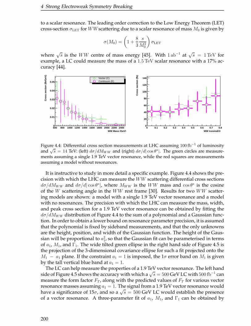
4 Strong Electroweak Symmetry Breaking
to a scalar resonance. The leading order correction to the Low Energy Theorem (LET)cross-section σLET for WW scattering due to a scalar resonance of mass M0 is given by
σ(M0) =
(1 +
8
3
s
M20
)σLET
where√s is the WW centre of mass energy [45]. With 1 ab−1 at
√s = 1 TeV for
example, a LC could measure the mass of a 1.5 TeV scalar resonance with a 17% ac-curacy [44].
WW Mass (GeV)600 800 1000 1200 1400 1600 1800 2000 2200 2400
Cro
ss s
ectio
n (f
b/G
eV)
0
0.01
0.02
0.03
0.04
0.05
Vector (C)Continuum (E)
)|*θWW |cosine(0 0.1 0.2 0.3 0.4 0.5 0.6 0.7 0.8
Cro
ss s
ectio
n (f
b)
0
20
40
60
80
100
120
140
Figure 4.4: Differential cross section measurements at LHC assuming 100 fb−1 of luminosityand
√s = 14 TeV: (left) dσ/dMWW and (right) dσ/d| cos θ∗|. The green circles are measure-
ments assuming a single 1.9 TeV vector resonance, while the red squares are measurementsassuming a model without resonances.
It is instructive to study in more detail a specific example. Figure 4.4 shows the pre-cision with which the LHC can measure the WW scattering differential cross sectionsdσ/dMWW and dσ/d| cos θ∗|, where MWW is the WW mass and cos θ∗ is the cosineof the W scattering angle in the WW rest frame [30]. Results for two WW scatter-ing models are shown: a model with a single 1.9 TeV vector resonance and a modelwith no resonances. The precision with which the LHC can measure the mass, width,and peak cross section for a 1.9 TeV vector resonance can be obtained by fitting thedσ/dMWW distribution of Figure 4.4 to the sum of a polynomial and a Gaussian func-tion. In order to obtain a lower bound on resonance parameter precision, it is assumedthat the polynomial is fixed by sideband measurements, and that the only unknownsare the height, position, and width of the Gaussian function. The height of the Gaus-sian will be proportional to a2
1, so that the Gaussian fit can be parameterised in termsof a1, M1, and Γ1. The wide tilted green ellipse in the right hand side of Figure 4.5 isthe projection of the 3-dimensional covariance ellipse for such a fit projected onto theM1 − a1 plane. If the constraint a1 = 1 is imposed, the 1σ error band on M1 is givenby the tall vertical blue band at a1 = 1.
The LC can help measure the properties of a 1.9 TeV vector resonance. The left handside of Figure 4.5 shows the accuracy with which a
√s = 500 GeV LC with 500 fb−1 can
measure the form factor FT , along with the predicted values of FT for various vectorresonance masses assuming a1 = 1. The signal from a 1.9 TeV vector resonance wouldhave a significance of 15σ, and so a
√s = 500 GeV LC would establish the presence
of a vector resonance. A three-parameter fit of a1, M1, and Γ1 can be obtained by
200

4.7 Conclusions
ECM=500 GEV L=500 fb
Re(FT)
Im
(FT
)
5
0.9 1 1.1 1.2 1.3 1.4-0.2
-0.1
0.0
0.1
0.2
5 555
5
1.2 TeV 1.6 TeV Mρ=2.5 TeV LET
95% C.L.
5555555555555555555555555555555555555555555555555555555555555555555555555555555555555555555555555555555555555555555555555555555555555555555555555555555555555555555555555555555555555555555555555555555555
55555555555555555555555555555555555555555555555555555555555555555555555555555555555555555555555555
555555555555555555555555555555555555555555555555555555555555555555555555555555555555555555555555555555555555555555555555555555555555555555555555555555555555555555555555555555555555555555555555555555555555555555555555555555555555555555555555555555555555555555555555555555555555555555555555555555555555
1650
1700
1750
1800
1850
1900
1950
2000
2050
2100
2150
0.5 0.6 0.7 0.8 0.9 1 1.1 1.2 1.3 1.4 1.5
a1
M1
(GeV
)Figure 4.5: Left: The 95% C.L. contour for FT measured at a LC with
√s = 500 GeV and
500 fb−1, along with values of FT for various vector resonance masses, assuming a1 = 1 .Right: Three dimensional covariance ellipses for fits of a1,M1,Γ1 projected onto the M1 − a1
plane. The wide tilted green ellipse (narrow tilted black ellipse) is obtained from LHC (LC)measurements. If it is assumed that a1 = 1 then the 1σ error for M1 from the LHC (LC) isgiven by the tall blue (short red) vertical band at a1 = 1.
combining the LC measurement of FT at√s = 500 GeV with a LC measurement
of FT at√s = 1000 GeV assuming a luminosity of 1000 fb−1. The projection of the
covariance ellipse for this fit onto the M1 − a1 plane is given by the narrow tiltedblack ellipse in the right hand side of Figure 4.5. If the constraint a1 = 1 is imposedthen the 1σ error band on M1 from LC measurements is given by the short verticalred band at a1 = 1.
The LHC is sensitive to vector resonances up to a mass of 1.5 GeV [28]. The LCcan distinguish the Standard Model from the Low Energy Theorem (LET) predictionwith 3.7 standard deviations at
√s = 500 GeV (L = 500fb−1) and with 10.7 standard
deviations at√s = 1000 GeV (L = 1000 fb−1). The LET prediction is given by the limit
of infinite mass. The mass sensitivity is 2.5 TeV and 4.1 TeV for√s = 500 GeV and√
s = 1000 GeV, where the sensitivity is defines as the mass which can be separatedwith 3σ from the LET.
4.7 Conclusions
While it is tempting to numerically combine the results of the existing LHC and LCstudies of strong WW scattering, this would be premature due to the mixed status ofthe theoretical and experimental approximations. For a meaningful comparison, it isessential that full six-fermion matrix elements are consistently used together withrealistic detector simulations. In particular, the effective-W approximation whichhas been adopted for most of the LHC studies misses the electroweak radiation of
201

4 Strong Electroweak Symmetry Breaking
transversally polarised W and Z bosons, which constitutes a numerically importantbackground that needs to be taken into account.
Nevertheless, one can already draw the conclusion that in the low-energy range itwill possible to measure anomalous couplings down to the natural scale 1/16π2. Acombination of LC and LHC data will considerably increase the resolving power ofthe LHC. Furthermore, the direct sensitivity of the LHC to resonances in the rangeabove 1 TeV can be fully exploited only if LC data on the cross section rise in thesub-TeV region are available.
202
Bibliography
[1] P.W. Higgs, Phys. Rev. Lett. 12 (1964) 132; Phys. Rev. Lett. 13 (1964) 508; Phys.Rev. 145 (1966) 1156; F. Englert and R. Brout, Phys. Rev. Lett. 13 (1964) 321;G.S. Guralnik, C.R. Hagen, and T.W. Kibble, Phys. Rev. Lett. 13 (1964) 585;T.W. Kibble, Phys. Rev. 155 (1967) 1554.
[2] S.L. Glashow, Nucl. Phys. 22 (1961) 579; A. Salam, in: N. Svartholm (ed.), Elemen-tary Particle Theory, Almqvist and Wiksells, Stockholm, 1968; S. Weinberg, Phys.Rev. Lett. 19 (1967) 1264.
[3] K. Hagiwara et al. (Particle Data Group), Phys. Rev. D. 66 (2002) 010001.
[4] see, e.g.: M.S. Chanowitz, LBNL-52452, hep-ph/0304199.
[5] B. Lee, C. Quigg and H. Thacker, Phys. Rev. Lett. 38 (1977) 883; Phys. Rev. D16(1977) 1519; D. Dicus and V. Mathur, Phys. Rev. D7 (1973) 3111.
[6] S. Weinberg, Phys. Rev. D13 (1976) 974; Phys. Rev. D19 (1979) 1277; L. Susskind,Phys. Rev. D20 (1979) 2619.
[7] For reviews of models of dynamical symmetry breaking, see: R. SekharChivukula, A. Cohen, and K. Lane, Nucl. Phys. B343 (1990) 554; G. Cvetic, Rev.Mod. Phys. 71 (1999) 513; C.T. Hill and E.H. Simmons, Strong Dynamics and Elec-troweak Symmetry Breaking, hep-ph/0203079, to appear in Phys. Rept.
[8] T. Appelquist and C. Bernard, Phys. Rev. D22 (1980) 200; A. Longhitano, Phys.Rev. D22 (1980) 1166; Nucl. Phys. B188 (1981) 118.
[9] S. Weinberg, Phys. Rev. Lett. 17 (1966) 616; M.S. Chanowitz, M. Golden, andH. Georgi, Phys. Rev. D36 (1987) 1490.
[10] S. Weinberg, Physica 96A (1979) 327.
[11] M. Peskin and T. Takeuchi, Phys. Rev. Lett. 65 (1990) 964; Phys. Rev. D46 (1992)381.
[12] K.J.F. Gaemers and G.J. Gounaris, Z. Phys. C1 (1979) 259; K. Hagiwara,K. Hikasa, R.D. Peccei, and D. Zeppenfeld, Nucl. Phys. B282 (1987) 253.
[13] A. Dobado and J.R. Pelaez, Phys. Rev. D56 (1997) 3057.
[14] S.N. Gupta, Quantum Electrodynamics, Gordon and Breach, 1981;M.S. Chanowitz, Phys. Rept. 320 (1999) 139.
[15] M. Diehl, O. Nachtmann, and F. Nagel, Eur. Phys. J. C27 (2003) 375.
203
Bibliography
[16] C.E. Vayonakis, Lett. Nuovo Cim. 17 (1976) 383; M.S. Chanowitz and M.K. Gail-lard, Nucl. Phys. B261 (1985) 379; G.J. Gounaris, R. Kogerler, and H. Neufeld,Phys. Rev. D34 (1986) 3257; Y.-P. Yao and C.-P. Yuan, Phys. Rev. D38 (1988) 2237;J. Bagger and C. Schmidt, Phys. Rev. D34 (1990) 264.
[17] M.S. Chanowitz and M.K. Gaillard, Phys. Lett. B142 (1984) 85; G.L. Kane,W.W. Repko, and W.R. Rolnick, Phys. Lett. B148 (1984) 367; S. Dawson, Nucl.Phys. B249 (1985) 42; J. Lindfors, Z. Phys. C28 (1985) 427; J.F. Gunion, J. Kali-nowski, and A. Tofighi-Niaki, Phys. Rev. Lett. 57 (1986) 2351.
[18] A. Denner and T. Hahn, Nucl. Phys. B525 (1998) 27.
[19] V. Barger, K. Cheung, and R.J.N. Phillips, Phys. Rev. D52 (1995) 3815.
[20] E.E. Boos, H.-J. He, W. Kilian, A. Pukhov, and P.M. Zerwas, Phys. Rev. D57 (1997)1553.
[21] E.E. Boos, H.-J. He, W. Kilian, A. Pukhov, and P.M. Zerwas, Phys. Rev. D61 (2000)077901.
[22] W. Kilian, in: Proceedings of the APS / DPF / DPB Summer Study on the Future ofParticle Physics (Snowmass 2001), eConf C010630 (2001) P106.
[23] R. Chierici, S. Rosati, and M. Kobel, LC-PHSM-2001-038, and in: J.A. Aguilar-Saavedra et al. (ECFA/DESY LC Physics Working Group), TESLA: Technicaldesign report. Part III: Physics at an e+e− Linear Collider, DESY-2001-011, hep-ph/0106315.
[24] W. Menges, A Study of Charged Current Triple Gauge Couplings at TESLA, LC-PHSM-2001-022.
[25] J. Bagger, V. Barger, K. Cheung, J. Gunion, T. Han, G.A. Ladinsky, R. Rosenfeld,and C.-P. Yuan, Phys. Rev. D49 (1994) 1246.
[26] J. Bagger, V. Barger, K. Cheung, J. Gunion, T. Han, G.A. Ladinsky, R. Rosenfeld,and C.-P. Yuan, Phys. Rev. D52 (1995) 3878.
[27] A. Dobado, M.J. Herrero, J.R. Pelaez, E. Ruiz Morales, and M.T. Urdiales, Phys.Lett. B352 (1995) 400; A. Dobado and M.T. Urdiales, Z. Phys. C71 (1996) 659.
[28] ATLAS Collaboration, Detector and Physics Performance Technical Design Report,CERN/LHCC/99-15.
[29] A.S. Belyaev, O.J.P. Eboli, M.C. Gonzalez-Garcia, J.K. Mizukoshi, S.F. Novaes,and I. Zacharov, Phys. Rev. D59 (1998) 015022.
[30] J.M. Butterworth, B.E. Cox, and J.R. Forshaw, Phys. Rev. D65 (2002) 096014.
[31] F. Gianotti et al., hep-ph/0204087.
[32] J. A. Aguilar-Saavedra et al., TESLA Technical Design Report Part III: Physics at ane+e− Linear Collider, DESY-01-011C.
204
Bibliography
[33] N. Amapane, M. Arneodo, G. Cerminara, A. Krokhotin, C. Mariotti, and P. Zych,work in progress.
[34] E. Accomando, A. Ballestrero, and E. Maina, work in progress.
[35] T. Sjostrand, Comput. Phys. Commun. 82 (1994) 74.
[36] A. Pukhov, E. Boos, M. Dubinin, V. Edneral, V. Ilyin, D. Kovalenko, A. Kryukov,V. Savrin, S. Shichanin, and A. Semenov, INP-MSU 98-41/542, hep-ph/9908288.
[37] S. Abdullin, A. Khanov and N. Stepanov, CMS TN/94-180.
[38] S. Boogert, B. Cox, I. Duerdoth, and A. Osorio, work in progress.
[39] P. Krstonosic et al., work in progress.
[40] M. Beyer et al., work in progress.
[41] W. Kilian, LC-TOOL-2000-039.
[42] M. Pohl and H. Schreiber, DESY 99–030.
[43] The American Linear Collider Working Group, T. Abe et al., Proc. of theAPS/DPF/DPB Summer Study on the Future of Particle Physics (Snowmass 2001) ed.N. Graf, hep-ex/0106057.
[44] T. L. Barklow, Proc. of the APS/DPF/DPB Summer Study on the Future of Par-ticle Physics (Snowmass 2001) ed. N. Graf, eConf C010630 (2001) E3067, hep-ph/0112286.
[45] T. L. Barklow et al., hep-ph/9704217.
205

Bibliography
206
5 Supersymmetric Models
Editors: K. Desch, K. Kawagoe, M.M. Nojiri, G. Polesello
5.1 Measurement of supersymmetric particle masses,mixings and couplings at LHC and LC
The precise measurement of the masses of the largest possible set of supersymmet-ric particles is the most important input to the reconstruction of the supersymmetrictheory, in particular of the SUSY breaking mechanism. At the LHC, the dominantproduction mechanism is pair production of gluinos or squarks and associated pro-duction of a gluino and a squark. For these processes, SUSY particle masses haveto be calculated from the reconstruction of long decay chains which end in the LSP.Invariant masses can only be estimated from the endpoints (edges) of invariant massspectra. In particular the LSP mass is only slightly constrained. This uncertaintypropagates into the errors of the heavier SUSY particle masses.
At a LC, the colour–neutral part of the SUSY particle spectrum can be reconstructedwith high precision if it is kinematically accessible. In particular, the LSP mass canbe reconstructed with a precision significantly better than 1 GeV. If this and furtherLC measurements are input into the LHC mass fits, significant improvement on themasses which can only be accessed by the LHC (in particular squarks and gluinos)can be achieved.
The following studies focus on an analysis of the SUSY benchmark point SPS 1a,a typical mSugra scenario, but further model points are investigated as well in Sec-tion 5.1.3. The main features of the SPS 1a benchmark scenario are summarised in Sec-tion 5.1.1 for later reference. Section 5.1.2 outlines simulations for the reconstructionof a large set of SUSY particles in ATLAS. Section 5.1.3 describes the reconstruction ofsquarks and gluinos in CMS. In Section 5.1.4 SUSY searches at the LC are discussedand the experimental accuracies achievable in the SPS 1a scenario are analysed. Theinfluence of LC mass measurements on the ATLAS and CMS analyses is discussed indetail in Section 5.1.5. In Section 5.1.6 it is demonstrated that LC predictions can becrucial for guiding the LHC search for the heaviest neutralino. In this way the heav-iest neutralino can be identified at the LHC and its mass can be measured with highprecision. Feeding this information back into the LC analysis leads to an improvedaccuracy in the determination of the SUSY parameters in the neutralino and charginosector. Section 5.1.7 focusses on stop and sbottom reconstruction at the LHC usinginput from the LC.
So far only few detailed case studies for SUSY parameter determinations at LHCand LC exist. Further LC information such as decay branching ratios is likely to behelpful for an extraction of SUSY particle couplings at the LHC. While the studiesperformed so far have mostly been restricted to the SPS 1a benchmark point, which
207
5 Supersymmetric Models
is a favourable scenario both for LHC and LC, examples of other possible scenariosshould be investigated as well. It can be expected that also in this case importantsynergy effects will arise from the LHC / LC interplay.
5.1.1 The SPS 1a benchmark scenario
H.-U. Martyn and G. Weiglein
5.1.1.1 Introduction
In the unconstrained version of the Minimal Supersymmetric extension of the Stan-dard Model (MSSM) no particular Supersymmetry (SUSY) breaking mechanism isassumed, but rather a parametrisation of all possible soft SUSY breaking terms isused. This leads to more than a hundred parameters (masses, mixing angles, phases)in this model in addition to the ones of the Standard Model. For performing detailedsimulations of experimental signatures within detectors of high-energy physics ex-periments it is clearly not practicable to scan over a multi-dimensional parameterspace. One thus often concentrates on certain “typical” benchmark scenarios.
The “Snowmass Points and Slopes” (SPS) [1] are a set of benchmark points andparameter lines in the MSSM parameter space corresponding to different scenariosin the search for Supersymmetry at present and future experiments. The SPS 1a ref-erence point is a “typical” parameter point of the minimal supergravity (mSUGRA)scenario. It gives rise to a particle spectrum where many states are accessible both atthe LHC and the LC, corresponding to a rather favourable scenario for phenomenol-ogy at LHC and LC. The SPS 1a benchmark scenario has been studied with detailedexperimental simulations at both colliders.
Since for no other parameter point in the MSSM a similar amount of informationabout the experimental capabilities of both the LHC and the LC is available, mostanalyses performed in the context of the LHC / LC Study Group have focussed onthis particular parameter point. It should be kept in mind, however, that the interplaybetween LHC and LC could be qualitatively very different in different regions of theMSSM parameter space. In order to allow a quantitative assessment of the LHC / LCinterplay also for other parameter regions, more experimental simulations for LHCand LC are required.
5.1.1.2 Definition of the SPS 1a benchmark point
The SPS benchmark points are defined in terms of low-energy MSSM parameters.The benchmark values for the SPS 1a point are the following (all mass parameters aregiven in GeV) [1,2]. The gluino mass Mg, the Supersymmetric Higgs mass parameterµ, the mass of the CP-odd Higgs boson MA, the ratio of the vacuum expectation val-ues of the two Higgs doublets tanβ, and the electroweak gaugino mass parametersM1 and M2 have the values
Mg = 595.2, µ = 352.4, MA = 393.6, tan β = 10, M1 = 99.1, M2 = 192.7.(5.1)
208
5.1 Measurement of supersymmetric particle masses, mixings and couplings at LHC and LC
The soft SUSY-breaking parameters in the diagonal entries of the squark and slep-ton mass matrices have been chosen to be the same for the first and second genera-tion. They have the values (these parameters are approximately equal to the sfermionmasses; the off-diagonal entries have been neglected for the first two generations; theindex i in MqiL refers to the generation)
Mq1L= Mq2L
= 539.9, MdR= 519.5, MuR
= 521.7, MeL= 196.6, MeR
= 136.2.(5.2)
The soft SUSY-breaking parameters in the diagonal entries of the squark and sleptonmass matrices of the third generation have the values
Mq3L= 495.9, MbR
= 516.9, MtR = 424.8, MτL = 195.8, MτR = 133.6, (5.3)
while the trilinear couplings of the third generation read
At = −510.0, Ab = −772.7, Aτ = −254.2. (5.4)
All mass parameters for the benchmark point SPS 1a are to be understood as definedin the DR scheme at the scale Q = 453.6 GeV. The value of the top-quark mass for allSPS benchmarks is chosen to be mt = 175 GeV.
As mentioned above, these low-energy parameters correspond to a “typical”mSUGRA point with an intermediate value of tan β. In order to obtain these low-energy parameters from the high-scale parameters m0, m1/2, A0 of the mSUGRA sce-nario a particular code had to be chosen. For the SPS benchmarks this was version7.58 of the program ISAJET [3]. Once the low-energy parameters have been fixed,this choice is no longer relevant. The mSUGRA parameters used for generating theSPS 1a benchmark values are
m0 = 100GeV, m1/2 = 250GeV, A0 = −100GeV, tan β = 10, µ > 0. (5.5)
5.1.1.3 Particle spectrum and decay modes
While the low-energy MSSM parameters have been fixed as benchmarks by defini-tion, the particle spectra, branching ratios, etc. for the SPS points should be calcu-lated with an appropriate program according to the specific requirements of the anal-ysis that is being performed. For simplicity, the spectrum shown in Fig. 5.1 and thebranching ratios of the SUSY particles and the Higgs bosons listed in Tab. 5.1–5.4,see Ref. [4], have been obtained with ISAJET 7.58, although parts of this code are notstate-of-the-art. The resulting spectra and branching ratios have been widely used forexploring the physics potential of LHC and LC.
The SPS 1a scenario yields a sparticle spectrum, see Fig. 5.1, of which many statesare accessible both at LHC and LC. Experimentally important and challenging, how-ever, are the τ -rich neutralino and chargino decays, see Tab. 5.2. This is a genericfeature of SUSY scenarios with intermediate or large values of tanβ (the parameterspace at smaller values of tan β is severely constrained by the exclusion bounds fromthe LEP Higgs searches [5, 6]). A non-negligible mixing leads to a significant masssplitting between the two staus so that the lighter stau becomes the lightest slep-ton. Neutralinos and charginos therefore decay predominantly into staus and taus,
209
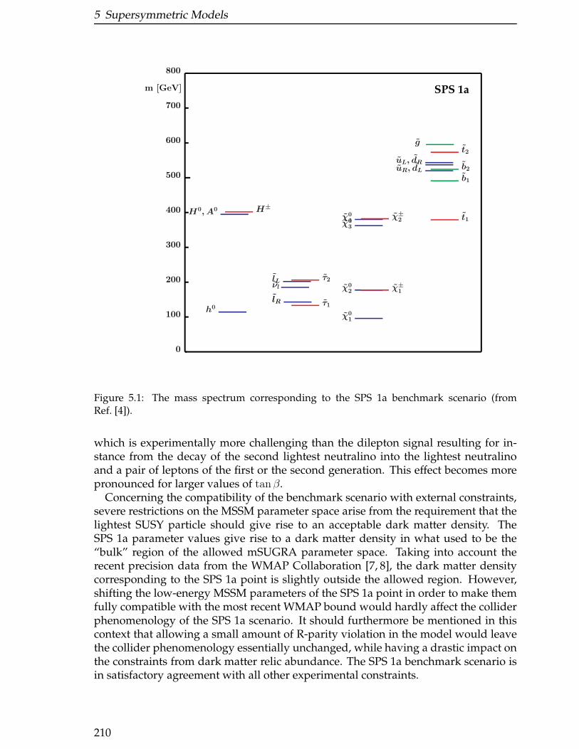
5 Supersymmetric Models
SPS 1a
0
100
200
300
400
500
600
700
800
m [GeV]
lR
lLνl
τ1
τ2
χ0
1
χ0
2
χ0
3
χ0
4
χ±
1
χ±
2
uL, dRuR, dL
g
t1
t2
b1
b2
h0
H0, A0 H±
Figure 5.1: The mass spectrum corresponding to the SPS 1a benchmark scenario (fromRef. [4]).
which is experimentally more challenging than the dilepton signal resulting for in-stance from the decay of the second lightest neutralino into the lightest neutralinoand a pair of leptons of the first or the second generation. This effect becomes morepronounced for larger values of tanβ.
Concerning the compatibility of the benchmark scenario with external constraints,severe restrictions on the MSSM parameter space arise from the requirement that thelightest SUSY particle should give rise to an acceptable dark matter density. TheSPS 1a parameter values give rise to a dark matter density in what used to be the“bulk” region of the allowed mSUGRA parameter space. Taking into account therecent precision data from the WMAP Collaboration [7, 8], the dark matter densitycorresponding to the SPS 1a point is slightly outside the allowed region. However,shifting the low-energy MSSM parameters of the SPS 1a point in order to make themfully compatible with the most recent WMAP bound would hardly affect the colliderphenomenology of the SPS 1a scenario. It should furthermore be mentioned in thiscontext that allowing a small amount of R-parity violation in the model would leavethe collider phenomenology essentially unchanged, while having a drastic impact onthe constraints from dark matter relic abundance. The SPS 1a benchmark scenario isin satisfactory agreement with all other experimental constraints.
210
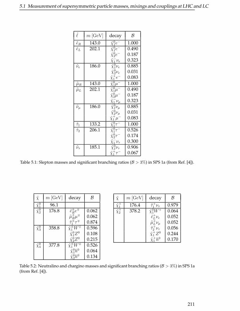
5.1 Measurement of supersymmetric particle masses, mixings and couplings at LHC and LC
ℓ m [GeV] decay BeR 143.0 χ0
1e− 1.000
eL 202.1 χ01e
− 0.490χ0
2e− 0.187
χ−1 νe 0.323
νe 186.0 χ01νe 0.885χ0
2νe 0.031χ+
1 e− 0.083
µR 143.0 χ01µ
− 1.000µL 202.1 χ0
1µ− 0.490
χ02µ
− 0.187χ−
1 νµ 0.323νµ 186.0 χ0
1νµ 0.885χ0
2νµ 0.031χ+
1 µ− 0.083
τ1 133.2 χ01τ
− 1.000τ2 206.1 χ0
1τ− 0.526
χ02τ
− 0.174χ−
1 ντ 0.300ντ 185.1 χ0
1ντ 0.906χ+
1 τ− 0.067
Table 5.1: Slepton masses and significant branching ratios (B > 3%) in SPS 1a (from Ref. [4]).
χ m [GeV] decay Bχ0
1 96.1χ0
2 176.8 e±Re∓ 0.062
µ±Rµ
∓ 0.062τ±1 τ
∓ 0.874χ0
3 358.8 χ±1 W
∓ 0.596χ0
1Z0 0.108
χ02Z
0 0.215χ0
4 377.8 χ±1 W
∓ 0.526χ0
1h0 0.064
χ02h
0 0.134
χ m [GeV] decay Bχ+
1 176.4 τ+1 ντ 0.979
χ+2 378.2 χ0
1W+ 0.064
e+Lνe 0.052µ+Lνµ 0.052τ+2 ντ 0.056χ+
1 Z0 0.244
χ+1 h
0 0.170
Table 5.2: Neutralino and chargino masses and significant branching ratios (B > 3%) in SPS 1a(from Ref. [4]).
211

5 Supersymmetric Models
q m [GeV] decay Bt1 379.1 χ0
1t 0.179χ0
2t 0.095χ+
1 b 0.726t2 574.7 χ+
1 b 0.206χ+
2 b 0.216Z0t1 0.225h0t1 0.042χ0
1t 0.030χ0
2t 0.080χ0
3t 0.033χ0
4t 0.166
q m [GeV] decay Bb1 491.9 χ0
1b 0.062χ0
2b 0.362χ−
1 t 0.428W−t1 0.133
b2 524.6 χ01b 0.148χ0
2b 0.171χ0
3b 0.053χ0
4b 0.072χ−
1 t 0.213W−t1 0.344
Table 5.3: Stop and sbottom masses and significant branching ratios (B > 3%) in SPS 1a (fromRef. [4]).
Higgs m [GeV] decay Bh0 114.0 τ−τ+ 0.051
bb 0.847cc 0.035
H0 394.1 τ−τ+ 0.059bb 0.807tt 0.031
χ01χ
02 0.034
A0 393.6 τ−τ+ 0.049bb 0.681tt 0.092
χ01χ
02 0.065
χ02χ
02 0.058
H+ 401.8 νττ+ 0.077
tb 0.770χ+
1 χ01 0.130
Table 5.4: Higgs masses and significant branching ratios (B > 3%) in SPS 1a (from Ref. [4]).
212
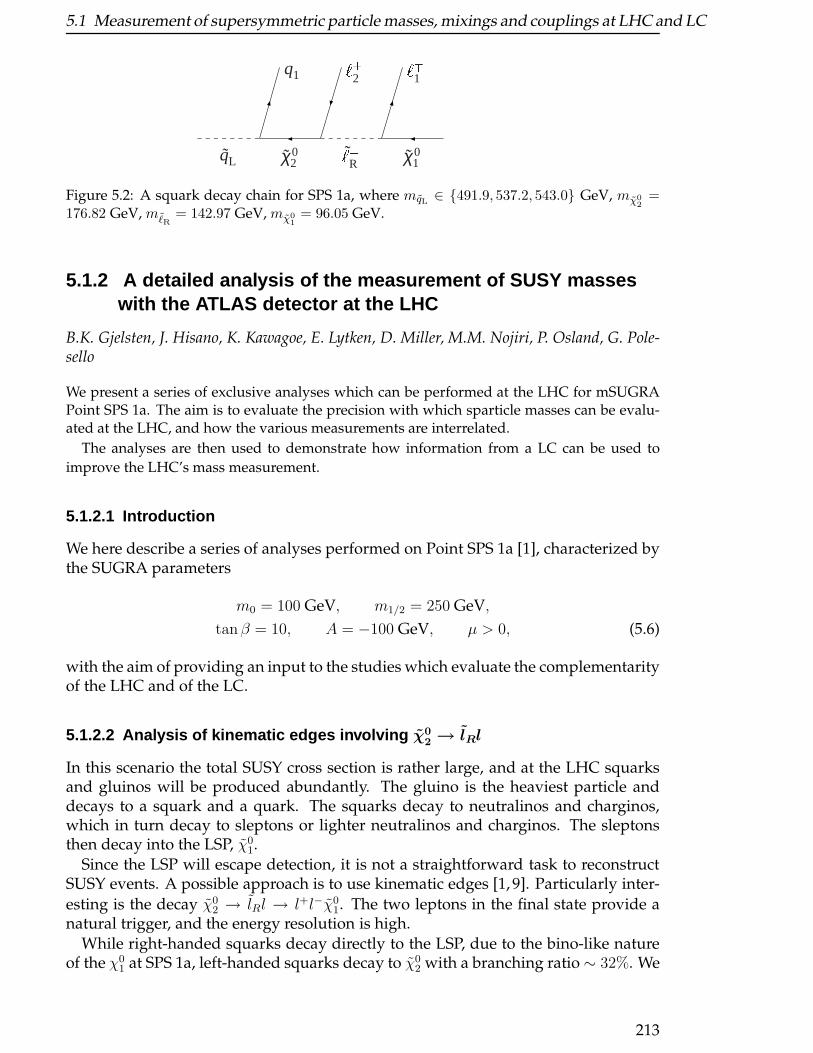
5.1 Measurement of supersymmetric particle masses, mixings and couplings at LHC and LC
qL χ02
q1 `2˜R
`1χ0
1
Figure 5.2: A squark decay chain for SPS 1a, where mqL ∈ 491.9, 537.2, 543.0 GeV, mχ02
=176.82 GeV, mℓR
= 142.97 GeV, mχ01
= 96.05 GeV.
5.1.2 A detailed analysis of the measurement of SUSY masseswith the ATLAS detector at the LHC
B.K. Gjelsten, J. Hisano, K. Kawagoe, E. Lytken, D. Miller, M.M. Nojiri, P. Osland, G. Pole-sello
We present a series of exclusive analyses which can be performed at the LHC for mSUGRAPoint SPS 1a. The aim is to evaluate the precision with which sparticle masses can be evalu-ated at the LHC, and how the various measurements are interrelated.
The analyses are then used to demonstrate how information from a LC can be used to
improve the LHC’s mass measurement.
5.1.2.1 Introduction
We here describe a series of analyses performed on Point SPS 1a [1], characterized bythe SUGRA parameters
m0 = 100 GeV, m1/2 = 250 GeV,
tanβ = 10, A = −100 GeV, µ > 0, (5.6)
with the aim of providing an input to the studies which evaluate the complementarityof the LHC and of the LC.
5.1.2.2 Analysis of kinematic edges involving χ02
→ lRl
In this scenario the total SUSY cross section is rather large, and at the LHC squarksand gluinos will be produced abundantly. The gluino is the heaviest particle anddecays to a squark and a quark. The squarks decay to neutralinos and charginos,which in turn decay to sleptons or lighter neutralinos and charginos. The sleptonsthen decay into the LSP, χ0
1.Since the LSP will escape detection, it is not a straightforward task to reconstruct
SUSY events. A possible approach is to use kinematic edges [1, 9]. Particularly inter-
esting is the decay χ02 → lRl → l+l−χ0
1. The two leptons in the final state provide anatural trigger, and the energy resolution is high.
While right-handed squarks decay directly to the LSP, due to the bino-like natureof the χ0
1 at SPS 1a, left-handed squarks decay to χ02 with a branching ratio ∼ 32%. We
213
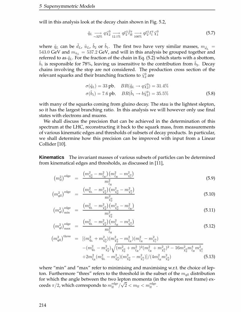
5 Supersymmetric Models
will in this analysis look at the decay chain shown in Fig. 5.2,
qL −→∼32%
qχ02 −→
12.1%ql±2 l
∓R −→
100%ql±2 l
∓1 χ
01 (5.7)
where qL can be dL, uL, b2 or b1. The first two have very similar masses, mdL=
543.0 GeV and muL= 537.2 GeV, and will in this analysis be grouped together and
referred to as qL. For the fraction of the chain in Eq. (5.2) which starts with a sbottom,
b1 is responsible for 78%, leaving us insensitive to the contribution from b2. Decaychains involving the stop are not considered. The production cross section of therelevant squarks and their branching fractions to χ0
2 are
σ(qL) = 33 pb, BR(qL → qχ02) = 31.4%
σ(b1) = 7.6 pb, BR(b1 → bχ02) = 35.5% (5.8)
with many of the squarks coming from gluino decay. The stau is the lightest slepton,so it has the largest branching ratio. In this analysis we will however only use finalstates with electrons and muons.
We shall discuss the precision that can be achieved in the determination of thisspectrum at the LHC, reconstructing it back to the squark mass, from measurementsof various kinematic edges and thresholds of subsets of decay products. In particular,we shall determine how this precision can be improved with input from a LinearCollider [10].
Kinematics The invariant masses of various subsets of particles can be determinedfrom kinematical edges and thresholds, as discussed in [11],
(m2ll
)edge=
(m2χ0
2−m2
lR
)(m2lR−m2
χ01
)
m2lR
(5.9)
(m2qll
)edge=
(m2qL−m2
χ02
)(m2χ0
2−m2
χ01
)
m2χ0
2
(5.10)
(m2ql
)edge
min=
(m2qL−m2
χ02
)(m2χ0
2−m2
lR
)
m2χ0
2
(5.11)
(m2ql
)edge
max=
(m2qL−m2
χ02
)(m2lR−m2
χ01
)
m2lR
(5.12)
(m2qll
)thres= [(m2
qL+m2
χ02)(m2
χ02−m2
lR)(m2
lR−m2
χ01)
−(m2qL−m2
χ02)√
(m2χ0
2+m2
lR)2(m2
lR+m2
χ01)2 − 16m2
χ02m4lRm2χ0
1
+2m2lR
(m2qL−m2
χ02)(m2
χ02−m2
χ01)]/(4m2
lRm2χ0
2) (5.13)
where “min” and “max” refer to minimising and maximising w.r.t. the choice of lep-ton. Furthermore “thres” refers to the threshold in the subset of the mqll distributionfor which the angle between the two lepton momenta (in the slepton rest frame) ex-
ceeds π/2, which corresponds to medgell /√
2 < mll < medgell .
214
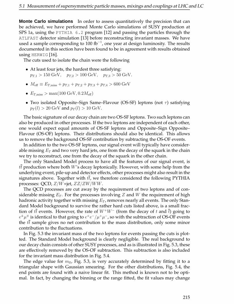
5.1 Measurement of supersymmetric particle masses, mixings and couplings at LHC and LC
Monte Carlo simulations In order to assess quantitatively the precision that canbe achieved, we have performed Monte Carlo simulations of SUSY production atSPS 1a, using the PYTHIA 6.2 program [12] and passing the particles through theATLFASTdetector simulation [13] before reconstructing invariant masses. We haveused a sample corresponding to 100 fb−1, one year at design luminosity. The resultsdocumented in this section have been found to be in agreement with results obtainedusing HERWIG[16].
The cuts used to isolate the chain were the following
• At least four jets, the hardest three satisfying:pT,1 > 150 GeV, pT,2 > 100 GeV, pT,3 > 50 GeV.
• Meff ≡ ET,miss + pT,1 + pT,2 + pT,3 + pT,4 > 600 GeV
• ET,miss > max(100 GeV, 0.2Meff)
• Two isolated Opposite–Sign Same–Flavour (OS-SF) leptons (not τ ) satisfyingpT (l) > 20 GeV and pT (l) > 10 GeV.
The basic signature of our decay chain are two OS-SF leptons. Two such leptons canalso be produced in other processes. If the two leptons are independent of each other,one would expect equal amounts of OS-SF leptons and Opposite–Sign Opposite–Flavour (OS-OF) leptons. Their distributions should also be identical. This allowsus to remove the background OS-SF contribution by subtracting the OS-OF events.
In addition to the two OS-SF leptons, our signal event will typically have consider-able missing ET and two very hard jets, one from the decay of the squark in the chainwe try to reconstruct, one from the decay of the squark in the other chain.
The only Standard Model process to have all the features of our signal event, istt production where both W ’s decay leptonically. However, with some help from theunderlying event, pile-up and detector effects, other processes might also result in thesignatures above. Together with tt, we therefore considered the following PYTHIAprocesses: QCD, Z/W+jet, ZZ/ZW/WW .
The QCD processes are cut away by the requirement of two leptons and of con-siderable missing ET . For the processes involving Z and W the requirement of highhadronic activity together with missing ET , removes nearly all events. The only Stan-dard Model background to survive the rather hard cuts listed above, is a small frac-tion of tt events. However, the rate of W+W− (from the decay of t and t) going toe±µ∓ is identical to that going to e+e−/µ+µ−, so with the subtraction of OS-OF eventsthe tt sample gives no net contribution to the mass distribution, only some minorcontribution to the fluctuations.
In Fig. 5.3 the invariant mass of the two leptons for events passing the cuts is plot-ted. The Standard Model background is clearly negligible. The real background toour decay chain consists of other SUSY processes, and as is illustrated in Fig. 5.3, theseare effectively removed by the OS-OF subtraction. This subtraction is also includedfor the invariant mass distribution in Fig. 5.4.
The edge value for mll, Fig. 5.3, is very accurately determined by fitting it to atriangular shape with Gaussian smearing. For the other distributions, Fig. 5.4, theend points are found with a naive linear fit. This method is known not to be opti-mal. In fact, by changing the binning or the range fitted, the fit values may change
215

5 Supersymmetric Models
(GeV)llm0 20 40 60 80 100
-1E
vent
s/1
GeV
/100
fb
0
200
400
600
800
(GeV)llm0 20 40 60 80 100
-1E
vent
s/1
GeV
/100
fb
0
200
400
600
800
Figure 5.3: Effect of subtracting background leptons, for∫Ldt = 100 fb−1. Left: Solid: OS-
SF, Dotted: OS-OF, Two upper curves: SUSY+SM, two lower curves: SM alone; Right: OS-SF−OS-OF. The triangular shape of the theoretical expectation is reproduced.
by typically a few GeV. For a more realistic situation one would need to investigatemore thoroughly how the theoretical distributions are distorted by sparticle widths,by the detector resolution and the cuts applied. As already discussed in [11], it isnot possible at the level of the present studies to perform a detailed estimate of thecorresponding systematic errors, therefore we include only the statistical errors fromthe fitting procedure for each edge. In addition one has the systematic error on theenergy scale. We use the ATLAS benchmark values, 0.1% for leptons and 1% for jets.The resulting values for the endpoints and the corresponding errors are given in table5.5.
Table 5.5: Endpoint values found from fitting the edges in Fig. 5.3 and Fig. 5.4, for 100 fb−1.
Edge Nominal Value Fit Value Syst. Error StatisticalEnergy Scale Error
m(ll)edge 77.077 77.024 0.08 0.05m(qll)edge 431.1 431.3 4.3 2.4
m(ql)edgemin 302.1 300.8 3.0 1.5
m(ql)edgemax 380.3 379.4 3.8 1.8
m(qll)thres 203.0 204.6 2.0 2.8m(bll)thres 183.1 181.1 1.8 6.3
5.1.2.3 Gluino mass measurement
In the considered point the gluino decays through g → qq, where q is any squarkflavour, except t2, for which the decay g → t2t is kinematically forbidden. Thusthe reconstruction of the gluino can be attempted adding a quark to an identified
216

5.1 Measurement of supersymmetric particle masses, mixings and couplings at LHC and LC
(GeV)qllm0 200 400 600
-1E
vent
s/5
GeV
/100
fb
0
200
400
600
(GeV)Thresqllm
0 200 400 600
-1E
vent
s/5
GeV
/100
fb
0
100
200
300
(GeV)Minqlm
0 200 400 600
-1E
vent
s/5
GeV
/100
fb
0
100
200
(GeV)Maxqlm
0 200 400 600
-1E
vent
s/5
GeV
/100
fb
0
100
200
300
(GeV)Thresbllm
0 200 400 600
-1E
vent
s/5
GeV
/100
fb
0
20
40
Figure 5.4: Invariant mass distributions with kinematical endpoints, for∫Ldt = 100 fb−1.
217
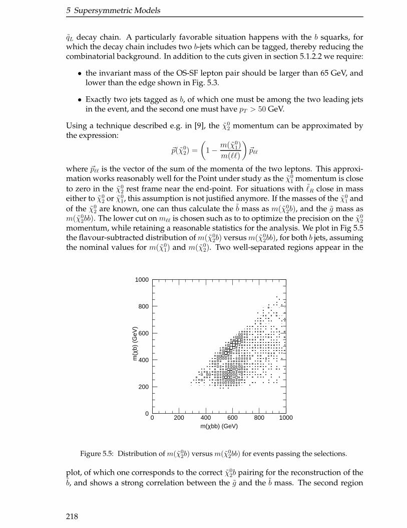
5 Supersymmetric Models
qL decay chain. A particularly favorable situation happens with the b squarks, forwhich the decay chain includes two b-jets which can be tagged, thereby reducing thecombinatorial background. In addition to the cuts given in section 5.1.2.2 we require:
• the invariant mass of the OS-SF lepton pair should be larger than 65 GeV, andlower than the edge shown in Fig. 5.3.
• Exactly two jets tagged as b, of which one must be among the two leading jetsin the event, and the second one must have pT > 50 GeV.
Using a technique described e.g. in [9], the χ02 momentum can be approximated by
the expression:
~p(χ02) =
(1− m(χ0
1)
m(ℓℓ)
)~pℓℓ
where ~pℓℓ is the vector of the sum of the momenta of the two leptons. This approxi-mation works reasonably well for the Point under study as the χ0
1 momentum is close
to zero in the χ02 rest frame near the end-point. For situations with ℓR close in mass
either to χ02 or χ0
1, this assumption is not justified anymore. If the masses of the χ01 and
of the χ02 are known, one can thus calculate the b mass as m(χ0
2b), and the g mass asm(χ0
2bb). The lower cut on mℓℓ is chosen such as to to optimize the precision on the χ02
momentum, while retaining a reasonable statistics for the analysis. We plot in Fig 5.5the flavour-subtracted distribution ofm(χ0
2b) versusm(χ02bb), for both b jets, assuming
the nominal values for m(χ01) and m(χ0
2). Two well-separated regions appear in the
0
200
400
600
800
1000
0 200 400 600 800 1000m(χbb) (GeV)
m(χ
b) (
GeV
)
Figure 5.5: Distribution of m(χ02b) versus m(χ0
2bb) for events passing the selections.
plot, of which one corresponds to the correct χ02b pairing for the reconstruction of the
b, and shows a strong correlation between the g and the b mass. The second region
218
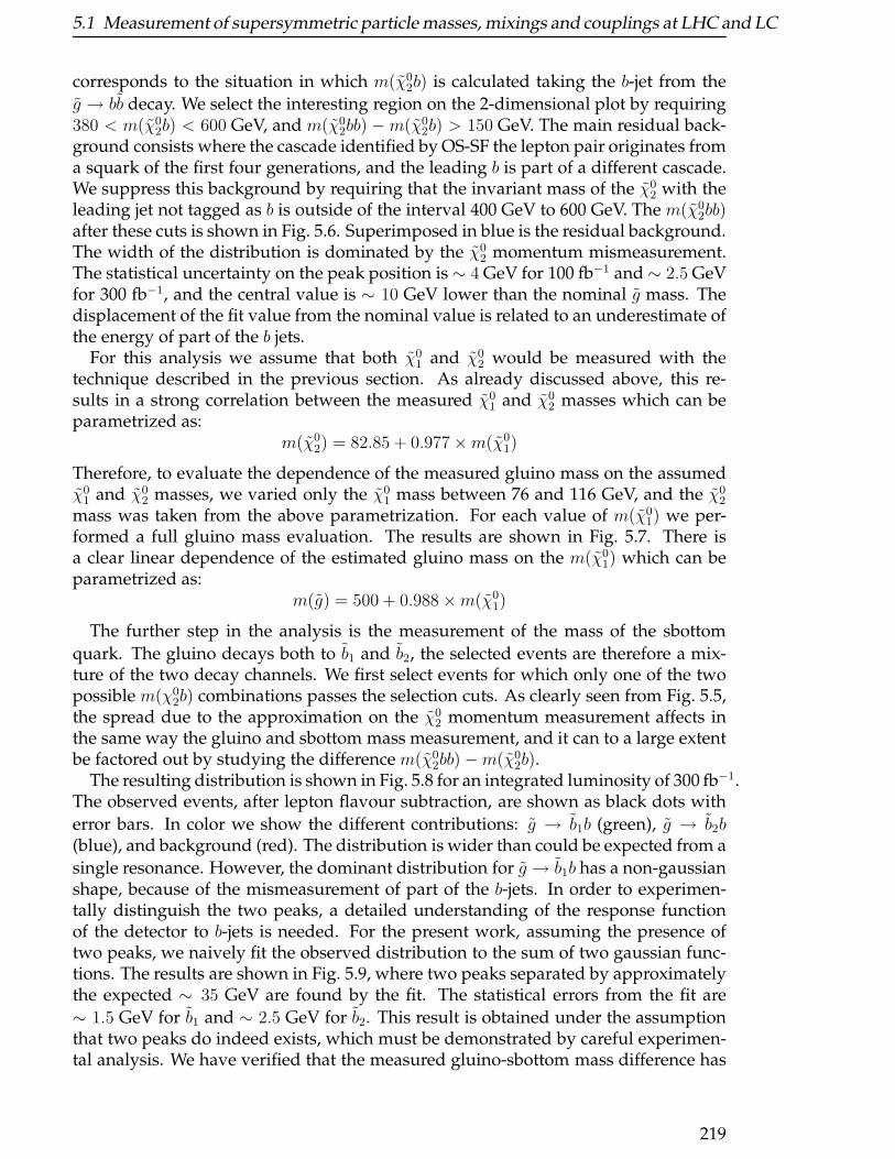
5.1 Measurement of supersymmetric particle masses, mixings and couplings at LHC and LC
corresponds to the situation in which m(χ02b) is calculated taking the b-jet from the
g → bb decay. We select the interesting region on the 2-dimensional plot by requiring380 < m(χ0
2b) < 600 GeV, and m(χ02bb) −m(χ0
2b) > 150 GeV. The main residual back-ground consists where the cascade identified by OS-SF the lepton pair originates froma squark of the first four generations, and the leading b is part of a different cascade.We suppress this background by requiring that the invariant mass of the χ0
2 with theleading jet not tagged as b is outside of the interval 400 GeV to 600 GeV. The m(χ0
2bb)after these cuts is shown in Fig. 5.6. Superimposed in blue is the residual background.The width of the distribution is dominated by the χ0
2 momentum mismeasurement.The statistical uncertainty on the peak position is∼ 4 GeV for 100 fb−1 and∼ 2.5 GeVfor 300 fb−1, and the central value is ∼ 10 GeV lower than the nominal g mass. Thedisplacement of the fit value from the nominal value is related to an underestimate ofthe energy of part of the b jets.
For this analysis we assume that both χ01 and χ0
2 would be measured with thetechnique described in the previous section. As already discussed above, this re-sults in a strong correlation between the measured χ0
1 and χ02 masses which can be
parametrized as:m(χ0
2) = 82.85 + 0.977×m(χ01)
Therefore, to evaluate the dependence of the measured gluino mass on the assumedχ0
1 and χ02 masses, we varied only the χ0
1 mass between 76 and 116 GeV, and the χ02
mass was taken from the above parametrization. For each value of m(χ01) we per-
formed a full gluino mass evaluation. The results are shown in Fig. 5.7. There isa clear linear dependence of the estimated gluino mass on the m(χ0
1) which can beparametrized as:
m(g) = 500 + 0.988×m(χ01)
The further step in the analysis is the measurement of the mass of the sbottom
quark. The gluino decays both to b1 and b2, the selected events are therefore a mix-ture of the two decay channels. We first select events for which only one of the twopossible m(χ0
2b) combinations passes the selection cuts. As clearly seen from Fig. 5.5,the spread due to the approximation on the χ0
2 momentum measurement affects inthe same way the gluino and sbottom mass measurement, and it can to a large extentbe factored out by studying the difference m(χ0
2bb)−m(χ02b).
The resulting distribution is shown in Fig. 5.8 for an integrated luminosity of 300 fb−1.The observed events, after lepton flavour subtraction, are shown as black dots with
error bars. In color we show the different contributions: g → b1b (green), g → b2b(blue), and background (red). The distribution is wider than could be expected from a
single resonance. However, the dominant distribution for g → b1b has a non-gaussianshape, because of the mismeasurement of part of the b-jets. In order to experimen-tally distinguish the two peaks, a detailed understanding of the response functionof the detector to b-jets is needed. For the present work, assuming the presence oftwo peaks, we naively fit the observed distribution to the sum of two gaussian func-tions. The results are shown in Fig. 5.9, where two peaks separated by approximatelythe expected ∼ 35 GeV are found by the fit. The statistical errors from the fit are
∼ 1.5 GeV for b1 and ∼ 2.5 GeV for b2. This result is obtained under the assumptionthat two peaks do indeed exists, which must be demonstrated by careful experimen-tal analysis. We have verified that the measured gluino-sbottom mass difference has
219
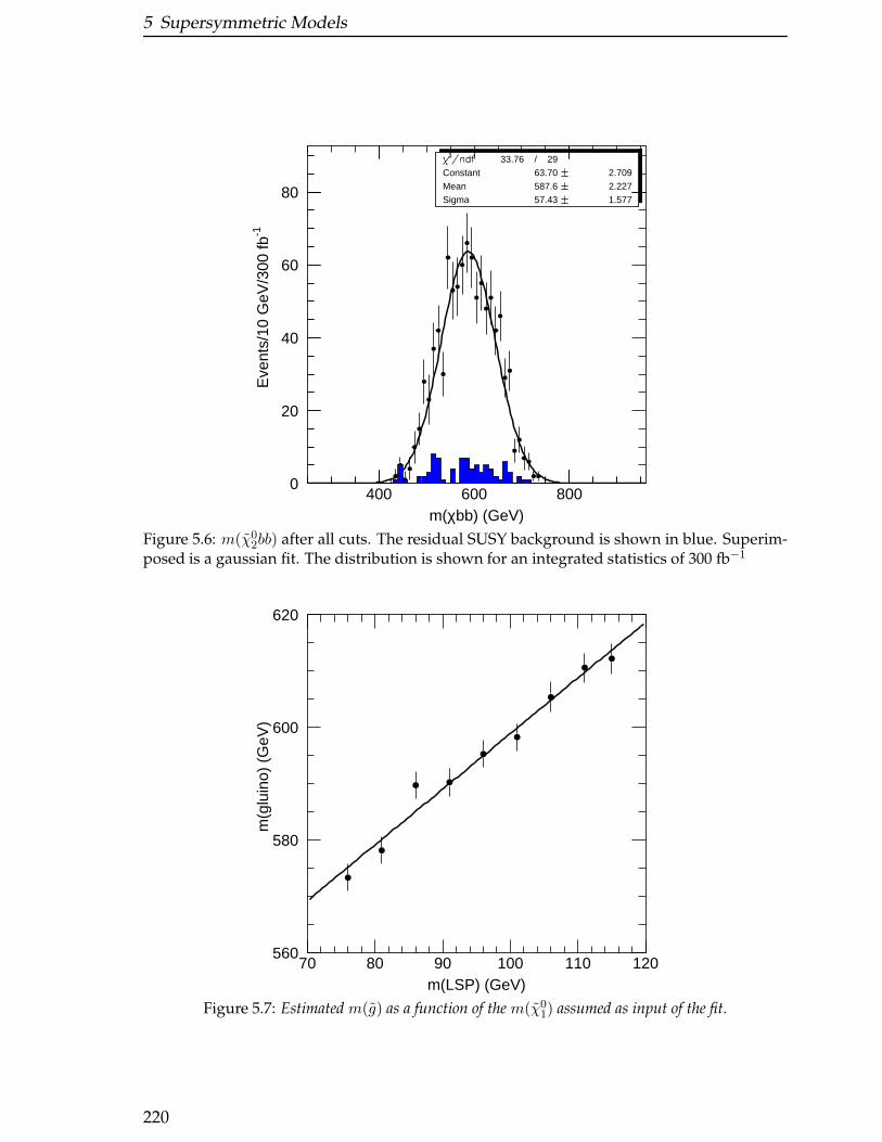
5 Supersymmetric Models
0
20
40
60
80
400 600 800
33.76 / 29
Constant 63.70 2.709
Mean 587.6 2.227
Sigma 57.43 1.577
m(χbb) (GeV)
Eve
nts/
10 G
eV/3
00 fb
-1
Figure 5.6: m(χ02bb) after all cuts. The residual SUSY background is shown in blue. Superim-
posed is a gaussian fit. The distribution is shown for an integrated statistics of 300 fb−1
560
580
600
620
70 80 90 100 110 120m(LSP) (GeV)
m(g
luin
o) (
GeV
)
Figure 5.7: Estimated m(g) as a function of the m(χ01) assumed as input of the fit.
220
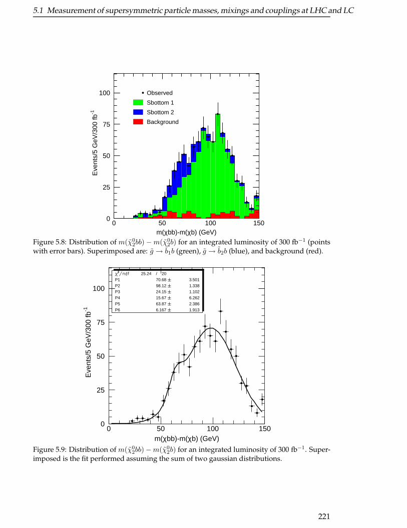
5.1 Measurement of supersymmetric particle masses, mixings and couplings at LHC and LC
0
25
50
75
100
0 50 100 150m(χbb)-m(χb) (GeV)
Eve
nts/
5 G
eV/3
00 fb
-1Observed
Sbottom 1
Sbottom 2
Background
Figure 5.8: Distribution of m(χ02bb)−m(χ0
2b) for an integrated luminosity of 300 fb−1 (pointswith error bars). Superimposed are: g → b1b (green), g → b2b (blue), and background (red).
0
25
50
75
100
0 50 100 150
25.24 / 20
P1 70.68 3.501
P2 98.12 1.338P3 24.15 1.102
P4 15.67 6.262
P5 63.87 2.386
P6 6.167 1.913
m(χbb)-m(χb) (GeV)
Eve
nts/
5 G
eV/3
00 fb
-1
Figure 5.9: Distribution of m(χ02bb)−m(χ0
2b) for an integrated luminosity of 300 fb−1. Super-imposed is the fit performed assuming the sum of two gaussian distributions.
221
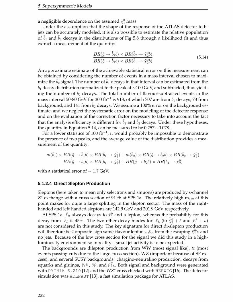
5 Supersymmetric Models
a negligible dependence on the assumed χ01 mass.
Under the assumption that the shape of the response of the ATLAS detector to b-jets can be accurately modeled, it is also possible to estimate the relative population
of b1 and b2 decays in the distributions of Fig 5.8 through a likelihood fit and thusextract a measurement of the quantity:
BR(g → b2b)× BR(b2 → χ02b)
BR(g → b1b)× BR(b1 → χ02b)
(5.14)
An approximate estimate of the achievable statistical error on this measurement canbe obtained by considering the number of events in a mass interval chosen to maxi-
mize the b2 signal. The number of b1 decays in that interval can be estimated from the
b1 decay distribution normalized to the peak at∼100 GeV, and subtracted, thus yield-
ing the number of b2 decays. The total number of flavour-subtracted events in the
mass interval 50-80 GeV for 300 fb−1 is 913, of which 707 are from b1 decays, 73 from
background, and 141 from b2 decays. We assume a 100% error on the background es-timate, and we neglect the systematic error on the modeling of the detector responseand on the evaluation of the correction factor necessary to take into account the fact
that the analysis efficiency is different for b1 and b2 decays. Under these hypotheses,the quantity in Equation 5.14, can be measured to be 0.257+-0.078.
For a lower statistics of 100 fb−1, it would probably be impossible to demonstratethe presence of two peaks, and the average value of the distribution provides a mea-surement of the quantity:
m(b1)× BR(g → b1b)×BR(b1 → χ02) +m(b2)× BR(g → b2b)×BR(b2 → χ0
2)
BR(g → b1b)×BR(b1 → χ02) +BR(g → b2b)× BR(b2 → χ0
2)
with a statistical error of ∼ 1.7 GeV.
5.1.2.4 Direct Slepton Production
Sleptons (here taken to mean only selectrons and smuons) are produced by s-channelZ∗ exchange with a cross section of 91 fb at SPS 1a. The relatively high m1/2 at thispoint makes for quite a large splitting in the slepton sector. The mass of the right-handed and left-handed sleptons are 142.9 GeV and 201.9 GeV respectively.
At SPS 1a ℓR always decays to χ01 and a lepton, whereas the probability for this
decay from ℓL is 45%. The two other decay modes for ℓL (to χ02 + ℓ and χ±
1 + ν)are not considered in this study. The key signature for direct di-slepton productionwill therefore be 2 opposite-sign same-flavour leptons, /ET from the escaping χ0
1’s andno jets. Because of the low cross section for the signal we did this study in a high-luminosity environment so in reality a small jet activity is to be expected.
The backgrounds are dilepton production from WW (most signal like), tt (mostevents passing cuts due to the large cross section), WZ (important because of SF ex-cess), and several SUSY backgrounds: chargino-neutralino production, decays from
squarks and gluinos, τ1τ1, νν, and ν ℓL. Both signal and background were generatedwith PYTHIA 6.210 [12] and the WZ∗ cross checked with HERWIG[16]. The detectorsimulation was ATLFAST[13], a fast simulation package for ATLAS.
222
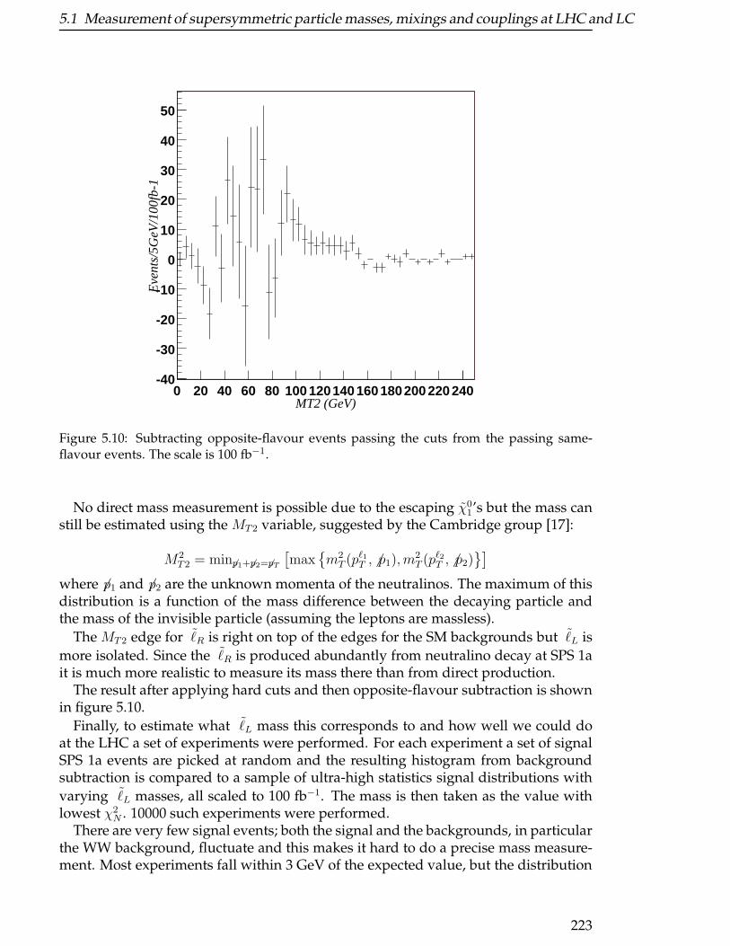
5.1 Measurement of supersymmetric particle masses, mixings and couplings at LHC and LC
MT2 (GeV)0 20 40 60 80 100 120140 160 180200 220 240
Eve
nts/
5GeV
/100
fb-1
-40
-30
-20
-10
0
10
20
30
40
50
Figure 5.10: Subtracting opposite-flavour events passing the cuts from the passing same-flavour events. The scale is 100 fb−1.
No direct mass measurement is possible due to the escaping χ01’s but the mass can
still be estimated using the MT2 variable, suggested by the Cambridge group [17]:
M2T2 = min6p1+ 6p2= 6pT
[max
m2T (pℓ1T , 6 p1), m
2T (pℓ2T , 6 p2)
]
where 6p1 and 6p2 are the unknown momenta of the neutralinos. The maximum of thisdistribution is a function of the mass difference between the decaying particle andthe mass of the invisible particle (assuming the leptons are massless).
The MT2 edge for ℓR is right on top of the edges for the SM backgrounds but ℓL is
more isolated. Since the ℓR is produced abundantly from neutralino decay at SPS 1ait is much more realistic to measure its mass there than from direct production.
The result after applying hard cuts and then opposite-flavour subtraction is shownin figure 5.10.
Finally, to estimate what ℓL mass this corresponds to and how well we could doat the LHC a set of experiments were performed. For each experiment a set of signalSPS 1a events are picked at random and the resulting histogram from backgroundsubtraction is compared to a sample of ultra-high statistics signal distributions with
varying ℓL masses, all scaled to 100 fb−1. The mass is then taken as the value withlowest χ2
N . 10000 such experiments were performed.There are very few signal events; both the signal and the backgrounds, in particular
the WW background, fluctuate and this makes it hard to do a precise mass measure-ment. Most experiments fall within 3 GeV of the expected value, but the distribution
223
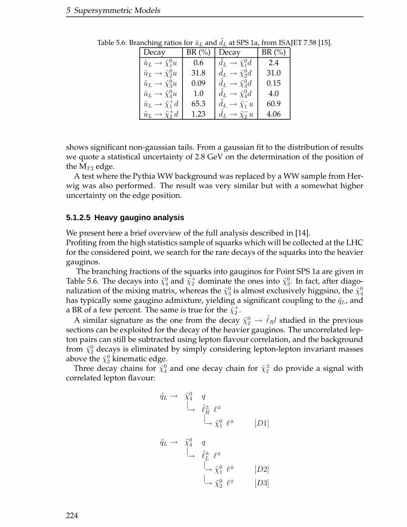
5 Supersymmetric Models
Table 5.6: Branching ratios for uL and dL at SPS 1a, from ISAJET 7.58 [15].
Decay BR (%) Decay BR (%)
uL → χ01u 0.6 dL → χ0
1d 2.4
uL → χ02u 31.8 dL → χ0
2d 31.0
uL → χ03u 0.09 dL → χ0
3d 0.15
uL → χ04u 1.0 dL → χ0
4d 4.0
uL → χ+1 d 65.3 dL → χ−
1 u 60.9
uL → χ+2 d 1.23 dL → χ−
2 u 4.06
shows significant non-gaussian tails. From a gaussian fit to the distribution of resultswe quote a statistical uncertainty of 2.8 GeV on the determination of the position ofthe MT2 edge.
A test where the Pythia WW background was replaced by a WW sample from Her-wig was also performed. The result was very similar but with a somewhat higheruncertainty on the edge position.
5.1.2.5 Heavy gaugino analysis
We present here a brief overview of the full analysis described in [14].Profiting from the high statistics sample of squarks which will be collected at the LHCfor the considered point, we search for the rare decays of the squarks into the heaviergauginos.
The branching fractions of the squarks into gauginos for Point SPS 1a are given inTable 5.6. The decays into χ0
4 and χ+2 dominate the ones into χ0
3. In fact, after diago-nalization of the mixing matrix, whereas the χ0
3 is almost exclusively higgsino, the χ04
has typically some gaugino admixture, yielding a significant coupling to the qL, anda BR of a few percent. The same is true for the χ+
2 .
A similar signature as the one from the decay χ02 → ℓRl studied in the previous
sections can be exploited for the decay of the heavier gauginos. The uncorrelated lep-ton pairs can still be subtracted using lepton flavour correlation, and the backgroundfrom χ0
2 decays is eliminated by simply considering lepton-lepton invariant massesabove the χ0
2 kinematic edge.Three decay chains for χ0
4 and one decay chain for χ±2 do provide a signal with
correlated lepton flavour:
qL → χ04 q|→ ℓ±R ℓ∓
|→ χ01 ℓ± [D1]
qL → χ04 q|→ ℓ±L ℓ∓
|→ χ01 ℓ± [D2]
|→ χ02 ℓ± [D3]
224
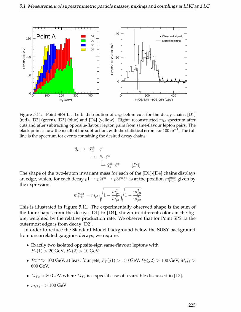
5.1 Measurement of supersymmetric particle masses, mixings and couplings at LHC and LC
0
50
100
150
0 100 200 300 400mll (GeV)
Eve
nts/
10 G
eV
D1
D2
D3
D4
Point A
0
20
40
0 200 400m(OS-SF)-m(OS-OF) (GeV)
Eve
nts/
10 G
eV/1
00 fb
-1
Observed signal
Expected signal
Figure 5.11: Point SPS 1a. Left: distribution of mℓℓ before cuts for the decay chains [D1](red), [D2] (green), [D3] (blue) and [D4] (yellow). Right: reconstructed mℓℓ spectrum aftercuts and after subtracting opposite-flavour lepton pairs from same-flavour lepton pairs. Theblack points show the result of the subtraction, with the statistical errors for 100 fb−1. The fullline is the spectrum for events containing the desired decay chains.
qL → χ±2 q′
|→ νℓ ℓ±
|→ χ±1 ℓ∓ [D4]
The shape of the two-lepton invariant mass for each of the [D1]-[D4] chains displaysan edge, which, for each decay p1 → p2ℓ± → p3ℓ±ℓ∓ is at the position mmax
l+l− given bythe expression:
mmaxl+l− = mp1
√1−
m2p2
m2p1
√1−
m2p3
m2p2
This is illustrated in Figure 5.11. The experimentally observed shape is the sum ofthe four shapes from the decays [D1] to [D4], shown in different colors in the fig-ure, weighted by the relative production rate. We observe that for Point SPS 1a theoutermost edge is from decay [D2].
In order to reduce the Standard Model background below the SUSY backgroundfrom uncorrelated gauginos decays, we require:
• Exactly two isolated opposite-sign same-flavour leptons withPT (1) > 20 GeV, PT (2) > 10 GeV
• PmissT > 100 GeV, at least four jets, PT (j1) > 150 GeV, PT (j2) > 100 GeV, Meff >
600 GeV.
• MT2 > 80 GeV, where MT2 is a special case of a variable discussed in [17].
• mℓ+ℓ− > 100 GeV
225
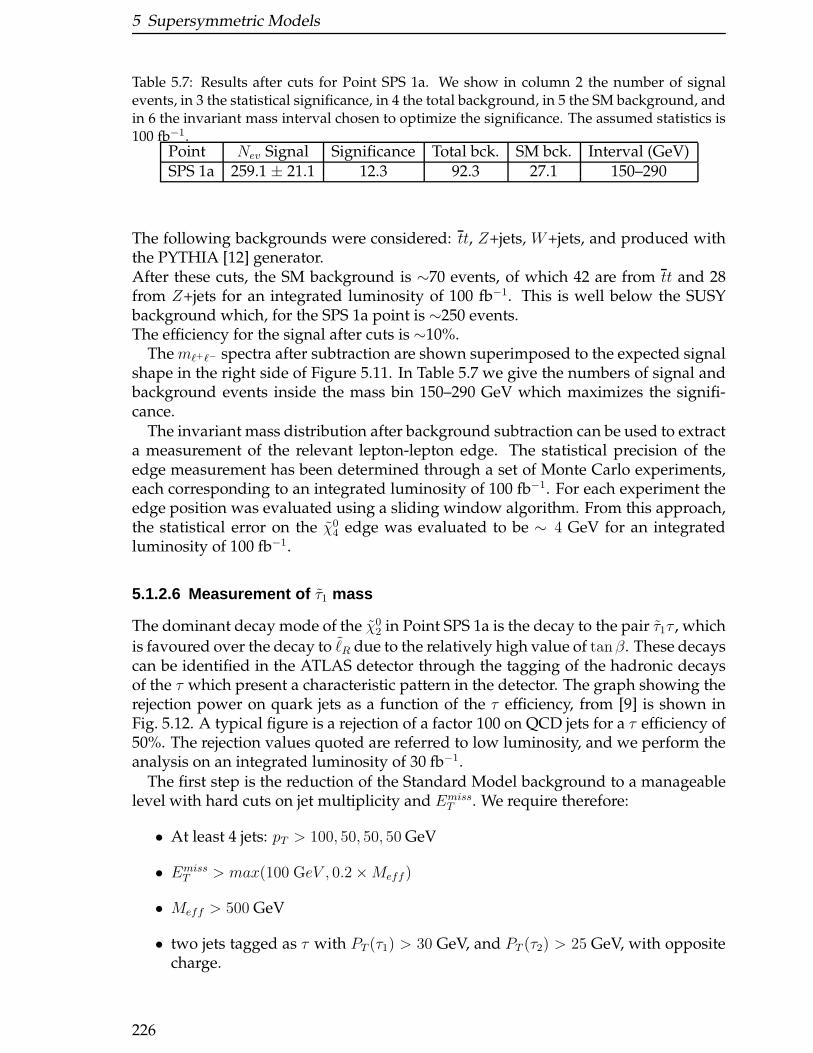
5 Supersymmetric Models
Table 5.7: Results after cuts for Point SPS 1a. We show in column 2 the number of signalevents, in 3 the statistical significance, in 4 the total background, in 5 the SM background, andin 6 the invariant mass interval chosen to optimize the significance. The assumed statistics is100 fb−1.
Point Nev Signal Significance Total bck. SM bck. Interval (GeV)SPS 1a 259.1 ± 21.1 12.3 92.3 27.1 150–290
The following backgrounds were considered: tt, Z+jets, W+jets, and produced withthe PYTHIA [12] generator.After these cuts, the SM background is ∼70 events, of which 42 are from tt and 28from Z+jets for an integrated luminosity of 100 fb−1. This is well below the SUSYbackground which, for the SPS 1a point is ∼250 events.The efficiency for the signal after cuts is ∼10%.
The mℓ+ℓ− spectra after subtraction are shown superimposed to the expected signalshape in the right side of Figure 5.11. In Table 5.7 we give the numbers of signal andbackground events inside the mass bin 150–290 GeV which maximizes the signifi-cance.
The invariant mass distribution after background subtraction can be used to extracta measurement of the relevant lepton-lepton edge. The statistical precision of theedge measurement has been determined through a set of Monte Carlo experiments,each corresponding to an integrated luminosity of 100 fb−1. For each experiment theedge position was evaluated using a sliding window algorithm. From this approach,the statistical error on the χ0
4 edge was evaluated to be ∼ 4 GeV for an integratedluminosity of 100 fb−1.
5.1.2.6 Measurement of τ1 mass
The dominant decay mode of the χ02 in Point SPS 1a is the decay to the pair τ1τ , which
is favoured over the decay to ℓR due to the relatively high value of tanβ. These decayscan be identified in the ATLAS detector through the tagging of the hadronic decaysof the τ which present a characteristic pattern in the detector. The graph showing therejection power on quark jets as a function of the τ efficiency, from [9] is shown inFig. 5.12. A typical figure is a rejection of a factor 100 on QCD jets for a τ efficiency of50%. The rejection values quoted are referred to low luminosity, and we perform theanalysis on an integrated luminosity of 30 fb−1.
The first step is the reduction of the Standard Model background to a manageablelevel with hard cuts on jet multiplicity and Emiss
T . We require therefore:
• At least 4 jets: pT > 100, 50, 50, 50 GeV
• EmissT > max(100 GeV , 0.2×Meff )
• Meff > 500 GeV
• two jets tagged as τ with PT (τ1) > 30 GeV, and PT (τ2) > 25 GeV, with oppositecharge.
226
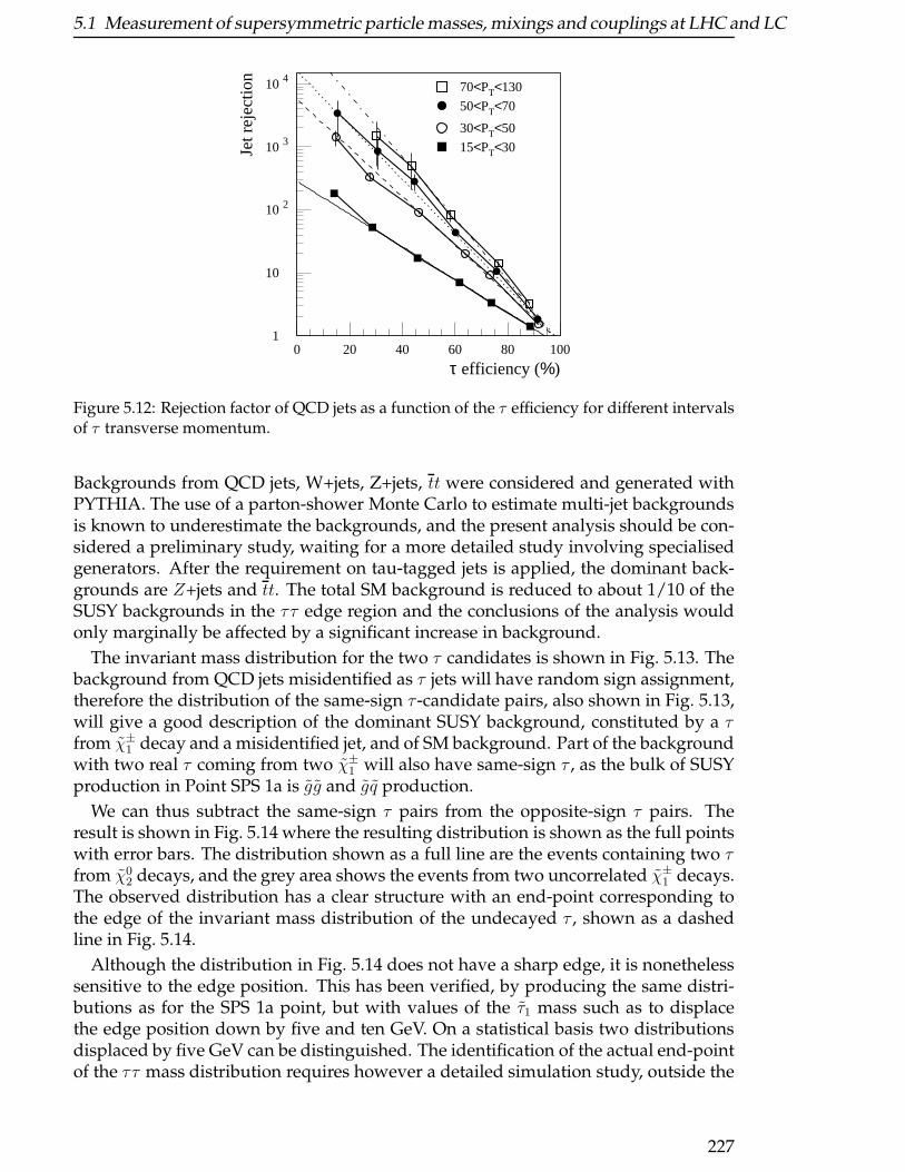
5.1 Measurement of supersymmetric particle masses, mixings and couplings at LHC and LC
1
10
10 2
10 3
10 4
0 20 40 60 80 100
τ efficiency (%)
Jet r
ejec
tion
70<PT<130
50<PT<70
30<PT<50
15<PT<30
Figure 5.12: Rejection factor of QCD jets as a function of the τ efficiency for different intervalsof τ transverse momentum.
Backgrounds from QCD jets, W+jets, Z+jets, tt were considered and generated withPYTHIA. The use of a parton-shower Monte Carlo to estimate multi-jet backgroundsis known to underestimate the backgrounds, and the present analysis should be con-sidered a preliminary study, waiting for a more detailed study involving specialisedgenerators. After the requirement on tau-tagged jets is applied, the dominant back-grounds are Z+jets and tt. The total SM background is reduced to about 1/10 of theSUSY backgrounds in the ττ edge region and the conclusions of the analysis wouldonly marginally be affected by a significant increase in background.
The invariant mass distribution for the two τ candidates is shown in Fig. 5.13. Thebackground from QCD jets misidentified as τ jets will have random sign assignment,therefore the distribution of the same-sign τ -candidate pairs, also shown in Fig. 5.13,will give a good description of the dominant SUSY background, constituted by a τfrom χ±
1 decay and a misidentified jet, and of SM background. Part of the backgroundwith two real τ coming from two χ±
1 will also have same-sign τ , as the bulk of SUSYproduction in Point SPS 1a is gg and gq production.
We can thus subtract the same-sign τ pairs from the opposite-sign τ pairs. Theresult is shown in Fig. 5.14 where the resulting distribution is shown as the full pointswith error bars. The distribution shown as a full line are the events containing two τfrom χ0
2 decays, and the grey area shows the events from two uncorrelated χ±1 decays.
The observed distribution has a clear structure with an end-point corresponding tothe edge of the invariant mass distribution of the undecayed τ , shown as a dashedline in Fig. 5.14.
Although the distribution in Fig. 5.14 does not have a sharp edge, it is nonethelesssensitive to the edge position. This has been verified, by producing the same distri-butions as for the SPS 1a point, but with values of the τ1 mass such as to displacethe edge position down by five and ten GeV. On a statistical basis two distributionsdisplaced by five GeV can be distinguished. The identification of the actual end-pointof the ττ mass distribution requires however a detailed simulation study, outside the
227

5 Supersymmetric Models
m(ττ) (GeV)
Eve
nts/
4 G
eV/1
00 fb
-1
Tau-OS SUSY
Tau-SS SUSY
SM
0
100
200
300
0 50 100 150 200
Figure 5.13: Invariant mass distribution of: opposite sign τ -tagged jets (full line); same-signτ -tagged jets (dashed line), SM background (grey). The integrated luminosity is 30 fb−1.
m(ττ) (GeV)
Eve
nts/
4 G
eV/1
00 fb
-1
Tau OS-SS
Tau undecayed
Z2 decays OS-SS
W1 decays OS-SS
0
100
200
300
400
0 50 100 150 200
Figure 5.14: Invariant mass distribution of τ -tagged jets after subtraction of same-sign back-ground (full circles). Superimposed are shown the distributions for: χ0
2 → τ1τ signal (fullline), χ±
1 decays (grey), undecayed τ ’s from χ02 (dashed line).
.
228
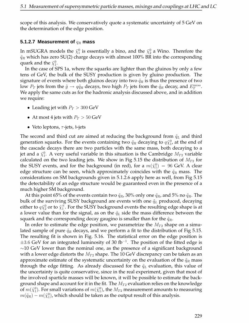
5.1 Measurement of supersymmetric particle masses, mixings and couplings at LHC and LC
scope of this analysis. We conservatively quote a systematic uncertainty of 5 GeV onthe determination of the edge position.
5.1.2.7 Measurement of qR mass
In mSUGRA models the χ01 is essentially a bino, and the χ0
2 a Wino. Therefore theqR which has zero SU(2) charge decays with almost 100% BR into the correspondingquark and the χ0
1.In the case of SPS 1a, where the squarks are lighter than the gluinos by only a few
tens of GeV, the bulk of the SUSY production is given by gluino production. Thesignature of events where both gluinos decay into two qR is thus the presence of twolow PT jets from the g → qqR decays, two high PT jets from the qR decay, and Emiss
T .We apply the same cuts as for the hadronic analysis discussed above, and in additionwe require:
• Leading jet with PT > 300 GeV
• At most 4 jets with PT > 50 GeV
• Veto leptons, τ -jets, b-jets
The second and third cut are aimed at reducing the background from qL and thirdgeneration squarks. For the events containing two qR decaying to qχ0
1, at the end ofthe cascade decays there are two particles with the same mass, both decaying to ajet and a χ0
1. A very useful variable in this situation is the Cambridge MT2 variablecalculated on the two leading jets. We show in Fig 5.15 the distribution of MT2 forthe SUSY events, and for the background (in red), for a m(χ0
1) = 96 GeV. A clearedge structure can be seen, which approximately coincides with the qR mass. Theconsiderations on SM backgrounds given in 5.1.2.6 apply here as well, from Fig 5.15the detectability of an edge structure would be guaranteed even in the presence of amuch higher SM background.
At this point 65% of the events contain two qR, 30% only one qR, and 5% no qR. Thebulk of the surviving SUSY background are events with one qL produced, decayingeither to qχ0
2 or to χ±1 . For the SUSY background events the resulting edge shape is at
a lower value than for the signal, as on the qL side the mass difference between thesquark and the corresponding decay gaugino is smaller than for the qR.
In order to estimate the edge position, we parametrize the MT2 shape on a simu-lated sample of pure qR decays, and we perform a fit to the distribution of Fig 5.15.The resulting fit is shown in Fig. 5.16. The statistical error on the edge position is±3.6 GeV for an integrated luminosity of 30 fb−1. The position of the fitted edge is∼10 GeV lower than the nominal one, as the presence of a significant backgroundwith a lower edge distorts the MT2 shape. The 10 GeV discrepancy can be taken as anapproximate estimate of the systematic uncertainty on the evaluation of the qR massthrough the edge fitting. As already discussed for the qL evaluation, this value ofthe uncertainty is quite conservative, since in the real experiment, given that most ofthe involved sparticle masses will be known, it will be possible to estimate the back-ground shape and account for it in the fit. TheMT2 evaluation relies on the knowledgeof m(χ0
1). For small variations of m(χ01), the MT2 measurement amounts to measuring
m(qR)−m(χ01), which should be taken as the output result of this analysis.
229
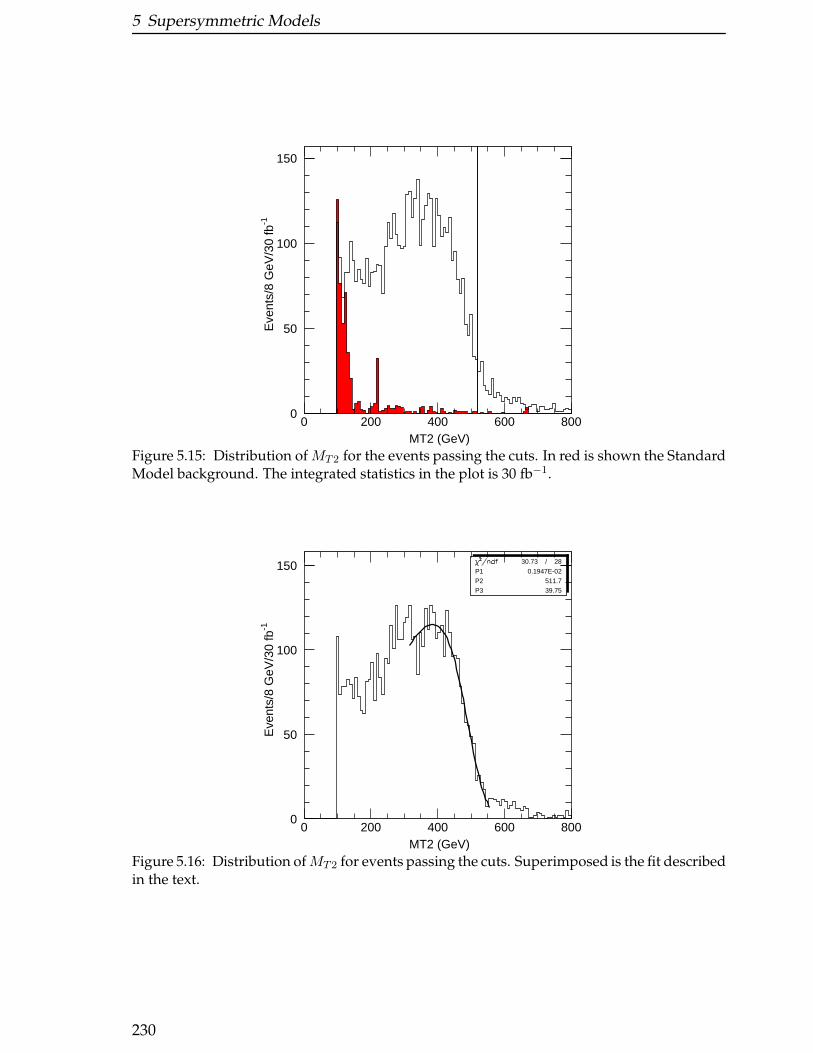
5 Supersymmetric Models
MT2 (GeV)
Eve
nts/
8 G
eV/3
0 fb
-1
0
50
100
150
0 200 400 600 800
Figure 5.15: Distribution ofMT2 for the events passing the cuts. In red is shown the StandardModel background. The integrated statistics in the plot is 30 fb−1.
0
50
100
150
0 200 400 600 800
30.73 / 28
P1 0.1947E-02
P2 511.7
P3 39.75
MT2 (GeV)
Eve
nts/
8 G
eV/3
0 fb
-1
Figure 5.16: Distribution ofMT2 for events passing the cuts. Superimposed is the fit describedin the text.
230
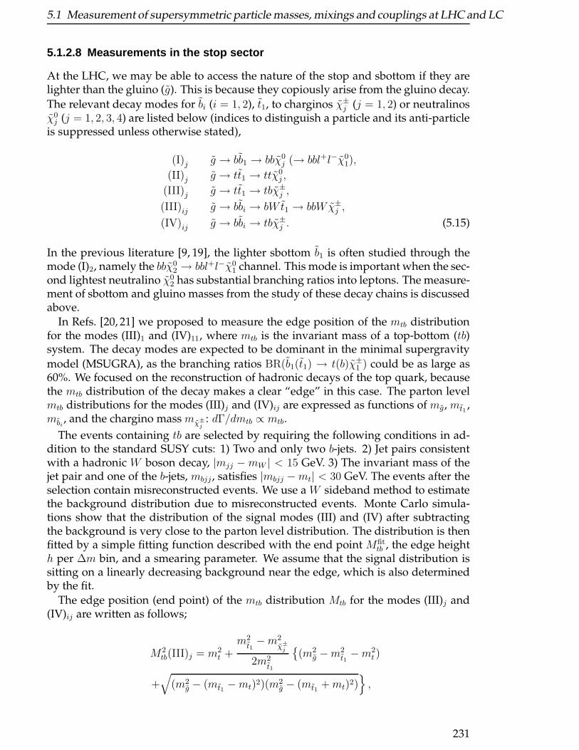
5.1 Measurement of supersymmetric particle masses, mixings and couplings at LHC and LC
5.1.2.8 Measurements in the stop sector
At the LHC, we may be able to access the nature of the stop and sbottom if they arelighter than the gluino (g). This is because they copiously arise from the gluino decay.
The relevant decay modes for bi (i = 1, 2), t1, to charginos χ±j (j = 1, 2) or neutralinos
χ0j (j = 1, 2, 3, 4) are listed below (indices to distinguish a particle and its anti-particle
is suppressed unless otherwise stated),
(I)j g → bb1 → bbχ0j (→ bbl+l−χ0
1),
(II)j g → tt1 → ttχ0j ,
(III)j g → tt1 → tbχ±j ,
(III)ij g → bbi → bW t1 → bbWχ±j ,
(IV)ij g → bbi → tbχ±j . (5.15)
In the previous literature [9, 19], the lighter sbottom b1 is often studied through themode (I)2, namely the bbχ0
2 → bbl+l−χ01 channel. This mode is important when the sec-
ond lightest neutralino χ02 has substantial branching ratios into leptons. The measure-
ment of sbottom and gluino masses from the study of these decay chains is discussedabove.
In Refs. [20, 21] we proposed to measure the edge position of the mtb distributionfor the modes (III)1 and (IV)11, where mtb is the invariant mass of a top-bottom (tb)system. The decay modes are expected to be dominant in the minimal supergravity
model (MSUGRA), as the branching ratios BR(b1(t1) → t(b)χ±1 ) could be as large as
60%. We focused on the reconstruction of hadronic decays of the top quark, becausethe mtb distribution of the decay makes a clear “edge” in this case. The parton levelmtb distributions for the modes (III)j and (IV)ij are expressed as functions of mg, mt1 ,mbi
, and the chargino mass mχ±
j: dΓ/dmtb ∝ mtb.
The events containing tb are selected by requiring the following conditions in ad-dition to the standard SUSY cuts: 1) Two and only two b-jets. 2) Jet pairs consistentwith a hadronic W boson decay, |mjj −mW | < 15 GeV. 3) The invariant mass of thejet pair and one of the b-jets, mbjj , satisfies |mbjj −mt| < 30 GeV. The events after theselection contain misreconstructed events. We use a W sideband method to estimatethe background distribution due to misreconstructed events. Monte Carlo simula-tions show that the distribution of the signal modes (III) and (IV) after subtractingthe background is very close to the parton level distribution. The distribution is thenfitted by a simple fitting function described with the end point Mfit
tb , the edge heighth per ∆m bin, and a smearing parameter. We assume that the signal distribution issitting on a linearly decreasing background near the edge, which is also determinedby the fit.
The edge position (end point) of the mtb distribution Mtb for the modes (III)j and(IV)ij are written as follows;
M2tb(III)j = m2
t +m2t1−m2
χ±
j
2m2t1
(m2
g −m2t1−m2
t )
+√
(m2g − (mt1 −mt)2)(m2
g − (mt1 +mt)2),
231
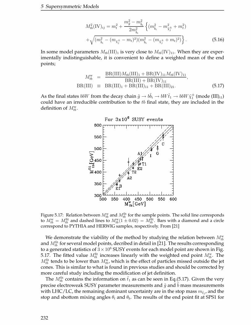
5 Supersymmetric Models
M2tb(IV)ij = m2
t +m2g −m2
bi
2m2bi
(m2
bi−m2
χ±
j+m2
t )
+√
(m2bi− (mχ±
j−mt)2)(m2
bi− (mχ±
j+mt)2)
. (5.16)
In some model parameters Mtb(III)1 is very close to Mtb(IV)11. When they are exper-imentally indistinguishable, it is convenient to define a weighted mean of the endpoints;
Mwtb =
BR(III)Mtb(III)1 + BR(IV)11Mtb(IV)11
BR(III) + BR(IV)11
,
BR(III) ≡ BR(III)1 + BR(III)11 + BR(III)21. (5.17)
As the final states bbW from the decay chain g → bbi → bW t1 → bbWχ±1 (mode (III)i1)
could have an irreducible contribution to the tb final state, they are included in thedefinition of Mw
tb .
Figure 5.17: Relation betweenMwtb and Mfit
tb for the sample points. The solid line correspondsto Mw
tb = Mfittb and dashed lines to Mw
tb (1 ± 0.02) = Mfittb . Bars with a diamond and a circle
correspond to PYTHIA and HERWIG samples, respectively. From [21]
We demonstrate the viability of the method by studying the relation between Mwtb
andMfittb for several model points, decribed in detail in [21]. The results corresponding
to a generated statistics of 3×10⁶ SUSY events for each model point are shown in Fig.5.17. The fitted value Mfit
tb increases linearly with the weighted end point Mwtb . The
Mfittb tends to be lower than Mw
tb , which is the effect of particles missed outside the jetcones. This is similar to what is found in previous studies and should be corrected bymore careful study including the modification of jet definition.
The Mfittb contains the information on t1 as can be seen in Eq.(5.17). Given the very
precise electroweak SUSY parameter measurements and g and b mass measurementswith LHC/LC, the remaining dominant uncertainty are in the stop mass mt1 , and thestop and sbottom mixing angles θt and θb. The results of the end point fit at SPS1 for
232
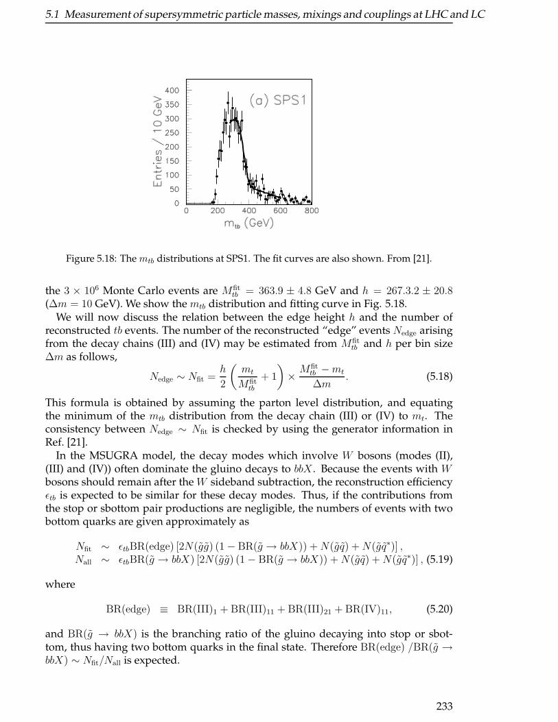
5.1 Measurement of supersymmetric particle masses, mixings and couplings at LHC and LC
Figure 5.18: The mtb distributions at SPS1. The fit curves are also shown. From [21].
the 3 × 10⁶ Monte Carlo events are Mfittb = 363.9 ± 4.8 GeV and h = 267.3.2 ± 20.8
(∆m = 10 GeV). We show the mtb distribution and fitting curve in Fig. 5.18.We will now discuss the relation between the edge height h and the number of
reconstructed tb events. The number of the reconstructed “edge” events Nedge arisingfrom the decay chains (III) and (IV) may be estimated from Mfit
tb and h per bin size∆m as follows,
Nedge ∼ Nfit =h
2
(mt
Mfittb
+ 1
)× Mfit
tb −mt
∆m. (5.18)
This formula is obtained by assuming the parton level distribution, and equatingthe minimum of the mtb distribution from the decay chain (III) or (IV) to mt. Theconsistency between Nedge ∼ Nfit is checked by using the generator information inRef. [21].
In the MSUGRA model, the decay modes which involve W bosons (modes (II),(III) and (IV)) often dominate the gluino decays to bbX . Because the events with Wbosons should remain after the W sideband subtraction, the reconstruction efficiencyǫtb is expected to be similar for these decay modes. Thus, if the contributions fromthe stop or sbottom pair productions are negligible, the numbers of events with twobottom quarks are given approximately as
Nfit ∼ ǫtbBR(edge) [2N(gg) (1− BR(g → bbX)) +N(gq) +N(gq∗)] ,Nall ∼ ǫtbBR(g → bbX) [2N(gg) (1− BR(g → bbX)) +N(gq) +N(gq∗)] , (5.19)
where
BR(edge) ≡ BR(III)1 + BR(III)11 + BR(III)21 + BR(IV)11, (5.20)
and BR(g → bbX) is the branching ratio of the gluino decaying into stop or sbot-tom, thus having two bottom quarks in the final state. Therefore BR(edge) /BR(g →bbX) ∼ Nfit/Nall is expected.
233
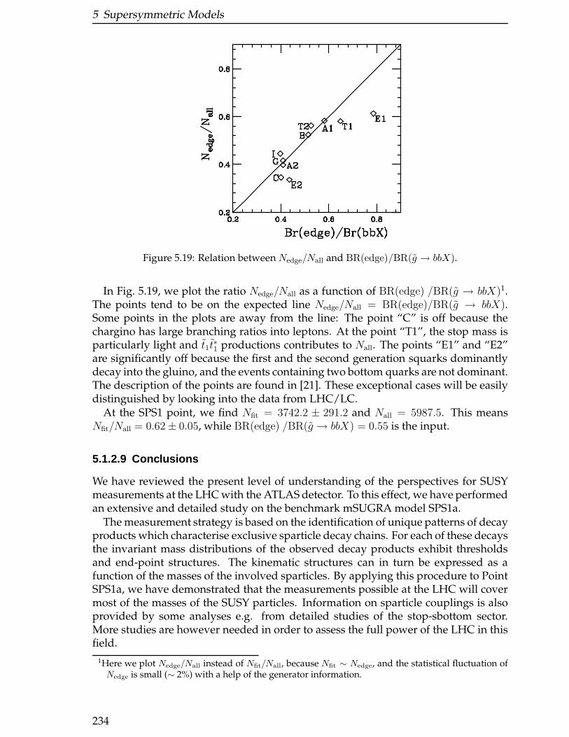
5 Supersymmetric Models
Figure 5.19: Relation between Nedge/Nall and BR(edge)/BR(g → bbX).
In Fig. 5.19, we plot the ratio Nedge/Nall as a function of BR(edge) /BR(g → bbX)1.The points tend to be on the expected line Nedge/Nall = BR(edge)/BR(g → bbX).Some points in the plots are away from the line: The point “C” is off because thechargino has large branching ratios into leptons. At the point “T1”, the stop mass isparticularly light and t1t
∗1 productions contributes to Nall. The points “E1” and “E2”
are significantly off because the first and the second generation squarks dominantlydecay into the gluino, and the events containing two bottom quarks are not dominant.The description of the points are found in [21]. These exceptional cases will be easilydistinguished by looking into the data from LHC/LC.
At the SPS1 point, we find Nfit = 3742.2 ± 291.2 and Nall = 5987.5. This meansNfit/Nall = 0.62± 0.05, while BR(edge) /BR(g → bbX) = 0.55 is the input.
5.1.2.9 Conclusions
We have reviewed the present level of understanding of the perspectives for SUSYmeasurements at the LHC with the ATLAS detector. To this effect, we have performedan extensive and detailed study on the benchmark mSUGRA model SPS1a.
The measurement strategy is based on the identification of unique patterns of decayproducts which characterise exclusive sparticle decay chains. For each of these decaysthe invariant mass distributions of the observed decay products exhibit thresholdsand end-point structures. The kinematic structures can in turn be expressed as afunction of the masses of the involved sparticles. By applying this procedure to PointSPS1a, we have demonstrated that the measurements possible at the LHC will covermost of the masses of the SUSY particles. Information on sparticle couplings is alsoprovided by some analyses e.g. from detailed studies of the stop-sbottom sector.More studies are however needed in order to assess the full power of the LHC in thisfield.
1Here we plot Nedge/Nall instead of Nfit/Nall, because Nfit ∼ Nedge, and the statistical fluctuation ofNedge is small (∼ 2%) with a help of the generator information.
234
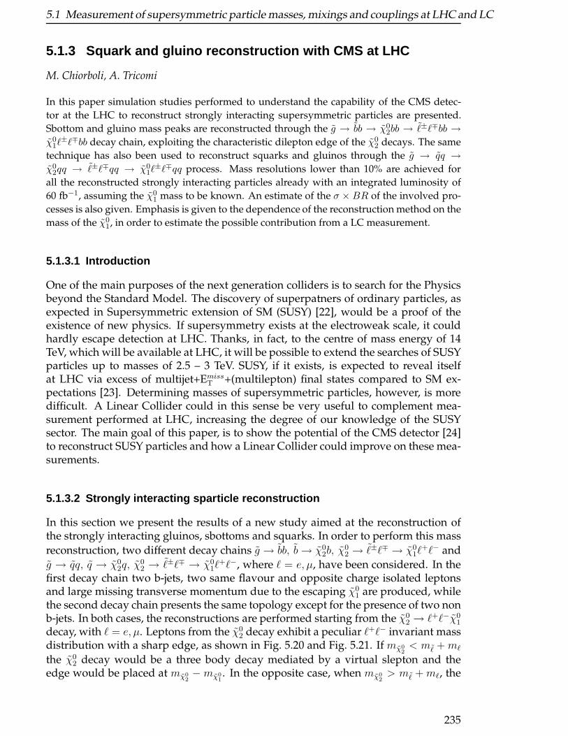
5.1 Measurement of supersymmetric particle masses, mixings and couplings at LHC and LC
5.1.3 Squark and gluino reconstruction with CMS at LHC
M. Chiorboli, A. Tricomi
In this paper simulation studies performed to understand the capability of the CMS detec-
tor at the LHC to reconstruct strongly interacting supersymmetric particles are presented.
Sbottom and gluino mass peaks are reconstructed through the g → bb → χ02bb → ℓ±ℓ∓bb →
χ01ℓ
±ℓ∓bb decay chain, exploiting the characteristic dilepton edge of the χ02 decays. The same
technique has also been used to reconstruct squarks and gluinos through the g → qq →χ0
2qq → ℓ±ℓ∓qq → χ01ℓ
±ℓ∓qq process. Mass resolutions lower than 10% are achieved for
all the reconstructed strongly interacting particles already with an integrated luminosity of
60 fb−1, assuming the χ01 mass to be known. An estimate of the σ × BR of the involved pro-
cesses is also given. Emphasis is given to the dependence of the reconstruction method on the
mass of the χ01, in order to estimate the possible contribution from a LC measurement.
5.1.3.1 Introduction
One of the main purposes of the next generation colliders is to search for the Physicsbeyond the Standard Model. The discovery of superpatners of ordinary particles, asexpected in Supersymmetric extension of SM (SUSY) [22], would be a proof of theexistence of new physics. If supersymmetry exists at the electroweak scale, it couldhardly escape detection at LHC. Thanks, in fact, to the centre of mass energy of 14TeV, which will be available at LHC, it will be possible to extend the searches of SUSYparticles up to masses of 2.5 – 3 TeV. SUSY, if it exists, is expected to reveal itselfat LHC via excess of multijet+EmissT +(multilepton) final states compared to SM ex-pectations [23]. Determining masses of supersymmetric particles, however, is moredifficult. A Linear Collider could in this sense be very useful to complement mea-surement performed at LHC, increasing the degree of our knowledge of the SUSYsector. The main goal of this paper, is to show the potential of the CMS detector [24]to reconstruct SUSY particles and how a Linear Collider could improve on these mea-surements.
5.1.3.2 Strongly interacting sparticle reconstruction
In this section we present the results of a new study aimed at the reconstruction ofthe strongly interacting gluinos, sbottoms and squarks. In order to perform this mass
reconstruction, two different decay chains g → bb, b→ χ02b, χ
02 → ℓ±ℓ∓ → χ0
1ℓ+ℓ− and
g → qq, q → χ02q, χ
02 → ℓ±ℓ∓ → χ0
1ℓ+ℓ−, where ℓ = e, µ, have been considered. In the
first decay chain two b-jets, two same flavour and opposite charge isolated leptonsand large missing transverse momentum due to the escaping χ0
1 are produced, whilethe second decay chain presents the same topology except for the presence of two nonb-jets. In both cases, the reconstructions are performed starting from the χ0
2 → ℓ+ℓ−χ01
decay, with ℓ = e, µ. Leptons from the χ02 decay exhibit a peculiar ℓ+ℓ− invariant mass
distribution with a sharp edge, as shown in Fig. 5.20 and Fig. 5.21. If mχ02< mℓ + mℓ
the χ02 decay would be a three body decay mediated by a virtual slepton and the
edge would be placed at mχ02−mχ0
1. In the opposite case, when mχ0
2> mℓ + mℓ, the
235
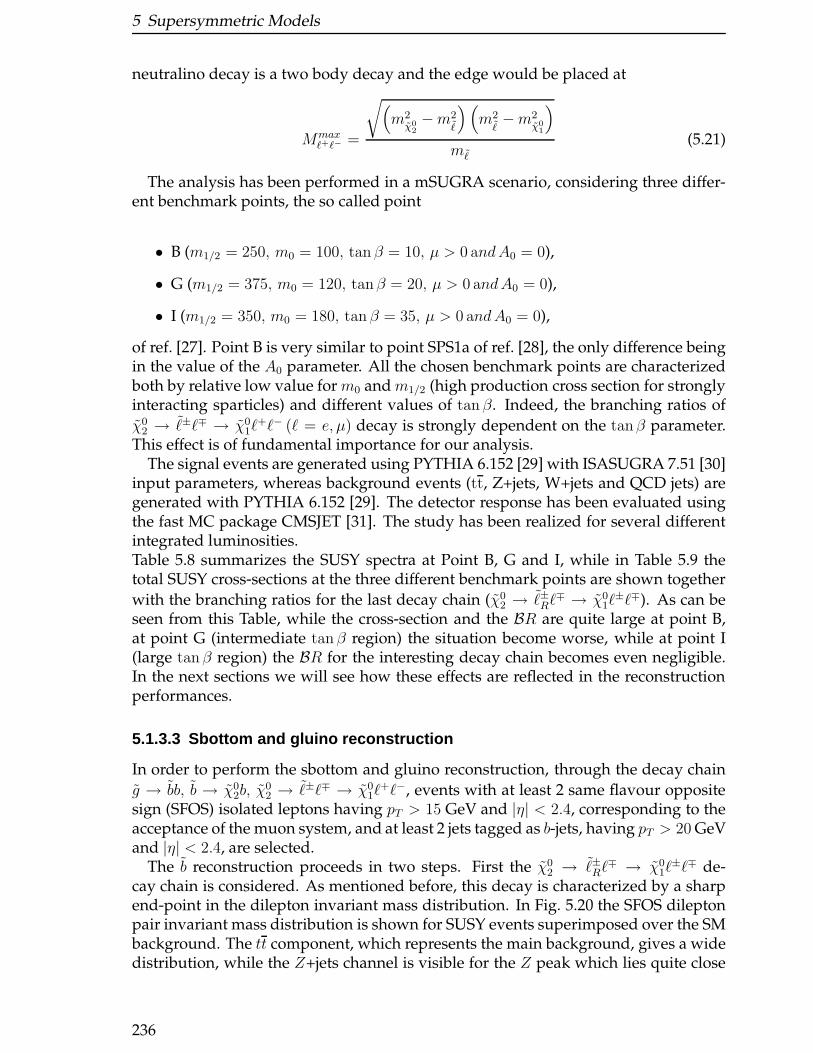
5 Supersymmetric Models
neutralino decay is a two body decay and the edge would be placed at
Mmaxℓ+ℓ− =
√(m2χ0
2−m2
ℓ
)(m2ℓ−m2
χ01
)
mℓ
(5.21)
The analysis has been performed in a mSUGRA scenario, considering three differ-ent benchmark points, the so called point
• B (m1/2 = 250, m0 = 100, tan β = 10, µ > 0 andA0 = 0),
• G (m1/2 = 375, m0 = 120, tanβ = 20, µ > 0 andA0 = 0),
• I (m1/2 = 350, m0 = 180, tan β = 35, µ > 0 andA0 = 0),
of ref. [27]. Point B is very similar to point SPS1a of ref. [28], the only difference beingin the value of the A0 parameter. All the chosen benchmark points are characterizedboth by relative low value for m0 and m1/2 (high production cross section for stronglyinteracting sparticles) and different values of tan β. Indeed, the branching ratios of
χ02 → ℓ±ℓ∓ → χ0
1ℓ+ℓ− (ℓ = e, µ) decay is strongly dependent on the tanβ parameter.
This effect is of fundamental importance for our analysis.The signal events are generated using PYTHIA 6.152 [29] with ISASUGRA 7.51 [30]
input parameters, whereas background events (tt, Z+jets, W+jets and QCD jets) aregenerated with PYTHIA 6.152 [29]. The detector response has been evaluated usingthe fast MC package CMSJET [31]. The study has been realized for several differentintegrated luminosities.Table 5.8 summarizes the SUSY spectra at Point B, G and I, while in Table 5.9 thetotal SUSY cross-sections at the three different benchmark points are shown together
with the branching ratios for the last decay chain (χ02 → ℓ±Rℓ
∓ → χ01ℓ
±ℓ∓). As can beseen from this Table, while the cross-section and the BR are quite large at point B,at point G (intermediate tan β region) the situation become worse, while at point I(large tan β region) the BR for the interesting decay chain becomes even negligible.In the next sections we will see how these effects are reflected in the reconstructionperformances.
5.1.3.3 Sbottom and gluino reconstruction
In order to perform the sbottom and gluino reconstruction, through the decay chain
g → bb, b → χ02b, χ
02 → ℓ±ℓ∓ → χ0
1ℓ+ℓ−, events with at least 2 same flavour opposite
sign (SFOS) isolated leptons having pT > 15 GeV and |η| < 2.4, corresponding to theacceptance of the muon system, and at least 2 jets tagged as b-jets, having pT > 20 GeVand |η| < 2.4, are selected.
The b reconstruction proceeds in two steps. First the χ02 → ℓ±Rℓ
∓ → χ01ℓ
±ℓ∓ de-cay chain is considered. As mentioned before, this decay is characterized by a sharpend-point in the dilepton invariant mass distribution. In Fig. 5.20 the SFOS dileptonpair invariant mass distribution is shown for SUSY events superimposed over the SMbackground. The tt component, which represents the main background, gives a widedistribution, while the Z+jets channel is visible for the Z peak which lies quite close
236
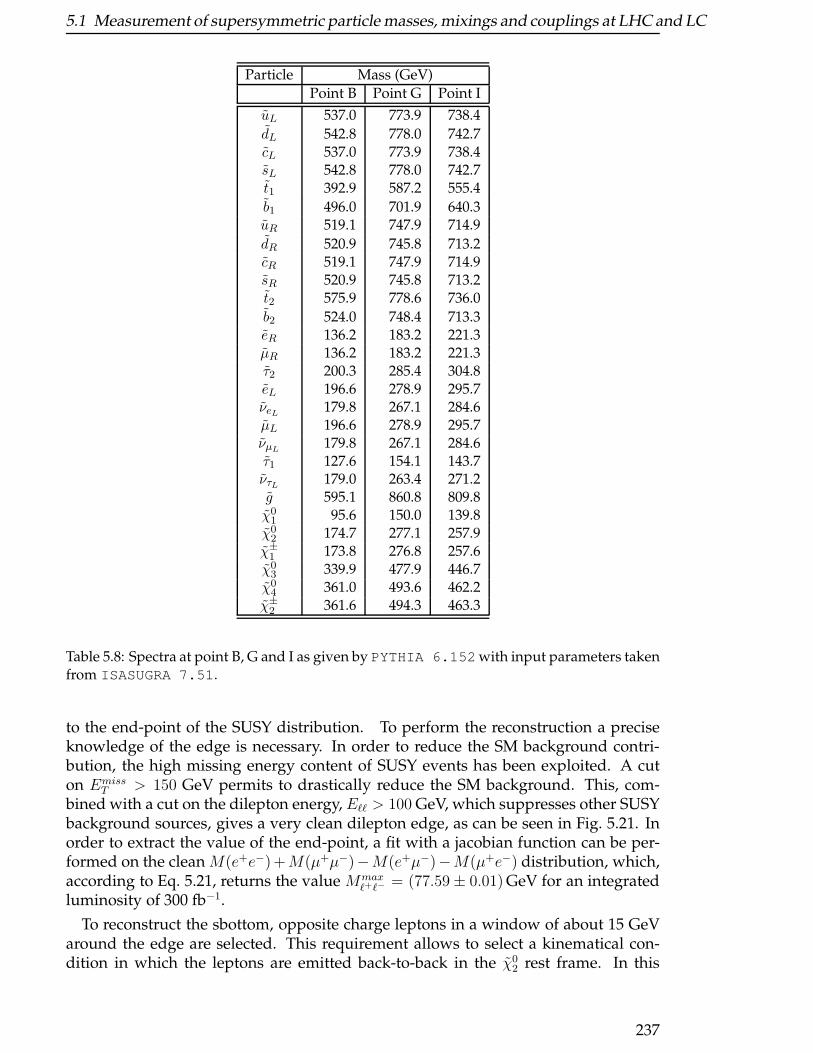
5.1 Measurement of supersymmetric particle masses, mixings and couplings at LHC and LC
Particle Mass (GeV)
Point B Point G Point I
uL 537.0 773.9 738.4
dL 542.8 778.0 742.7cL 537.0 773.9 738.4sL 542.8 778.0 742.7t1 392.9 587.2 555.4
b1 496.0 701.9 640.3uR 519.1 747.9 714.9
dR 520.9 745.8 713.2cR 519.1 747.9 714.9sR 520.9 745.8 713.2t2 575.9 778.6 736.0
b2 524.0 748.4 713.3eR 136.2 183.2 221.3µR 136.2 183.2 221.3τ2 200.3 285.4 304.8eL 196.6 278.9 295.7νeL
179.8 267.1 284.6µL 196.6 278.9 295.7νµL
179.8 267.1 284.6τ1 127.6 154.1 143.7ντL 179.0 263.4 271.2g 595.1 860.8 809.8χ0
1 95.6 150.0 139.8χ0
2 174.7 277.1 257.9χ±
1 173.8 276.8 257.6χ0
3 339.9 477.9 446.7χ0
4 361.0 493.6 462.2χ±
2 361.6 494.3 463.3
Table 5.8: Spectra at point B, G and I as given by PYTHIA 6.152 with input parameters takenfrom ISASUGRA 7.51 .
to the end-point of the SUSY distribution. To perform the reconstruction a preciseknowledge of the edge is necessary. In order to reduce the SM background contri-bution, the high missing energy content of SUSY events has been exploited. A cuton Emiss
T > 150 GeV permits to drastically reduce the SM background. This, com-bined with a cut on the dilepton energy, Eℓℓ > 100 GeV, which suppresses other SUSYbackground sources, gives a very clean dilepton edge, as can be seen in Fig. 5.21. Inorder to extract the value of the end-point, a fit with a jacobian function can be per-formed on the clean M(e+e−)+M(µ+µ−)−M(e+µ−)−M(µ+e−) distribution, which,according to Eq. 5.21, returns the value Mmax
ℓ+ℓ− = (77.59± 0.01) GeV for an integratedluminosity of 300 fb−1.
To reconstruct the sbottom, opposite charge leptons in a window of about 15 GeVaround the edge are selected. This requirement allows to select a kinematical con-dition in which the leptons are emitted back-to-back in the χ0
2 rest frame. In this
237
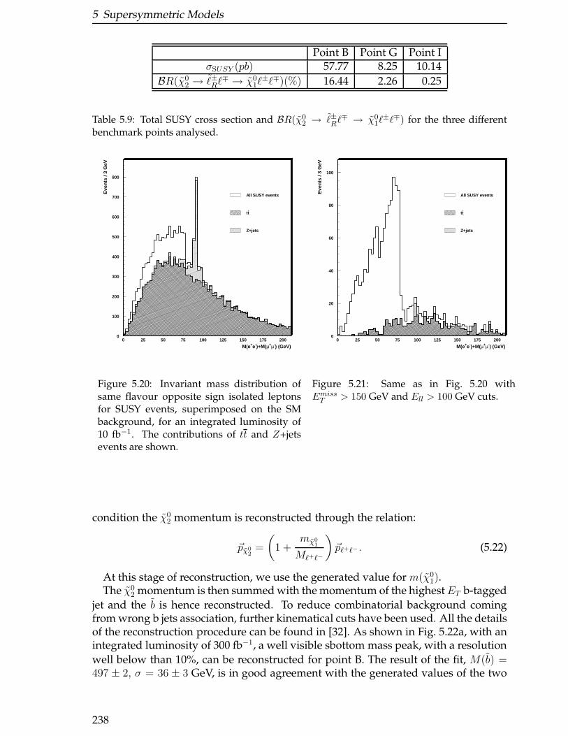
5 Supersymmetric Models
Point B Point G Point IσSUSY (pb) 57.77 8.25 10.14
BR(χ02 → ℓ±Rℓ
∓ → χ01ℓ
±ℓ∓)(%) 16.44 2.26 0.25
Table 5.9: Total SUSY cross section and BR(χ02 → ℓ±Rℓ
∓ → χ01ℓ
±ℓ∓) for the three differentbenchmark points analysed.
0
100
200
300
400
500
600
700
800
0 25 50 75 100 125 150 175 200
M(e+e-)+M(µ+µ-) (GeV)
Eve
nts
/ 3 G
eV
All SUSY events
tt-
Z+jets
0
20
40
60
80
100
0 25 50 75 100 125 150 175 200
M(e+e-)+M(µ+µ-) (GeV)
Eve
nts
/ 3 G
eV
All SUSY events
tt-
Z+jets
Figure 5.20: Invariant mass distribution ofsame flavour opposite sign isolated leptonsfor SUSY events, superimposed on the SMbackground, for an integrated luminosity of10 fb−1. The contributions of tt and Z+jetsevents are shown.
Figure 5.21: Same as in Fig. 5.20 withEmissT > 150 GeV and Ell > 100 GeV cuts.
condition the χ02 momentum is reconstructed through the relation:
~pχ02
=
(1 +
mχ01
Mℓ+ℓ−
)~pℓ+ℓ−. (5.22)
At this stage of reconstruction, we use the generated value for m(χ01).
The χ02 momentum is then summed with the momentum of the highestET b-tagged
jet and the b is hence reconstructed. To reduce combinatorial background comingfrom wrong b jets association, further kinematical cuts have been used. All the detailsof the reconstruction procedure can be found in [32]. As shown in Fig. 5.22a, with anintegrated luminosity of 300 fb−1, a well visible sbottom mass peak, with a resolution
well below than 10%, can be reconstructed for point B. The result of the fit, M(b) =497 ± 2, σ = 36 ± 3 GeV, is in good agreement with the generated values of the two
238
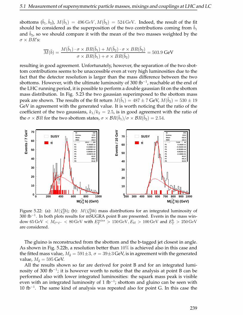
5.1 Measurement of supersymmetric particle masses, mixings and couplings at LHC and LC
sbottoms (b1, b2), M(b1) = 496 GeV ,M(b2) = 524 GeV. Indeed, the result of the fitshould be considered as the superposition of the two contributions coming from b1and b2, so we should compare it with the mean of the two masses weighted by theσ ×BR’s:
M(b) =M(b1) · σ × BR(b1) +M(b2) · σ ×BR(b2)
σ × BR(b1) + σ × BR(b2)= 503.9 GeV
resulting in good agreement. Unfortunately, however, the separation of the two sbot-tom contributions seems to be unaccessible even at very high luminosities due to thefact that the detector resolution is larger than the mass difference between the twosbottoms. However, with the ultimate luminosity of 300 fb−1, reachable at the end ofthe LHC running period, it is possible to perform a double gaussian fit on the sbottommass distribution. In Fig. 5.23 the two gaussian superimposed to the sbottom mass
peak are shown. The results of the fit return M(b1) = 487± 7 GeV, M(b2) = 530± 19GeV in agreement with the generated value. It is worth noticing that the ratio of thecoefficient of the two gaussians, k1/k2 = 2.5, is in good agreement with the ratio of
the σ × BR for the two sbottom states, σ × BR(b1)/σ × BR(b2) = 2.54.
0
10
20
30
40
50
60
70
0 200 400 600 800 1000
IDEntriesMeanRMS
103 1747
497.9 152.0
155.3 / 109P1 0.1932E-11P2 0.1266E+13P3 -0.8253E+12P4 0.3855E+10P5 -0.8367E-02P6 42.67P7 496.8P8 35.62
M(χ∼
20 b) (GeV)
Eve
nts
/ 7 G
eV
SUSY
tt-
0
10
20
30
40
50
60
70
200 300 400 500 600 700 800 900 1000
IDEntriesMeanRMS
203 1014
632.9 102.3
74.60 / 46P1 0.1462E-11P2 -0.1522E+16P3 -0.3530E+14P4 0.8525E+11P5 -0.1080E-01P6 46.07P7 591.0P8 38.55
M(χ∼
20 b) (GeV)
Eve
nts
/ 10
GeV
SUSY
tt-
Figure 5.22: (a): M(χ02b); (b): M(χ0
2bb) mass distributions for an integrated luminosity of300 fb−1. In both plots results for mSUGRA point B are presented. Events in the mass win-dow 65GeV < Mℓ+ℓ− < 80GeV with EmissT > 150GeV, Eℓℓ > 100GeV and EbT > 250GeVare considered.
The gluino is reconstructed from the sbottom and the b-tagged jet closest in angle.As shown in Fig. 5.22b, a resolution better than 10% is achieved also in this case andthe fitted mass value,Mg = 591±3, σ = 39±3 GeV, is in agreement with the generatedvalue, Mg = 595 GeV.
All the results shown so far are derived for point B and for an integrated lumi-nosity of 300 fb−1; it is however worth to notice that the analysis at point B can beperformed also with lower integrated luminosities: the squark mass peak is visibleeven with an integrated luminosity of 1 fb−1; sbottom and gluino can be seen with10 fb−1. The same kind of analysis was repeated also for point G. In this case the
239
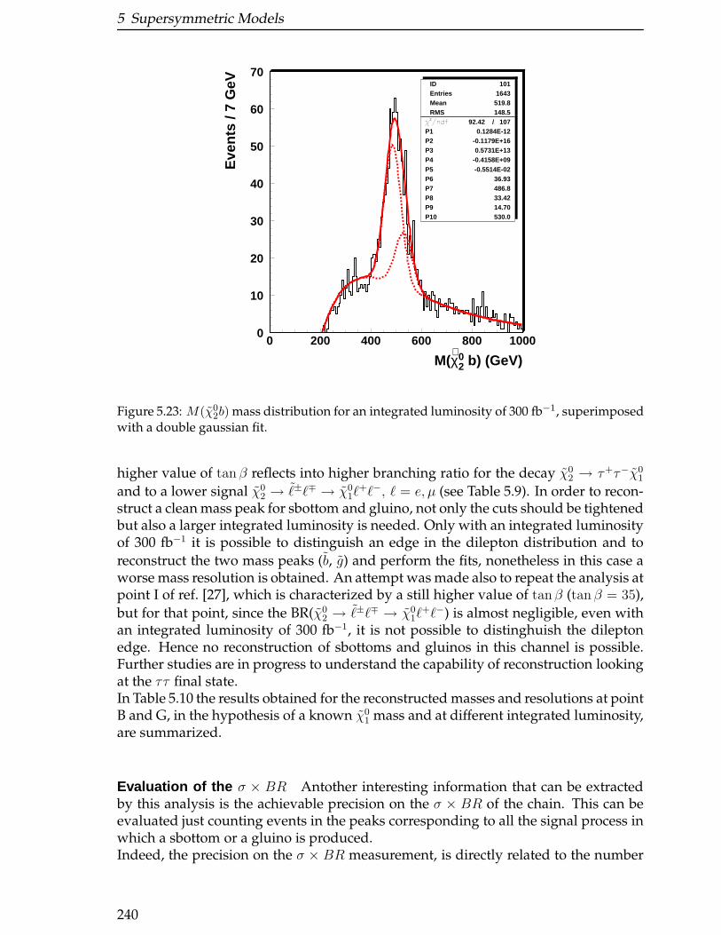
5 Supersymmetric Models
0
10
20
30
40
50
60
70
0 200 400 600 800 1000
IDEntriesMeanRMS
101 1643
519.8 148.5
92.42 / 107P1 0.1284E-12P2 -0.1179E+16P3 0.5731E+13P4 -0.4158E+09P5 -0.5514E-02P6 36.93P7 486.8P8 33.42P9 14.70P10 530.0
M(χ∼
20 b) (GeV)
Eve
nts
/ 7 G
eV
Figure 5.23: M(χ02b) mass distribution for an integrated luminosity of 300 fb−1, superimposed
with a double gaussian fit.
higher value of tan β reflects into higher branching ratio for the decay χ02 → τ+τ−χ0
1
and to a lower signal χ02 → ℓ±ℓ∓ → χ0
1ℓ+ℓ−, ℓ = e, µ (see Table 5.9). In order to recon-
struct a clean mass peak for sbottom and gluino, not only the cuts should be tightenedbut also a larger integrated luminosity is needed. Only with an integrated luminosityof 300 fb−1 it is possible to distinguish an edge in the dilepton distribution and to
reconstruct the two mass peaks (b, g) and perform the fits, nonetheless in this case aworse mass resolution is obtained. An attempt was made also to repeat the analysis atpoint I of ref. [27], which is characterized by a still higher value of tanβ (tan β = 35),
but for that point, since the BR(χ02 → ℓ±ℓ∓ → χ0
1ℓ+ℓ−) is almost negligible, even with
an integrated luminosity of 300 fb−1, it is not possible to distinghuish the dileptonedge. Hence no reconstruction of sbottoms and gluinos in this channel is possible.Further studies are in progress to understand the capability of reconstruction lookingat the ττ final state.In Table 5.10 the results obtained for the reconstructed masses and resolutions at pointB and G, in the hypothesis of a known χ0
1 mass and at different integrated luminosity,are summarized.
Evaluation of the σ × BR Antother interesting information that can be extractedby this analysis is the achievable precision on the σ × BR of the chain. This can beevaluated just counting events in the peaks corresponding to all the signal process inwhich a sbottom or a gluino is produced.Indeed, the precision on the σ × BR measurement, is directly related to the number
240
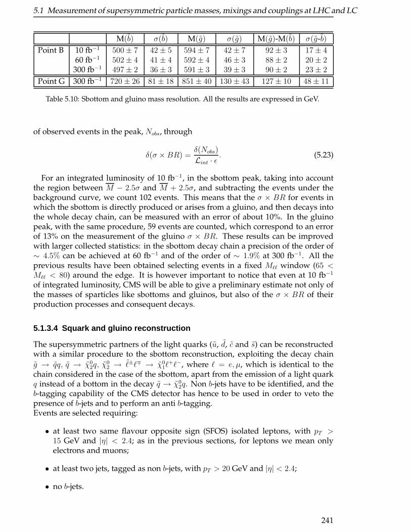
5.1 Measurement of supersymmetric particle masses, mixings and couplings at LHC and LC
M(b) σ(b) M(g) σ(g) M(g)-M(b) σ(g-b)
Point B 10 fb−1 500± 7 42± 5 594± 7 42± 7 92± 3 17± 460 fb−1 502± 4 41± 4 592± 4 46± 3 88± 2 20± 2
300 fb−1 497± 2 36± 3 591± 3 39± 3 90± 2 23± 2
Point G 300 fb−1 720± 26 81± 18 851± 40 130± 43 127± 10 48± 11
Table 5.10: Sbottom and gluino mass resolution. All the results are expressed in GeV.
of observed events in the peak, Nobs, through
δ(σ ×BR) =δ(Nobs)
Lint · ǫ. (5.23)
For an integrated luminosity of 10 fb−1, in the sbottom peak, taking into accountthe region between M − 2.5σ and M + 2.5σ, and subtracting the events under thebackground curve, we count 102 events. This means that the σ × BR for events inwhich the sbottom is directly produced or arises from a gluino, and then decays intothe whole decay chain, can be measured with an error of about 10%. In the gluinopeak, with the same procedure, 59 events are counted, which correspond to an errorof 13% on the measurement of the gluino σ × BR. These results can be improvedwith larger collected statistics: in the sbottom decay chain a precision of the order of∼ 4.5% can be achieved at 60 fb−1 and of the order of ∼ 1.9% at 300 fb−1. All theprevious results have been obtained selecting events in a fixed Mℓℓ window (65 <Mℓℓ < 80) around the edge. It is however important to notice that even at 10 fb−1
of integrated luminosity, CMS will be able to give a preliminary estimate not only ofthe masses of sparticles like sbottoms and gluinos, but also of the σ × BR of theirproduction processes and consequent decays.
5.1.3.4 Squark and gluino reconstruction
The supersymmetric partners of the light quarks (u, d, c and s) can be reconstructedwith a similar procedure to the sbottom reconstruction, exploiting the decay chain
g → qq, q → χ02q, χ
02 → ℓ±ℓ∓ → χ0
1ℓ+ℓ−, where ℓ = e, µ, which is identical to the
chain considered in the case of the sbottom, apart from the emission of a light quarkq instead of a bottom in the decay q → χ0
2q. Non b-jets have to be identified, and theb-tagging capability of the CMS detector has hence to be used in order to veto thepresence of b-jets and to perform an anti b-tagging.Events are selected requiring:
• at least two same flavour opposite sign (SFOS) isolated leptons, with pT >15 GeV and |η| < 2.4; as in the previous sections, for leptons we mean onlyelectrons and muons;
• at least two jets, tagged as non b-jets, with pT > 20 GeV and |η| < 2.4;
• no b-jets.
241

5 Supersymmetric Models
The reconstruction procedure starts, as in the sbottom case, from the identifica-tion of the dilepton edge and hence events in the window 65 GeV < Mℓℓ < 80 GeVare selected and associated to the most energetic jet to get the squark invariant massdistribution. In order to reduce the SM background a cut in the missing energy isimposed, as in the previous reconstruction and also similar kinematical cuts are usedto reduce the SUSY combinatorial background. A detailed description of all the cutsimposed can be found in ref. [33]. Given the very high σ×BR for squarks going intothe χ0
2-dilepton chain, which is about four times larger than for the sbottom chain, it isplausible to perform the reconstruction with an integrated luminosity lower than inthe sbottom case. In ref. [32] it has been shown that squark reconstruction will be pos-sible already with an integrated luminosity of 1 fb−1, corresponding to the first two orthree months of life of the Large Hadron Collider. The treatment of the combinatorialbackground is more complicated than for sbottom since in this case the contributionqg and qq processes cannot be neglected. However, similarly to the sbottom case, theuse of kinematical cuts allows a good combinatorial reduction. Figure 5.24 shows thesquark peak for Ej1 > 300 GeV, for a sample corresponding to 300 fb−1 of integratedluminosity. The measured values are:
M(χ02q) = 536± 1 GeV
σ[M(χ02q)] = 31± 1 GeV
Due to the Wino nature of χ02, the decay q → χ0
2 occurs almost uniquely for the leftsquarks, since the right squarks decay through q → χ0
1q with a BR larger than 0.99.The measured value has hence to be compared with the nominal values of the leftsquark, which are
M(dL) = M(sL) = 542.8 GeV
M(uL) = M(cL) = 537.0 GeV
The resolution of the σ×BR of the entire squark production and decay process canbe inferred by the number of events in the peak, which is 18048 at 300 fb−1, leadingto a value:
δ(σ ×BR)
σ × BR = 0.7% (5.25)
Gluino can be reconstructed going back in the decay chain with a procedure similarto the one used for the sbottom: after removing the most energetic jet from the list ofthe available jets, the one closest in angle to the reconstructed squark is associated toit. Figure 5.25 shows the final gluino peak for an integrated luminosity of 300 fb−1,after all the kinematical cuts described in ref. [33] are applied. The gaussian fit gives:
M(χ02qq) = 590± 2 GeV
σ[M(χ02qq)] = 59± 2 GeV
which is in agreement with the mass value of the generated gluino: M(g) = 595.1 GeV.Although the achieved resolution is worse than the one of the gluino reconstructedinto the sbottom chain, this result is remarkable since it has been obtained in a totallyindipendent way, and can eventually be combined with that in order to have a betterestimate of the gluino mass.
242
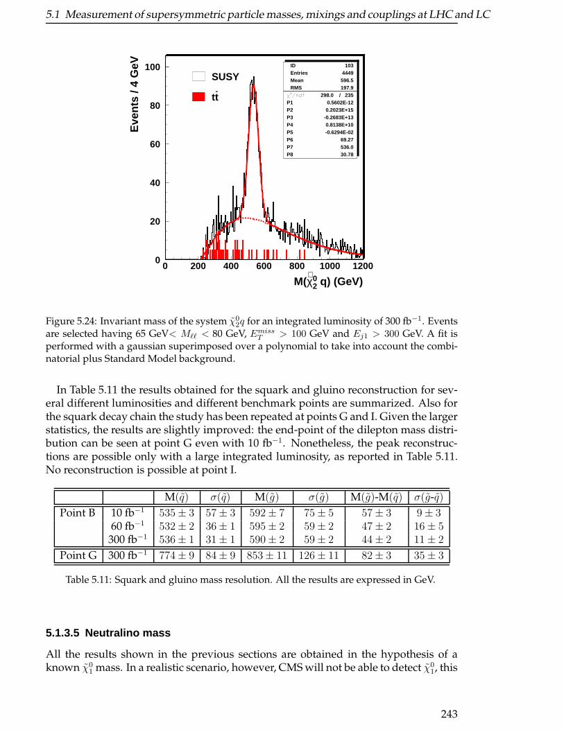
5.1 Measurement of supersymmetric particle masses, mixings and couplings at LHC and LC
0
20
40
60
80
100
0 200 400 600 800 1000 1200
IDEntriesMeanRMS
103 4449
596.5 197.9
298.0 / 235P1 0.5602E-12P2 0.2023E+15P3 -0.2683E+13P4 0.8138E+10P5 -0.6294E-02P6 69.27P7 536.0P8 30.78
M(χ∼
20 q) (GeV)
Eve
nts
/ 4 G
eV
SUSY
tt-
Figure 5.24: Invariant mass of the system χ02q for an integrated luminosity of 300 fb−1. Events
are selected having 65 GeV< Mℓℓ < 80 GeV, EmissT > 100 GeV and Ej1 > 300 GeV. A fit isperformed with a gaussian superimposed over a polynomial to take into account the combi-natorial plus Standard Model background.
In Table 5.11 the results obtained for the squark and gluino reconstruction for sev-eral different luminosities and different benchmark points are summarized. Also forthe squark decay chain the study has been repeated at points G and I. Given the largerstatistics, the results are slightly improved: the end-point of the dilepton mass distri-bution can be seen at point G even with 10 fb−1. Nonetheless, the peak reconstruc-tions are possible only with a large integrated luminosity, as reported in Table 5.11.No reconstruction is possible at point I.
M(q) σ(q) M(g) σ(g) M(g)-M(q) σ(g-q)
Point B 10 fb−1 535± 3 57± 3 592± 7 75± 5 57± 3 9± 360 fb−1 532± 2 36± 1 595± 2 59± 2 47± 2 16± 5
300 fb−1 536± 1 31± 1 590± 2 59± 2 44± 2 11± 2
Point G 300 fb−1 774± 9 84± 9 853± 11 126± 11 82± 3 35± 3
Table 5.11: Squark and gluino mass resolution. All the results are expressed in GeV.
5.1.3.5 Neutralino mass
All the results shown in the previous sections are obtained in the hypothesis of aknown χ0
1 mass. In a realistic scenario, however, CMS will not be able to detect χ01, this
243
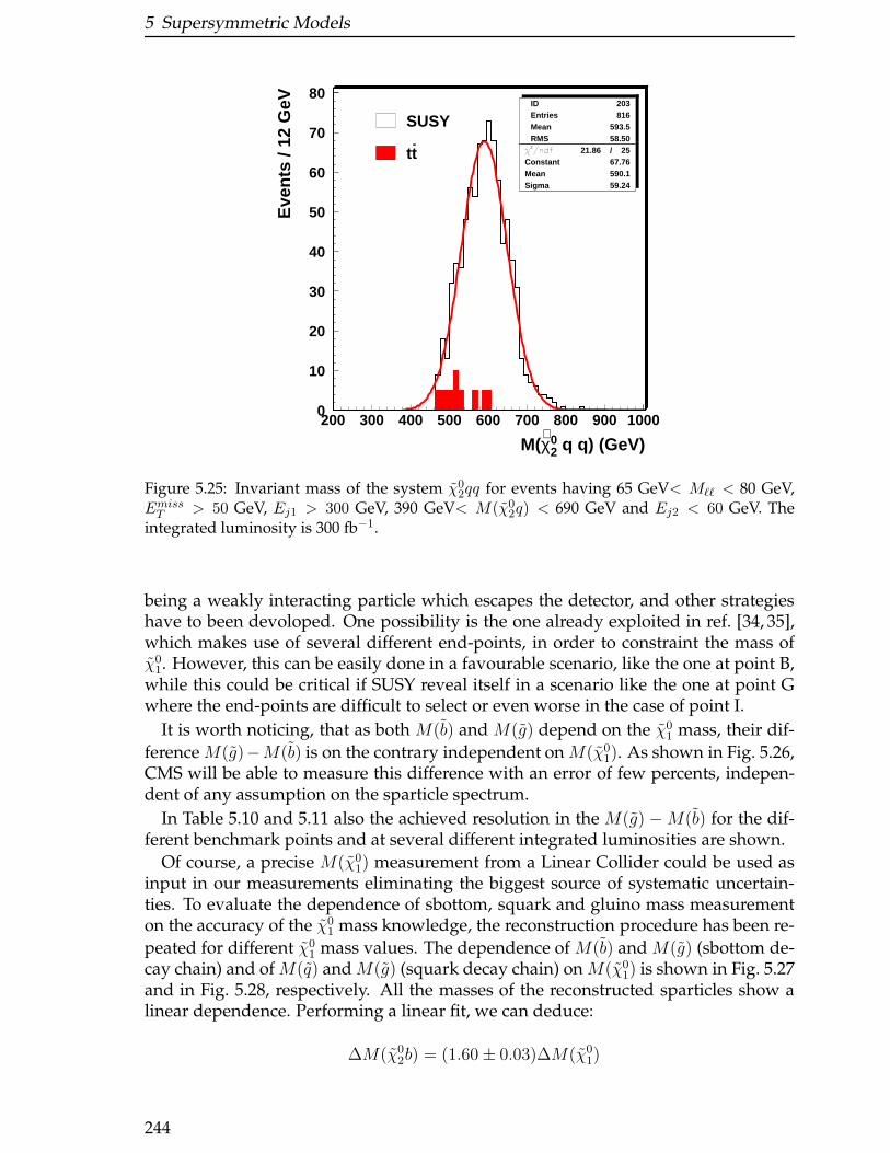
5 Supersymmetric Models
0
10
20
30
40
50
60
70
80
200 300 400 500 600 700 800 900 1000
IDEntriesMeanRMS
203 816
593.5 58.50
21.86 / 25Constant 67.76Mean 590.1Sigma 59.24
M(χ∼
20 q q) (GeV)
Eve
nts
/ 12
GeV
SUSY
tt-
Figure 5.25: Invariant mass of the system χ02qq for events having 65 GeV< Mℓℓ < 80 GeV,
EmissT > 50 GeV, Ej1 > 300 GeV, 390 GeV< M(χ02q) < 690 GeV and Ej2 < 60 GeV. The
integrated luminosity is 300 fb−1.
being a weakly interacting particle which escapes the detector, and other strategieshave to been devoloped. One possibility is the one already exploited in ref. [34, 35],which makes use of several different end-points, in order to constraint the mass ofχ0
1. However, this can be easily done in a favourable scenario, like the one at point B,while this could be critical if SUSY reveal itself in a scenario like the one at point Gwhere the end-points are difficult to select or even worse in the case of point I.
It is worth noticing, that as both M(b) and M(g) depend on the χ01 mass, their dif-
ference M(g)−M(b) is on the contrary independent on M(χ01). As shown in Fig. 5.26,
CMS will be able to measure this difference with an error of few percents, indepen-dent of any assumption on the sparticle spectrum.
In Table 5.10 and 5.11 also the achieved resolution in the M(g) −M(b) for the dif-ferent benchmark points and at several different integrated luminosities are shown.
Of course, a precise M(χ01) measurement from a Linear Collider could be used as
input in our measurements eliminating the biggest source of systematic uncertain-ties. To evaluate the dependence of sbottom, squark and gluino mass measurementon the accuracy of the χ0
1 mass knowledge, the reconstruction procedure has been re-
peated for different χ01 mass values. The dependence of M(b) and M(g) (sbottom de-
cay chain) and of M(q) and M(g) (squark decay chain) on M(χ01) is shown in Fig. 5.27
and in Fig. 5.28, respectively. All the masses of the reconstructed sparticles show alinear dependence. Performing a linear fit, we can deduce:
∆M(χ02b) = (1.60± 0.03)∆M(χ0
1)
244
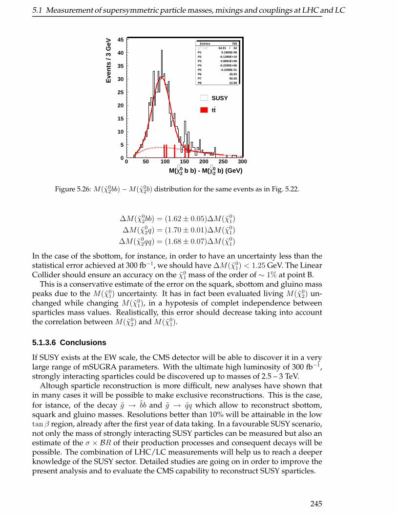
5.1 Measurement of supersymmetric particle masses, mixings and couplings at LHC and LC
0
5
10
15
20
25
30
35
40
45
0 50 100 150 200 250 300
Entries 769 64.91 / 62
P1 0.1865E-08P2 -0.1395E+10P3 0.9891E+08P4 -0.2290E+06P5 -0.1088E-01P6 26.83P7 90.05P8 22.89
M(χ∼
20 b b) - M(χ
∼20 b) (GeV)
Eve
nts
/ 3 G
eV
SUSY
tt-
Figure 5.26: M(χ02bb)−M(χ0
2b) distribution for the same events as in Fig. 5.22.
∆M(χ02bb) = (1.62± 0.05)∆M(χ0
1)
∆M(χ02q) = (1.70± 0.01)∆M(χ0
1)
∆M(χ02qq) = (1.68± 0.07)∆M(χ0
1)
In the case of the sbottom, for instance, in order to have an uncertainty less than thestatistical error achieved at 300 fb−1, we should have ∆M(χ0
1) < 1.25 GeV. The LinearCollider should ensure an accuracy on the χ0
1 mass of the order of ∼ 1% at point B.This is a conservative estimate of the error on the squark, sbottom and gluino mass
peaks due to the M(χ01) uncertainty. It has in fact been evaluated living M(χ0
2) un-changed while changing M(χ0
1), in a hypotesis of complet independence betweensparticles mass values. Realistically, this error should decrease taking into accountthe correlation between M(χ0
2) and M(χ01).
5.1.3.6 Conclusions
If SUSY exists at the EW scale, the CMS detector will be able to discover it in a verylarge range of mSUGRA parameters. With the ultimate high luminosity of 300 fb−1,strongly interacting sparticles could be discovered up to masses of 2.5 – 3 TeV.
Altough sparticle reconstruction is more difficult, new analyses have shown thatin many cases it will be possible to make exclusive reconstructions. This is the case,
for istance, of the decay g → bb and g → qq which allow to reconstruct sbottom,squark and gluino masses. Resolutions better than 10% will be attainable in the lowtan β region, already after the first year of data taking. In a favourable SUSY scenario,not only the mass of strongly interacting SUSY particles can be measured but also anestimate of the σ × BR of their production processes and consequent decays will bepossible. The combination of LHC/LC measurements will help us to reach a deeperknowledge of the SUSY sector. Detailed studies are going on in order to improve thepresent analysis and to evaluate the CMS capability to reconstruct SUSY sparticles.
245
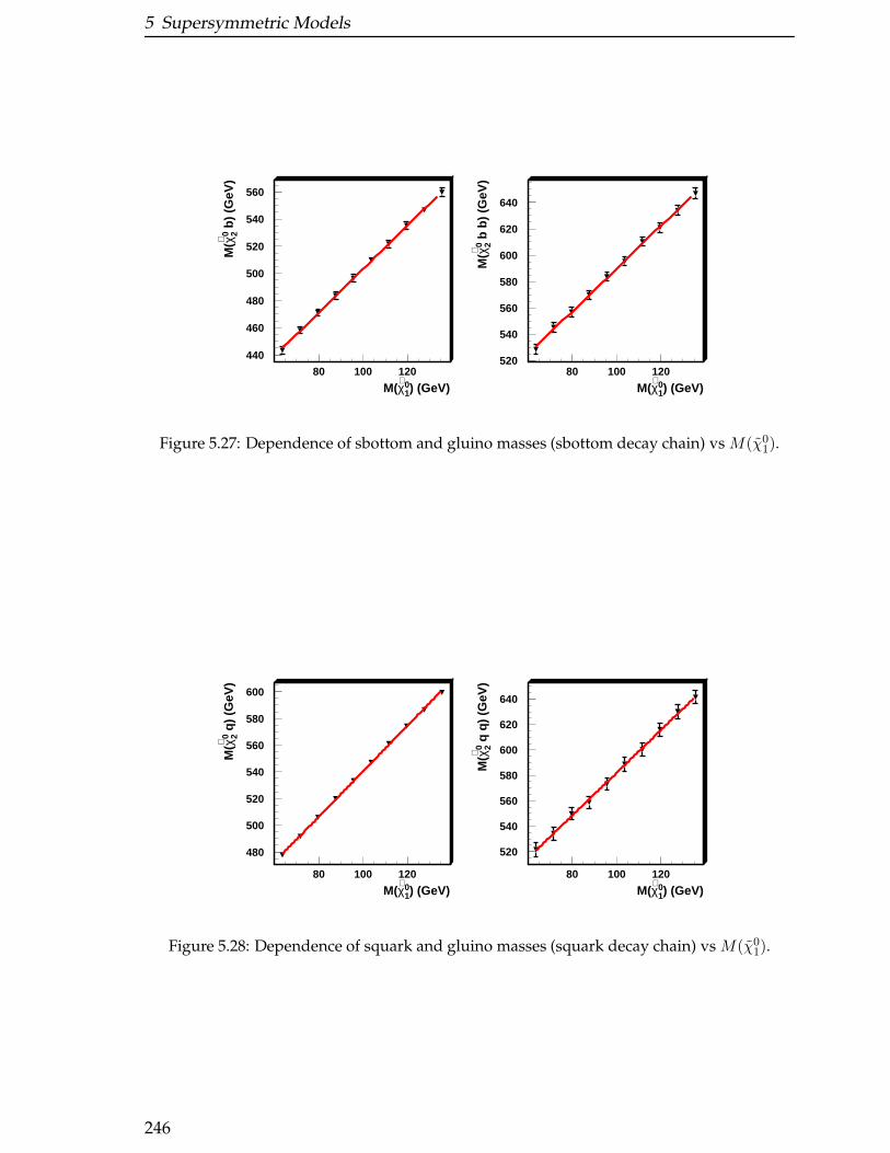
5 Supersymmetric Models
440
460
480
500
520
540
560
80 100 120
M(χ∼
10) (GeV)
M(χ∼
20 b)
(G
eV)
520
540
560
580
600
620
640
80 100 120
M(χ∼
10) (GeV)
M(χ∼
20 b
b) (
GeV
)
Figure 5.27: Dependence of sbottom and gluino masses (sbottom decay chain) vs M(χ01).
480
500
520
540
560
580
600
80 100 120
M(χ∼
10) (GeV)
M(χ∼
20 q)
(G
eV)
520
540
560
580
600
620
640
80 100 120
M(χ∼
10) (GeV)
M(χ∼
20 q
q) (
GeV
)
Figure 5.28: Dependence of squark and gluino masses (squark decay chain) vs M(χ01).
246
5.1 Measurement of supersymmetric particle masses, mixings and couplings at LHC and LC
5.1.4 Measurement of sparticle masses in mSUGRA scenarioSPS 1a at a Linear Collider
H.-U. Martyn
5.1.4.1 Introduction
If low energy supersymmetry will be discovered at the LHC its gross features maybe revealed, in particular for the coloured squark and gluino sector. However, a Lin-ear Collider will be indispensible in order to provide complementary information, inparticular in the slepton and neutralino/chargino sector, and to scrutinise the charac-teristics of the underlying SUSY structure. High precision LC experiments have to
• measure the masses, decay widths, production cross sections, mixing angles,etc., of the new particles,
• prove that each particle can be associated to its superpartner with the expectedspin and parity, gauge quantum numbers and couplings,
• reconstruct the low energy SUSY breaking parameters which would allow one touncover the fundamental theory and finally extrapolate its parameters to high(GUT, Planck) scales.
A concurrent operation of the LHC and LC would provide answers to these ele-mentary topics already after a few years of running. A nice example to support theircomplementarity is the SPS 1a benchmark point [1, 4]. With the recent progress incavity development TESLA energies of 1 TeV appear achievable, thus the completeslepton and neutralino/chargino spectra as well as the light stop 1 would be acces-sible. A peculiarity of this scenario is the large tan β = 10 leading to (incompletelymeasurable) multi τ final states from χ0
i , χ±i cascade decays. Therefore charged slep-
ton and sneutrino production are very important to measure the masses of the LSPχ0
1 and the light chargino χ±1 . The advantage of the LC is to explore the spectrum in
a bottom-up approach, i.e. selecting particular channels by the appropriate choice ofenergy and beam polarisations, while suppressing background reactions.
First studies of SPS 1a masses were based on extrapolations and estimates fromlow tan β scenarios [36]. Meanwhile more reliable simulations have become available.They typicaly assume integrated luminosities ofL = 250−500 fb−1 at
√s = 500 GeV to
be accumulated within a reasonable run time of one to two years. The LC luminosityis expected to scale linearly with energy. Beam polarisations of Pe− = ±0.8 and Pe+ =±0.6 are assumed. For the determination of sparticle properties of SPS 1a other thanmasses see [37].
5.1.4.2 Sleptons
Scalar leptons are produced in pairs
e+e− → ℓ+i ℓ−j , νℓ νℓ ℓ = e, µ, τ and [i, j = L,R or 1, 2] (5.27)
via s-channel γ/Z exchange and t-channel χ exchange for the first generation. The
L, R states can be determined using beam polarisation, e.g. ℓRℓR production is much
247

5 Supersymmetric Models
larger for right-handed e−R than for left-handed e−L electrons; positron polarisationfurther enhances the effect. The isotropic two-body decays
ℓ− → ℓ−χ0i , (5.28)
νℓ → ℓ−χ+i (5.29)
allow for a clean identification and lead to a uniform lepton energy spectrum. Theminimum and maximum (‘endpoint’) energies
E+/− =
√s
4
(1−
m2χ
m2ℓ
)(1± β) , (5.30)
ml =
√s
E− + E+
√E−E+ , (5.31)
mχ = ml
√1− E− + E+√
s/2(5.32)
can be used for an accurate determination of the masses of the primary slepton andthe secondary neutralino/chargino.
Charged slepton production in continuum Examples of mass measurements us-ing the lepton energy spectra of e+Le
−R → µRµR and eReR production at
√s = 400 GeV
are shown in fig. 5.29 [38]. With a moderate luminosity of L = 200 fb−1 the massescan be determined with (highly correlated) errors of δmµR
≃ δmχ01≃ 0.2 GeV, re-
spectively δmeR≃ δmχ0
1≃ 0.1 GeV. A simultaneous analysis of eReR, eReL and eLeL
Figure 5.29: Energy spectra of Eµ from the reaction e+Le−R → µ+
R µ−R → µ+χ0
1 µ−χ0
1 (left) andEe from the reaction e+Le
−R → e+R e
−R → e+χ0
1 e−χ0
1 (right),SPS 1a at√s = 400 GeV and L =
200 fb−1
production makes use of the different energy distributions of the final electrons andpositrons [39,40]. The symmetric background is eliminated by a double subtraction ofe− and e+ energy spectra and opposite electron beam polarisations. This essentiallyresults in a clean eReL sample where the endpoints from eR and eL decays are easilymeasurable. Assuming
√s = 500 GeV and L = 2 · 500 fb−1, both selectron masses can
be determined with an accuracy of δmeR, eL≃ 0.8 GeV.
248
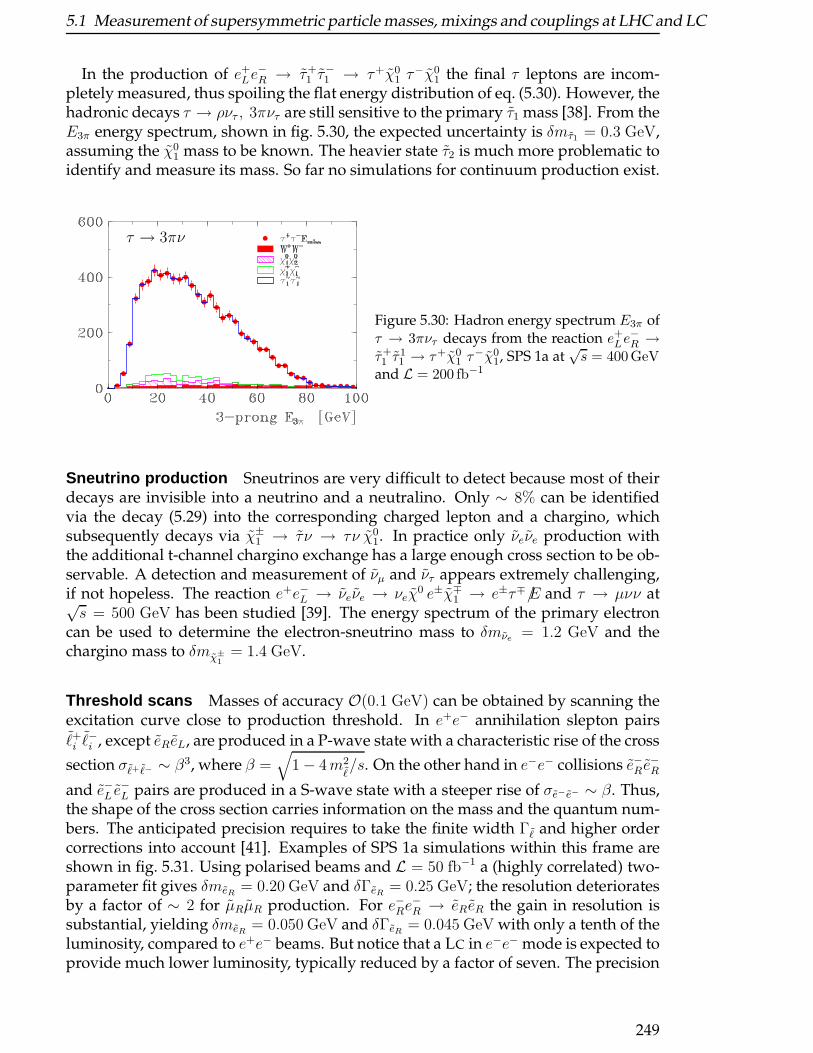
5.1 Measurement of supersymmetric particle masses, mixings and couplings at LHC and LC
In the production of e+Le−R → τ+
1 τ−1 → τ+χ0
1 τ−χ0
1 the final τ leptons are incom-pletely measured, thus spoiling the flat energy distribution of eq. (5.30). However, thehadronic decays τ → ρντ , 3πντ are still sensitive to the primary τ1 mass [38]. From theE3π energy spectrum, shown in fig. 5.30, the expected uncertainty is δmτ1 = 0.3 GeV,assuming the χ0
1 mass to be known. The heavier state τ2 is much more problematic toidentify and measure its mass. So far no simulations for continuum production exist.
τ → 3πν
Figure 5.30: Hadron energy spectrum E3π ofτ → 3πντ decays from the reaction e+Le
−R →
τ+1 τ
11 → τ+χ0
1 τ−χ0
1, SPS 1a at√s = 400GeV
and L = 200 fb−1
Sneutrino production Sneutrinos are very difficult to detect because most of theirdecays are invisible into a neutrino and a neutralino. Only ∼ 8% can be identifiedvia the decay (5.29) into the corresponding charged lepton and a chargino, whichsubsequently decays via χ±
1 → τ ν → τν χ01. In practice only νeνe production with
the additional t-channel chargino exchange has a large enough cross section to be ob-servable. A detection and measurement of νµ and ντ appears extremely challenging,if not hopeless. The reaction e+e−L → νeνe → νeχ
0 e±χ∓1 → e±τ∓E/ and τ → µνν at√
s = 500 GeV has been studied [39]. The energy spectrum of the primary electroncan be used to determine the electron-sneutrino mass to δmνe = 1.2 GeV and thechargino mass to δmχ±
1= 1.4 GeV.
Threshold scans Masses of accuracy O(0.1 GeV) can be obtained by scanning theexcitation curve close to production threshold. In e+e− annihilation slepton pairs
ℓ+i ℓ−i , except eReL, are produced in a P-wave state with a characteristic rise of the cross
section σℓ+ ℓ− ∼ β3, where β =√
1− 4m2ℓ/s. On the other hand in e−e− collisions e−R e
−R
and e−L e−L pairs are produced in a S-wave state with a steeper rise of σe−e− ∼ β. Thus,
the shape of the cross section carries information on the mass and the quantum num-bers. The anticipated precision requires to take the finite width Γℓ and higher ordercorrections into account [41]. Examples of SPS 1a simulations within this frame areshown in fig. 5.31. Using polarised beams and L = 50 fb−1 a (highly correlated) two-parameter fit gives δmeR
= 0.20 GeV and δΓeR= 0.25 GeV; the resolution deteriorates
by a factor of ∼ 2 for µRµR production. For e−Re−R → eReR the gain in resolution is
substantial, yielding δmeR= 0.050 GeV and δΓeR
= 0.045 GeV with only a tenth of theluminosity, compared to e+e− beams. But notice that a LC in e−e− mode is expected toprovide much lower luminosity, typically reduced by a factor of seven. The precision
249
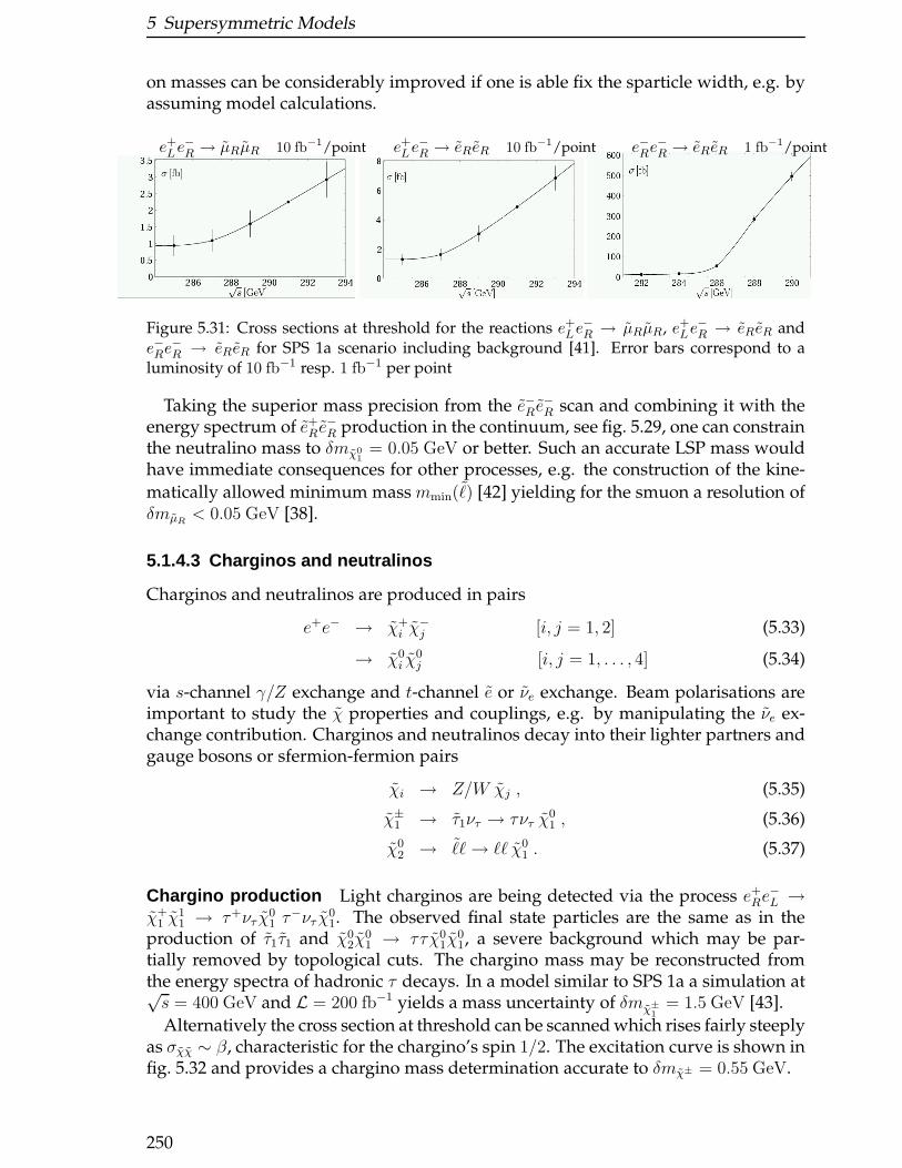
5 Supersymmetric Models
on masses can be considerably improved if one is able fix the sparticle width, e.g. byassuming model calculations.
e+Le−R → µRµR 10 fb−1/point e+Le
−R → eReR 10 fb−1/point e−Re
−R → eReR 1 fb−1/point
Figure 5.31: Cross sections at threshold for the reactions e+Le−R → µRµR, e+Le
−R → eReR and
e−Re−R → eReR for SPS 1a scenario including background [41]. Error bars correspond to a
luminosity of 10 fb−1 resp. 1 fb−1 per point
Taking the superior mass precision from the e−Re−R scan and combining it with the
energy spectrum of e+R e−R production in the continuum, see fig. 5.29, one can constrain
the neutralino mass to δmχ01
= 0.05 GeV or better. Such an accurate LSP mass wouldhave immediate consequences for other processes, e.g. the construction of the kine-
matically allowed minimum mass mmin(ℓ) [42] yielding for the smuon a resolution ofδmµR
< 0.05 GeV [38].
5.1.4.3 Charginos and neutralinos
Charginos and neutralinos are produced in pairs
e+e− → χ+i χ
−j [i, j = 1, 2] (5.33)
→ χ0i χ
0j [i, j = 1, . . . , 4] (5.34)
via s-channel γ/Z exchange and t-channel e or νe exchange. Beam polarisations areimportant to study the χ properties and couplings, e.g. by manipulating the νe ex-change contribution. Charginos and neutralinos decay into their lighter partners andgauge bosons or sfermion-fermion pairs
χi → Z/W χj , (5.35)
χ±1 → τ1ντ → τντ χ
01 , (5.36)
χ02 → ℓℓ→ ℓℓ χ0
1 . (5.37)
Chargino production Light charginos are being detected via the process e+Re−L →
χ+1 χ
11 → τ+ντ χ
01 τ
−ντ χ01. The observed final state particles are the same as in the
production of τ1τ1 and χ02χ
01 → ττχ0
1χ01, a severe background which may be par-
tially removed by topological cuts. The chargino mass may be reconstructed fromthe energy spectra of hadronic τ decays. In a model similar to SPS 1a a simulation at√s = 400 GeV and L = 200 fb−1 yields a mass uncertainty of δmχ±
1= 1.5 GeV [43].
Alternatively the cross section at threshold can be scanned which rises fairly steeplyas σχχ ∼ β, characteristic for the chargino’s spin 1/2. The excitation curve is shown infig. 5.32 and provides a chargino mass determination accurate to δmχ± = 0.55 GeV.
250
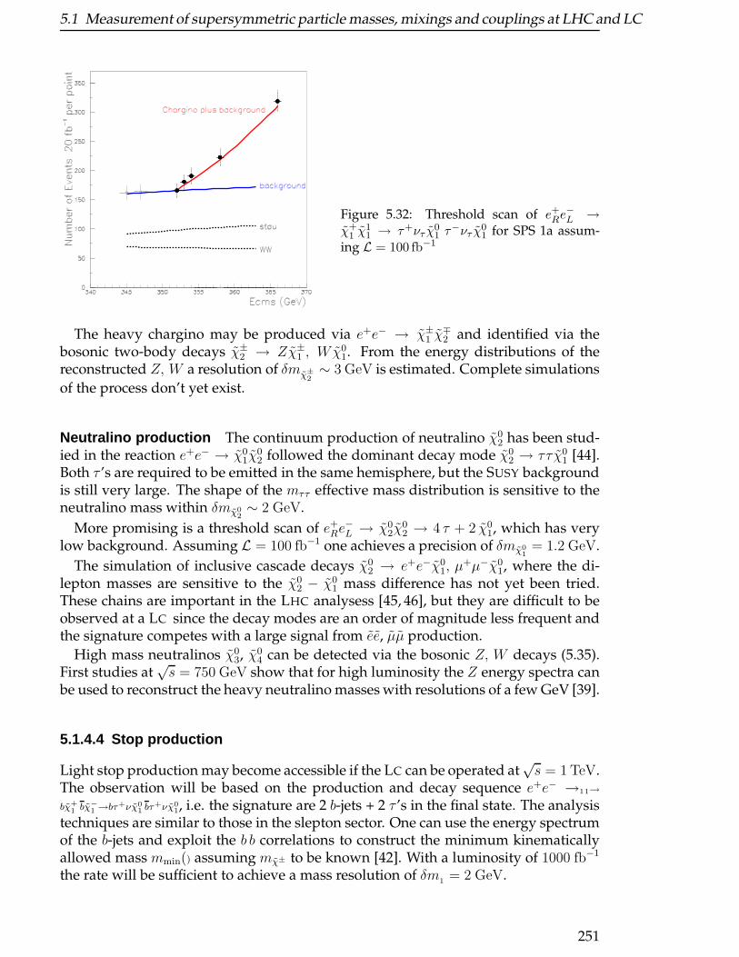
5.1 Measurement of supersymmetric particle masses, mixings and couplings at LHC and LC
Figure 5.32: Threshold scan of e+Re−L →
χ+1 χ
11 → τ+ντ χ
01 τ
−ντ χ01 for SPS 1a assum-
ing L = 100 fb−1
The heavy chargino may be produced via e+e− → χ±1 χ
∓2 and identified via the
bosonic two-body decays χ±2 → Zχ±
1 , W χ01. From the energy distributions of the
reconstructed Z, W a resolution of δmχ±
2∼ 3 GeV is estimated. Complete simulations
of the process don’t yet exist.
Neutralino production The continuum production of neutralino χ02 has been stud-
ied in the reaction e+e− → χ01χ
02 followed the dominant decay mode χ0
2 → ττχ01 [44].
Both τ ’s are required to be emitted in the same hemisphere, but the SUSY backgroundis still very large. The shape of the mττ effective mass distribution is sensitive to theneutralino mass within δmχ0
2∼ 2 GeV.
More promising is a threshold scan of e+Re−L → χ0
2χ02 → 4 τ + 2 χ0
1, which has verylow background. Assuming L = 100 fb−1 one achieves a precision of δmχ0
1= 1.2 GeV.
The simulation of inclusive cascade decays χ02 → e+e−χ0
1, µ+µ−χ0
1, where the di-lepton masses are sensitive to the χ0
2 − χ01 mass difference has not yet been tried.
These chains are important in the LHC analysess [45, 46], but they are difficult to beobserved at a LC since the decay modes are an order of magnitude less frequent andthe signature competes with a large signal from ee, µµ production.
High mass neutralinos χ03, χ0
4 can be detected via the bosonic Z, W decays (5.35).First studies at
√s = 750 GeV show that for high luminosity the Z energy spectra can
be used to reconstruct the heavy neutralino masses with resolutions of a few GeV [39].
5.1.4.4 Stop production
Light stop production may become accessible if the LC can be operated at√s = 1 TeV.
The observation will be based on the production and decay sequence e+e− →11→bχ+
1 bχ−
1 →bτ+νχ01 bτ
+νχ01, i.e. the signature are 2 b-jets + 2 τ ’s in the final state. The analysis
techniques are similar to those in the slepton sector. One can use the energy spectrumof the b-jets and exploit the b b correlations to construct the minimum kinematicallyallowed mass mmin() assuming mχ± to be known [42]. With a luminosity of 1000 fb−1
the rate will be sufficient to achieve a mass resolution of δm1 = 2 GeV.
251
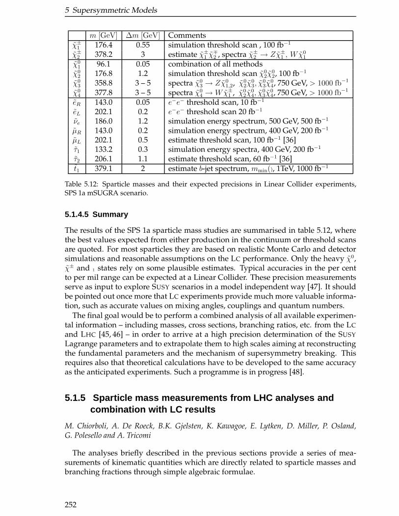
5 Supersymmetric Models
m [GeV] ∆m [GeV] Commentsχ±
1 176.4 0.55 simulation threshold scan , 100 fb−1
χ±2 378.2 3 estimate χ±
1 χ∓2 , spectra χ±
2 → Zχ±1 , W χ0
1
χ01 96.1 0.05 combination of all methodsχ0
2 176.8 1.2 simulation threshold scan χ02χ
02, 100 fb−1
χ03 358.8 3 – 5 spectra χ0
3 → Zχ01,2, χ0
2χ03, χ
03χ
04, 750 GeV, > 1000 fb−1
χ04 377.8 3 – 5 spectra χ0
4 → Wχ±1 , χ0
2χ04, χ
03χ
04, 750 GeV, > 1000 fb−1
eR 143.0 0.05 e−e− threshold scan, 10 fb−1
eL 202.1 0.2 e−e− threshold scan 20 fb−1
νe 186.0 1.2 simulation energy spectrum, 500 GeV, 500 fb−1
µR 143.0 0.2 simulation energy spectrum, 400 GeV, 200 fb−1
µL 202.1 0.5 estimate threshold scan, 100 fb−1 [36]τ1 133.2 0.3 simulation energy spectra, 400 GeV, 200 fb−1
τ2 206.1 1.1 estimate threshold scan, 60 fb−1 [36]t1 379.1 2 estimate b-jet spectrum, mmin(), 1TeV, 1000 fb−1
Table 5.12: Sparticle masses and their expected precisions in Linear Collider experiments,SPS 1a mSUGRA scenario.
5.1.4.5 Summary
The results of the SPS 1a sparticle mass studies are summarised in table 5.12, wherethe best values expected from either production in the continuum or threshold scansare quoted. For most sparticles they are based on realistic Monte Carlo and detectorsimulations and reasonable assumptions on the LC performance. Only the heavy χ0,χ± and 1 states rely on some plausible estimates. Typical accuracies in the per centto per mil range can be expected at a Linear Collider. These precision measurementsserve as input to explore SUSY scenarios in a model independent way [47]. It shouldbe pointed out once more that LC experiments provide much more valuable informa-tion, such as accurate values on mixing angles, couplings and quantum numbers.
The final goal would be to perform a combined analysis of all available experimen-tal information – including masses, cross sections, branching ratios, etc. from the LC
and LHC [45, 46] – in order to arrive at a high precision determination of the SUSY
Lagrange parameters and to extrapolate them to high scales aiming at reconstructingthe fundamental parameters and the mechanism of supersymmetry breaking. Thisrequires also that theoretical calculations have to be developed to the same accuracyas the anticipated experiments. Such a programme is in progress [48].
5.1.5 Sparticle mass measurements from LHC analyses andcombination with LC results
M. Chiorboli, A. De Roeck, B.K. Gjelsten, K. Kawagoe, E. Lytken, D. Miller, P. Osland,G. Polesello and A. Tricomi
The analyses briefly described in the previous sections provide a series of mea-surements of kinematic quantities which are directly related to sparticle masses andbranching fractions through simple algebraic formulae.
252
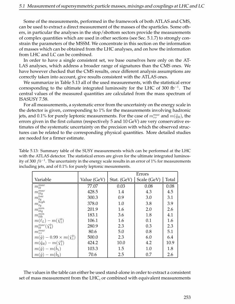
5.1 Measurement of supersymmetric particle masses, mixings and couplings at LHC and LC
Some of the measurements, performed in the framework of both ATLAS and CMS,can be used to extract a direct measurement of the masses of the sparticles. Some oth-ers, in particular the analyses in the stop/sbottom sectors provide the measurementsof complex quantities which are used in other sections (see Sec. 5.1.7) to strongly con-strain the parameters of the MSSM. We concentrate in this section on the informationof masses which can be obtained from the LHC analyses, and on how the informationfrom LHC and LC can be combined.
In order to have a single consistent set, we base ourselves here only on the AT-LAS analyses, which address a broader range of signatures than the CMS ones. Wehave however checked that the CMS results, once different analysis assumptions arecorrectly taken into account, give results consistent with the ATLAS ones.
We summarize in Table 5.13 all of the used measurements, with the statistical errorcorresponding to the ultimate integrated luminosity for the LHC of 300 fb−1. Thecentral values of the measured quantities are calculated from the mass spectrum ofISASUSY 7.58.
For all measurements, a systematic error from the uncertainty on the energy scale inthe detector is given, corresponding to 1% for the measurements involving hadronicjets, and 0.1% for purely leptonic measurements. For the case of mmax
ττ and m(qR), theerrors given in the first column (respectively 5 and 10 GeV) are very conservative es-timates of the systematic uncertainty on the precision with which the observed struc-tures can be related to the corresponding physical quantities. More detailed studiesare needed for a firmer estimate.
Table 5.13: Summary table of the SUSY measurements which can be performed at the LHCwith the ATLAS detector. The statistical errors are given for the ultimate integrated luminos-ity of 300 fb−1. The uncertainty in the energy scale results in an error of 1% for measurementsincluding jets, and of 0.1% for purely leptonic mesurements.
ErrorsVariable Value (GeV) Stat. (GeV) Scale (GeV) Total
mmaxℓℓ 77.07 0.03 0.08 0.08
mmaxℓℓq 428.5 1.4 4.3 4.5
mlowℓq 300.3 0.9 3.0 3.1
mhighℓq 378.0 1.0 3.8 3.9
mminℓℓq 201.9 1.6 2.0 2.6
mminℓℓb 183.1 3.6 1.8 4.1
m(ℓL)−m(χ01) 106.1 1.6 0.1 1.6
mmaxℓℓ (χ0
4) 280.9 2.3 0.3 2.3mmaxττ 80.6 5.0 0.8 5.1
m(g)− 0.99×m(χ01) 500.0 2.3 6.0 6.4
m(qR)−m(χ01) 424.2 10.0 4.2 10.9
m(g)−m(b1) 103.3 1.5 1.0 1.8
m(g)−m(b2) 70.6 2.5 0.7 2.6
The values in the table can either be used stand-alone in order to extract a consistentset of mass measurement from the LHC, or combined with equivalent measurements
253
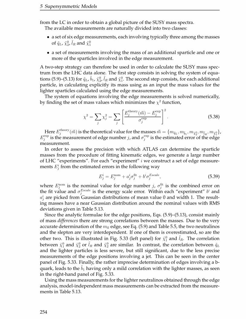
5 Supersymmetric Models
from the LC in order to obtain a global picture of the SUSY mass spectra.The available measurements are naturally divided into two classes:
• a set of six edge measurements, each involving typically three among the masses
of qL, χ02, lR and χ0
1
• a set of measurements involving the mass of an additional sparticle and one ormore of the sparticles involved in the edge measurement.
A two-step strategy can therefore be used in order to calculate the SUSY mass spec-trum from the LHC data alone. The first step consists in solving the system of equa-
tions (5.9)–(5.13) for qL, b1, χ02, lR and χ0
1. The second step consists, for each additionalparticle, in calculating explicitly its mass using as an input the mass values for thelighter sparticles calculated using the edge measurements.
The system of equations involving the edge measurements is solved numerically,by finding the set of mass values which minimizes the χ2 function,
χ2 =∑
j
χ2j =
∑
j
[Etheoryj (~m)− Eexp
j
σexpj
]2
. (5.38)
HereEtheoryj (~m) is the theoretical value for the masses ~m = mqL, mb1
, mχ02, mlR
, mχ01,
Eexpj is the measurement of edge number j, and σexp
j is the estimated error of the edgemeasurement.
In order to assess the precision with which ATLAS can determine the sparticlemasses from the procedure of fitting kinematic edges, we generate a large numberof LHC “experiments”. For each “experiment” i we construct a set of edge measure-ments Ei
j from the estimated errors in the following way
Eij = Enom
j + aijσfitj + biσEscalej , (5.39)
where Enomj is the nominal value for edge number j, σfit
j is the combined error onthe fit value and σEscalej is the energy scale error. Within each “experiment” bi andaij are picked from Gaussian distributions of mean value 0 and width 1. The result-ing masses have a near Gaussian distribution around the nominal values with RMSdeviations given in Table 5.13.
Since the analytic formulae for the edge positions, Eqs. (5.9)–(5.13), consist mainlyof mass differences there are strong correlations between the masses. Due to the veryaccurate determination of themll edge, see Eq. (5.9) and Table 5.5, the two neutralinosand the slepton are very interdependent. If one of them is overestimated, so are the
other two. This is illustrated in Fig. 5.33 (left panel) for χ01 and lR. The correlation
between χ01 and χ0
2 or lR and χ02 are similar. In contrast, the correlation between qL
and the lighter particles is less severe, but still significant, due to the less precisemeasurements of the edge positions involving a jet. This can be seen in the centerpanel of Fig. 5.33. Finally, the rather imprecise determination of edges involving a b-
quark, leads to the b1 having only a mild correlation with the lighter masses, as seenin the right-hand panel of Fig. 5.33.
Using the mass measurements for the lighter neutralinos obtained through the edgeanalysis, model-independent mass measurements can be extracted from the measure-ments in Table 5.13.
254
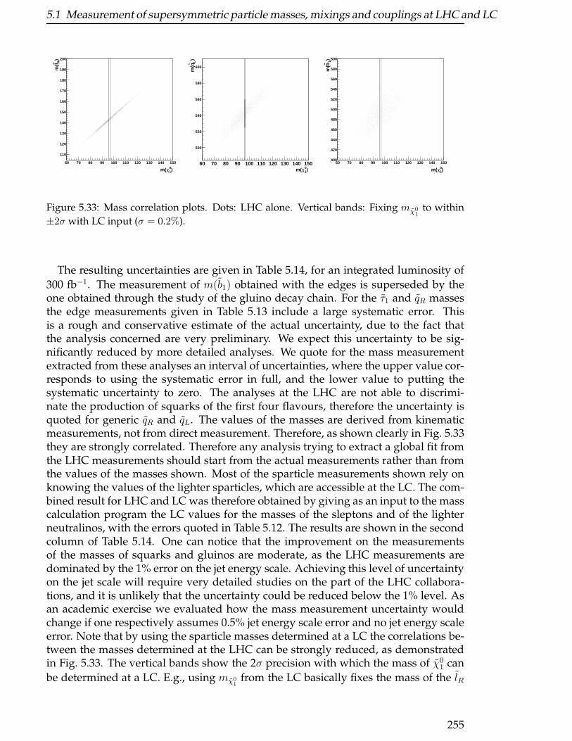
5.1 Measurement of supersymmetric particle masses, mixings and couplings at LHC and LC
)10χm(
60 70 80 90 100 110 120 130 140 150
)Rl~
m(
110
120
130
140
150
160
170
180
190
200
)10χm(
60 70 80 90 100 110 120 130 140 150
)L
q~m
(
500
520
540
560
580
600
)10χm(
60 70 80 90 100 110 120 130 140 150
) 1b~
m(
400
420
440
460
480
500
520
540
560
580
600
Figure 5.33: Mass correlation plots. Dots: LHC alone. Vertical bands: Fixing mχ01
to within
±2σ with LC input (σ = 0.2%).
The resulting uncertainties are given in Table 5.14, for an integrated luminosity of
300 fb−1. The measurement of m(b1) obtained with the edges is superseded by theone obtained through the study of the gluino decay chain. For the τ1 and qR massesthe edge measurements given in Table 5.13 include a large systematic error. Thisis a rough and conservative estimate of the actual uncertainty, due to the fact thatthe analysis concerned are very preliminary. We expect this uncertainty to be sig-nificantly reduced by more detailed analyses. We quote for the mass measurementextracted from these analyses an interval of uncertainties, where the upper value cor-responds to using the systematic error in full, and the lower value to putting thesystematic uncertainty to zero. The analyses at the LHC are not able to discrimi-nate the production of squarks of the first four flavours, therefore the uncertainty isquoted for generic qR and qL. The values of the masses are derived from kinematicmeasurements, not from direct measurement. Therefore, as shown clearly in Fig. 5.33they are strongly correlated. Therefore any analysis trying to extract a global fit fromthe LHC measurements should start from the actual measurements rather than fromthe values of the masses shown. Most of the sparticle measurements shown rely onknowing the values of the lighter sparticles, which are accessible at the LC. The com-bined result for LHC and LC was therefore obtained by giving as an input to the masscalculation program the LC values for the masses of the sleptons and of the lighterneutralinos, with the errors quoted in Table 5.12. The results are shown in the secondcolumn of Table 5.14. One can notice that the improvement on the measurementsof the masses of squarks and gluinos are moderate, as the LHC measurements aredominated by the 1% error on the jet energy scale. Achieving this level of uncertaintyon the jet scale will require very detailed studies on the part of the LHC collabora-tions, and it is unlikely that the uncertainty could be reduced below the 1% level. Asan academic exercise we evaluated how the mass measurement uncertainty wouldchange if one respectively assumes 0.5% jet energy scale error and no jet energy scaleerror. Note that by using the sparticle masses determined at a LC the correlations be-tween the masses determined at the LHC can be strongly reduced, as demonstratedin Fig. 5.33. The vertical bands show the 2σ precision with which the mass of χ0
1 can
be determined at a LC. E.g., using mχ01
from the LC basically fixes the mass of the lR
255
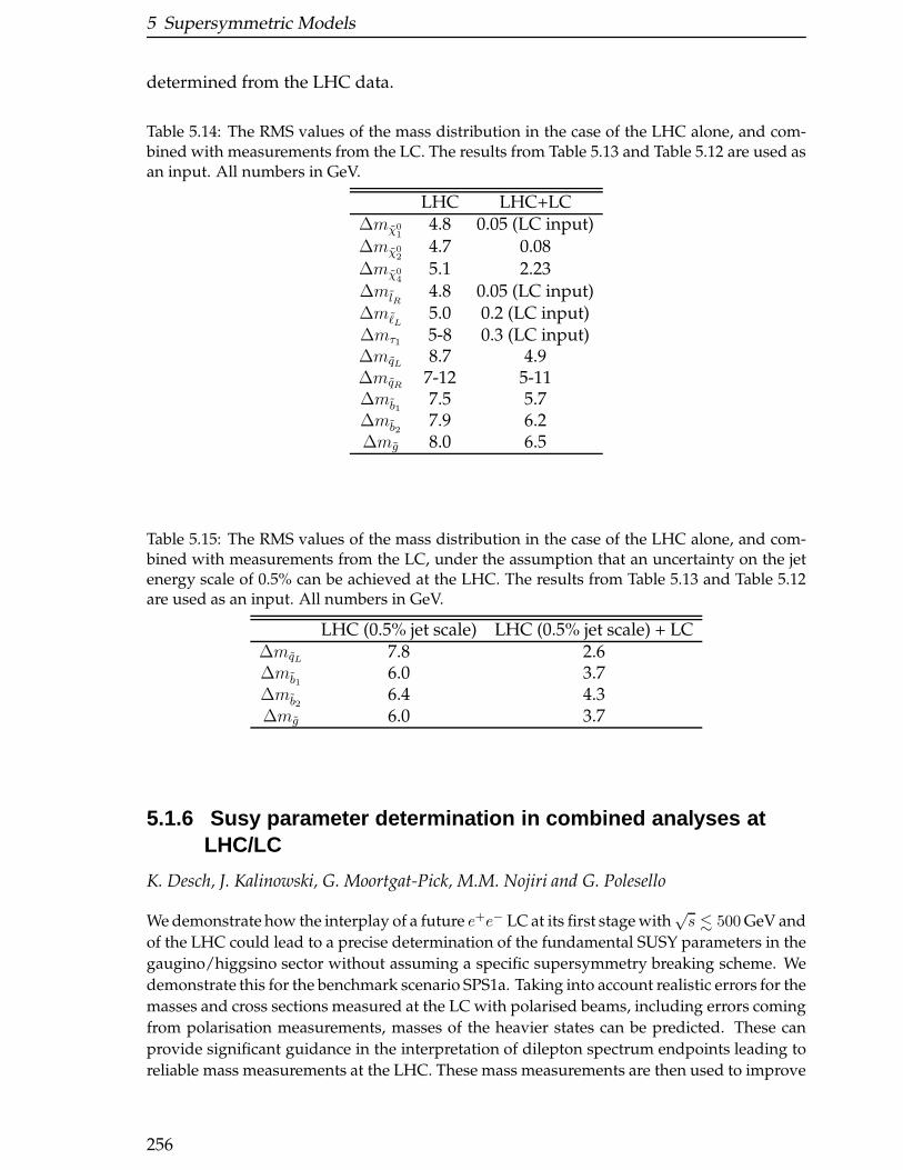
5 Supersymmetric Models
determined from the LHC data.
Table 5.14: The RMS values of the mass distribution in the case of the LHC alone, and com-bined with measurements from the LC. The results from Table 5.13 and Table 5.12 are used asan input. All numbers in GeV.
LHC LHC+LC∆mχ0
14.8 0.05 (LC input)
∆mχ02
4.7 0.08∆mχ0
45.1 2.23
∆mlR4.8 0.05 (LC input)
∆mℓL5.0 0.2 (LC input)
∆mτ1 5-8 0.3 (LC input)∆mqL 8.7 4.9∆mqR 7-12 5-11∆mb1
7.5 5.7∆mb2
7.9 6.2∆mg 8.0 6.5
Table 5.15: The RMS values of the mass distribution in the case of the LHC alone, and com-bined with measurements from the LC, under the assumption that an uncertainty on the jetenergy scale of 0.5% can be achieved at the LHC. The results from Table 5.13 and Table 5.12are used as an input. All numbers in GeV.
LHC (0.5% jet scale) LHC (0.5% jet scale) + LC∆mqL 7.8 2.6∆mb1
6.0 3.7∆mb2
6.4 4.3∆mg 6.0 3.7
5.1.6 Susy parameter determination in combined analyses atLHC/LC
K. Desch, J. Kalinowski, G. Moortgat-Pick, M.M. Nojiri and G. Polesello
We demonstrate how the interplay of a future e+e− LC at its first stage with√s <∼ 500 GeV and
of the LHC could lead to a precise determination of the fundamental SUSY parameters in the
gaugino/higgsino sector without assuming a specific supersymmetry breaking scheme. We
demonstrate this for the benchmark scenario SPS1a. Taking into account realistic errors for the
masses and cross sections measured at the LC with polarised beams, including errors coming
from polarisation measurements, masses of the heavier states can be predicted. These can
provide significant guidance in the interpretation of dilepton spectrum endpoints leading to
reliable mass measurements at the LHC. These mass measurements are then used to improve
256

5.1 Measurement of supersymmetric particle masses, mixings and couplings at LHC and LC
Table 5.16: The RMS values of the mass distribution in the case of the LHC alone, and com-bined with measurements from the LC, for the case where a vanishing uncertainty on the jetenergy scale at the LHC is assumed. The results from Table 5.13 and Table 5.12 are used as aninput. All numbers in GeV.
LHC (0% jet scale) LHC (0% jet scale) + LC∆mqL 7.4 0.8∆mb1
5.4 2.8∆mb2
5.8 3.4∆mg 5.2 2.3
the determination of the fundamental SUSY parameters. The results clearly demonstrate the
complementarity of the LHC and LC, and the benefit from the joint analyses of their data.
5.1.6.1 Introduction
Supersymmetry (SUSY) is one of the best motivated extensions of the Standard Model(SM). However, since SUSY has to be broken even the minimal version, the uncon-strained MSSM, has 105 new parameters. SUSY analyses at future experiments, at theLHC and at a future Linear Collider (LC) [49], will have to focus on the determinationof these parameters in as model-independent a way as possible.
With so many new parameters clear strategies will be needed in analysing the ex-perimental data [50]. An interesting possibility to resolve the new physics is to startwith the gaugino/higgsino particles which are expected to be among the lightestSUSY particles. In the unconstrained MSSM this sector depends only on 4 param-eters at tree level: M1, M2, µ and tan β – the U(1) and SU(2) gaugino masses, thehiggsino mass parameter and the ratio of the vacuum expectations of the two Higgsfields, respectively.
Some strategies have been worked out for the determination at the tree level theparameters M1, M2, µ, tan β even if only the light gaugino/higgsino particles, χ0
1, χ02
and χ±1 were kinematically accessible at the first stage of the LC [51]. In this report
we demonstrate how such an LC analysis could be strengthened if in addition someinformation on the mass of the heaviest neutralino from the LHC is available [52].We consider three scenarios: (i) stand alone LC data, (ii) when the LC data are sup-plemented by the heavy neutralino mass estimated from the LHC data, and (iii) jointanalysis of the LC and LHC data. In particular mass predictions of the heavier statesfrom the LC analysis are possible which lead to an improved possibility to correctlyinterpret LHC measurements of these particles. The results in the last scenario willclearly demonstrate the essentiality of the LHC and the LC and the benefit from thejoint analysis of their data.
In order to work out this hand-in-hand LHC+LC analysis for determining the tree-level SUSY parameters, we assume that only the first phase of a LC with a tun-able energy up to
√s = 500 GeV would overlap with the LHC running. Further-
more, we assume an integrated luminosity of∫L ∼ 500 fb−1 and polarised beams
with P (e−) = ±80%, P (e+) = ±60%. In the following σL will refer to cross sec-tions obtained with P (e−) = −80%, P (e+) = +60%, and σR with P (e−) = +80%,
257

5 Supersymmetric Models
P (e+) = −60%. We restrict ourselves to the CP conserving chargino/neutralino sec-tor and take the SPS1a as a working benchmark [1, 4]; the inclusion of CP violatingphases will be considered elsewhere. While the electroweak scale parameters of theSPS1a scenario are derived from a mSUGRA model, we do not impose any mSUGRArelations anywhere in this analysis. Thus the analysis and the results are qualitativelyvalid for any MSSM scenario with a similar mass spectrum.
Before presenting our results on the parameter determination, we first briefly reca-pitulate the main features of chargino and neutralino sectors and sketch our strategy.
5.1.6.2 The gaugino/higgsino sector
a) Chargino sector
The mass matrix of the charged gaugino W± and higgsino H± is given by2
MC =
(M2
√2mW cos β
√2mW sin β µ
)(5.40)
As a consequence of possible field redefinitions, the parameter M2 can be chosen realand positive. The two charginos χ±
1,2 are mixtures of the charged SU(2) gauginos andhiggsinos. Since the mass matrixMC is not symmetric, two different unitary matricesacting on the left– and right–chiral (W , H)L,R two–component states
(χ−
1
χ−2
)
L,R
= UL,R
(W−
H−
)
L,R
(5.41)
define charginos as mass eigenstates. For real MC the unitary matrices UL and URcan be parameterised as
UL,R =
(cos ΦL,R sin ΦL,R
− sin ΦL,R cos ΦL,R
)(5.42)
The mass eigenvalues m2χ±
1,2and the mixing angles are given by
m2χ±
1,2=
1
2(M2
2 + µ2 + 2m2W ∓∆C)
cos 2φL,R = −(M22 − µ2 ∓ 2m2
W cos 2β)/∆C
where ∆C = [(M22 − µ2)2 + 4m4
W cos2 2β + 4m2W (M2
2 + µ2) + 8m2WM2µ sin 2β]1/2.
The e+e− → χ±i χ
∓j production processes occur via the s-channel γ, Z0 and the t-
channel νe exchange. Since the two mixing angles ΦL,R enter the couplings in the χχZand eχνe vertices, the chargino production cross sections σ±ij = σ(e+e− → χ±
i χ∓j )
are bilinear functions of cos 2ΦL,R [54] and can be written as
σ±ij = c1 cos2 2ΦL + c2 cos 2ΦL + c3 cos2 2ΦR + c4 cos 2ΦR + c5 cos 2ΦL cos 2ΦR + c6(5.43)
2One should note the difference between our convention of taking χ− as “particles” and e.g. theconvention of [53].
258
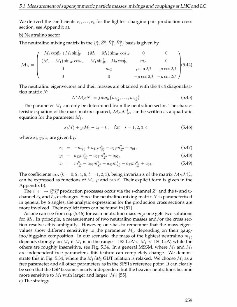
5.1 Measurement of supersymmetric particle masses, mixings and couplings at LHC and LC
We derived the coefficients c1, . . . , c6 for the lightest chargino pair production crosssection, see Appendix a).
b) Neutralino sector
The neutralino mixing matrix in the γ, Z0, H01 , H
02 basis is given by
MN =
M1 cos2W +M2 sin2
W (M2 −M1) sinW cosW 0 0
(M2 −M1) sinW cosW M1 sin2W +M2 cos2
W mZ 0
0 mZ µ sin 2β −µ cos 2β
0 0 −µ cos 2β −µ sin 2β
(5.44)
The neutralino eigenvectors and their masses are obtained with the 4×4 diagonalisa-tion matrix N :
N∗MNN† = fdiagmχ0
1, . . . , mχ0
4 (5.45)
The parameter M1 can only be determined from the neutralino sector. The charac-
teristic equation of the mass matrix squared,MNM†N , can be written as a quadratic
equation for the parameter M1:
xiM21 + yiM1 − zi = 0, for i = 1, 2, 3, 4 (5.46)
where xi, yi, zi are given by:
xi = −m6χ0
i+ a41m
4χ0
i− a21m
2χ0
i+ a01, (5.47)
yi = a42m4χ0
i− a22m
2χ0
i+ a02, (5.48)
zi = m8χ0
i− a63m
6χ0
i+ a43m
4χ0
i− a23m
2χ0
i+ a03, (5.49)
The coefficients akl, (k = 0, 2, 4, 6, l = 1, 2, 3), being invariants of the matrixMNMTN ,
can be expressed as functions of M2, µ and tanβ. Their explicit form is given in theAppendix b).
The e+e− → χ0i χ
0j production processes occur via the s-channel Z0 and the t- and u-
channel eL and eR exchanges. Since the neutralino mixing matrix N is parameterisedin general by 6 angles, the analytic expressions for the production cross sections aremore involved. Their explicit form can be found in [51].
As one can see from eq. (5.46) for each neutralino mass mχ0i
one gets two solutionsfor M1. In principle, a measurement of two neutralino masses and/or the cross sec-tion resolves this ambiguity. However, one has to remember that the mass eigen-values show different sensitivity to the parameter M1, depending on their gaug-ino/higgsino composition. In our scenario, the mass of the lightest neutralino mχ0
1
depends strongly on M1 if M1 is in the range −183 GeV< M1 < 180 GeV, while theothers are roughly insensitive, see Fig. 5.34. In a general MSSM, where M1 and M2
are independent free parameters, this feature can completely change. We demon-strate this in Fig. 5.34, where the M1/M2 GUT relation is relaxed. We choose M1 as afree parameter and all other parameters as in the SPS1a reference point. It can clearlybe seen that the LSP becomes nearly independent but the heavier neutralinos becomemore sensitive to M1 with larger and larger |M1| [55].c) The strategy
259
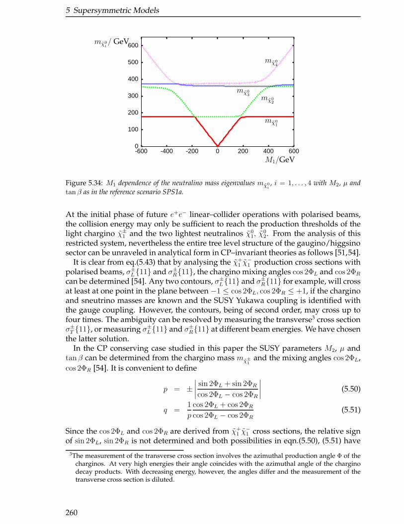
5 Supersymmetric Models
0
100
200
300
400
500
600
-600 -400 -200 0 200 400 600M1/GeV
mχ0i/ GeV
mχ01
mχ02
mχ03
mχ04
Figure 5.34: M1 dependence of the neutralino mass eigenvalues mχ0i, i = 1, . . . , 4 with M2, µ and
tan β as in the reference scenario SPS1a.
At the initial phase of future e+e− linear–collider operations with polarised beams,the collision energy may only be sufficient to reach the production thresholds of thelight chargino χ±
1 and the two lightest neutralinos χ01, χ
02. From the analysis of this
restricted system, nevertheless the entire tree level structure of the gaugino/higgsinosector can be unraveled in analytical form in CP–invariant theories as follows [51,54].
It is clear from eq.(5.43) that by analysing the χ+1 χ
−1 production cross sections with
polarised beams, σ±L 11 and σ±
R11, the chargino mixing angles cos 2ΦL and cos 2ΦR
can be determined [54]. Any two contours, σ±L 11 and σ±
R11 for example, will crossat least at one point in the plane between −1 ≤ cos 2ΦL, cos 2ΦR ≤ +1, if the charginoand sneutrino masses are known and the SUSY Yukawa coupling is identified withthe gauge coupling. However, the contours, being of second order, may cross up tofour times. The ambiguity can be resolved by measuring the transverse3 cross sectionσ±T 11, or measuring σ±
L 11 and σ±R11 at different beam energies. We have chosen
the latter solution.In the CP conserving case studied in this paper the SUSY parameters M2, µ and
tanβ can be determined from the chargino mass mχ±
1and the mixing angles cos 2ΦL,
cos 2ΦR [54]. It is convenient to define
p = ±∣∣∣∣sin 2ΦL + sin 2ΦR
cos 2ΦL − cos 2ΦR
∣∣∣∣ (5.50)
q =1
p
cos 2ΦL + cos 2ΦR
cos 2ΦL − cos 2ΦR(5.51)
Since the cos 2ΦL and cos 2ΦR are derived from χ+1 χ
−1 cross sections, the relative sign
of sin 2ΦL, sin 2ΦR is not determined and both possibilities in eqn.(5.50), (5.51) have
3The measurement of the transverse cross section involves the azimuthal production angle Φ of thecharginos. At very high energies their angle coincides with the azimuthal angle of the charginodecay products. With decreasing energy, however, the angles differ and the measurement of thetransverse cross section is diluted.
260

5.1 Measurement of supersymmetric particle masses, mixings and couplings at LHC and LC
to be considered. From p, q, the SUSY parameters are determined as follows (r2 =m2χ±
1
/m2W ):
M2 =mW√
2[(p+ q) sin β − (p− q) cosβ] (5.52)
µ =mW√
2[(p− q) sin β − (p+ q) cosβ] (5.53)
tanβ =
[p2 − q2 ±
√r2(p2 + q2 + 2− r2)
(√
1 + p2 −√
1 + q2)2 − 2r2
]η(5.54)
where η = 1 for cos 2ΦR > cos 2ΦL, and η = −1 otherwise. The parameters M2, µ areuniquely fixed if tanβ is chosen properly. Since tan β is invariant under simultaneouschange of the signs of p, q, the definition M2 > 0 can be exploited to remove thisoverall sign ambiguity.
The remaining parameter M1 can be obtained from the neutralino data [51]. Thecharacteristic equation for the neutralino mass eigenvalues eq. (5.46) is quadratic inM1 if M2, µ and tan β are already predetermined in the chargino sector. In principle,two neutralino masses are then sufficient to derive M1, as explained in the previoussection. The cross sections σ0
L,R12 and σ0L,R22 for production of χ0
1χ02 and χ0
2χ02
neutralino pairs4 with polarised beams can serve as a consistency check of the derivedparameters.
In practice the above procedure may be much more involved due to finite experi-mental errors of mass and cross section measurements, uncertainties from sneutrinoand selectron masses which enter the cross section expressions, errors on beam polar-isation measurement, etc. In addition, depending on the benchmark scenario, somephysical quantities in the light chargino/neutralino system may turn to be essentiallyinsensitive to some parameters. For example, as seen in fig. 5.34, the first two neu-tralino masses are insensitive to M1 if M1 ≫ M2, µ. Additional information from theLHC on heavy states, if available, can therefore be of great value in constraining theSUSY parameters.
Our strategy can be applied only at the tree level. Radiative corrections, whichin the electroweak sector can be O(10%), inevitably bring all SUSY parameters to-gether [57]. Nevertheless, tree level analyses should provide in a relatively model-independent way good estimates of SUSY parameters, which can be further refinedby including iteratively radiative corrections in an overall fit to experimental data.
5.1.6.3 SUSY parameters from the LC data
a) Experimental input at the LC
In this paper we take the unconstrained MSSM and adopt the SPS1a scenario de-fined at the electroweak scale [1, 4]. The relevant SUSY parameters are
M1 = 99.13 GeV , M2 = 192.7 GeV , µ = 352.4 GeV , tan β = 10 (5.55)
4The lightest neutralino–pair production cannot be observed. Alternatively, one can try to exploitphoton tagging in the reaction e+e− → γχ0
1χ01 [56].
261
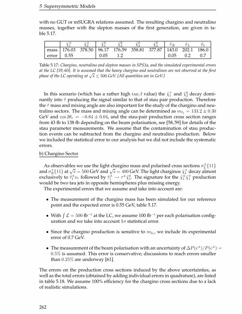
5 Supersymmetric Models
with no GUT or mSUGRA relations assumed. The resulting chargino and neutralinomasses, together with the slepton masses of the first generation, are given in ta-ble 5.17.
χ±1 χ±
2 χ01 χ0
2 χ03 χ0
4 eR eL νemass 176.03 378.50 96.17 176.59 358.81 377.87 143.0 202.1 186.0error 0.55 0.05 1.2 0.05 0.2 0.7
Table 5.17: Chargino, neutralino and slepton masses in SPS1a, and the simulated experimental errorsat the LC [59, 60]. It is assumed that the heavy chargino and neutralinos are not observed at the firstphase of the LC operating at
√s ≤ 500 GeV. [All quantities are in GeV.]
In this scenario (which has a rather high tanβ value) the χ+1 and χ0
2 decay domi-nantly into τ producing the signal similar to that of stau pair production. Thereforethe τ mass and mixing angle are also important for the study of the chargino and neu-tralino sectors. The mass and mixing angle can be determined as mτ1 = 133.2± 0.30GeV and cos 2θτ = −0.84 ± 0.04, and the stau-pair production cross section rangesfrom 43 fb to 138 fb depending on the beam polarisation, see [58,59] for details of thestau parameter measurements. We assume that the contamination of stau produc-tion events can be subtracted from the chargino and neutralino production. Belowwe included the statistical error to our analysis but we did not include the systematicerrors.
b) Chargino Sector
As observables we use the light chargino mass and polarised cross sections σ±L 11
and σ±R11 at
√s = 500 GeV and
√s = 400 GeV. The light charginos χ±
1 decay almostexclusively to τ±1 ντ followed by τ±1 → τ±χ0
1. The signature for the χ±1 χ
∓1 production
would be two tau jets in opposite hemispheres plus missing energy.The experimental errors that we assume and take into account are:
• The measurement of the chargino mass has been simulated for our referencepoint and the expected error is 0.55 GeV, table 5.17.
• With∫L = 500 fb−1 at the LC, we assume 100 fb−1 per each polarisation config-
uration and we take into account 1σ statistical error.
• Since the chargino production is sensitive to mνe , we include its experimentalerror of 0.7 GeV.
• The measurement of the beam polarisation with an uncertainty of ∆P (e±)/P (e±) =0.5% is assumed. This error is conservative; discussions to reach errors smallerthan 0.25% are underway [61].
The errors on the production cross sections induced by the above uncertainties, aswell as the total errors (obtained by adding individual errors in quadrature), are listedin table 5.18. We assume 100% efficiency for the chargino cross sections due to a lackof realistic simulations.
262
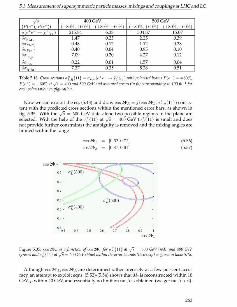
5.1 Measurement of supersymmetric particle masses, mixings and couplings at LHC and LC
√s 400 GeV 500 GeV
(P (e−), P (e+)) (−80%,+60%) (+80%,−60%) (−80%,+60%) (+80%,−60%)σ(e+e− → χ+
1 χ−1 ) 215.84 6.38 504.87 15.07
δσstat 1.47 0.25 2.25 0.39δσP (e−) 0.48 0.12 1.12 0.28δσP (e+) 0.40 0.04 0.95 0.10δσm
χ±
1
7.09 0.20 4.27 0.12
δσmνe0.22 0.01 1.57 0.04
δσtotal 7.27 0.35 5.28 0.51
Table 5.18: Cross sections σ±L,R11 = σL,R(e+e− → χ+1 χ
−1 ) with polarised beams P (e−) = ∓80%,
P (e+) = ±60% at√s = 400 and 500 GeV and assumed errors (in fb) corresponding to 100 fb−1 for
each polarisation configuration.
Now we can exploit the eq. (5.43) and draw cos 2ΦR = f(cos 2ΦL, σ±L,R11) consis-
tent with the predicted cross sections within the mentioned error bars, as shown infig. 5.35. With the
√s = 500 GeV data alone two possible regions in the plane are
selected. With the help of the σ±L 11 at
√s = 400 GeV (σ±
R11 is small and doesnot provide further constraints) the ambiguity is removed and the mixing angles arelimited within the range
cos 2ΦL = [0.62, 0.72] (5.56)
cos 2ΦR = [0.87, 0.91] (5.57)
cos 2ΦL
cos 2ΦR
σ±L (500)
σ±L (400)
σ±R(500)
Figure 5.35: cos 2ΦR as a function of cos 2ΦL for σ±L 11 at√s = 500 GeV (red), and 400 GeV
(green) and σ±R11 at√s = 500 GeV (blue) within the error bounds (theo+exp) as given in table 5.18.
Although cos 2ΦL, cos 2ΦR are determined rather precisely at a few per-cent accu-racy, an attempt to exploit eqns. (5.52)-(5.54) shows thatM2 is reconstructed within 10GeV, µ within 40 GeV, and essentially no limit on tanβ is obtained (we get tanβ > 6).
263
5 Supersymmetric Models
The main reason for this result is a relatively large error of the light chargino massmeasurement due to the χ+
1 → χ01τ
+ντ decay mode. Several methods exploiting othersectors of the MSSM have been proposed to measure tanβ in the high tanβ regime[58,62]. In the following we will exploit the neutralino sector (with eqns. (5.56), (5.57)as the allowed ranges for the chargino mixing angles) to improve constraints on M2,µ and tanβ, and to determine M1.
c) Neutralino Sector:
As observables we use the two light neutralino masses and polarised cross sectionsσ0L,R12 and σ0
L,R22 at√s = 400 GeV and
√s = 500 GeV. Although the production
of χ01χ
03 and χ0
1χ04 pairs is kinematically accessible at
√s = 500 GeV in the chosen
reference point SPS1a, the production rates are small and the heavy states χ03 and χ0
4
decay via cascades to many particles. This feature is quite common in large parts ofthe MSSM parameter space when the gaugino and higgsino mass parameters are nottoo close. Therefore in our analysis we take into account the experimental informationavailable only from the production of the light neutralino pairs.
The neutralino χ02 decays into τ±1 τ
∓ with almost 90%, followed by the τ±1 → τ±χ01.
Therefore the final states for the χ±1 χ
∓1 and χ0
1χ02 are the same (2τ + missing energy),
however with different topology. While for the charginos, the τ ’s tend to be in op-posite hemispheres with rather large invariant mass, in the χ0
1χ02 process both τ ’s,
coming from the χ02 decay, would be more often in the same hemisphere with smaller
invariant mass. This feature allows to separate the processes to some extent exploit-ing e.g. a cut on the opening angle between the two jets of the τ ′s. However, in thecase of χ0
1χ02, significant background from χ±
1 χ∓1 and τ±1 τ
∓1 remains.
We estimate the statistical error on σ(e+e− → χ01χ
02) based on the experimental
simulation presented in [60]. This simulation was performed at√s = 500 GeV for
unpolarised beams yielding an efficiency of 25%. We extrapolate the statistical errorsat different
√s and different polarisations as δσ/σ =
√S +B/S where we calculate
the number of signal (S) and background (B) events from the cross sections and theintegrated luminosity (100 fb−1) assuming the same efficiency as achieved for theunpolarised case. Since the cross sections for the SUSY background processes are alsoknown only with some uncertainty, we account for this uncertainty in the backgroundsubtraction by adding an additional systematic error (δσbg).
For the process χ02χ
02 → τ+τ−τ+τ−χ0
1χ01 no detailed simulation exists. From the τ -
tagging efficiency achieved in the χ01χ
02 channel, we assume that this final state can be
reconstructed with an efficiency of 15% with negligible background. This is justifiedsince no major SUSY background is expected for the 4-τ final state, BR(ντ → τ+τ−χ0
1)2
is only 0.5%. SM backgrounds arise mainly from Z pair production and are small.
For both processes we account in addition for polarisation uncertainties and uncer-tainties in the cross section predictions from the errors on the chargino and selectronmasses. Note that we implicitly assume that the branching ratio χ0
2 → τ+τ−χ01 is
known, which is a simplifaction. A full analysis will have to take into account the pa-rameter dependence of this branching ratio in addition, since it cannot be measureddirectly.
The neutralino cross sections depend onM1,M2, µ, tanβ and on slepton masses. We
264
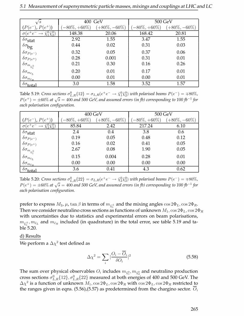
5.1 Measurement of supersymmetric particle masses, mixings and couplings at LHC and LC
√s 400 GeV 500 GeV
(P (e−), P (e+)) (−80%,+60%) (+80%,−60%) (−80%,+60%) (+80%,−60%)σ(e+e− → χ0
1χ02) 148.38 20.06 168.42 20.81
δσstat 2.92 1.55 3.47 1.55δσbg 0.44 0.02 0.31 0.03
δσP (e−) 0.32 0.05 0.37 0.06δσP (e+) 0.28 0.001 0.31 0.01δσm
χ±
1
0.21 0.30 0.16 0.26
δσmeL0.20 0.01 0.17 0.01
δσmeR0.00 0.01 0.00 0.01
δσtotal 3.0 1.58 3.52 1.57
Table 5.19: Cross sections σ0L,R12 = σL,R(e+e− → χ0
1χ02) with polarised beams P (e−) = ∓80%,
P (e+) = ±60% at√s = 400 and 500 GeV, and assumed errors (in fb) corresponding to 100 fb−1 for
each polarisation configuration.
400 GeV 500 GeV(P (e−), P (e+)) (−80%,+60%) (+80%,−60%) (−80%,+60%) (+80%,−60%)σ(e+e− → χ0
2χ02) 85.84 2.42 217.24 6.10
δσstat 2.4 0.4 3.8 0.6δσP (e−) 0.19 0.05 0.48 0.12δσP (e+) 0.16 0.02 0.41 0.05δσm
χ±1
2.67 0.08 1.90 0.05
δσmeL0.15 0.004 0.28 0.01
δσmeR0.00 0.00 0.00 0.00
δσtotal 3.6 0.41 4.3 0.62
Table 5.20: Cross sections σ0L,R22 = σL,R(e+e− → χ0
2χ02) with polarised beams P (e−) = ∓80%,
P (e+) = ±60% at√s = 400 and 500 GeV, and assumed errors (in fb) corresponding to 100 fb−1 for
each polarisation configuration.
prefer to express M2, µ, tanβ in terms of mχ±
1and the mixing angles cos 2ΦL, cos 2ΦR.
Then we consider neutralino cross sections as functions of unknownM1, cos 2ΦL, cos 2ΦR
with uncertainties due to statistics and experimental errors on beam polarisations,mχ±
1, meL
and meRincluded (in quadrature) in the total error, see table 5.19 and ta-
ble 5.20.
d) Results
We perform a ∆χ2 test defined as
∆χ2 =∑
i
|Oi −Oi
δOi|2 (5.58)
The sum over physical observables Oi includes mχ01, mχ0
2and neutralino production
cross sections σ0L,R12, σ0
L,R22 measured at both energies of 400 and 500 GeV. The∆χ2 is a function of unknown M1, cos 2ΦL, cos 2ΦR with cos 2ΦL, cos 2ΦR restricted tothe ranges given in eqns. (5.56),(5.57) as predetermined from the chargino sector. Oi
265
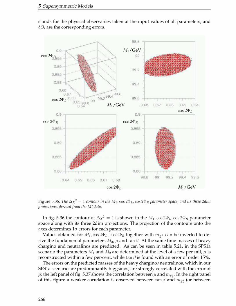
5 Supersymmetric Models
stands for the physical observables taken at the input values of all parameters, andδOi are the corresponding errors.
cos 2ΦL M1/GeV
cos 2ΦR cos 2ΦR
cos 2ΦL
M1/GeV
M1/GeV
cos 2ΦR
cos 2ΦL
Figure 5.36: The ∆χ2 = 1 contour in the M1, cos 2ΦL, cos 2ΦR parameter space, and its three 2dimprojections, derived from the LC data.
In fig. 5.36 the contour of ∆χ2 = 1 is shown in the M1, cos 2ΦL, cos 2ΦR parameterspace along with its three 2dim projections. The projection of the contours onto theaxes determines 1σ errors for each parameter.
Values obtained for M1, cos 2ΦL, cos 2ΦR together with mχ±
1can be inverted to de-
rive the fundamental parameters M2, µ and tan β. At the same time masses of heavychargino and neutralinos are predicted. As can be seen in table 5.21, in the SPS1ascenario the parameters M1 and M2 are determined at the level of a few per-mil, µ isreconstructed within a few per-cent, while tan β is found with an error of order 15%.
The errors on the predicted masses of the heavy chargino/neutralinos, which in ourSPS1a scenario are predominantly higgsinos, are strongly correlated with the error ofµ; the left panel of fig. 5.37 shows the correlation between µ andmχ0
4. In the right panel
of this figure a weaker correlation is observed between tanβ and mχ04
(or between
266
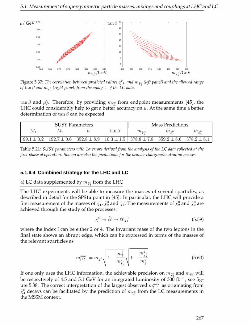
5.1 Measurement of supersymmetric particle masses, mixings and couplings at LHC and LC
340
345
350
355
360
365
370
360 365 370 375 380 385 390 395
6
8
10
12
14
16
18
20
360 365 370 375 380 385 390 395
mχ04/GeV mχ0
4/GeV
µ/ GeV tan β
Figure 5.37: The correlation between predicted values of µ and mχ04
(left panel) and the allowed rangeof tan β and mχ0
4(right panel) from the analysis of the LC data.
tan β and µ). Therefore, by providing mχ04
from endpoint measurements [45], theLHC could considerably help to get a better accuracy on µ. At the same time a betterdetermination of tanβ can be expected.
SUSY Parameters Mass PredictionsM1 M2 µ tan β mχ±
2mχ0
3mχ0
4
99.1± 0.2 192.7± 0.6 352.8± 8.9 10.3± 1.5 378.8± 7.8 359.2± 8.6 378.2± 8.1
Table 5.21: SUSY parameters with 1σ errors derived from the analysis of the LC data collected at thefirst phase of operation. Shown are also the predictions for the heavier chargino/neutralino masses.
5.1.6.4 Combined strategy for the LHC and LC
a) LC data supplemented by mχ04
from the LHC
The LHC experiments will be able to measure the masses of several sparticles, asdescribed in detail for the SPS1a point in [45]. In particular, the LHC will provide afirst measurement of the masses of χ0
1, χ02 and χ0
4. The measurements of χ02 and χ0
4 areachieved through the study of the processes:
χ0i → ℓℓ→ ℓℓχ0
1 (5.59)
where the index i can be either 2 or 4. The invariant mass of the two leptons in thefinal state shows an abrupt edge, which can be expressed in terms of the masses ofthe relevant sparticles as
mmaxl+l− = mχ0
i
√√√√1−m2ℓ
m2χ0
i
√√√√1−m2χ0
1
m2ℓ
(5.60)
If one only uses the LHC information, the achievable precision on mχ02
and mχ04
will
be respectively of 4.5 and 5.1 GeV for an integrated luminosity of 300 fb−1, see fig-ure 5.38. The correct interpretation of the largest observed mmax
l+l− as originating fromχ0
4 decays can be facilitated by the prediction of mχ04
from the LC measurements inthe MSSM context.
267
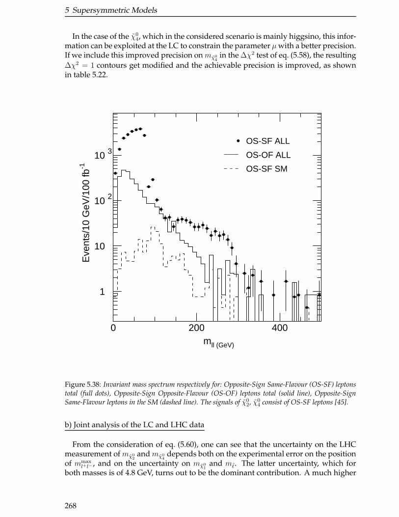
5 Supersymmetric Models
In the case of the χ04, which in the considered scenario is mainly higgsino, this infor-
mation can be exploited at the LC to constrain the parameter µwith a better precision.If we include this improved precision onmχ0
4in the ∆χ2 test of eq. (5.58), the resulting
∆χ2 = 1 contours get modified and the achievable precision is improved, as shownin table 5.22.
1
10
10 2
10 3
0 200 400
OS-SF ALL
OS-OF ALL
OS-SF SM
mll (GeV)
Eve
nts/
10 G
eV/1
00 fb
-1
Figure 5.38: Invariant mass spectrum respectively for: Opposite-Sign Same-Flavour (OS-SF) leptonstotal (full dots), Opposite-Sign Opposite-Flavour (OS-OF) leptons total (solid line), Opposite-SignSame-Flavour leptons in the SM (dashed line). The signals of χ0
2, χ04 consist of OS-SF leptons [45].
b) Joint analysis of the LC and LHC data
From the consideration of eq. (5.60), one can see that the uncertainty on the LHCmeasurement of mχ0
2and mχ0
4depends both on the experimental error on the position
of mmaxl+l− , and on the uncertainty on mχ0
1and mℓ. The latter uncertainty, which for
both masses is of 4.8 GeV, turns out to be the dominant contribution. A much higher
268
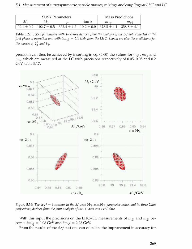
5.1 Measurement of supersymmetric particle masses, mixings and couplings at LHC and LC
SUSY Parameters Mass PredictionsM1 M2 µ tan β mχ±
2mχ0
3
99.1± 0.2 192.7± 0.5 352.4± 4.5 10.2± 0.9 378.5± 4.1 358.8± 4.1
Table 5.22: SUSY parameters with 1σ errors derived from the analysis of the LC data collected at thefirst phase of operation and with δmχ0
4= 5.1 GeV from the LHC. Shown are also the predictions for
the masses of χ±2 and χ0
3.
precision can thus be achieved by inserting in eq. (5.60) the values for mχ01, meR
andmeL
which are measured at the LC with precisions respectively of 0.05, 0.05 and 0.2GeV, table 5.17.
cos 2ΦL M1/GeV
cos 2ΦR cos 2ΦR
cos 2ΦL
M1/GeV
M1/GeV
cos 2ΦR
cos 2ΦL
Figure 5.39: The ∆χ2 = 1 contour in the M1, cos 2ΦL, cos 2ΦR parameter space, and its three 2dimprojections, derived from the joint analysis of the LC data and LHC data.
With this input the precisions on the LHC+LC measurements of mχ02
and mχ04
be-come: δmχ0
2= 0.08 GeV and δmχ0
4= 2.23 GeV.
From the results of the ∆χ2 test one can calculate the improvement in accuracy for
269
5 Supersymmetric Models
SUSY Parameters Mass PredictionsM1 M2 µ tanβ mχ±
2mχ0
3
99.1± 0.1 192.7± 0.3 352.4± 2.1 10.2± 0.6 378.5± 2.0 358.8± 2.1
Table 5.23: SUSY parameters with 1σ errors derived from the combined analysis of the LHC and LCdata with δmχ0
2= 0.08 GeV and δmχ0
4= 2.23 GeV derived from the LHC when using the LC input
of δmχ01
= 0.05 GeV.
the derived parameters by imposing the new mass constraints. The final results areshown in figure5.39 and table 5.23. The accuracy for the parameters µ and particularlytanβ is much better, as could be expected from fig. 5.37, where the allowed range of µand tan β from the LC analysis is considerably reduced once the measured mass mχ0
4
at the LHC is taken into account. In particular, the precision on tanβ becomes betterthan from other SUSY sectors [58, 62].
5.1.6.5 Summary
We have studied the prospects for the determination of the parameters which governthe chargino/neutralino sector of a general MSSM. We focus on the situation whereonly the lightest states (χ0
1, χ02, χ±
1 ) are accessible at the first stage of a LC. For a specificexample of the MSSM, the SPS1a scenario with a rather high tanβ = 10, we showhow the combination of the results from the two accelerators, LHC and LC, allows aprecise determination of the fundamental SUSY parameters. The analysis has beenperformed within the general frame of the unconstrained MSSM. Our strategy doesnot rely on any particular relations among the fundamental parameters, like the GUTor mSUGRA relations, and therefore is applicable for arbitrary MSSM parameterswhich lead to a phenomenology similar to the one studied.
Measuring with high precision the masses of the expected lightest SUSY particlesχ0
1, χ02, χ±
1 and their cross sections at the LC, and taking into account simulated massmeasurement errors and corresponding uncertainties for the theoretical predictions,we could determine the fundamental SUSY parameters M1, M2, µ at tree level for theSPS1a point within a few percent, while tanβ is estimated within∼ 15 %. The massesof heavier chargino and neutralinos can also be predicted at a level of a few percentand are used as input for the LHC analysis. The use of polarised beams at the LC isdecisive for deriving unique solutions.
If the LC analysis is supplemented with the LHC measurement of the heavy neu-tralino mass, the errors on µ and tanβ can be improved. However, the best resultsare obtained when first the LSP and slepton masses from the LC are fed to the LHCanalyses to get a precise experimental determination of the χ0
2 and χ04 masses, which
in turn are injected back to the analysis of the chargino/neutralino LC data. Thecombined strategy will provide in particular a precise measurement of the χ0
4 mass,the µ parameter with an accuracy at the ≤ O(1%) level, and an error on tanβ of theorder of ≤ 10%, reaching a stage where radiative corrections become relevant in theelectroweak sector and which will have to be taken into account in future fits [57].
270
5.1 Measurement of supersymmetric particle masses, mixings and couplings at LHC and LC
Appendix: Useful expressions for the gaugino/higgsino sec tor
a) For the lightest chargino pair production, σ±11 = σ(e−(p1)e+(p2)→ χ+
1 (p3)χ−1 (p4)),
the coefficients c1, . . . , c6 in eq. (5.43) are given by:
c1 =
∫
C
|Z|2cLRL2f2 + cRLR2f1
c2 =
∫
C
|Z|2cLRL2(1− 4L)(2f2 + f3) + cRLR2(1− 4R)(2f1 + f3)
−∫
C
GN4cLRL(2f2 + f3) + cRLR(2f1 + f3) −∫
C
Re(Z)NcLRLf3
c3 =
∫
C
|Z|2(cLRL2f1 + cRLR2f2)−
∫
C
ZN2cLRLf1 +
∫
C
N2cLRf1
c4 =
∫
C
|Z|2(1− 4L)cLRL2(2f1 + f3) + cRLR2(2f2 + f3)+
∫
C
N22cLRf1
+
∫
C
Re(Z)NcLRL−4f1 − f3 + 4L(2f1 + f3)+
∫
C
GN4cLR(2f1 + f3)
−∫
C
GRe(Z)4cLRL(2f1 + f3) + cRLR(2f2 + f3)
c5 =
∫
C
|Z|2(cLRL2 + cRLR2)f3 −
∫
C
Re(Z)NcLRLf3
c6 =
∫
C
|Z|2cLRL2(1− 8L) + cRLR2(1− 8L) + 16L2(cLRL
2 + cRLR2)(f1 + f2 + f3)
−∫
C
Re(Z)NcLRL(1− 4L)(2f1 + f3) +
∫
C
G2(cLR + cRL)(f1 + f2 + f3)
−∫
C
Re(Z)G8cRLR + cLRL(1− 4L)(f1 + f2 + f3) +
∫
C
N2cLRf1
+
∫
C
GN4cLR(2f1 + f3)
where∫C
=qχE3
b
12π
∫d cos θ, L = −1
2+ sin2 θW , R = sin2 θW , and
G = e2/s, Z = g2/ cos2 θW (s−m2Z + imZΓZ), N = g2/(t−m2
νe)
denote the γ, Z and νe propagators,
cLR = (1− P (e−))(1 + P (e+)), cRL = (1 + P (e−))(1− P (e+))
are the beam polarisation factors, and
f1 = (p1p4)(p2p3), f2 = (p1p3)(p2p4), f3 = sm2χ±
i/2
are the pure kinematic coefficients.b) The coefficients akl (k = 0, 2, 4, 6, l = 1, 2, 3), which appear in eqns. (5.47),(5.48)
and (5.49), are invariants of the matrixMNMTN . They can be expressed as functions
of the parameters M2, µ, tan β in the following way:
a63 = M22 + 2(µ2 +m2
Z)
271
5 Supersymmetric Models
a41 = M22 + 2(µ2 +m2
Z cos2 θW )
a42 = −2µm2Z sin 2β sin2 θW
a43 = 2µ2M22 + (µ2 +m2
Z)2 − 2m2ZµM2 sin 2β cos2 θW + 2m2
ZM22 sin2 θW
a21 = µ4 + 2µ2M22 + 2m2
Zµ2 cos2 θW +m4
Z cos2 θW − 2m2ZM2µ sin 2β cos2 θW
a22 = 2[m4ZM2 sin2 θW cos2 θW −m2
Zµ3 sin2 θW sin 2β −m2
ZµM22 sin2 θW sin 2β]
a23 = µ4M22 +m4
Zµ2 sin2 2β + 2m2
Zµ2M2
2 sin2 θW − 2m2ZM2µ
3 cos2 θW sin 2β +m4ZM
22 sin4 θW
a01 = µ4M22 +m4
Zµ2 cos4 θW sin2 2β − 2m2
Zµ3M2 cos2 θW sin 2β
a02 = 2m4Zµ
2M2 sin2 θW cos2 θW sin2 2β − 2m2Zµ
3M22 sin2 θW sin 2β
a03 = m4Zµ
2M22 sin4 θW sin2 2β
5.1.7 Determination of stop and sbottom sector by LHC and LC
J. Hisano, K. Kawagoe and M.M. Nojiri
The information on electroweak SUSY parameters from LC would significantly improve res-
olution of masses and mixing angles of stop and sbottom particles produced at LHC. An
example is shown for a Snowmass point SPS 1a, when the measurement of mixing angle is
possible by combining LHC and LC data.
5.1.7.1 Fits to stop and sbottom masses and mixings with LC in puts
In this section, we describe the fits to the stop and sbottom masses and mixings at
SPS 1 using LHC/LC data. At this point, b1, b2 ∼ 500 GeV, therefore direct production
of b at LC is not possible without significant extension of the energy. Therefore weconsider the fits of the mixing angle using LHC data and LC data at
√s = 500 GeV.
Note that all sleptons, the lighter chargino χ±1 , and the lightest and the second
lightest neutralinos χ01 and χ0
2 are within the reach of early stage of the LC at√s =
500 GeV. The LC measures the accessible sparticles masses precisely [64]. Further-more, Chargino and neutralino production cross sections and the first generationslepton production cross sections are sensitive to the gaugino masses M1 and M2.The expected errors at
√s = 500 GeV are given in [65].
The LC measurements improve the mass resolution of strongly interacting sparti-cles at LHC [63]. Errors of sparticles masses are estimated as ∆(mg −mχ0
1) = 2.5 GeV,
∆(mg − mb1) = 1.5 GeV and ∆(mg − mb2
) = 2.5 GeV at SPS 1a in [63] for∫Ldt =
300 fb−1. LHC also improve the resolution of weak SUSY parameters. Statistics of χ02
produced from q decay is huge. In addition, χ04(mχ0
4= 378 GeV) arises occasionally
from squark decays. The same flavor and opposite sign lepton pair arises from the
cascade decay χ02 → ll → llχ0
1 and χ04 → ll → llχ0
1. The end points of mll distribu-tion arising would be measured precisely at LHC. The errors of the end points are∆mll = 0.08(2.3) GeV for χ0
2(χ04) respectively [63]. This is translated into the mχ0
4error
∆mχ04
= 2.23 GeV which corresponds to ∆µ = 2.1 GeV. This is an example that thecombination of LHC and LC fits determines M1,M2, µ, tanβ better.
Given the precise determination of weak SUSY parameters, one can access thestructure of sbottom and stop mass matrices. The mass matrices are controlled by
272
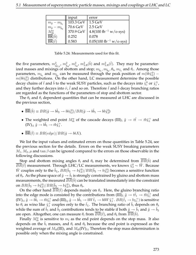
5.1 Measurement of supersymmetric particle masses, mixings and couplings at LHC and LC
input errormg −mb1
103.3 GeV 1.5 GeVmg −mb2
70.6 GeV 2.5 GeVMw
tb 370.9 GeV 4.8(100 fb−1 w/o sys)
BR(b) 0.252 0.078BR(t) 0.583 0.05(100 fb−1 w/o sys)
Table 5.24: Measurements used for this fit.
the five parameters, m2QL3
, m2bR
, m2tR
, m2LR(b) and m2
LR(t). They may be parameter-
ized masses and mixings of sbottom and stop; mb1, mb2
, θb, mt1 and θt. Among thoseparameters, mb1
and mb2can be measured through the peak position of m(bbχ0
2) −m(bbχ0
2) distributions. On the other hand, LC measurement determine the possible
decay chains of t and b to the weak SUSY particles, such as the decays into χ0i or χ±
i ,
and they further decays into ν, l and so on. Therefore t and b decay branching ratiosare regarded as the functions of the parameters of stop and sbottom sector.
The θb and θt dependent quantities that can be measured at LHC are discussed inthe previous section,
• BR(b) ≡ BR(g → bb2 → bbχ02)/BR(g → bb1 → bbχ0
2)
• The weighted end point Mwtb of the cascade decays (III)1 g → tt → tbχ+
1 and
(IV)i1 g → bbi → tbχ+1 .
• BR(t) ≡ BR(edge)/BR(g → bbX).
We list the input values and estimated errors on those quantities in Table 5.24, seethe previous section for the details. Errors on the weak SUSY breaking parametersM1,M2, µ and tan β can be ignored compared to the errors on those observable in thefollowing discussions.
Stop and sbottom mixing angles θt and θb may be determined from BR(b) andBR(t) measurement. Through LHC/LC measurements, we knows χ0
2 ∼ W . Because
W couples only to the bL, BR(b2 → bχ02)/BR(b2 → bχ0
2) becomes a sensitive function
of θb. As the phase space of g → bi is strongly constrained by gluino and sbottom mass
measurements, the measuredBR(b) can be translated immediately into the constraint
on BR(b2 → bχ02)/BR(b2 → bχ0
2), thus θb.On the other hand BR(t) depends mainly on θt. Here, the gluino branching ratio
into the edge mode is consisted by the contributions from (III)1 g → tt1 → tbχ+1 and
(IV)i1 g → bbi → tbχ+1 and (III)ij g → bb1→ bW t1 → bbWχ+
1 . BR(t1 → bχ+1 ) is sensitive
to θt as wino like χ+1 couples only to the tL. The branching ratio of bi depends on θb
while the sum of b1 and b2 contributions tends to be stable if both g → b1 and g → b2are open. Altogether, one can measure θt from BR(t), and θb from BR(b).
Finally Mwtb is sensitive to mt as the end point depends on the stop mass. It also
depends on the bi masses, and θt and θb because the end point is expressed as theweighted average of Mtb(III)1 and Mtb(IV)11 Therefore the stop mass determination ispossible only when the mixing angle is constrained.
273
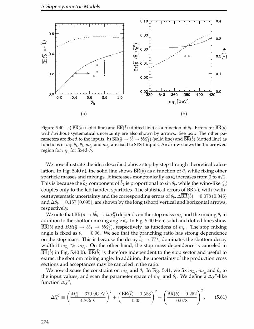
5 Supersymmetric Models
(a) (b)
Figure 5.40: a) BR(b) (solid line) and BR(t) (dotted line) as a function of θb. Errors for BR(b)with/without systematical uncertainty are also shown by arrows. See text. The other pa-rameters are fixed to the inputs. b) BR(g → bb → bbχ0
2) (solid line) and BR(b) (dotted line) asfunctions ofmt. θt, θb,mb1
andmb2are fixed to SPS 1 inputs. An arrow shows the 1-σ arrowed
region for mt1for fixed θt.
We now illustrate the idea described above step by step through theoretical calcu-
lation. In Fig. 5.40 a), the solid line shows BR(b) as a function of θb while fixing othersparticle masses and mixings. It increases monotonically as θb increases from 0 to π/2.
This is because the bL component of b2 is proportional to sin θb, while the wino-like χ02
couples only to the left handed sparticles. The statistical errors of BR(b), with (with-
out) systematic uncertainty and the corresponding errors of θb, ∆BR(b) = 0.078 (0.045)and ∆θb = 0.157 (0.095), are shown by the long (short) vertical and horizontal arrows,respectively.
We note that BR(g → bbi → bbχ02) depends on the stop massmt1 and the mixing θt in
addition to the sbottom mixing angle θb. In Fig. 5.40 Here solid and dotted lines show
BR(b) and BR(g → bb1 → bbχ02), respectively, as functions of mt1 . The stop mixing
angle is fixed as θt = 0.96. We see that the branching ratio has strong dependence
on the stop mass. This is because the decay bi → Wt1 dominates the sbottom decaywidth if mbi
≫ mt1 . On the other hand, the stop mass dependence is canceled in
BR(b) in Fig. 5.40 b). BR(b) is therefore independent to the stop sector and useful toextract the sbottom mixing angle. In addition, the uncertainty of the production crosssections and acceptances may be canceled in the ratio.
We now discuss the constraint on mt1 and θt. In Fig. 5.41, we fix mb1, mb2
and θb tothe input values, and scan the parameter space of mt1 and θt. We define a ∆χ2-likefunction ∆χ2,
∆χ2 ≡(Mw
tb − 370.9GeV
4.8GeV
)2
+
(BR(t)− 0.583
0.05
)2
+
(BR(b)− 0.252
0.078
)2
. (5.61)
274
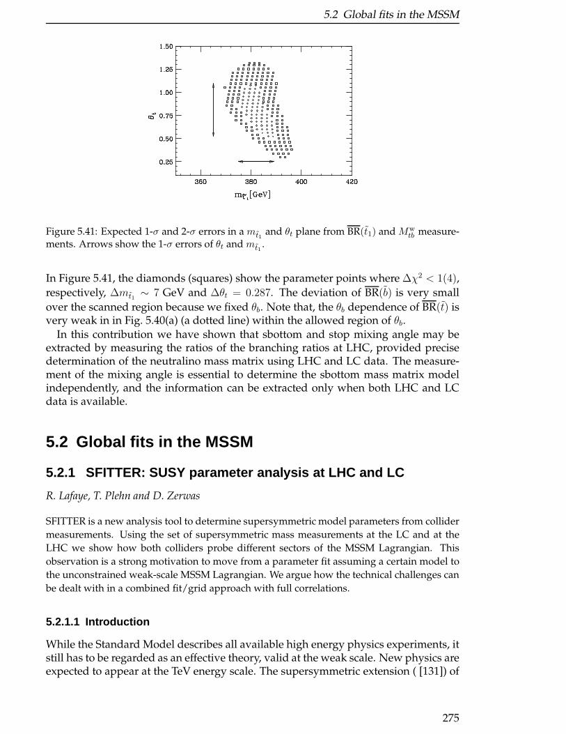
5.2 Global fits in the MSSM
Figure 5.41: Expected 1-σ and 2-σ errors in a mt1and θt plane from BR(t1) and Mw
tb measure-ments. Arrows show the 1-σ errors of θt and mt1
.
In Figure 5.41, the diamonds (squares) show the parameter points where ∆χ2 < 1(4),
respectively, ∆mt1 ∼ 7 GeV and ∆θt = 0.287. The deviation of BR(b) is very small
over the scanned region because we fixed θb. Note that, the θb dependence of BR(t) isvery weak in in Fig. 5.40(a) (a dotted line) within the allowed region of θb.
In this contribution we have shown that sbottom and stop mixing angle may beextracted by measuring the ratios of the branching ratios at LHC, provided precisedetermination of the neutralino mass matrix using LHC and LC data. The measure-ment of the mixing angle is essential to determine the sbottom mass matrix modelindependently, and the information can be extracted only when both LHC and LCdata is available.
5.2 Global fits in the MSSM
5.2.1 SFITTER: SUSY parameter analysis at LHC and LC
R. Lafaye, T. Plehn and D. Zerwas
SFITTER is a new analysis tool to determine supersymmetric model parameters from collider
measurements. Using the set of supersymmetric mass measurements at the LC and at the
LHC we show how both colliders probe different sectors of the MSSM Lagrangian. This
observation is a strong motivation to move from a parameter fit assuming a certain model to
the unconstrained weak-scale MSSM Lagrangian. We argue how the technical challenges can
be dealt with in a combined fit/grid approach with full correlations.
5.2.1.1 Introduction
While the Standard Model describes all available high energy physics experiments, itstill has to be regarded as an effective theory, valid at the weak scale. New physics areexpected to appear at the TeV energy scale. The supersymmetric extension ( [131]) of
275
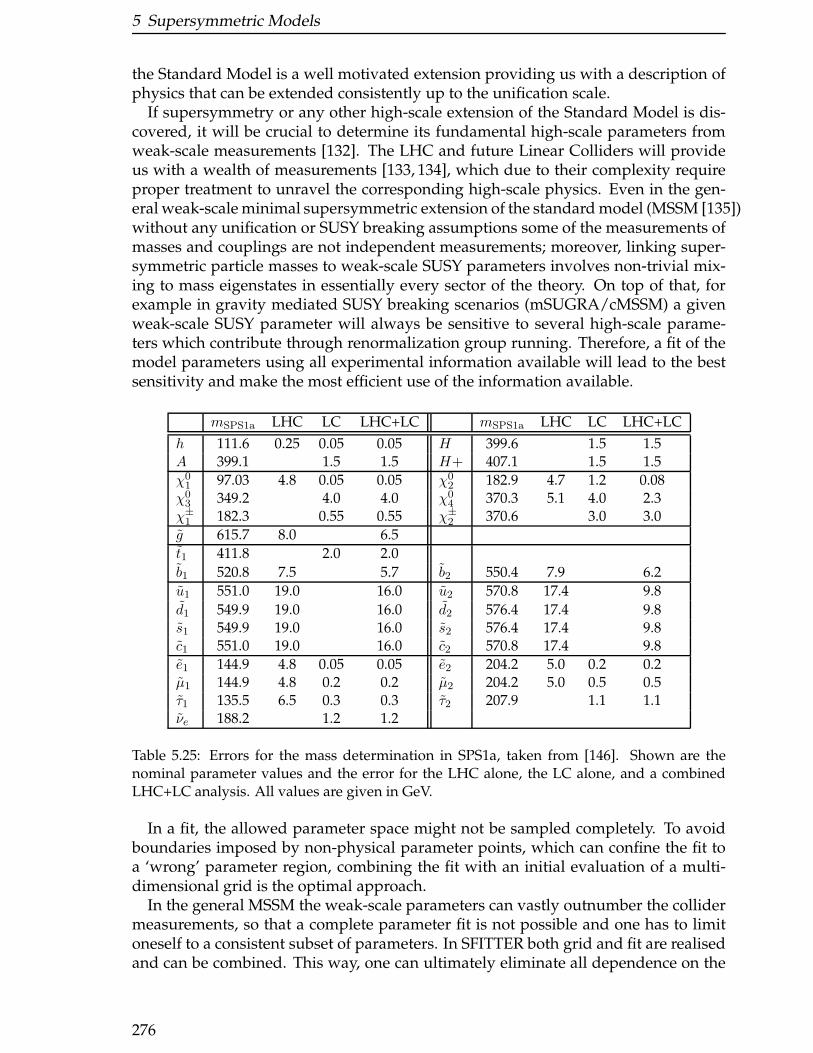
5 Supersymmetric Models
the Standard Model is a well motivated extension providing us with a description ofphysics that can be extended consistently up to the unification scale.
If supersymmetry or any other high-scale extension of the Standard Model is dis-covered, it will be crucial to determine its fundamental high-scale parameters fromweak-scale measurements [132]. The LHC and future Linear Colliders will provideus with a wealth of measurements [133, 134], which due to their complexity requireproper treatment to unravel the corresponding high-scale physics. Even in the gen-eral weak-scale minimal supersymmetric extension of the standard model (MSSM [135])without any unification or SUSY breaking assumptions some of the measurements ofmasses and couplings are not independent measurements; moreover, linking super-symmetric particle masses to weak-scale SUSY parameters involves non-trivial mix-ing to mass eigenstates in essentially every sector of the theory. On top of that, forexample in gravity mediated SUSY breaking scenarios (mSUGRA/cMSSM) a givenweak-scale SUSY parameter will always be sensitive to several high-scale parame-ters which contribute through renormalization group running. Therefore, a fit of themodel parameters using all experimental information available will lead to the bestsensitivity and make the most efficient use of the information available.
mSPS1a LHC LC LHC+LC mSPS1a LHC LC LHC+LC
h 111.6 0.25 0.05 0.05 H 399.6 1.5 1.5A 399.1 1.5 1.5 H+ 407.1 1.5 1.5
χ01 97.03 4.8 0.05 0.05 χ0
2 182.9 4.7 1.2 0.08χ0
3 349.2 4.0 4.0 χ04 370.3 5.1 4.0 2.3
χ±1 182.3 0.55 0.55 χ±
2 370.6 3.0 3.0
g 615.7 8.0 6.5
t1 411.8 2.0 2.0
b1 520.8 7.5 5.7 b2 550.4 7.9 6.2
u1 551.0 19.0 16.0 u2 570.8 17.4 9.8
d1 549.9 19.0 16.0 d2 576.4 17.4 9.8s1 549.9 19.0 16.0 s2 576.4 17.4 9.8c1 551.0 19.0 16.0 c2 570.8 17.4 9.8
e1 144.9 4.8 0.05 0.05 e2 204.2 5.0 0.2 0.2µ1 144.9 4.8 0.2 0.2 µ2 204.2 5.0 0.5 0.5τ1 135.5 6.5 0.3 0.3 τ2 207.9 1.1 1.1νe 188.2 1.2 1.2
Table 5.25: Errors for the mass determination in SPS1a, taken from [146]. Shown are thenominal parameter values and the error for the LHC alone, the LC alone, and a combinedLHC+LC analysis. All values are given in GeV.
In a fit, the allowed parameter space might not be sampled completely. To avoidboundaries imposed by non-physical parameter points, which can confine the fit toa ‘wrong’ parameter region, combining the fit with an initial evaluation of a multi-dimensional grid is the optimal approach.
In the general MSSM the weak-scale parameters can vastly outnumber the collidermeasurements, so that a complete parameter fit is not possible and one has to limitoneself to a consistent subset of parameters. In SFITTER both grid and fit are realisedand can be combined. This way, one can ultimately eliminate all dependence on the
276
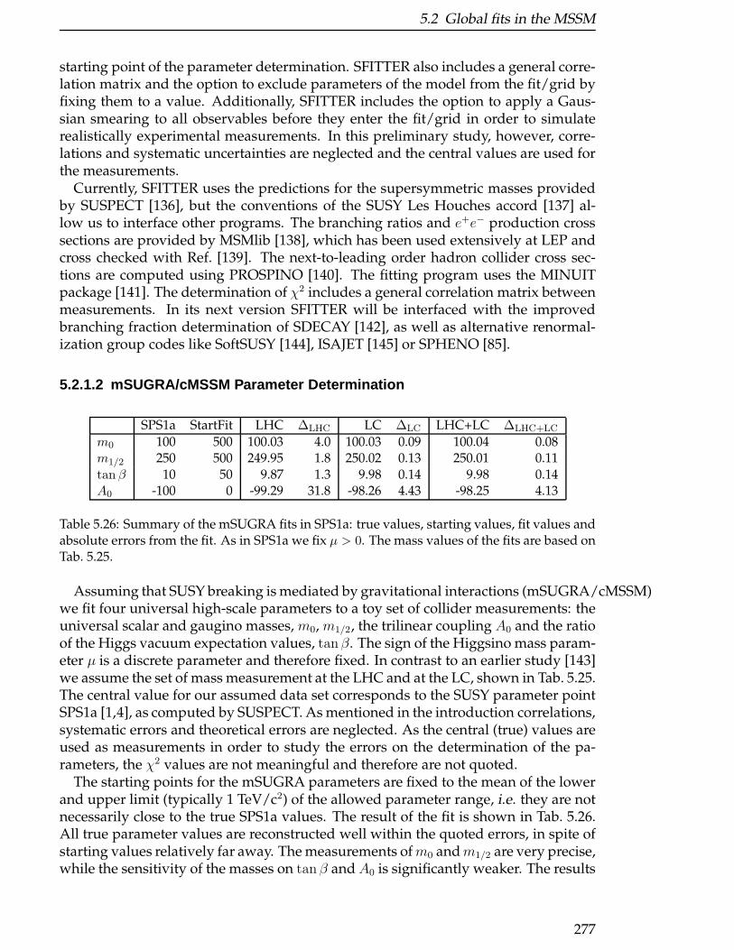
5.2 Global fits in the MSSM
starting point of the parameter determination. SFITTER also includes a general corre-lation matrix and the option to exclude parameters of the model from the fit/grid byfixing them to a value. Additionally, SFITTER includes the option to apply a Gaus-sian smearing to all observables before they enter the fit/grid in order to simulaterealistically experimental measurements. In this preliminary study, however, corre-lations and systematic uncertainties are neglected and the central values are used forthe measurements.
Currently, SFITTER uses the predictions for the supersymmetric masses providedby SUSPECT [136], but the conventions of the SUSY Les Houches accord [137] al-low us to interface other programs. The branching ratios and e+e− production crosssections are provided by MSMlib [138], which has been used extensively at LEP andcross checked with Ref. [139]. The next-to-leading order hadron collider cross sec-tions are computed using PROSPINO [140]. The fitting program uses the MINUITpackage [141]. The determination of χ2 includes a general correlation matrix betweenmeasurements. In its next version SFITTER will be interfaced with the improvedbranching fraction determination of SDECAY [142], as well as alternative renormal-ization group codes like SoftSUSY [144], ISAJET [145] or SPHENO [85].
5.2.1.2 mSUGRA/cMSSM Parameter Determination
SPS1a StartFit LHC ∆LHC LC ∆LC LHC+LC ∆LHC+LC
m0 100 500 100.03 4.0 100.03 0.09 100.04 0.08m1/2 250 500 249.95 1.8 250.02 0.13 250.01 0.11tan β 10 50 9.87 1.3 9.98 0.14 9.98 0.14A0 -100 0 -99.29 31.8 -98.26 4.43 -98.25 4.13
Table 5.26: Summary of the mSUGRA fits in SPS1a: true values, starting values, fit values andabsolute errors from the fit. As in SPS1a we fix µ > 0. The mass values of the fits are based onTab. 5.25.
Assuming that SUSY breaking is mediated by gravitational interactions (mSUGRA/cMSSM)we fit four universal high-scale parameters to a toy set of collider measurements: theuniversal scalar and gaugino masses, m0, m1/2, the trilinear coupling A0 and the ratioof the Higgs vacuum expectation values, tanβ. The sign of the Higgsino mass param-eter µ is a discrete parameter and therefore fixed. In contrast to an earlier study [143]we assume the set of mass measurement at the LHC and at the LC, shown in Tab. 5.25.The central value for our assumed data set corresponds to the SUSY parameter pointSPS1a [1,4], as computed by SUSPECT. As mentioned in the introduction correlations,systematic errors and theoretical errors are neglected. As the central (true) values areused as measurements in order to study the errors on the determination of the pa-rameters, the χ2 values are not meaningful and therefore are not quoted.
The starting points for the mSUGRA parameters are fixed to the mean of the lowerand upper limit (typically 1 TeV/c2) of the allowed parameter range, i.e. they are notnecessarily close to the true SPS1a values. The result of the fit is shown in Tab. 5.26.All true parameter values are reconstructed well within the quoted errors, in spite ofstarting values relatively far away. The measurements ofm0 andm1/2 are very precise,while the sensitivity of the masses on tan β and A0 is significantly weaker. The results
277
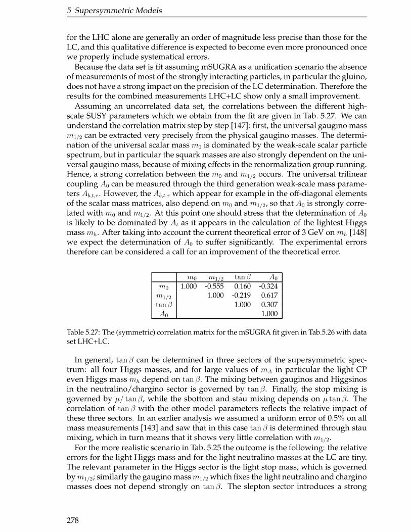
5 Supersymmetric Models
for the LHC alone are generally an order of magnitude less precise than those for theLC, and this qualitative difference is expected to become even more pronounced oncewe properly include systematical errors.
Because the data set is fit assuming mSUGRA as a unification scenario the absenceof measurements of most of the strongly interacting particles, in particular the gluino,does not have a strong impact on the precision of the LC determination. Therefore theresults for the combined measurements LHC+LC show only a small improvement.
Assuming an uncorrelated data set, the correlations between the different high-scale SUSY parameters which we obtain from the fit are given in Tab. 5.27. We canunderstand the correlation matrix step by step [147]: first, the universal gaugino massm1/2 can be extracted very precisely from the physical gaugino masses. The determi-nation of the universal scalar mass m0 is dominated by the weak-scale scalar particlespectrum, but in particular the squark masses are also strongly dependent on the uni-versal gaugino mass, because of mixing effects in the renormalization group running.Hence, a strong correlation between the m0 and m1/2 occurs. The universal trilinearcoupling A0 can be measured through the third generation weak-scale mass parame-ters Ab,t,τ . However, the Ab,t,τ which appear for example in the off-diagonal elementsof the scalar mass matrices, also depend on m0 and m1/2, so that A0 is strongly corre-lated with m0 and m1/2. At this point one should stress that the determination of A0
is likely to be dominated by At as it appears in the calculation of the lightest Higgsmass mh. After taking into account the current theoretical error of 3 GeV on mh [148]we expect the determination of A0 to suffer significantly. The experimental errorstherefore can be considered a call for an improvement of the theoretical error.
m0 m1/2 tan β A0
m0 1.000 -0.555 0.160 -0.324m1/2 1.000 -0.219 0.617tan β 1.000 0.307A0 1.000
Table 5.27: The (symmetric) correlation matrix for the mSUGRA fit given in Tab.5.26 with dataset LHC+LC.
In general, tanβ can be determined in three sectors of the supersymmetric spec-trum: all four Higgs masses, and for large values of mA in particular the light CPeven Higgs mass mh depend on tan β. The mixing between gauginos and Higgsinosin the neutralino/chargino sector is governed by tanβ. Finally, the stop mixing isgoverned by µ/ tanβ, while the sbottom and stau mixing depends on µ tanβ. Thecorrelation of tan β with the other model parameters reflects the relative impact ofthese three sectors. In an earlier analysis we assumed a uniform error of 0.5% on allmass measurements [143] and saw that in this case tan β is determined through staumixing, which in turn means that it shows very little correlation with m1/2.
For the more realistic scenario in Tab. 5.25 the outcome is the following: the relativeerrors for the light Higgs mass and for the light neutralino masses at the LC are tiny.The relevant parameter in the Higgs sector is the light stop mass, which is governedbym1/2; similarly the gaugino massm1/2 which fixes the light neutralino and charginomasses does not depend strongly on tan β. The slepton sector introduces a strong
278
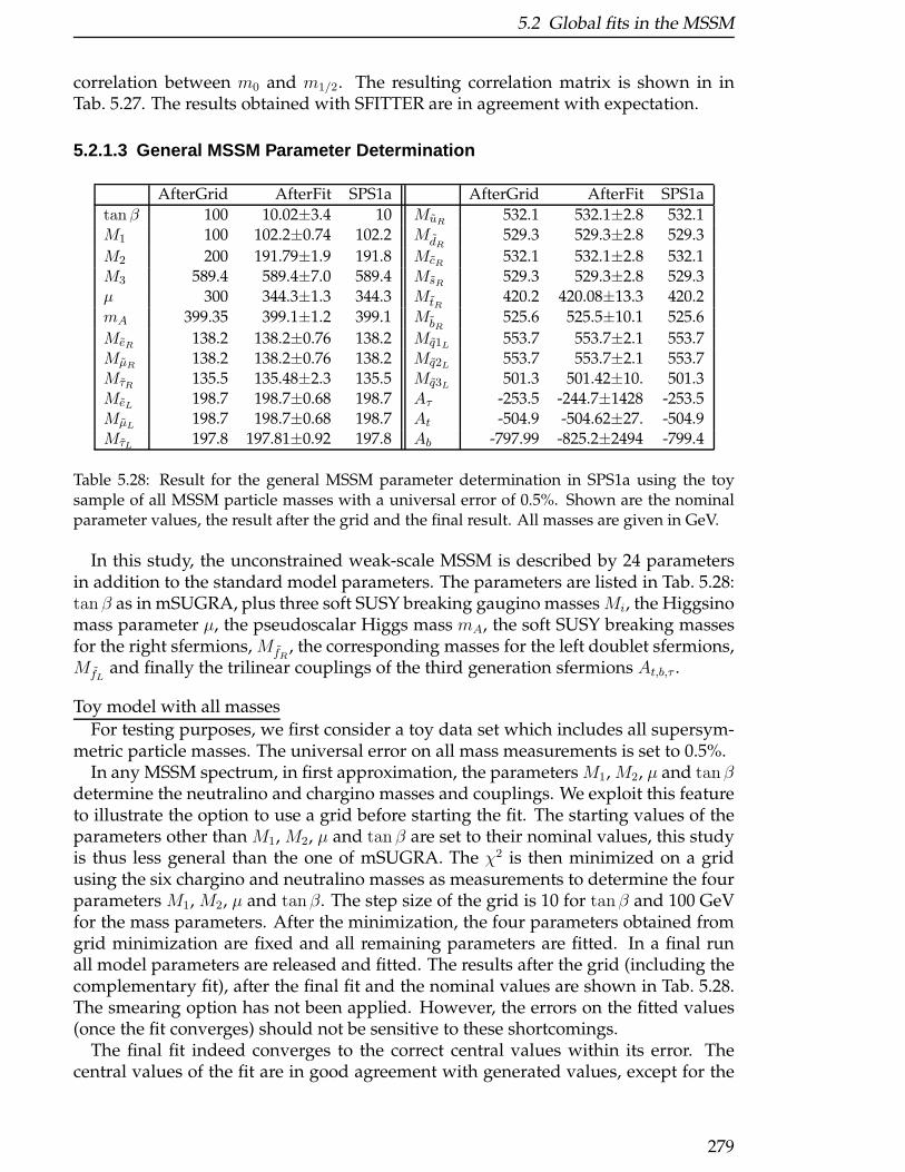
5.2 Global fits in the MSSM
correlation between m0 and m1/2. The resulting correlation matrix is shown in inTab. 5.27. The results obtained with SFITTER are in agreement with expectation.
5.2.1.3 General MSSM Parameter Determination
AfterGrid AfterFit SPS1a AfterGrid AfterFit SPS1a
tan β 100 10.02±3.4 10 MuR532.1 532.1±2.8 532.1
M1 100 102.2±0.74 102.2 MdR529.3 529.3±2.8 529.3
M2 200 191.79±1.9 191.8 McR 532.1 532.1±2.8 532.1M3 589.4 589.4±7.0 589.4 MsR
529.3 529.3±2.8 529.3µ 300 344.3±1.3 344.3 MtR
420.2 420.08±13.3 420.2mA 399.35 399.1±1.2 399.1 MbR
525.6 525.5±10.1 525.6
MeR138.2 138.2±0.76 138.2 Mq1L
553.7 553.7±2.1 553.7MµR
138.2 138.2±0.76 138.2 Mq2L553.7 553.7±2.1 553.7
MτR 135.5 135.48±2.3 135.5 Mq3L501.3 501.42±10. 501.3
MeL198.7 198.7±0.68 198.7 Aτ -253.5 -244.7±1428 -253.5
MµL198.7 198.7±0.68 198.7 At -504.9 -504.62±27. -504.9
MτL 197.8 197.81±0.92 197.8 Ab -797.99 -825.2±2494 -799.4
Table 5.28: Result for the general MSSM parameter determination in SPS1a using the toysample of all MSSM particle masses with a universal error of 0.5%. Shown are the nominalparameter values, the result after the grid and the final result. All masses are given in GeV.
In this study, the unconstrained weak-scale MSSM is described by 24 parametersin addition to the standard model parameters. The parameters are listed in Tab. 5.28:tan β as in mSUGRA, plus three soft SUSY breaking gaugino massesMi, the Higgsinomass parameter µ, the pseudoscalar Higgs mass mA, the soft SUSY breaking massesfor the right sfermions, MfR
, the corresponding masses for the left doublet sfermions,MfL
and finally the trilinear couplings of the third generation sfermions At,b,τ .
Toy model with all masses
For testing purposes, we first consider a toy data set which includes all supersym-metric particle masses. The universal error on all mass measurements is set to 0.5%.
In any MSSM spectrum, in first approximation, the parameters M1, M2, µ and tanβdetermine the neutralino and chargino masses and couplings. We exploit this featureto illustrate the option to use a grid before starting the fit. The starting values of theparameters other than M1, M2, µ and tan β are set to their nominal values, this studyis thus less general than the one of mSUGRA. The χ2 is then minimized on a gridusing the six chargino and neutralino masses as measurements to determine the fourparameters M1, M2, µ and tanβ. The step size of the grid is 10 for tanβ and 100 GeVfor the mass parameters. After the minimization, the four parameters obtained fromgrid minimization are fixed and all remaining parameters are fitted. In a final runall model parameters are released and fitted. The results after the grid (including thecomplementary fit), after the final fit and the nominal values are shown in Tab. 5.28.The smearing option has not been applied. However, the errors on the fitted values(once the fit converges) should not be sensitive to these shortcomings.
The final fit indeed converges to the correct central values within its error. Thecentral values of the fit are in good agreement with generated values, except for the
279

5 Supersymmetric Models
trilinear coupling Ab,τ . The problem is using only mass measurements to determinethe three entries in a (symmetric) scalar mass matrix: in the light slepton sector thereare three masses, left and right scalars plus the sneutrino, so the system is in principlecalculable. In the third generation squark sector we have three independent diagonalentries per generation and two off-diagonal entries. But the number of mass mea-surements is only four, therefore the system is underdetermined in first order. Theoff-diagonal entry in the mass matrix for down type scalars includes a term Ab,τ andan additional term µ tanβ. Even for very moderate values of tanβ the extraction ofAb,τ requires precise knowledge of tanβ. The use of branching ratios and cross sec-tion measurements (with polarised beams) which carry information about the scalarmixing angles should significantly improve the determination of At,b,τ .
Toy model with LHC-LC mass measurements
LHC LC LHC+LC SPS1a
tan β 10.22±9.1 10.26±0.3 10.06±0.2 10M1 102.45±5.3 102.32±0.1 102.23±0.1 102.2M2 191.8±7.3 192.52±0.7 191.79±0.2 191.8M3 578.67±15 fixed 500 588.05±11 589.4MτL fixed 500 197.68±1.2 199.25±1.1 197.8MτR 129.03±6.9 135.66±0.3 133.35±0.6 135.5MµL
198.7±5.1 198.7±0.5 198.7±0.5 198.7MµR
138.2±5.0 138.2±0.2 138.2±0.2 138.2MeL
198.7±5.1 198.7±0.2 198.7±0.2 198.7MeR
138.2±5.0 138.2±0.05 138.2±0.05 138.2Mq3L
498.3±110 497.6±4.4 521.9±39 501.3MtR
fixed 500 420±2.1 411.73±12 420.2
MbR522.26±113 fixed 500 504.35±61 525.6
Mq2L550.72±13 fixed 500 553.31±5.5 553.7
McR 529.02±20 fixed 500 531.70±15 532.1MsR
526.21±20 fixed 500 528.90±15 529.3Mq1L
550.72±13 fixed 500 553.32±6.5 553.7MuR
528.91±20 fixed 500 531.70±15 532.1MdR
526.2±20 fixed 500 528.90±15 529.3
Aτ fixed 0 -202.4±89.5 352.1±171 -253.5At -507.8±91 -501.95±2.7 -505.24±3.3 -504.9Ab -784.7±35603 fixed 0 -977±12467 -799.4mA fixed 500 399.1±0.9 399.1±0.8 399.1µ 345.21±7.3 344.34±2.3 344.36±1.0 344.3
Table 5.29: Result for the general MSSM parameter determination in SPS1a using the massmeasurements given in Tab. 5.25. Shown are the nominal parameter values and the resultafter fits to the different data sets. All masses are given in GeV.
In the study of the three data sets LHC, LC, and LHC+LC in the MSSM, a fit wasperformed for the data sets LHC and LC, whereas for LHC+LC additionally the GRIDwas used for M1, M2, µ and tan β with the five chargino and neutralino masses. Thestarting points were chosen to be the true values (with the exception of the parametersused in the grid). In order to obtain a solvable system, for the LHC data set mA, MtR ,
280
5.2 Global fits in the MSSM
MτL , Aτ were fixed. For the LC data set the first and second generation squark softSUSY breaking masses, the gluino massM3,MbR
andAb were fixed. These parameterswere chosen on the basis of the measurements available in Tab. 5.25. The values towhich these parameters were fixed is not expected to influence the final result of thefit. The results for the two data sets are shown in Tab. 5.29.
Note that the general rule that the LHC is not sensitive to weakly interacting par-ticle masses is not entirely true: while the LHC has the advantage of measuring thesquark and gluino masses, the first and second generation slepton mass parametersare also determined with a precision of the order of percent. The results in Tab. 5.29show that the LHC alone is well capable of determining for example all gaugino massparameters as well as most of the scalar mass parameters.
The situation at the LC is slightly different. Only marginal information on thesquark sector available at the LC. The measurement of At from the Higgs sectorshould be taken with a grain of salt (theoretical error on the lightest Higgs mass).Adding the stau mixing angle to the set of LC measurements will improve the deter-mination of Aτ . However, the measurements of the parameters, in particular sleptonand gaugino parameters are far more precise than at the LHC.
For the LHC+LC data set, a sufficient number of mass measurements is available,so that no parameters need to be fixed. The superiority of the combination of the mea-surements at the two colliders is obvious from this observation and from Tab. 5.29:The LHC contributes to reduce the error in the weak sector (M2) and the LC in thestrongly interacting sector (third generation squarks). Even more important: of 13parameters undetermined by either the LHC or the LC, 11 are determined with goodprecision in the combination. For Aτ , Ab, we expect an improvement with the use ofbranching ratios and cross section measurements.
A complete measurement of all parameters at the weak scale is particularly impor-tant if one wants to probe unification scenarios which link subsectors of the parameterspace which are independent at the weak scale. An advanced tool like SFITTER canextract the information to probe supersymmetry breaking scenarios from any set ofmeasurements, provided the set is sufficient to overconstrain the model parameters.
5.2.1.4 Conclusions
SFITTER is a new program to determine supersymmetric parameters from measure-ments. The parameters can be extracted either using a fit, a multi-dimensional grid,or a combination of the two. Correlations between measurements can be specifiedand are taken into account. While it is relatively easy to fit a fixed model with veryfew parameters for example at a high scale to a set of collider measurements, the de-termination of the complete set of weak-scale MSSM model parameters requires thismore advanced tool. A mSUGRA inspired fit does not include the full complexityand power of the combined LHC and LC data compared to the measurements at ei-ther collider alone. The results from SFITTER in the MSSM with the three data setsshow that only the combination of measurements of both the LHC and the LC offers acomplete picture of the MSSM model parameters in a reasonably model independentframework.
281
5 Supersymmetric Models
5.2.2 Fittino: A global fit of the MSSM parameters
P. Bechtle, K. Desch and P. Wienemann
If SUSY is realized, the pattern of its breaking can be generally expressed in terms of the
soft SUSY breaking Lagrangian. The program Fittino extracts the parameters of the MSSM
Lagrangian from simulated measurements at LHC and the LC in a global fit. No prior knowl-
edge of the parameters is assumed. Tree-level relations between observables and SUSY pa-
rameters are used to obtain start values for the fit. Without the information from all sectors
of the theory this fit does not converge. Therefore both the almost complete spectrum at LHC
and the precise measurements of the lighter SUSY particles at the LC is crucial. An example
fit is performed for SPS1a, assuming unification in the first two generations, flavor-diagonal
couplings and absence of CP-violating phases. As a result of the fit, a full error matrix of the
parameters is obtained.
5.2.2.1 Introduction
As for the program SFITTER, the aim of Fittino is the determination of the parame-ters of the MSSM. It is implemented in C++ and focusses on the determination of theparameters of the soft SUSY breaking Lagrangian Lsoft, obeying the following princi-ples:
• No a priori knowledge of SUSY parameters is assumed (but can be imposed ifdesired by the user).
• All measurements from future colliders could be used.
• All correlations among parameters and all influences of loop-induced effects,where parameters of one sector affect observables of other sectors of the theory,are taken into account, as far as they are implemented into the program whichprovides the theoretical predictions.
In this way an unbiased global fit is obtained. No attempt to extract SUSY parametersat the GUT scale is made, since the evolution of the parameters and their determina-tion at the low scale factorizes. The result of Fittino with the full errors of the lowenergy SUSY parameters can therefore be used later to extrapolate to the GUT scale.
However, all 105 possible parameters of LMSSM cannot be determined simultane-ously. Therefore, assumptions on the structure of LMSSM are made. All phases are setto 0, no mixing between generations is assumed and the mixing within the first twogenerations is set to 0. Thus the number of free parameters in the SUSY breaking sec-tor is reduced to 24. Further assumptions can be specified by the user. Observablesused in the fit can be
• Masses, limits on masses of unobserved particles
• Widths
• Cross-Sections
• Branching ratios
282
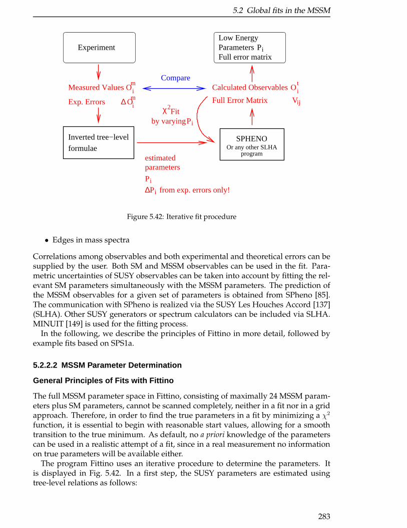
5.2 Global fits in the MSSM
Measured Values Oim
Exp. Errors O∆ im
Pi
P∆ i
estimatedparameters
from exp. errors only!
Inverted tree−level
formulae
χ2Fit
Piby varying
Oti
Vij
Calculated Observables
Full Error Matrix
Pi
Compare
Experiment ParametersFull error matrix
Low Energy
SPHENOOr any other SLHA
program
Figure 5.42: Iterative fit procedure
• Edges in mass spectra
Correlations among observables and both experimental and theoretical errors can besupplied by the user. Both SM and MSSM observables can be used in the fit. Para-metric uncertainties of SUSY observables can be taken into account by fitting the rel-evant SM parameters simultaneously with the MSSM parameters. The prediction ofthe MSSM observables for a given set of parameters is obtained from SPheno [85].The communication with SPheno is realized via the SUSY Les Houches Accord [137](SLHA). Other SUSY generators or spectrum calculators can be included via SLHA.MINUIT [149] is used for the fitting process.
In the following, we describe the principles of Fittino in more detail, followed byexample fits based on SPS1a.
5.2.2.2 MSSM Parameter Determination
General Principles of Fits with Fittino
The full MSSM parameter space in Fittino, consisting of maximally 24 MSSM param-eters plus SM parameters, cannot be scanned completely, neither in a fit nor in a gridapproach. Therefore, in order to find the true parameters in a fit by minimizing a χ2
function, it is essential to begin with reasonable start values, allowing for a smoothtransition to the true minimum. As default, no a priori knowledge of the parameterscan be used in a realistic attempt of a fit, since in a real measurement no informationon true parameters will be available either.
The program Fittino uses an iterative procedure to determine the parameters. Itis displayed in Fig. 5.42. In a first step, the SUSY parameters are estimated usingtree-level relations as follows:
283
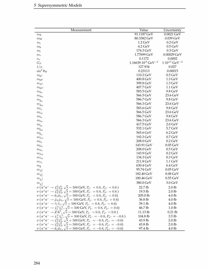
5 Supersymmetric Models
Measurement Value UncertaintymZ 91.1187 GeV 0.0021 GeVmW 80.3382 GeV 0.039 GeVmc 1.2 GeV 0.2 GeVmb 4.2 GeV 0.5 GeVmt 174.3 GeV 0.3 GeVmτ 1.77699 GeV 0.00029 GeVαs 0.1172 0.0002GF 1.16639·10-5 GeV−2 1·10-11 GeV−2
1/α 127.934 0.027sin2 θW 0.23113 0.00015mh0 110.2 GeV 0.5 GeVmH0 400.8 GeV 1.3 GeVmA0 399.8 GeV 1.3 GeVmH± 407.7 GeV 1.1 GeVmuL
583.5 GeV 9.8 GeVmuR
566.5 GeV 23.6 GeVmdL
586.7 GeV 9.8 GeV
mdR566.3 GeV 23.6 GeV
mcL583.6 GeV 9.8 GeV
mcR566.5 GeV 23.6 GeV
msL586.7 GeV 9.8 GeV
msR566.3 GeV 23.6 GeV
mtR417.5 GeV 2.0 GeV
mbR532.1 GeV 5.7 GeV
mbL565.6 GeV 6.2 GeV
mνeL192.3 GeV 0.7 GeV
meL208.0 GeV 0.2 GeV
meR143.91 GeV 0.05 GeV
mµL208.0 GeV 0.5 GeV
mµR143.9 GeV 0.2 GeV
mτR134.3 GeV 0.3 GeV
mτL211.8 GeV 1.1 GeV
mg 630.4 GeV 6.4 GeVmχ0
195.74 GeV 0.05 GeV
mχ02
182.40 GeV 0.08 GeV
mχ±
1
180.46 GeV 0.55 GeV
mχ±
2
380.0 GeV 3.0 GeV
σ ( e+e− → χ01χ
02,√s = 500 GeV, Pe− = 0.8, Pe+ = 0.6 ) 22.7 fb 2.0 fb
σ ( e+e− → χ02χ
02,√s = 500 GeV, Pe− = 0.8, Pe+ = 0.6 ) 19.5 fb 2.0 fb
σ ( e+e− → eLeL,√s = 500 GeV, Pe− = 0.8, Pe+ = 0.6) 205.0 fb 4.0 fb
σ ( e+e− → µLµL,√s = 500 GeV, Pe− = 0.8, Pe+ = 0.6) 36.8 fb 4.0 fb
σ ( e+e− → τ1τ1,√s = 500 GeV, Pe− = 0.8, Pe+ = 0.6) 39.1 fb 4.0 fb
σ ( e+e− → χ±1 χ
∓1 ,√s = 500 GeV, Pe− = 0.8, Pe+ = 0.6) 46.7 fb 1.0 fb
σ ( e+e− → Z h0,√s = 500 GeV, Pe− = 0.8, Pe+ = 0.6 ) 11.13 fb 0.21 fb
σ ( e+e− → χ±1 χ
∓1 ,√s = 500 GeV, Pe− = −0.8, Pe+ = −0.6 ) 104.8 fb 3.5 fb
σ ( e+e− → χ01χ
02,√s = 500 GeV, Pe− = −0.8, Pe+ = −0.6) 43.9 fb 2.0 fb
σ ( e+e− → χ02χ
02,√s = 500 GeV, Pe− = −0.8, Pe+ = −0.6) 43.8 fb 2.0 fb
σ ( e+e− → eLeL,√s = 500 GeV, Pe− = −0.8, Pe+ = −0.6) 97.4 fb 4.0 fb
284

5.2 Global fits in the MSSM
Measurement Value Uncertaintyσ ( e+e− → eLeR,
√s = 500 GeV, Pe− = −0.8, Pe+ = −0.6) 223.7 fb 4.0 fb
σ ( e+e− → eReR,√s = 500 GeV, Pe− = −0.8, Pe+ = −0.6) 29.0 fb 2.0 fb
σ ( e+e− → µLµL,√s = 500 GeV, Pe− = −0.8, Pe+ = −0.6) 22.7 fb 2.0 fb
σ ( e+e− → τ1τ1,√s = 500 GeV, Pe− = −0.8, Pe+ = −0.6) 25.7 fb 2.0 fb
BR ( h0 → bb ) 0.82 0.01
BR ( h0 → cc) 0.04 0.01
BR ( h0 → τ+τ− ) 0.14 0.01
Table 5.30: Simulated measurements at LHC and a 0.5 and 1 TeV LC. For the cross sections, thecorresponding center-of-mass energy and the electron and positron polarization are given.
1. µ,mA, tanβ,M1,M2,M3 are determined from gaugino and Higgs sector observ-ables using formulae from [150]. In order to extract these parameters, infor-mation from chargino cross-sections is needed, which enters in form of thechargino mixing angles cos 2φL and cos 2φR. These pseudo-observables are onlyused for the determination of the start values, no use is made of them for the fit.
2. At, Ab,MQ,MU ,MD are determined from the squark sector masses, using for-mulae from [151]. No mixing in the third generation is assumed to get the startvalues.
3. Aτ ,ML,ME are determined from the slepton sector masses, using formulae from[151]. No mixing in the third generation is assumed to get the start values.
Instead of the trilinear couplings At, Ab and Aτ the following sfermion mixing pa-rameters
Xt = At − µ/ tanβ
Xb = Ab − µ · tanβ
Xτ = Aτ − µ · tanβ
are used in the fit. This is done in order to reduce the correlations between the pa-rameters µ, tanβ and At, Ab and Aτ . The tree-level initialization is done such thatAt,b,τ = 0.
Since the mixing in the third generation has not been taken correctly into accounton tree-level, the parameters Xt, Xb, Xτ tend to be badly initialized. A global fitwith these starting values would most likely not converge. Therefore next the es-timates from the slepton sector are improved by fitting only the slepton parametersXτ ,ML,ME to the observables from the slepton sector, i. e. slepton masses and cross-sections. Observables not directly related to the slepton sector can degrade the fitresult, since parameters of other sectors are likely to be still wrong. In such a casea parameter of the slepton sector will be pulled into a wrong direction, in order tocompensate for the wrong parameters of other sectors. All parameters not from theslepton sector are fixed to their tree-level estimates obtained in the previous step.In this fit with reduced number of dimensions MINUIT can handle the correlationsamong the parameters better than in a global fit with all parameters free.
Then the third generation squark parameters are improved by only fitting Xt, Xb,MQ, MU , MD to the observables of the squark sector, masses and cross-sections. Allother parameters are fixed to their previous values.
285
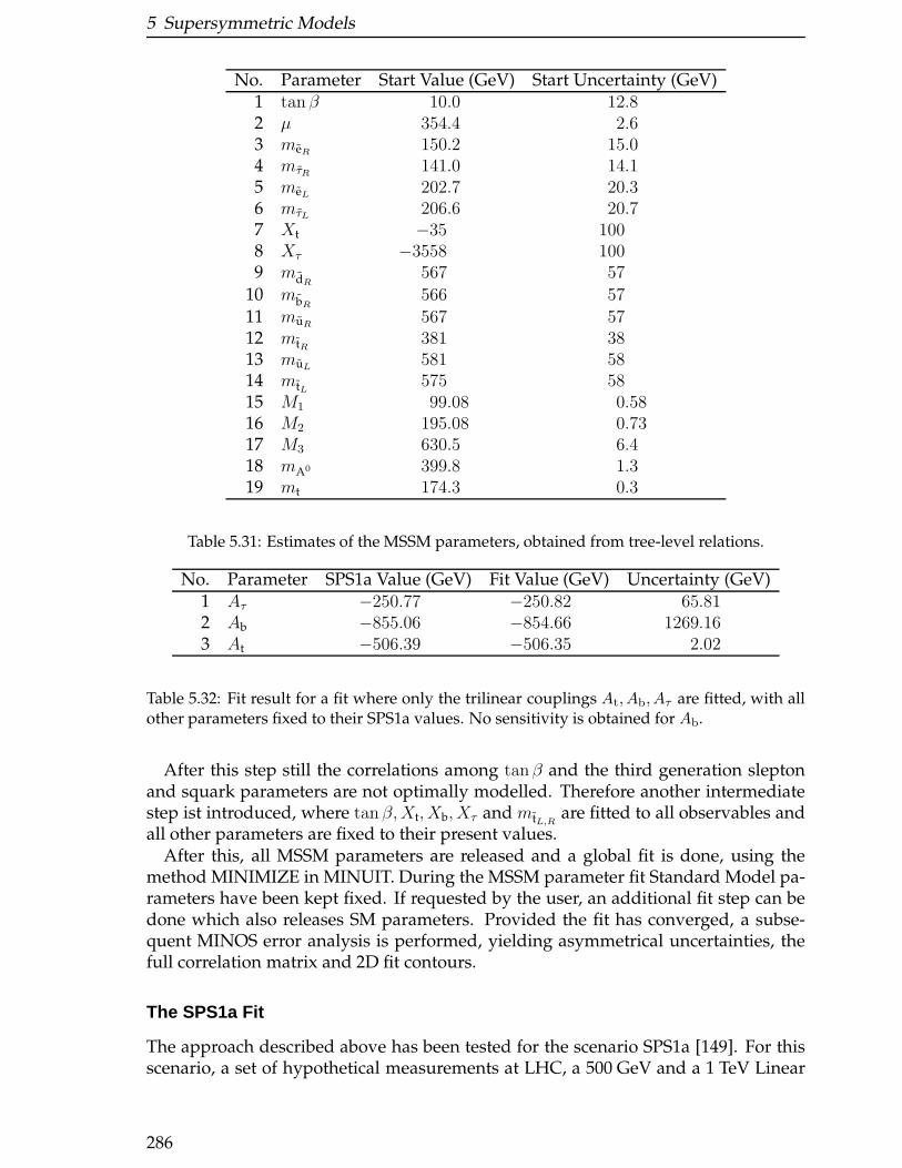
5 Supersymmetric Models
No. Parameter Start Value (GeV) Start Uncertainty (GeV)1 tan β 10.0 12.82 µ 354.4 2.63 meR
150.2 15.04 mτR 141.0 14.15 meL
202.7 20.36 mτL 206.6 20.77 Xt −35 1008 Xτ −3558 1009 mdR
567 57
10 mbR566 57
11 muR567 57
12 mtR381 38
13 muL581 58
14 mtL575 58
15 M1 99.08 0.5816 M2 195.08 0.7317 M3 630.5 6.418 mA0 399.8 1.319 mt 174.3 0.3
Table 5.31: Estimates of the MSSM parameters, obtained from tree-level relations.
No. Parameter SPS1a Value (GeV) Fit Value (GeV) Uncertainty (GeV)1 Aτ −250.77 −250.82 65.812 Ab −855.06 −854.66 1269.163 At −506.39 −506.35 2.02
Table 5.32: Fit result for a fit where only the trilinear couplings At, Ab, Aτ are fitted, with allother parameters fixed to their SPS1a values. No sensitivity is obtained for Ab.
After this step still the correlations among tanβ and the third generation sleptonand squark parameters are not optimally modelled. Therefore another intermediatestep ist introduced, where tan β,Xt, Xb, Xτ and mtL,R
are fitted to all observables andall other parameters are fixed to their present values.
After this, all MSSM parameters are released and a global fit is done, using themethod MINIMIZE in MINUIT. During the MSSM parameter fit Standard Model pa-rameters have been kept fixed. If requested by the user, an additional fit step can bedone which also releases SM parameters. Provided the fit has converged, a subse-quent MINOS error analysis is performed, yielding asymmetrical uncertainties, thefull correlation matrix and 2D fit contours.
The SPS1a Fit
The approach described above has been tested for the scenario SPS1a [149]. For thisscenario, a set of hypothetical measurements at LHC, a 500 GeV and a 1 TeV Linear
286
5.2 Global fits in the MSSM
Collider has been collected in Table 5.30. In this example a theoretical error on theprediction of the lightest Higgs boson mass of 500 MeV is included. All observablesfrom Table 5.30 were selected as input to fit the 24 parameters of the unconstrainedMSSM and the top quark mass. In order to reduce the number of fit parameters and tosimplify the fit procedure, unification of the first two generations has been assumed.Table 5.28 shows that this is a reasonable assumption which does not imply any lossof accurarcy.
The parameter Xb has been fixed to -4000 GeV. The reason for this is summarizedin Table 5.32. It contains the fitted trilinear couplings Aτ , At and Ab from a fit whereall other parameters from Table 5.33 are fixed to their SPS1a values. Evidently theselected observables have no sensitivity to Ab. Fixing Xb is a passable way to circum-vent this insensitivity.
Taking these simplifications into account, 18 MSSM parameters and the top quarkmass remain. All fitted parameters are listed in Table 5.33 including the predictedSPS1a values, the fitted values and the uncertainties from the fit. All fitted parametersexcept the third generation squark sector agree well with the generated values. Thediscrepancy in the third generation squark sector stems from the fact that Xb is fixedto an approximate value which does not coincide with its SPS1a value. The inclusionof a theoretical error of 500 MeV on the lightest Higgs mass increases the uncertaintyon tanβ by a factor of 2.
Albeit the fitted third generation squark parameters do not match their SPS1a val-ues, the obtained χ2 of the fit is only 0.043. This shows the importance to fit all pa-rameters simultaneously, since parameters fixed to wrong values tend to distort thewhole spectrum of the fitted parameters to compensate for the wrongly fixed param-eters. As it is obvious from Table 5.33, the systematic distortion can be much largerthan the 1σ uncertainties of the parameters.
Improving the determination of the trilinear couplings and a release of the Xb =−4000 GeV constraint requires the inclusion of additional, more sensitive observables.Good candidates are probably stop and stau polarization measurements. Unfortu-nately such predictions are not yet available in SPheno.
In addition the contribution of the various observables to the determination of agiven parameter has been studied by looking at ∆χ2 for the individual observablesif the parameter is changed by ±1σ. As an example, Table 5.34 summarizes the threemost important contributions to tanβ, µ, M1, M2 and M3.
It has also been tried to carry out fits using only a reduced set of measurements asinput such as they are available in ”LHC only” and ”LC only” scenarios. The ”LHConly” case shows a quite comprehensive particle spectrum but only poor informationon the slepton sector is avaiable. In contrast to that the ”LC only” scenario is char-acterized by an incomplete MSSM particle spectrum (no information from squarksector) but a very precise slepton and gaugino sector. Even when poorly determinedparameters are fixed (as in Table 5.29), no converging fits are obtained. This factshows the importance of combined LHC and LC data analyses.
5.2.2.3 Conclusions
Fittino is a program to determine the MSSM parameters from a global fit to mea-surements at the LHC and a future Linear Collider. No prior knowledge of any of
287
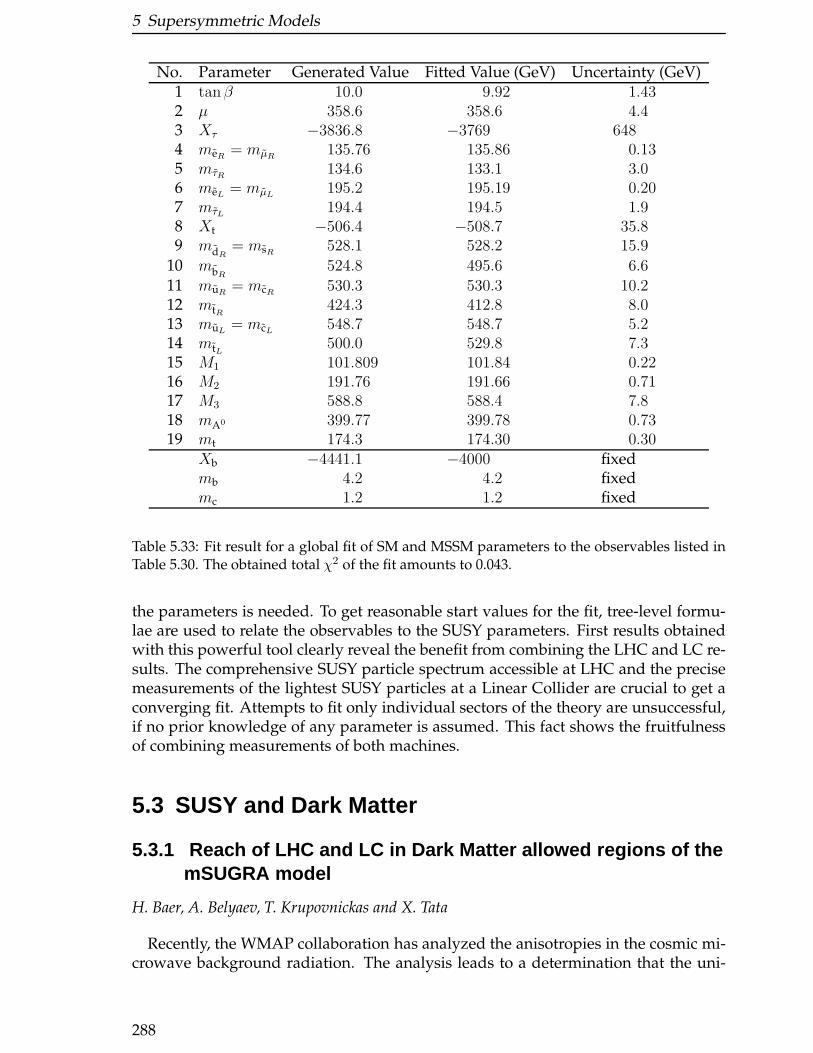
5 Supersymmetric Models
No. Parameter Generated Value Fitted Value (GeV) Uncertainty (GeV)1 tanβ 10.0 9.92 1.432 µ 358.6 358.6 4.43 Xτ −3836.8 −3769 6484 meR
= mµR135.76 135.86 0.13
5 mτR 134.6 133.1 3.06 meL
= mµL195.2 195.19 0.20
7 mτL 194.4 194.5 1.98 Xt −506.4 −508.7 35.89 mdR
= msR528.1 528.2 15.9
10 mbR524.8 495.6 6.6
11 muR= mcR
530.3 530.3 10.212 mtR
424.3 412.8 8.013 muL
= mcL548.7 548.7 5.2
14 mtL500.0 529.8 7.3
15 M1 101.809 101.84 0.2216 M2 191.76 191.66 0.7117 M3 588.8 588.4 7.818 mA0 399.77 399.78 0.7319 mt 174.3 174.30 0.30
Xb −4441.1 −4000 fixedmb 4.2 4.2 fixedmc 1.2 1.2 fixed
Table 5.33: Fit result for a global fit of SM and MSSM parameters to the observables listed inTable 5.30. The obtained total χ2 of the fit amounts to 0.043.
the parameters is needed. To get reasonable start values for the fit, tree-level formu-lae are used to relate the observables to the SUSY parameters. First results obtainedwith this powerful tool clearly reveal the benefit from combining the LHC and LC re-sults. The comprehensive SUSY particle spectrum accessible at LHC and the precisemeasurements of the lightest SUSY particles at a Linear Collider are crucial to get aconverging fit. Attempts to fit only individual sectors of the theory are unsuccessful,if no prior knowledge of any parameter is assumed. This fact shows the fruitfulnessof combining measurements of both machines.
5.3 SUSY and Dark Matter
5.3.1 Reach of LHC and LC in Dark Matter allowed regions of themSUGRA model
H. Baer, A. Belyaev, T. Krupovnickas and X. Tata
Recently, the WMAP collaboration has analyzed the anisotropies in the cosmic mi-crowave background radiation. The analysis leads to a determination that the uni-
288
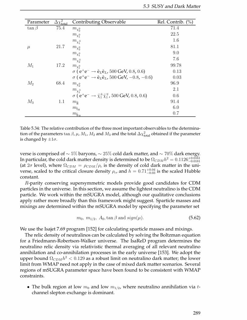
5.3 SUSY and Dark Matter
Parameter ∆χ2total Contributing Observable Rel. Contrib. (%)
tan β 75.4 mχ02
71.4
mχ01
22.5
mχ±
11.6
µ 21.7 mχ02
81.1
mχ01
9.0
mχ±
27.6
M1 17.2 mχ01
99.78
σ ( e+e− → eLeL, 500 GeV, 0.8, 0.6) 0.13σ ( e+e− → eLeL, 500 GeV, −0.8, −0.6) 0.03
M2 68.4 mχ02
96.9
mχ±
12.1
σ ( e+e− → χ±1 χ
∓1 , 500 GeV, 0.8, 0.6) 0.6
M3 1.1 mg 91.4mtR
6.0mbR
0.7
Table 5.34: The relative contribution of the three most important observables to the determina-tion of the parameters tan β, µ, M1, M2 and M3 and the total ∆χ2
total obtained if the parameteris changed by ±1σ.
verse is comprised of∼ 5% baryons, ∼ 25% cold dark matter, and∼ 70% dark energy.In particular, the cold dark matter density is determined to be ΩCDMh
2 = 0.1126+0.0161−0.0181
(at 2σ level), where ΩCDM = ρCDM/ρc is the density of cold dark matter in the uni-verse, scaled to the critical closure density ρc, and h = 0.71+0.04
−0.03 is the scaled Hubbleconstant.R-parity conserving supersymmetric models provide good candidates for CDM
particles in the universe. In this section, we assume the lightest neutralino is the CDMparticle. We work within the mSUGRA model, although our qualitative conclusionsapply rather more broadly than this framework might suggest. Sparticle masses andmixings are determined within the mSUGRA model by specifying the parameter set
m0, m1/2, A0, tan β and sign(µ). (5.62)
We use the Isajet 7.69 program [152] for calculating sparticle masses and mixings.The relic density of neutralinos can be calculated by solving the Boltzman equation
for a Friedmann-Robertson-Walker universe. The IsaReD program determines theneutralino relic density via relativistic thermal averaging of all relevant neutralinoannihilation and co-annihilation processes in the early universe [153]. We adopt theupper bound ΩCDMh
2 < 0.129 as a robust limit on neutralino dark matter; the lowerlimit from WMAP need not apply in the case of mixed dark matter scenarios. Severalregions of mSUGRA parameter space have been found to be consistent with WMAPconstraints.
• The bulk region at low m0 and low m1/2, where neutralino annihilation via t-channel slepton exchange is dominant.
289
5 Supersymmetric Models
• The stau co-annihilation region at low m0 where mτ1 ≃ mχ01.
• The hyperbolic branch/focus point region (HB/FP) at large m0, where |µ| be-comes small and the χ0
1 becomes partially higgsino-like.
• The A-annihilation funnel at large tanβ, where 2mχ01≃ mA, mH , and neutralino
annihilation takes place through the broad s-channel heavy higgs A and H res-onances.
In addition, there is a narrow region at low m1/2 where neutralino annihilation canoccur through the light Higgs h resonance, and an additional stop-neutralino co-annihilation region exists for particular A0 values.
The reach of the CERN LHC for SUSY in the mSUGRA model has been calculatedin Ref. [154] assuming 100 fb−1 of integrated luminosity. Briefly, sparticle pair pro-duction events were generated for many mSUGRA model parameter choices in them0 vs. m1/2 plane for various tan β values. A fast LHC detector simulation (CMSJET)was used, and cuts were imposed to extract signal rates in a variety of multileptonplus multijet plus missing transverse energy channels. Backgrounds were also calcu-lated from a variety of QCD and vector boson production processes. A large set ofselection cuts were used to give some optimization over broad regions of parameterspace. It was required to have at least a 5σ signal over background, with at least 10signal events in the sample.
The reach of the CERN LHC is shown in Fig. 5.43 for the case of tanβ = 10,µ > 0, A0 = 0 and mt = 175 GeV. The dark shaded (red) regions are disallowedby lack of radiative electroweak symmetry breaking (REWSB) (right hand side) orpresence of a stau LSP (left hand side). The light gray (yellow) region is excludedby LEP2 chargino searches (mχ+ > 103.5 GeV), while the region below the yellowcontour gives mh < 114.4 GeV, in contradiction of LEP2 SM Higgs searches (here,the SUSY h Higgs boson is essentially SM-like). The medium gray (green) regionshave ΩCDMh
2 < 0.129, and are allowed by WMAP. The broad HB/FP region is seen onthe right-hand side, while the stau co-annihilation region is shown on the left-handside. At the edge of the LEP2 excluded region is the light Higgs annihilation corri-dor. The reach of the Fermilab Tevatron via the trilepton channel is also shown [155],assuming a 5σ signal over background for 10 fb−1. The reach of the CERN LHC for100 fb−1 of integrated luminosity is shown by the contour labeled “LHC”. It extendsfrom m1/2 ∼ 1400 GeV (corresponding to a value of mg ∼ 3 TeV) on the left-handside, to m1/2 ∼ 700 GeV (corresponding to mg ∼ 1.8 TeV) on the right-hand side. Inparticular, for this value of tanβ, the LHC reach covers the entire stau co-annihilationregion, plus the low m1/2 portion of the HB/FP region. The outer limit of the reachcontour is mainly determined by events in the Emiss
T + jets channel, which arises fromgluino and squark pair production, followed by hadronic cascade decays.
We also show in the plot the reach of a√s = 500 and 1000 GeV LC, assuming 100
fb−1 of integrated luminosity [156]. Events were generated using Isajet 7.69, and com-pared against various SM backgrounds. The left-most portion of the reach contourarises where selectron and smuon pair production are visible, while the main portion(flat with m1/2) arises due to chargino pair searches. An additional reach is gainedbetween these two regions by searching for e+e− → χ0
2χ01 production, followed by
290
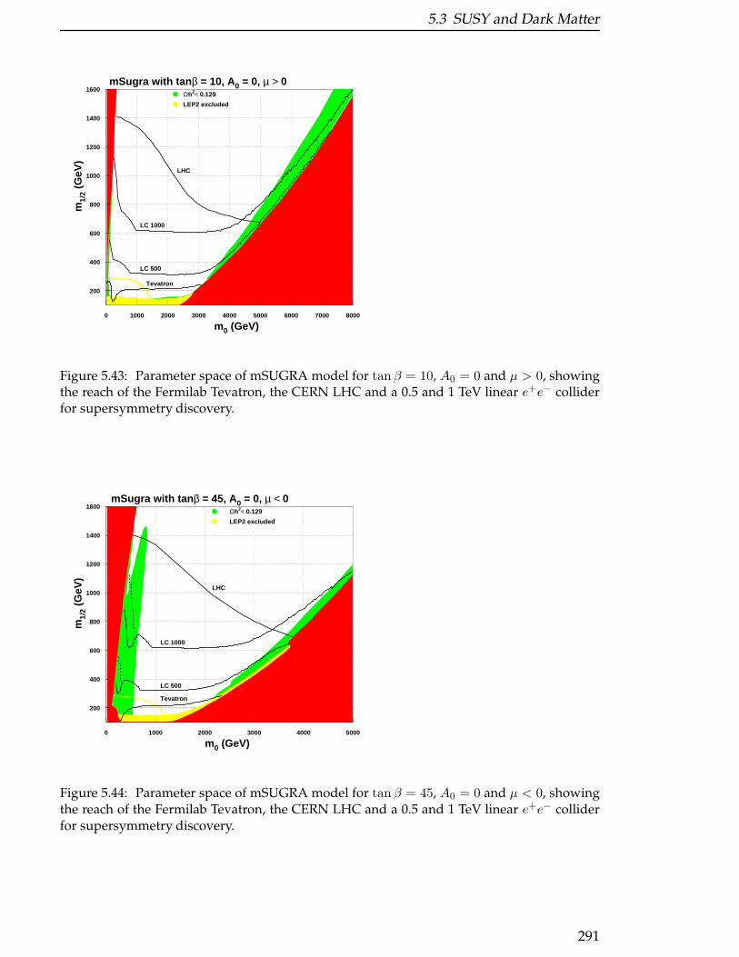
5.3 SUSY and Dark Matter
200
400
600
800
1000
1200
1400
1600
0 1000 2000 3000 4000 5000 6000 7000 8000
mSugra with tanβ = 10, A0 = 0, µ > 0
m0 (GeV)
m1/
2 (G
eV)
LHC
Tevatron
LC 500
LC 1000
Ωh2< 0.129
LEP2 excluded
Figure 5.43: Parameter space of mSUGRA model for tan β = 10, A0 = 0 and µ > 0, showingthe reach of the Fermilab Tevatron, the CERN LHC and a 0.5 and 1 TeV linear e+e− colliderfor supersymmetry discovery.
200
400
600
800
1000
1200
1400
1600
0 1000 2000 3000 4000 5000
mSugra with tanβ = 45, A0 = 0, µ < 0
m0 (GeV)
m1/
2 (G
eV)
LHC
Tevatron
LC 500
LC 1000
Ωh2< 0.129
LEP2 excluded
Figure 5.44: Parameter space of mSUGRA model for tan β = 45, A0 = 0 and µ < 0, showingthe reach of the Fermilab Tevatron, the CERN LHC and a 0.5 and 1 TeV linear e+e− colliderfor supersymmetry discovery.
291
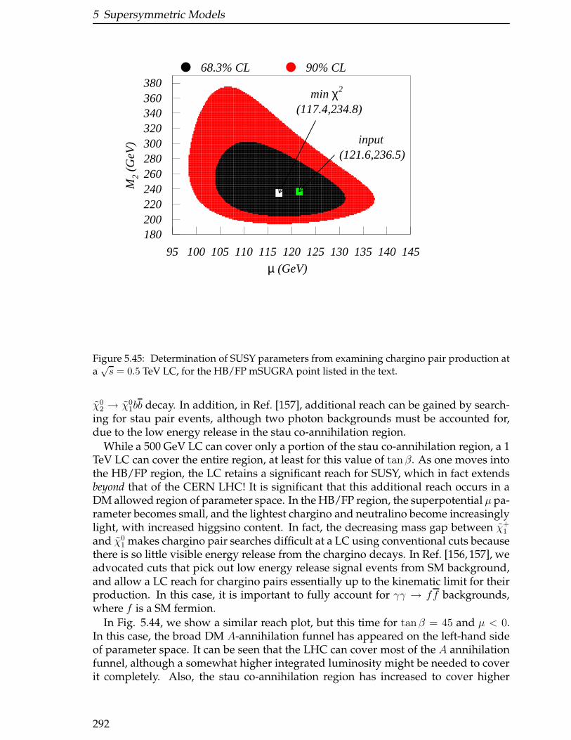
5 Supersymmetric Models
180200220240260280300320340360380
95 100 105 110 115 120 125 130 135 140 145
input(121.6,236.5)
min χ2
(117.4,234.8)
µ (GeV)
M2
(GeV
)
68.3% CL 90% CL
Figure 5.45: Determination of SUSY parameters from examining chargino pair production ata√s = 0.5 TeV LC, for the HB/FP mSUGRA point listed in the text.
χ02 → χ0
1bb decay. In addition, in Ref. [157], additional reach can be gained by search-ing for stau pair events, although two photon backgrounds must be accounted for,due to the low energy release in the stau co-annihilation region.
While a 500 GeV LC can cover only a portion of the stau co-annihilation region, a 1TeV LC can cover the entire region, at least for this value of tanβ. As one moves intothe HB/FP region, the LC retains a significant reach for SUSY, which in fact extendsbeyond that of the CERN LHC! It is significant that this additional reach occurs in aDM allowed region of parameter space. In the HB/FP region, the superpotential µ pa-rameter becomes small, and the lightest chargino and neutralino become increasinglylight, with increased higgsino content. In fact, the decreasing mass gap between χ+
1
and χ01 makes chargino pair searches difficult at a LC using conventional cuts because
there is so little visible energy release from the chargino decays. In Ref. [156, 157], weadvocated cuts that pick out low energy release signal events from SM background,and allow a LC reach for chargino pairs essentially up to the kinematic limit for theirproduction. In this case, it is important to fully account for γγ → ff backgrounds,where f is a SM fermion.
In Fig. 5.44, we show a similar reach plot, but this time for tanβ = 45 and µ < 0.In this case, the broad DM A-annihilation funnel has appeared on the left-hand sideof parameter space. It can be seen that the LHC can cover most of the A annihilationfunnel, although a somewhat higher integrated luminosity might be needed to coverit completely. Also, the stau co-annihilation region has increased to cover higher
292
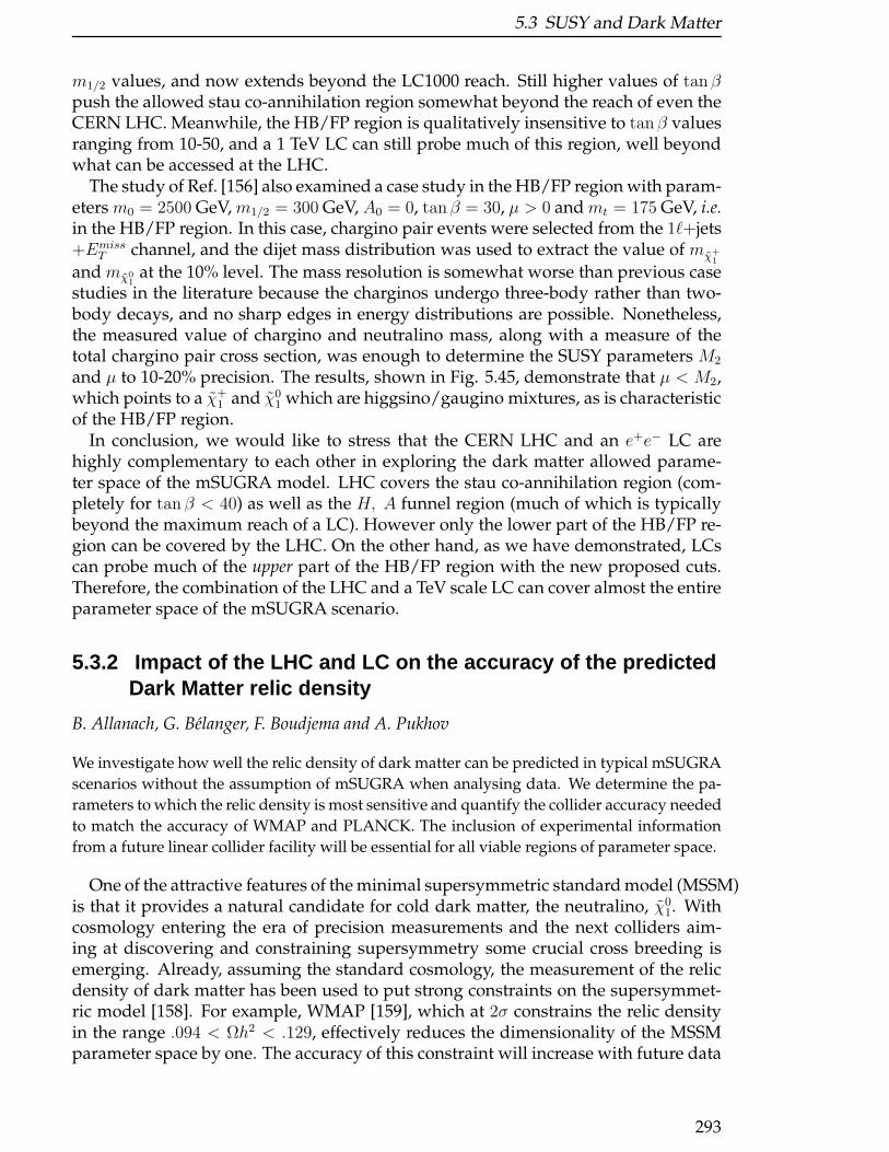
5.3 SUSY and Dark Matter
m1/2 values, and now extends beyond the LC1000 reach. Still higher values of tanβpush the allowed stau co-annihilation region somewhat beyond the reach of even theCERN LHC. Meanwhile, the HB/FP region is qualitatively insensitive to tanβ valuesranging from 10-50, and a 1 TeV LC can still probe much of this region, well beyondwhat can be accessed at the LHC.
The study of Ref. [156] also examined a case study in the HB/FP region with param-eters m0 = 2500 GeV, m1/2 = 300 GeV, A0 = 0, tanβ = 30, µ > 0 and mt = 175 GeV, i.e.in the HB/FP region. In this case, chargino pair events were selected from the 1ℓ+jets+Emiss
T channel, and the dijet mass distribution was used to extract the value of mχ+1
and mχ01
at the 10% level. The mass resolution is somewhat worse than previous casestudies in the literature because the charginos undergo three-body rather than two-body decays, and no sharp edges in energy distributions are possible. Nonetheless,the measured value of chargino and neutralino mass, along with a measure of thetotal chargino pair cross section, was enough to determine the SUSY parameters M2
and µ to 10-20% precision. The results, shown in Fig. 5.45, demonstrate that µ < M2,which points to a χ+
1 and χ01 which are higgsino/gaugino mixtures, as is characteristic
of the HB/FP region.In conclusion, we would like to stress that the CERN LHC and an e+e− LC are
highly complementary to each other in exploring the dark matter allowed parame-ter space of the mSUGRA model. LHC covers the stau co-annihilation region (com-pletely for tanβ < 40) as well as the H, A funnel region (much of which is typicallybeyond the maximum reach of a LC). However only the lower part of the HB/FP re-gion can be covered by the LHC. On the other hand, as we have demonstrated, LCscan probe much of the upper part of the HB/FP region with the new proposed cuts.Therefore, the combination of the LHC and a TeV scale LC can cover almost the entireparameter space of the mSUGRA scenario.
5.3.2 Impact of the LHC and LC on the accuracy of the predictedDark Matter relic density
B. Allanach, G. Belanger, F. Boudjema and A. Pukhov
We investigate how well the relic density of dark matter can be predicted in typical mSUGRA
scenarios without the assumption of mSUGRA when analysing data. We determine the pa-
rameters to which the relic density is most sensitive and quantify the collider accuracy needed
to match the accuracy of WMAP and PLANCK. The inclusion of experimental information
from a future linear collider facility will be essential for all viable regions of parameter space.
One of the attractive features of the minimal supersymmetric standard model (MSSM)is that it provides a natural candidate for cold dark matter, the neutralino, χ0
1. Withcosmology entering the era of precision measurements and the next colliders aim-ing at discovering and constraining supersymmetry some crucial cross breeding isemerging. Already, assuming the standard cosmology, the measurement of the relicdensity of dark matter has been used to put strong constraints on the supersymmet-ric model [158]. For example, WMAP [159], which at 2σ constrains the relic densityin the range .094 < Ωh2 < .129, effectively reduces the dimensionality of the MSSMparameter space by one. The accuracy of this constraint will increase with future data
293
5 Supersymmetric Models
from the PLANCK satellite, which expects precision on Ωh2 at the 2% level [160].In this paper, we look at the problem from the inverse perspective and examine
what is required from collider data in order to get a precise prediction for Ωh2, whichcould then be used to test the cosmology. For this we assume that supersymmetricparticles will be produced and measured at the LHC and the future linear collider(LC) and that enough information [161] will be present in order to discriminate be-tween various models of supersymmetry breaking. When we have identified a suc-cessful model of SUSY breaking, an accurate prediction of Ωh2 will allow us to testthe cosmological assumptions that go into its prediction.
In order to predict Ωh2 in the MSSM one generally needs to know all the underlyingparameters of the model, since that determines the available annihilation channels forneutralinos in the early universe. In the context of mSUGRA however, the scenariosallowed by WMAP are rather fine-tuned and one can concentrate only on a handfulof relevant observables. The point is that in mSUGRA the neutralino LSP happensto be, for practically all cases, an almost pure bino. This bino annihilates mainly intoleptons through the right-handed sleptons but this mechanism is not efficient enoughto satisfy the newest WMAP data. Then only three acceptable scenarios remain: coan-nihilation, rapid annihilation through Higgs exchange or a Higgsino LSP. Our studywill cover these three rather constrained regions in the mSUGRA parameter space.
We will investigate the accuracy required on a few of the most relevant collider ob-servables in order to control the uncertainty on the predicted Ωh2. These observablescould be either physical masses or Lagrangian parameters such as the chargino mix-ing parameter µ or tan β. We will refer throughout to two benchmarks on accuracy:those that produce a 10% change in Ωh2 (“WMAP accuracy”) and those which changeΩh2 by 2% (“PLANCK accuracy”). We only quote precisions on input parameters ob-tained by varying only one parameter at a time.
Although we mention some results obtained with the mSUGRA scenario, we con-centrate mainly on what we call the perturbed mSUGRA scenario (PmSUGRA). Inthis scenario we pick a parameter point in mSUGRA derived from the high-scaleparameters m0,M1/2, A0 then we examine the impact on Ωh2 of a parameter changewhile assuming the more general MSSM only. In practice we use an iterative procedureto determine the fractional change a = |∆p/p| in an input parameter p that will resultin a fractional change r = ∆Ω/Ω = 10% for WMAP accuracy. An estimate of thePLANCK accuracy can be obtained by dividing that of WMAP by a factor of 5, forthe interesting range of accuracies not exceeding 50%, say. Here we do not addressthe feasibility of any measurements, but rather only identify which measurementsare needed and with what precision. Preliminary investigations into the effects ofuncertainties in the predictions of the sparticle mass spectrum on Ωh2 were presentedin Refs. [162] and more details can be found in Ref. [163]. The relic density is com-puted with micrOMEGAs1.3 [164] with the supersymmetric spectrum provided bySOFTSUSY1.8.7 [144] and the interface between the two by the SUSY Les HouchesAccord [137].
5.3.2.1 Coannihilation
In mSUGRA at small M0 there exists a region with almost degenerate τ1 − χ01. In this
region the LSP is almost purely bino. The contribution of coannihilation channels is
294
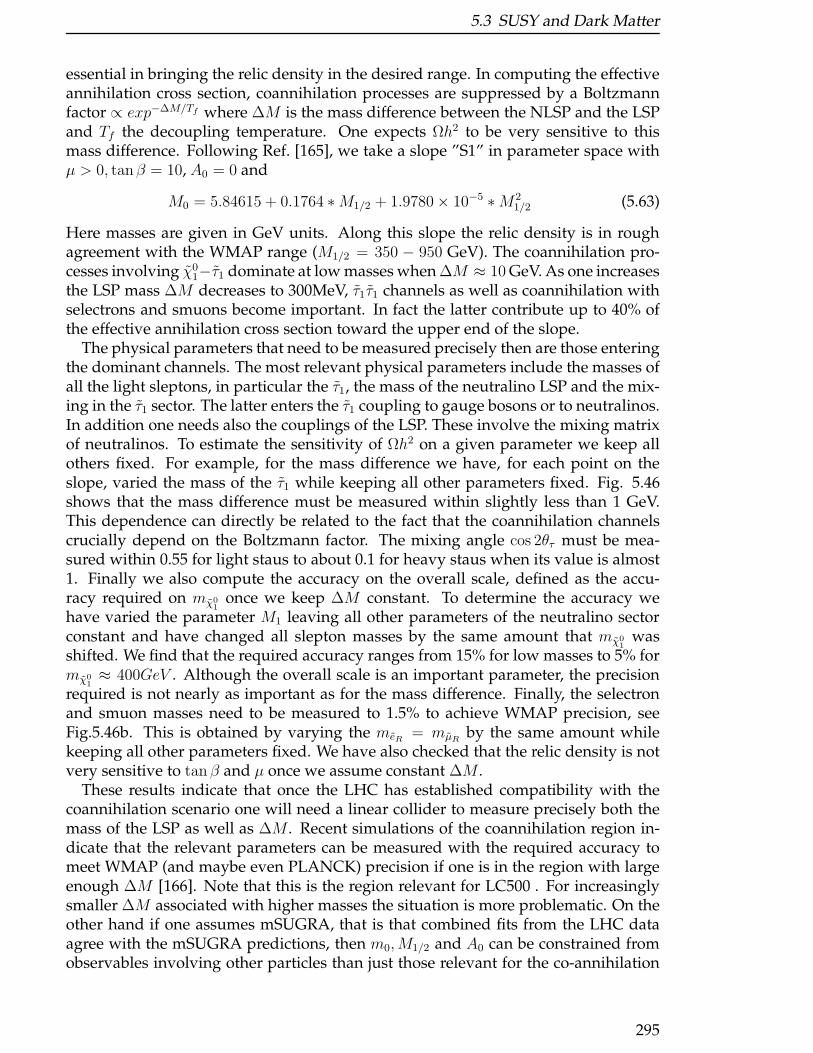
5.3 SUSY and Dark Matter
essential in bringing the relic density in the desired range. In computing the effectiveannihilation cross section, coannihilation processes are suppressed by a Boltzmannfactor ∝ exp−∆M/Tf where ∆M is the mass difference between the NLSP and the LSPand Tf the decoupling temperature. One expects Ωh2 to be very sensitive to thismass difference. Following Ref. [165], we take a slope ”S1” in parameter space withµ > 0, tanβ = 10, A0 = 0 and
M0 = 5.84615 + 0.1764 ∗M1/2 + 1.9780× 10⁻⁵ ∗M21/2 (5.63)
Here masses are given in GeV units. Along this slope the relic density is in roughagreement with the WMAP range (M1/2 = 350 − 950 GeV). The coannihilation pro-cesses involving χ0
1−τ1 dominate at low masses when ∆M ≈ 10 GeV. As one increasesthe LSP mass ∆M decreases to 300MeV, τ1τ1 channels as well as coannihilation withselectrons and smuons become important. In fact the latter contribute up to 40% ofthe effective annihilation cross section toward the upper end of the slope.
The physical parameters that need to be measured precisely then are those enteringthe dominant channels. The most relevant physical parameters include the masses ofall the light sleptons, in particular the τ1, the mass of the neutralino LSP and the mix-ing in the τ1 sector. The latter enters the τ1 coupling to gauge bosons or to neutralinos.In addition one needs also the couplings of the LSP. These involve the mixing matrixof neutralinos. To estimate the sensitivity of Ωh2 on a given parameter we keep allothers fixed. For example, for the mass difference we have, for each point on theslope, varied the mass of the τ1 while keeping all other parameters fixed. Fig. 5.46shows that the mass difference must be measured within slightly less than 1 GeV.This dependence can directly be related to the fact that the coannihilation channelscrucially depend on the Boltzmann factor. The mixing angle cos 2θτ must be mea-sured within 0.55 for light staus to about 0.1 for heavy staus when its value is almost1. Finally we also compute the accuracy on the overall scale, defined as the accu-racy required on mχ0
1once we keep ∆M constant. To determine the accuracy we
have varied the parameter M1 leaving all other parameters of the neutralino sectorconstant and have changed all slepton masses by the same amount that mχ0
1was
shifted. We find that the required accuracy ranges from 15% for low masses to 5% formχ0
1≈ 400GeV . Although the overall scale is an important parameter, the precision
required is not nearly as important as for the mass difference. Finally, the selectronand smuon masses need to be measured to 1.5% to achieve WMAP precision, seeFig.5.46b. This is obtained by varying the meR
= mµRby the same amount while
keeping all other parameters fixed. We have also checked that the relic density is notvery sensitive to tan β and µ once we assume constant ∆M .
These results indicate that once the LHC has established compatibility with thecoannihilation scenario one will need a linear collider to measure precisely both themass of the LSP as well as ∆M . Recent simulations of the coannihilation region in-dicate that the relevant parameters can be measured with the required accuracy tomeet WMAP (and maybe even PLANCK) precision if one is in the region with largeenough ∆M [166]. Note that this is the region relevant for LC500 . For increasinglysmaller ∆M associated with higher masses the situation is more problematic. On theother hand if one assumes mSUGRA, that is that combined fits from the LHC dataagree with the mSUGRA predictions, then m0,M1/2 and A0 can be constrained fromobservables involving other particles than just those relevant for the co-annihilation
295
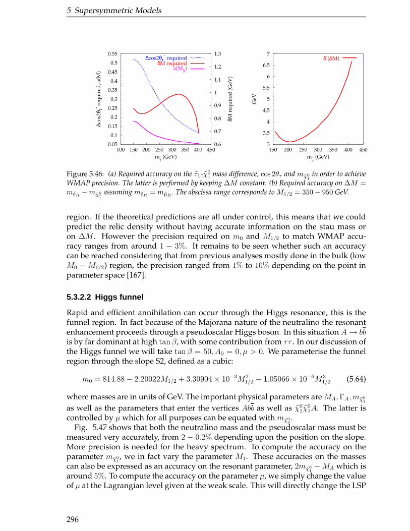
5 Supersymmetric Models
0.05
0.1
0.15
0.2
0.25
0.3
0.35
0.4
0.45
0.5
0.55
100 150 200 250 300 350 400 4500.6
0.7
0.8
0.9
1
1.1
1.2
1.3
∆co
s2θ τ
- req
uir
ed, a
(M)
δM r
equ
ired
(G
eV)
m~τ (GeV)
∆cos2θτ- required
δM requireda(Mχ)
3
3.5
4
4.5
5
5.5
6
6.5
7
150 200 250 300 350 400 450
GeV
me~ (GeV)
δ-(∆M)
Figure 5.46: (a) Required accuracy on the τ1-χ01 mass difference, cos 2θτ and mχ0
1in order to achieve
WMAP precision. The latter is performed by keeping ∆M constant. (b) Required accuracy on ∆M =meR
−mχ01
assuming meR= mµR
. The abscissa range corresponds to M1/2 = 350− 950 GeV.
region. If the theoretical predictions are all under control, this means that we couldpredict the relic density without having accurate information on the stau mass oron ∆M . However the precision required on m0 and M1/2 to match WMAP accu-racy ranges from around 1 − 3%. It remains to be seen whether such an accuracycan be reached considering that from previous analyses mostly done in the bulk (lowM0 −M1/2) region, the precision ranged from 1% to 10% depending on the point inparameter space [167].
5.3.2.2 Higgs funnel
Rapid and efficient annihilation can occur through the Higgs resonance, this is thefunnel region. In fact because of the Majorana nature of the neutralino the resonantenhancement proceeds through a pseudoscalar Higgs boson. In this situation A→ bbis by far dominant at high tan β, with some contribution from ττ . In our discussion ofthe Higgs funnel we will take tan β = 50, A0 = 0, µ > 0. We parameterise the funnelregion through the slope S2, defined as a cubic:
m0 = 814.88− 2.20022M1/2 + 3.30904× 10⁻³M21/2 − 1.05066× 10⁻⁶M3
1/2 (5.64)
where masses are in units of GeV. The important physical parameters are MA,ΓA, mχ01
as well as the parameters that enter the vertices Abb as well as χ01χ
01A. The latter is
controlled by µ which for all purposes can be equated with mχ03.
Fig. 5.47 shows that both the neutralino mass and the pseudoscalar mass must bemeasured very accurately, from 2 − 0.2% depending upon the position on the slope.More precision is needed for the heavy spectrum. To compute the accuracy on theparameter mχ0
1, we in fact vary the parameter M1. These accuracies on the masses
can also be expressed as an accuracy on the resonant parameter, 2mχ01−MA which is
around 5%. To compute the accuracy on the parameter µ, we simply change the valueof µ at the Lagrangian level given at the weak scale. This will directly change the LSP
296
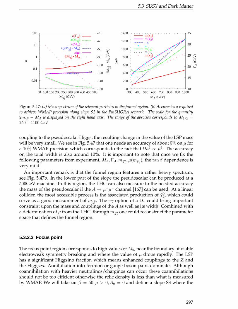
5.3 SUSY and Dark Matter
0.01
0.1
1
10
100
50 100 150 200 250 300 350 400 450 500-160
-140
-120
-100
-80
-60
-40
-20
a
2Mχ 10
- M
A (
GeV
)
Mχ10 (GeV)
a(ΓA)a(Mχ1
0)
a(MA)a(2Mχ1
0 - MA)
a(µ)2Mχ1
0 - MA
0
200
400
600
800
1000
1200
1400
300 400 500 600 700 800 900 100010
15
20
25
30
35
GeV
Γ A (
GeV
)
MA (GeV)
m(χ1)m(χ3)ΓAµm(lR)m(lL)m(χ2)
Figure 5.47: (a) Mass spectrum of the relevant particles in the funnel region. (b) Accuracies a requiredto achieve WMAP precision along slope S2 in the PmSUGRA scenario. The scale for the quantity2mχ0
1−MA is displayed on the right hand axis. The range of the abscissa corresponds to M1/2 =
250 − 1100 GeV.
coupling to the pseudoscalar Higgs, the resulting change in the value of the LSP masswill be very small. We see in Fig. 5.47 that one needs an accuracy of about 5% on µ fora 10% WMAP precision which corresponds to the fact that Ωh2 ∝ µ2. The accuracyon the total width is also around 10%. It is important to note that once we fix thefollowing parameters from experiment, MA,ΓA, mχ0
1, µ(mχ0
3), the tanβ dependence is
very mild.
An important remark is that the funnel region features a rather heavy spectrum,see Fig. 5.47b. In the lower part of the slope the pseudoscalar can be produced at a500GeV machine. In this region, the LHC can also measure to the needed accuracythe mass of the pseudoscalar if the A → µ+µ− channel [167] can be used. At a linearcollider, the most accessible process is the associated production of χ0
2, which couldserve as a good measurement of mχ0
1. The γγ option of a LC could bring important
constraint upon the mass and couplings of the A as well as its width. Combined witha determination of µ from the LHC, through mχ0
3one could reconstruct the parameter
space that defines the funnel region.
5.3.2.3 Focus point
The focus point region corresponds to high values of M0, near the boundary of viableelectroweak symmetry breaking and where the value of µ drops rapidly. The LSPhas a significant Higgsino fraction which means enhanced couplings to the Z andthe Higgses. Annihiliation into fermion or gauge boson pairs dominate. Althoughcoannihilation with heavier neutralinos/charginos can occur these coannihilationsshould not be too efficient otherwise the relic density is less than what is measuredby WMAP. We will take tanβ = 50, µ > 0, A0 = 0 and define a slope S3 where the
297
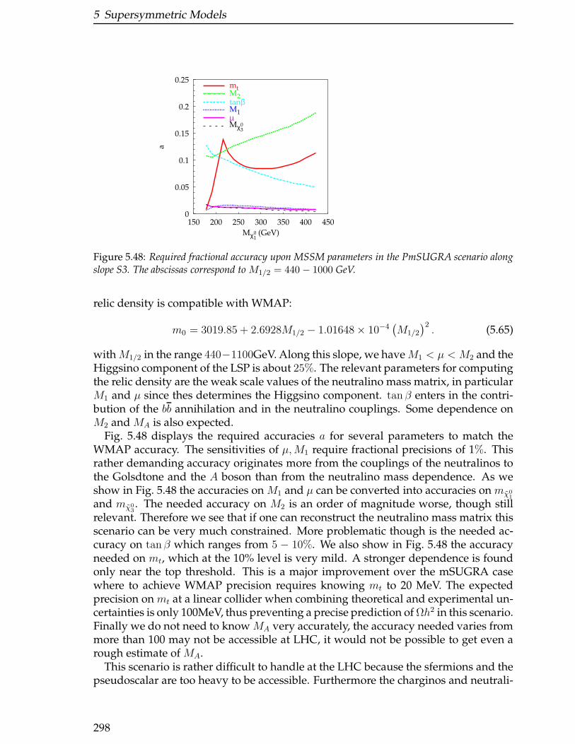
5 Supersymmetric Models
0
0.05
0.1
0.15
0.2
0.25
150 200 250 300 350 400 450
a
Mχ10 (GeV)
mtM2tanβM1µMχ3
0
Figure 5.48: Required fractional accuracy upon MSSM parameters in the PmSUGRA scenario alongslope S3. The abscissas correspond to M1/2 = 440 − 1000 GeV.
relic density is compatible with WMAP:
m0 = 3019.85 + 2.6928M1/2 − 1.01648× 10⁻⁴(M1/2
)2. (5.65)
withM1/2 in the range 440−1100GeV. Along this slope, we haveM1 < µ < M2 and theHiggsino component of the LSP is about 25%. The relevant parameters for computingthe relic density are the weak scale values of the neutralino mass matrix, in particularM1 and µ since thes determines the Higgsino component. tan β enters in the contri-bution of the bb annihilation and in the neutralino couplings. Some dependence onM2 and MA is also expected.
Fig. 5.48 displays the required accuracies a for several parameters to match theWMAP accuracy. The sensitivities of µ,M1 require fractional precisions of 1%. Thisrather demanding accuracy originates more from the couplings of the neutralinos tothe Golsdtone and the A boson than from the neutralino mass dependence. As weshow in Fig. 5.48 the accuracies on M1 and µ can be converted into accuracies on mχ0
1
and mχ03. The needed accuracy on M2 is an order of magnitude worse, though still
relevant. Therefore we see that if one can reconstruct the neutralino mass matrix thisscenario can be very much constrained. More problematic though is the needed ac-curacy on tan β which ranges from 5 − 10%. We also show in Fig. 5.48 the accuracyneeded on mt, which at the 10% level is very mild. A stronger dependence is foundonly near the top threshold. This is a major improvement over the mSUGRA casewhere to achieve WMAP precision requires knowing mt to 20 MeV. The expectedprecision on mt at a linear collider when combining theoretical and experimental un-certainties is only 100MeV, thus preventing a precise prediction of Ωh2 in this scenario.Finally we do not need to know MA very accurately, the accuracy needed varies frommore than 100 may not be accessible at LHC, it would not be possible to get even arough estimate of MA.
This scenario is rather difficult to handle at the LHC because the sfermions and thepseudoscalar are too heavy to be accessible. Furthermore the charginos and neutrali-
298
5.4 Further SUSY scenarios
nos cannot be measured easily. On the other hand, a LC has the possibility to measureprecisely the neutralino mass matrix provided there is enough energy to produce theneutralinos [168]. However a realistic study of the achievable accuracy in this sce-nario at a linear collider still needs to be performed as well as a study on how tobenefit from a combination of LHC and LC data. In particular the value of tanβmight be very difficult to pin down, although some information could be extractedfrom the light Higgs mass.
5.3.2.4 Conclusion
The relic density calculation often involves a large number of processes. The preciseknowledge of the cross-sections necessary to make an accurate prediction of the relicdensity of dark matter rests on a precise knowledge of the physical parameters of theMSSM. Nevertheless we have shown that within the scenarios that are favoured byWMAP, only a few parameters are needed to be measured with very high precision.Furthermore, using the collider data rather than relying on some theoretical preju-dice, considerably improves the precision of the prediction of Ωh2. Nevertheless theprecision required from colliders to match the WMAP accuracy is rather demanding.The LHC will be able to determine roughly which scenario one is in as well as pro-vide measurements of heavier particles (pseudoscalar, heavy neutralinos) that can beessential for an accurate prediction of the relic density, for example in the Higgs fun-nel or the focus point regions. However to make a prediction of Ωh2 that matches theWMAP accuracy, or even more so the PLANCK accuracy, one absolutely needs thehigh precision achievable at a linear collider.
5.4 Further SUSY scenarios
5.4.1 Non-decoupling effect in sfermion-chargino/neutra linocouplings
J. Guasch, W. Hollik and J. Sola
We analyze the radiative effects induced by a heavy squark sector in the lepton-slepton-
chargino/neutralino coupling. These effects are known to grow as the logarithm of the heavy
squark mass. We concentrate on a scenario where sleptons and (some) charginos/neutralinos
are light enough to be produced at an e+e− Linear Collider, whereas squarks are heavy and
can only be produced at the LHC. We conclude that the radiative effects of squarks are larger
than the expected accuracy of the coupling measurements at a LC. A knowledge of the squark
mass scale is necessary to provide a precise prediction for slepton-chargino/neutralino ob-
servables, but a moderate accuracy in the squark parameters is sufficient. These effects can be
treated introducing chargino/neutralino effective coupling matrices.
5.4.1.1 Introduction
The main aim of a high energy e+e− Linear Collider (LC) is to perform very high pre-cision measurements of the elementary particles properties at a level better than 1%,in order to discriminate different models of particle interactions. In order to be able
299
5 Supersymmetric Models
to compare these measurements with the underlying theory at this high level of ac-curacy, it is not sufficient to relate the different observables using lowest order in per-turbation theory: the computation of radiative corrections (strong and electroweak)form a necessary ingredient of this program.
In this note we concentrate on the properties of supersymmetric (SUSY) parti-cles [66–69]. It is known that the radiative corrections to some SUSY observablesdevelop radiative corrections which do not decouple if one takes some of the SUSYmasses to be large [70–77]. Furthermore, the observables which exhibit this non-decoupling behaviour are the ones that probe the SUSY nature of the particles understudy. Therefore the following situation could happen: some new physics is observedat the LHC and LC, which is roughly consistent with the predictions from SUSY mod-els, however at the LC only some of the new particles are visible, but, in order to pre-dict their production cross-sections and branching ratios at a sufficient level of accu-racy the properties of the heavy SUSY particles (visible at the LHC) are needed. Thissituation is, in fact, natural in SUSY models, where the strongly interacting SUSY par-ticles usually are predicted to be much heavier than the weakly interacting ones (seee.g. [1]). In this note we want to address this issue, asking ourselves: how large couldbe the effects of the heavy particles; how much accuracy on their masses is needed inorder to make sufficiently precise predictions for the light ones; and whether there issome way of avoiding the uncertainty introduced by the heavy particles.
For the sake of simplicity we will work in the following scenario: scalar-quarks(squarks) and the gluino are heavy, and beyond the reach of the LC, whereas scalar-leptons (sleptons) and some charginos/neutralinos are light, and can be studied at theLC. Then, we study the radiative effects of squarks in chargino/neutralino-lepton-slepton interactions, computing the value of the radiative corrections induced byquarks/squarks, and comparing them with the corrections from other sectors of themodel. We will analyze these effects in the partial decay widths of selectrons and theelectron-sneutrino into charginos and neutralinos.
5.4.1.2 Theoretical introduction: non-decoupling effect s and effectivecoupling matrices
We concentrate in the analysis of the sfermion decays as discussed thoroughly inRefs. [70, 71, 78, 79]5. In the radiative corrections of the partial decay widths
Γ(f → f ′χ) , (5.66)
f being a sfermion, f ′ a Standard Model (SM) fermion, and χ a chargino or neutra-lino, non-decoupling effects appear, and the radiative corrections grow as the loga-rithm of the largest SUSY mass of the model [70, 71]. These non-decoupling effectsreflect the fact that SUSY is (softly) broken, and the Yukawa couplings of the chargi-nos/neutralinos are no longer equal to the gauge bosons and Higgs bosons couplingsbeyond leading order.
A part of these corrections can be encoded in a set of counterterm expressionswhich appear in all observables. Concretely they can be written as a shift to the U , V
5The corresponding FORTRAN codes are available from [80]
300

5.4 Further SUSY scenarios
and N matrices that diagonalize the chargino and neutralino mass matrices6:
U = U + ∆U , V = V + ∆V , N = N + ∆N , (5.67)
where ∆U , ∆V , and ∆N are a certain combination of counterterms, which can becomputed using self-energies of gauge bosons, Higgs bosons, charginos and neutra-linos.
Unfortunately the full contributions to the expressions (5.67) are divergent. Theonly consistent subset of corrections which makes all the expressions in (5.67) finiteis the subset of fermion and sfermion loops contributing to the self-energies of thegauge bosons, Higgs bosons, charginos and neutralinos. With this restriction, we candefine effective coupling matrices
Ueff = U + ∆U (f) , V eff = V + ∆V (f) , N eff = N + ∆N (f) , (5.68)
where ∆U (f), ∆V (f), ∆N (f) are given by the expressions (5.67) taking into accountonly loops of fermions and sfermions. We will refer to these corrections as universalcorrections. They are the equivalent of the super-oblique corrections of Ref. [76].
As an example, we have computed analytically the electron-selectron contributionsto the ∆U and ∆V matrices (5.67), assuming zero mixing angle in the selectron sec-tor (θe = 0), we have identified the leading terms in the approximation mei
, mν ≫(MW ,Mi) ≫ me, and analytically canceled the divergences and the renormalizationscale dependent terms; finally, we have kept only the terms logarithmic in the sleptonmasses. The result reads as follows:
∆U(e)i1 =
α
4 π s2W
log
(M2
eL
M2X
) [U3i1
6− Ui2
√2MW (M cβ + µ sβ)
3 (M2 − µ2) (M21 −M2
2 )2
(M4 −M2 µ2+
+3M2 M2W + µ2M2
W +M4W +M4
W c4β + (µ2 −M2)M2i + 4M µM2
W s2β
) ],
∆U(e)i2 =
α
4 π s2W
log
(M2
eL
M2X
)Ui1
MW (M cβ + µ sβ)
3√
2 (M2 − µ2) (M21 −M2
2 )2 ×
×((M2 − µ2)2 + 4M2M2
W + 4µ2M2W + 2M4
W + 2M4W c4β + 8M µM2
W s2β
),
∆V(e)i1 =
α
4 π s2W
log
(M2
eL
M2X
) [V 3i1
6− Vi2
√2MW (µ cβ +M sβ)
3 (M2 − µ2) (M21 −M2
2 )2
(M4 −M2 µ2+
+3M2 M2W + µ2M2
W +M4W +M4
W c4β + (µ2 −M2)M2i + 4M µM2
W s2β
) ],
∆V(e)i2 =
α
4 π s2W
log
(M2
eL
M2X
)Vi1
MW (µ cβ +M sβ)
3√
2 (M2 − µ2) (M21 −M2
2 )2 ×
×((M2 − µ2)2 + 4M2M2
W + 4µ2M2W + 2M4
W + 2M4W c4β + 8M µM2
W s2β
),
(5.69)
M2eL
being the soft-SUSY-breaking mass of the (eL, ν) doublet, whereas MX is a SMmass.
In this way the effects of the (heavy) squarks can be encoded in the definition ofeffective couplings in the lepton-slepton-chargino/neutralino interactions.
6In this note we follow the notation and conventions of Ref. [70]. Note, in particular, that mf1> mf2
.
301
5 Supersymmetric Models
Γtree [GeV] δΓ(q)/Γ δΓ(l)/Γ δΓno−uni/Γ δΓ/Γe1 → e−χ0
1 0.110 0.043 0.032 -0.002 0.073e1 → e−χ0
2 0.047 0.030 0.034 -0.012 0.051e1 → νeχ
−1 0.081 0.026 0.033 0.006 0.065
e2 → e−χ01 0.194 0.052 0.034 0.000 0.086
νe → νeχ01 0.140 0.059 0.035 -0.005 0.089
νe → νeχ02 0.006 0.018 0.033 -0.014 0.036
νe → e−χ+1 0.016 0.024 0.033 0.002 0.059
Table 5.35: Tree-level partial decay widths and relative corrections for the selectron and sneu-trino decays into charginos and neutralinos for SPS 1a.
In the following we will separate three kind of corrections: the universal correc-tions induced by the quark-squark particles Ueff(q), V eff(q), N eff(q); the universal con-tributions induced by leptons-sleptons Ueff(l), V eff(l), N eff(l), and the non-universalcontributions.
5.4.1.3 Numerical Analysis
For the numerical analysis we choose some default typical set of input parameters.We will concentrate in the parameter set given by point 1a of the Snowmass Points andSlopes (SPS) [1]7. For completeness we give here the soft-SUSY-breaking parameters:
tanβ = 10,MA0 = 393.6 GeV, µ = 352.4 GeV,M = 192.7 GeV,M ′ = 99.1 GeV ,Md,sL
= 539.9 GeV,MbL= 495.9 GeV,Md,sR
= 519.5 GeV,MbR= 516.9 GeV,
Ad,s = 3524 GeV, Ab = −772.7 GeV,Mu,cR
= 521.7 GeV,MtR = 424.8 GeV, Au,c = 35.24 GeV, At = −510 GeV,Me,µL
= 196.6 GeV,MτL = 195.8 GeV,Me,µR= 136.2 GeV,MτR = 133.6 GeV,
Ae,µ = 3524 GeV, Aτ = −254.2 GeV,(5.70)
where the soft-SUSY-breaking trilinear couplings of the first and second generationsfermions have been chosen such that the non-diagonal elements of the sfermionmass matrix are zero.
However, a note of caution should be given, our computation is performed in theOn-shell renormalization scheme, whereas the SPS parameters are given in the DRrenormalization scheme, and one should make a scheme conversion of the param-eters, this conversion is beyond the scope of the present work. In this note we areinterested only in establishing whether the effects of heavy particles are important,and therefore we are only interested in obtaining a suitable SUSY spectrum, thereforewe treat the given numerical parameters of SPS 1a as On-shell SUSY parameters 8.
In Table 5.35 we show the partial decay widths of selectrons into charginos/neutralinosfor SPS 1a. We show: the tree-level partial widths Γtree; the relative correctionsinduced by quarks-squarks δΓ(q)/Γ; the relative corrections induced by the lepton-
7The spectrum and tree-level branching ratios for the several SPSs can be found e.g. in Ref. [4].8Of course, once we will be analyzing the real LC data, the DR-On-shell conversion will need to be
made in order to extract the fundamental soft-SUSY-breaking parameters.
302
5.4 Further SUSY scenarios
500 1000 1500 2000 2500 3000mq~ [GeV]
0
0.01
0.02
0.03
0.04
0.05
0.06
0.07
e~
1−>χ0
1e−
e~
1−>χ0
2e−
e~
1−>χ−
1νe
e~
2−>χ0
1e−
ν∼ −>χ0
1νe
ν∼ −>χ0
2νe
ν∼ −>χ+
1e−
Figure 5.49: Squark contributions to the radiative corrections of the partial decay widths ofsleptons (δΓ(q)/Γ) for SPS 1a as a function of a common soft-SUSY-breaking mass parameterfor all squarks.
slepton universal contributions (5.68) δΓ(l)/Γ; the process-dependent non-universalcontributions δΓno−uni/Γ; and the total corrections δΓ/Γ.
The universal corrections δΓ(q)/Γ and δΓ(l)/Γ in Table 5.35 represent a correctionthat will be present whenever a fermion-sfermion-chargino/neutralino coupling en-ters a given observable. The correction δΓno−uni/Γ represents the process-dependentpart. For the presented observables the non-universal corrections turn out to be quitesmall, but this is not necessarily always the case. From the values of Table 5.35 itis clear that the corrections of the quark-squark sector are as large as the correctionsfrom the (light) lepton-slepton sector, for the presented observables they amount to a2− 6% relative correction, depending on the particular decay channel.
For SPS 1a the squark mass scale is around 500 GeV, however the corrections growlogarithmically with the squark mass scale. In Fig. 5.49 we show the relative correc-tions induced by the quark-squark sector (δΓ(q)/Γ) in the observables of Table 5.35as a function of a common value for all soft-SUSY-breaking squark mass parametersin (5.70), in a range where the squarks are accessible at the LHC. The several linesin Fig. 5.49 are neatly grouped together: the upper lines correspond to the lightestneutralino (χ0
1) which is bino-like, whereas the lower lines correspond to the secondneutralino and lightest chargino (χ0
2, χ±1 ), which are wino-like. Since the coefficient of
the logarithm in the universal corrections (5.68) is proportional to the correspondinggauge coupling, the behaviour of the corrections is different between the two kinds ofgauginos, but similar for different gauginos of the same kind. We see that for a bino-like neutralino the corrections undergo an absolute shift of less than 2% (from 4.5%to 6.5% in the channel e1 → e−χ0
1) by changing the squark mass scale from 500 GeVto 3 TeV. For a wino-like gaugino the shift is much larger, being up to 4% in the caseunder study (from 2% to 6% in the νe → νeχ
02 channel). We conclude, therefore, that a
certain knowledge of the squark masses is necessary in order to provide a theoreticalprediction with an uncertainty below 1%, but only a rough knowledge of the scale isnecessary.
As explained previously these corrections admit a description in terms of effectivecoupling matrices. In Fig. 5.50 we show the relative finite shifts induced by the quark-
303
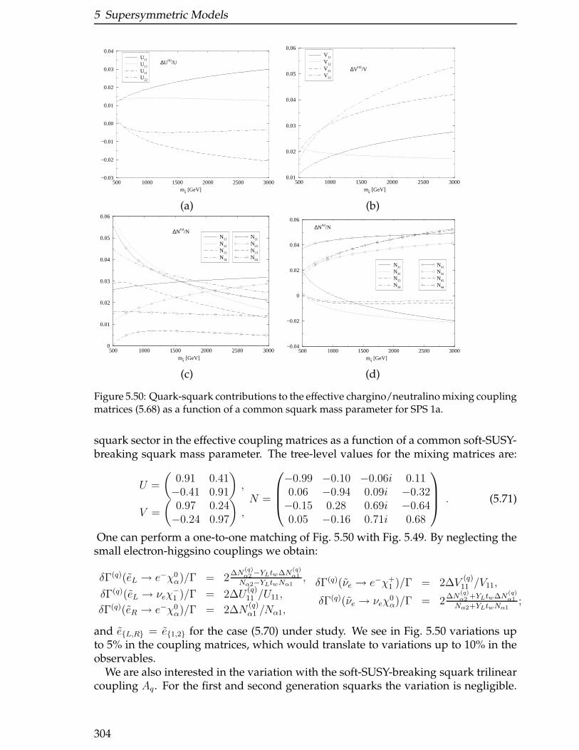
5 Supersymmetric Models
500 1000 1500 2000 2500 3000mq~ [GeV]
−0.03
−0.02
−0.01
0.00
0.01
0.02
0.03
0.04U11
U12
U21
U22
∆U(q)
/U
500 1000 1500 2000 2500 3000mq~ [GeV]
0.01
0.02
0.03
0.04
0.05
0.06V11
V12
V21
V22
∆V(q)
/V
(a) (b)
500 1000 1500 2000 2500 3000mq~ [GeV]
0
0.01
0.02
0.03
0.04
0.05
0.06
N21
N22
N23
N24
N11
N12
N13
N14
∆N(q)
/N
500 1000 1500 2000 2500 3000mq~ [GeV]
−0.04
−0.02
0
0.02
0.04
0.06
N31
N32
N33
N34
N41
N42
N43
N44
∆N(q)
/N
(c) (d)
Figure 5.50: Quark-squark contributions to the effective chargino/neutralino mixing couplingmatrices (5.68) as a function of a common squark mass parameter for SPS 1a.
squark sector in the effective coupling matrices as a function of a common soft-SUSY-breaking squark mass parameter. The tree-level values for the mixing matrices are:
U =
(0.91 0.41−0.41 0.91
),
V =
(0.97 0.24−0.24 0.97
),N =
−0.99 −0.10 −0.06i 0.110.06 −0.94 0.09i −0.32−0.15 0.28 0.69i −0.640.05 −0.16 0.71i 0.68
. (5.71)
One can perform a one-to-one matching of Fig. 5.50 with Fig. 5.49. By neglecting thesmall electron-higgsino couplings we obtain:
δΓ(q)(eL → e−χ0α)/Γ = 2
∆N(q)α2 −YLtw∆N
(q)α1
Nα2−YLtwNα1,
δΓ(q)(eL → νeχ−1 )/Γ = 2∆U
(q)11 /U11,
δΓ(q)(eR → e−χ0α)/Γ = 2∆N
(q)α1 /Nα1,
δΓ(q)(νe → e−χ+1 )/Γ = 2∆V
(q)11 /V11,
δΓ(q)(νe → νeχ0α)/Γ = 2
∆N(q)α2 +YLtw∆N
(q)α1
Nα2+YLtwNα1;
and eL,R = e1,2 for the case (5.70) under study. We see in Fig. 5.50 variations upto 5% in the coupling matrices, which would translate to variations up to 10% in theobservables.
We are also interested in the variation with the soft-SUSY-breaking squark trilinearcoupling Aq . For the first and second generation squarks the variation is negligible.
304
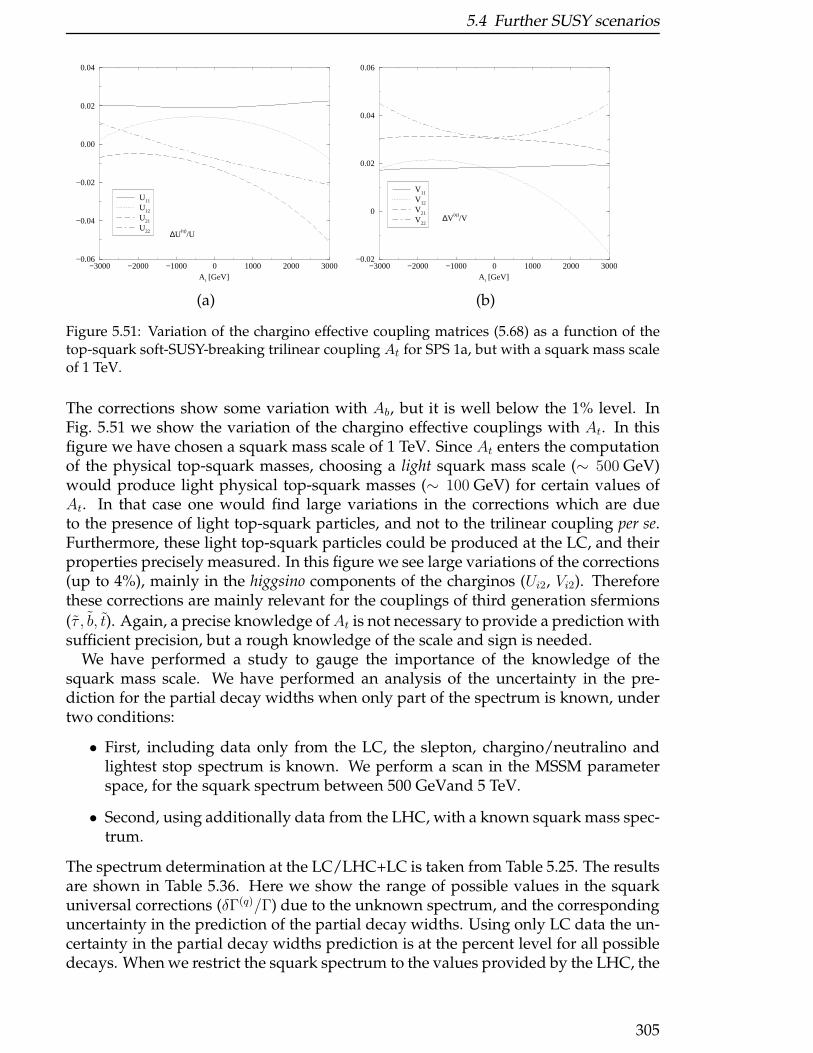
5.4 Further SUSY scenarios
−3000 −2000 −1000 0 1000 2000 3000A t [GeV]
−0.06
−0.04
−0.02
0.00
0.02
0.04
U11
U12
U21
U22 ∆U(q)
/U
−3000 −2000 −1000 0 1000 2000 3000A t [GeV]
−0.02
0
0.02
0.04
0.06
V11
V12
V21
V22∆V
(q)/V
(a) (b)
Figure 5.51: Variation of the chargino effective coupling matrices (5.68) as a function of thetop-squark soft-SUSY-breaking trilinear coupling At for SPS 1a, but with a squark mass scaleof 1 TeV.
The corrections show some variation with Ab, but it is well below the 1% level. InFig. 5.51 we show the variation of the chargino effective couplings with At. In thisfigure we have chosen a squark mass scale of 1 TeV. Since At enters the computationof the physical top-squark masses, choosing a light squark mass scale (∼ 500 GeV)would produce light physical top-squark masses (∼ 100 GeV) for certain values ofAt. In that case one would find large variations in the corrections which are dueto the presence of light top-squark particles, and not to the trilinear coupling per se.Furthermore, these light top-squark particles could be produced at the LC, and theirproperties precisely measured. In this figure we see large variations of the corrections(up to 4%), mainly in the higgsino components of the charginos (Ui2, Vi2). Thereforethese corrections are mainly relevant for the couplings of third generation sfermions
(τ , b, t). Again, a precise knowledge ofAt is not necessary to provide a prediction withsufficient precision, but a rough knowledge of the scale and sign is needed.
We have performed a study to gauge the importance of the knowledge of thesquark mass scale. We have performed an analysis of the uncertainty in the pre-diction for the partial decay widths when only part of the spectrum is known, undertwo conditions:
• First, including data only from the LC, the slepton, chargino/neutralino andlightest stop spectrum is known. We perform a scan in the MSSM parameterspace, for the squark spectrum between 500 GeVand 5 TeV.
• Second, using additionally data from the LHC, with a known squark mass spec-trum.
The spectrum determination at the LC/LHC+LC is taken from Table 5.25. The resultsare shown in Table 5.36. Here we show the range of possible values in the squarkuniversal corrections (δΓ(q)/Γ) due to the unknown spectrum, and the correspondinguncertainty in the prediction of the partial decay widths. Using only LC data the un-certainty in the partial decay widths prediction is at the percent level for all possibledecays. When we restrict the squark spectrum to the values provided by the LHC, the
305
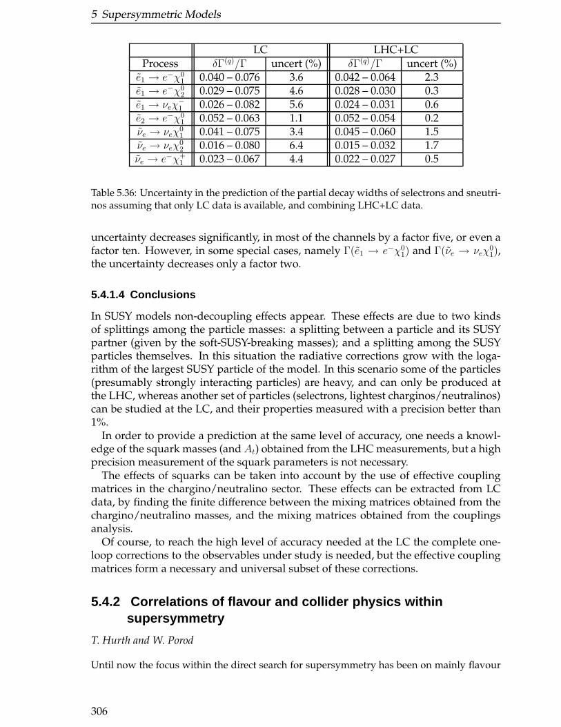
5 Supersymmetric Models
LC LHC+LCProcess δΓ(q)/Γ uncert (%) δΓ(q)/Γ uncert (%)e1 → e−χ0
1 0.040 – 0.076 3.6 0.042 – 0.064 2.3e1 → e−χ0
2 0.029 – 0.075 4.6 0.028 – 0.030 0.3e1 → νeχ
−1 0.026 – 0.082 5.6 0.024 – 0.031 0.6
e2 → e−χ01 0.052 – 0.063 1.1 0.052 – 0.054 0.2
νe → νeχ01 0.041 – 0.075 3.4 0.045 – 0.060 1.5
νe → νeχ02 0.016 – 0.080 6.4 0.015 – 0.032 1.7
νe → e−χ+1 0.023 – 0.067 4.4 0.022 – 0.027 0.5
Table 5.36: Uncertainty in the prediction of the partial decay widths of selectrons and sneutri-nos assuming that only LC data is available, and combining LHC+LC data.
uncertainty decreases significantly, in most of the channels by a factor five, or even afactor ten. However, in some special cases, namely Γ(e1 → e−χ0
1) and Γ(νe → νeχ01),
the uncertainty decreases only a factor two.
5.4.1.4 Conclusions
In SUSY models non-decoupling effects appear. These effects are due to two kindsof splittings among the particle masses: a splitting between a particle and its SUSYpartner (given by the soft-SUSY-breaking masses); and a splitting among the SUSYparticles themselves. In this situation the radiative corrections grow with the loga-rithm of the largest SUSY particle of the model. In this scenario some of the particles(presumably strongly interacting particles) are heavy, and can only be produced atthe LHC, whereas another set of particles (selectrons, lightest charginos/neutralinos)can be studied at the LC, and their properties measured with a precision better than1%.
In order to provide a prediction at the same level of accuracy, one needs a knowl-edge of the squark masses (and At) obtained from the LHC measurements, but a highprecision measurement of the squark parameters is not necessary.
The effects of squarks can be taken into account by the use of effective couplingmatrices in the chargino/neutralino sector. These effects can be extracted from LCdata, by finding the finite difference between the mixing matrices obtained from thechargino/neutralino masses, and the mixing matrices obtained from the couplingsanalysis.
Of course, to reach the high level of accuracy needed at the LC the complete one-loop corrections to the observables under study is needed, but the effective couplingmatrices form a necessary and universal subset of these corrections.
5.4.2 Correlations of flavour and collider physics withinsupersymmetry
T. Hurth and W. Porod
Until now the focus within the direct search for supersymmetry has been on mainly flavour
306

5.4 Further SUSY scenarios
diagonal observables. Recently lepton flavour violating signals at future electron positron
colliders have been studied. There is now the opportunity to analyze relations between col-
lider observables and low-energy observables in the hadronic sector. In a first work in this
direction, we study flavour violation in the squark decays of the second and third generation
taking into account results from B-physics, in particular from the rare decay b → sγ. We
show that correlations between various squark decay modes can be used to get more precise
information on various flavour violating parameters.
5.4.2.1 Sources of Flavour Violation
Within the Minimal Supersymmetric Standard Model (MSSM) there are two newsources of flavour changing neutral currents, namely new contributions which areinduced through the quark mixing like in the SM and generic supersymmetric con-tributions through the squark mixing. In contrast to the Standard Model (SM), thestructure of the unconstrained MSSM does not explain the suppression of FCNC pro-cesses which is observed in experiments; this is the essence of the well-known su-persymmetric flavour problem. Flavour changing neutral current (FCNC) processestherefore yield important (indirect) information on the construction of supersymmet-ric extensions of the SM and can contribute to the question of which mechanism ulti-mately breaks supersymmetry. The experimental measurements of the rates for theseprocesses, or the upper limits set on them, impose in general a reduction of the sizeof parameters in the soft supersymmetry-breaking terms.
To understand the sources of flavour violation that may be present in supersym-metric models, in addition to those enclosed in the CKM matrix K, one has to considerthe contributions to the squark mass matrices
M2f ≡
(M2
f, LL + Ff LL +Df LL M2f, LR + Ff LR
(M2
f, LR
)†+ Ff RL M2
f, RR + Ff RR +Df RR
), (5.72)
where f stands for up- or down-type squarks. The matrices Mu,LL and Md,LL arerelated by SU(2)L gauge invariance. In the super-CKM basis, where the quark massmatrices are diagonal and the squarks are rotated in parallel to their superpartners,the relation reads as K†M2
u,LLK = M2d,LL = M2
Q. In this basis the F-terms Ff LL, Ff RL,Ff RR as well as the D-terms Df LL and Df RR are diagonal. All the additional flavourstructure of the squark sector is encoded in the soft SUSY breaking terms M2
Q, M2f, RR
(=M2U for f = u and M2
D for f = d) and M f, LR2 (=vu(Au)∗ for f = u and vd(A
d)∗ forf = d). Note, that the A-matrices are in general non-hermitian.
These additional flavour structures induce flavour violating couplings to the neu-tral gauginos and higgsinos in the mass eigenbasis which give rise to additional con-tributions to observables in the K and B meson sector. At present, new physics con-tributions to s → d and b → d transitions are strongly constrained. In particular, thetransitions between first- and second-generation quarks, namely FCNC processes inthe K system, are the most formidable tools to shape viable supersymmetric flavourmodels. As was recently emphasized again [81], most of the phenomena involvingb → s transitions are still largely unexplored and leave open the possibility of largenew physics effects in spite of the strong bound of the famous B → Xsγ decay whichstill gives the most stringent bounds in this sector. Nevertheless, additional experi-mental information from the B → Xsℓ
+ℓ− decay at the B factories and new results
307
5 Supersymmetric Models
on the Bs − Bs mixing at the Tevatron might change this situation in the near fu-ture. Within the present analysis, we take the present phenomenological situationinto account by setting the off-diagonal elements with an index 1 to zero. Regardingthe b → s transitions, we restrict ourselves on the most powerful constraint from thedecay B → Xsγ only.
Two further remarks are in order: Within a phenomenological analysis of the con-straints on the flavour violating parameters in supersymmetric models with the mostgeneral soft terms in the squark mass matrices, we prefer to use the mass eigenstateformalism which remains valid (in contrast to the mass insertion approximation)when the intergenerational mixing elements are not small. Moreover, a consistentanalysis of the bounds should also include interference effects between the variouscontributions, namely the interplay between the various sources of flavour violationand the interference effects of SM, gluino, chargino, neutralino and charged Higgsboson contributions. In [82] such an analysis was performed for the example of therare decay B → Xsγ and new bounds on simple combinations of elements of the softpart of the squark mass matrices are found to be, in general, one order of magnitudeweaker that the bound on the single off-diagonal elements mLR,23 which was derivedin previous work [83, 84], where any kind of interference effects were neglected.
5.4.2.2 Squark decays
Squarks can decay into quarks of all generations of quarks once the most generalform the squark mass matrix is considered. The most important decays modes forthe example under study are:
ui → ujχ0k , djχ
+l (5.73)
di → djχ0k , ujχ
−l (5.74)
with i = 1, .., 6, j = 1, 2, 3, k = 1, ..4 and l = 1, 2. These decays are controlled by thesame mixing matrices as the contributions to b→ sγ. As this decay mode restricts thesize of some of the elements, the questions arises to which extent flavour violatingsquark decays are also restricted. We will show below that flavour violating decaymodes are hardly constrained by present days data.
We will take the so–called Snowmass point SPS#1a as a specific example whichis specified by m0 = 100 GeV, m1/2 = 250 GeV, A0 = −100 GeV, tanβ = 10 andsign(µ) = 1. At the electroweak scale one gets the following data: M2 = 192 GeV,µ = 351 GeV, mH+ = 396 GeV, mg = 594 GeV, mt1 = 400 GeV, mt2 = 590 GeV,mqR ≃ 550 GeV, and mqL ≃ 570 GeV. We have used the program SPheno [85] for thecalculation. In the following we will concentrate on the mixing between the secondand third generation. As a specific example we have added a set of flavour violatingparameters given in Table 5.37; the resulting up-squark masses in GeV are in ascend-ing order: 408, 510, 529, 542, 558 and 627. This point is a random one out of 1000points fulfilling the b → sγ constraint. For the calculation of BR(b → sγ) we haveused the formulas given in ref. [86]. Note, that for SPS#1a both, the chargino as wellas the gluino loops, are important for the calculation of BR(b→ sγ). Therefore, thereis an interplay between the flavour structure of the down-type squarks and of the oneof the up-type squarks.
308
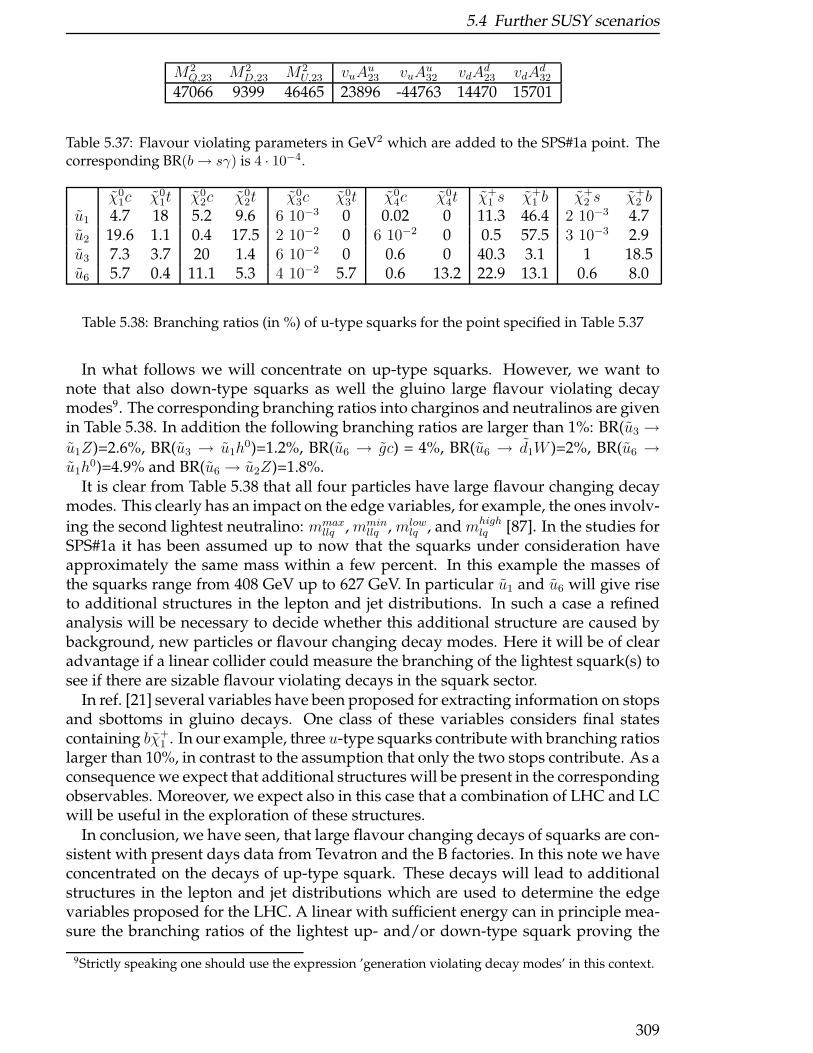
5.4 Further SUSY scenarios
M2Q,23 M2
D,23 M2U,23 vuA
u23 vuA
u32 vdA
d23 vdA
d32
47066 9399 46465 23896 -44763 14470 15701
Table 5.37: Flavour violating parameters in GeV2 which are added to the SPS#1a point. Thecorresponding BR(b→ sγ) is 4 · 10−4.
χ01c χ0
1t χ02c χ0
2t χ03c χ0
3t χ04c χ0
4t χ+1 s χ+
1 b χ+2 s χ+
2 bu1 4.7 18 5.2 9.6 6 10−3 0 0.02 0 11.3 46.4 2 10−3 4.7u2 19.6 1.1 0.4 17.5 2 10−2 0 6 10−2 0 0.5 57.5 3 10−3 2.9u3 7.3 3.7 20 1.4 6 10−2 0 0.6 0 40.3 3.1 1 18.5u6 5.7 0.4 11.1 5.3 4 10−2 5.7 0.6 13.2 22.9 13.1 0.6 8.0
Table 5.38: Branching ratios (in %) of u-type squarks for the point specified in Table 5.37
In what follows we will concentrate on up-type squarks. However, we want tonote that also down-type squarks as well the gluino large flavour violating decaymodes9. The corresponding branching ratios into charginos and neutralinos are givenin Table 5.38. In addition the following branching ratios are larger than 1%: BR(u3 →u1Z)=2.6%, BR(u3 → u1h
0)=1.2%, BR(u6 → gc) = 4%, BR(u6 → d1W )=2%, BR(u6 →u1h
0)=4.9% and BR(u6 → u2Z)=1.8%.It is clear from Table 5.38 that all four particles have large flavour changing decay
modes. This clearly has an impact on the edge variables, for example, the ones involv-
ing the second lightest neutralino: mmaxllq , mmin
llq , mlowlq , and mhigh
lq [87]. In the studies forSPS#1a it has been assumed up to now that the squarks under consideration haveapproximately the same mass within a few percent. In this example the masses ofthe squarks range from 408 GeV up to 627 GeV. In particular u1 and u6 will give riseto additional structures in the lepton and jet distributions. In such a case a refinedanalysis will be necessary to decide whether this additional structure are caused bybackground, new particles or flavour changing decay modes. Here it will be of clearadvantage if a linear collider could measure the branching of the lightest squark(s) tosee if there are sizable flavour violating decays in the squark sector.
In ref. [21] several variables have been proposed for extracting information on stopsand sbottoms in gluino decays. One class of these variables considers final statescontaining bχ+
1 . In our example, three u-type squarks contribute with branching ratioslarger than 10%, in contrast to the assumption that only the two stops contribute. As aconsequence we expect that additional structures will be present in the correspondingobservables. Moreover, we expect also in this case that a combination of LHC and LCwill be useful in the exploration of these structures.
In conclusion, we have seen, that large flavour changing decays of squarks are con-sistent with present days data from Tevatron and the B factories. In this note we haveconcentrated on the decays of up-type squark. These decays will lead to additionalstructures in the lepton and jet distributions which are used to determine the edgevariables proposed for the LHC. A linear with sufficient energy can in principle mea-sure the branching ratios of the lightest up- and/or down-type squark proving the
9Strictly speaking one should use the expression ’generation violating decay modes’ in this context.
309
5 Supersymmetric Models
hypothesis of large flavour violation in the squark sector. This information can thenbe put back in the analysis of the LHC data.
5.4.3 Supersymmetric lepton flavour violation at LHC and LC
F. Deppisch, J. Kalinowski, H. Pas, A. Redelbach and R. Ruckl
In supersymmetric extensions of the Standard Model, the Yukawa and/or mass terms of theheavy neutrinos can generate lepton flavour violating slepton mass terms. These new super-symmetric sources of lepton flavour violation may both enhance the rates of charged leptonflavour violating processes, lα → lβγ, and generate distinct final states, like lβ lα+jets+E/T , atfuture colliders. First, we discuss the sensitivity of future e+e− colliders to the SLFV indepen-dently of the lepton flavour violating mechanism. Second, we study lepton flavour violatingslepton pair production and decay at a future e+e− linear collider in the context of the see-saw mechanism in mSUGRA post-LEP benchmark scenarios. We investigate the correlationsof these signals with the corresponding lepton flavour violating rare decays lα → lβγ, andshow that these correlations are particularly suited for probing the origin of lepton flavourviolation.
5.4.3.1 Introduction
Neutrino oscillations imply the violation of individual lepton flavours and raise theinteresting possibility of observing lepton flavour violation in processes with chargedleptons, such as µ → eγ or τ → µγ. In the Standard Model these processes arestrongly suppressed due to small neutrino masses. In the supersymmetric extensionof the Standard Model, however, the situation may be quite different. For example,the slepton mass matrices need not simultaneously be diagonalized with the leptonmass matrices. When sleptons are rotated to the mass eigenstate basis, the sleptonmass diagonalization matrices Wiα enter the chargino and neutralino couplings
ei(W∗l)iαeαχ
0 + νi(W∗ν )iαeαχ
− + . . . (5.75)
and mix lepton flavour (Latin and Greek subscripts refer to the mass-eigenstate andflavour basis, respectively). Contributions from virtual slepton exchanges can there-fore enhance the rates of rare decays like µ → eγ. Furthermore, once superpart-ners are discovered, the supersymmetric lepton flavour violation (SLFV) can also besearched for directly at future colliders where the signal will come from the produc-tion of real sleptons (either directly or from chain decays of other sparticles), followedby their subsequent decays. Searches for SLFV at colliders have a number of advan-tages: superpartners can be produced with large cross-sections, flavour violation inthe production and decay of sleptons occurs at tree level and therefore is suppresedonly by powers of ∆ml/Γl [88] in contrast to the ∆ml/ml suppression in radiative lep-ton decays, where SLFV occurs at one-loop ( [89] and references therein). Generally,respecting the present bounds on rare lepton decays, large SLFV signals are possibleboth at the LHC [90] and at e+e− colliders [88,91–95]. This suggests that in some casesthe LHC and future e+e− colliders may provide competitive tools to search for andexplore supersymmetric lepton flavour violation.
In this note we first discuss the sensitivity at future e+e− colliders to SLFV indepen-dently of the lepton flavour violating mechanism. The simulation has been performed
310
5.4 Further SUSY scenarios
assuming a simplified situation with a pure 2-3 intergeneration mixing between νµand ντ , and ignoring any mixings with νe. In the analysis the mixing angle θ23 and∆m23 = |mν2 −mν3 | have been taken as free, independent parameters [93].
In the second part, SLFV generated by the seesaw mechanism is considered. Theheavy right-handed Majorana neutrinos give rise not only to light neutrino massesbut also to mixing of different slepton flavours due to the effects of the heavy neu-trinos on the renormalization-group running of the slepton masses. The implicationsof recent neutrino measurements on this mixing are investigated. Moreover we em-phasize the complementarity of the radiative decays lα → lβγ and the specific leptonflavour violating processes e±e− → l±β l
−α χ
0bχ
0a involving slepton pair production and
subsequent decay [95].
5.4.3.2 Sensitivity at future e+e− colliders to SLFV
In discussing the SLFV collider signals at future colliders, one has to distinguish twocases in which an oscillation of lepton flavour can occur: in processes with sleptonpair production and in processes with single slepton production, which differ in theinterference of the intermediate sleptons [88]. Slepton pair production is the dom-inant mechanism at lepton colliders, but it may also occur at hadron colliders viathe Drell-Yan process. Single sleptons may be produced in cascade decays of heav-ier non-leptonic superparticles. Such processes are particularly important for hadroncolliders, but they may also be relevant for lepton colliders where a single slepton canbe the decay product of a chargino or neutralino.
The amplitudes for pair production, f f → l+i l−i → l+α X l−β Y , and single produc-
tion, f f ′ → l+α X l−i → l+α X l−β Y , read, e.g.,
Mpairαβ =
∑
i
MpairP
i
q2 − m2i + imiΓi
WiαM+D
i
p2 − m2i + imiΓi
W ∗iβM−
D (s-channel)
(5.76)
Msinαβ =
∑
i
MsinP Wiα
i
q2 − m2i + imiΓi
W ∗iβM−
D (5.77)
whereMP andMD are the respective production and decay amplitudes for sleptonsin the absence of SLFV, and Wiα stands for the lepton flavour mixing matrix element.
For nearly degenerate in mass and narrow sleptons, ∆mij ≪ m and mΓij ≃ (miΓi+mjΓj)/2≪ m2, the products of slepton propagators can be simplified as follows
i
q2 − m2i + imiΓi
−iq2 − m2
j − imjΓj∼ 1
1 + i∆mij/Γij
π
mΓijδ(q2 − m2). (5.78)
Then, in the case of 2-3 intergeneration mixing, the cross-sections for the above pro-cesses (5.76, 5.77), take a particularly simple form [96]:
σpairαβ = χ23(3− 4χ23) sin2 2θ23 σ(f f → l+α l
−α )Br(l+α → l+α X)Br(l−α → l−α Y )
(5.79)
σsinαβ = χ23 sin2 2θ23 σ(f f ′ → l+α X l−α )Br(l−α → l−α Y ) (5.80)
311
5 Supersymmetric Models
where σ(f f ′ → l+α X l−α ), σ(f f → l+α l−α ) and Br(l±α → l±αX) are the corresponding
cross-sections and branching ratios in the absence of flavour violation. The sleptonflavour violating mixing effects are encoded in
χ23 =x2
23
2(1 + x223)
and sin2 2θ23 (5.81)
where x23 = ∆m23/Γ23. In the limit x23 ≫ 1, χ23 approaches 1/2, the interference can
be neglected and the cross-sections behave as σ ∼ sin2 2θ23 . In the opposite case, the
interference suppresses the flavour changing processes, and σ ∼ (∆m23 sin 2θ23)2.
To assess the sensitivity of a 500 GeV e+e− linear collider to the SLFV, the followingprocesses have been analysed
e+e− → νiνcj → τ±µ∓χ+
1 χ−1 (5.82)
e+e− → χ+2 χ
−1 → τ±µ∓χ+
1 χ−1 (5.83)
e+e− → χ02χ
01 → τ±µ∓χ0
1χ01 (5.84)
Here χ±1 → χ0
1ff′, and χ0
1 escapes detection. The signature of SLFV would be τ±µ∓ +4 jets+E/T , τ±µ∓+ℓ+2 jets+E/T , or τ±µ∓+E/T , depending on the hadronic or leptonicχ±
1 decay mode. The purely leptonic decay modes are overwhelmed by background.In particular, the neutralino pair production process (5.84), which could still be openif the second chargino and sleptons were too heavy for (5.82) and (5.83), is difficult toextract from background. On the other hand, with charginos decaying hadronically,the signal τ±µ∓ + 4 jets + E/T comes from both processes (5.82) and (5.83) and is SM-background free. The flavour-conserving processes analogous to (5.82) and (5.83), butwith two τ ’s in the final state where one of the τ ’s decays leptonically to µ, contributeto the background. On the other hand, if jets are allowed to overlap, an important SMbackground to the final states with τ±µ∓+ ≥ 3 jets + E/T comes from e+e− → ttg.
The simulation of the signal and background has been performed for one of theMSSM representative points chosen for detailed case studies at the ECFA/DESY Work-shop [64]: a mSUGRA scenario defined by m0 = 100 GeV, M1/2 = 200 GeV, A0 = 0GeV, tan β = 3 and sgn(µ) = +. A simple parton level simulation has been performedwith a number of kinematic cuts listed in [93]. For the processes (5.82) and (5.83)
we find after cuts the following cross-sections, χ23(3 − 4χ23) sin2 2θ23 × 0.51 fb and
χ23 sin2 2θ23 × 0.13 fb, respectively, while the background amounts to 0.28 fb.In Fig. 5.52 the significance is given by σd = S√
S+Bwhere S and B are the numbers
of signal and background events, respectively, for a given luminosity. Shown is the
region (to the right of the curves) in the ∆m23 − sin 2θ23 plane that can be explored orruled out at a 3σ level at a linear collider of energy 500 GeV for the given integratedluminosity. The contour A is for 500 fb−1 and B for 1000 fb−1. For comparison, theboundary C shows the reach in the process νiν
ci alone (previously studied in [88, 92])
using our cuts and assuming a luminosity of 500 fb−1. The chargino contribution
increases the sensitivity range to sin 2θ23 by 10-20%, while the sensitivity to ∆m23
does not change appreciably.In the same figure, the contour lines for constant branching ratios of τ → µγ are
shown for comparison [97]. In the limit of small mass splitting, Br(τ → µγ) can becalculated in the flavour basis using the mass insertion technique [98]. In our 2-3
312

5.4 Further SUSY scenarios
∆m23/GeV
sin 2θ23
Figure 5.52: Various 3σ significance contours in the ∆m23 − sin 2θ23 plane, for the SUSYpoint mentioned in the text. The contours A and B show the integrated signals (5.82–5.83)at√s =500 GeV and for 500 fb−1 and 1000 fb−1, respectively. The contour C shows the
ννc contribution separately for 500 fb−1 [93]. The dotted lines indicate contours for Br(τ →µγ)=10−7, 10−8 and 10−9 [97].
intergeneration mixing scenario the radiative process τ → µγ constrains the combi-nation of parameters
δµτ = sin 2θ23∆m23/m. (5.85)
The contours in Fig. 5.52 have been obtained from the approximate formula of Ref.[99], normalized to the current experimental limit,
Br(τ → µγ) ∼ 1.1× 10⁻⁶
(δµτ1.4
)2(100 GeV
m
)4
. (5.86)
This approximation only provides an order of magnitude estimate of the upper limitfor the supersymmetric contribution to the radiative lepton decay. The exact result,which is sensitive to the details of mass spectra and mixings, can in fact be muchsmaller due to cancellations among different contributions [89]. Fig. 5.52 demon-strates that information from slepton production and decay could be competitive tothe radiative lepton decays. In particular a LC can help to explore the small ∆m23 re-gion. It should be stressed, though, that in a given model for lepton flavour violationalso the correlation with µ → eγ has to be considered [95], which in many cases canyield a more severe bound, as discussed in the next section.
5.4.3.3 Case study for the supersymmetric seesaw model
As a definite and realistic example for SLFV we consider the seesaw mechanism inmSUGRA models. In supersymmetric theories with heavy right-handed Majorananeutrinos, the seesaw mechanism [100] can give rise to light neutrino masses at or be-low the sub-eV scale. Furthermore, the massive neutrinos affect the renormalization
313
5 Supersymmetric Models
group running of the slepton masses, generating flavour off-diagonal terms in themass matrix. These in turn lead to SLFV in scattering processes at high energies andin rare decays. For illustration of the potential and complementarity of such SLFVsearches we focus on the LC processes e±e− → l±β l
−α χ
0b χ
0a involving slepton pair pro-
duction and subsequent decay, and on the corresponding radiative decay lα → lβγ.In particular, in an early ATLAS note [101] τ → µγ is estimated to be observable atthe LHC for a branching ratio of order 10−7. However, the limit one can reasonablyexpect may be an order of magnitude better [102].
For our study we use the mSUGRA benchmark scenarios proposed in [103] forLC studies, concentrating on those which predict charged left-handed sleptons thatare light enough to be pair-produced at the center-of-mass energy
√s = 500 GeV.
Furthermore, we implement the seesaw mechanism assuming degenerate Majoranamasses for the right-handed neutrinos and constrain the neutrino Yukawa couplingsby the measured masses and mixings of the light neutrinos. Further sources of SLFVexist in other models such as GUTs [104]. However, no realistic three generation casestudy of effects for collider processes has been performed so far, so that we restrictthe discussion to the minimal seesaw model, here.
Supersymmetric seesaw mechanism
If three right-handed neutrino singlet fields νR are added to the MSSM particlecontent, one has the additional terms [105]
Wν = −1
2νcTR MνcR + νcTR YνL ·H2 (5.87)
in the superpotential. Here, Yν is the matrix of neutrino Yukawa couplings, M is theright-handed neutrino Majorana mass matrix, and L and H2 denote the left-handedlepton and hypercharge +1/2 Higgs doublets, respectively. At energies much belowthe mass scale MR of the right-handed neutrinos, Wν leads to the following massmatrix for the light neutrinos:
Mν = Y Tν M
−1Yν(v sin β)2. (5.88)
From that the light neutrino masses m1, m2, m3 are obtained after diagonalization bythe unitary MNS matrix U . The basis is chosen such that the matrices of the chargedlepton Yukawa couplings and Majorana masses are diagonal, which is always possi-ble.
Furthermore, the heavy neutrino mass eigenstates give rise to virtual correctionsto the slepton mass matrix that are responsible for lepton flavour violating processes.More specifically, in the mSUGRA models considered, the mass matrix of the chargedsleptons is given by
m2l
=
(m2lL
(m2lLR
)†
m2lLR
m2lR
)(5.89)
with
(m2lL
)ij = (m2L)ij + δij
(m2li
+m2Z cos 2β
(−1
2+ sin2 θW
))
314
5.4 Further SUSY scenarios
(m2lR
)ij = (m2R)ij + δij(m
2li−m2
Z cos 2β sin2 θW )
(m2lLR
)ij = Aijv cosβ − δijmliµ tanβ.
When m2l
is evolved from the GUT scale MX to the electroweak scale characteristicfor the experiments, one obtains
m2L = m2
01 + (δm2L)MSSM + δm2
L (5.90)
m2R = m2
01 + (δm2R)MSSM + δm2
R (5.91)
A = A0Yl + δAMSSM + δA, (5.92)
wherem0 is the common soft SUSY-breaking scalar mass andA0 the common trilinearcoupling. The terms (δm2
L,R)MSSM and δAMSSM are well-known flavour-diagonal MSSMcorrections. In addition, the evolution generates the off-diagonal terms δm2
L,R andδA which, in leading-log approximation and for degenerate right-handed Majoranamasses Mi = MR, i = 1, 2, 3, are given by [106]
δm2L = − 1
8π2(3m2
0 + A20)(Y
†ν Yν)ℓn
(MX
MR
)(5.93)
δm2R = 0 (5.94)
δA = − 3A0
16π2(YlY
†ν Yν)ℓn
(MX
MR
). (5.95)
In order to determine the product Y †ν Yν of the neutrino Yukawa coupling matrix
entering these corrections, one uses the expression
Yν =
√MR
v sin βR · diag(
√m1,√m2,√m3) · U †, (5.96)
which follows from UTMνU = diag(m1, m2, m3) and (5.88) [105]. Here, R is an un-known complex orthogonal matrix parametrizing the ambiguity in the relation ofYukawa coupling and mass matrices. In the following we will assume R to be realwhich suffices for the present purpose. In this case, R drops out from the productY †ν Yν ,
Y †ν Yν =
MR
v2 sin2 βU · diag(m1, m2, m3) · U †. (5.97)
Using existing neutrino data on the mass squared differences and the mixing matrixUtogether with bounds and assumptions on the absolute mass scale one can calculateY †ν Yν . The only free parameter is the Majorana mass scale MR. The result is then
evolved to the unification scaleMX and used as an input in the renormalization groupcorrections (5.93) to the slepton mass matrix. Finally, diagonalization of (5.89) yields
the slepton mass eigenvalues mi and eigenstates li (i = 1, 2, ...6).
Lepton flavour violating processes
The flavour off-diagonal elements (5.93) in m2l
(δA = 0 in the mSUGRA scenarios
of [103]) induce, among other SLFV effects, the processes e+e− → l+j l−i → l+β l
−α χ
0bχ
0a,
where SLFV can occur in the production and decay vertices. The helicity amplitudes
315

5 Supersymmetric Models
1011
1012
1013
1014
1015
MR / GeV
10-4
10-3
10-2
10-1
100
101
σ / f
b
Figure 5.53: Cross-sections at√s = 500 GeV for e+e− → µ+e− + 2χ0
1 (circles) and e+e− →τ+µ− + 2χ0
1 (triangles) in scenario B.
for the pair production of l+j and l−i , and the corresponding decay amplitudes are
given explicitly in [95]. In the approximation (5.79) for σpairαβ one finds
σpairαβ ∝
|(δmL)2αβ |2
m2Γ2σ(f f → l+α l
−α )Br(l+α → l+α χ0)Br(l
−α → l−α χ0) (5.98)
In the numerical evaluation no slepton degeneracy has been assumed as in (5.78),and the amplitude for the complete 2 → 4 processes is summed coherently over theintermediate slepton mass eigenstates.
Similary, the terms (5.93) are responsible for SLFV radiative decays lα → lβγ in-duced by photon-penguin type diagrams with charginos / sneutrinos or neutrali-nos / charged sleptons in the loop. Again schematically, the decay rates are givenby [105, 106]
Γ(lα → lβγ) ∝ α3m5lα
|(δmL)2αβ|2
m8tan2 β, (5.99)
where m stands for the relevant sparticle masses in the loop.
Scenario m1/2/GeV m0/GeV tanβ m6/GeV Γ6/GeV mχ01/GeV
B 250 100 10 208 0.32 98C 400 90 10 292 0.22 164G 375 120 20 292 0.41 154I 350 180 35 313 1.03 143
Table 5.39: Parameters of selected mSUGRA benchmark scenarios (from [103]). The sign of µis chosen to be positive and A0 is set to zero. Given are also the mass and total width of theheaviest charged slepton and the mass of the lightest neutralino.
316
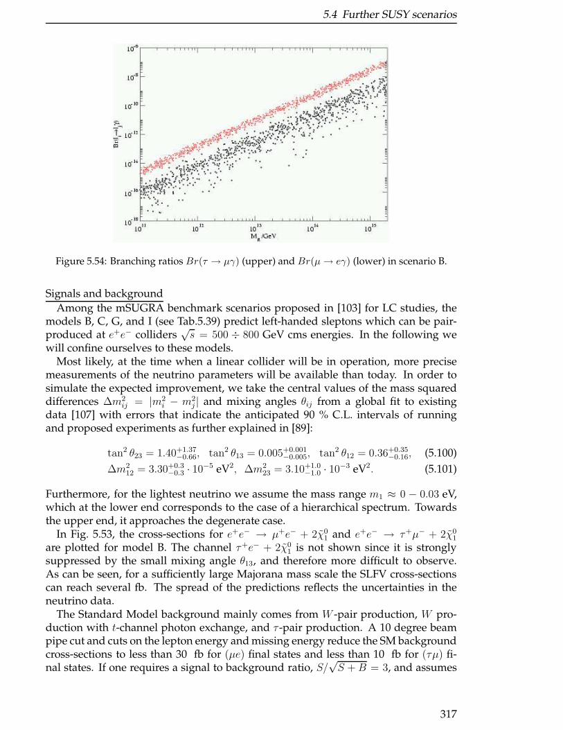
5.4 Further SUSY scenarios
Figure 5.54: Branching ratios Br(τ → µγ) (upper) and Br(µ→ eγ) (lower) in scenario B.
Signals and background
Among the mSUGRA benchmark scenarios proposed in [103] for LC studies, themodels B, C, G, and I (see Tab.5.39) predict left-handed sleptons which can be pair-produced at e+e− colliders
√s = 500 ÷ 800 GeV cms energies. In the following we
will confine ourselves to these models.Most likely, at the time when a linear collider will be in operation, more precise
measurements of the neutrino parameters will be available than today. In order tosimulate the expected improvement, we take the central values of the mass squareddifferences ∆m2
ij = |m2i − m2
j | and mixing angles θij from a global fit to existingdata [107] with errors that indicate the anticipated 90 % C.L. intervals of runningand proposed experiments as further explained in [89]:
tan2 θ23 = 1.40+1.37−0.66, tan2 θ13 = 0.005+0.001
−0.005, tan2 θ12 = 0.36+0.35−0.16, (5.100)
∆m212 = 3.30+0.3
−0.3 · 10−5 eV2, ∆m223 = 3.10+1.0
−1.0 · 10−3 eV2. (5.101)
Furthermore, for the lightest neutrino we assume the mass range m1 ≈ 0 − 0.03 eV,which at the lower end corresponds to the case of a hierarchical spectrum. Towardsthe upper end, it approaches the degenerate case.
In Fig. 5.53, the cross-sections for e+e− → µ+e− + 2χ01 and e+e− → τ+µ− + 2χ0
1
are plotted for model B. The channel τ+e− + 2χ01 is not shown since it is strongly
suppressed by the small mixing angle θ13, and therefore more difficult to observe.As can be seen, for a sufficiently large Majorana mass scale the SLFV cross-sectionscan reach several fb. The spread of the predictions reflects the uncertainties in theneutrino data.
The Standard Model background mainly comes from W -pair production, W pro-duction with t-channel photon exchange, and τ -pair production. A 10 degree beampipe cut and cuts on the lepton energy and missing energy reduce the SM backgroundcross-sections to less than 30 fb for (µe) final states and less than 10 fb for (τµ) fi-nal states. If one requires a signal to background ratio, S/
√S +B = 3, and assumes
317
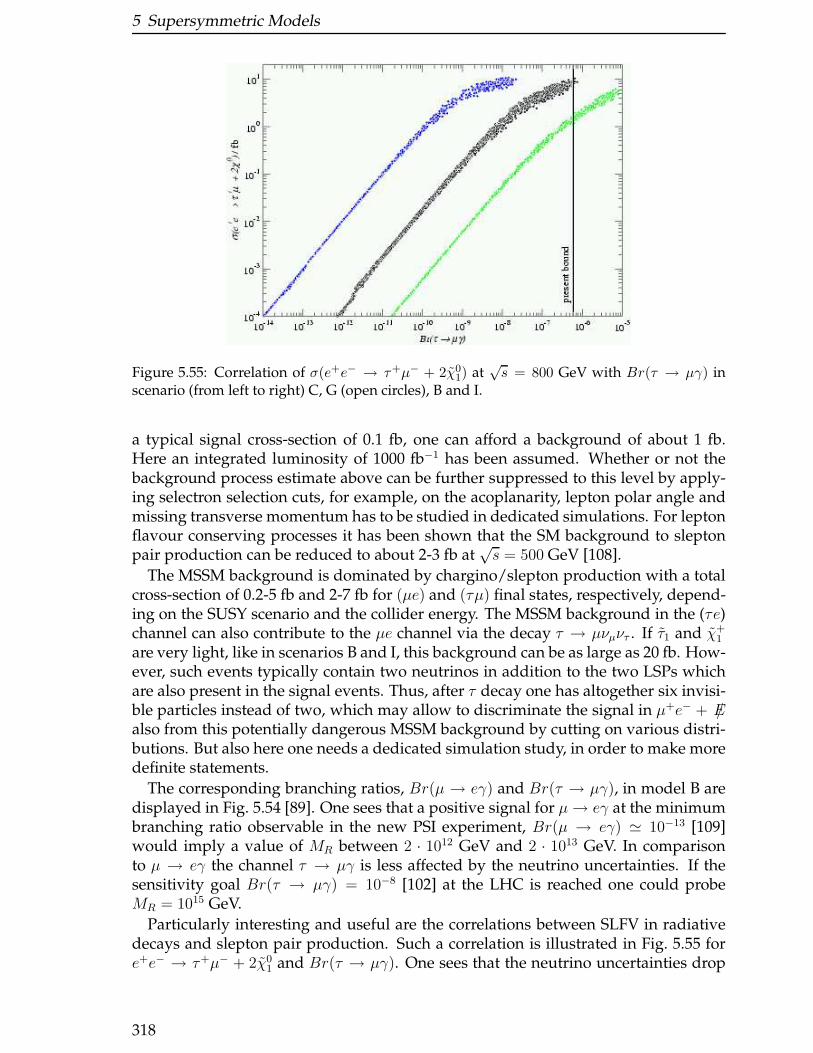
5 Supersymmetric Models
Figure 5.55: Correlation of σ(e+e− → τ+µ− + 2χ01) at
√s = 800 GeV with Br(τ → µγ) in
scenario (from left to right) C, G (open circles), B and I.
a typical signal cross-section of 0.1 fb, one can afford a background of about 1 fb.Here an integrated luminosity of 1000 fb−1 has been assumed. Whether or not thebackground process estimate above can be further suppressed to this level by apply-ing selectron selection cuts, for example, on the acoplanarity, lepton polar angle andmissing transverse momentum has to be studied in dedicated simulations. For leptonflavour conserving processes it has been shown that the SM background to sleptonpair production can be reduced to about 2-3 fb at
√s = 500 GeV [108].
The MSSM background is dominated by chargino/slepton production with a totalcross-section of 0.2-5 fb and 2-7 fb for (µe) and (τµ) final states, respectively, depend-ing on the SUSY scenario and the collider energy. The MSSM background in the (τe)channel can also contribute to the µe channel via the decay τ → µνµντ . If τ1 and χ+
1
are very light, like in scenarios B and I, this background can be as large as 20 fb. How-ever, such events typically contain two neutrinos in addition to the two LSPs whichare also present in the signal events. Thus, after τ decay one has altogether six invisi-ble particles instead of two, which may allow to discriminate the signal in µ+e− + /Ealso from this potentially dangerous MSSM background by cutting on various distri-butions. But also here one needs a dedicated simulation study, in order to make moredefinite statements.
The corresponding branching ratios, Br(µ → eγ) and Br(τ → µγ), in model B aredisplayed in Fig. 5.54 [89]. One sees that a positive signal for µ→ eγ at the minimumbranching ratio observable in the new PSI experiment, Br(µ → eγ) ≃ 10−13 [109]would imply a value of MR between 2 · 1012 GeV and 2 · 1013 GeV. In comparisonto µ → eγ the channel τ → µγ is less affected by the neutrino uncertainties. If thesensitivity goal Br(τ → µγ) = 10−8 [102] at the LHC is reached one could probeMR = 1015 GeV.
Particularly interesting and useful are the correlations between SLFV in radiativedecays and slepton pair production. Such a correlation is illustrated in Fig. 5.55 fore+e− → τ+µ− + 2χ0
1 and Br(τ → µγ). One sees that the neutrino uncertainties drop
318
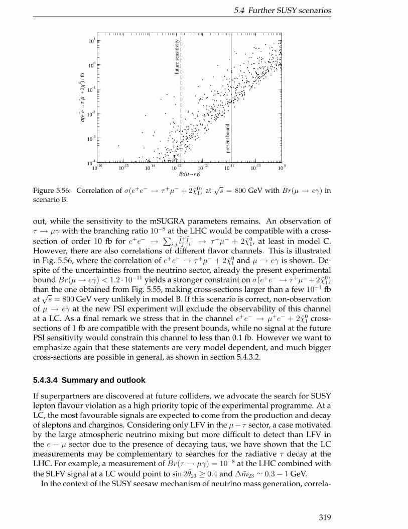
5.4 Further SUSY scenarios
10-16
10-15
10-14
10-13
10-12
10-11
10-10
10-9
Br(µ→eγ)
10-4
10-3
10-2
10-1
100
101
σ(e
+ e- →
τ+ µ- +
2χ
0 ) / f
b
pres
ent b
ound
futu
re s
ensi
tivity
Figure 5.56: Correlation of σ(e+e− → τ+µ− + 2χ01) at
√s = 800 GeV with Br(µ → eγ) in
scenario B.
out, while the sensitivity to the mSUGRA parameters remains. An observation ofτ → µγ with the branching ratio 10−8 at the LHC would be compatible with a cross-
section of order 10 fb for e+e− →∑
i,j l+j l
−i → τ+µ− + 2χ0
1, at least in model C.However, there are also correlations of different flavor channels. This is illustratedin Fig. 5.56, where the correlation of e+e− → τ+µ− + 2χ0
1 and µ → eγ is shown. De-spite of the uncertainties from the neutrino sector, already the present experimentalbound Br(µ→ eγ) < 1.2 ·10−11 yields a stronger constraint on σ(e+e− → τ+µ− +2χ0
1)than the one obtained from Fig. 5.55, making cross-sections larger than a few 10−1 fbat√s = 800 GeV very unlikely in model B. If this scenario is correct, non-observation
of µ → eγ at the new PSI experiment will exclude the observability of this channelat a LC. As a final remark we stress that in the channel e+e− → µ+e− + 2χ0
1 cross-sections of 1 fb are compatible with the present bounds, while no signal at the futurePSI sensitivity would constrain this channel to less than 0.1 fb. However we want toemphasize again that these statements are very model dependent, and much biggercross-sections are possible in general, as shown in section 5.4.3.2.
5.4.3.4 Summary and outlook
If superpartners are discovered at future colliders, we advocate the search for SUSYlepton flavour violation as a high priority topic of the experimental programme. At aLC, the most favourable signals are expected to come from the production and decayof sleptons and charginos. Considering only LFV in the µ− τ sector, a case motivatedby the large atmospheric neutrino mixing but more difficult to detect than LFV inthe e − µ sector due to the presence of decaying taus, we have shown that the LCmeasurements may be complementary to searches for the radiative τ decay at theLHC. For example, a measurement of Br(τ → µγ) = 10−8 at the LHC combined with
the SLFV signal at a LC would point to sin 2θ23 ≥ 0.4 and ∆m23 ≃ 0.3− 1 GeV.In the context of the SUSY seesaw mechanism of neutrino mass generation, correla-
319
5 Supersymmetric Models
tions between SLFV in radiative decays and slepton pair production have been foundparticularly interesting. For instance, in a given MSSM scenario the measurement ofτ → µγ at the LHC would imply a definite cross section for e+e− → τ+µ− + 2χ0
1
at the LC. Assuming a reasonable set of MSSM benchmark scenarios and Br(τ →µγ) = 10−8 and using the present neutrino data, one predicts σ(e+e− → τ+µ− + 2χ0
1)in the range 0.05 to 10 fb. However, the non-observation of µ → eγ with a branch-ing ratio of about 10−13 at the new PSI experiment would exclude the observabilityof σ(e+e− → τ+µ− + 2χ0
1) at a linear collider. While the former correlation involvingthe same lepton flavours is insensitive to the uncertainties in the neutrino data (Fig.5.55), the latter correlation is somewhat smeared out (Fig. 5.56). However, both typesof correlations remain sensitive to the mSUGRA parameters and, hence, provide veryuseful tools for probing the origin of lepton flavour violation.
The complementarity of the LHC and LC (and of low-energy experiments) in thecontext of lepton flavour violation is far from being exhausted by the present study.Quantitative analyses of the impact of precise mass measurements at the LC on identi-fying the LFV decay chains at the LHC (and vice-versa) and other important featurescall for detailed Monte Carlo simulations which should be undertaken in the nextround of the LHC/LC studies.
5.4.4 Detection difficulties for MSSM and other SUSY models f orspecial boundary conditions
J. Gunion
5.4.4.1 Anomaly-mediated boundary conditions — the degene rate wino-LSPscenario
One interesting limiting case of SUSY boundary conditions is loop-induced gaug-ino masses proportional to the respective renormalization group beta functions, asin Anomaly-Mediated SUSY breaking (AMSB) and the simplest moduli-dominatedSUSY breaking models. In such models, the mass difference ∆mχ1 ≡ mχ±
1− mχ0
1is
most typically very small. The phenomenology of χ±1 production and decay has been
studied extensively in [110,111], and also in [112,113]. For ∆mχ1 < mπ, as achievablein some models even after radiative corrections, the χ±
1 may exit the detector, lead-ing to an easily detected long-lived heavily-ionizing track (LHIT), or decay to a soft,but visible, e or µ track in the vertex detector and inner part of the tracker yieldinga disappearing isolated track (DIT). For ∆mχ1 above, but close to mπ, the χ±
1 decayto a soft π± may still have sufficient path length (including sufficient β) to leave adistinctive track in the vertex detector while also having low enough β (e.g. β < 0.8)to be highly-ionizing, yielding a “STUB” track; the decay π need not be visible. Forsomewhat larger ∆mχ1 , the STUB is not visible, but the soft π± will be detected andmay have a high impact parameter (HIP). For still larger ∆mχ1 , the π± will sim-ply be soft, but readily detected. Once ∆mχ1
>∼ 2 − 3 GeV, the χ±1 decay products
have significant energy. The most typical range for ∆mχ1 in the models studied is∆mχ1 ∈ [200 MeV, 2 GeV].
320
5.4 Further SUSY scenarios
Assuming that only the χ01 and χ±
1 are light, the primary LC SUSY processes areχ+
1 χ−1 , γχ+
1 χ−1 , and W∓χ0
1χ±1 production. Observable signatures are:
• ∆mχ1 < mπ : the χ±1 yields a ‘stable particle’ LHIT and/or DIT track and is easily
detected: χ+1 χ
−1 production will be easily seen.
• mπ < ∆mχ1 < 200 MeV: the χ±1 decay yields a STUB track. Assuming small γγ
background, no trigger would be needed; we denote such a signal by SNT.• 200 MeV < ∆mχ1 < 2 − 3 GeV: the χ±
1 decay yields a soft, possibly HIP (∆mχ1 <1 GeV), π track. Backgrounds from γγ-induced interactions are large. One musttag χ+
1 χ−1 production using e+e− → γχ+
1 χ−1 [114] or employ the more kinematically
limited W∓χ01χ
±1 final state.
• ∆mχ1 > 2−3 GeV: the χ±1 decay products are sufficiently energetic that γγ induced
backgrounds can be rejected to the extent necessary for mSUGRA-like mode detectionof direct e+e− → χ+
1 χ−1 production.
LEP experience suggests that these various signatures are all viable in their respectivedomains of validity for an appropriately designed detector. Current LEP2 (
√s ∼
200 GeV) analyzes exclude mχ±
1<√s/2 in the ‘stable’ and ‘standard’ regions of ∆mχ1
and mχ±
1< 80 GeV or so, assuming the νe is relatively heavy, in the mπ ≤ ∆mχ1 ≤
2 GeV region [115, 116]. The backgrounds to the ‘stable’ and γ-tag+soft-π signals arevery small, and we assume they remain so at higher
√s with simple cuts. (For the
γ-tag+soft-π signal, we require pγT > 10 GeV, 10 ≤ θγ ≤ 170.) The appropriate SUSY
discovery mode(s) at a√s = 600 GeV LC are shown as a function of ∆mχ1 and mχ±
1in
Fig. 5.57 [117]. We assume that 10 events are adequate to establish a signal. The rapidturn-on of χ+
1 χ−1 production allows one to probe almost to the kinematic limit [mχ±
1∼√
s/2 or (√s−pγT )/2], although the totally iron-clad SNT and HIP signatures disappear
at the largest mχ±
1values due to inadequate boost. The SNT signature is somewhat
suppressed at smaller mχ±
1as more of the χ±
1 ’s are boosted to β > 0.8. The discovery
reach of the SNT and HIP channels is increased only slightly for L = 50fb−1 → 1ab−1.Since ∆mχ1 ∈ [200 MeV, 2 GeV] is typical of models with loop-dominated gauginomasses, the γ-tag signals are of great importance.
Detector design is critical to observing the soft pion signatures. If the ~B field is toostrong, soft pions will curl up before they can be detected/tracked. Then, the onlysignal γχ+
1 χ−1 production yields γ + /M , which has a large γνν background. Fig. 5.57
illustrates the discovery reach. For mχ±
1<∼ 200 GeV (260 GeV), /M cuts can give S/B ≥
0.02 and S/√B ≥ 5 for L = 50fb−1 (∼ 1ab−1). The ℓ∓ + /M final state from W∓χ0
1χ±1
production will provide an alternative signal with similar reach in mχ±
1; the only SM
background is single W → ℓν production with the ℓ lost down the beam pipe.
Let us now consider the prospects for exploring the degenerate wino-LSP scenarioat the Tevatron and LHC. At hadron colliders, typical signatures of mSUGRA aretri–lepton events from neutralino–chargino production, like–sign di–leptons fromgluino pair production, and multijets+/ET from squark and gluino production. Thetri–lepton signal from χ±
1 χ02 production and the like–sign di–lepton signal from gg
production are both suppressed when ∆mχ1 is small by the softness of the leptonscoming from the χ±
1 decay(s). For the M2 < M1 << |µ| AMSB boundary condi-tions, the tri–lepton signal is further diminished by the suppression of the χ±
1 χ02 cross
section. For small enough ∆mχ1 , the LHIT and DIT ‘stable’-chargino signals will beviable [111, 117]. But, for larger ∆mχ1 , direct observation of the χ±
1 becomes more
321

5 Supersymmetric Models
10-1
1
100 120 140 160 180 200 220 240 260 280 300
10-1
1
100 120 140 160 180 200 220 240 260 280 300
Stable Chargino (LHIT)
Standard SUSY Search
γ+Secondary π Vertex ( γ+HIP)
Terminating Track Decaying to π (SNT)
γ+ππ
γ+M⁄
1 ab-150 fb-1
√s=600 GeV
Chargino Mass (GeV)
∆M (
GeV
)
Figure 5.57: Discovery reach for the various modes described in the text as a function of ∆mχ1
and mχ±
1at a√s = 600 GeV LC; from [117].
challenging. In this case, assuming that the g is light enough, the most obvious sig-nal for SUSY in degenerate models is jet(s) plus missing energy. In one AMSB study,it was found that gg production at the LHC will be sufficiently abundant that jets +/ET will probe up to mg ∼ 1.7 TeV (1 TeV) for L = 300fb−1 (L = 30fb−1), assumingthat squarks and sleptons are too heavy to provide useful signals [118, 119]. Usingmg ∼ 7mχ±
1, mg ∼ 1.7 TeV is equivalent to mχ±
1∼ 250 GeV, the effective reach of
a√s = 500 GeV LC. A more extensive reach for the jets + /ET channel at the LHC,
mg ∼ 2.1÷ 2.5 TeV, was found in [120].
An important question is whether direct detection of the charginos at the LHC ispossible when ∆mχ1 is large enough that the χ±
1 decay is prompt, but small enoughthat the (single) charged particle from its decay (a charged pion or lepton) is quitesoft. Direct detection might prove crucial to unambiguously showing that the modelis truly AMSB in character. The most difficult backgrounds to the soft (but isolated)π± tracks in this case are those arising from events containing the baryons Σ+, Σ−,Ξ,and Ω, all of which have decays in which a single soft pion emerges [111]. One mighthope to remove such backgrounds by requiring the soft pion track(s) to be sufficientlyisolated due to the fact that the normal hadrons above are not produced in isolation.So even if they decay to an isolated soft pion, there will be hadrons that are nearbyin ∆R that will be visible. In [120], this and the alternative possibility of detectingthe soft isolated ℓ± from the chargino decay are pursued. Aside from appropriate iso-lation requirements for the leptons, a critical ingredient is the use of the CambridgemTX variables [17] which provide sensitivity to mχ±
1when a χ+
1 χ−1 pair is produced
322
5.4 Further SUSY scenarios
through looking at distributions in mTX −mχ01. For this technique, it is necessary that
mχ01
be known (from kinematic endpoints) and that the bulk of the χ±1 come from the
two-body decay chain sequence q → qχ±1 → χ0
1eνeq or similar. As noted, squarksare not guaranteed to be sufficiently light to be abundantly produced in the AMSBmodels. But, assuming they are, [120] concludes that the isolation + mTX −mχ0
1pro-
cedures can determine the presence and mass of the χ±1 for ∆mχ1
>∼ 700 MeV. For∆mχ1 < 200 MeV, the HIT, DIT, STUB, HIP, . . . signatures make it easy to detect theχ±
1 . In the 200 < ∆mχ1 < 700 GeV part of parameter space, which unfortunatelyis somewhat preferred, techniques for direct χ±
1 detection have not yet been devel-oped. In this part of parameter space, the LHC is needed to see the gluino and squarksignatures while the LC is needed to directly observed the χ±
1 and determine its mass.
5.4.4.2 Baryonic R-parity violation coupled with the degen erate wino-LSPscenario
If one wishes to construct a “worst case” scenario for the hadron colliders, an obviousapproach is to assume: (1) a small ∆mχ1 AMSB (or other) scenario with 200 MeV <∼∆mχ1
<∼ 1 GeV; and (2) baryonic R-parity violation in which the χ01 decays to (semi-
soft) jets. A very incomplete consideration of this kind of scenario was given for theTevatron and the LC in [122] (see also the earlier discussion in [121]). The summarybelow is based on this reference.
First, because 200 MeV <∼ ∆mχ1 , the χ±1 decay will be prompt and there will be no
HIT, DIT, STUB, HIP, . . . type signatures. Second, because ∆mχ1<∼ 1 GeV, the leptons
(if significant in the χ±1 decays at all) will be very soft, making it impossible to look
for either the like-sign dilepton signal from gluino or squark pair production or thetri-lepton signal from χ±
1 χ02 production.
Other opportunities for SUSY detection depend in detail upon the χ01 → 3j decay
scenario. The rather strong upper bound on the baryonic R-parity violating couplingλ′′usd means that one (or more) of the ubd, ubs, csd, cbd, cbs channels will most likelydominate χ0
1 decay. All of these contain at least one heavy quark. Since SUSY pairproduction events contain at least two χ0
1’s, we can then use double-tagging to reducethe background relative to the signal. For all but the cds decay channel, at least twoof the jets in the final state will be b-jets. If cds decays dominate, we would havetwo c-jets. Since c-tagging will have lower efficiency than b-tagging, dominance ofχ0
1 decays by the cds channel results in the most difficult scenario for supersymmetrydetection. An exception is the case in which all the λ′′ are so small that the χ0
1 decay isnot prompt. If the χ0
1 is long-lived, then one reverts to the R-parity conserving signalsof the small ∆mχ1 case. If the χ0
1 decays within the detector after a substantial pathlength, the sudden appearance of three jets inside the detector will provide a clearsignature for SUSY. The most difficult case is when the χ0
1 → cds decay is prompt.In this case, since the χ0
1 decays promptly to jets, there will also be no missingenergy signal for gluino/squark production. In short, the only possible signal will bean excess of jets (some of which can be tagged with modest efficiency) due to the twoχ0
1 → cds decays. In addition, in the AMSB scenario (for which mg ∼ 3mχ±
1∼ mχ0
1)
each event will typically have a number of hard jets (from the g → q′qχ±1 decays)
accompanied by six jets from the χ01 decays. However, since some of the jets from
χ01 decay will be quite soft (unless mχ0
1is quite large) the excess of jets over standard
323
5 Supersymmetric Models
QCD will not be that pronounced and c tagging will not be very efficient. To date,there is no convincing study indicating that SUSY detection at the Tevatron or LHCwill be possible for this very difficult scenario when mg is sufficiently large that thegg production rate is not large. In other models with small ∆mχ1 , mg can be quite abit smaller and even of order mχ±
1. In this case, one loses the extra jets from g decay,
but the gg production rate is quite large and its detection at the LHC is fairly likelyafter cuts requiring a large number of jets and several c tags.
Thus, depending upon the exact model, the LC could be absolutely crucial for SUSYdetection. In fact, detection of e+e− → χ0
1χ01 → 6j would be completely straightfor-
ward at the LC and would provide a dramatic confirmation of SUSY as well as bary-onic R-parity violation. In addition, the e+e− → χ+
1 χ−1 → ℓ+ℓ− + 6j signal would
almost certainly be observable and allow an accurate determination of ∆mχ1 . Oncemχ0
1∼ mχ±
1is known from the LC data, it might be possible to return to the LHC data
and detect the gluino/squark signals that would have remained hidden without thisknowledge.
If baryonic R-parity violation is present, a very important goal will be to measurethe relevant λ′′. There are two possibilities at a hadron collider for directly determin-ing λ′′. If λ′′ is large, RPV-induced single squark production cross sections are alsotypically substantial, and, if a signal can be isolated, the cross section size gives ameasure of λ′′. If λ′′ is small, the decay path length for the χ0
1 might be observableand would again provide a measure of λ′′. However, rough estimates indicate thatthere is a region of intermediate λ′′ at higher mqR for which neither cτ(χ0
1) nor σ(qR)will be measurable. In this region, determination of λ′′ would only be possible if anRPV decay mode of the χ±
1 is competitive with its standard SUSY decay modes andthese can be separated from one another. The relative size of the branching ratioswould then provide a measure of λ′′. At an e+e− collider, if λ′′ is small it could againbe measured via the χ0
1 decay length or the relative branching ratio for RPV decaysversus normal SUSY decays. If λ′′ is large, these techniques would not be availableand in addition there are no sources of quarks or antiquarks as needed for squarkproduction via baryonic RPV couplings.
In short, there is a complicated model-dependent interplay between the abilitiesof the LHC and LC in models with small ∆mχ1 . If there is no sign of normal SUSYevents at the LHC, models having baryonic R-parity violation and small ∆mχ1 wouldprovide a possible explanation that might only be tested at the LC.
5.4.4.3 The gluino-LSP scenario
It is possible to write down SUSY models in which the gluino is the LSP [110,123,124].Other motivations for a light gluino include the ability to unify couplings for αs ∼0.12 [125] and a decreased level of fine tuning [126].
For a gluino-LSP, the detection of SUSY is quite different than in the usual χ01 LSP
scenarios. Techniques have been developed [110, 127] for detecting gg pair produc-tion at the Tevatron and LHC. They involve signatures related to a very heavy, possi-bly neutral, strongly interacting object moving through detectors composed of muchlighter objects. By a careful examination of these signatures, it is possible to con-clude [110, 127] (by combining Run I CDF/D0 data with Z pole data from LEP) thatmg <∼ 130 GeV is excluded except, possibly, for a small interval of mg ∼ 30 GeV. The
324
5.5 Determination of mSUGRA parameters and discrimination between SUSY breaking scenarios
same studies indicate that the range of sensitivity to mg will increase dramatically atthe LHC, with detection being possible up to mg ∼ 1 TeV.
In contrast, the discovery reach of the LC will be strictly limited by√s. By def-
inition of the scenario, the absolutely minimal energy required is√s > 2mg. But,
e+e− → gg is mediated by one-loop-induced γgg and Zgg couplings where the loopcontains one or two squarks. The virtual photon exchange diagrams vanish if (for anygiven flavor q) we have mqL = mqR . The virtual Z exchange diagrams vanish if thereis mass degeneracy for each quark isospin doublet, i.e. if md = mu, . . . , and if there ismass degeneracy also in each squark isospin doublet, i.e. if md1
= md2= mu1 = mu2 ,
. . . . Thus, given that for the first two families the quarks have small and not verydifferent masses while FCNC considerations require rather degenerate squarks, onlyloops involving top and bottom squarks and quarks contribute significantly. Still, de-spite the fact that mt >> mb, if there is only small splitting between the tL and tR andif the squark mixing is also small, gluino pair production in e+e− collisions will behard to observe, even with L = 1000fb−1 [128, 129].
It is also interesting to consider cross sections for gg production at a γC [130]. Theprocess γγ → gg is mediated by box diagrams containing one, two or three squarks.Other contributions to gg production arise from resolved photons. For a given valueofmg, the optimum machine energy (giving the largest cross section) is typically
√s ∼
3mg. For this optimal choice, σ(e−e− → γγ → gg) falls rapidly with increasing squarkmass and with decreasing mg. As an example, if mg ∼ 200 GeV and
√see ∼ 600 GeV
one finds σ(e−e− → γγ → gg) ∼ 0.1fb (0.005fb) for a general squark mass scale of800 GeV (1.5 TeV). For mg ∼ 150 GeV and the optimal choice of
√see ∼ 500 GeV, the
cross sections for these two squark mass scales will be about a factor of three smaller.Thus, there is no guarantee that gg production will be seen at a γC facility.
A final LC possibility is the tree-level process e+e− → qqgg (see, for example, [110]).However, this has a very limited kinematic reach. For example,
∑q σ(e+e− → qqgg) <
0.01fb for mg > 140 GeV at a√s = 500 GeV LC.
In short, while there are many scenarios for which an LC with√s <∼ 1 TeV and/or
the associated γC will allow g detection, there are also many scenarios for which theywill not.
Thus, if the gluino is the LSP and if squarks are considerably heavier (as typical forexisting models), it is conceivable that only the LHC would be capable of detectingSUSY until the
√s of the LC is increased well above the initial ∼ 500 GeV first stage
value.
5.5 Determination of mSUGRA parameters anddiscrimination between SUSY breaking scenarios
5.5.1 Complementarity of LHC and Linear Collidermeasurements of slepton and lighter neutralino masses
D.R. Tovey
The mSUGRA m0 −m1/2 plane is mapped to identify regions in which combination of LHC
and linear collider data can significantly improve the accuracy of lighter neutralino and charged
325
5 Supersymmetric Models
slepton mass measurements.
5.5.1.1 Introduction
It has recently become clear that measurements of the masses of supersymmetric par-ticles (sparticles) carried out at the LHC and at a
√s ≥ 500 GeV linear collider will in
many cases be complementary. The reason for this is that although the LHC will pro-vide the greater search reach for SUSY particles, only the LC will be able to provideaccurate (. 1%) measurements of the absolute masses of produced sparticles. LHCexperiments may be able to measure combinations of masses of heavier sparticlessuch as qL [172,173], but these can only be used to derive accurate absolute mass val-ues with LC input regarding absolute masses of lighter sparticles (lighter neutralinosor charged sleptons).
While this will be the case for many models, it is clear that there may also be modelswhere kinematics will require that a combination of LC and LHC data be used tomeasure even the masses of the lighter sparticles. This note seeks to identify andstudy such models occurring within the mSUGRA framework.
5.5.1.2 Parameter Space Scan
In this study we have chosen to work within the minimal Supergravity (mSUGRA)framework [174] used in many previous studies of LHC physics capabilities [172].In order to map out representative regions of parameter space in which LC and LHCsparticle mass measurements are complementary a scan ofm0−m1/2 parameter spacewas performed using isajet 7.51 [175] withA0 = 0, tan(β) = 10 and µ > 0. At eachpoint in parameter space the σ.BR for LHC events producing χ0
2 decaying to χ01 and
two leptons was calculated for two-body decays proceeding through an intermediate
lL or lR:
χ02 → l
+(−)L l−(+) → χ0
1l+l−, (5.102)
χ02 → l
+(−)R l−(+) → χ0
1l+l−, (5.103)
and three-body direct (i.e. not through Z0) decays:
χ02 → χ0
1l+l−. (5.104)
Fig. 5.58 shows a plot of the mSUGRA m0 −m1/2 plane with full contours indicat-ing constant values of σ.BR = 0.02 pb for χ0
2 decays direct to χ01 (black), through an
intermediate lR (blue) or an intermediate lL (red). Also shown (dashed) are contoursof constant m(χ0
2) +m(χ01) = 500 GeV (black), m(lR) = 250 GeV (blue) and m(lL) = 250
GeV (red). These dashed contours correspond to the kinematics limited sensitivities
of a√s = 500 GeV linear collider to the e+e− → χ0
2χ01, e+e− → l+R l
−R and e+e− → l+L l
−L
discovery channels respectively. It is expected that in the event of a SUSY signal be-
ing observed in the e+e− → l+R l−R or e+e− → l+L l
−L channels at a LC then the masses of
the produced sparticles will be measured to high accuracy [176]. In the case wheree+e− → χ0
2χ01 is kinematically accessible then accurate measurements of the χ0
2 and χ01
masses can be performed using threshold scans and dilepton invariant mass edgesprovided that slepton pair production (the dominant source of SUSY background)
326
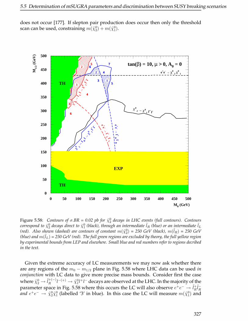
5.5 Determination of mSUGRA parameters and discrimination between SUSY breaking scenarios
does not occur [177]. If slepton pair production does occur then only the thresholdscan can be used, constraining m(χ0
2) +m(χ01).
M0 (GeV)
M1/
2 (G
eV)
tan(β) = 10, µ > 0, A0 = 0
e+e- → χ0 2 χ0 1
e+e
- → l + R l - R
e +e - →
l + L l - L
χ 0 2 → χ 0 1 l+ l -
χ0 2 →
l R l
→ χ
0 1 l
+ l-
χ0 2
→ l L
l →
χ0 1
l+ l
-
EXP
TH
TH1
2
3
4
7
5
6
1
3
2
6
4
5
0
50
100
150
200
250
300
350
400
450
500
0 50 100 150 200 250 300 350 400 450 500
EXP
TH
TH1
2
3
4
7
5
6
1
3
2
6
4
5
Figure 5.58: Contours of σ.BR = 0.02 pb for χ02 decays in LHC events (full contours). Contours
correspond to χ02 decays direct to χ0
1 (black), through an intermediate lR (blue) or an intermediate lL(red). Also shown (dashed) are contours of constant m(χ0
2) = 250 GeV (black), m(lR) = 250 GeV(blue) and m(lL) = 250 GeV (red). The full green regions are excluded by theory, the full yellow regionby experimental bounds from LEP and elsewhere. Small blue and red numbers refer to regions decribedin the text.
Given the extreme accuracy of LC measurements we may now ask whether thereare any regions of the m0 − m1/2 plane in Fig. 5.58 where LHC data can be used inconjunction with LC data to give more precise mass bounds. Consider first the case
where χ02 → l
+(−)R l−(+) → χ0
1l+l− decays are observed at the LHC. In the majority of the
parameter space in Fig. 5.58 where this occurs the LC will also observe e+e− → l+R l−R
and e+e− → χ02χ
01 (labelled ‘3’ in blue). In this case the LC will measure m(χ0
1) and
327

5 Supersymmetric Models
m(lR) from the dislepton channel and hence m(χ02) from an e+e− → χ0
2χ01 threshold
scan, with no input from the LHC. There is also a region (labelled ‘4’) where a LCwill see nothing and here there can be no input from LC data. In regions ‘1’ and ‘2’(hatched) however there is indeed complementarity between LHC and LC data. Inregion ‘1’ the LC measuresm(χ0
2) andm(χ01) which in turn allows the LHC to measure
m(lR). In region ‘2’ the LC measures m(lR) and m(χ01) enabling the LHC to measure
m(χ02). It should be noted that a LC could use the dilepton edge technique [172]
to gain independent sensitivity to m(lR) in region ‘1’, however in this case it is notclear that there would not still be an advantage to use of the high statistics LHC χ0
2
sample. In regions ‘5’ and ‘6’ the LHC can measure nothing as no dilepton signature isobserved (assuming an arbitrary 0.02 pb observation threshold) and only one channelis observed in LC data. In region ‘7’ no dilepton measurement channels are openeither at LHC or LC (although the LHC will still discover SUSY [178]).
Consider next the case where χ02 → l
+(−)L l−(+) → χ0
1l+l− decays are observed at the
LHC (red region). In region ‘1’ (hatched red) LHC and LC data is complementary be-cause the LC measures m(χ0
2)+m(χ01) from an e+e− → χ0
2χ01 threshold scan providing
input to LHC measurements of m(lL), m(χ02) and m(χ0
1) combinations. Note that here
constraints on m(lL) from LC dilepton edge measurements would be very difficultdue to dislepton SUSY background. In region ‘2’ (hatched red) the LC observes nei-
ther the e+e− → l+L l−L channel nor the e+e− → χ0
2χ01 channel but can still help the LHC
measure mass combinations involving m(lL) and m(χ02) by measuring m(χ0
1) using
e+e− → l+R l−R . In region ‘3’ the LC can measure m(χ0
1) and m(lL) from e+e− → l+L l−L
and hence m(χ02) from a e+e− → χ0
2χ01 threshold scan, with no LHC input, giving no
complementarity. In regions ‘4’, ‘5’ and ‘6’ the LC observes two channels, one chan-
nel or three channels respectively but the LHC sees no lL mediated χ02 decay. Again,
in a limited region of parameter space useful combined measurements significantlyimproving measurement accuracy can be carried out.
Consider finally the case where χ02 → χ0
1l+l− decays are observed at the LHC
(black). This region lies entirely within the LC reach in the e+e− → χ02χ
01 channel
and also the e+e− → χ02χ
02 and e+e− → χ+
1 χ−1 channels (not shown). The LC will
therefore be able to measure both m(χ02) and m(χ0
1) without reference to LHC dataand no additional input from the LHC will be required.
These results illustrate the scope for combined LC + LHC sparticle mass measure-ments for charged sleptons and lighter neutralinos. The regions of parameter spacewhere such an approach is applicable are admittedly rather limited but it must beremembered that these results were obtained using mSUGRA models with fixed val-ues of tan(β), A0 and sign(µ). While it is to be expected that similar behaviour willbe exhibited for other values of these parameters (although possibly modified at hightan(β) to take into account the large branching ratios to τ1 and τ2) very different phe-nomenology may occur in less constrained SUSY models. In these models combi-nation of results is still likely to be appropriate in regions where the LHC observes
two-body χ02 decay processes and the LC observes only e+e− → χ0
2χ01 or e+e− → l+l−
(but not both) however the size of these regions may be considerably enlarged. Fur-ther regions of interest may also arise where the LHC observes three-body χ0
2 decays
and the LC observes only e+e− → l+l− thereby providing input on m(χ01). Finally, in
less constrained models with different relationships between sparticle (e.g. gaugino)
328
5.5 Determination of mSUGRA parameters and discrimination between SUSY breaking scenarios
masses it may be advantageous to make use of LC χ01 mass measurements provided
by e.g. chargino or sneutrino decays.
5.5.1.3 Conclusions
The mSUGRA m0 −m1/2 plane has been mapped to identify regions in which com-bination of LHC and linear collider data can significantly improve the accuracy oflighter neutralino and charged slepton mass measurements.
5.5.2 Discriminating SUSY breaking scenarios
B.C. Allanach, D. Grellscheid and F. Quevedo
We approach the following questions: if supersymmetry is discovered, how can we select
among different supersymmetric extensions of the Standard Model? What observables best
distinguish the models and what is the required discriminating accuracy? We examine sce-
narios differing by the fundamental string scale and concentrate on GUT and intermediate
scale models. We scan over the parameters in each scenario, finding ratios of sparticle masses
that provide the maximum discrimination between them. The necessary accuracy for dis-
crimination is determined in each case. A future linear collider could provide the necessary
precision on slepton masses, whereas combined LHC and LC information could provide a
further check of the gluino to squark mass ratio.
5.5.2.1 Introduction
Supersymmetric (SUSY) phenomenology is notoriously complicated, and many stud-ies of experimental measurement capabilities have focused on individual points inthe parameter space (see, for example, SUSY studies in this document). Here, wewant to examine what is required to discriminate between different SUSY breakingscenarios, when the parameters within each are allowed to vary (as long as they agreewith current experimental data). By this we hope to provide guaranteed discrim-ination, whatever the parameter point, provided measurement accuracies are lowenough. The results we present here are updated versions of the ones in ref. [179],using a more up-to-date spectrum predictor: SOFTSUSY1.71[144].
Given that we need to scan over parameters in the scenarios we will consider, a de-tailed empirically-based analysis is unfeasible. The existence of SUSY backgroundsand signals depend crucially upon the part of MSSM parameter space one examines,thus it would be necessary to perform a separate study for each point in parameterspace. A more tractable analysis is followed: we try to find simple functions of spar-ticle masses that may be used to discriminate between some test scenarios. In thisinitial study, we examine sparticle mass ratios.
The three scenarios we choose to study are inspired by type I string models [180]:(1) String scale at the GUT scale MGUT ∼ O(1016) GeV, defined by the scale of elec-troweak gauge unification g1(MGUT ) = g2(MGUT ). (2) Intermediate string scale (MI =1011 GeV) with extra leptons to achieve gauge coupling unification at MI , which wewill refer to as early unification (EU) and (3) intermediate string scale (MI = 1011 GeV)
329

5 Supersymmetric Models
(a)
R1
R2
∆
∆
R
R
1
2
Model 1
Model 2
(b)
1.05
1.1
1.15
1.2
1.18 1.2 1.22 1.24 1.26 1.28 1.3
m~ g/
m~ q av
g
m~eL/m~eR
EUGUT
Mirage
Figure 5.59: Discriminating ratios and parameter scans: (a) schematic, (b) results of the scansfor the three scenarios considered.
with mirage unification [181] at MI . In scenarios (1) and (3), we assume that the low-energy effective field theory corresponds to the R-parity conserving MSSM. In orderto keep the volume of SUSY breaking parameter space manageable, we will here lookonly at the dilaton dominated limit of scenarios (1)-(3).
5.5.2.2 Discriminators
As advertised above, we use sparticle mass ratios to discriminate between models.Ratios rather than absolute masses are used in order to factor out dependence uponthe overall SUSY mass scale. Fig. 5.59a shows the idea: we expect each model toinhabit some closed 2-dimensional surface in the ratio space R1, R2. The “dis-tance” vector between the two regions is defined as the vector (∆R1,∆R2) where√
∆R21 + ∆R2
2, is minimised. It can only be defined when separation is achieved, iewhere the regions do not overlap. The distance vector is therefore the measurementaccuracy of the ratios R1,2 required to discriminate between the two models in allcases. In practice, we populate the regions with a random scan over parameter spacethat satisfy experimental constraints and do not have sparticles heavier than a fewTeV (see ref. [179] for details).
We achieve separation, as shown in figure 5.59b. The distance ratios here are shownto be (∆[mg/mqavq ],∆[meL
/meR]) = (0.03, 0.04) to discriminate EU and mirage scenar-
ios, (0.02, 0.07) to discriminate the EU and GUT scenarios and (0.05, 0.03) to discrim-inate between the GUT and mirage scenarios, in their respective dilaton-dominatedlimits. mqavg is an average over the first two generations’ squark masses.
5.5.2.3 Conclusions
We have examined three test SUSY breaking scenarios in the MSSM, finding discrim-inating ratios of sparticle masses. Simple combinations of two ratios can discriminateall three scenarios. The percent-level accuracies required indicate a rough level forthe desired accuracy upon sparticle masses. The combined experimental and theo-retical [169] errors should therefore not be larger than the percent-level in order to
330

5.5 Determination of mSUGRA parameters and discrimination between SUSY breaking scenarios
achieve discrimination. 3% accuracies on the measurements of meL/meR
would be re-quired in order to always discriminate between the scenarios. Such a precision shouldbe readily available at a future LC facility that has polarised beams. We require max-imum errors of 2% on mg/mqavq for discrimination. At the LHC, errors upon mg ormqav are expected to be of order 10%, too high for our purposes. At a 500 GeV LC onthe other hand, it is difficult to produce squarks and gluinos because they are typi-cally kinematically inaccessible. However a few-percent uncertainty upon the ratiomight be feasible if LC information on slepton and weak gaugino masses is fed intoan LHC analysis. New techniques to study discrimination in models which departfrom dilaton domination are currently underway [182].
5.5.3 Gravitino and goldstino at colliders
W. Buchmuller, K. Hamaguchi, M. Ratz and T. Yanagida
We consider theories with spontaneously broken global or local supersymmetry where the
pseudo-goldstino or the gravitino is the lightest superparticle (LSP). Assuming that the long-
lived next-to-lightest superparticle (NSP) is a charged slepton, we study several supergrav-
ity predictions: the NSP lifetime, angular and energy distributions in 3-body NSP decays.
The characteristic couplings of the gravitino, or goldstino, can be tested even for very small
masses.
Introduction
The discovery of supersymmetry at the Tevatron, the LHC or a future Linear Colliderwould raise the question how supersymmetry is realized in nature. Clearly, super-symmetry is broken. Spontaneously broken global supersymmetry would predict theexistence of a spin-1/2 goldstino (χ) whereas the theoretically favoured case of localsupersymmetry requires a massive spin-3/2 gravitino (ψ3/2).
In a recent paper [183] we have studied how a massive gravitino, if it is the lightestsuperparticle (LSP), may be discovered in decays of τ , the scalar τ lepton, whichis naturally the next-to-lightest superparticle (NSP). The determination of gravitinomass and spin appears feasible for gravitino masses in the range from about 1 GeV to100 GeV. As we shall discuss in this note, evidence for the characteristic couplings ofa pseudo-goldstino, which corresponds to the spin-1/2 part of the gravitino, can beobtained even for masses much smaller than 1 GeV.
The gravitino mass depends on the mechanism of supersymmetry breaking. It canbe of the same order as other superparticle masses, like in gaugino mediation [184]or gravity mediation [185]. But it might also be much smaller as in gauge mediationscenarios [186]. As LSP, the gravitino is an attractive dark matter candidate [187].
The τ NSP has generally a long lifetime because of the small, Planck scale sup-pressed coupling to the gravitino LSP. The production of charged long-lived heavyparticles at colliders is an exciting possibility [188]. They can be directly produced inpairs or in cascade decays of heavier superparticles. In the context of models withgauge mediated supersymmetry breaking the production of slepton NSPs has previ-ously studied for the Tevatron [189], for the LHC [190] and for a Linear Collider [191].
331
5 Supersymmetric Models
The dominant τ NSP decay channel is τ → τ +missing energy. In the following weshall study how to identify the gravitino or goldstino as carrier of the missing energy.First, one will measure the NSP lifetime. Since the gravitino couplings are fixed bysymmetry, the NSP lifetime is predicted by supergravity given the gravitino mass,which can be inferred from kinematics. Second, one can make use of the 3-body NSPdecay τ → τ +γ+X where X = ψ3/2 or X = χ. The angular and energy distributionsand the polarizations of the final state photon and lepton carry the information on thespin and couplings of gravitino or goldstino.
For gravitino masses in the range from about 10 keV to 100 GeV, the NSP is essen-tially stable for collider experiments, and one has to accumulate the NSPs to studytheir decay. Sufficiently slow, strongly ionizing sleptons will be stopped within thedetector. One may also be able to collect faster sleptons in a storage ring. For grav-itino masses less than O(10 keV) the τ can decay inside the detector, which may beadvantageous from the experimental point of view.
At LHC one expects O(106) NSPs per year which are mainly produced in cascadedecays of squarks and gluinos [192]. The NSPs are mostly produced in the forwarddirection [193] which should make it easier to accumulate τs in a storage ring. In aLinear Collider an integrated luminosity of 500 fb−1 will yield O(105) τs [10]. Notethat, in a Linear Collider, one can also tune the velocity of the produced τs by adjust-ing the e+e− center-of-mass energy. A detailed study of the possibilities to accumu-late τ NSPs is beyond the scope of this note. In the following we shall assume that asufficiently large number of τs can be produced and collected.
This study is strongly based on Ref. [183]. Here, we discuss in more detail thecase of a very light gravitino, or pseudo-goldstino, for which the τ NSP can decayinside the detector. Although in this case it is difficult to determine mass and spinof the gravitino, one can still see the characteristic coupling of the gravitino, which isessentially the goldstino coupling, via the 3-body decay τ → τ + γ+X with X = ψ3/2
or X = χ.
Planck mass from τ decays
The τ decay rate is dominated by the two-body decay into τ and gravitino,
Γ2−bodyτ =
(m2τ −m2
3/2 −m2τ
)4
48πm23/2 M
2Pm
3τ
1−
4m23/2 m
2τ(
m2τ −m2
3/2 −m2τ
)2
3/2
, (5.105)
where MP = (8πGN)−1/2 denotes the reduced Planck mass, mτ = 1.78 GeV is the τmass, mτ is the τ mass, and m3/2 is the gravitino mass. For instance, mτ = 150 GeVand m3/2 = 10 keV leads to a lifetime of Γ−1
τ ≃ 7.8 × 10⁻⁷ s, and mτ = 150 GeV andm3/2 = 75 GeV results in Γ−1
τ ≃ 4.4 y.Since the decay rate depends only on two unknown masses mτ and m3/2, indepen-
dently of other SUSY parameters, gauge and Yukawa couplings, it is possible to testthe prediction of the supergravity if one can measure these masses. The mass mτ
of the NSP will be measured in the process of accumulation. Although the outgoinggravitino is not directly measurable, its mass can also be inferred kinematically unless
332

5.5 Determination of mSUGRA parameters and discrimination between SUSY breaking scenarios
it is too small,
m23/2 = m2
τ +m2τ − 2mτEτ . (5.106)
The gravitino mass can be determined with the same accuracy as Eτ and mτ , i.e. withan uncertainty of a few GeV.
Once the masses mτ and m3/2 are measured, one can compare the predicted decayrate (5.105) with the observed decay rate, thereby testing an important supergravityprediction. In other words, one can determine the ‘supergravity Planck scale’ fromthe NSP decay rate which yields, up to O(α) corrections,
M2P(supergravity) =
(m2τ −m2
3/2 −m2τ
)4
48πm23/2 m
3τ Γτ
1−
4m23/2 m
2τ(
m2τ −m2
3/2 −m2τ
)2
3/2
.(5.107)
The result can be compared with the Planck scale of Einstein gravity, i.e. Newton’sconstant determined by macroscopic measurements, GN = 6.707(10) · 10−39 GeV−2
[194],
M2P(gravity) = (8πGN)−1 = (2.436(2) · 1018 GeV)2 . (5.108)
The consistency of the microscopic and macroscopic determinations of the Planckscale is an unequivocal test of supergravity.
Note that the measurement of the gravitino mass yields another important quantityin supergravity, the mass scale of spontaneous supersymmetry breaking MSUSY =√√
3MPm3/2. This is the analogue of the Higgs vacuum expectation value v in the
electroweak theory, where v =√
2mW/g = (2√
2GF)−1/2.
Gravitino and goldstino versus neutralino
If the measured decay rate and the kinematically determined mass of the invisibleparticle are consistent with Eq. (5.105), one already has strong evidence for super-gravity and the gravitino LSP. To analyze the couplings of the invisible particle, onecan study the 3-body decay τ → τ + γ + X for the gravitino X = ψ3/2 and compareit with the case where X is a hypothetical spin-1/2 neutralino. This is of particu-lar importance if the mass of the invisible particle is so small that the supergravityprediction for the NSP lifetime, as described in the previous section, cannot be tested.
The NSP τ is in general a linear combination of τR and τL, the superpartners of theright-handed and left-handed τ leptons τR and τL, respectively. The interaction of thegravitino ψ3/2 with scalar and fermionic τ leptons is described by the lagrangian [195],
L3/2 = − 1√2MP
[(Dν τR)∗ψµ γν γµ PRτ + (Dν τR) τPLγµ γ
ν ψµ], (5.109)
where Dν τR = (∂ν + ieAν)τR and Aν denotes the gauge boson. The interaction la-grangian of τL has an analogous form.
333
5 Supersymmetric Models
As an example for the coupling of a hypothetical spin-1/2 neutralino to τ and τ ,we consider the Yukawa interaction10,
LYukawa = h(τ ∗R λPR τ + τ ∗L λPL τ
)+ h.c. . (5.110)
Note that for very small coupling h, the τ decay rate could accidentally be consistentwith the supergravity prediction Eq. (5.105).
Also the goldstino χ has Yukawa couplings of the type given in Eq. (5.110). The full
interaction lagrangian is obtained by performing the substitution ψµ →√
23
1m3/2
∂µχ
in the supergravity lagrangian. The non-derivative form of the effective lagrangianfor χ is given by [196],
Leff =m2τ√
3MP m3/2
(τ ∗R χPR τ + τR τ PL χ)− mγ
4√
6MPm3/2
χ[γµ, γν ] γ Fµν , (5.111)
where we have neglected a quartic interaction term which is irrelevant for our dis-cussion. In the following, we consider a massive pseudo-goldstino χ, in order tocompare it with the massive gravitino and neutralino. Like a pseudo-Goldstone bo-son, the pseudo-goldstino has goldstino couplings and a mass which explicitly breaksglobal supersymmetry.
Note that the goldstino coupling to the photon supermultiplet is proportional tothe photino mass mγ . As a consequence, the contribution to 3-body τ -decay withintermediate photino (cf. Fig. 5.60(c)) is not suppressed for very large photino masses.As we shall see, this leads to significant differences between the angular distributionsfor pure Yukawa and goldstino couplings, even when χ and λ are very light.
In τ decays both, photon and τ lepton will mostly be very energetic. Hence the pho-ton energy Eγ and the angle θ between τ and γ can be well measured (cf. Fig. 5.61(a)).We can then compare the differential decay rate
∆(Eγ, cos θ) =1
αΓτ
d2Γ(τ → τ + γ +X)
dEγ d cos θ, (5.112)
for the gravitino LSP (X = ψ3/2), the pseudo-goldstino (X = χ) and the hypotheticalneutralino (X = λ). Details of the calculation are given in Ref. [183]. The differencesbetween ψ3/2, χ and λ become significant in the backward direction (cos θ < 0) asdemonstrated by Fig. 5.61 (b)-(d), where mτ = 150 GeV and mX = 75 GeV (X =ψ3/2, χ, λ). The three differential distributions are qualitatively different and shouldallow to distinguish experimentally gravitino, goldstino and neutralino.
Let us now consider the case of small mX . Then the goldstino lagrangian (5.111)effectively describes the gravitino interactions. Therefore, one can no longer distin-guish between gravitino and goldstino in this case. However, even for small mX onecan discriminate the gravitino or goldstino from the neutralino. The difference be-tween goldstino χ and neutralino λ stems from the photino contribution (cf. Fig. 5.60(c))which does not decouple for large photino mass mγ . This is different from the grav-itino case where the analogous diagram becomes irrelevant in the limit mγ ≫ mτ
which is employed throughout this study.
10This interaction would arise from gauging the anomaly free U(1) symmetry Lτ − Lµ, the difference
of τ - and µ-number, in the MSSM, with λ being the gaugino.
334
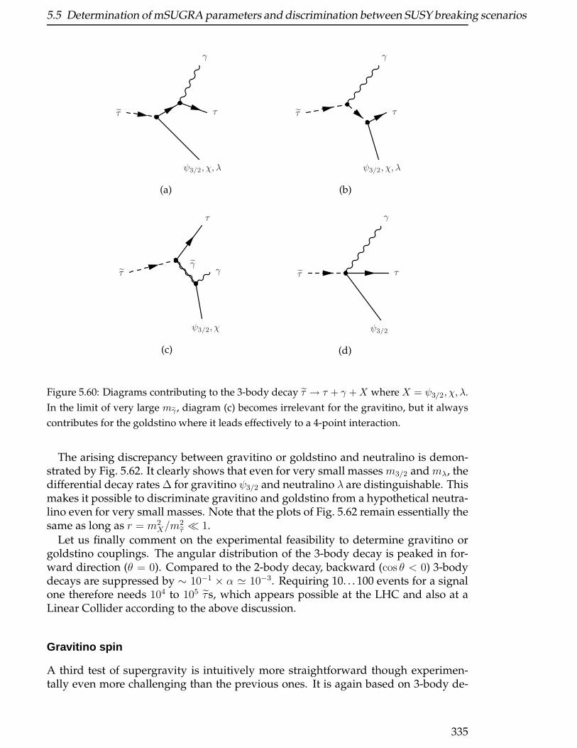
5.5 Determination of mSUGRA parameters and discrimination between SUSY breaking scenarios
τ
ψ3/2, χ, λ
τ
γ
(a)
τ
ψ3/2, χ, λ
τ
γ
(b)
γτ
ψ3/2, χ
γ
τ
(c)
τ
ψ3/2
τ
γ
(d)
Figure 5.60: Diagrams contributing to the 3-body decay τ → τ + γ +X where X = ψ3/2, χ, λ.
In the limit of very large mγ , diagram (c) becomes irrelevant for the gravitino, but it always
contributes for the goldstino where it leads effectively to a 4-point interaction.
The arising discrepancy between gravitino or goldstino and neutralino is demon-strated by Fig. 5.62. It clearly shows that even for very small masses m3/2 and mλ, thedifferential decay rates ∆ for gravitino ψ3/2 and neutralino λ are distinguishable. Thismakes it possible to discriminate gravitino and goldstino from a hypothetical neutra-lino even for very small masses. Note that the plots of Fig. 5.62 remain essentially thesame as long as r = m2
X/m2τ ≪ 1.
Let us finally comment on the experimental feasibility to determine gravitino orgoldstino couplings. The angular distribution of the 3-body decay is peaked in for-ward direction (θ = 0). Compared to the 2-body decay, backward (cos θ < 0) 3-bodydecays are suppressed by ∼ 10−1 × α ≃ 10−3. Requiring 10. . . 100 events for a signalone therefore needs 104 to 105 τs, which appears possible at the LHC and also at aLinear Collider according to the above discussion.
Gravitino spin
A third test of supergravity is intuitively more straightforward though experimen-tally even more challenging than the previous ones. It is again based on 3-body de-
335
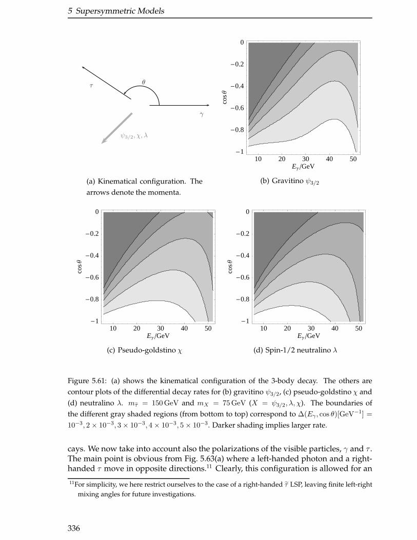
5 Supersymmetric Models
τ
ψ3/2, χ, λ
γ
θ
(a) Kinematical configuration. The
arrows denote the momenta.
10 20 30 40 50EΓ GeV
-1
-0.8
-0.6
-0.4
-0.2
0
cosΘ
(b) Gravitino ψ3/2
10 20 30 40 50EΓ GeV
-1
-0.8
-0.6
-0.4
-0.2
0
cosΘ
(c) Pseudo-goldstino χ
10 20 30 40 50EΓ GeV
-1
-0.8
-0.6
-0.4
-0.2
0
cosΘ
(d) Spin-1/2 neutralino λ
Figure 5.61: (a) shows the kinematical configuration of the 3-body decay. The others are
contour plots of the differential decay rates for (b) gravitino ψ3/2, (c) pseudo-goldstino χ and
(d) neutralino λ. mτ = 150GeV and mX = 75GeV (X = ψ3/2, λ, χ). The boundaries of
the different gray shaded regions (from bottom to top) correspond to ∆(Eγ , cos θ)[GeV−1] =
10−3, 2× 10⁻³, 3× 10⁻³, 4× 10⁻³, 5× 10⁻³. Darker shading implies larger rate.
cays. We now take into account also the polarizations of the visible particles, γ and τ .The main point is obvious from Fig. 5.63(a) where a left-handed photon and a right-handed τ move in opposite directions.11 Clearly, this configuration is allowed for an
11For simplicity, we here restrict ourselves to the case of a right-handed τ LSP, leaving finite left-right
mixing angles for future investigations.
336

5.5 Determination of mSUGRA parameters and discrimination between SUSY breaking scenarios
10 20 30 40 50 60 70EΓ GeV
-1
-0.8
-0.6
-0.4
-0.2
0co
sΘ
(a) Gravitino/goldstino
10 20 30 40 50 60 70EΓ GeV
-1
-0.8
-0.6
-0.4
-0.2
0
cosΘ
(b) Neutralino
Figure 5.62: Contour plots of the differential decay rates for (a) gravitino ψ3/2 and (b) neutra-
lino λ. mτ = 150GeV, mX = 0.1 GeV (X = ψ3/2, λ). The figures remain essentially the same
as long as r = m2X/m
2τ ≪ 1. The contours have the same meaning as in Fig. 5.61.
invisible spin-3/2 gravitino but it is forbidden for a spin-1/2 goldstino or neutralino.Unfortunately, measuring the polarizations is a difficult task.
As Fig. 5.63(a) illustrates, the spin of the invisible particle influences the angulardistribution of final states with polarized photons and τ leptons. An appropriateobservable is the angular asymmetry
ARL(cos θ) =
dΓ
d cos θ(τR → τR + γR +X)− dΓ
d cos θ(τR → τR + γL +X)
dΓ
d cos θ(τR → τR + γR +X) +
dΓ
d cos θ(τL → τR + γL +X)
, (5.113)
where X denotes gravitino (X = ψ3/2), goldstino (X = χ) or neutralino (X = λ). Notethat, as discussed before, the photino does not decouple in the case X = χ.
The three angular asymmetries are shown in Fig. 5.63 for mτ = 150 GeV and differ-ent masses of the invisible particle. As expected, the decay into right-handed τ andleft-handed photon at θ = π is forbidden for spin-1/2 invisible particles (χ and λ),whereas it is allowed for the spin-3/2 gravitino. This is clearly visible in Figs. 5.63(c)and (d); for small gravitino masses the goldstino component dominates the gravitinointeraction as illustrated by Fig. 5.63(b). The discrepancy between gravitino and gold-stino compared to a hypothetical neutralino persists for arbitrarily small mX , whichis analogous to the double differential distribution discussed in the previous section.
Conclusions
We have discussed how one may discover a massive gravitino, and thereby super-gravity, at the LHC or a future Linear Collider, if the gravitino is the LSP and a
337

5 Supersymmetric Models
γτ
θ = π
(a) Characteristic spin-3/2 process.
The thick arrows represent the spins.
-1 -0.5 0 0.5cosΘ
0.2
0.4
0.6
0.8
1
AR
LHc
osΘL
(b) mX = 10GeV.
-1 -0.5 0 0.5cosΘ
0.2
0.4
0.6
0.8
1
AR
LHc
osΘL
(c) mX = 30GeV.
-1 -0.5 0 0.5cosΘ
0.2
0.4
0.6
0.8
1
AR
LHc
osΘL
(d) mX = 75GeV.
Figure 5.63: (a) illustrates the characteristic spin-3/2 process: photon and τ lepton move in
opposite directions and the spins add up to 3/2, so the invisible particle also has spin 3/2. The
other figures show angular asymmetries for gravitino ψ3/2 (solid curve), goldstino χ (dashed
curve) and neutralino λ (dotted curve). mτ = 150GeV. The photon energy is larger than 10%
of the maximal kinematically allowed energy (cf. Ref. [183]). Note that the asymmetries only
depend on the ratio r = m2X/m
2τ (X = ψ3/2, χ, λ).
charged slepton is the NSP. With the gravitino mass inferred from kinematics, themeasurement of the NSP lifetime will test an unequivocal prediction of supergrav-ity. The analysis of 3-body NSP decays will reveal the couplings of the gravitino
338
5.5 Determination of mSUGRA parameters and discrimination between SUSY breaking scenarios
or the goldstino. For very small masses, one can distinguish the gravitino from theneutralino but not from the goldstino. For masses larger than about 1 GeV, the deter-mination of gravitino mass and spin appears feasible.
5.5.4 Reconstructing supersymmetric theories by coherent LHC
/ LC analyses
B.C. Allanach, G.A. Blair, S. Kraml, H.-U. Martyn, G. Polesello, W. Porod, P.M. Zerwas
Supersymmetry analyses will potentially be a central area for experiments at the LHC and
at a future e+e− linear collider. Results from the two facilities will mutually complement
and augment each other so that a comprehensive and precise picture of the supersymmetric
world can be developed. We will demonstrate in this report how coherent analyses at LHC
and LC experiments can be used to explore the breaking mechanism of supersymmetry and
to reconstruct the fundamental theory at high energies, in particular at the grand unification
scale. This will be exemplified for minimal supergravity in detailed experimental simulations
performed for the Snowmass reference point SPS1a.
5.5.4.1 Physics Base
The roots of standard particle physics are expected to go as deep as the Planck lengthof 10−33 cm where gravity is intimately linked to the particle system. A stable bridgebetween the electroweak energy scale of 100 GeV and the vastly different Planck scaleof ΛPL ∼ 1019 GeV, and the (nearby) grand unification scale ΛGUT ∼ 1016 GeV, is pro-vided by supersymmetry. If this scenario is realized in nature, experimental methodsmust be developed to shed light on the physics phenomena near ΛGUT/ΛPL. Amongother potential tools, the extrapolation of supersymmetry (SUSY) parameters mea-sured at the LHC and an e+e− linear collider with high precision, can play a centralrole [197]. A rich ensemble of gauge and Yukawa couplings, and of gaugino/higgsinoand scalar particle masses allows the detailed study of the supersymmetry breakingmechanism and the reconstruction of the physics scenario near the GUT/PL scale.
The reconstruction of physical structures at energies more than fourteen ordersabove the energies available through accelerators is a demanding task. Not only musta comprehensive picture be delineated near the electroweak scale, but the picturemust be drawn, moreover, as precisely as possible to keep the errors small enough sothat they do not blow up beyond control when the SUSY parameters are extrapolatedover many orders of magnitude. The LHC [198] and a future e+e− linear collider(LC) [199] are a perfect tandem for solving such a problem: (i) While the coloredsupersymmetric particles, gluinos and squarks, can be generated with large rates formasses up to 2 to 3 TeV at the LHC, the strength of e+e− linear colliders is the compre-hensive coverage of the non-colored particles, charginos/neutralinos and sleptons. Ifthe extended Higgs spectrum is light, the Higgs particles can be discovered and in-vestigated at both facilities; heavy Higgs bosons can be produced at the LHC in amajor part of the parameter space; at an e+e− collider, without restriction, for massesup to the beam energy; (ii) If the analyses are performed coherently, the accuracies inmeasurements of cascade decays at LHC and in threshold production as well as de-
339

5 Supersymmetric Models
cays of supersymmetric particles at LC complement and augment each other mutuallyso that a high-precision picture of the supersymmetric parameters at the electroweakscale can be drawn. Such a comprehensive and precise picture is necessary in orderto carry out the evolution of the supersymmetric parameters to high scales, driven byperturbative loop effects that involve the entire supersymmetric particle spectrum.
Minimal supergravity (mSUGRA) provides us with a scenario within which thesegeneral ideas can be quantified. The form of this theory has been developed in greatdetail, creating a platform on which semi-realistic experimental studies can be per-formed. Supersymmetry is broken in mSUGRA in a hidden sector and the breakingis transmitted to our eigenworld by gravity [200]. This mechanism suggests, yet doesnot enforce, the universality of the soft SUSY breaking parameters – gaugino andscalar masses, and trilinear couplings – at a scale that is generally identified withthe unification scale. The (relatively) small number of parameters renders mSUGRAa well-constrained system that suggests itself in a natural way as a test ground forcoherent experimental analyses at LHC and LC. The procedure will be exemplifiedfor a specific set of parameters, defined as SPS1a among the Snowmass referencepoints [1, 4].
5.5.4.2 Minimal Supergravity: SPS1a
The mSUGRA Snowmass reference point SPS1a is characterised by the following val-ues [1, 4]:
M1/2 = 250 GeV M0 = 100 GeVA0 = −100 GeV sign(µ) = +tanβ = 10
(5.114)
for the universal gaugino mass M1/2, the scalar mass M0, the trilinear coupling A0,the sign of the higgsino parameter µ, and tanβ, the ratio of the vacuum-expectationvalues of the two Higgs fields. As the modulus of the Higgsino parameter is fixedat the electroweak scale by requiring radiative electroweak symmetry breaking, µ isfinally given by:
µ = 357.4 GeV (5.115)
This reference point is compatible with the constraints from low-energy precisiondata, predicting BR(b→ sγ) = 2.7 ·10−4 and ∆[gµ−2] = 17 ·10−10. The amount of colddark matter is, with Ωχh
2 = 0.18, on the high side but still compatible with recentWMAP data [201] if evaluated on their own without reference to other experimentalresults; moreover, only a slight shift in M0 downwards drives the value to the centralband of the data while such a shift does not alter any of the conclusions in this reportin a significant way.
In the SPS1a scenario the squarks and gluinos can be studied very well at the LHCwhile the non-colored gauginos and sleptons can be analyzed partly at LHC and incomprehensive form at an e+e− linear collider operating at a total energy below 1 TeVwith high integrated luminosity close to 1 ab−1.
The masses can best be obtained at LHC by analyzing edge effects in the cascadedecay spectra. The basic starting point is the identification of the a sequence of two-
body decays: qL → χ02q → ℓRℓq → χ0
1ℓℓq. This is effected through the detection of an
340
5.5 Determination of mSUGRA parameters and discrimination between SUSY breaking scenarios
edge structure of the invariant mass of opposite-sign same-flavour leptons from theχ0
2 decay in events with multi-jets and EmissT . One can then measure the kinematic
edges of the invariant mass distributions among the two leptons and the jet resultingfrom the above chain, and thus an approximately model-independent determinationof the masses of the involved sparticles is obtained. This technique was developedin Refs. [11, 202] and is worked out in detail for point SPS1a in Ref. [203]. The four
sparticle masses (qL, χ02, ℓR, and χ0
1) thus measured are used as an input to additionalanalyses which rely on the knowledge of the masses of the lighter gauginos in orderto extract masses from the observed kinematic structures. Examples are the studies of
the decay g → b1b→ χ02bb, where the reconstruction of the gluino and sbottom mass
peaks relies on an approximate full reconstruction of the χ02, and the shorter decay
chains qR → qχ01 and χ0
4 → ℓℓ, which require the knowledge of the sparticle massesdownstream of the cascade. For SPS1a the heavy Higgs bosons can also be searchedfor in the decay chain: A0 → χ0
2χ02 → χ0
1χ01l
+l−l+l− [204]. The invariant four-leptonmass depends sensitively onmA0 andmχ0
1. The same holds true forH0. Note however
that the main source of the neutralino final states are A0 decays, and that the twoHiggs bosons A0 and H0 cannot be discriminated in this channel.
The mass measurements obtained at the LHC are thus very correlated among them-selves, and this correlation must be taken into account in the fitting procedure. An-other source of correlation comes from the fact that in most cases the uncertainty onthe mass measurement is dominated by the systematic uncertainty on the hadronicenergy scale of the experiment, which will affect all the measurements involving jetsapproximately by the same amount and in the same direction.
At linear colliders very precise mass values can be extracted from decay spectraand threshold scans [205–207]. The excitation curves for chargino production in S-waves [208] rise steeply with the velocity of the particles near the threshold and thusare very sensitive to their mass values; the same is true for mixed-chiral selectronpairs in e+e− → e+R e
−L and for diagonal pairs in e−e− → e−Re
−R, e
−L e
−L collisions [207].
Other scalar sfermions, as well as neutralinos, are produced generally in P-waves,with a somewhat less steep threshold behaviour proportional to the third power ofthe velocity [207,209]. Additional information, in particular on the lightest neutralinoχ0
1, can be obtained from decay spectra.
Typical mass parameters and the related measurement errors are presented in Ta-ble 5.40. The column denoted “LHC” collects the errors from the LHC analysis, thecolumn “LC” the errors expected from the LC operating at energies up to 1 TeV withan integrated luminosity of ∼ 1 ab−1. The error estimates are based on detector sim-ulations for the production of the light sleptons, eR, µR and τ1, in the continuum. Forthe light neutralinos and the light chargino threshold scans have been simulated. De-tails will be given elsewhere; see also Ref. [210]. The expected precision of the otherparticle masses is taken from Ref. [207], or it is obtained by scaling the LC errors fromthe previous analysis in Ref. [205], taking into account the fact that the χ0/χ± cascadedecays proceed dominantly via τ leptons in the reference point SPS1a, which is ex-perimentally challenging. The third column of Tab. 5.40 denoted “LHC+LC” presentsthe corresponding errors if the experimental analyses are performed coherently, i.e.the light particle spectrum, studied at LC with very high precision, is used as an inputset for the LHC analysis.
341
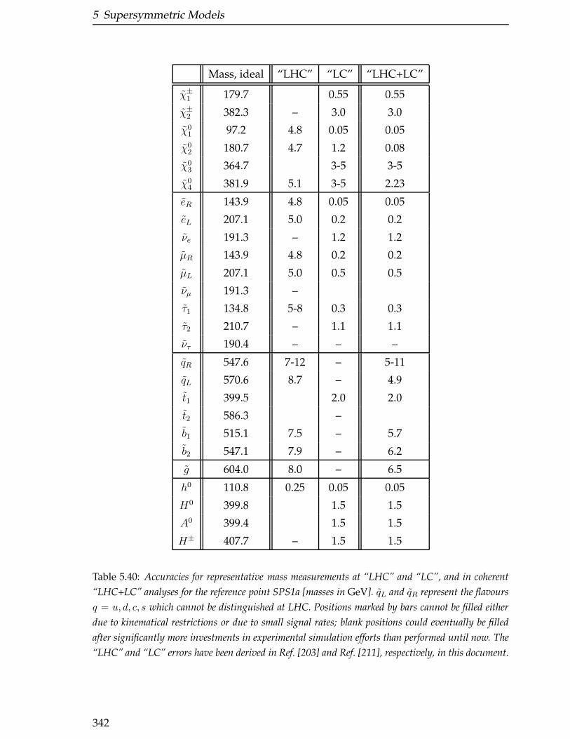
5 Supersymmetric Models
Mass, ideal “LHC” “LC” “LHC+LC”
χ±1 179.7 0.55 0.55
χ±2 382.3 – 3.0 3.0
χ01 97.2 4.8 0.05 0.05
χ02 180.7 4.7 1.2 0.08
χ03 364.7 3-5 3-5
χ04 381.9 5.1 3-5 2.23
eR 143.9 4.8 0.05 0.05
eL 207.1 5.0 0.2 0.2
νe 191.3 – 1.2 1.2
µR 143.9 4.8 0.2 0.2
µL 207.1 5.0 0.5 0.5
νµ 191.3 –
τ1 134.8 5-8 0.3 0.3
τ2 210.7 – 1.1 1.1
ντ 190.4 – – –
qR 547.6 7-12 – 5-11
qL 570.6 8.7 – 4.9
t1 399.5 2.0 2.0
t2 586.3 –
b1 515.1 7.5 – 5.7
b2 547.1 7.9 – 6.2
g 604.0 8.0 – 6.5
h0 110.8 0.25 0.05 0.05
H0 399.8 1.5 1.5
A0 399.4 1.5 1.5
H± 407.7 – 1.5 1.5
Table 5.40: Accuracies for representative mass measurements at “LHC” and “LC”, and in coherent
“LHC+LC” analyses for the reference point SPS1a [masses in GeV]. qL and qR represent the flavours
q = u, d, c, s which cannot be distinguished at LHC. Positions marked by bars cannot be filled either
due to kinematical restrictions or due to small signal rates; blank positions could eventually be filled
after significantly more investments in experimental simulation efforts than performed until now. The
“LHC” and “LC” errors have been derived in Ref. [203] and Ref. [211], respectively, in this document.
342
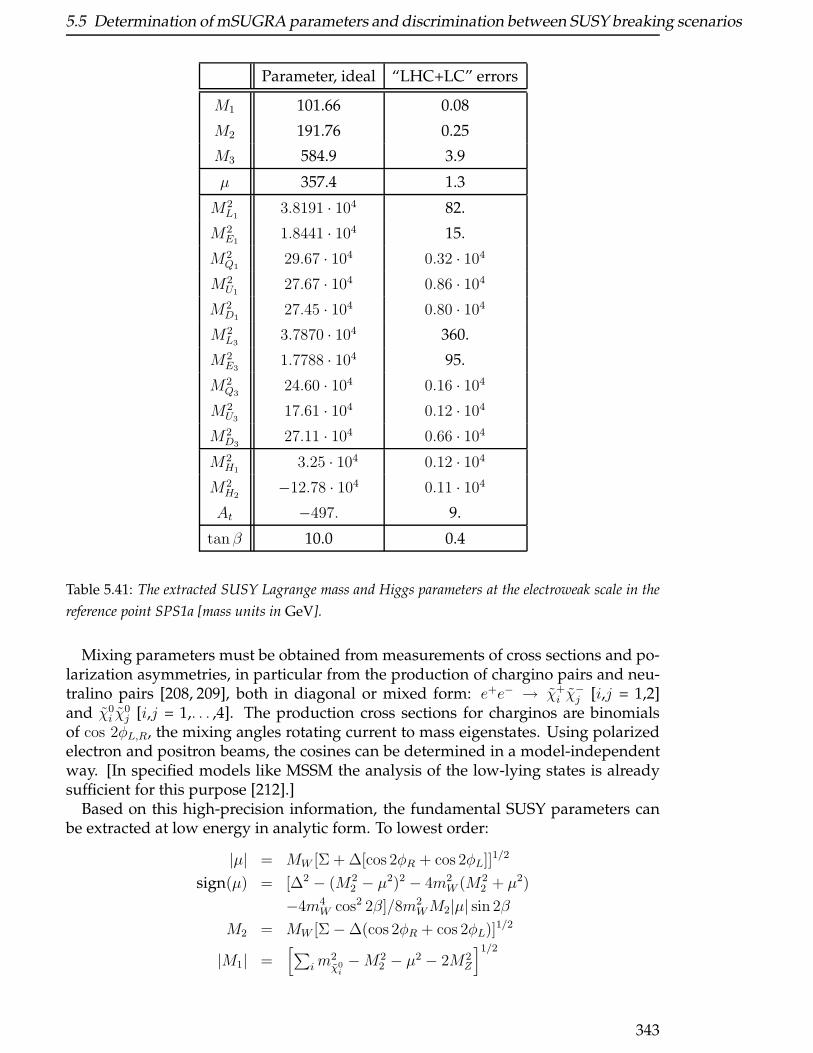
5.5 Determination of mSUGRA parameters and discrimination between SUSY breaking scenarios
Parameter, ideal “LHC+LC” errors
M1 101.66 0.08
M2 191.76 0.25
M3 584.9 3.9
µ 357.4 1.3
M2L1
3.8191 · 104 82.
M2E1
1.8441 · 104 15.
M2Q1
29.67 · 104 0.32 · 104
M2U1
27.67 · 104 0.86 · 104
M2D1
27.45 · 104 0.80 · 104
M2L3
3.7870 · 104 360.
M2E3
1.7788 · 104 95.
M2Q3
24.60 · 104 0.16 · 104
M2U3
17.61 · 104 0.12 · 104
M2D3
27.11 · 104 0.66 · 104
M2H1
3.25 · 104 0.12 · 104
M2H2
−12.78 · 104 0.11 · 104
At −497. 9.
tan β 10.0 0.4
Table 5.41: The extracted SUSY Lagrange mass and Higgs parameters at the electroweak scale in the
reference point SPS1a [mass units in GeV].
Mixing parameters must be obtained from measurements of cross sections and po-larization asymmetries, in particular from the production of chargino pairs and neu-tralino pairs [208, 209], both in diagonal or mixed form: e+e− → χ+
i χ−j [i,j = 1,2]
and χ0i χ
0j [i,j = 1,. . . ,4]. The production cross sections for charginos are binomials
of cos 2φL,R, the mixing angles rotating current to mass eigenstates. Using polarizedelectron and positron beams, the cosines can be determined in a model-independentway. [In specified models like MSSM the analysis of the low-lying states is alreadysufficient for this purpose [212].]
Based on this high-precision information, the fundamental SUSY parameters canbe extracted at low energy in analytic form. To lowest order:
|µ| = MW [Σ + ∆[cos 2φR + cos 2φL]]1/2
sign(µ) = [∆2 − (M22 − µ2)2 − 4m2
W (M22 + µ2)
−4m4W cos2 2β]/8m2
WM2|µ| sin 2β
M2 = MW [Σ−∆(cos 2φR + cos 2φL)]1/2
|M1| =[∑
im2χ0
i−M2
2 − µ2 − 2M2Z
]1/2
343
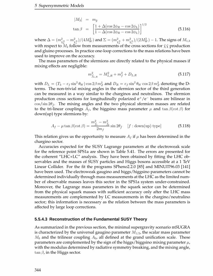
5 Supersymmetric Models
|M3| = mg
tanβ =
[1 + ∆(cos 2φR − cos 2φL)
1−∆(cos 2φR − cos 2φL)
]1/2
(5.116)
where ∆ = (m2χ±
2−m2
χ±
1)/(4M2
W ) and Σ = (m2χ±
2+m2
χ±
1)/(2M2
W )− 1. The signs of M1,3
with respect to M2 follow from measurements of the cross sections for χχ productionand gluino processes. In practice one-loop corrections to the mass relations have beenused to improve on the accuracy.
The mass parameters of the sfermions are directly related to the physical masses ifmixing effects are negligible:
m2fL,R
= M2L,R +m2
f +DL,R (5.117)
with DL = (T3 − ef sin2 θW ) cos 2βm2Z and DR = ef sin2 θW cos 2β m2
Z denoting the D-terms. The non-trivial mixing angles in the sfermion sector of the third generationcan be measured in a way similar to the charginos and neutralinos. The sfermionproduction cross sections for longitudinally polarized e+/e− beams are bilinear incos/sin 2θf . The mixing angles and the two physical sfermion masses are relatedto the tri-linear couplings Af , the higgsino mass parameter µ and tan β(cotβ) fordown(up) type sfermions by:
Af − µ tanβ(cotβ) =m2f1−m2
f2
2mfsin 2θf [f : down(up) type] (5.118)
This relation gives us the opportunity to measure Af if µ has been determined in thechargino sector.
Accuracies expected for the SUSY Lagrange parameters at the electroweak scalefor the reference point SPS1a are shown in Table 5.41. The errors are presented forthe coherent “LHC+LC” analysis. They have been obtained by fitting the LHC ob-servables and the masses of SUSY particles and Higgs bosons accessible at a 1 TeVLinear Collider. For the fit the programs SPheno2.2.0 [85] and MINUIT96.03 [141]have been used. The electroweak gaugino and higgs/higgsino parameters cannot bedetermined individually through mass measurements at the LHC as the limited num-ber of observable masses leaves this sector in the SPS1a system under-constrained.Moreover, the Lagrange mass parameters in the squark sector can be determinedfrom the physical squark masses with sufficient accuracy only after the LHC massmeasurements are complemented by LC measurements in the chargino/neutralinosector; this information is necessary as the relation between the mass parameters isaffected by large loop corrections.
5.5.4.3 Reconstruction of the Fundamental SUSY Theory
As summarized in the previous section, the minimal supergravity scenario mSUGRAis characterized by the universal gaugino parameter M1/2, the scalar mass parameterM0 and the trilinear coupling A0, all defined at the grand unification scale. Theseparameters are complemented by the sign of the higgs/higgsino mixing parameter µ,with the modulus determined by radiative symmetry breaking, and the mixing angle,tanβ, in the Higgs sector.
344
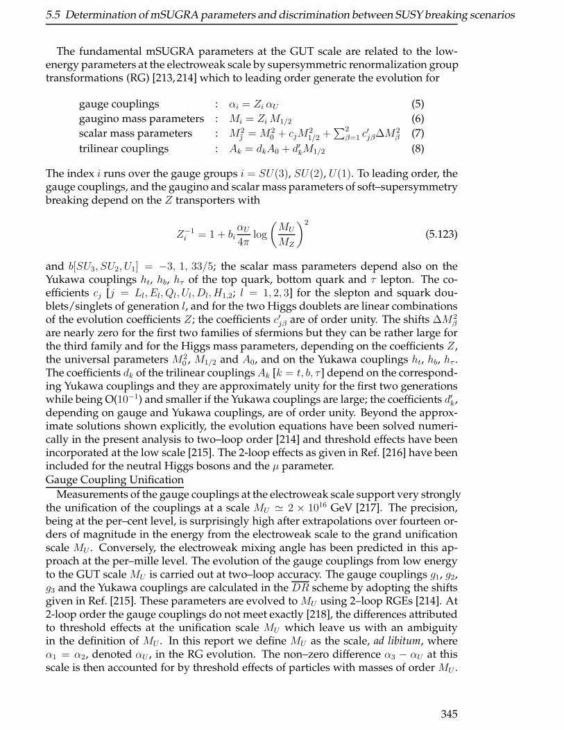
5.5 Determination of mSUGRA parameters and discrimination between SUSY breaking scenarios
The fundamental mSUGRA parameters at the GUT scale are related to the low-energy parameters at the electroweak scale by supersymmetric renormalization grouptransformations (RG) [213, 214] which to leading order generate the evolution for
gauge couplings : αi = Zi αU (5)
gaugino mass parameters : Mi = ZiM1/2 (6)
scalar mass parameters : M2 = M2
0 + cjM21/2 +
∑2β=1 c
′jβ∆M
2β (7)
trilinear couplings : Ak = dkA0 + d′kM1/2 (8)
The index i runs over the gauge groups i = SU(3), SU(2), U(1). To leading order, thegauge couplings, and the gaugino and scalar mass parameters of soft–supersymmetrybreaking depend on the Z transporters with
Z−1i = 1 + bi
αU4π
log
(MU
MZ
)2
(5.123)
and b[SU3, SU2, U1] = −3, 1, 33/5; the scalar mass parameters depend also on theYukawa couplings ht, hb, hτ of the top quark, bottom quark and τ lepton. The co-efficients cj [j = Ll, El, Ql, Ul, Dl, H1,2; l = 1, 2, 3] for the slepton and squark dou-blets/singlets of generation l, and for the two Higgs doublets are linear combinationsof the evolution coefficients Z; the coefficients c′jβ are of order unity. The shifts ∆M2
β
are nearly zero for the first two families of sfermions but they can be rather large forthe third family and for the Higgs mass parameters, depending on the coefficients Z,the universal parameters M2
0 , M1/2 and A0, and on the Yukawa couplings ht, hb, hτ .The coefficients dk of the trilinear couplingsAk [k = t, b, τ ] depend on the correspond-ing Yukawa couplings and they are approximately unity for the first two generationswhile being O(10−1) and smaller if the Yukawa couplings are large; the coefficients d′k,depending on gauge and Yukawa couplings, are of order unity. Beyond the approx-imate solutions shown explicitly, the evolution equations have been solved numeri-cally in the present analysis to two–loop order [214] and threshold effects have beenincorporated at the low scale [215]. The 2-loop effects as given in Ref. [216] have beenincluded for the neutral Higgs bosons and the µ parameter.Gauge Coupling Unification
Measurements of the gauge couplings at the electroweak scale support very stronglythe unification of the couplings at a scale MU ≃ 2 × 10¹⁶ GeV [217]. The precision,being at the per–cent level, is surprisingly high after extrapolations over fourteen or-ders of magnitude in the energy from the electroweak scale to the grand unificationscale MU . Conversely, the electroweak mixing angle has been predicted in this ap-proach at the per–mille level. The evolution of the gauge couplings from low energyto the GUT scale MU is carried out at two–loop accuracy. The gauge couplings g1, g2,g3 and the Yukawa couplings are calculated in the DR scheme by adopting the shiftsgiven in Ref. [215]. These parameters are evolved to MU using 2–loop RGEs [214]. At2-loop order the gauge couplings do not meet exactly [218], the differences attributedto threshold effects at the unification scale MU which leave us with an ambiguityin the definition of MU . In this report we define MU as the scale, ad libitum, whereα1 = α2, denoted αU , in the RG evolution. The non–zero difference α3 − αU at thisscale is then accounted for by threshold effects of particles with masses of order MU .
345
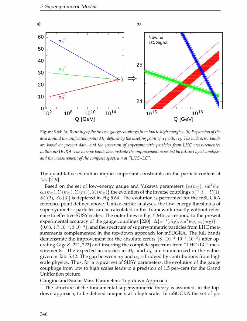
5 Supersymmetric Models
102 106 1010 1014
Q [GeV]
0
10
20
30
40
50
601- 1
2- 1
3- 1
⇒
1015 1016
Q [GeV]
24
25
Now &LC/GigaZ
a) b)
Figure 5.64: (a) Running of the inverse gauge couplings from low to high energies. (b) Expansion of the
area around the unification point MU defined by the meeting point of α1 with α2. The wide error bands
are based on present data, and the spectrum of superymmetric particles from LHC measurementes
within mSUGRA. The narrow bands demonstrate the improvement expected by future GigaZ analyses
and the measurement of the complete spectrum at “LHC+LC”.
The quantitative evolution implies important constraints on the particle content atMU [219].
Based on the set of low–energy gauge and Yukawa parameters α(mZ), sin2 θW ,αs(mZ), Yt(mZ), Yb(mZ), Yτ (mZ) the evolution of the inverse couplings α−1
i [i = U(1),SU(2), SU(3)] is depicted in Fig 5.64. The evolution is performed for the mSUGRAreference point defined above. Unlike earlier analyses, the low–energy thresholds ofsupersymmetric particles can be calculated in this framework exactly without refer-ence to effective SUSY scales. The outer lines in Fig. 5.64b correspond to the presentexperimental accuracy of the gauge couplings [220]: ∆α−1(mZ), sin2 θW , αs(mZ) =0.03, 1.7·10−4, 3·10−3, and the spectrum of supersymmetric particles from LHC mea-surements complemented in the top-down approach for mSUGRA. The full bandsdemonstrate the improvement for the absolute errors 8 · 10−3, 10−5, 10−3 after op-erating GigaZ [221, 222] and inserting the complete spectrum from “LHC+LC” mea-surements. The expected accuracies in MU and αU are summarized in the valuesgiven in Tab. 5.42. The gap between αU and α3 is bridged by contributions from highscale physics. Thus, for a typical set of SUSY parameters, the evolution of the gaugecouplings from low to high scales leads to a precision of 1.5 per–cent for the GrandUnification picture.
Gaugino and Scalar Mass Parameters: Top-down Approach
The structure of the fundamental supersymmetric theory is assumed, in the top-down approach, to be defined uniquely at a high scale. In mSUGRA the set of pa-
346
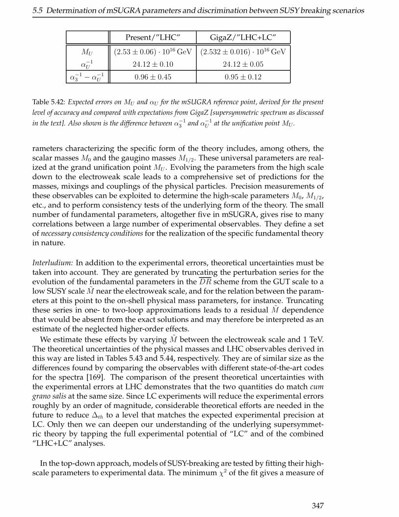
5.5 Determination of mSUGRA parameters and discrimination between SUSY breaking scenarios
Present/”LHC” GigaZ/”LHC+LC”
MU (2.53± 0.06) · 1016 GeV (2.532± 0.016) · 1016 GeV
α−1U 24.12± 0.10 24.12± 0.05
α−13 − α−1
U 0.96± 0.45 0.95± 0.12
Table 5.42: Expected errors on MU and αU for the mSUGRA reference point, derived for the present
level of accuracy and compared with expectations from GigaZ [supersymmetric spectrum as discussed
in the text]. Also shown is the difference between α−13 and α−1
U at the unification point MU .
rameters characterizing the specific form of the theory includes, among others, thescalar masses M0 and the gaugino masses M1/2. These universal parameters are real-ized at the grand unification point MU . Evolving the parameters from the high scaledown to the electroweak scale leads to a comprehensive set of predictions for themasses, mixings and couplings of the physical particles. Precision measurements ofthese observables can be exploited to determine the high-scale parameters M0, M1/2,etc., and to perform consistency tests of the underlying form of the theory. The smallnumber of fundamental parameters, altogether five in mSUGRA, gives rise to manycorrelations between a large number of experimental observables. They define a setof necessary consistency conditions for the realization of the specific fundamental theoryin nature.
Interludium: In addition to the experimental errors, theoretical uncertainties must betaken into account. They are generated by truncating the perturbation series for theevolution of the fundamental parameters in the DR scheme from the GUT scale to alow SUSY scale M near the electroweak scale, and for the relation between the param-eters at this point to the on-shell physical mass parameters, for instance. Truncatingthese series in one- to two-loop approximations leads to a residual M dependencethat would be absent from the exact solutions and may therefore be interpreted as anestimate of the neglected higher-order effects.
We estimate these effects by varying M between the electroweak scale and 1 TeV.The theoretical uncertainties of the physical masses and LHC observables derived inthis way are listed in Tables 5.43 and 5.44, respectively. They are of similar size as thedifferences found by comparing the observables with different state-of-the-art codesfor the spectra [169]. The comparison of the present theoretical uncertainties withthe experimental errors at LHC demonstrates that the two quantities do match cumgrano salis at the same size. Since LC experiments will reduce the experimental errorsroughly by an order of magnitude, considerable theoretical efforts are needed in thefuture to reduce ∆th to a level that matches the expected experimental precision atLC. Only then we can deepen our understanding of the underlying supersymmet-ric theory by tapping the full experimental potential of “LC” and of the combined“LHC+LC” analyses.
In the top-down approach, models of SUSY-breaking are tested by fitting their high-scale parameters to experimental data. The minimum χ2 of the fit gives a measure of
347

5 Supersymmetric Models
Particle ∆th [GeV] Particle ∆th [GeV]
χ+1 1.2 qR 8.4
χ+2 2.8 qL 9.1
χ01 0.34 t1 4.4
χ02 1.1 t2 8.3
χ03 0.6 b1 7.4
χ04 0.3 b2 8.2
eR 0.82 g 1.2
eL 0.31 h0 1.2
νe 0.24 H0 0.7
τ1 0.59 A0 0.7
τ2 0.30 H+ 1.0
ντ 0.25
Table 5.43: Theoretical errors of the SPS1a mass spectrum, calculated as difference between the mini-
mal and the maximal value of the masses if the scale M is varied between 100 GeV and 1 TeV.
mmaxll mmax
llq mminllq mhigh
lq mlowlq mmax
ττ mmaxll (χ0
4) mminllb
SPheno 2.2.0 80.64 454.0 216.8 397.2 325.6 83.4 283.4 195.9
∆exp 0.08 4.5 2.6 3.9 3.1 5.1 2.3 4.1
∆th 0.72 8.1 3.6 7.7 5.5 0.8 0.7 2.9
mqR −mχ01
mlL−mχ0
1mg −mb1
mg −mb2mg − 0.99mχ0
1mh0
SPheno 2.2.0 450.3 110.0 88.9 56.9 507.8 110.8
∆exp 10.9 1.6 1.8 2.6 6.4 0.25
∆th 8.1 0.23 6.8 7.6 1.3 1.2
Table 5.44: LHC observables assumed for SPS1a and their experimental (∆exp) and present theoretical
(∆th) uncertainties. [All quantities in GeV].
348
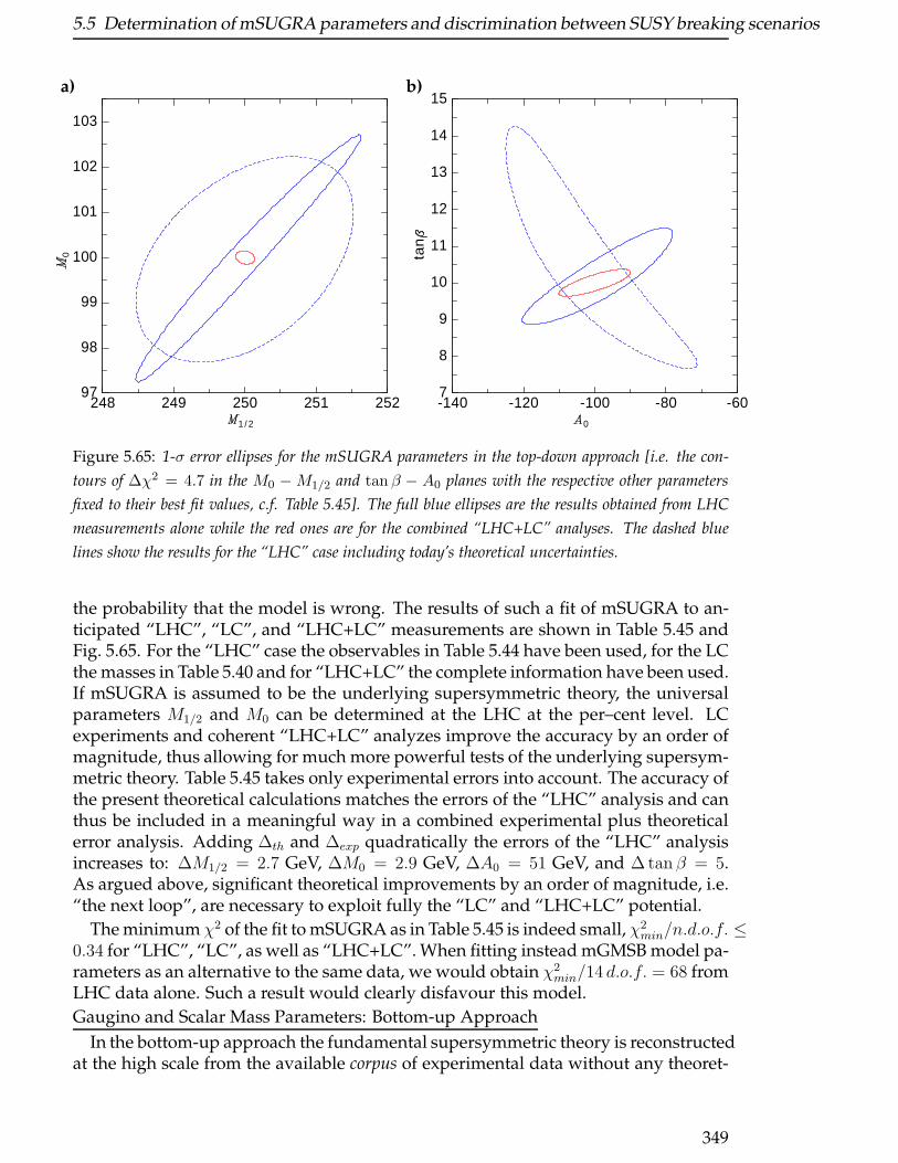
5.5 Determination of mSUGRA parameters and discrimination between SUSY breaking scenarios
248 249 250 251 2521 / 2
97
98
99
100
101
102
103
0
-140 -120 -100 -80 -600
7
8
9
10
11
12
13
14
15
tan
a) b)
Figure 5.65: 1-σ error ellipses for the mSUGRA parameters in the top-down approach [i.e. the con-
tours of ∆χ2 = 4.7 in the M0 −M1/2 and tan β − A0 planes with the respective other parameters
fixed to their best fit values, c.f. Table 5.45]. The full blue ellipses are the results obtained from LHC
measurements alone while the red ones are for the combined “LHC+LC” analyses. The dashed blue
lines show the results for the “LHC” case including today’s theoretical uncertainties.
the probability that the model is wrong. The results of such a fit of mSUGRA to an-ticipated “LHC”, “LC”, and “LHC+LC” measurements are shown in Table 5.45 andFig. 5.65. For the “LHC” case the observables in Table 5.44 have been used, for the LCthe masses in Table 5.40 and for “LHC+LC” the complete information have been used.If mSUGRA is assumed to be the underlying supersymmetric theory, the universalparameters M1/2 and M0 can be determined at the LHC at the per–cent level. LCexperiments and coherent “LHC+LC” analyzes improve the accuracy by an order ofmagnitude, thus allowing for much more powerful tests of the underlying supersym-metric theory. Table 5.45 takes only experimental errors into account. The accuracy ofthe present theoretical calculations matches the errors of the “LHC” analysis and canthus be included in a meaningful way in a combined experimental plus theoreticalerror analysis. Adding ∆th and ∆exp quadratically the errors of the “LHC” analysisincreases to: ∆M1/2 = 2.7 GeV, ∆M0 = 2.9 GeV, ∆A0 = 51 GeV, and ∆ tan β = 5.As argued above, significant theoretical improvements by an order of magnitude, i.e.“the next loop”, are necessary to exploit fully the “LC” and “LHC+LC” potential.
The minimum χ2 of the fit to mSUGRA as in Table 5.45 is indeed small, χ2min/n.d.o.f. ≤
0.34 for “LHC”, “LC”, as well as “LHC+LC”. When fitting instead mGMSB model pa-rameters as an alternative to the same data, we would obtain χ2
min/14 d.o.f. = 68 fromLHC data alone. Such a result would clearly disfavour this model.
Gaugino and Scalar Mass Parameters: Bottom-up Approach
In the bottom-up approach the fundamental supersymmetric theory is reconstructedat the high scale from the available corpus of experimental data without any theoret-
349

5 Supersymmetric Models
“LHC” “LC” “LHC+LC”
M1/2 250.0± 2.1 250.0± 0.4 250.0± 0.2
M0 100.0± 2.8 100.0± 0.2 100.0± 0.2
A0 −100.0± 34 −100.0± 27 −100.0± 14
tan β 10.0± 1.8 10.0± 0.6 10.0± 0.4
Table 5.45: Results for the high scale parameters in the top-down approach including the experimental
errors.
ical prejudice. This approach exploits the experimental information to the maximumextent possible and reflects an undistorted picture of our understanding of the basictheory.
At the present level of preparation in the “LHC” and “LC” sectors, such a programcan only be carried out in coherent “LHC+LC” analyses while the separate informa-tion from either machine proves insufficient. The results for the evolution of the massparameters from the electroweak scale to the GUT scale MU are shown in Fig. 5.66.
On the left of Fig. 5.66a the evolution is presented for the gaugino parameters M−1i ,
which clearly is under excellent control for the coherent “LHC+LC” analyses, while“LHC” [and “LC”] measurements alone are insufficient for the model-independentreconstruction of the parameters and the test of universality in the SU(3) × SU(2) ×U(1) group space. The error ellipse for the unification of the gaugino masses in thefinal analysis is depicted on the right of Fig. 5.66a. Technical details of the “LHC+LC”analysis can be found in Ref. [197].
In the same way the evolution of the scalar mass parameters can be studied, pre-sented in Figs. 5.66b separately for the first/second and the third generation in “LHC+LC”analyses. Compared with the slepton parameters, the accuracy deteriorates for thesquark parameters, and for the Higgs mass parameter M2
H2. The origin of the dif-
ferences between the errors for slepton and squark/Higgs mass parameters can betraced back to the numerical size of the coefficients in Eqs. (5.121). Typical examples,evaluated at Q = 500 GeV, read as follows [197]:
M2L1≃ M2
0 + 0.47M21/2 (5.124)
M2Q1≃ M2
0 + 5.0M21/2 (5.125)
M2H2≃ −0.03M2
0 − 1.34M21/2 + 1.5A0M1/2 + 0.6A2
0 (5.126)
|µ|2 ≃ 0.03M20 + 1.17M2
1/2 − 2.0A0M1/2 − 0.9A20 (5.127)
While the coefficients for the sleptons are of order unity, the coefficients cj for thesquarks grow very large, cj ≃ 5.0, so that small errors inM2
1/2 are magnified by nearlyan order of magnitude in the solution for M0. By close inspection of Eqs.(5.121) forthe Higgs mass parameter it turns out that the formally leading M2
0 part is nearlycancelled by the M2
0 part of c′j,β∆M2β . Inverting Eqs.(5.121) for M2
0 therefore gives riseto large errors in the Higgs case. Extracting the trilinear parametersAk is difficult andmore refined analyses based on sfermion cross sections and Higgs and/or sfermiondecays are necessary to determine these parameters accurately.
350
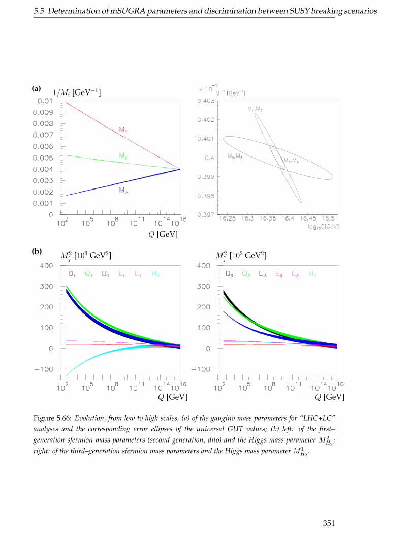
5.5 Determination of mSUGRA parameters and discrimination between SUSY breaking scenarios
(a) 1/Mi [GeV−1]
Q [GeV]
(b) M2j
[103 GeV2]
Q [GeV]
M2j
[103 GeV2]
Q [GeV]
Figure 5.66: Evolution, from low to high scales, (a) of the gaugino mass parameters for “LHC+LC”
analyses and the corresponding error ellipses of the universal GUT values; (b) left: of the first–
generation sfermion mass parameters (second generation, dito) and the Higgs mass parameter M2H2
;
right: of the third–generation sfermion mass parameters and the Higgs mass parameter M1H2
.
351

5 Supersymmetric Models
Parameter, ideal “LHC+LC” errors
M1 250. 0.15
M2 ditto 0.25
M3 2.3
ML1 100. 6.
ME1 ditto 12.
MQ1 23.
MU1 48.
ML3 7.
ME3 14.
MQ3 37.
MU3 58.
MH1 ditto 8.
MH2 41.
At −100. 40.
Table 5.46: Values of the SUSY Lagrange mass parameters after extrapolation to the unification scale
where gaugino and scalar mass parameters are universal in mSUGRA [mass units in GeV].
A representative set of the final mass values and the associated errors, after evolu-tion from the electroweak scale to MU , are presented in Table 5.46. It appears that thejoint “LHC+LC”analysis generates a comprehensive and detailed picture of the fun-damental SUSY parameters at the GUT/PL scale. Significant improvements howeverwould be welcome in the squark sector where reduced experimental errors wouldrefine the picture greatly.
5.5.4.4 Summary
We have shown in this brief report that in supersymmetric theories stable extrapola-tions can be performed from the electroweak scale to the grand unification scale, closeto the Planck scale. This feature has been demonstrated compellingly in the evolu-tion of the three gauge couplings and of the soft supersymmetry breaking parameters,which approach universal values at the GUT scale in minimal supergravity. As a de-tailed scenario we have adopted the Snowmass reference point SPS1a. It turns outthat the information on the mSUGRA parameters at the GUT scale from pure “LHC”analyses is too limited to allow for the reconstruction of the high-scale theory in amodel-independent way. The coherent “LHC+LC” analyses however in which themeasurements of SUSY particle properties at LHC and LC mutually improve eachother, result in a comprehensive and detailed picture of the supersymmetric particlesystem. In particular, the gaugino sector and the non-colored scalar sector are under
352
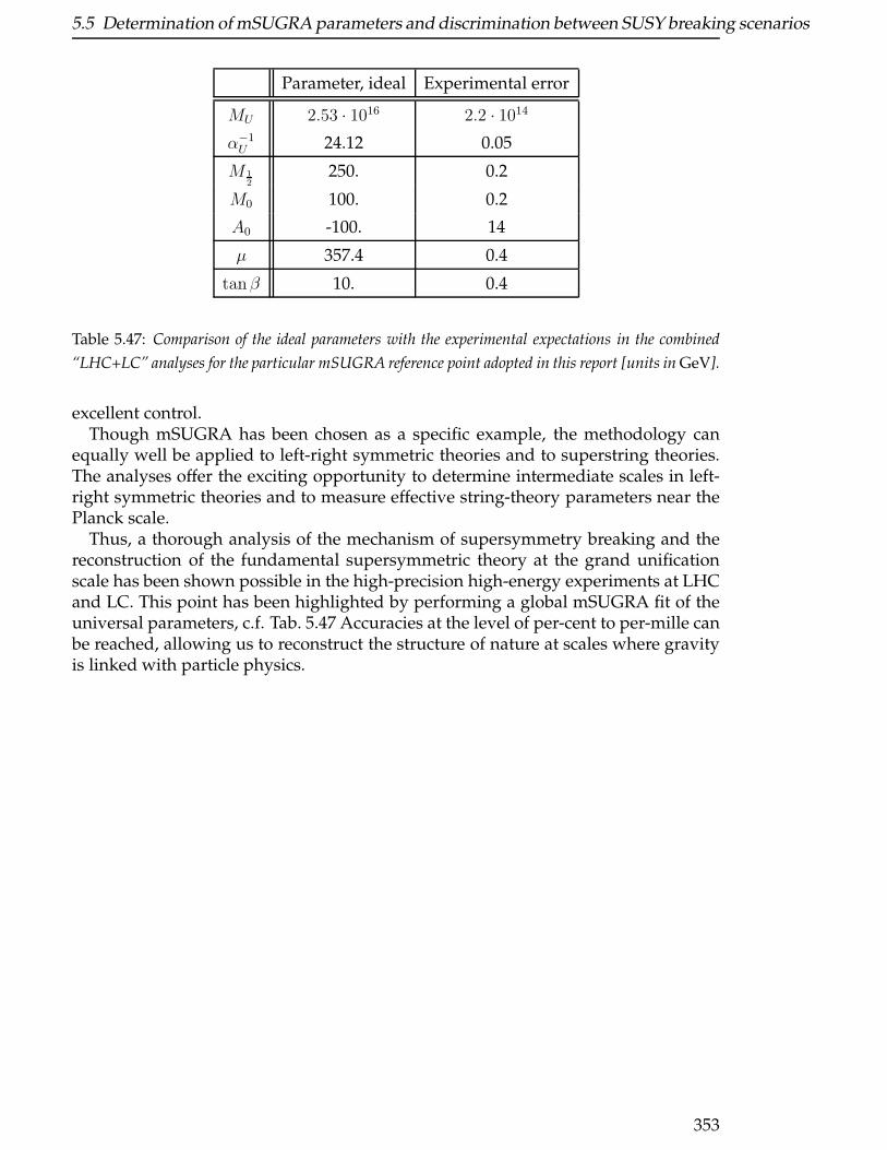
5.5 Determination of mSUGRA parameters and discrimination between SUSY breaking scenarios
Parameter, ideal Experimental error
MU 2.53 · 1016 2.2 · 1014
α−1U 24.12 0.05
M 12
250. 0.2
M0 100. 0.2
A0 -100. 14
µ 357.4 0.4
tanβ 10. 0.4
Table 5.47: Comparison of the ideal parameters with the experimental expectations in the combined
“LHC+LC” analyses for the particular mSUGRA reference point adopted in this report [units in GeV].
excellent control.Though mSUGRA has been chosen as a specific example, the methodology can
equally well be applied to left-right symmetric theories and to superstring theories.The analyses offer the exciting opportunity to determine intermediate scales in left-right symmetric theories and to measure effective string-theory parameters near thePlanck scale.
Thus, a thorough analysis of the mechanism of supersymmetry breaking and thereconstruction of the fundamental supersymmetric theory at the grand unificationscale has been shown possible in the high-precision high-energy experiments at LHCand LC. This point has been highlighted by performing a global mSUGRA fit of theuniversal parameters, c.f. Tab. 5.47 Accuracies at the level of per-cent to per-mille canbe reached, allowing us to reconstruct the structure of nature at scales where gravityis linked with particle physics.
353

5 Supersymmetric Models
354
Bibliography
[1] B. C. Allanach et al., in Proc. of the APS/DPF/DPB Summer Study onthe Future of Particle Physics (Snowmass 2001) ed. N. Graf, Eur. Phys.J. C 25 (2002) 113 [eConf C010630 (2001) P125] [arXiv:hep-ph/0202233];http://www.ippp.dur.ac.uk/∼georg/sps.
[2] G. Weiglein, arXiv:hep-ph/0301111.
[3] H. Baer, F. E. Paige, S. D. Protopopescu and X. Tata, arXiv:hep-ph/0001086;http://paige.home.cern.ch/paige.
[4] N. Ghodbane and H. U. Martyn, arXiv:hep-ph/0201233.
[5] R. Barate et al. [ALEPH Collaboration], Phys. Lett. B 565 (2003) 61 [arXiv:hep-ex/0306033].
[6] [LEP Higgs Working Group Collaboration], arXiv:hep-ex/0107030.
[7] C. L. Bennett et al., Astrophys. J. Suppl. 148 (2003) 1 [arXiv:astro-ph/0302207].
[8] D. N. Spergel et al., Astrophys. J. Suppl. 148 (2003) 175 [arXiv:astro-ph/0302209].
[9] See e.g., ATLAS detector and Physics Performance Technical Design Report,CERN-LHCC-99-14 and CERN-LHCC-99-15 (1999),http://atlas.web.cern.ch/Atlas/GROUPS/PHYSICS/TDR/access.html.
[10] TESLA, Technical Design Report Part III, eds. R.-D. Heuer, D. Miller, F. Richard,P. Zerwas, DESY 01-011 (2001), hep-ph/0106315;ACFA LC Working Group, K. Abe et al., KEK-REPORT-2001-11, hep-ph/0109166;American LC Working Group, T. Abe et al., SLAC-R-570 (2001), hep-ex/0106055.
[11] B. C. Allanach, C. G. Lester, M. A. Parker and B. R. Webber, JHEP 0009 (2000) 004[arXiv:hep-ph/0007009].
[12] T. Sjostrand, P. Eden, C. Friberg, L. Lonnblad, G. Miu, S. Mrenna, E. Norrbin,Comput.Phys.Commun. 135 (2001) 238; T. Sjostrand, L. Lonnblad and S. Mrenna,“PYTHIA 6.2: Physics and manual”, arXiv:hep-ph/0108264.
[13] E. Richter-Was, D. Froidevaux and L. Poggioli, “ATLFAST 2.0: a fast simulationpackage for ATLAS”, Tech. Rep. ATL-PHYS-98-131 (1998)
[14] G. Polesello, J. Phys. G 30 (2004) 1185.
355
Bibliography
[15] H. Baer, F. E. Paige, S. D. Protopopescu, X. Tata, hep-ph/9305342; hep-ph/980432; hep-ph/0001086.
[16] G. Marchesini, B.R. Webber, G. Abbiendi, I.G. Knowles, M.H. Seymour and L.Stanco, Comput. Phys. Commun. 67 (1992) 465;G. Corcella, I.G. Knowles, G. Marchesini, S. Moretti, K. Odagiri, P. Richardson,M.H. Seymour and B.R. Webber, JHEP 0101 (2001) 010 [hep-ph/9912396].
[17] C.G.Lester, D.J.Summers, Phys.Lett. B463 (1999) 99.
[18] G. Moortgat-Pick et al., these proceedings.
[19] I. Hinchliffe, F. E. Paige, M. D. Shapiro, J. Soderqvist and W. Yao, Phys. Rev. D55, 5520 (1997).
[20] J. Hisano, K. Kawagoe, R. Kitano and M. M. Nojiri, Phys. Rev. D 66, 115004(2002).
[21] J. Hisano, K. Kawagoe and M. M. Nojiri, Phys. Rev. D 68, 035007 (2003).
[22] H.P. Nilles, Phys. Rev. 110, (1984) 1
[23] H. Baer, C.H. Chen, F. Paige and X. Tata, Phys. Rev. D 52, (1995) 2746; Phys. Rev.D 53, (1996) 6241.
[24] The CMS Collaboration, CERN/LHCC 94-038.
[25] S. Abdullin and F. Charles, Nucl. Phys. B 547, (1999) 60; S. Abdullin, Z. Antunovicand M. Dzelalija, Mod. Phys. Lett. A 15, (2000) 465.
[26] H. Baer, C.H. Chen, F. Munroe, F. Paige and X. Tata, Phys. Rev. D 51, (1995) 1046.
[27] M. Battaglia et al., hep-ph/0106204 (2001); hep-ph/0112013 (2001).
[28] B.C. Allanach et al., hep-ph/0202233 (2002).
[29] T. Sjostrand, Computer Phys. Comm. 82, (1994) 74.
[30] F. Paige and S. Protopopescu, in Supercollider Physics, p. 41, ed. D. Soper (WorldScientific, 1986); H. Baer, F. Paige, S. Protopopescu and X. Tata, in Proceedings ofthe Workshop on Physics at Current Accelerators and Supercolliders, ed. J. Hewett, A.White and D. Zeppenfeld (Argonne National Laboratory, 1993).
[31] S. Abdullin, A. Khanov and N. Stepanov, CMS TN/94-180 (1994).
[32] M. Chiorboli, A. Tricomi, Squark and gluino reconstruction methods with the CMSdetector, CMS Note in preparation.
[33] M. Chiorboli, Supersymmetric Particle Reconstructions with the CMS detector atLHC, Ph.D. Thesis, Catania (2003),http://cmsdoc.cern.ch/documents/03/doc2003 002.pdf .
[34] ATLAS Collaboration, Detector and Physics Performance TDR,CERN/LHCC 99-14.
356

Bibliography
[35] I. Hincliffe et al., “Precision SUSY measurements at LHC: Point 3.”, ATLAS InternalNote, 1997, ATLAS-NOTE-Phys-109; F. Gianotti, “Precision SUSY measurementswith ATLAS for SUGRA Point 4”, ATLAS Internal Note, 1997, PHYS-No-110; G.Polesello et al., Precision SUSY measurements with ATLAS fro SUGRA point 5”,ATLAS Internal Note, 1997, PHYS-No-111.
[36] P. Grannis, hep-ex/0211002; M. Battaglia et al., hep-ph/0201177.
[37] J. Kalinowski, hep-ph/0309235.
[38] H.-U. Martyn, Linear Collider Note LC-PHSM-2003-071 and talk at ECFA/DESY
LC workshop Prague, November 2002,http://www-hep2.fzu.cz/ecfadesy/Talks/SUSY/
[39] U. Nauenberg, talk at ECFA/DESY LC workshop Prague, November 2002,http://www-hep2.fzu.cz/ecfadesy/Talks/SUSY/
[40] M. Dima et al, Phys. Rev. D 65 (2002) 71701.
[41] A. Freitas, A. v. Manteuffel, P.M. Zerwas, hep-ph/0310112.
[42] J. Feng, D. Finell, Phys. Rev. D 49 (1994) 2369.
[43] Y. Kato et al, APPI Winter Institute, February 2003.
[44] K. Desch, talk at ECFA/DESY LC workshop Prague, November 2002,http://www-hep2.fzu.cz/ecfadesy/Talks/SUSY/
[45] B.K. Gjelsten, J. Hisano, K. Kawagoe, E. Lytken, D. Miller, M. Nojiri, P. Osland,G. Polesello, contribution to this report.
[46] M. Chiorboli, A. Tricomi, contribution to this report.
[47] B. Allanach et al, contribution to this report.
[48] SPA Project (SUSY PARAMETER ANALYSIS), SUSY working group of the ECFA LC
STUDY, http://www-flc.desy.de/spa/
[49] A summary of current LHC and LC studies can be found e.g. in F.E. Paige,arXiv:hep-ph/0211017; J. Kalinowski, arXiv:hep-ph/0309235, and referencestherein.
[50] T. Tsukamoto, K. Fujii, H. Murayama, M. Yamaguchi and Y. Okada, Phys. Rev.D 51 (1995) 3153. J. L. Feng, M. E. Peskin, H. Murayama and X. Tata, Phys. Rev.D 52 (1995) 1418 [arXiv:hep-ph/9502260].
[51] S. Y. Choi, J. Kalinowski, G. Moortgat-Pick and P. M. Zerwas, Eur. Phys. J. C 22(2001) 563 [arXiv:hep-ph/0108117]; S. Y. Choi, J. Kalinowski, G. Moortgat-Pickand P. M. Zerwas, Eur. Phys. J. C 23 (2002) 769 [arXiv:hep-ph/0202039].
[52] K. Desch, J. Kalinowski, G. Moortgat-Pick, M. M. Nojiri and G. Polesello, JHEP0402 (2004) 035 [arXiv:hep-ph/0312069].
357

Bibliography
[53] H. E. Haber and G. L. Kane, Phys. Rep. 117 (1985) 75.
[54] S. Y. Choi, A. Djouadi, M. Guchait, J. Kalinowski, H. S. Song and P. M. Zerwas,Eur. Phys. J. C 14 (2000) 535 [arXiv:hep-ph/0002033]; S. Y. Choi, A. Djouadi,H. K. Dreiner, J. Kalinowski and P. M. Zerwas, Eur. Phys. J. C 7 (1999) 123[arXiv:hep-ph/9806279].
[55] G. Moortgat-Pick, A. Bartl, H. Fraas and W. Majerotto, arXiv:hep-ph/0002253.
[56] S. Ambrosanio, B. Mele, G. Montagna, O. Nicrosini and F. Piccinini, Nucl. Phys.B 478 (1996) 46 [arXiv:hep-ph/9601292].
[57] T. Blank and W. Hollik, hep-ph/0011092; H. Eberl, M. Kincel, W. Majerotto andY. Yamada, hep-ph/0104109. T. Fritzsche and W. Hollik, Eur. Phys. J. C 24 (2002)619 [arXiv:hep-ph/0203159].
[58] E. Boos, G. Moortgat-Pick, H. U. Martyn, M. Sachwitz and A. Vologdin,arXiv:hep-ph/0211040; E. Boos, H. U. Martyn, G. Moortgat-Pick, M. Sach-witz, A. Sherstnev and P. M. Zerwas, Eur. Phys. J. C 30 (2003) 395 [arXiv:hep-ph/0303110].
[59] H.U. Martyn, talk given at the ECFA/DESY Linear Collider workshop, Prague,November 2002, http://www-hep2.fzu.cz/ecfadesy/Talks/SUSY/, and LC-note LC-PHSM-2003-071. M. Dima et al., Phys. Rev. D 65 (2002) 071701.
[60] M. Ball, diploma thesis, University of Hamburg, January 2003, http://www-flc.desy.de/thesis/diplom.2002.ball.ps.gz; see also talk by K. Desch at theECFA/DESY Linear Collider workshop, Prague, November 2002, http://www-hep2.fzu.cz/ecfadesy/Talks/SUSY/.
[61] ’Polarisation Write-Up: Beam Polarisation at a future Linear Collider’, work-ing group document by the polarisation ‘POWER working group’, G. Moortgat-Pick et al., in preparation, further details: http://www.ippp.durham.ac.uk/ gu-drid/power.
[62] H. Baer, C. H. Chen, M. Drees, F. Paige and X. Tata, Phys. Rev. D 59 (1999) 055014[arXiv:hep-ph/9809223]; J. L. Feng and T. Moroi, Nucl. Phys. Proc. Suppl. 62(1998) 108 [arXiv:hep-ph/9707494]; V. D. Barger, T. Han and J. Jiang, Phys. Rev.D 63 (2001) 075002 [arXiv:hep-ph/0006223]; J. F. Gunion, T. Han, J. Jiang andA. Sopczak, hep-ph/0212151.
[63] G. Polesello, contribution to this report.
[64] J. A. Aguilar-Saavedra et al. [ECFA/DESY LC Physics Working Group],arXiv:hep-ph/0106315.
[65] K. Desch, J. Kalinowski, G. Moortgat-Pick, M. M. Nojiri and G. Polesello, contri-bution to this report.
[66] H. P. Nilles, Phys. Rept. 110 (1984) 1.
[67] H. E. Haber, G. L. Kane, Phys. Rept. 117 (1985) 75.
358
Bibliography
[68] A. B. Lahanas, D. V. Nanopoulos, Phys. Rept. 145 (1987) 1.
[69] S. Ferrara, ed., Supersymmetry, vol. 1-2. North Holland/World Scientific, Singa-pore, 1987.
[70] J. Guasch, W. Hollik, J. Sola, JHEP 0210 (2002) 040 [arXiv:hep-ph/0207364].
[71] J. Guasch, W. Hollik, J. Sola, Nucl. Phys. Proc. Suppl. 116, 301 (2003) [arXiv:hep-ph/0210118].
[72] A. Djouadi, W. Hollik and C. Junger, Phys. Rev. D 55 (1997) 6975 [arXiv:hep-ph/9609419].
[73] M. M. Nojiri, K. Fujii and T. Tsukamoto, Phys. Rev. D 54, 6756 (1996) [arXiv:hep-ph/9606370].
[74] H. C. Cheng, J. L. Feng and N. Polonsky, Phys. Rev. D 56, 6875 (1997) [arXiv:hep-ph/9706438].
[75] H. C. Cheng, J. L. Feng and N. Polonsky, Phys. Rev. D 57, 152 (1998) [arXiv:hep-ph/9706476].
[76] E. Katz, L. Randall and S. f. Su, Nucl. Phys. B 536 (1998) 3 [arXiv:hep-ph/9801416].
[77] K. i. Hikasa and Y. Nakamura, Z. Phys. C 70 (1996) 139 [Erratum-ibid. C 71 (1996)356] [arXiv:hep-ph/9501382].
[78] J. Guasch, J. Sola and W. Hollik, Phys. Lett. B 437 (1998) 88 [arXiv:hep-ph/9802329].
[79] J. Guasch, W. Hollik and J. Sola, Phys. Lett. B 510 (2001) 211 [arXiv:hep-ph/0101086].
[80] Programs to compute the one-loop corrected partial decay width:Γ(sfermion → fermion chargino/neutralino) available fromhttp://www-itp.physik.uni-karlsruhe.de/˜guasch/prog s
[81] M. Ciuchini, E. Franco, A. Masiero and L. Silvestrini, Phys. Rev. D 67 (2003)075016 [arXiv:hep-ph/0212397].
[82] T. Besmer, C. Greub and T. Hurth, Nucl. Phys. B 609 (2001) 359 [arXiv:hep-ph/0105292].
[83] F. Gabbiani, E. Gabrielli, A. Masiero and L. Silvestrini, Nucl. Phys. B 477 (1996)321 [arXiv:hep-ph/9604387].
[84] J. S. Hagelin, S. Kelley and T. Tanaka, Nucl. Phys. B 415 (1994) 293.
[85] W. Porod, Comput. Phys. Commun. 153 (2003) 275 [arXiv:hep-ph/0301101].
[86] F. Borzumati, C. Greub, T. Hurth and D. Wyler, Phys. Rev. D 62 (2000) 075005[arXiv:hep-ph/9911245].
359
Bibliography
[87] M. Chiorboli et al., these proceedings.
[88] N. Arkani-Hamed, J. L. Feng, L. J. Hall and H. Cheng, Phys. Rev. Lett. 77 (1996)1937 [hep-ph/9603431].
[89] F. Deppisch, H. Pas, A. Redelbach, R. Ruckl and Y. Shimizu, Eur. Phys. J. C 28(2003) 365 [arXiv:hep-ph/0206122].
[90] N. V. Krasnikov, JETP Lett. 65 (1997) 148 [arXiv:hep-ph/9611282]. S. I. Bityukovand N. V. Krasnikov, arXiv:hep-ph/9806504. K. Agashe and M. Graesser, Phys.Rev. D 61 (2000) 075008 [arXiv:hep-ph/9904422]; I. Hinchliffe and F. E. Paige,Phys. Rev. D 63 (2001) 115006 [arXiv:hep-ph/0010086]; J. Hisano, R. Kitano andM. M. Nojiri, Phys. Rev. D 65 (2002) 116002; D.F. Carvalho et al., hep-ph/0206148.
[91] N. Arkani-Hamed, J. L. Feng, L. J. Hall and H. Cheng, Nucl. Phys. B 505 (1997) 3[hep-ph/9704205].
[92] J. Hisano, M. M. Nojiri, Y. Shimizu and M. Tanaka, Phys. Rev. D 60 (1999) 055008[hep-ph/9808410].
[93] M. Guchait, J. Kalinowski and P. Roy, Eur. Phys. J. C 21 (2001) 163 [arXiv:hep-ph/0103161].
[94] W. Porod and W. Majerotto, Phys. Rev. D 66 (2002) 015003 [arXiv:hep-ph/0201284].
[95] F. Deppisch, H. Pas, A. Redelbach, R. Ruckl and Y. Shimizu, accepted for publi-cation in Phys. Rev. D, arXiv:hep-ph/0310053.
[96] J. Kalinowski, Acta Phys. Polon. B 32 (2001) 3755.
[97] J. Kalinowski, Acta Phys. Polon. B 33 (2002) 2613 [arXiv:hep-ph/0207051].
[98] F. Gabbiani, E. Gabrielli, A. Masiero and L. Silvestrini, Nucl. Phys. B 477 (1996)321 [arXiv:hep-ph/9604387].
[99] J. L. Feng, Y. Nir and Y. Shadmi, Phys. Rev. D 61 (2000) 113005 [arXiv:hep-ph/9911370].
[100] M. Gell-Mann, P. Ramond and R. Slansky, Print-80-0576 (CERN). T. Yanagida,Prog. Theor. Phys. 64 (1980) 1103; R. N. Mohapatra and G. Senjanovic, Phys. Rev.Lett. 44 (1980) 912; Phys. Rev. D 23 (1981) 165.
[101] L. Serin and R. Stroynowski, ATLAS Internal Note (1997).
[102] D. Denegri, priv. comm.
[103] M. Battaglia et al., Eur. Phys. J. C 22 (2001) 535 [arXiv:hep-ph/0106204].
360
Bibliography
[104] J. Hisano, T. Moroi, K. Tobe and M. Yamaguchi, Phys. Rev. D 53 (1996) 2442[arXiv:hep-ph/9510309]; Y. Okada, K. I. Okumura and Y. Shimizu, Phys. Rev.D 61, 094001 (2000) [arXiv:hep-ph/9906446]; T. Fukuyama, T. Kikuchi andN. Okada, Phys. Rev. D 68 (2003) 033012 [arXiv:hep-ph/0304190]; E. Jankowskiand D. W. Maybury, arXiv:hep-ph/0401132; M. Hirouchi and M. Tanaka, Phys.Rev. D 58 (1998) 032004 [arXiv:hep-ph/9712532].
[105] J. A. Casas and A. Ibarra, Nucl. Phys. B 618 (2001) 171 [arXiv:hep-ph/0103065].
[106] J. Hisano and D. Nomura, Phys. Rev. D 59 (1999) 116005 [arXiv:hep-ph/9810479].
[107] M. C. Gonzalez-Garcia, M. Maltoni, C. Pena-Garay and J. W. F. Valle, Phys. Rev.D 63 (2001) 033005 [arXiv:hep-ph/0009350].
[108] R. Becker and C. Vander Velde, IIHE-93-08 Prepared for Working Group on e+ e-Collisions at 500-GeV: The Physics Potential, Munich, Germany, 20 Nov 1992.
[109] T. Mori, for the MEG Collab., EXP PSI-R-99-05, Prepared for 31st Int. Conferenceon High Energy Physics (ICHEP 2002), Amsterdam, The Netherlands, 24-31 Jul 2002.See also http://meg.web.psi.ch/docs/calculator/index.html.
[110] C. H. Chen, M. Drees and J. F. Gunion, Phys. Rev. Lett. 76, 2002 (1996) [hep-ph/9512230]. Phys. Rev. D55, 330 (1997) [hep-ph/9607421]. and errata [hep-ph/9902309].
[111] J. F. Gunion and S. Mrenna, Phys. Rev. D62, 015002 (2000) [hep-ph/9906270].
[112] J. L. Feng, T. Moroi, L. Randall, M. Strassler and S. Su, Phys. Rev. Lett. 83, 1731(1999) [hep-ph/9904250].
[113] T. Gherghetta, G. F. Giudice and J. D. Wells, Nucl. Phys. B559, 27 (1999) [hep-ph/9904378].
[114] D.K. Ghosh, A. Kundu, P. Roy and S. Roy, Phys. Rev. D64 115001 (2001)[hep-ph/0104217]; D.K. Ghosh, P. Roy and S. Roy, JHEP 08, 031 (2000) [hep-ph/0004127]; D. Choudhury, D.K. Ghosh and S. Roy, Nucl. Phys. B646, 3 (2002)[hep-ph/0208240].
[115] P. Abreu et al. [DELPHI Collaboration], Eur. Phys. J. C11, 1 (1999) [hep-ex/9903071] and CERN-EP-2000-033.
[116] M. Acciarri et al. [L3 Collaboration], Phys. Lett. B482, 31 (2000) [hep-ex/0002043].
[117] J.F. Gunion and S. Mrenna, Phys. Rev. D64, 075002 (2001) [hep-ph/0103167].
[118] F.E. Paige and J. Wells, hep-ph/0001249.
[119] H. Baer, J. K. Mizukoshi and X. Tata, Phys. Lett. B488, 367 (2000) [hep-ph/0007073].
361

Bibliography
[120] A. J. Barr, C. G. Lester, M. A. Parker, B. C. Allanach and P. Richardson, JHEP0303, 045 (2003) [arXiv:hep-ph/0208214].
[121] J. Amundson et al., arXiv:hep-ph/9609374.
[122] See the contribution by H. Baer, C. Chen and J.Gunion in B. Allanach et al. [Rparity Working Group Collaboration], “Searching for R-parity violation at Run-II of the Tevatron,” arXiv:hep-ph/9906224.
[123] V.S. Kaplunovsky and J. Louis, Phys. Lett. B306, 269 (1993); A. Brignole, L.E.Ibanez and C. Munoz, Nucl. Phys. B422 , 125 (1994), [E: B436, 747 (1995)]; CERN-TH/97-143 [hep-ph/9707209].
[124] S. Raby, Phys. Rev. D56, 2852 (1997); S. Raby, Phys. Lett. B 422, 158 (1998)[arXiv:hep-ph/9712254].
[125] L.R. Roszkowski and M. Shifman, Phys. Rev. D53, 404 (1996).
[126] G. L. Kane and S. F. King, Phys. Lett. B 451, 113 (1999) [arXiv:hep-ph/9810374].
[127] S. Raby and K. Tobe, Nucl. Phys. B 539, 3 (1999) [arXiv:hep-ph/9807281].
[128] S. Berge and M. Klasen, arXiv:hep-ph/0303058.
[129] S. Berge and M. Klasen, Phys. Rev. D 66, 115014 (2002) [arXiv:hep-ph/0208212].
[130] S. Berge and M. Klasen, Eur. Phys. J. C 30, 123 (2003) [arXiv:hep-ph/0303032].
[131] J. Wess and B. Zumino, Nucl. Phys. B 70 (1974) 39.
[132] G. A. Blair, W. Porod and P. M. Zerwas, Eur. Phys. J. C 27 (2003) 263 [arXiv:hep-ph/0210058].
[133] ATLAS Collaboration, Detector and Physics Performance TDR, Vol. II,CERN/LHC/99-15; TESLA Technical Design Report (Part 3), R.D. Heuer,D.J. Miller, F. Richard and P.M. Zerwas (eds.), DESY 010-11 [arXiv:hep-ph/0106315]; American LC Working Group, T. Abe et al., SLAC-R-570 (2001),[arXiv:hep-ex/0106055-58]; ACFA LC Working Group, K. Abe et al., KEK-REPORT-2001-11, [arXiv:hep-ex/0109166].
[134] S. Y. Choi, A. Djouadi, M. Guchait, J. Kalinowski, H.S. Song and P. M. Zerwas,Eur. Phys. J. C 14 (2000) 535 [arXiv:hep-ph/0002033]; V. D. Barger, T. Han, T. J. Liand T. Plehn, Phys. Lett. B 475 (2000) 342 [arXiv:hep-ph/9907425]; S. Y. Choi,J. Kalinowski, G. Moortgat-Pick and P. M. Zerwas, Eur. Phys. J. C 22 (2001) 563[Addendum-ibid. C 23 (2002) 769] [arXiv:hep-ph/0108117]; K. Desch, J. Kali-nowski, G. Moortgat-Pick, M. M. Nojiri and G. Polesello, arXiv:hep-ph/0312069.
[135] P. Fayet and J. Iliopoulos, Phys. Lett. B 51 (1974) 461.
[136] A. Djouadi, J. L. Kneur and G. Moultaka, arXiv:hep-ph/0211331.
[137] P. Skands et al., arXiv:hep-ph/0311123.
362
Bibliography
[138] G. Ganis, MSMlib (unpublished)
[139] V. D. Barger, T. Falk, T. Han, J. Jiang, T. Li and T. Plehn, Phys. Rev. D 64 (2001)056007 [arXiv:hep-ph/0101106].
[140] W. Beenakker, R. Hopker, M. Spira and P. M. Zerwas, Nucl. Phys. B 492 (1997)51 [arXiv:hep-ph/9610490]; W. Beenakker, M. Kramer, T. Plehn, M. Spira andP. M. Zerwas, Nucl. Phys. B 515 (1998) 3 [arXiv:hep-ph/9710451]; W. Beenakker,M. Klasen, M. Kramer, T. Plehn, M. Spira and P. M. Zerwas, Phys. Rev. Lett. 83(1999) 3780 [arXiv:hep-ph/9906298].
[141] F. James and M. Roos, Comput. Phys. Commun. 10 (1975) 343.
[142] M. Muhlleitner, A. Djouadi and Y. Mambrini, arXiv:hep-ph/0311167.
[143] R. Lafaye, T. Plehn and D. Zerwas, Prepared for Workshop on Physics at TeV Collid-ers, Les Houches, France, 2003, LAPP-EXP-2003-27, CERN-TH/2003-312, LAL 04/06
[144] B. C. Allanach, Comput. Phys. Commun. 143 (2002) 305 [arXiv:hep-ph/0104145].
[145] H. Baer, F. E. Paige, S. D. Protopescu and X. Tata, arXiv:hep-ph/0312045.
[146] B. K. Gjelsten et al., H.-U. Martyn, M. Chiorboli et al., all in this report.
[147] M. Drees and S. P. Martin, arXiv:hep-ph/9504324.
[148] G. Degrassi, S. Heinemeyer, W. Hollik, P. Slavich and G. Weiglein, Eur. Phys. J.C 28 (2003) 133 [arXiv:hep-ph/0212020].
[149] F. James and M. Roos, “’Minuit’ A System For Function Minimization AndAnalysis Of The Parameter Errors And Correlations,” Comput. Phys. Commun.10 (1975) 343.
[150] K. Desch, J. Kalinowski, G. Moortgat-Pick, M. M. Nojiri and G. Polesello, “SUSYparameter determination in combined analyses at LHC/LC,” JHEP 0402 (2004)035 [arXiv:hep-ph/0312069].
[151] W. Porod, “Phenomenology of stops, sbottoms, staus and tau-sneutrino”,arXiv:hep-ph/9804208.
[152] Isajet 7.69, by F. Paige, S. Protopopescu, H. Baer and X. Tata, hep-ph/0312045(2003).
[153] H. Baer, C. Balazs and A. Belyaev, JHEP0203 (2002) 042.
[154] H. Baer, C. Balazs, A. Belyaev, T. Krupovnickas and X. Tata, JHEP0306 (2003)054.
[155] H. Baer, T. Krupovnickas and X. Tata, JHEP0307 (2003) 020.
[156] H. Baer, A. Belyaev, T. Krupovnickas and X. Tata, JHEP0402 (2004) 007.
363
Bibliography
[157] H. Baer, T. Krupovnickas and X. Tata, JHEP0406 (2004) 061.
[158] H. Baer, C. Balazs, JCAP, 0305:006, 2003; J. Ellis, K. Olive, Y. Santoso, V. Spanos,Phys. Lett., B565:176–182, 2003; U. Chattopadhyay, A. Corsetti, P. Nath, Phys.Rev., D68:035005, 2003. A. B. Lahanas, D. V. Nanopoulos, Phys. Lett., B568:55–62, 2003; G. Belanger, F. Boudjema, A. Cottrant, A. Pukhov, A. Semenov, hep-ph/0407218.
[159] D. N. Spergel et al., Astrophys. J. Suppl., 148:175, 2003; C. L. Bennett et al. Astro-phys. J. Suppl., 148:1, 2003.
[160] A. Balbi, et al., Astrophys. J., 588:L5–L8, 2003.
[161] B. C. Allanach, D. Grellscheid, and F. Quevedo, JHEP, 05:048, 2002; B. C. Al-lanach, D. Grellscheid, and F. Quevedo, JHEP, 07:069, 2004.
[162] B. C. Allanach, G. Belanger, F. Boudjema, A. Pukhov, and W. Porod, hep-ph/0402161.
[163] B. C. Allanach, G. Belanger, F. Boudjema, A. Pukhov, in preparation.
[164] G. Belanger, F. Boudjema, A. Pukhov, and A. Semenov, hep-ph/0405253;G. Belanger, F. Boudjema, A. Pukhov, and A. Semenov, Comput. Phys. Commun.,149:103, 2002.
[165] M. Battaglia et. al., Eur. Phys. J. C33 (2004) 273.
[166] P. Bambade, M. Berggren, F. Richard, and Z. Zhang, hep-ph/0406010; H.-U.Martyn, hep-ph/0408226.
[167] The Atlas Collaboration, Atlas Detector and Physics Performance Technical de-sign report, CERN-LHCC-99-14.
[168] S. Y. Choi, J. Kalinowski, G. Moortgat-Pick, and P. M. Zerwas, Eur. Phys. J.,C22:563–579, 2001; S. Y. Choi et al., Eur. Phys. J., C14:535–546, 2000.
[169] B. C. Allanach, S. Kraml and W. Porod, JHEP 0303 (2003) 016 [arXiv:hep-ph/0302102].
[170] J. Hisano, K. Kawagoe and M. M. Nojiri, arXiv:hep-ph/0304214.
[171] G. A. Blair et al., these proceedings.
[172] ATLAS Collaboration, Detector and Physics Performance Technical Design Re-port, CERN/LHCC/99-15.
[173] C.G. Lester et al, JHEP 0009 (2000) 004.
[174] L. Alvarez-Gaume, J. Polchinski and M.B. Wise, Nucl. Phys. B221 (1983) 495;L. Ibanez, Phys. Lett. B118 (1982) 73; J. Ellis, D.V. Nanopoulos and K. Tamvakis,Phys. Lett. B121 (1983) 123; K. Inoue et al., Prog. Theor. Phys. 68 (1982) 927; A.H.Chamseddine, R. Arnowitt and P. Nath, Phys. Rev. Lett. 49 (1982) 970.
364

Bibliography
[175] F. Paige and S. Protopopescu, in Supercollider Physics, ed. D. Soper (World Sci-entific, 1986); H. Baer, F. Paige, S. Protopopescu and X. Tata, in Proc. Workshopon Physics at Current Accelerators and Supercolliders, ed. J. Hewett, A. Whiteand D. Zeppenfeld (Argonne National Laboratory, 1993).
[176] TESLA Project, Technical Design Report, DESY-2001-011.
[177] H.-U. Martyn, Private Communication.
[178] D.R. Tovey, Eur. Phys. J. directC 4, N4 (2002) 1-24 (Atlas Scientific Note SN-ATLAS-2002-020).
[179] B. C. Allanach, D. Grellscheid and F. Quevedo, JHEP 0205 (2002) 048 [arXiv:hep-ph/0111057].
[180] K. Benakli, Phys. Rev. D 60 (1999) 104002 [arXiv:hep-ph/9809582]; C. P. Burgess,L. E. Ibanez and F. Quevedo, Phys. Lett. B 447 (1999) 257 [arXiv:hep-ph/9810535].
[181] L. E. Ibanez, arXiv:hep-ph/9905349.
[182] B.C. Allanach, D. Grellscheid and F. Quevedo, JHEP 0407 (2004) 069.
[183] W. Buchmuller, K. Hamaguchi, M. Ratz, T. Yanagida, hep-ph/0402179.
[184] D. E. Kaplan, G. D. Kribs, M. Schmaltz, Phys. Rev. D62 (2000) 035010;Z. Chacko, M. A. Luty, A. E. Nelson, E. Ponton, JHEP 01 (2000) 003;K. Inoue, M. Kawasaki, M. Yamaguchi, T. Yanagida, Phys. Rev. D45 (1992) 328.
[185] H. P. Nilles, Phys. Rept. 110 (1984) 1.
[186] G. F. Giudice, R. Rattazzi, Phys. Rept. 322 (1999) 419.
[187] M. Bolz, W. Buchmuller, M. Plumacher, Phys. Lett. B443 (1998) 209;M. Fujii, T. Yanagida, Phys. Lett. B549 (2002) 273;J. L. Feng, A. Rajaraman, F. Takayama, Phys. Rev. D68 (2003) 063504;W. Buchmuller, K. Hamaguchi, M. Ratz, Phys. Lett. B574 (2003) 156;M. Fujii, M. Ibe, T. Yanagida, Phys. Rev. D69 (2004) 015006;J. Ellis, K. A. Olive, Y. Santoso, V. C. Spanos, hep-ph/0312262.
[188] M. Drees, X. Tata, Phys. Lett. B252 (1990) 695.
[189] J. L. Feng, T. Moroi, Phys. Rev. D58 (1998) 035001;S. P. Martin, J. D. Wells, Phys. Rev. D59 (1999) 035008.
[190] S. Ambrosanio, B. Mele, S. Petrarca, G. Polesello, A. Rimoldi, JHEP 01 (2001)014.
[191] S. Ambrosanio, G. A. Blair, Eur. Phys. J. C12 (2000) 287;P. G. Mercadante, J. K. Mizukoshi, H. Yamamoto, Phys. Rev. D64 (2001) 015005.
[192] W. Beenakker, R. Hopker, M. Spira, P. M. Zerwas, Nucl. Phys. B492 (1997) 51.
365
Bibliography
[193] K. Maki, S. Orito, Phys. Rev. D57 (1998) 554.
[194] Particle Data Group, K. Hagiwara et al., Phys. Rev. D66 (2002) 010001.
[195] J. Wess, J. Bagger, Supersymmetry and Supergravity, Princeton University Press,Princeton, New Jersey, 1992.
[196] T. Lee, G.-H. Wu, Phys. Lett. B447 (1999) 83.
[197] G. A. Blair, W. Porod and P. M. Zerwas, Phys. Rev. D63 (2001) 017703 and Eur.Phys. J. C27 (2003) 263; P. M. Zerwas et al., Proceedings, Int. Conference on HighEnergy Physics ICHEP.2002, Amsterdam 2002.
[198] I. Hinchliffe et al., Phys. Rev. D 55, 5520 (1997); Atlas Collaboration, TechnicalDesign Report 1999, Vol. II, CERN/LHC/99-15, ATLAS TDR 15.
[199] TESLA Technical Design Report (Part 3), R. D. Heuer, D. J. Miller, F. Richardand P. M. Zerwas (eds.), DESY 010-11, hep-ph/0106315; American LC WorkingGroup, T. Abe et al., SLAC-R-570 (2001), hep-ex/0106055-58; ACFA LC WorkingGroup, K. Abe et al., KEK-REPORT-2001-11, hep-ex/0109166.
[200] A. H. Chamseddine, R. Arnowitt and P. Nath, Phys. Rev. Lett. 49 (1982) 970;H. P. Nilles, Phys. Rept. 110 (1984) 1.
[201] D. N. Spergel et al. [WMAP Collaboration], Astrophys. J. Suppl. 148 (2003) 175.
[202] H. Bachacou, I. Hinchliffe and F. E. Paige Phys.Rev. D62 (2000) 015009.
[203] M. Chiorboli et al., these proceedings.
[204] F. Moortgat, these proceedings.
[205] H.-U. Martyn and G. A. Blair, hep-ph/9910416.
[206] A. Freitas, D. J. Miller and P. M. Zerwas, Eur. Phys. J. C21 (2001) 361; A. Fre-itas, A. von Manteuffel and P. M. Zerwas, arXiv:hep-ph/0310182, Eur. Phys. J. inpress.
[207] A. Freitas et al, Proceedings, Int. Conference on High Energy PhysicsICHEP.2002, Amsterdam 2002.
[208] S.Y. Choi, A. Djouadi, M. Guchait, J. Kalinowski, H.S. Song and P.M. Zerwas,Eur. Phys. J. C14 (2000) 535.
[209] S.Y. Choi, J. Kalinowski, G. Moortgat-Pick and P.M. Zerwas, Eur. Phys. J. C22(2001) 563 and Eur. Phys. J. C23 (2002) 769.
[210] H.-U. Martyn, Talk at the Prague Session of the ECFA/DESY Workshop, 2002and Linear Collider Note LC-PHSM-2003-071.
[211] H.-U. Martyn, these proceedings.
366
Bibliography
[212] A detailed discussion for SPS1a can also be found in the contribution byK.Desch, J.Kalinowski, G.Moortgat-Pick, M.Nojiri, and G.Polesello, these pro-ceedings.
[213] K. Inoue, A. Kakuto, H. Komatsu, and S. Takeshita, Prog. Theor. Phys. 68, 927(1982); Erratum, ibid. 70, 330 (1983).
[214] S. Martin and M. Vaughn, Phys. Rev. D50, 2282 (1994); Y. Yamada,Phys. Rev. D50, 3537 (1994); I. Jack, D.R.T. Jones, Phys. Lett. B333 (1994) 372.
[215] J. Bagger, K. Matchev, D. Pierce, and R. Zhang, Nucl. Phys. B491 (1997) 3.
[216] G. Degrassi, P. Slavich and F. Zwirner, Nucl. Phys. B611 (2001) 403; A. Brignole,G. Degrassi, P. Slavich and F. Zwirner, Nucl. Phys. B631 (2002) 195; Nucl. Phys.B643 (2002) 79; A. Dedes and P. Slavich, Nucl. Phys. B657 (2003) 333; A. Dedes,G. Degrassi and P. Slavich, hep-ph/0305127.
[217] S. Dimopoulos, S. Raby and F. Wilczek, Phys. Rev. D24 (1981) 1681; L. E. Ibanez,G. G. Ross, Phys. Lett. B105 (1981) 439; U. Amaldi, W. de Boer and H. Furstenau,Phys. Lett. B260 (191) 447; P. Langacker and M. Luo, Phys. Rev. D44 (1991) 817;J. Ellis, S. Kelley, D. V. Nanopoulos, Phys. Lett. B260 (1991) 161.
[218] S. Weinberg, Phys. Lett. B91 (1980) 51; L.J. Hall, Nucl. Phys. B178 (1981) 75.
[219] G.G. Ross and R.G. Roberts, Nucl. Phys. B377 (1992) 571; H. Murayama andA. Pierce, Phys. Rev. D65 (2002) 055009.
[220] H. Hagiwara et al. [Particle Data Group Collaboration], Phys. Rev. D66 (2002)010001-1.
[221] K. Monig, in “Physics and Experiments with Future Linear e+e− Colliders”, eds.A. Para, H.E. Fisk, Melville 2001, hep-ex/0101005.
[222] J. Erler, S. Heinemeyer, W. Hollik, G. Weiglein and P.M. Zerwas, Phys. Lett.B486 (2000) 125.
367

Bibliography
368

6 Electroweak and QCD Precision Physics
Editors: E. Boos, A. De Roeck, S. Heinemeyer, W.J. Stirling
6.1 Top physics
E. Boos, A. Sherstnev, S. Slabospitsky, Z. Sullivan, S. Weinzierl
The top quark, with the mass slightly less than the mass of the gold nucleus, isthe heaviest elementary particle found. The direct top-quark mass (pole mass) mea-surement by the CDF [1] and D0 [2] collaborations in Run I at the Tevatron givesMt = 174.3± 5.1 GeV [3], which is in spectacular agreement with the result from theelectroweak (EW) data analysis by LEP and SLC [4]. This is a well known histori-cal example of important influence of lepton collider results on physics analyses athadron colliders.
The Standard Model (SM) top quark couplings are uniquely fixed by the princi-ple of gauge invariance, the structure of the quark generations, and a requirementof including the lowest dimension interaction Lagrangian. Within the SM the topquark is considered as a point-like particle, albeit its heavy mass. The mass of thetop quark is close to the electroweak breaking scale, and the top Yukawa couplingλt = (2
√2GF )1/2mt is numerically very close to unity. This suggests that a study of
the properties of the top quark might also reveal details of the electroweak symmetrybreaking mechanism. In particular, it has been argued that new physics might leadto measurable deviations from the Standard Model values.
The top quark decay width, Γt/|Vtb|2 = 1.39 GeV for the pole mass, was calculatedin the SM to second order in QCD [5] and to first order in EW [6] corrections includingthe W -boson and b-quark masses. Since the CKM matrix element Vtb is close to one,in the SM the top-quark lifetime τt ≈ 0.4 × 10⁻²⁴s is much smaller then the typicaltime for a formation of QCD bound states τQCD ≈ 1/Λ ≈ 3 × 10⁻²⁴s. Therefore, thetop quark decays long before it can hadronize [7] and it provides a very clean sourcefor fundamental information on the constituents of matter.
The physics of the top quark at the LHC [8] and LC [9] has been studied in greatdetail, including in many cases a realistic simulation of the detectors. We summarizehere only the basic predictions.
6.1.1 Top-quark production
At hadron and lepton colliders, top quarks may be produced either in pairs or singly.The pair-production cross section, about 850 pb, is known at the LHC to NLO level[10] including the re-summation of the Sudakov logarithms (NLL) [11]. About 90% of
369
6 Electroweak and QCD Precision Physics
the rate is due to gluon-gluon collisions, while quark-antiquark collisions give the re-maining 10%. The estimated overall theoretical systematic uncertainty is about 12%,which would lead to about 4% accuracy in the determination of the top-quark mass.However, combining various top-quark decay channels and using various methods,the error on the top-quark mass (dominated by systematics) is expected to reach∼ 0.5%, beyond which more data offers no obvious improvement.
A precise knowledge of the top-quark mass is necessary for many precision observ-ables. The better the top-quark mass from the LHC is known, the more appropriatethe energy interval for the threshold scan at the LC can be chosen for tt-pair produc-tion. Several NNLO calculations have been performed for various definitions of thethreshold top-quark mass parameter [12]. A delicate comparison of different calcu-lations leads to the conclusion that a scan at the threshold is expected to reduce theerror on the top mass down to δmt ≃ 100 MeV [9], a value not achievable at hadronmachines.
The total top-quark pair production cross section at the LC in the continuum hasbeen calculated to the NLO QCD [13] and 1-loop EW [14] level. The cross sectionis about 103 times smaller than at the LHC approaching about 0.85 pb at maximumaround 390 GeV and falling down with the energy as 1/s. However, a very cleanenvironment of the LC experiment and a possibility to use beam polarization allowaccess to unique information on various couplings, as we discuss later. In particular,an important aspect related to tt-production is the top-Higgs Yukawa coupling. Thissubject is considered in details in the section 3.
Single-top-quark production provides many new avenues to physics that cannot beobserved in tt production. Single-top-quark production allows a direct measurementof the CKM matrix element Vtb, and can provide a verification of the unitarity of theCKM matrix. The top quark is produced through a left-handed interaction and ishighly polarized. Since no hadronization occurs, spin correlations survive in the finaldecay products. Hence, single-top-quark production offers an opportunity to observethe polarization of the top-quark at production. Finally, measurement of the charged-current couplings of the top quark may probe non-standard couplings that wouldprovide hints about new physics. A survey of all new-physics-scenarios which havebeen studied is beyond the scope of this document and we refer the reader to thereview article [15] and the references therein.
The single-top-quark production rate at the LHC is known to the NLO level forall tree production mechanisms which are classified by the virtuality of the W -bosoninvolved: t-channel (q2
W < 0) [16], s-channel (q2W > 0) [17], and associated tW (q2
W =M2
W ) [18]. The representative diagrams for the three production mechanisms [19] areshown in Fig. 6.1. Note that the LHC is a pp-collider and therefore the cross sectionsfor t and t production are not equal for the t and s- channel mechanisms as shown inthe Table 6.1. For the associated W production channel, the cross section for t and tproduction are the same, giving a W−t+W+t cross section of about 60 pb.
It was demonstrated that single-top-quark production at the LHC could be ex-tracted from the backgrounds, see [19–23] for details. In order to do that correctly,fully differential Monte Carlo programs which include the decay of the top quarkand the complete irreducible non-resonant background have been used.
At the LC the single-top-quark production cross section was calculated to LO ate+e−, γγ and γe collision modes including various beam polarizations [24]. The re-
370
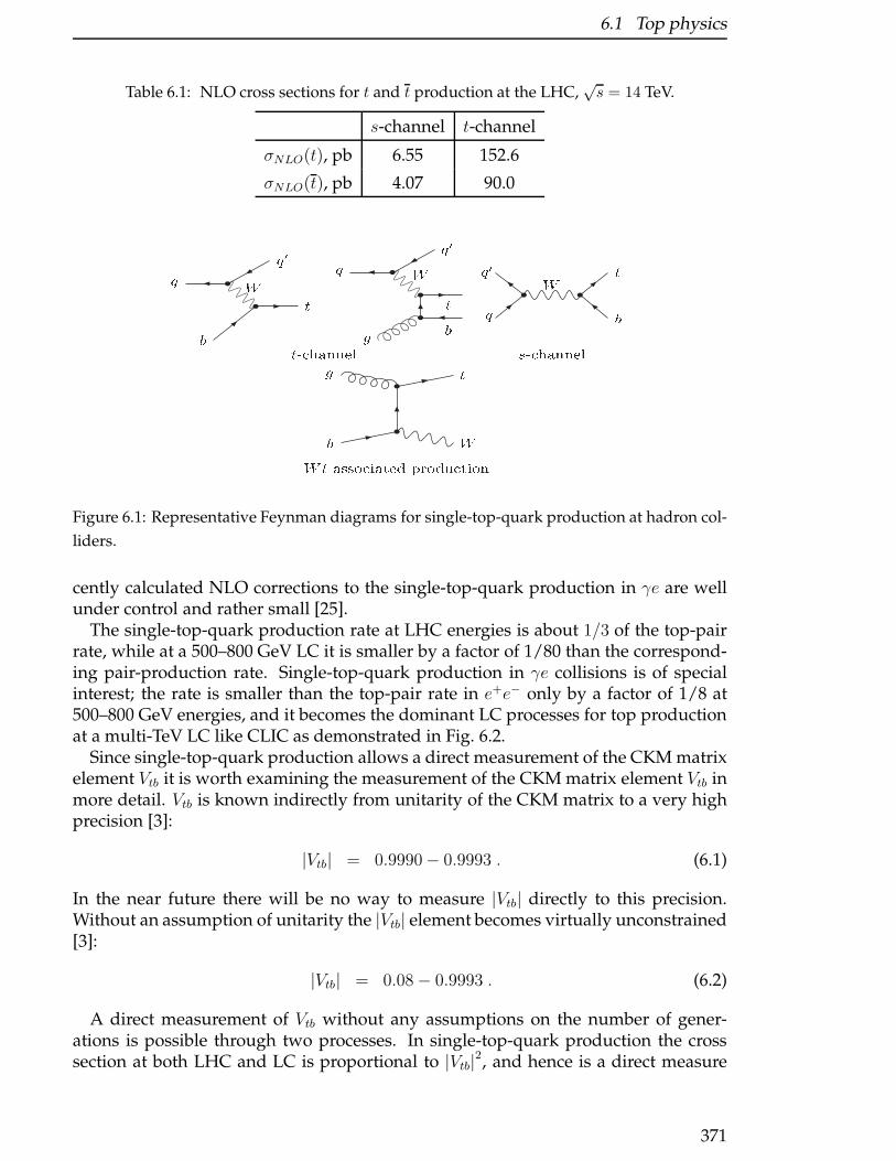
6.1 Top physics
Table 6.1: NLO cross sections for t and t production at the LHC,√s = 14 TeV.
s-channel t-channel
σNLO(t), pb 6.55 152.6
σNLO(t), pb 4.07 90.0
q q0W tb t- hannelq q0W tg b qq0 W tbs- hannel
bg
Wt
Wt asso iated produ tionFigure 6.1: Representative Feynman diagrams for single-top-quark production at hadron col-
liders.
cently calculated NLO corrections to the single-top-quark production in γe are wellunder control and rather small [25].
The single-top-quark production rate at LHC energies is about 1/3 of the top-pairrate, while at a 500–800 GeV LC it is smaller by a factor of 1/80 than the correspond-ing pair-production rate. Single-top-quark production in γe collisions is of specialinterest; the rate is smaller than the top-pair rate in e+e− only by a factor of 1/8 at500–800 GeV energies, and it becomes the dominant LC processes for top productionat a multi-TeV LC like CLIC as demonstrated in Fig. 6.2.
Since single-top-quark production allows a direct measurement of the CKM matrixelement Vtb it is worth examining the measurement of the CKM matrix element Vtb inmore detail. Vtb is known indirectly from unitarity of the CKM matrix to a very highprecision [3]:
|Vtb| = 0.9990− 0.9993 . (6.1)
In the near future there will be no way to measure |Vtb| directly to this precision.Without an assumption of unitarity the |Vtb| element becomes virtually unconstrained[3]:
|Vtb| = 0.08− 0.9993 . (6.2)
A direct measurement of Vtb without any assumptions on the number of gener-ations is possible through two processes. In single-top-quark production the crosssection at both LHC and LC is proportional to |Vtb|2, and hence is a direct measure
371

6 Electroweak and QCD Precision Physics
Figure 6.2: Top-quark cross sections at the LC
of |Vtb|2. The partial width of the top-quark decaying into bW is also proportional to|Vtb|2, and at a linear collider one can measure indirectly the partial width by extract-ing the total top quark width from the tt threshold and by measuring the branchingof t → Wb. The anticipated accuracy of a direct measurement of |Vtb| is about 7% atthe LHC [21] and in the e+e− option of a linear collider [8, 20, 24], and can possiblyreach 1% for a polarized γe− collider [24].
Note, the |Vtb|matrix element can be measured at a LC significantly more accuratelyas compared to the LHC. Therefore, its value could be used at LHC in single-topanalysis of the process t-channel qb→ q′t to measure the b-quark distribution functionin the proton. Such a measurement is of a great importance in order to get correctlythe MSSM Higgs production rate, especially at large values of tan β, and gives a niceexample of the potential LHC&LC interplay.
6.1.2 Spin correlations in top production and decays
Since the top quark decays before hadronization, its spin properties are not spoiled.Therefore spin correlations in top production and decays is an interesting issue intop-quark physics. As well known from the polarized top decays [27] the down typefermions are the best top-quark spin analyzers. Such a unique property of polarizedtop-quark decay is a consequence of the pure (V-A) structure of the charged currentsin the Standard Model. NLO corrections do not change this property drastically: tothe leptonic Kl they are very small −0.0015αs [28], and to quarks Kd,s they are about−6% [29].
The (V-A) structure of the top quark interaction leads to simple top-quark spinproperties for the single-top-quark production at the LHC. It was shown [30] thatthe top-quark spin in each event should follow the direction of the down-type quark
372

6.1 Top physics
momentum in the top-quark rest frame. This is the direction of the initial d-quark forthe s-channel, and the dominant direction of the final d-quark for the t-channel single-top-quark production processes. This follows from the above results on polarizedtop decays, because these two production modes could be considered as top-quarkdecays “backward in time” [31]. Further, the best variable to observe maximal top-quark spin correlations in single-top-quark s-channel or t-channel production andthe subsequent decay of the top-quark is the angle between this down-type quarkdirection in the production processes and the charged lepton (or d, s-quark) directionfrom the top-quark decay in the top-quark rest frame. Since the u-quark density isthe largest among the quark densities, the observed light-quark jet in the t-channel ispredominately initiated by d-quarks. It is useful to define the quantity [32]
a =1
2
(1 + cos θql
), (6.3)
where θql is the angle between the light-quark jet and the charged lepton. In the restframe of the top quark the differential cross section with respect to this variable isgiven by
dσ
da= σ (2Pa+ (1− P )) , (6.4)
where P is the polarization of the top quark. As an example, a plot for the spincorrelation is shown in Fig. 6.3, based on the complete LO matrix elements (cf. [20] fora method to extract this signal from the backgrounds). It was demonstrated that thetop spin correlation properties for the single top production and decay are preservedat next-to-leading order [33, 34].
051015202530
0 0.1 0.2 0.3 0.4 0.5 0.6 0.7 0.8 0.9 1dda
a33333333333333333333333333333333
33333333
Figure 6.3: The distribution for the angular correlation a for t-channel production at the LHC.
Spin properties of the t-quark in the tW production process follows from the anal-ogy of the tW production mode to radiative polarized top decay. Here one can find akinematic region in which top quarks are produced with the polarization vector pref-erentially close to the direction of the charged lepton or the d, s-quark momentumfrom the associated W decay. In this kinematic region the direction of the producedcharged lepton or the d, s-quark should be as close as possible to the direction of theinitial gluon beam in the top-quark rest frame [31] as demonstrated in Fig. 6.4.
The latter result of the LHC process is an additional nice example of ”theoretical”LHC&LC interplay. Indeed it has an immediate implication for single-top-quark pro-duction in γe collisions in the process γe → νetb. Here the directions of the initial
373
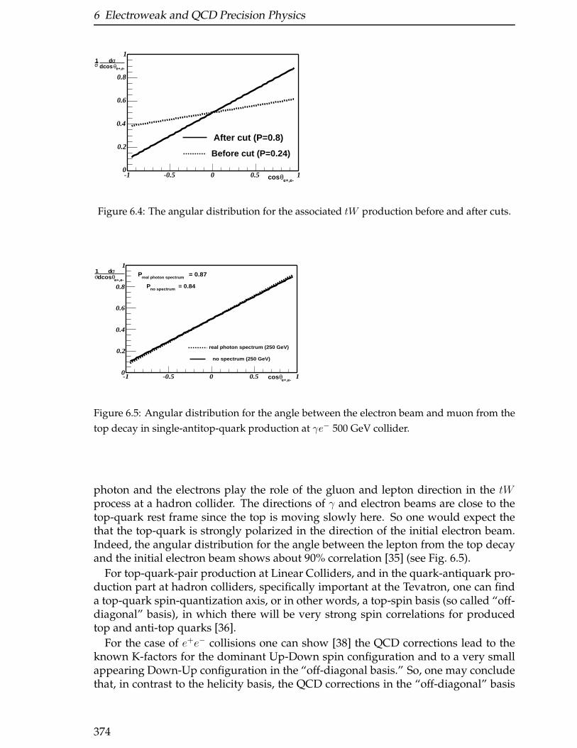
6 Electroweak and QCD Precision Physics
-1 -0.5 0 0.5 10
0.2
0.4
0.6
0.8
1
e+,e-θdcosσd σ
1
e+,e-θcos
Before cut (P=0.24)
After cut (P=0.8)
Figure 6.4: The angular distribution for the associated tW production before and after cuts.
-1 -0.5 0 0.5 10
0.2
0.4
0.6
0.8
1
e+,e-θdcosσd σ
1
e+,e-θcos
real photon spectrum (250 GeV)
no spectrum (250 GeV)
= 0.84no spectrumP
= 0.87real photon spectrumP
Figure 6.5: Angular distribution for the angle between the electron beam and muon from the
top decay in single-antitop-quark production at γe− 500 GeV collider.
photon and the electrons play the role of the gluon and lepton direction in the tWprocess at a hadron collider. The directions of γ and electron beams are close to thetop-quark rest frame since the top is moving slowly here. So one would expect thethat the top-quark is strongly polarized in the direction of the initial electron beam.Indeed, the angular distribution for the angle between the lepton from the top decayand the initial electron beam shows about 90% correlation [35] (see Fig. 6.5).
For top-quark-pair production at Linear Colliders, and in the quark-antiquark pro-duction part at hadron colliders, specifically important at the Tevatron, one can finda top-quark spin-quantization axis, or in other words, a top-spin basis (so called “off-diagonal” basis), in which there will be very strong spin correlations for producedtop and anti-top quarks [36].
For the case of e+e− collisions one can show [38] the QCD corrections lead to theknown K-factors for the dominant Up-Down spin configuration and to a very smallappearing Down-Up configuration in the “off-diagonal basis.” So, one may concludethat, in contrast to the helicity basis, the QCD corrections in the “off-diagonal” basis
374
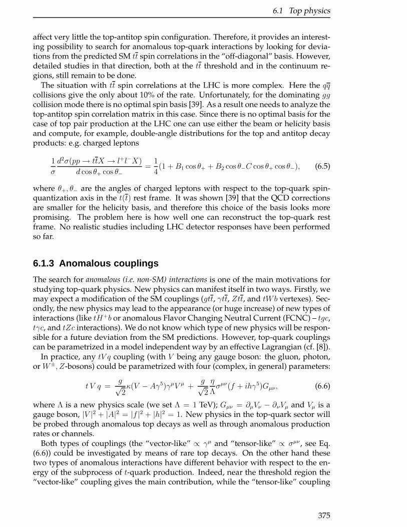
6.1 Top physics
affect very little the top-antitop spin configuration. Therefore, it provides an interest-ing possibility to search for anomalous top-quark interactions by looking for devia-tions from the predicted SM tt spin correlations in the “off-diagonal” basis. However,detailed studies in that direction, both at the tt threshold and in the continuum re-gions, still remain to be done.
The situation with tt spin correlations at the LHC is more complex. Here the qqcollisions give the only about 10% of the rate. Unfortunately, for the dominating ggcollision mode there is no optimal spin basis [39]. As a result one needs to analyze thetop-antitop spin correlation matrix in this case. Since there is no optimal basis for thecase of top pair production at the LHC one can use either the beam or helicity basisand compute, for example, double-angle distributions for the top and antitop decayproducts: e.g. charged leptons
1
σ
d2σ(pp→ ttX → l+l−X)
d cos θ+ cos θ−=
1
4(1 +B1 cos θ+ +B2 cos θ−C cos θ+ cos θ−), (6.5)
where θ+, θ− are the angles of charged leptons with respect to the top-quark spin-quantization axis in the t(t) rest frame. It was shown [39] that the QCD correctionsare smaller for the helicity basis, and therefore this choice of the basis looks morepromising. The problem here is how well one can reconstruct the top-quark restframe. No realistic studies including LHC detector responses have been performedso far.
6.1.3 Anomalous couplings
The search for anomalous (i.e. non-SM) interactions is one of the main motivations forstudying top-quark physics. New physics can manifest itself in two ways. Firstly, wemay expect a modification of the SM couplings (gtt, γtt, Ztt, and tWb vertexes). Sec-ondly, the new physics may lead to the appearance (or huge increase) of new types ofinteractions (like tH+b or anomalous Flavor Changing Neutral Current (FCNC) – tgc,tγc, and tZc interactions). We do not know which type of new physics will be respon-sible for a future deviation from the SM predictions. However, top-quark couplingscan be parametrized in a model independent way by an effective Lagrangian (cf. [8]).
In practice, any tV q coupling (with V being any gauge boson: the gluon, photon,or W±, Z-bosons) could be parametrized with four (complex, in general) parameters:
t V q =g√2κ(V −Aγ5)γµV µ +
g√2
η
Λσµν(f + ihγ5)Gµν , (6.6)
where Λ is a new physics scale (we set Λ = 1 TeV); Gµν = ∂µVν − ∂νVµ and Vµ is agauge boson, |V |2 + |A|2 = |f |2 + |h|2 = 1. New physics in the top-quark sector willbe probed through anomalous top decays as well as through anomalous productionrates or channels.
Both types of couplings (the “vector-like” ∝ γµ and “tensor-like” ∝ σµν , see Eq.(6.6)) could be investigated by means of rare top decays. On the other hand thesetwo types of anomalous interactions have different behavior with respect to the en-ergy of the subprocess of t-quark production. Indeed, near the threshold region the“vector-like” coupling gives the main contribution, while the “tensor-like” coupling
375
6 Electroweak and QCD Precision Physics
becomes essential at high values of√s ≫ mt. Note, that in hadronic collisions the
production of a system with the high values of√s is suppressed due to parton lumi-
nosities. Therefore, we may conclude very roughly that in the production processesthe “vector-like” couplings will be better investigated in hadronic collisions, whilea linear collider provides the better potential to probe the “tensor-like” interactions.So, one expects the only combine analysis of the LHC and LC data could provide tinyconstraints on the both types of couplings. Obviously that can not be achieved byanalyzing the data from the only one type of a collider.
6.1.3.1 Probes of anomalous gtt coupling
Due to gauge invariance, only “tensor-like” interaction (top quark anomalous chro-moelectric and chromomagnetic moments) (∝ σµν) could contribute to anomalous gttcouplings [8]. Such an anomalous coupling could be probed via the t-quark produc-tion at both LHC and LC machines. In hadronic collisions as it was shown in Ref. [40]the high-end tail of the top-quark pT and Mtt distributions are the observables mostsensitive to non-zero values of ηgf , with a reach for the combination 4mt
Ληgf as small
as ≃ 0.03. For these values only a minor change in the total tt rate is expected. Theinformation on ηgh could be obtained also by studying the correlation observablesbetween ℓ+ℓ− lepton pairs produced in the dilepton decays of tt pair [42]. In e+e−
collisions such a coupling could be investigated by a measurement of the energyspectrum of the additional light (gluon) jet radiated off the top quark in the processe+e− → ttg [40].
From the LHC collider alone one can achieve sensitivities to 4mt
Ληg of order 0.03
with 100 fb−1 of integrated luminosity. This is similar in magnitude to what can beobtained at a 500 GeV LC with an integrated luminosity of 50 fb−1. One should pointout that at the LHC and at LC different kinematic characteristics are mostly sensitiveto the anomalous moments. Therefore one expects that the combining analysis ofthe LHC and LC data will allow to get better accuracy in measurement of top-gluonanomalous couplings and possibly to distinguish chromoelectric and chromomag-netic moments by using polarized options of LC including photon collisions. Thepolarized electron-positron and photon-photon collisions are also allow to measureuniquely the γtt and Ztt anomalous couplings [41].
6.1.3.2 Search for anomalous Wtb couplings
The Wtb vertex structure can be probed and measured using either top-quark-pairor single-top-quark production processes. The total tt rate depends very weakly onthe Wtb vertex structure, as top quarks are dominantly produced on-shell [43]. How-ever, more sensitive observables, like C and P asymmetries, top-quark polarization,and spin correlations provide interesting information. The single-top-quark produc-tion rate is directly proportional to the square of the Wtb coupling, and therefore it ispotentially very sensitive to the Wtb structure [44]. The potential to measure anoma-lous Wtb couplings at the LHC via the production rate of single top quarks and fromkinematic distributions has been studied in several papers [21, 45–48].
The potential of the hadron colliders can be compared to the potential of a next gen-eration e+e− linear collider (LC) where the best sensitivity could be obtained in high
376
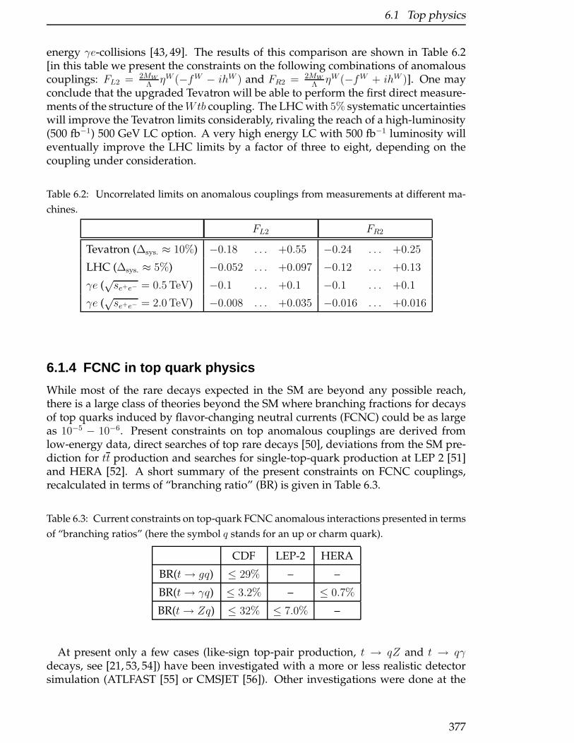
6.1 Top physics
energy γe-collisions [43, 49]. The results of this comparison are shown in Table 6.2[in this table we present the constraints on the following combinations of anomalouscouplings: FL2 = 2MW
ΛηW (−fW − ihW ) and FR2 = 2MW
ΛηW (−fW + ihW )]. One may
conclude that the upgraded Tevatron will be able to perform the first direct measure-ments of the structure of theWtb coupling. The LHC with 5% systematic uncertaintieswill improve the Tevatron limits considerably, rivaling the reach of a high-luminosity(500 fb−1) 500 GeV LC option. A very high energy LC with 500 fb−1 luminosity willeventually improve the LHC limits by a factor of three to eight, depending on thecoupling under consideration.
Table 6.2: Uncorrelated limits on anomalous couplings from measurements at different ma-
chines.
FL2 FR2
Tevatron (∆sys. ≈ 10%) −0.18 . . . +0.55 −0.24 . . . +0.25
LHC (∆sys. ≈ 5%) −0.052 . . . +0.097 −0.12 . . . +0.13
γe (√se+e− = 0.5 TeV) −0.1 . . . +0.1 −0.1 . . . +0.1
γe (√se+e− = 2.0 TeV) −0.008 . . . +0.035 −0.016 . . . +0.016
6.1.4 FCNC in top quark physics
While most of the rare decays expected in the SM are beyond any possible reach,there is a large class of theories beyond the SM where branching fractions for decaysof top quarks induced by flavor-changing neutral currents (FCNC) could be as largeas 10−5 − 10−6. Present constraints on top anomalous couplings are derived fromlow-energy data, direct searches of top rare decays [50], deviations from the SM pre-diction for tt production and searches for single-top-quark production at LEP 2 [51]and HERA [52]. A short summary of the present constraints on FCNC couplings,recalculated in terms of “branching ratio” (BR) is given in Table 6.3.
Table 6.3: Current constraints on top-quark FCNC anomalous interactions presented in terms
of “branching ratios” (here the symbol q stands for an up or charm quark).
CDF LEP-2 HERA
BR(t→ gq) ≤ 29% – –
BR(t→ γq) ≤ 3.2% – ≤ 0.7%
BR(t→ Zq) ≤ 32% ≤ 7.0% –
At present only a few cases (like-sign top-pair production, t → qZ and t → qγdecays, see [21, 53, 54]) have been investigated with a more or less realistic detectorsimulation (ATLFAST [55] or CMSJET [56]). Other investigations were done at the
377
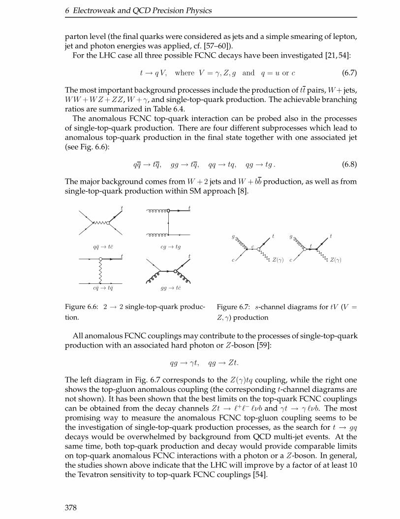
6 Electroweak and QCD Precision Physics
parton level (the final quarks were considered as jets and a simple smearing of lepton,jet and photon energies was applied, cf. [57–60]).
For the LHC case all three possible FCNC decays have been investigated [21, 54]:
t→ q V, where V = γ, Z, g and q = u or c (6.7)
The most important background processes include the production of tt pairs,W+ jets,WW +WZ+ZZ, W +γ, and single-top-quark production. The achievable branchingratios are summarized in Table 6.4.
The anomalous FCNC top-quark interaction can be probed also in the processesof single-top-quark production. There are four different subprocesses which lead toanomalous top-quark production in the final state together with one associated jet(see Fig. 6.6):
qq → tq, gg → tq, qq → tq, qg → tg . (6.8)
The major background comes from W +2 jets and W + bb production, as well as fromsingle-top-quark production within SM approach [8].
t
cq → tq
t
qq → tc
t
cg → tg
t
gg → tc
Figure 6.6: 2 → 2 single-top-quark produc-
tion.
c
c
g t
Z(γ)
t
c
g t
Z(γ)
Figure 6.7: s-channel diagrams for tV (V =
Z, γ) production
All anomalous FCNC couplings may contribute to the processes of single-top-quarkproduction with an associated hard photon or Z-boson [59]:
qg → γt, qg → Zt.
The left diagram in Fig. 6.7 corresponds to the Z(γ)tq coupling, while the right oneshows the top-gluon anomalous coupling (the corresponding t-channel diagrams arenot shown). It has been shown that the best limits on the top-quark FCNC couplingscan be obtained from the decay channels Zt → ℓ+ℓ− ℓνb and γt → γ ℓνb. The mostpromising way to measure the anomalous FCNC top-gluon coupling seems to bethe investigation of single-top-quark production processes, as the search for t → gqdecays would be overwhelmed by background from QCD multi-jet events. At thesame time, both top-quark production and decay would provide comparable limitson top-quark anomalous FCNC interactions with a photon or a Z-boson. In general,the studies shown above indicate that the LHC will improve by a factor of at least 10the Tevatron sensitivity to top-quark FCNC couplings [54].
378

6.1 Top physics
At a linear e+e− collider both methods of searching for FCNC interactions were con-sidered (see [60, 61]): tt-pair production via SM γ/Z-exchange with following FCNCdecays t→ qγ (Z):
e+e− → tt, with t→ qγ (Z), (6.9)
and single-top-quark production due to FCNC anomalous interactions with the SMdecay channel t→ bW :
e+e− → tu(c), with t→ bW. (6.10)
It was shown in [60], that the top-quark decay signal from the process (6.9) iscleaner than (tq) production (6.10). On the other hand, the cross sections for tq-processes is larger than for tt-production. At the same time the processes with FCNCtop-quark decays (6.9) could help to determine the nature of the couplings involved,tγq or tZq. Also, it was shown that beam polarization will be very useful to improvethe limits from tq production due to a substantial background decrease (see [60] fordetails).
Table 6.4: Future expectations on FCNC interactions from Run II of the Tevatron, LHC(CMS),
and linear e+e− collider.
Tevatron LHC e+e−
t→ Run II decay production√s > 500 GeV
g q 0.06% 1.6× 10⁻³ 1× 10⁻⁵ –
γ q 0.28% 2.5× 10⁻⁵ 3× 10⁻⁶ 4× 10⁻⁶
Z q 1.3% 1.6× 10⁻⁴ 1× 10⁻⁴ 2× 10⁻⁴
Table 6.4 presents a short comparison of LHC and LC potentials to investigateFCNC couplings. Branching ratios of order 10−6 are achievable, which are of interestfor some theories beyond the Standard Model, as discussed in Ref. [8]. Note that,due to the limited statistics which could be gathered in a future linear collider in thereaction e+e− → tt, the LHC has an advantage in the searches for rare top-quark de-cays. On the other hand, the future LC has a much smaller background. Therefore,both the LHC and a future LC have great potential to discover top-quark productiondue to anomalous interactions. Only for anomalous interactions with a gluon (tgc ortgu) will the LHC have an evident advantage. There are many studies devoted totop-quark rare decays, like t→ bWZ, t→ bH+, etc. However, almost all these inves-tigations were performed for the LHC option only. We refer the reader to the mostcomprehensive review [8].
It has to be stressed that different types of new interactions may manifest itself indifferent ways at different colliders even for the same observables. So, only mutualLHC&LC analysis will provide more definite conclusions about a type of possiblenew interactions.
379
6 Electroweak and QCD Precision Physics
6.2 Electroweak precision physics
U. Baur, S. Heinemeyer, S. Kraml, K. Monig, W. Porod and G. Weiglein
In this section the electroweak precision measurements, triple gauge boson cou-plings (TGC), and contact interactions are analyzed. Electroweak precision observ-ables can play a role in various models. In many physics scenarios they can provideinformation about new physics scales that are too heavy to be detected directly. Sev-eral possible applications of precision observables are discussed in different parts ofthis report. Examples of the application of electroweak precision observables are
• the search for new gauge bosons, see Sect. 7.3.3,
• limits for new physics scales in little Higgs models, see Sect. 3.6,
• investigations on strong electroweak symmetry breaking, see Sect. 4,
• the search for heavy scales in supersymmetric theories, which will be coveredin this section.
For the electroweak precision measurements (in the context of Supersymmetry) threeexample studies are presented. Physics scenarios which are dominated by LHC mea-surements can be probed much better if in addition the information from electroweakprecision observables, obtained at the LC, is used. The triple gauge couplings are an-alyzed in view of a possible combination of the results of the LHC and the LC. Inthe case that both colliders can obtain independently about the same uncertainty, thecombination of the two experiments can result in an even higher precision.
Concerning the physics of contact interactions a possible LHC/LC interplay couldarise as follows. Precision measurements of e+e− → ff at the LC and of Drell-Yanproduction at the LHC might exhibit deviations that could be interpreted in termsof contact interactions. While the LHC is sensitive to uu → ℓ+ℓ− and to a somewhatlesser extend to ud → ℓ+ℓ− the linear collider measures e+e− → qq with unidentifiedquarks, e+e− → bb and e+e− → ℓ+ℓ− with identified leptons. The combination of thetwo machines can thus disentangle the flavour structure of the new interactions incase a signal is seen.
6.2.1 Electroweak precision measurements at the LHC and the LC
The precision that can be achieved for electroweak precision observables (EWPO),including mt and mh has been analyzed in detail in Ref. [63] and is reviewed in Ta-ble 6.5. The numbers listed there represent the sensitivities that can be reached byeach individual collider. The reach of the LC is seen to exceed that of the LHC (dueto its cleaner environment) for all relevant observables. It is therefore difficult tofind a case of positive LHC/LC interplay by just looking at EWPO’s. This, however,changes if SUSY scenarios are analyzed. It is conceivable that part of the SUSY spec-trum, due to the large masses of some of the SUSY partners, can only be determinedby the LHC [64]. This may especially be relevant in the case of scalar top quarks whichplay an important role for the SUSY interpretation of EWPO’s, see e.g. Refs. [65, 66].In this case, the measurement of the SUSY mass spectrum at the LHC and the LC
380
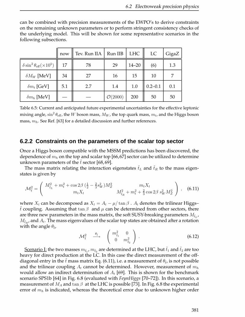
6.2 Electroweak precision physics
can be combined with precision measurements of the EWPO’s to derive constraintson the remaining unknown parameters or to perform stringent consistency checks ofthe underlying model. This will be shown for some representative scenarios in thefollowing subsections.
now Tev. Run IIA Run IIB LHC LC GigaZ
δ sin2 θeff(×105) 17 78 29 14–20 (6) 1.3
δMW [MeV] 34 27 16 15 10 7
δmt [GeV] 5.1 2.7 1.4 1.0 0.2–0.1 0.1
δmh [MeV] — — O(2000) 200 50 50
Table 6.5: Current and anticipated future experimental uncertainties for the effective leptonic
mixing angle, sin2 θeff , the W boson mass, MW , the top quark mass, mt, and the Higgs boson
mass, mh. See Ref. [63] for a detailed discussion and further references.
6.2.2 Constraints on the parameters of the scalar top sector
Once a Higgs boson compatible with the MSSM predictions has been discovered, thedependence ofmh on the top and scalar top [66,67] sector can be utilized to determineunknown parameters of the t sector [68, 69].
The mass matrix relating the interaction eigenstates tL and tR to the mass eigen-states is given by
M2t =
(M2
tL+m2
t + cos 2β (12− 2
3s2W )M2
Z mtXt
mtXt M2tR
+m2t + 2
3cos 2β s2
WM2Z
), (6.11)
where Xt can be decomposed as Xt = At − µ/ tanβ . At denotes the trilinear Higgs–t coupling. Assuming that tan β and µ can be determined from other sectors, thereare three new parameters in the mass matrix, the soft SUSY-breaking parametersMtL ,MtR , andAt. The mass eigenvalues of the scalar top states are obtained after a rotationwith the angle θt,
M2t
θt−→(m2t1
0
0 m2t2
). (6.12)
Scenario I: the two masses mt1 , mt2 are determined at the LHC, but t1 and t2 are tooheavy for direct production at the LC. In this case the direct measurement of the off-diagonal entry in the t mass matrix Eq. (6.11), i.e. a measurement of θt, is not possibleand the trilinear coupling At cannot be determined. However, measurement of mh
would allow an indirect determination of At [69]. This is shown for the benchmarkscenario SPS1b [64] in Fig. 6.8 (evaluated with FeynHiggs [70–72]). In this scenario, ameasurement ofMA and tan β at the LHC is possible [73]. In Fig. 6.8 the experimentalerror of mh is indicated, whereas the theoretical error due to unknown higher order
381

6 Electroweak and QCD Precision Physics
corrections has been neglected; see Ref. [69] for details. Fig. 6.8 demonstrates thatAt can be determined with LHC measurements alone; the allowed range is indicatedby the green (light shaded) area. However, the precise determination of mt at theLC improves the accuracy for At by about a factor of three over that which can beachieved with the LHC mt measurement. Concerning resolving the sign ambiguityof At, see Sect. 3.3.1.
-1000 -500 0 500 1000A t [GeV]
105
110
115
120
125
130m h [G
eV]
extraction of A t in SPS 1b
δmtexp
= 2.0 GeV
δmtexp
= 0.1 GeV
∆mhexp
Figure 6.8: Indirect determination of At in the SPS1b scenario for tan β = 30, δmexpt = 2 GeV
(LHC) and δmexpt = 0.1 GeV (LC). The statistical uncertainty of the Higgs boson mass, ∆mexp
h ,
is indicated. The SUSY parameters mt1,mt2
,mb1,mb2
are assumed to be given by the values
predicted by SPS1b with an uncertainty of 5%. MA and tan β are assumed to be determined
with a precision of 10% and 15%, respectively.
Scenario II: in this example [9,69], the lighter scalar top quark andMA are accessibleat the LC, whereas only a lower bound can be established for tanβ . The LC willprovide precise measurements of its mass, mt1 , and the t mixing angle, θt [74, 75].On the other hand, the heavier scalar top, t2, can only be detected at the LHC. Themeasurement of mh can then be used to obtain indirect limits on mt2 . Comparison ofthe indirectly determined mt2 with the value obtained from a direct measurement atthe LHC will provide a stringent consistency test of the MSSM. In Fig. 6.9 we showthe allowed region in the mt2 − mh-plane for this scenario. Assuming that the topquark mass can be determined with a precision of δmt = 0.1 GeV at the LC, one finds680 GeV <∼ mt2
<∼ 695 GeV. For comparison, for δmt = 2 GeV, as expected from LHC
experiments, one obtains 670 GeV <∼ mt2<∼ 705 GeV, i.e. the precise determination of
mt at the LC reduces the uncertainty of mt2 by about a factor 3. Again the theoreticalerror due to unknown higher order corrections tomh has been neglected; see Ref. [69]for details.
382
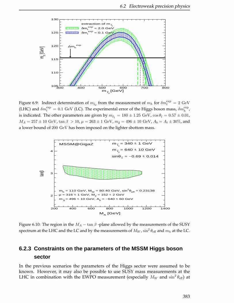
6.2 Electroweak precision physics
300 400 500 600 700 800m t2
~ [GeV]
105
110
115
120
125
130
m h [GeV
]
extraction of m t2 ~
δmtexp
= 2.0 GeV
δmtexp
= 0.1 GeV
∆mhexp
Figure 6.9: Indirect determination of mt2from the measurement of mh for δmexp
t = 2 GeV
(LHC) and δmexpt = 0.1 GeV (LC). The experimental error of the Higgs boson mass, δmexp
h ,
is indicated. The other parameters are given by mt1= 180 ± 1.25 GeV, cos θt = 0.57 ± 0.01,
MA = 257 ± 10 GeV, tan β > 10, µ = 263 ± 1 GeV, mg = 496 ± 10 GeV, Ab = At ± 30%, and
a lower bound of 200 GeV has been imposed on the lighter sbottom mass.
200 400 600 800 1000 1200 1400
MA [GeV]
2
3
4
tanβ
MSSM@GigaZ m t1 ~ = 340 +− 1 GeV
m t2 ~ = 640 +− 10 GeV
sinθ t~ = −0.69 +− 0.014
mh = 110 GeV, MW = 80.40 GeV, sin2θeff = 0.23138
µ = 316 +− 1 GeV, M2 = 152 +− 2 GeV
m g ~ = 496 +− 10 GeV, Ab = −640 +− 60 GeV
Figure 6.10: The region in the MA − tan β -plane allowed by the measurements of the SUSY
spectrum at the LHC and the LC and by the measurements of MW , sin2 θeff and mh at the LC.
6.2.3 Constraints on the parameters of the MSSM Higgs boson
sector
In the previous scenarios the parameters of the Higgs sector were assumed to beknown. However, it may also be possible to use SUSY mass measurements at theLHC in combination with the EWPO measurement (especially MW and sin2 θeff) at
383
6 Electroweak and QCD Precision Physics
the LC to obtain information on the (unknown) parameters of the Higgs sector [65].Scenario III: In Fig. 6.10 we show the parameter space of a scenario where the
MSSM Higgs mass scale, the mass of the CP -odd Higgs boson MA, cannot be mea-sured directly at the LHC nor the LC (for most of the shown parameter space). How-ever, the combination of LHC and LC mass measurements together with the MW ,sin2 θeff from GigaZ and the mh determination at the LC (see the plot for further de-tails) can set an upper bound of MA
<∼ 1200 GeV.
6.2.4 Triple gauge boson couplings
The LHC will significantly improve the precision of the measurements of the triplegauge boson couplings (TGC) compared to the LEP and Tevatron results [76]. Inthe SM, the TGC’s are uniquely fixed by gauge invariance. Extensions to the SM, inparticular models in which the W and Z bosons are composite objects, often lead todeviations from the SM predictions for the TGC’s.
Assuming electromagnetic gauge invariance, Lorentz invariance, and C-and P -conservation, five parameters can be used to describe the three gauge boson ver-tices [76]:
∆gZ1 = gZ1 − 1 , ∆κV = κV − 1 , λV (V = γ, Z) . (6.13)
In the SM, at tree level, all five parameters vanish.At the LHC, Wγ and WZ production can be used to constrain TGC’s. WW pro-
duction, which is also sensitive to the weak boson self-couplings, suffers from a largett background, and, therefore, is not considered. Wγ production probes the WWγcouplings ∆κγ and λγ . WZ production is sensitive to the WWZ couplings ∆gZ1 , ∆κZand λZ .
The experimental sensitivity to anomalous TGC’s arises from the growth of thenon-standard contributions to the helicity amplitudes with energy, and from mod-ifications to angular distributions. In hadronic collisions, one usually exploits theformer by measuring the transverse momentum distribution of the photon or Z bo-son [76]. The energy dependence is most pronounced for λV and ∆gZ1 . Figure 6.11shows the expected 95% confidence level constraints on TGC’s in ATLAS, resultingfrom two-parameter fits [54]. There are strong correlations between ∆gZ1 and the otherWWZ couplings, ∆κZ and λZ . At the LHC, the limits for λV and ∆gZ1 are of O(10−3),while the precision of ∆κV is O(10−2). An increase in the integrated luminosity by afactor 10 improves the limits by a factor 1.3 to 2. A similar improvement is observedif the machine energy is doubled. Doubling the energy and increasing the luminos-ity yields bounds which are up to a factor 7 more stringent than those obtained for√s = 14 TeV and 100 fb−1.At the LC, the most stringent bounds are obtained from angular distributions in
W pair production. Sensitivity bounds for√s = 800 GeV and an integrated lumi-
nosity of 1 ab−1 are shown in Fig. 6.12 [9]. For these bounds electron and positronpolarization has been assumed, Pe− = 0.8, Pe+ = 0.6. If positron polarizaation wouldnot be available, the bounds would be weakened by about a factor 2. For e+e− col-lisions at
√s = 500 GeV, but both beams polarized, one finds bounds which are a
factor 1.2 to 2 less stringent than those shown in Fig. 6.12. All bounds, with the ex-ception of those for ∆gZ1 , are of O(10−4) and thus are significantly better than those
384

6.2 Electroweak precision physics
Figure 6.11: Expected 95% CL constraints on TGC’s in ATLAS resulting from two-parameter
fits. Shown are results for√s = 14 TeV and 100 fb−1 (solid),
√s = 28 TeV and 100 fb−1
(dot-dash),√s = 14 TeV and 1000 fb−1 (dash), and
√s = 28 TeV and 1000 fb−1 (dotted). The
figure has been taken from Ref. [54].
∆gZ1 / 10-4
∆κΖ
/ 10-4
95 % CL1 σ
-10
-7.5
-5
-2.5
0
2.5
5
7.5
10
-40 -30 -20 -10 0 10 20 30 40
∆gZ1 / 10-4
λ Ζ / 1
0-4
95 % CL1 σ
-10
-7.5
-5
-2.5
0
2.5
5
7.5
10
-40 -30 -20 -10 0 10 20 30 40
∆κγ / 10-4
∆κΖ
/ 10-4
95 % CL1 σ
-10
-7.5
-5
-2.5
0
2.5
5
7.5
10
-10 -7.5 -5 -2.5 0 2.5 5 7.5 10
λγ / 10-4
λ Ζ / 1
0-4
95 % CL1 σ
-10
-7.5
-5
-2.5
0
2.5
5
7.5
10
-10 -7.5 -5 -2.5 0 2.5 5 7.5 10
Figure 6.12: 1σ and 95% CL (2D) contours for TGC’s in the 5-parameter fit of e+e− →W+W−
(√s = 800 GeV, L = 1000 fb−1, Pe− = 0.8, Pe+ = 0.6). The figure is taken from Ref. [9].
obtained at the LHC, even with an energy and/or luminosity upgrade. The resultsfor the anticipated precision of all TGC’s for LEP, the Tevatron assuming 1 fb−1 foreach experiment [77], the LHC assuming 30 fb−1 for each experiment [78] and forthe LC assuming either 500 fb−1 at
√s = 500 GeV or 1000 fb−1 at
√s = 800 GeV [9]
385
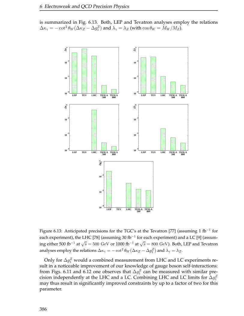
6 Electroweak and QCD Precision Physics
is summarized in Fig. 6.13. Both, LEP and Tevatron analyses employ the relations∆κγ = − cot2 θW (∆κZ −∆gZ1 ) and λγ = λZ (with cos θW = MW/MZ).
10-4
10-3
10-2
∆κγ
LEP TEV LHC TESLA TESLA500 800
10-4
10-3
10-2
∆λγ
LEP TEV LHC TESLA TESLA500 800
10-4
10-3
10-2
∆κZ
LEP TEV LHC TESLA TESLA500 800
10-4
10-3
10-2
∆λZ
LEP TEV LHC TESLA TESLA500 800
10-4
10-3
10-2
∆g1Z
LEP TEV LHC TESLA TESLA500 800
Figure 6.13: Anticipated precisions for the TGC’s at the Tevatron [77] (assuming 1 fb−1 for
each experiment), the LHC [78] (assuming 30 fb−1 for each experiment) and a LC [9] (assum-
ing either 500 fb−1 at√s = 500 GeV or 1000 fb−1 at
√s = 800 GeV). Both, LEP and Tevatron
analyses employ the relations ∆κγ = − cot2 θW (∆κZ −∆gZ1 ) and λγ = λZ .
Only for ∆gZ1 would a combined measurement from LHC and LC experiments re-sult in a noticeable improvement of our knowledge of gauge boson self-interactions:from Figs. 6.11 and 6.12 one observes that ∆gZ1 can be measured with similar pre-cision independently at the LHC and a LC. Combining LHC and LC limits for ∆gZ1may thus result in significantly improved constraints by up to a factor of two for thisparameter.
386
6.3 QCD studies
Electroweak radiative corrections within the SM to the TGC’s are of order ∼ 10−3
[79] and thus significantly larger than the expected sensitivities at the LC. Similarcorrections can be expected in the MSSM. No detailed study exists yet, but it can beexpected that LHC/LC analyses similar to the one presented in Sect 6.2.3 are possible.
Although (with the above exception) TGC’s can in general be determined muchmore precisely at a LC, a positive interplay with the LHC may arise in specific mod-els. For example, in models where the electroweak symmetry is broken dynamically,TGC’s may be related to the masses of heavy vector resonances which appear in thesemodels. These resonances have masses which typically are of O(1 − 2 TeV). A pre-cise measurement of the TGC’s at a 500–800 GeV LC may thus allow for an indirectdetermination of the masses of such resonances, and provide specific information fora search for such particles at the LHC (see Sect. 4 for more details).
One can also probe the self-couplings of the neutral gauge bosons (ZZγ,¿ Zγγ andZZZ couplings) at the LHC [80, 81] and LC [82]. In the SM, at tree level, these cou-plings all vanish. The sensitivity limits which can be achieved for these couplings atthe LHC strongly depend on the form factor scale assumed. For a form factor scalein the range of 2 − 3 TeV, the bounds which can be achieved at the LHC and LC aresimilar. They are about one order of magnitude larger than what the SM predicts atthe one-loop level [80].
6.2.5 Conclusions
In this section the electroweak precision measurements (in the context of supersym-metry) and triple gauge boson couplings (TGC) have been analyzed. Other applica-tions of electroweak precision observables can be found in Sects. 7.3.3, 3.6, 4.
For the electroweak precision measurements within Supersymmetry three exam-ple studies have been performed. Often SUSY scenarios possess scales that cannot bedetected at the LHC and LC. The three examples have shown how in this case elec-troweak precision observables (e.g. MW , sin2 θeff and mt), measured most accuratlyat the LC, can help to determine these heavy scales. The interplay of observablesmeasured at the LHC and at the LC, together with the precision observables can becrucial.
The triple gauge couplings have been analyzed in view of a possible combinationof the results of the LHC and the LC. In the case of ∆gZ1 both colliders can obtain inde-pendently about the same uncertainty. Thus the combination of the two experimentscan result in an higher precision by up to a factor of 2.
Concerning the physics of contact interactions the LHC/LC interplay could help todisentangle the flavour structure of the new interactions in case a signal is seen.
6.3 QCD studies
Both the Large Hadron Collider and the Linear Collider are ideal machines for testingQuantum Chromodynamics, and in particular for making precision measurementsrelated to the strong interaction. As has already been clearly demonstrated by past
387

6 Electroweak and QCD Precision Physics
and present machines (for example LEP and the CERN and Tevatron pp colliders), thetwo colliders are complementary in what they can measure and with what precision.The benchmark QCD measurements for each machine are:
Linear Collider [83]
• precision determination of αS through event shape observables, multijet finalstates, etc.
• Q2 evolution of αS and “higher-twist” (i.e. Q−n) contributions to hadronic ob-servables
• QCD effects in tt production, both at threshold and in the continuum
• fragmentation functions
• γγ physics
– unpolarised and polarised photon structure functions F γ2 (x,Q2) ( gγ1 (x,Q2))
at low x or high Q2
– γγ and γ∗γ∗ total cross sections as a test of non-perturbative and perturba-tive QCD (BFKL dynamics) respectively
LHC [84]
• production of high ET jets, to determine αS and pin down parton distributionfunctions (pdfs) and to calibrate backgrounds to new-physics processes
• W and Z total cross sections, as a test of precision NNLO QCD predictions
• W and Z transverse momentum distributions, as a test of Sudakov resumma-tion
• heavy flavour (c, b and t) cross sections, as a test of QCD dynamics, for examplethreshold resummations, production mechanisms for quarkonia, etc.
• prompt photon and diphoton production, to measure the gluon distributionand to calibrate backgrounds to Higgs production
• forward jet, W+ jet, heavy quark, .. production as a test of BFKL dynamics
• diffractive processes, both ‘hard’ and ‘soft’
In terms of the complementarity of the QCD measurements at the two machines, onecan note the following:
• There is a strong correlation between the gluon distribution and the strong cou-pling αS in the theoretical prediction for the large ET jet cross section at hadroncolliders. A precision measurement of αS at high Q2 at the LC can be fed backinto the LHC analysis to extract the gluon pdf from large ET jet and promptphoton data with greater precision, see Section 6.3.1 below.
388
6.3 QCD studies
• Among the backgrounds to Higgs → γγ production at the LHC, one of themost important arises from the fragmentation of a quark or gluon into a pho-ton, q, g → γ + X . A precise knowledge of these fragmentation functions isrequired to control the SM background. The LC can provide such information,particularly in the large z region. This is discussed in more detail in Section 6.3.3below.
• The tests of (small-x) BFKL dynamics at the two machines centre on the ex-change of a ‘perturbative pomeron’ between two softly scattered hadronic sys-tems, but utilise different initial and final states (γ∗γ∗ → qqqq for the LC andgg → gg, bbbb, ... for the LHC) and therefore have different systematics. Thephenomenology of such processes is not straightforward at either machine, andtherefore information from both will probably be necessary to provide firm ev-idence for BFKL effects. This is discussed in more detail in Section 6.3.2 below.
• If supplemented with forward detectors to measure the scattered protons, theLHC could also study γγ interactions. Centre-of-mass energy values,
√sγγ ,
above 1 TeV could be reached. If total γγ cross sections can be measured at thesehigh energies, with sufficiently small systematic errors, these measurements canbe used to estimate more accurately the expected background at a LC, particu-larly for a multi-TeV collider such as CLIC. Conversely, the measurement oftotal γγ cross sections at a LC, in particular at its derived photon collider, withmuch better precision than at the LHC will give improved understanding of theLHC results in the
√sγγ region of overlap, i.e. below 500 GeV.
6.3.1 Measurements of αS
A. De Roeck and W.J. Stirling
The strong coupling αS can in principle be measured at hadron colliders throughprocesses involving jets, either from ‘pure QCD’ multijet final states or from processeslike W+ jet production. Difficulties arise, however, from the need for an accuratemeasurement of the jet (i.e. parton) energies, which requires detailed knowledge ofcalorimeter response, fragmentation effects, the underlying event, etc.
A further problem is that αS is inevitably correlated with the parton distributionfunctions. For example, in the combination αSf(x,Q2), where f = q, g, at high xincreasing the value of αS will, via the DGLAP evolution equations, cause a decreasein f , thus compensating the effect due to the explicit factor of the coupling. In factfor this reason the W+ jet cross section at the Tevatron is relatively insensitive to thevalue of the coupling constant, see for example [85].
The inclusive high ET jet cross section offers high statistics and more sensitivity tothe coupling. For example, a recent measurement by the CDF collaboration at theTevatron pp collider [86] gives
αS(M2Z)NLO = 0.1178± 0.0001 (stat)
+0.0081
−0.0095(expt. syst.) (6.14)
There are many contributions to the experimental systematic error, the largest beingdue to the calorimeter response to jets.
389
6 Electroweak and QCD Precision Physics
The above result does not include any additional theoretical error from factorisa-tion and renormalisation scale dependence — the standard variation of these scales isestimated to give rise to an additional (theoretical) error of approximately±0.005 [88].There is also a systematic error from the dependence on the input parton distributionfunctions.1 Because of the strong correlation between these and αS , it is difficult to es-timate this accurately in isolation from the global pdf fit. Note that Tevatron large ETjet data are included in both the latest MRST [90] and CTEQ [91] global analyses, andhave some influence on the αS value that is a by-product of such studies.2 Combiningerrors in quadrature would give αS(M
2Z) = 0.118± 0.011 from the CDF jet data, to be
compared to the world average (PDG, 2002) value of αS(M2Z) = 0.1172± 0.002 [87].
When considering how such a measurement would extrapolate to the LHC, onecan assume that the NNLO corrections will be known (for a recent review of progressin this area, see for example [92]), and therefore that the theoretical systematic errorwill be much reduced. The statistical error will also be small, and the systematicerrors associated with the jet measurement may improve by a factor two or so, usingthe channel W → jets, in tagged tt events. However, the problem with the αS – pdfcorrelation will persist, indeed the jet cross section data will be used to pin down thegluon distribution at medium and high x. Note that even though the measurementsof αS will be made at a very high scaleQ ∼ Ejet
T ∼ O(TeV), this does not help improvethe precision on the derived value of αS(M
2Z).
At the e+e− colliders LEP and SLC, αS was measured in a number of ways, includ-ing (i) from the Z0 hadronic width via a global precision electroweak fit (αS(M
2Z) =
0.1200±0.0028 ±0.002 (scale), [87]) (LEP1 and SLC) and (ii) from various hadronic fi-nal state jet and event shapes measures (Thrust, C parameter,R3 etc, ...) at LEP1, LEP2and SLC. These latter measurements are all based on the basic O(αS) e
+e− → qqgprocess, with NLO O(α2
S) perturbative QCD corrections included. An average valuebased on many such measurements from all the collaborations at LEP and SLC isαS(M
2Z) = 0.122 ± 0.007, where the error is totally dominated by the theoretical un-
certainties associated with the choice of scale, and the effect of hadronisation on thedifferent quantities fitted [87].
Extrapolation of the hadronic final state αS measurement to a LC is reasonablystraightforward, assuming of course similar or even improved detector capabilities.3
With luminosities of order 1034 cm−2s−1 or greater, and centre-of-mass energies√s = 500 − 1000 TeV, a LC should produce enough e+e− → qq(g) events to achieve
a statistical error of order ∆αS(M2Z) ≃ 0.001 or better. Assuming hermetic detectors
with good calorimetry and tracking, the systematic uncertainties from detector ef-fects should also be controllable to this level of accuracy. The uncertainties associatedwith hadronisation depend quite sensitively on the observable, but in every case areexpected to decrease with increasing energy at least as fast as 1/Q. An order of magni-tude improvement can therefore be expected at a LC compared with LEP1/SLC, andonce again the associated uncertainty should be well below the ∆αS(M
2Z) = 0.001
level. This leaves the theoretical systematic error from unknown higher-order correc-
1A study of the impact of the pdf uncertainty on the production cross sections for Drell-Yan lepton
pairs and Higgs bosons at the LHC has been performed by Bourilkov as part of this workshop, see
Ref. [89].2For example, the most recent MRST value is αS(M2
Z) = 0.1165± 0.002 (expt.) ± 0.003 (theory).3The results for the estimated errors on αS at a LC in this section are taken from [83].
390
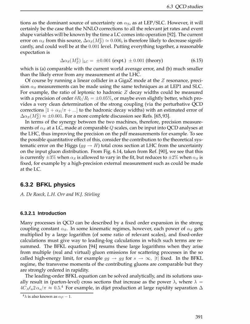
6.3 QCD studies
tions as the dominant source of uncertainty on αS, as at LEP/SLC. However, it willcertainly be the case that the NNLO corrections to all the relevant jet rates and eventshape variables will be known by the time a LC comes into operation [92]. The currenterror on αS from this source, ∆αS(M
2Z) ≃ 0.006, is therefore likely to decrease signifi-
cantly, and could well be at the 0.001 level. Putting everything together, a reasonableexpectation is
∆αS(M2Z) |LC = ±0.001 (expt.) ± 0.001 (theory) (6.15)
which is (a) comparable with the current world average error, and (b) much smallerthan the likely error from any measurement at the LHC.
Of course by running a linear collider in a GigaZ mode at the Z resonance, preci-sion αS measurements can be made using the same techniques as at LEP1 and SLC.For example, the ratio of leptonic to hadronic Z decay widths could be measuredwith a precision of order δRl/Rl = ±0.05%, or maybe even slightly better, which pro-vides a very clean determination of the strong coupling (via the perturbative QCDcorrections [1 + αS/π + ...] to the hadronic decay widths) with an estimated error of∆αS(M
2Z) ≈ ±0.001. For a more complete discussion see Refs. [65, 93].
In terms of the synergy between the two machines, therefore, precision measure-ments of αS at a LC, made at comparable Q scales, can be input into QCD analyses atthe LHC, thus improving the precision on the pdf measurements for example. To seethe possible quantitative effect of this, consider the contribution to the theoretical sys-tematic error on the Higgs (gg → H) total cross section at LHC from the uncertaintyon the input gluon distribution. From Fig. 6.14, taken from Ref. [90], we see that thisis currently ±3% when αS is allowed to vary in the fit, but reduces to±2% when αS isfixed, for example by a high-precision external measurement such as could be madeat the LC.
6.3.2 BFKL physics
A. De Roeck, L.H. Orr and W.J. Stirling
6.3.2.1 Introduction
Many processes in QCD can be described by a fixed order expansion in the strongcoupling constant αS . In some kinematic regimes, however, each power of αS getsmultiplied by a large logarithm (of some ratio of relevant scales), and fixed-ordercalculations must give way to leading-log calculations in which such terms are re-summed. The BFKL equation [94] resums these large logarithms when they arisefrom multiple (real and virtual) gluon emissions for scattering processes in the socalled high-energy limit, for example gg → gg for s → ∞, |t| fixed. In the BFKLregime, the transverse momenta of the contributing gluons are comparable but theyare strongly ordered in rapidity.
The leading-order BFKL equation can be solved analytically, and its solutions usu-ally result in (parton-level) cross sections that increase as the power λ, where λ =4CAℓn2αs/π ≈ 0.5.4 For example, in dijet production at large rapidity separation ∆
4λ is also known as αP − 1.
391

6 Electroweak and QCD Precision Physics
-6
-4
-2
0
2
4
6
-4 -3 -2 -1 0 1 2 3 4Per cent change in W cross section
χ2 increase in global analysis as theW and H cross sections are varied at the LHC
50
100
150
200
•A
•B
• C
•D
Per
cen
t cha
nge
in H
cro
ss s
ectio
n
+
50*
100*
•A*
•B*
•C*
•D*
Figure 6.14: Contours with ∆χ2 = 50, 100 . . . obtained by performing global pdf fits with the
values of σW and σH , at the LHC energy, fixed in the neighbourhood of their values predicted
by the unconstrained MRST2001 fit. The ∆χ2 = 50 contour is taken to represent the errors
on σW and σH (arising from the experimental errors on the data used in the global pdf fit).
The dashed contours are obtained if αS(M2Z) is allowed to vary. The superimposed solid
∆χ2 = 50, 100 contours are obtained if αS(M2Z) is fixed at 0.119.
in hadron colliders [95], BFKL predicts for the (qq, qg or gg) parton-level cross sectionσ ∼ eλ∆. In virtual photon - virtual photon scattering into hadrons, as measured forexample in e+e− collisions, BFKL becomes relevant when the electron and positronemerge with a small scattering angle and hadrons are produced centrally [96, 97]. Inthat case BFKL predicts σγ∗γ∗ ∼ (W 2/Q2)λ, where W 2 is the invariant mass of thehadronic system (equivalently, the photon-photon centre-of-mass energy) and Q2 isthe invariant mass of either photon.
6.3.2.2 Experimental status and improved predictions
The experimental status of BFKL is ambiguous at best, with existing results being farfrom definitive. The data tend to lie between the predictions of fixed-order QCD andanalytic solutions to the BFKL equation. This happens, for example, for the azimuthaldecorrelation in dijet production at the Fermilab Tevatron [98] and for the virtualphoton cross section at LEP [99]. Similar results are found for forward jet productionin deep inelastic ep collisions at HERA [100, 101].
It is not so surprising that analytic BFKL predicts stronger effects than seen in data.Analytic BFKL solutions implicitly contain sums over arbitrary numbers of gluons
392

6.3 QCD studies
with arbitrary energies, but the kinematics are leading-order only. As a result there isno kinematic cost to emit gluons, and energy and momentum are not conserved, andBFKL effects are artificially enhanced.
This situation can be remedied by a Monte Carlo implementation of solutions tothe BFKL equation [102,103]. In such an implementation the BFKL equation is solvedby iteration, making the sum over gluons explicit. Then kinematic constraints canbe implemented directly, and conservation of energy and momentum is restored.This tends to lead to a suppression of BFKL-type effects. The Monte Carlo approachhas been applied to dijet production at hadron colliders [102–105] leading to better(though still not perfect) agreement with the dijet azimuthal decorrelation data at theTevatron [102]. Predictions for the azimuthal angle decorrelation in dijet productionat the Tevatron and the LHC, as a function of the dijet rapidity difference ∆y, areshown in Fig. 6.15 [104]. The normalisation is such that 〈cos ∆φ〉 = 1 correspondsto jets which are back-to-back in the transverse plane, while completely uncorrelatedjets have 〈cos ∆φ〉 = 0. Kinematic suppression of gluon emission accounts for a sub-stantial part of the difference between analytic (asympototic) and Monte Carlo BFKLpredictions. This kinematic suppression is however not as dramatic at the LHC, be-cause of its relatively higher centre-of-mass energy compared to the jet transverse mo-mentum threshold. As a result, improved BFKL MC predictions tend to retain moreBFKL-type behaviour because of the greater phase space for emitting gluons [104].Studies of dijet production in BFKL physics therefore look promising at the LHC,and such studies will benefit from jet detection capabilities that extend far into theforward region and allow for pT thresholds as low as possible.
Other similar studies have considered forward W+ jet production at hadron col-liders [106], and the associated jet production in dijet production [107]. Applicationsto forward jet production at HERA and to virtual photon scattering in e+e− collisionsare underway; an update on the latter appears in the next section.
6.3.2.3 γ∗γ∗ scattering at the Linear Collider: a closer look
BFKL effects can arise in e+e− collisions via the scattering of virtual photons emittedfrom the initial e+ and e−. The scattered electron and positron appear in the forwardand backward regions (“double-tagged” events) with hadrons in between. With totalcentre-of-mass energy s, photon virtuality −Q2, and photon-photon invariant mass(= invariant mass of the final hadronic system) W 2, BFKL effects are expected in thekinematic regime where W 2 is large and
s≫ Q2 ≫ Λ2QCD.
At fixed order in QCD, the dominant process is four-quark production with t-channelgluon exchange (each photon couples to a quark box; the quark boxes are connectedvia the gluon). The corresponding BFKL contribution arises from diagrams with agluon ladder attached to the exchanged t-channel gluon.
The relative contributions of fixed-order QCD and BFKL are most easily under-stood by looking at
W 2Q21Q
22
d3σ
dW 2dQ21dQ
22
(6.16)
393
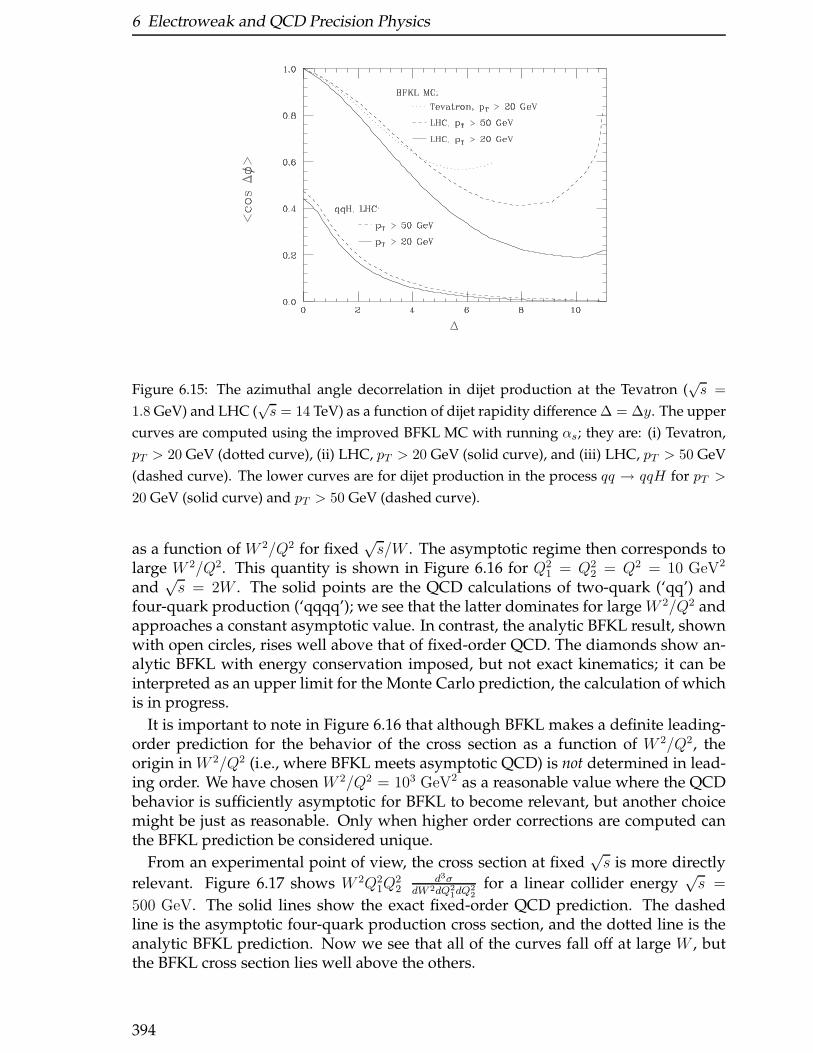
6 Electroweak and QCD Precision Physics
Figure 6.15: The azimuthal angle decorrelation in dijet production at the Tevatron (√s =
1.8 GeV) and LHC (√s = 14 TeV) as a function of dijet rapidity difference ∆ = ∆y. The upper
curves are computed using the improved BFKL MC with running αs; they are: (i) Tevatron,
pT > 20 GeV (dotted curve), (ii) LHC, pT > 20 GeV (solid curve), and (iii) LHC, pT > 50 GeV
(dashed curve). The lower curves are for dijet production in the process qq → qqH for pT >
20 GeV (solid curve) and pT > 50 GeV (dashed curve).
as a function of W 2/Q2 for fixed√s/W . The asymptotic regime then corresponds to
large W 2/Q2. This quantity is shown in Figure 6.16 for Q21 = Q2
2 = Q2 = 10 GeV2
and√s = 2W . The solid points are the QCD calculations of two-quark (‘qq’) and
four-quark production (‘qqqq’); we see that the latter dominates for large W 2/Q2 andapproaches a constant asymptotic value. In contrast, the analytic BFKL result, shownwith open circles, rises well above that of fixed-order QCD. The diamonds show an-alytic BFKL with energy conservation imposed, but not exact kinematics; it can beinterpreted as an upper limit for the Monte Carlo prediction, the calculation of whichis in progress.
It is important to note in Figure 6.16 that although BFKL makes a definite leading-order prediction for the behavior of the cross section as a function of W 2/Q2, theorigin in W 2/Q2 (i.e., where BFKL meets asymptotic QCD) is not determined in lead-ing order. We have chosen W 2/Q2 = 103 GeV2 as a reasonable value where the QCDbehavior is sufficiently asymptotic for BFKL to become relevant, but another choicemight be just as reasonable. Only when higher order corrections are computed canthe BFKL prediction be considered unique.
From an experimental point of view, the cross section at fixed√s is more directly
relevant. Figure 6.17 shows W 2Q21Q
22
d3σdW 2dQ2
1dQ22
for a linear collider energy√s =
500 GeV. The solid lines show the exact fixed-order QCD prediction. The dashedline is the asymptotic four-quark production cross section, and the dotted line is theanalytic BFKL prediction. Now we see that all of the curves fall off at large W , butthe BFKL cross section lies well above the others.
394
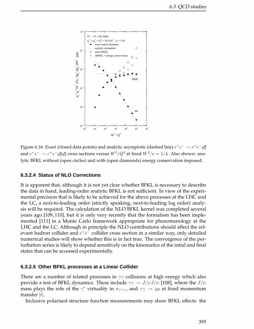
6.3 QCD studies
100
101
102
103
104
105
106
10-5
10-4
10-3
10-2
10-1
100
qqqq
ee → ee + qq, qqqq
q1
2 = q2
2 = Q2 = 10 GeV2, √s = 2 W exact matrix elements analytic asymptotic naive BFKL nBFKL + energy conservation
q 12 q22 W
2 d3 σ
/ dq 12 d
q 22 dW
2 (p
b)
W2 / Q
2
Figure 6.16: Exact (closed data points) and analytic asymptotic (dashed line) e+e− → e+e−qq
and e+e− → e+e−qqqq cross sections versus W 2/Q2 at fixed W 2/s = 1/4. Also shown: ana-
lytic BFKL without (open circles) and with (open diamonds) energy conservation imposed.
6.3.2.4 Status of NLO Corrections
It is apparent that, although it is not yet clear whether BFKL is necessary to describethe data in hand, leading-order analytic BFKL is not sufficient. In view of the experi-mental precision that is likely to be achieved for the above processes at the LHC andthe LC, a next-to-leading order (strictly speaking, next-to-leading log order) analy-sis will be required. The calculation of the NLO BFKL kernel was completed severalyears ago [109, 110], but it is only very recently that the formalism has been imple-mented [111] in a Monte Carlo framework appropriate for phenomenology at theLHC and the LC. Although in principle the NLO contributions should affect the rel-evant hadron collider and e+e− collider cross section in a similar way, only detailednumerical studies will show whether this is in fact true. The convergence of the per-turbation series is likely to depend sensitively on the kinematics of the intial and finalstates that can be accessed experimentally.
6.3.2.5 Other BFKL processes at a Linear Collider
There are a number of related processes in γγ collisions at high energy which alsoprovide a test of BFKL dynamics. These include γγ → J/ψJ/ψ [108], where the J/ψmass plays the role of the γ∗ virtuality in σγ∗γ∗ , and γγ → ρρ at fixed momentumtransfer |t|.
Inclusive polarised structure function measurements may show BFKL effects: the
395
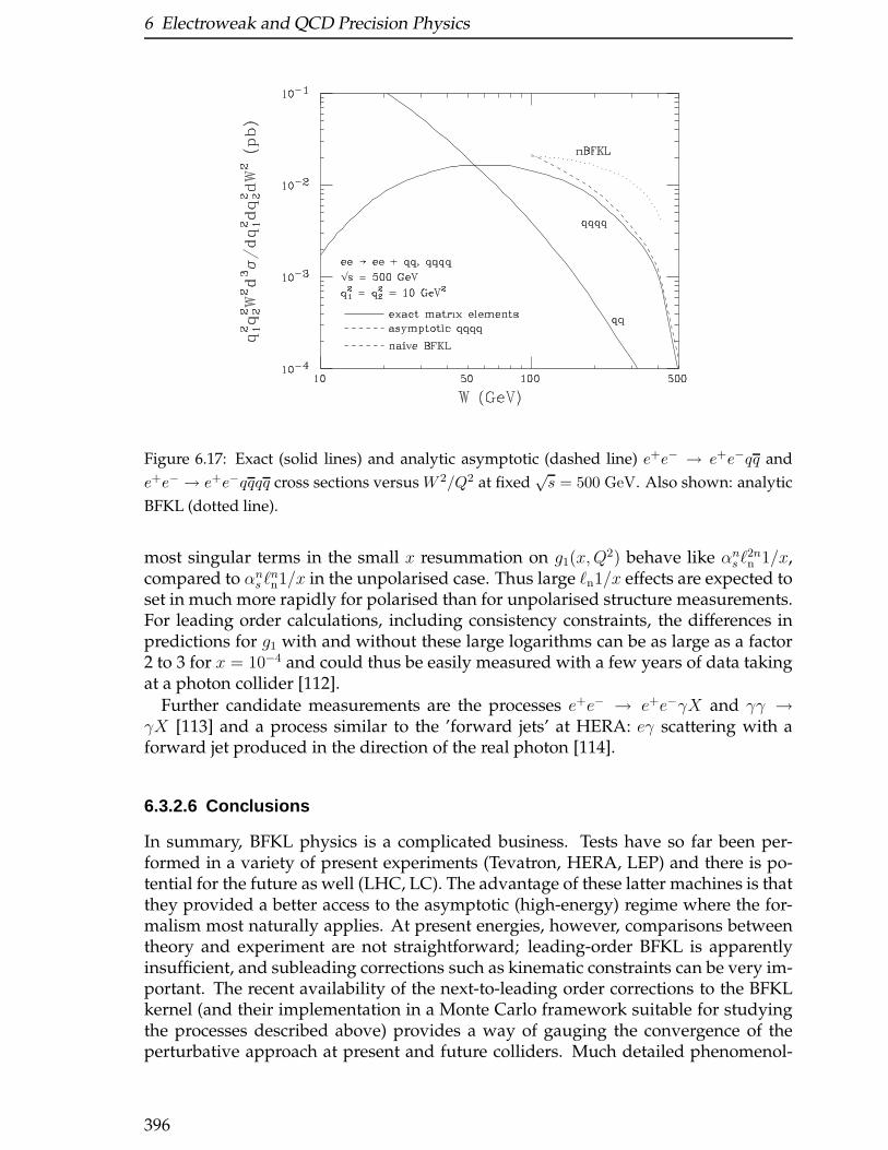
6 Electroweak and QCD Precision Physics
Figure 6.17: Exact (solid lines) and analytic asymptotic (dashed line) e+e− → e+e−qq and
e+e− → e+e−qqqq cross sections versus W 2/Q2 at fixed√s = 500 GeV. Also shown: analytic
BFKL (dotted line).
most singular terms in the small x resummation on g1(x,Q2) behave like αns ℓ
2nn 1/x,
compared to αns ℓnn1/x in the unpolarised case. Thus large ℓn1/x effects are expected to
set in much more rapidly for polarised than for unpolarised structure measurements.For leading order calculations, including consistency constraints, the differences inpredictions for g1 with and without these large logarithms can be as large as a factor2 to 3 for x = 10−4 and could thus be easily measured with a few years of data takingat a photon collider [112].
Further candidate measurements are the processes e+e− → e+e−γX and γγ →γX [113] and a process similar to the ’forward jets’ at HERA: eγ scattering with aforward jet produced in the direction of the real photon [114].
6.3.2.6 Conclusions
In summary, BFKL physics is a complicated business. Tests have so far been per-formed in a variety of present experiments (Tevatron, HERA, LEP) and there is po-tential for the future as well (LHC, LC). The advantage of these latter machines is thatthey provided a better access to the asymptotic (high-energy) regime where the for-malism most naturally applies. At present energies, however, comparisons betweentheory and experiment are not straightforward; leading-order BFKL is apparentlyinsufficient, and subleading corrections such as kinematic constraints can be very im-portant. The recent availability of the next-to-leading order corrections to the BFKLkernel (and their implementation in a Monte Carlo framework suitable for studyingthe processes described above) provides a way of gauging the convergence of theperturbative approach at present and future colliders. Much detailed phenomenol-
396
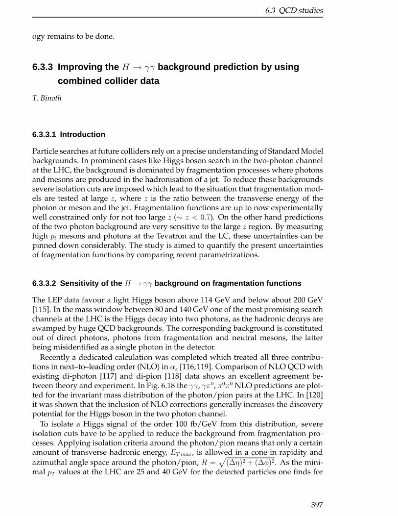
6.3 QCD studies
ogy remains to be done.
6.3.3 Improving the H → γγ background prediction by using
combined collider data
T. Binoth
6.3.3.1 Introduction
Particle searches at future colliders rely on a precise understanding of Standard Modelbackgrounds. In prominent cases like Higgs boson search in the two-photon channelat the LHC, the background is dominated by fragmentation processes where photonsand mesons are produced in the hadronisation of a jet. To reduce these backgroundssevere isolation cuts are imposed which lead to the situation that fragmentation mod-els are tested at large z, where z is the ratio between the transverse energy of thephoton or meson and the jet. Fragmentation functions are up to now experimentallywell constrained only for not too large z (∼ z < 0.7). On the other hand predictionsof the two photon background are very sensitive to the large z region. By measuringhigh pt mesons and photons at the Tevatron and the LC, these uncertainties can bepinned down considerably. The study is aimed to quantify the present uncertaintiesof fragmentation functions by comparing recent parametrizations.
6.3.3.2 Sensitivity of the H → γγ background on fragmentation functions
The LEP data favour a light Higgs boson above 114 GeV and below about 200 GeV[115]. In the mass window between 80 and 140 GeV one of the most promising searchchannels at the LHC is the Higgs decay into two photons, as the hadronic decays areswamped by huge QCD backgrounds. The corresponding background is constitutedout of direct photons, photons from fragmentation and neutral mesons, the latterbeing misidentified as a single photon in the detector.
Recently a dedicated calculation was completed which treated all three contribu-tions in next–to–leading order (NLO) in αs [116,119]. Comparison of NLO QCD withexisting di-photon [117] and di-pion [118] data shows an excellent agreement be-tween theory and experiment. In Fig. 6.18 the γγ, γπ0, π0π0 NLO predictions are plot-ted for the invariant mass distribution of the photon/pion pairs at the LHC. In [120]it was shown that the inclusion of NLO corrections generally increases the discoverypotential for the Higgs boson in the two photon channel.
To isolate a Higgs signal of the order 100 fb/GeV from this distribution, severeisolation cuts have to be applied to reduce the background from fragmentation pro-cesses. Applying isolation criteria around the photon/pion means that only a certainamount of transverse hadronic energy, ET max, is allowed in a cone in rapidity and
azimuthal angle space around the photon/pion, R =√
(∆η)2 + (∆φ)2. As the mini-mal pT values at the LHC are 25 and 40 GeV for the detected particles one finds for
397
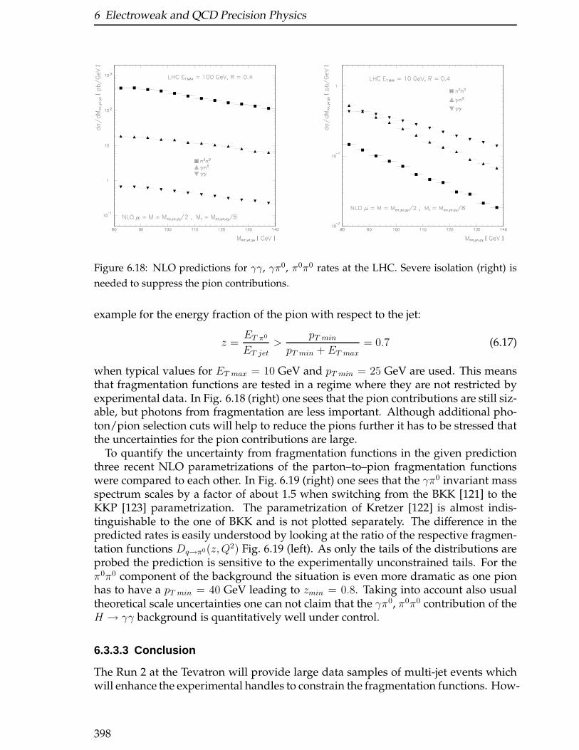
6 Electroweak and QCD Precision Physics
Figure 6.18: NLO predictions for γγ, γπ0, π0π0 rates at the LHC. Severe isolation (right) is
needed to suppress the pion contributions.
example for the energy fraction of the pion with respect to the jet:
z =ET π0
ET jet>
pT minpT min + ET max
= 0.7 (6.17)
when typical values for ET max = 10 GeV and pT min = 25 GeV are used. This meansthat fragmentation functions are tested in a regime where they are not restricted byexperimental data. In Fig. 6.18 (right) one sees that the pion contributions are still siz-able, but photons from fragmentation are less important. Although additional pho-ton/pion selection cuts will help to reduce the pions further it has to be stressed thatthe uncertainties for the pion contributions are large.
To quantify the uncertainty from fragmentation functions in the given predictionthree recent NLO parametrizations of the parton–to–pion fragmentation functionswere compared to each other. In Fig. 6.19 (right) one sees that the γπ0 invariant massspectrum scales by a factor of about 1.5 when switching from the BKK [121] to theKKP [123] parametrization. The parametrization of Kretzer [122] is almost indis-tinguishable to the one of BKK and is not plotted separately. The difference in thepredicted rates is easily understood by looking at the ratio of the respective fragmen-tation functions Dq→π0(z,Q2) Fig. 6.19 (left). As only the tails of the distributions areprobed the prediction is sensitive to the experimentally unconstrained tails. For theπ0π0 component of the background the situation is even more dramatic as one pionhas to have a pT min = 40 GeV leading to zmin = 0.8. Taking into account also usualtheoretical scale uncertainties one can not claim that the γπ0, π0π0 contribution of theH → γγ background is quantitatively well under control.
6.3.3.3 Conclusion
The Run 2 at the Tevatron will provide large data samples of multi-jet events whichwill enhance the experimental handles to constrain the fragmentation functions. How-
398
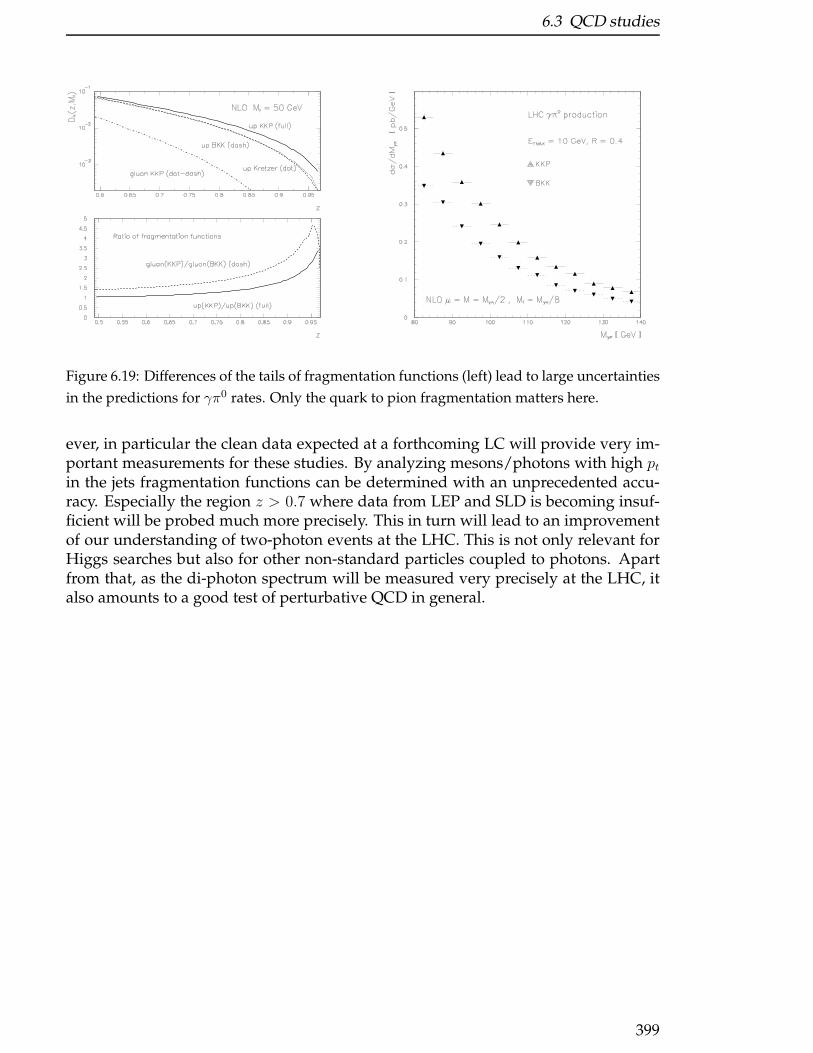
6.3 QCD studies
Figure 6.19: Differences of the tails of fragmentation functions (left) lead to large uncertainties
in the predictions for γπ0 rates. Only the quark to pion fragmentation matters here.
ever, in particular the clean data expected at a forthcoming LC will provide very im-portant measurements for these studies. By analyzing mesons/photons with high ptin the jets fragmentation functions can be determined with an unprecedented accu-racy. Especially the region z > 0.7 where data from LEP and SLD is becoming insuf-ficient will be probed much more precisely. This in turn will lead to an improvementof our understanding of two-photon events at the LHC. This is not only relevant forHiggs searches but also for other non-standard particles coupled to photons. Apartfrom that, as the di-photon spectrum will be measured very precisely at the LHC, italso amounts to a good test of perturbative QCD in general.
399

6 Electroweak and QCD Precision Physics
400
Bibliography
[1] F. Abe et al. [CDF Collaboration], Phys. Rev. Lett. 74 (1995) 2626 [arXiv:hep-ex/9503002].
[2] S. Abachi et al. [D0 Collaboration], Phys. Rev. Lett. 74 (1995) 2632 [arXiv:hep-ex/9503003].
[3] K. Hagiwara et al. [Particle Data Group Collaboration], Phys. Rev. D 66 (2002)010001.
[4] D. E. Groom et al. [Particle Data Group Collaboration], Eur. Phys. J. C 15 (2000)1.
[5] K. G. Chetyrkin, R. Harlander, T. Seidensticker and M. Steinhauser, Phys. Rev. D60 (1999) 114015 [arXiv:hep-ph/9906273].
[6] A. Denner and T. Sack, Nucl. Phys. B 358 (1991) 46.
[7] I. I. Bigi, Y. L. Dokshitzer, V. A. Khoze, J. H. Kuhn and P. M. Zerwas, Phys. Lett.B 181 (1986) 157.
[8] M. Beneke et al., arXiv:hep-ph/0003033, in “Standard model physics (and more)at the LHC” G. Altarelli and M. L. Mangano eds., Geneva, Switzerland: CERN(2000) 529 p.
[9] J. A. Aguilar-Saavedra et al. [ECFA/DESY LC Physics Working Group Collabo-ration], arXiv:hep-ph/0106315.
[10] P. Nason, S. Dawson and R. K. Ellis, Nucl. Phys. B 303 (1988) 607;W. Beenakker, H. Kuijf, W. L. van Neerven and J. Smith, Phys. Rev. D 40 (1989)54;M. L. Mangano, P. Nason and G. Ridolfi, Nucl. Phys. B 373 (1992) 295.
[11] S. Catani, M. L. Mangano, P. Nason and L. Trentadue, Nucl. Phys. B 478 (1996)273 [arXiv:hep-ph/9604351].
[12] A. H. Hoang and T. Teubner, Phys. Rev. D 58 (1998) 114023 [arXiv:hep-ph/9801397]; A. H. Hoang and T. Teubner, Phys. Rev. D 60 (1999) 114027[arXiv:hep-ph/9904468];K. Melnikov and A. Yelkhovsky, Nucl. Phys. B 528 (1998) 59 [arXiv:hep-ph/9802379];O. I. Yakovlev, Phys. Lett. B 457 (1999) 170 [arXiv:hep-ph/9808463];M. Beneke, A. Signer and V. A. Smirnov, Phys. Lett. B 454 (1999) 137 [arXiv:hep-ph/9903260];
401
Bibliography
T. Nagano, A. Ota and Y. Sumino, Phys. Rev. D 60 (1999) 114014 [arXiv:hep-ph/9903498].
[13] K. G. Chetyrkin, J. H. Kuhn and M. Steinhauser, Nucl. Phys. B 482 (1996) 213[arXiv:hep-ph/9606230];R. Harlander and M. Steinhauser, Eur. Phys. J. C 2 (1998) 151 [arXiv:hep-ph/9710413].
[14] W. Beenakker, S. C. van der Marck and W. Hollik, Nucl. Phys. B 365 (1991) 24;W. Beenakker, A. Denner and A. Kraft, Nucl. Phys. B 410 (1993) 219.
[15] D. Chakraborty, J. Konigsberg and D. Rainwater, arXiv:hep-ph/0303092.
[16] T. Stelzer, Z. Sullivan and S. Willenbrock, Phys. Rev. D 56 (1997) 5919 [arXiv:hep-ph/9705398];B. W. Harris, E. Laenen, L. Phaf, Z. Sullivan and S. Weinzierl, Phys. Rev. D 66(2002) 054024 [arXiv:hep-ph/0207055].
[17] M. C. Smith and S. Willenbrock, Phys. Rev. D 54 (1996) 6696 [arXiv:hep-ph/9604223].
[18] T. M. Tait, Phys. Rev. D 61 (2000) 034001 [arXiv:hep-ph/9909352];A. Belyaev and E. Boos, Phys. Rev. D 63 (2001) 034012 [arXiv:hep-ph/0003260];S. Zhu, Phys. Lett. B 524 (2002) 283 [Erratum-ibid. B 537 (2002) 351].
[19] A. S. Belyaev, E. E. Boos and L. V. Dudko, Phys. Rev. D 59 (1999) 075001[arXiv:hep-ph/9806332].
[20] T. Stelzer, Z. Sullivan and S. Willenbrock, Phys. Rev. D 58 (1998) 094021[arXiv:hep-ph/9807340].
[21] ATLAS Collab., “ATLAS Detector and Physics Performance Technical DesignReport”, CERN LHCC 99-14/15 (1999).
[22] E. Boos, L. Dudko, V. Savrin, CMS NOTE-2000/065, 2000;D. Green, K. Maeshima, R. Vidal, J. Womersley, W. Wu, CMS NOTE-1999/048,1999.
[23] B. W. Harris, E. Laenen, L. Phaf, Z. Sullivan and S. Weinzierl, Phys. Rev. D 66(2002) 054024 [arXiv:hep-ph/0207055].
[24] E. Boos, M. Dubinin, A. Pukhov, M. Sachwitz and H. J. Schreiber, Eur. Phys. J. C21 (2001) 81 [arXiv:hep-ph/0104279].
[25] J. H. Kuhn, C. Sturm and P. Uwer, arXiv:hep-ph/0303233.
[26] T. Affolder et al. [CDF Collaboration], Phys. Rev. Lett. 86 (2001) 3233 [arXiv:hep-ex/0012029].
[27] A. Czarnecki and M. Jezabek, Nucl. Phys. B 427 (1994) 3 [arXiv:hep-ph/9402326].
[28] A. Czarnecki, M. Jezabek and J. H. Kuhn, Nucl. Phys. B 351 (1991) 70.
402
Bibliography
[29] A. Brandenburg, Z. G. Si and P. Uwer, Phys. Lett. B 539 (2002) 235 [arXiv:hep-ph/0205023].
[30] G. Mahlon and S. Parke, Phys. Rev. D 55 (1997) 7249 [arXiv:hep-ph/9611367];Phys. Lett. B 476 (2000) 323 [arXiv:hep-ph/9912458].
[31] E. E. Boos and A. V. Sherstnev, Phys. Lett. B 534 (2002) 97 [arXiv:hep-ph/0201271].
[32] J. van der Heide, E. Laenen, L. Phaf and S. Weinzierl, Phys. Rev. D 62 (2000)074025 [arXiv:hep-ph/0003318].
[33] J. Campbell, R. K. Ellis and F. Tramontano, arXiv:hep-ph/0408158.
[34] Q. H. Cao and C. P. Yuan, arXiv:hep-ph/0408180.
[35] E.Boos and A.Sherstnev, in preparation
[36] S. Parke and Y. Shadmi, Phys. Lett. B 387 (1996) 199 [arXiv:hep-ph/9606419].
[37] G. Mahlon and S. Parke, Phys. Rev. D 53 (1996) 4886 [arXiv:hep-ph/9512264];Phys. Lett. B 411 (1997) 173 [arXiv:hep-ph/9706304].
[38] Y. Kiyo, J. Kodaira, K. Morii, T. Nasuno and S. Parke, Nucl. Phys. Proc. Suppl. 89(2000) 37 [arXiv:hep-ph/0006021].
[39] W. Bernreuther, A. Brandenburg, Z. G. Si and P. Uwer, arXiv:hep-ph/0304244.
[40] T. G. Rizzo, in 1996 DPF/DPB Summer Study on New Directions for High EnergyPhysics, Snowmass, CO, July 1996, eds. D.G. Cassel, L.Trindle Gennari and R.H.Siemann, hep-ph/9609311.
[41] W. Bernreuther, J. P. Ma and B. H. J. McKellar, Phys. Rev. D 51 (1995) 2475[arXiv:hep-ph/9404235].
[42] J. Lee, S. Y. Choi and C. S. Kim, hep-ph/9801236; S. Y. Choi, C. S. Kim and J. Lee,Phys. Lett. B 415, 67 (1997) [arXiv:hep-ph/9706379].
[43] E. Boos, A. Pukhov, M. Sachwitz and H. J. Schreiber, Z. Phys. C 75, 237 (1997)hep-ph/9610424;
[44] S. Parke, Proc. of the 1994 Meeting of the APS, (DPF 94), Albuquerque, NM, 2-6Aug 1994, DPF Conf.1994:0726-730 (QCD161:A6:1994), hep-ph/9409312.
[45] K. Whisnant, J. Yang, B. Young and X. Zhang, Phys. Rev. D 56, 467 (1997)[arXiv:hep-ph/9702305].
[46] F. Larios, E. Malkawi and C.-P. Yuan, Lectures given by C.-P. Yuan at the CCASTWorkshop on ’Physics at TeV Energy Scale ’ July 15-26, 1996, Beijing, China, hep-ph/9704288.
[47] E. Boos, L. Dudko and T. Ohl, Eur. Phys. J. C 11, 473 (1999) [arXiv:hep-ph/9903215].
403
Bibliography
[48] T. Tait and C. P. Yuan, Phys. Rev. D 63, 014018 (2001) [arXiv:hep-ph/0007298].
[49] J. Cao, J. Wang, J. M. Yang, B. Young and X. Zhang, Phys. Rev. D 58, 094004 (1998)[arXiv:hep-ph/9804343].
[50] F. Abe et al. [CDF Collaboration], Phys. Rev. Lett. 80 (1998) 2525.
[51] Obraztsov V.F., Slabospitsky S.R., and Yushchenko O.P., Phys. Lett. B 426, 393(1998) [arXiv:hep-ph/9712394];Abreu P. et al. [DELPHI Collaboration], Phys. Lett. B 446, 62 (1999) [arXiv:hep-ex/9903072];Abbiendi G. et al. [OPAL Collaboration], Phys. Lett. B 521, 181 (2001) [arXiv:hep-ex/0110009]. Achard P. et al. [L3 Collaboration], Phys. Lett. B 549, 290 (2002)[arXiv:hep-ex/0210041];A. Heister A. et al. [ALEPH Collaboration], Phys. Lett. B 543, 173 (2002)[arXiv:hep-ex/0206070].
[52] Wolf G., arXiv:hep-ex/0105055;Alan A.T. and Senol A., Europhys. Lett. 57, 669 (2002) [arXiv:hep-ph/0202119];Dannheim H. [H1 Collaboration], arXiv:hep-ex/0212004.
[53] Y. P. Gouz and S. R. Slabospitsky, Phys. Lett. B 457 (1999) 177 [arXiv:hep-ph/9811330].
[54] F. Gianotti et al., arXiv:hep-ph/0204087.
[55] Richter-Was E., Froidevaux D. and Poggioli L., “ATLFAST 2.0 a fast simulationpackage for ATLAS”, ATL-PHYS-98-131 (1998).
[56] Abdullin S., Khanov A., Stepanov N., “CMSJET”, CMS TN/94-180 (1994).
[57] E. Malkawi and T. Tait, Phys. Rev. D 54, 5758 (1996) [arXiv:hep-ph/9511337].
[58] T. Tait and C. P. Yuan, Phys. Rev. D 55, 7300 (1997) [arXiv:hep-ph/9611244].
[59] F. del Aguila, J.A. Aguilar-Saavedra and R. Miquel, Phys. Rev. Lett. 82, 1628(1999) [arXiv:hep-ph/9808400].
[60] Aguilar-Saavedra J.A. and Riemann T., arXiv:hep-ph/0102197;Aguilar-Saavedra J.A., Phys. Lett. B 502, 115 (2001) [arXiv:hep-ph/0012305].
[61] S. Bar-Shalom and J. Wudka, Phys. Rev. D 60 (1999) 094016 [arXiv:hep-ph/9905407];T. Han and J. L. Hewett, Phys. Rev. D 60 (1999) 074015 [arXiv:hep-ph/9811237].
[62] T. G. Rizzo, hep-ph/9910255.
[63] U. Baur, R. Clare, J. Erler, S. Heinemeyer, D. Wackeroth, G. Weiglein andD. R. Wood, in Proc. of the APS/DPF/DPB Summer Study on the Future of Parti-cle Physics (Snowmass 2001) ed. N. Graf, eConf C010630 (2001) P122 [arXiv:hep-ph/0111314].
404
Bibliography
[64] B. C. Allanach et al., in Proc. of the APS/DPF/DPB Summer Study on the Future ofParticle Physics (Snowmass 2001) ed. N. Graf, Eur. Phys. J. C 25 (2002) 113 [eConfC010630 (2001) P125] [arXiv:hep-ph/0202233];see: www.ippp.dur.ac.uk/ ∼georg/sps .
[65] J. Erler, S. Heinemeyer, W. Hollik, G. Weiglein and P. M. Zerwas, Phys. Lett. B486 (2000) 125 [arXiv:hep-ph/0005024].
[66] S. Heinemeyer, W. Hollik and G. Weiglein, Eur. Phys. J. C 9 (1999) 343 [arXiv:hep-ph/9812472].
[67] G. Degrassi, S. Heinemeyer, W. Hollik, P. Slavich and G. Weiglein, Eur. Phys. J.C 28 (2003) 133 [arXiv:hep-ph/0212020].
[68] S. Heinemeyer and G. Weiglein, arXiv:hep-ph/0012364.
[69] S. Heinemeyer, S. Kraml, W. Porod and G. Weiglein, JHEP 0309 (2003) 075[arXiv:hep-ph/0306181].
[70] S. Heinemeyer, W. Hollik and G. Weiglein, Comput. Phys. Commun. 124 (2000)76 [arXiv:hep-ph/9812320].
[71] M. Frank, S. Heinemeyer, W. Hollik and G. Weiglein, arXiv:hep-ph/0212037;T. Hahn, S. Heinemeyer, W. Hollik and G. Weiglein, in preparation.
[72] The FeynHiggs code can be obtained from www.feynhiggs.de .
[73] D. Cavalli et al., arXiv:hep-ph/0203056.
[74] M. Berggren, R. Keranen, H. Nowak and A. Sopczak, arXiv:hep-ph/9911345.
[75] A. Bartl, H. Eberl, S. Kraml, W. Majerotto and W. Porod, Eur. Phys. J. directC 2(2000) 6 [arXiv:hep-ph/0002115].
[76] S. Haywood et al., arXiv:hep-ph/0003275.
[77] R. M. Thurman-Keup, A. V. Kotwal, M. Tecchio and A. Byon-Wagner, Rev. Mod.Phys. 73 (2001) 267.
[78] M. Dobbs and L. Lefebvre, ATL-PHYS-2002-022 and ATL-PHYS-2002-023.
[79] E. N. Argyres, G. Katsilieris, A. B. Lahanas, C. G. Papadopoulos andV. C. Spanos, Nucl. Phys. B 391 (1993) 23.
[80] U. Baur and E.L. Berger, Phys. Rev. D47, 4889 (1992).
[81] U. Baur and D. L. Rainwater, Phys. Rev. D62, 113011 (2000).
[82] J. Alcaraz, Neutral Gauge Boson Pair Production in e+e− Linear colliders, Proceed-ings of the Worldwide Study on Physics and Experiments with Future Lineare+e− Colliders, Sitges 1999, Vol. 1, 431, Universitat Autonoma de Barcelone,Servei de Piblicacions.
405
Bibliography
[83] TESLA: Technical Design Report, Part III: Physics at en e+e− Linear Collider,Section 5.4, DESY-2001-011 (2001).
[84] S. Catai et al., in Report on the Workshop on Standard Model Physics (And More)at the LHC, eds. G. Altarelli and M.L. Mangano, CERN-2000-004 (2000)
[85] S. Abachi et al. [D0 Collaboration], FERMILAB-CONF-96-172-E Contributed to28th International Conference on High-energy Physics (ICHEP 96), Warsaw, Poland,25-31 Jul 1996.
[86] T. Affolder et al. [CDF Collaboration], Phys. Rev. Lett. 88 (2002) 042001[arXiv:hep-ex/0108034].
[87] K. Hagiwara et al. [Particle Data Group Collaboration], Phys. Rev. D 66 (2002)010001.
[88] W. T. Giele, E. W. Glover and J. Yu, Phys. Rev. D 53 (1996) 120.
[89] D. Bourilkov, arXiv:hep-ph/0305126.
[90] A. D. Martin, R. G. Roberts, W. J. Stirling and R. S. Thorne, Eur. Phys. J. C 28(2003) 455 [arXiv:hep-ph/0211080]; arXiv:hep-ph/0308087.
[91] J. Pumplin, D. R. Stump, J. Huston, H. L. Lai, P. Nadolsky and W. K. Tung, JHEP0207 (2002) 012 [arXiv:hep-ph/0201195].
[92] E. W. Glover, Nucl. Phys. Proc. Suppl. 116 (2003) 3 [arXiv:hep-ph/0211412].
[93] M. Winter, LC Note LC-PHSM-2001-016, available atwww.desy.de/ ∼lcnotes/notes.html ; talk given at the LHC/LC studygroup meeting, CERN, July 2002, see:www.ippp.dur.ac.uk/ ∼georg/lhclc/ .
[94] L.N. Lipatov, Sov. J. Nucl. Phys. 23 (1976) 338; E.A. Kuraev, L.N. Lipatov andV.S. Fadin, Sov. Phys. JETP 45 (1977) 199; Ya.Ya. Balitsky and L.N. Lipatov, Sov.J. Nucl. Phys. 28 (1978) 822.
[95] A.H. Mueller and H. Navelet, Nucl. Phys. B 282, 727 (1987).
[96] J. Bartels, A. De Roeck and H. Lotter, Phys. Lett. B 389 (1996) 742.
[97] S.J. Brodsky, F. Hautmann and D.E. Soper, Phys. Rev. D 56, 6957 (1997).
[98] S. Abachi et al. [D0 Collaboration], Phys. Rev. Lett. 77, 595 (1996).
[99] M. Wadhwa for the L3 collaboration, these proceedings.
[100] C. Adloff et al. [H1 Collaboration], Nucl. Phys. B 538 (1999) 3.
[101] J. Breitweg et al. [ZEUS Collaboration], Eur. Phys. J. C 6 (1999) 239.
[102] L.H. Orr and W.J. Stirling, Phys. Rev. D 56 (1997) 5875.
[103] C.R. Schmidt, Phys. Rev. Lett. 78 (1997) 4531.
406

Bibliography
[104] L.H. Orr and W.J. Stirling, Phys. Lett. B 429 (1998) 135; Phys. Lett. B 436 (1998)372.
[105] J. R. Andersen, V. Del Duca, S. Frixione, C. R. Schmidt and W. J. Stirling, JHEP0102 (2001) 007.
[106] J. R. Andersen, V. Del Duca, F. Maltoni and W. J. Stirling, JHEP 0105 (2001) 048.
[107] J. R. Andersen and W. J. Stirling, JHEP 0302 (2003) 018.
[108] J. Kwiecinski, L. Motyka and A. De Roeck, arXiv:hep-ph/0001180.
[109] V. S. Fadin and L. N. Lipatov, Phys. Lett. B 429 (1998) 127 [arXiv:hep-ph/9802290].
[110] M. Ciafaloni and G. Camici, Phys. Lett. B 430 (1998) 349 [arXiv:hep-ph/9803389].
[111] J. R. Andersen and A. Sabio Vera, Phys. Lett. B 567 (2003) 116 [arXiv:hep-ph/0305236].
[112] J. Kwiecinski and B. Ziaja, Phys. Rev. D 63, 054022 (2001) [arXiv:hep-ph/0006292].
[113] N. G. Evanson and J. R. Forshaw, [arXiv:hep-ph/9912487].
[114] J. G. Contreras and A. De Roeck, LC-TH-2001-031
[115] LEP Higgs working group, Phys. Lett. B 565 (2003) 61 [arXiv:hep-ex/0306033]. M. Grunewald, talk given at the workshop on “Electroweakprecision data and the Higgs mass”, DESY Zeuthen, February 2003, see:lepewwg.web.cern.ch/LEPEWWG/ .
[116] T. Binoth, J. P. Guillet, E. Pilon and M. Werlen, Eur. Phys. J. C 16 (2000) 311[arXiv:hep-ph/9911340].
[117] T. Binoth, J. P. Guillet, E. Pilon and M. Werlen, Phys. Rev. D 63 (2001) 114016[arXiv:hep-ph/0012191].
[118] T. Binoth, J. P. Guillet, E. Pilon and M. Werlen, Eur. Phys. J. C 24 (2002) 245.
[119] T. Binoth, J. P. Guillet, E. Pilon and M. Werlen, arXiv:hep-ph/0203064.
[120] Z. Bern, L. Dixon and C. Schmidt, Phys. Rev. D 66 (2002) 074018 [arXiv:hep-ph/0206194].
[121] J. Binnewies, B. A. Kniehl and G. Kramer, Phys. Rev. D 53 (1996) 6110[arXiv:hep-ph/9601278].
[122] S. Kretzer, Phys. Rev. D 62 (2000) 054001 [arXiv:hep-ph/0003177].
[123] B. A. Kniehl, G. Kramer and B. Potter, Nucl. Phys. B 582 (2000) 514 [arXiv:hep-ph/0010289].
407

Bibliography
408
7 New Gauge Theories
Editor: S. Riemann
D. Bourilkov, M. Dittmar, A. Djouadi, S. Godfrey, A. Nicollerat, F. Richard, S. Riemann,T. Rizzo
7.1 Scenarios with extra gauge bosons
New massive gauge bosons are suggested by most extensions of the Standard Modelgauge group; neutral heavy gauge bosons Z′ as well as charged bosons, W′. Withina variety of models the new bosons sit just below the Planck scale or near the weakscale or they originate in certain classes of theories with extra dimensions. Anotherrecent example for a theory beyond the Standard Model is the ’Little Higgs’ model.
For the physics program of near future colliders those predictions with gauge bosonsof a few hundred GeV or few TeV are of interest. Some of the models also include theexistence of an extended fermion sector.
Here, the following models will be considered:
• The popular scenario for extra gauge bosons is based on the symmetry break-ing schemes: SO(10)→SU(2)L×SU(2)R×U(1) predicts new neutral and chargedgauge bosons, Z′ and W′, and E6 →SU(3)×SU(2)×U(1)×U(1)Y ′ anticipates neu-tral Z′ bosons. Details about the models can be found in [1].
• The ’Little Higgs’ scenario [2–5] is proposed as an alternative to SUSY and extradimensions to provide a solution to the hierarchy problem. In these models newsymmetries imply the existence of a rich spectrum of new particles, in particularnew gauge bosons that could be light. The Higgs boson appears as a pseudo-Goldstone boson and is protected by the global symmetry from 1-loop quadraticdivergences.
• KK excitations of the Standard Model gauge bosons are a natural predictionof models with additional dimensions [6]. The details of such models are de-scribed in chapter 8.
• In the so called Universal Extra Dimension scenario (UED) [7] all SM fieldspropagate in extra dimensions, there is no direct vertex involving one non-zeroKaluza-Klein (KK) mode.
409
7 New Gauge Theories
7.1.1 Sensitivity to new physics models
New interactions beyond the Standard Model can be parametrized in terms of effec-tive four-fermion contact interactions [8],
LCI =∑
i,j=L,R
ηijg2
Λ2ij
(uF,iγµuF,i)(uf,jγ
µuf,j). (7.1)
with the helicity coefficients ηij and the couplings g (by convention g2 = 4π). Λ canbe interpreted as the compositeness scale, or it approximates the effects of exchangednew particles, MX ≈ Λ. Contact interactions preserve the chiral symmetry and theStandard Model matrix element is extended by an additional contact term.
The new interactions could arise in hadron-hadron collisions producing lepton orquark pairs at the LHC by means of the Drell-Yan mechanism or in fermion-pairproduction processes at lepton colliders. The parton cross section or the differentialcross section, respectively, have the form
dσ
d cosΩ∝
∑
i,j=L,R
ρij |Aij|2, (7.2)
with
Aij ∼ ASMij +ηij · sΛ2
ρLL,RR = (1 + cos θ)2 (7.3)
ρLR,RL = (1− cos θ)2.
The angular distribution functions, ρij , describe the exchange of the spin-1 particles.The sensitivity reaches for the new interactions can be tested by searching for devia-tions from the Standard Model expectations.
7.1.1.1 Sensitivity to Contact Interactions at the LHC and L C
The sensitivity reaches for various models of four-fermion contact interactions ex-pected for the LHC and LC have been determined [9–13]. Some main results aresummarized in Table 7.1 for qqee interactions at the LHC as well as for eeqq and eellinteractions at the LC (for Λeeqq(LC) the same strength of contact interaction to allquark flavors is assumed). New studies [13] show that these conservative boundsfor the LHC can be improved by a factor roughly 1.5. The sensitivity regions fore+e− → e+e− are related to an optimistic scenario for systematic uncertainties; withthe high statistics the systematic effects can be better controlled. A ’safe’ realistic sce-nario lowers the Λeeee bounds by a factor ≈ 2 [13]. With the LHC new interactionsbetween quarks and leptons can be examined whereas a LC opens the window tonew interactions between leptons only or leptons and quarks. In Ref. [14] also thesensitivity of LHC measurements to quark compositeness is derived by analysing thedijet angular distributions and the transverse energy distribution of jets. With an in-tegrated luminosity of 30 (300) fb−1 a sensitivity to compositeness of quarks up to ascale of 25 (40) TeV can be achieved.
This complementarity demonstrates the need to have both colliders to be sensitiveto the full spectrum of new physics.
410
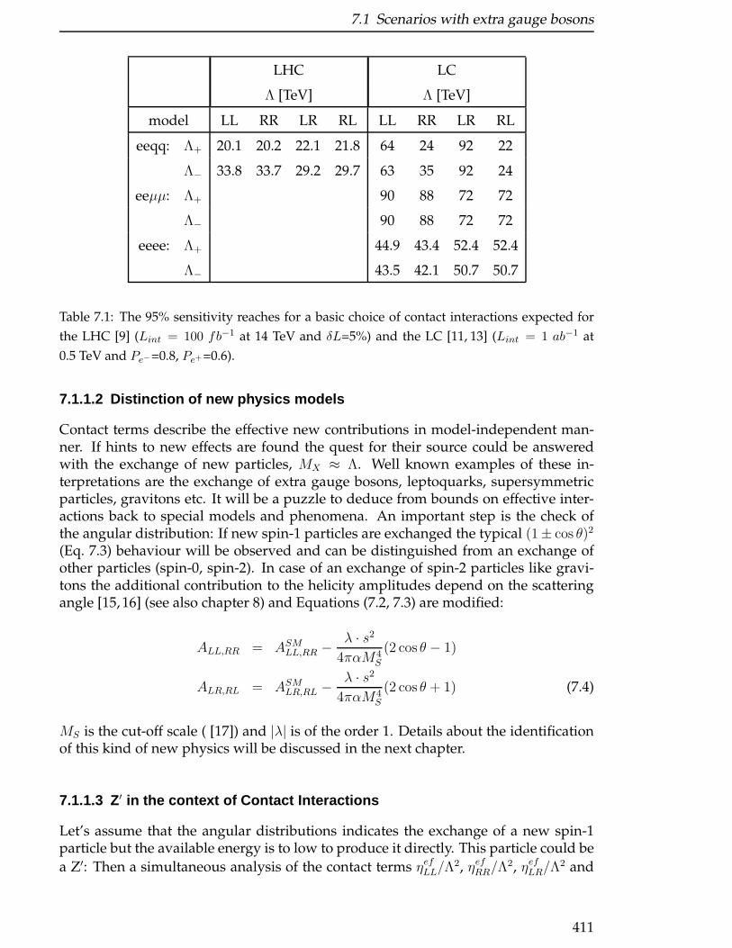
7.1 Scenarios with extra gauge bosons
LHC LC
Λ [TeV] Λ [TeV]
model LL RR LR RL LL RR LR RL
eeqq: Λ+ 20.1 20.2 22.1 21.8 64 24 92 22
Λ− 33.8 33.7 29.2 29.7 63 35 92 24
eeµµ: Λ+ 90 88 72 72
Λ− 90 88 72 72
eeee: Λ+ 44.9 43.4 52.4 52.4
Λ− 43.5 42.1 50.7 50.7
Table 7.1: The 95% sensitivity reaches for a basic choice of contact interactions expected for
the LHC [9] (Lint = 100 fb−1 at 14 TeV and δL=5%) and the LC [11, 13] (Lint = 1 ab−1 at
0.5 TeV and Pe−=0.8, Pe+=0.6).
7.1.1.2 Distinction of new physics models
Contact terms describe the effective new contributions in model-independent man-ner. If hints to new effects are found the quest for their source could be answeredwith the exchange of new particles, MX ≈ Λ. Well known examples of these in-terpretations are the exchange of extra gauge bosons, leptoquarks, supersymmetricparticles, gravitons etc. It will be a puzzle to deduce from bounds on effective inter-actions back to special models and phenomena. An important step is the check ofthe angular distribution: If new spin-1 particles are exchanged the typical (1± cos θ)2
(Eq. 7.3) behaviour will be observed and can be distinguished from an exchange ofother particles (spin-0, spin-2). In case of an exchange of spin-2 particles like gravi-tons the additional contribution to the helicity amplitudes depend on the scatteringangle [15, 16] (see also chapter 8) and Equations (7.2, 7.3) are modified:
ALL,RR = ASMLL,RR −λ · s2
4παM4S
(2 cos θ − 1)
ALR,RL = ASMLR,RL −λ · s2
4παM4S
(2 cos θ + 1) (7.4)
MS is the cut-off scale ( [17]) and |λ| is of the order 1. Details about the identificationof this kind of new physics will be discussed in the next chapter.
7.1.1.3 Z′ in the context of Contact Interactions
Let’s assume that the angular distributions indicates the exchange of a new spin-1particle but the available energy is to low to produce it directly. This particle could be
a Z′: Then a simultaneous analysis of the contact terms ηefLL/Λ2, ηefRR/Λ
2, ηefLR/Λ2 and
411
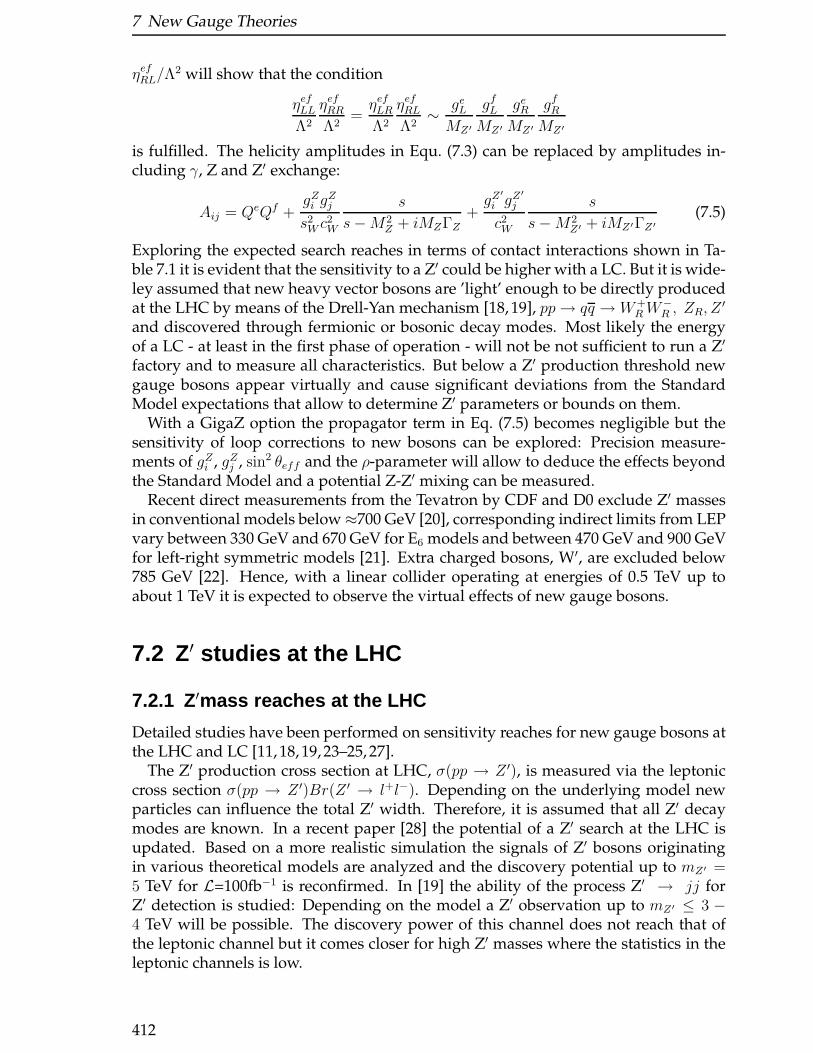
7 New Gauge Theories
ηefRL/Λ2 will show that the condition
ηefLLΛ2
ηefRRΛ2
=ηefLRΛ2
ηefRLΛ2∼ geLMZ′
gfLMZ′
geRMZ′
gfRMZ′
is fulfilled. The helicity amplitudes in Equ. (7.3) can be replaced by amplitudes in-cluding γ, Z and Z′ exchange:
Aij = QeQf +gZi g
Zj
s2W c
2W
s
s−M2Z + iMZΓZ
+gZ
′
i gZ′
j
c2W
s
s−M2Z′ + iMZ′ΓZ′
(7.5)
Exploring the expected search reaches in terms of contact interactions shown in Ta-ble 7.1 it is evident that the sensitivity to a Z′ could be higher with a LC. But it is wide-ley assumed that new heavy vector bosons are ’light’ enough to be directly producedat the LHC by means of the Drell-Yan mechanism [18, 19], pp→ qq →W+
RW−R , ZR, Z
′
and discovered through fermionic or bosonic decay modes. Most likely the energyof a LC - at least in the first phase of operation - will not be not sufficient to run a Z′
factory and to measure all characteristics. But below a Z′ production threshold newgauge bosons appear virtually and cause significant deviations from the StandardModel expectations that allow to determine Z′ parameters or bounds on them.
With a GigaZ option the propagator term in Eq. (7.5) becomes negligible but thesensitivity of loop corrections to new bosons can be explored: Precision measure-ments of gZi , gZj , sin2 θeff and the ρ-parameter will allow to deduce the effects beyondthe Standard Model and a potential Z-Z′ mixing can be measured.
Recent direct measurements from the Tevatron by CDF and D0 exclude Z′ massesin conventional models below≈700 GeV [20], corresponding indirect limits from LEPvary between 330 GeV and 670 GeV for E6 models and between 470 GeV and 900 GeVfor left-right symmetric models [21]. Extra charged bosons, W′, are excluded below785 GeV [22]. Hence, with a linear collider operating at energies of 0.5 TeV up toabout 1 TeV it is expected to observe the virtual effects of new gauge bosons.
7.2 Z′ studies at the LHC
7.2.1 Z′mass reaches at the LHC
Detailed studies have been performed on sensitivity reaches for new gauge bosons atthe LHC and LC [11, 18, 19, 23–25, 27].
The Z′ production cross section at LHC, σ(pp → Z ′), is measured via the leptoniccross section σ(pp → Z ′)Br(Z ′ → l+l−). Depending on the underlying model newparticles can influence the total Z′ width. Therefore, it is assumed that all Z′ decaymodes are known. In a recent paper [28] the potential of a Z′ search at the LHC isupdated. Based on a more realistic simulation the signals of Z′ bosons originatingin various theoretical models are analyzed and the discovery potential up to mZ′ =5 TeV for L=100fb−1 is reconfirmed. In [19] the ability of the process Z′ → jj forZ′ detection is studied: Depending on the model a Z′ observation up to mZ′ ≤ 3 −4 TeV will be possible. The discovery power of this channel does not reach that ofthe leptonic channel but it comes closer for high Z′ masses where the statistics in theleptonic channels is low.
412
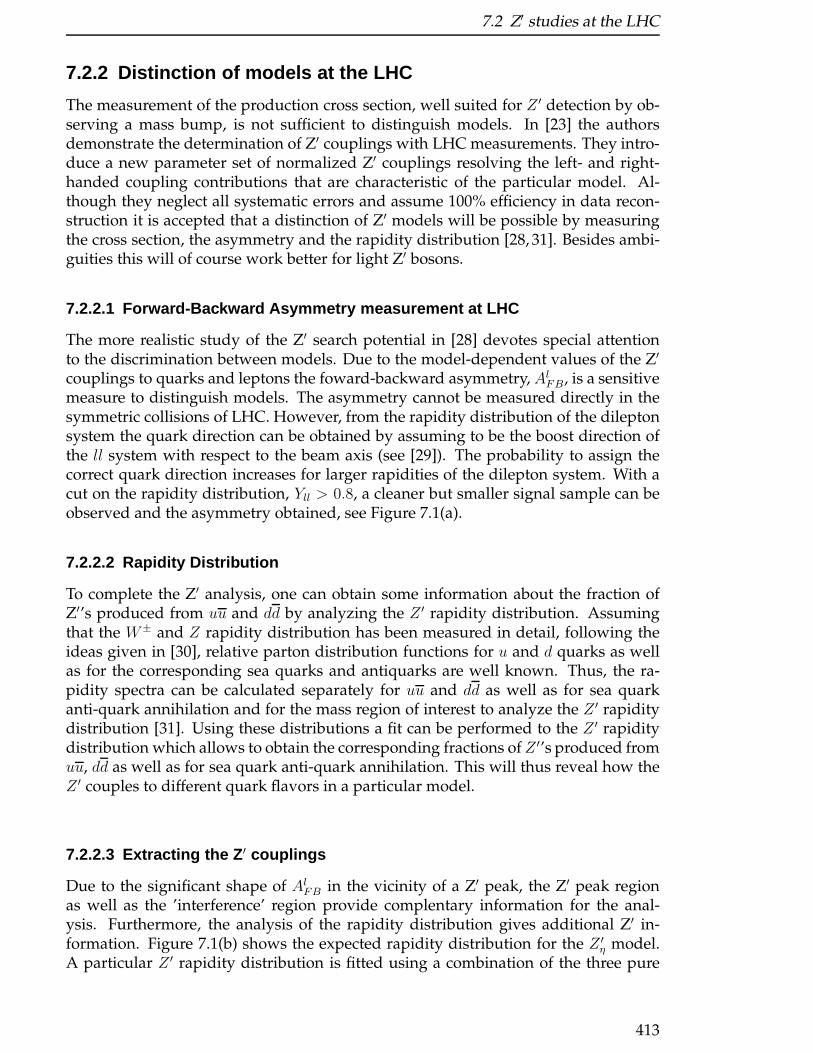
7.2 Z′ studies at the LHC
7.2.2 Distinction of models at the LHC
The measurement of the production cross section, well suited for Z ′ detection by ob-serving a mass bump, is not sufficient to distinguish models. In [23] the authorsdemonstrate the determination of Z′ couplings with LHC measurements. They intro-duce a new parameter set of normalized Z′ couplings resolving the left- and right-handed coupling contributions that are characteristic of the particular model. Al-though they neglect all systematic errors and assume 100% efficiency in data recon-struction it is accepted that a distinction of Z′ models will be possible by measuringthe cross section, the asymmetry and the rapidity distribution [28, 31]. Besides ambi-guities this will of course work better for light Z′ bosons.
7.2.2.1 Forward-Backward Asymmetry measurement at LHC
The more realistic study of the Z′ search potential in [28] devotes special attentionto the discrimination between models. Due to the model-dependent values of the Z′
couplings to quarks and leptons the foward-backward asymmetry, AlFB, is a sensitivemeasure to distinguish models. The asymmetry cannot be measured directly in thesymmetric collisions of LHC. However, from the rapidity distribution of the dileptonsystem the quark direction can be obtained by assuming to be the boost direction ofthe ll system with respect to the beam axis (see [29]). The probability to assign thecorrect quark direction increases for larger rapidities of the dilepton system. With acut on the rapidity distribution, Yll > 0.8, a cleaner but smaller signal sample can beobserved and the asymmetry obtained, see Figure 7.1(a).
7.2.2.2 Rapidity Distribution
To complete the Z′ analysis, one can obtain some information about the fraction ofZ′’s produced from uu and dd by analyzing the Z ′ rapidity distribution. Assumingthat the W± and Z rapidity distribution has been measured in detail, following theideas given in [30], relative parton distribution functions for u and d quarks as wellas for the corresponding sea quarks and antiquarks are well known. Thus, the ra-pidity spectra can be calculated separately for uu and dd as well as for sea quarkanti-quark annihilation and for the mass region of interest to analyze the Z ′ rapiditydistribution [31]. Using these distributions a fit can be performed to the Z ′ rapiditydistribution which allows to obtain the corresponding fractions ofZ ′’s produced fromuu, dd as well as for sea quark anti-quark annihilation. This will thus reveal how theZ ′ couples to different quark flavors in a particular model.
7.2.2.3 Extracting the Z ′ couplings
Due to the significant shape of AlFB in the vicinity of a Z′ peak, the Z′ peak regionas well as the ’interference’ region provide complentary information for the anal-ysis. Furthermore, the analysis of the rapidity distribution gives additional Z′ in-formation. Figure 7.1(b) shows the expected rapidity distribution for the Z ′
η model.A particular Z ′ rapidity distribution is fitted using a combination of the three pure
413
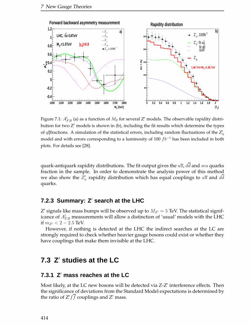
7 New Gauge Theories
[GeV]llM1000 1100 1200 1300 1400 1500 1600 1700 1800
FB
lA
-0.4
-0.2
0
0.2
0.4
0.6
0.8
1
1.2χZ’
ψZ’
ηZ’
LRZ’-1, L=100fbηZ’
Forward backward asymmetry measurement
|>0.8ll|y=1.5TeVZ’M
=14TeVsLHC, a)
|ll|Y0 0.2 0.4 0.6 0.8 1 1.2 1.4 1.6 1.8 2
dn
/ d
y
0
500
1000
1500
2000
2500
-1, 100fbη Z’
u: fit uη Z’d fit d
sum
ψ Z’
<1.55 TeVll1.45 TeV<M
Rapidity distributionb)
Figure 7.1: AlFB (a) as a function of Mll for several Z′ models. The observable rapidity distri-
bution for two Z′ models is shown in (b), including the fit results which determine the types
of qqfractions. A simulation of the statistical errors, including random fluctuations of the Z′η
model and with errors corresponding to a luminosity of 100 fb−1 has been included in both
plots. For details see [28].
quark-antiquark rapidity distributions. The fit output gives the uu, dd and sea quarksfraction in the sample. In order to demonstrate the analysis power of this methodwe also show the Z ′
ψ rapidity distribution which has equal couplings to uu and ddquarks.
7.2.3 Summary: Z ′ search at the LHC
Z′ signals like mass bumps will be observed up to MZ′ = 5 TeV. The statistical signif-icance of AlFB measurements will allow a distinction of ’usual’ models with the LHCif mZ′ < 2− 2.5 TeV.
However, if nothing is detected at the LHC the indirect searches at the LC arestrongly required to check whether heavier gauge bosons could exist or whether theyhave couplings that make them invisible at the LHC.
7.3 Z′ studies at the LC
7.3.1 Z′ mass reaches at the LC
Most likely, at the LC new bosons will be detected via Z-Z′ interference effects. Thenthe significance of deviations from the Standard Model expectations is determined bythe ratio of Z′ff couplings and Z′ mass.
414
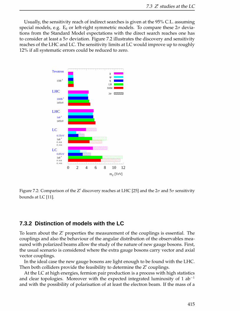
7.3 Z′ studies at the LC
Usually, the sensitivity reach of indirect searches is given at the 95% C.L. assumingspecial models, e.g. E6 or left-right symmetric models. To compare these 2σ devia-tions from the Standard Model expectations with the direct search reaches one hasto consider at least a 5σ deviation. Figure 7.2 illustrates the discovery and sensitivityreaches of the LHC and LC. The sensitivity limits at LC would improve up to roughly12% if all systematic errors could be reduced to zero.
0 2 4 6 8 10 12
SSM
LR
ηψχ
P-=0.8
P+=0.6
P-=0.8
P+=0.6
LC
LC
LHC
LHC
Tevatron
mZ' [TeV]
0.5TeV
0.8TeV
100fb-1
1ab-1
1ab-1
1ab-1
14TeV
14TeV
15fb-1
2σ
Figure 7.2: Comparison of the Z′ discovery reaches at LHC [25] and the 2σ and 5σ sensitivity
bounds at LC [11].
7.3.2 Distinction of models with the LC
To learn about the Z′ properties the measurement of the couplings is essential. Thecouplings and also the behaviour of the angular distribution of the observables mea-sured with polarized beams allow the study of the nature of new gauge bosons. First,the usual scenario is considered where the extra gauge bosons carry vector and axialvector couplings.
In the ideal case the new gauge bosons are light enough to be found with the LHC.Then both colliders provide the feasibility to determine the Z′ couplings.
At the LC at high energies, fermion pair production is a process with high statisticsand clear topologies. Moreover with the expected integrated luminosity of 1 ab−1
and with the possibility of polarisation of at least the electron beam. If the mass of a
415

7 New Gauge Theories
potential Z′ is known from LHC the Z′ model can be resolved with a good accuracy.Figure 7.3 demonstrates the powerful interplay of LHC and LC measurements: Lep-tonic final states obtained at a LC are analyzed with the knowledge of the mass of apotential Z′.
-0.5
-0.25
0
0.25
0.5
-0.4 -0.2 0 0.2 0.4
√s = 1.0 TeV, mZ' = 3.0 TeV
a'l
v'l
√s = 0.5 TeV, mZ' = 1.5 TeV
√s = 0.8 TeV, mZ' = 2.0 TeV√s = 0.8 TeV, mZ' = 1.5 TeV
χ
η
LR
-0.2
-0.1
0
0.1
0.2
-0.2 -0.1 0 0.1 0.2aN
l
vN l
χ
ψ
η
√s = 0.8 TeV
L=1ab-1
L=50fb-1
SM
mZ,[T
eV]
←
2010
64
Figure 7.3: Left figure: The 95% C.L. contours on leptonic Z′ couplings, assuming the mass
of the Z′ is measured at LHC. Right figure: The 95% C.L. contours on normalized leptonic Z′
couplings. The LC parameters are Lint = 1ab−1, ∆Lint = 0.2%, P− = 0.8, P+ = 0.6, ∆P− =
∆P+ = 0.5%, ∆sys(lept)=0.2%.
7.3.2.1 Sensitivity to Z ′ models beyond the LHC reach
An interesting situation arises if the Z′ is too heavy to be detected at the LHC, e.g.mZ′ > 5 TeV, or if the Z′ couplings to quarks are unexpectedly negligable. If theZ′ is not too heavy (approximately 6 TeV for the usual Z′ models) there is still thepossibility of measuring significant deviations from the Standard Model predictions.Instead of a direct implementation of the Z′ parameters normalized couplings haveto be considered:
aNf = a′f
√s
m2Z′ − s
; vNf = v′f
√s
m2Z′ − s
. (7.6)
It should be remarked that these normalized couplings correspond to contact interac-
tions, ηefij /Λ2 ≈ gei g
fj /M
2Z′ .
An example is given in Figure 7.3: A Z′ with mZ′ = 6 TeV realised in the χ modelcannot be seen at the LHC but can just be detected at the LC. The Z′ models are
416
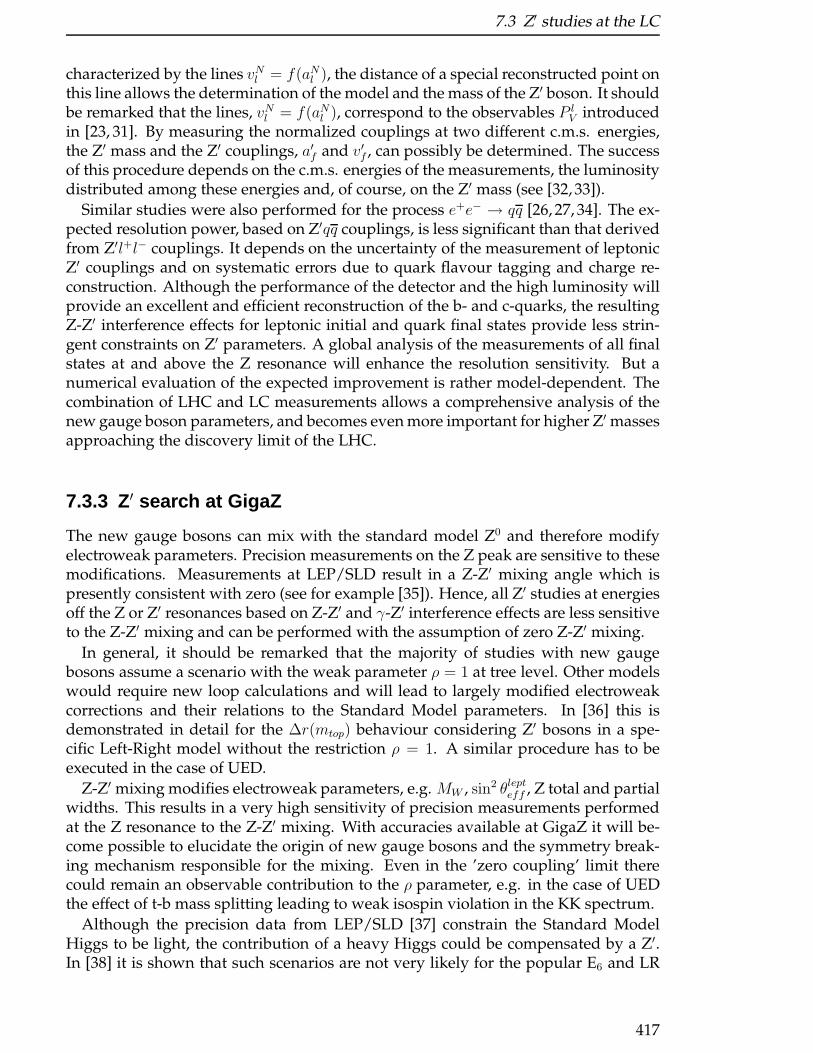
7.3 Z′ studies at the LC
characterized by the lines vNl = f(aNl ), the distance of a special reconstructed point onthis line allows the determination of the model and the mass of the Z′ boson. It shouldbe remarked that the lines, vNl = f(aNl ), correspond to the observables P l
V introducedin [23, 31]. By measuring the normalized couplings at two different c.m.s. energies,the Z′ mass and the Z′ couplings, a′f and v′f , can possibly be determined. The successof this procedure depends on the c.m.s. energies of the measurements, the luminositydistributed among these energies and, of course, on the Z′ mass (see [32, 33]).
Similar studies were also performed for the process e+e− → qq [26, 27, 34]. The ex-pected resolution power, based on Z′qq couplings, is less significant than that derivedfrom Z′l+l− couplings. It depends on the uncertainty of the measurement of leptonicZ′ couplings and on systematic errors due to quark flavour tagging and charge re-construction. Although the performance of the detector and the high luminosity willprovide an excellent and efficient reconstruction of the b- and c-quarks, the resultingZ-Z′ interference effects for leptonic initial and quark final states provide less strin-gent constraints on Z′ parameters. A global analysis of the measurements of all finalstates at and above the Z resonance will enhance the resolution sensitivity. But anumerical evaluation of the expected improvement is rather model-dependent. Thecombination of LHC and LC measurements allows a comprehensive analysis of thenew gauge boson parameters, and becomes even more important for higher Z′ massesapproaching the discovery limit of the LHC.
7.3.3 Z′ search at GigaZ
The new gauge bosons can mix with the standard model Z0 and therefore modifyelectroweak parameters. Precision measurements on the Z peak are sensitive to thesemodifications. Measurements at LEP/SLD result in a Z-Z′ mixing angle which ispresently consistent with zero (see for example [35]). Hence, all Z′ studies at energiesoff the Z or Z′ resonances based on Z-Z′ and γ-Z′ interference effects are less sensitiveto the Z-Z′ mixing and can be performed with the assumption of zero Z-Z′ mixing.
In general, it should be remarked that the majority of studies with new gaugebosons assume a scenario with the weak parameter ρ = 1 at tree level. Other modelswould require new loop calculations and will lead to largely modified electroweakcorrections and their relations to the Standard Model parameters. In [36] this isdemonstrated in detail for the ∆r(mtop) behaviour considering Z′ bosons in a spe-cific Left-Right model without the restriction ρ = 1. A similar procedure has to beexecuted in the case of UED.
Z-Z′ mixing modifies electroweak parameters, e.g. MW , sin2 θlepteff , Z total and partialwidths. This results in a very high sensitivity of precision measurements performedat the Z resonance to the Z-Z′ mixing. With accuracies available at GigaZ it will be-come possible to elucidate the origin of new gauge bosons and the symmetry break-ing mechanism responsible for the mixing. Even in the ’zero coupling’ limit therecould remain an observable contribution to the ρ parameter, e.g. in the case of UEDthe effect of t-b mass splitting leading to weak isospin violation in the KK spectrum.
Although the precision data from LEP/SLD [37] constrain the Standard ModelHiggs to be light, the contribution of a heavy Higgs could be compensated by a Z′.In [38] it is shown that such scenarios are not very likely for the popular E6 and LR
417

7 New Gauge Theories
models and they are already excluded by recent precision measurements. Never-theless, the discovery of Higgs bosons at the LHC gives a strong restriction for theextremely precise measurements with the GigaZ option at a LC. It is obvious thatGigaZ results have to be compatible with LHC results, LC results at high energiesand with the existing LEP/SLD/APV data. Only the consideration of all results willallow the extraction of the physics of symmetry breaking. Disagreements betweendirect measurements (including non-observation of hypothetical particles) and preci-sion measurements will improve the search strategies at least at the LHC. Examplesof the resolution power for new physics with GigaZ are given in Figures 7.4 and 7.5by demonstrating the (mis)matching of electroweak observables and new physics de-pending on the Standard Model Higgs mass.
Finally, in Figure 7.6 the mass regions covered by the LHC, LC and a GigaZ optionat the LC for various Z′ models are compared and summarized [38], the limits for theLC are given at the 95% C.L.
7.4 Z′ in Little Higgs models
In ’Little Higgs’ models (LHM) new symmetries imply the existence of a rich spec-trum of new particles, in particular new gauge bosons that could be light. In theminimal version of LHM only a triplet and a singlet of gauge bosons, a triplet ofHiggs bosons and a vector-like quark, T , are generated. This leads to two Z′: BH ,the U(1) singlet, and and the triplet ZH . For calculations the ’Little Higgs’ formalismincludes 3 new parameters: the mass scale f and the two coupling ratios, x = g′t/g
′
and y = gt/g [3]. Only with t − T mixing significant contributions from the T topseudoobservables at the Z resonance will be expected.
7.4.1 Studies at LC
In [38] it is discussed in detail how Z′ bosons arising from LHM influence measure-ments on the Z resonance and at high energies. It is still quite difficult to puzzlethe existing precision measurements from LEP/SLD and the search limits from theTevatron with future results from GigaZ, LC high energies and the LHC. A crucialpoint is the mass of the Higgs boson which is presently restricted to values below 200GeV. Performing a fine-tuning one can find bounds on the mass scale f as shown inFigure 7.7. (It should be remarked that here the scale f corresponds to the definitionin [3] and therefore it is a factor 1/
√2 smaller than the f used in section 3.6.)
In [39] the sensitivities of various observables to Z′ bosons in the LH and KK mod-els are examined. Figure 7.8 shows how the modified observables influence the χ2
distribution and therefore it illustrates the discrimination potential of the LC. For ex-ample, the LH model gives rise to large LR asymmetries while the Kaluza-Klein Z ′
does not. The χ2 contributions are given for 50 fb−1 but they reflect the relations ingeneral; a scaling to other luminosities and c.m.s. energies can be done following thewell known scaling law ∼ (s · Lint)1/4.
418
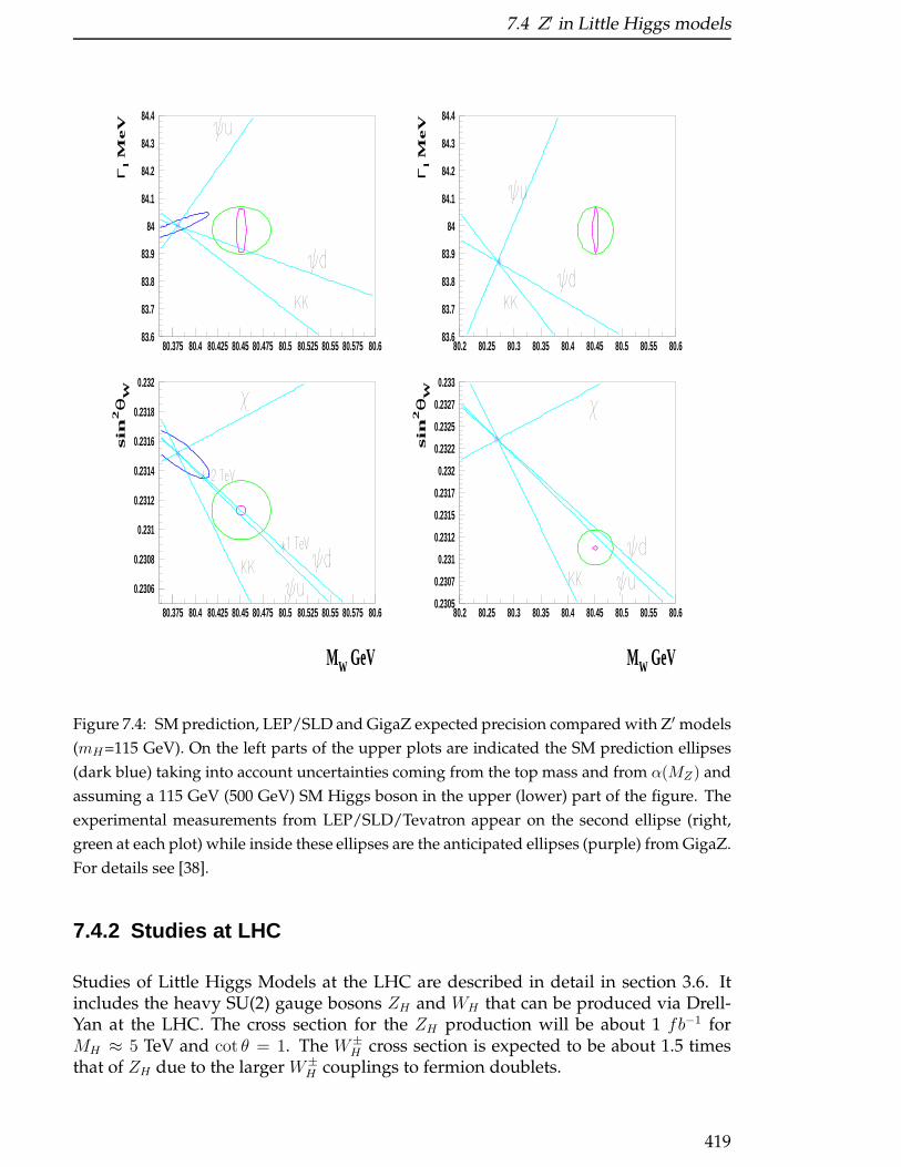
7.4 Z′ in Little Higgs models
83.6
83.7
83.8
83.9
84
84.1
84.2
84.3
84.4
80.375 80.4 80.425 80.45 80.475 80.5 80.525 80.55 80.575 80.6
Γl M
eV
0.2306
0.2308
0.231
0.2312
0.2314
0.2316
0.2318
0.232
80.375 80.4 80.425 80.45 80.475 80.5 80.525 80.55 80.575 80.6
MW GeV
sin
2θ
W
83.6
83.7
83.8
83.9
84
84.1
84.2
84.3
84.4
80.2 80.25 80.3 80.35 80.4 80.45 80.5 80.55 80.6
Γl M
eV
0.2305
0.2307
0.231
0.2312
0.2315
0.2317
0.232
0.2322
0.2325
0.2327
0.233
80.2 80.25 80.3 80.35 80.4 80.45 80.5 80.55 80.6
MW GeV
sin
2θ
W
Figure 7.4: SM prediction, LEP/SLD and GigaZ expected precision compared with Z′ models
(mH=115 GeV). On the left parts of the upper plots are indicated the SM prediction ellipses
(dark blue) taking into account uncertainties coming from the top mass and from α(MZ) and
assuming a 115 GeV (500 GeV) SM Higgs boson in the upper (lower) part of the figure. The
experimental measurements from LEP/SLD/Tevatron appear on the second ellipse (right,
green at each plot) while inside these ellipses are the anticipated ellipses (purple) from GigaZ.
For details see [38].
7.4.2 Studies at LHC
Studies of Little Higgs Models at the LHC are described in detail in section 3.6. Itincludes the heavy SU(2) gauge bosons ZH and WH that can be produced via Drell-Yan at the LHC. The cross section for the ZH production will be about 1 fb−1 forMH ≈ 5 TeV and cot θ = 1. The W±
H cross section is expected to be about 1.5 timesthat of ZH due to the larger W±
H couplings to fermion doublets.
419
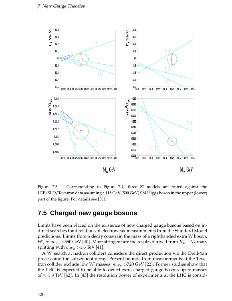
7 New Gauge Theories
83.6
83.7
83.8
83.9
84
84.1
84.2
84.3
84.4
80.375 80.4 80.425 80.45 80.475 80.5 80.525 80.55 80.575 80.6
Γl M
eV
0.2306
0.2308
0.231
0.2312
0.2314
0.2316
0.2318
0.232
80.375 80.4 80.425 80.45 80.475 80.5 80.525 80.55 80.575 80.6
MW GeV
sin
2θ
W
83.6
83.7
83.8
83.9
84
84.1
84.2
84.3
84.4
80.2 80.25 80.3 80.35 80.4 80.45 80.5 80.55 80.6
Γl M
eV
0.2305
0.2307
0.231
0.2312
0.2315
0.2317
0.232
0.2322
0.2325
0.2327
0.233
80.2 80.25 80.3 80.35 80.4 80.45 80.5 80.55 80.6
MW GeV
sin
2θ
W
Figure 7.5: Corresponding to Figure 7.4, three Z′ models are tested against the
LEP/SLD/Tevatron data assuming a 115 GeV (500 GeV) SM Higgs boson in the upper (lower)
part of the figure. For details see [38].
7.5 Charged new gauge bosons
Limits have been placed on the existence of new charged gauge bosons based on in-direct searches for deviations of electroweak measurements from the Standard Modelpredictions. Limits from µ decay constrain the mass of a righthanded extra W boson,W′, to mWR
>550 GeV [40]. More stringent are the results derived from KL−KS masssplitting with mWR
>1.6 TeV [41].
A W′ search at hadron colliders considers the direct production via the Drell-Yanprocess and the subsequent decay. Present bounds from measurements at the Teva-tron collider exclude low W′ masses, mWR
>720 GeV [22]. Former studies show thatthe LHC is expected to be able to detect extra charged gauge bosons up to massesof ≈ 5.9 TeV [42]. In [43] the resolution power of experiments at the LHC is consid-
420
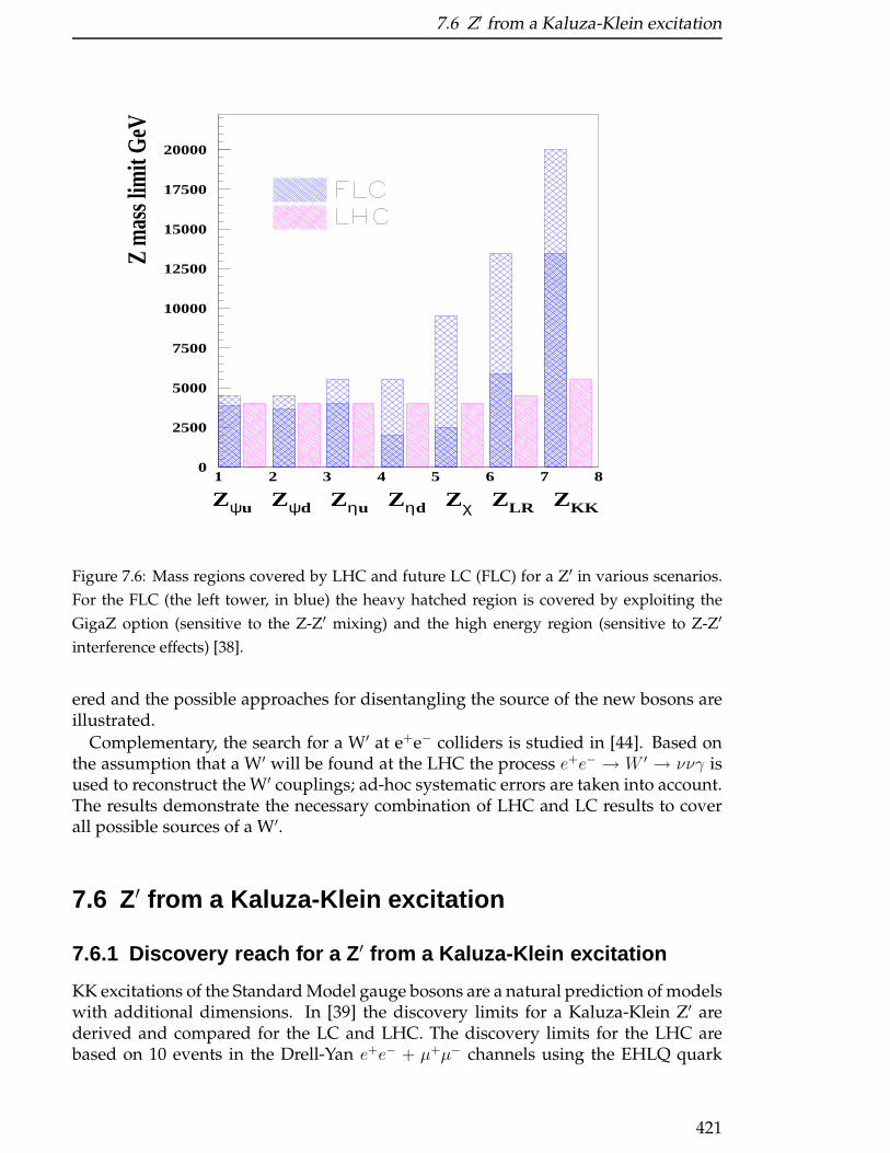
7.6 Z′ from a Kaluza-Klein excitation
0
2500
5000
7500
10000
12500
15000
17500
20000
1 2 3 4 5 6 7 8
Zψu Zψd Zηu Zηd Zχ ZLR ZKK
Z m
ass l
imit
GeV
Figure 7.6: Mass regions covered by LHC and future LC (FLC) for a Z′ in various scenarios.
For the FLC (the left tower, in blue) the heavy hatched region is covered by exploiting the
GigaZ option (sensitive to the Z-Z′ mixing) and the high energy region (sensitive to Z-Z′
interference effects) [38].
ered and the possible approaches for disentangling the source of the new bosons areillustrated.
Complementary, the search for a W′ at e+e− colliders is studied in [44]. Based onthe assumption that a W′ will be found at the LHC the process e+e− → W ′ → ννγ isused to reconstruct the W′ couplings; ad-hoc systematic errors are taken into account.The results demonstrate the necessary combination of LHC and LC results to coverall possible sources of a W′.
7.6 Z′ from a Kaluza-Klein excitation
7.6.1 Discovery reach for a Z ′ from a Kaluza-Klein excitation
KK excitations of the Standard Model gauge bosons are a natural prediction of modelswith additional dimensions. In [39] the discovery limits for a Kaluza-Klein Z′ arederived and compared for the LC and LHC. The discovery limits for the LHC arebased on 10 events in the Drell-Yan e+e− + µ+µ− channels using the EHLQ quark
421
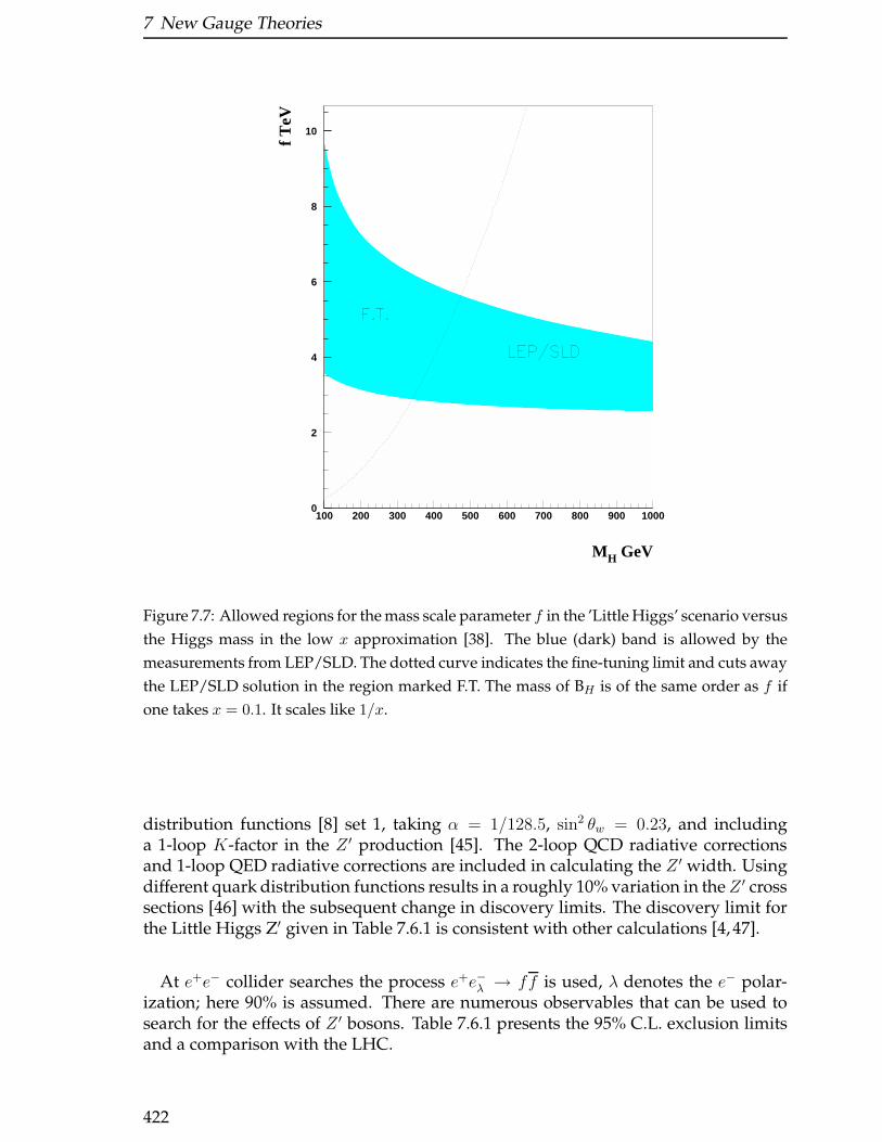
7 New Gauge Theories
0
2
4
6
8
10
100 200 300 400 500 600 700 800 900 1000
MH GeV
f T
eV
Figure 7.7: Allowed regions for the mass scale parameter f in the ’Little Higgs’ scenario versus
the Higgs mass in the low x approximation [38]. The blue (dark) band is allowed by the
measurements from LEP/SLD. The dotted curve indicates the fine-tuning limit and cuts away
the LEP/SLD solution in the region marked F.T. The mass of BH is of the same order as f if
one takes x = 0.1. It scales like 1/x.
distribution functions [8] set 1, taking α = 1/128.5, sin2 θw = 0.23, and includinga 1-loop K-factor in the Z ′ production [45]. The 2-loop QCD radiative correctionsand 1-loop QED radiative corrections are included in calculating the Z ′ width. Usingdifferent quark distribution functions results in a roughly 10% variation in theZ ′ crosssections [46] with the subsequent change in discovery limits. The discovery limit forthe Little Higgs Z′ given in Table 7.6.1 is consistent with other calculations [4, 47].
At e+e− collider searches the process e+e−λ → ff is used, λ denotes the e− polar-ization; here 90% is assumed. There are numerous observables that can be used tosearch for the effects of Z ′ bosons. Table 7.6.1 presents the 95% C.L. exclusion limitsand a comparison with the LHC.
422
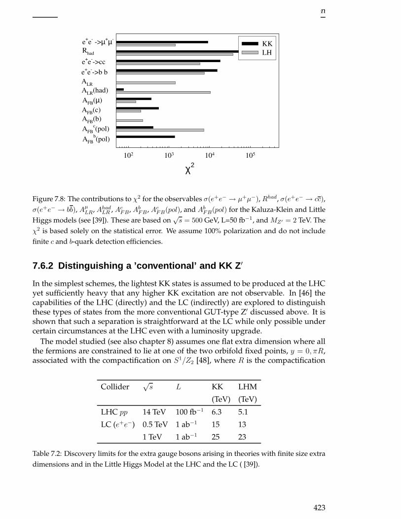
7.6 Z′ from a Kaluza-Klein excitation
χ2102 103 104 105
KK
LH
e+e
- ->µ+µ-
Rhad
e+e
-->cc
e+e
-->b b
ALR
ALR
(had)
AFB
(µ)
AFB
(c)
AFB
(b)
AFB
c(pol)
AFB
b(pol)
Figure 7.8: The contributions to χ2 for the observables σ(e+e− → µ+µ−), Rhad, σ(e+e− → cc),
σ(e+e− → bb), AµLR, AhadLR , AcFB , AbFB , AcFB(pol), and AbFB(pol) for the Kaluza-Klein and Little
Higgs models (see [39]). These are based on√s = 500 GeV, L=50 fb−1, and MZ′ = 2 TeV. The
χ2 is based solely on the statistical error. We assume 100% polarization and do not include
finite c and b-quark detection efficiencies.
7.6.2 Distinguishing a ’conventional’ and KK Z ′
In the simplest schemes, the lightest KK states is assumed to be produced at the LHCyet sufficiently heavy that any higher KK excitation are not observable. In [46] thecapabilities of the LHC (directly) and the LC (indirectly) are explored to distinguishthese types of states from the more conventional GUT-type Z′ discussed above. It isshown that such a separation is straightforward at the LC while only possible undercertain circumstances at the LHC even with a luminosity upgrade.
The model studied (see also chapter 8) assumes one flat extra dimension where allthe fermions are constrained to lie at one of the two orbifold fixed points, y = 0, πR,associated with the compactification on S1/Z2 [48], where R is the compactification
Collider√s L KK LHM
(TeV) (TeV)
LHC pp 14 TeV 100 fb−1 6.3 5.1
LC (e+e−) 0.5 TeV 1 ab−1 15 13
1 TeV 1 ab−1 25 23
Table 7.2: Discovery limits for the extra gauge bosons arising in theories with finite size extra
dimensions and in the Little Higgs Model at the LHC and the LC ( [39]).
423
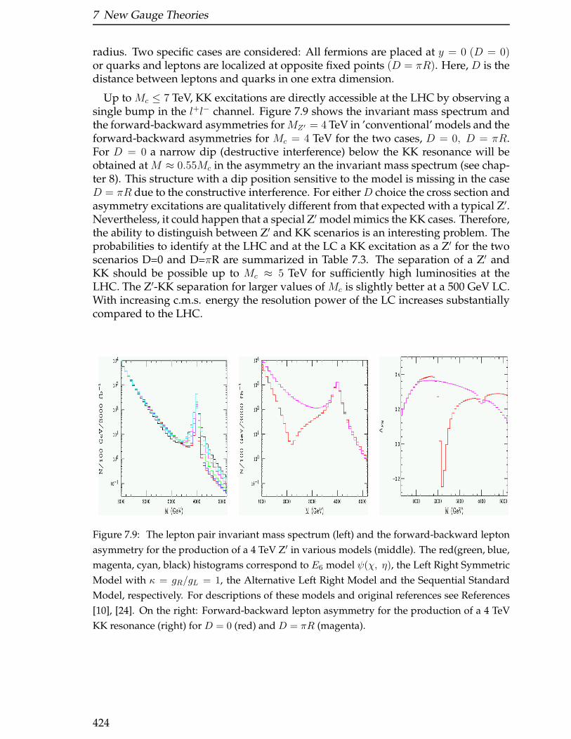
7 New Gauge Theories
radius. Two specific cases are considered: All fermions are placed at y = 0 (D = 0)or quarks and leptons are localized at opposite fixed points (D = πR). Here, D is thedistance between leptons and quarks in one extra dimension.
Up to Mc ≤ 7 TeV, KK excitations are directly accessible at the LHC by observing asingle bump in the l+l− channel. Figure 7.9 shows the invariant mass spectrum andthe forward-backward asymmetries forMZ′ = 4 TeV in ’conventional’ models and theforward-backward asymmetries for Mc = 4 TeV for the two cases, D = 0, D = πR.For D = 0 a narrow dip (destructive interference) below the KK resonance will beobtained at M ≈ 0.55Mc in the asymmetry an the invariant mass spectrum (see chap-ter 8). This structure with a dip position sensitive to the model is missing in the caseD = πR due to the constructive interference. For eitherD choice the cross section andasymmetry excitations are qualitatively different from that expected with a typical Z′.Nevertheless, it could happen that a special Z′ model mimics the KK cases. Therefore,the ability to distinguish between Z′ and KK scenarios is an interesting problem. Theprobabilities to identify at the LHC and at the LC a KK excitation as a Z′ for the twoscenarios D=0 and D=πR are summarized in Table 7.3. The separation of a Z′ andKK should be possible up to Mc ≈ 5 TeV for sufficiently high luminosities at theLHC. The Z′-KK separation for larger values of Mc is slightly better at a 500 GeV LC.With increasing c.m.s. energy the resolution power of the LC increases substantiallycompared to the LHC.
Figure 7.9: The lepton pair invariant mass spectrum (left) and the forward-backward lepton
asymmetry for the production of a 4 TeV Z′ in various models (middle). The red(green, blue,
magenta, cyan, black) histograms correspond to E6 model ψ(χ, η), the Left Right Symmetric
Model with κ = gR/gL = 1, the Alternative Left Right Model and the Sequential Standard
Model, respectively. For descriptions of these models and original references see References
[10], [24]. On the right: Forward-backward lepton asymmetry for the production of a 4 TeV
KK resonance (right) for D = 0 (red) and D = πR (magenta).
424
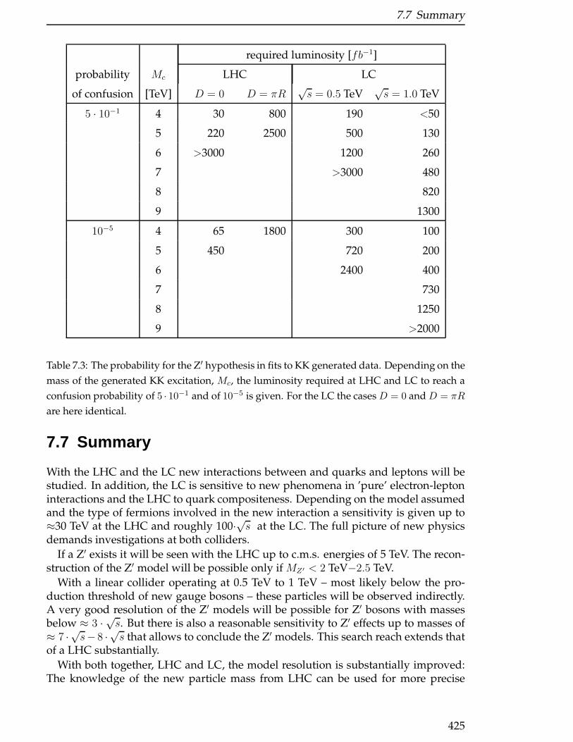
7.7 Summary
required luminosity [fb−1]
probability Mc LHC LC
of confusion [TeV] D = 0 D = πR√s = 0.5 TeV
√s = 1.0 TeV
5 · 10−1 4 30 800 190 <50
5 220 2500 500 130
6 >3000 1200 260
7 >3000 480
8 820
9 1300
10−5 4 65 1800 300 100
5 450 720 200
6 2400 400
7 730
8 1250
9 >2000
Table 7.3: The probability for the Z′ hypothesis in fits to KK generated data. Depending on the
mass of the generated KK excitation, Mc, the luminosity required at LHC and LC to reach a
confusion probability of 5 · 10−1 and of 10−5 is given. For the LC the cases D = 0 and D = πR
are here identical.
7.7 Summary
With the LHC and the LC new interactions between and quarks and leptons will bestudied. In addition, the LC is sensitive to new phenomena in ’pure’ electron-leptoninteractions and the LHC to quark compositeness. Depending on the model assumedand the type of fermions involved in the new interaction a sensitivity is given up to≈30 TeV at the LHC and roughly 100·√s at the LC. The full picture of new physicsdemands investigations at both colliders.
If a Z′ exists it will be seen with the LHC up to c.m.s. energies of 5 TeV. The recon-struction of the Z′ model will be possible only if MZ′ < 2 TeV−2.5 TeV.
With a linear collider operating at 0.5 TeV to 1 TeV – most likely below the pro-duction threshold of new gauge bosons – these particles will be observed indirectly.A very good resolution of the Z′ models will be possible for Z′ bosons with massesbelow ≈ 3 · √s. But there is also a reasonable sensitivity to Z′ effects up to masses of≈ 7 ·√s− 8 ·√s that allows to conclude the Z′ models. This search reach extends thatof a LHC substantially.
With both together, LHC and LC, the model resolution is substantially improved:The knowledge of the new particle mass from LHC can be used for more precise
425

7 New Gauge Theories
distinctions of the possible new physics sources.Without a LC it is more than challenging to find out the properties of new physics.
To enlighten a Confusion between models as for example in the case of KK excitationsand Z′ bosons the LC is essential.
The clean topologies and the high luminosity at a LC allow precison measurementsat high energies, completed by highest precision measurements on the Z peak. Theaccuracy of these measurements extends the sensitivity widely over the direct searchranges of a linear collider.
426
Bibliography
[1] P. Langacker, R. W. Robinett and J. L. Rosner, Phys. Rev. D 30 (1984) 1470;D. London and J. L. Rosner, Phys. Rev. D 34 (1986) 1530;R. W. Robinett, Phys. Rev. D 26 (1982) 2388;R. W. Robinett and J. L. Rosner, Phys. Rev. D 26 (1982) 2396;J. C. Pati and A. Salam, Phys. Rev. D 10 (1974) 275;R. N. Mohapatra and J. C. Pati, Phys. Rev. D 11 (1975) 566;L. S. Durkin and P. Langacker, Phys. Lett. B 166 (1986) 436.
[2] C. Csaki, J. Hubisz, G. D. Kribs, P. Meade and J. Terning, Phys. Rev. D 67 (2003)115002 [arXiv:hep-ph/0211124].
[3] J. L. Hewett, F. J. Petriello and T. G. Rizzo, JHEP 0310 (2003) 062 [arXiv:hep-ph/0211218].
[4] T. Han, H. E. Logan, B. McElrath and L. T. Wang, Phys. Rev. D 67 (2003) 095004[arXiv:hep-ph/0301040].
[5] T. Han, H. E. Logan, B. McElrath and L. T. Wang, Phys. Rev. D 67 (2003) 095004[arXiv:hep-ph/0301040].
[6] see for example: I. Antoniadis, Phys. Lett. B 246 (1990) 377;I. Antoniadis, C. Munoz and M. Quiros, Nucl. Phys. B 397 (1993) 515 [arXiv:hep-ph/9211309];I. Antoniadis and K. Benakli, Phys. Lett. B 326 (1994) 69 [arXiv:hep-th/9310151];I. Antoniadis and K. Benakli, Int. J. Mod. Phys. A 15 (2000) 4237 [arXiv:hep-ph/0007226];I. Antoniadis, K. Benakli and M. Quiros, Phys. Lett. B 331 (1994) 313 [arXiv:hep-ph/9403290].
[7] T. Appelquist, H. C. Cheng and B. A. Dobrescu, Phys. Rev. D 64 (2001) 035002[arXiv:hep-ph/0012100]; H. C. Cheng, K. T. Matchev and M. Schmaltz, Phys.Rev. D 66, 056006 (2002) [arXiv:hep-ph/0205314] and Phys. Rev. D 66, 036005(2002) [arXiv:hep-ph/0204342]; T. G. Rizzo, Phys. Rev. D 64, 095010 (2001)[arXiv:hep-ph/0106336].
[8] E. Eichten, I. Hinchliffe, K. D. Lane and C. Quigg, Rev. Mod. Phys. 56 (1984) 579[Addendum-ibid. 58 (1986) 1065].
[9] S. Jain, A. K. Gupta and N. K. Mondal, Phys. Rev. D 62 (2000) 095003 [arXiv:hep-ex/0005025].
427
Bibliography
[10] For a review of new gauge boson physics at colliders and details of the variousmodels, see J. L. Hewett and T. G. Rizzo, Phys. Rept. 183 (1989) 193;M. Cvetic and S. Godfrey, arXiv:hep-ph/9504216, and T. G. Rizzo, arXiv:hep-ph/9612440.
[11] S. Riemann, PREL-LCPHSM-2003-24;S. Riemann, LC-TH-2001-007.
[12] A. A. Pankov and N. Paver, Eur. Phys. J. C 29 (2003) 313 [arXiv:hep-ph/0209058];A. A. Babich, P. Osland, A. A. Pankov and N. Paver, Phys. Lett. B 518 (2001) 128[arXiv:hep-ph/0107159].
[13] D. Bourilkov, arXiv:hep-ph/0305125.
[14] Z. U. Usubov and O. B. Abdinov, Phys. Atom. Nucl. 64 (2001) 1288 [Yad. Fiz. 64(2001) 1364].
[15] G. F. Giudice, R. Rattazzi and J. D. Wells, Nucl. Phys. B 544 (1999) 3 [arXiv:hep-ph/9811291];S. Cullen, M. Perelstein and M. E. Peskin, Phys. Rev. D 62 (2000) 055012[arXiv:hep-ph/0001166].
[16] T. G. Rizzo, Phys. Rev. D 60 (1999) 115010 [arXiv:hep-ph/9904380].
[17] J. L. Hewett, Phys. Rev. Lett. 82 (1999) 4765 [arXiv:hep-ph/9811356].
[18] CMS Collaboration, Physics with CMS.
[19] ATLAS Collaboration, ATLAS Detector and Physics Performance, Technical De-sign Report, volume II, ATLAS TDR 15, CERN/LHCC 99-15, May 25, 1999.
[20] F. Abe et al. [CDF Collaboration], Phys. Rev. Lett. 79 (1997) 2198;B. Abbott et al. [D0 Collaboration], Phys. Rev. Lett. 82 (1999) 4769 [arXiv:hep-ex/9812010];A. Meyer [CDF Collaboration], Mod. Phys. Lett. A 18 (2003) 1643 [arXiv:hep-ex/0306046].
[21] [ALEPH Collaboration], arXiv:hep-ex/0212036.
[22] T. Affolder et al. [CDF Collaboration], Phys. Rev. Lett. 87 (2001) 231803[arXiv:hep-ex/0107008].
[23] M. Cvetic and P. Langacker, Phys. Rev. D 46 (1992) 4943 [Erratum-ibid. D 48(1993) 4484] [arXiv:hep-ph/9207216];F. Del Aguila and M. Cvetic, Phys. Rev. D 50 (1994) 3158 [arXiv:hep-ph/9312329].
[24] A. Leike, Phys. Rept. 317 (1999) 143 [arXiv:hep-ph/9805494].
[25] S. Godfrey, Phys. Rev. D 51 (1995) 1402 [arXiv:hep-ph/9411237];S. Godfrey, arXiv:hep-ph/9612384;S. Godfrey, in Proc. of the APS/DPF/DPB Summer Study on the Future of ParticlePhysics (Snowmass 2001) ed. N. Graf, eConf C010630 (2001) P344 [arXiv:hep-ph/0201093].
428
Bibliography
[26] A. Leike and S. Riemann, Z. Phys. C 75 (1997) 341 [arXiv:hep-ph/9607306].
[27] S. Riemann, arXiv:hep-ph/9610513.
[28] M. Dittmar, A. S. Nicollerat and A. Djouadi, Phys. Lett. B 583 (2004) 111[arXiv:hep-ph/0307020].
[29] M. Dittmar, Phys. Rev. D 55 (1997) 161 [arXiv:hep-ex/9606002].
[30] M. Dittmar, F. Pauss and D. Zurcher, Phys. Rev. D 56 (1997) 7284 [arXiv:hep-ex/9705004].
[31] F. del Aguila, M. Cvetic and P. Langacker, Phys. Rev. D 48 (1993) 969 [arXiv:hep-ph/9303299].
[32] S. Riemann, arXiv:hep-ph/9710564.
[33] T. G. Rizzo, Phys. Rev. D 55 (1997) 5483 [arXiv:hep-ph/9612304].
[34] R. Casalbuoni, S. De Curtis, D. Dominici, R. Gatto and S. Riemann, arXiv:hep-ph/0001215.
[35] P. Abreu et al. [DELPHI Collaboration], Z. Phys. C 65 (1995) 603.
[36] M. Czakon, J. Gluza, F. Jegerlehner and M. Zralek, Eur. Phys. J. C 13 (2000) 275[arXiv:hep-ph/9909242].
[37] LEP Electroweak Working Group and SLD Heavy Flavor and ElectroweakGroups, D. Abbaneo et al., LEPEWWG-2001-02, hep-ex/0112021.
[38] F. Richard, arXiv:hep-ph/0303107.
[39] S. Godfrey, Contribution to this report.
[40] G. Barenboim, J. Bernabeu, J. Prades and M. Raidal, Phys. Rev. D 55 (1997) 4213[arXiv:hep-ph/9611347].
[41] K. Hagiwara et al. [Particle Data Group Collaboration], Phys. Rev. D 66 (2002)010001 and 2003 off-year partial update for the 2004 edition available on thePDG WWW pages (URL: http://pdg.lbl.gov/).
[42] T. G. Rizzo, arXiv:hep-ph/9612440.
[43] M. Cvetic, P. Langacker and J. Liu, Phys. Rev. D 49 (1994) 2405 [arXiv:hep-ph/9308251].
[44] S. Godfrey, P. Kalyniak, B. Kamal and A. Leike, Phys. Rev. D 61 (2000) 113009[arXiv:hep-ph/0001074];S. Godfrey, P. Kalyniak, B. Kamal, M. A. Doncheski and A. Leike, Phys. Rev. D63 (2001) 053005 [arXiv:hep-ph/0008157].
[45] J. Kubar-Andre and F. E. Paige, Phys. Rev. D 19 (1979) 221;G. Altarelli, R. K. Ellis and G. Martinelli, Nucl. Phys. B 143 (1978) 521 [Erratum-ibid. B 146 (1978) 544].
429
Bibliography
[46] T. G. Rizzo, arXiv:hep-ph/9612440;T. G. Rizzo, arXiv:hep-ph/9609248;J. L. Hewett and T. G. Rizzo, Phys. Rev. D 45 (1992) 161.
[47] G. Burdman, M. Perelstein and A. Pierce, Phys. Rev. Lett. 90 (2003) 241802[Erratum-ibid. 92 (2004) 049903] [arXiv:hep-ph/0212228].
[48] See, for example, T.G. Rizzo and J.D. Wells, Phys. Rev. D61 (2000) 016007;P. Nath and M. Yamaguchi, Phys. Rev. D60 (1999) 116006;M. Masip and A. Pomarol, Phys. Rev. D60 (1999) 096005;L. Hall and C. Kolda, Phys. Lett. B459 (1999) 213;R. Casalbuoni, S. DeCurtis, D. Dominici and R. Gatto, Phys. Lett. B462 (1999) 48;A. Strumia, Phys. Lett. B466 (1999) 107;F. Cornet, M. Relano and J. Rico, Phys. Rev. D61 (2000) 037701;C.D. Carone, Phys. Rev. D61 (2000) 015008.
430
8 Models with Extra Dimensions
Editor: J.L. Hewett
M. Battaglia, D. Bourilkov, H. Davoudiasl, D. Dominici, J.F. Gunion, J.L. Hewett, T.G. Rizzo,M. Spiropulu, T. Tait
It has been proposed that the hierarchy between the electroweak and Planck scalesmay be related to the geometry of extra spatial dimensions. This idea makes use ofthe fact that gravity has yet to be probed at energy scales much above 10−3 eV inlaboratory experiments, admitting for the possibility that gravity behaves differentlythan expected at higher energies. If new dimensions are indeed related to the sourceof the hierarchy, then they should provide detectable signatures in experiments at theelectroweak scale.
Theoretical frameworks with extra dimensions have some general features. In mostscenarios, our observed 3-dimensional space is a 3-brane and is embedded in a higherD-dimensional spacetime, D = 3 + δ + 1, which is known as the ‘bulk.’ The δ extraspatial dimensions are orthogonal to our 3-brane. If the additional dimensions aresmall enough, the Standard Model gauge and matter fields are phenomenologicallyallowed to propagate in the bulk; otherwise they are stuck to the 3-brane. Gravity,however, propagates throughout the full higher dimensional volume. Conventionalwisdom dictates that if the additional dimensions are too large then deviations fromNewtonian gravity would result and hence the extra dimensional space must be com-pactified. As a result of compactification, fields propagating in the bulk expand intoa series of states known as a Kaluza-Klein (KK) tower, with the individual KK exci-tations being labeled by mode numbers. The collider signature for the existence ofadditional dimensions is the observation of a KK tower of states. The detailed prop-erties of the KK states are determined by the geometry of the compactified space andtheir measurement would reveal the underlying geometry of the bulk. A review ofextra dimensional models and their experimental signatures can be found in Ref. [1].
8.1 Large extra dimensions
In this scenario [2] the apparent gauge hierarchy is generated by a large volume of theextra dimensions. The Standard Model gauge and matter fields are confined to the 3-brane, while gravity propagates and becomes strong in the bulk. The Planck scale ofthe effective 4-dimensional theory is related to the Fundamental scale where gravitybecomes strong in the full higher dimensional spacetime, MD, via Gauss’ Law,
M2Pl = VδM
2+δD , (8.1)
where Vδ ∼ (2πRc)δ is the volume of the compactified space and Rc represents the
radius of the compactified dimensions. Taking MD ∼ 1 TeV eliminates the gauge
431

8 Models with Extra Dimensions
hierarchy and results in extra dimensions of size ∼ 0.1 mm to 1 fm for δ = 2 to 6. Thestates in the resulting KK tower of gravitons are evenly spaced with masses m~n =√~n2/R2
c , where ~n represents the KK level number, and couple to the wall fields withinverse Planck strength. The details of the KK decomposition for the bulk gravitonsand the derivation of their Feynman rules can be found in [3, 4]. We note that bothgravitensor and graviscalar fields result from the KK decomposition.
8.1.1 Indirect effects: graviton exchange
One collider signature for this scenario is that of virtual exchange of the gravitonKK excitation states in all 2 → 2 scattering processes. This results in deviations incross sections and asymmetries in SM processes as well as giving rise to new reac-tions which are not present at tree-level in the SM, such as gg → Gn → ℓ+ℓ−. Inparticular, as discussed in [3–8], the exchange of spin-2 graviton KK states modifiesthe differential cross section for fermion pair production in e+e− and pp collisions ina unique way, providing clear signatures for the existence of large extra dimensions.The exchange process is governed by the effective Lagrangian
L = i4λ
Λ2H
T µνTµν , (8.2)
employing the notation of [5], and is similar to a dimension-8 contact interaction.T µν is the conserved stress-energy tensor. The sum over the propagators for the fullgraviton KK tower is divergent for δ ≥ 1 and thus introduces a sensitivity to theunknown ultraviolet physics. Several approaches for regulating this sum may beemployed. The most model independent is the introduction of a naive cut-off, withthe cut-off being set to ΛH which is of order the fundamental scale MD. In addition,the parameter λ = ±1 is usually incorporated.• e+e− and µ+µ− Production at a Linear Collider
The effects of graviton exchange at a LC with√s = 500 GeV are computed here [8]
with a semi-analytical program in the improved Born approximation, using effectivecouplings. QED effects in the initial and final states are taken into account. Eventswithout substantial energy loss due to initial state radiation are selected by a cut onthe “effective” energy:
√s′/√s > 0.85. With this cut, the interactions occur close to
the nominal machine energy and offer the best sensitivity for manifestations of newphysics. The virtual graviton effects are computed using the calculations from [3,5,7].The sensitivity to graviton KK exchange is determined by a log likelihood fit. Twocases are distinguished:
1. Realistic: a cross section error is composed of the statistical error and a system-atic error of 0.5% coming from the experiment, 0.2% from the luminosity determina-tion, and a theoretical uncertainty of 0.5%. The forward-backward asymmetry errorconsists of the statistical error and a systematic uncertainty of 0.002 (absolute) fore+e− and 0.001 (absolute) for µ+µ− final states. The main origins of the latter are fromcharge confusion of the leptons and uncertainties in the acceptance edge determina-tion. Both of these effects are more important for electrons due to the forward peakin the differential cross section and the longer lever arm for measuring the muon mo-
432
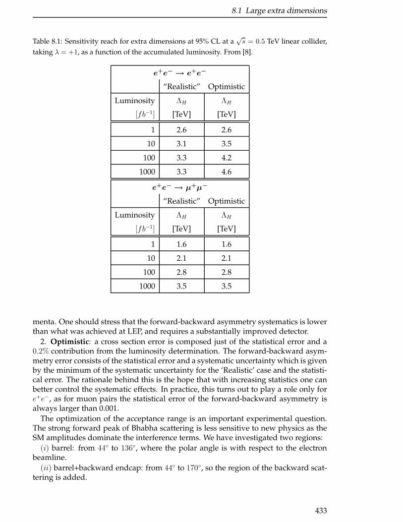
8.1 Large extra dimensions
Table 8.1: Sensitivity reach for extra dimensions at 95% CL at a√s = 0.5 TeV linear collider,
taking λ = +1, as a function of the accumulated luminosity. From [8].
e+e− → e+e−
“Realistic” Optimistic
Luminosity ΛH ΛH
[fb−1] [TeV] [TeV]
1 2.6 2.6
10 3.1 3.5
100 3.3 4.2
1000 3.3 4.6
e+e− → µ+µ−
“Realistic” Optimistic
Luminosity ΛH ΛH
[fb−1] [TeV] [TeV]
1 1.6 1.6
10 2.1 2.1
100 2.8 2.8
1000 3.5 3.5
menta. One should stress that the forward-backward asymmetry systematics is lowerthan what was achieved at LEP, and requires a substantially improved detector.
2. Optimistic: a cross section error is composed just of the statistical error and a0.2% contribution from the luminosity determination. The forward-backward asym-metry error consists of the statistical error and a systematic uncertainty which is givenby the minimum of the systematic uncertainty for the ‘Realistic’ case and the statisti-cal error. The rationale behind this is the hope that with increasing statistics one canbetter control the systematic effects. In practice, this turns out to play a role only fore+e−, as for muon pairs the statistical error of the forward-backward asymmetry isalways larger than 0.001.
The optimization of the acceptance range is an important experimental question.The strong forward peak of Bhabha scattering is less sensitive to new physics as theSM amplitudes dominate the interference terms. We have investigated two regions:
(i) barrel: from 44 to 136, where the polar angle is with respect to the electronbeamline.
(ii) barrel+backward endcap: from 44 to 170, so the region of the backward scat-tering is added.
433

8 Models with Extra Dimensions
Extra Dimensions Reach at FLC
e+e-
µ+µ-
γγ
Luminosity fb-1
Hewe
tt sc
ale M s T
eV
0
0.5
1
1.5
2
2.5
3
3.5
4
1 10 102
103
Figure 8.1: Evolution of the sensitivity reach for extra dimensions at a linear collider with√s = 0.5
TeV in different final states with the accumulated luminosity. MS = ΛH . From [8].
The sensitivity reach from our fits [8] for electron and muon pair production aresummarized in Table 8.1. They evolve from 2.6 (1.6) TeV for electrons (muons) atnominal luminosity to 3.3 (2.8) TeV for 100 fb−1. Here, the electron channel is sat-urated by the systematic uncertainties, while the muon channel is still statisticallydominated and continues to yield an improved sensitivity for the highest luminosi-ties. In the Table, only the numbers for the positive interference case (λ = +1) areshown, as the sensitivity reach for negative interference is practically the same. Theresults are also displayed in Fig. 8.1 and agree with estimates from [5, 7, 9].
It is interesting to note the large difference between the “Realistic” and the Opti-mistic scenarios for the two channels: while the systematic errors for the electronsstart to saturate above 10 fb−1, the muons do not show any saturation at all. This isexplained by the fact that for Bhabhas the sensitivity comes mainly from the crosssection measurement, while for muons it is dominated completely by the forward-backward asymmetry.
We also investigate the optimal acceptance region for this process. For final stateelectrons, the gain in sensitivity is below 1% from including the backward endcap,so the measurement may as well be restricted to the barrel region. For muons, thesensitivity comes from the asymmetry which is best measured at lower angles, hencethe results in the Table are derived under the assumption that both the barrel and thetwo endcaps are used i.e., from 10 to 170.
434
8.1 Large extra dimensions
• γγ Production at a Linear Collider
The production of photon pairs in e+e− collisions is described by t- and u-channelQED diagrams. The differential cross section has the following simple form
dσ
dΩ= |et + eu +New Physics|2 (8.3)
with (dσ
dΩ
)
QED
=α2
2s
[t
u+u
t
]=α2
s
[1 + cos2 θ
1− cos2 θ
]. (8.4)
Deviations from QED typically have the form:
dσ
dΩ=
(dσ
dΩ
)
QED
(1± s2 sin2 θ
2(LQED± )4
), (8.5)
dσ
dΩ=
(dσ
dΩ
)
QED
(1± λs2 sin2 θ
2πα(ΛH)4+ ...
). (8.6)
The QED cut-off in Equation (8.5) represents the basic form of possible modificationsto quantum electrodynamics. Equation (8.6) displays the deviations specifically dueto graviton KK exchange as calculated in [3, 10]. If we ignore the contributions fromhigher order graviton terms (denoted as ...), the two equations predict the same an-gular form of modifications to the differential cross section. Thus, it is particularlysimple to compare the results from different searches by transforming the relevantparameters; the relation is
ΛH = 2.57 LQED.The sensitivity reach from our fits [8] is summarized in Table 8.2 and Fig. 8.1. The
sensitivity evolves from 2 TeV at nominal luminosities to 3 TeV for 100 fb−1, where theprocess becomes saturated by systematic effects. As in the case of Bhabha scattering,there is no gain in sensitivity from going outside of the barrel region; in this case,the differential cross section is symmetric, exhibiting both a forward and a backwardpeak.
Summing over all fermion final states (e , µ , τ , c , b, and t) and examining the devia-tions in the total cross section, forward-backward asymmetry, and left-right asymme-try in each case, as well as the tau polarization asymmetry, yields the search reach [11]for ΛH shown in Fig. 8.2 as a function of integrated luminosity. We see that for a 1TeV LC, scales of order ΛH ∼ 8.4 TeV can be observed with 500 fb−1.
The sensitivities for virtual graviton exchange at the LHC have been evaluated in[12] and are found to be ΛH ≤ 7.5, 7.1 TeV for Drell-Yan and di-photon production,respectively. We see that this search region is comparable to that of a TeV-class LC.In addition, the spin-2 exchange also modifies the forward-backward asymmetry inDrell-Yan production; however, the utility of this asymmetry in extending the searchreach or for identifying the spin-2 nature of the exchange has yet to be analyzed.
If deviations are observed at the LC or LHC from the virtual exchange of new par-ticles, then it will be necessary to have techniques available to differentiate betweenthe possible scenarios giving rise to the effect. One such method is the use of trans-verse polarization at the LC. If longitudinal positron polarization is available at theLC, then spin rotators may be used to convert these to transversely polarized beams.
435
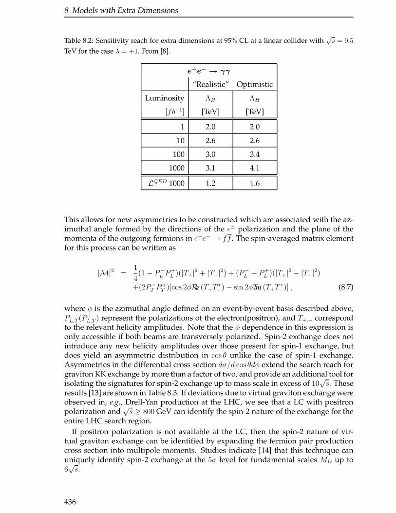
8 Models with Extra Dimensions
Table 8.2: Sensitivity reach for extra dimensions at 95% CL at a linear collider with√s = 0.5
TeV for the case λ = +1. From [8].
e+e− → γγ
“Realistic” Optimistic
Luminosity ΛH ΛH
[fb−1] [TeV] [TeV]
1 2.0 2.0
10 2.6 2.6
100 3.0 3.4
1000 3.1 4.1
LQED 1000 1.2 1.6
This allows for new asymmetries to be constructed which are associated with the az-imuthal angle formed by the directions of the e± polarization and the plane of themomenta of the outgoing fermions in e+e− → ff . The spin-averaged matrix elementfor this process can be written as
|M|2 =1
4(1− P−
L P+L )(|T+|2 + |T−|2) + (P−
L − P+L )(|T+|2 − |T−|2)
+(2P−T P
+T )[cos 2φRe (T+T
∗−)− sin 2φIm (T+T
∗−)] , (8.7)
where φ is the azimuthal angle defined on an event-by-event basis described above,P−L,T (P+
L,T ) represent the polarizations of the electron(positron), and T+,− correspondto the relevant helicity amplitudes. Note that the φ dependence in this expression isonly accessible if both beams are transversely polarized. Spin-2 exchange does notintroduce any new helicity amplitudes over those present for spin-1 exchange, butdoes yield an asymmetric distribution in cos θ unlike the case of spin-1 exchange.Asymmetries in the differential cross section dσ/d cos θdφ extend the search reach forgraviton KK exchange by more than a factor of two, and provide an additional tool forisolating the signatures for spin-2 exchange up to mass scale in excess of 10
√s. These
results [13] are shown in Table 8.3. If deviations due to virtual graviton exchange wereobserved in, e.g., Drell-Yan production at the LHC, we see that a LC with positronpolarization and
√s ≥ 800 GeV can identify the spin-2 nature of the exchange for the
entire LHC search region.
If positron polarization is not available at the LC, then the spin-2 nature of vir-tual graviton exchange can be identified by expanding the fermion pair productioncross section into multipole moments. Studies indicate [14] that this technique canuniquely identify spin-2 exchange at the 5σ level for fundamental scales MD up to6√s.
436
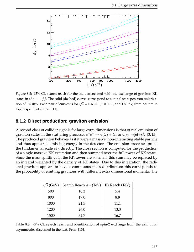
8.1 Large extra dimensions
Figure 8.2: 95% CL search reach for the scale associated with the exchange of graviton KK
states in e+e− → ff . The solid (dashed) curves correspond to a initial state positron polariza-
tion of 0 (60)%. Each pair of curves is for√s = 0.5 , 0.8 , 1.0 , 1.2 , and 1.5 TeV, from bottom to
top, respectively. From [11].
8.1.2 Direct production: graviton emission
A second class of collider signals for large extra dimensions is that of real emission ofgraviton states in the scattering processes e+e− → γ(Z) +Gn and pp→jet+Gn [3, 15].The produced graviton behaves as if it were a massive, non-interacting stable particleand thus appears as missing energy in the detector. The emission processes probethe fundamental scale MD directly. The cross section is computed for the productionof a single massive KK excitation and then summed over the full tower of KK states.Since the mass splittings in the KK tower are so small, this sum may be replaced byan integral weighted by the density of KK states. Due to this integration, the radi-ated graviton appears to have a continuous mass distribution; this corresponds tothe probability of emitting gravitons with different extra dimensional momenta. The
√s (GeV) Search Reach ΛH (TeV) ID Reach (TeV)
500 10.2 5.4
800 17.0 8.8
1000 21.5 11.1
1200 26.0 13.3
1500 32.7 16.7
Table 8.3: 95% CL search reach and identification of spin-2 exchange from the azimuthal
asymmetries discussed in the text. From [13].
437
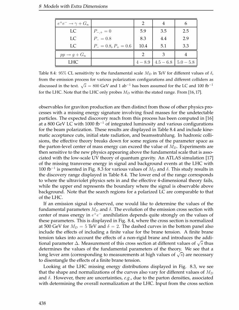
8 Models with Extra Dimensions
e+e− → γ +Gn 2 4 6
LC P−,+ = 0 5.9 3.5 2.5
LC P− = 0.8 8.3 4.4 2.9
LC P− = 0.8, P+ = 0.6 10.4 5.1 3.3
pp→ g +Gn 2 3 4
LHC 4− 8.9 4.5− 6.8 5.0− 5.8
Table 8.4: 95% CL sensitivity to the fundamental scale MD in TeV for different values of δ,
from the emission process for various polarization configurations and different colliders as
discussed in the text.√s = 800 GeV and 1 ab−1 has been assumed for the LC and 100 fb−1
for the LHC. Note that the LHC only probes MD within the stated range. From [16, 17].
observables for graviton production are then distinct from those of other physics pro-cesses with a missing energy signature involving fixed masses for the undetectableparticles. The expected discovery reach from this process has been computed in [16]at a 800 GeV LC with 1000 fb−1 of integrated luminosity and various configurationsfor the beam polarization. These results are displayed in Table 8.4 and include kine-matic acceptance cuts, initial state radiation, and beamsstrahlung. In hadronic colli-sions, the effective theory breaks down for some regions of the parameter space asthe parton-level center of mass energy can exceed the value of MD. Experiments arethen sensitive to the new physics appearing above the fundamental scale that is asso-ciated with the low-scale UV theory of quantum gravity. An ATLAS simulation [17]of the missing transverse energy in signal and background events at the LHC with100 fb−1 is presented in Fig. 8.3 for various values of MD and δ. This study results inthe discovery range displayed in Table 8.4. The lower end of the range correspondsto where the ultraviolet physics sets in and the effective 4-dimensional theory fails,while the upper end represents the boundary where the signal is observable abovebackground. Note that the search regions for a polarized LC are comparable to thatof the LHC.
If an emission signal is observed, one would like to determine the values of thefundamental parameters MD and δ. The evolution of the emission cross section withcenter of mass energy in e+e− annihilation depends quite strongly on the values ofthese parameters. This is displayed in Fig. 8.4, where the cross section is normalizedat 500 GeV for MD = 5 TeV and δ = 2. The dashed curves in the bottom panel alsoinclude the effects of including a finite value for the brane tension. A finite branetension takes into account the effects of a non-rigid brane and introduces the addi-tional parameter ∆. Measurement of this cross section at different values of
√s thus
determines the values of the fundamental parameters of the theory. We see that along lever arm (corresponding to measurements at high values of
√s) are necessary
to disentangle the effects of a finite brane tension.
Looking at the LHC missing energy distributions displayed in Fig. 8.3, we seethat the shape and normalizations of the curves also vary for different values of MD
and δ. However, there are uncertainties, e.g., due to the parton densities, associatedwith determining the overall normalization at the LHC. Input from the cross section
438

8.1 Large extra dimensions
measurement at the LC for a single value of√s would help to determine the overall
normalization at the LHC. With this information from the LC, the determination ofthe fundamental parameters from LHC data would be improved [19]. This will bequantified below.
Figure 8.3: Distribution of the missing transverse energy in background events and signal
events for 100 fb−1. The contribution of the three principal Standard Model background
processes is shown as well as the distribution of the signal for several values of δ and MD.
From [17].
8.1.3 Graviscalar effects in Higgs production
Another class of signals that can arise in models with large extra dimensions is asso-ciated with the allowed mixing between the Higgs boson and the graviscalar states.Such mixing is discussed in Sec 3.5 in this Report in the case of warped extra dimen-sions. The present scenario differs from the warped case in that there is a KK towerof densely-packed graviscalar states rather than a single radion. The graviscalar KK
states have masses m~n =√~n2/R2
c and couple to the trace of the stress-energy tensorwith inverse Planck strength. The presence of this graviscalar KK tower alters the
439
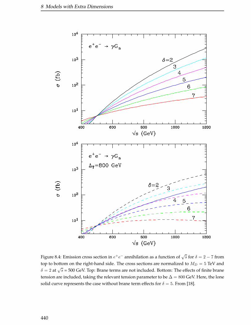
8 Models with Extra Dimensions
Figure 8.4: Emission cross section in e+e− annihilation as a function of√s for δ = 2− 7 from
top to bottom on the right-hand side. The cross sections are normalized to MD = 5 TeV and
δ = 2 at√s = 500 GeV. Top: Brane terms are not included. Bottom: The effects of finite brane
tension are included, taking the relevant tension parameter to be ∆ = 800 GeV. Here, the lone
solid curve represents the case without brane term effects for δ = 5. From [18].
440
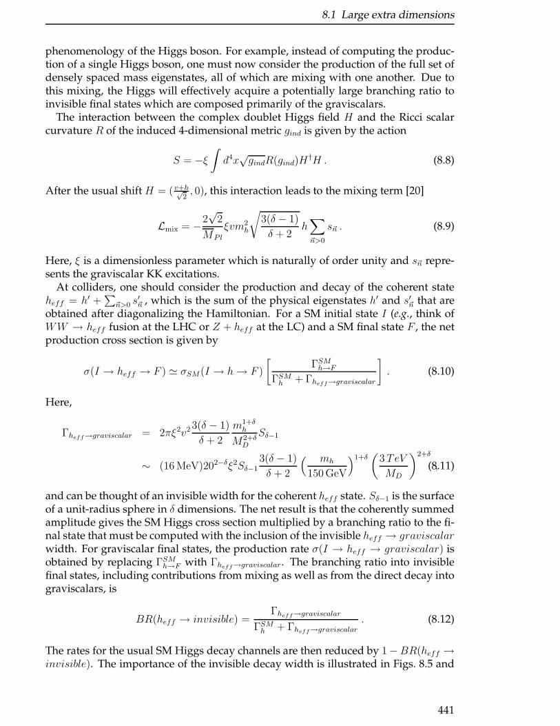
8.1 Large extra dimensions
phenomenology of the Higgs boson. For example, instead of computing the produc-tion of a single Higgs boson, one must now consider the production of the full set ofdensely spaced mass eigenstates, all of which are mixing with one another. Due tothis mixing, the Higgs will effectively acquire a potentially large branching ratio toinvisible final states which are composed primarily of the graviscalars.
The interaction between the complex doublet Higgs field H and the Ricci scalarcurvature R of the induced 4-dimensional metric gind is given by the action
S = −ξ∫d4x√gindR(gind)H
†H . (8.8)
After the usual shift H = (v+h√2, 0), this interaction leads to the mixing term [20]
Lmix = −2√
2
MP l
ξvm2h
√3(δ − 1)
δ + 2h∑
~n>0
s~n . (8.9)
Here, ξ is a dimensionless parameter which is naturally of order unity and s~n repre-sents the graviscalar KK excitations.
At colliders, one should consider the production and decay of the coherent stateheff = h′ +
∑~n>0 s
′~n , which is the sum of the physical eigenstates h′ and s′~n that are
obtained after diagonalizing the Hamiltonian. For a SM initial state I (e.g., think ofWW → heff fusion at the LHC or Z + heff at the LC) and a SM final state F , the netproduction cross section is given by
σ(I → heff → F ) ≃ σSM (I → h→ F )
[ΓSMh→F
ΓSMh + Γheff→graviscalar
]. (8.10)
Here,
Γheff→graviscalar = 2πξ2v23(δ − 1)
δ + 2
m1+δh
M2+δD
Sδ−1
∼ (16 MeV)202−δξ2Sδ−13(δ − 1)
δ + 2
( mh
150 GeV
)1+δ(
3 TeV
MD
)2+δ
,(8.11)
and can be thought of an invisible width for the coherent heff state. Sδ−1 is the surfaceof a unit-radius sphere in δ dimensions. The net result is that the coherently summedamplitude gives the SM Higgs cross section multiplied by a branching ratio to the fi-nal state that must be computed with the inclusion of the invisible heff → graviscalarwidth. For graviscalar final states, the production rate σ(I → heff → graviscalar) isobtained by replacing ΓSMh→F with Γheff→graviscalar. The branching ratio into invisiblefinal states, including contributions from mixing as well as from the direct decay intograviscalars, is
BR(heff → invisible) =Γheff→graviscalar
ΓSMh + Γheff→graviscalar. (8.12)
The rates for the usual SM Higgs decay channels are then reduced by 1−BR(heff →invisible). The importance of the invisible decay width is illustrated in Figs. 8.5 and
441

8 Models with Extra Dimensions
Figure 8.5: Contours of fixed Γheff→graviscalar (left) and fixed BR(heff → invisible) (right) in
the MD – ξ parameter space for mh = 120 GeV, taking δ = 2. The width contours correspond
to: 0.0001 GeV (large blue dashes), 0.001 GeV (solid red line), 0.01 GeV (green long dash
– short dash line), 0.1 GeV (short cyan dashes), and 1 GeV (purple dots). The BR contours
correspond to: 0.0001 (large blue dashes), 0.0005 (solid red line), 0.001 (green long dash – short
dash line), 0.005 (short cyan dashes), .01 (purple dots), .05 (long black dashes), 0.1 (chartreuse
long dashes with double dots), 0.5 (green dashes), and 0.85 (red long dash, short dot line at
high ξ and low MD). From [21].
Figure 8.6: As in Fig. 8.5 but for δ = 4.
442

8.1 Large extra dimensions
8.6 in the MD, ξ parameter space for mh = 120 GeV with δ = 2 and δ = 4, respectively.One should keep in mind that the SM Higgs boson with mass of 120 GeV would havea width of about 3.6 MeV. We thus see that the graviscalar mixing results in substantialcorrections to the expected Higgs width and a significant invisible branching fraction.
Detailed studies of the SM Higgs boson signal significance, with inclusive produc-tion, have been carried out by the ATLAS [22] and CMS [23] collaborations. Here, theresults of Fig. 25 in [23], obtained for L = 30 fb−1, are employed by reducing the SMHiggs boson signal rates in the usual visible channels by 1 − BR(heff → invisible).For L = 100 fb−1, the statistical significance in each channel is simply rescaled by√
100/30. To understand the impact of the invisible branching ratio, we focus onmh = 120 GeV and perform a full scan of the parameter space by varying MD and ξfor different values of the number of extra dimensions δ. It is found [21] that thereare regions at high ξ where the significance of the Higgs boson signal in the canonicalchannels drops below the 5 σ threshold. However, the LHC experiments will alsobe sensitive to an invisibly decaying Higgs boson produced via WW -fusion, withtagged forward jets. In Ref. [23] the results of a detailed CMS study for this modeare given in Fig. 25 for integrated luminosity of 10 fb−1. These results assume a 100%invisible branching ratio; they are rescaled here by multiplying the signal rate byBR(heff → invisible) and are adjusted for different luminosities by scaling statistical
significances according to√L(fb−1)/10. (The latter is probably somewhat inaccu-
rate for high-luminosity operation because of effects from pile-up.) The portion ofthe (MD, ξ) parameter space where the heff signal can be recovered at the 5σ levelthrough invisible decays for L = 30 fb−1 and L = 100 fb−1 is summarized in Fig. 8.7.It is important to observe that whenever the Higgs boson sensitivity is lost due to thesuppression of the canonical decay modes the invisible rate from WW fusion is largeenough to still ensure detection through a dedicated analysis.
As discussed in the previous section, the production of jets/γ+ missing energyfrom graviton emission is also sensitive to the values of MD and δ. For comparison,the 5σ search range given in Table 8.4 for MD is also displayed in Fig. 8.7. Also shownis the 95% CL lower limit onMD coming from the combination of LEP, LEP2 and Teva-tron data, as summarized in [24]. From Fig. 8.7 we observe that the invisible Higgsdecay width is predicted to probe (at 5 σ) parts of parameter space where the jets/γ+ missing energy signature either falls below this level or is not reliably computable.
A TeV-class e+e− linear collider will be able to see the heff Higgs signal regardlessof the magnitude of the invisible branching ratio simply by looking for a peak in theMX mass spectrum in e+e− → ZX events. As shown in [25], a substantial signal forthe case where X is an invisible final state is possible down to fairly low values ofBR(heff → invisible). We have employed the
√s = 350 GeV, L = 500 fb−1 results
of [25] to determine the portion of (MD, ξ) parameter space for which the invisibleHiggs signal will be observable at the LC at the 5σ or better level. This is the regionabove the light gray (yellow) curves in Fig. 8.7. The LC will be able to detect thissignal over a larger part of the parameter space than can the LHC.
443
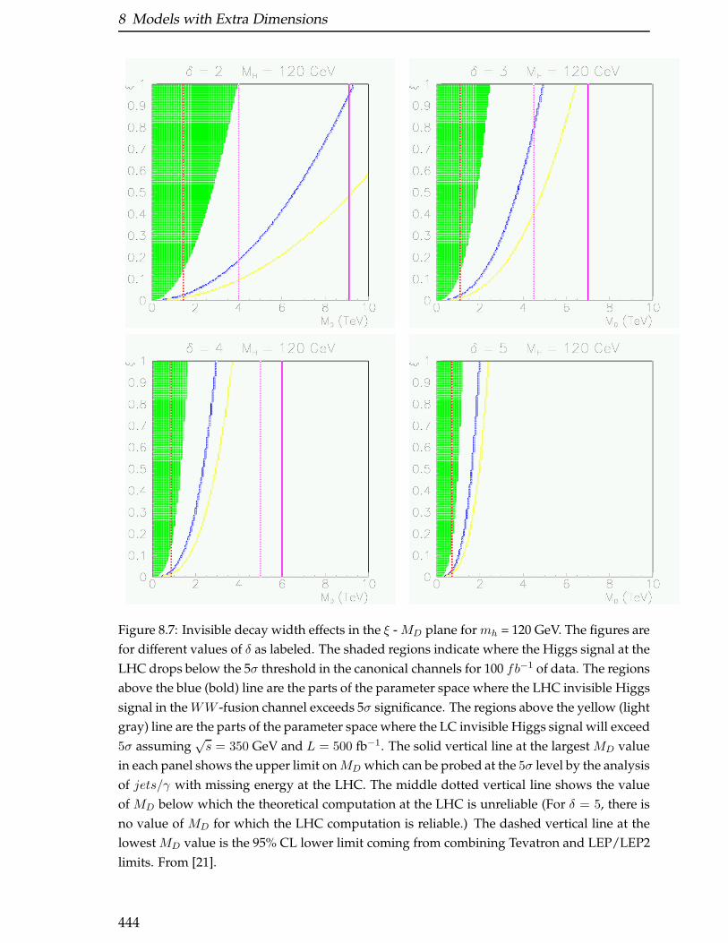
8 Models with Extra Dimensions
Figure 8.7: Invisible decay width effects in the ξ - MD plane for mh = 120 GeV. The figures are
for different values of δ as labeled. The shaded regions indicate where the Higgs signal at the
LHC drops below the 5σ threshold in the canonical channels for 100 fb−1 of data. The regions
above the blue (bold) line are the parts of the parameter space where the LHC invisible Higgs
signal in theWW -fusion channel exceeds 5σ significance. The regions above the yellow (light
gray) line are the parts of the parameter space where the LC invisible Higgs signal will exceed
5σ assuming√s = 350 GeV and L = 500 fb−1. The solid vertical line at the largest MD value
in each panel shows the upper limit onMD which can be probed at the 5σ level by the analysis
of jets/γ with missing energy at the LHC. The middle dotted vertical line shows the value
of MD below which the theoretical computation at the LHC is unreliable (For δ = 5, there is
no value of MD for which the LHC computation is reliable.) The dashed vertical line at the
lowest MD value is the 95% CL lower limit coming from combining Tevatron and LEP/LEP2
limits. From [21].
444
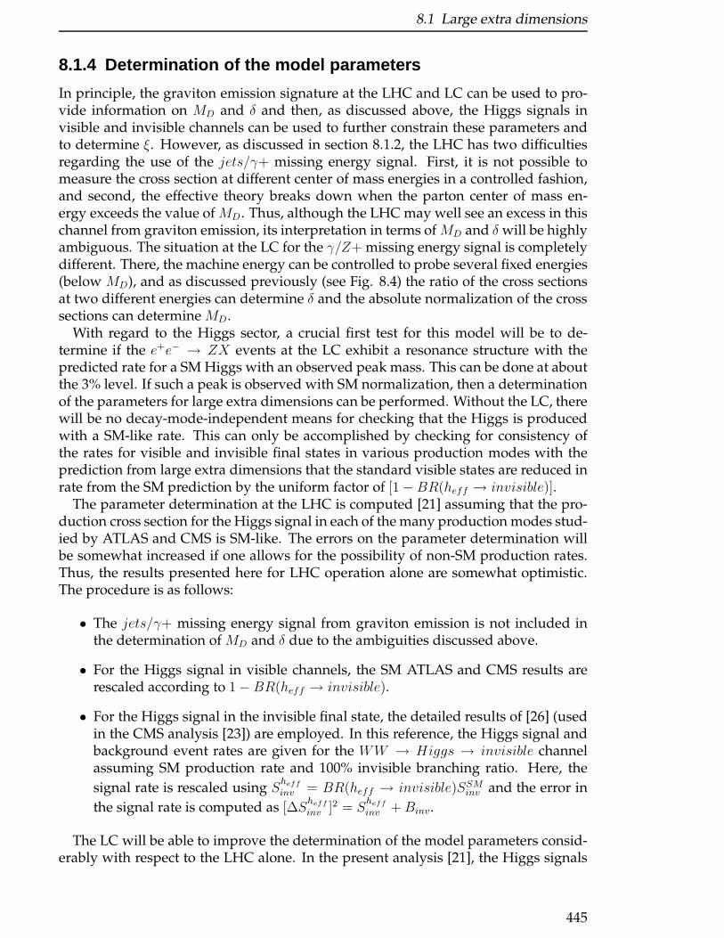
8.1 Large extra dimensions
8.1.4 Determination of the model parameters
In principle, the graviton emission signature at the LHC and LC can be used to pro-vide information on MD and δ and then, as discussed above, the Higgs signals invisible and invisible channels can be used to further constrain these parameters andto determine ξ. However, as discussed in section 8.1.2, the LHC has two difficultiesregarding the use of the jets/γ+ missing energy signal. First, it is not possible tomeasure the cross section at different center of mass energies in a controlled fashion,and second, the effective theory breaks down when the parton center of mass en-ergy exceeds the value of MD. Thus, although the LHC may well see an excess in thischannel from graviton emission, its interpretation in terms of MD and δ will be highlyambiguous. The situation at the LC for the γ/Z+ missing energy signal is completelydifferent. There, the machine energy can be controlled to probe several fixed energies(below MD), and as discussed previously (see Fig. 8.4) the ratio of the cross sectionsat two different energies can determine δ and the absolute normalization of the crosssections can determine MD.
With regard to the Higgs sector, a crucial first test for this model will be to de-termine if the e+e− → ZX events at the LC exhibit a resonance structure with thepredicted rate for a SM Higgs with an observed peak mass. This can be done at aboutthe 3% level. If such a peak is observed with SM normalization, then a determinationof the parameters for large extra dimensions can be performed. Without the LC, therewill be no decay-mode-independent means for checking that the Higgs is producedwith a SM-like rate. This can only be accomplished by checking for consistency ofthe rates for visible and invisible final states in various production modes with theprediction from large extra dimensions that the standard visible states are reduced inrate from the SM prediction by the uniform factor of [1− BR(heff → invisible)].
The parameter determination at the LHC is computed [21] assuming that the pro-duction cross section for the Higgs signal in each of the many production modes stud-ied by ATLAS and CMS is SM-like. The errors on the parameter determination willbe somewhat increased if one allows for the possibility of non-SM production rates.Thus, the results presented here for LHC operation alone are somewhat optimistic.The procedure is as follows:
• The jets/γ+ missing energy signal from graviton emission is not included inthe determination of MD and δ due to the ambiguities discussed above.
• For the Higgs signal in visible channels, the SM ATLAS and CMS results arerescaled according to 1− BR(heff → invisible).
• For the Higgs signal in the invisible final state, the detailed results of [26] (usedin the CMS analysis [23]) are employed. In this reference, the Higgs signal andbackground event rates are given for the WW → Higgs → invisible channelassuming SM production rate and 100% invisible branching ratio. Here, the
signal rate is rescaled using Sheff
inv = BR(heff → invisible)SSMinv and the error in
the signal rate is computed as [∆Sheff
inv ]2 = Sheff
inv +Binv.
The LC will be able to improve the determination of the model parameters consid-erably with respect to the LHC alone. In the present analysis [21], the Higgs signals
445

8 Models with Extra Dimensions
in both visible and invisible final states as well as the γ+ missing energy signal forgraviton production have been employed.
• For the process of graviton emission, the results from the TESLA study [16] (seeTable 8.4) have been used. The e+e− → νeνe+γ background has been computedusing the KK[27] and nunugpv [28] simulation programs. Results from the twoprograms agree well. It is assumed that measurements are performed at both√s = 500 , 1000 GeV with integrated luminosities of 1000 fb−1 and 2000 fb−1,
respectively. (Results obtained for 500 fb−1 and 1000 fb−1, respectively, are notvery different.)
• For the invisible Higgs signal, the results of [25] are employed from which thefractional error for the measurement of any given BR(heff → invisible) can beextracted.
• For the visible Higgs signal, the best available LC errors for the bb final stateare used, assuming operation at an energy of
√s = 500 GeV with luminosity of
1000 fb−1 and with polarization. The corresponding SM fractional error for thischannel at mh = 120 GeV is 0.02. This SM result is adjusted assuming signalrate reduction by the factor 1−BR(heff → invisible).
To determine how well the MD, ξ, δ parameters can be determined, specific in-put values, M0
D, ξ0, δ0, are chosen. The expected experimental errors are then com-
puted for each of the above observables assuming this input parameter set. The ex-pected ∆χ2 for each of the above observables is then computed for different values ofMD, ξ, δ.
The BR(heff → visible) measurement turns out to be important in discriminatingbetween different models when the invisible branching fraction is large (requiringsmall to moderate mh, small MD, δ = 2 or 3, and substantial ξ). In such a case,the visible branching fraction can be quite small and typically varies rapidly as afunction of the model parameters (in particular ξ), whereas the invisible branchingfraction, although large, will vary more slowly and will not provide as good a dis-crimination between different parameter values. Of course, if BR(heff → visible) isso small that the background is dominant, our ability to determine ξ, MD and δ fromthis measurement deteriorates. Complementary statements apply to the case whenBR(heff → invisible) is small and BR(heff → visible) is slowly varying.
Given the ∆χ2 for the five measurements outlined above, we will characterizethe net discrimination between models by using LHC data alone, ∆χ2(LHC), andLHC+LC data, ∆χ2(LHC + LC) (the latter being completely dominated by the LCinformation), where
∆χ2(LHC) = ∆χ2(LHC, Hvis) + ∆χ2(LHC, Hinv)
∆χ2(LC) = ∆χ2(LC, γ + missing energy) + ∆χ2(LC, Hinv) + ∆χ2(LC, Hvis)
∆χ2(LHC + LC) = ∆χ2(LHC) + ∆χ2(LC) . (8.13)
Note that since mh will be very precisely measured, one can concentrate on theability to determine the parameters MD, δ and ξ. Regions of parameter space cor-responding to a 95% CL determination, which for three parameters corresponds to
446
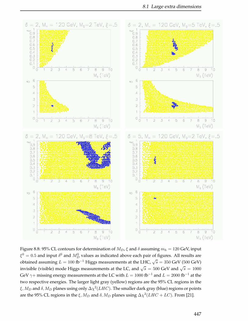
8.1 Large extra dimensions
Figure 8.8: 95% CL contours for determination of MD , ξ and δ assumingmh = 120 GeV, input
ξ0 = 0.5 and input δ0 and M0D values as indicated above each pair of figures. All results are
obtained assuming L = 100 fb−1 Higgs measurements at the LHC,√s = 350 GeV (500 GeV)
invisible (visible) mode Higgs measurements at the LC, and√s = 500 GeV and
√s = 1000
GeV γ+ missing energy measurements at the LC with L = 1000 fb−1 and L = 2000 fb−1 at the
two respective energies. The larger light gray (yellow) regions are the 95% CL regions in the
ξ,MD and δ,MD planes using only ∆χ2(LHC). The smaller dark gray (blue) regions or points
are the 95% CL regions in the ξ,MD and δ,MD planes using ∆χ2(LHC + LC). From [21].
447
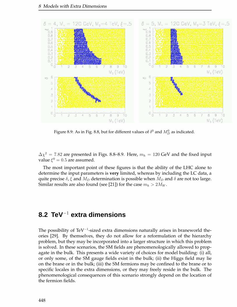
8 Models with Extra Dimensions
Figure 8.9: As in Fig. 8.8, but for different values of δ0 and M0D as indicated.
∆χ2 = 7.82 are presented in Figs. 8.8–8.9. Here, mh = 120 GeV and the fixed inputvalue ξ0 = 0.5 are assumed.
The most important point of these figures is that the ability of the LHC alone todetermine the input parameters is very limited, whereas by including the LC data, aquite precise δ, ξ and MD determination is possible when MD and δ are not too large.Similar results are also found (see [21]) for the case mh > 2MW .
8.2 TeV−1 extra dimensions
The possibility of TeV−1-sized extra dimensions naturally arises in braneworld the-ories [29]. By themselves, they do not allow for a reformulation of the hierarchyproblem, but they may be incorporated into a larger structure in which this problemis solved. In these scenarios, the SM fields are phenomenologically allowed to prop-agate in the bulk. This presents a wide variety of choices for model building: (i) all,or only some, of the SM gauge fields exist in the bulk; (ii) the Higgs field may lieon the brane or in the bulk; (iii) the SM fermions may be confined to the brane or tospecific locales in the extra dimensions, or they may freely reside in the bulk. Thephenomenological consequences of this scenario strongly depend on the location ofthe fermion fields.
448
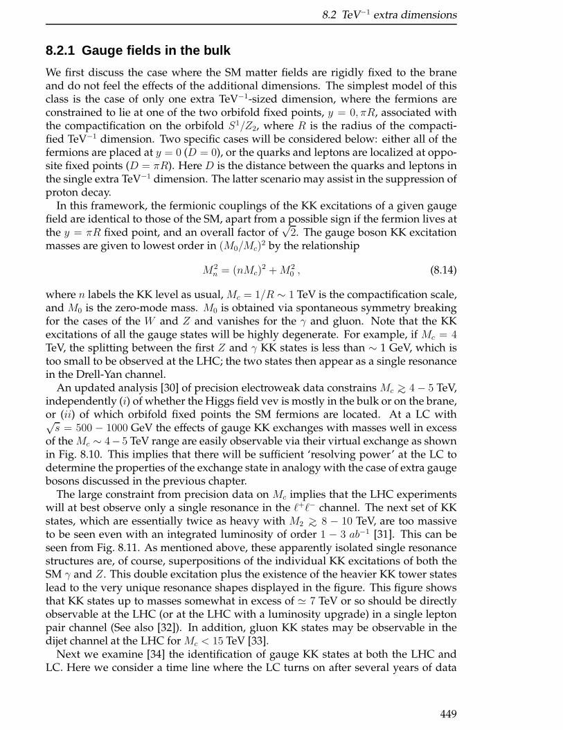
8.2 TeV−1 extra dimensions
8.2.1 Gauge fields in the bulk
We first discuss the case where the SM matter fields are rigidly fixed to the braneand do not feel the effects of the additional dimensions. The simplest model of thisclass is the case of only one extra TeV−1-sized dimension, where the fermions areconstrained to lie at one of the two orbifold fixed points, y = 0, πR, associated withthe compactification on the orbifold S1/Z2, where R is the radius of the compacti-fied TeV−1 dimension. Two specific cases will be considered below: either all of thefermions are placed at y = 0 (D = 0), or the quarks and leptons are localized at oppo-site fixed points (D = πR). Here D is the distance between the quarks and leptons inthe single extra TeV−1 dimension. The latter scenario may assist in the suppression ofproton decay.
In this framework, the fermionic couplings of the KK excitations of a given gaugefield are identical to those of the SM, apart from a possible sign if the fermion lives atthe y = πR fixed point, and an overall factor of
√2. The gauge boson KK excitation
masses are given to lowest order in (M0/Mc)2 by the relationship
M2n = (nMc)
2 +M20 , (8.14)
where n labels the KK level as usual, Mc = 1/R ∼ 1 TeV is the compactification scale,and M0 is the zero-mode mass. M0 is obtained via spontaneous symmetry breakingfor the cases of the W and Z and vanishes for the γ and gluon. Note that the KKexcitations of all the gauge states will be highly degenerate. For example, if Mc = 4TeV, the splitting between the first Z and γ KK states is less than ∼ 1 GeV, which istoo small to be observed at the LHC; the two states then appear as a single resonancein the Drell-Yan channel.
An updated analysis [30] of precision electroweak data constrains Mc >∼ 4− 5 TeV,independently (i) of whether the Higgs field vev is mostly in the bulk or on the brane,or (ii) of which orbifold fixed points the SM fermions are located. At a LC with√s = 500 − 1000 GeV the effects of gauge KK exchanges with masses well in excess
of the Mc ∼ 4− 5 TeV range are easily observable via their virtual exchange as shownin Fig. 8.10. This implies that there will be sufficient ‘resolving power’ at the LC todetermine the properties of the exchange state in analogy with the case of extra gaugebosons discussed in the previous chapter.
The large constraint from precision data on Mc implies that the LHC experimentswill at best observe only a single resonance in the ℓ+ℓ− channel. The next set of KKstates, which are essentially twice as heavy with M2 >∼ 8 − 10 TeV, are too massiveto be seen even with an integrated luminosity of order 1 − 3 ab−1 [31]. This can beseen from Fig. 8.11. As mentioned above, these apparently isolated single resonancestructures are, of course, superpositions of the individual KK excitations of both theSM γ and Z. This double excitation plus the existence of the heavier KK tower stateslead to the very unique resonance shapes displayed in the figure. This figure showsthat KK states up to masses somewhat in excess of ≃ 7 TeV or so should be directlyobservable at the LHC (or at the LHC with a luminosity upgrade) in a single leptonpair channel (See also [32]). In addition, gluon KK states may be observable in thedijet channel at the LHC for Mc < 15 TeV [33].
Next we examine [34] the identification of gauge KK states at both the LHC andLC. Here we consider a time line where the LC turns on after several years of data
449

8 Models with Extra Dimensions
Figure 8.10: 95% CL bound on the scaleMc from the reaction e+e− → ff , where f = µ, τ, c, b, t
have been summed over, as a function of the LC integrated luminosity . The solid (dashed)
curves assume a positron polarization P+ = 0(0.6); an electron polarization of 80% has been
assumed in all cases. From bottom to top the center of mass energy of the LC is taken to be
0.5, 0.8, 1, 1.2 and 1.5 TeV, respectively. From [11].
450
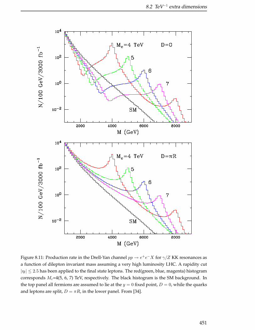
8.2 TeV−1 extra dimensions
Figure 8.11: Production rate in the Drell-Yan channel pp → e+e−X for γ/Z KK resonances as
a function of dilepton invariant mass assuming a very high luminosity LHC. A rapidity cut
|ηl| ≤ 2.5 has been applied to the final state leptons. The red(green, blue, magenta) histogram
corresponds Mc=4(5, 6, 7) TeV, respectively. The black histogram is the SM background. In
the top panel all fermions are assumed to lie at the y = 0 fixed point, D = 0, while the quarks
and leptons are split, D = πR, in the lower panel. From [34].
451
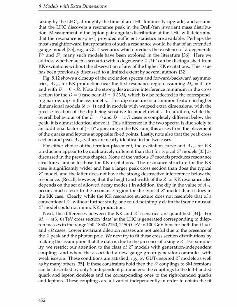
8 Models with Extra Dimensions
taking by the LHC, at roughly the time of an LHC luminosity upgrade, and assumethat the LHC discovers a resonance peak in the Drell-Yan invariant mass distribu-tion. Measurement of the lepton pair angular distribution at the LHC will determinethat the resonance is spin-1, provided sufficient statistics are available. Perhaps themost straightforward interpretation of such a resonance would be that of an extendedgauge model [35], e.g., a GUT scenario, which predicts the existence of a degenerateW ′ and Z ′; many such models have been explored in the literature [36]. Here weaddress whether such a scenario with a degenerate Z ′/W ′ can be distinguished fromKK excitations without the observation of any of the higher KK excitations. This issuehas been previously discussed to a limited extent by several authors [32].
Fig. 8.12 shows a closeup of the excitation spectra and forward-backward asymme-tries, AFB, for KK production near the first resonance region assuming Mc = 4 TeVand with D = 0, πR. Note the strong destructive interference minimum in the crosssection for the D = 0 case near M ≃ 0.55Mc which is also reflected in the correspond-ing narrow dip in the asymmetry. This dip structure is a common feature in higherdimensional models (δ > 1) and in models with warped extra dimensions, with theprecise location of the dip being sensitive to model details. In addition, while theoverall behaviour of the D = 0 and D = πR cases is completely different below thepeak, it is almost identical above it. This difference in the two spectra is due solely toan additional factor of (−1)n appearing in the KK sum; this arises from the placementof the quarks and leptons at opposite fixed points. Lastly, note also that the peak crosssection and peak AFB values are nearly identical in the two cases.
For either choice of the fermion placement, the excitation curve and AFB for KKproduction appear to be qualitatively different than that for typical Z ′ models [35] asdiscussed in the previous chapter. None of the various Z ′ models produces resonancestructures similar to those for KK excitations. The resonance structure for the KKcase is significantly wider and has a larger peak cross section than does the typicalZ ′ model, and the latter does not have the strong destructive interference below theresonance. (Recall, however, that the height and width of the Z ′ or KK resonance alsodepends on the set of allowed decay modes.) In addition, the dip in the value of AFBoccurs much closer to the resonance region for the typical Z ′ model than it does inthe KK case. Clearly, while the KK resonance structure does not resemble that of aconventional Z ′, without further study, one could not simply claim that some unusualZ ′ model could not mimic KK production.
Next, the differences between the KK and Z ′ scenarios are quantified [34]. ForMc = 4(5, 6) TeV cross section ‘data’ at the LHC is generated corresponding to dilep-ton masses in the range 250-1850 (2150, 2450) GeV in 100 GeV bins for both the D = 0and πR cases. Lower invariant dilepton masses are not useful due to the presence ofthe Z peak and the photon pole. We next try to fit these cross section distributions bymaking the assumption that the data is due to the presence of a single Z ′. For simplic-ity, we restrict our attention to the class of Z ′ models with generation-independentcouplings and where the associated a new gauge group generator commutes withweak isospin. These conditions are satisfied, e.g., by GUT-inspired Z ′ models as wellas by many others [35]. If these constraints hold then the Z ′ couplings to SM fermionscan be described by only 5 independent parameters: the couplings to the left-handedquark and lepton doublets and the corresponding ones to the right-handed quarksand leptons. These couplings are all varied independently in order to obtain the fit
452
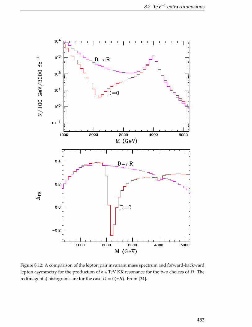
8.2 TeV−1 extra dimensions
Figure 8.12: A comparison of the lepton pair invariant mass spectrum and forward-backward
lepton asymmetry for the production of a 4 TeV KK resonance for the two choices of D. The
red(magenta) histograms are for the case D = 0(πR). From [34].
453

8 Models with Extra Dimensions
to the dilepton mass distribution with the best χ2 per degree of freedom, and the rel-evant probability (confidence level) of the fit is obtained using statistical errors only.The overall normalization of the cross section is determined at the Z-pole which isoutside of the fit region and is governed solely by SM physics.
The results [34] of performing these fits for different values of Mc and the twochoices D = 0, πR are displayed in Fig. 8.13. Explicitly, this shows the best fit prob-ability for the Z ′ hypothesis to the KK generated data. For example, taking the caseD = 0 with Mc = 4 TeV we see that with an integrated luminosity of order 60 fb−1 thebest fit probability is near a few×10−5. For such low probabilities one could certainlyclaim that the KK generated ‘data’ is not well fit by the Z ′ hypothesis. As the massof the KK state increases, the difference in the production cross section from the SMexpectation is reduced and greater statistics are needed; for Mc = 5 TeV an integratedluminosity of order 400 fb−1 is required to get to the same level of rejection of theZ ′ hypothesis. For the D = πR case, we see that the level of confusion between KKstates and Z ′ scenarios is potentially greater. Even for Mc = 4 TeV we see that onlyat very high integrated luminosities, of order ∼ 1.5 ab−1, can the KK and Z ′ scenariosbe distinguished at the level discussed above. For larger KK masses this separationbecomes essentially impossible at the LHC.
The corresponding analysis [34] for the LC is different since actual resonances arenot observed. It is assumed that data is taken at a single value of
√s so that the
mass of the KK or Z ′ resonance obtained from the LHC must be used as input tothe analysis. Without such input an analysis can still be performed provided datafrom at least two distinct values of
√s are available [37]. In that case Mc becomes an
additional fit parameter.
At the LC, a tower of gauge KK states with fixed Mc are exchanged in the processe+e− → ff . ‘Data’ is generated for both the differential cross section and the Left-Right polarization asymmetry, ALR as functions of the scattering angle cos θ in 20(essentially) equal sized bins, and including the effects of ISR. The electron beam isassumed to be 80% polarized and angular acceptance cuts are applied. Other detailedassumptions in performing this analysis are the same as those employed in Ref. [11].A fit is performed to this ‘data’ making the assumption that the deviations from theSM are due to the exchange of a single Z ′. For simplicity, we concentrate on theprocesses e+e− → µ+µ−, τ+τ− as only the two leptonic couplings are then involvedin performing the fits. In this case, the D = 0 and D = πR scenarios lead to identicalresults for the shifts in all observables at the LC. Adding new final states, such as bbor cc, may lead to potential improvements in the fit although additional parametersmust now be introduced and the D = 0 and D = πR cases would be distinct as at theLHC.
As in the above analysis for the LHC, the two assumed Z ′ couplings to leptons arevaried and the best χ2/df is obtained for the fit. For the case of a
√s = 500 GeV LC, we
find that an integrated luminosity of 300 fb−1 is roughly equivalent to 60 fb−1 at theLHC for the case of Mc = 4 TeV assuming D = 0. For larger values of Mc, 800 (2200)fb−1 at a 500 GeV LC gives equivalent discrimination power as 400 (7500) fb−1 atthe LHC assuming Mc = 5 (6) TeV. The results [34] for a 1 TeV LC are displayed inFig. 8.13. Here, we see that once the LC center-of-mass energy increases, it is superiorto the LHC in resolving power, but the analysis still relies upon the LHC for the inputvalue of Mc. This figure shows results for values of Mc beyond the range which is
454

8.2 TeV−1 extra dimensions
Figure 8.13: Top Panel: Probability associated with the best Z ′ fit hypothesis as a function of
the LHC integrated luminosity for the cases D = 0 (solid) and D = πR (dashed). Bottom
Panel: Same as the above but now for a 1 TeV LC using leptonic data only. In this case, the
D = 0 and D = πR cases are identical. The value of Mc is assumed to be determined at the
LHC. From [34].
455

8 Models with Extra Dimensions
directly observable at the LHCMc ≥ 7−8 TeV (although still assuming that the valueof Mc is an input). This would seem to imply that by extending the present analysisto include data from at least two values of
√s, KK/Z ′ separation may be feasible out
to very large masses at the LC.In summary, the power of the LC to discriminate between models is shown to be
better than that of the LHC, however, the LC analysis depends upon the LHC deter-mination of the resonance mass as an input.
8.2.2 Universal extra dimensions
In the scenario known as universal extra dimensions, all SM fields propagate in thebulk and branes need not be present. The simplest model of this type contains asingle extra dimension compactified on an S1/Z2 orbifold. Translational invariance inthe higher dimensional space is preserved. This leads to the tree-level conservationof the δ-dimensional momentum of the bulk fields, which in turn implies that KKnumber is conserved at tree-level while KK parity, (−1)n, is conserved to all orders.Two immediate consequences of KK number and parity conservation are that (i) attree-level, KK excitations can no longer be produced as s-channel resonances and canonly be produced in pairs, and (ii) the lightest KK particle (LKP) is stable and is thusa dark matter candidate [38]. The former results in a substantial reduction of thesensitivity to such states in precision electroweak and collider data with the presentbound on the mass of the first KK excitation being of order a few hundred GeV forδ = 1 [39].
Due to the conservation of KK parity, the phenomenology of universal extra dimen-sions resembles that of supersymmetric theories with R-parity conservation. EverySM field has KK partners. These KK partners carry a conserved quantum number,KK parity, which guarantees that the LKP is stable. Heavier KK modes decay viacascades to the LKP, which escapes detection resulting in a missing energy signature.The Lagrangian of the model includes both bulk terms and interactions which arelocalized at the orbifold fixed points. The bulk interactions yield masses for the KKstates as given in Eq. (8.14); these are highly degenerate within each KK level. Theboundary interactions take the form of loop induced localized kinetic terms [40] andare not universal for the different SM fields. The low scale boundary terms are de-termined via high energy parameters which are evolved through the renormalizationgroup. In addition, non-local radiative corrections [41] also affect the KK mass spec-trum. Combined, this has the effect of removing the degeneracy between the modesin a KK level and also affects their decay chains. A typical KK spectrum [43] is dis-played in Fig. 8.14. The KK modes with strong interactions receive larger correctionsthan those with only electroweak interactions. This spectrum resembles that of thesuperpartners in a Minimal Supersymmetric Standard Model where the sparticles alllie relatively close together.
Once the KK mass degeneracy is lifted, the states decay promptly. The resultingcollider phenomenology is strikingly similar to that of supersymmetry [43]. Indeed,if such a scenario were observed at the LHC, it is reasonable to expect that it would bemis-identified as the discovery of supersymmetry! Superpartner status would mostlikely be assigned to the various KK states. Hence, techniques to distinguish the twoscenarios need to be developed.
456
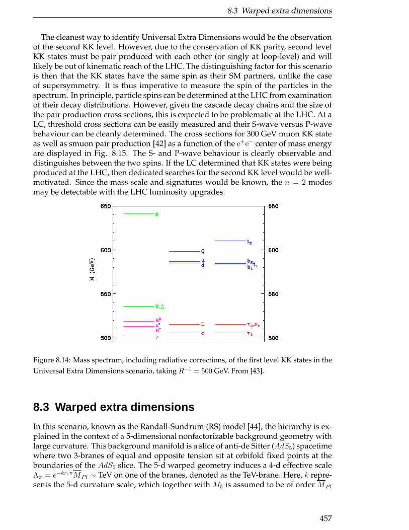
8.3 Warped extra dimensions
The cleanest way to identify Universal Extra Dimensions would be the observationof the second KK level. However, due to the conservation of KK parity, second levelKK states must be pair produced with each other (or singly at loop-level) and willlikely be out of kinematic reach of the LHC. The distinguishing factor for this scenariois then that the KK states have the same spin as their SM partners, unlike the caseof supersymmetry. It is thus imperative to measure the spin of the particles in thespectrum. In principle, particle spins can be determined at the LHC from examinationof their decay distributions. However, given the cascade decay chains and the size ofthe pair production cross sections, this is expected to be problematic at the LHC. At aLC, threshold cross sections can be easily measured and their S-wave versus P-wavebehaviour can be cleanly determined. The cross sections for 300 GeV muon KK stateas well as smuon pair production [42] as a function of the e+e− center of mass energyare displayed in Fig. 8.15. The S- and P-wave behaviour is clearly observable anddistinguishes between the two spins. If the LC determined that KK states were beingproduced at the LHC, then dedicated searches for the second KK level would be well-motivated. Since the mass scale and signatures would be known, the n = 2 modesmay be detectable with the LHC luminosity upgrades.
Figure 8.14: Mass spectrum, including radiative corrections, of the first level KK states in the
Universal Extra Dimensions scenario, taking R−1 = 500 GeV. From [43].
8.3 Warped extra dimensions
In this scenario, known as the Randall-Sundrum (RS) model [44], the hierarchy is ex-plained in the context of a 5-dimensional nonfactorizable background geometry withlarge curvature. This background manifold is a slice of anti-de Sitter (AdS5) spacetimewhere two 3-branes of equal and opposite tension sit at orbifold fixed points at theboundaries of the AdS5 slice. The 5-d warped geometry induces a 4-d effective scaleΛπ = e−krcπMP l ∼ TeV on one of the branes, denoted as the TeV-brane. Here, k repre-sents the 5-d curvature scale, which together with M5 is assumed to be of order MP l
457
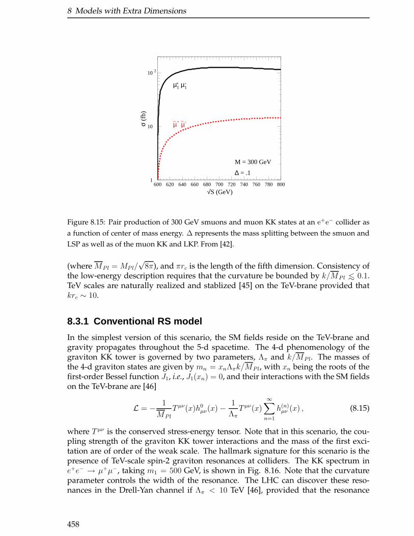
8 Models with Extra Dimensions
1
10
10 2
600 620 640 660 680 700 720 740 760 780 800
µ1 µ1
µ+ µ-~ ~
+ -
M = 300 GeV
∆ = .1
√S (GeV)
σ (f
b)
Figure 8.15: Pair production of 300 GeV smuons and muon KK states at an e+e− collider as
a function of center of mass energy. ∆ represents the mass splitting between the smuon and
LSP as well as of the muon KK and LKP. From [42].
(where MP l = MP l/√
8π), and πrc is the length of the fifth dimension. Consistency ofthe low-energy description requires that the curvature be bounded by k/MP l <∼ 0.1.TeV scales are naturally realized and stablized [45] on the TeV-brane provided thatkrc ∼ 10.
8.3.1 Conventional RS model
In the simplest version of this scenario, the SM fields reside on the TeV-brane andgravity propagates throughout the 5-d spacetime. The 4-d phenomenology of thegraviton KK tower is governed by two parameters, Λπ and k/MP l. The masses ofthe 4-d graviton states are given by mn = xnΛπk/MP l, with xn being the roots of thefirst-order Bessel function J1, i.e., J1(xn) = 0, and their interactions with the SM fieldson the TeV-brane are [46]
L = − 1
MP l
T µν(x)h0µν(x)−
1
Λπ
T µν(x)∞∑
n=1
h(n)µν (x) , (8.15)
where T µν is the conserved stress-energy tensor. Note that in this scenario, the cou-pling strength of the graviton KK tower interactions and the mass of the first exci-tation are of order of the weak scale. The hallmark signature for this scenario is thepresence of TeV-scale spin-2 graviton resonances at colliders. The KK spectrum ine+e− → µ+µ−, taking m1 = 500 GeV, is shown in Fig. 8.16. Note that the curvatureparameter controls the width of the resonance. The LHC can discover these reso-nances in the Drell-Yan channel if Λπ < 10 TeV [46], provided that the resonance
458
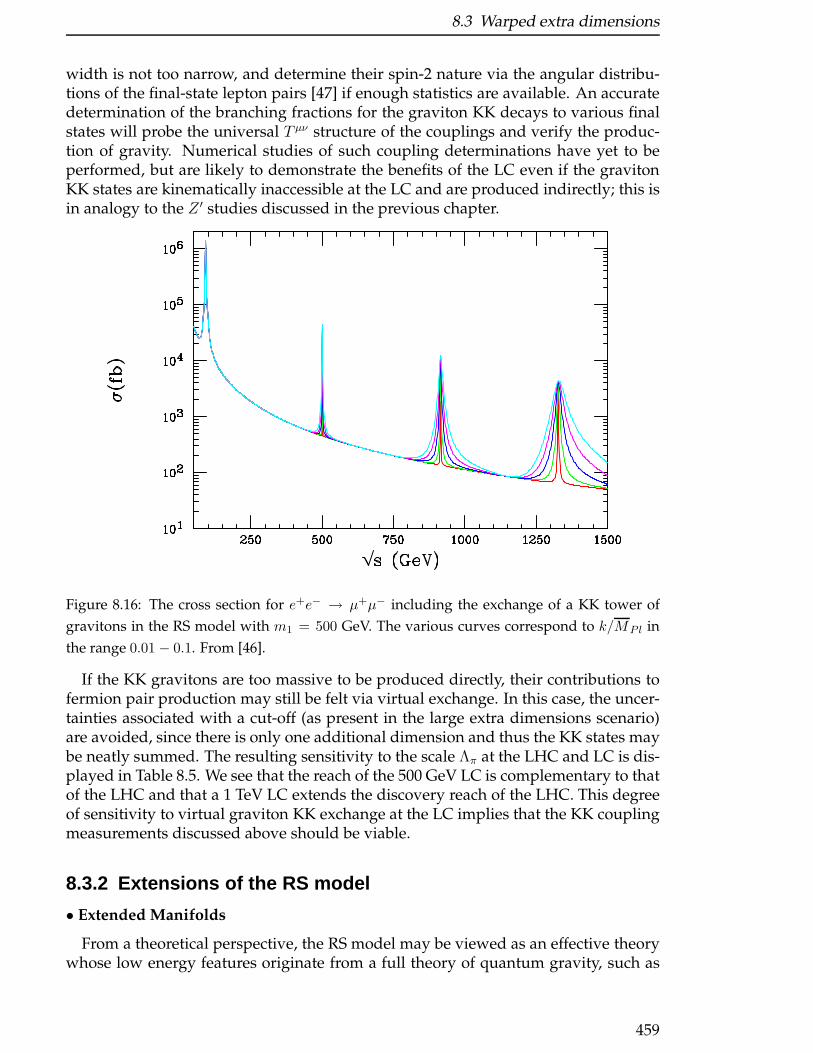
8.3 Warped extra dimensions
width is not too narrow, and determine their spin-2 nature via the angular distribu-tions of the final-state lepton pairs [47] if enough statistics are available. An accuratedetermination of the branching fractions for the graviton KK decays to various finalstates will probe the universal T µν structure of the couplings and verify the produc-tion of gravity. Numerical studies of such coupling determinations have yet to beperformed, but are likely to demonstrate the benefits of the LC even if the gravitonKK states are kinematically inaccessible at the LC and are produced indirectly; this isin analogy to the Z ′ studies discussed in the previous chapter.
Figure 8.16: The cross section for e+e− → µ+µ− including the exchange of a KK tower of
gravitons in the RS model with m1 = 500 GeV. The various curves correspond to k/MP l in
the range 0.01 − 0.1. From [46].
If the KK gravitons are too massive to be produced directly, their contributions tofermion pair production may still be felt via virtual exchange. In this case, the uncer-tainties associated with a cut-off (as present in the large extra dimensions scenario)are avoided, since there is only one additional dimension and thus the KK states maybe neatly summed. The resulting sensitivity to the scale Λπ at the LHC and LC is dis-played in Table 8.5. We see that the reach of the 500 GeV LC is complementary to thatof the LHC and that a 1 TeV LC extends the discovery reach of the LHC. This degreeof sensitivity to virtual graviton KK exchange at the LC implies that the KK couplingmeasurements discussed above should be viable.
8.3.2 Extensions of the RS model
• Extended Manifolds
From a theoretical perspective, the RS model may be viewed as an effective theorywhose low energy features originate from a full theory of quantum gravity, such as
459
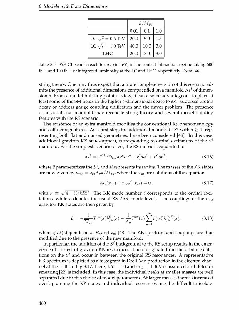
8 Models with Extra Dimensions
k/MP l
0.01 0.1 1.0
LC√s = 0.5 TeV 20.0 5.0 1.5
LC√s = 1.0 TeV 40.0 10.0 3.0
LHC 20.0 7.0 3.0
Table 8.5: 95% CL search reach for Λπ (in TeV) in the contact interaction regime taking 500
fb−1 and 100 fb−1 of integrated luminosity at the LC and LHC, respectively. From [46].
string theory. One may thus expect that a more complete version of this scenario ad-mits the presence of additional dimensions compactified on a manifoldMδ of dimen-sion δ. From a model-building point of view, it can also be advantageous to place atleast some of the SM fields in the higher δ-dimensional space to e.g., suppress protondecay or address gauge coupling unification and the flavor problem. The presenceof an additional manifold may reconcile string theory and several model-buildingfeatures with the RS scenario.
The existence of an extra manifold modifies the conventional RS phenomenologyand collider signatures. As a first step, the additional manifolds Sδ with δ ≥ 1, rep-resenting both flat and curved geometries, have been considered [48]. In this case,additional graviton KK states appear, corresponding to orbital excitations of the Sδ
manifold. For the simplest scenario of S1, the RS metric is expanded to
ds2 = e−2krcφηµνdxµdxν + r2
cdφ2 +R2dθ2 , (8.16)
where θ parameterizes the S1, andR represents its radius. The masses of the KK statesare now given by mnℓ = xnℓΛπk/MP l, where the xnℓ are solutions of the equation
2Jν(xnℓ) + xnℓJ′ν(xnℓ) = 0 , (8.17)
with ν ≡√
4 + (ℓ/kR)2. The KK mode number ℓ corresponds to the orbital exci-tations, while n denotes the usual RS AdS5 mode levels. The couplings of the mnℓ
graviton KK states are then given by
L = − 1
MP l
T µν(x)h0µν(x)−
1
ΛπT µν(x)
∞∑
n=1
ξ(nℓ)h(n,ℓ)µν (x) , (8.18)
where ξ(nℓ) depends on k ,R, and xnℓ [48]. The KK spectrum and couplings are thusmodified due to the presence of the new manifold.
In particular, the addition of the Sδ background to the RS setup results in the emer-gence of a forest of graviton KK resonances. These originate from the orbital excita-tions on the Sδ and occur in between the original RS resonances. A representativeKK spectrum is depicted as a histogram in Drell-Yan production in the electron chan-nel at the LHC in Fig 8.17. Here, kR = 1.0 and m10 = 1 TeV is assumed and detectorsmearing [22] is included. In this case, the individual peaks at smaller masses are wellseparated due to this choice of model parameters. At larger masses there is increasedoverlap among the KK states and individual resonances may be difficult to isolate.
460
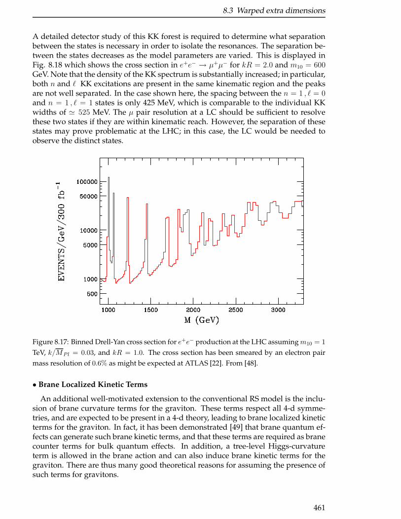
8.3 Warped extra dimensions
A detailed detector study of this KK forest is required to determine what separationbetween the states is necessary in order to isolate the resonances. The separation be-tween the states decreases as the model parameters are varied. This is displayed inFig. 8.18 which shows the cross section in e+e− → µ+µ− for kR = 2.0 and m10 = 600GeV. Note that the density of the KK spectrum is substantially increased; in particular,both n and ℓ KK excitations are present in the same kinematic region and the peaksare not well separated. In the case shown here, the spacing between the n = 1 , ℓ = 0and n = 1 , ℓ = 1 states is only 425 MeV, which is comparable to the individual KKwidths of ≃ 525 MeV. The µ pair resolution at a LC should be sufficient to resolvethese two states if they are within kinematic reach. However, the separation of thesestates may prove problematic at the LHC; in this case, the LC would be needed toobserve the distinct states.
Figure 8.17: Binned Drell-Yan cross section for e+e− production at the LHC assumingm10 = 1
TeV, k/MP l = 0.03, and kR = 1.0. The cross section has been smeared by an electron pair
mass resolution of 0.6% as might be expected at ATLAS [22]. From [48].
• Brane Localized Kinetic Terms
An additional well-motivated extension to the conventional RS model is the inclu-sion of brane curvature terms for the graviton. These terms respect all 4-d symme-tries, and are expected to be present in a 4-d theory, leading to brane localized kineticterms for the graviton. In fact, it has been demonstrated [49] that brane quantum ef-fects can generate such brane kinetic terms, and that these terms are required as branecounter terms for bulk quantum effects. In addition, a tree-level Higgs-curvatureterm is allowed in the brane action and can also induce brane kinetic terms for thegraviton. There are thus many good theoretical reasons for assuming the presence ofsuch terms for gravitons.
461
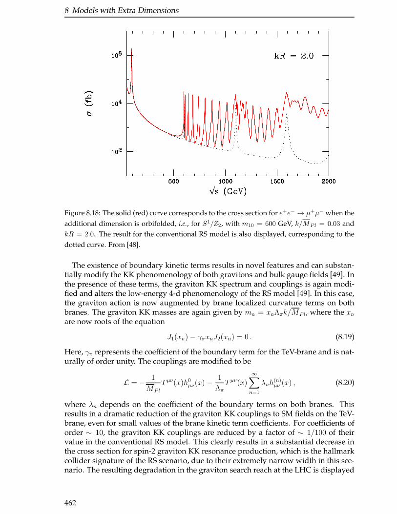
8 Models with Extra Dimensions
Figure 8.18: The solid (red) curve corresponds to the cross section for e+e− → µ+µ− when the
additional dimension is orbifolded, i.e., for S1/Z2, with m10 = 600 GeV, k/MP l = 0.03 and
kR = 2.0. The result for the conventional RS model is also displayed, corresponding to the
dotted curve. From [48].
The existence of boundary kinetic terms results in novel features and can substan-tially modify the KK phenomenology of both gravitons and bulk gauge fields [49]. Inthe presence of these terms, the graviton KK spectrum and couplings is again modi-fied and alters the low-energy 4-d phenomenology of the RS model [49]. In this case,the graviton action is now augmented by brane localized curvature terms on bothbranes. The graviton KK masses are again given by mn = xnΛπk/MP l, where the xnare now roots of the equation
J1(xn)− γπxnJ2(xn) = 0 . (8.19)
Here, γπ represents the coefficient of the boundary term for the TeV-brane and is nat-urally of order unity. The couplings are modified to be
L = − 1
MP l
T µν(x)h0µν(x)−
1
ΛπT µν(x)
∞∑
n=1
λnh(n)µν (x) , (8.20)
where λn depends on the coefficient of the boundary terms on both branes. Thisresults in a dramatic reduction of the graviton KK couplings to SM fields on the TeV-brane, even for small values of the brane kinetic term coefficients. For coefficients oforder ∼ 10, the graviton KK couplings are reduced by a factor of ∼ 1/100 of theirvalue in the conventional RS model. This clearly results in a substantial decrease inthe cross section for spin-2 graviton KK resonance production, which is the hallmarkcollider signature of the RS scenario, due to their extremely narrow width in this sce-nario. The resulting degradation in the graviton search reach at the LHC is displayed
462
8.3 Warped extra dimensions
in Fig 8.19 for 100 fb−1 of integrated luminosity. From this figure, it is clear that theLHC can no longer cover all of the interesting parameter space for this model. Forexample, a first graviton KK excitation of mass 600 GeV with k/MP l = 0.01 maystill miss detection. Very light KK gravitons may thus escape direct detection at theTevatron and LHC.
However, it is possible that such narrow resonances may be observed at the LC viaradiative return. The differential cross section for radiative return in e+e− → mu+µ−γ[50] including a 750 GeV KK state with γπ = −8 and k/MP l = 0.025, a resonancewhich is invisible at the LHC, is displayed in Fig. 8.19. From the figure we see thatthere is a sharply defined peak; the narrrow width approximation yields a ∼ 1 fb−1
cross section under the peak. Hence, the radiative return search technique at the LC isvery powerful and may guide dedicated analyses at the LHC in the search for narrowresonances.
8.3.3 Conclusions
Collider signatures for the presence of extra spatial dimensions are wide and var-ied, depending on the geometry of the additional dimensions. The basic signal is theobservation of a Kaluza-Klein (KK) tower of states corresponding to a particle prop-agating in the higher dimensional space-time. The measurement of the properties ofthe KK states determines the size and geometry of the extra dimensions.
In the scenario of large extra dimensions, where gravity alone can propagate in thebulk, the indirect effects and direct production of KK gravitons are both available atthe LHC and at the LC. For the indirect exchange of KK gravitons, the search reach ofthe LC exceeds that of the LHC for
√s >∼ 800 GeV. Measurement of the moments of the
resulting angular distributions at the LC can identify the spin-2 nature of the gravitonexchange for roughly half of the search reach range. If positron polarization is avail-able, then azimuthal asymmetries can (i) extend the search for graviton exchange bya factor of 2, probing fundamental scales of gravity up to 21 TeV for
√s = 1 TeV with
500 fb−1 of integrated luminosity, and (ii) identify the spin-2 exchange for the entireLHC search region. In the case of direct KK graviton production, the LHC and LChave comparable search reaches. However, the LHC is hampered by theoretical am-biguities due to a break-down of the effective theory when the parton-level center ofmass energy exceeds the fundamental scale of gravity; in this case the LHC may di-rectly detect effects of quantum gravity. Measurement of direct graviton productionat two different center of mass energies at the LC can determine the number of ex-tra dimensions and the absolute normalization of the cross section can determine thefundamental scale. Simultaneous determination of all the model parameters has beenexamined in a quantitative fashion with the result that data from the LC and LHC an-alyzed together substantially improves the accuracy of this determination over theLHC data taken alone.
Standard Model fields are allowed to propagate in extra dimensions with size lessthan TeV−1. Signatures for the KK states of the SM gauge fields mimic those for newheavy gauge bosons in extended gauge theories. The LHC may discover electroweakgauge KK states via direct production in the mass range Mc ≃ 4 − 6 TeV (lowermasses are excluded by LEP/SLC data), while indirect detection at the LC is possiblefor Mc <∼ 20 TeV for
√s = 1 TeV. Indirect detection of electroweak gauge KK states
463

8 Models with Extra Dimensions
Figure 8.19: Top: Search reach for the first graviton KK resonance employing the Drell-Yan
channel at the LHC with an integrated luminosity of 100 fb−1 as a function of the bound-
ary term coefficient γπ assuming γ0 = 0. From bottom to top on the RHS of the plot, the
curves correspond to k/MP l = 0.01, 0.025, 0.05, 0.075, 0.10, 0.125 and 0.15, respectively. The
unshaded region is that allowed by naturalness considerations and the requirement of a
ghost-free radion sector. From [49] Bottom: Differential cross section for e+e− → µ+µ−γ
including a 750 GeV graviton excitation with k/MP l = 0.025 and boundary term γπ = −8.
From [51].
464
8.3 Warped extra dimensions
is also possible at the LHC for Mc <∼ 12 TeV via a detailed study of the shape ofthe Drell-Yan lepton-pair invariant mass distribution. If discovered, a quantitativeanalyses shows that the determination of the mass of the first gauge KK excitationat the LHC, together with indirect effects at the LC can be used to distinguish theproduction of a KK gauge state from a new gauge field in extended gauge sectors.
The possibility of universal extra dimensions, where all SM fields are in the bulk,can cause confusion with the production of supersymmetric states, since the KK spec-trum and phenomenology resembles that of supersymmetry. In fact, the lightestKK state is a Dark Matter candidate. In this case, threshold production of the new(s)particle at the LC can easily determine its spin and distinguish universal extra di-mensions from supersymmetry. Spin determination analyses are on-going for theLHC.
Lastly, the presence of warped extra dimensions results in the resonance produc-tion of spin-2 gravitons. This produces a spectacular signature at the LHC for theconventional construction of the Randall-Sundrum model. However, extensions tothis model, such as the embedding in a higher dimension manifold, or the inclusionof kinetic brane terms, result in reduced coupling strengths and extremely narrow-width graviton KK states. Such states may be difficult to observe at the LHC andeven very light KK states may escape detection. In this case, radiative return at theLC may pinpoint the existence of these states, which can then be confirmed by a ded-icated search at the LHC.
465

8 Models with Extra Dimensions
466
Bibliography
[1] J. Hewett and M. Spiropulu, Ann. Rev. Nucl. Part. Sci. 52, 397 (2002) [arXiv:hep-ph/0205106].
[2] N. Arkani-Hamed, S. Dimopoulos and G. R. Dvali, Phys. Lett. B 429, 263 (1998)[arXiv:hep-ph/9803315]; Phys. Rev. D 59, 086004 (1999) [arXiv:hep-ph/9807344].
[3] G. F. Giudice, R. Rattazzi and J. D. Wells, Nucl. Phys. B 544, 3 (1999) [arXiv:hep-ph/9811291].
[4] T. Han, J. D. Lykken and R. J. Zhang, Phys. Rev. D 59, 105006 (1999) [arXiv:hep-ph/9811350].
[5] J. L. Hewett, Phys. Rev. Lett. 82, 4765 (1999) [arXiv:hep-ph/9811356].
[6] S. Nussinov and R. Shrock, Phys. Rev. D 59, 105002 (1999) [arXiv:hep-ph/9811323].
[7] T. G. Rizzo, Phys. Rev. D 59, 115010 (1999) [arXiv:hep-ph/9901209].
[8] D. Bourilkov, arXiv:hep-ph/0305125.
[9] S. Riemann, LC-TH-2001-007.
[10] K. Agashe and N. G. Deshpande, Phys. Lett. B 456, 60 (1999) [arXiv:hep-ph/9902263].
[11] T. G. Rizzo, arXiv:hep-ph/0303056.
[12] F. Gianotti et al., arXiv:hep-ph/0204087; V. Kabachenko, A. Miagkov, and A.Zenin, ATLAS Physics Note, ATL-PHYS-2001-012 (2001).
[13] T. G. Rizzo, JHEP 0302, 008 (2003) [arXiv:hep-ph/0211374].
[14] T. G. Rizzo, JHEP 0210, 013 (2002) [arXiv:hep-ph/0208027].
[15] E. A. Mirabelli, M. Perelstein and M. E. Peskin, Phys. Rev. Lett. 82, 2236 (1999)[arXiv:hep-ph/9811337].
[16] J. A. Aguilar-Saavedra et al. [ECFA/DESY LC Physics Working Group Collabo-ration], arXiv:hep-ph/0106315.
[17] L. Vacavant and I. Hinchliffe, J. Phys. G 27, 1839 (2001).
[18] T.G. Rizzo, contribution to this report.
467

Bibliography
[19] A. deRoeck, J. Lykken, and M. Spiropulu, in progress.
[20] G. F. Giudice, R. Rattazzi and J. D. Wells, Nucl. Phys. B 595, 250 (2001) [arXiv:hep-ph/0002178].
[21] M. Battaglia, D. Dominici, and J. Gunion, contribution to this report.
[22] ATLAS Collaboration, Technical Design Report, Vols 1 and 2. CERN ReportsCERN-LHCC-99-14/15 (1999).
[23] S. Abdullin et al., CMS Collaboration, CMS-NOTE-2003/033 (2003).
[24] G. F. Giudice and A. Strumia, Nucl. Phys. B 663, 377 (2003) [arXiv:hep-ph/0301232].
[25] M. Schumacher, LC note LC-PHSM-2003-096 (2003).
[26] O. J. P. Eboli and D. Zeppenfeld, Phys. Lett. B 495, 147 (2000) [arXiv:hep-ph/0009158].
[27] B. F. L. Ward, S. Jadach and Z. Was, Nucl. Phys. Proc. Suppl. 116, 73 (2003)[arXiv:hep-ph/0211132].
[28] G. Montagna, O. Nicrosini and F. Piccinini, Comput. Phys. Commun. 98 (1996)206.
[29] I. Antoniadis, Phys. Lett. B 246, 377 (1990); J. D. Lykken, Phys. Rev. D 54, 3693(1996) [arXiv:hep-th/9603133]; I. Antoniadis and M. Quiros, Phys. Lett. B 392, 61(1997) [arXiv:hep-th/9609209].
[30] See, for example, T. G. Rizzo and J. D. Wells, Phys. Rev. D 61, 016007 (2000)[arXiv:hep-ph/9906234]; P. Nath and M. Yamaguchi, Phys. Rev. D 60, 116004(1999) [arXiv:hep-ph/9902323]; M. Masip and A. Pomarol, Phys. Rev. D 60,096005 (1999) [arXiv:hep-ph/9902467]; L. J. Hall and C. F. Kolda, Phys. Lett. B459, 213 (1999) [arXiv:hep-ph/9904236]; R. Casalbuoni, S. De Curtis, D. Dominiciand R. Gatto, Phys. Lett. B 462, 48 (1999) [arXiv:hep-ph/9907355]; A. Strumia,Phys. Lett. B 466, 107 (1999) [arXiv:hep-ph/9906266]; F. Cornet, M. Relano andJ. Rico, Phys. Rev. D 61, 037701 (2000) [arXiv:hep-ph/9908299]; C. D. Carone,Phys. Rev. D 61, 015008 (2000) [arXiv:hep-ph/9907362].
[31] T. G. Rizzo, Phys. Rev. D 61, 055005 (2000) [arXiv:hep-ph/9909232]; Phys. Rev. D64, 015003 (2001) [arXiv:hep-ph/0101278].
[32] See, for example, the analysis by G. Azuelos and G. Polesello in, G. Azuelos et al.,“The beyond the standard model working group: Summary report,” Proceed-ings of Workshop on Physics at TeV Colliders, Les Houches, France, 21 May - 1Jun 2001, arXiv:hep-ph/0204031; G. Azuelos and G. Polesello, EPJ Direct (2003),ATLAS note SN-ATLAS-2003-023. T. G. Rizzo, in Proc. of the APS/DPF/DPB Sum-mer Study on the Future of Particle Physics (Snowmass 2001) ed. N. Graf, eConfC010630, P304 (2001) [arXiv:hep-ph/0109179].
468
Bibliography
[33] B. C. Allanach et al. [Beyond the Standard Model Working Group Collaboration],arXiv:hep-ph/0402295.
[34] T. G. Rizzo, JHEP 0306, 021 (2003) [arXiv:hep-ph/0305077], and contribution tothis report.
[35] For a review of new gauge boson physics at colliders and details of the variousmodels, see J. L. Hewett and T. G. Rizzo, Phys. Rept. 183, 193 (1989); M. Cveticand S. Godfrey, in Electroweak Symmetry Breaking and Beyond the Standard Model,ed. T. Barklow et al., (World Scientific, Singapore, 1995), hep-ph/9504216; T.G.Rizzo in New Directions for High Energy Physics: Snowmass 1996, ed. D.G. Cassel,L. Trindle Gennari and R.H. Siemann, (SLAC, 1997), hep-ph/9612440; A. Leike,Phys. Rept. 317, 143 (1999) [arXiv:hep-ph/9805494].
[36] This is a common feature of the class of models wherein the usual SU(2)L of theSM is the result of a diagonal breaking of a product of two or more SU(2)’s. For adiscussion of a few of these models, see H. Georgi, E. Jenkins and E. H. Simmons,Phys. Rev. Lett. 62, 2789 (1989) [Erratum-ibid. 63, 1540 (1989)]; V. D. Barger andT. Rizzo, Phys. Rev. D 41, 946 (1990); T.G. Rizzo, Int. J. Mod. Phys. A7, 91 (1992);R. S. Chivukula, E. H. Simmons and J. Terning, Phys. Lett. B 346, 284 (1995)[arXiv:hep-ph/9412309]; V. D. Barger, N. G. Deshpande, T. Kuo, A. Bagneid,S. Pakvasa and K. Whisnant, Int. J. Mod. Phys. A 2, 1327 (1987); A. Bagneid,T. K. Kuo and N. Nakagawa, Int. J. Mod. Phys. A 2, 1351 (1987); D. J. Muller andS. Nandi, Phys. Lett. B 383, 345 (1996) [arXiv:hep-ph/9602390]; X. Li and E. Ma,Phys. Rev. Lett. 47, 1788 (1981); Phys. Rev. D 46, 1905 (1992); E. Malkawi, T. Taitand C. P. Yuan, Phys. Lett. B 385, 304 (1996) [arXiv:hep-ph/9603349].
[37] T. G. Rizzo, Phys. Rev. D 55, 5483 (1997) [arXiv:hep-ph/9612304].
[38] G. Servant and T. M. P. Tait, Nucl. Phys. B 650, 391 (2003) [arXiv:hep-ph/0206071], New J. Phys. 4, 99 (2002) [arXiv:hep-ph/0209262]; H. C. Cheng,J. L. Feng and K. T. Matchev, Phys. Rev. Lett. 89, 211301 (2002) [arXiv:hep-ph/0207125].
[39] T. Appelquist, H. C. Cheng and B. A. Dobrescu, Phys. Rev. D 64, 035002 (2001)[arXiv:hep-ph/0012100]; T. G. Rizzo, Phys. Rev. D 64, 095010 (2001) [arXiv:hep-ph/0106336]; T. Appelquist and B. A. Dobrescu, Phys. Lett. B 516, 85 (2001)[arXiv:hep-ph/0106140].
[40] H. Georgi, A. K. Grant and G. Hailu, Phys. Lett. B 506, 207 (2001) [arXiv:hep-ph/0012379]; M. Carena, T. M. Tait and C. E. Wagner, Acta Phys. Polon. B 33,2355 (2002) [arXiv:hep-ph/0207056].
[41] H. C. Cheng, K. T. Matchev and M. Schmaltz, Phys. Rev. D 66, 036005 (2002)[arXiv:hep-ph/0204342];
[42] J.L. Hewett and T. Tait, contribution to this report.
[43] H. C. Cheng, K. T. Matchev and M. Schmaltz, Phys. Rev. D 66, 056006 (2002)[arXiv:hep-ph/0205314].
469

Bibliography
[44] L. Randall and R. Sundrum, Phys. Rev. Lett. 83, 3370 (1999) [arXiv:hep-ph/9905221].
[45] W. D. Goldberger and M. B. Wise, Phys. Rev. Lett. 83, 4922 (1999) [arXiv:hep-ph/9907447].
[46] H. Davoudiasl, J. L. Hewett and T. G. Rizzo, Phys. Rev. Lett. 84, 2080 (2000)[arXiv:hep-ph/9909255]; Phys. Rev. D 63, 075004 (2001) [arXiv:hep-ph/0006041].
[47] B. C. Allanach, K. Odagiri, M. A. Parker and B. R. Webber, JHEP 0009, 019 (2000)[arXiv:hep-ph/0006114].
[48] H. Davoudiasl, J. L. Hewett and T. G. Rizzo, JHEP 0304, 001 (2003) [arXiv:hep-ph/0211377].
[49] H. Davoudiasl, J. L. Hewett and T. G. Rizzo, Phys. Rev. D 68, 045002(2003) [arXiv:hep-ph/0212279]; JHEP 0308, 034 (2003) [arXiv:hep-ph/0305086],M. Carena, E. Ponton, T. M. P. Tait and C. E. M. Wagner, Phys. Rev. D 67, 096006(2003) [arXiv:hep-ph/0212307].
[50] T. Buanes, E. W. Dvergsnes and P. Osland, Eur. Phys. J. C 35, 555 (2004)[arXiv:hep-ph/0403267].
[51] J.L. Hewett, contribution to this report.
470
9 Conclusions and Outlook
The Large Hadron Collider and the Linear Collider will explore physics at the TeVscale, opening a new territory where ground-breaking discoveries are expected. Thereis a huge variety of possible manifestations of new physics in this domain that havebeen advocated in the literature, and even more possibilities surely exist beyond ourpresent imagination. The physics programme of both the LHC and the LC in explor-ing this territory will be very rich. The different characteristics of the two machinesgive rise to different virtues and capabilities. The high collision energy of the LHCleads to a large mass reach for the discovery of heavy new particles. The clean ex-perimental environment of the LC allows detailed studies of directly accessible newparticles and gives rise to a high sensitivity to indirect effects of new physics.
Thus, physics at LHC and LC is complementary in many respects. While qualita-tively this is obvious, a more quantitative investigation of the interplay between LHCand LC requires detailed information about the quantities that can be measured at thetwo colliders and the prospective experimental accuracies. Based on this input, casestudies employing realistic estimates for the achievable accuracy of both the experi-mental measurements and the theory predictions are necessary for different physicsscenarios in order to assess the synergy from the interplay of LHC and LC. The LHC/ LC Study Group was formed in order to tackle this task. The present report is thefirst step on this way, and summarises the initial results obtained within the LHC /LC Study Group. The results are based on a close collaboration between the LHC andLC experimental communities and many theorists.
A large variety of possible scenarios has been investigated, including differentmanifestations of physics of weak and strong electroweak symmetry breaking, super-symmetric models, new gauge theories, models with extra dimensions and possibleimplications of gravity at the TeV scale. For scenarios where detailed experimentalsimulations of the possible measurements and the achievable accuracies are availableboth for LHC and LC, the LHC / LC interplay has been investigated in a quantita-tive manner. In other scenarios many promising possibilities have been pointed outwhere the interaction between LHC and LC can be foreseen to have a large impact.
Based on the results in this report important synergy from a concurrent running ofLHC and LC has been established. The intimate interplay of the results of the twocollider facilities will allow one to probe, much more effectively and more conclu-sively than each machine separately, the fundamental interactions of nature and thestructure of matter, space and time.
Experience from the past shows that the gain of knowledge often proceeds in itera-tive steps. Once experimental data from both LHC and LC will be available, it is verylikely that new questions to the LHC will arise which weren’t apparent before. Thesynergy between LHC and LC will extend the physics potential of both machines. Re-sults from both colliders will be crucial in order to decipher the underlying physicsin the new territory that lies ahead of us and to draw the correct conclusions about
471
9 Conclusions and Outlook
its nature. This information will be decisive for guiding the way towards effectiveexperimental strategies and dedicated searches. It will not only sharpen the goals fora subsequent phase of running of both LHC and LC, but will also be crucial for thefuture roadmap of particle physics.
The interplay between LHC and LC is a very rich field, of which only very little hasbeen explored so far. The ongoing effort of the LHC and LC physics groups in per-forming thorough experimental simulations for different scenarios will enable furtherquantitative assessments of the synergy between LHC and LC. The exploratory workcollected in the present report is aimed to serve as a starting point for future studies.
Acknowledgements
This research was supported in part by the Alfred P. Sloan Foundation, by the Benoziyocenter for high energy physics, by the Bundesministerium fur Bildung und Forschung(BMBF, Bonn, Germany) under the contract numbers 05HT1WWA2, 05HT4WWA2,by the Davis Institute for High Energy Physics, by the Department of Science andTechnology, India, under project number SP/S2/K-01/2000-II, by the ’Erwin Schrodingerfellowship No. J2272’ of the ‘Fonds zur Forderung der wissenschaftlichen Forschung’of Austria by the European Community’s Human Potential Programme under con-tract HPRN-CT-2000-00149 Physics at Colliders and contracts HPRN-CT-2000-00131,HPRN-CT-2000-00148, HPRN-CT-2000-00152, by the France-Berkeley fund, by theGerman Federal Ministry of Education and Research (BMBF) within the Frameworkof the German-Israeli Project Cooperation (DIP), by the Grant-in-Aid for Science Re-search, Ministry of Education, Science and Culture, Japan, No. 11207101, 13135297,14046210, 14046225 and 14540260, by the KBN Grant 2 P03B 040 24 (2003-2005) and115/E-343/SPB/DESY/P-03/DWM517/2003-2005, by MECYT and FEDER under projectFPA2001-3598, by the Polish Committee for Scientific Research, grant no. 1 P03B 040 26and project no. 115/E-343/SPB/DESY/P-03/DWM517/2003-2005, by the RFBR grants04-02-16476 and 04-02-17448, by the Swiss Nationalfonds, by UK-PPARC, by the grantof the Program “Universities of Russia” UR.02.03.028, by the U.S. National ScienceFoundation under grants No. ITR-0086044, PHY-0122557, PHY-0139953, PHY-0239817,PHY-9600155, PHY-9970703, by the U.S. Department of Energy under grants DE-AC02-76CH02000, DE-AC02-76SF00515, DE-AC03-76SF00515, DE-FG02-91ER40674,DE-FG02-95ER40542, DE-FG02-91ER40685, DE-FG02-95ER40896, and by the Wiscon-sin Alumni Research Foundation.
472

This figure "sec410_thrscanSPS1.emem.gif" is available in "gif" format from:
http://arXiv.org/ps/hep-ph/0410364
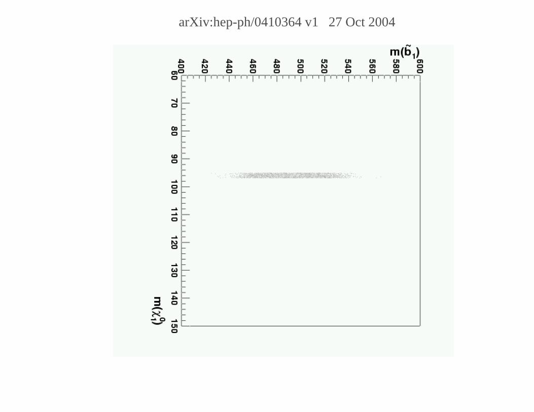
arXiv:hep-ph/0410364 v1 27 Oct 2004
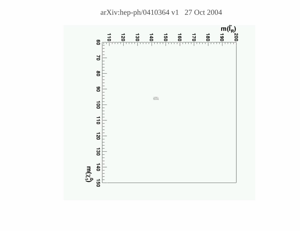
arXiv:hep-ph/0410364 v1 27 Oct 2004
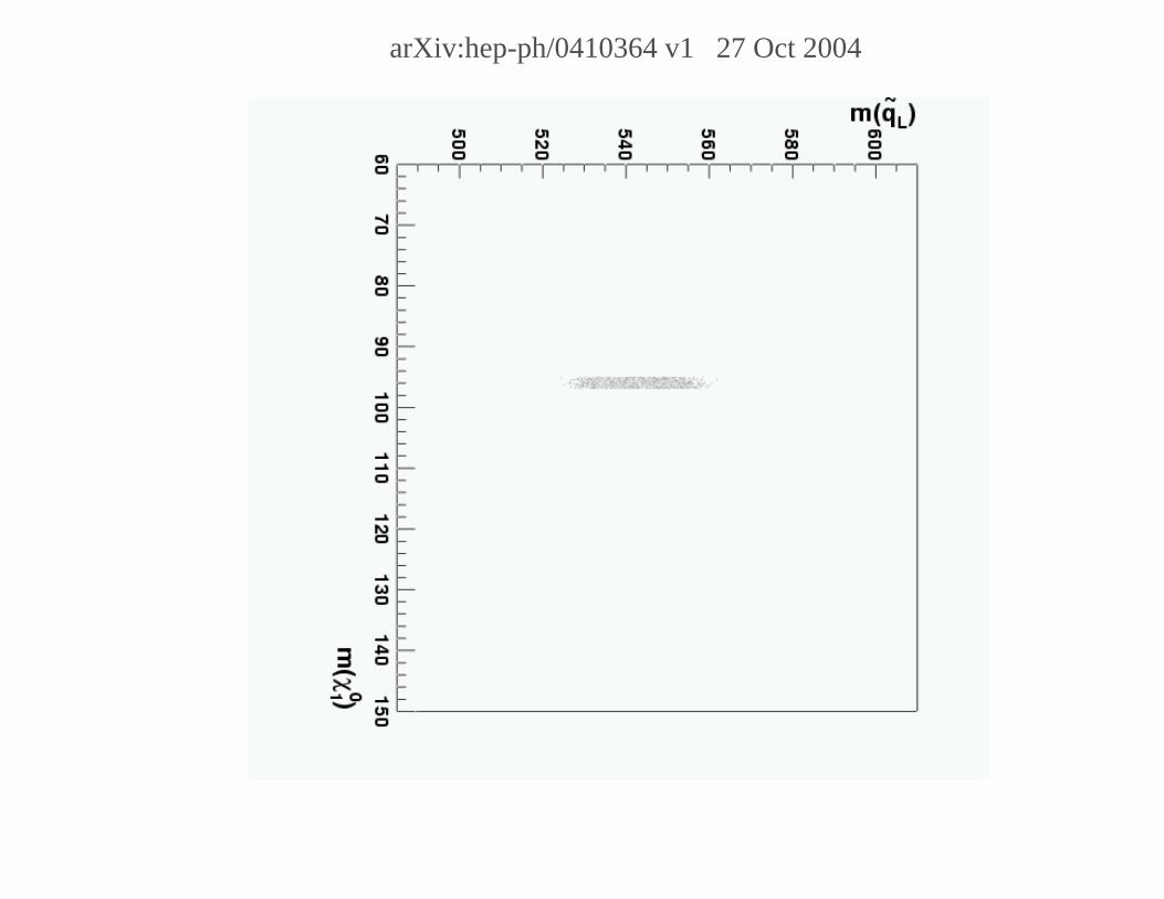
arXiv:hep-ph/0410364 v1 27 Oct 2004

This figure "sec254_bmchi_wmap_m1m210.gif" is available in "gif" format from:
http://arXiv.org/ps/hep-ph/0410364