Photoelectron imaging spectrometry: Principle and inversion methodC. Bordas, F. Paulig, H. Helm, and D. L. Huestis Citation: Review of Scientific Instruments 67, 2257 (1996); doi: 10.1063/1.1147044 View online: http://dx.doi.org/10.1063/1.1147044 View Table of Contents: http://scitation.aip.org/content/aip/journal/rsi/67/6?ver=pdfcov Published by the AIP Publishing Articles you may be interested in Blind restoration method of scanning tunneling and atomic force microscopy images J. Vac. Sci. Technol. B 14, 1552 (1996); 10.1116/1.589137 Potential inversion via variational generalized inverse J. Chem. Phys. 103, 9713 (1995); 10.1063/1.469934 Applications of inverse beamforming theory J. Acoust. Soc. Am. 98, 3250 (1995); 10.1121/1.413814 Inverse method and consistency examination for Lagrangian analysis AIP Conf. Proc. 309, 973 (1994); 10.1063/1.46197 Inverse problem for bremsstrahlung radiation Phys. Fluids B 4, 762 (1992); 10.1063/1.860221

This article is copyrighted as indicated in the article. Reuse of AIP content is subject to the terms at: http://scitationnew.aip.org/termsconditions. Downloaded to IP:

132.230.239.237 On: Thu, 02 Jul 2015 09:15:41

Photoelectron imaging spectrometry: Principle and inversion methodC. Bordas and F. PauligLaboratoire de Spectrome´trie Ionique et Mole´culaire, Universite´ Claude-Bernard Lyon I,43 Boulevard du 11 Novembre 1918, F69622 Villeurbanne, France

H. HelmFakultat fur Physik, Universita¨t Freiburg, Hermann-Herder-Strasse 3, D79104 Freiburg, Germany

D. L. HuestisMolecular Physics Laboratory, SRI International, Menlo Park, California 94205

~Received 24 January 1996; accepted for publication 28 February 1996!

A new photoelectron spectrometer has recently been used to analyze the energy and spatialdistribution of photoelectrons produced by multiphoton ionization of rare gases. It is based on theanalysis of the image obtained by projecting the expanding electron cloud resulting from theionization process onto a two-dimensional position sensitive detector by means of a static electricfield. In this article, we present the principle of this imaging spectrometer and the relevant equationsof motion of the charged particle in this device, together with an inversion method that allows us toobtain the energy and angular distribution of the electrons. We present here the inversion procedurerelevant to the case where the electrostatic energy acquired in the static field is large as comparedto the initial kinetic energy of the charged particles. A more general procedure relevant to anyregime will be described in a following article. ©1996 American Institute of Physics.@S0034-6748~96!02706-2#

I. INTRODUCTION

Photoelectron spectroscopy1 has been widely used in thepast decades to study photoionization or photodetachmentprocesses of various species from atoms2–5 to clusters,6–8

including small or complex molecules.9–13Most of the tech-niques applied so far are based on energy resolution by timeof flight ~TOF! measurements or employ electrostatic analyz-ers for energy analysis. These spectrometers10,13allow one tomeasure both energy and angular distributions. However, theenergy distribution is obtained for only a single orientationof the laser polarization at one time, and both energy andangular resolution are good to the extent that the acceptanceangle of the spectrometer is small. As a consequence, thedetection efficiency of this kind of photoelectron spectrom-eter is low, on the order of 1025 to 1024. In order to improvethe detection efficiency without loss of resolution, an inho-mogeneous magnetic field may be combined with the TOFprinciple. This is done in the so-called magnetic bottlespectrometer.14 In this spectrometer, all electrons emitted ina solid angle of 2P or 4P sr, according to the design of theapparatus, are detected. However, the measurement of theangular distribution, although possible, is not compatiblewith the detection of all electrons simultaneously and is usu-ally not attempted in practice. Standard TOF spectrometers,electrostatic analyzers, and magnetic bottles give an energyresolution in the range of 10–100 meV but suffer a substan-tial decrease in the detection efficiency at low energy. Simul-taneously, the relative energy resolution is poor near thresh-old. The zero electron kinetic energy photoelectronspectrometer ~ZEKE–PES!15–17 is specially tailored tohandle this kind of phenomenology: namely, the study ofthreshold electrons. However, this technique has severallimitations inherent to its principle. The ZEKE-PES has avery restricted range of energy~a fraction of meV above

threshold! and moreover it does not provide angular infor-mation. Hence, there is a real need for a new kind of photo-electron spectrometer combining high detection efficiency,including low velocity electrons, reasonable resolution, andsimultaneous measurements of angular distributions. The im-aging spectrometer introduced in 199318 combines the ad-vantages of the different methods mentioned above by mak-ing use of the possibilities offered by recent two-dimensionaldetection techniques. In this article we describe the principleof this technique and focus our attention on the inversionmethod required to extract the physical information fromelectron images in the simple case corresponding to currentexperimental setups. The general method, applicable to anyregime of the imaging spectrometer, poses essentially differ-ent algebraic problems that will be discussed in a separatearticle.

II. PRINCIPLE OF THE SPECTROMETER

A. Principle

The principle of the photoelectron imaging spectrometeris based on a very simple idea: photoelectrons produced attime t50 at a point source~r50! with a given kinetic energyW0 are found later on the surface of a sphere of radiusr texpanding with time according to:

r t5A2W0

mt. ~1!

For instance, electrons emitted with an initial kinetic energyof 1 eV are found after 20 ns on the surface of a sphere ofradius 12 mm. If we then apply ‘‘instantaneously’’ a highelectrostatic field, this sphere can be projected onto a posi-tion sensitive detector, producing an image that contains allthe spatial and energy information relevant to the process. In

2257Rev. Sci. Instrum. 67 (6), June 1996 0034-6748/96/67(6)/2257/12/$10.00 © 1996 American Institute of Physics This article is copyrighted as indicated in the article. Reuse of AIP content is subject to the terms at: http://scitationnew.aip.org/termsconditions. Downloaded to IP:

132.230.239.237 On: Thu, 02 Jul 2015 09:15:41

fact, this principle must be slightly modified in order to avoidthe problems related to the definition of an infinite electricfield established at a given timet50. A more realistic ex-periment, although analogous under certain conditions, con-sists of producing the photoelectrons in a region where ahomogeneous and constant electric field is applied. The staticfield is used to project the electrons onto the detector. Wewill see that, provided that the electrostatic energy gained inthe field is by far larger than the initial kinetic energy, oneobtains the same image as in the hypothetical experimentdescribed above. This experimental principle is shown sche-matically in Fig. 1.

B. Derivation of the equations of motion

Let O be the point at which the electrons are emitted,defined by its coordinatesx05y05z05O, andO8 the centerof the position sensitive detectorx085z085O and y085L,the distance between the region of interaction where photo-electrons are emitted and the detector. A homogeneous elec-tric field is applied along theOy axis. We propose that thephotoionization, or photodetachment, process is induced bylight polarized along theOz axis, parallel to the plane detec-tor according to Fig. 1. If an electron is ejected atO with aninitial kinetic energyW0 along the direction~Q,F!, the com-ponents of its initial velocityv0 are defined by

v0x5v0 sin Q cosF,~2!v0y5v0 sin Q sin F,

v0z5v0 cosQ,

with W0512mv0

2, wherem is the electron mass.The homogeneous electric fieldF, parallel to theOy axis

and perpendicular to the detector, projects this electron ontothe detector surface. The coordinates of the impact on thedetector can be derived using very simple algebra. Using thecoordinate axis defined in Fig. 1, one finds that these coor-dinates are

X52L cosF sin Q

r

3~Asin2 F sin2 Q1r2sin F sin Q!,

Z52L cosQ

r~Asin2 F sin2 Q1r2sin F sin Q!, ~3!

where

r5qFL

W0~4!

is the ratio between the electrostatic energy acquired in thefield and the initial kinetic energy of the electron~q is theelementary charge!.

Electric dipole selection rules and a linear polarization ofthe laser field alongOz lead to an initial angular distributionthat is cylindrically symmetric aroundOz, i.e., it is indepen-dent on the angleF but depends only on the angleQ and onthe energyW0. Hence, we can assign a given angular distri-butionF(W0 ,Q) at each energy channel that represents thenumber of electrons emitted in the solid angleV defined by~Q,F!. One immediately sees that, in order to preserve theinformation relative to this distribution in the image obtainedon the detector, the laser polarization must be parallel to thedetector. On the contrary, if the laser polarization was setperpendicular to the detector, the image would be symmetricaround this axis, i.e., around pointO8. Under such condi-tions, extracting both angular and energy distribution fromthe image would not be possible.

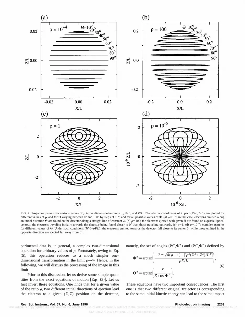
The first step in understanding the experimental processis to pay attention to the geometry of the impact positions asa function of the initial conditions. For this purpose, it isconvenient to work with the dimensionless unitsr, X/L, andZ/L. This is done in Fig. 2, where we have plotted the rela-tive coordinates of impact (X/L,Z/L) for different values ofr, and forQ varying between 0° and 180° by steps of 10°,and for all possible values ofF. The simplest case is ob-tained whenr is large compared to unity. Indeed, whenrtends to infinity, Eqs.~3! reduce to:

X52L cosF sin Q

Ar,

Z52L cosQ

Ar. ~5!

That is to say, for a given energy~i.e., a givenr!, electronsemitted along an initial directionQ are found on the detectoralong a straight line of constantZ with uXu<2L sinQ/Ar.This is clearly seen in Fig. 2~a!, wherer5104. This simplearrangement is no longer observed when the ratior de-creases. For example, atr5100 @see Fig. 2~b!#, the electronsejected with a givenQ are found on a quasielliptical contour,the electrons traveling initially towards the detector beingfound closer toO8 than those traveling outwards. When onedecreasesr further, the situation is even more complicatedand one reaches the patterns of Figs. 2~c! and 2~d! ~respec-tively, r51 and 1026!, where the link between impact posi-tion and original conditions is far from being simple. In thelimit r→0 @see Fig. 2~d!#, one can see complex patterns fordifferent values ofQ. Under such conditions~initial kineticenergy much larger than electrostatic energy!, the electronsemitted towards the detector fall on its centerO8, while thoseemitted in the opposite direction are ejected far away fromO8. From these considerations, we can deduce easily thatextracting the original distributionF(W0 ,Q) from the ex-

FIG. 1. Schematic of the projection method. Photoelectrons generated at apoint sourceO are accelerated towards a plane position sensitive detector bymeans of a homogeneous electric field.

2258 Rev. Sci. Instrum., Vol. 67, No. 6, June 1996 Photoelectron imaging This article is copyrighted as indicated in the article. Reuse of AIP content is subject to the terms at: http://scitationnew.aip.org/termsconditions. Downloaded to IP:

132.230.239.237 On: Thu, 02 Jul 2015 09:15:41

perimental data is, in general, a complex two-dimensionaloperation for arbitrary values ofr. Fortunately, owing to Eq.~5!, this operation reduces to a much simpler one-dimensional transformation in the limitr→`. Hence, in thefollowing, we will discuss the processing of the image in thislimit.

Prior to this discussion, let us derive some simple quan-tities from the exact equations of motion@Eqs. ~3!#. Let usfirst invert these equations. One finds that for a given valueof the ratior, two different initial directions of ejection leadthe electron to a given (X,Z) position on the detector,

namely, the set of angles~Q1,F1! and ~Q2,F2! defined by

F65arctanS 226A4~r11!2@r2~X21Z2!/L2#

rX/L D ,~6!

Q65arctanS X

Z cosF6D .These equations have two important consequences. The firstone is that two different original trajectories correspondingto the same initial kinetic energy can lead to the same impact

FIG. 2. Projection pattern for various values ofr in the dimensionless units:r, X/L, andZ/L. The relative coordinates of impact (X/L,Z/L) are plotted fordifferent values ofr, and forQ varying between 0° and 180° by steps of 10°, and for all possible values ofF. ~a! r5104; in that case, electrons emitted alongan initial directionQ are found on the detector along a straight line of constantZ. ~b! r5100; the electrons ejected with givenQ are found on a quasiellipticalcontour, the electrons traveling initially towards the detector being found closer to 08 than those traveling outwards.~c! r51. ~d! r51026; complex patternsfor different values ofQ. Under such conditions (W0@qFL), the electrons emitted towards the detector fall close to its center 08 while those emitted in theopposite direction are ejected far away from 08.

2259Rev. Sci. Instrum., Vol. 67, No. 6, June 1996 Photoelectron imaging This article is copyrighted as indicated in the article. Reuse of AIP content is subject to the terms at: http://scitationnew.aip.org/termsconditions. Downloaded to IP:

132.230.239.237 On: Thu, 02 Jul 2015 09:15:41

position. This leads to interference patterns that could be inprinciple observed on the detector. For presently realizablesystems, this pattern cannot be resolved and we will not dis-cuss this point further in this article. The second conse-quence is more trivial: Eqs.~6! are defined only for acces-sible (X,Z) couples, i.e., Eqs.~6! determine simply themaximum radius of the image, in other words, the maximumdistance fromO8 to the impact position. Indeed, this radiusR5AX21Z2 must be smaller thanRmax in order to get apositive argument under the square root in Eq.~6! with:

Rmax52LAr11

r. ~7!

This means that, when defining an experimental geometry, inparticular the effective radiusR0 of the position sensitivedetector and the distanceL between the ionization region andthe detector, one automatically imposes the lowestr valuecorresponding to the largest image visible in the system:

rmin511A11~R0

2/L2!

R02/2L2

, ~8a!

which reduces to

rmin5S 2LR0D 2 ~8b!

for larger values.The smallest value ofr is thus entirely defined by the

experimental geometry. Therefore, the spectrometer may bedesigned in order to operate only at larger values where aone-dimensional transformation is sufficient: for example,imposingr>1000 is equivalent to setL>16R0 . However,this does not mean that the exact 2D transformation is irrel-evant simply because one can imagine particular experimen-tal problems, or a specific environment, where the ionizationregion must be close to the detector as compared to its di-mension. Under such conditions,L!R0 andr is small. Thisis the case, for instance, if one wishes to work with a verylow electric field, which can be required for studying veryexcited states. The exact 2D inversion procedure relevant toany value ofr is essentially different from a technical pointof view and raises specific analytical and numerical prob-lems that will be discussed separately. This exact transfor-mation may in particular allow to built very compact imag-ing spectrometer with an extremely shortL distance that canfit in any environment.

C. Experimental setup

A schematic view of our experimental setup is shown inFig. 3. A homogeneous electric field~typically 10 to 200V/cm! is established by a set of cylindrical guard rings. Theregion of homogeneous field is about 10 cm long and 7 cmwide. On the high potential side, this region ends up with the2D detector itself. Helmoltz coils mounted outside thevacuum chamber orm-metal screen are used to reduce theearth’s and parasite magnetic fields. For a typical experimenton multiphoton ionization of gases, the vacuum chamber isfilled with 1025 Torr of the gas of interest~xenon, hydrogen,...!. The laser beam is focused by a 15 cm lens to the center

of the acceleration region. Under these conditions, the vol-ume of the electron source, where multiphoton ionizationoccurs, is about 100mm3. The detector is made of a tandemmicrochannel plate of 2 in. diameter positioned at one end ofthe spectrometer. In the case ofr@1, electrons hitting thedetector all have about the same kinetic energy, independentof the initial kinetic energy. Hence, the gain, and by way ofconsequence the detection efficiency, is independent of theinitial kinetic energy. Electrons exiting the channel plates arethen accelerated to 4–6 kV to impact on an ultrahigh vacuumgrade phosphor screen. The screen phosphorescence is accu-mulated on the charge-coupled-device~CCD! elements of aTektronix digital camera of 5123512 pixel resolution, andcooled down to about230°C by a Peltier element. The sig-nal is accumulated in the CCD over a few tens of laser shotsbefore being transferred to a microcomputer via a PrincetonInstruments controller. The signal can be summed and aver-aged over an arbitrary number of laser shots. The diameter ofthe detector combined with the resolution of the CCD allowsus to achieve a geometric resolution of about 100mm, whichis on the same order as the best we can do with the ionizationregion dimensions. In multiphoton ionization experiments ofxenon presented below, one can obtain a significant, al-though noisy, image with a single laser shot, i.e., about 1000electrons are detected simultaneously. However, it is recom-mended to work at low flux in order to avoid space chargeeffects and saturation of the detector. Notice that, at a pres-sure of 1025 Torr, about 105 atoms lie in the focal volume ofthe laser. In order to operate properly, the principle of ourspectrometer imposes that the dimensions of the ionizationregion are as small as possible. Indeed, the energy resolutionis directly limited by the geometric resolution on the detec-

FIG. 3. Schematic of the photoelectron imaging spectrometer.

2260 Rev. Sci. Instrum., Vol. 67, No. 6, June 1996 Photoelectron imaging This article is copyrighted as indicated in the article. Reuse of AIP content is subject to the terms at: http://scitationnew.aip.org/termsconditions. Downloaded to IP:

132.230.239.237 On: Thu, 02 Jul 2015 09:15:41

tor, which is itself limited by the initial dimension of theelectron cloud. This is easily achieved in multiphoton ioniza-tion experiments where electrons are extracted only in thefocal volume of the laser beam, but this poses some practicalproblems when single photon ionization or detachment areconcerned. This is in fact the most limiting restriction to thecapabilities of this kind of spectrometer. In single photonexperiments, the ionization volume must be defined by thecrossing between the laser and the molecular beams insteadof being determined only by the laser.

III. IMAGE PROCESSING IN THE LIMIT OF LARGEENERGY RATIO

The purpose of this section is to describe the numericalprocedures used to extract the relevant physical data fromraw experimental images, namely, the energy spectrum andthe angular distributions. First we will discuss the projectionprocess: giving a certain energy and angular distribution,what is the image obtained on the position sensitive detectorand what is the influence ofr? Second, in the limitr→`,how can we invert this image to get back to the originaldistribution? Owing to the one-dimensional nature of theproblem whenr→`, the usual answer to that kind of prob-lem would be to use a standard Abel inversion.19 However,instead of using this approximate general method, it is moreconvenient to use the ‘‘exact’’ back-projection method,which can then be extended to the complex 2D transforma-tion relevant to an arbitrary value ofr. This back projectionis exact only in the limit of continuous distribution. Ofcourse, the experimental data are, by nature, discrete, and thefinite dimensions of each pixel of the detector introducesome approximations in the transformation. We will discussthis point further.

We will first compare projection and back projection ofsimulated electronic distributions before presenting some ex-perimental results obtained in four-photon ionization of xe-non and molecular hydrogen.

A. Projection

For a given original angular distributionF(W0 ,Q), twodifferent numerical methods may be used to simulate theprojection achieved in the spectrometer. The first one relieson the explicit calculation of the exact Jacobian of the trans-formation from coordinates~Q,F! to (X,Z) for a given valueof r. The second one consists in launching a large number ofrandom trajectories statistically distributed according to theoriginal distribution F(W0 ,Q). In this article, the firstmethod will be used only in the limitr→`, while the secondmethod will be used for finite values ofr. This distinction ismade simply to avoid the complexity of the general transfor-mation and of the associated singularities that will be dis-cussed elsewhere. Electrons emitted in a given direction~Q,F! for a given value ofr will be found on the detector atthe position (X,Z) according to Eq.~3!. The angular distri-bution F(W0 ,Q) or equivalentlyF~r,Q! is, by definition,proportional to the number of electrons ejected in the solidangleV defined by the Euler angles~Q,F!. The correspond-ing number of electrons hitting the detector at position (X,Z)

by unit surface is simply the densityFd(r,X,Z), which isrelated to the original distribution by

Fd~r,X,Z!SXZ5F~r,Q!SQF , ~9!

whereSQF andSXZ are, respectively, the elementary surfaceon the sphere in the initial coordinates and the correspondingsurface on the plane detector.

The elementary surfaceSXZ5uJudQdF corresponds tothe elementary surface on a sphere of radiusL in the initialcoordinatesSQF5L2 sinQ dQ dF, and finally:

Fd~r,X,Z!5L2 sin Q uJu21F~r,Q!, ~10!

where the JacobianJ of the transformation is defined as:

J5]X

]Q

]Z

]F2

]X

]F

]Z

]Q. ~11!

Note that sinQ is always positive since 0<Q<P. The gen-eral expression of the Jacobian operatorJ calculated accord-ing to Eqs.~3! and ~11! is rather complex; however, it re-duces to a fairly simple analytic expression whenr→`. Inthat case, the transformation (X,Z)↔~Q,F! is given by Eqs.~5! and the expression of the Jacobian reduces to:

uJu54L2

rsin2 Qusin Fu, ~12!

and, accordingly:

Fd~r,X,Z!5F~r,Q!U r

4 sinQ sin F U. ~13!

A brief inspection of the set of Eq.~5! shows that for agiven r, in the limit of larger values, the coordinateZ de-pends only on the angleQ, while for that given pair ofr andZ values,X depends only onF. Thus, for a given pair ofrandZ0 values, one can define the quantityX0 as the maxi-mum value ofX electrons can reach according to Eq.~7! inthe limit of larger values:

Rmax5AX021Z0

252L

Ar, i.e., r5

4L2

X021Z0

2 . ~14!

Equation~5! can be easily inverted as:

Q5arccosSArZ02L D ,

~15!

F5arccosS XX0D .

These equations finally allow us to write down explicitly therelation between the density of electrons of a given initialkinetic energyW0 ~or alternativelyr! reaching the detector ata given position (X,Z), Fd(r,X,Z) and the initial distribu-tion F~r,Q!:

Fd~r,X,Z!5F~r,Q!r

4 sinQA12~X/X0!2, ~16!

if X<X0, and Fd(r,X,Z)50 otherwise. This function di-verges atX5X0, defined by Eq.~14!. The same problem ofdivergence occurs for finite values ofr, with the additionalproblem that the general form of Eq.~16! is by far more

2261Rev. Sci. Instrum., Vol. 67, No. 6, June 1996 Photoelectron imaging This article is copyrighted as indicated in the article. Reuse of AIP content is subject to the terms at: http://scitationnew.aip.org/termsconditions. Downloaded to IP:

132.230.239.237 On: Thu, 02 Jul 2015 09:15:41

complex. However, the experimental observable is not ex-actly Fd(r,X,Z) but rather its integral over a finite domaindefined by the CCD pixel. The integral ofFd(r,X,Z) over afinite surface is finite as shown below. All the equationspresented above, limited to a single energy channelr, can begeneralized easily by summing~or integrating! over a givendomain ofr, provided that ther values of interest are largeenough. As long as one works with continuous variables(X,Z), Eq. ~16! holds and the projection method~and corre-spondingly the inversion method! is exact. Once we take intoaccount the discrete nature of the detector, some approxima-tions must be made. Let us now define the pixel (i , j ) of theCCD as the surface defined by (i21)d<X< id and (j21)d<Z< jd, whered is the effective size of a~square!pixel. The physical quantity measured in the experiment~fora givenr! is the number of electrons collected at the pixelposition (i , j ):

f ~ i 0 ,i , j !5E~ j21!•d

j •d

dZE~ i21!•d

i •d

Fd~r,X,Z!dX, ~17!

where i 0 @with X05( i 020.5)d defined in Eq.~14!# is themaximum pixel value reachable for a given~r,Q! set. Bysubstituting Eq.~16! in Eq. ~17!, one finds:

f ~ i 0 ,i , j !5r

4 E~ j21!•d

j •d F~r,Q!

sin QdZE

~ i21!d

id dX

A12~X/X0!2

5r

4 E~ j21!•d

j •d F~r,Q!

sin QdZFarcsinS XX0

D G~ i21!d

i •d

X0 ,

~18!

whereQ andX0 are functions of the variableZ according toEqs. ~14! and ~15!. The integration over the variableZ re-maining in Eq.~18! is in the following approximated by asimple arithmetic averaging, which consists in substitutingZby its average value over the domain of integration:Z5( j20.5)d. This approximation is supported by the fact that thevariation ofJ along theZ axis is very smooth except in thevicinity of the center of the image, which usually containspoor information. This simplification introduced very minordiscrepancies forQ50°; however, an exact integration ofEq. ~18! is not necessary and we can simplify this expressionto:

f ~ i 0 ,i , j !5F ~ i 0 ,i , j !F~r,Q0!, ~19!

with the projection operator defined as:

F ~ i 0 ,i , j !5r

4

d

sin Q0FarcsinS XX0

D G~ i21!d

i •d

X0 ,

for i, i 0 ,~198!

F ~ i 0 ,i 0 , j !5r

4

d

sin Q0S P

22arcsin

~ i 021!d

X0DX0 ,

and

F ~ i 0 ,i , j !50 for i. i 0 ,

with Z05( j20.5)d, X05( i 020.5)d, and Q05arctan(X0/Z0).

Since we are dealing with discrete data, one has to defineprecisely the coordinates that we use, not only on the detec-tor ~which is imposed by experimental conditions!, but alsoin the space of angular and energy coordinates. The mostconvenient procedure is to define a discrete grid where theradiusR is proportional to the initial velocity of the electron,and the angle is the emission angleQ. The distributionF~r,Q! is replaced by the functionFRQ( i , j ) defined on adiscrete grid with the relation~pixel center: xi5 i20.5;zj5 j20.5!:

FRQ~ i , j !5F~r,Q!,

Q5arctan~xi /zj !, ~20!

r5r0

~xi21zj

2!5

r0Ri j2 ,

where r0 is determined by experimental parameters. Thisframework presents the advantage that a pixel to pixel cor-respondence is obtained for the electrons emitted atRmax~F50° in the present case! between both representations.The final expression for the discrete projection is

for all ~ i 0 , j 0!:

FXZ~ i 0 , j 0!5 (i> i0

@F ~ i ,i 0 , j 0!FRQ~ i , j 0!#, ~21!

whereFXZ andFRQ are the photoelectron distribution as afunction of the pixel number in the detector and in the initialcoordinates, respectively, and with the projection operatorF

defined by Eqs.~198!.Taking into account the symmetry of the image about

theOX andOZ axes allows a complete treatment of the dis-tribution. The major difference between Eq.~21! and thegeneral expression~arbitraryr! is that the sum reduces to asingle variable over the indexi ~X coordinate!, while in thegeneral transformation the sum would run on both indicesiand j . Thus, the two-dimensional inversion procedure is re-duced to a one-dimensional procedure. Equations~12!–~21!are relevant only under the condition thatr is large enough.In order to estimate the error introduced by this assumption,we calculate the projection pattern for arbitraryr values. Inorder to avoid the singularities and the complexity of thegeneral expression of the Jacobian, we simulate this casehere by launching a large number of electron trajectoriesdistributed according to the initial energy and angular distri-bution.

Figure 4 illustrates the projection process in a verysimple case. The top image of Fig. 4 represents the originalelectron distribution in the frame~R,Q! as defined above.The initial velocity distribution is a gaussian profile centeredat R05150 ~pixel units! and 10 pixels wide~R is propor-tional to the initial velocity!. FRQ( i , j ) is plotted in the topfigure: the angular distribution is chosen spherically symmet-ric in this case~Y00

2 !, i.e., the number of electrons emitted byunit of solid angle is a constant. As a consequence, Fig. 4~a!does not represent the total number of electrons: the actualnumber of electrons emitted in a given angular region~Q,Q1dQ! is proportional to@sinQ FRQ( i , j )dQ#. After projec-tion onto the plane detector, one obtains the image of Fig.

2262 Rev. Sci. Instrum., Vol. 67, No. 6, June 1996 Photoelectron imaging This article is copyrighted as indicated in the article. Reuse of AIP content is subject to the terms at: http://scitationnew.aip.org/termsconditions. Downloaded to IP:

132.230.239.237 On: Thu, 02 Jul 2015 09:15:41

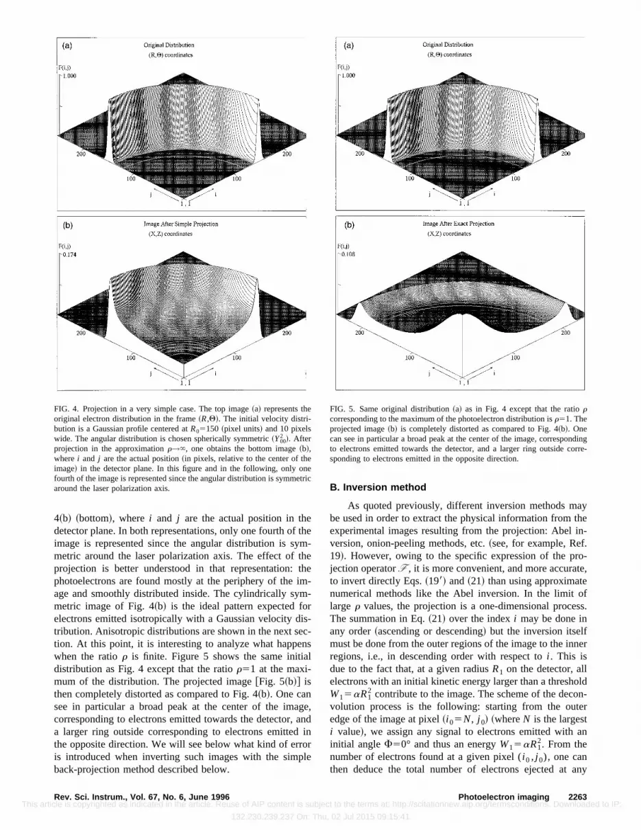
4~b! ~bottom!, where i and j are the actual position in thedetector plane. In both representations, only one fourth of theimage is represented since the angular distribution is sym-metric around the laser polarization axis. The effect of theprojection is better understood in that representation: thephotoelectrons are found mostly at the periphery of the im-age and smoothly distributed inside. The cylindrically sym-metric image of Fig. 4~b! is the ideal pattern expected forelectrons emitted isotropically with a Gaussian velocity dis-tribution. Anisotropic distributions are shown in the next sec-tion. At this point, it is interesting to analyze what happenswhen the ratior is finite. Figure 5 shows the same initialdistribution as Fig. 4 except that the ratior51 at the maxi-mum of the distribution. The projected image@Fig. 5~b!# isthen completely distorted as compared to Fig. 4~b!. One cansee in particular a broad peak at the center of the image,corresponding to electrons emitted towards the detector, anda larger ring outside corresponding to electrons emitted inthe opposite direction. We will see below what kind of erroris introduced when inverting such images with the simpleback-projection method described below.

B. Inversion method

As quoted previously, different inversion methods maybe used in order to extract the physical information from theexperimental images resulting from the projection: Abel in-version, onion-peeling methods, etc.~see, for example, Ref.19!. However, owing to the specific expression of the pro-jection operatorF , it is more convenient, and more accurate,to invert directly Eqs.~198! and~21! than using approximatenumerical methods like the Abel inversion. In the limit oflarge r values, the projection is a one-dimensional process.The summation in Eq.~21! over the indexi may be done inany order~ascending or descending! but the inversion itselfmust be done from the outer regions of the image to the innerregions, i.e., in descending order with respect toi . This isdue to the fact that, at a given radiusR1 on the detector, allelectrons with an initial kinetic energy larger than a thresholdW15aR1

2 contribute to the image. The scheme of the decon-volution process is the following: starting from the outeredge of the image at pixel~i 05N, j 0! ~whereN is the largesti value!, we assign any signal to electrons emitted with aninitial angleF50° and thus an energyW15aR1

2. From thenumber of electrons found at a given pixel (i 0 , j 0), one canthen deduce the total number of electrons ejected at any

FIG. 4. Projection in a very simple case. The top image~a! represents theoriginal electron distribution in the frame~R,Q!. The initial velocity distri-bution is a Gaussian profile centered atR05150 ~pixel units! and 10 pixelswide. The angular distribution is chosen spherically symmetric~Y00

2 !. Afterprojection in the approximationr→`, one obtains the bottom image~b!,wherei and j are the actual position~in pixels, relative to the center of theimage! in the detector plane. In this figure and in the following, only onefourth of the image is represented since the angular distribution is symmetricaround the laser polarization axis.

FIG. 5. Same original distribution~a! as in Fig. 4 except that the ratiorcorresponding to the maximum of the photoelectron distribution isr51. Theprojected image~b! is completely distorted as compared to Fig. 4~b!. Onecan see in particular a broad peak at the center of the image, correspondingto electrons emitted towards the detector, and a larger ring outside corre-sponding to electrons emitted in the opposite direction.

2263Rev. Sci. Instrum., Vol. 67, No. 6, June 1996 Photoelectron imaging This article is copyrighted as indicated in the article. Reuse of AIP content is subject to the terms at: http://scitationnew.aip.org/termsconditions. Downloaded to IP:

132.230.239.237 On: Thu, 02 Jul 2015 09:15:41

angleF with that given energy. This allows us to calculatethe contribution of electrons at this energy to the signal atpixel i51...i 0 according to the definition of the projectionoperatorF . This electron signal is then added to the back-projected image at the pixel position (i 0 , j 0), and subtractedfrom the projected~experimental! image at all pixel position( i , j 0) ~with i< i 0!. This procedure is repeated for the nextlower value~i 021! until the center of the image is reached.The whole procedure is done for each line~different j val-ues! separately. The mathematical expression of the inver-sion algorithm is as follows. For allj values; fori5N downto 1:

for all i 0< i :

FXZ~ i ! ~ i 0 , j !5FXZ

~ i11!~ i 0 , j !2F ~ i ,i 0 , j !

F ~ i ,i , j !FXZ

~ i11!~ i , j !,

FRQ~ i ! ~ i , j !5FRQ

~ i11!~ i , j !1FXZ

~ i11!~ i , j !

sin~u0!, ~22!

where the angleQ0 is defined by relation~20!, andFXZ(N11) is

the original projected~or experimental! image before inver-sion. In the energy-angle coordinates, we start withFRQ(N11)[0. After theN loops of the procedure~from i5N

down toi51!, one finds the final inverted imageFRQ(1) and the

residual image must beFXZ(1)[0.

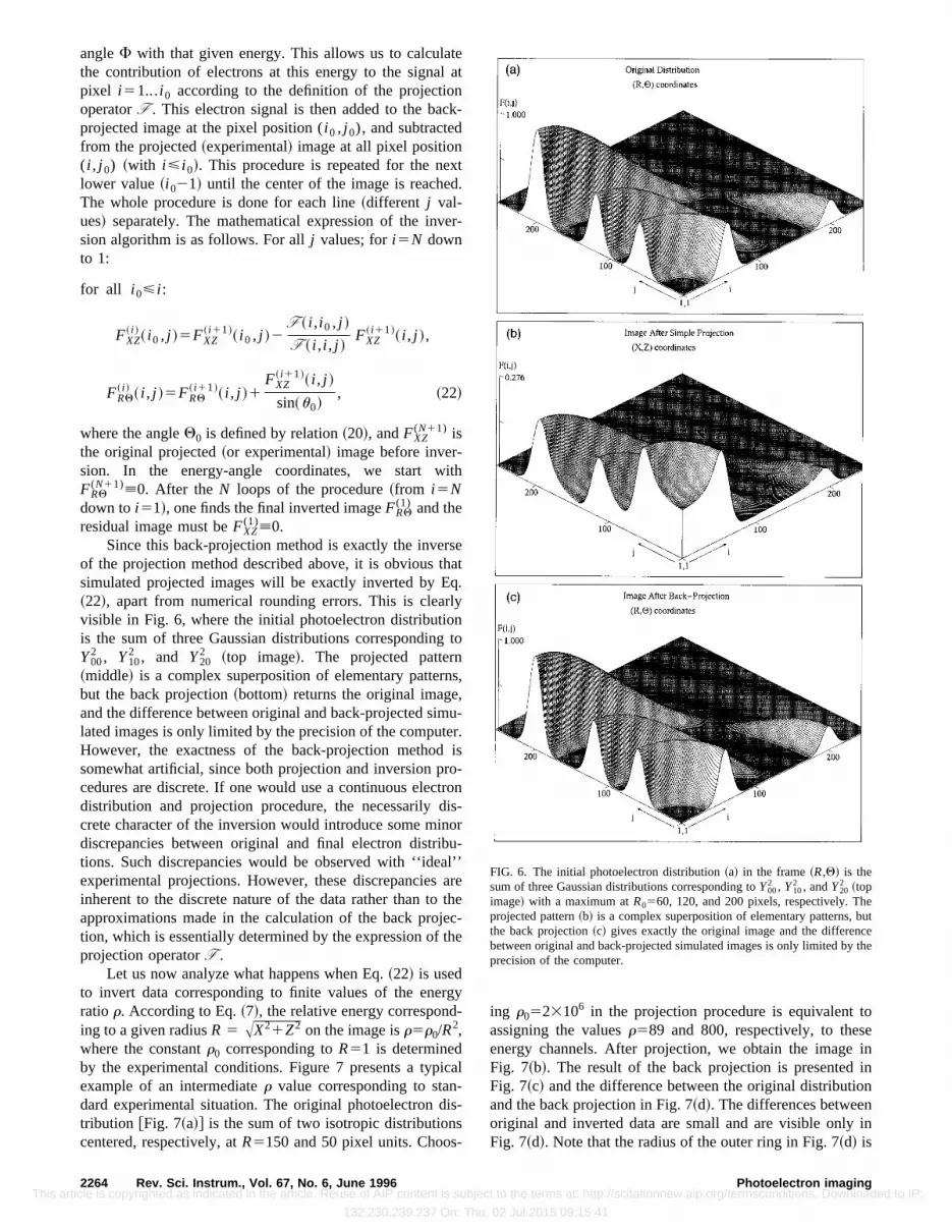
Since this back-projection method is exactly the inverseof the projection method described above, it is obvious thatsimulated projected images will be exactly inverted by Eq.~22!, apart from numerical rounding errors. This is clearlyvisible in Fig. 6, where the initial photoelectron distributionis the sum of three Gaussian distributions corresponding toY002 , Y10

2 , and Y202 ~top image!. The projected pattern

~middle! is a complex superposition of elementary patterns,but the back projection~bottom! returns the original image,and the difference between original and back-projected simu-lated images is only limited by the precision of the computer.However, the exactness of the back-projection method issomewhat artificial, since both projection and inversion pro-cedures are discrete. If one would use a continuous electrondistribution and projection procedure, the necessarily dis-crete character of the inversion would introduce some minordiscrepancies between original and final electron distribu-tions. Such discrepancies would be observed with ‘‘ideal’’experimental projections. However, these discrepancies areinherent to the discrete nature of the data rather than to theapproximations made in the calculation of the back projec-tion, which is essentially determined by the expression of theprojection operatorF .

Let us now analyze what happens when Eq.~22! is usedto invert data corresponding to finite values of the energyratio r. According to Eq.~7!, the relative energy correspond-ing to a given radiusR 5 AX21Z2 on the image isr5r0/R

2,where the constantr0 corresponding toR51 is determinedby the experimental conditions. Figure 7 presents a typicalexample of an intermediater value corresponding to stan-dard experimental situation. The original photoelectron dis-tribution @Fig. 7~a!# is the sum of two isotropic distributionscentered, respectively, atR5150 and 50 pixel units. Choos-

ing r0523106 in the projection procedure is equivalent toassigning the valuesr589 and 800, respectively, to theseenergy channels. After projection, we obtain the image inFig. 7~b!. The result of the back projection is presented inFig. 7~c! and the difference between the original distributionand the back projection in Fig. 7~d!. The differences betweenoriginal and inverted data are small and are visible only inFig. 7~d!. Note that the radius of the outer ring in Fig. 7~d! is

FIG. 6. The initial photoelectron distribution~a! in the frame~R,Q! is thesum of three Gaussian distributions corresponding toY00

2 , Y102 , andY20

2 ~topimage! with a maximum atR0560, 120, and 200 pixels, respectively. Theprojected pattern~b! is a complex superposition of elementary patterns, butthe back projection~c! gives exactly the original image and the differencebetween original and back-projected simulated images is only limited by theprecision of the computer.

2264 Rev. Sci. Instrum., Vol. 67, No. 6, June 1996 Photoelectron imaging This article is copyrighted as indicated in the article. Reuse of AIP content is subject to the terms at: http://scitationnew.aip.org/termsconditions. Downloaded to IP:

132.230.239.237 On: Thu, 02 Jul 2015 09:15:41

about 0.5% larger than the original diameter, while for theinner ring, this difference is negligible. This is obvious inFig. 7~d!, where the errors made for the outer ring~r'100!are clearly larger than those corresponding to the inner ring~r;1000!. The net effect of the finiter value in that range ofrelatively large values is mainly to introduce a small nonlin-earity in the energy scale, which increases asr decreases,~i.e., as one goes farther from the center of the image!. FromEq. ~7!, it appears thatr5100 corresponds to the condition~2L/Rmax!510, which is the worst condition that prevails inour experimental setup on the outer edge of the detector. Infact, the distortion of the image due to the small inhomoge-neities of the electric field are probably larger, especially onthe external zone of the detector where a perfect homogene-ity is harder to achieve. As a consequence, we can estimatethat, under our specific experimental conditions, the inver-sion algorithm described by Eqs.~19’! and~22! is sufficient.

Let us now investigate smallerr values, where the situ-ation becomes more critical. Under the conditions presentedin Fig. 5 ~r51!, the back-projection procedure leads to theimage of Fig. 8, which is to be compared with Fig. 5~a!. Thedifference between the initial distribution@Fig. 5~a!# and theback-projected image~Fig. 8! is drastic. Under these extreme

conditions, the energy scale is not simply distorted, but theapparent energy distribution is wrong: instead of peakingaroundR5150, two lobes appear. Note that for an initiallyanisotropic distribution, the angular pattern obtained fromthe inversion procedure would also be distorted. In this case,it is obvious that a more sophisticated inversion procedure isrequired. This situation arises when the distance between theelectron source and the screen is on the same order of mag-nitude as the image dimension on the detector.

C. Experimental images

As an illustration, we will show two examples of experi-mental results obtained with the photoelectron imaging spec-trometer in four-photon ionization of xenon and molecularhydrogen. Before carrying out the back projection, the centerof the experimental image must be determined. Generally,we use a numerical routine that finds the maximum of thefunction:

S5(pT~xp ,yp!T* ~xp ,yp!

FIG. 7. Typical example of intermediater values corresponding to a standard experimental situation. The original photoelectron distribution~a! is the sum oftwo isotropic distributions~Y00

2 ! centered, respectively, atR5150 and 50 in pixel units. The projection is made forr0523106, which is equivalent to assignthe valuesr589 and 800, respectively, to the energy channels. After projection, we obtain the image in~b!. The result of the back projection is presented in~c! and the difference between the original distribution and the back projection in~d!. The difference between original and inverted data is small and is visibleonly on ~d!. On the high energy channel, the error amounts to about 7% in intensity, but this corresponds, in fact, to less than 1% error in energy, while theerror made for the low energy channel is negligible.

2265Rev. Sci. Instrum., Vol. 67, No. 6, June 1996 Photoelectron imaging This article is copyrighted as indicated in the article. Reuse of AIP content is subject to the terms at: http://scitationnew.aip.org/termsconditions. Downloaded to IP:

132.230.239.237 On: Thu, 02 Jul 2015 09:15:41

5(pT~xp ,yp!T~2x02xp,2y02yp!, ~23!

whereT refers to the intensity of the original image at thepixel position specified byp, and T* refers to that of animage obtained by mirroring the original at the trial centerposition (x0 ,y0). Upon finding the center, the four quadrantsof the image are added for better statistical representationand are subjected to the back-projection procedure. As a con-sequence, the inverted images are symmetric about the ver-tical ~laser polarization! and horizontal axes. Similarly tosimulated images, only one fourth of the image is repre-sented in the figures.

There has been recently considerable interest in thestudy of multiphoton ionization of heavy rare gases in themoderate field regime20,21 as well as in the strong fieldregime.18,22 Rare gas atoms are ideal systems to study mul-tiphoton ionization processes due to the relative simplicity oftheir electronic structure and to the high value of their ion-ization potential. However, the detailed interpretation of theobserved effects, especially when strong laser fields are used,is often precluded by the complexity of the elementary pro-cesses involved. This point has motivated the study de-scribed in Ref. 23 concerned with the final state distributionand the respective angular distribution of photoelectrons ofabout 30 resonant intermediate Rydberg states that partici-pate in four-photon ionization of xenon. The main result ofthis work is the following: fornd Rydberg states, the branch-ing between the two ionization channel@ground channel:Xe1(2P3/2)1e2, and excited channel Xe1(2P1/2)1e2# mir-rors the mixing of core states in the three-photon intermedi-ate, while a major deviation from this rule appears for thens@ 32#~J51! states. The experiments are carried out a near-threshold intensities~1–5 GW/cm2! using a nanosecond dyelaser, linearly polarized, tuned to selectively excite withthree-photon transitions theJ51 andJ53 Rydberg states ofxenon lying below the first ionization limit, the absorption of

the fourth photon being sufficient to bring the system in thecontinuum above the first excited states of Xe1. The photo-electron imaging spectrometer was used to measure the rela-tive ionization yield as well as the angular distribution inboth ionization channels:@Xe1(2P3/2)1e2# and excited@Xe1(2P1/2)1e2#. An example of a raw experimental datarecorded with the 8d@12#~J51! intermediate state~l5318.375nm! is shown in Fig. 9~a!. The corresponding inverted imageis presented in Fig. 9~b!. The analysis of this image providesthe photoelectron energy spectrum@Fig. 10~a!# and the angu-lar distribution in both channels@Fig. 10~b!#. The advantageof using the imaging spectrometer in this experiment is thatit allows a fast and direct view of the processes involved inthe four-photon ionization with a good reliability as far asbranching ratios and angular distributions are concerned.This work is described in more detail in Refs. 23 and 24.

The experiments carried out on xenon do not requirehigh resolution, since the two ionization channels involved inthese experiments are separated by about 1.3 eV. The experi-ments conducted on molecular hydrogen briefly describedbelow are more characteristic of the capabilities of the imag-ing spectrometer from the point of view of energy resolution.

As a second example, we show a result obtained in thestudy of three-photon resonance enhanced, four-photon ion-ization of H2 with a selected intermediate level of theB

1(u1

FIG. 8. Back projection in the approximationr→` of the image of Fig. 5~b!obtained by projecting the distribution of Fig. 5~a! with r51; compare withFig. 5~a!. The difference between the initial distribution@Fig. 5~a!# and theback-projected image shown here is enormous. Under these extreme condi-tions, the energy scale is distorted, and the energy distribution is completelywrong; instead of peaking aroundR5150, it presents two lobes, inside andoutside.

FIG. 9. Example of raw experimental data obtained in resonant four-photonionization of xenon with the 8d[

12](J51) intermediate state~l5318.375

nm! ~a!. The corresponding inverted image is presented in~b!.

2266 Rev. Sci. Instrum., Vol. 67, No. 6, June 1996 Photoelectron imaging This article is copyrighted as indicated in the article. Reuse of AIP content is subject to the terms at: http://scitationnew.aip.org/termsconditions. Downloaded to IP:

132.230.239.237 On: Thu, 02 Jul 2015 09:15:41

state using a tunable UV laser of 5 ns duration, with focalintensities in the range 1–5 GW/cm2. This kind of transitionhas been studied by several authors in the past.25–27 Thiswork, presented in Ref. 28, was mainly concerned with theformation of very low energy photoelectrons and their asso-ciated angular distribution. Figure 11 shows a typical experi-mental result obtained when exciting theB1(u

1 ~v854,J850! intermediate state via the three-photonP1 transition.Two competing processes appear:~1! direct photoionization:

H2 ——→13hn

H2~B1(u

1,v854,J850!

——→1hn

H21~v150 or 1, N151 or 3!1e2;

~2! photodissociation followed by one-photon ionization ofthe excited atom:

H2 ——→13hn

H2~B1(u

1,v854,J850!

——→1hn

H~1s!1H~n52,l !;

then, a fifth photon ionizes the excited atom:

H~n52,l ! ——→1hn

H11e2.

Five ionization channels are open at 2 and 39 meV forv151~respectively,N153 and 1!, 274 and 310 meV forv150~respectively,N153 and 1!, and 533 meV for the dissocia-tive channel.

Note ~see Fig. 12! that the slow electron peaks at 2 and39 meV are fully resolved, while the two rotational branches

of the ground vibrational channel are not distinguishable.This is a result of the fact that the absolute velocity resolu-tion is a constant over the whole spectrum. As a conse-quence; the energy resolution drastically decreases as the en-

FIG. 10. The analysis of the experimental image presented in Fig. 9 pro-vides the photoelectron energy spectrum~a! and the angular distribution inboth ionization channels~b!.

FIG. 11. Typical experimental result obtained in resonant four-photon ion-ization ofH2 when exciting theB1(u

1 ~v854, J850! intermediate state viathe three-photonP1 transition:~a! experimental image;~b!: inverted image.

FIG. 12. Energy spectrum derived from the image of Fig. 11. Five ioniza-tion channels are open at 2 and 39 meV forv151 ~respectively,N153 and1!, 274 meV, and 310 meV forv150 ~respectively,N153 and 1!, and 533meV for the dissociative channel. Note that the slow electron peaks at 2 and39 meV are fully resolved, while the two rotational branches of the groundvibrational channel are not distinguishable. This result clearly shows that theenergy resolution drastically decreases as the energy increases.

2267Rev. Sci. Instrum., Vol. 67, No. 6, June 1996 Photoelectron imaging This article is copyrighted as indicated in the article. Reuse of AIP content is subject to the terms at: http://scitationnew.aip.org/termsconditions. Downloaded to IP:

132.230.239.237 On: Thu, 02 Jul 2015 09:15:41

ergy increases. As compared to previous results,25–27there isa sensible improvement of the resolution at low energy,while the resolution is lower above 0.5 eV. The point ofinterest for the present discussion is that, at threshold, a reso-lution on the order of 1 meV is easily achievable, while, athigher energy, conventional spectrometers are probably bet-ter from the point of view of the energy resolution. Furtherimprovements of this kind of spectrometer will probably al-low this system to become competitive, in terms of resolu-tion, with ZEKE-PES15–17 at threshold, with a much largerflexibility in the use of the apparatus.

IV. PROSPECTS

In this article, we have presented the experimental prin-ciple of the photoelectron imaging spectrometer, togetherwith the simplest inversion method that allows one to extractsignificant physical information from the experimental data.The direct back-projection method has been preferred to thecommon Abel inversion method owing to the specific natureof the photoelectron projection process. Note, however, thatthis method works properly only in the limit of larger ~elec-trostatic energy to initial kinetic energy ratio! values andgives qualitatively the same results as a standard inversionmethod, although it is more easily extended to the domain oflow r values.

The photoelectron imaging is being currently improvedfollowing two complementary directions. First, the spec-trometer itself would have better performance with a largerdetector. Indeed, the velocity resolution is mainly limited bythe ratio between the effective diameter of the photoelectrondetector and the electron source size. In most cases, the sizeof the region where photoelectrons are formed cannot bereduced arbitrarily and is governed by experimental condi-tions: density of species of interest, dimensions of a ion orlaser beam, etc. It is thus of primary interest to increase thesize of the detector. However, the extremely high efficiencyof the modern CCD cooled camera allows one to work withvery low gain electron to photon converters. Thus, a simplephosphorescent screen coupled to a postacceleration of thephotoelectrons may be sufficient when using a high perfor-mance CCD camera. Under these conditions, detectors largerthan 100 mm may be realized, allowing one to optimize theuse of a high-resolution~5123512 pixels or better! camera,which exceeds in performance, in the current experiment, theresolution of the MCP-phosphor screen itself. Along withthis technological modification, a second improvement is inprogress. As noted previously, the back-projection methoddescribed here is relevant only when one is concerned withlarger values. The full two-dimensional transformation rel-evant to any range of energy based on the set of exact Eqs.~3! will be presented in a forthcoming article.

Finally, it must be emphasized that bidimensional detec-tors combining electron or ion to photon conversion coupled

to CCD systems may be used in a wide variety of experi-ments such as photoionization and photodetachment, but alsophotodissociation and photofragmentation of complex spe-cies. For example, in the ‘‘Laboratoire de Spectrome´trie Io-nique et Moleculaire,’’ such a system is currently beingcoupled to the ion time-of-flight mass spectrometer of a laservaporization cluster source in order to study the photodetach-ment of negative metallic cluster ions.

ACKNOWLEDGMENT

The ’’Laboratoire de Spectrome´trie Ionique et Mole´cu-laire’’ is a ‘‘Unite Mixte de Recherche du CNRS, Grant No.5579’’.

1J. Berkowitz,Photoabsorption, Photoionization, and Photoelectron Spec-troscopy~Academic, New York, 1979!.

2S. Edelstein, M. Lambropoulos, J. A. Duncanson, and R. S. Berry, Phys.Rev. A 9, 2459~1974!.

3R. N. Compton, J. C. Miller, A. E. Carter, and P. Kruit, Chem. Phys. Lett.71, 87 ~1980!.

4P. Kruit, J. Kimman, H. G. Mu¨ller, and M. J. Van der Wiel, J. Phys. B16,937 ~1983!.

5E. Matthias, P. Zoller, D. S. Elliott, N. D. Piltch, S. J. Smith, and G.Leuchs, Phys. Rev. Lett.50, 1914~1983!.

6W. A. De Heer, Rev. Mod. Phys.65, 611 ~1993!.7K. Rademann, Ber. Bunseges. Phys. Chem.95, 563 ~1989!.8K. H. Meiwes-Broer, inAdvances in Metal and Semiconductor Clusters,edited by M. Duncan~JAI, Greenwich, 1993!, Vol. 1, p. 37.

9M. G. White, W. A. Chupka, M. Seaver, A. Woodward, and S. D. Colson,J. Chem. Phys.80, 678 ~1984!.

10Y. Achiba, K. Sato, and K. Kimura, J. Chem. Phys.82 3959 ~1985!.11S. T. Pratt, P. M. Dehmer, and J. L. Dehmer, J. Chem. Phys.85, 3379

~1986!.12P. J. Miller, W. A. Chupka, J. Winniczek, and M. G. White, J. Chem.Phys.89, 4058~1988!.

13S. W. Allendorf, D. J. Leahy, D. C. Jacobs, and R. N. Zare, J. Chem. Phys.91, 2216~1989!.

14P. Kruit and F. H. Read, J. Phys. E16, 313 ~1983!.15M. Sander, L. A. Chewter, K. Mu¨ller-Dethlefs, and E. W. Schlag, Phys.Rev. A 36, 4543~1987!.

16L. A. Chewter, M. Sander, K. Mu¨ller-Dethlefs, and E. W. Schlag, J.Chem. Phys.86, 4737~1987!.

17K. Muller-Dethlefs and E. W. Schlag, Annu. Rev. Phys. Chem.42, 109~1991!.

18H. Helm, N. Bjerre, M. J. Dyer, D. L. Huestis, and M. Saeed, Phys. Rev.Lett. 70, 3221~1993!.

19C. J. Dash, Appl. Opt.31, 1146~1992!.20S. T. Pratt, P. M. Dehmer, and J. L. Dehmer, Phys. Rev. A35, 3793

~1987!.21K. Sato, Y. Achiba, and K. Kimura, J. Chem. Phys.80, 57 ~1984!.22M. D. Perry and O. L. Landen, Phys. Rev. A38, 2815~1988!.23C. Bordas, M. J. Dyer, T. A. Fairfield, H. Helm, and K. C. Kulander, Phys.Rev. A 51, 3726~1995!.

24C. Bordas, M. J. Dyer, T. A. Fairfield, M. Saeed, and H. Helm, J. Phys.~Paris! IV C4, 647 ~1994!.

25S. T. Pratt, P. M. Dehmer, and J. L. Dehmer, J. Chem. Phys.78, 4315~1983!; Chem. Phys. Lett.105, 28 ~1984!.

26J. H. M. Bonnie, J. W. Verschuur, H. J. Hopman, and H. B. van Lindenvan den Heuvell, Chem. Phys. Lett.130, 43 ~1986!.

27E. Y. Xu, T. Tsuboi, R. Kachru, and H. Helm, Phys. Rev. A36, 5645~1987!.

28C. Bordas, M. J. Dyer, and H. Helm, J. Phys.~Paris! IV C4, 691 ~1994!.

2268 Rev. Sci. Instrum., Vol. 67, No. 6, June 1996 Photoelectron imaging This article is copyrighted as indicated in the article. Reuse of AIP content is subject to the terms at: http://scitationnew.aip.org/termsconditions. Downloaded to IP:

132.230.239.237 On: Thu, 02 Jul 2015 09:15:41