Photoassociative spectroscopy of the long-range state

Eur. Phys. J. D 5, 389–403 (1999) THE EUROPEANPHYSICAL JOURNAL Dc©

EDP SciencesSocieta Italiana di FisicaSpringer-Verlag 1999

Photoassociative spectroscopy of the Cs2 0−g long-range state

A. Fioretti, D. Comparat, C. Drag, C. Amiot, O. Dulieua, F. Masnou-Seeuws, and P. Pillet

Laboratoire Aime Cottonb, Universite Paris-Sud, Batiment 505, 91405 Orsay Cedex, France

Received: 20 May 1998 / Revised: 1st August 1998 / Accepted: 5 November 1998

Abstract. The photoassociative spectroscopy of the Cs2 0−g long-range molecular state dissociating intothe 6s 2S1/2 + 6p 2P3/2 asymptote is performed, using cold cesium atoms in a vapor-cell magneto-opticaltrap (MOT). Vibrational levels from v = 0 to v = 132 are identified, and their rotational structure is wellresolved up J = 8 for levels below v = 74. These data are analyzed in terms of the Rydberg-Klein-Rees(RKR) procedure, and correspond to 99.6% of an effective potential curve with a minimum at 12.36±0.05 Aand a 77.94±0.01 cm−1 depth. Both ab initio calculations and simple model estimations predict a double-well structure for this potential curve, which cannot be reproduced presently by the RKR approach butwhich is confirmed by the presence of giant structures in the spectrum. The 1u(6s 2S1/2 + 6p 2P3/2)long-range state is also observed for the first time in Cs2.

PACS. 32.80.Pj Optical cooling of atoms; trapping – 33.20.-t Molecular spectra – 34.20.-b Interatomicand intermolecular potentials and forces, potential energy surfaces for collisions

1 Introduction

Determination of the long-range interactions between twoneutral atoms have long been the object of a substantialeffort [1]. During the past decade, developments in lasercooling and trapping of atoms has opened the way to pho-toassociative spectroscopy of alkali dimers [2], yielding ac-curate determinations for the long range part of molecularpotential curves, in particular those correlated with theground s + s or the first excited s + p asymptotes. Theknowledge of these data is crucial in the interpretation ofmany new physical phenomena associated with cold atomdynamics, as for instance the prediction of the stability ofBose-Einstein condensates [3–5] which depends upon theground state scattering lengths.

Molecular photoassociation (PA) of cold atoms hasbeen demonstrated for all alkali atoms [6,7], but only veryrecently for the cesium atom [8]. Due to their very low rela-tive kinetic energy (kBT ≤ 1 mK ' 21 MHz), two free coldatoms can absorb a photon with a resonant wavelength, tocreate an excited molecule in a well-defined rovibrationalstate. As the Franck-Condon principle favors the excita-tion of vibrational levels close to the dissociation limit, thePA of cold atoms supplies a new high resolution methodcomplementary to the traditional bound-bound laser spec-troscopy, which is in most cases devoted to lower levels.The combination of both methods can lead to the com-plete description of a potential curve, and to the deter-

a e-mail: [email protected] CNRS II

mination of dissociation energies [9] or atomic radiativelifetimes [10–12] with an extremely high accuracy.

In a previous letter [8] we have reported on the firstobservation of molecular PA of cold cesium atoms in avapor-cell magneto-optical trap. In this first experimentwe have observed 63 lines ranging 10 cm−1 below the6s 2S1/2 + 6p 2P3/2 dissociation limit. Four accessibleHund’s case (c) long-range attractive potential curves (1g,0+u , 0−g and 1u) are converging towards this limit, and

these lines have been attributed to rovibrational levels ofthe 0−g state. The originality of the experiment was in the

detection of Cs+2 molecular ions by photoionization of Cs2

triplet ground state molecules, produced by spontaneousdecay of the excited molecular state formed by photoasso-ciation. Such molecules are indeed observed during theirfall outside the atomic trap, providing the first evidencefor the production of translationally cold molecules. Theballistic expansion of the molecular cloud has allowed usto determine a temperature of roughly 300 µK for themolecular sample, close to the estimated temperature ofthe initial atomic cloud (∼ 200 µK). The formation of coldmolecules in a photoassociative scheme (Fig. 1) is linkedto the particular shape of the 0−g potential curve, whichpresents a Condon point at intermediate internuclear dis-tances due to its double-well structure. This allows an effi-cient stabilization of cold molecules through spontaneousemission towards the lowest 3Σ+

u electronic state.

In this article, we report on the photoassociative spec-troscopy of the 0−g long-range state over a 80 cm−1 en-

ergy range below the 6s 2S1/2 + 6p 2P3/2 dissociationlimit. This involves the measurement of the energies of

390 The European Physical Journal D

10 20 30 40 50R (a0)

-400

-200

0

200

11000

11200

11400

11600

11800

10 20 30R (a0)

-5000

500

11000

13000

15000

25000

27000

X1Σg

+a

3Σu

+

ener

gy (

cm-1)

62S1/2+6

2S1/2

62S1/2+6

2P3/2

a3Σu

+6

2S1/2+6

2S1/2

62S1/2+5

2DJ(2)

3Πg

(2)3Σg

+

Cs2

+(X

2Σg

+)

0g

-

1u

1g

0u

+

(a) (b)

λ1

λ2

λ2

0g

-

62S1/2+6

2P3/2

Fig. 1. Optical transitions relevant for the present experiment.(a) Photoassociation and spontaneous decay indicated for the0−g → a3Σ+

u transition. (b) Resonant two-photon ionization ofthe a3Σ+

u levels. All potential curves are built from ab initio[55,56] and asymptotic [29,30] calculations.

the first 133 vibrational levels, with rotational structureresolved up to v = 74. These energies are fitted in theframework of the Rydberg-Klein-Rees (RKR) approach,providing 99.6% of the energy depth of an effective po-tential curve with a minimum at 12.36 ± 0.05 A, and a77.94± 0.01 cm−1 total depth. The RKR potential curveis discussed and compared to asymptotic model estima-tions and quantum chemistry computations, which predicta double-well shape for this state. The 0−g long-range statein Cs2 cannot be considered as a “pure long range state”,as defined by Stwalley et al. [13], as the hump between thetwo wells is influenced by short-range molecular forces.

The paper is organized in the following way: the exper-imental approach is described in Section 2 and the mea-surements of the energies of the detected 0−g ro-vibrationallevels are reported in Section 3. The basic principles of thefitting procedure are recalled in Section 4, yielding thebest possible potential curve for representing the data.The RKR potential curve is compared in Section 5 withthe potential curve computed by matching the asymptoticlong-range 0−g curve with the ab initio short range 0−gcurve. The origin of the double-well structure of the up-per 0−g curve of the cesium dimer is also carefully discussedusing asymptotic expansion.

2 Experimental setup

The principle of the experiment has been described inreference [8], and is recalled here for clarity. The coldCs atoms of a vapor cell magneto-optical trap (MOT)are illuminated with a cw laser to produce photoas-sociation. The experimental setup, already partly de-scribed in reference [14], is schematized in Figure 2. Thecold atoms are produced in a vapor loaded MOT [15],at the intersection of three pairs of mutually orthogo-nal, counter-propagating σ+−σ− laser beams of intensitynearly 2 mW/cm2 (to be compared with the saturation

D y ela se r C ooling an d

repum p in g lasers

M O T

T O F

M C P

T i : S apph ire

Pulsed N d : Y A G

C o m p u ter

Io d in e C e ll

F ab ry-P ero t T O F= T im e o f f l igh t

M C P= M icro c h an n e l P la tes

G a te d in te gra to r

λ2

λ1

Ar+ laser

Fig. 2. Scheme of the experimental setup. The optical andlaser setup for the MOT is not shown, as well as the two verticaltrapping laser beams.

intensity Is = 1.1 mW/cm2), at the zero magnetic fieldpoint of a pair of anti-Helmholtz coils with a magneticfield gradient of 15 Gauss/cm. The residual pressure is2 × 10−9 torr. The cooling and trapping laser beams aresplit from a slave diode laser (SDL 5422-H1, 150 mW,single mode, λ ∼ 852 nm) injection locked to a masterdiode laser. The master laser (SDL 5412-H1, 100 mW) isfrequency-narrowed by optical feedback from an extended,grating ended, cavity. Locking the master laser frequencyto a saturated absorption line of a cesium vapor ensuresits long-term stabilization. The trapping laser frequencyis tuned about 13 MHz (' 2.5 natural linewidths) on thered of the frequency ν4→5 of the 6s 2S1/2(F = 4) →6p 2P3/2(F ′ = 5) atomic transition. A repumping laserbeam (SDL 5712-H1, 100 mW, λ ∼ 852 nm) of frequencyν3→4 resonant with the 6s 2S1/2(F = 3)→ 6p 2P3/2(F ′ =4) transition is superimposed with two of the beams of thecooling laser, preventing atoms to be optically pumped inthe untrapped F = 3 hyperfine ground state. In theseconditions, the dimension (FWHM) of the cold sampleranges between 400–600 µm, the number of atoms in thetrap ranges between 1−5 × 107, thus leading to a peakdensity of the order of 1011 atoms/cm3. The estimatedtemperature of the cold atomic sample is T ' 200 µK[16].

In the first experiment [8], the cold Cs atoms werecontinuously illuminated by the beam of a diode laser(λ ∼ 852 nm, SDL 5712-H1, 100 mW) focused on a di-ameter of 100 µm, yielding a disposable intensity for PAin the MOT zone of 200 W/cm2. We were able to scan thewavelength of the laser diode on a 10 cm−1 range withoutmode jumps on the red-side of the trapping transition, byslowly changing the diode temperature.

In the present study, the diode laser has been re-placed by a Ti:sapphire laser (Coherent 899 ring laser)pumped by an Argon ion laser, allowing larger detuningsof the PA laser frequency. The maximum available powerin the experiment zone is 600 mW, focused on a spot with∼ 500 µm diameter. However, the power of the PA laserhas been gradually reduced for detunings smaller thanabout 2 cm−1 from ν4→5 in order to avoid perturbations

A. Fioretti et al.: Photoassociative spectroscopy of the Cs2 0−g long-range state 391

2000150010005000

time (ns)

dye laser pulse

high voltage pulse

MCP signal Cs+ Cs2+

Fig. 3. Typical detection time sequence. The time origin ischosen at the center of the high voltage accelerating pulse. TheCs+

2 and Cs+ ion pulses arrival times are in a ratio of ∼√

2.This sequence has a repetition rate of 10 Hz.

of the MOT operation. The frequency scale is calibratedusing a Fabry-Perot interferometer (750 MHz free spectralrange), and the absorption lines of iodine [17] (see Fig. 2).The PA laser spectral linewidth is 1 MHz and its frequencycan be continuously scanned on a 30 GHz range. The PAlaser excitation corresponds to the photoassociative reac-tion (Fig. 1a):

Cs (6s 2S1/2, F = 4) + Cs (6s 2S1/2, F = 4) + hν1 →

Cs2 (0−g (6s 2S1/2 + 6p 2P3/2; v, J)). (2.1)

As we have already mentioned, the photoassociative exci-tation of the Cs2 (0−g (6s 2S1/2 +6p 2P3/2; v, J)) state pro-duces, by spontaneous emission, transitionally cold Cs2

molecules in their lowest triplet state a3Σ+u . Evidence of

the photoassociative process is detected by ionization ofthe cold molecules into Cs+

2 , using a pulsed dye laser (dye:LDS 722; pulse duration 7 ns; pulse energy: 1 mJ) pumpedby the second harmonic of a Nd-YAG laser, running at10 Hz repetition rate. The dye laser is tuned at the wave-length λ2 ∼ 716 nm. The ionization process (Fig. 1b) isa resonant two-step photoionization via the vibrationallevels of an electronic molecular state correlated to the6s 2S1/2 + 5d 2D3/2,5/2 dissociation limit. The detectiontemporal sequence is shown in Figure 3. At the trap posi-tion, a pulsed high-voltage field (4.15 kV, 0.5 µs) is appliedby means of a pair of electric field grids spaced 15 mmapart. The produced Cs+ and Cs+

2 ions are expelled outof the interaction region in a 6 cm field-free zone con-stituting a time-of-flight mass spectrometer separating intime Cs+

2 ions (1.9 µs delay) from Cs+ ones (1.3 µs delay)(Fig. 3). The ions are detected by a pair of micro-channelplates and the Cs+

2 ion signal is recorded with a gated inte-grator. The whole acquisition is controlled by a computerrunning with the Labtech software.

500

250

0

-30 -25 -20 -15 -10

v=40 v=50 v=60

500

250

0

-80 -70 -60 -50 -40 -30

v=10 v=20 v=300g- (v=0)

500

250

0

-10 -8 -6 -4

v=70 v=90* * v=99v=12

1u (v=1)

500

250

0

-2.5 -2.0 -1.5 -1.0 -0.5 0.0

v=100 * v=110 v=120

Detuning (cm-1)

Cs 2

+ io

n yi

eld

Fig. 4. Experimental spectrum of Cs+2 ions as a function

of the PA laser frequency. Near the origin the PA laser de-stroys the MOT. The two arrows, respectively at δexp = 0and δexp = −0.375 cm−1, indicate the two molecular hyper-fine dissociation limits 6s 2S1/2(F = 3) + 6p 2P3/2(F ′ = 4) and6s 2S1/2(F = 4)+6p 2P3/2(F ′ = 5). The spectrum is the resultof over 200 single 30 GHz scans with slightly different experi-mental conditions and noise level. Points separation is 15 MHz.Data are renormalized to absolute ion counts. Levels of the 0−gseries are indicated by thick bars and those of the 1u serieswith thin ones. Stars indicate the three “giant” lines. Countson the first “giant line” are out of scale.

3 Experimental spectrum

The Cs+2 ion spectrum is recorded as a function of the PA

laser frequency, over a 80 cm−1 range (Fig. 4). The ori-gin of the energy scale is fixed at the 6s 2S1/2(F = 4) →6p 2P3/2(F ′ = 5) atomic transition, which corresponds to

an energy of 11 732.183 cm−1 [18] above the 6s 2S1/2(F =

4) + 6s 2S1/2(F = 4) asymptote. For detunings smaller

than 0.1 cm−1, the MOT is destroyed by the PA laser. Theposition of 133 lines has been determined with a maximumabsolute uncertainty of ± 300 MHz, mainly due to the un-certainties on the position of the iodine lines. They covera range of detunings from 0.4 cm−1 to −77.12 cm−1. Theabsolute maximum uncertainty within the first 5 cm−1

is estimated to be better than ± 150 MHz due to thecalibration with the atomic Cs lines. Moreover the fre-quency difference of two vibrational lines belonging to a


Cs 2

+ io

n yi

elds

(ar

b. u

n.)

3000200010000

PA laser relative frequency (MHz)

v=4

v=17

v=33

v=47

v=63

v=76

Fig. 5. Details of the rotational structure of different 0−g levels.The hyperfine structure becomes larger for higher values of vwhile the rotational structure decreases.

same scan of the Ti:sapphire laser is determined with anuncertainty smaller than ± 50 MHz. For detunings largerthan 8 cm−1 the rotational structure of the lines is re-solved with a ± 7 MHz accuracy in the relative positionof each rotational component.

According to the RKR analysis of Section 4, the linewith the largest detuning (−77.119 cm−1) in Figure 4 hasbeen labeled (v = 0, J = 2). Moreover, we have lookedfor ion signal at larger detunings up to 100 cm−1, findingno evidence for further lines. Most of the lines are accom-panied by a smaller one at 9.2 GHz to the blue (see forinstance the lines near v = 45 in Fig. 4), corresponding toa PA process between one Cs (6s 2S1/2, F = 4) and one

Cs (6s 2S1/2, F = 3) atom. This indicates that nearly 5%of colliding cold atoms undergoing photoassociation are inthe (F = 3) ground hyperfine level. This unusually largefraction of (F = 3) atoms is not explained in a normalMOT operation (with a strong and resonant repumpinglaser) and is due to cooperative effects between the traplaser and the PA laser [19].

For v > 80, the width of the resonances is nearly600 MHz and it can be attributed essentially to the hy-perfine structure of the 0−g state. The rotational structure,enlarged for a few lines in Figure 5, is resolved up to J = 8for most of the vibrational levels below v = 74 (Fig. 6).Levels above v = 74 have been arbitrarily labeled by J = 2in Figure 6, which is the most intense line in each resolvedrotational structure.

In the remaining part of the paper, we will concentrateon the analysis of the energy position of these lines, in or-der to provide an accurate description of the correspond-ing molecular state. However, we mention below severalother features which are also visible in Figure 4.

1. The modulation in the intensities of the lines, alreadymentioned in [8], is even better manifested over thelarger range of detunings investigated here. As dis-cussed for example in references [2,20–22], it is dueto the variation of the Franck-Condon factors for thePA transitions between the initial state of two coldfree atoms and the final ro-vibrational levels of the

0 1 2 3 4 5 6 7 8J

0102030405060708090

100110120130

v

Fig. 6. The (v, J) data set of the observed PA spectrum. Levelsused in the fit “F2” are shown with crosses.

0−g state. According to preliminary calculations, thespontaneous decay step and the ionization step do notaffect the modulation of the Cs+

2 signal. These datashould be considered for the determination of the Csscattering lengths, which is still an open problem [23,24]. Our previous analysis [8] gave an absolute valuelarger than 260a0, without determining its sign.

2. In contrast with similar photoassociation experiments[25,26], J values larger than the highest partial waveallowed by the trap temperature (at 200 µK, only s, pand d waves can penetrate into the molecular region)are observed. This is also due to cooperative effects oftrap lasers and PA laser, which provide an enhancedflux at short distances of colliding pairs with higherrelative orbital angular momenta [19]. This importantpoint is addressed elsewhere [27].

3. Compared to the spectrum observed in our previousstudy [8], new structures have now emerged in therange of 3–7 cm−1 due to the larger intensity avail-able for PA with the Ti:sapphire laser. We assign thesestructures to levels of the long-range 1u (6s 2S1/2 +

6p 2P3/2) state (drawn in Fig. 1), observed up to nowonly in a K2 PA experiment [28]. Asymptotic calcula-tions using parameters from references [29,30] predictfor this state a ' 7 cm−1 well depth, a ' 6 GHz widthfor the hyperfine structure, and a level spacing whichare compatible with the present observations. As forthe 0−g long-range state, the potential curve of the 1ustate is also exhibiting a Condon point at intermedi-ate distance (around 25a0), such that translationallycold Cs2 molecules are likely produced in their singletground state by spontaneous emission.

4. Three “giant” structures are clearly visible inFigure 4. The first one, already observed in our previ-ous work [8], is located on the top of the 0−g (v = 103)

level, at a detuning of 2.140 cm−1 (for the J = 3 com-ponent), and has a large rotational constant of about140 MHz. The second structure occurs in place of the0−g (v = 79) level, at a detuning of 6.153 cm−1 (forthe J = 3 component), with a rotational constant of


' 190 MHz). A preliminary estimation using ab initiopotentials defined in Section 5.2 suggest that it couldbe attributed to vibrational levels of the inner wellof the 0−g potential, populated by tunneling throughthe barrier, and also possibly perturbed by the up-per 3Σ+

g (0−g ) state correlated to 6s 2S1/2 + 5d 2D3/2

(see Fig. 1b). The third structure at a detuning of6.430 cm−1 has no resolved rotational structure. Weshall exclude these data from the {E(v, J)} set of mea-sured energies analyzed in the next section, attributedto levels lying in the 0−g external well.

4 Data representation and fitted potentialenergy curve

The quality of data representation can be judged by thefour criteria put in evidence by Tromp and Le Roy [31]:accuracy, physics, compactness and extrapolation ability.The problem is to construct an accurate potential curvegiving a compact physical representation of the observedrovibrational E(v, J) energy values. A usual approachis the Rydberg-Klein-Rees (RKR) method, which deter-mines the inner (R−) and outer (R+) turning points of theclassical vibrational motion for each level v from rotation-less energies G(v) and inertial rotational constants B(v).The most commonly used procedures to extract G(v) andB(v) from the {E(v, J)} set are the Dunham expansionand the near-dissociation (NDE) expansion, which arebriefly recalled below. The former one describes accuratelythe system around its equilibrium internuclear distance,but does not yield a correct asymptotic behaviour. Thelatter extrapolates the representation towards the dissoci-ation limit with good accuracy. In the set of experimentaldata for the {(v, J)} energy levels (Fig. 6), a systematicenergy shift due to temperature effects is expected [32],which can reach ∼ 100 MHz at 2 mK for the highest(J = 8) rotational level, but is negligible at the presentlevel of accuracy for J < 5. This effect corresponds tothe limit of the experimental resolution. Therefore the fol-lowing analysis will be restricted to J ≤ 5, but we havechecked that the quality of the results is not significantlymodified when including the highest J levels.

4.1 Dunham procedure

In the initial work of Dunham [33] the energies E(v, J) be-longing to a single electronic state of a diatomic moleculemay be written as the following expansion, so-called“Dunham-type”:

E(v, J) =∞∑l=0

∞∑m=0

Ylm(v + 1/2)l[J(J + 1)]m. (4.1)

The Ylm terms are known as the Dunham coefficients.Equation (4.1) can be recasted into:

E(v, J) =∞∑m=0

Km(v)[J(J + 1)]m (4.2)

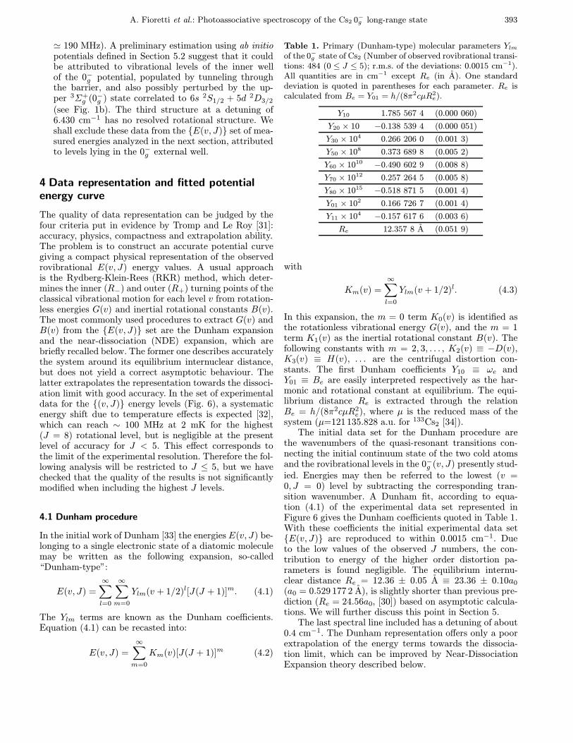
Table 1. Primary (Dunham-type) molecular parameters Ylmof the 0−g state of Cs2 (Number of observed rovibrational transi-tions: 484 (0 ≤ J ≤ 5); r.m.s. of the deviations: 0.0015 cm−1).All quantities are in cm−1 except Re (in A). One standarddeviation is quoted in parentheses for each parameter. Re iscalculated from Be = Y01 = h/(8π2cµR2

e).

Y10 1.785 567 4 (0.000 060)

Y20 × 10 −0.138 539 4 (0.000 051)

Y30 × 104 0.266 206 0 (0.001 3)

Y50 × 108 0.373 689 8 (0.005 2)

Y60 × 1010 −0.490 602 9 (0.008 8)

Y70 × 1012 0.257 264 5 (0.005 8)

Y80 × 1015 −0.518 871 5 (0.001 4)

Y01 × 102 0.166 726 7 (0.001 4)

Y11 × 104 −0.157 617 6 (0.003 6)

Re 12.357 8 A (0.051 9)

with

Km(v) =∞∑l=0

Ylm(v + 1/2)l. (4.3)

In this expansion, the m = 0 term K0(v) is identified asthe rotationless vibrational energy G(v), and the m = 1term K1(v) as the inertial rotational constant B(v). Thefollowing constants with m = 2, 3, . . . , K2(v) ≡ −D(v),K3(v) ≡ H(v), . . . are the centrifugal distortion con-stants. The first Dunham coefficients Y10 ≡ ωe andY01 ≡ Be are easily interpreted respectively as the har-monic and rotational constant at equilibrium. The equi-librium distance Re is extracted through the relationBe = h/(8π2cµR2

e), where µ is the reduced mass of thesystem (µ=121 135.828 a.u. for 133Cs2 [34]).

The initial data set for the Dunham procedure arethe wavenumbers of the quasi-resonant transitions con-necting the initial continuum state of the two cold atomsand the rovibrational levels in the 0−g (v, J) presently stud-ied. Energies may then be referred to the lowest (v =0, J = 0) level by subtracting the corresponding tran-sition wavenumber. A Dunham fit, according to equa-tion (4.1) of the experimental data set represented inFigure 6 gives the Dunham coefficients quoted in Table 1.With these coefficients the initial experimental data set{E(v, J)} are reproduced to within 0.0015 cm−1. Dueto the low values of the observed J numbers, the con-tribution to energy of the higher order distortion pa-rameters is found negligible. The equilibrium internu-clear distance Re = 12.36 ± 0.05 A ≡ 23.36 ± 0.10a0

(a0 = 0.529 177 2 A), is slightly shorter than previous pre-diction (Re = 24.56a0, [30]) based on asymptotic calcula-tions. We will further discuss this point in Section 5.

The last spectral line included has a detuning of about0.4 cm−1. The Dunham representation offers only a poorextrapolation of the energy terms towards the dissocia-tion limit, which can be improved by Near-DissociationExpansion theory described below.


4.2 The near-dissociation expansion theory

The analysis of PA data near the dissociation energy aimsat providing the long-range behaviour of the potentialcurve, which writes for R→∞:

V (R) = D − Cn/Rn (4.4)

where D is the energy at the molecular dissociation limitand Cn the leading long-range coefficient (n = 3 fordipole-dipole interaction in the present case). Dependingupon the choice for the energy origin, D can be either zero(origin at the dissociation limit) or the value of the welldepth De (origin at the minimum of the studied potentialwell). From equation (4.4), LeRoy and Bernstein [35] andStwalley [36,37] (see also Ref. [38]) derived the near disso-ciation limiting behavior K∞m (v) of the quantities Km(v)in equation (4.3). For the vibrational terms (m = 0):

G∞(v) ≡ K∞0 (v) = De −X0(n)(vD − v)2n/(n−2) (4.5)

and for the rotational constant (m = 1):

B∞(v) ≡ K∞1 (v) = X1(n)(vD − v)[2n/(n−2)−2]. (4.6)

More generally, if m > 0, the distortion terms are written:

K∞m (v) = Xm(n)(vD − v)[2n/(n−2)−2m]. (4.7)

In the above equations, vD is the effective vibrational(non-integer) index at the dissociation energy and,

Xm(n) = Xm(n)/[µn(C2

n)]1/(n−2)

(4.8)

where the quantities Xm(n) are known tabulated con-stants1 [39]. In the particular case of the Cs2 0−g state

dissociating into the limit Cs (6s 2S1/2)+Cs (6p 2P3/2),we have (setting n = 3):

Xm(3) = Xm(3)/µ3C23 . (4.9)

However, equations (4.4) and following are valid only forvery large internuclear distances (or for levels very closeto the dissociation limit), and when hyperfine structureand retardation effects are neglected. Moreover, furtherR−n terms beyond the dipole-dipole approximation in theexpansion (4.4) are required to reproduce larger parts ofPA spectra [40]. Such detailed long-range analysis of PAdata have been recently performed for the 0−g state in Na2

[11] and K2 [12], yielding an accurate value of the leadingcoefficient C3 in equation (4.4), directly related to the life-time of the first P3/2 atomic level. In the present case thiscannot easily be done as, in contrast with lighter alkalidimers, the 0−g state in Cs2 is no longer a pure long-rangemolecular state (see Sect. 5), and the hyperfine structureis much larger.

1 In the computer program we have used the values X0(3) =36 409.62 and X1(3) = 60 221.029 when energies are in cm−1,distances in A and mass in a.m.u.

Instead, we follow the procedure which has been suc-cessfully used for the Rb2 0−g state [41]. The near disso-ciation analysis is combined with the Dunham approachwithin the Near-Dissociation Expansion (NDE) theory de-veloped by Beckel and co-workers [42,43] and LeRoy andco-workers [44,45], in order to provide a description of theentire spectra. As the Dunham type expansion does nothave the correct limiting behavior and cannot be reliablyapplied to vibrational levels close to the dissociation limit,the near-dissociation expansion (NDE) expressions ensurethe correct Km(v) behavior both for near equilibrium andfor near dissociation spectral data by correcting the vibra-tional energy at infinity with a Pade approximant [L/M ]:

G(v) ≡ K0(v) = K∞0 (v)[L/M ]

= De −X0(n)(vD − v)2n/(n−2)[L/M ] (4.10)

where [L/M ], termed “outer” Pade expression, representthe ratio of two polynomials PL and QM depending uponthe variable z = (vD − v)γ :

PL = 1 +L∑i=1

pizα+i−1

QM = 1 +M∑j=1

qjzβ+j−1. (4.11)

Several fits have been performed to determine the valueof the exponents α, β, γ, L and M , and we choose the onewhich ensures the best compromise between the accuracyand the compactness of the representation of the {E(v, J)}set.

The other molecular parameters (with m > 0) are usu-ally corrected by an exponential expansion of order N :

Km(v) = K∞m (v) exp

[N∑l=1

sl(vD − v)l

]. (4.12)

Even though the parameters of such expansions haveno direct physical meaning, these analytical continua-tions (Eqs. (4.10, 4.12)) of long-range representations(Eqs. (4.5–4.7)) have been shown [38,44,45] to be far bet-ter for extrapolation towards high v values than simpleDunham-type expressions (Eqs. (4.2, 4.3)).

Another type of analytical long-range analysis is possi-ble as for example in the accurate study of the long-range0+u potential in Li2 by Martin et al. [40]. The authors use

higher order terms in the multipolar expansion of the po-tential (Eq. (4.4)), in order to extract the correspondinglong-range parameters Cn and the asymptotic form of theexchange energy. Our present study is concentrated ontothe representation of the part of the potential curve cov-ered by all the observed lines, by mixing in equation (4.10)the long-range behavior of the potential (a single Cn coef-ficient) and additional parameters (in the [L/M ] expres-sion).

The NDE analysis implies non-linear fits and does nothave a unique solution. Here the input are the G(v) and


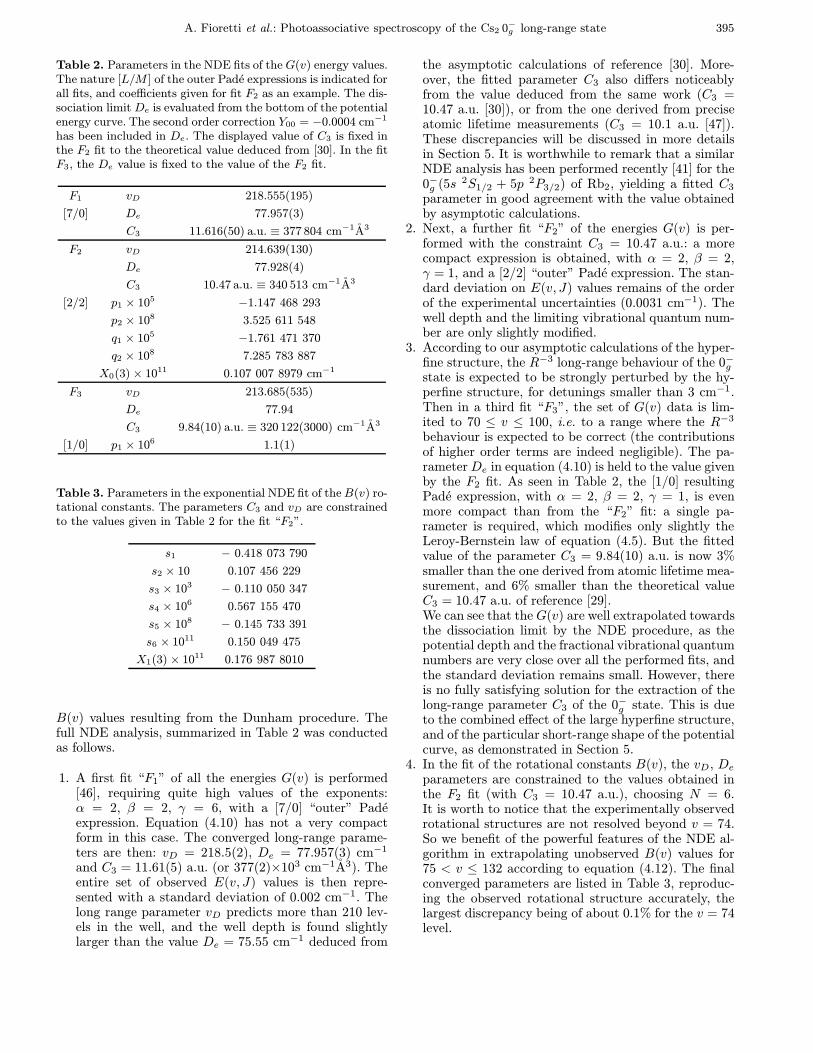
Table 2. Parameters in the NDE fits of theG(v) energy values.The nature [L/M ] of the outer Pade expressions is indicated forall fits, and coefficients given for fit F2 as an example. The dis-sociation limit De is evaluated from the bottom of the potentialenergy curve. The second order correction Y00 = −0.0004 cm−1

has been included in De. The displayed value of C3 is fixed inthe F2 fit to the theoretical value deduced from [30]. In the fitF3, the De value is fixed to the value of the F2 fit.

F1 vD 218.555(195)

[7/0] De 77.957(3)

C3 11.616(50) a.u. ≡ 377 804 cm−1A3

F2 vD 214.639(130)

De 77.928(4)

C3 10.47 a.u. ≡ 340 513 cm−1A3

[2/2] p1 × 105 −1.147 468 293

p2 × 108 3.525 611 548

q1 × 105 −1.761 471 370

q2 × 108 7.285 783 887

X0(3)× 1011 0.107 007 8979 cm−1

F3 vD 213.685(535)

De 77.94

C3 9.84(10) a.u. ≡ 320 122(3000) cm−1A3

[1/0] p1 × 106 1.1(1)

Table 3. Parameters in the exponential NDE fit of theB(v) ro-tational constants. The parameters C3 and vD are constrainedto the values given in Table 2 for the fit “F2”.

s1 − 0.418 073 790

s2 × 10 0.107 456 229

s3 × 103 − 0.110 050 347

s4 × 106 0.567 155 470

s5 × 108 − 0.145 733 391

s6 × 1011 0.150 049 475

X1(3) × 1011 0.176 987 8010

B(v) values resulting from the Dunham procedure. Thefull NDE analysis, summarized in Table 2 was conductedas follows.

1. A first fit “F1” of all the energies G(v) is performed[46], requiring quite high values of the exponents:α = 2, β = 2, γ = 6, with a [7/0] “outer” Padeexpression. Equation (4.10) has not a very compactform in this case. The converged long-range parame-ters are then: vD = 218.5(2), De = 77.957(3) cm−1

and C3 = 11.61(5) a.u. (or 377(2)×103 cm−1A3). Theentire set of observed E(v, J) values is then repre-sented with a standard deviation of 0.002 cm−1. Thelong range parameter vD predicts more than 210 lev-els in the well, and the well depth is found slightlylarger than the value De = 75.55 cm−1 deduced from

the asymptotic calculations of reference [30]. More-over, the fitted parameter C3 also differs noticeablyfrom the value deduced from the same work (C3 =10.47 a.u. [30]), or from the one derived from preciseatomic lifetime measurements (C3 = 10.1 a.u. [47]).These discrepancies will be discussed in more detailsin Section 5. It is worthwhile to remark that a similarNDE analysis has been performed recently [41] for the0−g (5s 2S1/2 + 5p 2P3/2) of Rb2, yielding a fitted C3

parameter in good agreement with the value obtainedby asymptotic calculations.

2. Next, a further fit “F2” of the energies G(v) is per-formed with the constraint C3 = 10.47 a.u.: a morecompact expression is obtained, with α = 2, β = 2,γ = 1, and a [2/2] “outer” Pade expression. The stan-dard deviation on E(v, J) values remains of the orderof the experimental uncertainties (0.0031 cm−1). Thewell depth and the limiting vibrational quantum num-ber are only slightly modified.

3. According to our asymptotic calculations of the hyper-fine structure, the R−3 long-range behaviour of the 0−gstate is expected to be strongly perturbed by the hy-perfine structure, for detunings smaller than 3 cm−1.Then in a third fit “F3”, the set of G(v) data is lim-ited to 70 ≤ v ≤ 100, i.e. to a range where the R−3

behaviour is expected to be correct (the contributionsof higher order terms are indeed negligible). The pa-rameterDe in equation (4.10) is held to the value givenby the F2 fit. As seen in Table 2, the [1/0] resultingPade expression, with α = 2, β = 2, γ = 1, is evenmore compact than from the “F2” fit: a single pa-rameter is required, which modifies only slightly theLeroy-Bernstein law of equation (4.5). But the fittedvalue of the parameter C3 = 9.84(10) a.u. is now 3%smaller than the one derived from atomic lifetime mea-surement, and 6% smaller than the theoretical valueC3 = 10.47 a.u. of reference [29].We can see that the G(v) are well extrapolated towardsthe dissociation limit by the NDE procedure, as thepotential depth and the fractional vibrational quantumnumbers are very close over all the performed fits, andthe standard deviation remains small. However, thereis no fully satisfying solution for the extraction of thelong-range parameter C3 of the 0−g state. This is dueto the combined effect of the large hyperfine structure,and of the particular short-range shape of the potentialcurve, as demonstrated in Section 5.

4. In the fit of the rotational constants B(v), the vD, De

parameters are constrained to the values obtained inthe F2 fit (with C3 = 10.47 a.u.), choosing N = 6.It is worth to notice that the experimentally observedrotational structures are not resolved beyond v = 74.So we benefit of the powerful features of the NDE al-gorithm in extrapolating unobserved B(v) values for75 < v ≤ 132 according to equation (4.12). The finalconverged parameters are listed in Table 3, reproduc-ing the observed rotational structure accurately, thelargest discrepancy being of about 0.1% for the v = 74level.


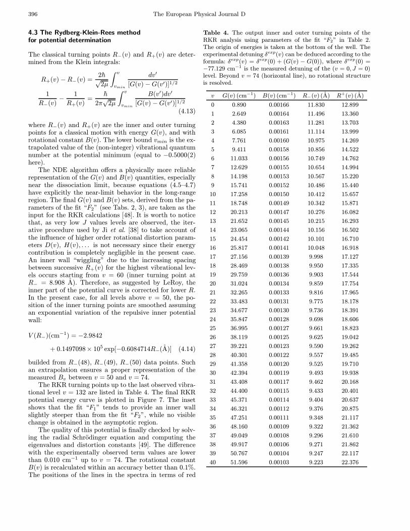
4.3 The Rydberg-Klein-Rees methodfor potential determination

The classical turning points R−(v) and R+(v) are deter-mined from the Klein integrals:

R+(v)−R−(v) =2~√

2µ

∫ v

vmin

dv′

[G(v)−G(v′)]1/2

1

R−(v)−

1

R+(v)=

~2π√

2µ

∫ v

vmin

B(v′)dv′

[G(v) −G(v′)]1/2

(4.13)

where R−(v) and R+(v) are the inner and outer turningpoints for a classical motion with energy G(v), and withrotational constant B(v). The lower bound vmin is the ex-trapolated value of the (non-integer) vibrational quantumnumber at the potential minimum (equal to −0.5000(2)here).

The NDE algorithm offers a physically more reliablerepresentation of the G(v) and B(v) quantities, especiallynear the dissociation limit, because equations (4.5–4.7)have explicitly the near-limit behavior in the long-rangeregion. The final G(v) and B(v) sets, derived from the pa-rameters of the fit “F2” (see Tabs. 2, 3), are taken as theinput for the RKR calculations [48]. It is worth to noticethat, as very low J values levels are observed, the iter-ative procedure used by Ji et al. [38] to take account ofthe influence of higher order rotational distortion param-eters D(v), H(v), . . . is not necessary since their energycontribution is completely negligible in the present case.An inner wall “wiggling” due to the increasing spacingbetween successive R+(v) for the highest vibrational lev-els occurs starting from v = 60 (inner turning point atR− = 8.908 A). Therefore, as suggested by LeRoy, theinner part of the potential curve is corrected for lower R.In the present case, for all levels above v = 50, the po-sition of the inner turning points are smoothed assumingan exponential variation of the repulsive inner potentialwall:

V (R−)(cm−1) = −2.9842

+ 0.1497098× 105 exp[−0.6084714R−(A)] (4.14)

builded from R−(48), R−(49), R−(50) data points. Suchan extrapolation ensures a proper representation of themeasured Bv between v = 50 and v = 74.

The RKR turning points up to the last observed vibra-tional level v = 132 are listed in Table 4. The final RKRpotential energy curve is plotted in Figure 7. The insetshows that the fit “F1” tends to provide an inner wallslightly steeper than from the fit “F2”, while no visiblechange is obtained in the asymptotic region.

The quality of this potential is finally checked by solv-ing the radial Schrodinger equation and computing theeigenvalues and distortion constants [49]. The differencewith the experimentally observed term values are lowerthan 0.010 cm−1 up to v = 74. The rotational constantB(v) is recalculated within an accuracy better than 0.1%.The positions of the lines in the spectra in terms of red

Table 4. The output inner and outer turning points of theRKR analysis using parameters of the fit “F2” in Table 2.The origin of energies is taken at the bottom of the well. Theexperimental detuning δexp(v) can be deduced according to theformula: δexp(v) = δexp(0) + (G(v) − G(0)), where δexp(0) =−77.129 cm−1 is the measured detuning of the (v = 0, J = 0)level. Beyond v = 74 (horizontal line), no rotational structureis resolved.

v G(v) (cm−1) B(v) (cm−1) R−(v) (A) R+(v) (A)

0 0.890 0.00166 11.830 12.899

1 2.649 0.00164 11.496 13.360

2 4.380 0.00163 11.281 13.703

3 6.085 0.00161 11.114 13.999

4 7.761 0.00160 10.975 14.269

5 9.411 0.00158 10.856 14.522

6 11.033 0.00156 10.749 14.762

7 12.629 0.00155 10.654 14.994

8 14.198 0.00153 10.567 15.220

9 15.741 0.00152 10.486 15.440

10 17.258 0.00150 10.412 15.657

11 18.748 0.00149 10.342 15.871

12 20.213 0.00147 10.276 16.082

13 21.652 0.00145 10.215 16.293

14 23.065 0.00144 10.156 16.502

15 24.454 0.00142 10.101 16.710

16 25.817 0.00141 10.048 16.918

17 27.156 0.00139 9.998 17.127

18 28.469 0.00138 9.950 17.335

19 29.759 0.00136 9.903 17.544

20 31.024 0.00134 9.859 17.754

21 32.265 0.00133 9.816 17.965

22 33.483 0.00131 9.775 18.178

23 34.677 0.00130 9.736 18.391

24 35.847 0.00128 9.698 18.606

25 36.995 0.00127 9.661 18.823

26 38.119 0.00125 9.625 19.042

27 39.221 0.00123 9.590 19.262

28 40.301 0.00122 9.557 19.485

29 41.358 0.00120 9.525 19.710

30 42.394 0.00119 9.493 19.938

31 43.408 0.00117 9.462 20.168

32 44.400 0.00115 9.433 20.401

33 45.371 0.00114 9.404 20.637

34 46.321 0.00112 9.376 20.875

35 47.251 0.00111 9.348 21.117

36 48.160 0.00109 9.322 21.362

37 49.049 0.00108 9.296 21.610

38 49.917 0.00106 9.271 21.862

39 50.767 0.00104 9.247 22.117

40 51.596 0.00103 9.223 22.376


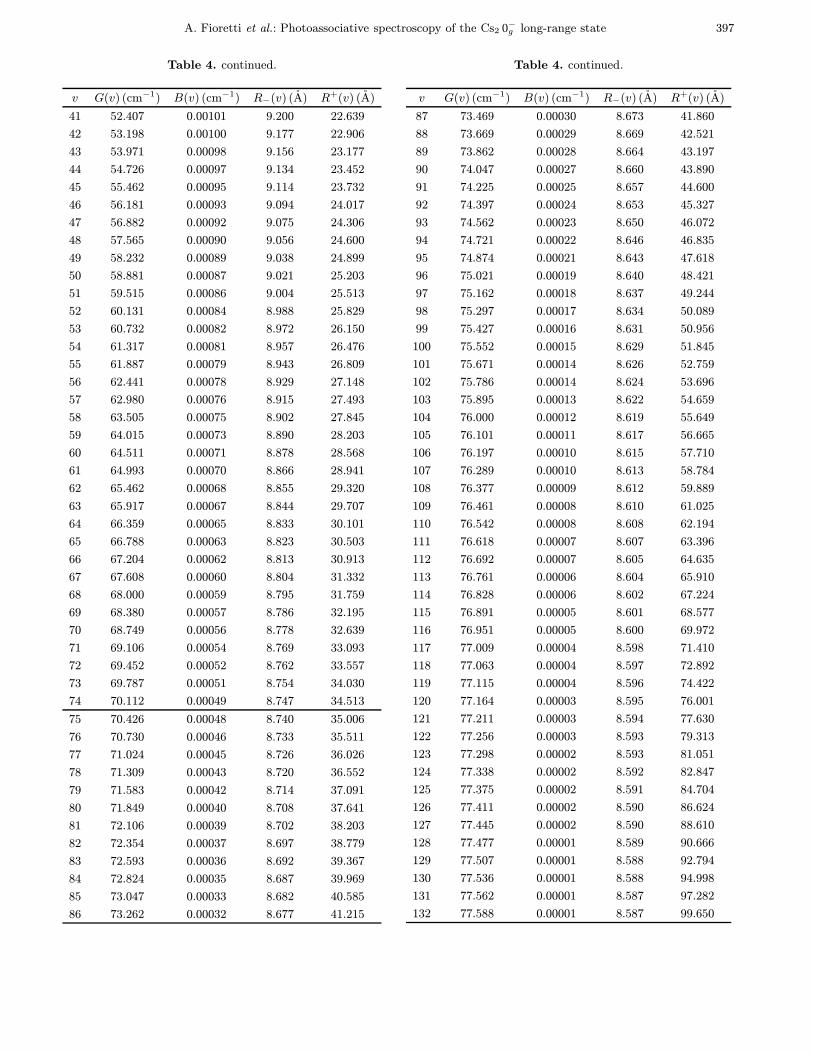
Table 4. continued.


41 52.407 0.00101 9.200 22.639

42 53.198 0.00100 9.177 22.906

43 53.971 0.00098 9.156 23.177

44 54.726 0.00097 9.134 23.452

45 55.462 0.00095 9.114 23.732

46 56.181 0.00093 9.094 24.017

47 56.882 0.00092 9.075 24.306

48 57.565 0.00090 9.056 24.600

49 58.232 0.00089 9.038 24.899

50 58.881 0.00087 9.021 25.203

51 59.515 0.00086 9.004 25.513

52 60.131 0.00084 8.988 25.829

53 60.732 0.00082 8.972 26.150

54 61.317 0.00081 8.957 26.476

55 61.887 0.00079 8.943 26.809

56 62.441 0.00078 8.929 27.148

57 62.980 0.00076 8.915 27.493

58 63.505 0.00075 8.902 27.845

59 64.015 0.00073 8.890 28.203

60 64.511 0.00071 8.878 28.568

61 64.993 0.00070 8.866 28.941

62 65.462 0.00068 8.855 29.320

63 65.917 0.00067 8.844 29.707

64 66.359 0.00065 8.833 30.101

65 66.788 0.00063 8.823 30.503

66 67.204 0.00062 8.813 30.913

67 67.608 0.00060 8.804 31.332

68 68.000 0.00059 8.795 31.759

69 68.380 0.00057 8.786 32.195

70 68.749 0.00056 8.778 32.639

71 69.106 0.00054 8.769 33.093

72 69.452 0.00052 8.762 33.557

73 69.787 0.00051 8.754 34.030

74 70.112 0.00049 8.747 34.513

75 70.426 0.00048 8.740 35.006

76 70.730 0.00046 8.733 35.511

77 71.024 0.00045 8.726 36.026

78 71.309 0.00043 8.720 36.552

79 71.583 0.00042 8.714 37.091

80 71.849 0.00040 8.708 37.641

81 72.106 0.00039 8.702 38.203

82 72.354 0.00037 8.697 38.779

83 72.593 0.00036 8.692 39.367

84 72.824 0.00035 8.687 39.969

85 73.047 0.00033 8.682 40.585

86 73.262 0.00032 8.677 41.215

Table 4. continued.


87 73.469 0.00030 8.673 41.860

88 73.669 0.00029 8.669 42.521

89 73.862 0.00028 8.664 43.197

90 74.047 0.00027 8.660 43.890

91 74.225 0.00025 8.657 44.600

92 74.397 0.00024 8.653 45.327

93 74.562 0.00023 8.650 46.072

94 74.721 0.00022 8.646 46.835

95 74.874 0.00021 8.643 47.618

96 75.021 0.00019 8.640 48.421

97 75.162 0.00018 8.637 49.244

98 75.297 0.00017 8.634 50.089

99 75.427 0.00016 8.631 50.956

100 75.552 0.00015 8.629 51.845

101 75.671 0.00014 8.626 52.759

102 75.786 0.00014 8.624 53.696

103 75.895 0.00013 8.622 54.659

104 76.000 0.00012 8.619 55.649

105 76.101 0.00011 8.617 56.665

106 76.197 0.00010 8.615 57.710

107 76.289 0.00010 8.613 58.784

108 76.377 0.00009 8.612 59.889

109 76.461 0.00008 8.610 61.025

110 76.542 0.00008 8.608 62.194

111 76.618 0.00007 8.607 63.396

112 76.692 0.00007 8.605 64.635

113 76.761 0.00006 8.604 65.910

114 76.828 0.00006 8.602 67.224

115 76.891 0.00005 8.601 68.577

116 76.951 0.00005 8.600 69.972

117 77.009 0.00004 8.598 71.410

118 77.063 0.00004 8.597 72.892

119 77.115 0.00004 8.596 74.422

120 77.164 0.00003 8.595 76.001

121 77.211 0.00003 8.594 77.630

122 77.256 0.00003 8.593 79.313

123 77.298 0.00002 8.593 81.051

124 77.338 0.00002 8.592 82.847

125 77.375 0.00002 8.591 84.704

126 77.411 0.00002 8.590 86.624

127 77.445 0.00002 8.590 88.610

128 77.477 0.00001 8.589 90.666

129 77.507 0.00001 8.588 92.794

130 77.536 0.00001 8.588 94.998

131 77.562 0.00001 8.587 97.282

132 77.588 0.00001 8.587 99.650


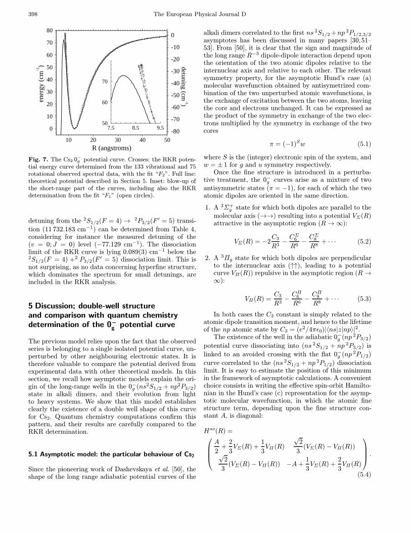
10 20 30 40 50R (angstroms)

0

10

20

30

40

50

60

70

80

ener

gy (

cm-1)

7.5 8.5 9.550

60

70

-80

-70

-60

-50

-40

-30

-20

-10

0

detuning (cm-1)

Fig. 7. The Cs2 0−g potential curve. Crosses: the RKR poten-tial energy curve determined from the 133 vibrational and 75rotational observed spectral data, with the fit “F2”. Full line:theoretical potential described in Section 5. Inset: blow-up ofthe short-range part of the curves, including also the RKRdetermination from the fit “F1” (open circles).

detuning from the 2S1/2(F = 4)→ 2P3/2(F ′ = 5) transi-

tion (11 732.183 cm−1) can be determined from Table 4,considering for instance the measured detuning of the(v = 0;J = 0) level (−77.129 cm−1). The dissociationlimit of the RKR curve is lying 0.089(3) cm−1 below the2S1/2(F = 4) +2 P3/2(F ′ = 5) dissociation limit. This isnot surprising, as no data concerning hyperfine structure,which dominates the spectrum for small detunings, areincluded in the RKR analysis.

5 Discussion; double-well structureand comparison with quantum chemistrydetermination of the 0�g potential curve

The previous model relies upon the fact that the observedseries is belonging to a single isolated potential curve, un-perturbed by other neighbouring electronic states. It istherefore valuable to compare the potential derived fromexperimental data with other theoretical models. In thissection, we recall how asymptotic models explain the ori-gin of the long-range wells in the 0−g (ns2S1/2 + np2P3/2)state in alkali dimers, and their evolution from lightto heavy systems. We show that this model establishesclearly the existence of a double well shape of this curvefor Cs2. Quantum chemistry computations confirm thispattern, and their results are carefully compared to theRKR determination.

5.1 Asymptotic model: the particular behaviour of Cs2

Since the pioneering work of Dashevskaya et al. [50], theshape of the long range adiabatic potential curves of the

alkali dimers correlated to the first ns 2S1/2 +np 2P1/2,3/2

asymptotes has been discussed in many papers [30,51–53]. From [50], it is clear that the sign and magnitude ofthe long range R−3 dipole-dipole interaction depend uponthe orientation of the two atomic dipoles relative to theinternuclear axis and relative to each other. The relevantsymmetry property, for the asymptotic Hund’s case (a)molecular wavefunction obtained by antisymetrized com-bination of the two unperturbed atomic wavefunctions, isthe exchange of excitation between the two atoms, leavingthe core and electrons unchanged. It can be expressed asthe product of the symmetry in exchange of the two elec-trons multiplied by the symmetry in exchange of the twocores

π = (−1)Sw (5.1)

where S is the (integer) electronic spin of the system, andw = ± 1 for g and u symmetry respectively.

Once the fine structure is introduced in a perturba-tive treatment, the 0−g curves arise as a mixture of twoantisymmetric states (π = −1), for each of which the twoatomic dipoles are oriented in the same direction.

1. A 3Σ+g state for which both dipoles are parallel to the

molecular axis (→→) resulting into a potential VΣ(R)attractive in the asymptotic region (R→∞):

VΣ(R) = −2C3

R3−CΣ6R6−CΣ8R8

+ · · · (5.2)

2. A 3Πg state for which both dipoles are perpendicularto the internuclear axis (↑↑), leading to a potentialcurve VΠ(R)) repulsive in the asymptotic region (R→∞):

VΠ(R) =C3

R3−CΠ6R6−CΠ8R8

+ · · · (5.3)

In both cases the C3 constant is simply related to theatomic dipole transition moment, and hence to the lifetimeof the np atomic state by C3 = (e2/4πε0)|〈ns|z|np〉|2.

The existence of the well in the adiabatic 0−g (np 2P3/2)

potential curve dissociating into (ns 2S1/2 + np 2P3/2) is

linked to an avoided crossing with the flat 0−g (np 2P1/2)

curve correlated to the (ns 2S1/2 + np 2P1/2) dissociationlimit. It is easy to estimate the position of this minimumin the framework of asymptotic calculations. A convenientchoice consists in writing the effective spin-orbit Hamilto-nian in the Hund’s case (c) representation for the asymp-totic molecular wavefunction, in which the atomic finestructure term, depending upon the fine structure con-stant A, is diagonal:

Hso(R) =A

2+

2

3VΣ(R) +

1

3VΠ(R)

√2

3(VΣ(R)− VΠ(R))

√2

3(VΣ(R)− VΠ(R)) −A+

1

3VΣ(R) +

2

3VΠ(R)

.

(5.4)


The upper diagonal element is attractive at large distanceswhile the lower diagonal element corresponds to a flatcurve. The R-dependent coupling is due to the differencebetween the two (Hund’s case (a)) potentials VΣ(R) andVΠ(R):

Hso12(R) =

√2

3(VΣ(R)− VΠ(R))

= −√

2C3

R3−

√2

3

CΠ6 − CΣ6

R6−

√2

3

CΠ8 − CΣ8

R8+ · · ·

(5.5)

In a model considering only the leading R−3 dipole dipoleinteraction and hence neglecting the R−6 and R−8 terms,the energy of the 0−g (ns 2S1/2 + np 2P3/2) curve is read-ily obtained after diagonalization the matrix in equa-tion (5.4):

V (0−g (np 2P3/2)) = E(np 2P3/2)−C3

R3

+1

2x

[√1 +

8

x2

(C3)2

R6− 1

](5.6)

where E∞(np 2P3/2) is the energy of the (ns 2S1/2 +

np 2P3/2) dissociation limit and x = ∆Efs − C3/R3 =

3A/2 − C3/R3 is the difference between the atomic fine

structure splitting ∆Efs = 3A/2 and the dipole-dipoleattractive interaction.

At large internuclear distances where the fine structuresplitting is much larger than the dipole-dipole interaction(x ' ∆Efs), the upper curve is attractive:

V (0−g (np 2P3/2)) ' E∞(np 2P3/2)−C3

R3+

2(C3)2

∆EfsR6·

(5.7)

The R−6 correction is always comparable to the terms ne-glected in multipole expansion (Eqs. (5.2, 5.3)). As theinternuclear distance is decreasing, the attractive dipole-dipole interaction and the fine structure splitting are com-parable in magnitude (x ' 0), and we can write:

V (0−g (np 2P3/2)) ' E(np 2P3/2) + (√

2− 1)C3

R3(5.8)

leading to a repulsive R−3 branch. A minimum in the po-tential is generated at a distance which decreases rapidlyfrom light to heavy atoms [52].

When the R−6 and R−8 terms of equations (5.2, 5.3)terms are considered, as the C6 and C8 coefficients arepositive, they introduce an attractive contribution whichtends to compensate the repulsive R−3 behaviour. ForNa2 and K2, the minimum occurs at very large distances(∼ 72a0 and ∼ 52a0 respectively [52]) where the R−6 andR−8 terms can safely be neglected, so that the pictureof a pure long range R−3 potential well is indeed valid.In the case of heavier alkalis, due to the large value ofthe fine structure splitting, the minimum occurs in a re-gion where the R−6 and R−8 terms should be introduced.

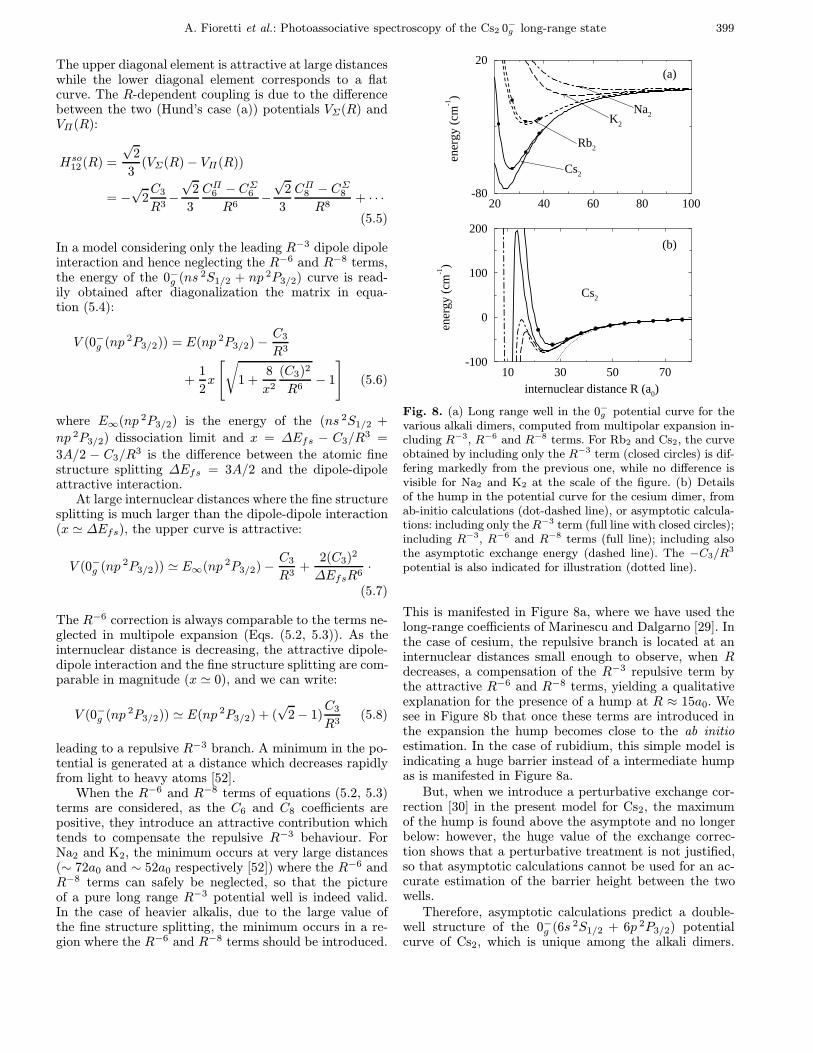
10 30 50 70internuclear distance R (a0)

-100

0

100

200

ener

gy (

cm-1)

20 40 60 80 100-80

20

ener

gy (

cm-1)

(a)

(b)

Na2K2

Rb2

Cs2

Cs2

Fig. 8. (a) Long range well in the 0−g potential curve for thevarious alkali dimers, computed from multipolar expansion in-cluding R−3, R−6 and R−8 terms. For Rb2 and Cs2, the curveobtained by including only the R−3 term (closed circles) is dif-fering markedly from the previous one, while no difference isvisible for Na2 and K2 at the scale of the figure. (b) Detailsof the hump in the potential curve for the cesium dimer, fromab-initio calculations (dot-dashed line), or asymptotic calcula-tions: including only theR−3 term (full line with closed circles);including R−3, R−6 and R−8 terms (full line); including alsothe asymptotic exchange energy (dashed line). The −C3/R3

potential is also indicated for illustration (dotted line).

This is manifested in Figure 8a, where we have used thelong-range coefficients of Marinescu and Dalgarno [29]. Inthe case of cesium, the repulsive branch is located at aninternuclear distances small enough to observe, when Rdecreases, a compensation of the R−3 repulsive term bythe attractive R−6 and R−8 terms, yielding a qualitativeexplanation for the presence of a hump at R ≈ 15a0. Wesee in Figure 8b that once these terms are introduced inthe expansion the hump becomes close to the ab initioestimation. In the case of rubidium, this simple model isindicating a huge barrier instead of a intermediate humpas is manifested in Figure 8a.

But, when we introduce a perturbative exchange cor-rection [30] in the present model for Cs2, the maximumof the hump is found above the asymptote and no longerbelow: however, the huge value of the exchange correc-tion shows that a perturbative treatment is not justified,so that asymptotic calculations cannot be used for an ac-curate estimation of the barrier height between the twowells.

Therefore, asymptotic calculations predict a double-well structure of the 0−g (6s 2S1/2 + 6p 2P3/2) potentialcurve of Cs2, which is unique among the alkali dimers.


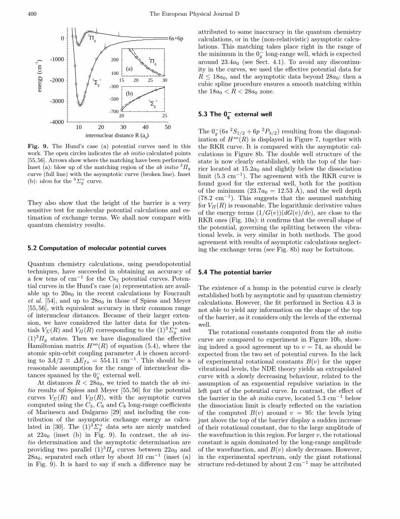
10 20 30 40 50internuclear distance R (a0)

-4000

-3000

-2000

-1000

0en

ergy

(cm

-1)

15 20 25 30100

200

20 25-700

-500

-300

3Πg

3Σg

+

3Σg

+

3Πg 6s+6p

(a)

(b)

Fig. 9. The Hund’s case (a) potential curves used in thiswork. The open circles indicates the ab initio calculated points[55,56]. Arrows show where the matching have been performed.Inset (a): blow up of the matching region of the ab initio 3Πg

curve (full line) with the asymptotic curve (broken line). Inset(b): idem for the 3Σ+

g curve.

They also show that the height of the barrier is a verysensitive test for molecular potential calculations and es-timation of exchange terms. We shall now compare withquantum chemistry results.

5.2 Computation of molecular potential curves

Quantum chemistry calculations, using pseudopotentialtechniques, have succeeded in obtaining an accuracy ofa few tens of cm−1 for the Cs2 potential curves. Poten-tial curves in the Hund’s case (a) representation are avail-able up to 20a0 in the recent calculations by Foucraultet al. [54], and up to 28a0 in those of Spiess and Meyer[55,56], with equivalent accuracy in their common rangeof internuclear distances. Because of their larger exten-sion, we have considered the latter data for the poten-tials VΣ(R) and VΠ(R) corresponding to the (1)3Σ+

g and

(1)3Πg states. Then we have diagonalized the effectiveHamiltonian matrix Hso(R) of equation (5.4), where theatomic spin-orbit coupling parameter A is chosen accord-ing to 3A/2 ≡ ∆Efs = 554.11 cm−1. This should be areasonable assumption for the range of internuclear dis-tances spanned by the 0−g external well.

At distances R < 28a0, we tried to match the ab ini-tio results of Spiess and Meyer [55,56] for the potentialcurves VΣ(R) and VΠ(R), with the asymptotic curvescomputed using the C3, C6 and C8 long-range coefficientsof Marinescu and Dalgarno [29] and including the con-tribution of the asymptotic exchange energy as calcu-lated in [30]. The (1)3Σ+

g data sets are nicely matchedat 22a0 (inset (b) in Fig. 9). In contrast, the ab ini-tio determination and the asymptotic determination areproviding two parallel (1)3Πg curves between 22a0 and28a0, separated each other by about 10 cm−1 (inset (a)in Fig. 9). It is hard to say if such a difference may be

attributed to some inaccuracy in the quantum chemistrycalculations, or in the (non-relativistic) asymptotic calcu-lations. This matching takes place right in the range ofthe minimum in the 0−g long-range well, which is expectedaround 23.4a0 (see Sect. 4.1). To avoid any discontinu-ity in the curves, we used the effective potential data forR ≤ 18a0, and the asymptotic data beyond 28a0: then acubic spline procedure ensures a smooth matching withinthe 18a0 < R < 28a0 zone.

5.3 The 0�g external well

The 0−g (6s 2S1/2 + 6p 2P3/2) resulting from the diagonal-ization of Hso(R) is displayed in Figure 7, together withthe RKR curve. It is compared with the asymptotic cal-culations in Figure 8b. The double well structure of thestate is now clearly established, with the top of the bar-rier located at 15.2a0 and slightly below the dissociationlimit (5.3 cm−1). The agreement with the RKR curve isfound good for the external well, both for the positionof the minimum (23.7a0 = 12.53 A), and the well depth(78.2 cm−1). This suggests that the assumed matchingfor VΠ(R) is reasonable. The logarithmic derivative valuesof the energy terms (1/G(v))(dG(v)/dv), are close to theRKR ones (Fig. 10a): it confirms that the overall shape ofthe potential, governing the splitting between the vibra-tional levels, is very similar in both methods. The goodagreement with results of asymptotic calculations neglect-ing the exchange term (see Fig. 8b) may be fortuitous.

5.4 The potential barrier

The existence of a hump in the potential curve is clearlyestablished both by asymptotic and by quantum chemistrycalculations. However, the fit performed in Section 4.3 isnot able to yield any information on the shape of the topof the barrier, as it considers only the levels of the externalwell.

The rotational constants computed from the ab initiocurve are compared to experiment in Figure 10b, show-ing indeed a good agreement up to v = 74, as should beexpected from the two set of potential curves. In the lackof experimental rotational constants B(v) for the uppervibrational levels, the NDE theory yields an extrapolatedcurve with a slowly decreasing behaviour, related to theassumption of an exponential repulsive variation in theleft part of the potential curve. In contrast, the effect ofthe barrier in the ab initio curve, located 5.3 cm−1 belowthe dissociation limit is clearly reflected on the variationof the computed B(v) around v = 95: the levels lyingjust above the top of the barrier display a sudden increaseof their rotational constant, due to the large amplitude ofthe wavefunction in this region. For larger v, the rotationalconstant is again dominated by the long-range amplitudeof the wavefunction, and B(v) slowly decreases. However,in the experimental spectrum, only the giant rotationalstructure red-detuned by about 2 cm−1 may be attributed


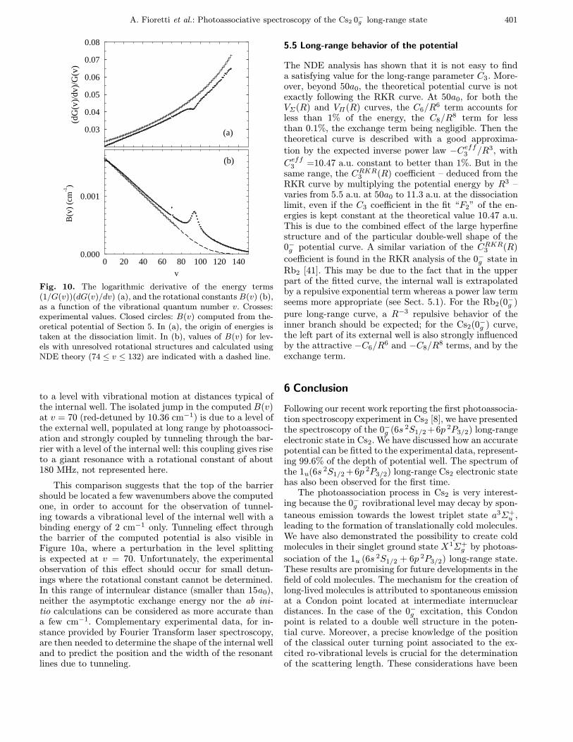
0 20 40 60 80 100 120 140v

0.000

0.001

B(v

) (c

m-1)

0.03

0.04

0.05

0.06

0.07

0.08

(dG

(v)/

dv)/

G(v

)

(a)

(b)

Fig. 10. The logarithmic derivative of the energy terms(1/G(v))(dG(v)/dv) (a), and the rotational constants B(v) (b),as a function of the vibrational quantum number v. Crosses:experimental values. Closed circles: B(v) computed from the-oretical potential of Section 5. In (a), the origin of energies istaken at the dissociation limit. In (b), values of B(v) for lev-els with unresolved rotational structures and calculated usingNDE theory (74 ≤ v ≤ 132) are indicated with a dashed line.

to a level with vibrational motion at distances typical ofthe internal well. The isolated jump in the computedB(v)at v = 70 (red-detuned by 10.36 cm−1) is due to a level ofthe external well, populated at long range by photoassoci-ation and strongly coupled by tunneling through the bar-rier with a level of the internal well: this coupling gives riseto a giant resonance with a rotational constant of about180 MHz, not represented here.

This comparison suggests that the top of the barriershould be located a few wavenumbers above the computedone, in order to account for the observation of tunnel-ing towards a vibrational level of the internal well with abinding energy of 2 cm−1 only. Tunneling effect throughthe barrier of the computed potential is also visible inFigure 10a, where a perturbation in the level splittingis expected at v = 70. Unfortunately, the experimentalobservation of this effect should occur for small detun-ings where the rotational constant cannot be determined.In this range of internulear distance (smaller than 15a0),neither the asymptotic exchange energy nor the ab ini-tio calculations can be considered as more accurate thana few cm−1. Complementary experimental data, for in-stance provided by Fourier Transform laser spectroscopy,are then needed to determine the shape of the internal welland to predict the position and the width of the resonantlines due to tunneling.

5.5 Long-range behavior of the potential

The NDE analysis has shown that it is not easy to finda satisfying value for the long-range parameter C3. More-over, beyond 50a0, the theoretical potential curve is notexactly following the RKR curve. At 50a0, for both theVΣ(R) and VΠ(R) curves, the C6/R

6 term accounts forless than 1% of the energy, the C8/R

8 term for lessthan 0.1%, the exchange term being negligible. Then thetheoretical curve is described with a good approxima-tion by the expected inverse power law −Ceff3 /R3, with

Ceff3 =10.47 a.u. constant to better than 1%. But in thesame range, the CRKR3 (R) coefficient – deduced from theRKR curve by multiplying the potential energy by R3 –varies from 5.5 a.u. at 50a0 to 11.3 a.u. at the dissociationlimit, even if the C3 coefficient in the fit “F2” of the en-ergies is kept constant at the theoretical value 10.47 a.u.This is due to the combined effect of the large hyperfinestructure and of the particular double-well shape of the0−g potential curve. A similar variation of the CRKR3 (R)

coefficient is found in the RKR analysis of the 0−g state inRb2 [41]. This may be due to the fact that in the upperpart of the fitted curve, the internal wall is extrapolatedby a repulsive exponential term whereas a power law termseems more appropriate (see Sect. 5.1). For the Rb2(0−g )

pure long-range curve, a R−3 repulsive behavior of theinner branch should be expected; for the Cs2(0−g ) curve,the left part of its external well is also strongly influencedby the attractive −C6/R

6 and −C8/R8 terms, and by the

exchange term.

6 Conclusion

Following our recent work reporting the first photoassocia-tion spectroscopy experiment in Cs2 [8], we have presentedthe spectroscopy of the 0−g (6s 2S1/2 +6p 2P3/2) long-rangeelectronic state in Cs2. We have discussed how an accuratepotential can be fitted to the experimental data, represent-ing 99.6% of the depth of potential well. The spectrum ofthe 1u(6s 2S1/2 +6p 2P3/2) long-range Cs2 electronic statehas also been observed for the first time.

The photoassociation process in Cs2 is very interest-ing because the 0−g rovibrational level may decay by spon-

taneous emission towards the lowest triplet state a3Σ+u ,

leading to the formation of translationally cold molecules.We have also demonstrated the possibility to create coldmolecules in their singlet ground state X1Σ+

g by photoas-

sociation of the 1u (6s 2S1/2 + 6p 2P3/2) long-range state.These results are promising for future developments in thefield of cold molecules. The mechanism for the creation oflong-lived molecules is attributed to spontaneous emissionat a Condon point located at intermediate internucleardistances. In the case of the 0−g excitation, this Condonpoint is related to a double well structure in the poten-tial curve. Moreover, a precise knowledge of the positionof the classical outer turning point associated to the ex-cited ro-vibrational levels is crucial for the determinationof the scattering length. These considerations have been


an important motivation for the present determination ofan accurate 0−g potential.

In order to reach this objective, we first have reportedexperimental results on a high resolution spectrum of theCs2 (0−g ) long-range electronic state. Vibrational levels ofthe external well have been assigned from v = 0 up to v =132, i.e.∼ 0.3 cm−1 below the dissociation limit 6s 2S1/2+

6p 2P3/2. The rotational structure up to J = 8 is wellresolved for levels below v = 74. Moreover, a vibrationalseries has been assigned to the 1u electronic state. Finally,three isolated structures have been observed: two of themexhibit a huge rotational constant, probably associatedwith vibrational levels of the 0−g inner well.

The RKR potential energy curve has been constructedfrom the 0−g vibrational and rotational observed data upto v = 74. Accurate determination of the inner and outerturning points of the classical vibrational motion havebeen reported, with a 1% accuracy. As the rotationalstructure is not resolved beyond v = 74 in the experi-ment, the rotational constants were extrapolated using theNDE theory of Le Roy and co-workers. The NDE fittingof the energies cannot provide a converged value for theC3 asymptotic parameter which varies by±10% accordingto the performed fit. The long-range behavior of the RKRpotential differs from the expected −C3/R

3 asymptoticlaw, preventing a reliable determination of the radiativelifetime of the 6p 2P3/2 atomic level, in contrast alreadyperformed for Na2 and K2 [9,12]. The RKR curve is prob-ably less precise above the v = 74 level (or outside the[16a0, 65a0] range of internuclear distances) as no exper-imental rotational constants are measured. In the fittingprocedure, we have constrained the evolution of the innerclassical turning point for v > 50, by assuming an expo-nential law for the repulsive branch of the potential. Abetter adapted variation of the repulsive branch could beintroduced in the fitting procedure, and could lead to ashift of the outer classical turning point possibly as largeas 1 A for the highest vibrational levels.

The existence of a barrier can be qualitatively pre-dicted at distances R ∼ 15a0 from asymptotic calcula-tions, and we have shown that the inner branch of theexternal well has a smooth repulsive behavior dominatedby a R−3 term. We have also discussed the reliabilityof a potential curve determined from ab initio calcula-tions matched around R ∼ 25a0 with asymptotic cal-culations at large distances: there is a good agreement(within 0.5 cm−1) for the prediction of the minimum andthe depth of the outer well. The experimental results pro-vide a test for the ab initio calculations in the region of thewell and confirm the accuracy of the theoretical long-rangecalculations. However, at smaller distances (R ≤ 15a0),very few experimental data are presently available to pre-cise the exact position and the shape of the hump. Theab initio calculations predict a barrier 5.3 cm−1 below thedissociation limit. On the contrary, the observation of agiant structure attributed to tunneling effect through thebarrier seems to indicate that the maximum of the humpis located closer to or above the dissociation limit.

Due to the importance of the long-range behavior ofthe potential for the determination of the scattering lengthand atomic lifetimes, and of the barrier for the productionof translationally cold molecules, further work should ad-dress these issues.

Informations are still lacking concerning the inner welland the barrier between the two wells. More data fromphotoassociation experiments would hardly offer possibil-ities for further investigations of the 0−g state in this regionbecause near the dissociation limit, the experimental res-olution is limited by the hyperfine structure leading to aquasi-continuum of states. It will be too difficult to getan experimental answer about the evolution of the innerclassical turning point by this way. Moreover, the presentfitting procedure is no longer appropriate as the energyof the highest levels in molecular potentials should not bedescribed through the usual JWKB quantization formula[57,58]. Direct spectroscopic determination of the innerwell is therefore necessary and could be obtained for in-stance by Fourier transform spectroscopy.

The authors are grateful to L. Cabaret for precious help withthe Ti:sapphire laser operation, and to Prof. W. Meyer forkindly providing cesium dimer potential curves. Discussionswith M. Allegrini, A. Crubellier, J. Pinard, and J. Verges aregratefully acknowledged. A. Fioretti is the recipient of an Eu-ropean TMR grant, contract no. ERBFMBICT961218.

References

1. H. Margenau, Rev. Mod. Phys. 11, 1 (1939).2. H.R. Thorsheim, J. Weiner, P.S. Julienne, Phys. Rev. Lett.

58, 2420 (1987).3. M.H. Anderson, J.R. Ensher, M.R. Matthews, C.E.

Wieman, E.A. Cornell, Science 269, 198 (1995).4. K.B. Davis, M.-O. Mewes, M.R. Andrews, N.J. van

Druten, D.S. Durfee, D.M. Kurn, W. Ketterle, Phys. Rev.Lett. 75, 3969 (1995).

5. C.C. Bradley, C.A. Sackett, J.J. Tollett, R.G. Hulet, Phys.Rev. Lett. 75, 1687 (1995).

6. P.D. Lett, P.S. Julienne, W.D. Philips, Annu. Rev. Phys.Chem. 46, 423 (1995).

7. J. Weiner, Adv. At. Mol. Opt. Phys. 35, 45 (1995); J.Weiner, V.S. Bagnato, S. Zilio, P.S. Julienne, Rev. Mod.Phys. (in press, 1999).

8. A. Fioretti, D. Comparat, A. Crubellier, O. Dulieu, F.Masnou-Seeuws, P. Pillet, Phys. Rev. Lett. 80, 4402(1998).

9. K.M. Jones, S. Maleki, S. Bize, P.D. Lett, C.J. Williams, H.Richling, H. Knockel, E. Tiemann, H. Wang, P.L. Gould,W.C. Stwalley, Phys. Rev. A 54, R1006 (1996).

10. W.I. McAlexander, E.R.I. Abraham, R.G. Hulet, Phys.Rev. A 54, R5 (1996).

11. K.M. Jones, P.S. Julienne, P.D. Lett, W.D. Phillips, E.Tiesinga, C.J. Williams, Europhys. Lett. 35, 85 (1996).

12. H. Wang, J. Li, X.T. Wang, C.J. Williams, P.L. Gould,W.C. Stwalley, Phys. Rev. A 55, R1569 (1997).

13. W.C. Stwalley, Y.H. Uang, G. Pichler, Phys. Rev. Lett.41, 1164 (1978).


14. I. Mourachko, D. Comparat, F. de Tomasi, A. Fioretti, P.Nosbaum, V.M. Akulin, P. Pillet, Phys. Rev. Lett. 80, 253(1998).

15. C. Monroe, W. Swann, H. Robinson, C. Wieman, Phys.Rev. Lett. 65, 1571 (1990).

16. S. Grego, M. Colla, A. Fioretti, J.H. Muller, P. Verkerk,E. Arimondo, Opt. Commun. 132, 519 (1996).

17. S. Gerstenkorn, J. Verges, J. Chevillard, Atlas du spectred’absorption de la molecule d’iode (Laboratoire Aime Cot-ton, Orsay, France, 1982).

18. G. Avila, P. Gain, E. de Clerq, P. Cerez, Metrologia 22,111 (1986).

19. V. Sanchez-Villicana, S.D. Gensemer, P.L. Gould, Phys.Rev. A 54, R3730 (1996).

20. R. Cote, A. Dalgarno, Y. Sun, R.G. Hulet, Phys. Rev. Lett.74, 3581 (1995).

21. P.S. Julienne, J. Res. Natl. Inst. Stand. Technol. 101, 487(1996).

22. P. Pillet, A. Crubellier, A. Bleton, O. Dulieu, P. Nosbaum,I. Mourachko, F. Masnou-Seeuws, J. Phys. B 30, 2801(1997).

23. M. Arndt, M. Ben Dahan, D. Guery-Odelin, M.W.Reynolds, J. Dalibard, Phys. Rev. Lett. 79, 625 (1997).

24. B.J. Verhaar, K. Gibble, S. Chu, Phys. Rev. A 48, R3429(1993).

25. M.E. Wagshul, K. Helmerson, P.D. Lett, S.L. Rolston,W.D. Philips, R. Heather, P.S. Julienne, Phys. Rev. Lett.70, 2074 (1993).

26. H. Wang, P.L. Gould, W.C. Stwalley, J. Chem. Phys. 106,7899 (1997).

27. A. Fioretti, D. Comparat, C. Drag, T.F. Gallagher, P.Pillet, Phys. Rev. Lett. (in press, 1999).

28. X. Wang, H. Wang, P.L. Gould, W.C. Stwalley, Phys. Rev.A 57, 4600 (1998).

29. M. Marinescu, A. Dalgarno, Phys. Rev. A 52, 311 (1995).30. M. Marinescu, A. Dalgarno, Z. Phys. D 36, 239 (1996).31. J.W. Tromp, R.J. Le Roy, J. Mol. Spectrosc. 109, 352

(1985).32. E. Tiesinga, C.J. Williams, P.S. Julienne, K.M. Jones, P.D.

Lett, W.D. Phillips, J. Res. Natl. Inst. Stand. Technol.101, 505 (1996).

33. J.L. Dunham, Phys. Rev. 41, 721 (1932).34. C.W. Mathews, K.N. Rao, Molecular Spectroscopy: Mod-

ern Research (Academic Press, Inc. US, 1972).

35. R.J. Le Roy, R.B. Bernstein, J. Chem. Phys. 52, 3869(1970).

36. W.C. Stwalley, Chem. Phys. Lett. 6, 241 (1970).37. W.C. Stwalley, J. Chem. Phys. 58, 3867 (1973).38. B. Ji, C.C. Tsai, Li Li, T.J. Whang, A.M. Lyyra, H. Wang,

J.T. Bahns, W.C. Stwalley, R.J. Le Roy, J. Chem. Phys.103, 7240 (1995).

39. R.J. Le Roy, R.B. Bernstein, Chem. Phys. Lett. 5, 42(1970).

40. F. Martin, M. Aubert-Frecon, R. Bacis, P. Crozet, C.Linton, S. Magnier, A.J. Ross, I. Russier, Phys. Rev. A55, 3458 (1997).

41. C. Amiot, Chem. Phys. Lett. 241, 133 (1995).42. A.R. Hashemi-Attar, C.L. Beckel, W.N. Keepin, S.A.

Sonnleitner, J. Chem. Phys. 70, 3881 (1979).43. C.L. Beckel, R.B. Kwong, A.R. Hashemi-Attar, R.J.

Le Roy, J. Chem. Phys. 81, 66 (1984).44. R.J. Le Roy, W.H. Lam, Chem. Phys. Lett. 71, 544 (1980).45. J.W. Tromp, R.J. Le Roy, Can. J. Phys. 60, 26 (1982).46. Computer codes which perform the NDE fits were kindly

supplied to C.A. by Professor Le Roy.47. R.J. Rafac, C.E. Tanner, A.E. Livingston, K.W. Kukla,

H.G. Berry, C.A. Kurtz, Phys. Rev. A 50, R1976 (1994).48. R.J. Le Roy, University of Waterloo Report, Chemical

Physics Research Report, p. 425 (1993).49. R.J. Le Roy, University of Waterloo Report, Chemical

Physics Research Report, p. 555 (1995).50. E.I. Dashevskaya, A.I. Voronin, E.E. Nikitin, Can. J. Phys

47, 1237 (1969).51. M. Movre, G. Pichler, J. Phys. B: At. Mol. Opt. Phys. 10,

2631 (1977).52. B. Bussery, M. Aubert-Frecon, J. Chem. Phys. 82, 3224

(1985).53. H. Wang, P.L. Gould, W.C. Stwalley, Z. Phys. D 36, 317

(1996).54. M. Foucrault, Ph. Millie, J.P. Daudey, J. Chem. Phys. 96,

1257 (1992).55. N. Spiess, Ph.D. thesis, Fachbereich Chemie, Universitat

Kaiserslautern, 1989.56. W. Meyer (private communication, 1989).57. C. Boisseau, E. Audouard, J. Vigue, Europhys. Lett. 41,

349 (1998).58. J. Trost, C. Elshka, H. Friedrich, J. Phys. B: At. Mol. Opt.

Phys. 31, 361 (1998).

Documents

Photoassociative spectroscopy of the long-range state