PERTURBATION THEORY FOR THE NONLINEAR

SCHRÖDINGER EQUATION WITH A RANDOM POTENTIAL

SHMUEL FISHMAN, YEVGENY KRIVOLAPOV, AND AVY SOFFER

Abstract. A perturbation theory for the Nonlinear Schrödinger Equation(NLSE) in 1D on a lattice was developed. The small parameter is the strengthof the nonlinearity. For this purpose secular terms were removed and a prob-abilistic bound on small denominators was developed. It was shown that thenumber of terms grows exponentially with the order. The results of the per-turbation theory are compared with numerical calculations. An estimate onthe remainder is obtained and it is demonstrated that the series is asymptotic.

1. Introduction

We consider the problem of dynamical localization of waves in a NonlinearSchrödinger Equation (NLSE) [1] with a random potential term on a lattice:

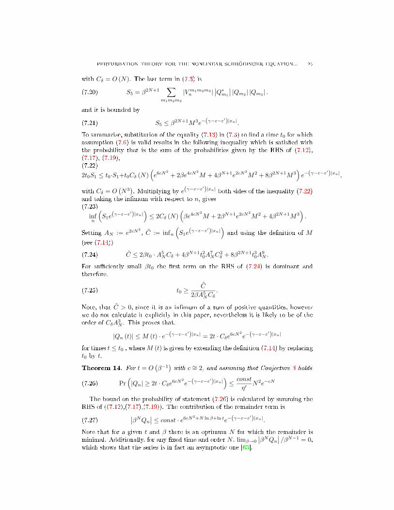
(1.1) i∂tψ = −J [ψ (x+ 1) + ψ (x− 1)] + εωxψ + β |ψ|2 ψwhere ψ = ψ (x, t) , x ∈ Z; and εωxω∈Ω is a collection of i.i.d. random variableschosen from the set Ω, with the probability measure µ (εx) . It will be assumed thatµ (ε (x)) is continuous, bounded and of nite support and, additionally, symmetric,µ (εx) = µ (−εx). We assume that exponential localization is known to take placefor all the energies of the linear problem (when β = 0 ). The decay rate γ and thelocalization length, ξ = 1/γ, are given for the linear part of the model (1.1) by theThouless formula [2]. In particular, if µ (εx) is a uniform distribution than as wasfound numerically (see Appendix), the function γ (E) is unimodal.

The NLSE was derived for a variety of physical systems under some approxima-tions. It was derived in classical optics where ψ is the electric eld by expandingthe index of refraction in powers of the electric eld keeping only the leading non-linear term [3]. For Bose-Einstein Condensates (BEC), the NLSE is a mean eldapproximation where the density β|ψ|2 approximates the interaction between theatoms. In this eld the NLSE is known as the Gross-Pitaevskii Equation (GPE)[4, 5, 6, 7, 8, 9]. Recently, it was rigorously established, for a large variety of in-teractions and of physical conditions, that the NLSE (or the GPE) is exact in thethermodynamic limit [10, 11]. Generalized mean eld theories, in which severalmean-elds are used, were recently developed [12, 13]. In the absence of random-ness (1.1) is completely integrable. For repulsive nonlinearity (β > 0) an initiallylocalized wavepacket spreads, while for attractive nonlinearity (β < 0) solitons arefound typically [1].

It is well known that in 1D in the presence of a random potential and in theabsence of nonlinearity (β = 0) with probability one all the states are exponentially

Date: January 23rd, 2009.Key words and phrases. Anderson localization, NLSE, random potential, nonlinear

Schrodinger, dynamical localization, diusion, sub-diusion.1

arX

iv:0

901.

4951

v2 [

cond

-mat

.dis

-nn]

7 S

ep 2

009

PERTURBATION THEORY FOR THE NONLINEAR SCHRÖDINGER EQUATION... 2

localized [14, 15, 16, 17]. Consequently, diusion is suppressed and in particulara wavepacket that is initially localized will not spread to innity. This is thephenomenon of Anderson localization. In 2D it is known heuristically from thescaling theory of localization [18, 16] that all the states are localized, while inhigher dimensions there is a mobility edge that separates localized and extendedstates. This problem is relevant for experiments in nonlinear optics, for exampledisordered photonic lattices [19], where Anderson localization was found in presenceof nonlinear eects as well as experiments on BECs in disordered optical lattices[20, 21, 22, 23, 24, 25, 26, 27, 28]. The interplay between disorder and nonlineareects leads to new interesting physics [26, 27, 29, 30, 31, 32]. In spite of theextensive research, many fundamental problems are still open, and, in particular,it is not clear whether in one dimension (1D) Anderson localization can survive theeects of nonlinearities. This will be studied here.

A natural question is whether a wave packet that is initially localized in spacewill indenitely spread for dynamics controlled by (1.1). A simple argument in-dicates that spreading will be suppressed by randomness. If unlimited spreadingtakes place the amplitude of the wave function will decay since the L2 norm isconserved. Consequently, the nonlinear term will become negligible and Andersonlocalization will take place as a result of the randomness. Contrary to this intu-ition, based on the smallness of the nonlinear term resulting from the spread ofthe wave function, it is claimed that for the kicked-rotor a nonlinear term leads todelocalization if it is strong enough [33]. It is also argued that the same mecha-nism results in delocalization for the model (1.1) with suciently large β, while,for weak nonlinearity, localization takes place [33, 34]. Therefore, it is predictedin that work that there is a critical value of β that separates the occurrence oflocalized and extended states. However, if one applies the arguments of [33, 34]to a variant of (1.1), results that contradict numerical solutions are found [35, 36].Recently, it was rigorously shown that the initial wavepacket cannot spread so thatits amplitude vanishes at innite time, at least for large enough β [37]. It doesnot contradict spreading of a fraction of the wavefunction. Indeed, subdiusionwas found in numerical experiments [33, 37, 38]. In dierent works [38, 39, 40]sub-diusion was reported for all values of β, but with a dierent power of thetime dependence (compared with Ref. [33]). It was also argued that nonlinearitymay enhance discrete breathers [31, 32]. In conclusion, it is not clear what is thelong time behavior of a wave packet that is initially localized, if both nonlinearityand disorder are present. This is the main motivation for the present work. Sinceheuristic arguments and numerical simulations produce conicting results, rigorousstatements are required for further progress.

More precisely, the question of dynamical localization can be rigorously formu-lated as follows: assume the initial state is, ψ (x, 0) ≡ u0 (x) , where u0 (x) is aneigenstate of the linear part of (1.1) which is localized near x = 0. Then for any0 < δ < 1, one has to prove that with probability 1 − δ (on the space of thepotentials)

(1.2) supx,t

∣∣∣eν|x|ψ (x, t)∣∣∣ < Mδ <∞

for some ν > 0.Rigorous results on dynamical localization for the linear case are well known

[41, 42, 43]. However, the nonlinear problem turns out to be very dicult to

PERTURBATION THEORY FOR THE NONLINEAR SCHRÖDINGER EQUATION... 3

handle, even numerically. Consider the case of small β. There are two possiblemechanisms for destruction of the localization due to nonlinearity.

One way of spreading is to spread into many random places with increasingnumber of them. In that case, due to conservation of the normalization of thesolution, the solution becomes small. But then, the nonlinear term becomes less andless important and we expect the linear theory to take over and lead to localization.While this argument sounds plausible there is no proof along this lines.

The second way of spreading is in a few xed number of spikes that hop randomlyto innity. In this case, the nonlinear term is always relevant. It is this (possible)process that makes the proof of localization in the nonlinear case so elusive. It alsoprecludes a quick numerical analysis of the problem: it may take exponentially longtime to see the hoping.

Rigorous results in this direction are of preliminary nature: In [44] it was shownthat dynamical localization holds for the linear problem perturbed by a periodicin time and exponentially localized in space small linear perturbation. In [45] theabove result was extended to a quasiperiodic in time perturbation. Such perturba-tions mimic the nonlinear term:

(1.3) |ψ|2 →

∣∣∣∣∣∣∑j

cjuj (x) eiEjt

∣∣∣∣∣∣2

where uj are the eigenfunctions of the linear problem with energies Ej . However inother situations time dependent terms may result in delocalization [46, 47]. Usingnormal form transformations Wang and Zhang [48] studied the limit of strong dis-order and weak nonlinearity, namely, ε = J + β, small. For initial wavefunctionswith tails of weight δ starting from point j0, they have proved, that the wave-function spreads as following. There exist C = C (A) > 0 and ε (A) > 0 andK = K (A) > A2 such that for all t ≤ (δ/C) ε−A the weight of the tails of thespreaded wavefunction starting from j = j0 + K is less that 2δ. On the basis ofthis result they have conjectured that the spread of the wave function is at mostlogarithmic in t.

Furthermore, it can be shown that NLSE has stationary solutions

(1.4) EψE = (−∂xx + εωx )ψE + β |ψE |2 ψEwhich are exponentially localized for almost all E with a localization length that isidentical to the one of the linear problem [49, 50, 51, 52, 53].

In our previous work [54] we have developed a perturbation theory in β. Byconsidering the rst order expansion we have proved that for times of order O

(β−2

)the solution of (1.1) remains exponentially localized. A result of similar nature fora nonlinear equation of a dierent structure was obtained in [55]. In the currentwork we consider an expansion of any order, N , in β. This expansion enables inprinciple the calculation of the solution to any order in N . A bound on the errorcan be computed using only propreties of the linear problem (β = 0). Thereforethis work has the potential to develop into a method for solution of some type ofnonlinear dierential equations. In Section 2 we construct the solution as a seriesin the eigenfunctions of the linear problem. Standard perturbation theory for thecoecients does not apply: we encounter small divisor problems and secular terms(formally innite). Removing the secular terms requires the renormalization ofthe original linear Hamiltonian by shifting the energies (Section 3). The estimates

PERTURBATION THEORY FOR THE NONLINEAR SCHRÖDINGER EQUATION... 4

of the small divisor terms are performed in the spirit of the work of Aizenman-Molchanov (A-M) [56]. In Section 4 the entropy problem is resolved by boundingan appropriate recursive relation. A general probabilistic bound on the terms ofthe perturbation theory is derived in Section 5 and the quality of the perturbationtheory is tested in Section 6. In Section 7 the remainder terms are controlled bya bootstrap argument. The results are summarized in Section 8 and the openproblems are listed there.

In summary, in this work a perturbation theory for (1.1) in powers of β wasdeveloped and bounds on the various terms were obtained. The work is only partlyrigorous. In some parts it relies on Conjectures that we test numerically.

2. Organization of the perturbation theory

Our goal is to analyze the nonlinear Schrödinger equation

(2.1) i∂tψ = H0ψ + β |ψ|2 ψ

where H0 is the Anderson Hamiltonian,

(2.2) H0ψ (x) = −J [ψ (x+ 1) + ψ (x− 1)] + εxψ (x) .

We assume throughout the paper that H0 satises the conditions for localization,namely, for almost all the realizations, ω, of the disordered potential, all the eigen-states of H0, um, are exponentially localized and have an envelope of the formof

(2.3) |um (x)| ≤ Dω,εeε|xm|e−γ|x−xm|,

where ε > 0, xm is the localization center which will be dened at the next sub-section, γ is the inverse of the localization length, ξ = γ−1, and Dω,ε is a constantdependent on ε and the realization of the disordered potential [57, 58] (better es-timates were proven recently in [59, 60]). It is of importance that Dω,ε does notdepend on the energy of the state. In the present work only realizations ω, where

(2.4) |Dω,ε| ≤ Dδ,ε <∞

are considered. This is satised for a set of a measure 1− δ , since (2.3) is falseonly for a measure zero of potentials.

2.1. Assignment of eigenfunctions to sites. It is tempting to assign eigenfunc-tions to sites by their maxima, namely, uEi is the eigenfunction with energy Ei anda maximum at site i. This assignment is very unstable with respect to the changeof realizations. This is due to the fact that the point where the maximum is found,which is sometimes called the localization center, may change as a result of a verysmall change in the on-site energies εx. To avoid this, the assignment is denedas the center of mass [61],

(2.5) xE =∑

xx |uEi (x)|2

Denition 1. The state uEi is assigned to site i if i = [xE ] . If several states areassigned to the same site we order them by energy.

PERTURBATION THEORY FOR THE NONLINEAR SCHRÖDINGER EQUATION... 5

2.2. The perturbation expansion. The wavefunction can be expanded using theeigenstates of H0 as

(2.6) ψ (x, t) =∑m

cm (t) e−iEmtum (x) .

For the nonlinear equation the dependence of the expansion coecients, cm (t) , isfound by inserting this expansion into (2.1), resulting in

i∂t∑m

cme−iEmtum (x) = H0

∑m

cme−iEmtum (x)(2.7)

+ β

∣∣∣∣∣∑m

cme−iEmtum (x)

∣∣∣∣∣2∑m3

cm3e−iEm3 tum3 (x) .

Multiplying by un (x) and integrating gives

(2.8) i∂tcn = β∑

m1,m2,m3

V m1m2m3n c∗m1

cm2cm3ei(Em1+En−Em2−Em3)t

where V m1m2m3n is an overlap sum

(2.9) V m1m2m3n =

∑x

un (x)um1 (x)um2 (x)um3 (x) .

By denition V m1m2m3n is symmetric with respect to an interchange of any two in-

dices. Additionally, since the un (x) are exponentially localized around xn, V m1m2m3n

is not negligible only when the interval,

(2.10) δm ≡ max [xn, xmi ]−min [xn, xmi ] ,

is of the order of the localization length, around xn,

|V m1m2m3n | ≤ D4

δ,εeε(|xn|+|xm1 |+|xm2 |+|xm3 |)

∑x

·e−γ(|x−xn|+|x−xm1 |+|x−xm2 |+|x−xm3 |)(2.11)

≤ D4δ,εe

ε(|xn|+|xm1 |+|xm2 |+|xm3 |)e−(γ−ε′)

3 (|xn−xm1 |+|xn−xm2 |+|xn−xm3 |)×

×∑x

·e−ε′(|x−xn|+|x−xm1 |+|x−xm2 |+|x−xm3 |)

≤ V ε,ε′

δ eε(|xn|+|xm1 |+|xm2 |+|xm3 |)e−13 (γ−ε′)(|xn−xm1 |+|xn−xm2 |+|xn−xm3 |).

Here we have used the triangle inequality

(|x− xn|+ |x− xm1 |) + (|x− xn|+ |x− xm2 |) +(2.12)

+ (|x− xn|+ |x− xm3 |) ≥ |xn − xm1 |+ |xn − xm2 |+ |xn − xm3 |

to obtain the second line. Our objective is to develop a perturbation expansion ofthe cm (t) in powers of β and to calculate them order by order in β. The requiredexpansion is

(2.13) cn (t) = c(0)n + βc(1)

n + β2c(2)n + · · ·+ βN−1c(N−1)

n + βNQn,

where the expansion is till order (N − 1) and Qn is the remainder term. We willassume the initial condition

(2.14) cn (t = 0) = δn0.

PERTURBATION THEORY FOR THE NONLINEAR SCHRÖDINGER EQUATION... 6

The equations for the two leading orders are presented in what follows. The leadingorder is

(2.15) c(0)n = δn0.

The equation for the rst order is(2.16)

i∂tc(1)n =

∑m1,m2,m3

V m1m2m3n c∗(0)

m1c(0)m2c(0)m3ei(En+Em1−Em2−Em3)t = V 000

n ei(En−E0)t

and its solution is

(2.17) c(1)n = V 000

n

(1− ei(En−E0)t

En − E0

).

The resulting equation for the second order is

i∂tc(2)n =

∑m1,m2,m3

V m1m2m3n c∗(1)

m1c(0)m2c(0)m3ei(En+Em1−Em2−Em3)t+(2.18)

+ 2∑

m1,m2,m3

V m1m2m3n c∗(0)

m1c(1)m2c(0)m3ei(En+Em1−Em2−Em3)t.

Substitution of the lower orders yields

i∂tc(2)n =

∑m

V m00n V 000

m

[(1− e−i(Em−E0)t

Em − E0

)ei(En+Em−2E0)t+(2.19)

+2(

1− ei(Em−E0)t

Em − E0

)ei(En−Em)t

]=∑m

V m00n V 000

m

Em − E0

[(ei(En+Em−2E0)t − ei(En−E0)t

)+

+2(ei(En−Em)t − ei(En−E0)t

)]=∑m

V m00n V 000

m

Em − E0

[ei(En+Em−2E0)t − 3ei(En−E0)t + 2ei(En−Em)t

].

We notice that divergence of this expansion for any value of β may result from threemajor problems: the secular terms problem, the entropy problem (i.e., factorialproliferation of terms), and the small denominators problem.

3. Elimination of secular terms

We rst show how to derive the equations for cn (t) where the secular terms areeliminated.

Proposition 2. To each order in β, ψ (x, t) can be expanded as

(3.1) ψ (x, t) =∑n

cn (t) e−iE′ntun (x)

with

(3.2) E′n ≡ E(0)n + βE(1)

n + β2E(2)n + · · ·

and E(0)n are the eigenvalues of H0, in such a way that there are no secular terms

to any given order. The E′n are called the renormalized energies.

PERTURBATION THEORY FOR THE NONLINEAR SCHRÖDINGER EQUATION... 7

Here we rst develop the general scheme for the elimination of the secular termsand then demonstrate the construction of E′n when the cn (t) are calculated to thesecond order in β (see 3.19,3.18).

Inserting the expansion into (2.1) yields

i∑m

[∂tcm − iE′mcm] e−iE′mtum (x) =

∑m

E(0)m cme

−iE′mtum (x) +

(3.3)

+β∑

m1m2m3

c∗m1cm2cm3e

i(E′m1−E′m2

−E′m3)tum1 (x)um2 (x)um3 (x) .

Multiplication by un (x) and integration gives(3.4)

i∂tcn =(E(0)n − E′n

)cn + β

∑m1m2m3

V m1m2m3n c∗m1

cm2cm3ei(E′n+E′m1

−E′m2−E′m3)t,

where the V m1m2m3n are given by (2.9). Following (2.13) we expand cn in orders of

β, namely,

(3.5) cn = c(0)n + βc(1)

n + β2c(2)n + · · · , .

Inserting this expansion into (3.4) and comparing the powers of β without expand-ing the exponent, produces the following equation for the k − th order

i∂tc(k)n = −

k−1∑s=0

E(k−s)n c(s)n +

(3.6)

+∑

m1m2m3

V m1m2m3n

[k−1∑r=0

k−1−r∑s=0

k−1−r−s∑l=0

c(r)∗m1c(s)m2

c(l)m3

]ei(E

′n+E′m1

−E′m2−E′m3)t.

Note that the exponent is of order O (1) in β, and therefore we may choose not to

expand it in powers of β. However, it generates an expansion where both E(l)m and

c(k)n depend on β. For the expansion (2.13) to be valid, both E

(l)m and c

(k)n should be

O (1) in β, this is satised since the RHS of (3.6) contains only c(r)n such that r < k.

Namely, this equation gives each order in terms of the lower ones, with the initial

condition of c(0)n (t) = δn0 . Solution of k equations (3.6) gives the solution of the

dierential equation (3.4) to order k. Since, the exponent in (3.6) is of order O (1)in β we can select its argument to be of any order in β. However, for the removalof the secular terms, as will be explained bellow, it is instructive to set the orderof the argument to be k− 1, as the higher orders were not calculated at this stage.Secular terms are created when there are time independent terms in the RHS ofthe equation above. We eliminate those terms by using the rst two terms in the

rst summation on the RHS. We make use of the fact that c(0)n = δn0 and c

(1)n can

be easily determined (see (3.9,3.12)), and used to calculate E(k)n=0 and E

(k−1)n 6=0 that

eliminate the secular terms in the equation for c(k)n , that is

(3.7) E(k)n c(0)

n + E(k−1)n c(1)

n = E(k)n δn0 + E(k−1)

n (1− δn0)V 000n

E′n − E′0,

PERTURBATION THEORY FOR THE NONLINEAR SCHRÖDINGER EQUATION... 8

where only the time-independent part of c(1)n was used. In other words, we choose

E(k)n and E

(k−1)n6=0 so that the time-independent terms on the RHS of (3.6) are elim-

inated. E(k)0 will eliminate all secular terms with n = 0, and E(k−1)

n will eliminateall secular terms with n 6= 0. In the following, we will demonstrate this procedure

for the rst two orders, and calculate c(1)n , and obtain an equation for c

(2)n .

In the rst order of the expansion in β we obtain

i∂tc(1)n = −E(1)

n c(0)n +

∑m1m2m3

V m1m2m3n c∗(0)

m1c(0)m2c(0)m3ei(E

′n+E′m1

−E′m2−E′m3)t(3.8)

= −E(1)n δn0 + V 000

n ei(E′n−E

′0)t.

For n = 0 the equation produces a secular term

i∂tc(1)0 = −E(1)

0 + V 0000(3.9)

c(1)0 = it ·

(E

(1)0 − V 000

0

).

Setting

(3.10) E(1)0 = V 000

0

will eliminate this secular term and gives

(3.11) c(1)0 = 0

For n 6= 0 there are no secular terms in this order, therefore nally

(3.12) c(1)n = (1− δn0)V 000

n

(1− ei(E

′n−E

′0)t

E′n − E′0

),

where to this order E′n = En and E′0 = E0.In the second order of the expansion in β we have

i∂tc(2)n = −E(1)

n c(1)n − E(2)

n c(0)n +

(3.13)

+∑

m1m2m3

V m1m2m3n

(c∗(1)m1

c(0)m2c(0)m3

+ 2c∗(0)m1

c(1)m2c(0)m3

)ei(E

′n+E′m1

−E′m2−E′m3)t

= −E(2)n δn0 − E(1)

n c(1)n +

∑m1

V m100n

(c∗(1)m1

ei(E′n+E′m1

−2E′0)t + 2c(1)m1ei(E

′n−E

′m1)t

).

For n = 0 it takes the form

i∂tc(2)0 = −E(2)

0 +∑m

V m000

(c∗(1)m ei(E

′m−E

′0)t + 2c(1)

m ei(E′0−E

′m)t).

Substitution of (3.9) and (3.12) yields

i∂tc(2)0 = −E(2)

0 +∑m 6=0

V m000 V 000

m

E′m − E′0

[(1− e−i(E

′m−E

′0)t)ei(E

′m−E

′0)t+(3.14)

+2(

1− ei(E′m−E

′0)t)ei(E

′0−E

′m)t]

= −E(2)0 +

∑m 6=0

V m000 V 000

m

E′m − E′0

(ei(E

′m−E

′0)t + 2ei(E

′0−E

′m)t − 3

),

PERTURBATION THEORY FOR THE NONLINEAR SCHRÖDINGER EQUATION... 9

and the secular term could be removed by setting

(3.15) E(2)0 = −3

∑m 6=0

V m000 V 000

m

E′m − E′0.

For n 6= 0 we have

i∂tc(2)n = −E(1)

n V 000n

(1− ei(E

′n−E

′0)t

E′n − E′0

)+(3.16)

+∑m

V m00n

(c∗(1)m ei(E

′n+E′m−2E′0)t + 2c(1)

m ei(E′n−E

′m)t)

=− E(1)n V 000

n

(1− ei(E

′n−E

′0)t

E′n − E′0

)+

+∑m 6=0

V m00n V 000

m

E′m − E′0

(ei(E

′n+E′m−2E′0)t + 2ei(E

′n−E

′m)t − 3ei(E

′n−E

′0)t).

We notice that the second term in the sum produces secular terms form = n. Thoseterms could be removed by setting

(3.17) − E(1)n V 000

n

E′n − E′0+

2V n00n V 000

n

E′n − E′0= 0 n 6= 0

E(1)n = 2V n00

n n 6= 0.

To conclude, up to the second order in β , the perturbed energies, which are requiredto remove the secular terms, are given by

(3.18) E′n = E(0)n + βV n00

n (2− δn0)− 3β2δn0

∑m6=0

(V 000m

)2E′m − E′0

,

and the corresponding correction to c(0)n is

(3.19)

i∂tc(2)n =

∑m6=0

Vm000 V 000

m

E′m−E′0

(ei(E

′m−E

′0)t + 2ei(E

′0−E

′m)t)

n = 02V n00n V 000

n

E′n−E′0ei(E

′n−E

′0)t +

∑m 6=0,n

2Vm00n V 000

m

E′m−E′0ei(E

′n−E

′m)t+

+∑m 6=0

Vm00n V 000

m

E′m−E′0

(ei(E

′n+E′m−2E′0)t − 3ei(E

′n−E

′0)t) n 6= 0

.

Note that in the calculation of cn to higher orders in β, a secular term of theorder β2 will be generated for n 6= 0 . Secular terms with increasing complexityare generated in the cancellation of higher orders, however, as demonstrated by

(3.7), secular terms are removed with the same c(0)n and c

(1)n which are presented in

(2.15,3.12).In the next section, the entropy problem will be studied. It will be shown that

the proliferation of terms in the expansion is at most exponential.

PERTURBATION THEORY FOR THE NONLINEAR SCHRÖDINGER EQUATION... 10

4. The entropy problem

Since the time dependence of all orders is bounded (excluding the secular terms),we can bound each order of the expansion by

∣∣∣c(0)n

∣∣∣ = δn0

(4.1)

∣∣∣c(1)n

∣∣∣ =

∣∣∣∣∣V 000n

(1− ei(E

′n−E

′0)t

E′n − E′0

)∣∣∣∣∣ ≤ 2∣∣∣∣ V 000

n

E′n − E′0

∣∣∣∣∣∣∣c(2)n

∣∣∣ =

∣∣∣∣∣∑m

∫ t

0

dt′(V m00n V 000

m

E′m − E′0

)(ei(E

′n+E′m−2E′0)t′ − 3ei(E

′n−E

′0)t′ + 2ei(E

′n−E

′m)t′

)∣∣∣∣∣≤ 2 ·

∑m

∣∣V m00n

∣∣ ∣∣V 000m

∣∣|E′m − E′0|

(1

|(E′n + E′m − 2E′0)|+

3|E′n − E′0|

+2

|E′n − E′m|

)et cetera. However, for convergence for a nite but possibly small β, it is essentialthat the number of terms on the RHS of (4.1) will not increase faster than expo-nentially in k, e.g. not as k!, where k is the expansion order. Next we will showthat the number of terms indeed increases at most exponentially in k.

We will designate the number of dierent products of order k of V ′s by Rk (ontop of it there is still a number of non vanishing terms in the sums over m, that

will be estimated in the next section). By replacing each c(l)n in (3.6) by Rl (the

integration with respect to time multiples the number of terms by a factor of 2, cf.(4.1)) we deduce a recursive expression for Rk

(4.2) Rk =k−1∑r=0

k−1−r∑l=0

RrRlRk−1−r−l R1 = 1 R0 = 1.

In order to nd an upper bound on Rk we examine the structure of the productsof V ′s we notice that each product could be uniquely labeled by a vector of zerosand m′is(4.3)V m100n V m2m30

m1· · ·V 0mk−10

mk−2V 000mk−1

→ m1, 0, 0,m2,m3, 0, · · · , 0,mk−1, 0, 0, 0, 0 ,

where the number of dierent summation indices mi is (k − 1) and the length of thelabeling vector is 3k. Since in each vector the last three elements should always bezeros the number of dierent congurations of this product is the number of ways

to distribute (k − 1) m′s in 3 (k − 1) cells (superscripts), namely, Rk <(

3(k−1)k−1

).

This is only an upper bound, since there may be some additional constraints, forexample, the rst three elements in the vector should never be all zeros. Subtracting

the cases when all three rst elements are zero(

3(k−2)k−1

)we obtain the bound

(4.4) Rk <

(3 (k − 1)k − 1

)−(

3 (k − 2)k − 1

).

This bound has the following asymptotics

(4.5) limk→∞

1k

ln[(

3k − 3k − 1

)−(

3k − 6k − 1

)]= ln

274,

PERTURBATION THEORY FOR THE NONLINEAR SCHRÖDINGER EQUATION... 11

namely,

(4.6) Rk ≤ ek ln 274 ≤ e2k.

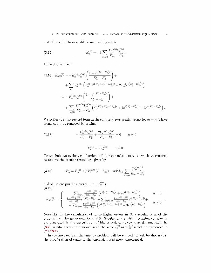
From Fig.4.1 we conclude that this bound is a tight bound of the exact solutionof the recurrence relation. This bound shows that the number of terms in the

0 50 100 150 200 250 3000

50

100

150

200

250

300

350

400

450

500

550

k

ln R

k

Figure 4.1. The solid line denotes the exact numerical solutionof the recurrence relation for Rk and dashed line is the asymptoticupper bound on this solution

(e2k).

expansion increases at most exponentially in k and therefore there is no entropyproblem.

5. Bounding the general term

As clear from (3.6) after the subtraction of all the secular terms in the precedingorders the dierential equation for the k-th order term is

i∂tc(k)n = −

k−1∑s=0

E(k−s)n c(s)n +

(5.1)

+∑

m1m2m3

V m1m2m3n

[k−1∑r=0

k−1−r∑s=0

k−1−r−s∑l=0

c(r)∗m1c(s)m2

c(l)m3

]ei(E

′n+E′m1

−E′m2−E′m3)t.

with the initial condition of c(0)n = δn0 and the rst term on the RHS is designed (see

Section 3) to eliminate all the time-independent part of of RHS of (5.1). Followingthe construction of the lower order terms in the preceding section by a repeatedapplication of (5.1) the structure of the general term in the expression for a given

order k can be obtained. Note that the structure E(l)n is similar to the structure of

c(l)n . The main blocks of the structure take the form

(5.2) ζm1m2m3n ≡ V m1m2m3

n

E′n − E′miwhere E′mi denotes a sum of eigenenergies (shifted so that the secular terms are

removed, see (3.2)) that may depend on the summation indices mi. Then any term

PERTURBATION THEORY FOR THE NONLINEAR SCHRÖDINGER EQUATION... 12

of order k is a product of k factors of the form (5.2) and k − 1 summations overthe indices mi

(5.3)

k terms︷ ︸︸ ︷ζm1m2m3n ζm4m5m6

m1· · · ζ000

m5ζ000m6

and following the last section there is an exponentially increasing (in k) number ofsuch terms. In order to bound the general term of order k we will rst bound onetypical block, namely,

(5.4) ζm1m2m3n ≡ V m1m2m3

n

E′n − E′miwhere E′mi is some sum of E′j . To bound (5.4) we will bound separately thedenominator and the numerator. Using Cauchy-Schwarz inequality,

(5.5) 〈|ζm1m2m3n |s〉 ≤

⟨1∣∣E′n − E′mi∣∣2s

⟩1/2 ⟨|V m1m2m3n |2s

⟩1/2

,

where 0 < s < 12 .

Conjecture 3. For the Anderson model, which is given by the linear part of (1.1),the joint distribution of R eigenenergies is bounded,

p (E1, E2, . . . , ER) ≤ DR

where DR ∝ R! <∞.

The conjecture is inspired by Theorem (3.1) of the recent paper by Aizenman andWarzel [62]. If one assumes that with probability one the proles of the eigenfunc-tions, namely, the squares of the eigenfunctions, which correspond to the eigenener-

gies EiRi=1 are substantially dierent such that α (as dened in Theorem (3.1) of[62]) is bounded away from zero, than taking the intervals Ij = dEj one nds that

the joint probability density can be bounded by DR ∝ R!αR

. It is not known how toprove that for the Anderson model the proles of the wave functions are distnictand how to quantify this. However, it is reasonable to assume distinctness sincedierent eigenfunctions are localized in dierent regions and therefore are aectedby dierent potentials. There are double humped states (consisting of nearly sym-metric and antisymmetric combinations of two humps), which have approximatelythe same squares, and therefore are natural candidates for states that may result inviolation of the conjecture. Nevertheless, those states are very rare and the dier-ence between their squares is exponential in the distance between the humps. Forthis it is crucial that many sites are invloved (therefore the counter example (2.1)of [62] is not generic). If the energies are assigned to specic locations than thefactorial term could be dropped, namely, DR ∝ α−R. This is due to the fact thatspecic assignment of energies chooses one of the R! permutations, mentioned in[62].

Corollary 4. Given 0 < s < 1, for f =R∑k=1

ckEik , where ck are integers (and the

assignment of eigenfunctions to sites is given by Denition 1) the following meanis bounded from above

(5.6)

⟨1|f |s

⟩≤ DR <∞.

PERTURBATION THEORY FOR THE NONLINEAR SCHRÖDINGER EQUATION... 13

where DR ∝ DR.

Proof. By Conjecture 3,

(5.7)

⟨1|f |s

⟩=∫p (E1, E2, . . . , ER) dE1dE2 · · · dER∣∣∣∣∣

R∑k=1

ckEik

∣∣∣∣∣s ≤ DR

∫dE1dE2 · · · dER∣∣∣∣∣

R∑k=1

ckEik

∣∣∣∣∣s ,

changing the variables to f,E2, E3, . . . , ER gives

(5.8)

⟨1|f |s

⟩≤ DR

∫ ∆

−∆

dE2 · · · dER|c1|

∫f(~E)

df1|f |s

,

where |c1| is the Jacobian and 2∆ is the support of the energies. Due to the factthat f (E1) is linear the multiplicity is one. Since the integrand is positive we canonly increase the integral by increasing the domain of integration of f . Designatingby f∞ the maximal value of f ,

(5.9)

⟨1|f |s

⟩≤ 2DR∆R−1 f

1−s∞

1− s≡ DR.

Conjecture 5. In the limit of R→∞, for 0 < s < 1 and for f =R∑k=1

ckEik , where

ck are integers (and the assignment of eigenfunctions to sites is given by Denition1)

(5.10)

⟨1|f |s

⟩ 1Rs/2

For large R the sum, f =R∑k=1

ckEik , can be eectively separated into groups of

terms that depend on dierent diagonal energies, εj . Therefore by the central limittheorem, f is eectively a Gaussian variable with 〈f〉 = 0 and

⟨f2⟩

= σ2R, where

σ2 is some constant. Therefore,(5.11)⟨

1|f |s

⟩ 2√

2πσ2R

∫ ∞0

df

fse−f

2/(2σ2R) =2

√2π(√

σ2R)s ∫ ∞

0

df

fse−f

2/2 R− s2 .

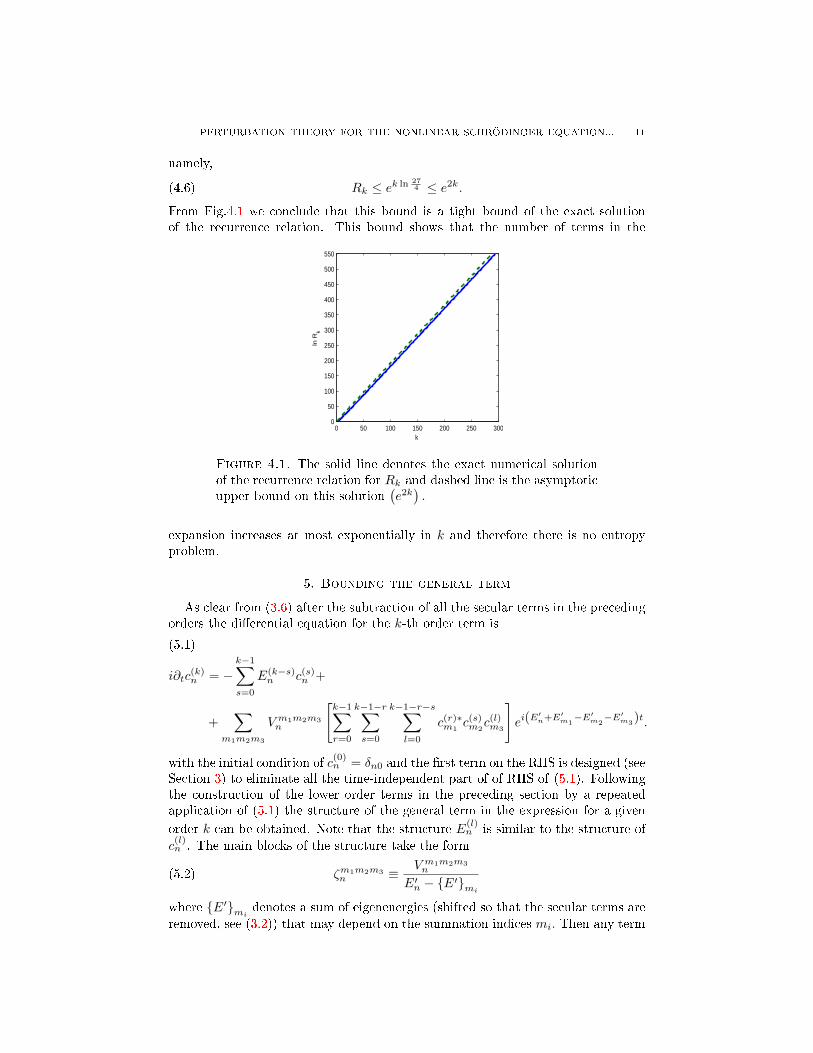
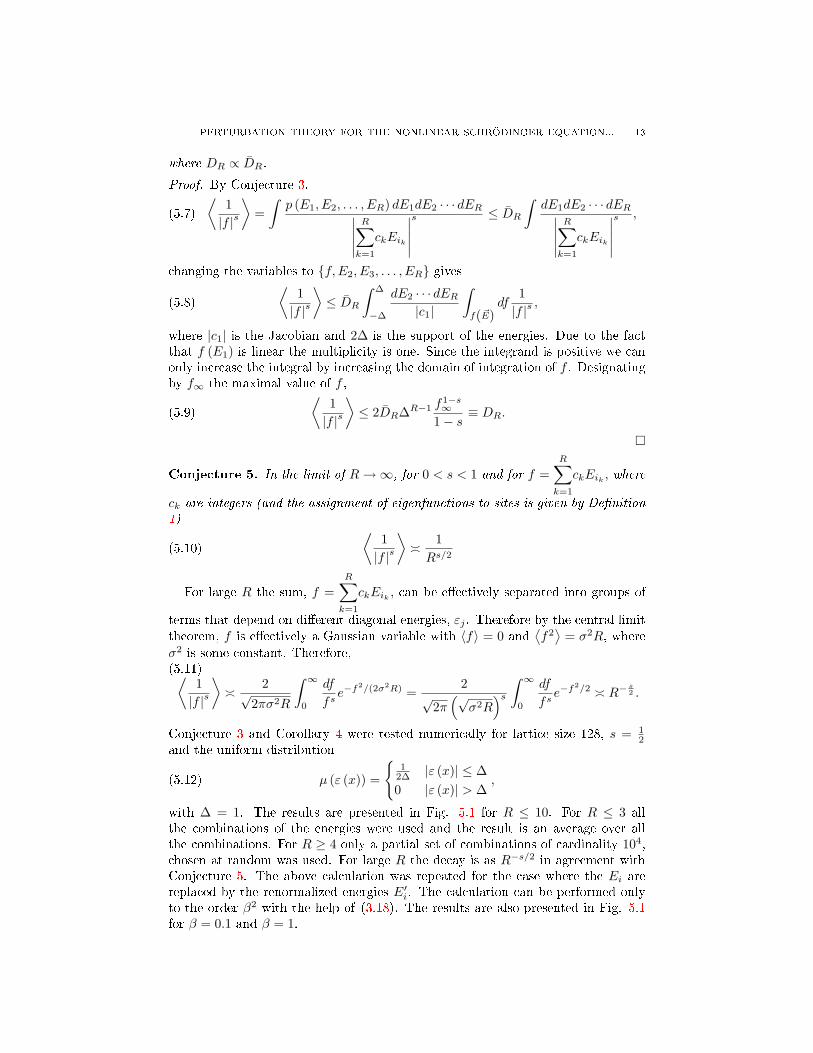
Conjecture 3 and Corollary 4 were tested numerically for lattice size 128, s = 12

and the uniform distribution

(5.12) µ (ε (x)) =

1

2∆ |ε (x)| ≤ ∆0 |ε (x)| > ∆

,

with ∆ = 1. The results are presented in Fig. 5.1 for R ≤ 10. For R ≤ 3 allthe combinations of the energies were used and the result is an average over allthe combinations. For R ≥ 4 only a partial set of combinations of cardinality 104,chosen at random was used. For large R the decay is as R−s/2 in agreement withConjecture 5. The above calculation was repeated for the case where the Ei arereplaced by the renormalized energies E′i. The calculation can be performed onlyto the order β2 with the help of (3.18). The results are also presented in Fig. 5.1for β = 0.1 and β = 1.

PERTURBATION THEORY FOR THE NONLINEAR SCHRÖDINGER EQUATION... 14

0.8 1 1.2 1.4 1.6 1.8 2 2.2 2.4 2.6−0.3

−0.2

−0.1

0

0.1

0.2

0.3

0.4

0.5

0.6

ln(R)

ln(<

|f|−

s >)

J = 1J = 0.5J = 0.25data 4data 5data 6data 7data 8data 9

Figure 5.1. The logarithm of⟨|f |−1/2

⟩as a function of the

logarithm of R. The lines designate denominators with β = 0,with the solid line (blue) is for J = 0.25 the dashed line (green) isfor J = 0.5 and the dot-dashed line (red) is for J = 1. The solidcircles and the squares are data with β = 1, and E′n calculated upto the second in β, such that dierent colors represent dierent J ,in the similar manner as for the lines. The solid squares are forparameters similar to the ones with the solid circles, but with therestriction that at least one of the states that corresponds to E′nwhich is localized near the origin.

Conjecture 6. Corollary 4 and Conjecture 5 hold also if the Ei are replaced bythe renormalized energies E′i.

The reason is that the various renormalized energies are dominated by dierentindependent random variables εi. The numerical calculations support this pointof view. In what follows Corollary 4 and Conjecture 6 (and not Conjecture 3) areused, and these were tested numerically (Fig. 5.1).

Using the bound on the overlap sum (2.11) and Corollary 4,(5.13)

〈|ζm1m2m3n |s〉δ ≤ Dδ

∣∣∣V ε,ε′δ

∣∣∣s eεs(|xn|+|xm1 |+|xm2 |+|xm3 |)e−13 (γ−ε′)s(|xn−xm1 |+|xn−xm2 |+|xn−xm3 |).

this proves the proposition:

Proposition 7. For some δ, ε, ε′ > 0 and 0 < s < 12 ,

(5.14) 〈|ζm1m2m3n |s〉δ ≤ F

′eεs(|xn|+Pi|xmi |)e−

13 (γ−ε′)sP

i|xn−xmi |

where F ′ = Dδ

∣∣∣V ε,ε′δ

∣∣∣s.

PERTURBATION THEORY FOR THE NONLINEAR SCHRÖDINGER EQUATION... 15

Using the Chebyshev inequality,

(5.15) Pr (|x| ≥ a) ≤ 〈|x|〉 /a,

where x is a random variable and a is a constant, one nds

Corollary 8.(5.16)

Pr(|ζm1m2m3n | ≥ F ′1/seε(|xn|+

Pi|xmi |)e−

13 (γ−ε′−η) P

i|xn−xmi |)≤ e−

ηs3

Pi|xn−xmi |

where F ′ = Dδ

∣∣∣V ε,ε′δ

∣∣∣s.A general term in the expression for dierent orders of c

(k)n is given by the form of

|ζm1m2m3n |

∣∣ζm4m5m6m1

∣∣ · · · ∣∣∣ζ000mk−1

∣∣∣ , i.e., it contains (k − 1) summations over indices

which run over all the lattice. First we construct a general procedure to bound aproduct of k, ζ 's. A product of two ζ 's is bounded by⟨∣∣∣∣∣∑

m1

ζm1m2m3n ζm4m5m6

m1

∣∣∣∣∣s⟩

δ

≤

⟨∑m1

|ζm1m2m3n |s

∣∣ζm4m5m6m1

∣∣s⟩δ

,

where 〈·〉δ denotes an average over realizations where (2.4) is satised.Using the Cauchy-Shwarz inequality∑

m1

⟨|ζm1m2m3n |s

∣∣ζm4m5m6m1

∣∣s⟩δ≤∑m1

⟨|ζm1m2m3n |2s

⟩1/2

δ

⟨∣∣ζm4m5m6m1

∣∣2s⟩1/2

δ

setting 0 < s < 14 (notice, that s < 1

4 and not s < 12 , due to (5.5)) and inserting

the bound on the average⟨|ζm1m2m3n |2s

⟩δfrom Proposition 7 gives⟨∣∣∣∣∣∑

m1

ζm1m2m3n ζm4m5m6

m1

∣∣∣∣∣s⟩

δ

(5.17)

≤ F ′ exp

[εs

(|xn|+

6∑i=2

|xmi |

)]e−s

γ−ε′3 (|xn−xm2 |+|xn−xm3 |)×

×∑m1

e2εs|xm1 | exp−sγ − ε′

3

(|xn − xm1 |+

6∑i=4

|xm1 − xmi |

),

where we have used the inequality(∑i

|xi|

)s≤∑i

|xi|s 0 < s < 1.

Using the triangle inequality in the same manner as in (2.12)

|xn − xm1 |+6∑i=4

|xm1 − xmi | ≥13

6∑i=4

|xn − xmi |+23

6∑i=4

|xm1 − xmi |(5.18)

PERTURBATION THEORY FOR THE NONLINEAR SCHRÖDINGER EQUATION... 16

we get

⟨∣∣∣∣∣∑m1

ζm1m2m3n ζm4m5m6

m1

∣∣∣∣∣s⟩

δ

(5.19)

≤ F ′ exp εs

(|xn|+

6∑i=2

|xmi |

)e−

γ−ε′3 s(|xn−xm2 |+|xn−xm3 |)×

× exp

[−γ − ε

′

9s

6∑i=4

|xn − xmi |

]∑m1

e2εs|xm1 |e−2 γ−ε

′3 s

6Pi=4|xm1−xmi |

= F ′′ exp

[sε

(|xn|+

6∑i=2

|xmi |

)− γ − ε′

9s

6∑i=4

|xn − xmi |

]e−

γ−ε′3 s(|xn−xm2 |+|xn−xm3 |),

where F ′′ (γ, ε′, s, ε) = F ′∑m1

e2εs|xm1 |e−2 γ−ε

′3 s

6Pi=4|xm1−xmi |

< ∞, in the following

also other convergent sums of this type will be denoted by F ′′.If the term we consider is a term in the perturbation expansion it should include

some factors ζm1m2m3m with somemi = 0.A simple example is where xm1 = xm2 = xm3 = 0

(5.20)⟨∣∣ζ000

m

∣∣s⟩δ≤ F ′e−s(γ−ε

′−ε)|xn|,

where the bound was calculated using Proposition 7. The product should terminatewith a term of the form ζ000

m therefore a term like (5.17) is a part of a product ofthe form,

(5.21)∑mi

|ζm1m2m3n |

∣∣ζm4m5m6m1

∣∣ ∣∣ζ000m2

∣∣ ∣∣ζ000m3

∣∣ ∣∣ζ000m4

∣∣ ∣∣ζ000m5

∣∣ ∣∣ζ000m6

∣∣ .To bound it we use the generalized Hölder inequality,

⟨k∏i=1

|xi|

⟩≤

k∏i=1

⟨|xi|k

⟩1/k

.

Applying it yields,

∑mi

⟨|ζm1m2m3n |s

∣∣ζm4m5m6m1

∣∣s ∣∣ζ000m2

∣∣s ∣∣ζ000m3

∣∣s ∣∣ζ000m4

∣∣s ∣∣ζ000m5

∣∣s ∣∣ζ000m6

∣∣s⟩δ

(5.22)

≤∑mi

(⟨|ζm1m2m3n |7s

⟩δ

⟨∣∣ζm4m5m6m1

∣∣7s⟩δ

6∏i=2

⟨∣∣ζ000mi

∣∣7s⟩δ

)1/7

PERTURBATION THEORY FOR THE NONLINEAR SCHRÖDINGER EQUATION... 17

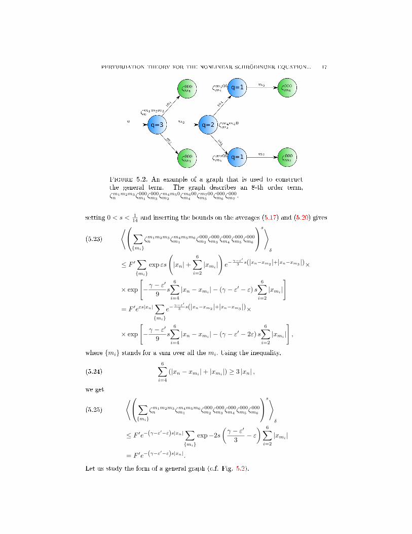
Figure 5.2. An example of a graph that is used to constructthe general term. The graph describes an 8-th order term,ζm1m2m3n ζ000

m1ζ000m3

ζm4m50m2

ζm600m4

ζm700m5

ζ000m6

ζ000m7

.

setting 0 < s < 114 and inserting the bounds on the averages (5.17) and (5.20) gives⟨∑mi

ζm1m2m3n ζm4m5m6

m1ζ000m2

ζ000m3

ζ000m4

ζ000m5

ζ000m6

s⟩δ

(5.23)

≤ F ′∑mi

exp εs

(|xn|+

6∑i=2

|xmi |

)e−

γ−ε′3 s(|xn−xm2 |+|xn−xm3 |)×

× exp

[−γ − ε

′

9s

6∑i=4

|xn − xmi | − (γ − ε′ − ε) s6∑i=2

|xmi |

]= F ′eεs|xn|

∑mi

e−γ−ε′

3 s(|xn−xm2 |+|xn−xm3 |)×

× exp

[−γ − ε

′

9s

6∑i=4

|xn − xmi | − (γ − ε′ − 2ε) s6∑i=2

|xmi |

],

where mi stands for a sum over all the mi. Using the inequality,

(5.24)

6∑i=4

(|xn − xmi |+ |xmi |) ≥ 3 |xn| ,

we get ⟨∑mi

ζm1m2m3n ζm4m5m6

m1ζ000m2

ζ000m3

ζ000m4

ζ000m5

ζ000m6

s⟩δ

(5.25)

≤ F ′e−(γ−ε′−ε)s|xn|∑mi

exp−2s(γ − ε′

3− ε) 6∑i=2

|xmi |

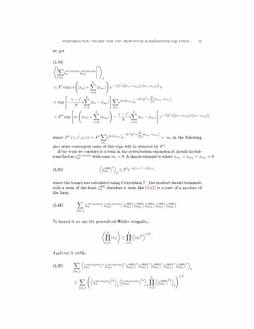
= F ′e−(γ−ε′−ε)s|xn|.

Let us study the form of a general graph (c.f. Fig. 5.2).

PERTURBATION THEORY FOR THE NONLINEAR SCHRÖDINGER EQUATION... 18

It can be described as a tree starting from n, the "root" and four types of branch-ing points, where q (0 ≤ q ≤ 3) branches continue while 3−q branches terminate. Abranch which continues is associated with a valuemi 6= 0, while a branch terminateswith mi = 0. In the above, bounds on branches with q = 0 and 3 are calculated,and are given by (5.14) and (5.20), respectively. The bounds for q = 1, 2 followsimilarly from Proposition 7. Along each bond from the "root" to the leaves aterm ζm1m2m3

n is multiplied. At a point from where q branches continue the ex-ponent is reduced by a factor of q. In other words, with xn and xm are connectedby a path that is crossing l branching points with ratios q1, . . . , ql the bound on

the product of the zetas contains a factor exp−γq |xn − xm| where q =l∏i=1

qi. The

total number of branch ends is also q. To terminate all the branches q factors ofthe form ζ000

mi (bounded by (5.20)) should be multiplied resulting in the a term thatmultiplies the bound on a sum of the form∑

mi

exp

[− (γ − ε′)

qs∑i

|xn − xmi | − (γ − ε′) s∑i

|xmi |

](5.26)

≤ exp− (γ − ε′)q

s∑i

|xn|∑mi

exp−(

1− 1q

)(γ − ε′) s

∑i

|xmi |

= e−γ−ε′q sq|xn|

∑mi

exp−(

1− 1q

)(γ − ε′) s

∑i

|xmi | ≡ Sεe−(γ−ε′)s|xn|

restoring the original convergence rate. As the product consists of k terms the

evaluation of |ζm1m2m3n |sk is required for the use of the Hölder inequality. Therefore

it is required that 0 < s < 1/2k.

Lemma 9. For a given k (the number of ζ's), δ, ε, ε′, η′ > 0 and 0 < s < 12k

(5.27)

⟨∣∣∣∣∣∣∑mi

ζm1m2m3n ζm4m5m6

m1· · · ζ000

mN−1

∣∣∣∣∣∣s⟩

δ

≤ F (k)δ e−(γ−ε−ε′)s|xn|

or using the Chebyshev inequality (5.15)(5.28)

Pr

∣∣∣∣∣∣∑mi

ζm1m2m3n ζm4m5m6

m1· · · ζ000

mN−1

∣∣∣∣∣∣ ≥(F

(k)δ

)1/s

e−(γ−ε−ε′−η′)|xn|

≤ e−η′s|xn|,where F

(k)δ is a constant which is built iteratively by the construction demonstrated

in (5.23) and (5.25) and is proportional to Dδ.

It is of importance, that any product with the same number of zetas has the

same bound with the same probability. This allows us to bound c(k)n by counting

the number of dierent congurations, Rk, of the product for a given k and thenmultiplying it by the bound of each product. This proves the theorem:

Theorem 10. For a given k and δ, ε, ε′, η′ > 0

(5.29) Pr(∣∣∣c(k)

n

∣∣∣ ≥ (F (k)δ

)keck

2+c′ke−(γ−ε−ε′−η′)|xn|)≤ e−c

′e−η

′|xn|/k.

PERTURBATION THEORY FOR THE NONLINEAR SCHRÖDINGER EQUATION... 19

where F(k)δ which is proportional to Dδ and c and c′ are constants.

Proof. Using Lemma 9 and summing over congurations denoted by ic one obtainsthe bound

⟨∣∣∣c(k)n

∣∣∣s⟩δ

=

⟨∣∣∣∣∣∣Rk∑ic=1

∑mi

ζm1m2m3n ζm4m5m6

m1· · · ζ000

mk−1

∣∣∣∣∣∣s⟩

δ

(5.30)

≤Rk∑ic=1

⟨∣∣∣∣∣∣∑mi

ζm1m2m3n ζm4m5m6

m1· · · ζ000

mk−1

∣∣∣∣∣∣s⟩

δ

≤ RkF (k)δ e−(γ−ε−ε′)s|xn|.

Using (4.6)

(5.31)⟨∣∣∣c(k)

n

∣∣∣s⟩δ≤ e2kF

(k)δ e−(γ−ε−ε′)s|xn|

or

(5.32) Pr(∣∣∣c(k)

n

∣∣∣ ≥ ec′/s (F (k)δ

)1/s

e−(γ−ε−ε′−η′)|xn|e2k/s

)≤ e−c

′e−η

′s|xn|

Choosing the largest s produces a bound where c, c′ are constants and F(k)δ is a

constant which is built iteratively by the construction demonstrated in (5.23) and(5.25) and is proportional to Dδ.

Remark 11. From (4.6) one sees that c w 2 and later we set c′ = cN .

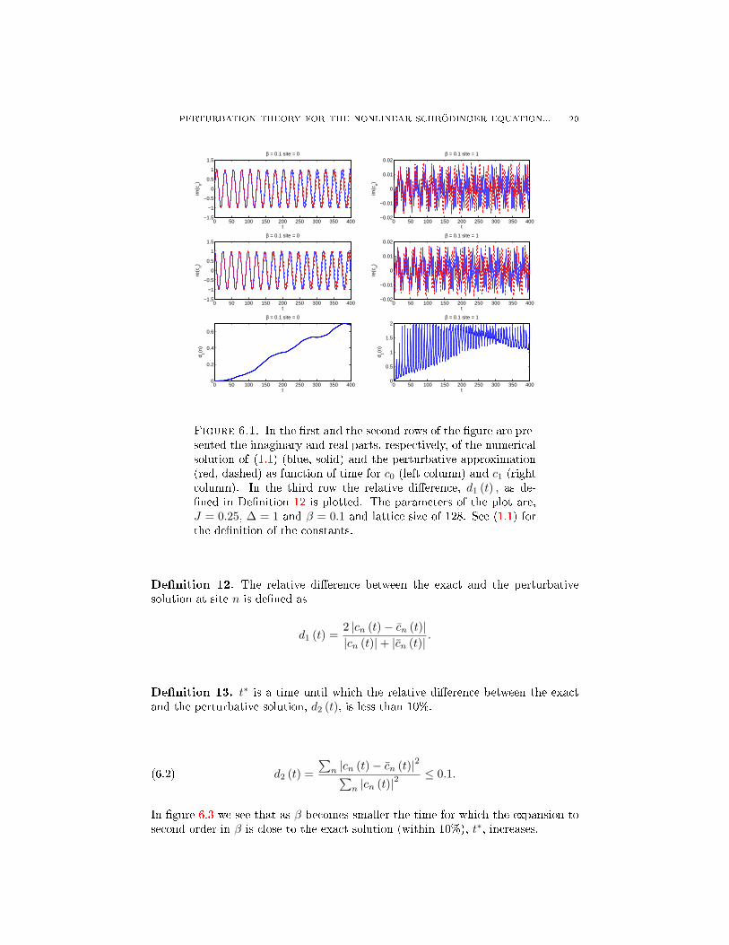
6. Numerical results

In this section we will check how well the perturbation series up to the secondorder in β approximates the numerical solution of (1.1). For this purpose we use the

expressions for c(1)n and c

(2)n which were obtained in (3.12) and (3.19), respectively,

and also the expression for the renormalized energies E′n up to second order in βwhich are given by (3.18). We use the perturbation expansion up to the secondorder in β, namely

(6.1) cn = c(0)n + βc(1)

n + β2 c(2)n

∣∣∣β=0

,

where we took c(2)n

∣∣∣β=0

in order to keep only the contribution of c(2)n up to the order

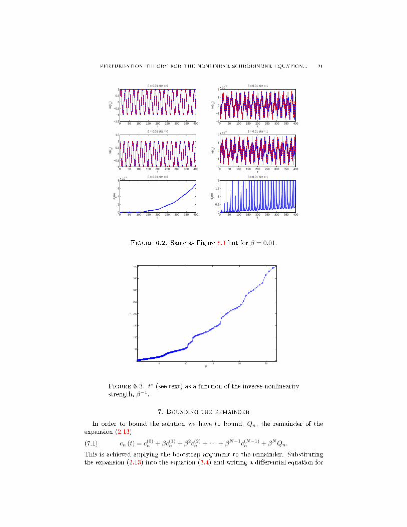
β2. To compare, we plot the real and the imaginary parts of both the numericalsolution of (1.1) with the distribution (5.12) and the perturbative approximationcn. From gures 6.1 and 6.2 we see that the correspondence between the numericalsolution of (1.1) and the perturbative approximation is good for times < 50 forβ = 0.1 and times < 200 for β = 0.01. Additionally, the correspondence of thecentral site, c0, which is used as the initial condition, cn (t = 0) = δn0, is much betterthan the correspondence of the neighboring sites. A possible explanation for thiscould be that the nonlinear perturbation is more pronounced at the states n withcn (t = 0) = 0, this is due to the fact that for β=0 those sites are unpopulated (zero)for all times, resulting in lower signal to noise ratio. To examine the convergencein time we will dene a time, t∗. For times t < t∗ the relative dierence betweenthe L2 norms of the exact and the approximate solutions, d2 (t), dened bellow, isless than 10%. It is instructive to introduce the following denitions.

PERTURBATION THEORY FOR THE NONLINEAR SCHRÖDINGER EQUATION... 20

0 50 100 150 200 250 300 350 400−1.5

−1

−0.5

0

0.5

1

1.5

t

im(c

n)

β = 0.1 site = 0

0 50 100 150 200 250 300 350 400−1.5

−1

−0.5

0

0.5

1

1.5

t

re(c

n)

β = 0.1 site = 0

0 50 100 150 200 250 300 350 4000

0.2

0.4

0.6

t

d 1(n)

β = 0.1 site = 0

0 50 100 150 200 250 300 350 400−0.02

−0.01

0

0.01

0.02

t

im(c

n)

β = 0.1 site = 1

0 50 100 150 200 250 300 350 400−0.02

−0.01

0

0.01

0.02

t

re(c

n)

β = 0.1 site = 1

0 50 100 150 200 250 300 350 4000

0.5

1

1.5

2

t

d 1(n)

β = 0.1 site = 1

Figure 6.1. In the rst and the second rows of the gure are pre-sented the imaginary and real parts, respectively, of the numericalsolution of (1.1) (blue, solid) and the perturbative approximation(red, dashed) as function of time for c0 (left column) and c1 (rightcolumn). In the third row the relative dierence, d1 (t) , as de-ned in Denition 12 is plotted. The parameters of the plot are,J = 0.25, ∆ = 1 and β = 0.1 and lattice size of 128. See (1.1) forthe denition of the constants.

Denition 12. The relative dierence between the exact and the perturbativesolution at site n is dened as

d1 (t) =2 |cn (t)− cn (t)||cn (t)|+ |cn (t)|

.

Denition 13. t∗ is a time until which the relative dierence between the exactand the perturbative solution, d2 (t), is less than 10%.

(6.2) d2 (t) =∑n |cn (t)− cn (t)|2∑

n |cn (t)|2≤ 0.1.

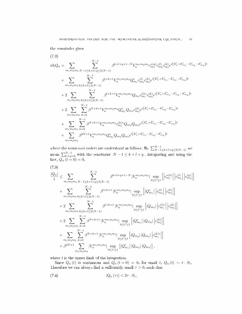
In gure 6.3 we see that as β becomes smaller the time for which the expansion tosecond order in β is close to the exact solution (within 10%), t∗, increases.

PERTURBATION THEORY FOR THE NONLINEAR SCHRÖDINGER EQUATION... 21

0 50 100 150 200 250 300 350 400−1.5

−1

−0.5

0

0.5

1

t

im(c

n)

β = 0.01 site = 0

0 50 100 150 200 250 300 350 400−1

−0.5

0

0.5

1

1.5

t

re(c

n)

β = 0.01 site = 0

0 50 100 150 200 250 300 350 4000

2

4

6

8x 10

−4

t

d 1(n)

β = 0.01 site = 0

0 50 100 150 200 250 300 350 400−2

−1

0

1

2x 10

−3

t

im(c

n)

β = 0.01 site = 1

0 50 100 150 200 250 300 350 400−2

−1

0

1

2x 10

−3

t

re(c

n)

β = 0.01 site = 1

0 50 100 150 200 250 300 350 4000

0.5

1

1.5

2

t

d 1(n)

β = 0.01 site = 1

Figure 6.2. Same as Figure 6.1 but for β = 0.01.

5 10 15 20 250

50

100

150

200

250

300

350

400

β−1

t*

Figure 6.3. t∗ (see text) as a function of the inverse nonlinearitystrength, β−1.

7. Bounding the remainder

In order to bound the solution we have to bound, Qn, the remainder of theexpansion (2.13)

(7.1) cn (t) = c(0)n + βc(1)

n + β2c(2)n + · · ·+ βN−1c(N−1)

n + βNQn.

This is achieved applying the bootstrap argument to the remainder. Substitutingthe expansion (2.13) into the equation (3.4) and writing a dierential equation for

PERTURBATION THEORY FOR THE NONLINEAR SCHRÖDINGER EQUATION... 22

the remainder gives

i∂tQn =∑

m1m2m3

N−1∑N−1≤k+l+q≤3(N−1)

βk+l+q+1−NV m1m2m3n c∗(q)m1

c(l)m2c(k)m3ei(E

′n+E′m1

−E′m2−E′m3)t

(7.2)

+∑

m1m2m3

N−1∑0≤k+l≤2(N−1)

βl+k+1V m1m2m3n Q∗m1

c(l)m2c(k)m3ei(E

′n+E′m1

−E′m2−E′m3)t

+ 2∑

m1m2m3

N−1∑0≤k+l≤2(N−1)

βl+k+1V m1m2m3n Qm3c

(l)∗m1

c(k)m2ei(E

′n+E′m1

−E′m2−E′m3)t

+ 2∑

m1m2m3

N−1∑k=0

βN+k+1V m1m2m3n Q∗m1

Qm2c(k)m3ei(E

′n+E′m1

−E′m2−E′m3)t

+∑

m1m2m3

N−1∑k=0

βN+k+1V m1m2m3n c(k)∗

m1Qm2Qm3e

i(E′n+E′m1−E′m2

−E′m3)t

+∑

m1m2m3

β2N+1V m1m2m3n Q∗m1

Qm2Qm3ei(E′n+E′m1

−E′m2−E′m3)t

where the sums over orders are understood as follows. By∑N−1N−1≤k+l+q≤3(N−1) we

mean∑N−1k,l,q=0 with the constraint N − 1 ≤ k + l + q . Integrating and using the

fact, Qn (t = 0) = 0,

|Qn|t≤

∑m1m2m3

N−1∑N−1≤k+l+q≤3(N−1)

βk+l+q+1−N |V m1m2m3n | sup

0≤t′≤t

[∣∣∣c∗(k)m1

∣∣∣ ∣∣∣c(l)m2

∣∣∣ ∣∣∣c(q)m3

∣∣∣](7.3)

+∑

m1m2m3

N−1∑0≤k+l≤2(N−1)

βl+k+1 |V m1m2m3n | sup

0≤t′≤t

[∣∣Q∗m1

∣∣ ∣∣∣c(l)m2

∣∣∣ ∣∣∣c(k)m3

∣∣∣]

+ 2∑

m1m2m3

N−1∑0≤k+l≤2(N−1)

βl+k+1 |V m1m2m3n | sup

0≤t′≤t

[|Qm3 |

∣∣∣c(l)∗m1

∣∣∣ ∣∣∣c(k)m2

∣∣∣]

+ 2∑

m1m2m3

N−1∑k=0

βN+k+1 |V m1m2m3n | sup

0≤t′≤t

[∣∣Q∗m1

∣∣ |Qm2 |∣∣∣c(k)m3

∣∣∣]

+∑

m1m2m3

N−1∑k=0

βN+k+1 |V m1m2m3n | sup

0≤t′≤t

[|Qm2 | |Qm3 |

∣∣∣c(k)∗m1

∣∣∣]+ β2N+1

∑m1m2m3

|V m1m2m3n | sup

0≤t′≤t

[∣∣Q∗m1

∣∣ |Qm2 | |Qm3 |],

where t is the upper limit of the integration.Since Qn (t) is continuous and Qn (t = 0) = 0, for small t, Qn (t) ∼ t · S1.

Therefore we can always nd a suciently small τ > 0, such that

(7.4) |Qn (τ)| < 2τ · S1,

PERTURBATION THEORY FOR THE NONLINEAR SCHRÖDINGER EQUATION... 23

where(7.5)

S1 =∑

m1m2m3

N−1∑N−1≤k+l+q≤3(N−1)

βk+l+q+1−N |V m1m2m3n | sup

0≤t′≤t

[∣∣∣c∗(k)m1

∣∣∣ ∣∣∣c(l)m2

∣∣∣ ∣∣∣c(q)m3

∣∣∣] .Assume, that there is some time, t, for which,

(7.6) |Qn (t)| > 2t · S1,

than since Qn (t) is continuous and (7.4) holds there is a time, t0, where

(7.7) |Qn (t0)| = 2t0 · S1.

Inserting this equality into the inequality (7.3), we get an interval 0 ≤ t ≤ t0 forwhich (7.4) holds (see (7.25)). We proceed by bounding S1 and other sums of (7.3).

Using the Theorem 10 obtained in the end of the Section 5, we can bound, S1.The inequality is violated with a probability found from (5.29). We start with thebound

S1 ≤∑mi

N−1∑N−1≤k+l+q≤3(N−1)

βk+l+q+1−N |V m1m2m3n | ×(7.8)

×ec′(k+l+q)+c(k2+l2+q2)e−(γ−ε′−η′)(|xm1 |+|xm2 |+|xm3 |)

we nd from (2.11)

∑m1m2m3

|V m1m2m3n | e−(γ−ε′−η′)(|xm1 |+|xm2 |+|xm3 |)

(7.9)

≤ V ε,ε′

δ

∑m1m2m3

eε(|xn|+|xm1 |+|xm2 |+|xm3 |)

× e−13 (γ−ε′)(|xn−xm1 |+|xn−xm2 |+|xn−xm3 |)e−(γ−η′−ε′)(|xm1 |+|xm2 |+|xm3 |)

≤ V ε,ε′

δ e−(γ−ε−ε′)|xn|∑

m1m2m3

e−23 (γ−η′−ε)(|xm1 |+|xm2 |+|xm3 |) = Cγ,ε,ε

′,η′

δ e−(γ−ε−ε′)|xn|

for γ3 < (γ − η′) . Therefore for η′ suciently small, substituting back we get

S1 ≤ Cγ,ε,ε′′,η′

δ e−(γ−ε−ε′)|xn|N−1∑

N−1≤k+l+q≤3(N−1)

βk+l+q+1−Nec(k2+l2+q2)ec

′(k+l+q)

(7.10)

≡ Cδ (N) e6cN2e−(γ−ε−ε′)|xn|,

where we used c′ = cN , and Cδ (N) = O(N3). For the bound (7.10) to be violated

at least one of the c(k)m has to satisfy the inequality (5.29) and the probability for

this is bounded by e−c′e−η

′|xm|/k. Therefore the probability that (7.10) will beviolated is bounded by

(7.11) e−c′N−1∑k=1

∞∑n=−∞

e−η′|xn|/k = e−c

′N−1∑k=1

(2

1− e−η′/k− 1)∼N−1∑k=1

k

η′∼ N2

η′e−cN ,

PERTURBATION THEORY FOR THE NONLINEAR SCHRÖDINGER EQUATION... 24

where we have expanded the exponent e−η′/k using the fact that for large N the

sum is dominated by terms with k 1 and η′/k 1. Setting c′ = N provides theconvergence of the probability with the expansion order, i.e.,(7.12)

Pr

( ∑m1m2m3

∑N−1N−1≤k+l+q≤3(N−1) β

k+l+q+1−N |V m1m2m3n |

∣∣∣c∗(k)m1

∣∣∣ ∣∣∣c(l)m2

∣∣∣ ∣∣∣c(q)m3

∣∣∣≥ Cδ (N) e6cN2

e−(γ−ε−ε′−η′)|xn|

)≤ const

η′N2e−cN .

Now we turn to nd the point t0 dened in (7.7). To bound other expressions in(7.3), we use

(7.13) |Qm (t0)| = 2t0 · S1 ≤M (t0) e−ν|xm|,

where following (7.12),

(7.14) M (t0) := 2t0Cδ (N) e6cN2

with ν = γ− ε− ε′. In what follows, unless stated dierently, M will mean M (t0).First we will bound the linear term in the Qn in (7.3). The sum over m2 and

m3 is bounded similarly to the sums in the inhomogeneous term and the sum overm1 is bounded using the bootstrap assumption (7.13), resulting in

S2 =∑m2m3

N−1∑0≤k+l≤2(N−1)

βl+k+1∑m1

|V m1m2m3n |

∣∣Q∗m1

∣∣ ∣∣∣c(l)m2

∣∣∣ ∣∣∣c(k)m3

∣∣∣(7.15)

≤M∑m2m3

N−1∑0≤k+l≤2(N−1)

βl+k+1ec(k2+l2)ec

′(k+l)∑m1

|V m1m2m3n | e−ν|xm1 |e−(γ−η′−ε′)(|xm2 |+|xm3 |)

for 13 (γ − ε′) < ν and γ

3 < γ − η′. This is similar to the sum in equation (7.9) andgives a result with a similar dependence on |xn|,

S2 ≤∑m2m3

N−1∑0≤k+l≤2(N−1)

βl+k+1∑m1

|V m1m2m3n |

∣∣Q∗m1

∣∣ ∣∣∣c(l)m2

∣∣∣ ∣∣∣c(k)m3

∣∣∣(7.16)

≤ Cδ (N) e2cN2Me−(γ−ε−ε′)|xn|.

with the same probability as in (7.11). Therefore the linear term in Qn is boundedby the probabilistic bound(7.17)

Pr

( ∑m1m2m3;l,k β

l+k+1 |V m1m2m3n |

∣∣Q∗m1

∣∣ ∣∣∣c(l)m2

∣∣∣ ∣∣∣c(k)m3

∣∣∣≥ βCδ (N) e4cN2

Me−(γ−ε−ε′−η′)|xn|

)≤ const

η′N2e−cN ,

with Cδ = O(N2). A similar bound is found for the third term on RHS of (7.3).

The fourth sum of equation (7.3)

(7.18) S4 =∑

m1m2m3;k

βN+k+1 |V m1m2m3n |

∣∣Q∗m1

∣∣ |Qm2 |∣∣∣c(k)m3

∣∣∣is bounded by

(7.19) Pr

∑

m1m2m3;k

βN+k+1 |V m1m2m3n |

∣∣Q∗m1

∣∣ |Qm2 |∣∣∣c(k)m3

∣∣∣≥ Cδ (N) e2cN2

βN+1M2e−(γ−ε−ε′−η′)|xn|

≤ const

η′N2e−cN ,

PERTURBATION THEORY FOR THE NONLINEAR SCHRÖDINGER EQUATION... 25

with Cδ = O (N). The last term in (7.3) is

(7.20) S5 = β2N+1∑

m1m2m3

|V m1m2m3n |

∣∣Q∗m1

∣∣ |Qm2 | |Qm3 | .

and it is bounded by

(7.21) S5 ≤ β2N+1M3e−(γ−ε−ε′)|xn|.

To summarize, substitution of the equality (7.13) in (7.3) to nd a time t0 for whichassumption (7.6) is valid results in the following inequality which is satised withthe probability that is the sum of the probabilities given by the RHS of (7.12),(7.17), (7.19),(7.22)

2t0S1 ≤ t0·S1+t0Cδ (N)(e6cN2

+ 2βe4cN2M + 4βN+1e2cN2

M2 + 8β2N+1M3)e−(γ−ε−ε′)|xn|,

with Cδ = O(N3). Multiplying by e(γ−ε−ε

′)|xn| both sides of the inequality (7.22)and taking the inmum with respect to n, gives(7.23)

infn

(S1e

(γ−ε−ε′)|xn|)≤ 2Cδ (N)

(βe4cN2

M + 2βN+1e2cN2M2 + 4β2N+1M3

).

Setting AN := e2cN2, C := infn

(S1e

(γ−ε−ε′)|xn|)and using the denition of M

(see (7.14))

(7.24) C ≤ 2βt0 ·A5NCδ + 4βN+1t20A

7NC

2δ + 8β2N+1t30A

9N .

For suciently small βt0 the rst term on the RHS of (7.24) is dominant andtherefore,

(7.25) t0 ≥C

2βA5NCδ

.

Note, that C > 0, since it is an inmum of a sum of positive quantities, howeverwe do not calculate it explicitly in this paper, nevertheless it is likely to be of theorder of CδA

3N . This proves that,

|Qn (t)| ≤M (t) · e−(γ−ε−ε′)|xn| = 2t · Cδe6cN2e−(γ−ε−ε′)|xn|

for times t ≤ t0 , whereM (t) is given by extending the denition (7.14) by replacingt0 by t.

Theorem 14. For t = O(β−1

)with c ∼= 2, and assuming that Conjecture 3 holds

Pr(|Qn| ≥ 2t · Cδe6cN2

e−(γ−ε−ε′)|xn|)≤ const

η′N2e−cN(7.26)

The bound on the probability of statement (7.26) is calculated by summing theRHS of ((7.12),(7.17),(7.19)). The contribution of the remainder term is

(7.27)∣∣βNQn∣∣ ≤ const · e6cN2+N ln β+ln te−(γ−ε−ε′)|xn|.

Note that for a given t and β there is an optimum N for which the remainder isminimal. Additionally, for any xed time and order N , limβ→0

∣∣βNQn∣∣ /βN−1 = 0,which shows that the series is in fact an asymptotic one [63].

PERTURBATION THEORY FOR THE NONLINEAR SCHRÖDINGER EQUATION... 26

8. Summary

In this paper a perturbation expansion in powers of β was developed (Sections2, 3) for the solution of the NLSE with a random potential. It required the removalof the secular terms for this problem. To best of our knowledge it is the rst timeit was done for a multivariate problem. The quality of the expansion to the secondorder was tested in Section 6. In Section 4 it was shown that the number of termsgrows exponentially with the order. In Section 5 a probabilistic bound on thegeneral term (5.29) was derived. It relies on the Conjecture 3. The resulting boundwas tested numerically. Finally, a bound on the remainder was obtained for a nitetime, showing that the series is asymptotic. For time shorter than t0 which is givenby (7.25) there is a front x (t) ∝ ln t such that for xn > x (t) both the remainder,βNQn (t) and cn (t) are exponentially small.

The work leaves several open problems that should be subject of further research:

(1) Turning the perturbation theory developed in the present work into a prac-tical method for solution of the NLSE and similar nonlinear dierentialequations. The control on the error should be obtained using the methodspresented in Sec. 7.

(2) Can the front x (t) ∝ ln t be found for arbitrarily long times ?(3) The asymptotic nature of the series. Is it just an asymptotic series or a

convergent one ?(4) If the series is asymptotic can it be resummed ?

(5) The eck2+c′k in (5.29) results from the repeated use of the Hölder inequality

and a very generous bound on the probability distributions. An eortshould be made to improve it.

(6) There are various properties of the Anderson model that have been usedhere. Some of them were tested numerically. It would be of great valueif Conjecture 3, Corollary 4 and Conjecture 5 were rigorously established,even at the limit of a strong disorder. In the present work we rely onlyon Corollary 4 (that was tested numerically, see Fig. 5.1). The rigorousproof of the unimodality of γ (E) for the uniform distribution of the randompotentials, εx, may also be useful.

(7) It would be very useful if Conjecture 6 could be rigorously obtained.

We enjoyed many extensive illuminating and extremely critical discussions withMichael Aizenman. We also had informative discussions with S. Aubry, V. Chu-laevski, S. Flach, I. Goldshield, M. Goldstein, I. Guarneri, M. Sieber, W.-M. Wangand S. Warzel. This work was partly supported by the Israel Science Foundation(ISF), by the US-Israel Binational Science Foundation (BSF), by the USA NationalScience Foundation (NSF), by the Minerva Center of Nonlinear Physics of ComplexSystems, by the Shlomo Kaplansky academic chair, by the Fund for promotion ofresearch at the Technion and by the E. and J. Bishop research fund. The workwas done partially while SF was visiting the Institute of Mathematical Sciences,National University of Singapore in 2006 and the Center of Nonlinear Physics ofComplex Systems in Dresden in 2007 and while YK visited the department of Math-ematics at Rutgers University and while AS was visiting the Lewiner Institute ofTheoretical Physics at the Technion in 2007. The visits were supported in part bythese Institutes.

PERTURBATION THEORY FOR THE NONLINEAR SCHRÖDINGER EQUATION... 27

−5 −4 −3 −2 −1 0 1 2 3 4 50

0.5

1

1.5

2

2.5

3

E

γ(E

)

J=0.25J = 0.5J = 1

Figure 8.1. The Lyapunov exponent as a function of energy forthe uniform distribution dened in (5.12). The solid (blue) lineis for J = 0.25, the dashed (green) line is for J = 0.5 and thedot-dashed line (red) is for J = 1.

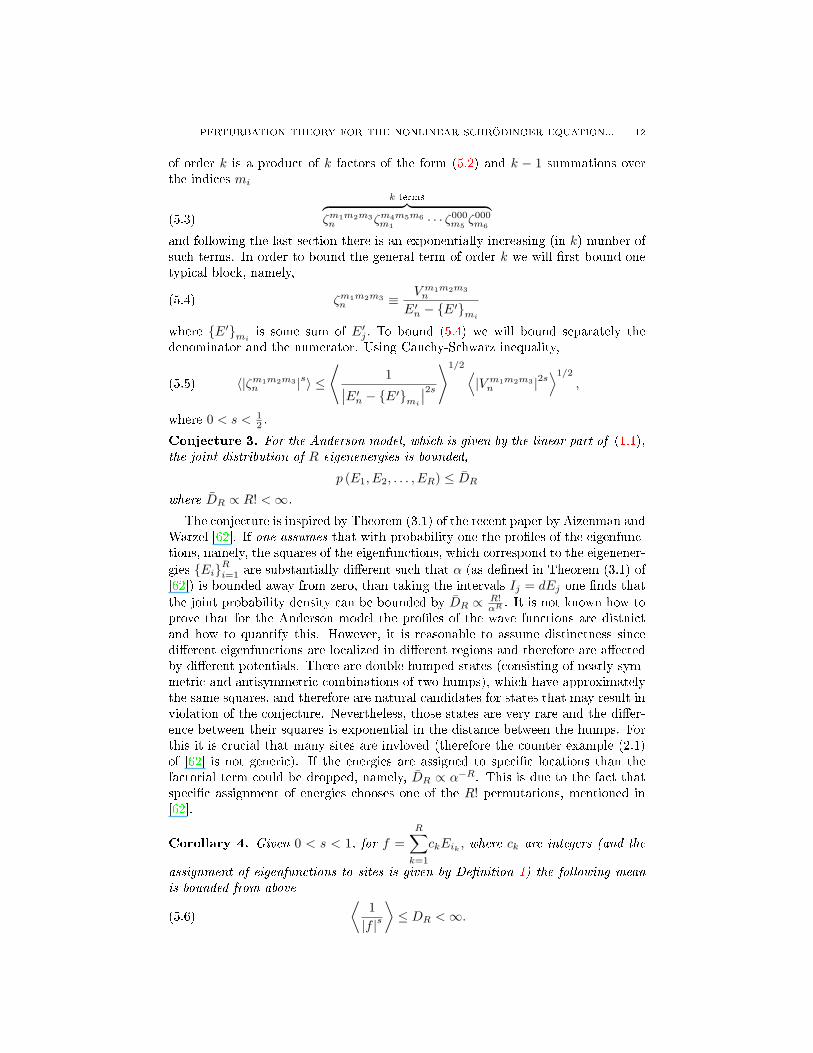
Appendix

The average Lyapunov exponent was calculated numerically using the transfermatrix technique for a uniform distribution dened in (5.12). The results are pre-sented in Fig. 8.1. It can be seen that γ (E) is unimodal.

References

[1] C. Sulem and P. L. Sulem. The nonlinear Schrödinger equation self-focusing and wave col-

lapse. Springer, 1999.[2] D. J. Thouless. Relation between density of states and range of localization for one dimen-

sional random systems. J. Phys. C: Solid State Phys., 5(1):77, 1972.[3] G. P. Agrawal. Nonlinear ber optics, volume 4th. Academic Press, Burlington, MA ; London,

2007.[4] F. Dalfovo, S. Giorgini, L. P. Pitaevskii, and S. Stringari. Theory of Bose-Einstein condensa-

tion in trapped gases. Rev. Mod. Phys., 71(3):463512, 1999.[5] L. P. Pitaevskii and S. Stringari. Bose-Einstein condensation. Clarendon Press, Oxford ; New

York, 2003.[6] A. J. Leggett. Bose-Einstein condensation in the alkali gases: Some fundamental concepts.

Rev. Mod. Phys., 73(2):307356, 2001.[7] L.P. Pitaevskii. Zh. Eksp. Theor. Phys., 40:646, 1961.[8] E.P. Gross. Structure of a quantized vortex in boson systems. Nuovo Cimento, 20(3):454477,

1961.[9] L.P. Pitaevskii. J. Math. Phys., 4:195, 1963.[10] L. Erdös, B. Schlein, and H. T. Yau. Rigorous derivation of the Gross-Pitaevskii equation.

Phys. Rev. Lett., 98(4):040404, 2007.[11] E. H. Lieb and R. Seiringer. Proof of Bose-Einstein condensation for dilute trapped gases.

Phys. Rev. Lett., 88(17):170409, 2002.

PERTURBATION THEORY FOR THE NONLINEAR SCHRÖDINGER EQUATION... 28

[12] L. S. Cederbaum and A. I. Streltsov. Best mean-eld for condensates. Phys. Lett. A,318(6):564569, 2003.

[13] O. E. Alon and L. S. Cederbaum. Pathway from condensation via fragmentation to fermion-ization of cold bosonic systems. Phys. Rev. Lett., 95(14):140402, 2005.

[14] P. W. Anderson. Absence of diusion in certain random lattices. Phys. Rev., 109(5):1492,1958.

[15] K. Ishii. Localization of eigenstates and transport phenomena in one-dimensional disorderedsystem. Suppl. Prog, Theor. Phys., 53(53):77138, 1973.

[16] P. A. Lee and T. V. Ramakrishnan. Disordered electronic systems. Rev. Mod. Phys.,57(2):287337, 1985.

[17] I. M. Lifshits, L. A. Pastur, and S. A. Gredeskul. Introduction to the theory of disordered

systems. Wiley, New York, 1988.[18] E. Abrahams, P. W. Anderson, D. C. Licciardello, and T. V. Ramakrishnan. Scaling theory of

localization - absence of quantum diusion in 2 dimensions. Phys. Rev. Lett., 42(10):673676,1979.

[19] T. Schwartz, G. Bartal, S. Fishman, and M. Segev. Transport and Anderson localization indisordered two-dimensional photonic lattices. Nature, 446(7131):5255, 2007.

[20] H. Gimperlein, S. Wessel, J. Schmiedmayer, and L. Santos. Ultracold atoms in optical latticeswith random on-site interactions. Phys. Rev. Lett., 95(17):170401, 2005.

[21] J. E. Lye, L. Fallani, M. Modugno, D. S. Wiersma, C. Fort, and M. Inguscio. Bose-Einsteincondensate in a random potential. Phys. Rev. Lett., 95(7):070401, 2005.

[22] D. Clement, A. F. Varon, M. Hugbart, J. A. Retter, P. Bouyer, L. Sanchez-Palencia, D. M.Gangardt, G. V. Shlyapnikov, and A. Aspect. Suppression of transport of an interactingelongated Bose-Einstein condensate in a random potential. Phys. Rev. Lett., 95(17):170409,2005.

[23] D. Clement, A. F. Varon, J. A. Retter, L. Sanchez-Palencia, A. Aspect, and P. Bouyer.Experimental study of the transport of coherent interacting matter-waves in a 1D randompotential induced by laser speckle. New J. Phys., 8:165, 2006.

[24] L. Sanchez-Palencia, D. Clement, P. Lugan, P. Bouyer, G. V. Shlyapnikov, and A. Aspect.Anderson localization of expanding Bose-Einstein condensates in random potentials. Phys.Rev. Lett., 98(21):210401, May 2007.

[25] J. Billy, V. Josse, Z. C. Zuo, A. Bernard, B. Hambrecht, P. Lugan, D. Clement, L. Sanchez-Palencia, P. Bouyer, and A. Aspect. Direct observation of Anderson localization of matterwaves in a controlled disorder. Nature, 453(7197):891894, June 2008.

[26] C. Fort, L. Fallani, V. Guarrera, J. E. Lye, M. Modugno, D. S. Wiersma, and M. Inguscio.Eect of optical disorder and single defects on the expansion of a Bose-Einstein condensatein a one-dimensional waveguide. Phys. Rev. Lett., 95(17):170410, 2005.

[27] E. Akkermans, S. Ghosh, and Z. H. Musslimani. Numerical study of one-dimensional andinteracting Bose-Einstein condensates in a random potential. J. Phys. B, 41(4):045302, 2008.

[28] T. Paul, P. Schlagheck, P. Leboeuf, and N. Pavlo. Superuidity versus Anderson localizationin a dilute Bose gas. Phys. Rev. Lett., 98(21):210602, 2007.

[29] A. R. Bishop. Fluctuation phenomena : disorder and nonlinearity. World Scientic, Singapore; River Edge, NJ, 1995.

[30] K. O. Rasmussen, D. Cai, A. R. Bishop, and N. Gronbech-Jensen. Localization in a nonlineardisordered system. Europhys. Lett., 47(4):421427, 1999.

[31] G. Kopidakis and S. Aubry. Intraband discrete breathers in disordered nonlinear systems. I.Delocalization. Physica D, 130(3-4):155186, 1999.

[32] G. Kopidakis and S. Aubry. Discrete breathers and delocalization in nonlinear disorderedsystems. Phys. Rev. Lett., 84(15):32363239, 2000.

[33] D. L. Shepelyansky. Delocalization of quantum chaos by weak nonlinearity. Phys. Rev. Lett.,70(12):17871790, 1993.

[34] A. S. Pikovsky and D. L. Shepelyansky. Destruction of Anderson localization by a weaknonlinearity. Phys. Rev. Lett., 100(9):094101, 2008.

[35] M. Mulansky. Localization properties of nonlinear disordered lattices. Universität Potsdam,Diploma thesis, 2009. http://nbn-resolving.de/urn:nbn:de:kobv:517-opus-31469.

[36] H. Veksler, Y. Krivolapov, and S. Fishman. Phys. Rev. E, 2009. to appear.[37] G. Kopidakis, S. Komineas, S. Flach, and S. Aubry. Absence of wave packet diusion in

disordered nonlinear systems. Phys. Rev. Lett., 100(8):084103, 2008.

PERTURBATION THEORY FOR THE NONLINEAR SCHRÖDINGER EQUATION... 29

[38] M. I. Molina. Transport of localized and extended excitations in a nonlinear Anderson model.Phys. Rev. B, 58(19):1254712550, 1998.

[39] S. Flach, D. Krimer, and Ch. Skokos. Universal spreading of wavepackets in disordered non-linear systems. Phys. Rev. Lett., 102:024101, 2009.

[40] C. Skokos, D.O. Krimer, Komineas, and S. S. Flach. Delocalization of wave packets in disor-dered nonlinear chains. Phys. Rev. E, 79:056211, 2009.

[41] J. M. Combes and P. D. Hislop. Localization for some continuous, random hamiltonians ind-dimensions. J. Funct. Anal., 124(1):149180, 1994.

[42] F. Germinet and S. De Bièvre. Dynamical localization for discrete and continuous randomSchrödinger operators. Commun. Math. Phys., 194(2):323341, 1998.

[43] F. Klopp. Localization for some continuous random Schrödinger-operators. Commun. Math.

Phys., 167(3):553569, 1995.[44] A. Soer and W.-M. Wang. Anderson localization for time periodic random Schrödinger

operators. Commun. Partial Dier. Equ., 28(1-2):333347, 2003.[45] J. Bourgain and W. M. Wang. Anderson localization for time quasi-periodic random

schrödinger and wave equations. Commun. Math. Phys., 248(3):429466, 2004.[46] W.-M. Wang. Logarithmic bounds on Sobolev norms for time dependent linear Schröinger

equations. Comm. Part. Di. Eq., 33(12):21642179, 2008.[47] V. Nersesyan. Growth of Sobolev norms and controllability of Schrödinger equation. Com-

mun. Math. Phys., 290:371387, 2009.[48] W.-M. Wang and Z. Zhang. Long time Anderson localization for nonlinear random

Schrödinger equation. J. Stat. Phys., 134:953, 2009.[49] C. Albanese and J. Fröhlich. Periodic-solutions of some innite-dimensional hamiltonian-

systems associated with non-linear partial dierence-equations .1. Commun. Math. Phys.,116(3):475502, 1988.

[50] C. Albanese, J. Fröhlich, and T. Spencer. Periodic-solutions of some innite-dimensionalhamiltonian-systems associated with non-linear partial dierence-equations .2. Commun.

Math. Phys., 119(4):677699, 1988.[51] C. Albanese and J. Fröhlich. Perturbation-theory for periodic-orbits in a class of innite

dimensional hamiltonian-systems. Commun. Math. Phys., 138(1):193205, 1991.[52] A. Iomin and S. Fishman. Localization length of stationary states in the nonlinear Schrödinger

equation. Phys. Rev. E, 76(5):056607, 2007.[53] S. Fishman, A. Iomin, and K. Mallick. Asymptotic localization of stationary states in the

nonlinear Schrödinger equation. Phys. Rev. E, 78:066605, 2008.[54] S. Fishman, Y. Krivolapov, and A. Soer. On the problem of dynamical localization in the

nonlinear Schrödinger equation with a random potential. J. Stat. Phys., 131(5):843865, 2008.[55] G. Benettin, J. Fröhlich, and A. Giorgilli. A Nekhoroshev-type theorem for Hamiltonian-

systems with innitely many degrees of freedom. Commun. Math. Phys., 119(1):95108, 1988.[56] M. Aizenman and S. Molchanov. Localization at large disorder and at extreme energies - an

elementary derivation. Commun. Math. Phys., 157(2):245278, 1993.[57] R. del Rio, S. Jitomirskaya, Y. Last, and B. Simon. What is localization ? Phys. Rev. Lett.,

75(1):117119, 1995.[58] R. del Rio, S. Jitomirskaya, Y. Last, and B. Simon. Operators with singular continuous

spectrum .IV. Hausdor dimensions, rank one perturbations, and localization. J. Anal. Math.,69:153200, 1996.

[59] S. De Bièvre and F. Germinet. Dynamical localization for the random dimer Schrödingeroperator. J. Stat. Phys., 98(5-6):11351148, 2000.

[60] F. Germinet and A. Klein. New characterizations of the region of complete localization forrandom Schrödinger operators. J. Stat. Phys., 122(1):7394, 2006.

[61] S. Fishman, Y. Krivolapov, and A. Soer. On the distribution of linear combinations ofeigenvalues of the Anderson model. work in progress.

[62] M. Aizenman and S. Warzel. On the joint distribution of energy levels of random Schrödingeroperators. J. Phys. A, 42:045201, 2009.

[63] A. Erdélyi. Asymptotic expansions. Dover, New-York, 1956.

PERTURBATION THEORY FOR THE NONLINEAR SCHRÖDINGER EQUATION... 30

Physics Department, Technion - Israel Institute of Technology, Haifa 32000, Is-

rael.

E-mail address: fishman@physics.technion.ac.il

Physics Department, Technion - Israel Institute of Technology, Haifa 32000, Is-

rael.

E-mail address: evgkr@tx.technion.ac.il

Mathematics Department, Rutgers University, New-Brunswick, NJ 08903, USA.

E-mail address: soffer@math.rutgers.edu