To appear in Journal of Parallel and Distributed Computing, October 1993.A preliminary version of this paper appears in the Proceedings of the 26th HawaiiInternational Conference on System Sciences, 1993.Performance Properties of Large ScaleParallel Systems�Anshul Gupta and Vipin KumarDepartment of Computer Science,University of MinnesotaMinneapolis, MN - 55455Email: agupta@cs.umn.edu and kumar@cs.umn.eduTR 92-32, September 1992 (Revised June 1993)AbstractThere are several metrics that characterize the performance of a parallel system, such as, parallel execution time,speedup and e�ciency. A number of properties of these metrics have been studied. For example, it is a wellknown fact that given a parallel architecture and a problem of a �xed size, the speedup of a parallel algorithmdoes not continue to increase with increasing number of processors. It usually tends to saturate or peak at acertain limit. Thus it may not be useful to employ more than an optimal number of processors for solving aproblem on a parallel computer. This optimal number of processors depends on the problem size, the parallelalgorithm and the parallel architecture. In this paper we study the impact of parallel processing overheads andthe degree of concurrency of a parallel algorithm on the optimal number of processors to be used when thecriterion for optimality is minimizing the parallel execution time. We then study a more general criterion ofoptimality and show how operating at the optimal point is equivalent to operating at a unique value of e�ciencywhich is characteristic of the criterion of optimality and the properties of the parallel system under study. We putthe technical results derived in this paper in perspective with similar results that have appeared in the literaturebefore and show how this paper generalizes and/or extends these earlier results.�This work was supported by IST/SDIO through the Army Research O�ce grant # 28408-MA-SDI to theUniversity of Minnesota and by the University of Minnesota ArmyHigh Performance Computing Research Centerunder contract # DAAL03-89-C-0038. 1

1 IntroductionMassively parallel computers employing hundreds to thousands of processors are commerciallyavailable today and o�er substantially higher raw computing power than the fastest sequentialsupercomputers. Availability of such systems has fueled interest in investigating the performanceof parallel computers containing a large number of processors [23, 8, 7, 27, 37, 30, 6, 33, 18, 32,17, 38, 34, 4, 5, 29].The performance of a parallel algorithm cannot be studied in isolation from the parallelarchitecture it is implemented on. For the purpose of performance evaluation we de�ne aparallel system as a combination of a parallel algorithm and a parallel architecture on whichit is implemented. There are several metrics that characterize the performance of a parallelsystem, such as, parallel execution time, speedup and e�ciency. A number of properties ofthese metrics have been studied. It is a well known fact that given a parallel architecture and aproblem instance of a �xed size, the speedup of a parallel algorithm does not continue to increasewith increasing number of processors but tends to saturate or peak at a certain value. As earlyas in 1967, Amdahl [2] made the observation that if s is the serial fraction in an algorithm,then its speedup for a �xed size problem is bounded by 1s , no matter how many processorsare used. Gustafson, Montry and Benner [18, 16] experimentally demonstrated that the upperbound on speedup can be overcome by increasing the problem size as the number of processorsis increased. Worley [37] showed that for a class of parallel algorithms, if the parallel executiontime is �xed, then there exists a problem size which cannot be solved in that �xed time nomatter how many processors are used. Flatt and Kennedy [8, 7] derived some important upperbounds related to the performance of parallel computers in the presence of synchronization andcommunication overheads. They show that if the parallel processing overhead for a certaincomputation satis�es certain properties, then there exists a unique value p0 of the number ofprocessors for which the parallel execution time is minimum (or the speedup is maximum) for agiven problem size. However, at this point, the e�ciency of the parallel execution is rather poor.Hence they suggest that the number of processors should be chosen to maximize the productof e�ciency and speedup. Flatt and Kennedy, and Tang and Li [33] also suggest maximizing aweighted geometric mean of e�ciency and speedup. Eager et. al. [6] proposed that an optimaloperating point should be chosen such the e�ciency of execution is roughly 0.5.Many of the results presented in this paper are extensions, and in some cases, generalizationsof the results of the above mentioned authors. Each parallel system has a unique overheadfunction, the value of which depends on the size of the problem being attempted and thenumber of processors being employed. Moreover, each parallel algorithm has an inherent degreeof concurrency that determines the maximum number of processors that can be simultaneouslykept busy at any given time while solving the problem of a given size. In this paper we studythe e�ects of the overhead function and the degree of concurrency on performance measuressuch as speedup, execution time and e�ciency and determine the optimal number of processorsto be used under various optimality criteria.We show that if the overhead function of a parallel system does not grow faster than �(p),where p is the number of processors in the parallel ensemble, then speedup can be maximized2

by using as many processors as permitted by the degree of the concurrency of the algorithm.If the overheads grow faster than �(p), then the number of processors that should be usedto maximize speedup is determined either by the degree of concurrency or by the overheadfunction. We derive the exact expressions for maximum speedup, minimum execution time, thenumber of processors that yields maximum speedup, and the e�ciency at the point of maximumspeedup. We also show that for a class of overhead functions, given any problem size, operatingat the point of maximum speedup is equivalent to operating at a �xed e�ciency and the relationbetween the problem size and the number of processors that yields maximum speedup is givenby the isoe�ciency metric of scalability [22, 10, 23]. Next, a criterion of optimality is describedthat is more general than just maximizing the speedup and similar results are derived underthis new condition for choosing the optimal operating point.The organization of the paper is as follows. In Section 2 we de�ne the terms to be usedlater in the paper. In Sections 3 and 4 we derive the technical results. In Section 5, we putthese results in perspective with similar results that have appeared earlier in the literatureand demonstrate that many of the results derived here are generalizations and/or extensionsof the earlier results. Throughout the paper, examples are used to illustrate these results inthe context of parallel algorithms for practical problems such as FFT, Matrix Multiplication,Shortest Paths, etc. Although, for the sake of ease of presentation, the examples are restrictedto simple and regular problems, the properties of parallel systems studied here apply to generalparallel systems as well.A preliminary version of this paper appears in [13].2 De�nitions and AssumptionsIn this section, we formally describe the terminology used in the rest of the paper.Parallel System : The combination of a parallel architecture and a parallel algorithm im-plemented on it. We assume that the parallel computer being used is a homogeneousensemble of processors; i.e., all processors and communication channels are identical inspeed.Problem Size W : The size of a problem is a measure of the number of basic operationsneeded to solve the problem. There can be several di�erent algorithms to solve the sameproblem. To keep the problem size unique for a given problem, we de�ne it as the numberof basic operations required by the fastest known sequential algorithm to solve the problemon a single processor. Problem size is a function of the size of the input. For example, forthe problem of computing an N -point FFT, W = �(N logN).According to our de�nition, the sequential time complexity of the fastest known serialalgorithm to solve a problem determines the size of the problem. If the time taken byan optimal (or the fastest known) sequential algorithm to solve a problem of size W ona single processor is TS, then TS / W , or TS = tcW , where tc is a machine dependentconstant. 3

Parallel Execution Time TP : The time elapsed from the moment a parallel computationstarts, to the moment the last processor �nishes execution. For a given parallel system,TP is normally a function of the problem size (W ) and the number of processors (p), andwe will sometimes write it as TP (W;p).Cost: The cost of a parallel system is de�ned as the product of parallel execution time andthe number of processors utilized. A parallel system is said to be cost-optimal if and onlyif the cost is asymptotically of the same order of magnitude as the serial execution time(i.e., pTP = �(W )). Cost is also referred to as processor-time product.Speedup S : The ratio of the serial execution time of the fastest known serial algorithm (TS)to the parallel execution time of the chosen algorithm (TP ).Total Parallel Overhead To: The sum total of all the overhead incurred due to parallel pro-cessing by all the processors. It includes communication costs, non-essential work andidle time due to synchronization and serial components of the algorithm. Mathematically,To = pTP � TS.In order to simplify the analysis, we assume that To is a non-negative quantity. This impliesthat speedup is always bounded by p. For instance, speedup can be superlinear and To canbe negative if the memory is hierarchical and the access time increases (in discrete steps)as the memory used by the program increases. In this case, the e�ective computationspeed of a large program will be slower on a serial processor than on a parallel computeremploying similar processors. The reason is that a sequential algorithm using M bytes ofmemory will use only Mp bytes on each processor of a p-processor parallel computer. Thecore results of the paper are still valid with hierarchical memory, except that the scalabilityand performance metrics will have discontinuities, and their expressions will be di�erentin di�erent ranges of problem sizes. The at memory assumption helps us to concentrateon the characteristics of the parallel algorithm and architectures, without getting into thedetails of a particular machine.For a given parallel system, To is normally a function of both W and p and we will oftenwrite it as To(W;p).E�ciency E : The ratio of speedup (S) to the number of processors (p). Thus, E = TSpTP =11+ ToTS .Degree of Concurrency C(W ): The maximum number of tasks that can be executed si-multaneously at any given time in the parallel algorithm. Clearly, for a given W , theparallel algorithm can not use more than C(W ) processors. C(W ) depends only on theparallel algorithm, and is independent of the architecture. For example, for multiplyingtwo N �N matrices using Fox's parallel matrix multiplication algorithm [9], W = N3 andC(W ) = N2 =W 2=3. It is easily seen that if the processor-time product [1] is �(W ) (i.e.,the algorithm is cost-optimal), then C(W ) � �(W ).4

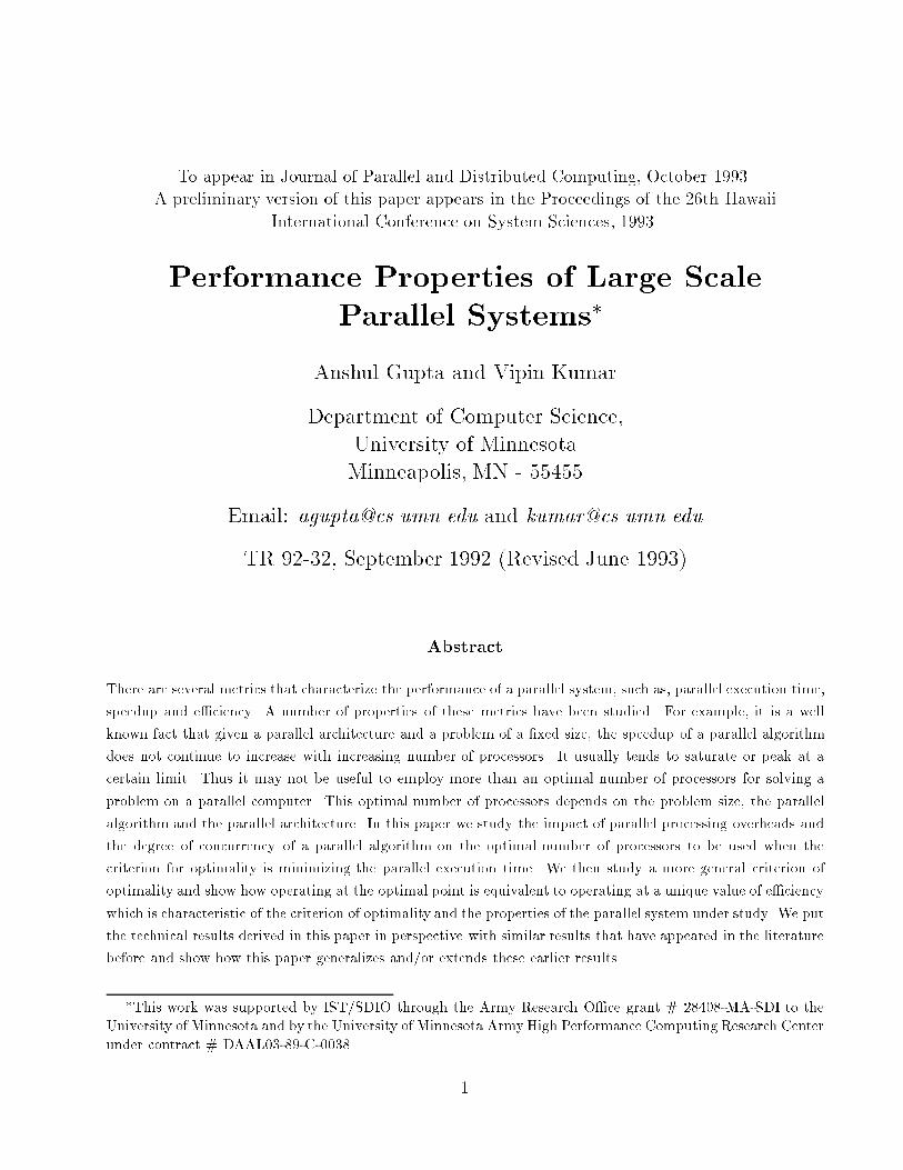
Maximum Number of Processors Usable, pmax: The number of processors that yield max-imum speedup Smax for a given W . This is the maximum number of processors one wouldlike to use because using more processors will not increase the speedup.3 Minimizing the Parallel Execution TimeIn this section we relate the behavior of the TP verses p curve to the nature of the overheadfunction To. As the number of processors is increased, TP either asymptotically approachesa minimum value, or attains a minimum and starts rising again. We identify the overheadfunctions which lead to one case or the other. We show that in either case, the problem can besolved in minimum time by using a certain number of processors which we call pmax. Using moreprocessors than pmax will either have no e�ect or will degrade the performance of the parallelsystem in terms of parallel execution time.Most problems have a serial component Ws | the part of W that has to be executedsequentially. In this paper the sequential component of an algorithm is not considered as aseparate entity, as it can be subsumed in To. While one processor is working on the sequentialcomponent, the remaining p� 1 are ideal and contribute (p� 1)Ws to To. Thus for any parallelalgorithm with a nonzero Ws, the analysis can be performed by assuming that To includes aterm equal to (p � 1)Ws. Under this assumption, the parallel execution time TP for a problemof size W on p processors is given by the following relation:TP = W + To(W;p)p (1)We now study the behavior of TP under two di�erent conditions.3.1 Case I: To � �(p)From Equation (1) it is clear that if To(W;p) grows slower than �(p), then the overall power of pin the R.H.S. of Equation (1) is negative. In this case it would appear that if p is increased, thenTP will continue to decrease inde�nitely. If To(W;p) grows as fast as �(p) then there will be alower bound on TP , but that will be a constant independent of W . But we know that for anyparallel system, the maximum number of processors that can be used for a given W is limitedby C(W ). So the maximum speedup is bounded by WC(W )W+To(W;C(W )) for a problem of size W andthe e�ciency at this point of peak performance is given by WW+To(W;C(W )) . Figure 1 illustratesthe curve of TP for the case when To � �(p).There are many important natural parallel systems for which the overhead function does notgrow faster than �(p). One such system is described in Example 1 below. Such systems typicallyarise while using shared memory or SIMD machines which do not have a message startup timefor data communication. 5

0Tminp20040060080010000 200 400 600 800 1000pmax = C(W ) 1200"Tp p!Figure 1: A typical TP verses p curve for To � �(p).Example 1: Parallel FFT on a SIMD HypercubeConsider a parallel implementation of the FFT algorithm [14] on a SIMD hypercube connectedmachine (e.g., the CM-2 [20]). If an N point FFT is being attempted on such a machine with pprocessors, Np units of data will be communicated among directly connected processors in log pof the logN iterations of the algorithm. For this parallel system W = N logN . As shown in[14], To = tw � Np log p � p = twN log p, where tw is the message communication time per word.Clearly, for a given W , To < �(p). Since C(W ) for the parallel FFT algorithm is N , there is alower bound on parallel execution time which is given by (1 + tw) logN . Thus, pmax for an Npoint FFT on a SIMD hypercube is N and the problem cannot be solved in less than �(logN)time.3.2 Case II: To > �(p)When To(W;p) grows faster than �(p), a glance at Equation (1) will reveal that the term Wpwill keep decreasing with increasing p, while the term Top will increase. Therefore, the overall TPwill �rst decrease and then increase with increasing p, resulting in a distinct minimum. Now wederive the relationship betweenW and p such that TP is minimized. Let p0 be the value of p forwhich the mathematical expression on the R.H.S of Equation (1) for TP attains its minimumvalue.At p = p0, TP is minimum and therefore ddpTP = 0.6

) ddp(W + To(W;p)p ) = 0) �Wp2 � To(W;p)p2 + ddpTo(W;p)p = 0) ddpTo(W;p) = Wp + To(W;p)p) ddpTo(W;p) = TP (2)For a given W , we can solve the above equation to �nd p0. A rather general form of theoverhead is one in which the overhead function is a sum of terms where each term is a productof a function of W and a function of p. In most real life parallel systems, these functionsof W and p are such that To can be written as �i=ni=1ciW yi(logW )uipxi(log p)zi , where ci's areconstants and xi � 0 and yi � 0 for 1 � i � n, and ui's and zi's are 0's or 1's. The overheadfunctions of all architecture-algorithm combinations that we have come across �t this form[24, 25, 31, 14, 12, 15, 36, 35, 11]. As illustrated by a variety of examples in this paper,these include important algorithms such as Matrix Multiplication, FFT, Parallel Search, �ndingShortest Paths in a graph, etc., on almost all parallel architectures of interest.For the sake of simplicity of the following analysis, we assume zi = 0 and ui = 0 for alli's. Analysis similar to that presented below can be performed even without this assumptionand similar results can be obtained (Appendix A). Substituting �i=ni=1ciW yipxi for To(W;p) inEquation (2), we obtain the following equation:�i=ni=1 cixiW yipxi�1 = W + �i=ni=1ciW yipxip) W = �i=ni=1ci(xi � 1)W yipxi (3)For the overhead function described above, Equation (3) determines the relationship betweenW and p for minimizing TP provided that To grows faster than �(p). Because of the nature ofEquation (3), it may not always be possible to express p as a function of W in a closed form. Sowe solve Equation (3), considering one R.H.S. term at a time and ignoring the rest. If the ithterm is being considered, the relation W = ci(xi � 1)W yipxi yields p = ( W 1�yici(xi�1)) 1xi = �(W 1�yixi ).It can be shown (Appendix B) that among all the i solutions for p obtained in this manner,the speedup is maximum for any given W when p = �(W 1�yjxj ) where 1�yjxj � 1�yixi for all i(1 � i � n). We call the jth term of To the dominant term if the value of 1�yjxj is the leastamong all values 1�yixi (1 � i � n) because this is the term that determines the order of p0 -7

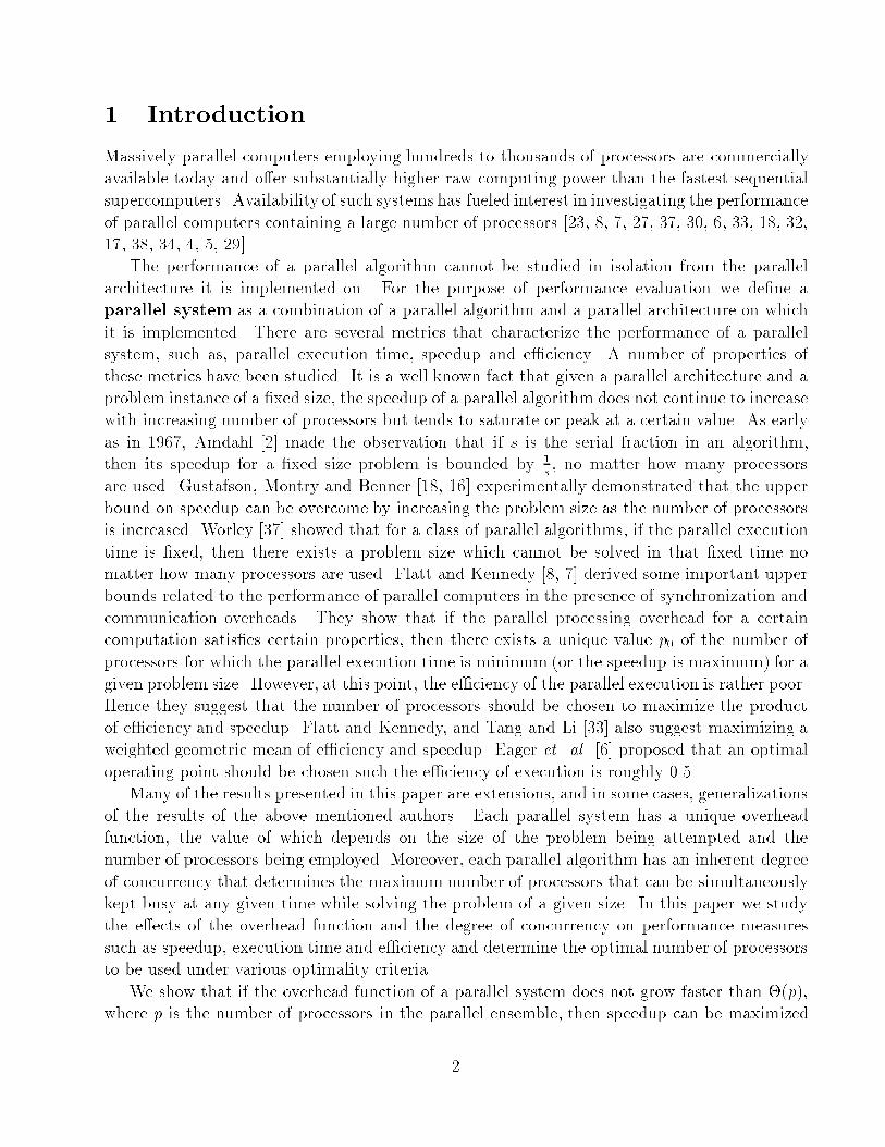
the solution to Equation (2) for large values of W and p. If jth term is the dominant term ofTo, then solving Equation (3) with respect to the jth term on the R.H.S. yields the followingapproximate expression for p0 for large values of W :p0 � ( W 1�yjcj(xj � 1)) 1xj (4)The value of p0 thus obtained can be used in the expression for TP to determine the minimumparallel execution time for a given W . The value of p0, when plugged in the expression fore�ciency, yields the following: E0 = WW + To) E0 � WW + cjW yj ( W 1�yjxj(cjxj�cj) 1xj )xj) E0 � 1� 1xj (5)Note that the above analysis holds only if xj, the exponent of p in the dominant term of Tois greater than 1. If xj � 1, then the asymptotically highest term in To (i.e., cjW yjpxj) is lessthan or equal to �(p) and the results for the case when To � �(p) apply.Equations (4) and (5) yield the mathematical values of p0 and E0 respectively. But thederived value of p0 may exceed C(W ). So in practice, at the point of peak performance (interms of maximum speedup or minimum execution time), the number of processors pmax isgiven by min(p0; C(W )) for a given W . Thus it is possible that C(W ) of a parallel algorithmmay determine the minimum execution time rather than the mathematically derived conditions.The following example illustrates this case:Example 2: Floyd's Striped Shortest Path Algorithm on MeshA number of parallel Shortest Path algorithms are discussed in [25]. Consider the implementationof Floyd's algorithm in which the N � N adjacency matrix of the graph is striped among pprocessors such that each processor stores Np full rows of the matrix. The problem size W hereis given by N3 for �nding all to all shortest paths on an N -node graph. In each of the Niterations of this algorithm, a processor broadcasts a row of length N of the adjacency matrixof the graph to every other processor. As shown in [25], if the p processor are connected in amesh con�guration with cut-through routing, the total overhead due to this communication isgiven by To = tsNp1:5+ tw(N +pp)Np. Here ts and tw are constants related to message startuptime and the speed of message transfer respectively. Since tw is often very small compared to ts,To = (ts+ tw)Np1:5+ twN2p � tsNp1:5+ twN2p = tsW 1=3p1:5+ twW 2=3p. From Equation (3), p0is equal to (W 2=3:5ts )2=3 � 1:59N4=3t2=3s . But since at most N processors can be used in this algorithm,8

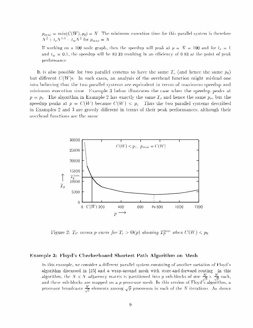
pmax = min(C(W ); p0) = N . The minimum execution time for this parallel system is thereforeN2 + tsN1:5 + twN2 for pmax = N .If working on a 100 node graph, then the speedup will peak at p = N = 100 and for ts = 1and tw = 0:1, the speedup will be 83.33 resulting in an e�ciency of 0.83 at the point of peakperformance.It is also possible for two parallel systems to have the same To (and hence the same p0)but di�erent C(W )s. In such cases, an analysis of the overhead function might mislead oneinto believing that the two parallel systems are equivalent in terms of maximum speedup andminimum execution time. Example 3 below illustrates the case when the speedup peaks atp = po. The algorithm in Example 2 has exactly the same To and hence the same po, but thespeedup peaks at p = C(W ) because C(W ) < po. Thus the two parallel systems describedin Examples 2 and 3 are grossly di�erent in terms of their peak performances, although theiroverhead functions are the same.0500010000Tminp150002000025000300000 C(W ) 200 400 600 p0 800 1000 1200

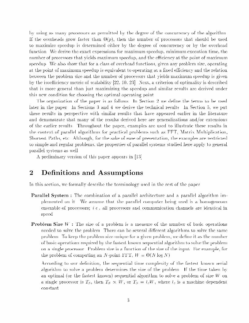
C(W ) < p0, pmax = C(W )"Tp p!Figure 2: TP verses p curve for To > �(p) showing TminP when C(W ) < p0.Example 3: Floyd's Checkerboard Shortest Path Algorithm on MeshIn this example, we consider a di�erent parallel system consisting of another variation of Floyd'salgorithm discussed in [25] and a wrap-around mesh with store-and-forward routing. In thisalgorithm, the N � N adjacency matrix is partitioned into p sub-blocks of size Npp � Npp each,and these sub-blocks are mapped on a p processor mesh. In this version of Floyd's algorithm, aprocessor broadcasts Npp elements among pp processors in each of the N iterations. As shown9

0Tminp500010000150002000025000300000 200 400 600 p0800 1000 1200� C(W )10000 10200

C(W ) > p0, pmax = p0"Tp p!Figure 3: TP verses p curve for To > �(p) showing TminP when C(W ) > p0.in [25], this results in a total overhead of To = tsNp1:5 + twN2p. Since the expression for To issame as that in Example 2, p0 = 1:59N4=3t2=3s again. But C(W ) for the checkerboard version of thealgorithm is W 2=3 = N2. Therefore pmax = p0 in this case as p0 < C(W ).For ts = 1 and tw = 0:1, Equation (3) yields a value of po = 738 for a 100 node graph. Thespeedup peaks with 738 processors at a value of 246, but the e�ciency at this peak speedup isonly 0.33.Figures 2 and 3 graphically depict TP as a function of p corresponding to Examples 2 and 3respectively.3.3 Minimizing TP and the Isoe�ciency FunctionIn this section we show that for a wide class of overhead functions, studying a parallel systemat its peak performance in terms of the speedup is equivalent to studying its behavior at a�xed e�ciency. The isoe�ciency metric [22, 10, 23] comes in as a handy tool to study the �xede�ciency characteristics of a parallel system. The isoe�ciency function relates the problem sizeto the number of processors necessary for an increase in speedup in proportion to the number ofprocessors used. If a parallel system incurs a total overhead of To(W;p) while solving a problemof size W on p processors, the e�ciency of the system is given by E = 11+To(W;p)W . In orderto maintain a constant e�ciency, W / To(W;p) or W = KTo(W;p) must be satis�ed, whereK = E1�E is a constant depending on the e�ciency to be maintained. This is the central relationthat is used to determine isoe�ciency as a function of p. From this equation, the problem size10

W can usually be obtained as a function of p by algebraic manipulations. If the problem sizeW needs to grow as fast as fE(p) to maintain an e�ciency E, then fE(p) is de�ned to be theisoe�ciency function of the parallel algorithm-architecture combination for e�ciency E.We now show that unless pmax = C(W ) for a parallel system, a unique e�ciency is attainedat the point of peak performance. This value of E depends only on the characteristics of theparallel system (i.e., the type of overhead function for the algorithm-architecture combination)and is independent of W or TP . For the type of overhead function assumed in Section 3.2, thefollowing relation determines the isoe�ciency function for an e�ciency E.W = E1 � E�i=ni=1ciW yipxi (6)Clearly, this equation has the same form as Equation (3), but has di�erent constants. Thedominant term on the R.H.S will yield the relationship between W and p in a closed form inboth the equations. If this is the jth term, then both the equations will become equivalentasymptotically if their jth terms are same. This amounts to operating at an e�ciency that isgiven by the following relation obtained by equating the coe�cients of the jth terms of Equations(3) and (6). E1� Ecj = cj(xj � 1)) E = 1 � 1xjThe above equation is in conformation with Equation (5). Once we know that working atthe point of peak performance amounts to working at an e�ciency of 1� 1xj , then, for a givenW ,we can �nd the number of processors at which the performance will peak by using the relation1� 1xj = WW+To(W;p) .As discussed in [22, 10], the relation between the problem size and the maximum numberof processors that can be used in a cost-optimal fashion for solving the problem is given bythe isoe�ciency function. Often, using as many processors as possible results in a non-cost-optimal system. For example, adding n numbers on an n-processor hypercube takes �(log n)time, which is the minimum execution time for this problem. This is not a cost optimal parallelsystem because W = �(N) < pTP = �(n log n). An important corollary of the result presentedin this section is that for the parallel systems for which the relationship between the problemsize and the number of processors for maximum speedup (minimum execution time) is given bythe isoe�ciency function, the asymptotic minimum execution time can be attained in a cost-optimal fashion. For instance, if �( nlogn) processors are used to add n numbers on a hypercube,the parallel system will be cost-optimal and the parallel execution time will still be �(log n).Note that the correspondence between the isoe�ciency function and the relation betweenW and p for operating at minimum TP will fail if the xj in the dominant term is less than orequal to 1. In this case, a term other than the one that determines the isoe�ciency functionwill determine the condition for minimum TP . 11

3.4 Summary of ResultsAt this point we state the important results of this section.. For parallel algorithms with To � �(p), the maximum speedup is obtained at p = C(W ) andfor algorithms with To > �(p), the maximum speedup is obtained at p = min(po; C(W )),where p0 for a given W is determined by solving Equation (3).. For the parallel algorithms with To of the form described in Section 3.2, if the jth term isthe dominant term in the expression for To and xj > 1, then the e�ciency at the point ofmaximum speedup always remains the same irrespective of the problem size, and is givenby E = 1 � 1xj .. For the parallel algorithms satisfying the above conditions, the relationship between theproblem size and the number of processors at which the speedup is maximum for thatproblem size, is given by the isoe�ciency function for E = 1 � 1xj , unless pmax = C(W ).4 Minimizing p(TP )rFrom the previous sections, it is clear that operating at a point where TP is minimummight notbe a good idea because for some parallel systems the e�ciency at this point might be low. Onthe other hand, the maximum e�ciency is always attained at p = 1 which obviously is the pointof minimum speedup. Therefore, in order to achieve a balance between speedup and e�ciency,several researchers have proposed to operate at a point where the value of p(TP )r is minimizedfor some constant r (r � 1) and for a given problem size W [8, 6, 33]. It can be shown [33] thatthis corresponds to the point where ESr�1 is maximized for a given problem size.p(TP )r = pTP (WS )r�1 = W rESr�1Thus p(TP )r will be minimum when ESr�1 is maximum for a given W and by minimizingp(TP )r, we are choosing an operating point with a concern for both speedup and e�ciency, theirrelative weights being determined by the value of r.Now let us locate the point where p(TP )r is minimum.p(TP )r = p(Te+Top )r = p1�r(Te + To)rAgain, as in the previous section, the following two cases arise:4.1 Case I: To � �(p r�1r )Since p(TP )r = p1�r(Te + To)r = (Tep 1�rr + Top 1�rr )r, if To � �(p r�1r ) then the overall powerof p in the expression for p(TP )r will become negative and hence its value will mathematicallytend to some lower bound as p;1. Thus using as many processors as are feasible will lead tominimum p(TP )r. In other words, for this case, p(TP )r is minimum when p = C(W ).12

4.2 Case II: To > �(p r�1r )If To grows faster than �(p r�1r ), then we proceed as follows. In order to minimize p(TP )r,ddp p(TP )r should be equal to zero.(1 � r)p�r(Te + To)r + rp(1�r)(Te + To)(r�1) ddpTo = 0) ddpTo = r � 1r TP (7)We choose the same type of overhead function as in Section 3.2. Substituting �i=ni=1ciW yipxifor To in Equation (7), we get the following equation:�i=ni=1cixiW yipxi�1 = r � 1rp (W + �i=ni=1 ciW yipxi)) W = �i=ni=1ci( rxir � 1 � 1)W yipxi (8)Now even the number of processors for which p(TP )r is minimum could exceed the value ofp that is permitted by the degree of concurrency of the algorithm. In this case the minimumpossible value for p(TP )r will be obtained when C(W ) processors are used. The followingexample illustrates this case.Example 4: Matrix Multiplication on MeshConsider a simple algorithm described in [12] for multiplying two N �N matrices on a pp�ppwrap-around mesh. As the �rst step of the algorithm, each processor acquires all those elementsof both the matrices that are required to generate the N2p elements of the product matrix whichare to reside in that processor. For this parallel system,W = N3 and To = tsppp+ twN2pp. Fordetermining the operating point where p(TP )2 is minimum, we substitute n = 2, r = 2, c1 = ts,c2 = tw , x1 = 1:5, x2 = 0:5, y1 = 0 and y2 = 23 in Equation (8). This substitution yields therelation W = 2tsp1:5 for determining the required operating point. In other words, the number ofprocessors p0 at which p(TP )2 is minimum is given by p0 = (W2ts)2=3 = N2(2ts)2=3 . But the maximumnumber of processors that this algorithm can use is only N2. Therefore, for ts < :5, p0 > C(W )and hence C(W ) processors should be used to minimize pT 2P .4.3 Minimizing p(TP )r and the Isoe�ciency FunctionIn this subsection we show that for a wide class of parallel systems, even minimizing p(TP )ramounts to operating at a unique e�ciency that depends only on the overhead function andthe value of r. In other words, for a given W , p(TP )r is minimum for some value of p and therelationship betweenW and this p for the parallel system is given by its isoe�ciency function fora unique value of e�ciency that depends only on r and the type of overhead function. Equation13

(8), which gives the relationship between W and p for minimum p(TP )r, has the same form asEquation (6) that determines the isoe�ciency function for some e�ciency E. If the jth terms ofthe R.H.S.s of Equations (6) and (8) dominate (and xj > r�1r ), then the e�ciency at minimump(TP )r can be obtained by equating the corresponding constants; i.e., Ecj1�E and cj( rxjr�1�1). Thisyields the following expression for the value of e�ciency at the point where p(TP )r is minimum:E = 1� r � 1rxj (9)The following example illustrates how the analysis of Section 4 can be used for chosing anappropriate operating point (in terms of p) for a parallel algorithm to solve a problem instanceof a given size. It also con�rms the validity of Equation (9).Example 5: FFT on a HypercubeConsider the implementation of the FFT algorithm on an MIMD hypercube using the binary-exchange algorithm. As shown in [14], for an N point FFT on p processors, W = N logN andTo = tsp log p+ twN log p for this algorithm. Taking ts = 2, tw = 0:1 and rewriting the expressionfor To in the form described in Section 3.2, we get the following:To � 2p log p+ 0:1 WlogW log pNow suppose it is desired to minimize p(TP )2, which is equivalent to maximizing the ES product.Clearly, the �rst term of To dominates and hence putting r = 2 and xj = 1 in Equation (9), ane�ciency of 0.5 is predicted when p(TP )2 is minimized. An analysis similar to that in Section4.2 will show that p(TP )r will be minimum when p � N2 is used.If a 1024 point FFT is being attempted, then Table I shows that at p = 512 the ES product isindeed maximum and the e�ciency at this point is indeed 0.5.Again, just like in Section 3.3, there are exceptions to the correspondence between theisoe�ciency function and the condition for minimum p(TP )r. If the jth term in Equation (6)determines the isoe�ciency function and in Equation (8), xj < r�1r , then the coe�cient of thejth term in Equation (8) will be zero or negative and some other term in Equation (8) willdetermine the relationship between W and p for minimum p(TP )r.The following subsection summarizes the results of this section.4.4 Summary of Results. For parallel algorithms with To � �(p r�1r ), the minimum value for the expression p(TP )ris attained at p = C(W ) and for algorithms with To > �(p r�1r ), it is attained at p =min(C(W ); p0), where p0 for a given W is obtained by solving Equation (8).14

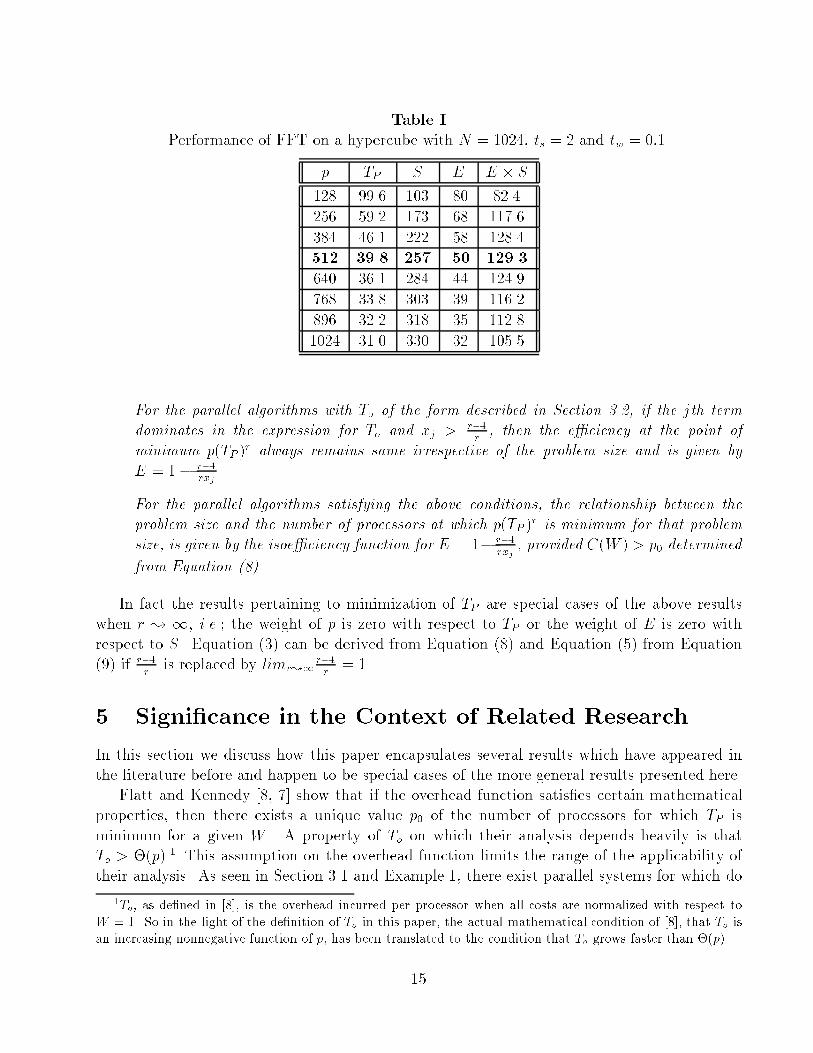
Table IPerformance of FFT on a hypercube with N = 1024, ts = 2 and tw = 0:1.p TP S E E � S128 99.6 103 .80 82.4256 59.2 173 .68 117.6384 46.1 222 .58 128.4512 39.8 257 .50 129.3640 36.1 284 .44 124.9768 33.8 303 .39 116.2896 32.2 318 .35 112.81024 31.0 330 .32 105.5. For the parallel algorithms with To of the form described in Section 3.2, if the jth termdominates in the expression for To and xj > r�1r , then the e�ciency at the point ofminimum p(TP )r always remains same irrespective of the problem size and is given byE = 1� r�1rxj .. For the parallel algorithms satisfying the above conditions, the relationship between theproblem size and the number of processors at which p(TP )r is minimum for that problemsize, is given by the isoe�ciency function for E = 1� r�1rxj , provided C(W ) > p0 determinedfrom Equation (8).In fact the results pertaining to minimization of TP are special cases of the above resultswhen r ; 1, i.e.; the weight of p is zero with respect to TP or the weight of E is zero withrespect to S. Equation (3) can be derived from Equation (8) and Equation (5) from Equation(9) if r�1r is replaced by limr;1 r�1r = 1.5 Signi�cance in the Context of Related ResearchIn this section we discuss how this paper encapsulates several results which have appeared inthe literature before and happen to be special cases of the more general results presented here.Flatt and Kennedy [8, 7] show that if the overhead function satis�es certain mathematicalproperties, then there exists a unique value p0 of the number of processors for which TP isminimum for a given W . A property of To on which their analysis depends heavily is thatTo > �(p).1 This assumption on the overhead function limits the range of the applicability oftheir analysis. As seen in Section 3.1 and Example 1, there exist parallel systems for which do1To, as de�ned in [8], is the overhead incurred per processor when all costs are normalized with respect toW = 1. So in the light of the de�nition of To in this paper, the actual mathematical condition of [8], that To isan increasing nonnegative function of p, has been translated to the condition that To grows faster than �(p).15

not obey this condition, and in such cases the point of peak performance is determined by thedegree of concurrency of the algorithm being used.Flatt and Kennedy show that the maximumspeedup attainable for a given problem is upper-bounded by 1ddp (pTP ) at p = p0. They also show that the better a parallel algorithm is (i.e., theslower To grows with p), the higher is the value of p0 and the lower is the value of e�ciencyobtained at this point. Equations (4) and (5) in this paper provide results similar to Flattand Kennedy's. But the analysis in [8] tends to conclude the following - (i) if the overheadfunction grows very fast with respect to p, then p0 is small, and hence parallel processing cannotprovide substantial speedups; (ii) if the overhead function grows slowly (i.e., closer to �(p)),then the overall e�ciency is very poor at p = p0. Note that if we keep improving the overheadfunction, the mathematically derived value of p0 will ultimately exceed the limit imposed by thedegree of concurrency on the number of processors that can be used. Hence, in practice no morethan C(W ) processors will be used. Thus, in this situation, the theoretical value of p0 and thee�ciency at this point does not serve a useful purpose because the point of peak performancee�ciency cannot be worse than WW+To(W;C(W )) . For instance, Flatt and Kennedy's analysis willpredict identical values of pmax and e�ciency at this operating point for the parallel systemsdescribed in Examples 2 and 3 because their overhead functions are identical. But as we saw inthese examples, this is not the case because the the value of C(W ) in the two cases is di�erent.In [27], Marinescu and Rice develop a model to describe and analyze a parallel computationon a MIMD machine in terms of the number of threads of control p into which the computation isdivided and the number events g(p) as a function of p. They consider the case where each eventis of a �xed duration � and hence To = �g(p). Under these assumptions on To, they conclude thatwith increasing number of processors, the speedup saturates at some value if To = �(p), and itasymptotically approaches zero if To = �(pm), where m � 2. The results of Sections 3.1 and 3.2are generalizations of these conclusions for a wider class of overhead functions. In Section 3.1we show that the speedup saturates at some maximum value if To � �(p), and in Section 3.2we show that speedup will attain a maximum value and then it will drop monotonically with pif To > �(p).Usually, the duration of an event or a communication step � is not a constant as assumed in[27]. In general, both � and To are functions of W and p. If To is of the form �g(p), Marinescuand Rice [27] derive that the number of processors that will yield maximum speedup will begiven by p = (W� + g(p)) 1g0(p) , which can be rewritten as �g0(p) = W+�g(p)p . It is easily veri�edthat this is a special case of Equation (2) for To = �g(p).Worley [37] showed that for certain algorithms, given a certain amount of time TP , therewill exist a problem size large enough so that it cannot be solved in time TP , no matter howmany processors are used. In Section 3, we describe the exact nature of the overhead functionfor which a lower bound exists on the execution time for a given problem size. This is exactlythe condition for which, given a �xed time, an upper bound will exist on the size of the problemthat can be solved within this time. We show that for a class of parallel systems, the relationbetween problem size W and the number of processors p at which the parallel execution timeTP is minimized, is given by the isoe�ciency function for a particular e�ciency.16

Several other researchers have used the minimum parallel execution time of a problem of agiven size for analyzing the performance of parallel systems [28, 26, 30]. Nussbaum and Agarwal[30] de�ne scalability of an architecture for a given algorithm as the ratio of the algorithm'sasymptotic speedup when run on the architecture in question to its corresponding asymptoticspeedup when run on an EREW PRAM. The asymptotic speedup is the maximum obtainablespeedup for a given problem size if an unlimited number of processors is available. For a �xedproblem size, the scalability of the parallel system, according to their metric, depends directly onthe minimum TP for the system. For the class of parallel systems for which the correspondencebetween the isoe�ciency function and the relation between W and p for minimizing TP exists,Nussbaum and Agarwal's scalability metric will yield results identical to those predicted by theisoe�ciency function on the behavior of these parallel systems.Eager et. al. [6] and Tang and Li [33] have proposed a criterion of optimality di�erentfrom optimal speedup. They argue that the optimal operating point should be chosen so thata balance is struck between e�ciency and speedup. It is proposed in [6] that the \knee" of theexecution time verses e�ciency curve is a good choice of the operating point because at thispoint the incremental bene�t of adding processors is roughly 12 per processor, or, in other words,e�ciency is 0.5. Eager et. al. and Tang and Li also conclude that for To = �(p), this is alsoequivalent to operating at a point where the ES product is maximum or p(TP )2 is minimum.This conclusion in [6, 33] is a special case of the more general case that is captured in Equation(9). If we substitute xj = 1 in Equation (9) (which is the case if To = �(p)), it can seen that weindeed get an e�ciency of 0.5 for r = 2. In general, operating at the optimal point or the \knee"referred to in [6] and [33] for a parallel system with To = �(pxj) will be identical to operatingat a point where p(TP )r is minimum, where r = 22�xj . This is obtained from Equation (9) forE = 0:5. Minimizing p(TP )r for r > 22�xj will result in an operating point with e�ciency lowerthan 0.5 but a higher speedup. On the other hand, minimizing p(TP )r for r < 22�xj will resultin an operating point with e�ciency higher than 0.5 and a lower speedup.In [21], Kleinrock and Huang state that the mean service time for a job is minimumfor p =1,or for as many processors as possible. This is true only under the assumption that To < �(p).For this assumption to be true, the parallel system has to be devoid of any global operation(such as broadcast, and one-to-all and all-to-all personalized communication [3, 19]) with amessage passing latency or message startup time. The reason is that such operations alwayslead to To � �(p). This class of algorithms includes some fairly important algorithms suchas matrix multiplication (all-to-all/one-to-all broadcast) [12], vector dot products (single nodeaccumulation) [15], shortest paths (one-to-all broadcast) [25], and FFT (all-to-all personalizedcommunication) [14], etc. The readers should note that the presence of a global communicationoperation in an algorithm is a su�cient but not a necessary condition for To � �(p).References[1] S. G. Akl. The Design and Analysis of Parallel Algorithms. Prentice-Hall, Englewood Cli�s, NJ, 1989.[2] G. M. Amdahl. Validity of the single processor approach to achieving large scale computing capabilities. InAFIPS Conference Proceedings, pages 483{485, 1967.17

[3] D. P. Bertsekas and J. N. Tsitsiklis. Parallel and Distributed Computation: Numerical Methods. Prentice-Hall, Englewood Cli�s, NJ, 1989.[4] E. A. Carmona and M. D. Rice. A model of parallel performance. Technical Report AFWL-TR-89-01, AirForce Weapons Laboratory, 1989.[5] E. A. Carmona and M. D. Rice. Modeling the serial and parallel fractions of a parallel algorithm. Journalof Parallel and Distributed Computing, 1991.[6] D. L. Eager, J. Zahorjan, and E. D. Lazowska. Speedup versus e�ciency in parallel systems. IEEETransactions on Computers, 38(3):408{423, 1989.[7] Horace P. Flatt. Further applications of the overhead model for parallel systems. Technical Report G320-3540, IBM Corporation, Palo Alto Scienti�c Center, Palo Alto, CA, 1990.[8] Horace P. Flatt and Ken Kennedy. Performance of parallel processors. Parallel Computing, 12:1{20, 1989.[9] G. C. Fox, M. Johnson, G. Lyzenga, S. W. Otto, J. Salmon, and D. Walker. Solving Problems on ConcurrentProcessors: Volume 1. Prentice-Hall, Englewood Cli�s, NJ, 1988.[10] Ananth Grama, Anshul Gupta, and Vipin Kumar. Isoe�ciency: Measuring the scalability of parallel al-gorithms and architectures. IEEE Parallel and Distributed Technology, 1(3):12{21, August, 1993. Alsoavailable as Technical Report TR 93-24, Department of Computer Science, University of Minnesota, Min-neapolis, MN.[11] Ananth Grama, Vipin Kumar, and V. Nageshwara Rao. Experimental evaluation of load balancing tech-niques for the hypercube. In Proceedings of the Parallel Computing '91 Conference, pages 497{514, 1991.[12] Anshul Gupta and Vipin Kumar. The scalability of matrix multiplication algorithms on parallel computers.Technical Report TR 91-54, Department of Computer Science, University of Minnesota, Minneapolis, MN,1991. A short version appears in Proceedings of 1993 International Conference on Parallel Processing, pagesIII-115{III-119, 1993.[13] Anshul Gupta and Vipin Kumar. Analyzing performance of large scale parallel systems. In Proceedings ofthe 26th Hawaii International Conference on System Sciences, 1993. To appear in Journal of Parallel andDistributed Computing, 1993.[14] Anshul Gupta and Vipin Kumar. The scalability of FFT on parallel computers. IEEE Transactions onParallel and Distributed Systems, 4(8):922{932, August 1993. A detailed version available as TechnicalReport TR 90-53, Department of Computer Science, University of Minnesota, Minneapolis, MN.[15] Anshul Gupta, Vipin Kumar, and A. H. Sameh. Performance and scalability of preconditioned conjugategradient methods on parallel computers. Technical Report TR 92-64, Department of Computer Science,University of Minnesota, Minneapolis, MN, 1992. A short version appears in Proceedings of the Sixth SIAMConference on Parallel Processing for Scienti�c Computing, pages 664{674, 1993.[16] John L. Gustafson. Reevaluating Amdahl's law. Communications of the ACM, 31(5):532{533, 1988.[17] John L. Gustafson. The consequences of �xed time performance measurement. In Proceedings of the 25thHawaii International Conference on System Sciences: Volume III, pages 113{124, 1992.[18] John L. Gustafson, Gary R. Montry, and Robert E. Benner. Development of parallel methods for a 1024-processor hypercube. SIAM Journal on Scienti�c and Statistical Computing, 9(4):609{638, 1988.[19] S. L. Johnsson and C.-T. Ho. Optimum broadcasting and personalized communication in hypercubes. IEEETransactions on Computers, 38(9):1249{1268, September 1989.[20] S. L. Johnsson, R. Krawitz, R. Frye, and D. McDonald. A radix-2 FFT on the connection machine. Technicalreport, Thinking Machines Corporation, Cambridge, MA, 1989.18

[21] L. Kleinrock and J.-H. Huang. On parallel processing systems: Amdahl's law generalized and some resultson optimal design. IEEE Transactions on Software Engineering, 18(5):434{447, May 1992.[22] Vipin Kumar, Ananth Grama, Anshul Gupta, and George Karypis. Introduction to Parallel Computing:Design and Analysis of Algorithms. Benjamin/Cummings, Redwood City, CA, 1994.[23] Vipin Kumar and Anshul Gupta. Analyzing scalability of parallel algorithms and architectures. TechnicalReport TR 91-18, Department of Computer Science Department, University of Minnesota, Minneapolis,MN, 1991. To appear in Journal of Parallel and Distributed Computing, 1994. A shorter version appears inProceedings of the 1991 International Conference on Supercomputing, pages 396-405, 1991.[24] Vipin Kumar and V. N. Rao. Parallel depth-�rst search, part II: Analysis. International Journal of ParallelProgramming, 16(6):501{519, 1987.[25] Vipin Kumar and Vineet Singh. Scalability of parallel algorithms for the all-pairs shortest path problem.Journal of Parallel and Distributed Computing, 13(2):124{138, October 1991. A short version appears inthe Proceedings of the International Conference on Parallel Processing, 1990.[26] Y. W. E. Ma and Denis G. Shea. Downward scalability of parallel architectures. In Proceedings of the 1988International Conference on Supercomputing, pages 109{120, 1988.[27] Dan C. Marinescu and John R. Rice. On high level characterization of parallelism. Technical Report CSD-TR-1011, CAPO Report CER-90-32, Computer Science Department, Purdue University, West Lafayette,IN, Revised June 1991. To appear in Journal of Parallel and Distributed Computing, 1993.[28] David M. Nicol and Frank H. Willard. Problem size, parallel architecture, and optimal speedup. Journalof Parallel and Distributed Computing, 5:404{420, 1988.[29] Sam H. Noh, Dipak Ghosal, and Ashok K. Agrawala. An empirical study of the e�ect of granularityon parallel algorithms on the connection machine. Technical Report UMIACS-TR-89-124.1, University ofMaryland, College Park, MD, 1989.[30] Daniel Nussbaum and Anant Agarwal. Scalability of parallel machines. Communications of the ACM,34(3):57{61, 1991.[31] Vineet Singh, Vipin Kumar, Gul Agha, and Chris Tomlinson. Scalability of parallel sorting on meshmulticomputers. International Journal of Parallel Programming, 20(2), 1991.[32] Xian-He Sun and John L. Gustafson. Toward a better parallel performance metric. Parallel Computing,17:1093{1109, December 1991. Also available as Technical Report IS-5053, UC-32, Ames Laboratory, IowaState University, Ames, IA.[33] Zhimin Tang and Guo-Jie Li. Optimal granularity of grid iteration problems. In Proceedings of the 1990International Conference on Parallel Processing, pages I111{I118, 1990.[34] Fredric A. Van-Catledge. Towards a general model for evaluating the relative performance of computersystems. International Journal of Supercomputer Applications, 3(2):100{108, 1989.[35] Jinwoon Woo and Sartaj Sahni. Hypercube computing: Connected components. Journal of Supercomputing,1991. Also available as TR 88-50 from the Department of Computer Science, University of Minnesota,Minneapolis, MN.[36] Jinwoon Woo and Sartaj Sahni. Computing biconnected components on a hypercube. Journal of Supercom-puting, June 1991. Also available as Technical Report TR 89-7 from the Department of Computer Science,University of Minnesota, Minneapolis, MN.[37] Patrick H. Worley. The e�ect of time constraints on scaled speedup. SIAM Journal on Scienti�c andStatistical Computing, 11(5):838{858, 1990.[38] Xiaofeng Zhou. Bridging the gap between Amdahl's law and Sandia laboratory's result. Communicationsof the ACM, 32(8):1014{5, 1989. 19

Appendix ALet To(W;p) = �i=ni=1 ciW yi(logW )uipxi(log p)zi , where ci's are constants and xi � 0 and yi � 0for 1 � i � n, and ui's and zi's are 0's or 1's. Now let us compute ddpTo(W;p).To(W;p) = �i=ni=1ciW yi(logW )uipxi(log p)ziddpTo(W;p) = �i=ni=1 ciW yi(logW )ui(xipxi�1(log p)zi + zipxi�1(log p)zi�1)If all zi's are either 0 or 1, then the above equations can be rewritten as:ddpTo(W;p) = �i=ni=1ciW yi(logW )ui(xipxi�1(xi log p)zi + zi)ddpTo(W;p) � �i=ni=1cixiW yi(logW )uixipxi�1Equating ddpTo(W;p) to TP according to Equation 2,�i=ni=1cixiW yi(logW )uixipxi�1 = W + �i=ni=1 ciW yi(logW )uipxi(log p)zipW = �i=ni=1 ci(xi � 1)W yi(logW )uipxi(log p)zi (10)The above equation determines the relation between W and p for which the parallel executiontime is minimized. The equation determining the isoe�ciency function for the parallel systemwith the overhead function under consideration will be as follows (see discussion in Section 3.3):W = E1� E�i=ni=1ciW yi(logW )uipxi(log p)zi (11)Comparing Equations 10 and 11, if the jth term in To is the dominant term and xj > 1, thenthe e�ciency at the point of minimum parallel execution time will be given by E0 � 1 � 1xj .Appendix BFrom Equation 3, the relation betweenW and p0 is given by the solution for p from the followingequation: W = �i=ni=1ci(xi � 1)W yipxiIf the jth term on R.H.S. of the above is the dominant term according to the condition describedin Section 3.2, then we take p0 � ( W 1�yjcj(xj�1)) 1xj as the approximate solution. Now we show thatthe speedup is indeed (asymptotically) maximum for this value of p0.S = WpW + To(W;p)20

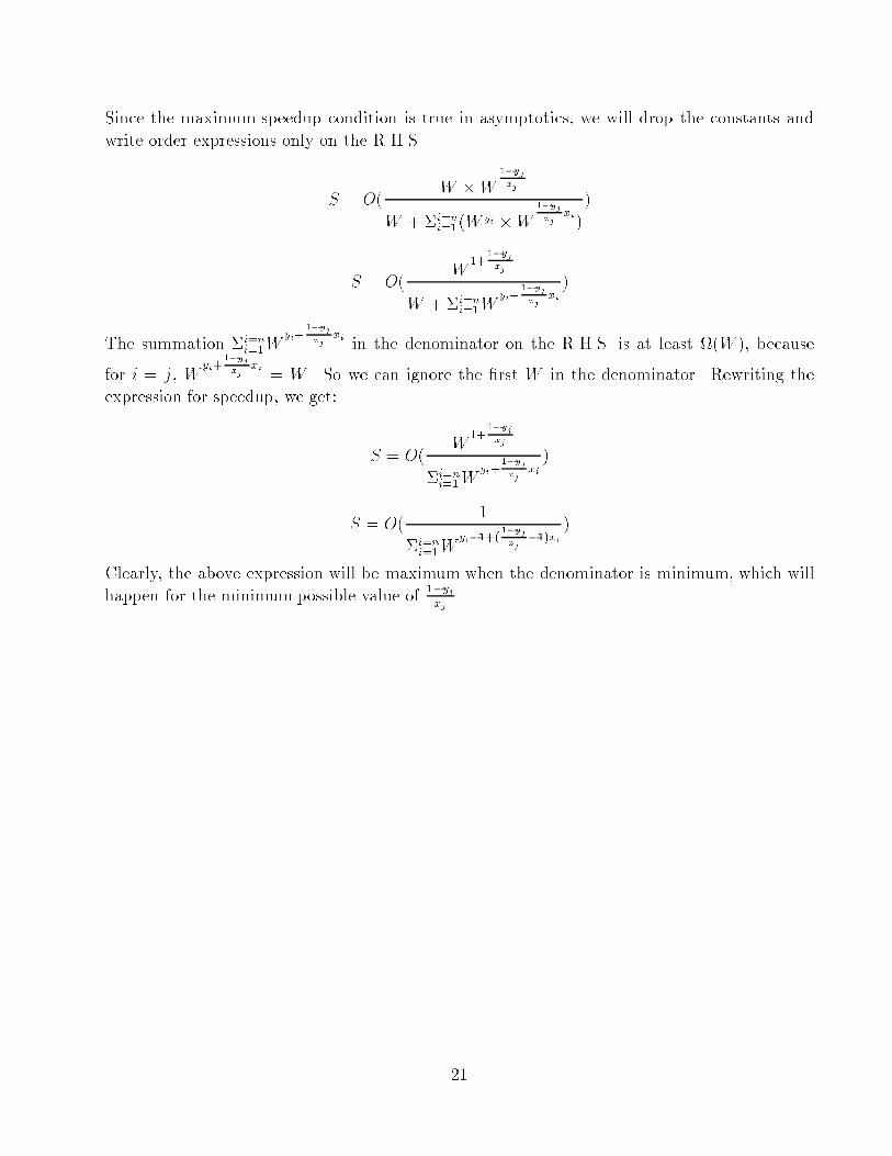
Since the maximum speedup condition is true in asymptotics, we will drop the constants andwrite order expressions only on the R.H.S..S = O( W �W 1�yjxjW + �i=ni=1 (W yi �W 1�yjxj xi))S = O( W 1+ 1�yjxjW + �i=ni=1W yi+ 1�yjxj xi )The summation �i=ni=1W yi+ 1�yjxj xi in the denominator on the R.H.S. is at least (W ), becausefor i = j, W yi+ 1�yjxj xi = W . So we can ignore the �rst W in the denominator. Rewriting theexpression for speedup, we get: S = O( W 1+ 1�yjxj�i=ni=1W yi+ 1�yjxj xi )S = O( 1�i=ni=1W yi�1+( 1�yjxj �1)xi )Clearly, the above expression will be maximum when the denominator is minimum, which willhappen for the minimum possible value of 1�yjxj .

21