DOCTORA L T H E S I S

Department of Engineering Sciences and MathematicsDivision of Fluid and Experimental Mechanics Smoothed Particle Hydrodynamic of

Hydraulic Jumps in Spillways

Patrick Jonsson

ISSN 1402-1544ISBN 978-91-7583-483-2 (print)ISBN 978-91-7583-484-9 (pdf)

Luleå University of Technology 2015

Patrick Jonsson Smoothed Particle H

ydrodynamic of H

ydraulic Jumps in Spillw

ays

Smoothed Particle Hydrodynamic ofHydraulic Jumps in Spillways

Patrick Jonsson

December 2015

Lulea University of Technology

Department of Engineering Sciences and Mathematics

Division of Fluid and Experimental Mechanics

Printed by Luleå University of Technology, Graphic Production 2015

ISSN 1402-1544ISBN 978-91-7583-483-2 (print)ISBN 978-91-7583-484-9 (pdf)

Luleå 2015

www.ltu.se

Smoothed Particle Hydrodynamic of Hydraulic Jumps

in Spillways

Copyright c© Patrick Jonsson (2015). This document is freely available

at

http://www.ltu.se

or by contacting Patrick Jonsson,

Patrick.Jonsson@ltu.se

The document may be freely distributed in its original form including

the current author’s name. None of the content may be changed or

excluded without permissions from the author.

Cover picture shows the spillway at Porjus hydropower station, located

in the northern part of Sweden, during spilling. Picture taken by c©Hans Blomberg 2007-05-07.

To my family

Preface

The work in this thesis started back in 2010 with my Master’s thesis.

Countless cups of coffee and probably an equal amount of profanities

later, I have reached the end of this, at times bumpy, journey. I have

learned so much during these last years and I have pushed myself to try

new things and questioned old truths with the support of those around

me. I wish to seize this opportunity to properly thank as many of those

as I possibly can.

To begin with, I would like to thank some very dear friends of mine.

Michael Wirven, my childhood buddy, who still is a very close friend.

The late, Anders Sigurdsson, who I shard many fun moments with dur-

ing my pilot-training, who, tragically, is no longer with us anymore.

Peter Eriksson, my fellow commander during my military service and

an appreciated metal-fan. Anders Pettersson, who, in a critical period,

kept me from quieting my engineering studies by just being a good friend.

Jesper Toyra, a stubborn, half-Finnish guy, who always has time for a

cup of coffee or a sauna, Helvetti!

Apart from my family, there are some key people who inspired me

to aim for a higher education and eventually to go for a Ph.D. degree.

These are my first math and science teacher Karl-Axel ”Kacke” Neiglick

and, also, Hampus Gavel together with his staff at SAAB Aerosystems,

Linkoping.

I like to thank my supervisors, Staffan Lundstrom, Gunnar Hell-

strom, Patrik Andreasson and Par Jonsen, for giving me the opportunity

of pursuing my Ph.D. degree and for believing in me. I also would like

i

to thank my colleagues and friends at the division for all the support.

Particularly, my friend and officemate Simon Johansson who has shared

my journey very closely. Our honest discussions, ranging from science to

girls, economics to picking blueberries and sometimes even religion and

how to tackle life’s problems, has inspired me greatly, especially when

we didn’t agreed. Another inspiring colleague was Andras Nemes, who I

met at Monash University in Melbourne, Australia. He opened the door

to the world of Python and showed me how to act as a ”senior” Ph.D.

student in an exemplary manner. I’m also very grateful to all the other

people who made the time in Melbourne a good time of my life, Ulrika,

Simon, Fanny, Thommaso, Pascal, Tim, James, Elisabeth, Andy, Mark,

John and David. I’ll probably bore my future grandchildren to death

by talking of my stay in Melbourne.

Finally, I want to express my deepest appreciation for my family who

always supports me and tries to show me the brighter side when I hit a

bump in the road. Thank you for showing me the real meaning of being

a team-player and all the other important stuff in life. Thank you for

driving me to hockey practice and tying me skates even if my lazy-self

claimed that I was ”tired, had a headache and a stomach-ache”. Thank

you for letting me follow my dreams when I wanted to become an airline

pilot even if I was much too young. I will always try to return the favour

and help you with what ever problem you have, because in the end, you

even taught me how to use a spoon.

Last, but far from least, I want to thank my beautiful Ulrika for

all your support and encouragement. Thanks for your patience when

you had to endure my endless nagging about work and occasional mood

swings. But, above all, thanks for just being you, a great life companion.

Babe, it’s finally over!

Patrick Jonsson

Borensberg, October 2015

ii

Acknowledgement

The research presented in this thesis was carried out as a part of ”Swedish

Hydropower Centre - SVC”. SVC has been established by the Swedish

Energy Agency, Elforsk and Svenska Kraftnat together with Lulea Uni-

versity of Technology, KTH Royal Institute of Technology, Chalmers

University of Technology and Uppsala University.

Participating companies and industry associations are:

Alstom Hydro Sweden, Andritz Hydro, E.ON Vattenkraft Sverige, Falu

Energi & Vatten, Fortum Generation, Holmen Energi, Jamtkraft, Jon-

koping Energi, Karlstads Energi, Malarenergi, Norconsult, Skelleftea

Kraft, Sollefteaforsens, Statkraft Sverige, Sweco Energuide, Sweco In-

frastructure, SveMin, Umea Energi, Vattenfall Research and Develop-

ment, Vattenfall Vattenkraft, Voith Hydro, WSP Sverige and AF Indus-

try.

iii

iv

Abstract

This thesis focus on the complex natural phenomena of hydraulic jumps

using the numerical method Smoothed Particle Hydrodynamics (SPH).

A hydraulic jump is highly turbulent and associated with turbulent en-

ergy dissipation, air entrainment, surface waves and spray and strong

dissipative processes. It can be found not only in natural streams and

in engineered open channels, but also in your kitchen sink at home.

The dissipative features are utilized in hydropower spillways and stilling

basins to reduce high velocity flows. Potentially, such flow can cause

erosion and reduce the lifetime and increase maintenance costs of spill-

ways and related structures which must be avoided. Usually, spillways

are engaged to safely pass extreme flooding events and redirect the flow

during maintenance shutdown of the production units, i.e. turbines and

generators. It is hence vital to understand and be able to predict the

involved processes in a hydraulic jump.

The Lagrangian, meshless particle based numerical method SPH has

been considered as the main computational method throughout this the-

sis. The ability of the SPH method to capture complex free-surfaces with

large deformation and fragmentation, found in hydraulic jumps, makes

it a strong modelling tool. However, the SPH method is less developed

compared to the established Finite Volume- (FVM) and Finite Element

(FEM) methods.

Initially, focus was on reproducing the results of previous studies

where the geometrical aspect of hydraulic jumps was the main consider-

ation (Paper A). Several modelling parameters were re-evaluated using

v

a dam-break test case in Paper B and later applied in Paper C. Paper

C, focused not only on the geometrical aspect of the hydraulic jump but

also on the internal flow field and its relation to the free-surface. Later

in Paper D, a new strategy on how to perform SPH hydraulic jump

simulations based on periodic open boundaries was developed. Finally,

the method developed was applied in two separate studies. In Paper E,

the SPH method was compared with experiments performed at Vatten-

fall Research & Development in Alvkarleby, Sweden. The SPH model,

comprised of a channel and a scaled spillway outlet chute, not only cap-

tured the jump position but also large scale flow features. The final

Paper F, was a continuation of Paper C where the internal flow field

and its dynamical relationship with the free surface was reinvestigated

using the more sophisticated SPH model.

vi

Appended Papers and

Division of Work

This thesis includes a summary and the following papers:

Paper A

P. Jonsson, P. Jonsen, P. Andreasson, T.S. Lundstrom and J.G.I. Hell-

strom, Smoothed Particle Hydrodynamics Modeling of Hydraulic Jumps.

Proceedings of Particle-Based Methods II - Fundamentals and Applica-

tions, Barcelona, Spain, 2011.

All simulations and analysis was performed by Jonsson under the super-

vision of Jonsen, Andreasson, Lundstrom and Hellstrom. All authors

contributed in writing the paper.

Paper B

P. Jonsson, P. Jonsen, P. Andreasson, T.S. Lundstrom and J.G.I. Hell-

strom, Modelling Dam Break Evolution Over a Wet Bed with Smoothed

Particle Hydrodynamics: A Parameter Study. Engineering 7, 5, 248-

260, 2015.

All simulations and analysis was performed by Jonsson under the super-

vision of Jonsen, Andreasson, Lundstrom and Hellstrom. All authors

vii

contributed in writing the paper.

Paper C

P. Jonsson, P. Jonsen, P. Andreasson, T.S. Lundstrom and J.G.I. Hell-

strom, Smoothed Particle Hydrodynamic Modelling of Hydraulic Jumps:

Bulk Parameters and Free Surface Fluctuations. Submitted to Journal

of Applied Fluid Mechanics.

All simulations and analysis was performed by Jonsson under the super-

vision of Jonsen, Andreasson, Lundstrom and Hellstrom. All authors

contributed in writing the paper.

Paper D

P. Jonsson, P. Andreasson, J.G.I. Hellstrom, P. Jonsen and T.S. Lund-

strom, Smoothed Particle Hydrodynamic Simulation of Hydraulic Jump

using Periodic Open Boundaries. Submitted to Applied Mathematical

Modelling.

Concept generation, simulations, analysis and writing the paper per-

formed by Jonsson under the supervision of Andreasson, Hellstrom,

Jonsen and Lundstrom.

Paper E

P. Jonsson, P. Andreasson, J.G.I. Hellstrom, P. Jonsen and T.S. Lund-

strom, A Three-Dimensional Smoothed Particle Hydrodynamic Study

of a Spillway Chute and Hydraulic Jumps. Submitted to Applied Math-

ematical Modelling.

viii

Concept generation, simulations, analysis and writing the paper per-

formed by Jonsson under the supervision of Andreasson, Hellstrom,

Jonsen and Lundstrom.

Paper F

P. Jonsson, P. Andreasson, J.G.I. Hellstrom, P. Jonsen and T.S. Lund-

strom, A Three-Dimensional Smoothed Particle Hydrodynamic Study

of Free Surface Fluctuations and Internal Flow Structures in Hydraulic

Jumps. Manuscript.

Concept generation, simulations, analysis and writing the paper per-

formed by Jonsson under the supervision of Andreasson, Hellstrom,

Jonsen and Lundstrom.

ix

x

Contents

Preface i

Acknowledgement iii

Abstract v

Appended Papers and Division of Work vii

I Summary 1

1 Introduction 3

1.1 Hydropower . . . . . . . . . . . . . . . . . . . . . . . . . . 3

1.2 Spillways . . . . . . . . . . . . . . . . . . . . . . . . . . . 7

1.3 Thesis Aim and Scope . . . . . . . . . . . . . . . . . . . . 9

2 Hydraulic Jump 11

2.1 Fundamentals . . . . . . . . . . . . . . . . . . . . . . . . . 11

2.2 General Equations . . . . . . . . . . . . . . . . . . . . . . 14

3 Smoothed Particle Hydrodynamic 19

3.1 Fundamentals . . . . . . . . . . . . . . . . . . . . . . . . . 20

3.1.1 Kernel Approximation . . . . . . . . . . . . . . . . 21

3.1.2 Particle Approximation . . . . . . . . . . . . . . . 22

3.1.3 Kernel Function . . . . . . . . . . . . . . . . . . . 23

xi

3.2 Continuity Equation . . . . . . . . . . . . . . . . . . . . . 25

3.3 Momentum Equation and Viscosity Treatment . . . . . . 25

3.3.1 Artificial Viscosity . . . . . . . . . . . . . . . . . . 26

3.3.2 Laminar Viscosity and SPS Turbulence . . . . . . 26

3.4 Equation of State . . . . . . . . . . . . . . . . . . . . . . . 28

3.5 Corrections . . . . . . . . . . . . . . . . . . . . . . . . . . 29

3.6 Time Integration and Time Step . . . . . . . . . . . . . . 30

3.7 Boundary Conditions . . . . . . . . . . . . . . . . . . . . . 31

3.7.1 Solid Wall Boundary Condition . . . . . . . . . . . 31

3.7.2 Periodic Open Boundary Condition . . . . . . . . 32

3.7.3 Inlet and Outlet Boundary Condition . . . . . . . 33

4 Summary of Appended Papers 35

4.1 Early Works . . . . . . . . . . . . . . . . . . . . . . . . . . 35

4.2 Transition Period . . . . . . . . . . . . . . . . . . . . . . . 38

4.3 Later Works . . . . . . . . . . . . . . . . . . . . . . . . . . 40

5 Conclusions 43

6 Future Work 45

II Papers 55

A Smoothed Particle Hydrodynamics Modeling of Hydraulic

Jumps 57

B Modelling Dam Break Evolution Over a Wet Bed with

Smoothed Particle Hydrodynamics: A Parameter Study 70

C Smoothed Particle Hydrodynamic Modelling of Hydraulic

Jumps: Bulk Parameters and Free Surface Fluctua-

tions 85

xii

D Smoothed Particle Hydrodynamic Simulation of Hy-

draulic Jump using Periodic Open Boundaries 98

E A Three-Dimensional Smoothed Particle Hydrodynamic

Study of a Spillway Chute and Hydraulic Jumps 131

F A Three-Dimensional Smoothed Particle Hydrodynamic

Study of Free Surface Fluctuations and Internal Flow

Structures in Hydraulic Jumps 168

xiii

xiv

Part I

Summary

Chapter 1

Introduction

Det man inte gor idag, behover man inte gora om imorron

(What you don’t do today, you don’t have to redo tomorrow)

- Simon Johansson

The water cycle, or the hydrological cycle, describes the continuous

movement of water in and around the Earth and is driven by the sun.

When the sun heats water in oceans and lakes, the water evaporates and

rises into the atmosphere where it cools and condensates into clouds.

Clouds and water vapour alike are transported in the atmosphere until

the water precipitates as rain, hail or snow depending on foremost the

temperature but also on other conditions. Some of the precipitation

evaporates back into the atmosphere while the rest provides runoff on

land surfaces and concentrate as discharge of creeks and rivers. Ulti-

mately, the water flows back to the oceans and lakes and the process

repeats itself. This cycle has been utilized to aid the development of

mankind since the dawn of civilization until today and beyond.

1.1 Hydropower

Some of the earliest innovations to facilitate labour coupled to hydropower

dates back to China and the Han Dynasty between 202 BC and 9 AD

3

[1]. The power produced was mainly used in the grinding of wheat and

other grains but also breaking of ore into manageable sizes during this

time period. Apart from China, other noticeable and distinguishable

hydraulic waterworks can be found throughout history where Imperial

Rome, Greece, India and Egypt are some key examples. However, it

was not until the late 1870’s the hydroelectric era commenced. The first

power plant produced, barely enough, electricity for a single lamp in

Cragside, Northumberland in England 1878. However, development was

fast and in less than 4 years, the first power plant to support several con-

sumers was opened in Wisconsin, USA. In Sweden, hydropower plants

have been constructed since the early 20th century and construction

peaked between 1950-1970. Since then, only a few new large hydropower

projects has been initiated. Instead, focus has been on upgrade and

maintenance to meet new demands regarding efficiency, power output,

environment and dam safety of an ageing fleet.

Hydropower is usually considered as a renewable, reliable and highly

efficient (can extract almost 96 % of the available energy) energy source.

Since no carbon dioxide is produced, it does not contribute to climate

change. Compared to other energy sources, advantages of hydropower

are low operating and maintenance costs and a long service life, typically

40 years or more before any major refurbishment is required. However,

initial costs are substantial and the payback time is long. Furthermore,

social and environmental issues including the displacement of popula-

tion, landscape modification, changes in water quality and impact on

fish migration and flooding must be addressed to implement hydropower

projects in a sustainable manner.

In 2014, hydropower production generated 64.2 TWh in Sweden,

which represents approximately 42 % of the total electricity produced

[2]. This can be compared with 3229 TWh corresponding to only 14.5 %

of the total electricity production worldwide in 2011 [3]. Swedish hy-

dropower is not only considered as a source of base load production but

4

serves also as a regulating source to balance rapid frequency fluctuations

in time on the electric grid. These fluctuations have increased in recent

years, coinciding with the introduction of more volatile renewable power

but also the deregulation of the electric market. The increased use of

hydropower as a regulatory mechanism to stabilize the energy grid has

created an environment where hydropower plants are regularly operated

at off-design conditions where starts and stops are frequent. The overall

impact of this strategy is still under active research but must be taken

into consideration during upgrade and refurbishment projects.

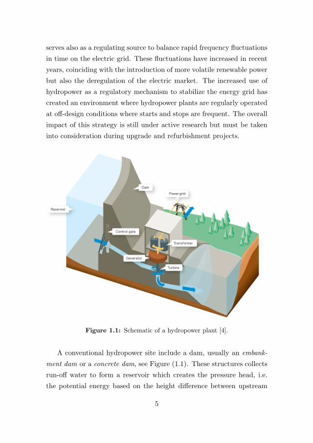
Figure 1.1: Schematic of a hydropower plant [4].

A conventional hydropower site include a dam, usually an embank-

ment dam or a concrete dam, see Figure (1.1). These structures collects

run-off water to form a reservoir which creates the pressure head, i.e.

the potential energy based on the height difference between upstream

5

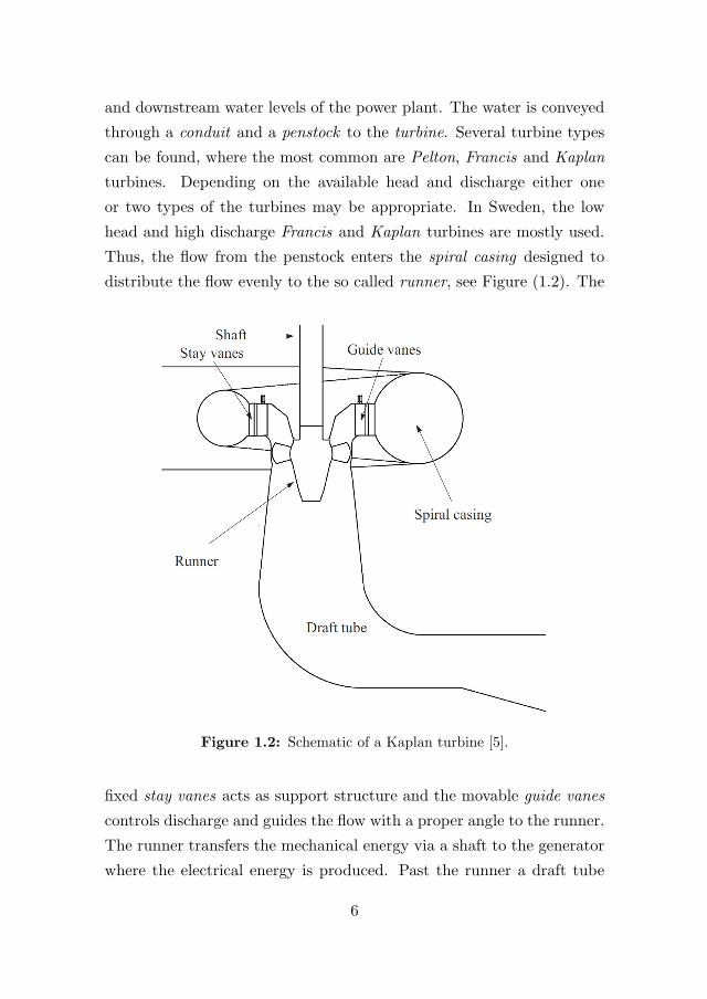
and downstream water levels of the power plant. The water is conveyed

through a conduit and a penstock to the turbine. Several turbine types

can be found, where the most common are Pelton, Francis and Kaplan

turbines. Depending on the available head and discharge either one

or two types of the turbines may be appropriate. In Sweden, the low

head and high discharge Francis and Kaplan turbines are mostly used.

Thus, the flow from the penstock enters the spiral casing designed to

distribute the flow evenly to the so called runner, see Figure (1.2). The

Figure 1.2: Schematic of a Kaplan turbine [5].

fixed stay vanes acts as support structure and the movable guide vanes

controls discharge and guides the flow with a proper angle to the runner.

The runner transfers the mechanical energy via a shaft to the generator

where the electrical energy is produced. Past the runner a draft tube

6

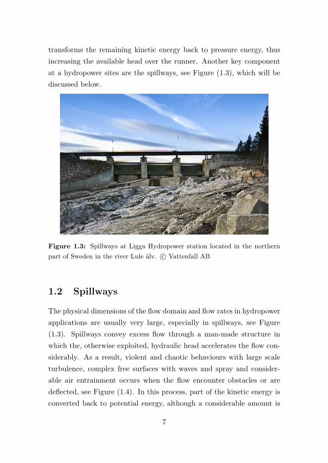
transforms the remaining kinetic energy back to pressure energy, thus

increasing the available head over the runner. Another key component

at a hydropower sites are the spillways, see Figure (1.3), which will be

discussed below.

Figure 1.3: Spillways at Ligga Hydropower station located in the northern

part of Sweden in the river Lule alv. c© Vattenfall AB

1.2 Spillways

The physical dimensions of the flow domain and flow rates in hydropower

applications are usually very large, especially in spillways, see Figure

(1.3). Spillways convey excess flow through a man-made structure in

which the, otherwise exploited, hydraulic head accelerates the flow con-

siderably. As a result, violent and chaotic behaviours with large scale

turbulence, complex free surfaces with waves and spray and consider-

able air entrainment occurs when the flow encounter obstacles or are

deflected, see Figure (1.4). In this process, part of the kinetic energy is

converted back to potential energy, although a considerable amount is

7

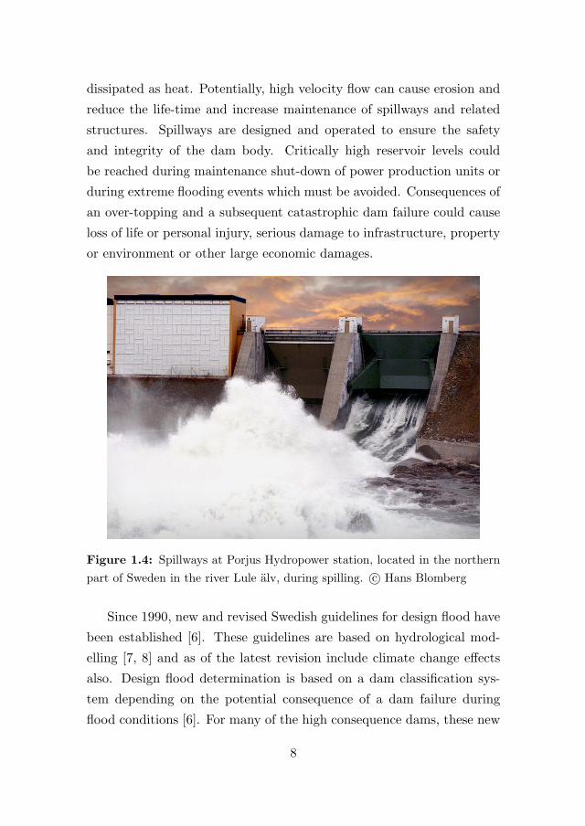
dissipated as heat. Potentially, high velocity flow can cause erosion and

reduce the life-time and increase maintenance of spillways and related

structures. Spillways are designed and operated to ensure the safety

and integrity of the dam body. Critically high reservoir levels could

be reached during maintenance shut-down of power production units or

during extreme flooding events which must be avoided. Consequences of

an over-topping and a subsequent catastrophic dam failure could cause

loss of life or personal injury, serious damage to infrastructure, property

or environment or other large economic damages.

Figure 1.4: Spillways at Porjus Hydropower station, located in the northern

part of Sweden in the river Lule alv, during spilling. c© Hans Blomberg

Since 1990, new and revised Swedish guidelines for design flood have

been established [6]. These guidelines are based on hydrological mod-

elling [7, 8] and as of the latest revision include climate change effects

also. Design flood determination is based on a dam classification sys-

tem depending on the potential consequence of a dam failure during

flood conditions [6]. For many of the high consequence dams, these new

8

requirements have implied that higher flow rates must be handled dur-

ing peak flooding events. Several strategies to tackle this new scenario

have been proposed where refurbishment of spillways to increase capac-

ity could be one possible solution or part thereof. In such refurbishment

projects, great care must be taken to ensure that the upgraded spill-

way meets the new demands. Still today, no computational method is

able to predict the full complexity of spillway channel flows [9]. Thus,

a combination of computational and physical modelling are used during

design and validation to ensure that the new design can handle the flow

in a safe and controlled manner.

1.3 Thesis Aim and Scope

Despite the last decades development of powerful numerical capabilities

with focus on aerated flows, many hydraulic engineering problems are

still out of reach [9]. Established Computational Fluid Dynamics (CFD)

methods such as Finite Volume Method (FVM) with Volume-Of-Fluid

(VOF) are difficult to apply to highly complex free surface flow prob-

lems [10]. However, the Lagrangian meshless particle method Smoothed

Particle Hydrodynamic (SPH), has turned out to be a promising tool

when applied to hydraulic engineering applications [11]. The inherent

ability of the SPH method to capture complex free surfaces with large

deformation and fragmentation makes it an interesting alternative to

already established methods. Hence, the main aim of this thesis is to

increase knowledge regarding SPH modelling of spillway channel flows.

However, a key aspect is to maintain a quality and trust perspective as

the method, in the hydraulic engineering community, is relatively un-

known. The complex but common phenomena of a hydraulic jump will

serve as a test case for the applicability of the SPH method to spillway

channel flows. A vision for the future is that SPH will be used as an

engineering tool for complex free surface problems in spillway design.

9

10

Chapter 2

Hydraulic Jump

Banana banana banana terracotta banana terracotta terracotta pie!

- System of a Down

This chapter aims to briefly introduce the complex phenomena of hy-

draulic jumps and some fundamental concepts. A complete literature

review would be a formidable undertaking as hydraulic jumps have been

studied for a long time due to its practical applicability in hydraulic en-

gineering. First to describe a hydraulic jump was the Italian polymath

Leonardo da Vinci (1452-1519) almost half a millennia ago [12]. Some

three hundred years later, the Italian engineer Bidone [13] performed

the first experiments and roughly in the same era the French hydraulic

engineer Belanger [14] proposed his theory of conjugate depths. Despite

the long history of hydraulic jump research, many aspects are still today

not fully understood.

2.1 Fundamentals

As described in the Spillways Section (1.2), the processes found in spill-

ways are usually violent and highly energetic. The high kinetic energy

levels or high velocity zones just downstream of the spillway gates must

be dissipated in order to avoid potential damage by erosion or cavitation.

11

This is commonly done in a so called stilling basin where a hydraulic

jump is triggered. However, hydraulic jumps are not only found in man-

made structures such as spillways but occur naturally in many other

flow situations as well. Other industrial applications of hydraulic jumps

include mixing and gas transfer in chemical processes, desalination of

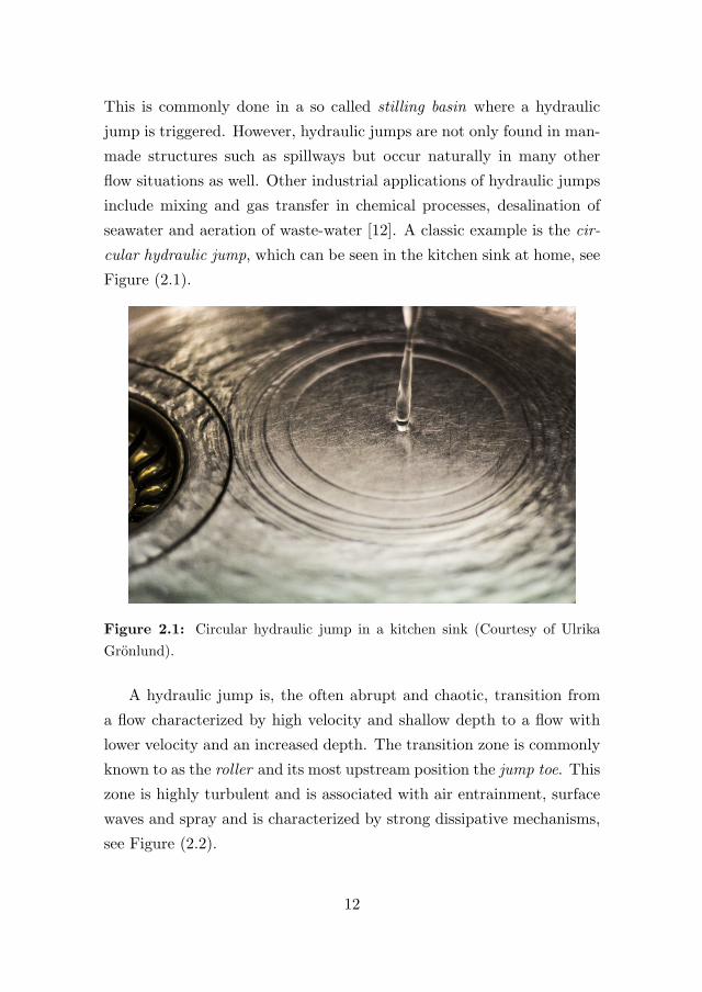
seawater and aeration of waste-water [12]. A classic example is the cir-

cular hydraulic jump, which can be seen in the kitchen sink at home, see

Figure (2.1).

Figure 2.1: Circular hydraulic jump in a kitchen sink (Courtesy of Ulrika

Gronlund).

A hydraulic jump is, the often abrupt and chaotic, transition from

a flow characterized by high velocity and shallow depth to a flow with

lower velocity and an increased depth. The transition zone is commonly

known to as the roller and its most upstream position the jump toe. This

zone is highly turbulent and is associated with air entrainment, surface

waves and spray and is characterized by strong dissipative mechanisms,

see Figure (2.2).

12

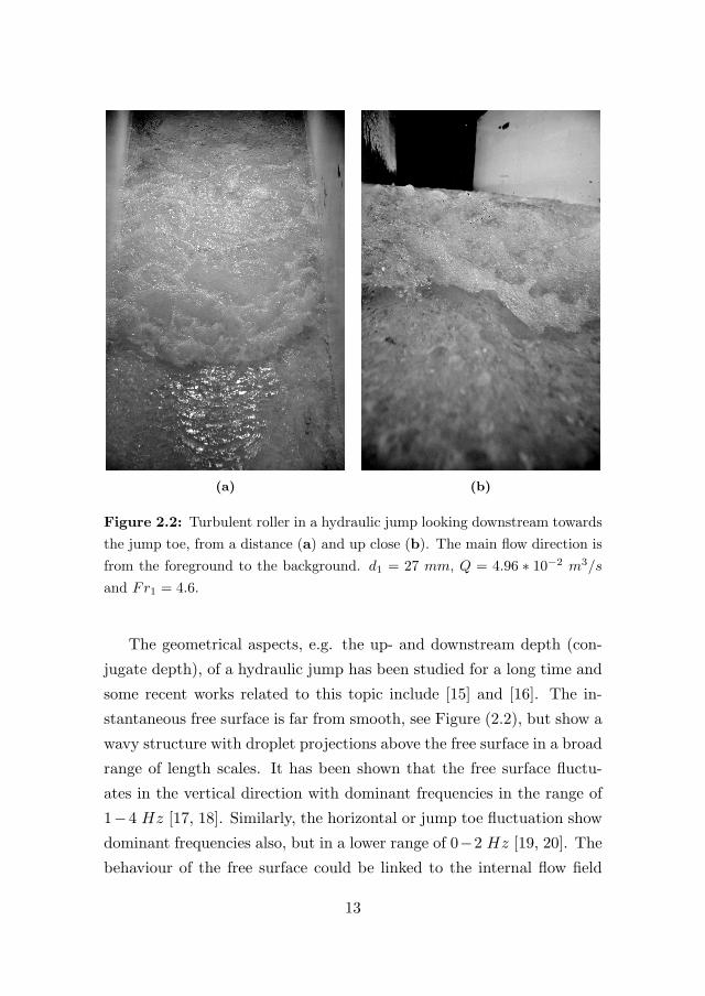
(a) (b)

Figure 2.2: Turbulent roller in a hydraulic jump looking downstream towards

the jump toe, from a distance (a) and up close (b). The main flow direction is

from the foreground to the background. d1 = 27 mm, Q = 4.96 ∗ 10−2 m3/s

and Fr1 = 4.6.

The geometrical aspects, e.g. the up- and downstream depth (con-

jugate depth), of a hydraulic jump has been studied for a long time and

some recent works related to this topic include [15] and [16]. The in-

stantaneous free surface is far from smooth, see Figure (2.2), but show a

wavy structure with droplet projections above the free surface in a broad

range of length scales. It has been shown that the free surface fluctu-

ates in the vertical direction with dominant frequencies in the range of

1−4 Hz [17, 18]. Similarly, the horizontal or jump toe fluctuation show

dominant frequencies also, but in a lower range of 0−2 Hz [19, 20]. The

behaviour of the free surface could be linked to the internal flow field

13

[17, 21]. However, internal flow structures have been difficult to study

due to the multiphase nature of the hydraulic jump, especially when op-

tical measurement techniques such as Particle Image Velocimetry (PIV)

has been used [22, 23]. Instead, the Bubble Image Velocimetry (BIV)

technique has shown to be a better alternative in the bubbly roller region

and has confirmed that different zones and mechanisms are active inside

the jump [24, 25]. These zones include for a steady jump, starting from

the bottom, a boundary layer, a jet core, a mixing layer and a recirculat-

ing zone. Inside the mixing layer, large coherent vortical structures are

observed which effects the free surface [26, 27, 24, 25]. These vortices

are also, to some extent, responsible for the air entrainment which has

been studied extensively, e.g. [28, 29]

2.2 General Equations

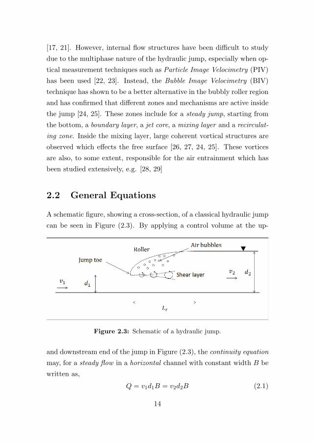
A schematic figure, showing a cross-section, of a classical hydraulic jump

can be seen in Figure (2.3). By applying a control volume at the up-

Figure 2.3: Schematic of a hydraulic jump.

and downstream end of the jump in Figure (2.3), the continuity equation

may, for a steady flow in a horizontal channel with constant width B be

written as,

Q = v1d1B = v2d2B (2.1)

14

where subscripts indicate positions, Q the discharge, v the velocity and

d the depth. For the same control volume, the momentum equation can

be written as,(1

2ρgd21 −

1

2ρgd22

)B − Ffric = ρQ (v2 − v1) (2.2)

where ρ is the density, g is the acceleration due to gravity and Ffric is

the drag force due to bottom friction. If neglecting the friction force,

Equation (2.1) and (2.2) can be rearranged to yield the dimensionless

ratio of conjugate or sequent depths first proposed by Belanger [14], i.e.

d2d1

=1

2

(√1 + 8Fr21 − 1

)(2.3)

where Fr is the dimensionless Froude number defined for a rectangular

channel as,

Fr1 =v1√gd1

. (2.4)

The Froude number is a key parameter regarding hydraulic jumps and

could be interpreted as proportional to the square root of the ratio of

internal forces and the weight of the fluid. Furthermore, Fr is coupled

to critical flow conditions which are obtained when the mean specific

energy assumes a minimum value. For an incompressible, frictionless

and a steady flow (Bernoulli equation assumptions) in a horizontal and

rectangular channel the mean specific energy could be written as,

E = d+Q2

2gd2B2, (2.5)

if combined with the continuity equation. For a constant Q and a given

cross-section the minimum specific energy Emin is obtained by solving,(∂E

∂d

)Q=constant

= 0, (2.6)

which has the following solution,

Emin =3

2dc (2.7)

15

where the critical depth is

dc =3

√Q2

gB2. (2.8)

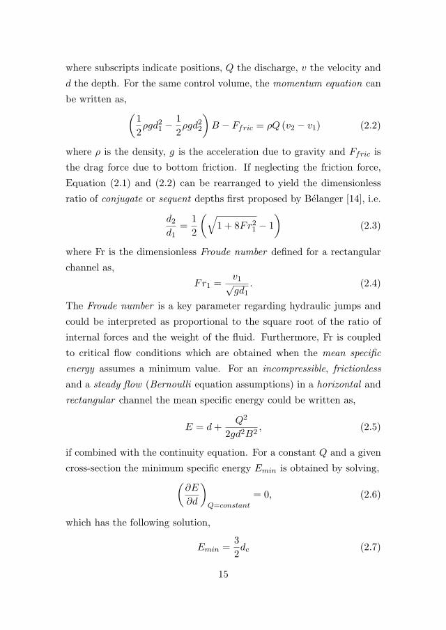
The specific energy could then be rewritten in dimensionless form ac-

cording to,E

dc=

d

dc+

1

2

(dcd

)2

(2.9)

which is valid for any Q and is plotted in Figure (2.4). In open chan-

Figure 2.4: Dimensionless specific energy.

nels, the Fr is defined to be unity for critical flow conditions. With

Figure (2.4) in mind, the following flow regimes could be defined. If

d < dc (d/dc < 1) an increase of the discharge Q and in turn the specific

energy E, implies that a minor decrease of d would occur only. This

state is referred to as supercritical flow conditions and are found in the

high velocity jet upstream the jump toe where Fr is by definition above

unity. If however, d > dc (d/dc > 1), the opposite will occur, where an

increase of E results in a much larger increase of d. This is referred to

16

as subcritical conditions where Fr is below unity and could be observed

downstream the roller region. An analogy between the sub- and super-

critical conditions together with the Fr and compressible flow and the

Mach number (Ma) are usually made [30].

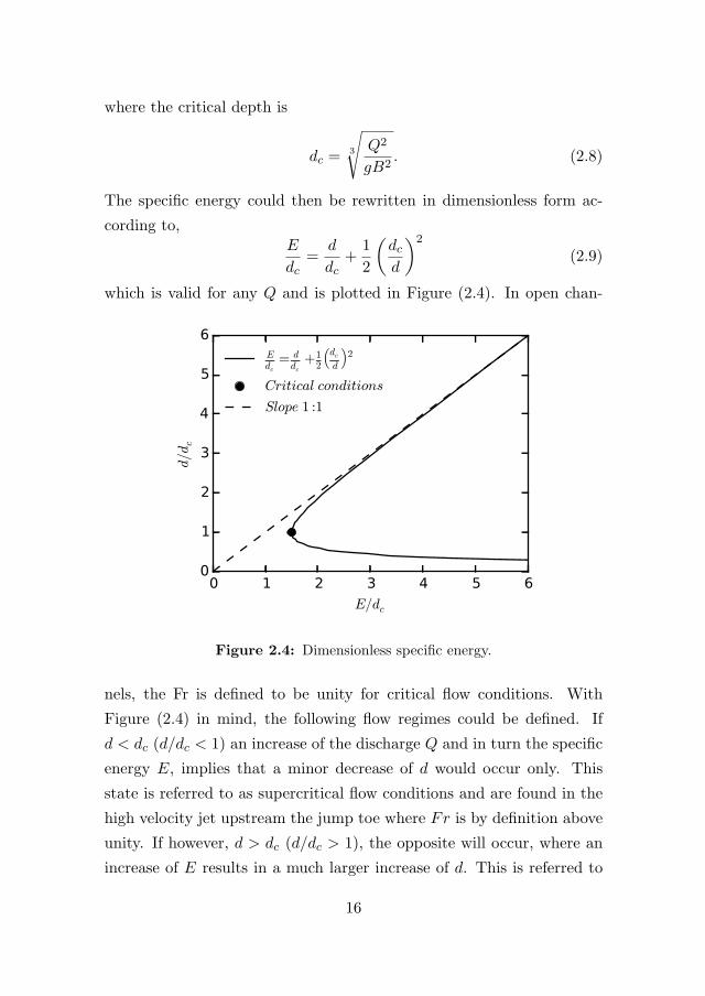
Based on the inflow Froude number Fr1, different types of hydraulic

jumps can be defined. However, these should be seen as rough guidelines

only, since different types of jumps can be obtained depending on the

inflow conditions [30]. The commonly used classification by Chow [31]

for horizontal and rectangular channels are summarized in Table (2.1).

Table 2.1: Hydraulic jump classification by Chow [31] [30].

Type Fr1 Characteristics

Critical flow 1 No hydraulic jump.

Undular jump 1-1.7 Free surface undulations downstream of

jump with low energy losses.

Weak jump 1.7-2.5 Low energy losses.

Oscillating jump 2.5-4.5 Unstable oscillating jump with wavy free

surface and production of large waves of

irregular period. To be avoided.

Steady jump 4.5-9 Steady jump with 45 − 70 % energy

loss. Low sensitivity to downstream con-

ditions. Best economical design.

Strong jump > 9 Rough jump with up to 85 % energy dis-

sipation. To be avoided due to risk of

channel bed erosion.

Another key aspect of a hydraulic jump is the longitudinal length

scale. Hager et al. [32] proposed that the characteristic longitudinal

scaling length for a hydraulic jump should be equal to the roller length.

This length begins at the upstream location of the jump toe and ends

at the surface stagnation point, i.e. the limit between backward and

17

forward flow. Hager et al. [32] reviewed a broad range of data and

correlations and proposed a empirical relationship for the roller length

Lr according to,

Lr

d1= 160tanh

(Fr120

)− 12 2 < Fr1 < 16 (2.10)

in wide (d1/B > 0.1), horizontal and rectangular channels.

18

Chapter 3

Smoothed Particle

Hydrodynamic

If you thought that science was certain - well, that is just an error on

your part.

- Richard P. Feynman

The SPH method will be presented in this chapter. Focus is on the mod-

els and concepts used in this thesis and should not be seen as a complete

description of the method. If a more thorough and detailed description

is requested the reader is referred to the textbooks by Liu et al. [33] and

Violeau [34], the numerous works by Monaghan [35, 36, 37] but also the

work of Gomez-Gesteira et al. [11]. Furthermore, the growing number

of Ph.D. thesis’s coupled to SPH are a good source of information as

well. These thesis’s together with validation test cases and other useful

information can be found at the SPH European Research Interest Com-

munity (SPHERIC), an ERCOFTAC special interest group, homepage

https://wiki.manchester.ac.uk/spheric/.

19

3.1 Fundamentals

SPH is a meshless, Lagrangian numerical method proposed indepen-

dently by Gingold and Monaghan [38] and Lucy [39]. Initially, the

method was applied to astrophysical problems in three-dimensional open

space. The method did not attract much attention in the research com-

munity until it was successfully applied to other fields. Especially, the

paper by Monaghan [40] focusing on free surface flows opened up the

field of fluid mechanics. Later, the hydropower community was broadly

introduced to SPH with the paper by Gomez-Gesteira et al. [11].

The dynamics of fluids are governed by a set of partial differential

equations (PDE), better known as the Navier-Stokes equations, of field

variables, i.e. density, velocity and energy. Analytical solutions can

only be obtained for a few simple cases. Instead, a numerical solution of

the PDE:s describing the problem are often the only possible strategy.

For the numerical approach, the problem domain is discretized into a

set of points or nodes. Next, a method approximating the values and

derivatives of the PDE:s at the nodes is required. Such method, reduces

the PDE:s to a set of ordinary differential equations (ODE) with respect

to time only which could be solved with standard integration techniques.

The SPH method employs the following steps [33]:

1. The problem domain is represented by a set of non-connected par-

ticles arbitrarily scattered in space.

2. The kernel approximation is applied for field functions, see Section

(3.1.1).

3. The continuous integrals is approximated with summations over

neighbouring particles known as the particle approximation, see

Section (3.1.2).

4. The particle approximation is performed at every time step and

depends on the local neighbouring particle distribution.

5. The particle approximations are performed to all field functions,

20

reducing the PDE:s to ODE:s with respect to time only.

6. The ODE:s are solved with explicit integration techniques.

3.1.1 Kernel Approximation

The first key step in the SPH method is the kernel approximation which

start with the following identity,

f(r) =

∫Ω

f(r′)δ(r− r′)dr′ (3.1)

where f is a function of the position vector r, δ(r−r′) is the Dirac delta

function,

δ(r− r′) =

⎧⎨⎩1 if r = r′

0 if r �= r′(3.2)

and Ω is the volume that contains r. If the Dirac delta function is

approximated with the kernel function W (r− r′, h), the kernel approx-

imation operator is obtained, i.e.

< f(r) >=

∫Ω

f(r′)W (r− r′, h)dr′ (3.3)

where h is the smoothing length determining the size of the kernel sup-

port domain. For more information regarding the kernel function, see

Section (3.1.3). The approximation of the spatial derivative ∇ · f(r) isobtained by substituting f(r) with ∇ · f(r) in Equation (3.3), i.e.

< ∇ · f(r) >=

∫Ω

[∇ · f(r′)]W (r− r′, h)dr′. (3.4)

By applying the divergence theorem and assuming that kernel support

domain is within the problem domain, Equation (3.4) can be simplified

accordingly,

< ∇ · f(r) >= −∫Ω

f(r′) · ∇W (r− r′, h)dr′. (3.5)

21

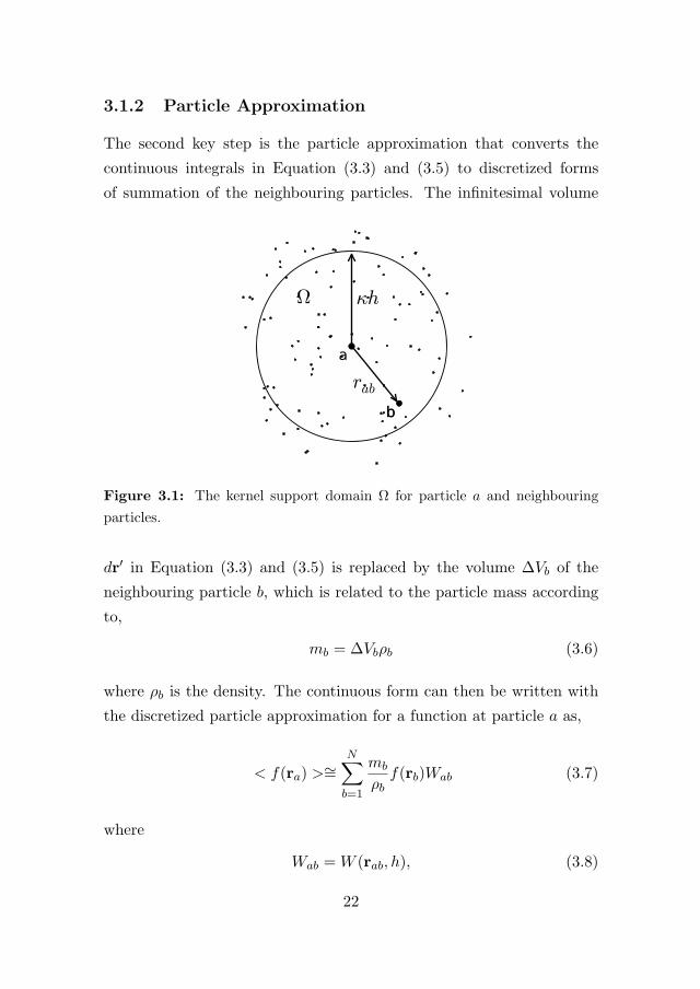
3.1.2 Particle Approximation

The second key step is the particle approximation that converts the

continuous integrals in Equation (3.3) and (3.5) to discretized forms

of summation of the neighbouring particles. The infinitesimal volume

Figure 3.1: The kernel support domain Ω for particle a and neighbouring

particles.

dr′ in Equation (3.3) and (3.5) is replaced by the volume ΔVb of the

neighbouring particle b, which is related to the particle mass according

to,

mb = ΔVbρb (3.6)

where ρb is the density. The continuous form can then be written with

the discretized particle approximation for a function at particle a as,

< f(ra) >∼=N∑b=1

mb

ρbf(rb)Wab (3.7)

where

Wab = W (rab, h), (3.8)

22

and the derivative as,

< ∇ · f(r) >∼=N∑b=1

mb

ρbf(rb) · ∇Wab (3.9)

where

∇Wab =rabrab

∂Wab

∂rab, (3.10)

rab = ra−rb, rab = |rab| is the distance between particle a and b and N is

the number of neighbouring particles within the kernel support domain,

see Figure (3.1).

3.1.3 Kernel Function

In general, the accuracy of the SPH interpolation increases with the

order of the polynomial used to define the kernel function. Furthermore,

the choice of kernel function significantly effects the overall performance

of the SPH algorithm. Several kernel functions can be found in the

literature but all satisfy the following conditions [33],

Unity:

∫Ω

W (r− r′, h)dr′ = 1 (3.11)

Compact support: W (r− r′, h) = 0 for |r− r′| > κh (3.12)

Positivity: W (r− r′, h) ≥ 0 inside the domain Ω (3.13)

Decay: Monotonically decreasing behavior of W (r− r′, h) (3.14)

Delta function property: limh→0

W (r− r′, h) = δ(r− r′) (3.15)

Symmetric: W (r− r′, h) should be an even function (3.16)

Smoothness: W (r− r′, h) should be sufficiently smooth (3.17)

where κ is a scaling factor dependent on the kernel function considered,

see Figure (3.1). The kernel function can be expressed as a function of

the non-dimensional distance s between particle a and b, i.e. s = rab/h.

Where the smoothing length h determines the area (2D) and volume

(3D) where neighbouring particles are considered, see Figure (3.1).

23

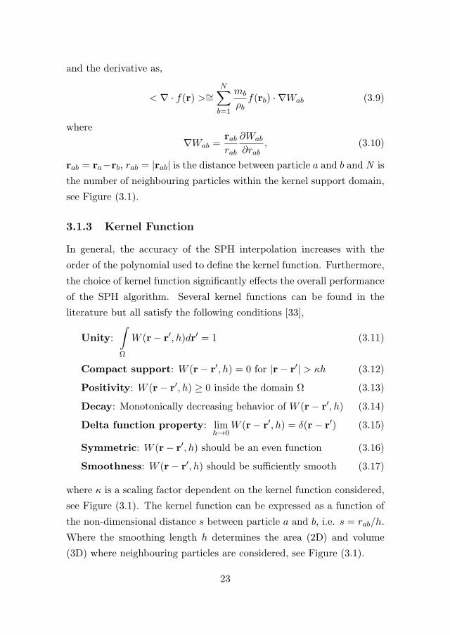
Figure 3.2: Kernel functions (solid lines) and its derivatives (dashed lines)

scaled with the dimensional factor αD

The following kernels functions has been used in thesis:

a, the widely used Cubic B-spline kernel [41] given by,

W (rab, h) = αD

⎧⎪⎪⎪⎨⎪⎪⎪⎩1− 3

2s2 + 3

4s3 if 0 ≤ s < 1

14(2− s)3 if 1 ≤ s < 2

0 if s ≥ 2

(3.18)

where αD is equal to 10/(7πh2

)(2D) and 1/

(πh3

)(3D), see Figure

(3.2). The cubic B-spline kernel resembles the Gaussian function while

having a narrower compact support.

b, the Wendland Quintic kernel [42] given by,

W (rab, h) = αD

(1− s

2

)4(2s+ 1) if 0 ≤ s ≤ 2 (3.19)

where αD is equal to 7/(4πh2

)(2D) and 21/

(16πh3

)(3D), see Figure

24

(3.2). The Wendland kernel provides a higher interpolation order at

the same time reducing the computational time compared to the Cubic

B-spline kernel [11].

3.2 Continuity Equation

The continuity equation is based on the fundamental principal of conser-

vation of mass. This principal states that the rate of change of matter

inside a system is in balance with the in- and outflow of matter through

the system boundaries. Matter can not, under normal conditions, be

created nor destroyed inside the system. The continuity equation can

consequently be formulated accordingly,

1

ρ

Dρ

Dt+∇ · u = 0, (3.20)

where u is the velocity vector. In weakly-compressible SPH the particle

mass is constant and density fluctuates only according to the continuity

equation which can be rewritten in SPH-notation as,

dρadt

=∑b

mbuab · ∇aWab. (3.21)

Other possible forms of the continuity equation can be found in the

literature [33].

3.3 Momentum Equation and Viscosity Treat-

ment

Newton’s Second Law of Motion states that the rate of change of mo-

mentum is equal to the sum of the forces. For fluids, the forces can be

divided into body forces (e.g. gravity, centrifugal and Coriolis force)

and surface forces such as pressure force and forces coupled to material

properties. The balanced momentum equation in vectorial notation then

25

reads,Du

Dt= −1

ρ∇P + g + Γ, (3.22)

where P is pressure, g is acceleration due to gravity and Γ are the viscous

and dissipative terms. Two different approaches on how to model the Γ

term has bee used in this thesis, see below.

3.3.1 Artificial Viscosity

The artificial viscosity approach proposed by Monaghan [35] has been

used extensively in the SPH community due to its simplicity and robust-

ness. As described by Monaghan [36], the artificial viscosity has limited

relation to real viscosities, but allows shock waves to be simulated by

smoothing the wave over several neighbouring particles and hence sta-

bilize the numerical solution. Furthermore, the artificial viscosity for-

mulation prevents particles from interpenetrating. In SPH notation,

Equation (3.22) can be written as,

dua

dt= −

∑b

mb

(Pb

ρ2b+

Pa

ρ2a+Πab

)∇aWab + g (3.23)

where

Πab =

⎧⎨⎩−αcabμab

ρabif vab · rab < 0

0 otherwise(3.24)

with

μab =hvab · rabr2ab + η2

(3.25)

where ρab = (ρa+ ρb)/2 and cab = (ca+ cb)/2 is the average density and

speed of sound respectively. The term η2 = 0.01h2 is added to keep the

denominator from vanishing and α is a problem dependent parameter.

3.3.2 Laminar Viscosity and SPS Turbulence

The artificial-viscosity model can be too dissipative [43] and can affect

shear and possibly fluid propagation if the flow is not driven by gravity

26

[11]. Furthermore, the value of the problem dependent parameter α is

usually difficult to set. An alternative approach to the artificial viscos-

ity model is the laminar viscosity and Sub-Particle Scale (SPS) model,

which is more appropriate to use when turbulent terms are involved

[11]. For this approach, the Γ term in Equation (3.22) is divided into

two parts, i.e.

Γ = ν0∇2u+1

ρ∇· →

τ . (3.26)

The first term in Equation (3.26) is the laminar viscous stresses which

can be expressed in SPH notation as [44],

ν0∇2u =∑b

mb

(4ν0rab · ∇aWab

(ρa + ρa)(r2ab + η2

))uab (3.27)

where ν0 = 10−6 [m2/s] is the kinematic viscosity of water. The second

term in Equation (3.26) is the SPS stress tensor and represents the effects

of turbulence. The model is based on the Large Eddy Simulation (LES)

approach and was for particle methods first proposed by Gotoh et al. [45]

for the incompressibleMoving Particle Semi-implicit (MPS) method. Lo

and Shao [46] implemented the same model for incompressible SPH. By

using Favre averaging, to account for compressibility, Dalrymple and

Rogers [43] introduced the SPS model into weakly-compressible SPH by

rewriting the second term in Equation (3.26) as,

1

ρ∇· →

τ=∑b

mb

(τbρ2b

+τaρ2a

)∇aWab. (3.28)

In Einstein notation, the shear stress component in i and j direction can

be approximated as

→τ ij

ρ= νt

(2Sij − 2

3kδij

)− 2

3ClΔ

2δij |Sij |2 (3.29)

where→τ ij is the sub-particle stress tensor, νt = [(CsΔl)]2 |S| is the tur-

bulent eddy viscosity, k the SPS turbulence kinetic energy, Cs = 0.12 the

27

Smagorinsky constant, Cl = 0.0066, Δl the particle to particle spacing

and |S| = 0.5(2SijSij) where Sij is an element of the SPS strain tensor.

The final momentum equation when including the laminar viscosity and

SPS model can be written in SPH notation as,

dua

dt=−

∑b

mb

(Pb

ρ2b+

Pa

ρ2a

)∇aWab + g

+∑b

mb

(4ν0rab · ∇aWab

(ρa + ρa)(r2ab + η2

))uab

+∑b

mb

(τbρ2b

+τaρ2a

)∇aWab.

(3.30)

3.4 Equation of State

To avoid an expensive computation of the Poisson’s equation and to

keep the explicit nature of the SPH method, an equation-of-state (EOS)

is used to relate the fluid pressure to local particle density [40]. A

handful of EOSs has been used throughout this thesis. However, the

most common, used primarily in the later works, is the Tait’s equation

where the pressure is related to the particle density according to the

following expression,

P = B

[(ρ

ρ0

)γ

− 1

](3.31)

where B = c20ρ0/γ, γ = 7, ρ0 = 1000 kg/m3 is the reference density of

water and c0 = c(ρ0) =√

(∂P/∂ρ) is the speed of sound at the reference

density [47]. Monaghan [40] suggested that the speed of sound c0 could

be artificially lowered without effecting the motion of the fluid. However,

a minimum value of at least 10 times the expected maximum velocity

should be chosen for c0 in order to keep the density variation within 1 %.

The lowered c0, also effects the time step considerably as the size of the

time step is restricted by the Courant-Fredrich-Levy (CFL) condition,

see Section (3.6) for further details.

28

3.5 Corrections

In literature, various methods can be found on how to increase the ac-

curacy of SPH solutions. One problem that has been highlighted is the

oscillation of the pressure field. Efforts to overcome this has focused on

correcting the density field, the kernel and kernel gradient. Also, efforts

has been made on developing an incompressible SPH solver [48]. Den-

sity fields are usually corrected by applying a filter over the density and

then re-assigning a new density to each particle at fixed time steps. Ker-

nel and kernel gradient corrections compensate for the truncated kernel

domain close to boundaries and free-surfaces where the consistency and

normalization conditions fail, see [49] for further details.

A fast and simple approach to correct the density field is the zeroth-

order Shepard filter [50]. At a fixed number of time steps (≈ 30) the

density of a particle is re-assigned according to,

ρnewa =∑b

ρbWabmb

ρb=∑b

mbWab (3.32)

where

Wab =Wab∑

b

Wabmbρb

. (3.33)

A higher ordered density correction method is the first-order Moving

Least Square (MLS) approach [51, 50].

Apart from the Shepard filter, a second correction methods has been

used in this thesis. The velocity field has been smoothed according to the

XSPH method proposed by Monaghan [52]. By applying this method,

particles are moved according to,

dradt

= ua + ε∑b

mb

ρabuabWab (3.34)

where ε = 0.5 and ρab = (ρa + ρb)/2 to obtain a more ordered flow and

to prevent particle penetration.

29

3.6 Time Integration and Time Step

Due to particle interactions, the magnitude of the dependent variables,

i.e. density, velocity and position, are changed at each time step. To

obtain the new state of a particle the governing equations must be in-

tegrated in time with, preferably, a second order accurate scheme. For

clarity only, the continuity (3.21), momentum (3.23 or 3.30) and the

position (3.34) equations can be simplified in the following form,

dρadt

= Da, (3.35)

dua

dt= Fa, (3.36)

dradt

= Ua. (3.37)

The explicit, second-order (in time), predictor-corrector based Symplec-

tic algorithm [53] is one of the time integration schemes used and is

given only. The Symplectic integration algorithm is time reversible in

the absence of friction and viscous effect and improve long term solu-

tion behaviour. During the predictor step, the position and density is

estimated at the middle of the time step as,

rn+ 1

2a = rna +

Δt

2una , (3.38)

ρn+ 1

2a = ρna +

Δt

2Dn

a (3.39)

where the superscript n denotes the time step and t = nΔt. During the

corrector step, the corrected velocity and position is obtained accord-

ingly,

un+1a = u

n+ 12

a +Δt

2Fn+ 1

2a , (3.40)

rn+1a = r

n+ 12

a +Δt

2un+1a . (3.41)

Finally, the corrected density can be obtained based on the updated

values of un+1a and rn+1

a [36].

30

For explicit time integration scheme the time step Δt is dependent

on the CFL-number mentioned above. However, further restrictions is

put on the time step which is determined according to

Δt = Ct ·min (Δtf ,Δtcv) (3.42)

where Ct = 0.2 is a constant,

Δtf = min(√

h/|fa|)

(3.43)

is based on the force per unit mass |fa| and

Δtcv = mina

⎛⎜⎜⎝ h

cs +maxb

∣∣∣∣ huab·rab(r2ab+η2)

∣∣∣∣

⎞⎟⎟⎠ (3.44)

which combines the CFL and a viscous condition [54].

3.7 Boundary Conditions

To properly define and implement boundary conditions has been recog-

nized as a difficult task as it does not appear in a natural way in SPH. A

brief discussion of the methods used and refereed to is included below.

3.7.1 Solid Wall Boundary Condition

Numerous approaches on how to implement solid wall boundary condi-

tions can be found in the literature, e.g. ghost particle [55], repulsive

particle [40], dynamic particle [56] and semi-analytical [57]. In the early

works, solid wall boundaries was modelled as rigid shell finite elements

where the coupling between the SPH particles and the boundaries was

governed by a penalty based node-to-surface contact algorithm. If the

SPH particles penetrated the boundaries a spring force was applied in

the normal direction of the finite element. This mechanism can be com-

pared to that of the repulsive particle method. In later works, the dy-

namic particle method proposed by Crespo et al. [56] was used. For

31

this method, wall particles satisfy the same equations as fluid particles

but are fixed in space. Thus, when a fluid particle approaches a fixed

wall, the density of the particle increases and by the EOS the pressure

increases as well. Due to the pressure term in the momentum equation,

the pressure increase results in a repulsive force between the particles.

To ensure a complete coverage of the kernel and that fluid particles

do not penetrate the boundaries, three layers of non-staggered particles

populated the boundaries.

3.7.2 Periodic Open Boundary Condition

The periodic open boundary is a classic condition in fluid mechanics. In

SPH, several variations of the periodic approach has been applied to a

range of problems, e.g. Couette and Poiseuille flow [44, 58].

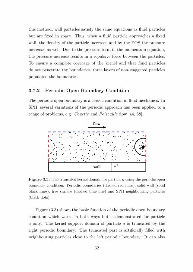
Figure 3.3: The truncated kernel domain for particle a using the periodic open

boundary condition. Periodic boundaries (dashed red lines), solid wall (solid

black lines), free surface (dashed blue line) and SPH neighbouring particles

(black dots).

Figure (3.3) shows the basic function of the periodic open boundary

condition which works in both ways but is demonstrated for particle

a only. The kernel support domain of particle a is truncated by the

right periodic boundary. The truncated part is artificially filled with

neighbouring particles close to the left periodic boundary. It can also

32

be seen as the truncated part is ”moved” to the left side. Furthermore,

if particle a leaves the right periodic boundary it is reintroduced at the

left periodic boundary. Apart from changing the particle coordinates

during the reintroduction step other variables can be changed too, e.g.

velocity components.

3.7.3 Inlet and Outlet Boundary Condition

The inlet and outlet boundary conditions are, as the periodic condition,

fundamental in fluid mechanics as well. However, only a few studies

focusing on this problem can be found in the literature. The problem

is not only coupled to how to apply such conditions but also how to

efficiently handle a varying number of particles during the simulation.

The inlet and outlet approach by Federico et al. [59], partly based on

the paper by Lastiwka et al. [60], will be introduced.

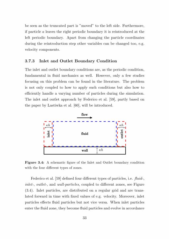
Figure 3.4: A schematic figure of the Inlet and Outlet boundary condition

with the four different types of zones.

Federico et al. [59] defined four different types of particles, i.e. fluid-,

inlet-, outlet-, and wall-particles, coupled to different zones, see Figure

(3.4). Inlet particles, are distributed on a regular grid and are trans-

lated forward in time with fixed values of e.g. velocity. Moreover, inlet

particles effects fluid particles but not vice versa. When inlet particles

enter the fluid zone, they become fluid particles and evolve in accordance

33

with the SPH equations. At the downstream end of the fluid zone a out-

let zone is situated. In this zone, fluid particles become outlet particles

where the physical variables are frozen in time except for their positions.

Federico et al. [59] showed that different tactics could be applied on how

to treat both inlet and outlet particles.

34

Chapter 4

Summary of Appended

Papers

Open to everything happy and sad

Seeing the good when it’s all going bad

Seeing the sun when I can’t really see

Hoping the sun will at least look at me

- Moby

The outcomes of a Ph.D. project are not only research in the form of

papers but also the development of the person enrolled. Thus, this

chapter aims to answer the questions how, why and what and highlight

some of the key advancements in my own development. Three distinct

periods can be identified during my Ph.D. studies which are the early

works (Paper A-C), the transition period and the later works (Paper

D-F) all of which will be discussed below.

4.1 Early Works

The early works started in the autumn of 2010 with my Master’s the-

sis, Smoothed Particle Hydrodynamics Modeling of Hydraulic Jumps,

and can be seen as a pre-study for my subsequent Ph.D. studies. The

35

Master’s thesis is not included in this thesis but is important to discuss.

The choice to go for the relatively unexplored SPH method was inspired

by the paper by Gomez-Gesteira et al. [11] published in an Extra Is-

sue of Journal of Hydraulic Research. The work in the Master’s thesis

was of trial-and-error character in the software LSTC LS-DYNA which

Jonsen had previous experience of and was at the time the only com-

mercial alternative available. However, the implementation was rather

unstable and many of the features was underdeveloped. Nevertheless,

LS-DYNA was used exclusively throughout the early works. The aim

of the Master’s thesis was to try to reproduce some of the findings in

previous studies, particularly how to perform 2D SPH hydraulic jump

simulations. Thus, the Tank approach by Lopez et al. [61] and a version

of the Inlet & Outlet approach by Federico et al. [59] was implemented

and tested in LS-DYNA. Depths and velocities was in good agreement

with theory and experiments for the Tank approach but no comparison

was done for the other case due to implementation errors in LS-DYNA.

As for many other studies, this study generated more questions than

answers which were coupled to pressure oscillation and overestimation,

smoothness of boundaries, particle refinement, multi-phase issues, etc.

With these questions in mind, Paper A aimed to answer the ques-

tion on how the outcomes are affected by the number of particles that

represent the system. However, such a question is quite intricate and

the only conclusion made was that a more refined case is able to resolve

more flow features. Furthermore, to tackle issues coupled to boundary

smoothness, rigid shell finite elements were applied as solid walls com-

pared to the Master’s thesis where SPH particles fixed in space and time

were used. Some of the issues regarding the Inlet & Outlet approach had

been solved and was applied. However, it is important to notice that

this approach differed to the one described in [59] and Section (3.7.3).

Specifically, all particles entering the computational domain throughout

the simulation had to be placed outside the domain initially. Further-

36

more, particles that left the domain through the outlet were not deleted

and no conditions could be applied to these particles. To compensate

for the inability to change the state of an outlet particle a weir was

placed close to the outlet. This version of the Inlet & Outlet condi-

tion together with load-balancing issues rendered an computationally

inefficient approach, as large computational times for a relative small

number of particles were obtained. Nevertheless, good agreement with

theory was obtained regarding various depths and the jump toe seemed

to stabilize in time. However, just as in the Master’s thesis the pressure

behaved non-physically and use of the Gruneisen EOS was questionable.

To increase the trustworthiness of the SPH-model used in Paper A,

several parameters were tested and re-evaluated in Paper B. The Dam

Break problem, considered as a validation test case within the SPH com-

munity, was chosen to validate the model and calibrate the parameters.

Just as in Paper A, particle resolution had a major impact on the results

and the pressure was generally overestimated even though three different

EOSs were tested. Another parameter of importance were the artificial

viscosity constants. These were, due to an assumed interdependency

with the refinement level, difficult and cumbersome to calibrate. The

analysis method by overlapping experimental and numerical outcomes

was inaccurate and should not be adopted. The new post-processing

method, described in the paper, was developed by myself only and was a

key advancement in my own development. Upon finishing the method,

I thought it was too cumbersome and unnecessarily complex and not

worthy of publication. Later however, I discovered that another group

had published a similar algorithm after I finished mine.

In Paper C, the 2D SPH-model used in Paper A was updated based

on the findings in Paper B in order to primarily study the fluctuating

behaviour of the free surface in the turbulent hydraulic jump roller. Yet

again, the spatial resolution was altered with similar outcomes as in Pa-

per A and B. The jump toe did not stabilize until it reached the inlet

37

and it was concluded that this was an effect of the boundary condition

used and the lack of bottom friction. However, this behaviour was more

likely to be coupled to an unbalance of the up- and downstream condi-

tions where presumingly the weir was too high. The propagation speed

was lowered with increasing spatial resolution and the coarsest case was

chosen for further studies due to time considerations. Time averaged

velocity fields and the free surface profiles was in good agreement with

experimental findings. The instantaneous velocity field showed large

coherent vortical structures close to the free surface which induced os-

cillation with dominant frequencies of approximately 3.5 Hz. This fre-

quency was comparable to experimental findings in the hydraulic jump

roller. However, the inability of the SPH-model to accurately capture

the position of large scaled oscillation and the decay in the downstream

direction created some concerns. More specifically, was the artificial vis-

cosity model adequate or should a more sophisticated turbulence model

be used? Furthermore, was the single phase approach, where the impact

of air entrainment is not taken care of, a too simple model?

4.2 Transition Period

No papers was published during this period but it was an important part

of my Ph.D. studies where my general understanding of the SPH-method

was significantly improved. I find this period very interesting and cre-

ative and it laid the foundation for the later works, hence, important to

discuss.

A number of deficiencies were identified during the work with the

SPH-solver implemented in LS-DYNA. These deficiencies were coupled

to the inability to change and modify the code and if the implemented

methods were applicable to fluid flows in general and hydraulic jumps

in particular. To wait for these deficiencies to be handled was never

an option. Thus, with a lust to know more and strengthened by the

38

post-processing project during Paper B, I initiated the work of my own

SPH-solver. Initially, the code was written in MatLab but was later,

during my visit to Monash University in Melbourne, Australia, ported

to Python. With the open source project Cython [62], the serial code

reached ”compiled speed” and some of the code features were,

• Kernel: Wendland [42],

• Viscosity treatment:

– Artificial Viscosity [35]

– Physical Viscosity [58]

• EOS: Tait’s [40, 47],

• Boundary Conditions:

– Solid Wall [58]

– Periodic Open

– Inlet & Outlet [59]

• Time Integration:

– Predictor-Corrector (2nd order)

– Beeman (4th order)

– Variable Time Step [54]

• Corrections:

– Shepard filter [50]

– XSPH [52]

• Efficiency: Domain Decomposition.

In order to verify the code the following cases were studied,

• Dam Break,

• Hydrostatic Tank,

• Poiseuille and Couette flow with periodic open boundaries and

• Pipe flow with Inlet & Outlet boundaries.

In spite of the efforts put into the SPH-solver it was terminated due to

primarily speed issues. At that time, the work to enhance the code to

operate in a massively parallel CPU or a GPGPU environment was too

daunting. Instead, inspired by the 2014 SPHERIC Workshop in Paris,

39

France, the open source project DualSPHysics [63] was chosen as main

computational tool and marked the end of the transition period.

4.3 Later Works

It is inspiring to see the efforts put into DualSPHysics project and its

predecessor SPHysics and, above all, the strategy to keep them as open

source projects where anyone can use and enhance the code free of

charge. In my personal opinion, I believe this is the future for most

computational software.

The Inlet & Outlet boundary condition was not implemented in Du-

alSPHysics. Instead, the periodic open boundary condition was applied

and tested in the proof of concept styled Paper D. The aim of Paper D

was to validate the periodic approach when applied to hydraulic jumps.

The new 2D SPH-model included not only the more sophisticated lam-

inar viscosity and Sub-particle-Scale viscosity model but also the 2nd

order accurate Symplectic time integration algorithm, in contrast to the

early works. The geometrical set-up was a combination of the Tank and

Inlet & Outlet approaches. A tank was used to provide a hydraulic head

and in turn a specific flow rate through a gate but also functioned as a

downstream condition for the hydraulic jump. Just as in the work by

Federico et al. [59], an initial guess of the position of the free surface was

also required. The effective gate opening was lowered as a result of pre-

sumingly the dynamic boundary particle method used as solid walls. To

ensure accurate flow rates and jump toe positions, quasi-stable in time,

the gate opening had to be calibrated. Once calibrated, the spatial res-

olution and a doubled simulation time was investigated but showed no

major impact. If however, the initial guess of the position of the hy-

draulic jump was altered the results improved. The periodic approach

lacked the stability and efficiency of the Inlet & Outlet approach but

was an improvement compared to the Tank approach.

40

The 2D model used in Paper D was later extended to 3D inPaper E.

The aim of Paper E was to investigate 3D hydraulic jumps downstream

of a downscaled hydropower overshot chute in a laboratory sized channel.

The SPH results was validated with experiments focusing on flow rates

and free surface profiles. Two stable modes, one detached and the other

submerged, were observed during experiments. Good agreement with

experiments was obtained for the detached mode after calibration of the

upstream depth and the flow rate. Furthermore, the SPH-model was

able to capture a well defined shear layer with large coherent structures

within the roller region comparable to experimental findings found in

literature. No calibration was required for the submerged mode as the

flow rate and free surface profiles was within the experimental range

from the beginning. A large recirculating zone close to one of the channel

side-walls was observed for this mode in experiments. This zone was not

only captured by the SPH-model but the initialisation processes could

be studied also.

In the final work, Paper F, the 3D SPH-model used in Paper E was

applied to a classic bottom outlet test case in order to continue the work

in Paper C. Thus, the aim of Paper F was to investigate the dynamical

relationship between the free surface and the internal flow structures.

Based on the findings in Paper D and E, both the gate opening and

tank depth were corrected and eventually 4 cases with different Fr were

studied. As a general result, cases with lower Fr showed better results

compared to the higher numbered cases. Similarly, as in Paper C, the

SPH-model was unable to capture the decay in the downstream direc-

tion even though a more sophisticated turbulence model was used. This,

together with the less accurate results of the higher cases might indi-

cate that the single-phase model was too simple and not adequate for

multi-phase hydraulic jump flows. The instantaneous velocity field for

the lower cases showed large vortical structures in a shear layer at the

roller region. For the lowest case, vortices were observed close to the free

41

surface comparable to those in Paper C and in-line with experimental

findings for similar Fr. The shear layer, for the slightly higher Fr, was

more embedded within the jump and showed clear signs of a recirculat-

ing zone above. It was shown that the vortices affected the free surface

as approximately the same dominant frequencies for the velocity compo-

nents and vertical free surface oscillations was obtained. However, both

the jump toe and velocity components in the horizontal direction was

difficult to quantify and agreed poorly with experiments. As a final re-

mark, the convective velocity determined by a cross-correlation analysis

was well within the experimental range.

42

Chapter 5

Conclusions

Det har gor sig inte av sig sjalvt

(This won’t workout by itself)

- Sassa, Grandpa

The main aim of this thesis was to increase knowledge regarding the

applicability of the SPH method to spillway channel flows. The complex

hydraulic jump served as a test case for validation as it is a utilized

feature in spillway stilling basins to reduce high kinetic energy flows.

A major part of this project has focused on different strategies on how

to perform efficient and trustworthy SPH simulations of hydraulic jumps.

The two existing tactics, the Tank and Inlet & Outlet approaches, have

been scrutinized where the later is in many aspects superior. In spite

of this, only one version of Inlet & Outlet approach was tested initially.

Instead, a third strategy based on the periodic open boundary condition

was developed and validated.

It was shown in the early works, that the SPH method was able to

capture many of the basic, yet important, geometrical aspects of a hy-

draulic jump. This include the crucial conjugate depth ratio which was

in good agreement with theory and confirmed the results of previous

studies. However, great care had to be taken when choosing the up- and

downstream conditions in order to stabilize the jump toe, which oth-

43

erwise, assumed a different position than expected. It was also shown,

that the SPH model was able to capture the free surface fluctuations

induced by large coherent structures close to free surface. Furthermore,

the spatial resolution of the SPH particles impacted the outcomes sig-

nificantly.

Even though, no papers was published during the transition period,

one of the most important conclusions in this work could be made. If,

in-depth knowledge of a computational method is required, one have to

write the code by themselves.

In the later works, the new strategy on how to perform SPH hy-

draulic jump simulations was developed. This enabled the use of the

highly efficient DualSPHysics code and hence three dimensional and

more realistic problems could be handled. The new concept was applied

to a downscaled hydropower overshot outlet chute in a laboratory sized

channel. The SPH model captured not only the free surface profile and

flow rates but also vortical structures within the hydraulic jump and

a large scaled recirculating zone downstream the model. Later, special

attention was given to the large coherent structures found within the

jump and its complex relationship with the fluctuating free surface. It

was shown that the SPH model was able to capture, to some extent,

the dynamics between the vortices produced in the mixing layer and the

impact on the free surface.

Hopefully, this work has increased the knowledge of SPH modelling

of spillway channel flow in general and more specifically the modelling

of hydraulic jumps. However, more research is still needed in order

for the SPH method to reach a broad recognition within the hydraulic

engineering community. Some improvements of present work will be

discussed in the following chapter.

44

Chapter 6

Future Work

Antligen mandag, antligen, a livet blir kul igen!

(Finally Monday, finally, and life becomes fun again!)

- Javlar Anamma

Coming to the end of the road, you realize that many of the ideas that

has come to mind will not be realized, at least not by yourself. Thus,

some of those ideas that I think would enhance the present work will be

discussed below.

Two of those, which are quite obvious from the discussion in the

Summary of Appended Papers Chapter (4) are the implementation of a

multi-phase model and the Inlet & Outlet boundary conditions. The

multi-phase model, including a secondary air phase, would enable a

study of the air entrainment process, not possible in the present work.

The Inlet & Outlet boundary conditions, would as discussed, increase the

efficiency of a future study and quite possibly also stabilize the jump toe

more quickly. Hence, reducing the overall computational time require-

ments.

As described in this thesis, hydraulic jumps are in many aspects

transient in their nature and display large oscillations of both the free

surface and the velocity field. This could potentially cause pressure

oscillations close to the bottom and, as a consequence, lead to crack

45

formations and erosion of the bedrock or concrete. A SPH study of

such processes, would be appropriate, if the incompressible version of

the SPH method where pressure prediction is enhanced compared to

the standard approach was implemented.

Another interesting approach is to increase the geometrical com-

plexity to include a more realistic terrain and spillway. Such study

would require, even on a model scale, large computational resources and

highly efficient codes in either massively parallel CPU or GPGPU envi-

ronments. The short-term goal could involve a correct discharge only.

However, the long term goal would be to develop an alternative to to-

day’s validation procedures involving downscaled physical models with

high manufacturing costs and low practical finite lifetimes.

As a final remark, in order to focus research efforts and to show the

benefits, it is important to understand the drawbacks of SPH. This could

be done in multiple studies or in a workshop environment where several

methods are compared when applied to the same specific problem.

Many of the ideas presented above as future work could be linked

to the so called Grand Challenges proposed by the SPHERIC organisa-

tion, https://wiki.manchester.ac.uk/spheric/. The Grand Chal-

lenges include Convergence, Numerical Stability, Boundary Conditions

and Adaptivity and are aimed to increase quality and trust in SPH sim-

ulations. These topics would not only improve the present work but will

most certainly dominate SPH research in the future.

46

Bibliography

[1] International Hydropower Association IHA. A brief history of hydropower.

http://www.hydropower.org/a-brief-history-of-hydropower/ Ac-

cessed: 2015-11-02.

[2] Svensk Energi Swedenrgy AB. Elaret & Verksamheten 2014, May 2015.

http://www.svenskenergi.se/Elfakta/Statistik/Elaret/ Accessed:

2015-11-02.

[3] World Energy Council. World energy resources: 2013 sur-

vey, Oct 2013. https://www.worldenergy.org/publications/2013/

world-energy-resources-2013-survey Accessed: 2015-11-02.

[4] Vattenfall AB. Hydro power how it works, Sep 2013. http://corporate.

vattenfall.com/about-energy/renewable-energy-sources/

hydro-power/how-it-works/ Accessed: 2015-11-02.

[5] Pontus Jonsson. Flow and pressure measurements in low-head hydraulic

turbines. PhD thesis, 2011.

[6] Svensk Energi, Svenska Kraftnat, and SveMin. Riktlinjer for bestamning

av dimensionerande floden for dammanlaggningar - utgava 2015 (in

Swedish), 2015.

[7] STEN BERGSTROM, JOAKIM HARLIN, and GORAN LINDSTROM.

Spillway design floods in sweden: I. new guidelines. Hydrological Sciences

Journal, 37(5):505–519, oct 1992. doi: 10.1080/02626669209492615.

[8] GORAN LINDSTROM and JOAKIM HARLIN. Spillway design floods

in sweden: II. applications and sensitivity analysis. Hydrological Sciences

Journal, 37(5):521–539, oct 1992. doi: 10.1080/02626669209492616.

47

[9] Hubert Chanson. Hydraulics of aerated flows: qui pro quo ? Journal

of Hydraulic Research, 51(3):223–243, jun 2013. doi: 10.1080/00221686.

2013.795917.

[10] Ruben Scardovelli and Stephane Zaleski. DIRECT NUMERICAL SIMU-

LATION OF FREE-SURFACE AND INTERFACIAL FLOW. Annu. Rev.

Fluid Mech., 31(1):567–603, jan 1999. doi: 10.1146/annurev.fluid.31.1.567.

[11] Moncho Gomez-Gesteira, Benedict D. Rogers, Robert A. Dalrymple, and

Alex J.C. Crespo. State-of-the-art of classical SPH for free-surface flows.

Journal of Hydraulic Research, 48(sup1):6–27, jan 2010. doi: 10.1080/

00221686.2010.9641242.

[12] Willi H. Hager. Energy Dissipators and Hydraulic Jump. Springer Nether-

lands, 1992. doi: 10.1007/978-94-015-8048-9.

[13] G. Bidone. Le Remou et sur la Propagation des Ondes (The Jump and

on the Wave Propagation). Academie Royale des Sciences de Turin, XXV

(12):21–112, dec 1819 (in French).

[14] J.B. Belanger. Essai sur la Solution Numerique de quelques Problemes

Relatifs au Mouvement Permanent des Eaux Courantes. (Essay on the

Numericla Solution of Some Problems relative to Steady Flow of Water).

Carilian-Goeury, Paris, France, 1828 (in French).

[15] Serhat Kucukali and Hubert Chanson. Turbulence measurements in the

bubbly flow region of hydraulic jumps. Experimental Thermal and Fluid

Science, 33(1):41–53, oct 2008. doi: 10.1016/j.expthermflusci.2008.06.012.

[16] Hubert Chanson. Convective transport of air bubbles in strong hydraulic

jumps. International Journal of Multiphase Flow, 36(10):798–814, oct

2010. doi: 10.1016/j.ijmultiphaseflow.2010.05.006.

[17] Michele Mossa. On the oscillating characteristics of hydraulic jumps. Jour-

nal of Hydraulic Research, 37(4):541–558, jul 1999. doi: 10.1080/00221686.

1999.9628267.

[18] Frederic Murzyn and Hubert Chanson. Free-surface fluctuations in hy-

draulic jumps: Experimental observations. Experimental Thermal and

Fluid Science, 33(7):1055–1064, oct 2009. doi: 10.1016/j.expthermflusci.

2009.06.003.

48

[19] Gangfu Zhang, Hang Wang, and Hubert Chanson. Turbulence and aer-

ation in hydraulic jumps: free-surface fluctuation and integral turbulent

scale measurements. Environmental Fluid Mechanics, 13(2):189–204, sep

2012. doi: 10.1007/s10652-012-9254-3.

[20] Hubert Chanson and Carlo Gualtieri. Similitude and scale effects of air

entrainment in hydraulic jumps. TJHR, 46(1):35–44, jan 2008. doi: 10.

1080/00221686.2008.9521841.

[21] Minnan Liu, Nallamuthu Rajaratnam, and David Z. Zhu. Turbulence

structure of hydraulic jumps of low froude numbers. Journal of Hy-

draulic Engineering, 130(6):511–520, jun 2004. doi: 10.1061/(asce)

0733-9429(2004)130:6(511).

[22] Hans G. Hornung, Christian Willert, and Stewart Turner. The flow field

downstream of a hydraulic jump. J. Fluid Mech., 287(-1):299, mar 1995.

doi: 10.1017/s0022112095000966.

[23] J. M. Lennon and D. F. Hill. Particle image velocity measurements of

undular and hydraulic jumps. Journal of Hydraulic Engineering, 132(12):

1283–1294, dec 2006. doi: 10.1061/(asce)0733-9429(2006)132:12(1283).

[24] Javier Rodrıguez-Rodrıguez, Carolina Marugan-Cruz, Alberto Aliseda,

and Juan Carlos Lasheras. Dynamics of large turbulent structures in a

steady breaker. Experimental Thermal and Fluid Science, 35(2):301–310,

feb 2011. doi: 10.1016/j.expthermflusci.2010.09.012.

[25] Chang Lin, Shih-Chun Hsieh, I-Ju Lin, Kuang-An Chang, and Ra-

jkumar V. Raikar. Flow property and self-similarity in steady hy-

draulic jumps. Exp Fluids, 53(5):1591–1616, sep 2012. doi: 10.1007/

s00348-012-1377-2.

[26] Dejiang Long, Nallamuthu Rajaratnam, Peter M. Steffler, and Peter R.

Smy. Structure of flow in hydraulic jumps. Journal of Hydraulic Research,

29(2):207–218, mar 1991. doi: 10.1080/00221689109499004.

[27] Jack W. Hoyt and R. H. J. Sellin. Hydraulic jump as “mixing layer”.

Journal of Hydraulic Engineering, 115(12):1607–1614, dec 1989. doi: 10.

1061/(asce)0733-9429(1989)115:12(1607).

[28] T. Brattberg, H. Chanson, and L. Toombes. Experimental investigations

of free-surface aeration in the developing flow of two-dimensional water

49

jets. Journal of Fluids Engineering, 120(4):738, 1998. doi: 10.1115/1.

2820731.

[29] F.J. Resch and H.J. Leutheusser. Le ressaut hydraulique: measure de

turbulence dans la region diphasique. (the hydraulic jump: turbulence

measurements in the two-phase flow region.). Journal La Houille Blanche,

4:279–293, 1972 (in French).

[30] Hubert Chanson. The hydraulics of open channel flow an introduction :

basic principles, sediment motion, hydraulic modelling, design of hydraulic

structures. Amsterdam ; London : Elsevier Butterworth-Heinemann, Am-

sterdam ; London, 2nd ed.. edition, 2004.

[31] Ven Te Chow. Open-channel hydraulics. McGraw-Hill, Tokyo, 1959. ISBN

0-07-010776-9.

[32] W. H. Hager, R. Bremen, and N. Kawagoshi. Classical hydraulic jump:

length of roller. Journal of Hydraulic Research, 28(5):591–608, sep 1990.

doi: 10.1080/00221689009499048.

[33] G. R. Liu, M. B. Liu, and GUI-Rong Liu. Smoothed Particle Hydrodynam-

ics: A Meshfree Particle Method. World Scientific Publishing Company,

10 2003. ISBN 9789812384560.

[34] Damien Violeau. Fluid Mechanics and the SPH Method. Oxford University

Press, may 2012. doi: 10.1093/acprof:oso/9780199655526.001.0001.

[35] J. J. Monaghan. Smoothed particle hydrodynamics. Annual Review of As-

tronomy and Astrophysics, 30(1):543–574, sep 1992. doi: 10.1146/annurev.

aa.30.090192.002551.

[36] J J Monaghan. Smoothed particle hydrodynamics. Reports on Progress

in Physics, 68(8):1703, 2005.

[37] J.J. Monaghan. Smoothed particle hydrodynamics and its diverse ap-

plications. Annu. Rev. Fluid Mech., 44(1):323–346, jan 2012. doi:

10.1146/annurev-fluid-120710-101220.

[38] R. A. Gingold and J. J. Monaghan. Smoothed particle hydrodynamics:

theory and application to non-spherical stars. Monthly Notices of the Royal

Astronomical Society, 181(3):375–389, dec 1977. doi: 10.1093/mnras/181.

3.375.

50

[39] L. B. Lucy. A numerical approach to the testing of the fission hypothesis.

The Astronomical Journal, 82:1013, dec 1977. doi: 10.1086/112164.

[40] J.J. Monaghan. Simulating free surface flows with SPH. Journal of Com-

putational Physics, 110(2):399–406, feb 1994. doi: 10.1006/jcph.1994.1034.

[41] J. J. Monaghan and J. C. Lattanzio. A refined particle method for as-

trophysical problems. Astronomy and Astrophysics, 149(1):135–143, aug

1985.

[42] Holger Wendland. Piecewise polynomial, positive definite and compactly

supported radial functions of minimal degree. Adv Comput Math, 4(1):

389–396, dec 1995. doi: 10.1007/bf02123482.

[43] R.A. Dalrymple and B.D. Rogers. Numerical modeling of water waves

with the SPH method. Coastal Engineering, 53(2-3):141–147, feb 2006.

doi: 10.1016/j.coastaleng.2005.10.004.

[44] Joseph P. Morris, Patrick J. Fox, and Yi Zhu. Modeling low reynolds num-

ber incompressible flows using SPH. Journal of Computational Physics,

136(1):214–226, sep 1997. doi: 10.1006/jcph.1997.5776.

[45] H. Gotoh, T. Shibihara, and M. Hayashii. Subparticle-scale model for the

MPS method-lagrangian flow model for hydraulic engineering. Comput.

Fluid Dynam. J., 09:339–347, 2001.

[46] Edmond Y.M. Lo and Songdong Shao. Simulation of near-shore solitary

wave mechanics by an incompressible SPH method. Applied Ocean Re-

search, 24(5):275–286, oct 2002. doi: 10.1016/s0141-1187(03)00002-6.

[47] George Keith Batchelor. An introduction to fluid dynamics. Cambridge

University Press, London, 1967.

[48] E.-S. Lee, C. Moulinec, R. Xu, D. Violeau, D. Laurence, and P. Stansby.

Comparisons of weakly compressible and truly incompressible algorithms

for the SPH mesh free particle method. Journal of Computational Physics,

227(18):8417–8436, sep 2008. doi: 10.1016/j.jcp.2008.06.005.

[49] J. Bonet and T.-S.L. Lok. Variational and momentum preservation as-

pects of smooth particle hydrodynamic formulations. Computer Methods

in Applied Mechanics and Engineering, 180(1-2):97–115, nov 1999. doi:

10.1016/s0045-7825(99)00051-1.

51

[50] Andrea Colagrossi and Maurizio Landrini. Numerical simulation of interfa-

cial flows by smoothed particle hydrodynamics. Journal of Computational

Physics, 191(2):448–475, nov 2003. doi: 10.1016/s0021-9991(03)00324-3.

[51] Gary A. Dilts. Moving-least-squares-particle hydrodynamics - consistency

and stability. International Journal for Numerical Methods in Engineering,

44(8):1115–1155, 1999.

[52] J.J. Monaghan. On the problem of penetration in particle methods.

Journal of Computational Physics, 82(1):1–15, may 1989. doi: 10.1016/

0021-9991(89)90032-6.

[53] Benedict J. Leimkuhler, Sebastian Reich, and Robert D. Skeel. Integra-

tion methods for molecular dynamics. In IN MATHEMATICAL AP-

PROACHES TO BIOMOLECULAR STRUCTURE AND DYNAMICS,

IMA VOLUMES IN MATHEMATICS AND ITS APPLICATIONS, pages

161–185. Springer, 1996.

[54] J. J. Monaghan and A. Kos. Solitary waves on a cretan beach. J.

Waterway, Port, Coastal, Ocean Eng., 125(3):145–155, may 1999. doi:

10.1061/(asce)0733-950x(1999)125:3(145).

[55] P.W. Randles and L.D. Libersky. Smoothed particle hydrodynamics:

Some recent improvements and applications. Computer Methods in

Applied Mechanics and Engineering, 139(1-4):375–408, dec 1996. doi:

10.1016/s0045-7825(96)01090-0.

[56] A. J. Crespo, M. Gomez-Gesteira, and R. A. Dalrymple. Boundary con-

ditions generated by dynamic particles in sph methods. Computers, ma-

terials and continua, 5(3):173–184, 2007. doi: 10.3970/cmc.2007.005.173.

[57] M. Ferrand, D. R. Laurence, B. D. Rogers, D. Violeau, and C. Kassiotis.

Unified semi-analytical wall boundary conditions for inviscid, laminar or

turbulent flows in the meshless SPH method. Int. J. Numer. Meth. Fluids,

71(4):446–472, mar 2012. doi: 10.1002/fld.3666.

[58] S. Adami, X.Y. Hu, and N.A. Adams. A generalized wall boundary con-

dition for smoothed particle hydrodynamics. Journal of Computational

Physics, 231(21):7057–7075, aug 2012. doi: 10.1016/j.jcp.2012.05.005.

[59] I. Federico, S. Marrone, A. Colagrossi, F. Aristodemo, and M. Antuono.

Simulating 2d open-channel flows through an SPH model. European

52

Journal of Mechanics - B/Fluids, 34:35–46, jul 2012. doi: 10.1016/j.

euromechflu.2012.02.002.

[60] Martin Lastiwka, Mihai Basa, and Nathan J. Quinlan. Permeable and

non-reflecting boundary conditions in SPH. Int. J. Numer. Meth. Fluids,

61(7):709–724, nov 2009. doi: 10.1002/fld.1971.

[61] David Lopez, Roberto Marivela, and Luis Garrote. Smoothed particle

hydrodynamics model applied to hydraulic structures: a hydraulic jump

test case. Journal of Hydraulic Research, 48(sup1):142–158, jan 2010. doi:

10.1080/00221686.2010.9641255.

[62] Stefan Behnel, Robert Bradshaw, Craig Citro, Lisandro Dalcin,

Dag Sverre Seljebotn, and Kurt Smith. Cython: The best of both

worlds. Computing in Science & Engineering, 13(2):31–39, mar 2011. doi:

10.1109/mcse.2010.118.

[63] A.J.C. Crespo, J.M. Domınguez, B.D. Rogers, M. Gomez-Gesteira,

S. Longshaw, R. Canelas, R. Vacondio, A. Barreiro, and O. Garcıa-Feal.

DualSPHysics: Open-source parallel CFD solver based on smoothed parti-

cle hydrodynamics (SPH). Computer Physics Communications, 187:204–

216, feb 2015. doi: 10.1016/j.cpc.2014.10.004.

53

54

Part II

Papers

Paper A

Smoothed Particle Hydrodynamics

Modeling of Hydraulic Jumps

II International Conference on Particle-based Methods – Fundamentals and Applications PARTICLES 2011

E. Oñate and D.R.J. Owen (Eds)

SMOOTHED PARTICLE HYDRODYNAMICS MODELING OF HYDRAULIC JUMPS

PATRICK JONSSON*, PÄR JONSÉN†, PATRIK ANDREASSON*, T. STAFFAN LUNDSTRÖM* AND J. GUNNAR I. HELLSTRÖM*

* Division of Fluid and Experimental Mechanics Luleå University of Technology (LTU)

SE-971 87, Luleå, Sweden e-mail: patrick.jonsson@ltu.se, www.ltu.se

† Division of Mechanics of Solid Materials Luleå University of Technology (LTU)

SE-971 87, Luleå, Sweden e-mail: par.jonsen@ltu.se, www.ltu.se

Key words: hydraulic jump, smoothed particle hydrodynamics, sph, particle study.

Abstract. This study focus on Smoothed Particle Hydrodynamics (SPH) modeling of two-dimensional hydraulic jumps in horizontal open channel flows. Insights to the complex dynamics of hydraulic jumps in a generalized test case serves as a knowledgebase for real world applications such as spillway channel flows in hydropower systems. In spillways, the strong energy dissipative mechanism associated with hydraulic jumps is a utilized feature to reduce negative effects of erosion to spillway channel banks and in the old river bed.

The SPH-method with its mesh-free Lagrangian formulation and adaptive nature results in a method that handles extremely large deformations and numerous publications using the SPH-method for free-surface flow computations can be found in the literature.

Hence, the main objectives with this work are to explore the SPH-methods capabilities to accurately capture the main features of a hydraulic jump and to investigate the influence of the number of particles that represent the system.

The geometrical setup consists of an inlet which discharges to a horizontal plane with an attached weir close to the outlet. To investigate the influence of the number of particles that represents the system, three initial interparticle distances were studied, coarse, mid and fine.

For all cases it is shown that the SPH-method accurately captures the main features of a hydraulic jump such as the transition between supercritical- and subcritical flow and the dynamics of the highly turbulent roller and the air entrapment process. The latter was captured even though a single phase was modeled only. Comparison of theoretically derived values and numerical results show good agreement for the coarse and mid cases. However, the fine case show oscillating tendencies which might be due to inherent numerical instabilities of the SPH-method or it might show a more physically correct solution. Further validation with experimental results is needed to clarify these issues.

P. Jonsson, P. Jonsén, P. Andreasson, T.S. Lundström and J.G.I. Hellström

2

1 INTRODUCTION The main components of a large scale hydropower station are a large reservoir dam where

rain and melt water is stored and the turbine/generator assembly which converts the potential energy stored in the water into electricity1. The hydropower sector contributes to almost half of the total power production in Sweden2. However, the overall contribution from the hydropower sector varies throughout the year due to variation in energy demand from the consumers which in turn is due to seasonal variation in temperature and maintenance shutdown of industrial processes. As production varies throughout the year and the amount of precipitation is uncontrollable the need to find ways to handle the water head in the reservoir is crucial to obtain optimal working conditions. If the inherent flow regulation by generation is insufficient, spillways are engaged. When spillways are used the potential energy of the water is converted to kinetic energy potentially causing erosion problems to structures in the spillway channel as well as in other water-ways downstream the spillway like old river beds. An effective way to reduce the high kinetic energy levels is to design the spillway channels to trigger a hydraulic jump which is a natural occurring phenomenon in free flowing fluids characterized by large energy dissipation mechanisms3. The main feature of a hydraulic jump is a sudden transition of shallow and fast moving flow into a relatively slow moving flow with rise of the fluid surface to keep continuity. The transition phase is known as the roller where the free surface is highly disturbed and air entrapment occurs.

Modeling of highly disturbed free surface flows such as the hydraulic jump is complex when grid based method is used. Severe problems with mesh entanglement and determination of the free surface have been encountered4. Meshfree methods such as the Smooth Particle Hydrodynamic (SPH) method have been shown to be a good alternative to grid based methods to overcome the above stated problems5,6. The SPH-method has matured rapidly during the last decade or even years and was thus chosen as the computational method.

The aim with this work is thus to explore the capability of the SPH-methods to accurately capture the main features of a hydraulic jump and to investigate the influence of the number of particles that represent the system.

2 METHOD

2.1 Smoothed particle hydrodynamics Smoothed Particle Hydrodynamics (SPH) is a meshfree, adaptive, Lagrangian particle

method for modeling fluid flow. The technique was first invented independently by Lucy7 and Gingold and Monaghan8 in the late seventies to solve astrophysical problems in three-dimensional open space. Movement of astronomical particles resembles the motion of fluids, thus it can be modeled by the governing equations of classical Newtonian hydrodynamics. The method did not attract much consideration in the research community until the beginning of the 1990 when the method was successfully applied to other areas than astrophysics. Today, the SPH-method has matured even further and is applied in a wide range of fields such as solid mechanics (e.g. high velocity impact and granular flow problems) and fluid dynamics (e.g. free-surface flows, incompressible and compressible flows).

In the SPH-method, the fluid domain is represented by a set of non-connected particles which possess individual material properties such as mass, density, velocity, position and

P. Jonsson, P. Jonsén, P. Andreasson, T.S. Lundström and J.G.I. Hellström

3

pressure9. Besides representing the problem domain and acting as information carriers the particles also act as the computational frame for the field function approximations. As the particles move with the fluid the material properties changes over time due to interaction with neighboring particles, hence making the technique a pure adaptive, mesh-free Lagrangian method. With adaptive is meant that at each time step the field approximation is done based on the local distribution of neighboring particles. The adaptive nature of the SPH-method together with the non-connectivity between the particles results in a method that is able to handle very large deformations as is the case for highly disordered free-surface flows such as hydraulic jumps.

To further clarify the methodology of the SPH-method, the following key steps is employed to reduce the partial differential equation (PDEs) governing the problem at hand to a set of ordinary differential equations (ODEs).

1. The problem domain is represented by a set of non-connected particles. 2. The integral representation method is used for field function approximation, known as

the kernel approximation.3. The kernel approximation is then further approximated using particles, i.e. the particle

approximation. The particle approximation replaces the integral in the kernel approximation by summations over all neighboring particles in the so called supportdomain.

4. The summations or the particle approximation are performed at each time step, hence the adaptive nature of the SPH-method as particle position and the magnitude of the individual properties varies with time.

5. The particle approximation is employed to all terms of the field functions and reduces the PDEs to discretized ODEs with respect to time only.

6. The ODEs are solved using standard explicit integration algorithms.

A more detailed description of the methodology and the kernel- and particle approximations can be found in the textbook by Liu and Liu9.

As concluded in previous work10,11 the SPH-method do not necessarily behave in the same manner as mesh-based computational methods where refinement of the mesh is anticipated to yield better solutions of the PDEs. Instead, further refinement or more particles in the SPH-method might lead to deterioration of solutions or even divergent behaviour. This may be caused by inherent numerical instabilities of the SPH-method.

2.2 Hydraulic jump The main characteristic of a hydraulic jump is the sudden transition of rapid shallow flow

to slow moving flow with rise of the fluid surface also known as a transition from supercritical to subcritical flow3. The transition is strongly dissipative which is favourable when energy should be consumed as when kinetic energy levels should be reduced in spillway flows. Further characteristics of hydraulic jumps is the development of a large-scale highly turbulent zone known as the “roller” with surface waves and spray, energy dissipation and air entrapment.

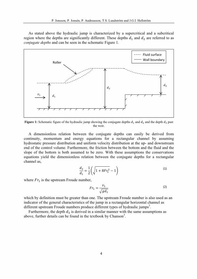
P. Jonsson, P. Jonsén, P. Andreasson, T.S. Lundström and J.G.I. Hellström

4

As stated above the hydraulic jump is characterized by a supercritical and a subcritical region where the depths are significantly different. These depths and are referred to as conjugate depths and can be seen in the schematic Figure 1.

Figure 1: Schematic figure of the hydraulic jump showing the conjugate depths and and the depth past the weir.

A dimensionless relation between the conjugate depths can easily be derived from continuity, momentum and energy equations for a rectangular channel by assuming hydrostatic pressure distribution and uniform velocity distribution at the up- and downstream end of the control volume. Furthermore, the friction between the bottom and the fluid and the slope of the bottom is both assumed to be zero. With these assumptions the conservations equations yield the dimensionless relation between the conjugate depths for a rectangular channel as,

(1)

where is the upstream Froude number,

(2)

which by definition must be greater than one. The upstream Froude number is also used as an indicator of the general characteristics of the jump in a rectangular horizontal channel as different upstream Froude numbers produce different types of hydraulic jumps3.

Furthermore, the depth is derived in a similar manner with the same assumptions as above, further details can be found in the textbook by Chanson3.

Roller

Fluid surfaceWall boundary

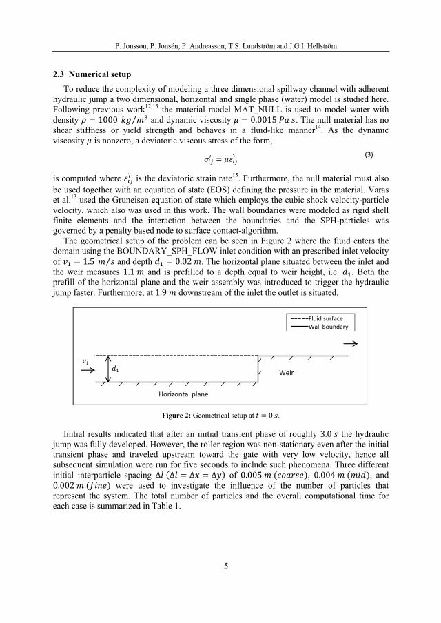
P. Jonsson, P. Jonsén, P. Andreasson, T.S. Lundström and J.G.I. Hellström

5

2.3 Numerical setup To reduce the complexity of modeling a three dimensional spillway channel with adherent

hydraulic jump a two dimensional, horizontal and single phase (water) model is studied here. Following previous work12,13 the material model MAT_NULL is used to model water with density and dynamic viscosity . The null material has no shear stiffness or yield strength and behaves in a fluid-like manner14. As the dynamic viscosity is nonzero, a deviatoric viscous stress of the form,

(3)

is computed where is the deviatoric strain rate15. Furthermore, the null material must also be used together with an equation of state (EOS) defining the pressure in the material. Varas et al.13 used the Gruneisen equation of state which employs the cubic shock velocity-particle velocity, which also was used in this work. The wall boundaries were modeled as rigid shell finite elements and the interaction between the boundaries and the SPH-particles was governed by a penalty based node to surface contact-algorithm.

The geometrical setup of the problem can be seen in Figure 2 where the fluid enters the domain using the BOUNDARY_SPH_FLOW inlet condition with an prescribed inlet velocity of and depth . The horizontal plane situated between the inlet and the weir measures and is prefilled to a depth equal to weir height, i.e. . Both the prefill of the horizontal plane and the weir assembly was introduced to trigger the hydraulic jump faster. Furthermore, at downstream of the inlet the outlet is situated.

Figure 2: Geometrical setup at .

Initial results indicated that after an initial transient phase of roughly the hydraulic jump was fully developed. However, the roller region was non-stationary even after the initial transient phase and traveled upstream toward the gate with very low velocity, hence all subsequent simulation were run for five seconds to include such phenomena. Three different initial interparticle spacing of , , and

were used to investigate the influence of the number of particles that represent the system. The total number of particles and the overall computational time for each case is summarized in Table 1.

Weir

Fluid surfaceWall boundary

Horizontal plane

P. Jonsson, P. Jonsén, P. Andreasson, T.S. Lundström and J.G.I. Hellström

6

Table 1: The total number of particles and the overall computational time for each case.

Case Total number of particles Computational time

All simulations where done using the commercial available software package LSTC LS-DYNA v. 971 R5.1.1 on HP Z600 Linux machines with eight to twelve cores.

3 RESULTS AND DISCUSSION This part will start with a qualitative comparison of the three cases at successive time steps

and end with a quantitative comparison of theoretically derived values and results from the simulations.

At the fast incoming fluid begins to flow into the initially stationary fluid which starts to move together downstream, i.e. in the positive x-direction. A wave forms and breaks as more water flows onto the horizontal plane and at roughly it reaches the weir and starts to spill over. The fluid reaches the outlet at roughly and in the meantime the roller region has moved closer to the weir. The roller continues to move downstream towards the weir until roughly when the velocity of the roller declines rapidly and change direction. Past a quasi-stationary state is attained as the velocity of roller upstream is very low. Figures 3-5 shows the three cases using the above stated number of particles with color coded velocities in the positive x-direction.

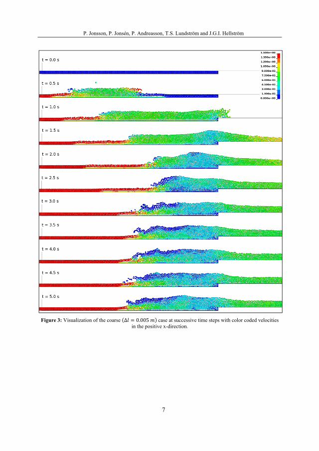
P. Jonsson, P. Jonsén, P. Andreasson, T.S. Lundström and J.G.I. Hellström

7

Figure 3: Visualization of the coarse case at successive time steps with color coded velocities in the positive x-direction.

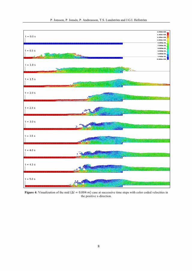
P. Jonsson, P. Jonsén, P. Andreasson, T.S. Lundström and J.G.I. Hellström

8

Figure 4: Visualization of the mid case at successive time steps with color coded velocities in the positive x-direction.

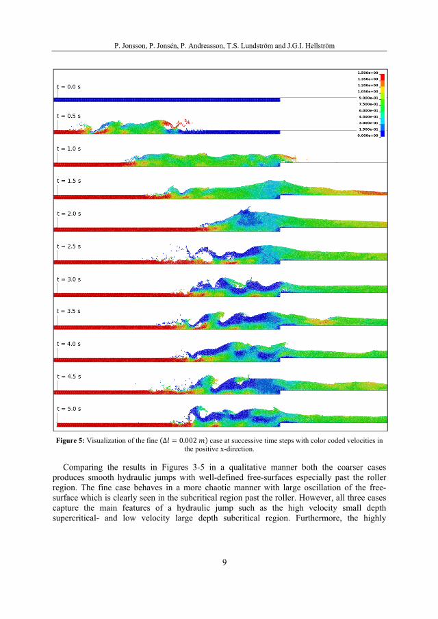
P. Jonsson, P. Jonsén, P. Andreasson, T.S. Lundström and J.G.I. Hellström

9

Figure 5: Visualization of the fine case at successive time steps with color coded velocities in the positive x-direction.

Comparing the results in Figures 3-5 in a qualitative manner both the coarser cases produces smooth hydraulic jumps with well-defined free-surfaces especially past the roller region. The fine case behaves in a more chaotic manner with large oscillation of the free-surface which is clearly seen in the subcritical region past the roller. However, all three cases capture the main features of a hydraulic jump such as the high velocity small depth supercritical- and low velocity large depth subcritical region. Furthermore, the highly

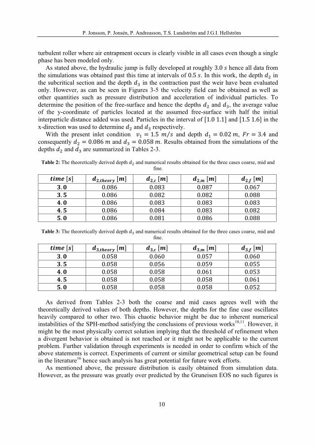
P. Jonsson, P. Jonsén, P. Andreasson, T.S. Lundström and J.G.I. Hellström

10

turbulent roller where air entrapment occurs is clearly visible in all cases even though a single phase has been modeled only.

As stated above, the hydraulic jump is fully developed at roughly hence all data from the simulations was obtained past this time at intervals of . In this work, the depth in the subcritical section and the depth in the contraction past the weir have been evaluated only. However, as can be seen in Figures 3-5 the velocity field can be obtained as well as other quantities such as pressure distribution and acceleration of individual particles. To determine the position of the free-surface and hence the depths and , the average value of the y-coordinate of particles located at the assumed free-surface with half the initial interparticle distance added was used. Particles in the interval of and in the x-direction was used to determine and respectively.

With the present inlet condition and depth , and consequently and . Results obtained from the simulations of the depths and are summarized in Tables 2-3.

Table 2: The theoretically derived depth and numerical results obtained for the three cases coarse, mid and fine.

Table 3: The theoretically derived depth and numerical results obtained for the three cases coarse, mid and fine.

As derived from Tables 2-3 both the coarse and mid cases agrees well with the theoretically derived values of both depths. However, the depths for the fine case oscillates heavily compared to other two. This chaotic behavior might be due to inherent numerical instabilities of the SPH-method satisfying the conclusions of previous works10,11. However, it might be the most physically correct solution implying that the threshold of refinement when a divergent behavior is obtained is not reached or it might not be applicable to the current problem. Further validation through experiments is needed in order to confirm which of the above statements is correct. Experiments of current or similar geometrical setup can be found in the literature16 hence such analysis has great potential for future work efforts.

As mentioned above, the pressure distribution is easily obtained from simulation data. However, as the pressure was greatly over predicted by the Gruneisen EOS no such figures is

P. Jonsson, P. Jonsén, P. Andreasson, T.S. Lundström and J.G.I. Hellström

11

shown. This behavior is at this stage not known to the authors but the validity of the Gruneisen EOS and the parameters used for current problem might be questionable.

5 CONCLUSIONS The capabilities of the SPH-method to accurately capture the main features of a hydraulic

jump such as the transition between supercritical- and subcritical flow has been demonstrated. Furthermore, the dynamics of the highly turbulent roller and the air entrapment process has been visualized even though a single phase has been modeled only. Comparison of theoretically derived values and numerical results of the depth in the subcritical section and the depth in the contraction past the weir show good agreement for the coarse and mid cases. The fine case show oscillating tendencies which might be due to inherent numerical instabilities of the SPH-method or it might show a more physically correct solution. Further validation through experiment is needed to clarify these issues.

6 ACKNOWLEDGEMENT The research presented was carried out as a part of "Swedish Hydropower Centre - SVC".

SVC has been established by the Swedish Energy Agency, Elforsk and Svenska Kraftnät together with Luleå University of Technology, The Royal Institute of Technology, Chalmers University of Technology and Uppsala University. www.svc.nu

REFERENCES [1] Hellström, J. G. I. (2009). Internal Erosion in Embankment Dams - Fluid Flow Through

and Deformation of Porous Media. Luleå: Luleå University of Technology. [2] Sandberg, E. (2009, June 3). Svensk energi. Retrieved January 30, 2011, from

http://www.svenskenergi.se/sv/Om-el/Elproduktion/ [3] Chanson, H. (2004). The Hydraulics of Open Channel Flow: An Introduction. Oxford:

Elsevier Ltd. [4] Scardovelli, R., & Zaleski, S. (1999). Direct numerical simulation of free-surface and

interfacial flow. Annual Review of Fluid Mechanics, 567-603. [5] López, D., Marivela, R., & Garrote, L. (2010). Smoothed particle hydrodynamics model

applied to hydraulic structure: a hydraulic jump test case. Journal of Hydraulic Research Vol. 48Extra Issue, 142-158.

[6] Federico, I., Marrone, S., Colagrossi, A., Aristodemo, F., & Veltri, P. (2010). Simulation of hydraulic jump through sph model. IDRA XXXII Italian Conference of Hydraulics and Hydraulic Construction. Palermo, Italy.

[7] Lucy, L. B. (1977). A numerical approach to testing of the fission hypothesis. TheAstronomical Journal, 1013-1024.

[8] Gingold, R. A., & Monaghan, J. J. (1977). Smoothed particle hydrodynamics: theory and application to non-spherical stars. Monthly Notices of the Poyal Astronomical Society, 181, 375-389.

[9] Liu, G. R., & Liu, M. B. (2009). Smoothed Particle Hydrodynamics : a meshfree particle method. Singapore: World Publishing Co. Pte. Ltd.

[10] Quinlan, N. J., Basa, M., & Lastiwka, M. (2006). Truncation error in mesh-free methods. International Journal for Numerical Methos in Engineering, 66:2064-2085.

P. Jonsson, P. Jonsén, P. Andreasson, T.S. Lundström and J.G.I. Hellström

12

[11] Graham, D. I., & Hughes, J. P. (2008). Accuracy of SPH viscous flow models. International Journal for Numerical Methods in Fluids, 56:1261-1269.

[12] Vesenjak, M., Müllerschön, H., Hummel, A., & Ren, Z. (2004). Simulation of Fuel Sloshing - Comperative Study. LS-DYNA Anwenderforum. Bamberg: DYNAmore GmgH.

[13] Varas, D., Zaera, R., & López-Puente, J. (2009). Numerical modeling of hydrodynamic ram phenomenon. International Journal of impact Engineering 36, 363-374.

[14] LSTC. (2010). LS-DYNA Keyword User´s Manual Version 971 Rev 5. Livermore: Livermore Software Technology Corporation (LSTC).

[15] Hallquist, J. O. (2006). LS-DYNA Theory Manual. Livermore Software Technology Corporation.

[16] Lennon, J. M., & Hill, D. F. (2006). Particle Image Velocity Measurements of Undular and Hydraulic Jumps. Journal of Hydraulic Engineering, 1283-1294.

Paper B

Modelling Dam Break Evolution

Over a Wet Bed with Smoothed

Particle Hydrodynamics: A

Parameter Study

Engineering, 2015, 7, 248-260Published Online May 2015 in SciRes. http://www.scirp.org/journal/enghttp://dx.doi.org/10.4236/eng.2015.75022

How to cite this paper: Jonsson, P., Jonsén, P., Andreasson, P., Lundström, T.S. and Hellström, J.G.I. (2015) Modelling Dam Break Evolution over a Wet Bed with Smoothed Particle Hydrodynamics: A Parameter Study. Engineering, 7, 248-260.http://dx.doi.org/10.4236/eng.2015.75022

Modelling Dam Break Evolution over a Wet Bed with Smoothed Particle Hydrodynamics: A Parameter StudyPatrick Jonsson, Pär Jonsén, Patrik Andreasson, T. Staffan Lundström,J. Gunnar I. HellströmDepartment of Engineering Sciences and Mathematics, Luleå University of Technology, Luleå, SwedenEmail: patrick.jonsson@ltu.se, par.jonsen@ltu.se, patrik.andreasson@ltu.se, staffan.lundstrom@ltu.se,gunnar.hellstrom@ltu.se

Received 25 April 2015; accepted 22 May 2015; published 25 May 2015

Copyright © 2015 by authors and Scientific Research Publishing Inc.This work is licensed under the Creative Commons Attribution International License (CC BY).http://creativecommons.org/licenses/by/4.0/

AbstractWhen investigating water flow in spillways and energy dissipation, it is important to know the behavior of the free surfaces. To capture the real dynamic behavior of the free surfaces is there-fore crucial when performing simulations. Today, there is a lack in the possibility to model such phenomenon with traditional methods. Hence, this work focuses on a parameter study for one al-ternative simulation tool available, namely the meshfree, Lagrangian particle method Smoothed Particle Hydrodynamics (SPH). The parameter study includes the choice of equation-of-state (EOS), the artificial viscosity constants, using a dynamic versus a static smoothing length, SPH particle spatial resolution and the finite element method (FEM) mesh scaling of the boundaries. The two dimensional SPHERIC Benchmark test case of dam break evolution over a wet bed was used for comparison and validation. The numerical results generally showed a tendency of the wave front to be ahead of the experimental results, i.e. to have a greater wave front velocity. The choice of EOS, FEM mesh scaling as well as using a dynamic or a static smoothing length showed little or no sig-nificant effect on the outcome, though the SPH particle resolution and the choice of artificial vis-cosity constants had a major impact. A high particle resolution increased the number of flow fea-tures resolved for both choices of artificial viscosity constants, but at the expense of increasing the mean error. Furthermore, setting the artificial viscosity constants equal to unity for the coarser cases resulted in a highly viscous and unphysical solution, and thus the relation between the ar-tificial viscosity constants and the particle resolution and its impact on the behavior of the fluid needed to be further investigated.

P. Jonsson et al.

249

KeywordsSPH, Dam Break, Smoothed Particle Hydrodynamics

1. IntroductionIn Sweden, hydropower plays a significant role in the supply of energy and it generates roughly 45% (66.0 TWh in 2011) of the total electricity power production [1]. The first larger hydropower plant in Sweden commenced its operation for almost 100 years ago and the latest was put into service in the 1970s. Hence, most of the hy-dropower plants in Sweden are old, which has initiated a number of projects on refurbishments. Due to the de-regulated energy market, hydropower plants are more and more run at off design conditions. Consequently, to have an optimal hydropower that, for instance, can run at the best efficiency point when the winnings are high, the plants must be modernized and adapted to the energy market. Other key aspects are new requirements on renewable and “green” energy sources. This makes the prospect of redesigning old hydropower stations evenhigher. Finally, the demand on hydropower as a short term regulating source is increasing to take care of more frequent and larger fluctuations in the energy system, mostly due to the on-going expansion of wind power. Re-garding the Swedish hydropower sector as a whole focus is set on the service and administration as well as re-furbishments of existing plants, to meet the new demands. To assess hydraulic properties in these projects, physical scale models are often used. Performance, accuracy and reliability of mathematical models are in these cases considered to be too poor. Hydropower hydraulics is characterized by large scales and flow rates. The geometry is usually partly formed by nature, i.e. to some extent chaotic at a scale of roughness. Furthermore, highly ae-rated and disturbed free surface flows are frequently encountered, for instance, in spillway channel flows and in energy dissipaters. This constitutes significant mathematical simulation challenges. Thus, there is a need of com-putationally robust and reliable numerical methods to handle these fundamentally complex problems. Modelling of highly disturbed aerated free surface flows is complex when grid based method is used [2]. Severe problems with mesh entanglement and determination of the free surface have been encountered [3]. The meshfree, La-grangian particle based method Smooth Particle Hydrodynamic (SPH), has shown to be a good alternative to grid based methods to overcome such problems [4] [5]. The technique was first proposed independently by [6][7] in the late seventies to solve astrophysical problems in a three-dimensional open space. Today, the SPH me-thod has been applied to a number of fields and problems [5] and the maturity of the method has increased sig-nificantly. Thus, SPH was chosen as the computational method in the present work. In the SPH method, the flu-id domain is represented by a set of non-connected particles which possess individual material properties such as density, velocity and pressure [8]. Besides representing the problem domain and acting as information carriers,the particles also act as the computational frame for the field function approximations. As the particles move with the fluid, their material properties change as a function of time and spatial co-ordinate due to interactions with neighboring particles. A major advantage of SPH is that the method is mesh-free, and thus considerable time is saved as compared with methods that need a predefined mesh. However, as the SPH is relatively unex-plored as compared with traditional finite volume method (FVM) and finite element method (FEM) methods,there are some areas that still need considerable attention. For instance, wall boundary conditions are generally difficult to set in SPH as they do not appear in a natural way within the SPH formalism. Furthermore, the SPH method is typically slower computational wise since the time step depends on the speed of sound and the expli-cit integration techniques used. The idealized dam break problem, where a given volume of initially stationary water is released onto a dry channel bed by a sudden removal of a gate, is a well-studied problem (e.g. [9]-[11]). After the gate has been removed, a negative surge propagates upstream and a dam break wave moves rapidly downstream. If, however, the dam break wave propagates over a wet bed (an initial fluid layer at rest), the flow field will become considerably different, see for instance [12] and [13]. Reference [13] studied the influence of adding a polymer in order to reduce the turbulence drag using a dam break setup. However, clean water test was conducted as well and the experimental results had been used by many authors as a validation test case such as [14]-[16]. The SPH European Research Interest Community (SPHERIC) has adopted the work by [13], and di-gitized wave profiles, wave velocity data and snapshots are available at wiki.manchester.ac.uk/spheric. The aim of this paper is to study the effects of several test parameters when applied to the SPHERIC test case based on

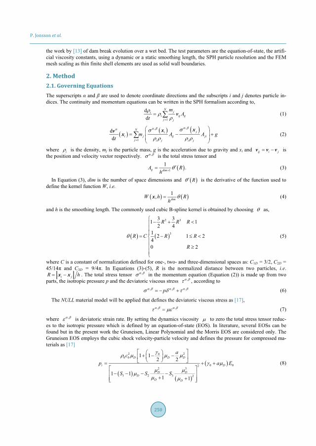
P. Jonsson et al.

250

the work by [13] of dam break evolution over a wet bed. The test parameters are the equation-of-state, the artifi-cial viscosity constants, using a dynamic or a static smoothing length, the SPH particle resolution and the FEM mesh scaling as thin finite shell elements are used as solid wall boundaries.

2. Method2.1. Governing EquationsThe superscripts and are used to denote coordinate directions and the subscripts i and j denotes particle in-dices. The continuity and momentum equations can be written in the SPH formalism according to,

1

dd

Nji

i ij ijj j

mA

tv (1)

,,

1

dd

N jii j ij ji

j i j i j

m A A gt

xxv x (2)

where i is the density, mj is the particle mass, g is the acceleration due to gravity and xi and ij i jv v v is the position and velocity vector respectively. , is the total stress tensor and

1

1 .ij dimA Rh

(3)

In Equation (3), dim is the number of space dimensions and R is the derivative of the function used to define the kernel function W, i.e.

1, dimW hh

Rx (4)

and h is the smoothing length. The commonly used cubic B-spline kernel is obtained by choosing as,

2 3

3

3 31 12 4

1 1 24

20

2

R R R

R C R R

R

(5)

where C is a constant of normalization defined for one-, two- and three-dimensional spaces as: C1D = 3/2, C2D =and C3D = s (3)-(5), R is the normalized distance between two particles, i.e.

i jR hx x . The total stress tensor , in the momentum equation (Equation (2)) is made up from two parts, the isotropic pressure p and the deviatoric viscous stress , , according to

, , ,p (6)

The NULL material model will be applied that defines the deviatoric viscous stress as [17],, , (7)

where , is deviatoric strain rate. By setting the dynamics viscosity to zero the total stress tensor reduc-es to the isotropic pressure which is defined by an equation-of-state (EOS). In literature, several EOSs can be found but in the present work the Gruneisen, Linear Polynomial and the Morris EOS are considered only. The Gruneisen EOS employs the cubic shock velocity-particle velocity and defines the pressure for compressed ma-terials as [17]

2 200 0

0 022 3

1 2 3 2

1 12 2

1 11 1

D D D

i D

D DD

D D

acp a E

S S S

(8)

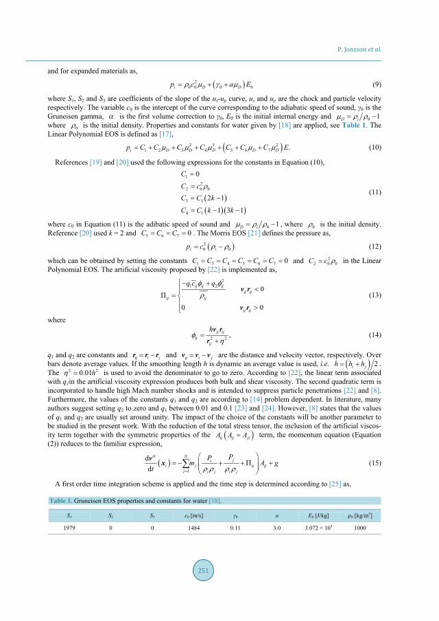
P. Jonsson et al.

251

and for expanded materials as,2

0 0 0 0i D Dp c a E (9)

where S1, S2 and S3 are coefficients of the slope of the us-up curve, us and up are the chock and particle velocity respectively. The variable c0 is the intercept of the curve corresponding to the adiabatic speed of sound, 0 is the Gruneisen gamma, is the first volume correction to 0, E0 is the initial internal energy and 0 1D iwhere 0 is the initial density. Properties and constants for water given by [18] are applied, see Table 1. The Linear Polynomial EOS is defined as [17],

2 3 21 2 3 4 5 6 7 .i D D D D Dp C C C C C C C E (10)

References [19] and [20] used the following expressions for the constants in Equation (10),

12

2 0 0

3 1

4 1

0

2 1

1 3 1

C

C cC C k

C C k k

(11)

where c0 in Equation (11) is the adibatic speed of sound and 0 1D i , where 0 is the initial density.Reference [20] used k = 2 and 5 6 7 0C C C . The Morris EOS [21] defines the pressure as,

20 0i ip c (12)

which can be obtained by setting the constants 1 3 4 5 6 7 0C C C C C C and 22 0 0C c in the Linear

Polynomial EOS. The artificial viscosity proposed by [22] is implemented as,2

1 2 0

0 0

ij ij ijij ij

ij ij

ij ij

q c qv r

v r

(13)

where

2 2 ,ij ijij

ij

hv rr

(14)

q1 and q2 are constants and ij i jr r r and ij i jv v v are the distance and velocity vector, respectively. Over bars denote average values. If the smoothing length h is dynamic an average value is used, i.e. 2i jh h h . The 2 20.01h is used to avoid the denominator to go to zero. According to [22], the linear term associated with q1in the artificial viscosity expression produces both bulk and shear viscosity. The second quadratic term is incorporated to handle high Mach number shocks and is intended to suppress particle penetrations [22] and [8]. Furthermore, the values of the constants q1 and q2 are according to [14] problem dependent. In literature, many authors suggest setting q2 to zero and q1 between 0.01 and 0.1 [23] and [24]. However, [8] states that the values of q1 and q2 are usually set around unity. The impact of the choice of the constants will be another parameter to be studied in the present work. With the reduction of the total stress tensor, the inclusion of the artificial viscos-ity term together with the symmetric properties of the ij ij jiA A A term, the momentum equation (Equation (2)) reduces to the familiar expression,

1

dd

Nji

i j ij ijj i j i j

PPm A

tgv x (15)

A first order time integration scheme is applied and the time step is determined according to [25] as,

Table 1. Gruneisen EOS properties and constants for water [18].

S1 S2 S3 c0 [m/s] 0 E0 [J/kg] 0 [kg/m3]

1979 0 0 1484 0.11 3.0 3.072 × 105 1000

P. Jonsson et al.

252

,iCFL i

i i

ht C Min

c v (16)

where CCFL is the Courant number usually set to unity. The smoothing length h is either static or dynamic. For the dynamic case h is obtained from,

d 1 .d 3 ih hdiv vt

(17)

For numerical reasons, a minimum and maximum value is imposed on the smoothing length, i.e. Hminh0 < h <Hmaxh0. In the present study, Hmin and Hmax were set equal to 0.5 and 1.5 respectively while h0 is the initial smoothing length given by 0 01.2h d , where d0 is the initial distance between particles. The impact on the re-sults from using a static or dynamic smoothing length will also be studied in the current study.

2.2. Boundary ConditionsSolid wall boundaries are modelled as rigid shell finite elements and the coupling between the boundaries and the SPH-particles are governed by a penalty based “node to surface” contact-algorithm [26]. This is a so-called one-way contact where the SPH particles are defined as the “slave side” and the FEM elements as the “master side”. In applying the penalty method, the slave nodes are checked for penetration through the master surface. If a slave node has penetrated, an interface spring is placed between the master surface and the node. The spring stiffness is chosen approximately in the order of magnitude of the stiffness of the interface element normal to the interface. The resultant force applied to the SPH particle in the normal direction of the FEM element is propor-tional to the amount of penetration. The wall boundaries used here can be compared with the Lennard-Jones-type boundary condition [24] where a central force is applied to a fluid particle. However, the normal compo-nent is considered only. Hence, the boundary condition used here is truly frictionless. For more information re-garding the contact algorithm see [17].

2.3. Geometrical SetupTo validate the SPH model experiment, the SPHERIC Benchmark test case of dam break evolution over a wet bed is used. Numerous authors have adopted this test case for validation proposes, e.g. [14]-[16]. The test case is based on the experimental work by [13] where water initially stored in a tank is released through a gate into a prefilled rectangular channel. The schematic arrangement and geometry is illustrated in Figure 1.

In the experiment by [13], several tank and channel depths were investigated. However, in the present work only one combination of tank and channel depth were considered, namely the tank depth LTD = 0.15 m and channel depth LCD = 0.018 m. The tank length LTL = 0.38 m was set as in the experiment and the channel lengthLCL = 1.62 m was smaller than in the experiment (LCL = 9.55 m) in order to reduce the overall number of particle and hence computational time. According to [13], a propagating bore develops after the removal of the gate. The stationary water in the channel resists the oncoming water and, as a consequence, a unstable “mushroom-like” wave forms and breaks in both forward and backward directions. In the experiment, the kinetic energy was usually enough to build up several breaking events until a smooth propagating bore was formed. Two CCD-cameras recorded the events, thus digitized snapshots, wave profile data and average wave front velocities isavailable for comparison. Here, wave profile is compared only. According to [2], a general difference of approx-imately 0.043 s is observed between experiments and SPH simulations, thus this time shift is accounted for in

Figure 1. Schemetic arrangement and geometry for the dam break test case.

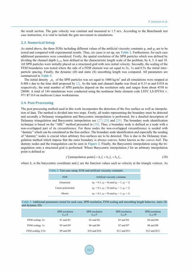
P. Jonsson et al.

253

the result section. The gate velocity was constant and measured to 1.5 m/s. According to the Benchmark test case instruction, it is vital to include the gate movement in simulations.

2.3. Numerical SetupAs stated above, the three EOSs including different values of the artificial viscosity constants q1 and q2 are to be tested and compared with experimental results. Thus, six cases is set up, see Table 2. Furthermore, for each case additional parameters were considered. Firstly, the spatial resolution of the SPH particles which was defined by dividing the channel depth LCD, here defined as the characteristic length scale of the problem, by 4, 5, 6 and 10. All SPH particles were initially placed on a structured grid with zero initial velocity. Secondly, the scaling of the FEM boundaries was tested where the side of a FEM element was set equal to 2x, 1x and 0.5x the initial inter-particle spacing. Finally, the dynamic (D) and static (S) smoothing length was compared. All parameters are summarized in Table 3.

The initial density 0 of the SPH particles was set equal to 1000 kg/m3 and all simulations were stopped at 0.488 s due to the time shift proposed by [2]. As the tank and channel depths was fixed at 0.15 m and 0.018 m respectively, the total number of SPH particles depend on the resolution only and ranges from about 4550 to 28600. A total of 144 simulations were conducted using the nonlinear finite element code LSTC LS-DYNA v. 971 R7.0.0 on multicore Linux workstations.

2.4. Post ProcessingThe post processing method used in this work incorporates the detection of the free surface as well as interpola-tion of data. The method is divided into two steps. Firstly, all nodes representing the boundary must be detected and secondly a Delaunay triangulation and Barycentric interpolation is performed, for a detailed description of Delaunay triangulation and Barycentric interpolation see [27] [28] and [29]. The boundary node identification technique is based on the “ARC” method presented in [30]. Thus, a boundary node is defined as a node with a non-overlapped part of its circumference. For these nodes the non-overlapped circumference is seeded with “dummy” which can be considered as the free-surface. The boundary node identification and especially the seeding of “dummy” nodes is crucial when arbitrary free-surfaces are to be detected. This is due to the Delaunay trian-gulation method which impose that the outer boundary is always convex, better known as the convex hull. The dummy nodes and the triangulation can be seen in Figure 2. Finally, the Barycentric interpolation using the tri-angulation onto a structured grid is performed. Where Barycentric interpolation f for an arbitrary interpolation point is defined as

1 1 2 2 3 3interpolation point ,f b f b f b f (18)

where bx is the barycentric coordinate and fx are the function values such as velocity at the triangle vertices. As

Table 2. Test case setup, EOS and artificial viscosity constants.

EOS Artificial viscosity constants

Gruneisen (q1 = 0.1; q2 = 0) and (q1 = 1; q2 = 1)

Linear polynomial (q1 = 0.1; q2 = 0) and (q1 = 1; q2 = 1)

Morris (q1 = 0.1; q2 = 0) and (q1 = 1; q2 = 1)

Table 3. Additional parameters tested for each case, SPH resolution, FEM scaling and smoothing length behavior, static (S) and dynamic (D).

SPH resolutionLCD/4

SPH resolutionLCD/5

SPH resolutionLCD/6

SPH resolutionLCD/10

FEM scaling: 2x S1 and D1 S2 and D2 S3 and D3 S4 and D4

FEM scaling: 1x S5 and D5 S6 and D6 S7 and D7 S8 and D8

FEM scaling: 0.5x S9 and D9 S10 and D10 S11 and D11 S12 and D12

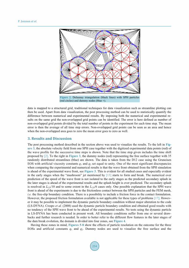
P. Jonsson et al.

254

Figure 2. Delaunay triangulation (black lines) with SPH particles (red circles) and dummy nodes (blue +).

data is mapped to a structured grid, traditional techniques for data visualization such as streamline plotting canthen be used. Apart from data visualization, the post processing method can be used to statistically quantify the difference between numerical and experimental results. By imposing both the numerical and experimental re-sults on the same grid the non-overlapped grid points can be identified. The error is here defined as number of non-overlapped grid points divided by the total number of points in the experiment for each time step. The mean error is then the average of all time step errors. Non-overlapped grid points can be seen as an area and hence when the non-overlapped area goes to zero the mean error goes to zero as well.

3. Results and DiscussionThe post processing method described in the section above was used to visualize the results. To the left in Fig-ure 3, the absolute velocity field from one SPH case together with the digitized experimental data points (red) of the wave profile for the successive time steps is shown. Note that the time step given includes the time shift proposed by [2]. To the right in Figure 3, the dummy nodes (red) representing the free surface together with 35 randomly distributed streamlines (blue) are shown. The data is taken from the D12 case using the Gruneisen EOS with artificial viscosity constants q1 and q2 set equal to unity. One of the most significant discrepancieswhen comparing the experimental and numerical results is that the wave front obtained from the SPH simulation is ahead of the experimental wave front, see Figure 3. This is evident for all studied cases and especially evident in the early stages when the “mushroom” jet mentioned by [13] starts to form and break. The numerical over prediction of the speed of the wave front is not isolated to the early stages as the predicted secondary splash in the later stages is ahead of the experimental results and the splash height is over predicted. The secondary splash is resolved in LCD/10 and to some extent in the LCD/6 cases only. One possible explanation that the SPH wave front is ahead of the experiments is due to the frictionless contact between the SPH particles and the FEM mesh, i.e. the free-slip boundary condition. There is a possibility to include a friction force in the contact formulation. However, the proposed friction formulation available is not applicable for these types of problems [17]. Howev-er it may be possible to implement the dynamic particle boundary condition without major alteration to the code (LS-DYNA). Crespo et al. (2008) used the dynamic particle boundary condition and obtained good results with no tendency of the SPH wave front to be ahead of the experimental results. No tests using the dynamic particle in LS-DYNA has been conducted in present work. All boundary conditions suffer from one or several draw-backs and further research is needed. In order to better refer to the different flow features in the later stages of the dam break evolution, the domain is divided into four zones, see Figure 4.

Having these zones in mind, Figures 5-8 show the effects of particle resolution on the outcome for the three EOSs and artificial constants q1 and q2. Dummy nodes are used to visualize the free surface and the

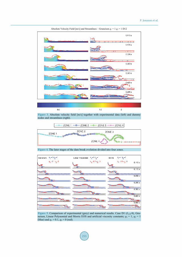
P. Jonsson et al.

255

Absolute Velocity Field [m/s] and Streamlines—Gruneisen q1 = 1 q2 = 1 D12

Figure 3. Absolute velocity field [m/s] together with experimental data (left) and dummy nodes and streamlines (right).

Figure 4. The later stages of the dam break evolution divided into four zones.

Figure 5. Comparison of experimental (grey) and numerical results. Case D1 (LCD/4), Gru-neisen, Linear Polynomial and Morris EOS and artificial viscosity constants; q1 = 1, q2 = 1(blue) and q1 = 0.1, q2 = 0 (red).

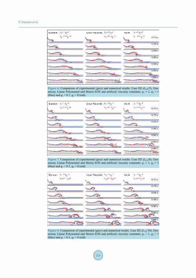
P. Jonsson et al.

256

Figure 6. Comparison of experimental (grey) and numerical results. Case D2 (LCD/5), Gru-neisen, Linear Polynomial and Morris EOS and artificial viscosity constants; q1 = 1, q2 = 1(blue) and q1 = 0.1, q2 = 0 (red).

Figure 7. Comparison of experimental (grey) and numerical results. Case D2 (LCD/6), Gru-neisen, Linear Polynomial and Morris EOS and artificial viscosity constants; q1 = 1, q2 = 1(blue) and q1 = 0.1, q2 = 0 (red).

Figure 8. Comparison of experimental (grey) and numerical results. Case D2 (LCD/10), Gru-neisen, Linear Polynomial and Morris EOS and artificial viscosity constants; q1 = 1, q2 = 1(blue) and q1 = 0.1, q2 = 0 (red).

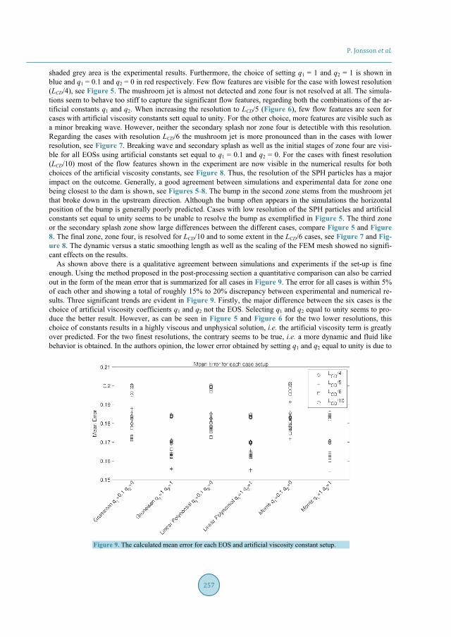
P. Jonsson et al.

257

shaded grey area is the experimental results. Furthermore, the choice of setting q1 = 1 and q2 = 1 is shown in blue and q1 = 0.1 and q2 = 0 in red respectively. Few flow features are visible for the case with lowest resolution(LCD/4), see Figure 5. The mushroom jet is almost not detected and zone four is not resolved at all. The simula-tions seem to behave too stiff to capture the significant flow features, regarding both the combinations of the ar-tificial constants q1 and q2. When increasing the resolution to LCD/5 (Figure 6), few flow features are seen for cases with artificial viscosity constants sett equal to unity. For the other choice, more features are visible such as a minor breaking wave. However, neither the secondary splash nor zone four is detectible with this resolution. Regarding the cases with resolution LCD/6 the mushroom jet is more pronounced than in the cases with lower resolution, see Figure 7. Breaking wave and secondary splash as well as the initial stages of zone four are visi-ble for all EOSs using artificial constants set equal to q1 = 0.1 and q2 = 0. For the cases with finest resolution (LCD/10) most of the flow features shown in the experiment are now visible in the numerical results for both choices of the artificial viscosity constants, see Figure 8. Thus, the resolution of the SPH particles has a major impact on the outcome. Generally, a good agreement between simulations and experimental data for zone one being closest to the dam is shown, see Figures 5-8. The bump in the second zone stems from the mushroom jet that broke down in the upstream direction. Although the bump often appears in the simulations the horizontal position of the bump is generally poorly predicted. Cases with low resolution of the SPH particles and artificial constants set equal to unity seems to be unable to resolve the bump as exemplified in Figure 5. The third zone or the secondary splash zone show large differences between the different cases, compare Figure 5 and Figure 8. The final zone, zone four, is resolved for LCD/10 and to some extent in the LCD/6 cases, see Figure 7 and Fig-ure 8. The dynamic versus a static smoothing length as well as the scaling of the FEM mesh showed no signifi-cant effects on the results.

As shown above there is a qualitative agreement between simulations and experiments if the set-up is fine enough. Using the method proposed in the post-processing section a quantitative comparison can also be carried out in the form of the mean error that is summarized for all cases in Figure 9. The error for all cases is within 5%of each other and showing a total of roughly 15% to 20% discrepancy between experimental and numerical re-sults. Three significant trends are evident in Figure 9. Firstly, the major difference between the six cases is the choice of artificial viscosity coefficients q1 and q2 not the EOS. Selecting q1 and q2 equal to unity seems to pro-duce the better result. However, as can be seen in Figure 5 and Figure 6 for the two lower resolutions, this choice of constants results in a highly viscous and unphysical solution, i.e. the artificial viscosity term is greatly over predicted. For the two finest resolutions, the contrary seems to be true, i.e. a more dynamic and fluid like behavior is obtained. In the authors opinion, the lower error obtained by setting q1 and q2 equal to unity is due to

Figure 9. The calculated mean error for each EOS and artificial viscosity constant setup.

P. Jonsson et al.

258

the highly viscous solution which reduces the wave front velocity and hence lowering the mean error. This makes it cumbersome to find a good relation of spatial resolution and artificial viscosity constants to obtain a trustworthy solution. Secondly, the results connected to the LCD/10 cases or the case with the highest resolution seems to produce the worst results. This is in sharp contrast to the expected outcome, as generally more nodes in any numerical method should produce a better result and also the qualitative investigation indicated this. One plausible explanation to this behavior is that more features are resolved using more particles such as the break-ing wave and zone four. Also, the height of the secondary splash produced mainly in the LCD/10 cases are gener-ally over predicted thus increasing the number of none overlapping grid points, i.e. increasing the mean error, as can be seen in Figure 8. Thirdly, all EOSs produce similar results which are expected as the density differences seen in the simulations are very small. However, the density differences are not small enough and unphysical pressure overestimation and large pressure oscillations are obtained ( 610∓ Pa), especially close to wall bounda-ries as well as near the free-surface. It is likely that the over prediction of pressure is due to the speed of sound c0

which was set equal to the physical speed of sound of 1484 m/s. Usually, c0 is set equal to at least 10 times the expected maximum velocity in the flow [24] [31]. Initial tests with reduced speed of sound

1 20 10 refc gH

were performed, where Href is the maximum water height in the tank (Href = 0.15 m) as according to [14]. How-ever, severe particle collapse and contact instabilities were obtained and, hence, the physical speed of sound was used. Generally, the pressure oscillations near wall boundaries and free surfaces can be avoided by use of either density filters or correction of the kernel and/or kernel gradient. Considerable efforts have been devoted to over-come these problems in the SPH research community [4]. Several corrections and filtering techniques have been proposed and are available in literature, see for instance [32].

In the zeroth order Shepard density filter, the simplest and quickest type of density filter, oscillations are smoothed out by filtering density and then re-assigning a new density to each particle [33]-[35]. Kernel and kernel gradient correction techniques are generally included to handle the truncated kernel function close to free-surfaces and boundaries where conditions of consistency and normalization fail [32] [34] [36] [37]. Furthermore, the development of a truly incompressible SPH (ISPH) solver have shown great promise in estimation of pres-sure and show less oscillations, see for instance [16]. As with boundary conditions no filtering or correction techniques are currently implemented in LS-DYNA and the effects of such methods are not possible to test atthis point.

4. ConclusionThe two dimensional (2D) SPHERIC Benchmark test case of dam break evolution over a wet bed has been used to investigate the impact of several parameters when performing free surface flow simulations. The choice of EOS, the artificial viscosity constants, a dynamic versus a static smoothing length, SPH particle resolution and the FEM mesh scaling of the boundaries were investigated. The numerical results showed generally a tendency to be ahead of the experimental results, i.e. to have a greater wave front velocity. This was argued to be an effect of using a frictionless contact algorithm between the SPH particles and the FEM boundaries. The choice of EOS, FEM mesh scaling as well as using a dynamic or a static smoothing length showed little or no significant im-provement to the result. However, all EOSs showed larger than physical pressure levels in the order of 106 Pa and large pressure oscillations. This is believed to be an effect of not reducing the speed of sound in the calcula-tions, which is usually done. The SPH particle resolution and the choice of artificial viscosity constants had a major impact. The method used for comparing numerical and experimental results showed increased mean error for both highly resolved cases and artificial viscosity constants set equal to 0.1 and 0. However, by visual ob-servation, it was noted that increasing the number of particles representing the system increased the number of flow features resolved and that a highly viscous solution was obtained by setting the artificial viscosity constant to unity. Thus, the relation between the artificial viscosity constants and the particle resolution and its impact on the behavior of the fluid needed to be further investigated.

AcknowledgementsThe research presented was carried out as a part of “Swedish Hydropower Centre—SVC”. SVC has been estab-lished by the Swedish Energy Agency, Elforsk and SvenskaKraftnät together with Luleå University of Technol-ogy, The Royal Institute of Technology, Chalmers University of Technology and Uppsala University. www.svc.nu

P. Jonsson et al.

259

References[1] Energi, S. (2012) The Electricity Year and Operations.

http://www.svenskenergi.se/Global/Statistik/El%C3%A5ret/Sv%20Energi_el%C3%A5ret2012_ENG.pdf[2] Violeau, D. (2012) Fluid Mechanics and the SPH Method: Theory and Applications. Oxford University Press, Oxford.

http://dx.doi.org/10.1093/acprof:oso/9780199655526.001.0001[3] Scardovelli, R. and Zaleski, S. (1999) Direct Numerical Simulation of Free-Surface and Interfacial Flow. Annual Re-

view of Fluid Mechanics, 31, 576-603. http://dx.doi.org/10.1146/annurev.fluid.31.1.567[4] Gomez-Gesteria, M., Rogers, B.D., Dalrymple, R.A. and Crespo, A.J.C. (2010) State-of-the-art of Classical SPH for

Free-Surface Flows. Journal of Hydraulic Research, 48, 6-27.http://dx.doi.org/10.1080/00221686.2010.9641242

[5] Monaghan, J.J. (2012) Smoothed Particle Hydrodynamics and Its Diverse Applications. Annual Review of Fluid Me-chanics, 44, 323-346. http://dx.doi.org/10.1146/annurev-fluid-120710-101220

[6] Lucy, L.B. (1977) A Numerical Approach to the Testing of the Fission Hypothesis. The Astronomical Journal, 82,1013-1024. http://dx.doi.org/10.1086/112164

[7] Gingold, R.A. and Monaghan, J.J. (1977) Smoothed Particle Hydrodynamics: Theory and Application to Non-Spherical Stars. Monthly Notice of the Royal Astronomical Society, 181, 375-389. http://dx.doi.org/10.1093/mnras/181.3.375

[8] Liu, G.R. and Liu, M.B. (2003) Smoothed Particle Hydrodynamics: A Meshfree Particle Method. World Publishing Co. Pte. Ltd., Singapore. http://dx.doi.org/10.1142/9789812564405

[9] Ritter, A. (1892) Die Fortpflanzung der Wasserwellen. Vereine Deutcher Ingenieure Zeitswchrift, 36, 947-954.[10] Schoklitsch, A. (1917) Über Dambruchwellen. Sitzungberichten der Königliche Akademie der Wissenschaften, 126,

1489-1514.[11] Whitham, G.B. (1955) The Effects of Hydraulic Resistance in Dam-Break Problem. Proceedings of the Royal Society

of London A, 227, 399-407. http://dx.doi.org/10.1098/rspa.1955.0019[12] Stansby, P.K., Chegini, A. and Barnes, T.C.D. (1998) The Initial Stages of Dam-Break Flow. Journal of Fluid Mecha-

nics, 374, 407-424. http://dx.doi.org/10.1017/S0022112098009975[13] Jánosi, I.M., Jan, D., Szabó, K.G. and Tél T. (2004) Turbulent Drag Reduction in Dam-Break Flows. Experiments in

Fluids, 37, 219-229. http://dx.doi.org/10.1007/s00348-004-0804-4[14] Crespo, A.J.C., Gómez-Gesteria, M. and Dalrymple, R.A. (2008) Modeling Dam Break Behaviour over a Wet Bed by

SPH Technique. Journal of Waterway, Port, Coastal, and Ocean Engineering, 134, 313-320. http://dx.doi.org/10.1061/(ASCE)0733-950X(2008)134:6(313)

[15] Gomez-Gesteira, M., Crespo, A.J.C., Rogers, B.D., Dalrymple, R.A., Dominguez, J.M. and Barreiro, A. (2012) SPHysics—Development of a Free-Surface Fluid Solver—Part 2: Efficiency and Test Cases. Computers and Geos-ciences, 48, 300-307. http://dx.doi.org/10.1016/j.cageo.2012.02.028

[16] Lee, E.-S., Moulinec, C., Xu, R., Violeau, D., Laurence, D. and Stansby, P. (2008) Comparisons of Weakly Compres-sible and Truly Incompressible Algorithms for the SPH Mesh Free Particle Method. Journal of Computational Physics,227, 8417-8436. http://dx.doi.org/10.1016/j.jcp.2008.06.005

[17] LS-DYNA Keyword User’s Manual (2012) Livermore Software Technology Corporation (LSTC), Version 971 R6.1.0.Vol. 1 and 2.

[18] Boyd, R., Royles, R. and El-Deeb, K.M.M. (2000) Simulation and Validation of UNDEX Phenomena Relating to Axisymmetric Structures. Proceedings of the 6th International LS-DYNA users conference, Dearborn, 9-11 April 2000,21-36.

[19] Johnson, A.F. and Holzapfel, M. (2006) Numerical Prediction of Damage in Composite Structures from Soft Body Impacts. Journal of Material Science, 41, 6622-6630. http://dx.doi.org/10.1007/s10853-006-0201-x

[20] Selezneva, M., Stone, P., Moffat, T., Behdinan, K. and Poon, C. (2010) Modeling Bird Impact on a Rotating Fan: The Influence of Bird Parameters. Proceedings of the 11th International LSDYNA Users Conference, Dearborn, 6-8 June 2010, 37-46.

[21] Morris, J.P., Fox, P.J. and Zhu, Y. (1997) Modeling Low Reynolds Number Incompressible Flows Using SPH. Journal of Computational Physics, 136, 214-226. http://dx.doi.org/10.1006/jcph.1997.5776

[22] Monaghan, J.J. (1992) Smoothed Particle Hydrodynamics. Annual Review of Astronomy and Astrophysics, 30, 543-574. http://dx.doi.org/10.1146/annurev.aa.30.090192.002551

[23] Dalrymple, R.A. and Rogers, B.D. (2006) Numerical Modeling of Water Waves with the SPH Method. Costal Engi-neering, 53, 141-147. http://dx.doi.org/10.1016/j.coastaleng.2005.10.004

P. Jonsson et al.

260

[24] Monaghan, J.J. (1994) Simulating Free Surface Flows with SPH. Journal of Computational Physics, 110, 399-406. http://dx.doi.org/10.1006/jcph.1994.1034

[25] Hallquist, J.O. (2006) LS-DYNA Theory Manual. Livermore Software Technology Corporation (LSTC), Livermore.[26] Jonsén, P., Pålsson, B.I. and Häggblad, H.-Å. (2012) A Novel Method for Full-Body Modeling of Grinding Charges in

Tumbling Mills. Minerals Engineering, 33, 2-12. http://dx.doi.org/10.1016/j.mineng.2012.01.017[27] Berg, M., van Kreveld, M., Overmars, M. and Schwarzkopf, O. (2000) Computational Geometry: Algorithms and Ap-

plications. 2nd Edition, Springer, Berlin. http://dx.doi.org/10.1007/978-3-662-04245-8[28] Ungar, A.A. (2010) Barycentric Calculus in Euclidean and Hyperbolic Geometry—A Comparative Introduction. World

Scientific Publishing Co. Pte. Ltd., Singapore.[29] Hellström, J.G.I., Frishfelds, V. and Lundström, T.S. (2010) Mechanisms of Flow-Induced Deformation of Porous

Media. Journal of Fluid Mechanics, 664, 220-237. http://dx.doi.org/10.1017/S002211201000368X[30] Dilts, G.A. (2000) Moving Least-Squares Particle Hydrodynamics II: Conservation and Boundaries. International

Journal for numerical methods in engineering, 48, 1503-1524. http://dx.doi.org/10.1002/1097-0207(20000810)48:10<1503::AID-NME832>3.0.CO;2-D

[31] Monaghan, J.J. and Kos, A. (1999) Solitary Waves on a Cretan Beach. Journal of Waterway, Port, Coastal and Ocean Engineering, 125, 145-155. http://dx.doi.org/10.1061/(ASCE)0733-950X(1999)125:3(145)

[32] Bonet, J. and Lok T.-S.L. (1999) Variational and Momentum Preservation Aspects of Smoothed Particle Hydrodyna-mic Formulations. Computer Methods in Applied Mechanics and Engineering, 180, 97-115. http://dx.doi.org/10.1016/S0045-7825(99)00051-1

[33] Colagrossi, A. and Landrini, M. (2003) Numerical Simulation of Interfacial Flows by Smoothed Particle Hydrodyna-mics. Journal of Computational Physics, 191, 448-475. http://dx.doi.org/10.1016/S0021-9991(03)00324-3

[34] Belytschko, T., Krongauz, Y., Dolbow, J. and Gerlach, C. (1998) On the Completeness of Meshfree Particle Methods.International Journal for Numerical Methods in Engineering, 43, 785-819. http://dx.doi.org/10.1002/(SICI)1097-0207(19981115)43:5<785::AID-NME420>3.0.CO;2-9

[35] Dilts, G.A. (1999) Moving-Least-Square-Particle Hydrodynamics—I. Consistency and Stability. International Journal for Numerical Methods in Engineering, 44, 1115-1155. http://dx.doi.org/10.1002/(SICI)1097-0207(19990320)44:8<1115::AID-NME547>3.0.CO;2-L

[36] Vila, J.P. (1999) On Particle Weighted Methods and Smoothed Particle Hydrodynamics. Mathematical Models and Methods in Applied Science, 9, 161-209. http://dx.doi.org/10.1142/S0218202599000117

[37] Chen, J.K. and Beraun J.E. (2000) A Generalized Smoothed Particle Hydrodynamics Method for Nonlinear Dynamic Problems. Computer Methods in Applied Mechanics and Engineering, 190, 225-239. http://dx.doi.org/10.1016/S0045-7825(99)00422-3

Paper C

Smoothed Particle Hydrodynamic

Modelling of Hydraulic Jumps: Bulk

Parameters and Free Surface

Fluctuations

Smoothed Particle Hydrodynamic Modelling of HydraulicJumps: Bulk Parameters and Free Surface Fluctuations

P. Jonsson1†, P. Jonsen2, P. Andreasson1, T.S. Lundstrom1, and J.G.I. Hellstrom1

1 Division of Fluid and Experimental Mechanics, Lulea University of Technology (LTU), Lulea, SE-971 87, Sweden2 Division of Mechanics and Solid Materials, Lulea University of Technology (LTU), Lulea, SE-971 87, Sweden

† Corresponding Author Email: patrick.jonsson@ltu.se

(Received ——; accepted ——)

ABSTRACT

A hydraulic jump is a rapid transition from supercritical flow to subcritical flow characterized by the devel-opment of large scale turbulence, surface waves, spray, energy dissipation and considerable air entrainment.Hydraulic jumps can be found in waterways such as spillways connected to hydropower plants and are aneffective way to eliminate problems caused by high velocity flow, e.g. erosion. Due to the importance of thehydropower sector as a major contributor to the Swedish electricity production, the present study focuseson Smoothed Particle Hydrodynamic (SPH) modelling of 2D hydraulic jumps in horizontal open channels.Four cases with different spatial resolution of the SPH particles were investigated by comparing the con-jugate depth in the subcritical section with theoretical results. These showed generally good agreementwith theory. The coarsest case was run for a longer time and a quasi-stationary state was achieved, whichfacilitated an extended study of additional variables. The mean vertical velocity distribution in the hori-zontal direction compared favourably with experiments and the maximum velocity for the SPH-simulationsindicated a too rapid decrease in the horizontal direction and poor agreement to experiments was obtained.Furthermore, the mean and the standard deviation of the free surface fluctuation showed generally goodagreement with experimental results even though some discrepancies were found regarding the peak in themaximum standard deviation. The free surface fluctuation frequencies were over predicted and the modelcould not capture the decay of the fluctuations in the horizontal direction.

Keywords: SPH, Hydraulic jump, Conjugate depth, Free surface fluctuation, Vertical velocity distribution.

NOMENCLATURE

Ai j Gradient of kernel functionA,P Statistical variablesCc f l Courant coefficientd1 Depth in supercritical sectiond2 Depth in subcritical sectionρ Densityδt Time stepε Deviatoric strain rateE Internal energyFr Froude numberf Frequencyg Gravitational accelerationη,η′ Average and standard deviation of

free surface fluctuationh Smoothing length

Lr Length of rollerm Massμ Dynamic viscosityν Kinematic viscosityσ Total stress tensorΠ Artificial viscosityq1,q2 Artificial viscosity constantsRe Reynolds numberR Normalized distance between particlesSt Strouhal numberτ Deviatoric viscous stressv1 Velocity in supercritical sectionVmax Horizontal maximum velocityW Kernel function

1. INTRODUCTION

Fluid mechanics of large hydropower plants arecharacterized by very high flow rates and largephysical dimensions both in production and spillwaterways. The hydraulic head harvested in pro-duction needs to be handled when spillways are en-gaged. In open spillways, this is done by accelerat-

ing the flow and then using the dissipative featuresof a hydraulic jump. Hydraulic jumps are an ef-fective way to eliminate problems caused by highvelocity flow, e.g. erosion. The lower velocitiespast the jump, may also create beneficial flow con-ditions for migrating species such as salmonoidsLundstrom et al. (2015). A hydraulic jump isa rapid transition from high velocity supercritical

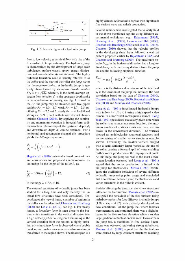
Fig. 1. Schematic figure of a hydraulic jump.

flow to low velocity subcritical flow with rise of thefree surface to keep continuity. The hydraulic jumpis characterized by the development of large scaleturbulence, surface waves, spray, energy dissipa-tion and considerable air entrainment. The highlyturbulent transition zone is usually referred to asthe roller and the start of the roller the jump toe orthe impingement point. A hydraulic jump is typ-ically characterised by its inflow Froude numberFr1 = v1/

√gd1, where v1 is the depth average up-

stream flow velocity, d1 is the upstream depth and gis the acceleration of gravity, see Fig. 1. Based onthe Fr, the jump may be classified into five types:undular Fr1 = 1.0−1.7, weak Fr1 = 1.7−2.5, os-cillating Fr1 = 2.5−4.5, steady Fr1 = 4.5−9.0 andstrong Fr1 > 9.0, each with its own distinct charac-teristics Chanson (2004). By applying the continu-ity and momentum equation in integral form, a di-mensionless relationship of the upstream depth d1and downstream depth d2 can be obtained. For ahorizontal and rectangular channel this procedureyields the Belanger equation,

d2

d1=

12

(√1+8Fr2

1 −1). (1)

Hager et al. (1990) reviewed a broad range of dataand correlations and proposed a semiempirical re-lationship for the length of the roller Lr as,

Lr

d1= 160tanh

(Fr1

20

)−12, (2)

in the range 2 < Fr1 < 16.

The external geometry of hydraulic jumps has beenstudied for a long time and only recently, the in-ternal flow structures have been considered. De-pending on the type of jump, a number of regions inthe roller can be identified Chanson and Brattberg(2000) and Lin et al. (2012), see Fig. 1. For steadyjumps, a boundary layer is seen close to the bot-tom which transitions in the vertical direction intoa high velocity jet or core region. Continuing in thevertical direction from the bottom, a highly turbu-lent air-water shear layer is observed where bubblebreak up and coalescences occurs and momentum istransferred to the region above. The final region is a

highly aerated recirculation region with significantfree surface wave and splash production.

Several authors have investigated the velocity fieldin the above-mentioned regions using different ex-perimental techniques, e.g. Rajaratnam (1965),Hornung et al. (1995), Lennon and Hill (2006),Chanson and Brattberg (2000) and Lin et al. (2012).Chanson (2010) showed that the velocity profilesin the developing shear layer followed a wall jetpattern proposed earlier by Rajaratnam (1965) andChanson and Brattberg (2000). The maximum ve-locity Vmax in the horizontal direction had a longitu-dinal decay with increasing distance from the jumptoe and the following empirical function

Vmax

v1= exp

(−0.028

(x− x1)

d1

), (3)

where x is the distance downstream of the inlet andx1 is the location of the jump toe, revealed the bestcorrelation based on the data of Chanson (2010),Chanson and Brattberg (2000), Kucukali and Chan-son (2008) and Murzyn and Chanson (2008).

Long et al. (1991) investigated hydraulic jumpswith inflow 4 < Fr1 < 9 using a high speed videocamera in a horizontal rectangular channel. Longet al. (1991) postulated that at any given time whenthe roller is at its most upstream location, the max-imum number of vortices exists and their size in-crease in the downstream direction. The vorticesshowed an anticlockwise rotational tendency andvortex-pairing of smaller vortex structures was ob-served. Eventually, the smaller vortices mergedwith a semi-stationary larger vortex at the end ofthe roller causing a forward spill of water enablingfurther vortex production at the impingement point.At this stage, the jump toe was at the most down-stream location observed and Long et al. (1991)argued that the vortex production is linked withthe jump toe fluctuations. Mossa (1999) investi-gated the oscillating behaviour of several differenthydraulic jump using point gauge and concludedthat a correlation between jump toe fluctuations andvortex structures in the roller is evident.

Besides affecting the jump toe, the vortex structuresinfluence the free surface. Mouaze et al. (2005) in-vestigated the behaviour of the free surfaces usingresistivity probes for four different hydraulic jumps(1.98 < Fr1 < 4.82) with partially developed in-flow conditions. At the jump toe, where bubbleswere generated and entrained, there was a slight in-crease in the free surface elevation while a suddenlarge gradient in fluctuation was seen. Downstreamthe jump toe, a maximum in free surface fluctu-ations was observed indicating strong turbulence.Mouaze et al. (2005) argued that the fluctuationswere caused by large coherent structures reaching

2

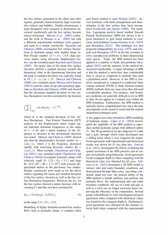
the free surface generated in the shear and rollerregions, generally characterized by large recircula-tion vortices and bubbles. Further downstream, alarge dissipative zone emerged as fluctuations de-creased significantly and the free surface becamealmost horizontal. Murzyn et al. (2007) contin-ued the work of Mouaze et al. (2005) but witha different experimental technique (wire gauges)and came to a similar conclusion. Kucukali andChanson (2008) investigated free surface fluctua-tions in hydraulic jumps with slightly larger in-flow Froude number (4.7 < Fr1 < 8.5) than pre-vious studies using ultrasonic displacement me-ters, see the extended report Kucukali and Chanson(2007). Yet again, data of the mean free surfaceelevation showed a gradual increase towards thetheoretical value in the downstream direction andthe peak in standard deviation was typically foundat 10 ≤ (x− x1)/d1 ≤ 15. Murzyn and Chanson(2009) (see extended report Murzyn and Chanson(2007)) used the same set-up and measuring appa-ratus as Kucukali and Chanson (2008) and showedthat the maximum standard deviation of free sur-face fluctuations was best correlated by the function

(η′

d1

)max

= 0.116(Fr1 −1)1.235 , (4)

where η′ is the standard deviation of free sur-face fluctuations. Fast Fourier Transform (FFT)analysis of the displacement meter output sig-nal indicated dominant frequencies in the rangeof 1 − 4 Hz and a minor tendency of the fre-quency to decrease in the downstream directionwas noted. Murzyn and Chanson (2009) showedalso that the dimensionless Strouhal number St =( f d1)/v1, where f is the frequency, decreasedrapidly with increasing Reynolds number Re =(v1d1)/ν. More recently, Chachereau and Chan-son (2011) (see extended report Chachereau andChanson (2010)) investigate hydraulic jumps withrelatively small Fr (2.4 < Fr1 < 5.1) and largeRe(6.6∗104 < Re < 1.3∗105

)with acoustic dis-

placement meters as the previously two studies.Similar conclusions were made as for the abovestudies regarding the mean and standard deviationof the free surface elevation as well as the free sur-face fluctuation frequencies. However, the St f s forthe free surface showed a minor decrease with in-creasing Fr and data was best correlated by

St f s = 0.143exp(−0.27Fr1) (5)

in the range 2.4 < Fr1 < 6.5.

Modelling of highly disturbed aerated free surfaceflows such as hydraulic jumps, is complex when

grid based method is used Violeau (2012). Se-vere problems with mesh entanglement and deter-mination of the free surface have been encoun-tered Scardovelli and Zaleski (1999). The mesh-free, Lagrangian particle based method SmoothParticle Hydrodynamic (SPH) has shown to be agood alternative to grid based methods to over-come such problems Gomez-Gesteira et al. (2010)and Monaghan (2012). The technique was firstproposed independently by Lucy (1977) and Gin-gold and Monaghan (1977) in the late seventies tosolve astrophysical problems in three-dimensionalopen spaces. Today, the SPH method has beenapplied to a number of fields and problems Mon-aghan (2012) and the maturity of the method hasincreased significantly. A major advantage of SPHis that the method is mesh-free, thus considerabletime is saved as compared to methods that needa predefined mesh. However, as the SPH is rela-tively unexplored as compared to traditional finitevolume methods (FVM) or finite element method(FEM) methods there are some areas that still needconsiderable attention. For instance, wall bound-ary conditions are generally difficult to set in SPHas they do not appear in a natural way within theSPH formalism. Furthermore, the SPH method istypically slower computational wise since the timestep depends on the speed of sound and the explicitintegration techniques used.

A few papers have been devoted to SPH modellingof hydraulic jumps. Lopez et al. (2010) investi-gated the capability of the SPH method to repro-duce mobile hydraulic jumps with different inflowFr. The 2D geometrical set-up composed of a tankand a gate, through which water discharged intoa stilling basin where a weir triggered the jumps.Good agreement with experimental and theoreticalresults was shown for Fr less than five. Jonssonet al. (2011) investigated the effects of altering thespatial resolution of the SPH particles and its im-pact on hydraulic jump behaviour. Good agreementfor the conjugate depth d2 when comparing with thetheoretical value was obtained for all cases. Fed-erico et al. (2012) developed a 2D SPH model toenforce inlet and outlet boundary conditions anddemonstrated through three cases, one being a hy-draulic jump test case, the general ability of theSPH method to handle uniform, non-uniform andunsteady flows. By implementing inlet and outletboundary conditions, the use of a tank and gate aswell as a weir was no longer necessary hence im-proving the efficiency of the computation. Severaljumps with different Fr were investigated and goodagreement when compared with theoretical valueswas found for the conjugate depth d2. Furthermore,good agreement was obtained for the internal ve-locity field when compared with the experimental

3

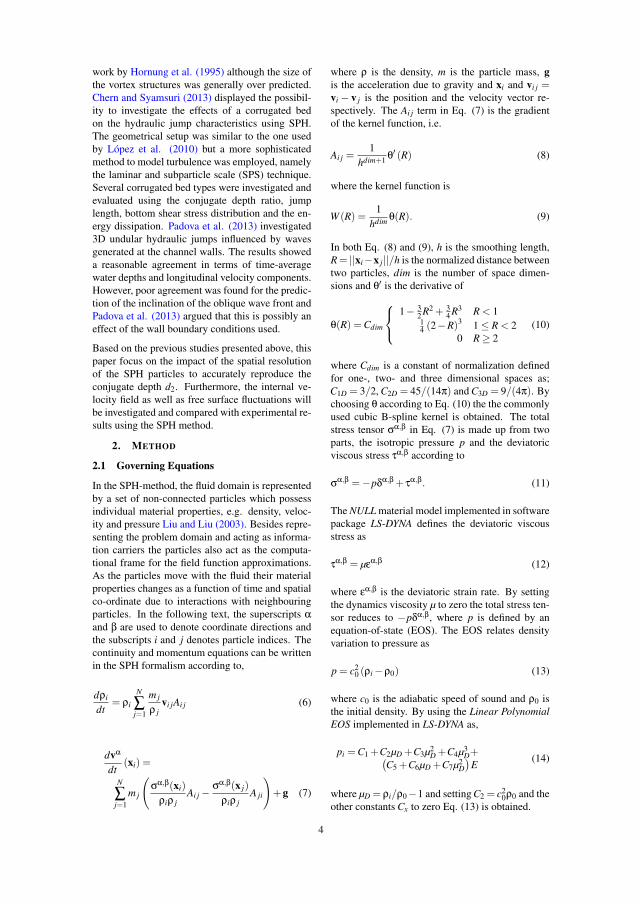
work by Hornung et al. (1995) although the size ofthe vortex structures was generally over predicted.Chern and Syamsuri (2013) displayed the possibil-ity to investigate the effects of a corrugated bedon the hydraulic jump characteristics using SPH.The geometrical setup was similar to the one usedby Lopez et al. (2010) but a more sophisticatedmethod to model turbulence was employed, namelythe laminar and subparticle scale (SPS) technique.Several corrugated bed types were investigated andevaluated using the conjugate depth ratio, jumplength, bottom shear stress distribution and the en-ergy dissipation. Padova et al. (2013) investigated3D undular hydraulic jumps influenced by wavesgenerated at the channel walls. The results showeda reasonable agreement in terms of time-averagewater depths and longitudinal velocity components.However, poor agreement was found for the predic-tion of the inclination of the oblique wave front andPadova et al. (2013) argued that this is possibly aneffect of the wall boundary conditions used.

Based on the previous studies presented above, thispaper focus on the impact of the spatial resolutionof the SPH particles to accurately reproduce theconjugate depth d2. Furthermore, the internal ve-locity field as well as free surface fluctuations willbe investigated and compared with experimental re-sults using the SPH method.

2. METHOD

2.1 Governing Equations

In the SPH-method, the fluid domain is representedby a set of non-connected particles which possessindividual material properties, e.g. density, veloc-ity and pressure Liu and Liu (2003). Besides repre-senting the problem domain and acting as informa-tion carriers the particles also act as the computa-tional frame for the field function approximations.As the particles move with the fluid their materialproperties changes as a function of time and spatialco-ordinate due to interactions with neighbouringparticles. In the following text, the superscripts αand β are used to denote coordinate directions andthe subscripts i and j denotes particle indices. Thecontinuity and momentum equations can be writtenin the SPH formalism according to,

dρi

dt= ρi

N

∑j=1

m j

ρ jvi jAi j (6)

dvα

dt(xi) =

N

∑j=1

m j

(σα,β(xi)

ρiρ jAi j − σα,β(x j)

ρiρ jA ji

)+g (7)

where ρ is the density, m is the particle mass, gis the acceleration due to gravity and xi and vi j =vi − v j is the position and the velocity vector re-spectively. The Ai j term in Eq. (7) is the gradientof the kernel function, i.e.

Ai j =1

hdim+1 θ′ (R) (8)

where the kernel function is

W (R) =1

hdim θ(R). (9)

In both Eq. (8) and (9), h is the smoothing length,R= ||xi−x j||/h is the normalized distance betweentwo particles, dim is the number of space dimen-sions and θ′ is the derivative of

θ(R) =Cdim

⎧⎨⎩

1− 32 R2 + 3

4 R3 R < 114 (2−R)3 1 ≤ R < 2

0 R ≥ 2(10)

where Cdim is a constant of normalization definedfor one-, two- and three dimensional spaces as;C1D = 3/2, C2D = 45/(14π) and C3D = 9/(4π). Bychoosing θ according to Eq. (10) the the commonlyused cubic B-spline kernel is obtained. The totalstress tensor σα,β in Eq. (7) is made up from twoparts, the isotropic pressure p and the deviatoricviscous stress τα,β according to

σα,β =−pδα,β + τα,β. (11)

The NULL material model implemented in softwarepackage LS-DYNA defines the deviatoric viscousstress as

τα,β = μεα,β (12)

where εα,β is the deviatoric strain rate. By settingthe dynamics viscosity μ to zero the total stress ten-sor reduces to −pδα,β, where p is defined by anequation-of-state (EOS). The EOS relates densityvariation to pressure as

p = c20 (ρi −ρ0) (13)

where c0 is the adiabatic speed of sound and ρ0 isthe initial density. By using the Linear PolynomialEOS implemented in LS-DYNA as,

pi =C1 +C2μD +C3μ2D +C4μ3

D+(C5 +C6μD +C7μ2

D)

E(14)

where μD = ρi/ρ0−1 and setting C2 = c20ρ0 and the

other constants Cx to zero Eq. (13) is obtained.

4

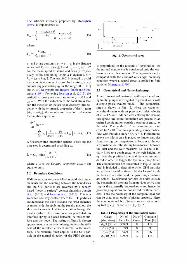
The artificial viscosity proposed by Monaghan(1992) is implemented as

Πi j =

{ −q1ci jφi j+q2φ2i j

ρi jvi jri j < 0

0 vi jri j > 0(15)

where

φi j =hvi jri j

r2i j +0.01h2

, (16)

q1 and q2 are constants, ri j = ri − r j is the distancevector and ci j = (ci + c j)/2 and ρi j = (ρi +ρ j)/2are the mean speed of sound and density, respec-tively. If the smoothing length h is dynamic, h =hi j = (hi +h j)/2. The term 0.01h2 is used to avoidthe denominator to go to zero. In literature, manyauthors suggest setting q1 in the range [0.01,0.1]and q2 = 0 Dalrymple and Rogers (2006) and Mon-aghan (1994). Following Jonsson et al. (2015), theartificial viscosity constants are set to q1 = 0.1 andq2 = 0. With the reduction of the total stress ten-sor, the inclusion of the artificial viscosity term to-gether with the symmetric properties of the Ai j term(Ai j =−A ji), the momentum equation reduces tothe familiar expression,

dvα

dt(xi) =

−N

∑j=1

m j

(pi

ρiρ j+

p j

ρiρ j+Πi j

)Ai j +g (17)

A first order time integration scheme is used and thetime step is determined according to,

δt =Cc f l min(

hi

ci + vi

)(18)

where Cc f l is the Courant coefficient usually setequal to unity.

2.2 Boundary Conditions

Wall boundaries were modelled as rigid shell finiteelements and the coupling between the boundariesand the SPH-particles are governed by a penaltybased “node-to-surface” contact-algorithm Jonsenet al. (2012) and Jonsson et al. (2015). This is aso-called one-way contact where the SPH particlesare defined as the slave side and the FEM elementsas master side. In applying the penalty method, theslave nodes are checked for penetration through themaster surface. If a slave node has penetrated, aninterface spring is placed between the master sur-face and the node. The spring stiffness is chosenapproximately in the order of magnitude as the stiff-ness of the interface element normal to the inter-face. The resultant force applied to the SPH par-ticle in the normal direction of the FEM element

Fig. 2. Geometrical setup.

is proportional to the amount of penetration. Asthe normal component is considered only the wallboundaries are frictionless. This approach can becompared with the Lennard-Jones-type boundarycondition where a central force is applied to fluidparticles Monaghan (1994).

2.3 Geometrical and Numerical setup

A two dimensional horizontal spillway channel andhydraulic jump is investigated in present work witha single phase (water) model. The geometricalsetup is shown in Fig. 2, where the water en-ters the domain with an prescribed inlet velocityof v1 = 1.5 m/s. All particles entering the domainthroughout the entire simulation are placed in anordered configuration outside the point of entry, i.e.the inlet. The depth d1 of the incoming jet is setequal to 2∗10−2 m, thus generating a supercriticalflow with Froude number Fr1 ≈ 3.4. Furthermore,above the inlet a gate is placed to hinder particlesfrom leaving the computational domain in the up-stream direction. The stilling basin located betweenthe inlet and the weir measures 1.1 m and is ini-tially filled to a depth equal to the weir height, i.e.d1. Both the pre-filled zone and the weir are intro-duced in order to trigger the hydraulic jump faster.The computational box illustrated in Fig. 2 (dottedline) is included to determine which SPH particlesare activated and deactivated. Nodes located insidethe box are activated and the governing equationsare solved. Deactivated particles or nodes outsidethe box maintain the state from previous active timestep or the externally imposed state and hence thegoverning equations are not solved for these parti-cles. Thus the boundary of the computational boxcan be used as an outlet if placed properly. Here,the computational box dimensions was set accord-ing to 0 ≤ x ≤ 1.9 and −0.1 ≤ y ≤ 0.5.

Table 1 Properties of the simulation cases.Cases Nr. of Nr. of Compute

(sim. time) Particles Cores Time [h]d1/4 (30s) 36879 8 114d1/5 (5s) 10749 8 9d1/6 (5s) 15479 16 26

d1/10 (5s) 42999 12 114

5

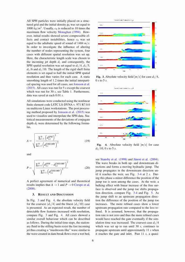
All SPH particles were initially placed on a struc-tured grid and the initial density ρ0 was set equal to1000 kg/m3. Usually, c0 is reduced to 10 times themaximum flow velocity Monaghan (1994). How-ever, initial results showed severe compressible ef-fects and contact instabilities, hence c0 was setequal to the adiabatic speed of sound of 1484 m/s.In order to investigate the influence of alteringthe number of nodes representing the system, fourcases with different spatial resolution was set up.Here, the characteristic length scale was chosen tothe incoming jet depth d1 and consequently, theSPH spatial resolution was set equal to d1/4, d1/5,d1/6 and d1/10. The length of the rigid shell finiteelements is set equal to half the initial SPH spatialresolution and thus varies for each case. A staticsmoothing length of 1.2 times the initial interparti-cal spacing was used for all cases, see Jonsson et al.(2015). All cases was run for 5 s except the coarsestwhich was run for 30 s, see Table 1. Furthermore,data was saved at each 0.01 s.

All simulations were conducted using the nonlinearfinite element code LSTC LS-DYNA v. 971 R7.0.0on multicore Linux workstations. The post process-ing method proposed by Jonsson et al. (2015) wasused to visualize and interpolate the SPH data. Sta-tistical measurements of the deviations of conjugatedepth d2 were determined by the following formu-las,

A =

√√√√√√ ∑Ni=1

(dSPH

2,i

)2

∑Ni=1

(dT HEORY

2,i

)2 (19)

and

P =

√√√√√√∑Ni=1

(dSPH

2,i −dT HEORY2,i

)2

∑Ni=1

(dT HEORY

2,i

)2 (20)

A perfect agreement of numerical and theoreticalresults implies that A → 1 and P → 0 Crespo et al.(2008).

3. RESULT AND DISCUSSION

In Fig. 3 and Fig. 4, the absolute velocity fieldfor the coarsest (d1/4) and the finest (d1/10) caseis presented. As an expected result, the number ofdetectable flow features increased with resolution,compare Fig. 3 and Fig. 4. All cases showed asimilar overall behaviour which can be describedas follows. During the initial time steps, the station-ary fluid in the stilling basin resist the fast incomingjet thus creating a “mushroom-like” wave similar tothe wave created in dam break flows over a wet bed,

Fig. 3. Absolute velocity field [m/s] for case d1/4,0 s to 5 s.

Fig. 4. Absolute velocity field [m/s] for cased1/10, 0 s to 5 s.

see Stansby et al. (1998) and Janosi et al. (2004).The wave breaks in both up- and downstream di-rections and forms a moving hydraulic jump. Thejump propagates in the downstream direction un-til it reaches the weir, see Fig. 3-4 at 2 s. Dur-ing this phase a minor difference the position of thejump toe is seen among the cases. At the weir, abulking effect with linear increase of the free sur-face is observed and the jump toe shifts propaga-tion direction, compare Fig. 3-4 and Fig. 5. Asthe jump shift to an upstream propagation direc-tion the difference of the position of the jump toeincreases. The more refined cases show a lowerupstream propagation rate compared to the less re-fined. It is assumed, however, that the propaga-tion rate is not zero and thus the more refined caseswould have reached the gate eventually if the sim-ulation time was increased. The coarsest case d1/4which was set up to run until 30 s, continues topropagate upstream until approximately 11 s whenit reaches the gate and inlet. Past 11 s, a quasi-

6

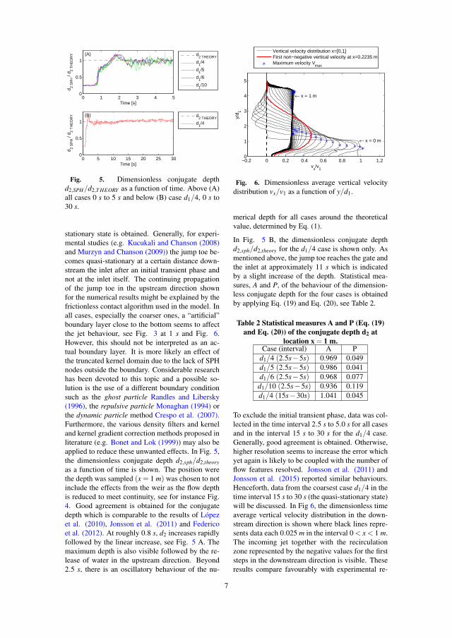
0 1 2 3 4 50

0.5

1(A)

Time [s]

d 2 S

PH

/ d 2

TH

EO

RY d

2 THEORY

d1/4

d1/5

d1/6

d1/10

0 5 10 15 20 25 300

0.5

1

Time [s]

d 2 S

PH

/ d 2

TH

EO

RY (B) d

2 THEORY

d1/4

Fig. 5. Dimensionless conjugate depthd2,SPH/d2,T HEORY as a function of time. Above (A)all cases 0 s to 5 s and below (B) case d1/4, 0 s to30 s.

stationary state is obtained. Generally, for experi-mental studies (e.g. Kucukali and Chanson (2008)and Murzyn and Chanson (2009)) the jump toe be-comes quasi-stationary at a certain distance down-stream the inlet after an initial transient phase andnot at the inlet itself. The continuing propagationof the jump toe in the upstream direction shownfor the numerical results might be explained by thefrictionless contact algorithm used in the model. Inall cases, especially the coarser ones, a “artificial”boundary layer close to the bottom seems to affectthe jet behaviour, see Fig. 3 at 1 s and Fig. 6.However, this should not be interpreted as an ac-tual boundary layer. It is more likely an effect ofthe truncated kernel domain due to the lack of SPHnodes outside the boundary. Considerable researchhas been devoted to this topic and a possible so-lution is the use of a different boundary conditionsuch as the ghost particle Randles and Libersky(1996), the repulsive particle Monaghan (1994) orthe dynamic particle method Crespo et al. (2007).Furthermore, the various density filters and kerneland kernel gradient correction methods proposed inliterature (e.g. Bonet and Lok (1999)) may also beapplied to reduce these unwanted effects. In Fig. 5,the dimensionless conjugate depth d2,sph/d2,theoryas a function of time is shown. The position werethe depth was sampled (x = 1 m) was chosen to notinclude the effects from the weir as the flow depthis reduced to meet continuity, see for instance Fig.4. Good agreement is obtained for the conjugatedepth which is comparable to the results of Lopezet al. (2010), Jonsson et al. (2011) and Federicoet al. (2012). At roughly 0.8 s, d2 increases rapidlyfollowed by the linear increase, see Fig. 5 A. Themaximum depth is also visible followed by the re-lease of water in the upstream direction. Beyond2.5 s, there is an oscillatory behaviour of the nu-

−0.2 0 0.2 0.4 0.6 0.8 1 1.20

1

2

3

4

5

vx/v

1

y/d 1

← x = 0 m

← x = 1 m

Vertical velocity distribution x=[0,1]First non−negative vertical velocity at x=0.2235 mMaximum velocity V

max

Fig. 6. Dimensionless average vertical velocitydistribution vx/v1 as a function of y/d1.

merical depth for all cases around the theoreticalvalue, determined by Eq. (1).

In Fig. 5 B, the dimensionless conjugate depthd2,sph/d2,theory for the d1/4 case is shown only. Asmentioned above, the jump toe reaches the gate andthe inlet at approximately 11 s which is indicatedby a slight increase of the depth. Statistical mea-sures, A and P, of the behaviour of the dimension-less conjugate depth for the four cases is obtainedby applying Eq. (19) and Eq. (20), see Table 2.

Table 2 Statistical measures A and P (Eq. (19)and Eq. (20)) of the conjugate depth d2 at

location x = 1 m.Case (interval) A P

d1/4 (2.5s−5s) 0.969 0.049d1/5 (2.5s−5s) 0.986 0.041d1/6 (2.5s−5s) 0.968 0.077

d1/10 (2.5s−5s) 0.936 0.119d1/4 (15s−30s) 1.041 0.045

To exclude the initial transient phase, data was col-lected in the time interval 2.5 s to 5.0 s for all casesand in the interval 15 s to 30 s for the d1/4 case.Generally, good agreement is obtained. Otherwise,higher resolution seems to increase the error whichyet again is likely to be coupled with the number offlow features resolved. Jonsson et al. (2011) andJonsson et al. (2015) reported similar behaviours.Henceforth, data from the coarsest case d1/4 in thetime interval 15 s to 30 s (the quasi-stationary state)will be discussed. In Fig 6, the dimensionless timeaverage vertical velocity distribution in the down-stream direction is shown where black lines repre-sents data each 0.025 m in the interval 0 < x < 1 m.The incoming jet together with the recirculationzone represented by the negative values for the firststeps in the downstream direction is visible. Theseresults compare favourably with experimental re-

7

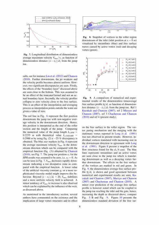
0 10 20 30 40 50 600.2

0.4

0.6

0.8

1

1.2

(x−x1)/d

1

Vm

ax/v

1

exp(−0.028*(x−x1)/d

1) (Chanson, 2010)

SPH d1/4 (Present Study)

Fig. 7. Longitudinal distribution of dimensionlessaverage maximum velocity Vmax/v1 as function ofdimensionless distance (x− x1)/d1 from the jumptoe.

sults, see for instance Lin et al. (2012) and Chanson(2010). Further downstream, the jet weakens andthe velocity profile becomes almost uniform. How-ever, two significant discrepancies are seen. Firstly,the effects of the “boundary layer” discussed aboveare seen close to the bottom. This was assumed tobe an effect of the truncated kernel and not an ac-tual boundary layer. Secondly, the velocity profilescollapse to zero velocity close to the free surface.This is an effect of the interpolation and averagingprocess as interpolation points outside the water aregiven a value of zero.

The red line in Fig. 6 represent the first positiondownstream the jump toe with non-negative aver-age velocity in the downstream direction. Hence,this position is interpreted as the end of the rollersection and the length of the jump. Comparingthe numerical value of the jump length Lr,SPH =0.2235 m with theoretical value Lr,T HEORY =0.2988 m by using Eq. (2) a −25 % discrepancy isobtained. The blue star markers in Fig. 6 representthe average maximum velocity Vmax in the down-stream direction which can be compared with theempirical function (Eq. (3)) obtained by Chanson(2010), see Fig. 7. The jump toe position x1 for theSPH results was assumed to be zero, i.e. x1 = 0. Ascan be seen in Fig. 7, Vmax decreases rapidly down-stream indicating a too dissipative zone as com-pared with the empirical function. A lower valueof the artificial viscosity constant q1 or a more so-phisticated viscosity model might improve this be-haviour. Beyond (x− x1)/d1 = 20, Vmax stabilizesand a more uniform velocity field is achieved. Aminor tendency of Vmax to increase is also observedwhich can be explained by the influence of the weir,as discussed above.

As mentioned in the introductory section, severalauthors have commented on the existence and theimplication of large vortex structures and its effect

0 0.1 0.2 0.3 0.4 0.5 0.6X [m]

Fig. 8. Snapshot of vortices in the roller regiondownstream of the inlet (inlet position at x = 0 m)visualized by streamlines (blue) and free surfacewaves caused by active vortex (red) and decayingvortex (green).

−10 0 10 20 300

1

2

3

4

5

6

7

8

(x−x1)/d

1

η/d 1

Fr1=4.7 ref 1

Fr1=5.0 ref 1

Fr1=3.1 ref 2

Fr1=4.2 ref 2

Fr1=3.2 ref 3

Fr1=3.4 ref 3

Fr1=3.9 ref 3

Fr1=3.4 ref 4

Fig. 9. A comparison of numerical and exper-imental results of the dimensionless timeaveragefree surface profile η/d1 as function of dimension-less distance (x− x1)/d1 from the jump toe. Ref 1Kucukali and Chanson (2007), ref 2 Murzyn andChanson (2007), ref 3 Chachereau and Chanson(2010) and ref 4 (present study).

on the free surface in the roller region. The vor-tex paring mechanism and the merging with thestationary vortex reported in Long et al. (1991)was not observed in present results. However, in-dividual vortices translated with increasing size inthe downstream direction in agreement with Longet al. (1991). Figure 8 present a snapshot of theflow structures found for the d1/4 case. The bluelines represents streamlines and an active vortexare seen close to the jump toe which is translat-ing downstream as well as a decaying vortex fur-ther downstream. The effects on the free surfaceof the vortices are marked in red and green. InFig. 9, the dimensionless average free surface pro-file η/d1 is shown and good agreement betweennumerical and experimental results are seen, Ku-cukali and Chanson (2007), Murzyn and Chanson(2007) and Chachereau and Chanson (2010). Aminor over prediction of the average free surfaceprofile is however noted which can be coupled tothe jump toe reaching the inlet and the gate, hence,increasing the depth as discussed above, compareFig. 5 B and Fig. 9. Figure 10 presents thedimensionless standard deviation of the free sur-

8

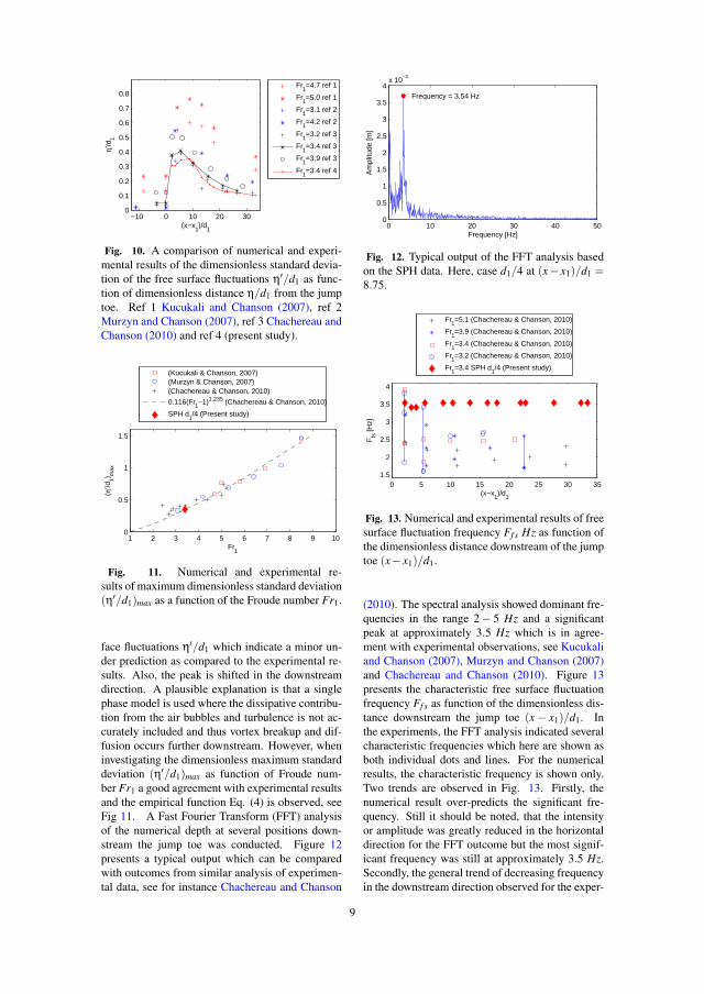
−10 0 10 20 300

0.1

0.2

0.3

0.4

0.5

0.6

0.7

0.8

(x−x1)/d

1

η′/d

1

Fr1=4.7 ref 1

Fr1=5.0 ref 1

Fr1=3.1 ref 2

Fr1=4.2 ref 2

Fr1=3.2 ref 3

Fr1=3.4 ref 3

Fr1=3.9 ref 3

Fr1=3.4 ref 4

Fig. 10. A comparison of numerical and experi-mental results of the dimensionless standard devia-tion of the free surface fluctuations η′/d1 as func-tion of dimensionless distance η/d1 from the jumptoe. Ref 1 Kucukali and Chanson (2007), ref 2Murzyn and Chanson (2007), ref 3 Chachereau andChanson (2010) and ref 4 (present study).

1 2 3 4 5 6 7 8 9 100

0.5

1

1.5

Fr1

(η′/d

1) max

(Kucukali & Chanson, 2007)(Murzyn & Chanson, 2007)(Chachereau & Chanson, 2010)

0.116(Fr1−1)1.235 (Chachereau & Chanson, 2010)

SPH d1/4 (Present study)

Fig. 11. Numerical and experimental re-sults of maximum dimensionless standard deviation(η′/d1)max as a function of the Froude number Fr1.

face fluctuations η′/d1 which indicate a minor un-der prediction as compared to the experimental re-sults. Also, the peak is shifted in the downstreamdirection. A plausible explanation is that a singlephase model is used where the dissipative contribu-tion from the air bubbles and turbulence is not ac-curately included and thus vortex breakup and dif-fusion occurs further downstream. However, wheninvestigating the dimensionless maximum standarddeviation (η′/d1)max as function of Froude num-ber Fr1 a good agreement with experimental resultsand the empirical function Eq. (4) is observed, seeFig 11. A Fast Fourier Transform (FFT) analysisof the numerical depth at several positions down-stream the jump toe was conducted. Figure 12presents a typical output which can be comparedwith outcomes from similar analysis of experimen-tal data, see for instance Chachereau and Chanson

0 10 20 30 40 500

0.5

1

1.5

2

2.5

3

3.5

4x 10

−3

Frequency [Hz]

Am

plitu

de [m

]

Frequency = 3.54 Hz

Fig. 12. Typical output of the FFT analysis basedon the SPH data. Here, case d1/4 at (x− x1)/d1 =8.75.

0 5 10 15 20 25 30 351.5

2

2.5

3

3.5

4

(x−x1)/d

1

Ffs

[Hz]

Fr1=5.1 (Chachereau & Chanson, 2010)

Fr1=3.9 (Chachereau & Chanson, 2010)

Fr1=3.4 (Chachereau & Chanson, 2010)

Fr1=3.2 (Chachereau & Chanson, 2010)

Fr1=3.4 SPH d

1/4 (Present study)

Fig. 13. Numerical and experimental results of freesurface fluctuation frequency Ff s Hz as function ofthe dimensionless distance downstream of the jumptoe (x− x1)/d1.

(2010). The spectral analysis showed dominant fre-quencies in the range 2 − 5 Hz and a significantpeak at approximately 3.5 Hz which is in agree-ment with experimental observations, see Kucukaliand Chanson (2007), Murzyn and Chanson (2007)and Chachereau and Chanson (2010). Figure 13presents the characteristic free surface fluctuationfrequency Ff s as function of the dimensionless dis-tance downstream the jump toe (x − x1)/d1. Inthe experiments, the FFT analysis indicated severalcharacteristic frequencies which here are shown asboth individual dots and lines. For the numericalresults, the characteristic frequency is shown only.Two trends are observed in Fig. 13. Firstly, thenumerical result over-predicts the significant fre-quency. Still it should be noted, that the intensityor amplitude was greatly reduced in the horizontaldirection for the FFT outcome but the most signif-icant frequency was still at approximately 3.5 Hz.Secondly, the general trend of decreasing frequencyin the downstream direction observed for the exper-

9

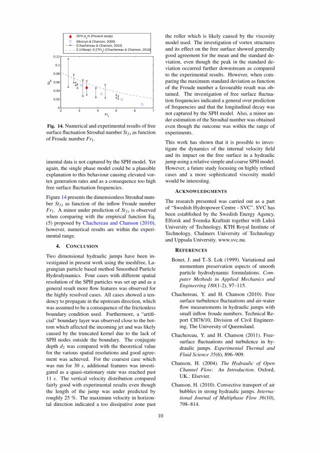
2 3 4 5 6 70

0.02

0.04

0.06

0.08

0.1

0.12

Fr1

St fs

SPH d1/4 (Present study)

(Murzyn & Chanson, 2009)(Chachereau & Chanson, 2010)0.143exp(−0.27Fr

1) (Chachereau & Chanson, 2010)

Fig. 14. Numerical and experimental results of freesurface fluctuation Strouhal number St f s as functionof Froude number Fr1.

imental data is not captured by the SPH model. Yetagain, the single phase model could be a plausibleexplanation to this behaviour causing elevated vor-tex generation rates and as a consequence too highfree surface fluctuation frequencies.

Figure 14 presents the dimensionless Strouhal num-ber St f s as function of the inflow Froude numberFr1. A minor under prediction of St f s is observedwhen comparing with the empirical function Eq.(5) proposed by Chachereau and Chanson (2010),however, numerical results are within the experi-mental range.

4. CONCLUSION

Two dimensional hydraulic jumps have been in-vestigated in present work using the meshfree, La-grangian particle based method Smoothed ParticleHydrodynamics. Four cases with different spatialresolution of the SPH particles was set up and as ageneral result more flow features was observed forthe highly resolved cases. All cases showed a ten-dency to propagate in the upstream direction, whichwas assumed to be a consequence of the frictionlessboundary condition used. Furthermore, a “artifi-cial” boundary layer was observed close to the bot-tom which affected the incoming jet and was likelycaused by the truncated kernel due to the lack ofSPH nodes outside the boundary. The conjugatedepth d2 was compared with the theoretical valuefor the various spatial resolutions and good agree-ment was achieved. For the coarsest case whichwas run for 30 s, additional features was investi-gated as a quasi-stationary state was reached past11 s. The vertical velocity distribution comparedfairly good with experimental results even thoughthe length of the jump was under predicted byroughly 25 %. The maximum velocity in horizon-tal direction indicated a too dissipative zone past

the roller which is likely caused by the viscositymodel used. The investigation of vortex structuresand its effect on the free surface showed generallygood agreement for the mean and the standard de-viation, even though the peak in the standard de-viation occurred further downstream as comparedto the experimental results. However, when com-paring the maximum standard deviation as functionof the Froude number a favourable result was ob-tained. The investigation of free surface fluctua-tion frequencies indicated a general over predictionof frequencies and that the longitudinal decay wasnot captured by the SPH model. Also, a minor un-der estimation of the Strouhal number was obtainedeven though the outcome was within the range ofexperiments.

This work has shown that it is possible to inves-tigate the dynamics of the internal velocity fieldand its impact on the free surface in a hydraulicjump using a relative simple and coarse SPH model.However, a future study focusing on highly refinedcases and a more sophisticated viscosity modelwould be interesting.

ACKNOWLEDGMENTS

The research presented was carried out as a partof “Swedish Hydropower Centre - SVC”. SVC hasbeen established by the Swedish Energy Agency,Elforsk and Svenska Kraftnat together with LuleaUniversity of Technology, KTH Royal Institute ofTechnology, Chalmers University of Technologyand Uppsala University. www.svc.nu.

REFERENCES

Bonet, J. and T.-S. Lok (1999). Variational andmomentum preservation aspects of smoothparticle hydrodynamic formulations. Com-puter Methods in Applied Mechanics andEngineering 180(1-2), 97–115.

Chachereau, Y. and H. Chanson (2010). Freesurface turbulence fluctuations and air-waterflow measurements in hydraulic jumps withsmall inflow froude numbers. Technical Re-port CH78/10, Division of Civil Engineer-ing, The University of Queensland.

Chachereau, Y. and H. Chanson (2011). Free-surface fluctuations and turbulence in hy-draulic jumps. Experimental Thermal andFluid Science 35(6), 896–909.

Chanson, H. (2004). The Hydraulic of OpenChannel Flow: An Introduction. Oxford,UK.: Elsevier.

Chanson, H. (2010). Convective transport of airbubbles in strong hydraulic jumps. Interna-tional Journal of Multiphase Flow 36(10),798–814.

10

Chanson, H. and T. Brattberg (2000). Experi-mental study of the air–water shear flow ina hydraulic jump. International Journal ofMultiphase Flow 26(4), 583–607.

Chern, M.-J. and S. Syamsuri (2013). Effect ofcorrugated bed on hydraulic jump charac-teristic using SPH method. Journal of Hy-draulic Engineering 139(2), 221–232.

Crespo, A. J., M. Gomez-Gesteira, and R. A.Dalrymple (2007). Boundary conditionsgenerated by dynamic particles in sphmethods. Computers, materials and con-tinua 5(3), 173–184.

Crespo, A. J., M. Gomez-Gesteira, and R. A.Dalrymple (2008). Modeling dam break be-havior over a wet bed by a SPH tech-nique. J. Waterway, Port, Coastal, OceanEng. 134(6), 313–320.

Dalrymple, R. and B. Rogers (2006). Numeri-cal modeling of water waves with the SPHmethod. Coastal Engineering 53(2-3), 141–147.

Federico, I., S. Marrone, A. Colagrossi, F. Aris-todemo, and M. Antuono (2012). Simulat-ing 2d open-channel flows through an SPHmodel. European Journal of Mechanics -B/Fluids 34, 35–46.

Gingold, R. A. and J. J. Monaghan (1977).Smoothed particle hydrodynamics: the-ory and application to non-spherical stars.Monthly Notices of the Royal AstronomicalSociety 181(3), 375–389.

Gomez-Gesteira, M., B. D. Rogers, R. A.Dalrymple, and A. J. Crespo (2010).State-of-the-art of classical SPH for free-surface flows. Journal of Hydraulic Re-search 48(sup1), 6–27.

Hager, W. H., R. Bremen, and N. Kawagoshi(1990). Classical hydraulic jump: length ofroller. Journal of Hydraulic Research 28(5),591–608.

Hornung, H. G., C. Willert, and S. Turner(1995). The flow field downstream of ahydraulic jump. Journal of Fluid Mechan-ics 287(-1), 299.

Janosi, I. M., D. Jan, K. G. Szabo, and T. Tel(2004). Turbulent drag reduction in dam-break flows. Exp Fluids 37(2), 219–229.

Jonsen, P., B. Palsson, and H.-A. Haggblad(2012). A novel method for full-body mod-elling of grinding charges in tumbling mills.Minerals Engineering 33(0), 2 – 12.

Jonsson, P., P. Jonsen, P. Andreasson, T. Lund-strom, and J. Hellstrom (2011). Smoothed

particle hydrodynamics modeling of hy-draulic jumps. In Proceedings of Particle-Based Methods II - Fundamentals and Ap-plications, Barcelona, Spain, pp. 490–501.

Jonsson, P., P. Jonsen, P. Andreasson, T. Lund-strom, and J. Hellstrom (2015). Modellingdam break evolution over a wet bed withsmoothed particle hydrodynamics: A param-eter study. Engineering 7(5).

Kucukali, S. and H. Chanson (2007). Turbulencein hydraulic jumps: Experimental measure-ments. Technical Report CH62/07, Divi-sion of Civil Engineering, The University ofQueensland.

Kucukali, S. and H. Chanson (2008). Turbulencemeasurements in the bubbly flow region ofhydraulic jumps. Experimental Thermal andFluid Science 33(1), 41–53.

Lennon, J. M. and D. F. Hill (2006). Particle im-age velocity measurements of undular andhydraulic jumps. Journal of Hydraulic En-gineering 132(12), 1283–1294.

Lin, C., S.-C. Hsieh, I.-J. Lin, K.-A. Chang, andR. V. Raikar (2012). Flow property and self-similarity in steady hydraulic jumps. ExpFluids 53(5), 1591–1616.

Liu, G. and M. Liu (2003). Smoothed Parti-cle Hydrodynamics : a meshfree particlemethod. Singapore: World Publishing Co.Pte. Ltd.

Long, D., N. Rajaratnam, P. M. Steffler, and P. R.Smy (1991). Structure of flow in hydraulicjumps. Journal of Hydraulic Research 29(2),207–218.

Lopez, D., R. Marivela, and L. Garrote (2010).Smoothed particle hydrodynamics model ap-plied to hydraulic structures: a hydraulicjump test case. Journal of Hydraulic Re-search 48(sup1), 142–158.

Lucy, L. B. (1977). A numerical approach to thetesting of the fission hypothesis. The Astro-nomical Journal 82(12), 1013–1024.

Lundstrom, T., M. Brynjell-Rahkola, A.-L.Ljung, J. Hellstrom, and T. Greean (2015).Evaluation of guiding device for downstreamfish migration with in-field particle track-ing velocimetry and cfd. Journal of AppliedFluid Mechanics 8(3), 579–589.

Monaghan, J. (1994). Simulating free surfaceflows with SPH. Journal of ComputationalPhysics 110(2), 399–406.

Monaghan, J. (2012). Smoothed particle hydro-dynamics and its diverse applications. Annu.Rev. Fluid Mech. 44(1), 323–346.

11

Monaghan, J. J. (1992). Smoothed particle hy-drodynamics. Annual Review of Astronomyand Astrophysics 30(1), 543–574.

Mossa, M. (1999). On the oscillating charac-teristics of hydraulic jumps. Journal of Hy-draulic Research 37(4), 541–558.

Mouaze, D., F. Murzyn, and J. R. Chaplin(2005). Free surface length scale estimationin hydraulic jumps. J. Fluids Eng. 127(6),1191.

Murzyn, F. and H. Chanson (2007). Free surface,bubbly flow and turbulence measurements inhydraulic jumps. Technical Report CH63/07,Division of Civil Engineering, The Univer-sity of Queensland.

Murzyn, F. and H. Chanson (2008). Experi-mental investigation of bubbly flow and tur-bulence in hydraulic jumps. EnvironmentalFluid Mechanics 9(2), 143–159.

Murzyn, F. and H. Chanson (2009). Free-surfacefluctuations in hydraulic jumps: Experimen-tal observations. Experimental Thermal andFluid Science 33(7), 1055–1064.

Murzyn, F., D. Mouaze, and J. Chaplin (2007).Air-water interface dynamic and free surfacefeatures in hydraulic jumps. Journal of Hy-draulic Research 45(5), 679–685.

Padova, D. D., M. Mossa, S. Sibilla, and E. Torti(2013). 3d SPH modelling of hydraulic jumpin a very large channel. Journal of HydraulicResearch 51(2), 158–173.

Rajaratnam, N. (1965). The hydraulic jump as awall jet. Journal of Hydraulic Division 91,107–132.

Randles, P. and L. Libersky (1996). Smoothedparticle hydrodynamics: Some recent im-provements and applications. ComputerMethods in Applied Mechanics and Engi-neering 139(1-4), 375–408.

Scardovelli, R. and S. Zaleski (1999). Direct nu-merical simulation of free-surface and inter-facial flow. Annu. Rev. Fluid Mech. 31(1),567–603.

Stansby, P. K., A. Chegini, and T. C. D. Barnes(1998). The initial stages of dam-break flow.Journal of Fluid Mechanics 374, 407–424.

Violeau, D. (2012). Fluid Mechanics and theSPH Method: Theory and Applications. Ox-ford: Oxford University Press.

12

Paper D

Smoothed Particle Hydrodynamic

Simulation of Hydraulic Jump using

Periodic Open Boundaries

Smoothed Particle Hydrodynamic

Simulation of Hydraulic Jump using

Periodic Open Boundaries

Patrick Jonsson1, Patrik Andreasson1, J. Gunnar I. Hellstrom1, Par

Jonsen2 and T. Staffan Lundstrom1

1Division of Fluid and Experimental Mechanics, Lulea University of

Technology (LTU), Lulea, SE-971 87, Sweden2Division of Mechanics of Solid Materials, Lulea University of Technology

(LTU), Lulea, SE-971 87, Sweden

Submitted to Applied Mathematical Modelling

Abstract

The natural phenomena hydraulic jump that is commonly used in

spillways as an energy dissipater coupled to hydropower applica-

tions has been investigated with Smoothed Particle Hydrodynam-

ics. A new approach is applied based on a periodic open boundary

condition. The geometrical setup consists of a horizontal stilling

basin and a tank. The tank provides a hydraulic head and in turn

a specific flow through the gate, and a downstream condition in

terms of a depth for the jump. The gate elevation has a major im-

pact and was calibrated to ensure a correct flow, when compared

to experiments. With the proper flow rate, the position of the

jump toe was significantly improved. However, for high Froude

number cases the position was still too close to the gate but could

be improved by including a correction based on the length of the

jump. The depths in both the super- and subcritical zones was in

1

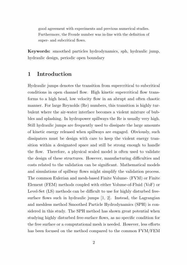
good agreement with experiments and previous numerical studies.

Furthermore, the Froude number was in-line with the definition of

super- and subcritical flows.

Keywords: smoothed particles hydrodynamics, sph, hydraulic jump,

hydraulic design, periodic open boundary

1 Introduction

Hydraulic jumps denotes the transition from supercritical to subcritical

conditions in open channel flow. High kinetic supercritical flow trans-

forms to a high head, low velocity flow in an abrupt and often chaotic

manner. For large Reynolds (Re) numbers, this transition is highly tur-

bulent where the air-water interface becomes a violent mixture of bub-

bles and splashing. In hydropower spillways the Re is usually very high.

Still hydraulic jumps are frequently used to dissipate the large amounts

of kinetic energy released when spillways are engaged. Obviously, such

dissipaters must be design with care to keep the violent energy tran-

sition within a designated space and still be strong enough to handle

the flow. Therefore, a physical scaled model is often used to validate

the design of these structures. However, manufacturing difficulties and

costs related to the validation can be significant. Mathematical models

and simulations of spillway flows might simplify the validation process.

The common Eulerian and mesh-based Finite Volume- (FVM) or Finite

Element (FEM) methods coupled with either Volume-of-Fluid (VoF) or

Level-Set (LS) methods can be difficult to use for highly disturbed free-

surface flows such in hydraulic jumps [1, 2]. Instead, the Lagrangian

and meshless method Smoothed Particle Hydrodynamics (SPH) is con-

sidered in this study. The SPH method has shown great potential when

studying highly disturbed free-surface flows, as no specific condition for

the free surface or a computational mesh is needed. However, less efforts

has been focused on the method compared to the common FVM/FEM

2

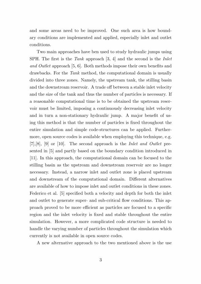
and some areas need to be improved. One such area is how bound-

ary conditions are implemented and applied, especially inlet and outlet

conditions.

Two main approaches have ben used to study hydraulic jumps using

SPH. The first is the Tank approach [3, 4] and the second is the Inlet

and Outlet approach [5, 6]. Both methods impose their own benefits and

drawbacks. For the Tank method, the computational domain is usually

divided into three zones. Namely, the upstream tank, the stilling basin

and the downstream reservoir. A trade off between a stable inlet velocity

and the size of the tank and thus the number of particles is necessary. If

a reasonable computational time is to be obtained the upstream reser-

voir must be limited, imposing a continuously decreasing inlet velocity

and in turn a non-stationary hydraulic jump. A major benefit of us-

ing this method is that the number of particles is fixed throughout the

entire simulation and simple code-structures can be applied. Further-

more, open source codes is available when employing this technique, e.g.

[7],[8], [9] or [10]. The second approach is the Inlet and Outlet pre-

sented in [5] and partly based on the boundary condition introduced in

[11]. In this approach, the computational domain can be focused to the

stilling basin as the upstream and downstream reservoir are no longer

necessary. Instead, a narrow inlet and outlet zone is placed upstream

and downstream of the computational domain. Different alternatives

are available of how to impose inlet and outlet conditions in these zones.

Federico et al. [5] specified both a velocity and depth for both the inlet

and outlet to generate super- and sub-critical flow conditions. This ap-

proach proved to be more efficient as particles are focused to a specific

region and the inlet velocity is fixed and stable throughout the entire

simulation. However, a more complicated code structure is needed to

handle the varying number of particles throughout the simulation which

currently is not available in open source codes.

A new alternative approach to the two mentioned above is the use

3

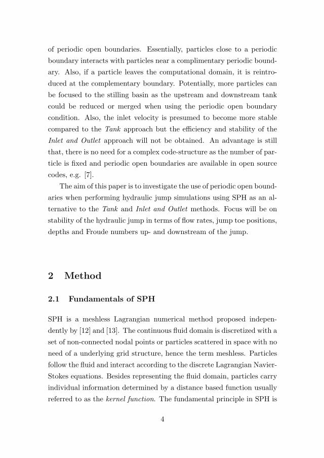
of periodic open boundaries. Essentially, particles close to a periodic

boundary interacts with particles near a complimentary periodic bound-

ary. Also, if a particle leaves the computational domain, it is reintro-

duced at the complementary boundary. Potentially, more particles can

be focused to the stilling basin as the upstream and downstream tank

could be reduced or merged when using the periodic open boundary

condition. Also, the inlet velocity is presumed to become more stable

compared to the Tank approach but the efficiency and stability of the

Inlet and Outlet approach will not be obtained. An advantage is still

that, there is no need for a complex code-structure as the number of par-

ticle is fixed and periodic open boundaries are available in open source

codes, e.g. [7].

The aim of this paper is to investigate the use of periodic open bound-

aries when performing hydraulic jump simulations using SPH as an al-

ternative to the Tank and Inlet and Outlet methods. Focus will be on

stability of the hydraulic jump in terms of flow rates, jump toe positions,

depths and Froude numbers up- and downstream of the jump.

2 Method

2.1 Fundamentals of SPH

SPH is a meshless Lagrangian numerical method proposed indepen-

dently by [12] and [13]. The continuous fluid domain is discretized with a

set of non-connected nodal points or particles scattered in space with no

need of a underlying grid structure, hence the term meshless. Particles

follow the fluid and interact according to the discrete Lagrangian Navier-

Stokes equations. Besides representing the fluid domain, particles carry

individual information determined by a distance based function usually

referred to as the kernel function. The fundamental principle in SPH is

4

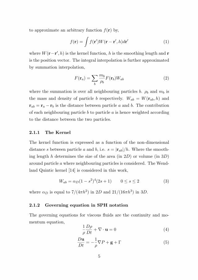
to approximate an arbitrary function f(r) by,

f(r) =

∫f(r′)W (r− r′, h)dr′ (1)

where W (r−r′, h) is the kernel function, h is the smoothing length and r

is the position vector. The integral interpolation is further approximated

by summation interpolation,

F (ra) =∑b

mb

ρbF (rb)Wab (2)

where the summation is over all neighbouring particles b. ρb and mb is

the mass and density of particle b respectively. Wab = W (rab, h) and

rab = ra − rb is the distance between particle a and b. The contribution

of each neighbouring particle b to particle a is hence weighted according

to the distance between the two particles.

2.1.1 The Kernel

The kernel function is expressed as a function of the non-dimensional

distance s between particle a and b, i.e. s = |rab|/h. Where the smooth-

ing length h determines the size of the area (in 2D) or volume (in 3D)

around particle a where neighbouring particles is considered. The Wend-

land Quintic kernel [14] is considered in this work,

Wab = αD(1− s2)4(2s+ 1) 0 ≤ s ≤ 2 (3)

where αD is equal to 7/(4πh2) in 2D and 21/(16πh3) in 3D.

2.1.2 Governing equation in SPH notation

The governing equations for viscous fluids are the continuity and mo-

mentum equation,1

ρ

Dρ

Dt+∇ · u = 0 (4)

Du

Dt= −1

ρ∇P + g + Γ (5)

5

where u is the velocity vector, P is the pressure pressure, g is the ac-

celeration due to gravity and Γ are the dissipative terms. In weakly-

compressible SPH simulations, the particle mass is constant and the

density fluctuates according to the continuity Equation (4) which can

be rewritten in SPH-notations as,

dρadt

=∑b

mbuab · ∇aWab. (6)

To keep the density fluctuations from diverging, a shepard filter is ap-

plied every 40th time step to correct the density field according to,

ρnewa =∑b

ρbWabmb

ρb=∑b

mbWab (7)

where

Wab =Wab∑

b

Wabmbρb

(8)

which is known as a zeroth-order correction. The momentum Equation

(5) can be written in SPH-notation as,

Du

Dt= −

∑b

mb

(Pb

ρ2b+

Pa

ρ2a

)∇aWab + g + Γ (9)

where the dissipative term Γ is usually represented by the artificial-

viscosity proposed by [15]. However, this approach can be too dissipa-

tive and effect the shear stresses in fluids [16]. Due to the shear flow

characteristics of the hydraulic jump [17, 18], the laminar viscosity and

Sub-Particle Scale (SPS) model is considered instead to handle the dis-

sipative terms [4]. Therefore, Γ in Equation (9) is divided into two

parts,

Γ = ν0∇2u+1

ρ∇· →

τ . (10)

The first term in Equation (10) is the laminar viscous stresses which can

be expressed in SPH notation as [19],

ν0∇2u =∑b

mb

(4ν0rab · ∇aWab

(ρa + ρa)(r2ab + η2

))uab (11)

6

where ν0 = 10−6 [m2/s] is the kinematic viscosity of water and η2 =

0.01h2. The second term in Equation (10) is the SPS stress tensor and

represents the effects of turbulence. The model is based on the Large

Eddy Simulation (LES) approach and was for particle methods first

proposed by [20] for the incompressible Moving Particle Semi-implicit

(MPS) method. Lo and Shao [21] implemented the same model for in-

compressible SPH. By using Favre averaging to account for compressibil-

ity, Dalrymple and Rogers [16] introduced the SPS model into weakly-

compressible SPH by rewriting the second term in Equation (10) as,

1

ρ∇· →

τ=∑b

mb

⎛⎝→

τb

ij

ρ2b+

→τa

ij

ρ2a

⎞⎠∇aWab. (12)

In Einstein notation, the shear stress component in i and j direction can

be approximated as

→τ ij

ρ= νt

(2Sij − 2

3kδij

)− 2

3ClΔ

2δij |Sij |2 (13)

where→τ ij is the sub-particle stress tensor, νt = [(CsΔl)]2 |S| is the

turbulent eddy viscosity, k the SPS turbulence kinetic energy, Cs =

0.12 the Smagorinsky constant, Cl = 0.0066, Δl the particle to particle

spacing and |S| = 0.5(2SijSij) where Sij is an element of the SPS strain

tensor. The final momentum equation can be rewritten as,

Du

Dt=−

∑b

mb

(Pb

ρ2b+

Pa

ρ2a

)∇aWab + g

+∑b

mb

(4ν0rab · ∇aWab

(ρa + ρa)(r2ab + η2

))uab

+∑b

mb

⎛⎝→

τb

ij

ρ2b+

→τa

ij

ρ2a

⎞⎠∇aWab

(14)

7

2.1.3 Equation of State

To avoid an expensive computation of the Poisson’s equation and to

keep the explicit nature of the method, an equation-of-state (EOS) is

used to relate the fluid pressure to local particle density [22]. Also,

the compressibility is altered implying that the speed of sound can be

artificially lowered. Therefore, a larger time step determined partly

by the Courant-Fredrich-Levy (CFL) condition can be applied. The

pressure is determined by,

P = B

[(ρ

ρ0

)γ

− 1

](15)

where B = c20ρ0/γ, γ = 7, ρ0 = 1000 kg/m3 is the reference density of

water and c0 = c(ρ0) =√

(∂P/∂ρ) is the speed of sound at the reference

density [23]. The reference speed of sound c0 was set to ten times the

maximum fluid velocity based on the depth in the tank in order to keep

the density variation within 1%.

2.1.4 Time stepping

The explicit, second-order (in time), predictor-corrector based Symplec-

tic algorithm is used for time integration [7]. For explicit time integra-

tion scheme the time step is dependent on the CFL-number mentioned

above. However, further restrictions is put on the time step which is

determined according to

Δt = Ct ·min (Δtf ,Δtcv) (16)

where Ct = 0.2 is a constant,

Δtf = min(√

h/|fa|)

(17)

is based on the force per unit mass |fa| and

Δtcv = mina

⎛⎜⎜⎝ h

cs +maxb

∣∣∣∣ huab·rab(r2ab+η2)

∣∣∣∣

⎞⎟⎟⎠ (18)

8

which combines the CFL and a viscous condition [24].

2.1.5 Particle motion

In order to obtain a more ordered flow and to prevent particle penetra-

tion, the XSPH method proposed by [25] is used for moving the particles,

i.e.dradt

= ua + ε∑b

mb

ρabuabWab (19)

where ε = 0.5 and ρab = (ρa + ρb)/2.

2.1.6 Wall boundary condition

The Dynamic Boundary Condition (DBC) proposed by [26] is applied

for impermeable solid walls. The boundary is populated by particles in

three non-staggered rows to insure that fluid particles is not penetrating

the boundaries and a complete coverage of the kernel compact support.

Wall particles satisfy the same equations as fluid particles but are fixed

in space. The fundamental principal of the method is that when a fluid

particle approaches a fixed wall particle density increases and by the

EOS the pressure increase. Due to the pressure term in the momentum

equation, the pressure increase results in a repulsive force between the

particles.

2.1.7 Periodic open boundary condition

Several variates of the periodic boundary condition are available. How-

ever, the essence is that particles close to a periodic boundary interacts

with particles near a complimentary boundary. Thus, information is

spreading both ways. Furthermore, if a particle leaves the computa-

tional domain through an open boundary the particle is reintroduced

at the complementary boundary. During the reintroduction step, par-

ticle coordinates are changed with fixed values and other variables e.g.

velocity are kept unchanged.

9

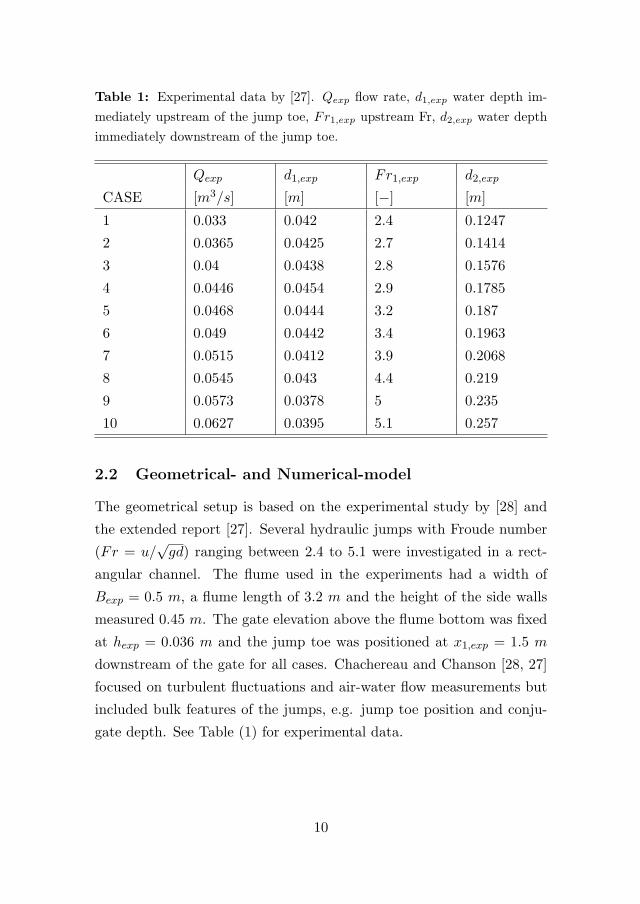
Table 1: Experimental data by [27]. Qexp flow rate, d1,exp water depth im-

mediately upstream of the jump toe, Fr1,exp upstream Fr, d2,exp water depth

immediately downstream of the jump toe.

Qexp d1,exp Fr1,exp d2,exp

CASE [m3/s] [m] [−] [m]

1 0.033 0.042 2.4 0.1247

2 0.0365 0.0425 2.7 0.1414

3 0.04 0.0438 2.8 0.1576

4 0.0446 0.0454 2.9 0.1785

5 0.0468 0.0444 3.2 0.187

6 0.049 0.0442 3.4 0.1963

7 0.0515 0.0412 3.9 0.2068

8 0.0545 0.043 4.4 0.219

9 0.0573 0.0378 5 0.235

10 0.0627 0.0395 5.1 0.257

2.2 Geometrical- and Numerical-model

The geometrical setup is based on the experimental study by [28] and

the extended report [27]. Several hydraulic jumps with Froude number

(Fr = u/√gd) ranging between 2.4 to 5.1 were investigated in a rect-

angular channel. The flume used in the experiments had a width of

Bexp = 0.5 m, a flume length of 3.2 m and the height of the side walls

measured 0.45 m. The gate elevation above the flume bottom was fixed

at hexp = 0.036 m and the jump toe was positioned at x1,exp = 1.5 m

downstream of the gate for all cases. Chachereau and Chanson [28, 27]

focused on turbulent fluctuations and air-water flow measurements but

included bulk features of the jumps, e.g. jump toe position and conju-

gate depth. See Table (1) for experimental data.

10

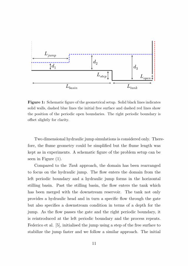
Figure 1: Schematic figure of the geometrical setup. Solid black lines indicates

solid walls, dashed blue lines the initial free surface and dashed red lines show

the position of the periodic open boundaries. The right periodic boundary is

offset slightly for clarity.

Two dimensional hydraulic jump simulations is considered only. There-

fore, the flume geometry could be simplified but the flume length was

kept as in experiments. A schematic figure of the problem setup can be

seen in Figure (1).

Compared to the Tank approach, the domain has been rearranged

to focus on the hydraulic jump. The flow enters the domain from the

left periodic boundary and a hydraulic jump forms in the horizontal

stilling basin. Past the stilling basin, the flow enters the tank which

has been merged with the downstream reservoir. The tank not only

provides a hydraulic head and in turn a specific flow through the gate

but also specifies a downstream condition in terms of a depth for the

jump. As the flow passes the gate and the right periodic boundary, it

is reintroduced at the left periodic boundary and the process repeats.

Federico et al. [5], initialised the jump using a step of the free surface to

stabilize the jump faster and we follow a similar approach. The initial

11

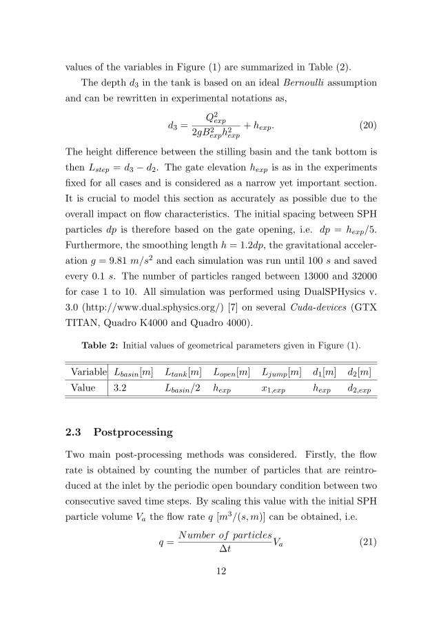
values of the variables in Figure (1) are summarized in Table (2).

The depth d3 in the tank is based on an ideal Bernoulli assumption

and can be rewritten in experimental notations as,

d3 =Q2

exp

2gB2exph

2exp

+ hexp. (20)

The height difference between the stilling basin and the tank bottom is

then Lstep = d3 − d2. The gate elevation hexp is as in the experiments

fixed for all cases and is considered as a narrow yet important section.

It is crucial to model this section as accurately as possible due to the

overall impact on flow characteristics. The initial spacing between SPH

particles dp is therefore based on the gate opening, i.e. dp = hexp/5.

Furthermore, the smoothing length h = 1.2dp, the gravitational acceler-

ation g = 9.81 m/s2 and each simulation was run until 100 s and saved

every 0.1 s. The number of particles ranged between 13000 and 32000

for case 1 to 10. All simulation was performed using DualSPHysics v.

3.0 (http://www.dual.sphysics.org/) [7] on several Cuda-devices (GTX

TITAN, Quadro K4000 and Quadro 4000).

Table 2: Initial values of geometrical parameters given in Figure (1).

Variable Lbasin[m] Ltank[m] Lopen[m] Ljump[m] d1[m] d2[m]

Value 3.2 Lbasin/2 hexp x1,exp hexp d2,exp

2.3 Postprocessing

Two main post-processing methods was considered. Firstly, the flow

rate is obtained by counting the number of particles that are reintro-

duced at the inlet by the periodic open boundary condition between two

consecutive saved time steps. By scaling this value with the initial SPH

particle volume Va the flow rate q [m3/(s,m)] can be obtained, i.e.

q =Number of particles

ΔtVa (21)

12

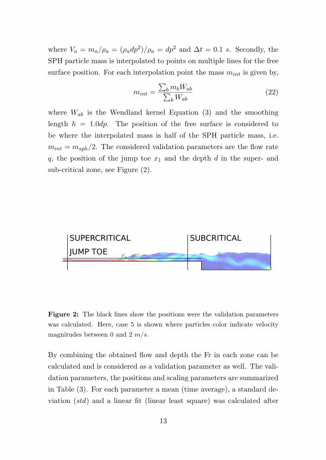
where Va = ma/ρa = (ρadp2)/ρa = dp2 and Δt = 0.1 s. Secondly, the

SPH particle mass is interpolated to points on multiple lines for the free

surface position. For each interpolation point the mass mint is given by,

mint =

∑bmbWab∑bWab

(22)

where Wab is the Wendland kernel Equation (3) and the smoothing

length h = 1.0dp. The position of the free surface is considered to

be where the interpolated mass is half of the SPH particle mass, i.e.

mint = msph/2. The considered validation parameters are the flow rate

q, the position of the jump toe x1 and the depth d in the super- and

sub-critical zone, see Figure (2).

Figure 2: The black lines show the positions were the validation parameters

was calculated. Here, case 5 is shown where particles color indicate velocity

magnitudes between 0 and 2 m/s.

By combining the obtained flow and depth the Fr in each zone can be

calculated and is considered as a validation parameter as well. The vali-

dation parameters, the positions and scaling parameters are summarized

in Table (3). For each parameter a mean (time average), a standard de-

viation (std) and a linear fit (linear least square) was calculated after

13

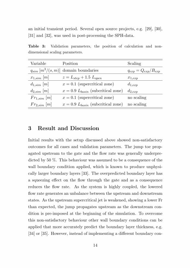
an initial transient period. Several open source projects, e.g. [29], [30],

[31] and [32], was used in post-processing the SPH-data.

Table 3: Validation parameters, the position of calculation and non-

dimensional scaling parameters.

Variable Position Scaling

qsim [m3/(s,m)] domain boundaries qexp = Qexp/Bexp

x1,sim [m] z = Lstep + 1.5 Lopen x1,exp

d1,sim [m] x = 0.1 (supercritical zone) d1,exp

d2,sim [m] x = 0.9 Lbasin (subcritical zone) d2,exp

Fr1,sim [m] x = 0.1 (supercritical zone) no scaling

Fr2,sim [m] x = 0.9 Lbasin (subcritical zone) no scaling

3 Result and Discussion

Initial results with the setup discussed above showed non-satisfactory

outcomes for all cases and validation parameters. The jump toe prop-

agated upstream to the gate and the flow rate was generally underpre-

dicted by 50 %. This behaviour was assumed to be a consequence of the

wall boundary condition applied, which is known to produce unphysi-

cally larger boundary layers [33]. The overpredicted boundary layer has

a squeezing effect on the flow through the gate and as a consequence

reduces the flow rate. As the system is highly coupled, the lowered

flow rate generates an unbalance between the upstream and downstream

states. As the upstream supercritical jet is weakened, showing a lower Fr

than expected, the jump propagates upstream as the downstream con-

dition is pre-imposed at the beginning of the simulation. To overcome

this non-satisfactory behaviour other wall boundary conditions can be

applied that more accurately predict the boundary layer thickness, e.g.

[34] or [35]. However, instead of implementing a different boundary con-

14

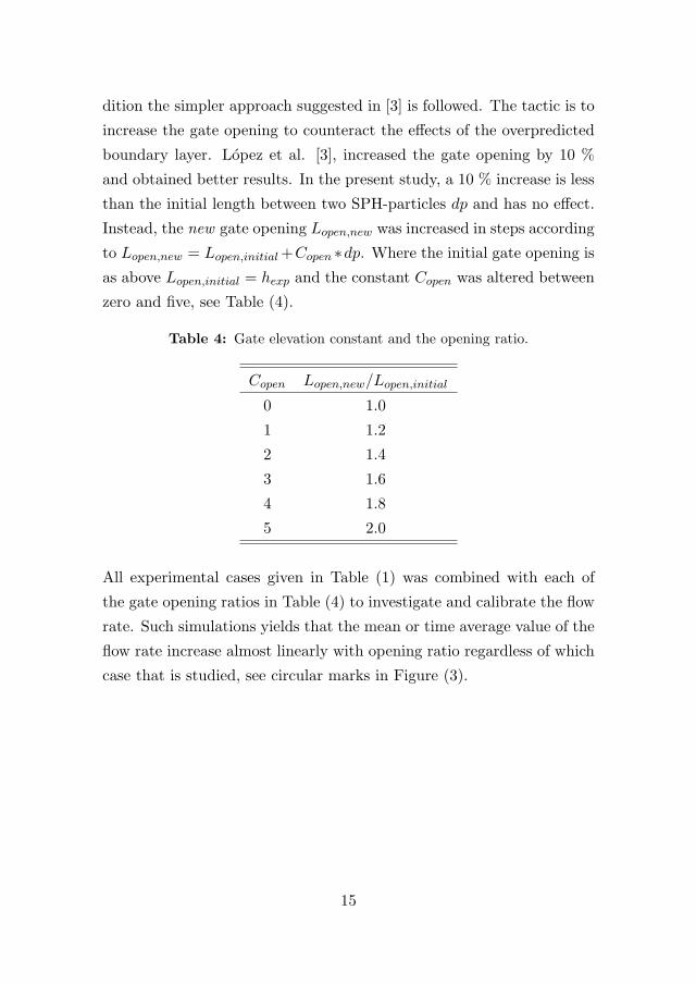
dition the simpler approach suggested in [3] is followed. The tactic is to

increase the gate opening to counteract the effects of the overpredicted

boundary layer. Lopez et al. [3], increased the gate opening by 10 %

and obtained better results. In the present study, a 10 % increase is less

than the initial length between two SPH-particles dp and has no effect.

Instead, the new gate opening Lopen,new was increased in steps according

to Lopen,new = Lopen,initial+Copen ∗dp. Where the initial gate opening is

as above Lopen,initial = hexp and the constant Copen was altered between

zero and five, see Table (4).

Table 4: Gate elevation constant and the opening ratio.

Copen Lopen,new/Lopen,initial

0 1.0

1 1.2

2 1.4

3 1.6

4 1.8

5 2.0

All experimental cases given in Table (1) was combined with each of

the gate opening ratios in Table (4) to investigate and calibrate the flow

rate. Such simulations yields that the mean or time average value of the

flow rate increase almost linearly with opening ratio regardless of which

case that is studied, see circular marks in Figure (3).

15

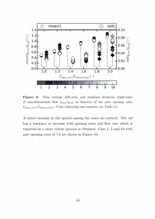
Figure 3: Time average (left-axis) and standard deviation (right-axis)

of non-dimensional flow qsim/qexp as function of the gate opening ratio

Lopen,new/Lopen,initial. Color indicating case number, see Table (1).

A minor increase in the spread among the cases are noticed. The std

has a tendency to increase with opening ratio and flow rate which is

expected as a more violent process is obtained. Case 1, 5 and 10 with

gate opening ratio of 1.6 are shown in Figure (4).

16

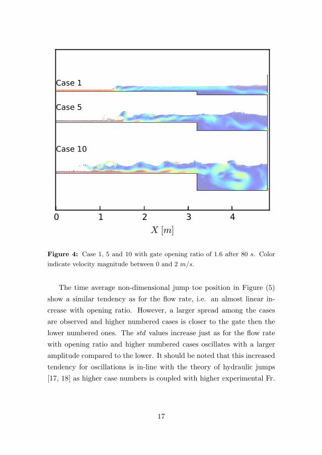
Figure 4: Case 1, 5 and 10 with gate opening ratio of 1.6 after 80 s. Color

indicate velocity magnitude between 0 and 2 m/s.

The time average non-dimensional jump toe position in Figure (5)

show a similar tendency as for the flow rate, i.e. an almost linear in-

crease with opening ratio. However, a larger spread among the cases

are observed and higher numbered cases is closer to the gate then the

lower numbered ones. The std values increase just as for the flow rate

with opening ratio and higher numbered cases oscillates with a larger

amplitude compared to the lower. It should be noted that this increased

tendency for oscillations is in-line with the theory of hydraulic jumps

[17, 18] as higher case numbers is coupled with higher experimental Fr.

17

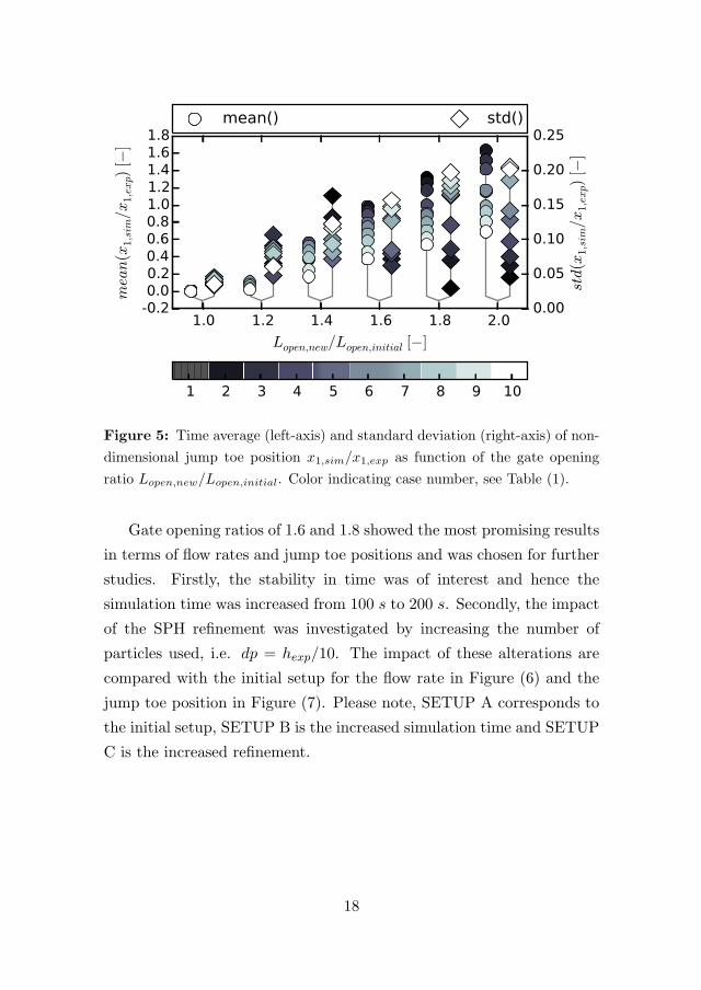
Figure 5: Time average (left-axis) and standard deviation (right-axis) of non-

dimensional jump toe position x1,sim/x1,exp as function of the gate opening

ratio Lopen,new/Lopen,initial. Color indicating case number, see Table (1).

Gate opening ratios of 1.6 and 1.8 showed the most promising results

in terms of flow rates and jump toe positions and was chosen for further

studies. Firstly, the stability in time was of interest and hence the

simulation time was increased from 100 s to 200 s. Secondly, the impact

of the SPH refinement was investigated by increasing the number of

particles used, i.e. dp = hexp/10. The impact of these alterations are

compared with the initial setup for the flow rate in Figure (6) and the

jump toe position in Figure (7). Please note, SETUP A corresponds to

the initial setup, SETUP B is the increased simulation time and SETUP

C is the increased refinement.

18

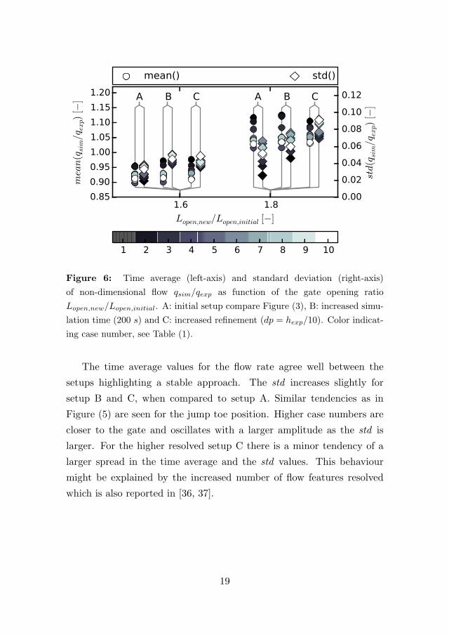
Figure 6: Time average (left-axis) and standard deviation (right-axis)

of non-dimensional flow qsim/qexp as function of the gate opening ratio

Lopen,new/Lopen,initial. A: initial setup compare Figure (3), B: increased simu-

lation time (200 s) and C: increased refinement (dp = hexp/10). Color indicat-

ing case number, see Table (1).

The time average values for the flow rate agree well between the

setups highlighting a stable approach. The std increases slightly for

setup B and C, when compared to setup A. Similar tendencies as in

Figure (5) are seen for the jump toe position. Higher case numbers are

closer to the gate and oscillates with a larger amplitude as the std is

larger. For the higher resolved setup C there is a minor tendency of a

larger spread in the time average and the std values. This behaviour

might be explained by the increased number of flow features resolved

which is also reported in [36, 37].

19

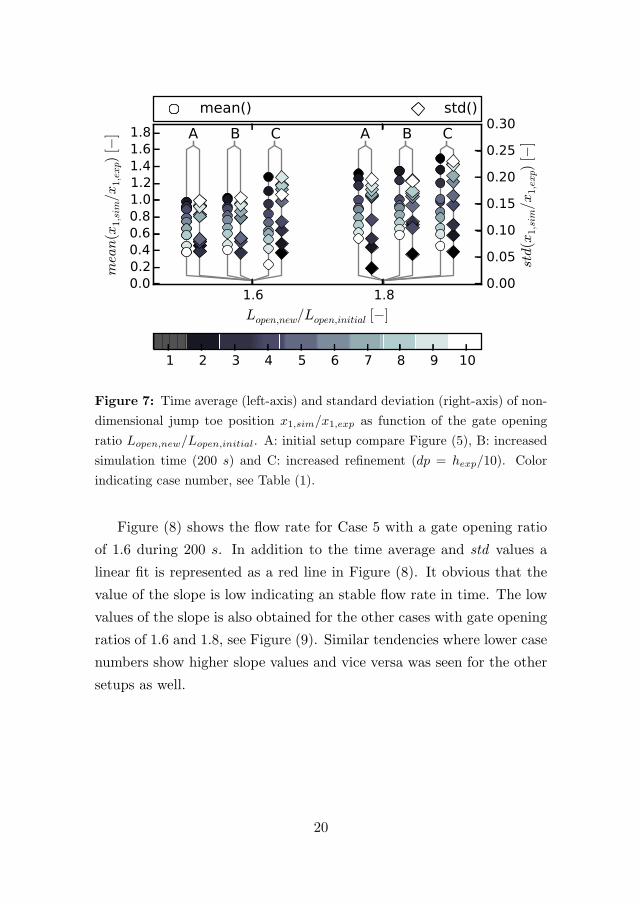
Figure 7: Time average (left-axis) and standard deviation (right-axis) of non-

dimensional jump toe position x1,sim/x1,exp as function of the gate opening

ratio Lopen,new/Lopen,initial. A: initial setup compare Figure (5), B: increased

simulation time (200 s) and C: increased refinement (dp = hexp/10). Color

indicating case number, see Table (1).

Figure (8) shows the flow rate for Case 5 with a gate opening ratio

of 1.6 during 200 s. In addition to the time average and std values a

linear fit is represented as a red line in Figure (8). It obvious that the

value of the slope is low indicating an stable flow rate in time. The low

values of the slope is also obtained for the other cases with gate opening

ratios of 1.6 and 1.8, see Figure (9). Similar tendencies where lower case

numbers show higher slope values and vice versa was seen for the other

setups as well.

20

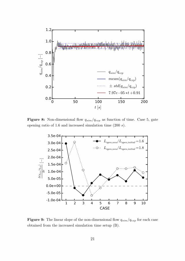
Figure 8: Non-dimensional flow qsim/qexp as function of time. Case 5, gate

opening ratio of 1.6 and increased simulation time (200 s).

Figure 9: The linear slope of the non-dimensional flow qsim/qexp for each case

obtained from the increased simulation time setup (B).

21

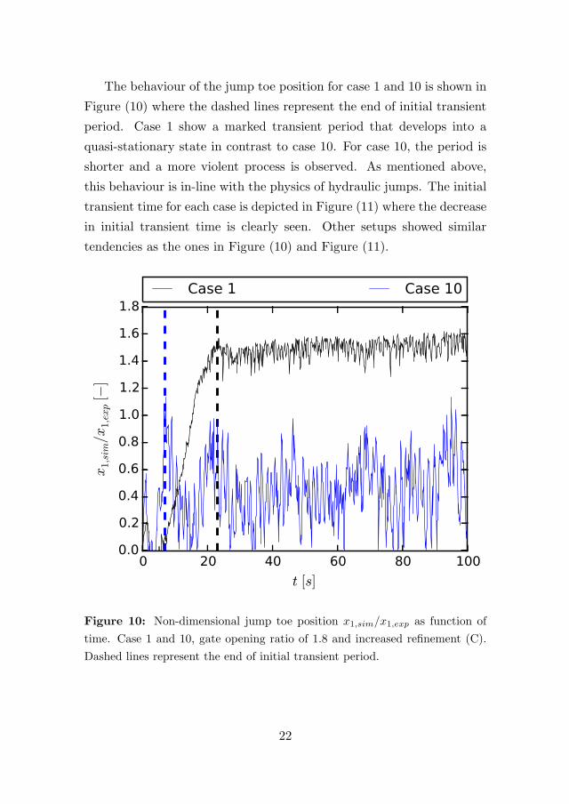
The behaviour of the jump toe position for case 1 and 10 is shown in

Figure (10) where the dashed lines represent the end of initial transient

period. Case 1 show a marked transient period that develops into a

quasi-stationary state in contrast to case 10. For case 10, the period is

shorter and a more violent process is observed. As mentioned above,

this behaviour is in-line with the physics of hydraulic jumps. The initial

transient time for each case is depicted in Figure (11) where the decrease

in initial transient time is clearly seen. Other setups showed similar

tendencies as the ones in Figure (10) and Figure (11).

Figure 10: Non-dimensional jump toe position x1,sim/x1,exp as function of

time. Case 1 and 10, gate opening ratio of 1.8 and increased refinement (C).

Dashed lines represent the end of initial transient period.

22

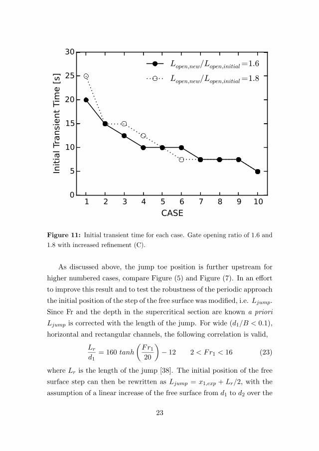
Figure 11: Initial transient time for each case. Gate opening ratio of 1.6 and

1.8 with increased refinement (C).

As discussed above, the jump toe position is further upstream for

higher numbered cases, compare Figure (5) and Figure (7). In an effort

to improve this result and to test the robustness of the periodic approach

the initial position of the step of the free surface was modified, i.e. Ljump.

Since Fr and the depth in the supercritical section are known a priori

Ljump is corrected with the length of the jump. For wide (d1/B < 0.1),

horizontal and rectangular channels, the following correlation is valid,

Lr

d1= 160 tanh

(Fr120

)− 12 2 < Fr1 < 16 (23)

where Lr is the length of the jump [38]. The initial position of the free

surface step can then be rewritten as Ljump = x1,exp + Lr/2, with the

assumption of a linear increase of the free surface from d1 to d2 over the

23

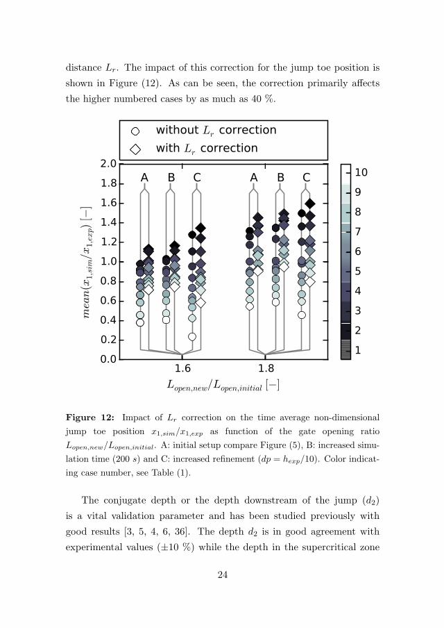
distance Lr. The impact of this correction for the jump toe position is

shown in Figure (12). As can be seen, the correction primarily affects

the higher numbered cases by as much as 40 %.

Figure 12: Impact of Lr correction on the time average non-dimensional

jump toe position x1,sim/x1,exp as function of the gate opening ratio

Lopen,new/Lopen,initial. A: initial setup compare Figure (5), B: increased simu-

lation time (200 s) and C: increased refinement (dp = hexp/10). Color indicat-

ing case number, see Table (1).

The conjugate depth or the depth downstream of the jump (d2)

is a vital validation parameter and has been studied previously with

good results [3, 5, 4, 6, 36]. The depth d2 is in good agreement with

experimental values (±10 %) while the depth in the supercritical zone

24

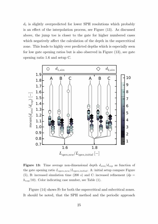
d1 is slightly overpredicted for lower SPH resolutions which probably

is an effect of the interpolation process, see Figure (13). As discussed

above, the jump toe is closer to the gate for higher numbered cases

which negatively affect the calculation of the depth in the supercritical

zone. This leads to highly over predicted depths which is especially seen

for low gate opening ratios but is also observed in Figure (13), see gate

opening ratio 1.6 and setup C.

Figure 13: Time average non-dimensional depth dsim/dexp as function of

the gate opening ratio Lopen,new/Lopen,initial. A: initial setup compare Figure

(5), B: increased simulation time (200 s) and C: increased refinement (dp =

hexp/10). Color indicating case number, see Table (1).

Figure (14) shows Fr for both the supercritical and subcritical zones.

It should be noted, that the SPH method and the periodic approach

25

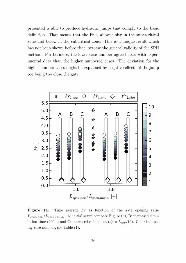
presented is able to produce hydraulic jumps that comply to the basic

definition. That means that the Fr is above unity in the supercritical

zone and below in the subcritical zone. This is a unique result which

has not been shown before that increase the general validity of the SPH

method. Furthermore, the lower case number agree better with exper-

imental data than the higher numbered cases. The deviation for the

higher number cases might be explained by negative effects of the jump

toe being too close the gate.

Figure 14: Time average Fr as function of the gate opening ratio

Lopen,new/Lopen,initial. A: initial setup compare Figure (5), B: increased simu-

lation time (200 s) and C: increased refinement (dp = hexp/10). Color indicat-

ing case number, see Table (1).

26

To further improve the results other periodic techniques can be im-

plemented. For the present work, coordinates has been changed only

when particles are reintroduced at a complementary boundary. How-

ever, other variables can be changed too, i.e. velocity. An interesting

technique is the Translating Periodic Boundary Condition [39] which

change both coordinates and velocities and thus approaches the Inlet

and Outlet technique. However, such technique may imply a major re-

vision of the code which is out of scope for present work.

4 Conclusion

We have investigated an alternative approach to hydraulic jump SPH

simulations by applying periodic open boundaries. It is shown that

after an initial transient period the hydraulic jump move into a quasi-

stationary state being stable in time. The gate elevation has a major

impact of the behaviour of the jump as the system is highly coupled.

A calibration of the opening is essential to obtain a correct flow rate to

ensure the development of a stable hydraulic jump. With a proper flow

rate, the position of the jump toe is significantly improved. The jump

toe oscillate with a larger amplitude for higher Fr which is in-line with

the theory of hydraulic jumps and is not seen as an numerical error.

The position of the jump was further improved by introducing a correc-

tion based on the empirical correlation of the jump length. To further

investigate the robustness of the periodic approach the simulation time

and SPH resolution was increased. However, both alteration show little

impact on the overall behaviour. Both the depth in the super- and sub-

critical section show good agreement with experiments found in previous

studies. The Fr is less than unity in the subcritical region and above

unity in the supercritical being in agreement with the definition. As a

final remark, the periodic approach lacks the efficiency of the Inlet and

Outlet approach but is better than the Tank approach in terms of flow

27

rate accuracy and jump toe stability.

Acknowledgement

The research presented was carried out as a part of “Swedish Hydropower

Centre - SVC”. SVC has been established by the Swedish Energy Agency,

Elforsk and Svenska Kraftnat together with Lulea University of Technol-

ogy, KTH Royal Institute of Technology, Chalmers University of Tech-

nology and Uppsala University. www.svc.nu.

References

[1] Damien Violeau. Fluid Mechanics and the SPH Method. Oxford University

Press, may 2012. doi: 10.1093/acprof:oso/9780199655526.001.0001.

[2] Ruben Scardovelli and Stephane Zaleski. DIRECT NUMERICAL SIMU-

LATION OF FREE-SURFACE AND INTERFACIAL FLOW. Annu. Rev.

Fluid Mech., 31(1):567–603, jan 1999. doi: 10.1146/annurev.fluid.31.1.567.

[3] David Lopez, Roberto Marivela, and Luis Garrote. Smoothed particle

hydrodynamics model applied to hydraulic structures: a hydraulic jump

test case. Journal of Hydraulic Research, 48(sup1):142–158, jan 2010. doi:

10.1080/00221686.2010.9641255.

[4] Ming-Jyh Chern and Sam Syamsuri. Effect of corrugated bed on hydraulic

jump characteristic using SPH method. Journal of Hydraulic Engineering,

139(2):221–232, feb 2013. doi: 10.1061/(asce)hy.1943-7900.0000618.

[5] I. Federico, S. Marrone, A. Colagrossi, F. Aristodemo, and M. Antuono.

Simulating 2d open-channel flows through an SPH model. European

Journal of Mechanics - B/Fluids, 34:35–46, jul 2012. doi: 10.1016/j.

euromechflu.2012.02.002.

[6] Diana De Padova, Michele Mossa, Stefano Sibilla, and Emanuela Torti.

3d SPH modelling of hydraulic jump in a very large channel. Journal of

Hydraulic Research, 51(2):158–173, apr 2013. doi: 10.1080/00221686.2012.

736883.

28

[7] A.J.C. Crespo, J.M. Domınguez, B.D. Rogers, M. Gomez-Gesteira,

S. Longshaw, R. Canelas, R. Vacondio, A. Barreiro, and O. Garcıa-Feal.

DualSPHysics: Open-source parallel CFD solver based on smoothed parti-

cle hydrodynamics (SPH). Computer Physics Communications, 187:204–

216, feb 2015. doi: 10.1016/j.cpc.2014.10.004.

[8] GPUSPH, accessed 2015-06-26. URL http://www.gpusph.org/.

[9] AQUAgpusph, accessed 2015-06-26. URL http://canal.etsin.upm.es/

aquagpusph/.

[10] PySPH, accessed 2015-06-26. URL https://code.google.com/p/

pysph/.

[11] Martin Lastiwka, Mihai Basa, and Nathan J. Quinlan. Permeable and

non-reflecting boundary conditions in SPH. Int. J. Numer. Meth. Fluids,

61(7):709–724, nov 2009. doi: 10.1002/fld.1971.

[12] R. A. Gingold and J. J. Monaghan. Smoothed particle hydrodynamics:

theory and application to non-spherical stars. Monthly Notices of the Royal

Astronomical Society, 181(3):375–389, dec 1977. doi: 10.1093/mnras/181.

3.375.

[13] L. B. Lucy. A numerical approach to the testing of the fission hypothesis.

The Astronomical Journal, 82:1013, dec 1977. doi: 10.1086/112164.

[14] Holger Wendland. Piecewise polynomial, positive definite and compactly

supported radial functions of minimal degree. Adv Comput Math, 4(1):

389–396, dec 1995. doi: 10.1007/bf02123482.

[15] J. J. Monaghan. Smoothed particle hydrodynamics. Annual Review of As-

tronomy and Astrophysics, 30(1):543–574, sep 1992. doi: 10.1146/annurev.

aa.30.090192.002551.

[16] R.A. Dalrymple and B.D. Rogers. Numerical modeling of water waves

with the SPH method. Coastal Engineering, 53(2-3):141–147, feb 2006.

doi: 10.1016/j.coastaleng.2005.10.004.

[17] Ven Te Chow. Open-channel hydraulics. McGraw-Hill, Tokyo, 1959. ISBN

0-07-010776-9.

[18] Hubert Chanson. The hydraulics of open channel flow an introduction :

basic principles, sediment motion, hydraulic modelling, design of hydraulic

29

structures. Amsterdam ; London : Elsevier Butterworth-Heinemann, Am-

sterdam ; London, 2nd ed.. edition, 2004.

[19] Joseph P. Morris, Patrick J. Fox, and Yi Zhu. Modeling low reynolds num-

ber incompressible flows using SPH. Journal of Computational Physics,

136(1):214–226, sep 1997. doi: 10.1006/jcph.1997.5776.

[20] H. Gotoh, T. Shibihara, and M. Hayashii. Subparticle-scale model for the

MPS method-lagrangian flow model for hydraulic engineering. Comput.

Fluid Dynam. J., 09:339–347, 2001.

[21] Edmond Y.M. Lo and Songdong Shao. Simulation of near-shore solitary

wave mechanics by an incompressible SPH method. Applied Ocean Re-

search, 24(5):275–286, oct 2002. doi: 10.1016/s0141-1187(03)00002-6.

[22] J.J. Monaghan. Simulating free surface flows with SPH. Journal of Com-

putational Physics, 110(2):399–406, feb 1994. doi: 10.1006/jcph.1994.1034.

[23] George Keith Batchelor. An introduction to fluid dynamics. Cambridge

University Press, London, 1967.

[24] J. J. Monaghan and A. Kos. Solitary waves on a cretan beach. J.

Waterway, Port, Coastal, Ocean Eng., 125(3):145–155, may 1999. doi:

10.1061/(asce)0733-950x(1999)125:3(145).

[25] J.J. Monaghan. On the problem of penetration in particle methods.

Journal of Computational Physics, 82(1):1–15, may 1989. doi: 10.1016/

0021-9991(89)90032-6.

[26] A. J. Crespo, M. Gomez-Gesteira, and R. A. Dalrymple. Boundary con-

ditions generated by dynamic particles in sph methods. Computers, ma-

terials and continua, 5(3):173–184, 2007. doi: 10.3970/cmc.2007.005.173.

[27] Yann Chachereau and Hubert Chanson. Free surface turbulence fluctu-

ations and air-water flow measurements in hydraulic jumps with small

inflow froude numbers. Technical Report CH78/10, Division of Civil En-

gineering, The University of Queensland, 2010.

[28] Yann Chachereau and Hubert Chanson. Free-surface fluctuations and

turbulence in hydraulic jumps. Experimental Thermal and Fluid Science,

35(6):896–909, sep 2011. doi: 10.1016/j.expthermflusci.2011.01.009.

30

[29] Fernando Perez and Brian E. Granger. IPython: A system for interactive

scientific computing. Computing in Science & Engineering, 9(3):21–29,

2007. doi: 10.1109/mcse.2007.53.

[30] John D. Hunter. Matplotlib: A 2d graphics environment. Computing in

Science & Engineering, 9(3):90–95, 2007. doi: 10.1109/mcse.2007.55.

[31] Stefan Behnel, Robert Bradshaw, Craig Citro, Lisandro Dalcin,

Dag Sverre Seljebotn, and Kurt Smith. Cython: The best of both

worlds. Computing in Science & Engineering, 13(2):31–39, mar 2011. doi:

10.1109/mcse.2010.118.

[32] S. van der Walt, S.C. Colbert, and G. Varoquaux. The NumPy array: A

structure for efficient numerical computation. Comput. Sci. Eng., 13(2):

22–30, mar 2011. doi: 10.1109/mcse.2011.37. URL http://dx.doi.org/

10.1109/mcse.2011.37.

[33] Moncho Gomez-Gesteira, Benedict D. Rogers, Robert A. Dalrymple, and

Alex J.C. Crespo. State-of-the-art of classical SPH for free-surface flows.

Journal of Hydraulic Research, 48(sup1):6–27, jan 2010. doi: 10.1080/

00221686.2010.9641242.

[34] S. Adami, X.Y. Hu, and N.A. Adams. A generalized wall boundary con-

dition for smoothed particle hydrodynamics. Journal of Computational

Physics, 231(21):7057–7075, aug 2012. doi: 10.1016/j.jcp.2012.05.005.

[35] M. Ferrand, D. R. Laurence, B. D. Rogers, D. Violeau, and C. Kassiotis.

Unified semi-analytical wall boundary conditions for inviscid, laminar or

turbulent flows in the meshless SPH method. Int. J. Numer. Meth. Fluids,

71(4):446–472, mar 2012. doi: 10.1002/fld.3666.

[36] P. Jonsson, P. Jonsen, P. Andreasson, T.S. Lundstrom, and J.G.I. Hell-

strom. Smoothed particle hydrodynamics modeling of hydraulic jumps.

In Proceedings of Particle-Based Methods II - Fundamentals and Applica-

tions, pages 490–501, Barcelona, Spain, 2011.

[37] Patrick Jonsson, Par Jonsen, Patrik Andreasson, T. Staffan Lundstrom,

and J. Gunnar I. Hellstrom. Modelling dam break evolution over a wet bed

with smoothed particle hydrodynamics: A parameter study. Engineering,

07(05):248–260, 2015. doi: 10.4236/eng.2015.75022.

31

[38] W. H. Hager, R. Bremen, and N. Kawagoshi. Classical hydraulic jump:

length of roller. Journal of Hydraulic Research, 28(5):591–608, sep 1990.

doi: 10.1080/00221689009499048.

[39] M. H. Siemann and P. H. Groenenboom. Modeling and validation of

guided ditching tests using a coupled sph-fe approach. In Proceedings of

9th International SPHERIC workshop, Paris, France, 2014.

32

Paper E

A Three-Dimensional Smoothed

Particle Hydrodynamic Study of a

Spillway Chute and Hydraulic Jumps

A Three-Dimensional Smoothed

Particle Hydrodynamic Study of a

Spillway Chute and Hydraulic Jumps

Patrick Jonsson1, Patrik Andreasson1, J. Gunnar I. Hellstrom1, Par

Jonsen2 and T. Staffan Lundstrom1

1Division of Fluid and Experimental Mechanics, Lulea University of

Technology (LTU), Lulea, SE-971 87, Sweden2Division of Mechanics of Solid Materials, Lulea University of Technology

(LTU), Lulea, SE-971 87, Sweden

Submitted to Applied Mathematical Modelling

Abstract

This study focus on 3D Smoothed Particle Hydrodynamics (SPH)

simulation of hydraulic jumps. Experiments in a channel with a

downscaled physical model of a hydropower spillway chute served

as a validation test case. Two stable modes was observed and flow

rates and free surface profiles was measured. Based on the exper-

iment, two SPH set-ups corresponding to each mode was created.

For the first mode which detached from the model, the initial set-

up had to be calibrated to achieve a flow rate and free-surface

position comparable to the experiment. The internal flow field

showed several large scaled coherent vortical structures in a well

defined shear layer in the roller region. The second mode did not

detach and no alteration of the initial set-up was needed to obtain

a flow rate and free-surface position as in the experiment. A large

recirculating zone close to one of the side-walls which effected the

1

jet direction was observed in the experiment and captured by the

SPH-model.

Keywords: smoothed particles hydrodynamics, sph, hydraulic jump,

hydraulic design, spillway chute

1 Introduction

Hydropower sites generally consists of a reservoir and a dam, a gener-

ating part (penstock, turbine-generator assembly, draft tube etc.) and

spillways. The reservoir and dam enables the build-up of a hydraulic

head utilized for production in the turbine-generator. Spillways are en-

gaged to safely pass extreme flooding events or redirect the flow during

maintenance shut-down of the turbine/generator. The physical dimen-

sions and flow rates and hence the Reynolds number (Re = uL/ν) in hy-

dropower applications are usually very large especially in spillway flows.

High kinetic energy flows can cause problems for structures located in

spillways in terms of erosion and must be avoided. Hydraulic jumps are

usually used to dissipate these high kinetic or super-critical flows where

the Froude number (Fr = u/√gd) by definition is above unity. The

transition from a low depth, high velocity super-critical flow to a large

depth, low velocity sub-critical flow is often abrupt and chaotic. Char-

acteristics of a hydraulic jump include large scale turbulence, surface

waves and spray, energy dissipation and considerable air entrainment.

The turbulent zone is commonly known as the “roller” or “jump toe”.

A substantial amount of experimental research has focused on hydraulic

jumps, e.g. [1, 2, 3]. The internal processes and flow structures in

a hydraulic jump are still under active research due to limitations in

experimental methods considering multi-phase flows. However, several

studies suggest that a shear layer with large scale vortical structures is

present in the roller region and at least partly responsible for jump toe

oscillation and air entrainment, i.e. [4, 5, 6, 7, 8, 9].

2

The violent behaviour of spillway-sized hydraulic jumps suggests that

special attention should be given to the design of such dissipaters. To

validate that the flow is kept within the design criteria, physical scale

models is often used. However, time and costs can be significant and

the reproducibility low for physical tests. Computational models can

provide a time and cost efficient alternative. The common Eulerian and

mesh-based Finite Volume- (FVM) or Finite Element (FEM) methods

coupled with either Volume-of-Fluid (VoF) or Level-Set (LS) methods

can be difficult to use for highly disturbed free-surface flows such in

hydraulic jumps [10, 11]. However, the work of [12] and [13] are notable

exceptions.

In the current study, the Lagrangian mesh-less method Smoothed

Particle Hydrodynamics (SPH) is considered. The SPH method was

first applied to astrophysical problems [14, 15] but has later successfully

been applied to other fields, e.g. [16, 17, 10]. The ability of the SPH

method to capture complex free-surfaces with large deformations and

fragmentation, makes it a strong tool for modelling hydraulic jumps.

Several previous studies has focused on SPH modelling of hydraulic

jumps. Lopez et al. [18] investigated a 2D mobile hydraulic jump and

showed good agreement with experiments regarding the conjugate depth,

i.e. the relation of the super- and sub-critical depth, for Fr less than

five. Jonsson et al. [19] investigated the effects of altering the spatial

resolution of the SPH particles and its impact on 2D hydraulic jumps.

Good agreement with theory for the conjugate depth was obtained. Fed-

erico et al. [20] developed a 2D SPH-model partly based on [21] which

incorporated inlet and outlet boundary condition. Several jumps with

different Fr were studied and good agreement with experiments regard-

ing the conjugate depth and the internal flow field was demonstrated.

Chern and Syamsuri [22] displayed the possibility to investigate the ef-

fects of a corrugated bed on the hydraulic jump characteristics using a

2D SPH-model. The geometrical set-up was similar to the one used by

3

[18] but a more sophisticated turbulence model was employed. Several

corrugated bed types were investigated and evaluated using the conju-

gate depth ratio, jump length, bottom shear stress distribution and the

energy dissipation. De Padova et al. [23] investigated 3D undular hy-

draulic jumps influenced by waves generated at the channel walls. The

free-surface elevation and velocity profiles showed satisfactory agreement

with measurements and most flow features were reproduced. Jonsson et

al. [24] showed that an alternative modelling approach based on peri-

odic open boundary condition can be used when simulating hydraulic

jumps. Good agreement with experiments was obtain in terms of flow

rates, jump toe positions and conjugate depths. Other SPH studies cou-

pled to hydraulic design and spillway flows can be found in literature,

i.e. sharp-crested weir [25], broad-crested weir and stepped spillway [26],

gate discharge measurements [27] and ski-jump spillway [28].

The aim of this paper is to show the applicability of the SPH-method

when performing 3D hydraulic jump simulations. An experiment with

a downscaled physical model of a hydropower outlet chute installed in

a channel serves as the validation test case. Focus will be on flow rates,

free-surface positions and major flow features downstream the chute.

2 Experimental setup

Experiments were performed in a horizontal rectangular channel at Vat-

tenfall Research & Development in Alvkarleby, Sweden. The channel

was connected to a shared water recirculation system with a capacity

of > 200 l/s. Flow rates will be given in litre/second (l/s) throughout

the text. A common high mounted overflow tank supplied the chan-

nel with water and the discharge was measured with a magnetic flow

meter with an accuracy of ± 0.4 % mounted on a 150 mm diameter

inlet-pipe. The water was allowed to flow through a smoothing section

in the upstream-part of the channel which reduced the large scaled flow

4

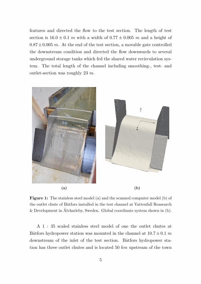
features and directed the flow to the test section. The length of test

section is 16.0 ± 0.1 m with a width of 0.77 ± 0.005 m and a height of

0.87±0.005 m. At the end of the test section, a movable gate controlled

the downstream condition and directed the flow downwards to several

underground storage tanks which fed the shared water recirculation sys-

tem. The total length of the channel including smoothing-, test- and

outlet-section was roughly 23 m.

(a) (b)

Figure 1: The stainless steel model (a) and the scanned computer model (b) of

the outlet chute of Batfors installed in the test channel at Vattenfall Reasearch

& Development in Alvkarleby, Sweden. Global coordinate system shown in (b).

A 1 : 35 scaled stainless steel model of one the outlet chutes at

Batfors hydropower station was mounted in the channel at 10.7± 0.1 m

downstream of the inlet of the test section. Batfors hydropower sta-

tion has three outlet chutes and is located 50 km upstream of the town

5

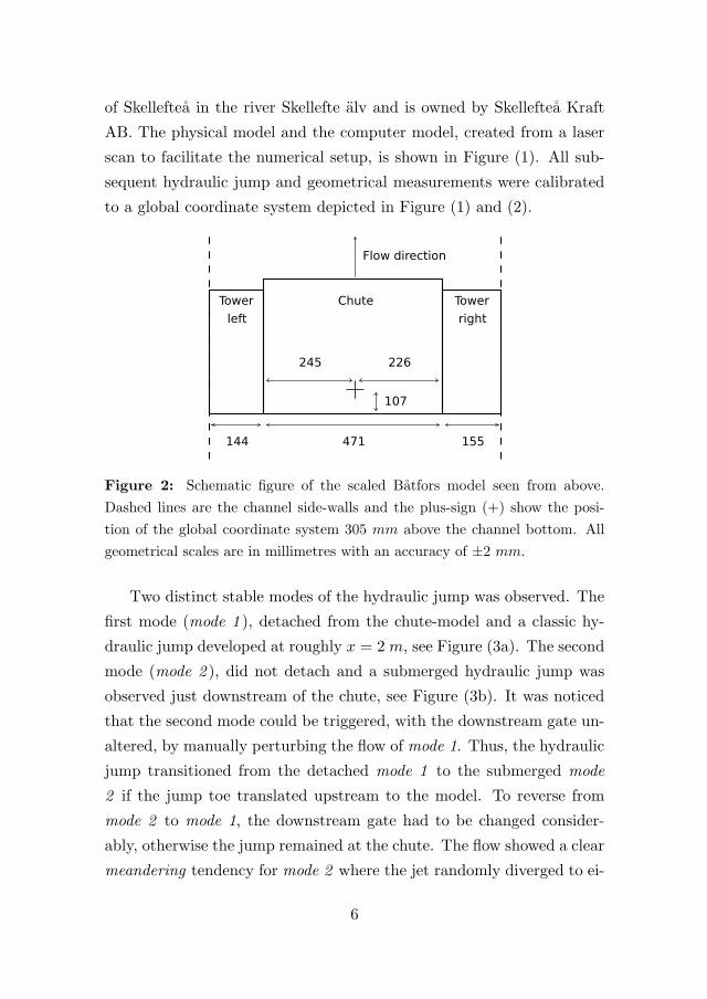
of Skelleftea in the river Skellefte alv and is owned by Skelleftea Kraft

AB. The physical model and the computer model, created from a laser

scan to facilitate the numerical setup, is shown in Figure (1). All sub-

sequent hydraulic jump and geometrical measurements were calibrated

to a global coordinate system depicted in Figure (1) and (2).

Figure 2: Schematic figure of the scaled Batfors model seen from above.

Dashed lines are the channel side-walls and the plus-sign (+) show the posi-

tion of the global coordinate system 305 mm above the channel bottom. All

geometrical scales are in millimetres with an accuracy of ±2 mm.

Two distinct stable modes of the hydraulic jump was observed. The

first mode (mode 1 ), detached from the chute-model and a classic hy-

draulic jump developed at roughly x = 2 m, see Figure (3a). The second

mode (mode 2 ), did not detach and a submerged hydraulic jump was

observed just downstream of the chute, see Figure (3b). It was noticed

that the second mode could be triggered, with the downstream gate un-

altered, by manually perturbing the flow of mode 1. Thus, the hydraulic

jump transitioned from the detached mode 1 to the submerged mode

2 if the jump toe translated upstream to the model. To reverse from

mode 2 to mode 1, the downstream gate had to be changed consider-

ably, otherwise the jump remained at the chute. The flow showed a clear

meandering tendency for mode 2 where the jet randomly diverged to ei-

6

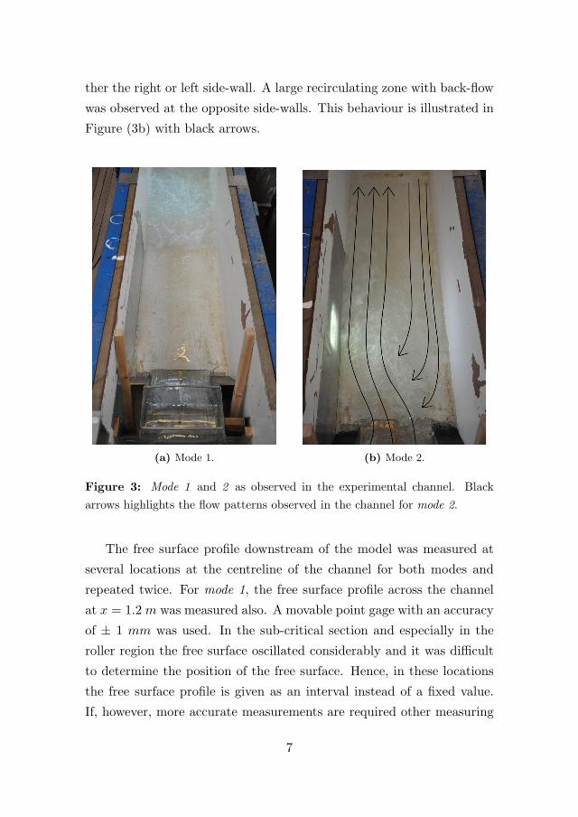
ther the right or left side-wall. A large recirculating zone with back-flow

was observed at the opposite side-walls. This behaviour is illustrated in

Figure (3b) with black arrows.

(a) Mode 1. (b) Mode 2.

Figure 3: Mode 1 and 2 as observed in the experimental channel. Black

arrows highlights the flow patterns observed in the channel for mode 2.

The free surface profile downstream of the model was measured at

several locations at the centreline of the channel for both modes and

repeated twice. For mode 1, the free surface profile across the channel

at x = 1.2 m was measured also. A movable point gage with an accuracy

of ± 1 mm was used. In the sub-critical section and especially in the

roller region the free surface oscillated considerably and it was difficult

to determine the position of the free surface. Hence, in these locations

the free surface profile is given as an interval instead of a fixed value.

If, however, more accurate measurements are required other measuring

7

techniques need to be considered, e.g. ultrasonic displacement meters

or conductivity probes [29].

3 Smoothed Particle Hydrodynamic

SPH is a meshless Lagrangian numerical method proposed indepen-

dently by [14] and [15]. The continuous fluid domain is discretized with

a set of non-connected nodal points or particles scattered in space with

no underlying grid structure. Particles follow the fluid and interact ac-

cording to the discrete Lagrangian Navier-Stokes equations. Besides

representing the fluid domain, particles carry individual information de-

termined by a distance based function usually referred to as the kernel

function. The fundamental principle in SPH is to approximate an arbi-

trary function f(r) by,

f(r) =

∫f(r′)W (r− r′, h)dr′ (1)

where W (r−r′, h) is the kernel function, h is the smoothing length and r

is the distance vector. The integral interpolation is further approximated

by summation interpolation according to,

F (ra) =∑b

mb

ρbF (rb)Wab (2)

where the summation is over all neighbouring particles b and ρb and mb

is the density and mass of particle b, respectively. The kernel function,

Wab, is expressed as a function of the non-dimensional distance s between

particles a and b, i.e. s = |ra−rb|/h. The smoothing length h determines

the size of the volume around particle a where neighbouring particles

are considered. The Wendland Quintic kernel [30] is considered in this

work and is given by,

Wab = αD(1− s2)4(2s+ 1) 0 ≤ s ≤ 2 (3)

where αD = 21/(16πh3) in 3D.

8

3.1 Governing equations

In weakly-compressible SPH the particle mass is constant and density

fluctuates only according to the continuity equation,

1

ρ

Dρ

Dt+∇ · u = 0 (4)

which can be rewritten in SPH-notation as,

dρadt

=∑b

mbuab · ∇aWab (5)

where u is the velocity vector. The momentum equation, which describe

the motion of viscous fluids, can be written as,

Du

Dt= −1

ρ∇P + g + Γ (6)

where P is pressure, g is acceleration due to gravity and Γ are the

dissipative terms. Usually, Γ is represented by the artificial-viscosity

proposed by [31]. However, this approach can be too dissipative and ef-

fect the shear stresses in fluids [32]. Due to the shear flow characteristics

of hydraulic jumps the laminar viscosity and Sub-Particle Scale (SPS)

model is considered instead [22, 24]. The SPS-model is based on the

Large Eddy Simulation (LES) approach [33, 34, 32]. Equation (6) can

then be rewritten in SPH notation as,

Du

Dt=−

∑b

mb

(Pb

ρ2b+

Pa

ρ2a

)∇aWab + g

+∑b

mb

(4ν0rab · ∇aWab

(ρa + ρa)(r2ab + η2

))uab

+∑b

mb

⎛⎝→

τb

ij

ρ2b+

→τa

ij

ρ2a

⎞⎠∇aWab

(7)

where ν0 = 10−6 [m2/s] is the kinematic viscosity of water and η2 =

0.01h2 [35]. In Einstein notation, the shear stress component in i and j

9

direction can be approximated as

→τ ij

ρ= νt

(2Sij − 2

3kδij

)− 2

3ClΔ

2δij |Sij |2 (8)

where→τ ij is the sub-particle stress tensor, νt = [(CsΔl)]2 |S| is the

turbulent eddy viscosity, k the SPS turbulence kinetic energy, Cs =

0.12 the Smagorinsky constant, Cl = 0.0066, Δl the particle to particle

spacing and |S| = 0.5(2SijSij) where Sij is an element of the SPS strain

tensor [36].

3.2 Equation of State

To avoid an expensive computation of the Poisson’s equation and to

keep the explicit nature of the SPH method, an equation-of-state (EOS)

is used to relate the fluid pressure to local particle density [37]. The

pressure is determined by,

P = B

[(ρ

ρ0

)γ

− 1

](9)

where B = c20ρ0/γ, γ = 7, ρ0 = 1000 kg/m3 is the reference density and

c0 = c(ρ0) =√

(∂P/∂ρ) is the speed of sound at the reference density

[38]. To keep the density variation within 1%, the reference speed of

sound c0 was set to 10 times the maximum fluid velocity based on the

initial depth in the upstream tank.

3.3 Time stepping

The explicit, second-order (in time), predictor-corrector based Symplec-

tic algorithm is used for time integration [36] and the time step is de-

termined according to

Δt = Ct ·min (Δtf ,Δtcv) (10)

where Ct = 0.4 is a constant.

Δtf = min(√

h/|fa|)

(11)

10

is based on the force per unit mass |fa| and

Δtcv = mina

⎛⎜⎜⎝ h

cs +maxb

∣∣∣∣ huab·rab(r2ab+η2)

∣∣∣∣

⎞⎟⎟⎠ (12)

which combines the Courant-Fredrich-Levy (CFL) and a viscous condi-

tion [39].

3.4 Corrections

Two types of corrections are applied. Firstly, the density field are

smoothed every 40th time step with a zeroth-order Shepard filter,

ρnewa =∑b

ρbWabmb

ρb=∑b

mbWab (13)

where

Wab =Wab∑

b

Wabmbρb

(14)

to keep the density fluctuations from diverging. Secondly, the SPH-

particles are moved according to the XSPH method proposed by [40]

in order to obtain a more ordered flow and to prevent particles from

penetrating. The change in position is given by,

dradt

= ua + ε∑b

mb

ρabuabWab (15)

where ε = 0.5 and ρab = (ρa + ρb)/2.

3.5 Boundary condition

Solid walls are modelled as fluid particles fixed in space known as the

Dynamic Boundary Condition (DBC) proposed by [41]. Boundary par-

ticles satisfy the same equations as the fluid particles. Hence, a repulsive

force is applied when a fluid particle approach the wall. The boundary is

11

populated by particles in three non-staggered rows to ensure that fluid

particles do not penetrate the boundaries and a complete coverage of

the kernel compact support.

Periodic open boundaries are applied in the up- and downstream end

of the computational model. Particles that leave trough the downstream

end are reintroduced at the upstream end of the computational model

and vice versa. In this study, particle coordinates are changed with fixed

values only.

4 Numerical-model

The geometrical setup of the SPH-model corresponds to the experimen-

tal channel described in the Experimental Section (2). However, due to

computational time considerations the channel length was considerably

shorten. The periodic approach introduced in [24] was adopted, where

the outlet flow is reintroduced in the upstream part of the channel. An

initial guess of where the hydraulic jump is positioned is required for

this method. Hence, two separate models were created for mode 1 and

mode 2 based on the experiments. The dimensions of the SPH-model

and the initial free surface can be seen in Figure (4) and summarized in

Table (1).

The initial spacing between SPH particles was set to dp = 0.01 m

and the smoothing length to h = 1.2∗dp. The gravitational accelerationg = 9.81 m/s2 was set in the negative z-direction (Figure (1,2)) and each

simulation was run until 100 s and saved every 1.0 s. The total number of

particles was 1.2 and 1.4 millions for mode 1 and 2, respectively, and the

total simulation time for both modes was roughly 30 h. All simulation

were performed using DualSPHysics v. 3.0 (http://www.dual.sphysics.org/)

[36] on a single GPU (NVIDIA GeForce GTX TITAN Black).

12

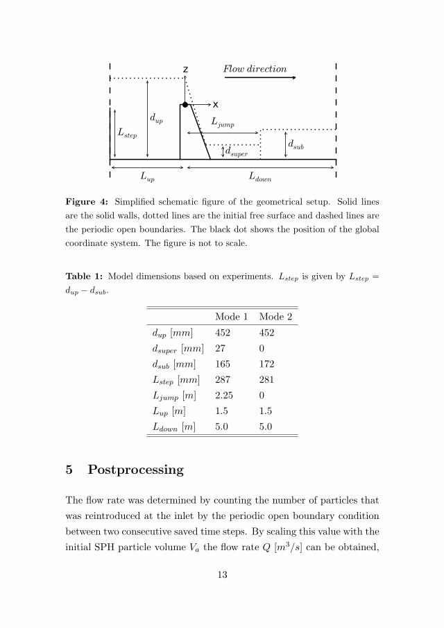
Figure 4: Simplified schematic figure of the geometrical setup. Solid lines

are the solid walls, dotted lines are the initial free surface and dashed lines are

the periodic open boundaries. The black dot shows the position of the global

coordinate system. The figure is not to scale.

Table 1: Model dimensions based on experiments. Lstep is given by Lstep =

dup − dsub.

Mode 1 Mode 2

dup [mm] 452 452

dsuper [mm] 27 0

dsub [mm] 165 172

Lstep [mm] 287 281

Ljump [m] 2.25 0

Lup [m] 1.5 1.5

Ldown [m] 5.0 5.0

5 Postprocessing

The flow rate was determined by counting the number of particles that

was reintroduced at the inlet by the periodic open boundary condition

between two consecutive saved time steps. By scaling this value with the

initial SPH particle volume Va the flow rate Q [m3/s] can be obtained,

13

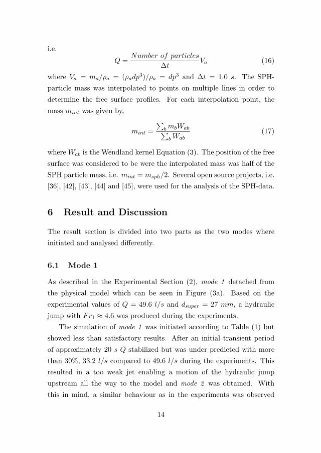
i.e.

Q =Number of particles

ΔtVa (16)

where Va = ma/ρa = (ρadp3)/ρa = dp3 and Δt = 1.0 s. The SPH-

particle mass was interpolated to points on multiple lines in order to

determine the free surface profiles. For each interpolation point, the

mass mint was given by,

mint =

∑bmbWab∑bWab

(17)

where Wab is the Wendland kernel Equation (3). The position of the free

surface was considered to be were the interpolated mass was half of the

SPH particle mass, i.e. mint = msph/2. Several open source projects, i.e.

[36], [42], [43], [44] and [45], were used for the analysis of the SPH-data.

6 Result and Discussion

The result section is divided into two parts as the two modes where

initiated and analysed differently.

6.1 Mode 1

As described in the Experimental Section (2), mode 1 detached from

the physical model which can be seen in Figure (3a). Based on the

experimental values of Q = 49.6 l/s and dsuper = 27 mm, a hydraulic

jump with Fr1 ≈ 4.6 was produced during the experiments.

The simulation of mode 1 was initiated according to Table (1) but

showed less than satisfactory results. After an initial transient period

of approximately 20 s Q stabilized but was under predicted with more

than 30%, 33.2 l/s compared to 49.6 l/s during the experiments. This

resulted in a too weak jet enabling a motion of the hydraulic jump

upstream all the way to the model and mode 2 was obtained. With

this in mind, a similar behaviour as in the experiments was observed

14

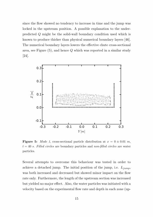
since the flow showed no tendency to increase in time and the jump was

locked in the upstream position. A possible explanation to the under-

predicted Q might be the solid-wall boundary condition used which is

known to produce thicker than physical numerical boundary layers [46].

The numerical boundary layers lowers the effective chute cross-sectional

area, see Figure (5), and hence Q which was reported in a similar study

[24].

Figure 5: Mode 1, cross-sectional particle distribution at x = 0 ± 0.01 m,

t = 40 s. Filled circles are boundary particles and non-filled circles are water

particles.

Several attempts to overcome this behaviour was tested in order to

achieve a detached jump. The initial position of the jump, i.e. Ljump,

was both increased and decreased but showed minor impact on the flow

rate only. Furthermore, the length of the upstream section was increased

but yielded no major effect. Also, the water particles was initiated with a

velocity based on the experimental flow rate and depth in each zone (up-

15

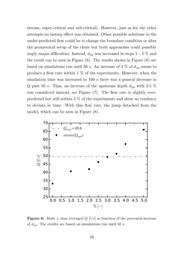
stream, super-critical and sub-critical). However, just as for the other

attempts no lasting effect was obtained. Other possible solutions to the

under-predicted flow could be to change the boundary condition or alter

the geometrical setup of the chute but both approaches could possibly

imply major difficulties. Instead, dup was increased in steps 1−5 % and

the result can be seen in Figure (6). The results shown in Figure (6) are

based on simulations run until 50 s. An increase of 3 % of dup seems to

produce a flow rate within 1 % of the experiments. However, when the

simulation time was increased to 100 s there was a general decrease in

Q past 50 s. Thus, an increase of the upstream depth dup with 3.5 %

was considered instead, see Figure (7). The flow rate is slightly over-

predicted but still within 5 % of the experiments and show no tendency

to deviate in time. With this flow rate, the jump detached from the

model, which can be seen in Figure (8).

Figure 6: Mode 1, time averaged Q [l/s] as function of the percental increase

of dup. The results are based on simulations run until 50 s.

16

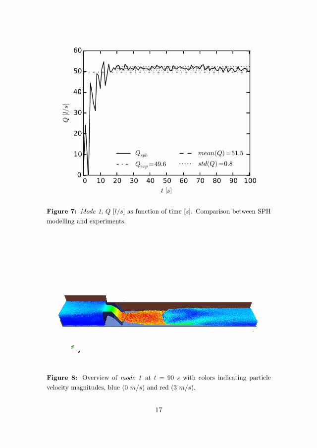
Figure 7: Mode 1, Q [l/s] as function of time [s]. Comparison between SPH

modelling and experiments.

Figure 8: Overview of mode 1 at t = 90 s with colors indicating particle

velocity magnitudes, blue (0 m/s) and red (3 m/s).

17

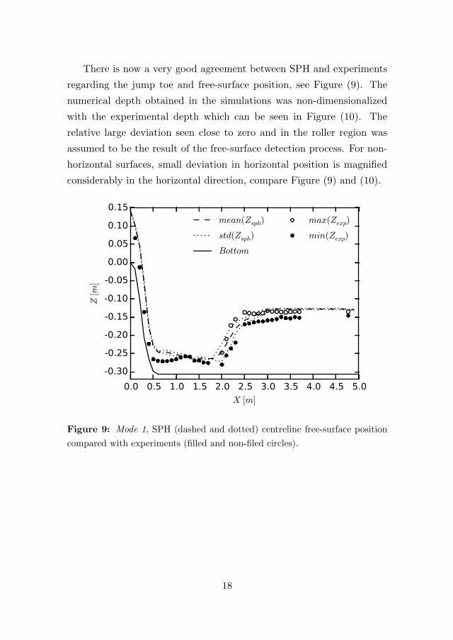
There is now a very good agreement between SPH and experiments

regarding the jump toe and free-surface position, see Figure (9). The

numerical depth obtained in the simulations was non-dimensionalized

with the experimental depth which can be seen in Figure (10). The

relative large deviation seen close to zero and in the roller region was

assumed to be the result of the free-surface detection process. For non-

horizontal surfaces, small deviation in horizontal position is magnified

considerably in the horizontal direction, compare Figure (9) and (10).

Figure 9: Mode 1, SPH (dashed and dotted) centreline free-surface position

compared with experiments (filled and non-filed circles).

18

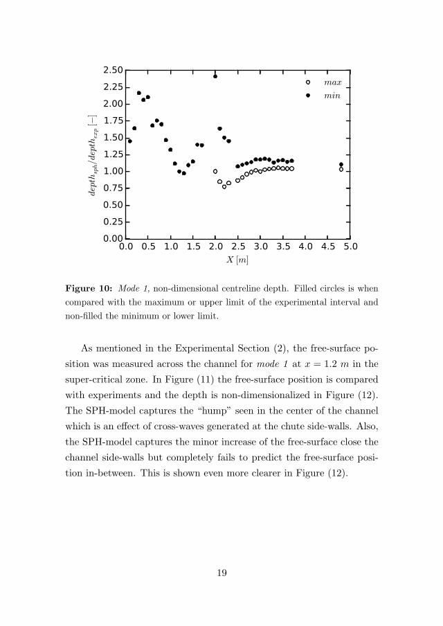
Figure 10: Mode 1, non-dimensional centreline depth. Filled circles is when

compared with the maximum or upper limit of the experimental interval and

non-filled the minimum or lower limit.

As mentioned in the Experimental Section (2), the free-surface po-

sition was measured across the channel for mode 1 at x = 1.2 m in the

super-critical zone. In Figure (11) the free-surface position is compared

with experiments and the depth is non-dimensionalized in Figure (12).

The SPH-model captures the “hump” seen in the center of the channel

which is an effect of cross-waves generated at the chute side-walls. Also,

the SPH-model captures the minor increase of the free-surface close the

channel side-walls but completely fails to predict the free-surface posi-

tion in-between. This is shown even more clearer in Figure (12).

19

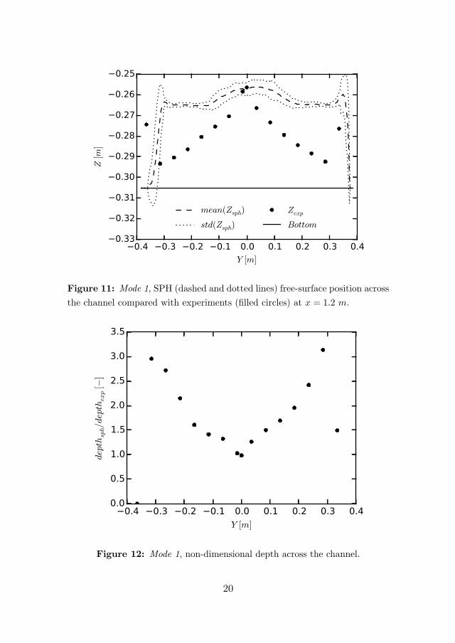
Figure 11: Mode 1, SPH (dashed and dotted lines) free-surface position across

the channel compared with experiments (filled circles) at x = 1.2 m.

Figure 12: Mode 1, non-dimensional depth across the channel.

20

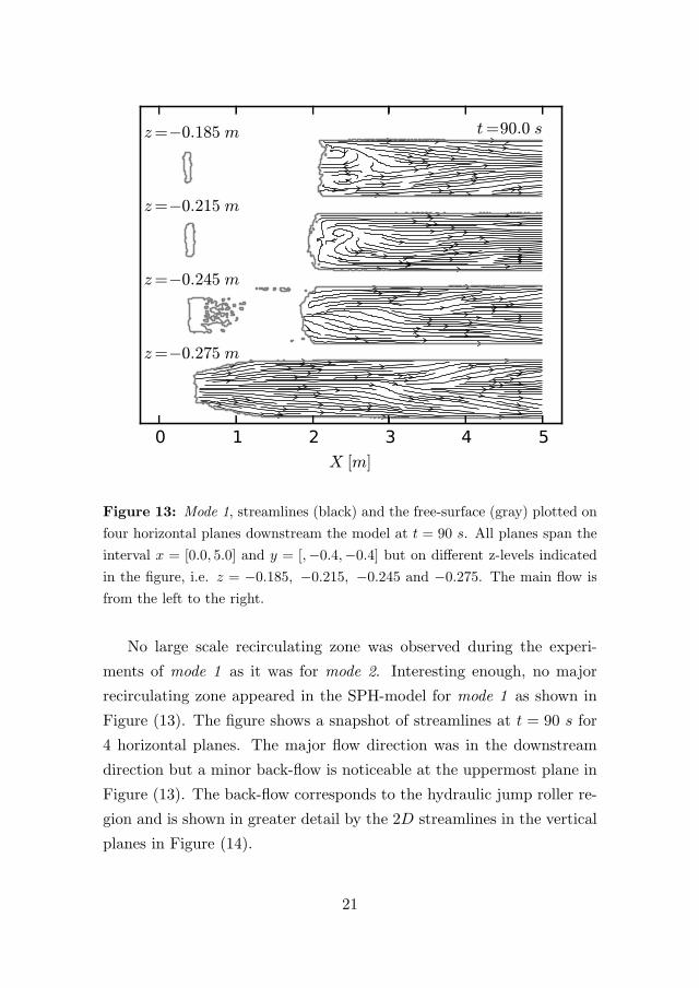
Figure 13: Mode 1, streamlines (black) and the free-surface (gray) plotted on

four horizontal planes downstream the model at t = 90 s. All planes span the

interval x = [0.0, 5.0] and y = [,−0.4,−0.4] but on different z-levels indicated

in the figure, i.e. z = −0.185, −0.215, −0.245 and −0.275. The main flow is

from the left to the right.

No large scale recirculating zone was observed during the experi-

ments of mode 1 as it was for mode 2. Interesting enough, no major

recirculating zone appeared in the SPH-model for mode 1 as shown in

Figure (13). The figure shows a snapshot of streamlines at t = 90 s for

4 horizontal planes. The major flow direction was in the downstream

direction but a minor back-flow is noticeable at the uppermost plane in

Figure (13). The back-flow corresponds to the hydraulic jump roller re-

gion and is shown in greater detail by the 2D streamlines in the vertical

planes in Figure (14).

21

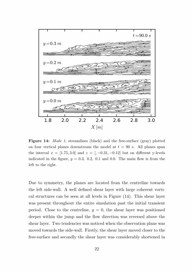
Figure 14: Mode 1, streamlines (black) and the free-surface (gray) plotted

on four vertical planes downstream the model at t = 90 s. All planes span

the interval x = [1.75, 3.0] and z = [,−0.31,−0.12] but on different y-levels

indicated in the figure, y = 0.3, 0.2, 0.1 and 0.0. The main flow is from the

left to the right.

Due to symmetry, the planes are located from the centreline towards

the left side-wall. A well defined shear layer with large coherent vorti-

cal structures can be seen at all levels in Figure (14). This shear layer

was present throughout the entire simulation past the initial transient

period. Close to the centreline, y = 0, the shear layer was positioned

deeper within the jump and the flow direction was reversed above the

shear layer. Two tendencies was noticed when the observation plane was

moved towards the side-wall. Firstly, the shear layer moved closer to the

free-surface and secondly the shear layer was considerably shortened in

22

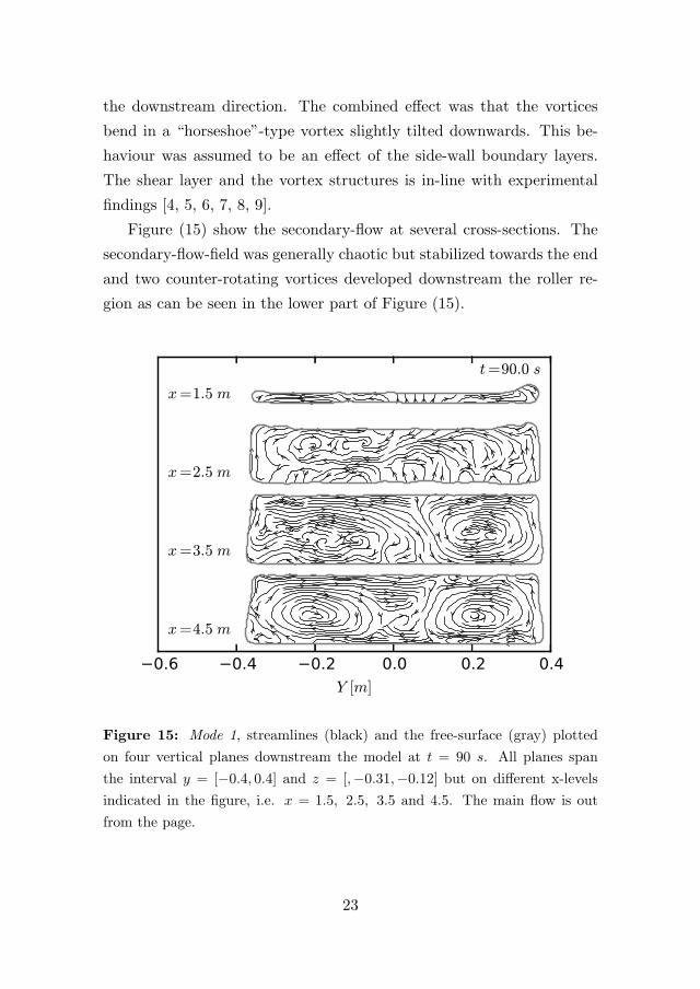
the downstream direction. The combined effect was that the vortices

bend in a “horseshoe”-type vortex slightly tilted downwards. This be-

haviour was assumed to be an effect of the side-wall boundary layers.

The shear layer and the vortex structures is in-line with experimental

findings [4, 5, 6, 7, 8, 9].

Figure (15) show the secondary-flow at several cross-sections. The

secondary-flow-field was generally chaotic but stabilized towards the end

and two counter-rotating vortices developed downstream the roller re-

gion as can be seen in the lower part of Figure (15).

Figure 15: Mode 1, streamlines (black) and the free-surface (gray) plotted

on four vertical planes downstream the model at t = 90 s. All planes span

the interval y = [−0.4, 0.4] and z = [,−0.31,−0.12] but on different x-levels

indicated in the figure, i.e. x = 1.5, 2.5, 3.5 and 4.5. The main flow is out

from the page.

23

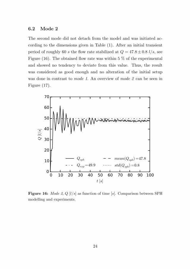
6.2 Mode 2

The second mode did not detach from the model and was initiated ac-

cording to the dimensions given in Table (1). After an initial transient

period of roughly 60 s the flow rate stabilized at Q = 47.8± 0.8 l/s, see

Figure (16). The obtained flow rate was within 5 % of the experimental

and showed no tendency to deviate from this value. Thus, the result

was considered as good enough and no alteration of the initial setup

was done in contrast to mode 1. An overview of mode 2 can be seen in

Figure (17).

Figure 16: Mode 2, Q [l/s] as function of time [s]. Comparison between SPH

modelling and experiments.

24

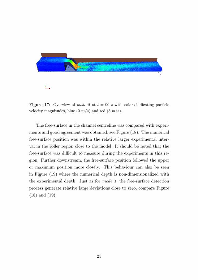
Figure 17: Overview of mode 2 at t = 90 s with colors indicating particle

velocity magnitudes, blue (0 m/s) and red (3 m/s).

The free-surface in the channel centreline was compared with experi-

ments and good agreement was obtained, see Figure (18). The numerical

free-surface position was within the relative larger experimental inter-

val in the roller region close to the model. It should be noted that the

free-surface was difficult to measure during the experiments in this re-

gion. Further downstream, the free-surface position followed the upper

or maximum position more closely. This behaviour can also be seen

in Figure (19) where the numerical depth is non-dimensionalized with

the experimental depth. Just as for mode 1, the free-surface detection

process generate relative large deviations close to zero, compare Figure

(18) and (19).

25

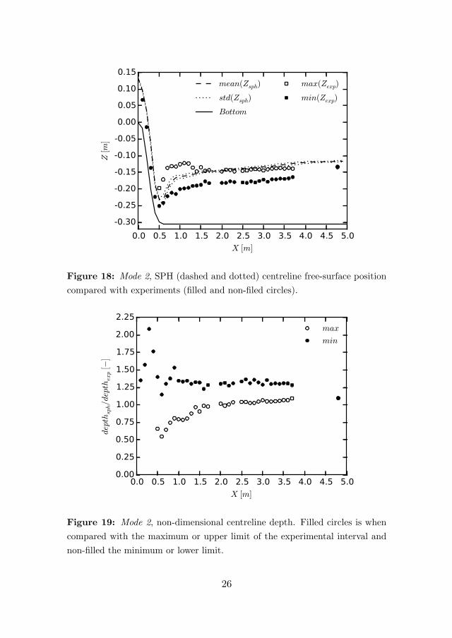
Figure 18: Mode 2, SPH (dashed and dotted) centreline free-surface position

compared with experiments (filled and non-filed circles).

Figure 19: Mode 2, non-dimensional centreline depth. Filled circles is when

compared with the maximum or upper limit of the experimental interval and

non-filled the minimum or lower limit.

26

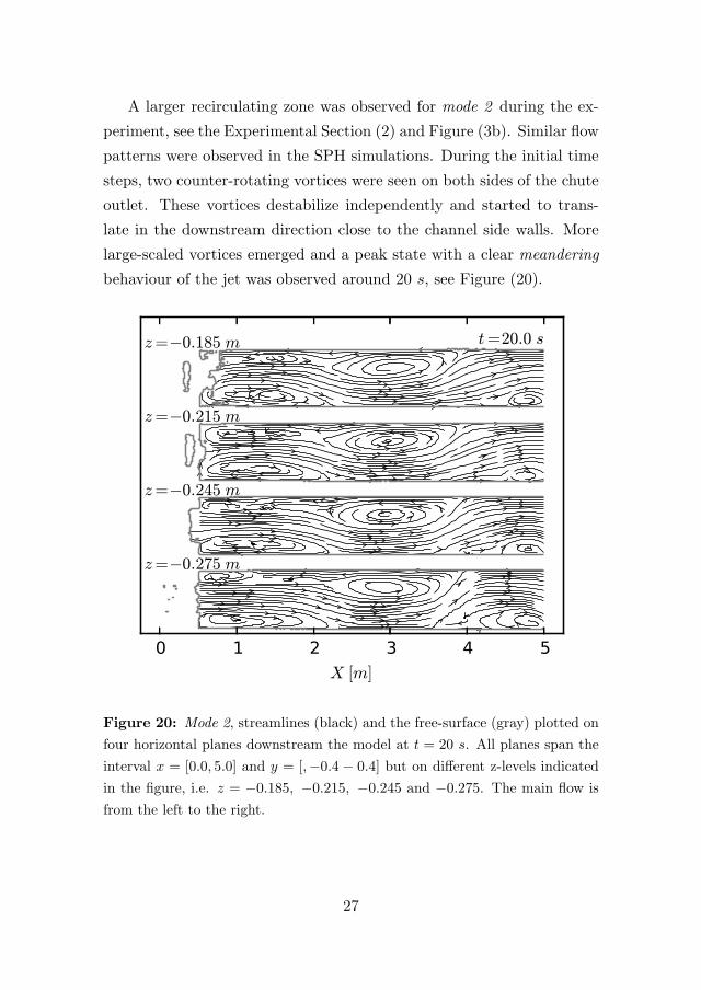
A larger recirculating zone was observed for mode 2 during the ex-

periment, see the Experimental Section (2) and Figure (3b). Similar flow

patterns were observed in the SPH simulations. During the initial time

steps, two counter-rotating vortices were seen on both sides of the chute

outlet. These vortices destabilize independently and started to trans-

late in the downstream direction close to the channel side walls. More

large-scaled vortices emerged and a peak state with a clear meandering

behaviour of the jet was observed around 20 s, see Figure (20).

Figure 20: Mode 2, streamlines (black) and the free-surface (gray) plotted on

four horizontal planes downstream the model at t = 20 s. All planes span the

interval x = [0.0, 5.0] and y = [,−0.4 − 0.4] but on different z-levels indicated

in the figure, i.e. z = −0.185, −0.215, −0.245 and −0.275. The main flow is

from the left to the right.

27

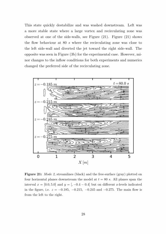
This state quickly destabilize and was washed downstream. Left was

a more stable state where a large vortex and recirculating zone was

observed at one of the side-walls, see Figure (21). Figure (21) shows

the flow behaviour at 80 s where the recirculating zone was close to

the left side-wall and diverted the jet toward the right side-wall. The

opposite was seen in Figure (3b) for the experimental case. However, mi-

nor changes to the inflow conditions for both experiments and numerics

changed the preferred side of the recirculating zone.

Figure 21: Mode 2, streamlines (black) and the free-surface (gray) plotted on

four horizontal planes downstream the model at t = 80 s. All planes span the

interval x = [0.0, 5.0] and y = [,−0.4 − 0.4] but on different z-levels indicated

in the figure, i.e. z = −0.185, −0.215, −0.245 and −0.275. The main flow is

from the left to the right.

28

7 Conclusion

The aim of this study was to investigate the applicability of the SPH

method when conducting 3D hydraulic jump simulations. We have

shown, based on experiments in a channel with a downscaled physi-

cal model that the SPH-method is able to capture several flow features.

Two SPH set-ups were created to investigate the two stable modes ob-

served in the experiment.

For the detached mode 1, initial results was non-satisfactory in terms

of flow rate and jump toe positions. However, the SPH-model showed

that it could capture the transitional behaviour between mode 1 and

mode 2. An increase of 3.5 % of the upstream depth generated the

correct behaviour of mode 1 as the jump toe detached and the flow

rate was within 5 % of the experiments. The free-surface position in

the centreline as wells as across the channel was in good agreement

with experiments. Even small scale features in the super-critical zone,

i.e. the “hump” generated by cross-waves at the chute side-walls was

captured. However, the lowered depth closer to the channel side-walls

was not obtained. It was also shown that the SPH-model was able

to capture the internal flow structures of a hydraulic jump as several

vortical structures was seen in a well defined shear layer in the roller

region.

The second mode required no alteration of the initial set-up and the

flow rate was within 5 % of the experiments. The free-surface position

was well within the experimental interval. The large scale recirculation

zone observed close to one of the channel side-walls was also captured

by the SPH-model.

Overall, the SPH-model is able to capture the major features ob-

served in experiments which strengthen the general validity of the SPH-

mehod. However, further studies focusing on the internal flow structures

and the dynamics would be beneficial to the understanding of hydraulic

jumps.

29

Acknowledgement

The research presented was carried out as a part of “Swedish Hydropower

Centre - SVC”. SVC has been established by the Swedish Energy Agency,

Elforsk and Svenska Kraftnat together with Lulea University of Technol-

ogy, KTH Royal Institute of Technology, Chalmers University of Tech-

nology and Uppsala University. www.svc.nu.

The authors would like to thank the staff at Vattenfall Research &

Development and Skelleftea Kraft AB for all the help and support during

measurements.

References

[1] Ven Te Chow. Open-channel hydraulics. McGraw-Hill, Tokyo, 1959. ISBN

0-07-010776-9.

[2] Hubert Chanson. The hydraulics of open channel flow an introduction :

basic principles, sediment motion, hydraulic modelling, design of hydraulic

structures. Amsterdam ; London : Elsevier Butterworth-Heinemann, Am-

sterdam ; London, 2nd ed.. edition, 2004.

[3] Hubert Chanson. Current knowledge in hydraulic jumps and related phe-

nomena. a survey of experimental results. European Journal of Mechanics

- B/Fluids, 28(2):191–210, mar 2009. doi: 10.1016/j.euromechflu.2008.06.

004.

[4] Jack W. Hoyt and R. H. J. Sellin. Hydraulic jump as “mixing layer”.

Journal of Hydraulic Engineering, 115(12):1607–1614, dec 1989. doi: 10.

1061/(asce)0733-9429(1989)115:12(1607).

[5] Hans G. Hornung, Christian Willert, and Stewart Turner. The flow field

downstream of a hydraulic jump. J. Fluid Mech., 287(-1):299, mar 1995.

doi: 10.1017/s0022112095000966.

[6] Michele Mossa and Umberto Tolve. Flow visualization in bubbly two-

phase hydraulic jump. Journal of Fluids Engineering, 120(1):160, 1998.

doi: 10.1115/1.2819641.

30

[7] S. K. Misra, J. T. Kirby, M. Brocchini, F. Veron, M. Thomas, and

C. Kambhamettu. The mean and turbulent flow structure of a weak

hydraulic jump. Physics of Fluids, 20(3):035106, 2008. doi: 10.1063/

1.2856269.

[8] Javier Rodrıguez-Rodrıguez, Carolina Marugan-Cruz, Alberto Aliseda,

and Juan Carlos Lasheras. Dynamics of large turbulent structures in a

steady breaker. Experimental Thermal and Fluid Science, 35(2):301–310,

feb 2011. doi: 10.1016/j.expthermflusci.2010.09.012.

[9] Gangfu Zhang, Hang Wang, and Hubert Chanson. Turbulence and aer-

ation in hydraulic jumps: free-surface fluctuation and integral turbulent

scale measurements. Environmental Fluid Mechanics, 13(2):189–204, sep

2012. doi: 10.1007/s10652-012-9254-3.

[10] Damien Violeau. Fluid Mechanics and the SPH Method. Oxford University

Press, may 2012. doi: 10.1093/acprof:oso/9780199655526.001.0001.

[11] Ruben Scardovelli and Stephane Zaleski. DIRECT NUMERICAL SIMU-

LATION OF FREE-SURFACE AND INTERFACIAL FLOW. Annu. Rev.

Fluid Mech., 31(1):567–603, jan 1999. doi: 10.1146/annurev.fluid.31.1.567.

[12] Jingsen Ma, Assad A. Oberai, Richard T. Lahey, and Donald A. Drew.

Modeling air entrainment and transport in a hydraulic jump using two-

fluid RANS and DES turbulence models. Heat and Mass Transfer, 47(8):

911–919, jul 2011. doi: 10.1007/s00231-011-0867-8.

[13] AdamWitt, John Gulliver, and Lian Shen. Simulating air entrainment and

vortex dynamics in a hydraulic jump. International Journal of Multiphase

Flow, 72:165–180, jun 2015. doi: 10.1016/j.ijmultiphaseflow.2015.02.012.

[14] R. A. Gingold and J. J. Monaghan. Smoothed particle hydrodynamics:

theory and application to non-spherical stars. Monthly Notices of the Royal

Astronomical Society, 181(3):375–389, dec 1977. doi: 10.1093/mnras/181.

3.375.

[15] L. B. Lucy. A numerical approach to the testing of the fission hypothesis.

The Astronomical Journal, 82:1013, dec 1977. doi: 10.1086/112164.

[16] J. J. Monaghan. Smoothed particle hydrodynamics. Annual Review of As-

tronomy and Astrophysics, 30(1):543–574, sep 1992. doi: 10.1146/annurev.

aa.30.090192.002551.

31

[17] J.J. Monaghan. Smoothed particle hydrodynamics and its diverse ap-

plications. Annu. Rev. Fluid Mech., 44(1):323–346, jan 2012. doi:

10.1146/annurev-fluid-120710-101220.

[18] David Lopez, Roberto Marivela, and Luis Garrote. Smoothed particle

hydrodynamics model applied to hydraulic structures: a hydraulic jump

test case. Journal of Hydraulic Research, 48(sup1):142–158, jan 2010. doi:

10.1080/00221686.2010.9641255.

[19] P. Jonsson, P. Jonsen, P. Andreasson, T.S. Lundstrom, and J.G.I. Hell-

strom. Smoothed particle hydrodynamics modeling of hydraulic jumps.

In Proceedings of Particle-Based Methods II - Fundamentals and Applica-

tions, pages 490–501, Barcelona, Spain, 2011.

[20] I. Federico, S. Marrone, A. Colagrossi, F. Aristodemo, and M. Antuono.

Simulating 2d open-channel flows through an SPH model. European

Journal of Mechanics - B/Fluids, 34:35–46, jul 2012. doi: 10.1016/j.

euromechflu.2012.02.002.

[21] Martin Lastiwka, Mihai Basa, and Nathan J. Quinlan. Permeable and

non-reflecting boundary conditions in SPH. Int. J. Numer. Meth. Fluids,

61(7):709–724, nov 2009. doi: 10.1002/fld.1971.

[22] Ming-Jyh Chern and Sam Syamsuri. Effect of corrugated bed on hydraulic

jump characteristic using SPH method. Journal of Hydraulic Engineering,

139(2):221–232, feb 2013. doi: 10.1061/(asce)hy.1943-7900.0000618.

[23] Diana De Padova, Michele Mossa, Stefano Sibilla, and Emanuela Torti.

3d SPH modelling of hydraulic jump in a very large channel. Journal of

Hydraulic Research, 51(2):158–173, apr 2013. doi: 10.1080/00221686.2012.

736883.

[24] P. Jonsson, P. Andreasson, J.G.I. Hellstrom, P. Jonse, and T.S. Lund-

strom. Smoothed particle hydrodynamic simulation of hydraulic jump

using periodic open boundaries. Submitted to Applied Mathematical Mod-

elling 2015.

[25] Angela Ferrari. SPH simulation of free surface flow over a sharp-crested

weir. Advances in Water Resources, 33(3):270–276, mar 2010. doi: 10.

1016/j.advwatres.2009.12.005.

32

[26] Sarhang M. Husain, Jowhar R. Muhammed, Harshinie U. Karunarathna,

and Dominic E. Reeve. Investigation of pressure variations over stepped

spillways using smooth particle hydrodynamics. Advances in Water Re-

sources, 66:52–69, apr 2014. doi: 10.1016/j.advwatres.2013.11.013.

[27] Kate Saunders, Mahesh Prakash, Paul W. Cleary, and Mark Cordell. Ap-

plication of smoothed particle hydrodynamics for modelling gated spillway

flows. Applied Mathematical Modelling, 38(17-18):4308–4322, sep 2014.

doi: 10.1016/j.apm.2014.05.008.

[28] EUN-SUG LEE. Application of weakly compressible and truly incom-

pressible SPH to 3-d water collapse in waterworks. JHR, 48(extra):000,

2009. doi: 10.3826/jhr.2010.0003.

[29] Yann Chachereau and Hubert Chanson. Free-surface fluctuations and

turbulence in hydraulic jumps. Experimental Thermal and Fluid Science,

35(6):896–909, sep 2011. doi: 10.1016/j.expthermflusci.2011.01.009.

[30] Holger Wendland. Piecewise polynomial, positive definite and compactly

supported radial functions of minimal degree. Adv Comput Math, 4(1):

389–396, dec 1995. doi: 10.1007/bf02123482.

[31] J. J. Monaghan. Smoothed particle hydrodynamics. Annual Review of As-

tronomy and Astrophysics, 30(1):543–574, sep 1992. doi: 10.1146/annurev.

aa.30.090192.002551.

[32] R.A. Dalrymple and B.D. Rogers. Numerical modeling of water waves

with the SPH method. Coastal Engineering, 53(2-3):141–147, feb 2006.

doi: 10.1016/j.coastaleng.2005.10.004.

[33] H. Gotoh, T. Shibihara, and M. Hayashii. Subparticle-scale model for the

MPS method-lagrangian flow model for hydraulic engineering. Comput.

Fluid Dynam. J., 09:339–347, 2001.

[34] Edmond Y.M. Lo and Songdong Shao. Simulation of near-shore solitary

wave mechanics by an incompressible SPH method. Applied Ocean Re-

search, 24(5):275–286, oct 2002. doi: 10.1016/s0141-1187(03)00002-6.

[35] Joseph P. Morris, Patrick J. Fox, and Yi Zhu. Modeling low reynolds num-

ber incompressible flows using SPH. Journal of Computational Physics,

136(1):214–226, sep 1997. doi: 10.1006/jcph.1997.5776.

33

[36] A.J.C. Crespo, J.M. Domınguez, B.D. Rogers, M. Gomez-Gesteira,

S. Longshaw, R. Canelas, R. Vacondio, A. Barreiro, and O. Garcıa-Feal.

DualSPHysics: Open-source parallel CFD solver based on smoothed parti-

cle hydrodynamics (SPH). Computer Physics Communications, 187:204–

216, feb 2015. doi: 10.1016/j.cpc.2014.10.004.

[37] J.J. Monaghan. Simulating free surface flows with SPH. Journal of Com-

putational Physics, 110(2):399–406, feb 1994. doi: 10.1006/jcph.1994.1034.

[38] George Keith Batchelor. An introduction to fluid dynamics. Cambridge

University Press, London, 1967.

[39] J. J. Monaghan and A. Kos. Solitary waves on a cretan beach. J.

Waterway, Port, Coastal, Ocean Eng., 125(3):145–155, may 1999. doi:

10.1061/(asce)0733-950x(1999)125:3(145).

[40] J.J. Monaghan. On the problem of penetration in particle methods.

Journal of Computational Physics, 82(1):1–15, may 1989. doi: 10.1016/

0021-9991(89)90032-6.

[41] A. J. Crespo, M. Gomez-Gesteira, and R. A. Dalrymple. Boundary con-

ditions generated by dynamic particles in sph methods. Computers, ma-

terials and continua, 5(3):173–184, 2007. doi: 10.3970/cmc.2007.005.173.

[42] Fernando Perez and Brian E. Granger. IPython: A system for interactive

scientific computing. Computing in Science & Engineering, 9(3):21–29,

2007. doi: 10.1109/mcse.2007.53.

[43] John D. Hunter. Matplotlib: A 2d graphics environment. Computing in

Science & Engineering, 9(3):90–95, 2007. doi: 10.1109/mcse.2007.55.

[44] Stefan Behnel, Robert Bradshaw, Craig Citro, Lisandro Dalcin,

Dag Sverre Seljebotn, and Kurt Smith. Cython: The best of both

worlds. Computing in Science & Engineering, 13(2):31–39, mar 2011. doi:

10.1109/mcse.2010.118.

[45] S. van der Walt, S.C. Colbert, and G. Varoquaux. The NumPy array:

A structure for efficient numerical computation. Computing in Science &

Engineering, 13(2):22–30, mar 2011. doi: 10.1109/mcse.2011.37.

[46] Moncho Gomez-Gesteira, Benedict D. Rogers, Robert A. Dalrymple, and

Alex J.C. Crespo. State-of-the-art of classical SPH for free-surface flows.

34

Journal of Hydraulic Research, 48(sup1):6–27, jan 2010. doi: 10.1080/

00221686.2010.9641242.

35

Paper F

A Three-Dimensional Smoothed

Particle Hydrodynamic Study of Free

Surface Fluctuations and Internal

Flow Structures in Hydraulic Jumps

A Three-Dimensional Smoothed

Particle Hydrodynamic Study of Free

Surface Fluctuations and Internal Flow

Structures in Hydraulic Jumps

Patrick Jonsson1, Patrik Andreasson1, J. Gunnar I. Hellstrom1, Par

Jonsen2 and T. Staffan Lundstrom1

1Division of Fluid and Experimental Mechanics, Lulea University of

Technology (LTU), Lulea, SE-971 87, Sweden2Division of Mechanics of Solid Materials, Lulea University of Technology

(LTU), Lulea, SE-971 87, Sweden

Manuscript

Abstract

This study focus on the ability of Smoothed Particle Hydrody-

namics to capture the dynamic relationship of the free surface and

the internal flow field in hydraulic jumps. A hydraulic jump is

a sudden and turbulent transition from supercirtical to subcriti-

cal flow and is a utilized feature to dissipate high kinetic flow in

spillways connected to hydropower dams. In this study a 3D,

laboratory scaled SPH-model of a classical bottom outlet with

periodic boundaries was used. Four cases with different Froude

number was investigated and, in general, cases with lower Froude

numbers showed better results than higher. The flow fields of the

lower Froude cases displayed a clear shear layer with large vor-

tical structures in good agreement with experiments. The free

1

surface behaviour was in good agreement in the roller region but

the fluctuations was damped significantly further downstream. Al-

most the same frequencies was found for the vertical free surface

and velocity component fluctuation which agreed well with exper-

iment. However, poor agreement was found for the jump toe and

horizontal velocity component. Finally, the convective velocity of

the large vortical structures was determined by two point cross-

correlation and was well within the experimental variation.

Keywords: Smoothed Particles Hydrodynamics, SPH, hydraulic jump,

free surface fluctuations

1 Introduction

In an open channel, a hydraulic jump is the sudden and rapid transition

from supercritical to subcritical flow. The transition is extremely turbu-

lent and associated with turbulent energy dissipation, air entrainment,

surface waves and spray and it is characterized by strong dissipative pro-

cesses. Hydraulic jumps occur both in natural streams and in engineered

open channels. Spillways connected to hydropower dams utilize the dis-

sipative processes in hydraulic jumps to reduce high kinetic energy flow.

Usually, spillways are engaged to safely pass extreme flooding events and

redirect the flow during maintenance shut-down of the production units,

i.e. turbines and generators. Furthermore, the physical dimensions and

flow rate considering hydropower applications are commonly very large

especially in spillway flow. Potentially, high velocity flow can cause ero-

sion and reduce the life-time and increase maintenance of spillways and

related structures. Hence, it is vital to understand and have the ability

to predict the involved processes present in a hydraulic jump.

Based on the approaching Froude number (Fr1 = u1/√gd1) where g

are the acceleration due to gravity and u1 and d1 are the supercritical jet

velocity and depth respectively, hydraulic jumps can be classified into

five types: undular Fr1 = 1.0 − 1.7, weak Fr1 = 1.7 − 2.5, oscillating

2

Fr1 = 2.5− 4.5, steady Fr1 = 4.5− 9.0 and strong Fr1 => 9.0 [1]. The

location were the jump initiate is usually referred to as the jump toe and

is the most upstream position of the turbulent and bubbly region known

as the roller. The hydraulic jump has been studied for a long time, but

the internal processes in the roller have been difficult to measure due

the high concentration of entrapped air.

However, first to study the velocity field in hydraulic jump was Rouse

et al. [2], who performed hot-wire measurements in an air duct shaped

to resemble a typical hydraulic jump. Rajaratnam [3] measured with

a pitot-tube the mean velocity field away from the roller in an actual

hydraulic jump. Hoyt and Sellin [4], suggested that a hydraulic jump

could be described as a mixing layer and showed the similarity with a

gas-mixing layer. The authors also described a periodic shedding of large

vortices at a given frequency and a merging processes where vortices

tend to braid around each other. Long et al. [5] argued that the roller

was made up of several anti-clockwise rotating vortices which increased

in size as they moved in the downstream direction by a vortex pairing

mechanism. The growth of vortices eventually caused a upstream spill of

water and the vortex behaviour was linked with jump toe fluctuations.

Long et al. [5] showed also by a Fourier analysis that the dominant

jump toe frequencies was roughly 0.5 Hz for Fr1 = 4 − 9. Hornung

et al. [6] investigated the flow field in the roller using Particle Imaging

Velocimetry (PIV) and showed that a strong but unstable shear layer

with distinct vortical structures were present. The authors discussed also

several vorticity generating mechanism where one being a breaking wave

example and the difficulties of data acquisition in a highly disturbed

multiphase flows. Lennon & Hill [7] measured, using PIV, both the

mean and turbulent velocity field in low Froude number jumps Fr1 =

1.37 − 2.99 and discussed as Hornung et al. [6] the limitations of the

optical technique in highly aerated flows.

Due to the multiphase nature of the hydraulic jump, few experimen-

3

tal studies has been able to show the instantaneous flow field of the roller.

However, the work of Rodrıguez-Rodrıguez et al. [8] and Lin et al. [9]

where the Bubble Image Velocimetry (BIV) technique was used disclosed

large instantaneous coherent structures within the roller region. Lin et

al. [9] showed that different types of zones inside the roller was present

for different types of jumps, i.e. different Fr1. Starting from the bot-

tom, both weak and steady jumps are divided into a boundary layer, a

jet core and a mixing layer. On top of the mixing layer, a recirculating

zone was observed for steady jumps only. Rodrıguez-Rodrıguez et al. [8]

studied hydraulic jumps with Fr1 = 1.44 − 2.29. Their results showed

that the dimensionless convective velocity uvort/u1 of the vortices was

nearly constant in time but decreased with increasing Froude number

uvort/u1 = 0.46 − 0.29. This was significantly slower compared to a

free turbulent mixing layer where uvort/u1 was expected to be 0.5 which

in turn influence the shear layer growth rate. However, Chanson [10]

showed for strong hydraulic jumps Fr1 = 5.1− 11.2 that the recirculat-

ing velocity above the shear layer urecirc/umax = −0.4 and argued that

a hydraulic jump could be compared with a free turbulent mixing layer.

The lower convective velocity was confirmed by Zhang et al. [11] who

obtained uvort/u1 ≈ 0.4 but reported no correlation with Fr1. Chanson

[10] concluded, in agreement with the findings of Long et al. [5], that

the jump toe fluctuations was caused by the large coherent structures

in the shear layer as their respective frequencies was almost equal.

Several authors has focused on characterizing the behaviour of the

free surface in the roller region, see especially [12, 13, 10, 14] and the

extended reports [15, 16, 17, 18]. Two basic statistical characteristics

of the free surface are the time averaged longitudinal profile or depth

dmean and the standard deviation dstd [19, 12, 13]. The dmean increased

at the jump toe and obtained the conjugate depth further downstream.

The dstd displayed a rapid increase at the jump toe and peaked in the

roller region [12, 13]. The rapid increase, highlighted the unsteady and

4

dynamic nature of the hydraulic jump with large vertical fluctuations in

space and time. The maximum dstd downstream of the jump toe showed

a dependency on the approaching Fr1. Past the turbulent roller, the dstd

decreased significantly indicating a dissipative zone [13]. The longitu-

dinal distribution of maximum velocity umax/u1 displayed a weakening

tendency in the downstream direction also [20, 12, 16, 21, 18, 11]. The

dissipative features seemed to be stronger for lower Fr1 close to the jump

toe when compared to higher Fr1. The vertical free-surface fluctuations

showed dominant frequencies Ffs in the range of 1−4Hz, when analysed

with Fast Fourier Transform (FFT) [22, 13]. The Ffs were many times

given as the dimensionless the Strouhal number Stfs = (Ffsd1)/u1 in-

stead. Murzyn & Chanson [13] suggested that the dominant frequency

decreased in the downstream direction from the jump toe. The hor-

izontal free surface fluctuations or the jump toe fluctuations showed

dominant frequencies Ftoe when analysed with FFT-analysis also. How-

ever, a lower range of 0 − 2 Hz with corresponding Strouhal number

Sttoe = 0.004− 0.01 are usually reported [23, 22, 24, 13, 10, 11]. Mossa

[22] showed a positive correlation between both jump toe fluctuations

and the horizontal velocity component and free-surface fluctuations and

the vertical velocity component. Liu et al. [25] reported a similar fre-

quency range for the velocity components. The behaviour of the free-

surface could hence be linked to the internal velocity field.

Although, the gain in both computational power and the develop-

ment of computational models has increased significantly, modelling of

highly aerated flows in hydraulic application has been proven difficult

due its turbulent and multiphase nature [26]. The common Eulerian

and mesh-based Finite Volume Method (FVM) coupled with for instance

Volume-of-Fluid (VoF) can be both difficult and too simple to use in

highly disturbed free-surface flows [26, 27, 28]. However, the work of

Witt et al. [29] is one exception but showed the high computational re-

quirements for hydraulic jump simulations using FVM. The Lagrangian

5

mesh-less method Smoothed Particle Hydrodynamic (SPH) is an alter-

native to the established FVM and is considered in present study. The

ability of the SPH method to capture complex free-surfaces with large

deformations and fragmentation, makes it an promising tool for mod-

elling hydraulic jumps.

Several previous studies has focused on SPH modelling of hydraulic

jumps. However, most works are focused on various geometrical aspects

of the hydraulic jump, i.e. the subcritical depth past the roller known

as the conjugate depth and/or the position of the jump toe [30, 31,

32, 33]. Some details of the internal velocity field was given by [34,

35, 36, 37]. Jonsson et al. [36] investigated, with a 2D SPH-model,

the free-surface fluctuations in a hydraulic jump with Fr1 = 3.4 and

obtained a dominant frequency in the same range as in experiments, i.e.

≈ 3 Hz. Results from 3D SPH model by the same authors [37] revealed

the presence of large vortical structures in a shear layer in the roller

region.

In light of the introduction above, this study will continue the work

of Jonsson et al. [36] but in a 3D set up at a typical laboratory scale.

The aim was to investigate if the the dynamics between the internal

flow field and the free surface could be captured with SPH. The present

work include several jumps with different Fr and the main aim was to

compare and validate the SPH results with the experimental findings

discussed above.

2 The SPH Method

Smoothed Particle Hydrodynamic is a meshless Lagrangian numerical

method proposed independently by [38] and [39]. The SPH-method was

first applied to astrophysical problems [38, 39], but was later successfully

applied in different fields [40, 41, 27]. The continuous fluid domain is

discretized by a set of non-connected nodal points or particles scattered

6

in space with no underlying grid structure. Particles follow the fluid and

interact according to the discrete Lagrangian Navier-Stokes equations.

Besides representing the fluid domain, particles carry individual infor-

mation determined by a distance based function usually referred to as

the kernel function. The fundamental principle in SPH is to approximate

an arbitrary function f(r) by,

f(r) =

∫f(r′)W (r− r′, h)dr′ (1)

where W (r−r′, h) is the kernel function, h is the smoothing length and r

is the distance vector. The integral interpolation is further approximated

by summation interpolation,

F (ra) =∑b

mb

ρbF (rb)Wab (2)

where the summation is over all neighbouring particles b and ρb and mb

are the density and mass of particle b, respectively. The kernel function,

Wab, is expressed as a function of the non-dimensional distance s between

particle a and b, i.e. s = |ra−rb|/h. The smoothing length h determines

the size of the volume around particle a where neighbouring particles

are considered. The Wendland Quintic kernel [42] is considered in this

work,

Wab = αD(1− s2)4(2s+ 1) 0 ≤ s ≤ 2 (3)

where αD = 21/(16πh3) in 3D due to efficiency and the higher order

interpolation [43].

2.1 Governing equations

The governing equations for viscous fluids are the continuity and mo-

mentum equation,1

ρ

Dρ

Dt+∇ · u = 0 (4)

Du

Dt= −1

ρ∇P + g + Γ (5)

7

where ρ = density, u = velocity vector, P = pressure and Γ = dissipative

terms.

In weakly-compressible SPH the particle mass is constant and density

fluctuates only according to Equation (4) which can be rewritten in SPH-

notation as,dρadt

=∑b

mbuab · ∇aWab. (6)

To keep the density fluctuations from diverging, a shepard filter was

applied every 40th time step to correct the density field according to,

ρnewa =∑b

ρbWabmb

ρb=∑b

mbWab (7)

where

Wab =Wab∑

b

Wabmbρb

(8)

which is known as a zeroth-order correction.

Usually, Γ in Equation (5) are represented by the artificial-viscosity

proposed by [44]. However, this approach can be too dissipative and ef-

fect the shear stresses in fluids [45]. Due to the shear flow characteristics

of the hydraulic jump the laminar viscosity and Sub-Particle Scale (SPS)

model was considered instead [32, 33, 37]. The SPS-model is based on

the Large Eddy Simulation (LES) approach [46, 47, 45]. Equation (5)

can hence be rewritten in SPH-notation as,

Du

Dt=−

∑b

mb

(Pb

ρ2b+

Pa

ρ2a

)∇aWab + g

+∑b

mb

(4ν0rab · ∇aWab

(ρa + ρa)(r2ab + η2

))uab

+∑b

mb

⎛⎝→

τb

ij

ρ2b+

→τa

ij

ρ2a

⎞⎠∇aWab

(9)

where ν0 = 10−6 [m2/s] is the kinematic viscosity of water and η2 =

0.01h2 [48]. In Einstein notation, the shear stress component in i and j

8

direction can be approximated as

→τ ij

ρ= νt

(2Sij − 2

3kδij

)− 2

3ClΔl2δij |Sij |2 (10)

where→τ ij is the sub-particle stress tensor, νt = [(CsΔl)]2 |S| is the

turbulent eddy viscosity, k the SPS turbulence kinetic energy, Cs =

0.12 the Smagorinsky constant, Cl = 0.0066, Δl the particle to particle

spacing and |S| = 0.5(2SijSij) where Sij is an element of the SPS strain

tensor [43].

2.2 Equation of State

To avoid an expensive computation of the Poisson’s equation and to

keep the explicit nature of the SPH method, an equation-of-state (EOS)

was used to relate the fluid pressure to local particle density [49]. The

pressure was determined by the Tait’s equation, i.e.

P = B

[(ρ

ρ0

)γ

− 1

](11)

where B = c20ρ0/γ, γ = 7, ρ0 = 1000 kg/m3 is the reference density and

c0 = c(ρ0) =√

(∂P/∂ρ) is the speed of sound at the reference density

[50]. To keep the density variation within 1 %, c0 was set equal to

10 times the maximum fluid velocity based on the initial depth in the

upstream tank.

2.3 Time stepping

The explicit, second-order (in time), predictor-corrector based Symplec-

tic algorithm was used for time integration [43] and the time step was

determined according to

Δt = Ct ·min (Δtf ,Δtcv) (12)

where Ct = 0.4 is a constant.

Δtf = min(√

h/|fa|)

(13)

9

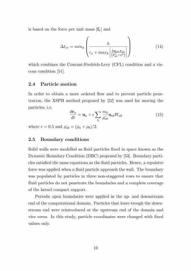
is based on the force per unit mass |fa| and

Δtcv = mina

⎛⎜⎜⎝ h

cs +maxb

∣∣∣∣ huab·rab(r2ab+η2)

∣∣∣∣

⎞⎟⎟⎠ (14)

which combines the Courant-Fredrich-Levy (CFL) condition and a vis-

cous condition [51].

2.4 Particle motion

In order to obtain a more ordered flow and to prevent particle pene-

tration, the XSPH method proposed by [52] was used for moving the

particles, i.e.dradt

= ua + ε∑b

mb

ρabuabWab (15)

where ε = 0.5 and ρab = (ρa + ρb)/2.

2.5 Boundary conditions

Solid walls were modelled as fluid particles fixed in space known as the

Dynamic Boundary Condition (DBC) proposed by [53]. Boundary parti-

cles satisfied the same equations as the fluid particles. Hence, a repulsive

force was applied when a fluid particle approach the wall. The boundary

was populated by particles in three non-staggered rows to ensure that

fluid particles do not penetrate the boundaries and a complete coverage

of the kernel compact support.

Periodic open boundaries were applied in the up- and downstream

end of the computational domain. Particles that leave trough the down-

stream end were reintroduced at the upstream end of the domain and

vice versa. In this study, particle coordinates were changed with fixed

values only.

10

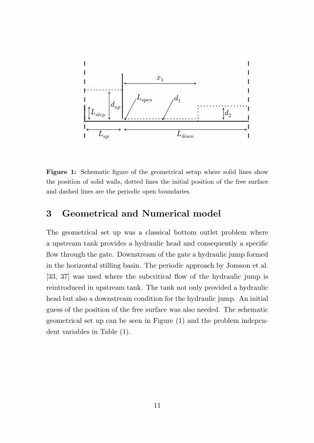
Figure 1: Schematic figure of the geometrical setup where solid lines show

the position of solid walls, dotted lines the initial position of the free surface

and dashed lines are the periodic open boundaries.

3 Geometrical and Numerical model

The geometrical set up was a classical bottom outlet problem where

a upstream tank provides a hydraulic head and consequently a specific

flow through the gate. Downstream of the gate a hydraulic jump formed

in the horizontal stilling basin. The periodic approach by Jonsson et al.

[33, 37] was used where the subcritical flow of the hydraulic jump is

reintroduced in upstream tank. The tank not only provided a hydraulic

head but also a downstream condition for the hydraulic jump. An initial

guess of the position of the free surface was also needed. The schematic

geometrical set up can be seen in Figure (1) and the problem indepen-

dent variables in Table (1).

11

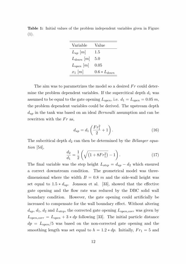
Table 1: Initial values of the problem independent variables given in Figure

(1).

Variable Value

Lup [m] 1.5

Ldown [m] 5.0

Lopen [m] 0.05

x1 [m] 0.6 ∗ Ldown

The aim was to parametrizes the model so a desired Fr could deter-

mine the problem dependent variables. If the supercitical depth d1 was

assumed to be equal to the gate opening Lopen, i.e. d1 = Lopen = 0.05 m,

the problem dependent variables could be derived. The upstream depth

dup in the tank was based on an ideal Bernoulli assumption and can be

rewritten with the Fr as,

dup = d1

(Fr212

+ 1

). (16)

The subcritical depth d2 can then be determined by the Belanger equa-

tion [54],d2d1

=1

2

(√(1 + 8Fr21

)− 1

). (17)

The final variable was the step height Lstep = dup − d2 which ensured

a correct downstream condition. The geometrical model was three-

dimensional where the width B = 0.8 m and the side-wall height was

set equal to 1.5 ∗ dup. Jonsson et al. [33], showed that the effective

gate opening and the flow rate was reduced by the DBC solid wall

boundary condition. However, the gate opening could artificially be

increased to compensate for the wall boundary effect. Without altering

dup, d1, d2 and Lstep, the corrected gate opening Lopen,corr was given by

Lopen,corr = Lopen + 3 ∗ dp following [33]. The initial particle distance

dp = Lopen/5 was based on the non-corrected gate opening and the

smoothing length was set equal to h = 1.2 ∗ dp. Initially, Fr1 = 5 and

12

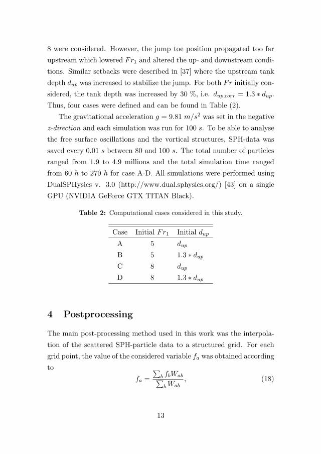
8 were considered. However, the jump toe position propagated too far

upstream which lowered Fr1 and altered the up- and downstream condi-

tions. Similar setbacks were described in [37] where the upstream tank

depth dup was increased to stabilize the jump. For both Fr initially con-

sidered, the tank depth was increased by 30 %, i.e. dup,corr = 1.3 ∗ dup.Thus, four cases were defined and can be found in Table (2).

The gravitational acceleration g = 9.81 m/s2 was set in the negative

z-direction and each simulation was run for 100 s. To be able to analyse

the free surface oscillations and the vortical structures, SPH-data was

saved every 0.01 s between 80 and 100 s. The total number of particles

ranged from 1.9 to 4.9 millions and the total simulation time ranged

from 60 h to 270 h for case A-D. All simulations were performed using

DualSPHysics v. 3.0 (http://www.dual.sphysics.org/) [43] on a single

GPU (NVIDIA GeForce GTX TITAN Black).

Table 2: Computational cases considered in this study.

Case Initial Fr1 Initial dup

A 5 dup

B 5 1.3 ∗ dupC 8 dup

D 8 1.3 ∗ dup

4 Postprocessing

The main post-processing method used in this work was the interpola-

tion of the scattered SPH-particle data to a structured grid. For each

grid point, the value of the considered variable fa was obtained according

to

fa =

∑b fbWab∑bWab

, (18)

13

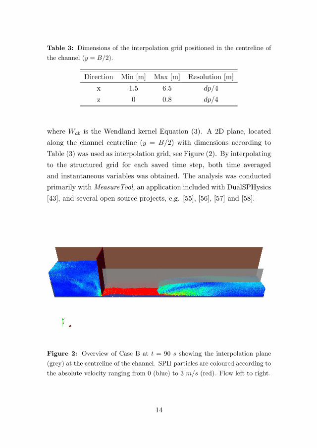
Table 3: Dimensions of the interpolation grid positioned in the centreline of

the channel (y = B/2).

Direction Min [m] Max [m] Resolution [m]

x 1.5 6.5 dp/4

z 0 0.8 dp/4

where Wab is the Wendland kernel Equation (3). A 2D plane, located

along the channel centreline (y = B/2) with dimensions according to

Table (3) was used as interpolation grid, see Figure (2). By interpolating

to the structured grid for each saved time step, both time averaged

and instantaneous variables was obtained. The analysis was conducted

primarily with MeasureTool, an application included with DualSPHysics

[43], and several open source projects, e.g. [55], [56], [57] and [58].

Figure 2: Overview of Case B at t = 90 s showing the interpolation plane

(grey) at the centreline of the channel. SPH-particles are coloured according to

the absolute velocity ranging from 0 (blue) to 3 m/s (red). Flow left to right.

14

5 Result and Discussion

5.1 Time averaged and instantaneous velocity field

The time averaged and the instantaneous velocity field at t = 80 s for

all cases are shown in Figure (3)-(6). However, we focus initially on

case A and B where the initial Fr1 = 5 only. The time averaged ve-

locity field showed basically the same tendencies for case A and B but

with some notable differences. The jet was deflected upwards, for both

cases, as it entered through the gate. This was possibly an effect of the

solid wall boundary condition as a high velocity would generate a large

upward force due the the EOS and momentum equation. Both case A

and B showed similar free surface profiles but the position of the jump

toe differed significantly. The time averaged velocity field showed that

the incoming jet was dissipated and deflected upwards past the roller

region. It is expected that the high velocity core is closer to the bottom

which was highlighted in the experimental work by Lin et al. [9]. This

behaviour could possibly be explained by the over estimated bound-

ary layer thickness usually observed with the DBC solid wall boundary

condition. Lennon & Hill [7] showed time averaged velocity fields but

investigate lower Fr which makes the comparison more difficult. An-

other notable difference was the size of the roller region, see the white

dashed line in Figure (3,4) which marks the zero velocity line. In case

A, the zone with reversed velocity was shallow and positioned close to

the free surface and roughly 20d1 long. The roller region considering

case B was much more dominant and the zero velocity line was deeper

within the jump and the length was roughly 30d1. An explanation for

this behaviour could be found when the instantaneous velocity field was

studied, see the lower parts of Figure (3) and (4). Case A showed large

vortical structures close to the free surface without any clear recirculat-

ing zone. In case B, the vortices were generally smaller except for the

one close to the jump toe and was located deeper within the jump.

15

Figure

3:Case

A.Above,

contours

ofthetim

eavera

genon-dim

ensio

nalvelo

cityu/u1in

thedow

nstrea

mdirectio

n.The

white

dashed

lineshow

thepositio

nofzero

velocity

intheroller

andtheblack

dashed

linethemaxim

um

velo

cityforeach

x-positio

n.Belo

w,insta

ntaneousvelo

cityfield

show

nas

streamlin

esatt=

80s.

Thetw

ored

dots

show

thepositio

nwhere

thevelo

citywassampled

fortheFFT

andcro

ss-correla

tionanalysis.

16

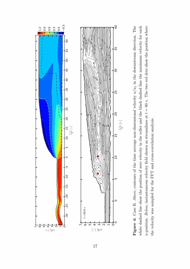
Figure

4:Case

B.Above,contours

ofthetimeaveragenon-dim

ensionalvelocity

u/u1in

thedow

nstream

direction.The

whitedashed

lineshow

thepositionofzero

velocity

intheroller

andtheblack

dashed

linethemaxim

um

velocity

foreach

x-position.Below,instantaneousvelocity

fieldshow

nas

streamlines

att=

80s.

Thetw

oreddots

show

thepositionwhere

thevelocity

wassampledfortheFFT

andcross-correlationanalysis.

17

Case B showed also a clear recirculating zone in contrast to Case A in

line with the findings of [9]. The vortices rotated in a counter-clockwise

manner but showed no merging or braiding behaviour as described in

[4, 5].

The time averaged and instantaneous velocity field of case C and

D is shown in Figure (5) and (6). The deflection of supercritical jet

was enhanced for these cases and disrupted the jump toe. Both cases

showed also more similarity to case A than case B and the reasons for

this behaviour is unclear but could possibly be linked to the missing

secondary air-phase.

18

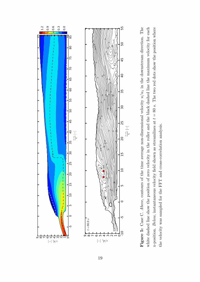
Figure

5:Case

C.Above,contours

ofthetimeaveragenon-dim

ensionalvelocity

u/u1in

thedow

nstream

direction.The

whitedashed

lineshow

thepositionofzero

velocity

intheroller

andtheblack

dashed

linethemaxim

um

velocity

foreach

x-position.Below,instantaneousvelocity

fieldshow

nas

streamlines

att=

80s.

Thetw

oreddots

show

thepositionwhere

thevelocity

wassampledfortheFFT

andcross-correlationanalysis.

19

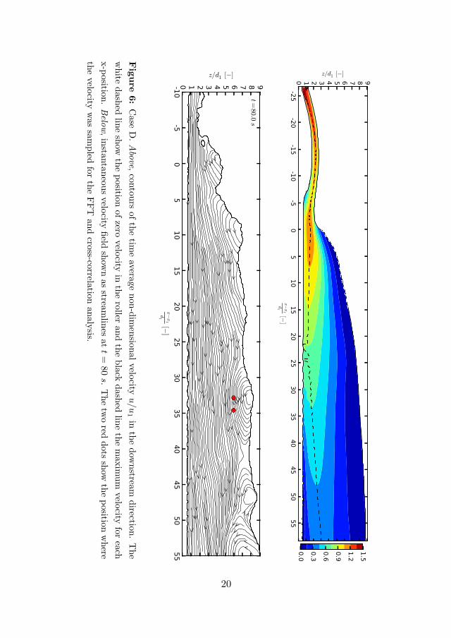
Figure

6:Case

D.Above,

contours

ofthetim

eavera

genon-dim

ensio

nalvelo

cityu/u1in

thedow

nstrea

mdirectio

n.The

white

dashed

lineshow

thepositio

nofzero

velocity

intheroller

andtheblack

dashed

linethemaxim

um

velo

cityforeach

x-positio

n.Belo

w,insta

ntaneousvelo

cityfield

show

nas

streamlin

esatt=

80s.

Thetw

ored

dots

show

thepositio

nwhere

thevelo

citywassampled

fortheFFT

andcro

ss-correla

tionanalysis.

20

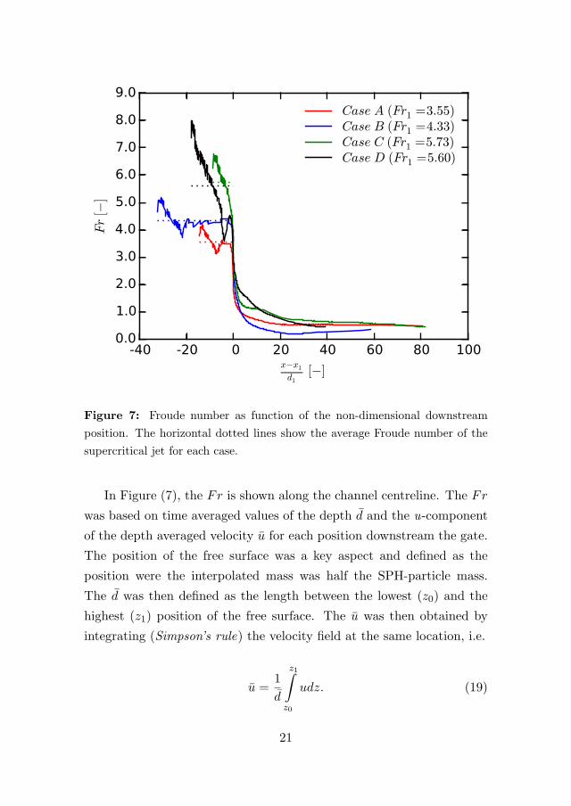
Figure 7: Froude number as function of the non-dimensional downstream

position. The horizontal dotted lines show the average Froude number of the

supercritical jet for each case.

In Figure (7), the Fr is shown along the channel centreline. The Fr

was based on time averaged values of the depth d and the u-component

of the depth averaged velocity u for each position downstream the gate.

The position of the free surface was a key aspect and defined as the

position were the interpolated mass was half the SPH-particle mass.

The d was then defined as the length between the lowest (z0) and the

highest (z1) position of the free surface. The u was then obtained by

integrating (Simpson’s rule) the velocity field at the same location, i.e.

u =1

d

z1∫z0

udz. (19)

21

All four cases behaved similarly in terms of Fr, see Figure (7). Cases

initiated with an extra 30% of dup, i.e. case B and D, achieved the target

Fr of 5 and 8 at the peak observed close to the gate. Case A and C

peaked roughly one unit below, i.e. Fr = 4 and 7. The zone between

the peak and the more stable plateau region, clearly seen for case B in

Figure (7), could be explained by the behaviour of the jet which deflected

and reconnected with the bottom in this zone, compare Figure (4) and

(7). Case A and B showed clear plateau regions which could be used as

the definition of the characteristic inflow Fr1. However, case C and D

showed no marked or a minor plateau region only which was an affect

of the highly deflected jet and the position of the jump toe, mentioned

above. This complicated a unified definition of the characteristic inflow

Fr1. Thus, the mean value of Fr in the entire supercritical zone was

used as Fr1 instead. This is shown in Figure (7) as dashed lines. For

case A and B, Fr1 coincided with the plateau which was favourable. For

case C and D, a higher Fr1 than case A and B was obtained which was

seen as good enough. The mean value of d and u in the supercritical

zones was used to define d1 and u1 used as scaling parameters in Figure

(3)-(6). Past the jump toe, Fr decreased rapidly and all cases stabilized

at roughly Fr = 0.5. The characteristic Fr2, d2 and u2 was determined

in a similar manner as above but in a region further downstream close

to the boundary.

The black dashed line in Figure (3)-(6) marked the maximum ve-

locity position along the channel centreline and was compared with

experimental data in Figure (8). All cases compared favourably with

experimental data between (x−x1)/d1 = 0−20 except for case D where

the dissipation was underestimated. Case B was too dissipative between

(x − x1)/d1 = 20 − 50 but the results were within the experimental

variation further downstream. Overall, the SPH model handled the dis-

sipation in a satisfactory manner.

22

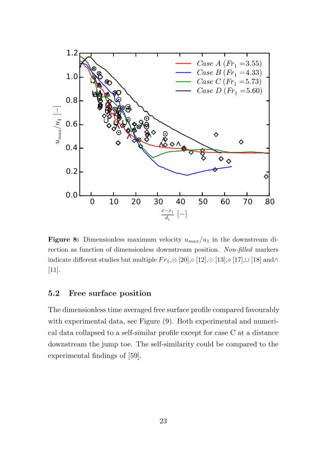
Figure 8: Dimensionless maximum velocity umax/u1 in the downstream di-

rection as function of dimensionless downstream position. Non-filled markers

indicate different studies but multiple Fr1,⊗ [20],◦ [12],� [13], [17],∪ [18] and∧[11].

5.2 Free surface position

The dimensionless time averaged free surface profile compared favourably

with experimental data, see Figure (9). Both experimental and numeri-

cal data collapsed to a self-similar profile except for case C at a distance

downstream the jump toe. The self-similarity could be compared to the

experimental findings of [59].

23

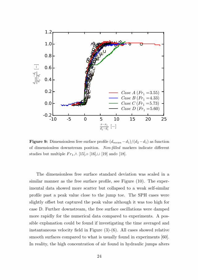
Figure 9: Dimensionless free surface profile (dmean−d1)/(d2−d1) as function

of dimensionless downstream position. Non-filled markers indicate different

studies but multiple Fr1,∧ [15],◦ [16],∪ [19] and [18].

The dimensionless free surface standard deviation was scaled in a

similar manner as the free surface profile, see Figure (10). The exper-

imental data showed more scatter but collapsed to a weak self-similar

profile past a peak value close to the jump toe. The SPH cases were

slightly offset but captured the peak value although it was too high for

case D. Further downstream, the free surface oscillations were damped

more rapidly for the numerical data compared to experiments. A pos-

sible explanation could be found if investigating the time averaged and

instantaneous velocity field in Figure (3)-(6). All cases showed relative

smooth surfaces compared to what is usually found in experiments [60].

In reality, the high concentration of air found in hydraulic jumps alters

24

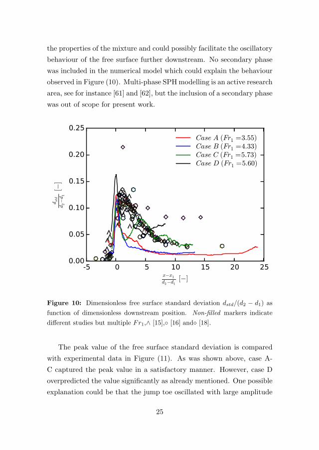
the properties of the mixture and could possibly facilitate the oscillatory

behaviour of the free surface further downstream. No secondary phase

was included in the numerical model which could explain the behaviour

observed in Figure (10). Multi-phase SPHmodelling is an active research

area, see for instance [61] and [62], but the inclusion of a secondary phase

was out of scope for present work.

Figure 10: Dimensionless free surface standard deviation dstd/(d2 − d1) as

function of dimensionless downstream position. Non-filled markers indicate

different studies but multiple Fr1,∧ [15],◦ [16] and [18].

The peak value of the free surface standard deviation is compared

with experimental data in Figure (11). As was shown above, case A-

C captured the peak value in a satisfactory manner. However, case D

overpredicted the value significantly as already mentioned. One possible

explanation could be that the jump toe oscillated with large amplitude

25

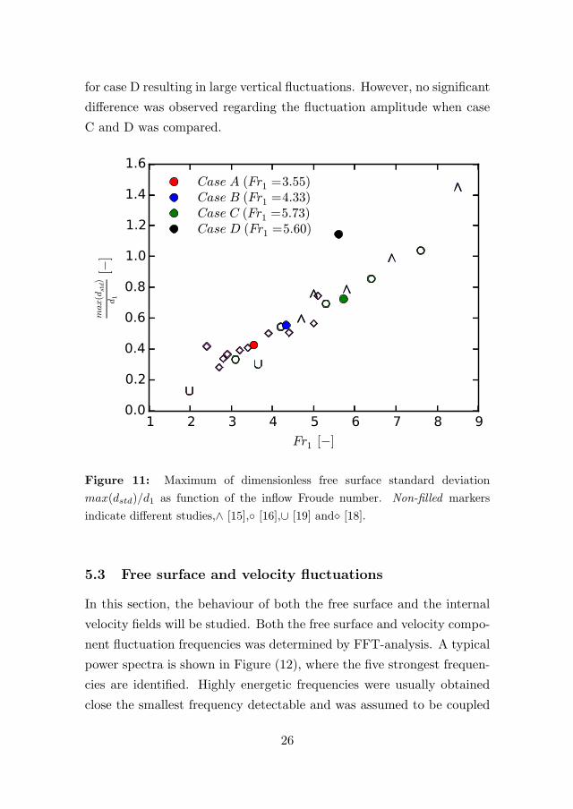
for case D resulting in large vertical fluctuations. However, no significant

difference was observed regarding the fluctuation amplitude when case

C and D was compared.

Figure 11: Maximum of dimensionless free surface standard deviation

max(dstd)/d1 as function of the inflow Froude number. Non-filled markers

indicate different studies,∧ [15],◦ [16],∪ [19] and [18].

5.3 Free surface and velocity fluctuations

In this section, the behaviour of both the free surface and the internal

velocity fields will be studied. Both the free surface and velocity compo-

nent fluctuation frequencies was determined by FFT-analysis. A typical

power spectra is shown in Figure (12), where the five strongest frequen-

cies are identified. Highly energetic frequencies were usually obtained

close the smallest frequency detectable and was assumed to be coupled

26

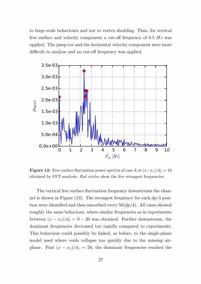
to large scale behaviours and not to vortex shedding. Thus, for vertical

free surface and velocity component a cut-off frequency of 0.5 Hz was

applied. The jump toe and the horizontal velocity component were more

difficult to analyse and no cut-off frequency was applied.

Figure 12: Free surface fluctuation power spectra of case A at (x−x1)/d1 = 10

obtained by FFT-analysis. Red circles show the five strongest frequencies.

The vertical free surface fluctuation frequency downstream the chan-

nel is shown in Figure (13). The strongest frequency for each dp/4 posi-

tion were identified and then smoothed every 50(dp/4). All cases showed

roughly the same behaviour, where similar frequencies as in experiments

between (x − x1)/d1 = 0 − 20 was obtained. Further downstream, the

dominant frequencies decreased too rapidly compared to experiments.

This behaviour could possibly be linked, as before, to the single-phase

model used where voids collapse too quickly due to the missing air-

phase. Past (x − x1)/d1 = 50, the dominant frequencies reached the

27

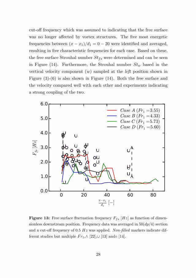
cut-off frequency which was assumed to indicating that the free surface

was no longer affected by vortex structures. The five most energetic

frequencies between (x− x1)/d1 = 0− 20 were identified and averaged,

resulting in five characteristic frequencies for each case. Based on these,

the free surface Strouhal number Stfs were determined and can be seen

in Figure (14). Furthermore, the Strouhal number Stw based in the

vertical velocity component (w) sampled at the left position shown in

Figure (3)-(6) is also shown in Figure (14). Both the free surface and

the velocity compared well with each other and experiments indicating

a strong coupling of the two.

Figure 13: Free surface fluctuation frequency Ffs [Hz] as function of dimen-

sionless downstream position. Frequency data was averaged in 50(dp/4) section

and a cut-off frequency of 0.5 Hz was applied. Non-filled markers indicate dif-

ferent studies but multiple Fr1,∧ [22],∪ [13] and◦ [14].

28

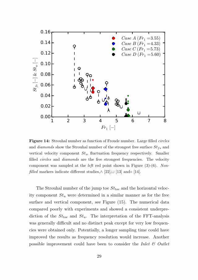
Figure 14: Strouhal number as function of Froude number. Large filled circles

and diamonds show the Strouhal number of the strongest free surface Stfs and

vertical velocity component Stw fluctuation frequency respectively. Smaller

filled circles and diamonds are the five strongest frequencies. The velocity

component was sampled at the left red point shown in Figure (3)-(6). Non-

filled markers indicate different studies,∧ [22],∪ [13] and◦ [14].

The Strouhal number of the jump toe Sttoe and the horizontal veloc-

ity component Stu were determined in a similar manner as for the free

surface and vertical component, see Figure (15). The numerical data

compared poorly with experiments and showed a consistent underpre-

diction of the Sttoe and Stu. The interpretation of the FFT-analysis

was generally difficult and no distinct peak except for very low frequen-

cies were obtained only. Potentially, a longer sampling time could have

improved the results as frequency resolution would increase. Another

possible improvement could have been to consider the Inlet & Outlet

29

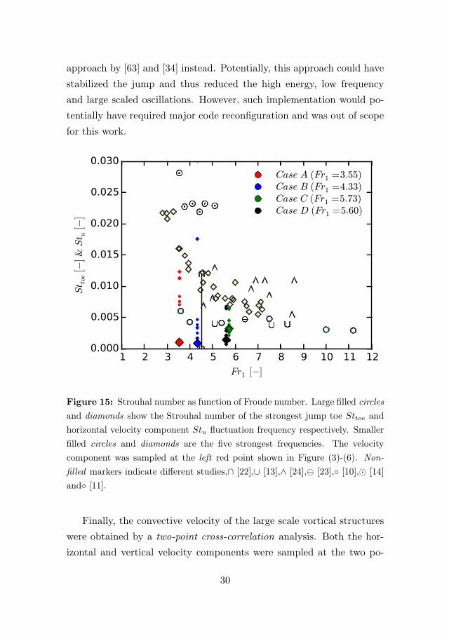
approach by [63] and [34] instead. Potentially, this approach could have

stabilized the jump and thus reduced the high energy, low frequency

and large scaled oscillations. However, such implementation would po-

tentially have required major code reconfiguration and was out of scope

for this work.

Figure 15: Strouhal number as function of Froude number. Large filled circles

and diamonds show the Strouhal number of the strongest jump toe Sttoe and

horizontal velocity component Stu fluctuation frequency respectively. Smaller

filled circles and diamonds are the five strongest frequencies. The velocity

component was sampled at the left red point shown in Figure (3)-(6). Non-

filled markers indicate different studies,∩ [22],∪ [13],∧ [24],� [23],◦ [10],� [14]

and [11].

Finally, the convective velocity of the large scale vortical structures

were obtained by a two-point cross-correlation analysis. Both the hor-

izontal and vertical velocity components were sampled at the two po-

30

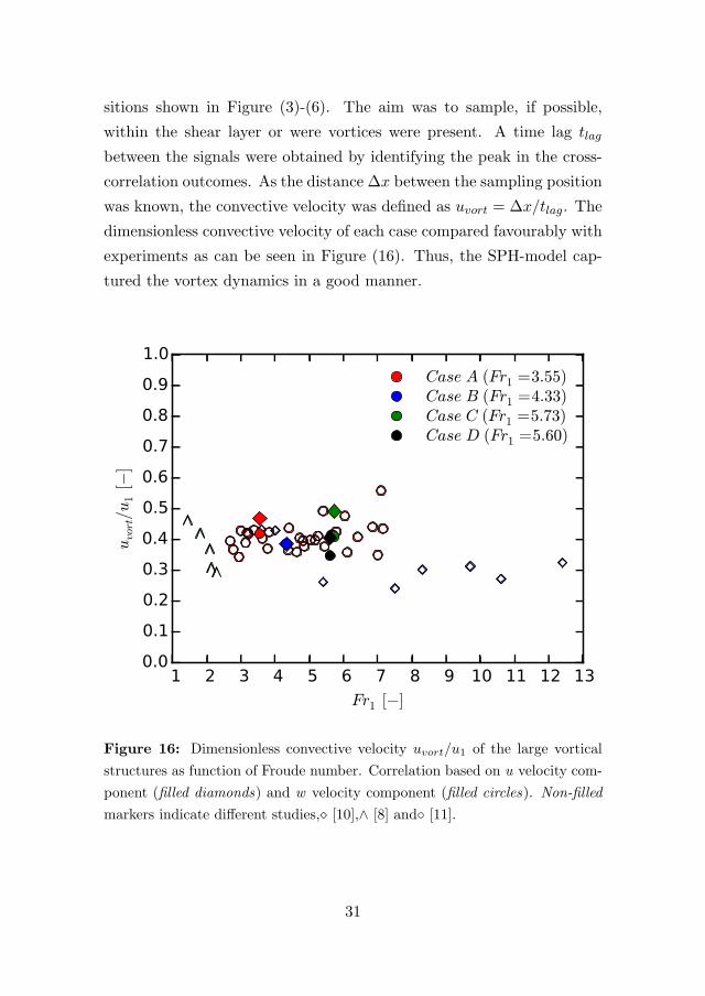
sitions shown in Figure (3)-(6). The aim was to sample, if possible,

within the shear layer or were vortices were present. A time lag tlag

between the signals were obtained by identifying the peak in the cross-

correlation outcomes. As the distance Δx between the sampling position

was known, the convective velocity was defined as uvort = Δx/tlag. The

dimensionless convective velocity of each case compared favourably with

experiments as can be seen in Figure (16). Thus, the SPH-model cap-

tured the vortex dynamics in a good manner.

Figure 16: Dimensionless convective velocity uvort/u1 of the large vortical

structures as function of Froude number. Correlation based on u velocity com-

ponent (filled diamonds) and w velocity component (filled circles). Non-filled

markers indicate different studies, [10],∧ [8] and◦ [11].

31

6 Conclusion

This paper has focused on the dynamic relationship between the free

surface and the internal flow structures found in hydraulic jumps. The

single-phase SPH-model considered was able to capture some key fea-

tures. Generally, jumps characterized with lower Fr (case A and B)

compared more favourably with experiments than higher (case C and

D). This behaviour could possibly be linked to the missing secondary

air phase in the numerical model as more air is entrained in higher Fr

jumps. In terms of velocity fields, case A and B showed the presence of a

shear layer with large vortical structures. In line with experimental find-

ings, case A developed a shear layer close to the free surface in contrast

to case B where the shear layer was more embedded within the jump

and showed clear signs of a recirculating zone above. The higher Fr,

developed no clear shear layer but vortices was present close to the free

surface similarly to case A. The upward deflected jet and the position of

the jump toe affected the determination of the characteristic inflow Fr1

negatively, especially for case C and D. Good agreement was obtained

for the free surface profile and for the peak in standard deviation except

for case D. All SPH-simulations showed a too dissipative zone past the

roller region in terms of free surface standard deviation, the fluctuation

frequencies and, to some extent, for the maximum velocity distribution.

Potentially, this could be traced to the single phase model approach or

possibly that the SPH refinement was too low and too few flow fea-

tures were resolved. However, for the roller region the Strouhal number

of the vertical free surface and velocity component fluctuations showed

similar values and was well within the experimental variation. Both

the jump toe and the horizontal velocity component fluctuations agreed

poorly with experiments. The large scale fluctuations could possibly be

damped if a Inlet & Outlet boundary condition was applied instead of

the periodic used in this work. Finally, good agreement was found for

the convective velocity of the large scale vortical structures obtained by

32

a cross-correlation based on both velocity components.

It is highly recommended, as a future work, to investigate the impact

of the inclusion of the secondary air phase and to implement and develop

proper inlet and outlet boundary conditions.

Acknowledgement

The research presented was carried out as a part of “Swedish Hydropower

Centre - SVC”. SVC has been established by the Swedish Energy Agency,

Elforsk and Svenska Kraftnat together with Lulea University of Technol-

ogy, KTH Royal Institute of Technology, Chalmers University of Tech-

nology and Uppsala University. www.svc.nu. The authors greatly ac-

knowledge Professor Mikael Sjodahl at Lulea University of Technology

for the discussions regarding the FFT and cross-correlation analysis.

References

[1] Ven Te Chow. Open-channel hydraulics. McGraw-Hill, Tokyo, 1959. ISBN

0-07-010776-9.

[2] H. Rouse, T. T. Siao, and S. Nagaratnam. Turbulence characteristics of

the hydraulic jump. Journal of the Hydraulics Division, 84(1):1–30, 1958.

[3] Nallamuthu Rajaratnam. The hydraulic jump as a well jet. Journal of the

Hydraulics Division, 91(5):107–132, 1965.

[4] Jack W. Hoyt and R. H. J. Sellin. Hydraulic jump as “mixing layer”.

Journal of Hydraulic Engineering, 115(12):1607–1614, dec 1989. doi: 10.

1061/(asce)0733-9429(1989)115:12(1607).

[5] Dejiang Long, Nallamuthu Rajaratnam, Peter M. Steffler, and Peter R.

Smy. Structure of flow in hydraulic jumps. Journal of Hydraulic Research,

29(2):207–218, mar 1991. doi: 10.1080/00221689109499004. URL http:

//dx.doi.org/10.1080/00221689109499004.

[6] Hans G. Hornung, Christian Willert, and Stewart Turner. The flow field

downstream of a hydraulic jump. J. Fluid Mech., 287(-1):299, mar 1995.

doi: 10.1017/s0022112095000966.

33

[7] J. M. Lennon and D. F. Hill. Particle image velocity measurements

of undular and hydraulic jumps. Journal of Hydraulic Engineering,

132(12):1283–1294, dec 2006. doi: 10.1061/(asce)0733-9429(2006)132:

12(1283). URL http://dx.doi.org/10.1061/(ASCE)0733-9429(2006)

132:12(1283).

[8] Javier Rodrıguez-Rodrıguez, Carolina Marugan-Cruz, Alberto Aliseda,

and Juan Carlos Lasheras. Dynamics of large turbulent structures in a

steady breaker. Experimental Thermal and Fluid Science, 35(2):301–310,

feb 2011. doi: 10.1016/j.expthermflusci.2010.09.012.

[9] Chang Lin, Shih-Chun Hsieh, I-Ju Lin, Kuang-An Chang, and Ra-

jkumar V. Raikar. Flow property and self-similarity in steady

hydraulic jumps. Exp Fluids, 53(5):1591–1616, sep 2012. doi:

10.1007/s00348-012-1377-2. URL http://dx.doi.org/10.1007/

s00348-012-1377-2.

[10] Hubert Chanson. Convective transport of air bubbles in strong hydraulic

jumps. International Journal of Multiphase Flow, 36(10):798–814, oct

2010. doi: 10.1016/j.ijmultiphaseflow.2010.05.006. URL http://dx.doi.

org/10.1016/j.ijmultiphaseflow.2010.05.006.

[11] Gangfu Zhang, Hang Wang, and Hubert Chanson. Turbulence and aer-

ation in hydraulic jumps: free-surface fluctuation and integral turbulent

scale measurements. Environmental Fluid Mechanics, 13(2):189–204, sep

2012. doi: 10.1007/s10652-012-9254-3.

[12] Serhat Kucukali and Hubert Chanson. Turbulence measurements in the

bubbly flow region of hydraulic jumps. Experimental Thermal and Fluid

Science, 33(1):41–53, oct 2008. doi: 10.1016/j.expthermflusci.2008.06.012.

URL http://dx.doi.org/10.1016/j.expthermflusci.2008.06.012.

[13] Frederic Murzyn and Hubert Chanson. Free-surface fluctuations in hy-

draulic jumps: Experimental observations. Experimental Thermal and

Fluid Science, 33(7):1055–1064, oct 2009. doi: 10.1016/j.expthermflusci.

2009.06.003. URL http://dx.doi.org/10.1016/j.expthermflusci.

2009.06.003.

[14] Yann Chachereau and Hubert Chanson. Free-surface fluctuations and

turbulence in hydraulic jumps. Experimental Thermal and Fluid Science,

34

35(6):896–909, sep 2011. doi: 10.1016/j.expthermflusci.2011.01.009. URL

http://dx.doi.org/10.1016/j.expthermflusci.2011.01.009.

[15] Serhat Kucukali and Hubert Chanson. Turbulence in hydraulic jumps:

Experimental measurements. Technical Report CH62/07, Division of Civil

Engineering, The University of Queensland, July 2007.

[16] Frederic Murzyn and Hubert Chanson. Free surface, bubbly flow and

turbulence measurements in hydraulic jumps. Technical Report CH63/07,

Division of Civil Engineering, The University of Queensland, July 2007.

[17] Hubert Chanson. Advective diffusion of air bubbles in hydraulic jumps

with large froude numbers: an experimental study. Technical Report

CH75/09, Division of Civil Engineering, The University of Queensland,

2009.

[18] Yann Chachereau and Hubert Chanson. Free surface turbulence fluctu-

ations and air-water flow measurements in hydraulic jumps with small

inflow froude numbers. Technical Report CH78/10, Division of Civil En-

gineering, The University of Queensland, 2010.

[19] D. Mouaze, F. Murzyn, and J. R. Chaplin. Free surface length scale

estimation in hydraulic jumps. Journal of Fluids Engineering, 127(6):

1191, 2005. doi: 10.1115/1.2060736. URL http://dx.doi.org/10.1115/

1.2060736.

[20] H. Chanson and T. Brattberg. Experimental study of the air–water shear

flow in a hydraulic jump. International Journal of Multiphase Flow, 26

(4):583–607, apr 2000. doi: 10.1016/s0301-9322(99)00016-6. URL http:

//dx.doi.org/10.1016/S0301-9322(99)00016-6.

[21] F. Murzyn and H. Chanson. Two-phase flow measurements in turbulent

hydraulic jumps. Chemical Engineering Research and Design, 87(6):789–

797, jun 2009. doi: 10.1016/j.cherd.2008.12.003. URL http://dx.doi.

org/10.1016/j.cherd.2008.12.003.

[22] Michele Mossa. On the oscillating characteristics of hydraulic jumps.

Journal of Hydraulic Research, 37(4):541–558, jul 1999. doi: 10.1080/

00221686.1999.9628267. URL http://dx.doi.org/10.1080/00221686.

1999.9628267.

35

[23] Michele Mossa and Umberto Tolve. Flow visualization in bubbly two-

phase hydraulic jump. Journal of Fluids Engineering, 120(1):160, 1998.

doi: 10.1115/1.2819641.

[24] Hubert Chanson and Carlo Gualtieri. Similitude and scale effects of air en-

trainment in hydraulic jumps. TJHR, 46(1):35–44, jan 2008. doi: 10.1080/

00221686.2008.9521841. URL http://dx.doi.org/10.1080/00221686.

2008.9521841.

[25] Minnan Liu, Nallamuthu Rajaratnam, and David Z. Zhu. Turbulence

structure of hydraulic jumps of low froude numbers. Journal of Hy-

draulic Engineering, 130(6):511–520, jun 2004. doi: 10.1061/(asce)

0733-9429(2004)130:6(511). URL http://dx.doi.org/10.1061/(ASCE)

0733-9429(2004)130:6(511).

[26] Hubert Chanson. Hydraulics of aerated flows: qui pro quo ? Journal of

Hydraulic Research, 51(3):223–243, jun 2013. doi: 10.1080/00221686.2013.

795917. URL http://dx.doi.org/10.1080/00221686.2013.795917.

[27] Damien Violeau. Fluid Mechanics and the SPH Method. Oxford University

Press, may 2012. doi: 10.1093/acprof:oso/9780199655526.001.0001.

[28] Ruben Scardovelli and Stephane Zaleski. DIRECT NUMERICAL SIMU-

LATION OF FREE-SURFACE AND INTERFACIAL FLOW. Annu. Rev.

Fluid Mech., 31(1):567–603, jan 1999. doi: 10.1146/annurev.fluid.31.1.567.

[29] AdamWitt, John Gulliver, and Lian Shen. Simulating air entrainment and

vortex dynamics in a hydraulic jump. International Journal of Multiphase

Flow, 72:165–180, jun 2015. doi: 10.1016/j.ijmultiphaseflow.2015.02.012.

[30] David Lopez, Roberto Marivela, and Luis Garrote. Smoothed particle

hydrodynamics model applied to hydraulic structures: a hydraulic jump

test case. Journal of Hydraulic Research, 48(sup1):142–158, jan 2010. doi:

10.1080/00221686.2010.9641255.

[31] P. Jonsson, P. Jonsen, P. Andreasson, T.S. Lundstrom, and J.G.I. Hell-

strom. Smoothed particle hydrodynamics modeling of hydraulic jumps.

In Proceedings of Particle-Based Methods II - Fundamentals and Applica-

tions, pages 490–501, Barcelona, Spain, 2011.

[32] Ming-Jyh Chern and Sam Syamsuri. Effect of corrugated bed on hydraulic

jump characteristic using SPH method. Journal of Hydraulic Engineering,

139(2):221–232, feb 2013. doi: 10.1061/(asce)hy.1943-7900.0000618.

36

[33] P. Jonsson, P. Andreasson, J.G.I. Hellstrom, P. Jonse, and T.S. Lund-

strom. Smoothed particle hydrodynamic simulation of hydraulic jump

using periodic open boundaries. Submitted to Applied Mathematical Mod-

elling 2015, .

[34] I. Federico, S. Marrone, A. Colagrossi, F. Aristodemo, and M. Antuono.

Simulating 2d open-channel flows through an SPH model. European

Journal of Mechanics - B/Fluids, 34:35–46, jul 2012. doi: 10.1016/j.

euromechflu.2012.02.002.

[35] Diana De Padova, Michele Mossa, Stefano Sibilla, and Emanuela Torti.

3d SPH modelling of hydraulic jump in a very large channel. Journal of

Hydraulic Research, 51(2):158–173, apr 2013. doi: 10.1080/00221686.2012.

736883.

[36] P. Jonsson, P. Jonsen, P. Andreasson, T.S. Lundstrom, and J.G.I. Hell-

strom. Smoothed particle hydrodynamic modelling of hydraulic jumps:

Bulk parameters and free surface fluctuations. Submitted to Journal of

Applied Fluid Mechanics 2015-06-08, .

[37] P. Jonsson, P. Andreasson, J.G.I. Hellstrom, P. Jonse, and T.S. Lund-

strom. A three-dimensional smoothed particle hydrodynamic study of a

spillway chute and hydraulic jumps. Submitted to Applied Mathematical

Modelling 2015, .

[38] R. A. Gingold and J. J. Monaghan. Smoothed particle hydrodynamics:

theory and application to non-spherical stars. Monthly Notices of the Royal

Astronomical Society, 181(3):375–389, dec 1977. doi: 10.1093/mnras/181.

3.375.

[39] L. B. Lucy. A numerical approach to the testing of the fission hypothesis.

The Astronomical Journal, 82:1013, dec 1977. doi: 10.1086/112164.

[40] J. J. Monaghan. Smoothed particle hydrodynamics. Annual Review of As-

tronomy and Astrophysics, 30(1):543–574, sep 1992. doi: 10.1146/annurev.

aa.30.090192.002551.

[41] J.J. Monaghan. Smoothed particle hydrodynamics and its diverse ap-

plications. Annu. Rev. Fluid Mech., 44(1):323–346, jan 2012. doi:

10.1146/annurev-fluid-120710-101220.

37

[42] Holger Wendland. Piecewise polynomial, positive definite and compactly

supported radial functions of minimal degree. Adv Comput Math, 4(1):

389–396, dec 1995. doi: 10.1007/bf02123482.

[43] A.J.C. Crespo, J.M. Domınguez, B.D. Rogers, M. Gomez-Gesteira,

S. Longshaw, R. Canelas, R. Vacondio, A. Barreiro, and O. Garcıa-Feal.

DualSPHysics: Open-source parallel CFD solver based on smoothed parti-

cle hydrodynamics (SPH). Computer Physics Communications, 187:204–

216, feb 2015. doi: 10.1016/j.cpc.2014.10.004.

[44] J. J. Monaghan. Smoothed particle hydrodynamics. Annual Review of As-

tronomy and Astrophysics, 30(1):543–574, sep 1992. doi: 10.1146/annurev.

aa.30.090192.002551.

[45] R.A. Dalrymple and B.D. Rogers. Numerical modeling of water waves

with the SPH method. Coastal Engineering, 53(2-3):141–147, feb 2006.

doi: 10.1016/j.coastaleng.2005.10.004.

[46] H. Gotoh, T. Shibihara, and M. Hayashii. Subparticle-scale model for the

MPS method-lagrangian flow model for hydraulic engineering. Comput.

Fluid Dynam. J., 09:339–347, 2001.

[47] Edmond Y.M. Lo and Songdong Shao. Simulation of near-shore solitary

wave mechanics by an incompressible SPH method. Applied Ocean Re-

search, 24(5):275–286, oct 2002. doi: 10.1016/s0141-1187(03)00002-6.

[48] Joseph P. Morris, Patrick J. Fox, and Yi Zhu. Modeling low reynolds num-

ber incompressible flows using SPH. Journal of Computational Physics,

136(1):214–226, sep 1997. doi: 10.1006/jcph.1997.5776.

[49] J.J. Monaghan. Simulating free surface flows with SPH. Journal of Com-

putational Physics, 110(2):399–406, feb 1994. doi: 10.1006/jcph.1994.1034.

[50] George Keith Batchelor. An introduction to fluid dynamics. Cambridge

University Press, London, 1967.

[51] J. J. Monaghan and A. Kos. Solitary waves on a cretan beach. J.

Waterway, Port, Coastal, Ocean Eng., 125(3):145–155, may 1999. doi:

10.1061/(asce)0733-950x(1999)125:3(145).

[52] J.J. Monaghan. On the problem of penetration in particle methods.

Journal of Computational Physics, 82(1):1–15, may 1989. doi: 10.1016/

0021-9991(89)90032-6.

38

[53] A. J. Crespo, M. Gomez-Gesteira, and R. A. Dalrymple. Boundary con-

ditions generated by dynamic particles in sph methods. Computers, ma-

terials and continua, 5(3):173–184, 2007. doi: 10.3970/cmc.2007.005.173.

[54] Hubert Chanson. The hydraulics of open channel flow an introduction :

basic principles, sediment motion, hydraulic modelling, design of hydraulic

structures. Amsterdam ; London : Elsevier Butterworth-Heinemann, Am-

sterdam ; London, 2nd ed.. edition, 2004.

[55] Fernando Perez and Brian E. Granger. IPython: A system for interactive

scientific computing. Computing in Science & Engineering, 9(3):21–29,

2007. doi: 10.1109/mcse.2007.53.

[56] John D. Hunter. Matplotlib: A 2d graphics environment. Computing in

Science & Engineering, 9(3):90–95, 2007. doi: 10.1109/mcse.2007.55.

[57] Stefan Behnel, Robert Bradshaw, Craig Citro, Lisandro Dalcin,

Dag Sverre Seljebotn, and Kurt Smith. Cython: The best of both

worlds. Computing in Science & Engineering, 13(2):31–39, mar 2011. doi:

10.1109/mcse.2010.118.

[58] Stefan van der Walt, S Chris Colbert, and Gael Varoquaux. The NumPy

array: A structure for efficient numerical computation. Computing in

Science & Engineering, 13(2):22–30, mar 2011. doi: 10.1109/mcse.2011.37.

[59] Hang Wang and Hubert Chanson. Experimental study of turbulent

fluctuations in hydraulic jumps. Journal of Hydraulic Engineering, 141

(7):04015010, jul 2015. doi: 10.1061/(asce)hy.1943-7900.0001010. URL

http://dx.doi.org/10.1061/(ASCE)HY.1943-7900.0001010.

[60] Yann Chachereau and Hubert Chanson. Bubbly flow measurements in hy-

draulic jumps with small inflow froude numbers. International Journal of

Multiphase Flow, 37(6):555–564, jul 2011. doi: 10.1016/j.ijmultiphaseflow.

2011.03.012. URL http://dx.doi.org/10.1016/j.ijmultiphaseflow.

2011.03.012.

[61] J.J. Monaghan and A. Kocharyan. SPH simulation of multi-phase

flow. Computer Physics Communications, 87(1-2):225–235, may 1995.

doi: 10.1016/0010-4655(94)00174-z. URL http://dx.doi.org/10.1016/

0010-4655(94)00174-Z.

39

[62] Athanasios Mokos, Benedict D. Rogers, Peter K. Stansby, and Jose M.

Domınguez. Multi-phase SPH modelling of violent hydrodynamics on

GPUs. Computer Physics Communications, 196:304–316, nov 2015. doi:

10.1016/j.cpc.2015.06.020. URL http://dx.doi.org/10.1016/j.cpc.

2015.06.020.

[63] Martin Lastiwka, Mihai Basa, and Nathan J. Quinlan. Permeable and

non-reflecting boundary conditions in SPH. Int. J. Numer. Meth. Fluids,

61(7):709–724, nov 2009. doi: 10.1002/fld.1971.

40