Embed Size (px)
Citation preview
American University in Cairo American University in Cairo
AUC Knowledge Fountain AUC Knowledge Fountain
Theses and Dissertations Student Research
2-1-2016
Passive aeration of wastewater using tray aerators Passive aeration of wastewater using tray aerators
Ayman Mostafa El-Zahaby
Follow this and additional works at: https://fount.aucegypt.edu/etds
Recommended Citation Recommended Citation
APA Citation El-Zahaby, A. (2016).Passive aeration of wastewater using tray aerators [Master's Thesis, the American University in Cairo]. AUC Knowledge Fountain. https://fount.aucegypt.edu/etds/132
MLA Citation El-Zahaby, Ayman Mostafa. Passive aeration of wastewater using tray aerators. 2016. American University in Cairo, Master's Thesis. AUC Knowledge Fountain. https://fount.aucegypt.edu/etds/132
This Master's Thesis is brought to you for free and open access by the Student Research at AUC Knowledge Fountain. It has been accepted for inclusion in Theses and Dissertations by an authorized administrator of AUC Knowledge Fountain. For more information, please contact [email protected].
The American University In Cairo
School of Science and Engineering
PASSIVE AERATION OF WASTEWATER USING TRAY
AERATORS
BY
AYMAN MOSTAFA EL-ZAHABY
A thesis submitted in partial fulfillment of the requirements for the degree of
Masters of Science in Environmental Engineering
Under the supervision of:
Dr. Ahmed S. El-Gendy
Associate Professor and Director of the Environmental Engineering Program, Department of Construction Engineering
The American University in Cairo
Fall, 2016

ii
Dedication
This work is dedicated to my wife Dina, my son Mostafa, and my daughter Layal for the hard times they
suffered throughout my research.

iii
Acknowledgment
This research work would never have been achieved without the support of many people. I owe
them great gratitude and thanks for their continuous advice, patience, and encouragement.
I would like to acknowledge the great support I received from my thesis advisor, Dr. Ahmed El-
Gendy. Thank you for your patience, and continuous advice. Your guidance in the methodology
of addressing the thesis topic, and analyzing the results will always be a milestone in my life that
I should never forget. I believe my research ability was developed mainly under your supervision.
My professor and mentor, Dr. Emad Imam, is also acknowledged for the support he provided
through different courses that I received under his supervision, which marked my mind set. I owe
you lot of thanks.
Thanks to Eng. Ahmed Saad and Mr. Mohamed Mostafa, from the Environmental lab, as well as
Mr. Mohamed Saied, and Mr. Kassem Ali from the Waste Management lab for supporting me in
the designing and conducting the experimental works. You were great company during my
research journey.
Special thanks go to my loving wife Dina for her support, encouragement, and understanding. You
afforded a lot taking care of our children while I was conducting this research. And to my beloved
children Mostafa and Layal for their true love and tender smiles which always helped me keep
going. I am totally grateful to my parents and big family who believed in me and offered prayers
and words of encouragement throughout these years.
I could not have done it without all of you.
iv
Abstract
Passive aeration units in water and wastewater treatment are aeration units that operate without the
need for electric energy. They depend on dropping the water through the aerator, while increasing
the surface area to volume ratio, and thus increasing the oxygen mass diffused into water. The
passive units include cascade aerators, and tray aerators. On the contrary to cascade and spray
aerators, tray aerators require a much smaller area for their installation. While researching the
design of tray aerators, a shortage of literature pertaining to the topic was observed. The research
objective is to develop a model for the design of tray aerators for the purpose of increasing the
dissolved oxygen in wastewater.
This thesis investigated the design parameters affecting the aeration performance of tray aerators
for wastewater treatment plants. A mathematical model was developed that predicts the aeration
performance of a tray aerator system as a function of the flow rate, number of trays, tray area,
spacing between trays, number and diameter of holes per tray. Results illustrate that the aeration
performance is directly proportional to the tray area, the spacing between trays, and number of
trays and is inversely proportional to the flow rate. The number and diameter of holes together
with the flow rate define the flow regime into dripping or jetting. The spacing between trays, the
number and diameter of holes had slight effect on the aeration performance.
The mass transfer coefficient (KL) is reported to be a variable rather than a constant figure. An
empirical equation for the estimation of KL as a function in the spacing between trays, flow rate,
and the total area of holes in the tray was developed from laboratory scale experiments. That
equation is validated in the laboratory scale experiments, as well as in pilot scale application using
real wastewater.
v
Table of Contents
Dedication ............................................................................................................................................... ii
Acknowledgment ................................................................................................................................... iii
Abstract ................................................................................................................................................. iv
Table of Contents .................................................................................................................................... v
List of Figures ........................................................................................................................................viii
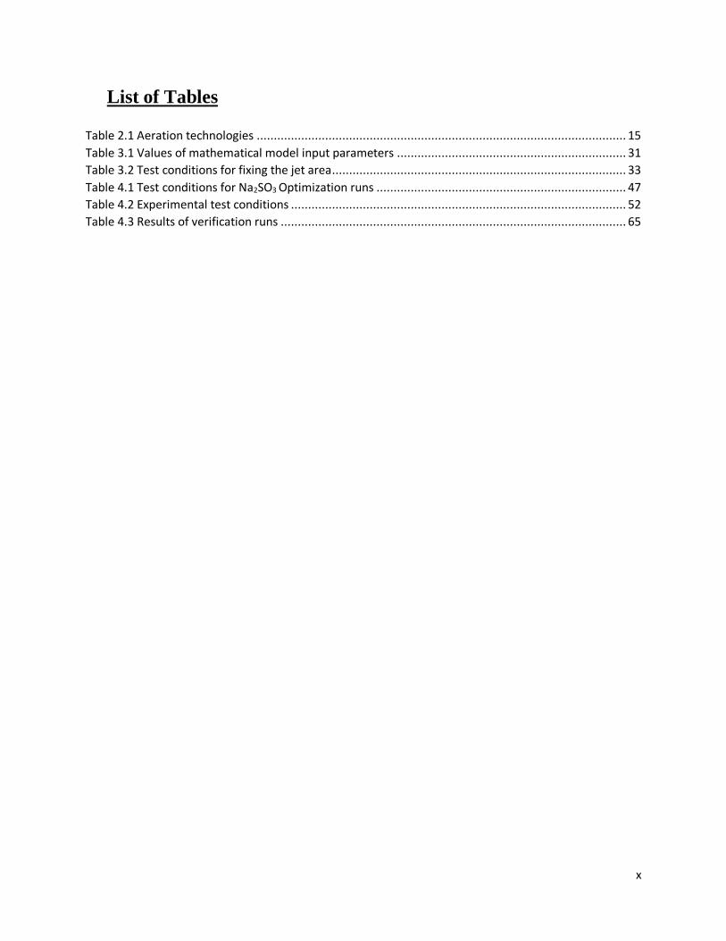
List of Tables ........................................................................................................................................... x
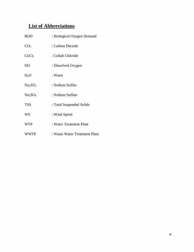
List of Abbreviations ............................................................................................................................... xi
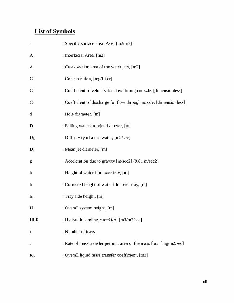
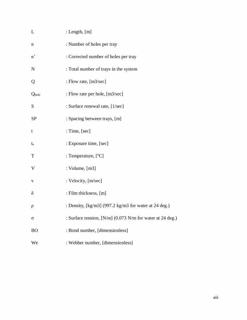
List of Symbols ...................................................................................................................................... xii
List of Subscripts.................................................................................................................................... xiv
1. Chapter 1: Introduction ................................................................................................................... 1
1.1. Problem Statement .................................................................................................................. 2
1.2. Objective.................................................................................................................................. 3
1.3. General Approach .................................................................................................................... 3
1.3.1. Phase I - Mathematical Model .......................................................................................... 4
1.3.2. Phase II – Laboratory Study .............................................................................................. 4
1.3.3. Phase III - Pilot Scale Study ............................................................................................... 4
1.4. Thesis Structure ....................................................................................................................... 5
2. Chapter 2: Background and Review of Literature ............................................................................. 6
2.1. Wastewater Treatment Background ......................................................................................... 7
2.1.1. Wastewater Treatment Processes ........................................................................................ 8
2.2. Mass Transfer Principals ......................................................................................................... 10
2.2.1. Mass Transfer Coefficient (KL) ......................................................................................... 12
2.2.2. Aeration Overview .......................................................................................................... 13
2.3. Aeration Systems ................................................................................................................... 14
2.3.1. Spray Aerators ................................................................................................................ 15
2.3.2. Cascade Aerators ............................................................................................................ 16
2.3.3. Multiple Tray Aerators .................................................................................................... 17
3. Phase I - Mathematical Model ....................................................................................................... 20
3.1. Introduction ........................................................................................................................... 21
3.2. Methodology ......................................................................................................................... 21
3.2.1. Flow Regimes ................................................................................................................. 22
vi
3.2.2. Hydraulic Design ............................................................................................................. 24
3.2.3. Mass Transfer ................................................................................................................. 27
3.2.4. Thin Film Aeration .......................................................................................................... 28
3.2.5. Water Jet Aeration ......................................................................................................... 28
3.2.6. Overall Aeration Through a Single Tray ........................................................................... 29
3.2.7. Number of Trays ............................................................................................................. 29
3.2.8. Model Assumptions ........................................................................................................ 30
3.2.9. Model Equations ............................................................................................................ 31
3.3. Results ................................................................................................................................... 31
3.3.1. Flow Regime ................................................................................................................... 31
3.3.2. Hydraulic Design ............................................................................................................. 32
3.3.3. Performance of Tray Aerator .......................................................................................... 34
3.3.4. Effect of Changing the Hole Diameter and Number of Holes ........................................... 34
3.3.5. Effect of Changing the Spacing Between Trays ................................................................ 35
3.3.6. Effect of Increasing the Number of Trays ........................................................................ 36
3.3.7. Effect of Changing the Tray Area and Flow Rate .............................................................. 37
3.4. Discussion .............................................................................................................................. 38
3.5. Conclusion ............................................................................................................................. 40
4. Phase II – Laboratory Study ............................................................................................................ 41
4.1. Introduction ........................................................................................................................... 42
4.2. Material and Methods............................................................................................................ 42
4.2.1. Preparing Deoxygenated (Synthetic) Water .................................................................... 43
4.2.1.1. Methods of Preparing Deoxygenated Water ............................................................... 43
4.2.1.2. Preparing Sodium Sulfite Stock Solution ..................................................................... 44
4.2.1.3. Preparing Cobalt Chloride Stock Solution .................................................................... 45
4.2.1.4. Testing the Optimum Dose ......................................................................................... 45
4.2.2. Experimental Setup ........................................................................................................ 47
4.2.3. Experimental Procedure ................................................................................................. 51
4.3. Results and Discussion ........................................................................................................... 53
4.3.1. Preparing Deoxygenated (Synthetic) Water .................................................................... 53
4.3.2. Laboratory Scale Test for Tray Aerator ............................................................................ 56
4.1. Discussion and Model Verification .......................................................................................... 58
4.2. Conclusion ............................................................................................................................. 66
vii
5. Phase III - Pilot Scale Study............................................................................................................. 67
5.1. Introduction ........................................................................................................................... 68
5.2. Material and Methods............................................................................................................ 68
5.3. Results and Discussion ........................................................................................................... 74
5.3.1. Effect of Changing the Hole Diameter ............................................................................. 74
5.3.2. Effect of Changing the Number of Trays.......................................................................... 75
5.3.3. Model Validation ............................................................................................................ 75
5.4. Conclusion ............................................................................................................................. 79
6. General Discussion......................................................................................................................... 80
6.1. Design Procedure ................................................................................................................... 82
6.1.1. Input Parameters ............................................................................................................ 82
6.1.2. Design Steps ................................................................................................................... 83
6.1.3. Output Parameters ......................................................................................................... 84
7. Conclusion ..................................................................................................................................... 85
References ............................................................................................................................................ 88
Annex I .................................................................................................................................................. 93
Annex II ................................................................................................................................................. 94
viii
List of Figures
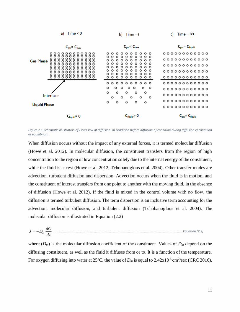
Figure 2.1 Schematic illustration of Fick’s law of diffusion. a) condition before diffusion b) condition
during diffusion c) condition at equilibrium ........................................................................................... 11
Figure 2.2: Spray aerators (Courtesy: (Scott et al. 1955)) ....................................................................... 16
Figure 2.3: Cascade aerators Nappe flow (Courtesy (Ohtsu et al. 2001)) ................................................ 17
Figure 2.4: Tray Aerator (Courtesy (Lekang 2013)) ................................................................................. 18
Figure 3.1 Free falling water regimes (a) Periodic dripping (b) Dripping faucet (c) Jetting (adopted from
((Clanet & Lasheras 1999))..................................................................................................................... 23
Figure 3.2 Schematic tray aerator setup ................................................................................................ 24
Figure 3.3 Flowchart of hydraulic design ................................................................................................ 26
Figure 3.4 Maximum number of holes for jetting flow regime at different flow rates ............................. 32
Figure 3.5 Typical change in DO resulting from changing the number of holes per tray and diameter of
holes. Results are for a single tray at Q = 1.157 m3/sec of water, DO0= zero, SP = 0.2 m, A=0.2x0.2 m2 .. 35
Figure 3.6 Typical change in DO resulting from changing the spacing between trays and diameter of
holes. Results are for a single tray at Q = 1.157 m3/sec of water, DO0= zero, h = 2 mm, A=0.2x0.2 m2. ... 36
Figure 3.7 Typical change in DO from the system resulting in change in tray spacing and number of trays
at different hole diameters. Results are for Q = 1.157 m3/sec of water, DO0= zero, SP = 0.2 m, A=0.2x0.2
m2 ......................................................................................................................................................... 37
Figure 3.8 Typical change in DO from the system resulting from change in flow rate and tray area.
Results are for N=10 trays, DO0= zero, SP = 0.1 m, h = 2 mm, A=0.2x0.2 m2 ........................................... 38
Figure 4.1 Phases of laboratory modelling ............................................................................................. 43
Figure 4.2 Experimental Setup ............................................................................................................... 49
Figure 4.3 Holes location on tray ........................................................................................................... 50
Figure 4.4 Tray frame assembly ............................................................................................................. 50
Figure 4.5 Tray frame – Angles Details ................................................................................................... 51
Figure 4.6 DO concentration response to different Na2SO3 doses at water volume of 300 ml ................. 54
Figure 4.7 DO concentration response to different Na2SO3 doses at water volume of 250 ml ................. 54
Figure 4.8 DO concentration response to different Na2SO3 doses at water volume of 200 ml ................. 55
Figure 4.9 Aeration efficiency from single tray at different hole diameters for 8 holes per tray,
20cmx20cm tray area a) Q=0.7728 L/min b) Q=1.2954 L/min c) Q=1.959 L/min ..................................... 59
Figure 4.10 Aeration efficiency from single tray at different hole diameters for 8 holes per tray,
20cmx20cm tray area a) 15 cm tray spacing b) 20 cm tray spacing c) 25 cm tray spacing ....................... 60
Figure 4.11 Aeration efficiency at different hole diameters for 8 holes per tray, 20cmx20cm tray area .. 61
Figure 4.12 Predicted DO from Analytical Model Vs. Laboratory Measured DO, KL=20cm/h (Liss & Slater
1974) ..................................................................................................................................................... 62
Figure 4.13 Predicted DO from Analytical Model Vs. Laboratory Measured DO, KL =41.8cm/h ............... 63
Figure 4.14 Regression analysis for KL estimation .................................................................................. 64
Figure 4.15 Predicted DO from Analytical Model Vs. Laboratory Measured DO, KL from regression model
.............................................................................................................................................................. 64
Figure 4.16 Predicted DO from Analytical Model Vs. validation runs Measured DO, KL from regression
model .................................................................................................................................................... 65
Figure 5.1 Zawyet Al Karadsah WWTP location ...................................................................................... 70
Figure 5.2 Schematic Diagram of the Full-Scale Setup (Sabry et al. 2011; El-Gendy et al. 2012) .............. 71
ix
Figure 5.3 Tray dimensions – (a) 3mm hole diameter. (b) 4mm hole diameter. (c) 5mm hole diameter. (d)
6mm hole diameter. .............................................................................................................................. 72
Figure 5.4 Water sampling ..................................................................................................................... 73
Figure 5.5 Pilot experiment setup .......................................................................................................... 76
Figure 5.6 Average aeration efficiency of all trays Vs. flow rate for different hole diameters and flow
rates ...................................................................................................................................................... 77
Figure 5.7 Pilot experiment results ........................................................................................................ 77
Figure 5.8 Predicted DO from Analytical Model Vs. Pilot Plant Measured DO, KL from regression model 78
Figure 5.9 Predicted DO from Analytical Model with =0.9 Vs. Pilot Plant Measured DO, KL from
regression model ................................................................................................................................... 79
x
List of Tables
Table 2.1 Aeration technologies ............................................................................................................ 15
Table 3.1 Values of mathematical model input parameters ................................................................... 31
Table 3.2 Test conditions for fixing the jet area...................................................................................... 33
Table 4.1 Test conditions for Na2SO3 Optimization runs ......................................................................... 47
Table 4.2 Experimental test conditions .................................................................................................. 52
Table 4.3 Results of verification runs ..................................................................................................... 65
xi
List of Abbreviations
BOD : Biological Oxygen Demand
CO2 : Carbon Dioxide
CoCl2 : Cobalt Chloride
DO : Dissolved Oxygen
H2O : Water
Na2SO3 : Sodium Sulfite
Na2SO4 : Sodium Sulfate
TSS : Total Suspended Solids
WS : Wind Speed
WTP : Water Treatment Plant
WWTP : Waste Water Treatment Plant
xii
List of Symbols
a : Specific surface area=A/V, [m2/m3]
A : Interfacial Area, [m2]
Aj : Cross section area of the water jets, [m2]
C : Concentration, [mg/Liter]
Cv : Coefficient of velocity for flow through nozzle, [dimensionless]
Cd : Coefficient of discharge for flow through nozzle, [dimensionless]
d : Hole diameter, [m]
D : Falling water drop/jet diameter, [m]
DL : Diffusivity of air in water, [m2/sec]
Dj : Mean jet diameter, [m]
g : Acceleration due to gravity [m/sec2] (9.81 m/sec2)
h : Height of water film over tray, [m]
h’ : Corrected height of water film over tray, [m]
hs : Tray side height, [m]
H : Overall system height, [m]
HLR : Hydraulic loading rate=Q/A, [m3/m2/sec]
i : Number of trays
J : Rate of mass transfer per unit area or the mass flux, [mg/m2/sec]
KL : Overall liquid mass transfer coefficient, [m2]
xiii
L : Length, [m]
n : Number of holes per tray
n’ : Corrected number of holes per tray
N : Total number of trays in the system
Q : Flow rate, [m3/sec]
Qhole : Flow rate per hole, [m3/sec]
S : Surface renewal rate, [1/sec]
SP : Spacing between trays, [m]
t : Time, [sec]
te : Exposure time, [sec]
T : Temperature, [oC]
V : Volume, [m3]
v : Velocity, [m/sec]
ẟ : Film thickness, [m]
ρ : Density, [kg/m3] (997.2 kg/m3 for water at 24 deg.)
σ : Surface tension, [N/m] (0.073 N/m for water at 24 deg.)
BO : Bond number, [dimensionless]
We : Webber number, [dimensionless]
xiv
List of Subscripts
c : Critical
f : Water film over tray
j : Water jet from tray
o : Outer
S : Saturation
0,1,2 : Initial, intermediate, final

1
1. Chapter 1: Introduction
2
Aeration is an important process in water and wastewater treatment plants. In Water Treatment
Plants (WTP), aeration may be used for oxidation of iron and manganese ions, removal of sulfides,
control of pH, and corrosion control. In Waste Water Treatment Plants (WWTP), aeration is mainly
intended to increase the Dissolved Oxygen (DO) in waste water to the limits suitable for the aerobic
degradation, as well as to keep the microorganisms in suspension state in the suspended growth
biological treatment processes. There are various aeration systems known for WWTPs, most of
them require energy for their operation. Therefore, the development of passive aeration units,
which rely on the potential energy of water in the form of water head, should serve in reducing the
operating costs of the WWTP.
1.1. Problem Statement
For developed and developing countries, installing adequate number of WWTPs, with sufficient
design capacities is a great challenge. That challenge increases in its severity when the country is
undergoing fast urbanization and development, due to the associated increase in water demand,
and consequently an increase in produced waste water that needs to be treated. Furthermore, the
investment cost as well as the running cost for WWTPs in many cases exceed the allocated budgets
of those countries.
Electricity requirements for the aeration process within a biological WWTP, often exceed 50% of
the total electricity consumption of the WWTP (Stoica et al. 2009). The power required to operate
mechanical aerators ranges from 20-40 Kw/1000m3 (Tchobanoglous et al. 2004; Sabry et al.
2010). Taking an example from the United States, in which the water-related infrastructure (WTPs
and WWTPs) represent around 3% of the county level total electricity (Hendrickson et al. 2015)
from which aeration of wastewater represent a significant amount of energy.
Egypt, as a developing country, has around 60% of its population with access to sanitation
facilities, while almost 100% of the population have access to improved water source (Odawara &
Loayza 2010). Therefore, there is a need to provide sanitation facilities to the remaining 40% of
the population. Country level electric energy figures indicate that the electricity consumed in Egypt
is around 148TWh (International Energy Agency 2015). Thus, the additional electricity
requirements that shall be associated with the aeration process of new WWTPs serving the
remaining 40% of the population is estimated to be in the range of 590MWh. These 590MWh
3
would require additional power plants to be added, in addition to transmission lines to the WWTPs.
This represents another investment cost adding to the investment cost of the WWTP. Furthermore,
the conventional mechanical aeration process requires regular maintenance for the moving parts,
and skilled labor to operate them (Sabry et al. 2010).
The aforementioned discussion clarifies the need to have an economical option for aeration that is
easy to operate. These criteria can be met by using passive aeration techniques, such as cascade
aerators, or tray aerator. Those passive aeration techniques would reduce the energy needed to
increase the dissolved oxygen in wastewater for trickling filters, but do not replace the aeration for
the suspension of microorganisms in activated sludge processes. Since cascade aerators require a
large area footprint for their installation (Tchobanoglous et al. 2004; Lytle et al. 1998; Scott et al.
1955), the use of tray aerators can offer a more practical option for places where land availability
is a constraint.
Literature about the design of tray aerators is limited and almost non-existing for their use for
aeration purpose. However, a few studies, separated with long time duration, were published on
the use of tray aerators for air stripping.
1.2. Objective
This research aims to investigate and develop a design model for tray aerators, as a passive aeration
unit, that serves in increasing the DO of effluent from anaerobic treatment for sewage treatment in
small communities. Design optimization is not covered in this work. Several factors affect the
design criteria for any waste water aeration device, including the category of aerobic treatment
unit that it serves, the chemical and physical properties of the water being aerated, the availability
and cost of electric energy, the land availability, and the climatic conditions in which the unit will
be installed.
1.3. General Approach
The following section summarizes the tasks planned to achieve the objectives of this research. The
tasks are divided into three main phases: (i) derivation of a mathematical model that describes the

4
aeration of water using tray aerator, (ii) experimentally investigate the performance of tray
aerators, and (iii) validating the performance of tray aerators using real wastewater.
1.3.1. Phase I - Mathematical Model
Hydraulic design of tray aerator
Aeration associated with thin films
Aeration associated with falling water
Overall aeration from tray aerators
Develop software model to test the hydraulic design and the aeration performance from
tray aerators
1.3.2. Phase II – Laboratory Study
Prepare deoxygenated water
Set-up a laboratory scale tray aerator
Experiment a number of trays aerator designs using chemically deoxygenated water
Compare aeration results from the experimented designs
Investigate the validity of the mathematical model against the experimental results
Propose an empirical equation for the volumetric mass transfer coefficient
1.3.3. Phase III - Pilot Scale Study
Set-up four parallel pilot scale tray aerator trains in a WWTP
Experiment the performance of each tray train for different wastewater flow rates
5
Validate the aeration model developed from Phase I - Mathematical Model and corrected
in Phase III - Pilot Scale Study
1.4. Thesis Structure
The thesis is divided into seven chapters.
Chapter 1 covers a general introduction of the subject, research motivation, objectives and related
tasks and activities.
Chapter 2 presents a comprehensive literature review discussing the mass transfer principals, types
of passive aeration systems, and the previous work related to tray aerators.
Chapter 3 encountered mathematical analysis for the flow of water over tray aerators as well as
the aeration associated with the falling water and thin film formed above the trays. This analysis
is then developed in a MATLab – Mathworks® function that predicts the flow regime and DO
concentration achieved from each tray.
Chapter 4 discusses the laboratory scale experiments that were conducted using a tray aerator. This
includes the deoxygenation techniques, the design of the laboratory scale tray aerator system, and
conducting the experiments that tested the impact of different design parameters on the tray aerator
efficiency. An empirical formula for the calculation of the oxygen mass transfer coefficient (KL)
is developed in this chapter.
Chapter 5 discusses the pilot scale application of the tray aerator system using real wastewater that
is pretreated in an anaerobic unit. Results from this phase are compared against the model
developed in previous chapters for validating their results using wastewater under real operating
conditions.
Chapter 6 is a general discussion highlighting the results from the three phases of the study, and
addresses the design procedure for tray aerators. A case study is illustrated pinpointing the design
process inputs and outputs.
Chapter 7 summarizes conclusion and recommendations.

6
2. Chapter 2: Background and Review of Literature
7
2.1. Wastewater Treatment Background
Wastewater treatment has been practiced since the 1900s, however; until early 1970s, it only
concerned with the removal of suspended solids, reduction of BOD and the elimination of
pathogens (Tchobanoglous et al. 2004). From the 1970s to 1980s, due to the development in the
studies on environmental impacts of wastewater discharge, and the focus on long term effects of
the discharge of specific constituents on the receiving water bodies, the treatment of nutrients such
as nitrogen and phosphorus were addressed, with higher treatment limits for the suspended solids,
BOD and pathogenic control (Tchobanoglous et al. 2004). Since the 1980s, improvement of water
quality continued to be addressed more strictly and with higher focus on constituents that have
adverse consequences on the environment and the long term health issues (Tchobanoglous et al.
2004). Among those constituents are pesticides, industrial chemicals, phenolic compounds,
volatile organic compounds, chlorine disinfection, and disinfection by products (Tchobanoglous
et al. 2004). Many other constituents are published by the concerned environmental protection
agencies (Tchobanoglous et al. 2004).
Wastewater can be defined as liquid waste, and includes domestic or municipal wastewater, and
industrial wastewater (McGhee & Steel 1991). Domestic wastewater originates from the water
used by a community for various daily applications. It can be classified into strong, medium or
weak depending on the concentration of different contaminants (McGhee & Steel 1991). Industrial
wastewater is the liquid discharged from industrial applications, such as manufacturing, dairy,
food processing, textile…(McGhee & Steel 1991). Industrial wastewater contains, in addition to
the organic and suspended constituents, heavy metals, phenolic compounds, and synthesized
organic compounds (Tchobanoglous et al. 2004).
Proper collection and treatment of wastewater is essential for the preservation of both water
resources and public health (Tchobanoglous et al. 2004). Wastewater collection from domestic
uses was known until the 1940s (Tchobanoglous et al. 2004). With the significant growth in
industrial applications after 1940, the separation of industrial wastewater from the domestic
wastewater became a concern (Tchobanoglous et al. 2004). This was due to the nature of
contaminants from industrial wastewater which had high concentrations of heavy metals and
synthesized organic compounds that were not effectively treated in conventional wastewater
treatment facilities (Tchobanoglous et al. 2004). Thus, industrial facilities had to install
8
pretreatment plants that collect their industrial waste and remove the non-conventional
contaminants prior to the disposal of their waste to the wastewater collection networks
(Tchobanoglous et al. 2004).
Regulations and standards for water disposal to receiving water bodies differ amongst countries
(Tchobanoglous et al. 2004; McGhee & Steel 1991). In the United States, the regulations establish
which bodies are quality limited, and which are effluent limited (McGhee & Steel 1991). Quality
limited bodies define the maximum acceptable contamination levels throughout the receiving
waterbodies without degradation from neither current nor future discharges, thus treatment degree
and flow rate from each discharge source is tailored to meet those quality limits (McGhee & Steel
1991). On the other side, effluent limited standards define the allowable contamination load for
each and every discharge source to the water body disregarding the water quality in the receiving
water body (McGhee & Steel 1991). Effluent limited standards dictate that wastewater shall be
treated to the level obtainable from secondary treatment processes (McGhee & Steel 1991).
2.1.1. Wastewater Treatment Processes
Wastewater may undergo several treatment processes prior to their final disposal to receiving
waterbodies, which are generally water sources for downstream communities. Treatment processes
are grouped into preliminary treatment, primary treatment, secondary treatment, and tertiary
treatment (Tchobanoglous et al. 2004; McGhee & Steel 1991).
Preliminary treatment concerns with regulating the incoming flow rate, as well as the removal of
constituents that may cause maintenance or operational problems to the subsequent processes
(Tchobanoglous et al. 2004; McGhee & Steel 1991). Those constituents include large floating
solids, grit and grease. The preliminary treatment is achieved using racks and coarse screens, grit
chambers or commuters (which reduce the size of the floating solids) (Tchobanoglous et al. 2004;
McGhee & Steel 1991).
Primary treatment removes a portion of suspended solids together with part of the organic load.
This is typically achieved using simple sedimentation tanks or fine screens (Tchobanoglous et al.
2004; McGhee & Steel 1991).
9
Secondary treatment processes are mainly intended to apply a controlled biological treatment to
the primary treated wastewater (Tchobanoglous et al. 2004; McGhee & Steel 1991). This
biological treatment enhances the activity of the available microorganisms, that degrades and
removes the organic material from the wastewater. Biological treatment process can be classified
according to the unit design into attached growth and suspended growth processes (Tchobanoglous
et al. 2004; McGhee & Steel 1991). In the attached growth techniques, the bacteria grow attached
to a fixed bed of media (rock or plastic) which floats on the water surface (Shammas & Wang
2010a). Whereas in the suspended growth techniques, the bacteria is in suspension by continuous
mixing and turbulence induced through an aeration device (activated sludge) (Shammas & Wang
2010b) or through mechanical mixers (anaerobic digesters) (Lyberatos & Pullammanappallil
2010). They can also be classified according to the type of bacteria into aerobic and anaerobic
processes (Tchobanoglous et al. 2004).
Tertiary treatment, which is sometimes termed advanced treatment receives the effluent from the
secondary treatment processes, and applies techniques related to suspended solids removal,
ammonia, nitrogen (total or organic), phosphorus, refractory organics, and dissolved solids
reduction so as to increase the quality of the treated wastewater (Tchobanoglous et al. 2004;
McGhee & Steel 1991). Tertiary treatment may also apply disinfection techniques to control the
pathogens available in the wastewater before their disposal (Tchobanoglous et al. 2004).
The level of treatment for the wastewater is generally governed by the applicable regulations
(McGhee & Steel 1991; El‐Gohary et al. 1998). However, the selection of the treatment processes
that are used is constrained by the initial and running costs, the land availability for the installation,
the complexity of the operation and maintenance of the units, (El‐Gohary et al. 1998) or the
environmental conditions which might deem some processes unsuitable (like the use of anaerobic
treatment in cold climate).
Aeration in wastewater treatment plants is an essential process for the effectiveness of aerobic
treatment units. Aerobic treatment units are widely used in wastewater treatment for their high
efficiency in removal of organic load in terms of Biological Oxygen Demand (BOD), and the
possibility of nutrient removal together with the removal of BOD and Total Suspended Solids
(TSS) (Chan et al. 2009). The aerobic treatment units rely on the presence and activity of aerobic
10
bacteria (aerobes) within the unit to degrades the organic matter in presence of oxygen into
biomass and CO2 (Chan et al. 2009).
2.2. Mass Transfer Principals
Aeration of water and wastewater is a mass transfer process governed by Fick’s law of molecular
diffusion. During the aeration process, oxygen from gas phase, which is in high oxygen
concentration, transfers to the water, which is of low oxygen concentration. Thus the driving force
is the concentration gradient (Howe et al. 2012; Bird et al. 2007).
Based on Fick’s law of molecular diffusion, the driving force for the mass transfer process is the
concentration gradient (Howe et al. 2012; Bird et al. 2007; Tchobanoglous et al. 2004). Any
constituent tends to transfer from the zone of high concentration to the zone of low concentration
until both zones reach an equilibrium state with similar concentrations as illustrated in Figure 2.1.
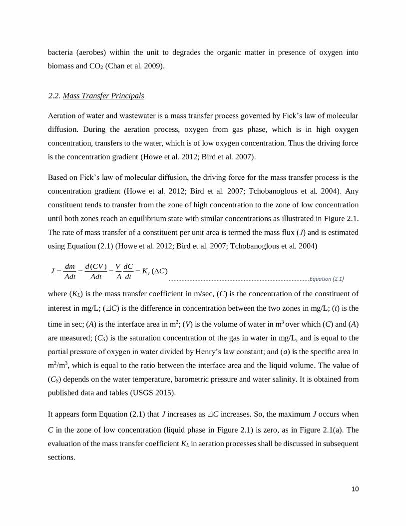
The rate of mass transfer of a constituent per unit area is termed the mass flux (J) and is estimated
using Equation (2.1) (Howe et al. 2012; Bird et al. 2007; Tchobanoglous et al. 2004)
( )( )L
dm d CV V dCJ K C
Adt Adt A dt
........................................................................................ Equation (2.1)
where (KL) is the mass transfer coefficient in m/sec, (C) is the concentration of the constituent of
interest in mg/L; (ΔC) is the difference in concentration between the two zones in mg/L; (t) is the
time in sec; (A) is the interface area in m2; (V) is the volume of water in m3 over which (C) and (A)
are measured; (CS) is the saturation concentration of the gas in water in mg/L, and is equal to the
partial pressure of oxygen in water divided by Henry’s law constant; and (a) is the specific area in
m2/m3, which is equal to the ratio between the interface area and the liquid volume. The value of
(CS) depends on the water temperature, barometric pressure and water salinity. It is obtained from
published data and tables (USGS 2015).
It appears form Equation (2.1) that J increases as ΔC increases. So, the maximum J occurs when
C in the zone of low concentration (liquid phase in Figure 2.1) is zero, as in Figure 2.1(a). The
evaluation of the mass transfer coefficient KL in aeration processes shall be discussed in subsequent
sections.
11
Figure 2.1 Schematic illustration of Fick’s law of diffusion. a) condition before diffusion b) condition during diffusion c) condition at equilibrium
When diffusion occurs without the impact of any external forces, it is termed molecular diffusion
(Howe et al. 2012). In molecular diffusion, the constituent transfers from the region of high
concentration to the region of low concentration solely due to the internal energy of the constituent,
while the fluid is at rest (Howe et al. 2012; Tchobanoglous et al. 2004). Other transfer modes are
advection, turbulent diffusion and dispersion. Advection occurs when the fluid is in motion, and
the constituent of interest transfers from one point to another with the moving fluid, in the absence
of diffusion (Howe et al. 2012). If the fluid is mixed in the control volume with no flow, the
diffusion is termed turbulent diffusion. The term dispersion is an inclusive term accounting for the
advection, molecular diffusion, and turbulent diffusion (Tchobanoglous et al. 2004). The
molecular diffusion is illustrated in Equation (2.2)
m
dCJ D
dz ......................................................................................................................................... Equation (2.2)
where (Dm) is the molecular diffusion coefficient of the constituent. Values of Dm depend on the
diffusing constituent, as well as the fluid it diffuses from or to. It is a function of the temperature.
For oxygen diffusing into water at 25oC, the value of Dm is equal to 2.42x10⁻⁵ cm2/sec (CRC 2016).
12
Through equating Equation (2.1) and Equation (2.2), the rate of oxygen transfer to water across an
air-water interface can be described with Equation (2.3) (Wójtowicz & Szlachta 2013; Bird et al.
2007; Gulliver & Rindels 1993).
L S L S
dC AK C C K a C C
dt V
......................................................................................... Equation (2.3)
2.2.1. Mass Transfer Coefficient (KL)
The mass transfer coefficient (KL), indicated in Equation (2.1) is a measure of gas flux per unit
concentration gradient, and has the dimensions of velocity. Extensive effort has been made by
several researchers to derive equations that can be used to estimate the value of KL, however, there
is no single equation that fits for all types of reactors or aerators (Garcia-Ochoa & Gomez 2009).
Some of those equations are empirical and based on experimental work, while others are
theoretical based. The theoretical models that predict KL are based either on the assumption of a
rigid interface surface indicated in the two film theory (Garcia-Ochoa & Gomez 2009; Bird et al.
2007; Tchobanoglous et al. 2004; Chapra 1997; Lewis & Whitman 1924; Whitman 1923), or the
assumption of surface renewal concept (Garcia-Ochoa & Gomez 2009; Bird et al. 2007;
Tchobanoglous et al. 2004; Chapra 1997), indicated in either the penetration theory (Higbie 1935),
or the surface renewal theory (Danckwerts 1951). Some models are based on a combination of the
two assumptions (Garcia-Ochoa & Gomez 2009).
The reciprocal of the mass transfer coefficient (1/KL) is an indicator of resistivity, and is the
summation of the resistivity from the gas side (1/HKg) and the resistivity from the liquid side (1/Kl)
(Tchobanoglous et al. 2004; Liss & Slater 1974) as indicated in Equation (2.4)
1 1 1
L g lK HK K
.................................................................................................................. Equation (2.4)
where (H) is Henry’s Law constant, (Kg) is the gas side mass transfer coefficient; (Kl) is the liquid
side mass transfer coefficient. In Equation (2.4), it should be noted that if Henry’s Law constant is
large, then the liquid side resistivity dominates, and the overall mass transfer coefficient is
approximately equal to the liquid side mass transfer coefficient, and vice versa (Tchobanoglous et
al. 2004; Liss & Slater 1974).
13
From the literature, KL is proportional to the molecular diffusion raised to the power ranging
between 0.5 (penetration and surface renewal theory) and 1 (two film theory) (Chapra 1997; Hsieh
et al. 1993). Furthermore, KL is found to have a dynamic value which is a function of the degree
of turbulence of the two interacting fluids (Jamnongwong et al. 2010; Tchobanoglous et al. 2004),
the chemical reactivity of gases (Wójtowicz & Szlachta 2013; Tchobanoglous et al. 2004; Liss &
Slater 1974), physical properties of gas and liquid, operational conditions, and geometrical
parameters of the reactor (Garcia-Ochoa & Gomez 2009; Tchobanoglous et al. 2004). Moreover,
KL changes with the change in water temperature (Tchobanoglous et al. 2004).
As the value of KL is sensitive to the temperature variation, Equation (2.5) describes the correction
of KL at any temperature (KL(T)) by knowing the value of KL at 20oC (KL(20)) (Tchobanoglous et al.
2004)
( 20)
( ) (20)
T
L T LK K ........................................................................................................................... Equation (2.5)
where θ is the temperature correction coefficient, ranging from 1.015 to 1.04, with typical value
of 1.024 (Tchobanoglous et al. 2004).
Due to the difficulty of estimating KL alone, most of the values reported in the literature are for the
volumetric mass transfer coefficient (KLa), which characterizes the mass transport for a studied
reactor operating under defined operating conditions and for specific constituents (Garcia-Ochoa
& Gomez 2009; Bird et al. 2007; Thacker et al. 2002; Hsieh et al. 1993; Nakasone 1987;
Kavanaugh & Trussell 1980). Among the limited number of reported values for air-water KL is the
proposed mean value between air and sea water KL=5.5x10⁻⁵ m/sec(Liss & Slater 1974). That value
shall be used in the mathematical model in chapter 3 only to test the model, and will be corrected
in chapter 4 after conducting the experimental work.
2.2.2. Aeration Overview
Some indicators are used to evaluated and compare between different aeration techniques and/or
different operating conditions for the aerator. Those indicators are Oxygen Transfer Rate (OTR),
Standard Oxygen Transfer Rate (SOTR), deficit ratio (r), and aeration efficiency(η).
14
The OTR is defined as “the quantity of oxygen transferred per unit time to a given volume of water
for equivalent conditions (temperature and chemical composition of water, depth at which air is
introduced, etc…)” (ASCE 2007; Tchobanoglous et al. 2004; Mueller et al. 2002). OTR is
equivalent to Equation (2.3) multiplied by the water volume as indicated in Equation (2.6).
L S
dCOTR V VK a C C
dt ..................................................................................................... Equation (2.6)
The SOTR is defined as “the quantity of oxygen transferred per unit time into a given volume of
water and reported at standard conditions (20oC, 1.00atm, and taking DO equal to zero)” (ASCE
2007; Mueller et al. 2002). The SOTR provides an indicator for the maximum driving force for the
gas transfer. The SOTR is calculated according to Equation (2.7).
2020o
o CL SC
SOTR VK a C ................................................................................................................... Equation (2.7)
Deficit ratio r is an indicator for the ratio of the oxygen deficit in the water prior to the aeration
device to the oxygen deficit after the aeration device as indicated in Equation (2.8) (Baylar et al.
2007; Nakasone 1987). For any aeration device, this indicator will have a value greater than one.
S US
S DS
C Cr
C C
....................................................................................................................................... Equation (2.8)
η is a ratio between DO added through the aeration device to the DO deficit prior to the aeration
device (Sabry et al. 2010; Moulick et al. 2010; Toombes & Chanson 2005; Gulliver & Rindels
1993). η is considered as the complementary to the inverse of r as indicated in Equation (2.9).
Higher values of η indicate more oxygen transfer and higher aeration performance.
11DS US
S DS
C C
C C r
...................................................................................................................... Equation (2.9)
2.3. Aeration Systems
Scott (1955) classified aeration of water into falling water aerators and diffused-air aerators.
Falling water aerators depends on dropping water through the process, hence the energy used is
the potential energy stored in the form of water head (Scott et al. 1955), while the diffused-air
aerators depend on forcing compressed air or pure oxygen through water using submerged orifices
15
or diffuser. (Scott et al. 1955; Tchobanoglous et al. 2004). Other aeration systems are mechanical
aerators, in which wastewater is agitated mechanically to boost the solution of air from the
atmosphere (Tchobanoglous et al. 2004).
Different types of passive aerators, which are commonly used in treatment units are illustrated in
Table 2.1 and detailed in subsequent sections.
Table 2.1 Aeration technologies
Aeration technology Feature Reference
Spray Aerator Large specific area
Low contact time
Large installation area
Not suitable for freezing weather
Energy needed to compress water
(Scott et al. 1955;
Sabry et al. 2010)
Cascade aerator Thin film aeration and air bubbles entrainment
High exposure time
Large installation area
No energy requirements
(Moulick et al.
2010; Baylar et
al. 2007;
Toombes &
Chanson 2005;
Scott et al. 1955;
Sabry et al. 2010)
Multiple tray aerator Thin film aeration and falling water
Large specific area
Small installation area
No energy requirements
(Scott et al. 1955)
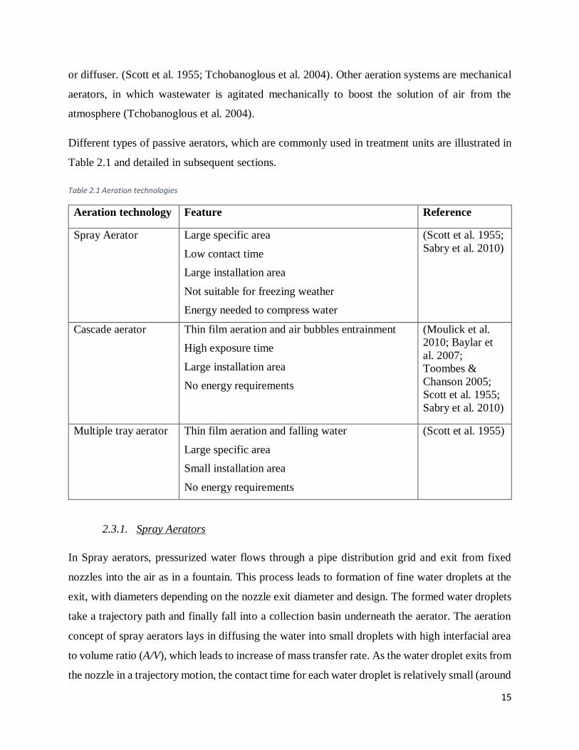
2.3.1. Spray Aerators
In Spray aerators, pressurized water flows through a pipe distribution grid and exit from fixed
nozzles into the air as in a fountain. This process leads to formation of fine water droplets at the
exit, with diameters depending on the nozzle exit diameter and design. The formed water droplets
take a trajectory path and finally fall into a collection basin underneath the aerator. The aeration
concept of spray aerators lays in diffusing the water into small droplets with high interfacial area
to volume ratio (A/V), which leads to increase of mass transfer rate. As the water droplet exits from
the nozzle in a trajectory motion, the contact time for each water droplet is relatively small (around
16
2 secs for a jet operating under a head of 6 meters), and hence the overall aeration efficiency is not
better than other types (Scott et al. 1955).
Other drawbacks of the spray aerators are their large installation area, they are not suitable during
freezing weather, and the nozzles have to be range from 25.4mm (1”) to 38.1mm (1.5”) to prevent
clogging (Scott et al. 1955). Figure 2.2 below illustrates the spray aerators.
Figure 2.2: Spray aerators (Courtesy: (Scott et al. 1955))
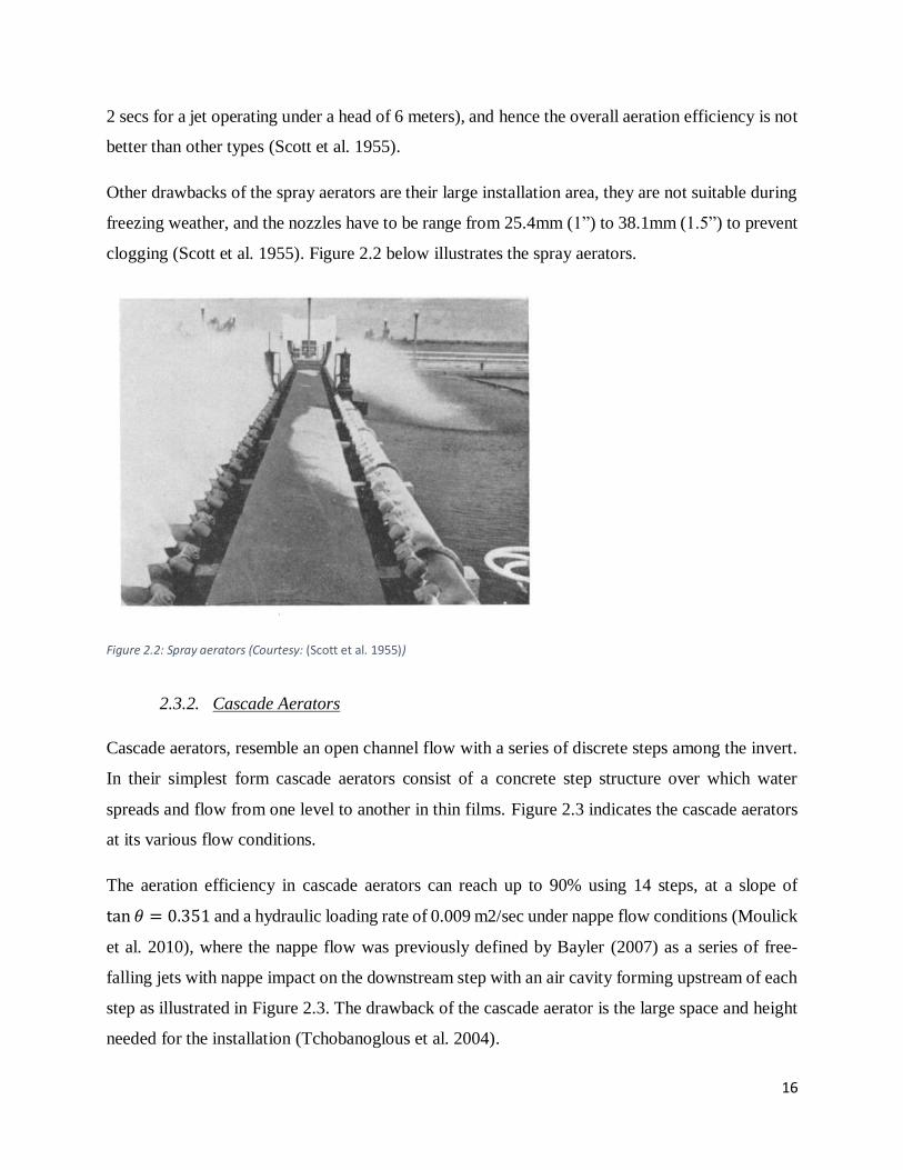
2.3.2. Cascade Aerators
Cascade aerators, resemble an open channel flow with a series of discrete steps among the invert.
In their simplest form cascade aerators consist of a concrete step structure over which water
spreads and flow from one level to another in thin films. Figure 2.3 indicates the cascade aerators
at its various flow conditions.
The aeration efficiency in cascade aerators can reach up to 90% using 14 steps, at a slope of
tan 𝜃 = 0.351 and a hydraulic loading rate of 0.009 m2/sec under nappe flow conditions (Moulick
et al. 2010), where the nappe flow was previously defined by Bayler (2007) as a series of free-
falling jets with nappe impact on the downstream step with an air cavity forming upstream of each
step as illustrated in Figure 2.3. The drawback of the cascade aerator is the large space and height
needed for the installation (Tchobanoglous et al. 2004).
17
Figure 2.3: Cascade aerators Nappe flow (Courtesy (Ohtsu et al. 2001))
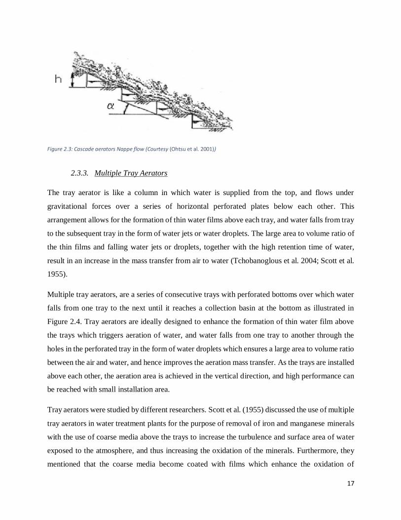
2.3.3. Multiple Tray Aerators
The tray aerator is like a column in which water is supplied from the top, and flows under
gravitational forces over a series of horizontal perforated plates below each other. This
arrangement allows for the formation of thin water films above each tray, and water falls from tray
to the subsequent tray in the form of water jets or water droplets. The large area to volume ratio of
the thin films and falling water jets or droplets, together with the high retention time of water,
result in an increase in the mass transfer from air to water (Tchobanoglous et al. 2004; Scott et al.
1955).
Multiple tray aerators, are a series of consecutive trays with perforated bottoms over which water
falls from one tray to the next until it reaches a collection basin at the bottom as illustrated in
Figure 2.4. Tray aerators are ideally designed to enhance the formation of thin water film above
the trays which triggers aeration of water, and water falls from one tray to another through the
holes in the perforated tray in the form of water droplets which ensures a large area to volume ratio
between the air and water, and hence improves the aeration mass transfer. As the trays are installed
above each other, the aeration area is achieved in the vertical direction, and high performance can
be reached with small installation area.
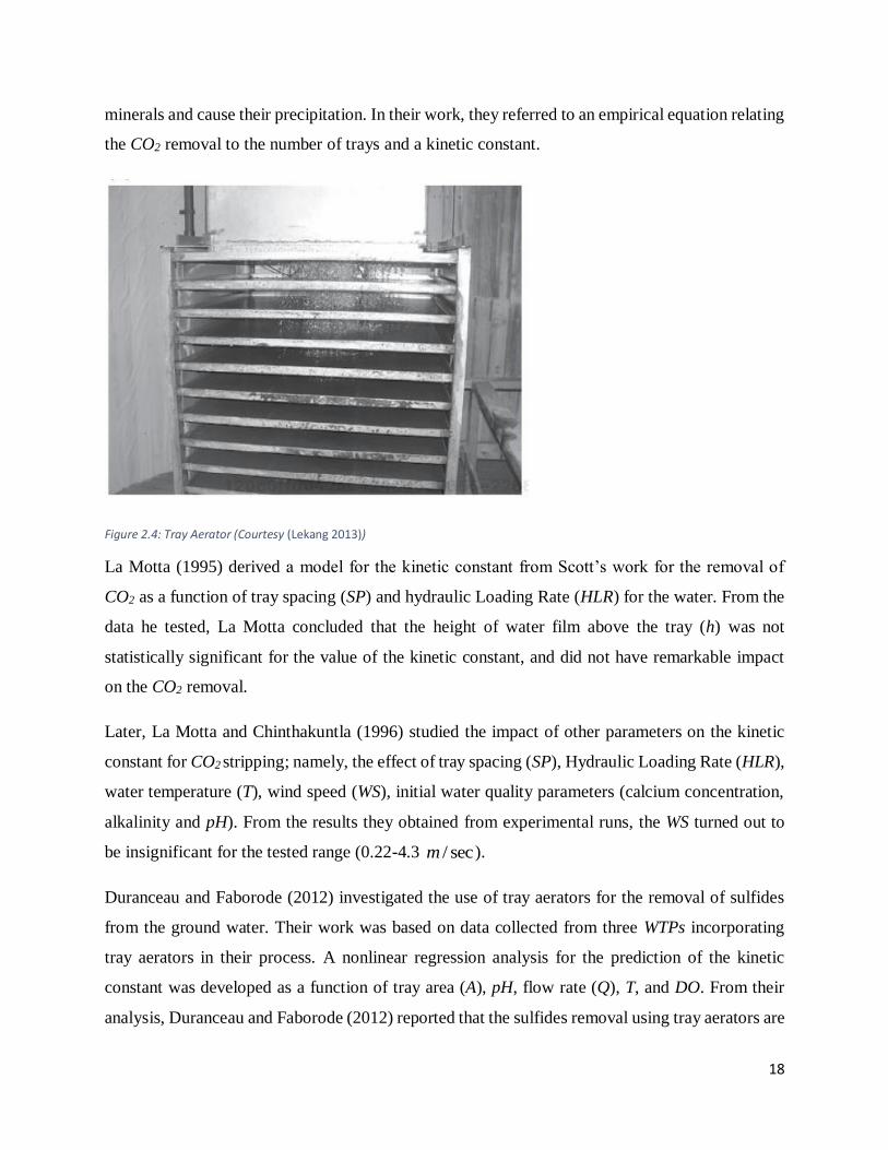
Tray aerators were studied by different researchers. Scott et al. (1955) discussed the use of multiple
tray aerators in water treatment plants for the purpose of removal of iron and manganese minerals
with the use of coarse media above the trays to increase the turbulence and surface area of water
exposed to the atmosphere, and thus increasing the oxidation of the minerals. Furthermore, they
mentioned that the coarse media become coated with films which enhance the oxidation of
18
minerals and cause their precipitation. In their work, they referred to an empirical equation relating
the CO2 removal to the number of trays and a kinetic constant.
Figure 2.4: Tray Aerator (Courtesy (Lekang 2013))
La Motta (1995) derived a model for the kinetic constant from Scott’s work for the removal of
CO2 as a function of tray spacing (SP) and hydraulic Loading Rate (HLR) for the water. From the
data he tested, La Motta concluded that the height of water film above the tray (h) was not
statistically significant for the value of the kinetic constant, and did not have remarkable impact
on the CO2 removal.
Later, La Motta and Chinthakuntla (1996) studied the impact of other parameters on the kinetic
constant for CO2 stripping; namely, the effect of tray spacing (SP), Hydraulic Loading Rate (HLR),
water temperature (T), wind speed (WS), initial water quality parameters (calcium concentration,
alkalinity and pH). From the results they obtained from experimental runs, the WS turned out to
be insignificant for the tested range (0.22-4.3 / secm ).
Duranceau and Faborode (2012) investigated the use of tray aerators for the removal of sulfides
from the ground water. Their work was based on data collected from three WTPs incorporating
tray aerators in their process. A nonlinear regression analysis for the prediction of the kinetic
constant was developed as a function of tray area (A), pH, flow rate (Q), T, and DO. From their
analysis, Duranceau and Faborode (2012) reported that the sulfides removal using tray aerators are

19
inversely proportional to the number of free protons (H+) and the HLR, and directly proportional
with A.

20
3. Phase I - Mathematical Model
21
3.1. Introduction
In any research work, modelling is the tool utilized by the researchers to interpret different
phenomena (response) into simple mathematical expression. Those expressions provide qualitative
and quantitative understanding of the phenomena (Heinz 2011). Modelling is either through
mathematical modelling, or experimental modelling. Mathematical modelling is mainly based on
theory, in which different mathematical expressions are solved simultaneously to develop a
formula that describes the response. Following mathematical modelling, experimental work is
needed to verify the developed mathematical model.
Among the main benefits of the mathematical modelling, is that the mathematical modelling assist
in predicting the input parameters which potentially impact the response, visualize the sensitivity
of the response to the change in those parameters, and provide guidance to the levels of test
conditions that need to be considered in the experimental modelling.
In the current chapter, the equations governing the mass transfer are considered as the basis for
developing the model. The literature review highlights the different flow regimes for the free
falling water through the tray holes, and the thresholds for each regime. The methodology
describes the procedure to develop a mathematical model that predicts the aeration performance
from tray aerators. The model is developed using MATLAB software. The results section shows
the results obtained from the model under different test conditions, as well as the impact of
changing each input parameter on the response of the aeration performance. The discussion
section, draws a comparison between the developed aeration model and other air striping models
for tray aerators that were developed in previous works.
3.2. Methodology
For this phase, a set of equations governing the flow and mass transfer for water in the tray aerators
were derived from the basic equations. This set of equations (which are shown later in this section)
were compiled in a MATLab - Mathworks function file to be used as a mathematical model for
designing the tray aerators.
22
In deriving the mathematical model for DO concentration in the effluent from tray aerators, the
model considered first a system of one aeration tray other than the distribution tray. Later, the
model is expanded to consider more than one tray. Water entering the distribution tray shall exhibit
two subsequent flow modes until it reaches the aeration tray; namely thin film formed above the
distribution tray and free falling water between the distribution and aeration trays. Each mode is
analyzed separately in the next sections.
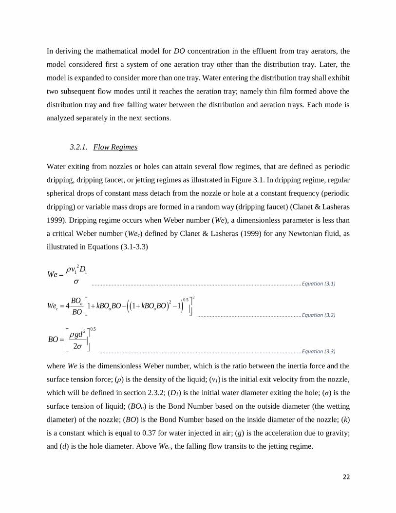
3.2.1. Flow Regimes
Water exiting from nozzles or holes can attain several flow regimes, that are defined as periodic
dripping, dripping faucet, or jetting regimes as illustrated in Figure 3.1. In dripping regime, regular
spherical drops of constant mass detach from the nozzle or hole at a constant frequency (periodic
dripping) or variable mass drops are formed in a random way (dripping faucet) (Clanet & Lasheras
1999). Dripping regime occurs when Weber number (We), a dimensionless parameter is less than
a critical Weber number (Wec) defined by Clanet & Lasheras (1999) for any Newtonian fluid, as
illustrated in Equations (3.1-3.3)
2
1 1v DWe
....................................................................................................................................... Equation (3.1)
2
0.52
4 1 1 1oc o o
BOWe kBO BO kBO BO
BO
................................................................... Equation (3.2)
0.52
2
gdBO
.................................................................................................................................. Equation (3.3)
where We is the dimensionless Weber number, which is the ratio between the inertia force and the
surface tension force; (ρ) is the density of the liquid; (v1) is the initial exit velocity from the nozzle,
which will be defined in section 2.3.2; (D1) is the initial water diameter exiting the hole; (σ) is the
surface tension of liquid; (BOo) is the Bond Number based on the outside diameter (the wetting
diameter) of the nozzle; (BO) is the Bond Number based on the inside diameter of the nozzle; (k)
is a constant which is equal to 0.37 for water injected in air; (g) is the acceleration due to gravity;
and (d) is the hole diameter. Above Wec, the falling flow transits to the jetting regime.
23
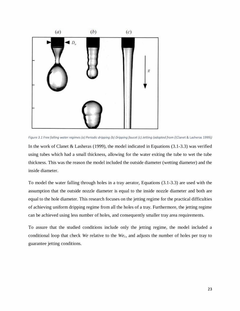
Figure 3.1 Free falling water regimes (a) Periodic dripping (b) Dripping faucet (c) Jetting (adopted from ((Clanet & Lasheras 1999))
In the work of Clanet & Lasheras (1999), the model indicated in Equations (3.1-3.3) was verified
using tubes which had a small thickness, allowing for the water exiting the tube to wet the tube
thickness. This was the reason the model included the outside diameter (wetting diameter) and the
inside diameter.
To model the water falling through holes in a tray aerator, Equations (3.1-3.3) are used with the
assumption that the outside nozzle diameter is equal to the inside nozzle diameter and both are
equal to the hole diameter. This research focuses on the jetting regime for the practical difficulties
of achieving uniform dripping regime from all the holes of a tray. Furthermore, the jetting regime
can be achieved using less number of holes, and consequently smaller tray area requirements.
To assure that the studied conditions include only the jetting regime, the model included a
conditional loop that check We relative to the Wec, and adjusts the number of holes per tray to
guarantee jetting conditions.
24
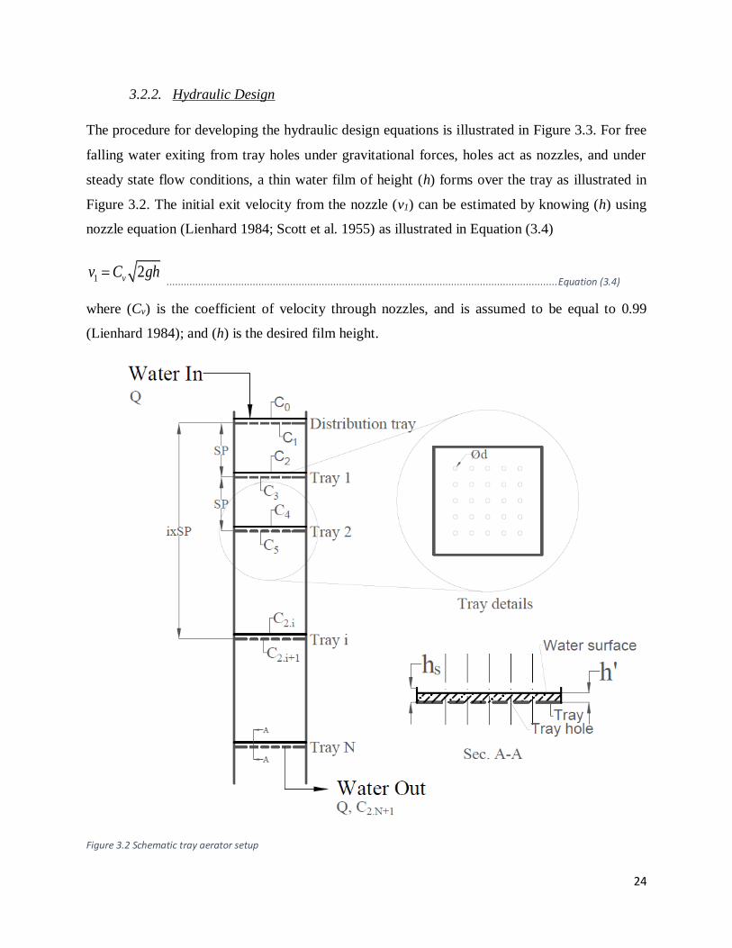
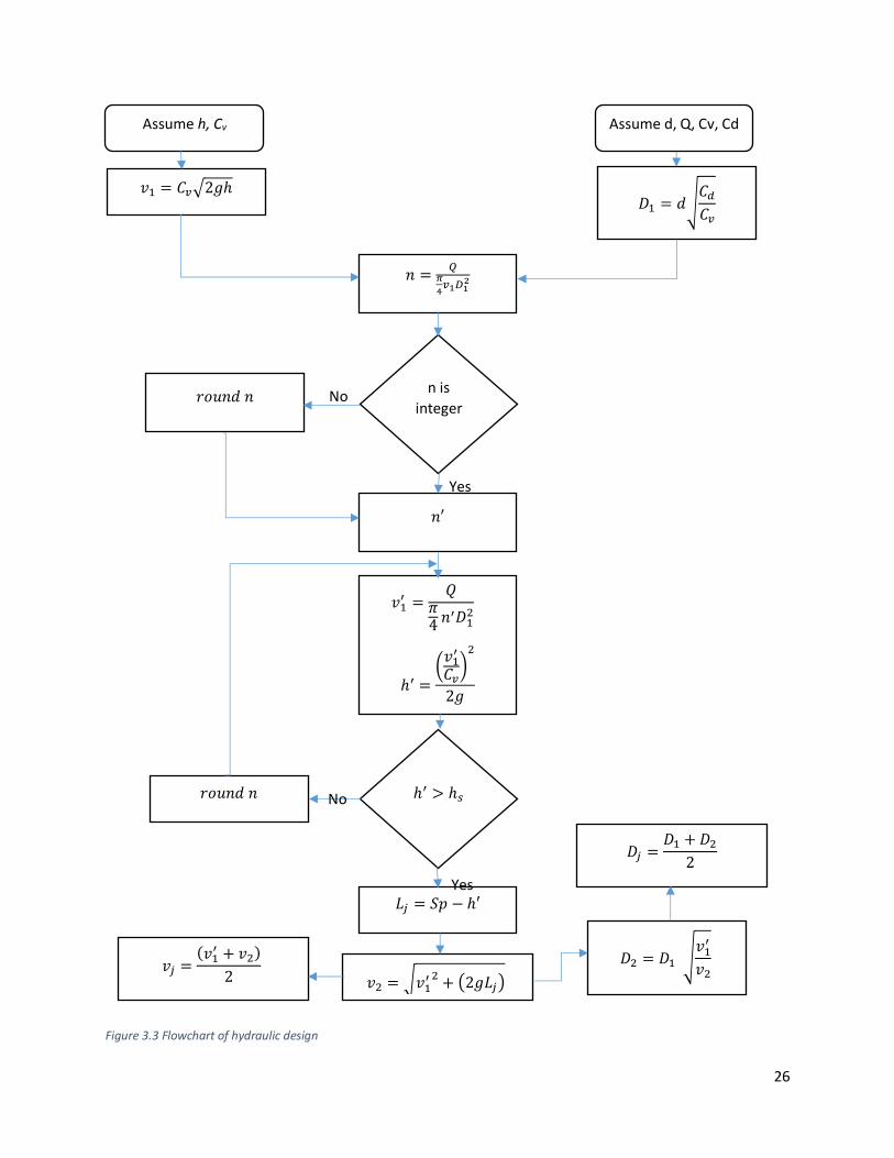
3.2.2. Hydraulic Design
The procedure for developing the hydraulic design equations is illustrated in Figure 3.3. For free
falling water exiting from tray holes under gravitational forces, holes act as nozzles, and under
steady state flow conditions, a thin water film of height (h) forms over the tray as illustrated in
Figure 3.2. The initial exit velocity from the nozzle (v1) can be estimated by knowing (h) using
nozzle equation (Lienhard 1984; Scott et al. 1955) as illustrated in Equation (3.4)
1 2vv C gh ........................................................................................................................................ Equation (3.4)
where (Cv) is the coefficient of velocity through nozzles, and is assumed to be equal to 0.99
(Lienhard 1984); and (h) is the desired film height.
Figure 3.2 Schematic tray aerator setup
25
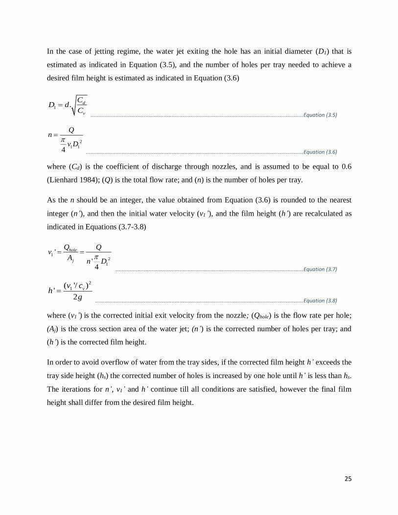
In the case of jetting regime, the water jet exiting the hole has an initial diameter (D1) that is
estimated as indicated in Equation (3.5), and the number of holes per tray needed to achieve a
desired film height is estimated as indicated in Equation (3.6)
1 . d
v
CD d
C
........................................................................................................................................ Equation (3.5)
2
1 14
Qn
v D
........................................................................................................................................... Equation (3.6)
where (Cd) is the coefficient of discharge through nozzles, and is assumed to be equal to 0.6
(Lienhard 1984); (Q) is the total flow rate; and (n) is the number of holes per tray.
As the n should be an integer, the value obtained from Equation (3.6) is rounded to the nearest
integer (n’), and then the initial water velocity (v1’), and the film height (h’) are recalculated as
indicated in Equations (3.7-3.8)
12
1
'
'4
hole
j
Q Qv
An D
........................................................................................................................ Equation (3.7)
2
1( '/ )'
2
vv ch
g
..................................................................................................................................... Equation (3.8)
where (v1’) is the corrected initial exit velocity from the nozzle; (Qhole) is the flow rate per hole;
(Aj) is the cross section area of the water jet; (n’) is the corrected number of holes per tray; and
(h’) is the corrected film height.
In order to avoid overflow of water from the tray sides, if the corrected film height h’ exceeds the
tray side height (hs) the corrected number of holes is increased by one hole until h’ is less than hs.
The iterations for n’, v1’ and h’ continue till all conditions are satisfied, however the final film
height shall differ from the desired film height.
26
Figure 3.3 Flowchart of hydraulic design
Assume h, Cv
𝑣1 = 𝐶𝑣ඥ2𝑔ℎ
𝑛 =𝑄
𝜋
4𝑣1𝐷1
2
Assume d, Q, Cv, Cd
𝐷1 = 𝑑ඨ𝐶𝑑
𝐶𝑣
n is
integer 𝑟𝑜𝑢𝑛𝑑 𝑛
𝑛′
𝑣1′ =
𝑄𝜋4 𝑛′𝐷1
2
ℎ′ =൬
𝑣1′
𝐶𝑣൰
2
2𝑔
ℎ′ > ℎ𝑠 𝑟𝑜𝑢𝑛𝑑 𝑛
𝐿𝑗 = 𝑆𝑝 − ℎ′
𝑣2 = ට𝑣1′ 2
+ ൫2𝑔𝐿𝑗൯
𝐷2 = 𝐷1 ඨ𝑣1
′
𝑣2
𝐷𝑗 =𝐷1 + 𝐷2
2
𝑣𝑗 =ሺ𝑣1
′ + 𝑣2ሻ
2
No
No
Yes
Yes
27
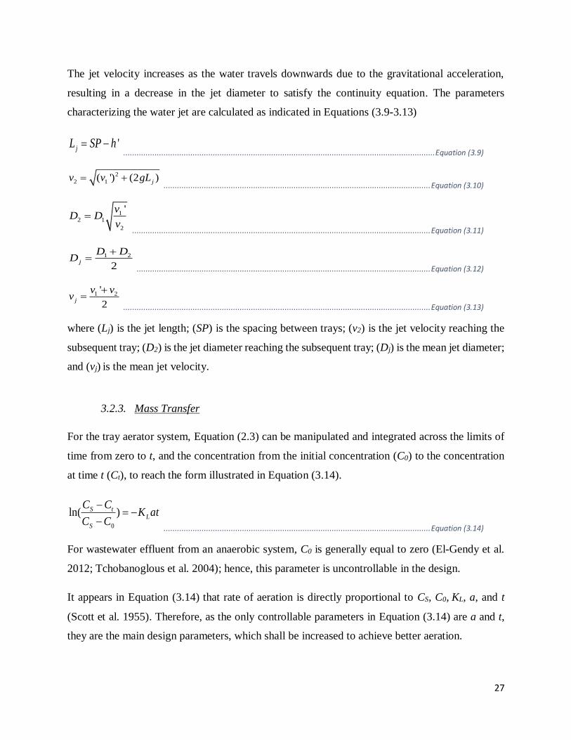
The jet velocity increases as the water travels downwards due to the gravitational acceleration,
resulting in a decrease in the jet diameter to satisfy the continuity equation. The parameters
characterizing the water jet are calculated as indicated in Equations (3.9-3.13)
'jL SP h ........................................................................................................................................... Equation (3.9)
2
2 1( ') (2 )jv v gL ....................................................................................................................... Equation (3.10)
12 1
2
'vD D
v
..................................................................................................................................... Equation (3.11)
1 2
2j
D DD
................................................................................................................................... Equation (3.12)
1 2'
2j
v vv
......................................................................................................................................... Equation (3.13)
where (Lj) is the jet length; (SP) is the spacing between trays; (v2) is the jet velocity reaching the
subsequent tray; (D2) is the jet diameter reaching the subsequent tray; (Dj) is the mean jet diameter;
and (vj) is the mean jet velocity.
3.2.3. Mass Transfer
For the tray aerator system, Equation (2.3) can be manipulated and integrated across the limits of
time from zero to t, and the concentration from the initial concentration (C0) to the concentration
at time t (Ct), to reach the form illustrated in Equation (3.14).
0
ln( )S tL
S
C CK at
C C
....................................................................................................................... Equation (3.14)
For wastewater effluent from an anaerobic system, C0 is generally equal to zero (El-Gendy et al.
2012; Tchobanoglous et al. 2004); hence, this parameter is uncontrollable in the design.
It appears in Equation (3.14) that rate of aeration is directly proportional to CS, C0, KL, a, and t
(Scott et al. 1955). Therefore, as the only controllable parameters in Equation (3.14) are a and t,
they are the main design parameters, which shall be increased to achieve better aeration.
28
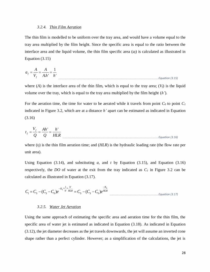
3.2.4. Thin Film Aeration
The thin film is modelled to be uniform over the tray area, and would have a volume equal to the
tray area multiplied by the film height. Since the specific area is equal to the ratio between the
interface area and the liquid volume, the thin film specific area (af) is calculated as illustrated in
Equation (3.15)
1
. ' 'f
f
A Aa
V A h h
......................................................................................................................... Equation (3.15)
where (A) is the interface area of the thin film, which is equal to the tray area; (Vf) is the liquid
volume over the tray, which is equal to the tray area multiplied by the film height (h’).
For the aeration time, the time for water to be aerated while it travels from point C0 to point C1
indicated in Figure 3.2, which are at a distance h’ apart can be estimated as indicated in Equation
(3.16)
' 'f
f
V Ah ht
Q Q HLR
.................................................................................................................... Equation (3.16)
where (tf) is the thin film aeration time; and (HLR) is the hydraulic loading rate (the flow rate per
unit area).
Using Equation (3.14), and substituting a, and t by Equation (3.15), and Equation (3.16)
respectively, the DO of water at the exit from the tray indicated as C1 in Figure 3.2 can be
calculated as illustrated in Equation (3.17).
1 '* *
'1 0 0( ) ( )
LL
KhK
h HLR HLRS S S SC C C C e C C C e
........................................................... Equation (3.17)
3.2.5. Water Jet Aeration
Using the same approach of estimating the specific area and aeration time for the thin film, the
specific area of water jet is estimated as indicated in Equation (3.18). As indicated in Equation
(3.12), the jet diameter decreases as the jet travels downwards, the jet will assume an inverted cone
shape rather than a perfect cylinder. However; as a simplification of the calculations, the jet is
29
modelled as a cylinder having a diameter of Dj, travelling with a velocity of vj, and a length of Lj.
The aeration time is estimated as indicated in Equation (3.19)
2
4
4
j j j
j
j jj j
A D La
V DD L
................................................................................................................ Equation (3.18)
j
j
j
Lt
v
.................................................................................................................................................. Equation (3.19)
where (aj) is the specific area of the jet; (Dj) is the mean jet diameter; (Vj) is the volume of water
within the jet; and (tj) is the jet aeration time.
Equation (3.14) is used to calculate the DO reaching the aeration tray by substituting a by aj from
Equation (3.18), and t by tj from Equation (3.19), as illustrated in Equation (3.20) where (C1) and
(C2) are the DO concentration at the exit point from the distribution tray, and the point reaching
the next aeration tray respectively as illustrated in Figure 3.2.
. .
2 1( ) L j jK a t
S SC C C C e
........................................................................................................... Equation (3.20)
3.2.6. Overall Aeration Through a Single Tray
For the estimation of the overall aeration occurring over a single tray other than the distribution
tray, Equation (3.17), and Equation (3.20) are combined to account for the two aeration regimes;
namely the thin film above the tray and the water jetting from the tray, as illustrated in Equation
(3.21).
1( . )
2 0( )L j jK a t
HLRS SC C C C e
............................................................................................... Equation (3.21)
3.2.7. Number of Trays
Now considering the case where there is a number of (N) consecutive trays arranged beneath each
other below the distribution tray, with a constant spacing between trays equal to (SP) as illustrated
in Figure 3.2. The influent DO to the (ith) tray is denoted as (C2i), where (i)=1: N is the number of
tray including the distribution tray. Water reaching the ith tray experience i-1 thin film above the
30
tray and i-1 falling water regimes. Thus Equation (3.21) can be generalized to include the tray
number as indicated in Equation (3.22)
1.( 1).( . )
2( 1) 0( )L j jK i a t
HLRi S SC C C C e
................................................................................... Equation (3.22)
where (C2(i-1)) is the influent DO to the (i-1th) tray; and (i) is the number of tray including the
distribution tray.
3.2.8. Model Assumptions
The current model is split into two parts. The first part studies the flow regime for water falling
from trays. It investigates the threshold for achieving the jetting regime at various hole diameter
and flow rate. The second part investigates the effect of different design parameters on the aeration
performance for a tray aerator system that is operating in the jetting regime conditions.
To simplify solving the model equations, the following set of assumptions are made:
1- The flow is at steady state conditions
2- The trays are perfectly horizontal
3- All trays are square with a cross section area (A).
4- All trays have the same number of holes and hole diameters, and are installed with constant
spacing (SP) between each other
5- The maximum allowable height for the thin film (hs) is 25x10-3 m, otherwise, the tray
would overflow.
6- The velocity distribution is uniform along the cross section of jets and the thin film.
7- The value for oxygen mass transfer coefficient (KL) between air and water is 5.5x10⁻⁵ m/sec
(Liss & Slater 1974).
8- The coefficient of discharge through holes (Cd) is equal to 0.6 (Lienhard 1984), and the
coefficient of velocity through holes (Cv) is equal to 0.99 (Lienhard 1984).
31
9- The inlet dissolved oxygen concentration (C0) to the system is zero
3.2.9. Model Equations
Two function files are developed using MATLab R2013b (8.2.0.701); the first file aims at
illustrating the threshold for the jetting regime, whereas the second file predicts the effluent DO
from a tray aerator system that is installed at a distance (SP) above the water surface in the
receiving tank. The receiving tank acts as the (Nth+1) tray. Both codes are based on the equations
derived in the methodology section, and are included in Annex I for reference. The model was
tested for the conditions indicated in Table 3.1.
Table 3.1 Values of mathematical model input parameters
Parameter Unit of Measurement Value
Flow rate Q x10-5 m3/sec (m3/day) 1.157(1), 1.736(1.5), 2.315(2),
2.894(2.5), 5.208(4.5)
Tray Area A m2 0.15x0.15, 0.2x0.2, 0.25x0.25
Number of trays N Dimensionless 1, 2, 3, 4, 5, 6, 7, 8, 9, 10
film height h x10-3 m 2, 3, 5, 10, 15, 20
Diameter of hole d x10-3 m 3, 4, 5, 6
Overall System height H m 1
Temperature oC 24
Oxygen mass transfer coefficient
KL
m/sec 5.5x10⁻⁵ (Liss & Slater 1974)
3.3. Results
3.3.1. Flow Regime
The first function file solves Equations (3.1-3.3) proposed by Clanet & Lasheras (1999) to get the
maximum number of holes among which water is uniformly distributed in a tray before it transits
from jetting to dripping for the set of tested diameters and flow rates. Results are illustrated in
Figure 3.4 where the maximum number of holes, for jetting regime, increases with the increase in
the total flow rate. Furthermore, the increase in the hole diameter results in a decrease in the
maximum number of holes. The maximum number of holes is not affected by the tray area.
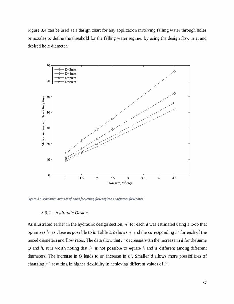
32
Figure 3.4 can be used as a design chart for any application involving falling water through holes
or nozzles to define the threshold for the falling water regime, by using the design flow rate, and
desired hole diameter.
Figure 3.4 Maximum number of holes for jetting flow regime at different flow rates
3.3.2. Hydraulic Design
As illustrated earlier in the hydraulic design section, n’ for each d was estimated using a loop that
optimizes h’ as close as possible to h. Table 3.2 shows n’ and the corresponding h’ for each of the
tested diameters and flow rates. The data show that n’ decreases with the increase in d for the same
Q and h. It is worth noting that h’ is not possible to equate h and is different among different
diameters. The increase in Q leads to an increase in n’. Smaller d allows more possibilities of
changing n’, resulting in higher flexibility in achieving different values of h’.
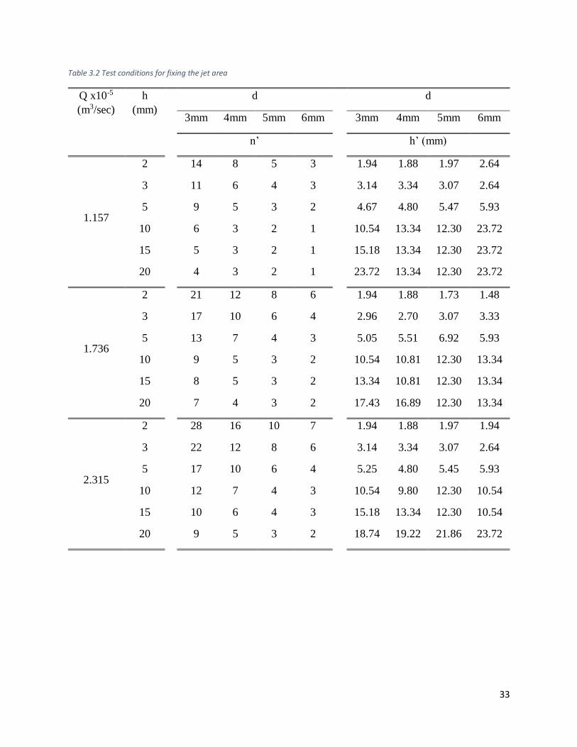
33
Table 3.2 Test conditions for fixing the jet area
Q x10-5
(m3/sec)
h
(mm)
d d
3mm 4mm 5mm 6mm 3mm 4mm 5mm 6mm
n’ h’ (mm)
1.157
2 14 8 5 3 1.94 1.88 1.97 2.64
3 11 6 4 3 3.14 3.34 3.07 2.64
5 9 5 3 2 4.67 4.80 5.47 5.93
10 6 3 2 1 10.54 13.34 12.30 23.72
15 5 3 2 1 15.18 13.34 12.30 23.72
20 4 3 2 1 23.72 13.34 12.30 23.72
1.736
2 21 12 8 6 1.94 1.88 1.73 1.48
3 17 10 6 4 2.96 2.70 3.07 3.33
5 13 7 4 3 5.05 5.51 6.92 5.93
10 9 5 3 2 10.54 10.81 12.30 13.34
15 8 5 3 2 13.34 10.81 12.30 13.34
20 7 4 3 2 17.43 16.89 12.30 13.34
2.315
2 28 16 10 7 1.94 1.88 1.97 1.94
3 22 12 8 6 3.14 3.34 3.07 2.64
5 17 10 6 4 5.25 4.80 5.45 5.93
10 12 7 4 3 10.54 9.80 12.30 10.54
15 10 6 4 3 15.18 13.34 12.30 10.54
20 9 5 3 2 18.74 19.22 21.86 23.72
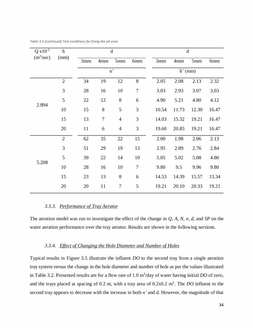
34
Table 3.2 (continued) Test conditions for fixing the jet area
Q x10-5
(m3/sec)
h
(mm)
d d
3mm 4mm 5mm 6mm 3mm 4mm 5mm 6mm
n’ h’ (mm)
2.894
2 34 19 12 8 2.05 2.08 2.13 2.32
3 28 16 10 7 3.03 2.93 3.07 3.03
5 22 12 8 6 4.90 5.21 4.80 4.12
10 15 8 5 3 10.54 11.73 12.30 16.47
15 13 7 4 3 14.03 15.32 19.21 16.47
20 11 6 4 3 19.60 20.85 19.21 16.47
5.208
2 62 35 22 15 2.00 1.98 2.06 2.13
3 51 29 19 13 2.95 2.89 2.76 2.84
5 39 22 14 10 5.05 5.02 5.08 4.80
10 28 16 10 7 9.80 9.5 9.96 9.80
15 23 13 8 6 14.53 14.39 15.57 13.34
20 20 11 7 5 19.21 20.10 20.33 19.21
3.3.3. Performance of Tray Aerator
The aeration model was run to investigate the effect of the change in Q, A, N, n, d, and SP on the
water aeration performance over the tray aerator. Results are shown in the following sections.
3.3.4. Effect of Changing the Hole Diameter and Number of Holes
Typical results in Figure 3.5 illustrate the influent DO to the second tray from a single aeration
tray system versus the change in the hole diameter and number of hole as per the values illustrated
in Table 3.2. Presented results are for a flow rate of 1.0 m3/day of water having initial DO of zero,
and the trays placed at spacing of 0.2 m, with a tray area of 0.2x0.2 m2. The DO influent to the
second tray appears to decrease with the increase in both n’ and d. However, the magnitude of that
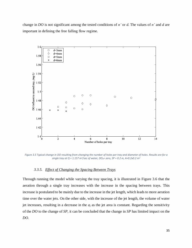
35
change in DO is not significant among the tested conditions of n’ or d. The values of n’ and d are
important in defining the free falling flow regime.
Figure 3.5 Typical change in DO resulting from changing the number of holes per tray and diameter of holes. Results are for a single tray at Q = 1.157 m3/sec of water, DO0= zero, SP = 0.2 m, A=0.2x0.2 m2
3.3.5. Effect of Changing the Spacing Between Trays
Through running the model while varying the tray spacing, it is illustrated in Figure 3.6 that the
aeration through a single tray increases with the increase in the spacing between trays. This
increase is postulated to be mainly due to the increase in the jet length, which leads to more aeration
time over the water jets. On the other side, with the increase of the jet length, the volume of water
jet increases, resulting in a decrease in the aj as the jet area is constant. Regarding the sensitivity
of the DO to the change of SP, it can be concluded that the change in SP has limited impact on the
DO.
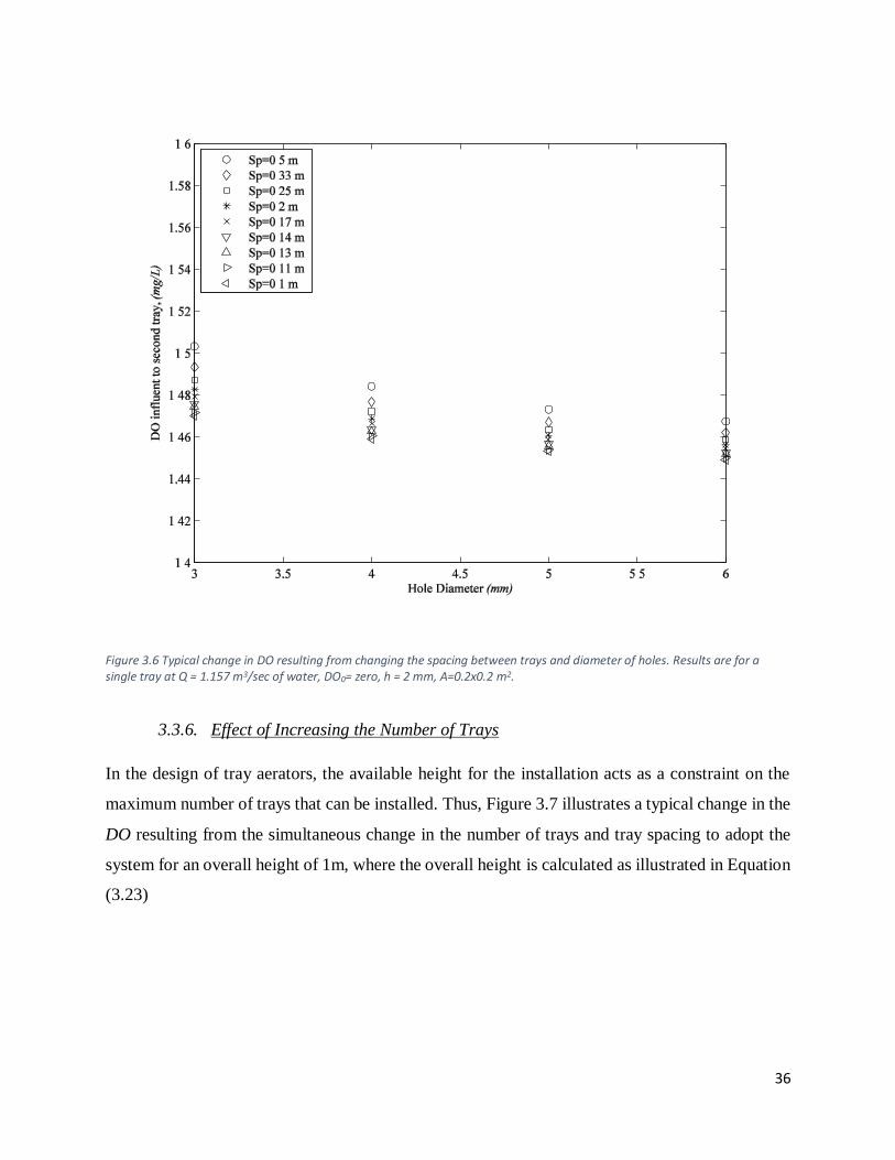
36
Figure 3.6 Typical change in DO resulting from changing the spacing between trays and diameter of holes. Results are for a single tray at Q = 1.157 m3/sec of water, DO0= zero, h = 2 mm, A=0.2x0.2 m2.
3.3.6. Effect of Increasing the Number of Trays
In the design of tray aerators, the available height for the installation acts as a constraint on the
maximum number of trays that can be installed. Thus, Figure 3.7 illustrates a typical change in the
DO resulting from the simultaneous change in the number of trays and tray spacing to adopt the
system for an overall height of 1m, where the overall height is calculated as illustrated in Equation
(3.23)
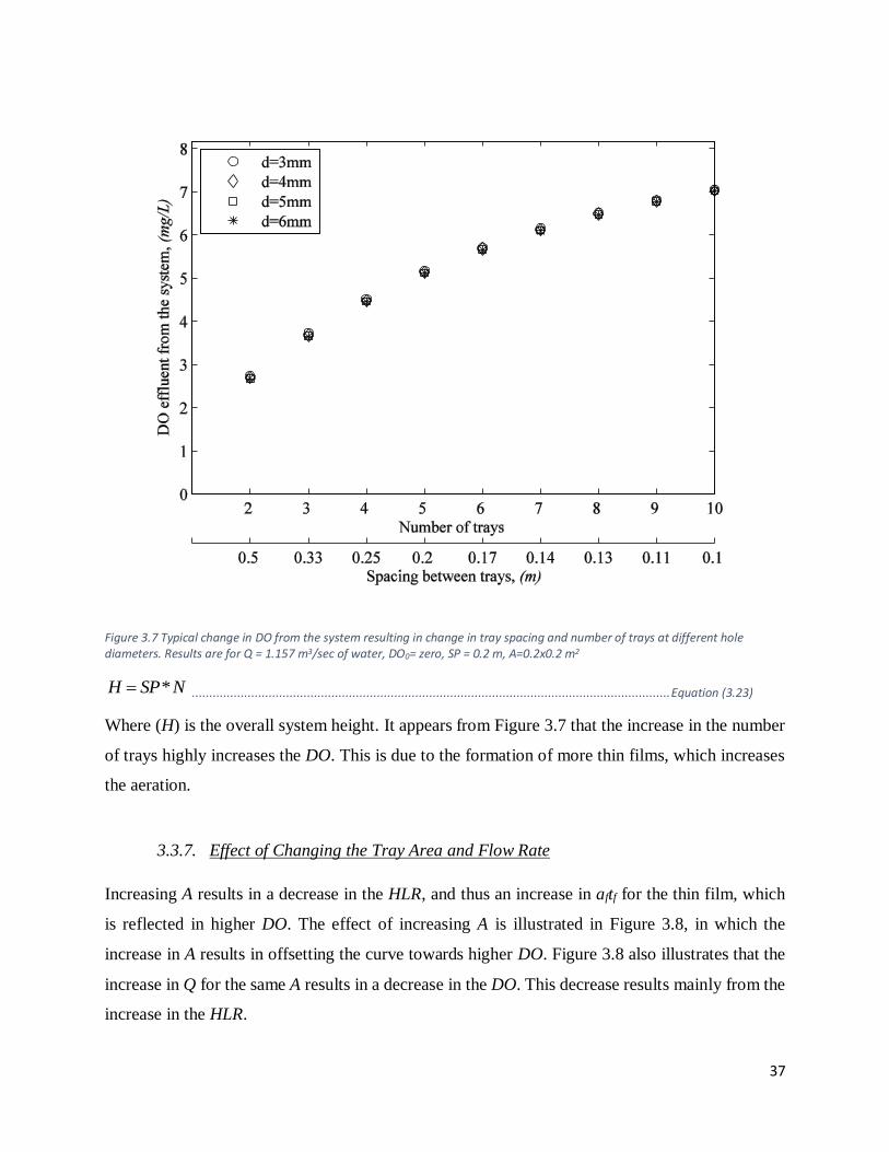
37
Figure 3.7 Typical change in DO from the system resulting in change in tray spacing and number of trays at different hole diameters. Results are for Q = 1.157 m3/sec of water, DO0= zero, SP = 0.2 m, A=0.2x0.2 m2
*H SP N ......................................................................................................................................... Equation (3.23)
Where (H) is the overall system height. It appears from Figure 3.7 that the increase in the number
of trays highly increases the DO. This is due to the formation of more thin films, which increases
the aeration.
3.3.7. Effect of Changing the Tray Area and Flow Rate
Increasing A results in a decrease in the HLR, and thus an increase in aftf for the thin film, which
is reflected in higher DO. The effect of increasing A is illustrated in Figure 3.8, in which the
increase in A results in offsetting the curve towards higher DO. Figure 3.8 also illustrates that the
increase in Q for the same A results in a decrease in the DO. This decrease results mainly from the
increase in the HLR.
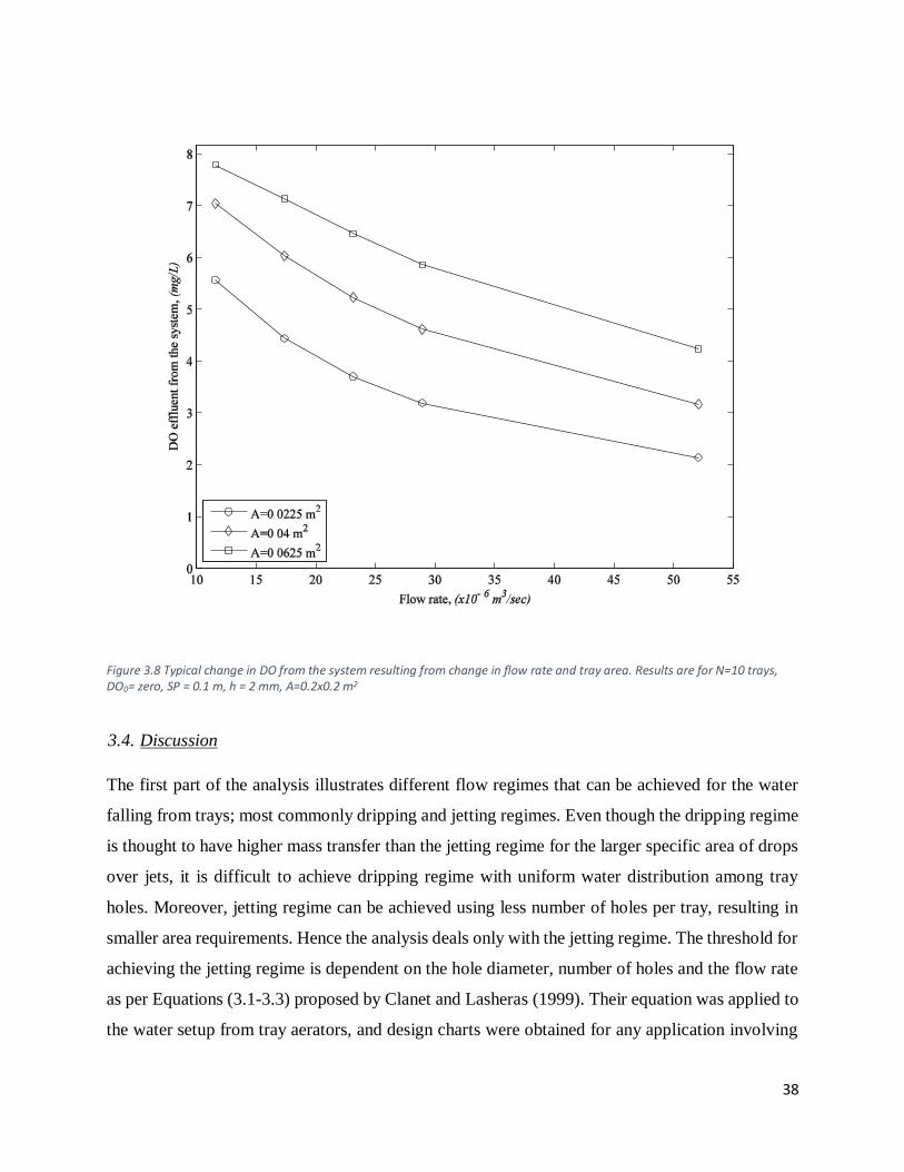
38
Figure 3.8 Typical change in DO from the system resulting from change in flow rate and tray area. Results are for N=10 trays, DO0= zero, SP = 0.1 m, h = 2 mm, A=0.2x0.2 m2
3.4. Discussion
The first part of the analysis illustrates different flow regimes that can be achieved for the water
falling from trays; most commonly dripping and jetting regimes. Even though the dripping regime
is thought to have higher mass transfer than the jetting regime for the larger specific area of drops
over jets, it is difficult to achieve dripping regime with uniform water distribution among tray
holes. Moreover, jetting regime can be achieved using less number of holes per tray, resulting in
smaller area requirements. Hence the analysis deals only with the jetting regime. The threshold for
achieving the jetting regime is dependent on the hole diameter, number of holes and the flow rate
as per Equations (3.1-3.3) proposed by Clanet and Lasheras (1999). Their equation was applied to
the water setup from tray aerators, and design charts were obtained for any application involving
39
falling water through holes or nozzles to define the threshold for the falling water regime, by using
the design flow rate, and desired hole diameter.
The second part of the study analyzed the hydraulic design of the tray aerators and the parameters
that might affect the aeration performance of tray aerators. The analysis addressed the estimation
of a, and t which are the design parameters for Equation (2.3). Those two parameters are dependent
on the d, Q, N, n, SP, and A. The impact of each parameter on the effluent DO was investigated
separately.
Changing d defines the flow regime into jetting or dripping, with minor effect on the effluent DO.
This slight impact of d on the DO is seen from Equation (3.18), where the value of aj is inversely
proportional with Dj, which is a function of d, SP, Q, and n. However, in order to limit the flow
regime to the jetting regime for a given Q, n changed accordingly to assure that We is greater that
Wec to satisfy Equation (3.1-3.3), mitigating the impact of changing d. Changing Q is inversely
proportional with the DO, and as a result has a high impact on its value., and is inversely
proportional. Increasing Q results in an increase in HLR, which in turn results in a decrease in tf as
illustration in Equation (3.16). Similarly, increasing A results in an increase in DO due to the
decrease in HLR. The DO increased slightly with the increase in SP, which was interpreted to be
due to the increase in Lj (Equation (3.10)), which led to the increase in v2 and vj, and a decrease in
D2 and Dj according to Equation (3.11-3.14). As a result, aj decreased (Equation (3.18)) and tj
increased (Equation (3.19)) resulting in higher mass of oxygen diffusing into the falling water.
Increasing N results in an increase in the number of thin films and water jets within the tray aerator
system, leading to an increase in DO. The exponential trend of increase in DO with the increase in
N (Figure 3.6) is the result of approaching the saturation level for DO.
These results when compared to the results achieved by La Motta for CO2 stripping (La Motta
1995; La Motta & Chinthakuntla 1996) appeared to be comparable. The empirical equation derived
by La Motta (1995) revealed that the effluent concentration is proportional to the tray spacing,
number of trays and the hydraulic loading rate, while the updated formula indicated by La Motta
and Chinthakuntla (1996) shows that the effluent concentration is proportional to the tray spacing,
hydraulic loading rate, temperature , number of trays and initial water quality parameters.
40
3.5. Conclusion
This phase investigates analytically the design parameters of passive aeration technique. This
technique is suitable as an intermediate stage after anaerobic treatment to enhance the performance
of the subsequent aerobic unit. A key benefit from tray aerators lies in the fact that they do not
require energy input for aeration in its operation, and hence sustains the natural resources and is
suitable for installation in rural areas.
The design equations for the tray aerator are introduced in this chapter, and were tested
mathematically to evaluate the sensitivity of the performance to the change in the design
parameters. Based on the current work, the aeration performance of the system for water falling
under jetting flow regime is mainly controlled by the thin film aeration, which is controlled by the
hydraulic loading rate. The number of holes, and hole diameters controls the flow regime to fall
within the jetting or dripping regime. They further control the height of the thin film to assure that
no overflow would occur from the tray sides.
From the limitations of the developed model is the value of Cd, which was assumed to be equal to
0.6 (Lienhard 1984). Several formulae were developed in published work for Cd. Jan et al. (2010)
presented an empirical formula for Cd from a bottom orifice of a conical hopper, where they found
that Cd is inversely proportional to the ratio between the water head to the hopper diameter, and
the ratio between the orifice diameter to the hopper diameter. Their results could not be adopted
in the current research as the range of validity for their results is for a minimum diameter of 11
mm, and a minimum water head of 300mm, which is much larger than the range of application for
tray aerators. Swamee & Swamee (2010) developed another explicit equation for Cd as a function
of the kinematic viscosity, orifice diameter, and water head. That explicit equation was missing
the units for each parameter; thus could not be utilized to verify Cd values.
Achieved results need to be followed by experimental work to introduce correction factors to verify
the equation results.

41
4. Phase II – Laboratory Study
42
4.1. Introduction
Experiments are considered as a powerful modelling technique. They are utilized by researchers
in almost all fields of inquiry to answer a question of interest regarding the response of a system
to a set of varying parameters or input parameters (Montgomery 2001). In the current research, a
set of experiments are conducted to test the aeration performance (the response) of tray aerators as
a result of varying the input parameters, which are the hole diameter, the number of holes per tray,
the spacing between trays, the water flow rate, and the spacing between trays.
Experimental work differs from the mathematical modelling in that the mathematical modelling
deals with the solution of mathematical equations to predict an expression for the response of the
system, whereas the experimental work observes the response of the system to the change in the
input parameters. The main purpose of splitting the current work into mathematical model and
experimental model is to develop the design equation in the mathematical model, which are then
verified using the experimental model.
In this chapter, a tray aerator module is designed and built at the Environmental Laboratory of the
American University in Cairo. That module is tested using deoxygenated water. The literature
review section shows the previous studies on the aeration technologies. It also discusses the
methods used in preparing deoxygenated water. The methodology describes the procedure and
material used to prepare the deoxygenated water, as well to examine the tray aerator system. The
results section shows the output charts from the model under different test conditions, as well as
the impact of changing each input parameter on the response of the aeration performance. The
discussion section draws a contrast for the experimental results with the mathematical model.
4.2. Material and Methods
In the current research, laboratory experimental runs were conducted to test the aeration
performance of tray aerators under different operating conditions. All the laboratory experiments
were designed and conducted in the Environmental Engineering Laboratories of the American
University in Cairo. The laboratory experimental work was divided into three subsequent steps;
preparing deoxygenated water, arrange the laboratory setup, and conducting the experiments as
illustrated in Figure 4.1
43
Figure 4.1 Phases of laboratory modelling
4.2.1. Preparing Deoxygenated (Synthetic) Water
4.2.1.1. Methods of Preparing Deoxygenated Water
Preparing deoxygenated water is common practice in conducting experiments that study the water
mass transfer, and aeration performance. The procedure recommended by the ASCE for
measurement of Oxygen Transfer in Clean water involves the deoxygenation of tap water using
Sodium Sulfite (Na2SO3) to deoxygenate the water followed by re-oxygenation to near saturation
level. The volumetric mass transfer coefficient is then obtained through recording and analyzing
the DO values at different time intervals during the re-oxygenation duration (ASCE 2007).
Published works show the possibility of preparing deoxygenated water either through nitrogen
bubbling, or by adding Na2SO3 with a catalyst (Garcia-Ochoa & Gomez 2009; Özbek & Gayik
2001; Liu et al. 1972). In the gassing out method, nitrogen is bubbled through the water to strip
out the DO, whereas in the Na2SO3 method, Na2SO3 reacts with the oxygen in the presence of a
cobalt or copper cation to form Na2SO4. Both nitrogen bubbling method and Na2SO3 method
produce comparable results in terms of achieving completely deoxygenated water as well as in the
values of oxygen mass transfer coefficient (Ghaly & Kok 1988).
The theoretical concentration of Na2SO3 required to deoxygenate 1 mg/L of the DO is around 7.88
mg/L of Na2SO3 (ASCE 2007); however, an excess to that theoretical concentration is usually
added in experiments. Ghaly & Kok (1988) used Na2SO3 equivalent to double the theoretical dose,
with cobalt chloride (CoCl2) with a concentration of 0.2mg/L, to study the oxygen mass transfer
coefficient. Adding Na2SO3 at a concentration of 14 mg/L for each mg/L of DO, which is
equivalent to an excess of about 77% from the theoretical dose, with CoCl2 as a catalyst at
concentration less than 0.5mg/L to fresh tap water results in zero DO water (Hsieh et al. 1993). In
their experiment, Hsieh, Ro and Stenstrom mentioned that the common practice in preparing
Prepare deoxygenated
water
Arrange laboratory
setup
Conduct experiments
44
deoxygenated water for laboratory work relies on an excess of 50% to 100% from the theoretical
Na2SO3 dose to reach complete deoxygenation. This excess dose was further explained to account
for the time needed by the system to uniformly distribute the Na2SO3 dose (Wójtowicz & Szlachta
2013). ASCE guideline (ASCE 2007) indicate that the Na2SO3 excess dose could vary from 20%
to 250% of the theoretical dose, depending on the transfer rate system, with the low range for the
low rate systems, and the high range for the high rate systems.
The second method, gassing out, is conducted by passing pure nitrogen gas (oxygen free) through
water leading to oxygen stripping. (Liu et al. 1972). (Özbek & Gayik 2001) introduced nitrogen at
a rate of 0.6L/min into 1L of distilled water for 30 minutes in order to reduce the water DO.
(Schladow et al. 2002; Lee 2002) used pure nitrogen bubbling for 6 hours through the water tank
to purge the oxygen from the water.
The tray aerators studied in this research are intended to aerate oxygen deficit wastewater. For the
laboratory work to mimic the operating conditions of the tray aerators, deoxygenated water was
needed. The method of adding Na2SO3 with CoCl2 as a catalyst was selected to prepare the
deoxygenated water for its simplicity and the availability of the chemicals in the local market.
Furthermore, the gassing out method required long lead time reaching up to 6 hours as per the
studies of (Schladow et al. 2002) and (Lee 2002) which was not practical for the number of
experimental runs.
Laboratory experiments were conducted in duplicates to estimate the optimum dose of Na2SO3.
For each experiment, DO values were recorded each 30 second, for a total duration of 1 hour. The
procedure involved the preparation of stock solution of Na2SO3 and CoCl2, then testing the
different doses of Na2SO3 in order to verify the suitable concentration that will be used in testing
the tray aerator system.
4.2.1.2. Preparing Sodium Sulfite Stock Solution
Na2SO3 with 20g/L concentration stock solution is prepared through adding 5g of Na2SO3 to 250ml
of distilled deionized water as per the following procedure.
Weight 5 g of Na2SO3 over an aluminum sheet using an Analytical balance KERN ALS 220-4
(Readability (d) 0.1mg, Linearity ±0.2mg), then pour the weighed Na2SO3 into a glass beaker, and
45
use a washing bottle filled with distilled deionized water to wash out any Na2SO3 sticking to the
aluminum sheet to the beaker. Then distilled deionized water is added to the beaker to completely
cover the powder. The solution is poured into a 250ml volumetric flask. The beaker is then washed
several times using the washing bottle and the solution is poured to the volumetric flask to assure
that all the 5g are contained within the flask. The solution in the flask is completed to the 250ml
level. A magnet is placed into the flask, then the flask is closed with a stopper and put on a magnetic
stirrer set to rotate on gentle speed for 30 minutes to mix the Na2SO3 in the water.
4.2.1.3. Preparing Cobalt Chloride Stock Solution
CoCl2 with 1g/L concentration stock solution is prepared through adding 0.25g of CoCl2 to 250ml
of distilled deionized water as per the following procedure.
Weight 0.25g of CoCl2 over an aluminum sheet using an Analytical balance KERN ALS 220-4
(Readability (d) 0.1mg, Linearity ±0.2mg), then pour the weighed CoCl2 into a glass beaker, and
use a washing bottle filled with distilled deionized water to wash out any CoCl2 sticking to the
aluminum sheet to the beaker. Then distilled deionized water is added to the beaker to completely
cover the powder. The solution is poured into a 250ml volumetric flask. The beaker is then washed
several times using the washing bottle and the solution is poured to the volumetric flask to assure
that all the 0.25g are contained within the flask. The solution in the flask is completed to the 250ml
level. A magnet is placed into the flask, then the flask is closed with a stopper and put on a magnetic
stirrer set to rotate on gentle speed for 30 minutes to mix the CoCl2 in the water.
4.2.1.4. Testing the Optimum Dose
In running the experiment, different concentrations from Na2SO3 are tested. The reaction of
Na2SO3 with the DO is governed by Equation (4.1)
2
2 3 2 2 40.5CoCl
Na SO O Na SO ................................................................................................ Equation (4.1)
Where the molecular weight of Na2SO3 is 126.042 g/mol; (0.5O2) is oxygen atom, which has a
molecular weight of 16 g/mol; and (Na2SO4) is sodium sulfate, which has a molecular weight of
46
142.042 g/mol. From stoichiometry, to reduce the DO by 1mg/L, it is required to add 126.042/16
mg/L of Na2SO3 (approximately 7.9mg/L).
CoCl2 is to be added as a catalyst at a concentration of 0.2mg/L (Ghaly & Kok 1988).
Required tools are:
o Stock solution 1g/L CoCl2
o Stock solution 20g/L Na2SO3
o Glass beaker 500ml
o HACH HQd30 meter equipped with DO measurement probe (LDO101)
o 1000microliter micropipette
Procedure:
o Calibrate the DO meter using the manufacturer’s recommended procedure
o Fill a specified volume of tap water, and pour to the beaker, record the water height
in the beaker.
o Measure the DO in the used water
o Set the DO meter for interval measurements according to the desired time step and
duration, start the measurement to record the DO, and duration.
o Add the desired concentration of CoCl2 from the stock solution according to Equation
(4.2)
𝑉ሺ𝑚𝑖𝑐𝑟𝑜𝑙𝑖𝑡𝑒𝑟ሻ = 250𝑚𝑙 ∗0.2
𝑚𝑔
𝐿
1𝑚𝑔
𝐿
...................................................................................... Equation (4.2)
o Add the desired concentration of Na2SO3 from the stock solution according to
Equation (4.3)
𝑉ሺ𝑚𝑖𝑐𝑟𝑜𝑙𝑖𝑡𝑒𝑟ሻ = 250𝑚𝑙 ∗7.9
𝑚𝑔
𝐿∗𝐷𝑂ሺ𝑖𝑛𝑖𝑡𝑖𝑎𝑙ሻ
𝑚𝑔
𝐿
20𝑚𝑔
𝐿
∗ %𝑟𝑒𝑞𝑢𝑖𝑟𝑒𝑑 ............................................. Equation (4.3)
o Keep the measurement running for at least one hour to reach steady increase in DO.
47
o Repeat the above steps according to the test conditions illustrated in Table 4.1
Table 4.1 Test conditions for Na2SO3 Optimization runs
Parameter Unit of Measurement Test range
Excess Na2SO3 % 50, 75, 100
Water volume mL 200, 250, 300
4.2.2. Experimental Setup
A laboratory scale tray aerator setup was designed and fabricated at the Environmental Lab. The
setup is illustrated in Figure 4.2, and is composed of four threaded steel rods each of 8mm diameter
and 1 m length. The four rods are fixed on steel supports using hexagonal nuts to hold the rods
vertically and at 1 m above the ground. Trays are made from polycarbonate sheets of 0.2m length,
and 0.2m width, having holes drilled according to the desired number of holes and hole diameter.
Figure 4.3 illustrates the tray manufacturing with the locations of the holes for an 8-hole tray. The
polycarbonate sheets are fixed on rectangular frames using antibacterial silicone. The rectangular
frames are fabricated from steel angles of 0.3mX0.3m legs as illustrated in Figure 4.4, and detailed
in Figure 4.5. Each rectangular frame with the polycarbonate sheet resemble a single tray which is
installed through the threaded rods and fixed in the desired position using hexagonal nuts. The
spacing between trays is adjusted through tightening or losing the nuts, and the trays horizontality
is adopted by spirit level and fine tuning of the nut location. In installing the polycarbonate sheets
over the rectangular frames, the sheets are rotated to assure that the holes from subsequent trays
will not fall above each other. This allows for more residence time for the water over the trays,
and potentially provides higher aeration.
A plastic cylindrical bucket of 45 L capacity is used as the test water tank. A 1” hole is drilled at
the center of the bucket base, and 1” pipe is fitted through that hole. The pipe was connected to a
90-degree elbow followed by another pipe, a water valve, and a centrifugal radial pump. The pump
had an operating discharge of 2L/min, at a head of 1m. The centrifugal pump delivered the test
water to the top of the tray aerator setup through flexible 1/8” pipe. The electrical connection of
48
the pump is fitted with a variable frequency switch to adjust the discharge flow through reducing
the rotating speed of the pump motor. A second pump is used in the experiment, which is a
submersible pump. The submersible pump is used to circulate the water in the feed bucket to assure
the uniform distribution of the Na2SO3 and CoCl2 solutions among the test water until the water
DO starts to increase, and is then switched off to avoid any eddies in the water.
Na2SO3 solution was prepared using pure Na2SO3 powder. The concentration of Na2SO3 in the
solution was calculated with an excess of 30% to completely deoxygenate the DO from the test
water according to Equation (4.4).
𝐷𝑜𝑠𝑒 ሺ𝑔ሻ = 𝑡𝑒𝑠𝑡 𝑤𝑎𝑡𝑒𝑟 𝑣𝑜𝑙𝑢𝑚𝑒 ∗7.9
𝑚𝑔
𝐿∗𝐷𝑂ሺ𝑖𝑛𝑖𝑡𝑖𝑎𝑙ሻ
𝑚𝑔
𝐿
1000𝑚𝑔
𝑔
∗ 130% ..................................................................... Equation (4.4)
The procedure of preparing the solution is by getting a 1L capacity flask, and put a magnet inside
it, then 1L of water from the feed bucket is withdrawn to the flask, then weighing the dose of
Na2SO3 on an aluminum sheet using KERN ALS 220-4 analytical balance. Na2SO3 dose is then
added to the water flask, and the flask top is sealed with parafilm.
The flask is then put on a magnetic stirrer and left under gentle mixing speed for 15 minutes for
the Na2SO3 to be completely dissolved in the water. Then the parafilm is removed from the flask
and the solution is poured to the feed bucket.
CoCl2 stock solution of 1g/L concentration is prepared using the same procedure indicated in the
previous section, a specified volume from the CoCl2 stock solution was added to the test water to
have a concentration of 0.2mg/L CoCl2 in the test water.
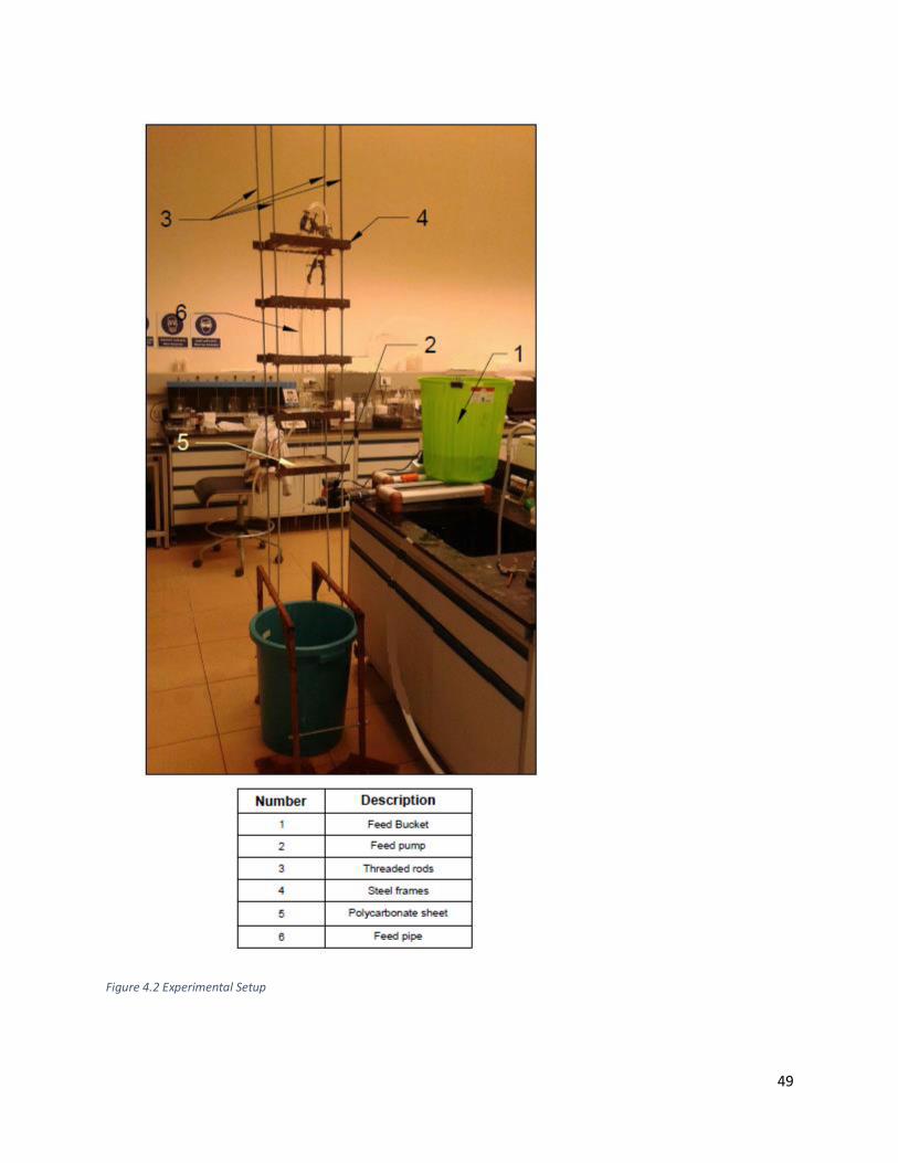
49
Figure 4.2 Experimental Setup
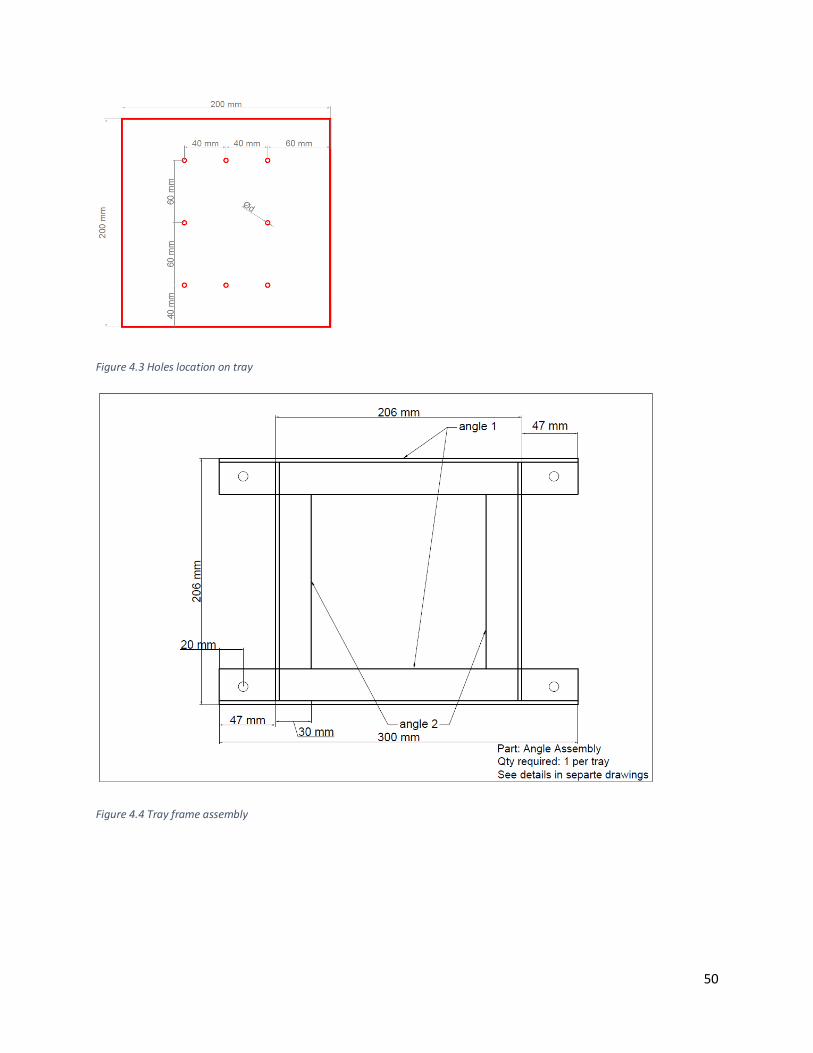
50
Figure 4.3 Holes location on tray
Figure 4.4 Tray frame assembly
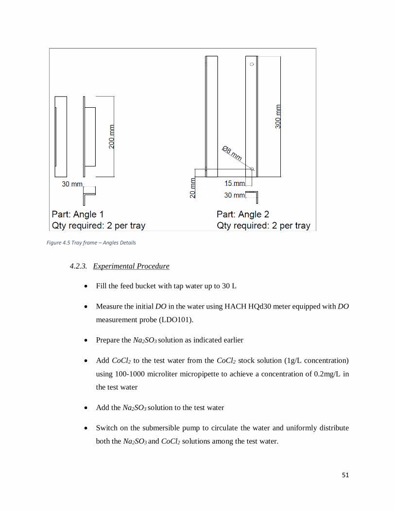
51
Figure 4.5 Tray frame – Angles Details
4.2.3. Experimental Procedure
Fill the feed bucket with tap water up to 30 L
Measure the initial DO in the water using HACH HQd30 meter equipped with DO
measurement probe (LDO101).
Prepare the Na2SO3 solution as indicated earlier
Add CoCl2 to the test water from the CoCl2 stock solution (1g/L concentration)
using 100-1000 microliter micropipette to achieve a concentration of 0.2mg/L in
the test water
Add the Na2SO3 solution to the test water
Switch on the submersible pump to circulate the water and uniformly distribute
both the Na2SO3 and CoCl2 solutions among the test water.
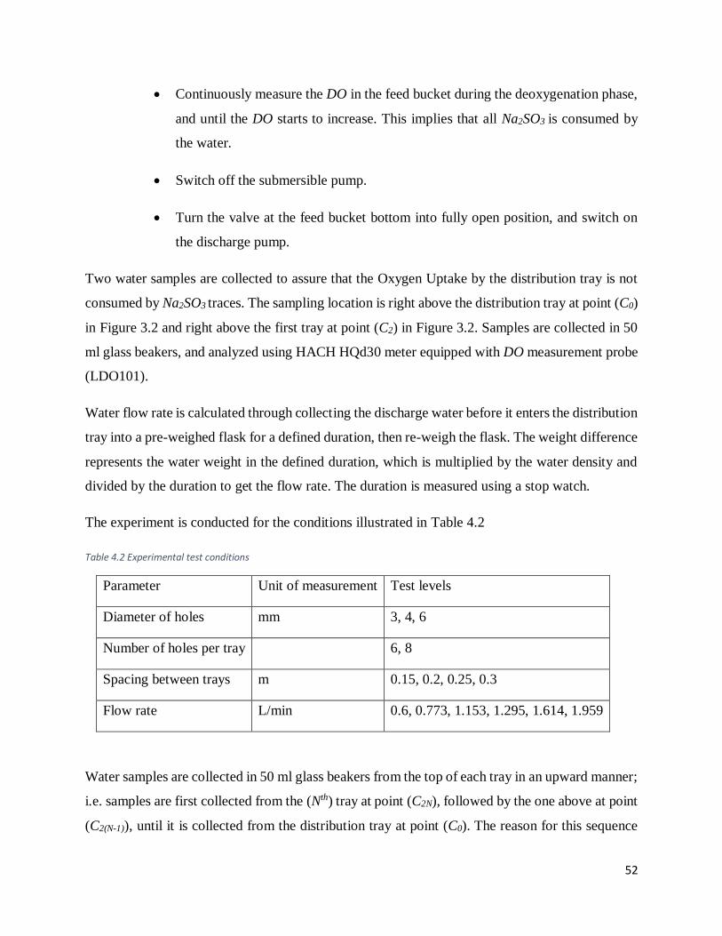
52
Continuously measure the DO in the feed bucket during the deoxygenation phase,
and until the DO starts to increase. This implies that all Na2SO3 is consumed by
the water.
Switch off the submersible pump.
Turn the valve at the feed bucket bottom into fully open position, and switch on
the discharge pump.
Two water samples are collected to assure that the Oxygen Uptake by the distribution tray is not
consumed by Na2SO3 traces. The sampling location is right above the distribution tray at point (C0)
in Figure 3.2 and right above the first tray at point (C2) in Figure 3.2. Samples are collected in 50
ml glass beakers, and analyzed using HACH HQd30 meter equipped with DO measurement probe
(LDO101).
Water flow rate is calculated through collecting the discharge water before it enters the distribution
tray into a pre-weighed flask for a defined duration, then re-weigh the flask. The weight difference
represents the water weight in the defined duration, which is multiplied by the water density and
divided by the duration to get the flow rate. The duration is measured using a stop watch.
The experiment is conducted for the conditions illustrated in Table 4.2
Table 4.2 Experimental test conditions
Parameter Unit of measurement Test levels
Diameter of holes mm 3, 4, 6
Number of holes per tray 6, 8
Spacing between trays m 0.15, 0.2, 0.25, 0.3
Flow rate L/min 0.6, 0.773, 1.153, 1.295, 1.614, 1.959
Water samples are collected in 50 ml glass beakers from the top of each tray in an upward manner;
i.e. samples are first collected from the (Nth) tray at point (C2N), followed by the one above at point
(C2(N-1)), until it is collected from the distribution tray at point (C0). The reason for this sequence
53
is to avoid the disturbance in the water flow which will result from reducing the tray exit flow
during the sample collection.
Once collected, the DO and temperature of the water samples are measured using the DO meter.
After collecting the sample from the distribution tray, the water flow rate is remeasured to assure
that it didn’t vary during the run. When the run is finished, the test conditions are changed to test
condition first through changing the flow rate, until all flow rates are tested, then changing (SP),
then other trays are installed to test different diameters. This arrangement served in reducing the
experimental time.
4.3. Results and Discussion
4.3.1. Preparing Deoxygenated (Synthetic) Water
Following charts illustrate the results obtained for the water DO for the tested excess doses of
Na2SO3 and water volume. The truncated duration from each run represent the time taken from
adding the Na2SO3 dose till the DO reaches the minimum concentration. Figure 4.6 illustrates the
response of the DO at different Na2SO3 doses for a water volume of 300 ml in the beaker, which
corresponds to a water height of 54mm. It appears from the results that all the tested doses were
sufficient to completely deoxygenate the water. Increasing the dose of Na2SO3 resulted in
increasing the duration before the DO starts to increase. Similar conclusion can be concluded from
Figure 4.7 for a water volume of 250 ml. However, testing water volume of 200 ml, the 50% excess
dose was not enough to totally deoxygenate the water as shown in Figure 4.8.
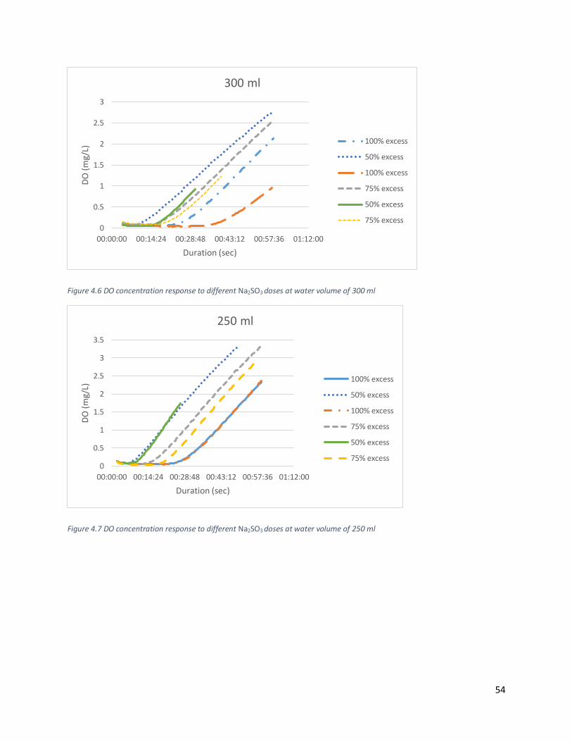
54
Figure 4.6 DO concentration response to different Na2SO3 doses at water volume of 300 ml
Figure 4.7 DO concentration response to different Na2SO3 doses at water volume of 250 ml
0
0.5
1
1.5
2
2.5
3
00:00:00 00:14:24 00:28:48 00:43:12 00:57:36 01:12:00
DO
(m
g/L)
Duration (sec)
300 ml
100% excess
50% excess
100% excess
75% excess
50% excess
75% excess
0
0.5
1
1.5
2
2.5
3
3.5
00:00:00 00:14:24 00:28:48 00:43:12 00:57:36 01:12:00
DO
(m
g/L)
Duration (sec)
250 ml
100% excess
50% excess
100% excess
75% excess
50% excess
75% excess
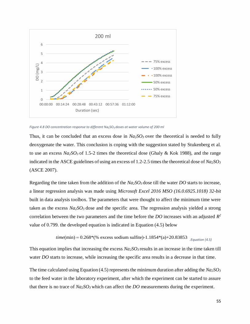
55
Figure 4.8 DO concentration response to different Na2SO3 doses at water volume of 200 ml
Thus, it can be concluded that an excess dose in Na2SO3 over the theoretical is needed to fully
deoxygenate the water. This conclusion is coping with the suggestion stated by Stukenberg et al.
to use an excess Na2SO3 of 1.5-2 times the theoretical dose (Ghaly & Kok 1988), and the range
indicated in the ASCE guidelines of using an excess of 1.2-2.5 times the theoretical dose of Na2SO3
(ASCE 2007).
Regarding the time taken from the addition of the Na2SO3 dose till the water DO starts to increase,
a linear regression analysis was made using Microsoft Excel 2016 MSO (16.0.6925.1018) 32-bit
built in data analysis toolbox. The parameters that were thought to affect the minimum time were
taken as the excess Na2SO3 dose and the specific area. The regression analysis yielded a strong
correlation between the two parameters and the time before the DO increases with an adjusted R2
value of 0.799. the developed equation is indicated in Equation (4.5) below
(min) 0.268*(% excess sodium sulfite)-1.1854*(a)+20.83853time . Equation (4.5)
This equation implies that increasing the excess Na2SO3 results in an increase in the time taken till
water DO starts to increase, while increasing the specific area results in a decrease in that time.
The time calculated using Equation (4.5) represents the minimum duration after adding the Na2SO3
to the feed water in the laboratory experiment, after which the experiment can be started to assure
that there is no trace of Na2SO3 which can affect the DO measurements during the experiment.
0
1
2
3
4
5
6
00:00:00 00:14:24 00:28:48 00:43:12 00:57:36 01:12:00
DO
(m
g/L)
Duration (sec)
200 ml
75% excess
100% excess
100% excess
50% excess
50% excess
75% excess
56
4.3.2. Laboratory Scale Test for Tray Aerator
When the experiments were conducted, the influent DO to the tray aerator system was not recorded
to be an absolute zero, the water entering the system was ranging from 0.01mg/L to 1.56mg/L for
some runs. Full data of recorded DO in the experimental work is tabulated in Annex II for
reference. For the purpose of fair comparison, all the recorded DO concentrations are converted
into aeration efficiency relative to the influent concentration based on the general equation of
aeration efficiency provided in section 2.2.2 (Equation (2.9)), however, the nomenclature of
Equation (2.9) is modified to suite the current experiment as indicated in Equation (4.6) below
2 02
0
DS US ii
S US S
C C C C
C C C C
, (i=1:N) ...................................................................... Equation (4.6)
Where (η) is the aeration efficiency, (CDS) is the downstream DO concentration; (CUS) is the
upstream DO concentration; (i) is the tray number, (C2i) is the DO concentration entering tray (i),
(C0) is the initial DO concentration entering the distribution tray, (CS) is the saturation DO at the
recorded water temperature, and (N) is the total number of examined trays. Following sections
present the effect of the different parameters on the aeration efficiency.
4.3.2.1. Effect of Changing the Spacing Between Trays
In order to study the impact of changing the spacing between trays, the results from each hole
diameter, from different hole diameters, of aeration efficiency obtained after the first tray at
different flow rates and spacing between trays, while fixing other parameters at 8 holes per tray,
and 20cmx20cm tray system are illustrated in Figure 4.9Error! Reference source not found..
The aeration efficiency obtained from the results in Figure 4.9 (a), (b), and (c) are compared
together. The increase in tray spacing from 15cm to 20cm, or from 20cm to 25cm, while
maintaining other parameters fixed (diameter, number of holes, flow rate, tray area, and number
of trays) results in an increase in aeration efficiency. However, the rate of increase in the aeration
efficiency when the spacing increased to 20cm is noted to be higher than when the spacing was
increased to 25cm. Therefore, the aeration efficiency is concluded to be directly proportional with
the tray spacing in an exponential form.
57
4.3.2.2. Effect of Changing the Hole Diameter
The general trend describing the impact of increasing the hole diameter among the tested diameters
in noted to slightly increase the aeration efficiency. Figure 4.10(a) is for the 15 cm tray spacing.
This spacing was tested for the 3mm and 4mm diameters only. The results show that the 3mm
holes provide higher aeration efficiency over the 4mm holes with the low and high flow rates,
while the 4mm diameter yields higher aeration efficiency for the medium flow rate. The overall
difference resulting from the change in hole diameter is within 5% difference.
The 20 cm spacing as illustrated in Figure 4.10(b) also shows that the difference in aeration
efficiency resulting from changing the hole diameters is inconsistent, where the 6mm diameter is
higher than the 3mm and the 4mm diameters for the high and low flow rates, and almost similar
to the 4mm diameter for the medium flow rate. The 3mm diameter gives the lowest aeration
efficiency with the low and medium flow rates, whereas the 4mm diameter results in the lowest
aeration efficiency with the high flow rate. The change in efficiency is also within 8%.
The 25 cm spacing was tested for the 4mm and the 6mm diameters only as illustrated in Figure
4.10(c) the aeration efficiency for both diameters is almost identical for the medium and high flow
rates, while for the low flow rate the 6mm holes result in an aeration efficiency around 4% higher
than the 4mm diameter.
The inconsistent trend for the impact of changing the hole diameters on the aeration efficiency is
thought to be due to the limited effect of the change in diameter over the aeration efficiency, as
was illustrated in the mathematical model.
4.3.2.3. Effect of Changing the Flow Rate
Through inspecting the results illustrated in Figure 4.10, the aeration efficiency is seen to be
affected by the flow rate. The values of the aeration efficiency demonstrate the decrease in aeration
efficiency resulting from the increase in the flow rate. Results postulate that there is an inversely
exponential relation between the flow rate and the aeration efficiency as illustrated in Figure
4.10(b), and Figure 4.10(c).
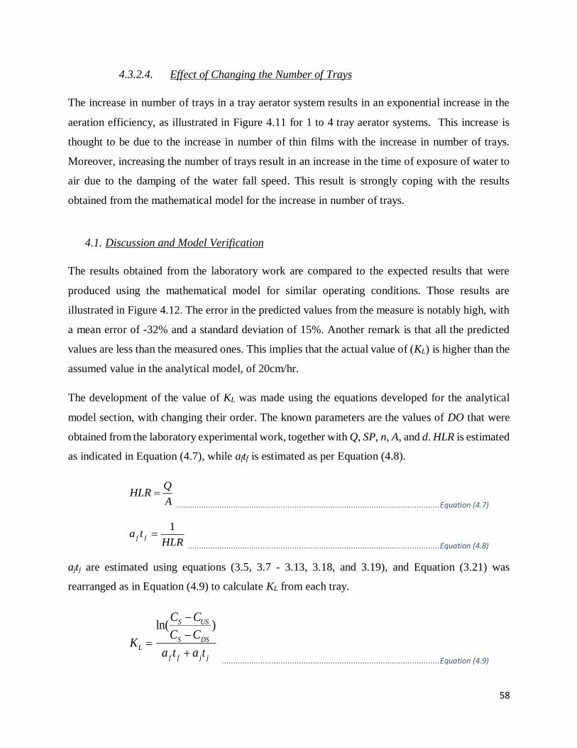
58
4.3.2.4. Effect of Changing the Number of Trays
The increase in number of trays in a tray aerator system results in an exponential increase in the
aeration efficiency, as illustrated in Figure 4.11 for 1 to 4 tray aerator systems. This increase is
thought to be due to the increase in number of thin films with the increase in number of trays.
Moreover, increasing the number of trays result in an increase in the time of exposure of water to
air due to the damping of the water fall speed. This result is strongly coping with the results
obtained from the mathematical model for the increase in number of trays.
4.1. Discussion and Model Verification
The results obtained from the laboratory work are compared to the expected results that were
produced using the mathematical model for similar operating conditions. Those results are
illustrated in Figure 4.12. The error in the predicted values from the measure is notably high, with
a mean error of -32% and a standard deviation of 15%. Another remark is that all the predicted
values are less than the measured ones. This implies that the actual value of (KL) is higher than the
assumed value in the analytical model, of 20cm/hr.
The development of the value of KL was made using the equations developed for the analytical
model section, with changing their order. The known parameters are the values of DO that were
obtained from the laboratory experimental work, together with Q, SP, n, A, and d. HLR is estimated
as indicated in Equation (4.7), while aftf is estimated as per Equation (4.8).
QHLR
A
.................................................................................................................... Equation (4.7)
1f fa t
HLR
............................................................................................................... Equation (4.8)
ajtj are estimated using equations (3.5, 3.7 - 3.13, 3.18, and 3.19), and Equation (3.21) was
rearranged as in Equation (4.9) to calculate KL from each tray.
ln( )S US
S DSL
f f j j
C C
C CK
a t a t
................................................................................................ Equation (4.9)
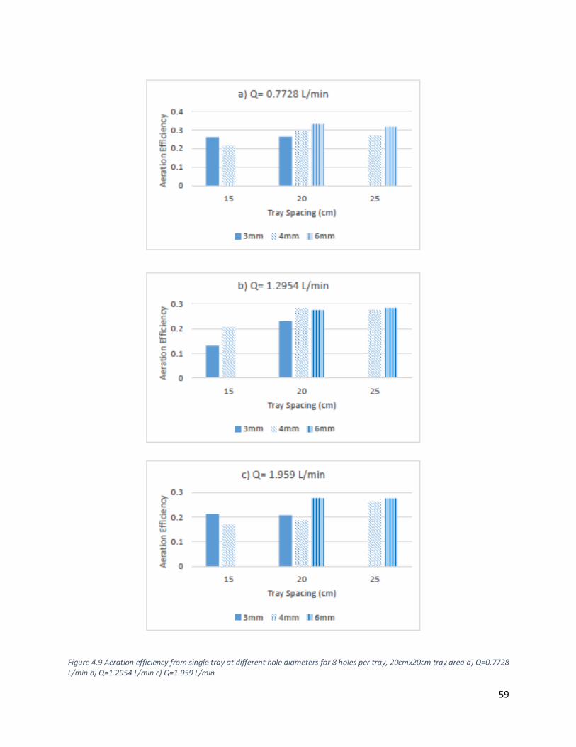
59
Figure 4.9 Aeration efficiency from single tray at different hole diameters for 8 holes per tray, 20cmx20cm tray area a) Q=0.7728 L/min b) Q=1.2954 L/min c) Q=1.959 L/min
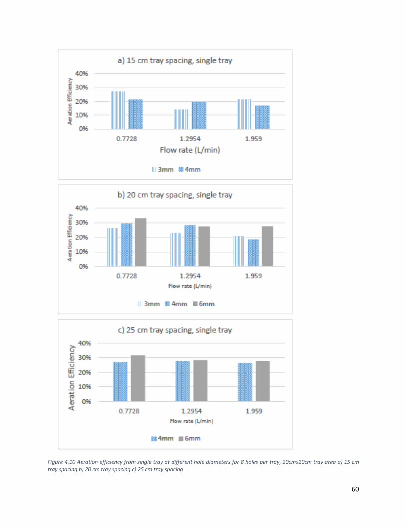
60
Figure 4.10 Aeration efficiency from single tray at different hole diameters for 8 holes per tray, 20cmx20cm tray area a) 15 cm tray spacing b) 20 cm tray spacing c) 25 cm tray spacing
61
Figure 4.11 Aeration efficiency at different hole diameters for 8 holes per tray, 20cmx20cm tray area
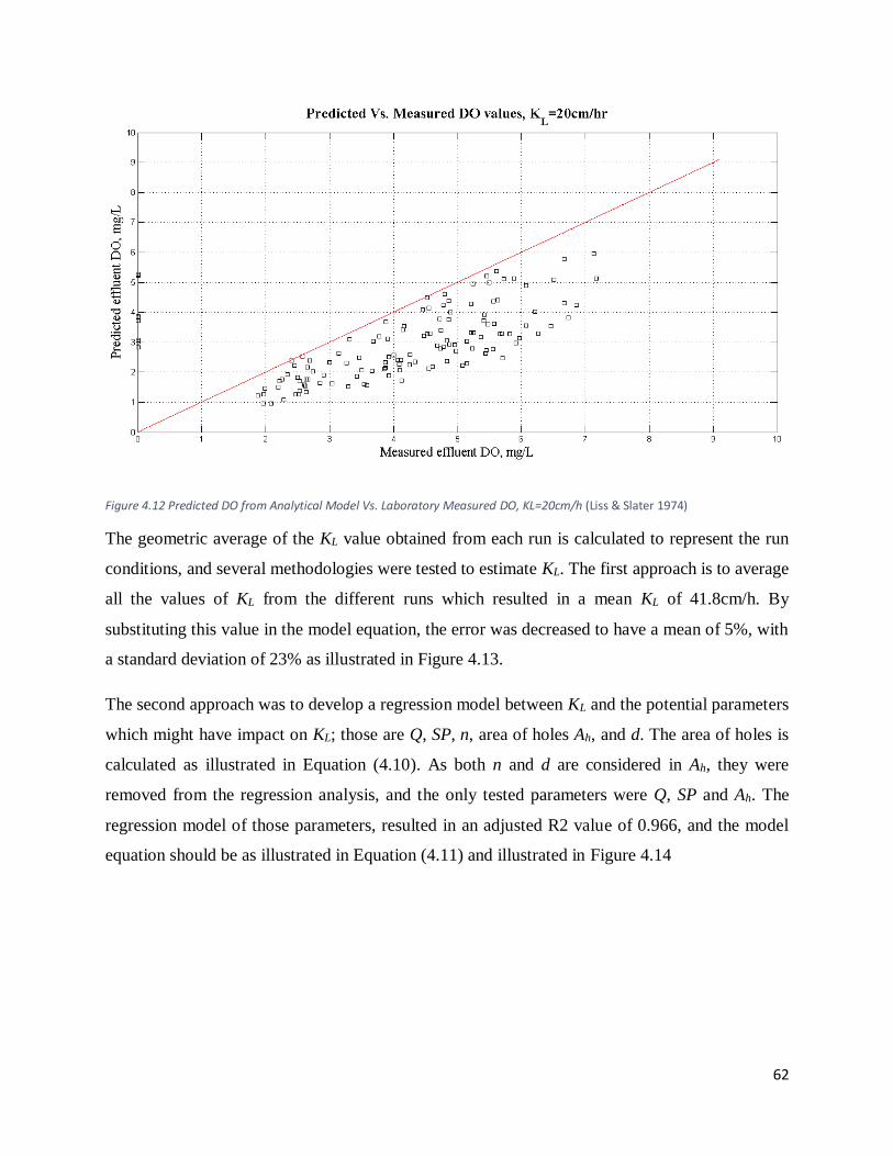
62
Figure 4.12 Predicted DO from Analytical Model Vs. Laboratory Measured DO, KL=20cm/h (Liss & Slater 1974)
The geometric average of the KL value obtained from each run is calculated to represent the run
conditions, and several methodologies were tested to estimate KL. The first approach is to average
all the values of KL from the different runs which resulted in a mean KL of 41.8cm/h. By
substituting this value in the model equation, the error was decreased to have a mean of 5%, with
a standard deviation of 23% as illustrated in Figure 4.13.
The second approach was to develop a regression model between KL and the potential parameters
which might have impact on KL; those are Q, SP, n, area of holes Ah, and d. The area of holes is
calculated as illustrated in Equation (4.10). As both n and d are considered in Ah, they were
removed from the regression analysis, and the only tested parameters were Q, SP and Ah. The
regression model of those parameters, resulted in an adjusted R2 value of 0.966, and the model
equation should be as illustrated in Equation (4.11) and illustrated in Figure 4.14
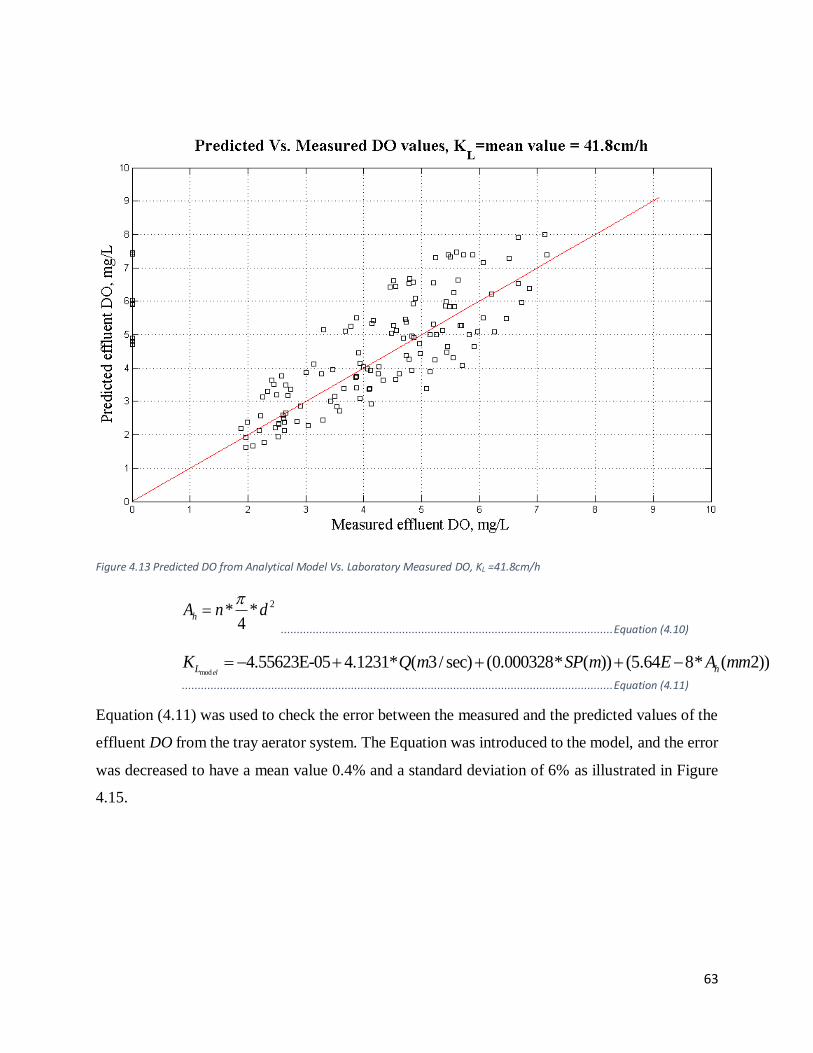
63
Figure 4.13 Predicted DO from Analytical Model Vs. Laboratory Measured DO, KL =41.8cm/h
2* *4
hA n d
........................................................................................................ Equation (4.10)
mod4.55623E-05 4.1231* ( 3/ sec) (0.000328* ( )) (5.64 8* ( 2))
elL hK Q m SP m E A mm
....................................................................................................................................... Equation (4.11)
Equation (4.11) was used to check the error between the measured and the predicted values of the
effluent DO from the tray aerator system. The Equation was introduced to the model, and the error
was decreased to have a mean value 0.4% and a standard deviation of 6% as illustrated in Figure
4.15.
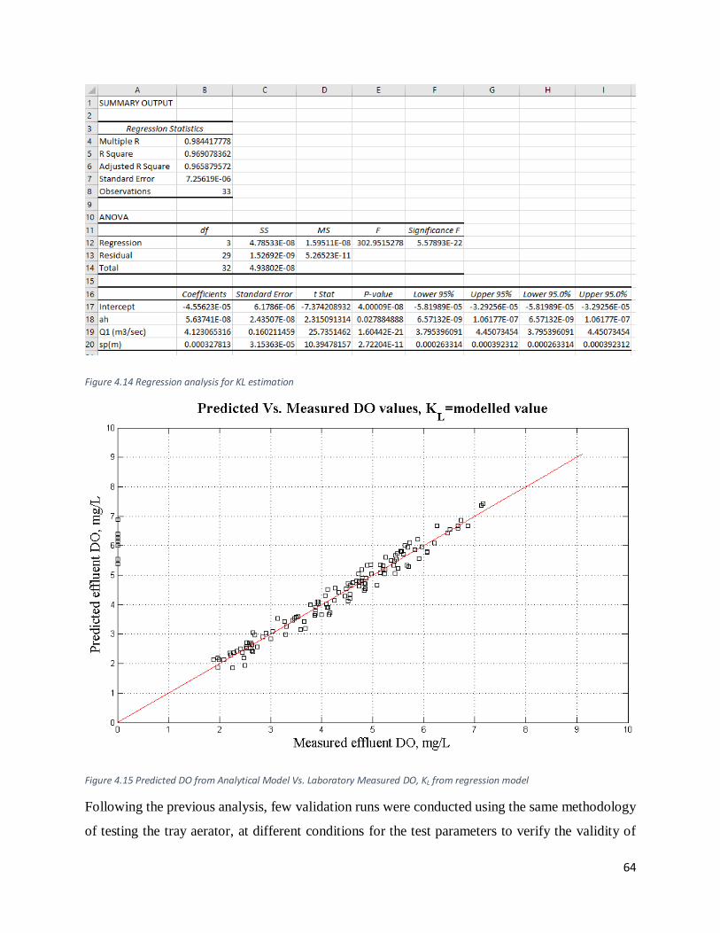
64
Figure 4.14 Regression analysis for KL estimation
Figure 4.15 Predicted DO from Analytical Model Vs. Laboratory Measured DO, KL from regression model
Following the previous analysis, few validation runs were conducted using the same methodology
of testing the tray aerator, at different conditions for the test parameters to verify the validity of
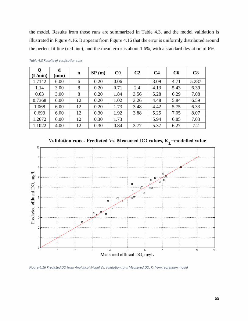
65
the model. Results from those runs are summarized in Table 4.3, and the model validation is
illustrated in Figure 4.16. It appears from Figure 4.16 that the error is uniformly distributed around
the perfect fit line (red line), and the mean error is about 1.6%, with a standard deviation of 6%.
Table 4.3 Results of verification runs
Q
(L/min)
d
(mm) n SP (m) C0 C2 C4 C6 C8
1.7142 6.00 6 0.20 0.06 3.09 4.71 5.287
1.14 3.00 8 0.20 0.71 2.4 4.13 5.43 6.39
0.63 3.00 8 0.20 1.84 3.56 5.28 6.29 7.08
0.7368 6.00 12 0.20 1.02 3.26 4.48 5.84 6.59
1.068 6.00 12 0.20 1.73 3.48 4.42 5.75 6.33
0.693 6.00 12 0.30 1.92 3.88 5.25 7.05 8.07
1.2672 6.00 12 0.30 1.73 5.94 6.85 7.03
1.1022 4.00 12 0.30 0.84 3.77 5.37 6.27 7.2
Figure 4.16 Predicted DO from Analytical Model Vs. validation runs Measured DO, KL from regression model
66
4.2. Conclusion
In the laboratory experimental model for the tray aerators, Na2SO3 reduction of the DO from water
was used to completely deoxygenate tap water. Several experiments were conducted to check the
optimum dose of Na2SO3 needed to completely deoxygenate water. This method proved good
results with the optimum dose to deoxygenate one mg/L of DO is equal to 130% of the
stoichiometric value of 7.9mg/L of Na2SO3.
Through testing the performance of the tray aerators on laboratory scale, the results illustrated that
the performance of the tray aerators is strongly affected by the number of trays used as well as the
flow rate. The aeration efficiency is directly proportional with the spacing between trays in an
exponential form, with the spacing of 20cm between trays considered as the optimum spacing
beyond which the increase in efficiency associated with the increase in spacing is not significant.
Changing the hole diameters didn’t result in significant change in the aeration efficiency. This
conclusion is in line with the results obtained from the mathematical modelling.
In the analysis of the results, an empirical equation for the mass transfer coefficient is developed
using linear regression analysis. That equation is a function of the area of holes, flow rate and the
tray spacing. The error in estimating the effluent DO through using this empirical equation was at
0.4% with a standard deviation of 6%.
The validation illustrated that the model is valid for number of holes, and flow rates other than
those used in developing the model. Pilot scale application in next chapter shall be utilized to
further validate the model with real wastewater.

67
5. Phase III - Pilot Scale Study
68
5.1. Introduction
Most studies and research work in the field of wastewater, if not all, starts by a mathematical
modelling, followed by laboratory scale experimental studies, and ends by a scaling up pilot scale
study. The main reason for conducting the scaling up pilot scale application is to investigate the
performance of the research subject under the normal operating conditions in the field rather than
the controlled conditions which characterize the laboratory experiments.
Furthermore, and specifically in water and wastewater oxygen transfer related work, some
parameters vary in the full scale application from the small scale laboratory application. Those
parameters are the oxygen saturation concentration value, and the oxygen mass transfer
coefficient. For the oxygen saturation concentration, a correction factor termed () is multiplied to
the published saturation values to account for the difference in saturation concentration between
wastewater and clean water. This correction factor is due to the effect of other gases, organics, and
salts as well as the difference in temperature and/or pressure of water from the tabulated values
(Leung et al. 2006; Mueller et al. 2002).
Regarding the correction in the mass transfer coefficient, a correction factor termed () is
multiplied to the mass transfer coefficient of clean water to account for different chemical and
process parameters, including the chemical oxygen demand, surface tension, liquid temperature,
presence of suspended solids, aeration methods and velocities (Leung et al. 2006; Mueller et al.
2002).
Another benefit from the pilot experiment is to investigate whether the tray holes will be clogged
from the microbial growth over the trays, which might affect the aerator hydraulics and consume
the added oxygen. If the clogging is to occur, the conclusion section shall propose a maintenance
technique suitable for sustaining the aerator performance.
5.2. Material and Methods
A full scale sequential anaerobic-aerobic wastewater treatment plant termed Zero Energy Compact
Unit (ZECU) was designed and built at Zawyat Al Karadsah wastewater treatment plant in
Fayyoum Governorate, by a research team led by Dr. Tarek Ismail Sabry and Dr. Ahmed Shafik
El-Gendy. The location of the plant is indicated in Figure 5.1. ZECU unit is composed of a three
69
stage anaerobic treatment unit, followed by a tray aerator unit, which discharges into a down-flow
aerobic unit as illustrated in Figure 5.2. The three stage anaerobic treatment unit is composed of
an up-flow anaerobic reactor, followed by a down-flow anaerobic packed-bed reactor, then an up-
flow anaerobic reactor. the aerobic unit is composed of an aerobic biological filter packed with
sponge media. The whole system is composed of two identical units, which have one influent
downstream the grit removal chamber (preliminary treatment). The system design flow rate is
9m3/day equally distributed between the two units. The actual flow of the system during the
experimental runs was approximately 4m3/day. ZECU treatment plant is selected to test the tray
aerators as that system is already operating with tray aerators, which can be easily replaced with
the test arrangements.
Four parallel tray trains were prepared at the American University in Cairo. Each train had 8 trays
other than the distribution tray. Trays were fixed on steel frames of 20cmX20cm inner dimensions,
which were fabricated using steel angles of 3cmX3cmX3mm dimensions as illustrated in Figure
4.4, and Figure 4.5. The only difference in the frames of the pilot scale arrangement from the those
in Figure 4.5 is in the diameter of the fixation holes of Angle 2, which was increased in the pilot
scale arrangement to 10mm instead of the indicated 8mm. This increase is to account for the larger
diameter steel threads used in the pilot arrangement to withstand the weight of the 10 trays in each
train.
In the pilot experiments, trays were made from 20cmX20cm polycarbonate sheets. Trays were cut
and drilled at the American University in Cairo - Architectural Engineering computer laboratory
using CNC laser cutting machine as illustrated in Figure 5.3 for the 3mm, 4mm, 5mm, and 6mm
hole diameter. The number of holes per tray (35, 20, 12, and 8 holes per tray for the 3mm, 4mm,
5mm and 6mm hole diameter respectively) were selected according to the results indicated in Table
3.2 for the case of 2.5m3/day flow rate that would result in 2mm film thickness. Fabricated trays
are fixed to the steel frames using antibacterial silicone to fill any voids of gaps between the tray
edges and the steel frame sides.
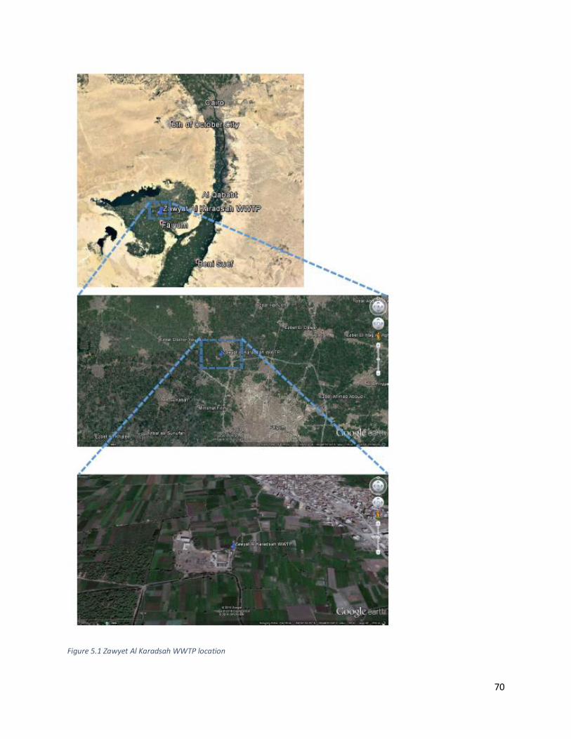
70
Figure 5.1 Zawyet Al Karadsah WWTP location
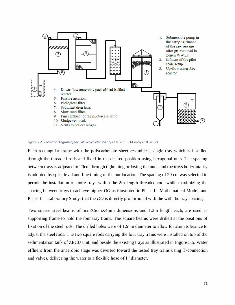
71
Figure 5.2 Schematic Diagram of the Full-Scale Setup (Sabry et al. 2011; El-Gendy et al. 2012)
Each rectangular frame with the polycarbonate sheet resemble a single tray which is installed
through the threaded rods and fixed in the desired position using hexagonal nuts. The spacing
between trays is adjusted to 20cm through tightening or losing the nuts, and the trays horizontality
is adopted by spirit level and fine tuning of the nut location. The spacing of 20 cm was selected to
permit the installation of more trays within the 2m length threaded rod, while maximizing the
spacing between trays to achieve higher DO as illustrated in Phase I - Mathematical Model, and
Phase II – Laboratory Study, that the DO is directly proportional with the with the tray spacing.
Two square steel beams of 5cmX5cmX4mm dimensions and 1.3m length each, are used as
supporting frame to hold the four tray trains. The square beams were drilled at the positions of
fixation of the steel rods. The drilled holes were of 12mm diameter to allow for 2mm tolerance to
adjust the steel rods. The two square rods carrying the four tray trains were installed on top of the
sedimentation tank of ZECU unit, and beside the existing trays as illustrated in Figure 5.5. Water
effluent from the anaerobic stage was diverted toward the tested tray trains using T-connection
and valves, delivering the water to a flexible hose of 1” diameter.
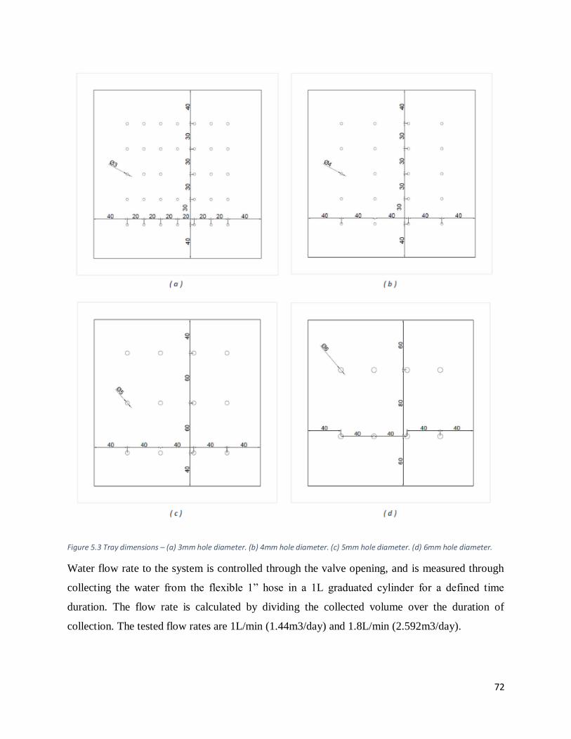
72
Figure 5.3 Tray dimensions – (a) 3mm hole diameter. (b) 4mm hole diameter. (c) 5mm hole diameter. (d) 6mm hole diameter.
Water flow rate to the system is controlled through the valve opening, and is measured through
collecting the water from the flexible 1” hose in a 1L graduated cylinder for a defined time
duration. The flow rate is calculated by dividing the collected volume over the duration of
collection. The tested flow rates are 1L/min (1.44m3/day) and 1.8L/min (2.592m3/day).
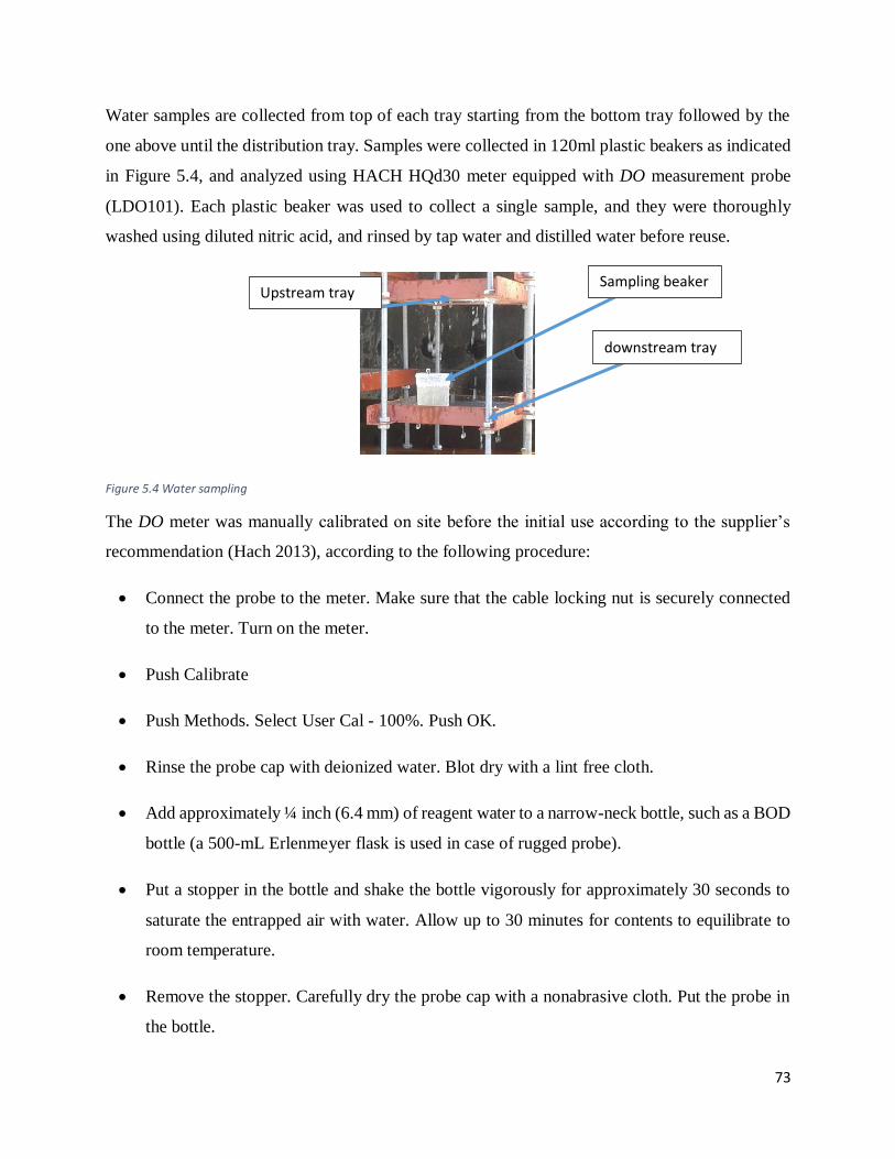
73
Water samples are collected from top of each tray starting from the bottom tray followed by the
one above until the distribution tray. Samples were collected in 120ml plastic beakers as indicated
in Figure 5.4, and analyzed using HACH HQd30 meter equipped with DO measurement probe
(LDO101). Each plastic beaker was used to collect a single sample, and they were thoroughly
washed using diluted nitric acid, and rinsed by tap water and distilled water before reuse.
Figure 5.4 Water sampling
The DO meter was manually calibrated on site before the initial use according to the supplier’s
recommendation (Hach 2013), according to the following procedure:
Connect the probe to the meter. Make sure that the cable locking nut is securely connected
to the meter. Turn on the meter.
Push Calibrate
Push Methods. Select User Cal - 100%. Push OK.
Rinse the probe cap with deionized water. Blot dry with a lint free cloth.
Add approximately ¼ inch (6.4 mm) of reagent water to a narrow-neck bottle, such as a BOD
bottle (a 500-mL Erlenmeyer flask is used in case of rugged probe).
Put a stopper in the bottle and shake the bottle vigorously for approximately 30 seconds to
saturate the entrapped air with water. Allow up to 30 minutes for contents to equilibrate to
room temperature.
Remove the stopper. Carefully dry the probe cap with a nonabrasive cloth. Put the probe in
the bottle.
Sampling beaker
downstream tray
Upstream tray
74
Push Read. The display shows "Stabilizing" and a progress bar as the probe stabilizes. The
display shows the standard value when the reading is stable.
Push Done to view the calibration summary.
Push Store to accept the calibration and return to the measurement mode. If a rugged probe,
install the shroud on the probe.
After each sample analysis, the DO probe was washed using clean water and dried by a clean
paper tissue.
5.3. Results and Discussion
5.3.1. Effect of Changing the Hole Diameter
Changing the hole diameters together with the number of holes per tray, to achieve similar film
height above the trays, is illustrated in terms of average aeration efficiency in Figure 5.6. The
average aeration efficiency is calculated as the geometric average of the efficiency obtained from
each tray using Equation (4.6), taking the DO value from the (i-1) tray as the upstream DO, and
the DO value from the (ith) tray as the downstream DO. It appears that there is no significant change
in aeration efficiency resulting from changing the hole diameter while maintaining the film height
constant for the 1L/min flow rate, however, as the flow rate increased to 1.8L/min, the aeration
efficiency from the small diameters (3mm and 4mm) are higher than the aeration efficiency from
the larger diameters (5mm and 6mm). The highest aeration efficiency is obtained from using 4mm
diameter holes.
As the test conditions in the pilot scale experiment is different from the test conditions of the
laboratory scale experiment, where in the pilot scale experiments both the diameter and number of
holes per tray changed simultaneously, while in the laboratory scale experiments either the hole
diameter or the number of holes was changing, therefore it is not possible to compare both results
together.
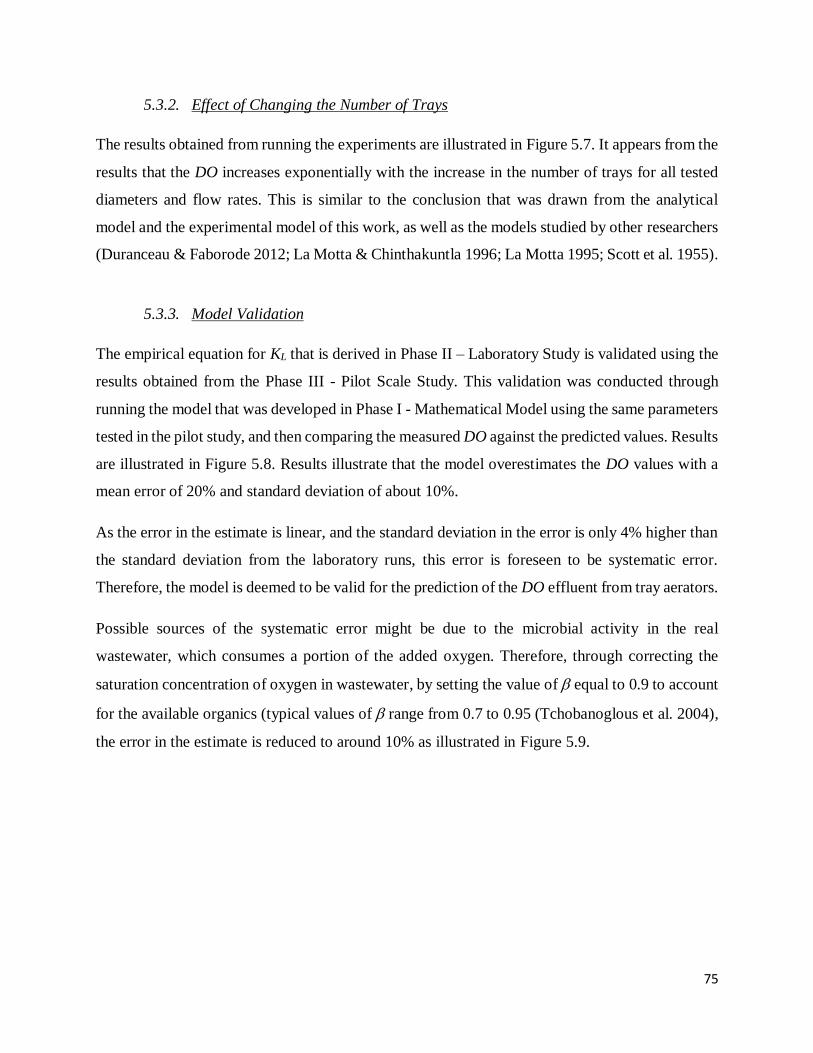
75
5.3.2. Effect of Changing the Number of Trays
The results obtained from running the experiments are illustrated in Figure 5.7. It appears from the
results that the DO increases exponentially with the increase in the number of trays for all tested
diameters and flow rates. This is similar to the conclusion that was drawn from the analytical
model and the experimental model of this work, as well as the models studied by other researchers
(Duranceau & Faborode 2012; La Motta & Chinthakuntla 1996; La Motta 1995; Scott et al. 1955).
5.3.3. Model Validation
The empirical equation for KL that is derived in Phase II – Laboratory Study is validated using the
results obtained from the Phase III - Pilot Scale Study. This validation was conducted through
running the model that was developed in Phase I - Mathematical Model using the same parameters
tested in the pilot study, and then comparing the measured DO against the predicted values. Results
are illustrated in Figure 5.8. Results illustrate that the model overestimates the DO values with a
mean error of 20% and standard deviation of about 10%.
As the error in the estimate is linear, and the standard deviation in the error is only 4% higher than
the standard deviation from the laboratory runs, this error is foreseen to be systematic error.
Therefore, the model is deemed to be valid for the prediction of the DO effluent from tray aerators.
Possible sources of the systematic error might be due to the microbial activity in the real
wastewater, which consumes a portion of the added oxygen. Therefore, through correcting the
saturation concentration of oxygen in wastewater, by setting the value of equal to 0.9 to account
for the available organics (typical values of range from 0.7 to 0.95 (Tchobanoglous et al. 2004),
the error in the estimate is reduced to around 10% as illustrated in Figure 5.9.
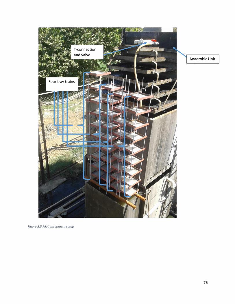
76
Figure 5.5 Pilot experiment setup
Anaerobic Unit
T-connection
and valve
Four tray trains
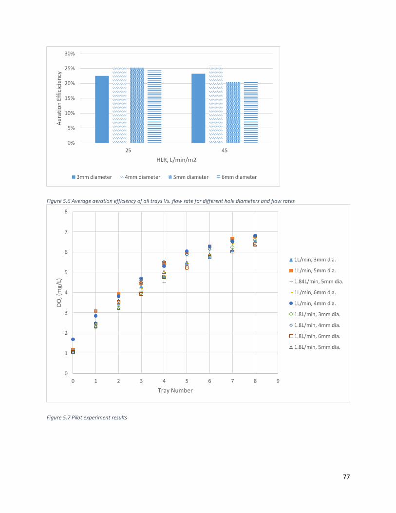
77
Figure 5.6 Average aeration efficiency of all trays Vs. flow rate for different hole diameters and flow rates
Figure 5.7 Pilot experiment results
0%
5%
10%
15%
20%
25%
30%
25 45
Aer
atio
n E
ffic
icie
ncy
HLR, L/min/m2
3mm diameter 4mm diameter 5mm diameter 6mm diameter
0
1
2
3
4
5
6
7
8
0 1 2 3 4 5 6 7 8 9
DO
, (m
g/L)
Tray Number
1L/min, 3mm dia.
1L/min, 5mm dia.
1.84L/min, 5mm dia.
1L/min, 6mm dia.
1L/min, 4mm dia.
1.8L/min, 3mm dia.
1.8L/min, 4mm dia.
1.8L/min, 6mm dia.
1.8L/min, 5mm dia.
78
Figure 5.8 Predicted DO from Analytical Model Vs. Pilot Plant Measured DO, KL from regression model
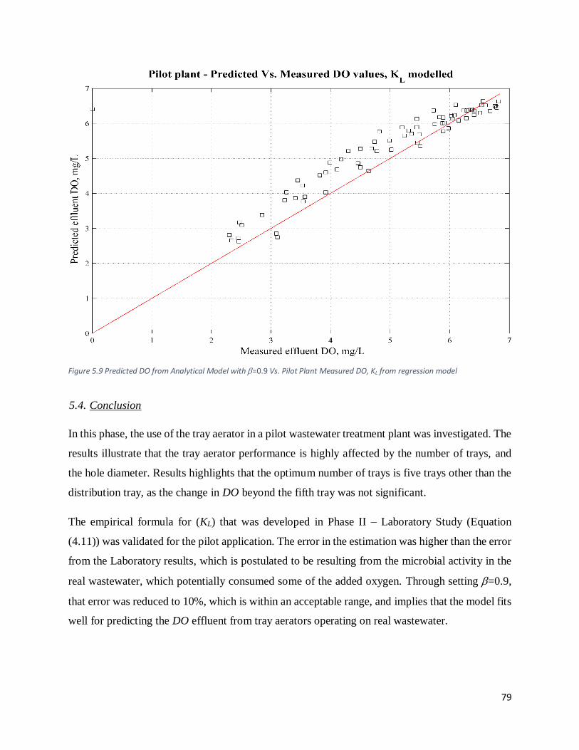
79
Figure 5.9 Predicted DO from Analytical Model with =0.9 Vs. Pilot Plant Measured DO, KL from regression model
5.4. Conclusion
In this phase, the use of the tray aerator in a pilot wastewater treatment plant was investigated. The
results illustrate that the tray aerator performance is highly affected by the number of trays, and
the hole diameter. Results highlights that the optimum number of trays is five trays other than the
distribution tray, as the change in DO beyond the fifth tray was not significant.
The empirical formula for (KL) that was developed in Phase II – Laboratory Study (Equation
(4.11)) was validated for the pilot application. The error in the estimation was higher than the error
from the Laboratory results, which is postulated to be resulting from the microbial activity in the
real wastewater, which potentially consumed some of the added oxygen. Through setting =0.9,
that error was reduced to 10%, which is within an acceptable range, and implies that the model fits
well for predicting the DO effluent from tray aerators operating on real wastewater.

80
6. General Discussion
81
Results from the developed equations illustrate that the aeration performance from tray aerators is
strongly driven by N and HLR. Increasing N results in an increase in the aeration efficiency as was
illustrated in Figure 3.7, Figure 4.11, and Figure 5.7. The three figures indicate that the effluent
DO increases exponentially with the increase in N. This exponential relation is explained to be due
to the decrease in the concentration gradient with the increase of the DO, resulting in a decrease
in mass flux, according to Fick’s law indicated in Equation (2.1). Similar dependence was observed
for the tray aerators studied for CO2 stripping (Scott et al. 1955; La Motta 1995; La Motta &
Chinthakuntla 1996) as well as for sulfide stripping (Duranceau & Faborode 2012).
The effect of the HLR on the aeration performance is highlighted in the mathematical model results
illustrated in Figure 3.8. Decreasing the HLR, which is either by increasing the tray area or
decreasing the flow, rate results in an increase in the DO. Similar conclusion was drawn from
Figure 4.10 for the laboratory study, however the results from the pilot scale application indicated
in Figure 5.6 were not sufficient to proof or reject that hypothesis. This relation between the DO
and the HLR is resulting from the increase of the interface time between water and air with the
decrease in the HLR. La Motta realized the same conclusion but for CO2 stripping, where the
model equations he developed illustrated that the CO2 stripping is inversely proportional with the
HLR (La Motta 1995; La Motta & Chinthakuntla 1996). Similarly, Duranceau and Faborode
reported that the sulfide stripping from tray aerators is inversely proportional with the HLR
(Duranceau & Faborode 2012).
Regarding the tray spacing, apparently from the mathematical model, the change in tray spacing
did not result in significant change in the aerator performance (Figure 3.6 and Figure 3.7), while
the results from the laboratory investigation indicated the increase in the aerator performance with
the increase of tray spacing (Figure 4.10). These contradicting conclusions were explained by the
analysis of KL. KL is a function of the degree of turbulence of the two interacting fluids
(Jamnongwong et al. 2010; Tchobanoglous et al. 2004). Since SP affects the jet velocity and
diameter according to Equations (3.9-3.13), the change in SP result in a change in the degree of
turbulence, and affects KL. The relation between KL and SP is indicated in Equation (4.11), in
which KL is proportional with SP. This analysis justifies the proportional relation of DO with SP.
This conclusion is aligned with the conclusion for CO2 stripping (La Motta 1995; La Motta &
82
Chinthakuntla 1996), whereas Duranceau and Faborode did not address SP in their analysis for
sulfide stripping (Duranceau & Faborode 2012).
Changing the hole diameter and/or the number of holes per tray did not have significant impact on
the aeration efficiency. The results from the three phases of this study show that the impact of
changing the hole diameter is limited and can be neglected if compared to the change of aeration
efficiency resulting from changing N, HLR, and SP. Even though the variation in d affects the
value of aj and tj as indicated in Equations (3.9-3.13, 3.18, & 3.19), the value of d changed with a
step of unity, and is constrained by the studied conditions to a maximum change of 3mm
(3mm≥d≥6mm) hindering the impact of changing d on the aeration performance. None of the
published studies addressed the impact of d on the performance of tray aerators (La Motta 1995;
La Motta & Chinthakuntla 1996; Duranceau & Faborode 2012).
Despite that d and n do not impact the aeration performance, they are important design parameters
for the tray aerator from a hydraulic prospective. Those two parameters, together with Q define
the flow regime over tray aerators. Underestimating the values of d and n for a design Q might
result in decreasing the flow rate effluent from tray holes resulting in water overflow from tray
sides, while overestimating d and n would necessitate larger A, and the flow of water would assume
dripping regime rather than jetting regime. this was highlighted in section 3.2.1 of this thesis and
illustrated in Figure 3.4. This needs to be verified in further works.
6.1. Design Procedure
In order to develop the design model for tray aerators, that can be used by engineers and consultants
to design an effective passive aeration module, some parameters should be acquired or measured.
6.1.1. Input Parameters
Design flow rate
Operating temperature
Influent DO
83
Minimum desired effluent DO
Maximum allowable height for system installation
6.1.2. Design Steps
The design procedure is indicated in the following steps:
Number of modules
The studied tray aerators were all having a tray area of 20cmX20cm. This constant A was
intentionally selected, so as to design the tray aerators in modules, depending on the expected flow
rate. each module should have an area of 20cmX20cm, and can serve a maximum flow rate of
2.5m3/day (the maximum tested flow rate). In order to select the proper number of modules, the
design flow rate should be divided among a number (nmodule) of modules to assure that none of
them would serve more than the maximum flow rate according to Equation (6.1)
3
mod 3
( / )
2.5( / )
design
ule
Q m dayn
m day ................................................................................................................ Equation (6.1)
And then the flow rate per module (Qmodule) would be calculated as indicated in Equation (6.2)
mod
mod
design
ule
ule
n ................................................................................................................................... Equation (6.2)
Hydraulic Design
For each tray, the number and diameter of holes should be properly selected to assure jetting
regime for water exiting from holes, and guarantees that no overflow would occur from tray sides.
The hydraulic design is an iterative process. Three initial assumptions are made, N=1 (other than
the distribution tray), d=3mm and n=1. The assumption for N shall be corrected from the aeration
design, which is illustrated in the next subsection. SP shall be calculated by knowing H, and N
according to Equation 3.23.
The design of the number of holes for a selected diameter is an iterative process, in which an initial
guess is made for n=1, for the diameter of 3mm. Then the iterations for D1, v1, and h are calculated
84
according to equations (3.5, 3.4, and 3.8). If h is greater than hs, n will be increased by 1, and new
iterations for v1, and h calculated.
The next step is to assure that the water exiting the tray holes will assume jetting regime. this will
be through estimating Lj, v2, and D2 using equations (3.9-3.11), and substituting in equations (3.1-
3.3) to assure that We is greater than Wec. n is increased by 1, and iterations for v1, h, Lj, v2, D2,
and We are calculated, until We is less than Wec. ndesign is equal to the last tested n-1.
The operating hydraulic parameters v1, h, Lj, v2, D2, vj, and dj are calculated using ndesign.
Aeration design
Following the determination of nmodule, Qmodule, d, ndesign, and for the assumed of N, Equations (3.22)
is solved and if C2(i-1) is greater than or equal the desired DOeffluent, the iterations for that diameter
is terminated. Else, N=N+1, and the whole iteration process is repeated. The same procedure will
be made for other diameters.
6.1.3. Output Parameters
The aforementioned design procedure shall result in the definition of the following parameters
Number of modules (nmodule)
Flow rate per module (Qmodule)
Number of holes per tray (ndesign)
Diameter of holes (d)
Number and Spacing between trays

85
7. Conclusion
86
Tray aerators, as a passive aeration unit, can increase the DO of effluent from anaerobic treatment
for sewage treatment in small communities. An aeration efficiency over 75% can be achieved with
a one meter drop in water height, utilizing five trays at 20cm apart.
The developed model equations (Equations 3.15, 3.16, 3.18, 3.19, and 3,22) illustrate that the DO
is controlled by the number of trays used, the flow rate, and area of trays. The number of holes per
tray, hole diameter, and flow rate define the flow regime into jetting regime or dripping regime.
Furthermore, proper combination of those three parameters assure the uniform flow of water over
the tray aerator system without the water overflow from the tray sides. Spacing between trays had
limited impact on the DO.
In the laboratory study, the model equation was verified against measured DO values effluent from
the tested tray aerator system. A correction to the model was introduced in the form of an empirical
formula for KL indicated in Equation (4.11). That empirical formula is developed from linear
regression analysis for the measured KL from various runs taking the area of holes, the flow rate
and the spacing between trays as the drivers. The set of equations from the mathematical model
were corrected with the empirical formula for KL, and the error in estimate was validated from
additional experimental runs.
The pilot scale study investigated the performance of the tray aerator system on anaerobically
treated wastewater. The measured DO effluent form the system was analyzed using the model
equations, and the error in estimate was recorded to be 20% ±10% for all the runs. Through
including =0.9, that error was reduced to 10%, which is within an acceptable range. This implied
that the model is valid for real wastewater application, however further studies shall be conducted
to investigate the accurate value for in the wastewater to be treated.
This research can be considered as a first step towards the complete analysis and development of
the tray aerators for passive aeration of wastewater. The developed model is validated for flow
rates ranging from 1m3/day to around 2.6m3/day, diameters of holes of 3, 4, 5, and 6 mm, trays
with an area of 0.2mX0.2m, and spacing ranging between 0.15m to 0.25m. The model could be
tested at other conditions to validate them.

87
Another further step, which was beyond the scope of the current work, is to optimize the design
parameters of the tray aerator system in order to achieve the highest possible aeration efficiency,
while keeping the system area and overall height as small as possible.
88
References
ASCE, 2007. Measurement of Oxygen Transfer in Clean Water. ASCE Standard, ASCE/EWRI,
pp.1–32. Available at: http://dx.doi.org/10.1061/9780784408483 [Accessed July 12, 2016].
Baylar, A., Bagatur, T. & Emiroglu, M.E., 2007. Prediction of oxygen content of nappe,
transition, and skimming flow regimes in stepped-channel chutes. Journal of Environmental
Engineering and Science, 6(2), pp.201–208. Available at:
http://www.icevirtuallibrary.com/doi/10.1139/s06-048 [Accessed July 1, 2016].
Bird, R.B., Stewart, W.E. & Lightfoot, E.N., 2007. Transport phenomena, J. Wiley.
Chan, Y.J. et al., 2009. A review on anaerobic–aerobic treatment of industrial and municipal
wastewater. Chemical Engineering Journal, 155(1–2), pp.1–18. Available at:
http://linkinghub.elsevier.com/retrieve/pii/S1385894709004902 [Accessed June 17, 2016].
Chapra, S.C., 1997. Surface water-quality modeling, McGraw-Hill.
Clanet, C. & Lasheras, J.C., 1999. Transition from dripping to jetting. Journal of Fluid
Mechanics, 383, pp.307–326.
CRC, 2016. Physical Constants of Organic Compounds W. M. Haynes, ed. Handbook of
Chemistry and Physics, 97th Edition (Internet Version 2017). Available at:
http://hbcponline.com/faces/contents/ContentsSearch.xhtml;jsessionid=5C9FAA1780A473
32E801A78C40222140 [Accessed August 28, 2016].
Danckwerts, P. V, 1951. Significance of liquid-film coefficients in gas absorption. Industrial and
engineering chemistry, 43(6), pp.1460–1467.
Duranceau, S.J. & Faborode, J.O., 2012. Predictive modeling of sulfide removal in tray aerators.
American Water Works Association. Journal, 104(2).
El-Gendy, A.S., Sabry, T.I. & El-Gohary, F.A., 2012. The Use of AN Aerobic Biological Filter
for Improving the Effluent Quality of A Two-Stage Anaerobic System. International Water
Technology Journal (IWTJ), 2(4), pp.298–308.
El‐Gohary, F.A. et al., 1998. Evaluation of wastewater treatment technologies for rural Egypt.
International Journal of Environmental Studies, 54(1), pp.35–55. Available at:
http://www.tandfonline.com/doi/abs/10.1080/00207239808711138 [Accessed June 14,
2016].
Garcia-Ochoa, F. & Gomez, E., 2009. Bioreactor scale-up and oxygen transfer rate in microbial
processes: An overview. Biotechnology Advances, 27(2), pp.153–176.
Ghaly, A.E. & Kok, R., 1988. The effect of sodium sulfite and cobalt chloride on the oxygen
transfer coefficient. Applied Biochemistry and Biotechnology, 19(3), pp.259–270.
Gulliver, J.S. & Rindels, A.J., 1993. MEASUREMENT OF AIR-WATER OXYGEN
TRANSFER AT HYDRAULIC STRUCTURES. Journal of Hydraulic Engineering,
119(3), pp.327–349. Available at: http://ascelibrary.org/doi/abs/10.1061/(ASCE)0733-
9429(1993)119:3(327) [Accessed June 2, 2016].
Hach, 2013. User Manual: Luminescent Dissolved Oxygen Probe - Model LDO10101,
LDO10103, LDO10105, LDO10110, LDO10115 or LDO10130. User Manual:
Luminescent Dissolved Oxygen Probe - Model LDO10101, LDO10103, LDO10105,
89
LDO10110, LDO10115 or LDO10130. Available at: http://mena.hach.com/intellical-
standard-ldo-sensor-1m-cable/product-downloads?id=24759766760&callback=pf
[Accessed August 15, 2016].
Heinz, S., 2011. Mathematical modeling, Berlin, Heidelberg: Springer. Available at:
http://library.aucegypt.edu:2048/login?url=http://dx.doi.org/10.1007/978-3-642-20311-4
[Accessed July 24, 2016].
Hendrickson, T.P. et al., 2015. Life-Cycle Energy Use and Greenhouse Gas Emissions of a
Building-Scale Wastewater Treatment and Nonpotable Reuse System. Environmental
science & technology, 49(17), pp.10303–11. Available at:
http://www.ncbi.nlm.nih.gov/pubmed/26230383 [Accessed October 2, 2016].
Higbie, R., 1935. The rate of absorption of a pure gas into still liquid during short periods of
exposure. Institution of Chemical Engineers, 35, pp.36–60.
Howe, K.J. et al., 2012. Principles of Water Treatment, Somerset, US: John Wiley & Sons.
Available at:
https://books.google.com/books?hl=en&lr=&id=dSZHAAAAQBAJ&oi=fnd&pg=PT10&d
q=“Kerry+J.,+Hand,+David+W.,+and+Crittenden,+John+C..+Principles+of+Water+Treatm
ent+(1).+Somerset,+US:+Wiley,+2012.+ProQuest+ebrary.+Web.+30+May”+"Kerry+J.,+H
and,+David+W.,+and [Accessed June 3, 2016].
Hsieh, C.-C., Ro, K.S. & Stenstrom, M.K., 1993. Estimating emissions of 20 VOCs. I: Surface
aeration. Journal of Environmental Engineering, 119(6), pp.1077–1098. Available at:
http://ascelibrary.org/doi/abs/10.1061/(ASCE)0733-9372(1993)119:6(1077) [Accessed June
8, 2016].
International Energy Agency, 2015. Key World Energy Statistics, Paris.
Jamnongwong, M. et al., 2010. Experimental study of oxygen diffusion coefficients in clean
water containing salt, glucose or surfactant: Consequences on the liquid-side mass transfer
coefficients. Chemical Engineering Journal, 165(3), pp.758–768. Available at:
http://linkinghub.elsevier.com/retrieve/pii/S1385894710008703 [Accessed July 12, 2016].
Jan, C., Asce, M. & Nguyen, Q., 2010. Discharge Coefficient for a Water Flow through a
Bottom Orifice of a Conical Hopper. Journal of Irrigation and Drainage Engineering,
136(August), pp.567–572.
Kavanaugh, M.C. & Trussell, R.R., 1980. Design of aeration towers to strip volatile
contaminants from drinking water. Journal (American Water Works Association), 72(12),
pp.684–692.
Lee, M., 2002. Visualization of oxygen transfer across the air–water interface using a
fluorescence oxygen visualization method. Water Research, 36(8), pp.2140–2146.
Available at: http://www.sciencedirect.com/science/article/pii/S0043135401004213
[Accessed July 1, 2016].
Lekang, O.-I., 2013. Aquaculture engineering. In Aquaculture engineering. Somerset, NJ, USA:
Wiley-Blackwell, pp. 155–178.
Leung, S.M. et al., 2006. Air/water oxygen transfer in a biological aerated filter. Journal of
environmental engineering, 132(2), pp.181–189. Available at:
http://ascelibrary.org/doi/abs/10.1061/(ASCE)0733-9372(2006)132:2(181) [Accessed July
90
1, 2016].
Lewis, W.K. & Whitman, W.G., 1924. Principles of Gas Absorption. Industrial & Engineering
Chemistry, 16(12), pp.1215–1220. Available at:
http://pubs.acs.org/doi/abs/10.1021/ie50180a002 [Accessed August 20, 2016].
Lienhard, J.H., 1984. Velocity Coefficients For Free Jets From Sharp-Edged Orifices. Journal of
Fluids Engineering, 106(1), p.13. Available at:
http://fluidsengineering.asmedigitalcollection.asme.org/article.aspx?articleID=1426001
[Accessed June 2, 2016].
Liss, P.S. & Slater, P.G., 1974. Flux of Gases across the Air-Sea Interface. Nature, 247(5438),
pp.181–184. Available at: http://www.nature.com/doifinder/10.1038/247181a0 [Accessed
August 20, 2016].
Liu, M.S., Branion, R.M.R. & Duncan, D.W., 1972. Oxygen transfer to water and to sodium
sulfite solutions. Journal - Water Pollution Control Federation, 44(1), pp.34–40. Available
at: http://www.jstor.org/stable/25037274 [Accessed June 8, 2016].
Lyberatos, G. & Pullammanappallil, P.C., 2010. Anaerobic Digestion in Suspended Growth
Bioreactors. In L. K. Wang, V. Ivanov, & J.-H. Tay, eds. Environmental Biotechnology.
Totowa, NJ: Humana Press, pp. 395–438. Available at:
http://link.springer.com/10.1007/978-1-60327-140-0.
Lytle, D.A. et al., 1998. Using aeration for corrosion control. American Water Works
Association, 90(3), pp.74–88.
McGhee, T.J. & Steel, E.W. (Ernest W., 1991. Water supply and sewerage 6th ed., New York:
McGraw-Hill.
Montgomery, D.C., 2001. Design and analysis of experiments 5th ed., New York: John Wiley.
La Motta, E.J., 1995. Chemical analysis of CO2 removal in tray aerators. Journal of the
American Water Resources Association, 31(2), pp.207–216. Available at:
http://doi.wiley.com/10.1111/j.1752-1688.1995.tb03374.x [Accessed August 20, 2016].
La Motta, E.J. & Chinthakuntla, S., 1996. Corrosion Control of Drinking Water Using Tray
Aerators. Journal of Environmental Engineering, 122(7), pp.640–648. Available at:
http://ascelibrary.org/doi/10.1061/%28ASCE%290733-
9372%281996%29122%3A7%28640%29 [Accessed August 20, 2016].
Moulick, S. et al., 2010. Aeration characteristics of a rectangular stepped cascade system. Water
Science & Technology, 61(2), p.415. Available at:
http://wst.iwaponline.com/cgi/doi/10.2166/wst.2010.828 [Accessed July 1, 2016].
Mueller, J.A., Boyle, W.C. & Popel, H.J., 2002. Aeration : principles and practice, Boca Raton:
CRC Press.
Nakasone, H., 1987. Study of Aeration at Weirs and Cascades. Journal of Environmental
Engineering, 113(1), pp.64–81. Available at:
http://ascelibrary.org/doi/10.1061/(ASCE)0733-9372(1987)113:1(64).
Odawara, R. & Loayza, N. V., 2010. Infrastructure And Economic Growth In Egypt, The World
Bank. Available at: http://elibrary.worldbank.org/doi/book/10.1596/1813-9450-5177
[Accessed October 1, 2016].
91
Ohtsu, I., Yasuda, Y. & Takahashi, M., 2001. Discussion of “Onset of Skimming Flow on
Stepped Spillways.” Journal of Hydraulic Engineering, 127(6), p.522. Available at:
http://link.aip.org/link/JHEND8/v127/i6/p522/s1&Agg=doi [Accessed August 20, 2016].
Özbek, B. & Gayik, S., 2001. The studies on the oxygen mass transfer coefficient in a bioreactor.
Process Biochemistry, 36(8–9), pp.729–741.
Sabry, T.I., El-Gendy, A.S. & El‐Gohary, F.A., 2011. An Integrated Anaerobic - Aerobic System
for Wastewater Treatment In Rural Areas. In An Integrated Anaerobic – Aerobic System for
Wastewater Treatment In Rural Areas. IWA Conferences.
Sabry, T.I., Hamdy, W. & AlSaleem, S.S., 2010. Application of Different Methods of Natural
Aeration of Wastewater and their Influence on the Treatment Efficiency of the Biological
Filtration. Journal of American Science, 6(12), pp.944–952. Available at:
http://www.jofamericanscience.org/journals/am-sci/am0612/.
Schladow, S.G. et al., 2002. Oxygen transfer across the air-water interface by natural convection
in lakes. Limnology and Oceanography, 47(5), pp.1394–1404. Available at:
http://onlinelibrary.wiley.com/doi/10.4319/lo.2002.47.5.1394/full [Accessed July 1, 2016].
Scott, G.R. et al., 1955. Aeration of Water: Revision of “Water Quality and Treatment,” Chapter
6. Journal (American Water Works Association), 47(9), pp.873–885. Available at:
http://www.jstor.org/stable/41254169 [Accessed June 2, 2016].
Shammas, N.K. & Wang, L.K., 2010a. Aerobic and Anaerobic Attached Growth
Biotechnologies. In L. K. Wang, V. Ivanov, & J.-H. Tay, eds. Environmental
Biotechnology. Totowa, NJ: Humana Press, pp. 671–720. Available at:
http://link.springer.com/10.1007/978-1-60327-140-0.
Shammas, N.K. & Wang, L.K., 2010b. Aerobic and Anoxic Suspended-Growth Biotechnologies.
In L. K. Wang, V. Ivanov, & J.-H. Tay, eds. Environmental Biotechnology. Totowa, NJ:
Humana Press, pp. 623–670. Available at: http://link.springer.com/10.1007/978-1-60327-
140-0 [Accessed June 20, 2016].
Stoica, A., Sandberg, M. & Holby, O., 2009. Energy use and recovery strategies within
wastewater treatment and sludge handling at pulp and paper mills. Bioresource Technology,
100(14), pp.3497–3505.
Swamee, P.K. & Swamee, N., 2010. Discharge equation of a circular sharp-crested orifice.
Journal of Hydraulic Research, 48(1), pp.106–107. Available at:
http://www.scopus.com/inward/record.url?eid=2-s2.0-77957657979&partnerID=tZOtx3y1.
Tchobanoglous, G. et al., 2004. Wastewater engineering : treatment and reuse, McGraw-Hill.
Thacker, N.P., Katkar, S.L. & Rudra, A., 2002. Evaluation of Mass-Transfer Coefficient of Free
Fall–Cascade-Aerator. Environmental monitoring and assessment, 74(1), pp.1–9. Available
at: http://link.springer.com/article/10.1023/A:1013809819910 [Accessed June 2, 2016].
Toombes, L. & Chanson, H., 2005. Air–Water Mass Transfer on a Stepped Waterway. Journal
of Environmental Engineering, 131(10), pp.1377–1386. Available at:
http://ascelibrary.org/doi/abs/10.1061/(ASCE)0733-9372(2005)131:10(1377).
USGS, 2015. DO Tables. DOTABLES. Available at:
http://water.usgs.gov/software/DOTABLES/ [Accessed November 17, 2015].

92
Whitman, B.Y.W.G., 1923. The Two-Film Theory of Gas Absorption. Chemical and
Metallurgical Engineering, 29(4), pp.146–148.
Wójtowicz, P. & Szlachta, M., 2013. Aeration performance of hydrodynamic flow regulators.
Water Science and Technology, 67(12), pp.2692–2698. Available at:
http://wst.iwaponline.com/cgi/doi/10.2166/wst.2013.181 [Accessed July 1, 2016].

93
Annex I
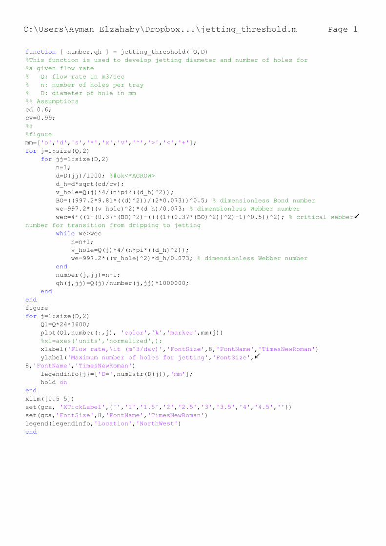
C:\Users\Ayman Elzahaby\Dropbox...\jetting_threshold.m Page 1
function [ number,qh ] = jetting_threshold( Q,D)%This function is used to develop jetting diameter and number of holes for%a given flow rate% Q: flow rate in m3/sec% n: number of holes per tray% D: diameter of hole in mm%% Assumptionscd=0.6;cv=0.99;%%%figuremm=['o','d','s','*','x','v','^','>','<','+'];for j=1:size(Q,2) for jj=1:size(D,2) n=1; d=D(jj)/1000; %#ok<*AGROW> d_h=d*sqrt(cd/cv); v_hole=Q(j)*4/(n*pi*((d_h)^2)); BO=((997.2*9.81*((d)^2))/(2*0.073))^0.5; % dimensionless Bond number we=997.2*((v_hole)^2)*(d_h)/0.073; % dimensionless Webber number wec=4*((1+(0.37*(BO)^2)-((((1+(0.37*(BO)^2))^2)-1)^0.5))^2); % critical webber number for transition from dripping to jetting while we>wec n=n+1; v_hole=Q(j)*4/(n*pi*((d_h)^2)); we=997.2*((v_hole)^2)*d_h/0.073; % dimensionless Webber number end number(j,jj)=n-1; qh(j,jj)=Q(j)/number(j,jj)*1000000; endendfigurefor j=1:size(D,2) Q1=Q*24*3600; plot(Q1,number(:,j), 'color','k','marker',mm(j)) %x1=axes('units','normalized',); xlabel('Flow rate,\it (m^3/day)','FontSize',8,'FontName','TimesNewRoman') ylabel('Maximum number of holes for jetting','FontSize',8,'FontName','TimesNewRoman') legendinfo{j}=['D=',num2str(D(j)),'mm']; hold onendxlim([0.5 5])set(gca, 'XTickLabel',{'','1','1.5','2','2.5','3','3.5','4','4.5',''})set(gca,'FontSize',8,'FontName','TimesNewRoman')legend(legendinfo,'Location','NorthWest')end
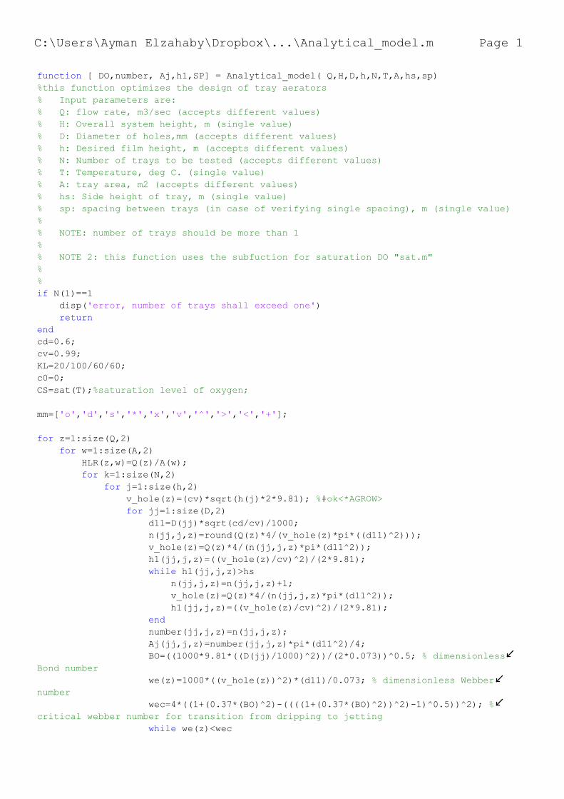
C:\Users\Ayman Elzahaby\Dropbox\...\Analytical_model.m Page 1
function [ DO,number, Aj,h1,SP] = Analytical_model( Q,H,D,h,N,T,A,hs,sp)%this function optimizes the design of tray aerators% Input parameters are:% Q: flow rate, m3/sec (accepts different values)% H: Overall system height, m (single value)% D: Diameter of holes,mm (accepts different values)% h: Desired film height, m (accepts different values)% N: Number of trays to be tested (accepts different values)% T: Temperature, deg C. (single value)% A: tray area, m2 (accepts different values)% hs: Side height of tray, m (single value)% sp: spacing between trays (in case of verifying single spacing), m (single value)%% NOTE: number of trays should be more than 1%% NOTE 2: this function uses the subfuction for saturation DO "sat.m"%%if N(1)==1 disp('error, number of trays shall exceed one') returnendcd=0.6;cv=0.99;KL=20/100/60/60;c0=0;CS=sat(T);%saturation level of oxygen; mm=['o','d','s','*','x','v','^','>','<','+']; for z=1:size(Q,2) for w=1:size(A,2) HLR(z,w)=Q(z)/A(w); for k=1:size(N,2) for j=1:size(h,2) v_hole(z)=(cv)*sqrt(h(j)*2*9.81); %#ok<*AGROW> for jj=1:size(D,2) d11=D(jj)*sqrt(cd/cv)/1000; n(jj,j,z)=round(Q(z)*4/(v_hole(z)*pi*((d11)^2))); v_hole(z)=Q(z)*4/(n(jj,j,z)*pi*(d11^2)); h1(jj,j,z)=((v_hole(z)/cv)^2)/(2*9.81); while h1(jj,j,z)>hs n(jj,j,z)=n(jj,j,z)+1; v_hole(z)=Q(z)*4/(n(jj,j,z)*pi*(d11^2)); h1(jj,j,z)=((v_hole(z)/cv)^2)/(2*9.81); end number(jj,j,z)=n(jj,j,z); Aj(jj,j,z)=number(jj,j,z)*pi*(d11^2)/4; BO=((1000*9.81*((D(jj)/1000)^2))/(2*0.073))^0.5; % dimensionless Bond number we(z)=1000*((v_hole(z))^2)*(d11)/0.073; % dimensionless Webber number wec=4*((1+(0.37*(BO)^2)-((((1+(0.37*(BO)^2))^2)-1)^0.5))^2); % critical webber number for transition from dripping to jetting while we(z)<wec
C:\Users\Ayman Elzahaby\Dropbox\...\Analytical_model.m Page 2
number(jj,j,z)=number(jj,j,z)-1; v_hole(z)=Q(z)*4/(number(jj,j,z)*pi*(d11^2)); h1(jj,j,z)=((v_hole(z)/cv)^2)/(2*9.81); Aj(jj,j,z)=number(jj,j,z)*pi*(d11^2)/4; BO=((1000*9.81*((D(jj)/1000)^2))/(2*0.073))^0.5; % dimensionless Bond number we(z)=1000*((v_hole(z))^2)*(d11)/0.073; % dimensionless Webber number wec=4*((1+(0.37*(BO)^2)-((((1+(0.37*(BO)^2))^2)-1)^0.5))^2); % critical webber number for transition from dripping to jetting end number(jj,j,z)=number(jj,j,z)-1; v_hole(z)=Q(z)*4/(number(jj,j,z)*pi*(d11^2)); h1(jj,j,z)=((v_hole(z)/cv)^2)/(2*9.81); Aj(jj,j,z)=number(jj,j,z)*pi*(d11^2)/4; BO=((1000*9.81*((D(jj)/1000)^2))/(2*0.073))^0.5; % dimensionless Bond number we(z)=1000*((v_hole(z))^2)*(d11)/0.073; % dimensionless Webber number wec=4*((1+(0.37*(BO)^2)-((((1+(0.37*(BO)^2))^2)-1)^0.5))^2); % critical webber number for transition from dripping to jetting SP(k)=H/(N(k)); L_jet(k,z)=SP(k)-h1(jj,j,z); v_jet(k,z)=sqrt(((v_hole(z))^2)+(2*9.81*(L_jet(k,z)))); d22(k,z)=d11*sqrt(v_jet(k,z)/v_hole(z)); dm(k,z)=(d11+d22(k,z))/2; v_mean(k,z)=(v_jet(k,z)+v_hole(z))/2; ad(k,z)=4/dm(k,z); % area to volume ratio in case of falling stream, assuming diameter equal hole diameter td(k,z)=(L_jet(k,z))/v_mean(k,z); %abc(k,z,jj)=ad(k,z)*td(k,z); L_jet2(k,z)=sp-h1(jj,j,z); v_jet2(k,z)=sqrt(((v_hole(z))^2)+(2*9.81*(L_jet2(k,z)))); d222(k,z)=d11*sqrt(v_jet2(k,z)/v_hole(z)); dm2(k,z)=(d11+d222(k,z))/2; v_mean2(k,z)=(v_jet2(k,z)+v_hole(z))/2; ad2(k,z)=4/dm2(k); % area to volume ratio in case of falling stream, assuming diameter equal hole diameter td2(k,z)=(L_jet2(k,z))/v_mean2(k,z); %% estimation of DO DO(jj,j,k,z,w)=CS-((CS-c0)*exp(-KL*(((1)/HLR(z,w))+((1)*ad(k,z)*td(k,z))))); DO2(jj,j,k,z,w)=CS-((CS-c0)*exp(-KL*(((N(k))/HLR(z,w))+((N(k))*ad2(k,z)*td2(k,z))))); DOT(jj,j,k,z,w)=CS-((CS-c0)*exp(-KL*(((N(k))/HLR(z,w))+((N(k))*ad(k,z)*td(k,z))))); %qh(jj,j,z)=Q(z)./number(jj,j,z); end end
C:\Users\Ayman Elzahaby\Dropbox\...\Analytical_model.m Page 3
end endend %% Create figure for DO from one tray and number of holes with const. jet area figure%axes('Position',[0.0380673499267936 0.0557935784749302 0.956808199121523 0.908388704318937])for i=1:size(D,2) plot(number(i,:,1),DO(i,:,4,1,2), 'color','k','marker',mm(i)) legendinfo{i}=['Hole Diameter=',num2str((D(i))),'mm']; hold on xlabel('Number of holes per tray','FontSize',7,'FontName','Arial','FontWeight','bold'); ylabel('DO influent to second tray\it mg/L' ,'FontSize',7,'FontName','Arial','FontWeight','bold') title('Typical DO profile Vs. number of holes at different hole diameters',... 'FontSize',7,'FontName','Arial','FontWeight','bold');end ylim([1.3 1.8]) set(gca,'FontSize',8,'FontName','Arial','FontWeight','bold')legend(legendinfo,'Location','NorthWest') % %% Create figure for DO from one tray for flow rate per hole and diameter% % figure% for i=1:size(D,2)% plot(qh(i,:,1)*1000000,DO(i,:,4,1,2), 'color',[rand(1),rand(1),rand(1)])% lgendinfo{i}=['Hole Diameter=',num2str((D(i))),'mm'];% hold on% xlabel('Flow rate per hole (x10^-^6 m^3/sec/hole)','FontSize',14);% ylabel('DO influent to second tray (mg/L)','FontSize',14)% title('Typical DO profile Vs. flow per hole for different hole diameters',...% 'FontSize',16);% end% ylim([1 2])% % set(gca,'FontSize',14)% legend(lgendinfo,'Location','NorthWest') %% Create figure for DO from one tray for jet area and spacing figurefor i=1:size(N,2) plot((D),DO(:,1,i,1,2), 'color','k','marker',mm(i)) lgendinfo{i}=['Spacing between trays=',num2str(SP(i)), ' m']; hold on xlabel('Hole Diameter\it mm' ,'FontSize',7,'FontName','Arial','FontWeight','bold'); ylabel('DO influent to second tray\it mg/L' ,'FontSize',7,'FontName','Arial','FontWeight','bold'); title('Typical DO profile Vs. spacing between trays for single tray system',... 'FontSize',7,'FontName','Arial','FontWeight','bold');
C:\Users\Ayman Elzahaby\Dropbox\...\Analytical_model.m Page 4
end% xlim([2 7])% set(gca, 'XTickLabel',{'','3','4','5','6',''})ylim([1.3 1.8])set(gca,'FontSize',8,'FontName','Arial','FontWeight','bold')legend(lgendinfo,'Location','NorthWest') %% Create figure for DO from system and number of trays at fixed spacing % figure% for i=1:size(D,2)% ee=DO2(i,1,:,1,2);% eee=permute(ee,[1,3,2,4,5]);% plot((N),eee, 'color','k','marker',mm(i))% lgendinfo{i}=['Hole Diameter=',num2str((D(i))),'mm'];% hold on% xlabel('Number of trays','FontSize',7,'FontName','Arial','FontWeight','bold');% ylabel('DO effluent from the system\it mg/L','FontSize',7,'FontName','Arial','FontWeight','bold');% title('Typical DO profile Vs. number of trays for fixed tray spacing',...% 'FontSize',7,'FontName','Arial','FontWeight','bold');% end% ylim([0 CS])% set(gca,'FontSize',8,'FontName','Arial','FontWeight','bold')% legend(lgendinfo,'Location','NorthWest')% Create figure for number of trays %% Create figure for system performance for a fixed height figurefor i=1:size(D,2) ee=DOT(i,1,:,1,2); eee=permute(ee,[1,3,2,4,5]); plot(N,eee,'color','k','marker',mm(i)) leegendinfo{i}=['Hole Diameter=',num2str((D(i))),'mm']; hold onendlegend(leegendinfo,'Location','NorthWest')xlabel('Number of trays','FontSize',7,'FontName','Arial','FontWeight','bold');ylabel('DO effluent from the system\it mg/L' ,'FontSize',7,'FontName','Arial','FontWeight','bold');set(gca,'XTickLabel',N)title('Typical DO profile Vs. number of trays for a 1m height system',... 'FontSize',7,'FontName','Arial','FontWeight','bold');ylim([0 CS])set(gca,'FontSize',8,'FontName','Arial','FontWeight','bold')first_axis = gca;sqz = 0.1; %// distance to squeeze the first plotset(first_axis,'units','normalized', 'Position', get(first_axis, 'Position') + [0 sqz 0 -sqz ]);ax2 = axes('Position', get(first_axis, 'Position') .* [1 1 1 0.001] - [0 sqz 0 0],'Color','none');xlim([SP(size(SP,2)) SP(1)]);set(get(gca, 'XLabel'),'String','Spacing between trays\it m' ,'FontSize',7,'FontName','Arial','FontWeight','bold');
C:\Users\Ayman Elzahaby\Dropbox\...\Analytical_model.m Page 5
set(gca,'XTickLabel',SP)set(ax2, 'XScale', get(first_axis, 'XScale')); %// make logarithmic if first axis is tooset(gca,'FontSize',8,'FontName','Arial','FontWeight','bold') %% Create figure for change in tray area and flow rate figurefor w=1:size(A,2) aaa=DOT(1,1,k,:,:); aa=permute(aaa,[4,5,1,2,3]); plot(Q*1000*1000,aa(:,w),'color','k','marker',mm(w)) leeegendinfo{w}=['Tray Area=',num2str((A(w))),' m']; hold on xlabel('Flow rate\it x10^-^6 m^3/sec' ,'FontSize',7,'FontName','Arial','FontWeight','bold'); ylabel('DO effluent from the system\it mg/L' ,'FontSize',7,'FontName','Arial','FontWeight','bold'); title('Typical DO profile Vs. flow rate for a 1m height system',... 'FontSize',7,'FontName','Arial','FontWeight','bold');endylim([0 CS])set(gca,'FontSize',8,'FontName','Arial','FontWeight','bold')legend(leeegendinfo,'Location','SouthWest')end

94
Annex II
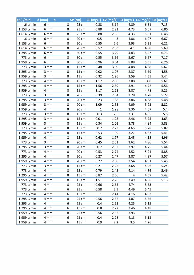
Q (L/min) d (mm) n SP (cm) C0 (mg/L) C2 (mg/L) C4 (mg/L) C6 (mg/L) C8 (mg/L)
.6 L/min 6 mm 8 25 cm 0.88 3.14 4.89 6.51 7.13
1.153 L/min 6 mm 8 25 cm 0.88 2.91 4.73 6.07 6.86
1.614 L/min 6 mm 8 25 cm 0.88 2.85 4.33 5.91 6.46
.6 L/min 6 mm 8 20 cm 0.5 3 4.86 6.07 6.67
1.153 L/min 6 mm 8 20 cm 0.55 2.6 3.93 5.21 6.21
1.614 L/min 6 mm 8 20 cm 0.57 2.63 4.1 4.98 5.69
1.295 L/min 6 mm 8 30 cm 0.55 3.29 4.83 5.97 6.73
.773 L/min 6 mm 8 30 cm 0.55 3.66 5.67 6.67 7.17
1.959 L/min 6 mm 8 30 cm 0.96 3.04 5.08 5.55 6.26
.773 L/min 3 mm 8 15 cm 0.48 3.09 4.08 4.98 5.67
1.295 L/min 3 mm 8 15 cm 0.02 1.07 2.37 3.59 4.58
1.959 L/min 3 mm 8 15 cm 0.32 1.96 3.59 4.55 5.44
.773 L/min 4 mm 8 15 cm 1.17 2.58 3.88 4.8 5.61
1.295 L/min 4 mm 8 15 cm 1.56 2.69 3.91 4.72 5.56
1.959 L/min 4 mm 8 15 cm 1.17 2.63 3.87 4.78 5.25
.773 L/min 3 mm 8 20 cm 0.39 2.34 3.78 4.78 5.72
1.295 L/min 3 mm 8 20 cm 0.23 1.88 3.86 4.68 5.48
1.959 L/min 3 mm 8 20 cm 1.09 2.53 4.09 5.23 5.82
1.959 L/min 4 mm 8 20 cm 1 1.98 3.36 4.57 5.4
.773 L/min 3 mm 8 15 cm 0.3 2.5 3.31 4.55 5.5
1.295 L/min 3 mm 8 15 cm 0.01 1.23 2.46 3.75 4.63
1.959 L/min 3 mm 8 15 cm 0.34 2.01 3.78 4.84 5.83
.773 L/min 4 mm 8 15 cm 0.7 2.23 4.65 5.28 5.87
1.295 L/min 4 mm 8 15 cm 0.53 1.99 3.27 4.83 5.41
1.959 L/min 4 mm 8 15 cm 0.62 1.97 3.43 4.12 4.96
.773 L/min 3 mm 8 20 cm 0.45 2.51 3.62 4.86 5.54
1.295 L/min 3 mm 8 20 cm 0.7 2.52 3.97 4.75 5.44
.773 L/min 4 mm 8 20 cm 0.53 2.74 4.52 5.21 5.88
1.295 L/min 4 mm 8 20 cm 0.27 2.47 3.87 4.87 5.57
1.959 L/min 4 mm 8 20 cm 0.27 2.08 3.54 4.61 5.45
.773 L/min 3 mm 8 15 cm 0.21 2.25 3.68 4.46 5.24
.773 L/min 4 mm 8 15 cm 0.79 2.45 4.14 4.86 5.46
1.295 L/min 4 mm 8 15 cm 0.87 2.66 4 4.57 5.42
1.959 L/min 4 mm 8 15 cm 1.51 2.26 3.49 4.66 5.13
.773 L/min 4 mm 8 25 cm 0.66 2.65 4.74 5.63
.773 L/min 4 mm 6 25 cm 0.58 2.9 4.49 5.45
.773 L/min 4 mm 6 15 cm 1 2.41 4.16 4.52
1.295 L/min 4 mm 8 25 cm 0.56 2.62 4.07 5.36
1.295 L/min 4 mm 6 25 cm 0.4 2.53 4.25 5.15
1.295 L/min 4 mm 6 15 cm 0.8 2.22 3.46 4.48
1.959 L/min 4 mm 8 25 cm 0.56 2.52 3.93 5.7
1.959 L/min 4 mm 6 25 cm 0.4 2.28 4.13 5.15
1.959 L/min 4 mm 6 15 cm 0.9 2.2 3.5 4.26


