Embed Size (px)
Citation preview
Journal of Computational Physics164,258–282 (2000)
doi:10.1006/jcph.2000.6593, available online at http://www.idealibrary.com on
Parallel Computation of Flow in HeterogeneousMedia Modelled by Mixed Finite Elements1
K. A. Cliffe,∗ I. G. Graham,† R. Scheichl,† and L. Stals‡∗AEA Technology, Harwell, Didcot, Oxon OX11 0RA, United Kingdom;†Department of Math. Sciences,
University of Bath, Bath BA2 7AY, United Kingdom; and‡Department of Computer Science,Old Dominion University, Norfolk, Virginia 23529-0162
E-mail: [email protected], [email protected], [email protected], [email protected]
Received August 2, 1999; revised July 12, 2000
In this paper we describe a fast parallel method for solving highly ill-conditionedsaddle-point systems arising from mixed finite element simulations of stochasticpartial differential equations (PDEs) modelling flow in heterogeneous media. Eachrealisation of these stochastic PDEs requires the solution of the linear first-ordervelocity–pressure system comprising Darcy’s law coupled with an incompressibil-ity constraint. The chief difficulty is that the permeability may be highly variable,especially when the statistical model has a large variance and a small correlationlength. For reasonable accuracy, the discretisation has to be extremely fine. We solvethese problems by first reducing the saddle-point formulation to a symmetric posi-tive definite (SPD) problem using a suitable basis for the space of divergence-freevelocities. The reduced problem is solved using parallel conjugate gradients precon-ditioned with an algebraically determined additive Schwarz domain decompositionpreconditioner. The result is a solver which exhibits a good degree of robustness withrespect to the mesh size as well as to the variance and to physically relevant values ofthe correlation length of the underlying permeability field. Numerical experimentsexhibit almost optimal levels of parallel efficiency. The domain decomposition solver(DOUG,http://www.maths.bath.ac.uk/∼parsoft) used here not only is ap-plicable to this problem but can be used to solve general unstructured finite elementsystems on a wide range of parallel architectures.c© 2000 Academic Press
Key Words:Raviart–Thomas mixed finite elements; second-order elliptic prob-lems; divergence-free space; heterogeneous media; groundwater flow; domain de-composition; parallel computation.
1 This work was supported in part by EPSRC Grant GR/L31715 and EPSRC CASE Award 97D00023.
258
0021-9991/00 $35.00Copyright c© 2000 by Academic PressAll rights of reproduction in any form reserved.

PARALLEL COMPUTATION OF FLOW IN HETEROGENEOUS MEDIA 259
1. INTRODUCTION
In this paper we describe, analyse, and implement a parallel algorithm for use in thenumerical simulation of stochastic partial differential equations (PDEs) modelling ground-water flow in heterogeneous media. The classical equations governing this application arethe first-order system consisting ofDarcy’s law,
Eq + (k/µ) E∇PR = E0, (1.1)
coupled with themass conservation law,
E∇ · Eq = 0, (1.2)
subject to appropriate boundary conditions. HereEq is thevelocity(more precisely the specificdischarge), andPR is theresidual pressure. The actual pressure isPR− ρgz, wherez isthe fluid height,ρ is the density, andg is the acceleration due to gravity. The functionsEqandPR are both to be determined from (1.1) and (1.2), withk denoting permeability andµdenoting the dynamic viscosity.
In contrast to the classical determinisic models,k will, in the probabilistic case consideredhere, be modelled using a Gaussian random field. The numerical treatment of this problemthen involves the solution of (1.1) and (1.2) for many differentrealisationsof k and subse-quent computation of statistical properties of the resulting velocity and/or pressure fields.In this paper we describe a fast parallel method for the solution of (1.1) and (1.2) whenk isany typical realisation. Although we do not carrry out here any statistical analysis involv-ing multiple simulations, a prime motivation of our work is to obtain a numerical methodwhich is sufficiently accurate and efficient to make such a statistical analysis possible. Forreasons described below, a typical simulation of (1.1) and (1.2) will involve the solutionof very large, highly ill-conditioned indefinite linear systems and the fast method proposedhere constitutes an essential tool which can be used in later statistical analyses. Because ofapplications in waste management and in the oil industry, there is a strong technologicalmotivation for such a tool.
The Gaussian random fields which determinek are characterised by a pair of parameters(σ 2, λ), whereσ 2 is thevarianceandλ is thelength scaleover which the field is correlated. Inaddition, the discrete model also depends onn, the number of degrees of freedom in the grid,althoughλ andn are typically related to each other. Extreme variations in these parameterscontribute to the ill-conditioning of the discretisation of (1.1) and (1.2), and a key test for ouralgorithm is whether it behaves robustly when subjected to variations in these parameters.
It is known that any realisation of the Gaussian random fieldk is Holder continuous, butnot in general differentiable, and so the resulting velocity and pressure fields have only lowregularity throughout the domain. Since this irregularity is global, it cannot be compensatedfor by local mesh refinement, and the only known way to achieve acceptable accuracy forthese problems is to use low-order approximation on a mesh which is (uniformly) as fine aspossible throughout the domain. In typical 2D simulations, the required number of degreesof freedomn for acceptable accuracy typically lies in the range 106 to 108. A key aim ofthe present paper is to provide usable methods for problems of this sort. The use of parallelcomputing power plays an essential rˆole in achieving this aim.
Because the variable of prime interest here is the flow velocityEq, the discretisationschemes of most interest are those which preserve conservation of mass (1.2) in an appro-priate way, with the prime candidates being mixed finite element or finite volume techniques.

260 CLIFFE ET AL.
Because of the lack of regularity in this problem, we discretise (1.1) and (1.2) using thelowest order mixed Raviart–Thomas elements on triangular meshes [3, 32]. ThenEq is ap-proximated in an appropriate subspace of the vector-valued piecewise linear functions. Theresulting discretisation enforces mass conservation on each element of the mesh and this inturn implies that the velocity field is in fact piecewise constant, making the computation ofparticle trajectories extremely simple.
This type of discretisation yields a symmetric indefinite system ofsaddle-pointtypewhich, in the presence of large variations ink and n, is very difficult to solve quicklyenough for the multiple statistical simulations described above. We describe a fast parallelsolver for these systems. The results in Section 5 show that, using our solver with a fixednumber of processors, the time taken for a solve scales almost linearly (i.e., optimally) innand is remarkably robust toσ 2 andλ. Moreover, almost 100% parallel efficiency is observedwhen the algorithm is tested on a machine with up to 10 processors. A modest decrease inefficiency is observed for higher numbers of processors.
Our solver is built on two essential steps. The first step decouples the velocity field inthe saddle-point problem from the pressure field. This is done by writing the velocity as thecurl of an appropriate discrete stream function, which automatically satisfies the discretecounterpart of the mass conservation law (1.2). The required discrete stream function turnsout to be a standard finite element approximation of the solution of a related symmetricpositive definite (SPD) problem which can be found independent of the pressure. SuchSPD systems are easier to solve than indefinite ones and this one turns out to have theadded advantage of being about five times smaller than the original saddle-point problem.A further advantage of this approach is that the approximate pressure (if it is required) canbe retrieved by solving a triangular system by simple back substitutions.
The second step in the solver is the application of parallel preconditioned conjugategradient methods to solve for the discrete stream function. This is done using additiveSchwarz preconditioners (e.g., [5]) based on solves in overlapping subdomains togetherwith a global coarse grid solve. It is known that this process can be used to build veryefficient “black-box” parallel solvers which are remarkably robust for problems with highlydiscontinuous coefficients discretised on unstructured meshes [15, 16]. We have recentlydeveloped a general parallel package which implements this type of solution strategy andwe use it here to solve the systems arising from the present application. This represents anextreme test for the package, and indeed for domain decomposition methods in general, andwe are pleased to be able to report good performance of the solver under these circumstances.
Other iterative methods for related problems are reported, for example, in [2, 38], althoughthere the emphasis is on finite volume/multigrid techniques.
The layout of this paper is as follows. In Section 2 we shall describe the background to thestatistical models of heterogeneous media. In Section 3 we briefly review the discretisationof (1.1) and (1.2) and describe the reduction of the saddle-point system to an SPD system.In Section 4 we describe the additive Schwarz procedure and its resilience to discontinuouscoefficients as well as our “black-box” package [19, 20]. In Section 5 we give a sequenceof experiments which show the performance of the method.
2. STATISTICAL MODELLING OF HETEROGENEOUS MEDIA
The flow of fluids in the rocks composing the earth’s crust is important in a numberof technological and industrial fields, most notably the hydrocarbon and water resourcesindustries. In the former, one is motivated to understand the underground flow of oil (and

PARALLEL COMPUTATION OF FLOW IN HETEROGENEOUS MEDIA 261
gas) in order to recover as much of this resource as possible. In the latter, a proper un-derstanding of the flow of groundwater and of the transport of chemicals in it is essentialnot only for good resource management and quality control but also for applications inpollution modelling. One option for the long-term disposal of radioactive waste is storagein an underground repository. In order to scientifically assess the safety of this option it isnecessary to model the transport of radionuclides in flowing groundwater. Thus, this topicis of general environmental importance.
From now on we restrict our attention to groundwater flow. One of the main character-istics of the rocks in the earth’s crust affecting this flow is their heterogeneity (i.e., spatialvariation). In particular the spatial variation of permeabilityk in (1.1) gives rise to variabilityin the flow velocity, which in turn affects the transport of dissolved chemicals or pollutants.This heterogeneity has two main aspects.
1. Uncertainty. Because the rock properties are varying in a complicated way and itis not possible to measure the permeability at each point in space, there is inevitablya degree of uncertainty concerning the values of the permeability. However, the per-meability is in principle required at every point and simple-minded interpolation ofmeasured values provides an insufficiently accurate approximation.2. Dispersion. The heterogeneity means that the velocity field varies on a rangeof length scales and so particle paths that are initially close together can becomeprogressively separated. This phenomenon—calledhydrodynamic dispersion—is theprimary mechanism for the spreading of a plume of pollutant as it is transported bythe groundwater flow [11].
A widely used method of treating heterogeneity, capable of dealing with both theseaspects, is stochastic modelling. The basic idea is to model the permeability field as astochastic spatial process, assuming that a single realisation of this stochastic process isa reasonable representation of the permeability field and that any of the realisations areequally probable given the information available from measurements. This approach leadsto the stochastic PDEs. (1.1) and (1.2), whereEq andPR are now random variables. Givencertain statistical properties ofk (which we now describe), it is of interest to study statisticalproperties of those random variables. Thus, it is essential that we can quickly and efficientlysolve (1.1) and (1.2) and, most importantly, compute the velocityEq for each realisation ofk. More detail on the following statistical background can be found in Refs. [1, 10].
A random fieldon an open domainÄ ⊂ R2 (also called aspatial process) is a set ofrandom variablesZ(Ex), each of which is associated with a pointEx ∈ Ä. This random fieldis calledGaussianif for each arbitraryn, each set ofn random variables located atnarbitrarily chosen spatial points is Gaussian. Such fields can be completely specified bytheir (spatially varying) mean and covariance functions, denoted respectively bym(Ex) and6(Ex, Ey) := E{(Z(Ex)−m(Ex)) (Z(Ey)−m(Ey))}, for Ex, Ey ∈ Ä.
In this paper we will be concerned only withstatistically homogeneous isotropicGaussianrandom fields whose mean and covariance have the particular forms
m(Ex) := m, 6(Ex, Ey) := σ 2 exp(−|Ex − Ey|/λ), (2.1)
for positive constantsm, σ , andλ. Elementary manipulations show that
E{(Z(Ex)− Z(Ey))2} = E{Z(Ex)2} + E{Z(Ey)2} − 2E{Z(Ex)Z(Ey)}= 2σ 2[1− exp(−|Ex − Ey|/λ)] = γ (|Ex − Ey|), (2.2)

262 CLIFFE ET AL.
whereγ (r ) := 2σ 2(1− exp(−r/λ)) is called thevariogram; see, e.g., [10]. The parameterλ is called thelength scale: (2.2) shows thatZ(Ex) and Z(Ey) can only be expected to beclose when|Ex − Ey| < λ. So, asλ→ 0, the random fieldZ becomes “rougher.”
We shall solve (1.1) and (1.2) in the case when logk is a realisation of such a Gaussianrandom field, usually called a “lognormal distribution.” There is some evidence from fielddata that this gives a reasonable representation of reality in certain cases [14, 24]. Thereare many good methods for generating realisations of Gaussian random fields, includingthose based on FFT [18, 33], direct simulation [12], and the turning bands method [28, 37].Here we use the turning bands approach that represents the field as a superposition ofone-dimensional fields, which are generated along lines radiating from the origin using aspectral technique.
Of particular importance to the accuracy of any discretisation is the question of regularityof this realisation. This question is thoroughly investigated in the statistical literature. Inparticular, it can be deduced from Adler [1] (see also [9]) that ifX denotes any realisation ofthe Gaussian random fieldZ introduced above then, with probability 1, there exists a positiveconstantAsuch that|X(Ex)− X(Ey)| ≤ A|Ex − Ey|α, for all Ex, Ey ∈ Ä, and 0< α < 1/2. It thenfollows from the elliptic PDE theory that ifk is any realisation of a lognormal distribution,then the velocity fieldEq appearing in (1.1) will not in general exhibit better thanCα regularity,thus motivating the use of low-order elements (see [9, Appendix] for more detail).
Once the system (1.1) and (1.2) has been solved for multiple realisations ofk and the stat-istical properties of the velocity field have been found, the dispersion present in the systemcan (at least when the molecular diffusion is small) be studied by looking at the statisticsof particle paths moving in the velocity field. In fact ifX′j denotes thej th coordinate ofthe particle displacement from its mean position then the spreading can be characterisedby the second order moment of the particle paths:X jl := E{X′j X′l } for j, l = 1, 2. ThevariablesX′j satisfy the system of differential equationsd X′j /dt = qj , whereqj is the j thcomponent of the velocity field. This model highlights another advantage of the low-ordermixed finite element method: Since the computed velocity field is constant on each element,the differential equation forX′j is trivially integrated in an element by element fashion, thusallowing the efficient computation of the many particle paths which would be required instatistical analyses.
Before continuing we remark that there are many stochastic models for groundwater flow(see, e.g., [27] for a review), We have chosen the given model here because it is a relativelysimple model which applies to fully saturated flows, but still has many of the featuresof some of the more complicated models. We remark also that more complicated modelsrequire more data to support them, and data are very often difficult to come by, especiallyin the case of deep geological waste disposal, our chief motivation for developing thisalgorithm.
3. DISCRETISATION AND REDUCTION TO SPD SYSTEM
For ease of notation, from now on we replacePR by p in (1.1) and we consider (1.1) and(1.2) on a simply connected open domainÄ ⊂ R2 with a polygonal boundary0, which isassumed partitioned into0D ∪ 0N . Each of0D and0N is assumed to consist of a finiteunion of intervals of0 and each of the intervals in0N is assumed to contain its end points.Throughout we shall assume that0D 6= ∅, a condition which is generically satisfied ingroundwater flow applications, where some inflow and outflow must occur. The extension

PARALLEL COMPUTATION OF FLOW IN HETEROGENEOUS MEDIA 263
to the case when0D = ∅ (when p is non-unique) can easily be made by imposing anextra condition onp in the weak form below (e.g., thatp should have a prescribed meanvalue—See [13]).
Let Eν(Ex) denote the outward unit normal fromÄ at Ex ∈ 0. We describe the solution of(1.1) and (1.2) in the case whereµ is a positive constant andk is a general symmetricuniformly positive definite 2× 2 matrix-valued function onÄ. (In Section 5,k will bea scalar multiple of the identity.) This system is to be solved subject to mixed boundaryconditions:
p = q on0D, and Eq · Eν = 0 on0N . (3.1)
Let (·, ·)L2(Ä)d denote the usual inner product inL2(Ä)d, for d = 1, 2. Then introduce the
spaceH(div, Ä) :={Ev ∈ L2(Ä)2 : div Ev ∈ L2(Ä)}, with the inner product(Eu, Ev)H(div,Ä) :=
(Eu, Ev)L2(Ä)2 + (div Eu, div Ev)L2(Ä). Introduce also the subspaceH0,N(div, Ä) :={Ev ∈ H(div, Ä) : Ev · Eν|N = 0} and, forEu, Ev ∈ H0,N(div, Ä) andw ∈ L2(Ä), define
m(Eu, Ev) := (µk−1Eu, Ev)L2(Ä)2, b(Ev,w) :=−(div Ev,w)L2(Ä), and
G(Ev) :=−∫0D
gEv · Eν ds.
Then the weak form of (1.1), (1.2) is to find(Eq, p) ∈ H0,N(div, Ä)× L2(Ä) such that
m(Eq, Ev)+ b(Ev, p) = G(Ev), for all Ev ∈ H0,N(div, Ä),
b(Eq, w) = 0, for allw ∈ L2(Ä).
}(3.2)
The mixed finite element discretisation of (3.2) is obtained by choosing finite dimensionalsubspacesV ⊂ H0,N(div, Ä)andW ⊂ L2(Ä)and seeking( EQ, P) ∈ V ×W to satisfy (3.2)for all Ev ∈ V andw ∈W. By choosing bases{Evi : i = 1, . . . ,nV} and{w j : j = 1, . . . ,nW}for V andW and writing
EQ =nV∑i=1
qi Evi , P =nW∑j=1
pjw j ,
the discrete problem reduces to the indefinite linear equation system(M B
BT 0
)(q
p
)=(
f
0
)in RnV × RnW , (3.3)
whereMi,i ′ :=m(Evi , Evi ′), Bi, j := b(Evi , w j ), and fi :=G(Evi ).To constructV andW, let T denote a triangulation ofÄ into conforming triangles
T ∈ T . We assume that thecollision points(i.e., end-points of the intervals in0N) arenodal points of this triangulation. LetE denote the set of all edges of the triangles inT . It is convenient to think of these edges as open. For anyE ∈ E , we let EνE denotethe unit normal to the edgeE which, for convenience, is assumed to be oriented so thatEνE ∈ {Ex ∈ R2 : x1 > 0} ∪ {(0, 1)T }. Let EI , ED andEN denote the edgesE ∈ E which lie,respectively, inÄ,0D and0N . The spaceV is defined to be the space of all functionsEv ∈ H0,N(div, Ä) such that for allT ∈ T , there exist scalarsαT , βT andγT such that
Ev(Ex) =(αT
βT
)+ γT Ex, for all Ex ∈ T. (3.4)

264 CLIFFE ET AL.
EachEv ∈ V can be completely determined by specifying the constant value ofEv · EνE foreachE ∈ EI ∪ ED and the standard basis forV is constructed by associating with each edgeE ∈ EI ∪ ED, a functionEvE ∈ V with the property that
EvE · EνE′ = δE,E′ (3.5)
with δ denoting the Kronecker delta. The spaceW is chosen as the space of piecewiseconstant functions onÄ, with basis consisting of the characteristic functionswT of each ofthe trianglesT ∈ T . Thus
nV = (#EI + #ED), nW = (#T ), (3.6)
where, throughout, #A denotes the number of elements of a (finite) setA.Although the analysis below is given for system (3.3) with permeabilityk, in the practical
implementation of (3.3) we shall replacek in m by k, the piecewise constant interpolationof k at the centroids of the triangles in the meshT . This is very useful practically sincethe generation of the Gaussian random fieldk is expensive and it is important to sample itat as few points as possible. It is shown in [9, Appendix] that this approximation does notdegrade the estimate for the error‖Eq − EQ‖H(div,Ä).
With the motivation given in Section 1, we now introduce our decoupling procedure for(3.3).
3.1. General Decoupling Procedure
The decoupling can be achieved by finding a basis{z1, . . . , zn◦ } of ker BT . (SinceBT hasfull rank,n◦ = nV − nW .) If we have such a basis, then the solutionq of (3.3) can be written
q=n◦∑
j=1
q◦ j z j = ZTq◦ , (3.7)
for someq◦ ∈ Rn◦ whereZ denotes then◦ × nV matrix with rowszT1 , . . . , z
Tn◦ . Also, since
Z B= (BT ZT )T = 0, multiplying the first (block) row of (3.3) byZ shows thatq◦ is asolution of the linear system
A◦q◦ = f
◦(3.8)
whereA◦ = Z M ZT andf
◦ = Zf. SinceM is SPD, so isA◦
andq◦ is the unique solution of(3.8). Thus, if the basis{z1, . . . , zn◦ } of ker BT can be found, then the velocityq in (3.3) canbe computed by solving the decoupled SPD system (3.8) rather than the indefinite coupledsystem (3.3). If the pressurep is also of interest, it may be found by computing acomplemen-tary basis{zn◦+1, . . . , znV } with the property that span{z1, . . . , zn◦ , zn◦+1, . . . , znV } = RnV .If Z′ then denotes the matrix with rowszT
n◦+1, . . . , zTnV , thenp is the unique solution of the
nW × nW system
(Z′B)p= Z′(f − Mq). (3.9)
We show in the next two sections that, in the particular case (3.3),
(i) It is always easy to find a basis{z1, . . . , zn◦ } of ker BT .

PARALLEL COMPUTATION OF FLOW IN HETEROGENEOUS MEDIA 265
(ii) The resulting matrix A◦
in the reduced problem (3.8) is in general a bordered matrix,whose main block consists of the stiffness matrix arising from a standard piecewise linearfinite element approximation to an associated H1-elliptic problem, and the number ofborders is one less than the number of disconnected components in0N.
(iii) The system (3.8) is about 5 times smaller than (3.3).
Note that a choice of complimentary basis (in fact a subset of the fundamental basis{e1, . . . ,enV } of RnV ) can be made so that the coefficient matrixZ′B in (3.9) is lowertriangular (see [9, 35] for a proof).
To establish conclusions (i)–(iii) we need to exploit the particular properties of (3.3). Inparticular note that finding a basis{z1, . . . , zn◦ } of ker BT is equivalent to finding a basisv◦→
1, . . . , v◦→
n◦ of the finite element space
V◦ := { EV ∈ V : b( EV,W) = 0 for all W ∈W}.
To see why letZ = (Zi, j ) be the matrix with rowszT1 , . . . , z
Tn◦ . Then the formulae
v◦→i =
nV∑j=1
Zi, j Ev j , i = 1, . . . ,n◦ (3.10)
(where{Ev j } is the basis ofV), determine the basis{v◦→i }. Conversely, if the basis{v◦→i } of V◦
is known, then the matrixZ (and hence the basisz1, . . . , zn◦ of ker BT ) is determined by(3.10).
3.2. Basis ofV◦
As a first step, recall thatT is the set of all triangles in the mesh and thatE = EI ∪ ED ∪ EN
is the set of all edges of the mesh (assumed to be open intervals). Analogously we can writeN = NI ∪ND ∪NN , withNI ,ND andNN denoting the nodes inÄ,0D and0N . Recallthat the end points of each of the components of0N belong to0N and, since the collisionpoints between Neumann and Dirichlet boundaries are mesh points, these end points lie inNN .
For P ∈ N , let8P denote the piecewise linear hat function satisfying8P(P′) = δP,P′ .The basis forV◦ will be constructed from the fundamental functions:
E9P = Ecurl8P = (∂8P/∂x2,−∂8P/∂x1)T . (3.11)
(i.e.,8P is the stream function forE9P). The functions (3.11) clearly satisfy divE9P = 0 oneach triangle of the mesh, and a subset of them lie inV◦ as the following proposition shows.(For a proof, see [3, Corollary III3.2].)
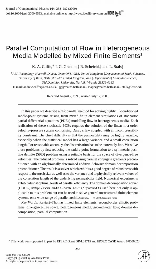
PROPOSITION3.1. For each P∈ NI ∪ND, E9P ∈ V◦ .Note that eachE9P can be expressed as a local linear combination of the basis functionsEvE of V satisfying (3.5); in fact only thoseEvE corresponding to edgesE touching nodePappear in the expansion ofE9P (see Fig. 1).
The functions introduced in Proposition 3.1 span a subset ofV◦ , but for general boundaryconditions, there are not enough of them to constitute a basis forV◦ . A small number of
266 CLIFFE ET AL.
FIG. 1. Divergence-free basis functionsE9P (left) and∑
P∈N`NE9P (right).
additional basis functions may need to be added. LetnC denote the number of connectedcomponents in0N and write
0N = 01N ∪ 02
N ∪ · · · ∪ 0nCN , 0`N ∩ 0`
′N = ∅ for all 1≤ `, `′ ≤ nC .
For ` = 1, . . . ,nC , let N `N ⊂ N denote the set of mesh nodes on0`N . The following is
proved using elementary arguments in [9].
PROPOSITION3.2. For each` = 1, . . . ,nC ,∑P∈N `
N
E9P ∈ V◦ . (3.12)
The functions (3.12) are nonlocal linear combinations of the functionsEvE; however, thenonlocality of
∑P∈N `
N
E9P is confined to the vicinity of0`N (see Fig. 1). The number ofsuch triangles is typically onlyO((#T )1/2).
From these elementary results we have our first theorem. It shows that when0N 6= ∅,by combining all the functions found in Proposition 3.1 with all but one of the functions inProposition 3.2, we have the required basis.
THEOREM3.3. Suppose nC 6= 0. Then a basis forV◦ is
{ E9P: P ∈ NI ∪ND} ∪∑
P∈N `N
E9P : ` = 1, . . . ,nC − 1
. (3.13)
Proof. Supposenc 6= 0. Consider a typical Neumann boundary segment0`N . Since0D 6= ∅, this contains #N `
N nodes and #N `N − 1 edges. Summing over= 1, . . . ,nC , we
obtain #EN = #NN − nC . Therefore, the number of functions in (3.13) is
(#NI + #ND + nC − 1) = (#N − #NN + nC − 1) = (#N − #EN − 1). (3.14)
Furthermore, since we assumed thatÄ is simply connected, we can apply Euler’s polyhedrontheorem to obtain
(#N − #EN − 1) = (#EI + #ED)− (#E − #N + 1) = (#EI + #ED)− #T , (3.15)
Now recalling thatn◦ = nV − nW = (#EI + #ED)− #T , it follows from (3.14) and (3.15)that the number of functions in (3.13) isn◦ = dimV◦ , as required.
PARALLEL COMPUTATION OF FLOW IN HETEROGENEOUS MEDIA 267
To complete the proof we merely need to show that the functions in (3.13) are linearlyindependent. So suppose{αP : P ∈ NI ∪ND} and{β` : ` = 1, . . . ,nC − 1} are scalars suchthat
E0=∑
P∈NI ∪ND
αP E9P +nC−1∑`=1
β`∑
P∈N `N
E9P. (3.16)
Using the linearity of Ecurl, this may be rewritten
E0=∑P∈N
αP E9P =∑P∈N
αP Ecurl8P = Ecurl
(∑P∈N
αP8P
), (3.17)
whereαP :=β` when P ∈ N `N for ` = 1, . . . ,nC − 1 andαP := 0 for P ∈ N nC
N . But thisimplies that
∑P∈N αP8P is constant onÄ and hence (sinceN nC
N 6= ∅), αP = 0 for allP ∈ N .
Remark 3.4. In the pure Dirichlet case (i.e.,0N = ∅), a suitable basis is{ E9P : P ∈N , P 6= P0} for any choice ofP0 ∈ N . The proof follows exactly the same steps with afew changes in notation.
The construction in (3.11), in which divergence-free Raviart–Thomas elements are writ-ten as the curls of suitable stream functions, appears at several points in the literature,e.g., [7, 21] and later in the development of preconditioning strategies for the saddle pointsystem (3.3), [13, 23, 29]. This construction is also found in the subsequent unpublishedmanuscript [22], although the principal subject of that paper is the solution of the Stokesproblem.
In this paper we give for the first time an explicit basis forV◦ in the case of general mixedboundary conditions and an algorithmic description of the use of this basis in a solver for(3.3). Recently, the same idea has been investigated in 3D [4], although in that paper themethod is developed only for the case of uniform rectangular grids.
In the related but different case of the Stokes problem there is a large literature concerningdivergence-free elements; see, for example, [17, 21, 30, 36]. However in the Stokes case, af-ter decoupling, the discrete stream function appears underneath a (relatively ill-conditioned)fourth-order operator, whereas for groundwater flow only a second-order operator appears.For this reason, it is perhaps surprising that the divergence-free reduction has received moreattention in the literature for the Stokes problem than for problems like groundwater flow.
The procedure given here has a non-trivial extension to 3D. Here the “stream functions”(or more precisely the vector potentials) are no longer the hat functions but rather theNedelec edge elements [3, p. 117] and graph theoretic methods are needed to select anappropriate basis [34, 35].
3.3. Implementation
To implement the decoupled system (3.8) for determiningq◦ (and henceq) we must workwith the matrix A
◦and right hand sidef
◦. A direct elementwise assembly of these from
Raviart–Thomas basis functions can be easily given (see, e.g., [9]). Alternatively,A◦
canalso be determined from a standard piecewise linear approximation of a related bilinearform, without the assembly of any Raviart–Thomas stiffness matrix entries.
268 CLIFFE ET AL.
First observe thatA◦
is formally defined in terms of multiplications with the matrixZwhich, through (3.10), represents the basis{v◦→i } of V◦ in terms of the basis{Ev j } of V. In thespecific system (3.3) the{Ev j } are the Raviart–Thomas velocity basis functions{EvE: E ∈EI ∪ ED}, whereas the{v◦→i } are the basis functions specified in Theorem 3.3. Thus, we canidentify the rows ofZ with the indicesP ∈NI ∪ND and` = 1, . . . ,nC − 1, whereas thecolumns ofZ correspond toE ∈ EI ∪ ED. Then we can rewrite (3.10) as
E9P =∑
E∈EI ∪ED
ZP,EEvE, P ∈NI ∪ND (3.18)
and ∑P∈N `
N
E9P =∑
E∈EI ∪ED
Z`,EEvE, ` ∈ 1, . . . ,nC − 1. (3.19)
With the same convention we can write the elements of the matrixM appearing in (3.3) as
ME,E′ = m(EvE, EvE′), E, E′ ∈ EI ∪ ED. (3.20)
Now introduce the bilinear form
a(ζ,8) := (µK−1 E∇ζ, E∇8)L2(Ä)2, ζ,8 ∈ H1(Ä), (3.21)
whereK = STkS, andS= [ 0 1−1 0
]. Then, forP, P′ ∈ N , set
AP,P′ = a(8P,8P′),
where{8P}are the piecewise linear hat functions introduced at the beginning of Section 3.2.Thus, (after specifying an ordering of the nodes inN ),A is a standard finite element stiffnessmatrix corresponding to the bilinear forma(·, ·) with a natural boundary condition on allof 0. Let A denote the minor of this matrix obtained by restricting toP, P′ ∈ NI ∪ND.(This corresponds to imposing an essential boundary condition on0N .) Moreover, definethe matrices
CP,`′ :=∑
P′∈N `′N
AP,P′ , and D`,`′ :=∑
P∈N `N
∑P′∈N `′
N
AP,P′ ,
for P ∈ NI ∪ND and`, `′ = 1, . . . ,nC − 1. The following result shows thatA◦
can beobtained by applying a small number of elementary operations toA.
THEOREM3.5.
A◦ =
[A C
CT D
].
Remark 3.6. The role of bilinear form (3.21) in the theory of the Raviart–Thomasapproximation of second-order elliptic problems was pointed out by [13, 29]. However,those references were not concerned with the construction of a basis forV◦ and so (3.21)was not used there in the way it is used here.
PARALLEL COMPUTATION OF FLOW IN HETEROGENEOUS MEDIA 269
Proof of Theorem 3.5.For P, P′ ∈ NI ∪ND we have
A◦
P,P′ =∑
E,E′∈EI ∪ED
ZP,E ME,E′ZP′,E′ = m( E9P, E9P′) = (µk−1 Ecurl8P, Ecurl8P′)L2(Ä)2
= (µk−1SE∇8P, SE∇8P′)L2(Ä)2 = a(8P,8P′) = AP,P′ = AP,P′ .
Similarly, for P ∈ NI ∪ND and ` = 1, . . . ,nC − 1 we haveA◦
P,`′ = CP,`′ . Completelyanalogous arguments show thatA
◦`,`′ = D`,`′ , `, `
′ = 1, . . . ,nC − 1, and sinceA◦
is sym-metric the theorem follows.
Remark 3.7. Observe that the decoupled system (3.8) is about five times smaller thanthe original indefinite system (3.3). More precisely, the dimension of (3.8) is smaller thanthat of (3.3) by a factor
F := #EI + #ED + #T#EI + #ED − #T .
Note that 3(#T ) = 2(#EI )+ #ED + #EN and that, under reasonable grid regularity assump-tions, #EI is the dominant part of #E as #T →∞. Thus,F → 5 as #T →∞.
Remark 3.8. The coefficient matrixA◦
is a bordered matrix with major block consistingof the standard piecewise linear finite element stiffness matrixA, and with the width ofthe bordernC − 1, wherenC is the number of disconnected components in the Neumannboundary0N . If nC = 1, thenA
◦ = A. In general, systems of this form can be solved bystandard block elimination algorithms usingnC solves withA.
The average number of nonzero entries ofA per row approaches 7 as the number ofunknownsn in A tends to infinity and the bandwidth (which depends on the orderingof the degrees of freedom) is in generalO(n1/2). In comparison, for the matrix in thecoupled system (3.3), the average number of nonzero entries per row approaches 5.4 andthe bandwidth is stillO(n1/2) (see [35] for details).
On the other hand, under reasonable grid regularity assumptions, the condition numberof A is O(n) and the coupled matrix does have a better condition number(O(n1/2) in fact).However, sinceA is SPD, we can apply preconditioned conjugate gradients, and a range ofoptimal preconditioners are available which ensure in theory that the number of iterationsdoes not grow asn increases. (In Section 4 we present a parallel implementation wherethe number of iterations grows withO(n1/6).) To solve system (3.3) on the other hand, wewould have to fall back on other Krylov subspace methods such as MINRES [31]. Here (inthe unpreconditioned case) the number of iterations can only be expected to grow no fasterthan the condition number of the matrix (i.e.,O(n1/2) and optimal preconditioners are notreadily available (see [35] for details). So from several points of view, the reduction to SPDmakes practical sense.
4. PARALLEL ITERATIVE METHOD
In this section we briefly describe our parallel solver for the velocity systems (3.8) arisingin Section 3. Our method is based on the conjugate gradient algorithm with additive Schwarzpreconditioner and uses the implementation provided by theDOUG package [20] for generalunstructured systems. Although the applications in the present paper are on uniform meshes,
270 CLIFFE ET AL.
this uniform structure is not exploited in the solver and so the computing times reportedshould be comparable to those required for more general unstructured applications. Also,although our application here is two-dimensional, we mention that theDOUG code handlesquite general three-dimensional problems. Full details are given in [19, 20].
The first step in our parallelisation involves the partition of the domainÄ (in this caseusing the mesh partitioning softwareMETIS [25]) into non-overlapping connected subdo-mainsÄi , i = 1, . . . , s, each consisting of a union of elements of the mesh. TheMETIS
software strives to ensure that theÄi are of comparable size (“load-balancing”) and theinterfaces between them contain as few edges as possible (to minimise communication).These subdomains are then used for parallelisation of the vector-vector and matrix–vectoroperations required in the conjugate gradient algorithm. Good parallel efficiency is achievedfor matrix–vector products by ensuring that the necessary communication of boundary databetween neighbouring subdomains is overlapped with computations in the (independent)subdomain interiors.
For preconditioning we use the unstructured version of the classical two-level additiveSchwarz method (e.g., [6]), which has the general form
P−1 := RTH A−1
H RH +s∑
i=1
RTi A−1
i Ri . (4.1)
In (4.1) the matricesA−1i represent local solves of the underlying PDE on overlapping
extensionsÄi of theÄi with homogeneous Dirichlet condition imposed on the parts of∂Äi which do not intersect with∂Ä. The restriction operatorRi is taken to be the simpleinjection operator.
In our particular implementation of (4.1),Äi is constructed by adding to eachÄi all theelements of the mesh which touch its boundary∂Äi . The resulting extended subdomainsÄi then have overlapδ, say, withδ bounded above (respectively below) by the maximum(respectively minimum) diameter of all the elements of the mesh. This choice of overlaprepresents a compromise between the competing demands of condition number optimalityand efficiency of the parallelisation (the former requiring, at least in theory, a reasonableoverlap and the latter requiring that the overlap should be as small as possible). This choicealso means thatAi is simply the minor ofA obtained by removing all the rows and columnscorresponding to nodes not onÄi ∪ ∂Äi .
In the present version of theDOUG package the subdomain solvesA−1i are done using a
direct frontal solver and so, to achieve good efficiency, the underlying subdomains shouldnot become too large. InDOUG the default size is 1000 degrees of freedom (and this iswhat we use in the present paper). Since the package is designed to run on any number ofprocessors, we allow the possibility that each processor will handle several subdomains.
The preconditioner (4.1) also contains a coarse grid solve,A−1H , which handles the global
interaction of the subdomains. This distinguishes (4.1) from block-Jacobi-like methodsand is essential for the construction of optimal preconditioners. There is no need for thecoarse mesh to be related directly to the fine mesh, but in principle it should be capable ofrepresenting the solution of the underlying PDE with appropriate accuracy. What this meansin practice is that, if one has constructed a fine mesh which provides a sufficiently goodresolution of the underlying problem, then one requires also a coarse mesh with the samequalitative properties at the coarser level. Such a coarsening may sometimes be available(e.g., from an earlier stage of a refinement process) but, since this is not always the case,

PARALLEL COMPUTATION OF FLOW IN HETEROGENEOUS MEDIA 271
the DOUG package produces a coarsening automatically. For this, an adaptive piecewiseuniform strategy is used, the efficiency of which is discussed in detail in [19]. In (4.1) theoperatorRT
H denotes piecewise linear interpolation from coarse to fine mesh,RH denotesits transpose, andAH is the Galerkin productAH = RT
H ARH .In the present version ofDOUG the coarse mesh problem is assembled and solved directly
using the frontal method on a master processor. In order to maintain efficient parallelisation,the time for this should not exceed the time which is being taken by the processors whichare working on the subdomain solves. Ifn denotes the total number of degrees of freedomin the problem andnp is the number of processors then (assuming load balancing) eachprocessor has to solven/(1000∗ np) problems, each with 1000 unknowns. The cost of afrontal solve for a finite element problem withN degrees of freedom (in 2D) is about 8N3/2
(see the references in [19]). Thus, for parallel efficiency the dimension of the coarse gridproblemnH is chosen inDOUG to satisfy
n3/2H = cost of solving subproblems on processors=
(n
(1000∗ np)
)∗ 10003/2. (4.2)
Note that for a fixednp this implies thatnH = O(n2/3).The asymptotic performance of the preconditioner (4.1) is analysed in [6], where it is
shown that for general symmetric positive definite problems
κ(P−1A) = O((H/δ)2), asH, h→ 0 (4.3)
whereκ denotes the 2-norm condition number,h, H denote the fine and coarse meshdiameters, andδ denotes the overlap in the subdomainsÄi .
Then with theDOUG code as described above applied to a problem on a uniform finemeshn ≈ h−2, the overlap isδ = h ≈ n−1/2 and the coarse mesh (which will be almostuniform) hasnH = O(n2/3) degrees of freedom and diameterH ≈ n−1/2
H = O(n−1/3). Theestimate (4.3) then reduces toκ(P−1A) = O((n1/2n−1/3)2) = O(n1/3) and the number ofiterations of the conjugate gradient method will grow no faster thanO(n1/6). We examinenumerically in the following section the sharpness of this estimate.
We shall also discuss the performance of this method in the presence of very roughcoefficients. A lot is known about this case provided the jumps occur on a coarser scalethan the fine mesh being used to compute the solution. In the case of certain two-leveldomain decomposition methods on structured meshes, for example, the effect of the jumpscan be removed completely provided the coarse mesh resolves the jumping regions. In theunstructured case this is no longer true, indeed the preconditioned problem may be justas ill-conditioned as the original matrix as the jumps worsen. An example showing thiswas given in [15, 16], where it is also shown that the condition number is not a very goodguide in this case to the behaviour of the preconditioned conjugate gradient (PCG) method,since the preconditioned problem has only a small cluster of eigenvalues near the originwith the others lying in a bounded region away from the origin as the jumps get worse.The general proof of this phenomenon led in [15, 16] to the proof that the correspondingPCG method in fact is very resilient to jumping coefficients even in the unstructured case.Roughly speaking [15] shows that in the case of a piecewise constant coefficientk withrespect to a fixed number of regions of the domain, the number of PCG iterations will growonly logarithmically in the quantity max|k|/min|k|, whereas the condition number itselfgenerally grows linearly in max|k|/min|k|.
272 CLIFFE ET AL.
The results in [15, 16] apply when the jumping coefficient varies on a coarser scale thanthe fine mesh and so they do not strictly apply to the case of the heterogeneous mediaconsidered in the next section, where the coefficient varies on the fine mesh scale. However,interestingly, the numerical results given below indicate that in some sense the results of[15, 16] hold true even in this extreme case, although at the time of writing we know of noproof of this.
5. NUMERICAL RESULTS
In this section we report on a number of experiments on the parallel solution of (1.1),(1.2) in the special case when the domainÄ is [0, 1]× [0, 1], the viscosityµ is taken to be1, and the permeabilityk is chosen so that logk is a realisation of a Gaussian random fieldonÄ (as described in Section 2) with zero mean, varianceσ 2, and length scaleλ.
We discretise this problem using the mixed finite element discretisation with lowest orderRaviart–Thomas elements as described in Section 3 on a uniform meshT onÄ obtainedby first subdividing the mesh intoN2 equal squares [(i − 1)/N, i /N] × [( j − 1)/N, j/N]and then further subdividing each square into two triangles. This is done by colouring thesquares in a red/black checkerboard pattern and then using a diagonal drawn from bottomleft to top right for red squares and from top right to bottom left for black squares. We replacek on each element with its constant interpolant at the centroid of the element, an approachwhich allows an efficient implementation and maintains the accuracy of the discretisation(see [9, Appendix]). This approach only makes statistical sense when the length scaleλ isof the order of the mesh diameter, equivalently
λ = C`/N, (5.1)
for some constantC` ≥ 1, asN →∞. However, sinceN must already be large enough toensure acceptable accuracy (i.e.,N ∼ 103, or 104), fairly fine length scales are treatable bythis choice, and it is widely used in hydrogeological modelling. Smaller length scales couldbe treated by an appropriate upscaling ofk in each element, but this would be expensive andcan be expected to have only minor effect on the dispersion in the velocity field, which is themain phenomenon of interest here. So, throughout this section,k is replaced by its piecewiseconstant interpolantk, which is computed using the turning bands algorithm [28, 37].
We assume that there is zero flow across the bottom and top ofÄ and that the residualpressurep is required to have value 1 at the left-hand boundary and 0 at the right-handboundary (corresponding to a prescribed pressure gradient across the domain). Thus, in(3.1) we have0D = {0, 1} × (0, 1) and
g(Ex) ≡ 1 for Ex ∈ {0} × [0, 1], g(Ex) ≡ 0 for Ex ∈ {1} × (0, 1). (5.2)
We shall give results here only for the computation of the velocityq in (3.3) by solvingthe decoupled system (3.8) forq◦ . In the case of the particular boundary conditions (5.2),the computation reduces to the solution of the linear system
[A c
cT d
][η◦
ρ◦
]=[ϕ◦
ξ◦
], (5.3)

PARALLEL COMPUTATION OF FLOW IN HETEROGENEOUS MEDIA 273
whereA is a square sparse matrix, and (since0N here contains only two components)c isa single column vector andd is a scalar. All of these are obtained by elementary row andcolumn operations on a standard piecewise linear finite element matrix (see Section 3.3).Block elimination in this case requires solutions of two systems of the form
Au = b. (5.4)
In the special case here, where the Dirichlet datag is constant on each component of0D, itturns out thatϕ◦ = 0 and we only need to solve (5.4) once. The timings in Section 5.2 arefor this task.
The sparse, SPD, and highly ill-conditioned problem (5.4) is solved by the paralleliterative method described in Section 4. There are three parameters which determine thedifficulty of (5.4): the mesh parameterN, the varianceσ 2, and the length scaleλ. We areinterested in the efficiency of this parallel method as well as its robustness with respectto these parameters. For our tests we allowσ 2 to vary independently, andλ to vary as in(5.1) for some constantC` to be specified below. From a numerical point of view theseare particularly difficult problems, since the realisation ofk varies from element to elementand may take wildely differing values across the domain. AsC` decreases, the probabilityof large jumps ink between neighbouring elements increases (see Section 2). On the otherhand, to illustrate the effect of increasingσ 2, in Fig. 2 we give a gray scale plot of the valuesof logk for a single realisation in the caseN = 256 andλ = 10/N for two different values ofσ 2. Observe that the pattern is independent ofσ 2, but that the scale changes asσ 2 increases.In fact the numerical range of logk grows linearly in
√σ 2, and so the condition number
κ of the matrixA will grow like exp (2√σ 2) asσ 2 increases. To emphasise the effect that
this will have on the conditioning of (5.4) observe, for example, that max|k|/min |k| ∼ 109
whenσ 2 = 8.
5.1. Selection of Stopping Criterion
Since we have in mind here the solution of a range of problems of varying difficulty byan iterative method, it is important to design a stopping criterion which ensures reasonablyuniform accuracy across all problems. This ensures that subsequent comparison of solutiontimes will be meaningful. In this section we describe a heuristically based approach todesigning such a stopping criterion.
The preconditioned conjugate gradient (PCG) method for (5.4) with SPD preconditionerP produces a sequence of iteratesui and residualsr i which satisfyr i = b− Aui = Aei whereei = u− ui is the error at thei th iterate. This algorithm also computes thepreconditionedresidualzi = P−1r i = (P−1A)ei . Typical stopping criteria for the PCG method involverequiring thatzi be small in some norm. More precisely we have the standard estimate forthe relative error reduction
‖ei ‖2/‖e0‖2 ≤ κ‖zi ‖2/‖z0‖2, (5.5)
whereκ denotes the condition number ofP−1A with respect to‖ · ‖2. From this it followsthat the stopping criterion
‖zi ‖2/‖z0‖2 ≤ ε/κ (5.6)
is sufficient to ensure the required relative error reduction‖ei ‖2/‖e0‖2 ≤ ε.

274 CLIFFE ET AL.
FIG. 2. Gray scale plot of log(k) for σ 2 = 1 (top) andσ 2 = 8 (bottom).
Of courseκ is unknown and some authors (e.g., [26]) suggest estimatingκ dynamicallyduring the CG iteration. However, even if such a procedure is adopted, the resulting stoppingcriterion (5.6) is often over-pessimistic due to the fact that the smallest constantκ such that(5.5) holds for alli is often very much smaller than the true condition number ofP−1A.
Here we are interested in a class of problems which depend on parametersσ 2, N, andλ.For a restricted range of problems (which are small enough so that the exact solution can

PARALLEL COMPUTATION OF FLOW IN HETEROGENEOUS MEDIA 275
be computed by a direct solver), we compute theeffective condition number,
κ := κ(σ 2, N, λ) := ‖ei ‖2‖e0‖2
‖z0‖2‖zi ‖2 , (5.7)
for some specifiedi as the parametersσ 2, N, andλ change. Our practical stopping criterionis then to choose the firsti such that
‖zi ‖2‖z0‖2 ≤ ε/κ. (5.8)
The result of this exercise is that ˜κ is found to vary only very mildly with these parameters(see (5.9) below).
To obtainκ(σ 2, N, λ) experimentally, we solved the test problems using the conjugategradient method with additive Schwarz preconditioner as described in Section 4, with initialguessu0 = 0, and we iterated until the relative error‖ei ‖2/‖e0‖2 was less thanε = 10−4
(with the exact solutionu found using a direct solver). From this solution we computed ˜κ
above.First, we studied the variation with respect toσ 2, and here we fixedN = 32 andλ =
10/N. In Fig. 3 (left) we plot computed values of ˜κ againstσ 2 (solid line). The best leastsquares straight line fit to these points (dotted line) yields an empirical approximation forthe variation of ˜κ with σ 2 as: 0.26+ 0.13σ 2. To test the validity of this, we recomputed theabove experiments using the stopping criterion (5.8) with ˜κ = 0.26+ 0.13σ 2 andε = 10−4.The relative error‖ei ‖2/‖e0‖2 remained in the interval [2× 10⁻⁵, 1.4× 10⁻⁴] asσ 2 rangedbetween 1 and 8, indicating that this is a reasonable approximation of how ˜κ varies withσ 2.
To study variation with respect toλ, we setN = 32 andσ 2 = 4 and computed ˜κ forλ = 10/16, 10/32, . . . ,10/1024. A log2− log2 plot of these results is given in Fig. 3 (right)(solid line). The dotted line shows the best computed straight line fit and suggests that ˜κ
decreases withO(λ−0.4) asλ increases. From this observation we propose the empiricalmodelκ = (0.26+ 0.13σ 2)(0.46λ−0.4). To demonstrate the validity of this we recomputedthese experiments using this value of ˜κ in stopping criterion (5.8) whereσ 2 = 4, N = 32,andε = 10−4. We found that the resulting relative error lay in the range [6× 10⁻⁵, 1.4×10⁻⁴] indicating a stopping criterion which is robust to variations inλ.
Finally, to model variations with respect toN we computed ˜κ in (5.7) for N = 16, 32,64, 128 in the caseσ 2 = 4 andλ = 10/16. These experiments suggested that there is no
FIG. 3. Variation of κ with σ 2 (left) and withλ for σ 2 = 4 (right) (N = 32).
276 CLIFFE ET AL.
TABLE I
Study of the Iteration Count (λ = 10/N)
With coarse grid Without coarse grid
N n σ 2 No. It. ‖zi ‖2/‖z0‖2 No. It. ‖zi ‖2/‖z0‖2
128 16383 1 21 7.72× 10⁻¹⁰ 123 1.80× 10⁻⁹
2 22 1.20× 10⁻⁹ 137 1.18× 10⁻⁹
4 26 5.67× 10⁻¹⁰ 174 8.14× 10⁻¹⁰
6 29 6.98× 10⁻¹⁰ 198 6.82× 10⁻¹⁰
8 33 3.97× 10⁻¹⁰ 223 4.22× 10⁻¹⁰
256 65535 1 23 9.52× 10⁻¹⁰ 270 1.33× 10⁻⁹
2 26 7.82× 10⁻¹⁰ 320 1.09× 10⁻⁹
4 31 5.47× 10⁻¹⁰ 454 6.67× 10⁻¹⁰
6 34 5.58× 10⁻¹⁰ 602 5.57× 10⁻¹⁰
8 41 3.81× 10⁻¹⁰ 740 3.76× 10⁻¹⁰
512 262143 1 27 4.45× 10⁻¹⁰ 593 1.10× 10⁻⁹
2 29 7.87× 10⁻¹⁰ 742 8.34× 10⁻¹⁰
4 38 4.94× 10⁻¹⁰ 1155 5.48× 10⁻¹⁰
6 46 4.33× 10⁻¹⁰ 1677 4.13× 10⁻¹⁰
8 57 2.64× 10⁻¹⁰ >2000
1024 1048575 1 33 3.44× 10⁻¹⁰ 1059 8.74× 10⁻⁹
2 35 6.40× 10⁻¹⁰ 1598 6.46× 10⁻⁹
4 45 4.15× 10⁻¹⁰ >20006 57 3.12× 10⁻¹⁰ >20008 70 1.74× 10⁻¹⁰ >2000
noticeable increase in the value of ˜κ asN increases. Thus, we postulate that
κ(σ 2, N, λ) ≈ (0.26+ 0.13σ 2)(0.46λ−0.4) (5.9)
asσ 2, λ, andN vary. In the experiments in the next section we use this formula for ˜κ in thestopping criterion (5.8).
5.2. Performance of Iterative Method
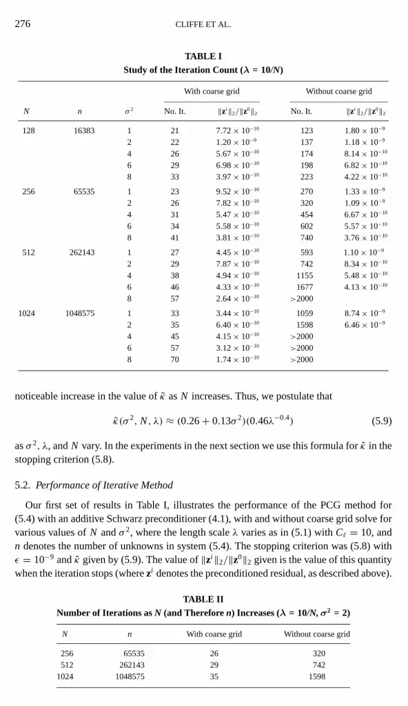
Our first set of results in Table I, illustrates the performance of the PCG method for(5.4) with an additive Schwarz preconditioner (4.1), with and without coarse grid solve forvarious values ofN andσ 2, where the length scaleλ varies as in (5.1) withC` = 10, andn denotes the number of unknowns in system (5.4). The stopping criterion was (5.8) withε = 10−9 andκ given by (5.9). The value of‖zi ‖2/‖z0‖2 given is the value of this quantitywhen the iteration stops (wherezi denotes the preconditioned residual, as described above).
TABLE II
Number of Iterations asN (and Thereforen) Increases (λ = 10/N,σ2 = 2)
N n With coarse grid Without coarse grid
256 65535 26 320512 262143 29 742
1024 1048575 35 1598
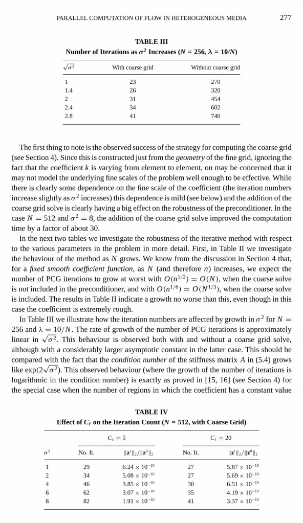
PARALLEL COMPUTATION OF FLOW IN HETEROGENEOUS MEDIA 277
TABLE III
Number of Iterations asσ2 Increases (N = 256,λ = 10/N)√σ 2 With coarse grid Without coarse grid
1 23 2701.4 26 3202 31 4542.4 34 6022.8 41 740
The first thing to note is the observed success of the strategy for computing the coarse grid(see Section 4). Since this is constructed just from thegeometryof the fine grid, ignoring thefact that the coefficientk is varying from element to element, on may be concerned that itmay not model the underlying fine scales of the problem well enough to be effective. Whilethere is clearly some dependence on the fine scale of the coefficient (the iteration numbersincrease slightly asσ 2 increases) this dependence is mild (see below) and the addition of thecoarse grid solve is clearly having a big effect on the robustness of the preconditioner. In thecaseN = 512 andσ 2 = 8, the addition of the coarse grid solve improved the computationtime by a factor of about 30.
In the next two tables we investigate the robustness of the iterative method with respectto the various parameters in the problem in more detail. First, in Table II we investigatethe behaviour of the method asN grows. We know from the discussion in Section 4 that,for a fixed smooth coefficient function, as N (and thereforen) increases, we expect thenumber of PCG iterations to grow at worst withO(n1/2) = O(N), when the coarse solveis not included in the preconditioner, and withO(n1/6) = O(N1/3), when the coarse solveis included. The results in Table II indicate a growth no worse than this, even though in thiscase the coefficient is extremely rough.
In Table III we illustrate how the iteration numbers are affected by growth inσ 2 for N =256 andλ = 10/N. The rate of growth of the number of PCG iterations is approximatelylinear in
√σ 2. This behaviour is observed both with and without a coarse grid solve,
although with a considerably larger asymptotic constant in the latter case. This should becompared with the fact that thecondition numberof the stiffness matrixA in (5.4) growslike exp(2
√σ 2). This observed behaviour (where the growth of the number of iterations is
logarithmic in the condition number) is exactly as proved in [15, 16] (see Section 4) forthe special case when the number of regions in which the coefficient has a constant value
TABLE IV
Effect of C` on the Iteration Count (N = 512, with Coarse Grid)
C` = 5 C` = 20
σ 2 No. It. ‖zi ‖2/‖z0‖2 No. It. ‖zi ‖2/‖z0‖2
1 29 6.24× 10⁻¹⁰ 27 5.87× 10⁻¹⁰
2 34 5.08× 10⁻¹⁰ 27 5.69× 10⁻¹⁰
4 46 3.85× 10⁻¹⁰ 30 6.51× 10⁻¹⁰
6 62 3.07× 10⁻¹⁰ 35 4.19× 10⁻¹⁰
8 82 1.91× 10⁻¹⁰ 41 3.37× 10⁻¹⁰
278 CLIFFE ET AL.
TABLE V
Effect of Aspect RatioL on Iteration Count
(with Coarse Grid)
L No. It. ‖zi ‖2/‖z0‖2
1 31 5.47× 10⁻¹⁰
4 42 6.01× 10⁻¹⁰
16 50 5.13× 10⁻¹⁰
64 65 7.56× 10⁻¹⁰
is small compared to the number of elements on the fine mesh. Here we have computedthe harder problem where the coefficient has a different value on each element but we stillobserve the same good behaviour. It remains an open question to prove this.
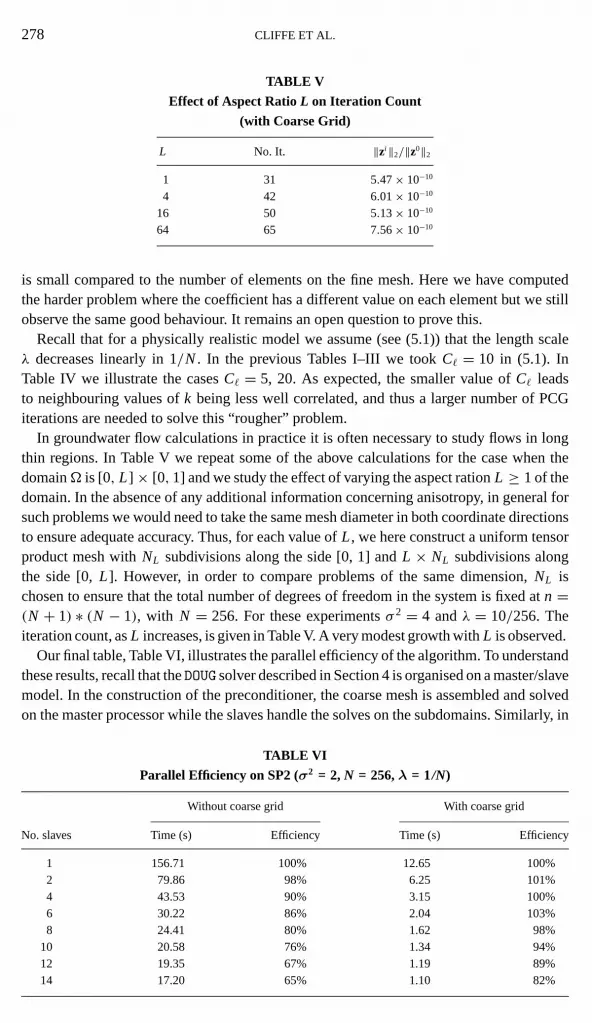
Recall that for a physically realistic model we assume (see (5.1)) that the length scaleλ decreases linearly in 1/N. In the previous Tables I–III we tookC` = 10 in (5.1). InTable IV we illustrate the casesC` = 5, 20. As expected, the smaller value ofC` leadsto neighbouring values ofk being less well correlated, and thus a larger number of PCGiterations are needed to solve this “rougher” problem.
In groundwater flow calculations in practice it is often necessary to study flows in longthin regions. In Table V we repeat some of the above calculations for the case when thedomainÄ is [0, L] × [0, 1] and we study the effect of varying the aspect rationL ≥ 1 of thedomain. In the absence of any additional information concerning anisotropy, in general forsuch problems we would need to take the same mesh diameter in both coordinate directionsto ensure adequate accuracy. Thus, for each value ofL, we here construct a uniform tensorproduct mesh withNL subdivisions along the side [0, 1] andL × NL subdivisions alongthe side [0,L]. However, in order to compare problems of the same dimension,NL ischosen to ensure that the total number of degrees of freedom in the system is fixed atn =(N + 1) ∗ (N − 1), with N = 256. For these experimentsσ 2 = 4 andλ = 10/256. Theiteration count, asL increases, is given in Table V. A very modest growth withL is observed.
Our final table, Table VI, illustrates the parallel efficiency of the algorithm. To understandthese results, recall that theDOUG solver described in Section 4 is organised on a master/slavemodel. In the construction of the preconditioner, the coarse mesh is assembled and solvedon the master processor while the slaves handle the solves on the subdomains. Similarly, in
TABLE VI
Parallel Efficiency on SP2 (σ2 = 2, N = 256,λ = 1/N)
Without coarse grid With coarse grid
No. slaves Time (s) Efficiency Time (s) Efficiency
1 156.71 100% 12.65 100%2 79.86 98% 6.25 101%4 43.53 90% 3.15 100%6 30.22 86% 2.04 103%8 24.41 80% 1.62 98%
10 20.58 76% 1.34 94%12 19.35 67% 1.19 89%14 17.20 65% 1.10 82%

FIG. 4. Vector plot of the velocity forσ 2 = 1, 4, and 8 (N = 256, λ = 10/N).
279
280 CLIFFE ET AL.
the execution of dot and matrix–vector products, the slaves do the local calculations whilethe master is responsible for collating global information (see also [19]). In Table VI wegive the parallel efficiency results as a function of the number of slave processors. Thetimes recorded are those obtained on the 16 node IBM SP2 at the Daresbury Laboratory,United Kingdom (Peak performance: 20 GFlops/sec per processor). The efficiency columnis computed in each case ast (1)/(st(s)), wheret (s) is the time required by the solver whens slaves are used. Because of the master-slave set up, it may be argued that to achieve thetiming t (s) we actually uses+ 1 processors. While this is strictly true, it is easily seen thatif we recomputed the efficiencies using the formula 2t (1)/((s+ 1)t (s)), then efficienciesof well over 100% will result. These figures indicate that there is no bottleneck present incommunication between master and slave. In effect, the bulk of the computation is doneon the slaves and so the figures in Table VI give an accurate impression of the parallelefficiency of the algorithm.
In Table VI, note especially the improved parallel efficiency of the method with thecoarse grid compared to that without. This indicates the success of the the parallelizationstrategy implemented inDOUG: the coarse solve is not only necessary to obtain good theo-retical results, it also gives much improved timings and efficiency even though in principlemuch more communication is needed. The key is the overlapping of communication withcomputation implemented inDOUG [19, 20].
Efficiencies of greater than 100% for small numbers of processors are not unusual, dueto cache effects as well as small differences in the actual quality of the solution producedat the end of the PCG iteration (see also [19]).
Finally, in Fig. 4 we plot the velocity fields corresponding to the problem (1.1) and(1.2) with boundary conditions (5.2) in the caseN = 256,λ = 10/N, andσ 2 = 1, 4, 8respectively. Note the increased dispersion in the flow paths asσ 2 increases.
ACKNOWLEDGMENTS
We thank Professor Thomas Russell for kindly sending us a copy of Hecht’s unpublished manuscript [22]. Wealso thank Dr. Andy Wood for useful discussions.
Note added in proof.After this work was completed, the paper “Mixed Finite Element Methods and Tree–Cotree Implicit Condensation,” by P. Alotto and I. Perugia [Calcolo36, 233 (1999)], came to our attention. Thispaper uses related algebraic techniques to speed up the iterative solution of saddle-point problems. However, thereduced systems which result there are of Schur-complement type and therefore entirely different from ours.
REFERENCES
1. R. J. Adler,The Geometry of Random Fields(Wiley, Chichester, 1980).
2. S. F. Ashby, R. D. Falgout, S. G. Smith, and T. W. Fogwell, Multigrid preconditioned conjugate gradientsfor the numerical solution of groundwater flow on the Cray T3D, inProc. ANS Confer. on Mathematics andComputations, Reactor Physics, and Environmental Analysis(Portland, OR, 1995), Vol. 1, p. 405.
3. F. Brezzi and M. Fortin,Mixed and Hybrid Finite Element Methods(Springer-Verlag, New York, 1991).
4. Z. Cai, R. R. Parashkevov, T. F. Russell, and X. Ye, Domain decomposition for a mixed finite element methodin three dimensions,SIAM J. Numer. Anal.(1998), to appear.
5. T. F. Chan and T. Mathew, Domain decomposition methods, inActa Numerica 1994(Cambridge Univ. Press,Cambridge, UK, 1994).
6. T. F. Chan, B. F. Smith, and J. Zou, Overlapping Schwarz methods on unstructured meshes using non-matchingcourse grids,Numer. Math.73, 149 (1996).

PARALLEL COMPUTATION OF FLOW IN HETEROGENEOUS MEDIA 281
7. G. Chavent, G. Cohen, J. Jaffre, M. Dupuy, and I. Ribera, Simulation of two-dimensional water flooding byusing mixed finite elements,Soc. Pet. Eng. J.24, 382 (1984).
8. P. G. Ciarlet,The Finite Element Method for Elliptic Problems(North–Holland, Amsterdam, 1978).
9. K. A. Cliffe, I. G. Graham, R. Scheichl, and L. Stals, Parallel Computation of Flow in Heterogeneous MediaUsing Mixed Finite Elements, Bath Mathematics Preprint 99/16 (University of Bath, 1999).
10. N. A. C. Cressie,Statistics for Spatial Data(Wiley, London, 1993).
11. G. Dagan,Flow and Transport in Porous Formations(Springer-Verlag, New York, 1989).
12. C. R. Dietrich and G. N. Newsam, A fast and exact method for multidimensional Gaussian stochastic simu-lations.Water Resour. Res.29(8), 2861 (1993).
13. R. E. Ewing and J. Wang, Analysis of the Schwarz algorithm for mixed finite element methods,RAIRO Model.Math. Anal. Num.26(6), 739 (1992).
14. L. W. Gelhar, A stochastic conceptual analysis of one-dimensional groundwater flow in nonuiform homoge-neous media,Water Resour. Res.11, 725 (1975).
15. I. G. Graham and M. J. Hagger, Unstructured additive Schwarz–CG method for elliptic problems with highlydiscontinuous coefficients,SIAM J. Sci. Comput.20, 2041 (1999).
16. I. G. Graham and M. J. Hagger, Additive Schwarz, CG and discontinuous coefficients, inDomain Decompo-sition Methods in Science and Engineering, edited by P. E. Bjørstad, M. S. Espedal, and D. E. Keyes (DomainDecomposition Press, Bergen, 1998).
17. D. F. Griffiths, The construction of approximately divergence-free finite elements, inThe Mathematics ofFinite Elements and Applications(Academic Press, New York, 1979), Vol. 3.
18. A. L. Gutjahr, D. McKay, and J. L. Wilson, Fast Fourier transform methods for random field generation,EosTrans. AGU68(44), 1265 (1987).
19. M. J. Hagger, Automatic domain decomposition on unstructured grids (DOUG), Adv. Comput. Math.9, 281(1998).
20. M. J. Hagger and L. Stals,DOUG User Guide, Version 1.98, Technical Report, University of Bath (1998),available athttp://www.maths.bath.ac.uk/∼parsoft.
21. F. Hecht, Construction d’une base de fonctions P1 non-conformes `a divergence nulle dansR3, RAIRO Model.Math. Anal. Num.15, 119 (1981).
22. F. Hecht, Construction d’une base pour des ´elements finis mixtes `a divergence faiblement nulle, unpublishedreport (1988).
23. R. Hiptmair, T. Schiekofer, and B. Wohlmuth, Multilevel preconditioned augmented Lagrangian techniquesfor 2nd order mixed problems,Computing57, 25 (1996).
24. R. J. Hoeksema and P. K. Kitanidis, Analysis of the spatial structure of properties of selected aquifers,WaterResour. Res.21, 825 (1985).
25. G. Karypis and V. Kumar, A fast and high quality multilevel scheme for partitioning irregular graphs,SIAMJ. Sci. Comput.20, 359 (1999).
26. E. F. Kaasschieter, A practical termination criterion for the conjugate gradient method,BIT 28, 308 (1988).
27. C. E. Kolterman and S. M. Gorelick, Heterogeneity in sedimentary deposits: A review of structure-imitating,process-imitating and descriptive approaches,Water Resour. Res.32(9), 2617 (1996).
28. A. Mantoglou, Digital simulation of multivariate two- and three-dimensional stochastic processes with aspectral Turning Bands method,Math. Geol.19(2), 129 (1987).
29. T. P. Mathew, Schwarz alternating and iterative refinement methods for mixed formulations of elliptic prob-lems. 1. Algorithms and numerical results,Numer. Math.65, 445 (1993).
30. J. C. Nedelec,Elements finis mixtes incompressibles pour l’´equation de Stokes dansR3, Numer. Math.39,97 (1982).
31. C. C. Paige and M. A. Saunders, Solution of sparse indefinite systems of linear equations,SIAM J. Num. Anal.12(4), 617 (1975).
32. P. A. Raviart and J. M. Thomas, A mixed finite element method for 2-nd order elliptic problems, inMath-ematical Aspects of the Finite Element Method, edited by I. Galligani and E. Magenes, Lecture Notes inMathematics (Springer-Verlag, New York, 1977), Vol. 606, p. 292.

282 CLIFFE ET AL.
33. M. L. Robin, A. L. Gutjahr, E. A. Sudicky, and J. L. Wilson, Cross-correlated random field generation withthe direct Fourier transform method,Water Resour. Res.29, 2395 (1993).
34. R. Scheichl, A decoupled iterative method for mixed problems using divergence-free finite elements, BathMathematics Preprint 00/11 (University of Bath, 2000).
35. R. Scheichl,Iterative Solution of Saddle-Point Problems Using Divergence-Free Finite Elements with Appli-cations to Groundwater Flow, Ph.D. thesis, in preparation (University of Bath, 2000).
36. F. Thomasset,Implementation of Finite Element Methods for Navier–Stokes Euations(Springer-Verlag, NewYork, 1981).
37. A. F. B. Tompson, R. Ababou, and L. W. Gelhar, Implementation of the three-dimensional Turning Bandsrandom field generator,Water Resour. Res.25(10), 2227 (1989).
38. C. Wagner, W. Kinzelbach, and G. Wittum, Schur-complement multigrid, a robust method for groundwaterflow and transport problems,Numer. Math.75, 523 (1997).


