OR\G\NAL HUD-OOOl+04<::l•

•

•

•

•

•

•

•

• THE URBAN INSTITUTE

2100 M Street, NW, Washington, D,C. 20037

•

•

Project Report

I

•i

U.1. 113165

• ECONOMIC ANALYSIS OF EFFECTS

BUSINESS CYCLES ON THE ECONOMY OF OF CITIES

• INFLATION, THE BUSINESS CYCLE

• . AND STATE AND LOCAL GOVERNMENT FINANCES

Roy Bahl and Larry DeBoer~~tropolitan Studies Program

The Maxwell School of Citizenship andPublic Affairs

• Cooperative Agreement Number HA-5455

Cooperative Agreement Amount $134,976• Submitted To:

u.S. DEPARTMENT OF HOUSING AND URBAN DEVELOPMENT

• Henry ColemanEconomist

Economic Development and Public FinanceRoom 8218

451 Seventh Street, S.W. Washington, D.C.

• Original Submission: August 1982

Revised: February 1983

Submitted By:• THE URBAN INSTITUTE 2100 M Street, N.W.

Washington, D.C. 20037 (202) 833-7200

• George E. Peterson, Principal Investigator

•

•

•

•

•

•

•

•

•

•

•

•

ii

TABLE OF CONTENTS

InflationInflationary Impacts on Public Expenditures and

Tax Rates: TheoryM~asuring Expenditure and Revenue ImpactsExpenditure - Inflation ImpactsEstimates of the Expenditure Impact of InflationExpected Revenue ImpactsApproaches to Estimating Inflation Impacts on RevenuesEstimated Revenue ImpactsThe Budgetary Effects of InflationLabor Cost~

Non-Labor CostCapital CostsTran5f~r Payment~

RecessionThe Expected Impacts of RecessionStudies of th~ Fiscal Impact of RecessionThe Perversity HypothesisFiscal Performance During Recessions: The LiteratureFiscal Performanc~ During Recessions: Empirical EvidenceThe Fiscal Eftect~ of Recession

Rt'venuesExpc:ndituresBorrowing and Spending

Conclusions

Footnotes

Page No.

2

51819232628313237454748

50515353566266666869

76

80

iii

LIST OF TABLES AND FIGURES

•

•

4 INDEXES OF PURCHASING POWER OF 1972 REVENUE BASE

2 THE COMPOSITION OF STATE AND LOCAL GOVERNMENTEXPENDITURES: 1965-1980

5 AVERAGE ANNUAL WAGES AND SALARIES PER FULL TIMEEQUIVALENT EMPLOYEE BY INDUSTRY t 1962-1979

No.

1

3

6

7

Figures

1

2

3

4

5

Title

ALTERNATIVE MEASURES OF PRICE LEVEL INCREASE

EXPENDITURE AND REVENUE INFLATION INDEXES FORSTATE AND LOCAL GOVERNMENTS: 1972-76

AVERAGE ANNUAL SUPPLEMENTS TO WAGES AND SALARIESPER FULL TINE EQUIVALENT EMPLOYEE BY INDUSTRY,1962-1976

STATE AND LOCAL GOVERNMENT INDICATORS IN RECESSIONAND EXPAND ION

LOCAL GOVERNMENT RESPONSE TO PURE INFLATION

COMMUNITY RESPONSE TO PURE INFLATION

COMMUNlTY RESPONSE TO DIFFERENTIAL INFLATION RATES

YIELDS OF U.S. TREASURY AND MUNICIPAL BONDS

VALUE OF SLG LONG AND SHORT-TERM HUNICIPAL ISSUESAND SLG GROSS FIXED CAPITAL FORMATION

Page No.

4

20

25

35

40

41

60

6

11

15

71

72

•

•

•

•

•

•

•

•

•

•I

• H1FLATION, THE RUSINESS CYCLE AND*STATE AND

LOCAL GOVERNMENT FINANCES

Roy Bahl ** and Larry DeBoer***

• More than any other single factor, the performance of the national

economy shapes the financiaJ health of state and local governments.

• Slower economic ~rowth, a higher rate of inflation, and recessions or

the expectation of recessions all affect the structure and growth of

state and local government bud~ets. Tn some cases, iFflation and

• cyclical fluctuations increase bud~et deficits and push governments a

step closer to insolvency, in others the unfavorable budgetary effects

art: cu~hioned by revenue systems which are bouyant with respect to

• rising prices, and in still others the revenue-dampening effects of slow

national ~rowth an~ recessi.on are more than offset by the gains from

inflation and from regional shifts in economic activity. The nature of

• these effects, their measurement, and how they differ across state and

local governments are important national policy concerns.

In this paper, we try to explain how inflation and business cycles

• at feet state and local government budgets. As is the case with most

applications 0 f economic theory, we are left with the unsatisfying

answer that "it depends," .•. on various price and income elasticities,

• on the kinds of discretionary responses which governments take, on the

kind of recession and inflation being faced, on the type of government

being discussed, etc. The few earlier studies which have attempted to

• estimate inflation and recession impacts are reviewed here to search for

some consensus about what have been the actual effects. While the

answers one gets from such a review are tentative and qualified, the

•

•2

•overall picture that emerges gives some evidence about how inflation and

recession compromise or enhance the fiscal health of state and local

~overnments. •

Inflation

After a re]atively long period of price stability, consumer prices

began to rise sharply in 1973, increased by 11 percent in 1974 and 9.2

percent in 1975. After falling off to about 6 percent for two years.

pricto's again increased at double-digit rates for three years before

•

•softening during the 1981-83 recession. The question at hand is how

thi!': inflation pattern haE affected state and local government budgetary

position. !-1icroecooo(lJic theory suggests what we might expect in such a •case. I f the i ocrease in prices of all goods is uniform, L e., there

is no change in relative prices. and if the state and local government

tax system is fuJ]y responsive to inflation, there will be no real •effects on lludgets and no induced fiscal responses. Tax collections

1will be higner, but tux burdens will not, public employees will earn

more but not: reliltive to the private sector. etc. The relative position

of the state aod local ~overnment sector would not have changed.

In reali tv, price increases have not been uniform and state and

•

local government revenue systems have varied widely in their response to

inflation. Does this mean that inflation has caused state and local •government expenditures to grow at a rate above or below expenditures in

all other sectors of the economy? If so. with what consequences for

government budgets? •

•

•3

• The price indexes shown in Ta.ble 1 may help answer une part of this

que:,t ion. Price increClses have not been uniform, indeed, changes in the

• relative prices of energy and food were at the heart of the high

inflat ion r<1.te~ of the mid-1970s and the softening of prices in the

early 19805. As for measuring the increase in prices faced by state and

• local governments. one has to rely on the implicit deflator for state

and local government purchases as reported in the National Income

Accounts. As may be seen in Table 1, this index increased faster than

the implicit price deflator for GNP, a comparable measure of the overall• inflat inn rate in the economy. On first blush it would appear that

inflation has driven up the relative price of state and local government

purchases and in ~o doing h8S stimulatd expenditures.• Even i.f tlte relative price of purchases by state and local

governments does not increase. inflation can affect budgets if tax

systems do not fully capture inflation-induced increases in income. • consumption. and property values. So while it is intuitively obvious

that inflated prices raise the cost of providing government services and

stimulate tax bases, it is less obvious whether the revenue or the

• expenditure ef fects clominate. A further complication is the need to

consider the adjustments caused by inflation, i.e .• the public

employment reductions brought on by increased wage rates, the capital

•

•

project postponements caused by higher interest rates, or the tax rate

adjustments brought on by revenue shortfalls.

We be~fn this inquiry about these very complicated fiscal impacts

of inflation by tracing out a set of a priori expectations. and then

looking for confirmation in the empirical work on the subject.

•

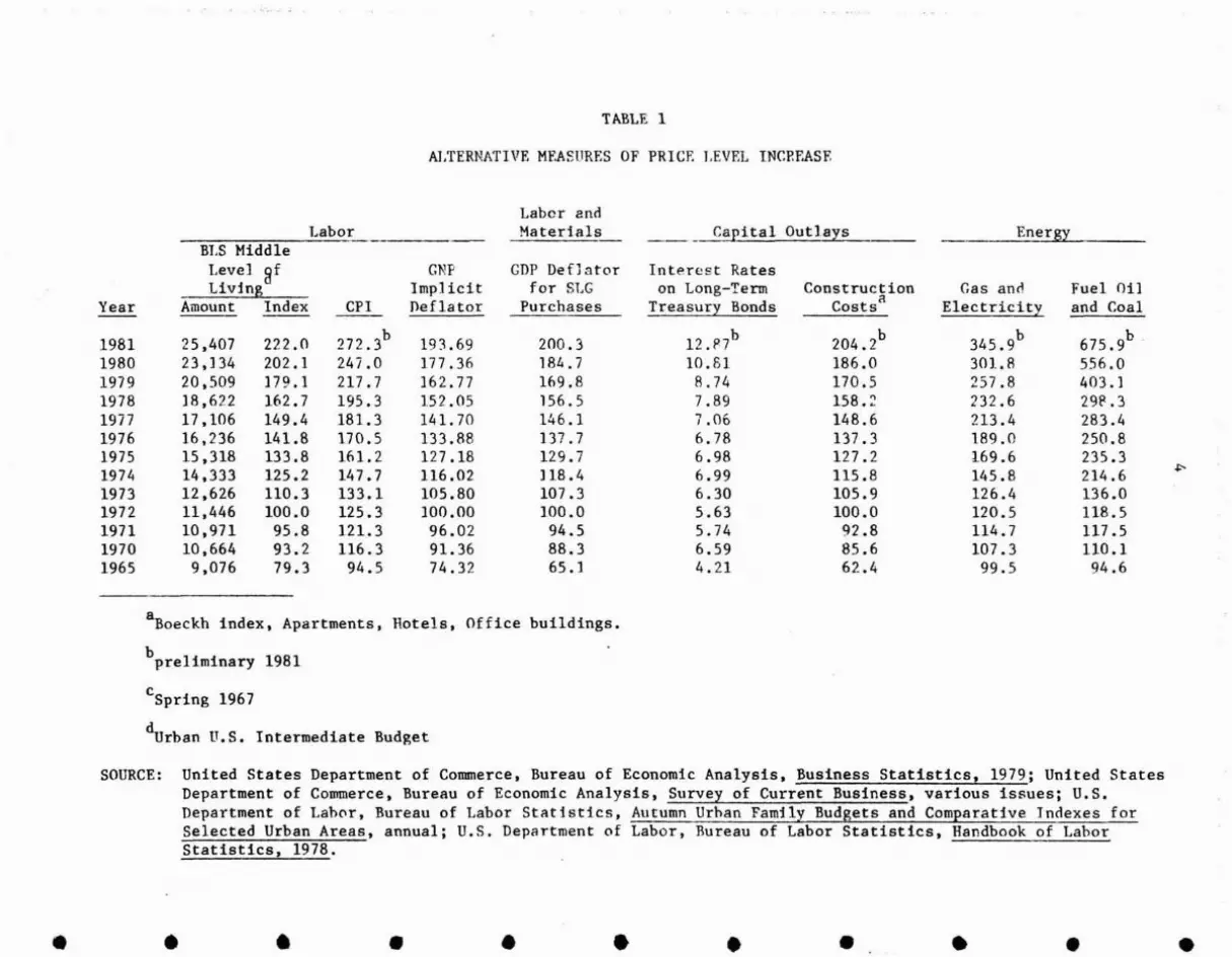
TABLE 1

ALTERNATIVE MEASURES OF PRICE LEVEL INCP.F.ASF.

Laber andLabor Materials __~ita1 Outlays Energy

BLS MiddleLevel ~f GNP GDP DefJ ator Interest RatesLiving Implicit for SLG on Long-Term Construction Gas ancl Fuel Oil

Year Amount Index CPI Deflator Purchases Treasury Bonds CostsR Electricity and Coal

1981 25.407 222.0 272.3b 193.69 200.3 12.nb 204.2b345.9

b 675.9b .1980 23.134 202.1 247.0 177 .36 184.7 10.81 186.0 301.8 556.01979 20.509 179.1 217.7 162.77 169.8 8.74 170.5 257.8 403.11978 18.622 162.7 195.3 152.05 156.5 7.89 158.~ 232.6 29P.31977 17 .106 149.4 181.3 141. 70 146.1 7.06 148.6 213.4 283.41976 16,236 141.8 170.5 133.88 137.7 6.78 137.3 189.0 250.81975 15,318 133.8 161.2 127.18 129.7 6.98 127 .2 169.6 235.31974 14.333 125.2 147.7 116.02 ] 18.4 6.99 115.8 145.8 214.6 ~

1973 12 .626 110.3 133.1 105.80 107.3 6.30 105.9 126.4 136.01972 11.446 100.0 125.3 100.00 100.0 5.63 100.0 120.5 118.51971 10,971 95.8 121.3 96.02 94.5 5.74 92.8 114.7 117.51970 10.664 93.2 116.3 91.36 88.3 6.59 85.6 107.3 110.11965 9,076 79.3 94.5 74.32 65. ] 4.21 62.4 99.5 94.6

a Hotels. Office buildings.Boeckh index, Apartments,

bpreliminary 1981

cSpring 1967

d BudgetUrban U.S. Intermediate

SOURCE: United States Department of Commerce. Bureau of Economic Analysis. Business Statistics, 1979; United StatesDepartment of Commerce. Bureau of Economic Analysis, Survey of Current Business, various issues; U.S.Department of Labor, Bureau of Labor Statistics. Autumn Urhan Family Budgets and Comparative Indexes forSelected Urban Areas, annual; U.S. Department of Labor. Bureau of Labor Statistics, Handbook of LahorStatistics. 1978 .

• • • • • • • • • • •

•5

• laTnflationarv ~mpacts on Public Expenditures and Tax Rates: Theory

lnf lat ion exerts an absolute price effect, a real income effect,

and a relative price effect on government expenditures. The absolute • price effect is the one most often discussed. As the general price

level in the economy rises, the price that state and local governments

pay for their policemen, firemen, utilities, typewriters, etc •• also • rises. If revenues and expenditures both rise by the general inflation

rate, cet. par., then budgets will increase in proportion to the

increase in prices and there will be no change in the quantity of inputs• employed, nominal tax rates or effective tax rates.

This case is shown in Figure 1. Assume an indifference curve (11)

• which describes state ~nd local government preferences for a public good

(G), and the proportion nf the tax base which remains untaxed (R). 2

These preferences reEl ect g:overnment of ficials' judgements about their

• re-election chance5, given each tax level/public goods pair.

Preferences also depend on the~;e officials' sense of community needs, ,on

the desire of hureaucrats tc enlarge their departments, and so on.

• Utility increases. eeL par. with an increase in public goods prOVided

and with an increase in the untaxed port jon of the taxable base (8

decrease in the nominal tax r~·?). The convex shape of the indifference

curve implies declining margin<-!l utility of public goods supplied and of

the untaxed portion of the b~~e (increasing marginal disutility of the

nominal tax rate).

• The concern of the governn'ental decisionmaker in this model is how

hi.s reading of constituent prf:ferences, and his available resources, can

~

R(=l)

Percent ofBase Untaxed(Tax Ratel-R)

6

FIGURE 1

LOCAL GOVERNMENT RESPONSE TO PURE INFLATION

Pub lie Goods

•

•

•

•

•

•

•

•

•

•

•

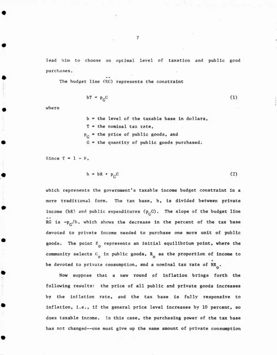
•7

• lead him to choose nn optimal level of taxation and public good

purchases.

• The hudget line (RG) represents the constraint

bT PGC (1)

• where

b = the level of the taxable base in dollars,

T the nominal tax rate,

PG the price of public ~oods, and

• G = the quantity of public goods purchased~

Since T 1 - ~,

• (2)

which . represents the government's taxable income budget constraint in a

more tradi tional form. The tax base, b, is divided between private

• income (bR) and public expenditures (PeG). The slope of the budget line

RG is -PG/b, which shO\JS the decrease in the percent of the tax base

devoted to private income needed to purchase one more unit of public

• goods. The point F. represents an initial equilibrium point, where the a

community selects (; in public goods, R as the proportion of income to o 0

be devoted to private consumption, and a nominal tax rate of RR • o

Now suppose that a new round of inflation brings forth the • following results: the price of all public and private goods increases

by the inflation rate, and the tax base is fully responsive to

inflation, i.e., if the general price level increases by 10 percent, so • does taxable income. In this case, the purchasing power of the tax base

has not changed--one must give up the same amount of private consumption

•

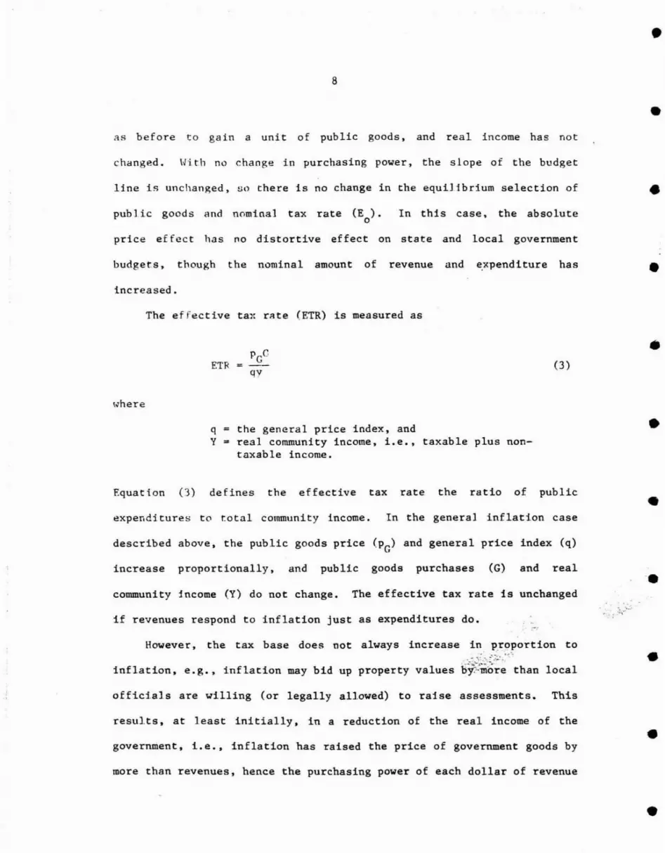
8

•

•as before to gain a unit of public goods, and real income has not

changed. With no change in purchasing power, the slope of the budget

line is unchanged, 90 there is no change in the equilibrium selection of

pub lie goods and nominal tax rate (E). In this case, the absolute o

price ef feet has no distortive effect on state and local government

budgets, though the nominal amount of revenue and ~xpenditure has

increased.

The effective tax rate (ETR) is measured as

ETR (3)

\.;rhere

q the general price index, and Y = real community income, i.e., taxable plus non­

taxable income.

Equation (3) defines the effective tax rate the ratio of public

expenditures to total community income. In the general inflation case

described above, the public goods price (PC) and general price index (q)

increase proportionally, and public goods purchases (G) and real

community income (Y) do not change. The effective tax rate is unchanged

if revenues respond to inflation just as expenditures do.

However, the tax base does not always increase in p.r9Portion to

inflation, e. g., inflation may bid up property values bij~~:~~<'than local

officials are willing (or legally allowed) to raise assessments. This

results, at least initially, in a reduction of the real income of the

•

•

•

•

•

-. :" ; :z,.:-"~'..

•

• government, i.e., inflation has raised the price of government goods by

more than revenues, hence the purchasing power of each dollar of revenue

•

•

•

•

•

•

•

•

•

•

•

•

9

has o..:clined. Tn such a case, the government may react hy reducing the

quantity of inputs and (short of increased grants, borrowing or drawing

on fund balances) total exp~nditures will not increase hy the full rate

of inflation. Call this the 'real income effect and note that its

potential dampening effect on state and local government expenditures

varies dir~ctly with the income elasticity of demand of state and local

governments for public goods. In the extreme case where the

government's demand for public goods is perfectly income inelastic,

nominal tax rates will be increased to fully compensate for the loss in

purchasing ?ower.

These points can also be demonstrated with Figure 1. Assume that

the tax base does not rise proportionally wi th the price of public

goods, i.e., the purchasing power of the tax base declines. The slope

of the bud~~t line, -PG/b, becomes steeper and shifts to RG*. If the

new equilibrium point were at El

, the community will choose to purchase

fewer public goods and levy a higher nominal tax rate (RRl

) than before.

The effective tax rate. on the other hand, will decline. In equation

(3), note that the public goods price (PG) increases proportionally with

the general price index (q), while purchases of public goods (G)

decline. On the ('ther hand, an equilibrium at EZ

would indicate how

much the nominal tax rate would have to increase to offset the reduced

purchasing power of the tax base. At point E2

, public goods purchased

remain constant and so does the effective tax rate. This is the case

where the government's income elasticity of demand for public goods is

zero: real government resourc~s decline, but no change in public goods

purchased occurs.

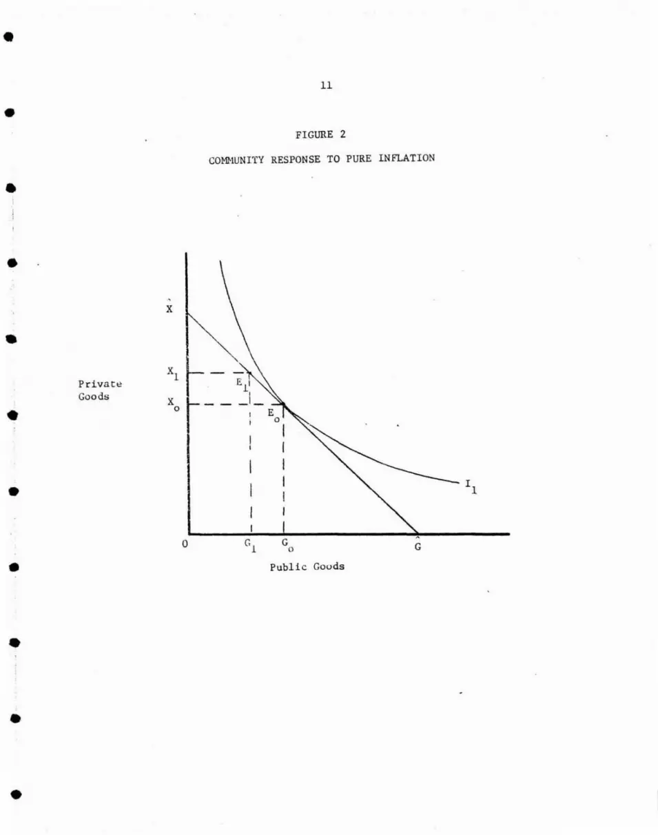
•10

• If the tax base does not increase with the general rate of

inflation, an interesting difference emerges between the expected

reaction of tht: 'community' and government decisfonmakers. This can be

demonstrated through i1 eomparison of Fi~ures 1 and 2. Figure 2 shows a •

community indifference curve, II' mapping voter-consumer preferences

between

is

public goods (C) and private goods (X). The budget constraint • qY (4)

where • q the genera] price index,

Y = real community income,

the price of private goods,

private goods purchased,

Pc the price of public goods,

C public goods purchased.

•

The slope of the budget line in Figure 2 is -PC/px' the negative of the • price ratie.

the

Assume that the

same allocation

equilibrium points E in Figures 1 and o

of community resources between public

2 represent

and private • goods. In each Figure, C public goods are provided. The tax base, b

o

(some fraction of total community income) must be taxed at rate RR to o

provide this leveJ of public goods at price PGo. The untaxed portion of • the tax base (R b) plus that fraction of community income not included

o

in the tax base go to purchase X private goods at price p • o xo

In a pure inflationary environment, all prices and nominal

community income increase by the same proportion. In budget constraint •

•

•

•

•

11

FIGURE 2

COMHUNITY RESPONSE TO PURE INFLATION

•x

•Private

XlEll

GoodsX _I-

• 0 E0

III

• I 11I

II

0 Gl

G G0

• Public Gouds

•

•

•

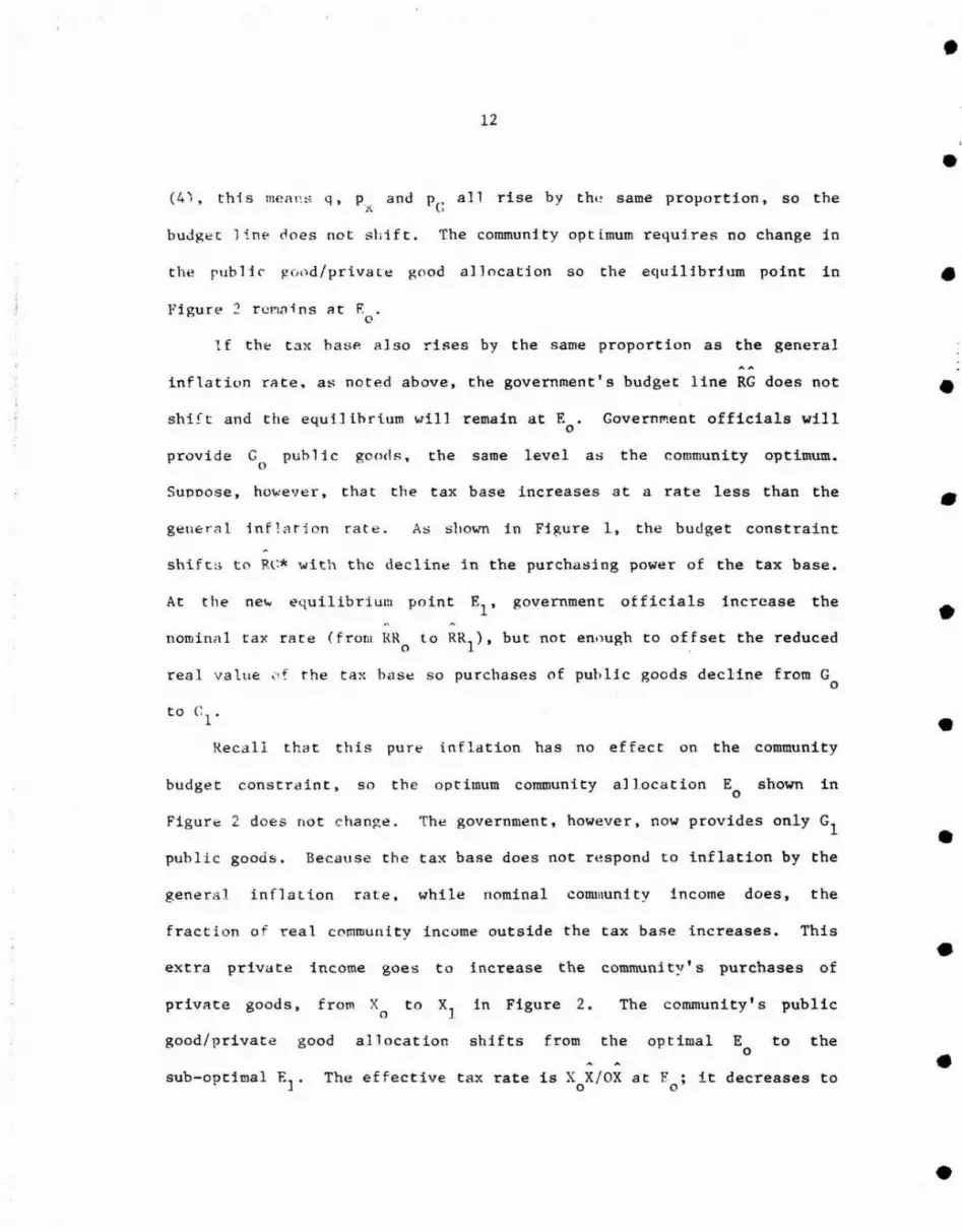
•12

• (4~. this meaf'.:'; q. Px and Pc: all rise by thl! same proportion. so the

budget 1 'ine <loes not sLift. The community opt imum requires no change in

the public l!(i()d/prival~ good a] location so the equilibrium point in • Figure ~ ren<lins at E .

()

t f the tax hase a1 so rises by the same proportion as the general

inflation rate, a~ noted above. the government's budget line RG does not • shift and the equil ihrillm will remain at E.

o Government officials will

provide G o

public goods, the same level as the community optimum.

Supoose. however. that the tax base increases at a rate less than the • gener-ell inf~arion rate. As shown in Figure l. the budget constraint

shifts to RC* with the decline in the purchasing power of the tax base.

At the new equilibrium point El

• government officials increase the • nominal tax rate (frOTH l{R

o to RR

l ). but not en()U~h to offset the reduced

real value 0f the tax base so purchases of pull lie goods decline from G o

• Recall that this pure inflation has no effect on the community

budget constraint. so the optimum community a] location E o

shown in

Figure 2 does not change. The government. however. now provides only Gl • public goods. Because the tax base does not respond to inflation by the

general inflation rate. while nominal community income does. the

fraction of real community income outside the tax base increases. This

• extra private income goes to increase the community's purchases of

private goods. from X o

to Xl in Figure 2. The community's public

good/private good alJocation shifts from the optimal E to the o

sub-optimal E]. The effective tax rate is X X/OX at F. ; it decreases to • o 0

•

•13

XIX/OX at the sub-optimal allocation El

. The local public sector is too

small.

• The obvious question is, 1f the optimal allocation is at E , and o

the communi.ty is at El

, why does the community not decrease its private

~ood purchases and increase its public good purchases to get back to E ? o

• In Fi~ure I, maintaining the supply of public goods at G with thel

inflationary budget constraint RG* requires the government to select

point E on its hudget line. At E , the nominal tax rate increases to2 2

• (l-R ), completely offsetting the decline in the purchasing power of the2

tax base. As noted ubove, an allocation at point E requires that the2

government's income elasticity of demand for public goods be zero. If

• public goods are normal goods. this elasticity will be positive. The

decline in government income will cause reductions in public goods

purchases.

The answer to the question posed above then, is that the local• government is unab Ie or unwilling to increase the nominal tax rate

enough to offset the real dec] ine in the tax base. This phenomenon

might be labeled "tax rate illusion." There are legal and psycholo~ical• barriers to large tax rate increases. Government officials may face tax

rate ceilings or limits to the amount tax rates may rise in anyone

year. Here the community is effectively signalling its government that• in spite of any fall in the effective tax rate, there should be no large

increases in the nominal rate. In this case the community apparently

'liews a nominal rise in tax rates as a real subtraction from private • income: hence, the term tax rate illusion. Governments which face no

•

•14

• tax rate limitations may themselves "suffer" from tax rate illusion and

be unwilling

increase.

to fully offset their real revenue decline with a tax rate

• ..!

-,i

There is aJso a 'relative price' effect

expenditures. If all prices in the economy increase

in the absenc.e of a real income effect there is no

of inflation on

at the same rate,

inducement to cut • back consumption of anyone good at the expense of another. However, if

the price of some goods increases faster than others, some substitution

takes p1 ace with the degree of substitution depending on the price • elasticiti~s of demdnd for the products. Suppose, that the price of

inputs purchased bv state and local governments increased faster than

the prices of all other goods and services. Holding all else constant. • one would expect rational consumer-voters to respond by choosing a

smaller state and local p,overnment sector. For example, if the price of

school

~.•

teachers in(~reased relative to all else. it is likely that, cet.

fewer teachers would be hired than under a slower rate of •

inflation. However. since the state and local government sector is

thought to have a price inelastic demand.

3relative price effects may not be great.

the retrenchment induced by • In real terms differential rates of inflation between public and

private goods result in a relative price change. In Figure 3, pub lie

goods (G) become more expensive relative to private goods (X). This is •

shown through a shift in the budget line from XG to XG'. Equilibrium

goods.

point El shows a decrease in purchases in both private goods and public

The move from Eo to El

is caused by a substitution effect.

resulting from the relative price change. and an income effect,

•

•

•

•

•

15

FIGURE 3

CO~1UNITY RESPONSE TO DIFFERENTIAL INFLATION RATES

x*•

•

•

•

•

•

•

•

Private Goods

x

X I

Z

o G1G Z Go G'

Public Goods

G* G

16

rest!] t in~ from the <iecrease in purchasing power caused by the price

ris~. If, however, purchasing power does not decline--as it will not if

iflcome increases with the ~el1eral inflation rate--there is no income

effect. 1 n this case the response of the communi ty to the differential

inflation rates is a shift from Eo to E2

; in real terms, to purchase

more private goods and fewer public goods.

Although the govp.rnment in Figure 3 is providing fewer pub] ic

gC'ods, the effective tax rate may rise or fall, depending on the price

elasti.cities of pubHc and private goods. This can be shown with the

f0110wing equations. Th2 equation for the budget lines in Figure 3 is:

•

•

•

•

•

where

qY pX+p.c~x t·

(4)

•qY nC'nti na 1 community income;

Px = the pri ce of private goods;

PC the price of public goods.

The effective tax rate (~TR) is

•

ETRp Cr,

qY(5) •

which can be written as

ETR1

(6) •If a good is price inelastic, expenditures on that good will rise with

increases in price; if a good is price elastic, expenditures on that

good will fall. Thus, if the demand for public goods is price inelastic•

•

•17

• relative to the demand for private goods, expenditures on public goods

(PeG) may increase relative to expenditures on private goods (pxX) and

• the effective tax rate will rise, as shown in equation (6).

Real income and relative price effects can work in the same or in

opposite directions in terms of their aggregate impacts on state and

• local government expenditures, Le., general inflation will increase

state and local governl'1ent expenditures while rising relative prices of

inputs and the declining purchasing power of the tax base will set in

• motion discretionary expenditure cuts that will offset some of this

increase. If relative prices of state and local government inputs fall,

then the upward pressure on expenditures will be reinforced as

• consumer-voters (and

government goods. It

bureaucrats)

is important

demand

to note

more of the now-cheaper

that absolute price effects

are more "automatic" (the city simply pays the higher price of gasoline

• for its police cars), but relative price effects and real income effects

require discretionary actions (the city must take some policy action to

reduce its fleet of cars).

• The relative price effect may

local government services provided,

also change

or even the

the mix

methods

of

of

state and

providing

services. For example. a higher price of garbage collectors can lead to

• fewer collectors

privatization of

and more expensive and efficient

the service. The first option will

equipment, or to

depend on whether

the technology will permit the substitution of capital for labor and the

• second

lower.

on whether the relative price

The answers vary from function

of

to

private provision

function.

is somehow

The dual solutions to the question of the state and local

•

18

•

•government dis(~retionHry response to inflation point out the importance

of the relative resp0n!;e of revenues and expenditures. Only if revenue • and expendi tures gro,," at the general inflation rate will there be not

tax rate il1u5j0n, and no real discretionary response by state and local

governments tt' j nflation. If revenues are stimulated more than

• expenditures, the government realizes an "inflationary dividend" and may

increase rea] expenditures and reduce tax rates. In this case the

effective tax rate would climb with inflation. This argument is often

made for the response of Federal income tax receipts to inflation. If • expenditures are stimulated more than revenues, tax rate illusion

prevents the consumet--voter optimum from being maintained in an

inflationarv environment. The effective tax rate falls .. • The important empirical issue, then, is the relative effect of

inflation on expenditures and revenues. This issue is addressed in the

fo]lowin~ sections. • Heasuring Expenditure and Revenue Impacts

The measurement of the impact of inflation on state and local

government finances in a complex problem. If inflation' 8 impact was • merely an absolute price effect, the problem would be much simplified.

Expenditures and revenues would increase at the general rate of

inflation, with nu induced discretionary effects. It is the real income • and relative price effects that complicate matters, Le., inflation

stimulates revenues and expenditures, which induces discretionary

responses. If expendj tures grow more than revenues, nominal tax rate • increases, real expenditure cuts and effective tax rate declines will

likely resul t. If pub lic goods become relatively more expensive than

•

•19

• private goods, the state and local government will likely cut

expenditures, change the mix of services provided, and either increase

• or decrease the effective tax rate. An aggregation of these "automatic"

or "potential" effects with the discretionary actions they stimulate

utll miss the pure impact of inflation on state and local government

• finances. This is bec.ause the automatic and discretionary effects are

often in opposite directions, for example, the automatic increase in

public goods prices versus the discretionary cuts in programs or

• employment. The separation of these automatic anrl discretionary

•

•

•

•

•

•

tiE E (7)o

20

'fABLE 2

THE COMPOS1T]ON OF STATE AND LOCAL GOVERN!'fENTFXPl<:NDITURF.S: 1965-1980

Percent of Total ExpendituresOh j E:ct 1965 1970 1975 1980

Labor Costs 41.6 42.5 39.7 37.9

Materials, Equipment andS I" a 20.6 23.6 28.4 33.2. upp 1es

Construction 18.9 16.4 13.7 11.9

T.ond and Equipment 5.1 3.6 3.2 2.6

Tnterest 3.4 3.4 3.8 4.1

Transfer Payments 4.7 5.5 4.2 3.5

Inf>urance Benefits andI<.epayments 5.7 4.9 7.0 6.7

aTotal current expenditures minus total wages and salaries.

SOURCE: U.S. Bureau of the Census, Governmental Finances in 1979-80(1974-75, 1969-70, 1964-65), GF80, No.5 (Washington, D.C.:Government Printjng Office, 1981).

•

•

•

•

•

•

•

•

•

•

•

•21

• wherp-

E expenditures in year t t

• E expenditures in some base yearo

and the change in expenditures due to inflation (E) is

toE PE0 (8)

• where

p = some percent increase in an appropriate price index.

Hence, the share of eypenditure increase due to inflation is

• pF.o-_._-- (9)E -F

t 0

As noted above, this result gi.ves an estimate of the direct. probably• maximum, impact of inflation. It assumes no discretionary quantity

adjustments.

The estimation tJ.E/I\f. is a simple exercise if only an appropriate• price index is available. Unfortunately. the choice and the measurement

of such an index is anything but simple. The problem is that an

aggregate price index for state and local government expenditures would • have to take into aCC0unt the differential growth in prices for each

component of the state and local government budget. L e., a· kind of

market basket survey of state and local government purchases is • necessary. The Implicit Price Deflator for state and local government

purchases (see Table 2) provides such an estimate, but is flawed for the

purposes at hand in that it cannot reflect the wide variation in the

• package of services purchased by different state and local governments.

•

•22

• Tt is not avail abi e on a regional basis. The only way around this

problem woulJ seem to be construction of a price index for each

government, weighted to reflect the composition of purchases by that

4 • government.

Tf labor costs are assumed to respond fully to the rate of

inflation, the proper index would be a cost-of-living measure. This • likely would play the strongest role in determi.ning the wage rate

increase necessary to compensate public employees' for rising consumer

prices. There are few choices of an index for this purpose. The Bureau

• of Labor Statistics estimates, for 39 metropolitan areas, the cost of

Sthree "levels" of living. This is a market basket survey and :i s

limited by its relativelv narrow coverage. On the other hand, it has

the strengths of allowing for some regional variations in the • cost-of-living and having been constructed explicitly for the purpose of

measuring annual changes in the cost-of-living. Some analysts have

chosen another alternative, i.e., to deflate labor cost increases by the • national CPT and thereby assume uniform price increases across the

nation. If, in fact, prices are growing faster in the growing region,

the index overestimates the effects of inflation on labor costs in the • declining regions. On the other hand, if public sector labor unions

bargain with national price index information (or if governments make

wage agreements with nati-onal price level increases in mind), the • national CPI may not be so inappropriate an index. Moreover, the CPI is

available with relatively little time lag whereas the BLS index is

produced with a one to two year lag. •

•

•23

• The problem of choosing an appropriate tndex is even more difficult

for non] abor costs because of the wide range of goods and services

involved. One possibility is to use the Implicit Price Deflator (IPD) • for state and local government purchases, however, as noted above, this

index has the disadvantages of including labor costs and allowing for

neither price level variations across regions nor variations in the type• of materialf; purchased. The latter problem may be resolved by choosing

a great numher of specific price indexes, the very laborious procedure

6followed by Greytak and Jump, and by the City of Washington, D.C. in• estimating inflation effects in conjunction with its long-term

expenditure forecast. 7

In sum, even if the inflCltion impact is defined only in terms of• direct price effects, and even if we assume that state and local

governments must pay the full price increases, measurement wi] 1 be quite

subjective. The answer we get for an inflCltion impact will vary• considerably according to the index chosen. This is not to say that one

cannot gain some idea about the impact of inflation from such

estimation, but rather that the impacts should be interpreted with these• conceptual and empirical flaws in mind.

Estimates of the Expenditure Impact of Inflation

• There are surprisingly few studies of the impact of inflation on

state and local government expenditures. The best and most careful

research is a series of studies carried out in the Metropolitan Studies

• Program of Syracuse University's Maxwell School, under the leadership of

8David Greytak and Bernard Jump. Working with data for New York City

for the 1965-1972 period, for a sample of six local governments, and for

•

•24

the entire state and local government sector during the 1971-1974 •period, they computed expenditure-inflation indexes. The Greytak and

Jump series attempts to estimate how much expenditures would grow if

they responded fully to price increases, e.g., they assume a zero price •elasticity of demand for public employees and estimate the potential for

expenditure growth due to inflation.

Their results indicate that the inflationary impact during the • 1972-1974 period was greater than that for the entire 1967-1972 period.

Moreover, they show that the inflation impact on expenditures could have

• accounted for virtually all of the expenditure increase of state and

local governments over the 1972-1974 period. Actual state and local

government expenditures increased by only about 18 percent during these

• two fiscal 'years, but if state and local governments had fully responded

to the effects of inflation, expenditures would have increased by 25

percent, i.e., if state and local governments had maintained 1972

• employment levels nnd real nonlabor expenditures and had compensated

employees and transfer recipients for increases in the cost-of-living,

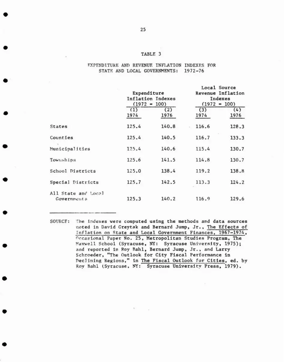
expenditures would have increased by 25.3 percent by 1974 (see Table 3). • An application of the Greytak-Jump method, still using the 1972

base, to 1976 expenditures shows an expenditure-inflation index of

140.2, suggest ing that inflation potentially accounted for about 80

9 • percent of total expenditure growth between 1972 and 1976. For the

state and local government sector as a whole, one might conclude from

these results that inflation accounted for virtually all of the • expenditure increase between 1972 and 1976. 10

•

•

•

•

25

TABLE 3

EXPENDITURE AND REVENUE INFLATION INDEXES FORSTATE AND LOCAL GOVERNMENTS: 1972-76

•

ExpenditureInflation Indexes

(1972 = 100)(1) (2)

1974 1976

Local SourceRevenue Inflation

Indexes(1972 0: 100)

(3) (4)1974 1976

•

•

•

•

•

•

•

States 125.4 140.8 116.6 128.3

Counties 125.4 140.5 116.7 133.3

HunicipaJiUes 125.4 140.6 115.4 130.7

Towrlshi ps 125.6 141.5 114.8 130.7

School Districts 125.0 138.4 119.2 138.8

Special Districts 125.7 142.5 113.3 124.2

All State ane !..OC;1]

Governl'1e(lts 125.3 140.2 116.9 129.6

SOURCF: 'r.he indexes \Jere computed using the methods and data sourcesnoted in David Creytak and Bernard Jump, Jr., The Effects ofInflation on State and Local Government Finances, 1967-1974,0~casional Paper No. 25, Metropolitan Studies Program, TheMaxwell School (Syracuse, NY: Syracuse UniverRity, 1975);and reported in Roy Rah1, Bernard Jump, Jr., and LarrySchroeder, liThe Outlook for City Fiscal Performance inDec] ining Regions," in The Fiscal Outlook for Cities, ed. byRoy Bahl (Syracuse, NY: Syracuse University Press, 1979).

26

This conclusion certainly does not hold for all local government,

because expenditure mixes vary substantially. Greytak and Jump carried

out case studies of the fiscal performance of six local governments

during the 1977-1974 period to show the wide variation in the effects of

•

•

•inflation on expenditures. \fhile the aggregate state and local

The percent of expenditure

government expenditure inflation index was 125.3 the indexes for these

governments over the same period range from 165.9 in Snowhomish County,

hi ] 23 0 i' n k 11Was ngton to .• New Yor City.

increase attrihuted to inflation ranged from 93 and 88 percent in

Atlanta and New York City to 60 percent in Orange County, California.

Charken and ~alker have used a wage index to estimate that 75

percent of the expenditure increase in Los Angeles between 1973 and 1978

could be attributed to inflation.l2

Cupoli, Peek and Zorn used the

Greytak-Jump method to estimate that nearly 76 percent of the

Washington, D.C. expenditures increase (excluding transfers) between

1972 and 1975 was due to inflation.13

The City of Dallas has used its

forecasting model to ask the interesting and related question of how

14much will future expenditures respond to higher rates of inflation.

Working with a low vs. a high inflation rate scenario. they conclude

that a difference of 5 percent in total general expenditures might be

expected between 1980 and 1984.15

Expected Revenue Impact~

Revenues also respond to inflation in that the nominal value of tax

bases rises with increasing incomes, ~rices and property values. Hence,

there is clearly a potential to capture increased revenues induced by

inflation. For sales and income taxes, the revenue response is more or

•

•

•

•

•

•

•

•

•27

• le~s automat _i c and estimatton of the inflation effects is

straightforward euough. However, in the case of the property tax, the

• problem is far more complicated. Land and improvement values have

increased dralliatically during recent inflationary periods, thereby

providing equallY dramatic increases in the potential for increased

• property tax revenues. Indeed, in terms of the potential revenue

effects of inflation, the property tax may be the biggest winner of all.

But who would argue that local governments may easily capture this

• potential increase in the tax base? The major impediment to property

tax revenue growth during inflation, of course, is the revaluation of

properties. The political obstacles to such revaluation are well known.

• Indeed, Proposition 13 was partly a result of property tax assessments

reflectillg skyrocketing property values. The California solution to

hold taxable property value growth to an arbitrary 2 percent suggests

• that during times of inflation, good assessment practices are even more

objectionable to voters than bad practices.

If the problem of estimating inflationary impacts is difficult for

• the property tax, it is next to impossible for most intergovernmental

grants. One might hypothesize that because the more elastic Federal and

state tax structures respond to inflation, Federal and state aids will

• also respond proportionately--as if they were an income-elastic tax. We

might offer a crude test of this hypothesis by examining the long-term

(1965-1980) responsiveness of the grant share of Federal government

• expenditures (FIB) to changes in nominal income (Y), and the CPT (C):

•

•28

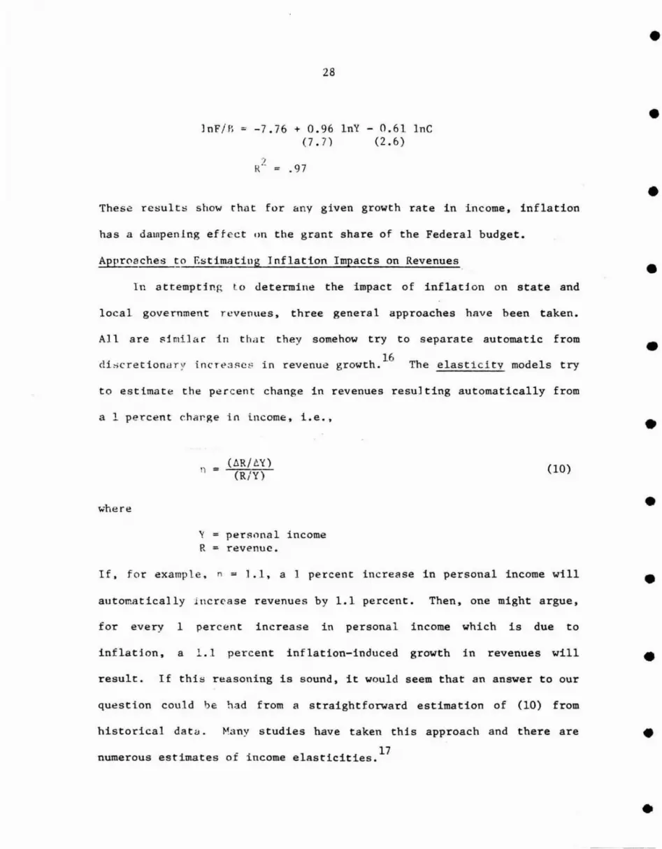
lnF/B -7.76 + 0.96 (7.7)

lnY - 0.61 (2.6)

InC •

These re~;ults show that for any given growth rate in income. inflation • has a dalnpenlng effect on the grant share of the Federal budget.

Approaches to Estimating Inf1ati.on Impacts on Revenues.

In attempting to uetermine the impact of inflation on state and •

local government revenues, three general approaches have been taken.

All are ~imi1ar in that they somehow try to separate automatic from

16dio;cretionClry incre:3scs in revenue growth. The elasticity models try

• to estimate the percent change in revenues resulting automatically from

a 1 percent chapge in income. Le., •

where

n = (liR/c.y) (R/Y)

(10)

• y

R per~onal

= revenue. income

If, for example, n = ].1. a I percent increase in personal income will • automatically incrC'ase revenues by 1.1 percent. Then, one might argue,

for every I percent increase in personal income which is due to

inflation. a 1.1 percent inflation-induced growth in revenues will • result. If this reasoning is sound, it would seem that an answer to our

question could be had from a straightforward estimation of (10) from

historical data. Many studies have taken this

i - . 1 17numerous est mates ot 1ncome e asticities.

approach and there are •

•

•

•

•

29

As ;t method for picking up inflationary impacts, the elasticity

approach hi:ls important weaknesses. It assumes that the effects of

inflation can he adeouately measured by the growth in nominal personal

income, e.g., a I. percent real and 4 percent inflationary growth in

personal income vs. any 8 percent growth in personal income would have

otherwise. One is that price increases may somehow change the structure

of personal income and consumption and therefore the elasticity of the

tax in the future. This possibility would be missed in a

straightforward e1asticity estimation which typically assumes away price

effects. For example, if the ratio of taxable to total consumption rose

wi th increasing prices, so would the sales tax elasticity. There are

other examples.Tfl arldition to the "progressivity" effects under state

income taxe~ (i.e .• bracket creep), one might question whether inflation

;tffects the S(;lIrce di stribution of income, particularly capital gains,

and thereby aftect~ total taxable income.

A separate but equally serious problem with the elasticity approach

has to do with the difficulty of separating automatic from discretionary

effects on revenue growth. Particularly in the case of the property tax

it is all but impossible to identify an "automatic" responsiveness of

tax revenues to growth in either personal income or price levels. These

caveats suggest that straightforward use of historical data to provide

an estimate of the revenue-inflation impact will be problematic.

An alternative to the elasticity approach is that taken by Greytak

and Jump. They have attempted to estimate the potential tax base

response to price increase. They ask the question "how much would

•

•

•

•

•

•

•

•

an identical effect on revenues. There are reasons to believe

30

revenues grow in response to inflation if tax bases increased at their

•

•fu] 1 potentia} and if effective tax rates remained constant?" They

b~gin with 1972 and inflate each tax base and user charge base by an

"appropriate" index--taken from the CPl. WPl or the BLS family

expenditure sUlvey. For example. for the property tax. they used BLS

price indexes for residential housing and residential rents. and various

Boeckh indexes for co~nercial and industrial properties.

The problem vf estimatjn~ the revenue impact of inflation is

•

•

for a great\; r i ncre<i!;e in revenues than most governments will be willing

analogous to that on the expenditure side: the potential effects are

•(C'r po Ii t ieall J CIt. l e) tC' accept. The response to this increased revenue

potential by statl: and local governments has been to allow effective

property tax r3 tes to fa 11 by faiUng to reassess and in some cases to

index statl! t c':' es or reduce income tax rates. In sum. a part of the

potential rever;\1e :-:<timulus of inflation has been foregone.

A third approach, taken by the ACIR. is a substantial improvement

h 1 .. . i method .18 Th h d t d V I' d 1on tee astlclty estlmat on ey ave a ap e oge s. mo e

of state and local government expenditure growth during the business

19cycle, and estimated

bR = l.15 - 0.12bG + 236.42bD(5.54) (11.28)

')

R" = 0.883 DW - 1.35

where

bR = change in own-source revenuebG = change in nominal GNP gapbD = change in implicit price deflator.

•

•

•

•

•

•

•31

• The product of the actual change in the deflator between two periods

(liD) <ind the regression coefficient (236.42) gives an estimate of the

• effects of inflation on own-source revenues, holding constant the change

in the nominal CNP gap for that period. The ACIR study, while carefully

done, is linl1ted by their assumption that revenue changes (automatic and

• di~cretionary) can be explained by movements in the business cycle and

the price level. There is a voluminous literature which argues that

expe~diture, and therefore revenue and tax rate levels are responsive to

• changes in population, Federal grants, changing economic stnlcture,

19aetc. The omission of thef:;e important variables leads to (an

uncertain) bias in the results.

• The di fferences among the elasticity, ACIR and the Greytak-Jump

approaches lie in the question asked. The elasticity approach asks how

revenues, net of any discretiol1ary change, respond to changes in nominal

• persona) income. The ACIR approach attempts to explain actual changes

in revenue during inflationary periods, including the effects of

discretionary actions. Creytr.k-Jump attempt to estimate the potential

• response to inflation, Le., how much more taxable capacity would be

available to ~('vernrnents simplv because of inflation if the governments

could and actually did permit the inflation to be reflected in the tax

• bases. The interpretation of results from these studies must keep their

different questions in mind.

F.stimated Revenue Impacts

• The Greytak and Jump indexes in Table 3 show that state and local

government revenue potential grew by 16.9 percent between 1972 and 1974,

i.e., if the 1972-1974 increase in the nominal values of tax bases had

•

•32

• been taxed at 1972 effective rates, the revenues raised by state and

local governments would have increased by 16.9 percent, solely because

of inflation. • The ACIR study a] so concludes that state and local government

revenues are stimulated by inflation, that they are between 6 and 16

percent higher than 20

they otherwise would have been. Their estimate of • an aggregate inflation stimulus of about $77 billion in revenues between

1973 and 1976 is substantially greater than the $40 billion estimated

with the Greytak-Jump method between 1972 and 1976. The difference is • easily expJ ained. The ACIR method does not adjust for widespread tax

rate increases during this period, Le., the tax rate increases are

viewed as pRrt of the effects of inflation. This is perfectly correct • if the objective is to show the direct and induced effects of inflation

on local government revenues, and if the effect of other factors which

determine tax rates is removed. • The conclusion of these analyses would seem to be that inflation

exerts a quite stimulative effect on nominal state and local government

revenues. The Greytak-Jump method implies a hypothetical increase • slightJy less than the growth in the CPI for the 1972-1976 period, the

ACIR method pre-iicts an inflation effect which is greater than the CPI

increase. Obviously, there still remains the issue of great variations • in this effect by type of jurisdiction.

The Pudgetary Effects of Inflation

The really important question is the net effect of inflation on the • budget, Le., whether inflation drives up revenues by more than it

drives up costs. The ACIR answer for the 1973-1976 period is that it

•

•33

• does, while the Greytak-Jump approach yields a conclusion for the

1972-1976 period that it does not. The ACIR estimates net revenue gains

• durin~ the lq73-l97b period as equtvalent to 0.6 percent of own source

revenues in ]973, J.9 percent in 1974, 5.5 percent in 1975, and 2.9

percent in 1976. 21

However, discretionary rate changes are included in

• thei r estimates of revenue increase due to inflation, causing one to

suspect an overestimate of the pure inflation effects on the revenue

side (becau:;e other factors may have caused the tax rate increase).

• ttoreover, they do not consider price effects on any expenditure

bar,e--they "dJust reVi:Ouue purchasing power by the IPD for state and

local gover~Ment purchases--causing one to suspect an underestimate of

• the infl3tiG~ t'~[ectR on expenditures. Again, the ACIR estimates are of

the total rllre~t and indirect effects of inflation on budgets and take

into aCC0 1!nt dny discretionary tax and expenditure ad.iustments the

• government FC!Y have made because of inflation.

The Creytak-Jump estimates, to the contrary, are of how

expenditures and revenues would respond to inflation if n~ discretionary

adjustments were made, i.e., no tax rate changes, all inflation-induced

changes in the tax base are captured, the number of employees and

quantities of goods purchased remain constant, and no programs are cut

• back. Hence, their estimates are of the potential effects of inflation,

but under the assumption that governments make no quantity or price (tax

rate and real wage rate) responses.

• The Greytak-Jump estimates show that expenditures were potentially

more responsive to inflation than were own-source revenues, at both the

state and local levels during the 1972-1974 and 1972-1976 periods (see

•

34

Table 3). Indeed, while inflation was driving up expenditures by about

25 percent bet\yeen 1972 and 1974, it was increasing revenues by only

about 17 percent. \fui1e both indexes continued to increase during the

1974-76 period, the relative cooling of inflationary pressure did allow

inflation-induced increases in state and local revenue bases to nearly

keep pace with the pressures of inflation on expenditures.

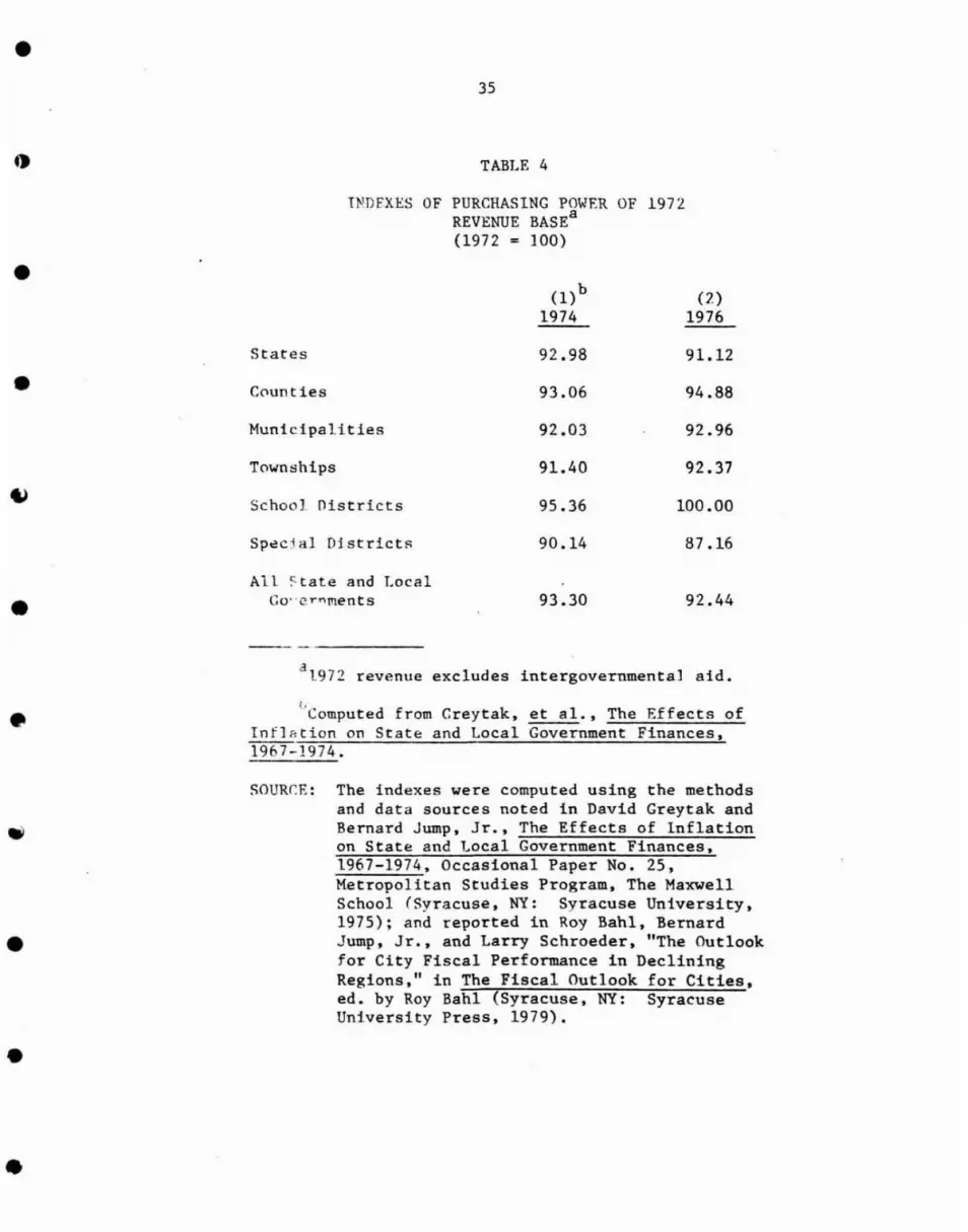
Another way to describe the budgetary effects of inflation is to

consider the impli.cations for the purchasing power of state and local

government rev~nues. Purchasing power indexes for the several levels of

government. based on 1972 revenue bases, are shown in Table 4. For

example, a purchasing power index of 90 would imply that after

accounting for the effects of inflation on revenues and expenditures,

the revenue base would be 10 percent too small to finance a constant

level of services. The period 1973-74 was especially severe for

inflationary pressures on state and local governments with the

purchasing power index falling nearly 7 percent. The situation did· not

worsen markedly between 1974 and 1976--the potential growth in revenues

was adequate to cover about 92 percent of the inflation induced-increase

in expenditures.

While the inflation indexes in Table 4 suggest that state and local

government sector purchasing power fell between 1972 and 1976, the

actual effect of inflation almost certainly has been more severe than is

indicated by these estimates. This is because the revenue and

expenditure inflation indexes measure the potential impact of inflation

on the budget--these estimates are not meant to imply that state and

local governments actually realized these revenue base effects or made

•

•

•

•

•

•

•

•

•

•35

TABLE 4

INDEXES OF PURCHASING POWER OF REVENUE BASEa

(1972 = 100)

1972

• (l)b 1974

(2) 1976

States 92.98 91.12

• C0unties 93.06 94.88

Municipalities 92.03 92.96

T0wnships 91.40 92.37

School Oistricts 95.36 100.00

Spoi!c:ial Districts 90.14 87.16

• All. State and Local

Go' "crr"lments 93.30 92.44

----------a1.972 revenue excludes intergovernmental aid.

• [,

Computed from Creytak, et al., The Effects of Inflation on State and Local Government Finances, 1967-1974.

•

SOURCE: The indexes were computed using the methods and data sources noted in David Greytak and Bernard Jump, Jr., The Effects of Inflation on State and Local Government Finances, 1967-1974, Occasional Paper No. 25, Metropolitan Studies Program, The Maxwell School (Syracuse, NY: Syracuse University, 1975); and reported in Roy Bahl, Bernard Jump, Jr., and Larry Schroeder, "The Outlook for City Fiscal Performance in Declining Regions," in The Fiscal Outlook for Cities, ed. by Roy Bahl (Syracuse, NY: Syracuse University Press, 1979).

•

•

these expenditures.

36

Assessment lags would mean that actual property

•

taxes would not

effect of price

grow as implied here and therefore the detrimental

22indexes on hudgets would actually be understated.

•Moreover, for declining cities it is altogether possible that property

values did not keep pace with the general rates of increase in property

values experienced in the rest of the nation.

There is little doubt but that the potential effects of inflation

on s~ate and local government budgets are substantial. The expenditure

impac~s may n0t show up immediately, because of lagged responses, or

directly, beccll\se governments may compensate for price increases by

•

cutting services. Rut it seems clear that inflation has important and

substantial elfects on the cost side of the budget. The effects on the

revenue side '''3y be much less pronounced, particularly for property

taxes and purticul~r]v in timeR of taxpayer resistance. On the basis of

this eviden,.I.·. j t \;OU' d seem reasonab Ie to conclude that inflation does

reduce the pu ((.hasing power of state and local government revenues and

•

•may do so bj .':\ substantial amount. The 7 to 8 percent reductions

suggested in tl'w (;7' e.vtak-Jump analysis of the 1972-74 period do not seem

too far from the lnark given the overall inflation rates experienced

dependent on the property tax, the effect may be much greater.

It' is likely, then, that the real income effect reduces the

purchasing power of the state and local government tax base. In

response to this real income decline, increases in tax rates and

reductions in real expenditures may be anticipated.' If a government

resorts entirely to tax rate hikes, it may offset the real tax base

during that perio~. For local governments which are more heavily

•

•

•

•

•

•

•

•

•

•

•

•

•

•

37

decline and hold the effective tax rate constant. It is more likely.

however. that state and local governments will respond to inflation with

real cuts in expenditures.

Th~ expenditure impacts of inflation are a complicated matter

involving direct. automatic effects and indirect. discretionary effects.

These effects depend on input price movements. which are difficult to

measure; on the impact of institutional arrangements. such as public

employee unions; and on the political will of state and local

governments to undertake discretionary actions. We may never be able to

sort out the "pure" effects of inflation. but we may begin to examine

the empirical evidence ~n this question by considering the evidence for

the m~jor components of state and local government expenditures: labor

costs, materia ls, equipment. supplies. capital outlays. and transfer

payments.

Labor Costs

Since shout 37 percent of state and local government expenditures

are for wages and salaries. an understanding of how inflation has

stimulated labur costs is important. The same scenario as above holds:

labor costs are pushed up by inflation. cet. par •• to the extent each of

the following ig true:

--coITImunjty income increases in proportion to inflation;--the local revenue structure is inflation responsive;--the re~ative price of labor decreases;--the d~mand for labor is price inelastic;--th~ demand for labor is income elastic.

•38

The inflationary impacts on labor expenditures are dampened to the • extent:

---communi ty income increases less than in proportion to infJation;

--the local revenue structure is not inflation responsive; • --the relative price of labor rises;--the demand for labor is price elastic;--the demand for labor is income inelastic.

Inflationary impacts on labor costs cannot be read from available • data in a straightforward way. Some method of estimation is necessary.

When labor rosts increase faster than the rate of inflation, the

empi rica! p t"ob J em is how much of the increase should be assigned to • inflation. nnl~ .1pproach is to assume that the full rate of inflation is

captured in 1abor Lost increases. i. e., wage increases fully reflect

cost-af-living increments. Thi~ implies that state and local government • labor expenditures are indexed to cost-of-living increases and that the

price elasticity of demand for public employees is zero. In the sixties

and early seventies this may have been an appropriate assumption for • estimation--public employees received cost-of-living increments and real

wage tncreases. Average public employee wages increased by more than

the full CPI increase, pub 1 ic employees were not being laid off, and • revenues were more than keeping pace with inflation.

The increasing rates of inflation beginning in about 1973 changed

this pattern as state and local governments began to adjust their • spending patterns to rising input prices. Through most of the 1970s,

average compensation (including supplements) of state and local

government workers increased because of inflation, but at a rate less • 24

than the CPT. An index of the actual increase in state and local

•

•39

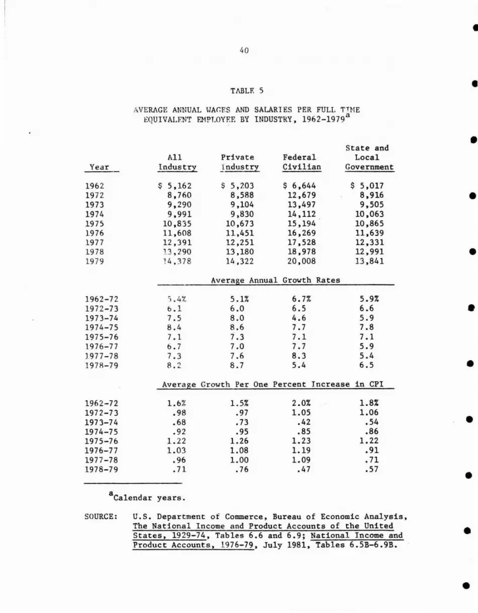
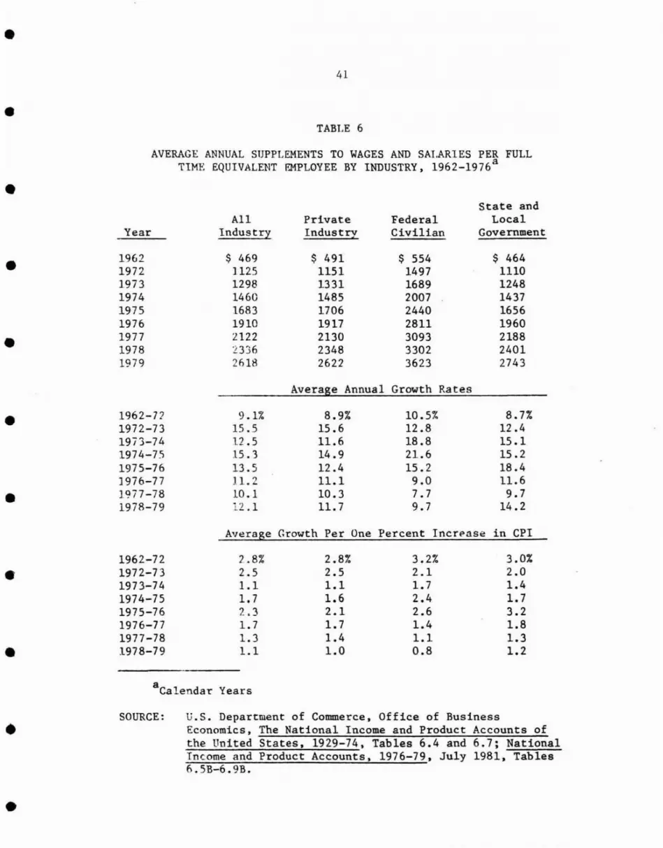
• government employee wages shows less growth than the CPT since 1973 (see

Tables 5 and 6). Moreover, there has been a marked slowing in the rate

• of growth in public employment rolls.

The stnr~1 these data tell is that sometime after 1973 state and

local governmt'tlts began to usc discretionary actions to offset some of

• the expenditure impacts of inflation. This response was possible

because wage rate increments are a negotiated, discretionary action of

state and local governments. 1. e., governments aren't required to pay

• fulJ cost-of-livinp, increments in the same way that they are required to

pay a hl~her price for a gallon of gasoline. This feature has been used

to kt.~ep t~le growth in the price of state and local government labor

input!~ 10"1 relative to the general price level.• This statr of affairs leaves a complicated set of effects to sort

out:

inflation has increased the wage rate paid in the• state and local governm~nt sector thereby increasing potential expenditures; some of this potential increase has been offset, however, because revenue growth has not kept pace with inflation, and because the ensuing 'real income effect' has dampened public employment growth.• state and local governments negotiated lower wage increments· for public employees, after 1973. than the rate of inflation. This has kept some of the inflationary pressure off state and local government expenditures. • the combination of higher labor costs due to general inflation and revenue increases below the general inflation rate may have dampened public employment growth, but th~ lower relative price• effect after 1973 may· have increased it. In aggregate, labor costs would probably have been lower under a lower rate of inflation because the income elasticity of demand for labor is greater than the price elasticity.

•

40

TABLE 5

•

•AVERAGE ANNUAL \JAr.F:S AND SALARIES PER FULL TTHE

EQUIVALENT E}1PLOYEE BY INDUSTRY, 1962-1979a

Year

196219721973197419751976197719781979

AllIndustry

$ 5,1628,7609,2909,991

10,83511,60812,39113,290'14,378

Privatelndustry

$ 5,2038,5889,1049,830

10,67311,45112,25113 ,18014,322

FederalCivilian

$ 6,64412,67913 ,49714,11215,19416,26917,52818,97820,008

State andLocal

Government

$ 5,0178,9169,505

10,06310,86511,63912,33112,99113 ,841

•

•

•Average Annual Growth Rates

1962-721972-731973-741974-751975-761976-771977-78197R-79

'i.4Z6.17.58.47.16.77.38.2

5.1i.6.08.08.67.37.07.68.7

6.7i.6.54.67.77.17.78.35.4

5.9i.6.65.97.87.15.95.46.5

•

•Average Growth Per One Percent Increase in CPI

1962-721972-731973-741974-751975-761976-771977 -781978-79

1.6%.98.68.92

1.221.03

.96

.71

1.5i..97.73.95

1.261.081.00

.76

2.0i.1.05

.42

.851.231.191.09

.47

1.8%1.06

.54

.861.22

.91

.71

.57

•

•a Calendar years.

SOURCE: U.S. Department of Commerce, Bureau of Economic Analysis,The National Income and Product Accounts of the UnitedStates, 1929-74, Tables 6.6 and 6.9; National Income andProduct Accounts, 1976-79, July 1981, Tables 6.5B-6.9B.

•

•

•41

•TABLE 6

AVERAGE ANNUAL SUPPLEMENTS TO WAGES AND SALARIES PER FULLTIME EQUIVALENT EMPLOYEE BY INDUSTRY, 1962-1976a

• State andAll Private Federal Local

Year Industry Industry Civilian Government

• 1962 $ 469 $ 491 $ 554 $ 4641972 ] 125 1151 1497 11101973 1298 1331 1689 12481974 1460 1485 2007 14371975 1683 1706 2440 16561976 1910 1917 2811 1960

• 1977 2122 2130 3093 21881978 '2336 2348 3302 24011979 2618 2622 3623 2743

Average Annual Growth Rates

• 1962-77 9.1% 8.9% 10.5% 8.7%1972-73 15.5 15.6 12 .8 12.41973-74 12.5 11.6 18.8 15.11974-75 15.3 14.9 21.6 15.21975-76 13 .5 12.4 15.2 18.4] 976-77 11.2 11.1 9.0 11.6

• 1977-78 10.1 10.3 7.7 9.71978-79 12.1 11. 7 9.7 14.2

Average Growth Per One Percent Incn"ase in CPI

1962-72 2..8% 2.8% 3.2% 3.0%

• 1972-73 2.5 2.5 2.1 2.01973-74 1.1 1.1 1.7 1.41974-75 1.7 1.6 2.4 1.71975-76 2.3 2.1 2.6 3.21976-77 1.7 1.7 1.4 1.81977-78 1.3 1.4 1.1 1.3

• 1978-79 1.1 1.0 0.8 1.2

a Calendar Years

•

•

SOURCE: U.S. Department of Commerce, Office of BusinessEconomics, The National Income and Product Accounts ofthe United States, 1929-74, Tables 6.4 and 6.7; NationalIncome and Product Accounts, 1976-79, July 1981, Tables6.5B-6.9B.

•42

increased Federal grants in the mid-1970s made up •for some of the real revenue loss due to inflationand thereby stimulated public employment growth.

To belabor a point, the public employment effects of inflation are not

easily deduced. As was described above, state and local government • employment has increased throughout most of the past decade. This

increase has come about for a myriad of reasons including increasing

• incomes, changing voter tastes, needs related to urbanization, etc. The

question here is whether this rate of increase would have been higher or

lower if the rate of inflation had been lower. The answer would appear

• to be that ilif1fltion has dampened the growth in state and local

government ernploylllelll.

To sort out tl.: s net impact, an income and a substitution effect

• have to be ident: if ;. ~'J. First, the income effect. If the purchasing

power of state 8nr. JQC'}] go\'ernment revenue declines during inflationary

periods, layoffs or a slower rate of employment growth might be • expected. Governments. like any consumer, will purchase fewer inputs

when real income falls. If the local revenue structure were responsive

to inflation or had there been a very low inflation rate, real revenues • would have been higher and a higher level of state and local government

employment ~ould have resulted. While this real income effect probably

dominates the inflatiop impact on employment, there may be an offsetting • or reinforcing substitution effect due to the changing relative price of

labor. The substitution effect is likely to be small because the demand

for public employees is quite price inelastic, Le •• as wage rates go • down (relative to other prices), state and local governments will

increase their employment rolls (or at least let them grow faster than

•

•43

• they would have otherwise) but not by very much. For example,

Ehrenberg's estimates would suggest that a 10 perc~nt wage rate

increment wouln reduce public sector employment by only 3 to 4

25• percent.

1n fact, through most of the 19705, inflation has outrun the

increase in stAte and local government labor costs and, as a result, the

• si7.e of the real public employment budget is likely smaller than it

would have been under a zero rate of inflation. This, in turn, suggests

that a part of the cost of inflation is borne directly by public

• employees (in the form of lower real wages) and in part by residents (in

the form of the lower public service levels attributable to having fewer

public employees) . • A number of qualifiers have to be offered to this speculation.

There is simply too much variation in functional responsibility, labor

practices, revenue structures and economic conditions to permit such a • generali:>:ation about the effect of inflation on labor costs for all

state and local governments. Where unions are strong, public employee

26compensation tends to be higher, hence, one might conclude that cet. • ~. labor cost s will better keep pace with inflation in heavily

unionized areas of the Northeast and Industrial Midwest. Where public

employee organization is weak, labor would seem much more vulnerable to• the prospect of bearing a substantial share of the burden of inflation.

Another important difference is whether the local revenue structure

• is responsive to increasing prices. For states and some local

governments that rely heavily on sales and income taxes, the purchasing

power of local government revenues may respond to inflation. That is,

•

•44

• the inflation-induced increase in sales and income tax bases may

generClte revenues which are more than adequate to cover the

inflation-induced increase in the cost of providing a constant level of • services. This would increase real government revenues and suggest both

a greater willingness on the part of government to grant cost-of-living

increases, and a lesser propensity to cut employment rolls. The net • impact of inflation in such a case is to increase the public employment

budget. Public employees and residents share in the benefits of

inflat ion at the expense of taxpayers who must foot the bill for the • increRsed rosr. If taxpayers instead force a discretionary tax

reduction, the real income of the government declines and the process is

as described above. • Still other factors would cause us to question generalizations

about the i.mpact of inflation. For examples, governments have different

functional responsibilities, hence, different uniformed, blue collar, • and white collar employment mixes; and the precarious financial position

of a Cleveland or a Detroit may hold wage responses to inflation below

what they otherwise might have been. All of these reasons suggest that • the average response deduced above must be interpreted cautiously.

Labor costs may well have responded less than proportionately to

inflation for the state and local government sector as a whole since • 1973, but for some government.3 the response was quite different from

this average.

Finally, there is the qu@stion of Federal grants. An increase in • Federal assistance, particularly programs such as CETA, kept public

employment levels higher than they otherwise would have been.

•

•

• Particularly hetween 1970 and

grants shored up the real income

• and held

levels.

public employment at

Non-Labor Cost

45

1978, the large increases in Federal

position of state and local governments

what might be termed artifically high

Non-labor expendi tures respond to inflation more directly, since

• governments have little control over prices paid for materials and

supplies purchased. The al ternatives are simply to pay the higher

price, or to reduce the quality or quantity of the inputs used. The

• former is often the choice because the nature of the production process

in the state and local sector leaves little room for substitution

27between lahor and non-labor inputs.

• To examine the diLect effects of price increases on non1abor costs,

assume tha t the government makes no quality or quantity adjustments.

The lnflation impact \~ill then depend on whether the unit cost of

• materials purchased by state and local governments has risen as fast as

the general price level. The cost of materials/supplies, etc., to

governments is a weighted average: the quantity of each type of • purchase weighted by the increase in the appropriate price index.

Greytak, Gustely and Dinkelmeyer constructed such an index for New York

City material input costs for the 1965-1972 period, using over 60 • 28categories of purchases and a separate price index for each. Their

findings showed the cost of supplies to be increasing at a slower rate

than the CPl, but materials and equipment to be increasing at about the• same rate. Using a similar method for the 1971-1974 period, Greytak and

Jump found the same relationship between the increasing price of

•

•46

• material inputs and the CPI--material input prices increased by about 90

percent of the rate of increase in the consumer price index. However,

for five other local government areas studied, they found the materials • price response to vary from about 60 percent of the cPt in Orange County

California to about 93 percent 29in Atlanta, Georgia. Cupoli, Peek and

Zorn, studying Washington, D.C. expenditures for the 1972-1975 period • estimated that inflation drove up material costs by 31.6 percent as

against a 28.7 percent increase in the CPI. 30

Governments may not elect to pay the full cost increase implied. • If the net effect of inflation is to lower the purchasing power of

government revenues, some quantity adjustments will also take place.

Examples would be deferral of road maintenance, telephone use • restrictions, reduced school busing service, restricted travel, deferral

of office machine replacement, keeping the city swimming pool closed and

postponing the purchase of tools, repair parts, etc. This is the same • kind of real income effect as noted above; if real government revenues

fall when the inflation rate rises, the quantity of inputs will be

reduced, i.e., they will be at a lower level than would have been the • case with a lower inflation rate. Unfortunately, data limitations make

it impossibJe to observe actual price and quantity adjustments. One can

only conclude that where inflation dampens real revenue growth, it • probably has had the net effect of lowering the quantity of materials,

supplies used. Hence, state and local government expenditures on these

items have not like) v risen by the full amount implied by the price • increase.

•

•

•

•

•

•

•

•

•

•

•

•

47

Capital Costs

The effect of inflation on capital expenditures is more difficult

to sort out. The question is whether capital expenditures would be

higher or lower, cet. par., under a lower rate of inflation. One might

begin with a cons:f.deration of the potential impact, Le., assume that

governments would not alter their capital project plans, and estimate

the increased cost of those projects due to inflation. When viewed this

way, the issue is simply how much have construction and financing costs

risen, and what is the relative importance of each of these in the

makeup of total capital costs. Between 1965 and 1980, construction

costs increased by 130 percent and interest rates on treasury bonds by

205 percent. lnfla t:f.on clearly had an upward pressure on the amount

spent.

Was there a displacement toward or away from capital expenditures

because of an increase in the relative price of capital expenditures?

Over most of the present decade, capital construction costs have

increased at less than the general inflation rate while interest rates

have grown faster (see Table 2). One can only speculate about the net

impact of these relative price changes, but it is clear that state and

local governments have many discretionary options for countering

increased capital project costs. Governments may avoid inflationary

effects by reducing the size or quality of a project, postponing

construction or even cancelling it altogether. For examples, the

proposed highway construction may be two-lane instead of four-lane or it

may not go as far, the sewer system may not be extended for another two

years or the municipal auditorium may never be built. These effects of

•48

inflation are not easily measureable and surely don't show up in • budgets, but they may well be the most important impacts. Again, we

cannot observe the quality and quantity adjustments actually made, but

the evidence of recent years shows that state and local governments have

31substantially slowed their rate of capital formation.

• Transfer Payments

Inflation also affects state and· local government expenditures by • raising expenditures on transfer payments-~particularly public

measured, yet we know that transfer

assistance and medicaid payments.

payments respond

These effects

to

are

inflation in

not easily

• that income maintenance is related to the cost-of-living and medical

assistance is related to medical costs.

of inflation are especially difficult

However, the long-term effects

to estimate because state and • local governments have some discretion over how much they will spend on

these programs. Again it is the problem of

and an indirect effect.

inflation exerting a direct

• Medicaid and AFDC are the most important of the transfer payment

programs

former,

in state and local government budgets. With respect to

states have three avenues open in adjusting the level

the

of •

payments in the face of increasing prices. They may change eligibility

rules thereby undertaking

levels, i.e., number of

a quantity adjustment; they may adjust benefit

hospital days insured, number of physical • benefits, drug and dental allowances; and they may adjust fee schedules.

Following the medicare reimbursement schedule, which is essentially

indexed, gives the greatest inflationary response. Though states have •

attempted to slow the increase in medicaid costs by reducing primary

•

•49

• health care services, they have been heavily burdened by the rising cost

of hospital and nursing home services. Davis and Schoen report that

real annual medicaid paym~nts per recipient rose by only $23, from $338

in 1969 to $361 in 1977. the number of recipients doubled, and the• 32

general price of medical care nearly doubled. At least half of the

state and local government expenditure increase of medicaid might be

attributed to inflation.• An even greater proportion of the recent increase in state and

local government expenditures for public assistance may be attributed to

inflation. Since 1970, there has been little real growth in state and • local government expenditures for public assistance. though nominal

expend! tures by state and local governments increased by 90 percent •

This pattern, however, masks a real expenditure increase due to an • increased number of recipients between 1970 and 1975 and real

33expenditure cutbacks after 1975.

• Another major type of transfer payment is state aid to local

government. It would seem interesting to raise the issue of whether

inflation would affect a state's choice between direct spending and

• local assistance. That is, as inflation drives up state government

costs. cet. par., is there a tendency to cut hack on aid to local

governments rather than reduce the scope or quality of direct state

• expenditures? A time series analysis of the 1957-1980 period suggests

that this may indeed be the case. A simple estimate of the determinants

of long-term changes in the state aid share of total state government

• expenditures shows

•

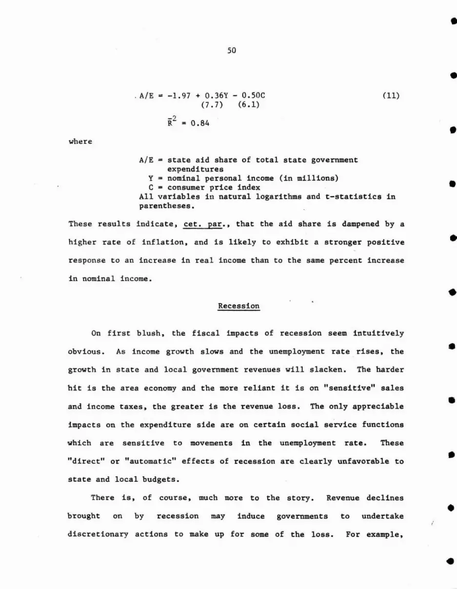
•50

• . AlE = -1.97 + 0.36Y - O.SOC (11)

(7.7) (6.1)

_'"I

R"" = 0.84 • where

AlE = state aid share of total state government expenditures

Y = nominal personal income (in millions) C = consumer price index •

All variables in natural logarithms and t-statistics in parentheses.

These results indicate. cet. par., that the aid share is dampened by a

higher rate of inflation, and is likely to exhibit a stronger positive • response to an increase in real income than to the same percent increase

in nominal income.

• Recession

On first blush, the fiscal impacts of recession seem intuitively

obvious. As income growth slows and the unemployment rate rises, the • growth in state and local government revenues will slacken. The harder

hit is the area economy and the more reliant it is on "sensitive" sales

and income taxes, the greater is the revenue loss. The only appreciable • impacts on the expenditure side are on certain social service functions

which are sensitive to movements in the unemployment rate. These

"direct" or "automatic" effects of recession are clearly unfavorable to • state and local budgets.

There is, of course, much more to the story. Revenue declines

brought on by recession may induce governments to undertake • discretionary actions to make up for some of the loss. For example,

•

•51

• state and local governments may increase tax rates or layoff workers.

Such discretionary actions are an important impact of the business

• cycle, but should be separated from the more "pure" effects noted above.

The Expected Impacts of Recession

Recession may be viewed as a reduction in real incomes, and the

• impact on the state and local governme~t sector depends in part on the

income elasticity of demand for public goods. The more elastic is this

demand, the more sensitive will be the state and local government sector

• to recession. While the demand for local public goods appears to be

income elastic, suggesting a substantial fiscal response to recession,

there are reasons to expect that discretionary actions might be taken to

• cushion the decline. A first reason is that governments may expect the

recession to be short-lived and take temporary measures to fund existing

programs.

e. A second possibility is that expenditures may be rigid downward

because many state and local government expenditures are in the nature

of fixed commitments and cannot be dismissed. These include debt,

• pensions, "safety net" expenditures, a large portion of wages and

salaries, and much of the general overhead of the government. To

maintain these, tax rates may be increased to compensate for the revenue

• loss due to the recession •

The fiscal impact of recession may also be cushioned by some

built-in downward rigidity of tax structures. In states with a

• progressive income tax, the revenue losses attributable to slow real

income growth and increasing unemployment are partially recouped by the

"bumping-up" of higher income families into higher marginal tax

•

•52

• brackets. This effect would be especially important when the rate of

inflation was also high. In general, however, sales and income taxes

will be more responsive to recession than the property tax. To be sure, • the growth in the property tax base will be slower: the demand for

housing and industrial-commercial space will be off from previous levels

and hence there will be a slower increase in values of existing • properties. In the worst cases, abandonments, vacancies or tax

delinquency may occur. Still, the growth rate in most of the property

tax base will not be substantially affected by recession. The poor • reassessment plact ices which characterize the U. S. property tax system

~

would appear to have at least one advantage.

Final] y, the impact of recession on budgets may be softened by • discretionary expenditure adjustments which take some of the pressure

off current budgets. The timing of fiscal adjustments is an important

if often overlooked issue. Whil e it is interesting to learn how state • and local governments alter their taxes and expenditures in the face of

recession, it is as interesting to learn when they make these

adjustments. On the expenditure side, there may well be a lag before • reductions begin, with temporary shortfalls made up in anyone of a

number of ways: depleting accumulated balances, short-term borrowing,

underfunded pension systems, selling off financial and real assets, • deferring compensation increases, etc. It may be that the full effects

.of recession on the expenditure side are not felt for several years and

even then occur over a period of time. The expenditure effects of • recession may be much greater than is indicated in most surveys.

•

•53

• Studies of the Fiscal Impact of Recession

The answer to the question of how have state and local government

budgets fared during recession is to be found in empirical analysis •

• Following the discussion above, it would seem reasonable to separately

review the evidence from two kinds of studies: first the studies of

fiscal performance during the recession and then those few studies which • have attempted to address the more difficult question of the pure fiscal

impact of the recession.

The Perversity HyPothesis• During the 19505 and 1960s a number of authors engaged in a debate

over the direction of the state and local government sector's response

to the business cycle. These authors recognized that the sector was • large enough to signi ficantly offset or reinforce the· Federal

government's stabilization policy. Early in the debate it was asserted

that the state and local sector responded to the business cycle• pro-cyclically (the "perversity hypothesis"), that is, during recession

governments would cut back expenditures and borrowing, and increase tax

rates. These actions would tend to counteract a stabilization policy of• the Federal government. Later several authors claimed that state and

local governments act counter-cyclically. In a recession, this would

• mean decreases in revenue collections and increases in expenditures and

borrowing, reinforcing Federal counter-cyclical policy.

The important division of direct or automatic responses and

• discretionary responses often went unexamined in the perversity

34hypothesis debate. However, these concepts can be used to analyze the

claims of the supporters and opponents of the perversity hypothesis •

•

•54

• Aut0matic responses of state and local governments tend to be more or

35less countercyclical. Tax bases--retail sales, income, new

construction, and so on--tend to decline in recession, reducing

revenues. Expenditures increase with unemployment to the extent the • government provides welfare services. Because most state and local

governments lack the ability to run deficits, the discretionary response

in recession must be towards balancing the budget. Tax rates will • likely be increased and expenditures cut. The relative magnitudes of

these opposing effects will determine whether the state and local

government response to the business cycle is pro- or counter-cyclical. • The perversity hypothesis argument, that state and local

governments respond to the business cycle pro-cyclically, was based on

three points. First, the model of an economic downturn was the Great • 36Depression, i.e., a deep, prolonged fall in economic activity.

Second. the income elasticity of state and local revenues was considered

to be relatively low. Revenues were viewed as unresponsive to the • business cycle. Third, the expenditures of state and local governments

were thought not likely to vary with the business cycle. It was pointed

• out that one-third of these expenditures were for schools, which could

not be cut in expansion and would not automatically increase in

37recession.

• Since the automatic responses of expenditures and revenues were

slight, the role of these responses in stabilizing the economy would be

insignificant. In a deep recession, however, budget balancing • discretionary actions would be required. These perverse discretionary

responses would outweigh the feeble countercyclical automatic responses,

•

•55

• and the net impact of state and local governments on the economy would

be pro-cyclical.

• Those authors who argued that state and local governments act

counter-cyclically took a different view on the above three points. The

model of recession used was the short, mild downturn of the 1950s. 38

• Eevenues was considered to be relatively income elastic, and thus more

sensitive to recession and expansion. Expenditures, too, were likely to

vary counter-cyclically, especially with the growth of public assistance

• programs in the 39

1960s. The counter-cyclical response of state and

local government budgets would be large. But, due to the mildness of

the recession, strong pro-cyclical discretionary actions would not be

• required • The counter-cyclical response would likely outweigh the

pro-cyclical.

Supporters of the counter-cyclical state and local government

• posi tion also noted that lags in the discretionary response to the

business cycle have counter-cyclical effects. Information about revenue

shortfalls will not be available instantly, and once such information is

• available, discretionary action in response will also take time.

Furthermore, if government officials expect the recession to be short,

they may not be averse to depleting their accumulated balances or

• issuing short-term debt rather than cutting expenditures or raising

taxes. While state and local governments are unlikely to respond

intentionally with discretionary countercyclical policy, the effects of

• information lags and uncertainty may delay discretionary pro-cyclical

40policy until the recovery begins.

•

56

•

•The pro- and counter-cyclical positions can be reconciled. First,

most supporters of the counter-cyclical hypothesis agree that while

these governments respond to mild recessions counter-cyclically, they • are likely to act pro-cyclically in serious contractions. Second, it is

probable that both revenues and expenditures have become more sensitive

to the business cycle since the Great Depression. The mix of revenue • sources has moved away from the less responsive property tax, toward the

more responsive sales and income taxes. Improved property assessment

practices, the removal of necessities from the sales tax base, and the • imposition of more progressive income taxes have also contributed to the

41responsiveness of revenues to economic fluctuations. Thus, the pro-

and counter-cyclical proponents may each have been correct in their • times.

Finally, some analysts in the mid-1960s pointed out that state and

local government behavior was neither pro-cyclical nor counter-cyclical, • but unrelated to the business cycle. The secular growth of the state

and local sector in response to rising populations and public services

42demand appeared to overwhelm any cyclical effects. Perhaps for this • reason, the investigation of the state and local response to the

business cycle lapsed for nearly ten years in the late 1960s and early

1970s. •

Fiscal Performance During Recessions: The Literature

The unstable economic environment of the 1970s and 1980s has

rekindled interest in the response of state and local governments to • recession. A number of analysts have attempted to understand the fiscal

effects of recession by studying the budgetary performance of state and

•

•57

local governments during the 1974-75 and 1981-82 recessions. Two • conclusions might be drawn from this work: (a) the budgets of state and

local governments were squeezed during the recession, so that

compensating tax increases and expenditure reductions did take place, • and (b) the fiscal squeeze was more severe for central cities,

particularly those in the older industrial region.

• The evidence clearly points to increasing fiscal stress during

recession years. The financial collapse of New York City was long in

43the making but ultimately brought on by the recession. The near

• collapse of Yonkers, Buffalo and New York State can be traced to the

effects of recession, though all were brought to the brink by the

long-term decline in their economic base. In each case the response was

• some combinati.on of increased taxes and expenditure cutbacks. Stanley's

case studies of Detroit, St. Louis, Buffalo, Cleveland and New York City

(carried out in late 1975) indicated projected budget deficits which

• would require either, or both, sizable expenditure cutbacks or tax rate

'-14increases. Congressional testimony from representatives of many

different state and local governments tended to support the claim that

• the recession was forcing drastic fiscal adjustments at the state and

45local government level.

At leas t two surveys tried to more systematically ferret out the

• tax and expenditure adjustments made by state and local governments in

response to the 1974-75 recession. A Joint Economic Committee survey,

covering 48 states and 140 local governments, concluded that state and • local governments did indeed raise taxes, cut expenditures and postpone

or cancel capital improvement investments because of the recession.

•

46

•58

• But the estimated deflationary adjustments were a relatively modest 3.5

percent of total state and local government own-source revenue. Indeed,

the results of this survey do not indicate pressure of a magnitude that

• would bring on acute fiscal distress. The second survey, carried out by

the Senate Subcommittee on Intergovernmental Relations, covered about

47400 jurisdictions. Though no estimates were made of the magnitude of

fiscal adjustments, it was found that one-third of these governments • raised taxes, over half instituted personnel limitations and about

one-fifth delayed or canceled capital projects. Again, the effects of • the recession--as indicated in these surveys--are not as far reaching as

might have been imagined.

There has been some survey work that indicates a similar response • by state and local governments in the 1981-82 recession. A JEC mail

questionnaire to 48 large cities revealed a pattern of service level

48cuts, capital proj ect deferrals and tax increases in FY 1982. Tax • rate increases were reported by 20 and user charge increases by 31 of

the 48 cities in the survey. An ACIR survey underlines this finding on

the increases use of user charges--2l5 of 307 responding cities reported • 49increases. The National Conference of State Legislatures' fiscal

survey at the end of 1981 shows 29 states with prospects for FY deficits

or thin budget mar~ins, and 24 states reporting employment reductions in • 50the preceding year. None of these surveys provided enough information

to estimate the severity of cut~acks or tax increases in response to the

1981-82 recession. The Tax Foundation in its very useful annual • compendium of state tax actions, reports that tax actions in 30 states

51in fiscal 1981 will raise revenues by a net $2.5 billion per year.

•

•59

• While this is the highest annual statutory increase in 10 years, it

represents only about 1.5 percent of total state government tax

revenues.

• If the overall fiscal effects of these recessions were not so

devastating on a nationwide basis, it may be asked whether there have

been substantial variations in these effects across regions or across • levels of government. The answer is that there clearly have been, with

metropolitan central cities in particular and governments in the

declining regions in general, feeling the most pressure. The recession • hit the older central cities hardest--they went in earlier and deeper

and have come out slower than the rest of the country. This was true in

52the 1969-1972 recession-recovery and for the 1974-1978 • 53recession-recovery. All of the surveys mentioned above concluded that.

fiscal adjustments were more drastic in the more distressed cities and

regions. The JEC survey found that the most severe fiscal adjustments• 54took place in areas where the unemployment rate was higher. Other JEC

surveys, of 67 large cities in 1977,55 and of 48 large cities in 1981,56

reached a similar conclusion. Most studies have concluded that city• governments were hardest pressed~ but the National Governors'

Association has argued that state governments were also forced to

57

• budgetary adjustments by the 1973/75 recession. A GAO study has

concluded that states fared better than cities, and counties better than

. 58 either.

• If there is a general conclusion to be drawn from these studies, it

would seem to be that there are great variations in the magnitude of

budgetary adjustments resulting from recession. Though in aggregate the

•

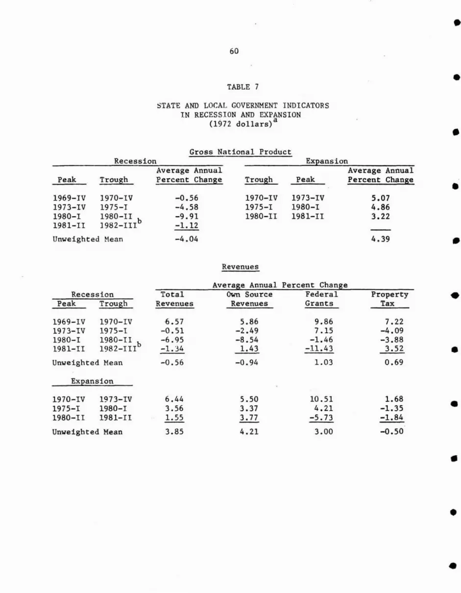
60

TABLE 7

STATE AND LOCAL GOVERNMENT INDICATORSIN RECESSION AND EXPANSION

(1972 dollars) a

Gross National Product

•

•

•

Peak

RecessionAverage Annual

Trough Percent Change Trough

ExpansionAverage Annual

Peak Percent Change •

Unweighted Mean

1969-IV1973-IV1980-11981-II

1970-IV1975-11980-II1982-Illb

-0.56-4.58-9.91-1.12

-4.04

1970-IV1975-11980-11

1973-IV1980-11981-II

5.074.863.22

4.39 •Revenues

Average Annual Percent ChangeRecession Total Own Source Federal Property •Peak Trough Revenues Revenues Grants Tax

1969-IV 1970-IV -6.57 5.86 9.86 7.221973-IV 1975-1 -0.51 -2.49 7.15 -4.091980-1 1980-II -6.95 -8.54 -1.46 -3.881981-II 1982-I1Ib -1.34 1.43 -11. 43 3.52 •Unweighted Mean -0.56 -0.94 1.03 0.69

Expansion

1970-IV 1973-IV 6.44 5.50 10.51 1.68 •1975-1 1980-1 3.56 3.37 4.21 -1.351980-11 1981-II 1.55 3.77 -5.73 -1.84

Unweighted Mean 3.85 4.21 3.00 -0.50

•

•

•

•61

• TABLE 7 (CONT. )

Expenditures

• RecessionAverage AnnualPercent Change

Total TransferPeak Trough Expenditures Payments

• 1969-1V 1970-lV 9.31 16.711973-1V 1975-1 2.59 -2.011975-1 1980-11 -3.53 0.211981-II 1982-IIIb 5.34 4.66

• Unweighted Mean 3.43 4.89

Expansion

1970-IV 1973-IV 4.87 4.32

• 1975-1 1980-1 2.29 2.841980-11 1981-U "-0.92 1.37

Unweighted }1ean 2.08 2.84

•Recession

Surplus (less Socia] Insurance)(billions of dollars)

Expansion

PeakAverage Annual

Trough Absolute Change PeakAverage Annual

Trough Absolute Change

adeflated with the GNP implicit price deflator.

b recession trough not yet determined.

Unweighted Mean

•

•

1969-IV1973-IV1975-11981-11

1970-1V1975-11980-111982-1IIb

-4.33-6.14-6.92-4.40

-5.45

1970-IV1975-11980-1I

1973-1V1980-11981-11

2.631.503.22

2.45

•

•

SOURCE: U.S. Department of Commerce, Bureau of Economic Analysis, TheNational Income and Product Accounts of the United States,-r929-74;

, National Income and Product Accounts, 1976-79, July 1981;----~~ ' Survey of Current Business, July 1978; July 1981; October1982 •

•62

• adjustments do not appear to have been all that great, for some

governments they may have been substantial. It does seem clear,

ho~ever, that there is a pattern to fiscal adjustment during periods of • recession. State and local governments tend to slow down on spending

increases and increase tax rates, but the latter is undertaken later,

after other available funding opportunities are exhausted. • These surveys are useful in helping analysts understand what

governments do in response to national recessions. However, the studies

cannot bell' us get at the pure effects of recession because they are • unable to abstract from the fiscal influences of all other factors,

e.g., population declIne, tax limitations, inflation. In particular,

the. failure to separate inflation from recession effects is a major • problem with this literature.

Fiscal Performance During Recessions: Empirical Evidence

Data on the fiscal performance of the state and local government • sector in expansion and recession periods during the 1969-81 period are

59shown in Table 7. While one may learn something by studying this

pattern of cyclical respon:-;e, it has to be remembered that "all else" • has not been held constant, e.g., adjustments to the recent declines in

Federal grants.

The trend in own source revenues appears to give a particularly • clear indication of cyclical response in the 1970s and 19808. On the

average during expansions, the percent increase in own source revenue is

similar to the percent increase in GNP. During recessions, however, the • rate of decline In own source revenues is only about one-fourth that of

1n GNP. One possible explanation for this is that the income elasticity

•

•63

• of the state and local tax base is lower during recessions than during

expansions. This is because downward-revisions in property values

during hard times are less likely than upward revisions during expansion

• and because consumers may cut savings before they begin reducing their

taxable consumption. This seems unlikely, in part because the tax base

• may have had time to adjust during the long expansions (averaging 12

quarters) but not during short recessions (averaging 3 quarters). If

anything, the automatic revenue effects of recession (e.g., the slowing

• property value growth due to a slowdown in new construction) may not be

felt until the expansion.

A more likely explanation of this pattern is that state and local

• governments make discretionary changes in tax rates and bases during

recessions to offset automatic revenue decline, and to attempt to

maintain the growth in public services. For example, the near 6 percent

• rise in own-sour,:e revenue in the 1969-70 recession is probably a legacy

of the rapid expansion of the state and local government sector in the

1960s, and suggests discretionary revenue increases which more than

• offset the mild automatic drop implied by the GNP figures. The same

pattern emerged during the 1973-75 recession when own source revenue

fell only half as much as GNP, but during the short, sharp recession of

• 1980, the drop in own source revenue almost matched the fall in GNP.

The 1980 recession was simply too short for discretionary actions to

occur during the recession. The fact that own source revenue increased

• faster than GNP in the brief 1980-81 expansion lends support to this

point: the offsetting discretionary actions in response to the 1980

recession may have shown up during the 1980-81 expansion. In the early

•

•64

• stages of the present recessi on. own source revenue have continued to

increase.

The simple unweighted means of Federal grant growth during • recession and expansion imply that grants have been pro-cyclical-­

increasing less during recessions than during expansions--and have

agg~avated the state and local sector's budget problems during • recession. Closer inspection reveals that Federal grant behavior has

been dominated by a longer term trend of decline rather than by cyclical

variation. The Federal grant growth rate peaked during the 1970-73 • expansion. and since has fallen. irrespective of expansions or

contractions. The most significant drop in Federal grants has occurred

since 1981, and this very likely has contributed to the pro-cyclical own • source revenue response by the state and local sector.

The behavior of the property tax during this period has been quite

erratic and there is little evidence of a strong cyclical effect. More • likely, the revenue performance of the property tax is dominated by

other factors, e.g •• Propositions 13 and 2!z, discretionary rate actions

of pressed local governments, etc. The rebound of property tax receipts • during the current recession is likely a discretionary response to the

long recession and the drop in Federal aid.

Until the 1981-82 recession, the rate of increase in total • expendi tures by state and local governments was slowing. The rapid

growth during 1969-70 recession, probably the last gasp of the expansion

of the 19608, gave way to a growth rate roughly the same as GNP during .'the 1970-73 expansion. Expenditures continued to grow during the

1973-75 recession. but the expansion of 1975-80 brought an expenditure

•

•65

• growth rate well below that of GNP. During the brief 1980 downturn,

real expenditures declined, but they have increased during the early

• part of the current recession. This is probably less due to the cycle

than to the state and local sector replacing some of the social service

financial responsibil::l.ty previously supplied by the Federal government.

• A clear cyclical trend in state and local go~ernment expenditures is not

easily found.

A counter-cyclical pattern is evident in state and local transfer

• payments, Le., transfer payments have risen at a greater rate during

recessions than during expansions. Note, however, that in the 1973-75

and 1980 recessions the transfer payment growth rates were low relative

• to the growth rates during expansion. It may be that welfare

eligibility requirements are met by new recipients with a lag, meaning

that increases in payments occur during recoveries. Another explanation

• is that transfer payments on the state and local level are not as

"uncontrollable" as are entitlement programs on the Federal level, and

are thus subject to discretionary cuts in the face of declining

• revenues .

The state and local surplus shows the change in the difference

between absolute revenue and expenditure growth (net of contributions

• and outlays ot retirement programs). It is an attempt to measure the

change in the sector's net contribution to aggregate demand. In every

recession shown l-;.t>re the measure has moved towards a deficit, and in

• every expansion, towards a surplus. This implies that the state and

local sector has had a net countercyclical impact on the economy, i.e.,

•

•66

• the automatic counter-cyclical response to the business cycle has

outweighed the discretionary pro-cyclical response.

Some recent trends may lessen is counter-cyclical pattern. The • annual rate of decline in the surplus in the most recent recession is

the smallest in a decade. This has occurred even after the apparently

high rate of surplus accumulation in the preceding expansion. The • continuous decline in property tax revenues between 1973 and 1981 may

have restricted counter-cyclical options. especially of local

governments. The recent rapid fall in grants has contributed to a • pro-cyclical rise in own source revenues during the most recent

recession. as governments have increased tax rates to maintain

expenditures. Although the state and local sector has had a • counter-cyclical influence in the past. the indications are that this

effect may be less pronounced in the future.

The Fiscal Effects of Recession • Recession creates idle resources. 1. e .• a gap between actual and

full employment levels of economic activity. This in turn creates a gap

between actual and full employment levels of revenue and expenditure. • It seems clear that a proper measure of the effects of recession on

revenues would center on the estimati.on of such a gap. and the few

studies which have addressed the revenue-recession impact have taken • this approach.

Revenues. The Council of Economic Advisors estimates full employment

receipts for· state and local governments by applying actual average tax •

•

•67

• rates to full employmp.nt tax

60bases. They estimated the revenue loss

due to the recession to be 4.3 percent of actual revenues in 1974, 9.1

• percent in 1975 and 6.6 percent in 1976. Vogel adjusted these estimates

to account for discretionary tax rate increases by state and local

governments during recessions and, hence, for a CEA overestimate of full

• employment 61

receipts.· His method shows the revenue shortfall to be

about half that of the CEA for the 1971 recession. Crider used

estimated elasticities by type of tax and computed revenue yield under a

• recession and full emploYDlent 62

scenario. He found revenues to be below

their potential by 4.8 percent in 1974 and 10 percent in 1975. His

estimates include only 0\010 source revenues. The ACIR estimated a model

• similar to Vogel's to find a revenue loss equivalent to 8.4 percent of

revenues in 1975. 63 However, the ACIR considered only 0'WD. source

revenue whe"~As the CEA and Vogel considered total revenues.

• These approaches share t\JO problems. All explain changes in actual

revenues hence, include the discretionary reaction of state and local

governments to recession and inflation. Vogel attempts to adjust for

• this but it :i - 1"\(\( likely that his adjustments account for the full

amount of discretionary change. The other problem has to do with model

specification, i.e., with the failure to account for other factors which

• influence revenue growth. All attempt to control for inflation but none

consider secular trends in regional income or interregional migration.

In sum, none of these estimates are of the pure effects of recession.

• The ACIR al~o used this regression method to estimate the

recession-related revenue loss for 1976 on a state-by-state basis. As

might have heen expected the variation is wide, ranging from percentage

•

•68

revenue losses of 20.5 percent in Maine and 16.3 percent in Connecticut • to less then 5 percent in several states. The greatest impact is in the

industrial stetes of the Mideas't and the Northeast. When the recession

effects are separately estimated for all state and for all local • governments, the cone Ius ions are that state own-source revenues are

almost twice

revenues.

as sensJtive to the business cycle as local own-source

•

argued that a

Expenditure~.

on state and

deferral effect causes state and local governments to

l.ittle attention has been paid the impact of recession

64local expenditures. Here and elsehwere it has been

• postpone expenditure increases during a recession and in its immediate

aftermath. The ACIR has estimated such a

that a recessionary gap tends to increase

deferral effect. They find

expenditures immediately but • results in a decrease in expenditures during the following fiscal

65 year. When both the current and deferred effects are considered, the

recession impact on expenditures is negligible. Again, it is important • to note that these are estimates based on how much state and local

governments actually

effects of recession.

spend, hence may include far more than just the

• Crider, assuming that real earnings of state and local government

employees dec '.:1 'led by 1.4 percent between

recession, estimates a $3 billion decline

1973 and 1975 because of

in expenditures.66

This

the

was • partially offset by a $1 billion increase in state and local government

spending for welfare and

recession-related decline.

related

As the

services, hence, a

ACIR, he effectively

$2 billion

concludes a • miniscule expenditure effect of recession.

•

•69

• Borrowing cmd Spending. The market for state and local government

debt, and the interest rate or yield of state and local government bonds

• varies with the business cycle. This variation is evident in Figure 4.

Since about 40 percent of state and local government capital spending is

financed by bond 67

issues. one would expect that capital spending would

• also vary cyclically. Until recently. however. this has not been the

case. Figure 5 shows that although growth in both short and long-term

debt has been sporadic. between 1947 and 1975 there were no significant

• declines in state and local government capital spending. Only after the

recessions of 1973-1975 and 1980 did capital spending fall.

Clearly. when borrowing is expensive or when funds are not

• available. state and local governments have historically fallen back on

other forms of financing. During the 19505 and early 19605 it was noted

that state and local government construction work varied only half as

• much as bond sales, so state and local government must have used

temporary or short-term financing while construction continued on its

68 course. The pattern continued later in the 1960s and analysts

• examined the possible responses to high interest rates by state and

local governments. Governments may increase tax rates or cut current

expenditures to compensate for borrowing reductions; they may shift to

• short-term borrowing until long-term financing costs fall; they may

postpone borrowing until just before the funds are needed. rather than

borrowing well in advance; they may draw down accumulated liquid

• assets; they may increase their reliance on intergovernmental aid; or

they may postpone or cancel capital projects. In a survey which asked

state and local government officials how the credit crunch of 1966

•

•70

• affected their borrowing and capital spending plans. it was found that

while long-term borrowing was reduced 20 percent from planned levels.

planned capital spending was reduced by less than 2 69

percent. • Municipal yields did jump in 1966. and there was a pause in the growth

of long and short-term debt. but little change in the growth of state

and local government capital spending. The survey found three • explanations for the relatively small t:!ffect of the credit crunch on

capital spending. The first is that borrowing for capital projects is

done in advance of need. Many government officials reported that • "borrowing postponements for abandonments could not have affected 1966

contract awards because the funds would be needed only in the future."70

This leads to a second explanation. that state and local • governments reduced their liquidity levels in order to maintain planned

capital spending. Note in Figure 4 that municipal yields were quite

stable between 1901 and 1965. This period of stability in credit • markets allowed state and local governments to build liquidity (the

ratio of liquid assets to total expenditures). The ratio fell from .57

in 1966 to .37 in 1969. 71 A third explanation for the continuation of •

capital spending growth is that state and local governments resorted to

short-term debt as a substitute for long-term debt. This explanation

does not appear to be confirmed by our data. Both long- and short-term • debt experienced a pause in growth in 1966 (see Figure 5). It may be

that actual short-term debt was increased over the original planned

amount. something which would only be apparent from survey data. • Of the possible responses to high interest rates described above.

three predominated in 1966: state and local governments postponed

•

• • • • • • • • • •FIGURE 4

.....

Municipal Bonds

U.S. TreasuryBonds

SOURCE: U.S. Department of Commerce. BusinessStatistics. 1979. and Survey ofCurrent Business. various issues.

YIELDS OF U.S. TREASURY AND MUNICIPAL BONDS(P=Recession Peak; T=Recession Trough)

2

3

7

9

4

8

6

5

11

10

YIELD(percent)

12

1

P T P P T P T P P T P T

1948 49 53 54 57 58 6061 1966 69 70 73 75 80 1981

YEARS

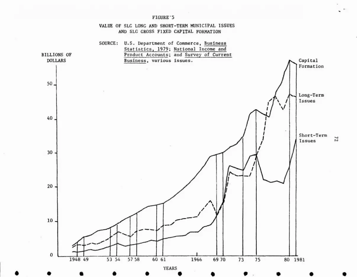
FIGURE-S

VALUE OF SLG LONG AND SHORT-TERM MUNICIPAL ISSUESAND SLG GROSS FIXED CAPITAL FORMATION

BILLIONS OFDOLLARS

SOURCE: U.S. Department of Commerce t BusinessStatistics, 1979; National Income andProduct Accounts; and Survey of CurrentBusiness t various issues.

••

Short-TermIssues

CapitalFormation

Long-TermIssues

80 1981

•75

•736970

•1966

"/ \/ \

/,...---_/

60 61

YEARS

•••53 54 57 58

•1948 49

o

20

30

40

50

10

••

•73

• borrowing, reduced liquidity levels and issued short-term debt. There

is little evidence of tax increases, current expenditure reductions, or

capital spending reductions.

• A similar survey of state and local governments was taken in 1970,

72after another period of unsettled credit conditions. Again, it was

found that state and local governments significantly reduced their • planned long-term borrowing without a similar reduction in planned

capital spending. In 1969, however, short-term borrowing predominated

over borrowing postponement and reduced liquidity as the method of • alternative financing. Our data confirm these points. Figure 4 shows a

rise in municipal yields in 1969 that was unprecedented at the time.

Clearly credit conditions were unsettled. Long-term debt, shown in • Figure 5, records a sharp drop in 1969, while short-term debt shows a

substantial increase. This is consistent with the idea that state and

local governments used short-term as a substitute for long-term debt. • Capital spending did not decline, although its growth rate was reduced.

It is likely that while capital spending reductions were small

relative to borrowing reductions in 1969, they were larger than the• spending reductions which occurred in 1966. Continued tightness in

credit markets may have had a cumulative effect on the financial

strength of state and local governments. Such tightness did continue• after 1966, and by 1970 municipal yields were twice their 1965 level.

In addition, the liquidity ratio was at its lowest point in ten years in

• 1969. State and local government officials may have been less inclined

to speculate on a drop in long-term rates after five years of rapid

increase by issuing short-term debt. They could not resort to liquidity

•

•74

financing as r~adi1y with liquidity levels so low. A reduction in • planned capital spending became an option more often used in 1969 then

it was in 1966.

The problems of state and local governments with credit markets • intensified during the 1970s. As of 1974 the liquidity ratio was still

relatively low at

between 1970 and

.48.

1973.

As shown in Figure 4. the municipal yield fell

but remained several points higher than the • stable rate of the early 1960s. The yield again"jumped to new record

levels by 1975. The depth of

problems for state and local

the 1973-1975

governments.

recession

Commercial

caused

banks

new

and • insurance companies experienced sharp drops in profits during this

period. These institutions are usually the prime source

municipal debt, wh tel-} is used as a tax-free shelter for

of demand for

income. With • little income to pr0tect from taxes, banks and insurance companies cut

their demand for tax-free municipal bonds. State and local governments

turned to individual buyers to market their long-term debt. Since these •

new buyers were generally in lower tax brackets than were the

institutions,

securities. 73

municipal yields

The spread between

moved

these

closer to those of taxable

rates usually diminishes during •

recessions and increases during expansions, but the 1973-1975 recession

was

on

so serious that the

municipals, there

spread disappeared.

was no difference

In spite of the tax savings

between the taxable and •

non-taxable interest rates. Long-term borrowing became expensive for

state and local governments.

In 1969 state and local governments substituted short-term debt for •

long-term debt. With the New York City fiscal crisis of 1975. the

•

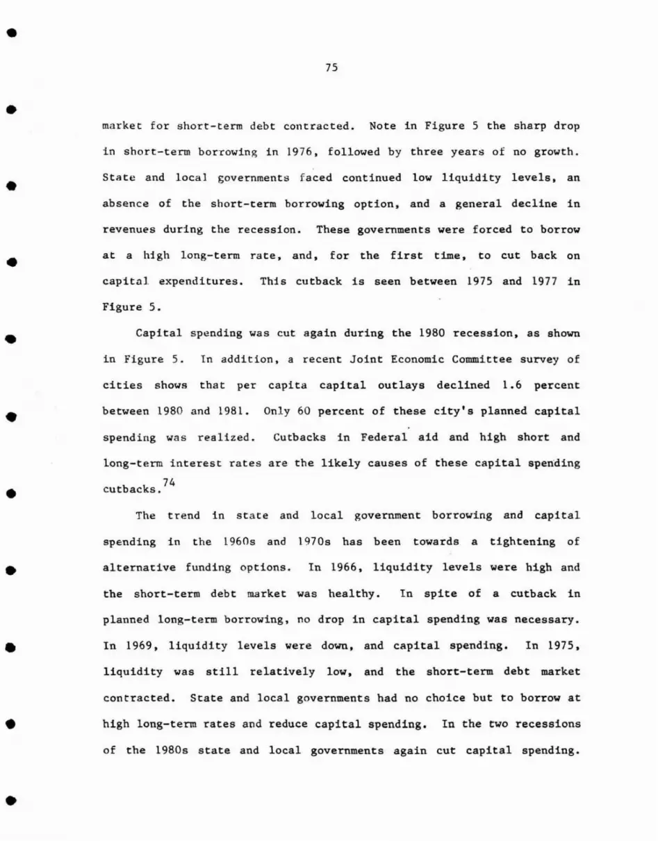
•75

• market for short-term debt contracted. Note in Figure 5 the sharp drop

in short-term borrowing in 1976, followed by three years of no growth.

• State and local governments faced continued low liquidity levels, an

absence of the short-term horrowing option, and a general decline in

revenues during the recession. These governments were forced to borrow

• at a high long-term rate, and, for the first time, to cut back on

capital expenditures. This cutback is seen between 1975 and 1977 in

Figure 5.

• Capital spending was cut again during the 1980 recession, as shown

in Figure 5. In addition, a recent Joint Economic Committee survey of

cities shows that per capita capital outlays declined 1.6 percent

• between 1980 and 1981. Only 60 percent of these city's planned capital

spending was realized. Cutbacks in Federal aid and high short and

long-term interest rates are the likely causes of these capital spending

• cutbacks. 74

The trend in state and local government borrowing and capital

spending in the 1960s and 1970s has been towards a tightening of

• alternative funding options. In 1966, liquidity levels were high and

the short-term debt market was healthy. In spite of a cutback in

planned long-term borrowing, no drop in capital spending was necessary.

• In 1969, liquidity levels were down, and capital spending. In 1975,

liquidity was still relatively low, and the short-term debt market

contracted. State and local governments had no choice but to borrow at

• high long-term rates and reduce capital spending. In the two recessions

of the 1980s state and local governments again cut capital spending.

•

•76

• Reducing capital spending during recessions now appears to be an action

state and local governmentB will continue to take.

Conclusions • The main finding of the ACIR study, State-Local Finances in

Recession and Inflation, is that the combined fiscal effects of • recession and inflation on aggregate state and local government finances

are not flexcessively severe. ,,75 While this result correctly describes

their findings, it may be misleading. Indeed, the conclusions one might • draw from thiB chapter are that the effects of inflation and recession

are quite severe for certain types of state and local governments and

may be a substantial and increaRing problem for the entire sector. • Studies of the 1973-1976 period place the revenue loss due to

recession at S to 10 percent of total state and local government

revenues, with the 10 percent loss a more realistic estimate at the • height of the recession. For some governments, notably those located in

the declining regions and state governments with highly elastic tax

structures, the revenue loss was estimated to be as high as 20 percent. • Little impact on state and local government expenditures could be found.

Several conclusions might be drawn from these results. First, even a 5

to 10 percent loss in revenue potential is considerable and a IS to 20 • percent loss is disastrous. Second, many of those states which have

elastic revenue structures and are therefore most susceptible to

recession impacts are located in the declining region. Third, even • these estimates understate the fiscal impact of recession in that they

show the loss in revenue potential but do not adjust for the

•

•77

• discretionary actions taken by these governments in the face of revenue

loss. Hence. the actual revenue growth in Massachusetts may be 20

percent less than its full employment/noninflationary amount in 1976,

• but the gap may have been 30 percent if the state and local governments

had not increased tax rates tn make up for some of the loss. Finally

• expenditure impacts have not been estimated as important, yet most

surveys show the recession induced important program cutbacks and

deferrals.

• The inflation studies are also subject to the problem of whether

and how to count the induced fiscal adjustments resulting from rising

prices. The best research seems to imply an impact resulting in a 5 to

• 10 percent loss in purchasing power of state and local government

revenues during the 1971-1974 period. The effect cooled off thereafter

and inflation-induced revenue and expenditure increases were about

• parallel bet~een 1974 and 1976. There have been no thorough, comparable

studies since 1975. At least three important implications for the

future might be drawn from this work: local governments which are more

• labor intensive and mor~ reliant on property taxation will be hurt most;

when the inflation rate rises to high levels the impact on expenditures

outstrips that on revenues; inflation induces service level cutbacks

• which may have longer run effects on the viability of local economies.

One cannot easily infer the future from these studies, and there

are no reliable models which allow forecasts. But these results do give

• some basis for judging the probable impacts of inflation and business

cycles on state and local government finances. Inflation rates are

likely to remain high (relative to real GNP growth) in the near future.

•

•78

• This will harm local governments most because of their labor intensive

expenditure base and their reliance on the property tax. Especially if

inflation and slow economic growth combine to keep real private earnings

• from growing, there will be heavy voter resistance to discretionary

attempts to capture the inflation-induced growth in property values.

Among local governments, thosE' wi th already high property tax rates and • little new construction, and those with stronger public employee

unions--the older central cities--will be hurt most.

A buffer against this inflation effect is the possibility of • increased state aid since inflation could increase state revenues by

more than it increases a much less labor-intensive expenditure base.

The states that stand to gain most are those with progressive income tax • structures, broad-based sales taxes, and relatively less' direct

expenditure responsibility. This includes many of the older states in

the north, but there is some question about the ability of these states • to withstand further increases in the effective tax rate. Indeed, New

York is a good example of a state whose progressive tax structure has

captured inflation-induced revenue increases but where an already high • average tax rate has forced tax reductions. Still, we are led once

again to the conclusion that state government discretionary action will

play a pivotal role in determining local government fiscal health. • If inflation occurs in concert with recession, the situation is

altered to the detriment of state governments because they lose some of

the revenue increments capt1lrtcd by inflation. Those states with the • less elastic revenue structurp.~ suffer less from recession, but on the

other hand, they gain less frem inflation. The most important feature

•

•79

• of recession, hO'Never, is that some state and local governments suffer

mor.e than others. Again, it is those governments in the declining

• regions whose economies suffer most during recession. Therefore, older

central citie~ suffer disproportionately heavier revenue losses during

recession and are located in states 'Nhich are likely to be facing a

• similar situation, therefore reducing the chances for marked increases

in state aj d. If thi~ comes at a time when inflation is driving up

local costs but having little effect on property tax revenues, these

• central cities become doubly-Jamned.

•

•

•

•

•

80

FOOTNOTES

*This paper draws from Chapter IV of Roy Bahl, State and LocalGovernment Finances in a Changing National Economy (New York: OxfordUniversity Press, forthcoming); and Larry DeBoer. "The Response of Stateand Local Government Finances to Economic Fluctuations" (SyracuseUniversity, Ph.D. dissertation, 1983).

**Professor of Economics and Publ ie Administration, and Director,Metropolitan Studies Program, The Maxwell School, Syracuse University.

***Assistant Professor of Economics, Ball State University.

1Except in the case of graduated rate taxes where 'bracket creep'will increase tax burdens.

laThe r~ader not interested in the microeconomics of this issue mayskip this s~ction without significant loss in continuity.

2 .In other words, total income is divided first into a 'taxable' and

a 'nontaxable' component. The former, our concern here, is then dividedbetween private goods and taxes whereas the latter is out of reach ofthe public sector and is used exclusively for private goods. Thetaxable/non-taxable shares of total income are determined by the natureof the state and local government tax base, constitutional limits, etc.

3The conceptual problems with defining and using prices indexes tomeasure inflation in the public sector are considerably more complexthan imp lied here. For a thorough discussion, see David Greytak andBernard Jump, Jr., The Impact of Inflation on the Expenditures andRevenues of Six Local Governments, 1971-1974, Monograph No.4,Metropolitan Studies Program, The Maxwell School (Syracuse, New York:Syracuse University, December 1975).

4Unfortunately, the price indexes which would be used for such aconstruction (1. e., CPI, WPI) are not available on a government-by­government basis. Hence, one might be able to use these indexes toaccount for the different mix of expenditures of different localgovernments, but not for the differential rates of price increase indifferent regions of the county.

5See, for example, Bureau of Labor Statistics, "Autumn 1976 UrbanFamily Budgets and Comparative Indexes for Selected Urban' Areas"(Washington, D. C. : U. S. Department of Labor, April 27, 1977), pp.79-369.

6Greytak and Jump, The Impact of Inflation on the Expenditures andRevenues of Six Local Governments, 1971-1974.

•

•

•

•

•

•

•

•

•

•

•

•

•

•

•

•

•

•

•

•

•

81

7Multi-Year Financial Plan FY 1979-83, District of Columbia Government, September 1977; and Roy Bahl, Larry Schroeder, Marla Share and Anne Hoffman, "Local Government Revenue and Expenditure Forecasting: Washington. D.C." Occasional Paper No. 51, Metropolitan Studies Program, The Maxwell School (Syracuse. New York: Syracuse University, September 1981) .

8David Greytak. Richard Custely, and Robert J. Dinkelmeyer, "The Effect:s of Inflation on Local Government Expenditures," National Tax Joun,al, Vol. XXVII, No.4 (December 1974): 583-598; Roy Bahl, Alan Campb~ll and David Greytak. Taxes, Expenditures, and the Economic Base: A Case Study of New York City (New York: Praeger Publishers, 1974), chapters 3 and 4; David Greytak and Bernard Jump, Jr., "The Impact of Inflation on State and Local Government Finances, 1967-1974," Occasional Paper No. 25. Metropolitan Studies Program, The Maxwell School (Syracuse. New York: Syracuse University 1975); Greytak and Jump, The Impact of lnflation on the Expenditures and Revenues of Six Local Governments. 1.971-1974; David Greytak and Bernard Jump, Jr., "Inflation and Local Government Expenditures and Revenues: Methods and Case Studies," PUblic Finance Quarterly, Vol. 5, No.3 (July 1977): 275-30l.

<) Roy Bahl. Bernard Jump. _-rr., and Larry Schroeder, "The Outlook for

City Fiscal Performance in Dec~ining Regions." in The Fiscal Outlook for Cities. ed. by Roy Bahl (Syracuse, New York: Syracuse University Press, 1978). pp. 11-16.

10Robert Crider reached a similar conclusion with an index constructed by weighting components of local government compensation and other expenditures by the CPI and WPI. See The Impact of Inflation on State and Local Government. Urban and Regional Development Series No. 5 (Columbus, Ohio: Academy for Contemporary Problems, July 1978).

11 The other four local governments studied were Erie County, New York; Roanoke, Virginia; Urange County, California; and Atlanta, Georgia.

12Jan Chaiken and Warren Walker, "Growth in Hunicipal Expenditures: A Case Study of Los Angeles," The Rand Corporation (June 1979).

t3Cupoli, Peek and Zorn. An Analysis of the Effects of Inflation on Finances in Washin~ton. D.C.

14City of Dallas. Summary Long Range Financial Plan, 1979-80 to 1983-84 (Dallas, Texas: Office of Hanagement Services, August 1979); Roy Poahl, Larry Schroeder and Kurt Zorn, "Local Government Revenue Expenditure Forecast~,'g: Dallas, Texas," Occasional Paper No. 49, Metropolitan Studie~ Program, The Maxwell School (Syracuse, New York: Syracuse University. September 1981).

•

•82

•15scenario of percent increase used:The following in prices was

19131 1982 1983 1984

Personnel: High Inflation 7.5 7.0 6.5 6.SLow Tnf1ation 6.5 6.0 6.0 5.5 •

Non-Personnel: High Inflation 11.0 10.0 9.0 9.0Low Inflation 9.0 8.0 7.0 6.5

16The separation of automatic from dfscretionary changes in theestimation of revenue-income elasticities for state and localgovernments is discussed in Roy Bahl and Larry Schroeder, ForecastingLocal Government Budgets, Occasional Paper No. 38, Metropolitan StudiesProgram, The Maxwe 11 School (Syracuse, New York: Syracuse University1979) .

17 These are revieyed in Bahl and Schroeder, "Forecasting LocalGovernment Budgets."

18Advisory Conunission on Intergovernmental Relations, State-LocalFinances in Recession and Tnflation (Washington, D.C.: GovernmentPrinting Office, May 1979) •

. 9 .1 Robert C. Vogel, "The Responsivt!ness of State and Local Receipts

to Changes in Economic Activity: Extending the Concept of the FullEmployment Dudget," Joint Economic Committee of the U.S. Congress,Studies in Price Stability c1.nd Economic Growth (Washington, D.C.:Government Printing Office, June 1975); and Robert Vogel and RobertTrost, "The Response of State Government Receipts to EconomicFluctutions and the Allocation of Counter-Cyclical Revenue SharingGrants," The Review of Economics and Statistics, Vol. LXI, No.3 (August1979): 389-400.

19aFor a review of this literature, see Roy Bahl, Marvin Johnson andMichael Wasylenko, "State and Local Government Expenditure Determinants:The Traditional View and a New Approach," in Public Employment and Stateand Local Government Fj nance, ed. by Roy Bahl, Jesse Burkhead andBernard Jump, Jr. (Cambridge, Mass.: Ballinger Publishing Company,1980), pp. 65-111.

20Advisory Commission on Intergovernmental Relations, State-LocalFinances in Recession and Inflation, p. 34.

')1- Ib id., p. 38.

•

•

•

•

•

•

•

•

•83

•

•

•

•

•

•

•

•

•

12There also may be a lag in collective bargaining agreements which would cause these expenditure effects to be overestimated. Yet, it would be easier to believe that over the longer run public employee wage rates will catch up with those, in the private sector than to believe that property tax assessment lags will be eliminated.

24See Jesse Burkhead and Shawoa Grosskopf, "Trends in Public Employment and Compensation," in Public Employment and State and Local Government Finances, ed. by Roy BahI, Jesse Burkhead and Bernard Jump, Jr. (Cambridge, Mass.: Ballinger Publishing Co., 1980); and Shawna Grosskopf, "Public Employment Trends and Problems," in Urban Government Finances in the 1980s, ed. by Roy Bahl (Beverly Hills, California: Sage Publications, 1981).

25See Ronald Ehrenberg, "The Demand for State and Local Government Employees," American Economic Review 63 (June 1973).

')6 ... See, for ex~mple, R. Ehrenberg, "Municipal Government Structure,

Unionization, and the \-lages of Firefighters," Industrial and Labor Relations Revjew (October 1973).

27The assumption of a constant labor share of total expenditures has been studied. See Thomas Borcherding and Robert Deacon, "The Demand for Services of Non-Federal Governments," American Economic Review 62 (December 1972).

28Greytak. Gustely. and Dinkelmeyer, "The Effects of Inflation on Local Government 'Expenditures."

29Greytak and Jump, Jr. , "Inflation and Local Government Expenditures and Revenues: Hethods and Case Studies."

30Edward M. Cupoli, v1illiam A. Peek and C. Kurt Zorn, "An Analysis of the Effects of Inflation on Finances in Washington. D.C.," Occasional Paper No. 36, Metropolitan Studies Program. The Maxwell School (Syracuse. New York: Syracuse University, April 1979).

31George Peterson, "Capital Spending and Capital Obsolescence: The Outlook for Cities," in The Fiscal Outlook for Cities, ed. by Roy Bahl (Syracuse, New York: Syracuse University Press, 1978), pp. 49-74.

32Karen Davis and Cathy Schoen. Health and the War on Poverty: A Ten Year Appraisal (Washington, D.C.: Brookings Institute, 1978), Chapter 3.

33For detail on this pattern of growth, see Ann Kalman Bixby, "Social Welfare Expenditures, Fiscal Year 1979," Social Security Bulletin, Vol 44, No. 11 (November 1981): 3-12.

•

84

•

34An early article which doesresponses is Melvin ~bite andfluctuations on Municipal Finance,"

separate automatic and discretionaryAnne White, "Impact of EconomicNational Tax Journal 7 (March 1954).

•

35Gramli~h compares the countercyclical response of state and localbudgets to the automatic stahilizers in the Federal budget. See EdwardM. Gramlich. "The New York City Fiscal Crisis: What Happened and Whatis to be Done?" American Economic Review 66 (May 1976).

36See Alvin Hansen and Harvey Perloff, State and Local Finance in

the National Economy (New York: W.W. Norton and Co., 1944).

37Mabel Newcomber, "State and Local Financing in Relation to

Economic Fluctuations." National Tax Journal 7 (June 1954); and EugeneMyers and Randall Stout, "The Role of States and Local Governments inNational Fiscal Policy." National Tax Journal 10 (June 1957).

38'James A. Maxwell. "Countercyclical Role of State and I.ocal

Governments," National Tax Journal 11 (December 1958); Morton Baratz andHelen Farr, "Is Municipal Fi.nnnce Fiscally Perverse?" National TaxJournal 12 (September 1959).

39Robert W. Rnfuse. Jr. • "Cyclical Behavior of State-Local

Firian~e." in Essays in Fiscal Federali sm, edited by Richard Musgrave(Washington, D.C.: The Brookings Institution, 1965); and Ansel Sharp,"The Eehavior of Selected State and Local Fiscal Variables During thePhases of the Cycles 1949-61," in 1965 Proceedings of the Fifty-EighthAnnual Conference on Taxation (Harrisburg, Pa.: National TaxAssociation. 1966).

40See Baratz and Farr, "ls Municipal Finance Fiscally Perverse?"Natiunal Tax Journal. 12 (September 1959).

4~ennis Zinunennan, "The Sensitivity of the State-Local Tax Systemto Economic Activity: Experi ence From the Great Depression to the1970s," in The Business Cycle and Public Policy, 1929-80, U.S. Congress,Joint Economic COMmittee (Washington, D.C.: Government Printing Office,1980) .

42Rafuse, "Cyclical Behavior of State-Local Finances"; and Sharp,

"The Behavior of Selected State and Local Fiscal Variables During thePhases of the Cycles ]949-61."

43Roy Bahl, Alan Campbell, David Greytak, Bernard Jump, Jr., and

David Puryear, "Impact of Economic Base Erosion, Inflation andRetirement Costs on Local Governments," Testimony: Fiscal Relations inthe American Federal System: Hearings before a Subcommittee onGovernment Operations. House of Representatives, 94th Congress t FirstSession, July 15, 1975.

•

•

•

•

•

•

•

•

•

•

•85

44David T. Stanley, "Running Short, Cutting Down: Five Cities in

Financial Distress" (Washington, D.C.: The Brookings Institution, March 1979), unpublished manuscript.

45U• S . Senate Committee on Government Operations, Subcommittee on Interp,overnmental Relations, Intergovernmental Anti-Recession Assistance • Act of 1975, Hearings on S. 1359 94th Congress, 1st Session (Washington, D.C.: Government Printin~ Office, 1975); U.S. House of Representatives, Committee on Government Operations, Subcommittee on Intergovernmental Relations

• Anti-Recession Assistance Act Bills, 95th Congress, 1st Printing Office, March 1, 2,

46U.S. Congress, Joint

Affairs, The Current Fiscal

and Human Resources, Intergovernmental of 1977, Hearings on H.R. 3730 and Related Session (Washington, D.C.: Government

and 8, 1977), pp. 143-292.

Economic Committee, Subcommittee on Urban Position of State and Local Governments,

Survey of 48 State Governments and 140 Local Governments, 94th Congress,• 1st Session (Washington, D.C.: Government Printing Office, December 17, 1975) .

47 U. S . Senate, Committee on Governmental Affairs, Subcommittee on Intergovernmental Relations, The Counter-Cyclical Assistance Program:

• An Analysis of Its Initial (Washington, D.C.: Government

48U.S. Congress, Joint Survey: Fiscal Condition of 48 (Washington. D.C.: Government

•

Impact, 95th Congress, 1st Session Printing Office, February 28, 1977).

Economic Committee, Emergency Interim Large Cities, 97th Congress, 1st Session

Printing Office, January 14, 1982).

49preliminary results reported in Municipal Finance Officers Association, Resources in Review (Washington, D.C.: MFOA, 1982), p. 11.

50Stephen Cold and Karen Benker, State Fiscal Conditions as State

Entered 1982 (Denver: National Conference of State Legislatures, 1982).

• 51Tax Foundation, Tax Review, Vol. XLII, No.8

•

52Kathryn Nelson and Clifford Patrick, Employment During the 1969-1972 Business Cycle: Regional Record (Oakridge, Tennessee: Oakridge June 1975), p. 15.

(September 1981).

Decentralization of The National and

National Laboratory,

53John C. Zamzow, "The Current Recession: Its Regional Impact," Testimony for Subcommittee on Fiscal and Intergovernmental Policy of the Joint Economic Committee, October 16, 1979; and Bah1, Jump and Schroeder, "The Outlook for City Fiscal Performance in Declining • Regions."

•

•86

54U•S. Congress. Joint Economic Committee. Subcommittee on Urban Affairs, The Current Fiscal Position of State and Local Governments, Survey of 48 State Governments and 140 Local Governments, 94th Congress, 1st Session (Washington, D.C.: Government Printing Office, December 17, 1975).

55U • 5 • Congress, Joint Economic Committee. Subcommittees on Economic Growth and Stabilization and on Fiscal and Intergovernmental Pol icy, The Current Fiscal Condition of Ci t:les: A Survey of 67 of the 75 Largest Cities, 95th Congress. 1st Session (Washington, D.C.: Government Print1ng Office, July 28, 1977).

56U. 5 • Congress, Joint Economic Committee, Emergency Interim Survey: Fiscal C.ondition of 48 Large Cities, 97th .Congress, 1st Session (Washington, D.C..: Government Printing Office, January 14, 1982).

57National Association of State Budget Officers, State Fiscal Survey Fiscal Years 1975, 1976 and 1977. Summary Report (Lexington, KY: National Association of State Budget Officers, February 1977), p. 3.

58The Comptroller General of the United States, Report to Congress, Antirecession Assistance is Helping but Distribution Formula Needs Reassessment (\~ashington, D.C.: General Accounting Office, July 20, 1977). For more details, see The Comptroller General of the United States, Impact of Antirecession Assistance on 15 State Governments, Impact of Antirecession Assistance on 16 County Governments: and Impact of Antirecession Assistance on 21 City Governments (Washington, D.C.: General Accounting Office, February 22, 1978).

59The percentage changes shown in Table 7 are average annual percent changes calcu] Clted from the quarterly National Income Account series. For example. the 1Q73-IV to 1975-1 recession lasted 5 quarters. The average quarterly change in GNP over that period was -1.17 percent, which is a -4.58 annual rate. National peak and trough dates are available in U.S. Department of Commerce, Bureau of Economic Analysis. Business Conditions Digest, a monthly publication. As the time of this writing the peak and trou~h dates of the current recession have not been determined. The second quarter of 1981 is used as the peak of this recession, and the average annual percent change is calculated using the last observation in the data series.

60See, for example, U.S. President, Economic Report of the President. 1977.

6~ogel, "The Responsiveness of State and Local Receipts to Changes in Economic Activity: Extending the Concept of the Full Employment Budget"; and Vogel and Trost, "The Response of State Government Receipts to Economic Fluctuations and the Allocation of Counter-Cyclical Revenue Sharing Grants."

•

•

•

•

•

•

•

•

•

•

•87

• 62Crider, The Impact of Recession on State and Local Finance.

63Vogel's estimated equation is

InR = 3.04 + 0.0151 lnR + 1.39 lnP + 0.37 In(GAP)• (61. 2) (34.7) (10.4)

R2 .. 0.99 m-l = 1.27

The ACIR equation is shown on page 27.

BahI, Jump and Schroeder, "The Outlook for City Fiscal• 64

Performance in Declining Regions."

65ACIR , State-Local Finances in Recession and Inflation, pp. 80-81.

66

• 67

Cri.der, The Impact of Recession on State and Local Finance.

Paul Schneiderman, "State and Local Government Gross Fixed CapitCll Formation: 1958-73," Survey of Current Business 55 (October 1975) .

68~1anuel Gottlieb, "Cyclical Timing of Municipal Bond Issues," The

Quarterly Review of Economics and Business 1 (May 1961).• 69Paul McGouldrick and John Peterson, "Monetary Restraint and

Borrowing and Capital Spending by Larr,e State and Local Governments in 1966," Federal Reserve Bulletin 54 (July 1968).

Gottlieb, "Cyclical Timing of Municipal Bond Issues."• 70

71Crider, The Impact of Recession on State and Local Finance.

72John Peterson, "Response of State and Local Governments to

• Varying Credit Conditions," Federal Reserve Bulletin 57 (March 1971).

73Lynn Browne and Richard Syron, "Big City Bonds After New York," New England Economic Review (July/August 1977).

74U.S. Congress. Joint Economic Committee. Trends in the Fiscal -::C-:o:-::n",,:"d_i_t_i_on=-,=,"0,=,"f~C;..,;i;..,;t;;..i_e....;;s_:__1-,9_8_0_-_8_2 (Washington, D. C. : Government Printing• Office, 1982).

75ACIR , State-Local Finances in Recession and Inflation, pp. 80-81. It should be noted that they caution and demonstrate that this conclusion does not hold for all states.

•

•

•

•

•

•

•

•

•

•

•

•

•