Advances in Engineering Software 78 (2014) 41–51

Contents lists available at ScienceDirect

Advances in Engineering Software

journal homepage: www.elsevier .com/locate /advengsoft

Optimization of mixed integer nonlinear economic lot schedulingproblem with multiple setups and shelf life using metaheuristicalgorithms

http://dx.doi.org/10.1016/j.advengsoft.2014.08.0040965-9978/� 2014 Elsevier Ltd. All rights reserved.

⇑ Corresponding author at: Centre of Advanced Manufacturing and MaterialProcessing (AMMP Centre), University of Malaya, 50603 Kuala Lumpur, Malaysia.Tel.: +60 126283265; fax: +60 379675330.

E-mail addresses: maryam_mohammadi@siswa.um.edu.my (M. Mohammadi),nurmaya@um.edu.my (S.N. Musa), bahreininejad@um.edu.my (A. Bahreininejad).

Maryam Mohammadi, S. Nurmaya Musa, Ardeshir Bahreininejad ⇑Centre of Advanced Manufacturing and Material Processing (AMMP Centre), University of Malaya, 50603 Kuala Lumpur, MalaysiaDepartment of Mechanical Engineering, Faculty of Engineering, University of Malaya, 50603 Kuala Lumpur, Malaysia

a r t i c l e i n f o a b s t r a c t

Article history:Received 31 March 2014Received in revised form 24 July 2014Accepted 13 August 2014

Keywords:Economic lot scheduling problemMultiple setupsGenetic algorithmParticle swarm optimizationSimulated annealingArtificial bee colony

This paper addresses the economic lot scheduling problem where multiple items produced on a singlefacility in a cyclical pattern have shelf life restrictions. A mixed integer non-linear programming modelis developed which allows each product to be produced more than once per cycle and backordered. How-ever, production of each item more than one time may result in an infeasible schedule due to the over-lapping production times of various items. To eliminate the production time conflicts and to achieve afeasible schedule, the production start time of some or all the items must be adjusted by either advancingor delaying. The objective is to find the optimal production rate, production frequency, cycle time, as wellas a feasible manufacturing schedule for the family of items, in addition to minimizing the long-run aver-age cost. Metaheuristic methods such as the genetic algorithm (GA), simulated annealing (SA), particleswarm optimization (PSO), and artificial bee colony (ABC) algorithms are adopted for the optimizationprocedures. Each of such methods is applied to a set of problem instances taken from literature andthe performances are compared against other existing models in the literature. The computational per-formance and statistical optimization results shows the superiority of the proposed metaheuristic meth-ods with respect to lower total costs compared with other reported procedures in the literature.

� 2014 Elsevier Ltd. All rights reserved.

1. Introduction

Economic lot scheduling problem (ELSP) is concerned withscheduling the production of multiple items in a single facility ona periodical basis with the restriction that one item is producedat a time. Narro Lopez and Kingsman [1] provided an excellentreview of this problem and the solution approaches. Throughoutthe past half century, a considerable amount of research on thisproblem has been published with several directions of extensions.Subsequently, various heuristic approaches have been suggestedusing any of the basic period approach [2], common cycle approach[3], or time-varying lot size approach [4]. This study deals withcommon cycle approach, where the objective is to determine theoptimal cycle time.

In industry, products are stocked and used up during the pro-duction cycle. If they are stored more than a specified period of

time, some products may get spoiled. This time restriction of lifefor a product is called shelf life. Shelf life constraints directly influ-ence the wastage, out-of-stock rates, and inventory levels [5]. Gen-erally, the inventory systems assume implicitly unlimited shelflives for the stored items. However, storing products beyond a spe-cific shelf life may bring about the deterioration or diminution ofthe products. It might also lead to loss of the profitable or fruitfullife of a product in an emerging market of new competitive prod-ucts [6]. Therefore, when the optimal cycle time goes beyond thetime restriction of life for an item, the cycle time period must bedecreased to less than or equal to the shelf life to ensure a feasibleschedule. This storage time can be lowered by regular restocking ofthe items, and subsequently decreasing the inventory maintainedin the stock [7].

Silver [8] studied the ELSP with shelf life constraint while disal-lowing the production cost under the postulation that the produc-tion rate variation does not impose any further cost. Two options ofdecreasing the cycle time and the production rate were investi-gated, and it was concluded that it is more cost-efficient to reducethe production rate. Sarker and Babu [7] exploited the Silver’smodels [8,9] by considering production time cost, and a limited

42 M. Mohammadi et al. / Advances in Engineering Software 78 (2014) 41–51

shelf life for each item. They found that when the production costis included into the model, it might be more efficient to reduce thecycle time rather than the manufacturing rate.

Goyal [10] investigated the results obtained by Sarker and Babu[7], and suggested that their proposed model can be improved byallowing the production of items more than one time in a cycle.Viswanathan [11] implied that Sarker and Babu’s model [7] offersa feasible schedule only when all the items produced have thesame frequency. Viswanathan [11] also stated that althoughGoyal’s suggestion [10] can incur a lower inventory cost, hismethod does not assure a feasible production schedule. Yan et al.[12] tackled the problem of schedule infeasibility, and made theproduction of each item more than once in every cycle permissible.Yan et al. [12] indicated that advancing or delaying the manufac-turing start times of some items can lead to a feasible productionplan. Accordingly, costs associated to the adjustment schedulemust be taken into account.

Since ELSP is categorized as NP-hard [13] which leads to diffi-culty of checking every possible schedule in a reasonable amountof computational time, recently, metaheuristic algorithms havebeen implemented effectively to solve the problem.

Khouja et al. [14] proposed a genetic algorithm (GA) for solv-ing the ELSP applying the basic period approach, and showed thatthe GA is appropriate for solving the problem. Moon et al. [15]addressed the ELSP based on the time-varying lot size method,and suggested a hybrid genetic algorithm (HGA) to solve themodel. The obtained results by the HGA surpassed the best-known Dobson’s heuristic [16]. Chatfield [17] proposed a GA,namely, genetic lot scheduling procedure, to solve the ELSP usingthe extended basic period (EBP) approach. Their method wascompared with the well-known benchmark problem presentedby Bomberger [18]. The results outlined that the proposedapproach offers better optimization reliability. Jenabi et al. [19]solved the ELSP in a flow shop setting utilizing the HGA and sim-ulated annealing (SA) algorithm. Their computational resultsindicated the superiority of the proposed HGA compared to theSA with respect to the solution quality. However, the proposedSA outperformed the HGA in terms of the required computationaltime.

Chandrasekaran et al. [20] investigated the ELSP with the time-varying lot size approach and sequence-independent/sequence-dependent setup times of parts, and applied the GA, the SA, andthe ant colony optimization (ACO) algorithms. The computationalperformance analyses revealed the effectiveness of the proposedmetaheuristic methods. Raza and Akgunduz [21] examined theELSP with time-varying lot size approach using the SA, and con-ducted a comparative study of heuristic algorithms on the prob-lem. They compared the results with Dobson’s heuristic [16] andMoon et al. [15], and concluded that the SA finds the best-knownsolution for the suggested problem. Bulut et al. [22] proposed aGA for the ELSP under the EBP approach and power-of-two (PoT)policy. The experimental results showed that the proposed GA ishighly competitive to the best-performing algorithms from theexisting literature under the EBP and PoT policy.

To the best of the authors’ knowledge, there has been noresearch on the ELSP with multiple products having various pro-duction frequencies, and respecting the shelf life and backorderingconstraints using the metaheuristic methods. In this paper, theproposed ELSP model by Yan et al. [12] is modified. A computa-tional study of the well-known metaheuristic algorithms, namelythe GA, the SA, the particle swarm optimization (PSO), and the arti-ficial bee colony (ABC) algorithms are presented to solve the pro-posed model. Accordingly, the performance of the best existingapproach presented by Yan et al. [12] and the proposed metaheu-ristic algorithms are evaluated and compared.

The rest of this paper is organized as follows: Section 2 presentsthe mathematical formulation. In Section 3, applied methodsare explained. Section 4 demonstrates numerical examples and dis-cusses the computational results. Finally, conclusions are given inSection 5.

2. Problem description and model formulation

In this section, a mathematical model for the ELSP is presentedbased on the integration and modification of the models presentedby Goyal [10] and Yan et al. [12]. Consider N types of items are pro-duced on a single machine in the manufacturing cycle time of T,investigating the effect of constituent costs in an inventory systemwith shelf life constraint and production of items more than oncein a cycle. The objective is to minimize the total cost, in additionto obtaining a feasible production schedule, the optimum produc-tion frequency, production rate, backorder level, batch size for eachitem, and optimal production cycle time for the family of itemsusing optimization engines.

The mathematical model studied throughout the paper is basedon the following assumptions and notations:

Assumptions

i. Each item has a deterministic and constant demand

rate

ii. Each item has a deterministic and constant setup time iii. Each item has a finite production rate iv. Each item is produced per cycle v. Each item has a specified shelf life vi. Backordering is permissible vii. The first in first out (FIFO) rule is considered for the

inventory transactions

Indices

i Product (i = 1, 2, . . ., N) N Total number of products b, w Production batch ðb;w ¼ 1;2; . . . ;x ¼

PNi¼1uiÞ

j

Batch number (j = 1, 2, . . ., ui)

Parameters

Di Demand rate for item i (units/year) Pmax

i

Maximum possible production rate for item i (units/year)

Rmini

Ratio of demand to maximum production rate

Li

Shelf life of item i (years) ti Setup time for item i (years) Si Setup cost for item i (dollars/year) Hi Inventory holding cost for item i (dollars/unit/year) Bi Backordering cost for item i (dollars/unit/year) O Machine operating cost (dollars/year)

Variables

pi Production rate for item i ri Ratio of demand to production rate for item i ui Production frequency for item i per cycle si Cycle time for item i 1i Production start time for item i Qi Production batch size for item i Mi Maximum backorder level for item i ki Machine time for item i Xi Production time for item i cb

i

1; if item i is produced in the bth batch0; otherwise

�

aji

Production start time advancement for item i in its jth

production batch

M. Mohammadi et al. / Advances in Engineering Software 78 (2014) 41–51 43

bji

Production start time delay for item i in its jth

production batch

T Entire production cycle time CðTÞ Total cost over the entire production cycle time

2.1. Objective function

CðTÞ ¼ OXN

i¼1

ri þ1T

XN

i¼1

ðSi þ OtiuiÞ þT2

XN

i¼1

HiDiBið1� riÞuiðHi þ BiÞ

þ 1T

XN

i¼1

Hi þ Bi

2Di

Xui

j¼1

ðajiÞ

2þXui

j¼1

ðbjiÞ

2 !

ð1� riÞ !

ð1Þ

The objective function aims at minimizing the total cost whichcomprises of machine operating, setup, inventory holding, andbackordering costs, in addition to an adjustment cost in case ofoverlapping production times of different items which leads toan infeasible schedule. A detailed description for the adjustmentcost can be found in Yan et al. [12].

2.2. Constrains

For a feasible solution, the total setup time and production timefor N products cannot go beyond the cycle time T [8], that is:

XN

i¼1

tiui þ TDi

pi

� �6 T ð2Þ

Eq. (2) can be rearranged as:

PNi¼1tiui

1�PN

i¼1ri

6 T ð3Þ

where ri ¼ Dipi

.

1�PN

i¼1ri is the long-run proportion of time available for set-

ups. For infinite horizon problem 1�PN

i¼1ri

� �> 0 is necessary

for the existence of a feasible solution [15].Therefore, it is necessary that:

XN

i¼1

ri < 1 ð4Þ

The adopted production rate for each item should not exceedthe maximum possible production rate. Hence:

pi 6 Pmaxi for i ¼ 1;2; . . . ;N ð5Þ

or,

Rmini 6 ri for i ¼ 1;2; . . . ;N ð6Þ

where Rmini ¼ Di

Pmaxi

.It is assumed that:

XN

i¼1

Rmini 6 1 ð7Þ

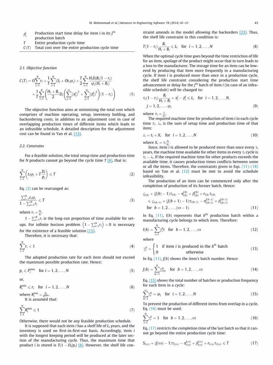
Otherwise, there would not be any feasible production schedule.It is supposed that each item i has a shelf life of Li years, and the

inventory is used on first-in-first-out basis. Accordingly, item iwith the longest keeping period will be produced at the later sec-tion of the manufacturing cycle. Thus, the maximum time thatproduct i is stored is T(1 � Di/pi) [8]. However, the shelf life con-

straint amends in the model allowing the backorders [23]. Thus,the shelf life constraint in this condition is:

Tð1� riÞBi

Hi þ Bi6 Li for i ¼ 1;2; . . . ;N ð8Þ

When the optimal cycle time goes beyond the time restriction of lifefor an item, spoilage of the product might occur that in turn leads toa loss to the manufacturer. The storage time for an item can be low-ered by producing that item more frequently in a manufacturingcycle. If item i is produced more than once in a production cycle,the shelf life constraint considering the production start timeadvancement or delay for the jth batch of item i (in case of an infea-sible schedule) will be changed to:

sið1� riÞBi

Hi þ Biþ aj

i � bji 6 Li for i ¼ 1;2; . . . ;N;

j ¼ 1;2; . . . ;ui ð9Þ

where si ¼ Tui

.The required machine time for production of item i in each cycle

time si; ki, is the sum of setup time and production time of thatitem:

ki ¼ ti þ Xi for i ¼ 1;2; . . . ;N ð10Þ

where Xi ¼ siDipi:

Since, item i is allowed to be produced more than once every si

years, the machine time available for other items in every si cycle issi � ki. If the required machine time for other products exceeds theavailable time, it causes production times conflicts between someor all the items. Therefore, the constraints given in Eqs. (11)–(18)based on Yan et al. [12] must be met to avoid the scheduleinfeasibility.

The production of an item can be commenced only after thecompletion of production of its former batch. Hence:

1IðbÞ þ ðJðbÞ � 1ÞsIðbÞ � aJðbÞIðbÞ þ bJðbÞ

IðbÞ þ rIðbÞsIðbÞ

6 1Iðbþ1Þ þ ðJðbþ 1Þ � 1ÞsIðbþ1Þ � aJðbþ1ÞIðbþ1Þ þ bJðbþ1Þ

Iðbþ1Þ

for b ¼ 1;2; . . . ; ðx� 1Þ ð11Þ

In Eq. (11), I(b) represents that bth production batch within amanufacturing cycle belongs to which item. Therefore:

IðbÞ ¼XN

i¼1

cbi i for b ¼ 1;2; . . . ;x ð12Þ

where

cbi ¼

1 if item i is produced in the bth batch0 otherwise

(ð13Þ

In Eq. (11), J(b) shows the item’s batch number. Hence:

JðbÞ ¼Xb

w¼1

cwIðbÞ for b ¼ 1;2; . . . ;x ð14Þ

Eq. (15) shows the total number of batches or production frequencyfor each item in a cycle:Xxb¼1

cbi ¼ ui for i ¼ 1;2; . . . ;N ð15Þ

To prevent the production of different items from overlap in a cycle,Eq. (16) must be used:XN

i¼1

cbi ¼ 1 for b ¼ 1;2; . . . ;x ð16Þ

Eq. (17) restricts the completion time of the last batch so that it can-not go beyond the entire production cycle time:

SIðxÞ þ ðJðxÞ � 1ÞsIðxÞ � aJðxÞIðxÞ þ bJðxÞ

IðxÞ þ rIðxÞsIðxÞ 6 T ð17Þ

44 M. Mohammadi et al. / Advances in Engineering Software 78 (2014) 41–51

It should be noted that for attaining production feasibility pro-duction start time for a batch can be either advanced or delayed,but both cannot occur. Therefore:

aji � b

ji ¼ 0 for i ¼ 1;2; . . . ;N; j ¼ 1;2; . . . ;ui ð18Þ

Eq. (19) can be used to obtain the lot size for each item:

Q i ¼ Disi for i ¼ 1;2; . . . ;N ð19Þ

The optimum backorder level for each item can be expressed as Eq.(20):

Mi ¼ siDið1� riÞHi

Hi þ Bifor i ¼ 1;2; . . . ;N ð20Þ

Constraints (21) are the non-negativity constraints:

T P 0ri � 0 for i ¼ 1;2; . . . ;N

aji;b

ji � 0 for i ¼ 1;2; . . . ;N; j ¼ 1;2; . . . ;ui

ui > 0 integer for i ¼ 1;2; . . . ;N

ð21Þ

3. Applied metaheuristic algorithms

The formulation given in Section 2 is a nonlinear mixed integerprogramming problem. These characteristics justify the model tobe adequately hard to be solved using exact methods. To deal withthe complexity and find near-optimal results in a reasonable com-putational time, metaheuristic approaches are widely used forwhich the GA, the SA, the PSO and the ABC algorithms areexplained in the following subsections.

3.1. Genetic algorithm

Genetic algorithm (GA) is a stochastic search technique basedon the natural evolutionary processes. Fundamental of the GAwas primarily instated by Holland [24]. Simplicity and capabilityof finding quick reasonable solutions for intricate searching andoptimization problems have brought about a growing interest overthe GA. GA contains a set of individuals that constitute the popula-tion. Every individual in the population is represented by a partic-ular chromosome which indicates a plausible solution to theexisting problem. Throughout consecutive repetitions, called gen-erations, the chromosomes evolve. During each generation, the fit-ness of each chromosome in the population is evaluated. Upon theselection of some chromosomes from the existing generation asparents, offspring will be produced by either crossover or mutationoperators. The algorithm stops when a termination condition isreached. The required steps to solve the proposed model by a GAare described in the following subsections.

3.1.1. Initial conditionsThe primary data needed to start the GA method comprises two

sections:

1. Model data: includes quantities to compute the requiredvariables.

2. The GA data: involves the probability of operating crossoverknown as crossover rate represented by ‘Pc’, the probability ofoperating mutation called mutation rate represented by ‘Pm’,the number of chromosomes kept in each generation that isnamed population size, and indicated by ‘Npop’, and maximumnumber of generations denoted by ‘max gene’.

In this paper, both the crossover and mutation rates alter in therange [0.1,1]. The computational results show that the effect of Pc

on the total cost value is positive. Therefore, the smaller the

crossover probability, the lesser the total cost will be. However,C(T) will decrease as Pm increase. Additionally, several populationsizes in the range [50,200] are examined in the experiments.

3.1.2. Chromosome representationThe GA starts with encoding the variables of the problem as

finite-length strings called chromosomes. Since the proposedmodel in this paper is a non-linear problem containing three differ-ent types of variables (discrete, continuous, and binary), a realnumber representation is applied to lessen this intricacy. MatrixA1 presents an example of a chromosome:

A1 ¼s1 s2 � � � sN

p1 p2 � � � pN

u1 u2 � � � uN

264

375 ð22Þ

This matrix contains three rows and N columns. The three elementsof each column represent the cycle time s (floating point), adoptedproduction rate p (integer), and production frequency u (integer)for every item. Furthermore, the first row of the matrix presentsthe cycle time, the second row indicates the adopted productionrate, and the third one presents the production frequency for allitems.

An infeasible production plan may occur as products areallowed to have more than one setup per cycle. In order to attainfeasibility, the production start time(s) of one or more of the itemscan be advanced (aj

i) or delayed (bji). However, an item’s production

start time for a batch can be adjusted by either advancing or delay-ing, but not both. Matrix A2 represents the chromosome for thefloating point variables aj

i and bji:

A2 ¼

a11;b

11 a2

1;b21 � � � aumax

1 ;bumax1

a12;b

12 a2

2;b22 � � � aumax

2 ;bumax2

� � � � � � � � �a1

N;b1N a2

N ;b2N � � � aumax

N ;bumaxN

266664

377775 ð23Þ

This matrix has N rows showing the number of products and umax

columns ðumax ¼maxfu1;u2; . . . ;uNgÞ. It should be noticed that asui is different for various items, the rest of non-existent elements inthe row is considered to be zero.

Matrix A3, with the order of N �x shows the binary variable cbi ;

where x is the total number of production frequencies. To have afeasible schedule for each column only one non-zero value of 1must be generated. The mechanism of generating 1 and 0 is ran-dom (1 and 0 indicate whether the item is produced or not duringcycle time T). The summation of values in each row shows the pro-duction frequency for each item.

A3 ¼

c11 c2

1 � � � cx1

c12 c2

2 � � � cx2

� � � � � � � � � � � �c1

N c2N � � � cx

N

26664

37775 ð24Þ

When the GA generates a randomly initial population of variable c,the matrix may have more than one value of 1 in each column.Therefore, the columns of matrix c must be rechecked. If the num-ber of value of 1 in per column is greater than one, the values of 1must be changed to 0, and only one value of 1 is kept. In order toselect which of those ones must convert to 0, a cost for each ele-ment is considered in the form of (O � Di/pi). Those 1s that havehigher costs will be changed to 0.

3.1.3. Initial populationGA starts with a group of chromosome known as ‘population’.

The initial population is generated randomly by keeping the value

M. Mohammadi et al. / Advances in Engineering Software 78 (2014) 41–51 45

of each variable in the range specified by its lower and upperbounds.

3.1.4. CrossoverThe crossover is the main operator of generating new chromo-

somes. It applies on two parent chromosomes with the predeter-mined crossover rate (Pc), and produces two offspring bycombining the features of both parent chromosomes. In thisresearch, the arithmetic crossover operator that linearly combinesparent chromosome vector is used to produce offspring. The twooffspring are obtained using Eqs. (25) and (26):

offspringð1Þ ¼ r � parentð1Þ þ ð1� rÞ � parentð2Þ ð25Þ

offspringð2Þ ¼ r � parentð2Þ þ ð1� rÞ � parentð1Þ ð26Þ

where r is a random number in the range [0,1]. For the integer vari-ables the amount of produced offspring is rounded. Fig. 1 showshow the crossover operator for the continuous variablessi;aj

i; andbji works.

3.1.5. MutationMutation exerts stochastic change in chromosome genes with

probability Pm. It is considered as a background operator thatmaintains genetic diversity within the population.

Suppose a particular gene such as gj is chosen for mutation;then the value of gj will be changed to the new value g’j usingEqs. (27) and (28):

g0j ¼ gj � ðgj � lbjÞ � r � 1� zmax gene

� �ð27Þ

g0j ¼ gj þ ðubj � gjÞ � r � 1� zmax gene

� �ð28Þ

where j is an integer random number in the range [1, N], lbj and ubj

are the lower and upper bounds of the specific gene, r is a randomvariable within the range [0, 1], and z is an integer random numberin the range [1, Npop]. A random number y will be generated. Whenrandom number y is less than 0.5, Eq. (27), and when it is greaterthan 0.5, Eq. (28) is used. For the integer variables the amounts pro-duced by Eqs. (27) and (28) are rounded. For the binary variable cb

i ,an integer number in the range [1, N �x] is generated in order toselect an element. Then, if the selected element is 1, it will bereplaced with 0, and vice versa.

3.1.6. EvaluationWhen new chromosomes are produced by the genetic opera-

tors, a fitness value must be assigned to chromosomes of each gen-eration in order to evaluate them. This evaluation is achieved bythe objective function to measure the fitness of each individualin the population. As explained in Section 2.2, the mathematical

Fig. 1. An example of a crossover operation.

model of this research contains different constraints, which maylead to the production of infeasible chromosomes. Therefore, oneof the main issues in employing the GAs to solve a constrainedproblem is how to handle the constraints. In order to deal withinfeasibility, the penalty policy is applied, which is the transforma-tion of a constrained optimization problem into an unconstrainedone. It can be attained by adding or multiplying a specific amountto/by the objective function value according to the amount ofobtained constraints’ violations in a solution [25].

In the proposed algorithm, once a constraint is violated a pen-alty will be considered in the form of a positive and known coeffi-cient. When a chromosome is feasible, its penalty is zero while incase of infeasibility, the coefficient is selected sufficiently large.Therefore, the fitness function for a chromosome will be equal tothe sum of the objective function value and penalties. The penaltypolicy is employed for all the metaheuristic algorithms proposed inthis research.

3.1.7. SelectionSelection is the driving force in a GA that determines the evolu-

tionary process flow. In each generation, individuals are chosen toreproduce, creating offspring for the new population. Therefore, itprovides the selection of the individual, and the number of its cop-ies that will be chosen as parent chromosomes. Usually, the fittestindividuals will have a larger probability to be selected for the nextgeneration. In this research, the ‘‘roulette wheel’’ method has beenapplied for the selection process. The selection probability, pj, forindividual j with fitness Cj, is calculated by Eq. (29) [26]:

pj ¼CjPNpop

j¼1 Cj

ð29Þ

The selection process is based on spinning the wheel the number oftimes equal to Npop, each selecting a single chromosome for thenew procedure.

3.1.8. New populationFitness function value of all members, including parents and

offspring are assessed in this stage. Next, the chromosomes withhigher fitness scores are chosen in order to generate a newpopulation.

3.1.9. Stopping criteriaThe selection and reproduction of parents will be continued

until the algorithm reaches a stopping criterion. The procedurecan be ended after a predetermined number of generations, orwhen no substantial improvement during any one generation isachieved. In this study, the process is stopped when the numberof iterations has reached the maximum generations.

3.2. Simulated annealing algorithm

Simulated annealing (SA) is an effective stochastic search algo-rithm for solving combinatorial and global optimization problems.The basic thought is inspired from the analogy with the physicalannealing process of solids. Based on this procedure, the SA algo-rithm explores different areas of the search space of a problemby annealing from a high to a low temperature. During the searchprocess both better solutions as well as worse solutions areaccepted with a probability related to the temperature in the cool-ing schedule at that time. This feature brings about escaping fromthe local optima.

In this paper, a population-based SA is utilized. Unlike theconventional SA, population-based SA iterates a population ofsolutions rather than a single solution. During each iteration, itexplores the candidate solutions around several promising

46 M. Mohammadi et al. / Advances in Engineering Software 78 (2014) 41–51

samples, and prevents the candidate solution from being stagnatedin one local optimum. This not only enhances the search speed, butalso yields a solution near the global optimum [27,28]. The mainsteps of the SA algorithm are described below.

3.2.1. InitializationIn this step, the input parameters of the SA algorithm are initial-

ized. The parameters are:

(i) Initial temperature

The initial temperature (/0) is the starting point of temperaturecomputation in every iteration. /0 should be adequately high toescape a premature convergence. Practically, the SA algorithmbegins with an initial temperature where most of the moves areaccepted.

(ii) Population size

The population size (Npop) is the number of sustaining solu-tions in every generation.

(iii) Iteration

It shows the number of iteration in each temperature.

(iv) Temperature reduction rule

Cooling schedule determines the functional form of the changein temperature required in the SA method. A geometric tempera-ture reduction rule which is the most commonly utilized decre-ment rule is applied for this study. If the temperature at kth

iteration is /k, then the temperature at (k + 1)th iteration is givenby [29]:

/kþ1 ¼ /k � h; 0 < h < 1 ð30Þ

where h denotes the cooling factor.

(v) Final temperatureThe temperature is remained fixed once it reaches the lowest

temperature limit (/f).In our implementation, various values for the initial and final

temperature, population size, number of neighbors, cooling factor,and number of iteration were examined in order to find the propervalues of the SA algorithm’s parameters.

3.2.2. Neighborhood representationThe neighborhood search structure is a procedure that gener-

ates a new solution that slightly changes the current solution. Todelineate the neighborhood configuration, the following processis used in order to prevent the fast convergence of the SA. Thenumber of neighborhood searches in each temperature level(epoch length) is considered 10. It is the number of solutions whichare accessible in an immediate move from the current solution.

Suppose a particular vector such as xj is selected; then the valueof xj will be changed to the new value x’j using Eqs. (31) and (32).

x0j ¼ xj � r � 0:1� ðxj � lbjÞ ð31Þx0j ¼ xj þ r � 0:1� ðubj � xjÞ ð32Þ

where j is an integer value in range [1, N], lbj and ubj are the lowerand upper bounds of the specific vector, and r is a random variablein the range [0, 1]. For the integer variables the amounts producedby Eqs. (31) and (32) are rounded.

For the binary variable c, two integer numbers y1 and y2 aregenerated, where y1 is in range [1, (N �x) � 1] and y2 is in range

[y1 + 1, N �x] in order to select the columns of matrix c. Then, ifthe elements in the selected columns are 1s, they will be replacedwith 0s, and vice versa.

For variables a and b, the same integer numbers y1 and y2 areused to select the elements. Then the following equations areemployed to change the chosen elements:

x0ðy1 :y2Þ ¼ xðy1 :y2Þ � r � 0:1� xðy1 :y2Þ � 0� �

ð33Þx0ðy1 :y2Þ ¼ xðy1 :y2Þ þ r � 0:1� 1� xðy1 :y2Þ

� �ð34Þ

where r is a random number in the range [0, 1]. The quantity of gen-erated random numbers must be equal to (y2 � y1 + 1).

For selecting which equation to be used, a random number inthe range [0, 1] is generated. Then, if random number is less than0.5, Eqs. (31) and (33), and if it is greater than 0.5, Eqs. (32) and(34), will be used.

3.2.3. Main loop of the SA algorithmThe SA algorithm begins with a high temperature and selects

initial solutions (S0) randomly. The initial value of /0 performs asa controller factor of the temperature. Next, a new solution (Sn)within the neighborhood of the current solution (S) is computedin each iteration. In the minimization problem, if the value of theobjective function, C(Sn), is smaller than the previous value, C(S),the new solution is accepted. Otherwise, in order to avoid the localoptimum solution, the new solution is accepted with a stochasticfunction given in Eq. (35):

p ¼ e�ðCðSn Þ�CðSÞÞ

/ ð35Þ

where / is the current state temperature. This procedure is reiter-ated until the desired condition of the algorithm is attained.

3.3. Particle swarm optimization algorithm

The Particle swarm optimization (PSO) algorithm is a stochasticoptimization technique which was initially introduced by Kennedyand Eberhart [30]. It is a population-based evolutionary computa-tion method for solving continuous optimization problems. Theidea of the procedure was inspired by the social behavior of fishschooling or bird flocking choreography.

The PSO method exchanges the information among individuals(particles) and the population (swarm). Every particle continuouslyupdates its flying path based on its own best previous experiencein which the best previous position is acquired by all members ofparticle’s neighborhood. Moreover, in the PSO, all particles assumethe whole swarm as their neighborhood. Therefore, there occurssocial sharing of information between particles of a population,and particles benefit from the neighboring experience or the expe-rience of the whole swarm in the searching procedure [31].

Every particle in the swarm has five individual properties: (i)position, (ii) velocity, (iii) objective function value related to theposition, (iv) the best position explored so far by the particle, and(v) objective function value related to the best position of the par-ticle. In any iteration of PSO, the velocity and position of particlesare updated according to Eqs. (36) and (37) [32]:

miþ1 ¼ wmi þ c1r1ðpi � xiÞ þ c2r2ðgi � xiÞ ð36Þxiþ1 ¼ xi þ miþ1 ð37Þ

where i = 1, 2,. . ., Npop and Npop is the size of the population; vi isthe velocity of ith particle, w is the inertia weight which is devel-oped to better control exploration and exploitation usually in range[0.8, 1.2]; c1 is the cognitive component (self-confidence of the par-ticle); r1 and r2 are random numbers uniformly distributed withinthe range [0, 1]; pi is the best solution found by particle i; xi is thecurrent value particle i; c2 is the social component (swarm

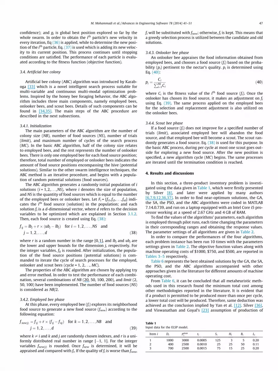
Table 1Input data for the ELSP model.

Item i Di Pmaxi ti Si Hi Bi Li

1 1000 3000 0.0005 125 3 5 0.202 400 2500 0.0010 25 25 50 0.113 700 2500 0.0015 75 15 25 0.20

M. Mohammadi et al. / Advances in Engineering Software 78 (2014) 41–51 47

confidence); and gi is global best position explored so far by thewhole swarm. In order to obtain the ith particle’s new velocity inevery iteration, Eq (36) is applied, while to determine the new posi-tion of the ith particle, Eq. (37) is used which is adding its new veloc-ity to its current position. This process continues until stoppingconditions are satisfied. The performance of each particle is evalu-ated according to the fitness function (objective function).

3.4. Artificial bee colony

Artificial bee colony (ABC) algorithm was introduced by Karab-oga [33] which is a novel intelligent search process suitable formulti-variable and continuous multi-modal optimization prob-lems. Inspired by the honey bee foraging behavior, the ABC algo-rithm includes three main components, namely employed bees,onlooker bees, and scout bees. Details of such components can befound in [34,35]. The main steps of the ABC procedure aredescribed in the next subsections.

3.4.1. InitializationThe main parameters of the ABC algorithm are the number of

colony size (NB), number of food sources (NS), number of trials(limit), and maximum number of cycles of the search process(MC). In the basic ABC algorithm, half of the colony size relatesto employed bees, and the rest represents the number of onlookerbees. There is only one employed bee for each food source position;therefore, total number of employed or onlooker bees indicates theamount of food source positions encompassing the hive (potentialsolutions). Similar to the other swarm intelligence techniques, theABC method is an iterative procedure, and begins with a popula-tion of random potential solutions (food sources).

The ABC algorithm generates a randomly initial population of isolutions (i = 1,2, . . . ,NS), where i denotes the size of population,and NS is the quantity of food sources which is equal to the numberof the employed bees or onlooker bees. Let Fi = {fi1, fi2, . . . , fid} indi-cates the ith food source (solution) in the population; and eachsolution fi is a d-dimensional vector, where d refers to the decisionvariables to be optimized which are explained in Section 3.1.2.Then, each food source is created using Eq. (38):

f ij ¼ lbj þ r � ðubj � lbjÞ for i ¼ 1;2; . . . ;NS and

j ¼ 1;2; . . . ; d ð38Þ

where r is a random number in the range [0,1], and lbj and ubj arethe lower and upper bounds for the dimension j, respectively. Forthe integer variables, fij is rounded. After initialization, the popula-tion of the food source positions (potential solutions) is com-manded to iterate the cycle of search processes for the employed,onlooker and scout bees (cycle = 1, 2,. . ., MC).

The properties of the ABC algorithm are chosen by applying tryand error method. In order to test the performance of each combi-nation, several combinations of NB (20, 50, 100, 200), and limit (2,50, 100) have been implemented. The number of food sources (NS)is considered as NB/2.

3.4.2. Employed bee phaseAt this phase, every employed bee (fi) explores its neighborhood

food source to generate a new food source (fnew) according to thefollowing equation:

f newðjÞ ¼ f ij þ r � ðf ij � f kjÞ for k ¼ 1;2; . . . ;NB and

j ¼ 1;2; . . . ; d ð39Þ

where k – i and k and j are randomly chosen indexes, and r is a uni-formly distributed real number in range [�1, 1]. For the integervariables fnew(j) is rounded. Once fnew is determined, it will beappraised and compared with fi. If the quality of fi is worse than fnew,

fi will be substituted with fnew; otherwise, fi is kept. This means thata greedy selection process is utilized between the candidate and oldsolutions.

3.4.3. Onlooker bee phaseAn onlooker bee appraises the food information obtained from

employed bees, and chooses a food source (fi) based on the proba-bility (pi) pertinent to the nectar’s quality. pi is determined usingEq. (40):

pi ¼CiPNSi¼1Ci

ð40Þ

where Ci is the fitness value of the ith food source (fi). Once theonlooker has chosen its food source, it makes an adjustment on fi

using Eq. (39). The same process applied on the employed beesfor the selection and replacement adjustment is also utilized onthe onlooker bees.

3.4.4. Scout bee phaseIf a food source (fi) does not improve for a specified number of

trials (limit), associated employed bee will abandon the foodsource, and that employed bee will become a scout. The scout ran-domly generates a food source. Eq. (38) is used for this purpose. Inthe basic ABC process, during per cycle at most one scout goes out-side for exploring a new food source. After the new position isspecified, a new algorithm cycle (MC) begins. The same processesare iterated until the termination condition is reached.

4. Results and discussions

In this section, a three-product inventory problem is investi-gated using the data given in Table 1, which were firstly presentedby Silver [8], and later were applied by many authors[6,7,9,12,36,37]. In order to find near-optimum solutions, the GA,the SA, the PSO, and the ABC algorithms were coded in MATLAB7.14.0.739, and run on a laptop equipped with an Intel Core i5 pro-cessor working at a speed of 2.67 GHz and 4 GB of RAM.

To find the values of the algorithms’ parameters, each algorithmis employed through pilot runs, each time changing the parametersin their corresponding ranges and obtaining the response values.The parameter settings of all algorithms are given in Table 2.

In order to compare the performances of the four algorithms,each problem instance has been run 10 times with the parameterssettings given in Table 2. The objective function values along withmachine operating costs of $1000, $750, and $500, are reported inTables 3–5 respectively.

Table 6 represents the best obtained solutions by the GA, the SA,the PSO, and the ABC algorithms accompanied with otherapproaches given in the literature for different amounts of machineoperating cost.

From Table 6, it can be concluded that all metaheuristic meth-ods used in this research found the minimum total cost amongother methodologies reported in the literature. It is evident thatif a product is permitted to be produced more than once per cycle,a lower total cost will be produced. Therefore, same deduction wasachieved as the conclusion implied by Yan et al. [12]. Silver [36],and Viswanathan and Goyal’s [23] assumption of production of

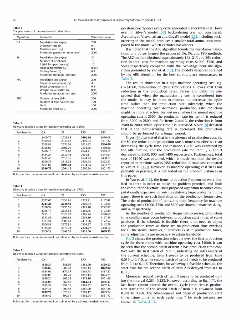
Table 2The parameters of the metaheuristic algorithms.

Algorithm Parameter Parameter value

GA Population size (Npop) 200Crossover rate (Pc) 0.1Mutation rate (Pm) 0.9Maximum generation (max gene) 2000

SA Population size (Npop) 30Number of neighbors 10Initial Temperature (/0) 10Final Temperature (/f) 0.001Cooling factor (h) 0.9Maximum iteration (max iter) 2000

PSO Population size (Npop) 200Cognitive component (c1) 4Social component (c2) 0.5Weight for velocities (w) 0.95Maximum iteration (max iter) 2000

ABC Number of bees (NB) 200Number of food sources (NS) 100Limit 100Maximum cycle (MC) 2000

Table 3Objective function values for machine operating cost $1000.

Problem No. GA SA PSO ABC

1 2400.75 2528.85 2490.24 2476.082 2399.24 2536.62 2498.24 2401.223 2398.84 2530.66 2621.92 2394.064 2398.66 2506.99 2594.25 2469.865 2406.10 2517.90 2644.21 2399.176 2424.24 2532.44 2639.11 2444.517 2417.43 2518.36 2644.23 2400.738 2399.35 2513.32 2609.94 2492.879 2401.02 2498.21 2634.34 2492.79

10 2396.73 2504.15 2500.24 2401.73

Bold specifies the minimum total cost obtained by each metaheuristic method.

Table 4Objective function values for machine operating cost $750.

Problem No. GA SA PSO ABC

1 2377.65 2353.86 2237.71 2137.482 2243.23 2238.49 2305.74 2192.553 2390.32 2435.55 2328.78 2222.074 2298.74 2336.58 2365.45 2193.295 2295.15 2328.97 2305.74 2228.686 2343.53 2301.82 2603.10 2167.397 2303.54 2306.48 2432.56 2172.528 2306.81 2275.81 2308.37 2142.799 2314.24 2376.73 2138.37 2300.10

10 2300.22 2341.56 2432.56 2038.73

Bold specifies the minimum total cost obtained by each metaheuristic method.

Table 5Objective function values for machine operating cost $500.

Problem No. GA SA PSO ABC

1 1869.27 1888.96 1881.90 1830.802 1846.07 1908.28 1880.13 1822.023 1854.96 1877.17 1865.78 1837.274 1845.08 1904.28 1892.13 1824.715 1859.20 1902.28 1878.10 1851.696 1858.05 1880.56 1862.94 1856.477 1895.32 1898.11 1869.82 1867.348 1884.38 1900.46 1887.09 1887.289 1839.20 1879.16 1901.17 1899.74

10 1896.42 1892.31 1862.94 1831.72

Bold specifies the minimum total cost obtained by each metaheuristic method.

48 M. Mohammadi et al. / Advances in Engineering Software 78 (2014) 41–51

per item exactly once every cycle generated higher total cost. How-ever, in Silver’s model [36] backordering was not considered.According to Viswanathan and Goyal’s model [23], including back-ordering in the model produces a smaller total annual cost com-pared to the model which excludes backorders.

It is noted that the ABC algorithm founds the best-known solu-tions, and outperformed the proposed GA, SA, and PSO methods.The ABC method obtained approximately 14%, 21% and 26% reduc-tion in total cost for machine operating costs $1000, $750, and$500 respectively compared with the two-stage heuristic algo-rithm presented by Yan et al. [12]. The model’s variables obtainedby the ABC algorithm for the best solutions are summarized inTable 7.

The results show that in a high machine operating cost, e.g.O = $1000, diminution of cycle time causes a lower cost thanreduction in the production rates. Sarker and Babu [7] alsoproved that when the manufacturing cost is considered intothe model, it may be more economical to decrease the cycletime rather than the production rate. Adversely, when themachine operating cost decreases, production rate reductionmight be more effective. For instance, when the annual machineoperating cost is $500, the production rate for item 1 is reducedfrom 3000 to 2800, and for items 2 and 3, the reduction is from2500 to 2000; while, cycle time T is increased. Silver [8] declaredthat if the manufacturing rate is decreased, the productionshould be performed for a longer period.

Silver [8] also stated that in the absence of production cost, i.e.O = $0, the reduction in production rate is more cost-effective thandecreasing the cycle time. For instance, O = $0 was examined bythe ABC method, and the production rate for item 1, 2, and 3decreased to 2000, 800, and 1400 respectively. Furthermore, totalcost of $1040 was obtained, which is much less than the resultsreported in previous works (45% reduction in total cost comparedto Yan et al. [12]). However, as machine operating cost $0 is notprobable in practice, it is not tested on the problem instances inthis paper.

In Yan et al. [12], the items’ production frequencies were lim-ited to three in order to make the problem practical, and limitthe computational effort. Their proposed algorithm becomes com-putationally expensive for solving relatively large problems. In thispaper, there is no such limitation on the production frequencies.The order of production of items, and their frequency for machineoperating costs $1000, $750, and $500 are shown in matrices A4, A5,and A6 respectively.

As the number of production frequency increases, productiontime conflicts may occur between production start times of someproducts. If the schedule is feasible, there is no need to adjustthe production times as there are no production time overlapsfor all the items. However, if conflicts exist in production times,some adjustments are necessary to attain feasibility.

Fig. 2 shows the production schedule over the first productioncycle for three items with machine operating cost $1000. It canbe seen that the second batch of item 2 has production time con-flict with the first batch of item 1, indicating the infeasibility ofthe current schedule. Item 1 needs to be produced from time0.016 to 0.115, while second batch of item 2 needs to be producedfrom 0.1 to 0.116. Therefore, for achieving a feasible schedule, thestart time for the second batch of item 2 is delayed from 0.1 to0.115.

Moreover, second batch of item 3 needs to be produced dur-ing the interval 0.281–0.323. However, according to Eq. (17), thelast batch cannot exceed the overall cycle time. Hence, produc-tion start time of the second batch of item 3 is advanced from0.281 to 0.258. The advancement and delay of production starttimes (time units) in each cycle time T for each instance areshown in Tables 8–13.

Table 6Comparisons of the best obtained solutions and previously reported results.

Operating cost GA SA PSO ABC Silver [36] Viswanathan and Goyal [23] Yan et al. [12] Impr.* (%)

O = $1000 $2396.73 $2498.21 $2490.24 $2394.06 $3678 $3084 $2788 14.13O = $750 $2243.23 $2238.49 $2138.37 $2038.73 $3428 $2881 $2590 21.28O = $500 $1839.20 $1877.17 $1862.94 $1822.02 $3178 $2638 $2454 25.75

* Solution improvement.

Table 7Optimization results for different machine operating costs (O) obtained by the ABCmethod offering superior results.

Item i pi ri ui si Qi Mi T

$10001 3000 0.33 1 0.30 300 75 0.302 2500 0.16 3 0.10 40 113 2500 0.28 2 0.15 105 28

$7501 3000 0.33 2 0.165 165 41 0.332 2500 0.16 3 0.11 44 123 2500 0.28 3 0.11 77 21

$5001 2800 0.36 2 0.20 200 48 0.402 2000 0.20 4 0.10 40 113 2000 0.35 3 0.133 93 23

Table 8Production start time advancements for machine operating cost $1000.

a j = 1 j = 2 j = 3 j = 4 j = 5 j = 6

i = 1 0 0 0 0 0 0i = 2 0 0 0 0 0 0i = 3 0 0 0 0 0 0.023

Table 9Production start time delays for machine operating cost $1000.

b j = 1 j = 2 j = 3 j = 4 j = 5 j = 6

i = 1 0 0 0 0 0 0i = 2 0 0 0.015 0 0 0i = 3 0 0 0 0 0 0

Table 10Production start time advancements for machine operating cost $750.

a j = 1 j = 2 j = 3 j = 4 j = 5 j = 6 j = 7 j = 8

i = 1 0 0 0 0 0 0.0218 0 0i = 2 0 0 0 0 0 0 0 0i = 3 0 0 0 0 0.0520 0 0 0

Table 11Production start time delays for machine operating cost $750.

b j = 1 j = 2 j = 3 j = 4 j = 5 j = 6 j = 7 j = 8

i = 1 0 0 0 0 0 0 0 0i = 2 0 0 0 0 0 0 0 0i = 3 0 0 0 0 0 0 0 0

M. Mohammadi et al. / Advances in Engineering Software 78 (2014) 41–51 49

A4 ¼0 1 0 0 0 01 0 1 0 1 00 0 0 1 0 1

264

375

A5 ¼0 1 0 0 0 1 0 01 0 0 1 0 0 1 00 0 1 0 1 0 0 1

264

375

A6 ¼0 1 0 0 0 1 0 0 01 0 0 1 1 0 0 1 00 0 1 0 0 0 1 0 1

264

375

The results also indicate that for each item the storage period wasnot exceeded its shelf life (Eq. (9)), which prevents the spoilage ofproducts.

Furthermore, to display the convergence of the suggested GA,SA, PSO, and ABC methods, the graphic illustrations of convergencepath corresponding to the fitness function in terms of the genera-tion number for machine operating cost $1000 are shown inFigs. 3–6 respectively.

Fig. 2. Production schedule before adjustment for machine operating cost $1000.

Table 12Production start time advancements for machine operating cost $500.

a j = 1 j = 2 j = 3 j = 4 j = 5 j = 6 j = 7 j = 8 j = 9

i = 1 0 0 0 0 0 0.0414 0 0 0i = 2 0 0 0 0 0.0414 0 0 0 0i = 3 0 0 0 0 0 0 0 0 0.0045

Table 13Production start time delays for machine operating cost $500.

b j = 1 j = 2 j = 3 j = 4 j = 5 j = 6 j = 7 j = 8 j = 9

i = 1 0 0 0 0 0 0 0 0 0i = 2 0 0 0 0.0385 0 0 0 0 0i = 3 0 0 0 0 0 0 0.0255 0 0

Fig. 3. The graph of convergence path by GA for machine operating cost $1000.

Fig. 4. The graph of convergence path by SA for machine operating cost $1000.

Fig. 5. The graph of convergence path by PSO for machine operating cost $1000.

Fig. 6. The graph of convergence path by ABC for machine operating cost $1000.

50 M. Mohammadi et al. / Advances in Engineering Software 78 (2014) 41–51

5. Conclusions

A mixed-integer non-linear model has been addressed in thispaper which considers the practical characteristics, including back-ordering, shelf life, and multiple setups for each product in a man-ufacturing cycle. The paper investigated the problem of obtainingthe optimum production rate and production frequency for eachitem, the optimal production cycle time for all the products, inaddition to a feasible manufacturing schedule. However, theassumption of production of items more than once in a cycle mightcause an infeasible schedule due to the overlapping productiontimes of various items. To eliminate the production time conflictsand to achieve a feasible schedule, the production start time ofsome or all the items must be adjusted by either advancing ordelaying.

The solution of the large scale proposed ELSP model may be outof reach using the existing approaches based on the complexityand the required computational efforts associated with the model.Thus, efficient heuristic methods are required to solve the NP-hardmodel for large problems usually found in real-world situations. Inthis paper, effective solution approaches based on real-coded GA,SA, PSO, and ABC algorithms for integer, non-integer, and binaryvariables are presented for solving the proposed model. The resultsindicate the efficiency of the applied metaheuristic methods insolving the proposed model. Comparisons were based on the per-centage improvement in the total cost. All the applied methodsshowed an impressive performance and excellent solution quali-ties. The metaheuristic algorithms can also efficiently handlelarge-sized instances in a moderate computational time. However,the ABC method produced the lowest cost, which may indicate itssuperiority in searching for solutions of similar problems. There-fore, the ABC-based approaches can be served as a useful deci-sion-support tool for production managers.

Acknowledgment

This research was fully funded by University of Malaya underthe UMRG programme Grant Number of UM.TNC2/RC/AET/261/1/1/RP017-2012A.

References

[1] Narro Lopez MA, Kingsman BG. The economic lot scheduling problem: theoryand practice. Int J Prod Econ 1991;23:147–64.

M. Mohammadi et al. / Advances in Engineering Software 78 (2014) 41–51 51

[2] Brander P, Forsberg R. Determination of safety stocks for cyclic schedules withstochastic demands. Int J Prod Econ 2006;104:271–95.

[3] Khoury B, Abboud N, Tannous M. The common cycle approach to the ELSPproblem with insufficient capacity. Int J Prod Econ 2001;73:189–99.

[4] Giri B, Moon I, Yun W. Scheduling economic lot sizes in deterioratingproduction systems. Naval Res Log 2003;50:650–61.

[5] Lütke Entrup M, Günther HO, Van Beek P, Grunow M, Seiler T. Mixed-IntegerLinear Programming approaches to shelf-life-integrated planning andscheduling in yoghurt production. Int J Prod Res 2005;43:5071–100.

[6] Xu Y, Sarker BR. Models for a family of products with shelf life, andproduction and shortage costs in emerging markets. Comput Oper Res 2003;30:925–38.

[7] Sarker BR, Sobhan Babu P. Effect of production cost on shelf life. Int J Prod Res1993;31:1865–72.

[8] Silver EA. Shelf life considerations in a family production context. Int J Prod Res1989;27:2021–6.

[9] Silver EA. Deliberately slowing down output in a family production context. IntJ Prod Res 1990;28:17–27.

[10] Goyal S. A note on effect of production cost on shelf-life. Int J Prod Res1994;32:2243–5.

[11] Viswanathan S. A note on ‘Effect of production cost on shelf life’. Int J Prod Res1995;33:3485–6.

[12] Yan C, Liao Y, Banerjee A. Multi-product lot scheduling with backordering andshelf-life constraints. Omega 2013;41:510–6.

[13] Hsu WL. On the general feasibility test of scheduling lot sizes for severalproducts on one machine. Manage Sci 1983;29:93–105.

[14] Khouja M, Michalewicz Z, Wilmot M. The use of genetic algorithms to solve theeconomic lot size scheduling problem. Eur J Oper Res 1998;110:509–24.

[15] Moon I, Silver EA, Choi S. Hybrid genetic algorithm for the economic lot-scheduling problem. Int J Prod Res 2002;40:809–24.

[16] Dobson G. The economic lot-scheduling problem: achieving feasibility usingtime-varying lot sizes. Oper Res 1987;35:764–71.

[17] Chatfield DC. The economic lot scheduling problem: a pure genetic searchapproach. Comput Oper Res 2007;34:2865–81.

[18] Bomberger EE. A dynamic programming approach to a lot size schedulingproblem. Manage Sci 1966;12:778–84.

[19] Jenabi M, Fatemi Ghomi S, Torabi SA, Karimi B. Two hybrid meta-heuristics forthe finite horizon ELSP in flexible flow lines with unrelated parallel machines.Appl Math Comput 2007;186:230–45.

[20] Chandrasekaran C, Rajendran C, Krishnaiah Chetty O, Hanumanna D.Metaheuristics for solving economic lot scheduling problems (ELSP) usingtime-varying lot-sizes approach. Eur J Ind Eng 2007;1:152–81.

[21] Raza AS, Akgunduz A. A comparative study of heuristic algorithms oneconomic lot scheduling problem. Comput Ind Eng 2008;55:94–109.

[22] Bulut O, Tasgetiren MF, Fadiloglu MM. A genetic algorithm for the economiclot scheduling problem under extended basic period approach and power-of-two policy. Advanced intelligent computing theories and applications: Withaspects of artificial intelligence. Springer; 2012.

[23] Viswanathan S, Goyal S. Incorporating planned backorders in a familyproduction context with shelf-life considerations. Int J Prod Res 2000;38:829–36.

[24] Holland JH. Adaptation in natural and artificial systems: an introductoryanalysis with applications to biology, control, and artificial intelligence. UMichigan Press; 1975.

[25] Pasandideh SHR, Niaki STA, Yeganeh JA. A parameter-tuned genetic algorithmfor multi-product economic production quantity model with space constraint,discrete delivery orders and shortages. Adv Eng Software 2010;41:306–14.

[26] Gen M, Cheng R, Lin L. Network models and optimization: multi objectivegenetic algorithm approach. Springer; 2008.

[27] Cho Hl, Oh SY, Choi D-H. A new evolutionary programming approach based onsimulated annealing with local cooling schedule. Evolutionary ComputationProceedings, 1998. IEEE World Congress on Computational Intelligence. The1998 IEEE International Conference on: IEEE; 1998. p. 598–602.

[28] Zhou E, Chen X. A new population-based simulated annealing algorithm.Simulation conference (WSC), Proceedings of the 2010 winter: IEEE; 2010. p.1211–22.

[29] Kirkpatrick S. Optimization by simulated annealing: quantitative studies. J StatPhys 1984;34:975–86.

[30] Kennedy J, Eberhart R. Particle swarm optimization. Proceedings of IEEEinternational conference on neural networks: Perth, Australia; 1995. p. 1942–8.

[31] Chen YY, Lin JT. A modified particle swarm optimization for productionplanning problems in the TFT Array process. Expert Syst Appl 2009;36:12264–71.

[32] Coelho LdS, Sierakowski CA. A software tool for teaching of particle swarmoptimization fundamentals. Adv Eng Softw 2008;39:877–87.

[33] Karaboga D. An idea based on honey bee swarm for numerical optimization.Techn. Rep. TR06, Erciyes Univ. Press, Erciyes; 2005.

[34] Pan QK, Fatih Tasgetiren M, Suganthan PN, Chua TJ. A discrete artificial beecolony algorithm for the lot-streaming flow shop scheduling problem. InformSci 2011;181:2455–68.

[35] Sulaiman MH, Mustafa MW, Shareef H, Abd. Khalid SN. An application ofartificial bee colony algorithm with least squares support vector machine forreal and reactive power tracing in deregulated power system. Int J Elec Power2012;37:67–77.

[36] Silver EA. Dealing with a shelf life constraint in cyclic scheduling by adjustingboth cycle time and production rate. Int J Prod Res 1995;3:623–9.

[37] Sharma S. Optimal production policy with shelf life including shortages. J OperRes Soc 2004;55:902–9.