Embed Size (px)
Citation preview

Optimal Endogenous Carbon Taxes
for
Electric Power Supply Chains with Power Plants
Anna Nagurney∗
Radcliffe Institute Fellow
Radcliffe Institute for Advanced Study
34 Concord Avenue
Harvard University
Cambridge, Massachusetts 02138
and
Department of Finance and Operations Management
Isenberg School of Management
University of Massachusetts
Amherst, Massachusetts 01003
Zugang Liu and Trisha Woolley
Department of Finance and Operations Management
Isenberg School of Management
University of Massachusetts
Amherst, Massachusetts 01003
February 2006; appears in Mathematical and Computer Modelling 44 (2006), pp. 899-916.
Abstract: In this paper, we develop a modeling and computational framework that allows
for the determination of optimal carbon taxes applied to electric power plants in the con-
text of electric power supply chain (generation/distribution/consumption) networks. The
adoption of carbon/pollution taxes both internationally and regionally has been fueled by
global climate change and fuel security risks with a significant portion of such policy inter-
ventions directed at the electric power industry. The general framework that we develop
allows for three distinct types of carbon taxation environmental policies, beginning with a
completely decentralized scheme in which taxes can be applied to each individual power gen-
erator/power plant in order to guarantee that each assigned emission bound is not exceeded,
to two versions of a centralized scheme, one which assumes a fixed bound over the entire
1

electric power supply chain in terms of total carbon emissions and the other which allows
the bound to be a function of the tax. The behavior of the various decision-makers in the
electric power supply chain network is described, along with the three taxation schemes, and
the governing equilibrium conditions, which are formulated as finite-dimensional variational
inequality problems. Twelve numerical examples are presented in which the optimal carbon
taxes, as well as the equilibrium electric power flows and demands, are computed. The nu-
merical results demonstrate, as the theory predicts, that the carbon taxes achieve the desired
goal, in that the imposed bounds on the carbon emissions are not exceeded. Moreover, they
illustrate the spectrum of scenarios that can be explored in terms of changes in he bounds
on the carbon emissions; changes in emission factors; changes in the demand functions, etc.
∗ This research was supported, in part, by NSF Grant. No.: IIS 00026471. The research of
the first author was also supported, in part, by the Radcliffe Institute for Advanced Study at
Harvard University under its 2005-2006 Radcliffe Fellows Program. This support is gratefully
acknowledged and appreciated.
Keywords: electric power, supply chains, carbon taxes, variational inequalities, network
equilibria, environmental policies, renewable energy
2

1. Introduction
Electric power is a fundamental resource that has fueled modern economies and societies
from its role in the lighting and heating of homes and offices to the running of computers,
which underpin our communications, manufacturing processes and financial services, and
even transportation. Electric power is so essential to our every day lives that when failures
arise the impact is wide and vividly apparent as the biggest blackout in US history in 2003
graphically illustrated. Indeed, in modern societies there are few goods or services that
do not depend directly on electricity. Globally, in 2002, 16.1 trillion kilowatt hours were
supplied, with United States being the largest producer and consumer of electric energy (see
[1]). In the past half-century, the total annual electricity use in the US alone has grown every
year but two. The US electrical industry has more than half a trillion dollars of net assets,
$220 billion in annual sales, and consumes almost 40% of domestic primary energy (coal,
natural gas, uranium, and oil), or about 40 quadrillion British Thermal Units (BTUs) (see
[2] – [4]). This industry is growing, with the expectation that the total global consumption
of electricity will reach 23.1 trillion kilowatt hours in 2025. For background on the electric
power industry, see [5] – [7].
However, despite the major positive economic impacts of electric power, the heavy reliance
on fossil fuel sources before conversion to electricity has had, at the same time, an immense
environmental impact. For example, of the total US emissions of carbon dioxide and nitrous
oxide, more than a third arises from generating electricity. In China, in turn, the electric
power sector currently accounts for more than one-third of its annual coal consumption
with such power plants generating over 75% of the air pollution in China (cf. [8]). Fossil
fuels, which include coal, are expected to be used in 36% of the electricity production into
2020, and presently account for 39% of the electricity generated worldwide. With growing
accumulating evidence of global warming, any policy aimed at mitigating the immense risks
of unstable climate must directly consider the electricity industry ([9], [10]).
As noted in Wu et al. [11], pollution taxes, and, in particular, carbon taxes are a powerful
policy mechanism that can address market failures in energy. Currently, market prices for
energy do not capture its many external costs in the form of regional and global pollution
and also hide market distortions. The usefulness of carbon taxes has been noted by among
3

others, Baranzini, Goldemberg, and Speck [12], whereas Painuly [13] has argued for the
encouragement of power generation from renewable sources, including solar power and wind
power through the use of green credits. Such credits are now being utilized in the European
Union as well as in several states in the US (cf. [14], [15]). Hence, a mathematical modeling
framework that can capture the interactions among decision-makers in an electric power
supply chain network from power generators, along with the power plant production options;
the suppliers as well as ultimate consumers, coupled with the incorporation of environmental
policies, such as carbon taxes, is of great practical as well as policy-making importance.
Recently, Wu et al. [11] proposed an electric power supply chain network equilibrium
model with carbon taxes that are applied a priori to distinct power generator/power plant
combinations and demonstrated that the model could be reformulated and solved as a trans-
portation network equilibrium problem with elastic demands. However, in that model, the
government authority would have to conduct simulation exercises to determine the carbon
tax assignment in order to achieve some goal. In this paper, in contrast, we demonstrate
how carbon taxes can be determined optimally and endogenously within a generalized elec-
tric power supply chain network equilibrium model. In particular, we allow the government
to impose bound(s) on the total amount of carbon emissions and the optimal carbon taxes
guarantee that the bound(s) are not exceeded.
Since electric power plants may be under different governmental jurisdictions either in
the US or abroad we propose both a decentralized carbon taxation scheme as well as two
centralized schemes. In the former environmental policy framework, a bound on carbon
emissions can be applied on each power generator/power plant with a resulting distinct tax;
in the latter framework there is a single carbon emission bound imposed on the entire elec-
tric power supply chain network with a resulting single tax. We note that Nagurney and
Matsypura [16] were the first to introduce a general electric power supply chain network
equilibrium model, which was, subsequently, shown by Nagurney and Liu [17] to be trans-
formable into a transportation network equilibrium model over an appropriately constructed
abstract network. This identification validated a hypothesis made over half a century ago in
the book by Beckmann, McGuire, and Winsten [18].
The paper is organized as follows. In Section 2, we present the electric power supply chain
4

network equilibrium model with three distinct carbon taxation schemes. We also demon-
strate the relationship between carbon taxes and weights associated with environmental
criteria and the concommitant multicriteria decision-making akin to the work of Nagurney
and Toyasaki [19]. In Section 3, we present twelve numerical examples in which the optimal
taxes and the equilibrium electric power flows between tiers of decision-makers and the de-
mands for electric power are computed. We also report the prices at the demand markets
at the equilibrium. In Section 4, we summarize the results in this paper and present our
conclusions.
5

2. The Electric Power Supply Chain Network Model with Power Plants and
Optimal Endogenous Carbon Taxes
In this Section we develop the electric power supply chain network equilibrium model
that includes power plants as well as carbon taxes under three distinct taxation schemes.
We begin with a decentralized taxation scheme outlined in Section 2.1 and then turn to the
centralized schemes in Section 2.2. The presentation of the model follows the description
of the electric supply chain network model with pollution taxes (which, however, were fixed
and assigned a priori) in [11].
In particular, we consider G power generators (sometimes also referred to as “gencos”),
each of which, typically, owns and operates M power plants. A specific power plant may
use a different primary energy fuel such as, for example, coal, natural gas, uranium, oil,
sun, wind, etc., with different associated costs. In addition, each power plant will also have
associated costs that fully reflect policy objectives, which here will be in the form of carbon
taxes. There are S power suppliers, T transmission service providers, and K consumer
markets, as depicted in Figure 1. The majority of the needed notation is given in Table 1.
An equilibrium solution is denoted by “∗”. All vectors are assumed to be column vectors,
except where noted otherwise.
The top-tiered nodes in the electric power supply chain network in Figure 1, enumerated
by 1, . . . , g . . . , G, represent the G electric power generators, who are the decision-makers
who own and operate the electric power generating facilities or power plants denoted by the
second tier of nodes in the network. The gencos produce electric power using the different
power plants and sell to the power suppliers in the third tier. Node gm in the second
tier corresponds to genco g’s power plant m, with the second tier of nodes enumerated as:
11, . . . , GM . We assume that each electric power generator seeks to determine his optimal
production portfolio across his power plants and his sales allocations of the electric power to
the suppliers in order to maximize his own profit.
6

Table 1: Notation for the Electric Power Supply Chain Network Model
Notation Definitionqgm quantity of electricity produced by generator g using power plant m, where
g = 1, . . . , G; m = 1, . . . , Mqm G-dimensional vector of electric power generated by the gencos using
power plant m with components: q1m, . . . , qGm
q GM -dimensional vector of all the electric power outputs generatedby the gencos at the power plants
Q1 GMS-dimensional vector of electric power flows between the power plants ofthe power generators and the power suppliers with component gms denotedby qgms
Q2 STK-dimensional vector of power flows between suppliers and demandmarkets with component stk denoted by qt
sk and denoting the flow betweensupplier s and demand market k via transmission provider t
d K-dimensional vector of market demands with component k denoted by dk
fgm(qm) power generating cost function of power generator g using power plant m
with marginal power generating cost with respect to qgm denoted by ∂fgm
∂qgm
cgms(qgms) transaction cost incurred by power generator g using power plant min transacting with power supplier s with marginal transaction cost
denoted by ∂cgms(qgms)∂qgms
egm amount of carbon emitted by genco g using power plant m per unitof electric power produced
h S-dimensional vector of the power suppliers’ supplies of the electricpower with component s denoted by hs, with hs ≡
∑Gg=1
∑Mm=1 qgms
cs(h) ≡ cs(Q1) operating cost of power supplier s with marginal operating cost with
respect to hs denoted by ∂cs
∂hsand the marginal operating cost with respect
to qgms denoted by ∂cs(Q1)∂qgms
ctsk(q
tsk) transaction cost incurred by power supplier s in transacting with
demand market k via transmission provider t with marginal transaction
cost with respect to qtsk denoted by
∂ctsk(qt
sk)
∂qtsk
cgms(qgms) transaction cost incurred by power supplier s in transacting withpower generator g for power generated by plant m with marginal transaction
cost denoted by ∂cgms(qgms)∂qgms
ctsk(Q
2) unit transaction cost incurred by consumers at demand market kin transacting with power supplier s via transmission provider t
ρ3k(d) demand market price function at demand market k
7

� ��11 � ��
· · · 1m · · · � ��1M · · · � ��
G1 � ��· · · Gm · · · � ��
GM
Transmission ServiceProviders
� ��1 · · · � ��
G
?
SS
SSSw
��
��
�/ ?
SS
SSSw
��
��
�/
� ��1 · · · � ��
SSuppliers
Power Plants
� ��1 · · · � ��
K
SS
SSSw?
��
��
�/
SS
SSSw?
��
��
�/
Demand Markets
Power Generators
1,· · ·,T 1,· · ·,T
Figure 1: The Electric Power Supply Chain Network with Power Plants
8

Power suppliers, which are represented by the third tiered nodes in Figure 1, func-
tion as intermediaries. The nodes corresponding to the power suppliers are enumerated
as: 1, . . . , s, . . . , S with node s corresponding to supplier s. They purchase electric power
from the power generators and are aware as to the types of power plants used by the gener-
ators. They also sell the electric power to the consumers at the different demand markets.
We assume that the power suppliers compete with one another in a noncooperative manner.
However, the suppliers do not physically possess electric power at any stage of the supplying
process; they only hold and trade the right for the electric power.
The bottom-tiered nodes in Figure 1 represent the demand markets, which can be distin-
guished from one another by their geographic locations or the type of associated consumers
such as whether they correspond, for example, to businesses or to households. There are K
bottom-tiered nodes with node k corresponding to demand market k.
A transmission service is necessary for the physical delivery of electric power from the
power generators to the points of consumption. The transmission service providers are the
entities who own and operate the electric power transmission and distribution systems, and
distribute electric power from power generators to the consumption markets. Since the
transmission service providers do not make decisions such as to where or from whom the
electric power will be delivered, they are not represented by nodes in the network model.
The structure of the network in Figure 1 guarantees that the conservation of flow equations
associated with the electric power production and distribution are satisfied. The flows on
the links joining the genco nodes in Figure 1 to the power plant nodes are respectively:
q11, . . . , qgm, . . . , qGM ; the flows on the links from the power plant nodes to the supplier
nodes are given, respectively, by the components of the vector Q1, whereas the flows on
the links joining the supplier nodes with the demand markets are given by the respective
components of the vector: Q2.
2.1 A Decentralized Carbon Taxation Scheme
We now describe the behavior of the electric power generators, the suppliers, and the
consumers at the demand markets. We first consider a decentralized carbon taxation scheme.
We then state the equilibrium conditions of the electric power supply chain network and
9

provide the variational inequality formulation. Subsequently, we discuss how centralized
taxation schemes can be substituted for the decentralized scheme.
The Behavior of the Power Generators and their Optimality Conditions
Let egm; g = 1, . . . , G; m = 1, . . . , M denote the carbon emissions generated per unit of
electric power produced by genco g using his power plant m. Hence, the total amount of
carbon emissions associated with genco g and power plant m is egmqgm.
Let ρ∗1gms denote the unit price charged by power generator g for the transaction with
power supplier s for power produced at plant m with g = 1, . . . , G; m = 1, . . . , M , and
s = 1, . . . , S. ρ∗1gms is an endogenous variable and can be determined once the complete
electric power supply chain network equilibrium model is solved.
Let τgm; g = 1, . . . , G; m = 1, . . . , M , denote the unit tax that the governmental or
responsible environmental authority will charge genco g operating power plant m for his
carbon emissions and group all these taxes into the vector τ . The optimal values of these
taxes, denoted by the components of the vector τ ∗, are endogenous and are determined once
the complete model is solved. As we will later see, the taxes guarantee that bounds on the
carbon emissions, also imposed by the responsible authority, are not exceeded. The bounds
are denoted by Bgm; g = 1, . . . , G; m = 1, . . . , M and reflect the maximum carbon emissions
allowed by the responsible authority for the particular genco/power plant combination. The
complete electric power supply chain network equilibrium model captures the complex in-
teractions among the various decision-makers and its solution yields the equilibrium electric
power flows and demands as well as the optimal carbon taxes.
Since we have assumed that each individual power generator is a profit-maximizer, the
optimization problem of power generator g can be expressed as follows:
MaximizeM∑
m=1
S∑
s=1
ρ∗1gmsqgms −
M∑
m=1
fgm(qm) −M∑
m=1
S∑
s=1
cgms(qgms) −M∑
m=1
τ ∗gmegmqgm (1)
subject to:S∑
s=1
qgms = qgm, m = 1, . . . , M, (2)
qgms ≥ 0, m = 1, . . . , M ; s = 1, . . . , S. (3)
10

The first term in the objective function (1) represents the revenue and the next two terms
represent the power generation cost and transaction costs, respectively. The last term in (1)
denotes the total payout in carbon taxes by the genco based on the total carbon pollution
emitted by his power plants. Conservation of flow equation (2) states that the amount
of power generated at a particular power plant (and corresponding to a particular genco)
is equal to the electric power transacted by the genco from that power plant with all the
suppliers, and this holds for each of the power plants.
Assume, as was done in [11], that the generating cost and the transaction cost functions
for each power generator are continuously differentiable and convex, and that the power
generators compete in a noncooperative manner in the sense of Nash [20,21]. The optimality
conditions for all power generators simultaneously, under the above assumptions (cf. [22]),
coincide with the solution of the following variational inequality: determine (q∗, Q1∗) ∈ K1
satisfyingG∑
g=1
M∑
m=1
[∂fgm(q∗m)
∂qgm+ τ ∗
gmegm
]× [qgm − q∗gm]
+G∑
g=1
M∑
m=1
S∑
s=1
[∂cgms(q
∗gms)
∂qgms− ρ∗
1gms
]× [qgms − q∗gms] ≥ 0, ∀(q, Q1) ∈ K1, (4)
where K1 ≡ {(q, Q1)|(q, Q1) ∈ RGM+GMS+ and (2) holds}.
The Behavior of Power Suppliers and their Optimality Conditions
The power suppliers, in turn, are involved in transactions both with the power generators
and with the consumers at demand markets through the transmission service providers.
Since electric power cannot be stored, the total amount of electricity sold by a power
supplier is equal to the total electric power that he purchased from the generators and
produced via the different power plants available to the generators, that is:
K∑
k=1
T∑
t=1
qtsk =
G∑
g=1
M∑
m=1
qgms, s = 1, . . . , S. (5)
Let ρt∗2sk denote the price charged by power supplier s to demand market k via transmission
service provider t. This price is determined endogenously in the model once the entire
11

network equilibrium problem is solved. As noted above, it is assumed that each power
supplier seeks to maximize his own profit. Hence the optimization problem faced by supplier
s may be expressed as follows:
MaximizeK∑
k=1
T∑
t=1
ρt∗2skq
tsk − cs(Q
1) −G∑
g=1
M∑
m=1
ρ∗1gmsqgms −
G∑
g=1
M∑
m=1
cgms(qgms) −K∑
k=1
T∑
t=1
ctsk(q
tsk)
(6)
subject to:K∑
k=1
T∑
t=1
qtsk =
G∑
g=1
M∑
m=1
qgms (7)
qgms ≥ 0, g = 1, . . . , G, m = 1, . . . , M, (8)
qtsk ≥ 0, k = 1, . . . , K; t = 1, . . . , T. (9)
The first term in (6) denotes the revenue of supplier s; the second term denotes the operating
cost of the supplier; the third term denotes the payments for the electric power to the various
gencos, and the final two terms represent the various transaction costs.
We assume that the transaction costs and the operating costs in (6) are all continu-
ously differentiable and convex, and that the power suppliers compete in a noncooperative
manner. Hence, the optimality conditions for all suppliers, simultaneously, under the above
assumptions (see [16]), can be expressed as the following variational inequality: determine
(Q2∗, Q1∗) ∈ K2 such that
S∑
s=1
K∑
k=1
T∑
t=1
[∂ct
sk(qt∗sk)
∂qtsk
− ρt∗2sk
]× [qt
sk − qt∗sk]
+G∑
g=1
M∑
m=1
S∑
s=1
[∂cs(Q
1∗)
∂qgms
+∂cgms(q
∗gms)
∂qgms
+ ρ∗1gms
]× [qgms − q∗gms] ≥ 0, ∀(Q2, Q1) ∈ K2, (10)
where K2 ≡ {(Q2, Q1)|(Q2, Q1) ∈ RSTK+GMS+ and (7) holds}.
For notational convenience, and as was done in [11], we let
hs ≡G∑
g=1
M∑
m=1
qgms, s = 1, . . . , S. (11)
12

As defined in Table 1, the operating cost of power supplier s, cs, is a function of the total
electricity inflows to the power supplier, that is:
cs(h) ≡ cs(Q1), s = 1, . . . , S. (12)
Hence, his marginal cost with respect to hs is equal to the marginal cost with respect to
qgms:∂cs(h)
∂hs
≡ ∂cs(Q1)
∂qgms
, s = 1, . . . , S, m = 1, . . . , M, g = 1, . . . , G. (13)
After the substitution of (11) and (13) into (10), and algebraic simplification, we obtain a
variational inequality equivalent to (10), as follows: determine (h∗, Q2∗, Q1∗) ∈ K3 such that
S∑
s=1
∂cs(h∗)
∂hs
× [hs − h∗s] +
S∑
s=1
K∑
k=1
T∑
t=1
[∂ct
sk(qt∗sk)
∂qtsk
− ρt∗2sk
]× [qt
sk − qt∗sk]
+G∑
g=1
M∑
m=1
S∑
s=1
[∂cgms(q
∗gms)
∂qgms+ ρ∗
1gms
]× [qgms − q∗gms] ≥ 0, ∀(h, Q1, Q2, ) ∈ K3, (14)
where K3 ≡ {(h, Q2, Q1)|(h, Q2, Q1) ∈ RS(1+TK+GM)+ and (7) and (11) hold}.
Equilibrium Conditions for the Demand Markets
At each demand market k the following conservation of flow equation must be satisfied:
dk =S∑
s=1
T∑
t=1
qtsk, k = 1, . . . , K. (15)
The market equilibrium conditions at demand market k take the form: for each power
supplier s; s = 1, ..., S and transaction mode t; t = 1, ..., T :
ρt∗2sk + ct
sk(Q2∗)
{= ρ3k(d
∗), if qt∗sk > 0,
≥ ρ3k(d∗), if qt∗
sk = 0.(16)
According to (16) (see also [11]), consumers at a demand market will purchase power
from a supplier via a transmission provider, provided that the purchase price plus the unit
transaction cost is equal to the price that the consumers are willing to pay at that demand
market. If the purchase price plus the unit transaction cost exceeds the price the consumers
13

are willing to pay, then there will be no transaction between that supplier and demand
market via that transmission provider. The equivalent variational inequality takes the form:
determine (Q2∗, d∗) ∈ K4, such that
S∑
s=1
K∑
k=1
T∑
t=1
[ρt∗
2sk + ctsk(Q
2∗)]× [qt
sk − qt∗sk] −
K∑
k=1
ρ3k(d∗) × [dk − d∗
k] ≥ 0, ∀(Q2, d) ∈ K4, (17)
where K4 ≡ {(Q2, d)|(Q2, d) ∈ RK(ST+1)+ and (15) holds}.
Decentralized Carbon Tax Equilibrium Conditions
Unlike the model of Wu et al. [11], which considered pollution taxes applied to each
genco/power plant combination that were fixed and assigned a priori, we here assume that
the taxes are endogenous and optimal in the following sense. We assume, as is commonly
done in real-life environmental policy-making (see also, e.g., the book by Dhanda, Nagurney,
and Ramanujam [23]), and as was noted earlier, that bounds are applied in terms of the
maximum carbon emissions that are allowed for each genco/power plant combination. If
the particular genco/power plant emits fewer carbons than the imposed limit, then it is not
taxed; a tax is assigned if the emissions equal the bound. Mathematically, this statement
corresponds to the following carbon tax equilibrium conditions under a decentralized tax
scheme: for all power generators g; g = 1, . . . , G, and for all power plants m; m = 1, . . . , M ,
a carbon tax policy is said to be in equilibrium if:
Bgm − egmq∗gm
{= 0, if τ ∗
gm > 0,≥ 0, if τ ∗
gm = 0.(18)
Such a decentralized carbon taxation scheme would be reasonable, for example, if each
power plant would reside in a different jurisdiction. Of course, if a given genco owns a subset
of power plants (which may correspond to different fuel source options), then those links
would just be eliminated from the network in Figure 1 and the notation altered accordingly.
The Equilibrium Conditions for the Electric Power Supply Chain Network
In equilibrium, the optimality conditions for all the power generators, the optimality condi-
tions for all the power suppliers, and the equilibrium conditions for all the demand markets,
14

as well as the carbon tax equilibrium conditions must be simultaneously satisfied so that
no decision-maker has any incentive to alter his transactions. We now formally state the
equilibrium conditions for the entire electric power supply chain network with endogenous,
decentralized carbon taxes.
Definition 1: Electric Power Supply Chain Network Equilibrium with Endoge-
nous, Decentralized Carbon Taxes
The equilibrium state of the electric power supply chain network with power plants and en-
dogenous, decentralized carbon taxes is one where the electric power flows between the tiers of
the network coincide and the electric power flows, the demands, and the carbon taxes satisfy
the sum of conditions (4), (14), (17), and the decentralized carbon tax equilibrium conditions
(18).
We now state and prove:
Theorem 1: Variational Inequality Formulation of the Electric Power Supply
Chain Network Equilibrium with Decentralized Carbon Taxes
The equilibrium conditions governing the electric power supply chain network according to
Definition 1 coincide with the solution of the variational inequality given by: determine
(q∗, h∗, Q1∗, Q2∗, d∗, τ ∗) ∈ K5 satisfying:
G∑
g=1
M∑
m=1
[∂fgm(q∗m)
∂qgm+ τ ∗
gmegm
]× [qgm − q∗gm] +
S∑
s=1
∂cs(h∗)
∂hs× [hs − h∗
s]
+G∑
g=1
M∑
m=1
S∑
s=1
[∂cgms(q
∗gms)
∂qgms+
∂cgms(q∗gms)
∂qgms
]× [qgms − q∗gms]
+S∑
s=1
K∑
k=1
T∑
t=1
[∂ct
sk(qt∗sk)
∂qtsk
+ ctsk(Q
2∗)
]× [qt
sk − qt∗sk] −
K∑
k=1
ρ3k(d∗) × [dk − d∗
k]
+G∑
g=1
M∑
m=1
[Bgm − egmq∗gm
]×
[τgm − τ ∗
gm
]≥ 0,
∀(q, h, Q1, Q2, d, τ) ∈ K5, (19)
15

where
K5 ≡ {(q, h, Q1, Q2, d, τ)|(q, h, Q1, Q2, d, τ) ∈ R2GM+S+GMS+TSK+K+
and (2), (5), (11), and (15) hold}.
Proof: We first prove that an equilibrium according to Definition 1 coincides with the
solution of variational inequality (19). Note that (see also, e.g., [22]), if τ ∗ ∈ RGM+ satisfies
equilibrium conditions (18) then it also satisfies the following inequality:
G∑
g=1
M∑
m=1
[Bgm − egmq∗gm
]×
[τgm − τ ∗
gm
]≥ 0, ∀τ ∈ RMG
+ . (20)
Summation of (4), (14), (17), and (20) (which is equivalent to the satisfaction of the carbon
tax equilibrium conditions (18)), after algebraic simplifications, yields variational inequality
(19).
We now prove the converse, that is, a solution to variational inequality (19) satisfies the
sum of conditions (4), (14), (17), and the carbon tax equilibrium conditions (18), and is,
therefore, an electric power supply chain network equilibrium pattern according to Definition
1.
First, we add the term ρ∗1gms −ρ∗
1gms to the first term in the third summand expression in
(19). Then, we add the term ρt∗2sk − ρt∗
2sk to the first term in the fourth summand expression
in (19). Since these terms are all equal to zero, they do not change (19). Hence, we obtain
the following inequality:
G∑
g=1
M∑
m=1
[∂fgm(q∗m)
∂qgm
+ τ ∗gmegm
]× [qgm − q∗gm] +
S∑
s=1
∂cs(h∗)
∂hs
× [hs − h∗s]
+G∑
g=1
M∑
m=1
S∑
s=1
[∂cgms(q
∗gms)
∂qgms
+∂cgms(q
∗gms)
∂qgms
+ ρ∗1gms − ρ∗
1gms
]× [qgms − q∗gms]
+S∑
s=1
K∑
k=1
T∑
t=1
[∂ct
sk(qt∗sk)
∂qtsk
+ ctsk(q
t∗sk) + ρt∗
2sk − ρt∗2sk
]× [qt
sk − qt∗sk]
−K∑
k=1
ρ3k(d∗) × [dk − d∗
k]
16

+G∑
g=1
M∑
m=1
[Bgm − egmq∗gm
]×
[τgm − τ ∗
gm
]≥ 0, ∀(q, h, Q1, Q2, d, τ) ∈ K5, (21)
which can be rewritten as:
G∑
g=1
M∑
m=1
[∂fgm(q∗m)
∂qgm+ τ ∗
gmegm
]× [qgm −q∗gm]+
G∑
g=1
M∑
m=1
S∑
s=1
[∂cgms(q
∗gms)
∂qgms− ρ∗
1gms
]× [qgms −q∗gms]
+S∑
s=1
∂cs(h∗)
∂hs× [hs − h∗
s] +S∑
s=1
K∑
k=1
T∑
t=1
[∂ct
sk(qt∗sk)
∂qtsk
− ρt∗2sk
]× [qt
sk − qt∗sk]
+S∑
s=1
M∑
m=1
G∑
g=1
[∂cgms(q
∗gms)
∂qgms+ ρ∗
1gms
]× [qgms − q∗gms]
+S∑
s=1
K∑
k=1
T∑
t=1
[ρt∗
2sk + ctsk(q
t∗sk)
]× [qt
sk − qt∗sk] −
K∑
k=1
ρ3k(d∗) × [dk − d∗
k]
+G∑
g=1
M∑
m=1
[Bgm − egmq∗gm
]×
[τgm − τ ∗
gm
]≥ 0, ∀(q, h, Q1, Q2, d, τ) ∈ K5. (22)
Clearly, (22) is the sum of the optimality conditions (4) and (14) and the inequality
formulations of equilibrium conditions (16) and (18) given, respectively, by (17) and (20),
and is, hence, according to Definition 1 an electric power supply chain network equilibrium
with endogenous, decentralized carbon taxes. 2
Note that the solution of variational inequality (19) yields the equilibrium electric power
flows (see also the network in Figure 1), the equilibrium demands, as well as the optimal
carbon taxes. If desired, once variational inequality (19) is solved, one can also determine the
prices associated with the power generators; ρ∗1gms for g = 1, . . . , G; m = 1, . . . , M , and s =
1, . . . , S, as well as the prices associated with the suppliers/transmission providers/demand
markets and denoted by ρt∗2sk; s = 1, . . . , S; k = 1, . . . , K, and t = 1, . . . , T . The procedure
would be similar to that described in [11].
Remark
Note that in the case of objective function (1) and, hence, also variational inequality (19),
the taxes could also be interpreted as “weights” asssociated with the minimization of the
17

carbon emissions for each genco and power plant. Weights associated with environmental
criteria in the form of total emission generation in the context of multicriteria decision-
making and supply chains have been proposed and discussed in Nagurney and Toyasaki
[19]. Of course, such weights would reflect that the gencos assign such weights to pollution
emission minimization themselves and are self-directed, whereas environmental policies, in
the form of carbon taxes, are imposed by an authority. It is interesting to see, however,
that positive, self-induced decision-making in terms of environmental decision-making could
have the same result as the imposition of taxes. However, the weights would have to be
determined endogenously to have the precise correspondence between the electric supply
chain network with multicriteria decision-makers and the model with carbon taxes proposed
above. The same analogies can be made for the two carbon taxation schemes below.
2.2 Centralized Carbon Taxation Schemes
In the case of a centralized carbon taxation scheme, we first consider the case in which
there is a fixed bound B for all the carbon emissions generated in the electric power supply
chain and the carbon tax is now denoted by T . We then turn to the case in which the bound
can vary as a function of the tax.
Centralized Carbon Tax Equilibrium Conditions – Fixed Bound
In this case, we have, analogous to equilibrium conditions (18), the following centralized
carbon tax equilibrium conditions, which state that if the amount of carbon produced in
equilibrium is less than the carbon emission bound then the tax will be zero; if the tax is
positive, then the emissions are at the bound:
B −G∑
g=1
M∑
m=1
egmq∗gm
{= 0, if T ∗ > 0,≥ 0, if T ∗ = 0.
(23)
Clearly equilibrium conditions (23) can be formulated as the inequality:B −
G∑
g=1
M∑
m=1
egmq∗gm
× [T − T ∗] ≥ 0, ∀T ≥ 0. (24)
We, hence, have the following definition.
18
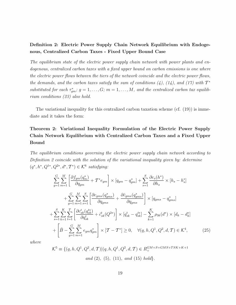
Definition 2: Electric Power Supply Chain Network Equilibrium with Endoge-
nous, Centralized Carbon Taxes - Fixed Upper Bound Case
The equilibrium state of the electric power supply chain network with power plants and en-
dogenous, centralized carbon taxes with a fixed upper bound on carbon emissions is one where
the electric power flows between the tiers of the network coincide and the electric power flows,
the demands, and the carbon taxes satisfy the sum of conditions (4), (14), and (17) with T ∗
substituted for each τ ∗gm; g = 1, . . . , G; m = 1, . . . , M , and the centralized carbon tax equilib-
rium conditions (23) also hold.
The variational inequality for this centralized carbon taxation scheme (cf. (19)) is imme-
diate and it takes the form:
Theorem 2: Variational Inequality Formulation of the Electric Power Supply
Chain Network Equilibrium with Centralized Carbon Taxes and a Fixed Upper
Bound
The equilibrium conditions governing the electric power supply chain network according to
Definition 2 coincide with the solution of the variational inequality given by: determine
(q∗, h∗, Q1∗, Q2∗, d∗, T ∗) ∈ K6 satisfying:
G∑
g=1
M∑
m=1
[∂fgm(q∗m)
∂qgm
+ T ∗egm
]× [qgm − q∗gm] +
S∑
s=1
∂cs(h∗)
∂hs
× [hs − h∗s]
+G∑
g=1
M∑
m=1
S∑
s=1
[∂cgms(q
∗gms)
∂qgms+
∂cgms(q∗gms)
∂qgms
]× [qgms − q∗gms]
+S∑
s=1
K∑
k=1
T∑
t=1
[∂ct
sk(qt∗sk)
∂qtsk
+ ctsk(Q
2∗)
]× [qt
sk − qt∗sk] −
K∑
k=1
ρ3k(d∗) × [dk − d∗
k]
+
B −
G∑
g=1
M∑
m=1
egmq∗gm
× [T − T ∗] ≥ 0, ∀(q, h, Q1, Q2, d, T ) ∈ K4, (25)
where
K5 ≡ {(q, h, Q1, Q2, d, T )|(q, h, Q1, Q2, d, T ) ∈ RGM+S+GMS+TSK+K+1+
and (2), (5), (11), and (15) hold}.
19

Centralized Carbon Taxation Scheme - Elastic Bound
We now consider a carbon taxation scheme in which the carbon emission bound is elastic in
that it is no longer fixed but is a function of the carbon tax. Such a scheme would reflect, for
example, the situation where the government might be willing to assign a different bound
on carbon emissions, depending upon the size of the tax. Hence, we now assume rather
than a bound B as in (23), a bound denoted by B(T ) where this function is assumed to be
continuous.
Centralized Carbon Tax Equilibrium Conditions – Elastic Bound
In this case, the carbon tax equilibrium conditions (cf. (23)) would be as follows.
B(T ∗) −G∑
g=1
M∑
m=1
egmq∗gm
{= 0, if T ∗ > 0,≥ 0, if T ∗ = 0.
(26)
Clearly equilibrium conditions (23) can be formulated as the inequality:
B(T ∗) −
G∑
g=1
M∑
m=1
egmq∗gm
× [T − T ∗] ≥ 0, ∀T ≥ 0. (27)
As for the behavior of the electric power supply chain network decision-makers, it remains
as described in Section 2.1, except that now we substitute T ∗ for each τ ∗gm; g = 1, . . . , G;
m = 1, . . . , M , as we did for the centralized scheme in the case of a fixed upper bound for
carbon emissions. Such a substitution (again) needs to be made in (1) and in (4) with the
resulting definition below:
Definition 3: Electric Power Supply Chain Network Equilibrium with Endoge-
nous, Centralized Carbon Taxes - Elastic Bound Case
The equilibrium state of the electric power supply chain network with power plants and en-
dogenous, centralized carbon taxes with an elastic carbon emission bound is one where the
electric power flows between the tiers of the network coincide and the electric power flows,
20

the demands, and the carbon taxes satisfy the sum of conditions (4), (14), (17), with T ∗ sub-
stituted for each τ ∗gm; g = 1, . . . , G; m = 1, . . . , M , and the centralized carbon tax equilibrium
conditions (26) also holds.
The variational inequality for the centralized carbon taxation scheme with an elastic
bound is also immediate:
Theorem 3: Variational Inequality Formulation of the Electric Power Supply
Chain Network Equilibrium with Centralized Carbon Taxes and an Elastic Car-
bon Emission Bound
The equilibrium conditions governing the electric power supply chain network according to
Definition 3 coincide with the solution of the variational inequality given by: determine
(q∗, h∗, Q1∗, Q2∗, d∗, T ∗) ∈ K6 satisfying:
G∑
g=1
M∑
m=1
[∂fgm(q∗m)
∂qgm+ T ∗egm
]× [qgm − q∗gm] +
S∑
s=1
∂cs(h∗)
∂hs× [hs − h∗
s]
+G∑
g=1
M∑
m=1
S∑
s=1
[∂cgms(q
∗gms)
∂qgms+
∂cgms(q∗gms)
∂qgms
]× [qgms − q∗gms]
+S∑
s=1
K∑
k=1
T∑
t=1
[∂ct
sk(qt∗sk)
∂qtsk
+ ctsk(Q
2∗)
]× [qt
sk − qt∗sk] −
K∑
k=1
ρ3k(d∗) × [dk − d∗
k]
+
B(T ∗) −
G∑
g=1
M∑
m=1
egmq∗gm
× [T − T ∗] ≥ 0,
∀(q, h, Q1, Q2, d, T ) ∈ K6. (28)
Each of the variational inequality problems (19), (25), and (28) can be put into standard
variational inequality form (cf. Nagurney [22]) given by: determine X∗ ∈ K such that
〈F (X∗), X − X∗〉 ≥ 0, ∀X ∈ K (29)
by defining the vector X and the function F that enters the variational inequality accord-
ingly. Qualitative properties of existence of a solution can then be obtained for variational
21

inequalities (19) and (25) by noting, first, that, due to the bound(s) on the carbon emissions,
the electric power outputs are bounded. If one further assumes that the imposed tax can
be reasonably assumed to be bounded (although the bound may be vary large), then we
know that the feasible set will be compact and existence of a solution will then follow from
the standard theory of variational inequalities (see [22]), since under our previously given
assumptions, the corresponding function F is continuous. In the case of variational inequal-
ity (28), one can assume similar conditions or a coercivity condition on the corresponding
function F . Monotonicity of F can be obtained for both variational inequalities (19) and
(25) under analogous assumptions as those given in Nagurney and Matsypura [16]; the same
holds in the case of F for variational inequality (28) with the additional assumption that the
function B(T ) is monotone.
22

3. Numerical Examples
In this Section, we provide numerical examples to demonstrate how the theoretical results
in this paper can be applied in practice.
Clearly, there are distinct variational inequality algorithms that may be applied to solve
variational inequalities (19), (25), and/or (28), and, in particular, we note the modified pro-
jection method (see [24]) which was been successfully applied to solve variational inequality
problems in which the function F (cf. (29)) is monotone and Lipschitz continuous; see, e.g.,
[16] and [25].
Wu et al. [11], in turn, proposed an Euler method for the electric power supply chain
network equilibrium problem with power plants and preassigned carbon taxes. That Euler
method was introduced by Dupuis and Nagurney [26] and is a special case of a general
iterative scheme for the solution of variational inequalities as well as projected dynamical
systems. Wu et al. [11] showed that such the electric power supply chain problem with
preassigned taxes could be transformed into a transportation network equilibrium problem
over an appropriately constructed abstract network or supernetwork.
In the models developed in this paper, however, in which the carbon taxes are no longer
pre-assigned but, are endogenous and reflect particular goals of governmental/environmental
authorities, we can no longer transform the variational inequalities (19), (25), and (28)
directly into transportation network equilibrium problems (as was also done by [27] for
supply chain network equilibrium problems in the case of products). However, we can still
exploit the connection by noticing that the variational inequality problems in this paper are
defined over feasible sets that are, in effect, decomposable into subproblems in the flows and
subproblems in carbon taxes. Furthermore, the former subproblems retain the transportation
network structure identified in [11]. Analogously, we can construct path flow versions of each
of these variational inequalities over the corresponding abstract transportation network and
there will be an additional term in each case to correspond to the particular carbon taxation
scheme equilibrium condition. We can then apply the Euler method, whose general statement
to solve a variational inequality given by: determine x∗ ∈ K such that
〈F (x∗), x − x∗〉 ≥ 0, ∀x ∈ K, (30)
23

is given immediately following.
The Euler Method
The Euler method (see [26]) has been applied by Nagurney and Zhang [28] to solve the
variational inequality governing elastic demand transportation network equilibrium problems
in path flows and by Zhang and Nagurney [29] for the formulation in link flows. Convergence
results can be found in the above references.
For the solution of (30), the Euler method takes the form: at iteration l compute xl+1 by
solving the variational inequality problem:
xl+1 = PK(xl − alF (xl)), (31)
where PK is the projection operator, and the sequence {al} must satisfy the conditions:∑∞
l=0 al = ∞, al > 0, for all l, and al → 0, as l → ∞.
The Euler method was implemented in FORTRAN and the computer system used was
a Sun system at the University of Massachusetts at Amherst. The convergence criterion
utilized was that the absolute value of the electric flows and the carbon taxes between two
successive iterations differed by no more than 10−6. The sequence {αl} in the Euler method
cf. (31) was set to: {1, 12, 1
2, 1
3, 1
3, 1
3, . . .}.
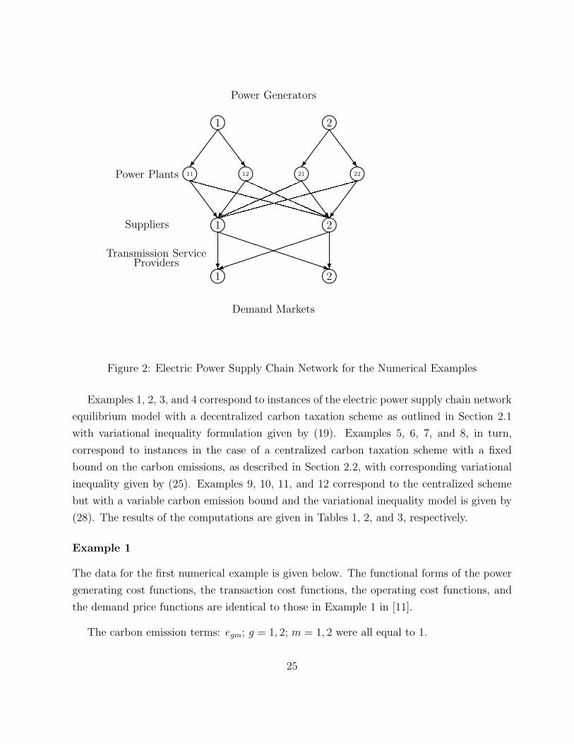
In all the numerical examples, the electric power supply chain network consisted of
two power generators, with two power plants each, two power suppliers, one transmission
provider, and two demand markets as depicted in Figure 2.
24
n11 n12 n21 n22
Transmission ServiceProviders
n1 n2S
SS
Sw
��
��/
SS
SSw
��
��/
n1 n2Suppliers
Power Plants
n1 n2
SS
SSw
��
��/
SS
SSw
��
��/
Demand Markets
Power Generators
?
PPPPPPPPPPPPq
������������) ?
Figure 2: Electric Power Supply Chain Network for the Numerical Examples
Examples 1, 2, 3, and 4 correspond to instances of the electric power supply chain network
equilibrium model with a decentralized carbon taxation scheme as outlined in Section 2.1
with variational inequality formulation given by (19). Examples 5, 6, 7, and 8, in turn,
correspond to instances in the case of a centralized carbon taxation scheme with a fixed
bound on the carbon emissions, as described in Section 2.2, with corresponding variational
inequality given by (25). Examples 9, 10, 11, and 12 correspond to the centralized scheme
but with a variable carbon emission bound and the variational inequality model is given by
(28). The results of the computations are given in Tables 1, 2, and 3, respectively.
Example 1
The data for the first numerical example is given below. The functional forms of the power
generating cost functions, the transaction cost functions, the operating cost functions, and
the demand price functions are identical to those in Example 1 in [11].
The carbon emission terms: egm; g = 1, 2; m = 1, 2 were all equal to 1.
25

The power generating cost functions for the power generators were given by:
f11(q1) = 2.5q211+q11q21+2q11, f12(q2) = 2.5q2
12+q11q12+2q22, f21(q1) = .5q221+.5q11q21+2q21,
f22(q2) = .5q222 + q12q22 + 2q22.
The transaction cost functions faced by the power generators and associated with trans-
acting with the power suppliers were given by:
c111(q111) = .5q2111 + 3.5q111, c112(q112) = .5q2
112 + 3.5q112, c121(q121) = .5q2121 + 3.5q121,
c122(q122) = .5q2122 + 3.5q122,
c211(q211) = .5q2211 + 2q211, c212(q212) = .5q2
212 + 2q212, c221(q221) = .5q2221 + 2q221,
c222(q222) = .5q2222 + 2q222.
The operating costs of the power generators, in turn, were given by:
c1(Q1) = .5(
2∑
i=1
qi1)2, c2(Q
1) = .5(2∑
i=1
qi2)2.
The demand market price functions at the demand markets were:
ρ31(d) = −1.33d1 + 366.6, ρ32 = −1.33d2 + 366.6,
and the transaction costs between the power suppliers and the consumers at the demand
markets were given by:
c1sk(q
1sk) = q1
sk + 5, s = 1, 2; k = 1, 2.
All other transaction costs were assumed to be equal to zero.
In Example 1, the carbon emission bounds were: B11 = B12 = B21 = B22 = 100.
The computed equilibrium electric power flows and demands and the optimal taxes are
given in Table 1. Note that the imposed bounds were sufficiently high so that all optimal
taxes were identically equal to 0.00 since the carbon emissions generated by each genco and
26

power plant combination were less than the imposed bound. The total carbon emissions
were: 22.56, 9.93, 22.90, and 92.38, respectively, for genco 1/power plant 1; genco 1/power
plant 2, and so on.
The price of electric power at the first demand market was 268.33 and at the second
demand market the price was also 268.33. The demand was 73.89 at each demand market.
The optimality/equilibrium conditions were satisfied with excellent accuracy.
Example 2
Example 2 was constructed from Example 1 as follows. It had the identical data but since
genco 2/power plant 2 emitted over 92 units of carbon, we set B22 = 23, which was approx-
imately the next highest amount of carbon emitted by another genco/power plant combina-
tion. The computed solution is given in Table 2.
The total amounts of carbon emitted were now: 29.86, 31.17, 30.20, and 23.00 for genco
1/power plant 1; genco 1/power plant 2, and so on, respectively. Note that, as the theory
predicts, the endogenous carbon taxes guaranteed that, in equilibrium, the amount of carbon
emitted by each power plant would not exceed the imposed bound. Only the second genco
was taxed and it was for the emissions at his second power plant. All other taxes were
equal to zero since the amounts of carbon emitted did not exceed the corresponding imposed
bound of 100 at each of those power plants.
The prices of electric power at the demand markets were now both equal to 290.63 and the
demand for electric power was equal to 57.12 at each demand market. Hence, the consumers
had an increase in the price relative to that in Example 1 since now there was an additional
tax levied.
Example 3
Example 3 was constructed from Example 2. The data were identical to the data in Example
2, except that now we set all the bounds as follows: B11 = B12 = B21 = B22 = 23. Hence, we
tightened the bounds on all the genco power plants, in comparison to the bounds imposed in
Example 1 and in Example 2. Again, the computed solution is given in Table 1. Note that
27

in Example 3, all the optimal taxes are now positive since the amounts of carbon emitted
by the various power plants are at the imposed bounds.
The price of electric power at each demand market was now equal to 305.42, whereas the
demand was reduced to 46 at each demand market. Hence, tighter carbon emission bounds,
as expected, resulted in higher demand market prices due to greater carbon taxes applied to
all the gencos’ power plants. Note that in our framework we are able to determine precisely
the carbon taxes that should be assigned in order to achieve the desired environmental policy
goal.
Example 4
Example 4 was constructed from Example 3 except that now the emission factor e11 = 2.
Hence, its value was now doubled. The equilibrium solution is given in Table 1. Note that
the electric power output of the first genco and the first power plant was essentially halved
in comparison to the corresponding output in Example 3. Again, the endogenous carbon
taxes had the desired effect in that the carbon emissions at each genco/power plant did not
exceed the imposed bounds of 23. Interestingly, the carbon taxes increased for all the gencos
and power plants although it was only the first genco and his first power plant that had its
emissions factor doubled. The demand for electric power at the demand markets decreases
to 40.30 at each demand market since the price of electric power has now increased and it is
equal to 313.00 at both demand markets.
Example 5
Examples 5, 6, 7, and 8 assumed a single centralized carbon taxation scheme in which the
bound on carbon emissions was fixed. The egm; g = 1, 2; m = 1, 2 were set equal to 1. The
remaining data were as given in Example 1 except that in Example 5 we set B = 100. Note
that this bound represents the bound on the total amount of carbon emitted by all the power
plants of all the gencos in the electric power supply chain network. The computed solution
for Example 5 is given in Table 2. The demand was 50.00 at each of the two demand markets
and the demand market price was 300.10.
28

Equilibrium Solution Example 1 Example 2 Example 3 Example 4Computed Equilibrium Power Flows
q∗11 22.56 29.86 23.00 11.51q∗12 9.93 31.17 23.00 23.02q∗21 22.90 30.20 23.00 23.02q∗22 92.38 23.00 23.00 23.05q∗111 11.28 14.93 11.50 5.76q∗112 11.28 14.93 11.50 5.76q∗121 4.97 15.59 11.50 11.51q∗122 4.97 15.59 11.50 11.51q∗211 11.45 15.10 11.50 11.51q∗212 11.45 15.10 11.50 11.51q∗221 46.19 11.50 11.50 11.52q∗222 46.19 11.50 11.50 11.52h∗
1 73.89 57.12 46.00 40.30h∗
2 73.89 57.12 46.00 40.30q1∗11 36.94 28.56 23.00 20.15
q1∗12 36.94 28.56 23.00 20.15
q1∗21 36.94 28.56 23.00 20.15
q1∗22 36.94 28.56 23.00 20.15
Computed Equilibrium Demandsd∗1 73.89 57.12 46.00 40.30d∗2 73.89 57.12 46.00 40.30
Computed Optimal Taxesτ∗11 0.00 0.00 76.43 77.86
τ∗12 0.00 0.00 76.43 92.38
τ∗21 0.00 0.00 77.93 105.41
τ∗22 0.00 130.26 169.93 185.96
Table 2: Solutions to Examples 1, 2, 3, and 4
29
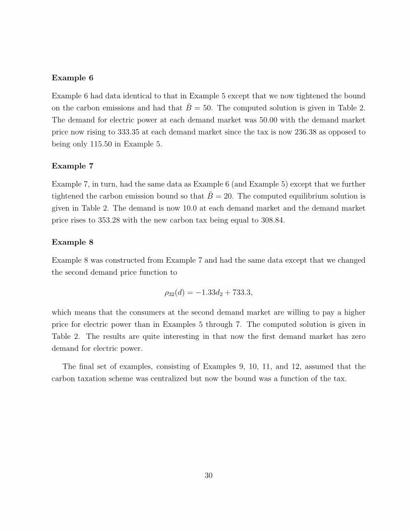
Example 6
Example 6 had data identical to that in Example 5 except that we now tightened the bound
on the carbon emissions and had that B = 50. The computed solution is given in Table 2.
The demand for electric power at each demand market was 50.00 with the demand market
price now rising to 333.35 at each demand market since the tax is now 236.38 as opposed to
being only 115.50 in Example 5.
Example 7
Example 7, in turn, had the same data as Example 6 (and Example 5) except that we further
tightened the carbon emission bound so that B = 20. The computed equilibrium solution is
given in Table 2. The demand is now 10.0 at each demand market and the demand market
price rises to 353.28 with the new carbon tax being equal to 308.84.
Example 8
Example 8 was constructed from Example 7 and had the same data except that we changed
the second demand price function to
ρ32(d) = −1.33d2 + 733.3,
which means that the consumers at the second demand market are willing to pay a higher
price for electric power than in Examples 5 through 7. The computed solution is given in
Table 2. The results are quite interesting in that now the first demand market has zero
demand for electric power.
The final set of examples, consisting of Examples 9, 10, 11, and 12, assumed that the
carbon taxation scheme was centralized but now the bound was a function of the tax.
30

Equilibrium Solution Example 5 Example 6 Example 7 Example 8Computed Equilibrium Power Flows
q∗11 15.20 7.48 2.85 2.87q∗12 6.63 3.17 1.10 1.10q∗21 15.53 7.82 3.19 3.20q∗22 62.65 31.53 12.86 12.91q∗111 7.60 3.74 1.43 1.43q∗112 7.60 3.74 1.43 1.43q∗121 3.31 1.59 0.55 0.55q∗122 3.31 1.59 0.55 0.55q∗211 7.76 3.91 1.59 1.60q∗212 7.76 3.91 1.59 1.60q∗221 31.32 15.77 6.43 6.46q∗222 31.32 15.77 6.43 6.46h∗
1 50.00 25.00 10.00 10.00h∗
2 50.00 25.00 10.00 10.00q1∗11 25.00 12.50 5.00 0.00
q1∗12 25.00 12.50 5.00 10.00
q1∗21 25.00 12.50 5.00 0.00
q1∗22 25.00 12.50 5.00 10.00
Computed Equilibrium Demandsd∗1 50.00 25.00 10.00 0.00d∗2 50.00 25.00 10.00 20.00
Computed Optimal TaxT ∗ 115.50 236.38 308.91 656.96
Table 3: Solutions to Examples 5, 6, 7, and 8
31

Example 9
Example 9 had the same input data as Example 5 but the bound on the carbon emissions
was now elastic and given by:
B(T ) = T + 100.
The equilibrium solution is reported in Table 3. The total carbon emissions are equal
to 133.79 with the value of B(T ∗)=133.79. The demand is 66.90 at each demand market
and the demand market price is 277.63 at each demand market. The optimal carbon tax
T ∗ = 33.79.
Example 10
Example 10 had the same data as Example 9 except that the carbon emission bound function
was now given by:
B(T ) = T + 50.
The computed equilibrium solution is reported in Table 3. The total carbon emissions
are now equal to 119.16 and this is also the value of B(T ∗). The demand for electric power
is equal to 59.58 at each demand market and the demand market price is 287.36 at each
demand market. The optimal carbon tax is now T ∗ = 69.16. Hence, the tax is now higher
than in Example 9 and the emissions are reduced. The demand market prices increase due
to the higher tax.
Example 11
Example 11 had the same data as the two preceding examples but differed in the elastic
carbon emission bound function which was now even “tighter” and given by:
B(T ) = T + 20.
The computed electric power flows, demands, and the optimal carbon tax are reported
in Table 3.
The demand for electric power is now 55.19 at each demand market. The optimal tax
is now T ∗ = 90.39 and the total carbon emissions generated equal to 110.39, which is
32

equal to the bound B(T ∗). Recall that in this example, as in the two preceding ones, the
emission terms egm; g = 1, 2; m = 1, 2 are all equal to 1. The demand is now 55.19 at each
demand market and the demand market price is now 293.19 at each demand market. Hence,
the carbon tax increases as do the demand market prices whereas the demands for electric
power decrease, in comparison to the values in Examples 9 and 10.
Example 12
Example 12 was constructed from Example 10 and had the identical data except that we now
modified the second demand market demand function to be as in Example 8. The solution
computed by the Euler method is given in Table 3. The demand for electric power at the
first demand market now drops to zero (as it did in Example 8) whereas the demand for
electric power at the second demand market is now equal to 178.61. The optimal carbon
tax is now T ∗ = 128.61 and the demand market price is equal to 406.34 at the first demand
market and to 495.65 at the second demand market. The total carbon emitted is now equal
to 178.61 which is also the value of the bound B(T ∗).
33

Equilibrium Solution Example 9 Example 10 Example 11 Example 12Computed Equilibrium Power Flows
q∗11 20.41 18.15 16.80 27.32q∗12 8.96 7.95 7.35 12.06q∗21 20.74 18.48 17.13 27.65q∗22 83.68 74.58 69.11 111.57q∗111 10.20 9.08 8.40 13.66q∗112 10.20 9.08 8.40 13.66q∗121 4.48 3.98 3.67 6.03q∗122 4.48 3.98 3.67 6.03q∗211 10.37 9.24 8.57 13.83q∗212 10.37 9.24 8.57 13.83q∗221 41.84 37.29 34.56 55.79q∗222 1.84 37.29 34.56 55.79h∗
1 66.90 59.58 55.19 89.31h∗
2 66.90 59.58 55.19 89.31q1∗11 33.45 29.79 27.60 0.00
q1∗12 33.45 29.79 27.60 89.31
q1∗21 33.45 29.79 27.60 0.00
q1∗22 33.45 29.79 27.60 89.31
Computed Equilibrium Demandsd∗1 66.90 59.58 55.19 0.00d∗2 66.90 59.58 55.19 178.61
Computed Optimal TaxT ∗ 33.79 69.16 90.38 128.61
Table 4: Solutions to Examples 9, 10, 11, and 12
34

4. Summary and Conclusions
In this paper, we presented a modeling and computational framework that may help
policy-makers to determine the optimal carbon taxes on the power plants in the electric power
generation industry. This general electric power supply chain network modeling framework
utilizes variational inequality theory and is capable of identifying the optimal carbon taxes
as well as the equilibrium electric power transaction flows and the demands for electric
power (along with the associated prices) under three distinct carbon taxation environmental
policies. Specifically, the first model, a completely decentralized scheme, allows the policy-
makers to determine the optimal tax for each individual electric power plant which guarantees
that the emission bound or quota of each plant is not exceeded. The second and third models,
on the other hand, both enforce a “global” emission bound on the entire industry by imposing
a uniform tax rate on the generating plants. However, the second policy assumes that the
global emission bound is fixed while the third policy allows the bound to be a function of
the tax.
We then discovered that the three variational inequality models were decomposable into
subproblems that can be efficiently solved using the Euler method. Twelve numerical exam-
ples were presented to illustrate the impacts of the three distinct carbon taxation policies on
the electric power supply chain networks. These numerical examples also demonstrate how
policy-makers can determine the optimal taxes in order to achieve environmental objectives.
This research is a contribution to the growing research in the development of rigorous
mathematical frameworks for environmental-energy modeling.
35

References
1. Energy (SICs: 4911, 4920), Encyclopedia of Global Industries. Online Edition. Thomson
Gale, (2006).
2. Edison Electric Institute, Statistical yearbook of the electric utility industry 1999, Wash-
ington, DC, (2000).
3. Energy Information Administration, Electric power annual 1999, vol. II, DOE/EIA-0348
(99)/2, Washington, DC, (2000).
4. Energy Information Administration, Annual energy review 2004, DOE/EIA-0348, Wash-
ington, DC, (2005).
5. J. Casazza and F. Delea, Understanding Electric Power Systems. John Wiley & Sons,
New York, (2003).
6. H. Singh, Editor, IEEE Tutorial on Game Theory Applications in Power Systems. IEEE,
(1999).
7. G. Zaccour, Editor, Deregulation of Electric Utilities. Kluwer Academic Publishers,
Boston, Massachusetts, (1998).
8. Pew Center, Developing countries & global climate change: electric power options in
China, Executive summary;
http://www.pewclimate.org/global-warming-in-depth/all reports/china/pol china execsummary
9. J. Poterba, Global warming policy: A public finance perspective. Journal of Economic
Perspectives 7, 73-89,(1993).
10. W. R. Cline, The economics of global warming. Institute for International Economics,
Washington, DC, (1992).
11. K. Wu, A. Nagurney, Z. Liu and J. Stranlund, Modeling generator power plant port-
folios and pollution taxes in electric power supply chain networks: A transportation net-
36

work equilibrium transformation., (2006) (To appear in Transportation Research D; see also
http://supernet.som.umass.edu)
12. A. Baranzini, J. Goldemberg and S. Speck, A future for carbon taxes. Ecological Eco-
nomics 32, 395-412, (2000).
13. J. P. Painuly, Barriers to renewable energy penetration; a framework for analysis. Re-
newable Energy 24, 73-89, (2001).
14. RECS Renewable energy certificate system; http://www.recs.org (1999).
15. G. J. Schaeffer, M. G. Boots, J. W. Martens and M. H. Voogt, Tradable Green Cer-
tificates: A New Market-Based Incentive Scheme for Renewable Energy. Energy Research
Centre of the Netherlands (ECN) Report, ECN-I–99-004, (1999).
16. A. Nagurney and D. Matsypura, A supply chain network perspective for electric power
generation, supply, transmission, and consumption. In: Advances in Computational Eco-
nomics, Finance and Management Science, E. J. Kontoghiorghes and C. Gatu, (Eds.),
Springer, Berlin, Germany, in press, (2005); appears in abbreviated and condensed form
in: Proceedings of the International Conference in Computing, Communications and Control
Technologies, Austin, Texas, Volume VI, pp. 127-134, (2004).
17. A. Nagurney and Z. Liu, Transportation network equilibrium reformulations of electric
power networks with computations. Isenberg School of Management, University of Massa-
chusetts, Amherst,(2005); see: http://supernet.som.umass.edu
18. M. J. Beckmann, C. B. McGuire and C. B. Winsten, Studies in the Economics of
Transportation. Yale University Press, New Haven, Connecticut, (1956).
19. A. Nagurney and F. Toyasaki, Supply chain supernetworks and environmental criteria.
Transportation Research D 8, 185-213, (2003).
20. J. F. Nash, Equilibrium points in n-person games. Proceedings of the National Academy
of Sciences 36, 48-49, (1950).
37

21. J. F. Nash, Noncooperative games. Annals of Mathematics 54, 286-298, (1951).
22. A. Nagurney, Network Economics: A Variational Inequality Approach. Kluwer Academic
Publishers, Dordrecht, The Netherlands, (1999).
23. K. K. Dhanda, A. Nagurney and P. Ramanujam, Environmental Networks: A Framework
for Economic Decision-Making and Policy Analysis. Edward Elgar Publishers, Cheltenham,
England, (1999).
24. G. M. Korpelevich, The extragradient method for finding saddle points and other prob-
lems. Matekon 13, 35-39, (1977).
25. A. Nagurney, J. Dong and D. Zhang, A supply chain network equilibrium model. Trans-
portation Research E 38, 281-303, (2002).
26. P. Dupuis and A. Nagurney, Dynamical systems and variational inequalities. Annals of
Operations Research 44, 9-42,(1993).
27. A. Nagurney, On the relationship between supply chain and transportation network
equilibria: A supernetwork equivalence with computations. Transportation Research E , in
press, (2005).
28. A. Nagurney and D. Zhang, Projected Dynamical Systems and Variational Inequalities
with Applications. Kluwer Academic Publishers, Boston, Massachusetts, (1996).
29. D. Zhang and A. Nagurney, Formulation, stability, and computation of traffic network
equilibria as projected dynamical systems. Journal of Optimization Theory and Applications
93, 417-444, (1997).
38


