INOM EXAMENSARBETE ELEKTROTEKNIK,AVANCERAD NIVÅ, 30 HP

, STOCKHOLM SVERIGE 2020

Optimal Control Model for an Autonomous Underwater Vehicle

GUSTAV HOLM

KTHSKOLAN FÖR ELEKTROTEKNIK OCH DATAVETENSKAP

Abstract

The main goal with this thesis was to develop an optimal control model for anautonomous underwater vehicle (AUV) and evaluate whether reference track-ing using Model Predictive Control (MPC) based on a linear dynamics modeldescribing all six degrees of freedom (DOF) is a suitable method for waypointnavigation. MPC is an advanced receding horizon optimal control method capa-ble of including constraints in the optimization. The drawback with this methodis that it is computationally heavy and since the dynamic AUV behavior is bothcomplex and nonlinear there are two open research questions: Does MPC im-prove reference tracking and is it computationally feasible?

Optimal control requires accurate dynamics models of the targeted system tofunction and ensure robustness. At the start of this thesis the targeted AUV wasan unmodelled vehicle and therefore modeling, model analysis and linearizationtechniques constitutes a big part of this thesis and creating a nonlinear dynam-ics model was a big task in this project.

To ensure that reference tracking using optimal control strategies was feasible,state-feedback solutions together with standard techniques for stability analysis,controllability and observability were investigated. A linear quadratic regula-tor (LQR) was designed using a linear time-invariant (LTI) dynamics modelaugmented with integral action and error dynamics to create a performancereference for the MPC implementation. The final step during this thesis wasto implement MPC reference tracking using integral action on both states andinputs and the results from this controller was then compared to the resultsfrom the LQR controller in terms of performance.

A model generator capable of creating 6 DOF nonlinear dynamics models withvarying complexity has been designed. This generator was used to derive twodi↵erent linear models describing the dynamic AUV behavior. These linearmodels were analyzed and the necessary model parameters were estimated us-ing simulation and then compared to physical data and live testing. Resultsfrom the LQR controller using an augmented error dynamics model is promis-ing in terms of reference tracking. Due to a time varying reference and anunder-actuated vehicle the resulting performance of the MPC controller doesnot match the results from the LQR controller. Overall, model-based optimalcontrol show potential as a method for dynamic control and waypoint naviga-tion for AUV applications, but further work with parameter estimation, modelvalidation and control objective definition is required to ensure feasibility in aphysical implementation.

i

Sammanfattning

Huvudmalet med detta examensarbete var att utveckla en modell for optimalstyrning av en autonom undervattensfarkost och utvardera om reglering medmodel predictive control (MPC) tillsammans med en linjar systemmodell sombeskriver farkostens rorelse i alla sex frihetsgrader (DOF) ar en lamplig metodfor waypoint navigering. MPC ar en avancerad metod for optimal styrningsom anvander en rorlig horisont och mojligor att begransningar pa tillstandoch styrsignaler kan inkluderas i optimeringen. Nackdelen med denna metod aratt den ar berakningstung och eftersom farkostens dynamiska beteende ar badekomplext och icke-linjart sa ar de tva huvudfragorna om en linjar systemmodellresulterar i tillracklig hog prestanda och om berakningstiden ar tillrackligt lag.

Optimala regulatorer behover noggranna dynamiska modeller for att fungera ochsakerstalla robusta losningar. Nar detta examensarbete startade sa fanns ingendynamisk modell tillganglig och darfor utgjorde modellering, modellanalys ochlinjarisering en stor del av arbetet och skapandet av en ickelinjar systemmodellbetraktades som en av huvuduppgifterna.

For att sakerstalla att reglering med optimala styrmetoder var mojligt sa un-dersoktes forst tillstandsaterkoppling tillsammans med standardmetoder for sta-bilitetsanalys, styrbarhet och observerbarhet. En linjarkvadratisk regulator(LQR) skapades med en linjar dynamisk modell som forstarkts med felregleringoch integrerade tillstand for att anvandas som referens till MPC implementa-tionen. Som sista steg skapades en MPC regulator forstarkt med integreradetillstand och styrsignaler. Darefter jamfordes resulaten fran denna implementa-tion med resultaten fran LQR.

En modellgenerator kapabel till att skapa ickelinjara dynamiska modeller i 6frihetsgrader designades. Den har generatorn anvandes sedan for att bygga tvalinjara modeller som beskriver farkostens dynamiska beteende. Dessa linjaramodeller undersoktes och alla nodvandiga parametrar estimerades med hjalp avsimulering och utvarderades sedan mot insamlad data och farkostens beteendevid fysiska tester. Resultaten fran LQR med en modell for feldynamik ar lo-vande med avseende pa reglering. Pa grund av en tidsvarierande referens ochatt farkosten ar underaktuerad ar MPC regulatorns prestanda ej likvardig medprestandan fran LQR. Overgripande sa visar modellbaserad optimal styrningstor potential som metod for dynamisk styrning och tillampningar pa autonomaundervattensfarkoster men mer arbete inom parameterestimering, modellanalysoch formuleringen av styrobjektiv ar nodvandigt for att kunna sakerstalla pre-standa och implementationsmojligheterna i ett fysiskt system.

ii

Acknowledgements

First of all I want to thank Jakob Kuttenkeuler for giving me the opportunityto write this thesis at the KTH Centre for Naval Architecture and for invitingme to be a part of the LoLo development team. To be a part of this team hasprovided both knowledge and understanding about maritime robotics and thecraft itself which has been a valuable resource throughout this thesis.

I am grateful for the help and support provided by my supervisor ClemensDeutsch who, throughout this thesis, has pushed me in the right direction andhelped me to put focus and e↵ort into reaching as far as possible.

I extend my gratitude to Jonas Martensson at the Division of Decision andControl Systems for taking on the role of examiner and Joana Filipa GouveiaFonseca for helping me with control related problems and for providing adviceon implementation aspects of MPC and LQR.

Lastly I want to thank my family and friends for their support, even though notalways understanding the theoretical aspects of my work.

Stockholm, December 2019Gustav Holm

iii

Contents

1 Introduction 1

1.1 Background . . . . . . . . . . . . . . . . . . . . . . . . . . . . . . 11.2 Purpose . . . . . . . . . . . . . . . . . . . . . . . . . . . . . . . . 11.3 Objective . . . . . . . . . . . . . . . . . . . . . . . . . . . . . . . 21.4 Method . . . . . . . . . . . . . . . . . . . . . . . . . . . . . . . . 21.5 Limitations . . . . . . . . . . . . . . . . . . . . . . . . . . . . . . 21.6 Software . . . . . . . . . . . . . . . . . . . . . . . . . . . . . . . . 31.7 Thesis Outline . . . . . . . . . . . . . . . . . . . . . . . . . . . . 4

2 Theoretical Concepts 5

2.1 SNAME notation of motion . . . . . . . . . . . . . . . . . . . . . 52.2 Degrees of Freedom . . . . . . . . . . . . . . . . . . . . . . . . . . 62.3 Vehicle Description . . . . . . . . . . . . . . . . . . . . . . . . . . 62.4 Coordinate Frames . . . . . . . . . . . . . . . . . . . . . . . . . . 7

2.4.1 NED {n} . . . . . . . . . . . . . . . . . . . . . . . . . . . 82.4.2 BODY {b} . . . . . . . . . . . . . . . . . . . . . . . . . . 82.4.3 VP {p} . . . . . . . . . . . . . . . . . . . . . . . . . . . . 9

2.5 Positions and Euler Angles . . . . . . . . . . . . . . . . . . . . . 92.6 Hydrodynamic Derivatives . . . . . . . . . . . . . . . . . . . . . . 102.7 Vehicle Symmetry . . . . . . . . . . . . . . . . . . . . . . . . . . 10

3 Modeling 12

3.1 Mass and Inertia . . . . . . . . . . . . . . . . . . . . . . . . . . . 123.2 Coriolis and Centripetal Forces . . . . . . . . . . . . . . . . . . . 133.3 Damping Forces . . . . . . . . . . . . . . . . . . . . . . . . . . . . 143.4 Restoring Forces . . . . . . . . . . . . . . . . . . . . . . . . . . . 143.5 Actuators and Control Surfaces . . . . . . . . . . . . . . . . . . . 15

3.5.1 Propeller Thrust . . . . . . . . . . . . . . . . . . . . . . . 163.5.2 Rudders . . . . . . . . . . . . . . . . . . . . . . . . . . . . 183.5.3 Elevator . . . . . . . . . . . . . . . . . . . . . . . . . . . . 183.5.4 Elevons . . . . . . . . . . . . . . . . . . . . . . . . . . . . 183.5.5 Combined Actuator Expression . . . . . . . . . . . . . . . 19

3.6 Equations of Motion . . . . . . . . . . . . . . . . . . . . . . . . . 193.7 Parameter Estimation . . . . . . . . . . . . . . . . . . . . . . . . 193.8 nonlinear State-Space . . . . . . . . . . . . . . . . . . . . . . . . 203.9 Linearization . . . . . . . . . . . . . . . . . . . . . . . . . . . . . 20

3.9.1 Vessel parallel coordinates LTI-Model . . . . . . . . . . . 203.9.2 Jacobian LTV-Model . . . . . . . . . . . . . . . . . . . . . 21

3.10 Discretization . . . . . . . . . . . . . . . . . . . . . . . . . . . . . 22

iv

4 Control 23

4.1 Existing System . . . . . . . . . . . . . . . . . . . . . . . . . . . . 234.2 Model Analysis . . . . . . . . . . . . . . . . . . . . . . . . . . . . 23

4.2.1 Stability . . . . . . . . . . . . . . . . . . . . . . . . . . . . 234.2.2 Controllability . . . . . . . . . . . . . . . . . . . . . . . . 244.2.3 Observability . . . . . . . . . . . . . . . . . . . . . . . . . 24

4.3 Model Augmentations . . . . . . . . . . . . . . . . . . . . . . . . 254.4 Linear Control Methods . . . . . . . . . . . . . . . . . . . . . . . 26

4.4.1 State-Feedback . . . . . . . . . . . . . . . . . . . . . . . . 264.4.2 LQR . . . . . . . . . . . . . . . . . . . . . . . . . . . . . . 26

4.5 MPC . . . . . . . . . . . . . . . . . . . . . . . . . . . . . . . . . . 274.5.1 Basic Formulation . . . . . . . . . . . . . . . . . . . . . . 274.5.2 Additional Augmentations . . . . . . . . . . . . . . . . . . 27

5 Results 30

6 Analysis and Discussion 37

7 Conclusion 39

8 Future Work 40

References 42

v

Definitions

LoLo - Name of the vehicleMPC - Model Predictive ControlLTV - Linear Time-VaryingLTI - Linear Time-InvariantDOF - Degree of FreedomAUV - Autonomous Underwater VehicleLQR - Linear Quadratic RegulationKTH - Royal Institute of TechnologySMaRC - Swedish Maritime Robotics CentreSISO - Single-Input Single-OutputMIMO - Multiple-Input Multiple-OutputSF - State-FeedbackNED - North East DownBODY - BodyVP - Vessel ParallelSNAME - Society of Naval Architects and Marine EngineersVBS - Variable Buoyancy SystemWGS - World Geodetic SystemBIBO - Bounded-Input Bounded-OutputARE - Algebraic Riccati EquationRPM - Revolutions Per MinuteZOH - Zero Order HoldAOA - Angle of Attack

vi

Notations

CG - Center of gravityCB - Center of buoyancyCO - Center of arbitrary coordinate systeml - Length of vehicleb - Width of vehicleh - Height of vehiclexg - Distance from CO to CG {x}yg - Distance from CO to CG {y}zg - Distance from CO to CG {z}xb - Distance from CO to CG {x}yb - Distance from CO to CG {y}zb - Distance from CO to CG {z}Ayz - Front cross section areaAxy - Top cross section areaAxz - Side cross section areaAr - Area of ruddersAe - Area of elevatorAev - Area of elevonslroll - Distance from rudder to CO {z}lpitch - Distance from elevator to CO{x}lyaw - Distance from rudder to CO {x}lpx - Distance from propeller to CO {x}lpy - Distance from propeller to CO {y}lepitch - Distance from elevons to CO {x}leroll - Distance from elevons to CO {y}m - Craft weightIx - Inertia in rollIy - Inertia in pitchIz - Inertia in yawIxy - Coupled inertia for roll and pitchIxz - Coupled inertia for roll and yawIyz - Coupled inertia for pitch and yaw⇢ - Density of waterg - Gravitational accelerationW - Gravitation forceB - Buoyancy forceXu - Added mass in surgeXv - Added mass in surge due to swayXw - Added mass in surge due to heaveXp - Added mass in surge due to rollXq - Added mass in surge due to pitchXr - Added mass in surge due to yawYv - Added mass in sway

vii

Yw - Added mass in sway due to heaveYp - Added mass in sway due to rollYq - Added mass in sway due to pitchYr - Added mass in sway due to yawZw - Added mass in heaveZp - Added mass in heave due to rollZq - Added mass in heave due to pitchZr - Added mass in heave due to yawKp - Added mass in rollKq - Added mass in roll due to pitchKr - Added mass in roll due to yawMq - Added mass in pitchMr - Added mass in pitch due to yawNr - Added mass in yawXu - Linear drag coe�cient in surgeX|u|u - Quadratic drag coe�cient in surgeYv - Linear drag coe�cient in swayY|v|v - Quadratic drag coe�cient in swayZw - Linear drag coe�cient in heaveZ|w|w - Quadratic drag coe�cient in heaveKp - Linear drag coe�cient in rollK|p|p - Quadratic drag coe�cient in rollMq - Linear drag coe�cient in pitchM|q|q - Quadratic drag coe�cient in pitchNr - Linear drag coe�cient in yawN|r|r - Quadratic drag coe�cient in yawT - Thrust generated by propellerL - Lift force generated by actuatorD - Drag force generated by actuator� - Rudder deflection angle↵ - Vehicle angle of attackR - Engine RPMt - Timeh - Sampling intervalCd - Drag coe�cientCL - Lift coe�cient

viii

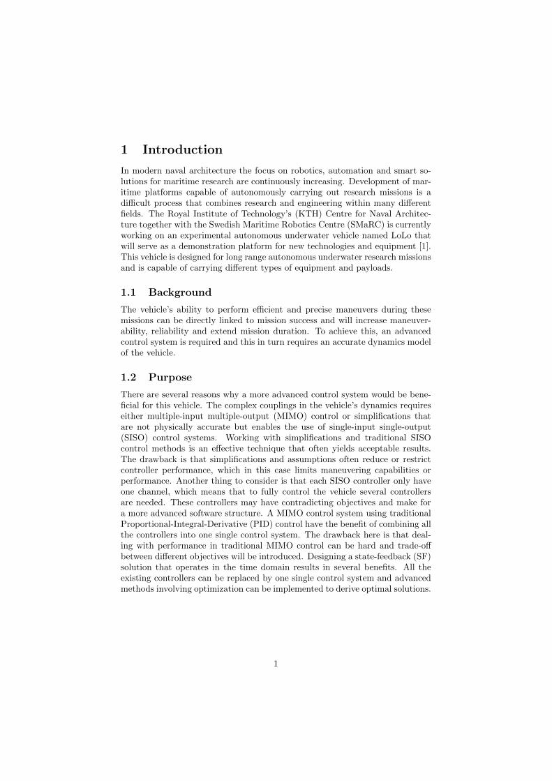
1 Introduction

In modern naval architecture the focus on robotics, automation and smart so-lutions for maritime research are continuously increasing. Development of mar-itime platforms capable of autonomously carrying out research missions is adi�cult process that combines research and engineering within many di↵erentfields. The Royal Institute of Technology’s (KTH) Centre for Naval Architec-ture together with the Swedish Maritime Robotics Centre (SMaRC) is currentlyworking on an experimental autonomous underwater vehicle named LoLo thatwill serve as a demonstration platform for new technologies and equipment [1].This vehicle is designed for long range autonomous underwater research missionsand is capable of carrying di↵erent types of equipment and payloads.

1.1 Background

The vehicle’s ability to perform e�cient and precise maneuvers during thesemissions can be directly linked to mission success and will increase maneuver-ability, reliability and extend mission duration. To achieve this, an advancedcontrol system is required and this in turn requires an accurate dynamics modelof the vehicle.

1.2 Purpose

There are several reasons why a more advanced control system would be bene-ficial for this vehicle. The complex couplings in the vehicle’s dynamics requireseither multiple-input multiple-output (MIMO) control or simplifications thatare not physically accurate but enables the use of single-input single-output(SISO) control systems. Working with simplifications and traditional SISOcontrol methods is an e↵ective technique that often yields acceptable results.The drawback is that simplifications and assumptions often reduce or restrictcontroller performance, which in this case limits maneuvering capabilities orperformance. Another thing to consider is that each SISO controller only haveone channel, which means that to fully control the vehicle several controllersare needed. These controllers may have contradicting objectives and make fora more advanced software structure. A MIMO control system using traditionalProportional-Integral-Derivative (PID) control have the benefit of combining allthe controllers into one single control system. The drawback here is that deal-ing with performance in traditional MIMO control can be hard and trade-o↵between di↵erent objectives will be introduced. Designing a state-feedback (SF)solution that operates in the time domain results in several benefits. All theexisting controllers can be replaced by one single control system and advancedmethods involving optimization can be implemented to derive optimal solutions.

1

1.3 Objective

The main objective of this thesis was to evaluate whether model-predictive con-trol (MPC) reference tracking using a linearized dynamics model of the vehicleLoLo is a suitable method for waypoint tracking or regulation in terms of perfor-mance and computational time. To reach this final objective, there are severalother tasks or goals that need to be achieved.

1.4 Method

This thesis was divided into three phases.

• Phase 1: The first phase covers all the theoretical aspects and includes afour week long study in naval architecture, modeling and control of navalvessels. The purpose of this phase was to familiarize with the vehicle’sexisting systems, prerequisites and emphasis was put on how modeling andcontrol was applied in practice by naval architects and marine engineers.

• Phase 2: The second phase included all the modeling. Here, the pur-pose was to derive a complete dynamics model describing all 6 degreesof freedrom (DOF) of the vehicle. From there the dynamics model wastranslated into a state-space representation and parameters describing dy-namic behavior was estimated. The final step in phase two was to createthe linear models representing the vehicle’s nonlinear dynamics.

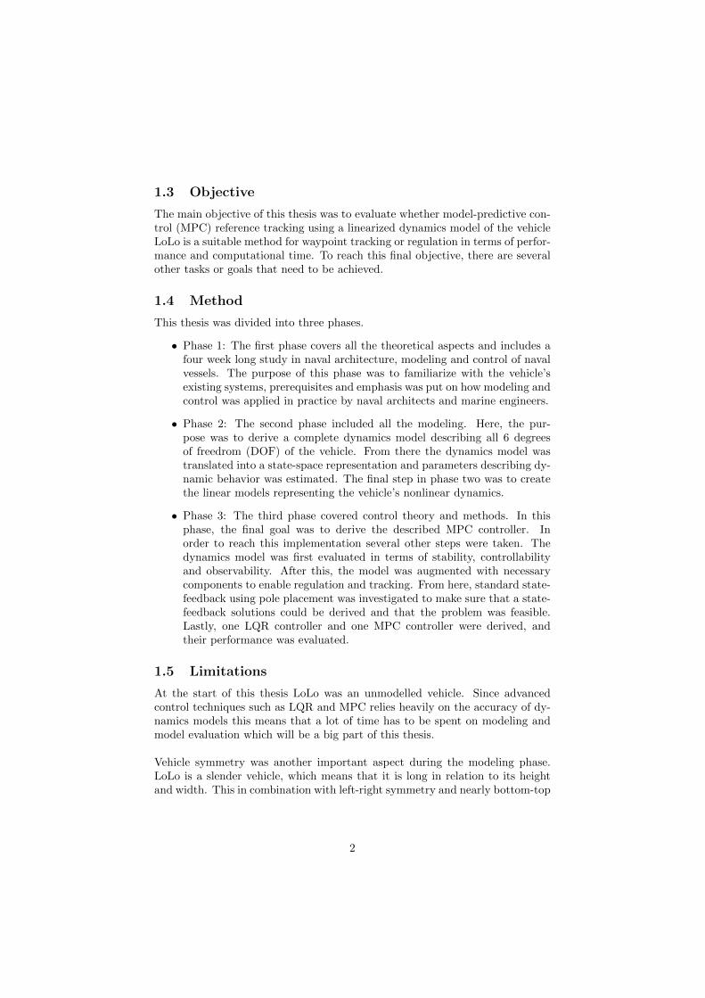
• Phase 3: The third phase covered control theory and methods. In thisphase, the final goal was to derive the described MPC controller. Inorder to reach this implementation several other steps were taken. Thedynamics model was first evaluated in terms of stability, controllabilityand observability. After this, the model was augmented with necessarycomponents to enable regulation and tracking. From here, standard state-feedback using pole placement was investigated to make sure that a state-feedback solutions could be derived and that the problem was feasible.Lastly, one LQR controller and one MPC controller were derived, andtheir performance was evaluated.

1.5 Limitations

At the start of this thesis LoLo was an unmodelled vehicle. Since advancedcontrol techniques such as LQR and MPC relies heavily on the accuracy of dy-namics models this means that a lot of time has to be spent on modeling andmodel evaluation which will be a big part of this thesis.

Vehicle symmetry was another important aspect during the modeling phase.LoLo is a slender vehicle, which means that it is long in relation to its heightand width. This in combination with left-right symmetry and nearly bottom-top

2

symmetry allows for a number of simplifications. These simplifications drasti-cally reduce the number of elements in the matrices that describe vehicle dy-namics. This will be further explained in Section 3.

When modeling the vehicle LoLo, a modeling technique using hydrodynamicderivatives was used. These hydrodynamic derivatives are parameters that de-scribe how di↵erent forces and torques a↵ect the vehicle and are strictly design-dependent. Determining values for each of these parameters is time consumingand a big project by itself. Therefore, dummy values, simplifications and as-sumptions will instead be used during this thesis. The result of this is that themodel will not be a perfect resemblance of the physical system but su�cientto evaluate performance of di↵erent controllers and determine feasibility for ad-vanced control methods.

Even though the vehicle dynamics are more accurately described by a nonlinearmodel on the form x = f(t,⌫, ⌧ ), the intention with this thesis is to evaluatewhether MPC using linear dynamics can be implemented to generate good ref-erence tracking performance. Using a linear model to describe the dynamics ofa nonlinear system have both pros and cons. As mentioned before, the accuracyis of great concern. If the model dynamics are too far from the actual vehicledynamics the resulting controllers will not perform well enough. However, theupside of using linear models is that the computational capacity required toderive the control solutions is drastically reduced which might be crucial foradvanced methods like MPC to be feasible in practice. This creates a trade-o↵between model accuracy and computational e↵ort, and the question stands if asu�ciently accurate linear model can be derived and whether the computationaltime needed by the MPC controller using this linear model is acceptable.

The vehicle has two types of actuators, control surfaces and propellers. Thecontrol surfaces are represented by rudders, elevator and elevons and constitutethe majority of the actuators. In this thesis control surfaces were modeled assymmetrical foils and when deflected an angle � under forward speed u they cre-ates two forces, commonly described as lift (L) and drag (D). This means that,depending on the rudder position, each rudder has the capability of producinga maximum of two forces and two moments. All of these forces and momentswill be described in Section 3, but since L

D ⇡ 5 for low values of � the e↵ect ofdrag was neglected in the controllers. Some of the moments induced by lift anddrag were also neglected due to short distances between CO and the actuator.

1.6 Software

During this thesis, Matlab was the main software used. Matlab is an advancedcomputing environment that uses it’s own programming language and a widevariety of built in toolboxes that simplify calculations, for example the sym-bolic math toolbox that enables solving and manipulation of symbolic valuedmath functions [2] that has been used extensively throughout this thesis. For

3

constrained optimization and MPC, the third-party toolbox YALMIP [3] hasbeen used. YALMIP is an optimization toolbox that provides a frameworkwhich enables the user to formulate constrained optimization problems withan alternative setup and a variety of di↵erent solvers. For optimization, Mat-lab’s built-in solvers Quadprog and Fmincon have been used together with theexternal solver Gurobi [4]. All of these solvers have their own strengths andweaknesses, but overall the more advanced Gurobi solver has yielded the bestresults in terms of computation time.

1.7 Thesis Outline

This report starts with Section 2 about the theoretical concepts necessary tounderstand the methods used in this thesis. Section 3 describes the modelingphase of this thesis. There, the techniques used to derive a complete lineardynamics model from a physical system is presented. In Section 4 the conceptsused to analyze and augment the dynamics models together with the theoreticalaspects of state-feedback, LQR and MPC are presented. A short descriptionof the vehicle’s existing systems is also included. Section 5 covers the resultsobtained during this thesis from both modeling and control. In Section 6 allthe results and key concepts are evaluated. Lastly, Section 7 and 8 presentssome final thoughts about the method used and future work needed to furtherimprove the dynamics model and controllers derived during this thesis.

4

2 Theoretical Concepts

In this section, some of the key concepts necessary to understand the workperformed during this thesis are described together with a description of thevehicle LoLo.

2.1 SNAME notation of motion

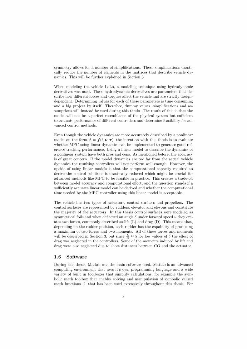
Throughout this thesis and in this report the Society of Naval Architects andMarine Engineers (SNAME) notation of motion [5] was used to describe forces,moments, positions, angles, linear and angular velocities. This notation facil-itates keeping track of di↵erent quantities, which is of great importance whenworking with systems with complex and coupled dynamics and simplifies bothcalculation and analysis. In Table 1 an overview of the notation is presentedand in Figure 1 the DOFs are illustrated from the vehicle perspective.

Table 1: SNAME notation for marine vessels

DOFForcesand

moments

Linearand

angularvelocities

Positionsandeulerangles

1 Motion in x (Surge) X u x2 Motion in y (Sway) Y v y3 Motion in z (Heave) Z w z4 Rotation around x (Roll) K p �

5 Rotation around y (Pitch) M q ✓

6 Rotation around z (Yaw) N r

5

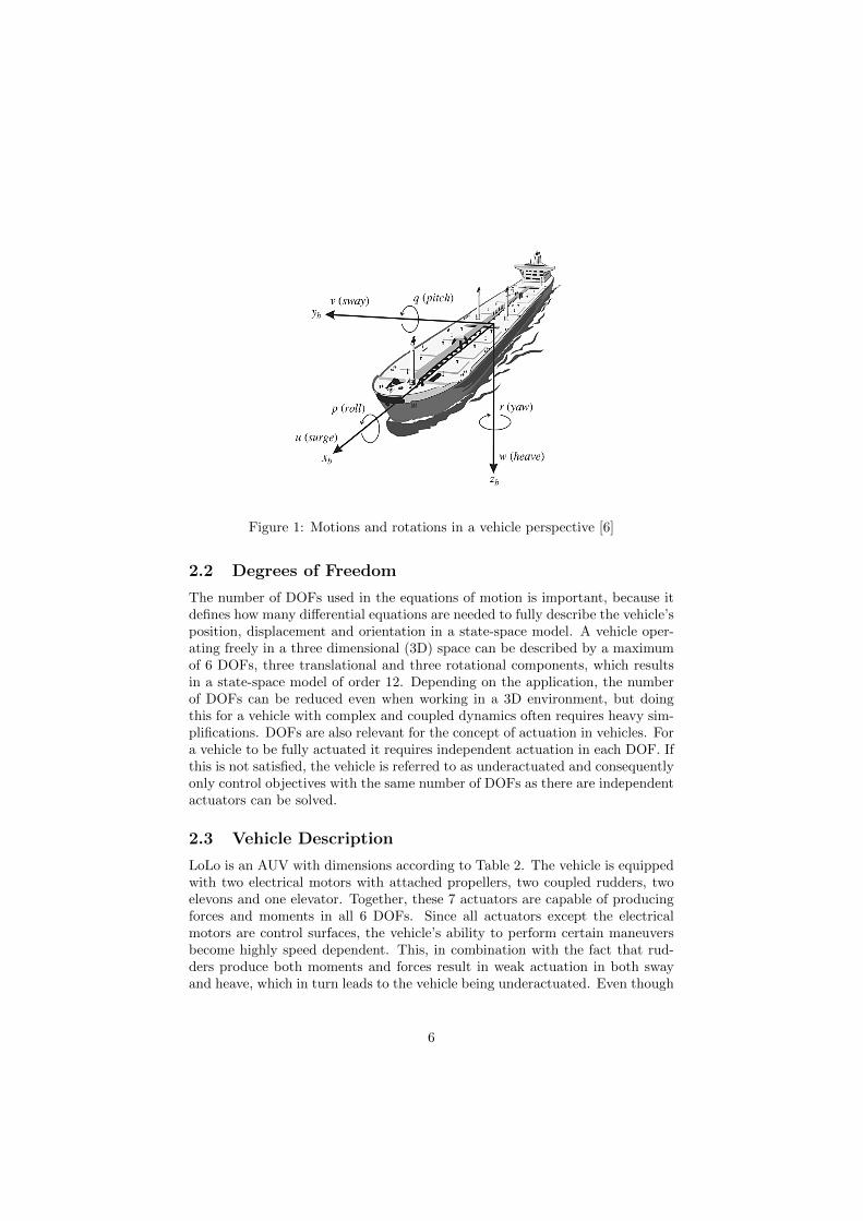
Figure 1: Motions and rotations in a vehicle perspective [6]

2.2 Degrees of Freedom

The number of DOFs used in the equations of motion is important, because itdefines how many di↵erential equations are needed to fully describe the vehicle’sposition, displacement and orientation in a state-space model. A vehicle oper-ating freely in a three dimensional (3D) space can be described by a maximumof 6 DOFs, three translational and three rotational components, which resultsin a state-space model of order 12. Depending on the application, the numberof DOFs can be reduced even when working in a 3D environment, but doingthis for a vehicle with complex and coupled dynamics often requires heavy sim-plifications. DOFs are also relevant for the concept of actuation in vehicles. Fora vehicle to be fully actuated it requires independent actuation in each DOF. Ifthis is not satisfied, the vehicle is referred to as underactuated and consequentlyonly control objectives with the same number of DOFs as there are independentactuators can be solved.

2.3 Vehicle Description

LoLo is an AUV with dimensions according to Table 2. The vehicle is equippedwith two electrical motors with attached propellers, two coupled rudders, twoelevons and one elevator. Together, these 7 actuators are capable of producingforces and moments in all 6 DOFs. Since all actuators except the electricalmotors are control surfaces, the vehicle’s ability to perform certain maneuversbecome highly speed dependent. This, in combination with the fact that rud-ders produce both moments and forces result in weak actuation in both swayand heave, which in turn leads to the vehicle being underactuated. Even though

6

a variable buoyancy system (VBS) has not been implemented, the AUV is as-sumed to be neutrally buoyant to simplify modeling and to remove some of thespeed dependency. The AUV operates at relative low speeds of 1�3 m/s, the en-gines are limited to ±500 [RPM ] and rudders operate in between ±20 degrees.CG and CB are located at the same x and y coordinates, whereas the distancebetween zg and zb is 0.4 m. Further, the vehicle’s moment of inertia are calcu-lated assuming a block shape body and the vehicle design is presented in Figure2.

Figure 2: Vehicle design

Table 2: LoLo’s physical data

l - 3.8 m

b - 1.05 m

h - 0.6 m

m - 300 kg

Ix - 37 kgm2

Iy - 370 kgm2

Iz - 389 kgm2

2.4 Coordinate Frames

Throughout this thesis a number of di↵erent coordinate frames have been used.Understanding what di↵erent notations mean, how vehicle dynamics are de-scribed and how to transform di↵erent motions between coordinate frames wasan important aspect when both modeling and when regulating the system to adesired target or way point. Below is a short description of the three most impor-tant coordinate frames, North-East-Down (NED), Body Coordinates (BODY)and Vessel Parallel Coordinates (VP). The center of origin in each coordinate

7

system can be chosen arbitrarily, e.g. the fore of the vehicle to create a safetymargin for movement in surge, but to simplify modeling, the best location isusually when it coincides with CG and CB in the lateral coordinates x and y.

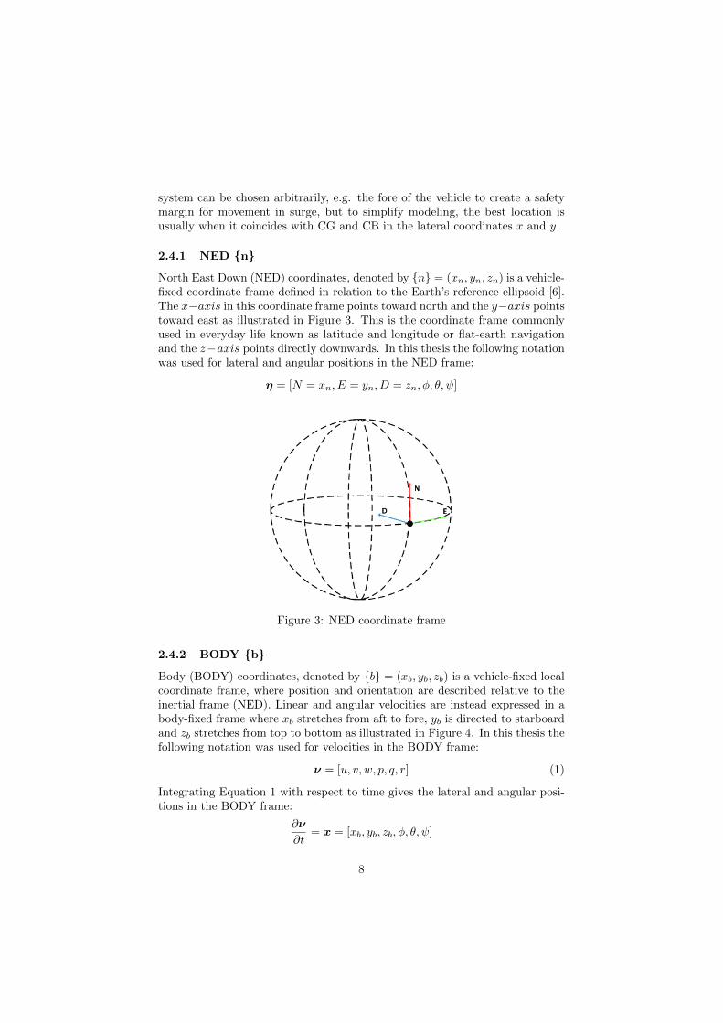
2.4.1 NED {n}

North East Down (NED) coordinates, denoted by {n} = (xn, yn, zn) is a vehicle-fixed coordinate frame defined in relation to the Earth’s reference ellipsoid [6].The x�axis in this coordinate frame points toward north and the y�axis pointstoward east as illustrated in Figure 3. This is the coordinate frame commonlyused in everyday life known as latitude and longitude or flat-earth navigationand the z�axis points directly downwards. In this thesis the following notationwas used for lateral and angular positions in the NED frame:

⌘ = [N = xn, E = yn, D = zn,�, ✓, ]

Figure 3: NED coordinate frame

2.4.2 BODY {b}

Body (BODY) coordinates, denoted by {b} = (xb, yb, zb) is a vehicle-fixed localcoordinate frame, where position and orientation are described relative to theinertial frame (NED). Linear and angular velocities are instead expressed in abody-fixed frame where xb stretches from aft to fore, yb is directed to starboardand zb stretches from top to bottom as illustrated in Figure 4. In this thesis thefollowing notation was used for velocities in the BODY frame:

⌫ = [u, v, w, p, q, r] (1)

Integrating Equation 1 with respect to time gives the lateral and angular posi-tions in the BODY frame:

@⌫

@t= x = [xb, yb, zb,�, ✓, ]

8

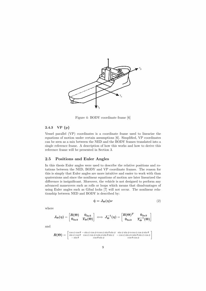
Figure 4: BODY coordinate frame [6]

2.4.3 VP {p}

Vessel parallel (VP) coordinates is a coordinate frame used to linearize theequations of motion under certain assumptions [6]. Simplified, VP coordinatescan be seen as a mix between the NED and the BODY frames translated into asingle reference frame. A description of how this works and how to derive thisreference frame will be presented in Section 3.

2.5 Positions and Euler Angles

In this thesis Euler angles were used to describe the relative positions and ro-tations between the NED, BODY and VP coordinate frames. The reason forthis is simply that Euler angles are more intuitive and easier to work with thanquaternions and since the nonlinear equations of motion are later linearized thedi↵erence is insignificant. Moreover, the vehicle is not designed to perform anyadvanced maneuvers such as rolls or loops which means that disadvantages ofusing Euler angles such as Gibal locks [7] will not occur. The nonlinear rela-tionship between NED and BODY is described by:

⌘ = J⇥(⌘)⌫ (2)

where

J⇥(⌘) =

R(⇥) 03x3

03x3 T⇥(⇥)

�() J�1

⇥ (⌘) =

R(⇥)

T03x3

03x3 T�1⇥ (⇥)

�

and

R(⇥) =

cos cos ✓ � sin cos�+cos sin ✓ sin� sin sin�+cos cos� sin ✓sin cos ✓ cos cos�+sin� sin ✓ sin � cos sin�+sin ✓ sin cos�� sin ✓ cos ✓ sin� cos ✓ cos�

�

9

and

T⇥(⇥) =

2

41 sin� tan ✓ cos� tan ✓0 cos� � sin�0 sin�

cos ✓cos�cos ✓

3

5

2.6 Hydrodynamic Derivatives

Hydrodynamic derivatives are widely used to model the hydrodynamic forcesof dynamical systems such as aircrafts and naval vessels. This concept assumesthat added mass due to viscous e↵ects and damping which is the fluid resistancecan be expressed by constant parameters when the vehicle is moving in relativecalm water with none to low wave excitation. As an example, the linear hy-drodynamic damping in X due to a velocity in surge u would be expressed asX = Xuu and the simplification can be seen in Equation 3.

X =1

2⇢CdAyzu

2⇡ Xuu (3)

2.7 Vehicle Symmetry

The downside of modeling with hydrodynamic derivatives is that the value fora large number of parameters need to be determined which can be both di�cultand time consuming. Luckily, symmetry conditions can be used to significantlyreduce the number of parameters needed. M is generally a full matrix describ-ing the vehicles mass and moment of inertia, but since M = M t

> 0 and thevehicle is assumed to be both bottom-top symmetrical and port-starboard sym-metrical the following cases can be derived.

• XY-symmetry (bottom-top) results in the following case:

M =

2

6666664

m11 m12 0 0 0 m16

m21 m22 0 0 0 m26

0 0 m33 m34 m35 00 0 m43 m44 m45 00 0 m53 m54 m55 0

m61 m62 0 0 0 m66

3

7777775

• XZ-symmetry (port-starboard) results in the following case:

M =

2

6666664

m11 0 m13 0 m15 00 m22 0 m24 0 m26

m31 0 m33 0 m35 00 m42 0 m44 0 m46

m51 0 m53 0 m55 00 m62 0 m64 0 m66

3

7777775

10

• Combining the two previous cases results in:

M =

2

6666664

m11 0 0 0 0 00 m22 0 0 0 m26

0 0 m33 0 m35 00 0 0 m44 0 00 0 m53 0 m55 00 m62 0 0 0 m66

3

7777775(4)

11

3 Modeling

The second phase of this thesis covered modeling of the AUV. Initially the goalwas to create a complete nonlinear dynamics model of the vehicle using thegeneral technique described by Fossen’s robot like vectorial model [6] and thencustomize the model to give a good representation of the target vehicle LoLo andits dynamics. When the model was created the equations of motion needed tobe converted to state-space form. From there di↵erent linearization techniqueswere investigated and in the final step the model was discretized. Initially theplan was to place the coordinate frame origin CO in the bow of the vehicle, butthis was later changed and the origin was placed in CG to simplify both theequations of motion and the linearization process. The created model has theform:

⌘ = J⇥(⌘)⌫ (5)

M ⌫ + C(⌫)⌫ + D(⌫)⌫ + g(⌘) + g0 = ⌧ (6)

⌘ = [N,E,D,�, ✓, ] (7)

⌫ = [u, v, w, p, q, r] (8)

where the positions and angles (⌘) are described in NED and the linear andangular velocities (⌫) are described in BODY. M represent the vehicle’s massand inertia, C(⌫) represent Coriolis and centripetal forces, D(⌫) representdamping forces, ⌧ represent actuator forces and g(⌘) + g0 represent restoringforces. Section 3.1 to 3.5 describes how each of these matrices are derived.

3.1 Mass and Inertia

The mass and inertia matrix M can be seen as a combination of three di↵erentmatrices:

M = MRB +MT +MAM

where MRB is the rigid body mass matrix, MT is a matrix describing massand inertia changes due to reference frame position and orientation in relationto CG and MAM is a full matrix of hydrodynamic derivatives describing addedmass due to viscous e↵ects. The full mass and inertia matrix has the form:

M =

2

664

m�Xu �Xv �Xw �Xp mzg�Xq myg�Xr

�Xv m�Yv �Yw �mzg�Yp �Yq mxg�Yr

�Xw �Yw m�Zw myg�Zp �mxg�Zq �Zr

�Xp �mzg�Yp myg�Zp Ix�Kp �Ixy�Kq �Izx�Kr

mzg�Xq �Yq �mxg�Zq �Ixy�Kq Iy�Mq �Iyz�Mr

�myg�Xr mxg�Yr �Zr �Izx�Kr �Iyz�Mr Iz�Nr

3

775

Using the case described by Equation 4 together with a coordinate frame originlocated in CG(xg, yg, zg = 0) and the assumption that MRB >> MAM , themass and inertia matrix can be reduced to the following form:

12

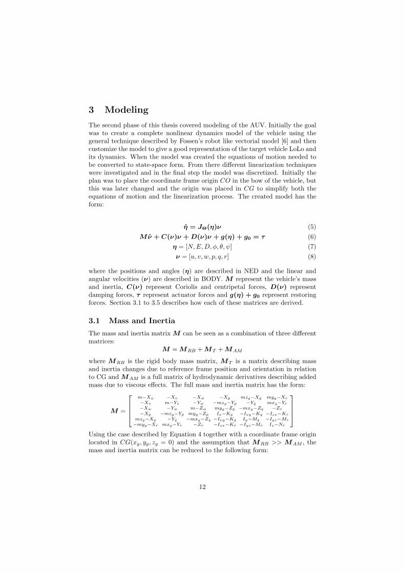
M =

2

6666664

m 0 0 0 0 00 m 0 0 0 00 0 m 0 0 00 0 0 Ix 0 00 0 0 0 Iy 00 0 0 0 0 Iz

3

7777775(9)

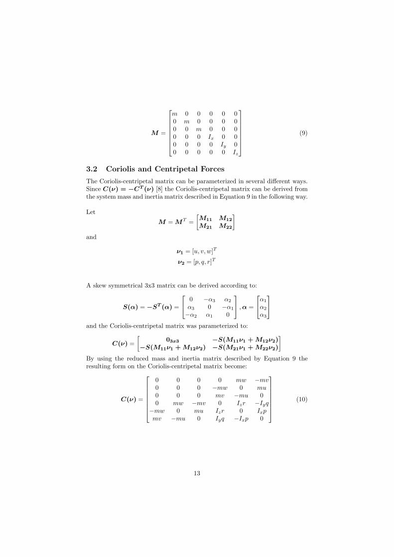
3.2 Coriolis and Centripetal Forces

The Coriolis-centripetal matrix can be parameterized in several di↵erent ways.Since C(⌫) = �CT

(⌫) [8] the Coriolis-centripetal matrix can be derived fromthe system mass and inertia matrix described in Equation 9 in the following way.

Let

M = MT =

M11 M12

M21 M22

�

and

⌫1 = [u, v, w]T

⌫2 = [p, q, r]T

A skew symmetrical 3x3 matrix can be derived according to:

S(↵) = �ST(↵) =

2

40 �↵3 ↵2

↵3 0 �↵1

�↵2 ↵1 0

3

5 ,↵ =

2

4↵1

↵2

↵3

3

5

and the Coriolis-centripetal matrix was parameterized to:

C(⌫) =

03x3 �S(M11⌫1 + M12⌫2)

�S(M11⌫1 + M12⌫2) �S(M21⌫1 + M22⌫2)

�

By using the reduced mass and inertia matrix described by Equation 9 theresulting form on the Coriolis-centripetal matrix become:

C(⌫) =

2

6666664

0 0 0 0 mw �mv

0 0 0 �mw 0 mu

0 0 0 mv �mu 00 mw �mv 0 Izr �Iyq

�mw 0 mu Izr 0 Ixp

mv �mu 0 Iyq �Ixp 0

3

7777775(10)

13

3.3 Damping Forces

In general the damping of a submerged AUV is both nonlinear and coupled[6]. To fully describe this dynamic behavior a matrix on the following form isrequired:

D(⌫)⌫ =

2

6666664

|⌫|TDn1⌫|⌫|TDn2⌫|⌫|TDn3⌫|⌫|TDn4⌫|⌫|TDn5⌫|⌫|TDn6⌫

3

7777775

where |⌫| = [|u|, |v|, |w|, |p|, |q|, |r|]T and Dni, i = 1, 2, 3, 4, 5, 6 are full matri-ces with dimension 6x6. This description requires a large number of unknownparameter values and is therefore not practical. One method used to simplifythe expression for damping is to separate it into two terms, one linear and onequadratic:

D(⌫) = [D + DN(⌫)]

and then assume that the vehicle only performs non-coupled motions. Thisresults in the following expression for damping:

D(⌫) = �diag{Xu, Yv, Zw,Kp,Mq, Nr}

� diag{X|u|u|u|, Y|v|v|v|, Z|w|w|w|,K|p|p|p|,M|q|q|q|, N|r|r|r|} (11)

3.4 Restoring Forces

Restoring forces include everything that force the vehicle back to an equilibriumwhere (�, ✓ = 0). For LoLo this includes two types of forces, displacement forces(g(⌘)) due to the location of CG and CB together with forces originating fromballast tank displacement g0. The ballast tank system, refereed to as VBS, isnot yet implemented and the tank configuration is not determined. Therefore,g0 = 0 but the expressions are still included in the report for future use. Thefull expression of restoring forces become:

g(⌘) =

2

6666664

(W �B) sin ✓�(W �B) cos ✓ sin��(W �B) cos ✓ sin�

�(ygW � ybB) cos ✓ cos�+ (zgW � zbB) cos ✓ sin�(zgW � zbB) sin ✓ + (xgW � xbB) cos ✓ cos��(xgW � xbB) cos ✓ sin�� (ygW � ybB) sin ✓

3

7777775(12)

The vehicle is assumed to be neutrally buoyant (W = B) and placing thecoordinate frame origin properly results in xg, xb, yg, yb, zg = 0 and Equation 12can be reduced to:

14

g(⌘) =

2

6666664

000

�zbB cos ✓ sin��zbB sin ✓

0

3

7777775(13)

Below is the expression for forces due to ballast tank use, where Vi is the volumeof tank i.

g0 =

2

6666664

00

�Zballast

�Kballast

�Mballast

0

3

7777775= ⇢g

2

6666664

00

�Pn

i=1 Vi

�Pn

i=1 yiViPni=1 xiVi

0

3

7777775= 0 (14)

3.5 Actuators and Control Surfaces

One of the most important aspects of modeling a vehicle is to accurately describeits actuators. To achieve a good physical description, both the magnitude ofeach force as well as how it enters or a↵ects the system is required. In thisthesis, all rudders and fins are modelled as symmetrical foils [9] and the thrustgenerated by the propellers are derived from provided propeller design data. Intotal, the vehicle has 7 actuators as described in Section 3.5 but the two ruddersbeing mechanically coupled results in 6 possible control actions. Further more,the elevons attached to the sides of the vehicle were not implemented untilmid November and therefore only included in the dynamics model and not themodel used by the controllers. Equation 15 and 16 are the formulas used todetermine the rudder, elevator and elevon forces. CL is a lift coe�cient andwas approximated with 0.1� according to typical data for symmetrical foilsillustrated by Figure 5. The approximation used in Equation 16 is valid for thesmall control surface deflection angles assumed in this thesis.

L =1

2A⇢v

2CL (15)

D ⇡ sin �L (16)

15

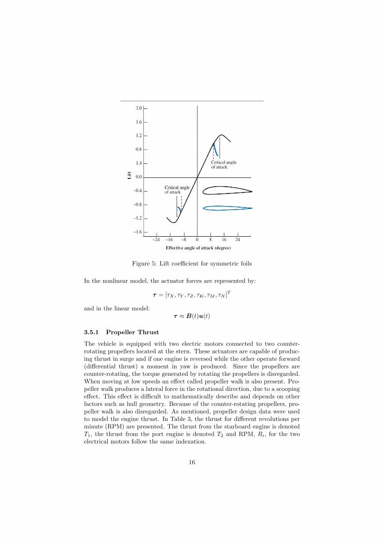
Figure 5: Lift coe�cient for symmetric foils

In the nonlinear model, the actuator forces are represented by:

⌧ = [⌧X , ⌧Y , ⌧Z , ⌧K , ⌧M , ⌧N ]T

and in the linear model:⌧ ⇡ B(t)u(t)

3.5.1 Propeller Thrust

The vehicle is equipped with two electric motors connected to two counter-rotating propellers located at the stern. These actuators are capable of produc-ing thrust in surge and if one engine is reversed while the other operate forward(di↵erential thrust) a moment in yaw is produced. Since the propellers arecounter-rotating, the torque generated by rotating the propellers is disregarded.When moving at low speeds an e↵ect called propeller walk is also present. Pro-peller walk produces a lateral force in the rotational direction, due to a scoopinge↵ect. This e↵ect is di�cult to mathematically describe and depends on otherfactors such as hull geometry. Because of the counter-rotating propellers, pro-peller walk is also disregarded. As mentioned, propeller design data were usedto model the engine thrust. In Table 3, the thrust for di↵erent revolutions perminute (RPM) are presented. The thrust from the starboard engine is denotedT1, the thrust from the port engine is denoted T2 and RPM, Ri, for the twoelectrical motors follow the same indexation.

16

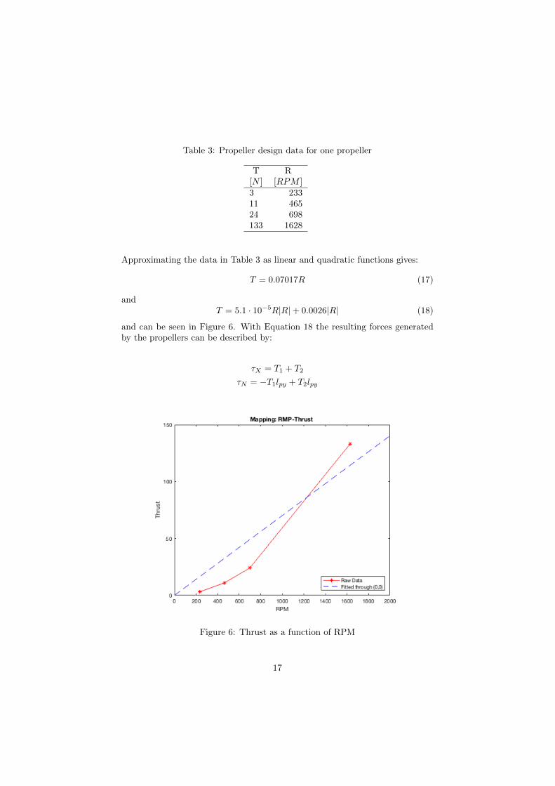
Table 3: Propeller design data for one propeller

T[N ]

R[RPM ]

3 23311 46524 698133 1628

Approximating the data in Table 3 as linear and quadratic functions gives:

T = 0.07017R (17)

andT = 5.1 · 10�5

R|R|+ 0.0026|R| (18)

and can be seen in Figure 6. With Equation 18 the resulting forces generatedby the propellers can be described by:

⌧X = T1 + T2

⌧N = �T1lpy + T2lpy

Figure 6: Thrust as a function of RPM

17

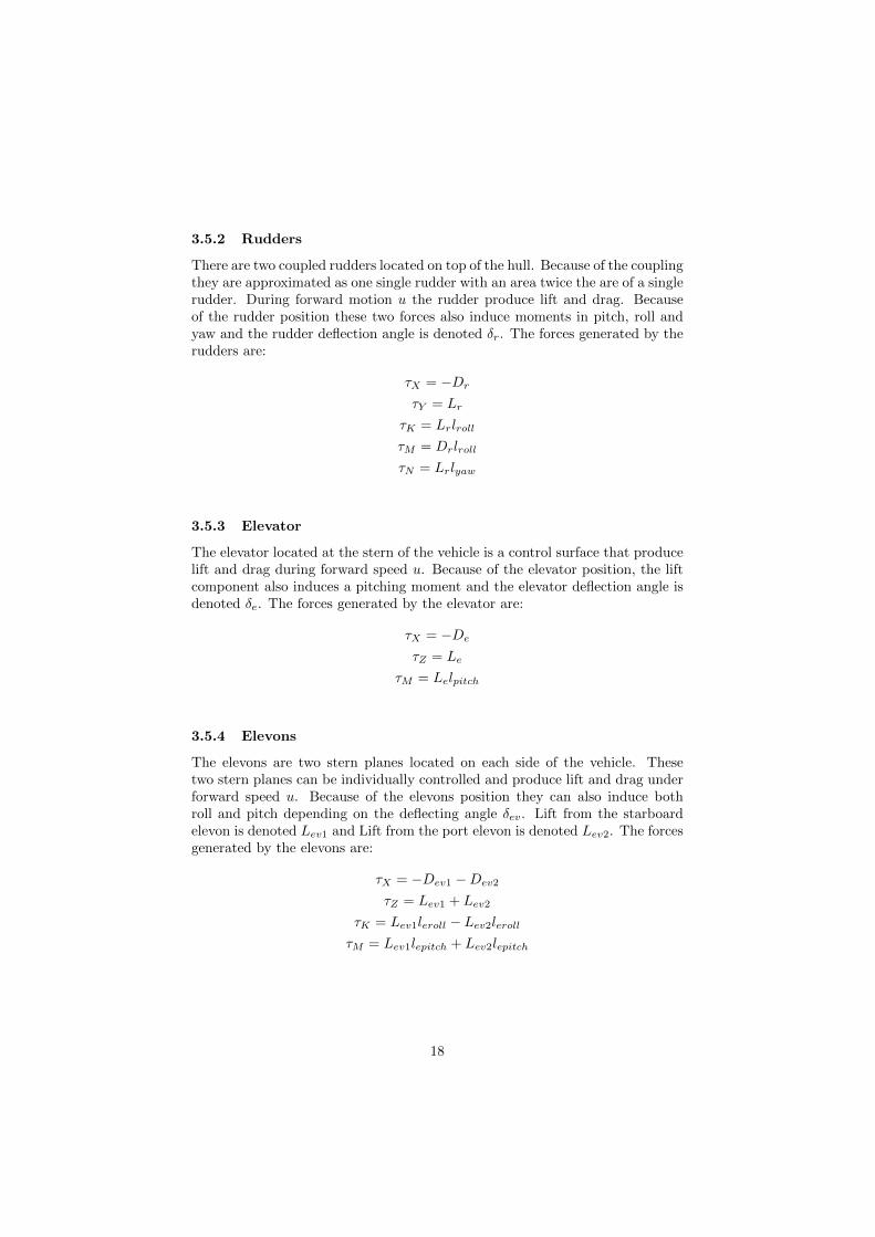
3.5.2 Rudders

There are two coupled rudders located on top of the hull. Because of the couplingthey are approximated as one single rudder with an area twice the are of a singlerudder. During forward motion u the rudder produce lift and drag. Becauseof the rudder position these two forces also induce moments in pitch, roll andyaw and the rudder deflection angle is denoted �r. The forces generated by therudders are:

⌧X = �Dr

⌧Y = Lr

⌧K = Lrlroll

⌧M = Drlroll

⌧N = Lrlyaw

3.5.3 Elevator

The elevator located at the stern of the vehicle is a control surface that producelift and drag during forward speed u. Because of the elevator position, the liftcomponent also induces a pitching moment and the elevator deflection angle isdenoted �e. The forces generated by the elevator are:

⌧X = �De

⌧Z = Le

⌧M = Lelpitch

3.5.4 Elevons

The elevons are two stern planes located on each side of the vehicle. Thesetwo stern planes can be individually controlled and produce lift and drag underforward speed u. Because of the elevons position they can also induce bothroll and pitch depending on the deflecting angle �ev. Lift from the starboardelevon is denoted Lev1 and Lift from the port elevon is denoted Lev2. The forcesgenerated by the elevons are:

⌧X = �Dev1 �Dev2

⌧Z = Lev1 + Lev2

⌧K = Lev1leroll � Lev2leroll

⌧M = Lev1lepitch + Lev2lepitch

18

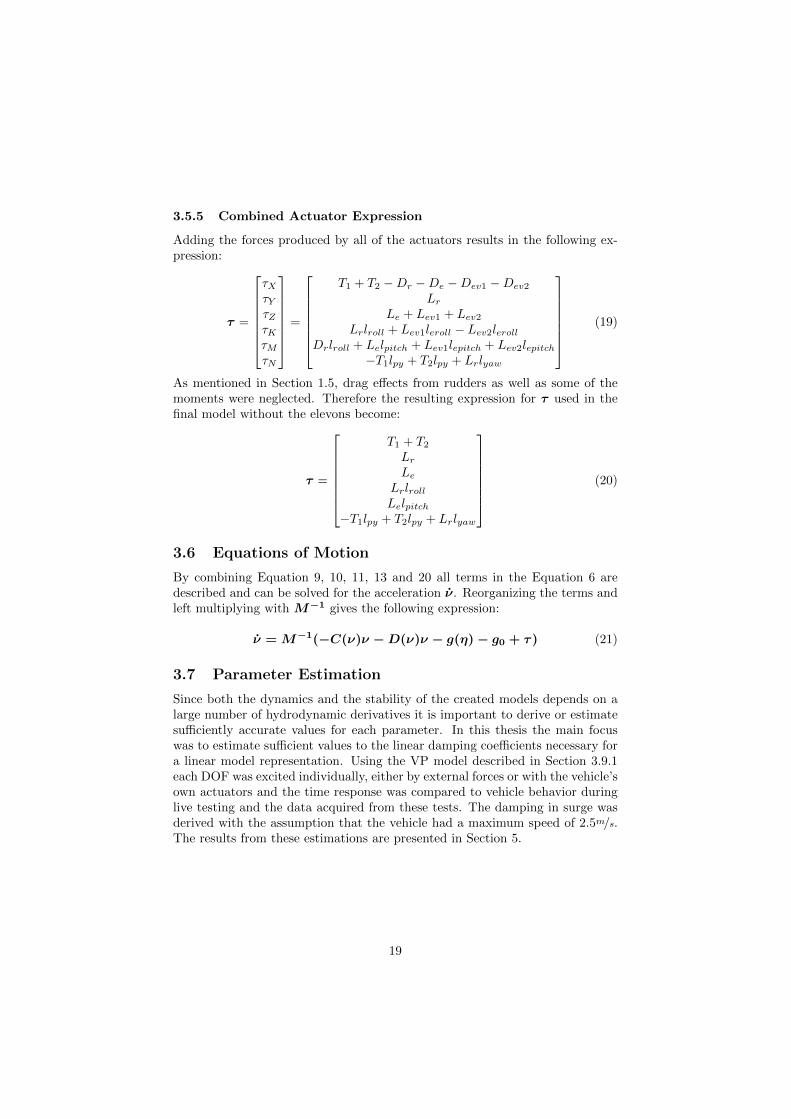
3.5.5 Combined Actuator Expression

Adding the forces produced by all of the actuators results in the following ex-pression:

⌧ =

2

6666664

⌧X

⌧Y

⌧Z

⌧K

⌧M

⌧N

3

7777775=

2

6666664

T1 + T2 �Dr �De �Dev1 �Dev2

Lr

Le + Lev1 + Lev2

Lrlroll + Lev1leroll � Lev2leroll

Drlroll + Lelpitch + Lev1lepitch + Lev2lepitch

�T1lpy + T2lpy + Lrlyaw

3

7777775(19)

As mentioned in Section 1.5, drag e↵ects from rudders as well as some of themoments were neglected. Therefore the resulting expression for ⌧ used in thefinal model without the elevons become:

⌧ =

2

6666664

T1 + T2

Lr

Le

Lrlroll

Lelpitch

�T1lpy + T2lpy + Lrlyaw

3

7777775(20)

3.6 Equations of Motion

By combining Equation 9, 10, 11, 13 and 20 all terms in the Equation 6 aredescribed and can be solved for the acceleration ⌫. Reorganizing the terms andleft multiplying with M�1 gives the following expression:

⌫ = M�1(�C(⌫)⌫ � D(⌫)⌫ � g(⌘) � g0 + ⌧ ) (21)

3.7 Parameter Estimation

Since both the dynamics and the stability of the created models depends on alarge number of hydrodynamic derivatives it is important to derive or estimatesu�ciently accurate values for each parameter. In this thesis the main focuswas to estimate su�cient values to the linear damping coe�cients necessary fora linear model representation. Using the VP model described in Section 3.9.1each DOF was excited individually, either by external forces or with the vehicle’sown actuators and the time response was compared to vehicle behavior duringlive testing and the data acquired from these tests. The damping in surge wasderived with the assumption that the vehicle had a maximum speed of 2.5m/s.The results from these estimations are presented in Section 5.

19

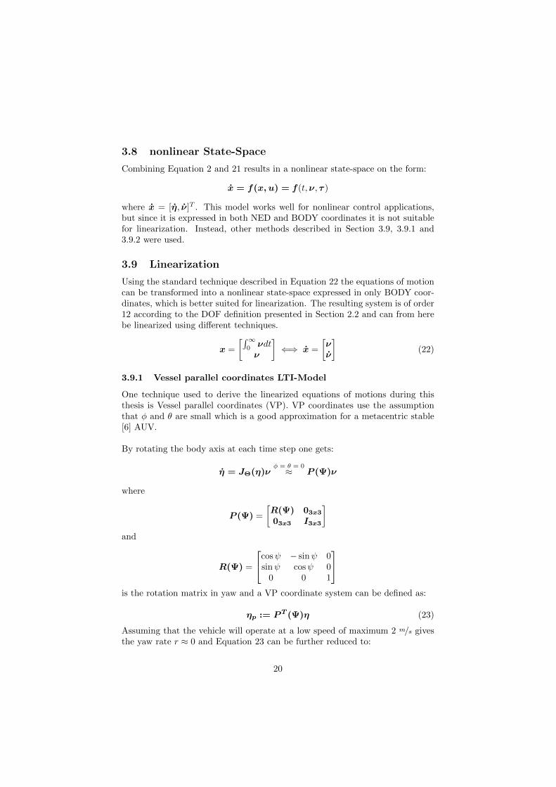
3.8 nonlinear State-Space

Combining Equation 2 and 21 results in a nonlinear state-space on the form:

x = f(x, u) = f(t,⌫, ⌧ )

where x = [⌘, ⌫]T . This model works well for nonlinear control applications,but since it is expressed in both NED and BODY coordinates it is not suitablefor linearization. Instead, other methods described in Section 3.9, 3.9.1 and3.9.2 were used.

3.9 Linearization

Using the standard technique described in Equation 22 the equations of motioncan be transformed into a nonlinear state-space expressed in only BODY coor-dinates, which is better suited for linearization. The resulting system is of order12 according to the DOF definition presented in Section 2.2 and can from herebe linearized using di↵erent techniques.

x =

R10 ⌫dt⌫

�() x =

⌫⌫

�(22)

3.9.1 Vessel parallel coordinates LTI-Model

One technique used to derive the linearized equations of motions during thisthesis is Vessel parallel coordinates (VP). VP coordinates use the assumptionthat � and ✓ are small which is a good approximation for a metacentric stable[6] AUV.

By rotating the body axis at each time step one gets:

⌘ = J⇥(⌘)⌫� = ✓ = 0

⇡ P ( )⌫

where

P ( ) =

R( ) 03x3

03x3 I3x3

�

and

R( ) =

2

4cos � sin 0sin cos 00 0 1

3

5

is the rotation matrix in yaw and a VP coordinate system can be defined as:

⌘p := P T( )⌘ (23)

Assuming that the vehicle will operate at a low speed of maximum 2 m/s givesthe yaw rate r ⇡ 0 and Equation 23 can be further reduced to:

20

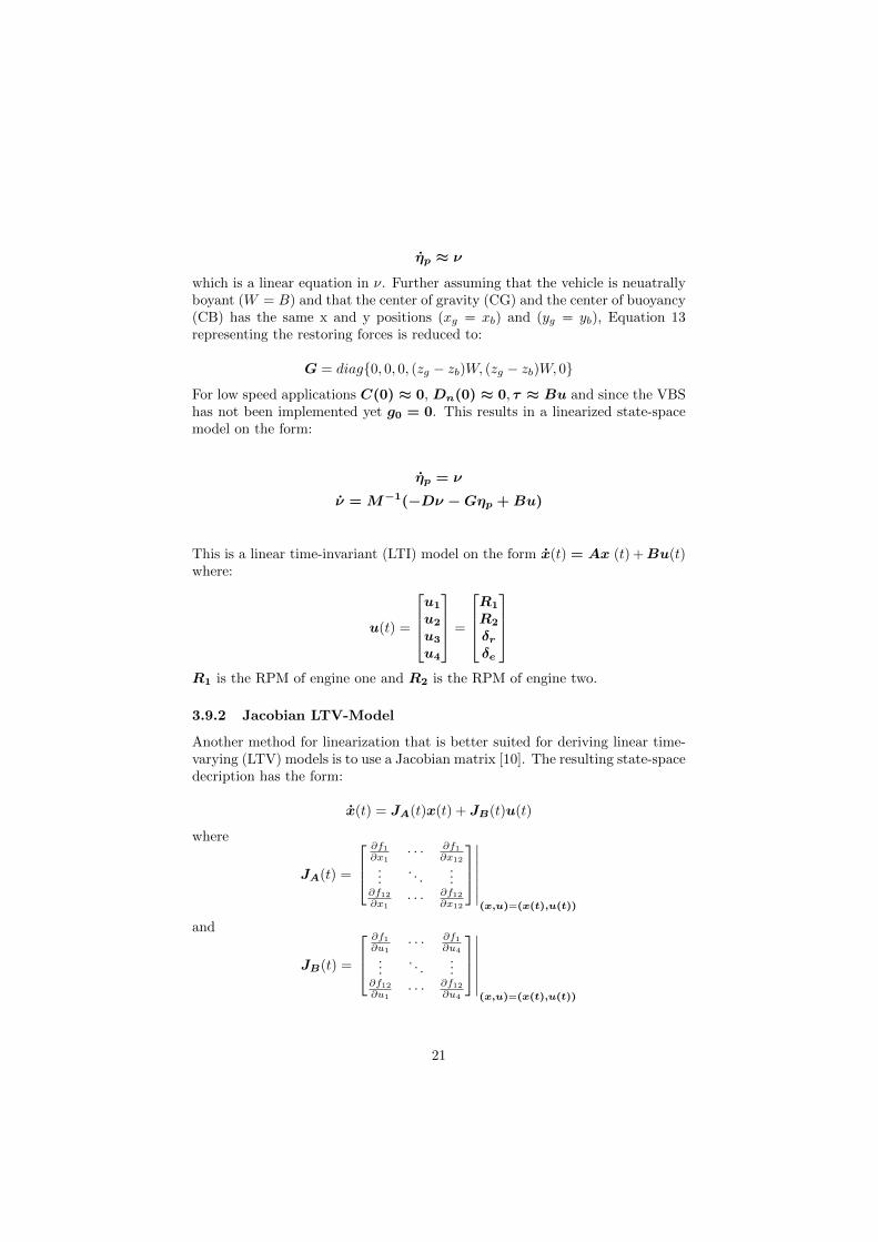
⌘p ⇡ ⌫

which is a linear equation in ⌫. Further assuming that the vehicle is neuatrallyboyant (W = B) and that the center of gravity (CG) and the center of buoyancy(CB) has the same x and y positions (xg = xb) and (yg = yb), Equation 13representing the restoring forces is reduced to:

G = diag{0, 0, 0, (zg � zb)W, (zg � zb)W, 0}

For low speed applications C(0) ⇡ 0, Dn(0) ⇡ 0, ⌧ ⇡ Bu and since the VBShas not been implemented yet g0 = 0. This results in a linearized state-spacemodel on the form:

⌘p = ⌫

⌫ = M�1(�D⌫ � G⌘p + Bu)

This is a linear time-invariant (LTI) model on the form x(t) = Ax (t) +Bu(t)where:

u(t) =

2

664

u1

u2

u3

u4

3

775 =

2

664

R1

R2

�r�e

3

775

R1 is the RPM of engine one and R2 is the RPM of engine two.

3.9.2 Jacobian LTV-Model

Another method for linearization that is better suited for deriving linear time-varying (LTV) models is to use a Jacobian matrix [10]. The resulting state-spacedecription has the form:

x(t) = JA(t)x(t) + JB(t)u(t)

where

JA(t) =

2

64

@f1@x1

· · ·@f1@x12

.... . .

...@f12@x1

· · ·@f12@x12

3

75

�������(x,u)=(x(t),u(t))

and

JB(t) =

2

64

@f1@u1

· · ·@f1@u4

.... . .

...@f12@u1

· · ·@f12@u4

3

75

�������(x,u)=(x(t),u(t))

21

This model is similar to the LTI-model derived by a VP coordinate frame inSection 3.9.1, but with the di↵erence that this model can be re-evaluated forcurrent values of x and u thus creating a LTV model. Using a Jacobian onthe nonlinear equations of motion also allows for di↵erent model complexities,where certain applications require more or less accurate models.

3.10 Discretization

To make a MPC implementation possible, the last step in the modeling processis to transform the continuous time model into a discrete time model on the formx[t+ 1] = A[t]x[t] +B[t]u[t]. Like in the continuous time case, this model canbe both time variant and invariant, and both types were used during this thesis.There exists several di↵erent techniques for discretization of a continuous timesystem. Due to time constraints and since the discretization was not consideredas important as the MPC implementation itself, Matlab’s built in continuous todiscrete (C2D) function together with a sampling time h of 0.2 s was used.

22

4 Control

The third phase of this thesis covers control aspects. The ultimate goal wasto achieve MPC reference tracking using a LTV model describing the completedynamics of the vehicle. To reach this goal there are a number of necessary stepsthat need to be taken. The stability, controllability and observability needs to beevaluated to ensure that solutions can be derived and that the control problemis feasible. In this phase the elevons are not considered a part of the physicalsystem and therefore not included as actuators in the controllers, resulting in atotal of 4 actuators.

4.1 Existing System

The vehicle’s existing control system uses standard PID controllers, either work-ing as individual units or connected into cascade controllers. Even though thissolution is simple and performs well, there are some major drawbacks. Eachoutput needs its own controller which makes the software structure more com-plicated than necessary. Each controller also works under the assumption ofdecoupled motions, which can lead to performance limitations or contradictingcontrol objectives. Tuning all these individual controllers can also be a problem.Every time the vehicle configuration is changed all of the controllers have to beretuned.

4.2 Model Analysis

Before any type of control implementation is created model analysis is usuallyperformed. This analysis often consist of three steps. Stability, controllabilityand observability. The purpose of these tests are to find out what is physicallypossible to do in terms of control, regulation and estimation. If the results fromthese tests are not satisfactory, there usually is no point in continuing with thecontrol implementation. Instead, more work with modeling or other techniquessuch as the use of observers need to be employed to ensure that the desiredcontrol objectives can be met.

4.2.1 Stability

Stability is one of the fundamental principles in control engineering [11]. Eventhough controllers can be designed that stabilize unstable systems, the stabilityof a system is important because it defines how the system behaves in terms ofsolutions, equilibria and whether a bounded input generates a bounded output(BIBO). The poles and zeros of a system can further be analyzed to determineother physical limitations such as bandwidth, frequency response and the high-est achievable controller performance.

There are several methods that can be used to determine whether a system isstable or not but during this thesis standard methods for evaluating eigenvalues

23

of the system matrix A were used. The system equilibria was also considered bylooking at 0 = A(t)x(t)+B(t)u(t). This equation shows that local equilibriumexists everywhere in IR3 thus making this a pure regulation problem.

During live tests of the vehicle’s basic systems and functions during Autumn2019, both stability and system equilibria were inferred from dynamic and staticbehavior in the water. Even though this is a visual confirmation it is still a strongstability proof.

4.2.2 Controllability

The concept of controllability denotes whether a controller can drive the statesof the system to any arbitrary point in IR3 or not, also refereed to as the con-trollable subspace [13]. Since the goal of this thesis is reference tracking toarbitrary way points controllability is of great importance and to ensure thatfeasible solutions exist to any waypoint, the controllable subspace need to beequal to IR3. To check for controllability, the standard method where rank(C)must be equal to the system order was used:

C =⇥B AB · · · A

n�1B⇤

Results from this test will be presented in Section 5.

4.2.3 Observability

The concept of observability denotes whether all of the internal system statescan be inferred from external outputs or not [12]. Observability was evaluatedusing the the standard test for observability were rank(O) must be equal to thesystem order:

O =

2

6664

C

CA

...CA

n�1

3

7775

With this test it can be shown that rank(O) < the order of the system thusmaking it unobservable. However, the vehicle itself is equipped with sensorscapable of measuring all the 12 states in real-time which completely removesthis problem since state values can always be measured. If these sensor mea-surements would not have been available, other methods including observers[13] would have been needed.

Even though observability does not impose a problem for the control implemen-tation it introduces another concept previously not mentioned. The output ofa system, described by y = Cx(t), shows which quantities are of importanceand is often used in regulation applications such as integral states described inSection 4.3. In general a system of square form is desired [14] which leads toC 2 IR4x12 to ensure that the number of inputs are equal to the number of

24

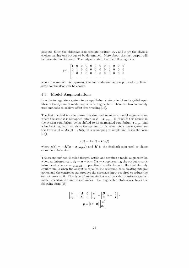
outputs. Since the objective is to regulate position, x, y and z are the obviouschoices leaving one output to be determined. More about this last output willbe presented in Section 6. The output matrix has the following form:

C =

2

664

1 0 0 0 0 0 0 0 0 0 0 00 1 0 0 0 0 0 0 0 0 0 00 0 1 0 0 0 0 0 0 0 0 0· · · · · · · · · · · ·

3

775

where the row of dots represent the last undetermined output and any linearstate combination can be chosen.

4.3 Model Augmentations

In order to regulate a system to an equilibrium state other than its global equi-librium the dynamics model needs to be augmented. There are two commonlyused methods to achieve o↵set free tracking [15].

The first method is called error tracking and requires a model augmentationwhere the state x is remapped into e = x � xtarget. In practice this results inthe system equilibrium being shifted to an augmented equilibrium xtarget anda feedback regulator will drive the system to this value. For a linear system onthe form x(t) = Ax(t) + Bu(t) this remapping is simple and takes the form[15]:

e(t) = Ae(t) +Bu(t)

where u(t) = �K(x � xtarget) and K is the feedback gain used to shapeclosed loop behavior.

The second method is called integral action and requires a model augmentationwhere an integral state xi = y � r = Cx � r representing the output error isintroduced, where r = ytarget. In practice this tells the controller that the onlyequilibrium is when the output is equal to the reference, thus creating integralaction and the controller can produce the necessary input required to reduce theoutput error to 0. This type of augmentation also provide robustness againstmodel uncertainties and disturbances. The augmented state-space takes thefollowing form [15]:

xxi

�=

A 0

C 0

� xxi

�+

B0

�u�

0

I

�r

y =⇥C 0

⇤ xxi

�

25

4.4 Linear Control Methods

Linear control methods include state-feedback control solutions to systems onthe form x(t) = A(t)x(t)+B(t)u(t), where the solution has the form u(t) = �Lx(t).

4.4.1 State-Feedback

State-feedback, or pole placement as it is often referred to, is usually the firststep when employing linear control methods. This method exploits the prop-erty that the eigenvalues of the system matrix A(t) corresponds to the openloop poles of the system. Feeding back u(t) = �Kx (t) allows a designer toplace the closed loop poles of x(t) = (A(t) �B(t)K)x(t) in any arbitrary po-sition provided that the system is controllable [13]. Since the pole placementfor stable systems is known this method is suitable for both regulation and sta-bilization and creates understanding of what state-feedback control is trying toachieve. However, this method is rarely used in practice since state-feedbackonly addresses stability and not performance. Performance analysis requires in-vestigation of e.g. time or frequency responses for each individual pole. Insteadsome of the more advanced methods described in Section 4.4.2 and 4.5 can beused.

4.4.2 LQR

A linear-quadratic regulator (LQR) is an optimal state-feedback controller thatuses linear constraints and a quadratic cost function to operate a target systemat a minimal cost [16]. The advantage of working with LQR control instead ofstate-feedback is that when the control horizon N is allowed to reach infinity(infinite horizon LQR) [12] the optimization converges and the solution fromthe algebraic Riccati equation (ARE) can be used to derive the optimal state-feedback. Another advantage with this method is that e↵ort is usually shiftedfrom optimizing the controller performance to weighting di↵erent performanceobjectives. The proof for this method will be left out, but for a continuous-timelinear-system and a quadratic cost function J on the form:

minu

J =

Z 1

0xTQ1x + uTQ2u

s.t x = Ax + Bu

Where Q1 and Q2 are matrices defining the state and input weights. Theoptimal solution is given by:

u = �Kx

where

K = Q�12 BTP

26

is the optimal gain and P is chosen as the solution to the ARE:

ATP + PA � PBR�1BTP + Q = 0

Solving LQR problems numerically is challenging but e�cient solvers that canhandle these structures exists and the hardest task is to weigh the cost functionand augment the model to behave according to the control objective.

Since this formulation can not handle additional state or input constraints thereexists one major drawback. The optimal gain K does not consider physicallimitations on inputs and therefore the input u = �Kx has to be manuallysaturated.

4.5 MPC

Model predictive control, or receding horizon LQR with constraints [12], is anadvanced control method where a cost function J is minimized over a fixed hori-zon N subject to the discrete time system dynamics x[t+1] = Ax [t]+Bu [t].When the optimal input sequence u⇤ 2 IR

N�1 is obtained, the first controlaction u⇤

1 is taken and the entire optimization is repeated. The basic formu-lation is similar to the LQR controller presented in Section 4.4.2, but the useof discrete dynamics and an iterative finite horizon allows additional state andinput constraints to be implemented directly in the optimization.

4.5.1 Basic Formulation

There are several ways to formulate a MPC algorithm depending on whetherthe cost function is a�ne in u and how the terminal set xN is handled to ensurefuture stability and feasibility [12]. In this thesis, the formulation presented inEquation 24 together with di↵erent model augmentations presented in Section4.5.2 was used.

minu

N�1X

t=0

xTt Q1xt + uT

t Q2ut + xTNQNxN

s.t x[t+ 1] = Ax [t]+Bu [t]

|u1,t| 500

|u2,t| 500

|u3,t| 0.3491

|u4,t| 0.3491

(24)

4.5.2 Additional Augmentations

When working with MPC regulation and tracking there are some problems thatneed to be addressed. Forcing the output y to a reference point r leads to theoutput error relation:

27

et = rt � Cxt ! 0

steady state ek = 0 is desired but to achieve this, uk 6= 0 which is not a steadystate. One way to deal with this is to augment the system using input incre-ments [17].

Let:ut = ut�1 +�u (25)

and define ut�1 as a new state variable and �u as the new control input.This leads to an augmented formulation with integral action on the input thatcircumvents the steady-state problem on the form:

min�u

N�1X

t=0

(r � Cx)Tt Q1(r � Cx)t +�uTt Q2�ut

s.t

xt+1

ut+1

�=

A B0 I

� xt

ut

�+

BI

��ut

(26)

This is now a state-space model of order 16, where:

yt =⇥C 0

⇤ xt

ut

�(27)

To ensure o↵set-free tracking integral states may need to be introduced on thestate variable x as well. Using a method similar to the one described in Equa-tion 25 and 26 the system can be described in both state and input incrementsas described in [18] and [19].

Let:

�xt+1 = A�xt + B�ut (28)

where �xt = xt � xt�1. The output yt need to be connected to �xk andyt = Cxt gives:

yt = yt�1 + C�xt (29)

Combining Equation 28 and 29 and choosing:

x =

�xt

yt�1

�

as the new state vector gives the state space model:

�xt+1

yt

�=

A 0

C I

� �xt

yt�1

�+

B0

��ut (30)

This is also a state-space model of order 16 that can replace the linear constraintsin Equation 26 to create integral action on both state and input, where:

28

yt =⇥C I

⇤ �xk

yt�1

�(31)

The augmented MPC formulation described by Equation 30 has one weakness.Augmenting both states and inputs with increments, without adding states thatdescribe how u is a↵ected by �u removes the option to constrain the input aspresented in Equation 24. This can be handled in two ways. Either 4 additionalstates that describe the relation between u and �u are added, which directlyenables constraints on u with the downside of increasing the state-space orderto 20. The other option is to let the Matlab algorithm keep track of the truevalue of u independent from the state-space model and use this information toconvert limitations on u to limitations on �u and constrain these in the MPCformulation.

29

5 Results

The number of steps taken from unmodelled vehicle to controller evaluation hasproduced several di↵erent results. From all the theory and work with modeling,a generator that can produce symbolic models has been created. This modelgenerator takes simplifications and assumptions such as axes of symmetry andwhether the vehicle is neutrally buoyant or not as input and produces a fullnonlinear model according to these conditions.

With the model generator and the linearization techniques described in Section3, two linear state-space models on the form x(t) = A(t)x(t) + B(t)u(t) rep-resenting the nonlinear dynamics of LoLo were created. The system matrix forthe model derived with the use of a VP reference frame can be seen in Equation32.

A =

2

6666664

0 0 0 0 0 0 1 0 0 0 0 00 0 0 0 0 0 0 1 0 0 0 00 0 0 0 0 0 0 0 1 0 0 00 0 0 0 0 0 0 0 0 1 0 00 0 0 0 0 0 0 0 0 0 1 00 0 0 0 0 0 0 0 0 0 0 10 0 0 0 0 0 �0.0667 0 0 0 0 00 0 0 0 0 0 0 �8.33 0 0 0 00 0 0 0 0 0 0 0 �10 0 0 00 0 0 �32.2 0 0 0 0 0 �10.94 0 00 0 0 0 �3.18 0 0 0 0 0 �1.62 00 0 0 0 0 0 0 0 0 0 0 �3.86

3

7777775(32)

The model generated with the use of a Jacobi matrix has a sparse structuresimilar to the one presented in Equation 32. The di↵erence with this Jacobimatrix model is that additional couplings between DOFs may be introduced inthe nonlinear representation which allows that a linearization of varying com-plexity can be produced.

In Section 3.5.1 two functions for the propeller thrust are presented and theycan be seen in Figure 6. In the electrical motors operating range of -500 to 500RPM, Equation 17 representing linear thrust fitted through 0 has a significantlyhigher value than the nonlinear thrust represented in Equation 18. Therefore,Equation 18 linearized around 500 RPM are used in the final dynamics model.

The results from the standard test for controllability indicates that the vehicle iscontrollable under forward speed (u > 0), but not while standing still (u = 0).Since rudders and foils only produce forces during forward motion this wasexpected, but this resulted in some changes to the structure of the input matrixB(t). The resulting input matrix can be seen in Equation 33 where actuatorforces are linearized around (R, u) = (500, 1). The result of this linearization isthat actuators are assumed to produce the same amount of force independentof the vehicle’s velocity in surge u.

30

B =

2

6666664

0 0 0 00 0 0 00 0 0 00 0 0 00 0 0 00 0 0 0

0.0002 0.0002 0 00 0 0.0212 00 0 0 0.01910 0 0.0365 00 0 0 0.0260

�3.6⇥10�5 3.6⇥10�5 0.0202 0

3

7777775(33)

For these models to be useful in controller design and simulation the hydrody-namic derivatives describing linear damping had to be determined. The esti-mated parameter values can be found in Table 4 and were derived according tothe description in Section 2.6. All simulations of dynamic behavior during thisthesis was performed using the Euler forward method:

x(t+ h) = x(t) + x(t)h

where h is a time step and (t+h) ⇡ (t+1) when working with discrete systemsand dynamics.

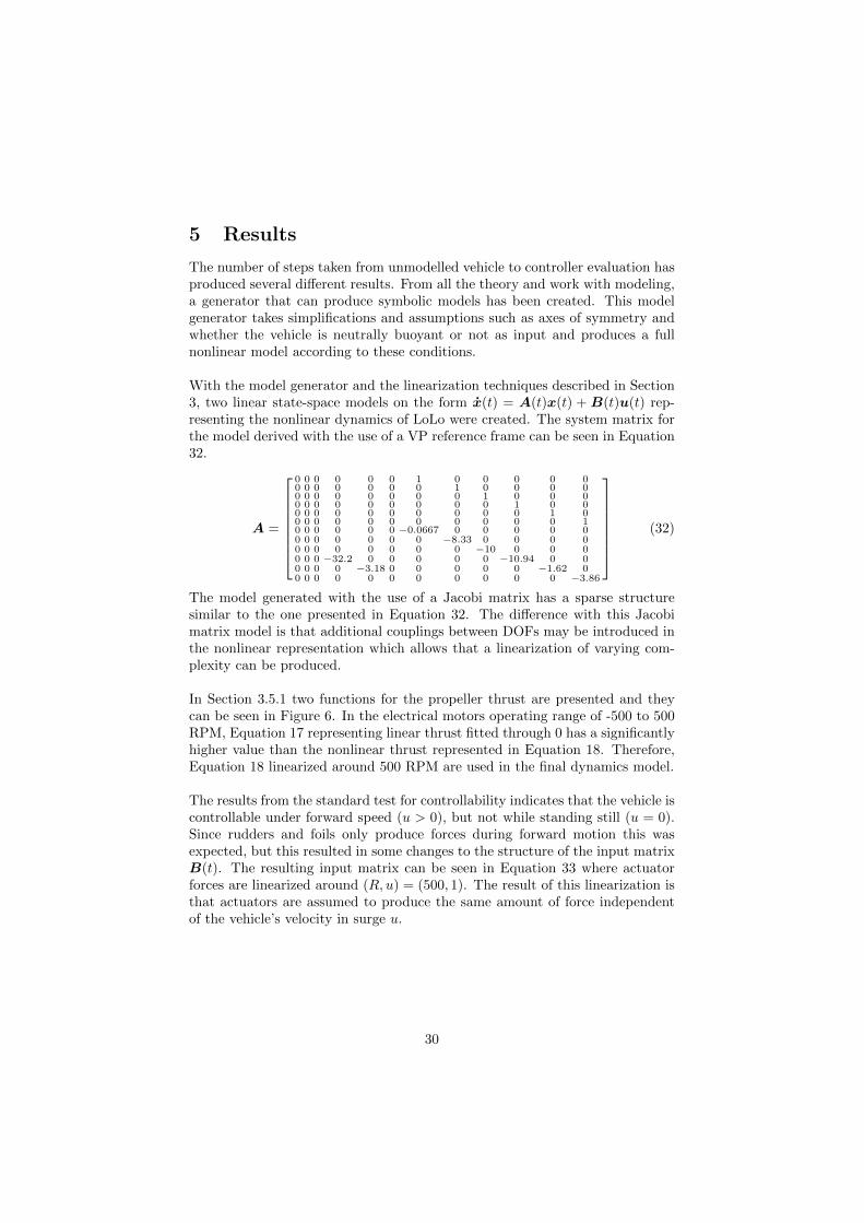
Since the hydrodynamic derivatives influence both stability and dynamic be-havior their values are of great importance. In Figure 7 - 12 the time responsefor surge, sway, heave, pitch, roll and yaw rate using the parameter values inTable 4 are presented. From the time response, stability and boundedness canalso be inferred for each DOF since the vehicle returns to its equilibrium aftersubjected to external disturbances and the parameter values creates an upperbound on the velocities.

Table 4: Estimated linear damping coe�cients

Xu = �20Yv = �2500Zw = �3000Kp = �400Mq = �600Nr = �1500

31

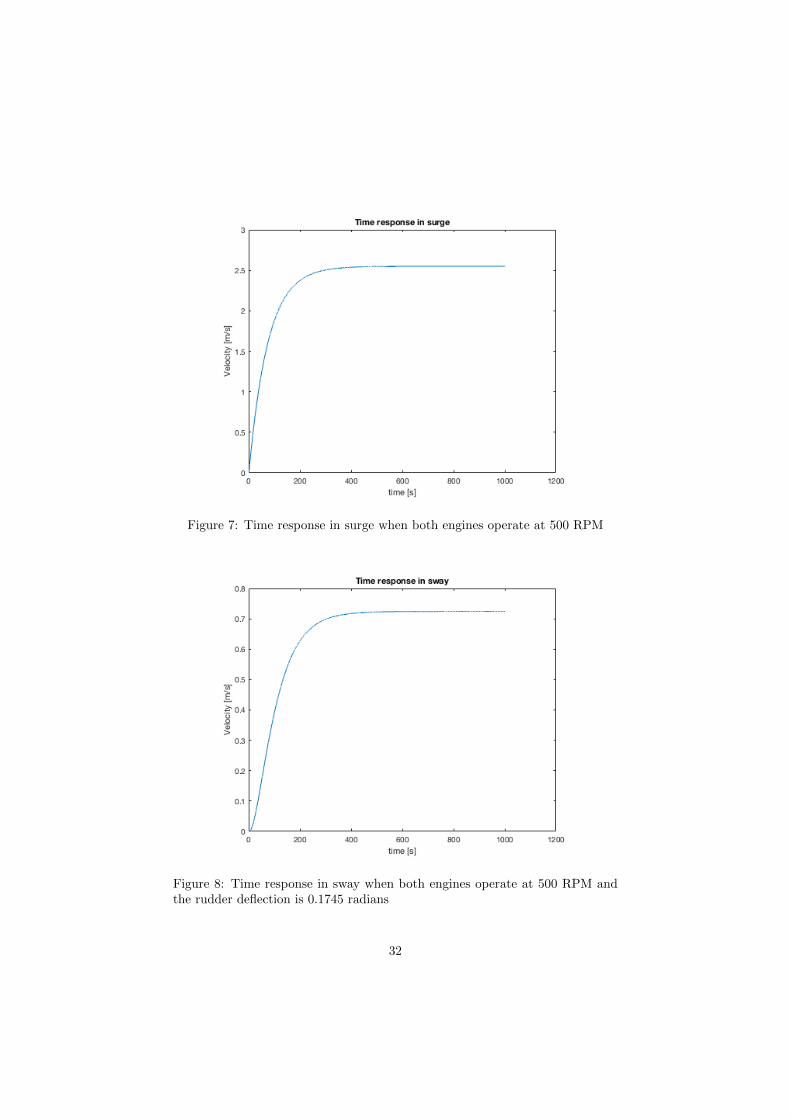
Figure 7: Time response in surge when both engines operate at 500 RPM

Figure 8: Time response in sway when both engines operate at 500 RPM andthe rudder deflection is 0.1745 radians

32

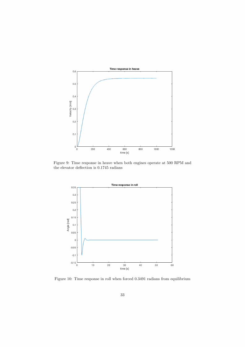
Figure 9: Time response in heave when both engines operate at 500 RPM andthe elevator deflection is 0.1745 radians

Figure 10: Time response in roll when forced 0.3491 radians from equilibrium

33

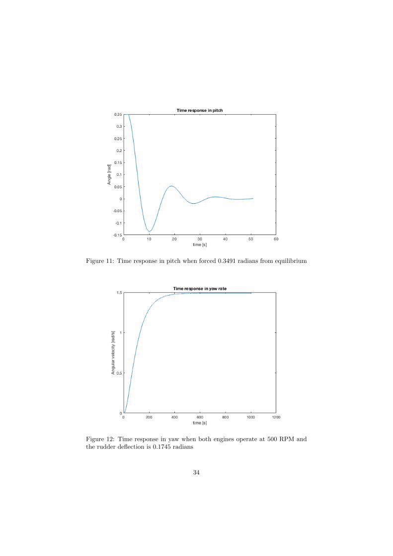
Figure 11: Time response in pitch when forced 0.3491 radians from equilibrium

Figure 12: Time response in yaw when both engines operate at 500 RPM andthe rudder deflection is 0.1745 radians

34

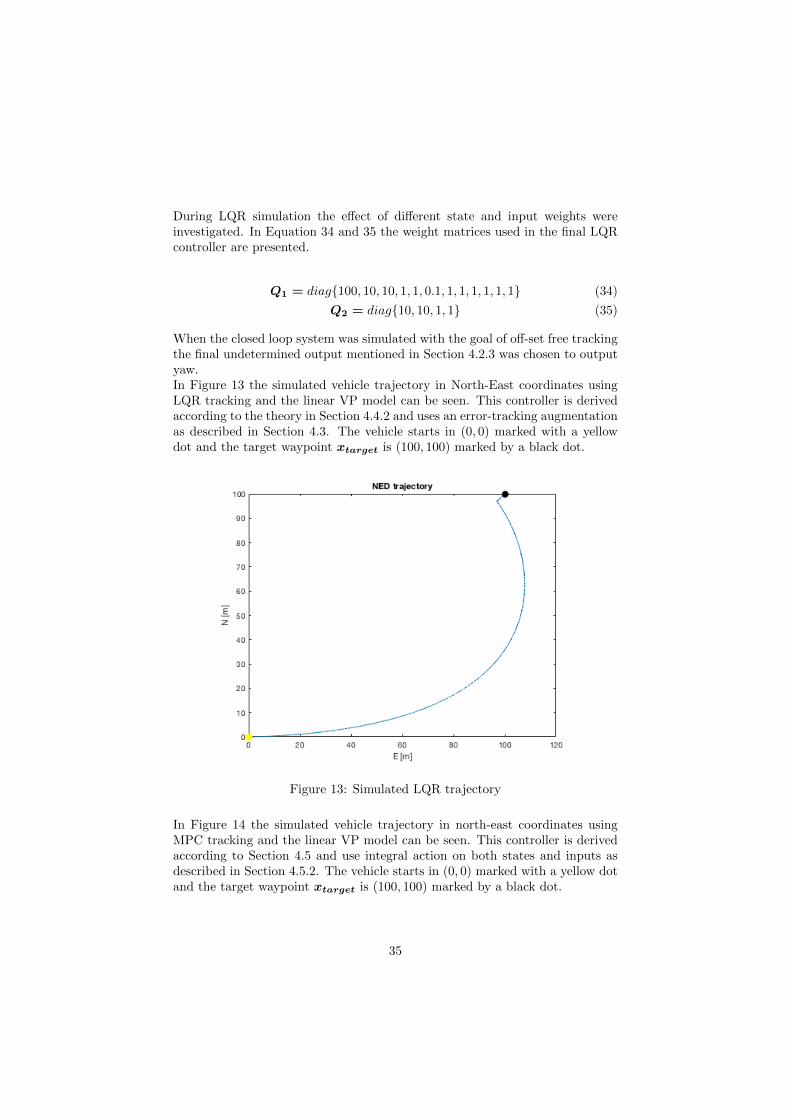
During LQR simulation the e↵ect of di↵erent state and input weights wereinvestigated. In Equation 34 and 35 the weight matrices used in the final LQRcontroller are presented.

Q1 = diag{100, 10, 10, 1, 1, 0.1, 1, 1, 1, 1, 1, 1} (34)

Q2 = diag{10, 10, 1, 1} (35)

When the closed loop system was simulated with the goal of o↵-set free trackingthe final undetermined output mentioned in Section 4.2.3 was chosen to outputyaw.In Figure 13 the simulated vehicle trajectory in North-East coordinates usingLQR tracking and the linear VP model can be seen. This controller is derivedaccording to the theory in Section 4.4.2 and uses an error-tracking augmentationas described in Section 4.3. The vehicle starts in (0, 0) marked with a yellowdot and the target waypoint xtarget is (100, 100) marked by a black dot.

Figure 13: Simulated LQR trajectory

In Figure 14 the simulated vehicle trajectory in north-east coordinates usingMPC tracking and the linear VP model can be seen. This controller is derivedaccording to Section 4.5 and use integral action on both states and inputs asdescribed in Section 4.5.2. The vehicle starts in (0, 0) marked with a yellow dotand the target waypoint xtarget is (100, 100) marked by a black dot.

35

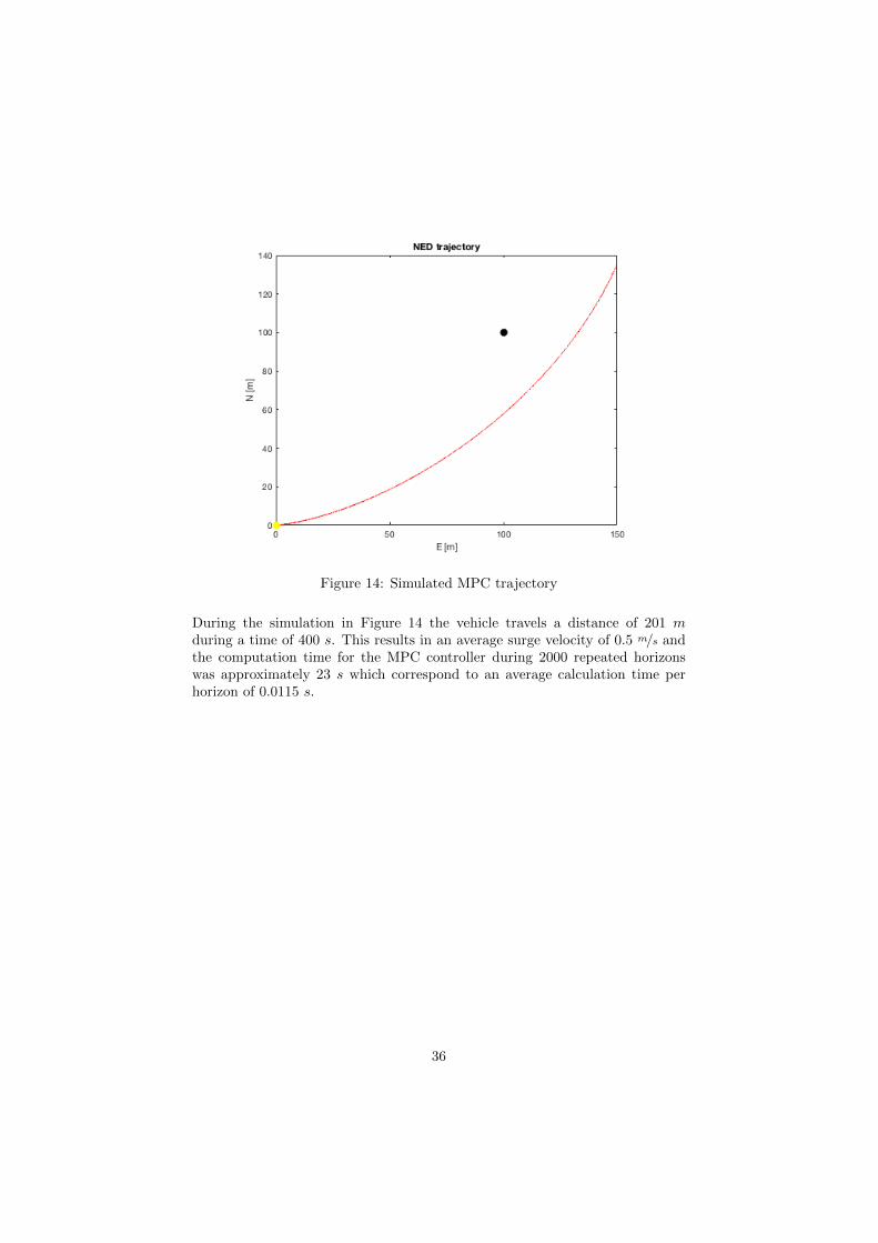
Figure 14: Simulated MPC trajectory

During the simulation in Figure 14 the vehicle travels a distance of 201 m

during a time of 400 s. This results in an average surge velocity of 0.5 m/s andthe computation time for the MPC controller during 2000 repeated horizonswas approximately 23 s which correspond to an average calculation time perhorizon of 0.0115 s.

36

6 Analysis and Discussion

When the nonlinear dynamics model was derived it was decided that creating afull-scale model including all the couplings and dynamical e↵ects and subsequentdown-scaling was more beneficial than starting from a simple model with sub-sequent up-scaling. The reason for this is that the full-scale model is a suitablerepresentation of the physical system whereas the simple model is an approx-imation. This is important, since the linear models derived later on becomeeither a linearization of an accurate model or a linearization of an approximatemodel. In practice this makes a big di↵erence for how model dependent resultscan be interpreted. Another benefit with the creation of a full-scale model isthat this model can be used for other purposes such as simulation.

During the modeling phase the ambition was first to place the coordinate frameorigin in the bow of the vehicle. The reason for this was that during motionthere is not much use in knowing the distance from an obstacle to a point locatedinside the vehicle. Placing the coordinate frame in the bow provides the truedistance to an obstacle. The downside with this placement is that the expres-sion for the equations of motion become increasingly complex and dynamicalbehavior become harder to evaluate. Because of this, the coordinate frame ori-gin was changed from the bow of the vehicle to coincide with CG. The benefitswith this location is that rotational and translational components due to a shiftof coordinate frame origin is avoided. Additionally, a coordinate frame locatedin CG is what allowed for other simplifications e.g. the ones used in Section 3.4,where Equation 12 could be reduced to Equation 13.

As mentioned in Section 1, this thesis focus on control methods using linear mod-els. There are several reasons for this, the main one being the time requiredto derive the control inputs. Using a linear model to describe the dynamicbehavior of a nonlinear system will reduce the model accuracy but the upsideis that the calculation time for advanced methods such as MPC is drasticallyreduced. This creates a trade-o↵ between model accuracy and the calculationtime needed by the controller. Both accuracy and calculation time is impor-tant for the implementation in a physical system due to limited computationalpower. If the calculation time is to long the controller will not have enough timeto derive the necessary input required at time t and a delay is introduced intothe system. This delay limits performance and can cause instability. Model ac-curacy is important for robustness and to make sure that the derived solutionswork in the physical system.

The modeling technique described by [6] where the state-space model is de-scribed in both NED and BODY coordinates work for nonlinear control ap-plications, but is not suitable for linear applications. Since [N,E,D] 6= [x, y, z]and the mapping between these coordinates is nonlinear a su�cient linear modelwith mixed coordinates is hard to derive. As described in Section 3.9 a linearmodel expressed in only BODY coordinates has been used which have caused

37

a number of di�culties. Tracking a waypoint in the global NED frame can beseen as a constant reference. However, in the BODY frame this reference istime-varying and depends on xb, yb, zb and . This adds a level of complexityin the controller when the reference has to be remapped into a new coordinateframe. In the LQR solution no impact from this mapping have been discoveredin the results but implementing this reference map in the MPC algorithm proveddi�cult and might be one reason to the low tracking performance generated byMPC.

There are two main reasons why a MPC solution is more beneficial than a LQRsolution. The MPC framework have the ability to handle constrained optimiza-tion and because of this the controller can directly handle physical limitationson states and inputs unlike LQR where signals have to be physically limitedbefore implemented. Since MPC is a receding horizon online algorithm a typeof feedback mechanism is also implemented and some capability to handle pre-diction errors due to discrepancies between the system model and the physicalsystem is introduced. As mentioned in Section 1 calculation time for the MPCcontroller was of concern. Receding horizon constrained optimization is far moredemanding than infinite horizon LQR and for the MPC controller to be feasiblein practise the calculation time for each horizon needs to be shorter than thediscrete sampling time h. As presented in Section 5 the calculation time perhorizon was 0.0115 s when a sampling time of 0.2 s was used making this con-troller feasible in terms of calculation time with the used hardware.

The e↵ect of the discretization technique used during this thesis was not stud-ied. Discretization technique and sampling time are both factors that can e↵ectthe result, dynamic behavior and needs to be investigated to ensure that thediscrete time linear system is a good representation of continuous time dynam-ics. The order in which linearization and discretization were performed mightalso a↵ect the result but since the goal was to investigate control models andnot validate dynamics models this result is left as future work.

The adaption of control surfaces such as rudders, elevator and elevons for actu-ation instead of electrical motors that can generate thrust in di↵erent directionsis an active design choice. Control surfaces are more energy e�cient than electri-cal motors which is beneficial for the energy consumption and increase missionduration. The downside is that all the produced forces are speed dependent andthe existing configuration makes LoLo an underactuated AUV. While forwardspeed makes the vehicle controllable as described in Section 4.2.2 underactua-tion is a physical property and since no independent forces can be produced ineither sway or heave a control objective in these DOFs is hard to satisfy. Tomuch focus on controllability while not fully respecting underactuation mightbe one of the reasons to the low tracking performance generated by MPC. Away to deal with this problem is presented in Section 8.

Another factor that concern a physical control implementation is model valida-

38

tion. To ensure that the derived controllers produce su�cient tracking perfor-mance in a physical implementation the accuracy of the dynamics models needsto be evaluated. The hydrodynamic parameters used in this thesis are estimatesand constitute a fraction of the parameters required to fully describe the non-linear dynamic behaviour of an AUV. Because of this the true performance ofan implemented controller can only be verified in physical testing or with a per-fectly accurate dynamics model with all hydrodynamic parameters determined.The results derived in this thesis can therefore only be used as proof of conceptand to deduce feasibility in terms of performance and suitability.

Since ✓ and � are approximated to 0 in the linear model, one dynamic e↵ect iscompletely neglected in the dynamics model. This dynamic e↵ect is a conse-quence of that the vehicle hull itself work as control surface when the angle ofattack (AOA) is not zero. The projected hull-area is significantly larger thanany of the control surfaces and because of this large forces will be producedwhen the AOA is di↵erent from zero. These forces might create a problem in aphysical implementation and have to be further evaluated.In Section 4.2.3 the output of the system was introduced and a free choice ofthe fourth and last output was mentioned. Since the vehicle is underactuatedand therefore have a hard time fulfilling a control objective in 6 DOFs, waschosen as the last output. The reason for this is that underactuation in swaycan be compensated by actuation in yaw and choosing yaw as the final outputallows the controllers to track desired angular orientation and the vehicle canreach any desired waypoint.

7 Conclusion

All the results from this thesis indicates that waypoint tracking with optimalcontrol using a linear dynamics model is feasible but also model dependent. Toensure that a physical implementation is possible either physical tests with thederived controllers or model validation including derivation of accurate hydro-dynamic parameters is required. Another conclusion that can be inferred fromthat LoLo is underactuated and the results of this thesis is that this vehiclemight not be able to utilize the full e↵ect of an advanced controller like MPCand simpler methods like LQR might be a more viable choice.

39

8 Future Work

To further improve the results and work produced by this thesis there are atleast four possible routes one may take. Common for all of these four routes arethat extensive work with the vehicle model is required. While the full modelcreated in this thesis is a complete description of the AUV dynamics, work todetermine all the hydrodynamic derivatives is still needed to ensure that themodel provides an accurate representation of the physical system. Before thedynamics model is properly evaluated, no results from the derived controllerscan be trusted to solve the tracking problem in a physical implementation.

To circumvent the problem of waypoints and vehicle dynamics being described indi↵erent reference frames, an approach described by Equation 36 through 45 canbe used. The benefit with this model is that it describes the vehicle dynamicscompletely in the NED and the reference waypoints can be directly tracked.The dowside however, is that additional nonlinear couplings are introduced andcreating a su�cient linear representation becomes more di�cult.

M⇤(⌘)⌘ + C⇤

(⌫, ⌘)⌘ + D⇤(⌫, ⌘)⌘ + g⇤

(⌘) + g⇤0(⌘) = ⌧⇤ (36)

Where

⌘ = J⇥(⌘)⌫ (37)

⌘ = J⇥(⌘)⌫ + J⇥(⌘)⌫ (38)

(39)

and

M⇤(⌘) = J�T

⇥ (⌘)MJ�1⇥ (⌘) (40)

C⇤(⌫, ⌘) = J�T

⇥ (⌘)[C(⌫) � MJ�1⇥ (⌘)J⇥(⌘)]J�1

⇥ (⌘) (41)

D⇤(⌫, ⌘) = J�T

⇥ (⌘)D(⌫)J�1⇥ (⌘) (42)

g⇤(⌘) + g⇤

0(⌘) = J�T⇥ (⌘)[g(⌘) + g0] (43)

⌧⇤= J�T

⇥ (⌘)⌧ (44)

(45)

Another viable option is to apply MPC tracking using the full nonlinear dy-namics model. This nonlinear model is a good representation of the vehicledynamics and the derived input sequences should therefore be more accurate.The downside with this approach is that all hydrodynamic derivatives need tobe determined and the calculation time for nonlinear MPC is significantly highercompared to linear MPC and might make this route infeasible with the currentAUV hardware configuration.

Since the vehicle is underactuated in both sway and heave, another approachis to create a new dynamics model where underactuated states are indirectly

40

controlled by actuated states and combine this model with better suited controlobjective. This new model could also be separated into a lateral and a longitu-dinal subsystems that are more or less decoupled. This separation would requirethe use of two di↵erent controllers but these subsystems are significantly lesscomplex making a state feedback solutions more viable.

Since this thesis indicates that LQR is a viable control method for waypointtracking, a compelling alternative is to keep improving the LQR controller andtest it in the physical system.

41

References

[1] C. Deutsch, L. Moratelli, S. Thune and J. Kuttenkeuler. ”Design of an AUVResearch Platform for Demonstration of Novel Technologies”. AutonomousUnderwater Vehicle Workshop, Portugal, 2018, IEEE/OES.

[2] Symbolic Math Toolbox. https://www.mathworks.com/help/symbolic/index.html?stid=CRUX lftnav. [Accessed Feb. 24 2020]

[3] Yalmip. https://yalmip.github.io. [Accessed Feb. 24 2020]

[4] Gurobi Optimization - The fastest solver. https://www.gurobi.com. [AccessedFeb. 24 2020]

[5] Nomenclature for Treating the Motion of a Submerged Body Through a Fluid.The Society of Naval Architects and Marine Engineers, Technical and Re-search Bulletin No. 1-5, April 1950, pp. 1-15.

[6] Thor I. Fossen. ”Handbook of Marine Craft Hydrodynamics And MotionControl”. John Wiley & Sons, United Kingdom, 2011.

[7] Gimbal Angles. https://www.hq.nasa.gov/alsj/gimbals.html [Accessed Feb.25 2020]

[8] Thor I. Fossen and Svein I. Sagatun. ”Adaptive Control of nonlinear under-water robotics systems”. Modeling, Identification and Control, Vol. 12, No.2, 1991, pp. 95-105.

[9] E. Torenbeek and H. Wittenberg. ”Flight Physics, Essentials of AeronauticalDisciplines and Technology, with Historical Notes”. Springer, Netherlands,2002.

[10] L. Ljung and T. Glad. ”Modeling and Identification of Dynamic Systems”.Studentlitteratur AB, Sweden, 2016.

[11] T. Glad and L. Ljung. ”Reglerteknik, Grundlaggande Teori”. Studentlitter-atur AB, Sweden, 2006.

[12] M. Johansson ”Notes on Model Predictive Control”. Decision and controlsystems, Royal Institute of Technology, Sweden, 2017.

[13] A. Lindquist and J. Sand. revised by X. Hu ”An Introduction to Mathe-matical Systems Theory”. Optimization and systems theory, Royal Instituteof Technology, Sweden, 2019.

[14] W. Chang and C. Yu. The relative gain for non-square multivariable sys-tems. Chemical Engineering Science, VOL. 45, No 5, 1990.

[15] Hassan K. Khalil. ”Nonlinear Control”. Pearson Education Limited, Eng-land, 2015.

42

[16] U. Jonsson in collaboration with C. Trygger and P. Ogren. ”Optimal Con-trol Lecture Notes”. Optimization and systems theory, Royal Institute ofTechnology, Sweden, 2010.

[17] N. zmeneno. ”Introduction to Model Predictive Control - Tracking”. Elec-trical Engineering, Czech Technical University, Czech, 2017.

[18] Michael A. Stephens, C Manzie and Malcolm C. Good. ”Model PredictiveControl for Reference Tracking on an Industrial Machine Tool Servo Drive”.IEEE Transactions on industrial informatics, VOL. 9, No. 2, May 2013.

[19] David D. Ruscio ”Model Predictive Control with Integral Action: A simpleMPC algorithm”. Modeling, Identification and Control, Vol. 34, No. 3, 2013,pp. 119-129.

43

www.kth.seTRITA-EECS-EX-2020:79