Embed Size (px)
Citation preview
1
NONLINEAR PROGRAMMING PROCESS OPTIMIZATION
L. T. Biegler Chemical Engineering Department
Carnegie Mellon University Pittsburgh, PA 15213
[email protected] http://dynopt.cheme.cmu.edu
October, 2003
2
Nonlinear Programming and Process Optimization
Introduction
Unconstrained Optimization
� Algorithms � Newton Methods � Quasi-Newton Methods
Constrained Optimization
� Kuhn-Tucker Conditions � Special Classes of Optimization Problems
Successive Quadratic Programming (SQP) � Reduced Gradient Methods (GRG2, CONOPT, MINOS)
Process Optimization
� Black Box Optimization � Modular Flowsheet Optimization – Infeasible Path � The Role of Exact Derivatives
SQP for Large-Scale Nonlinear Programming
� Reduced space SQP � Numerical Results – GAMS Models � Realtime Process Optimization � Tailored SQP for Large-Scale Models
Further Applications
� Sensitivity Analysis for NLP Solutions � Multiperiod Optimization Problems
Summary and Conclusions
3
References for Nonlinear Programming and Process Optimization
Bailey, J. K., A. N. Hrymak, S. S. Treiber and R. B. Hawkins, "Nonlinear Optimization of a Hydrocracker Fractionation Plant," Comput. chem. Engng, , 17, p. 123 (1993). Beale, E. M. L., "Numerical Methods," in Nonlinear Programming (J. Abadie, ed.), North Holland, Amsterdam, p. 189 (1967) Berna, T., M. H. Locke and A. W. Westerberg, "A New Approach to Optimization of Chemical Processes," AIChE J.. 26, p. 37 (1980). Betts, J.T., Huffman, W.P., "Application of sparse nonlinear programming to trajectory optimization" J. Guid. Control Dyn., 15, no.1, p. 198 (1992) Biegler, L. T., and R. R. Hughes, "Infeasible Path Optimization of Sequential Modular Simulators," AIChE J., 26, p. 37 (1982) Biegler, L. T., J. Nocedal and C. Schmid, "Reduced Hessian Strategies for Large-Scale Nonlinear Programming," SIAM Journal of Optimization, 5, 2, p. 314 (1995). Biegler, L. T., J. Nocedal, C. Schmid and D. J. Ternet, "Numerical Experience with a Reduced Hessian Method for Large Scale Constrained Optimization," Computational Optimization and Applications, 15, p. 45 (2000) Biegler, L. T., Claudia Schmid, and David Ternet, "A Multiplier-Free, Reduced Hessian Method For Process Optimization," Large-Scale Optimization with Applications, Part II: Optimal Design and Control, L. T. Biegler, T. F. Coleman, A. R. Conn and F. N. Santosa (eds.), p. 101, IMA Volumes in Mathematics and Applications, Springer Verlag (1997) Chen, H-S, and M. A. Stadtherr, "A simultaneous modular approach to process flowsheeting and optimization," AIChE J., 31, p. 1843 (1985) Dennis, J. E. and R. B. Schnabel, Numerical Methods for Unconstrained Optimization and Nonlinear Equations. Prentice Hall, New Jersey (1983) reprinted by SIAM. Edgar, T. F, D. M. Himmelblau and L. S. Lasdon, Optimization of Chemical Processes, McGraw-Hill, New York (2001) Fletcher, R., Practical Methods of Optimization. Wiley, New York (1987). Gill, P. E., W. Murray, M. A. Saunders and M. H. Wright, Practical Optimization,. Academic Press (1981). Grossmann, I. E., and L. T. Biegler, "Optimizing Chemical Processes," Chemtech, p. 27, 25, 12 (1996) Han, S-P., "A globally convergent method for nonlinear programming," JOTA, 22, p. 297 (1977)
Karush, W., MS Thesis, Department of Mathematics, University of Chicago (1939)
Kisala, T.P.; Trevino-Lozano, R.A., Boston, J.F., Britt, H.I., and Evans, L.B., "Sequential modular and simultaneous modular strategies for process flowsheet optimization", Comput. Chem. Eng., 11, 567-79 (1987)
4
Kuhn, H. W. and A. W. Tucker, "Nonlinear Programming," in Proceedings of the Second Berkeley Symposium on Mathematical Statistics and Probability, p. 481, J. Neyman (ed.), University of California Press (1951)
Lang, Y-D and L. T. Biegler, "A unified algorithm for flowsheet optimization," Comput. chem. Engng, , 11, p. 143 (1987). Liebman, J., L. Lasdon, L. Shrage and A. Waren, Modeling and Optimization with GINO, Scientific Press, Palo Alto (1984) Locke, M. H. , R. Edahl and A. W. Westerberg, "An Improved Successive Quadratic Programming Optimization Algorithm for Engineering Design Problems," AIChE J., 29, 5, (1983). Murtagh, B. A. and M. A. Saunders, "A Projected Lagrangian Algorithm and Its Implementation for Sparse Nonlinear Constraints", Math Prog Study, 16, 84-117, 1982. Nocedal, J. and M. Overton, "Projected Hessian updating algorithms for nonlinearly constrained optimization," SIAM J. Num. Anal., 22, p. 5 (1985) Nocedal, J. and S. J. Wright, Nonlinear Optimization, Springer (1998) Powell, M. J. D., "A Fast Algorithm for Nonlinear Constrained Optimization Calculations," 1977 Dundee Conference on Numerical Analysis, (1977) Schmid, C. and L. T. Biegler, "Quadratic Programming Algorithms for reduced Hessian SQP," Computers and Chemical Engineering , 18, p. 817 (1994). Schittkowski, Klaus, More test examples for nonlinear programming codes , Lecture notes in economics and mathematical systems # 282, Springer-Verlag, Berlin ; New York (1987) Ternet, D. J. and L. T. Biegler, "Recent Improvements to a Multiplier Free Reduced Hessian Successive Quadratic Programming Algorithm," Computers and Chemical Engineering, 22, 7/8. p. 963 (1998) Varvarezos, D. K., L. T. Biegler, I. E. Grossmann, "Multiperiod Design Optimization with SQP Decomposition," Computers and Chemical Engineering, 18, 7, p. 579 (1994) Vasantharajan, S., J. Viswanathan and L. T. Biegler, "Reduced Successive Quadratic Programming implementation for large-scale optimization problems with smaller degrees of freedom," Comput. chem. Engng 14, 907 (1990). Wilson, R. B., "A Simplicial Algorithm for Concave Programming," PhD Thesis, Harvard University (1963) Wolbert, D., X. Joulia, B. Koehret and L. T. Biegler, "Flowsheet Optimization and Optimal Sensitivity Analysis Using Exact Derivatives," Computers and Chemical Engineering, 18, 11/12, p. 1083 (1994)
5
Introduction Optimization: given a system or process, find the best solution to this process within constraints. Objective Function: indicator of "goodness" of solution, e.g., cost, yield, profit, etc. Decision Variables: variables that influence process behavior and can be adjusted for optimization. In many cases, this task is done by trial and error (through case study). Here, we are interested in a systematic approach to this task - and to make this task as efficient as possible. Some related areas: - Math programming - Operations Research Currently - Over 30 journals devoted to optimization with roughly 200 papers/month - a fast moving field!
6
Viewpoints
Mathematician - characterization of theoretical properties of optimization, convergence, existence, local convergence rates. Numerical Analyst - implementation of optimization method for efficient and "practical" use. Concerned with ease of computations, numerical stability, performance. Engineer - applies optimization method to real problems. Concerned with reliability, robustness, efficiency, diagnosis, and recovery from failure.
7
Optimization Literature - Engineering
1. Edgar, T.F., D.M. Himmelblau, and L. S. Lasdon, Optimization of Chemical Processes, McGraw-Hill, 2001. 2. Papalambros, P.Y. & D.J. Wilde, Principles of Optimal Design. Cambridge Press, 1988. 3. Reklaitis, G.V., A. Ravindran, & K. Ragsdell, Engineering Optimization. Wiley, 1983. 4. Biegler, L. T., I. E. Grossmann & A. Westerberg, Systematic Methods of Chemical Process Design, Prentice Hall, 1997.
- Numerical Analysis
1. Dennis, J.E.&R. Schnabel, Numerical Methods of Unconstrained Optimization, SIAM (1995) 2. Fletcher, R., Practical Methods of Optimization, Wiley, 1987. 3. Gill, P.E, W. Murray and M. Wright, Practical Optimization, Academic Press, 1981. 4. Nocedal, J. and S. Wright, Numerical Optimization, Springer, 1998
8
UNCONSTRAINED MULTIVARIABLE
OPTIMIZATION Problem: Min f(x) (n variables) Note: Equivalent to Max -f(x) x ∈ R
n Organization of Methods Nonsmooth Function
- Direct Search Methods - Statistical/Random Methods
Smooth Functions
- 1st Order Methods - Newton Type Methods - Conjugate Gradients
9
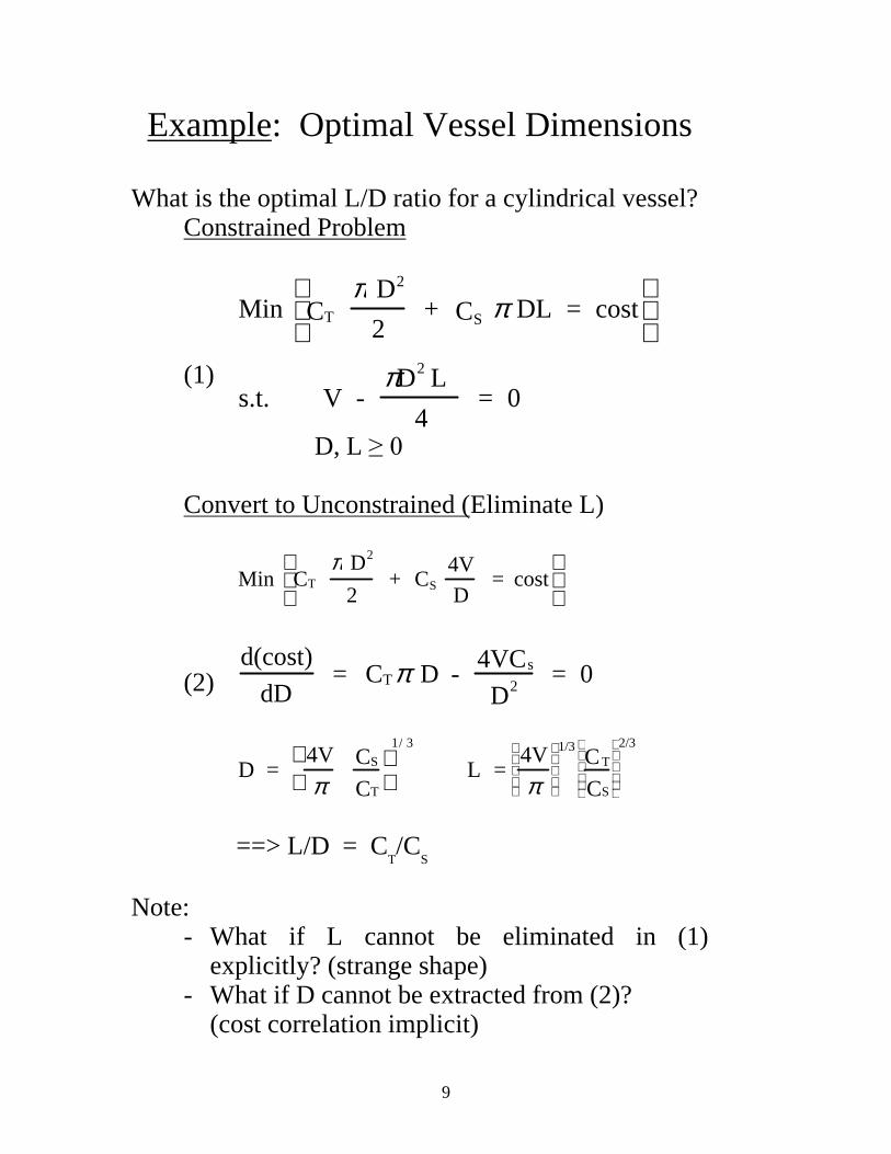
Example: Optimal Vessel Dimensions
What is the optimal L/D ratio for a cylindrical vessel? Constrained Problem
(1)
Min TC 2π D
2 + S C π DL = cost
s.t. V - 2πD L
4 = 0
D, L ��� Convert to Unconstrained (Eliminate L)
Min TC
2π D
2 + S C
4V
D = cost
(2) d(cost)
dD = TC π D - s4VC
2D = 0
D = 4V
π SC
TC
1/ 3
L =4V
π
1/3TC
SC
2/3
==> L/D = C
T/C
S
Note:
- What if L cannot be eliminated in (1) explicitly? (strange shape) - What if D cannot be extracted from (2)? (cost correlation implicit)
10
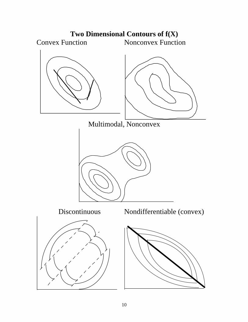
Two Dimensional Contours of f(X) Convex Function Nonconvex Function
Multimodal, Nonconvex
Discontinuous Nondifferentiable (convex)
11
Some Important Points We will develop methods that will find a local minimum point x* for f(x) for a feasible region defined by the constraint functions: f(x*) �� I�[�� IRU� DOO� [� VDWLVI\LQJ� WKH�constraints in some neighborhood around x* Finding and verifying global solutions to this NLP will not be considered here. It requires an exhaustive (spatial branch and bound) and it much more expensive. A local solution to the NLP is also a global solution under the following sufficient conditions based on convexity. A convex function φ(x) for x in some domain X, if and only if it satisfies the relation:
φ(α y + (1−α) z) ��α φ(y) + (1-α) φ(z) for any α, 0 ��α ��1, at all points y and z in X.
12
Some Notation Matrix Notation - Some Definitions
• Scalars - Greek letters, α, β, γ • Vectors - Roman Letters, lower case • Matrices - Roman Letters, upper case
Matrix Multiplication - C = A B if A ∈ ℜ n x m, B ∈ ℜ m x p
and C ∈ ℜ n x p, cij = Σk aik bkj
Transpose - if A ∈ ℜ n x m, then interchanging rows and columns leads to AT∈ ℜ m x n Symmetric Matrix - A ∈ ℜ n x n (square matrix) and A = AT Identity Matrix - I, square matrix with ones on diagonal and zeroes elsewhere. Determinant - "Inverse Volume" measure of a square matrix
det(A) = Σi (-1)i+j Aij Aij for any j, or
det(A) = Σj (-1)i+j Aij Aij for any i, where Aij is the determinant of an order n-1 matrix with row i and column j removed. Singular Matrix - det (A) = 0
13
Eigenvalues - det(A- λ I) = 0 Eigenvector - Av = λ v
• These are characteristic values and directions of a matrix.
• For nonsymmetric matrices eigenvalues can be complex, so we often use singular values,
σ = λ(ATΑ)1/2 ≥ 0 Some Identities for Determinant
det(A B) = det(A) det(B) det (A) = det(AT)
det(αA) = αn det(A) det(A) = Πi λi(A) Vector Norms
|| x ||p = {Σi |xi|p}1/p
(most common are p = 1, p = 2 (Euclidean) and p = ∞ (max norm = maxi|xi|)) Matrix Norms ||A|| = max ||A x||/||x|| over x (for p-norms)
||A||1 - max column sum of A, maxj (Σi |Aij|)
||A||∞ - maximum row sum of A, maxi (Σj |Aij|)
||A||2 = [σmax(Α)] (spectral radius)
||A||F = [Σi Σj (Aij)2]1/2 (Frobenius norm)
κ(Α) = ||A|| ||A−1|| (condition number) = σmax/σmin (using 2-norm)
14
UNCONSTRAINED METHODS THAT USE
DERIVATIVES
Gradient Vector - (∇ f(x))
∇ f =
∂f /1∂x
∂f /2∂x
.... ..
∂f / n∂x
Hessian Matrix (∇ 2f(x) - Symmetric)
2∇ f(x) =
2∂ f
12∂x
2∂ f
1∂x 2∂x⋅ ⋅ ⋅ ⋅
2∂ f
1∂x n∂x
... . . ... ... .2∂ f
n∂x 1∂x
2∂ f
n∂x 2∂x⋅ ⋅ ⋅ ⋅
2∂ f
n2∂x
Note: 2∂ f
∂ x j∂xi =
2∂ f
j∂x i∂x
15
Eigenvalues (Characteristic Values) Find x and λ where Ax
i = λ
i x
i, i = i,n
Note: Ax - λx = (A - λI) x = 0 or det (A - λI) = 0 For this relation λ is an eigenvalue and x is an eigenvector of A. If A is symmetric, all λ
i are real
λi > 0, i = 1, n; A is positive definite
λi < 0, i = 1, n; A is negative definite
λi = 0, some i: A is singular
Quadratic Form can be expressed in Canonical Form (Eigenvalue/Eigenvector) x
TAx ⇒ A X = X Λ
X - eigenvector matrix (n x n) Λ - eigenvalue (diagonal) matrix = diag(λ
i)
If A is symmetric, all λ
i are real and X can be chosen
orthonormal (X-1 = X
T). Thus, A = X Λ X
-1 = X Λ X
T For Quadratic Function: Q(x) = a
Tx = 1
2 x
T A x
define: z = X
Tx , Q(x) = Q(z) = x = Xz, (a
TX) z + 1
2 z
T Λ z
Minimum occurs at (if λ
i > 0)
x = -A-1a or x = Xz = -X(Λ
-1X
Ta)
16
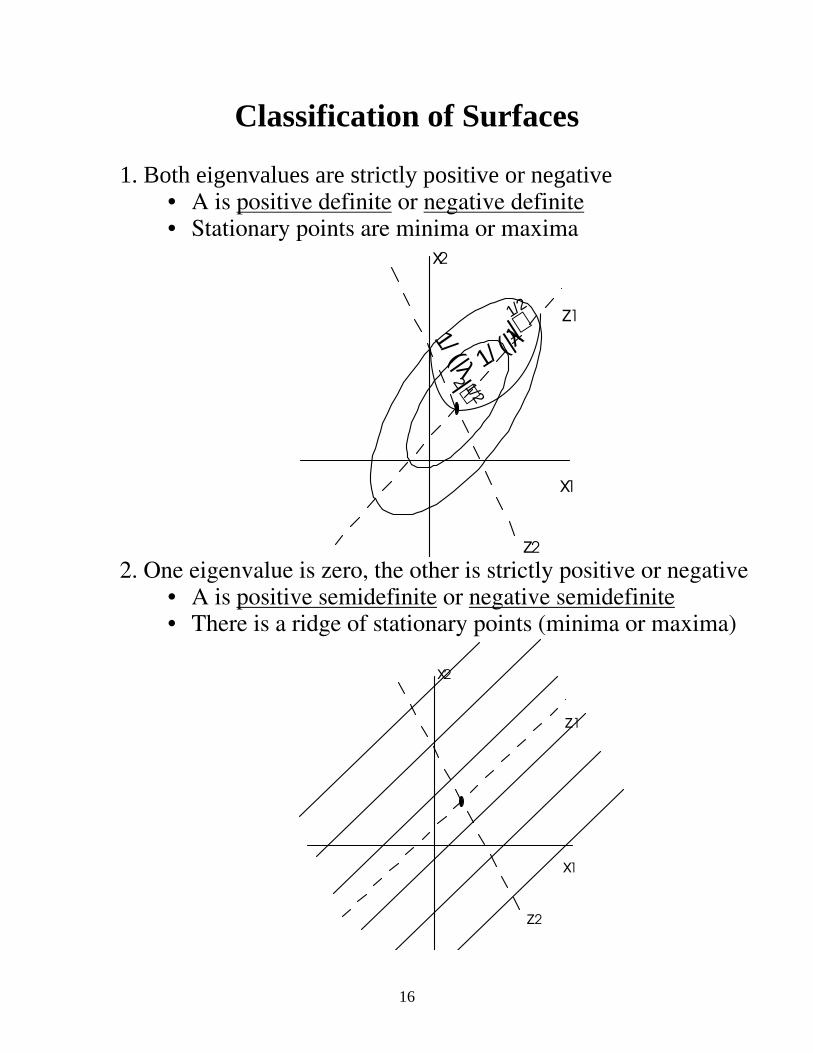
Classification of Surfaces 1. Both eigenvalues are strictly positive or negative
• A is positive definite or negative definite • Stationary points are minima or maxima
x1
x2
z1
z2
1/ (|λ1|)1/2
1/ (|λ2|) 1/2
2. One eigenvalue is zero, the other is strictly positive or negative • A is positive semidefinite or negative semidefinite • There is a ridge of stationary points (minima or maxima)
x1
x2
z1
z2
17
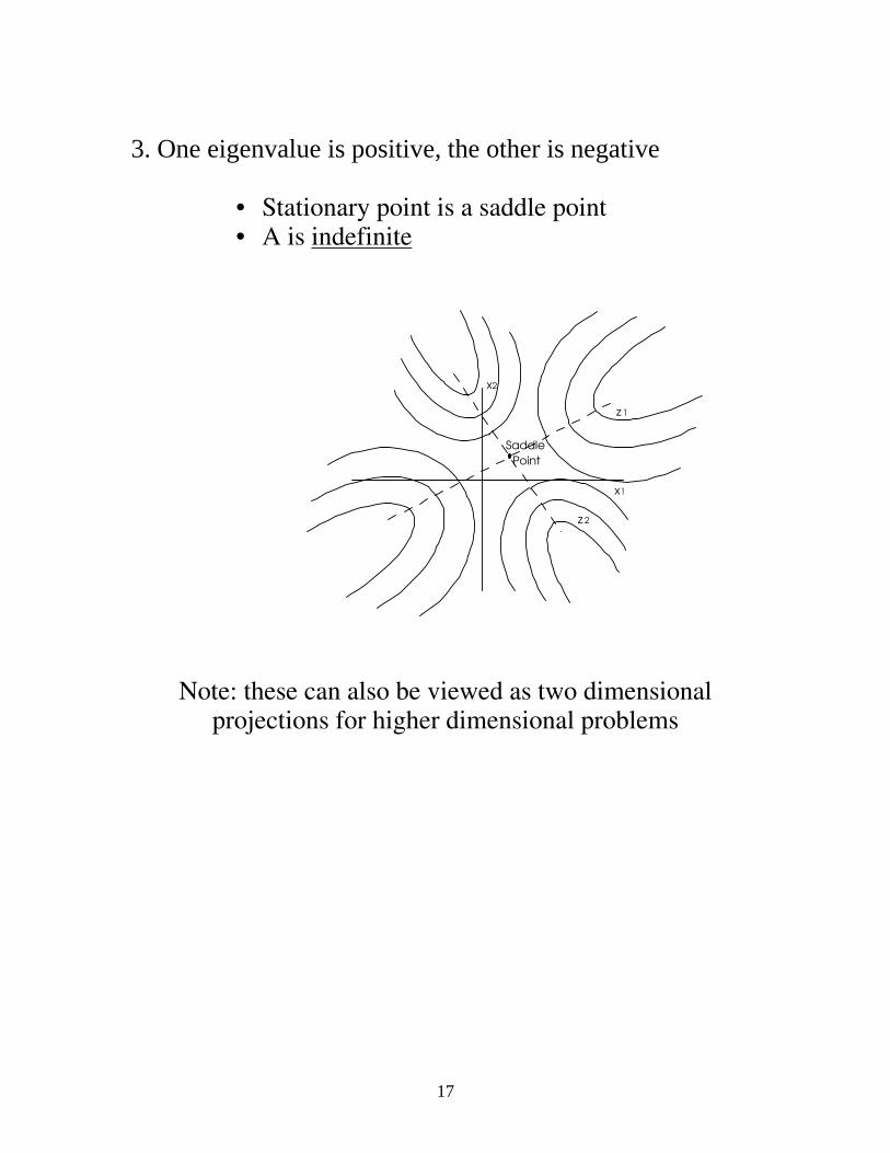
3. One eigenvalue is positive, the other is negative
• Stationary point is a saddle point • A is indefinite
x1
x2
z 1
z 2
Saddle
Point
Note: these can also be viewed as two dimensional projections for higher dimensional problems
18
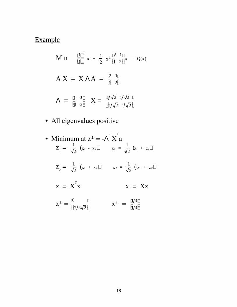
Example
Min T1
1
x +
1
2 Tx
2 1
1 2
x = Q(x)
A X = X Λ A = 2 1
1 2
Λ = 1 0
0 3
X =
1 2 1 2
-1 2 1 2
• All eigenvalues positive
• Minimum at z* = -Λ-1
XT
a z
1 = 1
2 1x - 2x( ) 1x =
1
2 1z + 2z( )
z
2 = 1
2 1x + 2x( ) 2x =
1
2 1-z + 2z( )
z = X
Tx x = Xz
z* = 0
2 3 2
x* =
1 3
1 3
19
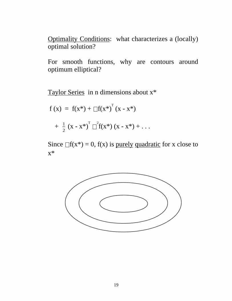
Optimality Conditions: what characterizes a (locally) optimal solution? For smooth functions, why are contours around optimum elliptical? Taylor Series in n dimensions about x* f (x) = f(x*) + ∇ f(x*)
T (x - x*)
+ 1
2 (x - x*)
T ∇
2f(x*) (x - x*) + . . .
Since ∇ f(x*) = 0, f(x) is purely quadratic for x close to x*
20
Comparison of Optimization Methods
1. Convergence Theory • Global Convergence - will it converge to a local
optimum (or stationary point) from a poor starting point?
• Local Convergence Rate - how fast will it converge close to the solution?
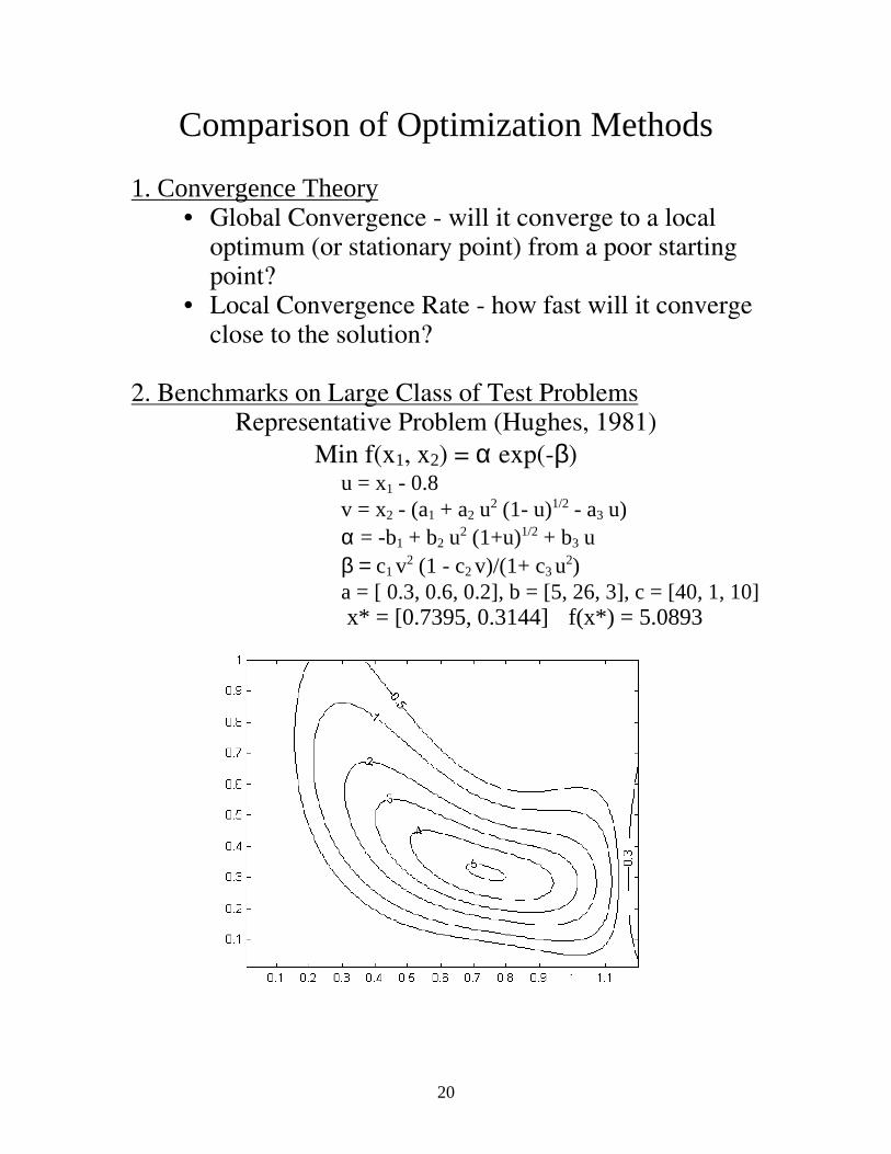
2. Benchmarks on Large Class of Test Problems
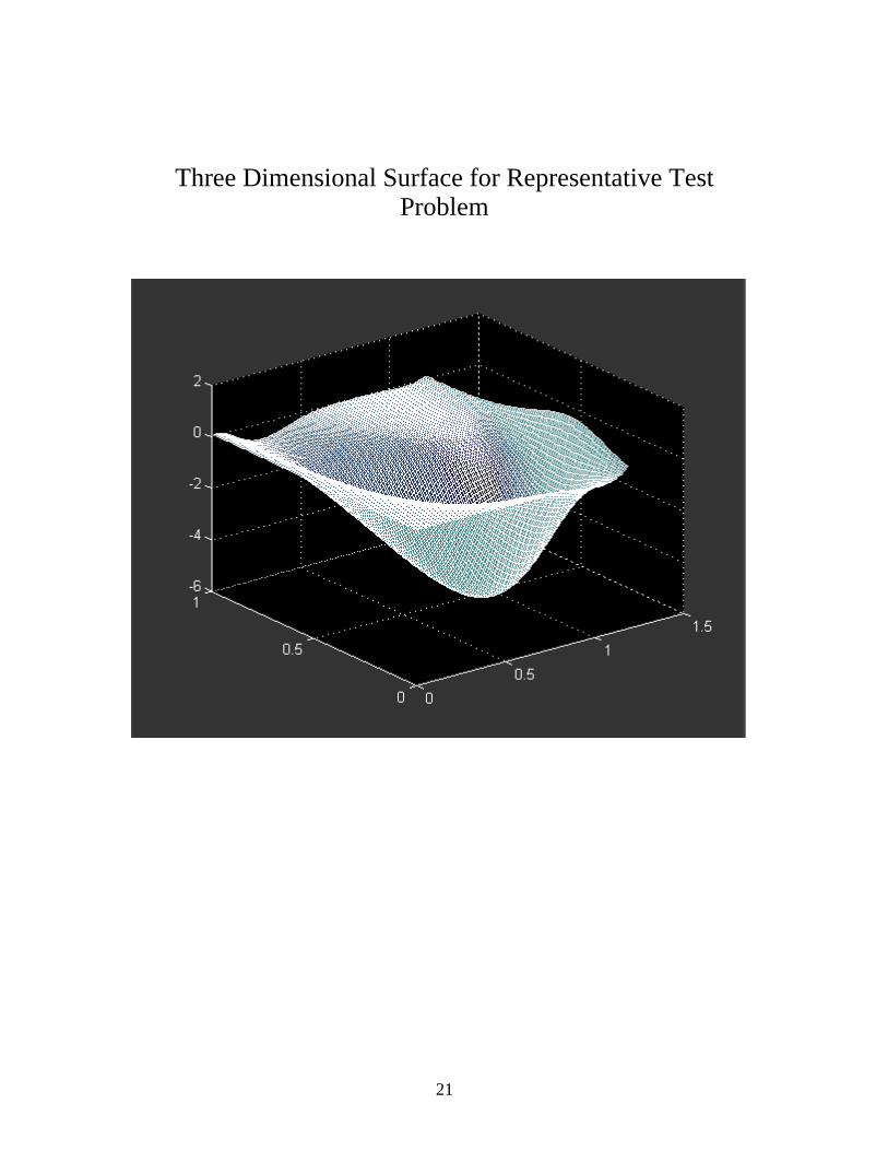
Representative Problem (Hughes, 1981) Min f(x1, x2) = α exp(-β)
u = x1 - 0.8 v = x2 - (a1 + a2 u2 (1- u)1/2 - a3 u) α = -b1 + b2 u2 (1+u)1/2 + b3 u β = c1 v2 (1 - c2 v)/(1+ c3 u2) a = [ 0.3, 0.6, 0.2], b = [5, 26, 3], c = [40, 1, 10] x* = [0.7395, 0.3144] f(x*) = 5.0893
21
Three Dimensional Surface for Representative Test Problem

22
Regions of Minimum Eigenvalues for Representative Test Problem
[0, -10, -50, -100, -150, -200]
-
10-
10-10
-
10
0
0
-
50
-
50
-
50
-
100
-
100
-
150
-
200
23
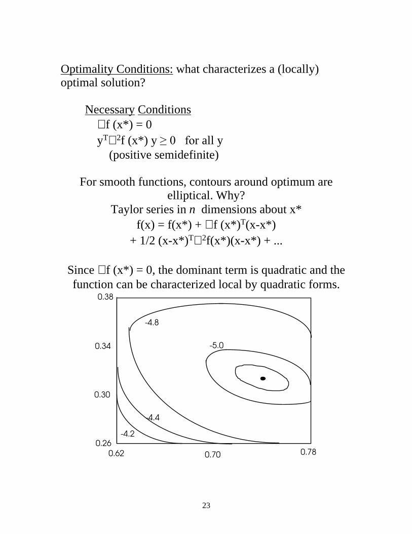
Optimality Conditions: what characterizes a (locally) optimal solution?
Necessary Conditions ∇ f (x*) = 0 yT∇ 2f (x*) y ������IRr all y (positive semidefinite)
For smooth functions, contours around optimum are
elliptical. Why? Taylor series in n dimensions about x*
f(x) = f(x*) + ∇ f (x*)T(x-x*) + 1/2 (x-x*)T∇ 2f(x*)(x-x*) + ...
Since ∇ f (x*) = 0, the dominant term is quadratic and the function can be characterized local by quadratic forms.
0.62 0.70 0.78
0.38
0.26
0.30
0.34 -5.0
-4.8
-4.4
-4.2
24
NEWTON’S METHOD
Taylor Series for f(x) about xk Take derivative wrt x, set LHS §��
0 §∇ f(x) = ∇ f(xk) + ∇2
f(xk) (x - xk)
⇒ (x - xk) ≡ d = - (∇2
f(xk))-1 ∇ f(xk)
Notes:
1. f(x) is convex (concave) if ∇2
f(x) is all positive (negative) semidefinite, i.e. minj λj ≥ 0 (maxj λj ���� 2. Method can fail if: - x
0 far from optimum
- ∇2
f is singular at any point - function is not smooth 3. Search direction, d, requires solution of linear equations. 4. Near solution k+1x - x * = K kx - x *
2
25
BASIC NEWTON ALGORITHM
0. Guess x0, Evaluate f(x
0).
1. At xk, evaluate ∇ f(xk). 2. Evaluate B
k from Hessian or an approximation.
3. Solve: Bk d = -∇ f(xk) If convergence error is less than tolerance: e.g., || ∇ f(xk) || ≤ ε and ||d|| ≤ ε STOP, else go to 4. 4. Find α so that 0 < α ≤ 1 and f(xk + αd) < f(xk) sufficiently (Each trial requires evaluation of f(x)) 5. xk+1 = xk + αd. Set k = k + 1 Go to 1.
26
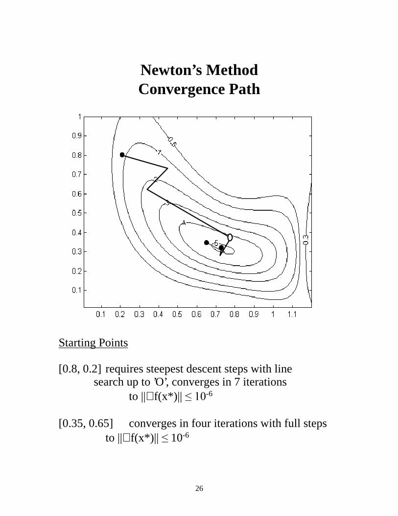
Newton’s Method Convergence Path
Starting Points [0.8, 0.2] requires steepest descent steps with line search up to ’O’, converges in 7 iterations to ||∇ f(x*)|| ����-6 [0.35, 0.65] converges in four iterations with full steps to ||∇ f(x*)|| ��10-6
27
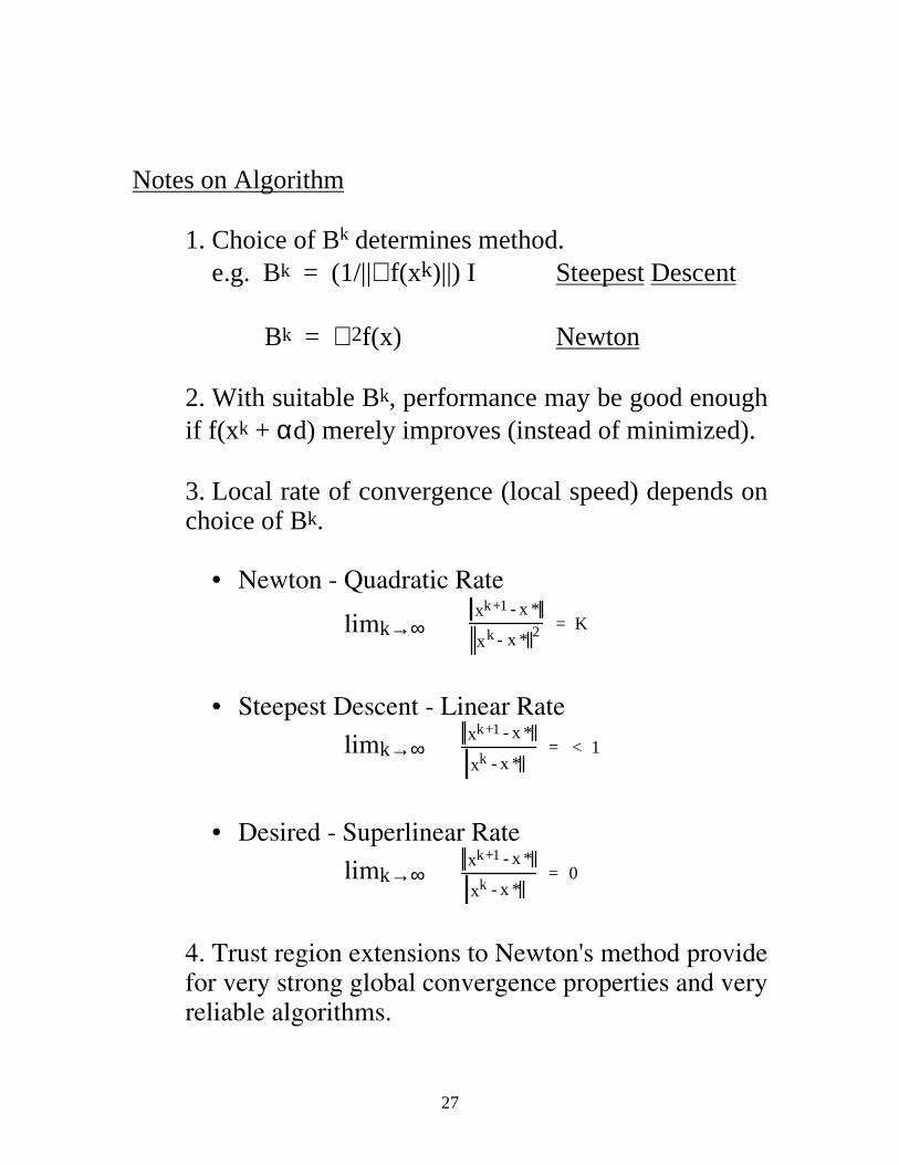
Notes on Algorithm
1. Choice of Bk determines method. e.g. Bk = (1/||∇ f(xk)||) I Steepest Descent Bk = ∇ 2f(x) Newton 2. With suitable Bk, performance may be good enough if f(xk + αd) merely improves (instead of minimized). 3. Local rate of convergence (local speed) depends on choice of Bk. • Newton - Quadratic Rate
limk→∞ k+1x - x *
kx - x * 2 = K
• Steepest Descent - Linear Rate
limk→∞ k+1x - x *
kx - x * = < 1
• Desired - Superlinear Rate
limk→∞ k+1x - x *
kx - x * = 0
4. Trust region extensions to Newton's method provide for very strong global convergence properties and very reliable algorithms.
28
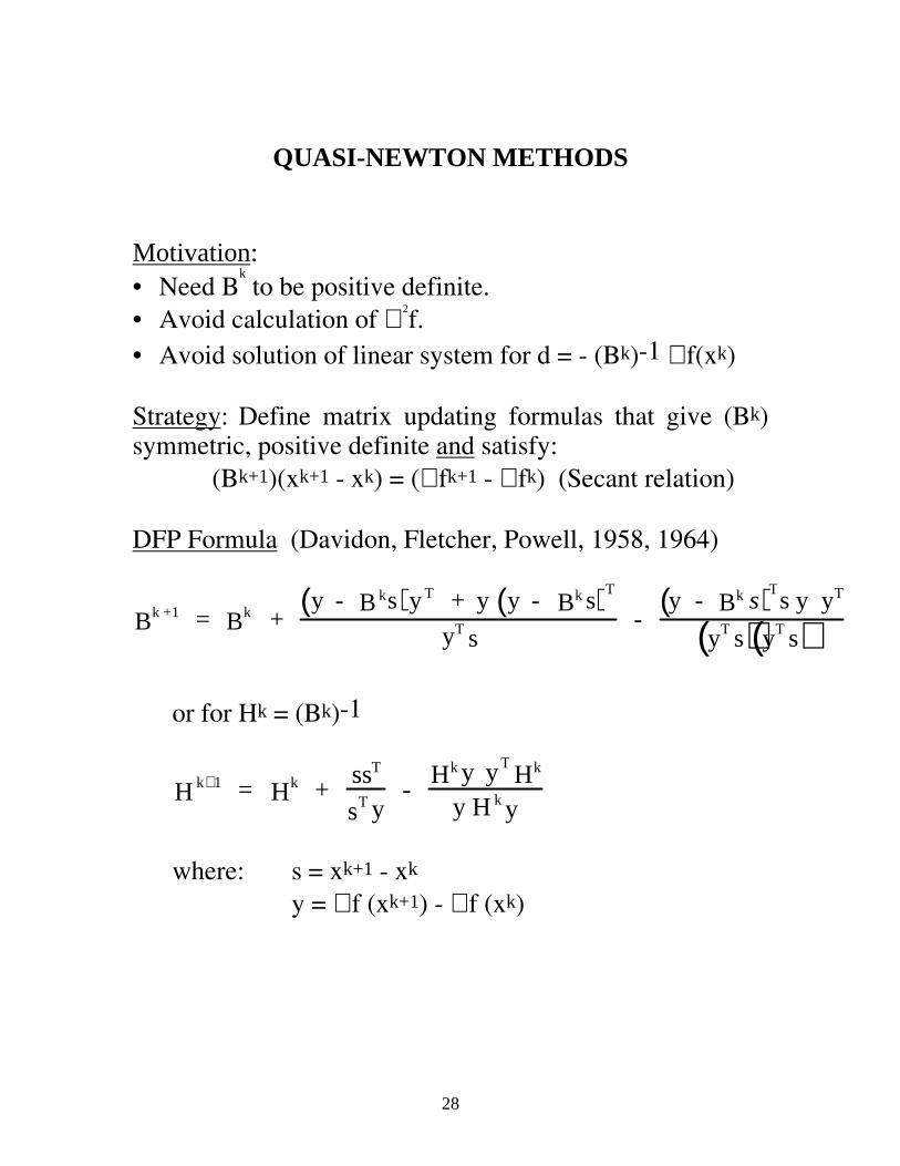
QUASI-NEWTON METHODS
Motivation: • Need B
k to be positive definite.
• Avoid calculation of ∇ 2
f. • Avoid solution of linear system for d = - (Bk)-1 ∇ f(xk) Strategy: Define matrix updating formulas that give (Bk) symmetric, positive definite and satisfy: (Bk+1)(xk+1 - xk) = (∇ fk+1 - ∇ fk) (Secant relation) DFP Formula (Davidon, Fletcher, Powell, 1958, 1964)
k +1B = kB + y - kB s( ) Ty + y y - kB s( )T
Ty s -
y - kB s( )Ts y Ty
Ty s( ) Ty s( ) or for Hk = (Bk)-1
k+1H = kH +
TssTs y
- kH y Ty kH
ky H y
where: s = xk+1 - xk y = ∇ f (xk+1) - ∇ f (xk)
29
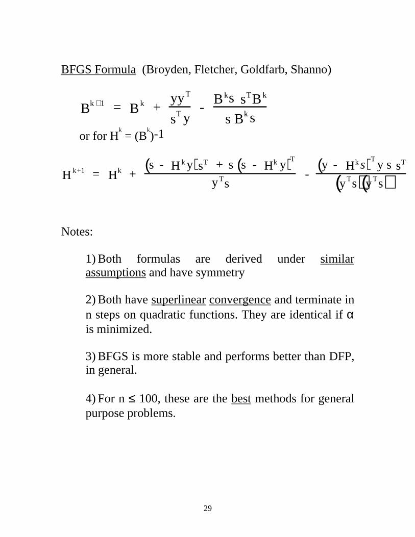
BFGS Formula (Broyden, Fletcher, Goldfarb, Shanno)
k +1B = kB +
TyyTs y
- kB s Ts kB
ks B s
or for Hk = (B
k)-1
k+1H = kH + s - kH y( ) Ts + s s - kH y( )T
Ty s -
y - kH s( )Ty s Ts
Ty s( ) Ty s( )
Notes:
1) Both formulas are derived under similar assumptions and have symmetry 2) Both have superlinear convergence and terminate in n steps on quadratic functions. They are identical if α is minimized. 3) BFGS is more stable and performs better than DFP, in general. 4) For n ≤ 100, these are the best methods for general purpose problems.
30
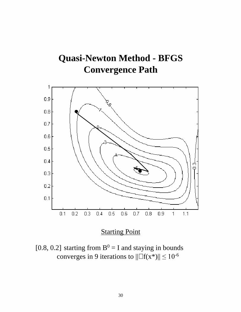
Quasi-Newton Method - BFGS Convergence Path
Starting Point [0.8, 0.2] starting from B0 = I and staying in bounds converges in 9 iterations to ||∇ f(x*)|| ����-6
31
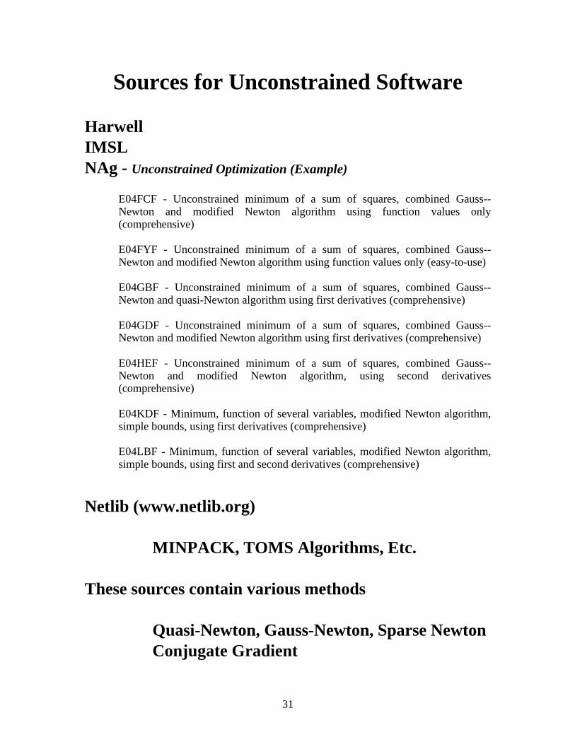
Sources for Unconstrained Software
Harwell IMSL NAg - Unconstrained Optimization (Example)
E04FCF - Unconstrained minimum of a sum of squares, combined Gauss--Newton and modified Newton algorithm using function values only (comprehensive) E04FYF - Unconstrained minimum of a sum of squares, combined Gauss--Newton and modified Newton algorithm using function values only (easy-to-use) E04GBF - Unconstrained minimum of a sum of squares, combined Gauss--Newton and quasi-Newton algorithm using first derivatives (comprehensive) E04GDF - Unconstrained minimum of a sum of squares, combined Gauss--Newton and modified Newton algorithm using first derivatives (comprehensive) E04HEF - Unconstrained minimum of a sum of squares, combined Gauss--Newton and modified Newton algorithm, using second derivatives (comprehensive) E04KDF - Minimum, function of several variables, modified Newton algorithm, simple bounds, using first derivatives (comprehensive) E04LBF - Minimum, function of several variables, modified Newton algorithm, simple bounds, using first and second derivatives (comprehensive)
Netlib (www.netlib.org)
MINPACK, TOMS Algorithms, Etc. These sources contain various methods
Quasi-Newton, Gauss-Newton, Sparse Newton Conjugate Gradient
32
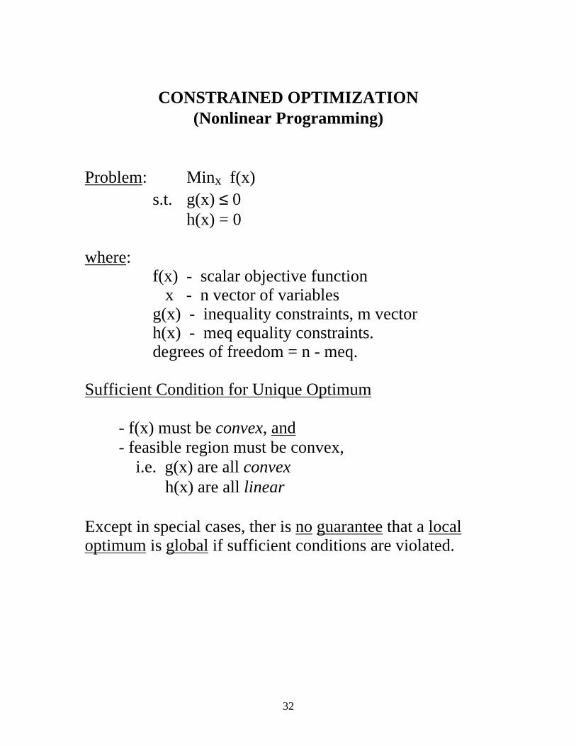
CONSTRAINED OPTIMIZATION
(Nonlinear Programming)
Problem: Minx f(x) s.t. g(x) ≤ 0 h(x) = 0 where:
f(x) - scalar objective function x - n vector of variables g(x) - inequality constraints, m vector h(x) - meq equality constraints. degrees of freedom = n - meq.
Sufficient Condition for Unique Optimum
- f(x) must be convex, and - feasible region must be convex, i.e. g(x) are all convex h(x) are all linear
Except in special cases, ther is no guarantee that a local optimum is global if sufficient conditions are violated.
33
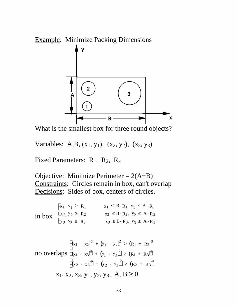
Example: Minimize Packing Dimensions
23
1
A
B
y
x
What is the smallest box for three round objects? Variables: A,B, (x1, y1), (x2, y2), (x3, y3) Fixed Parameters: R1, R2, R3 Objective: Minimize Perimeter = 2(A+B) Constraints: Circles remain in box, can’t overlap Decisions: Sides of box, centers of circles.
in box
1x , 1y ≥ 1R 1x ≤ B- 1R , 1y ≤ A - 1R
2, x 2 y ≥ 2R 2x ≤ B- 2R , 2 y ≤ A - 2R
3,x 3 y ≥ 3R 3x ≤ B- 3R , 3 y ≤ A - 3R
no overlaps 1x - 2x( )2 + 1y - 2y( )2 ≥ 1R + 2R( )2
1x - 3x( )2 + 1y - 3y( )2 ≥ 1R + 3R( )2
2x - 3x( )2 + 2y - 3y( )2 ≥ 2R + 3R( )2
x1, x2, x3, y1, y2, y3, A, B ≥ 0
34
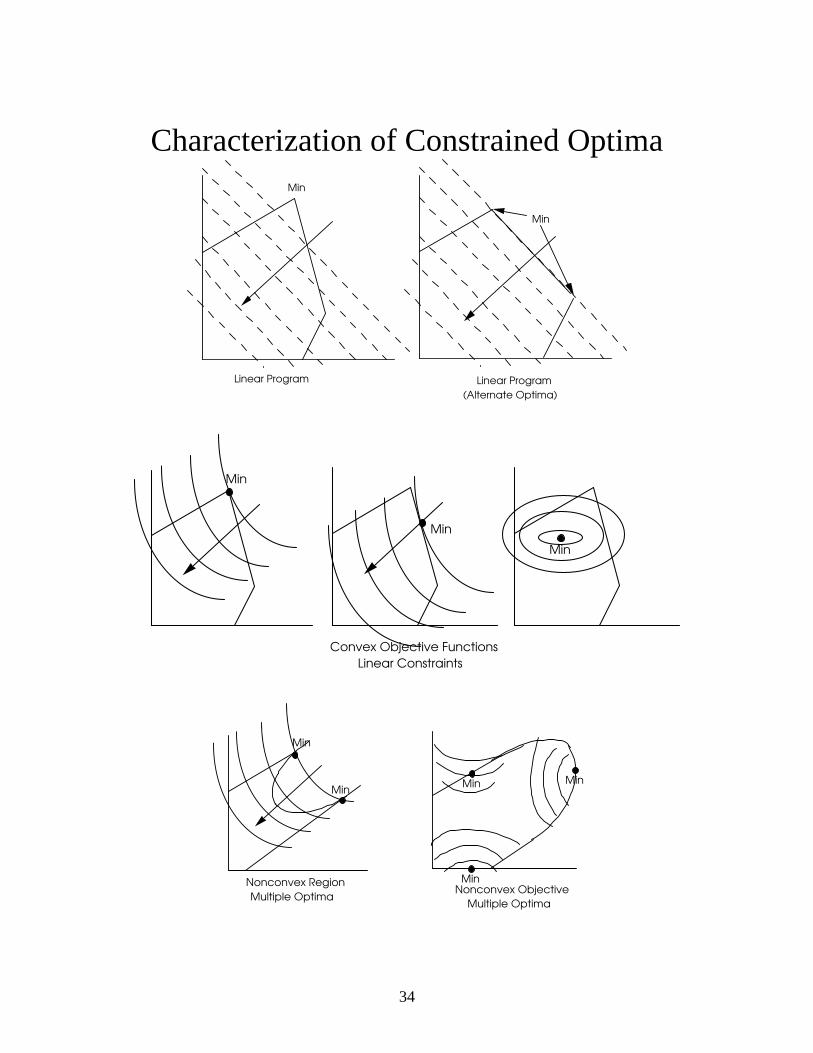
Characterization of Constrained Optima Min
Linear Program
Min
Linear Program
(Alternate Optima)
Min
Min
Min
Convex Objective Functions
Linear Constraints
Min
Min
Min
Nonconvex Region
Multiple Optima
MinMin
Nonconvex Objective
Multiple Optima
35
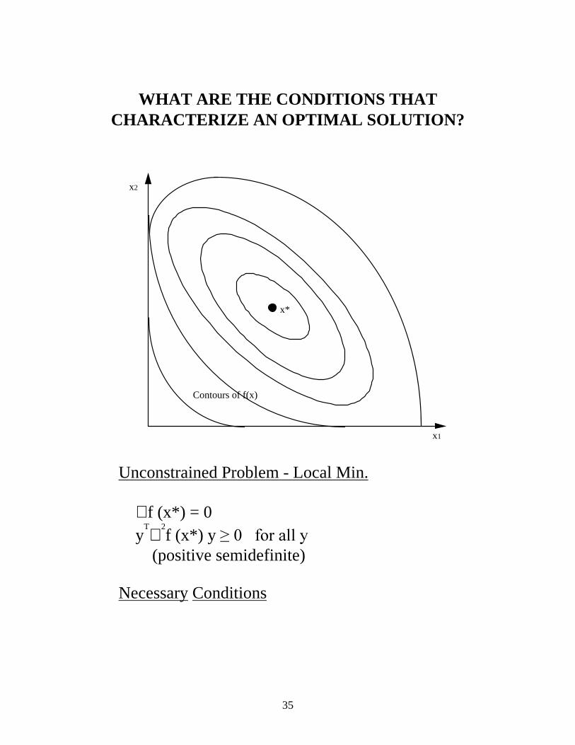
WHAT ARE THE CONDITIONS THAT
CHARACTERIZE AN OPTIMAL SOLUTION?
x1
x2
x*
Contours of f(x)
Unconstrained Problem - Local Min. ∇ f (x*) = 0 y
T∇
2f (x*) y ������IRU�DOO�\
(positive semidefinite) Necessary Conditions
36
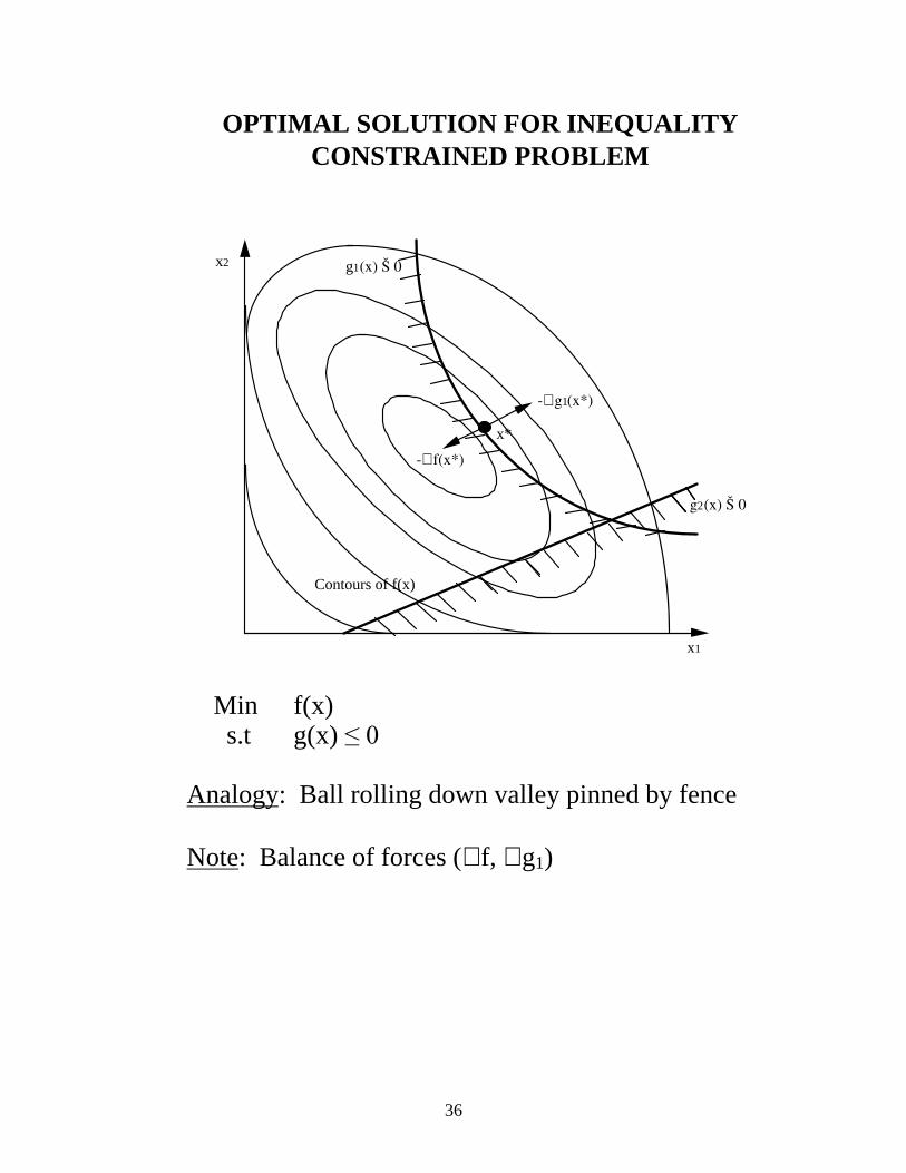
OPTIMAL SOLUTION FOR INEQUALITY CONSTRAINED PROBLEM
x1
x2
x*
Contours of f(x)
g1(x) Š 0
g2(x) Š 0
-∇ g1(x*)
-∇ f(x*)
Min f(x) s.t g(x) ��� Analogy: Ball rolling down valley pinned by fence Note: Balance of forces (∇ f, ∇ g1)

37
OPTIMAL SOLUTION FOR GENERAL CONSTRAINED PROBLEM
x1
x2
x*
Contours of f(x)
g1(x) Š 0
g2(x) Š 0
-∇ g1(x*)
-∇ f(x*)
-∇ h(x*)
h(x) = 0
Problem: Min f(x) s.t. g(x) ��� h(x) = 0 Analogy: Ball rolling on rail pinned by fences Balance of forces: ∇ f, ∇ g1, ∇ h
38
OPTIMALITY CONDITIONS FOR LOCAL
OPTIMUM
1st Order Kuhn - Tucker Conditions (Necessary) ∇ L (x*, u, v) = ∇ f(x*) + ∇ g(x*) u + ∇ h(x*) v = 0 (Balance of Forces) u ��� (Inequalities act in only one direction) g (x*) ������K��[ �� �� (Feasibility) uj gj(x*) = 0 (Complementarity - either uj = 0 or gj(x*) = 0 at constraint or off) u, v are "weights" for "forces," known as • Kuhn - Tucker & Lagrange multipliers • Shadow prices • Dual variables
2nd Order Conditions (Sufficient)
- Positive curvature in "constraint" directions. - p
T ∇
2L (x*) p > 0, where p are all constrained
directions.
39
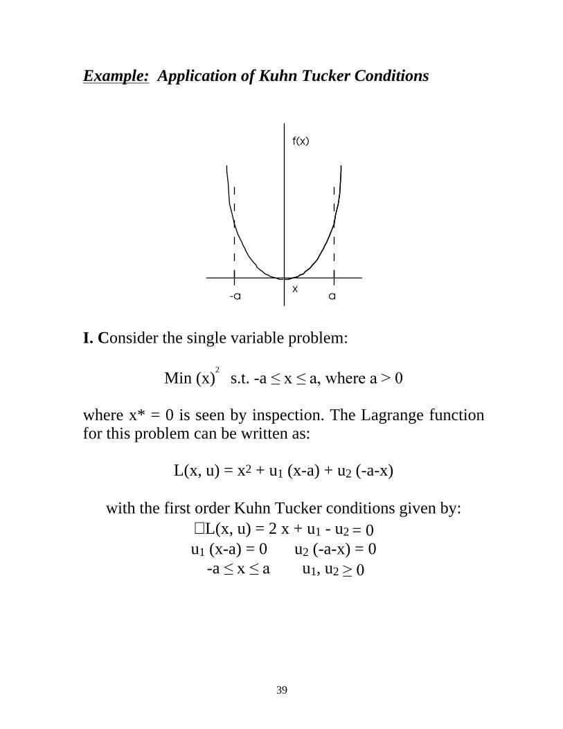
Example: Application of Kuhn Tucker Conditions
-a a
f(x)
x
I. Consider the single variable problem:
Min (x)2 s.t. -a ��[���D��ZKHUH�D�!��
where x* = 0 is seen by inspection. The Lagrange function for this problem can be written as:
L(x, u) = x2 + u1 (x-a) + u2 (-a-x)
with the first order Kuhn Tucker conditions given by: ∇ L(x, u) = 2 x + u1 - u2 = 0 u1 (x-a) = 0 u2 (-a-x) = 0
-a ��[���D u1, u2 ���
40
Consider three cases:
u1 > 0, u2 = 0; u1 = 0, u2 > 0;
u1 = u2 = 0.
• Upper bound is active, x = a, u1 = -2a, u2 = 0 • Lower bound is active, x = -a, u2 = -2a, u1 = 0 • Neither bound is active, u1 = 0, u2 = 0, x = 0
Evaluate the second order conditions. At x* = 0 we have
∇xxL (x*, u*, v*) = 2 > 0
pT ∇
xxL (x*, u*, v*) p = 2 (∆x)
2 > 0
for all allowable directions. Therefore the solution x* = 0 satisfies both the sufficient first and second order Kuhn Tucker conditions for a local minimum.
41
a-a
f(x)
x
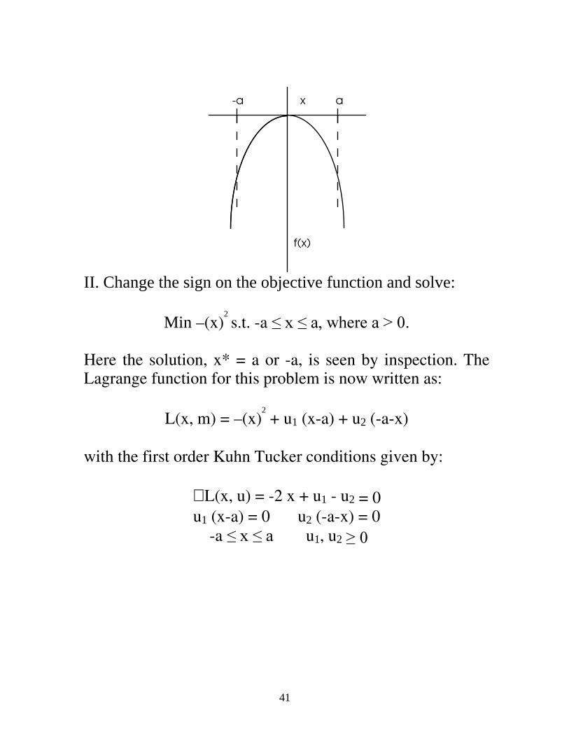
II. Change the sign on the objective function and solve:
Min –(x)2 s.t. -a ��[���D��ZKHUH�D�!���
Here the solution, x* = a or -a, is seen by inspection. The Lagrange function for this problem is now written as:
L(x, m) = –(x)2 + u1 (x-a) + u2 (-a-x)
with the first order Kuhn Tucker conditions given by:
∇ L(x, u) = -2 x + u1 - u2 = 0 u1 (x-a) = 0 u2 (-a-x) = 0
-a ��[���D u1, u2 ���
42
Consider three cases:
u1 > 0, u2 = 0; u1 = 0, u2 > 0; u1 = u2 = 0.
• Upper bound is active, x = a, u1 = 2a, u2 = 0 • Lower bound is active, x = -a, u2 = 2a, u1 = 0 • Neither bound is active, u1 = 0, u2 = 0, x = 0
Check the second order conditions to discriminate among these points. At x = 0, we realize allowable directions p = ∆x > 0 and - ∆x and we have:
pT ∇
xxL (x, u, v) p = -2 (∆x)
2 < 0
For x = a or x = -a, we require the allowable direction to satisfy the active constraints exactly. Here, any point along the allowable direction, x* must remain at its bound. For this problem, however, there are no nonzero allowable directions that satisfy this condition. Consequently the solution x* is defined entirely by the active constraint. The condition:
pT ∇
xxL (x*, u*, v*) p > 0
for all allowable directions, is vacuously satisfied - because there are no allowable directions.
43
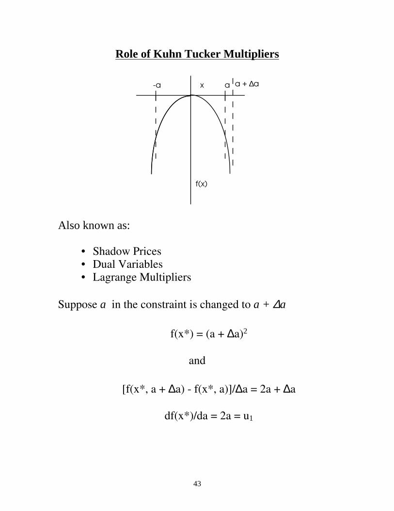
Role of Kuhn Tucker Multipliers
a-a
f(x)
x a + ∆a
Also known as:
• Shadow Prices • Dual Variables • Lagrange Multipliers
Suppose a in the constraint is changed to a + ∆a
f(x*) = (a + ∆a)2
and
[f(x*, a + ∆a) - f(x*, a)]/∆a = 2a + ∆a
df(x*)/da = 2a = u1
44
SPECIAL "CASES" OF NONLINEAR PROGRAMMING
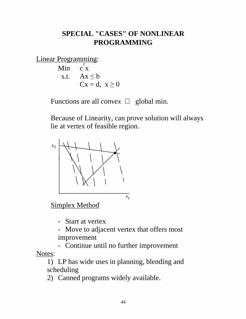
Linear Programming:
Min cTx
s.t. Ax ��E Cx = d, x ��� Functions are all convex ⇒ global min. Because of Linearity, can prove solution will always lie at vertex of feasible region.
x2
x1 Simplex Method - Start at vertex - Move to adjacent vertex that offers most improvement - Continue until no further improvement
Notes: 1) LP has wide uses in planning, blending and scheduling 2) Canned programs widely available.
45
Example: Simplex Method
Min -2x1 - 3x
2 Min -2x
1 - 3x
2 s.t. 2x
1 + x
2 ��� ⇒ s.t. 2x
1 + x
2 + x
3 = 5
x1, x
2 ��� x
1, x
2, x
3 ���
(add slack variable) Now, define f = -2x
1 - 3x
2 ⇒ f + 2x
1 + 3x
2 = 0
Set x1, x
2 = 0, x3 = 5 and form tableau
x
1 x
2 x3 f b x1, x
2
nonbasic 2 1 1 0 5 x
3
basic 2 3 0 1 0 To decrease f, increase x
2. How much? so x3 ���
x
1 x
2 x3 f b
2 1 1 0 5 -4 0 -3 1 -15 f can no longer be decreased! Optimal The underlined terms are -(reduced gradients) for nonbasic variables (x
1, x
3). x
2 is basic at optimum.
46
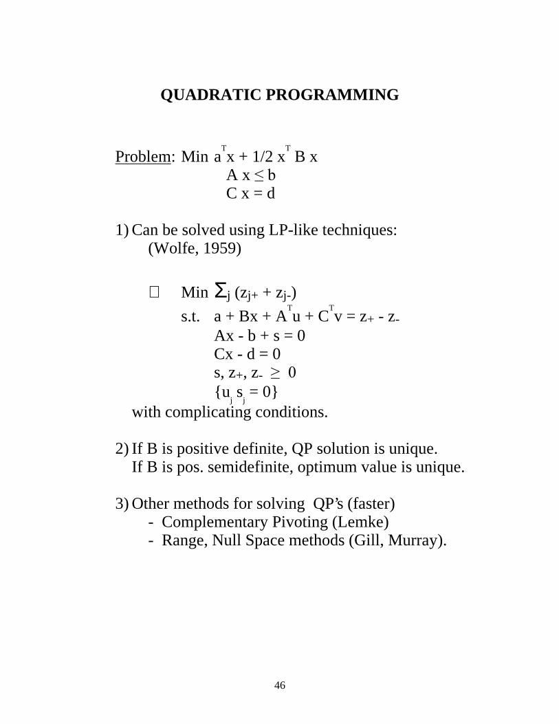
QUADRATIC PROGRAMMING
Problem: Min aTx + 1/2 x
T B x
A x ��E C x = d 1) Can be solved using LP-like techniques: (Wolfe, 1959)
⇒ Min Σj (zj+ + zj-)
s.t. a + Bx + ATu + C
Tv = z+ - z-
Ax - b + s = 0 Cx - d = 0 s, z+, z- ���� {u
j s
j = 0}
with complicating conditions. 2) If B is positive definite, QP solution is unique. If B is pos. semidefinite, optimum value is unique. 3) Other methods for solving QP’s (faster) - Complementary Pivoting (Lemke) - Range, Null Space methods (Gill, Murray).
47
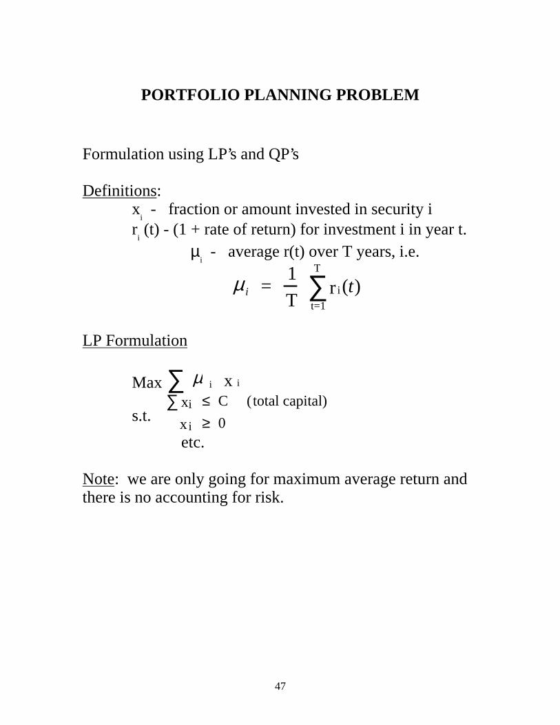
PORTFOLIO PLANNING PROBLEM
Formulation using LP’s and QP’s Definitions:
xi - fraction or amount invested in security i
ri (t) - (1 + rate of return) for investment i in year t.
µi - average r(t) over T years, i.e.
iµ = 1
T ir
t=1
T
∑ (t)
LP Formulation
Max iµ ix∑
s.t. ix ≤ C (total capital)∑
ix ≥ 0
etc.
Note: we are only going for maximum average return and there is no accounting for risk.
48
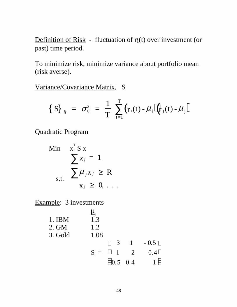
Definition of Risk - fluctuation of ri(t) over investment (or past) time period. To minimize risk, minimize variance about portfolio mean (risk averse). Variance/Covariance Matrix, S
ijS{ } = ij2σ =
1
T ir (t) - iµ( )
t =1
T
∑ jr (t) - jµ( )
Quadratic Program
Min x
T S x
s.t.
jx∑ = 1
jµ∑ jx ≥ R
jx ≥ 0, . . .
Example: 3 investments
µj
1. IBM 1.3 2. GM 1.2 3. Gold 1.08
S =
3 1 - 0.5
1 2 0.4
-0.5 0.4 1
49
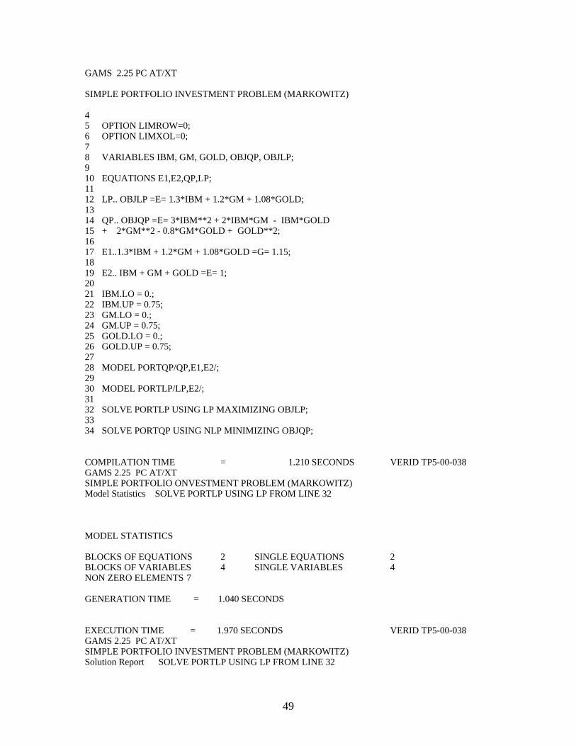
GAMS 2.25 PC AT/XT SIMPLE PORTFOLIO INVESTMENT PROBLEM (MARKOWITZ) 4 5 OPTION LIMROW=0; 6 OPTION LIMXOL=0; 7 8 VARIABLES IBM, GM, GOLD, OBJQP, OBJLP; 9 10 EQUATIONS E1,E2,QP,LP; 11 12 LP.. OBJLP =E= 1.3*IBM + 1.2*GM + 1.08*GOLD; 13 14 QP.. OBJQP =E= 3*IBM**2 + 2*IBM*GM - IBM*GOLD 15 + 2*GM**2 - 0.8*GM*GOLD + GOLD**2; 16 17 E1..1.3*IBM + 1.2*GM + 1.08*GOLD =G= 1.15; 18 19 E2.. IBM + GM + GOLD =E= 1; 20 21 IBM.LO = 0.; 22 IBM.UP = 0.75; 23 GM.LO = 0.; 24 GM.UP = 0.75; 25 GOLD.LO = 0.; 26 GOLD.UP = 0.75; 27 28 MODEL PORTQP/QP,E1,E2/; 29 30 MODEL PORTLP/LP,E2/; 31 32 SOLVE PORTLP USING LP MAXIMIZING OBJLP; 33 34 SOLVE PORTQP USING NLP MINIMIZING OBJQP; COMPILATION TIME = 1.210 SECONDS VERID TP5-00-038 GAMS 2.25 PC AT/XT SIMPLE PORTFOLIO ONVESTMENT PROBLEM (MARKOWITZ) Model Statistics SOLVE PORTLP USING LP FROM LINE 32 MODEL STATISTICS BLOCKS OF EQUATIONS 2 SINGLE EQUATIONS 2 BLOCKS OF VARIABLES 4 SINGLE VARIABLES 4 NON ZERO ELEMENTS 7 GENERATION TIME = 1.040 SECONDS EXECUTION TIME = 1.970 SECONDS VERID TP5-00-038 GAMS 2.25 PC AT/XT SIMPLE PORTFOLIO INVESTMENT PROBLEM (MARKOWITZ) Solution Report SOLVE PORTLP USING LP FROM LINE 32
50
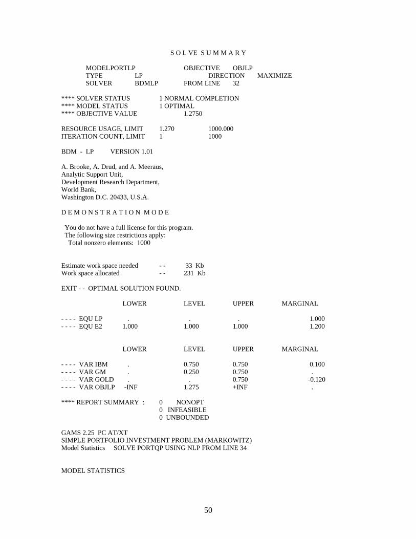
S O L VE S U M M A R Y
MODEL PORTLP OBJECTIVE OBJLP TYPE LP DIRECTION MAXIMIZE SOLVER BDMLP FROM LINE 32
**** SOLVER STATUS 1 NORMAL COMPLETION **** MODEL STATUS 1 OPTIMAL **** OBJECTIVE VALUE 1.2750 RESOURCE USAGE, LIMIT 1.270 1000.000 ITERATION COUNT, LIMIT 1 1000 BDM - LP VERSION 1.01 A. Brooke, A. Drud, and A. Meeraus, Analytic Support Unit, Development Research Department, World Bank, Washington D.C. 20433, U.S.A. D E M O N S T R A T I O N M O D E You do not have a full license for this program. The following size restrictions apply: Total nonzero elements: 1000 Estimate work space needed - - 33 Kb Work space allocated - - 231 Kb EXIT - - OPTIMAL SOLUTION FOUND. LOWER LEVEL UPPER MARGINAL - - - - EQU LP . . . 1.000 - - - - EQU E2 1.000 1.000 1.000 1.200 LOWER LEVEL UPPER MARGINAL - - - - VAR IBM . 0.750 0.750 0.100 - - - - VAR GM . 0.250 0.750 . - - - - VAR GOLD . . 0.750 -0.120 - - - - VAR OBJLP -INF 1.275 +INF . **** REPORT SUMMARY : 0 NONOPT 0 INFEASIBLE 0 UNBOUNDED GAMS 2.25 PC AT/XT SIMPLE PORTFOLIO INVESTMENT PROBLEM (MARKOWITZ) Model Statistics SOLVE PORTQP USING NLP FROM LINE 34 MODEL STATISTICS
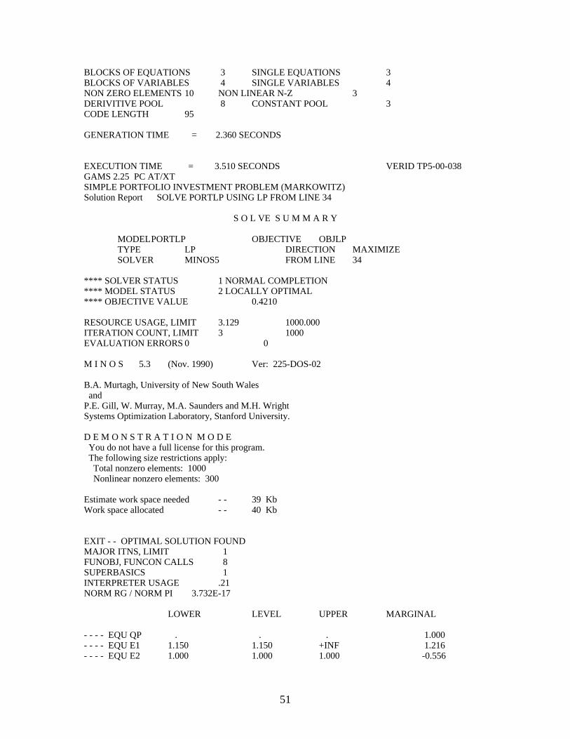
51
BLOCKS OF EQUATIONS 3 SINGLE EQUATIONS 3 BLOCKS OF VARIABLES 4 SINGLE VARIABLES 4 NON ZERO ELEMENTS 10 NON LINEAR N-Z 3 DERIVITIVE POOL 8 CONSTANT POOL 3 CODE LENGTH 95 GENERATION TIME = 2.360 SECONDS EXECUTION TIME = 3.510 SECONDS VERID TP5-00-038 GAMS 2.25 PC AT/XT SIMPLE PORTFOLIO INVESTMENT PROBLEM (MARKOWITZ) Solution Report SOLVE PORTLP USING LP FROM LINE 34
S O L VE S U M M A R Y
MODEL PORTLP OBJECTIVE OBJLP TYPE LP DIRECTION MAXIMIZE SOLVER MINOS5 FROM LINE 34
**** SOLVER STATUS 1 NORMAL COMPLETION **** MODEL STATUS 2 LOCALLY OPTIMAL **** OBJECTIVE VALUE 0.4210 RESOURCE USAGE, LIMIT 3.129 1000.000 ITERATION COUNT, LIMIT 3 1000 EVALUATION ERRORS 0 0 M I N O S 5.3 (Nov. 1990) Ver: 225-DOS-02 B.A. Murtagh, University of New South Wales and P.E. Gill, W. Murray, M.A. Saunders and M.H. Wright Systems Optimization Laboratory, Stanford University. D E M O N S T R A T I O N M O D E You do not have a full license for this program. The following size restrictions apply: Total nonzero elements: 1000 Nonlinear nonzero elements: 300 Estimate work space needed - - 39 Kb Work space allocated - - 40 Kb EXIT - - OPTIMAL SOLUTION FOUND MAJOR ITNS, LIMIT 1 FUNOBJ, FUNCON CALLS 8 SUPERBASICS 1 INTERPRETER USAGE .21 NORM RG / NORM PI 3.732E-17 LOWER LEVEL UPPER MARGINAL - - - - EQU QP . . . 1.000 - - - - EQU E1 1.150 1.150 +INF 1.216 - - - - EQU E2 1.000 1.000 1.000 -0.556
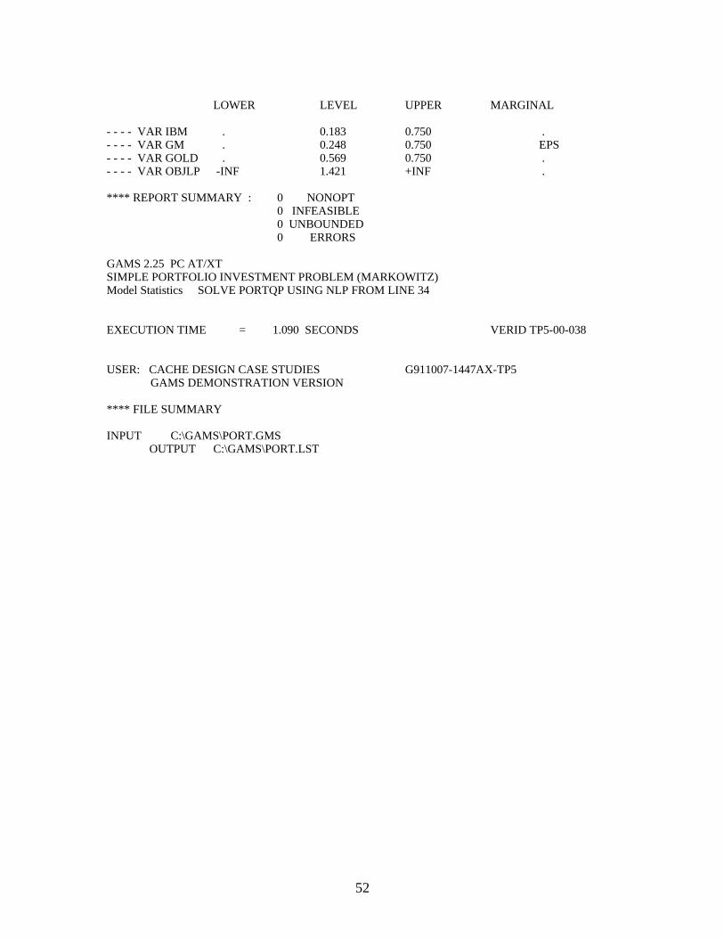
52
LOWER LEVEL UPPER MARGINAL - - - - VAR IBM . 0.183 0.750 . - - - - VAR GM . 0.248 0.750 EPS - - - - VAR GOLD . 0.569 0.750 . - - - - VAR OBJLP -INF 1.421 +INF . **** REPORT SUMMARY : 0 NONOPT 0 INFEASIBLE 0 UNBOUNDED 0 ERRORS GAMS 2.25 PC AT/XT SIMPLE PORTFOLIO INVESTMENT PROBLEM (MARKOWITZ) Model Statistics SOLVE PORTQP USING NLP FROM LINE 34 EXECUTION TIME = 1.090 SECONDS VERID TP5-00-038 USER: CACHE DESIGN CASE STUDIES G911007-1447AX-TP5 GAMS DEMONSTRATION VERSION **** FILE SUMMARY INPUT C:\GAMS\PORT.GMS
OUTPUT C:\GAMS\PORT.LST
53
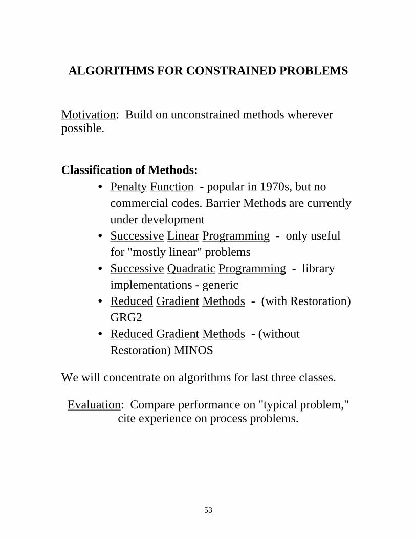
ALGORITHMS FOR CONSTRAINED PROBLEMS
Motivation: Build on unconstrained methods wherever possible. Classification of Methods:
• Penalty Function - popular in 1970s, but no commercial codes. Barrier Methods are currently under development
• Successive Linear Programming - only useful for "mostly linear" problems
• Successive Quadratic Programming - library implementations - generic
• Reduced Gradient Methods - (with Restoration) GRG2
• Reduced Gradient Methods - (without Restoration) MINOS
We will concentrate on algorithms for last three classes.
Evaluation: Compare performance on "typical problem," cite experience on process problems.
54
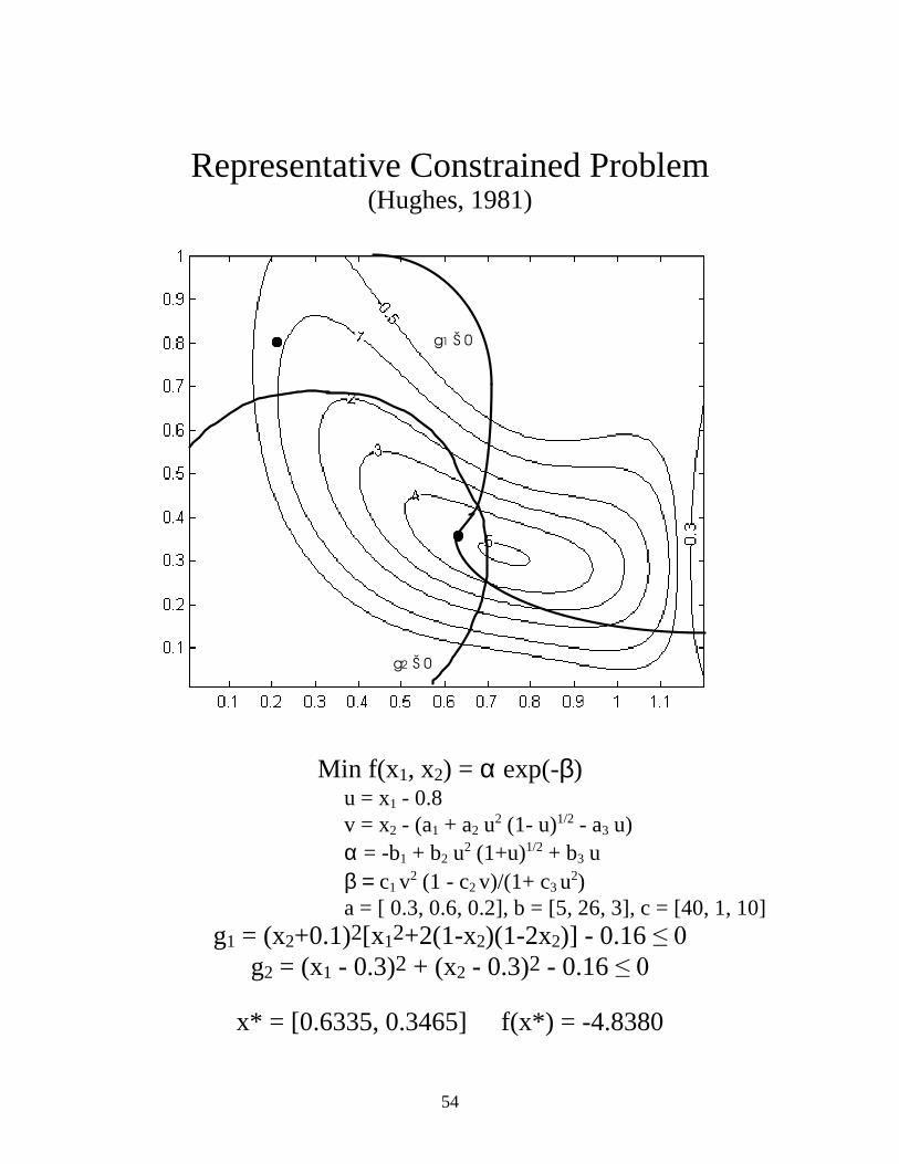
Representative Constrained Problem
(Hughes, 1981)
g1 Š 0
g2 Š 0
Min f(x1, x2) = α exp(-β) u = x1 - 0.8 v = x2 - (a1 + a2 u2 (1- u)1/2 - a3 u) α = -b1 + b2 u2 (1+u)1/2 + b3 u β = c1 v2 (1 - c2 v)/(1+ c3 u2) a = [ 0.3, 0.6, 0.2], b = [5, 26, 3], c = [40, 1, 10]
g1 = (x2+0.1)2[x12+2(1-x2)(1-2x2)] - 0.16 ��� g2 = (x1 - 0.3)2 + (x2 - 0.3)2 - 0.16 ���
x* = [0.6335, 0.3465] f(x*) = -4.8380
55
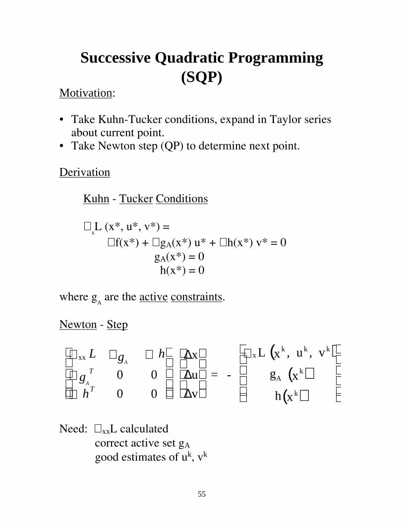
Successive Quadratic Programming (SQP)
Motivation: • Take Kuhn-Tucker conditions, expand in Taylor series
about current point. • Take Newton step (QP) to determine next point. Derivation
Kuhn - Tucker Conditions ∇
xL (x*, u*, v*) =
∇ f(x*) + ∇ gA(x*) u* + ∇ h(x*) v* = 0 gA(x*) = 0 h(x*) = 0
where gA are the active constraints.
Newton - Step
xx∇ LA
g∇ ∇ h
Ag∇ T 0 0
∇ hT 0 0
∆x
∆u
∆v
= -
x∇ L kx , ku , kv( )Ag kx( )h kx( )
Need: ∇ xxL calculated
correct active set gA good estimates of uk, vk
56
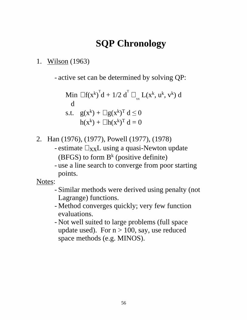
SQP Chronology
1. Wilson (1963)
- active set can be determined by solving QP: Min ∇ f(xk)
Td + 1/2 d
T ∇
xx L(xk, uk, vk) d
d s.t. g(xk) + ∇ g(xk)T d ��� h(xk) + ∇ h(xk)T d = 0
2. Han (1976), (1977), Powell (1977), (1978) - estimate ∇ xxL using a quasi-Newton update (BFGS) to form Bk (positive definite) - use a line search to converge from poor starting points.
Notes: - Similar methods were derived using penalty (not Lagrange) functions. - Method converges quickly; very few function evaluations. - Not well suited to large problems (full space update used). For n > 100, say, use reduced space methods (e.g. MINOS).
57
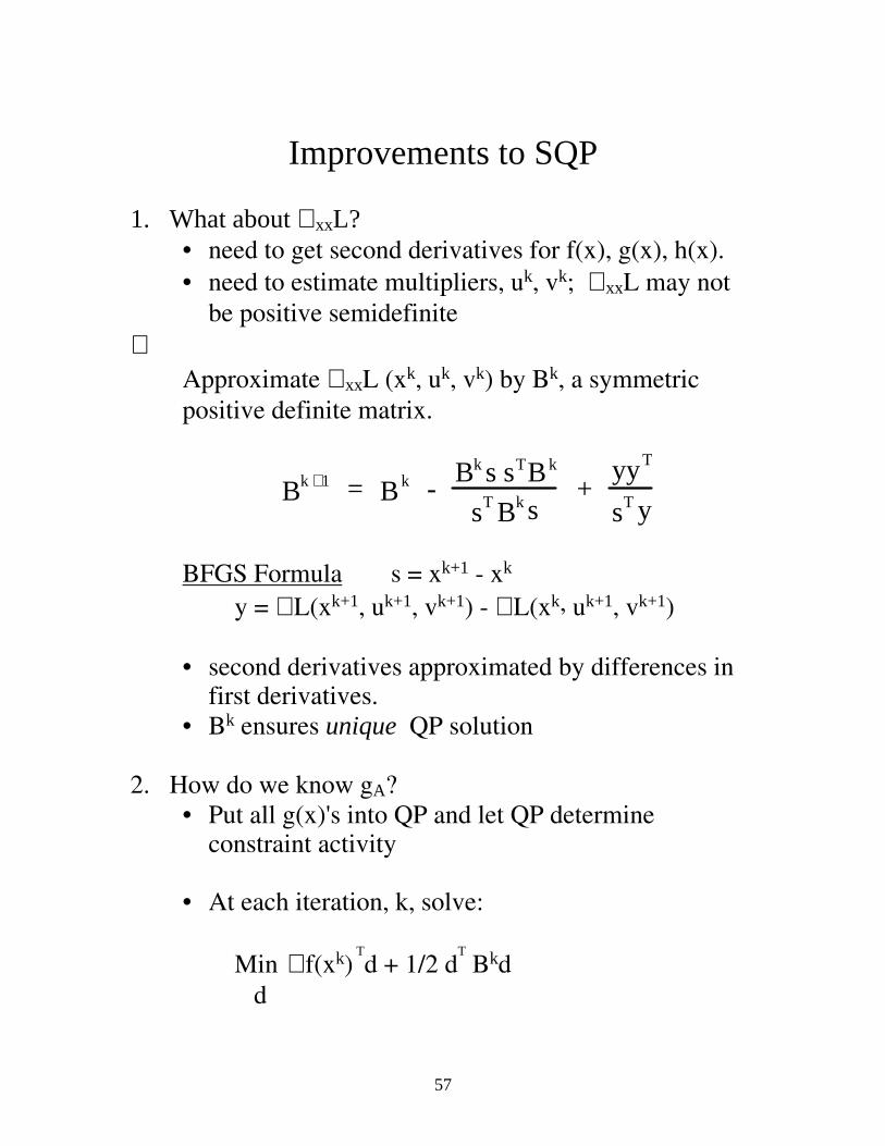
Improvements to SQP 1. What about ∇ xxL?
• need to get second derivatives for f(x), g(x), h(x). • need to estimate multipliers, uk, vk; ∇ xxL may not
be positive semidefinite ⇒
Approximate ∇ xxL (xk, uk, vk) by Bk, a symmetric positive definite matrix.
k +1B = kB - kB Ts s kB
Ts kB s +
TyyTs y
BFGS Formula s = xk+1 - xk y = ∇ L(xk+1, uk+1, vk+1) - ∇ L(xk, uk+1, vk+1) • second derivatives approximated by differences in
first derivatives. • Bk ensures unique QP solution
2. How do we know gA? • Put all g(x)'s into QP and let QP determine
constraint activity • At each iteration, k, solve: Min ∇ f(xk)
Td + 1/2 d
T Bkd
d
58
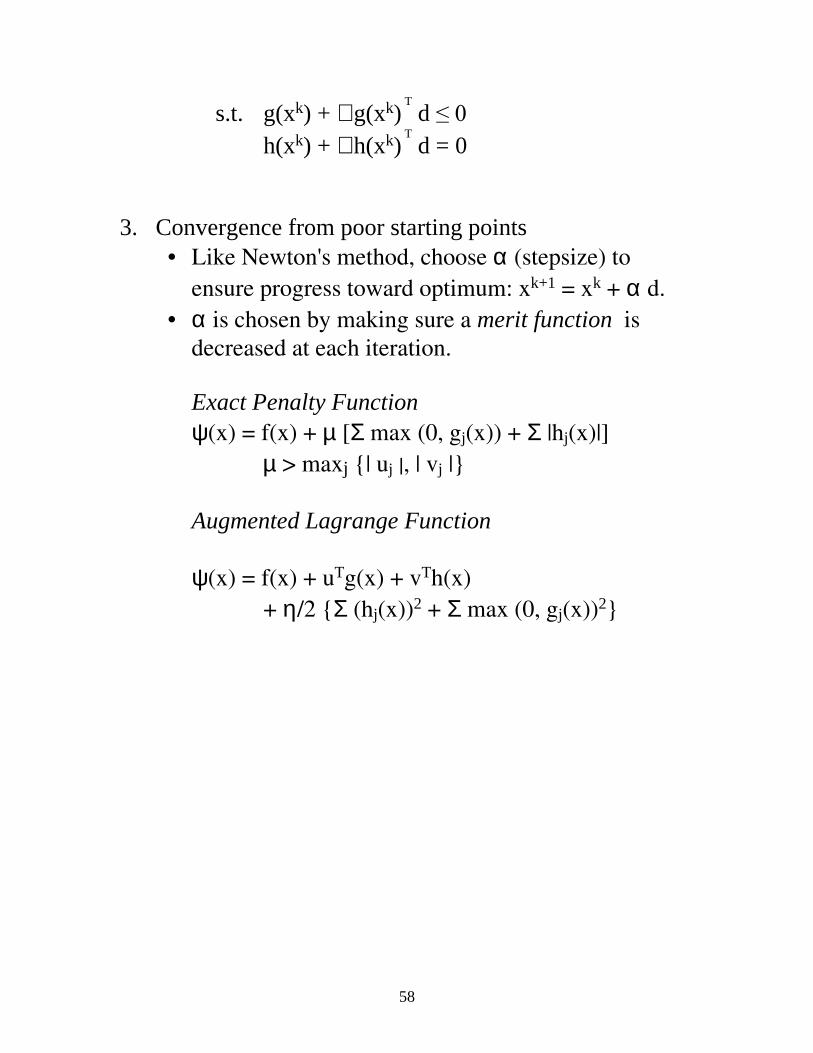
s.t. g(xk) + ∇ g(xk) T d ���
h(xk) + ∇ h(xk) T d = 0
3. Convergence from poor starting points
• Like Newton's method, choose α (stepsize) to ensure progress toward optimum: xk+1 = xk + α d.
• α is chosen by making sure a merit function is decreased at each iteration.
Exact Penalty Function ψ(x) = f(x) + µ [Σ max (0, gj(x)) + Σ |hj(x)|] µ > maxj {| uj |, | vj |} Augmented Lagrange Function ψ(x) = f(x) + uTg(x) + vTh(x) + η/2 {Σ (hj(x))2 + Σ max (0, gj(x))2}
59
Newton-Like Properties
Fast (Local) Convergence
B = ∇ xxL Quadratic ∇ xxL is p.d and B is Q-N 1 step Superlinear B is Q-N update, ∇ xxL not p.d 2 step Superlinear
Can enforce Global Convergence
Ensure decrease of merit function by taking α ��� Trust regions provide a stronger guarantee of global convergence - but harder to implement.
60
Basic SQP Algorithm
0. Guess x0, Set B0 = I (Identity). Evaluate f(x0), g(x0) and h(x0). 1. At xk, evaluate ∇ f(xk), ∇ g(xk), ∇ h(xk). 2. If k > 0, update Bk using the BFGS Formula. 3. Solve: Mind ∇ f(xk)Td + 1/2 dTBkd s.t. g(xk) + ∇ g(xk)Td ≤ 0 h(xk) + ∇ h(xk)Td = 0 If Kuhn-Tucker error is less than tolerance: e.g., ∇ LTd ≤ ∇ fTd + Σ ujgj + Σvjhj ≤ ε STOP, else go to 4.
4. Find α so that 0 < α ≤ 1 and ψ(xk + αd) < ψ(xk) sufficiently (Each trial requires evaluation of f(x), g(x) and h(x)). 5. xk+1 = xk + αd. Set k = k + 1 Go to 1.
61
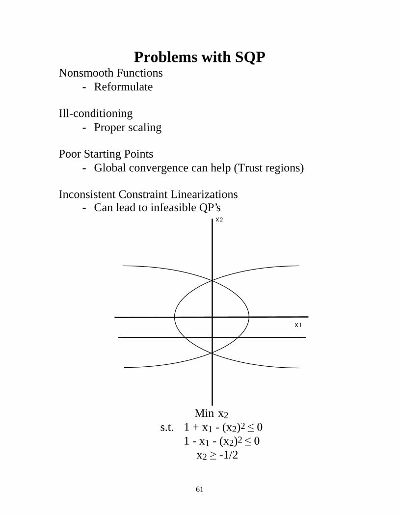
Problems with SQP Nonsmooth Functions
- Reformulate
Ill-conditioning - Proper scaling
Poor Starting Points - Global convergence can help (Trust regions)
Inconsistent Constraint Linearizations - Can lead to infeasible QP’s
x2
x1
Min x2
s.t. 1 + x1 - (x2)2 ��� 1 - x1 - (x2)2 ���
x2 ��-1/2
62
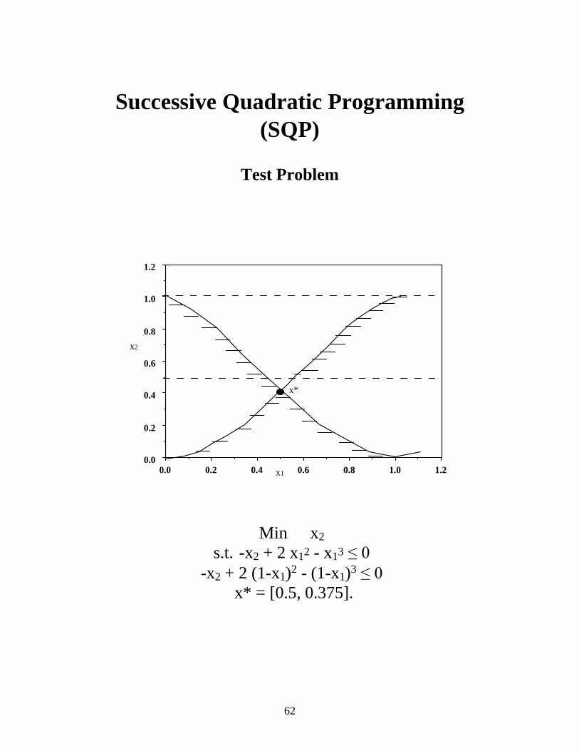
Successive Quadratic Programming
(SQP)
Test Problem
1.21.00.80.60.40.20.00.0
0.2
0.4
0.6
0.8
1.0
1.2
x1
x2
x*
Min x2 s.t. -x2 + 2 x12 - x13 ���
-x2 + 2 (1-x1)2 - (1-x1)3 ��� x* = [0.5, 0.375].
63
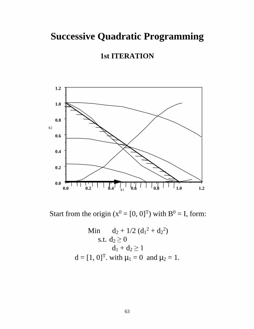
Successive Quadratic Programming
1st ITERATION
1.21.00.80.60.40.20.00.0
0.2
0.4
0.6
0.8
1.0
1.2
x1
x2
Start from the origin (x0 = [0, 0]T) with B0 = I, form:
Min d2 + 1/2 (d12 + d2
2) s.t. d2 ���
d1 + d2 ��� d = [1, 0]T. with µ1 = 0 and µ2 = 1.
64
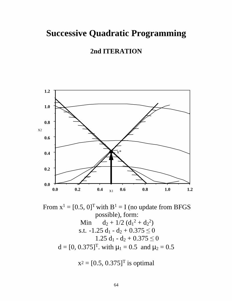
Successive Quadratic Programming
2nd ITERATION
1.21.00.80.60.40.20.00.0
0.2
0.4
0.6
0.8
1.0
1.2
x1
x2
x*
From x1 = [0.5, 0]T with B1 = I (no update from BFGS possible), form:
Min d2 + 1/2 (d12 + d2
2) s.t. -1.25 d1 - d2 + 0.375 ���
1.25 d1 - d2 + 0.375 ��� d = [0, 0.375]T. with µ1 = 0.5 and µ2 = 0.5
x2 = [0.5, 0.375]T is optimal
65
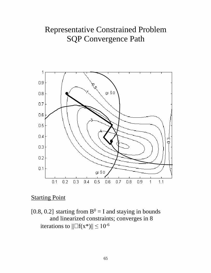
Representative Constrained Problem SQP Convergence Path
g1 Š 0
g2 Š 0
Starting Point [0.8, 0.2] starting from B0 = I and staying in bounds and linearized constraints; converges in 8 iterations to ||∇ f(x*)|| ����-6
66
Reduced Gradient Method with Restoration (GRG)
Motivation: • Decide which constraints are active or inactive, partition
variables as dependent and independent. • Solve unconstrained problem in space of independent
variables. Derivation: Min f(x) s.t. g(x) + s = 0 (add slack variable) c(x) = 0 l ��[���X��V���� ⇒ Min f(z) h(z) = 0 a ��]���E
Let zT = [zIT zD
T] to optimize wrt zI with h(zI, zD) = 0 we need a constrained derivative or reduced gradient wrt zI. Dependent variables are zD ∈ Rm
Strictly speaking, the z variables are partitioned into:
zD - dependent or basic variables
zB - bounded or nonbasic variables
zI - independent or superbasic variables
Note the analogy to linear programming. In fact, superbasic variables are required only if the problem is nonlinear.
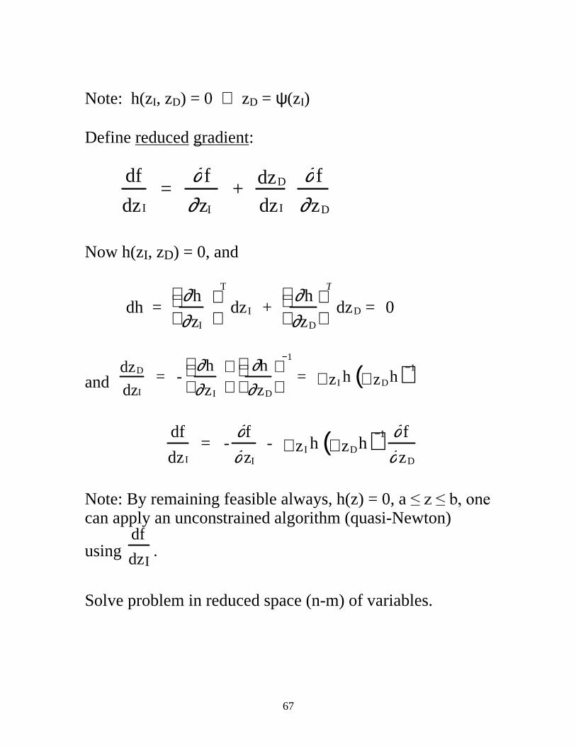
67
Note: h(zI, zD) = 0 ⇒ zD = ψ(zI) Define reduced gradient:
df
Idz =
∂f
I∂z + Ddz
Idz
∂f
D∂z
Now h(zI, zD) = 0, and
dh = ∂h
I∂z
T
Idz + ∂h
D∂z
T
Ddz = 0
and Ddz
Idz = -
∂h
I∂z
∂h
D∂z
−1
= I∇ z h D∇ z h( )−1
df
Idz = -
∂f
I∂z - I∇ z h D∇ z h( )−1 ∂f
D∂z
Note: By remaining feasible always, h(z) = 0, a ��]���E��RQH�can apply an unconstrained algorithm (quasi-Newton)
using df
Idz .
Solve problem in reduced space (n-m) of variables.
68
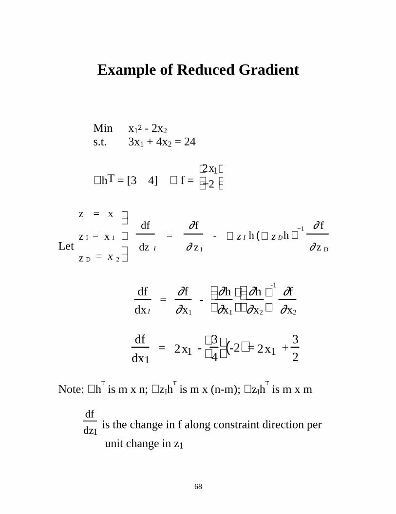
Example of Reduced Gradient
Min x12 - 2x2 s.t. 3x1 + 4x2 = 24
∇ hT = [3 4] ∇ f = 12x
−2
Let
z = x
Iz = 1x
Dz = 2x
df
Idz =
∂ f
I∂ z - I∇ z h D∇ z h( )
−1 ∂ f
D∂ z
df
Idx =
∂f
1∂x -
∂h
1∂x
∂h
2∂x
-1 ∂f
2∂x
df
1dx = 1 2x -
3
4
-2( ) = 1 2x +
3
2
Note: ∇ h
T is m x n; ∇ zIh
T is m x (n-m); ∇ zIh
T is m x m
df
1dz is the change in f along constraint direction per
unit change in z1
69
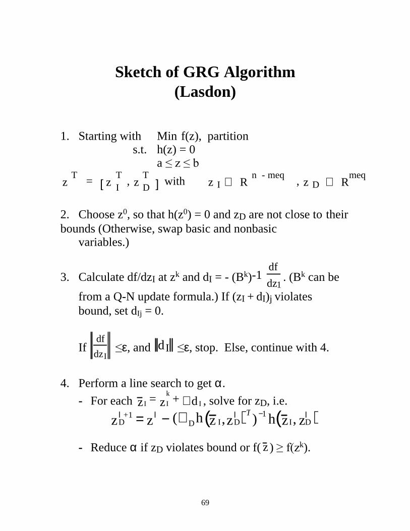
Sketch of GRG Algorithm (Lasdon)
1. Starting with Min f(z), partition s.t. h(z) = 0 a ��]���E
Tz =
IT
z ,DT
z[ ] with Izn - meq
∈ R , Dzmeq
∈ R 2. Choose z0, so that h(z0) = 0 and zD are not close to their bounds (Otherwise, swap basic and nonbasic variables.)
3. Calculate df/dzI at zk and dI = - (Bk)-1 df
1dz . (Bk can be
from a Q-N update formula.) If (zI + dI)j violates bound, set dIj = 0.
If df
Idz �ε, and Id �ε, stop. Else, continue with 4.
4. Perform a line search to get α.
- For each Iz = I
k
z + I∝ d , solve for zD, i.e.
��DO +1z = Oz − (∇ Dh Iz , D
Oz( )T)−1 h Iz , D
Oz( )
- Reduce α if zD violates bound or f( z ) ��I�]k).
70
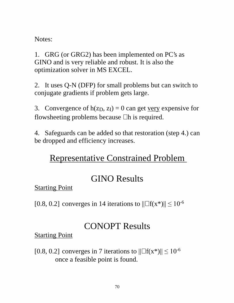
Notes: 1. GRG (or GRG2) has been implemented on PC’s as GINO and is very reliable and robust. It is also the optimization solver in MS EXCEL. 2. It uses Q-N (DFP) for small problems but can switch to conjugate gradients if problem gets large. 3. Convergence of h(zD, zI) = 0 can get very expensive for flowsheeting problems because ∇ h is required. 4. Safeguards can be added so that restoration (step 4.) can be dropped and efficiency increases.
Representative Constrained Problem
GINO Results Starting Point [0.8, 0.2] converges in 14 iterations to ||∇ f(x*)|| ����-6
CONOPT Results Starting Point [0.8, 0.2] converges in 7 iterations to ||∇ f(x*)|| ����-6
once a feasible point is found.
71
Reduced Gradient Method without Restoration (MINOS/Augmented)
Motivation: Efficient algorithms are available that solve linearly constrained optimization problems (MINOS): Min f(x) s.t. Ax ��E Cx = d Extend to nonlinear problems, through successive linearization. Strategy: (Robinson, Murtagh & Saunders) 1. Partition variables into basic (dependent) variables, zB, nonbasic variables (independent variables at bounds), zN, and superbasic variables, (independent variables between bounds), zS. 2. Linearize constraints about starting point, z ⇒ Dz = c.
3. Let ψ = f (z) + vTh (z) + β (hTh) (Augmented Lagrange) and solve linearly constrained problem:
Min ψ (z) s.t. Dz = c, a ��]���E using reduced gradients (as in GRG) to get z#. 4. Linearize constraints about z# and go to 3. 5. Algorithm terminates when no movement occurs between steps 3) and 4).
72
Notes: 1. MINOS has been implemented very efficiently to take care of linearity. It becomes LP Simplex method if problem is totally linear. Also, very efficient matrix routines. 2. Although no restoration takes place, constraint
nonlinearities are reflected in ψ (z) during step 3). Hence MINOS is more efficient than GRG. 3. Major iterations (steps 3) - 4)) converge at a quadratic rate.
Representative Constrained Problem MINOS Results
Starting Point [0.8, 0.2] converges in 4 major iterations, 11 function calls to ||∇ f(x*)|| ����-6
73
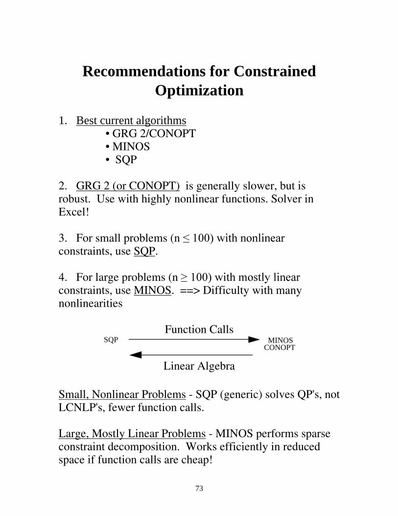
Recommendations for Constrained Optimization
1. Best current algorithms
• GRG 2/CONOPT • MINOS • SQP
2. GRG 2 (or CONOPT) is generally slower, but is robust. Use with highly nonlinear functions. Solver in Excel! 3. For small problems (n �������ZLWK�QRQOLQHDU�constraints, use SQP. 4. For large problems (n �������ZLWK�PRVWO\�OLQHDU�constraints, use MINOS. ==> Difficulty with many nonlinearities
Function Calls
SQP MINOSCONOPT
Linear Algebra
Small, Nonlinear Problems - SQP (generic) solves QP's, not LCNLP's, fewer function calls. Large, Mostly Linear Problems - MINOS performs sparse constraint decomposition. Works efficiently in reduced space if function calls are cheap!
74
Available Software for Constrained Optimization
NaG Routines E04MFF - LP problem (dense) E04NCF - Convex QP problem or linearly-constrained linear least-squares problem (dense) SQP Routines E04UCF - Minimum, function of several variables, sequential QP method, nonlinear constraints, using function values and optionally first derivatives (forward communication, comprehensive) E04UFF - Minimum, function of several variables, sequential QP method, nonlinear constraints, using function values and optionally first derivatives (reverse communication, comprehensive) E04UNF - Minimum of a sum of squares, nonlinear constraints, sequential QP method, using function values and optionally first derivatives (comprehensive)
GAMS Programs CONOPT - Generalized Reduced Gradient method with restoration MINOS - Generalized Reduced Gradient method without restoration A new student version of GAMS is now available from the CACHE office. The cost for this package including Process Design Case Students, GAMS: A User’s Guide, and GAMS - The Solver Manuals, and a CD-ROM is $65 per CACHE supporting departments, and $100 per non-CACHE supporting departments and individuals. To order please complete standard order form and fax or mail to CACHE Corporation. More information can be found on http://www.che.utexas.edu/cache/gams.html
MS Excel Solver uses Generalized Reduced Gradient method with restoration
75
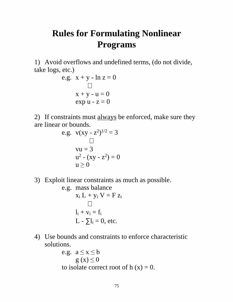
Rules for Formulating Nonlinear Programs
1) Avoid overflows and undefined terms, (do not divide, take logs, etc.)
e.g. x + y - ln z = 0 ⇓ x + y - u = 0 exp u - z = 0
2) If constraints must always be enforced, make sure they are linear or bounds. e.g. v(xy - z2)1/2 = 3 ⇓ vu = 3 u2 - (xy - z2) = 0 u ��� 3) Exploit linear constraints as much as possible.
e.g. mass balance xi L + yi V = F zi ⇓ li + vi = fi L - ∑li = 0, etc.
4) Use bounds and constraints to enforce characteristic solutions.
e.g. a ��[���E g (x) ��� to isolate correct root of h (x) = 0.
76
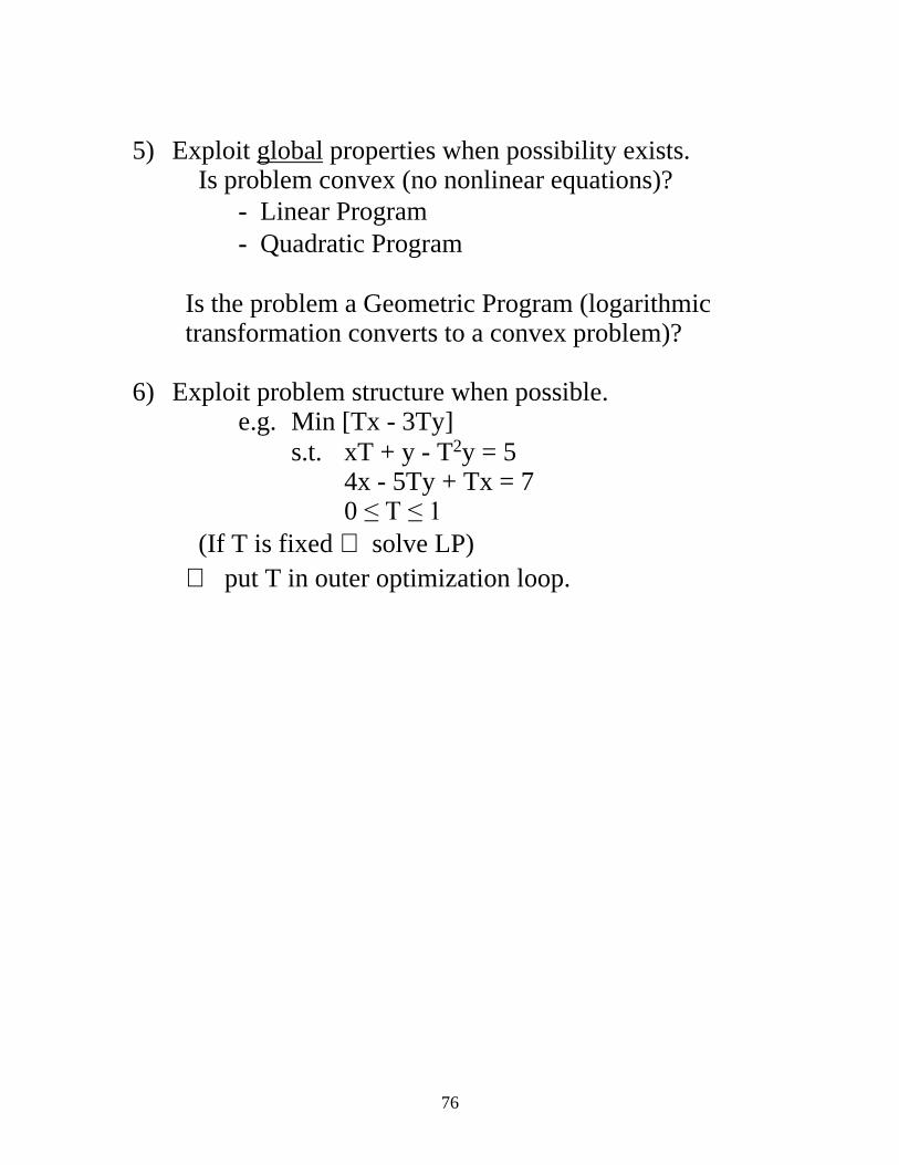
5) Exploit global properties when possibility exists.
Is problem convex (no nonlinear equations)? - Linear Program - Quadratic Program Is the problem a Geometric Program (logarithmic transformation converts to a convex problem)?
6) Exploit problem structure when possible. e.g. Min [Tx - 3Ty] s.t. xT + y - T2y = 5 4x - 5Ty + Tx = 7 0 ��7���� (If T is fixed ⇒ solve LP) ⇒ put T in outer optimization loop.
77
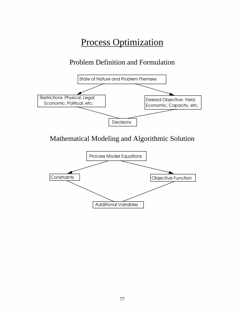
Process Optimization
Problem Definition and Formulation
State of Nature and Problem Premises
Restrictions: Physical, Legal
Economic, Political, etc.Desired Objective: Yield,
Economic, Capacity, etc.
Decisions
Mathematical Modeling and Algorithmic Solution
Process Model Equations
Constraints Objective Function
Additional Variables
78
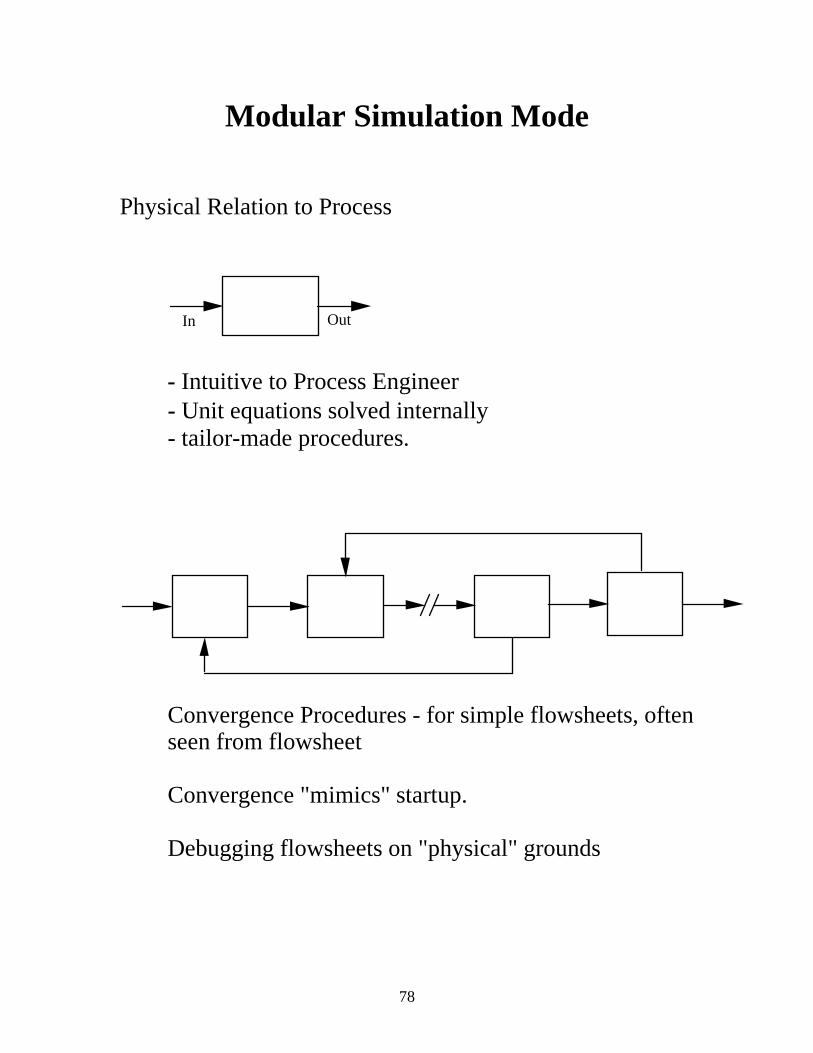
Modular Simulation Mode
Physical Relation to Process
In Out
- Intuitive to Process Engineer - Unit equations solved internally - tailor-made procedures.
Convergence Procedures - for simple flowsheets, often seen from flowsheet Convergence "mimics" startup. Debugging flowsheets on "physical" grounds
79
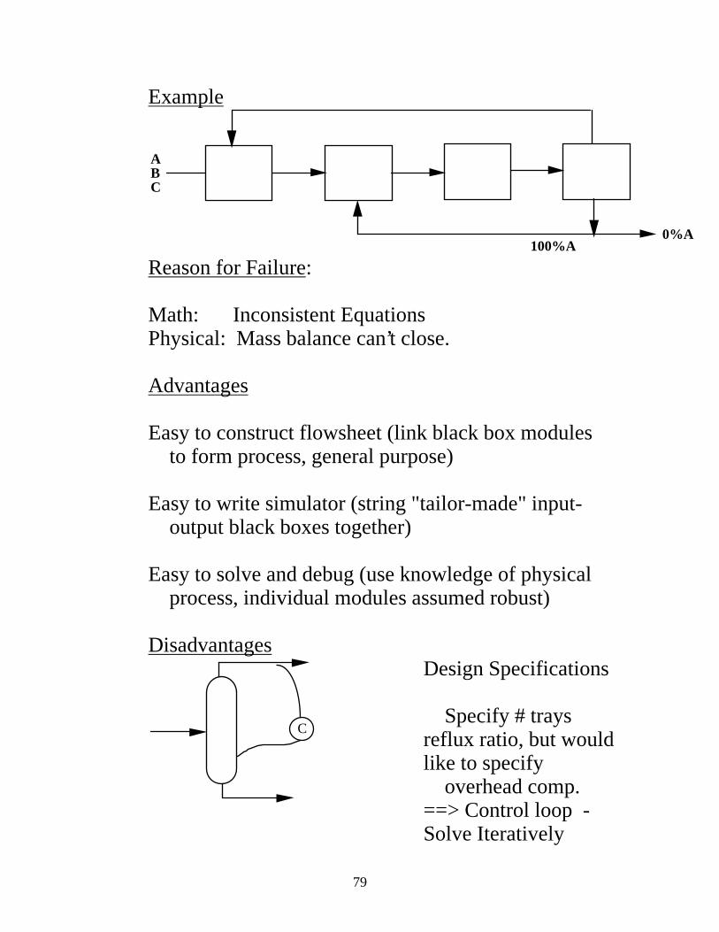
Example
ABC
100%A0%A
Reason for Failure: Math: Inconsistent Equations Physical: Mass balance can’t close. Advantages Easy to construct flowsheet (link black box modules to form process, general purpose) Easy to write simulator (string "tailor-made" input- output black boxes together) Easy to solve and debug (use knowledge of physical process, individual modules assumed robust) Disadvantages
C
Design Specifications Specify # trays reflux ratio, but would like to specify overhead comp. ==> Control loop -Solve Iteratively
80
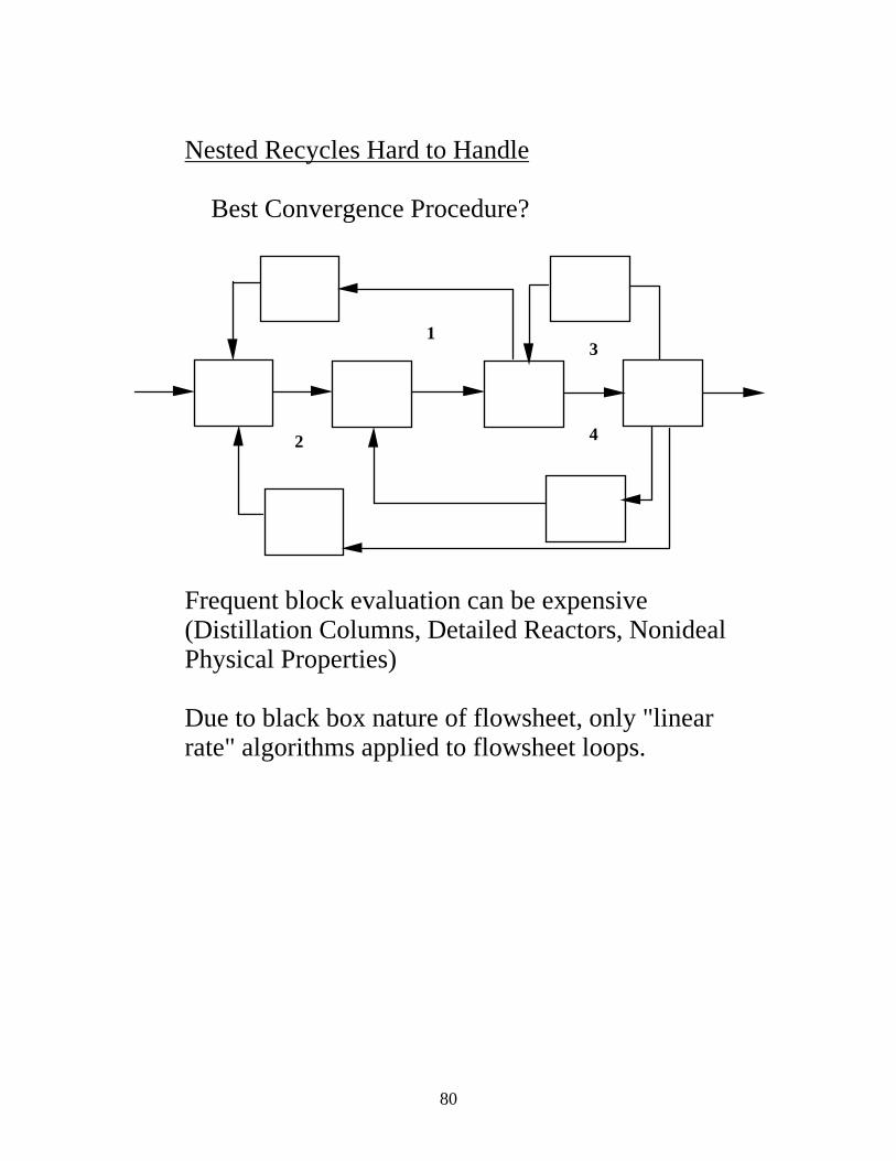
Nested Recycles Hard to Handle Best Convergence Procedure?
13
2 4
Frequent block evaluation can be expensive (Distillation Columns, Detailed Reactors, Nonideal Physical Properties) Due to black box nature of flowsheet, only "linear rate" algorithms applied to flowsheet loops.
81
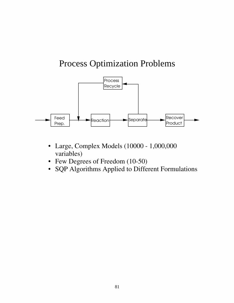
Process Optimization Problems
Feed
Prep.Reaction Separate
Recover
Product
Process
Recycle
• Large, Complex Models (10000 - 1,000,000
variables) • Few Degrees of Freedom (10-50) • SQP Algorithms Applied to Different Formulations
82
Process Optimization Chronology
Before 1980 - Process optimization was not used at all in industry (Blau, Westerberg)
• methods to expensive and unreliable
direct search methods noisy function values and gradient calculations
• uncertainty in problem definition • penalty for failure greater than incentive for
improvement
Since 1980 - widespread use of optimization in design, operations and control
• powerful NLP algorithms (SQP)
- allows simultaneous model solution and optimization
- direct handling of constraints • more flexible problem formulations and
specifications
Literature Summary in Process Optimization
83
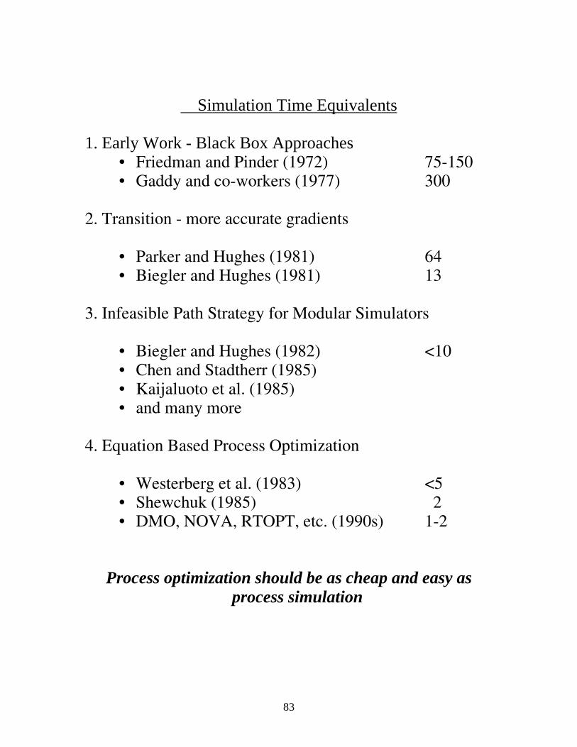
Simulation Time Equivalents
1. Early Work - Black Box Approaches
• Friedman and Pinder (1972) 75-150 • Gaddy and co-workers (1977) 300
2. Transition - more accurate gradients
• Parker and Hughes (1981) 64 • Biegler and Hughes (1981) 13
3. Infeasible Path Strategy for Modular Simulators
• Biegler and Hughes (1982) <10 • Chen and Stadtherr (1985) • Kaijaluoto et al. (1985) • and many more
4. Equation Based Process Optimization
• Westerberg et al. (1983) <5 • Shewchuk (1985) 2 • DMO, NOVA, RTOPT, etc. (1990s) 1-2
Process optimization should be as cheap and easy as process simulation
84
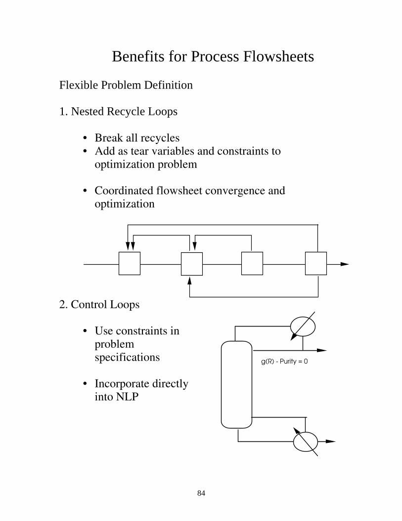
Benefits for Process Flowsheets
Flexible Problem Definition 1. Nested Recycle Loops
• Break all recycles • Add as tear variables and constraints to
optimization problem • Coordinated flowsheet convergence and
optimization
2. Control Loops
• Use constraints in problem specifications
• Incorporate directly
into NLP
g(R) - Purity = 0
85
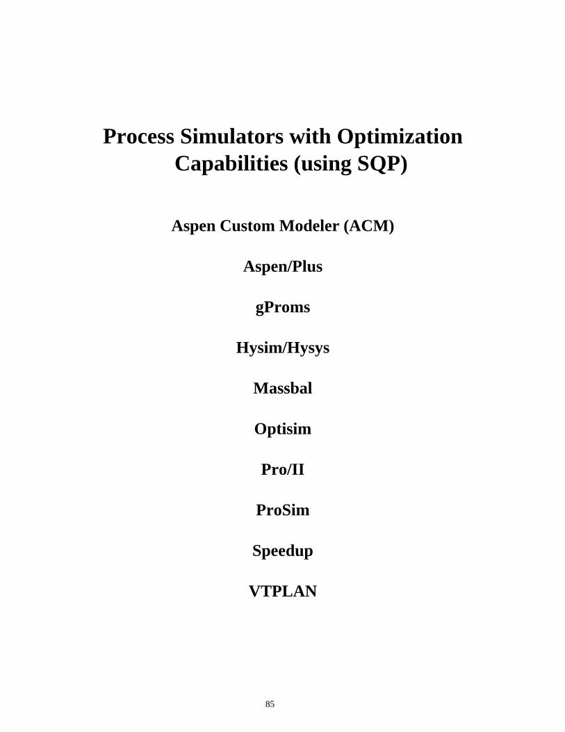
Process Simulators with Optimization Capabilities (using SQP)
Aspen Custom Modeler (ACM)
Aspen/Plus
gProms
Hysim/Hysys
Massbal
Optisim
Pro/II
ProSim
Speedup
VTPLAN
86
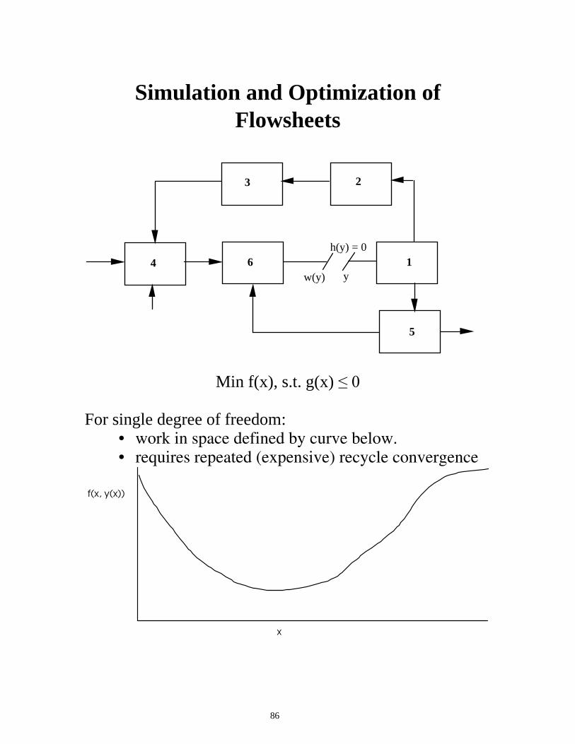
Simulation and Optimization of Flowsheets
4
3 2
1
5
6h(y) = 0
w(y) y
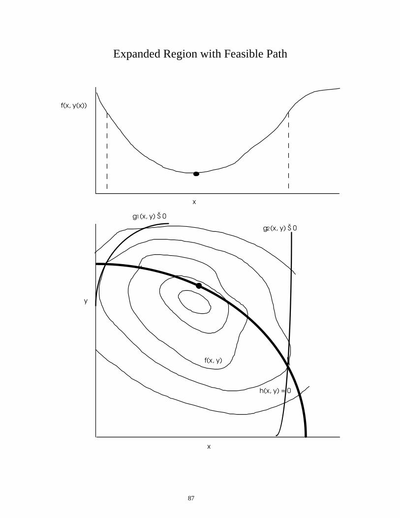
Min f(x), s.t. g(x) ��� For single degree of freedom:
• work in space defined by curve below. • requires repeated (expensive) recycle convergence
f(x, y(x))
x
87
Expanded Region with Feasible Path
f(x, y(x))
x
y
x
h(x, y) = 0
g1(x, y) Š 0
g2(x, y) Š 0
f(x, y)
88
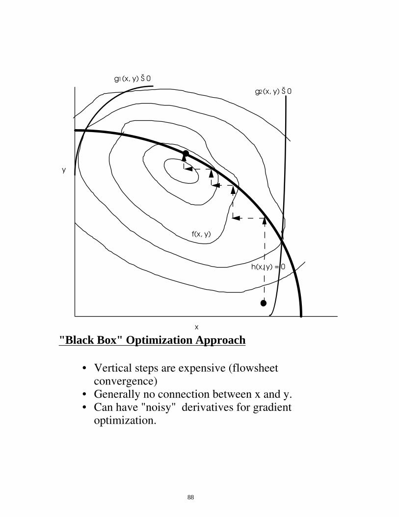
y
x
h(x, y) = 0
g1(x, y) Š 0
g2(x, y) Š 0
f(x, y)
"Black Box" Optimization Approach
• Vertical steps are expensive (flowsheet
convergence) • Generally no connection between x and y. • Can have "noisy" derivatives for gradient
optimization.
89
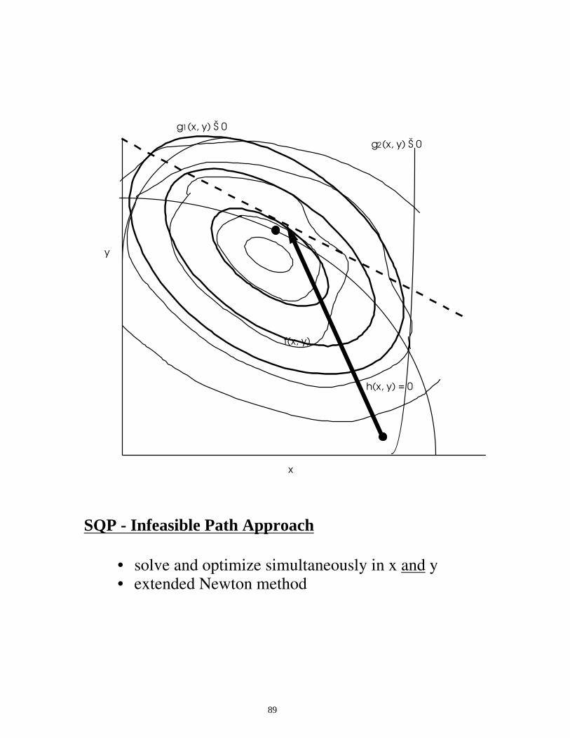
y
x
h(x, y) = 0
g1(x, y) Š 0
g2(x, y) Š 0
f(x, y)
SQP - Infeasible Path Approach
• solve and optimize simultaneously in x and y • extended Newton method
90
Optimization Capability for Modular Simulators
(FLOWTRAN, Aspen/Plus, Pro/II, HySys)
Architecture
- Replace convergence with optimization block - Some in-line FORTRAN needed - easy to do - Executive, preprocessor, modules intact.
Examples
- Chosen to demonstrate performance and capability.
1. Single Unit and Acyclic Optimization - Distillation columns & sequences
2. "Conventional" Process Optimization - NH3 synthesis - Monochlorobenzene process
3. Complicated Recycles & Control Loops - Cavett problem - Variations of above
91
SCOPT-Flowtran Optimization Option
User Interface for Flowtran 1. Start with working simulation 2. Formulate optimization problem 3. Define functions with in-line FORTRAN 4. Define variables with PUT statements 5. Replace control loops if desired (see next page) 6. Replace convergence block with optimization block
- Set optimization parameters (or place at end)
Architecture of SCOPT
- NEW BLOCK, added to object code - Executive, modules remain intact.
92
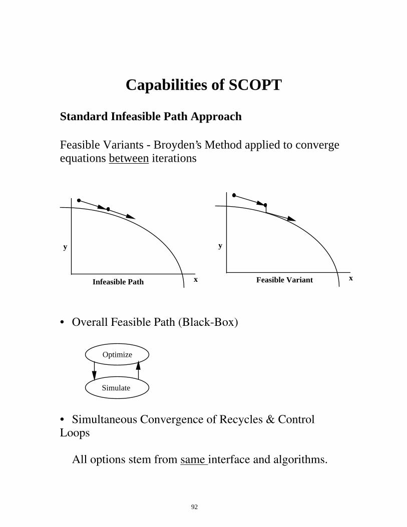
Capabilities of SCOPT Standard Infeasible Path Approach Feasible Variants - Broyden’s Method applied to converge equations between iterations
y
x
y
xInfeasible Path Feasible Variant • Overall Feasible Path (Black-Box)
Optimize
Simulate
• Simultaneous Convergence of Recycles & Control Loops All options stem from same interface and algorithms.
93
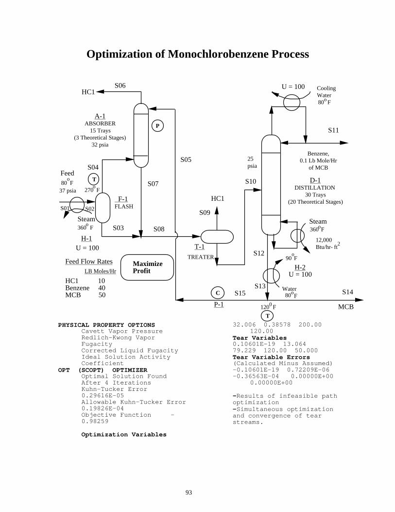
Optimization of Monochlorobenzene Process
S06HC1
A-1ABSORBER
15 Trays(3 Theoretical Stages)
32 psia
P
S04Feed80
oF
37 psia
T
270o
F
S01 S02
Steam360
oF
H-1U = 100
MaximizeProfit
Feed Flow RatesLB Moles/Hr
HC1 10Benzene 40MCB 50
S07
S08
S05
S09
HC1
T-1
TREATER
F-1FLASH
S03
S10
25psia
S12
S13S15
P-1
C
1200 F
T
MCB
S14
U = 100 CoolingWater80o F
S11
Benzene,0.1 Lb Mole/Hr
of MCB
D-1DISTILLATION
30 Trays(20 Theoretical Stages)
Steam360oF
12,000Btu/hr- ft
2
90oF
H-2U = 100
Water80o
F
PHYSICAL PROPERTY OPTIONS
Cavett Vapor Pressure Redlich-Kwong Vapor Fugacity Corrected Liquid Fugacity Ideal Solution Activity Coefficient
OPT (SCOPT) OPTIMIZER Optimal Solution Found After 4 Iterations Kuhn-Tucker Error 0.29616E-05 Allowable Kuhn-Tucker Error 0.19826E-04 Objective Function -0.98259 Optimization Variables
32.006 0.38578 200.00 120.00 Tear Variables 0.10601E-19 13.064 79.229 120.00 50.000 Tear Variable Errors (Calculated Minus Assumed) -0.10601E-19 0.72209E-06 -0.36563E-04 0.00000E+00 0.00000E+00 -Results of infeasible path optimization -Simultaneous optimization and convergence of tear streams.
94
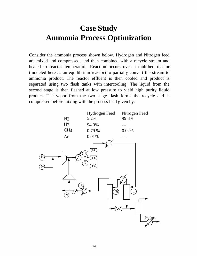
Case Study Ammonia Process Optimization
Consider the ammonia process shown below. Hydrogen and Nitrogen feed are mixed and compressed, and then combined with a recycle stream and heated to reactor temperature. Reaction occurs over a multibed reactor (modeled here as an equilibrium reactor) to partially convert the stream to ammonia product. The reactor effluent is then cooled and product is separated using two flash tanks with intercooling. The liquid from the second stage is then flashed at low pressure to yield high purity liquid product. The vapor from the two stage flash forms the recycle and is compressed before mixing with the process feed given by:
Hydrogen Feed Nitrogen Feed N2 5.2% 99.8% H2 94.0% --- CH4 0.79 % 0.02%
Ar 0.01% ---
H2
N2
Pr
Tr
To
T Tf fν
Product
95
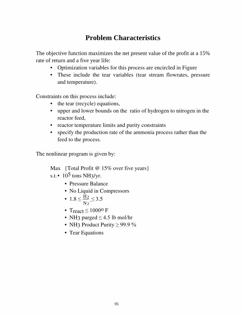
Problem Characteristics The objective function maximizes the net present value of the profit at a 15% rate of return and a five year life:
• Optimization variables for this process are encircled in Figure • These include the tear variables (tear stream flowrates, pressure
and temperature). Constraints on this process include:
• the tear (recycle) equations, • upper and lower bounds on the ratio of hydrogen to nitrogen in the
reactor feed, • reactor temperature limits and purity constraints • specify the production rate of the ammonia process rather than the
feed to the process. The nonlinear program is given by:
Max {Total Profit @ 15% over five years} s.t. • 105 tons NH3/yr.
• Pressure Balance • No Liquid in Compressors
• 1.8 �� 2H
2N ���.5
• Treact ������o F • NH3 purged ������OE�PRO�KU
• NH3 Product Purity ��������
• Tear Equations
96
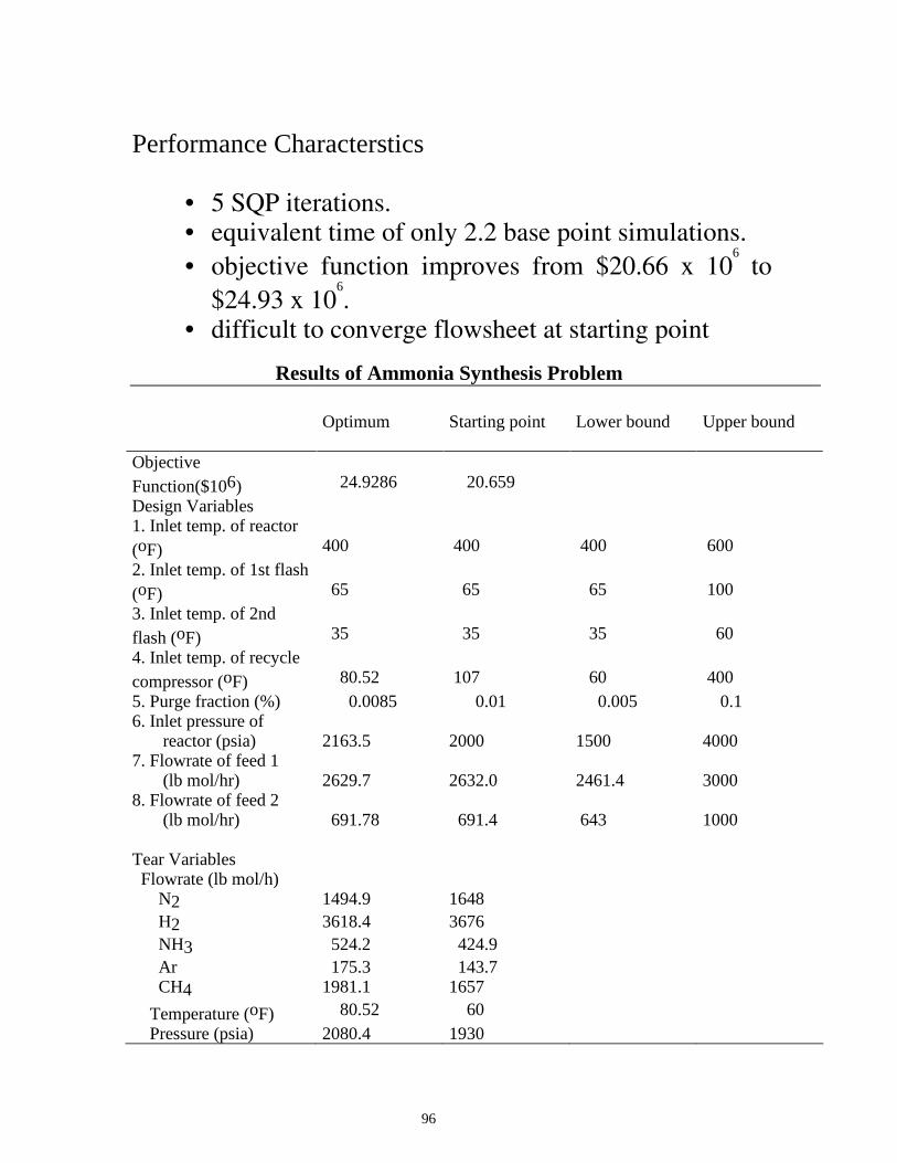
Performance Characterstics
• 5 SQP iterations. • equivalent time of only 2.2 base point simulations. • objective function improves from $20.66 x 10
6 to
$24.93 x 10⁶.
• difficult to converge flowsheet at starting point
Results of Ammonia Synthesis Problem Optimum Starting point
Lower bound
Upper bound
Objective Function($106)
24.9286
20.659
Design Variables 1. Inlet temp. of reactor (oF)
400
400
400
600
2. Inlet temp. of 1st flash (oF)
65
65
65
100
3. Inlet temp. of 2nd flash (oF)
35
35
35
60
4. Inlet temp. of recycle compressor (oF)
80.52
107
60
400
5. Purge fraction (%) 0.0085 0.01 0.005 0.1 6. Inlet pressure of reactor (psia)
2163.5
2000
1500
4000
7. Flowrate of feed 1 (lb mol/hr)
2629.7
2632.0
2461.4
3000
8. Flowrate of feed 2 (lb mol/hr)
691.78
691.4
643
1000
Tear Variables Flowrate (lb mol/h) N2 1494.9 1648 H2 3618.4 3676 NH3 524.2 424.9 Ar 175.3 143.7 CH4 1981.1 1657
Temperature (oF) 80.52 60 Pressure (psia) 2080.4 1930
97
How accurate should gradients be for Optimization?
Recognizing True Solution • KKT conditions and Reduced Gradients determine
the true solution • Derivative Errors will lead to wrong solutions being
recognized! Performance of Algorithms Constrained NLP algorithms are gradient based (SQP, Conopt, GRG2, MINOS, etc.) Global and Superlinear convergence theory assumes accurate gradients How accurate should derivatives be? Are exact derivatives needed?
98
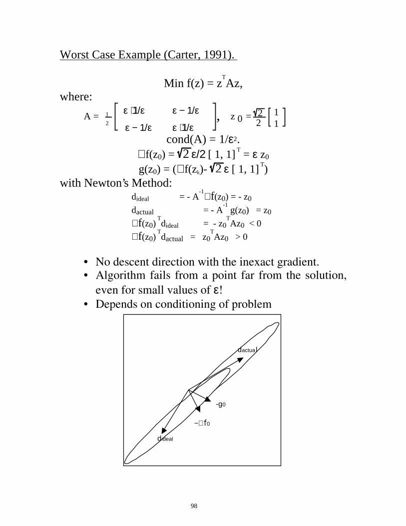
Worst Case Example (Carter, 1991).
Min f(z) = zTAz,
where:
A = 1
2
ε + 1/ε ε − 1/ε
ε − 1/ε ε + 1/ε, z 0 = 2
2 1
1
cond(A) = 1/ε2. ∇ f(z0) = 2 ε/2 [ 1, 1] T = ε z0 g(z0) = (∇ f(zk)- 2 ε [ 1, 1] T)
with Newton’s Method: dideal = - A
-1∇ f(z0) = - z0
dactual = - A-1 g(z0) = z0
∇ f(z0) T
dideal = - z0TAz0 < 0
∇ f(z0) T
dactual = z0TAz0 > 0
• No descent direction with the inexact gradient. • Algorithm fails from a point far from the solution,
even for small values of ε! • Depends on conditioning of problem
-g0
−∇ f0
dactua l
dideal
99
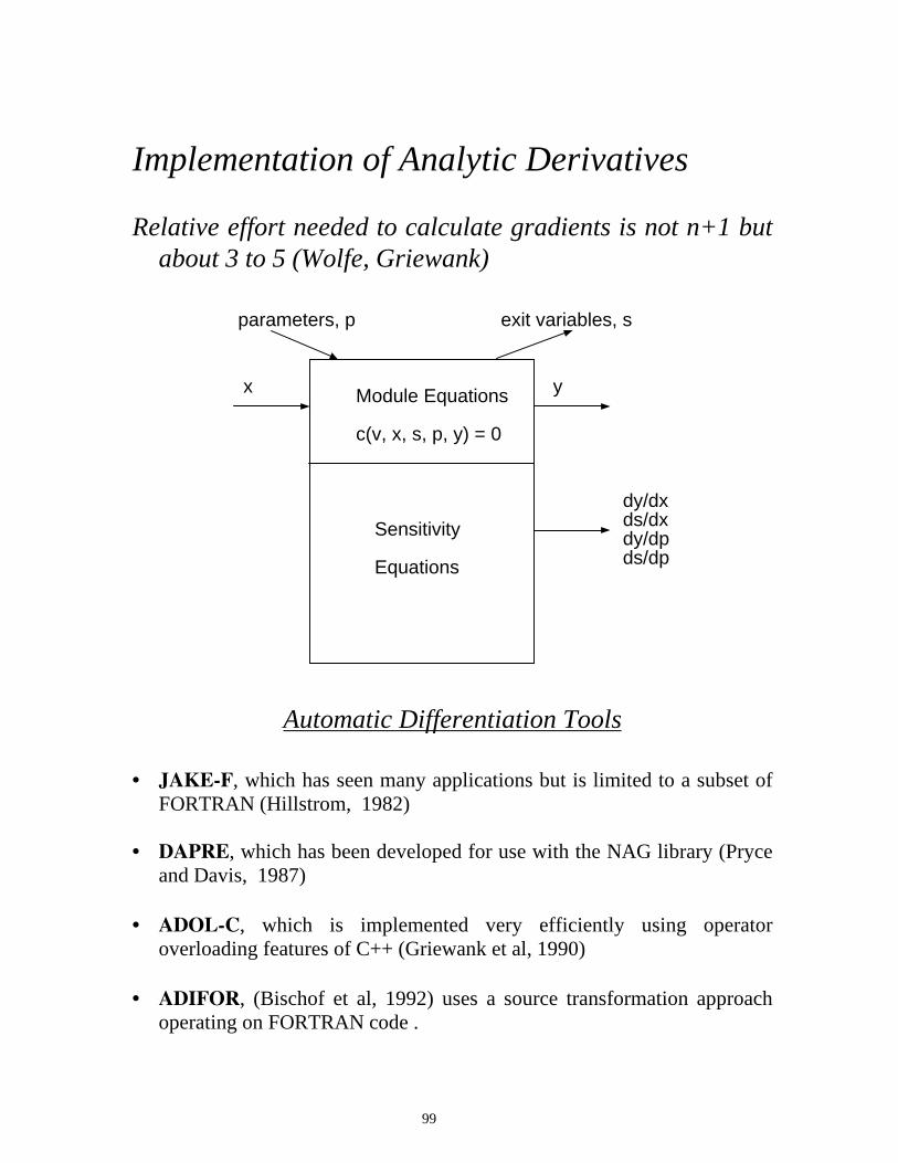
Implementation of Analytic Derivatives Relative effort needed to calculate gradients is not n+1 but
about 3 to 5 (Wolfe, Griewank)
Module Equations
c(v, x, s, p, y) = 0
Sensitivity
Equations
x y
parameters, p exit variables, s
dy/dxds/dxdy/dpds/dp
Automatic Differentiation Tools • JAKE-F, which has seen many applications but is limited to a subset of
FORTRAN (Hillstrom, 1982) • DAPRE, which has been developed for use with the NAG library (Pryce
and Davis, 1987)
• ADOL-C, which is implemented very efficiently using operator overloading features of C++ (Griewank et al, 1990)
• ADIFOR, (Bischof et al, 1992) uses a source transformation approach operating on FORTRAN code .
100
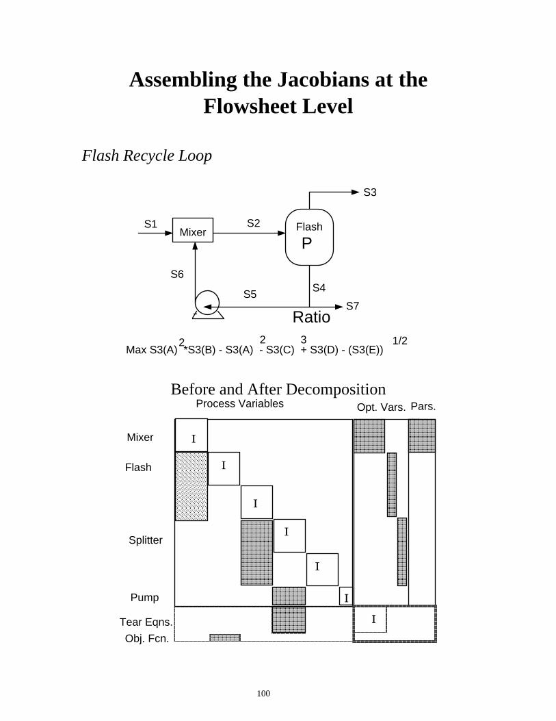
Assembling the Jacobians at the Flowsheet Level
Flash Recycle Loop
S1 S2
S3
S7
S4S5
S6
P
Ratio
Max S3(A) *S3(B) - S3(A) - S3(C) + S3(D) - (S3(E))2 2 3 1/2
Mixer Flash
Before and After Decomposition
Tear Eqns.
Obj. Fcn.
I
I
I
I
I
I
I
Process Variables Opt. Vars. Pars.
Mixer
Flash
Splitter
Pump
101
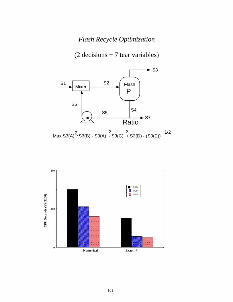
Flash Recycle Optimization
(2 decisions + 7 tear variables)
S1 S2
S3
S7
S4S5
S6
P
Ratio
Max S3(A) *S3(B) - S3(A) - S3(C) + S3(D) - (S3(E))2 2 3 1/2
Mixer Flash
1 20
100
200
GRG
SQP
rSQP
Numerical Exact
CP
U S
econ
ds (
VS
3200
)
102
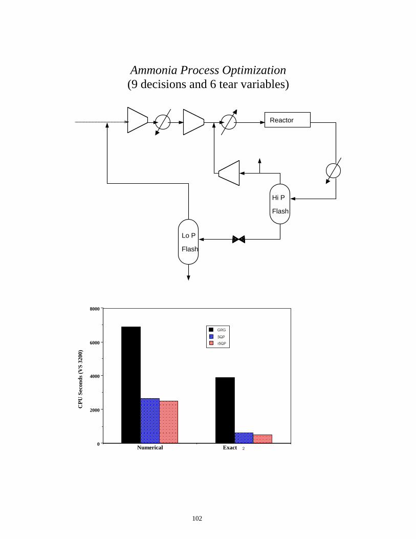
Ammonia Process Optimization (9 decisions and 6 tear variables)
Reactor
Hi P
Flash
Lo P
Flash
1 20
2000
4000
6000
8000
GRG
SQP
rSQP
Numerical Exact
CP
U S
econ
ds (
VS
3200
)
103
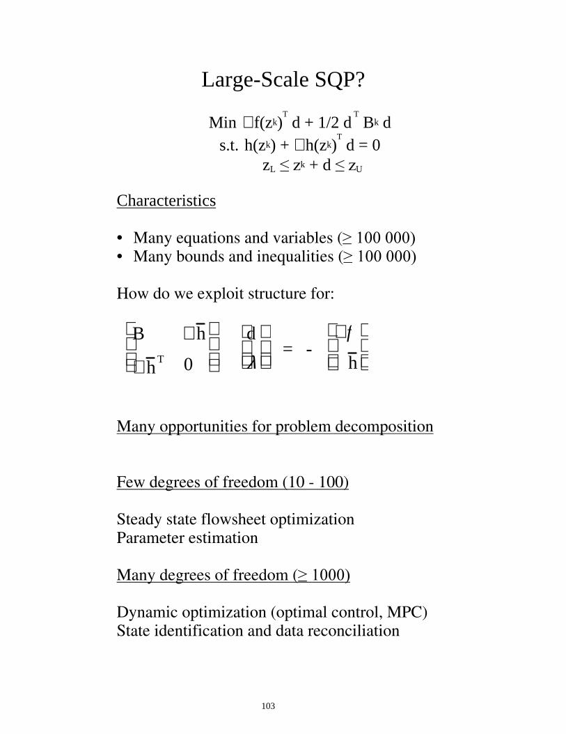
Large-Scale SQP?
Min ∇ f(zk)T d + 1/2 d
T Bk d
s.t. h(zk) + ∇ h(zk)T d = 0
zL ��]k + d ��]U
Characteristics • Many equations and variables (���������� • Many bounds and inequalities (���������� How do we exploit structure for:
B ∇ h
T ∇ h 0
d
λ
= -
∇ f
h
Many opportunities for problem decomposition Few degrees of freedom (10 - 100) Steady state flowsheet optimization Parameter estimation Many degrees of freedom (������� Dynamic optimization (optimal control, MPC) State identification and data reconciliation
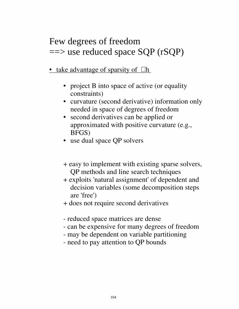
104
Few degrees of freedom ==> use reduced space SQP (rSQP) • take advantage of sparsity of ∇ h
• project B into space of active (or equality constraints)
• curvature (second derivative) information only needed in space of degrees of freedom
• second derivatives can be applied or approximated with positive curvature (e.g., BFGS)
• use dual space QP solvers
+ easy to implement with existing sparse solvers,
QP methods and line search techniques + exploits 'natural assignment' of dependent and
decision variables (some decomposition steps are 'free')
+ does not require second derivatives - reduced space matrices are dense - can be expensive for many degrees of freedom - may be dependent on variable partitioning - need to pay attention to QP bounds
105
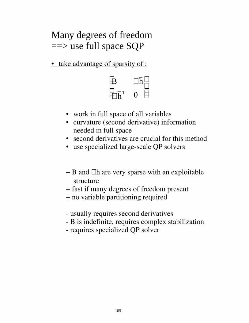
Many degrees of freedom ==> use full space SQP • take advantage of sparsity of :
B ∇ h T ∇ h 0
• work in full space of all variables • curvature (second derivative) information
needed in full space • second derivatives are crucial for this method • use specialized large-scale QP solvers
+ B and ∇ h are very sparse with an exploitable
structure + fast if many degrees of freedom present + no variable partitioning required - usually requires second derivatives - B is indefinite, requires complex stabilization - requires specialized QP solver
106
What about Large-Scale NLPs?
• SQP Properties:
- Few function evaluations. - Time consuming on large problems: QP algorithms are dense implementations; need to store full space matrix.
• MINOS Properties:
- Many function evaluations. - Efficient for large, mostly linear, sparse problems. - Reduced space matrices stored.
• Characteristics of Process Optimization Problems:
- Large models - Few degrees of freedom - Both CPU time and function evaluations are important.
⇒ Development of reduced space SQP method (rSQP) through Range/Null space Decomposition.
107
y
x
h(x, y) = 0
g1(x, y) Š 0
g2(x, y) Š 0
f(x, y)
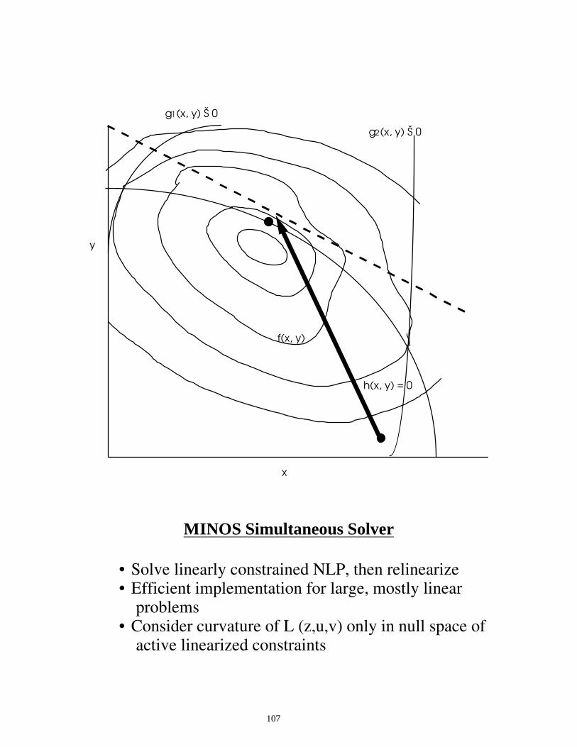
MINOS Simultaneous Solver
• Solve linearly constrained NLP, then relinearize • Efficient implementation for large, mostly linear
problems • Consider curvature of L (z,u,v) only in null space of
active linearized constraints
108
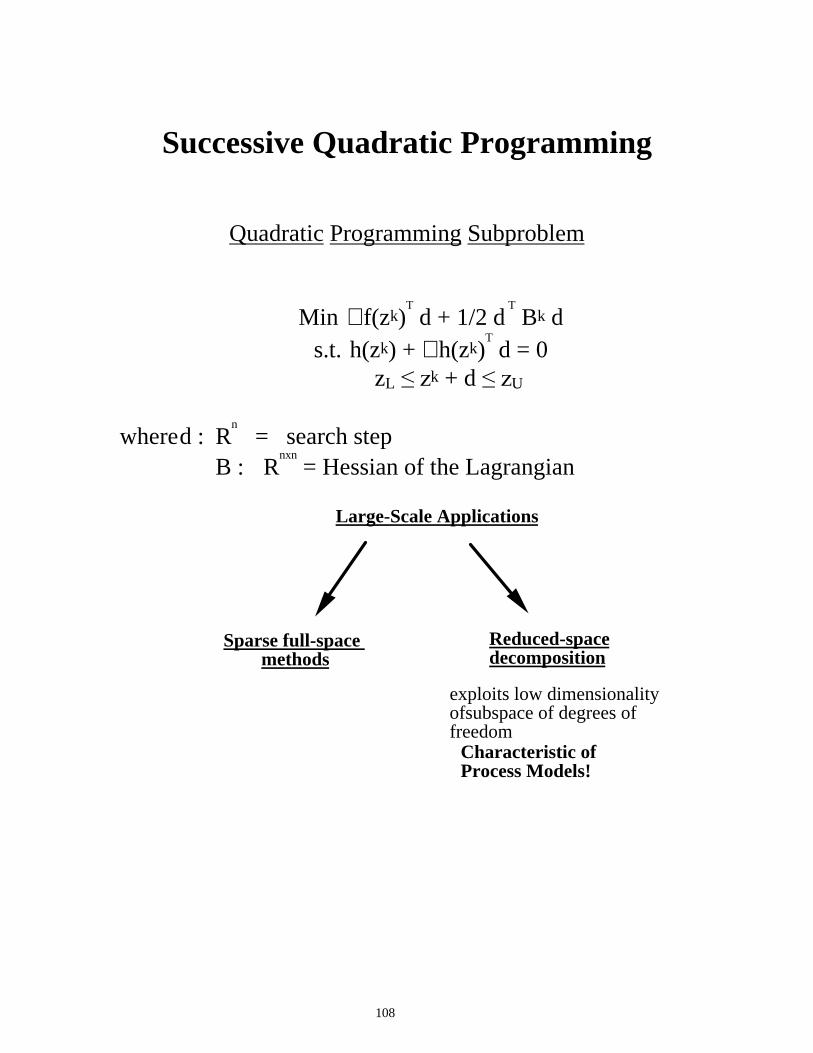
Successive Quadratic Programming
Quadratic Programming Subproblem
Min ∇ f(zk)T d + 1/2 d
T Bk d
s.t. h(zk) + ∇ h(zk)T d = 0
zL ��]k + d ��]U
where d : Rn = search step
B : Rnxn
= Hessian of the Lagrangian
Large-Scale Applications
Sparse full-space methods
Reduced-spacedecomposition
exploits low dimensionality ofsubspace of degrees of freedom
Characteristic of Process Models!
109
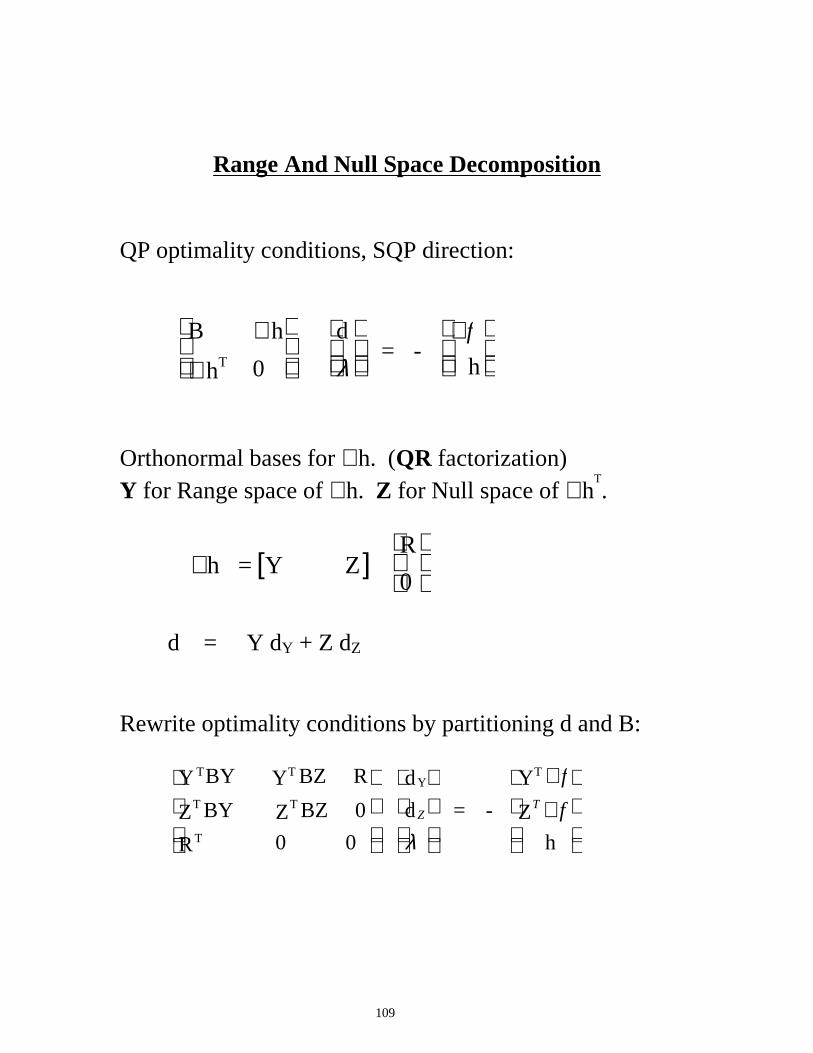
Range And Null Space Decomposition
QP optimality conditions, SQP direction:
B ∇ h
T ∇ h 0
d
λ
= -
∇ f
h
Orthonormal bases for ∇ h. (QR factorization) Y for Range space of ∇ h. Z for Null space of ∇ h
T.
∇ h = Y Z[ ] R
0
d = Y dY + Z dZ
Rewrite optimality conditions by partitioning d and B:
TY BY TY BZ RTZ BY TZ BZ 0TR 0 0
Yd
Zd
λ
= -
TY ∇ fTZ ∇ f
h
110
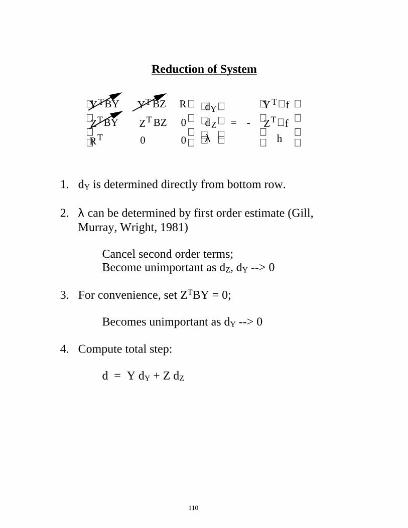
Reduction of System
TY BY TY BZ R
TZ BY TZ BZ 0TR 0 0
Yd
Zd
λ
= -
TY ∇ fTZ ∇ f
h
1. dY is determined directly from bottom row. 2. λ can be determined by first order estimate (Gill, Murray, Wright, 1981) Cancel second order terms; Become unimportant as dZ, dY --> 0 3. For convenience, set ZTBY = 0; Becomes unimportant as dY --> 0 4. Compute total step: d = Y dY + Z dZ
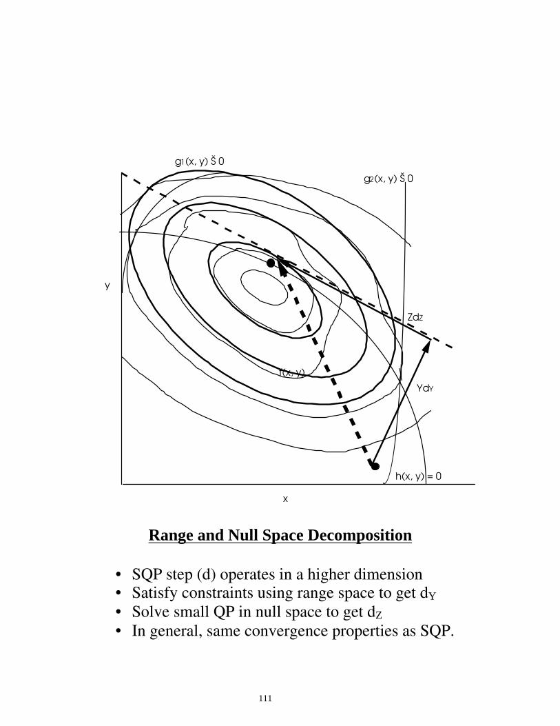
111
y
x
h(x, y) = 0
g1(x, y) Š 0
g2(x, y) Š 0
f(x, y)
YdY
ZdZ
Range and Null Space Decomposition
• SQP step (d) operates in a higher dimension • Satisfy constraints using range space to get dY • Solve small QP in null space to get dZ • In general, same convergence properties as SQP.
112
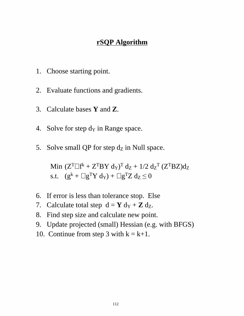
rSQP Algorithm
1. Choose starting point. 2. Evaluate functions and gradients. 3. Calculate bases Y and Z. 4. Solve for step dY in Range space. 5. Solve small QP for step dZ in Null space.
Min (ZT∇ fk + ZTBY dY)T dZ + 1/2 dZT (ZTBZ)dZ
s.t. (gk + ∇ gTY dY) + ∇ gTZ dZ ���
6. If error is less than tolerance stop. Else 7. Calculate total step d = Y dY + Z dZ. 8. Find step size and calculate new point. 9. Update projected (small) Hessian (e.g. with BFGS) 10. Continue from step 3 with k = k+1.
113
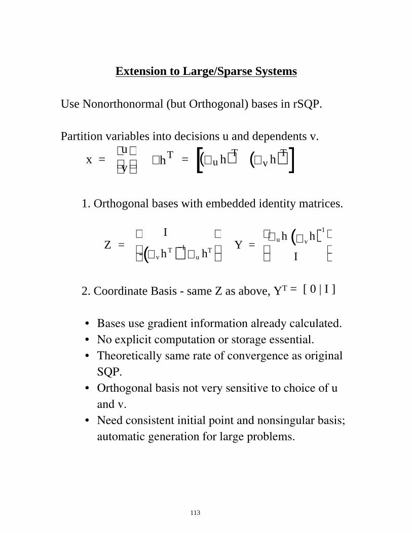
Extension to Large/Sparse Systems
Use Nonorthonormal (but Orthogonal) bases in rSQP. Partition variables into decisions u and dependents v.
x = u
v
T∇ h = u∇ h( )T
v∇ h( )T[ ]
1. Orthogonal bases with embedded identity matrices.
Z = I
- v∇ h T( )−1
u∇ hT
Y =
u∇ h v∇ h( )-1
I
2. Coordinate Basis - same Z as above, YT = [ 0 | I ]
• Bases use gradient information already calculated. • No explicit computation or storage essential. • Theoretically same rate of convergence as original SQP. • Orthogonal basis not very sensitive to choice of u and v. • Need consistent initial point and nonsingular basis; automatic generation for large problems.
114
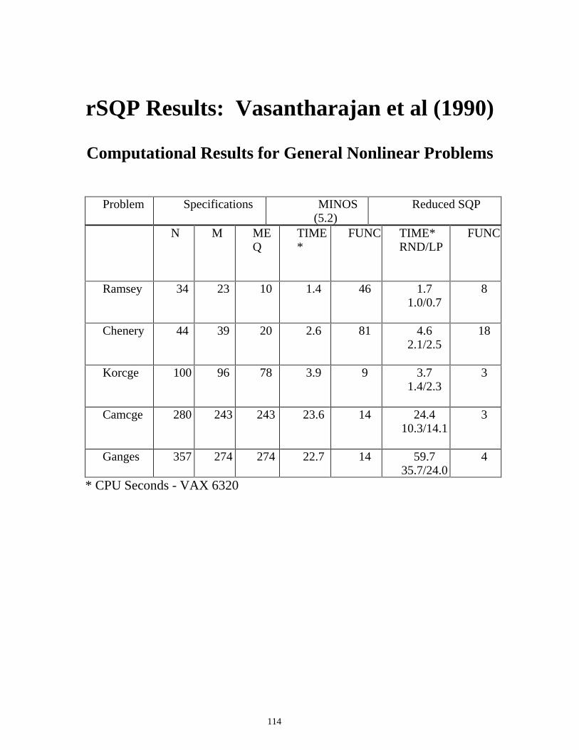
rSQP Results: Vasantharajan et al (1990)
Computational Results for General Nonlinear Problems
N M MEQ
TIME*
FUNC TIME* RND/LP
FUNC
Ramsey 34 23 10 1.4 46 1.7 1.0/0.7
8
Chenery 44 39 20 2.6 81 4.6 2.1/2.5
18
Korcge 100 96 78 3.9 9 3.7 1.4/2.3
3
Camcge 280 243 243 23.6 14 24.4 10.3/14.1
3
Ganges 357 274 274 22.7 14 59.7 35.7/24.0
4
* CPU Seconds - VAX 6320
Problem Specifications MINOS (5.2)
Reduced SQP
115
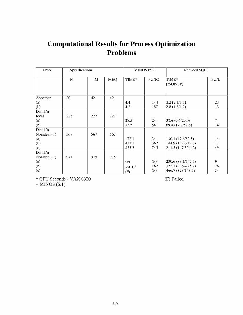
Computational Results for Process Optimization Problems
N M MEQ TIME* FUNC TIME* (rSQP/LP)
FUN.
Absorber (a) (b)
50 42 42 4.4 4.7
144 157
3.2 (2.1/1.1) 2.8 (1.6/1.2)
23 13
Distill’n Ideal (a) (b)
228
227
227
28.5 33.5
24 58
38.6 (9.6/29.0) 69.8 (17.2/52.6)
7 14
Distill’n Nonideal (1) (a) (b) (c)
569
567
567
172.1 432.1 855.3
34 362 745
130.1 (47.6/82.5) 144.9 (132.6/12.3) 211.5 (147.3/64.2)
14 47 49
Distill’n Nonideal (2) (a) (b) (c)
977
975
975
(F)
520.0+
(F)
(F) 162 (F)
230.6 (83.1/147.5) 322.1 (296.4/25.7) 466.7 (323/143.7)
9 26 34
* CPU Seconds - VAX 6320 (F) Failed + MINOS (5.1)
Prob. Specifications MINOS (5.2) Reduced SQP
116
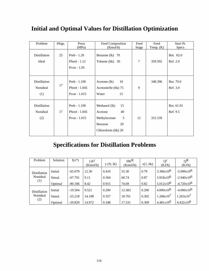
Initial and Optimal Values for Distillation Optimization
Problem #Stgs.
Press (MPa)
Feed Composition (Kmol/h)
Feed Stage
Feed Temp. (K)
Start Pt. Specs
Distillation
Ideal
25
Preb - 1.20
Pfeed - 1.12
Pcon - 1.05
Benzene (lk) 70
Toluene (hk) 30
7
359.592
Bot. 65.0
Ref. 2.0
Distillation
Nonideal
(1)
17
Preb - 1.100
Pfeed - 1.045
Pcon - 1.015
Acetone (lk) 10
Acetonitrlle (hk) 75
Water 15
9
348.396
Bot. 70.0
Ref. 3.0
Distillation
Nonideal
(2)
17
Preb - 1.100
Pfeed - 1.045
Pcon - 1.015
Methanol (lk) 15
Acetone 40
Methylacetate 5
Benzene 20
Chloroform (hk) 20
12
331.539
Bot. 61.91
Ref. 9.5
Specifications for Distillation Problems
Problem Solution f(x*) LKc
(Kmol/h)
y (N, lk)
HKR (Kmol/h)
x(1, hk)
Qc (KJ/h)
QR (KJ/h)
Distillation Nonideal
(1)
Initial
Simul.
Optimal
-65.079
-67.791
-80.186
12.30
9.11
8.42
0.410
0.304
0.915
55.30
60.74
74.69
0.79
0.87
0.82
3.306x10⁶
3.918x10⁶
5.012x10⁶
-5.099x10⁶
-2.940x10⁶
-4.720x10⁶ Distillation Nonideal
(2)
Initial
Simul.
Optimal
-19.504
-25.218
-29.829
9.521
14.108
14.972
0.200
0.357
0.348
12.383
18.701
17.531
0.200
0.302
0.309
4.000x10⁶
1.268x10⁷
4.481x10⁶
-4.000x10⁶
1.263x10⁷
4.432x10⁶
117
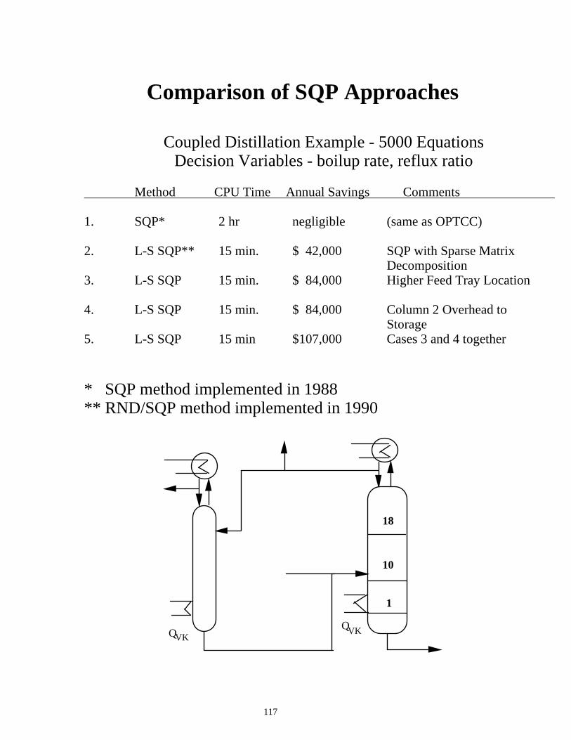
Comparison of SQP Approaches
Coupled Distillation Example - 5000 Equations Decision Variables - boilup rate, reflux ratio
Method CPU Time Annual Savings Comments 1. SQP* 2 hr negligible (same as OPTCC) 2. L-S SQP** 15 min. $ 42,000 SQP with Sparse Matrix Decomposition 3. L-S SQP 15 min. $ 84,000 Higher Feed Tray Location 4. L-S SQP 15 min. $ 84,000 Column 2 Overhead to Storage 5. L-S SQP 15 min $107,000 Cases 3 and 4 together * SQP method implemented in 1988 ** RND/SQP method implemented in 1990
18
10
1
QVKQVK
118
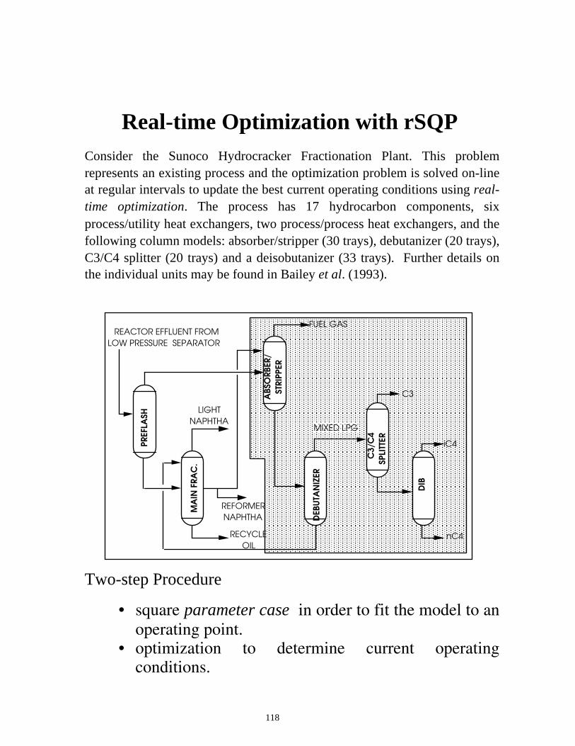
Real-time Optimization with rSQP Consider the Sunoco Hydrocracker Fractionation Plant. This problem represents an existing process and the optimization problem is solved on-line at regular intervals to update the best current operating conditions using real-time optimization. The process has 17 hydrocarbon components, six process/utility heat exchangers, two process/process heat exchangers, and the following column models: absorber/stripper (30 trays), debutanizer (20 trays), C3/C4 splitter (20 trays) and a deisobutanizer (33 trays). Further details on the individual units may be found in Bailey et al. (1993).
REACTOR EFFLUENT FROM
LOW PRESSURE SEPARATOR
PR
EFL
ASH
MA
IN F
RA
C.
RECYCLE
OIL
REFORMER
NAPHTHA
C3
/C4
SP
LITT
ER
nC4
iC4
C3
MIXED LPG
FUEL GAS
LIGHT
NAPHTHA
AB
SO
RB
ER
/
STR
IPP
ER
DEB
UTA
NIZ
ER
DIB
Two-step Procedure
• square parameter case in order to fit the model to an operating point.
• optimization to determine current operating conditions.
119
Optimization Case Study Characteristics The model consists of 2836 equality constraints and only ten independent variables. It is also reasonably sparse and contains 24123 nonzero Jacobian elements. The form of the objective function is given below.
P = z iC iG
i ∈ G∑ + z iC i
E
i ∈ E∑ + z i C i
P m
m = 1
NP
∑ − U
where P = profit,
CG = value of the feed and product streams valued as gasoline, zi = stream flowrates
CE = value of the feed and product streams valued as fuel,
CPm = value of pure component feed and products, and U = utility costs.
Cases Considered:
1. Normal Base Case Operation
2. Simulate fouling by reducing the heat exchange coefficients for the debutanizer
3. Simulate fouling by reducing the heat exchange coefficients for splitter feed/bottoms exchangers
4. Increase price for propane
5. Increase base price for gasoline together with an increase in the octane credit
120
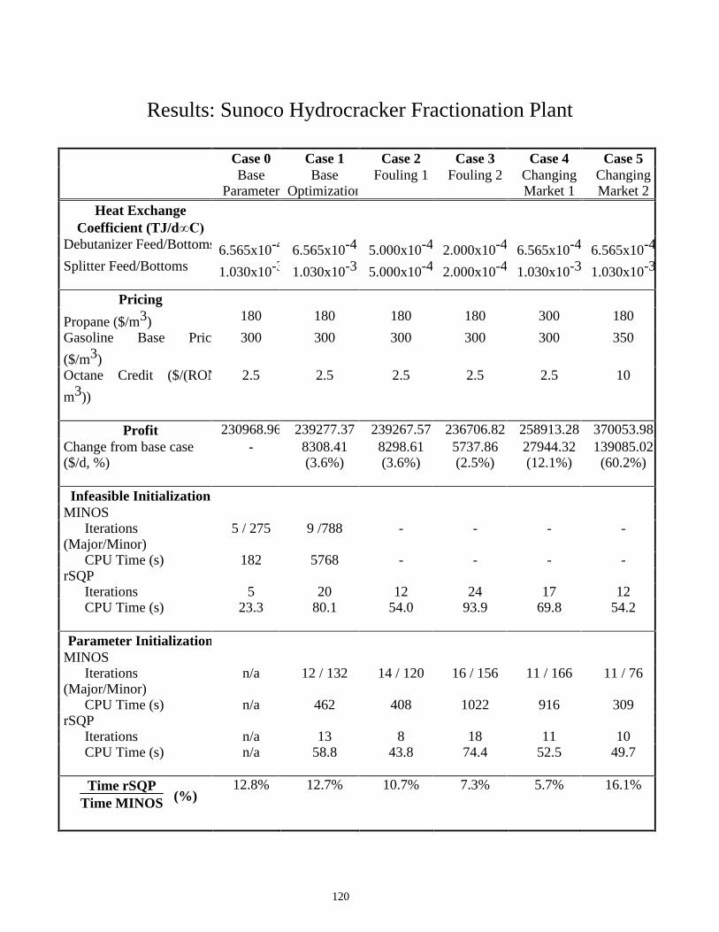
Results: Sunoco Hydrocracker Fractionation Plant
Case 0 Case 1 Case 2 Case 3 Case 4 Case 5 Base
Parameter Base
OptimizationFouling 1 Fouling 2 Changing
Market 1 Changing Market 2
Heat Exchange Coefficient (TJ/d�&�
Debutanizer Feed/Bottoms 6.565x10⁻⁴ 6.565x10⁻⁴ 5.000x10⁻⁴ 2.000x10⁻⁴ 6.565x10⁻⁴ 6.565x10⁻⁴
Splitter Feed/Bottoms
1.030x10⁻³ 1.030x10⁻³ 5.000x10⁻⁴ 2.000x10⁻⁴ 1.030x10⁻³ 1.030x10⁻³
Pricing
Propane ($/m3) 180 180 180 180 300 180
Gasoline Base Price
($/m3)
300 300 300 300 300 350
Octane Credit ($/(RON
m3))
2.5 2.5 2.5 2.5 2.5 10
Profit 230968.96 239277.37 239267.57 236706.82 258913.28 370053.98 Change from base case ($/d, %)
- 8308.41 (3.6%)
8298.61 (3.6%)
5737.86 (2.5%)
27944.32 (12.1%)
139085.02 (60.2%)
Infeasible Initialization MINOS Iterations (Major/Minor)
5 / 275 9 /788 - - - -
CPU Time (s) 182 5768 - - - - rSQP Iterations 5 20 12 24 17 12 CPU Time (s)
23.3 80.1 54.0 93.9 69.8 54.2
Parameter Initialization MINOS Iterations (Major/Minor)
n/a 12 / 132 14 / 120 16 / 156 11 / 166 11 / 76
CPU Time (s) n/a 462 408 1022 916 309 rSQP Iterations n/a 13 8 18 11 10 CPU Time (s)
n/a 58.8 43.8 74.4 52.5 49.7
Time rSQPTime MINOS (%)
12.8% 12.7% 10.7% 7.3% 5.7% 16.1%
121
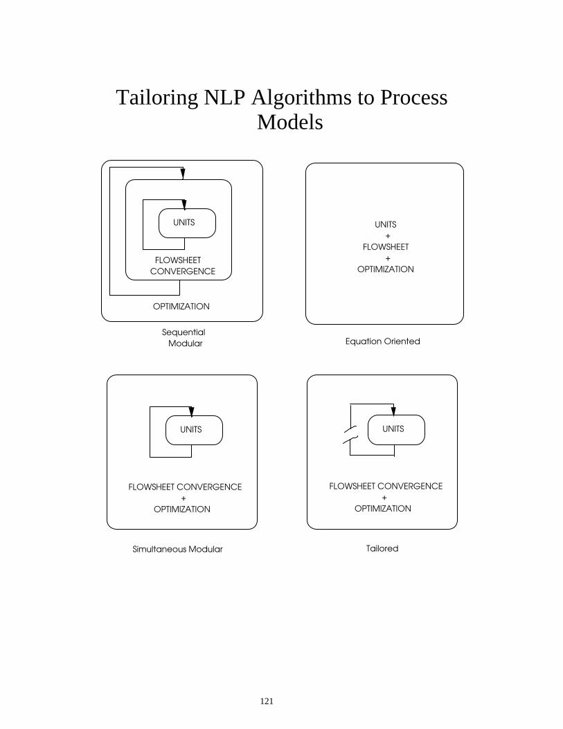
Tailoring NLP Algorithms to Process Models
UNITS
UNITS
FLOWSHEET
CONVERGENCE
OPTIMIZATION
UNITS
+
FLOWSHEET
+
OPTIMIZATION
FLOWSHEET CONVERGENCE
+
OPTIMIZATION
Sequential
Modular Equation Oriented
Simultaneous Modular
UNITS
FLOWSHEET CONVERGENCE
+
OPTIMIZATION
Tailored
122
How can (Newton-based) Procedures/Algorithms be
Reused for Optimization? Can we still use a simultaneous strategy? Examples • Equilibrium stage models with tridiagonal structures
(e.g., Naphthali-Sandholm for distillation) • Boundary Value Problems using collocation and
multiple shooting (e.g., exploit almost block diagonal structures)
• Partial Differential Equations with specialized linear
solvers
rSQP for the Tailored Approach + Easy interface to existing packages (UNIDIST, NRDIST,
ProSim) + Adapt to Data and Problem Structures + Similar Convergence Properties and Performance + More Flexibility in Problem Specifiction
123
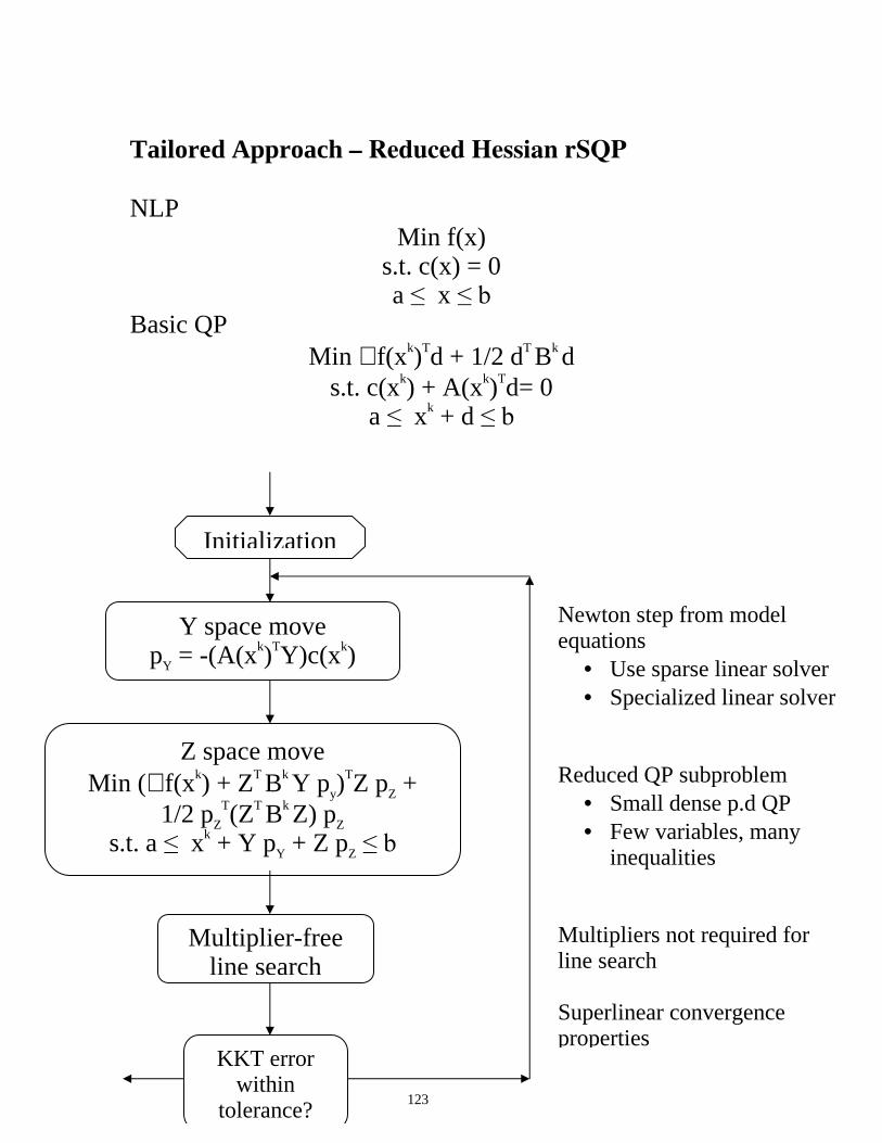
Tailored Approach – Reduced Hessian rSQP
NLP
Min f(x) s.t. c(x) = 0 a ���x ��E
Basic QP Min ∇ f(xk)Td + 1/2 dT Bk d
s.t. c(xk) + A(xk)Td= 0 a ���xk + d ��E
Y space move pY = -(A(xk)TY)c(xk)
Z space move Min (∇ f(xk) + ZT Bk Y py)
TZ pZ + 1/2 pZ
T(ZT Bk Z) pZ s.t. a ���xk + Y pY + Z pZ ��E
Initialization
Multiplier-free line search
KKT error within
tolerance?
Newton step from model equations
• Use sparse linear solver • Specialized linear solver
Reduced QP subproblem
• Small dense p.d QP • Few variables, many
inequalities Multipliers not required for line search Superlinear convergence properties
124
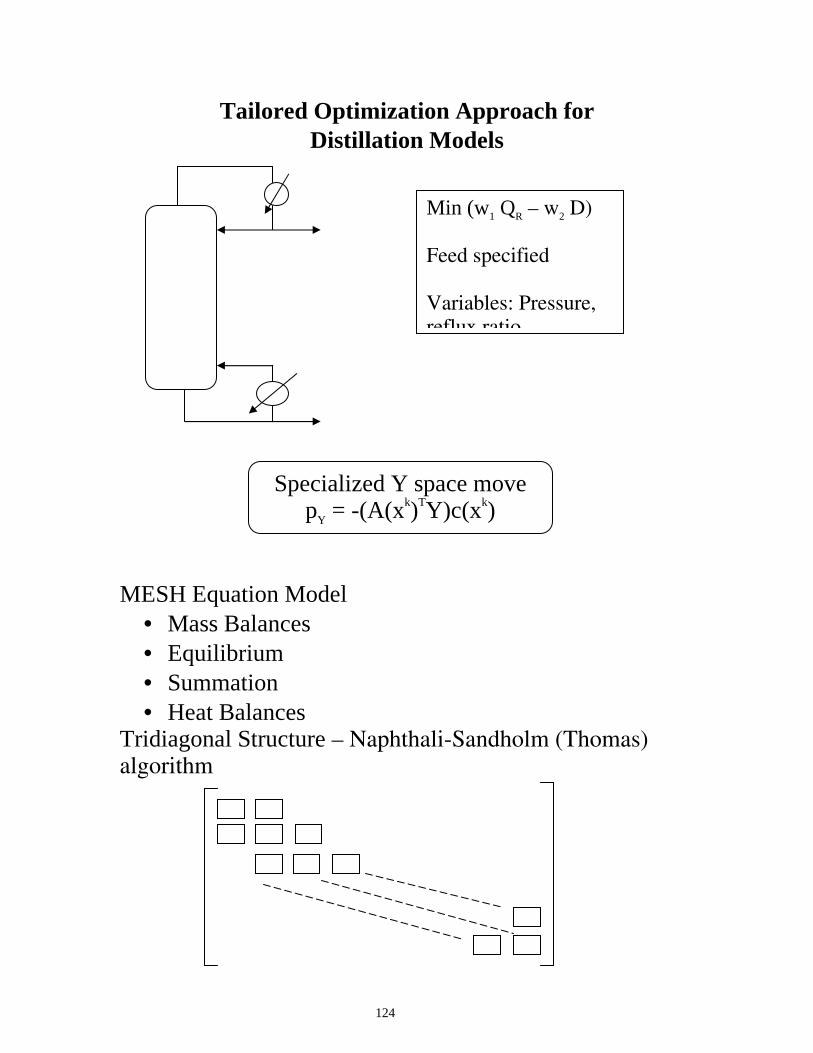
Tailored Optimization Approach for Distillation Models
MESH Equation Model
• Mass Balances • Equilibrium • Summation • Heat Balances
Tridiagonal Structure – Naphthali-Sandholm (Thomas) algorithm
Min (w1 QR – w2 D) Feed specified Variables: Pressure, reflux ratio
Specialized Y space move pY = -(A(xk)TY)c(xk)
125
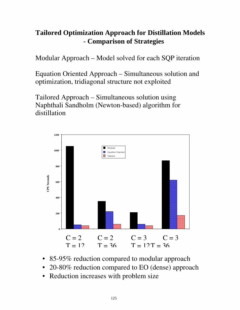
Tailored Optimization Approach for Distillation Models - Comparison of Strategies
Modular Approach – Model solved for each SQP iteration Equation Oriented Approach – Simultaneous solution and optimization, tridiagonal structure not exploited Tailored Approach – Simultaneous solution using Naphthali Sandholm (Newton-based) algorithm for distillation
1 2 3 4
0
200
400
600
800
1000
1200
Modular
Equation Oriented
Tailored
CP
U S
econ
ds
• 85-95% reduction compared to modular approach • 20-80% reduction compared to EO (dense) approach • Reduction increases with problem size
C = 2 C = 2 C = 3 C = 3 T = 12 T = 36 T = 12 T = 36
126
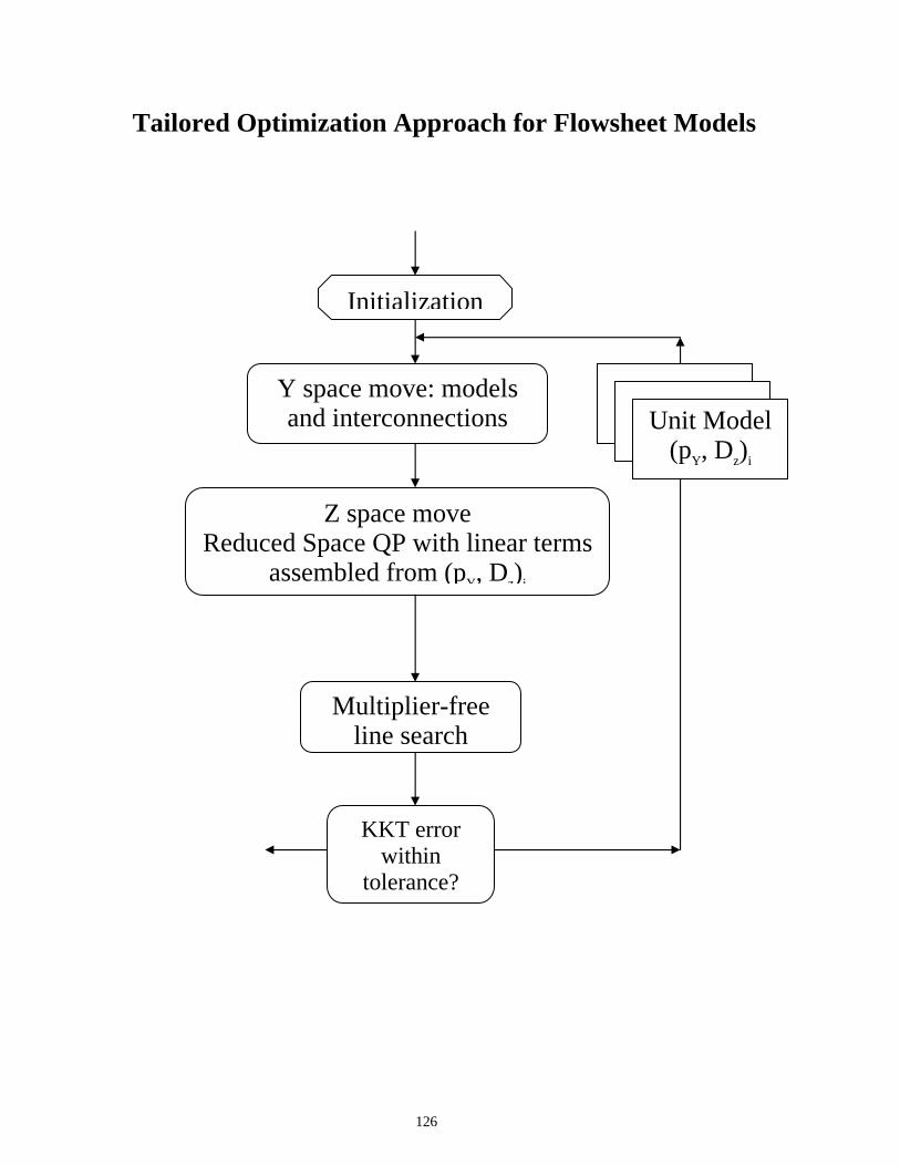
Tailored Optimization Approach for Flowsheet Models
Y space move: models and interconnections
Z space move Reduced Space QP with linear terms
assembled from (pY, Dz)i
Initialization
Multiplier-free line search
KKT error within
tolerance?
Unit Model (pY, Dz)i
127
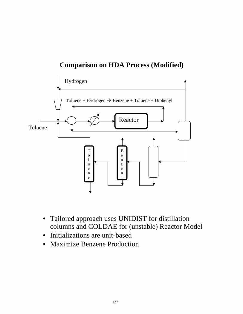
Comparison on HDA Process (Modified)
• Tailored approach uses UNIDIST for distillation columns and COLDAE for (unstable) Reactor Model
• Initializations are unit-based • Maximize Benzene Production
Reactor
Benzene
Toluene
Hydrogen
Toluene
Toluene + Hydrogen Æ Benzene + Toluene + Diphenyl
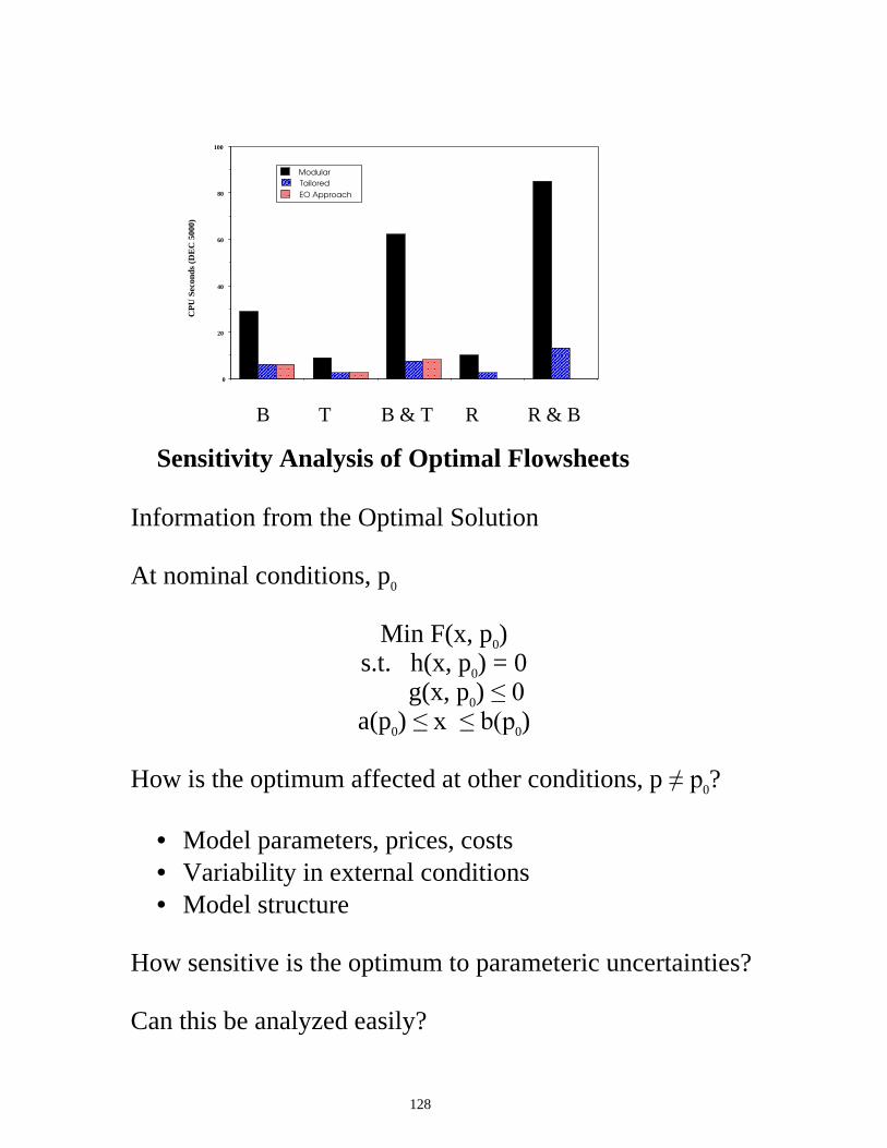
128
1 2 3 4 5
0
20
40
60
80
100
Modular
Tailored
EO ApproachC
PU
Sec
onds
(D
EC
500
0)
Sensitivity Analysis of Optimal Flowsheets
Information from the Optimal Solution At nominal conditions, p0
Min F(x, p0) s.t. h(x, p0) = 0 g(x, p0) ��� a(p0) ��[����E�S0)
How is the optimum affected at other conditions, p ��S0?
• Model parameters, prices, costs • Variability in external conditions • Model structure
How sensitive is the optimum to parameteric uncertainties? Can this be analyzed easily?
B T B & T R R & B
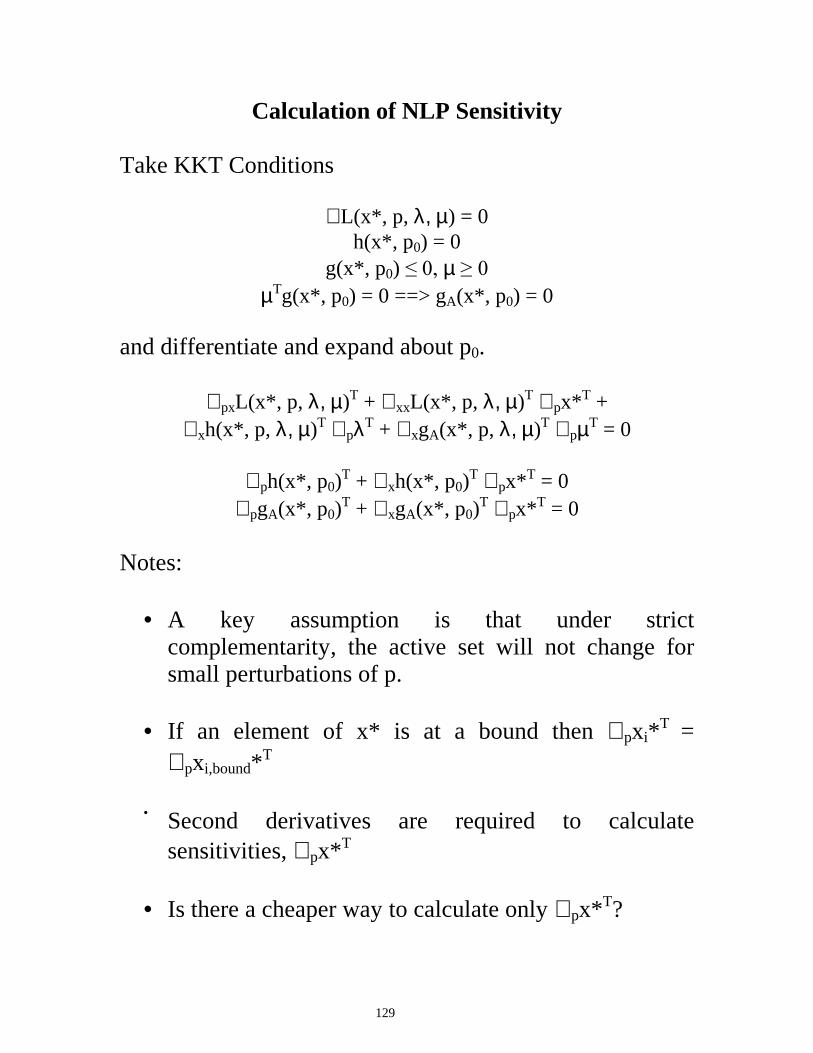
129
Calculation of NLP Sensitivity Take KKT Conditions
∇ L(x*, p, λ, µ) = 0 h(x*, p0) = 0
g(x*, p0) �����µ ��� µTg(x*, p0) = 0 ==> gA(x*, p0) = 0
and differentiate and expand about p0.
∇ pxL(x*, p, λ, µ)T + ∇ xxL(x*, p, λ, µ)T ∇ px*T + ∇ xh(x*, p, λ, µ)T ∇ pλT + ∇ xgA(x*, p, λ, µ)T ∇ pµT = 0
∇ ph(x*, p0)
T + ∇ xh(x*, p0)T ∇ px*T = 0
∇ pgA(x*, p0)T + ∇ xgA(x*, p0)
T ∇ px*T = 0 Notes:
• A key assumption is that under strict complementarity, the active set will not change for small perturbations of p.
• If an element of x* is at a bound then ∇ pxi*
T = ∇ pxi,bound*
T
• Second derivatives are required to calculate sensitivities, ∇ px*T
• Is there a cheaper way to calculate only ∇ px*T?
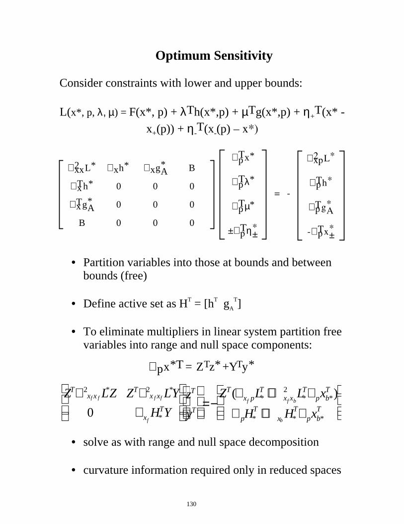
130
Optimum Sensitivity Consider constraints with lower and upper bounds: L(x*, p, λ, µ) = F(x*, p) + λTh(x*,p) + µTg(x*,p) + η+
T(x* -
x+(p)) + η-T(x-(p) – x*)
∇ xx2 L* ∇ xh* ∇ xgA* B
∇ xTh* 0 0 0
∇ xTgA* 0 0 0
B 0 0 0
∇ pTx*
∇ pTλ*
∇ pTµ*
±∇ pTη±*
= -
∇ xp2 L*
∇ pTh*
∇ pTgA*
-∇ pTx±*
• Partition variables into those at bounds and between
bounds (free) • Define active set as HT = [hT gA
T] • To eliminate multipliers in linear system partition free
variables into range and null space components:
∇ px*T = ZTz* +YTy*
ZT∇ 2xf x f L
*Z ZT∇ 2x f xf L
*Y
0 ∇ xfH*
TY
zT
yT
=−
ZT(∇ xf pL*T +∇ xf xb
2 L*T∇ pxb*
T )
∇ pH*T +∇ xb
H*T∇ pxb*
T
• solve as with range and null space decomposition • curvature information required only in reduced spaces
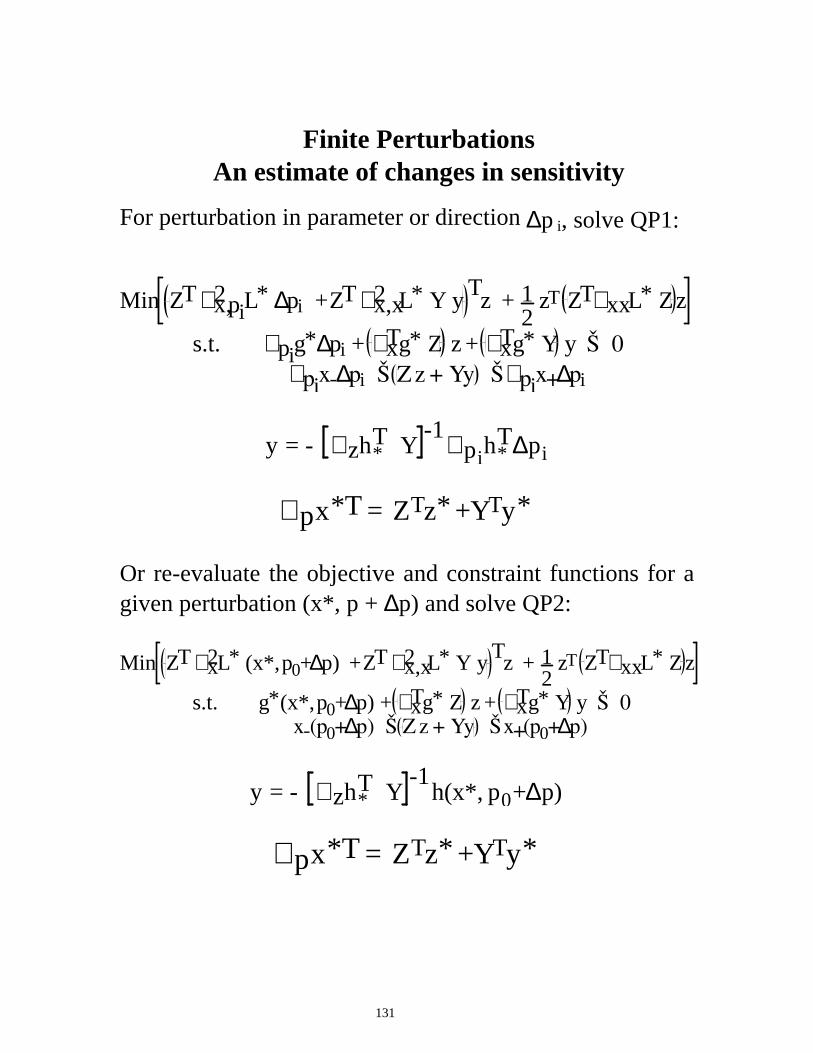
131
Finite Perturbations
An estimate of changes in sensitivity
For perturbation in parameter or direction ∆p i, solve QP1:
Min ZT ∇ x,pi2 L* ∆pi + ZT ∇ x,x2 L* Y y Tz + 1
2 zT ZT∇ xxL* Zz
s.t. ∇ pig*∆pi + ∇ xTg* Z z + ∇ xTg* Y y Š 0
∇ pix-∆pi Š Z z + Y y Š ∇ pix+∆pi
y = - ∇ zh*T Y
-1∇ pih*T∆pi
∇ px*T = ZTz* +YTy*
Or re-evaluate the objective and constraint functions for a given perturbation (x*, p + ∆p) and solve QP2:
Min ZT ∇ x2L* (x*, p0+∆p) + ZT ∇ x,x2 L* Y y Tz + 12
zT ZT∇ xxL* Z z
s.t. g*(x*, p0+∆p) + ∇ xTg* Z z + ∇ xTg* Y y Š 0 x-(p0+∆p) Š Z z + Y y Š x+(p0+∆p)
y = - ∇ zh*T Y
-1h(x*, p0+∆p)
∇ px*T = ZTz* +YTy*
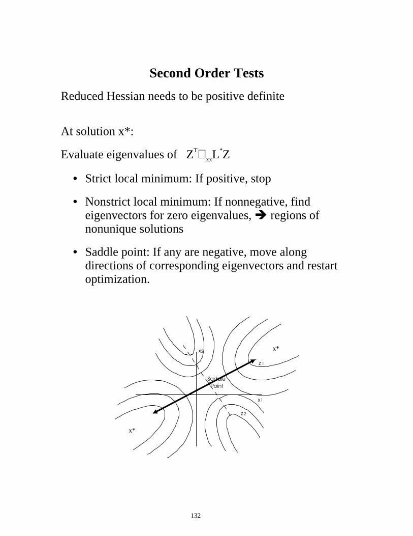
132
Second Order Tests
Reduced Hessian needs to be positive definite
At solution x*:
Evaluate eigenvalues of ZT∇ xxL*Z
• Strict local minimum: If positive, stop
• Nonstrict local minimum: If nonnegative, find eigenvectors for zero eigenvalues, Î regions of nonunique solutions
• Saddle point: If any are negative, move along directions of corresponding eigenvectors and restart optimization.
x1
x2
z 1
z 2
Saddle
Point
x*
x*
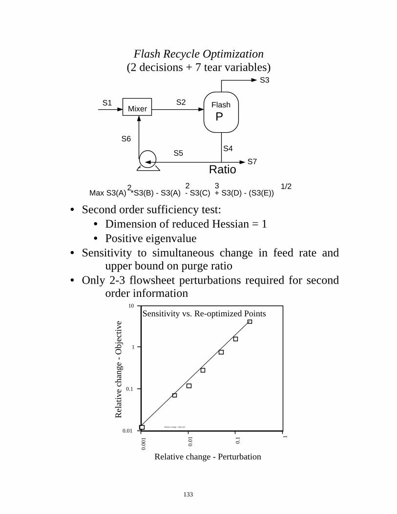
133
Flash Recycle Optimization (2 decisions + 7 tear variables)
S1 S2
S3
S7
S4S5
S6
P
Ratio
Max S3(A) *S3(B) - S3(A) - S3(C) + S3(D) - (S3(E))2 2 3 1/2
Mixer Flash
• Second order sufficiency test:
• Dimension of reduced Hessian = 1 • Positive eigenvalue
• Sensitivity to simultaneous change in feed rate and upper bound on purge ratio
• Only 2-3 flowsheet perturbations required for second order information
0.01
0.1
1
10
Rel
ativ
e ch
ange
- O
bjec
tive
0.00
1
0.01 0.1 1
Relative change - Perturbation
Sensitivity vs. Re-optimized Points
Relative change - Objective
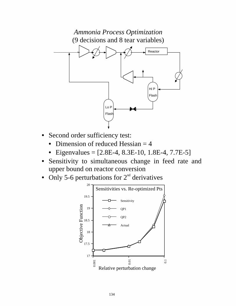
134
Ammonia Process Optimization (9 decisions and 8 tear variables)
Reactor
Hi P
Flash
Lo P
Flash
• Second order sufficiency test:
• Dimension of reduced Hessian = 4 • Eigenvalues = [2.8E-4, 8.3E-10, 1.8E-4, 7.7E-5]
• Sensitivity to simultaneous change in feed rate and upper bound on reactor conversion
• Only 5-6 perturbations for 2nd derivatives
17
17.5
18
18.5
19
19.5
20
Obj
ecti
ve F
unct
ion
0.00
1
0.01 0.1
Relative perturbation change
Sensitivities vs. Re-optimized Pts
Actual
QP2
QP1
Sensitivity
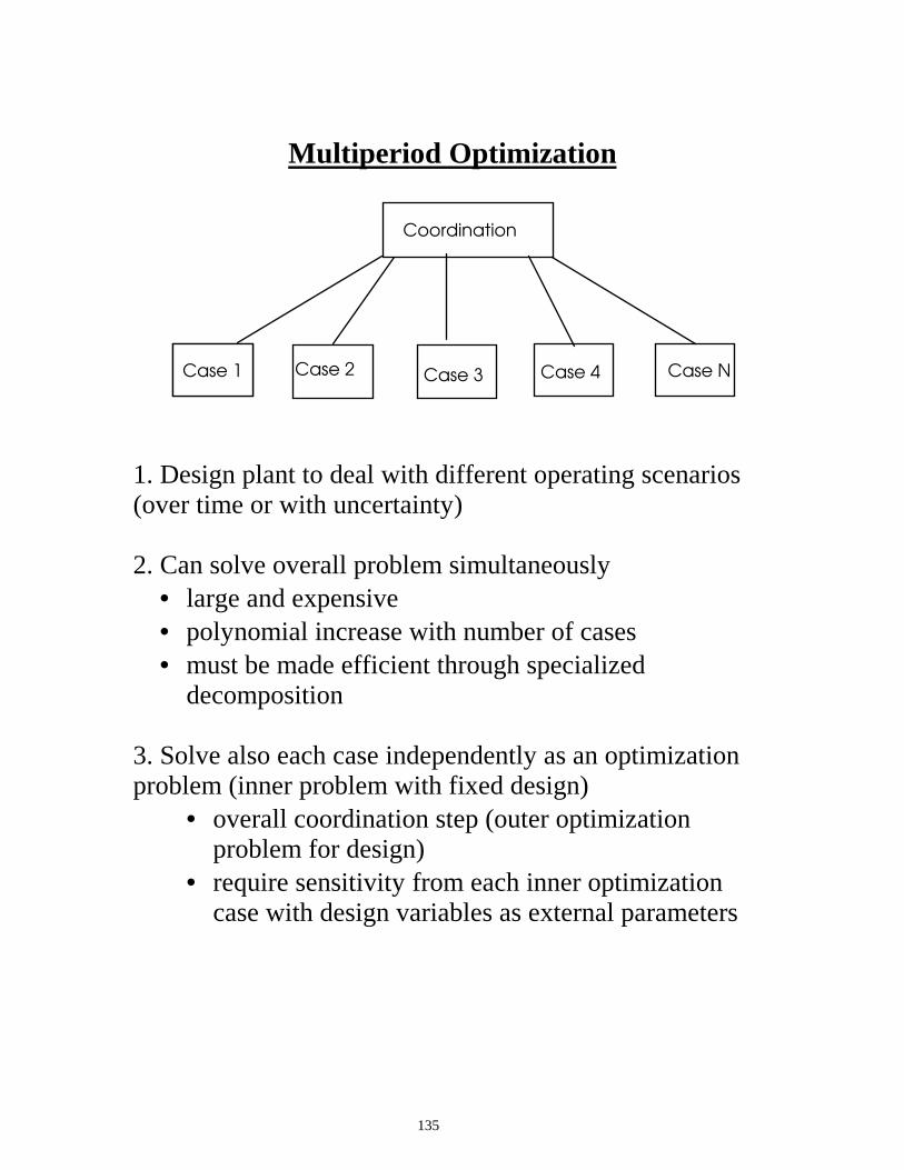
135
Multiperiod Optimization
Coordination
Case 1 Case 2 Case 3 Case 4 Case N
1. Design plant to deal with different operating scenarios (over time or with uncertainty) 2. Can solve overall problem simultaneously
• large and expensive • polynomial increase with number of cases • must be made efficient through specialized
decomposition 3. Solve also each case independently as an optimization problem (inner problem with fixed design)
• overall coordination step (outer optimization problem for design)
• require sensitivity from each inner optimization case with design variables as external parameters
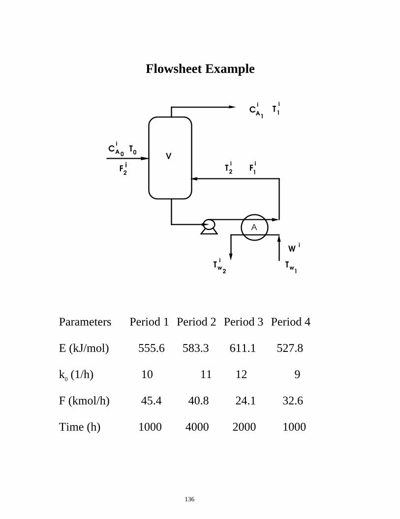
136
Flowsheet Example
Ti
1
A
i C
Ti
2F
i
1F
i2
TwTi
w
W i
i C T
0A
A
0
2 1
1
V
Parameters Period 1 Period 2 Period 3 Period 4 E (kJ/mol) 555.6 583.3 611.1 527.8 k0 (1/h) 10 11 12 9 F (kmol/h) 45.4 40.8 24.1 32.6 Time (h) 1000 4000 2000 1000
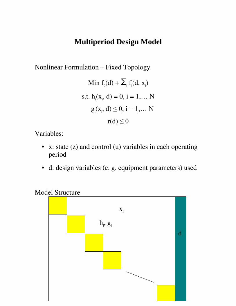
137
Multiperiod Design Model
Nonlinear Formulation – Fixed Topology
Min f0(d) + Σi fi(d, xi)
s.t. hi(xi, d) = 0, i = 1,… N
gi(xi, d) �����L� ���«�1
r(d) ���� Variables:
• x: state (z) and control (u) variables in each operating period
• d: design variables (e. g. equipment parameters) used
Model Structure
d
xi
hi, gi
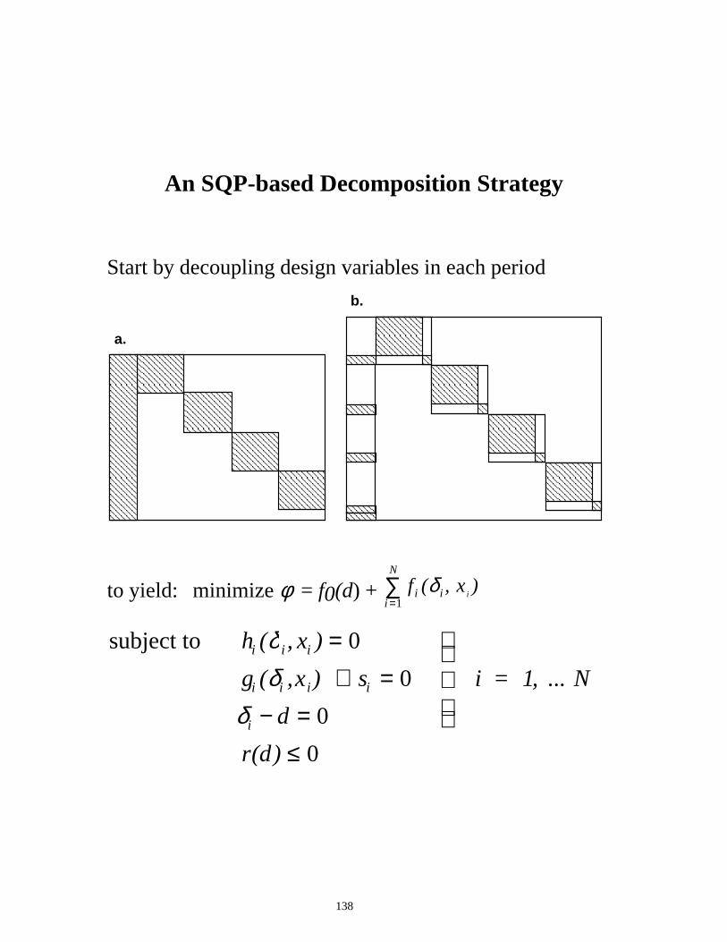
138
An SQP-based Decomposition Strategy
Start by decoupling design variables in each period
a.
b.
to yield: minimize φ = f0(d) + f ii =1
N
∑ (δi , x i)
subject to hi (δi , xi ) = 0
gi (δi ,x i) + si = 0
δi − d = 0
i = 1, ... N
r(d) ≤ 0
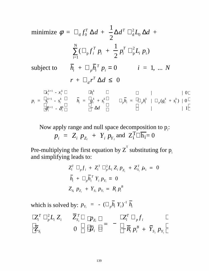
139
minimize φ = ∇ d f0T ∆d +
1
2∆dT ∇ d
2 L0 ∆d +
( ∇ p f iT pi +
1
2pi
T ∇ p2 Li pi)
i=1
N
∑
subject to h i + ∇ ph iT pi = 0 i = 1, ... N
r + ∇ d rT ∆d ≤ 0
pi =
x ik +1 - x i
k
sik +1 - si
k
δik +1 - δi
k
h i =
hik
gik + si
k
− ∆d
∇ ph i =
| | 0
∇ phik | ∇ p (gi
k + sik ) | 0
| | I
Now apply range and null space decomposition to pi:
pi = Zi pZi + Yi pY i
and ZiT∇ hi= 0
Pre-multiplying the first equation by ZT substituting for pi
and simplifying leads to:
ZiT
∇ p f i + ZiT ∇ p
2 Li Zi pZi + ZS i
T µ
i = 0
h i + ∇ ph iT Yi pYi
= 0
ZSi pZi
+ YS i pYi
= Ri piB
which is solved by: pYi
= - (∇ ph i Yi)-1 h i
ZiT ∇ p
2 Li Zi Z S i
T
Z Si 0
pZi
µ i
= −
ZiT ∇ p f i
−R i piB + Y S i
pYi
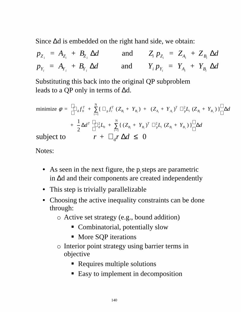
140
Since ∆d is embedded on the right hand side, we obtain:
pZ i = AZi
+ BZ i ∆d and Zi pZi
= ZAi + Z Bi
∆d
pYi = AY i
+ BY i ∆d and Yi pYi
= YAi + YBi
∆d
Substituting this back into the original QP subproblem leads to a QP only in terms of ∆d. minimize φ = ∇ d f 0
T + { ∇ p fiT (ZBi
+ YBi) + (ZAi
+ Y Ai)T ∇ p
2 Lii =1
N
∑ (Z Bi+ YB i
) }
∆d
+ 1
2∆dT ∇ d
2 L0 + { (ZBi+ YBi
)T ∇ p2 Li
i =1
N
∑ (Z Bi+ YB i
) }
∆d
subject to r + ∇ dr ∆d ≤ 0
Notes:
• As seen in the next figure, the pi steps are parametric in ∆d and their components are created independently
• This step is trivially parallelizable
• Choosing the active inequality constraints can be done through: o Active set strategy (e.g., bound addition)
� Combinatorial, potentially slow � More SQP iterations
o Interior point strategy using barrier terms in objective � Requires multiple solutions � Easy to implement in decomposition
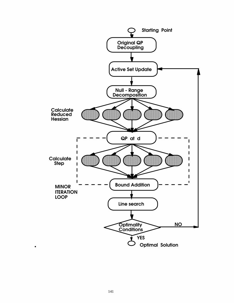
141
�
Starting Point
Original QP Decoupling
Null - Range Decomposition
QP at d
Calculate Step
Calculate Reduced Hessian
Line search
Optimality Conditions
NO
YES
Optimal Solution
Active Set Update
Bound AdditionMINOR ITERATION LOOP
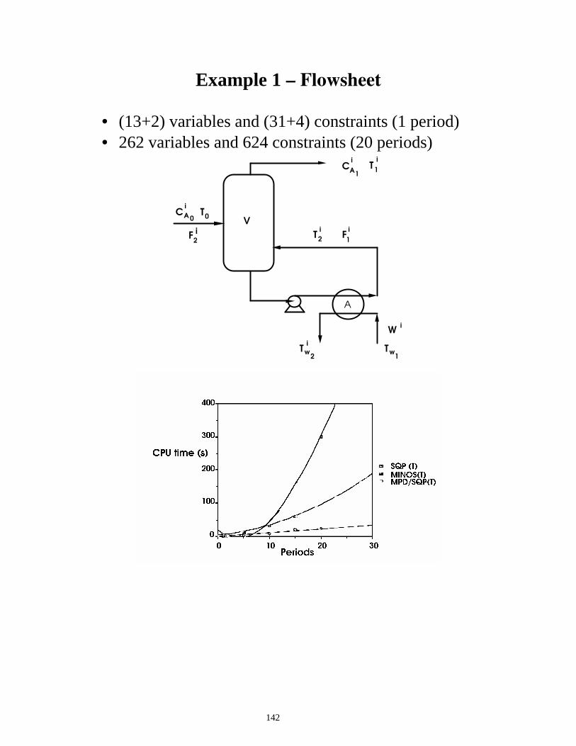
142
Example 1 – Flowsheet
• (13+2) variables and (31+4) constraints (1 period) • 262 variables and 624 constraints (20 periods)
Ti
1
A
i C
Ti
2F
i
1F
i2
TwTi
w
W i
i C T
0A
A
0
2 1
1
V
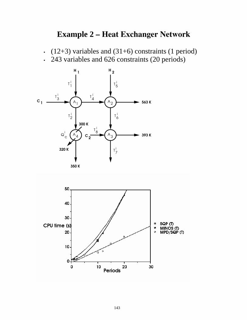
143
Example 2 – Heat Exchanger Network
• (12+3) variables and (31+6) constraints (1 period)
• 243 variables and 626 constraints (20 periods)
C1
C2
H1
H2
T1
563 K
393 K
T2
T3
T4
T8
T7
T6
T5
350 K
Qc
300 K
A1
A3
A2
i i
i
i
i
i
i
i i
4A
320 K
144
Summary and Conclusions
1. Widely Used Methods Surveyed
• Unconstrained Newton and Quasi Newton Methods
• KKT Conditions and Specialized Methods • Successive Quadratic Programming (SQP) • Reduced Gradient Methods (GRG2, MINOS)
2. SQP for Large-scale Nonlinear Programming
• Reduced Hessian SQP • Orthogonal vs. Coordinate Bases
3. Process Optimization Applications
• Modular Flowsheet Optimization • Importance of Accurate Derivatives • Equation Oriented Models and Optimization • Realtime Process Optimization • Tailored SQP for Large-scale Models
4. Further Applications
• Sensitivity Analysis for NLP Solutions • Multiperiod Optimization Problems


