On unifying multiblock analysis with application to decentralizedprocess monitoring

S. Joe Qin1*, Sergio Valle1 and Michael J. Piovoso2

1Department of Chemical Engineering, The University of Texas at Austin, Austin, TX 78712, USA2DuPont Central Research and Development, Central Science and Engineering Experimental Station, PO Box

80101, Wilmington, DE 19880-0101, USA

SUMMARY

Westerhuis et al. (J. Chemometrics 1998; 12: 301–321) show that the scores of consensus PCA and multiblockPLS (Westerhuis and Coenegracht, J. Chemometrics 1997; 11: 379–392) can be calculated directly from theregular PCA and PLS scores respectively. In this paper we show that both the loadings and scores of consensusPCA can be calculated directly from those of regular PCA, and the multiblock PLS loadings, weights and scorescan be calculated directly from those of regular PLS. The orthogonal properties of four multiblock PCA and PLSalgorithms are explored. The use of multiblock PCA and PLS for decentralized monitoring and diagnosis isderived in terms of regular PCA and PLS scores and residuals. While the multiblock analysis algorithms arebasically equivalent to regular PCA and PLS, blocking of process variables in a large-scale plant based onprocess knowledge helps to localize the root cause of the fault in a decentralized manner. New definitions ofblock and variable contributions to SPE and T2 are proposed for decentralized monitoring. This decentralizedmonitoring method based on proper variable blocking is successfully applied to an industrial polyester filmprocess. Copyright 2001 John Wiley & Sons, Ltd.

KEY WORDS: consensus PCA; multiblock PCA; multiblock PLS; decentralized process monitoring;contribution plots

1. INTRODUCTION

In a recent paper, Westerhuis et al. [1] provide a comprehensive analysis of several multiblock andhierarchical PCA and PLS algorithms, including (i) consensus PCA (CPCA) [2], (ii) hierarchicalPCA (HPCA) [3], (iii) multiblock PLS (MBPLS) [2,4] and hierarchical PLS (HPLS) [2,5]. The basicidea of the multiblock algorithms is to divide the descriptor variables (X) into several blocks in thePCA case and divide the response variables (Y) into several blocks in the PLS case so as to obtainlocal information (block scores) and global information (super scores) simultaneously from the data.The CPCA and MBPLS algorithms normalize the block loadings and super loadings, while the HPCAand HPLS algorithms normalize the super scores and block scores. Westerhuis et al. [1] give thesealgorithms in a unified notation.

A major contribution of Westerhuis et al. [1] is that they prove that the super scores of CPCA andMBPLS are identical to the scores of regular PCA and PLS of the entire variable set respectively.

JOURNAL OF CHEMOMETRICSJ. Chemometrics 2001; 15: 715–742DOI: 10.1002/cem.667

* Correspondence to: S. J. Qin, Department of Chemical Engineering The University of Texas at Austin, Austin, TX 78712,USA.E-mail: qin@che.utexas.eduContract/grant sponsor: National Science Foundation; Contract/grant number: CTS-9814340Contract/grant sponsor: Texas Higher Education Coordinating BoardContract/grant sponsor: DupontContract/grant sponsor: Consejo Nacional de Ciencia y Tecnologıa (CONACyT)Contract/grant sponsor: Instituto Tecnologico de Durango (ITD)

Copyright 2001 John Wiley & Sons, Ltd. Received 13 July 2000Accepted 15 November 2000

Westerhuis et al. [1] further demonstrate that the HPCA and HPLS algorithms suffer fromconvergence problems. Although a specific solution of HPCA and HPLS can be obtained repetitivelyby using a specific initialization procedure, the objective function of HPCA is still not clear. Becausethe super scores of CPCA and MBPLS are identical to the scores of PCA and PLS respectively,Westerhuis et al. [1] suggest using the regular PCA and PLS scores to calculate the block scores andloadings for CPCA and MBPLS. This suggestion for CPCA is similar to the multiblock PCA(MBPCA) algorithm described by Cheng and McAvoy [6] but the latter uses the block scores todeflate the residual matrices to obtain orthogonal block scores.

In this paper we provide further analysis of the CPCA algorithm of Wold et al. [2], the MBPLSalgorithm of Westerhuis and Coenegracht [7], the MBPLS algorithm of Wangen and Kowalski [4]and the MBPCA algorithm of Cheng and McAvoy [6]. We first point out that although theconclusions of Westerhuis et al. [1] are correct, the proof contains errors. A correct proof is providedin this paper. In addition to the identical scores between CPCA/MBPLS and PCA/PLS, we show thatthe CPCA and MBPLS loadings (both super loadings and block loadings) can be calculated directlyfrom the loadings of regular PCA and PLS algorithms respectively. Furthermore, we explore theorthogonal properties and rank conditions of the CPCA, MBPCA and MBPLS algorithms. The fouralgorithms analyzed in this paper are:

� CPCA [2], which normalizes the loadings and deflates the residuals based on super scores;� MBPCA [6], which deflates the residuals based on block scores;� MBPLST [7], which normalizes the super loadings and deflates the residuals based on super

scores;� MBPLSb [4], which normalizes the super loadings and deflates the residuals based on block

scores.

For the MBPCA and MBPLSb algorithms we demonstrate that the block residuals are deflated tozero when the number of factors reaches the rank of that block. This situation is not desirable in manycases and raises questions about the objective of deflating residuals based on block scores.

Since our analysis indicates that CPCA and MBPLS are so closely related to regular PCA and PLS,we examine how CPCA and MBPLS can be used for decentralized process monitoring of large-scaleplants [6–9]. The use of multiblock analysis methods for process monitoring and diagnosis can beobtained directly by regrouping the contributions of regular PCA and PLS models. Furthermore, sincethe block scores in CPCA and MBPLST are correlated, we propose the use of block squared predictionerror (SPE) and block Hotelling’s T2 for process monitoring with appropriate alarm thresholds. Thedecentralized monitoring strategy is applied to an industrial polyester film process for fault detectionand diagnosis.

2. MULTIBLOCK AND CONSENSUS PCA AND PLS

2.1. Regular PCA and PLS

We assume that the data matrix X ∈ �N � M, where N is the number of observations and M is numberof variables, is divided into B blocks based on prior knowledge:

X � �X1 X2 � � � XB�

Each block Xb ∈ �N � mb has mb variables. We assume that no variables can appear more than once inX, therefore M ��B

b�1 mb. The response data matrix Y ∈ �N � P is unpartitioned for simplicity, butone could partition Y into several blocks.

716 S. J. QIN, S. VALLE AND M. J. PIOVOSO

Copyright 2001 John Wiley & Sons, Ltd. J. Chemometrics 2001; 15: 715–742

In multiblock PCA and PLS algorithms each variable in the data blocks Xb is often scaled to havezero mean and variance of 1/mb to make each block contribute about the same variance to the superscores [1]. In this presentation we assume that the data X are already scaled according to this rule orotherwise scaled based on prior information [3].

The regular PCA and PLS algorithms based on the non-linear iterative partial least squares(NIPALS) method are summarized in Appendices I.1 and I.2 respectively. We use ti, pi and Xi � 1 torepresent the scores, loadings and residuals for the ith PCA factor, and ti, pi, Xi � 1, Yi � 1, wi and qi torepresent the ith PLS scores, loadings, residuals and weights for X and Y respectively. In the regularPCA model we have the following orthogonal properties.

1 tTi tj � 0�i �� j.2 pT

ip

j� 0�i �� j and pi = 1.

3 XTi tj � 0�i � j.

The orthogonal properties for the PLS algorithm are as follows [10].1 tTi tj � 0�i �� j.2 wT

i wj � 0�i �� j and wi = 1.3 XT

i tj � 0�i � j.4 YT

i tj � 0�i � j.

2.2. CPCA and MBPCA

The CPCA algorithm [2] normalizes the block loadings and super loadings and deflates the residualmatrices based on super scores. For easy reference the CPCA algorithm is given in Appendix I.3.Westerhuis et al. [1] show that these treatments make the super scores of CPCA identical to the scoresof regular PCA. In their proof they used the relation (Equation (24) in Reference [1])

Xb�i � Xb�ipb�ipT

b�i� Xb�i�1

which is not true in general. A correct proof of their conclusion is given in Appendix II.1 of thispaper. To thoroughly prove that tT,i = ti for all PCs, we need to show that the residuals from PCA andthose from CPCA are the same, which is

Xi � �X1�i X2�i � � � XB�i� 1�This part is shown in Appendix II.1 as well.

Westerhuis et al. [1] suggest the following algorithm to calculate the CPCA model based on thecorresponding PCA scores ti. The original CPCA algorithm can be found in References [1,2] or inAppendix I.3 of this paper.

CPCA algorithm based on PCA scores

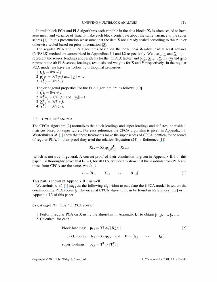
1 Perform regular PCA on X using the algorithm in Appendix I.1 to obtain t1, t2, …, ti, ….2 Calculate, for each i,

block loadings: pb�i � XTb�iti�XT

b�iti 2�block scores: tb�i � Xb�ipb�i and Ti � �t1�i � � � tB�i�

super loadings: pT �i � TTi ti�TT

i ti

UNIFYING MULTIBLOCK ANALYSIS 717

Copyright 2001 John Wiley & Sons, Ltd. J. Chemometrics 2001; 15: 715–742

3 Deflate residuals:

Xb�i�1 � I � titTi �tT

i ti�Xb�i

In this CPCA algorithm no NIPALS iterations are involved except for the calculation of regularPCA scores. This algorithm is advantageous since it makes use of regular PCA in the calculation.

Cheng and McAvoy [6] propose an MBPCA algorithm that is also calculated from the regular PCAmodel. Instead of using the scores from regular PCA, the MBPCA algorithm uses the loadings fromregular PCA, which is summarized as follows.

MBPCA algorithm based on PCA loadings

1 Scale X similarly to that of Appendix I.1. Set X1 = X and i = 1.2 Perform regular PCA on Xi based on the algorithm in Appendix I.1 to obtain the first loadings

pi1. Divide each pi1 into blocks:

pTi1� �pT

1�ipT

2�i� � � pT

B�i�

in the same way as X is divided.3 Calculate, for each b,

block scores: tb�i � Xb�ipb�i

block loadings: pb�i � XTb�itb�i�tT

b�itb�i

4 Deflate residuals:

Xb�i�1 � Xb�i � tb�ipTb�i

Form

Xi�1 � �X1�i�1 � � � XB�i�1�and return to step 2.

Note that in MBPCA neither tb,i nor pb,i is normalized. Since the (super) loading pi1 is normalized,tb,i is uniquely determined and so is pb,i. The MBPCA algorithm deflates residuals based on the blockscores, which makes the block scores mutually orthogonal. This procedure is analogous to that ofMBPLSb [4].

2.3. MBPLST and MBPLSb

The MBPLST algorithm [7] normalizes the block weights and super weights and deflates the residualsbased on super scores. It is given in Appendix I.4 for easy reference. The super scores of MBPLST areidentical to the scores of regular PLS with properly scaled data [1], but the proof in Reference [1] isincorrect. We show in Appendix II.2 that the MBPLST super scores and residuals are the same as thePLS scores and residuals for each factor; that is,

tT �i � ti

ui � ui

Xi � �X1�i � � � XB�i�Yi � Yi

718 S. J. QIN, S. VALLE AND M. J. PIOVOSO

Copyright 2001 John Wiley & Sons, Ltd. J. Chemometrics 2001; 15: 715–742

As a result, Westerhuis et al. [1] suggest using regular PLS scores to calculate the weights andloadings for MBPLST, which is summarized as follows.

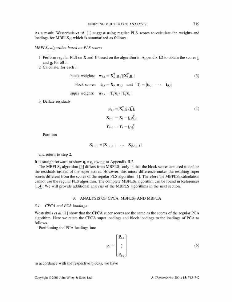
MBPLST algorithm based on PLS scores

1 Perform regular PLS on X and Y based on the algorithm in Appendix I.2 to obtain the scores tiand ui for all i.

2 Calculate, for each i,

block weights: wb�i � XTb�iui�XT

b�iui 3�block scores: tb�i � Xb�iwb�i and Ti � �tb�i � � � tB�i�

super weights: wT �i � TTi ui�TT

i ui3 Deflate residuals:

pb�i � XTb�iti�tT

i ti 4�

Xi�1 � Xi � tipTb�i

Yi�1 � Yi � tiqTi

Partition

Xi � 1 = [X1,i � 1 … XB,i � 1]

and return to step 2.

It is straightforward to show qi = qi owing to Appendix II.2.The MBPLSb algorithm [4] differs from MBPLST only in that the block scores are used to deflate

the residuals instead of the super scores. However, this minor difference makes the resulting superscores different from the scores of the regular PLS algorithm [1]. Therefore the MBPLSb calculationcannot use the regular PLS algorithm. The complete MBPLSb algorithm can be found in References[1,4]. We will provide additional analysis of the MBPLS algorithms in the next section.

3. ANALYSIS OF CPCA, MBPLST AND MBPCA

3.1. CPCA and PCA loadings

Westerhuis et al. [1] show that the CPCA super scores are the same as the scores of the regular PCAalgorithm. Here we relate the CPCA super loadings and block loadings to the loadings of PCA asfollows.

Partitioning the PCA loadings into

pi�

p1�i

���

pB�i

���������� 5�

in accordance with the respective blocks, we have

UNIFYING MULTIBLOCK ANALYSIS 719

Copyright 2001 John Wiley & Sons, Ltd. J. Chemometrics 2001; 15: 715–742

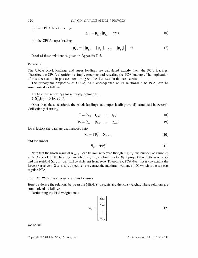
(i) the CPCA block loadingspb�i � p

b�i�p

b�i �b� i 6�

(ii) the CPCA super loadings

pTT �i � p

1�i p

2�i � � � p

B�i

� �i 7�

Proof of these relations is given in Appendix II.3.

Remark 1

The CPCA block loadings and super loadings are calculated exactly from the PCA loadings.Therefore the CPCA algorithm is simply grouping and rescaling the PCA loadings. The implicationof this observation in process monitoring will be discussed in the next section.

The orthogonal properties of CPCA, as a consequence of its relationship to PCA, can besummarized as follows.

1 The super scores tT,i are mutually orthogonal.2 XT

b�itT �j � 0 for i � j.

Other than these relations, the block loadings and super loading are all correlated in general.Collectively denoting

T � �tT �1 tT �2 � � � tT �a� 8�Pb � �pb�1 pb�2 � � � pb�a� 9�

for a factors the data are decomposed into

Xb � TPTb � Xb�a�1 10�

and the model Xb � TPTb 11�

Note that the block residual Xb,a � 1 can be non-zero even though a mb, the number of variablesin the Xb block. In the limiting case where mb = 1, a column vector Xb is projected onto the scores tT,i,and the residual Xb,a � 1 can still be different from zero. Therefore CPCA does not try to extract thelargest variance in Xb; its sole objective is to extract the maximum variance in X, which is the same asregular PCA.

3.2. MBPLST and PLS weights and loadings

Here we derive the relations between the MBPLST weights and the PLS weights. These relations aresummarized as follows.

Partitioning the PLS weights into

wi �

w1�i

w2�i

���

wB�i

��������

�������� 12�

we obtain

720 S. J. QIN, S. VALLE AND M. J. PIOVOSO

Copyright 2001 John Wiley & Sons, Ltd. J. Chemometrics 2001; 15: 715–742

(i) the MBPLST block weightswb�i � wb�i�wb�i �b� i 13�

(ii) the MBPLST super weights

wTT �i � w1�i � � � wB�i

� � �i 14�(iii) the MBPLST block loadings

pb�i � pb�i

where pb,i is the corresponding block in the PLS loadings pi

(iv) qi = qi. Proof of these relations is given in Appendix II.4.

Remark 2

The MBPLST block loadings, block weights and super weights are calculated exactly from theloadings and weights of regular PLS. Therefore the MBPLST algorithm is simply grouping andrescaling the PLS loadings and weights. The implication of this observation in terms of its use inprocess monitoring will be explored in the next section.

Owing to this equivalence, it is straightforward to obtain the following orthogonal properties ofMBPLST.

1 The super scores tT,i are mutually orthogonal.2 XT

b�itT �j � 0 for i � j.3 YT

i tT �j � 0 for i � j.

No other orthogonality can be obtained in terms of the MBPLST weights and block scores.Similarly to CPCA, MBPLST decomposes the block data into

Xb � TPTb � Xb�a�1 15�

Y � TQT � Ya�1 16�where

Q � �q1 � � � qa�In the limiting case of mb = 1, i.e. only one variable in a block, the MBPLST algorithm still projectsthis Xb into a number of dimensions, and the residual Xb,a � 1 can still be non-zero. Therefore theobjective function of MBPLST is the same as that of PLS, paying no attention to deflating blockresiduals.

3.3. MBPCA and MBPLSb

A common feature between MBPCA and MBPLSb is that the block scores are used in deflating theresidual matrices. This treatment makes MBPCA and MBPLSb scores different from those of PCAand PLS respectively [1]. However, these algorithms achieve orthogonality in the block scores, whichis summarized as follows.

1 In MBPCA the block scores

tTb�itb�j � 0 �i �� j

UNIFYING MULTIBLOCK ANALYSIS 721

Copyright 2001 John Wiley & Sons, Ltd. J. Chemometrics 2001; 15: 715–742

and the block loadings

pTb�ipb�j � 0 �i �� j

2 In MBPLSb the block scores

tTb�itb�j � 0 �i �� j

Proof of these relations is given in Appendix II.5.

4. MULTIBLOCK PLS AND CPCA FOR PROCESS MONITORING

4.1. Monitoring and diagnosis based on SPE

Multiblock PLS and PCA algorithms have been used for process monitoring and diagnosis [3,6–9].Owing to the equivalence between CPCA and PCA and that between MBPLST and PLS, we exploreways to use these algorithms for decentralized process monitoring and diagnosis. We assume that lprincipal components are used in CPCA or PCA with the PCA loadings as �P � P�, where P ∈�M � l and � P � �M�M�l�. We denote the principal eigenvalues of XTX as � = diag{�1,…,�l} andthe residual eigenvalues as � � diag��l�1� � � � � �M�. The loading matrices can be further partitionedbased on blocking:

P � P1

���

PB

����������� P �

P1

���

PB

�������� 17�

In PCA, P and P are orthogonal but Pb and Pb are not.A decentralized multiblock monitoring approach detects and diagnoses a fault using the block

squared prediction error (SPE) and block Hotelling’s T2 statistic in conjunction with the super SPEand super T2. For a new sample

xT � �xT1 � � � xT

B� 18�

we denote the CPCA or MBPLST prediction as �x � ��xT1 � � � �xT

B�. The block SPE is

SPEb � xb � �xb2 � xb2 19�

where xb � xb � �xb.If we use regular PCA or PLS for monitoring, the SPE for all variables is

SPE � x � �x2 � x2 � xb2 20�

where

xT � xT1 � � � xT

B

� � 21�

The confidence limit for SPE is well defined in Reference [11]. According to Equation (1), theresiduals from CPCA and MBPLST are identical to the residuals from PCA and PLS respectively.

722 S. J. QIN, S. VALLE AND M. J. PIOVOSO

Copyright 2001 John Wiley & Sons, Ltd. J. Chemometrics 2001; 15: 715–742

Therefore, from Equations (19) and (20),

SPE ��B

b�1

SPEb 22�

Consequently, the CPCA- and MBPLS-based monitoring is simply grouping the contributions to theSPE of PCA and PLS in terms of blocks. Furthermore, one can calculate the contribution to SPEb fromthe kth variable in the bth block as

SPEb�k � xb�k � �xb�k�2 � x2b�k 23�

and use it to further localize variables most affected by the fault. From Equation (19) we obtain

SPEb ��mb

k�1

SPEb�k

In order to use SPEb for fault detection and identification, it is desirable to derive a confidence limitfor it. Since SPEb is a quadratic form of a multivariate normal vector x, we can derive its confidencelimit using the result of Box [12]. Based on first and second moments of SPEb, it is easy to show thatSPEb is distributed approximately as gb�

2(hb), where

gSPEb � tr PT

b Pb �� �2

� ��tr PT

b Pb �� �

� tr Pb � PT

b

� �2� ��

tr Pb � PT

b

� �24�

hSPEb � tr PT

b Pb �� �� �2�

tr PTb Pb �� �2

� �� tr Pb

� PTb

� �� �2�tr Pb

� PTb

� �2� �

25�

and � � diag �a�1� � � � � �M

� �. Therefore the confidence limit for SPEb is �2

b � gSPEb �2

�hSPEb � for a

given confidence 1��. Nomikos and MacGregor [13] discussed this approach for the derivation ofthe SPE control limit. A Banferroni adjustment is needed between the limits of SPE and SPEb.

If SPEb � �2b, the variables in the bth block are normal or not affected by the fault. Otherwise, a

fault has occurred in the bth block. The decentralized monitoring procedure based on CPCA andMBPLST can be summarized as follows.

1 Use PCA (or PLS) to model the data X (and Y) which are properly scaled for each block.Calculate SPE, SPEb and SPEb,k for a new sample.

2 If SPE is out of limit, a fault is detected.3 If, further, SPEb is out of limit, then the bth block is affected by the fault.4 If, further, SPEb,k is large compared to others in the same block, then the kth variable in the bth

block is heavily affected by the fault.

The SPEb and SPEb,k can be plotted as contribution plots as in regular PCA and PLS monitoring.Note that the contribution plot approach only indicates which variables are most affected by the fault,which are not necessarily the causes of the fault. Counter-examples are given in Reference [14]. Notefurther that MacGregor et al. [8] discussed the use of SPEb for monitoring, but no confidence limitswere derived.

UNIFYING MULTIBLOCK ANALYSIS 723

Copyright 2001 John Wiley & Sons, Ltd. J. Chemometrics 2001; 15: 715–742

4.2. Monitoring and diagnosis based on T2

The block Hotelling’s T2 statistic can be calculated as

T2b � tT

b��1b tb

where �b is the covariance matrix of tb. Since tb (b = 1, …, B) in CPCA and MBPLS are correlated,�b is no longer diagonal and can even be singular. If �b is singular, which is possible for CPCA andMBPLS, a pseudoinverse of �b should be used instead [15]:

T2b � tT

b��b tb 26�

It is easy to show that the confidence limit for T2b is �2

�lb� for a given confidence 1��, where lb is therank of �b. To use the super scores for fault detection, the Hotelling’s T 2 is

T2 � tTT�

�1T tT

Since the super scores of CPCA are identical to the scores of PCA, and the super scores of MBPLST

are identical to the scores of PLS,

T2 � tT��1t � xTP��1PTx ��a

i�1

�Mk�1

pki

xk

� �2��i 27�

for which the confidence limit is well established [16]. Note that there is no apparent relation betweenT2 and T2

b .The contribution to the T 2 index defined in Reference [17] is based on each principal component,

which does not give an overall contribution of each variable. To overcome this problem, Nomikos[18] rewrites Equation (27) as

T2 ��Mk�1

tT��1pkxk

where pk is the kth row of P, then defines

tT��1pkxk

as the contribution of kth variable. Note that this approximation is not a symmetric treatment of the tscore vector. As a result, negative contributions arise [19,20].

In this paper we provide a new definition of variable contribution and block contribution to T2

which avoids the aforementioned problems. Rewrite Equation (27) as

T2 � xTP��1PTx � ��1�2PTx2 ��B

b�1

��1�2PTb xb

����������

2

28�

where Pb is as defined in Equation (17).

724 S. J. QIN, S. VALLE AND M. J. PIOVOSO

Copyright 2001 John Wiley & Sons, Ltd. J. Chemometrics 2001; 15: 715–742

We define block contributions as

T2b � ��1�2PT

b xb2 ��mb

k�1

��1�2pb�k

xb�k

����������

2

29�

and the contribution of the kth variable in the bth block as

T2b�k � ��1�2p

b�kxb�k2 �

�a

i�1

p2b�k�ix

2b�k��i �

�a

i�1

T2b�k�i��i

where

PTb � �p

b�1p

b�2� � � p

b�mb�

and

T2b�k�i � p2

b�k�ix2b�k

is the contribution of the ith component of the kth variable in the bth block, which is defined inReference [17]. Since, in practice, one is mainly interested in the contribution of each variable or eachblock, T2

b�k and Tb are more convenient than T2b�k�i.

To obtain the control limit for T2b in Equation (29), the same results as in Reference [12] can be

applied, since T2b is in quadratic form. Under normal conditions,

T2b � gT

b�2�hT

b � � �2b

with confidence 1��, where

gTb � tr�SbPb�

�1PTb �2��tr�SbPb�

�1PTb�

hTb � tr�SbPb�

�1PTb��2�tr�SbPb�

�1PTb �2�

and Sb = cov(xb).The control limits �2

b b � 1� 2� � � �B� may be used as an indication of out-of-control blocks.Contributing variables in the out-of-control blocks can be further examined based on T2

b�k . The controllimit for T2

b�k can be derived similarly to that of T2b by assuming a normal distribution for xb,k.

Similarly to the SPE-based monitoring, the monitoring and diagnosis based on T2 and T2b can be

summarized as follows.

1 Use PCA (or PLS) to model the data X (and Y) which are properly scaled for each block.Calculate T2�T2

b and T2b�k for a new sample.

2 If T2 is out of limit, a fault is detected which violates the T 2 index.3 If, further, T2

b is out of limit, then the bth block is affected by the fault.4 If, further, T2

b�k is large compared to others in the same block, then the kth variable in the bthblock is heavily affected by the fault, which indicates a potential cause of the fault.

Note that blocking the variables plays an important role in these monitoring schemes. It is thereforeimportant to block or group the variables based on process knowledge such as different processgroups or units.

A comment on the scaling of the process variables is in order. Westerhuis et al. [1] suggest scalingthe variance of each variable based on the number of variables in that block. This scaling scheme puts

UNIFYING MULTIBLOCK ANALYSIS 725

Copyright 2001 John Wiley & Sons, Ltd. J. Chemometrics 2001; 15: 715–742

equal weight on each block, but it could artificially overweight blocks that have fewer variables. If thenumber of variables in each block is roughly equal, this scaling scheme is not much different from theregular zero-mean and unit-variance scaling.

5. DECENTRALIZED MONITORING OF A POLYESTER FILM PROCESS

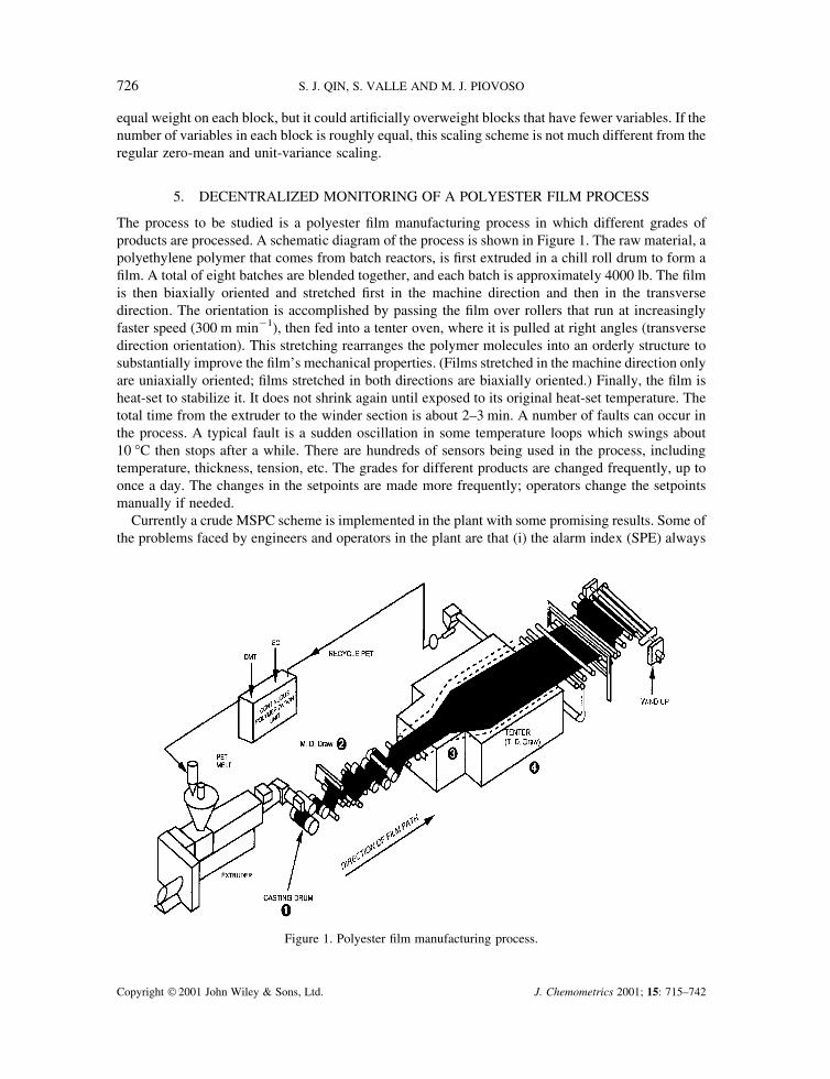
The process to be studied is a polyester film manufacturing process in which different grades ofproducts are processed. A schematic diagram of the process is shown in Figure 1. The raw material, apolyethylene polymer that comes from batch reactors, is first extruded in a chill roll drum to form afilm. A total of eight batches are blended together, and each batch is approximately 4000 lb. The filmis then biaxially oriented and stretched first in the machine direction and then in the transversedirection. The orientation is accomplished by passing the film over rollers that run at increasinglyfaster speed (300 m min�1), then fed into a tenter oven, where it is pulled at right angles (transversedirection orientation). This stretching rearranges the polymer molecules into an orderly structure tosubstantially improve the film’s mechanical properties. (Films stretched in the machine direction onlyare uniaxially oriented; films stretched in both directions are biaxially oriented.) Finally, the film isheat-set to stabilize it. It does not shrink again until exposed to its original heat-set temperature. Thetotal time from the extruder to the winder section is about 2–3 min. A number of faults can occur inthe process. A typical fault is a sudden oscillation in some temperature loops which swings about10 °C then stops after a while. There are hundreds of sensors being used in the process, includingtemperature, thickness, tension, etc. The grades for different products are changed frequently, up toonce a day. The changes in the setpoints are made more frequently; operators change the setpointsmanually if needed.

Currently a crude MSPC scheme is implemented in the plant with some promising results. Some ofthe problems faced by engineers and operators in the plant are that (i) the alarm index (SPE) always

Figure 1. Polyester film manufacturing process.

726 S. J. QIN, S. VALLE AND M. J. PIOVOSO

Copyright 2001 John Wiley & Sons, Ltd. J. Chemometrics 2001; 15: 715–742

exceeds limits and (ii) the contribution plots used to identify root causes often indicate multiplesuspects, which makes it difficult to identify the real fault. Also, the contribution plot as in Reference[17] does not have a confidence limit, making it difficult to determine what is abnormal. It is not untilrecently that control limits on contribution plots are discussed [22]. Multiple grades of products aremodeled with only one MSPC model with mean adjustment, and obvious clusters of different gradesare visible in an MSPC plot.

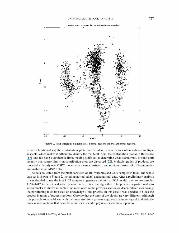
The data collected from the plant consisted of 103 variables and 2879 samples in total. The wholedata set is shown in Figure 2, including normal (dots) and abnormal data. After a preliminary analysisit was decided to use the first 1167 samples to generate the normal PCA model, then to use samples1168–1417 to detect and identify new faults to test the algorithm. The process is partitioned intoseven blocks as shown in Table I. As mentioned in the previous section on decentralized monitoring,the partitioning must be based on knowledge of the process. In this case it was decided to block theprocess in terms of process sections. Observe that the sizes of the blocks are very different. Althoughit is possible to have blocks with the same size, for a process engineer it is more logical to divide theprocess into sections that describe a unit or a specific physical or chemical operation.

Figure 2. Four different clusters: dots, normal region; others, abnormal regions.

UNIFYING MULTIBLOCK ANALYSIS 727

Copyright 2001 John Wiley & Sons, Ltd. J. Chemometrics 2001; 15: 715–742

Table I. Polyester film manufacturing process variables divided intoblocks

Block number Process section Variables in each block

1 Drying zone 1–92 Extrusion zone 10–293 Melt pipes zone 1 30–404 Melt pipes zone 2 41–525 Die zone 53–616 Casting zone 62–777 Tenter zone 78–103

Figure 3. SPE and T2 for the whole process in standard MSPC monitoring.

728 S. J. QIN, S. VALLE AND M. J. PIOVOSO

Copyright 2001 John Wiley & Sons, Ltd. J. Chemometrics 2001; 15: 715–742

Trying to identify the variables responsible for the out-of-control situation using contribution plotsis a difficult task, as is shown in Figure 3 when a standard PCA model is applied to all variables. InFigure 3, variable 28 is the one that is contributing most to the out-of-control situation, but the SPEand T2 do not agree for the other variables. Also observe how difficult is to define which variable isresponsible for the out-of-control situation, since no control limits are available in the contributionplots and many variables are contributing at the same magnitude.

If the process is divided into blocks as defined in Table I, it is possible to apply decentralizedmonitoring to identify which block contains the disturbance. The SPEb is calculated for each block asshown in Figure 4, and it is found that the fault is located mainly in block 2. The SPE limit in block 3is also violated, but its value is not as high as in block 2.

To identify the fault, a hierarchical contribution plot is shown in Figure 5. It is found from the topplot that blocks 2 and 3 are the blocks where the fault is located according to SPE. The bottom plot inFigure 5 shows the contribution plot for the SPE index for block 2, which clearly identifies that

Figure 4. SPE for each block with control limits in decentralized monitoring.

UNIFYING MULTIBLOCK ANALYSIS 729

Copyright 2001 John Wiley & Sons, Ltd. J. Chemometrics 2001; 15: 715–742

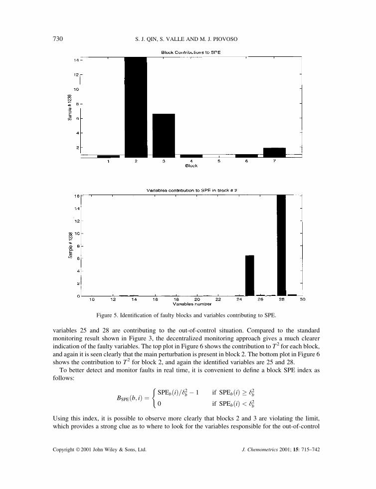
variables 25 and 28 are contributing to the out-of-control situation. Compared to the standardmonitoring result shown in Figure 3, the decentralized monitoring approach gives a much clearerindication of the faulty variables. The top plot in Figure 6 shows the contribution to T 2 for each block,and again it is seen clearly that the main perturbation is present in block 2. The bottom plot in Figure 6shows the contribution to T2 for block 2, and again the identified variables are 25 and 28.

To better detect and monitor faults in real time, it is convenient to define a block SPE index asfollows:

BSPEb� i� � SPEbi���2b � 1 if SPEbi� �2

b

0 if SPEbi� �2b

�

Using this index, it is possible to observe more clearly that blocks 2 and 3 are violating the limit,which provides a strong clue as to where to look for the variables responsible for the out-of-control

Figure 5. Identification of faulty blocks and variables contributing to SPE.

730 S. J. QIN, S. VALLE AND M. J. PIOVOSO

Copyright 2001 John Wiley & Sons, Ltd. J. Chemometrics 2001; 15: 715–742

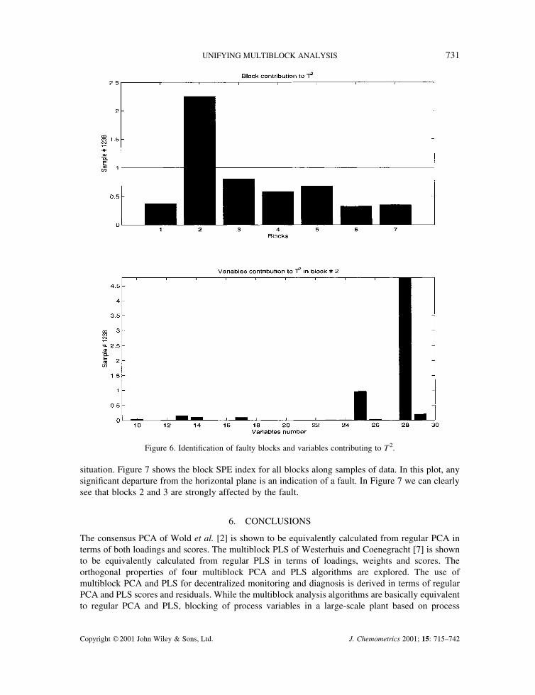
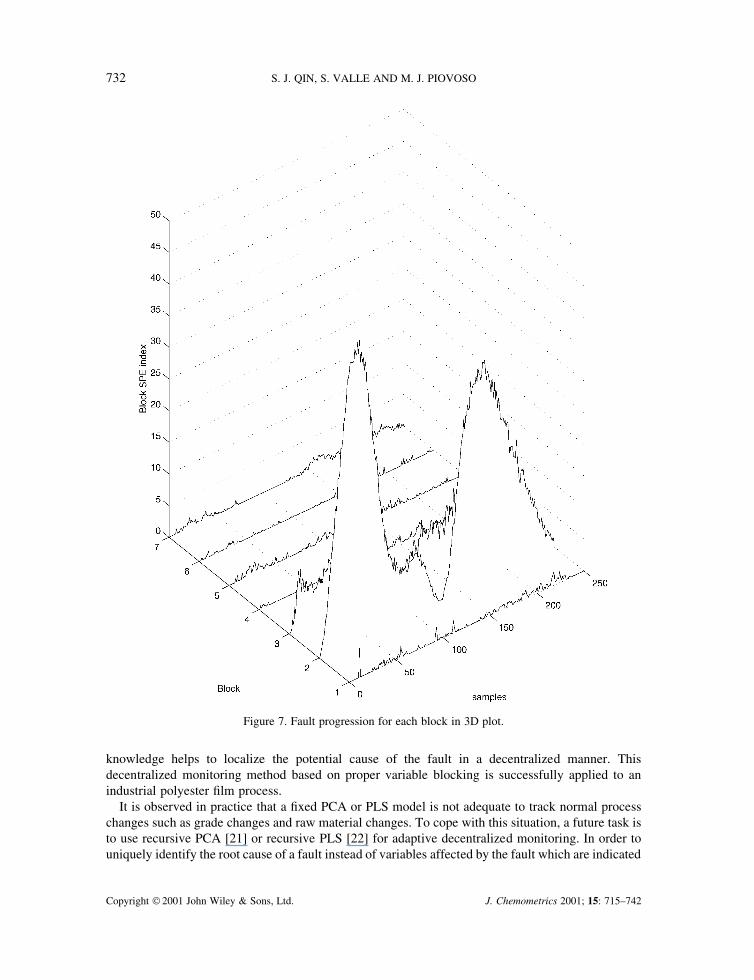
situation. Figure 7 shows the block SPE index for all blocks along samples of data. In this plot, anysignificant departure from the horizontal plane is an indication of a fault. In Figure 7 we can clearlysee that blocks 2 and 3 are strongly affected by the fault.

6. CONCLUSIONS

The consensus PCA of Wold et al. [2] is shown to be equivalently calculated from regular PCA interms of both loadings and scores. The multiblock PLS of Westerhuis and Coenegracht [7] is shownto be equivalently calculated from regular PLS in terms of loadings, weights and scores. Theorthogonal properties of four multiblock PCA and PLS algorithms are explored. The use ofmultiblock PCA and PLS for decentralized monitoring and diagnosis is derived in terms of regularPCA and PLS scores and residuals. While the multiblock analysis algorithms are basically equivalentto regular PCA and PLS, blocking of process variables in a large-scale plant based on process

Figure 6. Identification of faulty blocks and variables contributing to T2.

UNIFYING MULTIBLOCK ANALYSIS 731

Copyright 2001 John Wiley & Sons, Ltd. J. Chemometrics 2001; 15: 715–742

knowledge helps to localize the potential cause of the fault in a decentralized manner. Thisdecentralized monitoring method based on proper variable blocking is successfully applied to anindustrial polyester film process.

It is observed in practice that a fixed PCA or PLS model is not adequate to track normal processchanges such as grade changes and raw material changes. To cope with this situation, a future task isto use recursive PCA [21] or recursive PLS [22] for adaptive decentralized monitoring. In order touniquely identify the root cause of a fault instead of variables affected by the fault which are indicated

Figure 7. Fault progression for each block in 3D plot.

732 S. J. QIN, S. VALLE AND M. J. PIOVOSO

Copyright 2001 John Wiley & Sons, Ltd. J. Chemometrics 2001; 15: 715–742

by contributions, fault identification indices [23] can be developed in the context of decentralizedmonitoring. Finally, alternative methods for partitioning the data, such as multiscale monitoringapproaches [24,25], could be integrated in the decentralized monitoring approach to provide flexiblepartition and interpretation of information contained in the process data.

ACKNOWLEDGEMENTS

Financial support from the National Science Foundation under CTS-9814340, Texas HigherEducation Coordinating Board, DuPont through a DuPont Young Professor Grant, Consejo Nacionalde Ciencia y Tecnologıa (CONACyT) and Instituto Tecnologico de Durango (ITD) is gratefullyacknowledged. Comments from one anonymous reviewer of this paper are greatly appreciated whichenhanced our results.

APPENDIX I

I.1. Regular PCA algorithm

1. Scale X = [X1 X2 … XB] to zero mean and variance of 1/mb in each variable, or use someother scaling method. Set X1 = X and i = 1.

2. Choose a start ti and iterate the following equations until convergence of ti:

pi� XT

i ti�XTi ti

ti � Xipi

3. Residual deflation:

Xi�1 � Xi � tipTi

Set i : = i � 1 and return to step 2.

I.2. Regular PLS algorithm

1. Scale X = [X1 X2 … XB] similarly to the regular PCA algorithm in Appendix I.1 and scaleY to zero mean and unit variance. Set X1 = X, Y1 = Y and i = 1.

2. Choose a start ui and iterate the following equations until convergence of ti:

wi � XTi ui�XT

i uiti � Xiwi

qi� YT

i ti�tTi ti

ui � Yiqi�qT

iq

i

3. Residual deflation:

pi� XT

i ti�tTi ti

Xi�1 � Xi � tipTi

Yi�1 � Yi � tiqTi

UNIFYING MULTIBLOCK ANALYSIS 733

Copyright 2001 John Wiley & Sons, Ltd. J. Chemometrics 2001; 15: 715–742

Set i : = i � 1 and return to step 2.

Note that qi is not normalized to make the inner regression coefficient bi � uTi ti�tT

i ti � 1.

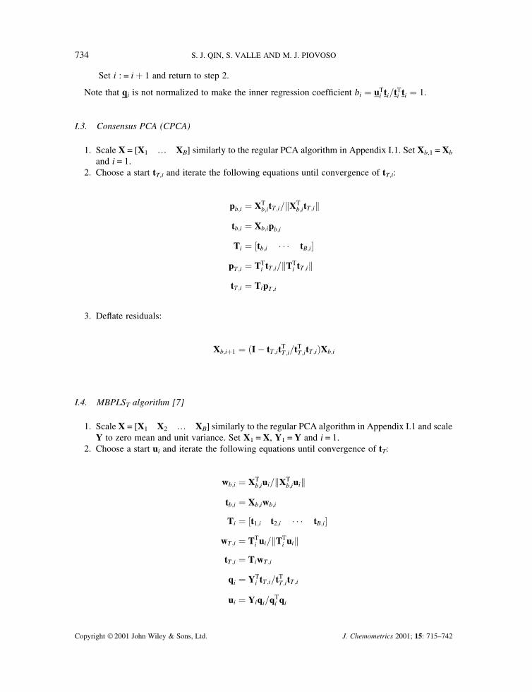
I.3. Consensus PCA (CPCA)

1. Scale X = [X1 … XB] similarly to the regular PCA algorithm in Appendix I.1. Set Xb,1 = Xb

and i = 1.2. Choose a start tT,i and iterate the following equations until convergence of tT,i:

pb�i � XTb�itT �i�XT

b�itT �itb�i � Xb�ipb�i

Ti � �tb�i � � � tB�i�pT �i � TT

i tT �i�TTi tT �i

tT �i � TipT �i

3. Deflate residuals:

Xb�i�1 � I � tT �itTT �i�tT

T �itT �i�Xb�i

I.4. MBPLST algorithm [7]

1. Scale X = [X1 X2 … XB] similarly to the regular PCA algorithm in Appendix I.1 and scaleY to zero mean and unit variance. Set X1 = X, Y1 = Y and i = 1.

2. Choose a start ui and iterate the following equations until convergence of tT:

wb�i � XTb�iui�XT

b�iuitb�i � Xb�iwb�i

Ti � �t1�i t2�i � � � tB�i�wT �i � TT

i ui�TTi ui

tT �i � TiwT �i

qi � YTi tT �i�tT

T �itT �i

ui � Yiqi�qTi qi

734 S. J. QIN, S. VALLE AND M. J. PIOVOSO

Copyright 2001 John Wiley & Sons, Ltd. J. Chemometrics 2001; 15: 715–742

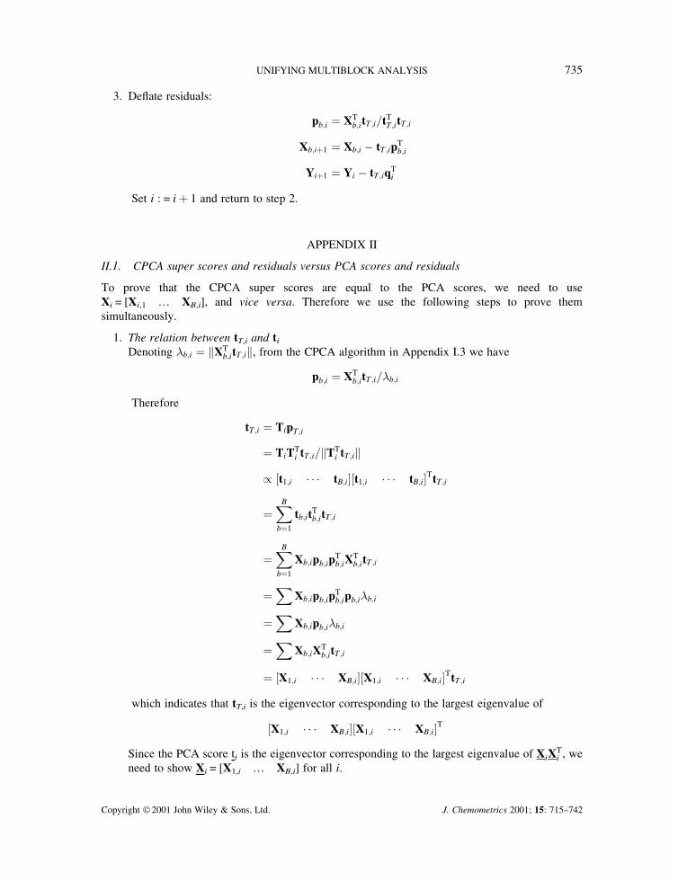
3. Deflate residuals:

pb�i � XTb�itT �i�tT

T �itT �i

Xb�i�1 � Xb�i � tT �ipTb�i

Yi�1 � Yi � tT �iqTi

Set i : = i � 1 and return to step 2.

APPENDIX II

II.1. CPCA super scores and residuals versus PCA scores and residuals

To prove that the CPCA super scores are equal to the PCA scores, we need to useXi = [Xi,1 … XB,i], and vice versa. Therefore we use the following steps to prove themsimultaneously.

1. The relation between tT,i and ti

Denoting �b�i � XTb�itT �i, from the CPCA algorithm in Appendix I.3 we have

pb�i � XTb�itT �i��b�i

Therefore

tT �i � TipT �i

� TiTTi tT �i�TT

i tT �i

� �t1�i � � � tB�i��t1�i � � � tB�i�TtT �i

��B

b�1

tb�itTb�itT �i

��B

b�1

Xb�ipb�ipTb�iX

Tb�itT �i

��

Xb�ipb�ipTb�ipb�i�b�i

��

Xb�ipb�i�b�i

��

Xb�iXTb�itT �i

� �X1�i � � � XB�i��X1�i � � � XB�i�TtT �i

which indicates that tT,i is the eigenvector corresponding to the largest eigenvalue of

�X1�i � � � XB�i��X1�i � � � XB�i�T

Since the PCA score ti is the eigenvector corresponding to the largest eigenvalue of XiXTi , we

need to show Xi = [X1,i … XB,i] for all i.

UNIFYING MULTIBLOCK ANALYSIS 735

Copyright 2001 John Wiley & Sons, Ltd. J. Chemometrics 2001; 15: 715–742

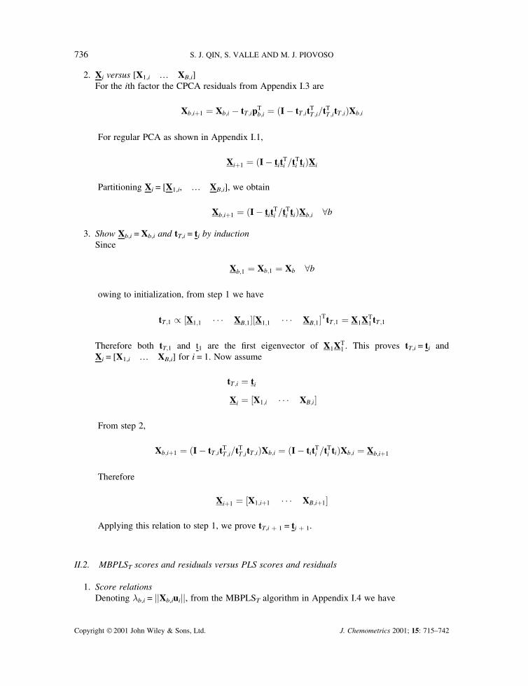
2. Xi versus [X1,i … XB,i]For the ith factor the CPCA residuals from Appendix I.3 are

Xb�i�1 � Xb�i � tT �ipTb�i � I � tT �itT

T �i�tTT �itT �i�Xb�i

For regular PCA as shown in Appendix I.1,

Xi�1 � I � titTi �tT

i ti�Xi

Partitioning Xi = [X1,i, … XB,i], we obtain

Xb�i�1 � I � titTi �tT

i ti�Xb�i �b

3. Show Xb,i = Xb,i and tT,i = ti by inductionSince

Xb�1 � Xb�1 � Xb �b

owing to initialization, from step 1 we have

tT �1 � �X1�1 � � � XB�1��X1�1 � � � XB�1�TtT �1 � X1XT1 tT �1

Therefore both tT,1 and t1 are the first eigenvector of X1XT1 . This proves tT,i = ti and

Xi = [X1,i … XB,i] for i = 1. Now assume

tT �i � ti

Xi � �X1�i � � � XB�i�

From step 2,

Xb�i�1 � I � tT �itTT �i�tT

T �itT �i�Xb�i � I � titTi �tT

i ti�Xb�i � Xb�i�1

Therefore

Xi�1 � �X1�i�1 � � � XB�i�1�

Applying this relation to step 1, we prove tT,i � 1 = ti � 1.

II.2. MBPLST scores and residuals versus PLS scores and residuals

1. Score relationsDenoting �b,i = ��Xb,iui��, from the MBPLST algorithm in Appendix I.4 we have

736 S. J. QIN, S. VALLE AND M. J. PIOVOSO

Copyright 2001 John Wiley & Sons, Ltd. J. Chemometrics 2001; 15: 715–742

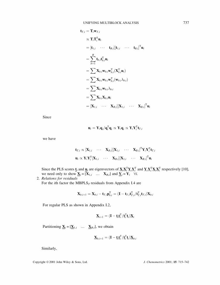
tT �i � TiwT �i

� TiTTi ui

� �t1�i � � � tB�i��t1�i � � � tB�i�Tui

��B

b�1

tb�itTb�iui

��

Xb�iwb�iwTb�iXT

b�iui�

��

Xb�iwb�iwTb�iwb�i�b�i�

��

Xb�iwb�i�b�i

��

Xb�iXb�iui

� �X1�i � � � XB�i��X1�i � � � XB�i�Tui

Since

ui � Yiqi�qTi qi � Yiqi � YiYT

i tT �i

we have

tT �i � �X1�i � � � XB�i��X1�i � � � XB�i�TYiYTi tT �i

ui � YiYTi �X1�i � � � XB�i��X1�i � � � XB�i�Tui

Since the PLS scores ti and ui are eigenvectors of XiXTi YiY

Ti and YiY

Ti XiX

Ti respectively [10],

we need only to show Xi = [X1,i … XB,i] and Yi = Yi �i.2. Relations for residuals

For the ith factor the MBPLST residuals from Appendix I.4 are

Xb�i�1 � Xb�i � tT �ipTb�i � I � tT �itT

T �i�tTT �itT �i�Xb�i

For regular PLS as shown in Appendix I.2,

Xi�1 � I � titTi �tT

i ti�Xi

Partitioning Xi = [X1,i … XB,i], we obtain

Xb�i�1 � I � titTi �tT

i ti�Xb�i

Similarly,

UNIFYING MULTIBLOCK ANALYSIS 737

Copyright 2001 John Wiley & Sons, Ltd. J. Chemometrics 2001; 15: 715–742

Yi�1 � I � tT �itTT �i�tT

T �itT �i�Yi

Yi�1 � I � titTi �tT

i ti�Yi

3 Score and residual equivalence by inductionSince Xb,1 = Xb,1 = Xb and Y1 = Y1 = Y owing to initialization, from step 1 we have

tT �1 � X1XT1 Y1YT

1 tT �1

u1 � Y1YT1 X1XT

1 u1

Therefore both tT,1 and t1 are the first eigenvector of X1XT1 Y1YT

1 and both u1 and u1 are the firsteigenvector of Y1YT

1 X1XT1 . This proves

tT �1 � t1

u1 � u1

Now assume

tT �i � ti

ui � ui

Xi � �X1�i � � � XB�i�Yi � Yi

From step 2,

Xb�i�1 � I � tT �itTT �i�tT

T �itT �i�Xb�i � I � titTi �tT

i ti�Xb�i � Xb�i�1

Therefore

Xi�1 � �X1�i�1 � � � XB�i�1�

Similarly,

Yi�1 � I � titTi �tT

i ti�Yi � Yi�1

Applying these relations to step 1, we prove

tT �i�1 � ti�1

ui�1 � ui�1

II.3. Equivalence of CPCA loadings and PCA loadings

1. From PCA in Appendix I.1,

738 S. J. QIN, S. VALLE AND M. J. PIOVOSO

Copyright 2001 John Wiley & Sons, Ltd. J. Chemometrics 2001; 15: 715–742

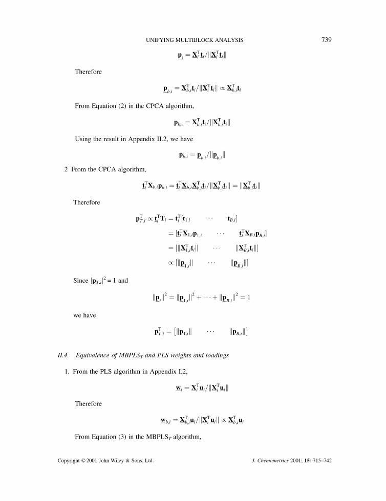
pi� XT

i ti�XTi ti

Therefore

pb�i

� XTb�iti�XT

i ti � XTb�iti

From Equation (2) in the CPCA algorithm,

pb�i � XTb�iti�XT

b�iti

Using the result in Appendix II.2, we have

pb�i � pb�i�p

b�i

2 From the CPCA algorithm,

tTi Xb�ipb�i � tT

i Xb�iXTb�iti�XT

b�iti � XTb�iti

Therefore

pTT �i � tT

i Ti � tTi �t1�i � � � tB�i�

� �tTi X1�ip1�i � � � tT

i XB�ipB�i�� �XT

1�iti � � � XTB�iti�

� �p1�i � � � p

B�i�

Since �pT,i�2 = 1 and

pi2 � p

1�i2 � � � � � p

B�i2 � 1

we have

pTT �i � p1�i � � � pB�i

� �II.4. Equivalence of MBPLST and PLS weights and loadings

1. From the PLS algorithm in Appendix I.2,

wi � XTi ui�XT

i ui

Therefore

wb�i � XTb�iui�XT

i ui � XTb�iui

From Equation (3) in the MBPLST algorithm,

UNIFYING MULTIBLOCK ANALYSIS 739

Copyright 2001 John Wiley & Sons, Ltd. J. Chemometrics 2001; 15: 715–742

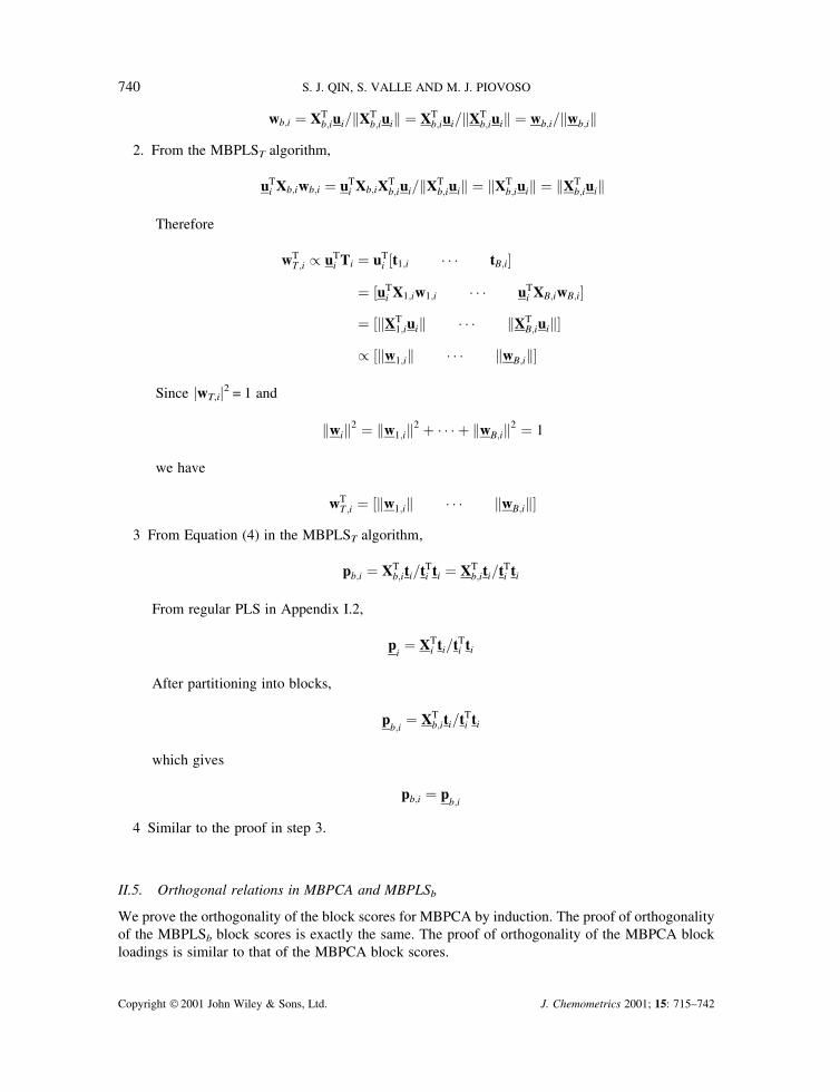
wb�i � XTb�iui�XT

b�iui � XTb�iui�XT

b�iui � wb�i�wb�i2. From the MBPLST algorithm,

uTi Xb�iwb�i � uT

i Xb�iXTb�iui�XT

b�iui � XTb�iui � XT

b�iui

Therefore

wTT �i � uT

i Ti � uTi �t1�i � � � tB�i�

� �uTi X1�iw1�i � � � uT

i XB�iwB�i�� �XT

1�iui � � � XTB�iui�

� �w1�i � � � wB�i�

Since �wT,i�2 = 1 and

wi2 � w1�i2 � � � � � wB�i2 � 1

we have

wTT �i � �w1�i � � � wB�i�

3 From Equation (4) in the MBPLST algorithm,

pb�i � XTb�iti�tT

i ti � XTb�iti�tT

i ti

From regular PLS in Appendix I.2,

pi� XT

i ti�tTi ti

After partitioning into blocks,

pb�i

� XTb�iti�tT

i ti

which gives

pb�i � pb�i

4 Similar to the proof in step 3.

II.5. Orthogonal relations in MBPCA and MBPLSb

We prove the orthogonality of the block scores for MBPCA by induction. The proof of orthogonalityof the MBPLSb block scores is exactly the same. The proof of orthogonality of the MBPCA blockloadings is similar to that of the MBPCA block scores.

740 S. J. QIN, S. VALLE AND M. J. PIOVOSO

Copyright 2001 John Wiley & Sons, Ltd. J. Chemometrics 2001; 15: 715–742

From the MBPCA algorithm described in Section 2.2,

tb�i�1 � Xb�i�1pb�i�1

� Xb�i � tb�ipTb�i�pb�i�1

Therefore, for j = i � 1,

tTb�itb�j � tT

b�itb�i�1

� tTb�iXb�i � tT

b�itb�ipTb�i�pb�i�1

� tTb�itb�ipT

b�i � tTb�itb�ipT

b�i�pb�i�1

� 0

Assuming tTb�itb�j � 0 for j = i � k, then

tb�i�k�1 � Xb�i�k�1pb�i�k�1

� I ��i�k

j�1

tb�jtTb�j�tT

b�jtb�j

� �Xb�ipb�i�k�1

tTb�itb�i�k�1 � tT

b�i � tTb�itb�itT

b�i�tTb�itb�i

� �Xb�ipb�i�k�1

� 0

which proves tTb�itb�j � 0 for i j. By symmetry,

tTb�itb�j � 0 for i � j

REFERENCES

1. Westerhuis JA, Kourti T, MacGregor JF. Analysis of multiblock and hierarchical PCA and PLS models. J.Chemometrics 1998; 12: 301–321.

2. Wold S, Hellberg S, Lundstedt T, Sjostrom M, Wold H. Proc. Symp. on PLS Model Building: Theory andApplications, 1987.

3. Wold S, Kettaneh N, Tjessem K. Hierarchical multiblock PLS and PC models for easier model interpretationand as an alternative to variable selection. J. Chemometrics 1996; 10: 463–482.

4. Wangen LE, Kowalski BR. A multiblock partial least squares algorithm for investigating complex chemicalsystems. J. Chemometrics 1988; 3: 3–20.

5. Slama CF. Multivariate statistical analysis of data from an industrial fluidized catalytic process using PCAand PLS. Master’s Thesis, McMaster University, 1991.

6. Cheng G, McAvoy TJ. Multi-block predictive monitoring of continuous processes. Proc. IFACADCHEM’97, Banff, 1997.

7. Westerhuis JA, Coenegracht PMJ. Multivariate modeling of the pharmaceutical two-step process of wetgranulation and tableting with multiblock partial least squares. J. Chemometrics 1997; 11: 379–392.

8. MacGregor JF, Jaeckle C, Kiparissides C, Koutodi M. Process monitoring and diagnosis by multiblock PLSmethods. AIChE J. 1994; 40: 826–828.

9. Kourti T, Nomikos P, MacGregor JF. Analysis, monitoring, and fault diagnosis of batch processes usingmulti-block and multi-way PLS. J. Process Control 1995; 5: 277–284.

10. Hoskuldsson A. PLS regression models. J. Chemometrics 1988; 2: 211–228.11. Jackson JE, Mudholkar GS. Control procedures for residuals associated with principal component analysis.

Technometrics 1979; 21: 341–349.12. Box GEP. Some theorems on quadratic forms applied in the study of analysis of variance problems, I. Effect

of inequality of variance in the one-way classification. Ann. Math. Statist. 1954; 25: 290–302.

UNIFYING MULTIBLOCK ANALYSIS 741

Copyright 2001 John Wiley & Sons, Ltd. J. Chemometrics 2001; 15: 715–742

13. Nomikos P, MacGregor JF. Multivariate SPC charts for monitoring batch processes. Technometrics 1995;37: 41–59.

14. Yue H, Qin SJ. Reconstruction-based fault identification using a combined index. Ind. Engng. Chem. Res.2000; in press.

15. Mardia KV. Mahalanobis distances and angles. In Multivariate Analysis— IV, Krishnaiah PR (ed.). North-Holland: Amsterdam, 1977; 495–511.

16. Jackson JE. A User’s Guide to Principal Components. Wiley-Interscience: New York, 1991.17. Miller P, Swanson RE, Heckler CF. Contribution plots: the missing link in multivariate quality control. Proc.

Fall Conf. of the ASQC and ASA, Milwaukee, WI, 1993.18. Nomikos P. Detection and diagnosis of abnormal batch operations based on multi-way principal component

analysis. ISA Trans. 1996; 35: 147–168.19. Kourti T, MacGregor JF. Multivariate SPC methods for process and product monitoring. J. Qual. Technol.

1996; 28: 409–428.20. Westerhuis JA, Gurden SP, Smilde AK. Generalized contribution plots in multivariate statistical process

monitoring. Chemometrics Intell. Lab. Syst. 2000; 51: 95–114.21. Li W, Yue H, Valle S, Qin J. Recursive PCA for adaptive process monitoring. J. Process Control 2000; 10:

471–486.22. Qin SJ. Recursive PLS algorithms for adaptive data modeling. Comput. Chem. 1998; 22: 503–514.23. Dunia R, Qin SJ. A unified geometric approach to process and sensor fault identification and reconstruction:

the unidimensional fault case. Comput. Chem. Engng 1998; 22: 927–943.24. Bakshi BR. Multiscale PCA with application to multivariate statistical process monitoring. AIChE J. 1998;

44: 1597–1610.25. Misra M, Yue H, Qin SJ. Multivariate process monitoring and fault diagnosis by multi-scale PCA. Proc.

AIChE Ann. Meet., Dallas, TX, 1999.26. Miller SM. Modelling and quality control strategies for batch cooling crystallizers. PhD Thesis, The

University of Texas at Austin, 1993.

742 S. J. QIN, S. VALLE AND M. J. PIOVOSO

Copyright 2001 John Wiley & Sons, Ltd. J. Chemometrics 2001; 15: 715–742