On subwavelength imaging of Maxwell’s fish eye lens

Fei Sun1 and Sailing He

1, 2

1 Centre for Optical and Electromagnetic Research, Zhejiang University

2 Department of Electromagnetic Engineering, School of Electrical Engineering,

RoyalInstitute of Technology, S-100 44 Stockholm, Sweden

AAAAbstractbstractbstractbstract

Both explicit analysis and FEM numerical simulation are used to analyze the field distribution of a

line current in the so-called Maxwell’s fish eye lens, which has been claimed recently to be able to

achieve perfect imaging [4]. We show that such a Maxwell’s fish eye lens cannot give perfect

imaging due to the fact that high order modes of the object field can hardly reach the image point

in the Maxwell’s fish eye. If only zero order mode is excited, a subwavelength image can be

achieved, however, its spot-size is larger than the spot size of the source field. The image

resolution is determined by the field spot size of the image corresponding to the zeroth order

component of the object field. Our explicit analysis consists very well with the FEM results for a

modified fish eye bounded with perfectly electrical conductor (PEC). Explicit condition is given

for achieving a subwavelength image. When this condition is not satisfied, a single line current

source may give multiple image spots.

1. Introduction

Maxwell’s fish eye was proposed by Maxwell in1854 [1]. Maxwell’s fish eye gives a good image

with equal light paths from the view point of geometry optics [1-3]. Recently, Leonhardt claimed

that Maxwell’s fish eye can give perfect imaging in wave optics and he modified the original fish

eye lens, which is infinitely large, so that the device becomes finite (bounded with a PEC

boundary) [4, 5]. Leonhardt gave an explicit solution with very small spot sizes of the object and

image fields for a modified fish eye with a line current source in the object point and a line current

drain at the image point [4]. However, this configuration is not practical for imaging. For example,

we don’t know beforehand the distribution of fluorescent points in bio imaging, and thus we

cannot determine where to put the active drains in order to achieve an image of excellent

resolution. Apparently this is not a conventional concept for imaging. In a conventional image, we

consider a very sharp field distribution (produced by some kind of source) and see if a lens can

give a very sharp field distribution at another space point (without any active drain). In this paper,

we study the subwavelength imaging (in a conventional sense) properties of the Maxwell’s fish

eye lens in wave optics. We show that perfect imaging can not be achieved due to the fact that

high order modes of the object field will decay quickly before reaching the image point in the

Maxwell’s fish eye. However, it can still give a subwavelength image and the image resolution is

determined by the image field spot size corresponding to the zeroth order component of the object

field. Both explicit analysis and FEM simulation are used and they consist very well.

2. Mode analysis for a line current in Maxwell’s fish eye

Maxwell’s fish eye has the following refraction index profile [2]:

0

2

0

2

1 ( / )

nn

r R=

+ (1)

where 0n and 0R are the refraction index constant and radius of the reference sphere,

respectively, and r is the distance between a space point and the center of Maxwell’s fish eye.

First we set a field source at the center of Maxwell’s fish eye. The Helmholtz equation for the field

(with a vacuum wave number 2

kc

ω πλ

= = ) in a cylindrical coordinate system whose origin is

located at the center of Maxwell’s fish eye in 2D space can be written as:

22 2

2 2

( ) ( )1 1( ) ( ) ( , )k k

k

E r E rr n k E r g r

r r r rθ

θ∂ ∂∂ + + =

∂ ∂ ∂ (2)

where ( , )g r θ is the source term and ( , ) 0g r θ = （ when 0r ≠ ). Through variables

separation ( ) ( ) ( )k rE r E r Eθ θ= and the following variable substitution:

2 2

0

2 2

0

( )r R

rr R

ζ −=+

(3)

2 2 2

0 0 (1 )R n k v v= + (4)

equation (2) becomes (we first consider space point 0r ≠ ):

22

20

Em Eθ

θθ∂ + =∂

(5)

2 22

2 2

( ) ( )(1 ) 2 [ (1 ) ] ( ) 0

1

r rr

E r E r mv v E rζ ζ

ζ ζ ζ∂ ∂− − + + − =

∂ ∂ − (6)

The solution of Eq. (5) can be expressed as ( ) imE e θθ θ = , where m is the mode order of angular

momentum. Equation (6) is the general Legendre equation, whose solution is a superposition of

the associated Legendre functions. Thus if we set a source at the origin in Maxwell’s fish eye

medium the general solution of the field is:

0

( ) [ ( ( )) ( ( ))]m m im

k m v m v

m

E r a P r b P r e θζ ζ+∞

== + −∑ (7)

Here we see that the field distribution in Maxwell’s fish eye medium can be expressed as a

superposition of different order modesm . 0m ≠ and 0m = represent the high order modes and

the zero order mode, respectively, and the high order modes correspond to high angular frequency

components. Different sources can excite different modes. If we set some kind of source (at the

center of Maxwell’s fish eye) that can only excite the zero order mode, the field distribution in

Maxwell’s fish eye can be written as:

0 0( ) ( ( )) ( ( ))k v vE r a P r b P rζ ζ= + − (8)

For a given vacuum wavelength λ , quadratic equation (4) for v gives two different values of v :

1v and 2v (satisfying 1 2 1v v+ = − ). Since 1( ) ( )v vP Pζ ζ− −= , expression (8) for the zero order

mode can be expressed as:

1 1 1 20 0( ) ( ) ( ) ( ) ( )k v v v vE r a P b P AE r BE rζ ζ= + − = + (9)

where

( ( )) ( ( ))( )

4sin( )

l

l l

l

iv

v v

v

l

P r e P rE r

v

πζ ζπ

− −= (l=1, 2) (10)

and0

1 24sin( ) 4sin( )

A Ba

v vπ π+ = ,

1 2

0

1 24sin( ) 4sin( )

iv ive A e B

bv v

π π

π π+ = − .

Leonhard has shown that a field distribution described by expression (10) has such properties

[4]:ln

( ) ~ , 02lv

rE r r

π→ ,

ln( ) ~ ,

2l

l

iv

v

rE r e r

π

π→ ∞ and 0

l

ikt

vE e dk+∞ −

−∞=∫ for 0t < .

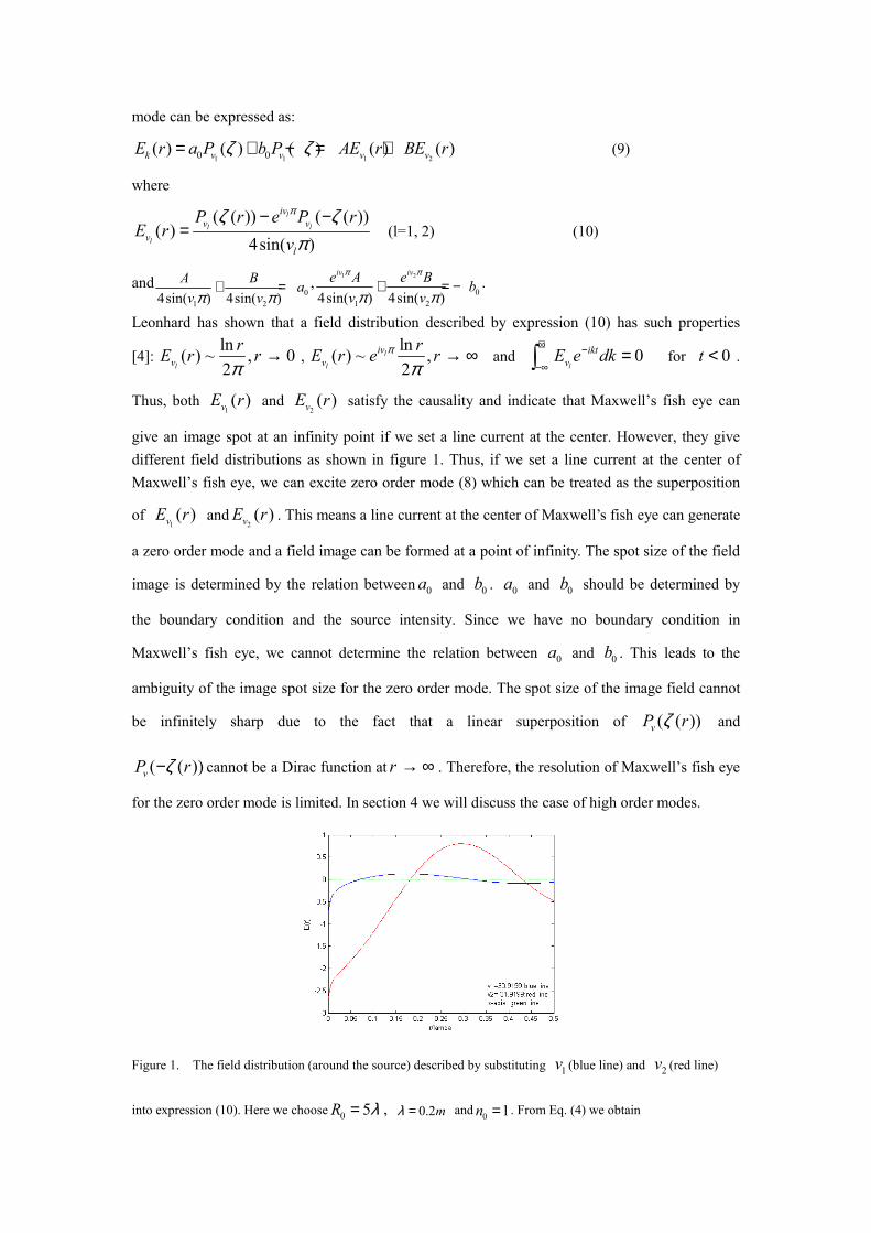
Thus, both 1( )vE r and

2( )vE r satisfy the causality and indicate that Maxwell’s fish eye can

give an image spot at an infinity point if we set a line current at the center. However, they give

different field distributions as shown in figure 1. Thus, if we set a line current at the center of

Maxwell’s fish eye, we can excite zero order mode (8) which can be treated as the superposition

of 1( )vE r and

2( )vE r . This means a line current at the center of Maxwell’s fish eye can generate

a zero order mode and a field image can be formed at a point of infinity. The spot size of the field

image is determined by the relation between 0a and 0b . 0a and 0b should be determined by

the boundary condition and the source intensity. Since we have no boundary condition in

Maxwell’s fish eye, we cannot determine the relation between 0a and 0b . This leads to the

ambiguity of the image spot size for the zero order mode. The spot size of the image field cannot

be infinitely sharp due to the fact that a linear superposition of ( ( ))vP rζ and

( ( ))vP rζ− cannot be a Dirac function at r → ∞ . Therefore, the resolution of Maxwell’s fish eye

for the zero order mode is limited. In section 4 we will discuss the case of high order modes.

Figure 1. The field distribution (around the source) described by substituting 1v (blue line) and 2v (red line)

into expression (10). Here we choose0 5R λ= , 0.2mλ = and

0 1n = . From Eq. (4) we obtain

130.9199v = and

2 -31.9199v = .

When the line current is not at the center of the Maxwell’s fish eye, we can use the following

Möbius transformation to calculate the field distribution [4]:

0( )z z

w z zz z∞

∞

−= −−

(11)

where*

01/z z∞ = − , 0z and z∞ are the positions for the line current and its image. By Möbius

transformation, we can obtain the field distribution when the line current is located at 0z in a 2D

Maxwell’s fish eye:

0 0( ) ( ( )) ( ( ))k v vE z a P z b P zξ ξ= + − (12)

where

2 2

0

2 2

0

| ( ) |( )

| ( ) |

w z Rz

w z Rξ −=

+ (13)

From equations (11) and (12), we can see 0a and 0b are independent of source position 0z .

However, the zero order mode field produced by a line current is different when the line current is

located at different places (i.e., different 0z ) of Maxwell’s fish eye. In general, the zero order

mode field around the line current and its image is not of circular shape. The spot size of the zero

order mode around the line current and its image are also finite and still related to constants 0a

and 0b .

3．．．． Condition for subwavelength imaging for the object field of zero order mode

In a modified fish eye, we can use PEC boundary condition to determine the relation between 0a

and 0b , and consequently calculate the finite spot size of the zero order mode around the line

current and its image. By using the method of images [4], we can obtain the field distribution for

the zero order mode in the modified fish eye when the line current is located at 0z :

'( ) ( ) ( / *)k k kE z E z E R z= − (14)

whereR is the radius of the modified fish eye. When we set the line current at the center of the

modified fish eye, we have 0 0z = and z∞ = ∞ . By using equations (11), (13), and (14), we can

obtain the field at the center of the modified fish eye

0 0| | 0lim '( ) ( )[ ( 1) (1)]k v v

r zE z a b P P

= →= − − − (15)

On the other hand, we can also determine this value by setting boundary condition ( ) 0kE r = at

r R= in equation (8) (without using the method of images). This leads to

2 2 2 2

0 00 02 2 2 2

0 0

( ) ( ) 0v v

R R R Ra P b P

R R R R

− −+ − =+ +

. Thus the field produced by a line current at the center

of the modified fish eye can be written as:

2 2

0

2 2

00 2 2

0

2 2

0

( )

'( ) [ ( ) ( )]

( )

v

k v v

v

R RP

R RE z a P P

R RP

R R

ξ ξ

−+= − −−−+

(16)

Consequently, the field at the center of modified fish eye can also be expressed as:

2 2

0

2 2

00 2 2| | 0

0

2 2

0

( )

lim '( ) [ ( 1) (1)]

( )

v

v v vr z

v

R RP

R RE z a P P

R RP

R R

= →

−+= − −−−+

(17)

If we set a line current at the center of modified fish eye, the field distribution should be the same

regardless we use the method of images or not. Thus equations (15) and (17) should be identical,

i.e.,

0 0b = (18)

2 2 2 2

0 0

2 2 2 2

0 0

( ) ( )v v

R R R RP P

R R R R

− −= −+ +

(19)

When 0R R= , condition (19) is satisfied. This means that when the radius of the PEC boundary

equates the radius of the reference sphere of Maxwell’s fish eye, an image spot can be formed if

we set a line current in the modified fish eye. When 0R R≠ , a single line current source may give

many image spots (as shown later at the end of this section). And the shape of those images may

be different from the shape of the object. When equation (19) is satisfied, by substituting (18) and

(12) into Eqs. (14), we can obtain the following field distribution in a modified fish eye when the

line current is located at 0z :

0'( ) [ ( ( )) ( ( / *)]k v vE z a P z P R zξ ξ= − (20)

where 0a is determined by the intensity of the source, and ( )zξ can be determined by Eq. (13).

For example, we choose 0 5R R λ= = and 0.2mλ = , and set a line current at 0 ( 0.5 ,0)z m− .

We can use Eqs. (11), (13) and (20) to calculate the field distribution in the modified fish eye:

2 2

0 2 2

3 8 cos 3 3 8 cos 3( ) [ ( ) ( )]

5 5 5 5k v v

r r r rE z a P P

r r

θ θ+ − − + += −+ +

(21)

Comparing with Leonhardt’s solution [4]:

0'( ) {[ ( ( )) ( ( / *)] [ ( ( )) ( ( / *)]}4sin( )

i v

k v v v v

aE z P z P R z e P z P R z

v

πξ ξ ξ ξπ

= − − − − , (22)

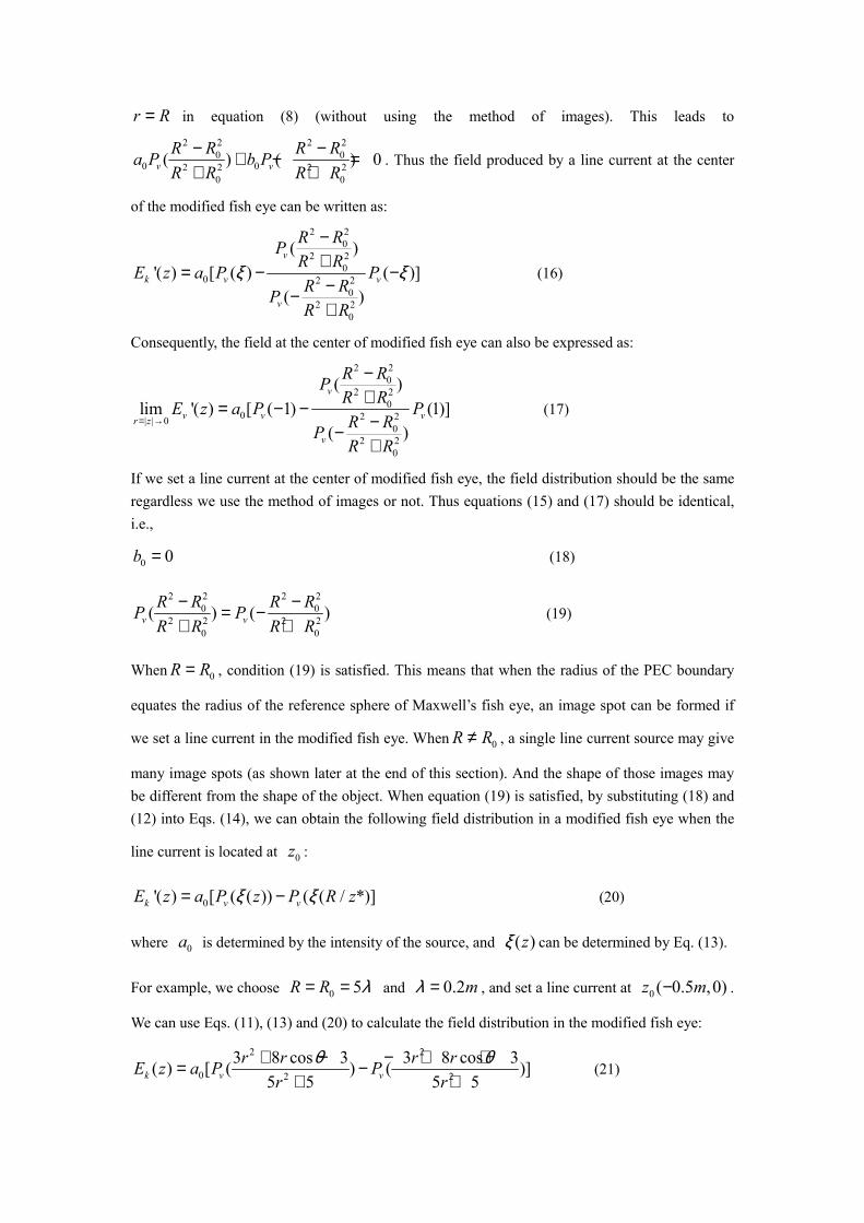
The results of our analytical solutions (20) and (21) agree well with FEM simulation results as

shown in Fig. 2. We can see the spot size around the image point is 0.2925FWHM λ=

(indicating subwavelength image), which is larger than the spot size around the source

point 0.173FWHM λ= .

Figure 2 The absolute value of the normalized field distribution around the line current (a) and its image (b) in x

direction: green line is from the FEM simulation result when we set a line current at (-0.5m, 0); blue dashed line is

our analytical result of Eq. (21); red line is Leonhardt ’s analytical result of Eq. (22) for a situation when one sets a

line current source at (-0.5m,0) and a line current drain at (0.5m,0). The structure of modified fish eye is

0 5R R λ= = and0 1n = . The incident wave length is 0.2mλ = .

From this figure we see that Maxwell’s fish eye lens can give a good image of subwavelength

resolution if only zero order mode is excited, however, the spot-size of the image field is still

larger than the spot size of the source field (indicating that it can not give a perfect image). Adding

a special line current drain at the image point [4] can sharpen the image spot size for a very special

excitation of object field with only zeroth order mode. However, it is not practical to add active

drains in a real imaging application, as we don’t know beforehand the distribution of object/source

points and consequently cannot determine where to put the active drains. Furthermore, a simple

line drain can not produce enough high order modes to make the image as sharp as one wishes (for

perfect image) though it can help to recover a very special object field distribution around the

image position. We will not discuss the situation of active drains in this paper.

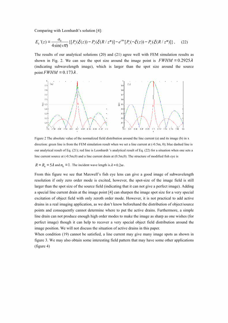
When condition (19) cannot be satisfied, a line current may give many image spots as shown in

figure 3. We may also obtain some interesting field pattern that may have some other applications

(figure 4)

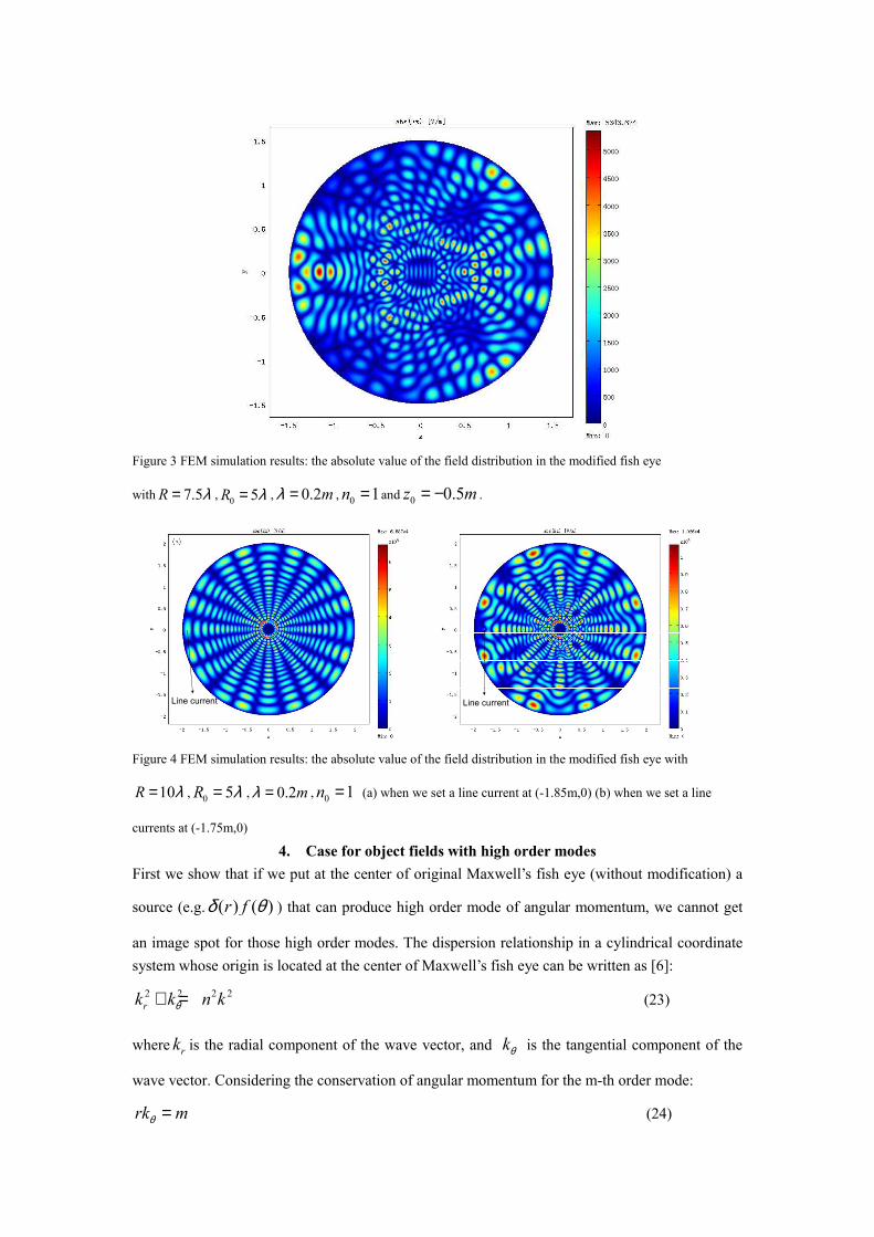
Figure 3 FEM simulation results: the absolute value of the field distribution in the modified fish eye

with 7.5R λ= ,0 5R λ= , 0.2mλ = ,

0 1n = and0 0.5z m= − .

Line currentLine current Line currentLine current

Figure 4 FEM simulation results: the absolute value of the field distribution in the modified fish eye with

10R λ= ,0 5R λ= , 0.2mλ = ,

0 1n = (a) when we set a line current at (-1.85m,0) (b) when we set a line

currents at (-1.75m,0)

4. Case for object fields with high order modes

First we show that if we put at the center of original Maxwell’s fish eye (without modification) a

source (e.g. ( ) ( )r fδ θ ) that can produce high order mode of angular momentum, we cannot get

an image spot for those high order modes. The dispersion relationship in a cylindrical coordinate

system whose origin is located at the center of Maxwell’s fish eye can be written as [6]:

2 2 2 2

rk k n kθ+ = (23)

where rk is the radial component of the wave vector, and kθ is the tangential component of the

wave vector. Considering the conservation of angular momentum for the m-th order mode:

rk mθ = (24)

For a high order mode 0m ≠ in the Maxwell’s fish eye, there is still a caustic [6]. When 0m ≠ ,

from equation (24) we can see that kθ increases toward the center. Consequently, we can see

from Eq. (23) that radial component rk varies from a real value to an imaginary value as 0r → .

The turning point of 0rk = is the radius of the caustic cR . Inside the caustic, rk is an imaginary

number and the angular momentum state become evanescent (i.e., decay quickly) along the radial

direction. The detailed information carried by the high order modes can hardly propagate to the far

field without great damping. Only the zero order mode ( 0m = ), which doesn’t have the caustic,

can propagate to the far field in Maxwell’s fish eye. Thus, if we put at the center of Maxwell’s fish

eye a special source that can excite only (or mainly) high order mode, the field cannot go to the far

field, and consequently a subwavelength image can not be formed. If we transform this source

position to another point of Maxwell’s fish eye or add PEC boundary to Maxwell’s fish eye, the

situation remains the same: subwavelength image can not be achieved.

We can use FEM simulation to verify this in a modified fish eye with 0 10R R λ= = and 0 1n = .

Our simulation is for TE wave in 2D space with 0.2mλ = . This structure satisfies condition (19).

We set a small circle (with radius 0r ) located at 0 ( 0.5 ,0)z m− with boundary condition

3exp( ')E iγθ= V/m to introduce high order mode. We first choose 3

0 10r λ−= and 0γ =

and the simulation result is shown in Fig. 5. Note that the field generated by boundary

condition 3E = on this small circle will contain some high order mode (and thus the object field

is quite sharp as compared to Fig. 2(a)), as the zero order mode produced by a line current at

(-0.5m, 0) is not a circle as we have discussed in Section 2. Since it also contains some zero order

mode, a good image spot can still be formed. However, if we change 0γ = to 5γ = , the

situation will be completely different. The simulation result is shown in figure 6. Boundary

condition 3exp( 5 ')E i θ= on a small circle gives more energy to high order modes (the object

field is very sharp). These high order modes cannot propagate to the far field (the ratio of the field

around the object to the field around the image position is about 5/ ~ 10o iE E ). Consequently,

good image can not be achieved, as shown in Fig. 6(b).

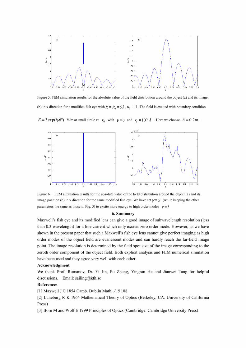
Figure 5. FEM simulation results for the absolute value of the field distribution around the object (a) and its image

(b) in x direction for a modified fish eye with0 5R R λ= = ,

0 1n = . The field is excited with boundary condition

3exp( ')E iγθ= V/m at small circle r= 0r with 0γ = and 3

0 10r λ−= . Here we choose 0.2mλ = .

Figure 6. FEM simulation results for the absolute value of the field distribution around the object (a) and its

image position (b) in x direction for the same modified fish eye. We have set 5γ = (while keeping the other

parameters the same as those in Fig. 5) to excite more energy to high order modes 5γ =

6. Summary

Maxwell’s fish eye and its modified lens can give a good image of subwavelength resolution (less

than 0.3 wavelength) for a line current which only excites zero order mode. However, as we have

shown in the present paper that such a Maxwell’s fish eye lens cannot give perfect imaging as high

order modes of the object field are evanescent modes and can hardly reach the far-field image

point. The image resolution is determined by the field spot size of the image corresponding to the

zeroth order component of the object field. Both explicit analysis and FEM numerical simulation

have been used and they agree very well with each other.

Acknowledgment

We thank Prof. Romanov, Dr. Yi Jin, Pu Zhang, Yingran He and Jianwei Tang for helpful

discussions. Email: sailing@kth.se

References

[1] Maxwell J C 1854 Camb. Dublin Math. J. 8 188

[2] Luneburg R K 1964 Mathematical Theory of Optics (Berkeley, CA: University of California

Press)

[3] Born M and Wolf E 1999 Principles of Optics (Cambridge: Cambridge University Press)

[4] Ulf Leonhardt, New Journal of Physics, 11, 093040, 2009

[5] Leonhardt U and Philbin T G Phys. Rev. A 81, 011804, 2010

[6] Zubin Jacob, Leonid V. Alekseyev and Evgenii Narimanov ,OPTICS EXPRESS Vol. 14, No.

18 ,2006