On learning dynamics underlying the evolution of learning rules

Theoretical Population Biology 91 (2014) 20–36

Contents lists available at ScienceDirect

Theoretical Population Biology

journal homepage: www.elsevier.com/locate/tpb

On learning dynamics underlying the evolution of learning rulesSlimane Dridi, Laurent Lehmann ∗

Department of Ecology and Evolution, University of Lausanne, Switzerland

a r t i c l e i n f o

Article history:Available online 17 September 2013

Keywords:Fluctuating environmentsEvolutionary game theoryStochastic approximationReinforcement learningFictitious playProducer–scrounger game

a b s t r a c t

In order to understand the development of non-genetically encoded actions during an animal’s lifespan,it is necessary to analyze the dynamics and evolution of learning rules producing behavior. Owing tothe intrinsic stochastic and frequency-dependent nature of learning dynamics, these rules are oftenstudied in evolutionary biology via agent-based computer simulations. In this paper, we show thatstochastic approximation theory can help to qualitatively understand learning dynamics and formulateanalytical models for the evolution of learning rules. We consider a population of individuals repeatedlyinteracting during their lifespan, and where the stage game faced by the individuals fluctuates accordingto an environmental stochastic process. Individuals adjust their behavioral actions according to learningrules belonging to the class of experience-weighted attraction learning mechanisms, which includesstandard reinforcement and Bayesian learning as special cases. We use stochastic approximation theoryin order to derive differential equations governing action play probabilities, which turn out to havequalitative features of mutator-selection equations. We then perform agent-based simulations to findthe conditions where the deterministic approximation is closest to the original stochastic learningprocess for standard 2-action 2-player fluctuating games, where interaction between learning rules andpreference reversal may occur. Finally, we analyze a simplified model for the evolution of learning ina producer–scrounger game, which shows that the exploration rate can interact in a non-intuitive waywith other features of co-evolving learning rules. Overall, our analyses illustrate the usefulness of applyingstochastic approximation theory in the study of animal learning.

© 2013 Elsevier Inc. All rights reserved.

1. Introduction

The abundance of resources and the environments to whichorganisms are exposed vary in space and time. Organisms are thusfacing complex fluctuating biotic and abiotic conditions to whichthey must constantly adjust (Shettleworth, 2009; Dugatkin, 2010).

Animals have a nervous system, which can encode behavioralrules allowing them to adjust their actions to changing environ-mental conditions (Shettleworth, 2009; Dugatkin, 2010). In par-ticular, the presence of a reward system allows an individual toreinforce actions increasing satisfaction and material rewards andthereby adjust behavior by learning to produce goal-oriented ac-tion paths (Thorndike, 1911; Herrnstein, 1970; Sutton and Barto,1998; Niv, 2009). It is probable that behaviors as different as for-aging, mating, fighting, cooperating, nest building, or informationgathering all involve adjustment of actions to novel environmentalconditions by learning, as they have evolved to be performed un-der various ecological contexts andwith different interaction part-ners (Hollis et al., 1995; Chalmeau, 1994; Villarreal and Domjan,1998; Walsh et al., 2011; Plotnik et al., 2011).

∗ Corresponding author.E-mail address: [email protected] (L. Lehmann).

0040-5809/$ – see front matter© 2013 Elsevier Inc. All rights reserved.http://dx.doi.org/10.1016/j.tpb.2013.09.003

In the fields of evolutionary biology and behavioral ecologythere is a growing interest in understanding how natural selectionshapes the learning levels and abilities of animals, but this is metwith difficulties (McNamara and Houston, 2009; Hammersteinand Stevens, 2012; Fawcett et al., 2013; Lotem, 2013). Focusingon situation specific actions does not help to understand theeffects of natural selection on behavioral rules because one focuseson produced behavior and not the rules producing the behavior(e.g., Dijker, 2011). In order to understand the dynamics andevolution of learning mechanisms and other behavioral rules, anevolutionary analysis thus has to consider explicitly the dynamicsof state variables on two timescales. First, one has to considerthe timescale of an individual’s lifespan; that is, the behavioraltimescale during which genetically encoded behavioral rulesproduce a dynamic sequence of actions taken by the animal.Second, there is the generational timescale, duringwhich selectionoccurs on the behavioral rules themselves.

It is the behavioral timescale, where learning may occur, thatseems to be the most reluctant to be analyzed (Lotem, 2013). Thismay stem from the fact that learning rules intrinsically encompassconstraints about the use of information and the expression ofactions (in the absence of unlimited powers of computation),which curtails the direct application of standard optimalityapproaches for studying dynamic behavior such as optimal control

http://dx.doi.org/10.1016/j.tpb.2013.09.003

http://www.elsevier.com/locate/tpb

http://www.elsevier.com/locate/tpb

http://crossmark.crossref.org/dialog/?doi=10.1016/j.tpb.2013.09.003&domain=pdf

mailto:[email protected]

http://dx.doi.org/10.1016/j.tpb.2013.09.003

S. Dridi, L. Lehmann / Theoretical Population Biology 91 (2014) 20–36 21

theory and dynamic programming. Indeed, the dynamics of eventhe simplest learning rule, such as reinforcement learning by trial-and-error, is hardly amenable to mathematical analysis withoutsimplifying assumptions and focusing only on asymptotics (Bushand Mostelller, 1951; Norman, 1968; Rescorla and Wagner, 1972;Börgers and Sarin, 1997; Stephens and Clements, 1998; butsee Izquierdo et al., 2007 for predictions in finite time).

Further, the difficulty of analyzing learning dynamics isincreased by two biological features that need to be takeninto account. First, varying environments need to be consideredbecause learning is favored by selection when the environmentfaced by the individuals in a population is not absolutely fixedacross and/or within generations (Boyd and Richerson, 1985;Rogers, 1988; Stephens, 1991; Feldman et al., 1996; Wakanoet al., 2004; Dunlap and Stephens, 2009). Second, frequency-dependence needs to be considered because learning is likely tooccur in situations where there are social interactions between theindividuals in the population (Chalmeau, 1994; Hollis et al., 1995;Villarreal and Domjan, 1998; Giraldeau and Caraco, 2000; Arbillyet al., 2010, 2011b; Plotnik et al., 2011).

All these features taken together make the analysis of the evo-lution of learning rules more challenging to analyze than standardevolutionary game theory models focusing on actions or strate-gies for constant environments (e.g., Axelrod and Hamilton, 1981;Maynard Smith, 1982; Binmore and Samuelson, 1992; Leimar andHammerstein, 2001; McElreath and Boyd, 2007; André, 2010). Al-though there has been some early studies on evolutionarily sta-ble learning rules (Harley, 1981; Houston, 1983; Houston andSumida, 1987; Tracy and Seaman, 1995), this research field hasonly recently been reignited by the use of agent-based simula-tions (Großet al., 2008; Josephson, 2008; Hamblin and Giraldeau,2009; Arbilly et al., 2010, 2011a,b; Katsnelson et al., 2011). It isnoteworthy that during the gap in time in the study of learningin behavioral ecology, the fields of game theory and economicshave witnessed an explosion of theoretical studies of learning dy-namics (e.g., Jordan, 1991; Erev and Roth, 1998; Fudenberg andLevine, 1998; Camerer and Ho, 1999; Hopkins, 2002; Hofbauer andSandholm, 2002; Foster and Young, 2003; Young, 2004; Sandholm,2011). This stems from an attempt to understand how humanslearn to play in games (e.g., Camerer, 2003) and to refine staticequilibrium concepts by introducing dynamics. Even if such mo-tivations can be different from the biologists’ attempt to under-stand the evolution of animal behavior, the underlying principlesof learning are similar since actions leading to high experiencedpayoffs (or imagined payoffs) are reinforced over time.

Interestingly, mathematicians and game theorists have also de-veloped tools to analytically approximate intertwined behavioraldynamics, in particular stochastic approximation theory (Ljung,1977; Benveniste et al., 1991; Fudenberg and Levine, 1998; Benaïmand Hirsch, 1999a; Kushner and Yin, 2003; Young, 2004; Sand-holm, 2011). Stochastic approximation theory allows one to ap-proximate byway of differential equations discrete time stochasticlearning processes with decreasing (or very small) step-size, andthereby understand qualitatively their dynamics and potentiallyconstruct analytical models for the evolution of learning mecha-nisms. This approach does not seem so far to have been applied inevolutionary biology.

In this paper, we analyze by means of stochastic approxi-mation theory an extension to fluctuating social environmentsof the experience-weighted attraction learning mechanism (EWAmodel, Camerer and Ho, 1999; Ho et al., 2007). This is a paramet-ric model, where the parameters describe the psychological char-acteristics of the learner (memory, ability to imagine payoffs ofunchosen actions, exploration/exploitation inclination), andwhichencompasses as a special case various learning rules used in evolu-tionary biology such as the linear operator (McNamara and Hous-ton, 1987; Bernstein et al., 1988; Stephens and Clements, 1998),

relative payoff sum (Harley, 1981; Hamblin and Giraldeau, 2009)and Bayesian learning (Rodriguez-Gironés and Vásquez, 1997;Geisler and Diehl, 2002). We apply the EWA model to a situationwhere individuals facemultiple periods of interactions during theirlifetime, andwhere each period consists of a game (like a prisoner’sdilemma game, a Hawk–Dove game), whose type changes stochas-tically according to an environmental process.

The paper is organized in three parts. First, we define themodeland derive by way of stochastic approximation theory a set ofdifferential equations describing action play probabilities out ofwhich useful qualitative features about learning dynamics can beread. Second, we use the model to compare analytical and simula-tion results under some specific learning rules. Finally, we derivean evolutionary model for patch foraging in a producer–scroungercontext, where both evolutionary and behavioral time scales areconsidered.

2. Model

2.1. Population

We consider a haploid population of constant size N . Althoughwe are mainly interested in investigating learning dynamics, weendow for biological concreteness the organisms with a simplelife cycle. This is as follows. (1) Each individual interacts sociallywith others repeatedly and possibly for T time periods. (2) Eachindividual produces a large number of offspring according toits gains and losses incurred during social interactions. (3) Allindividuals of the parental generation die and N individuals fromthe offspring generation are sampled to form the new adultgeneration.

2.2. Social decision problem in a fluctuating environment

The social interactions stage of the life cycle, stage (1), is themain focus of this paper and it consists of the repeated play ofa game between the members of the population. At each timestep t = 1, 2, . . . , T , individuals play a game, whose outcomedepends on the state of the environment ω. We denote the setof environmental states by Ω , which could consist of good andbad weather, or any other environmental biotic or abiotic featureaffecting the focal organism. The dynamics of environmental statesωt

Tt=1 is assumed to obey a homogeneous and aperiodic Markov

Chain, and we write µ(ω) for the probability of occurrence ofstate ω under the stationary distribution of this Markov Chain(e.g., Karlin and Taylor, 1975; Grimmett and Stirzaker, 2001).

For simplicity, we consider that the number of actions staysconstant across environmental states (only the payoffs vary), thatis, at every time step t , all individuals have a fixed behavioralrepertoire that consists of the set of actions A = 1, . . . ,m.The action taken by individual i at time t is a random variabledenoted by ai,t , and the action profile in the population at timet is at = (a1,t , . . . , aN,t). This process generates a sequence ofaction profiles atTt=1. The payoff to individual i at time t whenthe environment is in state ωt is denoted πi(ai,t , a−i,t , ωt), wherea−i,t = (a1,t , . . . , ai−1,t , ai+1,t , . . . , aN,t) is the action profile ofthe remaining individuals in the population (all individuals excepti). Note that this setting covers the case of an individual decisionproblem (e.g., a multi-armed bandit), where the payoff πi(ai,t , ωt)of individual i is independent of the profile of actions a−i,t of theother members of the population.

2.3. Learning process

We assume that individuals learn to choose their actions inthe game but are unable to detect the current state ωt of theenvironment. Each individual is characterized by a genetically

22 S. Dridi, L. Lehmann / Theoretical Population Biology 91 (2014) 20–36

determined learning rule, which prescribes how its current actionsdepend on its private history. The learning rules we considerbelong to the class of rules defined by the so-called experience-weighted-attraction (EWA) learning model (Camerer and Ho,1999; Camerer, 2003; Ho et al., 2007). The reason why we useEWA is that it encapsulates many standard learning rules andtranslates well the natural assumption that animals have internalstates, which are modified during the interactions with theirenvironment, and that internal states have a direct (but possiblynoisy) influence on action (Enquist and Ghirlanda, 2005). In EWAlearning, the internal states are attractions or ‘‘motivations’’ foractions, and the mapping from internal states (motivations) toaction choice is realized via a probabilistic choice rule.

2.3.1. Dynamics of motivationsWe first describe the dynamics ofmotivations. To each available

action a of its action setA, individual ihas an associatedmotivationMi,t(a) at time t that is updated according to

Mi,t+1(a) =ni,t

ni,t+1φi,tMi,t(a)

+1

ni,t+1δi + (1 − δi)1(a, ai,t)πi(a, a−i,t , ωt), (1)

where

ni,t+1 = 1 + ρini,t (2)

is individual i’s count of the number of steps of play. The initialconditions of Eqs. (1) and (2) are the values of the state variables atthe first period of play (t = 1); that is,Mi,1(a) and ni,1.

The updating rule of motivations (Eq. (1)) is a weighted averagebetween the previous motivation to action a, Mi,t(a), and areinforcement to that action, δi + (1−δi)1(a, ai,t)πi(a, a−i,t , ωt),which itself depends on the payoff πi(a, a−i,t , ωt) that wouldobtain if action a was played at t . Eq. (1) is equivalent to Eq. 2.2of Camerer and Ho (1999) with the only difference that the payoffdepends here on the current state of the environment, ωt , so thatindividuals face a stochastic game.

The first term in Eq. (1) weights the previousmotivation by twofactors: φi,t , a positive dynamic memory parameter that indicateshowwell individual i remembers the previousmotivation; and theexperienceweight ni,t/ni,t+1, which is the ratio between the previ-ous experience count to the new one. Eq. (2) shows that the expe-rience count is updated according to another memory parameter,ρi ∈ [0, 1]. If ρi = 1, the individual counts the number of interac-tions objectively, i.e., ni,t = t (if ni,1 = 1), otherwise subjectively.

The reinforcement term to action a in Eq. (1) is weighted by1/ni,t+1 and depends on δi, which varies between 0 and 1. This cap-tures the ability of an individual to observe (or mentally simulate)non-realized payoffs, while 1(a, ai,t) is the action indicator func-tion of individual i, given by

1(a, ai,t) =

1, if ai,t = a,0, otherwise. (3)

With these definitions, we can see that depending on the value ofδi, an individual can reinforce an unchosen action according to thepayoff that action would have yielded had it been taken. Indeed,when individual i does not take action a at time t [1(a, ai,t) = 0],the numerator of the second term is δiπi(a, a−i,t , ωt). If δi = 0,this cancels out and the payoff associated to the unchosen action ahas no effect on the update of motivational states. But if δi = 1, thenumerator of the second term isπi(a, a−i,t , ωt), and themotivationis updated according to the payoff individual iwould have obtainedby taking action a. All values of δi between 0 and 1 allow toreinforce unchosen actions according to their potential payoff.

On the other hand, if action a is played at time t; namely,1(a, ai,t) = 1, the numerator of the second term reduces to the re-alized payoff πi(a, a−i,t , ωt), irrespective of the value of δi. Hence,δi plays a role only for updating motivations of unchosen actions,which occurs when individuals are belief-based or Bayesian learn-ers as will be detailed below, after we have explained how the ac-tions themselves are taken by an individual.

2.3.2. Action play probabilitiesThe translation of internal states (motivations) into action

choice can take many forms. But it is natural to assume that theprobability pi,t(a) = Prai,t = a that individual i takes action a attime t is independent of other individuals and takes the ratio form

pi,t(a) =f (Mi,t(a))

k∈A

f (Mi,t(k)), (4)

where f (·) is a continuous and increasing function of its argument(this ratio form could be justified by appealing to the choice axiomof Luce, 1959, p. 6).

The choice rule (Eq. (4)) entails that the action that hasmaximalmotivation at time t is chosen with the greatest probability. This isdifferent from choosing deterministically the action that has thehighest motivation. Indeed, this type of choice function allows onetomodel errors or exploration in the decision process of the animal(an action with a low motivation has still a probability of beingchosen).

Errors can be formally implemented by imposing that

pi,t(a) = Pra = argmaxb∈A

[Mi,t(b) + ε(b)] (5)

where (ε(b))b∈A are small perturbations that are independentlyand identically distributed (i.i.d.) among choices. The idea is hereto first perturb motivations by adding a small random vector ε oferrors and then choose the action that has the biggest motivation.The probability that action a has maximal perturbed motivationdefines the probability pi,t(a) with which action awill be chosen.

The maximizing assumption in Eq. (5) restricts the possibilitiesfor the form taken by f . In fact, the only function satisfying atthe same time both Eqs. (4)–(5) is f (M) = exp(λiM) for 0 <λi < ∞depending on the distribution of perturbations (Sandholm,2011, Chap. 6). Replacing this expression for f in Eq. (4), we obtainthat an organism chooses its actions according to the so-called logitchoice function

pi,t(a) =exp[λiMi,t(a)]

k∈A

exp[λiMi,t(k)], (6)

which is in standard use across disciplines (Luce, 1959; Andersonet al., 1992; McKelvey and Palfrey, 1995; Fudenberg and Levine,1998; Sutton and Barto, 1998; Camerer and Ho, 1999; Achbanyet al., 2006; Ho et al., 2007; Arbilly et al., 2010, 2011b).

The parameter λi can be seen as individual i’s sensitivityto motivations, errors in decision-making, or as a proneness toexplore actions that have not been expressed so far. Depending onthe value of λi, we can obtain almost deterministic action choiceor a uniform distribution over actions. If λi goes to zero, action ais chosen with probability pi,t(a) → 1/m (where m is the numberof available actions). In this case, choice is random and individuali is a pure explorer. If, on the other hand, λi becomes very large(λi → ∞), then the action a∗

= argmaxb∈A [Mi,t(b)] with thehighest motivation is chosen almost deterministically, pi,t(a∗) →

1. In this case, individual i does not explore, it only exploits actionsthat led to high payoff. For intermediate values of λi, individual itrades off exploration and exploitation.


Table 1Special cases of EWA learning (Eqs. (1)–(4)). The first column gives the usual name of the learning rule found in the literature. The other columns give theparameter values in the EWA model to obtain this rule and the explicit expression of motivation updating (Mi,t+1(a)). A cell with a dot (.) means that theparameter in the corresponding column can take any value. A value of φi,t with the subscript t removed means that φi is a constant. The first part of the tablegives the rules already defined in the literature while the second part gives PRL, ERL, and IL, the three learning rules introduced in this paper. See Appendix D foran explanation of how to obtain Tit-for-Tat from EWA, where Li(a) is the aspiration level by i for action a.

Learning rule φi,t ρi δi λi ni,1 Mi,t+1(a) pi,t (a)

Linear operator 0 < φi <

1ρi = φi 0 . 1/(1 −

ρi)

φiMi,t (a) + (1 −

φi)1(a, ai,t )πi(a, a−i,t , ωt )

.

Relative payoff sum 0 < φi ≤

10 0 . 1 φiMi,t (a) + 1(a, ai,t )πi(a, a−i,t , ωt ) ∝ Mi,t (a)

Cournot adjustment 0 0 1 ∞ 1 πi(a, a−i,t , ωt ) ∝ exp[λiMi,t (a)]

Stochastic fictitious play (FP)(equivalent to Bayesian learningwith Dirichlet distributed priors)

1 1 1 λi > 0 . tt+1Mi,t (a) +

1t+1πi(a, a−i,t , ωt ) ∝ exp[λiMi,t (a)]

Tit-for-Tat 0 0 1 ∞ 1 πi(a, a−i,t , ωt ) − Li(a) ∝ exp[λiMi,t (a)]

Pure reinforcement learning (PRL) 1 +1t 1 0 λi > 0 1 Mi,t (a) +

1t+11(a, ai,t )πi(a, a−i,t , ωt ) ∝ exp[λiMi,t (a)]

Exploratory reinforcement learning(ERL)

1 1 0 λi > 0 1 tt+1Mi,t (a) +

1t+11(a, ai,t )πi(a, a−i,t , ωt ) ∝ exp[λiMi,t (a)]

Payoff-informed learning (IL) 1 +1t 1 1 λi > 0 1 Mi,t (a) +

1t+1πi(a, a−i,t , ωt ) ∝ exp[λiMi,t (a)]

Note: The expression ∝ exp[λiMi,t (a)] refers to the logit choice rule Eq. (6).

2.3.3. Learning rules in the EWA genotype spaceIn the EWAmodel, individuals differ by the value of the four pa-

rameters φi,t , ρi, δi, λi and the initial values of the state variables,Mi,1(a) and ni,1. These can be thought of as the genotypic valuesof individual i, and particular choice of these parameters provideparticular learning rules. In Table 1, we retrieve from the model(Eq. (1)) some standard learning rules, which are special cases ofthe genotype space. The Linear Operator rule (Bush andMostelller,1951; Rescorla andWagner, 1972; McNamara and Houston, 1987;Bernstein et al., 1988; Stephens and Clements, 1998; Hamblinand Giraldeau, 2009), Relative Payoff Sum (Harley, 1981; Hous-ton, 1983; Houston and Sumida, 1987; Tracy and Seaman, 1995),Cournot Adjustment (Cournot, 1838), and Fictitious Play (Brown,1951; Fudenberg and Levine, 1998; Hofbauer and Sandholm, 2002;Hopkins, 2002) all can be expressed as special cases of EWA.

One of the strengths of EWA is that it encompasses at thesame time both reinforcement learning (like the linear operator orrelative payoff sum) and belief-based learning (like fictitious play)despite the fact that these two types of learning rules are usuallythought of as cognitively very different (Erev and Roth, 1998;Hopkins, 2002; van der Horst et al., 2010). Reinforcement learningis the simplest translation of the idea that actions associated to highrewards aremore often repeated,while belief-based learning relieson updating beliefs (probability distributions) over the actions ofother players and/or the state of the environment, which occursin Bayesian learning. In the EWA model, belief-based learningis made possible thanks to the ability to imagine outcomes ofunchosen actions (Emery and Clayton, 2004); this is captured bythe parameter δi, which is the key to differentiate reinforcementfrom belief-based learning models.

Belief-based learning is captured in the EWA model sincemotivations can represent the expected payoff of action over thedistribution of beliefs of the actions of other players (Camerer andHo, 1999), and the logit choice function further allows an individualto best respond to the actions of others. It then turns out that theSmooth Fictitious Play (FP) rule (Table 1) is equivalent to Bayesianlearning for initial priors over the actions of others (stage gamet = 1) that follow a Dirichlet distribution (Fudenberg and Levine,1998, p. 48–49).

In EWA, the learning dynamics of an individual (Eqs. (1)–(4)) isa complex discrete time stochastic process because action choiceis probabilistic and it depends on the (random) actions played byother individuals in the population, and on the random variable

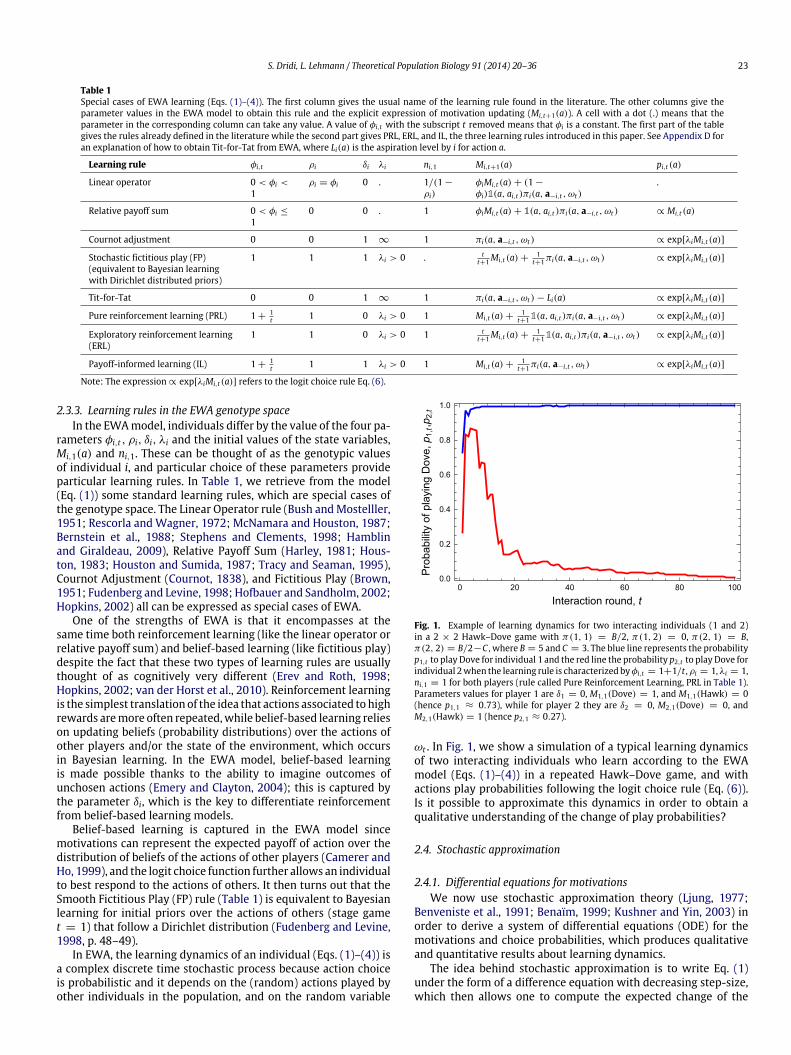
Fig. 1. Example of learning dynamics for two interacting individuals (1 and 2)in a 2 × 2 Hawk–Dove game with π(1, 1) = B/2, π(1, 2) = 0, π(2, 1) = B,π(2, 2) = B/2−C , where B = 5 and C = 3. The blue line represents the probabilityp1,t to play Dove for individual 1 and the red line the probability p2,t to play Dove forindividual 2when the learning rule is characterized byφi,t = 1+1/t ,ρi = 1,λi = 1,ni,1 = 1 for both players (rule called Pure Reinforcement Learning, PRL in Table 1).Parameters values for player 1 are δ1 = 0, M1,1(Dove) = 1, and M1,1(Hawk) = 0(hence p1,1 ≈ 0.73), while for player 2 they are δ2 = 0, M2,1(Dove) = 0, andM2,1(Hawk) = 1 (hence p2,1 ≈ 0.27).

ωt . In Fig. 1, we show a simulation of a typical learning dynamicsof two interacting individuals who learn according to the EWAmodel (Eqs. (1)–(4)) in a repeated Hawk–Dove game, and withactions play probabilities following the logit choice rule (Eq. (6)).Is it possible to approximate this dynamics in order to obtain aqualitative understanding of the change of play probabilities?

2.4. Stochastic approximation

2.4.1. Differential equations for motivationsWe now use stochastic approximation theory (Ljung, 1977;

Benveniste et al., 1991; Benaïm, 1999; Kushner and Yin, 2003) inorder to derive a system of differential equations (ODE) for themotivations and choice probabilities, which produces qualitativeand quantitative results about learning dynamics.

The idea behind stochastic approximation is to write Eq. (1)under the form of a difference equation with decreasing step-size,which then allows one to compute the expected change of the


dynamics over one time step. These expected dynamics give riseto differential equations, which describe very closely the long-runstochastic dynamics of the motivations (see Benaïm, 1999, for astandard reference, and Hopkins, 2002, for an application of thisprinciple to learning). To that aim, we write Eq. (1) asMi,t+1(a) − Mi,t(a)

=1

ni,t+1

−ϵi,tMi,t(a) + Ri(a, ai,t , a−i,t , ωt)

(7)

whereϵi,t = 1 + ni,t(ρi − φi,t) (8)is a decay rate andRi(a, ai,t , a−i,t , ωt)

=δi + (1 − δi)1(a, ai,t)

πi(a, a−i,t , ωt) (9)

can be interpreted as the net reinforcement of the motivation ofaction a.

In order to use stochastic approximation theory, we need thatthe step-size of the process satisfies

∞

t=1(1/ni,t) = ∞ andlimt→∞(1/ni,t) = 0 (Benaïm, 1999, p. 11), where the first condi-tion entails that the steps are large enough to eventually overcomeinitial conditions, while the second condition entails that the stepseventually become small enough so that the process converges.This is ensured here by setting ρ = 1 in Eq. (2). We further assumea constant value of ϵi from now on (this is the case for all rules inTable 1, but a slowly varying ϵi,t is still amenable to an analysis viastochastic approximation). Note however that the assumption thatρ = 1 reduce to some extent the number of learning rules that onecan analyze in the EWA model, but the approximation can still beuseful for small constant step-sizes, for instance if one considers aLinear Operator Rule (Table 1) with φi close to 1 (see Benaïm andHirsch, 1999b; Izquierdo et al., 2007, for results on processes withconstant step-sizes).

With these assumptions, we show in Appendix A (Eqs. (A.1)–(A.12)) that the differential equation arising from taking theexpected motion of the stochastic dynamics in Eq. (7) is

Mi(a) = −ϵiMi(a) + Ri(a), (10)where

Ri(a) = [pi(a) + δi(1 − pi(a))]

a−i∈AN−1

p−i(a−i)πi(a, a−i) (11)

and

πi(a, a−i) =

ω∈Ω

µ(ω)πi(a, a−i, ω). (12)

Here, a dot accent is used to denote a derivative, i.e., dx/dt = x,Ri(a) is the expected reinforcement to the motivation of actiona of individual i over the distribution of action probabilitiesin the population (where AN−1 is the set of action profiles ofindividuals different than i), and πi(a, a−i) is the average payoffover the distribution of environmental states. Because the actionplay probabilities of the focal individual, pi(a), and the remainingindividuals in the population p−i(a−i) =

i=j pj(aj) (Eq. (A.2)),

depend on the motivations, Eq. (10) is a differential of the formMi(a) = Fi(M), for all actions a and individual i in the population,where M denotes the vector collecting the motivations of allactions and individuals in the population. Hence, Eqs. (10)–(12)define a bona fide autonomous system of differential equations.

Eq. (11) shows that the deterministic approximation rests onthe ‘‘average game’’ with payoffs given by πi(a, a−i), i.e., a gamewhere each payoff matrix entry (Eq. (12)) is a weighted average ofthe corresponding entries of the stage games over the distributionof environmental states µ(ω). Hence, if one wants to consider asituation where the stage game fluctuates, one does not need tospecify a series of stage games, but only the average game resultingfrom taking the weighted average of the payoffs of the originalstage games.

2.4.2. Differential equations for action play probabilitiesUsing the logit choice rule (Eq. (6)) and the dynamics of

motivations (Eq. (10)), we can derive a differential equation for thechoice probability for each action a of individual i

pi(a) = pi(a)

ϵik∈A

logpi(k)pi(a)

pi(k)

+ λi

Ri(a) −

k∈A

Ri(k)pi(k)

, (13)

(Appendix A, Eqs. (A.13)–(A.20)). Because Ri(a) depends onthe action play probabilities, Eq. (13) also defines a bona fideautonomous system of differential equations, but this time directlyfor the dynamics of action. The first term in brackets in Eq. (13)describes a perturbation to the choice probability. This representsthe exploration of action by individual i (it is an analogue ofmutation in evolutionary biology), and brings the dynamics backinto the interior of the state space if it gets too close to theboundary. The second term in the brackets takes the same formas the replicator equation (Hofbauer and Sigmund, 1998; Tuylset al., 2003); that is, if the expected reinforcement, Ri(a), to action ais higher than the average expected reinforcement,

k Ri(k)pi(k),

then the probability of expressing action a increases.Eq. (13) is the ‘‘final’’ point of the stochastic approximation ap-

plied to our model. We now have a system of differential equa-tions [of dimension N × (m − 1)], which describes the ontogenyof behavior of the individuals in the population. Standard resultsfrom stochastic approximation theory guarantee that the origi-nal stochastic dynamics (Eqs. (1)–(4)) asymptotically follows veryclosely the deterministic path of the differential equation (13). Forinstance, if the limit set of Eq. (13) consists of isolated equilibria,the stochastic process (Eqs. (1)–(4)) will converge to one of theseequilibria almost surely (Benaïm, 1999; Borkar, 2008).

More generally, the differential equations for the action prob-abilities are unlikely to depend only on the probabilities as is thecase in Eq. (13). For instance, when the choice rule is the so-calledpower choice, the dynamics of actions will also depend on the dy-namics of motivations (i.e., f (M) = Mλi in Eq. (4), which givesrise to pi(a) = [λipi(a)/Mi(a)]

Ri(a) −

k∈A Ri(k)pi(k)pi(a)/

pi(k)1/λi, Eq. (A.22)). This is one of the reasons why the logit

choice rule is appealing; namely, it yields simplifications allowingone to track only the dynamics of choice probabilities (Eq. (13)).

3. Applications

3.1. Pure reinforcement vs. payoff-informed learning

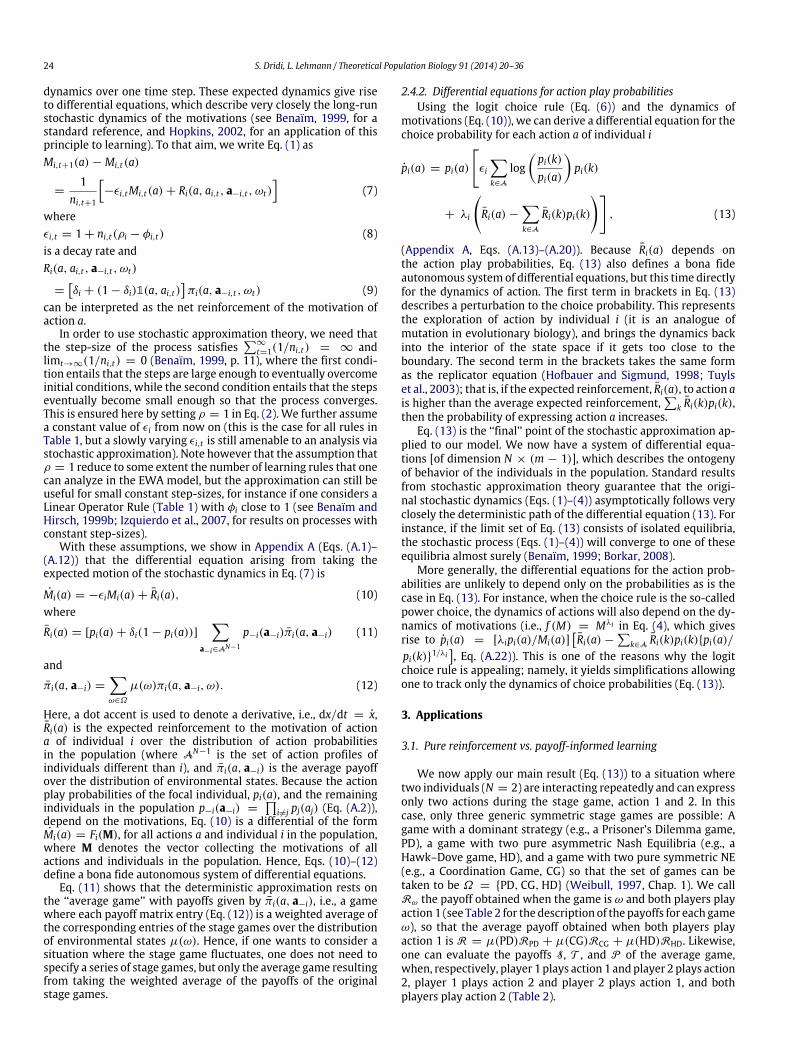
We now apply our main result (Eq. (13)) to a situation wheretwo individuals (N = 2) are interacting repeatedly and can expressonly two actions during the stage game, action 1 and 2. In thiscase, only three generic symmetric stage games are possible: Agame with a dominant strategy (e.g., a Prisoner’s Dilemma game,PD), a game with two pure asymmetric Nash Equilibria (e.g., aHawk–Dove game, HD), and a game with two pure symmetric NE(e.g., a Coordination Game, CG) so that the set of games can betaken to be Ω = PD, CG,HD (Weibull, 1997, Chap. 1). We callRω the payoff obtained when the game is ω and both players playaction 1 (see Table 2 for the description of the payoffs for each gameω), so that the average payoff obtained when both players playaction 1 is R = µ(PD)RPD + µ(CG)RCG + µ(HD)RHD. Likewise,one can evaluate the payoffs S, T , and P of the average game,when, respectively, player 1 plays action 1 andplayer 2 plays action2, player 1 plays action 2 and player 2 plays action 1, and bothplayers play action 2 (Table 2).


Table 2Payoff matrices for the average Hawk–Dove game and the three associated sub-games. In each matrix, the rows correspond to the actions of player 1 (first row gives action1, while second row gives action 2) and the columns correspond to the actions of player 2 (first column gives action 1, while second column gives action 2). Payoffs areto row player (player 1). The matrix at the top shows the payoffs in the average Hawk–Dove Game (denoted G), and the three matrices below contain the payoffs of thesub-games ω (PD, HD, and CG). In the Prisoner’s Dilemma (Left), we assume TPD > RPD > PPD > SPD and (TPD + SPD)/2 < RPD . In the Hawk–Dove (Middle), we haveTHD > RHD, SHD > PHD, PHD > RHD . In the Coordination Game (Right), RCG > SCG, RCG = PCG, SCG = TCG .

G Dove Hawk

Dove R = B/2 S = 0Hawk T = B P = B/2 − C

PD Cooperate Defect HD Dove Hawk CG Left Right

Cooperate RPD SPD Dove RHD SHD Left RCG SCGDefect TPD PPD Hawk THD PHD Right TCG PCG

Weassume that individuals playing this stochastic gameuse thelearning rules characterized by

φi,t = 1 +1t

and ρi = 1 (14)

so that when δi = 0 we obtain a form of reinforcement learning,which we call Pure Reinforcement Learning (PRL: see Table 1)becausemotivations are updated only according to realized payoffsand there is no discounting of the past. When δi = 1 we obtaina rule we call Payoff-Informed Learning (IL: see Table 1) since inthat case an individual updates motivations according not only torealized but also to imagined payoffs. The individual has here allinformation about possible payoffs at each decision step t , hencethe name of the learning rule.

Substituting Eqs. (14) into Eq. (8) gives ϵi,t = 0 (since nt = t)and thus ϵi = 0 in Eq. (13). Letting p1 = p1(1) be the probabilitythat individual 1 plays action 1 and p2 = p2(1) be the probabilitythat individual 2 plays action 1, we then obtain from Eq. (8), theabove assumptions, and Table 2, that the action play probabilitiessatisfy the dynamics

p1 = p1(1 − p1)λ1[p2R + (1 − p2)Sp1 + δ1(1 − p1)− p2T + (1 − p2)P δ1p1 + (1 − p1)], (15)

p2 = p2(1 − p2)λ2[p1R + (1 − p1)Sp2 + δ2(1 − p2)− p1T + (1 − p1)P δ2p2 + (1 − p2)]. (16)

In order to compare the dynamics predicted by Eqs. (15)–(16) tothat obtained from iterating Eq. (1) with logit choice function Eq.(6) (agent-based simulations), we assume that the average gameis a Hawk–Dove game (Maynard Smith and Price, 1973; MaynardSmith, 1982). Hence, action 1 can be thought as ‘‘Dove’’ and action2 as ‘‘Hawk’’. We now focus on two specific interactions in thisHawk–Dove game: PRL vs. PRL, and PRL vs. IL, and in order to carryout the numerical analysis, we also assume that the probabilityµ(ω) that game ω obtains in any period obeys an uniformdistribution, which gives µ(PD) = µ(CG) = µ(HD) = 1/3.

3.1.1. PRL vs. PRLWhen two PRL play against each other (Eqs. (15)–(16) with δi =

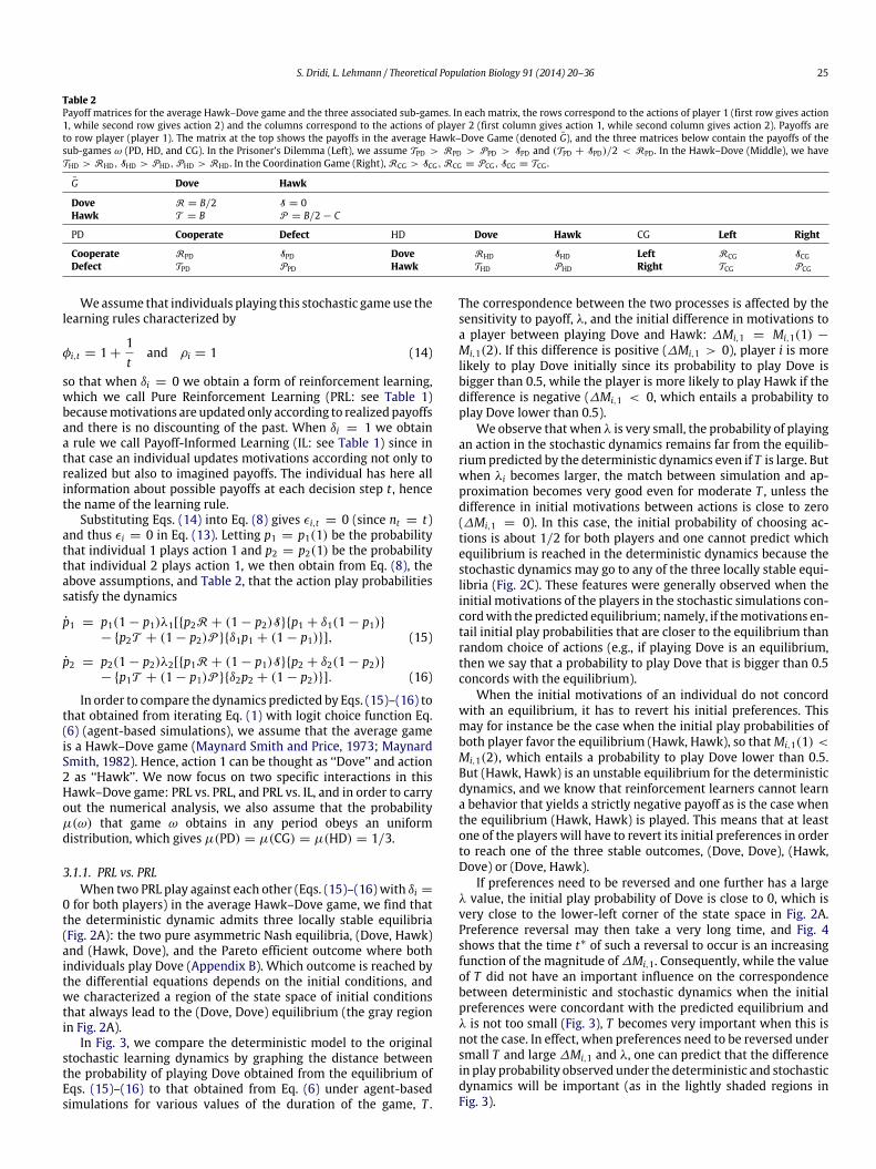
0 for both players) in the average Hawk–Dove game, we find thatthe deterministic dynamic admits three locally stable equilibria(Fig. 2A): the two pure asymmetric Nash equilibria, (Dove, Hawk)and (Hawk, Dove), and the Pareto efficient outcome where bothindividuals play Dove (Appendix B). Which outcome is reached bythe differential equations depends on the initial conditions, andwe characterized a region of the state space of initial conditionsthat always lead to the (Dove, Dove) equilibrium (the gray regionin Fig. 2A).

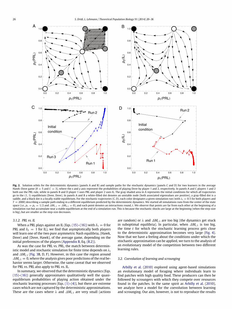
In Fig. 3, we compare the deterministic model to the originalstochastic learning dynamics by graphing the distance betweenthe probability of playing Dove obtained from the equilibrium ofEqs. (15)–(16) to that obtained from Eq. (6) under agent-basedsimulations for various values of the duration of the game, T .

The correspondence between the two processes is affected by thesensitivity to payoff, λ, and the initial difference in motivations toa player between playing Dove and Hawk: ∆Mi,1 = Mi,1(1) −

Mi,1(2). If this difference is positive (∆Mi,1 > 0), player i is morelikely to play Dove initially since its probability to play Dove isbigger than 0.5, while the player is more likely to play Hawk if thedifference is negative (∆Mi,1 < 0, which entails a probability toplay Dove lower than 0.5).

We observe that when λ is very small, the probability of playingan action in the stochastic dynamics remains far from the equilib-riumpredicted by the deterministic dynamics even if T is large. Butwhen λi becomes larger, the match between simulation and ap-proximation becomes very good even for moderate T , unless thedifference in initial motivations between actions is close to zero(∆Mi,1 = 0). In this case, the initial probability of choosing ac-tions is about 1/2 for both players and one cannot predict whichequilibrium is reached in the deterministic dynamics because thestochastic dynamics may go to any of the three locally stable equi-libria (Fig. 2C). These features were generally observed when theinitial motivations of the players in the stochastic simulations con-cordwith the predicted equilibrium; namely, if themotivations en-tail initial play probabilities that are closer to the equilibrium thanrandom choice of actions (e.g., if playing Dove is an equilibrium,then we say that a probability to play Dove that is bigger than 0.5concords with the equilibrium).

When the initial motivations of an individual do not concordwith an equilibrium, it has to revert his initial preferences. Thismay for instance be the case when the initial play probabilities ofboth player favor the equilibrium (Hawk, Hawk), so thatMi,1(1) <Mi,1(2), which entails a probability to play Dove lower than 0.5.But (Hawk, Hawk) is an unstable equilibrium for the deterministicdynamics, and we know that reinforcement learners cannot learna behavior that yields a strictly negative payoff as is the case whenthe equilibrium (Hawk, Hawk) is played. This means that at leastone of the players will have to revert its initial preferences in orderto reach one of the three stable outcomes, (Dove, Dove), (Hawk,Dove) or (Dove, Hawk).

If preferences need to be reversed and one further has a largeλ value, the initial play probability of Dove is close to 0, which isvery close to the lower-left corner of the state space in Fig. 2A.Preference reversal may then take a very long time, and Fig. 4shows that the time t∗ of such a reversal to occur is an increasingfunction of the magnitude of ∆Mi,1. Consequently, while the valueof T did not have an important influence on the correspondencebetween deterministic and stochastic dynamics when the initialpreferences were concordant with the predicted equilibrium andλ is not too small (Fig. 3), T becomes very important when this isnot the case. In effect, when preferences need to be reversed undersmall T and large ∆Mi,1 and λ, one can predict that the differencein play probability observed under the deterministic and stochasticdynamics will be important (as in the lightly shaded regions inFig. 3).


Fig. 2. Solution orbits for the deterministic dynamics (panels A and B) and sample paths for the stochastic dynamics (panels C and D) for two learners in the averageHawk–Dove game (B = 5 and C = 3), where the x and y axis represent the probabilities of playing Dove by player 1 and 2, respectively. In panels A and C players 1 and 2both use the PRL rule, while in panels B and D player 1 uses PRL and player 2 uses IL. The gray shaded area in A represents the initial conditions for which all trajectoriesgo to the (1, 1) equilibrium (Dove, Dove). In panels A and B a white-filled dot denotes an unstable node (both associated eigenvalues are positive), a gray-filled dot is asaddle, and a black dot is a locally stable equilibrium. For the stochastic trajectories (C, D), each color designates a given simulation run (with λi = 0.5 for both players andT = 2000) describing a sample path ending in a different equilibrium predicted by the deterministic dynamics. We started all simulations runs from the center of the statespace (i.e., p1 = p2 = 1/2 and ∆M1,1 = ∆M2,1 = 0), and each point denotes an interactions round, t . We observe that points are far from each other at the beginning of asimulation run but accumulate near a stable equilibrium at the end of a simulation run. This is because the stochastic shocks are large at the beginning (when the step-sizeis big), but are smaller as the step-size decreases.

3.1.2. PRL vs. ILWhen a PRL plays against an IL (Eqs. (15)–(16)) with δ1 = 0 for

PRL and δ2 = 1 for IL), we find that asymptotically both playerswill learn one of the two pure asymmetric Nash equilibria, (Hawk,Dove) and (Dove, Hawk), of the average game, depending on theinitial preferences of the players (Appendix B, Eq. (B.2)).

As was the case for PRL vs. PRL, the match between determin-istic model and stochastic simulation for finite time depends on λiand ∆Mi,1 (Fig. 3B, D, F). However, in this case the region around∆Mi,1 = 0,where the analysis gives poor predictions of the real be-havior seems larger. Otherwise, the same caveat that we observedfor PRL vs. PRL also apply to PRL vs. IL.

In summary, we observed that the deterministic dynamics (Eqs.(15)–(16)) generally approximates qualitatively well the quasi-equilibrium probabilities of playing action obtained under thestochastic learning processes (Eqs. (1)–(4)), but there are extremecases which are not captured by the deterministic approximations.These are the cases where λ and ∆Mi,1 are very small (actions

are random) or λ and ∆Mi,1 are too big (the dynamics get stuckin suboptimal equilibria). In particular, when ∆Mi,1 is too big,the time t for which the stochastic learning process gets closeto the deterministic approximation becomes very large (Fig. 4).Now that we have a feeling about the conditions under which thestochastic approximation can be applied, we turn to the analysis ofan evolutionary model of the competition between two differentlearning rules.

3.2. Coevolution of learning and scrounging

Arbilly et al. (2010) explored using agent-based simulationsan evolutionary model of foraging where individuals learn tofind patches with high quality food. These producers can then befollowed by scroungers with which they compete over resourcesfound in the patches. In the same spirit as Arbilly et al. (2010),we analyze here a model for the coevolution between learningand scrounging. Our aim, however, is not to reproduce the results


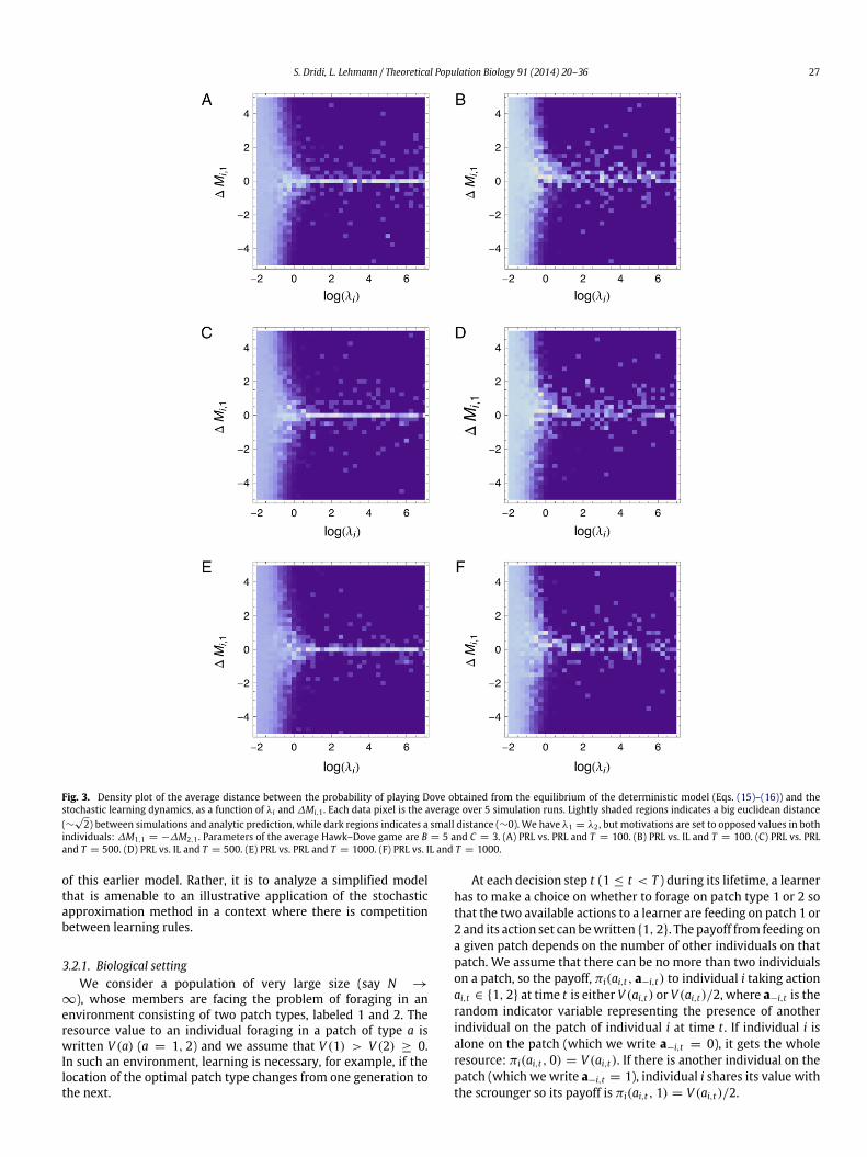
Fig. 3. Density plot of the average distance between the probability of playing Dove obtained from the equilibrium of the deterministic model (Eqs. (15)–(16)) and thestochastic learning dynamics, as a function of λi and ∆Mi,1 . Each data pixel is the average over 5 simulation runs. Lightly shaded regions indicates a big euclidean distance(∼

√2) between simulations and analytic prediction, while dark regions indicates a small distance (∼0). We have λ1 = λ2 , but motivations are set to opposed values in both

individuals: ∆M1,1 = −∆M2,1 . Parameters of the average Hawk–Dove game are B = 5 and C = 3. (A) PRL vs. PRL and T = 100. (B) PRL vs. IL and T = 100. (C) PRL vs. PRLand T = 500. (D) PRL vs. IL and T = 500. (E) PRL vs. PRL and T = 1000. (F) PRL vs. IL and T = 1000.

of this earlier model. Rather, it is to analyze a simplified modelthat is amenable to an illustrative application of the stochasticapproximation method in a context where there is competitionbetween learning rules.

3.2.1. Biological settingWe consider a population of very large size (say N →

∞), whose members are facing the problem of foraging in anenvironment consisting of two patch types, labeled 1 and 2. Theresource value to an individual foraging in a patch of type a iswritten V (a) (a = 1, 2) and we assume that V (1) > V (2) ≥ 0.In such an environment, learning is necessary, for example, if thelocation of the optimal patch type changes from one generation tothe next.

At each decision step t (1 ≤ t < T ) during its lifetime, a learnerhas to make a choice on whether to forage on patch type 1 or 2 sothat the two available actions to a learner are feeding on patch 1 or2 and its action set can bewritten 1, 2. The payoff from feeding ona given patch depends on the number of other individuals on thatpatch. We assume that there can be no more than two individualson a patch, so the payoff, πi(ai,t , a−i,t) to individual i taking actionai,t ∈ 1, 2 at time t is either V (ai,t) or V (ai,t)/2, where a−i,t is therandom indicator variable representing the presence of anotherindividual on the patch of individual i at time t . If individual i isalone on the patch (which we write a−i,t = 0), it gets the wholeresource: πi(ai,t , 0) = V (ai,t). If there is another individual on thepatch (which we write a−i,t = 1), individual i shares its value withthe scrounger so its payoff is πi(ai,t , 1) = V (ai,t)/2.


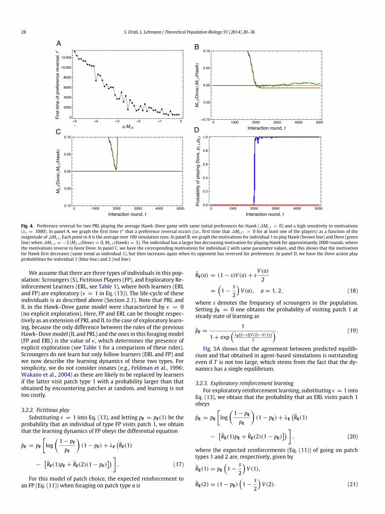
Fig. 4. Preference reversal for two PRL playing the average Hawk–Dove game with same initial preferences for Hawk (∆Mi,1 < 0) and a high sensitivity to motivations(λi = 1000). In panel A, we graph the first time t∗ that a preference reversal occurs (i.e., first time that ∆Mi,t∗ > 0 for at least one of the players) as a function of themagnitude of∆Mi,1 . Each point in A is the average over 100 simulation runs. In panel B, we graph themotivations for individual 1 to play Hawk (brown line) and Dove (greenline) when ∆M1,1 = −3 (M1,1(Dove) = 0,M1,1(Hawk) = 3). The individual has a larger but decreasing motivation for playing Hawk for approximately 2000 rounds, wherethe motivations reverse to favor Dove. In panel C, we have the corresponding motivations for individual 2 with same parameter values, and this shows that the motivationfor Hawk first decreases (same trend as individual 1), but then increases again when its opponent has reversed his preferences. In panel D, we have the Dove action playprobabilities for individual 1 (blue line) and 2 (red line).

We assume that there are three types of individuals in this pop-ulation: Scroungers (S), Fictitious Players (FP), and Exploratory Re-inforcement Learners (ERL, see Table 1), where both learners (ERLand FP) are exploratory (ϵ = 1 in Eq. (13)). The life-cycle of theseindividuals is as described above (Section 2.1). Note that PRL andIL in the Hawk–Dove game model were characterized by ϵ = 0(no explicit exploration). Here, FP and ERL can be thought respec-tively as an extension of PRL and IL to the case of exploratory learn-ing, because the only difference between the rules of the previousHawk–Dovemodel (IL and PRL) and the ones in this foragingmodel(FP and ERL) is the value of ϵ, which determines the presence ofexplicit exploration (see Table 1 for a comparison of these rules).Scroungers do not learn but only follow learners (ERL and FP) andwe now describe the learning dynamics of these two types. Forsimplicity, we do not consider innates (e.g., Feldman et al., 1996;Wakano et al., 2004) as these are likely to be replaced by learnersif the latter visit patch type 1 with a probability larger than thatobtained by encountering patches at random, and learning is nottoo costly.

3.2.2. Fictitious playSubstituting ϵ = 1 into Eq. (13), and letting pF = pF(1) be the

probability that an individual of type FP visits patch 1, we obtainthat the learning dynamics of FP obeys the differential equation

pF = pF

log

1 − pFpF

(1 − pF) + λF

RF(1)

−RF(1)pF + RF(2)(1 − pF)

. (17)

For this model of patch choice, the expected reinforcement toan FP (Eq. (11)) when foraging on patch type a is

RF(a) = (1 − s)V (a) + sV (a)2

=

1 −

s2

V (a), a = 1, 2, (18)

where s denotes the frequency of scroungers in the population.Setting pF = 0 one obtains the probability of visiting patch 1 atsteady state of learning as

pF =1

1 + exp

λF[2−s][V (2)−V (1)]2

. (19)

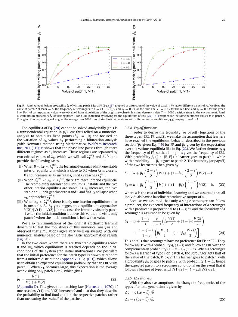
Fig. 5A shows that the agreement between predicted equilib-rium and that obtained in agent-based simulations is outstandingeven if T is not too large, which stems from the fact that the dy-namics has a single equilibrium.

3.2.3. Exploratory reinforcement learningFor exploratory reinforcement learning, substituting ϵ = 1 into

Eq. (13), we obtain that the probability that an ERL visits patch 1obeys

pE = pE

log

1 − pEpE

(1 − pE) + λE

RE(1)

−RE(1)pE + RE(2)(1 − pE)

, (20)

where the expected reinforcements (Eq. (11)) of going on patchtypes 1 and 2 are, respectively, given by

RE(1) = pE1 −

s2

V (1),

RE(2) = (1 − pE)1 −

s2

V (2). (21)


Fig. 5. Panel A: equilibrium probability pF of visiting patch 1 for a FP (Eq. (19)) graphed as a function of the value of patch 1, V (1), for different values of λi . We fixed thevalue of patch 2 at V (2) = 5, the frequency of scroungers to s = (3 −

√5)/2 and λi = 0.03 for the blue line, λi = 0.15 for the red line, and λi = 0.3 for the green

line. Dots of corresponding colors were obtained from simulations of the original stochastic learning dynamics after T = 1000 decision steps in the environment. PanelB: equilibrium probability pE of visiting patch 1 for a ERL (obtained by solving for the equilibrium of Eqs. (20)–(21) graphed for the same parameter values as in panel A.Triangles of corresponding colors give the average over 1000 runs of stochastic simulations with different initial conditions (pE,1) ranging from 0 to 1.

The equilibria of Eq. (20) cannot be solved analytically (this isa transcendental equation in pE). We thus relied on a numericalanalysis to obtain its fixed points (pE = 0) and focused onthe variation of λE values by performing a bifurcation analysis(with Newton’s method using Mathematica, Wolfram Research,Inc., 2011). Fig. 6 shows that the phase line passes through threedifferent regimes as λE increases. These regimes are separated bytwo critical values of λE, which we will call λ

crit1E and λ

crit2E , and

provide the following cases.(I) When 0 < λE < λ

crit1E , the learning dynamics admit one stable

interior equilibrium, which is close to 0.5 when λE is close to0 and increases as λE increases, until λE reaches λ

crit1E .

(II) When λcrit1E < λE < λ

crit2E , there are three interior equilibria.

The ‘‘completely interior’’ equilibrium is unstable and the twoother interior equilibria are stable. As λE increases, the twostable equilibria get closer to 0 and 1 and finally collapsewhenλE approaches λ

crit2E .

(III) When λE > λcrit2E , there is only one interior equilibrium that

is unstable. As λE gets bigger, this equilibrium approachesV (2)/[V (1) + V (2)]. In this case, the learner visits only patch1when the initial condition is above this value, and visits onlypatch 0 when the initial condition is below that value.

We also ran simulations of the original stochastic learningdynamics to test the robustness of this numerical analysis andobserved that simulations agree very well on average with ournumerical analysis based on the stochastic approximation results(Fig. 5B).

In the two cases where there are two stable equilibria (casesII and III), which equilibrium is reached depends on the initialconditions of the system (the initial motivations). We postulatethat the initial preference for the patch types is drawn at randomfrom a uniform distribution (Appendix D, Eq. (C.3)), which allowsus to obtain an expected equilibrium probability that an ERL visitspatch 1. When λE becomes large, this expectation is the averageover visiting only patch 1 or 2, which gives

pE =V (1)

V (1) + V (2)(22)

(Appendix D). This gives the matching law (Herrnstein, 1970), ifone rescales V (1) and V (2) between 0 and 1 so that they describethe probability to find food at all in the respective patches ratherthan measuring the ‘‘value’’ of the patches.

3.2.4. Payoff functionsIn order to derive the fecundity (or payoff) functions of the

three types (ERL, FP, and S), we make the assumption that learnershave reached the equilibrium behavior described in the previoussection (pF given Eq. (19) for FP and pE given by the expectationover the various equilibria like in Eq. (22). We further denote by qthe frequency of FP, so that 1 − q − s gives the frequency of ERL.With probability pi (i ∈ E, F), a learner goes to patch 1, whilewith probability 1− pi, it goes to patch 2. The fecundity (or payoff)of the two learners is then given by

bF = α + pF

2 − s2

V (1) + (1 − pF)

2 − s2

V (2) − k,

bE = α + pE

2 − s2

V (1) + (1 − pE)

2 − s2

V (2) − k, (23)

where k is the cost of individual learning and we assumed that allindividuals have a baseline reproductive output of α.

Because we assumed that only a single scrounger can followa producer, the expected frequency of interactions of a scroungerwith a producer is proportional to (1− s)/s, and the fecundity of ascrounger is assumed to be given by

bS = α +1 − ss

q

1 − s

pF

V (1)2

+ (1 − pF)V (2)2

+

1 − q − s1 − s

pE

V (1)2

+ (1 − pE)V (2)2

. (24)

This entails that scroungers have no preference for FP or ERL. Theyfollow an FPwith a probability q/(1−s) and follow an ERLwith thecomplementary probability (1− q− s)/(1− s). When a scroungerfollows a learner of type i on patch a, the scrounger gets half ofthe value of the patch, V (a)/2. This learner goes to patch 1 witha probability pi, or goes to patch 2 with probability 1 − pi, hencethe expected payoff to a scrounger conditional on the event that itfollows a learner of type i is pi[V (1)/2] + [1 − pi][V (2)/2].

3.2.5. ESS analysisWith the above assumptions, the change in frequencies of the

types after one generation is given by∆q = q

bF − b

/b

∆s = sbS − b

/b, (25)


Fig. 6. Bifurcation diagram for the differential equation (20) that describes the learning behavior of ERL in the producer–scrounger model as a function of λE . The thincurves describe the equilibrium values of pE and the thick vertical lines are phase lines at the corresponding values of λE . Dots on the phase lines denote interior equilibria.Our numerical exploration suggests that there are three possible phase lines depending on the value of λE (indicated by I, II, and III). Parameter values: s = (3 −

√5)/2,

V (1) = 5.3, V (2) = 5.

Fig. 7. Solution orbits of the evolutionary dynamics (Eq. (25)) in the pro-ducer–scrounger model on the 3-strategy simplex as a function of λE and λF . In thelight shaded region, ERL is themost performant (pE > pF), while in the dark shadedregion, FP is the most performant (pF > pE). The simplex drawn in the light regionis plotted for pE > pF and hence verifies that the mix between ERL and scroungersis the unique ESS. The simplex in the dark region corresponds to the case where theunique ESS is the mix between FP and scroungers. At the corner labeled FP on thesimplices, we have (q = 1, s = 0), at the corner ERL we have (q = 0, s = 0) and atthe corner S we have (q = 0, s = 1). A white-filled dot denotes an unstable node,a gray-filled dot is a saddle, and the black dot corresponds to the unique ESS. Thesesimplices were produced using the Baryplot package (McElreath, 2010) for R (R De-velopment Core Team, 2011). Parameter values for the shading: s =

3 −

√5

/2,V (1) = 5.3, V (2) = 5.

where b = qbF+sbS+(1−q−s)bE is themean reproductive outputin the population. The evolutionary dynamics (Eq. (25) with Eqs.(23)–(24)) displays five stationary states, which we write underthe form (q∗, s∗, 1 − q∗

− s∗). There are the three trivial equilibria

[(1, 0, 0),(0, 1, 0), (0, 0, 1)], one equilibrium with a coexistencebetween FP and scroungers, ( 1

2 (√5 − 1), 1

2 (3 −√5), 0), and

one with a coexistence between ERL and scroungers at the samefrequency as in the previous case: (0, 1

2 (3 −√5), 1

2 (√5 − 1)).

Because the payoff to scroungers exceeds that of producers whenthey are in low frequency s → 0 (for V (1) > 0 and/or V (2) > 0),the two equilibria where there is a mix between scroungers andproducers are stable in a reduced 2-strategy dynamics (on the facesof the simplex). Hence, the three trivial equilibria are unstable. Thequestion then is which one of the two other equilibria obtains.Because the fecundity of each type of producer does not depend onthe other type and in the sameway on the frequency of scroungers(Eq. (23)), the mix between scroungers and FP is invaded by ERL ifthey producemore resources. Namely, if the latter visit more oftenthe optimal patch, which obtains if

pE > pF. (26)

This invasion condition is not necessarily satisfied when λE >λF, and in Fig. 7 we display the regions of values of λF and λE whereit is satisfied. These regions seem to alternate in a non-trivial way.Interestingly, the region where ERL outcompetes FP looks fairlylarge for our parameter values. When λE becomes very large, it ispossible to have an exact invasion condition by substituting Eqs.(19) and (22) into Eq. (27), which implies that ERL invades thestable mix of FP and S if and only if

λF <2 log

V (1)V (2)

[V (1) − V (2)]

1 +

√5

/2. (27)

Summing up the above analysis, there is a globally stable statefor the 3-strategy replicator dynamics in this producer–scroungermodel that is the mix between scroungers and the mostperformant producer. In this unique evolutionarily stable state,producers are in frequency

√5 − 1

/2. Which of the producer

type will be maintained in the population (FP or ERL) criticallydepends on the exploration rate (λF and λE). It is noteworthy thatit is not the learner with the highest value of λi that will invade.The main reason for this is that increasing λE for ERL does notalways leads to a higher probability of visiting patch 1. When λE


is relatively small, this is actually true (in regime I of the learningdynamics of ERL, Fig. 6) but when λE grows (regimes II and III),ERL suddenly becomes prone to absorption in a state where itvisits patch 2 with a probability greater than 0.5 (pE < 0.5). Thismakes ERL less performant than FP for high values of λi (the upper-right region in Fig. 7). Further, when λi is very small (the lower-left region in Fig. 7), ERL seems to be less sensitive than FP to anincrease in λi.

4. Discussion

In this paper, we used stochastic approximation theory (Ljung,1977; Benveniste et al., 1991; Fudenberg and Levine, 1998; Be-naïm, 1999; Kushner and Yin, 2003; Sandholm, 2011) in order toanalyze the learning of actions over the course of an individual’slifespan in a situation of repeated social interactions with envi-ronmentally induced fluctuating game payoffs. This setting mayrepresent different ecological scenarios and population structures,where interactions can be represented as an iterated N-persongame or a multi-armed bandit. The learning dynamics was as-sumed to follow the experience-weighted attraction (EWA) learn-ing mechanism (Camerer and Ho, 1999; Ho et al., 2007). This is amotivational-based learning process, which encompasses as spe-cial cases various learning rules used in biology such as the lin-ear operator (McNamara andHouston, 1987; Bernstein et al., 1988;Stephens and Clements, 1998), relative payoff sum (Harley, 1981;Hamblin and Giraldeau, 2009) and Bayesian learning (Rodriguez-Gironés and Vásquez, 1997; Geisler and Diehl, 2002).

When a behavioral process has a decreasing step-size (or a verysmall constant step-size), stochastic approximation theory showsthat the behavioral dynamics is asymptotically driven by the ex-pected motion of the original stochastic recursions. Stochastic ap-proximation is thus appealing because once the expected motionof the stochastic learning process is derived, one is dealing withdeterministic differential equations that are easier to analyze. Fur-ther, the differential equations governing action play probabilitiesunder the EWAmodel that we have obtained (Eq. (13)) have a use-ful interpretation. They show that learning is driven by a balancebetween two forces. First, the exploration of actions that tends tobring the dynamics out of pure states, which is analogous to mu-tation in evolutionary biology. Second, the exploitation of actionsleading to higher expected reinforcement, which is analogous toselection in evolutionary biology. This second part actually takesthe same qualitative form as the replicator equation (Eq. (13)),since actions leading to an expected reinforcement higher than theaverage expected reinforcement will have a tendency to be playedwith increased probability. Although it may be felt in retrospectthat this result is intuitive, it is not directly apparent in the originalstochastic recursions of the behavioral rule, which encompassesparameters tuning the levels of cognition of individuals (Eq. (1)).

Our model is not the first where analogues of replicatordynamics appear out of an explicit learning scheme (e.g., Börgersand Sarin, 1997; Hopkins, 2002; Tuyls et al., 2003; Hofbauerand Sigmund, 2003). But, apart from Hopkins (2002), we are notaware of results that link the replicator dynamics to reinforcementlearning and belief-based learning at the same time, whichwas extended here to take fluctuating social environments intoaccount. Although we considered only individual learning withoutenvironmental detection in our formalization (i.e., individualslearn the average game), the reinforcement of motivations couldtake social learning into account (e.g., Cavalli-Sforza and Feldman,1983; Schlag, 1998; Sandholm, 2011), and/or individuals maydetect changes in the environment so that the motivationsthemselves may depend on environmental states (e.g., evaluatethe dynamics of motivations Mt(a, ω) for action-state pairs). The

consequences of incorporating these features for action ontogenymay be useful to analyze in future research.

We applied our results to analyze the dynamics of action playprobabilities in a situation of repeated pairwise interactions in a2 × 2 fluctuating game with average Hawk–Dove payoffs, wherewe investigated interactions between different learning rules, asituation that is very rarely addressed analytically (but see Leslieand Collins, 2005; Fudenberg and Takahashi, 2011). Comparisonwith stochastic simulations of the original learning dynamicsindicate that the deterministic dynamics generally approximatesqualitativelywell the quasi-equilibriumof action play probabilitiesobtained under the original stochastic process. Even if the theorycan only prove that the stochastic approximation of processeswith decreasing step-sizes ‘‘works’’ when time becomes very large(the differential equation are guaranteed to track the solutionsof the stochastic process only asymptotically, Benaïm, 1999), oursimulations suggest that stochastic approximation can, under goodcircumstances, give fair predictions for finite-time behavior (in ourcase, for T = 100, 500, and 1000), and also for the ontogenyof behavior (Fig. 8). This may be useful in the context of animalbehavior, when lifespan is short.

We also observed one limitation associated with using stochas-tic approximation in our examples. Namely, there are situationsthat are not captured by the deterministic approximation. Theseinvolve the cases where the sensitivity to payoff (λ) and the dif-ference between initial motivations (∆Mi,1) are very small so thatactions are random, and the cases where λ and ∆Mi,1 are very bigso that the dynamics get stuck in suboptimal equilibria. In particu-lar, when ∆Mi,1 is very large, individuals may have to reverse theirinitial preferences and thismakes very large the time forwhich thestochastic learning process gets close to its asymptotic approxima-tion.

Finally, we applied our results to analyze the evolutionary com-petition between learners and scroungers in a producer–scroungergame, where we considered that learners are producers (whosearch and find good patches of food) and scroungers follow theproducers. Three types were present in the population: individ-uals who learn according to Exploratory Reinforcement Learn-ing, individuals who learn according to Stochastic Fictitious Play(Table 1), and scroungers. This evolutionary model leads, at theESS, to the co-existence of scrounger with the most performant ofthe two learning rules. In particular, we showed that the explo-ration rate (λi) influences which is the most performant producer,but the effect of λi is non-linear. This shows that different learningrules are very differently affected by varying the exploration rate.The exploration rate and the choice rule (Eq. (4)) thus makes partof the definition of a learning rule, and λi may interact in a non-intuitive way with the other parameter of the process that affectmotivation updating.

While in this paper we analyzed certain learning rules withdecreasing step-size, it remains an open empirical question todocument how common this type of learning rules are in nature.It seems that previous work in animal psychology and behavioralecology focused more on rules with constant step-sizes (e.g., thelinear operator, Bush and Mostelller, 1951; Rescorla and Wagner,1972; Hamblin and Giraldeau, 2009; Arbilly et al., 2010) becausethe step-size has here a clear interpretation in terms of a discountfactor (or learning rate) and takes into account known phenomenasuch as habituation or forgetting. But it will be relevant todetermine how well rules with decreasing step-size fit animalbehavior. In particular, we suspect that such behavioral rules coulddescribe accurately learning processes where early experience iscritical to shape general behavior andwhere further information isused only to fine tune actions (e.g., developmental processes) andwhere preference reversal becomes unlikely.

In summary, although we illustrated some shortcoming ofapplying stochastic approximation, we showed that it can be a


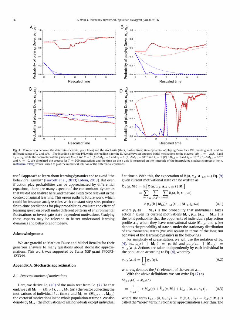
Fig. 8. Comparison between the deterministic (thin, plain lines) and the stochastic (thick, dashed lines) time dynamics of playing Dove for a PRL meeting an IL, and fordifferent values of λi and ∆Mi,1 . The blue line is for the PRL while the red line is for the IL. We always set opposed initial motivations to the players (∆M1,1 = −∆M2,1) andλ1 = λ2 , while the parameters of the game are B = 5 and C = 3. (A) ∆M1,1 = 1 and λi = 1. (B) ∆M1,1 = 10−1 and λi = 1. (C) ∆M1,1 = 1 and λi = 10−1 . (D) ∆M1,1 = 10−1

and λi = 10. We simulated the process for T = 500 interactions and the time on the x-axis is measured on the timescale of the interpolated stochastic process (the τnin Benaïm, 1999), which is used to plot the numerical solution of the differential equations.

useful approach to learn about learning dynamics and to avoid ‘‘thebehavioral gambit’’ (Fawcett et al., 2013; Lotem, 2013). But evenif action play probabilities can be approximated by differentialequations, there are many aspects of the concomitant dynamicsthatwedid not analyze here, and that are likely to be relevant in thecontext of animal learning. This opens paths to future work, whichcould for instance analyze rules with constant step-size, producefinite-time predictions for play probabilities, evaluate the effect oflearning speed on payoff under different patterns of environmentalfluctuations, or investigate state-dependent motivations. Studyingthese aspects may be relevant to better understand learningdynamics and behavioral ontogeny.

Acknowledgments

We are grateful to Mathieu Faure and Michel Benaïm for theirgenerous answers to many questions about stochastic approxi-mations. This work was supported by Swiss NSF grant PP00P3-123344.

Appendix A. Stochastic approximation

A.1. Expected motion of motivations

Here, we derive Eq. (10) of the main text from Eq. (7). To thatend, we callMi,t = (Mi,t(1), . . . ,Mi,t(m)) the vector collecting themotivations of individual i at time t and Mt = (M1,t , . . . ,MN,t)the vector ofmotivations in thewhole population at time t .We alsodenote byM−i,t themotivations of all individuals except individual

i at time t . With this, the expectation of Ri(a, ai,t , a−i,t , ωt) Eq. (9)given current motivational state can be written as

Ri,t(a,Mt) = ERi(a, ai,t , a−i,t , ωt) | Mt

=

h∈A

a−i∈AN−1

ω∈Ω

Ri(a, h, a−i, ω)

× pi,t(h | Mi,t)p−i,t(a−i | M−i,t)µ(ω), (A.1)

where pi,t(h | Mi,t) is the probability that individual i takesaction h given its current motivations Mi,t , p−i,t(a−i | M−i,t) isthe joint probability that the opponents of individual i play actionprofile a−i when they have motivational state M−i,t , and µ(ω)denotes the probability of stateω under the stationary distributionof environmental states (we will reason in terms of the long runbehavior of the learning dynamics in the following).

For simplicity of presentation, we will use the notation of Eq.(4), i.e., pi,t(k | Mi,t) = pi,t(k) and p−i,t(a−i | M−i,t) =

p−i,t(a−i). Actions are taken independently by each individual inthe population according to Eq. (4), whereby

p−i,t(a−i) =

i=j

pj,t(aj), (A.2)

where aj denotes the j-th element of the vector a−i.With the above definitions, we can write Eq. (7) as

Mi,t+1(a) − Mi,t(a)

=1

nt+1

−ϵiMi,t(a) + Ri,t(a,Mt) + Ui,t+1(a, at , ωt)

, (A.3)

where the term Ui,t+1(a, at , ωt) = Ri(a, at , ωt) − Ri,t(a,Mt) iscalled the ‘‘noise’’ term in stochastic approximation algorithm. The


expression Ui,t+1(a, at , ωt) is subscribed by t + 1 (and not t)in the stochastic approximation literature because it determinesthe value of the state variable at time t + 1. It follows from thedefinition of the noise that Ui,t(ai, at , ωt)t≥1 is a sequence ofmartingale differences adapted to the filtration generated by therandom variables Mtt≥1. That is, E[Ui,t+1(a, at , ωt)|Mt ] = 0.Since the payoffs are bounded, we also have E[Ui,t(a, at , ωt)

2] <

∞. We further assume that the choice probability (Eq. (4)) iscontinuous in the motivations of the players, such that theexpected reinforcement Ri,t(a,Mt) is Lipschitz continuous in themotivations. With this, −ϵiMi,t(a) + Ri,t(a,Mt) is a well-behavedvector field and standard results from stochastic approximationtheory (Benaïm, 1999; Benaïm and El Karoui, 2005, p. 173) allowus to approximate the original stochastic process (Eq. (A.3)) withthe deterministic differential equation

Mi(a) = −ϵiMi(a) + Ri(a,M). (A.4)

The solutions of the original stochastic recursion (Eq. (1))asymptotically track solutions of this differential equation. In par-ticular, it has been established that the stochastic process almostsurely converges to the internally chain recurrent set of the differ-ential equation (A.4) (Benaïm, 1999, Prop. 4.1 and Th. 5.7). The sim-plest form of a chain recurrent set is the set of equilibrium pointsof the dynamics (the particular applications of our model that westudy do not go beyond these cases). Note that in continuous timethe equations are deterministic and we remove the subscript t toMt for ease of presentation.

A.2. Differential equation in terms of mean payoff

Here, we show that it is possible to simplify the expressionof the expected reinforcement Ri,t(a,Mt) for our explicit learningmodel (Eq. (1)). First, recall from Eq. (9) that for action a of playeri, the realized reinforcement has the form

Ri(a, ai,t , a−i,t , ωt) =δi + (1 − δi)1(a, ai,t)

πi(a, a−i,t , ωt). (A.5)

We see that

Ri(a, ai,t , a−i,t , ωt) =

πi(a, a−i,t , ωt) if ai,t = a,δiπi(a, a−i,t , ωt) if ai,t = a. (A.6)

In order to find an expression for the expected reinforcementRi,t(a,Mt), it is useful to rewrite Eq. (A.5) as

Ri(a, ai,t , a−i,t , ωt) =δi + (1 − δi)1(a, ai,t)

×

a−i∈AN−1

πi(a, a−i, ωt)1(a−i, a−i,t), (A.7)

since 1(a−i, a−i,t) = 1 if a−i = a−i,t , 0 otherwise. Now, giventhat the event a = (a1, . . . , ai−1, a, ai+1, . . . , aN) occurs withprobability pi,t(a)p−i,t(a−i) at time t , we deduce that the expectedreinforcement of the motivation of action a is

Ri,t(a,Mt) =

ω∈Ω

µ(ω)

pi,t(a)

a−i∈AN−1

p−i,t(a−i)πi(a, a−i, ω)

+ δi(1 − pi,t(a))

a−i∈AN−1


. (A.8)

Factoring out, we have

Ri,t(a,Mt) =

ω∈Ω

µ(ω)

pi,t(a) + δi(1 − pi,t(a))

×

a−i∈AN−1


. (A.9)

Define the average payoff

πi(a, a−i) =

ω∈Ω

µ(ω)πi(a, a−i, ω). (A.10)

Taking expectation, then produces

Ri,t(a,Mt) = [pi,t(a) + δi(1 − pi,t(a))]

×

a−i∈AN−1

p−i,t(a−i)πi(a, a−i), (A.11)

and substituting into Eq. (A.3) shows that we can write thedifferential equation for the motivations (Eq. (A.4)) as

Mi(a) = −ϵiMi(a) + [pi(a) + δi(1 − pi(a))]

×

a−i∈AN−1

p−i(a−i)πi(a, a−i). (A.12)

A.3. Differential equation for the choice probabilities

A.3.1. Logit choiceHere,wederive theODE for the choice probabilities (Eq. (13)) by

combining the ODE for the motivations (Eq. (10)) with the choicerule (Eq. (4)), under the assumption that the choice rule is the logitchoice function (Eq. (6)).

Differentiating the left and right member of Eq. (4) with respectto time t , we have by the chain rule

pi(a) =

k∈A

dpi(a)dMi(k)

Mi(k), (A.13)

and substituting Eq. (4) gives

pi(a) =df (Mi(a))dMi(a)

Mi(a)k∈A

f (Mi(k))

− pi(a)k∈A

df (Mi(k))dMi(k)

Mi(k)h∈A

f (Mi(h)). (A.14)

Using f (M) = exp (λiM) in the choice function (Eq. (4)) givesEq. (6), which implies

df (Mi(a))dMi(a)

×1

k∈A

f (Mi(k))= λipi(a), (A.15)

whereby Eq. (A.14) can be written as

pi(a) = λipi(a)

Mi(a) −

k∈A

Mi(k)pi(k)

. (A.16)

Using the explicit expression for the differential equation of themotivations (Eq. (A.4)), this is

1λipi(a)

pi(a) = ϵi

k∈A

Mi(k) − Mi(a)pi(k)

+ Ri(a) −

k∈A

Ri(k)pi(k). (A.17)

But from the choice probabilities (Eq. (6)) we have the identity

pi(k)pi(a)

=exp [λiMi(k)]exp [λiMi(a)]

, (A.18)

which gives

logpi(k)pi(a)

= λi (Mi(k) − Mi(a)) (A.19)


and on substitution into Eq. (A.17) produces

pi(a) = pi(a)

ϵik∈A

logpi(k)pi(a)

pi(k)

+ λi

Ri(a) −

k∈A

Ri(k)pi(k)

. (A.20)

A.3.2. Power choiceHere, we perform the same derivation as in the last section

but assume that f (M) = Mλi in Eq. (4). In this case,[df (Mi(a))/dMi(a)] /

k∈A f (Mi(k)) =

λiMi(a)λi−1

/

k∈A f(Mi(k)) = λipi(a)/Mi(a), whereby using Mi(a) = −ϵiMi(a)+ Ri(a)in Eq. (A.14) yields

pi(a) = λipi(a)

−ϵi +

Ri(a)Mi(a)

−

k∈A

pi(k)

−ϵi +Ri(k)Mi(k)

.

(A.21)

Since −ϵi cancels from this equation and for non-negativemotivations we have the equality pi(a)/pi(k) = [Mi(a)/Mi(k)]λi ,we can write

pi(a) = [λipi(a)/Mi(a)]

×

Ri(a) −

k∈A

pi(k)pi(a)pi(k)

1/λiRi(k)

. (A.22)

Appendix B. Learning to play Hawk and Dove

Here, we analyze qualitatively the vector fields of Eqs. (15)–(16)with an average Hawk–Dove game. We used Mathematica (Wol-fram Research, Inc., 2011) to compute equilibria, eigenvalues andcomplicated algebraic expressions. We first study the interactionbetween two PRL and then the interaction between PRL and IL.

B.1. PRL vs. PRL

Pure Reinforcement Learning corresponds to δi = 0. Thus,replacing δ1 = δ2 = 0 in Eqs. (15)–(16) and using the payoffs ofthe Hawk–Dove game (Table 2) produces

p1 = p1(1 − p1)λ1

×

p1p2

B2

+ (1 − p1)p2B + (1 − p2)

B2

− C

,

p2 = p2(1 − p2)λ2

×

p2p1

B2

+ (1 − p2)p1B + (1 − p1)

B2

− C

. (B.1)

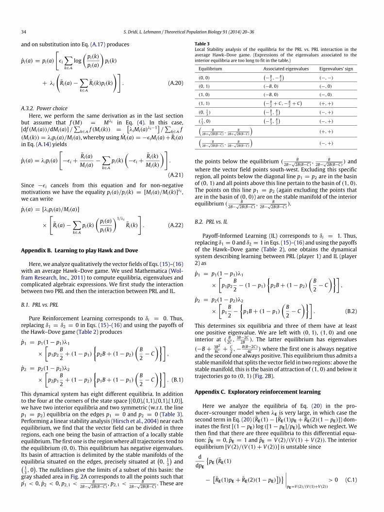
This dynamical system has eight different equilibria. In additionto the four at the corners of the state space [(0,0),(1,1),(0,1),(1,0)],we have two interior equilibria and two symmetric (w.r.t. the linep1 = p2) equilibria on the edges p1 = 0 and p2 = 0 (Table 3).Performing a linear stability analysis (Hirsch et al., 2004) near eachequilibrium, we find that the vector field can be divided in threeregions, each one being the basin of attraction of a locally stableequilibrium. The first one is the regionwhere all trajectories tend tothe equilibrium (0, 0). This equilibrium has negative eigenvalues.Its basin of attraction is delimited by the stable manifolds of theequilibria situated on the edges, precisely situated at

0, 1

3

and 1

3 , 0. The nullclines give the limits of a subset of this basin: the

gray shaded area in Fig. 2A corresponds to all the points such thatp1 < 0, p2 < 0, p2,1 < B

2B−√2B(B−C)

, p2,1 < B2B−

√2B(B−C)

. These are

Table 3Local Stability analysis of the equilibria for the PRL vs. PRL interaction in theaverage Hawk–Dove game. (Expressions of the eigenvalues associated to theinterior equilibria are too long to fit in the table.)

Equilibrium Associated eigenvalues Eigenvalues’ sign

(0, 0)−

B2 , − B

2

(−, −)

(0, 1) (−B, 0) (−, 0)

(1, 0) (−B, 0) (−, 0)

(1, 1)−

B2 + C, − B

2 + C

(+, +)

(0, 13 )

−

B3 , B

3

(−, +)

( 13 , 0)

−

B3 , B

3

(−, +)

B2B+

√2B(B−C)

, B2B+

√2B(B−C)

(+, +)

B2B−

√2B(B−C)

, B2B−

√2B(B−C)

(−, +)

the points below the equilibrium ( B2B−

√2B(B−C)

, B2B−

√2B(B−C)

) andwhere the vector field points south-west. Excluding this specificregion, all points below the diagonal line p1 = p2 are in the basinof (0, 1) and all points above this line pertain to the basin of (1, 0).The points on this line p1 = p2 (again excluding the points thatare in the basin of (0, 0)) are on the stable manifold of the interiorequilibrium ( B

2B−√2B(B−C)

, B2B−

√2B(B−C)

).

B.2. PRL vs. IL

Payoff-Informed Learning (IL) corresponds to δi = 1. Thus,replacing δ1 = 0 and δ2 = 1 in Eqs. (15)–(16) and using the payoffsof the Hawk–Dove game (Table 2), one obtains the dynamicalsystem describing learning between PRL (player 1) and IL (player2) as

p1 = p1(1 − p1)λ1

×

p1p2

B2

− (1 − p1)p2B + (1 − p2)

B2

− C

,

p2 = p2(1 − p2)λ2

×

p1

B2

−

p1B + (1 − p1)

B2

− C

. (B.2)

This determines six equilibria and three of them have at leastone positive eigenvalue. We are left with (0, 1), (1, 0) and oneinterior at ( B

2C , 3B−2C2B ). The latter equilibrium has eigenvalues

(−B +3B28C +

C2 , − B(B−2C)

4C ) where the first one is always negativeand the second one always positive. This equilibrium thus admits astablemanifold that splits the vector field in two regions: above thestable manifold, this is the basin of attraction of (1, 0) and below ittrajectories go to (0, 1) (Fig. 2B).

Appendix C. Exploratory reinforcement learning

Here we analyze the equilibria of Eq. (20) in the pro-ducer–scrounger model when λE is very large, in which case thesecond term in Eq. (20) (RE(1) − [RE(1)pE + RE(2)(1 − pE)]) dom-inates the first [(1 − pE) log ([1 − pE]/pE)], which we neglect. Wethen find that there are three equilibria to this differential equa-tion: pE = 0, pE = 1 and pE = V (2)/(V (1) + V (2)). The interiorequilibrium [V (2)/(V (1) + V (2))] is unstable since

ddpE

pERE(1)

−RE(1)pE + RE(2)(1 − pE)

pE=V (2)/(V (1)+V (2))

> 0 (C.1)


forV (1) > V (2) ≥ 0. Thus, an ERLwill learn to go on patch type 1 ifits initial probability to go on it is greater than V (2)/(V (1)+V (2)),and it will learn to go on patch 2 otherwise. If one draws the initialcondition at random from a uniform distribution on [0, 1], theexpected equilibrium probability to go on patch type 1 for an ERLis

pE = 0 ×V (2)

V (1) + V (2)+ 1 ×

1 −

V (2)V (1) + V (2)

=

V (1)V (1) + V (2)

. (C.2)

More generally, Eq. (20) is characterized by several stableequilibria and in order to define the expected equilibrium behaviorof ERL we follow the same argument by having a distributionover the initial conditions. We call E the set of stable equilibria,peE the value of stable equilibrium e, and βe the size of thebasin of attraction of equilibrium e. Then, we define the expectedprobability to go on patch 1 of ERL as

pE =

e∈E

βepeE, (C.3)

where, by a slight abuse of notation, we still use pE to denote theaverage.

For instance, when we are in equilibrium regime I (Fig. 6),i.e., when there is one stable equilibrium, there is only one termin the sum of Eq. (C.3). When we are in equilibrium regime II andIII, there are two terms in the sum.

Appendix D. Tit-for-Tat from EWA

Here, we derive the Tit-for-Tat strategy (Rapoport andChammah, 1965;Axelrod, 1980; Axelrod andHamilton, 1981) fromEWA. This is not a learning rule, but it is interesting that it can bederived from the EWA framework by appealing to the concept ofaspiration levels, which are often used in learning models (Galeet al., 1995;Wakano and Yamamura, 2001;Macy and Flache, 2002;Cho and Matsui, 2005; Izquierdo et al., 2007; Chasparis et al.,2010). This provides a payoff-based (i.e., quantitative) version ofTFT, which is easier to justify in terms of neuronal decision-makingthan the traditional version based on actions of opponent (whichis more qualitative). To that aim, we need that the parameters areφi = 0, ρi = 0, δi = 1, ni,1 = 1, and λi = ∞ (Table 1), and wesubtract aspiration levels to the original motivations, that is,

Mi,t+1(a) = πi(a, a−i,t , ωt) − Li(a), (D.1)

where Li(a) is the aspiration level of individual i for action a.In order to prove that Eq. (D.1) combinedwith Eq. (6) are indeed

Tit-for-Tat, consider an individual iwho is engaged in the repeatedplay of the Prisoner’s Dilemmawith a fixed opponent playing a−i,t .The payoff matrix is

R ST P

,

with the traditional assumptions that T > R > P > S and(T + S)/2 < R.

For Eqs. (D.1) and (6)with λi = ∞ to produce TFT behavior, oneneeds thatMi,t+1(C) > Mi,t+1(D), if a−i,t = C,Mi,t+1(C) < Mi,t+1(D), if a−i,t = D,

(D.2)

where a−i,t denotes here the action of the single opponent ofindividual i. Substituting the definition of the motivations (Eq.(D.1)) into Eq. (D.2), we have

πi(C, C) − Li(C) > πi(D, C) − Li(D), if a−i,t = C,πi(C,D) − Li(C) < πi(D,D) − Li(D), if a−i,t = D (D.3)

where Li(C) is the aspiration level of individual i for cooperation,Li(D) its aspiration level for defection, and where we removed thedependence of the payoffs on the environmental state ωt , becausewe consider a fixed game. Substituting the payoff from the payoffmatrix, Eq. (D.1) produces TFT behavior if

R − Li(C) > T − Li(D), if a−i,t = C,S − Li(C) < P − Li(D), if a−i,t = D,

(D.4)

which can be expressed as the single condition

T − R < Li(D) − Li(C) < P − S. (D.5)

We remark that this payoff-based version of TFTneeds that individ-ual i has a bigger aspiration level for defection, i.e., individual i ex-pects more of defection than of cooperation (because T −R > 0).Also, clearly not all Prisoner’s Dilemmagames satisfy conditionD.5.More precisely, this condition entails that defection needs to riskdominate cooperation (T − P < R − S) for our version of TFT tobe implementable.

References

Achbany, Y., Fouss, F., Yen, L., Pirotte, A., Saerens, M., 2006. Optimal tuningof continual online exploration in reinforcement learning. In: Kollias, S.,Stafylopatis, A., Duch, W., Oja, E. (Eds.), Artificial Neural Networks – ICANN2006. In: Lecture Notes in Computer Science, vol. 4131. Springer, Berlin /Heidelberg, pp. 790–800.

Anderson, S.P., de Palma, A., Thisse, J.-F., 1992. Discrete Choice Theory of ProductDifferentiation. The MIT Press, Cambridge, MA.

André, J.-B., 2010. The evolution of reciprocity: social types or social incentives?The American Naturalist 175, 197–210.

Arbilly, M., Motro, U., Feldman, M.W., Lotem, A., 2010. Co-evolution of learningcomplexity and social foraging strategies. Journal of Theoretical Biology 267,573–581.

Arbilly, M., Motro, U., Feldman, M.W., Lotem, A., 2011a. Evolution of social learningwhen high expected payoffs are associated with high risk of failure. Journal ofThe Royal Society Interface 8, 1604–1615.

Arbilly, M., Motro, U., Feldman, M.W., Lotem, A., 2011b. Recombination and theevolution of coordinated phenotypic expression in a frequency-dependentgame. Theoretical Population Biology 80, 244–255.

Axelrod, R., 1980. Effective choice in the prisoner’s dilemma. The Journal of ConflictResolution 24, 3–25.

Axelrod, R., Hamilton, W.D., 1981. The evolution of cooperation. Science 211,1390–1396.

Benaïm, M., 1999. Dynamics of stochastic approximation algorithms. In: Azéma, J.,et al. (Eds.), Séminaire de Probabilités XXXIII, vol. 1709. Springer, Berlin,pp. 1–68.

Benaïm, M., El Karoui, N., 2005. Promenade Aléatoire: Chaînes de Markov etSimulations; Martingales et Stratégies. Editions de l’Ecole Polytechnique,Palaiseau, France.

Benaïm, M., Hirsch, M.W., 1999a. Mixed equilibria and dynamical systems arisingfrom fictitious play in perturbed games. Games and Economic Behavior 29,36–72.

Benaïm, M., Hirsch, M.W., 1999b. Stochastic approximation algorithms withconstant step size whose average is cooperative. The Annals of AppliedProbability 9, 216–241.

Benveniste, A., Metivier, M., Priouret, P., 1991. Adaptive Algorithms and StochasticApproximations. Springer-Verlag, New York (NY).

Bernstein, C., Kacelnik, A., Krebs, J.R., 1988. Individual decisions and the distributionof predators in a patchy environment. Journal of Animal Ecology 57, 1007–1026.

Binmore, K.G., Samuelson, L., 1992. Evolutionary stability in repeated games playedby finite automata. Journal of Economic Theory 57, 278–305.

Börgers, T., Sarin, R., 1997. Learning through reinforcement and replicatordynamics. Journal of Economic Theory 77, 1–14.

Borkar, V.S., 2008. Stochastic Approximation: A Dynamical Systems Viewpoint.Cambridge University Press, Cambridge, MA.

Boyd, R., Richerson, P.J., 1985. Culture and the Evolutionary Process. University ofChicago Press.

Brown, G.W., 1951. Iterative solution of games by fictitious play. In: ActivityAnalysis of Production and Allocation. Wiley, New York, pp. 374–376.

Bush, R.R., Mostelller, F., 1951. A mathematical model for simple learning.Psychological Review 58, 313–323.

Camerer, C.F., 2003. Behavioral Game Theory: Experiments in Strategic Interaction.Princeton University Press, Princeton, NJ.

Camerer, C., Ho, T.H., 1999. Experienced-weighted attraction learning in normalform games. Econometrica 67, 827–874.

Cavalli-Sforza, L.L., Feldman, M.W., 1983. Cultural versus genetic adaptation.Proceedings of the National Academy of Sciences of the United States ofAmerica 80, 4993–4996.

Chalmeau, R., 1994. Do chimpanzees cooperate in a learning task? Primates 35,385–392.

http://refhub.elsevier.com/S0040-5809(13)00083-X/sbref1
























Chasparis, G., Shamma, J., Arapostathis, A., 2010. Aspiration learning in coordinationgames. In 49th IEEE Conference on Decision and Control (CDC), pages5756–5761.

Cho, I.-K., Matsui, A., 2005. Learning aspiration in repeated games. Journal ofEconomic Theory 124, 171–201.

Cournot, A.A., 1838. Recherches sur les Principes Mathématiques de la Théorie desRichesses. Hachette, L., Paris, France.

Dijker, A., 2011. Physical constraints on the evolution of cooperation. EvolutionaryBiology 38, 124–143.

Dugatkin, L.A., 2010. Principles of Animal Behavior, second ed. WW Norton & Co,New York (NY).

Dunlap, A.S., Stephens, D.W., 2009. Components of change in the evolutionof learning and unlearned preference. Proceedings of the Royal Society B:Biological Sciences 276, 3201–3208.

Emery, N.J., Clayton, N.S., 2004. The mentality of crows: Convergent evolution ofintelligence in corvids and apes. Science 306, 1903–1907.

Enquist, M.E., Ghirlanda, S., 2005. Neural Networks and Animal Behavior. PrincetonUniversity Press, Princeton, NJ.

Erev, I., Roth, A.E., 1998. Predicting howpeople play games: Reinforcement learningin experimental games with unique, mixed strategy equilibria. AmericanEconomic Review 88, 848–881.

Fawcett, T.W., Hamblin, S., Giraldeau, L.-A., 2013. Exposing the behavioral gambit:the evolution of learning and decision rules. Behavioral Ecology 24, 2–11.

Feldman, M., Aoki, K., Kumm, J., 1996. Individual versus social learning:evolutionary analysis in a fluctuating environment. Anthropological Science104, 209–232.

Foster, D.P., Young, H., 2003. Learning, hypothesis testing, and nash equilibrium.Games and Economic Behavior 45, 73–96.

Fudenberg, D., Levine, D.K., 1998. The Theory of Learning in Games. MIT Press,Cambridge, MA.

Fudenberg, D., Takahashi, S., 2011. Heterogeneous beliefs and local information instochastic fictitious play. Games and Economic Behavior 71, 100–120.

Gale, J., Binmore, K.G., Samuelson, L., 1995. Learning to be imperfect: the ultimatumgame. Games and Economic Behavior 8, 56–90.

Geisler, W.S., Diehl, R.L., 2002. Bayesian natural selection and the evolutionof perceptual systems. Philosophical Transactions: Biological Sciences 357,419–448.

Giraldeau, L.-A., Caraco, T., 2000. Social Foraging Theory. PrincetonUniversity Press,Princeton, NJ.

Grimmett, G.R., Stirzaker, D.R., 2001. Probability and Random Processes, third ed.Oxford University Press, Oxford.

Groß, R., Houston, A.I., Collins, E.J., McNamara, J.M., Dechaume-Moncharmont, F.-X.,Franks, N.R., 2008. Simple learning rules to cope with changing environments.Journal of The Royal Society Interface 5, 1193–1202.

Hamblin, S., Giraldeau, L.-A., 2009. Finding the evolutionarily stable learning rulefor frequency-dependent foraging. Animal Behaviour 78, 1343–1350.

Hammerstein, P., Stevens, J.R. (Eds.), 2012. Evolution and the Mechanisms ofDecision Making. MIT Press, Cambridge, MA.

Harley, C.B., 1981. Learning the evolutionarily stable strategy. Journal of TheoreticalBiology 89, 611–633.

Herrnstein, R.J., 1970. On the law of effect. Journal of the Experimental Analysis ofBehavior 13, 243–266.

Hirsch, M.W., Smale, S., Devaney, R.L., 2004. Differential Equations, DynamicalSystems, and an Introduction to Chaos. Academic Press, San Diego, CA.

Ho, T.H., Camerer, C.F., Chong, J.-K., 2007. Self-tuning experience weightedattraction learning in games. Journal of Economic Theory 133, 177–198.

Hofbauer, J., Sandholm, W.H., 2002. On the global convergence of stochasticfictitious play. Econometrica 70, 2265–2294.

Hofbauer, J., Sigmund, K., 1998. Evolutionary Games and Population Dynamics.Cambridge University Press, Cambridge, MA.

Hofbauer, J., Sigmund, K., 2003. Evolutionary game dynamics. Bulletin of theAmerican Mathematical Society 40, 479–519.

Hollis, K.L., Dumas, M.J., Singh, P., Fackelman, P., 1995. Pavlovian conditioning ofaggressive behavior in blue gourami fish (Trichogaster trichopterus): winnersbecomewinners and losers stay losers. Journal of Comparative Psychology 109,123–133.

Hopkins, E., 2002. Two competing models of how people learn in games.Econometrica 70, 2141–2166.

Houston, A.I., 1983. Comments on ‘‘Learning the evolutionarily stable strategy’’.Journal of Theoretical Biology 105, 175–178.

Houston, A.I., Sumida, B.H., 1987. Learning rules, matching and frequencydependence. Journal of Theoretical Biology 126, 289–308.

Izquierdo, L.R., Izquierdo, S.S., Gotts, N.M., Polhill, J.G., 2007. Transient andasymptotic dynamics of reinforcement learning in games. Games and EconomicBehavior 61, 259–276.

Jordan, J.S., 1991. Bayesian learning in normal form games. Games and EconomicBehavior 3, 60–81.

Josephson, J., 2008. A numerical analysis of the evolutionary stability of learningrules. Journal of Economic Dynamics and Control 32, 1569–1599.

Karlin, S., Taylor, H.E., 1975. A First Course in Stochastic Processes. Academic Press,San Diego, CA.

Katsnelson, E., Motro, U., Feldman, M.W., Lotem, A., 2011. Evolution of learnedstrategy choice in a frequency-dependent game. Proceedings of the RoyalSociety B: Biological Sciences.

Kushner, H.J., Yin, G.G., 2003. Stochastic Approximation and Recursive Algorithmsand Applications, second ed. Springer, New York (NY).

Leimar, O., Hammerstein, P., 2001. Evolution of cooperation through indirectreciprocity. Proceedings of the Royal Society B: Biological Sciences 268,745–753.

Leslie, D.S., Collins, E.J., 2005. Individual q-learning in normal form games. SIAMJournal on Control and Optimization 44, 495–514.

Ljung, L., 1977. Analysis of recursive stochastic algorithms. IEEE Transactions onAutomatic Control 22, 551–575.

Lotem, A., 2013. Learning to avoid the behavioral gambit. Behavioral Ecology 24,13–13.

Luce, R.D., 1959. Individual Choice Behavior. Wiley, New York.Macy, M.W., Flache, A., 2002. Learning dynamics in social dilemmas. Proceedings of

the National Academy of Sciences 99, 7229–7236.Maynard Smith, J., 1982. Evolution and the Theory of Games. Cambridge University

Press, Cambridge.Maynard Smith, J., Price, G.R., 1973. The logic of animal conflict. Nature 246, 15–18.McElreath, R., 2010. Baryplot 1.0.McElreath, R., Boyd, R., 2007. Mathematical Models of Social Evolution: A Guide for

the Perplexed. University Of Chicago Press, Chicago.McKelvey, R.D., Palfrey, T.R., 1995. Quantal response equilibria for normal form

games. Games and Economic Behavior 10, 6–38.McNamara, J.M., Houston, A.I., 1987. Memory and the efficient use of information.

Journal of Theoretical Biology 125, 385–395.McNamara, J.M., Houston, A.I., 2009. Integrating function and mechanism. Trends

in Ecology & Evolution 24, 670–675.Niv, Y., 2009. Reinforcement learning in the brain. Journal of Mathematical

Psychology 53, 139–154.Norman, M.F., 1968. Some convergence theorems for stochastic learning models

with distance diminishing operators. Journal of Mathematical Psychology 5,61–101.

Plotnik, J.M., Lair, R., Suphachoksahakun,W., DeWaal, F.B.M., 2011. Elephants knowwhen they need a helping trunk in a cooperative task. Proceedings of theNational Academy of Sciences 108, 5116–5121.

R Development Core Team 2011. R: A Language and Environment for StatisticalComputing. R Foundation for Statistical Computing, Vienna, Austria.

Rapoport, A., Chammah, A.M., 1965. Prisoner’s Dilemma. University of MichiganPress, Ann Arbor.

Rescorla, R.A., Wagner, A.R., 1972. A theory of pavlovian conditioning: Variationsin the effectiveness of reinforcement and nonreinforcement. In: Black, A.H.,Prokasy, W.F. (Eds.), Classical Conditioning II: Current Research and Theory.Appleton-Century-Crofts, New York (NY), pp. 64–99.

Rodriguez-Gironés, M.A., Vásquez, R.A., 1997. Density-dependent patch exploita-tion and acquisition of environmental information. Theoretical Population Bi-ology 52, 32–42.

Rogers, A.R., 1988. Does biology constrain culture. American Anthropologist 90,819–831.

Sandholm, W.H., 2011. Population Games and Evolutionary Dynamics. MIT Press,Cambridge, MA.

Schlag, K.H., 1998. Why imitate, and if so, how? Journal of Economic Theory 78,130–156.

Shettleworth, S.J., 2009. Cognition, Evolution, and Behavior. Oxford UniversityPress, New York (NY).

Stephens, D.W., 1991. Change, regularity, and value in the evolution of animallearning. Behavioral Ecology 2, 77–89.

Stephens, D.W., Clements, K.C., 1998. Game theory and learning. In: Game Theoryand Animal Behavior. Oxford University Press, New York, pp. 239–260.

Sutton, R.S., Barto, A.G., 1998. Reinforcement Learning. MIT Press, Cambridge, MA.Thorndike, E.L., 1911. Animal Intelligence. Hafner, Darien, CT.Tracy, N.D., Seaman, J.W., 1995. Properties of evolutionarily stable learning rules.

Journal of Theoretical Biology 177, 193–198.Tuyls, K., Verbeeck, K., Lenaerts, T., 2003. A selection–mutation model for Q-

learning in multi-agent systems. In: Proceedings of the Second InternationalJoint Conference on Autonomous Agents and Multiagent Systems. ACM,Melbourne, Australia, pp. 693–700.

van der Horst, W., van Assen, M., Snijders, C., 2010. Analyzing behavior impliedby EWA learning: an emphasis on distinguishing reinforcement from belieflearning. Journal of Mathematical Psychology 54, 222–229.

Villarreal, R., Domjan, M., 1998. Pavlovian conditioning of social affirmative behav-ior in the mongolian gerbil (Meriones unguiculatus). Journal of ComparativePsychology 112, 26–35.

Wakano, J.Y., Aoki, K., Feldman, M.W., 2004. Evolution of social learning: amathematical analysis. Theoretical Population Biology 66, 249–258.

Wakano, J.Y., Yamamura, N., 2001. A simple learning strategy that realizes robustcooperation better than pavlov in iterated prisoners’ dilemma. Journal ofEthology 19, 1–8.

Walsh, P.T., Hansell, M., Borello, W.D., Healy, S.D., 2011. Individuality in nestbuilding: do southern masked weaver (Ploceus velatus) males vary in theirnest-building behaviour? Behavioural Processes 88, 1–6.

Weibull, J.W., 1997. Evolutionary Game Theory. MIT Press, Cambridge, MA.Wolfram Research, Inc. 2011. Mathematica, Version 8.0.4. Champaign, Illinois.Young, H.P., 2004. Strategic Learning and its Limits. OxfordUniversity Press, Oxford.









































































Documents

On learning dynamics underlying the evolution of learning rules