On interactive fuzzy numbers ∗

Robert Fullerrfuller@abo.fi

Peter Majlenderpeter.majlender@abo.fi

Abstract

In this paper we will introduce a measure of interactivity between marginaldistributions of a joint possibility distribution C as the expected value of theinteractivity relation between the γ-level sets of its marginal distributions.

1 Introduction

The concept of conditional independence has been studied in depth in possibilitytheory, for good surveys see, e.g. Campos and Huete [5, 6]. The notion of non-interactivity in possibility theory was introduced by Zadeh [10]. Hisdal [4] demon-strated the difference between conditional independence and non-interactivity. Inthis paper we will introduce a measure of interactivity between fuzzy numbers viatheir joint possibility distribution. A fuzzy set A in R is said to be a fuzzy numberif it is normal, fuzzy convex and has an upper semi-continuous membership func-tion of bounded support. The family of all fuzzy numbers will be denoted by F .A γ-level set of a fuzzy set A in Rm is defined by [A]γ = {x ∈ Rm : A(x) ≥ γ}if γ > 0 and [A]γ = cl{x ∈ Rm : A(x) > γ} (the closure of the support of A) ifγ = 0. If A ∈ F is a fuzzy number then [A]γ is a convex and compact subset ofR for all γ ∈ [0, 1]. Fuzzy numbers can be considered as possibility distributions[10]. A fuzzy set B in Rm is said to be a joint possibility distribution of fuzzynumbers Ai ∈ F , i = 1, . . . ,m, if it satisfies the relationship

maxxj∈R, j 6=i

B(x1, . . . , xm) = Ai(xi), ∀xi ∈ R, i = 1, . . . ,m.

Furthermore, Ai is called the i-th marginal possibility distribution of B, and theprojection of B on the i-th axis is Ai for i = 1, . . . ,m. Fuzzy numbers Ai ∈ F ,i = 1, . . . ,m, are said to be non-interactive if their joint possibility distribution isgiven by B(x1, . . . , xm) = min{A1(x1), . . . , Am(xm)}, for all x1, . . . , xm ∈ R.

∗The final version of this paper appeared in: Fuzzy Sets and Systems, 143(2004) 355-369.

1

Furthermore, in this case the equality [B]γ = [A1]γ × · · · × [Am]γ holds for anyγ ∈ [0, 1].

IfA,B ∈ F are non-interactive then their joint membership function is definedby A × B. It is clear that in this case any change in the membership function ofA does not effect the second marginal possibility distribution and vice versa. Onthe other hand, A and B are said to be interactive if they can not take their valuesindependently of each other [1].

Figure 1: Non-interactive possibility distributions.

Definition 1.1 [2] A function f : [0, 1] → R is said to be a weighting function iff is non-negative, monotone increasing and satisfies the following normalizationcondition ∫ 1

0f(γ)dγ = 1.

Different weighting functions can give different (case-dependent) importancesto γ-levels sets of fuzzy numbers. If f is a step-wise linear function then we canhave discrete weights. This definition is motivated in part by the desire to giveless importance to the lower levels of fuzzy sets (it is why f should be monotoneincreasing).

2 Central values

In this section we shall introduce the notion of average value of real-valued func-tions on γ-level sets of joint possibility distributions and we shall show how theseaverage values can be used for measuring interactions between γ-level sets of itsmarginal distributions.

Let B be a joint possibility distribution in Rn, let γ ∈ [0, 1] and let g : Rn → Rbe an integrable function. It is well-known from analysis that the average value offunction g on [B]γ can be computed by

C[B]γ (g) =1∫

[B]γ dx

∫[B]γ

g(x)dx

=1∫

[B]γ dx1 . . . dxn

∫[B]γ

g(x1, . . . , xn)dx1 . . . dxn.

We will call C as the central value operator.

2

Note 2.1 If [B]γ is a degenerated set, that is∫[B]γ

dx = 0,

then we compute C[B]γ (g) as the limit case of a uniform approximation of [B]γ withnon-degenerated sets [3]. That is, let

S(ε) = {x ∈ Rn|∃c ∈ [B]γ ‖x− c‖ ≤ ε}, ε > 0.

Then obviously ∫S(ε)

dx > 0, ∀ε > 0,

and we define the central value of g on [B]γ as

C[B]γ (g) = limε→0CS(ε)(g) = lim

ε→0

1∫S(ε) dx

∫S(ε)

g(x)dx. (1)

If g : R → R is an integrable function and A ∈ F then the average value offunction g on [A]γ is defined by

C[A]γ (g) =1∫

[A]γ dx

∫[A]γ

g(x)dx.

Especially, if g(x) = x, for all x ∈ R is the identity function (g = id) andA ∈ F is a fuzzy number with [A]γ = [a1(γ), a2(γ)] then the average value of theidentity function on [A]γ is computed by

C[A]γ (id) =1∫

[A]γ dx

∫[A]γ

xdx =1

a2(γ)− a1(γ)

∫ a2(γ)

a1(γ)xdx =

a1(γ) + a2(γ)2

,

which remains valid in the limit case a2(γ) − a1(γ) = 0 for some γ. BecauseC[A]γ (id) is nothing else, but the center of [A]γ we will use the shorter notationC([A]γ) for C[A]γ (id).

It is clear that C[B]γ is linear for any fixed joint possibility distribution B andfor any γ ∈ [0, 1]. Let us denote the projection functions on R2 by πx and πy, thatis, πx(u, v) = u and πy(u, v) = v for u, v ∈ R.

The following theorems shows two important properties of the central valueoperator.

3

Theorem 2.1 If A,B ∈ F are non-interactive and g = πx + πy is the additionoperator on R2 then

C[A×B]γ (πx + πy) = C[A]γ (id) + C[B]γ (id) = C([A]γ) + C([B]γ),

for all γ ∈ [0, 1].

Proof 1 If A and B are non-interactive then [C]γ = [A]γ × [B]γ for all γ ∈ [0, 1],that is,

C[C]γ (πx + πy) =1∫

[A]γ×[B]γ dxdy

∫[A]γ×[B]γ

(x+ y)dxdy

=1

[a2(γ)− a1(γ)][b2(γ)− b1(γ)]

∫ a2(γ)

a1(γ)

∫ b2(γ)

b1(γ)(x+ y)dxdy

=1

[a2(γ)− a1(γ)][b2(γ)− b1(γ)]

×[[b2(γ)− b1(γ)]

∫[A]γ

xdx+ [a2(γ)− a1(γ)]∫

[B]γydy

]=

1a2(γ)− a1(γ)

∫[A]γ

xdx+1

b2(γ)− b1(γ)

∫[B]γ

ydy

=a1(γ) + a2(γ)

2+b1(γ) + b2(γ)

2= C([A]γ) + C([B]γ),

Theorem 2.2 If A,B ∈ F are non-interactive and p = πxπy is the multiplicationoperator on R2 then

C[A×B]γ (πxπy) = C[A]γ (id) · C[B]γ (id) = C([A]γ) · C([B]γ),

for all γ ∈ [0, 1].

Proof 2 If A and B are non-interactive then [C]γ = [A]γ × [B]γ for all γ ∈ [0, 1],that is,

C[C]γ (πxπy) =1∫

[A]γ×[B]γ dxdy

∫[A]γ×[B]γ

xydxdy

=1

[a2(γ)− a1(γ)][b2(γ)− b1(γ)]

∫ a2(γ)

a1(γ)

∫ b2(γ)

b1(γ)xydxdy

=1

[a2(γ)− a1(γ)][b2(γ)− b1(γ)]

∫ a2(γ)

a1(γ)xdx ·

∫ b2(γ)

b1(γ)ydy

=a1(γ) + a2(γ)

2·b1(γ) + b2(γ)

2= C([A]γ) · C([B]γ).

4

The following definition is crucial for our theory.

Definition 2.1 Let C be a joint possibility distribution with marginal possibilitydistributions A,B ∈ F , and let γ ∈ [0, 1]. The measure of interactivity betweenthe γ-level sets of A and B is defined by

R[C]γ (πx, πy) = C[C]γ((πx − C[C]γ (πx))(πy − C[C]γ (πy))

).

Using the definition of central value we have

R[C]γ (πx, πy) =1∫

[C]γ dxdy

∫[C]γ

(x− C[C]γ (πx)) · (y − C[C]γ (πy))dxdy

=1∫

[C]γ dxdy

∫[C]γ

xydxdy − C[C]γ (πy) ·1∫

[C]γ dxdy

∫[C]γ

xdxdy

− C[C]γ (πx) ·1∫

[C]γ dxdy

∫[C]γ

ydxdy + C[C]γ (πx) · C[C]γ (πy)

= C[C]γ (πxπy)− C[C]γ (πx) · C[C]γ (πy),

for all γ ∈ [0, 1].Recall that two ordered pairs (x1, y1) and (x2, y2) of real numbers are concor-

dant if (x1 − x2)(y1 − y2) > 0; and discordant if (x1 − x2)(y1 − y2) < 0.

Note 2.2 The interactivity relation computes the average value of the interactivityfunction

g(x, y) = (x− C[C]γ (πx))(y − C[C]γ (πy)),

on [C]γ . Suppose that we choose a point x ∈ R then [C]γ will impose a con-straint on possible values of y. The value of g(x, y) is positive (negative) if andonly if (x, y) and (C[C]γ (πx), C[C]γ (πy)) are concordant (discordant). Looselyspeaking, the value of R[C]γ (πx, πy) is positive if the ’strength’ of (x, y) and(C[C]γ (πx), C[C]γ (πy)) that are concordant is bigger than the strength of those onesthat are discordant.

Consider now the case depicted on Fig.2. After some calculations we find

C[C]γ (πx) =a1(γ) + a2(γ)

2= C([A]γ),

and

C[C]γ (πy) =b1(γ) + b2(γ)

2= C([B]γ).

5

If A takes u then B can take only a single value v. We can easily see that in thiscase

g(x, y) = (x− C([A]γ))(y − C([B]γ),

will always be positive.

Let A,B ∈ F with [A]γ = [a1(γ), a2(γ)] and [B]γ = [b1(γ), b2(γ)]. In [2] weintroduced the notion of f -weighted covariance of possibility distributions A andB as

Covf (A,B) =∫ 1

0

a2(γ)− a1(γ)2

·b2(γ)− b1(γ)

2f(γ)dγ.

The main drawback of that definition is that Covf (A,B) is always non-negativefor any A and B. Based on the notion of central values we shall introduce a noveldefinition of covariance, that agrees with the principle of ’falling shadows’. Fur-thermore, we shall use this new definition of covariance to measure interactionsbetween two fuzzy numbers.

Definition 2.2 LetC be a joint possibility distribution in R2. LetA,B ∈ F denoteits marginal possibility distributions. The covariance of A and B with respect to aweighting function f (and with respect to their joint possibility distributioin C) isdefined by

Covf (A,B) =∫ 1

0R[C]γ (πx, πy)f(γ)dγ

=∫ 1

0

[C[C]γ (πxπy)− C[C]γ (πx) · C[C]γ (πy)

]f(γ)dγ.

(2)

If A and B are non-interactive then from Theorem 2.2 it follows that

R[C]γ (πx, πy) = C[A×B]γ (πxπy)− C([A]γ) · C([B]γ) = 0

for all γ ∈ [0, 1], which directly implies the following theorem:

Theorem 2.3 If A,B ∈ F are non-interactive then Covf (A,B) = 0 for anyweighting function f .

Note 2.3 If we consider (2) with the constant weighting function f(γ) = 1 for allγ ∈ [0, 1] then we get

Covf (A,B) =∫ 1

0R[C]γ (πx, πy)dγ.

6

That is, Covf (A,B) simple sums up the interactivity measures level-wisely. In (2)f(γ) weights the importance of the interactivity between the γ-level sets of A andB. It can happen that we care more about interactivites on higher levels than onlower levels.

Now we illustrate our approach to interactions by several simple examples.Let A,B ∈ F and suppose that their joint possibility distribution C is defined

by (see Fig. 2)

[C]γ = {t(a1(γ), b1(γ)) + (1− t)(a2(γ), b2(γ)) | t ∈ [0, 1]},

for all γ ∈ [0, 1]. It is easy to check that A and B are really the marginal distribu-tions of C. In this case A and B are interactive. We will compute the measure ofinteractivity between A and B.

Figure 2: Joint possibility distribution C.

Let γ be arbitrarily fixed, and let a1 = a1(γ), a2 = a2(γ), b1 = b1(γ), b2 =b2(γ). Then the γ-level set of C can be calculated as {(c(y), y)|b1 ≤ y ≤ b2}where

c(y) =b2 − yb2 − b1

a1 +y − b1b2 − b1

a2 =a2 − a1

b2 − b1y +

a1b2 − a2b1

b2 − b1.

Since all γ-level sets of C are degenerated, i.e. their integrals vanish, the followingformal calculations can be done∫

[C]γdxdy =

∫ b2

b1

[x]c(y)c(y)dy,

∫[C]γ

xydxdy =∫ b2

b1

y

[x2

2

]c(y)c(y)

dy,

which turns into

C[C]γ (πxπy) =1∫

[C]γ dxdy

∫[C]γ

xydxdy

=1

b2 − b1

∫ b2

b1

yc(y)dy

=1

(b2 − b1)2

[13(a2 − a1)(b32 − b31) +

12(a1b2 − a2b1)(b22 − b21)

]

=2(a2 − a1)(b21 + b1b2 + b22) + 3(a1b2 − a2b1)(b1 + b2)

6(b2 − b1)

=(a2 − a1)(b2 − b1)

3+a1b2 + a2b1

2.

7

Hence, we have

R[C]γ (πx, πy) = C[C]γ (πxπy)− C[C]γ (πx)C[C]γ (πy)

=(a2 − a1)(b2 − b1)

3+a1b2 + a2b1

2−

(a1 + a2)(b1 + b2)4

=(a2 − a1)(b2 − b1)

12,

and, finally, the covariance of A and B with respect to their joint possibility distri-bution C is

Covf (A,B) =112

∫ 1

0[a2(γ)− a1(γ)][b2(γ)− b1(γ)]f(γ)dγ.

Note 2.4 In this case Covf (A,B) > 0 for any weighting function f ; and ifA(u) ≥ γ for some u ∈ R then there exists a unique v ∈ R that B can take(see Fig. 2), furthermore, if u is moved to the left (right) then the correspondingvalue (that B can take) will also move to the left (right).

Let A,B ∈ F and suppose that their joint possibility distribution D is definedby (see Fig. 3)

[D]γ = {t(a1(γ), b2(γ)) + (1− t)(a2(γ), b1(γ)) | t ∈ [0, 1]}.

for all γ ∈ [0, 1]. In this case A and B are interactive. We will compute now themeasure of interactivity between A and B.

Figure 3: Joint possibility distribution D.

After similar calculations we get

C[D]γ (πxπy) = −(a2 − a1)(b2 − b1)

3+a1b1 + a2b2

2,

which implies that

R[D]γ (πx, πy) = C[D]γ (πxπy)− C[D]γ (πx)C[D]γ (πy) = −(a2 − a1)(b2 − b1)

12,

and we find

Covf (A,B) = −112

∫ 1

0[a2(γ)− a1(γ)][b2(γ)− b1(γ)]f(γ)dγ.

8

Note 2.5 In this case Covf (A,B) < 0 for any weighting function f ; and ifA(u) ≥ γ for some u ∈ R then there exists a unique v ∈ R that B can take(see Fig. 3), furthermore, if u is moved to the left (right) then the correspondingvalue (that B can take) will move to the right (left).

Now consider the case when A(x) = B(x) = (1 − x) · χ[0,1](x) for x ∈ R,that is, [A]γ = [B]γ = [0, 1− γ] for γ ∈ [0, 1]. Suppose that their joint possibilitydistribution is given by

F (x, y) = (1− x− y) · χT (x, y),

where T = {(x, y) ∈ R2|x ≥ 0, y ≥ 0, x + y ≤ 1}. This situation is depicted onFig. 4, where we have shifted the fuzzy sets to get a better view of the situation.

Figure 4: Joint possibility distribution F .

It is easy to check that A and B are really the marginal distributions of F . A γ-level set of F is computed by [F ]γ = {(x, y) ∈ R2|x ≥ 0, y ≥ 0, x+ y ≤ 1− γ}.Then

R[F ]γ (πx, πy) =1∫

[F ]γ dxdy

∫[F ]γ

xydxdy

−

(1∫

[F ]γ dxdy

∫[F ]γ

xdxdy

)(1∫

[F ]γ dxdy

∫[F ]γ

ydxdy

),

where, ∫[F ]γ

dxdy =(1− γ)2

2,

and, ∫[F ]γ

xydxdy =∫ 1−γ

0

∫ 1−γ−x

0xydxdy =

12

∫ 1−γ

0x(1− γ − x)2dx

=1− γ

2

∫ 1−γ

0x2dx−

12

∫ 1−γ

0x3dx =

(1− γ)4

24,

furthermore, ∫[F ]γ

xdxdy =∫

[F ]γydxdy =

∫ 1−γ

0

∫ 1−γ−x

0ydxdy

=12

∫ 1−γ

0(1− γ − x)2dx =

(1− γ)3

6,

9

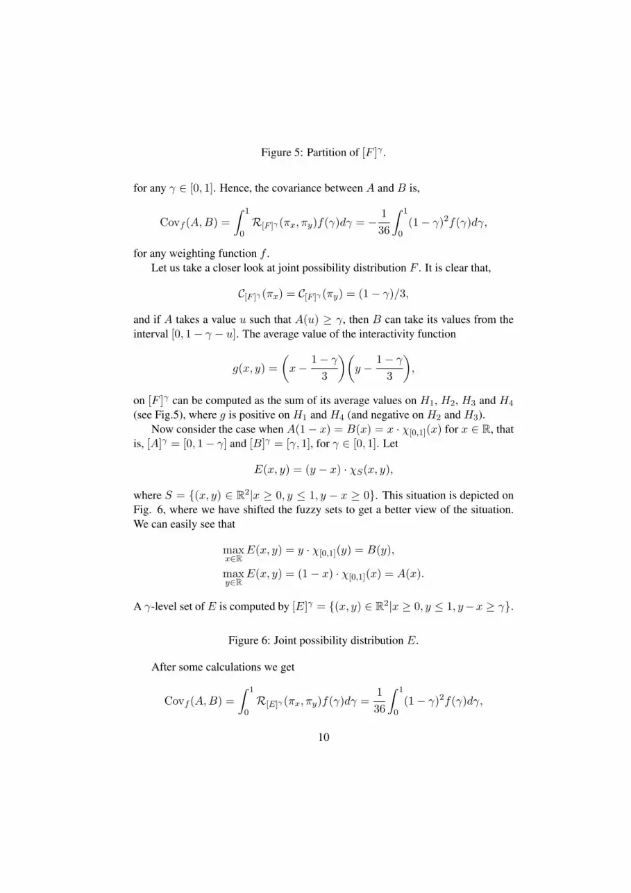
Figure 5: Partition of [F ]γ .

for any γ ∈ [0, 1]. Hence, the covariance between A and B is,

Covf (A,B) =∫ 1

0R[F ]γ (πx, πy)f(γ)dγ = −

136

∫ 1

0(1− γ)2f(γ)dγ,

for any weighting function f .Let us take a closer look at joint possibility distribution F . It is clear that,

C[F ]γ (πx) = C[F ]γ (πy) = (1− γ)/3,

and if A takes a value u such that A(u) ≥ γ, then B can take its values from theinterval [0, 1− γ − u]. The average value of the interactivity function

g(x, y) =(x−

1− γ3

)(y −

1− γ3

),

on [F ]γ can be computed as the sum of its average values on H1, H2, H3 and H4

(see Fig.5), where g is positive on H1 and H4 (and negative on H2 and H3).Now consider the case when A(1− x) = B(x) = x · χ[0,1](x) for x ∈ R, that

is, [A]γ = [0, 1− γ] and [B]γ = [γ, 1], for γ ∈ [0, 1]. Let

E(x, y) = (y − x) · χS(x, y),

where S = {(x, y) ∈ R2|x ≥ 0, y ≤ 1, y − x ≥ 0}. This situation is depicted onFig. 6, where we have shifted the fuzzy sets to get a better view of the situation.We can easily see that

maxx∈R

E(x, y) = y · χ[0,1](y) = B(y),

maxy∈R

E(x, y) = (1− x) · χ[0,1](x) = A(x).

A γ-level set of E is computed by [E]γ = {(x, y) ∈ R2|x ≥ 0, y ≤ 1, y−x ≥ γ}.

Figure 6: Joint possibility distribution E.

After some calculations we get

Covf (A,B) =∫ 1

0R[E]γ (πx, πy)f(γ)dγ =

136

∫ 1

0(1− γ)2f(γ)dγ,

10

for any weighting function f .We can also use the principle of central values to introduce the notion of ex-

pected value of functions on fuzzy sets. Let g : R → R be an integrable functionand let A ∈ F . Let us consider again the average value of function g on [A]γ

C[A]γ (g) =1∫

[A]γ dx

∫[A]γ

g(x)dx.

Definition 2.3 The expected value of function g on A with respect to a weightingfunction f is defined by

Ef (g;A) =∫ 1

0C[A]γ (g)f(γ)dγ =

∫ 1

0

1∫[A]γ dx

∫[A]γ

g(x)dxf(γ)dγ.

Especially, if g is the identity function then we get

Ef (id;A) = Ef (A) =∫ 1

0

a1(γ) + a2(γ)2

f(γ)dγ,

which is thef -weighted possibilistic expected value value of A introduced in [2].Let us denoteR[A]γ (id, id) the average value of function g(x) = (x−C([A]γ))2

on the γ-level set of an individual fuzzy number A. That is,

R[A]γ (id, id) =1∫

[A]γ dx

∫[A]γ

x2dx−(

1∫[A]γ dx

∫[A]γ

xdx

)2

.

Definition 2.4 The variance of A is defined as the expected value of functiong(x) = (x− C([A]γ))2 on A. That is,

Varf (A) = Ef (g;A) =∫ 1

0R[A]γ (id, id)f(γ)dγ.

From the equality,

R[A]γ (id, id) =1

a2(γ)− a1(γ)

∫ a2(γ)

a1(γ)x2dx−

(1

a2(γ)− a1(γ)

∫ a2(γ)

a1(γ)xdx

)2

=a2

1(γ) + a1(γ)a2(γ) + a22(γ)

3−(a1(γ) + a2(γ)

2

)2

=a2

1(γ)− 2a1(γ)a2(γ) + a22(γ)

12=

(a2(γ)− a1(γ))2

12,

we get,

Varf (A) =∫ 1

0

(a2(γ)− a1(γ))2

12f(γ)dγ.

11

Note 2.6 The expected value of the identity function on an individual fuzzy number(with respect to a weighting function f ) coincides with the definition of f -weightedpossibilistic mean value of fuzzy numbers introduced in [2]. The f -weighted vari-ance is almost the same as in [2] (the same up to a scalar multiplier).

Note 2.7 The covariance between marginal distributions A and B of a joint pos-sibility distribution C is nothing else but the expected value of their interactivityfunction on C (with respect to a weighting function f ).

The next theorem about the bilinearity of the interactivity relation operator caneasily be proved.

Theorem 2.4 Let C be a joint possibility distribution in R2, and let λ, µ ∈ R.Then

R[C]γ (λπx + µπy, λπx + µπy) =

λ2R[C]γ (πx, πx) + µ2R[C]γ (πy, πy) + 2λµR[C]γ (πx, πy).

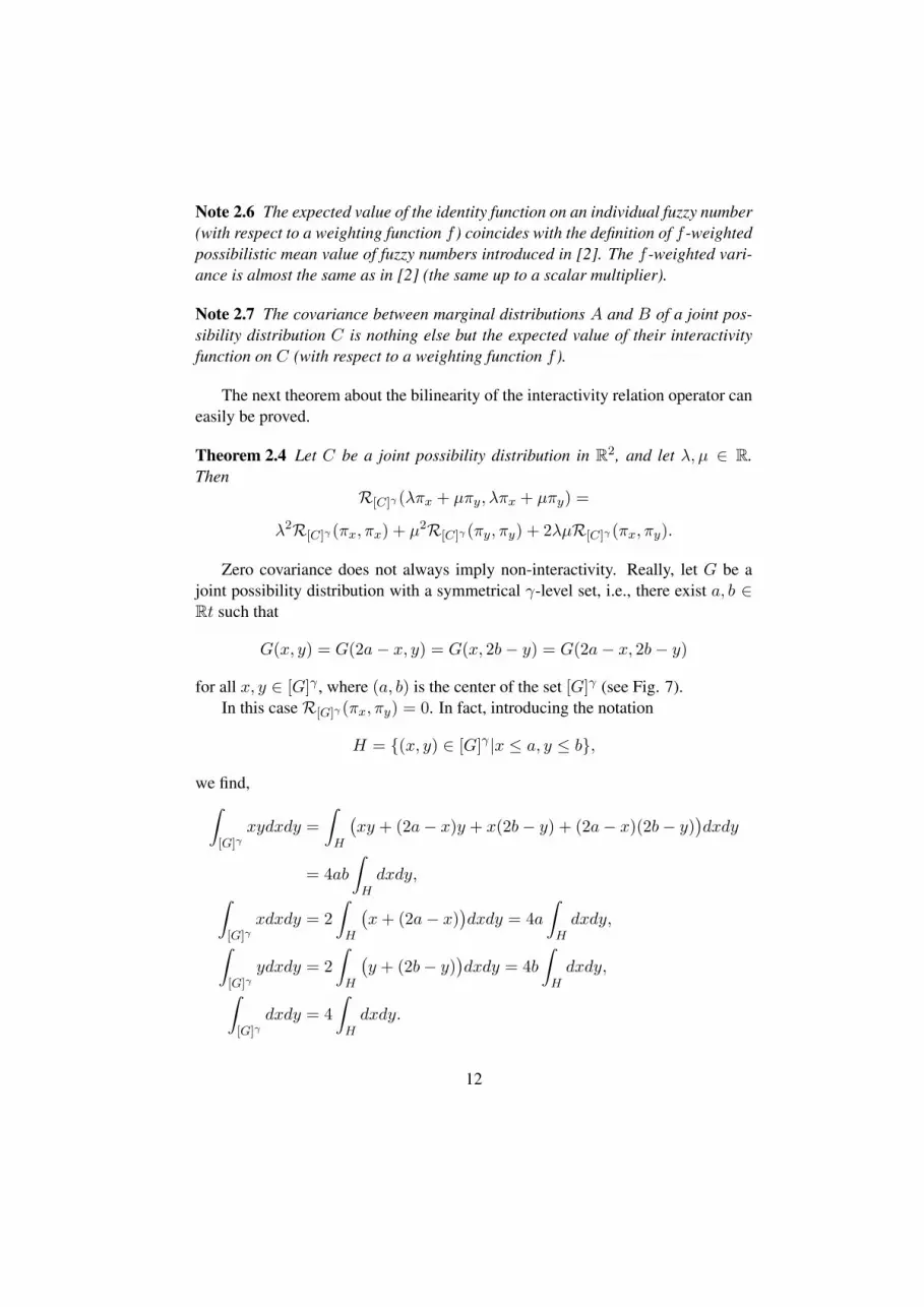
Zero covariance does not always imply non-interactivity. Really, let G be ajoint possibility distribution with a symmetrical γ-level set, i.e., there exist a, b ∈Rt such that

G(x, y) = G(2a− x, y) = G(x, 2b− y) = G(2a− x, 2b− y)

for all x, y ∈ [G]γ , where (a, b) is the center of the set [G]γ (see Fig. 7).In this caseR[G]γ (πx, πy) = 0. In fact, introducing the notation

H = {(x, y) ∈ [G]γ |x ≤ a, y ≤ b},

we find,∫[G]γ

xydxdy =∫H

(xy + (2a− x)y + x(2b− y) + (2a− x)(2b− y)

)dxdy

= 4ab∫Hdxdy,∫

[G]γxdxdy = 2

∫H

(x+ (2a− x)

)dxdy = 4a

∫Hdxdy,∫

[G]γydxdy = 2

∫H

(y + (2b− y)

)dxdy = 4b

∫Hdxdy,∫

[G]γdxdy = 4

∫Hdxdy.

12

Figure 7: Joint possibility distribution G.

That is,

R[G]γ (πx, πy) =1∫

[G]γ dxdy

∫[C]γ

xydxdy

−(

1∫[G]γ dxdy

∫[C]γ

xdxdy

)(1∫

[G]γ dxdy

∫[C]γ

ydxdy

)= 0.

If all γ-level sets ofG are symmetrical then the covariance between its marginaldistributions A and B becomes zero for any weighting function f , that is,

Covf (A,B) = 0,

even though A and B may be interactive.

Note 2.8 Consider a symmetrical joint possibility distribution with center (0, 0),that is, G(x, y) = G(−x, y) = G(x,−y) = G(−x,−y), for all x, y. So, if(u, v) ∈ [G]γ for some u, v ∈ R then (−u, v), (u,−v) and (−u,−v) will alsobelong to [G]γ , therefore, simple algebra shows that the equation∫

[G]γxydxdy = 0,

holds for any γ ∈ [0, 1]. In a similar manner we can prove the relationships∫[G]γ

xdxdy =∫

[G]γydxdy = 0

for any γ ∈ [0, 1]. So, the average value of function

g(x, y) = (x− 0)(y − 0) = xy,

on [G]γ is zero (independently of γ).

Note 2.9 Let X and Y be random variables with joint probability distributionfunction H and marginal distribution functions F and G, respectively. Then thereexists a copula C (which is uniquely determined on Range F× Range G) such thatH(x, y) = C(F (x), G(y)) for all x, y [9]. Based on this fact, several indeces ofdependencies were introduced in [7, 8]. Furthermore, any copula C satisfies therelationship [8]

W (x, y) = max{x+ y − 1, 0} ≤ C(x, y) ≤M(x, y) = min{x, y},

13

For uniform distributions on [a1(γ), a2(γ)] and [b1(γ), b2(γ)] we look for a jointdistribution defined on the Cartesian product of this level intervals (with uniformmarginal distributions on [a1(γ), a2(γ)] and [b1(γ), b2(γ)]): this joint distributioncan always be characterized by a unique copula C, which may depend also on γ(see [7]). For non-interactive situation, C is just the product (with zero covariance,this is Theorem 2.3); Fig. 2 is linked to copula M (with correlation 1); and Fig. 3is linked to copula W (with correlation -1).

3 Summary

We have introduced the notion of covariance between marginal distributions of ajoint possibility distribution C as the expected value of their interactivity functionon C. We have interpreted this covariance as a measure of interactivity betweenmarginal distributions. We have shown that non-interactivity entails zero covari-ance, however, zero covariance does not always imply non-interactivity. The mea-sure of interactivity is positive (negative) if the expected value of the interactivityrelation on C is positive (negative). The concept introduced in this paper can beused in capital budgeting decisions where (estimated) future costs and revenues aremodelled by interactive fuzzy numbers.

4 Acknowledgements

The authors thank the anonymous referee for his/her helpful note (Note 2.9) andsuggestions on the earlier version of this paper.

References

[1] D. Dubois and H. Prade, Possibility Theory: An Approach to ComputerizedProcessing of Uncertainty, Plenum Press, New York, 1988.

[2] R. Fuller and P. Majlender, On weighted possibilistic mean and variance offuzzy numbers, Fuzzy Sets and Systems. (to appear)

[3] R. Fuller and P. Majlender, Correction to: “On interactive fuzzy num-bers” [Fuzzy Sets and Systems, 143(2004) 355-369] Fuzzy Sets and Systems152(2005) 159-159.

[4] E. Hisdal, Conditional possibilities independence and noninteraction, FuzzySets and Systems, 1(1978) 283-297.

14

[5] L. M. de Campos and J. F. Huete, Independence concepts in possibility the-ory: Part I, Fuzzy Sets and Systems, 103(1999) 127-152.

[6] L. M. de Campos, J. F. Huete, Independence concepts in possibility theory:Part II, Fuzzy Sets and Systems, 103(1999) 487-505.

[7] R.B. Nelsen, An introduction to copulas, Lecture Notes in Statistics, 139,Springer-Verlag, New York, 1999.

[8] R.B. Nelsen, J. J. Quesada-Molina, J. A. Rodrıguez-Lallena and M. Ubeda-Flores, Distribution functions of copulas: a class of bivariate probability in-tegral transforms, Statist. Probab. Lett., 54 (2001) 277-282.

[9] A. Sklar, Fonctions de repartition a n dimensions et leurs marges, Publ. Inst.Statist. Univ. Paris, 8(1959) 229-231.

[10] L. A. Zadeh, Concept of a linguistic variable and its application to approxi-mate reasoning, I, II, III, Information Sciences, 8(1975) 199-249, 301-357;9(1975) 43-80.

Main results

The main results of this paper are,

• The f -weighted possibilistic variance of fuzzy number A is defined by

Varf (A) =∫ 1

0

(a2(γ)− a1(γ))2

12f(γ)dγ.

• The measure of covariance between A and B (with respect to their jointdistribution C and weighting function f ) by

Covf (A,B) =∫ 1

0R[C]γ (πx, πy)f(γ)dγ =

∫ 1

0cov(Xγ , Yγ)f(γ)dγ,

where Xγ and Yγ are random variables whose joint distribution is uniformon [C]γ for all γ ∈ [0, 1]; furthermore cov(Xγ , Yγ) denotes the probabilisticcovariance between marginal random variables Xγ and Yγ . If f(γ) = 2γthen we write simple Cov(A,B), that is

Cov(A,B) =∫ 1

02γcov(Xγ , Yγ)dγ,

15

Citations

[A7] Robert Fuller and Peter Majlender, On interactive fuzzy numbers, FUZZYSETS AND SYSTEMS 143(2004) 355-369. [MR2052672]

in journals

A7-c6 Hong, D.H., Kim, K.T., A maximal variance problem, APPLIED MATH-EMATICS LETTERS, 20 (10), pp. 1088-1093. 2007

http://dx.doi.org/10.1016/j.aml.2006.12.008

Fuller and Majlender [A7] presented the idea of interaction be-tween a marginal distribution of a joint possibility distribution.They introduced the notion of covariance between fuzzy num-bers via their joint possibility distribution to measure the degreeto which the fuzzy numbers interact. (page 1088)

A7-c5 Jian-li ZHAO, Zhi-gang JIA, Ying LI, Weighted Ranking and Simple Op-eration Approaches of Fuzzy-number Based on Four-dimensional Represen-tations, FUZZY SYSTEMS AND MATHEMATICS, 2007, Vol.21 No.2 pp.97-101.

A7-c4 B. Bede and J. Fodor, Product Type Operations between Fuzzy Numbersand their Applications in Geology, ACTA POLYTECHNICA HUNGAR-ICA, Vol. 3, No. 1, pp. 123-139. 2006

http://www.bmf.hu/journal/Bede_Fodor_5.pdf

A7-c3 Przemysław Grzegorzewski and Edyta Mrowka, Trapezoidal approxima-tions of fuzzy numbers, FUZZY SETS AND SYSTEMS 153(1): 115-135JUL 1 2005

http://dx.doi.org/10.1016/j.fss.2004.02.015

in proceedings

A7-c2 Pierpaolo D’Urso, Fuzzy Clustering of Fuzzy Data, in: J. Valente deOliveira and W. Pedrycz eds., Advances in Fuzzy Clustering and its Ap-plications, John Wiley & Sons, [ISBN 978-0-470-02760-8], pp. 155-192.2007

16

A7-c1 J. Fodor, B. Bede, Arithmetics with Fuzzy Numbers: a Comparative Overview,SAMI 2006 conference, Herlany, Slovakia, [ISBN 963 7154 44 2], pp.54-68.2006

http://www.bmf.hu/conferences/sami2006/Fodor.pdf

17