Embed Size (px)
Citation preview

413
Charles University Center for Economic Research and Graduate Education
Academy of Sciences of the Czech Republic Economics Institute
OLIGOPOLISTIC PRICE COMPETITION WITH INFORMED AND UNINFORMED
BUYERS
Michal Ostatnický
CERGE-EI
WORKING PAPER SERIES (ISSN 1211-3298) Electronic Version

Working Paper Series 413 (ISSN 1211-3298)
Oligopolistic Price Competition with Informed and Uninformed Buyers
Michal Ostatnický
CERGE-EI
Prague, August 2010
ISBN 978-80-7343-211-9 (Univerzita Karlova. Centrum pro ekonomický výzkum a doktorské studium) ISBN 978-80-7344-201-9 (Národohospodářský ústav AV ČR, v.v.i.)

Oligopolistic Price Competition
with Informed and Uninformed Buyers*
Michal Ostatnický†
WP 413
Abstract
The standard price competition of two or more players leads to Bertrand equilibrium in basic
economic theory (if complete information is assumed, there are no capacity constraints, etc.).
In reality, even on highly competitive Internet-based markets, the prices of seemingly
undifferentiated goods (e.g. books and CDs on Amazon and similar e-shops) vary, although
competition seems prima facie based on prices. I follow the literature that originated with
Varian’s (1980) model, especially Kocas and Kiyak (2006), and analyze oligopolistic markets
where buyers have reservation values drawn from a common distribution function rather than
a single value (inelastic demand), as typically assumed in the models of Varian’s or Kocas
and Kiyak’s type. The model presented in this paper is developed from the simplest
symmetric set-up (uninformed buyers are assigned to sellers evenly) to the most complex
asymmetric set-up with many competing sellers (uninformed buyers are distributed over
sellers unevenly). The most complex set-up theoretically rationalizes the empirical findings
of Kocas and Kiyak. In the equilibrium of my model, all sellers randomly choose prices from
a non-trivial interval for (almost) every seller, while in Kocas and Kiyak’s theoretical model
only two sellers randomize while others always offer the same price.
Abstrakt
Standardní soutěž v cenách dvou nebo více hráčů vede ve standardní ekonomické teorii k
Bertrandově rovnováze (předpokládáme-li úplnou informaci, není omezována kapacita, atd.).
V reálném prostředí, a to i v prostředí velmi fragmentovaného trhu na internetu, jsou ceny
nerozlišitelného zboží (například knih a CD) různé, ačkoli se trh zřejmě řídí pravidly cenové
soutěže. Vycházím z literatury, která se odvíjí od Varianova (1980) modelu, zejména ze
studie Kocase a Kiyaka (2006) a studuji oligopolistické trhy, kde mají kupující cenové limity
náhodně rozděleny, tj. není to jedna fixní hodnota jako v dosud publikované literatuře typu
Varianovy studie nebo modelu Kocase a Kiyaka. Zde analyzovaný model je vyvíjen od
nejjednodušší struktury (neinformovaní kupující jsou rovnoměrně rozděleni k prodávajícím),
až po nejsložitější (nerovnoměrné rozdělení kupujících). Nejsložitější struktura dává
racionální podklad empirickým zjištěním Kocase a Kiyaka. V rovnovážném bodě modelu
(téměř) každý prodávající volí ceny náhodně z netriviálního intervalu, oproti tomu v
teoretickém modelu Kocase a Kiyaka pouze dva prodávající volí ceny náhodně a ostatní volí
vždy fixní cenu.
Keywords: oligopoly, price competition, price dispersion.
JEL classification: L11, D43.
*I would like to thank Andreas Ortmann who gave me valuable comments while writing this paper, Levent
Celik for helpful comments in the last stage, and Avner Shaked for hints given
during the early stages of writing this paper. †CERGE-EI is a joint workplace of the Center for Economic Research and Graduate Education, Charles
University, and the Economics Institute of Academy of Sciences of the Czech Republic.
Address: CERGE-EI, P.O. Box 882, Politických vězňů 7, Prague 1, 111 21, Czech Republic
1

I. Introduction
In this paper, I follow the literature on price dispersion. Using the concept of
informed and uninformed buyers, I show that price competition with no capacity
constraint can result in pricing that differs from the Bertrand equilibrium pricing
and fits empirically observed behavior. Specifically, I derive a model that fits Kocas
and Kiyak’s (2006) empirical findings better than their own model.
The basic features of the model I develop in this paper have been applied before
in a simpler, slightly different set-up. The informed buyers1 know the prices posted
by all sellers and choose the seller with the lowest price, and the uninformed buyers2
choose sellers randomly. Sellers choose prices so that they benefit maximally from
uninformed buyers (which entices sellers to choose high prices) and informed buyers
(which entices sellers to choose low prices).
The literature on this topic was initiated by Salop and Stiglitz (1977), and fol-
lowed by Varian (1980).3 These articles present models without sequential search
in their articles. Consumers are either fully informed or never search and stay unin-
formed. Other examples of such models can be found in Braverman (1980), Stiglitz
(1979), and Narasimhan (1988). In the present paper, I follow this precedent.4
Non-sequential, Varian-type search models have been applied to explain pro-
motional strategies (Raju, Srinivasan, and Lal, 1990), international trade (Neven,
Norman, and Thisse, 1991 or Baye and De Vries, 1992) and other applications where
buyers may have an exogenously given tendency to prefer one product (seller) over
another. All these models (with one laudable exception to be discussed presently)
assume either a symmetry of sellers, meaning uninformed consumers are distributed
paper, Levent Celik for helpful comments in the last stage, and Avner Shaked for hints givenduring the early stages of writing this paper.
1In the literature they are also called switchers, or searchers, even though search may not bemodelled in the paper. I stick to the term “informed buyers” in this paper.
2In the literature they are also called non-searchers or loyal buyers.3The model I derive in this paper is mainly based on Varian (1980) and Kocas and Kiyak
(2006), so I refer to these models as Varian-type models.4A related stream of literature does feature sequential search. Burdett and Judd (1983), Rein-
ganum (1979), Stahl (1989), Stiglitz (1987), and Wilde and Schwartz (1979) are prominent exam-ples.
2

evenly over sellers, or a duopoly configuration.5
Recently, informed by Varian-type models, empirical researchers have used data
collected from Internet e-shops (e.g. Clay, Ramayya, Wolff, and Fernandes, 2002;
Clemons, Hann, and Hitt, 2002; or Iyer and Pazgal, 2003).
The most recent and most relevant research in the present context is Kocas and
Kiyak (2006). These authors take the Varian (1980) model, where uninformed buy-
ers choose a seller randomly (i.e. the probability an uniformed buyer chooses a spe-
cific seller is equal for all sellers) and add an asymmetry introduced by Narasimhan
(1988): Uninformed buyers always go to “their” seller. The amount of uninformed
buyers (which can be thought of as loyal) can be different for every seller. Kocas
and Kiyak show that at most two sellers offer discounts,6 while others choose the
monopoly price. This theoretical result does not correspond well to the reality of
the online-book retailer market in which all sellers offer discounts.7 The authors en-
rich the model by seller-specific reservation prices to increase price dispersion. They
fail, however, to get mixed strategies for all sellers as observed in reality. The result
seems to be caused by the assumption of fixed reservation values. In this paper, I
show that by relaxing this assumption and, instead, assuming that the reservation
prices of all buyers are drawn from a commonly known distribution function, all
sellers apply indeed mixed strategies. I also show that the lower bound of the sup-
port of the mixed-strategy distribution function is increasing with the increasing
share of uninformed buyers. This result is in line with the empirical findings that
Kocas and Kiyak provide.
I develop my model from the simplest set-up to the most complex, analyz-5Additionally, Sinitsyn (2008) theoretically characterizes the basic features of the Varian-type
model class. He shows that for a Varian-type model with heterogeneous tastes, a mixed-strategyequilibrium exists and identifies the basic features of the support of the equilibrium strategies.
6Offering a discount implies that they follow a mixed strategy in equilibrium. The mixedstrategy nature of the equilibrium is standard in non-sequential, Varian-type models. The mixedstrategy equilibrium results from optimal price-setting to capture the informed buyers (setting alow enough price to beat competitors) and to gain from the uniformed ones (setting a high enoughprice). Kocas and Kiyak show that in their set-up “only those with the least to lose from deep pricecuts will offer discounts” (Kocas and Kiyak, 2006, page 90), and others do not want to competeand sell only to the uninformed buyers.
7The fact that all sellers offer discounts is empirically documented in their article; see Figure3 of Kocas and Kiyak (2006).
3

ing gradually symmetric duopoly and oligopoly (section II) and then asymmetric
duopoly and oligopoly (section III).8 Section IV concludes.
II. Symmetric model
I start the analysis with the simplest possible model: symmetric duopoly. Two
sellers offer undifferentiated products. Both sellers have to post a price so that
everyone can buy the product at the given price, and they cannot discriminate
between individual buyers. There is a mass of potential buyers willing to buy one
unit of the product. Each buyer has a reservation value drawn from a commonly
known distribution function; the reservation value itself is the private information
of each buyer.
A buyer can either be informed about prices posted by the sellers or be unin-
formed. An informed buyer either buys one unit of the product from the seller with
the lower posted price (if it is lower than the reservation value) and leaves the mar-
ket or does not buy anything. An uninformed buyer chooses randomly, with equal
probabilities, one seller and then compares the posted price with his reservation
value. If the reservation value is higher than the posted price, the buyer gets one
unit of the product and leaves the market; otherwise, he does not buy the product
and, without checking the price of the other seller, he leaves the market.9
The game is one-shot. There is no repetition. Search is not possible.10
The model is symmetric because the probability that an uninformed buyer comes
to one of the sellers equals the probability he comes to the other. From a seller’s
perspective, there is a fixed probability that a specific buyer comes to her whatever
price she posts. It is the probability that the buyer is uninformed and he (randomly,
with probability 1/2) chooses to come to the seller. The probability that an informed8The last, and most complex, model includes also the simpler cases. Due to its complexity, I
think it is better to understand the mechanics of simpler models first.9The difference between informed and uninformed buyers is usually their search cost. A general
search cost would make the model too complicated to be solvable, so it is assumed that some buyershave a zero search cost and some of them have too high a search cost to perform any search.
10It will be shown that the game has a unique equilibrium in mixed strategies, so a finitelyrepeated game has unique equilibrium with the same properties as the presently analyzed one-round game.
4
buyer comes to the seller is equal to the probability that the seller posts a price that
is lower than her competitor’s (and lower than the buyer’s reservation value).11
This model is similar to Varian’s model, with two exceptions: I do not assume
perfect competition, and the reservation price is specified by a distribution function
rather than by a single value identical for all buyers. Perfect competition, as in Var-
ian’s model, can be approximated by zero expected profit in the symmetric model.
In the asymmetric model, a zero expected profit equilibrium cannot be reached, and
asymmetry rules out perfect competition. Varian’s single value reservation price is
a degenerate case of the distribution function assumption.
I first show that, as in other similar models, a pure strategy equilibrium does
not exist. Thereafter, I derive a mixed strategy equilibrium. All propositions in this
paper have a common part of the assumptions that are formulated in the following
paragraph.
Common Assumptions
There is a mass of buyers whose distribution of reservation prices, D(·), generates
a profit function with a single finite local maximum (monopoly price and profit).
For notation simplicity, denote D(p) = 1−D(p). Sellers produce identical units of a
good at no cost. Buyers are either informed or uninformed about the prices posted
by sellers.
Proposition 1
Suppose the Common Assumptions hold, and there are two sellers. Then no
pure-strategy equilibrium exists when the probability that a seller sells the good at
a higher price than a competitor is positive, and there are some informed buyers on
the market.
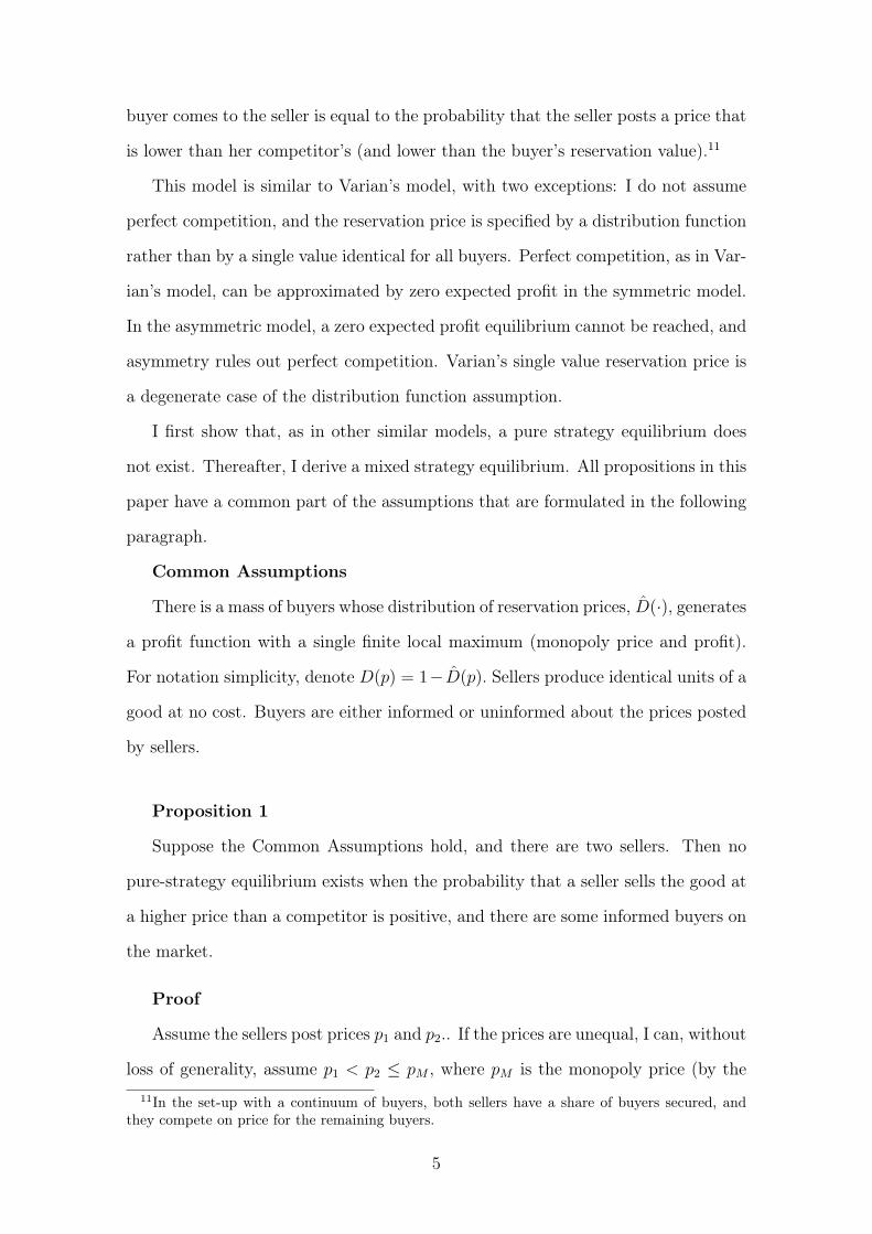
Proof
Assume the sellers post prices p1 and p2.. If the prices are unequal, I can, without
loss of generality, assume p1 < p2 ≤ pM , where pM is the monopoly price (by the11In the set-up with a continuum of buyers, both sellers have a share of buyers secured, and
they compete on price for the remaining buyers.
5

definition of a monopoly price, no seller chooses a price bigger than the monopoly
price, although they generally can). Seller 1 can increase the expected profit by
marginally increasing her price. If 0 < p1 = p2a any seller can increase the expected
profit by decreasing her price. The case of 0 = p1 < p2 cannot be an equilibrium
either because the expected profit is zero, and both sellers can earn strictly positive
expected profit by posting pM or, in fact, any positive price within the reservation
price distribution support. •
The logic behind the mixed-strategy equilibrium results from an optimal weight-
ing of two considerations: making money on volume and competing with the other
seller for informed buyers through a low price on the one hand and profiting from
a higher price on uninformed buyers on the other. The resulting equilibrium is
derived from the distribution function of the buyer’s reservation price.
Proposition 2
Suppose the Common Assumptions hold. Assume that there are two sellers, and
the probability that a buyer is uninformed (chooses randomly between the sellers)
is 0 < α < 1;12 he is informed and comes to the seller with the best price.
Then there is a unique (symmetric) mixed-strategy equilibrium with a price-
mixing cumulative distribution function (cdf):
β(p) = 0, p ≤ a,
=1− α/2
1− α
(1− α
2− α
M
pD(p)
), p ∈ [a, b],
= 1, p ≥ b,
where M is the monopoly profit:
M = max qqD(q);
12For example, each seller has ‘in expectation’ secured by α/2 fraction of the market, i.e. theseller sells on average to this amount of buyers. Of course, the offered price must be smaller thanthe buyer’s reservation price for the seller to be able to sell the product to him.
6

a solves the implicit equation
aD(a) =α
2− αM ;
and b = pM = argmaxqαqD(q) is the monopoly price.
The expected profit is α2maxq qD(q), i.e. the profit a seller would secure by
setting a monopoly price and selling to ‘her’ at a fraction of the market.
Proof
The beginning of the proof is standard, similar to the proofs done by, for exam-
ple, Varian (1980) or Baye and De Vries (1992). We find the equilibrium mixing
strategy represented by a distribution function of price choice. By the definition
of mixed-strategy equilibrium a the distribution function makes the competitor in-
different between price choices over a specified interval (the support of the mixing
function).
Let βi be the mixed strategy distribution function of seller i, i = 1, 2 (I as-
sume that even an asymmetric distribution may exist though I will show later that
the distribution function β() is unique and therefore, the symmetric equilibrium is
unique). Assume first that the support of the distribution function is an interval
(ai, bi).13 The lower bounds of the supports of both βi must be identical because
setting a lower ai < a would be a mistake, increasing it by half of the difference
(a−i − ai) would increase the profit due to the single local maximum of the profit
function property (the probability of winning informed buyers would be 1 in both
cases, and the profit would be higher when the price is set to (a−i − ai)/2).13The interval is open, i.e. the probability that a player chooses a price equal to a or b is zero.
It is shown later that there are no mass points of the distributions.
7

The expected profit function can be expressed as
πi(p) =α
2pD(p) + (1− α)pD(p) (1− β−i(p))
=(1− α
2
)(α/2
1− α/2pD(p) +
1− α
1− α/2pD(p)(1− β−i(p))
)=
(1− α
2
)pD(p)
(1− 1− α
1− α/2β−i(p)
)=
(1− α
2
)pD(p)(1− cβ−i(p)),
where c = 1−α1−α/2
.
From this point on, I simplify the notation of the profit and the distribution
function indices: π() = πi() and β() = β−i().
For the competitor to be indifferent between choosing prices p1, p2 ∈ (a, b), the
expected profits related to the two prices must be equal.
π(p1) = π(p2)
p1D(p1)(1− cβ(p1)) = p2D(p2)(1− cβ(p2))
1− cβ(p1)
1− cβ(p2)=
p2D(p2)
p1D(p1).
Since β(a) = 0, I can rewrite the equation to
1− cβ(p1) =aD(a)
p1D(p1)(1)
that gives me the mixed strategy function formula
β(p) =1
c− aD(a)
cpD(p).
The expected profit is equal to π = (1 − α/2)aD(a) because setting the price
equal to the lower bound a we would sell the good to all searchers almost sure,14
and the expected profit of all choices of price must be equal. From the equality14As the support of the mixed strategy is open, a is never chosen. A completely correct proof
would use limits and is straightforward.
8
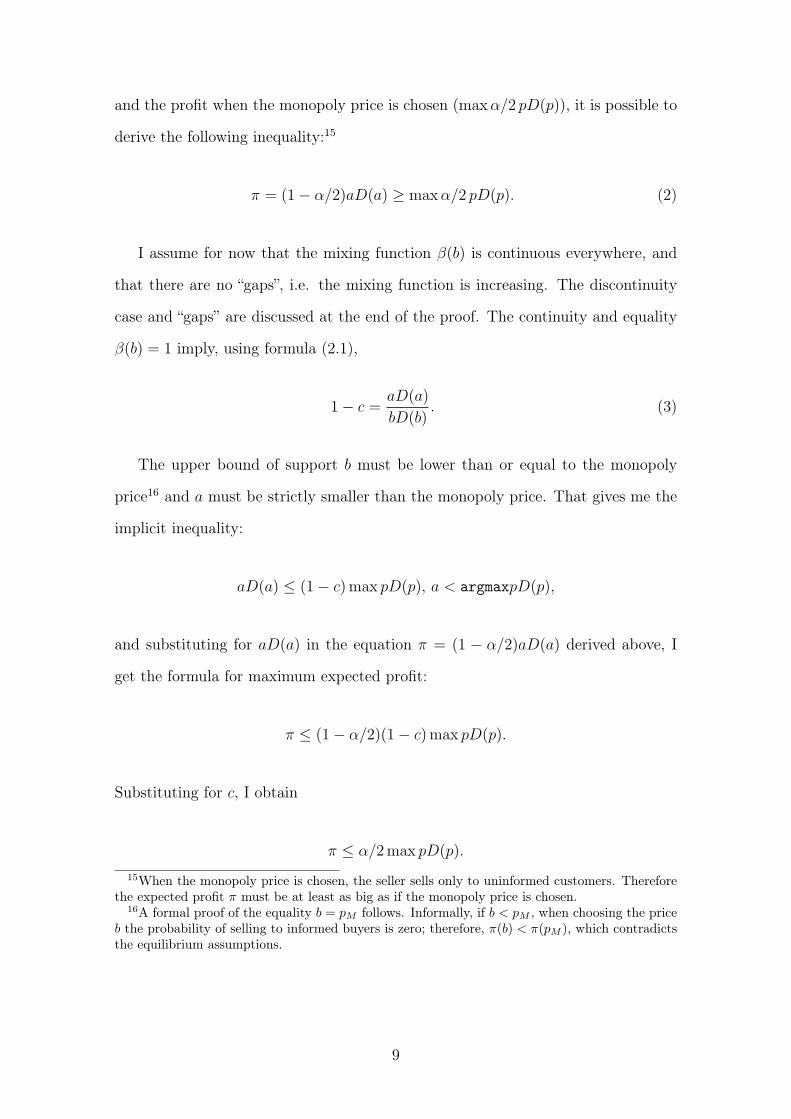
and the profit when the monopoly price is chosen (maxα/2 pD(p)), it is possible to
derive the following inequality:15
π = (1− α/2)aD(a) ≥ maxα/2 pD(p). (2)
I assume for now that the mixing function β(b) is continuous everywhere, and
that there are no “gaps”, i.e. the mixing function is increasing. The discontinuity
case and “gaps” are discussed at the end of the proof. The continuity and equality
β(b) = 1 imply, using formula (2.1),
1− c =aD(a)
bD(b). (3)
The upper bound of support b must be lower than or equal to the monopoly
price16 and a must be strictly smaller than the monopoly price. That gives me the
implicit inequality:
aD(a) ≤ (1− c)max pD(p), a < argmaxpD(p),
and substituting for aD(a) in the equation π = (1 − α/2)aD(a) derived above, I
get the formula for maximum expected profit:
π ≤ (1− α/2)(1− c)max pD(p).
Substituting for c, I obtain
π ≤ α/2max pD(p).
15When the monopoly price is chosen, the seller sells only to uninformed customers. Thereforethe expected profit π must be at least as big as if the monopoly price is chosen.
16A formal proof of the equality b = pM follows. Informally, if b < pM , when choosing the priceb the probability of selling to informed buyers is zero; therefore, π(b) < π(pM ), which contradictsthe equilibrium assumptions.
9
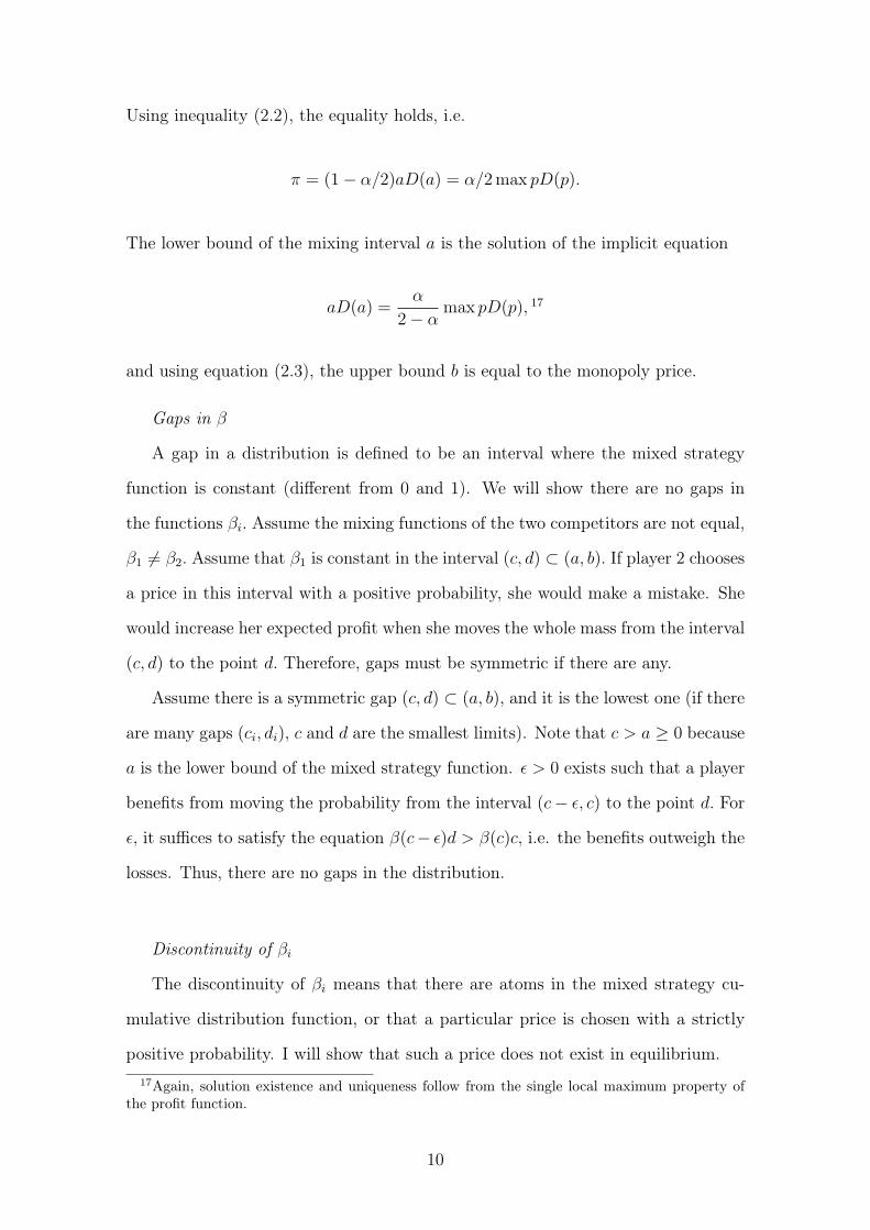
Using inequality (2.2), the equality holds, i.e.
π = (1− α/2)aD(a) = α/2max pD(p).
The lower bound of the mixing interval a is the solution of the implicit equation
aD(a) =α
2− αmax pD(p), 17
and using equation (2.3), the upper bound b is equal to the monopoly price.
Gaps in β
A gap in a distribution is defined to be an interval where the mixed strategy
function is constant (different from 0 and 1). We will show there are no gaps in
the functions βi. Assume the mixing functions of the two competitors are not equal,
β1 = β2. Assume that β1 is constant in the interval (c, d) ⊂ (a, b). If player 2 chooses
a price in this interval with a positive probability, she would make a mistake. She
would increase her expected profit when she moves the whole mass from the interval
(c, d) to the point d. Therefore, gaps must be symmetric if there are any.
Assume there is a symmetric gap (c, d) ⊂ (a, b), and it is the lowest one (if there
are many gaps (ci, di), c and d are the smallest limits). Note that c > a ≥ 0 because
a is the lower bound of the mixed strategy function. ϵ > 0 exists such that a player
benefits from moving the probability from the interval (c− ϵ, c) to the point d. For
ϵ, it suffices to satisfy the equation β(c− ϵ)d > β(c)c, i.e. the benefits outweigh the
losses. Thus, there are no gaps in the distribution.
Discontinuity of βi
The discontinuity of βi means that there are atoms in the mixed strategy cu-
mulative distribution function, or that a particular price is chosen with a strictly
positive probability. I will show that such a price does not exist in equilibrium.17Again, solution existence and uniqueness follow from the single local maximum property of
the profit function.
10

First, note that there can be only a symmetric equilibrium. We have shown
before that the lower bounds of the mixing intervals are identical for all sellers.
The formula for the mixing function β() is dependent only on the share of unin-
formed buyers α, mixing interval lower bound a and the distribution function of
the reservation prices. Therefore, the distribution function must be identical for all
sellers.
This implies that, if there were a mass point, it would be identical for both
players. In that case, an undercutting procedure would start - a move of the mass
point to a slightly smaller price would be beneficial (again, recall that a > 0).
Therefore, the mixed strategy cumulative distribution functions βi are continuous.
•
The solution can be evaluated even in the extreme case of α = 1 when each
seller owns half of the market. In that case, the mixing interval shrinks to one point
a = b = pmonopoly. In the other extreme, α = 0, when all buyers are informed, and
the lower bound of the interval as well as the expected profit are equal to 0, the
upper bound should be also 0. Therefore, even the limits in extreme cases are in
line with the existing theory.
The above model has been developed for price competition between two sellers.
Naturally, we may ask what happens when a higher number of sellers enters the
market. I keep the basic set-up unchanged and solve it for an arbitrary number
of N competing sellers. The characteristics of the buyers remain the same. The
probability of a buyer choosing a seller randomly (and not searching for the lowest
price) is α. It means that every seller has secured a α/N share of the market. The
model equilibrium is characterized in the following proposition.
11

Proposition 3
Assume that the Common Assumptions hold, and there are N sellers. Assume
that the probability a buyer is uninformed and chooses randomly between the sellers
is 0 < α < 1, and the probability a buyer chooses one particular seller is identical
for all sellers and is equal to α/N. The probability that a buyer is informed and
knows the posted prices of all sellers in advance is therefore 1− α.
Then, there is no pure-strategy equilibrium, and a unique symmetric mixed-
strategy equilibrium with price-mixing cdf is
β(p) = 0, p ≤ a
= 1−(
α
N(1− α)
M
pD(p)− α
N(1− α)
) 1N−1
, p ∈ [a, b]
= 1, p ≥ b,
where M is the monopoly profit, b = pM the monopoly price, and a solves the
implicit equation aD(a) = αN−(N−1)α
M.
The expected profit is αNmaxq qD(q), i.e. the profit a seller would secure setting
a monopoly price and selling to ‘her’ fraction of market.
Proof
The proof of the non-existence of the pure-strategy equilibrium is analogous to
the proof of Proposition 1.
The logic behind the derivation of the mixed-strategy equilibrium copies the
proof of Proposition 2; thus I indicate here just the key points of the proof.
I assume the symmetry of the equilibrium. Let β(p) label the mixed strategy
cdf and the interval (a,b) its support. The associated cdf of minimum price set by
N − 1 competitors is B(p) = 1− (1−β(p))N−1. I can express the expected profit as
π(p) =α
Np+ (1− α)p(1−B(p)).
Using the argument that π(p1) = π(p2), ∀p1, p2 ∈ (a, b) I get the counterpart
12

of the equation (2.1):
1− cB(p) =aD(a)
pD(p), (4)
where c = 1−α1−N−1
Nα. Substituting for B(·) and rearranging the equation I obtain the
formula for the mixing function:
β(p) = 1−(1
c
aD(a)
pD(p)− 1− c
c
) 1N−1
.
Setting the price at the lower bound of the interval (a,b), the seller sells to all
informed buyers almost sure, and I have to have at least the profit of selling only
to uninformed buyers at the monopoly price, so18
π =
(1− N − 1
Nα
)aD(a) ≥ max
α
NqD(q). (5)
Equation (2.4) expressed for p = b gives me the inequality
aD(a) = (1− c)bD(b) ≤ (1− c)max qD(q), a < argmaxqD(q).
Together with (2.5) and substituting for c I get
aD(a) =α
N − (N − 1)αmax qD(q),
and
π =α
Nmax qD(q).
Substituting for c and aD(a) in the equation defining β(p), I obtain the final form
of the mixing function.
The proof of the continuity and strict monotonicity (no gaps property) of the
distribution function β(·) is completely analogous to the proof of Proposition 2.18As in the previous proof, the precise derivation of the first equality is the limit π = (Probability
of winning)*(amount won), where the first term approaches 1 when p → a, and the second termapproaches max α
N qD(q).
13

Uniqueness of the upper bound
If there were two different upper bounds b1 = b2, then there would need to be
a gap or a mass point in the mixing function, which is ruled out. If b < pM , then
the expected profit would need to be smaller than α/NpM ; therefore, sellers would
tend to choose p = pM , and the upper bound is therefore unique.
Uniqueness of the lower bound
Assume sellers choose different lower bounds a1 ≤ a2 ≤ a3 ≤ ... The lowest of all
bounds has to be equal to a1 = a. To set a lower bound is unprofitable, and someone
has to choose it because the equilibrium profit is equal to the profit gained from
choosing a. Also, at least one other player has to have the lower bound equal to a;
otherwise, seller 1 would tend to increase her lower bound. Assume that M < N
players have the lower bound of the mixing interval equal to a and the seller M +1
has the lower bound equal to a > a. When I set the number of sellers N to be a
parameter of the function β = β(p,N), then the mixing function of the first M
sellers β1 in the first part of the interval would be β1(p) = β(p,M), p ∈ (a, a). As
∂∂N
β(p,N) < 0, the inequality β1(p) < β(p,M), p ∈ (a, a) holds, and the player
would get a higher-than-equilibrium profit choosing a price from the interval (a, a)
that is, however, outside her mixing interval. Therefore, her mixing interval lower
bound has to be equal to a, and the equilibrium is unique.
Because the bounds of the supports of the mixed strategy cumulative distribu-
tion functions are equal for all sellers, there are no gaps or mass points, and since
the mixed strategies follow the above derived formulae, the equilibrium is unique.
•
Equilibrium prices can be influenced by a variation of two basic parameters, the
fraction of informed buyers 1 − α and the number of competitors N. The increas-
ing number of informed buyers (or the increasing probability of the buyer being
informed) directly lowers the (expected) profit of sellers and changes the division
of the surplus in favor of the buyers.19 The lower bound of the mixing interval19I assume there are no search costs in the model. A natural extension of the model would be
the introduction of the endogenous choice of the fractions of informed buyers. In such a model,
14

decreases towards zero faster than linearly as the fraction of searchers increases.
The shape of the mixing function itself stretches out proportionally over the mixing
interval.
The effect of increased competition differs from the effect of the increased propor-
tion of informed buyers. The expected buyers’ and sellers’ surpluses do not change
in the case of increased competition, only the sellers’ surplus is spread across a
larger number of sellers. The lower bound of the mixing interval (the interval of
prices that can be posted by sellers in equilibrium) is inversely proportional to the
number of sellers. The shape of the mixing function thus changes as the number of
competitors increases; the probability of choosing a smaller price close to the lower
bound decreases and the probability of choosing a price close to the monopoly price
increases. There are two countervailing phenomena that influence the expected
minimum price on the market: a decreased lower bound of the mixing interval that
decreases the expected minimum price on the market and the shifted weight of the
mixing function towards the monopoly price, which increases the expected minimum
price. I now analyze the minimum in more detail.
Keeping the notation of Proposition 3, the expected minimum price for N sellers
is20
Epmin = a+
∫ b
a
(α
N(1− α)
(M
pD(p)− 1
)) NN−1
dp.
The effect of increased competition can be determined from the derivative of the
expected minimum with respect to N :
dEpmin
dN=
∫ b
a
d
dN
(α
N(1− α)
(M
pD(p)− 1
)) NN−1
dp.
The expression in the outer brackets gets a value of 1 for p = a and a value of 0
for p = b; thus, its values in the integration limits belong to the interval (0, 1). The
I would observe not only a transfer of surplus from sellers to buyers, but also a decrease of totalsurplus due to increased search costs.
20The expected minimum price is equal to∫ b
apdB(p), where B(p) = 1−(1−β(p))N . Integrating
by parts, I get the formula for the expected minimum price.
15
exponent is always bigger than 1, and it is decreasing in N so the whole function
is decreasing in N, and the derivative is always negative (the derivative exists). It
implies that the expected minimum price decreases with increasing competition.
This result implies that informed buyers benefit from increased competition,
sellers maintain the expected sum of profits unchanged as competition increases,
and uninformed buyers fully pay the benefit of informed buyers.
To summarize, an increased number of informed buyers depletes the profit of
sellers. An increased number of sellers leads to the total volume of profits being split
across a larger number of competing sellers, while the absolute value remains un-
changed. Informed buyers benefit from increased competition while the uninformed
lose.
III. Asymmetric model
I now add asymmetry to the model. In the symmetric set-up presented so far,
uninformed buyers randomly selected a seller they decided to visit. Randomness
was symmetric with respect to sellers: The probability that a specific uninformed
buyer would visit a specific seller was equal across all sellers and buyers. In an
asymmetric set-up, the probability that a buyer visits a specific seller may differ
across sellers.
An asymmetric set-up can capture the behavior of uninformed buyers that for
various reasons may not be randomizing. A real-life situation captured by such
a model would be brand sensitivity (or even loyalty). A fraction α1 of potential
buyers prefers a particular seller, another fraction α2 of buyers prefers a different
seller, and the remaining buyers are searchers. If we randomly select a buyer in
this brand sensitivity model, the probability that he prefers the first seller is α1,
and the probability that he prefers the second seller is α2. Thus, in the brand
sensitivity model, I can think of buyers that prefer a seller as uninformed buyers
and of searchers as informed buyers.21
21The model can be used in the field of promotion if I assume brand sensitivity, or loyalty, canbe endogenized assuming it can be changed by sellers’ investments.
16

The formulation of the model remains essentially the same as in the symmetric
case with the exception that uninformed buyers are positioned asymmetrically. For
every seller, I specify her share of buyers who are not informed of the lowest price
and/or who do not go directly to other sellers. These shares may be different for
every seller.22 As in the previous section, I first analyze the simplest possible model
- the competition of two sellers.
Proposition 4
Assume that the Common Assumptions hold, and there are two sellers. Assume
that the probability a buyer is uninformed and visits the first seller is α1, and the
probability the buyer is uninformed and visits the second seller is α2.23 Assume,
without loss of generality, that α1 > α2. The remaining probability 1 − α1 − α2
represents informed buyers.
Then there is a unique mixed-strategy equilibrium with price-mixing cdf of the
first seller:24
β1(p) = 0, p < a,
=1− α1
1− α1 − α2
(1− aD(a)
pD(p)
), p ∈ [a, pM),
= 1, p ≥ pM ,
and the price-mixing cdf of the second seller
β2(p) = 0, p < a,
=1− α2
1− α1 − α2
(1− aD(a)
pD(p)
), p ∈ [a, pM ],
= 1, p ≥ pM ,
22Or, in other words, I specify the probabilities that a specific buyer visits each seller even ifthe seller does not post the lowest price on the market.
23This means the first seller has secured a fraction α1 of the market and the second seller hassecured α2 of the market.
24Note there is a positive probability that seller 1 chooses the monopoly price, and the mixedstrategy distribution function has a mass point in pM . The result and the mathematic propertiesof the equilibrium are discussed between this Proposition and the Proof.
17

where M is the monopoly profit, pM the monopoly price, and a solves the implicit
equation
aD(a) =α1
1− α2
M.
The expected profit of the stronger seller (the seller with a higher share of unin-
formed buyers) is α1maxq qD(q), and the profit of the weaker seller is α1 maxq qD(q)−
(α1 − α2)aD(a). •
In equilibrium an interesting behavior can be seen close to the monopoly price.
On the graph below, the equilibrium of the set-up α1 = 0.2, α2 = 0.1, and D(p) =
1− p, (uniformly distributed reservation values of buyers over the interval (0, 1)) is
plotted. The monopoly price is 1/4, and the lower bound of the mixed strategies is
approximately 0.06 .
We can see that there is a probability of more than 10% that the stronger seller
sets the monopoly price. The behavior of the weaker and the stronger seller just
below the monopoly price is clearly visible there. The weaker player sets a price
from any interval (pM − ϵ, pM), ϵ > 0 with positive probability, but the price
pM is never selected. This behavior prevents the stronger player from shifting the
probability mass to pM so that a gap would appear under the monopoly price. On
the contrary, the stronger player selects the prices below the monopoly price with
probabilities much lower than 1 so that the weaker player is motivated to assign
18

some probability to these prices. The mass point in the monopoly price is formed
by the “remaining” probability.
Mathematically, this situation is described by the supports of the associated
probability functions. The support of the weaker seller is (a, pM), i.e. any price can
be selected but pM . The support of the stronger seller is (a, pM ], i.e. any price can
be selected including pM , which is selected with a positive probability.
Proof of Proposition 4
The proof follows the same logic as the proofs of Propositions 2 and 3. First, I
develop the expected profit function of the two competing sellers. In the previous
section, the expected profit functions coincided for both sellers, and the equilibrium
strategies were equivalent. Because the set-up is asymmetric, the solution cannot
be symmetric either. I have to develop profit functions and strategies for each seller
individually. I label the first seller’s expected profit function and strategy (the cdf
of the price choice) π1(p) and β1(p), respectively, and π2(p) and β2(p) analogously
label the corresponding variables for the second seller. The expected profit functions
of the two sellers are:
π1(p) = α1pD(p) + (1− (α1 + α2))pD(p) (1− β2(p))
= (1− α2)pD(p)(α1
1− α2
+1− α1 − α2
1− α2
− 1− α1 − α2
1− α2
β2(p)
= (1− α2)pD(p)(1− c1β2(p)),
π2(p) = (1− α1)pD(p)(1− c2β1(p)),
where c1 =1−α1−α2
1−α2and c2 =
1−α1−α2
1−α1.
I continue to evaluate the strategy of the ‘weaker’ second seller (the seller with
a smaller amount of uninformed buyers). The formulae relevant for the first seller
apply analogously for a couple of the following steps.
The first seller has to be indifferent between prices in the mixing interval, there-
19

fore
π1(p1) = π1(p2)
p1D(p1)(1− c1β2(p1)) = p2D(p2)(1− c1β2(p2))
1− c1β2(p1)
1− c1β2(p2)=
p2D(p2)
p1D(p1).
I label the lower bounds for the first and second player a1 and a2 and the upper
bounds b1 and b2. Note that I do not assume there is not a mass point in bi. In fact,
I will show that seller 1 chooses price b1 with a positive probability. I evaluate the
previous formula at p1 = b2, p2 = a2 and find (1− c1)b2D(b2) = a2D(a2) or
α1
1− α2
b2D(b2) = a2D(a2).
If the second seller sets the price p = a225 and wins the informed buyers, she
gets a profit of at least α2M, where M denotes the monopoly profit with respect
to the demand function D(·). Otherwise she would prefer to sell to her fraction of
the market α2 at the monopoly price pM . This argument can be expressed as the
equality (1 − α1)a2D(a2) ≥ α2M. Rearranging terms, I get (1−α1)α1
(1−α2)α2b2D(b2) ≥ M.
Using an analogical procedure, I get (1−α2)α2
(1−α1)α1b1D(b1) ≥ M. Note that b1 = b2. If not,
there would be a gap between b1 and b2, and subsequently, it would be beneficial to
switch some mass of the distribution function of the strategy from the lower bound
of the gap to the upper bound of the gap for one player. Thus, in equilibrium,
b1 = b2 = b. The previous two equations imply that bD(b) = M. Then, I can
express the lower bounds as
a2D(a2) =α1
1− α2
M,
25The seller chooses this price, in fact, with zero probability; therefore, it would be an invalidargument. I use it to simplify the full argumentation of setting price p = a2 + ϵ and evaluatingthe limit ϵ → 0.
20

and
a1D(a1) =α2
1− α1
M.
However, I know that a1 = a2 otherwise the strategy of one seller would be
irrational. Namely, as α1 > α2 and thus a2 > a1, the first player would prefer to
move the mass of the function β1(·) from the interval (a1, a2) to the point a2− ϵ and
increase the expected profit. In fact, the first seller would not be willing to select a
price lower than a2 – even if the probability of winning is 1, she would not get more
than α1M in expected value. Therefore, I let the second player’s strategy remain
the same as derived above and derive the first player’s strategy that satisfies the
equality a1 = a2 and the requirement that the second player is indifferent between
choosing any price from the interval [a2, b2]. As before,
π2(p1) = π2(p2)
p1D(p1)(1− c2β1(p1)) = p2D(p2)(1− c2β1(p2))
1− c2β1(p1)
1− c2β1(p2)=
p2D(p2)
p1D(p1).
As defined earlier, β1(a2) = 0. Setting p2 = a2 and rearranging, I get
β1(p) =1
c2
(1− a2D(a2)
pD(p)
). (6)
Because the following equalities hold,26 β1(pM−) = 1c2
(1− a2D(a2)
pMD(pM )
)< 1 and
β1(pM) = 1, the stronger player sets the monopoly price with a positive probability.
This function leaves the second player indifferent between prices within the interval
[a2, pM), and the above derived strategy leaves the first player indifferent between
prices within the interval [a2, pM ].
Therefore, the system26The notation β1(pM−) assigns the left limit of the function β1 in the point pM .
21

β2(p) =1
c1
(1− aD(a)
pD(p)
), p ∈ [a, pM ]
β1(p) =1
c2
(1− aD(a)
pD(p)
), p ∈ [a, pM)
β1(pM) = 1,
aD(a) =α1
1− α2
constitutes the equilibrium.
Uniqueness
I have derived a formula for a mixing function that leaves the opponent indif-
ferent between choosing prices from the interval [a2, pM) in the previous part of the
proof. This formula defines a unique solution if:
1. the lower and upper bounds of the support are unique and
2. the functions are strictly increasing in the support.27
The uniqueness of the upper bound has been shown before. It needs to be shown
that the functions have to be strictly increasing in the support (or that there are
no gaps in the support) and that the lower bound is unique.
There are no gaps in the distribution functions βi
If there is a gap in a distribution function there must be the same in the second
one; otherwise, the second seller would not behave rationally. As in the proof of
Proposition 2, it is possible to show that shifting some mass from the lower bound
of the gap to the upper bound, the seller would benefit; therefore, there can be no
gap in the distribution function.
There are no mass points except the one in pM for β1
The situation of a symmetric mass point, i.e. the situation where both β1 and
β2 have a mass point for the same price, would initiate an undercutting procedure.27Theoretically, if my opponent never chooses prices from a specific interval I do not need to
‘make him indifferent’ in that interval and I would not need to follow the prescribed formula. Inthat case there would exist infinitely many strategies.
22

Therefore, there can be no symmetric mass point. If there is a mass point in
x ∈ (a, pM) in the function βi and β−i < 1, then it it easy to show that shifting the
mass of the probability function β−i from the interval (x, x+ϵ1) to the point x−ϵ2 for
some ϵ1, ϵ2 > 0 would increase the expected profit of the seller −i. Therefore, there
can be no mass point in any of the two distribution functions with the mentioned
exception.
The lower bound a is unique
As the functions βi must be increasing in (a, pM) and there are no mass points,
the functions can be represented by the formulae derived above for a given a. If I
assume that a < α1
1−α2, then the stronger seller has no incentive to set a positive
probability to the prices in the interval (a, α1
1−α2), which violates the no gaps prop-
erty. If, in contrast, a > α1
1−α2, the values of mixing functions at monopoly prices
are βi(pM) < 1 for both functions, which violates the no mass points property.
Therefore, the lower bound a = α1
1−α2is unique. •
I have found an interesting result. In an asymmetric duopoly, the weaker seller
(the one with the smaller share of uninformed buyers) gains from the position of
the stronger seller. If the stronger seller’s market share increases, the weaker seller’s
expected profit rises as fast as the stronger seller’s even though the weaker seller
does not invest in capturing a larger share of the market. Also, it is much more
probable that the weaker seller sets a lower price than the stronger one and wins
the searchers. The wider the gap between the weaker and the stronger seller, i.e.
the bigger difference between the market shares of the two sellers, the higher the
probability that the stronger seller sets the monopoly price and sells to ‘her’ market
share.
The above-mentioned facts have consequences for buyers. If we start from a
symmetric position and let one seller capture a larger market share, then the ex-
pected profit of the sellers increases as if both players’ market shares increase in
the same way. The increase of the sellers’ profit is not paid by the buyers who
caused the market share to increase but in the majority by previously uninformed
23

buyers and partially by informed buyers. When, in contrast, I start from an asym-
metric position and the gap between the sellers’ market shares moves towards the
symmetric position so that more buyers become uninformed, the expected profit of
the sellers does not change. The buyers who switch from informed to uninformed
necessarily lose (recall I do not have search cost in the model), therefore informed
buyers benefit from the increased market share of the weaker seller.
The last step is to develop the most general model. It is an asymmetric model
of competition among N sellers when every individual seller has secured her own
market share αi, or the probability that a specific uninformed buyer visits her.
This model, naturally, covers all the already-analyzed specific cases. It will help us
understand the logic and nature of the equilibrium.
Proposition 5
Assume that the Common Assumptions hold, and there are N sellers. Assume
that the probability a buyer chooses to visit seller i is αi.28 The sellers are, without
loss of generality, sorted according to ascending market share: α1 ≤ α2 ≤ · · · ≤ αN .
The remaining probability 1−∑
αi represents informed buyers.
Then there is a unique mixed-strategy equilibrium, where the price-mixing cdfs
βi can be expressed as29
βi(p) = 0, p ≤ ai,
= 1−∏
j,aj<p k1
m−1
j
kip ∈ [ai, pM),
= 1, p ≥ pM
ki = (1 + ci((∏j<i
(1− βj(ai))− 1)))aiD(ai)
cipD(p)− 1− ci
ci
ci =1−A1−A−i
, A =∑
αi, A−i = A− αi,
m = maxl(al < p),
28This means that each seller has “in expectation” secured a fraction αi of the market.29For the weakest seller 1, the function is continuous; for other sellers, there can be a disconti-
nuity in pM , i.e. they can choose the price pM with a positive probability.
24

where M is the monopoly profit and pM the monopoly price. The lower bound of
every distribution function ai is chosen as the solution of the implicit equation valid
∀i > 1 and for i = 1 if α1 = α2
(αi + (1−A)(∏j<i
(1− βj(ai))))aiD(ai) = αiM,
where M is the monopoly profit. If α1 < α2, then a1 = a2.
The expected profits of sellers are αiM, ∀i > 1, and i = 1 if α1 = α2, i.e. the
profit the first seller would secure setting a monopoly price and selling to ‘her’
fraction of market. If α1 < α2, then the first seller’s expected profit is α2M − (α2−
α1)a2D(a2), i.e. the profit of the second-weakest seller minus the difference of the
profit from the uninformed buyers at the lower bound of the mixing interval.
Proof
The proof follows the standard line used in the previous proofs. First, the profit
function of each seller is defined. I use the fact that each seller has to have identical
expected profits for all prices she is willing to set to obtain a system of equations
that defines the mixed strategy cumulative distribution functions of all players.
Assume that α1 ≤ α2 ≤ · · · ≤ αN . Label the respective mixing functions for
sellers i = 1, . . . , N βi(p) and the supports of the mixing functions (ai, bi].30 To keep
the notation simple, I use the fact that a1 ≤ a2 ≤ · · · ≤ aN , and will be proven
later, and no step in the proof depends on this fact. I denote A =∑N
j=1 αj and
A−i = A− αi.
The expected profit of seller i is her expected profit from uninformed buyers
who come directly to her and the expected profit from the searchers if she selects30Later I will show that the weakest seller chooses the upper bound with zero probability and
others may choose it with a positive probability.
25

the lowest price on the market.
πi(p) = αipD(p) + (1−A)pD(p)∏j =i
(1− βj(p))
= (1−A−i)pD(p)(1 + ci(∏j =i
(1− βj(p))− 1)),
where ci =1−A
1−A−i.
I compare the seller’s expected profits for two different price choices. We know
that they have to be equal if we want her to randomize between them (or other
prices with an identical outcome): πi(p1) = πi(p2), ∀p1, p2 ∈ (ai, bi]. This equation
gives us the relationship
p1D(p1)
p2D(p2)=
1 + ci(∏
j =i(1− βj(p2))− 1)
1 + ci(∏
j =i(1− βj(p1))− 1).
I use ai as the reference value,31 and the fact that βj(ai) = 0∀j > i and βj(p) =
0∀j, aj ≥ p to get the equality
aiD(ai)
pD(p)=
1 + ci(∏
j,aj<p&j =i(1− βj(p))− 1)
1 + ci(∏
j<i(1− βj(ai))− 1).
Rearranging the terms, I get one equation from the system defining the mixing
function
∏j,aj<p&j =i
(1− βj(p)) = (1 + ci(∏j<i
(1− βj(ai))− 1))aiD(ai)
cipD(p)− 1− ci
ci=: ki(p).
If I use a logarithm for every equation from the system,
∏j,aj<p&j =i
(1− βj(p)) = ki(p), i = 1 . . .m,m = maxl(al < p), (7)
31Though ai lies outside the interval (ai, bi), I can use the limit p1 → ai+ to verify the correctnessof this equation. The proof that ai cannot be chosen with a positive probability is straightforward.
26

I get a system of linear equations:
∑j,aj<p&j =i
log(1− βj(p)) = log(ki(p)), i = 1 . . .m,m = maxl(al < p).
I think of the expressions xi(p) = log(1 − βi(p)) as unknowns. Then assigning
yi(p) = log(ki(p)), vectors X(p) = xi(p), Y (p) = yi(p) the system of equations
can be rewritten as AX=Y, where A is a matrix of ones with zeroes on the diagonal.
The solution of the system is xi =∑
j,aj<p yj/(m− 1)− yi. Solving the substitution
I get the formula for βi(p) :
βi(p) = 1−∏
j,aj<p k1
m−1
j
ki.
I need to determine the values of ai to finish the analysis. Observe that the
distribution function βi of at least one player cannot have a mass point in the
monopoly price. If every distribution function had one, the undercutting process
would start. Also, βi(pM − ϵ) < 1,∀i, ϵ > 0. If some player sets βi(pM − ϵ) = 1, a
gap in the distribution function of other players would emerge between pM − ϵ and
pM and thus, the strategy of player i would be sub-optimal.
Assume that the mixing function of player i satisfies limp→pM βi(p) = 1.32 Then,
using equation (2.7), ∀l = i, limp→pM kl(p) = 0. The equation can be translated to
(αl + (1−A)(∏j<l
(1− βj(al))))alD(al) = αlpMD(pM). (8)
This equation says that al is chosen so that the expected profit setting the price
to al equals the expected profit when the price is set equal to the monopoly price
and selling only to uninformed buyers. The assumed properties of the function
D(·) (or pD(p)) ensure the uniqueness of the solution. It means the equation has
a unique solution for al, l = i. If seller l’s mixing interval lower boundary would32I know there is at least one - the one whose distribution function does not have a mass point
in pM .
27

be higher, al > al, then βi(p) < βi(p), i < l, p ∈ (al, al).33 This would mean that
seller l would get a higher profit choosing p ∈ (al, al) than what she would get in
equilibrium, αlpMD(pM). Therefore choosing any lower bound other than al is not
an equilibrium strategy.
The above derived formula also gives us the reason why al, l = i are sorted
increasingly a1 ≤ a2 ≤ · · · ≤ aN . The proof by contradiction is apparent. I show
later that even the value ai itself is sorted in the chain.
I need to analyze the two following cases. In the first case, the two least powerful
sellers have the same market share, or α1 = α2. In the second case, the least powerful
seller has a strictly smaller market share than all other sellers, or α1 < α2. I continue
the analysis with the more complicated second case.
From the previous analysis, I know that the lower bounds of the distribution
functions ai are specified by the above-mentioned formula except, possibly, for one.
Assume that all ai are given by formula (2.8), then inequality a1 < a2 ≤ · · · ≤ aN
holds. However in that case, seller 1 would choose a sub-optimal strategy, and she
would prefer to shift the lower bound a1 upwards. In other words, there must be
at least two players choosing the smallest value of the lower bound of their mixing
probability function support. This implies that if a1 is derived from equality (2.8),
there must be ai such that ai = a1. Seller i would, however, make a mistake doing
this because she would lower her expected profit and prefer to choose the price pM .
Therefore, player 1 must be the one who does not set the lower bound a1 according
to formula (2.8). The value of k1(pM) > 0 and due to equality (2.7), all other players
choose the monopoly price with a positive probability.
I still need to find the value of a1. The selection of a1 = a2 is an equilibrium
choice. I need to show that it is a unique choice that leads to an equilibrium. If
seller 1 chooses a smaller value of the lower bound a1 < a2, she would not gain the
maximum expected profit. If seller 1 chooses a lower bound bigger than a2, other
players will adapt to her choice and select strategies such that player 1 gets a higher33This follows directly the formula for βi(p) and the fact that ki(p) < 1, p > ai.
28
profit than choosing a1 = a2. There is no reason, however, why seller 2 would not
mimic player 1’s strategy and obtain a higher expected profit. That would not be
an equilibrium, however, because it has been proven that seller 2 chooses the lower
bound a2 with respect to equation (2.8). Therefore, the choice a1 = a2 is the unique
equilibrium choice. Also, this is the final fragment from the proof of the inequality
chain a1 ≤ a2 ≤ · · · ≤ aN .34
The first case, when there are at least two sellers with the same, smallest market
share is easier to analyze. There is an obvious equilibrium when every seller chooses
the lower bound according to formula (2.8), and all mixing functions are continuous
everywhere. I need to review the situation when one player chooses a different lower
bound. When one player chooses a different lower bound ai than the one derived
from equation (2.8), she must get a higher expected profit (she does not want to get
a lower expected profit). There is always a player who would be willing to mimic
player i′s strategy and grab the same profit. Then we would have two players not
following equation (2.8), which is ruled out in an equilibrium. •
We see that the equilibrium of the most complex model corresponds to, and
includes, all three specific models presented before. The model describes symmetric
competition and asymmetric competition of two or more sellers. The main feature,
the uniqueness of the solution, remains preserved even in the most complicated set-
up. The equilibrium uniqueness implies that even in a finitely repeated competition
model, the equilibrium remains unique and fully defined by the proposed general-
model solution. The general model applies even to finitely repeated competition
with variable market shares if current actions do not change future market share.
Compared to welfare implications derived from the three previously analyzed
models, there are no qualitatively new results in this general model. I can, however,
summarize and generalize those presented earlier.
I have distinguished three groups of agents in the analysis: sellers, informed
buyers, and uninformed buyers. The expected profit of sellers is always equal to34In fact, the first inequality holds with equality.
29

the profit they would gain from selling to their market share at the monopoly price
with one exception - the seller with the smallest market share (the “weakest” seller),
who obtains almost the same expected profit as the second-weakest seller (with the
difference of the profit from uninformed buyers at the lower bound). Every seller
has an expected profit proportional to her own market share; only the uniquely
weakest seller’s expected profit is driven, apart from luck, by the expected profit
of the second-weakest seller. This exception has more impact as the gap widens
between the uniquely weakest seller and the second-weakest seller.
The buyers are assumed to be informed or uninformed, and uninformed buyers
rely on the sellers to which they go. Their individual expected profit is higher if
their seller is weaker (again, with the exception of the weakest seller). Informed
buyers benefit from market fragmentation the most. For them, it is beneficial to
face many weak sellers, and strong sellers do not have a significant impact on their
profit because they do not push the prices down. In the exceptional case, with the
existence of one (uniquely) weakest seller, the shift of the lower bound of the weakest
seller’s mixing interval subsequently increasing the seller’s welfare is absorbed by
the corresponding uninformed buyers (and there are few of them as the seller is
the weakest one) and, more importantly, by the informed buyers. Informed buyers
are, therefore, heavily dependent on the market structure, especially on the market
shares of the weakest sellers.
IV. Conclusion
In this paper, I have developed an oligopolistic model of sellers who compete
on price for informed buyers, and have secured their share of uninformed buyers.
Informed buyers know which seller sets the lowest price, and uninformed, or “loyal”,
buyers do not search for the lowest price but go to one seller only without knowing
ex-ante his posted price. The basic, and for the result crucial, difference from previ-
ously published models is the reservation values of buyers. In the model presented
in this paper, the reservation values are randomly drawn from a common distribu-
tion function rather than a pre-defined single value that has been used previously
30

in the existing literature.
I have found that there is a unique mixed-strategy, Nash equilibrium of this
model. In the equilibrium, every seller chooses randomly a price between an en-
dogenously determined lower bound and the monopoly price associated with the
demand function generated by the reservation value distribution function. Com-
pared to the theoretical and empirical results of Kocas and Kyiak (2006), the model
presented in this paper, namely the equilibrium strategy of sellers, explains the em-
pirical findings of Kocas and Kyiak better than their own theoretical model. The
main difference is that in my models all sellers, not just the two weakest, choose
their prices randomly from a non-trivial interval.
There are several welfare implications in the result. As derived in the text,
the expected profit, or the seller’s surplus, is equal to the profit that every seller
would get setting the monopoly price and selling to her share of the market (to
the uninformed buyers who visit this seller) plus the difference between the ‘market
share value’ of the two weakest sellers.35 As for buyers, the non-searchers’ sur-
plus increases with increased competition between sellers and a constant amount of
searchers. Searchers benefit from increased competition in every situation with one
exception.
The interesting exception from the rule “bigger competition = bigger buyer sur-
plus” is the entry of a new seller who becomes the uniquely weakest one on the
market. Imagine there are several sellers, and all with a positive market share.
If a seller with no market share enters, she gets the expected profit close to the
profit of the second weakest seller and thus steals a share of the total surplus. As
the expected profit of the incumbent sellers does not change, their share on the
total surplus remains constant. Therefore, the entrant steals the surplus fully from
buyers.
The model applies to many areas. It naturally follows and generalizes the lit-35A seller becomes weaker as a smaller amount of uninformed buyers come to her. The lower
bound of the mixing strategy support of the two weakest sellers is identical – the same result asin the findings of Kocas and Kyiak.
31

erature originated in Varian’s article and also the vast literature on the Hotelling
lemma: the size and distribution of the network of stores influences the size of the
seller’s market share. In fact, the present paper integrates the two concepts into
one model: oligopolistic competition is introduced into Varian’s model. Another
straightforward application, apart from the analysis of concentration/location of
stores, would be a study of advertisement from a competitive (not demand enhanc-
ing) point of view.
As a theoretical extension of the model, I would like to study further the in-
troduction of production costs, the introduction of costs to increase market share
(the model would approach the literature on promotions), and the introduction of
search costs (the model would approach the literature on search mentioned in the
introduction). It would also be interesting to introduce bounded rationality or in-
complete information into the model.36 Sellers, for example, might not know the
competitors’ market shares and may just have estimates. It might be interesting to
develop some kind of learning model that would fit reality better than the existing
models do, the present one included.
36This extension would target the field of experimental economics; see, for example, Huck,Muller, and Vriend (2002).
32
References
Baye, Michael R., and Casper G. De Vries, 1992. Mixed Strategy Trade Equilibria.
The Canadian Journal of Economics 25(2), 281-93.
Braverman, Avishay, 1980. Consumer Search and Alternative Market Equilibria.
Review of Economic Studies 47, 487-502.
Burdett, Kenneth, and Kenneth L. Judd, 1983. Equilibrium Price dispersion.
Econometrica 51, 955-70.
Clay, Karen, Krishnan Ramayya, Eric Wolff, and Danny Fernandes, 2002. Retail
Strategies on the Web: Evidence from the Online Book Industry. The Journal
of Industrial Economics 50(3), 351-367.
Clemons, Eric K., Il-Horn Hann, and Lorin M. Hitt, 2002. Price Dispersion and Dif-
ferentiation in Online Travel: An Empirical Investigation. Management Science
48(4), 534-549.
Huck, Steffen, Wieland Muller, and Nicolaas J. Vriend, 2002. The East End, the
West End, and King’s Cross: On Clustering in the Four-Player Hotelling Game.
Economic Inquiry 40(2), 231-240.
Iyer, Ganesh, and Amit Pazgal, 2003. Internet Shopping Agents: Virtual Co-
Location and Competition. Marketing Science 22(1), 85-106.
Kocas, Cenk, and Tunga Kiyak, 2006. Theory and Evidence on Pricing by Asym-
metric Oligopolies. International Journal of Industrial Organization 24, 83-105.
Narasimhan, Chakravarthi, 1988. Competitive Promotional Strategies. The Jour-
nal of Business 61(4), 427-449.
Neven, D., G.Norman, and J.F.Thisse, 1991. Attitudes Towards Foreign Products
and International Price Competition. The Canadian Journal of Economics 24(1),
1-11.
Raju, J.S., V.Srinivasan, and R.Lal, 1990. The Effects of Brand Loyalty on Com-
petitive Price Promotional Strategies. Management Science 276-304.
33

Reinganum, Jennifer F., 1979. A Simple Model of Equilibrium Price Dispersion.
Journal of Political Economy 87, 851-58.
Salop, Steven C., and Joseph E. Stiglitz, 1979. Bargains and Ripoffs: A Model of
Monopolistically Competitive Price Dispersion. Review of Economic Studies 44,
493-510.
Sinitsyn, Maxim, 2008. Characterization of the Support of the Mixed Strategy Price
Equilibria in Oligopolies with Heterogeneous Consumers. Economics Letters
99(2), 242-245.
Stahl, Dale O., 1989. Oligopolistic Pricing with Sequential Consumer Search. The
American Economic Review 79(4), 700-12.
Stiglitz, Joseph E., 1987. Competition and the Number of Firms in the Market.
Journal of Political Economy 95, 1041-61.
Stiglitz, Joseph E., 1979. Equilibrium in Product Markets with Imperfect Informa-
tion. The American Economic Review 69, 339-45.
Varian, Hal R., 1980. A Model of Sales. The American Economic Review 70(4),
651-59.
Wilde, Louis L., and Allan Schwartz, 1979. Equilibrium Comparison Shopping.
Review of Economic Studies 46, 543-53.
34

Working Paper Series ISSN 1211-3298 Registration No. (Ministry of Culture): E 19443 Individual researchers, as well as the on-line and printed versions of the CERGE-EI Working Papers (including their dissemination) were supported from the following institutional grants:
• Economic Aspects of EU and EMU Entry [Ekonomické aspekty vstupu do Evropské unie a Evropské měnové unie], No. AVOZ70850503, (2005-2010);
• Economic Impact of European Integration on the Czech Republic [Ekonomické dopady evropské integrace na ČR], No. MSM0021620846, (2005-2011);
Specific research support and/or other grants the researchers/publications benefited from are acknowledged at the beginning of the Paper. (c) Michal Ostatnický, 2010 All rights reserved. No part of this publication may be reproduced, stored in a retrieval system or transmitted in any form or by any means, electronic, mechanical or photocopying, recording, or otherwise without the prior permission of the publisher. Published by Charles University in Prague, Center for Economic Research and Graduate Education (CERGE) and Economics Institute ASCR, v. v. i. (EI) CERGE-EI, Politických vězňů 7, 111 21 Prague 1, tel.: +420 224 005 153, Czech Republic. Printed by CERGE-EI, Prague Subscription: CERGE-EI homepage: http://www.cerge-ei.cz Phone: + 420 224 005 153 Email: [email protected] Web: http://www.cerge-ei.cz Editor: Byeongju Jeong Editorial board: Jan Kmenta, Randall Filer, Petr Zemčík The paper is available online at http://www.cerge-ei.cz/publications/working_papers/. ISBN 978-80-7343-211-9 (Univerzita Karlova. Centrum pro ekonomický výzkum a doktorské studium) ISBN 978-80-7344-201-9 (Národohospodářský ústav AV ČR, v. v. i.)


