Observations of turbulent mixing and hydrography in the marginal ice zone of the Barents Sea

Observations of turbulent mixing and hydrography in the marginal ice

zone of the Barents Sea

Arild Sundfjord,1,2,3 Ilker Fer,1,4 Yoshie Kasajima,1,4 and Harald Svendsen1

Received 7 February 2006; revised 13 November 2006; accepted 1 December 2006; published 4 May 2007.

[1] Measurements of hydrography, currents, microstructure shear, and temperature weremade at ice drift stations in the marginal ice zone (MIZ) of the northern Barents Sea.Highly variable mixing regimes were observed within and below the pycnocline. Elevatedturbulent dissipation (5�15 � 10�7 W kg�1) was associated with strong vertical shearbetween the surface layer and the subsurface currents, as well as strong tidal flow overshallow topography. Dissipation in the pycnocline was enhanced at stations with strongwind forcing. During drifts under relatively calm wind and away from strong fronts andabrupt topography, station-mean dissipation values were up to a factor 50 lower anddouble diffusion contributed significantly to the vertical heat flux where hydrographyfavored diffusive layering. Independent measures of turbulent length scale from densityoverturns compared well with those inferred from the dissipation measurements. Thevariability of dissipation was better captured using a scaling by shear suggested for shelvesrather than shear variance models appropriate to the deep open ocean. Sufficientlyresolved patches of enhanced temperature microstructure used in combination withdissipation measurements suggest mixing efficiency of Rf � 0.2 for patches stable todouble diffusion, comparable to the conventional upper bound of Rf � 0.17. Mixingefficiency for double-diffusive convection favorable cases is found to be significantlylarger, Rf � 0.36. Water mass modification and fluxes of nutrients and dissolved carbonwere found to have large local variability in accordance with the observed variability ofvertical mixing in the MIZ.

Citation: Sundfjord, A., I. Fer, Y. Kasajima, and H. Svendsen (2007), Observations of turbulent mixing and hydrography in the

marginal ice zone of the Barents Sea, J. Geophys. Res., 112, C05008, doi:10.1029/2006JC003524.

1. Introduction

[2] This work is part of an integrated physical-biological-chemical project, ‘‘Carbon flux and ecosystem feed back inthe northern Barents Sea in an era of climate change’’(CABANERA), aimed at assessing how the extent andposition of the marginal ice zone (MIZ) influence thenatural and anthropogenic carbon cycle. The efficiency ofvertical mixing and diffusion processes affects the verticalexchanges of the carbon system constituents, thus influenc-ing how CO2 is absorbed by the ocean from the atmosphere,dissolved, and further transported deeper in the watercolumn. Detailed knowledge of the mixing processes isnecessary to quantify the rate at which nutrients becomeavailable to primary production and thus increase thebiological uptake of carbon in the surface layer. The BarentsSea may act to mitigate the increase in the atmospheric CO2

content. In this large transit shelf sea, water properties aresubstantially modified [Pfirman et al., 1994]. Atlantic water

entering the Barents Sea from the south loses heat, thusenhancing its ability to absorb CO2 from the atmosphere[Kaltin et al., 2002]. Recent studies suggest that largeamounts of CO2 from the atmosphere can be sequesteredthrough surface cooling and brine rejection during icefreezing [Omar et al., 2003]. Primary production is com-paratively large in the Barents Sea [Sakshaug, 2004], whichis crucial for the transformation of carbon from inorganic toorganic form and possible burial in sediments.[3] The MIZ of the Barents Sea is considered to be

important both for water mass modification and biologicalproduction, yet studies of the oceanic turbulence are rela-tively scarce in this environment. Results and insight gainedfrom previous turbulence studies at other sites are notdirectly applicable because, for example, previous driftmeasurements under sea ice were typically from thickdrifting pack ice [Padman and Dillon, 1991; Robertson etal., 1995; McPhee and Stanton, 1996] or from fast ice[Crawford et al., 1999], under which the effects of wind andocean currents will be different than in the upper part of thewater column of a shelf sea MIZ. Experiments using mast-mounted instruments at fixed depths and focusing primarilyon the under-ice boundary layer have been performed, forexample, in the Greenland Sea MIZ [Morison et al., 1987].Vertical profiling studies on ice-free shelves [e.g.,MacKinnonand Gregg, 2003b; Fer, 2006], and near shelf breaks

JOURNAL OF GEOPHYSICAL RESEARCH, VOL. 112, C05008, doi:10.1029/2006JC003524, 2007ClickHere

for

FullArticle

1Geophysical Institute, University of Bergen, Bergen, Norway.2Norwegian Polar Institute, Tromsø, Norway.3Now at Norwegian Institute for Water Research, Tromsø, Norway.4Bjerknes Centre for Climate Research, Bergen, Norway.

Copyright 2007 by the American Geophysical Union.0148-0227/07/2006JC003524$09.00

C05008 1 of 23

http://dx.doi.org/10.1029/2006JC003524

[Inall et al., 2000], will have relevance for the processes in theBarents Sea, but again the turbulence characteristics in theupper part of the water column will be different.[4] The purpose of this paper is to describe the vertical

mixing processes in the Barents Sea MIZ, and to relate themixing within and below the pycnocline to hydrography,currents, wind and tides. We will also discuss consequencesfor water mass transformations and the biogeochemicalcycles. A better understanding of these relations will helpto improve their representation in numerical ocean models,including those incorporating biogeochemical cycles.[5] The data set presented herein was collected from the

R.V. Jan Mayen during two multidisciplinary cruises as ajoint effort of the CABANERA and the Polar OceanClimate Processes (ProClim) projects. A detailed accountof the upper ocean boundary layer dynamics is given by Ferand Sundfjord [2007].[6] The study area and the dominant water masses and

current systems are described in section 2. In section 3, anoverview of the sampling and instrumentation is given,along with data processing routines and methods for quan-tification of turbulent dissipation and diffusivity. The char-acteristics of hydrography and currents, and observations ofturbulent dissipation and mixing are presented in section 4.Subsequently in section 5, we compare turbulence measure-ments with available methods and parameterizations andrelate observations to forcing mechanisms and hydrography.A discussion of implications for water mass modification,

nutrient fluxes and carbon cycling is given in section 6,followed by a summary in section 7.

2. Survey Site and Water Masses

[7] The Barents Sea (Figure 1) is a shelf sea with acomplex bottom topography with depths ranging from 50 mat the shallow banks to 500 m in the deeper channels andtroughs (average depth �230 m), and is an area of conflu-ence and mixing of different water masses. Warm, salineand nutrient-rich Atlantic Water (AW, T > 3�C, S > 34.95 asdefined by Carmack [1990]) enters the Barents Sea from thesouthwest, between Norway and Bear Island. Away fromthe coast, AW occupies the whole water column in thesouthern part of the Barents Sea. After crossing the PolarFront, the AW subducts to a core depth of �150�250 m[Loeng, 1991], beneath relatively cold and less saline water,and it can be found in most of the central and northeasternBarents Sea in modified form. The AW throughflow in theBarents Sea exits between Novaya Zemlya and Franz JosefLand (typically with T < 0�C [Schauer et al., 2002a]) andthen continues northeast to the shelf break at St. AnnaTrough (see Figure 1 for place names). The Barents Seabranch of AW contributes to the lower part of the coldhalocline (the transitional layer isolating the cold uppersurface waters from the warmer water of Atlantic originbelow) and to the renewal of intermediate water in theArctic Ocean [Schauer et al., 2002b].

Figure 1. (a) Map showing the location of the study area and (b) a blow-up with mean positions of theice drift stations (2004: dots; 2005: squares). Isobaths are gray-shaded at 100, 200, 300, 500, 1000, and2000 m. The approximate location of the Polar Front (after Loeng [1991]) is indicated with the hatchedtrace. Abbreviations in Figure 1a mark the locations of St. Anna Trough (SA), the Kara Sea (KS), NovayaZemlya (NZ), Franz Josef Land (FJ), and the coast of Norway (NO).

C05008 SUNDFJORD ET AL.: TURBULENT MIXING IN THE BARENTS SEA MIZ

2 of 23

C05008

[8] A northern AW current branch, the West SpitsbergenCurrent (WSC), follows the west coast of Spitsbergen andthe continental slope eastward into the Arctic Ocean[Mosby, 1938] where it submerges below less saline water.Along the northern perimeter of the Barents Sea, WSC hasits core at �100�150 m [Saloranta and Haugan, 2001].The volume fluxes of the WSC and the Barents Sea branchof AW are comparable [Schauer et al., 2002b], but the WSCretains more of the AW characteristics and is swifter. Thebulk of the heat supplied to the interior Arctic Ocean istherefore contained in the WSC. This northern AW branchalso contributes to the halocline and intermediate waters ofthe deep Arctic Ocean, in particular of the Nansen andAmundsen basins. Part of this current flows into thenorthern Barents Sea through deep channels around FranzJosef Land and Kvitøya [Pfirman et al., 1994].[9] Ice and low-salinity surface water enters the northern

Barents Sea mainly from the interior Arctic Ocean and theKara Sea. Following Pfirman et al. [1994], we define ArcticWater (ArW) with 34.3 < S < 34.7 and T < �1�C. Aseasonal Surface Melt Water (SMW, with S typically lessthan that of ArW) forms during summer.[10] The tidal currents in the northern and western

Barents Sea are among the strongest found on the ArcticOcean shelves [Kowalik and Proshutinsky, 1994], particu-larly around Bear Island and Spitsbergen Bank [Kowalikand Proshutinsky, 1995]. Other subsurface net currents, inaddition to the AW flows, are density driven [Adlandsvikand Loeng, 1991].[11] The wind regime of the Barents Sea is dominated by

the passage of low-pressure systems, typically from south-west to northeast, correlated with the strength of the low-pressure near Iceland. Winds are particularly strong inwinter with frequent gale-force storms [Gathman, 1986],mainly due to the annual cycle of the Icelandic low. Thelocal wind stress is generally larger away from the ice edgecompared to the interior pack ice, owing to thecorresponding differences in air-sea exchanges [Guest etal., 1995].

3. Measurements and Methods

3.1. Survey Overview

[12] During two cruises, 20 July to 3 August 2004 and18 May to 4 June 2005, measurements of currents, hydrogra-phy and microscale shear, temperature, and conductivitywere made at eight drift stations in the northern Barents Seaand across the shelf break into the deep Arctic Ocean

(Figure 1). Measurements were occasionally interruptedowing to ice and weather conditions or instrument malfunc-tion. Observations of hydrography and currents are givenfor all stations, whereas turbulence characteristics are pre-sented for the six stations with the most comprehensive datasets. A survey overview is given in Table 1. Time is givenas decimal day of year (doy), with doy = 0.5 at 12:00 UTCon 1 January.[13] At all stations, except the open water station XVIII,

the R.V. Jan Mayen stayed moored or close to a selectedlarge ice floe. Occasionally the vessel deviated from thedrift to perform diverse operations in the vicinity or toadjust her heading to the prevailing wind direction.

3.2. Wind, Ice, and Tides

[14] Wind speed and direction at 10-m height wererecorded at 1-min intervals by an automatic ship-mountedweather station and were corrected for the ship speed loggedfrom a GPS system. After removing spikes induced byabrupt vessel motion, wind stress was calculated from t =rairCDW

2 where rair = 1.25 kg m�3 is the density of air, CD

is the air-ice-sea drag coefficient and W is the wind speed.We use CD = 2.7 � 10�3 based on the threshold valuesbetween the 50% ice-covered outer and diffuse MIZ regions[Guest et al., 1995]. The work done by the wind is E10 =tW = rairCDW

3.[15] The ice cover was visually assessed from the vessel

at 10% cover classes. Average ice thickness and floe keeldepth were measured by scuba divers using pressure gaugesalong transects below the main ice floe near which thesampling was done. The ice parameters given in Table 1 arerepresentative of the stations but some local variability isexpected.[16] The current measurements (section 3.3) do not re-

solve the whole water column and are not of sufficientduration to reliably infer tidal constituents. We thereforecompute tidal elevations and currents for the study areausing the high-resolution Arctic Ocean Tidal Inverse Model(AOTIM-5) [Padman and Erofeeva, 2004, and referencestherein]. AOTIM-5 model water depth is within 10% of themean observed depth for each station (5.2% on the average).We therefore do not scale the currents with depth whencomparing the model tidal current and depth averagedcurrent measurements (section 4.2).

3.3. Current Measurements

[17] Ocean current profiles were collected using a vessel-mounted 150 kHz RD Instruments Acoustic Doppler Cur-

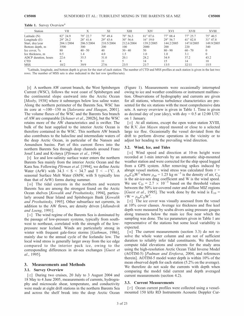
Table 1. Survey Overviewa

Station VII X XI XIII XIV XVI XVII XVIII

Latitude (N) 82� 24.9 79� 22.7 79� 49.4 79� 56.3 81� 07.6 77� 08.4 77� 25.7 75� 40.5Longitude (E) 29� 26.2 28� 41.6 29� 43.6 30� 56.6 16� 19.0 29� 56.7 41� 02.8 31� 47.8Start, doy/year 204.1/2004 206.5/2004 210.5/2004 212.6/2004 139.2/2005 144.2/2005 147.0/2005 149.9/2005Bottom depth, m 3500 300 200 100 2000 200 220 340Ice cover, % 80 40–50 40 30–40 50 80–90 60–70 0Ice thickness, m 0.5 1.4 4.0 1.5 1.0 1.0 3.1 0ADCP duration, hours 22.6 35.5 31.0 20.1 28.2 34.9 37.2 43.2CTD 4 9 11 5 14 15 14 10MSS 10/2 39/9 27/6 23/5 21/7 13/5 32/11 15/5

aLatitude, longitude, and bottom depth is given for the start of each station. The number of CTD and MSS profiles at each station is given in the last tworows. The number of MSS sets is also indicated in the last row (profiles/sets).


3 of 23

C05008

rent Profiler (ADCP). Continuous profiles were averagedevery 5 min in 8 m (2004) and 4 m (2005) depth bins withthe first bin centered at �21 m and 15 m, respectively, andthe deepest bin with good data at �250 m. Absolutecurrents were obtained by referencing to the surface, andwere found to be in good agreement with bottom trackreferencing when available.[18] The magnitude of shear, Sh = ((@u/@z)2 + (@v/@z)2)1/2,

where u and v are the east and north components of thevelocity, was computed by first differencing at 16-m mov-ing intervals. Accordingly, the first value of shear is at 29 m(2004) and 23 m (2005). The 16-m interval was chosen toavoid the contribution of noise which increasingly domi-nated the vertical wavenumber spectra at increasing wave-numbers (decreasing length scale).

3.4. Hydrography

[19] Conductivity, temperature, depth (CTD) profileswere made using a Sea-Bird SBE9 system. During part ofthe 2004 cruise this instrument malfunctioned and a SAIVSD204 CTD system with relatively crude resolution andaccuracy was deployed. The SBE9 was calibrated postcruisein 2004, and the data corrected for drift were used tocalibrate the SAIV data. In 2005, CTD data were calibratedagainst salinity samples analyzed with a Guildline PortasalSalinometer at the Geophysical Institute, University ofBergen. All corrected CTD data were postprocessed accord-ing to standard procedures as recommended by the manu-facturer, and bin averaged to 1 m resolution. Precisiontemperature and conductivity measurements at higher reso-lution were made with the microstructure profiler describedin the following section.[20] The depth of the surface mixed layer (Dmixed) was

calculated using the split-and-merge method described byThomson and Fine [2003]. We used an improved version(kindly provided by R. Thomson) which includes a secondrun through the split-and-merge procedure using a lowerboundary depth determined by the first run. The sensitivityof the results to initial choices of boundary depth, errorthreshold (here, set to 0.5 and 0.05 for the first and the

second run, respectively), and number of segment breakuppoints is thus reduced.[21] The base of the pycnocline (Dpyc) was identified

objectively as the first depth below the depth of maximumdensity gradient where the density difference was less than0.01 kg m�3 per meter for at least three consecutive 1-mintervals.

3.5. Turbulence and Mixing

3.5.1. MSS Profiler, Deployment, and Data Reduction[22] At the six selected stations (Table 2), a total of 155micro-

structure profiles in 43 sets were collected using a 1.4-m-longloosely tethered free-fall MSS profiler [Prandke and Stips,1998]. The instrument is equipped with two airfoil shearprobes (PNS98) aligned parallel to each other, fast responseconductivity (capillary type two electrode probe) andtemperature (FP07) sensors, an acceleration sensor, andconventional CTD sensors for precision measurements.All sensors sample at 1024 Hz to 16 bit resolution. Thesensors are protected by a probe guard which is the source oftwo significant narrow-band noise peaks in the shear spectraat �24 Hz and at 44 Hz. The buoyancy of the instrumentis adjusted to a typical fall speed of 0.7�0.9 m s�1. With anominal fall speed of 0.8 m s�1, the 24 Hz peak induced bythe guard corresponds to a wavenumber of 30 cycles permeter (cpm). The wavenumber range chosen for the analysisis well below this peak.[23] Several successive profiles, typically 3�5 repeats

(hereinafter called a ‘set’), were conducted every �4 hoursto cover different phases of the tidal cycle within the stationtime (20�43 hours); a compromise in order to accommo-date the multidisciplinary user groups on the vessel. Occa-sionally turbulence profiles were interrupted by strong windor rapid vessel/ice drift. A deployment overview is given inTable 1. The profiles were terminated at �60 m in 2004 andat �150 m in 2005. The dissipation values in the upper5�10 m have been discarded because of noise frominstrument acceleration and turbulence generated by theship’s keel.

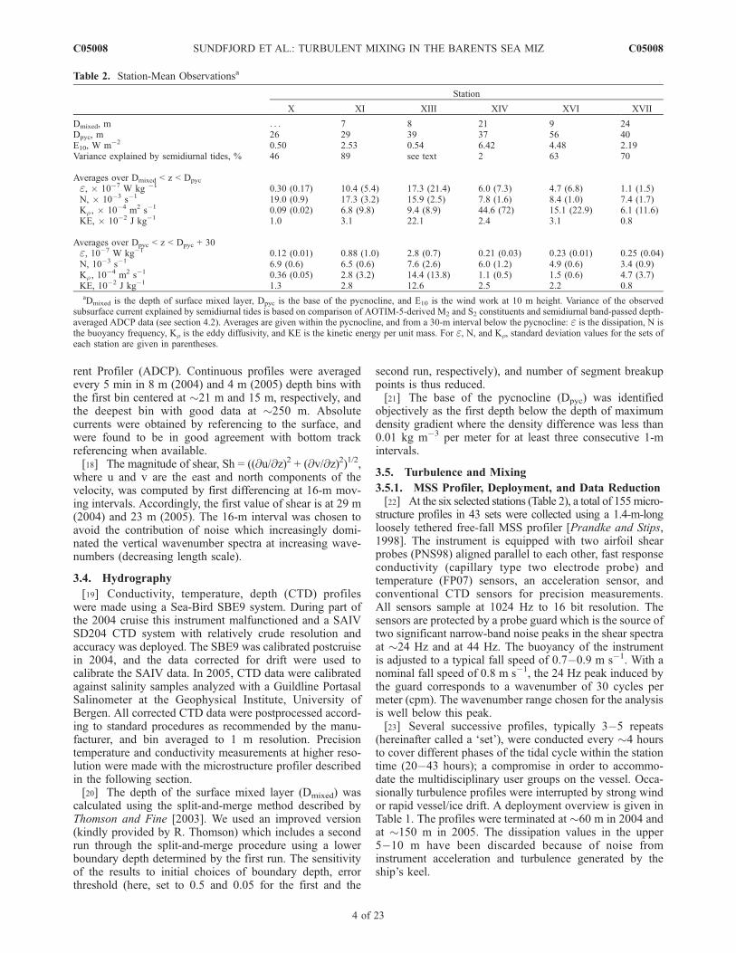
Table 2. Station-Mean Observationsa

Station

X XI XIII XIV XVI XVII

Dmixed, m . . . 7 8 21 9 24Dpyc, m 26 29 39 37 56 40E10, W m�2 0.50 2.53 0.54 6.42 4.48 2.19Variance explained by semidiurnal tides, % 46 89 see text 2 63 70

Averages over Dmixed < z < Dpyc

e, � 10�7 W kg �1 0.30 (0.17) 10.4 (5.4) 17.3 (21.4) 6.0 (7.3) 4.7 (6.8) 1.1 (1.5)N, � 10�3 s�1 19.0 (0.9) 17.3 (3.2) 15.9 (2.5) 7.8 (1.6) 8.4 (1.0) 7.4 (1.7)Kr , � 10�4 m2 s�1 0.09 (0.02) 6.8 (9.8) 9.4 (8.9) 44.6 (72) 15.1 (22.9) 6.1 (11.6)KE, � 10�2 J kg�1 1.0 3.1 22.1 2.4 3.1 0.8

Averages over Dpyc < z < Dpyc + 30e, 10�7 W kg�1 0.12 (0.01) 0.88 (1.0) 2.8 (0.7) 0.21 (0.03) 0.23 (0.01) 0.25 (0.04)N, 10�3 s�1 6.9 (0.6) 6.5 (0.6) 7.6 (2.6) 6.0 (1.2) 4.9 (0.6) 3.4 (0.9)Kr , 10

�4 m2 s�1 0.36 (0.05) 2.8 (3.2) 14.4 (13.8) 1.1 (0.5) 1.5 (0.6) 4.7 (3.7)KE, 10�2 J kg�1 1.3 2.8 12.6 2.5 2.2 0.8aDmixed is the depth of surface mixed layer, Dpyc is the base of the pycnocline, and E10 is the wind work at 10 m height. Variance of the observed

subsurface current explained by semidiurnal tides is based on comparison of AOTIM-5-derived M2 and S2 constituents and semidiurnal band-passed depth-averaged ADCP data (see section 4.2). Averages are given within the pycnocline, and from a 30-m interval below the pycnocline: e is the dissipation, N isthe buoyancy frequency, Kr is the eddy diffusivity, and KE is the kinetic energy per unit mass. For e, N, and Kr, standard deviation values for the sets ofeach station are given in parentheses.


4 of 23

C05008

[24] Full-scan data acquired by all sensors are edited fortransmission errors and spikes and then averaged to 256 Hzto reduce noise. Precision CTD data are low-passed at 10 Hzusing a phase-preserving fourth-order Butterworth filter.Temperature is then corrected for the time-response lagrelative to the conductivity sensor using a 55 scan (for256 Hz data) recursive filter. The profiles are averaged at10 cm intervals (within ±0.05 dbar of 0.1 dbar intervaltarget pressures, referred to as depth with negligible error).Conductivity is corrected against SBE deployed typicallywithin 15�20 min of the MSS. Salinity is 0.5 m median-filtered to further reduce spikes prior to calculating potentialtemperature, q, and potential density anomaly, sq.3.5.2. Stability and Richardson Number[25] The buoyancy frequency, N = [�(g/r) (@sq/@z)]

1/2, iscalculated using the Thorpe ordered sq profiles [Thorpe,1977] with density gradient obtained from the slope oflinear fits of sq against depth in 4-m sliding boxcarwindows. The Richardson number, Ri = N2/Sh2, is calcu-lated at moving 16-m intervals, below which the noise in theADCP derived shear substantially increases. In Ri calcu-lations, the buoyancy frequency is averaged at depth inter-vals corresponding with the depth range used to calculateshear. An average Ri profile is calculated for each MSS setusing set averaged N2 and Sh2 averaged over 6 subsequentADCP profiles (30 min) centered at the mean time of theMSS set.3.5.3. Dissipation and Eddy Diffusivity[26] Time series of small-scale shear, @u0/@z, measured by

the shear probes are converted into vertical wavenumberspace using a smooth fall-speed profile, invoking Taylor’sfrozen turbulence hypothesis which is valid at the fallspeeds reported here. The fall speed is derived from thetime derivative of the 2-Hz low-passed pressure record. Thedissipation rate of turbulent kinetic energy per unit mass, e,is calculated using the isotropic relation e = 7.5nh(@u0/@z)2i[Yamazaki and Osborn, 1990], where n is the viscosity ofseawater and @u0/@z is the shear resolved at centimeterscales. Here n is approximated as a function of temperatureand ranges within 1.55�1.9 � 10�6 m2 s�1 for the recordedrange of temperatures, �1.8 to 5�C. Shear wavenumberspectra are calculated using half overlapping 256-point (1 s)Hanning windows, corresponding to 0.8-m for a nominalfall speed of 0.8 m s�1. The shear variance is obtained byintegrating the shear wavenumber spectrum between 2 cpm,a limitation due to the length of the profiler, and an uppercutoff number depending on the Kolmogorov wavenumber,(e/n3)1/4/2p cpm. The upper cutoff is determined by itera-tion, similar to that described by Moum et al. [1995], and isset to maximum 30 cpm (or 14 cpm when 2�14 cpmintegrated e < 2 � 10�8 W kg�1). This range is not affectedby the narrowband noise peaks (see, e.g., the shear spectrain Figure 11 in section 5.2). A correction, typically within afactor of 1.2 for e < 10�7 W kg�1 and about a factor of 1.7for e � 10�6 W kg�1, is applied for the lost varianceassuming the Nasmyth’s form as tabulated by Oakey [1982].A further check is employed by comparing dissipation valuesfrom both probes, and anomalous data were discarded priorto averaging at 0.5 m bins. The noise level measured inquiet regions appears to be about 1 � 10�8 W kg�1,relatively high as a result of high fall speed and small massof the profiler. ‘‘Pseudo’’ dissipation rates, derived identi-

cally from spectral analysis of the acceleration sensordivided by the fall speed [Moum and Lueck, 1985] are<10�10 W kg�1.[27] The vertical diffusivity for mass is approximated

using Kr = Ge/N2 [Osborn, 1980], where G, the dissipationratio, is related to the mixing efficiency. A commonly usedvalue of G = 0.2 [Moum, 1996] yields an upper limit for Kr.When calculating Kr we adopt G = 0.12 as recommended byArneborg [2002] and consistent with the observations of StLaurent and Schmitt [1999]. A more detailed discussion isgiven in section 5.2.[28] An independent estimate of eddy diffusivity for heat,

KT, is made using the Osborn-Cox model [Osborn and Cox,1972] as KT = 3kTCx, where kT = 1.4 � 10�7 m2 s�1 is themolecular diffusivity for heat, Cx = h(@T0/@z)2i/h@T/@zi2 isthe Cox number and the factor 3 assumes full isotropy. Thedissipation rate of thermal variance is c = 2kTh3(@T0/@z)2i.The temperature gradient spectrum in the dissipation rangeoften adheres to the Batchelor form [Dillon and Caldwell,1980]. Slow fall speed and a fast response temperaturesensor with a known response function are needed tosufficiently resolve the temperature gradient spectrum. Be-cause the signal acquired by the fast response temperaturesensor was pre-emphasized for frequencies >1 Hz in aseparate channel, we were able to partly resolve the tem-perature gradient spectrum for active patches (in contrast tothe resolved shear spectrum every 0.5 m). Thermal gra-dients are deconvolved from the pre-emphasized signal, andtemperature spectra are obtained using the transfer functionfor the ideal amplification of the circuit. The transferfunction H2(f) = [1 + (2pftW�0.32)2]�2 [Gregg andMeagher, 1980] is applied to correct for the response timeof the FP07. Here W is the fall rate of the profiler, f is thefrequency in Hz and t = 12 � 10�3 s is the response time.We then convert this corrected temperature spectrum to @T0/@t spectrum by multiplying by (2pf )2. The frequencydomain @T0/@t spectrum is then converted to vertical wave-number domain @T0/@z spectrum by dividing the frequencyby W and multiplying the spectrum by W. We detected apatch as a segment of @T0/@z when the 1- to 30-Hz band-passed variances calculated at 1-s intervals exceeded fivetimes the noise level for the same frequency band. A modelnoise spectrum derived from quiet portions of the temper-ature gradient record is removed from the wavenumberspectrum computed over the length of the segment (at least3 m). We obtain c by fitting the Batchelor’s form to theresolved wavenumber band corresponding to 1�30 Hz, ofthe spectrum using the measured e for the patch. Using thebackground temperature gradient derived from the precisiontemperature profile, this yields an estimate for Cox numberand KT.3.5.4. Overturns[29] In a stratified flow the largest scale associated with

overturning eddies is the Ozmidov scale, LO = (e/N3)1/2

[Ozmidov, 1965]. Local instabilities in the water column canbe detected, in practice, using Thorpe scale analysis[Thorpe, 1977]. In this process, the profile of density isreordered to a sorted, statically stable profile. The r.m.s. ofdisplacements required for this reordering within an over-turn is called the Thorpe scale (LT): Dillon [1982] showedthat LO = 0.8LT, thus allowing e to be inferred from LT


5 of 23

C05008

(section 5.1). We detected density overturns using 10-cmaveraged sq profiles evaluated from the precision sensors ofthe microstructure profiler, with a noise threshold set to0.002 kg m�3 determined after run-length tests of Galbraithand Kelley [1996]. An additional water-mass test [Galbraithand Kelley, 1996] excluded artificial overturn signaturesresulting from the presence of different water masses andtemperature-conductivity sensor mismatch.3.5.5. Double Diffusion[30] Double diffusion driven by the difference in molec-

ular diffusivities for heat and salt [Turner, 1973] can inducesignificant vertical fluxes. A prerequisite for double diffu-sion is that both temperature and salinity either increase ordecrease with depth and is expected for positive values ofthe density ratio, Rr = (b @S/@z)/(a @T/@z), with 0 < Rr < 1favorable for salt fingering and Rr > 1 for double diffusiveconvection (DDC, also referred to as diffusive layering).Here a is the thermal expansion coefficient and b is thehaline contraction coefficient. Equivalently, diffusive layer-ing is expected for �90� < Tu < �45� where Turner angle isTu = arctan[(1 + Rr)/(1 � Rr)]. The predominant stratifi-cation in the Barents Sea with cold and less saline wateroverlying warm and salty water is susceptible to DDC.[31] We identify diffusive layers from temperature pro-

files recorded by the fast response thermistor, averaged over10 samples (i.e., �26 Hz), using a histogram approach[Padman and Dillon, 1988]. Heat fluxes resulting from thediffusive layers were calculated from [Kelley, 1990]

FH ¼ 0:0032r0cpa�1 � exp 4:8R�0:72

r

h i� gk2Tn

�1� �1=3� aDTð Þ4=3;

ð1Þ

where r0 is the mean density, cp is the specific heat, g is thegravitational acceleration, kT is the molecular diffusivity ofheat, n is the viscosity, and DT is the temperature differencebetween adjacent layers. The variability of Rr and DTacross individual steps in a staircase can significantly affectthe mean flux relative to that calculated from bulk densityratio and mean DT [Padman and Dillon, 1987]. Inevaluating FH we used DT of each step and calculated Rr

using temperature and salinity contrasts between adjacentlayers and local a and b.

4. Observations

4.1. Environmental Forcing and Ice Conditions

4.1.1. Ice Conditions[32] Ice concentration maps covering the study site at the

beginning of each cruise are shown in Figure 2. Satellite-derived (AMSR-E) sea ice concentration data on 6.25 kmgrid are used [Kaleschke et al., 2001]. According to thevisual observations, the ice cover was between 40�90% atthe drift stations (Table 1), and varied by up to 20% withinthe station time depending on wind and currents. Stationswere occupied within �10 nautical miles from the ice edge(defined as the transition to very open drift ice, <10%). Incontrast to the spring 2005 when the southern ice edgereached �76�N, in July 2004, a large area of open waterfollowed the northern continental shelf slope, and most ofthe central Barents Sea was ice free (Figure 2).4.1.2. Tides[33] Tidal current speed derived fromAOTIM-5 (section 3.2)

using the four main constituents M2, S2, K1, and O1 isshown for periods covering each drift station in Figure 3.Predictions are obtained for the mean location of eachstation during the drift. Tidal currents were very weak atstations VII and XIV, located at the shelf break north ofSpitsbergen. Three of the stations occupied in 2004 wereduring transition from neap to spring tide (Figure 3a). Thestation depths were shallower for the later of these stations,leading to a large increase in tidal currents despite theirgeographical proximity. Stations XVI, XVII and XVIII,surveyed in 2005, were in an area with more modest tidalcurrents and narrower spring-neap range (Figure 3b).4.1.3. Wind[34] Measured wind for each cruise is shown in Figures 3c�3d.

The lowest wind speeds were observed at X and XIII withmean wind work of �0.5 W m�2 (Table 2). All the otherstations had considerable energy input from winds, with thelargest values found at XIV, XVI and XVIII. At the lattertwo, microstructure sampling had to be interrupted owing tothe strong winds.

Figure 2. Ice concentrations at the beginning of each cruise: (a) 20 July 2004 and (b) 19 May 2005.Station positions are indicated with white dots and squares. See Figure 1b for station names. Satellite-derived data are obtained from http://iup.physik.uni-bremen.de:8084/amsr/amsre.html.


6 of 23

C05008

4.2. Hydrography and Currents

[35] In the following, we cluster stations according totheir geographical locations and corresponding dominantwater masses and large-scale current features: the Northernshelf break stations (VII and XIV), the Interior stations (X,XI, XIII), and the Southern MIZ stations (XVI, XVII andXVIII). The corresponding CTD profiles (Figure 4), T-Sdiagrams (Figure 5), layer and M2-phase averaged currents(Figure 6) and current profiles along the principal axisensemble-averaged during flood and ebb (Figure 7) arepresented. Station mean properties are given in Table 2.4.2.1. Northern Shelf Break Stations: VII and XIV[36] In this area the mean ice and surface water drift is

southwest toward the Fram Strait. A layer of Surface MeltWater (SMW) overlies the seasonal pycnocline, atop ArW.The permanent pycnocline separates this from AW,which flows eastward along the shelf break, following thetopography.[37] Station VII, located north of the steepest part of the

shelf slope had a <10 m deep surface mixed layer consistingof near-freezing melt water (Figure 4a). A pronouncedhalocline reached down to 30 m and temperature remainednear freezing to �50 m, where a transitional zone from ArWto AW started. Both temperature and salinity increaseddown to �100 m and remained quasi-uniform with depth.At the shelf slope north of Spitsbergen, station XIV startedat the �2000 m isobath and gradually drifted shelfward tothe 1200 m isobath. Dmixed and Dpyc were deeper at this

station, and temperature remained >�1�C at all depths.Lateral interleaving was observed at depths >80 m whereAW was dominant (Figure 4b). Here local instabilitiesassociated with large covarying fluctuations in temperatureand salinity reaching 1�C and 0.2, respectively, over O(1 m)were seen. Although similar in vertical structure, XIV waswarmer, more saline and denser than VII in the upper 100 m(Figure 5a).[38] Surface currents of 20�35 cm s�1 at VII, directed

southeastward (Figure 6a), were mainly wind forced. Thisstation was located north of the core of the AW inflow. Thesouth–southeast net current (time averaged over two M2

cycles) below the pycnocline was only weakly influencedby tides. At XIV, surface currents toward southwest wereclearly wind driven (Figure 6b) while below the pycnoclinea large net current to the northeast, with tidal modulations,was observed (Figure 7b).4.2.2. Interior Stations: X, XI, and XIII[39] Located in the northern part of the Barents Sea

proper, the interior stations are characterized by Arctic typewater (ArW and SMW) through most of the water column,and modified and diluted AW near the bottom in deepertrenches. The general ice and surface drift pattern is to thesouthwest. Mean pathways of the deeper water are largelyunknown.[40] Of the Interior stations X and XI were relatively deep

(300 and 200 m respectively) and were characterized bylow-salinity melt water with T > 0�C (Figures 4c and 4d)

Figure 3. (top) Tidal current speeds from AOTIM-5 predicted at the mean position of each station for(a) 2004 and (b) 2005. Duration of each station is marked by vertical lines, with names indicated.(bottom) Wind speed (line) and direction (crosses) for (c) 2004 and (d) 2005. Start times of the MSS setsare marked by arrowheads on top.


7 of 23

C05008

atop a sharp pycnocline extending to 25�30 m with waternear freezing before a gradual transition to warmer andmore saline water toward the bottom. At the shallower(100 m) station XIII, temperature was uniform with depth,around �0.7�C, and stratification was controlled by salinity.The main pycnocline was confined to the upper �40 m,followed by weaker stratification (Figure 4e). The horizon-tal line in T-S space at this station (Figure 5a) indicatescontinuous vertical heat exchange. The absence of a verticaltemperature gradient suggests that in addition to solarheating, heat was advected in near the bottom. At nearbyXI the water at depths >75 m was warmer than atcorresponding depths at XIII, indicating a possible heatsource. At X lateral interleaving was seen, particularlybetween 10�30 m and 50�100 m. As the main character-istics of X and XI are similar, only XI is shown in Figure 5a.Below the temperature minimum at �50 m the T-S tracefollows a mixing line with the AW found north of the shelfbreak.

[41] Stations X and XI were similar in surface and deepcurrent pattern (Figures 6 and 7), however, strong wind atXI (Figure 3) led to strong NNE surface current andenhanced average shear at depths <30 m, correspondingwith the base of the pycnocline. At station X, AOTIM-5-derived tidal phase was comparable to that of the depth-mean ADCP current. The discrepancy in the magnitude ofvelocity until doy = 209.5 (Figure 8a), i.e., the NE bias inADCP-derived currents, is caused by a residual current, asseen in the drift path in Figure 8b, likely forced by southerlywind of �5 m s�1 during �24 hours preceding the drift.Increasing wind stress by the end of the drift was accom-panied by larger current velocities and more intense surfacelayer shear. An estimate of the relative contribution ofdominant semidiurnal band tides to forcing and variabilityof currents at each station is made by comparing thesemidiurnal band inferred from AOTIM-5 and depth-averaged ADCP currents. At the latitudes of the survey,the period of inertial oscillations is only �15 min shorter

Figure 4. Representative CTD profiles from the Northern shelf slope stations (a) VII and (b) XIV, theInterior MIZ stations (c) X, (d) XI, and (e) XIII, and the Southern MIZ stations (f) XVI, (g) XVII, and(h) XVIII. Station-mean depths of the surface mixed layer, Dmixed, (dashed gray lines) and the base of thepycnocline, Dpyc, (solid gray lines) are indicated.


8 of 23

C05008

than the 12.42 hour period of the dominant M2 tide [Peaseet al., 1995]. The two can therefore not be separated withconfidence through harmonic analysis of the ADCP timeseries. Assuming that AOTIM-5 predictions at each stationare representative for the tides in the area, we compare thedominant semidiurnal tides (M2 + S2) to depth-averagedADCP current band-passed over the semidiurnal band(frequencies between 0.079 and 0.085 cph covering M2,S2 and the inertial frequency). The variance explained bythe tides in the semidiurnal band is summarized in Table 2.At station X, this crude comparison attributes 46% of thevariability to tidal currents. When comparing depth-aver-aged currents to results from a depth-integrated model, inaddition to the uncertainty associated with AOTIM-5results, some uncertainty arises from using ADCP currentscovering a fraction of the water column: Near the criticallatitude where M2 period equals the inertial period, thevertical distribution of the current is highly nonuniform[Nøst, 1994] and the unresolved fraction of the watercolumn can contribute significantly to the depth average.[42] During the shallow drift at XIII, bottom depth spanned

50�150 m over the complex topography near Kvitøya.Net wind-driven transport was negligible (Figure 6e),and the drift path (not shown) was almost a pure ellipsereturning to the same position after one near-inertial (�M2)cycle. The current reached 50 cm s�1 in the upper 50 m,which induced large drag and bottom-enhanced shear abovethe sea floor at shallows. Current direction rotated CCWwith depth part of the time, suggesting upward energypropagation [Leaman and Sanford, 1975].4.2.3. Southern MIZ Stations: XVI, XVII, and XVIII[43] The southern part of the Barents Sea is dominated

by AW. Here the incoming AW crosses the Polar Front

and subducts beneath ice and Arctic type water flowingsouthwest.[44] At the ice-free water reference station south of the

Polar Front, XVIII, water at all depths was of Atlantic origin

Figure 5. Temperature-salinity plots from (a) the Northern and Interior stations and (b) the SouthernMIZ stations. Shaded boxes denote the Atlantic Water (AW), the Cold Halocline Water (CHW), and theBarents Sea Branch Water (BSBW). Markers are placed at 50-m intervals from surface to a commonmaximum depth of 200 m, except for XIII, which was �150 m at the deepest. T-S values are bin-averaged over 5-m intervals for clarity. Dotted contours are sq isolines, and the dashed line is the freezingtemperature.

Figure 6. Average vectors of surface drift (gray) anddepth-averaged current from below the pycnocline (black)at the Northern shelf slope (a) VII and (b) XIV, the InteriorMIZ (c) X, (d) XI, and (e) XIII, and the Southern MIZ(f) XVI, (g) XVII, and (h) XVIII. Averaging is done overthe first 24.8 hours (2 M2 cycles) of each station whenstation duration allows (22.6 hours at VII, 20.1 hours atXIII). Only the surface current is shown for XIII owing tolarge depth variability during station time.


9 of 23

C05008

(Figure 4h). At the beginning of the station time there was asmall density gradient near the surface. The passage of astorm (Figure 3b) mixed down the warmer surface water andhomogenized the upper water column. Net depth-averagedcurrent was weak at this station (Figures 6h and 7h).[45] In the northern part of Hopen Deep, at XVI, below a

shallow mixed layer and a main pycnocline extending downto >50 m, the water column was rather homogeneous withAW influence (T > 1�C, S > 34.9) (Figure 4f). At thebeginning, strong wind from east led to a significant net

westerly drift. The principal axis of the depth-averagedcurrent is along 40� true and the mean current profile duringfloods is negative along this axis, i.e., toward the southwest(Figure 7f). The net current below the pycnocline, however,is to the south–southeast (Figure 6e).[46] Farther east, at XVII, a deep surface mixed layer was

dominated by ArW (Figure 4g), but higher temperature andsalinity toward the bottom indicate some intrusion of andmixing with modified AW. Salinity-compensated tempera-ture fluctuations were associated with this horizontal inter-

Figure 7. Ensemble averaged velocity profiles during times of flood (thick line) and ebb (thin line)along the principle axis of the depth-averaged current at the Northern shelf slope (a) VII and (b) XIV, theInterior MIZ (c) (X, (d) XI, and (e) XIII, and the Southern MIZ (f) XVI, (g) XVII, and (h) XVIII. Theellipses of the depth-averaged current are shown as insets with the principle axis orientation indicated asdegrees true. Orthogonal lines emanating from the origin are 10 cm s�1, shown for reference. Note thatthe horizontal scale is different in Figure 7e.

Figure 8. (a) East (black) and north (gray) components of the depth-averaged ADCP velocity (solidlines) at station X compared with AOTIM-5-derived tidal velocity (dashed lines). Arrowheads on topshow start times of the MSS sets. (b) Surface drift path at X.


10 of 23

C05008

leaving. Surface currents were shifted westward by windforcing during the first�15 hours. The net current (i.e., 2 M2

cycles averaged out) below the pycnocline was small(Figure 6g), comparable to that of the Interior stations. Thisis consistent with the average current profiles approximatelymirroring each other during flood and ebb (Figure 7g).[47] Although station XVI was not on the direct path

from XVIII to XVII, the T-S plot in Figure 5b illustratesthe changes that the AW undergoes as it flows northeast inthe Barents Sea. At ice-free XVIII, heat exchange with theatmosphere is the only significant modification, as inferredfrom the vertical line in T-S space. At XVI a less salineand cooler upper layer is seen owing to interaction withice. At the eastern station, XVII, a greater part of the watercolumn had low temperature but the intermediate part ofthe water column overlaps that of XVI in T-S space.Hydrography at depth >100 m is similar to the character-istics of modified AW outflow to the Kara Sea (BarentsSea Branch Water, BSBW, T < 0, 34.7 < S < 34.9, as

defined by Schauer et al. [2002a]). Note that all threestations have nearly identical density at 200 m depth. Theenhanced near-bottom salinities at both XVI and XVIIindicate advection of brine-enriched water from nearbybanks [Midttun, 1985].[48] The surface waters of both XVI and XVII fall within

the definition of Cold Halocline Water (CHW) as defined bySteele et al. [1995]. Rudels et al. [2004] distinguish betweenthe CHW formed near the northern shelf break and thatformed near the Polar Front in the central Barents Sea, withthe latter being more saline. This difference is seen betweenthe T-S plots in Figures 5a and 5b. Being closer to the shelfslope when the two branches meet at the St. Anna Trough,the Barents Sea CHW eventually contributes to the lowerpart of the Arctic Ocean halocline particularly in theMakarov and Canada basins, whereas the WSC branchmainly forms the halocline of the Nansen and Amundsenbasins. Contributions to intermediate Arctic Ocean waters

Figure 9. Profiles of (a, c) the station-mean dissipation, e, from shear measurements and (b, d) thecorresponding eddy diffusivity, Kr in the upper 60 m for (top) the Northern and Interior stations and(bottom) the Southern MIZ stations.


11 of 23

C05008

from the two AW branches have similar geographicaldistribution.

4.3. Diapycnal Mixing

[49] The dynamics of the upper mixing layer for the 2005survey is described by Fer and Sundfjord [2007]. In contrastto a profile in open water, the mean e profile under ice waselevated from levels predicted by constant-stress wall scal-ing within 2.5 times the ice-keel depth. At the base of themixing layer below ice, they reported vertical eddy diffu-sivities of 1–10 � 10�4 m2 s�1, with corresponding heatfluxes of 10�20 W m�2.[50] Here we focus on mixing within and below the

pycnocline. Station-mean dissipation and diffusivity profilesfrom the upper 60 m (section 3.5), are shown in Figure 9.For each station, average values of e within (Dmixed < z <Dpyc) and below the pycnocline (Dpyc < z < Dpyc + 30) aretabulated in Table 2. The salient features can be described asfollows. At all stations but X (below 15 m), e-profiles wereabove the noise level of the instrument (Figure 9). TypicalKr profiles show large diffusivity, >10�4 m2 s�1, through-out the water column and exceeding 10�3 m2 s�1 for highlyturbulent portions. In the upper 15 m at X, where e is abovethe noise level, Kr is of the order 10

�5 m2 s�1, comparableto the open-ocean thermocline levels. This low level ofturbulent activity is due to weak wind forcing and oceancurrent, and strong stratification particularly at the dilutedsurface layer (Figure 4c). Overall, eddy diffusivities withinthe pycnocline were greater than below it at all stations,except at stations X and XIII where the wind forcing wasnegligible. For stronger wind and tidal forcing, dissipationwithin the pycnocline was at least 5 times larger than thatbelow the pycnocline (particularly at XIV and XVI). At XI,where wind forcing was strong and the surface mixed layerwas shallow, a large portion of the wind energy dissipationlikely penetrated to the pycnocline yielding average dissi-pation of 10�6 W kg�1 within the pycnocline. The largestdissipation within the pycnocline was observed at theshallow XIII (e = 1.7 � 10�6 W kg�1), influenced bystrong tidal currents. Here boundaries at the bottom andunder the ice stirred by the barotropic tide can cover asignificant fraction of the water column (bottom depthspanned 50�150 m, section 4.2). Current profiles at XIIIshow strong depth dependence (Figure 7e); hence barocli-nicity and turbulence generated by the mean shear can alsobe responsible for the enhanced dissipation. Currents sug-gest an upward low-mode energy propagation (Table 3 insection 5.4.2) and internal wave generation over complextopography at the site can be of importance (section 5.4).

5. Results and Discussion

5.1. Overturns

[51] Density overturns in each microstructure profile wereidentified (section 3.5), applying thresholds for noise andT-S correlations to ensure that the identified overturns werenot spurious. On average, more than two overturns weredetected per profile at all stations except XVIII.[52] In the following we evaluate the LO / LT relation-

ship, i.e., the length scales associated with the largest scaleof turbulent eddies in a stratified flow and density overturns.The background buoyancy frequency, N, was calculated

using the density gradient from the slope of linear fit ofThorpe-sorted sq against depth within 1 m above and beloweach overturn. Of the 375 identified overturns with densityfluctuations significantly greater than the set noise thresh-old, 259 satisfied the conditions of the water-mass test andthat N was greater than twice its error estimate. Finally 191overturns had accompanying e measurement. We alsoevaluated the density ratio, Rr, for each patch, again usingvertical gradients derived from linear fits, to delineatediffusive layering favorable overturns. As no significantdifference was found between patches with backgroundRr < 0 or Rr > 1, all 191 overturns were evaluated (Figure 10)to obtain LO = (0.7 ± 1.1)LT

(1.1±0.1), where the uncertaintiesare the standard errors. Stations with higher mean dissipa-tion (XI, XIII) gave somewhat higher estimates for Thorpescales compared with the less energetic stations. The expo-nent on LT is not significantly different than unity, and weobtain a maximum-likelihood estimate (mle) from a log-normal distribution of the ratio r = LO/LT of 0.9 with 95%confidence limits CI = [0.8 1.0]. The estimate of r in thiswork is comparable to previously reported estimates of r =0.8 (±0.4) in the seasonal oceanic thermocline [Dillon,1982]; r = 0.66 (±0.27) [Crawford, 1986] in the permanentoceanic thermocline; r = 0.95 (±0.6) [Ferron et al., 1998] inthe Romanche Fracture zone for q < 2�C; and r = 0.7�1.1from overflow of a high-latitude sill-fjord [Fer, 2006]. Wesuggest that dissipation in the MIZ of the Barents Sea canbe estimated from CTD data with sufficient resolution as e =(rLT)

2N3, using r = 0.9.

5.2. Diffusivity for Heat and Dissipation Ratio

[53] Eddy diffusivity obtained from the Osborn’s model(section 3.5) is often calculated using a dissipation ratio G =0.2, which gives a theoretical upper limit for Kr. Dissipationratio G is related to the flux Richardson number, Rf, as G =Rf/(1 � Rf) and G = 0.2 follows from the theoretical criticalvalue of Rf � 0.17 [Ellison, 1957]. Rf is also referred to asmixing efficiency and is defined as the ratio of the rate ofpotential energy change to the work done for turbulentproduction. The magnitude of the mixing efficiency isreported to depend on the Richardson number, the processesgenerating the turbulence (e.g., shear production, DDC, gridgenerated turbulence) [Linden, 1979], and more recentlydifferential diffusion [Jackson and Rehmann, 2003]. Adiscussion with respect to patchy oceanic turbulence isgiven by Arneborg [2002] who recommended Rf = 0.11(G = 0.12), a value supported by microstructure measure-ments [St Laurent and Schmitt, 1999]. When dissipation rateof temperature variance, c, and of TKE, e, are availablethrough microstructure measurements, the dissipation ratiois typically estimated from G � cN2/(2h@T/@zi2e), which isonly valid if KT = Kr and conditions for validity of bothOsborn-Cox and Osborn models are satisfied [see Ruddicket al., 1997]. The values compiled by Ruddick et al. [1997]range from 0 < Rf < 0.26.[54] Using Reynolds analogy, when the flow is highly

turbulent and when temperature and salinity contributeequally to the stratification, Kr is approximately equal tothe diffusivities for heat, KT, or for salt. When the stratifi-cation is weak or in the presence of double diffusionOsborn’s model can give erroneous results. Recent labora-tory results [Barry et al., 2001] (BIWI hereafter) and direct


12 of 23

C05008

numerical simulations [Shih et al., 2005] (SKIF hereafter)showed that, for e/nN2 < 1000, Osborn’s model overesti-mated the measurements with a factor of 2 and for larger e/nN2 the discrepancy was systematically larger exceeding1 order of magnitude for e/nN2 � 104. The nondimensionalparameter e/nN2 is in the form of a Reynolds number and isoften referred to as buoyancy Reynolds number or turbulentactivity index. BIWI proposed Kr = 17n2/3kT

1/3(e/nN2)1/3 fore/nN2 > 800 (the constant and the threshold is different thanthose reported in BIWI owing to a factor 2.8 error indissipation measurements [Jackson and Rehmann, 2003]).Using a wider range of e/nN2 SKIF proposed Kr = 2n(e/nN2)1/2 for e/nN2 > 100. Note the scaling with differentpowers of the buoyancy Reynolds number for the differentmodels. In the following we present independent estimatesfor diffusivity for heat derived from temperature microstruc-ture, compare to diffusivity of mass inferred from Osborn’smodel, BIWI and SKIF and estimate the dissipation ratio forthe survey area.[55] We obtained KT using the Osborn-Cox model (sec-

tion 3.5) for segments of enhanced temperature gradientvariance. Of the 567 detected segments (patches), 407satisfied the conditions (1) background stratification andtemperature gradients are greater than twice the errorestimate, (2) there are accompanying e measurements,(3) temperature-gradient spectrum acceptably conforms tothe Batchelor’s form in the resolved wavenumber range, and(4) patch is located below the mixed layer. The lattercondition is imposed to exclude the effects of significantstabilizing buoyancy flux observed in the mixed layer inresponse to melting of the ice [Fer and Sundfjord, 2007]when the assumptions behind the Osborn-Cox model willnot hold. An example of two of the patches, detected at XIV,is given in Figure 11. Each patch is susceptible to diffusive

layering with Rr > 1 but the one at about 130 m has Ri � 5and less microstructure shear variance, whereas that at�30mhas Ri � 2.2 with e five fold larger. The shear spectra fromboth probes and both patches agree with the Nasmyth’suniversal form. The dT0/dz spectra are visually consistentwith the best fit Batchelor forms in the resolved wave-number range, derived using the reliably measured e. Thesecond patch is just above the AW core and the enhancedtemperature microstructure is related to the mixing of heatfrom AW toward upper layers.[56] The variation of KT with the buoyancy Reynolds

number is shown in Figure 12 together with expectedrelations for the Osborn (for Kr), SKIF and BIWI models.Values of KT are comparable to Kr estimates using G = 0.2(typical value), G = 0.12 (used in this study) and G = 0.33(survey mean value derived using the observations dis-cussed below). There is a robust increase with increasinge/nN2, consistent with the slope expected from the Osbornmodel over the observed range of e/nN2. No significantregime shift is seen around e/nN2 � 800 (BIWI) or �100(SKIF). Although there is large scatter and measurementuncertainty, KT ffi Kr / e/N2 scaling describes the obser-vations reasonably well whereas BIWI and SKIF modelssignificantly underestimate KT for e/nN2 > 1000. A recentstudy measured vertical eddy diffusivity directly in anestuary [Etemad-Shahidi and Imberger, 2005] and com-pared with indirect methods of Osborn, Osborn-Cox andBIWI. They reported that best estimates were obtained fromOsborn-Cox model whereas BIWI model overestimated themeasurements by a factor of 10, different from our results.[57] The dissipation ratio G � cN2/(2h@T/@zi2e) derived

from the patches (407 data points in total) cover a range of0.014 � 9.3 and is log-normally distributed between G =0.01�1 falling on a straight line in normal probability plot

Figure 10. Log-log scatter plot of the Thorpe scale, LT, versus the Ozmidov scale, LO. Data points fromwhen the background stratification was stable to DDC (crosses) and diffusive layer favorable (dots) areshown separately. The equation resulting from the least-squares regression is indicated with ± standarderror. The 95% confidence interval of the maximum likelihood estimator from a log-normal distributionof the LO/LT ratio is [0.8 1.0].


13 of 23

C05008

of log10(G) (Figure 13a). The probability distribution iscalculated from the histogram of log10(G) and the distribu-tion in the range 0.01 < G < 1 (solid dots in Figure 13b) isfitted to the lognormal probability density function using anonlinear least squares fit. The mean value of G obtainedfrom the fit is 0.33, consistent with the maximum-likelihoodestimator (mle) from log-normal distribution of G = 0.34(95% CI = [0.30 0.38]). This is larger than values reportedfor typical oceanic conditions, however, it is comparable to

the upper range of values compiled in Table 2 of Ruddick etal. [1997] (Rf = 0.25 yields G = 0.33). The majority of thepatches have bulk Rr values favorable for double diffusion:102 patches with Rr < 0 (diffusively stable) and 305 withRr > 0. The mle values obtained for double-diffusively stableand DDC-favorable cases are G = 0.25 (95% CI = [0.2 0.3])and G = 0.56 (95% CI = [0.48 0.67]), respectively.Corresponding values of mixing efficiency are Rf = 0.2(double-diffusively stable) and Rf = 0.36 (DDC-favorable).

Figure 11. Two examples of patches of enhanced temperature gradient. The profiles are (left)temperature and 30 Hz low-passed temperature gradient and (middle) 10 Hz low-passed shear from oneof the shear probes. The vertical extent of the patches are indicated by gray boxes. (right) The temperaturegradient spectra (FdT/dz) and shear spectra (Fdu/dz) calculated for each patch. The corresponding graytraces are the Batchelor’s and Nasmyth’s form of the universal FdT/dz and Fdu/dz spectra, respectively.Shear spectra from both shear probes are shown (thin and thick traces). The dashed shear spectrum is thatinferred from the acceleration sensor of the instrument (acceleration spectrum divided by the sinkingspeed squared) and is indicative of the noise induced by the instrument’s motion. The dashed dT/dzspectra are the noise level inferred from quiescent portions of the temperature gradient record. The meanvalues of the Richardson number, Ri, the density ratio, Rr, the dissipation of temperature variance, c, theCox number, Cx, and the dissipation of TKE, e, are indicated for each patch. Both patches are recorded atstation XIV.


14 of 23

C05008

Consistent results are obtained by regressing x = e/N2

against y = c/(2h@T/@zi2) on log-log space to obtain arelation of the form y = axb. The exponent ‘‘b’’ is notsignificantly different than unity for both diffusively stableand unstable conditions (Figure 14), hence the best fit valueof coefficient ‘‘a’’ is equivalent to the diffusivity ratio equalto 0.2 for the stable cases, but increases to 0.7 for Rr > 0.The difference is significant at 95% confidence. Ourmicrostructure data sampling strategy (profiler sink speedof 0.7�0.9 m s�1) and the high noise level of dissipationmeasurements do not allow us to pin down the reasonsbehind the G-Rr dependence. The patches to which theanalysis applies are at least 3 m thick, significantly greaterthan the typical observed diffusive layer thickness of about1 m (section 5.3). Values of G associated with Rr > 0 mayhave contributions from (1) convecting DDC layers,(2) enhancements of shear at high-gradient interfaces sep-arating the layers [Padman, 1994], and (3) the turbulentstructure in the remaining portion of the patch. The mixingefficiency from DDC alone will be large, because almost allthe TKE diffusion appears as buoyancy flux. The apparentincrease in the mixing efficiency for DDC-favorable patchesin our data set is a result of combination of the threemechanisms listed above.[58] Heat flux, FH = rCPKTdT/dz, where cp is the specific

heat and dT/dz is the background temperature gradient, iscalculated for the detected patches and is presented for tworepresentative stations (X and XVII) in Figure 15. Enhancedpositive heat fluxes are correlated with Turner angle,Tu <�50�, susceptible for diffusive layering. Temperatureanomalies from the average temperature on the station-meanisopycnal are in excess of ±0.8�C at both stations. Patches

Figure 12. Variation of the diffusivity for heat, KT, withthe buoyancy Reynolds number, e/nN2 estimated fordetected turbulent temperature patches (407 in total). Thevalues of KT are averaged in equally spaced logarithmicbins of e/nN2. Error bars indicate ±1 standard deviation overthe number of data points indicated at top. The modelsshown are that of Osborn using G = 0.12, 0.2, and 0.33(dashed lines), SKIF (thin black line), and BIWI (thick grayline).

Figure 13. (a) Normal probability plot for log10G. (b) Probability density derived from the histogram oflog10G (solid and open circles) and the normal probability density function (black curve) fitted (nonlinearleast squares fit) to the values of G < 1 (solid circles). The expected mean value and 95% confidenceintervals for the fitted distribution are indicated.


15 of 23

C05008

of warm intrusions are observed along isopycnals, compen-sated by salinity.

5.3. Double Diffusion

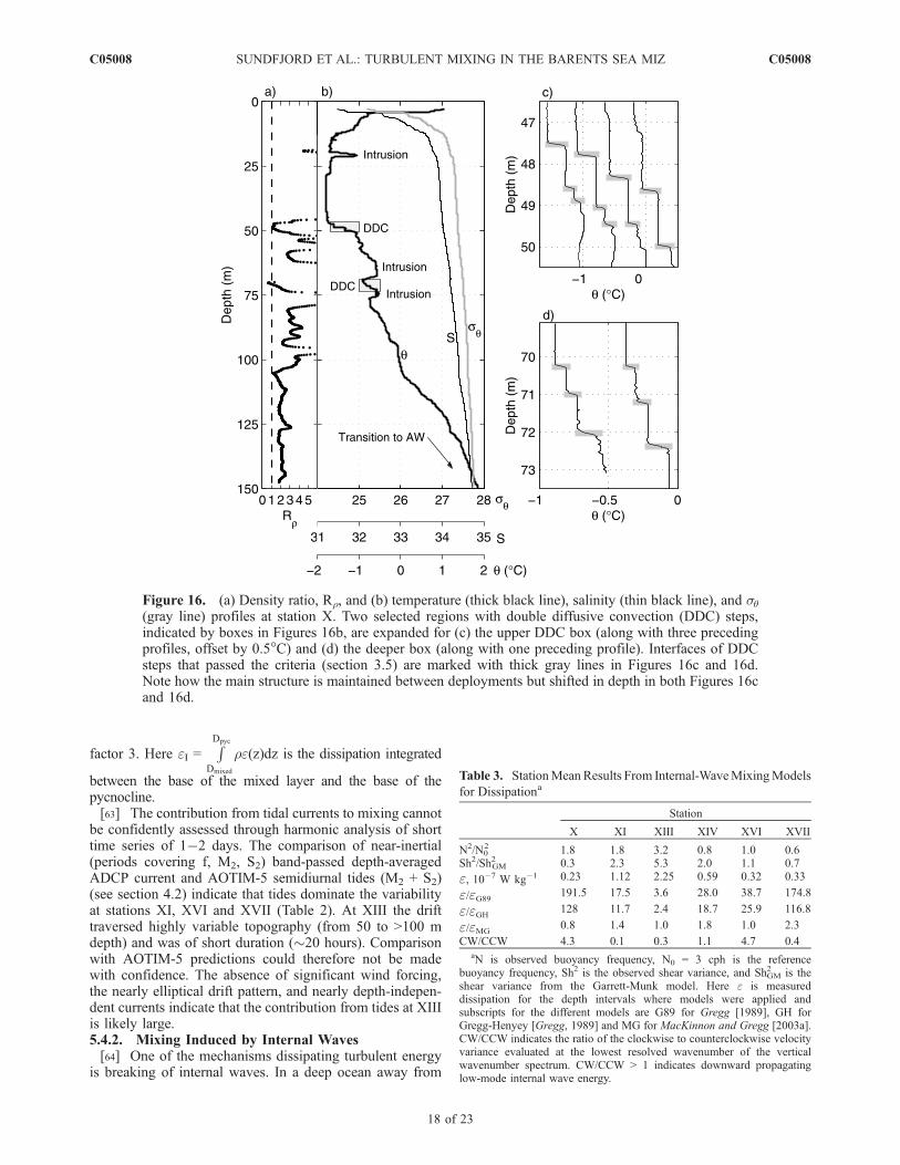
[59] The water column in the MIZ of the Barents Sea wasobserved to be favorable for double diffusion typically inthe upper parts of warm intrusions and below the seasonalpycnocline in the transition zone to AW (see, e.g., Turnerangle <�45� in Figures 15a and 15c). At stations withmodest levels of shear-driven turbulent mixing, step struc-tures indicating diffusive layers were seen (at X, XVII andto some extent at XIV and XVI). Using the methoddescribed in section 3.5 we have identified individual stepsand calculated resulting heat fluxes based on local densityratio and temperature difference across the steps.[60] The largest number of diffusive layers was found at

Interior station X (see sample profiles in Figure 16), where19 of 39 profiles contained one or more depth segmentswith steps fulfilling the criteria for layer height, temperaturedifference across the step, and that Rr > 1. Diffusive layerswith mean thickness of �0.7 m and mean temperaturedifference of 0.14�C were found at 40�75 m, between theregion of uniformly low temperatures and the transitionallayer to AW. The resulting heat fluxes in the identified DDClayers ranged from 0.3 to 33 W m�2 (mean heat flux for alllayers was 6.3 W m�2). At the eastern station XVII stepswere found at depths >60 m in 15 of the 32 profiles. Thelayers were typically twice as thick of those at X but withslightly smaller temperature increments. Mean diffusive heatflux was 10.7 W m�2, with maximum values �50 W m�2.At stations XIV (northern Shelf Break) and XVI (just northof the Polar Front) fewer diffusive layers were detected, in7 (of 21) and 3 (of 13) profiles respectively. Their character-istics were similar, with mean heights of �1.0 m andtemperature steps of 0.10�C, all found in the upper part ofthe AW layers, typically around 60 m depth. Mean heatfluxes were around 3 W m�2 and maximum values were inexcess of 10 W m�2. These DDC staircases appeared to beof more transient nature than those observed at X and XVII,

where the same structure could be detected in severalconsecutive profiles.[61] Local diffusive heat fluxes are of comparable magni-

tude to heat flux calculations from available patches based onthe Osborn-Cox model (section 5.2) at stations X and XVII.At X, mean heat flux in active patches was �15 W m�2,2.5 times greater than the mean flux through the observedDDC steps. At XVII, mean FH at depths where DDC wasseen to occur (>60 m) was �50 W m�2; 5 times the meanDDC fluxes. Bearing in mind that the overall mean heatfluxes are not resolved and are biased large through aver-aging over patches of enhanced temperature gradient vari-ance, our data show that in comparison with turbulent heatfluxes, DDC can be important for vertical heat fluxes inareas with moderate or low mechanical stirring and favor-able hydrographic conditions. To our knowledge, double-diffusive mixing associated with horizontal intrusions hasnot previously been reported for the Barents Sea proper, butthis process is believed to be dominant for vertical heatfluxes in the quieter parts of the interior Arctic Ocean [e.g.,Padman and Dillon, 1989; Carmack et al., 1997; Rudels etal., 1999] and in the permanent pycnocline at the slope ofthe western Weddell Sea [Robertson et al., 1995]. At thedeep shelf slope north of Svalbard Perkin and Lewis [1984]report heat fluxes of up to O(10) W m�2 associated withdouble diffusion, typically for depth >140 m over bottomdepths of 1000�2000 m (see, e.g., their station 215, atnearly the same location as our XIV). Their data suggestthat more efficient and persistent double-diffusive fluxescan be expected at greater depths than sampled by ourprofiles.

5.4. Response to Forcing

5.4.1. Wind and Tidal Currents[62] In this section we investigate relationships between

the observed dissipation within and below the pycnocline,and forcing mechanisms induced by wind and oceaniccurrents. Using the stations occupied in 2005, Fer andSundfjord [2007] show that the dissipation in the surface

Figure 14. Regression of x = e/N2 on y = c/[2(dT/dz)2] on log-log space for (a) diffusively stablepatches (102 data points) and (b) double diffusion favorable patches (305 data points). The best-fit valuesof ‘‘a’’ and ‘‘b’’ and their 95% confidence intervals are indicated.


16 of 23

C05008

mixed layer is significantly correlated with wind stress andthat the depth of mixing and the entrainment into the mixedlayer scale with under-ice friction velocity, which in turndepends on the wind speed. Since wind energy and associ-ated current shear can protrude beyond the mixed layer itmay also be possible to diagnose dissipation of TKE withinthe pycnocline as a function of wind energy. Significantcorrelation between depth-integrated dissipation within thepycnocline and the wind speed is found at stations with

considerable wind forcing (E10 > 2 W m�2, i.e., all stationsexcept X and XIII). The relationship is strongest whenscaled with the thickness and depth of the pycnocline,implying that a shallow pycnocline is more influenced bythe wind. If we assume that the fraction of E10 available formixing decreases linearly with depth from its surface valueto zero at the base of the pycnocline, a scaling of the formeI / E10

Dpyc�Dmixed

Dpycexplains 62% of the variability when

dissipation values varied by a factor 10 and wind work by a

Figure 15. Depth versus time maps of heat flux (boxes in color) and Turner angle (black isolines) at(a) X and (c) XVII, and of temperature anomaly along mean isopycnals at (b) X and (d) XVII. Isopycnals,sq > 27, are contoured at 0.05 intervals in Figures 15b and 15d. Heat fluxes from Osborn-Cox method areshown for all available patches (23 at X, and 192 at XVII). The vertical extent of each box shows theposition of the patch in the water column whereas the horizontal extent is arbitrary.


17 of 23

C05008

factor 3. Here eI =RDpyc

Dmixed

re(z)dz is the dissipation integrated

between the base of the mixed layer and the base of thepycnocline.[63] The contribution from tidal currents to mixing cannot

be confidently assessed through harmonic analysis of shorttime series of 1�2 days. The comparison of near-inertial(periods covering f, M2, S2) band-passed depth-averagedADCP current and AOTIM-5 semidiurnal tides (M2 + S2)(see section 4.2) indicate that tides dominate the variabilityat stations XI, XVI and XVII (Table 2). At XIII the drifttraversed highly variable topography (from 50 to >100 mdepth) and was of short duration (�20 hours). Comparisonwith AOTIM-5 predictions could therefore not be madewith confidence. The absence of significant wind forcing,the nearly elliptical drift pattern, and nearly depth-indepen-dent currents indicate that the contribution from tides at XIIIis likely large.5.4.2. Mixing Induced by Internal Waves[64] One of the mechanisms dissipating turbulent energy

is breaking of internal waves. In a deep ocean away from

Figure 16. (a) Density ratio, Rr, and (b) temperature (thick black line), salinity (thin black line), and sq(gray line) profiles at station X. Two selected regions with double diffusive convection (DDC) steps,indicated by boxes in Figures 16b, are expanded for (c) the upper DDC box (along with three precedingprofiles, offset by 0.5�C) and (d) the deeper box (along with one preceding profile). Interfaces of DDCsteps that passed the criteria (section 3.5) are marked with thick gray lines in Figures 16c and 16d.Note how the main structure is maintained between deployments but shifted in depth in both Figures 16cand 16d.

Table 3. StationMean Results From Internal-WaveMixingModels

for Dissipationa

Station

X XI XIII XIV XVI XVII

N2/N02 1.8 1.8 3.2 0.8 1.0 0.6

Sh2/Sh2GM 0.3 2.3 5.3 2.0 1.1 0.7

e, 10�7 W kg�1 0.23 1.12 2.25 0.59 0.32 0.33

e/eG89 191.5 17.5 3.6 28.0 38.7 174.8

e/eGH 128 11.7 2.4 18.7 25.9 116.8

e/eMG0.8 1.4 1.0 1.8 1.0 2.3

CW/CCW 4.3 0.1 0.3 1.1 4.7 0.4aN is observed buoyancy frequency, N0 = 3 cph is the reference

buoyancy frequency, Sh2 is the observed shear variance, and ShGM2 is the

shear variance from the Garrett-Munk model. Here e is measureddissipation for the depth intervals where models were applied andsubscripts for the different models are G89 for Gregg [1989], GH forGregg-Henyey [Gregg, 1989] and MG for MacKinnon and Gregg [2003a].CW/CCW indicates the ratio of the clockwise to counterclockwise velocityvariance evaluated at the lowest resolved wavenumber of the verticalwavenumber spectrum. CW/CCW > 1 indicates downward propagatinglow-mode internal wave energy.


18 of 23

C05008

boundaries the amount of turbulent mixing due to internalwaves can be estimated using the Garrett-Munk internalwave model spectrum [Garrett and Munk, 1975], assumingthat the energy is transferred from the frequency and lengthscales where internal waves are generated to the scaleswhere they break and dissipate. A commonly used modelthat incorporates easily observable O(10-m) shear andstratification is proposed by Gregg [1989],

eG89 ¼ 7� 10�10 N2=N20

� �Sh4=Sh4GM� �

; ð2Þ

where N is the observed buoyancy frequency, N0 = 5.24 �10�3 s�1 (� 3 cycles per hour) is the canonical deep oceanstratification, Sh4 is observed squared-shear variance andShGM

4 is the squared-shear variance of the Garrett-Munkmodel. The above model, based on modifications on theanalytic model by Henyey et al. [1986], is a simplifiedversion, referenced to 30� latitude and neglects latitudedependence. At high latitudes the effect of latitude can beimportant and we therefore apply the more general, so-called Gregg-Henyey model [Gregg, 1989],

eGH ¼ 1:7� 10�6f cosh�1 N0=fð Þ N2=N20

� �Sh4=Sh4GM� �

; ð3Þ

where f is the local Coriolis parameter.

[65] MacKinnon and Gregg [2003a] proposed an alterna-tive dissipation scaling for shallow shelf application basedon low-passed fine-scale shear,

eMG ¼ e0 N=N0

� �Sh=Sh0� �

: ð4Þ

[66] Here e0 is a constant typically chosen to match thesurvey average, Sh is shear and Sh0 is reference shear level(MacKinnon and Gregg applied Sh0 = N0, for simplicity).This scaling assumes that the low-mode ‘‘background’’shear is decoupled from higher-mode waves.[67] Because the water column is stratified below Dmixed

(the mixed bottom boundary layer is not resolved), internalwaves can be supported and we apply the above models,accordingly, below the mixed layer from the first depth atwhich 16-m shear is available. We used 16-m finitedifferenced shear calculated from ADCP data, and applieda correction factor of 2.26 and 2.61, from 4-m and 8-m binsizes, respectively, for attenuation of the shear variancespectrum due to ADCP bin size and finite differenceinterval length [Gregg and Sanford, 1988; Wijesekera etal., 1993]. The ratio of the observed dissipation to thatinferred from the models (equations (3) and (4)) are given inTable 3, together with the stratification and shear variancewith respect to the GM levels. ShGM

2 is approximated from

Figure 17. (a) Profiles of the ratio of the observed dissipation, eobs, to that derived from Gregg-Henyeymodel eGH (red, equation (3)) and MacKinnon and Gregg model, eMG (black, equation (4)). Ordinate isdepth scaled with the base of the pycnocline. Distribution of (b) eobs, (c) eMG, and (d) eGH in log-logN2 � Sh2 space. Note the different color scale in Figure 17d.


19 of 23

C05008

equation (A11) of Gregg and Kunze [1991] for a cutoffvertical wavenumber corresponding to 16 m. In evaluatingeMG, we use e0 = 4.5 � 10�8 W kg�1, the mle value of alldissipation measurements below Dmixed. The open-oceaninternal wave models do not reproduce the observationssatisfactorily. The profiles of the ratio of observed toinferred dissipation are presented for eGH and eMG inFigure 17a, together with the distribution in N2 � Sh2 space(Figures 17b�17d), following MacKinnon and Gregg[2003a] and Carter et al. [2005]. The predictions fromthe Gregg-Henyey model do not agree with our observa-tions, whereas the pattern (in N2 � Sh2 space) resultingfrom the MacKinnon and Gregg scaling compare reason-ably well with the data set. The observed variability of e isbetter captured by e / NSh consistent with the Kr / N�1

scaling appropriate for lakes and fjords [Gargett andHolloway, 1984; D’Asaro and Lien, 2000; Fer et al.,2004; Fer, 2006]. A good agreement with the internalwave-wave interaction models and the observations isexpected only if the mixing is predominantly due to internalwaves, which is not the case in our survey where meanshear is also important. We cannot assess the contribution ofinternal wave induced mixing relative to that induced bymean shear because the observations are uncorrelated withthe Gregg-Henyey model. The fairly good agreement withthe MacKinnon and Gregg model, on the other hand, can befortuitous and not entirely representative of mixing due towave-wave interaction, because the employed survey meane0 clearly comprises dissipation induced by mean shear aswell as other processes.[68] Internal waves dissipating energy near the pycno-

cline are mostly generated elsewhere. Inertial waves aretypically generated at the surface and have downwardenergy propagation. Internal waves generated by flowinteracting with topography or those reflecting from thebottom will have upward propagating energy. This ismanifested in the clockwise (CW) and counterclockwise(CCW) rotary component vertical wavenumber spectra ofshear or velocity, where an excess of CW (in the NorthernHemisphere) at low wavenumbers indicates downwardpropagating near-inertial energy [Kunze and Sanford,1984]. The CW/CCW variance ratios evaluated at thelowest resolved wavenumber of the station averaged veloc-ity spectra are given in Table 3. The ratios suggest that thereis upward propagating low-mode internal wave energy atstations XI and XIII near Kvitøya where large tidal flow andenhanced mixing was observed, and to a lesser extent eastof the Great Bank, at XVII. The observed levels of mixingcan be associated with generation of internal waves oversteep topography, comparable to the observations of Padmanand Dillon [1991] at the deep shelf slope at the northern edgeof the Yermak Plateau, north of Spitsbergen. They foundhighest e to be correlated with the diurnal tide, interactingwith steep topography at the shelf slope and generatinginternal waves.

6. Implications

6.1. Water Mass Modification

[69] At station XIV, at the northern shelf break, e waslarge within the pycnocline and decayed with depth. Heatfluxes were thus modest in the rather strong mean vertical

temperature gradient between the base of the pycnoclineand top of the AW (�100 m) (Figure 4b). Patches ofenhanced temperature gradient variance (section 5.2) hadmean upward heat flux of �50 W m�2, with peak values inexcess of 200 W m�2. As the WSC continues its flownortheastward along the slope, a heat sink is continuouslyavailable as more ice and cold surface water is encountered.By losing sufficient heat, the near-surface water at XIV canobtain the same temperature-salinity characteristics as theCHW observed farther north at station VII (Figure 5a), northof the shelf break. Although the modified AW at drift stationsXVI and XVII was colder than that at XIV, significant upwardheat fluxes were found also in this southern MIZ area. Atstation XVI, just north of the Polar Front in the central BarentsSea, mean upward fluxes of 16 W m�2 were seen in activepatches below the pycnocline. Following the Barents Seabranch of AW farther en route to the Kara Sea, heat fluxes atXVII larger than ±10 W m�2 were found at the top/bottom ofwarm intrusions between 50 and 150 m, with a net upwardheat flux of �2 W m�2. Owing to this heat loss from themodified AW, the near-bottom waters at station XVII canattain the characteristics of BSBW (Figure 5b) without furtheradmixture of high-salinity water.[70] The relatively deep stations in the Interior MIZ (X

and XI) were surveyed in late July 2004, when the surfacewater was relatively warm (Figures 4c and 4d). As a resultthe cold ArW layer (20�50 m depth) at X receiveddownward heat fluxes of 15 W m�2 from above, in additionto upward fluxes of �20 W m�2 from the warm AW below.A similar pattern with pulses of up to 1 order of magnitudelarger fluxes was observed at station XI, where turbulencewas more intense. The opposing heat fluxes will warm andhomogenize the vertical temperature distribution as themelting season progresses, and the subsurface water is notlikely to attain the characteristics of CHW during summer inthis part of the Barents Sea.

6.2. Temporal Evolution of Stratification

[71] Vigorous mixing implies a downward flux of buoy-ancy by moving less dense water downward and heavywater upward [Gregg, 1987]. During melting of sea ice thebuoyancy flux is downward [McPhee, 1990]. Buoyancyadded owing to melting and/or solar heating will competewith the opposing effect of vertical mixing, and if largeenough, can maintain the stratification. As an illustration ofhow the balance between buoyancy flux from verticalmixing and that from melting and solar heating changeswith the progress of the melting season, we make samplecalculations using observations of mixing from station XIIIand for simplicity assume horizontal homogeneity. For Kr �O(10�3) m2 s�1 and a density gradient across the pycnoclineof �0.02 kg m�4, the mass flux through the pycnocline isKrdr/dz = 2 � 10�5 kg m�2 s�1, or �1.7 kg m�2 d�1. Thismust be compensated for by the release of melt water and/orheating of the surface water. A rough estimate of meandensity loss by melting 1.5 m thick ice with S = 6 over a30 day period at a premelting surface salinity of 34 is1.2 kg m�2 d�1, comparable to the vertical diffusionthrough the pycnocline. Following the completion ofmelting, the pycnocline will be eroded unless compensatedby density reduction at the surface by thermal expansion ofwater through solar heating. Assuming a temperature


20 of 23

C05008

increase of 5�C (from �1.8� to 3.2�C) in 30 days for a 10 mthick surface layer, the mean density reduction rate wouldbe 0.1 kg m�2 d�1, not enough to maintain a strong postmeltstratification. The turbulence dissipation rate used above isfrom near spring tide and during part of the lunar cycle theforcing will be weaker. Nevertheless, even a considerablysmaller diffusivity will be large enough to erode stratifica-tion after all ice has melted, and a new, reduced densitygradient must balance vertical fluxes with the buoyancyproduction. At stations with weaker turbulence, for exam-ple, nearby station X, the vertical mixing will be suppressedby the excess buoyancy produced by melting [see Fer andSundfjord, 2007] and the surface mixed layer will becomeincreasingly diluted and warm as melting and solar heatingcontinues.

6.3. Nutrient Fluxes and Primary Production

[72] After the first seasonal bloom, nutrients in thesurface mixed layer are depleted and subsequent primaryproduction in the surface layer of the Barents Sea is oftencontrolled by the vertical flux of nutrients, supplied frombelow through mixing. Substantial production may also takeplace within the pycnocline where, after the intense firstbloom phase, a chlorophyll a maximum is often observed.The position and extent of this maximum within thepycnocline is influenced by the vertical mixing efficiency,as well as other factors, for example, light penetration depth[Sakshaug, 1997; Reigstad et al., 2002; Sakshaug, 2004].[73] Profiles of concentrations of nutrients (nitrate, phos-

phate and silicate), chlorophyll a, and bacterial biomass forthe CABANERA drift stations are given by M. Sturluson etal. (Bacterial abundance, biomass and production duringspring bloom in the northern Barents Sea, submitted toMarine Biology Research, 2007, hereafter referred to asSturluson et al., submitted manuscript, 2007). As anexample of how turbulence controls the vertical nutrient fluxwe contrast two nearby stations with very different turbu-lence intensities: X and XIII. At station X, using Kr � 1.0 �10�5 m2 s�1 (Table 2) and nitrate concentration gradientbetween the surface and subpycnocline layers of dC/dz =10 mg m�4 (approximated from Table 4 and Figure 3 ofSturluson et al. (submitted manuscript, 2007)), the nitrateflux is KrdC/dz � 9 mg nitrate m�2 d�1. At station XIIIdiffusivity at the pycnocline was �100 times larger. Usingthe observed, considerably smaller, nitrate gradient of�2.0 mg m�4, a flux of 150 mg m�2 d�1, about 15 timesgreater than at X, would be expected. The contrast betweenthe two stations in terms of vertical distribution of nutrientsand biomass of phytoplankton and bacteria is substantial(Sturluson et al., submitted manuscript, 2007). Nitrate wasnearly depleted in the upper �10 m of both stations.However, while the concentration at X reached 10 mMat 100 m it was only 4 mM at XIII, indicating considerableupward transport here. A small peak in chlorophyll aobserved in the pycnocline of X was absent at XIII, likelyowing to rapid vertical mixing. Bacterial production andbiomass was found to be 5�10 times greater at XIII andalmost evenly distributed throughout the water column, asopposed to being confined mostly to the pycnocline at X.[74] Similar comparisons for the other stations of the

CABANERA surveys also show agreement between themeasured profiles of nutrients and primary production/

bacterial biomass, and what one would expect from ob-served vertical mixing and hydrography. The approach usedabove has previously been shown to give estimates of newproduction in agreement with values inferred from in vivoincubation experiments [Law et al., 2001].

6.4. Implications for Carbon Uptake

[75] Net sequestration of CO2 in both inorganic andbiological form can take place in the Barents Sea MIZ.According to Omar et al. [2003], the partial pressure of CO2

of AW entering the Barents Sea is in equilibrium with theatmosphere. During winter, the solubility of CO2 in the coldsurface layer increases and more CO2 can be absorbed asthe AW transits the Barents Sea. Kaltin et al. [2002] foundthis cooling effect to be more important than the biologicaluptake from late winter to early summer in the Barents Sea.Our measurements suggest that mixing and heat loss can belarge enough to form Cold Halocline Water both around theWSC and along the southern perimeter of the MIZ late inthe season (May�July), and such formation is also expectedduring winter and spring when CO2 concentrations arepotentially highest. Inorganic carbon concentrations forthe survey are not available at present. We therefore cannotassess the efficiency of the inorganic pump directly. Nev-ertheless, we note that the response time for equilibrating adifference in partial pressure of CO2 between surface waterand atmosphere depends on the diffusivity within the upperocean which is shown to vary significantly with turbulenceforcing.[76] During the productive season, carbon is utilized for

primary production and inorganic carbon concentrations inthe upper ocean are reduced, accordingly. The undersatu-rated surface water can thus efficiently absorb CO2 from theatmosphere, at least until the onset of freezing in earlywinter. Part of the biologically absorbed carbon is trans-ported from the surface into deeper waters by sinking anddiffusion, where it may be buried in the sediments, orremineralized in the sediments or in the water column,potentially increasing the local CO2 content. As seen atour stations along the AW route toward the Kara Sea,formation of Barents Sea Branch Water, which can laterenter the Arctic Ocean below the halocline, can take placealso during the productive season. This water mass can thusbe enriched in carbon by remineralization of particulateorganic carbon sinking from the upper ocean primaryproduction and is likely to capture and export CO2 through-out the year, with either the inorganic or biological pumpbeing dominant. Sediment burial within the Barents Sea willdepend on distribution and vertical export of primaryproduction, which is linked to the local strength of turbulentmixing.

7. Summary

[77] Measurements of hydrography, currents and turbu-lence were made in late July 2004 and late May 2005 atdrifting ice stations in the MIZ of the Barents Sea, coveringa broad range of forcing conditions. The microstructureshear measurements within and below the pycnocline showhigh, and highly variable, e values. Turbulent kinetic energyis primarily generated by wind and/or tides at most stations,with the notable exception of station XIV where substantial


21 of 23

C05008

shear was induced by the surface drift opposing the deeperAW current. At stations with less kinetic energy, doublediffusion can give significant heat fluxes when the hydrog-raphy is favorable. The diffusive layers detected from high-resolution temperature profiles were O(1 m) thick and willnot be detectable by conventional CTD surveys. Dissipationratio, G, and mixing efficiency estimates from patches oftemperature microstructure where both dissipation of TKEand dissipation of temperature variance were measured arelog-normally distributed with a mean value about 50%larger than values typically used for shear measurements.Mixing efficiency appears to depend on Rr; for diffusivelystable conditions Rf approaches the widely used value of0.17 (G � 0.25) but is �0.36 (G � 0.56) for patches wherestratification is favorable for DDC. Comparison with tur-bulent length scales inferred independently from densityoverturns supports the generally high levels of dissipation.Within the seasonal pycnocline, station-mean e is �3 �10�8 W kg�1 in low-energy areas and >1 � 10�6 W kg�1 inareas with strong forcing. Corresponding diffusivity valuesrange from Kr � 1 � 10�5 m2 s�1, comparable to the‘background’ diffusivity found in the deeper open oceanpycnocline, to 1�5 � 10�3 m2 s�1 in energetic areas.Below the pycnocline the dissipation of turbulent kineticenergy is generally smaller (1�30 � 10�8 W kg�1) anddespite the stratification being weaker the resulting diffu-sivities are lower than within the pycnocline at moststations. Upward propagating energy was inferred overrough topography near Kvitøya. Given the observed bottom-enhancedmixing and strong tidal currents we expect internaltide generation at this site. When tuned with a representativesurvey mean dissipation, the MacKinnon and Gregg[2003a] model reproduced the observed variability of dis-sipation with depth and in stratification-shear space fairlywell. Although utilized to describe the mixing due tointernal wave-wave interaction mechanisms, the appropriatescaling of MacKinnon and Gregg can be representative ofthe observed mixing in the Barents Sea MIZ when tunedwith a mean dissipation level representative of all processesat play, which in turn can be adoptable in regional numericalmodel studies. Future field work with thorough spatial andtemporal sampling of both fine structure and microstructureis needed to corroborate our relatively scarce observationsand interpretation.

[78] Acknowledgments. We thank Captain Hansen and the crew ofR/V Jan Mayen, and cruise leader P. Wassmann for their efforts. We alsothank R. Thomson, M. Krassovski, and R. Hourston for providing process-ing routines and documentation for the updated version of the S-M method.Helpful comments and suggestions of two anonymous reviewers aregratefully acknowledged. This work was supported by the NorwegianResearch Council project grants 155936/S30, project ‘‘CABANERA,’’and grant 155923/700, ‘‘ProClim.’’ This is publication A 152 from theBjerknes Centre for Climate Research.

ReferencesAdlandsvik, B., and H. Loeng (1991), A study of the climatic system in theBarents Sea, Polar Res., 10(1), 45–49.

Arneborg, L. (2002), Mixing efficiencies in patchy turbulence, J. Phys.Oceanogr., 32(5), 1496–1506.

Barry, M. E., G. N. Ivey, K. B. Winters, and J. Imberger (2001), Measure-ments of diapycnal diffusivities in stratified fluids, J. Fluid Mech., 442,267–291.

Carmack, E. (1990), Large scale physical oceanography of polar oceans, inPolar Oceanography, Part A: Physical Science, edited by W. O. Smith,pp. 171–222, Elsevier, New York.

Carmack, E. C., K. Aagaard, J. H. Swift, R. W. MacDonald, F. A.McLaughlin, E. P. Jones, R. G. Perkin, J. N. Smith, K. M. Ellis, andL. R. Killius (1997), Changes in temperature and tracer distributionswithin the Arctic Ocean: Results from the 1994 Arctic Ocean section,Deep Sea Res., Part II, 44(8), 1487–1502.

Carter, G. S., M. C. Gregg, and R. C. Lien (2005), Internal waves, solitary-like waves, and mixing on the Monterey Bay shelf, Cont. Shelf Res., 25,1499–1520.

Crawford, G., L. Padman, and M. McPhee (1999), Turbulent mixing inBarrow Strait, Cont. Shelf Res., 19, 205–245.

Crawford, W. R. (1986), A comparison of length scales and decay times ofturbulence in stably stratified flows, J. Phys. Oceanogr., 16(11), 1847–1854.

D’Asaro, E. A., and R. C. Lien (2000), The wave-turbulence transition forstratified flow, J. Phys. Oceanogr., 30(7), 1669–1678.

Dillon, T. M. (1982), Vertical overturns: A comparison of Thorpe andOzmidov length scales, J. Geophys. Res., 87(C12), 9601–9613.

Dillon, T. M., and D. R. Caldwell (1980), The Batchelor spectrum anddissipation in the upper ocean, J. Geophys. Res., 85(C4), 1910–1916.

Ellison, T. H. (1957), Turbulent transport of heat and momentum from aninfinite rough plane, J. Fluid Mech., 2, 456–466.

Etemad-Shahidi, A., and J. Imberger (2005), Vertical eddy diffusivity esti-mations in Swan River Estuary, Dyn. Atmos. Oceans, 39(3–4), 175–187.

Fer, I. (2006), Scaling turbulent dissipation in an Arctic fjord, Deep SeaRes., Part II, 53(1–2), 77–95.

Fer, I., and A. Sundfjord (2007), Observations of upper ocean boundarylayer dynamics in the marginal ice zone, J. Geophys. Res., 112, C04012,doi:10.1029/2005JC003428.

Fer, I., R. Skogseth, and P. M. Haugan (2004), Mixing of the Storfjordenoverflow (Svalbard Archipelago) inferred from density overturns,J. Geophys. Res., 109, C01005, doi:10.1029/2003JC001968.

Ferron, B., H. Mercier, K. Speer, A. E. Gargett, and K. L. Polzin (1998),Mixing in the Romanche Fracture Zone, J. Phys. Oceanogr., 28(10),1929–1948.

Galbraith, P. E., and D. E. Kelley (1996), Identifying overturns in CTDprofiles, J. Atmos. Oceanic Technol., 13, 688–702.

Gargett, A. E., and G. Holloway (1984), Dissipation and diffusion byinternal wave breaking, J. Mar. Res., 42, 15–27.

Garrett, C., and W. Munk (1975), Space-time scales of internal waves: Aprogress report, J. Geophys. Res., 80(3), 291–297.

Gathman, S. G. (1986), Climatology, in The Nordic Seas, edited by B. G.Hurdle, pp. 1–18, Springer, New York.

Gregg, M. C. (1987), Diapycnal mixing in the thermocline: A review,J. Geophys. Res., 92(C5), 5249–5286.

Gregg, M. C. (1989), Scaling turbulent dissipation in the thermocline,J. Geophys. Res., 94(C7), 9686–9698.

Gregg, M. C., and E. Kunze (1991), Shear and strain in Santa MonicaBasin, J. Geophys. Res., 96(C9), 16,709–16,719.

Gregg, M. C., and T. B. Meagher (1980), The dynamic response of glassrod thermistors, J. Geophys. Res., 85(C5), 2779–2786.

Gregg, M. C., and T. B. Sanford (1988), The dependence of turbulentdissipation on stratification in a diffusively stable thermocline, J. Geo-phys. Res., 93(C10), 12,381–12,392.

Guest, P. S., J. W. Glendening, and K. L. Davidson (1995), An observa-tional and numerical study of wind stress variations within marginal icezones, J. Geophys. Res., 100(C6), 10,887–10,904.

Henyey, F., J. Wright, and S. M. Flatte (1986), Energy and action flowthrough the internal wave field: An eikonal approach, J. Geophys. Res.,91(C7), 8487–8495.

Inall, M. E., T. P. Rippeth, and T. J. Sherwin (2000), Impact of nonlinearwaves on the dissipation of internal tidal energy at a shelf break,J. Geophys. Res., 105(C4), 8687–8705.

Jackson, P. R., and C. R. Rehmann (2003), Laboratory measurements ofdifferential diffusion in a diffusively stable, turbulent flow, J. Phys. Ocea-nogr., 33(8), 1592–1603.

Kaleschke, L., C. Lupkes, T. Vihma, J. Haarpaintner, A. Bochert, J. Hartmann,and G. Heygster (2001), SSM/I sea ice remote sensing for mesoscaleocean-atmosphere interaction analysis, Can. J. Remote Sens., 27(5),526–537.

Kaltin, K., L. G. Anderson, K. Olsson, A. Fransson, and M. Chierici(2002), Uptake of atmospheric carbon dioxide in the Barents Sea,J. Mar. Syst., 38(1–2), 31–45.

Kelley, D. E. (1990), Fluxes through diffusive staircases: A new formula-tion, J. Geophys. Res., 95(C3), 3365–3371.

Kowalik, Z., and A. Y. Proshutinsky (1994), The Arctic Ocean tides, in ThePolar Oceans and Their Role in Shaping the Global Environment: TheNansen Centennial Volume, Geophys. Monogr. Ser., vol. 85, edited byO. Johannessen, R. D. Muench, and J. E. Overland, pp. 137–158, AGU,Washington, D. C.


22 of 23

C05008

Kowalik, Z., and A. Y. Proshutinsky (1995), Topographic enhancement oftidal motion in the western Barents Sea, J. Geophys. Res., 100(C2),2613–2637.

Kunze, E., and T. B. Sanford (1984), Observations of near-inertial waves ina front, J. Phys. Oceanogr., 14(3), 566–581.

Law, C. S., A. P. Martin, M. I. Liddicoat, A. J. Watson, K. J. Richards, andE. M. S. Woodward (2001), A Lagrangian SF6 tracer study of an antic-yclonic eddy in the North Atlantic: Patch evolution, vertical mixing andnutrient supply to the mixed layer, Deep Sea Res., Part II, 48, 705–724.

Leaman, K. D., and T. B. Sanford (1975), Vertical energy propagation ofinertial waves: A vector spectral analysis of velocity profiles, J. Geophys.Res., 80(15), 1975–1978.

Linden, P. F. (1979), Mixing in stratified fluids, Geophys. Astrophys. FluidDyn., 13, 3–23.

Loeng, H. (1991), Features of the physical oceanographic conditions of theBarents Sea, Polar Res., 10(1), 5–18.

MacKinnon, J. A., and M. C. Gregg (2003a), Mixing on the late-summerNew England Shelf—Solibores, shear and stratification, J. Phys. Ocea-nogr., 33(7), 1476–1492.

MacKinnon, J. A., and M. C. Gregg (2003b), Shear and baroclinic energyflux on the summer New England Shelf, J. Phys. Oceanogr., 33(7),1462–1475.

McPhee, M. (1990), Small scale processes, in Polar Oceanography, Part A:Physical Science, edited by W. O. Smith, pp. 287–334, Elsevier, NewYork.

McPhee, M., and T. P. Stanton (1996), Turbulence in the statically unstableoceanic boundary layer under Arctic leads, J. Geophys. Res., 101(C3),6409–6428.

Midttun, L. (1985), Formation of dense bottom water in the Barents Sea,Deep Sea Res., 32(10), 1233–1241.

Morison, J. H., M. McPhee, and G. A. Maykut (1987), boundary layer,upper ocean, and ice observations in the Greenland Sea marginal icezone, J. Geophys. Res., 92(C7), 6987–7011.

Mosby, H. (1938), Svalbard waters, Geofys. Publ., 12(4), 1–85.Moum, J. N. (1996), Efficiency of mixing in the main thermocline,J. Geophys. Res., 101(12), 12,057–12,069.

Moum, J. N., and R. G. Lueck (1985), Causes and implications of noise inoceanic dissipation measurements, Deep Sea Res., 32(4), 379–390.

Moum, J. N., M. C. Gregg, R. C. Lien, and M. E. Carr (1995), Comparisonof turbulent kinetic energy dissipation rate estimates from two oceanmicrostructure profilers, J. Atmos. Oceanic Technol., 12(2), 346–366.

Nøst, E. (1994), Calculating tidal current profiles from vertically integratedmodels near the critical latitude in the Barents Sea, J. Geophys. Res.,99(C4), 7885–7901.

Oakey, N. S. (1982), Determination of the rate of dissipation of turbulentenergy from simultaneous temperature and velocity shear microstructuremeasurements, J. Phys. Oceanogr., 12(3), 256–271.

Omar, A., T. Johannessen, K. Kaltin, and A. Olsen (2003), Anthropogenicincrease of oceanic pCO2 in the Barents Sea surface water, J. Geophys.Res., 108(C12), 3388, doi:10.1029/2002JC001628.

Osborn, T. R. (1980), Estimates of the local rate of vertical diffusion fromdissipation measurements, J. Phys. Oceanogr., 10(1), 83–89.

Osborn, T. R., and C. S. Cox (1972), Oceanic fine structure, Geophys. FluidDyn., 3, 321–345.

Ozmidov, R. V. (1965), On the turbulent exchange in a stably stratifiedocean, Atmos. Oceanic Phys., 8, 853–860.

Padman, L. (1994), Momentum fluxes through sheared oceanic thermoha-line steps, J. Geophys. Res., 99(C11), 22,491–22,499.

Padman, L., and T. M. Dillon (1987), Vertical heat fluxes through theBeaufort Sea thermohaline staircase, J. Geophys. Res., 92(C10),10,799–10,806.

Padman, L., and T. M. Dillon (1988), On the horizontal extent of thermoha-line steps in the Canada Basin, J. Phys. Oceanogr., 18(10), 1458–1462.

Padman, L., and T. M. Dillon (1989), Thermal microstructure and internalwaves in the Canada Basin diffusive staircase, Deep Sea Res., 36, 531–542.

Padman, L., and T. M. Dillon (1991), Turbulent mixing near the YermakPlateau during the Coordinated Eastern Arctic Experiment, J. Geophys.Res., 96(C3), 4769–4782.

Padman, L., and L. Erofeeva (2004), A barotropic inverse tidal model forthe Arctic Ocean, Geophys. Res. Lett., 31(2), L02303, doi:10.1029/2003GL019003.

Pease, C. H., P. Turet, and R. S. Pritchard (1995), Barents Sea tidal andinertial motions from Argos ice buoys during the Coordinated EasternArctic Experiment, J. Geophys. Res., 100(C12), 24,705–24,718.

Perkin, R. G., and E. L. Lewis (1984), Mixing in the West SpitsbergenCurrent, J. Phys. Oceanogr., 14(8), 1315–1325.

Pfirman, S. L., D. Bauch, and T. Gammelsrød (1994), The northern BarentsSea: Water mass distribution and modification, in The Polar Oceans andTheir Role in Shaping the Global Environment: The Nansen CentennialVolume, Geophys. Monogr. Ser., vol. 85, edited by O. M. Johannessen,R. D. Muench, and J. E. Overland, pp. 77–94, AGU, Washington, D. C.

Prandke, H., and A. Stips (1998), Test measurements with an operationalmicrostructure-turbulence profiler: Detection limit of detection rates,Aquat. Sci., 60, 191–209.

Reigstad, M., P. Wassmann, C. Wexels Riser, S. Øygarden, and F. Rey(2002), Variations in hydrography, nutrients and chlorophyll a in themarginal ice-zone and the central Barents Sea, J. Mar. Syst., 38, 9–29.

Robertson, R., L. Padman, and M. D. Levine (1995), Fine structure, micro-structure, and vertical mixing processes in the upper ocean in the westernWeddell Sea, J. Geophys. Res., 100(C9), 18,517–18,535.

Ruddick, B. R., D. Walsh, and N. S. Oakey (1997), Variations in apparentmixing efficiency in the North Atlantic Central Water, J. Phys. Ocea-nogr., 27(12), 2589–2605.

Rudels, B., G. Bjork, R. D. Muench, and U. Schauer (1999), Double-diffusive layering in the Eurasian Basin of the Arctic Ocean, J. Mar.Syst., 21, 3–27.

Rudels, B., E. P. Jones, U. Schauer, and P. Eriksson (2004), Atlantic sourcesof the Arctic Ocean surface and halocline waters, Polar Res., 23(2), 181–208.

Sakshaug, E. (1997), Biomass and productivity distributions and theirvariability in the Barents Sea, ICES J. Mar. Sci., 54, 341–350.

Sakshaug, E. (2004), Primary and secondary production in the Arctic seas,in The Organic Carbon Cycle in the Arctic Ocean, edited by R. Stein andR. W. MacDonald, pp. 57–81, Springer, New York.

Saloranta, T. M., and P. M. Haugan (2001), Interannual variability in thehydrography of Atlantic water northwest of Svalbard, J. Geophys. Res.,106(C7), 13,931–13,943.

Schauer, U., H. Loeng, B. Rudels, V. K. Ozhigin, and W. Dieck (2002a),Atlantic Water flow through the Barents and Kara seas, Deep Sea Res.,Part I, 49, 2281–2298.

Schauer, U., B. Rudels, E. P. Jones, L. G. Anderson, R. D. Muench,G. Bjork, J. H. Swift, V. Ivanov, and A. M. Larsson (2002b), Con-fluence and redistribution of Atlantic Water in the Nansen, Amund-sen and Makarov basins, Ann. Geophys., 20(2), 257 – 273.

Shih, L. H., J. R. Koseff, G. N. Ivey, and J. H. Ferziger (2005), Parameter-ization of turbulent fluxes and scales using homogeneous sheared stablystratified turbulence simulations, J. Fluid Mech., 525, 193–214.

St Laurent, L. C., and R. W. Schmitt (1999), The contribution of salt fingersto vertical mixing in the North Atlantic Tracer Release Experiment,J. Phys. Oceanogr., 29(7), 1404–1424.

Steele, M., J. H. Morison, and T. B. Curtin (1995), Halocline water forma-tion in the Barents Sea, J. Geophys. Res., 100(C1), 881–894.

Thomson, R. E., and I. Fine (2003), Estimating mixed layer depth fromoceanic profile data, J. Atmos. Oceanic Technol., 20(2), 319–329.

Thorpe, S. A. (1977), Turbulence and mixing in a Scottish loch, Philos.Trans. R. Soc., Ser. A, 286, 125–181.

Turner, J. S. (1973), Buoyancy Effects in Fluids, 351 pp., Cambridge Univ.Press, New York.

Wijesekera, H. W., T. M. Dillon, and L. Padman (1993), Some statisticaland dynamical properties of turbulence in the oceanic pycnocline,J. Geophys. Res., 98(C12), 22,665–22,679.

Yamazaki, H., and T. Osborn (1990), Dissipation estimates for stratifiedturbulence, J. Geophys. Res., 95(C6), 9739–9744.

��I. Fer, Y. Kasajima, and H. Svendsen, Geophysical Institute, University of

Bergen, Allegaten 70, N-5007 Bergen, Norway. ([email protected];[email protected]; [email protected])A. Sundfjord, Norwegian Institute for Water Research, N-9296, Tromsø,

Norway. ([email protected])


23 of 23

C05008

Documents

Observations of turbulent mixing and hydrography in the marginal ice zone of the Barents Sea