Object Detection \u0026 Recognition Based On SVM

$Page 1: Object Detection \u0026 Recognition Based On SVM$
Object Detection & Recognition Based On SVM

Support Vector Machine (SVM)

• Currently, SVM is widely used in object detection & recognition, content-based image retrieval, text recognition, biometrics, speech recognition, etc.

V. Vapnik

• A classifier derived from statistical learning theory by Vapnik, et al. in 1992

• SVM became famous when, using images as input, it gave accuracy comparable to neural-network with hand-designed features in a handwriting recognition task

A Support Vector Machine (SVM) performs classification by constructing an N-dimensional hyperplane that optimally separates the data into two categories. SVM models are closely related to neural networks. In fact, a SVM model using a sigmoid kernel function is equivalent to a two-layer, perceptron neural network.

Support Vector Machine (SVM) models are a close cousin to classical multilayer perceptron neural networks. Using a kernel function, SVM’s are an alternative training method for polynomial, radial basis function and multi-layer perceptron classifiers in which the weights of the network are found by solving a quadratic programming problem with linear constraints, rather than by solving a non-convex, unconstrained minimization problem as in standard neural network training.

https://www.dtreg.com/solution/view/21



In the parlance of SVM literature, a predictor variable is called an attribute, and a transformed attribute that is used to define the hyperplane is called a feature. The task of choosing the most suitable representation is known as feature selection. A set of features that describes one case (i.e., a row of predictor values) is called a vector. So the goal of SVM modeling is to find the optimal hyperplane that separates clusters of vector in such a way that cases with one category of the target variable are on one side of the plane and cases with the other category are on the other size of the plane. The vectors near the hyperplane are the support vectors. The figure below presents an overview of the SVM process.

UMUC Data Mining Lecture 2 5By Dr. Borne 2005

SVM Process Overview

SVMTraining

SVMClassification

Initial Classification

Data

Weights

Data

ElementsIn

Classification

ElementsOut of

Classification

Discriminant Function

The classifier is said to assign a feature vector x to class wi if

( ) ( ) for all i jg g j i x x

An example we’ve learned before: Minimum-Error-Rate Classifier

For two-category case, 1 2( ) ( ) ( )g g g x x x

1 2Decide if ( ) 0; otherwise decide g x

1 2( ) ( | ) ( | )g p p x x x

( ) ( ) for all i jg g j i x x

1 2( ) ( ) ( )g g g x x x

1 2Decide if ( ) 0; otherwise decide g x

1 2( ) ( | ) ( | )g p p x x x

Discriminant Function• It can be arbitrary functions of x, such as:

Nearest Neighbor

Decision Tree

LinearFunctions

( ) Tg b x w x

NonlinearFunctions

( ) Tg b x w x

Linear Discriminant Function

• g(x) is a linear function:

( ) Tg b x w x

x1

x2

wT x + b = 0

wT x + b < 0

wT x + b > 0

A hyper-plane in the feature space

(Unit-length) normal vector of the hyper-plane:

wnw

n

( ) Tg b x w x

wnw

• How would you classify these points using a linear discriminant function in order to minimize the error rate?

denotes +1denotes -1

x1

x2

Infinite number of answers!


x1

x2




x1

x2



x1

x2


Which one is the best?



Large Margin Linear Classifier

“safe zone”

• The linear discriminant function (classifier) with the maximum margin is the best Margin is defined as the

width that the boundary could be increased by before hitting a data point

Why it is the best? Robust to outliners and

thus strong generalization ability

Margin

x1

x2


Large Margin Linear Classifier • Given a set of data points:

With a scale transformation on both w and b, the above is equivalent to

x1

x2


For 1, 0

For 1, 0

Ti i

Ti i

y b

y b

w x

w x

{( , )}, 1,2, ,i iy i nx , where

For 1, 1

For 1, 1

Ti i

Ti i

y b

y b

w x

w x

For 1, 0

For 1, 0

Ti i

Ti i

y b

y b

w x

w x

{( , )}, 1, 2, ,i iy i nx

For 1, 1

For 1, 1

Ti i

Ti i

y b

y b

w x

w x

• We know that

The margin width is:

x1

x2


1

1

T

T

b

b

w xw x

Margin

wT x + b = 0

wT x + b = -1w

T x + b = 1

x+

x+

x-

( )2 ( )

M

x x nwx xw w

n

Support Vectors


1

1

T

T

b

b

w xw x

( )2 ( )

M

x x nwx xw w

• Formulation:

x1

x2


Margin

wT x + b = 0

wT x + b = -1w

T x + b = 1

x+

x+

x-n

such that

2maximize w

For 1, 1

For 1, 1

Ti i

Ti i

y b

y b

w x

w x


2maximize w

For 1, 1

For 1, 1

Ti i

Ti i

y b

y b

w x

w x

x1

x2


Margin

wT x + b = 0

wT x + b = -1w

T x + b = 1

x+

x+

x-n

21minimize 2

w

For 1, 1

For 1, 1

Ti i

Ti i

y b

y b

w x

w x

Large Margin Linear Classifier • Formulation:

such that

21minimize 2

w

For 1, 1

For 1, 1

Ti i

Ti i

y b

y b

w x

w x

x1

x2


Margin

wT x + b = 0

wT x + b = -1w

T x + b = 1

x+

x+

x-n

( ) 1Ti iy b w x

21minimize 2

w

Large Margin Linear Classifier • Formulation:

such that

( ) 1Ti iy b w x

21minimize 2

w

Solving the Optimization Problem

( ) 1Ti iy b w x

21minimize 2

w

s.t.

Quadratic programming with linear constraints

2

1

1minimize ( , , ) ( ) 12

nT

p i i i ii

L b y b

w w w x

s.t.

Lagrangian Function

0i

( ) 1Ti iy b w x

21minimize 2

w

2

1

1minimize ( , , ) ( ) 12

nT

p i i i ii

L b y b

w w w x

0i

2

1

1minimize ( , , ) ( ) 12

nT

p i i i ii

L b y b

w w w x

s.t. 0i

0pLb

0pL

w 1

n

i i ii

y

w x

1

0n

i ii

y


2

1

1minimize ( , , ) ( ) 12

nT

p i i i ii

L b y b

w w w x

0i

0pLb

0pL

w 1

n

i i ii

y

w x

1

0n

i ii

y

2

1

1minimize ( , , ) ( ) 12

nT

p i i i ii

L b y b

w w w x

s.t. 0i

1 1 1

1maximize 2

n n nT

i i j i j i ji i j

y y

x x

s.t. 0i 1

0n

i ii

y

, and

Lagrangian Dual Problem


2

1

1minimize ( , , ) ( ) 12

nT

p i i i ii

L b y b

w w w x

0i

1 1 1

1maximize 2

n n nT

i i j i j i ji i j

y y

x x

0i 1

0n

i ii

y

The solution has the form:

( ) 1 0Ti i iy b w x

From KKT condition, we know:

Thus, only support vectors have 0i

1 SV

n

i i i i i ii i

y y

w x x

get from ( ) 1 0, where is support vector

Ti i

i

b y b w xx

x1

x2

wT x + b = 0

wT x + b = -1

wT x + b = 1

x+

x+

x-

Support Vectors


( ) 1 0Ti i iy b w x

0i

1 SV

n

i i i i i ii i

y y

w x x

get from ( ) 1 0, where is support vector

Ti i

i

b y b w xx

SV

( ) T Ti i

i

g b b

x w x x x

The linear discriminant function is:

Notice it relies on a dot product between the test point x and the support vectors xi

Also keep in mind that solving the optimization problem involved computing the dot products xi

Txj between all pairs of training points


SV

( ) T Ti i

i

g b b

x w x x x


• What if data is not linear separable? (noisy data, outliers, etc.)

Slack variables ξi can be added to allow mis-classification of difficult or noisy data points

x1

x2


wT x + b = 0

wT x + b = -1

wT x + b = 1 1

21

2

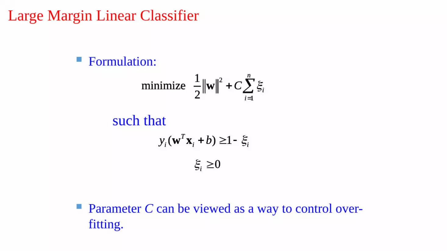
Formulation:

( ) 1Ti i iy b w x

2

1

1minimize 2

n

ii

C

w

such that

0i

Parameter C can be viewed as a way to control over-fitting.


( ) 1Ti i iy b w x

2

1

1minimize 2

n

ii

C

w

0i

Formulation: (Lagrangian Dual Problem)

1 1 1

1maximize 2

n n nT

i i j i j i ji i j

y y

x x

such that0 i C

1

0n

i ii

y


1 1 1

1maximize 2

n n nT

i i j i j i ji i j

y y

x x

0 i C

1

0n

i ii

y

Non-linear SVMs Datasets that are linearly separable with noise work out great:

0 x

0 x

x2

0 x

But what are we going to do if the dataset is just too hard?

How about… mapping data to a higher-dimensional space:

Non-linear SVMs: Feature Space General idea: the original input space can be mapped to some

higher-dimensional feature space where the training set is separable:

Φ: x → φ(x)

This slide is courtesy of www.iro.umontreal.ca/~pift6080/documents/papers/svm_tutorial.ppt

29

0 5

Not linearly separable data.

Need to transform the coordinates: polar coordinates, kernel transformation into higher dimensional space (support vector machines).

Distance from center (radius)

Ang

ular

de g

r ee

(ph a

s e)

Linearly separable data.

polar coordinates

Dataset with noise Hard Margin: So far we

require all data points be classified correctly

- No training error What if the training set is

noisy? - Solution 1: use very

powerful kernels

denotes +1

denotes -1

Overfitting?

Nonlinear SVMs: The Kernel Trick With this mapping, our discriminant function is now:

SV

( ) ( ) ( ) ( )T Ti i

i

g b b

x w x x x

No need to know this mapping explicitly, because we only use the dot product of feature vectors in both the training and test.

A kernel function is defined as a function that corresponds to a dot product of two feature vectors in some expanded feature space:

( , ) ( ) ( )Ti j i jK x x x x

SV

( ) ( ) ( ) ( )T Ti i

i

g b b

x w x x x

( , ) ( ) ( )Ti j i jK x x x x

Non-linear SVMs

Nonlinear SVMs: The Kernel Trick

2-dimensional vectors x=[x1 x2];

let K(xi,xj)=(1 + xiTxj)2

,

Need to show that K(xi,xj) = φ(xi) Tφ(xj):

K(xi,xj)=(1 + xi

Txj)2,

= 1+ xi12xj1

2 + 2 xi1xj1 xi2xj2+ xi2

2xj22 + 2xi1xj1 + 2xi2xj2

= [1 xi12 √2 xi1xi2 xi2

2 √2xi1 √2xi2]T [1 xj12 √2 xj1xj2 xj2

2 √2xj1 √2xj2] = φ(xi)

Tφ(xj), where φ(x) = [1 x12 √2 x1x2 x2

2 √2x1 √2x2]

An example:

Linear kernel:

2

2( , ) exp( )2

i ji jK

x xx x

( , ) Ti j i jK x x x x

( , ) (1 )T pi j i jK x x x x

0 1( , ) tanh( )Ti j i jK x x x x

Examples of commonly-used kernel functions:

Polynomial kernel: Gaussian (Radial-Basis Function (RBF) ) kernel:

Sigmoid:

In general, functions that satisfy Mercer’s condition can be kernel functions.

Nonlinear SVMs: The Kernel Trick

2

2( , ) exp( )2

i ji jK

x xx x

( , ) Ti j i jK x x x x

( , ) (1 )T pi j i jK x x x x

0 1( , ) tanh( )Ti j i jK x x x x

Nonlinear SVM: Optimization

Formulation: (Lagrangian Dual Problem)

1 1 1

1maximize ( , )2

n n n

i i j i j i ji i j

y y K

x x

such that 0 i C

1

0n

i ii

y

The solution of the discriminant function is

SV

( ) ( , )i ii

g K b

x x x

The optimization technique is the same.

1 1 1

1maximize ( , )2

n n n

i i j i j i ji i j

y y K

x x

0 i C

1

0n

i ii

y

SV

( ) ( , )i ii

g K b

x x x

Support Vector Machine: Algorithm

• 1. Choose a kernel function

• 2. Choose a value for C

• 3. Solve the quadratic programming problem (many software packages available)

• 4. Construct the discriminant function from the support vectors

Properties of SVM

• Flexibility in choosing a similarity function• Sparseness of solution when dealing with large data sets - only support vectors are used to specify the separating hyperplane • Ability to handle large feature spaces - complexity does not depend on the dimensionality of the feature space• Overfitting can be controlled by soft margin approach• Nice math property: a simple convex optimization problem which is guaranteed

to converge to a single global solution• Feature Selection

SVM Applications• SVM has been used successfully in many real-world problems: - Text (and hypertext) categorization - Image classification - Bioinformatics (Protein classification, Cancer classification) - Hand-written character recognition - Electronic nose

Electronic nose

● Wide emerging field of cheap analysis devices● Can be used for food science● Automatic food quality determination

SVM and Neural networks

● SVM • Support vector machines are

relatively new form of supervised machine learning.

● Artificial neural networks• Artificial neural network by their model

mimics human brain structure.

Difference between SVM and ANN

● SVM is fast● Must preform grid

search to find optimum solution

● Construct mathematical model of problem

● ANN learns, opposite to SVM

● Can work efficiently than SVM

● Processing speed depends on neuron count

42

Image Classification by SVM

• Process

Raw image

s

Formatted

vectors

Training

Data

K-fold

Cross validation

SVM (with best C)

Test Data

Accuracy

1 0:49 1:25 …1 0:49 1:25 … ：：2 0:49 1:25 … ：

1/4

3/4

K = 6

Some Issues• Choice of kernel - Gaussian or polynomial kernel is default - if ineffective, more elaborate kernels are needed - domain experts can give assistance in formulating appropriate

similarity measures

• Choice of kernel parameters - e.g. σ in Gaussian kernel - σ is the distance between closest points with different

classifications - In the absence of reliable criteria, applications rely on the use

of a validation set or cross-validation to set such parameters.

• Optimization criterion – Hard margin v.s. Soft margin - a lengthy series of experiments in which various parameters

are tested

Summary: Support Vector Machine

1. Large Margin Classifier • Better generalization ability & less over-fitting

2. The Kernel Trick• Map data points to higher dimensional space in order to make them

linearly separable.• Since only dot product is used, we do not need to represent the

mapping explicitly.

Classification

• Everyday, all the time we classify things.• Eg crossing the street:

• Is there a car coming?• At what speed?• How far is it to the other side?• Classification: Safe to walk or not!!!

• Decision tree learningIF (Outlook = Sunny) ^ (Humidity = High)THEN PlayTennis =NOIF (Outlook = Sunny)^ (Humidity = Normal)THEN PlayTennis = YES

Outlook

Sunny Overcast Rain

Humidity Yes Wind

High Normal

YesNo

Strong Weak

YesNo

Training examples:Day Outlook Temp. Humidity Wind PlayTennisD1 Sunny Hot High Weak NoD2 Overcast Hot High Strong Yes

Classification tasks• Learning Task

– Given: Expression profiles of leukaemia patients and healthy persons.

– Compute: A model distinguishing if a person has leukaemia from expression data.

• Classification Task– Given: Expression profile of a new patient + a learned

model – Determine: If a patient has leukaemia or not.

Problems in classifying data• Often high dimension of data.• Hard to put up simple rules.• Amount of data.• Need automated ways to deal with the data.• Use computers – data processing, statistical analysis,

try to learn patterns from the data (Machine Learning)

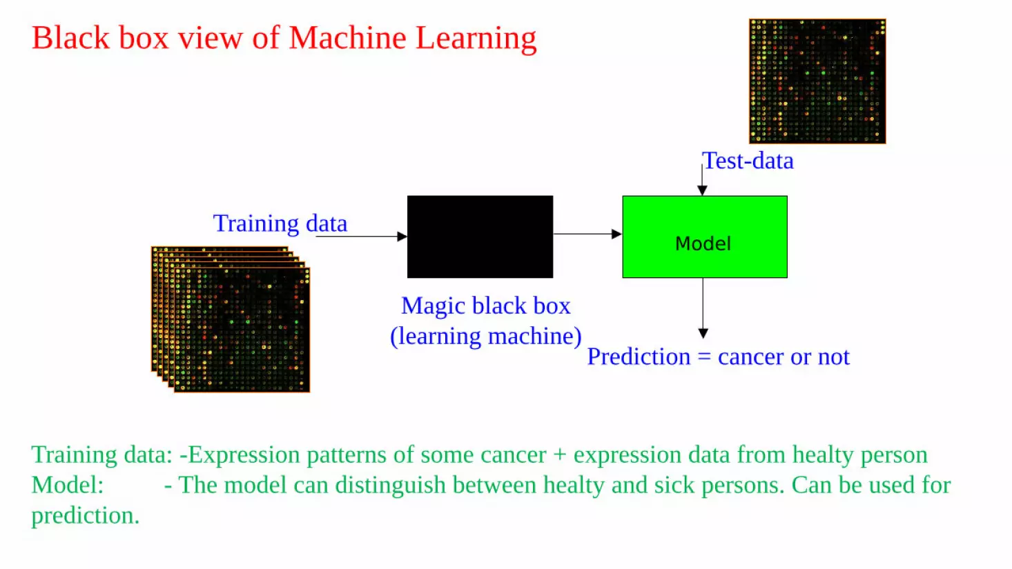
Black box view of Machine Learning

Magic black box(learning machine)

Training data Model

Training data: -Expression patterns of some cancer + expression data from healty personModel: - The model can distinguish between healty and sick persons. Can be used for prediction.

Test-data

Prediction = cancer or not

Model

Tennis example

Humidity

Temperature

= play tennis= do not play tennis


Documents

Object Detection \u0026 Recognition Based On SVM