O Evolutionary multiobjective optimization of the multi-location transshipment problem

ORI GIN AL PA PER

Evolutionary multiobjective optimizationof the multi-location transshipment problem

Nabil Belgasmi Æ Lamjed Ben Saıd Æ Khaled Ghedira

Received: 20 January 2007 / Revised: 21 June 2007 / Accepted: 21 June 2007 /

Published online: 28 March 2008

� Springer-Verlag 2008

Abstract We consider a multi-location inventory system where inventory choices

at each location are centrally coordinated. Lateral transshipments are allowed as

recourse actions within the same echelon in the inventory system to reduce costs and

improve service level. However, this transshipment process usually causes unde-

sirable lead times. In this paper, we propose a multiobjective model of the multi-

location transshipment problem which addresses optimizing three conflicting

objectives: (1) minimizing the aggregate expected cost, (2) maximizing the

expected fill rate, and (3) minimizing the expected transshipment lead times. We

apply an evolutionary multiobjective optimization approach using the strength Pa-

reto evolutionary algorithm (SPEA2), to approximate the optimal Pareto front.

Simulation with a wide choice of model parameters shows the different trades-off

between the conflicting objectives.

Keywords Multi-location transshipment problem �Multiobjective optimization problems � Multiobjective evolutionary algorithms �Pareto optimality

N. Belgasmi (&)

Ecole nationale des Sciences de l’Informatique (ENSI), Tunis, Tunisia

e-mail: [email protected]

L. Ben Saıd � K. Ghedira

Laboratoire de l’Ingenierie Intelligente des Informations (LI3), ISG de Tunis, Universite de Tunis,

41 avenue de la Liberte, cite Bouchoucha 2000, Tunis, Tunisia


K. Ghedira


123

Oper Res Int J (2008) 8:167–183

DOI 10.1007/s12351-008-0015-5

1 Introduction

Practical optimization problems, especially supply chain optimization problems,

seem to have a multiobjective nature much more frequently than a single objective

one. Usually, some performance criteria are to be maximized, while the others

should be minimized.

Physical pooling of inventories has been widely used in practice to reduce cost

and improve customer service (Herer et al. 2005). Transshipments are recognized as

the monitored movements of material among locations at the same echelon. It

affords a valuable mechanism for correcting the discrepancies between the

locations’ observed demand and their on-hand inventory. Subsequently, transship-

ments may reduce costs and improve service without increasing the system-wide

inventories (Herer et al. 2001).

The study of multi-location models with transshipments is an important

contribution for mathematical inventory theory as well as for inventory practice.

The idea of lateral transshipments is not new. The first study dates back to the

sixties. The two-location-one-period case with linear cost functions was considered

by (Aggarwal 1967). Krishnan and Rao (1965) studied with N-location-one-period

model, where the cost parameters are the same for all locations. Jonsson and

Silver (1987) incorporated non-negligible replenishment lead times and transship-

ment lead times among stocking locations to the multi-location model. The effect

of lateral transshipment on the service levels in a two-location-one-period model

was studied by Tagaras (1989). In all works, only minimization of the expected

total cost is considered. Transshipment lead times were often assumed to be

negligible despite its direct impact on service levels. This is a noticeable

limitation.

The contribution of this paper is twofold. We, first propose a multiobjective

multi-location transshipment (MOMT) model which minimizes the aggregate cost

and transshipment lead times while maximizing the global fill rate. Second, we

apply a recent multiobjective evolutionary algorithm named SPEA2, to find Pareto

optimal solutions of the considered problem.

The remainder of this paper is organized as follows. In ‘‘Model’’, we

formulate the multiobjective transshipment model. In ‘‘Multiobjective optimiza-

tion’’, we give a brief description of the multiobjective evolutionary

optimization, and we present the SPEA2 algorithm. In ‘‘Optimization results’’,

we show our experimental results. In ‘‘Conclusion’’, we state our concluding

remarks.

2 Model

2.1 Model description

We consider the following real-life problem where we have n stores selling a

single product. The stores may differ in their cost and demand parameters. The

system inventory is reviewed periodically (Fig. 1). At the beginning of the

168 N. Belgasmi et al.

123

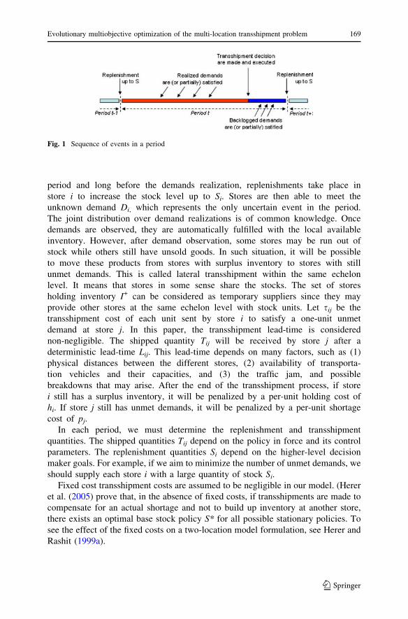
period and long before the demands realization, replenishments take place in

store i to increase the stock level up to Si. Stores are then able to meet the

unknown demand Di, which represents the only uncertain event in the period.

The joint distribution over demand realizations is of common knowledge. Once

demands are observed, they are automatically fulfilled with the local available

inventory. However, after demand observation, some stores may be run out of

stock while others still have unsold goods. In such situation, it will be possible

to move these products from stores with surplus inventory to stores with still

unmet demands. This is called lateral transshipment within the same echelon

level. It means that stores in some sense share the stocks. The set of stores

holding inventory I+ can be considered as temporary suppliers since they may

provide other stores at the same echelon level with stock units. Let sij be the

transshipment cost of each unit sent by store i to satisfy a one-unit unmet

demand at store j. In this paper, the transshipment lead-time is considered

non-negligible. The shipped quantity Tij will be received by store j after a

deterministic lead-time Lij. This lead-time depends on many factors, such as (1)

physical distances between the different stores, (2) availability of transporta-

tion vehicles and their capacities, and (3) the traffic jam, and possible

breakdowns that may arise. After the end of the transshipment process, if store

i still has a surplus inventory, it will be penalized by a per-unit holding cost of

hi. If store j still has unmet demands, it will be penalized by a per-unit shortage

cost of pj.

In each period, we must determine the replenishment and transshipment

quantities. The shipped quantities Tij depend on the policy in force and its control

parameters. The replenishment quantities Si depend on the higher-level decision

maker goals. For example, if we aim to minimize the number of unmet demands, we

should supply each store i with a large quantity of stock Si.

Fixed cost transshipment costs are assumed to be negligible in our model. (Herer

et al. (2005) prove that, in the absence of fixed costs, if transshipments are made to

compensate for an actual shortage and not to build up inventory at another store,

there exists an optimal base stock policy S* for all possible stationary policies. To

see the effect of the fixed costs on a two-location model formulation, see Herer and

Rashit (1999a).

Fig. 1 Sequence of events in a period

Evolutionary multiobjective optimization of the multi-location transshipment problem 169

123

The following notation is used in our model formulation:

n Number of stores

Si Order quantities for store i

S Vector of order quantities, S = (S1, S2,…, Sn) (decision variable)

Di Demand realized at i

D Vector of demands, D = (D1, D2,…, Dn)

hi Unit inventory holding cost at i

pj Unit penalty cost for shortage at j

sij Unit cost of transshipment from i to j

Tij Amount transshipped from i to j

Lij Unit transshipment lead time from i to j

I+ Set of stores with surplus inventory (before transshipment)

I– Set of stores with unmet demands (before transshipment)

2.2 Modeling assumptions

Several assumptions are made in this study to avoid pathological cases:

• Assumption 1 (lead time) All transshipment lead times are both positive and

deterministic. The whole transshipment process is supposed to take place within

the same period. In other words, all lead times Lij are less than the duration of

the period. This may avoid shipped inventory at period t to arrive at period

t + 1. Replenishment lead times are negligible between the central warehouse

and all the stores.

• Assumption 2 (demand) Customers’ demands at each store are fulfilled either by

the local available inventory or by the shipped quantities that may come from

other stores. In addition, since the transshipment lead times are not negligible,

we assume that customers would wait until the end of the transshipment process.

Unmet demands after transshipment realization are lost.

• Assumption 3 (transshipment policy) The transshipment policy is stationary, that

is, the transshipment quantities are independent of the period in which they are

made; they depend only on the available inventory after demand observation. In

this study, we will employ a transshipment policy known as complete pooling.

This transshipment policy can be described as (Herer and Rashit 1999b): the

amount transshipped from one location to another will be the minimum between

(1) the surplus inventory of sending location and (2) the shortage inventory at

receiving location. The optimality of the complete pooling policy is ensured

under some reasonable assumptions detailed in Tagaras (1999).

• Assumption 4 (teplenishment policy) At the beginning of every period, replen-

ishments take place to increase inventory position of store i up to Si taking into

account the remaining inventory of the previous period. The optimality of the

order-up-to policy in the absence of fixed costs is proven in Herer et al. (2005).


123

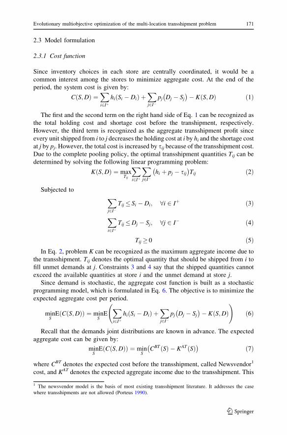
2.3 Model formulation

2.3.1 Cost function

Since inventory choices in each store are centrally coordinated, it would be a

common interest among the stores to minimize aggregate cost. At the end of the

period, the system cost is given by:

C S;Dð Þ ¼X

i2Iþ

hi Si � Dið Þ þX

j2I�pj Dj � Sj

� �� K S;Dð Þ ð1Þ

The first and the second term on the right hand side of Eq. 1 can be recognized as

the total holding cost and shortage cost before the transhipment, respectively.

However, the third term is recognized as the aggregate transshipment profit since

every unit shipped from i to j decreases the holding cost at i by hi and the shortage cost

at j by pj. However, the total cost is increased by sij because of the transshipment cost.

Due to the complete pooling policy, the optimal transshipment quantities Tij can be

determined by solving the following linear programming problem:

K S;Dð Þ ¼ maxTij

X

i2Iþ

X

j2I�hi þ pj � sij

� �Tij ð2Þ

Subjected toX

j2I�Tij� Si � Di; 8i 2 Iþ ð3Þ

X

i2Iþ

Tij�Dj � Sj; 8j 2 I� ð4Þ

Tij� 0 ð5ÞIn Eq. 2, problem K can be recognized as the maximum aggregate income due to

the transshipment. Tij denotes the optimal quantity that should be shipped from i to

fill unmet demands at j. Constraints 3 and 4 say that the shipped quantities cannot

exceed the available quantities at store i and the unmet demand at store j.Since demand is stochastic, the aggregate cost function is built as a stochastic

programming model, which is formulated in Eq. 6. The objective is to minimize the

expected aggregate cost per period.

minS

E C S;Dð Þð Þ ¼ minS

EX

i2Iþ

hi Si � Dið Þ þX

j2I�pj Dj � Sj

� �� K S;Dð Þ

!ð6Þ

Recall that the demands joint distributions are known in advance. The expected

aggregate cost can be given by:

minS

E C S;Dð Þð Þ ¼ minS

CBT Sð Þ � KAT Sð Þ� �

ð7Þ

where CBT denotes the expected cost before the transshipment, called Newsvendor1

cost, and KAT denotes the expected aggregate income due to the transshipment. This

1 The newsvendor model is the basis of most existing transshipment literature. It addresses the case

where transshipments are not allowed (Porteus 1990).


123

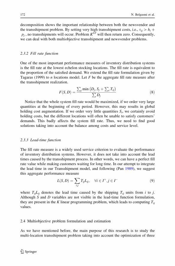
decomposition shows the important relationship between both the newsvendor and

the transshipment problem. By setting very high transshipment costs, i.e., sij [ hi +

pj , no transshipments will occur. Problem KAT will then return zero. Consequently,

we can deal with both multiobjective transshipment and newsvendor problems.

2.3.2 Fill rate function

One of the most important performance measures of inventory distribution systems

is the fill rate at the lowest echelon stocking locations. The fill rate is equivalent to

the proportion of the satisfied demand. We extend the fill rate formulation given by

Tagaras (1999) to n locations model. Let F be the aggregate fill rate measure after

the transshipment realization.

F S;Dð Þ ¼P

j min Dj; Sj þP

i Tij

� �P

Djð8Þ

Notice that the whole system fill rate would be maximized, if we order very large

quantities at the beginning of every period. However, this may results in global

holding cost augmentation. If we order very little quantities Si, we certainly avoid

holding costs, but the different locations will often be unable to satisfy customers’

demands. This badly affects the system fill rate. Thus, we need to find good

solutions taking into account the balance among costs and service level.

2.3.3 Lead-time function

The fill rate measure is a widely used service criterion to evaluate the performance

of inventory distribution systems. However, it does not take into account the lead

times caused by the transshipment process. In other words, we can have a perfect fill

rate value while making customers waiting for long time. In our attempt to integrate

the lead time in our Transshipment model, and following (Pan 1989), we suggest

this aggregate performance measure

L S;Dð Þ ¼X

i;j

TijLij; 8i 2 Iþ; j 2 I� ð9Þ

where TijLij denotes the lead time caused by the shipping Tij units from i to j.Although S and D variables are not visible in the lead-time function formulation,

they are present in the K linear programming problem, which leads to computing Tij

values.

2.4 Multiobjective problem formulation and estimation

As we have mentioned before, the main purpose of this research is to study the

multi-location transshipment problem taking into account the optimization of three


123

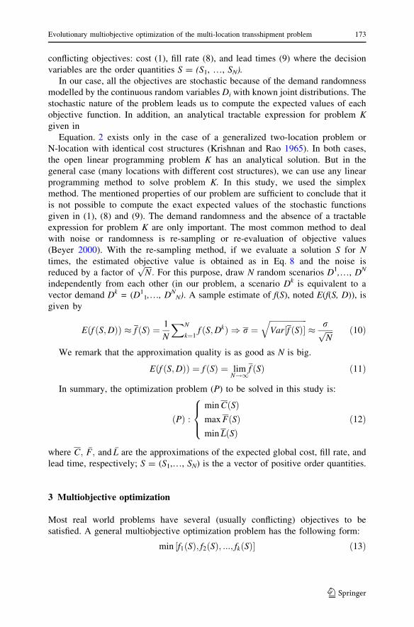
conflicting objectives: cost (1), fill rate (8), and lead times (9) where the decision

variables are the order quantities S = (S1, …, SN).In our case, all the objectives are stochastic because of the demand randomness

modelled by the continuous random variables Di with known joint distributions. The

stochastic nature of the problem leads us to compute the expected values of each

objective function. In addition, an analytical tractable expression for problem Kgiven in

Equation. 2 exists only in the case of a generalized two-location problem or

N-location with identical cost structures (Krishnan and Rao 1965). In both cases,

the open linear programming problem K has an analytical solution. But in the

general case (many locations with different cost structures), we can use any linear

programming method to solve problem K. In this study, we used the simplex

method. The mentioned properties of our problem are sufficient to conclude that it

is not possible to compute the exact expected values of the stochastic functions

given in (1), (8) and (9). The demand randomness and the absence of a tractable

expression for problem K are only important. The most common method to deal

with noise or randomness is re-sampling or re-evaluation of objective values

(Beyer 2000). With the re-sampling method, if we evaluate a solution S for Ntimes, the estimated objective value is obtained as in Eq. 8 and the noise is

reduced by a factor offfiffiffiffiNp

: For this purpose, draw N random scenarios D1,…, DN

independently from each other (in our problem, a scenario Dk is equivalent to a

vector demand Dk = (D11,…, DN

N). A sample estimate of f(S), noted E(f(S, D)), is

given by

E f ðS;DÞð Þ � f ðSÞ ¼ 1

N

XN

k¼1f ðS;DkÞ ) r ¼

ffiffiffiffiffiffiffiffiffiffiffiffiffiffiffiffiffiffiffiVar½f ðSÞ�

q� rffiffiffiffi

Np ð10Þ

We remark that the approximation quality is as good as N is big.

E f ðS;DÞð Þ ¼ f ðSÞ ¼ limN!1

f ðSÞ ð11Þ

In summary, the optimization problem (P) to be solved in this study is:

ðPÞ :

min C Sð Þmax F Sð Þmin L Sð Þ

8><

>:ð12Þ

where C; �F; and �L are the approximations of the expected global cost, fill rate, and

lead time, respectively; S = (S1,…, SN) is the a vector of positive order quantities.

3 Multiobjective optimization

Most real world problems have several (usually conflicting) objectives to be

satisfied. A general multiobjective optimization problem has the following form:

min f1ðSÞ; f2ðSÞ; :::; fkðSÞ½ � ð13Þ


123

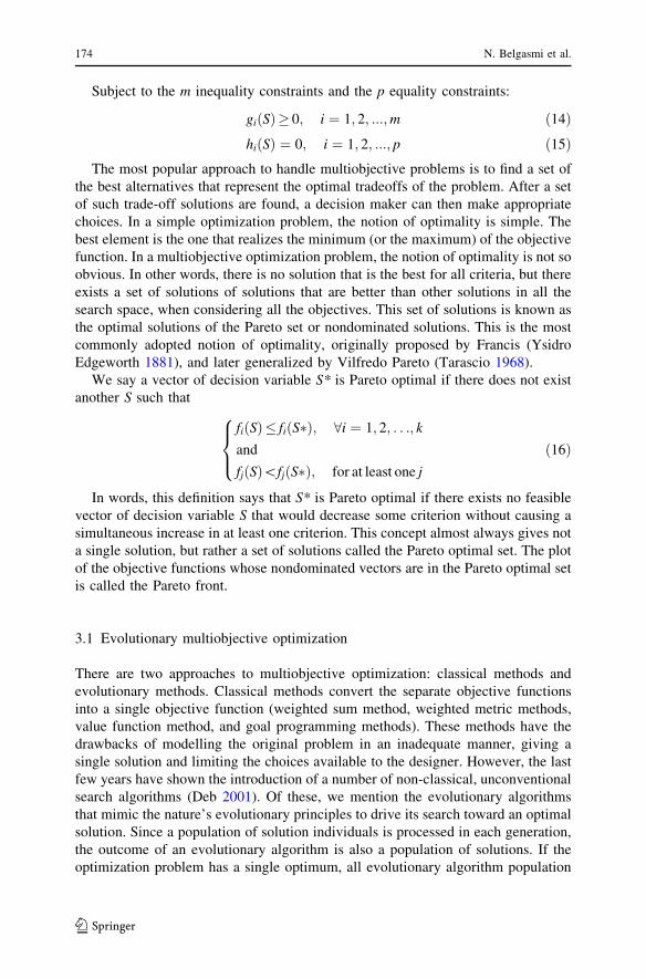
Subject to the m inequality constraints and the p equality constraints:

giðSÞ� 0; i ¼ 1; 2; :::;m ð14ÞhiðSÞ ¼ 0; i ¼ 1; 2; :::; p ð15Þ

The most popular approach to handle multiobjective problems is to find a set of

the best alternatives that represent the optimal tradeoffs of the problem. After a set

of such trade-off solutions are found, a decision maker can then make appropriate

choices. In a simple optimization problem, the notion of optimality is simple. The

best element is the one that realizes the minimum (or the maximum) of the objective

function. In a multiobjective optimization problem, the notion of optimality is not so

obvious. In other words, there is no solution that is the best for all criteria, but there

exists a set of solutions of solutions that are better than other solutions in all the

search space, when considering all the objectives. This set of solutions is known as

the optimal solutions of the Pareto set or nondominated solutions. This is the most

commonly adopted notion of optimality, originally proposed by Francis (Ysidro

Edgeworth 1881), and later generalized by Vilfredo Pareto (Tarascio 1968).

We say a vector of decision variable S* is Pareto optimal if there does not exist

another S such that

fiðSÞ� fiðS�Þ; 8i ¼ 1; 2; . . .; k

and

fjðSÞ\fjðS�Þ; for at least one j

8><

>:ð16Þ

In words, this definition says that S* is Pareto optimal if there exists no feasible

vector of decision variable S that would decrease some criterion without causing a

simultaneous increase in at least one criterion. This concept almost always gives not

a single solution, but rather a set of solutions called the Pareto optimal set. The plot

of the objective functions whose nondominated vectors are in the Pareto optimal set

is called the Pareto front.

3.1 Evolutionary multiobjective optimization

There are two approaches to multiobjective optimization: classical methods and

evolutionary methods. Classical methods convert the separate objective functions

into a single objective function (weighted sum method, weighted metric methods,

value function method, and goal programming methods). These methods have the

drawbacks of modelling the original problem in an inadequate manner, giving a

single solution and limiting the choices available to the designer. However, the last

few years have shown the introduction of a number of non-classical, unconventional

search algorithms (Deb 2001). Of these, we mention the evolutionary algorithms

that mimic the nature’s evolutionary principles to drive its search toward an optimal

solution. Since a population of solution individuals is processed in each generation,

the outcome of an evolutionary algorithm is also a population of solutions. If the

optimization problem has a single optimum, all evolutionary algorithm population


123

individuals can be expected to converge to that optimum. This ability to find

multiple optimal solutions in one single simulation run makes evolutionary

algorithms suitable in solving multiobjective optimization problems.

3.2 Strength Pareto evolutionary algorithm (SPEA2)

Many multiobjective evolutionary algorithms have been proposed in the last few

years. Comparative studies have shown for large number of test cases that among all

major multiobjective EAs, strength Pareto evolutionary algorithm (SPEA2) is

clearly superior. The key results of the comparison (E.Zitzler et al. 2002) were: (1)

SPEA2 performs better SPEA on all test problems, and (2) SPEA2 and NSGA-II

show the best performance overall. But in higher dimensional spaces, SPEA2 seems

to have advantages over PESA and NSGA-II. In addition, it was proven that SPEA2

is less sensitive to noisy function evaluations since it saves the non-dominated

solutions in an archive. In this study, we used SPEA2 to solve instances of the

proposed multiobjective transshipment problem.

At the beginning of the optimization process (E.Zitzler et al. 2002), an initial

population is generated randomly. In our multi-location problem, an individual is a

base stock decision S = (S1, S2, …, Sn) consisting of n genes Si. At each generation,

all the individuals are evaluated. A fine-grained fitness assignment strategy is used

to perform individuals’ evaluation. It incorporates Pareto dominance and density

information. In other words, good individuals are the less dominated and the well

spaced ones. The good individuals are conserved in an external set (archive). This is

called the environmental selection. If the archive is full, a truncation operator is

used to determine which individuals should be removed from the archive. The

truncation operator is based on the distance of the kth nearest neighbour

computation method (Silverman 1986). In other words, an individual is removed

if it has the minimum distance to the other individuals. This mechanism preserves

the diversity of the optimal Pareto front. The archived individuals participate in the

creation of other individuals for the coming generations. These steps are repeated

for a fixed number of generations. The resulting optimal Pareto front is located in

the archive. The main loop of the SPEA2 algorithm is as follow:

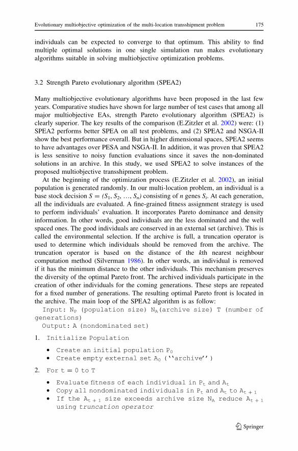
Input: NP (population size) NA(archive size) T (number ofgenerations)

Output: A (nondominated set)

1. Initialize Population

• Create an initial population P0• Create empty external set A0 (‘‘archive’’)

2. For t = 0 to T

• Evaluate fitness of each individual in Pt and At

• Copy all nondominated individuals in Pt and At to At + 1

• If the At + 1 size exceeds archive size NA reduce At + 1

using truncation operator


123

• If the At + 1 size is less than archive size then usedominated individuals in Pt and At to fill At + 1

• Perform Binary Tournament Selection with replacement onAt + 1 to fill the mating pool

• Apply crossover and mutation to the mating pool andupdate At + 1

End For

4 Optimization results

In this section, we report on our numerical study. We first report a study conducted

to analyze the shape of the cost, fill rate, and lead time functions. Than, the resulting

objective and solution spaces are considered. The corresponding Pareto fronts are

analyzed and discussed. Secondly, we describe the experimental design, which

serves as the base for our experiments. We describe and analyze the results obtained

for this basic experiment. This leads to understand the importance of our

multiobjective model.

4.1 A detailed example

The first exemplary inventory model consists of two locations with the following

parameters:

To construct the shape of each objective function, we generated 30.000 samples

of each function with respect to the setting given in Table 1. Each sample consists

of a random value of S = (S1, S2).

4.1.1 Objectives sampling

Figure 2 (left) illustrates the convexity of the aggregate cost function. Figure 2

(right) shows that the area around the optimum is very flat as mentioned by Arnold

and Kochel (1996). Figure 2 (middle) illustrates the projection of the aggregate cost

function on the (S1, S2) plane. Notice that for higher inventory levels (Si [ 250), the

cost function grows linearly since it is proportional to the system holding costs.

Table 1 Multi-location system

configurationParameter Value

Holding cost (hi) 3

Shortage cost (pj) 2

Lead time (Lij) 5

Transshipment cost (sij) 0.5

Demand distribution (Di) N(100, 20)


123

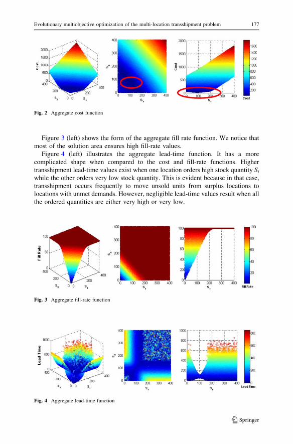
Figure 3 (left) shows the form of the aggregate fill rate function. We notice that

most of the solution area ensures high fill-rate values.

Figure 4 (left) illustrates the aggregate lead-time function. It has a more

complicated shape when compared to the cost and fill-rate functions. Higher

transshipment lead-time values exist when one location orders high stock quantity Si

while the other orders very low stock quantity. This is evident because in that case,

transshipment occurs frequently to move unsold units from surplus locations to

locations with unmet demands. However, negligible lead-time values result when all

the ordered quantities are either very high or very low.

Fig. 2 Aggregate cost function

Fig. 3 Aggregate fill-rate function

Fig. 4 Aggregate lead-time function


123

Notice that all the objective functions of this studied case are symmetric

relatively to the plane S1 = S2. This is evident since all the considered locations

have identical cost and demand structures.

Obviously, an individual consists of two genes only, each for one location. The

multiobjective evolutionary optimization process was started with the parameters in

Table 2.

To show the results of the evolutionary optimization, we have experienced four

multiobjective problems detailed in the sections below. For each problem, we

describe the objective sampled using 12,000 points. Both Pareto fronts and its

corresponding solution spaces are presented and analyzed.

4.1.2 Cost vs. fill-rate problem

Assume that decision makers’ aims are minimizing aggregate cost while maximiz-

ing the fill rate in a multi-location system with lateral transshipment. This is a bi-

objective problem, which we note C/F problem (cost/fill rate problem).

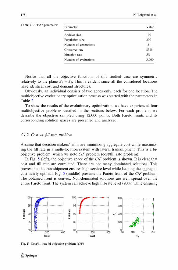
In Fig. 5 (left), the objective space of the C/F problem is shown. It is clear that

cost and fill rate are correlated. There are not many dominated solutions. This

proves that the transshipment ensures high service level while keeping the aggregate

cost nearly optimal. Fig. 5 (middle) presents the Pareto front of the C/F problem.

The obtained front is convex. Non-dominated solutions are well spread over the

entire Pareto front. The system can achieve high fill-rate level (90%) while ensuring

Table 2 SPEA2 parametersParameter Value

Archive size 100

Population size 200

Number of generations 15

Crossover rate 85%

Mutation rate 5%

Number of evaluations 3,000

Fig. 5 Cost/fill rate bi-objective problem (C/F)


123

a low-cost value ($50). However, increasing the fill rate up to (100%) affects the

cost considerably ($200). The solution space of the resulting C/F Pareto front is

given in Fig. 5 (right). It is shown that there is a wide range of inventory choices

that provide non-dominated solutions. This may be due to the flatness of the cost

function around the optimum.

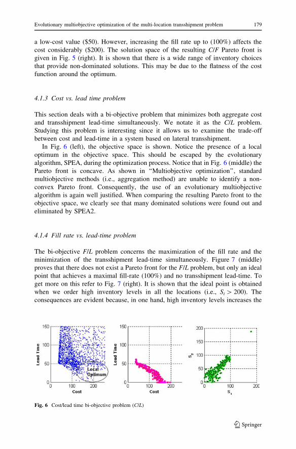
4.1.3 Cost vs. lead time problem

This section deals with a bi-objective problem that minimizes both aggregate cost

and transshipment lead-time simultaneously. We notate it as the C/L problem.

Studying this problem is interesting since it allows us to examine the trade-off

between cost and lead-time in a system based on lateral transshipment.

In Fig. 6 (left), the objective space is shown. Notice the presence of a local

optimum in the objective space. This should be escaped by the evolutionary

algorithm, SPEA, during the optimization process. Notice that in Fig. 6 (middle) the

Pareto front is concave. As shown in ‘‘Multiobjective optimization’’, standard

multiobjective methods (i.e., aggregation method) are unable to identify a non-

convex Pareto front. Consequently, the use of an evolutionary multiobjective

algorithm is again well justified. When comparing the resulting Pareto front to the

objective space, we clearly see that many dominated solutions were found out and

eliminated by SPEA2.

4.1.4 Fill rate vs. lead-time problem

The bi-objective F/L problem concerns the maximization of the fill rate and the

minimization of the transshipment lead-time simultaneously. Figure 7 (middle)

proves that there does not exist a Pareto front for the F/L problem, but only an ideal

point that achieves a maximal fill-rate (100%) and no transshipment lead-time. To

get more on this refer to Fig. 7 (right). It is shown that the ideal point is obtained

when we order high inventory levels in all the locations (i.e., Si [ 200). The

consequences are evident because, in one hand, high inventory levels increases the

Fig. 6 Cost/lead time bi-objective problem (C/L)


123

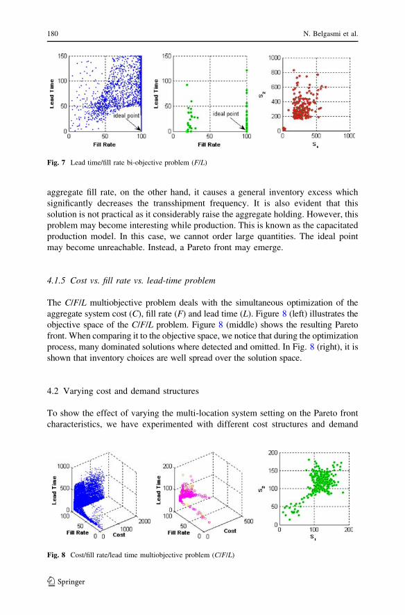
aggregate fill rate, on the other hand, it causes a general inventory excess which

significantly decreases the transshipment frequency. It is also evident that this

solution is not practical as it considerably raise the aggregate holding. However, this

problem may become interesting while production. This is known as the capacitated

production model. In this case, we cannot order large quantities. The ideal point

may become unreachable. Instead, a Pareto front may emerge.

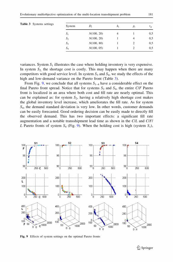
4.1.5 Cost vs. fill rate vs. lead-time problem

The C/F/L multiobjective problem deals with the simultaneous optimization of the

aggregate system cost (C), fill rate (F) and lead time (L). Figure 8 (left) illustrates the

objective space of the C/F/L problem. Figure 8 (middle) shows the resulting Pareto

front. When comparing it to the objective space, we notice that during the optimization

process, many dominated solutions where detected and omitted. In Fig. 8 (right), it is

shown that inventory choices are well spread over the solution space.

4.2 Varying cost and demand structures

To show the effect of varying the multi-location system setting on the Pareto front

characteristics, we have experimented with different cost structures and demand

Fig. 7 Lead time/fill rate bi-objective problem (F/L)

Fig. 8 Cost/fill rate/lead time multiobjective problem (C/F/L)


123

variances. System S1 illustrates the case where holding inventory is very expensive.

In system S2, the shortage cost is costly. This may happen when there are many

competitors with good service level. In system S3 and S4, we study the effects of the

high and low-demand variance on the Pareto front (Table 3).

From Fig. 9, we conclude that all systems S1–4 have a considerable effect on the

final Pareto front spread. Notice that for systems S2 and S4, the entire C/F Pareto

front is localized in an area where both cost and fill rate are nearly optimal. This

can be explained as: for system S2, having a relatively high shortage cost makes

the global inventory level increase, which ameliorates the fill rate. As for system

S4, the demand standard deviation is very low. In other words, customer demands

can be easily forecasted. Good ordering decision can be easily made to directly fill

the observed demand. This has two important effects: a significant fill rate

augmentation and a notable transshipment lead time as shown in the C/L and C/F/

L Pareto fronts of system S4 (Fig. 9). When the holding cost is high (system S1),

Table 3 Systems settingsSystem Di hi pi sij

S1 N(100, 20) 4 1 0,5

S2 N(100, 20) 1 4 0,5

S3 N(100, 80) 1 2 0,5

S4 N(100, 05) 1 2 0,5

Fig. 9 Effects of system settings on the optimal Pareto fronts


123

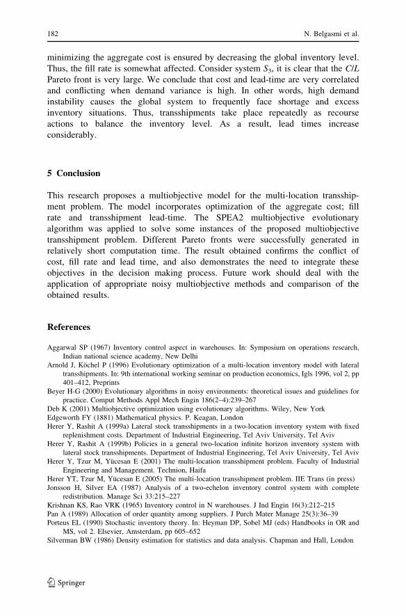
minimizing the aggregate cost is ensured by decreasing the global inventory level.

Thus, the fill rate is somewhat affected. Consider system S3, it is clear that the C/LPareto front is very large. We conclude that cost and lead-time are very correlated

and conflicting when demand variance is high. In other words, high demand

instability causes the global system to frequently face shortage and excess

inventory situations. Thus, transshipments take place repeatedly as recourse

actions to balance the inventory level. As a result, lead times increase

considerably.

5 Conclusion

This research proposes a multiobjective model for the multi-location transship-

ment problem. The model incorporates optimization of the aggregate cost; fill

rate and transshipment lead-time. The SPEA2 multiobjective evolutionary

algorithm was applied to solve some instances of the proposed multiobjective

transshipment problem. Different Pareto fronts were successfully generated in

relatively short computation time. The result obtained confirms the conflict of

cost, fill rate and lead time, and also demonstrates the need to integrate these

objectives in the decision making process. Future work should deal with the

application of appropriate noisy multiobjective methods and comparison of the

obtained results.

References

Aggarwal SP (1967) Inventory control aspect in warehouses. In: Symposium on operations research,

Indian national science academy, New Delhi

Arnold J, Kochel P (1996) Evolutionary optimization of a multi-location inventory model with lateral

transshipments. In: 9th international working seminar on production economics, Igls 1996, vol 2, pp

401–412, Preprints

Beyer H-G (2000) Evolutionary algorithms in noisy environments: theoretical issues and guidelines for

practice. Comput Methods Appl Mech Engin 186(2–4):239–267

Deb K (2001) Multiobjective optimization using evolutionary algorithms. Wiley, New York

Edgeworth FY (1881) Mathematical physics. P. Keagan, London

Herer Y, Rashit A (1999a) Lateral stock transshipments in a two-location inventory system with fixed

replenishment costs. Department of Industrial Engineering, Tel Aviv University, Tel Aviv

Herer Y, Rashit A (1999b) Policies in a general two-location infinite horizon inventory system with

lateral stock transshipments. Department of Industrial Engineering, Tel Aviv University, Tel Aviv

Herer Y, Tzur M, Yucesan E (2001) The multi-location transshipment problem. Faculty of Industrial

Engineering and Management. Technion, Haifa

Herer YT, Tzur M, Yucesan E (2005) The multi-location transshipment problem. IIE Trans (in press)

Jonsson H, Silver EA (1987) Analysis of a two-echelon inventory control system with complete

redistribution. Manage Sci 33:215–227

Krishnan KS, Rao VRK (1965) Inventory control in N warehouses. J Ind Engin 16(3):212–215

Pan A (1989) Allocation of order quantity among suppliers. J Purch Mater Manage 25(3):36–39

Porteus EL (1990) Stochastic inventory theory. In: Heyman DP, Sobel MJ (eds) Handbooks in OR and

MS, vol 2. Elsevier, Amsterdam, pp 605–652

Silverman BW (1986) Density estimation for statistics and data analysis. Chapman and Hall, London


123

Tagaras G (1989) Effects of pooling on the optimization and service levels of two-location inventory

systems. IIE Trans 21(3):250–257

Tagaras G (1999) Pooling in multi-location periodic inventory distribution systems. Omega 39–59

Tarascio V (1968) Pareto’s methodological approach to economics. University of North Carolina Press,

Chapel Hill

Zitzler E, Laumanns M, Thiele L (2002) SPEA2: improving the strength pareto evolutionary algorithm

for multiobjective optimisation. In: Giannakoglou K, Tsahalis D, Periaux J, Papailiou K, Fogarty T

(eds) Evolutionary methods for design, optimisation, and control. CIMNE, Barcelona, pp 19–26


123

Documents

O Evolutionary multiobjective optimization of the multi-location transshipment problem