arX

iv:g

r-qc

/941

2040

v3 2

7 O

ct 1

995

MIT-CTP-2384TUTP-94-22

gr-qc/9412040November 1994

A Note on the Semi-Classical Approximationin Quantum Gravity∗

Gilad Lifschytz, Samir D. Mathur

Center for Theoretical Physics, Laboratory for Nuclear Scienceand Department of Physics,

Massachusetts Institute of Technology, Cambridge MA 02139, USA.e-mail: gil1 or mathur @mitlns.mit.edu

and

Miguel Ortiz

Institute of Cosmology, Department of Physics and Astronomy,Tufts University, Medford, MA 02155, USA.

e-mail: mortiz@tufts.edu

Abstract: We re-examine the semiclassical approximation for quantum gravity in the canon-

ical formulation, focusing on the definition of a quasiclassical state for the gravitational field.

It is shown that a state with classical correlations must be a superposition of states of the

form eiS . In terms of a reduced phase space formalism, this type of state can be expressed

as a coherent superposition of eigenstates of operators that commute with the constraints

and so correspond to constants of the motion. Contact is made with the usual semiclassical

approximation by showing that a superposition of this kind can be approximated by a WKB

state with an appropriately localised prefactor. A qualitative analysis is given of the effects of

geometry fluctuations, and the possibility of a breakdown of the semiclassical approximation

due to interference between neighbouring classical trajectories is discussed. It is shown that

a breakdown in the semiclassical approximation can be a coordinate dependent phenomenon,

as has been argued to be the case close to a black hole horizon.

∗ This work was supported in part by funds provided by the U.S. Department of Energy

(D.O.E.) under cooperative agreement DE-FC02-94ER40818, and in part by the National

Science Foundation.

1 Introduction

Although we have few clues about the final form of a quantum theory of gravity,there is at least one constraint that we can be sure of: That the theory should, insome limit, describe quantum matter fields interacting with an essentially classicalbackground spacetime in what is known as the semiclassical limit of quantum gravity.In some formulations of quantum gravity, such as perturbation theory around a fixedbackground, the semiclassical limit is guaranteed. However, at a more fundamentallevel we expect the notion of spacetime to be a derived concept. In any theory reflectingthis feature, it is interesting to understand how the notion of a classical backgroundemerges.

Some considerable work towards understanding the semiclassical limit has beendone in the canonical approach to quantum gravity using the ADM formulation [1].In this approach there is no background spacetime, since the dynamical variables arethe 3-metrics of spacelike hypersurfaces, plus the matter fields on these hypersurfaces.Employing the Dirac procedure, physical states must be annihilated by the momentumand Hamiltonian constraints. The momentum constraints reduce the configurationspace to the space of all 3-geometries (the equivalence classes of 3-metrics under spatialdiffeomorphisms). The Hamiltonian constraint is imposed by the Wheeler–DeWittequation

HΨ[h, φ] = 0 (1)

which has the effect of factoring out translations in the time direction, and is a directanalogue of the Klein-Gordon equation for the quantized relativistic particle.

The semiclassical limit is obtained by expanding the Wheeler–DeWitt equationin powers of the gravitational coupling constant G. This really involves two sepa-rate approximations: A WKB approximation (effectively in h) in the gravitational(or more generally classical) sector, and a Born-Oppenheimer approximation separat-ing the gravity and matter (classical and quantum) parts. At each order, one performsfirst the gravitational WKB approximation, and then solves the remaining equation forthe matter state. In this way the complete solution of the Wheeler–DeWitt equation issplit into a product of a purely gravitational piece representing the classical geometryand a mixed piece representing quantum field theory on that background (for simplicitywe shall assume that the gravitational field is the only classical variable).

To first order, the expansion of the Wheeler–DeWitt equation yields the first WKBapproximation

Ψ[h, φ] = eiSHJ [hij ]/hG,1

2Gijkl

δSHJ

δhij

δSHJ

δhkl

− 2√hR = 0 (2)

to the gravitational Wheeler–DeWitt equation, where SHJ [hij ] is a Hamilton–Jacobifunctional for general relativity. We shall refer to a state of this form, without aprefactor, as a first order WKB state. This first order approximation depends only onthe gravitational degrees of freedom.

1

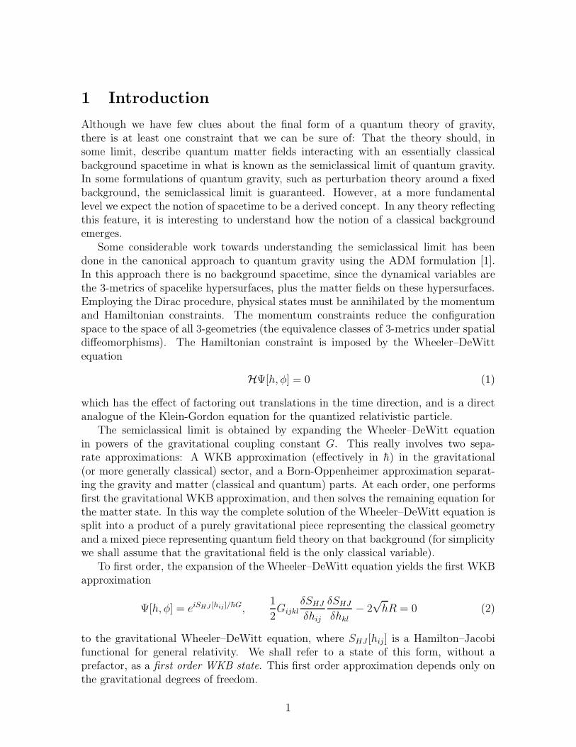
Some sample foliations are shown.

of Einstein’s equations given by . Each plane represents a different classical solution

S[h]

Each plane is made up of the set of all folations of the classical solution.S[h] hGiven , each defines a unique classical solution, so that the planes do not intersect.

Figure 1: A congruence of classical solutions in superspace. Each clas-sical solution is shown as a plane in the diagram, which contains thedifferent trajectories in superspace corresponding to that solution, givenby different choices of the lapse and shift functions.

Any functional SHJ [hij ] that solves the Hamilton–Jacobi equation defines a con-gruence of classical trajectories in superspace, made up of all possible foliations of allsolutions of Einstein’s equations defined by SHJ (see Fig. 1).

As was shown by Lapchinski and Rubakov, and later by Banks [2, 3], the next orderapproximation is obtained by solving two equations: An equation for the gravitationalWKB prefactor D[h], and a functional differential equation for the remainder of thestate χ[h, f ] that depends on the matter variables f . Solving the equation for χ[h, f ]is equivalent to solving the functional Schrodinger equation along each of the congru-ence of eikonal trajectories corresponding to the set of all foliations of all solutions ofEinstein’s equations given by SHJ [hij ].

The semiclassical approximation to second order should yield a state that repre-sents a quantum matter field propagating on a quasiclassical background spacetime.The results we have described are not quite the whole story, since they do not in them-selves provide a complete description of such a quantum state. A careful treatmentof the gravitational degrees of freedom is needed in order to restrict the semiclassicalapproximation to the propagation of quantum matter fields on a single background.

A semiclassical state with a gravitational WKB part that defines a congruence ofclassical trajectories on superspace is not suitable for describing classical behaviour.

2

In Ref. [4], an approximate form of the Wigner function was used to argue that ageneric first order gravitational WKB state has classical correlations between coor-dinates and momenta. However, it was later pointed out in a simple example thatthe exact Wigner function of a general WKB state does not exhibit such correlations[5, 6], unless a particular form of the WKB prefactor is chosen, corresponding to acoherent superposition of first order WKB states. These results are analogous to thesimple statement in quantum mechanics that a plane wave does not exhibit classicalcorrelations, but that plane wave states may be superposed to construct a coherentstate.

1.1 An Outline

We shall argue in this paper that in quantum gravity, a quasiclassical state1 shouldbe a ‘coherent state’ in an appropriately defined sense: The uncertainty of a completeset of spacetime diffeomorphism invariant operators (constants of the motion) shouldbe small (a similar proposal was made some years ago Komar [7]). We shall showthat this condition, although somewhat formal, can be realised in a concrete way.Since the classical counterparts of the diffeomorphism invariants together specify aunique classical solution, this point of view reinforces the notion that a classical statein quantum gravity gives rise to only an approximate background spacetime. We shallgo on to argue that a coherent state can and must be used as the gravitational stateproviding a background for the semiclassical approximation. The approximate natureof the background described by such a state will be shown to determine some limits ofthe semiclassical approximation.

The Hamilton–Jacobi formalism can be used to define a natural complete set of dif-feomorphism invariant operators. Through the Hamilton–Jacobi formalism, we shallshow that a first order WKB state approximates an eigenstate with respect to halfof these operators (the α’s of Hamilton–Jacobi theory). Given this simple observa-tion it follows that a coherent or quasiclassical state is approximated by a coherentsuperposition of first order WKB states. The rewriting of our quasiclassical statesin quantum gravity as coherent superpositions of first order WKB states makes di-rect contact with the work of Gerlach [8]. He observed that a superposition of WKBstates can be arranged to have support only in a narrow ‘tube’ in superspace around3-geometries comprising a solution of Einstein’s equations. This observation relates themetric-dependent and coordinate invariant notions of what constitutes a quasiclassicalstate. Gerlach’s interpretation seems to have fallen out of favour in recent years, butwe hope to revive it in this paper.

The fact that a coherent state can be written in the WKB approximation using themetric representation is important for a second reason. It allows us to use the coherentstate in the standard semiclassical approximation as described above. An important

1We shall use ‘quasiclassical’ to describe a state that approximates classical behaviour, and ‘semi-classical’ to describe a state that is a product of a part that is quasiclassical and a part that isnot.

3

consequence of the connection between first order WKB states and α eigenstates isthat the expectation value of conjugate operators (the β operators of Hamilton–Jacobitheory) in such a state is maximally uncertain. Thus a first order WKB state cannot beexpected to have a Wigner function with strong correlations between coordinates andmomenta, and so is not appropriate for describing a background spacetime. However,a coherent state can be used as a background for the semiclassical approximation. Itexhibits quasiclassical correlations and its WKB approximation is precisely a secondorder WKB state of the form

Ψ[hij ] =1

D[hij]eiSHJ [hij ]

with an appropriately chosen prefactor D[hij]. D[hij] is given by rewriting the coherentsuperposition of first order WKB states as a second order WKB state. Using thelanguage of Vilenkin [9], the WKB prefactor can be regarded as providing a measure onthe space of all classical solutions compatible with SHJ [hij ]. A coherent superpositionis simply a WKB state with this measure concentrated around a minimally narrowband of classical solutions which effectively represent a single classical spacetime (thewidth of such a band is determined by the condition that the prefactor be of secondorder in the WKB approximation, and thus not vary too rapidly)2.

After establishing the validity of the semiclassical approximation using a coherentquasiclassical state, we shall go on to discuss in the last part of the paper the situationsthat can lead to a breakdown of this approximation scheme. Normally, the breakdownof the semiclassical approximation is thought to be governed by the behaviour of matterfields on a fixed classical background, with large quantum fluctuations in the matterfields leading to a loss of classical behaviour. Even in more careful studies of correc-tions to the semiclassical approximation [13], the emphasis has been on corrections tothe equation describing evolution along individual eikonal trajectories (the functionalSchrodinger equation), rather than on interference between neighbouring trajectories.

The notion that a state in quantum gravity can at best describe a small neigh-bourhood of classical backgrounds indicates a simple limitation of the semiclassicalapproximation. Recall that the fact that macroscopically different eikonal trajectoriesin superspace (corresponding to different classical solutions) can lead to different mat-ter evolution, underlies the notion of decoherence between different classical histories.

2One word of warning should be added: The description of a quasiclassical state as a second orderWKB state gives special prominence to a particular solution SHJ of the Hamilton–Jacobi equations,and so hides a natural symmetry present in a coherent superposition. It appears according to thisdescription that SHJ restricts us to a congruence of spacetimes fixed by specifying half of the gaugeinvariant degrees of freedom, and that the prefactor then restricts the support of the wavefunctionalto a small subset of these. The diffeomorphism invariant description of the state is somewhat moresymmetric, and the wavefunctional is better thought of as having support on a tube in superspace.There are many classical solutions that run within this tube, but all have constants-of-the-motionwithin a narrow spread. No particular solution (or set of solutions) is preferred as a background forthe semiclassical approximation, but the narrow width of the tube means that in most circumstancessemiclassical physics is not sensitive to the particular choice of background.

4

This is commonly believed to provide a promising explanation of the emergence of ourclassical world. However, because any quasiclassical state describing the gravitationalbackground has a finite spread, the mechanism responsible for decoherence can actuallyspoil classical behaviour [14]: If neighbouring geometries contained within the spreadof a quasiclassical state lead to substantially different matter evolution, then the no-tion of quantum field theory on a fixed background breaks down. We shall discussthis aspect of the semiclassical approximation in the last section of this paper. It isof particular interest since it has recently been shown that problems of this kind spoilthe semiclassical approximation close to a black hole horizon [15, 16, 17].

It is appropriate at this point to mention two caveats to our work. First of all, weshall not discuss the mechanisms by which one may arrive at the quasiclassical statesdescribed in this paper. Our emphasis is simply on describing states that could rea-sonably be called classical and should therefore arise naturally from initial conditions,decoherence or some similar mechanism explaining the emergence of classical configu-rations. For this reason, we shall also not discuss the possibility of superpositions orensembles of quasiclassical states. We refer the reader to the extensive literature onquantum cosmology for an open ended discussion of some of these issues. Secondly,the approach we take compares and relates quantisation in the metric representationto that using the constants of the motion as the fundamental observables. One wouldhope that at some fundamental level these descriptions are equivalent. However, itshould be pointed out that this equivalence is not yet understood. For example, It hasbeen noted recently [10] that there can be more than one way of defining the Hilbertspace in quantum gravity. More precisely, even though one knows the algebra of oper-ators of a theory, the choice of what states are physical and what states are unphysicalcan be made in more than one way, thus giving inequivalent quantum theories. Theresulting quantum theories are also likely to depend on the classical variables used as astarting point for quantisation. Nevertheless, a valuable tool in resolving ambiguities ofthis kind is to study the semiclassical limit of quantum gravity, since this gives definiteinformation about the physical spectrum of the desired theory of quantum gravity. Al-though it is known that there are difficulties in operator ordering the Wheeler–DeWittoperator that block the construction of wavefunctionals [11, 12], any reasonable quan-tisation in a metric (or connection) representation should be equivalent to quantisationin terms of constants of the motion, at least in the semiclassical limit.

1.2 A simple example

Before beginning a discussion of WKB states in quantum gravity, it is useful to runthrough the definition of a quasiclassical state for the simple case of the relativisticparticle. For the sake of extreme simplicity, we shall work with a massless particlein 1+1 dimensional flat spacetime. The unconstrained phase space for the particleconsists of the spacetime coordinates xµ and their conjugate momenta. Time transla-tions are generated by the constraint p2 = 0 so that physical states in the coordinate

5

representation satisfy the Klein–Gordon equation

h2∂µ∂µψ(xµ) = 0 (3)

In this simple case, we know that the space of physical states is just the set of allfunctions ψ+(x+) +ψ−(x−). However, let us try to find solutions in the WKB approx-imation. We write

ψ(xµ) = eiS0(xµ)/h+iS1(xµ)+ihS2(xµ)+... (4)

The first term in an expansion in powers of h yields the Hamilton–Jacobi equation

h2(∂µS0)(∂µS0) = 0 (5)

for S0(xµ), so that

ψ0(xµ;P,±) = eiS0(xµ;P,±)/h = eiPµxµ/h = eiPx±/h (6)

is a first order WKB state. A solution of the Hamilton–Jacobi equation is given byany function of the form S0 = Pµx

µ = Px±, with Pµ = (P,±P ) where P and thechoice of sign enter as simple constants of integration (we are ignoring an additiveconstant). S0 then defines the congruence of trajectories with momentum Pµ, since theHamilton–Jacobi function assigns a momentum

pµ =∂S(xµ;P ;±)

∂xµ= Pµ (7)

at each spacetime point. For any value of P , Pµ = (P, P ) defines the congruenceof left moving trajectories with momentum P and Pµ = (P,−P ) the right-movingtrajectories. By specifying a second constant

X =∂S0(x

µ;P,±)

∂P= x± (8)

a particular trajectory is selected from the congruence (essentially by specifying thevalue of x at t = 0). Thus specifying a value for P andX completely specifies a classicalsolution. We may invert the relations (7) and (8) to obtain X and P as functions ofxµ and pµ. X(xµ, pµ) and P (xµ, pµ) are then constants of the motion. They thushave weakly vanishing Poisson brackets with the constraint p2 = 0 3. They are alsoconjugate operators with quantum commutators {X,P} = 1.

The second order WKB state is obtained by solving the Klein–Gordon equation toorder h. From this it follows that

∂µS1∂µS0 = 0

3Note that for left-moving solutions {X(xµ, pµ), pµpµ} = {x+, p20 − p2

1} = 2(p0 − p1) which shouldbe regarded as being proportional to the Hamiltonian constraint for the left-moving sector. Similarreasoning applies to the right-moving sector.

6

so that ∂∓S1 = 0. The imaginary part of S1 becomes the WKB prefactor so that thesecond order WKB state is of the form

ψ(xµ) =1

D(xµ)eiS0(xµ)/h =

1

D(x±)eiPx±/h (9)

where D(xµ) = e−iS1(xµ), ignoring any lower order correction to S0.In order to get a state that is localised in both momentum and position, we simply

construct the relativistic analogue of a coherent state in terms of the constants ofthe motion X(xµ, pµ) and P (xµ, pµ). These constants of the motion are precisely thefunctions of xµ and pµ that define classical behaviour. In order to define a coherentstate, we must first introduce some scales into the problem. We can study a systemwith a given characteristic momentum and characteristic spacetime resolution whoseproduct is much larger than h. We can then define a Gaussian superposition of firstorder WKB states of the form

ψ(xµ) =1

(16π3P 2/hω)1/4

∫

dPe−(P−P )2/2hωeiPµxµ/he−i(P−P )X/h (10)

where the last term is a phase that fixes X to be localised around X, and ω indicatesthat the uncertainties in position and momentum need not be equal. There is onlyconstructive interference between the oscillating functions when (8) is satisfied.

Performing the integral in (10) gives

ψ(xµ) =

(

hω

4πP 2

)1/4

e−ω(x0±x1−X)2/2heiPµxµ/h (11)

This is exactly of the second order WKB form (9), with S1 giving a prefactor that isa function of the combination X = x0 ± x1 (i.e. gives a measure on the congruence oftrajectories with fixed P ), and is in this sense localised around solutions with X = Xas expected.

The Wigner function for the quasiclassical state (11) can be easily computed, andis equal to

F (xµ, pµ) =∫

duψ∗(xµ − uµ/2)ψ(xµ + uµ/2)e−ipµuµ/h

=

(

4h3π

ω

)1/2

e−ω(x±−X)2/he−(P−p0)2/hωδ(p0 ± p1) (12)

which is exactly of the form one expects for a left (right) moving classical particle,localised in momentum and in x+ (x−).

We could instead have worked directly in terms of eigenstates of the operators Xand P . For a massless particle, the first order WKB states are exact eigenstates ofthe operator P . A coherent superposition of such states is clearly localised in bothP and X and in this sense is quasiclassical. It is easy to check (and follows from

7

the superposition principle) that a state of this kind has support only on xµ within anarrow tube around the trajectory defined by the mean values of P and X.

We are now ready to begin a rudimentary discussion of quasiclassical states inquantum gravity. In section 2, we shall review the standard semiclassical approximationin quantum gravity, obtained by expanding the Wheeler–DeWitt equation in powers ofthe Planck mass, and show how the WKB approximation for the quantum gravitationaldegrees of freedom, and the functional Schrodinger equation for the matter degrees offreedom arise. In section 3, we shall discuss the application of the Hamilton–Jacobiformalism to the gravitational field. Much of this discussion is somewhat formal (atleast in the context of an infinite number of degrees of freedom), but it is useful forunderstanding first order WKB states and their relation to gauge invariant quantizationon the space of all classical solutions. An appendix contains some details of how theHamilton–Jacobi formalism leads to the definition of gauge invariant operators in a1+1 dimensional cosmological model. In section 4, we run through the three equivalentdefinitions of a quasiclassical state for the gravitational field – as a coherent state interms of constants of the motion, as a superposition of first order WKB states, andas a second order WKB state with a localised prefactor – making use of some of theideas discussed in section 3. It follows directly from the last definition that the usualsemiclassical approximation applies for this gravitational state and yields the functionalSchrodinger equation, but now effectively on a single background spacetime. Section 5contains a discussion of corrections to the semiclassical approximation arising from anexcessive sensitivity of the matter evolution to very small changes in the backgroundspacetime.

2 The semiclassical approximation

Expanding the Wheeler–DeWitt and momentum constraint equations order by orderin the gravitational coupling constant G leads to what is now well known as the semi-classical approximation of quantum gravity. In this section, we shall give a brief reviewof some of the large amount of work on this subject (see [2, 3, 4, 9, 13, 18, 19] andreferences therein).

We shall ignore the details of the momentum constraint in the following discussion,and assume that spatial diffeomorphism invariance is imposed at all orders. We shallassume a compact spatial topology, although this discussion can be generalized to openspacetimes with well-defined asymptotics (see for example the Appendix).

The Wheeler-DeWitt equation reads

− 16πGh2Gijklδ2Ψ[f, h]

δhijδhkl−

√hR

16πGΨ[f, h] + HmatterΨ[f, h] = 0 (13)

taking c = 1. Consider expanding the state Ψ as

Ψ = ei(S0/G+S1+GS2+···)/h (14)

8

where each Si is assumed to be of the same order. Eq. (13) can then be expandedperturbatively in G. The zeroth order equation (order 1/G2) simply states thatS0[f, h] = S0[h] is independent of the matter degrees of freedom. At the first non-trivial order (order 1/G), we find that S0[h] must be a solution of the general relativisticHamilton–Jacobi equation [8, 20]

1

2Gijkl

δS0

δhij

δS0

δhkl− 2

√hR = 0. (15)

There is a large freedom in specifying solutions of the Hamilton–Jacobi equation (15),since it is necessary to specify a set of integration constants. This is familiar fromHamilton–Jacobi theory, as we shall see in the next section.

At the next order, we obtain an equation for S1[f, h]. It is convenient to splitS1[f, h] into two functionals χ[f, h] and D[h], where

1

D[h]eiS0[h]/hG (16)

is the second order WKB approximation to the purely gravitational Wheeler–DeWittequation. The equation for the WKB prefactor D[h] is

GijklδS0[h]

δhij

δD[h]

δhkl− 1

2Gijkl

δ2S0[h]

δhijδhklD[h] = 0. (17)

The remaining condition on χ[f, h],

ihGijklδS0

δhij

δχ[f, h]

δhkl= Hmatterχ[f, h] (18)

is an evolution equation for the functional χ[f, h] on the whole of superspace (the spaceof all 3-geometries), and as such, its solution requires initial data for χ[f, h] on a surfacein superspace that is crossed once by each classical trajectory defined by S0[hij ].

Let us now recall how Eq. (18) is closely related to the functional Schrodinger equa-tion. Having specified the initial data, it can be solved by the method of characteristicsalong the eikonal tracks on superspace defined by S0. These tracks are the integralcurves of the Hamilton–Jacobi momenta, and are defined as solving the equations

πij = δS0[h]/δhij ordhij(x, τ)

dτ= −2N(x, τ)Kij(x, τ) + ∇(iNj)(x, τ) (19)

These are the set of solutions of Einstein’s equations defined by the Hamilton–Jacobifunctional S0[h]. The solution of Eq. (19) requires a choice of integration constantsand a choice of lapse and shift functions N(x, τ) and Ni(x, τ). The integration con-stants specify different classical solutions while the lapse and shift are just choices ofcoordinates on each of these spacetimes. Along each eikonal, Eq. (18) becomes thefunctional Schrodinger equation

ihδχ[f, h]

δτ= Hmatterχ[f, h] (20)

9

where τ is the time parameter corresponding to the chosen foliation.As an aside, we remark that there are two potential integrability conditions to

worry about when solving Eq. (18) using the method of characteristics. Firstly, Eq.(19) can be integrated using different lapse and shift functions, corresponding to usingdifferent coordinates on the background spacetime. We expect (20) to be covariantunder changes of coordinates, but this is not always the case. Integration with differentlapse and shift functions can lead to ambiguities in the definition of χ[f, h], as has beendiscussed by various authors [21, 12, 22]. We shall ignore this problem here. Secondly,there is the question of different integration constants in the solution of Eq. (19),corresponding to integration of (18) along different classical spacetimes. To the presentorder this causes no problems, since in general there is at most one solution to Einstein’sequations that passes through any point in superspace and is compatible with a givenHamilton-Jacobi functional S0[h] (that is the eikonals never intersect). However, as weshall see in Sec. 5, evolution along neighbouring eikonals is an important issue whenconsidering corrections to the semiclassical approximation.

It is possible to extend this approximate solution to the Wheeler–DeWitt equa-tion beyond second order. At that point the semiclassical picture of field theory on afixed background is lost. In principle, though, the approximation scheme can be con-tinued, separating the higher order WKB approximations in the gravitational sectorand corrections to the evolution equation in the matter sector [13]. A general under-standing of these corrections is useful in determining the validity of the second orderapproximation.

Although it might seem that obtaining the functional Schrodinger equation is allthere is to the semiclassical approximation, there is still the question of whether theconstruction described above really describes quantum field theory on a single space-time. Since each eikonal trajectory defined by S0[h] is exactly classical, it does notmake sense to regard a WKB state as describing an ensemble of independent classicalsolutions. Even if some form of decoherence is invoked, it is impossible for a quantumstate to describe an ensemble of strictly classical spacetimes. To complete the semiclas-sical picture, we must understand the nature of the gravitational background providedby the gravitational WKB state.

3 Hamilton–Jacobi formalism in quantum gravity

Let us begin by considering the general relativistic Hamilton-Jacobi equation (15) (seeRef. [7]). In order to specify a solution of (15), it is necessary to supply a seriesof constants of integration which are usually called α–parameters in Hamilton–Jacobitheory (see for example Ref. [23]). Any solution S takes the form S[hij(x);αI ], whereαI represents an infinite number of integration constants (equivalent to two field theorydegrees of freedom in 3+1 dimensions [19]), and so labels different solutions S[h] of the

10

Hamilton–Jacobi equation. Given a Hamilton–Jacobi functional S[h;αI ], the relation

πij =δS[hij;αI ]

δhij

(21)

gives the momenta conjugate to h in terms of h and αI . Eqs. (21), replacing πij withdhij/dτ for some parameter τ , are a set of first order differential equations (c.f. Eqs.(19)), that yield a congruence of solutions to Einstein’s equations, but require a furtherset of integration constants to pick out a particular solution. Equivalently, a classicalsolution can be fixed by defining the values of a set of functionals

βI =δS[hij;αI ]

δαI

, (22)

which are precisely the integration constants for (21), and then solving for hij . The setof all hij that satisfy this equation form sheaf of trajectories in superspace defining asolution of Einstein’s equations (in the same way that (8) specified a set of coordinatesmaking up a classical trajectory). From either (21) or (22) it follows that a singlesolution of Einstein’s equations requires a choice of values for both the αI and βI

parameters. It also follows that given a set of αI parameters (i.e. a Hamilton–Jacobifunctional), a 3-geometry hij fixes a unique value of βI for which the αI , βI spacetimecontains hij.

Eqs. (21) and (22) can be turned around to give a set of conjugate functionalsαI [hij , π

ij] and βI [hij, πij ] which are constants of the motion – that is they have weakly

vanishing Poisson bracket with the Hamiltonian constraint. These definitions provide acanonical transformation between the hij(x) and πij(x) and the αI and βI , so that theHamiltonian vanishes in the new coordinates. We are free to write our theory in termsof these constants of the motion. The αI and βI are coordinates and momenta on thephysical phase space4 (if we assume that we have solved the momentum constraint) andso are the correct variables to use for quantization according to the Dirac procedure.They can be thought of as parameterizing classical solutions of the Einstein equations[24], in the sense that fixing the values of αI [hij , π

ij] and βI [hij , πij] yields a classical

solution simply by solving the equations

αI [hij , πij] = αI , βI [hij , π

ij] = βI . (23)

In quantum gravity, classical correlations correspond precisely to the specificationof these constants of the motion. Of course it is unreasonable to expect that all ofthe gravitational degrees of freedom behave classically, but certainly a quantum staterepresenting a classical background spacetime must have a very small spread in those αI

and βI that are macroscopically observable. This simple observation can be applied togreat effect in understanding the relationship between WKB states and quasiclassicalstates in quantum gravity.

4Of course the implicit equations (21) are extremely difficult to solve in four dimensions, and sothis discussion should be regarded as somewhat formal in this sense.

11

4 Quasi–classical states in quantum gravity

The standard Hamilton–Jacobi theory of the last section helps one to understand firstorder WKB states of the form eiS[hij ;αI ]. It is clear that a WKB state supplies thevalues of the αI parameters, since S[hij;αI ] defines a family of solutions to Einstein’sequations with fixed αI and arbitrary βI (it is of course in this sense that the WKBstate contains information about a congruence of spacetimes).

Let us now imagine promoting the Poisson bracket algebra

{αI , βJ} ≈ δIJ , {H, αI} ≈ {H, βI} ≈ 0 (24)

to an operator algebra in the space of functionals Ψ[hij(x)], ignoring any anomaliesor ordering ambiguities. Although the Hamiltonian vanishes in the αI or βI repre-sentation, so that any state Ψ[αI ] or Ψ[βI ] is automatically a physical state, this is asomewhat formal statement. We can make more useful observations by continuing towork in the metric representation.

The important thing to notice is that the first order WKB state eiS[hij;αI ]/hG is anapproximate eigenstate of the operator αI [hij , π

ij] with eigenvalue αI in the sense that:

αIeiS[hij;αI ]/hG = αIe

iS[hij ;αI ]/hG +O(hG). (25)

Here we assume that some of the αI are large compared to hG, which is equivalent tothe assumption that underlies the semiclassical approximation that the characteristic(length) scales of the gravitational field are well above the Planck scale. It is easy tosee why (25) is true under these conditions: We write αI [hij , π

ij] as an operator byreplacing the πij by ihδ/δhij . Then the leading order contribution to the rhs comeswhen all derivatives bring down the exponent with its accompanying powers of 1/hG.In this leading term, the derivatives are replaced by πij = δS[hij, αI ]/δhij and by thedefinition of αI [hij, π

ij ], αI [hij , δS[hij, αI ]/δhij ] = αI . This is nothing more than thestandard first order WKB approximation in a different guise. It is more difficult tocompute the second order correction or prefactor for an eigenstate of αI . An eigenstateof αI must have maximal uncertainty in βI : As a functional of hij , Ψ0[hij , αI ] is dampedonly where hij is not found within any classical solution defined by αI and βI for anyβI .

The above discussion shows clearly why a first order WKB state endowed with ageneric prefactor is not quasiclassical – in general the constants of the motion thatdefine the classical correlations are not well localised. The αI eigenstates provide anextreme example of this. Another important aspect of the WKB approximation isevident – that it treats the conjugate variables αI and βI asymmetrically, so that theeikonal trajectories that lead to the functional Schrodinger equation in the semiclassicalapproximation are defined by a single value of the αI but restricted in the βI only bythe prefactor. On the other hand, a classical spacetime is defined by a pair αI and βI

of gauge invariant quantities, and any classical correlations imply a knowledge of boththe αI ’s and βI ’s to a good degree of accuracy. It is clear that a quasiclassical quantum

12

state should be close to a coherent state, at least with respect to those operators αI

and βI that correspond to macroscopic correlations.Let us write exact eigenstates of αI which are also exact physical states as ΨαI

[hij ].A general physical state is a superposition of eigenstates of αI . A quasiclassical statein quantum gravity is a coherent superposition of αI eigenstates ΨαI

[hij ]:

|Ψ〉 =∫

dαI ω(αI)|αI〉 or Ψ[hij] =∫

dαI ω(αI)ΨαI[hij] (26)

where ω(αI) is a distribution that ensures a close to minimal uncertainty in both setsof observables αI and βI . Thus Ψ[hij ] in (26) has support only on a restricted regionof superspace centered around a classical solution, and is compatible with classicalcorrelations which effectively measure the gauge invariant quantities αI and βI .

Let us now consider how to write (26) in its second order WKB approximation. Wewrite a state which approximates a classical spacetime with parameters αI and βI as

|Ψ〉 =∫

dαI e−i(αI−αI )βI/hGe−(αI−αI )2/2hG|αI〉 (27)

so that ω(αI) = e−i(αI−αI)βI/hGe−(αI−αI)2/2hG. The phase in ω(αI) fixes the mean valueof the βI . Here we are working with αI and βI normalized so that they have the samedimensions and that [αI , βJ ] = ihGδIJ . We assume that some αI and βI are largecompared to

√hG so that there is a large dimensionless parameter with respect to

which we can perform the expansion. This is related to the physical criterion thatfluctuations should be small compared to the characteristic scale of the solution. Forexample, a cosmology with a maximal size of the order of the Planck scale (see Sec. 6for an example) should not be considered classical. The choice of ω(αI) in (27) ensuresthat αI and βI are localized to within

√hG of their mean values αI and βI .

In the metric representation we have by (25) that

ΨαI[hij] ∼= eiS[hij ;αI ]/hG (28)

to first order, so that

ΨG[hij ] ∼=∫

dαI e−i(αI−αI)βI/hGe−(αI−αI)2/2hGeiS[hij;αI ]/hG. (29)

The integration in (29) can be performed after expanding eiS[hij;αI ] in powers of αI − αI

(which is forced to be small by the Gaussian). Keeping the relevant terms contributingto S0 and D of Sec. 1, the result is

ΨG[hij ] ∼= eiS[αI ]/hGe−(S′[αI ]−βI)2/2hG (30)

where S[αI ] = S[hij ;αI ], S′[αI ] = δS[hij;αI ]/δαI . To derive this result, we have used

the fact that the integration in (29) is over a Gaussian and that all the eigenvaluesof δIJ + iδ2S/δαIδαJ have positive real part. The first term in (30) is the first orderWKB approximation for αI = αI , the center of the Gaussian, and is the only rapidly

13

oscillating term of order 1/hG. The other term belongs in the next order correction,S1 – although it may appear to be of the same order as the first term, the width of theGaussian makes it an order of magnitude lower. This second term damps 3-geometrieshij which are not compatible with βI = βI . Although the αI and βI damping inthis representation occur in different ways, the resulting state is damped away froma narrow tube surrounding the mean spacetime given by αI and βI . This is preciselywhat one expects for a Gaussian superposition (26).

The definition of a semiclassical state is not limited to the case where ω(αI) is anexact Gaussian. A general ω(αI) in (26) will do equally well provided that it is peakedaround some αI and that its Fourier transform ω(βI) is peaked around some βI so that∆αI ,∆βI ∼

√hG. Under these conditions one can write (26) to a good approximation

as

Ψ[hij] = eiS[hij ,αI ]ω

(

S ′(αI) − βI√hG

)

(31)

where ω contributes the damping in βI , and both it and its derivatives belong to S1 orlower order terms.

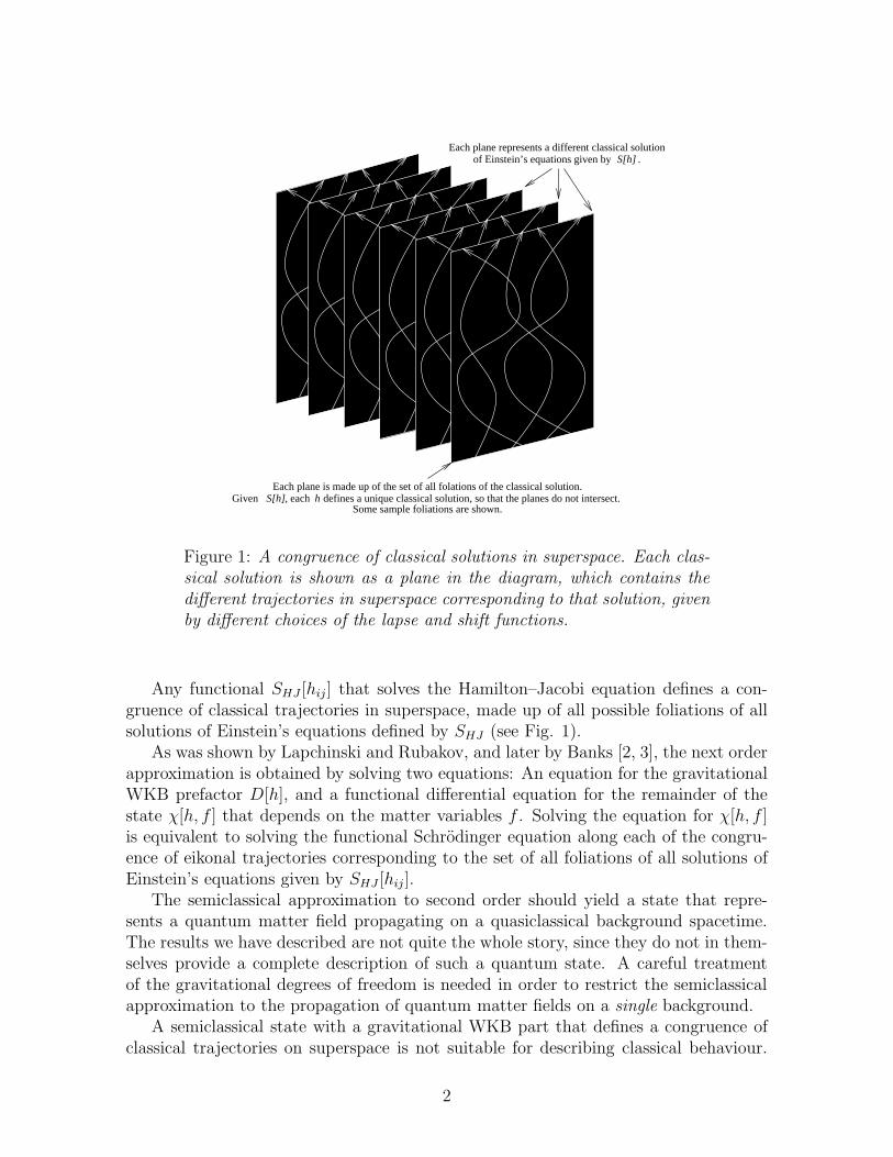
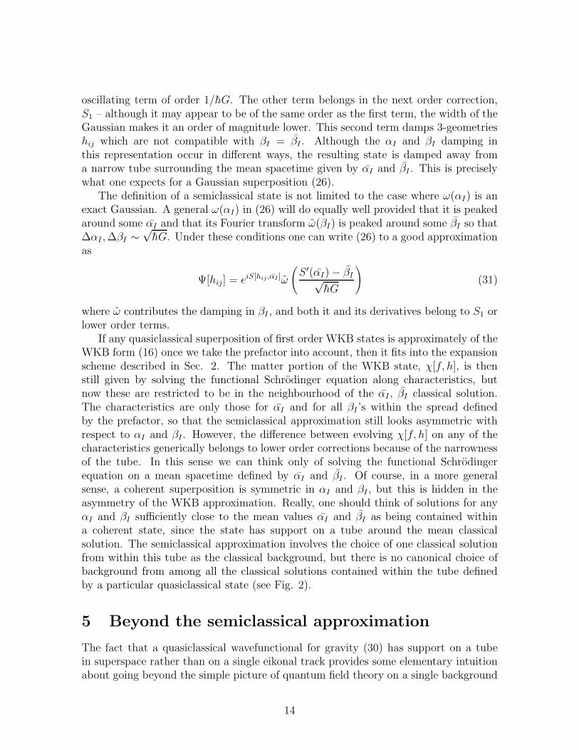
If any quasiclassical superposition of first order WKB states is approximately of theWKB form (16) once we take the prefactor into account, then it fits into the expansionscheme described in Sec. 2. The matter portion of the WKB state, χ[f, h], is thenstill given by solving the functional Schrodinger equation along characteristics, butnow these are restricted to be in the neighbourhood of the αI , βI classical solution.The characteristics are only those for αI and for all βI ’s within the spread definedby the prefactor, so that the semiclassical approximation still looks asymmetric withrespect to αI and βI . However, the difference between evolving χ[f, h] on any of thecharacteristics generically belongs to lower order corrections because of the narrownessof the tube. In this sense we can think only of solving the functional Schrodingerequation on a mean spacetime defined by αI and βI . Of course, in a more generalsense, a coherent superposition is symmetric in αI and βI , but this is hidden in theasymmetry of the WKB approximation. Really, one should think of solutions for anyαI and βI sufficiently close to the mean values αI and βI as being contained withina coherent state, since the state has support on a tube around the mean classicalsolution. The semiclassical approximation involves the choice of one classical solutionfrom within this tube as the classical background, but there is no canonical choice ofbackground from among all the classical solutions contained within the tube definedby a particular quasiclassical state (see Fig. 2).

5 Beyond the semiclassical approximation

The fact that a quasiclassical wavefunctional for gravity (30) has support on a tubein superspace rather than on a single eikonal track provides some elementary intuitionabout going beyond the simple picture of quantum field theory on a single background

14

(b)(a)

band localised in

surface of constant tube localised in and

β

βα α

Figure 2: For simplicity, in this figure, each classical trajectory is rep-resented by a single line, so that the box represents a gauge-fixed versionof superspace with a fixed choice of lapse and shift functions definingeach classical solution. The three dimensions of the box represent the αI

and βI degrees of freedom and the time direction. (a) shows a narrowband of trajectories with a fixed value of αI and with different valuesof βI . The choice of SHJ fixes the value of the αI – the surface shown– and the prefactor then determines the region of superspace on whichthe functional has support – the band within the surface. The bold lineindicates a mean trajectory which is surrounded by other sample trajec-tories. (b) more accurately represents a quasi-classical state. Since weare considering a superposition of αI eigenstates, the wave functionalhas support off the surface of constant αI , and throughout a narrowtube centered around the mean trajectory. The lines represent classicaltrajectories with different values of both αI and βI in the neighbourhoodof the mean trajectory which is shown in bold.

15

spacetime. As was mentioned at the end of the last section, there is no preferred choiceof classical background from among all of those contained within the tube, and so ifthe semiclassical approximation is to hold, the physics of the matter fields had betterbe independent of this choice.

When one wants to talk about quantum gravity either outside or beyond the semi-classical approximation, one has a fundamental problem: The lack of a backgroundspacetime, and of the notion of matter fields living on that background makes life dif-ficult, since it is unclear what is meant by a unitary theory and how to define an innerproduct under these circumstances. Our discussion of the semiclassical approximationsuggests that some or all of these concepts make sense only to the same order as thesemiclassical approximation, but nonetheless form the basis of our current descriptionof nature. The semiclassical approximation using states is in this sense much the sameas the sentiments expressed over the years by Wheeler [25], since the Planck scaleuncertainties in αI and βI can be related to fluctuations in the underlying spacetimeswhich are generically on the Planck scale.

In this section we shall examine what we can learn qualitatively about correctionsarising from geometry fluctuations. A careful analysis of corrections to the semiclassicalapproximation was carried out by Kiefer and Singh [26] by expanding the semiclassicalapproximation to third order. These authors derived a series of correction terms to thefunctional Schrodinger equation, consisting of corrections in the integration of matterfields along eikonal tracks and interference effects between eikonal tracks. In Ref. [26]the former were shown to be small, but the corrections due to interference, proportionalto

δχ[f, hij ]

δhij(32)

projected in a direction transverse to the eikonal trajectories, were neglected. We shalltake a geometrical approach to the computation of these interference effects.

The basic quantity we wish to estimate is the state of matter on any given hyper-surface hij

Ψhij[f ] ≡ Ψ[f, hij ].

To the order of the semiclassical approximation (equations (17) and (18)), the evolutionof this state is given by taking hij to be embedded only in the spacetimes labeled byαI and some βI . Then one finds that Ψhij

[f ] is a solution to the functional Schrodingerequation on a fixed background.

A set of corrections to this approximation come from taking into account the con-tributions from all the possible spacetimes labeled by αI and βI which are not dampedin the Gaussian state and which pass through hij . A simple way to get qualitativeinformation about these corrections is to consider solving the functional Schrodingerequation on all of these spacetimes5 and comparing the properties of the solutions. In

5Not necessarily just those eikonal tracks with αI = αI and βI within the spread defined bythe prefactor should be used, but all classical solutions within the tube. Recall that although theWKB approximation picks out eikonal tracks with a fixed value of αI and different values of βI , theunderlying state is approximately symmetric in αI and βI .

16

order to solve the functional Schrodinger equation for the set of spacetimes defined by(30), it is necessary to give initial data on each of them (that is on a surface in super-space transverse to the tube). Sticking to the philosophy that we wish to construct asclassical a state as possible, this initial data should be arranged to make the correctionsto the semiclassical approximation as small as possible.

If there are to be only Planck scale corrections to the semiclassical approximation,the difference between Schrodinger evolution of matter states on each of the spacetimesshould be small, except at the Planck scale. If this difference were large, the resultsobtained to the order of the semiclassical approximation would not be consistent. It isclear that one situation in which the semiclassical approximation breaks down unex-pectedly is when the evolution of the matter state has sensitive dependence on the αI

and βI parameters.When comparing Schrodinger evolutions on different backgrounds, we need to com-

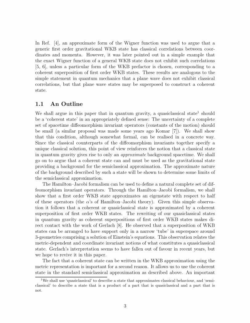
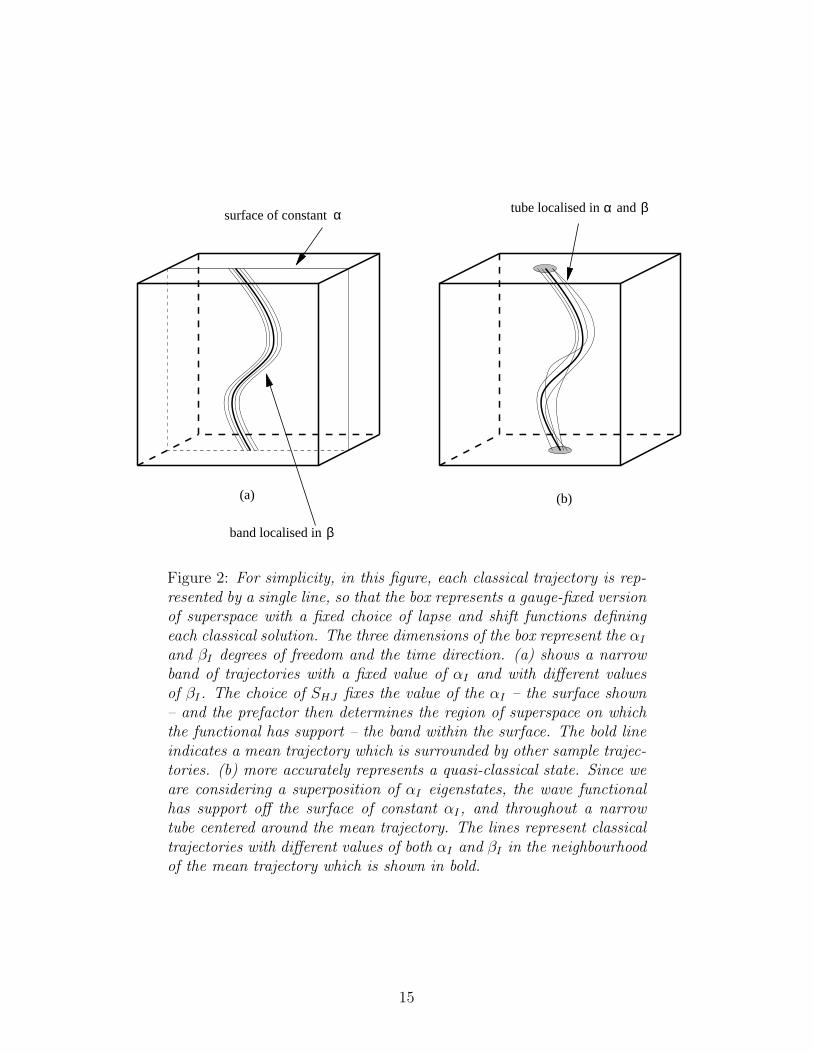
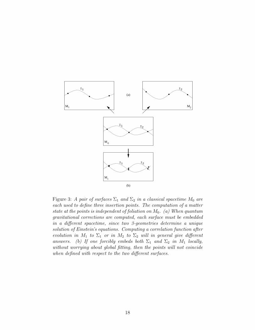
pare different Ψ[f, hij ] for the same hij . This must be done in a coordinate invariantfashion and without reference to a spacetime. Some discussion of this issue can befound in Ref. [16]. The comparison of states on entire hypersurfaces is fairly straight-forward, but this does not provide a local description of the interference effect. Alocal comparison of matter states can be made by using matter correlation functionsin the different spacetimes within the Gaussian spread. Since the basic variables are3-metrics, an insertion point (i.e. an event) can only be defined geometrically by itsposition on a 3-geometry (one might for example define a hypersurface by its intrinsicgeometry and then fix a point by its value of the intrinsic curvature). A correlationfunction should thus be defined by a 3-geometry that contains all the insertion points,and by the location within the given 3-geometry of the points. On a single classicalbackground, the same correlation function can be defined using many different choicesof a 3-geometry that passes through all the insertion points. However, quantum me-chanically all of these choices are different. When we come to compute the correlationfunction on different spacetimes within the tube, each choice of 3-geometry identifiesa different set of alternative classical spacetimes in which the 3-geometry can be em-bedded, and so gives different results (see Fig. 3(a)). Forcing an embedding of bothsurfaces into a second spacetime is possible locally, but in this case the foliation de-pendence occurs because the location of the insertion points in this second spacetimedepends on the choice of surface (see Fig. 3(b)). It follows that the size of the correc-tions to the semiclassical approximation obtained by comparing correlation functionsdepends on how one chooses to foliate the original or mean spacetime. This dependenceon foliation is inevitable if we wish to compare local quantities.

However small the dependence on the choice of foliation, for corrections to the func-tional Schrodinger equation, coordinate invariance is lost6. In some dramatic situationswhere evolution with respect to certain foliations is very sensitive to small differences inαI and βI , this can lead to very different conclusions about the size of quantum gravityeffects in different foliations (or frames of reference). This might look puzzling since we

6This foliation dependence is independent of the anomalies discussed in Sec. 2 and in Refs. [21,12, 22].

17

Σ1 Σ2

Σ1 Σ2

Σ1 Σ2

M2

M0

(b)

M1

(a)

M1

Figure 3: A pair of surfaces Σ1 and Σ2 in a classical spacetime M0 areeach used to define three insertion points. The computation of a matterstate at the points is independent of foliation on M0. (a) When quantumgravitational corrections are computed, each surface must be embeddedin a different spacetime, since two 3-geometries determine a uniquesolution of Einstein’s equations. Computing a correlation function afterevolution in M1 to Σ1 or in M2 to Σ2 will in general give differentanswers. (b) If one forcibly embeds both Σ1 and Σ2 in M1 locally,without worrying about global fitting, then the points will not coincidewhen defined with respect to the two different surfaces.

18

started off with the Wheeler–DeWitt equation which is supposed to impose coordinateinvariance. Recall, however, that the familiar notion of coordinate invariance comesfrom the covariance of matter evolution on a fixed background spacetime, which is validonly in the semiclassical approximation. To this order, observations are independent ofa choice of foliations of the mean background spacetime. It is this notion which breaksdown when one takes into account the geometry fluctuations which are higher ordercorrections. This is because the meaning of the Wheeler–DeWitt equation is differentat this next order, since the notion of diffeomorphism invariance is now a property ofthe combined matter–gravity system, not just of matter on a fixed background.

Generally one might expect interference effects of the kind we have described toalways be restricted to the Planck scale in any reasonable models. However, it is im-portant to note that we cannot trust our usual intuition about quantum gravity whenquantifying these effects, since they are not defined by the quantities one normally as-sociates with a breakdown in the semiclassical approximation such as large curvatureor backreaction. What makes this discussion particularly relevant is that in black holephysics, quantum gravity effects that normally occur at the Planck scale can be magni-fied to the classical scale by the apparently chaotic behaviour of functional Schrodingerevolution on certain hypersurfaces close to the horizon. In a variety of models, it hasbeen shown that the evolution of matter states on foliations corresponding to outsideobservers close to a black hole horizon is extremely sensitive to very small fluctuationsin the background geometry, so that the projection of (32) transverse to the classicalsolution is very large (see [16], and also [17] for a related discussion). Since large cor-rections are present in this case for only a very specific foliation, this indicates thata breakdown in coordinate invariance accompanies the breakdown in the semiclassicalapproximation. In an effective description, the results of certain sets of observationsnear the black hole horizon are not covariant, providing an explanation for the quan-tum gravitational origin of the spacetime complementarity proposed by ’t Hooft [27]and Susskind [28].

6 Conclusions

We have shown that the appropriate state to consider as quasiclassical in quantumgravity is a superposition of WKB type states which is peaked around some values ofthe reduced phase space variables, with close to minimal uncertainty in the reducedphase space variables. A first order WKB state on the other hand is an approximateeigenstate of half of these variables and hence not adequate. When matter is present,this is perfectly compatible with the derivation of the Schrodinger equation from theWheeler–DeWitt constraint. This makes more precise the meaning of a semiclassicalapproximation in quantum gravity.

Using a superposition of WKB states, we were able to give a heuristic treatmentof higher order effects due to the quantum nature of the background geometry. Thisallowed us to see that the semiclassical approximation can be inconsistent because of thesensitivity of matter propagation to small fluctuations in the background geometry. An

19

example of this type of situation is given by the breakdown of a semiclassical descriptionof matter propagating on a black hole spacetime [15, 16]. We also showed that as aconsequence of quantum fluctuations, coordinate invariance is lost on the Planck scale,and in certain cases, such as near the black hole, this extends to macroscopic scales.

We have not discussed in this paper how it is that a system described by theWheeler–DeWitt equation comes to find itself in the particular state that exhibitssemiclassical behaviour. There is in principle no kinematical reason to prefer this stateover any other. Perhaps the most likely answer to this question is that decoherenceeffectively forces any state to a configuration in which observations are equivalent tothose within the Gaussian state. However, the important point is that decoherencecannot drive a state towards any configuration for which the background spacetime ismore classical than the one we have described.

Acknowledgments

We are grateful to S. Carroll, D. Giulini, J. Halliwell, R. Jackiw, E. Keski–Vakkuri,J. Samuel, T. P. Singh and A. Vilenkin for helpful discussions. After this work wascompleted, the authors learned that results overlapping with the discussion in theappendix have been obtained independently by J-G. Demers [29].

Appendix: A two-dimensional example

The use of Hamilton–Jacobi theory to reduce to the physical degrees of freedom wasdiscussed rather abstractly in Sec. 3. It is instructive to illustrate this using a general1+1 dimensional dilaton gravity model. The model we shall consider was discussedby Louis-Martinez et al [30], and we shall make extensive use of their results. Relatedwork on open and closed spacetimes can be found in Ref. [31].

A.1. Classical theory: closed universe

Let us focus primarily on the case of a closed cosmology. Consider the action,

S =∫

Md2x

√−g [φR− V (φ)] (33)

where x is a periodic coordinate (with period 2π), so that M = S1 × R. This modelreduces to minisuperspace and string inspired models for particular choices of V (φ).For example, a constant potential V (φ) = −4λ2 gives the closed universe version [32]of the CGHS model [33].

Working with the parameterization

ds2 = e2ρ(

−N2dt2 + (dx+N⊥dt)2)

(34)

20

for the metric gµν , the canonical variables are ρ(x) and φ(x), with conjugate momenta

Πφ =2

N(N⊥ρ

′ +N ′⊥ − ρ) (35)

Πρ = − 2

N

(

φ−N⊥φ′)

(36)

while the lapse and shift functions N and N⊥ are Lagrange multipliers. As usual, theHamiltonian is just a sum of the Hamiltonian and diffeomorphism constraints

H =∫

dx [NH +N⊥H⊥] (37)

where

H = 2φ′′ − 2φ′ρ′ − 1

2ΠρΠφ + e2ρV (φ), (38)

H⊥ = ρ′Πρ + φ′Πφ − Π′ρ. (39)

The Hamilton-Jacobi equation reads

g[φ, ρ] +δS

δφ

δS

δρ= 0 (40)

where

g[φ, ρ] = −4φ′′ + 4φ′ρ′ − 2e2ρV (φ). (41)

This is solved by the functional

S[φ, ρ;C] = 2∫

dx

{

QC + φ′ ln

[

2φ′ −QC

2φ′ +QC

]}

(42)

where C is a constant,

QC [φ, ρ] = 2[

(φ′)2 + (C + j(φ)) e2ρ]

1

2 (43)

and

dj(φ)

dφ= V (φ). (44)

(42) is also invariant under spatial diffeomorphisms.In the Hamilton–Jacobi functional (42), we see the presence of a parameter C

which is the α parameter in this problem. To deduce C as a functional of φ, ρ andtheir conjugate momenta, we must invert the relations

δS

δφ=

g[φ, ρ]

QC [φ, ρ],

δS

δρ= QC [φ, ρ]. (45)

21

These lead to the definition

C = e−2ρ(

1

4Π2

ρ − (φ′)2)

− j(φ) (46)

Similarly we can define the quantity β, which we shall call P following [30], as

P =δS

δC= −

∫

dx2e2ρΠρ

Π2ρ − 4(φ′)2

. (47)

It is easy to check that C and P are conjugate and that they have weakly vanishingPoisson brackets with the constraints.

From Eq. (42) for the Hamilton–Jacobi functional, we can solve the classical equa-tions of motion, using the relations

Πφ =δS

δφ, Πρ =

δS

δρ(48)

and Eqs. (35) and (36).For a constant potential V (φ) = −4λ2, and taking σ = 1 and M = 0, there are

homogeneous solutions

ds2 =λ2P 2

π2e−2λ2Pt/π(−dt2 + dx2) (49)

and

φ =C

4λ2− e−2λ2Pt/π (50)

for all values of C and P .Armed with a solution of the Hamilton–Jacobi equation, it is interesting to look

briefly at the quantisation of this model. We may promote Πφ and Πρ to operators

Πφ(x) = −ih δ

δφ(x), Πφ(x) = −ih δ

δφ(x)(51)

With any ordering of the constraints, the first order WKB approximation is of coursegiven by

Ψ[φ, ρ] = eiS[φ,ρ;C]/h (52)

There is however a convenient choice of operator ordering [30]

H =1

2g[φ, ρ] +

1

4QC0

[φ, ρ]ΠφQ−1C0

[φ, ρ]Πρ,

H⊥ = φ′Πφ + ρ′Πρ − Π′ρ (53)

which depends on a parameter C0. With this choice of ordering (52) is an exact solutionof the constraint equations in the particular case where the value of C in S[φ, ρ;C] isequal to C0.

22

Let us now use this exact solution as a first order WKB solution and continue theWKB expansion (as we did for the relativistic particle where all the first order WKBstates eiPx±/h were exact solutions of the Klein–Gordon equation). Writing

Ψ[φ, ρ] = eiS[φ,ρ;C0]/h+iS1[φ,ρ] (54)

the equation for S1 isδS1[φ, ρ]

δφ= − g[φ, ρ]

Q2C0

[φ, ρ]

δS1[φ, ρ]

δρ(55)

Note that this equation is not solved by S[φ, ρ;C] because of the minus sign. We canhowever find an exact solution of this equation by remembering that we expect theprefactor −i lnS1 to be a weight function over different values of P , the conjugate toC. Indeed, if we define the functional

P [φ, ρ] ≡ −1

2

∫

dxQC0

[φ, ρ]

(C + j(φ))(56)

where we have replaced Πρ in (47) by its classical value given by the Hamilton–Jacobifunctional, then an arbitrary function of P solves (55) and the WKB approximationcentered around C0 is of the form

Ψ[φ, ρ] =1

D[P [φ, ρ]]eiS[φ,ρ;C=C0] (57)

If we take D[P [φ, ρ]] to be a Gaussian, then we obtain an explicit expression for thequasiclassical state to this order. Note that for a general D[P [φ, ρ]], (57) is no longeran exact solution of the constraint equation, meaning that at least some of the Si, i ≥ 2must be non-zero.

A.2. Classical theory: spacetimes with boundary

The case of an open universe has been studied by various authors [31]. It has beenshown that the variable C is related to the ADM mass of the spacetime, while P ,integrated throughout a spacelike slice, is related to the time at infinity (or moreprecisely, to the synchronization between times at infinity). These results are in keepingwith the much earlier work of Regge and Teitelboim [34] on conserved charges incanonical quantum gravity in open universes.

It is interesting to note that while P is associated with a constant of the motion asdescribed in Refs. [31], a closely related quantity provides a local geometric definitionof time for different hypersurfaces within a static spacetime. Consider any 1-geometryassociated with a hypersurface in a static classical solution. It can be intrinsicallydescribed by the function φ(s), where s is the proper distance along the hypersurfacemeasured from some base point B at infinity, and φ is the value of the dilaton field.Let φ0(s) be the function defining a constant time surface t = t1 passing throughB = φ0(0). Consider now a set of hypersurfaces passing through B that are defined by

23

φi(s) which differ from φ0(s) only in some finite interval 0 < s < s0. For s > s0, φi(s)also define constant time hypersurfaces but at some time ti = t0 + ∆ti.

Using (46) to give Πρ in terms of C and φ, we can define a quantity

Ti(S) = −∫ S

0ds

[

(

dφi

ds

)2+ C + j(φi)

]1/2

(C + j(φi))

closely related to P . Here S > s0 so that the integration extends well into the regionwhere φi(s) = φ0(s).

Now in a static coordinate system

ds2 = e2ρ(−dt2 + dx2)

we can compute the change in the time coordinate along any hypersurface using

(

dt

dx

)2

= 1 −e−2ρ

(

dφi

dx

)2

(

dφi

ds

)2 .

Since in the static coordinate system Πρ = 0, it follows that

(

dt

dx

)2

= 1 +C + j(φi)(

dφi

ds

)2 .

From this expression we deduce that

∆ti =∫

dx

[

(

dφi

ds

)2+ C + j(φi)

]1/2

(

dφi

ds

) =∫ S

0ds

[

(

dφi

ds

)2+ C + j(φi)

]1/2

eρ(

dφi

ds

) .

By definition ∆t is zero for φ0, but is non-zero for any φi(s) over the region 0 < s < s0.The connection between ∆ti and Ti(S) emerges by noting that any static solution

has

eρ = c0

(

dφ

ds

)

where c0 is some constant of proportionality (this can be shown using Eqs. (38) and(46)). From this it follows that

∆ti(S) =Ti(S)

c0.

24

References

[1] R.Arnowitt, S. Deser and C. Misner Phys. Rev. 117, (1960) 1595.

[2] V. Lapchinsky and V. Rubakov, Acta Phys. Pol. B10 (1979) 1041

[3] T. Banks, Nucl. Phys. B249 (1985) 332

[4] J. J. Halliwell Phys. Rev. D36, (1987) 3626.

[5] A. Anderson, Phys. Rev. D42, (1990) 585.

[6] S. Habib and R. Laflamme, Phys. Rev. D42 (1990) 4056.

[7] P. Bergmann, Phys. Rev. 144 (1966) 1078; A. Komar, Phys. Rev. 153 (1967)1385; A. Komar, Observables, correspondence and quantized gravitation, in Magic

Without Magic, ed. J. Klauder, San Francisco, 1972.

[8] U. Gerlach, Phys. Rev. 177 (1969) 1929.

[9] A. Vilenkin, Phys. Rev. D39 (1989) 1116;

[10] D. Cangemi, R. Jackiw and B. Zwiebach, Physical states in matter coupled dilatongravity, UCLA Report No. UCLA-95-TEP-16 (hep-th/9505161).

[11] N.C. Tsamis and R.P. Woodard, Phys. Rev. D36 (1987) 3641-3650.

[12] D. Cangemi and R. Jackiw, Phys. Lett. B337 (1994) 271.

[13] C. Kiefer, The semiclassical approximation to quantum gravity, Freiburg Univer-sity Report No. THEP-93/27, in Canonical Gravity – from Classical to Quantum,edited by J. Ehlers and H. Friedrich (Springer, Berlin 1994) (gr-qc/9312015).

[14] J-P. Paz and S. Sinha, Phys. Rev. D44 (1991) 1038; S. Mathur, in Banff/CAPWorkshop on Thermal Field Theories, Banff, Canada, edited by F. C. Khannaet. al. (World Scientific, Singapore, 1994).

[15] S. D. Mathur, Black hole entropy and the semiclassical approximation, MIT re-port No. CTP-2304, to appear in the proceedings of the International Colloquiumon Modern Quantum Field Theory II at TIFR (Bombay), January 1994 (hep-th/9404135).

[16] E. Keski-Vakkuri, G. Lifshytz, S. Mathur and M. E. Ortiz, Phys. Rev. D51

(1995) 1764.

[17] Y. Kiem, H. Verlinde and E. Verlinde Quantum Horizons and complementarity,CERN-TH.7469/94 (hep-th/9502074).

25

[18] J. Hartle, Progress in quantum cosmology, in Proceedings, 12th Conference onGeneral Relativity and Gravitation, Boulder, 1989, edited by N. Ashby, D. F.Bartlett and W. Wyss (CUP, Cambridge, 1990).

[19] C. J. Isham, Canonical quantum gravity and the problem of time, presented atthe 19th International Colloquium of Group Theoretical Methods in Physics,Salamanca, Spain, July 1992 (gr-qc/9210011).

[20] A. Peres Nuovo Cimento XXVI, (1962) 53.

[21] K. V. Kuchar, Phys. Rev. D39 (1989) 1579.

[22] D. Giulini and C. Kiefer, Consistency of semiclassical gravity, Freiburg ReportTHEP-94-20 (gr-qc/9409014).

[23] H. Goldstein Classical Mechanics, Addison-Wesley publishing Company, (1980).

[24] C. Crnkovic and E. Witten, Covariant description of canonical formalism ingeometrical theories, in Three Hundred Years of Gravitation, eds. S. Hawkingand W. Israel, Cambridge University Press, Cambridge, UK 1987.

[25] See for instance C. Misner, K. Thorne and J. A. Wheeler, Gravitation, W. H.Freeman, San Francisco (1971).

[26] C. Kiefer and T. Singh, Phys. Rev. D44, (1991) 1067.

[27] G. ’t Hooft, Nucl. Phys. B335 (1990) 138, and references therein.

[28] L. Susskind, Phys. Rev. D49 (1994) 6606.

[29] J-G. Demers, private communication.

[30] D. Louis-Martinez, J. Gegenberg and G. Kunstatter, Phys. Lett. B321(1994)193

[31] T. Banks and M. O’Loughlin, Nucl. Phys. B362 (1991) 649; A. Ashtekar andJ. Samuel, Bianchi cosmologies: the role of spatial topology, Syracuse ReportPRINT-91-0253 (1991); K. V. Kuchar, Geometrodynamics of Schwarzschild blackholes, Utah Preprint UU-REL-94/3/1, (gr-qc/9403003); H. A. Kastrup and T.Thiemann, Nucl. Phys. B425 (1994) 665.

[32] F. D. Mazzitelli and J. G. Russo, Phys. Rev. D47 (1993) 4490.

[33] C. G. Callan, S. B. Giddings, J. A. Harvey and A. Strominger, Phys. Rev. D 45

(1992) R1005. For reviews see J. A. Harvey and A. Strominger, Quantum aspectsof black holes, in the proceedings of the 1992 TASI Summer School in Boulder,Colorado (World Scientific, 1993), and S. B. Giddings, Toy models for black holeevaporation, in the proceedings of the International Workshop of Theoretical

26

Physics, 6th Session, June 1992, Erice, Italy, ed. V. Sanchez (World Scientific,1993).

[34] T. Regge and C. Teitelboim, Ann. Phys. 88 (1974) 286.

27