arX

iv:m

ath/

0508

242v

2 [

mat

h.PR

] 2

9 Se

p 20

06

Normal Approximations for Descents and Inversions of

Permutations of Multisets

Mark Conger and D. Viswanath ∗

February 2, 2008

Abstract

Normal approximations for descents and inversions of permutations of the set {1, 2, . . . , n}are well known. We consider the number of inversions of a permutation π(1), π(2), . . . , π(n) of amultiset with n elements, which is the number of pairs (i, j) with 1 ≤ i < j ≤ n and π(i) > π(j).The number of descents is the number of i in the range 1 ≤ i < n such that π(i) > π(i + 1).We prove that, appropriately normalized, the distribution of both inversions and descents of arandom permutation of the multiset approaches the normal distribution as n → ∞, providedthat the permutation is equally likely to be any possible permutation of the multiset and noelement occurs more than αn times in the multiset for a fixed α with 0 < α < 1. Both normalapproximation theorems are proved using the size bias version of Stein’s method of auxiliaryrandomization and are accompanied by error bounds.

1 Introduction

Let π(1), π(2), . . . , π(n) be a permutation of the multiset {1n1 , 2n2 , . . . , hnh} with n1 + · · ·+nh = n.The number of inversions, denoted inv(π), is defined as the number of pairs (i, j) with 1 ≤ i < j ≤ nand π(i) > π(j). The number of descents, denoted des(π), is the number of positions i with1 ≤ i < n and π(i) > π(i + 1). Assume that π is uniformly distributed. In this article, we useStein’s method to prove normal approximations with error bounds for inv(π) and des(π).

In the special case where π is a uniformly distributed permutation of the set {1, 2, . . . , n}, thedistributions of both inv(π) and des(π) admit simple descriptions. The distribution of inv(π) isequal to that of the sum X1 + · · · + Xn−1, where the random variables Xi, 1 ≤ i ≤ n − 1, areindependent with Xi uniformly distributed over the set {0, 1, . . . , i}. To obtain the distributionof des(π), we need the sum X1 + · · · +Xn−1 + Xn, where the Xi are independent and uniformlydistributed in the interval [0, 1]. The probability that this sum lies in the interval [d, d + 1] equalsthe probability that des(π) equals d. According to Knuth [14], the first of these two results wasnoticed by O. Rodriguez in 1839. The result about des(π) was alluded to by Barton and Mallows[2]. An elegant proof is due to Stanley [18].

∗Department of Mathematics, University of Michigan, 530 Church Street, Ann Arbor, MI 48109, U.S.A.,

mconger@umich.edu and divakar@umich.edu. This work was supported by a research fellowship from the Sloan

Foundation.

1

Normal approximations to des(π) and inv(π) in this special case can be obtained using theseresults and standard versions of the central limit theorem. The bounds

∣

∣

∣P

(

des(π) − (n− 1)/2√

(n + 1)/12≤ x

)

− Φ(x)∣

∣

∣≤ C√

n(1.1a)

∣

∣

∣P

(

inv(π) − 1

2

(n2

)

√

n(n− 1)(2n + 5)/72≤ x

)

− Φ(x)∣

∣

∣≤ C√

n, (1.1b)

where C is a constant and Φ is the standard normal distribution, were proved using the method ofexchangeable pairs [17, 20] by Fulman [9]. Other proofs of (1.1a) using Stein’s method are sketchedin [4] and [10].

From the survey by Barton and Mallows [2], it appears that the asymptotic normality of a quan-tity closely related to des(π), where π is a uniformly distributed permutation of the set {1, . . . , n},was stated by Bienyame in 1874 (Bull. Soc. Math. France, vol. 2, p. 153-154). Bienyame wasinterested in statistical applications. So were Levene and Wolfowitz [15] who stated that runs werewidely used in quality control and in the study of economic time series. Runs are the monotonesegments within a sequence of numbers and are closely related to descents. An early proof of theasymptotic normality of descents, which is implied by (1.1a), is due to Wolfowitz [21].

Let {1n1 , 2n2 , . . . , hnh} be a multiset, where na, 1 ≤ a ≤ h, are positive integers. Let n =n1 + n2 + . . . + nh be the number of elements of the multiset. Let α be a fixed number in (0, 1).We assume that na ≤ αn for 1 ≤ a ≤ h. Let π be a uniformly distributed permutation of thismultiset. We consider inv(π) and des(π) in this more general situation. The bounds that we obtainfor the errors in the normal approximations to these quantities depend upon α and become infiniteas α → 1. Let h : R → R be a bounded and piecewise continuously differentiable function and letβ = max(1/2, α). We use the size-bias version of Stein’s method introduced by Baldi, Rinott andStein [1] and prove that, for n large enough,

∣

∣Eh( inv(π) − µ

σ

)

− Φh∣

∣ ≤ C

(

‖h‖β(1 − β)(β(1 − β)n1/2 − C1n−1/2)

+‖Dh‖

(β(1 − β)n1/3 − C2n−2/3)3/2

)

where C, C1, and C2 are some positive constants, Φh is the expectation of h with respect to thestandard normal distribution, and µ and σ2 are the mean and variance of inv(π), respectively. Ifα ≥ 1/2, then β = α. Therefore the bound above diverges as α→ 1. We prove a similar result fordes(π).

Bounds such as the one given in the previous paragraph require h to be continuous. Goldstein[10] has proved a normal approximation theorem that holds for non-smooth h. We use that theoremto prove that

∣

∣

∣P

(

inv(π) − µ

σ≤ x

)

− Φ(x)∣

∣

∣≤ C(β)/

√n

and that∣

∣

∣P

(

des(π) − µ

σ≤ x

)

− Φ(x)∣

∣

∣≤ C(β)/

√n.

These results are contained in Theorems 2.12 and 2.16 of this paper. The quantity C(β) divergeswhen α → 1. As before β = max(1/2, α). When the n elements of the multiset are distinct, with

2

n ≥ 2, we may use α = 1/n and β = 1/2. Therefore the results stated above imply (1.1a) and(1.1b).

The generating function of the number of permutations of a multiset with a given number ofinversions is a rational function. Using this generating function, Diaconis [7] has shown that theasymptotic distribution of inv(π), where π is uniformly distributed over permutations of a multiset,is normal. Theorem 2.12 about inv(π) is accompanied by an error bound of the correct order, whichis O(1/

√n), and the dependence of the error bound on α is also explicitly shown in our theorem.

The generating function for the number of permutations of a multiset with a given number ofdescents, which is related to Foata’s correspondence, was found by MacMahon [14] [16]. However,normal approximations to this quantity, such as the approximation given in Theorem 2.16, do notseem to be available.

Segments of π(1), . . . , π(n) between successive descents, or runs, are in ascending order. Knuth[14] has stated that runs are important in the study of sorting algorithms because runs are segmentsthat are already in sorted order. Among the applications of descents and inversions to the studyof sorting algorithms, multiway merging with replacement selection merits special mention. In thissorting method, the given sequence is first split into runs and the runs are merged together. Ourresults are pertinent to sorting algorithms if the keys used for sorting are allowed to repeat. Forexample, Theorem 2.16 about des(π) gives an idea of how many runs to expect if multiway mergingis used on a sequence of records with repeated keys.

Descents and inversions have been used as test statistics in the special case where π is a per-mutation of {1, 2, . . . , n}. As already mentioned, early work on runs and descents was stimulatedby statistical applications. Of the ten empirical tests for the randomness of a sequence of distinctnumbers discussed by Knuth [13], one is based on runs and descents. Taking our results into ac-count, inversions and descents can be used to test if a given permutation of a multiset of numbersis random. There are other ways to test if a given permutation of a multiset of numbers is random.If a permutation passes n empirical tests for randomness but fails the n + 1st, it is not random.Therefore having a greater number of empirical tests available makes for more robust testing [13].

DNA sequences are strings of the four letters A, C, G, and T . It is now well known that thesesequences are far from random [12]. It has even been suggested that these sequences are similar tohuman languages [8]. Some commonly used compression algorithms such as the Lempel-Ziv methodfail to compress typical DNA sequences however [12]. The entropy estimates of DNA sequencesgiven in [12] and [8] proceed by dividing the sequence into blocks in some way. For instance, blocksof 6 consecutive letters are considered in [12]. These entropy estimates show that DNA sequencesare not random.

In Section 3, we report the descents and inversions of the 19th chromosome of the humangenome mainly as an illustration. We consider all 24 possible orderings of A, C, G, and T . Withrespect to each of these orderings, a calculation of descents and inversions shows that the numberof descents and inversions of the DNA sequence departs from the mean by a large multiple of thestandard deviation. It may be of some interest that this method of showing the DNA sequence tobe far from random considers only single letters without dividing them into blocks.

Although we consider all possible orderings of A, C, G, and T , it must be noted that themolecular weights of the corresponding compounds implies the order C < T < A < G. This is asnatural as any order one can hope to find among four physical objects.

Our interest in permutations of multisets was provoked by their connection to riffle shuffles ofdecks with repeated cards [5].

3

We do not give explicit numerical constants in our Theorems 2.12 and 2.16 about descentsand inversions of permutations of multisets. It is worth noting that explicit numerical constantsare not given for most of the detailed examples in Stein’s book [20], and all the examples in thepapers by Baldi, Rinott, and Stein [1], by Goldstein and Rinott [11], and by Rinott and Rotar [17].Furthermore, even the asymptotic normality for descents of permutations of multisets implied byTheorem 2.16 is a new result, and so is Theorem 2.12 which shows the dependence of the boundsfor normal approximation on the size of the multiset and the parameter α that characterizes themultiset.

2 Descents and inversions of permutations of multisets

If W ≥ 0 is a non-negative and integrable random variable, the distribution of W ∗ is said to be W -size biased, if E(Wf(W )) = EWE(f(W ∗)) for all continuous functions f for which the expectationon the left hand side of the equality exists.

Stein’s method [19] [20] refers to the use of auxiliary randomization to find normal approxima-tions to the distribution of some random variables. In the theorem below, the auxiliary random-ization requires the construction of W ∗ which must be W -size biased. The theorem below can befound in [1], but we follow its formulation in [11].

Theorem 2.1. Let W be a non-negative random variable with EW = µ and Var(W ) = σ2. Let

W ∗ be jointly defined with W such that its distribution is W -size biased. Let h be a function from

R to R such that h is continuous and its derivative Dh is piecewise continuous. Then

∣

∣Eh(W − µ

σ

)

− Φh∣

∣ ≤ 2‖h‖ µσ2

√

Var(

E(W ∗ −W |W ))

+ ‖Dh‖ µσ3

E(W ∗ −W )2,

where Φh is the expectation of h with respect to the standard normal distribution and ‖·‖ is the

supremum norm.

When h is the indicator function of the half line (−∞, x], the following theorem found in [10]applies. Its proof uses a smoothing inequality and other techniques found in [17].

Theorem 2.2. Let W be a non-negative random variable with EW = µ and Var(W ) = σ2. Let

W ∗ be jointly defined with W such that its distribution is W -size biased. Let |W ∗ −W | ≤ B and

let A = B/σ. Let B ≤ σ3/2/√

6µ. Then

∣

∣P(W − µ

σ≤ x

)

− Φ(x)∣

∣ ≤ 0.4A +µ

σ(64A2 + 4A3) +

23µ

σ2

√

Var(

E(W ∗ −W |W ))

,

where Φ is the standard normal distribution.

In Theorems 2.1 and 2.2 above, we added the superscript ∗ to W to denote a random variablewith the W -size biased distribution. In the lemma below, random variables Xi with the superscript∗ do not necessarily have the Xi-size biased distribution. Here and later, our convention is to usethe superscript ∗ when random variables are constructed as a part of the size biasing procedure.This notation is due to [1].

The construction of size biased variables in this paper will be based on the following lemmafound in [1] and [11].

4

Lemma 2.3. Let W = X1 + X2 + . . . + Xn, where each Xi is a non-negative random variable

with finite mean. Let I be a random variable which is independent of the Xi and which satisfies

P(I = i) = EXi/∑n

j=1EXj . Define W ∗ as W ∗ = X∗

1 +X∗

2 + · · · +X∗

n, where for given I X∗

I has

the XI-size biased distribution and

P(

(X∗

1 ,X∗

2 , . . . ,X∗

n) ∈ A∣

∣I = i,X∗

i = x)

= P(

(X1,X2, . . . ,Xn) ∈ A∣

∣Xi = x). (2.1)

Then W ∗ has the W -size biased distribution.

Whenever Lemma 2.3 is applied here, we will find Xi are 0-1 valued random variables, and thesize biased distribution for such variables is concentrated at 1. Therefore, for our purposes, (2.1)can be written as P

(

(X∗

1 ,X∗

2 , . . . ,X∗

n) ∈ A∣

∣I = i)

= P(

(X1,X2, . . . ,Xn) ∈ A∣

∣Xi = 1).Let π be a uniformly distributed permutation of the multiset {1n1 , 2n2 , . . . , hnh} and n = n1 +

n2 + . . . + nh. Each na, 1 ≤ a ≤ h, is a positive integer. The symbols i, j, k, l, with and withoutnumerical subscripts, are used to index the set {1, 2, . . . , n}. The symbols a, b, c, d are used to indexthe set {1, 2, . . . , h}. We also assume na ≤ αn for 1 ≤ a ≤ h and for some α in (0, 1), n ≥ 4, andh ≥ 2.

Define Xij , for i < j, as 1 if π(i) > π(j) and as 0 otherwise. Some facts about the jointdistribution of Xij will be necessary. Denote the probabilities

P(Xij = 1) with i < j,

P(Xij1 = 1,Xij2 = 1) with i < j1 and i < j2,

P(Xi1j = 1,Xi2j = 1) with i1 < j and i2 < j,

P(Xik = 1,Xkj = 1) with i < k < j,

P(Xi1j1 = 1,Xi2j2 = 1) with i1 < j1, i2 < j2, and (i1, j1) 6= (i2, j2)

by p1, p2, p3, p4, and p5, respectively. Elementary arguments can be used to deduce formulas, suchas p1 =

∑

a<b nanb/(n(n − 1)) and p4 =∑

a<b<c nanbnc/(n(n − 1)(n − 2)), for p1, p2, p3, p4, andp5. From such formulas, we deduce

p1 =n2 −∑a n

2a

2n(n − 1)

p2 + p3 + p4 =5n3/6 − n2 + (−3n/2 + 1)

∑

a n2a + (2/3)

∑

a n3a

n(n− 1)(n − 2)

p4 =n3/6 − (n/2)

∑

a n2a + (1/3)

∑

a n3a

n(n− 1)(n − 2)

p5 =n4/4 − n3 + n2/2 + (1/4)

(∑

a n2a

)2+ (−n2/2 + 2n − 1/2)

∑

a n2a −

∑

a n3a

n(n− 1)(n − 2)(n − 3). (2.2)

The formulas in (2.2) will be used to derive expressions for Var(inv(π)) and Var(des(π)).The assumption na ≤ αn, for some α ∈ (0, 1), is used in the two lemmas below. The lemmas,

however, are worded in terms of β = max(1/2, α) and use the weaker assumption na ≤ βn forβ ∈ [1/2, 1). In both the lemmas the assumption na ≤ βn implies h ≥ 2.

Lemma 2.4. Assume β ∈ [1/2, 1), na ≥ 0 for all a, and∑

a na = n. If na ≤ βn for 1 ≤ a ≤ h,then 2β(1 − β)n2 ≤ n2 −∑a n

2a ≤ n2 and 3β(1 − β)n3 ≤ n3 −∑a n

3a ≤ n3.

5

Proof. To lower bound n2 −∑a n2a, note that x ≥ y > 0, δ > 0, and y− δ ≥ 0 imply (x+ δ)2 +(y−

δ)2 > x2 + y2. Thus for a given sum x+ y, the quantity x2 + y2 increases when the difference x− yis increased. Thus given

∑

a na = n and the constraints na ≥ 0, the quantity∑

a n2a is increased

whenever two positive numbers are chosen from na, 1 ≤ a ≤ h, and the lesser of them is decreasedand the greater increased by the same amount. Therefore, under the constraints na ≤ βn,

∑

a n2a

is maximum when n1 = βn, n2 = (1− β)n, and na = 0 for a > 2. The lower bound for n3 −∑a n3a

is also obtained when n1 = βn, n2 = (1 − β)n, and na = 0 for a > 2. The upper bounds aretrivial.

Concerning the lemma below, it is worth noting that β4−4β4+4β−1 = (1−β)2(β2+2β−1) > 0for β ∈ [1/2, 1).

Lemma 2.5. Assume β ∈ [1/2, 1), na ≥ 0 for all a, and∑

a na = n. If na ≤ βn for 1 ≤ a ≤ h,

(β4 − 4β2 + 4β − 1)n4 ≤ n4/3 +(

∑

an2

a

)2 − (4n/3)∑

an3

a ≤ n4/3.

Proof. The upper bound follows from the inequality n∑

a n3a ≥

(∑

a n2a

)2.

We prove the lower bound assuming β > 1/2. The proof for β = 1/2 can be obtained withminor changes. The proof will make careful use of the Kuhn-Tucker conditions as explained in [3,Theorem 9.2-3].

We attempt to minimize J(n1, n2, . . . , nh) =(∑

a n2a

)2 − (4n/3)∑

a n3a subject to the affine

constraints∑

a na = n, −na ≤ 0, and na − βn ≤ 0, where the last two constraints hold for1 ≤ a ≤ h. We assume n1 ≥ n2 ≥ · · · ≥ nh ≥ 0 without loss of generality.

Let DJ be the gradient vector whose ath entry is

∂J

∂na= 4na

∑

bn2

b − 4nn2a = 4na

∑

bnb(nb − na).

The sum of the entries of DJ must be 0 because the term 4nanb(nb − na) in ∂J/∂na is canceledby the term 4nanb(na − nb) in ∂J/∂na. If there exists an a such that n1 > na > 0, then the firstentry of DJ must be strictly negative and therefore some other entry must be strictly positive.

Let u ∈ Rh be the vector with all entries equal to 1. Let va ∈ Rh be the vector with its athentry equal to −1 and all other entries equal to 0. Let w1 = −v1. Note that na−βn = 0 is possibleonly if a = 1 as we have assumed β > 1/2 and n1 ≥ n2 ≥ · · ·

Suppose (n1, n2, . . . , nh) is a local minimum of J . The Kuhn-Tucker conditions require that itmust be possible to make all entries of DJ zero by adding multiples of certain vectors. We arealways allowed to add any real multiple of u because the constraint

∑

a na = n is always in force.We are allowed to add a positive multiple of va if and only if na = 0 because the constraint −na ≤ 0can then be violated by making an infinitesimal change to na. We are allowed to add a positivemultiple of w1 if and only if n1 − βn = 0 by a similar reason.

Let us first consider the type of local minimum where the Kuhn-Tucker conditions can besatisfied without adding a positive multiple of w1. Suppose n1 > na > 0 for some a for such a localminimum. Then the first entry of DJ is strictly negative and some other entry is strictly positive.If the positive entry is ∂J/∂nb, then nb must be nonzero and therefore nb > 0. Such a DJ cannotbe made zero by adding a multiple of u and positive multiples of vc corresponding to nc = 0. Theonly way to make the bth entry of DJ equal to 0 is by adding a negative multiple of u. But this

6

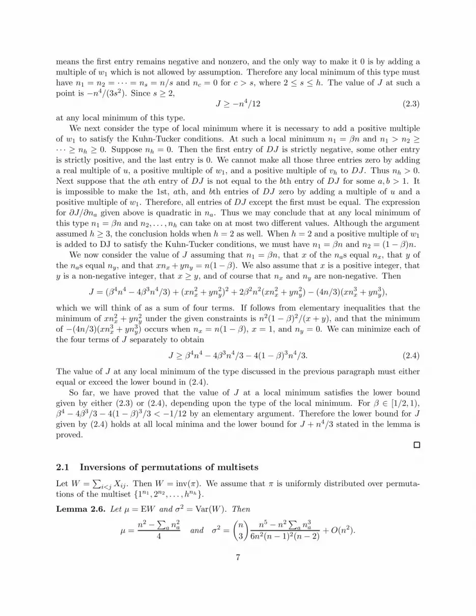
means the first entry remains negative and nonzero, and the only way to make it 0 is by adding amultiple of w1 which is not allowed by assumption. Therefore any local minimum of this type musthave n1 = n2 = · · · = ns = n/s and nc = 0 for c > s, where 2 ≤ s ≤ h. The value of J at such apoint is −n4/(3s2). Since s ≥ 2,

J ≥ −n4/12 (2.3)

at any local minimum of this type.We next consider the type of local minimum where it is necessary to add a positive multiple

of w1 to satisfy the Kuhn-Tucker conditions. At such a local minimum n1 = βn and n1 > n2 ≥· · · ≥ nh ≥ 0. Suppose nh = 0. Then the first entry of DJ is strictly negative, some other entryis strictly positive, and the last entry is 0. We cannot make all those three entries zero by addinga real multiple of u, a positive multiple of w1, and a positive multiple of vh to DJ . Thus nh > 0.Next suppose that the ath entry of DJ is not equal to the bth entry of DJ for some a, b > 1. Itis impossible to make the 1st, ath, and bth entries of DJ zero by adding a multiple of u and apositive multiple of w1. Therefore, all entries of DJ except the first must be equal. The expressionfor ∂J/∂na given above is quadratic in na. Thus we may conclude that at any local minimum ofthis type n1 = βn and n2, . . . , nh can take on at most two different values. Although the argumentassumed h ≥ 3, the conclusion holds when h = 2 as well. When h = 2 and a positive multiple of w1

is added to DJ to satisfy the Kuhn-Tucker conditions, we must have n1 = βn and n2 = (1 − β)n.We now consider the value of J assuming that n1 = βn, that x of the nas equal nx, that y of

the nas equal ny, and that xnx + yny = n(1− β). We also assume that x is a positive integer, thaty is a non-negative integer, that x ≥ y, and of course that nx and ny are non-negative. Then

J = (β4n4 − 4β3n4/3) + (xn2x + yn2

y)2 + 2β2n2(xn2

x + yn2y) − (4n/3)(xn3

x + yn3y),

which we will think of as a sum of four terms. If follows from elementary inequalities that theminimum of xn2

x + yn2y under the given constraints is n2(1 − β)2/(x + y), and that the minimum

of −(4n/3)(xn3x + yn3

y) occurs when nx = n(1 − β), x = 1, and ny = 0. We can minimize each ofthe four terms of J separately to obtain

J ≥ β4n4 − 4β3n4/3 − 4(1 − β)3n4/3. (2.4)

The value of J at any local minimum of the type discussed in the previous paragraph must eitherequal or exceed the lower bound in (2.4).

So far, we have proved that the value of J at a local minimum satisfies the lower boundgiven by either (2.3) or (2.4), depending upon the type of the local minimum. For β ∈ [1/2, 1),β4 − 4β3/3 − 4(1 − β)3/3 < −1/12 by an elementary argument. Therefore the lower bound for Jgiven by (2.4) holds at all local minima and the lower bound for J + n4/3 stated in the lemma isproved.

2.1 Inversions of permutations of multisets

Let W =∑

i<j Xij . Then W = inv(π). We assume that π is uniformly distributed over permuta-tions of the multiset {1n1 , 2n2 , . . . , hnh}.Lemma 2.6. Let µ = EW and σ2 = Var(W ). Then

µ =n2 −∑a n

2a

4and σ2 =

(

n

3

)

n5 − n2∑

a n3a

6n2(n− 1)2(n− 2)+O(n2).

7

Proof. Since µ =(

n2

)

p1, where p1 = EXij, and p1 is given by (2.2), the expression for µ in thelemma must hold.

We first show that

σ2 =

(

n

2

)

(p1 − p21) + 2

(

n

3

)

(p2 + p3 + p4 − 3p21) + 6

(

n

4

)

(p5 − p21), (2.5)

where the pi are given by (2.2). If Var(W ) with W =∑

i<j Xij is written as a sum of variances

and covariances of the Xij , there are(n2

)

variance terms each of which is equal to p1 − p21. There

are(n3

)

terms of the form 2Covar(Xij1 ,Xij2) with i < j1 < j2 and each of those is equal to2(p2 − p2

1). We can account for terms of the form 2Covar(Xi1j ,Xi2j) with i1 < i2 < j and of theform 2Covar(Xik,Xkj) with i < k < j similarly. Thus far we have explained the first two termsof (2.5). All the other terms in the expansion of Var(W ) are of the form 2Covar(Xiij1,Xi2j2) withi1 < j1, i2 < j2, and (i1, j1) < (i2, j2) in lexicographic order. The last term of (2.5) follows if wenote that the number of such terms is 3

(n4

)

.The expression for σ2 in the lemma is deduced using (2.2), (2.5), and the two inequalities

∑

a n2a < n2 and

∑

a n3a < n3.

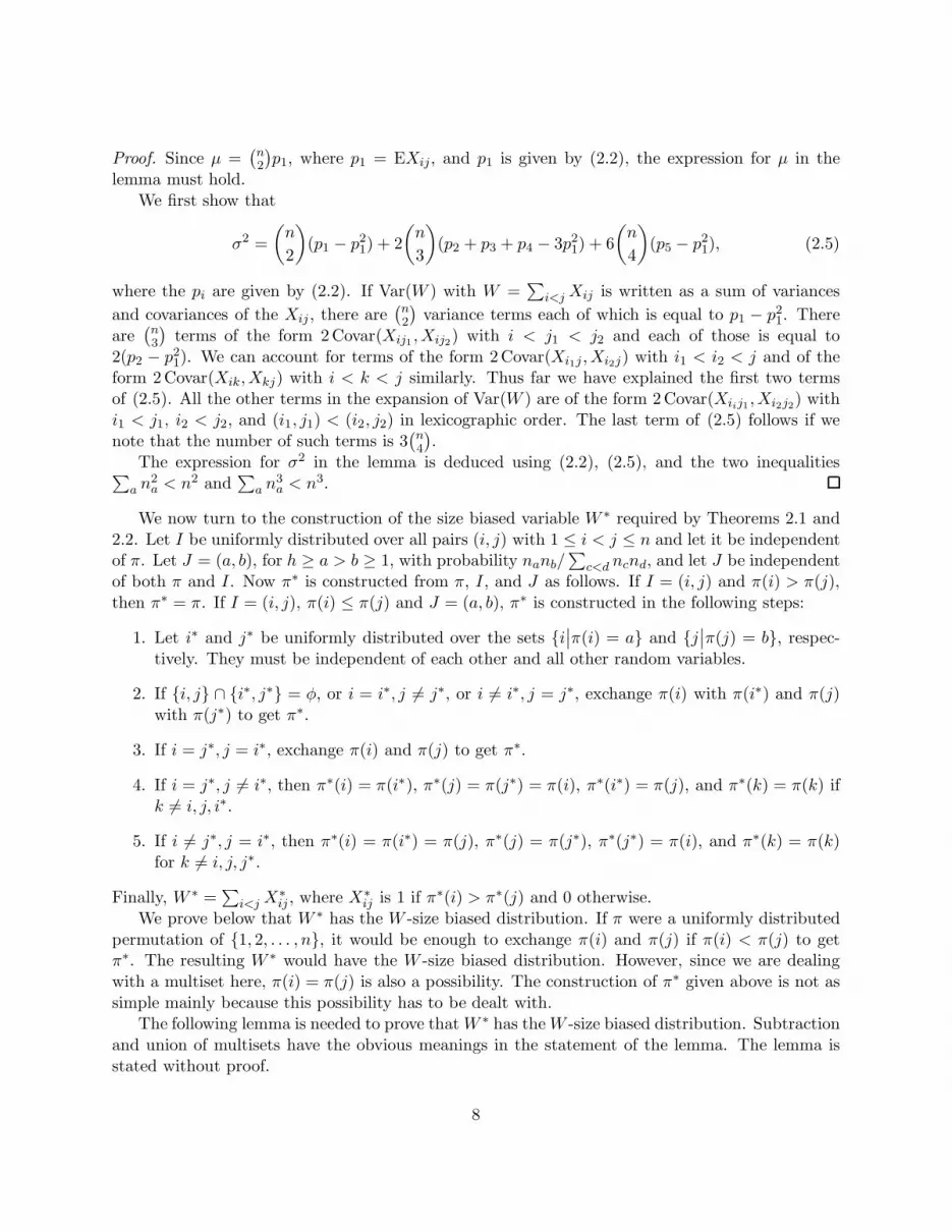
We now turn to the construction of the size biased variable W ∗ required by Theorems 2.1 and2.2. Let I be uniformly distributed over all pairs (i, j) with 1 ≤ i < j ≤ n and let it be independentof π. Let J = (a, b), for h ≥ a > b ≥ 1, with probability nanb/

∑

c<d ncnd, and let J be independentof both π and I. Now π∗ is constructed from π, I, and J as follows. If I = (i, j) and π(i) > π(j),then π∗ = π. If I = (i, j), π(i) ≤ π(j) and J = (a, b), π∗ is constructed in the following steps:

1. Let i∗ and j∗ be uniformly distributed over the sets {i∣

∣π(i) = a} and {j∣

∣π(j) = b}, respec-tively. They must be independent of each other and all other random variables.

2. If {i, j} ∩ {i∗, j∗} = φ, or i = i∗, j 6= j∗, or i 6= i∗, j = j∗, exchange π(i) with π(i∗) and π(j)with π(j∗) to get π∗.

3. If i = j∗, j = i∗, exchange π(i) and π(j) to get π∗.

4. If i = j∗, j 6= i∗, then π∗(i) = π(i∗), π∗(j) = π(j∗) = π(i), π∗(i∗) = π(j), and π∗(k) = π(k) ifk 6= i, j, i∗.

5. If i 6= j∗, j = i∗, then π∗(i) = π(i∗) = π(j), π∗(j) = π(j∗), π∗(j∗) = π(i), and π∗(k) = π(k)for k 6= i, j, j∗.

Finally, W ∗ =∑

i<j X∗

ij , where X∗

ij is 1 if π∗(i) > π∗(j) and 0 otherwise.We prove below that W ∗ has the W -size biased distribution. If π were a uniformly distributed

permutation of {1, 2, . . . , n}, it would be enough to exchange π(i) and π(j) if π(i) < π(j) to getπ∗. The resulting W ∗ would have the W -size biased distribution. However, since we are dealingwith a multiset here, π(i) = π(j) is also a possibility. The construction of π∗ given above is not assimple mainly because this possibility has to be dealt with.

The following lemma is needed to prove that W ∗ has theW -size biased distribution. Subtractionand union of multisets have the obvious meanings in the statement of the lemma. The lemma isstated without proof.

8

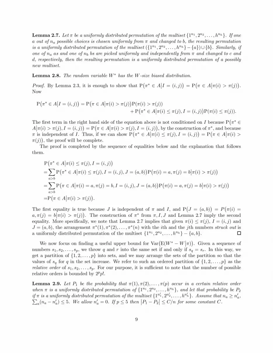
Lemma 2.7. Let π be a uniformly distributed permutation of the multiset {1n1 , 2n2 , . . . , hnh}. If one

a out of na possible choices is chosen uniformly from π and changed to b, the resulting permutation

is a uniformly distributed permutation of the multiset ({1n1 , 2n2 , . . . , hnh}−{a})∪{b}. Similarly, if

one of na as and one of nb bs are picked uniformly and independently from π and changed to c and

d, respectively, then the resulting permutation is a uniformly distributed permutation of a possibly

new multiset.

Lemma 2.8. The random variable W ∗ has the W -size biased distribution.

Proof. By Lemma 2.3, it is enough to show that P(

π∗ ∈ A∣

∣I = (i, j))

= P(

π ∈ A∣

∣π(i) > π(j))

.Now

P(

π∗ ∈ A∣

∣I = (i, j))

= P(

π ∈ A∣

∣π(i) > π(j))

P(π(i) > π(j))

+ P(

π∗ ∈ A∣

∣π(i) ≤ π(j), I = (i, j))

P(π(i) ≤ π(j)).

The first term in the right hand side of the equation above is not conditioned on I because P(

π∗ ∈A∣

∣π(i) > π(j), I = (i, j))

= P(

π ∈ A∣

∣π(i) > π(j), I = (i, j))

, by the construction of π∗, and becauseπ is independent of I. Thus, if we can show P

(

π∗ ∈ A∣

∣π(i) ≤ π(j), I = (i, j))

= P(

π ∈ A∣

∣π(i) >π(j)

)

, the proof will be complete.The proof is completed by the sequence of equalities below and the explanation that follows

them.

P(

π∗ ∈ A∣

∣π(i) ≤ π(j), I = (i, j))

=∑

a>b

P(

π∗ ∈ A∣

∣π(i) ≤ π(j), I = (i, j), J = (a, b))

P(

π(i) = a, π(j) = b∣

∣π(i) > π(j))

=∑

a>b

P(

π ∈ A∣

∣π(i) = a, π(j) = b, I = (i, j), J = (a, b))

P(

π(i) = a, π(j) = b∣

∣π(i) > π(j))

=P(

π ∈ A∣

∣π(i) > π(j))

.

The first equality is true because J is independent of π and I, and P(

J = (a, b))

= P(

π(i) =a, π(j) = b

∣

∣π(i) > π(j))

. The construction of π∗ from π, I, J and Lemma 2.7 imply the secondequality. More specifically, we note that Lemma 2.7 implies that given π(i) ≤ π(j), I = (i, j) andJ = (a, b), the arrangement π∗(1), π∗(2), . . . , π∗(n) with the ith and the jth numbers struck out isa uniformly distributed permutation of the multiset {1n1 , 2n2 , . . . , hnh} − {a, b}.

We now focus on finding a useful upper bound for Var(

E(W ∗ −W∣

∣π))

. Given a sequence ofnumbers s1, s2, . . . , sp, we throw q and r into the same set if and only if sq = sr. In this way, weget a partition of {1, 2, . . . , p} into sets, and we may arrange the sets of the partition so that thevalues of sq for q in the set increase. We refer to such an ordered partition of {1, 2, . . . , p} as therelative order of s1, s2, . . . , sp. For our purpose, it is sufficient to note that the number of possiblerelative orders is bounded by 2pp!.

Lemma 2.9. Let P1 be the probability that π(1), π(2), . . . , π(p) occur in a certain relative order

when π is a uniformly distributed permutation of {1n1 , 2n2 , . . . , hnh}, and let that probability be P2

if π is a uniformly distributed permutation of the multiset {1n′

1 , 2n′

2 , . . . , hn′

h}. Assume that na ≥ n′a,∑

a(na − n′a) ≤ 5. We allow n′a = 0. If p ≤ 5 then∣

∣P1 − P2

∣

∣ ≤ C/n for some constant C.

9

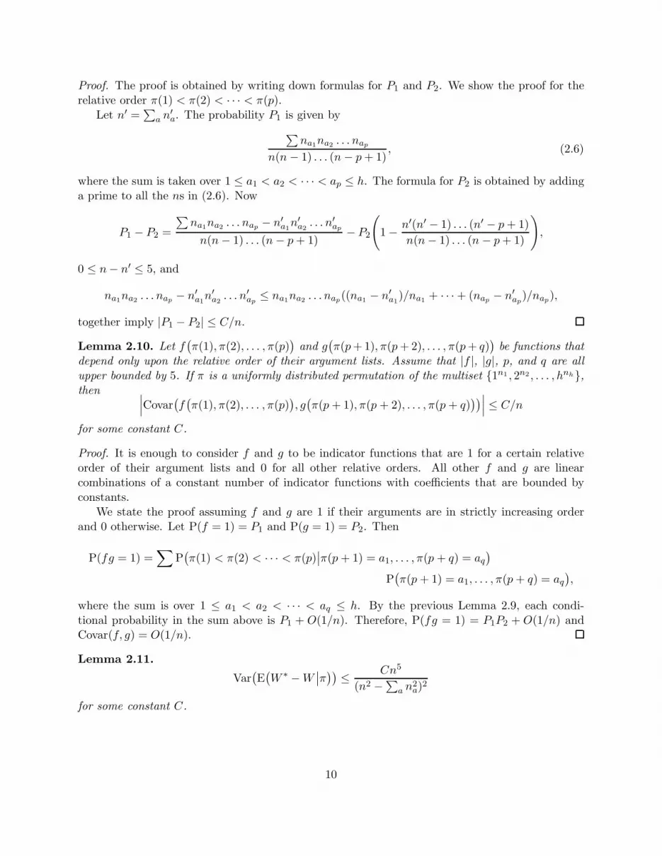
Proof. The proof is obtained by writing down formulas for P1 and P2. We show the proof for therelative order π(1) < π(2) < · · · < π(p).

Let n′ =∑

a n′

a. The probability P1 is given by

∑

na1na2

. . . nap

n(n− 1) . . . (n− p+ 1), (2.6)

where the sum is taken over 1 ≤ a1 < a2 < · · · < ap ≤ h. The formula for P2 is obtained by addinga prime to all the ns in (2.6). Now

P1 − P2 =

∑

na1na2

. . . nap − n′a1n′a2

. . . n′ap

n(n− 1) . . . (n− p+ 1)− P2

(

1 − n′(n′ − 1) . . . (n′ − p+ 1)

n(n− 1) . . . (n − p+ 1)

)

,

0 ≤ n− n′ ≤ 5, and

na1na2

. . . nap − n′a1n′a2

. . . n′ap≤ na1

na2. . . nap((na1

− n′a1)/na1

+ · · · + (nap − n′ap)/nap),

together imply |P1 − P2| ≤ C/n.

Lemma 2.10. Let f(

π(1), π(2), . . . , π(p))

and g(

π(p+ 1), π(p+ 2), . . . , π(p+ q))

be functions that

depend only upon the relative order of their argument lists. Assume that |f |, |g|, p, and q are all

upper bounded by 5. If π is a uniformly distributed permutation of the multiset {1n1 , 2n2 , . . . , hnh},then

∣

∣

∣Covar

(

f(

π(1), π(2), . . . , π(p))

, g(

π(p + 1), π(p + 2), . . . , π(p + q)))

∣

∣

∣≤ C/n

for some constant C.

Proof. It is enough to consider f and g to be indicator functions that are 1 for a certain relativeorder of their argument lists and 0 for all other relative orders. All other f and g are linearcombinations of a constant number of indicator functions with coefficients that are bounded byconstants.

We state the proof assuming f and g are 1 if their arguments are in strictly increasing orderand 0 otherwise. Let P(f = 1) = P1 and P(g = 1) = P2. Then

P(fg = 1) =∑

P(

π(1) < π(2) < · · · < π(p)∣

∣π(p + 1) = a1, . . . , π(p + q) = aq

)

P(

π(p + 1) = a1, . . . , π(p + q) = aq

)

,

where the sum is over 1 ≤ a1 < a2 < · · · < aq ≤ h. By the previous Lemma 2.9, each condi-tional probability in the sum above is P1 + O(1/n). Therefore, P(fg = 1) = P1P2 + O(1/n) andCovar(f, g) = O(1/n).

Lemma 2.11.

Var(

E(

W ∗ −W∣

∣π))

≤ Cn5

(n2 −∑a n2a)

2

for some constant C.

10

Proof. If π(i) > π(j), E(

W ∗ −W∣

∣π, I = (i, j))

= 0. If π(i) ≤ π(j),

E(

W ∗ −W∣

∣π, I = (i, j))

=1

∑

a>b nanb

∑

i∗,j∗

n∑

l=1

ψπ(i, j, i∗, j∗, l),

where (i∗, j∗) takes all∑

a>b nanb possible values with π(i∗) > π(j∗) and ψπ(i, j, i∗, j∗, l) is thechange in the number of inversions between position l and positions i, j, i∗, j∗ when π(i), π(j),π(i∗), π(j∗) are exchanged to construct π∗. Note that |ψπ| ≤ 4. We now have

E(

W ∗ −W∣

∣π)

=1

(n2

)∑

a>b nanb

∑

i,j

∑

i∗,j∗

n∑

l=1

ψπ(i, j, i∗, j∗, l), (2.7)

where i, j take all values satisfying 1 ≤ i < j ≤ h and π(i) ≤ π(j), and where i∗, j∗ take values asalready indicated.

We use (2.7) to write Var(

E(

W ∗ −W∣

∣π))

as a sum of variance and covariance terms. Thenumber of variance terms is bounded by n5. The number of covariance terms

Covar(

ψπ(i1, j1, i∗

1, j∗

1 , l1), ψπ(i2, j2, i∗

2, j∗

2 , l2))

(2.8)

with {i1, j1, i∗1, j∗1 , l1} ∩ {i2, j2, i∗2, j∗2 , l2} 6= φ is fewer than 25n9. Since |ψπ| ≤ 4, the contribution ofthe variance terms and covariance terms with the property just described is bounded by 16(n5 +

25n9)/((n

2

)

1

2(n2 −∑a n

2a))2

. We have used∑

a>b nanb = 1

2(n2 −∑a n

2a) to obtain this bound.

Covariance terms of the form (2.8) with {i1, j1, i∗1, j∗1 , l1} ∩ {i2, j2, i∗2, j∗2 , l2} = φ remain to beconsidered. The number of such terms is fewer than n10. Lemma 2.10 can be applied to arguethat such covariances are O(1/n) as we may use the fact that π is uniformly distributed to assumei1, j1, i

∗

1, j∗

1 , l1 = 1, 2, 3, 4, 5 and i2, j2, i∗

2, j∗

2 , l2 = 6, 7, 8, 9, 10 with no loss of generality. The proofcan now be easily completed.

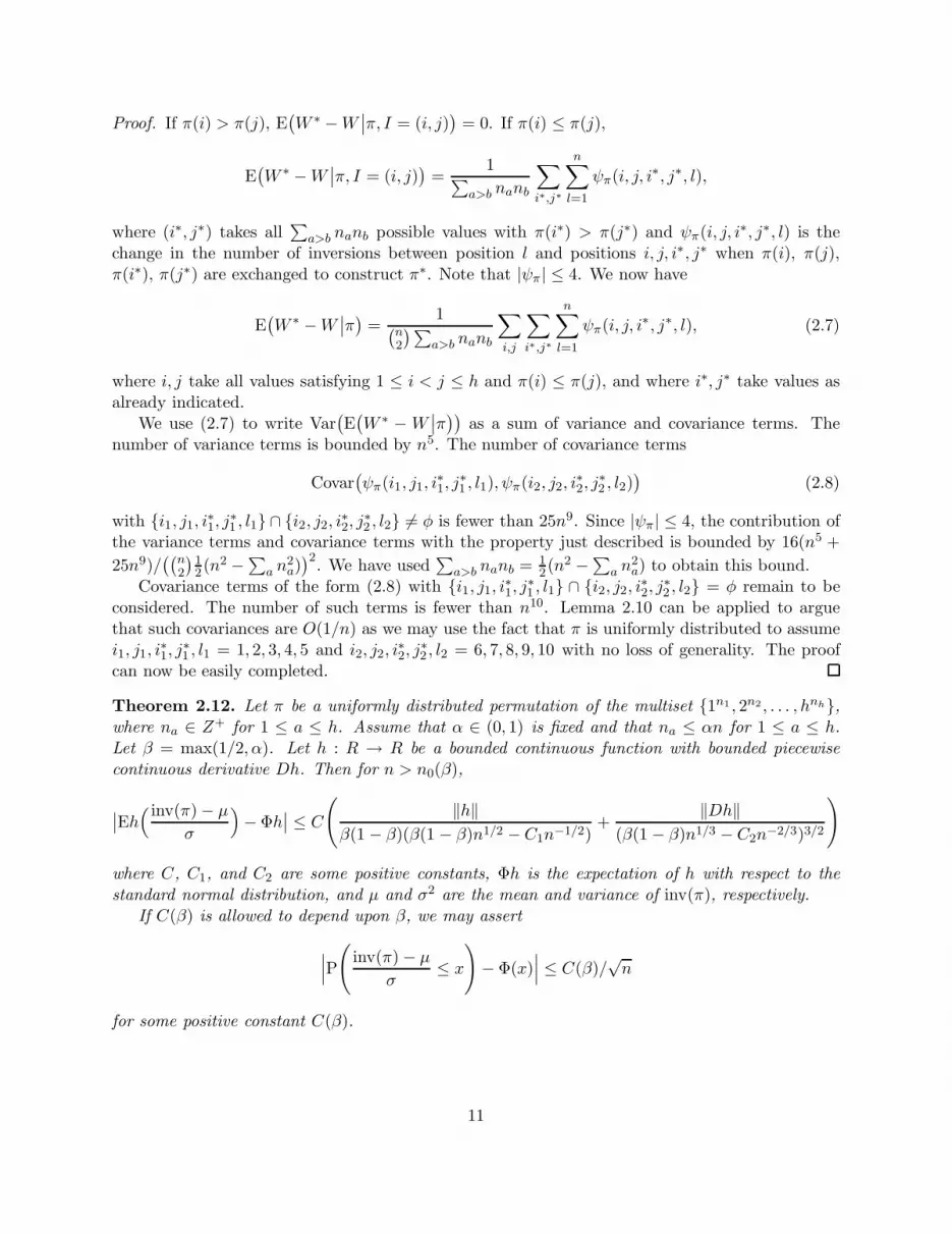
Theorem 2.12. Let π be a uniformly distributed permutation of the multiset {1n1 , 2n2 , . . . , hnh},where na ∈ Z+ for 1 ≤ a ≤ h. Assume that α ∈ (0, 1) is fixed and that na ≤ αn for 1 ≤ a ≤ h.Let β = max(1/2, α). Let h : R → R be a bounded continuous function with bounded piecewise

continuous derivative Dh. Then for n > n0(β),

∣

∣Eh( inv(π) − µ

σ

)

− Φh∣

∣ ≤ C

(

‖h‖β(1 − β)(β(1 − β)n1/2 − C1n−1/2)

+‖Dh‖

(β(1 − β)n1/3 − C2n−2/3)3/2

)

where C, C1, and C2 are some positive constants, Φh is the expectation of h with respect to the

standard normal distribution, and µ and σ2 are the mean and variance of inv(π), respectively.

If C(β) is allowed to depend upon β, we may assert

∣

∣

∣P

(

inv(π) − µ

σ≤ x

)

− Φ(x)∣

∣

∣≤ C(β)/

√n

for some positive constant C(β).

11

Proof. Let W = inv(π). By Lemmas 2.4 and 2.6, σ2 ≥ (β(1− β)/12)n3 +O(n2) and µ ≤ n2/4. ByLemmas 2.4 and 2.11, Var

(

E(

W ∗−W∣

∣π))

≤ Cn/(β(1−β))2 for some constant C. By construction

of the size biased variable W ∗,∣

∣W ∗ −W∣

∣ ≤ 4n, and therefore E(

W ∗ −W)2 ≤ 16n2. If we note

that Var(

E(

W ∗ −W∣

∣W))

≤ Var(

E(

W ∗ −W∣

∣π))

, Theorem 2.1 can be applied to prove the firstpart of this theorem.

The second part is proved using Theorem 2.2. By construction of W ∗, |W ∗ −W | ≤ 4n. There-fore we can take B = 4n. The inequality B ≤ σ3/2/

√6µ must hold for large enough n by bounds

for σ and µ given above.

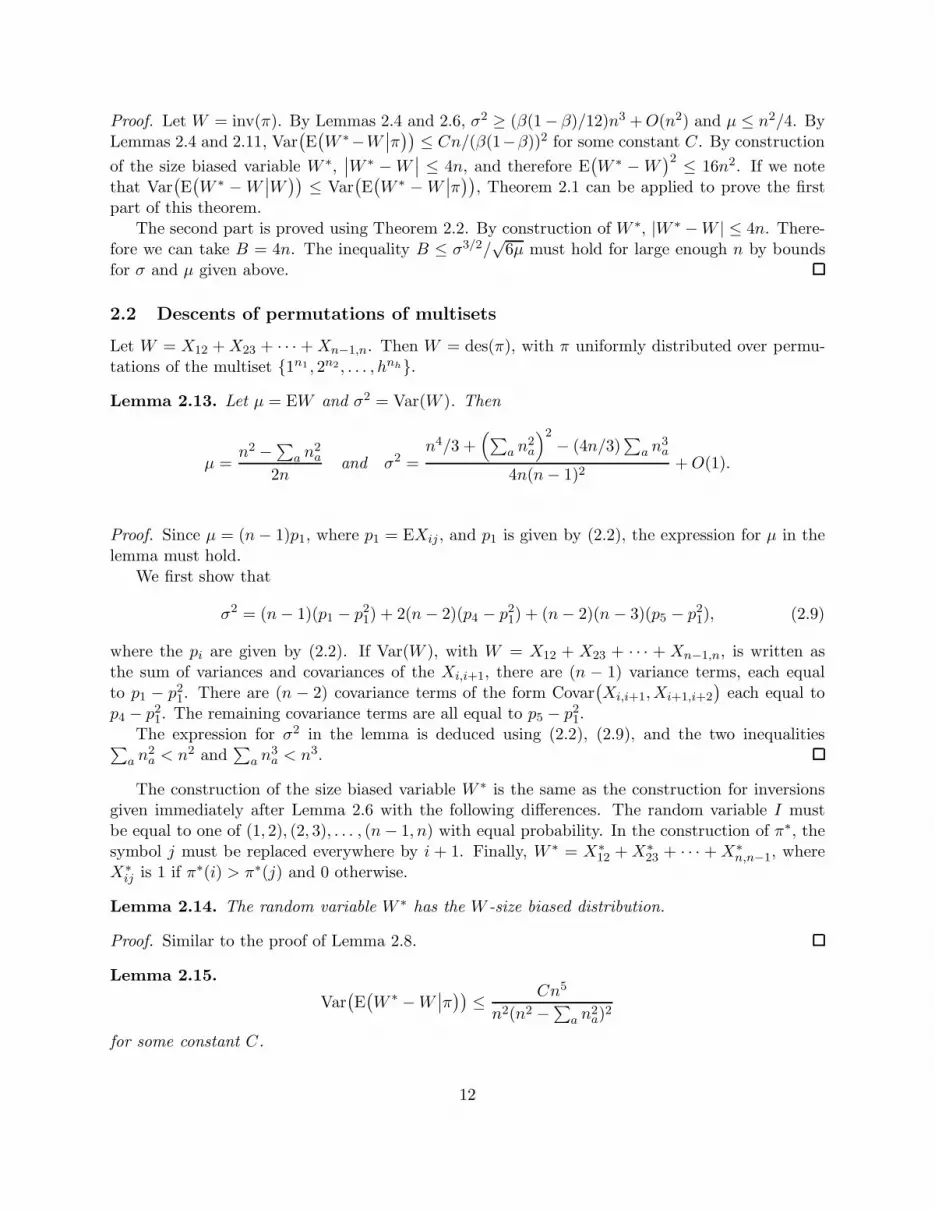
2.2 Descents of permutations of multisets

Let W = X12 +X23 + · · · +Xn−1,n. Then W = des(π), with π uniformly distributed over permu-tations of the multiset {1n1 , 2n2 , . . . , hnh}.

Lemma 2.13. Let µ = EW and σ2 = Var(W ). Then

µ =n2 −∑a n

2a

2nand σ2 =

n4/3 +(

∑

a n2a

)2

− (4n/3)∑

a n3a

4n(n− 1)2+O(1).

Proof. Since µ = (n− 1)p1, where p1 = EXij , and p1 is given by (2.2), the expression for µ in thelemma must hold.

We first show that

σ2 = (n− 1)(p1 − p21) + 2(n− 2)(p4 − p2

1) + (n− 2)(n − 3)(p5 − p21), (2.9)

where the pi are given by (2.2). If Var(W ), with W = X12 + X23 + · · · + Xn−1,n, is written asthe sum of variances and covariances of the Xi,i+1, there are (n − 1) variance terms, each equalto p1 − p2

1. There are (n − 2) covariance terms of the form Covar(

Xi,i+1,Xi+1,i+2

)

each equal top4 − p2

1. The remaining covariance terms are all equal to p5 − p21.

The expression for σ2 in the lemma is deduced using (2.2), (2.9), and the two inequalities∑

a n2a < n2 and

∑

a n3a < n3.

The construction of the size biased variable W ∗ is the same as the construction for inversionsgiven immediately after Lemma 2.6 with the following differences. The random variable I mustbe equal to one of (1, 2), (2, 3), . . . , (n− 1, n) with equal probability. In the construction of π∗, thesymbol j must be replaced everywhere by i + 1. Finally, W ∗ = X∗

12 +X∗

23 + · · · +X∗

n,n−1, whereX∗

ij is 1 if π∗(i) > π∗(j) and 0 otherwise.

Lemma 2.14. The random variable W ∗ has the W -size biased distribution.

Proof. Similar to the proof of Lemma 2.8.

Lemma 2.15.

Var(

E(

W ∗ −W∣

∣π))

≤ Cn5

n2(n2 −∑a n2a)

2

for some constant C.

12

Proof. By arguing as in the proof of Lemma 2.11, we get

E(

W ∗ −W∣

∣π)

=2

n(n2 −∑a n2a)

∑

i

∑

i∗,j∗

ψπ(i, i∗, j∗). (2.10)

In (2.10), i takes all values such that π(i) ≤ π(i+1), (i∗, j∗) takes all values such that π(i∗) > π(j∗),and ψπ(i, i∗, j∗) = des(π∗)−des(π), where π∗ is constructed by exchanging π(i), π(i+1), π(i∗), π(j∗)as described. Note that |ψπ| ≤ 7.

We use (2.10) to write Var(

E(

W ∗−W∣

∣π))

as the sum of variance and covariance terms. Thereare O(n3) variance terms of the Var(ψπ). The number of terms of the form

Covar(

ψπ(i1, i∗

1, j∗

1), ψπ(i2, i∗

2, j∗

2 ))

, (2.11)

where one of the numbers {i1, i∗1, j∗1} differs from one of the numbers {i2, i∗2, j∗2} by 3 or less inmagnitude is O(n5). The magnitude of such covariance terms and of the variance terms is boundedby 49. The number of covariance terms of the form (2.11) where none of the numbers {i1, i∗1, j∗1}differs from any one of the numbers {i2, i∗2, j∗2} by 3 or less in magnitude is O(n6). By Lemma 2.10,the magnitude of such covariance terms is O(1/n). The proof is now easily completed.

It is worth noting again that β4 − 4β2 + 4β − 1 = (1 − β)2(β2 + 2β − 1) > 0 for β ∈ [1/2, 1).

Theorem 2.16. Let π be a uniformly distributed permutation of the multiset {1n1 , 2n2 , . . . , hnh},where na ∈ Z+ for 1 ≤ a ≤ h. Assume that α ∈ (0, 1) is fixed and that na ≤ αn for 1 ≤ a ≤ h.Let β = max(1/2, α). Let h : R → R be a bounded continuous function with bounded piecewise

continuous derivative Dh. Then for n > n0(β),

∣

∣Eh(des(π) − µ

σ

)

− Φh∣

∣ ≤ C

(

‖h‖β(1 − β)

√n(β4 − 4β2 + 4β − 1 − C1n−1)

+‖Dh‖

((β4 − 4β2 + 4β − 1)n1/3 − C2n−2/3)3/2

)

where C, C1, and C2 are some positive constants, Φh is the expectation of h with respect to the

standard normal distribution, and µ and σ2 are the mean and variance of des(π), respectively.

If C(β) is allowed to depend upon β, we may assert

∣

∣

∣P

(

des(π) − µ

σ≤ x

)

− Φ(x)∣

∣

∣≤ C(β)/

√n

for some positive constant C(β).

Proof. Let W = des(π). By Lemmas 2.4, 2.5 and 2.13 σ2 ≥ ((β4 − 4β2 + 4β − 1)/4)n + O(1) andµ ≤ n/2. By Lemmas 2.4 and 2.15, Var

(

E(

W ∗ −W∣

∣π))

≤ C/(

nβ2(1 − β)2)

for some constant C.

By construction of the size biased variable W ∗,∣

∣W ∗ −W∣

∣ ≤ 7, and therefore E(

W ∗ −W)2 ≤ 49.

If we note that Var(

E(

W ∗ −W∣

∣W))

≤ Var(

E(

W ∗ −W∣

∣π))

, Theorem 2.1 can be applied to provethe first part of this theorem.

The second part is proved using Theorem 2.2. By construction of W ∗, |W ∗ −W | ≤ 8. Thereforewe can take B = 8. The inequality B ≤ σ3/2/

√6µ must hold for large enough n by bounds for σ

and µ given above.

13

A C G T

A 4229414 2833985 4154304 3165323

C 4221129 4044958 1057112 4150574

G 3423863 3180474 4056078 2846197

T 2508620 3414357 4239118 4260148

A C G T

A 103435711266825 94175991781325 94404662110136 103982892949612

C 99617649978799 90771286164651 90984870248490 100143945584446

G 99861289457776 91000167345198 91214277105966 100388853252680

T 103452603097706 94178097170636 94406787118036 104000539364403

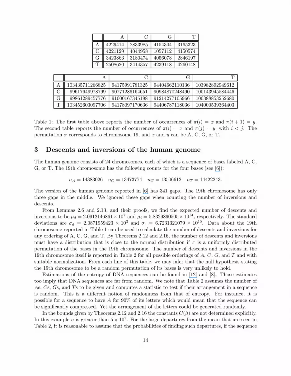
Table 1: The first table above reports the number of occurrences of π(i) = x and π(i + 1) = y.The second table reports the number of occurrences of π(i) = x and π(j) = y, with i < j. Thepermutation π corresponds to chromosome 19, and x and y can be A, C, G, or T.

3 Descents and inversions of the human genome

The human genome consists of 24 chromosomes, each of which is a sequence of bases labeled A, C,G, or T. The 19th chromosome has the following counts for the four bases (see [6]):

nA = 14383026 nC = 13473774 nG = 13506612 nT = 14422243.

The version of the human genome reported in [6] has 341 gaps. The 19th chromosome has onlythree gaps in the middle. We ignored these gaps when counting the number of inversions anddescents.

From Lemmas 2.6 and 2.13, and their proofs, we find the expected number of descents andinversions to be µd = 2.0912146861×107 and µi = 5.8329890505×1014 , respectively. The standarddeviations are σd = 2.0871959423 × 103 and σi = 6.7231321079 × 1010. Data about the 19thchromosome reported in Table 1 can be used to calculate the number of descents and inversions forany ordering of A, C, G, and T. By Theorems 2.12 and 2.16, the number of descents and inversionsmust have a distribution that is close to the normal distribution if π is a uniformly distributedpermutation of the bases in the 19th chromosome. The number of descents and inversions in the19th chromosome itself is reported in Table 2 for all possible orderings of A, C, G, and T and withsuitable normalization. From each line of this table, we may infer that the null hypothesis statingthe 19th chromosome to be a random permutation of its bases is very unlikely to hold.

Estimations of the entropy of DNA sequences can be found in [12] and [8]. Those estimatestoo imply that DNA sequences are far from random. We note that Table 2 assumes the number ofAs, Cs, Gs, and T s to be given and computes a statistic to test if their arrangement in a sequenceis random. This is a different notion of randomness from that of entropy. For instance, it ispossible for a sequence to have A for 90% of its letters which would mean that the sequence canbe significantly compressed. Yet the arrangement of the letters could be generated randomly.

In the bounds given by Theorems 2.12 and 2.16 the constants C(β) are not determined explicitly.In this example n is greater than 5× 107. For the large departures from the mean that are seen inTable 2, it is reasonable to assume that the probabilities of finding such departures, if the sequence

14

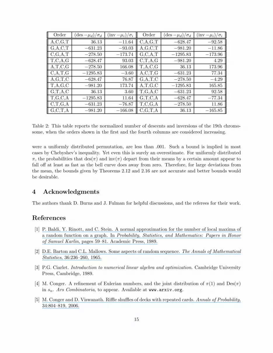
Order (des−µd)/σd (inv−µi)/σi Order (des−µd)/σd (inv−µi)/σi

A,C,G,T 36.13 −11.64 C,A,G,T −628.47 −92.58

G,A,C,T −631.23 −93.03 A,G,C,T −981.20 −11.86

C,G,A,T −278.50 −173.74 G,C,A,T −1295.83 −173.96

T,C,A,G −628.47 93.03 C,T,A,G −981.20 4.29

A,T,C,G −278.50 166.08 T,A,C,G 36.13 173.96

C,A,T,G −1295.83 −3.60 A,C,T,G −631.23 77.34

A,G,T,C −628.47 76.87 G,A,T,C −278.50 −4.29

T,A,G,C −981.20 173.74 A,T,G,C −1295.83 165.85

G,T,A,C 36.13 3.60 T,G,A,C −631.23 92.58

T,G,C,A −1295.83 11.64 G,T,C,A −628.47 −77.34

C,T,G,A −631.23 −76.87 T,C,G,A −278.50 11.86

G,C,T,A −981.20 −166.08 C,G,T,A 36.13 −165.85

Table 2: This table reports the normalized number of descents and inversions of the 19th chromo-some, when the orders shown in the first and the fourth columns are considered increasing.

were a uniformly distributed permutation, are less than .001. Such a bound is implied in mostcases by Chebyshev’s inequality. Yet even this is surely an overestimate. For uniformly distributedπ, the probabilities that des(π) and inv(π) depart from their means by a certain amount appear tofall off at least as fast as the bell curve does away from zero. Therefore, for large deviations fromthe mean, the bounds given by Theorems 2.12 and 2.16 are not accurate and better bounds wouldbe desirable.

4 Acknowledgments

The authors thank D. Burns and J. Fulman for helpful discussions, and the referees for their work.

References

[1] P. Baldi, Y. Rinott, and C. Stein. A normal approximation for the number of local maxima ofa random function on a graph. In Probability, Statistics, and Mathematics: Papers in Honor

of Samuel Karlin, pages 59–81. Academic Press, 1989.

[2] D.E. Barton and C.L. Mallows. Some aspects of random sequence. The Annals of Mathematical

Statistics, 36:236–260, 1965.

[3] P.G. Ciarlet. Introduction to numerical linear algebra and optimization. Cambridge UniversityPress, Cambridge, 1989.

[4] M. Conger. A refinement of Eulerian numbers, and the joint distribution of π(1) and Des(π)in sn. Ars Combinatoria, to appear. Available at www.arxiv.org.

[5] M. Conger and D. Viswanath. Riffle shuffles of decks with repeated cards. Annals of Probability,34:804–819, 2006.

15

[6] International Human Genome Consortium. Finishing the euchromatic sequence of the humangenome. Nature, 431:931–945, 2004.

[7] P. Diaconis. Group Representations in Probability and Statistics. Institute of MathematicalStatistics, USA, 1988.

[8] R.N. Mantegna et al. Linguistic features of noncoding dna. Physical Review Letters, 15:3169–3172, 1994.

[9] J. Fulman. Stein’s method and non-reversible Markov chains. In Stein’s method: expository

lectures and applications, pages 66–77. Institute of Mathematical Statistics, Hayward, CA,2004.

[10] L. Goldstein. Berry Esseen bounds for combinatorial central limit theorems and pattern oc-curences, using zero and size biasing. Journal of Applied Probability, 42:661–683, 2005.

[11] L. Goldstein and Y. Rinott. Multivariate normal approximations by Stein’s method and sizebias couplings. Journal of Applied Probability, 33:1–17, 1996.

[12] V.D. Gusev, L.A. Nemytikov, and N.A. Chuzanova. On the complexity measure of geneticsequences. Bioinformatics, 15:994–999, 1999.

[13] D.E. Knuth. Seminumerical Algorithms, The Art of Computer Programming, Vol. 2. Addison-Wesley, Massachusetts, 3rd edition, 1997.

[14] D.E. Knuth. Searching and Sorting, The Art of Computer Programming, Vol. 3. Addison-Wesley, Massachusetts, 3rd edition, 1998.

[15] H. Levene and J. Wolfowitz. The covariance matrix of runs up and down. The Annals of

Mathematical Statistics, 15:58–69, 1944.

[16] P.A. MacMahon. Combinatory Analysis, Vol. 1. Cambridge University Press, Cambridge,1915.

[17] Y. Rinott and V. Rotar. On coupling constructions and rates in the CLT for dependentsummands with applications to the antivoter model and U-statistics. The Annals of Applied

Probability, 7:1080–1105, 1997.

[18] R. Stanley. Eulerian partitions of a unit hypercube. In M. Aigner, editor, Higher Combina-

torics. Reidel, Dordrecht, 1977.

[19] C. Stein. A bound for the error in the normal approximation of the distribution of a sum ofdependent random variables. Proceedings of the Sixth Berkeley Symposium on Mathematical

Statistics and Probability, 2:583–602, 1972.

[20] C. Stein. Approximate Computation of Expectations. Institute of Mathematical Statistics,Hayward, CA, 1986.

[21] J. Wolfowitz. Asymptotic distribution of runs up and down. The Annals of Mathematical

Statistics, 15:163–172, 1944.

16