arX

iv:1

212.

6907

v1 [

cs.N

I] 3

1 D

ec 2

012

Nonlinear Instabilities of D2TCP-II

Abhisek Mukhopadhyay1 Priya Ranjan2

Abstract— In the era of heavy-duty transmission controlprotocols (TCP), adapted for extremely hi-bandwidth data-centers; the fundamental question of stable interaction witheither proposed/customized active queue management(AQM)orpopularly discussed Random Early Detection (RED) remainsa hotly debated issue. While there are claims of “oscillation”only dynamical behavior, there are equally large numberof claims which demonstrate the chaotic nature of differentflavors of TCP and their AQM interaction. In this work,we provide a sound and analytical mathematical model ofDTCP/D2TCP and study their interaction with threshold basedpacket marking policy. Our work shows that for a simplescenario this interaction is chaotic in nature and has largevariability in dynamical behavior over orders of magnitudechanges in parameter range as demonstrated by bifurcationdiagrams. We conclude with numerical simulation evidence thatchaotic behavior of protocols is inherent in their design whichthey inherit from their early vanilla TCP days, and it hasserious implications for data-center throughput, load batchingand collapse in Incast kind of scenario.

I. I NTRODUCTION

In the era of record breaking memory to memory through-put, dynamical behavior of Internet protocols has become keyto achieving predictability, optimal utilization of resourcesand dynamic stability in throughput allocation among partic-ipating agents/devices/entities. With the recent proposals ofDCTCP, D2TCP, CTCP, D3 etc, a new research area of super-optimal and dynamically oscillating behavior of transportprotocols has been forging itself.

We based our analysis and discrete time models in contrastto the early claims of periodic only behavior in DCTCPand its different relatives and derivatives. We show againthat discrete time models are the right framework to thinkabout next generation successors of TCP and chaos remainsa dominant phenomenon in the case of wildly fluctuatingparameter ranges. In particular, we compare its dynamicalbehavior with switched power electronic circuits and impactoscillators.

II. OBJECTIVE OF THE STUDY

The objectives of our study are as follows:

1) Build a discrete time mathematical model of DCTCP-AQM interaction.

2) Use techniques from discrete time maps to analyzetheir behavior.

1A.Mukhopadhyay is with the department of Electronics and Commu-nication Engineering, National Institute of Technology, Durgapur, WestBengal, India-71320.E-Mail- abhisekmukhopadhyay[at]gmail. com

2 P. Ranjan is with the department of Electronics and CommunicationEngineering, Templecity Institute of Technology and Engineering, Khurda,Orissa, India-752057.E-mail-pranjan[at]gmail. com

3) Simulate and demonstrate chaotic behavior.

III. DCTCP CONGESTION CONTROL ALGORITHM:AN

OVERVIEW

In this section we describe qualitatively the DCTCPalgorithm[1] with its major algorithmic details so as to laya foundation for our discrete modeling. We also describethe fact that D2TCP [2] can be built upon DCTCP throughcertain specific changes and we also argue that D2TCPis more general and that DCTCP forms a special case ofD2TCP.

A. A simple active queue management scheme at the Switch:

The marking scheme involves the use of only a singleparameterK. An arriving packet is marked with its CE(Congestion Experienced) bit set to 1 iff upon its arrival theinstantaneous queue size is greater thanK.

B. ECN Echo at receiver

A difference between conventional TCP receivers andDCTCP receiver is in the way the status of the incoming CEbits are conveyed back to the sender. For the DCTCP receiverACKs (ACK- Acknowledgment Packet) every single incom-ing packet and its ECN(External Congestion Notification)-Echo flag bit set to 1 when a marked packet (CE=1) isreceived. DCTCP tries to convey the exact sequence of thereceived code points. This is accomplished by sending adelayed ACK (1 cumulative ACK for a set of m receivedpackets) which contains the sequence of ECN- Echo flagbased on last m incoming packets. Thus the controller at thesender can make out the congestion status in the queue uponreception of the delayed ACK.

C. Controller at the sender

The sender maintains a running estimate of the fractionof packets that are marked. Calledα, Which is updated ineveryRTT (Round Trip Time) as follows:

α ←− (1− g) ·α + g ·F (1)

g here is the weight associated to the marked fraction.Fis the fraction of packets marked and is given by the dropprobability in the current window. Given the fact that thesender receives Marks for every packet sent when the queuelength is higher than the threshold and does not receive anymarks when the queue length is below thresholdK thus (9)implies thatα estimates the probability that the queue size isgreater thanK. Essentially,α close to 0 implies low levelsof congestion and when close to 1 implies high levels ofcongestion.

D. Window size control at the sender :

The only difference between a DCTCP Sender and aTCP Sender is how each react on receiving the ACK withECN flag on. In the slow start phase the Window sizeincreases slowly in both the cases to estimate the availablebandwidth. On receiving congestion notification The TCPalways controls congestion by halving the window sizeand then slowly increasing additively in the congestionavoidance phase. Where as in the DCTCP scheme when itsenses congestion the window size is modified as:

cwnd←− (1−α2) · cwnd (2)

Thus the congestion extent determines the change in thewindow size. It is only slightly reduced at low levels ofcongestion and when congestion levels are high ,say 1 thenthe congestion window is reduced by half as in TCP.This isthe chief contribution of DCTCP in maintaining a low queuelength without compromising throughput.

In Deadline Aware Data Center TCP (D2TCP) all theessential components of DCTCP is kept same but theα(congestion history parameter) is modified as :α = αγ Whereγ is the deadline factor. A highγ implies acloser deadline and a low value ofγ implies far deadline.So DCTCP is a special case of D2TCP withγ = 1 whichimplies long lived flows with no deadline.

IV. CONVENTIONAL RED CONTROLLER AT SWITCH

The RED [3] mechanism is available as an External Con-gestion Notification (ECN) mechanism in modern switches.This section gives a brief discussion on the RED (RandomEarly Detection) at the switch and the modification thatneeds to be made in order to support the DCTCP queuemanagement scheme without the need of extra externalhardware. We present here a discrete model of the REDsystem and the sampling interval is one RTT.

The RED module calculates exponentially weighted mov-ing average of the queue size at the switch end.

Let w be the exponential averaging weight andqk be theinstantaneous queue size. On each packet arrival the REDalgorithm updates its average queue length(qk) to:

qk+1 = (1−w) ·qk +w ·qk+1 (3)

If the average queue length is below a certain advertisedthresholdqmin then the packet is admitted into the queue forsubsequent transmission through the link and when it exceedsqmax it is either dropped or marked as per requirement. If itlies in the range ofqmin andqmax then it is dropped/markedwith a probabilityp given by:

pk+1 =

0 if qk+1 < qminqk+1−qminqmax−qmin

· pmax if qmin ≤ qk+1≤ qmax

1 if qk+1 > qmax

(4)

A. Implementation of DCTCP packet marking strategythrough RED

To implement DCTCP packet marking strategy throughRED we need to:

1) Setqmin = qmax = K2) The decision making should be with respect to the

instantaneous queue size(qk) instead of the averagequeue size.

Thus implementing the above (4) becomes

pk+1 =

{

0 if qk+1≤ K

1 if qk+1 > K(5)

Thus,(5) gives us the hard control required in the case ofDCTCP algorithm.

V. DERIVATION OF A DISCRETE MODEL FOR A NETWORK

EMPLOYING DCTCPAT THE SENDER END AND MODIFIED

RED AT THE SWITCH.

A. Background

We model the D2TCP system along with its implicitcongestion control mechanism at the switch implementedthrough available RED module, as a discrete time mapobtained by periodically sampling the system state. Sincewindow size and queue size behave as step functions of anRTT,one RTT is the sampling interval that captures theirchanges. Based on the DCTCP algorithm we propose ourdiscrete model that takes window size and congestion historyas state variables. We develop the expressions for a singleactive connection so as to present the dynamics of the queuesize and study the effect of the changes of parameter on theit. The model can be extended without the loss of generalityto N synchronized connections.

B. The model

A complex network employing DCTCP is essentially afeedback loop in which the senders adjust their rate byobserving the rate of packet loss i. e by a feedback fromthe router. Each flow at a router sends packets that are

Fig. 1. Figure showing the feedback mechanism of DCTCP

queued in the shallow buffer1 for subsequent transmissionthrough the link. The packets are marked following a controlstrategy employed at the router end. DCTCP employs a

1Shallow Buffer means buffers having low capacity in high speed switches

bursty marking strategy at the router following (5). Whenthe sender notices the packets are being marked it adjusts itssending rate accordingly,In the case of DCTCP the windowsize is reduced following a congestion history parameterα. The logical structure of DCTCP congestion controller isgiven in Figure 1. This forms the basis of formulation of thediscrete mathematics in subsequent sections and its physicalimplications. A similar analysis has been done in[4] to modelthe behavior of TCP-RED interaction.

C. A discrete modeling of the system

1) Assumptions: We make the following assumptions inour model.

• There is one active connection and the connection islong lived that is, there is always sufficient data to send.

• The ACK packets are never lost.• Round Trip propagation delay in the link and the packet

size is constant.• The state variables of the system are sampled at the end

of every RTT interval.• The process starts with an empty buffer.

2) Dynamical Modeling of the parameters: We first modelthe dynamics of the window sizeW using a discrete approx-imation of (2) for more general D2TCP case. LetWk ,qk

,αk andγ be the window size ,instantaneous queue size ,theweighted fraction of the marked packets and the deadline ofthe flow at the end of thekth sampling interval. The windowsize for the next interval is determined by the queue size inthat interval2, it is given by:

Wk+1 =

{

(1−αγ

k2 ) ·Wk if qk+1 > K,

Wk +1 otherwise.(6)

The queue size at the sampling periodk + 1 can bedetermined from the window size atk and the queue sizeduring kth interval as:

qk+1 = qk +Wk−CM·RTTk+1

= qk +Wk−CM· (qk ·

MC

+ d)

=Wk−C ·dM

(7)

In (7) , CM gives the link capacity in packets/s.

RT Tk+1 = d+qk ·MC ; gives the Round Trip Time at

the k+1th intervald- Round trip propagation delay in the linkC-Capacity andM -Packet Size.

As the buffer is limited by its sizeB. And a negative queuesize has no meaning,we can set realistic bounds onqk+1 as,

qk+1 = min(max(Wk−C ·dM

,0),B) (8)

2The window size calculated at thekth interval determines how manypackets to schedule for transfer in the next interval so the window size inthe kth interval participates in the queue generation in thek+1th interval

The probabilisticbursty marking scheme at the switch re-mains (5).The congestion history parameter is updated everyRT T as,

αk+1 = (1− g) ·αk + g · pk+1 (9)

Or alternatively,using (5),

αk+1 =

{

(1− g) ·αk+ g if qk+1 > K,

(1− g) ·αk otherwise.(10)

D. The Map

In this model as the instantaneous queue size is taken intoconsideration for the marking of packets so, the queue buildup has no memory and depends only on the window sizeof the previous instant. Thus, the queue sizeqk is not anindependent parameter. The independent parameters are thecongestion history (αk) and the window size (Wk).Substituting (7) in (6) we have,

Wk+1 =

{

(1−αγ

k2 ) ·Wk if Wk−

C·dM > K,

Wk +1 otherwise.(11)

and substituting (7) in (10) we have,

αk+1 =

{

(1− g) ·αk + g if Wk−C·dM > K,

(1− g) ·αk otherwise.(12)

thus (7),(11),(12) give the map form that can be used tomodel the dynamics of the system.

E. Mathematical analysis of phase space and the borders.

The map ofW has two distinct regions of operation sepa-rated by a borderqk+1 =K. This border on the instantaneousqueue size reflects on the sender side as a new border:Wk = K∗ whereK∗ = C·d

M +K. In The additive increase phasewhere if theWk is less than a threshold valueK∗ implying,qk+1 < K the definition of the map in (11) says that thewindow size slowly increases and this additive increase isindependant ofα. As a result of the additive increase, thewindow size after a certain time hits the threshold (K∗) andthe map becomes discontinuous as the control mechanismkicks in, making the evolution of the window dependenton both the state variables (αk&Wk). The use of congestionhistory to determine the next window size when congestion isdetected is the key feature of DCTCP,thus a highαk impliesa higher cut in the window size in the next stage and viceversa. These features of the evolution of the window size aredemonstrated graphically in Fig. 2 & Fig. 3.

The evolution ofα also follows a similar algorithm withborders playing the role for the discontinuity induced. TheCongestion history for the next step is determined using theknowledge of the queue size in the current step. As long asthe system senses congestion i. eqk+1 > K the congestionhistory successively increases, simultaneously window sizemultiplicatively decreases until it hits the borderK∗ fromthe right side. When theWk becomes less thanK∗ i. ethere is ’no congestion’ feedback,α successively decreasesand correspondingly window size goes into the additive

increase phase until congestion arises again,i. e this timethecongestion window hits the borderK∗ from the left.

Thus, the congestion control system operates by succes-sively switching between two subsystems as a result of thesystem states colliding with border values. This in turn leadsto chaotic dynamics throughborder collision bifurcation aswe will demonstrate later.

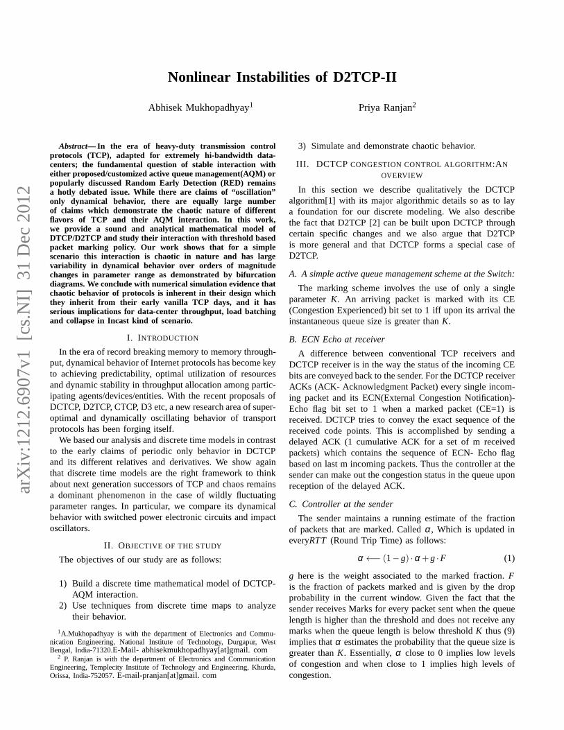
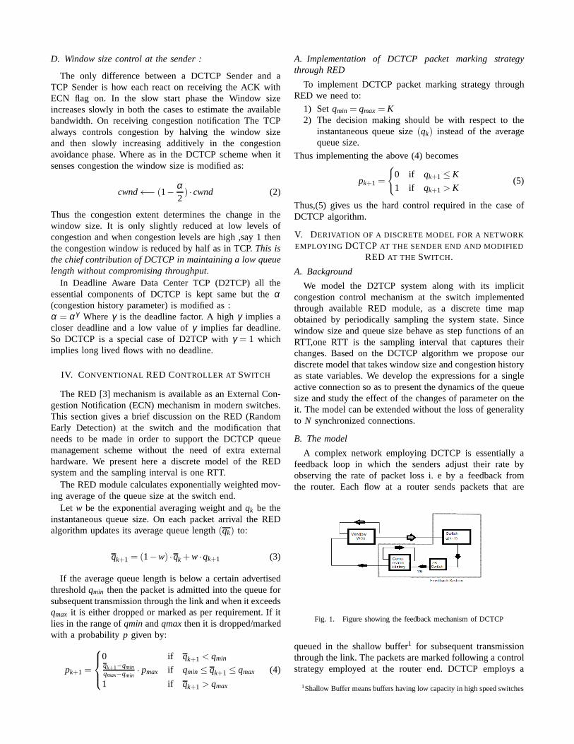
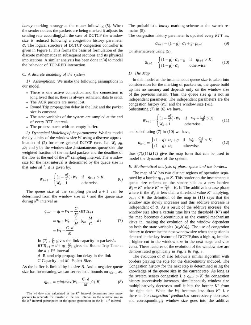
The first and the second return maps forα are given inFig. 4 for the evolution ofqk+1 = 35 through successiveiterations. for generating the maps we use,γ = 1,d =30µs,C = 10Gbps,g = 1/16,K = 15packets, M = 1Kb

30 40 50 60 70 80 90 10020

30

40

50

60

70

80

90

100

Wk(packets)

Wk+

1 (

pa

cke

ts)

constant map

αk=0

αk=0.3

αk=0.6

αk=0.9

Fig. 2. Figure showing the 1st return map ofW at different congestion levels whenK=15

0 0.1 0.2 0.3 0.4 0.5 0.6 0.7 0.8 0.9 135

40

45

50

55

60

65

70

75

αk

Wk+

1,W

k+

2 in

pa

cke

ts

Wk+1

Wk+2

Borderline queue (K) window size=C.d/M + K

Fig. 3. Figure showing the 1st and 2nd return map ofWk = 71.62(qk+1 = 35) atdifferent congestion levels when K=15

0 0.1 0.2 0.3 0.4 0.5 0.6 0.7 0.8 0.9 10

0.1

0.2

0.3

0.4

0.5

0.6

0.7

0.8

0.9

αk

αk+

1,α

k+2

αk+1

αk+2

Fig. 4. Figure showing the 1st and 2nd return map ofα whenWk = 71.62(qk+1 = 35)when K=15

VI. N UMERICAL ANALYSIS

The behavior of the map can be explored in parameterspace numerically,in order to find interesting dynamicalphenomena.

A whole range of dynamical scenarios are presented in thissection. The effect of the changes on the system described bypiecewise smooth discontinuous maps are reflected throughbifurcation diagrams.

A. Bifurcation diagrams

When the future state of a dynamical variable is dependenton a particular parameter(s) then variation in the parame-ter(s) would result in change in the dynamical behavior ofthe system on a whole. A bifurcation diagram shows thequalitative changes in the nature or the number of steady statesolutions of the dynamical system as a parameter varies. Onthe horizontal axis we plot the parameter value. The verticalaxis displays a measure of the corresponding fixed points orperiodic orbits3,which coincides with the queue build up inthe present context.

The way to read a bifurcation diagram is to fix a point inthe horizontal axis and draw a vertical line through it. Thenumber of points where the bifurcation curve intersects thevertical line gives us the number of equilibrium points in thatgiven configuration. A single point implies there is a stablefixed point and multiple points imply a periodic long-termbehavior of the system.

We investigate the dynamical behavior of the instantaneousqueue size in a DCTCP (D2TCP) system with a singleconnection when the parameters like Marked fraction weight(g),the round trip propagation delay (d),deadline(γ) and themarking threshold (K) are varied. We draw the bifurcationdiagram by plotting the successive maxima and minima ofthe instantaneous queue size4(in packets) against a parametersetup. Other system parameters are kept fixed at:

C = 10Gbps;M = 1Kb;B = 200packets.

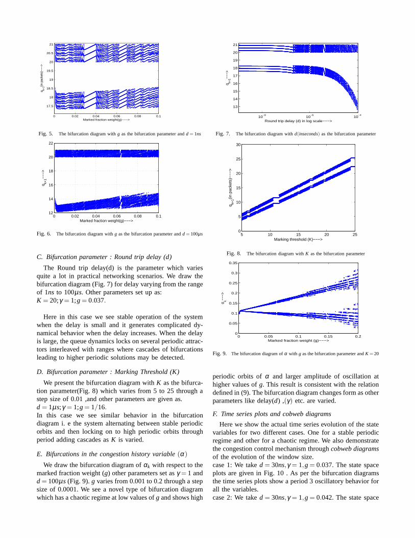
B. Bifurcation parameter : Marked fraction weight (g)

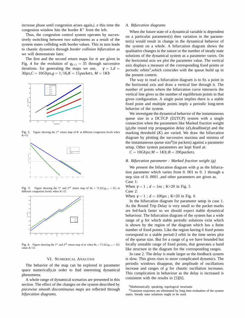
We present the bifurcation diagram withg as the bifurca-tion parameter which varies from 0. 001 to 0. 1 through astep size of 0. 0001 ,and other parameters are given as.Case 1:Whenγ = 1 ; d = 1ns ; K=20 in Fig. 5Case 2:Whenγ = 1 ; d = 100µs ; K=20 in Fig. 6

In the bifurcation diagram for parameter setup in case 1.As the Round Trip Delay is very small so the packet marksare fed-back faster so we should expect stable dynamicalbehaviour. The bifurcation diagram of the system has a widerange ofg for which stable periodic solutions exist whichis shown by the region of the diagram which has a finitenumber of fixed points. Like the region having 6 fixed pointscorrespond to a stable period-3 orbit in the time series plotof the queue size. But for a range ofg we have bounded butlocally unstable range of fixed points, that generates a bandlike structure in the diagram for the corresponding ranges.

In case 2. The delay is made larger so the feedback systemis slow. This gives rises to more complicated dynamics. Theperiodic windows disappear, the amplitude of oscillationsincrease and ranges ofg for chaotic oscillation increases.This complication in behaviour as the delay is increased isconsistent with the results in [5][6].

3Mathematically speaking, topological invariants4Transient responses are eliminated by long time evaluationof the system

states. Steady state solutions ought to be used

0 0.02 0.04 0.06 0.08 0.1

17.5

18

18.5

19

19.5

20

20.5

21

Marked fraction weight(g)−−−>

q k+1(in

pac

kets

)−−−

>

Fig. 5. The bifurcation diagram withg as the bifurcation parameter andd = 1ns

0 0.02 0.04 0.06 0.08 0.112

14

16

18

20

22

Marked fraction weight(g)−−−>

q k+1−−

−>

Fig. 6. The bifurcation diagram withg as the bifurcation parameter andd = 100µs

C. Bifurcation parameter : Round trip delay (d)

The Round trip delay(d) is the parameter which variesquite a lot in practical networking scenarios. We draw thebifurcation diagram (Fig. 7) for delay varying from the rangeof 1ns to 100µs. Other parameters set up as:K = 20;γ = 1;g = 0.037.

Here in this case we see stable operation of the systemwhen the delay is small and it generates complicated dy-namical behavior when the delay increases. When the delayis large, the queue dynamics locks on several periodic attrac-tors interleaved with ranges where cascades of bifurcationsleading to higher periodic solutions may be detected.

D. Bifurcation parameter : Marking Threshold (K)

We present the bifurcation diagram withK as the bifurca-tion parameter(Fig. 8) which varies from 5 to 25 through astep size of 0.01 ,and other parameters are given as.d = 1µs;γ = 1;g = 1/16.In this case we see similar behavior in the bifurcationdiagram i. e the system alternating between stable periodicorbits and then locking on to high periodic orbits throughperiod adding cascades asK is varied.

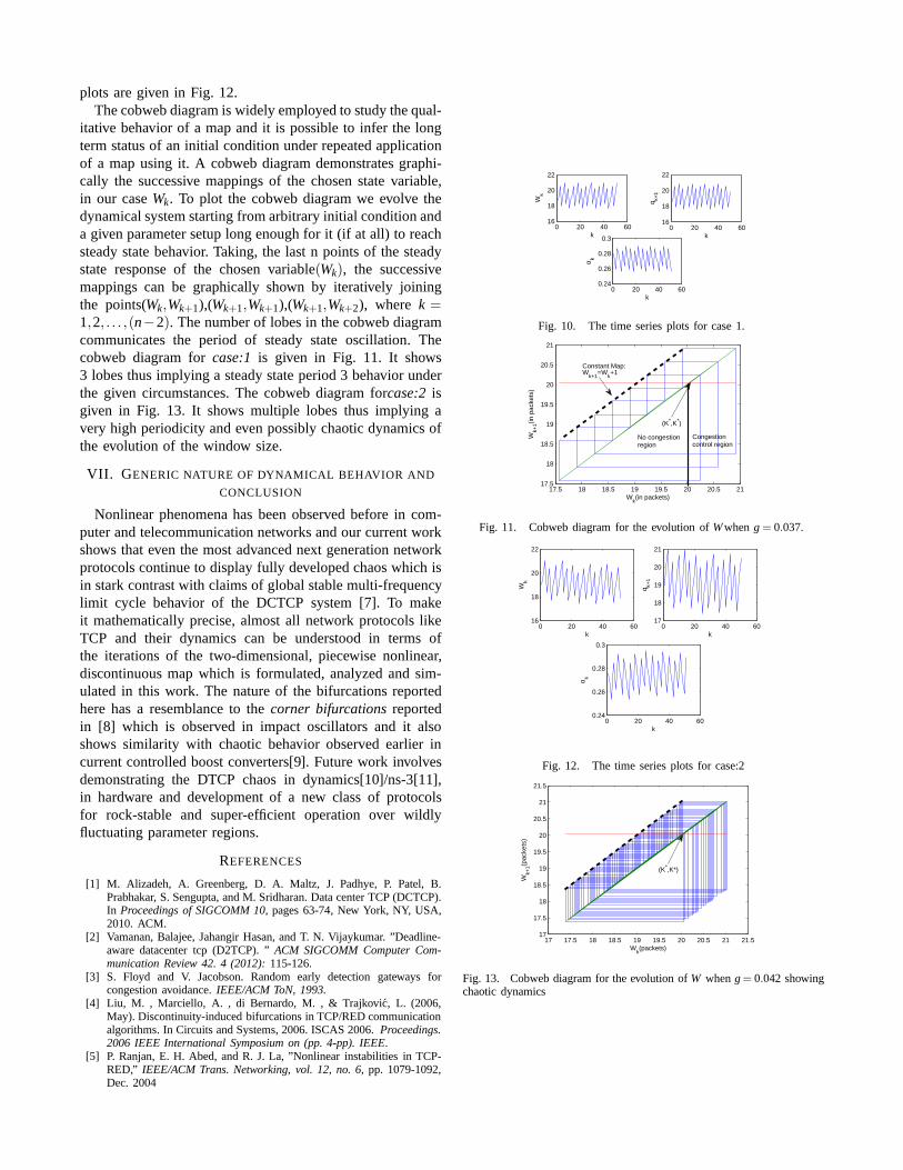
E. Bifurcations in the congestion history variable (α)

We draw the bifurcation diagram ofαk with respect to themarked fraction weight (g) other parameters set asγ = 1 andd = 100µs (Fig. 9).g varies from 0.001 to 0.2 through a stepsize of 0.0001. We see a novel type of bifurcation diagramwhich has a chaotic regime at low values ofg and shows high

10−8

10−6

10−4

13

14

15

16

17

18

19

20

21

Round trip delay (d) in log scale−−−>

q k+1−−

−>

Fig. 7. The bifurcation diagram withd(inseconds) as the bifurcation parameter

5 10 15 20 250

5

10

15

20

25

30

Marking threshold (K)−−−>

q k+1(in

pac

kets

)−−

−>

Fig. 8. The bifurcation diagram withK as the bifurcation parameter

0 0.05 0.1 0.15 0.20

0.05

0.1

0.15

0.2

0.25

0.3

0.35

Marked fraction weight (g)−−−>

α k−−−>

Fig. 9. The bifurcation diagram ofα with g as the bifurcation parameter andK = 20

periodic orbits ofα and larger amplitude of oscillation athigher values ofg. This result is consistent with the relationdefined in (9). The bifurcation diagram changes form as otherparameters like delay(d) ,(γ) etc. are varied.

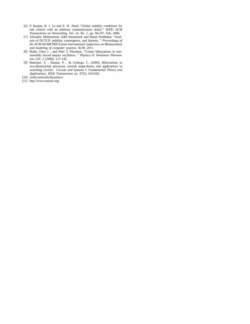
F. Time series plots and cobweb diagrams

Here we show the actual time series evolution of the statevariables for two different cases. One for a stable periodicregime and other for a chaotic regime. We also demonstratethe congestion control mechanism throughcobweb diagramsof the evolution of the window size.case 1: We taked = 30ns,γ = 1,g = 0.037. The state spaceplots are given in Fig. 10 . As per the bifurcation diagramsthe time series plots show a period 3 oscillatory behavior forall the variables.case 2: We taked = 30ns,γ = 1,g = 0.042. The state space

plots are given in Fig. 12.The cobweb diagram is widely employed to study the qual-

itative behavior of a map and it is possible to infer the longterm status of an initial condition under repeated applicationof a map using it. A cobweb diagram demonstrates graphi-cally the successive mappings of the chosen state variable,in our caseWk. To plot the cobweb diagram we evolve thedynamical system starting from arbitrary initial condition anda given parameter setup long enough for it (if at all) to reachsteady state behavior. Taking, the last n points of the steadystate response of the chosen variable(Wk), the successivemappings can be graphically shown by iteratively joiningthe points(Wk,Wk+1),(Wk+1,Wk+1),(Wk+1,Wk+2), where k =1,2, . . . ,(n−2). The number of lobes in the cobweb diagramcommunicates the period of steady state oscillation. Thecobweb diagram forcase:1 is given in Fig. 11. It shows3 lobes thus implying a steady state period 3 behavior underthe given circumstances. The cobweb diagram forcase:2 isgiven in Fig. 13. It shows multiple lobes thus implying avery high periodicity and even possibly chaotic dynamics ofthe evolution of the window size.

VII. G ENERIC NATURE OF DYNAMICAL BEHAVIOR AND

CONCLUSION

Nonlinear phenomena has been observed before in com-puter and telecommunication networks and our current workshows that even the most advanced next generation networkprotocols continue to display fully developed chaos which isin stark contrast with claims of global stable multi-frequencylimit cycle behavior of the DCTCP system [7]. To makeit mathematically precise, almost all network protocols likeTCP and their dynamics can be understood in terms ofthe iterations of the two-dimensional, piecewise nonlinear,discontinuous map which is formulated, analyzed and sim-ulated in this work. The nature of the bifurcations reportedhere has a resemblance to thecorner bifurcations reportedin [8] which is observed in impact oscillators and it alsoshows similarity with chaotic behavior observed earlier incurrent controlled boost converters[9]. Future work involvesdemonstrating the DTCP chaos in dynamics[10]/ns-3[11],in hardware and development of a new class of protocolsfor rock-stable and super-efficient operation over wildlyfluctuating parameter regions.

REFERENCES

[1] M. Alizadeh, A. Greenberg, D. A. Maltz, J. Padhye, P. Patel, B.Prabhakar, S. Sengupta, and M. Sridharan. Data center TCP (DCTCP).In Proceedings of SIGCOMM 10, pages 63-74, New York, NY, USA,2010. ACM.

[2] Vamanan, Balajee, Jahangir Hasan, and T. N. Vijaykumar.”Deadline-aware datacenter tcp (D2TCP). ”ACM SIGCOMM Computer Com-munication Review 42. 4 (2012): 115-126.

[3] S. Floyd and V. Jacobson. Random early detection gateways forcongestion avoidance.IEEE/ACM ToN, 1993.

[4] Liu, M. , Marciello, A. , di Bernardo, M. , & Trajkovic, L.(2006,May). Discontinuity-induced bifurcations in TCP/RED communicationalgorithms. In Circuits and Systems, 2006. ISCAS 2006.Proceedings.2006 IEEE International Symposium on (pp. 4-pp). IEEE.

[5] P. Ranjan, E. H. Abed, and R. J. La, ”Nonlinear instabilities in TCP-RED,” IEEE/ACM Trans. Networking, vol. 12, no. 6, pp. 1079-1092,Dec. 2004

0 20 40 6016

18

20

22

k

Wk

0 20 40 6016

18

20

22

k

q k+1

0 20 40 600.24

0.26

0.28

0.3

k

α k

Fig. 10. The time series plots for case 1.

17.5 18 18.5 19 19.5 20 20.5 2117.5

18

18.5

19

19.5

20

20.5

21

Wk(in packets)

Wk+

1(in p

acke

ts)

Constant Map:W

k+1=W

k+1

(K*,K*)

No congestionregion

Congestion control region

Fig. 11. Cobweb diagram for the evolution ofWwhen g = 0.037.

0 20 40 6016

18

20

22

k

Wk

0 20 40 6017

18

19

20

21

k

q k+1

0 20 40 600.24

0.26

0.28

0.3

k

α k

Fig. 12. The time series plots for case:2

17 17.5 18 18.5 19 19.5 20 20.5 21 21.517

17.5

18

18.5

19

19.5

20

20.5

21

21.5

Wk(packets)

Wk+

1(pac

kets

)

(K*,K*)

Fig. 13. Cobweb diagram for the evolution ofW wheng = 0.042 showingchaotic dynamics

[6] P. Ranjan, R. J. La and E. H. Abed, ”Global stability conditions forrate control with an arbitrary communication delay,”’IEEE/ ACMTransactions on Networking, Vol. 14, No. 1, pp. 94-107, Feb. 2006.

[7] Alizadeh, Mohammad, Adel Javanmard, and Balaji Prabhakar. ”Anal-ysis of DCTCP: stability, convergence, and fairness. ”Proceedings ofthe ACM SIGMETRICS joint international conference on Measurementand modeling of computer systems. ACM, 2011.

[8] Budd, Chris J. , and Petri T. Piiroinen. ”Corner bifurcations in non-smoothly forced impact oscillators. ”Physica D: Nonlinear Phenom-ena 220. 2 (2006): 127-145.

[9] Banerjee, S. , Ranjan, P. , & Grebogi, C. (2000). Bifurcations intwo-dimensional piecewise smooth maps-theory and applications inswitching circuits. Circuits and Systems I: Fundamental Theory andApplications, IEEE Transactions on, 47(5), 633-643.

[10] yorke.umd.edu/dynamics/[11] http://www.nsnam.org/