Non-linear Dependence in Stock Returns: Does Trading Frequency Matter

Non-linear Dependence in StockReturns: Does Trading Frequency

Matter?

Pradeep K. Yadav, Krishna Paudyal and Peter F. Pope*

1. INTRODUCTON

In this paper we extend previous research into the non-lineardynamics of stock returns. Hinich and Paterson (1985),Scheinkman and LeBaron (1989), Brock et al. (1991), Hsieh(1991), Lane, Peel and Raeburn (1996), Gilmore (1996) andYadav et al. (1996) have examined whether stock returns exhibitsignificant non-linear dependence and, in particular, behaviourconsistent with chaotic dynamics. Based on the accumulatedevidence to date, stock returns display clear evidence of non-linear behaviour, but the evidence for chaotic dynamics is, atbest, weak. However, with the exception of Scheinkman andLeBaron (1989) who examine a small number of individual stockreturns series, most prior work has focused analysis on stockindices rather than individual stock returns. It is possible thatstock index returns behave differently to the underlying stocksand that the aggregation process used to compute index returnsmasks more complex, and possibly chaotic, dynamics ofindividual stock returns series. Further, most prior workexamines US stock returns data. As yet it is unclear whetherstock prices generated in different economic and institutional

Journal of Business Finance & Accounting, 26(5) & (6), June/July 1999, 0306-686X

ß Blackwell Publishers Ltd. 1999, 108 Cowley Road, Oxford OX4 1JF, UKand 350 Main Street, Malden, MA 02148, USA. 651

* The authors are respectively from the University of Strathclyde, Glasgow CaledonianUniversity and Lancaster University. They acknowledge the Economic and Social ResearchCouncil (ESRC) Research Grant #R000233234. (Paper received July 1996, revised andaccepted November 1998)

Address for correspondence: Pradeep K. Yadav, Professor of Finance, Department ofAccounting and Finance, University of Strathclyde, Curran Building, 100 Cathedral Street,Glasgow G4 0LN, UK.e-mail: [email protected]

environments display properties similar to those uncovered forthe US.

In this paper we analyse a large sample of 176 individual UKstock return series. As far as we are aware this is the first extensiveanalysis of disaggregated stock returns data. Second, we analyseportfolios based on trading frequency. Market microstructuretheory suggests that trading frequency will be related to the priceformation process. Cross-sectional differences in tradingfrequency will reflect differences in the rate of informationarrival, differences in the activities of uniformed investors, e.g.noise traders, and transaction cost differences. If non-linearbehaviour is related to such factors, conditioning tests of non-linearity on trading frequency will increase the chances ofidentifying the existence and nature of any non-linearity.1

Compared with most prior research in the area, we reportresults based on more informative and more powerful diagnostictests of non-linearity.2 Prior work has primarily relied on the BDSstatistic as the main diagnostic test, primarily because when atime series contains a significant noise component it is difficult tojudge the statistical significance of the correlation dimension andthe largest Lyapunov exponent, the two most popular tests usedin physical sciences research. In this paper we overcome thisnoise problem by using bootstrapping techniques similar toTheiler et al. (1992). We also employ a test based on �-estimators(Savit and Green, 1991). This test has the advantage, relative toBDS statistic, of providing an intuitively appealing direct, non-parametric measure of lag dependence and predictability in atime series.

Consistent with prior research we find evidence of significantnon-linear structure in raw returns and linearly filtered returns.However, the non-linearity seems to be attributable toconditional heteroskedasticity effects and virtually disappears inEGARCH residuals. Further, there appears to be no systematicvariation in non-linear structure across trading frequency-partitioned portfolios.

The remainder of the paper is organised as follows: Section 2outlines the methodology and testing procedures; Section 3describes the data and reports the empirical results; and Section4 concludes.

652 YADAV, PAUDYAL AND POPE

ß Blackwell Publishers Ltd 1999

2. TESTS FOR NON-LINEARITY AND DETERMINISTIC CHAOS

(i) Filtered Returns Series

In common with previous research (e.g. Hsieh, 1991) we filter outlinear dependencies in the conditional mean due to day-of-the-week effects and the serial correlation expected to result frominfrequent trading. We regress raw returns Rt on dummy variablesfor different days of the week and p lagged returns, where themaximum lag length p is chosen on the basis of the AkaikeInformation criterion. All tests for non-linear structure are appliedto both linearly filtered returns series and to returns filtered forARCH-type non-linearity.3 Based on the results of Loudon, Wattand Yadav (1998), we initially generated residuals fromEGARCH(1,1) and GARCH(1,1) models.4 Preliminary analysisrevealed that results relating to the correlation dimension, thelargest Lyapunov exponent and the BDS statistic are qualitativelysimilar for both sets of residuals. Therefore we only report theresults of analysis based on the EGARCH filtered returns and theseare standardised returns et=�t .

5

(ii) Diagnostic Tests for Non-Linearity

(a) BDS-Statistic

Tests for deterministic chaotic dynamics are based on calculatingcorrelation integrals corresponding to different èmbedding dim-ensions'. The correlation integral for one dimension is defined as:

C1�"� � LimN!1

1

N �N ÿ 1�Xi; j

I "1 �i; j�

where I "1 �i; j� is an indicator function that equals one ifjXi ÿ Xj j < " and zero otherwise. C1�"� represents the fractionof the pairs of points that are within a `distance' of " from eachother. Similarly, the correlation integral Cm�"� for an embeddingdimension m is defined in terms of the n-dimensional vectorspm�t� constructed by taking m consecutive values of the timeseries from time period t onwards (t � 1; . . . �N ÿ m��:

Cm�"� � LimN!1

1

�N ÿ m � 1��N ÿ m�Xi; j

I "1 �i; j�

NON-LINEAR DEPENDENCE IN STOCK RETURNS 653


where I "m�i; j� is an indicator function that equals one ifpm�i� ÿ pm�j�, the n-dimensional `distance' between pm�i� andpm�j� is less than ", and is zero otherwise. Intuitively, thesummation represents the number of pairs �i; j� for which thecorresponding components of pm�i� and pm�j� are within adistance of " from each other.

The Brock, Dechert and Scheinkman (BDS) (1987) test detectsclustering in data that occurs more frequently than would beexpected for a purely random iid process. Under the nullhypothesis of iid, for any fixed " and m, Cm�"� ! �C1�"��m withprobability 1 as the number of data points N !1. BDS showthat the statistic:

Wm�"; N � ��Np �Cm�"� ÿ �C1�"��m �

�m�"; N �has a standard normal limiting distribution.

Brock, Dechert and Scheinkman (1987) and Brock, Hsieh andLeBaron (1991) show that the BDS statistic has high poweragainst both deterministic and stochastic non-linear models.However, they also show that the critical values of the BDSstatistic are slightly different for GARCH/EGARCH residuals,even for several thousand observations. Therefore, we assess thesignificance of the BDS statistics for EGARCH residuals on thebasis of the critical values reported in Hsieh (1991).

(b) Savit-Green �-estimators

Savit and Green (1991) show that correlation integrals can beused to estimate the characteristics of deterministic depen-dencies in chaotic time series. They show that for an iid series thestatistic:

�1�"� � 1ÿ C21 �"�

C2�"�is zero. The extent to which �1(") deviates from zero provides anindication of the first lag dependence in a time series.6 Similarly:

�j�"� ��

1ÿ C2j �"�

Cjÿ1�"�Cj�1�"��



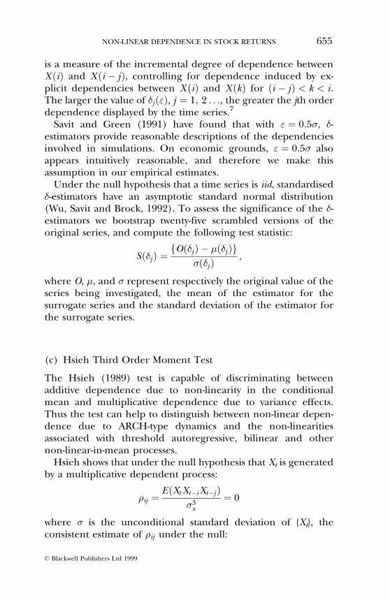
is a measure of the incremental degree of dependence betweenX �i� and X �i ÿ j�, controlling for dependence induced by ex-plicit dependencies between X �i� and X �k� for �i ÿ j� < k < i.The larger the value of �j�"�, j � 1; 2 . . ., the greater the jth orderdependence displayed by the time series.7

Savit and Green (1991) have found that with " � 0:5�, �-estimators provide reasonable descriptions of the dependenciesinvolved in simulations. On economic grounds, " � 0:5� alsoappears intuitively reasonable, and therefore we make thisassumption in our empirical estimates.

Under the null hypothesis that a time series is iid, standardised�-estimators have an asymptotic standard normal distribution(Wu, Savit and Brock, 1992). To assess the significance of the �-estimators we bootstrap twenty-five scrambled versions of theoriginal series, and compute the following test statistic:

S��j� �fO��j� ÿ ��j�g

��j� ;

where O, �, and � represent respectively the original value of theseries being investigated, the mean of the estimator for thesurrogate series and the standard deviation of the estimator forthe surrogate series.

(c) Hsieh Third Order Moment Test

The Hsieh (1989) test is capable of discriminating betweenadditive dependence due to non-linearity in the conditionalmean and multiplicative dependence due to variance effects.Thus the test can help to distinguish between non-linear depen-dence due to ARCH-type dynamics and the non-linearitiesassociated with threshold autoregressive, bilinear and othernon-linear-in-mean processes.

Hsieh shows that under the null hypothesis that Xt is generatedby a multiplicative dependent process:

�ij �E�XtXtÿiXtÿj�

�3x

� 0

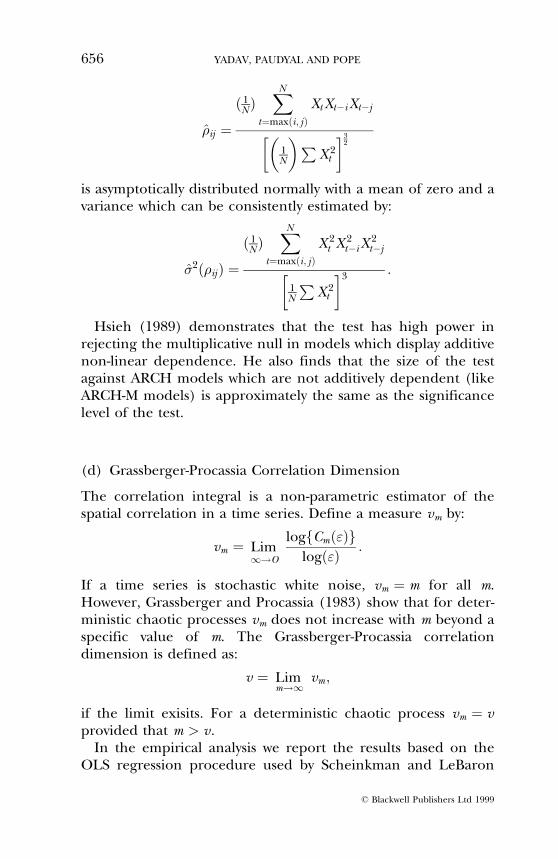
where � is the unconditional standard deviation of {Xt}, theconsistent estimate of �ij under the null:



�̂ij �� 1

N �XN

t�max�i; j�XtXtÿiXtÿj

��1N

�PX 2

t

�32

is asymptotically distributed normally with a mean of zero and avariance which can be consistently estimated by:

�̂2��ij� �� 1

N �XN

t�max�i; j�X 2

t X 2tÿiX

2tÿj�

1N

PX 2

t

�3 :

Hsieh (1989) demonstrates that the test has high power inrejecting the multiplicative null in models which display additivenon-linear dependence. He also finds that the size of the testagainst ARCH models which are not additively dependent (likeARCH-M models) is approximately the same as the significancelevel of the test.

(d) Grassberger-Procassia Correlation Dimension

The correlation integral is a non-parametric estimator of thespatial correlation in a time series. Define a measure vm by:

vm � Lim1!O

logfCm�"�glog�"� :

If a time series is stochastic white noise, vm � m for all m.However, Grassberger and Procassia (1983) show that for deter-ministic chaotic processes vm does not increase with m beyond aspecific value of m. The Grassberger-Procassia correlationdimension is defined as:

v � Limm!1

vm ;

if the limit exisits. For a deterministic chaotic process vm � vprovided that m > v.

In the empirical analysis we report the results based on theOLS regression procedure used by Scheinkman and LeBaron



(1989) and Ramsey and Yuan (1989 and 1990) to estimate thecorrelation dimension. The slope of the regression of log �Cm�"��on log (") is estimated over a suitably chosen segment, for which" is `close to' zero and reasonably linear.8 The choice of " issubjective, based on a visual inspection of the flog�Cm�"�� vs log�"�g plot. For the data in this paper the cut off "corresponds in almost all cases to about 10% of the range of datavalues and the plot over this restricted range is close to linear.

Eckmann and Ruelle (1992) and Smith (1992) discuss theconstraints on the ability of the Grassberger-Procassia algorithmto estimate correlation dimensions. They show that " has to be`small' compared to D, the diameter of the reconstructedattractor. Eckmann and Ruelle argue that ordinarily "/D shouldnot be greater than about 0.1 and this leads to a maximumpossible estimate of about 6±7 for 5000 data points. However, fora broad band estimate corresponding to a root mean squareerror of 1, which is reasonable if we only wish to place an upperlimit on the number of degrees of freedom, a dimension of up toabout 10 can be estimated with 5,000 data points. In this paper,the time series analysed have about 5,000 data points. Hence, theestimation is effectively confined to embedding dimensionsequal to ten or less.

To address the problems of there being no estimate ofstandard errors associated with estimates of vm and thecorrelation dimension from standard estimation techniques,9

and the fact that, for finite data sets, the value of vm estimated forpure stochastic white noise will be less than m, we follow theapproach of Scheinkman and LeBaron (1989) of comparing theestimates with those from a `scrambled' series obtained byrandomly shuffling the original series. Such randomisation of theoriginal series destroys any deterministic structure. FollowingTheiler et al. (1992), we use bootstrapping.10 Thus we generate25 scrambled series, and compute vm (m � 1; . . . 10)11 for each.Let O�vm� be the value of vm for the original series and �(vm) and�(vm) be the mean and standard deviation of the estimates of vm

for the random surrogate series. A measure of the significance ofO (vm) can be defined by the difference between the original andthe mean surrogate value of vm divided by the standard deviationof the surrogate values. The significance S is a dimensionlessquantity expressing the difference in terms of `sigmas':



S � fO�vm� ÿ ��vm�g��vm� :

If the distribution of surrogate vm is approximately Gaussian,S � 2 will indicate approximately a 5% significance level. Thedistribution is, in general, unknown. However, even if thedistribution is clearly non-Gaussian, p-values can be defined interms of rank statistics. So, if the observed time series has a vm

which is in the lower four percentiles of all surrogate values, thena (two sided) p-value of 0.08 could reasonably be quoted.

(e) Largest Positive Lyapunov Exponent

Lyapunov exponents quantifiy the sensitive dependence ofchaotic systems to initial conditions. Consider a very small ballwith radius "(0) at time t � 0 in the state space of a system. Theball may distort to an ellipsoid as the dynamic system evolves. Letthe length of the j th principal axis of this ellipsoid at time t be"j�t�. The spectrum of Lyapunov exponents �j from an initialstate 0 are defined (Farmer, 1982) by:

�j � Limt!1

Lim"�0�!0

�1

tlog

"j�t�"j�0�

�:

Generally, where system state space has dimensionality D, there isa spectrum of D Lyapunov exponents, each reflecting divergenceof the trajectory in a particular direction. Positive Lyapunovexponents indicate system divergence. The rate of trajectorydivergence increases with the magnitude of the positiveexponents, and the time scale of system predictability decreases.Negative Lyapunov exponents indicate system convergence andthe time scale on which transient perturbations of the state of thesystem decay. A necessary (but not sufficient) condition forchaotic dynamics is the presence of at least one positiveLyapunov exponent. If no Lyapunov exponents are positive,the system is not chaotic. Therefore, examination of the sign ofthe largest Lyapunov exponent �1 is informative about thepresence of chaotic dynamics.

We employ the numerical algorithm developed in Wolf et al.(1985)12 to estimate the largest positive Lyapunov exponent.Inferences based on the Lyapunov exponent are limited in power



by the size of the data set. Eckmann and Ruelle (1992) suggestthat the minimum number of data points is approximately thesquare of the number of points required when basing inferenceson correlation dimensions. We attempt to mitigate this problemby bootstrapping as in the Theiler et al. (1992) surrogate datamethod. Hence, for the largest positive Lyaponov exponent �1 wefollow a procedure similar to the one described earlier for eachof the vm. We generate twenty-five `scrambled' series, compute �1

in each case (for the chosen values of embedding dimension,evolution time etc.) and measure the significance of the valueO(�1) computed for the original series by:

S�1 �fO��1� ÿ ��1�g

��1�where ��1� and ��1� are the mean and standard deviationrespectively of the estimates of �1 for the random surrogateseries.

3. EMPIRICAL RESULTS

(i) Data

The analysis is based on 21 years' daily price data for individualstocks traded on the London Stock Exchange from January 1970to December 1990. Stocks are required to satisfy the followingcriteria to be included in the sample:

(a) Daily prices (unadjusted and adjusted for capitalisationchanges) are available on Datastream for the entire sampleperiod;

(b) Dividends and ex-dividend dates are available from theLondon Business School Share Price Database ;

(c) A stock must trade at least once during each month in thesample period.13

A total of 176 stocks satisfy the above criteria. We form value-weighted and equally-weighted portfolios containing all 176stocks and four equally weighted, equal sized portfolios based ontrading frequency ranks. Trading frequency-rank portfolios arebased on the median number of days elapsing between the last



trade in a month and the end of the month, as reported by theLSPD. Quartile 1 is the portfolio comprising the most activelytraded stocks and quartile 4 comprises the least actively tradedstocks.

(ii) Portfolio Summary Statistics

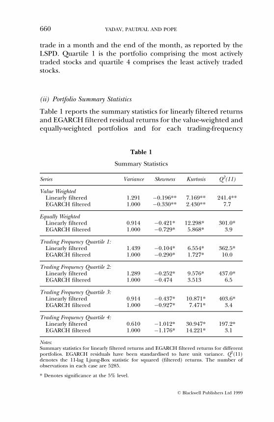
Table 1 reports the summary statistics for linearly filtered returnsand EGARCH filtered residual returns for the value-weighted andequally-weighted portfolios and for each trading-frequency

Table 1

Summary Statistics

Series Variance Skewness Kurtosis Q2(11)

Value WeightedLinearly filtered 1.291 ÿ0.196** 7.169** 241.4**EGARCH filtered 1.000 ÿ0.330** 2.430** 7.7

Equally WeightedLinearly filtered 0.914 ÿ0.421* 12.298* 301.0*EGARCH filtered 1.000 ÿ0.729* 5.868* 3.9

Trading Frequency Quartile 1:Linearly filtered 1.439 ÿ0.104* 6.554* 362.5*EGARCH filtered 1.000 ÿ0.290* 1.727* 10.0

Trading Frequency Quartile 2:Linearly filtered 1.289 ÿ0.252* 9.576* 437.0*EGARCH filtered 1.000 ÿ0.474 3.513 6.5



Notes:Summary statistics for linearly filtered returns and EGARCH filtered returns for differentportfolios. EGARCH residuals have been standardised to have unit variance. Q2(11)denotes the 11-lag Ljung-Box statistic for squared (filtered) returns. The number ofobservations in each case are 5285.

* Denotes significance at the 5% level.



ranked portfolio. There is excess kurtosis in all cases, the fattesttails being found for companies with relatively low tradingfrequency. The EGARCH filtered returns continue to displaysignificant excess kurtosis, although the magnitude is muchreduced compared with the linearly filtered residuals.

Table 1 also shows that the Ljung-Box statistic is insignificant forboth the linearly-filtered and the EGARCH-filtered returns,indicating that all linear dependence in conditional mean hasbeen removed through the filtering process. However, the LjungBox statistic for squared linearly-filtered returns is highlysignificant in all cases, suggesting that an ARCH/GARCHrepresentation is appropriate. The insignificant Ljung Box statisticfor squared EGARCH-filtered returns suggests that theEGARCH(1,1) model is generally a good description of the time-varying volatility structure.

(iii) Are Portfolio Returns iid?

BDS statistics were calculated for each portfolio for values ofm � 2; 3; . . . 10 and for the `distance' measure " approximatelyequal to 0:5�; �; 1:5� and 2�, where � is the standard deviationof the corresponding series.14 We report BDS statistics form � 2; 4; 5 and 8 in Table 2. Hsieh (1991) shows that the (one-tailed) 2.5% level critical values of the BDS statistic deviate fromthe normal distribution in simulations on EGARCH (1,1)residuals. Therefore we use one-tailed critical values from Hsieh(1991, Table XIII) for the tests on the EGARCH residuals.15

Table 2 shows that the null hypothesis of iid is conclusivelyrejected for the linearly-filtered series. The lowest BDS statisticexceeds 12. For the EGARCH-filtered series, the null hypothesis ofiid is marginally rejected at conventional significance levels for onlya few (m; ") pairs. Among these portfolios, marginal rejection of iidis more likely for the relatively infrequently traded stocks inquartiles 3 and 4. The results provide strong evidence of non-lineardependence, but they also suggest that this dependence is due toconditional heteroscedasticity. This is consistent with the results ofScheinkman and LeBaron (1989) and Hsieh (1991) for the US,and those for three Far-Eastern indices reported by Yadav, Paudyaland Pope (1996). Consistency of findings across different marketsettings having different trading mechanisms suggests that non-



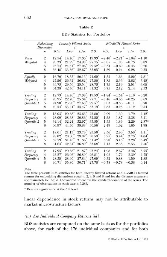
linear dependence in stock returns may not be attributable tomarket microstructure factors.

(iv) Are Individual Company Returns iid?

BDS statistics are computed on the same basis as for the portfoliosabove, for each of the 176 individual companies and for both

Table 2

BDS Statistics for Portfolios

Embedding Linearly Filtered Series EGARCH Filtered SeriesDimension " "

m 0.5� 1.0� 1.5� 2.0� 0.5� 1.0� 1.5� 2.0�

Value 2 12.54* 14.46* 17.33* 19.93* ÿ2.40* ÿ2.21* ÿ1.84* ÿ1.10Weighted 4 20.33* 21.99* 24.90* 27.75* ÿ0.85 ÿ1.05 ÿ0.73 0.09

5 23.74* 24.81* 27.06* 29.52* ÿ0.34 ÿ0.69 ÿ0.45 0.268 36.48* 33.36* 32.67* 33.05* 1.59 ÿ0.24 ÿ0.28 0.35

Equally 2 16.70* 18.33* 20.13* 21.62* 1.32 1.65 2.22* 2.81*

Weighted 4 27.56* 26.32* 26.82* 27.50* 1.85 2.36* 2.82* 3.48*

5 33.73* 29.56* 28.54* 28.73* 1.75 2.19 2.51* 3.05*

8 64.38* 42.46* 34.11* 31.32* 0.75 2.12 2.14 2.33

Trading 2 12.73* 14.76* 17.38* 19.53* ÿ1.84* ÿ1.54* ÿ1.10 ÿ0.20Frequency 4 20.95* 22.78* 25.34* 27.71* ÿ0.46 ÿ0.63 ÿ0.25 0.69Quartile 1 5 24.90* 25.90* 27.65* 29.57* 0.03 ÿ0.36 ÿ0.11 0.70

8 40.54* 35.24* 33.47* 33.19* 2.83 ÿ0.23 ÿ1.12 0.54

Trading 2 18.03* 20.58* 23.63* 25.80* 0.99 1.30 1.79 2.42*

Frequency 4 28.09* 28.68* 30.86* 32.52* 1.58 1.87 2.38 3.11Quartile 2 5 34.14* 32.24* 32.97* 33.85* 1.35 1.89 2.29 2.87*

8 60.97* 44.40* 38.88* 36.56* 2.49 1.62 1.65 1.98

Trading 2 18.61* 21.13* 23.73* 25.50* 2.56* 2.96* 3.53* 4.11*

Frequency 4 28.02* 28.60* 29.82* 30.59* 3.25* 3.44* 3.73* 4.04*

Quartile 3 5 32.79* 31.45* 31.36* 31.42* 3.20* 3.13* 3.28* 3.49*

8 51.64* 42.61* 36.89* 33.68* 2.13 2.53 2.55 2.56*

Trading 2 17.95* 20.38* 21.87* 23.24* 1.98 2.67* 3.46* 3.75*

Frequency 4 25.27* 26.96* 26.89* 26.81* 1.02 1.72 2.39* 2.75*

Quartile 4 5 28.35* 28.90* 27.84* 27.09* 0.32 0.88 1.50 1.888 40.71* 35.80* 30.71* 27.78* ÿ0.78 ÿ0.78 ÿ0.38 0.14

Notes:The table presents BDS statistics for both linearly filtered returns and EGARCH filteredreturns for embedding dimensions equal to 2, 4, 5 and 8 and for the distance measure "approximately to 0.5�, �, 1.5� and 2�, where � is the standard deviation of the series. Thenumber of observations in each case is 5,285.

* Denotes significance at the 5% level.



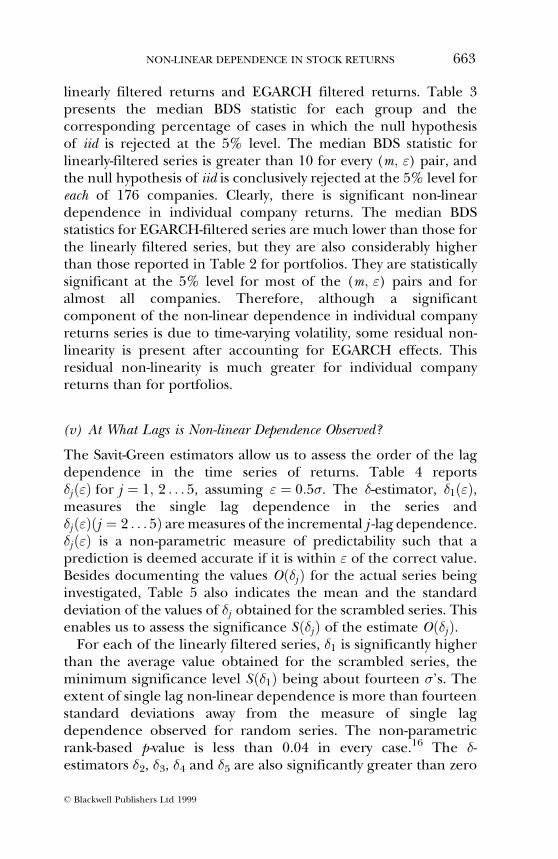
linearly filtered returns and EGARCH filtered returns. Table 3presents the median BDS statistic for each group and thecorresponding percentage of cases in which the null hypothesisof iid is rejected at the 5% level. The median BDS statistic forlinearly-filtered series is greater than 10 for every (m; ") pair, andthe null hypothesis of iid is conclusively rejected at the 5% level foreach of 176 companies. Clearly, there is significant non-lineardependence in individual company returns. The median BDSstatistics for EGARCH-filtered series are much lower than those forthe linearly filtered series, but they are also considerably higherthan those reported in Table 2 for portfolios. They are statisticallysignificant at the 5% level for most of the (m; ") pairs and foralmost all companies. Therefore, although a significantcomponent of the non-linear dependence in individual companyreturns series is due to time-varying volatility, some residual non-linearity is present after accounting for EGARCH effects. Thisresidual non-linearity is much greater for individual companyreturns than for portfolios.

(v) At What Lags is Non-linear Dependence Observed?

The Savit-Green estimators allow us to assess the order of the lagdependence in the time series of returns. Table 4 reports�j�"� for j � 1; 2 . . . 5, assuming " � 0:5�. The �-estimator, �1�"�,measures the single lag dependence in the series and�j�"��j � 2 . . . 5� are measures of the incremental j -lag dependence.�j�"� is a non-parametric measure of predictability such that aprediction is deemed accurate if it is within " of the correct value.Besides documenting the values O��j� for the actual series beinginvestigated, Table 5 also indicates the mean and the standarddeviation of the values of �j obtained for the scrambled series. Thisenables us to assess the significance S��j� of the estimate O��j�.

For each of the linearly filtered series, �1 is significantly higherthan the average value obtained for the scrambled series, theminimum significance level S��1� being about fourteen �'s. Theextent of single lag non-linear dependence is more than fourteenstandard deviations away from the measure of single lagdependence observed for random series. The non-parametricrank-based p-value is less than 0.04 in every case.16 The �-estimators �2, �3, �4 and �5 are also significantly greater than zero



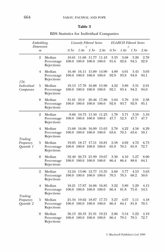
Table 3

BDS Statistics for Individual Companies


m 0.5� 1.0� 1.5� 2.0� 0.5� 1.0� 1.5� 2.0�

2 Median 10.61 11.68 11.77 11.43 3.33 3.68 3.20 2.78Percentage 100.0 100.0 100.0 100.0 91.6 92.6 94.5 92.9Rejections

4 Median 16.40 16.11 15.80 14.90 4.09 4.01 3.45 3.03Percentage 100.0 100.0 100.0 100.0 92.9 93.8 94.8 94.1

176Rejections

Individual 5 Median 19.13 17.78 16.88 15.90 4.22 3.89 3.31 2.91Companies Percentage 100.0 100.0 100.0 100.0 92.1 93.4 94.2 94.0

Rejections




TradingRejections

Frequency 5 Median 19.05 18.17 17.51 16.81 2.58 4.02 4.72 6.73Quartile 1 Percentage 100.0 100.0 100.0 100.0 65.9 70.5 65.9 72.7

Rejections




TradingRejections


Rejections




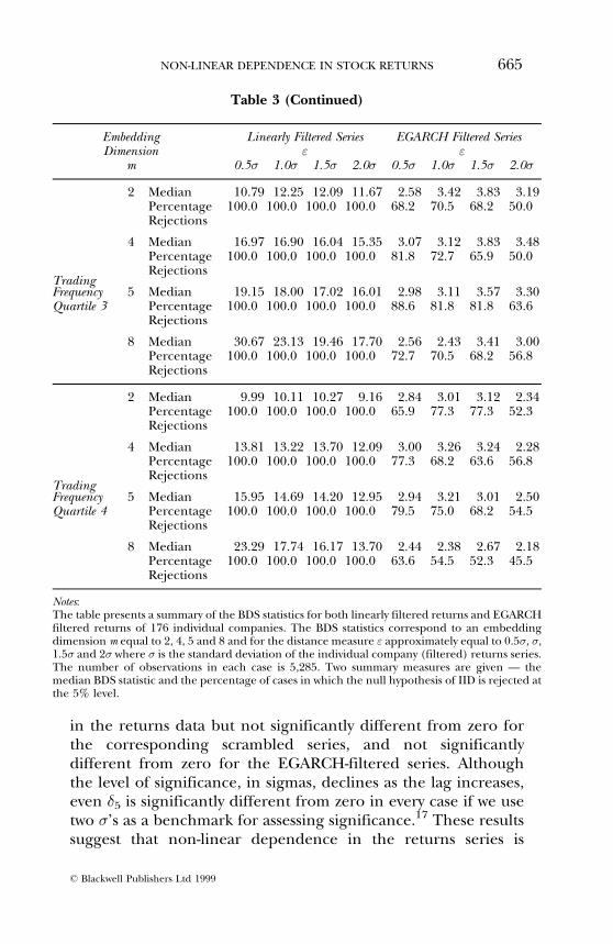
in the returns data but not significantly different from zero forthe corresponding scrambled series, and not significantlydifferent from zero for the EGARCH-filtered series. Althoughthe level of significance, in sigmas, declines as the lag increases,even �5 is significantly different from zero in every case if we usetwo �'s as a benchmark for assessing significance.17 These resultssuggest that non-linear dependence in the returns series is

Table 3 (Continued)


m 0.5� 1.0� 1.5� 2.0� 0.5� 1.0� 1.5� 2.0�



TradingRejections


Rejections




TradingRejections


Rejections


Notes:The table presents a summary of the BDS statistics for both linearly filtered returns and EGARCHfiltered returns of 176 individual companies. The BDS statistics correspond to an embeddingdimension m equal to 2, 4, 5 and 8 and for the distance measure " approximately equal to 0.5�, �,1.5� and 2� where � is the standard deviation of the individual company (filtered) returns series.The number of observations in each case is 5,285. Two summary measures are given Ð themedian BDS statistic and the percentage of cases in which the null hypothesis of IID is rejected atthe 5% level.



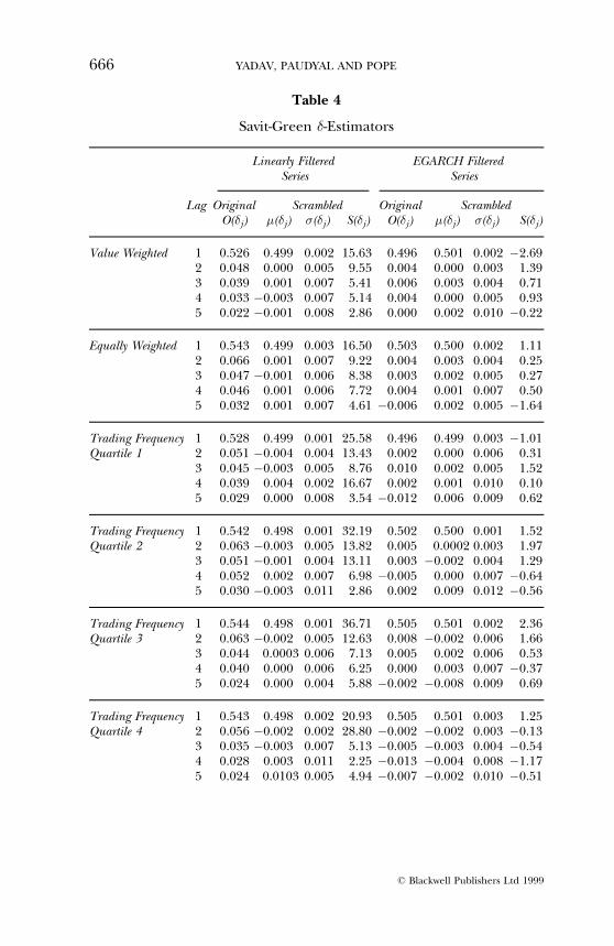
Table 4

Savit-Green �-Estimators

Linearly Filtered EGARCH FilteredSeries Series

Lag Original Scrambled Original ScrambledO(�j) �(�j) �(�j) S(�j) O(�j) �(�j) �(�j) S(�j)

Value Weighted 1 0.526 0.499 0.002 15.63 0.496 0.501 0.002 ÿ2.692 0.048 0.000 0.005 9.55 0.004 0.000 0.003 1.393 0.039 0.001 0.007 5.41 0.006 0.003 0.004 0.714 0.033 ÿ0.003 0.007 5.14 0.004 0.000 0.005 0.935 0.022 ÿ0.001 0.008 2.86 0.000 0.002 0.010 ÿ0.22

Equally Weighted 1 0.543 0.499 0.003 16.50 0.503 0.500 0.002 1.112 0.066 0.001 0.007 9.22 0.004 0.003 0.004 0.253 0.047 ÿ0.001 0.006 8.38 0.003 0.002 0.005 0.274 0.046 0.001 0.006 7.72 0.004 0.001 0.007 0.505 0.032 0.001 0.007 4.61 ÿ0.006 0.002 0.005 ÿ1.64

Trading Frequency 1 0.528 0.499 0.001 25.58 0.496 0.499 0.003 ÿ1.01Quartile 1 2 0.051 ÿ0.004 0.004 13.43 0.002 0.000 0.006 0.31

3 0.045 ÿ0.003 0.005 8.76 0.010 0.002 0.005 1.524 0.039 0.004 0.002 16.67 0.002 0.001 0.010 0.105 0.029 0.000 0.008 3.54 ÿ0.012 0.006 0.009 0.62

Trading Frequency 1 0.542 0.498 0.001 32.19 0.502 0.500 0.001 1.52Quartile 2 2 0.063 ÿ0.003 0.005 13.82 0.005 0.0002 0.003 1.97

3 0.051 ÿ0.001 0.004 13.11 0.003 ÿ0.002 0.004 1.294 0.052 0.002 0.007 6.98 ÿ0.005 0.000 0.007 ÿ0.645 0.030 ÿ0.003 0.011 2.86 0.002 0.009 0.012 ÿ0.56

Trading Frequency 1 0.544 0.498 0.001 36.71 0.505 0.501 0.002 2.36Quartile 3 2 0.063 ÿ0.002 0.005 12.63 0.008 ÿ0.002 0.006 1.66

3 0.044 0.0003 0.006 7.13 0.005 0.002 0.006 0.534 0.040 0.000 0.006 6.25 0.000 0.003 0.007 ÿ0.375 0.024 0.000 0.004 5.88 ÿ0.002 ÿ0.008 0.009 0.69

Trading Frequency 1 0.543 0.498 0.002 20.93 0.505 0.501 0.003 1.25Quartile 4 2 0.056 ÿ0.002 0.002 28.80 ÿ0.002 ÿ0.002 0.003 ÿ0.13

3 0.035 ÿ0.003 0.007 5.13 ÿ0.005 ÿ0.003 0.004 ÿ0.544 0.028 0.003 0.011 2.25 ÿ0.013 ÿ0.004 0.008 ÿ1.175 0.024 0.0103 0.005 4.94 ÿ0.007 ÿ0.002 0.010 ÿ0.51



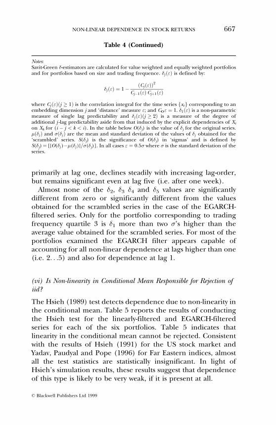
primarily at lag one, declines steadily with increasing lag-order,but remains significant even at lag five (i.e. after one week).

Almost none of the �2, �3 �4 and �5 values are significantlydifferent from zero or significantly different from the valuesobtained for the scrambled series in the case of the EGARCH-filtered series. Only for the portfolio corresponding to tradingfrequency quartile 3 is �1 more than two �'s higher than theaverage value obtained for the scrambled series. For most of theportfolios examined the EGARCH filter appears capable ofaccounting for all non-linear dependence at lags higher than one(i.e. 2. . .5) and also for dependence at lag 1.

(vi) Is Non-linearity in Conditional Mean Responsible for Rejection ofiid?

The Hsieh (1989) test detects dependence due to non-linearity inthe conditional mean. Table 5 reports the results of conductingthe Hsieh test for the linearly-filtered and EGARCH-filteredseries for each of the six portfolios. Table 5 indicates thatlinearity in the conditional mean cannot be rejected. Consistentwith the results of Hsieh (1991) for the US stock market andYadav, Paudyal and Pope (1996) for Far Eastern indices, almostall the test statistics are statistically insignificant. In light ofHsieh's simulation results, these results suggest that dependenceof this type is likely to be very weak, if it is present at all.

Table 4 (Continued)

Notes:Savit-Green �-estimators are calculated for value weighted and equally weighted portfoliosand for portfolios based on size and trading frequence. �j �"� is defined by:

�j �"� � 1ÿ �Cj �"��2Cjÿ1�"�Cj�1�"�

where Cj �"��j � 1� is the correlation integral for the time series fxtg corresponding to anembedding dimension j and `distance' measure "; and Co" � 1. �1�"� is a non-parametricmeasure of single lag predictability and �j �"��j � 2� is a measure of the degree ofadditional j -lag predictability aside from that induced by the explicit dependencies of Xt

on Xk for (i ÿ j < k < i). In the table below O(�j) is the value of �j for the original series.��j � and ��j � are the mean and standard deviation of the values of �j obtained for the`scrambled' series. S(�j) is the significance of O(�j) in `sigmas' and is defined byS(�j)� [{O(�j )ÿ�(�j )}=�(�j)]. In all cases " � 0:5� where � is the standard deviation of theseries.



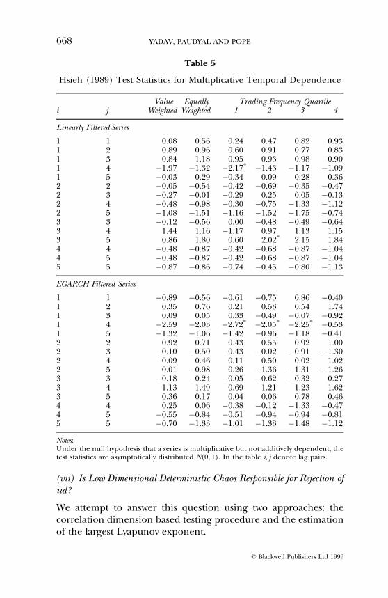
(vii) Is Low Dimensional Deterministic Chaos Responsible for Rejection ofiid?

We attempt to answer this question using two approaches: thecorrelation dimension based testing procedure and the estimationof the largest Lyapunov exponent.

Table 5

Hsieh (1989) Test Statistics for Multiplicative Temporal Dependence

Value Equally Trading Frequency Quartilei j Weighted Weighted 1 2 3 4

Linearly Filtered Series

1 1 0.08 0.56 0.24 0.47 0.82 0.931 2 0.89 0.96 0.60 0.91 0.77 0.831 3 0.84 1.18 0.95 0.93 0.98 0.901 4 ÿ1.97 ÿ1.32 ÿ2.17* ÿ1.43 ÿ1.17 ÿ1.091 5 ÿ0.03 0.29 ÿ0.34 0.09 0.28 0.362 2 ÿ0.05 ÿ0.54 ÿ0.42 ÿ0.69 ÿ0.35 ÿ0.472 3 ÿ0.27 ÿ0.01 ÿ0.29 0.25 0.05 ÿ0.132 4 ÿ0.48 ÿ0.98 ÿ0.30 ÿ0.75 ÿ1.33 ÿ1.122 5 ÿ1.08 ÿ1.51 ÿ1.16 ÿ1.52 ÿ1.75 ÿ0.743 3 ÿ0.12 ÿ0.56 0.00 ÿ0.48 ÿ0.49 ÿ0.643 4 1.44 1.16 ÿ1.17 0.97 1.13 1.153 5 0.86 1.80 0.60 2.02* 2.15 1.844 4 ÿ0.48 ÿ0.87 ÿ0.42 ÿ0.68 ÿ0.87 ÿ1.044 5 ÿ0.48 ÿ0.87 ÿ0.42 ÿ0.68 ÿ0.87 ÿ1.045 5 ÿ0.87 ÿ0.86 ÿ0.74 ÿ0.45 ÿ0.80 ÿ1.13

EGARCH Filtered Series

1 1 ÿ0.89 ÿ0.56 ÿ0.61 ÿ0.75 0.86 ÿ0.401 2 0.35 0.76 0.21 0.53 0.54 1.741 3 0.09 0.05 0.33 ÿ0.49 ÿ0.07 ÿ0.921 4 ÿ2.59 ÿ2.03 ÿ2.72* ÿ2.05* ÿ2.25* ÿ0.531 5 ÿ1.32 ÿ1.06 ÿ1.42 ÿ0.96 ÿ1.18 ÿ0.412 2 0.92 0.71 0.43 0.55 0.92 1.002 3 ÿ0.10 ÿ0.50 ÿ0.43 ÿ0.02 ÿ0.91 ÿ1.302 4 ÿ0.09 0.46 0.11 0.50 0.02 1.022 5 0.01 ÿ0.98 0.26 ÿ1.36 ÿ1.31 ÿ1.263 3 ÿ0.18 ÿ0.24 ÿ0.05 ÿ0.62 ÿ0.32 0.273 4 1.13 1.49 0.69 1.21 1.23 1.623 5 0.36 0.17 0.04 0.06 0.78 0.464 4 0.25 0.06 ÿ0.38 ÿ0.12 ÿ1.33 ÿ0.474 5 ÿ0.55 ÿ0.84 ÿ0.51 ÿ0.94 ÿ0.94 ÿ0.815 5 ÿ0.70 ÿ1.33 ÿ1.01 ÿ1.33 ÿ1.48 ÿ1.12

Notes:Under the null hypothesis that a series is multiplicative but not additively dependent, thetest statistics are asymptotically distributed N(0, 1). In the table i, j denote lag pairs.



(a) Correlation Dimension Based Testing Procedure

Table 6 reports the values of vm for embedding dimensions m �2; 3; . . . 15 for the six sample portfolios and the correspondingscrambled series. We report the mean and standard deviation ofthe values of vm for the scrambled series and the significancelevels in sigmas of the value of O(vm).

Table 6 first indicates that vm increases as the embeddingdimension m increases, but by varying degrees, even in the case ofthe random scrambled series. vm is always less than m and thedifference between m and vm increases as m increases. Thisconfirms the suggestion in Eckmann and Ruelle (1992) that, forfinite data sets, there should be upper bound on the estimatedvalue of the correlation dimension.

Second, in every case vm is considerably lower for the linearlyfiltered series than for the EGARCH-filtered series. Also, in everycase it is lower than the corresponding average value for thescrambled series. In most cases, the difference between a linearly-filtered series and its counterpart is more than two sigmas. Incontrast, O(vm) for EGARCH-filtered residuals is not consistentlyand significantly less than the average vm for the correspondingscrambled series, particularly for high embedding dimensions. Insome cases O(vm) is greater than �(vm), and, even where it is less,there are several cases where the difference is less than �(vm).Clearly, the correlation integrals reflect evidence of non-lineardynamics in the linearly filtered series, but not in the EGARCH-filtered series.

Third, the evidence of non-linear dynamics appears to begreatest for the equally weighted portfolio and for the lowesttrading frequency portfolio. In these two cases, vm appears to bestabilising at around 6.5 and 7.5 respectively, and (as with theother linearly-filtered series) is also significantly below the valuefor the corresponding scrambled series. For other cases, vm

continues to increase with m, albeit at a decreasing rate, and doesnot show clear signs of stabilising even for m� 15.18 This suggeststhat the evidence consistent with chaotic dynamics is greatestwhen the differences in the price adjustment delays acrossdifferent stocks in a portfolio are likely to be highest, as in anequally weighted portfolio and the low trading frequencyportfolio. The result is also consistent with the results reported



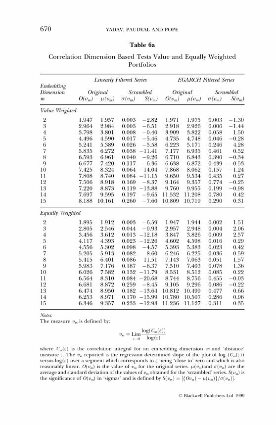
Table 6a

Correlation Dimension Based Tests Value and Equally WeightedPortfolios

Linearly Filtered Series EGARCH Filtered SeriesEmbeddingDimension Original Scrambled Original Scrambledm O(vm) �(vm) �(vm) S(vm) O(vm) �(vm) �(vm) S(vm)

Value Weighted

2 1.947 1.957 0.003 ÿ2.82 1.971 1.975 0.003 ÿ1.303 2.964 2.984 0.003 ÿ6.51 2.918 2.926 0.006 ÿ1.444 3.798 3.801 0.008 ÿ0.40 3.909 3.822 0.058 1.505 4.496 4.590 0.017 ÿ5.46 4.735 4.748 0.046 ÿ0.286 5.241 5.389 0.026 ÿ5.58 6.223 5.171 0.246 4.287 5.835 6.272 0.038 ÿ11.41 7.177 6.935 0.461 0.528 6.593 6.961 0.040 ÿ9.26 6.710 6.843 0.390 ÿ0.349 6.677 7.420 0.117 ÿ6.36 6.638 6.872 0.439 ÿ0.53

10 7.425 8.324 0.064 ÿ14.04 7.868 8.062 0.157 ÿ1.2411 7.808 8.740 0.084 ÿ11.15 9.650 9.534 0.435 0.2712 7.506 8.918 0.169 ÿ8.37 9.164 9.357 0.774 ÿ0.2513 7.220 8.873 0.119 ÿ13.88 9.760 9.955 0.199 ÿ0.9814 7.697 9.595 0.197 ÿ9.65 11.532 11.208 0.780 0.4215 8.188 10.161 0.260 ÿ7.60 10.809 10.719 0.290 0.31

Equally Weighted

2 1.895 1.912 0.003 ÿ6.59 1.947 1.944 0.002 1.513 2.805 2.546 0.044 ÿ0.93 2.957 2.948 0.004 2.064 3.456 3.612 0.013 ÿ12.18 3.847 3.826 0.009 2.575 4.117 4.393 0.023 ÿ12.26 4.602 4.598 0.016 0.296 4.556 5.302 0.098 ÿ4.57 5.393 5.383 0.023 0.427 5.205 5.913 0.082 8.60 6.246 6.225 0.036 0.598 5.415 6.401 0.086 ÿ11.51 7.143 7.063 0.051 1.579 5.983 7.176 0.187 ÿ6.37 7.510 7.403 0.078 1.36

10 6.026 7.582 0.132 ÿ11.79 8.531 8.512 0.085 0.2211 6.564 8.310 0.084 ÿ20.68 8.744 8.756 0.455 ÿ0.0312 6.681 8.872 0.259 ÿ8.45 9.105 9.296 0.086 ÿ0.2213 6.474 8.950 0.182 ÿ13.64 10.812 10.499 0.477 0.6614 6.253 8.971 0.170 ÿ15.99 10.780 10.507 0.286 0.9615 6.346 9.357 0.233 ÿ12.93 11.236 11.127 0.311 0.35

Notes:The measure vm is defined by:

vm � Lim"!0

log�Cm�"��log(")

where Cm(") is the correlation integral for an embedding dimension m and `distance'measure ". The vm reported is the regression determined slope of the plot of log (Cm("))versus log(") over a segment which corresponds to " being `close to' zero and which is alsoreasonably linear. O(vm) is the value of vm for the original series. �(vm)and �(vm) are theaverage and standard deviation of the values of vm obtained for the `scrambled' series. S(vm) isthe significance of O(vm) in `sigmas' and is defined by S�vm� � �fOvm� ÿ ��vm�g=��vm��.



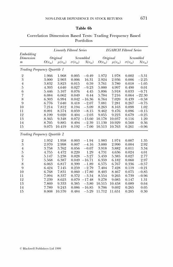
Table 6b

Correlation Dimension Based Tests: Trading Frequency BasedPortfolios


Trading Frequency Quartile 1

2 1.966 1.968 0.005 ÿ0.49 1.972 1.978 0.002 ÿ3.313 3.000 2.903 0.006 16.31 2.924 2.936 0.006 ÿ2.254 3.832 3.823 0.015 0.59 3.761 3.780 0.018 ÿ1.055 4.393 4.640 0.027 ÿ9.23 5.000 4.997 0.490 0.016 5.446 5.107 0.076 4.45 5.896 5.918 0.033 ÿ0.717 6.084 6.062 0.049 0.44 5.784 7.216 0.064 ÿ22.308 6.303 6.994 0.042 ÿ16.36 6.764 7.020 0.439 ÿ0.589 6.776 7.640 0.418 ÿ2.07 7.081 7.281 0.267 ÿ0.75

10 7.214 7.812 0.194 ÿ3.09 8.263 8.163 0.098 1.0211 8.091 8.574 0.059 ÿ8.15 9.462 9.476 0.096 ÿ0.1512 8.199 9.020 0.404 ÿ2.03 9.055 9.223 0.679 ÿ0.2513 8.365 9.348 0.072 ÿ13.60 10.178 10.037 0.116 1.2014 8.705 9.885 0.494 ÿ2.39 11.130 10.929 0.560 0.3615 9.075 10.419 0.192 ÿ7.00 10.513 10.763 0.261 ÿ0.96


2 1.952 1.958 0.003 ÿ1.94 1.983 1.974 0.007 1.353 2.970 2.998 0.007 ÿ4.16 3.000 2.990 0.004 2.924 3.758 3.762 0.056 ÿ0.07 3.918 3.882 0.011 3.345 4.755 4.472 0.220 1.29 4.731 4.636 0.024 4.016 5.147 5.238 0.028 ÿ3.27 5.459 5.385 0.027 2.777 5.568 6.387 0.049 ÿ16.71 6.359 6.182 0.060 2.978 6.063 6.817 0.399 ÿ1.89 6.575 6.767 0.336 ÿ0.579 6.424 7.145 0.259 ÿ2.79 7.404 7.428 0.119 ÿ0.21

10 6.768 7.831 0.060 ÿ17.80 8.403 8.467 0.075 ÿ0.8511 7.094 8.337 0.372 ÿ3.34 8.554 9.265 0.739 ÿ0.9612 7.239 8.623 0.079 ÿ17.48 9.278 9.085 0.147 1.3113 7.869 9.333 0.385 ÿ3.80 10.515 10.458 0.089 0.6414 7.789 9.243 0.086 ÿ16.85 9.706 9.692 0.265 0.0515 8.008 10.570 0.484 ÿ5.29 11.712 11.651 0.205 0.30



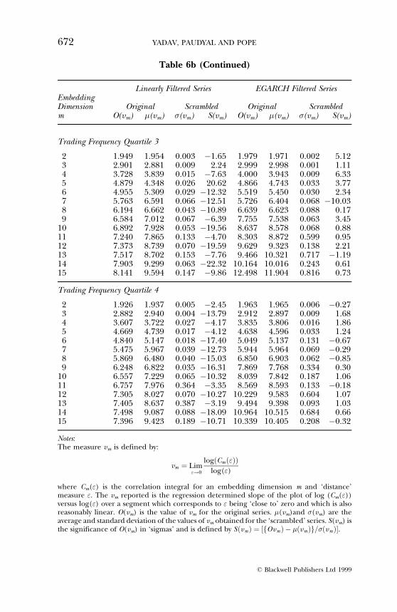
Table 6b (Continued)



2 1.949 1.954 0.003 ÿ1.65 1.979 1.971 0.002 5.123 2.901 2.881 0.009 2.24 2.999 2.998 0.001 1.114 3.728 3.839 0.015 ÿ7.63 4.000 3.943 0.009 6.335 4.879 4.348 0.026 20.62 4.866 4.743 0.033 3.776 4.955 5.309 0.029 ÿ12.32 5.519 5.450 0.030 2.347 5.763 6.591 0.066 ÿ12.51 5.726 6.404 0.068 ÿ10.038 6.194 6.662 0.043 ÿ10.89 6.639 6.623 0.088 0.179 6.584 7.012 0.067 ÿ6.39 7.755 7.538 0.063 3.45

10 6.892 7.928 0.053 ÿ19.56 8.637 8.578 0.068 0.8811 7.240 7.865 0.133 ÿ4.70 8.303 8.872 0.599 0.9512 7.373 8.739 0.070 ÿ19.59 9.629 9.323 0.138 2.2113 7.517 8.702 0.153 ÿ7.76 9.466 10.321 0.717 ÿ1.1914 7.903 9.299 0.063 ÿ22.32 10.164 10.016 0.243 0.6115 8.141 9.594 0.147 ÿ9.86 12.498 11.904 0.816 0.73


2 1.926 1.937 0.005 ÿ2.45 1.963 1.965 0.006 ÿ0.273 2.882 2.940 0.004 ÿ13.79 2.912 2.897 0.009 1.684 3.607 3.722 0.027 ÿ4.17 3.835 3.806 0.016 1.865 4.669 4.739 0.017 ÿ4.12 4.638 4.596 0.033 1.246 4.840 5.147 0.018 ÿ17.40 5.049 5.137 0.131 ÿ0.677 5.475 5.967 0.039 ÿ12.73 5.944 5.964 0.069 ÿ0.298 5.869 6.480 0.040 ÿ15.03 6.850 6.903 0.062 ÿ0.859 6.248 6.822 0.035 ÿ16.31 7.869 7.768 0.334 0.30

10 6.557 7.229 0.065 ÿ10.32 8.039 7.842 0.187 1.0611 6.757 7.976 0.364 ÿ3.35 8.569 8.593 0.133 ÿ0.1812 7.305 8.027 0.070 ÿ10.27 10.229 9.583 0.604 1.0713 7.405 8.637 0.387 ÿ3.19 9.494 9.398 0.093 1.0314 7.498 9.087 0.088 ÿ18.09 10.964 10.515 0.684 0.6615 7.396 9.423 0.189 ÿ10.71 10.339 10.405 0.208 ÿ0.32

Notes:The measure vm is defined by:

vm � Lim"!0

log�Cm�"��log(")

where Cm(") is the correlation integral for an embedding dimension m and `distance'measure ". The vm reported is the regression determined slope of the plot of log (Cm("))versus log(") over a segment which corresponds to " being `close to' zero and which is alsoreasonably linear. O(vm) is the value of vm for the original series. �(vm)and �(vm) are theaverage and standard deviation of the values of vm obtained for the `scrambled' series. S(vm) isthe significance of O(vm) in `sigmas' and is defined by S�vm� � �fOvm� ÿ ��vm�g=��vm��.



by Scheinkman and LeBaron (1989) that individual companyreturns are more random, with less deterministic non-linearity,than portfolio returns. However, whatever the evidence on thepresence of some (potentially chaotic) deterministic non-linearity, clearly there is also significant noise. Because of thenoise and the number of data points, it is difficult for us to reachunequivocal conclusions. Overall, the evidence does not appearto provide strong support for low dimensional chaotic evolutionof the system.

(b) The Largest Lyapunov Exponent

Table 7 reports the results of estimating the largest Lyapunovexponent �1 for each of the six portfolios and the associatedscrambled series, using the Wolf et al. (1985) algorithm. Thereported results correspond to an embedding dimension of 4, atime delay (�) of 1, a minimum and maximum separation atreplacement of 2% and 15% of the range of time series values, aminimum orientation error of 30ë and an evolution time (evolve)of 1, 2, 3 and 4 time steps.

The results are qualitatively similar for all portfolios. Thelargest Lyapunov exponent for the linearly-filtered series achievesa reasonably stable value after a small number of òrbits' in allcases, and the results are reasonably consistent across differentevolution times. The median estimate varies from about 0.03 bitsper day to about 0.12 bits per day. This can be interpreted asindicating that if one bit of information is available (e.g. that thereturn is positive), then that information will, on average, haveno value after about thirty days at the lower end of the spectrumand after about eight days at the upper end. The estimates of thelargest Lyapunov exponent for the random scrambled series aremore than two �'s higher in most cases, with a rank statistic p-value less than 0.04 in almost all cases. Consistent with our earlierresults, the median largest Lyapunov exponent is lowest inmagnitude for the least frequently traded stocks and increasesmonotonically with trading frequency. Similarly, the medianlargest Lyapunov exponent is higher for the value weightedportfolio than for the equally weighted portfolio. In contrast, theestimates of the largest Lyapunov exponent for the EGARCH-filtered series are not significantly different from those for the



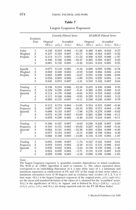
Table 7

Largest Lyapunov Exponent

Linearly Filtered Series EGARCH Filtered SeriesEvolution

Time Original Scrambled Original ScrambledO(�1) �(�1) �(�1) S(�1) O(�1) �(�1) �(�1) S(�1)

Value 1 0.149 0.210 0.005 ÿ11.28 0.408 0.405 0.010 0.37Weighted 2 0.127 0.193 0.007 ÿ10.17 0.360 0.364 0.007 ÿ0.56Portfolio 3 0.114 0.171 0.005 ÿ11.52 0.308 0.323 0.008 ÿ1.97

4 0.106 0.168 0.006 ÿ10.47 0.305 0.303 0.007 0.235 0.081 0.132 0.005 ÿ9.42 0.244 0.243 0.005 0.25

Equally 1 0.077 0.118 0.005 ÿ8.16 0.289 0.293 0.006 ÿ0.78Weighted 2 0.069 0.108 0.004 ÿ8.93 0.248 0.266 0.006 ÿ2.84Portfolio 3 0.063 0.099 0.005 ÿ6.67 0.235 0.240 0.006 ÿ0.86

4 0.056 0.093 0.006 ÿ5.89 0.234 0.229 0.004 1.445 0.045 0.074 0.007 ÿ4.31 0.183 0.182 0.007 0.04

Trading 1 0.138 0.218 0.006 ÿ12.58 0.433 0.430 0.008 0.33Frequency 2 0.129 0.199 0.007 ÿ9.41 0.389 0.385 0.009 0.43Quartile 3 0.114 0.178 0.008 ÿ8.04 0.333 0.333 0.005 ÿ0.081 4 0.111 0.168 0.006 ÿ9.95 0.329 0.312 0.005 3.12

5 0.092 0.135 0.007 ÿ6.11 0.248 0.246 0.003 0.70

Trading 1 0.113 0.174 0.004 ÿ14.85 0.354 0.355 0.003 ÿ0.46Frequency 2 0.097 0.157 0.006 ÿ10.34 0.305 0.313 0.004 ÿ1.99Quartile 3 0.088 0.143 0.007 ÿ7.98 0.278 0.278 0.009 ÿ0.022 4 0.072 0.136 0.005 ÿ13.69 0.265 0.266 0.006 ÿ0.11

5 0.059 0.109 0.005 ÿ9.40 0.210 0.210 0.005 ÿ0.11

Trading 1 0.106 0.167 0.007 ÿ8.63 0.249 0.248 0.007 0.09Frequency 2 0.105 0.155 0.005 ÿ10.02 0.227 0.231 0.009 ÿ0.44Quartile 3 0.084 0.141 0.005 ÿ12.30 0.202 0.204 0.008 ÿ0.203 4 0.077 0.134 0.007 ÿ8.15 0.200 0.198 0.004 0.49

5 0.060 0.108 0.003 ÿ14.88 0.150 0.159 0.005 ÿ1.87

Trading 1 0.035 0.046 0.007 ÿ1.74 0.167 0.165 0.004 0.61Frequency 2 0.034 0.044 0.004 ÿ2.50 0.151 0.155 0.006 ÿ0.61Quartile 3 0.030 0.042 0.004 ÿ3.24 0.130 0.139 0.006 ÿ1.404 4 0.024 0.039 0.004 ÿ3.71 0.135 0.133 0.007 0.23

5 0.020 0.030 0.003 ÿ4.16 0.096 0.106 0.006 ÿ1.65

Notes:The largest Lyapunov exponent �1 quantifies sensitive dependence to initial conditions.The Wolf et al. (1985) algorithm is used to estimate �1. The values separated abovecorrespond to an embedding dimension of 4, a time delay (tau) of 1, a minimum andmaximum separation at replacement of 2% and 15% of the range of time series values, amaximum orientation error of 30 degrees and an evolution time (evolve) of 1, 2, 3 or 4time steps. O(�1) is the largest Lyapunov exponent of the original series. �(�1) and �(�1)are the mean and standard deviation of the values of �1 obtained for the `scrambled' series.S(�1) is the significance of O(�1) in `sigmas' and is defined by S(�1) = [{O(�1) ÿ�(�1)}/�(�1)]. �(�1), �(�1) and S(�1) are being reported only for the FT All Share Index.



scrambled series, the difference seldom being more than two �'sin magnitude.

Overall, these results suggest that there are differences betweenthe linearly filtered series and the random series, but notbetween the EGARCH-filtered series and the random series.However, it is relevant to note that the largest Lyapunovexponents for the random series are not only positive but alsolarger in magnitude than those for the (potentially not sorandom) linearly-filtered series. This highlights the limitations ofthe Lyapunov exponent measure for systems with significantstochastic noise. It also shows that inferring chaos from a positivelargest Lyapunov exponent can be misleading and underscoresthe need to use bootstrapping based on surrogate data to test thesignificance of the estimate for chaos. Since there appears to beexplosive divergence in the random scrambled series, we cannotconclusively establish that the difference in the estimates of thelargest Lyapunov exponent between the actual series and thescrambled series signals chaotic sensitive dependence on initialconditions.

4. CONCLUSIONS

This paper investigates non-linear dependence in individual andportfolio stock returns for the UK market. We examine anexhaustive sample of UK stocks over a sample period of twenty-one years. The results are analysed on the basis of the tradingfrequency of individual companies.

The results reveal that non-linear dependence is highlysignificant in all cases for both individual stocks and stockportfolios. Most of the non-linear dependence is over a one dayinterval, but statistically significant non-linear dependence isobserved up to five trading days. Closer examination reveals thatmost of the non-linear dependence is in the form of EGARCH-type conditional heteroskedasticity. However, statistically signifi-cant non-linearity in addition to an EGARCH(1,1) dependencealso appears to be present. This additional non-linearity is greaterfor individual stocks than for portfolios, and greater forportfolios of smaller, less-liquid stocks. Further analysis (notreported) reveals that the non-linear dependence does not



appear to be caused by non-stationarity of the underlyingeconomic variables since the results are robust across differentsub-periods. Nor does the observed non-linear dependenceappear to be caused by non-linearity in the conditional mean.No clear support in favour of low dimensional chaos appears inthe results. That said, the limited evidence in this regard, basedon correlation dimensions, is somewhat stronger for portfolioswith relatively greater price adjustment delays across the differentstocks in the portfolio. Our results are broadly consistent withprevious US work based on stock indices. This consistencysuggests that differences between countries in the institutionalarrangements do not affect the time series dynamics of stockreturns.

NOTES

1 The effects of infrequent trading on daily portfolio returns are welldocumented and, as a first approximation, described through linear models(Cohen et al., 1986, chapter 6). When price-adjustment delays related toinfrequent trading are attributable to transaction costs we might expectthreshold non-linearity in returns, where the structure of the dynamicsdepends on trading frequency (Hsieh, 1991; and Yadav, Paudyal and Pope,1994).

2 Similar tests are used in Yadav, Paudyal and Pope (1996) to analyse indexreturns for three Far Eastern markets.

3 ARCH-class effects in stock returns have been widely documented in theliterature. See, for example, Engle and Mustafa (1992) and Blair, Poon andTaylor (1998) for individual US stocks, Akgiray (1989) for US stock indices,and Loudon, Watt and Yadav (1998) for UK stock portfolios.

4 Using EGARCH/GARCH filtered returns involves a recursive filter, and inthe context of Broomhead et al. (1992) can potentially induce distortionswhen calculating attractor dimensions.

5 EGARCH filtered returns also enable direct comparability with the resultsfor the US reported by Hsieh (1991).

6 A measure of the degree of predictability coming from single lagdependence is given by:

�1�"� � C1�"�1ÿ �1�"� :

7 A general predictability index can be defined by:

� � C1�"��1j�1�1ÿ �j�"��

where C1 � � � 1. The lower bound corresponds to an iid series, and theupper bound to a completely predictable series.



8 Cutler (1991) uses a generalised least squares procedure; Ramsey and Yuan(1990) use a random coefficient regression; and Smith (1991 and 1992) andLiu et al. (1992) use a collection of (differently defined) point estimators.

9 Brock and Baek (1991) suggest an approach for estimating standard error.10 The popular bootstrap method is pioneered in Efron (1982).11 It is possible to use a similar procedure for the Correlation integral Cm�"�

directly or for the correlation dimension v. We do not choose thecorrelation dimension since it is defined in terms of a limit which, ingeneral, may not exist. We do not choose Cm�"� since it involves an arbitrarychoice of " instead of capturing the relationship between log�Cm�"�� andlog(") over a wide range. In this context, see the personal communicationof Smith cited in Theiler et al. (1992, p. 11).

12 This is often regarded as the seminal methodological contribution in theliterature on procedures to calculate the largest Lyapunov exponent forarbitrary dimensional systems from observed data. Other methods includeAbarbanel et al. (1991), Sanu and Sawada (1985), Eckmann et al. (1986),and Dechert and Gencay (1992). Matrix techniques also estimate additionalLyapunov exponents from the product of local Jacobian matrices. However,the largest exponent is often difficult enough to estimate and additionalexponents will arguably be less stable. Moreover, it is also argued that thejoint estimation of additional exponents can potentially `compromise' eventhe stability of the largest exponent. We do acknowledge that the Wolf et al.(1985) algorithm used by us may have less power than some of thesealternatives and we need to interpret our results in this context.

13 Criteria (a) and (b) introduce survivorship bias, but this does not appearimportant in the context of the study. Criteria (c) is included to mitigatelarge distortions in observed returns series due to infrequent trading.

14 " has often been defined in terms of the maximum spread in the data.15 In fact the critical value is not exact because Hsieh (1991) uses 1,000

observations in his simulations whereas each series in our sample consists of5,285 observations.

16 The �j measure is clearly significantly greater than zero also for the randomseries. This could be due to the presence of fat tails in the unconditionaldistribution and is being separately investigated.

17 The benchmark of 2 sigmas represents significance at the 5% level only ifthe distribution involved is Gaussian. Clearly, this may not be the case.

18 It appears that vm could well stop increasing with m for an m > 15, and inthat sense provide evidence for `chaos' just as in the case of Scheinkmanand LeBaron (1989) it stabilised at about m � 13. However, in view of thesmall number of data points, estimations in this paper have been keptconfined to m �< 15. For m > 15, the number of independent m-historiesdecreases to levels which are too low to inspire confidence.

REFERENCES

Abarbanel, H.D.I., R. Brown and M.B. Kennel (1991), `Lyapunov Exponents inChaotic Systems: Their Importance and their Evaluation Using ObservedData', International Journal of Modern Physics B, Vol. 5, pp. 1347±75.

Akgiray, V. (1989), `Conditional Heteroskedasticity in Time Series of StockReturns: Evidence and Forecast', Journal of Business, Vol. 62, pp. 55±80.



Blair, B, S.H. Poon and S. Taylor, (1998), `Modelling S&P 100 Volatility: TheInformation Content of Stock Returns, Working Paper (LancasterUniversity).

Brock W.A. and E.G. Baek (1991), `Some Theory of Statistical Inference forNonlinear Science', Review of Economic Studies, Vol. 58, pp. 691±716.

________, W. Dechert and J. Scheinkman (1987), À Test for IndependenceBased on the Correlation Dimension', Working Paper (University ofWisconsin, Madison, University of Houston, and University of Chicago).

________, D.A. Hsieh and B. LeBaron (1991), `Nonlinear Dynamics, Chaos, andInstability: Statistical Theory and Economic Evidence' (The MIT Press).

Broomhead, D.S., J.P. Huke and M.R. Muldoon (1992), `Linear Filters andNonlinear Systems', Journal of Royal Statistical Society B, Vol. 54, pp. 373±82.

Cohen K.J., S.F. Maier, R.A. Schwartz and D.K. Whitcomb (1986), TheMicrostructure of Securities Markets (Prentice Hall).

Cutler, C.D. (1991), `Some Results on the Behaviour and Estimation of theFractal Dimensions of Distributions on Attractors', Journal of StatisticalPhysics, Vol. 62, pp. 651±708.

Dechert, W. and R. Gencay (1992), `Lyapunov Exponents as a NonparametricDiagnostic for Stability Analysis', Journal of Applied Econometrics, Vol. 7,Supplement, pp. S41±S60.

Eckmann, J.P. and D. Ruelle (1992), `Fundamental Limitations for EstimatingDimensions and Lyapunov Exponents in Dynamical Systems', Physica D,Vol. 56, pp. 185±87.

________, S.O.Kamphorst, D. Ruelle and S. Ciliberto (1986), `LyapunovExponents from Time Series', Physical Review A, Vol. 34, pp. 4971±979.

Efron, B. (1982), `The Jackknife, the Bootstrap and Other Resampling Plans',Regional Conference Series in Applied Mathematics, Vol. 38 (Society forIndustrial and Applied Mathematics).

Engle, R.F. and C. Mustafa (1992), Ìmplied ARCH Models from Option Prices',Journal of Econometrics, Vol. 52, pp. 289±311.

Farmer, J. (1982), `Chaotic Attractors of an Finite-Dimensional DynamicalSystem', Physica D, 4, pp. 366±93.

Gilmore, C.G. (1996), `Detecting Linear and Non-linear Dependence in StockReturns: New Methods Derived from Chaos Theory', Journal of BusinessFinance & Accounting, Vol. 23, Nos. 9 &10, pp. 1357±77.

Grassberger, P. and I. Procaccia (1983), `Measuring the Strangeness of StrangeAttractors', Physica 9D, pp. 189±208.

Hinich, M. and D. Patterson (1985), Èvidence of Nonlinearity in StockReturns', Journal of Business and Economic Statistics, Vol. 3, pp. 69±77.

Hsieh, D.A. (1989), `Testing for Nonlinearity in Daily Foreign Exchange RateCharges', Journal of Business, Vol. 62, pp. 339±68.

________ (1991), `Chaos and Nonlinear Dynamics: Application to FinancialMarkets', Journal of Finance, Vol. 46, pp. 1839±77.

Lane, J.A., D.A. Peel and E.J. Raeburn (1996), `Some Empirical Evidence on theTime Series Properties of Four U.K. Asset Prices', Economica, Vol. 63, pp.405±26.

Liu, T., C, Granger and W.P. Heller (1992), Ùsing the Correlation Exponent toDecide if an Economic Series is Chaotic', Journal of Applied Econometrics Vol.7 (Supplement), pp. S25±S39.

Loudon, G., W.H. Watt and P.K. Yadav (1998), Àn Empirical Analysis ofAlternative Parametric ARCH Models' (Royal Bank of Scotland DiscussionPaper, University of Strathclyde).



Ramsey, J. and H. Yuan (1989), `Bias and Error Bias in Dimension Calculationand Their Evaluation in Some Simple Models', Physics Letters A, Vol. 134,pp. 287±97.

________ ________ (1990), `The Statistical Properties of DimensionCalculations Using Small Data Sets', Nonlinearity, Vol. 3, pp. 155±76.

Sano, M. and Y. Sawada (1985), `Measurement of the Lyapunov Spectrum froma Chaotic Time Series', Physical Review Letters, Vol. 55, No. 10, pp. 1082±85.

Savit, R. and M. Green (1991), `Time Series and Dependent Variables', PhysicaD, Vol. 50, pp. 95±116.

Scheinkman J. and B. LeBaron (1989), `Non-linear Dynamics and StockReturns', Journal of Business, Vol. 62, pp 311±37.

Smith R.L. (1991), Òptimal Estimation of Fractal Dimension', in M. Casdagliand E. Eubank (eds.), Nonlinear Modeling and Forecasting (SFI Studies in theScience of Complexity, Vol 12, Addison-Wesley).

________ (1992), Èstimating Dimension in Noisy Chaotic Time Series,' Journalof the Royal Statistical Society B, Vol. 54, pp. 329±51.

Theiler, J., B. Galdrikian, A. Longtin, S. Eubank and J. Farmer (1992), `Testingfor Nonlinearity: The Method of Surrogate Data', Working Paper (LosAlamos National Laboratory).

Wolf, A., J.B. Swift, H.L. Swinney and J.A. Vastano (1985), `DeterminingLyapunov Exponents from a Time Series', Physica 16D, pp. 285±317.

Wu, K., R. Savit and W.A. Brock (1992), `Statistical Tests for DeterministicEffects in Broad Band Time Series', Working Paper (Department ofPhysics, University of Michigan and Department of Economics, Universityof Wisconsin).

Yadav, P.K., K. Paudyal and P.F. Pope (1994), `Threshold AutoregressiveModelling in Finance: The Price Differences of Equivalent Assets',Mathematical Finance, Vol. 4, No.2, pp. 205±21.

________ ________ ________ (1996), `Non-linear Dependence in Daily StockIndex Returns: Evidence from Pacific Basin Markets', Advances in PacificBasin Financial Markets II, pp. 349±78.



Documents

Non-linear Dependence in Stock Returns: Does Trading Frequency Matter