arX

iv:h

ep-p

h/99

0353

4v1

30

Mar

199

9

NON-EQUILIBRIUM PHASE TRANSITIONS IN

CONDENSED MATTER AND COSMOLOGY: SPINODAL

DECOMPOSITION, CONDENSATES AND DEFECTS∗

D. Boyanovsky(a,b), H.J. de Vega(b,a) and R. Holman(c)

(a)Department of Physics and Astronomy, University of Pittsburgh, Pittsburgh, PA 15260 USA

(b) LPTHE† Universite Pierre et Marie Curie (Paris VI) et Denis Diderot (Paris VII), Tour 16,

1er. etage, 4, Place Jussieu 75252 Paris, Cedex 05, France

(c) Department of Physics, Carnegie Mellon University, Pittsburgh, PA 15213, USA

(February 1, 2008)

Abstract

These lectures address the dynamics of phase ordering out of equilibrium in

condensed matter and in quantum field theory in cosmological settings, em-

phasizing their similarities and differences. In condensed matter we describe

the phenomenological approach based on the Time Dependent Ginzburg-

Landau (TDGL) description. After a general discussion of the main exper-

imental and theoretical features of phase ordering kinetics and the descrip-

tion of linear (spinodal) instabilities we introduce the scaling hypothesis and

show how a dynamical correlation length emerges in the large N limit in

condensed matter systems. The large N approximation is a powerful tool in

quantum field theory that allows the study of non-perturbative phenomena

in a consistent manner. We study the exact solution to the dynamics after

a quench in this limit in Minkowski space time and in radiation dominated

Friedman-Robertson-Walker Cosmology. There are some remarkable similar-

ities between these very different settings such as the emergence of a scaling

regime and of a dynamical correlation length at late times that describe the

formation and growth of ordered regions. In quantum field theory and cosmol-

ogy this length scale is constrained by causality and its growth in time is also

associated with coarsening and the onset of a condensate. We provide a den-

sity matrix interpretation of the formation of defects and the classicalization

of quantum fluctuations.

∗Lectures delivered at the NATO Advanced Study Institute:

Topological Defects and the Non-Equilibrium Dynamics of Symmetry Breaking Phase Transitions

†Laboratoire Associe au CNRS UMR 7589.

1

I. PHASE ORDERING KINETICS: AN INTERDISCIPLINARY FASCINATING

PROBLEM

The dynamics of non-equilibrium phase transitions and the ordering process that occursuntil the system reaches a broken symmetry equilibrium state play an important role inmany different areas. Obviously in the physics of binary fluids and ferromagnets (domainwalls) superfluids (vortex formation), and liquid crystals (many possible defects) to namebut a few in condensed matter, but also in cosmology and particle physics. In cosmologydefects produced during Grand Unified Theory (GUT) or the Electro-weak (EW) phasetransition can act as seeds for the formation of large scale structure and the dynamics ofphase ordering and formation of ordered regions is at the heart of Kibble’s mechanism ofdefect formation [1–4]. Current and future measurements of Cosmic Microwave Backgroundanisotropies will determine the nature of the cosmological phase transitions that influencedstructure formation [5]. Also at even lower energies, available with current and forthcomingaccelerators (RHIC and LHC) the phase transitions predicted by the theory of strong interac-tions, Quantum Chromodynamics (QCD) could occur out of equilibrium via the formationof coherent condensates of low energy Pions. These conjectured configurations known as‘Disoriented Chiral Condensates’ are similar to the defects expected in liquid crystals orferromagnets and their charge distribution could be an experimental telltale of the QCDphase transitions [6]. Whereas the GUT phase transition took place when the Universe wasabout 10−35 seconds old and the temperature about 1023K, and the EW phase transitionoccured when the Universe was 10−12 seconds old and with a temperature 1015K, the QCDphase transition took place at about 10−5 seconds after the Big Bang, when the temperaturewas a mere 1012K. This temperature range will be probed at RHIC and LHC within thenext very few years. The basic problem of describing the process of phase ordering and thecompetition between different broken symmetry states on the way towards reaching equilib-rium is common to all of these situations. The tools, however, are necessarily very different:whereas ferromagnets, binary fluids or alloys etc, can be described via a phenomenological(stochastic) description, certainly in quantum systems a microscopic formulation must beprovided. In these lectures we describe a program to include ideas from condensed matterto the realm of quantum field theory, to describe phenomena on a range of time and spa-tial scales of unprecedented resolution (time scales ≤ 10−23 seconds, spatial scales ≤ 10−15

meters) that require a full quantum field theoretical description.

II. MAIN IDEAS FROM CONDENSED MATTER:

Before tackling the problem of describing phase ordering kinetics in quantum systemsstarting from a microscopic theory, it proves illuminating to understand a large body of the-oretical and experimental work in condensed matter systems [7]- [10]. Although ultimatelythe tools to study the quantum problem will be different, the main physical features todescribe are basically the same: the formation and evolution of correlated regions separatedby ‘walls’ or other structures. Inside these regions an ordered phase exists which eventuallygrows to become macroscopic in size. Before attempting to describe the manner in whicha given system orders after being cooled through a phase transition an understanding ofthe relevant time scales is required. Two important time scales determine if the transition

2

occurs in or out of equilibrium: the relaxation time of long wavelength fluctuations (sincethese are the ones that order) τrel(k) and the inverse of the cooling rate tcool = T (t)/T (t).If τrel(k) << tcool then these wavelengths are in local thermodynamical equilibrium (LTE),but if τrel(k) >> tcool these wavelengths fall out of LTE and freeze out, for these the phasetransition occurs in a quenched manner. These modes do not have time to adjust locallyto the temperature change and for them the transition from a high temperature phase to alow temperature one occur instantaneously. This description was presented by Zurek [11]analysing the emergence of defect networks after a quenched phase transition. Whereas theshort wavelength modes are rapidly thermalized (typically by collisions) the long-wavelengthmodes with k << 1/ξ(T ) with ξ(T ) the correlation length (in the disordered phase) becomecritically slowed down. As T → T+

c the long wavelength modes relax very slowly, they fallout of LTE and any finite cooling rate causes them to undergo a quenched non-equilibriumphase transition. As the system is quenched from T > Tc (ordered phase) to T << Tc

(disordered phase) ordering does not occur instantaneously. The length scale of the orderedregions grows in time (after some initial transients) as the different broken symmetry phasescompete to select the final equilibrium state. A dynamical length scale ξ(t) typically emergeswhich is interpreted as the size of the correlated regions, this dynamical correlation lengthgrows in time to become macroscopically large [7–10].

The phenomenological description of phase ordering kinetics begins with a coarse grainedlocal free energy functional of a (coarse grained) local order parameter M(~r) [7,8] whichdetermines the equilibrium states. In Ising-like systems this M(~r) is the local magnetization(averaged over many lattice sites), in binary fluids or alloys it is the local concentrationdifference, in superconductors is the local gap, in superfluids is the condensate fraction etc.The typical free energy is (phenomenologically) of the Landau-Ginzburg form:

F [M ] =∫

dd~x

1

2[∇M(~x)]2 + V [M(~x)]

V [M ] =1

2r(T ) M2 +

λ

4M4 ; r(T ) = r0(T − Tc) (2.1)

The equilibrium states for T < Tc correspond to the broken symmetry states with M =±M0(T ) with

M0(T ) =

0 for T > Tc√

r0

λ(Tc − T )

12 for T < Tc

(2.2)

Below the critical temperature the potential V [M ] features a non-convex region with∂2V [M ]/∂M2 < 0 for

− Ms(T ) < M < Ms(T ) ; Ms(T ) =

√

r0

3λ(T − Tc)

12 (T < Tc) (2.3)

this region is called the spinodal region and corresponds to thermodynamically unstablestates. The lines Ms(T ) vs. T and M0(T ) vs. T [see eq.(2.2)] are known as the classicalspinodal and coexistence lines respectively.

The states between the spinodal and coexistence lines are metastable (in mean-fieldtheory). As the system is cooled below Tc into the unstable region inside the spinodal, the

3

equilibrium state of the system is a coexistence of phases separated by domains and theconcentration of phases is determined by the Maxwell construction and the lever rule.

Question: How to describe the dynamics of the phase transition and the process ofphase separation?

Answer: A phenomenological but experimentally succesful description, Time DependentGinzburg-Landau theory (TDGL) where the basic ingredient is Langevin dynamics [7]- [10]

∂M(~r, t)

∂t= −Γ[~r, M ]

δF [M ]

δM(~r, t)+ η(~r, t) (2.4)

with η(~r, t) a stochastic noise term, which is typically assumed to be white (uncorrelated)and Gaussian and obeying the fluctuation-dissipation theorem:

〈η(~r, t)η(~r′, t′)〉 = 2 T Γ(~r) δ3(~r − ~r′)δ(t − t′) ; 〈η(~r, t)〉 = 0 (2.5)

the averages 〈· · ·〉 are over the Gaussian distribution function of the noise. There are twoimportant cases to distinguish: NCOP: Non-conserved order parameter, with Γ = Γ0 aconstant independent of space, time and order parameter, and which can be absorbed in arescaling of time. COP: Conserved order parameter with

Γ[~r] = −Γ0 ∇2~r

where Γ0 could depend on the order parameter, but here we will restrict the discussion tothe case where it is a constant. In this latter case the average over the noise of the Langevinequation can be written as a conservation law

∂M

∂t= −∇ · J + η ⇒ ∂

∂t〈∫

d3 ~rM(~r, t)〉 = 0

~J = ~∇~r

[

−Γ0δF [M ]

δM

]

≡ ~∇~rµ (2.6)

where µ is recognized as the chemical potential. Examples of the NCOP are the magnetiza-tion in ferromagnets, the gap in superconductors and the condensate density in superfluids(the total particle number is conserved but not the condensate fraction), of the COP: theconcentration difference in binary fluids or alloys. For a quench from T > Tc deep into thelow temperature phase T → 0 the thermal fluctuations are suppressed after the quench andthe noise term is irrelevant. In this situation of experimental relevance of a deep quench thedynamics is now described by a deterministic equation of motion,

for NCOP:

∂M

∂t= −Γ0

δF [M ]

δM(2.7)

for COP:

∂M

∂t= ∇2

[

Γ0δF [M ]

δM

]

(2.8)

which is known as the Cahn-Hilliard equation [7,8]. In both cases the equations of motionare purely diffusive

4

dF

dt=∫

d3rδF [M ]

δM(~r, t)

∂M(~r, t)

∂t= −Γ0

∫

d3r(

δFδM

)2NCOP

∫

d3r(

~∇ δFδM

)2COP

(2.9)

and in both cases dFdt

< 0. Thus, the energy is always diminishing and there is no possibilityof increasing the free energy. Thus overbarrier thermal activation cannot be described inthe absence of thermal noise, which is clear since thermal activation is mediated by largethermal fluctuations. The fact that this phenomenological description is purely dissipativewith an ever diminishing free energy is one of the fundamental differences with the quantumfield theory description studied in the next sections.

A. Critical slowing down in NCOP:

Critical slowing down of long-wavelength fluctuations is built in the TDGL description.Consider the case of NCOP and linearize the TDGL equation above the critical temperaturefor small amplitude fluctuations near M = 0. Neglecting the noise term for the moment andtaking the Fourier transform of the small amplitude fluctuations we find

dmk(t)

dt≈ −Γ0

[

k2 + r0(T − Tc)]

mk(t) (2.10)

showing that long-wavelength small amplitud fluctuations relax to equilibrium mk = 0 on atime scale given by

τk ∝[

k2 + r0(T − Tc)]−1

(2.11)

As T → T+c the long-wavelength modes are critically slowed down and relax to equilibrium

on very long time scales. Therefore a TDGL description leads to the conclusion that if thecooling rate is finite, the long-wavelength modes will fall out of LTE and become quenched.As the temperature falls below the critical, these modes will become unstable and will growexponentially.

B. Linear instability analysis:

Let us consider now the situation for T << Tc and neglect the thermal noise. The earlytime evolution after the quench is obtained by linearizing the TDGL equation around ahomogeneous mean field solution Mo(t). Writing

M(~r, t) = Mo(t) +1√Ω

∑

~k 6=0

mk(t) ei~k·~r (2.12)

where Ω is the volume of the system, and considering only the linear term in the fluctuationsmk(t) the linearized dynamics is the following: COP: for Mo(t) the conservation gives

dMo(t)

dt= 0

5

since Mo is the volume integral of the order parameter [see eq.(2.6)] and for the fluctuationswe obtain

dmk(t)

dt= ω(k) mk(t) ; ω(k) = −Γ0 k2

[

k2 +∂2V [M ]

∂M2

∣

∣

∣

∣

∣

Mo

]

(2.13)

In the spinodal region ∂2V [M ]∂M2

∣

∣

∣

Mo

< 0 there is a band of unstable wave vectors k2 <∣

∣

∣

∣

∂2V [M ]∂M2

∣

∣

∣

Mo

∣

∣

∣

∣

for which the frequencies are positive and the fluctuations away from the mean

field grow exponentially.NCOP: separate the ~k 6= 0 from the ~k = 0 in the linearized equation of motion:

dMo(t)

dt= −Γ0

dV [M ]

dM

∣

∣

∣

∣

∣

Mo

(2.14)

dmk(t)

dt= −Γ0

[

δF [M ]

δM

]

Mo(t)

mk(t) = −Γ0

[

k2 +∂2V [M ]

∂M2

∣

∣

∣

∣

∣

Mo

]

(2.15)

whereas the first equation (2.14) determines that Mo(t) rolls down the potential hill towardsthe equilibrium solution, the second equation also displays the linear instabilities for the sameband of wave vectors as in the COP in the spinodal region |Mo(t)| ≤ Ms(T ) [see eq. (2.3)] forwhich the fluctuations grow exponentially in time. Thus in the linearized approximation forboth NCOP and the COP the spinodal instabilities are manifest as exponentially growingfluctuations. These instabilities are the hallmark of the process of phase separation and arethe early time indications of the formation and growth of correlated regions which will beunderstood in an exactly solvable example below.

C. The scaling hypothesis: dynamical length scales for ordering

The process of ordering is described by the system developing ordered regions or domainsthat are separated by walls or other type of defects. The experimental probe to studythe domain structure and the emergence of long range correlations is the equal time paircorrelation function

C(~r, t) = 〈M(~r, t)M(~0, t)〉 (2.16)

where 〈· · ·〉 stands for the statistical ensemble average in the initial state (or average over thenoise in the initial state before the quench) and will become clear(er) below. It is convenientto expand the order parameter in Fourier components

M(~r, t) =1√Ω

∑

~k

mk(t) ei~k·~x

and to consider the spatial Fourier transform of the pair correlation function

S(~k, t) = 〈m~k(t)m−~k(t)〉 (2.17)

6

known as the structure factor or power spectrum which is experimentally measured byneutron (in ferromagnets) or light scattering (in binary fluids) [12]. The scaling hypothesisintroduces a dynamical length scale L(t) that describes the typical scale of a correlatedregion and proposes that

C(~r, t) = f

(

|~r|L(t)

)

⇒ S(~k, t) = Ld(t) g(kL(t)) (2.18)

where d is the spatial dimensionality and f and g are scaling functions. Ultimately scalingis confirmed by experiments and numerical simulations and theoretically it emerges from arenormalization group approach to dynamical critical phenomena which provides a calcula-tional framework to extract the scaling functions and the deviations from scaling behavior [7].This scaling hypothesis describes the process of phase ordering as the formation of ordered‘domains’ or correlated regions of typical spatial size L(t). For NCOP typical growth lawsare L(t) ≈ t1/2 (with some systems showing weak logarithmic corrections) and L(t) ≈ t1/3

for scalar and ≈ t1/4 for vector order parameter in the COP case [7,9,10].

D. An exactly solvable (and relevant) example: the Large N limit

We consider the case where the order parameter has N -components and transformsas a vector under rotations in an N-dimensional Euclidean space, i.e. ~M(~r, t) =(M1(~r, t), M2(~r, t), · · · , MN(~r, t)). For N = 1 an example is the Ising model, for N = 2superfluids or superconductors (where the components are the real and imaginary part ofthe condensate fraction or the complex gap respectively), N = 3 is the spin one Heisenbergantiferromagnet, etc. For N = 1 the topological defects are domain walls (topological inone spatial dimension), for N = 2 they are vortices in d = 2 and vortex lines in d = 3, forN = d = 3 the topological defects are monopoles or skyrmions which are possible excita-tions in Quantum Hall systems and also appear in nematic liquid crystals [2]. For N → ∞and fixed d no topological defects exist. However the exact solution of the large N modelgives insight and is in fairly good agreement with growth laws for fixed N systems whichhad been studied experimentally and numerically [7,10]. In quantum field theory the non-equilibrium dynamics of phase transitions has been studied in Minkowsky and cosmologicalspace-times [15–19]. In cosmological space-times it has been implemented to study the col-lapse of texture-like configurations [5,13,14] (see later). The large N limit is an exactlysolvable limit that serves as a testing ground for establishing the fundamental concepts andthat can be systematically improved in a consistent 1/N expansion. It provides a consistentformulation which is non-perturbative, renormalizable and numerically implementable andhas recently been invoked in novel studies of non-equilibrium dynamics in quantum spinglasses and disordered systems [20].

The exact solution for the dynamics in the large N limit, being available both in thecondensed matter TDGL description of phase ordering kinetics and in Quantum Field The-ory in Minkowsky and Cosmological space times, allow us to compare directly the physicsof phase ordering in these situations. Thus we begin by implementing this scheme in theNCOP case for the TDGL description.

7

What is the 〈· · ·〉 in the equations of the previous section?: consider that before thequench the system in in equilibrium in the disordered phase at T >> Tc and with a veryshort correlation length (ξ(T ) ≈ 1/T ). The ensemble average in this initial state is therefore

〈M i(~r, 0)M j(~r′, 0)〉 = ∆ δijδ3(~r − ~r′)

〈M i(~r, 0)〉 = 0 (2.19)

where ∆ specifies the initial correlation. Now consider a critical quench where the system israpidly cooled through the phase transition to almost zero temperature but in the absence

of explicit symmetry breaking fields (for example a magnetic field). The average of theorder parameter will remain zero through the process of spinodal decomposition and phaseordering. During the initial stages, linear instabilities will grow exponentially with mi

k(t) ≈mi

k(0) eω(k)t ; ω(k) = k2 − r(0) for k2 < r(0) and at early times

〈mi~k(t)mj

−~k(t)〉 ≈ ∆ e2ω(k)t (2.20)

hence fluctuations begin to grow exponentially and eventually will sample the broken sym-metry states and the exponential growth must shut-off. The large N limit is implementedby writing the potential term in the free energy as

V [ ~M ] = −r(T )

2~M2 +

λ

4N( ~M2)2 ; ~M2 = ~M · ~M (2.21)

where λ is kept finite in the large N limit. We will focus on the NCOP case with a quenchto zero temperature and rescale the order parameter, time and space as

~M =

√

r(0)

λ~η ; r(0) Γ0 t = τ ;

√

r(0) ~x = z (2.22)

after which the evolution equation for the NCOP case becomes

∂~η

∂τ= ∇2~η +

(

1 − ~η2

N

)

~η (2.23)

where derivatives are now with respect to the rescaled variables. The large N limit is solvedby implementing a Hartree-like factorization [7]

~η2 → 〈~η2〉 = N〈η2i 〉 no sum over i (2.24)

Then for each component the NCOP equation becomes

∂ηi

∂τ=[

∇2 + M2(t)]

ηi (2.25)

M2(t) = 1 − 〈η2i 〉 (2.26)

the eq.(2.26) is a self-consistent condition that must be solved simultaneously with theequation of motion for the components. Thus the large N approximation linearizes theproblem at the expense of a self-consistent condition. The solution for each component isobviously

8

ηi,~k(τ) = ηi,~k(0) e−k2τ+b(τ) ; b(τ) =∫ τ

0M2(τ ′)dτ ′ (2.27)

Consider for a moment that the ~k = 0 mode is slightly displaced at the initial time, then itwill roll down the potential hill to a final equilibrium position for which M2(∞) ηi(∞) = 0 (sothe time derivative vanishes in equilibrium). If ηi(∞) 6= 0 is a broken symmetry minimum ofthe free energy, then M2(τ) → 0 when τ → ∞. This is the statement of Goldstone’s theoremthat guarantees that the perpendicular fluctuations are soft modes. This asymptotic limitallows the solution of the self-consistent condition

M2(τ) = 1 − 〈η2i (τ)〉 = 1 − ∆ e2b(τ)

∫

ddk

(2π)de−k2τ = 1 − ∆ e2b(τ) (8πt)−

d2 (2.28)

The vanishing of the right hand side in the asymptotic time regime leads to the self-consistentsolution

b(τ) → d

4ln[

τ

τ0

]

⇒ M2(τ) → d

4τ(2.29)

where τ0 is a constant related to ∆. This self-consistent solution results in the followingasymptotic behavior

ηi,~k(τ) → ηi,~k(0)(

τ

τ0

)d4

e−k2τ (2.30)

Introducing the dynamical length scale L(τ) = τ12 it is straightforward to find the structure

factor and the pair correlation function

S(~k, t) ∝ Ld(t) e−2(kL(t))2 (2.31)

C(~r, t) ∝ e− r2

8L2(t) ; L(t) = t12 (2.32)

This behavior should not be interpreted as diffusion, because of the Ld(t) in eqn. (2.31)which is a result of the self-consistent condition.

Important Features:

• The ‘effective squared mass’ M2(t)t→∞→ 0: asymptotically there are massless excita-

tions identified as Goldstone bosons.

• Since M2(t) → 0 asymptotically, the self-consistent condition results in that 〈 ~M2〉 →Nr(0)/

√λ, i.e. the fluctuations sample the broken symmetry states, which are equi-

librium minima of the free energy. These fluctuations begin to grow exponentially atearly times due to spinodal instabilities.

• A dynamical correlation length emerges L(t) = t1/2 which determines the size of thecorrelated regions or ‘domains’. A scaling solution emerges asymptotically with thenatural scale determined by the size of the ordered regions. These regions grow withthis law until they become macroscopically large. Although this a result obtained inthe large N limit, similar growth laws had been found for NCOP both analyticallyand numerically for N = 1 etc. [7]

9

• Coarsening: The expression for the structure factor (2.31) shows that at large times

only the very small wavevectors contribute to S(~k, t), however the self-consistencycondition forces the

∫

kd−1 dk S(k, t) → constant thus asymptotically the structurefactor is peaked at wavevectors k ≈ L−1(t) with an amplitude Ld(t) thus becoming a

delta function S(~k, t)t→∞→ δd(~k). The position of the peak in S(~k, t) moving towards

longer wavelength is the phenomenon of coarsening and is observed via light scattering.At long times a zero momentum condensate is formed [10] and a Bragg peak develops atzero momentum, this condensate however grows as a power of time and only becomesmacroscopic at asymptotically large times. Coarsening is one of the experimentalhallmarks of the process of phase ordering, revealed for example in light scattering[12] and is found numerically in many systems [7]. Thus the large N limit, althoughnot being able to describe topological defects offers a very good description of theordering dynamics.

III. PHASE ORDERING IN QUANTUM FIELD THEORY I: MINKOWSKI

SPACE-TIME

A. A quench in Q.F.T.

The dynamics is completely determined by the microscopic field theoretical Hamiltonian.For a simple scalar theory the Hamiltonian operator is given by

H =∫

d3x

1

2Π2(~x, t) +

1

2[~∇Φ(~x, t)]2 + V [Φ(~x, t)]

(3.1)

where Φ is the quantum mechanical field and Π its canonical momentum. We want todescribe a quenched scenario where the initial state of the system for t < 0 is the groundstate (or density matrix, see later) of a Hamiltonian for which the potential is convex forall values of the field, for example that of an harmonic oscillator, in which case the wavefunction(al) Ψ[Φ] is a Gaussian centered at the origin. At t = 0 the potential is changed sothat for t > 0 it allows for broken symmetry states. This can be achieved for example bythe following form

V [Φ] =1

2m2(t)Φ2 +

λ

4Φ4 (3.2)

m2(t) =

+m20 > 0 for t < 0

−m20 < 0 for t > 0

(3.3)

Although in Minkowski space-time this is an ad-hoc choice of a time dependent potentialthat mimics the quench [21], we will see in the next section that in a cosmological settingthe mass term naturally depends on time through the temperature dependence and that itchanges sign below the critical temperature as the Universe cools off. Most of the resultsobtained in Minkowski space-time will translate onto analogous results in a Friedmann-Robertson-Walker cosmology. Unlike the phenomenological (but succesful) description ofthe dynamics in condensed matter systems, in a microscopic quantum theory the dynamicsis completely determined by the Schrodinger equation for the time evolution of the wave

10

function or alternatively the Liouville equation for the evolution of the density matrix inthe case of mixed states. We will cast our study in terms of a density matrix in general,such a density matrix could describe pure or mixed states and obeys the quantum Liouvilleequation

i∂ρ(t)

∂t=[

H(t), ρ(t)]

(3.4)

Question: How does the wave function(al) or the density matrix evolve after a quench?

B. A simple quantum mechanical picture:

In order to gain insight into the above question, let us consider a simple case of onequantum mechanical degree of freedom q and the quench is described in terms of an harmonicoscillator with a time dependent frequency ω2(t) = −ǫ(t) ω2

0 ; ω20 > 0 with ǫ(t) the sign

function, so that ω2(t < 0) > 0 ; ω2(t > 0) < 0. Furthermore let us focus on the evolution ofa pure state (the density matrix is simple the product of the wave function and its complexconjugate). Consider that at t < 0 the wave function corresponds to the ground state of the(upright) harmonic oscillator. For t > 0 the wave function obeys

i∂Ψ[q, t]

∂t=

[

−1

2

d2

dq2− 1

2ω2

0 q2

]

Ψ[q, t] (3.5)

Since the initial wave function is a gaussian and under time evolution with a quadraticHamiltonian Gaussians remain Gaussians, the solution of this Schrodinger equation is givenby

Ψ[q, t] = N(t) e−A(t)

2q2

(3.6)

dlnN(t)

dt= − i

2A(t) (3.7)

idA

dt= A2 + ω2

0

Separating the real and imaginary parts of A(t) it is straightforward to find that|N(t)|4/Re[A(t)] is constant, a consequence of unitary time evolution. Eq.(3.8) can be castin a more familiar form by a simple substitution

A(t) = −iφ(t)

φ(t)⇒ φ(t) − ω2

0 φ(t) = 0 (3.8)

where the equation for φ was obtained by inserting the above expression for A(t) in (3.8).The solution is φ(t) = a eω0 t + b e−ω0 t featuring exponential growth. This is the quantummechanical analog of the spinodal instabilities described in the previous section. The equaltime two-point function is given by

〈q2〉(t) = A−1R (t) = |φ(t)|2 ≈ e2ω0 t (3.9)

11

The width of the Gaussian state increases in time (while the amplitude decreases to maintaina constant norm) and the quantum fluctuations grow exponentially. As the Gaussian wavefunction spreads out the probability for finding configurations with large amplitude of thecoordinates increases. These is the quantum mechanical translation of the linear spinodalinstabilities. When the non-linear contributions to the quantum mechanical potential areincluded the single particle quantum mechanical wave function will simply develop two peaksand eventually re-collapse by focusing near the origin undergoing oscillatory motion between‘collapses’ and ‘revivals’. In the case of a full quantum field theory there are infinitely manydegrees of freedom and the energy is transferred between many modes. This simple quantummechanical example paves the way for understanding in a simple manner the main featuresof a quench in the large N limit in quantum field theory, to which we now turn our attention.

C. Back to the original question: Large N in Q.F.T.

We now consider the large N limit of a full Q.F.T. in which

~Φ(~x, t) = (Φ1(~x, t), Φ2(~x, t), · · · , ΦN (~x, t)) (3.10)

and similarly for the canonical momenta ~Π. The Hamiltonian operator is of the form (3.1)with

V [~Φ] =1

2m2(t) ~Φ · ~Φ +

λ

8N[~Φ · ~Φ]2 (3.11)

with m2(t) given by (3.3). Let us focus on the case in which the initial state pure andsymmetric, i.e. 〈Φ〉 = 0, with < · · · > being the expectation value in this initial state. Themore complicated case of a mixed state, described by a density matrix is studied in detailin [16–18] and the main features are the same as those revealed by the simpler scenario of apure state. The large N limit is implemented in a similar manner as in the TDGL example,via a Hartree like factorization

(~Φ · ~Φ)2 → 2 〈~Φ · ~Φ〉 ~Φ · ~Φ (3.12)

where the expectation value is in the time evolved quantum state (in the Schrodinger picture)or in the initial state of the Heisenberg operators (in the Heisenberg picture). Via thisfactorization the Hamiltonian becomes quadratic at the expense of a self-consistent conditionas it will be seen below. It is convenient to introduce the spatial Fourier transform of thefields as

~Φ(~x, t) =1√Ω

∑

~k

~Φ~k(t) ei~k·~x (3.13)

with Ω the spatial volume, and a similar expansion for the canonical momentum Π(~x, t).The Hamiltonian becomes

H =∑

~k

1

2~Π~k · ~Π

−~k +1

2W 2

k (t) ~Φ~k · ~Φ−~k

(3.14)

W 2k (t) = m2(t) + k2 +

λ

2N

∫

d3k

(2π)3〈~Φ~k · ~Φ−~k〉(t) (3.15)

12

The problem now has decoupled in a set of infinitely many harmonic oscillators, that areonly coupled through the self-consistent condition in the frequencies (3.15). To induce aquench, the time dependent mass term has the form proposed in eq. (3.3).

Just as in the simple quantum mechanical case, we consider the initial state to be aGaussian centered at the origin in field space, which is the ground state of the (upright)harmonic oscillators for t < 0. Since a Gaussian is always a Gaussian under time evolutionwith a quadratic Hamiltonian, we propose the wave function(al) that describes the (pure)quantum mechanical state to be given by

Ψ[~Φ, t] = Πk

Nk(t) e−Ak(t)

2~Φ~k

·~Φ−~k

; Ak(t = 0) = Wk(t < 0) (3.16)

Time evolution of this wavefunction(al) is determined by the Schrodinger equation: in theSchrodinger representation the canonical momentum becomes a differential (functional) op-

erator, ~Π~k → −iδ/δ~Φ−~k and the Schrodinger equation becomes a functional differential

equation. Comparing the powers of Φ~k in this differential equation, one obtains the follow-ing evolution equations for Nk(t) and Ak(t)

d

dtln Nk(t) = − i

2Ak(t) (3.17)

idAk(t)

dt= A2

k(t) − W 2k (t) (3.18)

As in the single particle case, the constancy of |Nk(t)|4/Re[Ak(t)] is a consequence of unitarytime evolution. The non-linear equation for the kernel Ak(t) can be simplified just as in thesingle particle case by writing

Ak(t) = −iφk(t)

φk(t)⇒ φk(t) + W 2

k (t) φk(t) = 0 (3.19)

and taking the expectation value of Φ2 in this state we obtain

〈~Φ~k · ~Φ−~k〉(t) = N |φk(t)|2 (3.20)

Hence we find a self-consistent condition much like the one obtained in the large N limit forTDGL. The equations for the mode functions and the self-consistent condition for t > 0 aretherefore given by

φk(t) + [k2 + M2(t)] φk(t) = 0 (3.21)

M2(t) = −m20 +

λ

2

∫

d3k

(2π)3|φk(t)|2 (3.22)

where the integral in the self-consistent term in (3.22) is simply 〈Φ2i 〉. There are two funda-

mental differences between the quantum dynamics determined by the equations of motionand the classical dissipative dynamics of the TDGL phenomenological description given insec. II:

• The equations of motion and the self-consistency condition equations (3.21)-(3.22) leadimmediately to the conservation of energy [15,16].

13

• The evolution equations are time reversal invariant.

These properties must be contrasted to the purely dissipative evolution dictated by theTDGL equations as is clear from eq. (2.9). Consider a very weakly coupled theory λ <<1 and very early times, then the self-consistent term can be neglected and we see thatfor k2 < m2

0 the modes grow exponentially. This instability again is the manifestation ofspinodal growth [22–24,16,17]. Since the mode functions grow exponentially, fairly soon, ata time scale ts ≈ m−1

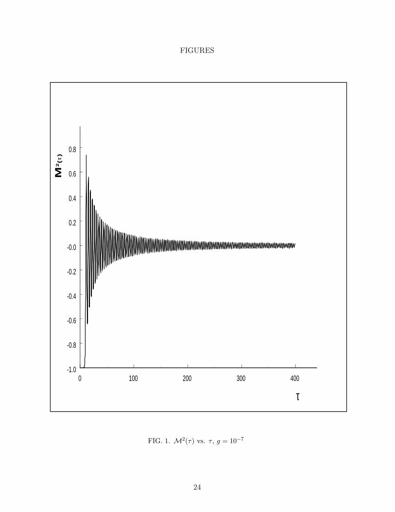
0 ln(1/λ) the self-consistent term begins to cancel the negative masssquared and M2(t) becomes smaller. We find numerically that this effective mass vanishesasymptotically, as shown in Fig. 1.

D. Emergence of condensates and classicality:

The physical mechanism here is similar to that in the classical TDGL, but in terms ofquantum fluctuations. The quantum fluctuations with wave vectors inside the spinodallyunstable band grow exponentially, these make the 〈Φ2〉 self-consistent field to grow non-perturbatively large until when 〈Φ2〉 ≈ m2

0/λ when the self-consistent (mean) field begins tobe of the same order as m2

0 (the tree level mass term). At this point the quantum fluctuationsbecome non-perturbatively large and sample field configurations near the equilibrium min-ima of the potential. The spinodal instabilities are shutting off since the effective squaredmass M2(t) is vanishing.

When M2(t) vanishes, the equations for the mode functions become those of a freemassless field, with solutions of the form φk(t) = Ak eikt + Bk e−ikt, whereas for the k = 0mode the solution must be of the form φ0(t) = a + bt with a; b 6= 0 since the Wronskian ofthe mode function and its complex conjugate is a constant. This in turn determines thatthe low k (long wavelength) behavior of the mode functions is given by

φk(t) = a cos kt + bsin kt

k(3.23)

This behavior at long wavelength has a remarkable consequence: at very long time thepower spectrum |φk(t)|2, which is the equivalent of S(k, t) for TDGL (see eq. (2.17)) isdominated by the small k-region, in particular k << 1/t, with an amplitude that grows

quadratically with time. Then the structure factor S(~k, t) = |φk(t)|2 features a peak thatmoves towards longer wavelengths at longer times and whose amplitude grows with time insuch a way that asymptotically

∫∞0 k2S(~k, t)dk/2π2 → m2

0/λ and the integral is dominatedby a very small region in k that gets narrower at longer times. This is the equivalent ofcoarsening in the TDGL solution in the large N limit, where the asymptotic time regimewas dominated by the formation of a long-wavelength condensate. Fig. 2 shows the powerspectrum at two (large) times displaying clearly the phenomenon of coarsening and theformation of a non-perturbative condensate.

The pair correlation function can now be calculated using this power spectrum [17]

C(~r, t) =1

2 π2r

∫ ∞

0k sin kr |φ2

k(t)| dk . (3.24)

14

At long times and distances the integral is dominated by the very long wavelength modes,in particular by the term ∝ sin[kt]/k of φk(t), hence the integral can be done analyticallyand we find

C(~r, t) =A

rΘ(2t − r) (3.25)

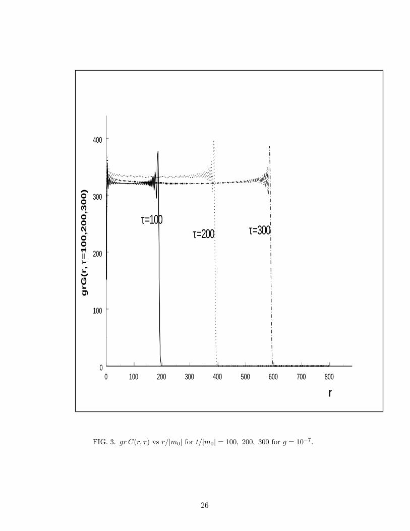
with A a constant. This is a remarkable result: the correlation falls off as 1/r inside domainsthat grow at the speed of light. This correlation function is shown in Fig. 3 at severaldifferent (large) times. This correlation function is of the scaling form: introducing thedynamical length scale L(t) = t it is clear that [17]

C(~r, t) ∝ L−1(t)f(r/L(t)) ; f(s) =Θ(2 − s)

s(3.26)

We interpret these ‘domains’ as being a non-perturbative condensate of Goldstonebosons, with a non-perturbatively large number of them ∝ 1/λ, such that the mean squareroot fluctuation of the field samples the (non-perturbative) equilibrium minima of the poten-tial. In particular an important conclusion of this analysis is that the long-wavelength modesacquire very large amplitudes, their phases vary slowly as a function of time (for k << 1/t),therefore these fluctuations which began their evolution as being quantum mechanical, nowhave become classical.

E. O.K...O.K. but where are the defects?

At this point our analysis begs this question. To understand the answer it is convenientto back track the analysis to the beginning. The initial quantum state is given by a thewave-function(al) (3.16), thus the most probable field configurations found in this ensembleare those whose spatial Fourier transform are given by

|Φk| ∝1

√

Wk(t < 0)∝ 1√

k2 + m20

(3.27)

(restoring h would multiply Φk by√

h). Then typical long-wavelength field configurationsthat are represented in the quantum ensemble described by this initial wave-function(al) areof rather small amplitude. The initial correlations are also rather short ranged on scalesm−1

0 . Under time evolution the probability distribution is given by

P[Φ, t] = |Ψ[Φ, t]|2 = ΠNi=1Πk

|Nk(t)|2e−

|Φik(t)|2

|φk(t)|2

(3.28)

At times longer than the regime dominated by the exponential growth of the spinodallyunstable modes, the power spectrum |φ2

k(t)|2 obtains the largest support for long wavelengthsk << m2

0 and with amplitudes ≈ m20/λ. Therefore field configurations with typical spatial

Fourier transform φk(t) are very likely to be found in the ensemble. These field configurationsare primarily made of long-wavelength modes and their amplitudes are non-perturbatively

15

large, of the order of the amplitude of the fields in the broken symmetry minima. A typicalsuch configuration can be written as

Φi(~x, t)typical ≈∑

k

|φk(t)| cos[~k · ~x + δi~k] (3.29)

where the phases δi~k

are randomly distributed with a Gaussian probability distribution sincethe density matrix is gaussian in this approximation. We note that a particular choice ofthese phases leads to a realization of a likely configuration in the ensemble that breaks trans-

lational invariance. In fact translations can be absorbed by a change in the phases, thusaveraging over these random phases restores translational invariance. Since the quantumstate (or density matrix) is translational invariant a particular spatial profile for a field con-figuration corresponds to a particular representative of the ensemble. Combining all of theabove results together we can present the following consistent interpretation of the orderingprocess and the formation of coherent non-perturbative structures during the dynamics ofsymmetry breaking in the large N limit [17] :

• The early time evolution occurs via the exponential growth of spinodally unstablelong wavelength modes. This unstable growth leads to a rapid growth of fluctuations〈Φ2〉(t) which in turn increases the self-consistent contribution and tends to cancel thenegative mass squared. The effective mass of the excitations −m2

0 + λ2N

〈Φ2〉(t) → 0and the asymptotic excitations are Goldstone bosons.

• At times larger than the spinodal time ts ≈ m−10 ln(1/λ), the effective mass vanishes

and the power spectrum or structure factor S(k, t) = |φk(t)|2 displays the features ofcoarsening: a peak that moves towards longer wavelengths and increases in amplitude,resulting in a long-wavelength condensate at asymptotically long times.

• For large time a dynamical correlation length emerges L(t) = t and at long distancesthe pair correlation function is of the scaling form C(~r, t) ∝ L−1(t)f(r/L(t)). Thelength scale L(t) determines the size of the correlated regions and determines thatthese regions grow at the speed of light. Inside these regions there is a non-perturbativecondensate of Goldstone bosons with a typical amplitude of the order of the value ofthe homogeneous field at the equilibrium broken symmetry minima.

The similarity between these results and those of the more phenomenological TDGL descrip-tion in condensed matter systems is rather striking. The features that are determined bythe structure of the quantum field theory are [17]: i) the scaling variable s = r/t with equalpowers of distance and time is a consequence of the Lorentz invariance of the underlyingtheory, ii) the fact that the pair correlation function vanishes for r > 2t is manifestly a con-sequence of causality. An analysis of the correlations and defect density during the spinodaltime scale has been performed in [25] and related recent studies had been performed in [26].

IV. PHASE ORDERING IN QUANTUM FIELD THEORY II: FRW COSMOLOGY

16

A. Cosmology 101 (the basics):

On large scales > 100 Mpc the Universe appears to be homogeneous and isotropic asrevealed by the isotropy and homogeneity of the cosmic microwave background and some ofthe recent large scale surveys [5]. The cosmological principle leads to a simple form of themetric of space time, the Friedmann-Robertson-Walker (FRW) metric in terms of a scalefactor that determines the Hubble flow and the curvature of spatial sections. Observationsseem to favor a flat Universe for which the space time metric is rather simple:

ds2 = dt2 − a2(t) d~x2 (4.1)

the time and spatial variables t, ~x in the above metric are called comoving time and spatialdistance respectively and have the interpretation of being the time and distance measuredby an observer locally at rest with respect to the Hubble flow. At this point we must notethat physical distances are given by ~lphys(t) = a(t) ~x. An important concept is that ofcausal (particle) horizons: events that cannot be connected by a light signal are causallydisconnected. Since light travels on null geodesics ds2 = 0 the maximum physical distancethat can be reached by a light signal at time t is given by

dH(t) = a(t)∫ t

0

dt′

a(t′)(4.2)

It will prove convenient to change coordinates to conformal time by defining a conformaltime variable

η =∫ t

0

dt′

a(t′)⇒ ds2 = C2(η) (dη2 − d~x2) ; C(η) = a(t(η)) (4.3)

in terms of which the causal horizon is simply given by dH(η) = C(η) η and physicaldistances as ~xphys = C(η) ~x. This metric is of the same form as that of Minkowski spacetime. For energies well below the Planck scale MP l ≈ 1019Gev gravitation is well describedby classical General Relativity and the Einstein equations:

Rµν − 1

2gµνR =

8π

M2P l

T µν (4.4)

where we have been cavalier and set c = 1 (as well as h = 1). Rµν is the Ricci tensor, Rthe Ricci scalar and T µν the matter field energy momentum tensor. The above equationis classical but one seeks to understand the dynamics of the Early Universe in terms of aquantum field theory that describes particle physics, thus the question: what is exactly theenergy momentum tensor?, in Einstein’s equations it is a classical object, but in QFT it isan operator. The answer to this question is: gravity is classical, fields are quantum mechan-ical, but T µν → 〈T µν〉, i.e. it is the expectation value of a quantum mechanical operator

in a quantum mechanical state. This quantum mechanical state, either pure or mixed isdescribed by a wave-function(al) or a density matrix whose time evolution is dictated by thequantum equations of motion: the Schrodinger equation for the wave functions or the quan-tum Liouville equation for a density matrix. Consistency with the postulate of homogeneityand isotropy requires that the expectation value of the energy momentum tensor must have

17

the fluid form and in the rest frame of the fluid takes the form 〈T µν〉 = diagonal(ρ, p, p, p)with ρ the energy density and p the pressure. The time and spatial components of Einstein’sequations lead to the Friedman equation

a2(t)

a2(t)=

8π

3M2P l

ρ(t) (4.5)

2a(t)

a(t)+

a2(t)

a2(t)= − 8π

M2P l

p(t) (4.6)

Combining these two equations one arrives at a simple and intuitive equation which isreminiscent of the first law of thermodynamics:

d

dt(ρa3(t)) = −p

da3(t)

dt⇒ ρ + 3

a

a(ρ + p) = 0 (4.7)

The alternative form shown on the right hand side of (4.7) is the covariant conservation

of energy. Since the physical volume of space is V0 a3(t) (with V0 the comoving volume)the above equation is recognized as dU = −p dV which is the first law of thermodynamicsfor adiabatic processes. To close the set of equations and obtain the dynamics we needan equation of state p = p(ρ): two very relevant cases are: i) radiation dominated (RD)with p = ρ/3 and matter dominated (MD) p = 0 (dust) Universes. In our study we willfocus on the RD case. The equation of state for RD is that for blackbody radiation forwhich the entropy is S = CV T 3 (with C a constant). Since V (t) = V0 a3(t) is the physicalvolume, the equation (4.7) which dictates adiabatic (isoentropic) expansion leads to a timedependence of the temperature: T (t) = T0/a(t). Now the cooling is done by the expansionof the Universe and a phase transition will occur when the Universe cools below the criticaltemperature for a given theory. For the GUT transition Tc ≈ 1016 Gev ≈ 1029K, for theEW transition Tc ≈ 100 Gev ≈ 1015K. Returning now back to the large N study of thedynamics of phase transitions, we can include the effect of cooling by the expansion of theUniverse by replacing the time dependent mass term m2(t) in (3.11) by

m2(t) = m20

[

T 2(t)

T 2c

− 1

]

; T (t) =Ti

a(t)(4.8)

This form is consistent with the Landau-Ginzburg description including the time depen-dence of the temperature via the isentropic expansion of the Universe, but perhaps moreimportantly it can be proven in a detailed manner from the self-consistent renormalizationof the mass in an expanding Universe [15]. Thus the large N limit in a RD FRW cosmologywill be studied by using the potential (3.11) but with the time dependent mass given by(4.8).

B. Large N in a RD FRW Cosmology

The large N limit is again implemented via the Hartree-like factorization (3.12) perform-ing the spatial Fourier transforms of the fields and their canonical momenta and includingthe proper scale factors, the Hamiltonian now becomes [15]

18

H(t) =∑

k

1

2a3(t)~Π~k · ~Π

−~k + W 2k (t) ~Φ~k · ~Φ−~k

(4.9)

W 2k (t) =

k2

a2+ m2(t) +

λ

2N〈~Φ~k · ~Φ−~k〉 (4.10)

where now the expectation value is in terms of a density matrix ρ[Φ(~.), Φ(~.); t] since we areconsidering the case of a thermal ensemble as the initial state.

We propose the following Gaussian ansatz for the functional density matrix elements inthe Schrodinger representation [15]

ρ[Φ, Φ, t] =∏

~k

Nk(t) exp

−Ak(t)

2~Φ~k · ~Φ−~k +

A∗k(t)

2~Φ~k · ~Φ−~k + Bk(t) ~Φ~k · ~Φ−~k

(4.11)

This form of the density matrix is dictated by the hermiticity condition ρ†[Φ, Φ, t] =ρ∗[Φ, Φ, t]; as a result of this, Bk(t) is real. The kernel Bk(t) determines the amount ofmixing in the density matrix, since if Bk = 0, the density matrix corresponds to a pure statebecause it is a wave functional times its complex conjugate. The kernels Ak(0) ; Bk(0) arechosen such that the initial density matrix is thermal with a temperature Ti > Tc [15]. Fol-lowing the same steps as in Minkowski space time, the time evolution of this density matrixcan be found in terms of a set of mode functions φk(t) that obey the following equations ofmotion and self-consistency condition

φk(t) + 3a

aφk(t) +

[

k2

a2(t)+ M2(t)

]

φk(t) = 0 (4.12)

M2(t) = m20

[

T 2i

T 2c a2(t)

− 1

]

+λ

2

∫

d3k

(2π)3|φk(t)|2 coth

Wk(0)

2Ti

. (4.13)

This equations can be cast in a more familiar form by changing coordinates to conformaltime (see eq. (4.3)) and (conformally) rescaling the mode functions φk(t) = fk(η)/C(η) toobtain the following equations for the conformal time mode functions fk(η) in an RD FRWcosmology

f ′′k (η) +

[

k2 + C2(η)M2(η)]

fk(η) = 0 (4.14)

where primes now refer to derivatives with respect to conformal time. For RD FRW C(η) =1 + η/2 (in units of m−1

0 which is the only dimensionful variable). The above equations ofmotion has now an analogous form as those solved in the case of Minkowski space-time.

As the temperature falls below the critical the effective squared mass term becomesnegative and spinodal instabilities trigger the process of phase ordering. This results in thatthe quantum fluctuations quantified by 〈~Φ2〉 grow exponentially. These spinodal instabilitiesmake the self-consistent field grow at early times and tends to overcome the negative signof the squared mass, eventually reaching an asymptotic regime in which the total effectivemass M2(η) vanishes.

Again this behavior determines that the fluctuations are sampling the equilibrium broken

symmetry minima of the initial potential, i.e. 〈~Φ2〉 → 2Nm20

λ.

19

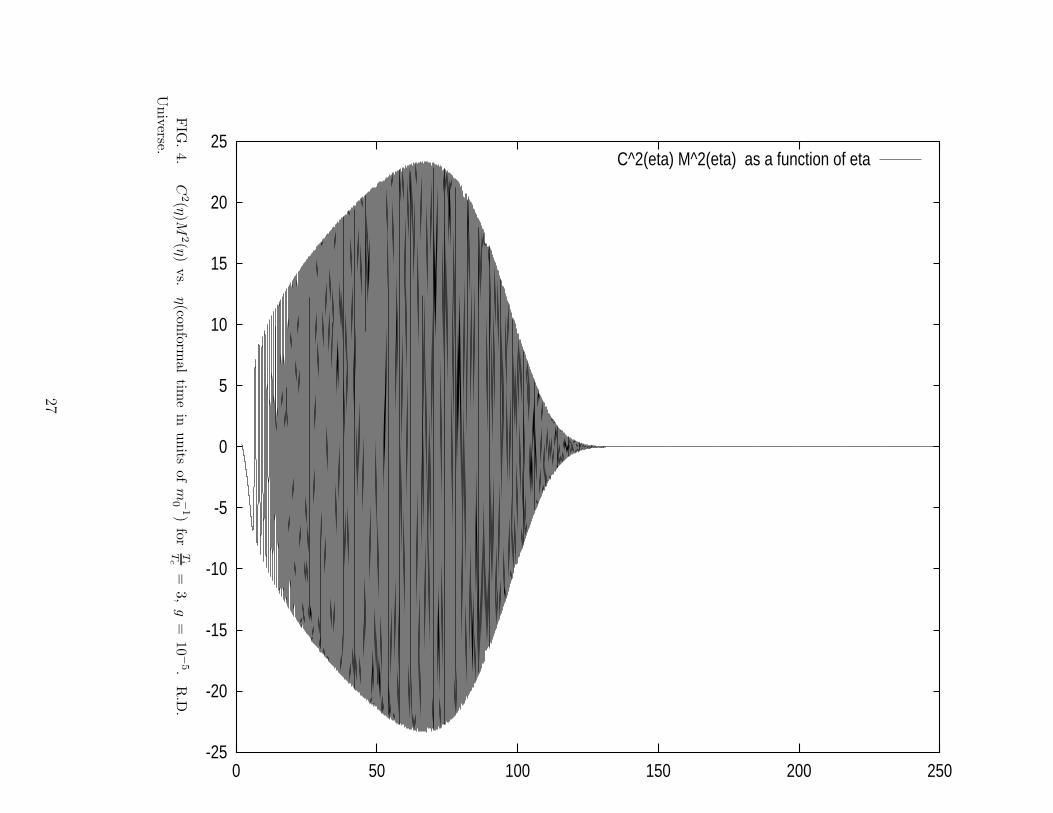
Although, just as in Minkowski space-time the effective mass vanishes asymptotically, thenon-equilibrium evolution is rather different. We find numerically [19] that asymptoticallythe effective mass term C2(η)M2(η) vanishes as −15/4η2.

Fig. 4 displays C2(η)M2(η) as a function of conformal time for the case of Ti/Tc = 1.1with Tc ∝ m0/

√λ [15,24].

We see that at very early time the mass is positive, reflecting the fact that the initialstate is in equilibrium at an initial temperature larger than the critical. As time evolves thetemperature is red-shifted and cools and at some point the phase transition occurs, whenthe mass vanishes and becomes negative.

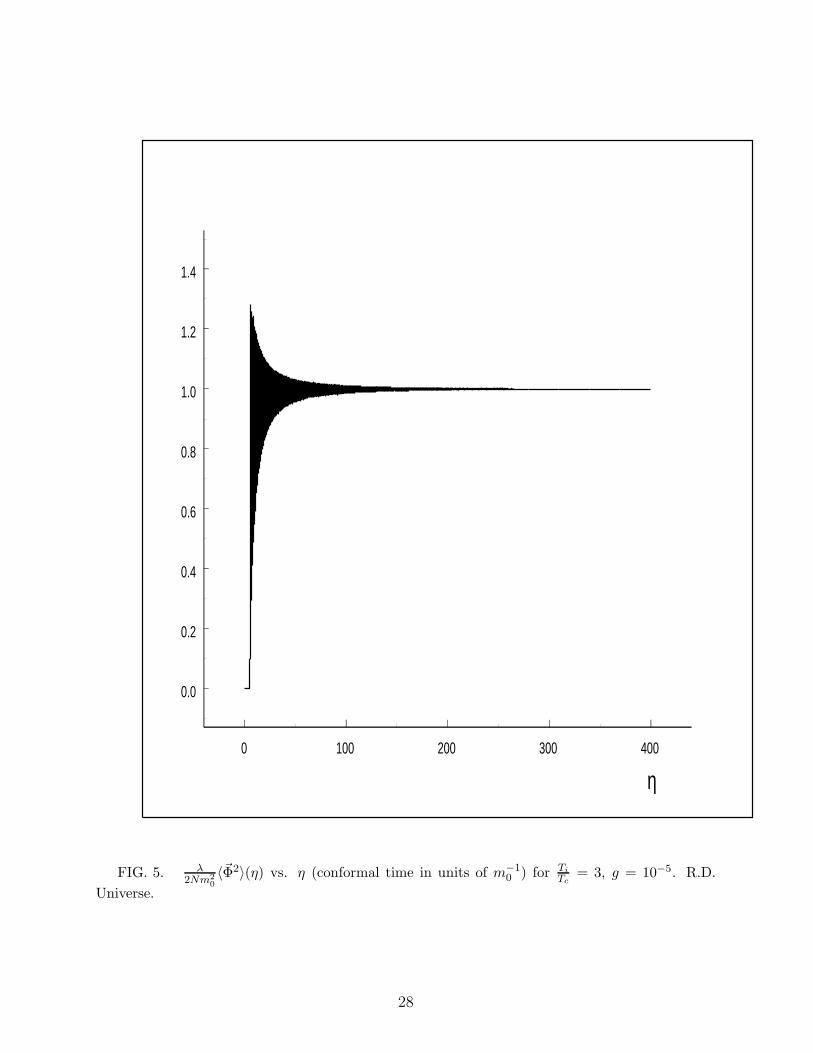
Figure 5 displays λ2Nm2

0〈~Φ2〉(η) vs. η in units of m−1

0 for Ti

Tc= 3, g = 10−5 for an R.D.

Universe. Clearly at large times the non-equilibrium fluctuations probe the broken symmetrystates.

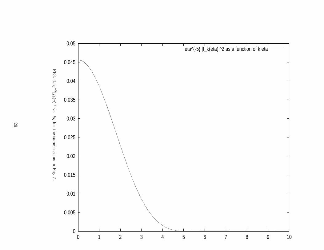
This particular asymptotic behavior of the mass determines that the mode functionsfk(η) grow as η5/2 for k < 1/η and oscillate in the form e±ikη for k > 1/η. This behavior isconfirmed numerically [19]. We find both analytically and numerically that asymptoticallythe mode functions are of the scaling form

fk(η) = Aη52

J2(kη)

(kη)2(4.15)

Where A is a numerical constant and J2(x) is a Bessel function.Figure 6 displays η−5|fk(η)|2 as a function of the scaling variable kη revealing the scaling

behavior.It is remarkable that this is exactly the same scaling solution found in the classical non-

linear sigma model in the large N limit and that describes the collapse of textures [13], andalso within the context of TDGL equations in the large N limit applied to cosmology [14].

The growth of the long-wavelength modes and the oscillatory behavior of the short wave-length modes again results in that the peak of the structure factor S(k, η) = |fk(η)|2 movestowards longer wavelengths and the maximum amplitude increases. This is the equivalentof coarsening and the onset of a condensate.

Although quantitatively different from Minkowsky space time, the qualitative featuresare similar. Asymptotically the non-equilibrium dynamics results in the formation of a non-perturbative condensate of long-wavelength Goldstone bosons. We can now compute thepair correlation function C(r, η) from the mode functions (4.15) and find that it is cutoffby causality at r = 2η. The correlation function is depicted in Fig. 4 for two different(conformal) times.

The scaling form of the pair correlation function is

C(r, η) = η2 χ(r/η)

where χ(x) is a hump-shaped function as shown in fig. 7.Clearly a dynamical length scale L(η) = η emerges as a consequence of causality, much

in the same manner as in Minkowsky space time. The physical dynamical correlation lengthis therefore given by ξphys(η) = C(η)L(η) = dH(t), that is the correlated domains grow againat the speed of light and their size is given by the causal horizon. The interpretation of thisphenomenon is that within one causal horizon there is one correlated domain, inside which

20

the mean square root fluctuation of the field is approximately the value of the equilibriumminima of the tree level potential, this is clearly consistent with Kibble’s original observation[1,2]. Inside this domain there is a non-perturbative condensate of Goldstone bosons [19].

V. CONCLUSIONS AND LOOKING AHEAD

In these lectures we have discussed the multidisciplinary nature of the problem of phaseordering kinetics and non-equilibrium aspects of symmetry breaking. Main ideas from con-densed matter were discussed and presented in a simple but hopefully illuminating frame-work and applied to the rather different realm of phase transitions in quantum field theory asneeded to understand cosmology and particle physics. The large N approximation has pro-vided a bridge that allows to cross from one field to another and borrow many of the ideasthat had been tested both theoretically and experimentally in condensed matter physics.There are, however, major differences between the condensed matter and particle physics-cosmology applications that require a very careful treatment of the quantum field theorythat cannot be replaced by simple arguments. The large N approximation in field theoryprovides a robust, consistent non-perturbative framework that allows the study of phaseordering kinetics and dynamics of symmetry breaking in a controlled and consistently im-plementable framework, it is renormalizable, respects all symmetries and can be improvedin a well defined manner. This scheme extracts cleanly the non-perturbative behavior, thequantum to classical transition and allows to quantify in a well defined manner the emer-gence of classical stochastic behavior arising from non-perturbative physics. The emergenceof scaling and a dynamical correlation length are robust features of the dynamics and theKibble-Zurek scenario describes fairly well the general features of the dynamics, albeit thedetails require careful study, both analytically and numerically.

Of course this is just the beginning, we expect a wealth of important phenomena to berevealed beyond the large N , such as the approach to equilibrium, the emergence of othertime scales associated with a hydrodynamic description of the evolution at late times anda more careful understanding of the reheating process and its influence on cosmologicalobservables. Although within very few years the wealth of observational data will providea more clear picture of the cosmological fluctuations, it is clear that the program thatpursues a fundamental understanding of the underlying physical mechanisms will continueseeking to provide a consistent microscopic description of the dynamics of cosmological phasetransitions.

VI. ACKNOWLEDGEMENTS:

D. B. thanks the organizors of the school, Henri (‘Quique’) Godfrin and Yuri Bunkov fora very stimulating school and for their warm hospitality and Tom Kibble and Ana Achucarrofor their kind invitation and patience. D. B. thanks the N.S.F for partial support throughgrant awards: PHY-9605186 and INT-9815064 and LPTHE for warm hospitality, H. J. deVega thanks the Dept. of Physics at the Univ. of Pittsburgh for hospitality. R. H., issupported by DOE grant DE-FG02-91-ER40682. We thank NATO for partial support.

21

REFERENCES

[1] T. W. B. Kibble, J. Phys. A 9, 1387 (1976), and contribution to these proceedings.[2] M. B. Hindmarsh and T.W.B. Kibble, Rep. Prog. Phys. 58:477 (1995).[3] For a classification of topological defects in terms of the underlying group structure see

T. Kibble’s contribution to these proceedings.[4] A. Vilenkin and E.P.S. Shellard, ‘Cosmic Strings and other Topological Defects’, Cam-

bridge Monographs on Math. Phys. (Cambridge Univ. Press, 1994).[5] For a comprehensive review of the status of theory and experiment see: Proceedings of

the ‘D. Chalonge’ School in Astrofundamental Physics at Erice, edited by N. Sanchezand A. Zichichi, 1996 World Scientific publisher and 1997, Kluwer Academic publishers.In particular the contributions by G. Smoot, A. N. Lasenby and A. Szalay.,R. Durrer, M. Kunz and A. Melchiorri astro-ph/9811174, M. Kunz and R. Durrer, Phys.Rev. D55, R4516 (1997) and R. Durrer’s lectures in these proceedings.

[6] See for example: K. Rajagopal in ‘Quark Gluon Plasma 2’, (Ed. R. C. Hwa, WorldScientific, 1995).

[7] A. J. Bray, Adv. Phys. 43, 357 (1994).[8] J. S. Langer in ‘Solids far from Equilibrium’, Ed. C. Godreche, (Cambridge Univ.

Press 1992); J. S. Langer in ‘Far from Equilibrium Phase Transitions’, Ed. L. Garrido,(Springer-Verlag, 1988); J. S. Langer in ‘Fluctuations, Instabilities and Phase Tran-sitions’, Ed. T. Riste, Nato Advanced Study Institute, Geilo Norway, 1975 (Plenum,1975).

[9] G. Mazenko in in ‘Far from Equilibrium Phase Transitions’, Ed. L. Garrido, (Springer-Verlag, 1988).

[10] C. Castellano and M. Zannetti, cond-mat/9807242; C. Castellano, F. Corberi and M.Zannetti, Phys. Rev. E56, 4973 (1997); F. Corberi, A. Coniglio and M. Zannetti, Phys.Rev. E51, 5469 (1995).

[11] W. H. Zurek, Nature 317, 505 (1985); Acta Physica Polonica B24, 1301 1993); Phys.Rep. 276, (1996), see also W. H. Zurek’s contribution to these proceedings.

[12] W. I. Goldburg and J. S. Huang, in ‘Fluctuations, Instabilities and Phase Transitions’,Ed. T. Riste, Nato Advanced Study Institute, Geilo Norway, 1975 (Plenum, 1975); J.S. Huang, W. I. Goldburg and M. R. Moldover, Phys. Rev. Lett. 34, 639 (1975).

[13] N. Turok and D. N. Spergel, Phys. Rev. Lett. 66, 3093 (1991); D. N. Spergel, N. Turok,W. H. Press and B. S. Ryden, Phys. Rev. D43, 1038 (1991).

[14] J. A. N. Filipe and A. J. Bray, Phys. Rev. E50, 2523 (1994); J. A. N. Filipe, (Ph. D.Thesis, 1994, unpublished).

[15] D. Boyanovsky, H. J. de Vega and R. Holman, Phys. Rev. D 49, 2769 (1994); D.Boyanovsky, D. Cormier, H. J. de Vega, R. Holman et S. Prem Kumar, Phys. Rev.D57, 2166, (1998), (and references therein).

[16] D. Boyanovsky, H. J. de Vega, R. Holman, D.-S. Lee and A. Singh, Phys. Rev. D51,4419 (1995). D. Boyanovsky, H. J. de Vega and R. Holman, Proceedings of the SecondParis Cosmology Colloquium, Observatoire de Paris, June 1994, pp. 127-215, H. J. deVega and N. Sanchez, Editors (World Scientific, 1995); Advances in AstrofundamentalPhysics, Erice Chalonge School, N. Sanchez and A. Zichichi Editors, (World Scientific,1995). D. Boyanovsky, H. J. de Vega, R. Holman and J. Salgado, Phys. Rev. D54, 7570(1996); D. Boyanovsky, D. Cormier, H. J. de Vega, R. Holman, A. Singh, M. Srednicki;

22

Phys. Rev. D56 (1997) 1939. D. Boyanovsky, H. J. de Vega and R. Holman, Vth.Erice Chalonge School, Current Topics in Astrofundamental Physics, N. Sanchez andA. Zichichi Editors, World Scientific, 1996, p. 183-270. D. Boyanovsky, M. D’Attanasio,H. J. de Vega, R. Holman and D. S. Lee, Phys. Rev. D52, 6805 (1995). D. Boyanovsky,H. J. de Vega, R. Holman and J. Salgado, Phys. Rev. D57, 7388 (1998).

[17] D. Boyanovsky, H. J. de Vega, R. Holman and J. Salgado, hep-ph/9811273, to appearin Phys. Rev. D.

[18] F. Cooper, S. Habib, Y. Kluger, E. Mottola, Phys.Rev. D55 (1997), 6471. F. Cooper, S.Habib, Y. Kluger, E. Mottola, J. P. Paz, P. R. Anderson, Phys. Rev. D50, 2848 (1994).F. Cooper, Y. Kluger, E. Mottola, J. P. Paz, Phys. Rev. D51, 2377 (1995); F. Cooperand E. Mottola, Mod. Phys. Lett. A 2, 635 (1987); F. Cooper and E. Mottola, Phys.Rev. D36, 3114 (1987); F. Cooper, S.-Y. Pi and P. N. Stancioff, Phys. Rev. D34, 3831(1986).

[19] D. Boyanovsky, H. J. de Vega and R. Holman, in preparation.[20] L. F. Cugliandolo and D. S. Dean, J. Phys. A28, 4213 (1995); ibid L453, (1995); L.

F. Cugliandolo, J. Kurchan and G. Parisi, J. Physique (France) 4, 1641 (1994) and L.Cugliandolo’s contribution to this School.

[21] Relaxing the assumption of an instantaneous quench and allowing for a time dependenceof the cooling mechanism has been recently studied by M. Bowick and A Momen, hep-ph/9803284.

[22] E. J. Weinberg and A. Wu, Phys. Rev. D36, 2474 (1987); A. Guth and S.-Y. Pi, Phys.Rev. D32, 1899 (1985).

[23] D. Boyanovsky and H. J. de Vega, Phys. Rev. D47, 2343 (1993); D. Boyanovsky Phys.Rev. E48, 767 (1993).

[24] D. Boyanovsky, D.-S. Lee and A. Singh, Phys. Rev. D48, 800 (1993).[25] G. Karra and R.J.Rivers, Phys.Lett. B414 (1997), 28; R.J.Rivers, 3rd. Colloque Cos-

mologie, Observatoire de Paris, June 1995, p. 341 in the Proceedings edited by H Jde Vega and N. Sanchez, World Scientific. A.J. Gill and R.J. Rivers, Phys.Rev. D51(1995), 6949; G.J. Cheetham, E.J. Copeland, T.S. Evans, R.J. Rivers, Phys.Rev.D47(1993),5316.

[26] ‘Defect Formation and Critical Dynamics in the Early Universe’, G. J. Stephens, E.A. Calzetta, B. L. Hu, S. A. Ramsey, gr-qc/9808059 (1998). ‘Counting Defects in anInstantaneous Quench’, D. Ibaceta and E. Calzetta, hep-ph/9810301 (1998).

23

FIGURES

0 100 200 300 400

τ

-1.0

-0.8

-0.6

-0.4

-0.2

-0.0

0.2

0.4

0.6

0.8

M2(τ

)

FIG. 1. M2(τ) vs. τ , g = 10−7

24

0.0 0.1 0.2 0.3 0.4 0.5 0.6 0.7 0.8 0.9 1.0 1.1 1.2

q

0

20

40

60

80

100

120

140

160

√g

|U

(τ=

100)|

0.0 0.1 0.2 0.3 0.4 0.5 0.6 0.7 0.8 0.9 1.0 1.1 1.2

q

0

100

200

300

400

√g

|U

(τ=

200)|

FIG. 2. g|φk(τ = 100, 200)|2 vs. q = k/|m0|, g = 10−7

25

0 100 200 300 400 500 600 700 800

r

0

100

200

300

400

grG

(r,τ=

10

0,2

00

,30

0)

τ=100τ=200 τ=300

FIG. 3. gr C(r, τ) vs r/|m0| for t/|m0| = 100, 200, 300 for g = 10−7.

26

-25

-20

-15

-10

-5

0

5

10

15

20

25

0 50 100 150 200 250

C^2(eta) M^2(eta) as a function of eta

FIG

.4.

C2(η

)M2(η

)vs.

η(con

formal

time

inunits

ofm

−1

0)

forT

i

Tc

=3,

g=

10−

5.R

.D.

Universe.

27

0 100 200 300 400

η

0.0

0.2

0.4

0.6

0.8

1.0

1.2

1.4

FIG. 5. λ2Nm2

0〈~Φ2〉(η) vs. η (conformal time in units of m−1

0 ) for Ti

Tc= 3, g = 10−5. R.D.

Universe.

28

0

0.005

0.01

0.015

0.02

0.025

0.03

0.035

0.04

0.045

0.05

0 1 2 3 4 5 6 7 8 9 10

eta^-5 |f_k(eta)|^2 as a function of k eta

FIG

.6.

η−

5|fk (η

)| 2vs.

kη

forth

esam

ecase

asin

Fig.

5.

29

0 100 200 300 400 500 600 700 800 900

r

-10

10

30

50

70

90

110

130

150

C(r

,η)

η=400

η=250

FIG. 7. C(r, η) vs. r for η = 250, 400 (in units of m−10 ) for Ti

Tc= 3, g = 10−5. R.D. FRW

Universe.

30