Embed Size (px)
Citation preview
Mon. Not. R. Astron. Soc. 380, 381–398 (2007) doi:10.1111/j.1365-2966.2007.12087.x
Non-dissipative tidal synchronization in accreting binary whitedwarf systems
Etienne Racine,1 E. Sterl Phinney1 and Phil Arras2
1Department of Physics, Mathematics and Astronomy, California Institute of Technology, Pasadena, CA 91125, USA2Kavli Institute for Theoretical Physics, University of California at Santa Barbara, Santa Barbara, CA 93106, USA
Accepted 2007 June 7. Received 2007 June 6; in original form 2006 December 4
ABSTRACTWe study a non-dissipative hydrodynamical mechanism that can stabilize the spin of the accre-tor in an ultracompact double white dwarf (WD) binary. This novel synchronization mechanismrelies on a non-linear coupling between tides and the uniform (or rigid) rotation mode, whichspins down the background star. The essential physics of the synchronization mechanism issummarized as follows. As the compact binary coalesces due to gravitational wave emission,the largest star eventually fills its Roche lobe and accretion starts. The accretor then spins up dueto infalling material and eventually reaches a spin frequency where a normal mode of the star isresonantly driven by the gravitational tidal field of the companion. If the resonating mode satis-fies a set of specific criteria, which we elucidate in this paper, it exchanges angular momentumwith the background star at a rate such that the spin of the accretor locks at this resonant fre-quency, even though accretion is ongoing. Some of the accreted angular momentum that wouldotherwise spin up the accretor is fed back to the orbit through this resonant tidal interaction. Inthis paper we solve analytically a simple dynamical system that captures the essential featuresof this mechanism. Our analytical study allows us to identify two candidate Rossby modes thatmay stabilize the spin of an accreting WD in an ultracompact binary. These two modes are thel = 4, m = 2 and l = 5, m = 3 Chandrasekhar–Friedman–Schutz (CFS) unstable hybrid r modes,which, for an incompressible equation of state, stabilize the spin of the accretor at frequency2.6 ωorb and 1.54 ωorb, respectively, where ωorb is the binary’s orbital frequency. For an n =3/2 polytrope, the accretor’s spin frequency is stabilized at 2.13 ωorb and 1.41 ωorb, respec-tively. Since the stabilization mechanism relies on continuously driving a mode at resonance,its lifetime is limited since eventually the mode amplitude saturates due to non-linear mode–mode coupling. Rough estimates of the lifetime of the effect lie from a few orbits to possiblymillions of years. We argue that one must include this hydrodynamical stabilization effect tounderstand stability and survival rate of ultracompact binaries, which is relevant in predictingthe Galactic WD gravitational background that LISA will observe.
Key words: gravitational waves – stellar dynamics – binaries: close – novae, cataclysmicvariables – white dwarfs.
1 M OT I VAT I O N , M A I N R E S U LT SA N D O U T L I N E
The collection of ∼100–200 million double white dwarf (WD) bi-naries (WD–WD) populating the Galaxy generates an importantgravitational wave background that the planned LISA mission willbe sensitive to. Predicting the properties of this gravitational wavebackground requires accurate population synthesis models, which
E-mail: [email protected]
in turn necessitate precise understanding of dynamics of WD–WDbinaries, which we now briefly summarize.
Upon formation a WD–WD binary will have its constituents sep-arated widely enough so that no mass transfer is occurring. Duringthis detached phase the orbital motion of the binary is well approxi-mated by that of point particles in Newtonian gravity, supplementedby leading-order tidal coupling and dissipative contributions due togravitational wave emission, computed from the Burke–Thorne po-tential. As the binary coalesces, the larger WD will eventually fill itsRoche lobe, signalling the onset of mass transfer. A sizable fractionof Galactic WD–WD binaries are compact enough so that this mass
C© 2007 The Authors. Journal compilation C© 2007 RAS
Dow
nloaded from https://academ
ic.oup.com/m
nras/article/380/1/381/1327835 by guest on 27 May 2022
382 E. Racine, E. S. Phinney and P. Arras
transfer phase will be reached within a Hubble time. During masstransfer the binary’s dynamics is substantially more complicatedthan during the detached phase, since the accretion rate and orbitalparameters are coupled to one another. In particular the question ofwhether or not WD–WD binaries survive mass transfer for a longtime, as opposed to merging shortly after mass transfer begins, isnot fully understood at the present time. If indeed such compactbinaries are stable, then they will be among the strongest persis-tent sources contributing to the Galactic gravitational wave back-ground for LISA. There are currently at least two observed ultra-compact WD–WD candidate systems, namely, RX J0806.3+1527(Strohmayer 2005) and V407 Vul (Strohmayer 2004; Ramsay et al.2005).
The problem of stability of accreting WD binaries has been in-vestigated in detail by Marsh, Nelemans & Steeghs (2004). Theyshow that for mass ratios lying between guaranteed stability andguaranteed instability, the stability of accreting WD–WD binariesis closely related to the strength of the dissipative synchronizationtorque Tdiss that couples the accretor’s spin and the orbit, which isassumed to be of the form
Tdiss = 1
τSI ( − ωorb), (1)
where τ S is the synchronization time-scale, I the accretor’s momentof inertia, the spin frequency of the accretor and ωorb the binary’sorbital frequency. Their result is that for accreting WD–WD binariesto be stable the synchronization time-scale must be 103 yr.
The essential contribution of the present paper is to highlighta non-dissipative hydrodynamical mechanism that may affect sig-nificantly the evolution of the spin frequency of the accretor, andtherefore impact the stability analysis of Marsh et al. (2004). Specif-ically we show that resonant tidal excitation of generalized r modes1
(or Rossby modes) in the accretor may stabilize its spin at a givenresonant frequency of the order of the orbital frequency. During thistype of hydrodynamical resonance locking (Witte & Savonije 1999)phase, some of the angular momentum carried by accreted materialthat would contribute to spin up the WD is instead fed back intothe orbit, which contributes to make the binary more stable to masstransfer.
1.1 The tidal stabilization mechanism
The physical foundation of the stabilization mechanism we analyseis the coupling of the uniform rotation mode with other stellar modesexcited by the companion’s tidal field. Formally this coupling comesout naturally from second-order stellar perturbation theory (Schenket al. 2002), but may be understood schematically as follows. Con-sider a perturbation of a uniformly rotating star characterized bya fluid Lagrangian displacement vector field ξ. The total angularmomentum of the perturbed star may be computed as an expansionin ξ, which can be formally written as
Jstar = J0 + J1[ξ] + J2[ξ, ξ], (2)
where J0 is the total angular momentum of the unperturbed star.Perturbation theory of uniformly rotating stars yields that J1 dependsonly on the uniform rotation mode (Schenk et al. 2002), all otherstellar modes contributing only in J2. This implies that the first twoterms in the right-hand side of (2) can be meaningfully combined
1 Generalized r modes are predominantly toroidal perturbations whoserestoring force is provided by the Coriolis force, which makes them dy-namically unimportant in non-rotating stars.
into a term of the form I, where I is the moment of inertia of a starrotating uniformly at spin frequency , since the angular momentumJ0 + J1 is carried entirely by the uniform rotation mode.2 Taking atime derivative of (2) then yields
J star = d
dt(I) + d
dtJ2[ξ, ξ]. (3)
In binary systems one may compute the contribution to the externaltorque on the star due to non-dissipative tidal coupling3 as an ex-pansion in ξ as well, using either the binary’s equation of motionas done in Appendix D, or equivalently the tidal interaction poten-tial. The total torque on the accretor is then the sum of this tidaltorque − J tidal and the accretion-induced torque − J acc,4 leading tothe following angular momentum conservation equation
d
dt(I) + J 2[ξ, ξ] = −( J tidal + J acc). (4)
Expanding the Lagrangian displacement ξ (x, t) in terms of normalmodes ξα(x)5 as
ξ(x, t) =∑
α
cα(t)ξα(x) + c.c., (5)
one finds that − J tidal does not equal J 2[ξ, ξ], the difference betweenboth terms describing how the uniform rotation mode couples toother stellar modes. This coupling however should not depend onwhether the perturbed star is part of a binary system or not. Thusthere should exist a derivation of this coupling contained entirelywithin the framework of stellar perturbation theory. This derivationis indeed given in Schenk et al. (2002) and yields the same answeras equation (4) when specialized to a binary system.
Now in studies of accreting binary systems it is generally assumedthat the difference between the terms − J tidal and J 2 in (4) is neg-ligible compared to the accretion-induced torque J acc. In situationswhere the tidal response of the accretor’s normal modes to the grav-itational field of its companion lies away from any resonance, thisyields a very good approximation. However, as the accretor accu-mulates material and spins up, it becomes possible to sweep throughtidal resonances, in which case the back-reaction of the resonatingmode on spin frequency evolution may not be neglected. The modeamplitude grows on a short time-scale and the difference betweenJ 2 and − J tidal may become comparable in magnitude to J acc. Aswe show in this paper, for a simple model where a single modedominates the tidal response of the star, equation (4) assumes theformd
dt = − 1
IJ acc − να
d
dt|cα|2, (6)
2 However, in situations where the unperturbed star has significant differ-ential rotation, it is not clear if this result carries over as the formalism ofSchenk et al. (2002) has not been yet extended to unperturbed stars withdifferential rotation.3 Here by ‘non-dissipative tidal coupling’ we simply mean the coupling be-tween the mass multipole moments of the accreting star induced by the fluidperturbation and the Newtonian gravitational tidal field of the companion.In this paper we omit dissipative tidal coupling for the purpose of computingthe tidal response of the accretor. We do however mention it when discussingstability issues later in this section.4 We introduce minus signs here to follow the convention used in the body ofthe paper, which defines J tidal and J acc as rates of change of orbital angularmomentum due to tidal interactions and accretion, respectively. This impliesin particular that J acc must be negative.5 In this work the mode eigenfunctions have dimensions of length, so themode amplitude coefficients cα are dimensionless. The normalization con-dition on the eigenfunctions we use is detailed in Appendix C.
C© 2007 The Authors. Journal compilation C© 2007 RAS, MNRAS 380, 381–398
Dow
nloaded from https://academ
ic.oup.com/m
nras/article/380/1/381/1327835 by guest on 27 May 2022

Tidal coupling in white dwarf binaries 383
where cα is the amplitude of the resonating mode and να is a pa-rameter describing the coupling between the resonating mode anduniform rotation. This parameter typically scales as να ∼ ωα, ωα
being the mode eigenfrequency. In the context of a binary systemone may also interpret the second term in the right-hand side of (6)as the difference between the external tidal torque due to the com-panion and the angular momentum carried by the resonant mode. Ifνα is positive and large enough, it may then be possible that whenmode amplitude cα grows rapidly due to resonant excitation, theaccretion-induced torque J acc is balanced by the hydrodynamicalback-reaction term, resulting in a spin that is nearly constant intime. The value of this quasi-static spin frequency is determined bythe eigenfrequency of the resonant mode.
Let us again emphasize that this spin stabilization mechanismis entirely hydrodynamical since it relies solely on tidal excitationof normal modes of a perfect fluid. No internal damping is neededto stabilize the spin in this scenario. However, as opposed to dis-sipative synchronization, the lifetime of this mechanism is limitedsince it requires continuously driving a mode near resonance. Even-tually the mode amplitude will grow large enough so that non-linearmode–mode coupling cannot be neglected. Generically mode–modecoupling sets a saturation amplitude beyond which it is not possi-ble to drive the mode effectively. The lifetime of our stabilizationmechanism therefore depends crucially on this saturation amplitudewhich, for resonant tidal excitation of modes, is not well known. Acomputation of this saturation amplitude, as well as understandingthe evolution of the binary when the mode saturates, likely requiressimulating a large network of coupled modes following the workof Brink, Teukolsky & Wasserman (2004, 2005), who studied theproblem of growth of r modes unstable to gravitational radiationreaction. As this is a very complicated dynamical system, we shallremain cautious and not speculate any further on the fate of thebinary after saturation.
1.2 Overview of the results
The central result of this paper is the proof that there exists modesin a rotating star whose resonant tidal excitation can stabilize thespin of the accretor in ultracompact binary WD systems. This resultis derived following a number of steps. First, we solve analyticallythe coupled system of equations describing the time evolution of thespin frequency of the accretor and the mode amplitude cα . Thissystem may be written as
= − 1
IJ acc − να
d
dt|cα|2, (7)
cα + iωαcα = Fα exp
[− imα
(φorb −
∫(t ′)dt ′
)], (8)
where Fα is the overlap of the mode eigenfunction with the externaltidal field and φorb is the binary’s orbital phase. To solve system (7)–(8) we make the following three simplifying approximations: (i) weassume the accretion-induced torque is constant, (ii) we neglect theback-reaction of the modes on orbital evolution for the purpose ofsolving (8) and (iii) we assume the accretor is slowly rotating, thatis,
√M/R3. (Throughout we employ geometric units G =
c = 1.) In the case of a mode which stabilizes the spin frequency, theanalytic solution for the spin frequency during resonance lockingmay be written as
(t) = res −√
I να|Fα|2λα| J acc| (t − t0)
, (9)
where res is the spin frequency at which mode α resonates, λα isa dimensionless number of the order of unity and time t0 is definedas the time when the mode enters resonance regime.
Once system (7)–(8) is solved, we investigate whether or notsolution (9) is physically realized by some set of normal modes ofthe accretor. We show that solution (9) is only valid for resonantlyexcited modes whose back-reaction parameter να and tidal couplingstrength Fα satisfy the following bound
να|Fα|2 0.4
( | J acc|I
)3/2
. (10)
In order to stabilize the spin of the accretor at frequency of the or-der of the orbital frequency, one needs to focus attention to modeswith low corotating-frame eigenfrequencies, as the stabilization fre-quency res is related to orbital frequency ωorb by
res = ωorb − ωα
mα
. (11)
The ideal candidate modes are generalized (or hybrid) r modes(Rossby modes) (Bryan 1889; Lindblom & Ipser 1999), since theireigenfrequencies scale as ωα ∼ . Therefore they are very low-frequency modes in slowly rotating stars, compared to, say, f modes.We then show that in ultracompact binary WD systems the follow-ing generalized r modes are potential candidates for stabilizing thespin of the accreting star.
(i) The l = 4, m = 2 r mode with eigenfrequency ω42 =−1.232 .This mode stabilizes the spin at frequency res,42 = 2.60 ωorb.
(ii) The l = 5, m = 3 r mode with eigenfrequency ω53 =−1.053 . This mode stabilizes the spin at frequency res,53 =1.54 ωorb.
There exist other candidate modes with polar quantum numberl = 6 but they satisfy bound (10) only marginally.
As mentioned previously equation (9) is valid only up to a certaintime tmax when the resonant mode amplitude becomes large enoughso that non-linear hydrodynamical effects (mode–mode coupling)saturate its growth. In that regime the simple model we analyse heredoes not describe correctly the tidal response of the star. As men-tioned previously the fate of binary in the saturation regime remainsan open problem. Denoting the saturation mode amplitude as csat,the lifetime6 Tlif of the hydrodynamical stabilizing mechanism isthen found to be
Tlif ∼ |csat|2 I να
| J acc|. (12)
The current uncertainty in the saturation amplitude and differentchoices of orbital parameters together give estimates for the lifetimeof the mechanism ranging from a few orbits to thousands, possiblymillions of years. We also investigate how our results change whenthe stellar model is an n = 3/2 polytrope. In that case we find thatback-reaction of the l = 5, m = 3 Chandrasekhar–Friedman–Schutz(CFS) unstable r mode may or may not be strong enough to stabilizethe spin, depending on accretion rate and compactness of the binary.If it is not strong enough, then the l = 4, m = 2 CFS unstable modewill be able to stabilize the spin in the case of an n = 3/2 polytrope.
6 By lifetime we here mean the time interval during which the tidal responseof star and the distribution of angular momentum is correctly described bythe model studied in this paper.
C© 2007 The Authors. Journal compilation C© 2007 RAS, MNRAS 380, 381–398
Dow
nloaded from https://academ
ic.oup.com/m
nras/article/380/1/381/1327835 by guest on 27 May 2022

384 E. Racine, E. S. Phinney and P. Arras
1.3 Implications of the stabilization mechanism on binarystability and observations
Before going ahead with the detailed derivation of the results pre-sented above, we will discuss briefly some observational conse-quences of our tidal stabilization mechanism. More specifically wetake a look at how the stability analysis of Marsh et al. (2004) ismodified when the binary is in the resonance locking regime. Duringresonance locking the spin frequency of the accretor is essentiallyconstant, so equation (6) yields
d
dt|cα|2 = − J acc
I να
. (13)
The evolution equation of the orbital angular momentum is givenby
J orb = J GW + J acc + J tidal,diss − mαbα
d
dt|cα|2, (14)
where J GW is the angular momentum loss due to gravitationalwaves, J tidal,diss is the dissipative tidal torque usually modelled asin equation (1) and the last term of the right-hand side is due tomodal tidal coupling (see Appendix D). The number bα , sometimescalled wave action, is mode energy at unit amplitude divided bycorotating-frame mode frequency. Substituting (13) into (14) yields
J orb = J GW + (1 − xα) J acc + J tidal,diss, (15)
where
xα = −mαbα
I να
. (16)
For the two r modes mentioned previously, bα is negative and there-fore xα is positive, and is interpreted as the fraction of accretedangular momentum that is fed back to the orbit by the resonant tidalinteraction. It turns out that for both modes xα is approximately equalto 0.5. The binary is more stable to mass transfer during the reso-nance locking regime, as the coefficient in front of a term driving aninstability is reduced. Stability of the binary under mass transfer isgoverned by the evolution of the Roche lobe overfill parameter ≡R2 − RL, where R2 is the donor radius and RL is the donor Roche lobesize. The equation governing the evolution of the overfill parameterduring resonance locking is given by
1
2R2
d
dt= 1
2
[(ζ2 − ζr L )
M2
M2− a
a
]
= − J GW
Jorb− I
τS Jorb( − ωorb) + σ
M2
M2, (17)
where q is the mass ratio, M2 is the donor mass and σ is defined as
σ = 1 + 1
2(ζ2 − ζrL ) − q − (1 − xα)
√(1 + q)Rh/a. (18)
The quantity Rh is the radius of the orbit around the accretor that hasthe same specific angular momentum as the accreted mass, and canbe conveniently approximated by the following expression (Verbunt& Rappaport 1988)
Rh
a= 0.088 − 0.049 log q + 0.115 log2 q + 0.020 log3 q, (19)
which is valid for the range 0.001 < q < 1. For mass ratios rangingfrom 0.1 to 1, we have Rh/a ∼ 0.15 in order of magnitude. Lastlywe have
ζ2 = d log R2
d log M2, (20)
ζrL = d log(RL/a)
d log M2, (21)
0
0.05
0.1
0.15
0.2
0.25
0.3
0.35
0.4
0 0.1 0.2 0.3 0.4 0.5 0.6 0.7 0.8 0.9 1
M2
(sol
ar m
ass)
M1 (solar mass)
Figure 1. The boundary of the regimes of guaranteed stability in two cases:(solid line) when no modes are driven, which is the criterion of Marsh, Nele-mans and Steeghs (2004) and (dashed line) during resonance locking, whichis equation (22) with xα = 0.5. The binary is stable to mass transfer in theregion of the graph below the line corresponding to the appropriate regime.Clearly resonance locking increases significantly the parameter space overwhich the binary can undergo stable equilibrium mass transfer.
with typical values −0.6 < ζ 2 < − 0.3 and ζrL 1/3. The binarywill be unstable if mass transfer M2 < 0 increases the overfill, sincea larger overfill implies in turn a larger mass transfer and thus theprocess runs away, leading to the destruction of the binary.
Let us now look for quasi-equilibrium solutions to (17), that is,solutions to = 0. The first term on the right-hand side of (17) ispositive and the second one is negative, since during resonance lock-ing the (constant) spin frequency is larger than the orbital frequency.However, in the limit of very weak dissipative tidal coupling (τ S ∼1015 yr), which we assume in this paper, the second term can be ne-glected and the criterion for existence a stable equilibrium solutionis simply σ > 0, which translates to
q < 1 + 1
2(ζ2 − ζrL ) − (1 − xα)
√(1 + q)Rh/a. (22)
Using Eggleton’s zero-temperature mass–radius relation and his ap-proximation for ζrL as both quoted by Marsh et al. (2004), we cancompare stability criterion (22) to the stability criterion of Marshet al. (2004) (equation 31 of that paper); the result is shown inFig. 1.
Now if σ 0, we have > 0 (still neglecting dissipative tidalcoupling) and no stable equilibrium solution exists during resonancelocking. In that case, the accretion rate will keep increasing until itbecomes too strong for hydrodynamical spin stabilization to operate,and the accretor can potentially be spun up through the resonancewithout saturation of the mode amplitude. A precise modelling ofthe evolution of accretion rate during resonance locking is requiredto accurately quantify this effect, which we do not address in thepresent paper.
It is also interesting to ask what the observational signature of theresonance locking regime would be, for example, in the evolutionof orbital frequency. Before resonance occurs the effect of tidalcoupling due to modes on orbital angular momentum evolution isnegligible. The equation governing the rate of change of orbitalangular momentum in this regime is thus equation (15), with xα
taken to be zero. As resonance is approached, we show in Section 4and Fig. 2 (later) that the accretor’s spin gets stabilized over a time-scale of about a year. Once the spin is stabilized the orbital angular
C© 2007 The Authors. Journal compilation C© 2007 RAS, MNRAS 380, 381–398
Dow
nloaded from https://academ
ic.oup.com/m
nras/article/380/1/381/1327835 by guest on 27 May 2022
Tidal coupling in white dwarf binaries 385
momentum evolves according to (15) with xα 0.5 for the modesconsidered here. This implies that one should observe a suddendecrease δωorb in the time derivative of the orbital frequency ωorb atthe onset of resonance locking regime, given by
δωorb = 3xα
ωorb
JorbJ acc
= 3xα
ωorb
Jorb
√M1 Rh M2 (23)
which is negative since J acc < 0. Since ωorb is negative because ofmass transfer,7 onset of resonance locking produces an increase inthe magnitude of ωorb. Alternatively one may rewrite (23) in termsof orbital period derivative Porb as
δ Porb = −3xα
Porb
Jorb
√M1 Rh M2
∼ 6 × 10⁻⁵
√1 + q
q2
(Porb
10 min
)(M1
M
)−1
×( |M2|
10−5 M yr−1
)min yr−1, (24)
where we have assumed xα = 0.5 and the order of magnitude Rh ∼0.15a to obtain the second line. Once the resonant mode saturates,the stabilization mechanism turns off and we may essentially resetxα to zero in (15), leading to a rapid increase in ωorb, given by thenegative of (23). Unfortunately this observational signature doesnot correspond to what is seen in RX J0806.3+1527 and V407 Vul,where the orbital frequency is observed to be increasing with timeat a rate consistent with orbital dynamics being entirely dominatedby gravitational wave radiation reaction. Resonance locking due totidal excitation of r modes tends to push the stars apart even fur-ther than mass transfer alone and thus provides no immediate helpin identifying the exact nature of these two systems. However, ourhydrodynamical stabilization mechanism nevertheless plays a sig-nificant role in the orbital evolution of semidetached ultracompactbinary WDs. It must therefore be taken into account for identifyingthe region of parameter space where these systems are stable to masstransfer.
1.4 Outline
Our paper is structured as follows. We start in Section 2 by brieflyreviewing the essential material from perturbation theory of rotatingstars required for our analysis. We give a more detailed review inAppendix A for the reader interested in a streamlined introductionto the detailed, heavily mathematical formalism of Schenk et al.(2002). In Section 3 we derive the evolution equation for the spin fre-quency of the accretor including tidal effects. This evolution equa-tion is essentially a version of (3) where J tidal and J2[ξ, ξ] are givenexplicitly in terms of a mode expansion of the fluid displacementvector field. We also give the evolution equation for the orbital fre-quency, needed to justify approximations used later in Section 4.In Section 4 we construct a simple dynamical system where we as-sume that a single mode is dynamically relevant for spin evolution.There we solve the equations of motion of this dynamical systemboth analytically and numerically, modelling the accretor as an in-compressible, slowly rotating Maclaurin spheroid. In this section we
7 Unless the binary is in accretion turn-on phase, where the mass transfer ratecan be substantially below its equilibrium value, in which case it possible tohave overall increasing orbital frequency.
also identify relevant candidate modes for stabilization and performthe estimate of the mechanism’s lifetime.
2 E L E M E N T S O F P E RT U R BAT I O N T H E O RYO F ROTAT I N G S TA R S
In this paper we use perturbation theory of uniformly rotating stars aspresented by Schenk et al. (2002), which is a very mathematical bodyof work. In this section we present the essential elements requiredfor the analysis of this paper, and give a more detailed review forthe interested reader in Appendix A. We use geometric units G =c = 1 throughout this paper.
The perturbed stated of a uniformly rotating star can be entirelydescribed by a Lagrangian fluid displacement vector field ξ(x, t),which tells how fluid elements are displaced from their backgroundposition x in the frame corotating with the star. This fluid displace-ment is expanded in phase space as follows:[ξ(x, t)
π(x, t)
]=∑
α
cα(t)
[ξα(x)
πα(x)
]+ c.c., (25)
where π is the momentum canonically conjugate to ξ. A givenmode ξα with associated eigenfrequency ωα is solution to a specificeigenvalue equation (equation A9). The mode amplitude coefficientscα(t) obey the following evolution equation, which is deduced bysubstituting expansion (25) into Euler’s equation,
cα + iωαcα = i
bα
∫d3x ρ ξ∗
α(x) · aext(x, t), (26)
where ρ is background mass density and aext is the acceleration fieldexperienced by the fluid elements due to external perturbations, forexample, a companion object in a binary. The constant bα is givenby
bα = 2i
∫d3x ρ ξ∗
α · (Ω × ξα
)+ 2ωα
∫d3x ρ |ξα|2, (27)
where is the angular frequency of the star and Ω is a unit vectorpointing into the direction of the background star’s angular mo-mentum vector. The complete tidal response of a rotating star to aprescribed external perturbation is then obtained by solving (26) forall modes of the star and substituting the results in expansion (25).
2.1 Adiabatic approximation for time-dependent spinfrequency
So far the formalism discussed here applies for constant backgroundspin frequency Ω. In accreting WD binaries, the spin of the accretorwill change in time so we need to discuss how to incorporate this inour analysis. A few complications arise in the case of time-varyingspin. However, if the spin of the star varies slowly in time com-pared to eigenfrequencies of dynamically relevant modes, we canstill use normal modes that are solution of (A9) in the followingway. Consider the (infinite) sequence of vector spaces of solutionsto (A9) for some range of spin frequencies (min, max), wheremin > 0 and max < break-up. Label the normal modes as [ξα(x,), ωα()], where denotes which vector space the mode labelledwith quantum numbers α belongs to.8 Assume now a displacement
8 One does not necessarily need to consider this sequence of Hilbert spacesto analyse the case of time-dependent spin frequency. We refer the reader toappendix A of Bondarescu, Teukolsky & Wasserman (2007) for a detaileddiscussion of perturbation theory of stars with generic time-dependent spinfrequency.
C© 2007 The Authors. Journal compilation C© 2007 RAS, MNRAS 380, 381–398
Dow
nloaded from https://academ
ic.oup.com/m
nras/article/380/1/381/1327835 by guest on 27 May 2022
386 E. Racine, E. S. Phinney and P. Arras
of the form ξ(x, t) = exp[−i∫
ωα() dt]ξα(x, ). We then have
ξ = −iωαξ + O(ξ/), (28)
the second term being a measure of the change in the mode eigen-function as the star is spun up or down.9 If the time-scale of changeof the spin frequency is much longer than the inverse normal modefrequency, the second term is negligible and we get
ξ = −ω2αξ − i
∂ωα
∂ξ. (29)
Again if the time-scale of change of the spin frequency is muchlonger than the inverse normal mode frequency, we can drop thesecond term in the right-hand side and we then see that our ansatz forthe fluid displacement satisfies (A9) with B → B(t), up to correctionsof the order of /(ωα), which we assume are much less than orderunity.10 In this adiabatic-type approximation, we can then expand ageneric fluid displacement in phase space as follows:[ξ(x, t)
π(x, t)
]=∑
α
cα(t)
[ξα(x, )
πα(x, )
]+ c.c., (30)
where the set ξα(x, ), πα(x, ) are the normal modes and theirconjugate momenta obtained from perturbation theory of stars spin-ning at constant frequency. The time evolution of the mode ampli-tude coefficients is then given by (A25), again up to corrections ofthe order of /(ωα), where now ξα and bα depend slowly on timedue to evolution of spin frequency. In the rest of this paper we willalways omit the labels on the modes and their frequencies. It willbe understood that a given mode (ξα , ωα) depends on spin frequencyin the context of the adiabatic approximation detailed here.
2.2 Mode amplitude evolution equation for tidal excitationin binary systems
We now specialize to the case where the external acceleration vec-tor aext is generated by the Newtonian gravitational field ext of acompanion object. We model the companion simply as a point par-ticle of mass M2 and assume that the orbital angular momentum isaligned with the spin axis of the perturbed star. The mode amplitudeforcing term (the right-hand side of equation A25) is then given by
fα ≡ i
bα
〈ξα, aext〉
= − i
bα
∫d3x ρ ξ∗
α · ∇ext
= − i
bα
∫d3x δρ∗
α ext, (31)
where δρα is the Eulerian density perturbation of mode α. Since thebackground star is axisymmetric we may write the density pertur-bation due to mode α as
δρα = gα(r , θ )eimαφ. (32)
9 It is possible to make a continuous, one-to-one identification of modesbetween vector spaces of neighbouring frequencies, as long as one is a finitedistance away from = 0. The change in mode eigenfunctions can bemeaningfully computed with the help of this identification.10 For compact WD binaries with accretion rates of the order of10−5 M yr−1, spin frequency of the order of the orbital frequency andmode frequency of the order of the spin frequency, the ratio /ωα is ofthe order of 10−8 to 10−9. The adiabatic approximation is thus fully justifiedfor such systems.
In this paper we will use the convention mα 0, which implies ωα
may be positive or negative.11
Writing the orbital separation vector d pointing from the accretorto the donor as d = d (cos φorb, sin φorb, 0). We then make use of thefollowing expansion for the external Newtonian potential ext (Ho& Lai 1999):
ext(x, t) = −M2
∑l,m
Wlmrl
dl+1e−imφorb(t)Ylm(θ, ϕ), (33)
where x are inertial coordinates and where
Wlm = (−)(l+m)/2
[4π
2l + 1(l + m)!(l − m)!
]1/2
×[
2l
(l + m
2
)!
(l − m
2
)!
]−1
, (34)
the symbol (−)n being zero if n is not an integer. Substituting ex-pansion (33) into (31) and using φ = ϕ − ∫ (t ′)dt ′ then yields
fα = Fα exp
−imα
[φorb(t) −
∫ t
(t ′)dt ′]
≡ Fαe−imαu(t), (35)
where Fα is the following complex number
Fα = iM2
bα
∞∑l=mα
∫d3x g∗
α(r , θ )Wlmα
r l
dl+1
×Ylmα(θ, φ)e−imαφ. (36)
The mode amplitude then satisfies
cα + iωαcα = Fαe−imαu(t). (37)
If the force term oscillates at a frequency far from the mode’s normalfrequency, we may write the following approximate solution to (37):
cα = iFαe−imαu(t)
mα u − ωα
. (38)
Equation (38) is only valid if the mode has not encountered a reso-nance at an earlier time, in which case (38) needs to be supplementedby a homogeneous solution to (37) obtained by matching to the so-lution to (37) during resonance (Flanagan & Racine 2006).
3 E VO L U T I O N O F S P I N A N D O R B I TA LF R E QU E N C I E S
In this section we give evolution equations for the spin frequency ofthe perturbed star and the orbital frequency of a binary undergoingconservative mass transfer. These quantities are essential in solvingthe mode amplitude equation of motion (37) since they determinethe phase u(t) of the forcing term.
3.1 Evolution of spin frequency
We obtain the evolution equation for the spin frequency from thefundamental equation
dJstar
dt= Text, (39)
11 The convention used in Schenk et al. (2002) is to choose ωα positive andthus differs from ours. If needed, see Appendix A for more details aboutmode pair notation.
C© 2007 The Authors. Journal compilation C© 2007 RAS, MNRAS 380, 381–398
Dow
nloaded from https://academ
ic.oup.com/m
nras/article/380/1/381/1327835 by guest on 27 May 2022
Tidal coupling in white dwarf binaries 387
where Text is the external torque acting on the star. In Appendix B weshow explicitly that the total angular momentum of the perturbedstar is given by
Jstar = I00 +[
1 + d ln I0
d ln 0
]I0δ +
∫d3x ρ · (ξ × π), (40)
where I0 is the unperturbed star’s moment of inertia, 0 is the un-perturbed star’s spin frequency, and δ is the perturbation in thestar’s spin frequency, so that the full spin frequency is = 0 +δ. Assuming that the change in the star’s moment of inertia due tochanges in spin and mass (because of accretion) can be neglected,(39) then gives
d
dt= 1
I
[Text − d
dt
∫d3x ρ · (ξ × π)
], (41)
where I now stands for the moment of inertia of a non-spinning star,as we neglect the effect of spin on I. Equation (41) is the desiredevolution equation for the spin frequency. In Appendix B, we derivea form of the spin evolution equation in terms of mode amplitudecoefficients, which is given by equation (B15) below.
At this point of our analysis it is worth discussing the compatibil-ity of equation (B12) with the theorem of Goldreich & Nicholson(1989), who show that the secular change in specific angular mo-mentum of a fluid element following a suitably defined ‘backgroundtrajectory’ vanishes if the star is subject to the gravitational perturba-tion of a companion object rotating around the star. We want to pointout here that this theorem does not necessarily imply that the spinof the star cannot be altered, in the sense discussed in Section A2,by tidal interactions. This important point can be illustrated simplyas follows. Label by x0 the location at t = 0 of a fluid element of theunperturbed star. We denote the trajectory this fluid element wouldfollow if the star were to remain unperturbed at all times by x (x0,t). Assume now that at t = 0 a perturbation is turned on and that theexact state of the star is described by fluid elements following thetrajectory y (x0, t). In the language of perturbation theory describedin this paper, the fluid displacement vector is defined as
y(x0, t) = x(x0, t) + ξ(x0, t). (42)
Note however that the trajectory x(x0, t) does not describe the back-ground state defined in Goldreich & Nicholson (1989). They insteaddecompose the exact state as follows:
y(x0, t) = x∗(x0, t) + ξ∗(x0, t), (43)
where the time average of the perturbation ξ∗ about the backgroundtrajectory x∗ is required to vanish. Now in general, the time aver-age of the perturbation ξ about the unperturbed trajectory x doesnot vanish, one specific example being when a mode of the star isresonantly excited. Hence what Goldreich and Nicholson call thebackground state in general differs from the unperturbed state. Tolinear order in ξ, we have
x∗(x0, t) = x(x0, t) + 〈ξ(x0, t)〉 + O(ξ2), (44)
where here the brackets 〈 〉 denote a suitably defined time averag-ing procedure about the unperturbed state (Goldreich & Nicholson1989). The point is that the quantity 〈ξ〉 contains in general differ-ential rotation modes and therefore the background state describedby fluid trajectories x∗ does not generically describe a fluid in uni-form (rigid) rotation. One therefore may not interpret the theoremof Goldreich & Nicholson (1989) as implying that tidal interactionscannot change the spin of a star, in the sense defined in Section A2.Still the theorem of Goldreich & Nicholson (1989) may in princi-ple be converted into an evolution equation for the secular change
of the spin frequency if one decomposes the background state onto the basis of Jordan chain modes describing arbitrary differentialrotation and then isolates the rate of change of the coefficient c1 ofthe uniform rotation Jordan chain mode.
Now in the special case where 〈ξ〉 vanishes, then the backgroundstate of Goldreich & Nicholson does correspond to the unperturbedstate (which here is a uniformly rotating star). In that case theirtheorem does indeed imply that the secular change in the spin fre-quency of the star vanishes, in the context of a star perturbed by anorbiting companion object. We can easily show explicitly that thisresult is compatible with the equation of motion (B12) we derivedrigorously using perturbation theory of uniformly rotating stars. Tocarry out this proof one first makes the ansatz = 0 to solvethe mode amplitude evolution equation (37). One then finds thatcA(t) = |cA|e−im Au(t), where |cA| is constant. Clearly the time av-erage of cA(t) over a time-scale long compared to 1/u is zero andtherefore 〈ξ〉 = 0. Using this form of the mode amplitude coeffi-cients, the form (D10) for the total external torque applied on thestar and averaging equation (B12) over a time-scale long comparedto 1/u, one finds immediately that the time averaged change in thespin frequency vanishes, consistent with the ansatz used to solvethe mode amplitude evolution equation. Thus a constant spin fre-quency is the solution to the time averaged spin evolution equation,consistent with the theorem of Goldreich & Nicholson. However, inmore general situations where the frequency u of the driving term inthe mode amplitude evolution equation (37) varies in time, leadingpossibly to resonant excitations of normal modes, one obtains thetime evolution of the spin frequency of the star by solving simulta-neously (37) and (B12), as long as the adiabatic approximation ofSection 2.1 is valid.
3.2 Orbital frequency evolution
We next give the evolution equation for the orbital frequency ωorb.Below we assume a Newtonian quasi-circular orbit, that is, ω2
orb =(M1 + M2)/d3 ≡ M/d3, with M being constant. We follow Marshet al. (2004) closely. We assume the orbital angular momentumJorb evolves due to three effects, namely, emission of gravitationalwaves, mass transfer and tidal coupling. We may then write
J orb = J GW + J acc + J tidal, (45)
where
J GW = − 32
5d4µM2 Jorb. (46)
In Appendix D, we review the computation of J tidal in Newtoniangravity and show that it can be written to leading order in the fluidperturbation as a sum over modes as follows:
J tidal = −∑
α
mαbα
d
dt|cα|2 + 1
τSI ( − ωorb), (47)
the second term in the right-hand side modelling dissipative tidalcoupling. As noted in appendix K of Schenk et al. (2002), each in-dividual term of the above sum does not correspond to the angularmomentum deposited in mode α; the term J2[ζ, ζ] (cf. equation B1)giving the angular momentum in the star carried by the perturba-tion contains in general cross-terms between different modes. For aquasi-circular orbit and conservative mass transfer we have
J orb =[
− ωorb
3ωorb+ (1 − q)
M2
M2
]Jorb, (48)
C© 2007 The Authors. Journal compilation C© 2007 RAS, MNRAS 380, 381–398
Dow
nloaded from https://academ
ic.oup.com/m
nras/article/380/1/381/1327835 by guest on 27 May 2022
388 E. Racine, E. S. Phinney and P. Arras
where q is the mass ratio M2/M1. We then obtain the followingevolution equation for orbital frequency:
ωorb = −3ωorb
[− 32
5d4µM2 + J acc
Jorb− (1 − q)
M2
M2
− 1
Jorb
∑α
mαbα
d
dt|cα|2 + I ( − ωorb)
JorbτS
]. (49)
Comparing (B12) and (49) and assuming that the binary is in aregime where ∼ ωorb, that is, close to synchronization, we thensee that roughly, ωorb ∼ (R/d)2. Thus for the purpose of solving(37), we will assume as a first approximation that ωorb is constant,since u(t) is dominated by spin frequency time evolution. We shallleave including back-reaction on orbital parameters when solvingfor the mode amplitude for a future publication.
4 A S I N G L E G E N E R A L I Z E D RO S S B Y M O D EA S S Y N C H RO N I Z I N G M E C H A N I S M
In this section we develop and analyse a simple dynamical systemthat attempts to extract the dominant features of the synchronizationmechanism we propose, namely, the stabilization of the accretingstar’s spin frequency through resonant tidal excitation of normalmodes. The essential features of the physical system we model inthis section may be summarized as follows. To begin with considera compact, detached binary WD system. The binary is compactenough that it coalesces due to gravitational wave emission. Thesystem eventually reaches a point where the larger, less massiveWD fills its Roche lobe and mass transfer begins. The accretingWD spins up as it accumulates material from its companion andeventually reaches a spin frequency at which one of its normal modesis resonantly driven. The amplitude of the mode then grows rapidlyand may affect significantly the evolution of the spin frequency,depending on the size of mode back-reaction (cf. equation B12).
Our aim is to solve the coupled dynamical equations (37) and(B12) for mode amplitude and spin frequency for a single resonantmode and use this solution to catalogue which modes are suitablecandidates for stabilizing the spin of the accretor. In this paper wewill focus solely on the excitation of generalized Rossby modes(Bryan 1889; Lindblom & Ipser 1999), since their normal frequen-cies scale as the star’s spin frequency, and may then resonate whenthe star’s spin frequency is of the order of the orbital frequency.Other modes like f and p modes resonate only at spin frequenciesmuch larger than synchronized spin frequency. It is then likely thatdissipative tidal coupling prevents the accretor from reaching a largeenough spin for such modes to stabilize it. For stars with buoyancy,g modes are also potential candidates for spin stabilization at spinfrequency of the order of the orbital frequency, but we will not in-vestigate them in this paper. In Appendix C we review the propertiesof generalized r modes needed for our purposes. For a modern, in-depth discussion of these modes, the interested reader is invited toconsult Lindblom & Ipser (1999).
4.1 Main assumptions and evolution equations
The dynamical system we study in this section is of course a crudeapproximation to the true dynamics of the binary. The main assump-tions we make when solving (37) and (B12) are the following.
(i) First we assume, as mentioned at the end of Section 3.2, thatorbital frequency is constant for the purpose of solving the modeamplitude evolution equation (37).
(ii) We assume the accretor spins slowly enough so that (1) wemay use appropriate approximate formulae for the r-mode eigen-functions and eigenfrequencies and (2) we may consider its momentof inertia as constant.
(iii) We assume a constant torque on the star due to accretion ofmaterial from the companion.
(iv) We assume that the Rossby modes are driven solely by thegravitational tidal field of the companion, that is, we neglect theexternal forcing due to impact of infalling material on the surfacestar when computing the driving term in equation (37).
(v) Lastly, we assume that the evolution of the spin frequencydescribed by equation (41) is dominated by a single r mode.
A given r mode may be a suitable candidate for tidal synchroniza-tion only if it satisfies the following four criteria: (i) its azimuthalquantum number m must be non-zero, otherwise the tidal drivingterm does oscillate in time (cf. equation 37) and resonance is notpossible; (ii) its quantum numbers must satisfy
l + m = even, (50)
otherwise the mode does not couple to the Newtonian tidal field (cf.equations 34, 36 and C16);12 (iii) for m>0 the mode’s dimensionlessfrequency w = ω/2 must satisfy the condition
λ ≡ m + 2w > 0 (51)
for resonance to be at all possible, as can be seen from (11) and(iv) the mode’s back-reaction parameter να , encountered in equa-tion (6) and defined precisely by equations (52) and (57) below,must be positive and large enough (how large will be determinedlater in Section 4.2) for the mode to be a candidate for tidal syn-chronization. As shown in Table E1 in Appendix E, there are fivecandidate modes, with l 6, satisfying criteria (i)–(iii). Each candi-date mode is marked by an asterisk in that table. We shall see belowthat modes will l 7 are not expected to satisfy criterion (iv) forgeneric binaries, which is why they are excluded from Table E1.
As mentioned above our model dynamical system consists of twocoupled differential equations, one for the (complex) mode ampli-tude cα and one for the spin frequency of the star . For a singlemode, spin frequency evolution equation (41) reduces to
= 1
I
[Text − 2
⟨Ω × ξα, −iωαξα + Ω × ξα
⟩ d
dt|cα|2
]
≡ 1
I
[Text − κα
d
dt|cα|2
]. (52)
Conservation of angular momentum yields
Text = − J tidal − J acc
= mαbα
d
dt|cα|2 − J acc, (53)
where J tidal and J acc are the rates of change of orbital angular mo-mentum due tidal interactions and accretion, respectively. We thenobtain the following system of equations
= acc − να
d
dt|cα|2, (54)
12 Note that this condition excludes the so-called classical r modes since theyhave l = m + 1. This restriction on l + m is lifted if we allow misalignmentof the spin and the orbital angular momentum. However, since we expectmost of the WD spin to come from accretion, the amount of misalignmentshould be small and tidal coupling of r modes with l + m odd should besuppressed by some power of this small misalignment angle.
C© 2007 The Authors. Journal compilation C© 2007 RAS, MNRAS 380, 381–398
Dow
nloaded from https://academ
ic.oup.com/m
nras/article/380/1/381/1327835 by guest on 27 May 2022
Tidal coupling in white dwarf binaries 389
cα + iωαcα = Fαe−imαu, (55)
where the quantities acc and να are given by
acc = − 1
IJ acc, (56)
να = 1
I(κα − mαbα), (57)
where acc is assumed constant. For the analysis of system (54)–(55) performed in the next subsection, the only information we needabout the parametersFα and να is that they are of the form (constant)× . Explicit expressions for Fα and να for generalized r modes ofslowly rotating stars are provided in Appendix E.
4.2 Approximate analytic solution
Let us start our analytic investigation of system (54)–(55) by defininga few quantities as follows:
γα ≡ cα
Fα
eimαu, (58)
να ≡ 1
3να|Fα|2, (59)
λα ≡ mα + 2wα, (60)
resα ≡ mα
λα
ωorb. (61)
Definition (59) is such that parameter να is dimensionless and con-stant. We can then rewrite the system (54)–(55) as follows:
= acc −[να
3 d
dt|γα|2
][1 + O(1/2/)], (62)
γ α + [iλα
( − res
α
)γα
][1 + O(/2)] = 1. (63)
The scaling of the error terms in (62) comes from assuming that thetime-scale for evolution of |γ α|2 is at most the ‘no back-reaction’resonance time-scale tres ∼ −1/2. The main advantage of this for-mulation of the evolution equations is that we have got rid of theterm e−imαu in the mode amplitude equation of motion. However,the presence of the 3 factor in the evolution equation (62) for thespin still makes the equation very complicated to solve. But sincewe expect back-reaction of the modes on the spin to be dynamicallyrelevant mostly in the vicinity of the resonance, we simplify (62) byreplacing by res
α in the second term of the right-hand side. Wecan estimate the errors introduced by this approximation as follows.Away from resonance the solution for the rescaled mode amplitudeγ α is given by
|γα|2 = 1
λ2α
( − res
α
)2
[1 + O
(
λα
( − res
α
))
+O
(
λ2α
( − res
α
)2
)],
(64)
yielding simply
= acc[1 + O(να)] (65)
in that regime. Numerically the O(να) corrections lie within therange 10−5 to 10−7 for modes of interest, independently of whether
or not is replaced by resα in the right-hand side of (62). Thus
replacing by resα in the second term of the right-hand side of
(62) introduces negligible corrections away from resonance. Nowapproximations (64) and (65) fail when resonance regime is reached,which is when the dominant error terms in (64) become of the orderof unity, that is,
− resα ∼ 1/2, (66)
or alternatively when
∼ resα
[1 + O
(1/2
resα
)]. (67)
For accreting binary WDs these correction terms are typically ofthe order of 10−4. Thus approximating by res
α in the right-handside of (62) introduces negligible corrections also in the resonanceregime. Defining
να = να
(res
α
)3, (68)
the system of equations we solve here can be written in its final formas
= acc − να
d
dt|γα|2, (69)
γ α + iλα
[ − res
α
]γα = 1. (70)
The initial conditions we impose to integrate system (69)–(70) arethe following. We assume accretion begins at t = 0 and that theaccretor is not spinning prior to accreting phase. This implies ofcourse (0) = 0. For the mode amplitude we assume that it starts atits equilibrium tide value, namely, γ α(0) = i/λα res
α , obtained bysetting γ α = 0 at t = 0 in (70). We are now ready to solve (69)–(70)analytically. Writing mode amplitude γ α as
γα = γ Rα + iγ I
α , (71)
with γ R,Iα real, we may rewrite (69) using (70) as follows:
= acc − 2ναγRα . (72)
Taking a time derivative of (72) and using (70) once more yields
+ 2να = −hα
( − res
α
), (73)
where the quantity hα is defined as
hα = 2ναλαγIα . (74)
Then the imaginary part of (70) may be rewritten as follows:
hα = −λ2α( − res
α )(acc − ). (75)
So far all that has been done is rewriting system (54)–(55) in aslightly different, but very useful form. We are now ready to identifythe crucial approximation needed to solve (73) and (75) simultane-ously. The key lies in realizing that for a large enough value of να ,which will be determined below, we may discard the term on theleft-hand side of (73). This approximation essentially yields someaverage spin frequency since we are dropping a term that gener-ates oscillations in at frequency ∼ √
hα . This average frequencysolution is obtained directly from equation (73) and is equal to
= resα − 2να
hα
(76)
Substituting (76) into (75) then gives
hα = 2λ2αναacch2
α
h3α + 4λ2
αν2α
, (77)
C© 2007 The Authors. Journal compilation C© 2007 RAS, MNRAS 380, 381–398
Dow
nloaded from https://academ
ic.oup.com/m
nras/article/380/1/381/1327835 by guest on 27 May 2022

390 E. Racine, E. S. Phinney and P. Arras
which is then easily integrated. The result is the following cubicequation for hα
h3α −
[4λ2
ανα
(acct − res
α
)+ 4ν2α(
resα
)2
]hα − 8λ2
αν2α
≡ h3α − a1(t)hα − a0 = 0. (78)
The average frequency is then given by (76), choosing the uniqueroot of (78) that satisfies the initial condition hα(0) = 2να/
resα . The
explicit form of the complete solution is
(t) = res − 2να
θ (tc − t)
[a0
2+√
a20
4− a1(t)3
27
]1/3
+ 2θ (t − tc)
√a1(t)
3cos
[1
3arccos
(33/2a0
2a1(t)3/2
)]
+ θ (tc − t)
[a0
2−√
a20
4− a1(t)3
27
]1/3−1
, (79)
where the critical time tc is defined such that
a1(tc) =(
27a20
4
)1/3
. (80)
Clearly solution (79) is not particularly revealing. In the large t limithowever solution (79) assumes the following very simple form
(t) = resα −
[να
λ2αacc(t − t0)
]1/2
for t t0, (81)
where
t0 = resα
acc− να
λ2α(res
α )2acc res
α
acc. (82)
The constant t0 is essentially the time it would take to spin the starup to the resonant frequency in the absence of mode back-reaction.
It should be clear that approximation (76), leading to the large tsolution (81), must necessarily fail when back-reaction parameterνα is small, since in that case the star spins up through the resonance.An argument that shows this goes as follows. Assume (76) and (77)to be valid at t = 0. Initially we have hα > 0 and hence hα > 0.Equation (77) then implies hα > hα(0) > 0 for all time, which meansthat < res
α for all time, which cannot be true for να less than somecritical value νcrit, since in the limit να → 0, the solution for the spinapproaches (t) → acct continuously. Approximation (76) cantherefore work well for all time only for modes that will stabilizethe spin frequency, that is, modes with να > νcrit. The value of νcrit
may then be estimated by finding when approximation (76) fails,which is when ∼ 2να . Using (76) and (77), we have
2να
= −3(
2λ2αναacc
)2 h4α(
h3α + 4λ2
αν2α
)3 . (83)
This expression has a maximum at h3α = 16λ2
αν2α/5. Putting this value
for hα in (83) and requiring ∼ 2να then yields the following valuefor the critical value νcrit of the back-reaction parameter
νcrit = 0.24√
λα3/2acc . (84)
Along with the late-time solution (81) for spin frequency, equa-tion (84) is one of our key results. Again only modes with να νcrit may effectively stabilize the spin of the accretor through tidalresonance. Modes with back-reaction parameters να νcrit do nothave a strong enough stabilizing effect on the spin to prevent the ac-cretor from being spun up through the resonance. For the candidatemodes shown in Table E1,
√λα 1.7 so a more conservative form
of (84) that we may apply to all candidate modes is νcrit = 0.4 3/2acc .
Another useful version of bound (84) that must be satisfied by spinstabilizing modes is the following:
να
resα
0.24√
λα
∣∣∣∣ Fα
resα
∣∣∣∣−2(
1/2acc
resα
)3
. (85)
The latter version of the critical bound highlights better its depen-dence on tidal coupling strength, as να/res
α is independent of binaryparameters while the back-reaction parameter να , to which bound(84) refers to, depends on those parameters.
4.3 Numerical results
Here we present results of numerical integration of the system ofequations (54)–(55) and compare with the approximate analytic so-lution derived in Section 4.2 above. For realistic accretion rates,numerical integration of (54)–(55) is challenging because of a dras-tic separation of time-scales. The time-scale of accretion-inducedspin-up is of the order of ∼10−3 yr−1, while the characteristic time-scale of the mode amplitude equation away from resonance is∼−1 ∼ 10−2 s−1. Stable numerical integration of system (54)–(55)using a Runge–Kutta scheme from = 0 to = res takes a verylong time and is not a desirable approach. What we do instead is startnumerical integration close to resonance and use initial conditionsfor mode amplitude derived from the approximate solution (38) toequation of motion (37). In Fig. 2 we show the time evolution of thespin frequency of the accretor obtained from integrating (54)–(55)using such approximate initial conditions. The resonant mode usedhere is the l = 5, m = 3, w = −0.5266 generalized r mode, and weused the same values for tidal ratio and mass ratio as reported inTable E1. We normalize units of time res = 1. In these units weused a value of acc = 10−9, its value in Hz yr−1 depending on thevalue of the orbital frequency. For an orbital period of ∼5 min, theaccretion spin-up rate is ∼3 × 10⁻⁵ Hz yr−1. For these parametersbound (85) isν53
res53
2.2 × 10⁻², (86)
which is satisfied as one can see from Table E1. We thus expect themode to stabilize the spin for this particular choice of parameters.
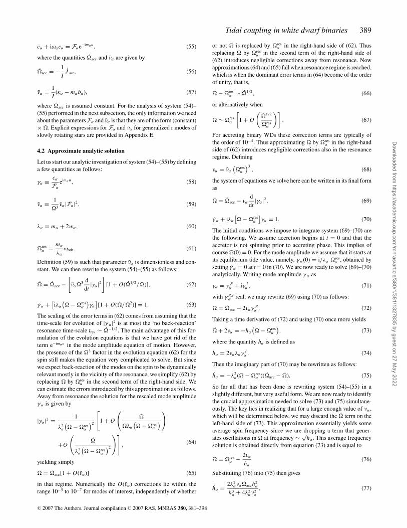
In Fig. 3 we show the relative error between the spin frequencyobtained from numerical integration of (54)–(55) and the full ana-lytic approximation (79). The relative error is less than 10−7, which
0.995
0.996
0.997
0.998
0.999
1
0 2e+06 4e+06 6e+06 8e+06 1e+07 1.2e+07 1.4e+07
Ω /
Ωre
s
Ωres t
Figure 2. The time evolution of accretor’s spin frequency obtained by in-tegrating system (54)–(55) numerically. The following model parameterswere used for moment of inertia of the accretor, the tidal ratio, the mass ratioand accretion-induced spin-up rate, respectively: I = 0.4MR2, R/d = 0.2,q = 0.25 and acc = 10−9.
C© 2007 The Authors. Journal compilation C© 2007 RAS, MNRAS 380, 381–398
Dow
nloaded from https://academ
ic.oup.com/m
nras/article/380/1/381/1327835 by guest on 27 May 2022
Tidal coupling in white dwarf binaries 391
0
1e-08
2e-08
3e-08
4e-08
5e-08
6e-08
7e-08
8e-08
0 2e+06 4e+06 6e+06 8e+06 1e+07 1.2e+07 1.4e+07
(Ωnu
mer
ical
- Ω
anal
ytic
)/Ω
num
eric
al
Ωres t
Figure 3. The relative error between the spin frequency obtained numeri-cally and the approximate analytic solution derived in Section 4.2.
gives additional strong justification to the various approximationsmade in deriving this analytic solution. We attribute the initial dis-crepancy between the numerical solution and the analytic solution toour practical choice of initial conditions for numerical integration.
4.4 Lifetime of synchronizer
The synchronizing mechanism we propose is based on exciting amode close to its resonance frequency over a long period of time.This process obviously cannot last forever since the mode amplitudegrows as
√t − t0 in the regime where the spin is stabilized, as can
be seen by combining (81) and (69)
|γα|2 = |γα(0)|2 + acct − resα
να
+ 1√λ2
αναacc(t − t0)
acct − resα
να
acc
να
(t − t0). (87)
After a certain amount of time the mode amplitude will reach a valuewhere the resonant mode couples significantly to other modes of thestar through non-linear hydrodynamical effects (see Schenk et al.2002; Brink et al. 2004, 2005), which saturates the growth of themode amplitude. As shown by Brink et al. (2004, 2005), a preciseunderstanding of the evolution of a perturbed star in the regimewhere a mode saturates requires a simulation involving thousandsof modes.
Denoting the saturation amplitude csat, we obtain the followingestimate for the duration Tlif of the stabilization mechanism pre-sented
Tlif ∼ |csat|2 να
|Fα|2acc∼ |csat|2 να
acc
∼ 1.5 × 10¹⁰ |csat|2res
, (88)
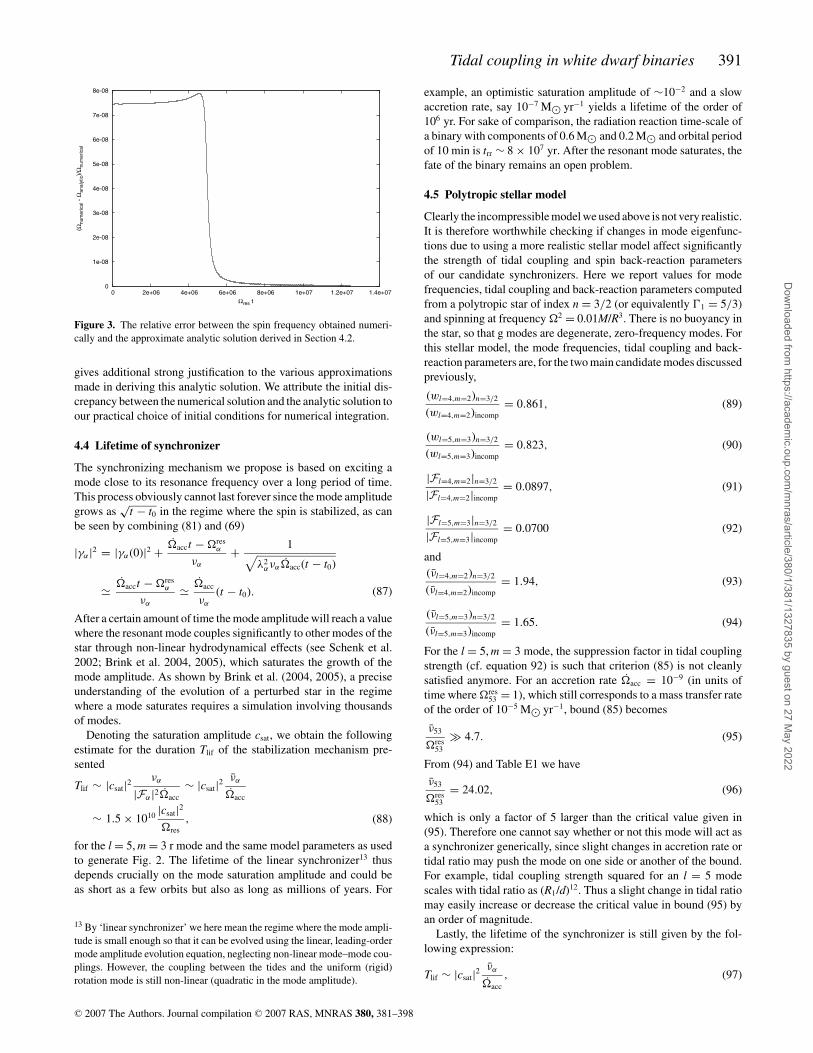
for the l = 5, m = 3 r mode and the same model parameters as usedto generate Fig. 2. The lifetime of the linear synchronizer13 thusdepends crucially on the mode saturation amplitude and could beas short as a few orbits but also as long as millions of years. For
13 By ‘linear synchronizer’ we here mean the regime where the mode ampli-tude is small enough so that it can be evolved using the linear, leading-ordermode amplitude evolution equation, neglecting non-linear mode–mode cou-plings. However, the coupling between the tides and the uniform (rigid)rotation mode is still non-linear (quadratic in the mode amplitude).
example, an optimistic saturation amplitude of ∼10−2 and a slowaccretion rate, say 10−7 M yr−1 yields a lifetime of the order of106 yr. For sake of comparison, the radiation reaction time-scale ofa binary with components of 0.6 M and 0.2 M and orbital periodof 10 min is trr ∼ 8 × 10⁷ yr. After the resonant mode saturates, thefate of the binary remains an open problem.
4.5 Polytropic stellar model
Clearly the incompressible model we used above is not very realistic.It is therefore worthwhile checking if changes in mode eigenfunc-tions due to using a more realistic stellar model affect significantlythe strength of tidal coupling and spin back-reaction parametersof our candidate synchronizers. Here we report values for modefrequencies, tidal coupling and back-reaction parameters computedfrom a polytropic star of index n = 3/2 (or equivalently 1 = 5/3)and spinning at frequency 2 = 0.01M/R3. There is no buoyancy inthe star, so that g modes are degenerate, zero-frequency modes. Forthis stellar model, the mode frequencies, tidal coupling and back-reaction parameters are, for the two main candidate modes discussedpreviously,
(wl=4,m=2)n=3/2
(wl=4,m=2)incomp= 0.861, (89)
(wl=5,m=3)n=3/2
(wl=5,m=3)incomp= 0.823, (90)
|Fl=4,m=2|n=3/2
|Fl=4,m=2|incomp= 0.0897, (91)
|Fl=5,m=3|n=3/2
|Fl=5,m=3|incomp= 0.0700 (92)
and(νl=4,m=2)n=3/2
(νl=4,m=2)incomp= 1.94, (93)
(νl=5,m=3)n=3/2
(νl=5,m=3)incomp= 1.65. (94)
For the l = 5, m = 3 mode, the suppression factor in tidal couplingstrength (cf. equation 92) is such that criterion (85) is not cleanlysatisfied anymore. For an accretion rate acc = 10−9 (in units oftime where res
53 = 1), which still corresponds to a mass transfer rateof the order of 10−5 M yr−1, bound (85) becomes
ν53
res53
4.7. (95)
From (94) and Table E1 we have
ν53
res53
= 24.02, (96)
which is only a factor of 5 larger than the critical value given in(95). Therefore one cannot say whether or not this mode will act asa synchronizer generically, since slight changes in accretion rate ortidal ratio may push the mode on one side or another of the bound.For example, tidal coupling strength squared for an l = 5 modescales with tidal ratio as (R1/d)12. Thus a slight change in tidal ratiomay easily increase or decrease the critical value in bound (95) byan order of magnitude.
Lastly, the lifetime of the synchronizer is still given by the fol-lowing expression:
Tlif ∼ |csat|2 να
acc, (97)
C© 2007 The Authors. Journal compilation C© 2007 RAS, MNRAS 380, 381–398
Dow
nloaded from https://academ
ic.oup.com/m
nras/article/380/1/381/1327835 by guest on 27 May 2022
392 E. Racine, E. S. Phinney and P. Arras
so for the same accretion rate, the lifetime increases only by a factorof 1.65 (cf. equation 94) compared to the incompressible case.
5 C O N C L U S I O N A N D F U T U R E WO R K
In this paper we suggest a non-dissipative mechanism that can sta-bilize the spin of the accretor in an ultracompact binary WD sys-tem. The effect that stabilizes the spin of the accreting WD is theback-reaction of a resonantly driven generalized r mode on the uni-form rotation mode. For the model we analyse in detail we assumethat only a single mode is dynamically relevant (see Section 4 formore details). We also assume slow rotation of the accretor, constantaccretion torque, constant orbital parameters and a perfect incom-pressible fluid equation of state. By integrating the equations ofmotion of our model both numerically and analytically we showthat pure hydrodynamics may stabilize the spin of the accretor. Nodissipative effects are required for synchronization. However, thelifetime of the synchronizing mechanism is limited since it requiresdriving the mode continuously very close to resonance. Eventuallythe mode enters a non-linear regime where it couples to other modes,which saturates the growth of the resonant mode’s amplitude. At thatpoint the synchronizing mechanism most likely shuts off. A correctcomputation of the saturation amplitude involves simulating a net-work of coupled modes following the footsteps of Brink et al. (2004,2005), a challenging task that we leave here as an open problem.More future work includes solving the full equations of motion,where the accretion rate and orbital parameters are computed andevolved rather than assumed to be constant external input quantities.In addition if mode damping time-scales turn out to be comparableto the lifetime of the synchronizer, then one should include damp-ing when solving the mode amplitude evolution equation. It wouldalso be interesting to investigate the properties of the stabilizationmechanism if the accretor experiences core crystallization, as theproperties of the r modes (i.e. frequency spectrum, strength of tidalcoupling, etc.) existing in the fluid shell surrounding the core differfrom the case of a fluid spheroid.
AC K N OW L E D G M E N T S
ER wishes to thank Jeandrew Brink for many useful discussions onr modes. ER and ESP acknowledge support from NASA ATP grantNNG04GK98G awarded to ESP.
R E F E R E N C E S
Bondarescu R., Teukolsky S. A., Wasserman I., 2007, preprint(arXiv:0704.0799)
Brink J., 2005, PhD thesis, Cornell UniversityBrink J., Teukolsky S. A., Wasserman I., 2004, Phys. Rev. D, 70, 124017Brink J., Teukolsky S. A., Wasserman I, 2005, Phys. Rev. D, 71, 064029Bryan G. H., 1889, Phil. Trans. R. Soc. London, A180, 187Dyson J., Schutz B. F., 1979, R. Soc. London Proc. Ser., 368, 389Flanagan E. E., Racine E., 2007, Phys. Rev. D, 75, 044001Goldreich P., Nicholson P., 1989, ApJ, 342, 1075Ho W. C. G., Lai D., 1999, MNRAS, 308, 153Lindblom L., Ipser J. R., 1999, Phys. Rev. D, 59, 044009Marsh T. R., Nelemans G., Steeghs D., 2004, MNRAS, 350, 113Ramsay G., Hakala P., Wu K., Cropper M., Mason K. O., Cordova F. A.,
Priedhorsky W., 2005, MNRAS, 357, 49Schenk A. K., Arras P., Flanagan E. E., Teukolsky S. A., Wasserman, I.,
2002, Phys. Rev. D, 65, 024001Strohmayer T. E., 2004, ApJ, 610, 416Strohmayer T. E., 2005, ApJ, 627, 920
Verbunt F., Rappaport S., 1988, ApJ, 332, 193Witte M. G., Savonije G. J., 1999, A&A, 350, 129
A P P E N D I X A : P E RT U R BAT I O N S O FU N I F O R M LY ROTAT I N G S TA R S
In this section we review basic material from perturbation theory ofuniformly rotating stars developed in Schenk et al. (2002) that is re-quired for the analysis of this paper. This section is rather technicalbut the formalism reviewed here is essential in correctly analysingthe tidal response of a rotating star. We hope to provide the interestedreader an accessible introduction to the beautiful, albeit mathemat-ically heavy, work of Schenk et al. (2002). We refer the reader tothat paper for complete details. We employ units where G = c = 1throughout.
Begin by considering an unperturbed star of mass M and radiusR uniformly rotating at constant spin frequency . The radius ofthe spinning star is defined as the radius of the sphere enclosingthe same total volume as the star. The hydrodynamical equations ofmotion in the frame corotating with the star are
∂ρ
∂t+ ∇ · (ρu) = 0, (A1)
DuDt
+ Ω × (2u + Ω × x) = − 1
ρ∇ p − ∇ + aext, (A2)
where ρ is mass density, p is pressure, u is the fluid velocity,
the self-gravitational potential and aext is an acceleration field pro-duced by some external perturbation. The operator D/Dt is the usualconvective time derivative. For the unperturbed star, ρ does not de-pend on time and the velocity u vanishes. The corotating frame isrelated to the inertial frame by the simple coordinate transformationφ = ϕ − ∫ dt , where φ is the corotating azimuthal coordinateand ϕ is the inertial azimuthal coordinate. If a fluid element of theunperturbed star located at x is displaced by the vector ξ (x, t), thelinearized hydrodynamical equations for the Lagrangian displace-ment vector ξ take the form
ξ + B · ξ + C · ξ = aext, (A3)
where the action of the operator B on a vector is defined as
B · ξ ≡ 2Ω × ξ. (A4)
For stars without buoyancy, the action of the operator C on a vectoris given by
C · ξ = ∇[
p
ρ2δρ + δ
]= ∇
[1
ρδ p + δ
], (A5)
where is the adiabatic index of the perturbation, which we heretake to be the same as the background star. The quantities δp andδρ are the Eulerian perturbations in the pressure and density, respec-tively. In terms of the displacement vector the density perturbationis
δρ = −∇ · (ρξ). (A6)
The gravitational potential perturbation δ obeys
∇2δ = 4πδρ. (A7)
The fluid displacement equation of motion (A3) can also be obtainedfrom the following Lagrangian density
L = 1
2ξ · ξ + 1
2ξ · B · ξ − 1
2ξ · C · ξ + aext · ξ. (A8)
C© 2007 The Authors. Journal compilation C© 2007 RAS, MNRAS 380, 381–398
Dow
nloaded from https://academ
ic.oup.com/m
nras/article/380/1/381/1327835 by guest on 27 May 2022
Tidal coupling in white dwarf binaries 393
The normal modes of the star are obtained by assuming displace-ments of the form ξ (x, t) = e−iωtξ(x) and no external forces. Onemust then solve the following eigenvalue equation for the normalmodes
[−ω2 − iωB + C] · ξ(x) = 0. (A9)
A mode (ξA, ωA) is solution to equation (A9). Later in the paperwe will use the notation wA ≡ ωA/2 for dimensionless modefrequencies. Note that given a mode (ξA, ωA) with ωA = 0, thereexists another distinct mode (ξB, ωB) solution to (A9) with ξB =ξ∗
A
and ωB = −ωA. Thus modes with non-zero frequency always occurin pairs.
A1 Phase-space expansion formalism
The eigenvalue equation (A9) satisfied by a given mode is peculiarin the sense that the operator acting on the perturbation depends onthe eigenvalue ω. This property leads to the fact that although it ispossible to find a complete set of solutions to (A9) so that a genericfluid displacement may be expanded as
ξ(x, t) =∑
α
qα(t)ξα(x), (A10)
the evolution equations for the mode amplitude coefficients qα(t) arenot in general uncoupled from one another. To get around this prob-lem one needs to look at the fluid perturbation in phase space (Dyson& Schutz 1979; Schenk et al. 2002). A general fluid displacementvector is expanded in phase space as follows:
ζ(x, t) ≡[ξ(x, t)
π(x, t)
]=∑
A
cA(t)
[ξA(x)
πA(x)
], (A11)
where
π = ξ + 1
2B · ξ (A12)
is the momentum conjugate to ξ obtained from the Lagrangian den-sity (A8). Using (A3) the evolution equation for the phase-spacevector ζ is easily seen to be
ζ =( − 1
2 B 1
−C + 14 B2 − 1
2 B
)· ζ +
[0
aext
]≡ T · ζ + F. (A13)
Thus the eigenvalue equation equivalent to (A9) in phase space is
[T + iωA] ζ A = 0. (A14)
An important point to note here is that operator T is not Hermitian,which leads to the existence of left eigenvectorsχA distinct from theright eigenvectors ζA which incidentally do not form a completebasis; to form a complete basis, one needs to include all Jordanchain modes [see appendix A of Schenk et al. (2002) for a completediscussion] that satisfy[T† − iω∗
A
]χA = 0. (A15)
We will write the right and left eigenmodes as follows:
ζ A =[ξA
πA
], (A16)
χA =[σA
τ A
]. (A17)
Now it is always possible to choose χA to be dual to ζA in the sensethat
〈χA, ζB〉 ≡ 〈σA, ξB〉 + 〈τ A,πB〉 = δAB, (A18)
where the inner product of two vector fields is defined as
〈ξ, ξ′〉 =∫
d3x ρ(x) ξ∗(x) · ξ′(x). (A19)
Substituting (A16)–(A17) into (A14) and (A15) yields
πA = −iωAξA + 1
2B · ξA, (A20)
σA = iω∗Aτ A − 1
2B · τ A. (A21)
If we now assume that all mode frequencies are real, it is thenpossible to show the following [this proof is a little involved; werefer the reader to appendix A of Schenk et al. (2002) for details]:
τ A = − i
bAξA, (A22)
where bA is a (real) constant. This constant is determined from (A18),which may be rewritten as
bAδAB = 〈ξA, iB · ξB〉 + (ωA + ωB)〈ξA, ξB〉. (A23)
The orthonormality relation (A18) allows us to invert expansion(A11) to get
cA = i
bA
⟨ξA, −iωAξ + 1
2B · ξ + π
⟩. (A24)
Finally, (A18) may also be used to extract from (A13) the followingevolution equation for mode amplitude
cA + iωAcA = i
bA〈ξA, aext〉. (A25)
To summarize, the tidal response of a rotating star is described bya Lagrangian fluid displacement vector field ξ (x, t) and its canoni-cally conjugate momentum π (x, t). These two vector fields may bedecomposed in phase space into normal modes according to (A11), agiven normal mode (ξA, ωA) satisfying the eigenvalue equation (A9).The time evolution of a given mode amplitude is governed byequation (A25).
A2 An important set of zero-frequency Jordan chain modes
As mentioned in the previous section the modes ζA analysed abovedo not form a complete basis on which one may expand an arbitraryfluid perturbation. To form a complete basis one needs to add allJordan chain modes. A Jordan chain of length pA associated witha given eigenfrequency ωA is a set of vectors ζA,σ , 0 σ pA
satisfying
[T + iωA] ζ A,σ = ζ A,σ−1, (A26)
for 1 σ pA
and
[T + iωA] ζ A,0 = 0. (A27)
The associated left eigenvectors satisfy[T† − iω∗
A
]χA,σ = χA,σ−1, (A28)
for 1 σ pA
and[T† − iω∗
A
]χA,0 = 0. (A29)
The generalized orthonormality condition for Jordan chains adoptedin Schenk et al. (2002) is
〈χA,σ , ζB,τ 〉 = δABδpA ,σ+τ . (A30)
C© 2007 The Authors. Journal compilation C© 2007 RAS, MNRAS 380, 381–398
Dow
nloaded from https://academ
ic.oup.com/m
nras/article/380/1/381/1327835 by guest on 27 May 2022

394 E. Racine, E. S. Phinney and P. Arras
The equations of motion for the associated mode amplitudes in theabsence of external forcing can be shown to be (see appendix A ofSchenk et al. 2002)
cA,σ + iωAcA,σ = cA,σ+1, for σ < pA, (A31)
cA,pA + iωAcA,pA = 0. (A32)
The main reason motivating us to discuss Jordan chains in thispaper is that all differential rotation modes must be Jordan chains oflength 1. One proves this as follows. The fluid velocity perturbationcorresponding to a differential rotation mode is of the form
∂ξ(x, t)
∂t≡ δu(x) = r⊥δ(r⊥)eφ, (A33)
where r⊥ = r sin θ . The velocity perturbation being time-independent first proves that the mode is a zero-frequency pertur-bation. Now any normal mode is a Jordan chain of length p 0, sowe have (dropping A subscripts)
δu(x) =p∑
σ=0
cσ (t)ξσ (x). (A34)
The mode amplitude equations of motion (A31)–(A32) show thatcσ (t), in the case of a zero-frequency chain, is a polynomial in tof order p − σ . Since δu is independent of time but non-vanishing,then the chain must be of length 1. In particular, the uniform rotationmode [δ(r⊥) = δ = constant] which moves the star from a givenbackground spin frequency to a new background spin frequency + δ falls into this category. From equation (A34) one imme-diately finds that for a generic differential rotation mode, the modefunction ξ0 is
ξ0 = γ δu, (A35)
where γ is a constant fixed by an overall mode normalization con-dition. The defining equations of Jordan chains (A26) and (A27) arethen used to show that ξ1 is solution to
C · ξ1 = −B · ξ0. (A36)
In the case of uniform rotation, we use the convention
ξ0 = Ω × x. (A37)
The complete expression for the uniform rotation Jordan chain istherefore
ζ0 =[
ξ012 B · ξ0
], (A38)
ζ1 =[
ξ112 B · ξ1 + ξ0
], (A39)
with ξ0 and ξ1 given by (A37) and (A36), respectively. Throughoutthis paper, when we say the spin of the star changes, we mean thatthe amplitude of the above uniform rotation Jordan chain modechanges. The amplitude of the uniform rotation mode defines thenatural coordinate system corotating with the star in which stellarperturbation theory is applied. In the specific application we considerin this paper, it is the time dependence of the coordinate systemcorotating with the star due to the evolution of the uniform rotationmode that is responsible for the resonant excitation of normal modesin an accreting WD part of a binary system.
Lastly, it will be useful later on to know the left Jordan chainassociated with the uniform rotation mode. The defining equations(A28) and (A29), along with (A30) and (A38)–(A39) give
χ0 = 1
β
[− 12 B · ξ0
ξ0
], (A40)
χ1 = 1
β
[12 B · ξ1 + ξ0
−ξ1
], (A41)
where
β = 〈ξ0, ξ0〉 + 〈ξ1, C · ξ1〉. (A42)
The constant β ensures that the left and right eigenvectors given in(A40)–(A41) and (A38)–(A39) satisfy the orthonormality condition(A30).
A3 Mode pair index notation
As mentioned previously, modes with non-zero frequencies alwaysoccur in pairs. We may then rewrite the phase-space expansion indexA as the pair of indices (α, ε), ε = ±, with the following identifica-tions:
ωα,+ = ωα, (A43)
ωα,− = −ωα, (A44)
ξα,+ = ξα, (A45)
ξα,− = ξ∗α. (A46)
Equations (A43)–(A46) and (A23) then imply
bα,+ = bα, (A47)
bα,− = −bα. (A48)
Since the fluid displacement and its conjugate momentum are realvector fields, equations (A43)–(A46), (A24) and (A47)–(A48) yield
cα,+ = cα, (A49)
cα,− = c∗α. (A50)
If the perturbation is dominated by modes with non-zero frequencywe may rewrite expansion (A11) as follows:[ξ(x, t)
π(x, t)
]=∑
A
cA(t)
[ξA(x)
πA(x)
]
=∑
α
cα(t)
[ξα(x)
πα(x)
]+ c.c., (A51)
where c.c. stands for complex conjugate.
A P P E N D I X B : D E TA I L E D D E R I VAT I O N O FS P I N F R E QU E N C Y E VO L U T I O N E QUAT I O N
The differential equation governing the time evolution of the spinfrequency Ω of the star can be obtained using results of Schenket al. (2002), who rigorously derive the evolution equation of theuniform rotation mode amplitude to second order in stellar perturba-tion theory. Here we shall instead derive the evolution equation forthe spin frequency following the procedure sketched in Section 1.Our evolution equation of course matches the result of Schenk et al.(2002). However, we believe our derivation is slightly simpler tofollow so it is worth including it here. We start from the expressionfor the component of the angular momentum of the perturbed star
C© 2007 The Authors. Journal compilation C© 2007 RAS, MNRAS 380, 381–398
Dow
nloaded from https://academ
ic.oup.com/m
nras/article/380/1/381/1327835 by guest on 27 May 2022
Tidal coupling in white dwarf binaries 395
along its unperturbed spin axis, and expand it to second order in theperturbation. A direct computation yields
Jstar =∫
d3x ρ(x) Ω · (x + ξ) × [Ω0 × (x + ξ) + ξ]
=∫
d3x ρ(x) Ω · (x + ξ) × [Ω0 × x + π]
=∫
d3x ρ r 2⊥ +
∫d3x ρ Ω · (ξ × π)
+∫
d3x ρ[(Ω0 × ξ) · (Ω × x) + Ω · (x × π)]
≡ 0 I0 + J2[ζ, ζ] + J1[ζ], (B1)
where Ω0 = 0Ω is the unperturbed spin frequency vector, whichwas denoted by Ω in Appendix A. The full spin frequency of thestar is now written as
Ω = Ω0 + δ Ω. (B2)
Let us now focus on the term J1[ζ]. Using the defining equations(A37) and (A40) for the uniform rotation Jordan chain, we mayrewrite J1[ζ] as follows:
J1[ζ] =∫
d3x ρ[(Ω0 × ξ) · (Ω × x) + Ω · (x × π)]
=∫
d3x ρ[−ξ · (Ω0 × ξ0) + π · ξ0]
=⟨
− 1
2B · ξ0, ξ
⟩+ 〈ξ0,π〉
= β〈χ0, ζ〉= β c1(t), (B3)
where the last line has been obtained using Jordan chain orthonor-mality condition (A30). Thus the piece of the angular momentumlinear in the perturbation depends only on the amplitude c1 of theuniform rotation mode. It is independent of all other modes of thestar from orthonormality condition (A30). It remains to relatethe coefficient c1 to the spin frequency perturbation and to com-pute the quantity β defined in (A42). Using (A38), the velocityperturbation is
δu = r⊥δ eφ = δ (Ω × x) = δ ξ0, (B4)
which gives simply (cf. equation A34)
c0 = c1 = δ. (B5)
We now turn to the computation of β (cf. equation A42). The firstterm of the right-hand side of (A42) is easily shown to be
〈ξ0, ξ0〉 = I0, (B6)
the unperturbed moment of inertia of the star about its spin axis. Thisresult leads us to expect that the second term of (A42) is related tothe perturbation of the star’s moment of inertia under uniform spin-up. The moment of inertia of the perturbed star about its spin axisis given by
I =∫
d3x ρ
(x + ξ)2 − [(x + ξ) · Ω]2
. (B7)
Expanding this expression to leading order in ξ yields after somealgebra and an integration by parts
I = I0 −∫
d3x ∇ · (ρξ)[x2 − (x · Ω)2]. (B8)
If the perturbation consists of uniform spin-up, we then have, sinceρξ0 is divergenceless,
I = I0 − c1
∫d3x ∇ · (ρξ1)[x2 − (x · Ω)2] ≡ I0 + δ I . (B9)
On the other hand we have, from (A36)
〈ξ1, C · ξ1〉 = −〈ξ1, B · ξ0〉
= −∫
d3x ρξ1 · [2Ω0 × (Ω × x)]
= 0
∫d3x ρξ1 · ∇[x2 − (Ω · x)2]
= −0
∫d3x ∇ · (ρξ1)[x2 − (Ω · x)2]
= 0
c1δ I , (B10)
where the last line has been obtained using (B9). We finally have
J1[ζ] =[
I0 + 0
c1δ I
]c1
= I0δ + 0δ I
=[
1 + d ln I0
d ln 0
]I0δ. (B11)
In this paper we assume that the star spins slowly enough so that thechange in moment of inertia due to change in spin may be neglected.Taking a time derivative of (B1) then yields, in the context of theadiabatic approximation detailed in Section 2.1,
d
dt= 1
I
[Text − d
dt
∫d3x ρ Ω · (ξ × π)
], (B12)
where Text is the total external torque applied on the star, and I isnow the moment of inertia of the non-rotating star. In the applica-tion we consider below there will be two contributions to the totalexternal torque, namely, an accretion-induced torque and the torqueon the star due to tidal interactions. In terms of sums over modes,equation (B12) can be rewritten as
= Text
I− 1
I
d
dt
∑A,B
c∗AcB
⟨Ω × ξA,
[1
2B − iωB
]ξB
⟩
≡ Text
I− 1
I
d
dt
∑A,B
c∗AcBKAB, (B13)
where (A11) has been used. Since ξA ∝ eim Aφ , the only termscontributing to the above double sum have mA = mB , that is,KAB ∝ δm Am B . For modes that do not resonate, we may use ap-proximate solution (38) for the mode amplitudes to split the doublesum of (B13) in two pieces, one that includes terms where eithermode A or mode B resonates and another involving modes that donot resonate. We write this split as follows:
= Text
I− 1
I
d
dt
∑A,B
(r)c∗
AcBKAB
− 1
I
d
dt
∑A,B
(nr) F∗AFB
(m Au − ωA)(m Au − ωB)KAB . (B14)
Since all terms in the sum over non-resonant modes depend on timeonly through the star’s spin frequency,14 we may replace the operator
14 Orbital frequency also depends on time but in this paper we will keeporbital parameters fixed for the purpose of computing the time evolution ofthe spin frequency. We motivate this approximation in the next subsection.
C© 2007 The Authors. Journal compilation C© 2007 RAS, MNRAS 380, 381–398
Dow
nloaded from https://academ
ic.oup.com/m
nras/article/380/1/381/1327835 by guest on 27 May 2022

396 E. Racine, E. S. Phinney and P. Arras
d/d t acting on each term of this sum by AB/, with AB beingof the order of unity. This leads to the following expression:
= 1
Ieff
Text − d
dt
∑A,B
(r)c∗
AcBKAB
, (B15)
where the effective moment of inertia Ieff is given by
Ieff = I
1 + 1
I
∑A,B
(nr) ABF∗AFB
(m Au − ωA)(m Bu − ωB)KAB
. (B16)
Although we are unable to prove that the sum over all non-resonant modes is small compared to unity, we suspect it is thecase since a typical driving amplitude FA scales as R/d to somepower p 2, where R is the accretor’s radius and d orbital separa-tion. Even though the binary is quite compact (i.e. R/d is not thatsmall, may be of the order of ∼0.2), the leading term in the sumover non-resonant modes, which scales as (R/d)4, is of the order of10−2 to 10−3. It thus appears unlikely to us that the sum over allnon-resonant modes may contribute to more than a few per cent tothe effective moment of inertia Ieff defined in (B16).
A P P E N D I X C : B R I E F OV E RV I E W O FG E N E R A L I Z E D R M O D E S
Here we briefly summarize the properties of generalized r modesneeded for this paper. This section relies heavily on the work ofLindblom & Ipser (1999); Brink et al. (2004, 2005). Note howeverthat we use the frequency sign convention of Schenk et al. (2002)instead of the frequency convention of Lindblom & Ipser (1999);Brink et al. (2004, 2005). For l 2 the Lagrangian displacement ofa given mode ξA can be written as
(ξA)i = ψA
42Qi j
A∂ jδUA, (C1)
where ψA is a normalization constant fixed below and where thehydrodynamic potential δUA is given by
δUA = βAPm
l (ξ )
Pml (ξ0)
Pml (µ)eim Aφ, (C2)
where βA is a constant and where (ξ, µ, φ) are a bispheroidal coordi-nate system defined below. We will henceforth drop all A subscriptsfor notational convenience since no ambiguity occurs in what fol-lows. In Cartesian coordinates, the tensor Qi j is given by
Qi j = 1
w2 − 1
[δi j − 1
w2δi zδ j z + i
wεi j z
], (C3)
where w = ω/2 and εi j z = δi xδ j y − δiyδ j x . The bispheroidal coor-dinates (ξ, µ, φ), essential to write a separated solution for δU, areexplained in detail in Lindblom & Ipser (1999). They are related toCartesian coordinates by the following relations:
x = b(1 − ξ 2)1/2(1 − µ2)1/2 cos φ, (C4)
y = b(1 − ξ 2)1/2(1 − µ2)1/2 sin φ, (C5)
z = b
(√1 − w2
w
)ξµ, (C6)
where
b2 = a2
1 − w2
[(1 + ζ 2
0 ) − w2], (C7)
the parameters a and ζ 0 being the standard parameters describingthe background spheroid, namely, a is the focal radius and ζ 0 is
related to the spheroid’s eccentricity by e2 = 1/(1 + ζ 20). Note also
that bispheroidal coordinates depend on normal mode frequency.The volume of the star is covered by ξ0 ξ 1, −ξ0 µ ξ0,where
ξ 20 = a2ζ 2
0
b2
w2
1 − w2. (C8)
We use the convention of Brink et al. (2004) for mode normalization,namely, a mode of unit amplitude has (rotating frame) energy equalto the fixed value MR22. In the slow rotation approximation onecan show (Brink 2005) that the normalization constant ψ is
ψ = 2M1
R1
2
β
(1 − w2
3
)1/2 [(l − m)!
(l + m)!
(2l + 1)
l(l + 1)
]1/2
, (C9)
where = /break-up ≡ /√
M1/R31 . Lastly we give a formula
for the density perturbation of a normalized mode
δρ = ψρ2δ(p)[δU + δ], (C10)
where δ(p) is a delta function with the background pressure as itsargument and δ is the gravitational potential perturbation of themode. The density perturbation is non-zero only on the surface
of the star. On this surface the function δ is equal to
δ| = β D(ζ0)Pml (µ)eimφ, (C11)
where D(ζ 0) is a known function of ζ 0 (cf. equations 7.1 and 7.4of Lindblom & Ipser 1999). It is also important to note that on thesurface of the star, we have δU| = βPm
l (µ)eimφ (Lindblom & Ipser1999). In the slowly rotating limit, one can show
D(ζ0) = 3
2(l − 1). (C12)
The coordinate µ appearing first in (C11) is part of the spheroidalcoordinate system defined by the relations
x = a(1 + ζ 2)1/2(1 − µ2)1/2 cos φ, (C13)
y = a(1 + ζ 2)1/2(1 − µ2)1/2 sin φ, (C14)
z = aζµ. (C15)
In the slowly rotating limit, the spheroidal coordinate system be-comes the usual spherical coordinate system (r, θ , φ) on the surfaceof the star. In this approximation we then have
δρ = ψβ2l + 1
2(l − 1)ρ2δ(p)Pm
l (cos θ )eimφ
= M
R2
2
4
2l + 1
l − 1
[3(1 − w2)
πl(l + 1)
]1/2
δ(r − R)Ylm(θ, φ), (C16)
where we made use of (C9), (C12) and the slow rotation limit of thepressure distribution of an incompressible fluid spheroid, which is
p = 2πρ2
3(R2 − r 2). (C17)
A P P E N D I X D : T I DA L C O U P L I N G TO R QU E
Here we derive the rate of change of orbital angular momentuminduced by the excitation of normal modes in one of the stars of thebinary. This result is well known but we include the derivation herein the context of perturbations of rotating stars for completeness.Consider a rotating star perturbed by the following Lagragian fluiddisplacement vector field
C© 2007 The Authors. Journal compilation C© 2007 RAS, MNRAS 380, 381–398
Dow
nloaded from https://academ
ic.oup.com/m
nras/article/380/1/381/1327835 by guest on 27 May 2022
Tidal coupling in white dwarf binaries 397
ξ(x, t) =∑
A
cA(t)ξA(x). (D1)
The net force Fext on the perturbed star due to the companion’stidal field is given by
Fext =∫
dMaext(y, t), (D2)
where dM is the mass of a fluid element and y =x +ξ is the locationof that fluid element. Now we have dM = d3x ρ(x), where ρ(x) isthe background density and x is the background location of the fluidelement. To leading order in the perturbation we then get
Fext =∫
d3x ρ(x)aext(x + ξ, t)
=∫
d3x ρ(x) aext(x, t) + ξ · ∇aext(x, t)
≡ F(0)ext(t) + F(1)
ext[ξ]. (D3)
The zeroth-order force term describes the binary’s motion when nomodes are excited. The term depending on ξ can be rewritten asfollows:
F(1)ext[ξ] =
∫d3x ρ(x) ξi (x, t)∂i aext(x, t)
=∑
A
∫d3x ρ(x) cA(t)ξ i
A(x)∂i aext(x, t)
=∑
A
cA(t)
∫d3x δρA(x) aext(x, t). (D4)
The external acceleration is given by
aext(x, t) = −∇ext(|x − d(t)|)= ∇ (d)ext(|x − d|), (D5)
where d is the binary’s orbital separation vector and ∇ (d) denotes thegradient operator with respect to d, keeping the field point x fixed.We then have
F(1)ext[ξ] =
∑A
cA∇ (d)
∫d3x δρAext
=∑
A
−icAbA∇ (d) f ∗A , (D6)
where (31) has been used. If we write d = d(cos φ, sin φ), thebinary’s equation of motion (ignoring gravitational radiation reac-tion and mass transfer) is then
d − dφ2 + Mtot
d2= 1
µ
∑A
icAbA∂d f ∗A , (D7)
dφ + 2dφ = 1
µd
∑A
icAbA∂φ f ∗A . (D8)
The rate of change of orbital angular momentum due to tidal cou-pling is then given by
J tidal =∑
A
icAbA∂φ f ∗A
= −∑
A
m AcAbA f ∗A
= −∑
A
m AcAbA
[c∗
A − iωAc∗A
], (D9)
where (35) has been used. Using mode pair notation, that is, equa-tions (A43)–(A46), (A47)–(A48) and (A49)–(A50), we may furthersimplify this result to finally arrive at
J tidal = −∑
α
mαbα
d
dt|cα|2. (D10)
A P P E N D I X E : C O M P U TAT I O N O F T I DA LC O U P L I N G A N D BAC K - R E AC T I O NPA R A M E T E R S
In this section we gather analytic results for integrals required inSection 4.
E1 Mode amplitude driving term
The first quantity we compute is the driving term Fα appearing inequation (37). To compute this quantity we need
〈ξα, −∇ext〉 = −∫
d3x δρ∗αext. (E1)
Using (33) and (C16) we immediately obtain
〈ξα, −∇ext〉 = 2 M1 M2
d
(R1
d
)l
Wlm(2l + 1)
4(l − 1)
×[
3(1 − w2α)
πl(l + 1)
]1/2
e−imαu . (E2)
The normalization convention we choose in Appendix C impliesbα = M1R2
1/(2wα) (see also appendix A of Schenk et al. 2002)and we get
Fα = iwαM2
M1/21 R3/2
1
[R1
d
]l+1
Wlm(2l + 1)
2(l − 1)
√3(1 − w2
α)
πl(l + 1)
= iqwα
[R1
d
]l+1
Wlm(2l + 1)
2(l − 1)
√3(1 − w2
α)
πl(l + 1), (E3)
where q = M2/M1 is the mass ratio.
E2 Integrals in the spin frequency evolution equation
We next compute some of the integrals appearing in equation (B13).These are more tricky since they cannot be reduced to contributionsfrom the surface of the star alone. It possible to evaluate these in-tegrals analytically for a fluid displacement vector composed of asuperposition of generalized r modes using a recursion technique(Brink 2005), but a general closed-form expression for the integralsappearing in equation (B13) is not available. In the model where asingle r-mode pair is assumed to be dynamically relevant however,the required integral is
1
2κα = −iωα〈z × ξα, ξα〉 + 〈z × ξα, z × ξα〉, (E4)
which we now give in the slow rotation approximation. Using (C1)and (C3) we have, dropping the α and 1 subscripts below for brevity,
1
2κ =
ψ2ρ
164(1 − w2)2
∫d3x
(δ j p − 1
w2z j z p − i
wε j pz
)
× (X jk − 2iw ε jkz)
(δkq − 1
w2zk zq + i
wεkqz
)×∂pδU ∗∂qδU , (E5)
C© 2007 The Authors. Journal compilation C© 2007 RAS, MNRAS 380, 381–398
Dow
nloaded from https://academ
ic.oup.com/m
nras/article/380/1/381/1327835 by guest on 27 May 2022
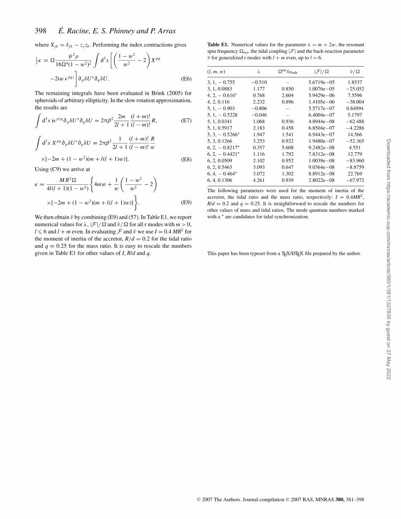
398 E. Racine, E. S. Phinney and P. Arras
where Xjk = δ jk − z j zk . Performing the index contractions gives
12 κ =
ψ2ρ
164(1 − w2)2
∫d3x
[(1 − w2
w2− 2
)X pq
−2iw ε pqz
]∂pδU ∗∂qδU . (E6)
The remaining integrals have been evaluated in Brink (2005) forspheroids of arbitrary ellipticity. In the slow rotation approximation,the results are∫
d3x iε pzq∂pδU ∗∂qδU = 2πβ2 2m
2l + 1
(l + m)!
(l − m)!R, (E7)
∫d3x X pq∂pδU ∗∂qδU = 2πβ2 1
2l + 1
(l + m)!
(l − m)!
R
w
×[−2m + (1 − w2)(m + l(l + 1)w)]. (E8)
Using (C9) we arrive at
κ = M R2
4l(l + 1)(1 − w2)
4mw + 1
w
(1 − w2
w2− 2
)
×[−2m + (1 − w2)(m + l(l + 1)w)]
. (E9)
We then obtain ν by combining (E9) and (57). In Table E1, we reportnumerical values for λ, |F |/ and ν/ for all r modes with m > 0,l 6 and l + m even. In evaluating F and ν we use I = 0.4 MR2 forthe moment of inertia of the accretor, R/d = 0.2 for the tidal ratioand q = 0.25 for the mass ratio. It is easy to rescale the numbersgiven in Table E1 for other values of I, R/d and q.
Table E1. Numerical values for the parameter λ = m + 2w, the resonantspin frequency res, the tidal coupling |F | and the back-reaction parameterν for generalized r modes with l + m even, up to l = 6.
(l, m, w) λ res/ωorb |F |/ ν/
3, 1, − 0.755 −0.510 – 5.6719e−05 1.85373, 1, 0.0883 1.177 0.850 1.0076e−05 −25.0524, 2, − 0.616∗ 0.768 2.604 5.9429e−06 7.55964, 2, 0.116 2.232 0.896 1.4105e−06 −38.0045, 1, − 0.903 −0.806 – 5.5717e−07 0.849945, 1, − 0.5228 −0.046 – 6.4004e−07 5.17975, 1, 0.0341 1.068 0.936 4.8944e−08 −62.4885, 1, 0.5917 2.183 0.458 6.8504e−07 −4.22865, 3, − 0.5266∗ 1.947 1.541 6.9443e−07 14.5665, 3, 0.1266 3.253 0.922 1.9480e−07 −52.3656, 2, − 0.8217∗ 0.357 5.608 9.2482e−08 4.5516, 2, − 0.4421∗ 1.116 1.792 7.8312e−08 12.7796, 2, 0.0509 2.102 0.952 1.0039e−08 −83.9606, 2, 0.5463 3.093 0.647 9.0364e−08 −8.87596, 4, − 0.464∗ 3.072 1.302 8.8912e−08 22.7696, 4, 0.1306 4.261 0.939 2.8022e−08 −67.972
The following parameters were used for the moment of inertia of theaccretor, the tidal ratio and the mass ratio, respectively: I = 0.4MR2,R/d = 0.2 and q = 0.25. It is straightforward to rescale the numbers forother values of mass and tidal ratios. The mode quantum numbers markedwith a ∗ are candidates for tidal synchronization.
This paper has been typeset from a TEX/LATEX file prepared by the author.
C© 2007 The Authors. Journal compilation C© 2007 RAS, MNRAS 380, 381–398
Dow
nloaded from https://academ
ic.oup.com/m
nras/article/380/1/381/1327835 by guest on 27 May 2022


