Nitrogen uptake by phytoplankton in the Huon

Estuary: with special reference to the

physiology of the toxic dinoflagellate

Gymnodinium catenatum

By

Paul B. Armstrong

Bachelor of Applied Science with Honours

Submitted in fulfilment of the requirements for the degree of Master of Applied Science in

Aquaculture

National Centre for Marine Conservation and Resource Sustainability

University of Tasmania

November 2010

Declaration of Originality and Authority of Access

I certify that this thesis contains no material which has been accepted for the degree

or diploma by the University or any other institution, except by way of background

information duly acknowledged in the thesis. This thesis to the best of my knowledge

and belief contains no material previously published or written by another person

except where due acknowledgment is made in the text of the thesis.

This thesis may be made available for loan. Copying of any part of this thesis is

prohibited for two years from the date this statement was signed; after that time

limited copying is permitted in accordance with the Copyright Act 1968.

Paul B. Armstrong

November 2010

Acknowledgements

I would like to thank my supervisors Dr. Peter Thompson, Dr. Christopher Bolch and

Dr. Susan Blackburn for providing advice, support and encouragement during my

research and the preparation of this thesis.

I would also like to thank those people who provided technical assistance including:

Pru Bonham (CSIRO) - HPLC analysis of phytoplankton pigments

Val Latham and Kate Berry (CSIRO) - Nutrient analysis (nitrate, phosphate, silicate)

Andy Revill and Rebecca Esmay (CSIRO) - Stable isotope analysis of phytoplankton

samples

111

Abstract

The Huon Estuary is a micro-tidal estuary in south-east Tasmania that is an important

area for salmon aquaculture. In 2008 the salmon aquaculture industry in Australia is

worth $260M (AUD) per year. Salmon aquaculture began in the Huon Estuary in the

1980's and production has since increased significantly. The Huon Estuary is

nitrogen (N) limited and salmon farming is a significant input of N to this ecosystem.

Both industry and government regulators are alert to the potential for eutrophication

and increased harmful algal blooms if the assimilative capacity for N of the estuary is

exceeded. As part of a larger project on the ecology of the Huon Estuary, this PhD

research has two main objectives; firstly to determine whether phytoplankton in the

Huon Estuary are using nitrogen that had, primarily, an oceanic source (e.g. nitrate)

or was more locally supplied or regenerated (e.g. ammonium and urea) and secondly

to examine the physiology of G. catenatum a toxic dinoflagellate that dominates the

summer and autumn Huon Estuary phytoplankton biomass in many years.

Uptake rates of NO3, NH4+ and urea were measured on four occasions (28-29 May

2003, 23-24 Sept 2003, 18-19 Nov 2003, and 24-25 Feb 2004) in the Huon Estuary

using a 15N tracer technique. Uptake rates were measured at Garden Island and

Hideaway Bay in the lower estuary and at 5 and 20 m during the day and also at 5

and 20 m during the night. The mean uptake rates (mean across time of year, site,

time of day and depth) for NH 4+ (0.13 j.tg N jig chl a If') and urea (0.09 jig N jig chl a

If 1 ) were 4.5 and 3.2 times higher than the uptake of NO3" ( 0.3 i.tg N jig ch la li t ).

Overall NH4+, NO3" and urea were responsible for 52, 37.5 and 10.5% of N uptake

respectively.

Gymnodinium catenatum is a toxic dinoflagellate that blooms periodically in the

Huon Estuary and in years that it blooms it dominates the phytoplankton biomass and

has caused closure of shellfish farms in the area. Laboratory experiments on effect of

temperature and irradiance on growth rate, effect of different nitrogen species on

growth rate and preferential uptake of different nitrogen species by G. catenatum

iv

were undertaken to better understand the physiology of this species and to test a

hypothesis that G. catenatum vertically migrates to access NH 4+ at depth during

summer. The effect of 12 different temperatures ranging from 11.9-25.2 °C and

irradiances from 5-283 gmol photons 1112 s-I on growth and biochemical composition

of G. catenatum. The highest predicted growth rates (>0.2 d -I ) occurred during

summer and autumn as might be expected based on observations of bloom dynamics

of this species in the Huon Estuary which supports both a summer and autumn bloom

in many years

G. catenatum was able to grow using NO3 - , NH4+ or urea as its sole nitrogen source.

There was no significant difference in growth on any of these nitrogen sources.

Preferential uptake of NH4+, NO3 - or urea was examined by growing G. catenatum on

a mixture of NO3 - , NI-14+ and urea. The results clearly showed that NH4+ was taken

up first, followed by NO3 - and finally urea. Maximum mean uptake rates were 170,

98 and 30 pg cell' hour -I respectively for NH4 +, NO3 - and urea.

In addition to the laboratory experiments the nitrogen uptake characteristics of a

bloom of G. catenatum was examined at Pelican Island, Southport (30-31/03/2004)

nearby the Huon Estuary. Mean urea uptake was greatest (0.045 ligN [tg chl a If')

followed by NH4+ (0.029 lagN chl all') and the lowest uptake was of NO 3 - (0.025

pgN 1.1g chl ali t ). For G. catenatum growing in the Huon Estuary it seems

increasingly apparent that it functions as a nitrogen scavenger. When N

concentrations are exhausted, it is able to migrate through the water column seeking

whatever form of nitrogen is available.

Table of Contents

1 Introduction 1

1.1 Eutrophication in coastal ecosystems 1

1.2 The Huon Estuary 9

1.3 Research Objectives 13

1.4 References 15

2 Nitrogen uptake by phytoplankton in the Huon Estuary, south-east

Tasmania, Australia 20

2.1 Introduction 20

2.2 Methods 22

2.2.1 CTD profiles 27

2.2.2 Phytoplanlcton Counts 28

2.2.3 CHEMTAX 29

2.2.4 Statistical analysis 30

2.2.4.1 Phytoplankton Dynamics 30

2.2.4.2 Nitrogen uptake data 30

2.3 Results 32

2.3.1 Late autumn 35

2.3.2 Early spring 36

2.3.3 Late spring 39

2.3.4 Late summer 41

2.3.5 Effect of Season on phytoplankton composition 43

2.3.6 Comparison of Nitrate, Ammonium and Urea uptake: all Huon Estuary

data. 47

2.3.6.1 Effect of season on combined nitrogen uptake and specific uptake

of different nitrogen species 49

2.3.6.2 Effect of Season, time of day and depth on ammonium uptake 51

2.3.6.3 Effect of Season, time of day and depth on nitrate uptake 54

2.3.6.4 Effect of Season, time of day and depth on urea uptake 55 vi

2.3.6.5 % N uptake for NH4+ , NO3 - and urea 59

2.4 Discussion 60

2.4.1 Comparison of N uptake characteristics of the Huon Estuary with other

ecosystems 60

2.4.2 Late autumn 62

2.4.3 Early spring 63

2.4.4 Late Spring 64

2.4.5 Late Summer 66

2.4.6 Summary 68

2.5 Appendix 69

2.6 References 72

3 Effect of temperature and irradiance on the growth and biochemical

composition of the toxic dinoflagellate Gymnodinium catenatum from south-east

Tasmania, Australia 77

3.1 Introduction 77

3.2 Methods 80

3.2.1 Strain and culture conditions 80

3.2.2 Temperature and irradiance gradient incubator table 81

3.2.3 Effect of culture vessels 83

3.2.4 Preconditioning of t versus I experimental cultures 83

3.2.5 Temperature and irradiance experiment 84

3.2.6 Growth at high temperature and high light 87

3.2.6.1 Pre-acclimatisation 87

3.2.6.2 Culture conditions 87

3.2.6.3 Growth at 28.5 °C 87

3.2.6.4 Growth at 25.0 °C 87

3.2.7 Growth rates 88

3.2.8 Growth vs. irradiance curves 89

3.2.9 Biochemical analysis 90

vii

3.2.10 G. catenatum energetics model 92

3.2.11 Statistical analysis 92

3.3 Results 93

3.3.1 Vessel effects on growth rate 93

3.3.2 Effect of temperature and irradiance on growth 94

3.3.2.1 Comparison of different methods for determining growth rate 95

3.3.2.2 Growth vs. irradiance curves 96

3.3.2.3 The effect of temperature on maximum growth ( pmax) 99

3.3.2.4 The effect of temperature on the initial slope (a) 100

3.3.2.5 The effect of temperature on irradiance co-efficient (Ek) 101

3.3.2.6 The effect of temperature on compensation irradiance (E c) 102

3.3.3 Effect of high temperature and high irradiance on growth rate 103

3.3.4 Effect of light and temperature on biochemical composition 105

3.3.5 A model for carbon: chlorophyll a 111

3.3.6 Energetics model 114

3.4 Discussion 118

3.4.1 Effect of temperature and irradiance on Gymnodinium catenatum

growth 118

3.4.2 Effect of temperature on parameters of the growth vs. irradiance curve

120

3.4.2.1 Maximum growth rate (lima') 120

3.4.2.2 Initial slope (a) 127

3.4.2.3 Irradiance co-efficient (Ek) 128

3.4.2.4 Compensation irradiance (E c) 128

3.4.3 Effect of temperature and irradiance on the bio-chemical composition

of G. cat enatum 129

3.4.4 Carbon:chlorophyll a 132

3.4.4.1 Energetics model 133

3.4.5 Summary 133

3.5 References 135

viii

4 Nitrogen preference and uptake by Gymnodinium catenatum in culture 139

4.1 Introduction 139

4.2 Methods 141

4.2.1 Determining tolerance to ammonium concentrations 141

4.2.2 Growth on ammonium 142

4.2.3 Growth on Urea 143

4.2.4 Preferential uptake of different nitrogen species 144

4.3 Results 145

4.3.1 Growth on different nitrogen species 145

4.3.2 Preferential uptake of different nitrogen species 148

4.4 Discussion 150

4.4.1 Summary 153

4.5 References 154 ,

5 Nitrogen uptake during a Gymnodinium Catenatum bloom at Southport,

south-east Tasmania, Australia 158

5.1 Introduction 158

5.2 Methods 159

5.2.1 Nitrogen uptake 160

5.2.2 Nutrient Analysis 163

5.2.3 High performance liquid chromatography 164

5.2.4 Phytoplankton Counts 164

5.2.5 CTD profiles 165

5.2.6 CHEMTAX 165

5.2.7 Statistical analysis 166

5.3 Results 167

5.3.1 Phytoplanlcton composition 167

5.3.2 N uptake 171

5.4 Discussion 176

5.4.1 Day 178

ix

5.4.2 Night 180

5.4.3 Summary 181

5.5 Appendix 182

5.6 References 183

6 Summary 186

6.1 Background 186

6.2 Nitrogen uptake dynamics in the Huon Estuary 187

6.3 Physiology and ecology of G. catenatum 189

6.4 Future Research 192

6.5 References 194

List of Figures

Figure 1.1 A simple conceptual map of the niche space associated with nutrient

concentrations and turbulence. Adapted from Margalef (1978). 5

Figure 1.2 Location and features of the Huon Estuary in south-eastern Tasmania,

adapted from CSTRO Huon Estuary Study Team (2000) 10

Figure 1.3 Location of the Huon Estuary catchment, adapted from CS1R0 Huon

Estuary Study Team (2000). Also in this map is the D'Entrecasteaux Channel, Port

Esperance (Dover) and Southport. 11

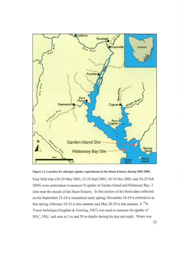
Figure 2.1 Location for nitrogen uptake experiments in the Huon Estuary during

2003-2004 23

Figure 2.2 A) Chla, B) temperature, C) salinity and D) irradiance at the surface (5m)

and bottom (20m) during the four field trips in the Huon Estuary 33

Figure 2.3 Mean ambient concentrations of nutrients (NH, NO3 ", urea, Silicate and

PO43 ) at surface (5m) and bottom (20m) depth during each of the field trips 34

Figure 2.4 Conductivity, temperature and depth profile of Hideaway Bay site during

the day for the late autumn (28/05/2003) N uptake experiment 36

Figure 2.5 CTD profile of Hideaway Bay site during the day for the early spring

(23/09/2003) N uptake experiment 39

Figure 2.6 CTD profile of Hideaway Bay site during the day for the late spring

(18/11/2003) N uptake experiment 41

Figure 2.7 CTD profile of Hideaway Bay site during the day for the late summer

(24/02/2004) N uptake experiment 43

xi

Figure 2.8 Phytoplankton composition derived from pigments from HPLC analysis of

samples and subsequent analysis using Chemtax V1.1. Hideaway Bay and Garden

Island in the Huon estuary during late autumn (28-29/05/2003), early spring (23-

24/09/2003), late spring (18-19/11/2003) and late summer (24-25/02/2004are

presented 45

Figure 2.9 Mean phytoplankton abundance (relative amount of chl a) on four field

trips A) dinoflagellate, B) diatom, C) cryptophyte and D) prasinophyte (across site,

depth, time) phytoplankton in the Huon Estuary. Standard errors are displayed (n=4).

46

Figure 2.10 Mean specific uptake rates for ammonium, nitrate and urea averaged

across all depths, times, and seasons). Standard error are displayed (n=96) and where

there are different subscripts on the bars there were significant differences. 49

Figure 2.11 Mean combined nitrogen uptake (NH4 ++NO3 --Eurea pooled across both

sites) in the surface (5m) and during the day for the four field trips in the Huon

Estuary. 95% confidence intervals (n=6) are displayed and significant differences

between field trips are indicated where subscripts on bars are different 50

Figure 2.12 Mean specific combined nitrogen uptake (NH4 ++NO3 --Eurea pooled

across both sites) in the surface (5m) and during the day for the four field trips in the

Huon Estuary. Standard error bars (n=6) are displayed and significant differences

between field trips are indicated where subscripts on bars are different 50

Figure 2.13 Uptake of NH4+, NO3 - and urea in the surface (5m) during the day in A)

28 May 2003, B) 23 September 2003, C) 18 November 2003, D) 24 February 2004.

95 % confidence intervals (n=6) are displayed and different subscripts on bars

indicate where there are Significant differences. 51

Figure 2.14 Mean NH 4+ uptake from four field trips A) Day at surface (5m) and B)

Night at surface (5m). 95% Confidence intervals (n=6) are displayed and different

xii

subscripts on bars indicate where there are significant differences between fieldtrips.

Where there is an * on bars from the same field trip in both A) and B) subfigures this

indicates a significant difference between them 53

Figure 2.15 Mean NH 4+ uptake from four field trips at depth (20m). 95% Confidence

intervals (n=12) are displayed and different subscripts on bars indicate where there

are significant differences. 53

Figure 2.16 Mean NH4+ uptake during the day and night at depth (20m). 95%

Confidence intervals (n=24) are displayed and different subscripts on bars indicate

where there are significant differences 54

Figure 2.17 Mean NO 3 uptake from four field trips A) surface (5m) and B) depth

(20m). 95% Confidence intervals (n=12) are displayed and different subscripts on

bars indicate where there are significant differences between fieldtrips. Where there is

an * on bars from the same field trip in both A) and B) subfigures this indicates a

significant difference between them 55

Figure 2.18 Mean Urea uptake from four field trips A) surface (5m) and B) depth

(20m). 95% Confidence intervals (n=12) are displayed and different subscripts on

bars indicate where there are significant differences between fieldtrips. Where there is

an * on bars from the same field trip in both A) and B) subfigures this indicates a

significant difference between them 57

Figure 2.19 Mean Urea uptake from four field trips A) Day and B) Night. 95%

Confidence intervals (n=12) are displayed and different subscripts on bars indicate

where there are significant differences between fieldtrips. Where there is an * on bars

from the same field trip in both A) and B) subfigures this indicates a significant

difference between them. 58

Figure 2.20 Mean Urea uptake during the day and night and at surface (5m) and depth

(20m). 95% Confidence intervals (n=24) are displayed and different subscripts on

bars indicate where there are significant differences. 58

Figure 2.21 Change in surface (5m) A) NO 3 - (iiM) and B) N:P on the four field trips

in the Huon Estuary. Reference lines are included for half Saturation constant (Ks)

for NO3 - uptake by coastal phytoplankton (Eppley et al., 1969) and Redfield ratio for

N:P (Redfield, 1958) 66

Figure 2.22 Mean uptake rates (from Hideaway Bay and Garden Island) during the

day at 5m, night at 5m, day at 20m and night 20m for A) NH4 + , B) NO3 - and C) Urea.

Error bars are 95% Confidence intervals. Note the different N uptake scale for NO 3 - .

69

Figure 3.1 Layout of the temperature and irradiance gradient table. 82

Figure 3.2 70 ml polycarbonate container with 50 ml glass test tube attached to the

top via a polypropylene custom made adapter. 82

Figure 3.3 Cell density vs. fluorescence of G. catenatum fit with a linear model.

Grown at 22.0 °C and —300 Amol photons m -2 s-1 89

Figure 3.4 Mean growth rate and standard error (n=4) of Gymnodinium catenatum

gown in three different culture vessels. Statistically significant differences are

indicated by superscripts. 93

Figure 3.5 Fluorescence of two Gymnodinium catenatum cultures following

inoculation on day zero and grown under different temperature and irradiance

conditions. 95

Figure 3.6 Comparison of growth rate by cell counts and growth rate by fluorescence

of Gymnodinium catenatum. 96

xiv

Figure 3.7 Growth vs. irradiance curves using the modified model of Platt et al.

(1975) (Equation 2) for Gymnodinium catenatum at twelve different temperatures. A

data point was excluded from the model fit at 20.7 °C (open circle). 98

Figure 3.8 Effect of temperature on onax of Gymnodinium catenatum. Each [t ina,,

value is from the modified model of Platt etal. (1975). Standard errors were also

estimated from the model. For details regarding the open circle see section 3.2.8 and

for the grey circle see section 3.2.6. 100

Figure 3.9 Effect of temperature on a of Gymnodinium catenatum. Each a value is

from the modified model of Platt etal. ((1975)). The standard error for a was

estimated from the model. 101

Figure 3.10 The effect of temperature on the half-saturation co-efficient for growth as

a function of irradiance (Ek) for Gymnodinium catenatum. Ek was calculated from the

model of Platt, Denman etal. (1975) 102

Figure 3.11 Effect of temperature on Ec of Gymnodinium catenatum. Each E, value is

from the modified model of Platt, Denman etal. (1975) (Equation 2). The standard

error for Ec is also from the model 103

Figure 3.12 Growth rates of Gymnodinium catenatum at 25 and 28.5 °C and 291 and

458 innol photons m -2 s-1 . Superscript text indicates where there were significant

differences (P<0.05) between growth rates. 104

Figure 3.13 Growth vs. irradiance curve of Gymnodinium catenatum grown at 24.9 to

25.0 °C with growth rates for cultures gown at 291 and 458 gmol photons 111-2 s-1 added. The modified model of Platt, Denman etal. (1975) was fitted to the data... 105

Figure 3.14 Effect of irradiance on C and chla quotas for Gymnodinium catenatum

are plotted on separate axes for six binned temperature groups 108

XV

Figure 3.15 The effect of irradiance on C:chla of Gymnodinium catenatum on

cultures binned into six temperature groups. Straight lines are fitted to the C:chla data

for each binned temperature group. The dotted line represents the expected C:chla

ratio from Geider's model (Geider, 1987) 110

Figure 3.16 Effect of temperature on in C:chla in Gymnodinium catenatum cultures

grown at irradiances >200 gmol photons I11-2 s -1 . The white circle was treated as an

outlier and excluded from the regression. 111

Figure 3.17 The effect of temperature on m(slope) of the line fit to C:chla vs

irradiance for Gymnodinium catenatum binned into six temperature groups (data from

Figure 3.15). 112

Figure 3.18 The effect of temperature on the y-intercept of the line fitted to C:chla vs.

irradiance for Gymnodinium catenatum binned into six temperature groups (data from

Figure 3.15). 113

Figure 3.19 Effect of temperature and irradiance on C:chla of Gymnodinium

catenatum. A 3D surface from the model (Equation 11) is used to describe the data.

114

Figure 3.20 Model of temperature effect on energetic costs for Gymnodinium

catenatum in light saturated (1000 gmol photons m -2 S-1 ) conditions 116

Figure 3.21 Model of temperature effect on energetic costs for Gymnodinium

catenatum in light limited (<80 gmol photons I11-2 s -1 ) conditions 117

Figure 3.22 Contour plot of growth rate (d -1 ) of Gymnodinium catenatum grown at

different combinations of temperature and irradiance. 119

Figure 3.23 Effect of temperature on Gymnodinium catenatum growth rate in

different studies. All growth rates were adjusted based on the daily irradiance of the

present study (9.07 mol photons r11-2 day-1 ). 124

xvi

Figure 3.24 Gymnodinium catenatum growth vs. irradiance comparison: the

modified model of Platt et al. (1975) (Equation 2) is fitted to data from 15.0 °C

(Yamamoto et al., 2002) and 15.5 °C from the present study. 126

Figure 3.25 Mean (+/- 1 SE) temperature in the surface (0-2m) and sub-surface

waters of the Huon Estuary (1996-1998). Data for the lower estuary (from Port Huon

to Huon Island) from the Huon Estuary Study (CSIRO Huon Estuary Study Team,

2000) 127

Figure 4.1 Mean growth of G. catenatum (GCHUO2, GCHUll and GCDE08) at

different concentrations of NH4+. Subscripts indicate significant differences between

treatments. Error bars are +1 standard error from the mean (n=3) 146

Figure 4.2 Growth of two strains of Gymnodinium catenatum (HUO2 and VSO4) on

NO3- and NH. Error bars are +1 standard error from the mean (n=3) 147

Figure 4.3 Growth of two strains of Gymnodinium catenatum (HUO2 and V504) on

NO3- and urea. Error bars are +1 standard error from the mean (n=3) 148

Figure 4.4 Preferential uptake of nitrogen species by Gymnodinium catenatum.

Mean NO3 -, NH4+ and urea concentrations for G. catenatum over the 29 day

experiment period (data from HUO2, VSO4 and LV01 strains). Error bars are +1

SEM (n=3). 149

Figure 4.5 Mean uptake rates for NO3 -, NH4+ and urea (data from GCH1J02, GCVSO4

and GCLV01 strains) for G. catenatum over the 29 day experiment period. Error bars

are +1-1 standard error from the mean (n=3) 150

Figure 5.1 Location for nitrogen uptake experiments near Pelican Island at Southport,

30-31/3/2004. 160

Figure 5.2 Phytoplankton composition (based on HPLC determined pigments and

subsequent CHEMTAX analysis from samples during bloom of G. catenatum at

xvii

Pelican Island, Southport during Day and night and Surface (5m) and depths (10 and

15m) 168

Figure 5.3 Total chi a, chl a attributed to G. catenatum and G. catenatum cell counts

at Pelican Island, Southport during Day and night and Surface (5m) and depths (10

and 15m). G. catenatum attributed chi a calculated based on 60 pg chl a cell -1 (Hallegraeff et al., 1991). 169

Figure 5.4 Profiles of temperature, irradiance, salinity and fluorescence at Pelican

Island, Southport (30-31/03/2004) at A) day and B) night. 170

Figure 5.5 Absolute and specific uptake rates of NH4 +, NO3- and urea at Pelican

Island, Southport during the day and night and at the surface (5m) and depth (10 and

15m) 172

Figure 5.6 Mean uptake for NH4+, NO3- and urea when both times and depths were

combined from Southport (see Fig 1.1 for location). Standard errors are included

(n=12) 173

Figure 5.7 Uptake of NH4, NO3 -, and urea during the day and night at Southport.

Least square means and upper and lower 95% confidence intervals. 174

Figure 5.8 Uptake of NH4 , NO3-, and urea at surface and bottom depths in

Southport. Least square means and upper and lower 95% confidence intervals are

shown 175

Figure 5.9 Uptake of the three different N species at surface and bottom during the

day and night at Southport. Least square means and upper and lower 95% confidence

intervals are shown. 175

Figure 5.10 Comparison with A) NH4+and B) NO3- G. catenatum uptake kinetics data

from Flynn, Flynn etal. (1996) 178

xviii

Figure 6.1 Surface nutrient concentrations from weekly samples at 5 sites during

1996-1998 (adapted from Thompson et al. 2008). The y-axes on the left is for nitrate

and silicate and the y-axes on the right is for ammonium and phosphate. Mean +1- 1

SE 187

xix

List of Tables

Table 2.1 Estimated proportions (% of ambient concentration) of 15N added as a

tracer for all field trips in the Huon Estuary 27

Table 2.2 Phytoplankton composition by cell count of field trips undertaken in the

Huon Estuary. Cell counts for the first trip 28-29/05/2003 were not available. 47

Table 2.3 An overall comparison of the uptake of nitrate, ammonium and urea by

phytoplankton in the Huon Estuary sampled during four seasons, at two locations,

two times of day and two depths (n=96). 48

Table 2.4 Results of ANOVA for effect of Season on absolute nitrogen uptake during

the day and at surface (5m) in the Huon Estuary. 70

Table 2.5 Results of ANOVA for effect of Season on specific nitrogen uptake during

the day and at surface (5m) in the Huon Estuary. 70

Table 2.6 Results of ANOVA for effect of Season on specific uptake of NH4, NO3

and Urea during the day and at surface (5m) in the Huon Estuary. 70

Table 2.7 Results of ANOVA for effect of Season, time of day and depth on NH4+

uptake in the Huon Estuary 70

Table 2.8 Results of ANOVA for effect of season, time of day and depth on NO 3 -

uptake in the Huon Estuary. 70

Table 2.9 Results of ANOVA for effect of season, time of day and depth on urea

uptake in the Huon Estuary. 71

Table 3.1 Temperature, irradiance and initial starting cell densities for each culture of

G. catenatum in the temperature gradient table. 86

xx

Table 3.2 Parameters of the modified model of Platt etal. (1975) fit to the growth vs.

irradiance data for Gymnodinium catenatum at twelve different temperatures. The

standard error (SE) for these parameters are included. Ek was calculated by solving

the modified model of Platt et al. (1975) (Equation 2) at the irradiance corresponding

to half onax. 99

Table 3.3 Parameters from the modified model of Logan (1976) for Gymnodinium

catenatum GCHUO2. 100

Table 3.4 Parameter estimates from the modified model of Platt, Denman etal.

(1975) for growth at 24.9 to 25 °C with new growth rates added from cultures grown

at 298 and 454 [tmol t11-2 s -1 105

Table 3.5 Mean biochemical quotas of Gymnodinium catenatum grown at

temperatures ranging from 13.4 to 25.2 °C and irradiances between 5 and 280 urnol

photons I11-2 s.

Table 3.6 Temperature range and number of cultures in each binned temperature

group. Binned temperature groups were used to examine the trends in biochemical

composition with temperature and irradiance. 106

Table 3.7 Conditions for different experiments on effect of temperature on growth

rate of Gymnodinium catenatum 125

Table 4.1 Gymnodinium catenatum strain details. 141

Table 4.2 Comparison of half saturation constants(Ks) for NO3 - and NH 4+ between

phytoplankton species from different classes 152

Table 5.1 Percent* (% of ambient concentration) of 15N added as a tracer for the

Southport fieldtrip. 163

Table 5.2 Representative cell count of lugols fixed phytoplankton collected from 5m

during the day at Southport 30/03/2004. 169 xxi

Table 5.3 Ambient, tracer and total NH 4+, NO3- and urea concentrations at different

times and depths for Southport N uptake experiment. 171

Table 5.4 Percentage uptake of NH4+, NO3- , and urea during the day at 5 and 15m

and during the night at 5 and 10m for the Southport fieldtrip 171

Table 5.5 Three way ANOVA for the effect of Nitrogen species (N), Time of day (T)

and Depth (D) on the specific uptake of nitrogen at Southport during a Gymondium

catenatum bloom 173

Table 5.6 Results of ANOVA for effect of nitrogen species, time of day and depth on

nitrogen uptake at Southport. Data were log transformed (log(x+0.05)) failed

Kolmogorov-Smimov test (with Lilliefors' correction) for normality but passed

levene's median test for equal variance. 182

1 INTRODUCTION

1.1 Eutrophication in coastal ecosystems

Eutrophication is widely considered to be one of the greatest threats to estuarine and

coastal ecosystems around the world (Howarth et al., 2002, Howarth et al., 2005).

Eutrophication as defined by Nixon (1995) is an increase in the rate of supply of

organic matter to an ecosystem. The rate of organic matter supply to an aquatic

ecosystem can increase through a number of different mechanisms. Clearing of

catchments is widely associated with more runoff and a greater supply of organic matter and nutrients into downstream water bodies. Agriculture and sewage may be

the source of more inorganic nutrients which can, in turn, support more photosynthesis and thereby contribute more organic matter into an ecosystem (Laws,

1993). The organic loading itself may result in anoxia thereby changing the cycling of

N and P sometimes resulting in these nutrients becoming periodically more abundant

in the water column. Thus there are a range of different mechanisms whereby an

aquatic ecosystem may become more eutrophic (Smith et al., 1999). The responses of

ecosystems, however, to an increase in organic matter supply can be complex

depending on a large number of physical and biological factors (Cloem, 2001). In

most cases the organisms that can directly use the nutrients, typically photosynthetic

autotrophs, are the first to respond to eutrophication (Philippart & Cadee, 2000). The

magnitude of these responses, however, is determined by the nature of the inputs and

by complex interactions between physics, chemistry and biology within the water

body and its sediments.

In some coastal ecosystems moderate eutrophication is considered beneficial because

it increases primary productivity and this in turn increases the biomass of fish and/or

shellfish species for human consumption (Nixon, 1990, Jorgensen & Richardson,

1996). However in most coastal ecosystems eutrophication has deleterious effects

such as:

1

• Shifts in phytoplankton community composition. Decoupling of base trophic

levels with higher trophic levels that can result in a shift towards toxic species

of phytoplanIcton.

• Low dissolved oxygen concentrations (hypoxia) and absence of oxygen

(anoxia) can be the result of increased plant, animal and bacterial respiration

caused by increased organic matter from primary production (autochthonous)

or organic matter input from outside the ecosystem (allochthonus).

• Increased turbidity caused by greater phytoplanlcton biomass can degrade or

destroy seagrass and macroalgae habitats for which light transmission down

through the water column to the bottom is important.

In almost all ecosystems, sometime during the annual cycle one nutrient or a

sequence of different nutrients can become limiting to primary production (Elser et

cd., 1990). When a nutrient is limiting for primary productivity an increase in the rate

of supply of that nutrient will stimulate primary productivity (Smayda, 1989).

Typically more biomass is produced as a response to more nutrients (Clark, 1989,

Vollenweider, 1992). Thus increased nutrient inputs also result in an increased

organic matter supply to the ecosystem. For temperate coastal ecosystems primary

productivity in these systems is usually limited by the availability of N (Ryther &

Dunstan, 1971, Howarth & Marino, 2006). The reason that eutrophication is

becoming such a widespread threat to coastal ecosystems is that there has been a

rapid increase in the amount of nitrogen getting into our aquatic ecosystems from

sewage and agriculture (Nixon, 1990) (Galloway etal., 2004). In the 1950's fertiliser

production using the Haber process began resulting in the steady increase in N

fertilizer and subsequent runoff of relatively more N into the coastal zone. A classic

example is the steady rise in N in the plume off the Mississippi River during the last

50 years (Turner etal., 1998). In this case there has been a relative decline in the

silicate concentrations producing a large scale example of selective resource

limitation with an impact on the ecology ranging from phytoplankton to fish. The

continental shelf off the Mississippi River has seen the ratio of silicate to dissolved in 2

organic nitrogen loading ratio has declined from around 3:1 to 1:1 during this century

because of fertilizer application, agriculture and other land-use practices in the

watershed. Diatoms require dissolved silicate and their growth can become Silicate

limited when the atomic ratio of silicate to dissolved inorganic nitrogen

(Silicate:D1N) approaches 1:1. Considerable research indicates this shift in N loading

is the primary reason this coastal ecosystem now produces a large anoxic zone

potentially supporting disruptive harmful algal blooms (Turner et al., 1998).

Harmful algal blooms (HAB) have been classified depending upon their type of

impact into three categories (after Hallegraeff, 1993):

1. Those not directly toxic to humans or other organisms. This type of HAB is

typically a large bloom that causes high biological oxygen demand (BOD)

during decomposition. Particularly in situations with low rates of mixing the

resulting hypoxia or anoxia can lead to the death of other organisms. Large

fish kills have been associated with this type of bloom.

2. Toxic algal blooms caused by a range of species, most commonly

dinoflagellates, that have a negative biological effect upon humans. For

example a range of species produce toxins which effect people once ingested.

These include:

a. PSP - paralytic shellfish poisoning, same toxins are found in

cyanobacteria

b. DSP - diarrheic shellfish poisoning

c. ASP - Amnesic shellfish poisoning

d. Ciguatera poisoning

e. NSP - neurotoxic shellfish poisoning

3. Blooms causing direct negative biological effects upon organisms other than

humans. For example HAB species that kill fish via damaged or clogged gills

and a range of other known and unknown mechanisms.

3

Four explanations for the apparent increase in algal blooms have been proposed: a

greater scientific awareness of toxic species; the growing utilization of coastal waters

for aquaculture; the stimulation of plankton blooms by domestic, industrial and

agricultural wastes and/or unusual climate conditions; and the transportation of algal

cysts either in ships' ballast water or associated with moving shellfish stocks from

one area to another (Hallegraeff, 1993). Most of the species known to cause HABs

are dinoflagellates.

The continuous plankton recorder transects of the North Atlantic (Edwards &

Richardson, 2004, Edwards et al., 2001) have shown clear evidence that whole

regions of the ocean have increased abundances of dinoflagellates. The mechanism

proposed to explain the growing dominance of dinoflagellates observed in the pelagic

ocean is warming due to climate change. The proponents hypothesized that warming

of the ocean surface due to climate change results in increased temperature

stratification. An increase in stratification would reduce vertical mixing, the major

process whereby nitrate is injected into the euphotic zone. It is not yet clear whether

global warming is having a global impact on stratification through warming, or polar

ice melting or increased precipitation. If large scale changes to stratification do occur

the consequences could be significant in terms of increase HABs. The seasonal

pattern of stratification and blooms may provide some insights.

Low stratification or high turbulence has a seasonal dynamic in the temperate zone.

Conditions of high turbulence and high nutrients are typically found in winter. The

diatom blooms that are associated with the transition from winter into spring suggest

diatoms are more capable of coping with turbulence than species that occur later in a

seasonal succession. This seasonal cycle of diatoms in spring often leading to

dinoflagellate blooms in summer or autumn and the commonly associated reduction

in turbulence was conceptualized by Margalef (1978). Margalef (1978) defined

niches for diatoms and dinoflagellates along 2 axis, one the concentration of nutrients

and the second the amount of turbulence (Fig. 1). Others have refined Margeler s

seminal work (Margalef, 1978) by expanding the conceptual space and populating it 4

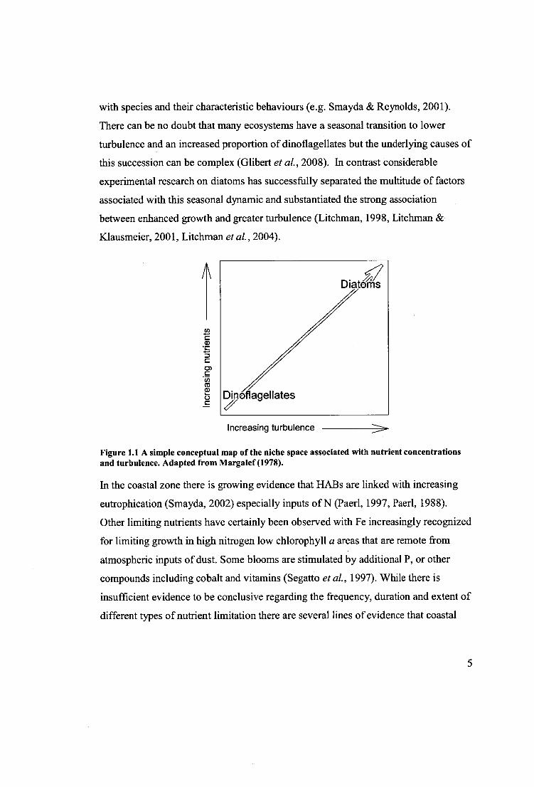
with species and their characteristic behaviours (e.g. Smayda & Reynolds, 2001).

There can be no doubt that many ecosystems have a seasonal transition to lower

turbulence and an increased proportion of dino flagellates but the underlying causes of

this succession can be complex (Gilbert et al., 2008). In contrast considerable

experimental research on diatoms has successfully separated the multitude of factors

associated with this seasonal dynamic and substantiated the strong association

between enhanced growth and greater turbulence (Litchman, 1998, Litchman &

Klausmeier, 2001, Litchman et al., 2004).

Incr

easi

ng n

utrie

nts

Increasing turbulence

Figure 1.1 A simple conceptual map of the niche space associated with nutrient concentrations and turbulence. Adapted from Margalef (1978).

In the coastal zone there is growing evidence that HABs are linked with increasing

eutrophication (Smayda, 2002) especially inputs of N (Paerl, 1997, Paerl, 1988).

Other limiting nutrients have certainly been observed with Fe increasingly recognized

for limiting growth in high nitrogen low chlorophyll a areas that are remote from

atmospheric inputs of dust. Some blooms are stimulated by additional P. or other

compounds including cobalt and vitamins (Segatto etal., 1997). While there is

insufficient evidence to be conclusive regarding the frequency, duration and extent of

different types of nutrient limitation there are several lines of evidence that coastal

5

ecosystems are more likely to be periodically limited by the availability of N than

other nutrients (Graneli etal., 1990, Ryther & Dunstan, 1971, Bricker etal., 1999).

One consequence of the importance of nitrogen to phytoplanlcton dynamics has been a great deal of research upon the nitrogen nutrition of phytoplankton. It has been

commonly assumed that phytoplankton should grow better on NH 4+ than NO 3 -,

particularly under conditions of low irradiance, as growth on NO 3 - imposes a

substantial extra cost in terms of reducing power. There is, however, little evidence

of this factor being a significant determinant of growth rates even at very low

irradiances (Thompson etal., 1989). Many species preferentially take up NH4 + over

NO3- when both are present, with some indication of a threshold effect (Dortch et al.,

1991, Dortch, 1990). A considerable amount of research has been focused on

answering the question, if not determined by an energetic constraint then what would

control the balance between NO3 - and NH4+ assimilation?

Although there is substantial geographic and temporal variation one of the most

persistent observations of phytoplankton ecology at temperate latitudes is a spring

bloom that consumes most of the available NO 3" in the euphotic zone. Frequently

this bloom is composed largely of diatoms leading to a hypothesis that diatoms may

have enhanced genetic capabilities and thus be physiologically more capable of using

NO3-. Experiments to test this hypothesis have shown that some species do grow

better on particular forms of NO3 - (Levasseur et al., 1993) but not necessarily

diatoms. Experiments on diatoms in turbulent environments also have a long history

examining aspects of their physiology that might be advantageous (Marra, 1978)

relative to dinoflagellates (Chan, 1978). More recently there has been a refinement of

the general hypothesis that turbulence favours diatoms to include NO3 - uptake and

reduction as a method to use the excess light energy that must periodically be

acquired by a phytoplankton cell in a well mixed water column (Lomas & Glibert,

2000, Lomas & Gilbert, 1999) and a chlorophyll content adapted to the average

irradiance. Indeed some fraction of the competitive advantage diatoms possess in

turbulent environments seems to be associated with the reduction of NO3 - . 6

Temporal variability in nutrient availability exists on many time scales such as

seasonal fluctuations at mid to high latitudes (Parsons & Takahashi, 1973), estuaries

which experience nutrient pulses associated variations in flow (Mallin et al., 1993)

and on shorter time scales especially in near shore environments (Fong et al., 1993).

If the nutrient pulses are rare relative to the life spans of the organisms then long

lived species will dominate, while intermediate pulses should give a mixture of

species and a rise in diversity (Floder & Sommer, 1999). Long periods of high

nutrient availability with low N:P ratios are often associated with a loss of diversity

and nuisance algal blooms (Birch etal., 1981).

Harmful algal blooms, however, are rarely diatoms and frequently occur later in the

season when NO3 - is relatively less available. Many HAB have also been associated

with greater availability of reduced N such as N114+ or dissolved organic N (DON).

Relatively little research has been conducted on the capacity of phytoplanIcton to use

organic N for growth. Most of this has focused on urea as a proxy for all forms of

organic N. Early research demonstrated the importance of urea in the natural

environment, where it was frequently observed to be z50% of all N uptake (e.g.

McCarthy, 1972). Similar results have been reported in a range of studies although

there are relatively few studies and a generic perspective is not easily obtained. Other

organic forms of dissolved N have received relatively little attention, although the

pioneering work of Antia (e.g. Antia & Harrison, 1991 and references therein) did

show considerable capacity of many species to use many forms of DON even though

their growth rates were low. In the field it has been shown that phytoplankton will

use a range of DON (Hellebust, 1970, Hollibaugh, 1976). Use of DON is still being

actively investigated today (e.g. Stolte etal., 2002, Bronk etal., 2007) and some

interesting recent work again showing taxonomic differences in DON use (Wawrik et

al., 2009). The use of DON and the use of specific forms of DON would seem to

have a significant genetic component that may be important in defming the ecological

niche occupied by some species, a subject that requires further investigation.

7

Perhaps the most intriguing differences in the use of NO 3- versus NH 4+ is the contrast

between the two dominant picoplanktors, Synechococcus and Prochlorococcus.

These two genera dominate the world's oceans yet Prochlorococcus has only very

limited capacity to use NO3 -. Although the lack of nitrate reductase is not universal

among strains of Prochlorococcus it is important in determining its niche (Moore et

al., 1998, Rocap etal., 2003). Thus the availability of different forms of nitrogen is

an important factor contributing to the relative success and productivity of different

phytoplankton (Berg etal., 1997). Typically, the abundance of dinoflagellates can be

correlated with low nitrate concentrations and high rates of NH4 + or dissolved organic

nitrogen (DON) supply (Carlsson et al., 1998). Many studies show that

phytoplankton biomass may increase with overall nitrogen availability (Boynton et

al., 1982) and the DON component may shape the phytoplankton succession and lead

to a harmful algal bloom (Paerl, 1988) . While molecular techniques are making it

easier to assess whether a species has the potential to use a particular form of N they

cannot tell us whether this capacity actually provides a competitive advantage. Field

experiments that measure fluxes and laboratory experiments that assess outcomes

with, and without, a specific nitrogen source are still the major tools to determine

whether a specific nitrogen compound is important in ecology of a particular species.

This sort of research seems likely to be required for all flAB species.

As discussed above the availability of particular forms of nitrogen often has a

seasonal dynamic but it may also have a spatial component. For example, point

sources can provide locally elevated concentrations of particular forms of nitrogen.

Often the euphotic zone can be stripped on DIN during a spring bloom. The nitrate in

deeper waters is not readily available to photosynthetic organisms. Some large scale

dinoflagellate blooms have been shown to vertically migrate during the dark for this

N returning to the euphotic zone for light energy during the day (Eppley et al., 1968,

Hasle, 1950, Cullen & Horrigan, 1981). Considerable work has been done on the

physiology of vertical migration through temperature and nutrient gradients

(Kamykowski, 1981, Kamykowski, 1995, Kamykowski & Yamazaki, 1997). Field

8

observations indicate that G. catenatum vertically migrates through temperature,

salinity and nutrient gradients in the Huon Estuary (Doblin etal., 2006). Testing the

hypothesis that G. catenatum may vertically migrate to access NO3 - or NH4+ was one

of the major components of this research.

In the coastal zone and following the spring bloom the water column is often

resupplied with DIN in forms other than NO3 -. If the water column is stratified this

can result in elevated NH4+ near the bottom. This is especially true if dissolved

oxygen is low (Laws, 1993) due to inhibition of de-nitrification (Bonin & Raymond,

1990). In stratified ecosystems with low vertical exchange the NH 4+ gradient can be

considerable and again dinoflagellates may migrate vertically to access this N source.

1.2 The Huon Estuary

The Huon River estuary and its catchment is located in southeast Tasmania between

latitude 42° 45' S and 43° 45' S (Figure 1.2 and Figure 1.3). Tasmania is the

southernmost island state of Australia. Tasmania has a maritime climate that is

dominated by zonal westerly's, resulting in a variable cool temperate climate. The

Huon Estuary is a drowned river valley — 401cm long and 4.51cm wide at the mouth (at

Huon Island) where it joins the southern end of the D'Entrecasteaux Channel, a semi-

protected channel formed between the Tasmanian mainland and Bruny Island (Figure

1.3). The depth ranges from 40m at the mouth to 10 m at Port Huon, above which the

depth decreases rapidly to between 2 and 4 m deep on the east and west sides of Egg

Island (Figure 1.2). It is a salt wedge estuary, with the marine water extending from

the mouth of the estuary up to Ranelagh, upstream of Huonville (Figure 1.2) where

saltwater can penetrate under low river flows.

9

et'

Port Huon

Cygnet

10

Figure 1.2 Location and features of the Huon Estuary in south-eastern Tasmania, adapted from CSIRO Huon Estuary Study Team (2000).

The catchment of the Huon Estuary is classified as largely natural as it has been

subject to only moderate modification by human activity. Much of the upper

catchment remains as undisturbed native forest, increasing areas of the mid- and

lower-catchment are now been subjected to managed forestry activities.

Approximately, 5.6 % of the total catchment has been cleared- for a patchwork of

primary agriculture activity such as horticulture and livestock grazing. Human

10

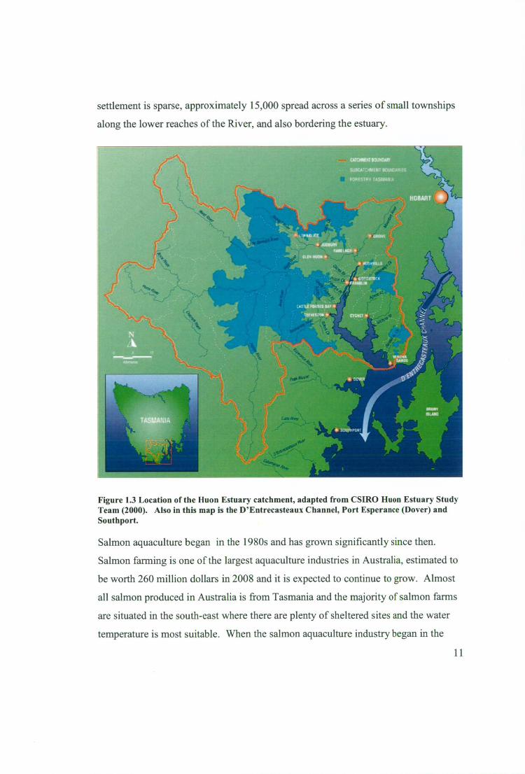
settlement is sparse, approximately 15,000 spread across a series of small townships

along the lower reaches of the River, and also bordering the estuary.

Figure 1.3 Location of the Huon Estuary catchment, adapted from CSIRO Huon Estuary Study Team (2000). Also in this map is the D'Entrecasteaux Channel, Port Esperance (Dover) and Southport.

Salmon aquaculture began in the 1980s and has grown significantly since then.

Salmon farming is one of the largest aquaculture industries in Australia, estimated to

be worth 260 million dollars in 2008 and it is expected to continue to grow. Almost

all salmon produced in Australia is from Tasmania and the majority of salmon farms

are situated in the south-east where there are plenty of sheltered sites and the water

temperature is most suitable. When the salmon aquaculture industry began in the

11

early 1980's there was limited understanding and knowledge of environmental

effects. As salmon farming continued to grow in Tasmania it became increasingly

recognised that expansion needed to be underpinned by a sound scientific knowledge

of the effects of salmon farming on the environment.

In 1996 a large study commenced in the Huon Estuary- the Huon Estuary Study

(HES). The goal of the HES was to examine the physical and biological

characteristics and environmental status of the estuary and to gain an integrated

understanding of the system. One of the key drivers for the research was too examine

potential impacts of salmon farming on the Estuary. The 3 year HES involved

collection of physical, chemical and biological data throughout the estuary and the

development of a relatively simple (2D box) coupled hydrodynamic and bio-

geochemical model. Nutrient data from the Huon Estuary Study indicated that it is a

N limited system.

Models based upon data from the HES predicted that a doubling in the production of

salmon would result in only a small increase in the likelihood of algal blooms, while

greater inputs could significantly increase the likelihood of phytoplankton blooms

and potential eutrophication, but that further investigation was required to improve

understanding of the links between nitrogen and phytoplankton growth and biomass

in the Huon Estuary. A key gap identified from the HES was the lack of knowledge

on how different forms of N may affect the phytoplankton biomass and its

composition in the estuary.

The biogeochemical model from the more recent Aquafin CRC was used to calculate

nitrogen budgets for the Huon Estuary and D'entrecasteaux Channel in 2002

(Vollcman etal., 2009). The largest input of N (60%) to the Huon Estuary and

D'entrecasteaux Channel comes from the surrounding marine waters. This N is

mostly delivered in winter and is primarily NO3 - . The Huon River delivers about 23

% but this is mostly considered refactory N. Salmon aquaculture accounts for 17% of

the N and while it is only a relatively small amount almost all of this N is labile NH4 + .

12

For the D'entrecasteaux Channel and Huon Estuary in 2002, N from salmon

aquaculture was estimated to be 843 tonnes: 313 tonnes of N input to the Huon and

543 input into the D'Entrecasteaux Channel. The salmon aquaculture industry has

increased production significantly since 2002 and in 2009 it is estimated that there

will be a 210% increase in N to 1747 tonnes across both the Huon Estuary and

D'Entrecasteaux Channel. But industry and regulators have capped production in the

Huon Estuary, so only 243 tonnes of N will be input to the Huon in 2009. However

there will be a —3 times increase in the D'Entrecasteaux from 530 to 1747 tonnes in

2009.

Dinoflagellates are important components of the phytoplankton community in the

Huon Estuary, often forming the majority of the biomass. Periodic blooms of the

toxic species, G. catenatum, result in closure of shellfish farms in the Huon Estuary

and D'Entrecasteaux Channel (Hallegraeff et al., 1989). This large dinoflagellate

species (35um) intermittently forms dense and often mono-specific blooms in the

Huon Estuary and is a major contributor to the phytoplankton biomass in the estuary

during blooms (Thompson et al., 2008, Hallegraeff et al., 1995). Blooms occur only

in some years and not in others and appear to be associated with particular climatic

triggers (early summer rainfall followed by periods of low winds; Hallegraeff et al.,

1995). However, these triggers have not proven to be universally required as

significant blooms have occurred without these cues. During bloom years, the

phytoplankton biomass is also much greater than would be predicted from the

available NO3 - in the estuary. As G. catenatum is capable of rapid diurnal vertical

migration it has been hypothesised that these blooms may be using NH4+ derived

from bottom waters (Doblin et al., 2006).

1.3 Research Objectives

This research will combine laboratory and field experiments to address the current

lack of knowledge on the effects of nutrient input composition on phytoplankton in

the Huon Estuary. The first objective of this research was to determine whether 13

phytoplankton in the Huon Estuary are using nitrogen that has an oceanic source

(primarily NO3) or more locally supplied or regenerated source (primarily NH 4+ and

urea). Given the large role G. catenatum plays in the Huon Estuary with high

biomass blooms forming during summer and autumn it was also considered that

better understanding the physiology of G. catenatum would be key to understanding

phytoplankton dynamics in the Huon Estuary. The second objective of this research

was to understand the physiological responses of G. catenatum to light, temperature

and different nitrogen species. Specifically, this thesis sets out to:

• Determine the nitrogen uptake preference and dynamics of the seasonal

phytoplankton assemblage in the Huon Estuary (Chapter 2)

• Investigate the effect of temperature and irradiance on growth rate and

biochemical composition of G. catenatum (Chapter 3)

• Describe the physiology and nutrient uptake dynamics and preference of the

dinoflagellate Gymnodinium catenatum, a significant seasonal contributor to

the phytoplankton biomass in the Huon Estuary (Chapters 4).

• Determine whether diurnally migrating G. catenatum blooms are able to

access and uptake nitrogen available at depth during the night in the field

(Chapter 5).

-

14

1.4 References

Antia, N. J. & Harrison, P. J. 1991. The role of dissolved organic nitrogen in phytoplankton nutrition, cell biology and ecology. Phycologia 30:1-89.

Berg, G. M., Glibert, P. M., Lomas, M. W. & Burford, M. A. 1997. Organic nitrogen uptake and growth by the chrysophyte Aureococcus anophagefferens during a brown tide event. Mar Biol 129:377-87.

Birch, P. B., Gordon, D. M. & McComb, A. J. 1981. Nitrogen and phosphorus- nutrition of Cladophora in the Peel-Harvey estuarine system, Western Australia. Botanica Marina 24:381-87.

Bonin, P. & Raymond, N. 1990. Effects of oxygen on denitrification in marine-sediments. Hydrobiologia 207:115-22.

Boynton, W. R., Kemp, W. M. & Keefe, C. W. 1982. A comparative analysis of nutrients and other factors influencing estuarine phytoplankton production. In: Kennedy, V. S. [Ed.] Estuarine Comparisons. Academic Press, New York, pp. 69-90.

Bricker, S. B., Clement, C. G., Pirhalla, D. E., Orlando, S. P. & Farrow, D. R. G. 1999. National estuarine eutrophication assessment: Effects of nutrient enrichment in the Nation's estuaries. National Oceanic and Atmospheric Admistration, Silver Spring, USA.

Bronk, D. A., See, J. H., Bradley, P. & Killberg, L. 2007. DON as a source of bioavailable nitrogen for phytoplankton. Biogeosciences 4:283-96.

Carlsson, P., Edling, H. & Bechemin, C. 1998. Interactions between a marine dinoflagellate (Alexandrium catenella) and a bacterial community utilizing riverine humic substances. Aquat. Microb. EcoL 16:65-80.

Chan, A. T. 1978. Comparative physiological study of marine diatoms and dinoflagellates in relation to irradiance and cell size. I. Growth under continuous light. J Phycol 14:396-402.

Clark, R. B. 1989. Marine Pollution. Oxford, New York, Cloern, J. E. 2001. Our evolving conceptual model of the coastal eutrophication

problem. Mar. Ecol.-Prog. Ser. 210:223-53. Cullen, J. J. & Horrigan, S. G. 1981. Effects of nitrate on the diurnal vertical

migration, carbon to nitrogen ratio, and the photosynthetic capacity of the dinoflagellate Gymnodinium splendens. Mar. Biol. 62:81-89.

Doblin, M. A., Thompson, P. A., Revill, A. T., Butler, E. C. V., Blackburn, S. I. & Hallegraeff, G. M. 2006. Vertical migration of the toxic dinoflagellate Gymnodinium catenatum under different concentrations of nutrients and humic substances in culture. Harmful Algae 5:665-77.

Dortch, 0., Thompson, P. A. & Harrison, P. J. 1991. Short-Term Interaction between Nitrate and Ammonium Uptake in Thalassiosira-Pseudonana - Effect of Preconditioning Nitrogen-Source and Growth-Rate. Mar Biol 110:183-93.

Dortch, Q. 1990. The interaction between ammonium and nitrate uptake in phytoplankton. Mar. EcoL-Prog. Ser. 61:183-201.

15

Edwards, M., Reid, P. & Planque, B. 2001. Long-term and regional variability of phytoplankton biomass in the Northeast Atlantic (1960-1995). ICES J. Mar. Sci. 58:39-49.

Edwards, M. & Richardson, A. J. 2004. Impact of climate change on marine pelagic phenology and trophic mismatch. Nature 430:881-84.

Elser, J. J., Marzolf, E. R. & Goldman, C. R. 1990. Phosphorus and Nitrogen Limitation Of Phytoplankton Growth In The Fresh-Waters Of North-America-A Review And Critique Of Experimental Enrichments. Canadian Journal of Fisheries and Aquatic Sciences 47:1468-77.

Eppley, R. W., Holmhans, 0. & Strickla, J. D. 1968. Some observations on vertical migration of dinoflagellates. J. PhycoL 4:333-40.

Floder, S. & Sommer, U. 1999. Diversity in planktonic communities: An experimental test of the intermediate disturbance hypothesis. Limnol. Oceanogr. 44:1114-19.

Fong, P., Zedler, J. B. & Donohoe, R. M. 1993. Nitrogen vs phosphorus limitation of algal biomass in shallow coastal lagoons. Limnol. Oceanogr. 38:906-23.

Galloway, J. N., Dentener, F. J., Capone, D. G., Boyer, E. W., Howarth, R. W., Seitzinger, S. P., Asner, G. P., Cleveland, C. C., Green, P. A., Holland, E. A., Karl, D. M., Michaels, A. F., Porter, J. H., Townsend, A. R. & Vorosmarty, C. J. 2004. Nitrogen cycles: past, present, and future. Biogeochemistry 70:153- 226.

Glibert, P. M., Burkholder, J. M., Graneli, E. & Anderson, D. M. 2008. Advances and insights in the complex relationships between eutrophication and HABs: Preface to the special issue. Harmful Algae 8:1-2.

Graneli, E., Wallstrom, K., Larsson, U., Graneli, W. & Elmgren, R. 1990. Nutrient limitation of primary production in the Baltic sea area. Ambio 19:142-51.

Hallegueff, G. M. 1993. A review of harmful algal blooms and their apparent global increase. Phycologia 32:79-99.

Hallegraeff, G. M., Mccausland, M. A. & Brown, R. K. 1995. Early Warning of Toxic Dinoflagellate Blooms of Gymnodinium-Catenatum in Southern Tasmanian Waters. J Plankton Res 17:1163-76.

Hallegraeff, G. M., Stanley, S. 0., Bolch, C. J. & Blackburn, S. 1. 1989. Gymnodinium catenatum blooms and shellfish toxicity in Southern Tasmania, Australia. In: Okaichi, T., Anderson, D. M. & Nemoto, T. [Eds.] Red Tides: Biology, Environmental Science and Toxicology. Elsevier, pp. 75-78.

Hasle, G. R. 1950. Phototactic vertical migration in marine dinoflagellates. Oikos 2:162-75.

Hellebust, J. A. 1970. The uptake and utilization of organic substrates by marine phytoplankters. In: Hood, D. W. [Ed.] Organic matter in natural waters. National Science Foundation, Institute of Marine Science, University of Alaska, pp. 223-56.

Hollibaugh, J. T. 1976. Biological degradation of arginine and glutamic-acid in seawater in relation to growth of phytoplankton. Mar. Biol. 36:303-12.

16

Howarth, R. W. & Marino, R. 2006. Nitrogen as the limiting nutrient for eutrophication in coastal marine ecosystems: Evolving views over three decades. LimnoL Oceanogr. 51:364-76.

Howarth, R. W., Ramakrishna, K., Choi, E., Elmgren, R., Martinelli, L., Mendoza, A., Moomaw, W., Palm, C., Boy, R., Scholes, M. & Zhao-Lang, Z. 2005. Nutrient management, responses assesment. In: Etchevers, J. & Tiessen, H. [Eds.] Ecosystems and Human Wellbeing. Island Press, Washington DC, pp. 295-311.

Howarth, R. W., Sharpley, A. 8c Walker, D. 2002. Sources of nutrient pollution to coastal waters in the United States: Implications for achieving coastal water quality goals. Estuaries 25:656-76.

Jorgensen, B. B. & Richardson, K. 1996. Ezarophication in Coastal Marine Systems. American Geophysical Union, Washington DC,

Kamykowski, D. 1981. Laboratory experiments on the diurnal vertical migration of marine dinoflagellates through temperature-gradients. Mar. Biol. 62:57-64.

Kamykowski, D. 1995. Trajectories of autotrophic marine dinoflagellates. J. PhycoL 31:200-08.

Kamykowski, D. & Yamazaki, H. 1997. A study of metabolism-influence orientation in the diel vertical migration of marine dinoflagellates. LimnoL Oceanogr. 42:1189-202.

Laws, E. A. 1993. Aquatic Pollution: An introductory text. John Wiley and Sons, New York,

Levasseur, M., Thompson, P. A. & Harrison, P. J. 1993. Physiological Acclimation of Marine-Phytoplankton to Different Nitrogen-Sources. J Phycol 29:587-95.

Litchman, E. 1998. Population and community responses of phytoplankton to fluctuating light. Oecologia 117:247-57.

Litchman, E. & Klausmeier, C. A. 2001. Competition of phytoplankton under fluctuating light. American Naturalist 157:170-87.

Litchman, E., Klausmeier, C. A. & Bossard, P. 2004. Phytoplankton nutrient competition under dynamic light regimes. LimnoL Oceanogr. 49:1457-62.

Lomas, M. W. & Gilbert, P. M. 1999. Temperature regulation of nitrate uptake: A novel hypothesis about nitrate uptake and reduction in cool-water diatoms. LimnoL Oceanogr. 44:556-72.

Lomas, M. W. & Glibert, P. M. 2000. Comparisons of nitrate uptake, storage, and reduction in marine diatoms and flagellates. J Phycol 36:903-13.

Mallin, M. A., Paerl, H. W., Rudek, J. & Bates, P. W. 1993. Regulation of estuarine primary production by watershed rainfall and river flow. Mar. EcoL-Prog. Ser. 93:199-203.

Margalef, R. 1978. Life-forms of phytoplankton as survival alternatives in an unstable environment. Oceanologica Acta 1:493-509.

Marra, J. 1978. Effect of short-term variations in light-intensity on photosynthesis of a marine phytoplankter - laboratory simulation study. Mar. Biol. 46:191-202.

McCarthy, J. J. 1972. The uptake of urea by natural populations of marine phytoplankton. LimnoL Oceanogr. 17:738-48.

17

Moore, L. R., Rocap, G. & Chisholm, S. W. 1998. Physiology and molecular phylogeny of coexisting Prochlorococcus ecotypes. Nature 393:464-67.

Nixon, S. W. 1990. Marine Eutrophication - A Growing International Problem. Ambio 19:101-01.

Nixon, S. W. 1995. Coastal Marine Eutrophication - A Definition, Social Causes, And Future Concerns. 41:199-219.

Paerl, H. W. 1988. Nuisance phytoplankton blooms in coastal, estuarine, and inland waters. LimnoL Oceanogr. 33:823-47.

Paerl, H. W. 1997. Coastal eutrophication and harmful algal blooms: Importance of atmospheric deposition and groundwater as "new" nitrogen and other nutrient sources. Limnol. Oceanogr. 42:1154-65.

Parsons, T. R. & Takahashi, M. 1973. Environmental-control of phytoplankton cell size. Limnol. Oceanogr. 18:511-15.

Philippart, C. J. M. & Cadee, G. C. 2000. Was total primary production in the western Wadden Sea stimulated by nitrogen loading? 54:55-62.

Rocap, G., Larimer, F. W., Lamerdin, J., Malfatti, S., Chain, P., Ahlgren, N. A., Arellano, A., Coleman, M., Hauser, L., Hess, W. R., Johnson, Z. I., Land, M., Lindell, D., Post, A. F., Regala, W., Shah, M., Shaw, S. L., Steglich, C., Sullivan, M. B., Ting, C. S., Tolonen, A., Webb, E. A., Zinser, E. R. & Chisholm, S. W. 2003. Genome divergence in two Prochlorococcus ecotypes reflects oceanic niche differentiation. Nature 424:1042-47.

Ryther, J. H. & Dunstan, W. M. 1971. Nitrogen,Phosphorus, And Eutrophication In The Coastal Marine Environment. Science 171:1008-13.

Segatto, A. Z., Graneli, E. & Haraldsson, C. 1997. Effects of cobalt and vitamin B12 additions on the growth of two phytoplanIcton species. La Mer 35:5-14.

Smayda, T. J. 1989. Primary production and the global epidemic of phytoplankton blooms in the sea: A linkage? In: Cosper, E. M., J., C. E. & Bricelj, V. M. [Eds.] Novel Phytoplankton Blooms: Causes and Impacts of Recurrent Brown Tides and Other Unusual Blooms. Springer-Verlag, Berlin, pp. 449-83.

Smayda, T. J. 2002. Adaptive ecology, growth strategies and the global bloom expansion of dinoflagellates. J. Oceanogr. 58:281-94.

Smayda, T. J. & Reynolds, C. S. 2001. Community assembly in marine phytoplankton: application of recent models to harmful dinoflagellate blooms. J. Plankton Res. 23:447-61.

Smith, V. H., Tilman, G. D. & Nekola, J. C. 1999. Eutrophication: Impacts of excess nutrient inputs on freshwater, marine, and terrestrial ecosystems. Environ. Pollut. 100:179-96.

Stolte, W., Panosso, R., Gisselson, L. A. & Graneli, E. 2002. Utilization efficiency of nitrogen associated with riverine dissolved organic carbon (> 1 kDa) by two toxin-producing phytoplankton species. Aquat. Microb. Ecol. 29:97-105.

Team, H. E. S. 2000. Huon Estuary Study, Environmental research for integrated catchment management and aquaculture. Final Report to FRDC. CSIRO Division of Marine Research, Hobart, Tasmania, Australia.

18

Thompson, P. A., Bonham, P. I. & Swadling, K. M. 2008. Phytoplankton blooms in the Huon Estuary, Tasmania: top-down or bottom-up control? J. Plankton Res. 30:735-53.

Thompson, P. A., Levasseur, M. E. & Harrison, P. J. 1989. Light-Limited Growth on Ammonium Vs Nitrate - What Is the Advantage for Marine-Phytoplankton. Limnol. Oceanogr. 34:1014-24.

Turner, R. E., Qureshi, N., Rabalais, N. N., Dortch, Q., Justic, D., Shaw, R. F. & Cope, J. 1998. Fluctuating silicate : nitrate ratios and coastal plankton food webs. Proc. Natl. Acad. Sci. U. S. A. 95:13048-51.

Vollcman, J. K., Thompson, P. A., Herzfeld, M., Wild-Allen, K., Blackburn, S. B., Macleod, C., Swadling, K., Foster, S., Bonham, P:, Holdsworth, D., Clementson, L., Skerratt, J., Rosebrock, U., Andrewartha, J. & Revill, A. 2009. A whole-of-ecosystem assessment of environmental issues for salmonid aquaculture. Aquafin CRC Project 4.2(2), Fisheries and Research Development Corporation Project No.2004/074.

Vollenweider, R. A. 1992. Coastal Marine Eutrophication. In: Vollenweider, R. A., Marchetti, R. & Viviani, R. [Eds.] Coastal Marine Eutrophication. London, pp. 1-20.

Wawrik, B., Callaghan, A. V. & Bronk, D. A. 2009. Use of Inorganic and Organic Nitrogen by Synechococcus spp. and Diatoms on the West Florida Shelf as Measured Using Stable Isotope Probing. Applied and Environmental Microbiology 75:6662-70.

19

2 NITROGEN UPTAKE BY

PHYTOPLANKTON IN THE HUON

ESTUARY, SOUTH-EAST TASMANIA,

AUSTRALIA

2.1 Introduction

The Huon Estuary has been the subject of intensive environmental studies since 1996

as part of a program to ensure the sustainability of aquaculture in the Estuary. One of

the key topics being addressed is the link between nutrients and phytoplanlcton

blooms in the estuary. The Huon Estuary Study (Team, 2000) suggested that

phytoplankton growth in the Huon Estuary is limited primarily by the availability of

nitrogen (N).

In coastal ecosystems the main sources of N used by phytoplankton are nitrate

(NO3-), ammonium (NH4 4) and urea (Twomey et al., 2005). Some phytoplankton

are able to use all these sources of N for growth (Antia etal., 1975). However there

is evidence that some species/groups of phytoplankton favour/prefer one form of

nitrogen over another. For example diatoms have been shown to be associated with

increased NO3- uptake (Heil etal., 2007, Berg etal., 2003, Bode & Dortch, 1996). In

addition to some species groups having preferences for particular N substrates there

are a number of environmental factors that also have an effect on N uptake,

including: temperature, light, substrate concentration and inhibition (Varela &

Harrison, 1999, Dortch, 1990).

Dinoflagellates are important components of the phytoplankton community in the

Huon Estuary, often forming the majority of the biomass. Periodic blooms of the

toxic species, G. catenatum, result in closure of shellfish farms in the Huon Estuary

20

and D'Entrecasteaux Channel (Hallegraeff et al., 1989). This large dinoflagellate

species (35um) intermittently forms dense and often mono-specific blooms in the

Huon Estuary and is a major contributor to the phytoplankton biomass in the estuary

during blooms (Thompson etal., 2008, Hallegaeff et al., 1995). Blooms occur only

in some years and not in others and appear to be associated with particular climatic

triggers (early summer rainfall followed by periods of low winds; Hallegraeff et al.,

1995). However, these triggers have not proven to be universally required as

significant blooms have occurred without these cues. During bloom years, the

phytoplankton biomass is also much greater than would be predicted from the

available NO3- in the estuary. As G. catenatum is capable of rapid diurnal vertical

migration it has been hypothesised that these blooms may be using NH 4+ derived

from bottom waters (Doblin et al., 2006). Field observations indicate that G.

catenatum vertically migrates diurnally from 5m to 20m through temperature,

salinity and nutrient gradients in the Huon Estuary (Doblin et al., 2006). Testing the

hypothesis that G. catenatum may vertically migrate to access NO3 - or NH4+ was one

of the major components of this research. For this reason N uptake experiments were

to be setup at 5m and 20m during the day when it was expected that G. catenatum

would be concentrated at 5m. Experiments were also set up at 5m and 20m during

the night when it was expected that G. catenatum would be concentrated at 20m.

However, large blooms of G. catenatum were rare in the Huon Estuary in 2002, 2003

and 2004. So our 2003-2004 field trips, were unable to provide information about the

N uptake strategies of G. catenatum during a vertically migrating bloom. For this

reason we focused on determining which nitrogen sources: nitrate (NO3-), ammonium

(NH4 +) or urea are important for supporting phytoplankton growth in the Huon

Estuary. These field experiments have focused upon whether the phytoplankton are

using nutrients that have an oceanic source (primarily nitrate) or more locally

supplied or regenerated nutrients (primarily ammonium and urea). Given that

phytoplankton in Australian estuaries are nitrogen limited (Harris, 2001) the

possibility exists that additional nitrogen inputs to the ecosystem may cause an

increase in phytoplankton biomass or increase blooms of nuisance or toxic species.

21

The research in this chapter is designed to investigate which of these N sources

supports the growth of phytoplankton in this region.

2.2 Methods

The research included 4 field trips in the Huon Estuary on the 28-29 May 2003, 23-24

September 2003, 18-19 November 2003, and 24-25 February 2004. It is recognized

that 4 sampling trips per year, even when statistically different, may not fully

represent seasonal affects. Regardless, for the sake of simplicity in presentation, these

temporal periods are referred to as seasons. During these field trips a 15N tracer

technique was used to measure uptake of 3 different nitrogen (N) sources (NO3 -,

NH4+ and urea) by the natural phytoplankton assemblage. Two sites, Garden Island

(latitude 43° 16' 3" S longitude 147° 6' 30" E) and Hideaway Bay (latitude 43° 16' 14"

S longitude 147° 5' 2" E), were used for this field work (Figure 2.1). N uptake

experiments were setup at 5 m and 20 m water depth during both the day and night.

22

cc

(

N 4'160,0 ce 4., Garden Island Site

,. c, luns

1

Hideaway Bay Site

Figure 2.1 Location for nitrogen uptake experiments in the Huon Estuary during 2003-2004.

Four field trips (28-29 May 2003, 23-24 Sept 2003, 18-19 Nov 2003, and 24-25 Feb

2004) were undertaken to measure N uptake at Garden Island and Hideaway Bay: 2

sites near the mouth of the Huon Estuary. In this section of the thesis data collected

on the September 23-24 is considered early spring, November 18-19 is referred to as

late spring, February 24-25 is late summer and May 28-29 is late autumn. A 15N

Tracer technique (Dugdale & Goering, 1967) was used to measure the uptake of

NO3-, NH4+ and urea at 5 m and 20 m depths during the day and night. Water was 23

collected from the 2 depths using a 10 1 Niskin bottle and dispensed into 500m1 glass

Schott bottles made by Schott Duran. The water collected for the incubations were

not pre-filtered before dispensing into the 500 ml Schott bottles. There were two main

reasons for not pre-filtering the water for the incubations. Firstly, ensuring that long

chains of G. catenatum were not excluded from incubations. G. catenatum chains of 4

to 8 cells are common. A quick estimate of the size of these chains, 30 microns x 8

cells = 240 microns suggests that screening at 200 microns (a commonly used screen)

would exclude a proportion of this species. Secondly, we wanted to estimate the real

in situ N uptake rate including, losses due to grazing. For each depth three 500 ml

schott bottles were spiked with 0.3 1.1M 15N- NO3- (99.3 atom percent 15N), three 500

ml schott bottles were spiked with 0.1 1.1M 15N-NH4+ (99.6 atom percent 15N) and

three 500 ml schott bottles were spiked with 0.068 i.tM 15N-urea (98.61 atom percent

15N). In addition at each depth one 500m1 schott bottle was filled with water but not

spiked with any 15N substrate, this unspiked bottle was used to determine the

background 15N (un-enriched atom % excess). These samples were incubated in 500

ml Schott bottles for 4 hours in-situ at the depths they were collected from. Four

hour incubations were chosen because they are short enough to limit the chances of

substrate exhaustion (La Roche, 1983) and also reduce the problems caused by

substrate dilution(Glibert et al., 1982), but an incubation period of 2-6 hours is also

long enough to minimise the bias introduced by initial high uptake rates that

sometimes occur in phytoplankton (Dugdale & Wilkerson, 1986). After the

incubation the water samples were filtered onto pre-combusted (450°C for 4 hours)

25 mm WhatmanTm glass fibre filters and stored frozen until analysis. The filters

were dried in an oven at 60°C overnight before they were analysed using a Carlo Erba

NA1500 CNS analyzer interfaced via a Conflo II to a Finnigan-MAT Delta S isotope

ratio mass spectrometer to determine the N isotope ratios. Absolute uptake rates were

calculated using the Dugdale and Goering (1967) equation:

p = Na t(Rt) l

24

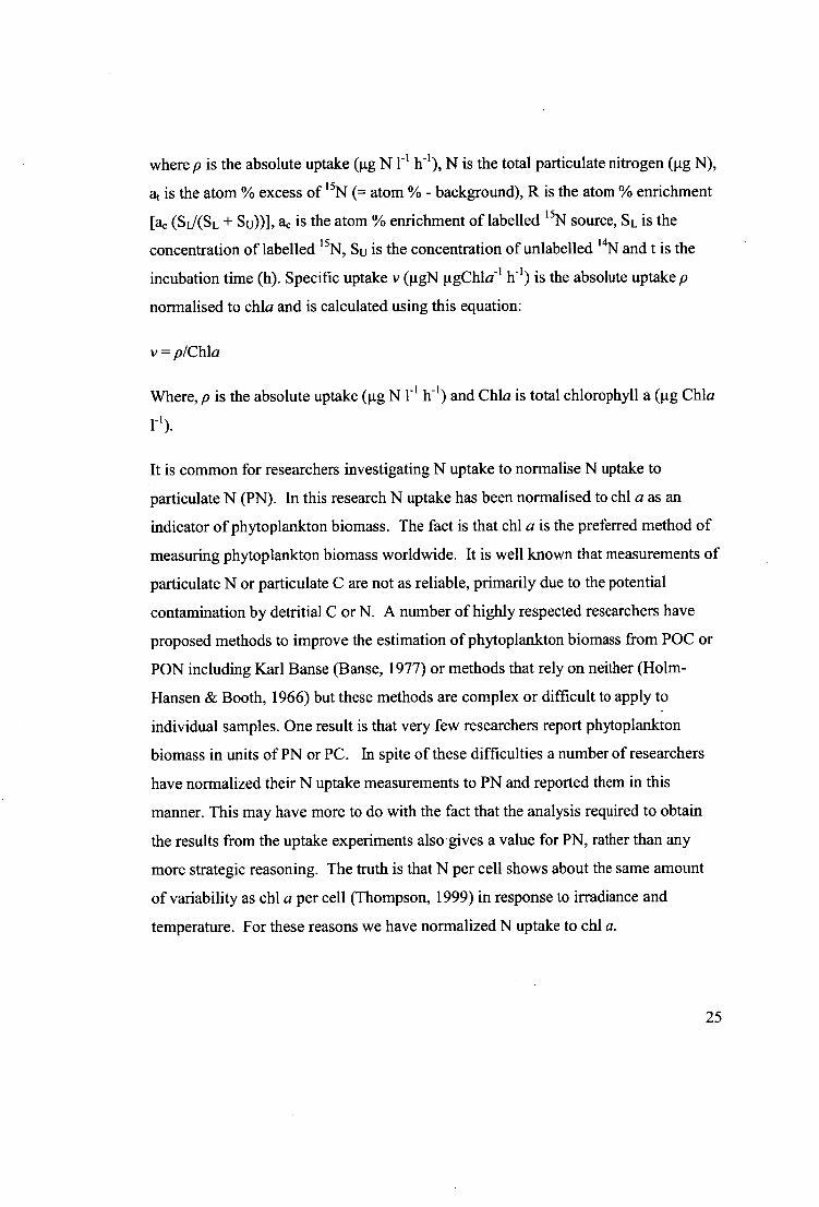
where p is the absolute uptake 0.1g N r' N is the total particulate nitrogen (jig N),

at is the atom % excess of 15N (= atom % - background), R is the atom % enrichment

[a, (SIASL + Sep], ae is the atom % enrichment of labelled 15N source, SL is the

concentration of labelled 15N, Su is the concentration of unlabelled 14N and t is the

incubation time (h). Specific uptake v (ligN i.tgChla -1 II I ) is the absolute uptake p

normalised to chla and is calculated using this equation:

v = p/Chla

Where, p is the absolute uptake (4 N r' II I ) and Chia is total chlorophyll a (jig Chla

It is common for researchers investigating N uptake to normalise N uptake to

particulate N (PN). In this research N uptake has been normalised to chi a as an

indicator of phytoplankton biomass. The fact is that chl a is the preferred method of

measuring phytoplankton biomass worldwide. It is well known that measurements of

particulate N or particulate C are not as reliable, primarily due to the potential

contamination by detritial C or N. A number of highly respected researchers have

proposed methods to improve the estimation of phytoplankton biomass from POC or

PON including Karl Banse (Banse, 1977) or methods that rely on neither (Holm-

Hansen & Booth, 1966) but these methods are complex or difficult to apply to

individual samples. One result is that very few researchers report phytoplankton

biomass in units of PN or PC. In spite of these difficulties a number of researchers

have normalized their N uptake measurements to PN and reported them in this

manner. This may have more to do with the fact that the analysis required to obtain

the results from the uptake experiments also gives a value for PN, rather than any

more strategic reasoning. The truth is that N per cell shows about the same amount

of variability as chl a per cell (Thompson, 1999) in response to irradiance and

temperature. For these reasons we have normalized N uptake to chi a.

25

When water was collected for the N uptake experiments, triplicate 10 ml samples

were taken for measurement of ambient NO3-, NH4 + and urea concentrations and 2 L

was filtered for pigment analyses using high performance liquid chromatography

(HPLC).

Nutrient samples were stored at -20 °C prior to analysis. Analytical techniques for

nitrate and/or nitrite (Wood etal., 1967), silicate (Murphy 84 Riley, 1962) and

phosphate (Armstrong, 1951) were adapted and performed using Quick-Chem Tm

methods on a flow injection LACHAT instrument as per the following protocols for

nitrate and/or nitrite (Quik-ChemTm Method 31-107-04-1-A; detection limit 0.03—

mM), silicate (Quik-ChemTM Method 31-114-27-1-D; detection limit —0.05 mM)

and phosphate (Quik-ChemTM Method 31-115-01-1-G; detection limit —0.02 mM).

Ammonium was measured using the technique of Kerouel and Aminot (Kerouel &

Aminot, 1997) adapted for flow injection (Watson etal., 2004)with a detection limit

of —0.05 mM. Urea samples were analysed using a diacetyl monoxime technique

according to the method of (Mulvenna & Savidge, 1992). To reduce the health risks

associated with thio-semicarbazide, a reagent for this technique, we substituted

semicarbazide (a less toxic but similar compound).

It was not possible to measure ambient concentrations of nutrients prior to

commencing an experiment. Consequently fixed concentrations of NO3 -, NH4+ and

urea were added as listed above, with a target of 10% of the ambient concentration.

The majority (59%) of 15N additions were <15% of ambient concentrations. There

were, however, a number of instances where ambient concentration were less, at

certain depths or times of the year, than anticipated. Adding less 15N may have been

more appropriate at these times of the year although it increases the likelihood of

running out of labelled substrate and thus underestimating uptake rates. Under

conditions of extreme N limitation where 0.3 j.tM 15N- NO3-, 0.1 gM 15N-NH4+ or

0.068 uM 15N-urea represent substantially more than 15% of the ambient

concentration the labelled N is no longer a tracer but becomes an increasingly

important source. Under these conditions it is likely that real in situ uptake rates were 26

overestimated by the technique. The worst cases were for nitrate in late spring and

late summer (Table 2.1) where uptake of nitrate is probably over estimated in the

results presented here.

Table 2.1 Estimated proportions (% of ambient concentration) of 15N added as a tracer for all field trips in the Huon Estuary.

28/05/2003

23/09/2003

18/11/2003

24/02/2004

site time depth (m) %"N NH 4+ °/0 1 N NO3" )̀/0 "N urea 5 11 9 22 day Hideaway 20 18 9 19

Bay 5 8 8 16 night 20 19 7 13 5 7 9 33 day Garden 20 12 7 20

Island 5 15 8 25 night 20 12 8 13 5 13 9 14 day Hideaway 20 32 8 16

Bay 5 25 8 20 night 20 65 8 20 5 60 8 11 day Garden 20 91 8 13

Island 5 43 8 19 night 20 98 8 15 5 15 430 21 day Hideaway 20 16 54 17

Bay 5 10 820 32 night 20 13 40 14 5 114 3000a 17

Garden day 20 13 44 15 Island 5 229 3000a 34 night 20 20 52 16

5 36 295 15 day Hideaway 20 7 53 15 Bay 5 23 485 11 night 20 6 58 13

5 32 663 10 Garden day 20 10 61 9 Island 5 7 51 8 night 20 23 1785 9

Date

a % enrichment calculated by using the detection limit (0.03 mM) of the NO 3" detection method used.

2.2.1 CTD profiles

A SeabirdTM SBE19+ conductivity, temperature and depth (CTD) profiler was used to

measure the salinity, temperature and fluorescence of the water column during the

field experiments. The measurements throughout the water column presented are the

27

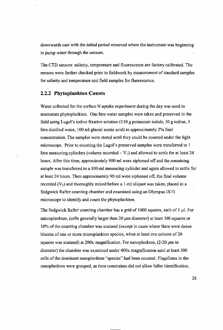
downwards cast with the initial period removed where the instrument was beginning

to pump water through the sensors.

The CTD sensors: salinity, temperature and fluorescence are factory calibrated. The

sensors were further checked prior to fieldwork by measurement of standard samples

for salinity and temperature and field samples for fluorescence.

2.2.2 Phytoplankton Counts

Water collected for the surface N uptake experiment during the day was used to

enumerate phytoplankton. One litre water samples were taken and preserved in the

field using Lugol's iodine fixative solution (110 g potassium iodide, 50 g iodine, 1

litre distilled water, 100 ml glacial acetic acid) to approximately 2% final

concentration. The samples were stored until they could be counted under the light

microscope. Prior to counting the Lugol's preserved samples were transferred to 1

litre measuring cylinders (volume recorded — V1) and allowed to settle for at least 24

hours. After this time, approximately 900 ml were siphoned off and the remaining

sample was transferred to a 100-ml measuring cylinder and again allowed to settle for

at least 24 hours. Then approximately 90 ml were siphoned off, the final volume

recorded (V2) and thoroughly mixed before a 1-ml aliquot was taken, placed in a

Sedgwick Rafter counting chamber and examined using an Olympus IX71

microscope to identify and count the phytoplankton.

The Sedgwick Rafter counting chamber has a grid of 1000 squares, each of 1 tl. For

microplankton, (cells generally larger than 20 tm diameter) at least 100 squares or

10% of the counting chamber was scanned (except in cases where there were dense

blooms of one or more microplankton species, when at least one column of 20

squares was scanned) at 200x magnification. For nanoplankton, (2-20 1-1.M in

diameter) the chamber was examined under 400x magnification until at least 300

cells of the dominant nanoplankton "species" had been counted. Flagellates in the

nanoplankton were grouped, as time constraints did not allow fuller identification.

28

Cells per litre =

cell "species" count * (1000 / number squares counted) * (V2 *1000 /V1)

2.2.3 CHEMTAX

Pigment data from HPLC analysis was further analysed to give the proportions of

chlorophyll a present in the following algal taxonomic categories: Cyanophyta,

Prochlorophyta, Chrysophyta, Cryptophyta, Bacillariophyta (diatoms), Haptophyta,

Prasinophyceae, and Dinophyta (Mackey et al., 1996). Initial input ratio matrices

were adjusted from those proposed in Mackey, Mackey et al. (1996) by including

four types of Haptophytes:

Haptophyte N — Type 1 = fucoxanthin e.g. Isochrysis spp.

Haptophyte S- Type 2 = Chl c3 + fucoxanthin e.g. Ochrosphaera neopolitana

Haptophyte Type 3 = Chi c3+ 19'Hexanoyloxyfucoxanthin + fucoxanthin + and

sometimes 19'butanoyl derivative e.g. Chyrsochromulina strobulis

Haptophyte Type 4 = c3 + 19'butanoyloxyfucoxanthin +19'hexanoyloxyfucoxanthin

and fucoxanthin e.g. Imantonia rotunda.

The peridinin:chlorophyll a ratio was modified from 0.515:1 as in Mackey, Mackey

etal. to 0.36:1 after Hallegraeff, Nichols etal. (1991). The latter was based on

extensive culture studies for Gymnodinium catenatum. This has the effect of

increasing the proportion of the chlorophyll a that CHEMTAX will allocate to

dinoflagellates for a given amount of peridinin. Based on personal observations this

results in CHEMTAX estimates of dinoflagellates that are more consistent with the

estimated proportion of biomass calculated by cell counts and adjusted for cellular

bio-volumes.

29

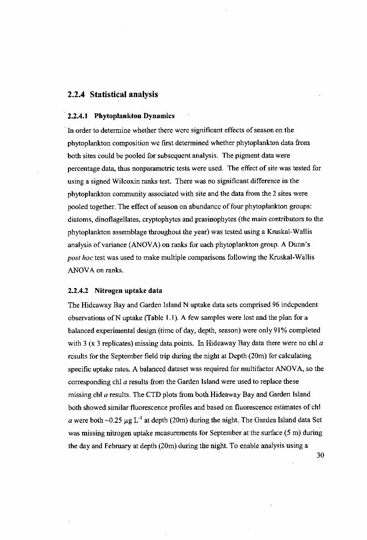
2.2.4 Statistical analysis

2.2.4.1 Phytoplankton Dynamics

In order to determine whether there were significant effects of season on the

phytoplanlcton composition we first determined whether phytoplankton data from

both sites could be pooled for subsequent analysis. The pigment data were

percentage data, thus nonparametric tests were used. The effect of site was tested for

using a signed Wilcoxin ranks test. There was no significant difference in the

phytoplankton community associated with site and the data from the 2 sites were

pooled together. The effect of season on abundance of four phytoplankton groups:

diatoms, dinoflagellates, cryptophytes and prasinophytes (the main contributors to the

phytoplankton assemblage throughout the year) was tested using a Kruskal-Wallis

analysis of variance (ANOVA) on ranks for each phytoplankton group. A Dunn's

post hoc test was used to make multiple comparisons following the Kruskal-Wallis

ANOVA on ranks.

2.2.4.2 Nitrogen uptake data

The Hideaway Bay and Garden Island N uptake data sets comprised 96 independent

observations of N uptake (Table 1.1). A few samples were lost and the plan for a

balanced experimental design (time of day, depth, season) were only 91% completed

with 3 (x 3 replicates) missing data points. In Hideaway Bay data there were no chl a

results for the September field trip during the night at Depth (20m) for calculating

specific uptake rates. A balanced dataset was required for multifactor ANOVA, so the

corresponding chl a results from the Garden Island were used to replace these

missing chl a results. The CTD plots from both Hideaway Bay and Garden Island

both showed similar fluorescence profiles and based on fluorescence estimates of chi

a were both —0.25 jig L -1 at depth (20m) during the night. The Garden Island data Set

was missing nitrogen uptake measurements for September at the surface (5 m) during

the day and February at depth (20m) during the night. To enable analysis using a 30

multifactor ANOVA a balanced data set was achieved by constructing the missing

data from the mean and standard deviation across the 4 field trips (Table 2.1) for the

corresponding depth and time (Little & Rubin, 1987).

Comparisons between the Hideaway Bay and Garden Island sites results for NH 4+,

NO 3 -, urea and absolute N (NH4++NO3 -+urea) uptake using paired t tests. The tests

for normality and equal variance were Kolmogorov-Smimov test (with Lilliefors'

correction) and Levene median test. Where data was not normally distributed (NH4 +,

Urea and absolute N (NH4 ++NO3 -+urea) uptake) 0.05 was added to make all values

positive and then they were log transformed. Following the transformation only urea

did not conform to a normal distribution. Where there were no significant differences

between sites data was pooled across sites for subsequent statistical analyses.

An overall analysis to determine whether there were differences between uptake of

NH4+, NO3 - and urea in the Huon Estuary (averaged across season, time of day and

depth) was undertaken using a non-parametric Kruskal-Wallis ANOVA on ranks test

(P=<0.001) and post hoc multiple comparisons made using Tukey's Test.

A subset of the data: nitrogen uptake during the day and at the surface (5m) was used

to examine the effect of time of year on absolute and specific nitrogen (NH 4++NO3 -

+urea) uptake. For absolute N uptake (NE4++NO3 -+urea), data were log transformed

and analysed by ANOVA. Post hoc multiple comparisons of this data were made

using the Holm-Sidak test. Specific N uptake (NH 4++NO3 -+urea) data were analysed

by ANOVA and post hoc multiple comparisons were made using the Holm-Sidak

test.

Differences between specific uptake of NH, NO3 - and urea at four times

throughout the year (during the day and at surface (5m)) were also analysed using a

two-way ANOVA, followed by post hoc multiple comparisons by the Holm-Sidak.

Prior to analysis by ANOVA, data were transformed (log(x+0.05)), but they still

failed the Levene Median test for equal variance.

31

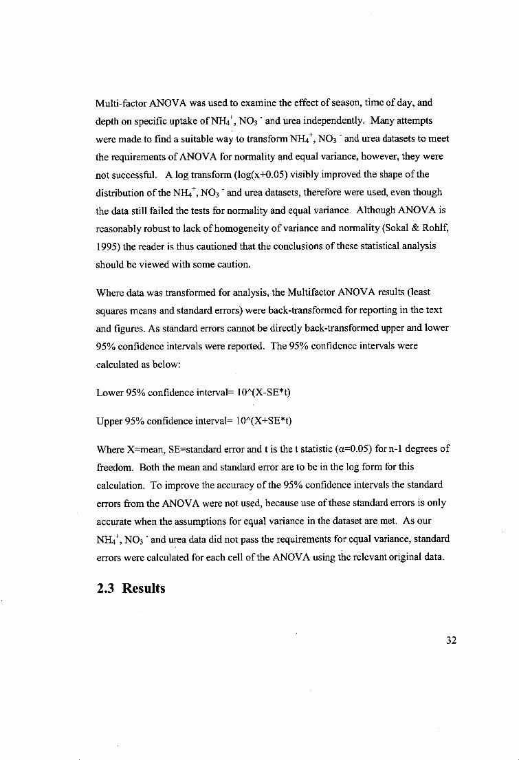
Multi-factor ANOVA was used to examine the effect of season, time of day, and

depth on specific uptake of NH4+, NO3 - and urea independently. Many attempts

were made to find a suitable way to transform NI-14 +, NO3 - and urea datasets to meet

the requirements of ANOVA for normality and equal variance, however, they were

not successful. A log transform (log(x+0.05) visibly improved the shape of the

distribution of the NH4+, NO3 - and urea datasets, therefore were used, even though

the data still failed the tests for normality and equal variance. Although ANOVA is

reasonably robust to lack of homogeneity of variance and normality (Sokal & Rohlf,

1995) the reader is thus cautioned that the conclusions of these statistical analysis

should be viewed with some caution.

Where data was transformed for analysis, the Multifactor ANOVA results (least

squares means and standard errors) were back-transformed for reporting in the text

and figures. As standard errors cannot be directly back-transformed upper and lower

95% confidence intervals were reported. The 95% confidence intervals were

calculated as below:

Lower 95% confidence interval= 10^(X-SE*t)

Upper 95% confidence interval= 10^(X+SE*0

Where X=mean, SE=standard error and t is the t statistic (a=0.05) for n-1 degrees of

freedom. Both the mean and standard error are to be in the log form for this

calculation. To improve the accuracy of the 95% confidence intervals the standard

errors from the ANOVA were not used, because use of these standard errors is only

accurate when the assumptions for equal variance in the dataset are met. As our

NH4+, NO3 - and urea data did not pass the requirements for equal variance, standard

errors were calculated for each cell of the ANOVA using the relevant original data.

2.3 Results

32

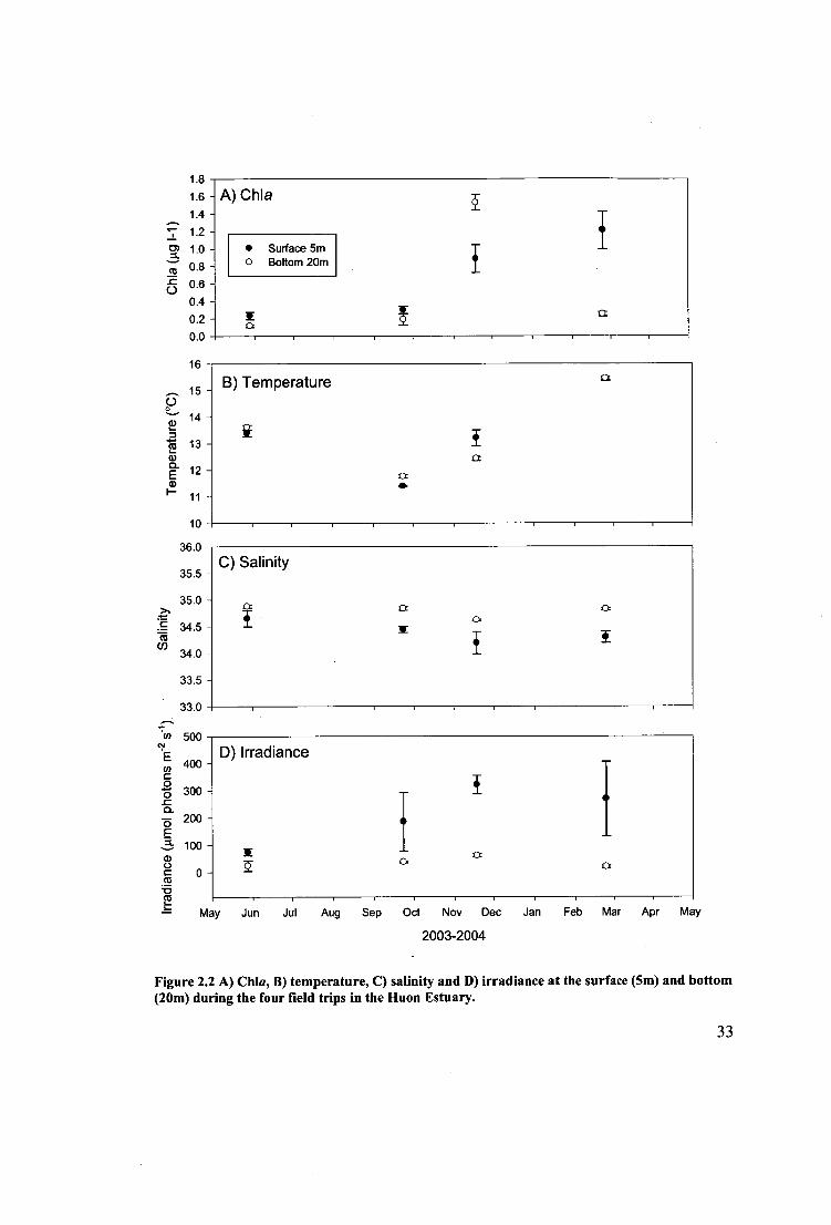
1.8 1.6 - 1.4 - —

'7 1.2-S c) 1.0 O 0.8 - _c 0.6 - 0

0.4 - 0.2 - 0.0

A) Chla

• Surface 5m o Bottom 20m fI

a

Jul Aug Sep

B) Temperature

C) Salinity

D) Irradiance

16

15 -

14 -

13 -

12 -

11 -

10

36.0

35.5 -

35.0

To co 34.0 -

33.5 -

33.0

(1) 500 c 4 • 400 - c O

•

300 - .c ca. • 200 - E a 100 - o C 0 - co CO

- May Jun Oct Nov Dec Jan Feb Mar Apr May

2003-2004

Tem

per

atu

re (

°C)

Figure 2.2 A) Chla, B) temperature, C) salinity and D) irradiance at the surface (5m) and bottom (20m) during the four field trips in the Huon Estuary.

33

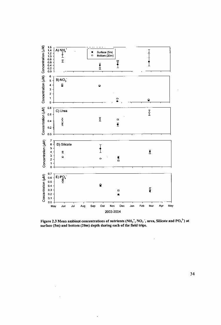
Co

nce

ntra

tion

(pM

) Concen

trat

ion

(pM

) Co

ncen

trat

ion

(PM

) Co

nce

ntra

tion

(pM

) Con

cen

trat

ion

(pM

)

0.6 -

0.4 - a

C) Urea

1.6 1.4 - 1.2 - 1.0 - 0.8 - 0.6 - 0.4 - 0.2 - 0.0

A) NH4 • Surface (5m) o Bottom (20m)

6

5

4

3

2

1

0

0.8

B)NO3-

a 411-

0.2 -

0.0

7 6 5 - 4 -

3 - 2 - 1 -

0

0.7

0.6 -

0.5 -

0.4 -

0.3 -

0.2 -

0.1 -

E) 74-

a a

D) Silicate

a a

0.0

May Jun Jul Aug Sep Oct Nov Dec Jan Feb Mar Apr May

2003-2004

Figure 2.3 Mean ambient concentrations of nutrients (NH 4+, NO3 ", urea, Silicate and PO43-) at surface (5m) and bottom (20m) depth during each of the field trips.

34

2.3.1 Late autumn

- Physical conditions

During the late autumn field trip the temperature ranged from 13.5 °C at the surface

and was 13.7°C at a depth of 30 m (Figure 2.4). Salinity was also fresher (34.0) from

the surface to 3m depth while at depths below the salinity was closer to a salinity

expected of a full marine environment (>34.8). At the surface irradiance was 90

[Lmol photons m -2 s-1 and decreased quickly in the surface layers. At depths of 30

metres there was very little irradiance —40 limo' photons Tr1-2

Chemical conditions

In late Autumn [NO3 and [Silicate] ] were high at —4 jtM in the surface (5m), at

depth (20m), [NO 3 was similar at —4 i_tM but the [Silicate] was 2.8 ji.M. In the

surface (5m) [NH] and [urea] were 1.1 and 0.3 i.tM respectively. At depth (20m)

[NH] was lower, 0.7 gM and [urea] was slightly increased at 0.4 i.tM. At the

surface (5m) and depth (20m) [PO43-] was 0.55 and 0.5 1.1M, respectively.

Biological conditions

During the late autumn field trip chlorphyll a (chla) was lowest 0.23 and 0.1 ug

respectively in both the surface (5m) and at depth (20m). Fluorescence was at its

maximum near the surface 0.7 units and decreased with depth to 0.3 units. The

phytoplankton assemblage was dominated by dinoflagellates (49% of total chl a).

The next two most dominant groups were prasinophytes and diatoms 23 and 19% of

total chl a, respectively. The remainder of the phytoplankton consisted of

cryptophytes and haptophytes type N (only contain fucoxanthin). Based upon

CHEMTAX analysis of the HPLC pigment data there were no significant differences

in phytoplankton community composition between site, day or night and surface or

depth. There was no microscopic examination of samples in late autumn to

substantiate the CHEMTAX phytoplankton community composition.

35

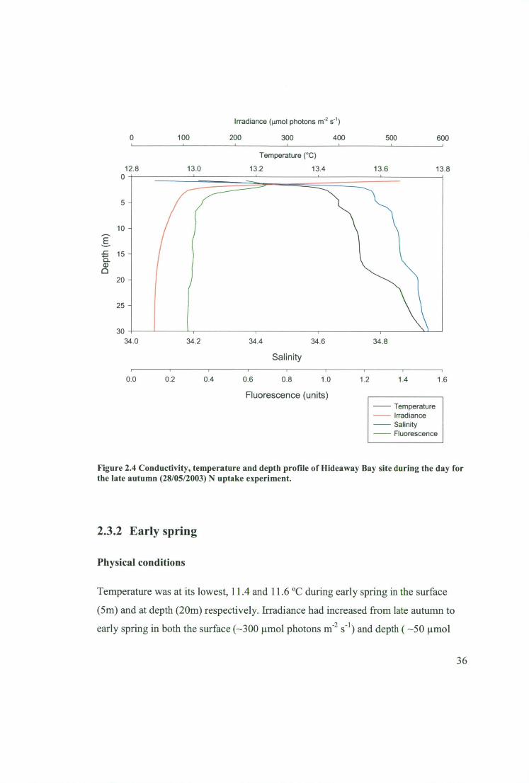
10 -

20 -

25 -

30

Irradiance (prnol photons rri 2 S-1 )

100 200 300 400 500 600

Temperature (°C)

12.8 13.0 13.2 13.4

13.6 13.8

34.0

34.2 34.4 34.6

34.8

Salinity

0.0 0.2 0.4 0.6 0.8 1.0

1.2

1.4

1.6

Fluorescence (units)

— Temperature Irradiance

Salinity Fluorescence

Figure 2.4 Conductivity, temperature and depth profile of Hideaway Bay site during the day for the late autumn (28/05/2003) N uptake experiment.

2.3.2 Early spring

Physical conditions

Temperature was at its lowest, 11.4 and 11.6 °C during early spring in the surface

(5m) and at depth (20m) respectively. Irradiance had increased from late autumn to

early spring in both the surface (-300 iimol photons ni2 s-1 ) and depth ( —50 ilmol

36

photons I/1-2 s-1 ). Relative to late autumn the salinity was lower (34.5 and 34.8) in

early spring at surface and depth, respectively.

Chemical conditions

NO3- concentrations were still — 4 i.tM in both the surface (5m) and at depth (20m) in

early spring. The concentration of NH4+ reached was at its lowest in both the surface

and at depth, 0.4 and 0.2 1iN4 respectively, during early spring compared with the

other field trips. The concentrations of urea at both depths were —0.5 W. The

concentrations of silicate were at their highest in the surface (5m) during the early

spring —5 JIM. At depth the silicate concentration was less than half this

concentration (2.3 gM). Concentrations of phosphate (PO4 3") were —0.4 1.1M at

surface (5m) and depth (20m).

Biological conditions

During early spring the chla concentrations were low and similar in both the surface

and at depth (0.3 and 0.2 jig 14 , respectively ). Fluorescence was greatest near the

surface 0.3 units and decreased to — 0.27 units at depths below 17 m. Phytoplankton

were dominated by diatoms at the surface (30-40% of total chlorophyll a) and even

more dominated at depth (50-60%). Dinoflagellates represented 20-30% of the

phytoplankton. There was one exception to these generalisations at Hideaway Bay

during the night at the surface (5m). In this sample dinoflagellates accounted for >

60% of the phytoplankton. The remainder of the phytoplankton were composed of

chryptophytes, prasinophytes, chlorophytes, haptophytes types N and S and

cyanobacteria. The chlorophytes and cyanobacteria seemed to be restricted to the

surface (5m) samples. The most numerous diatoms in this sample were

Pseudonitzschia pseudodelicatissima (1248 cell L-1 ), Nitzscia closterium (793),

Skeletonema costatum (521 cell L -1 ) and Chaetoceross spp. >15i.tm (401 cell 1- ')

(Table 2.1). The dinoflagellates were represented by 15 p.m Gymnodiniod

dinoflagellates (273 cell 1 -1 ), Gymnodinium catenatum (132 cell 1 - ') Dinophysis spp.

37

(36 cell 1- ') and Ceratium spp. (27 cell 1 - '). There were no cryptophytes observed in

these samples. It very likely that they were identified in CHEMTAX because of the

alloxanthin in the relatively large population of pigmented Dinophysis species with

chloroplasts that originate from cryptophytes via the intermediate host of Myrionecta

rubra (=Mesodinium rubrum) (Park et al., 2006, Nagai etal., 2008)

38

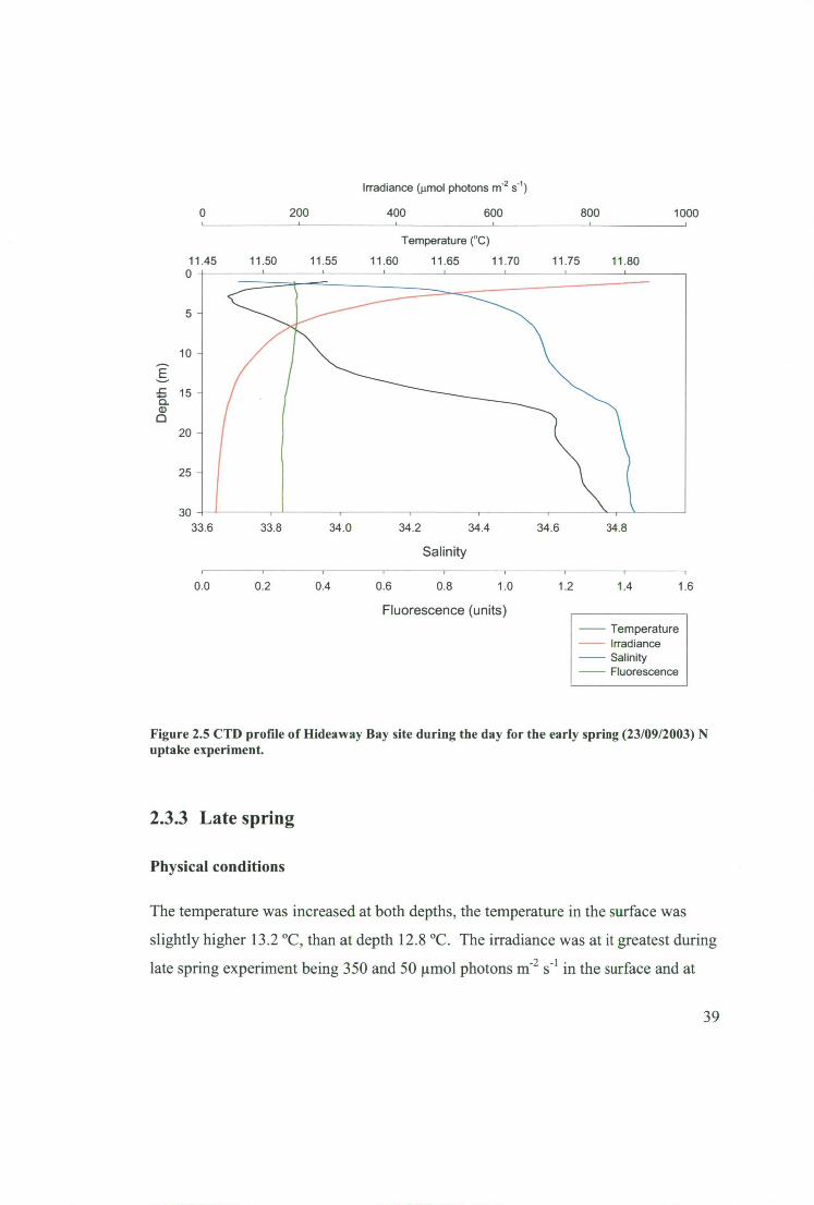
10 -

20 -

25 -

30

Irradiance (gmol photons m-2 s-1 )

0 200 400 600 800 1000

Temperature (°C)

11.50 11.55 11.60 11.65 11.70

11.75 11.80

33.6

33.8

34.0

34.2 34.4

34.6

34.8

Salinity

11.45 0

0.0 0.2 0.4 0.6 0.8 1.0

Fluorescence (units) — Temperature

--- Irradiance Salinity Fluorescence

1.2

1.4

1.6

Figure 2.5 CTD profile of Hideaway Bay site during the day for the early spring (23/09/2003) N uptake experiment.

2.3.3 Late spring

Physical conditions

The temperature was increased at both depths, the temperature in the surface was

slightly higher 13.2 °C, than at depth 12.8 °C. The irradiance was at it greatest during

late spring experiment being 350 and 50 gmol photons I/1-2 s -1 in the surface and at

39

depth respectively. The salinity was lower ( 34.4 and 34.6) than in the previous early

spring field trip at surface (5m) and depth (20m) respectively.

Chemical conditions

The concentration of NO3- in late spring decreased in the surface and at depth to 0.2

and 1 I.LM respectively from the NO3 - concentrations — 4 jim in early spring. The

NH 4+ concentration increased from its lowest concentrations in early spring to 0.5 and

0.7 jiM for the surface and at depth respectively. The urea concentration showed a

slight decrease from early spring to late spring, from 0.5 to 0.38 j.tM in the surface.

However at depth urea concentration remained the same as in early spring —0.44.

Silicate was at its lowest concentration in the surface and at depth, 2.5 and 2 11M

respectively. PO43- also reached its lowest concentration during late spring in the

surface and at depth, 0.2 and 0.3 gM respectively.

Biological conditions

Chla increases in the surface and at depth to 0.9 and 1.5 jig F l respectively during late

spring. Fluorescence was at its lowest near the surface (0.4 units) and then reached its

maximum (0.8 units) at — 7 m. The chi a then decreases again with depth to 0.6 jig 1 -1

at 25m. The phytoplankton community shifted to a cryptophyte (40-60% of total

chlorophyll a) domination. Diatoms and prasinophytes were the next most dominant

components of the community. There were also a small portion of dinoflagellates in

all samples and some cyanobacteria present in the surface samples from Hideaway

Bay. There was one sample that had a clearly different composition from all the

others. This sample was dominated instead by diatoms and had a large % of

dinoflagellates. There were no clear trends between sites, time of day or depth. The

cryptophytes were comprised of small round flagellates (863 cell F 1 ). The diatoms

were dominated by a high numbers of Guinardia flaccida (41223 cell and

Rhizosolenia fragillissima (4607 cell 1 -1 ). The majority of the dinoflagellates were

40

12.0

Temperature (°C)

12.5 13.0 13.5

33.8 34.0 33.6 34.2

34.4

34.6

Salinity

1.2 1.4 1.6 0.0 0.2 0.4 0.6 0.8 1.0

200 400 600 800 1000 1200

5-

10 -

E

20 -

25 -

30

14.5 14.0

Ceratium spp.( 1024 cell 0, Dinophysis spp.(228 cell 14 ) and G. catenatum (33 cell

r').

Irradiance (p.mol photons m-2 s-1 )

Fluorescence (units) — Temperature — Irradiance — Salinity — Fluorescence

Figure 2.6 CTD profile of Hideaway Bay site during the day for the late spring (18/11/2003) N uptake experiment.

2.3.4 Late summer

Physical conditions

Temperatures were at their highest in late summer, 15.5 °C for both surface (5m) and

at depth (20m). However the irradiance had decreased since the field trip in early

spring and was now at 130 umol photons m -2 s-1 in the surface (5m) and at —20 umol

41

photons rn -2 s -1 at depth (20). In the surface (5m) the salinity was 34.4 the same as

late spring. However at depth (20 m) the salinity was 34.8 slightly greater than in late

spring.

Chemical conditions

NO 3 - was still at low concentrations in both the surface and at depth during late

summer, 0.3 and 0.4 [iM, respectively. Both NH' and urea showed increases from

late spring to late summer. NH 4+ concentrations increased to 0.6 1.1.N4 in the surface

and to 1.1 iiM in at depth (20 m). Urea showed an increase to 0.6 iiM in both the

surface and at depth from concentrations below 0.4 iiM in late spring. Silicate

increased from its lowest concentrations that occurred during late spring to 4 tiM and

3.7 AM in the surface and at depth, respectively. PO4 3- showed a similar trend

increasing from the lowest concentrations that occurred in late spring to —0.3 1AM in

both the surface and at depth.

Biological conditions

Chia concentration reached their maximum 1.2 ug r' in the surface (5 m) during late

summer. However at depth (20 m) the chla concentration decreased to 0.3 ug 1 -1 close

to the lowest chla concentrations recorded at depth during late autumn and early

spring. Fluorescence showed that the max concentrations, >1.2 units occurred

between 3 and 10 m depth and decreased to between 0.1 and 0.3 units. Composition

of samples was not clearly dominated by any one taxonomic group. A mixture of

diatoms, cryptophytes, prasinophytes and dinoflagellates were present. These

samples had the most variable composition and there were no clear trends associated

with time of day, location or depth. There were also small proportions of haptophyte

N and S and cyanobacteria groups in some of these samples. The most numerous

diatoms were S. costatum (938150 cell 0, N. closterium (49499 cell 14 ), Chaetoceross spp. (29695 cell r'). The dinoflagellates were represented by G.

42

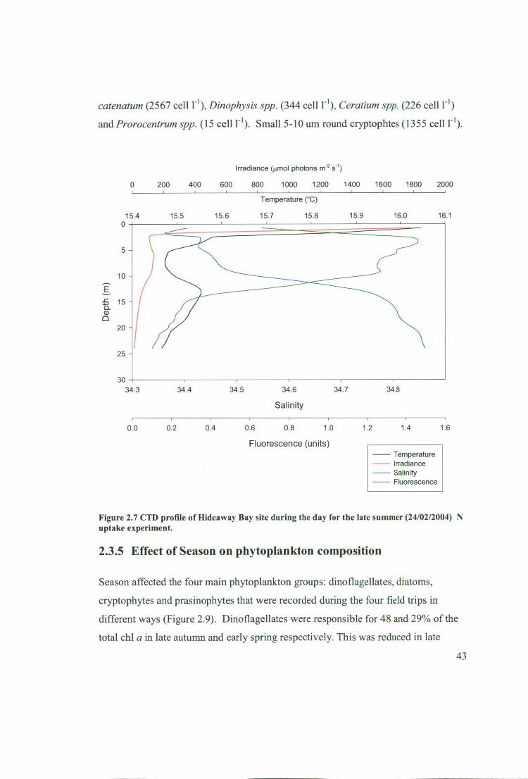
16.1 15.8 15.5 15.6 15.7 15.4 15.9 16.0

catenatum (2567 cell 1- '), Dinophysis spp. (344 cell 1 -1 ), Ceratium spp. (226 cell 1 -1 )

and Prorocentrum spp. (15 cell l'). Small 5-10 urn round cryptophtes (1355 cell 1 -1 ).

Irradiance (Amol photons rn -2 s-1 )

0 200 400 600 800 1000 1200 1400 1600 1800 2000

Temperature (°C)

34.3

Salinity

0.0 0.2 0.4 0.6 0.8 1.0

1.2

1.4

1.6

Fluorescence (units)

— Temperature — Irradiance

— Salinity — Fluorescence

Figure 2.7 CTD profile of Hideaway Bay site during the day for the late summer (24/02/2004) N uptake experiment.

2.3.5 Effect of Season on phytoplankton composition

Season affected the four main phytoplankton groups: dinoflagellates, diatoms,

cryptophytes and prasinophytes that were recorded during the four field trips in

different ways (Figure 2.9). Dinoflagellates were responsible for 48 and 29% of the

total chl a in late autumn and early spring respectively. This was reduced in late

43

spring and late summer where only 7 and 14% respectively, of the total chi a

belonged to the dinoflagellates. The cryptophytes showed the opposite pattern where

9 and 10% of total chla was attributed to them in late autumn and early spring

respectively. Whilst in late spring and late summer the cryptophytes accounted for a

much larger amount of the chla, being 40 and 29% respectively. The high proportion

of `cryptophytes' during late spring and late summer probably represents Dinophysis

species. During early spring and late summer the diatoms contributed the most to

total chl a, 47 and 38% respectively. During late autumn and late spring the diatoms

contributed less to the total chla, 18 and 31% respectively. The prasinophytes were

greatest during late autumn and late spring, 23 and 21% respectively. In early spring

the prasinopytes were at their lowest, 9% of the total chl a. During late summer the

prasinophytes accounted for 15% of the total chl a.

44

1.2

1.0 - b) 23-24/09/2003

0.8 -

0.6 -

0.4 -

0.2 -

0.0

C) 18-19/11/2003

jlji l O

1.2

1.0 -

0.8 -

0.6 -

0.4 -

0.2 -

0.0

rela

tive

amou

nt o

f Chl

a re

lativ

e a

mou

nt o

f Chi

a re

lativ

e a

mou

nt o

f Ch

ia r

ela

tive

amou

nt o

f C

hia

1.2

1.0 -

0.8 -

0.6 -

0.4 -

0.2 -

0.0

1.2

1.0 -

0.8 -

0.6 -

0.4 -

0.2 -

0.0

a) 28-29/05/2003

d) 24-25/02/2004

Iii i ii (‘ oao osi 5

\ de, b(c‘ 0 (30

. re* -4§\\I N\V‘6 ■61"'c' 0\ G\(e ‘ G\

site, time and depth Prasinophytes Dinoflagellates Cryptophytes Haptophytes N Haptophytes S Chlorophytes Cyanobacteria Diatoms

Figure 2.8 Phytoplankton composition derived from pigments from HPLC analysis of samples and subsequent analysis using Chemtax V1.1. Hideaway Bay and Garden Island in the Huon estuary during late autumn (28-29/05/2003), early spring (23-24/09/2003), late spring (18- 19/11/2003) and late summer (24-25102/2004are presented.

45

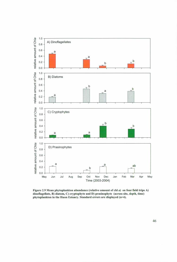
a

0.0

1.0

Jul Aug Sep Oct

Nov Dec

1.0

0.8 - A) Dinoflagellates • B) Diatoms

a

0.6 -

0.4 -

0.2 -

0.0

1.0

0.8

0.6

0.4

0.2

•

0.8 - C) Cryptophytes

Jan Feb Mar Apr May

0.6 -

0.4 -

0.2 -

0.0

1.0

0.8 -

0.6 -

0.4 -

0.2 -

0.0 May Jun

D) Prasinophytes

a

NIP

a b

a .11

Time (2003-2004)

Figure 2.9 Mean phytoplankton abundance (relative amount of chl a) on four field trips A) dinoflagellate, B) diatom, C) cryptophyte and D) prasinophyte (across site, depth, time) phytoplankton in the Huon Estuary. Standard errors are displayed (n=4).

rela

tive

amou

nt o

f Chi

a re

lativ

e am

ount

of C

hia

rela

tive

amou

nt o

f Chi

a re

lativ

e am

ount

of C

hla

46

Table 2.2 Phytoplankton composition by cell count of field trips undertaken in the Huon Estuary. Cell counts for the first trip 28-29/05/2003 were not available.

TAXON Huon 23/09/2003 (cells 1 .1 )

Huon 18/11/2003

(cells 1 -1 )

Huon 24/02/2004 (cells 0)

Amphora 54 Cerataulina pelagica 682 519 Coscinodiscus sp 21 319 871 Lauderia annulata 86 82 Melosira 352 Nitzschia closterium 793 2385 49499 Nitzschia sp 91 Pleurosigma 18 171 Pseudonitzschia pseudodelicatissima 1248 2136 19234 Guinardia striata = Rhizosolenia stolterfothii 569 56 Skeletonema costatum 521 1602 938150 Eucampia 360 Grammatophora 311 Paralia 280 Guinardia delicatula = Rhizosolenia delicatula 227 936 Corethron criophilum 77 Chaetoceros spp > 10um 401 1988 6630 Chaetoceros spp < 10um 1681 29695 Leptocylindrus danicus 91 341 104 Guinardia flaccida 9 41223 61 Dactyliosolen fragillissimus = Rhizosolenia fragillissima 4607 1608 Rhizosolenia fallax 58 557 787 Gymnodinioid dinoflagellate 15um 273 Prorocentrum 15 Ceratium spp 27 1024 226 Dissodinium (Pyrocystis) lunula 13 Dinophysis spp 36 228 344 Gymnodinium catenatum 132 33 2657 Mesodinium rubrum 1450 flagellates 5-10 urn round 863 1355

2.3.6 Comparison of Nitrate, Ammonium and Urea uptake: all

Huon Estuary data.

In terms of understanding the nutrient dynamics of the Huon Estuary the comparison

of nitrate, ammonium and urea uptake is the most basic, and potentially the most

useful, for comparison with other studies. Paired t tests showed there was no

47

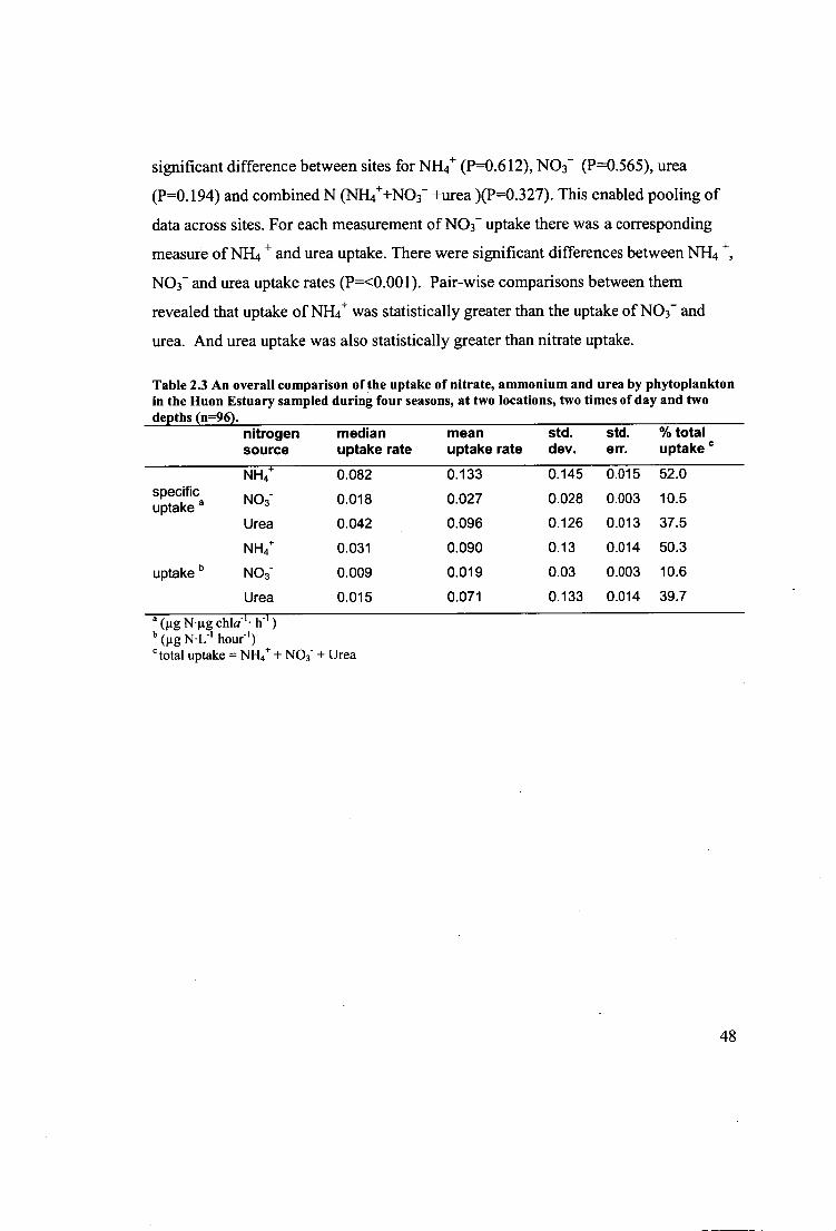
significant difference between sites for NH4+ (P=0.612), NO3- (P=0.565), urea

(P=0.194) and combined N (NH4++NO 3- +urea )(P=0.327). This enabled pooling of

data across sites. For each measurement of NO 3- uptake there was a corresponding

measure of NH4 + and urea uptake. There were significant differences between NH 4 +,

NO3- and urea uptake rates (P=<0.001). Pair-wise comparisons between them

revealed that uptake of NH4 + was statistically greater than the uptake of NO 3- and

urea. And urea uptake was also statistically greater than nitrate uptake.

Table 2.3 An overall comparison of the uptake of nitrate, ammonium and urea by phytoplankton in the Huon Estuary sampled during four seasons, at two locations, two times of day and two depths (n=96).

nitrogen source

median uptake rate

mean uptake rate

std. dev.

std. err.

% total uptake

specific uptake a

uptake b

NH 4+

NO3-

Urea NH4+ NO3- Urea

0.082

0.018

0.042

0.031

0.009

0.015

0.133

0.027

0.096

0.090

0.019

0.071

0.145

0.028

0.126

0.13

0.03

0.133

0.015

0.003

0.013

0.014

0.003

0.014

52.0

10.5

37.5

50.3

10.6

39.7

(pg N-gg chla-l • ) b (ug N.L-I hour') c total uptake = + NO3 - + Urea

48

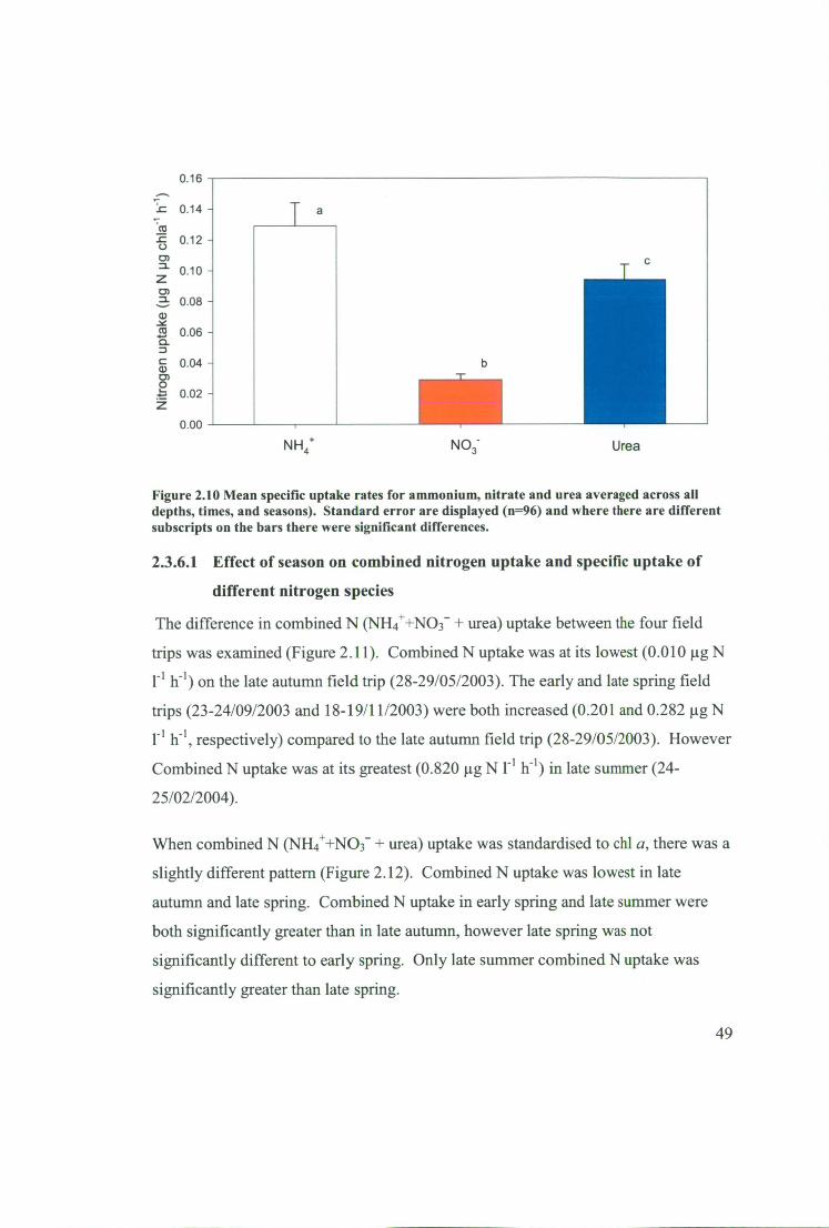
Nitr

ogen

upt

ake

(pg

N p

g ch

le h-

1)

0.16

0.14 -

0.12 -

0.10 -

0.08 -

0.06 -

0.04 -

0.02 -

0.00

a

b

T C

-r

NH4 +

NO3- Urea

Figure 2.10 Mean specific uptake rates for ammonium, nitrate and urea averaged across all depths, times, and seasons). Standard error are displayed (n=96) and where there are different subscripts on the bars there were significant differences.

2.3.6.1 Effect of season on combined nitrogen uptake and specific uptake of

different nitrogen species

The difference in combined N (NH4++NO3- + urea) uptake between the four field

trips was examined (Figure 2.11). Combined N uptake was at its lowest (0.010 lig N

r' if') on the late autumn field trip (28-29/05/2003). The early and late spring field

trips (23-24/09/2003 and 18-19/11/2003) were both increased (0.201 and 0.282 lig N

F' h- ', respectively) compared to the late autumn field trip (28-29/05/2003). However

Combined N uptake was at its greatest (0.820 jig N r' if') in late summer (24-

25/02/2004).

When combined N (NH4++NO3- + urea) uptake was standardised to chi a, there was a

slightly different pattern (Figure 2.12). Combined N uptake was lowest in late

autumn and late spring. Combined N uptake in early spring and late summer were

both significantly greater than in late autumn, however late spring was not

significantly different to early spring. Only late summer combined N uptake was

significantly greater than late spring.

49

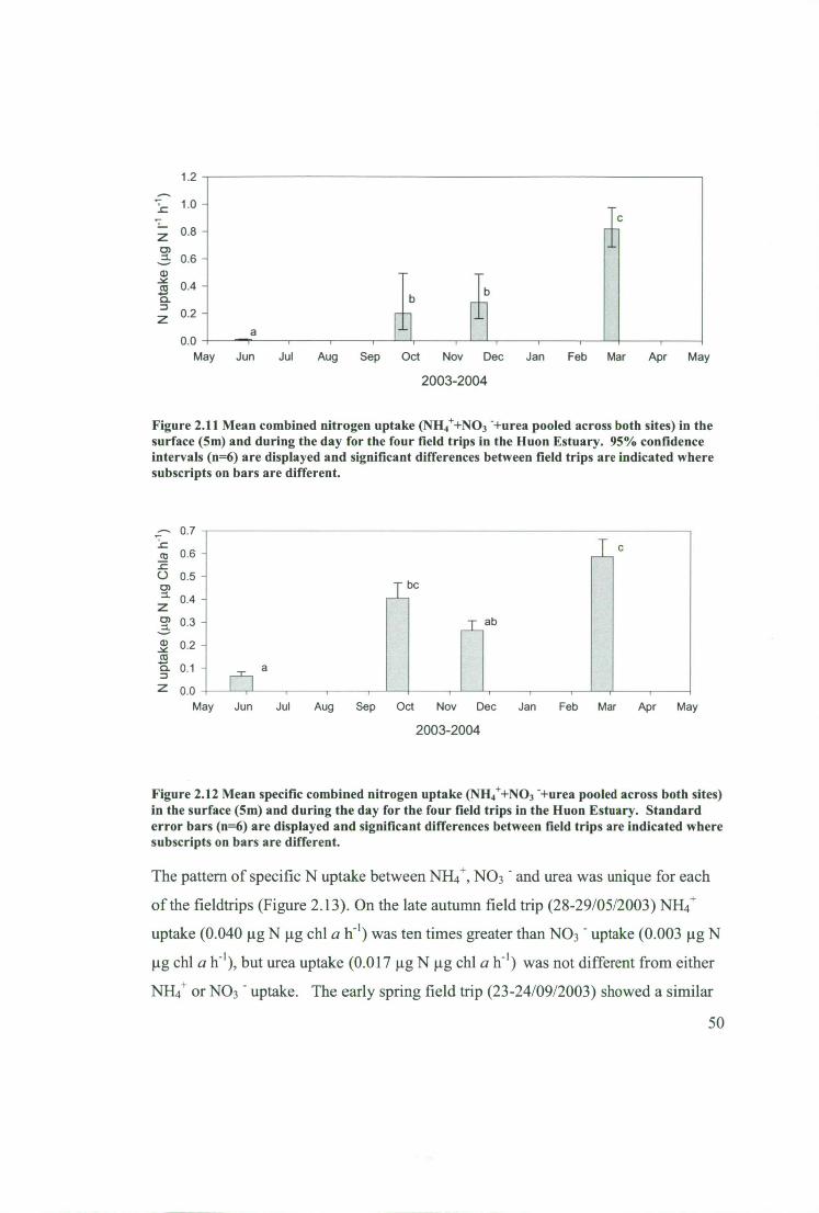
1.2

1 .0

2 0.8 - co =- 0.6 —

a) co 0.4 — ca.

a

0.0 -""7

May Jun Jul Aug Sep Oct Nov Dec Jan Feb Mar Apr May

2003-2004

Figure 2.11 Mean combined nitrogen uptake (NH 4++NO3 --I-urea pooled across both sites) in the surface (5m) and during the day for the four field trips in the Huon Estuary. 95% confidence intervals (n=6) are displayed and significant differences between field trips are indicated where subscripts on bars are different.

0.7 :c co 0.6 -

o .c 0.5 -

C) • 0.4 - Z co 0.3 -

•

=

• 0.2

S. 0.1 - a Z 0.0

May

T bc

T ab

a

Jun Jul Aug Sep Oct Nov Dec Jan Feb Mar Apr May

2003-2004

ri

Figure 2.12 Mean specific combined nitrogen uptake (NH 4++NO3 -+urea pooled across both sites) in the surface (5m) and during the day for the four field trips in the Huon Estuary. Standard error bars (n=6) are displayed and significant differences between field trips are indicated where subscripts on bars are different.

The pattern of specific N uptake between NH4 +, NO3 and urea was unique for each

of the fieldtrips (Figure 2.13). On the late autumn field trip (28-29/05/2003) NH4+

uptake (0.040 jig N jig chl a If') was ten times greater than NO 3 - uptake (0.003 jig N

jig chl a W I ), but urea uptake (0.017 jig N jig chl a If') was not different from either

NH4+ or NO3 - uptake. The early spring field trip (23-24/09/2003) showed a similar

50

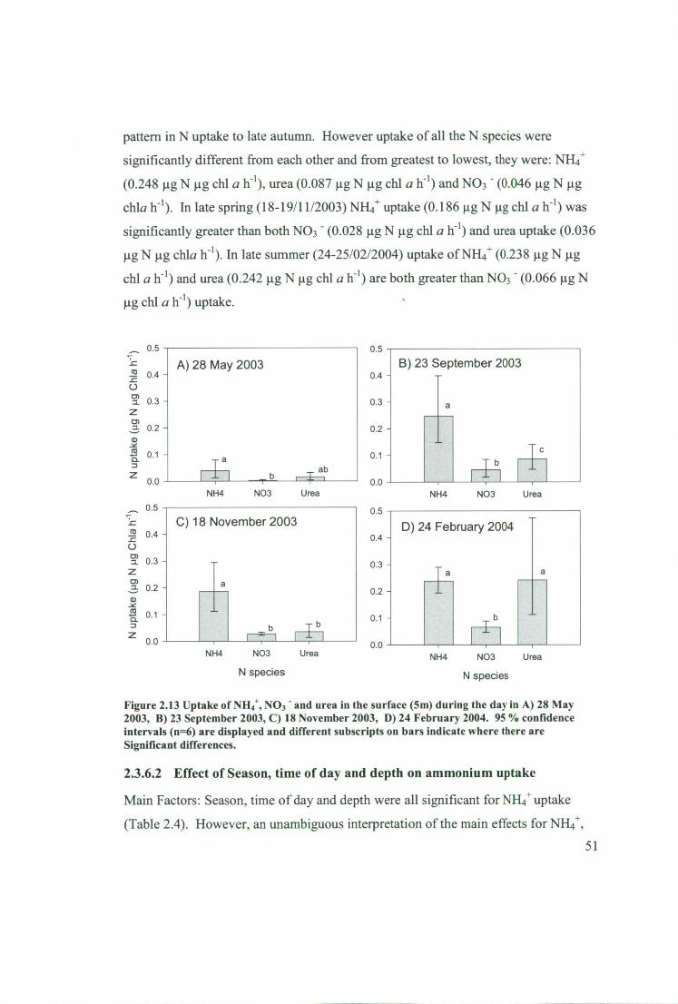
0.4 -

0.3 - fa 0.2 -

0.1 -

0.5

B) 23 September 2003

0.0 NH4 NO3 Urea

0.5

D) 24 February 2004 0.4 -

0.3 - a

0.2 -

0.1 -

0.0

ta

0.4 -

0.3 -

0.2 -

0.1 -

0.5

C) 18 November 2003

0.0

pattern in N uptake to late autumn. However uptake of all the N species were

significantly different from each other and from greatest to lowest, they were: NH 4+ (0.248 gg N lig chi a hi ), urea (0.087 lig N tg chi a 11-1 ) and NO3 - (0.046 lig N lig

chla hi ). In late spring (18-19/11/2003) NH 4+ uptake (0.186 lig N ig chl a h-I ) was

significantly greater than both NO3 - (0.028 lig N gg chi a II I ) and urea uptake (0.036

lig N gg chlah -I ). In late summer (24-25/02/2004) uptake of NI-I4+ (0.238 lig N gg

chl a h-I ) and urea (0.242 gig N Kg chi al-1 1 ) are both greater than NO 3 - (0.066 gg N

chl all') uptake.

N u

ptak

e (pig

N li

g C

hia

h-1)

N u

ptak

e (u

g N

pg

Chi

a h-

1)

0.5

A) 28 May 2003

T a

I I

NH4 NO3

Urea

0.4 -

0.3 -

0.2 -

0.1 -

0.0 ab

NH4 NO3 Urea NH4

NO3

Urea

N species N species

Figure 2.13 Uptake of NH 4+ , NO3 - and urea in the surface (5m) during the day in A) 28 May 2003, B) 23 September 2003, C) 18 November 2003, D) 24 February 2004. 95 % confidence intervals (n=6) are displayed and different subscripts on bars indicate where there are Significant differences.

2.3.6.2 Effect of Season, time of day and depth on ammonium uptake

Main Factors: Season, time of day and depth were all significant for NH4+ uptake

(Table 2.4). However, an unambiguous interpretation of the main effects for NH 4+ , 51

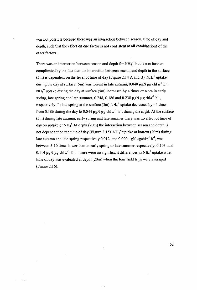
was not possible because there was an interaction between season, time of day and

depth, such that the effect on one factor is not consistent at all combinations of the

other factors.

There was an interaction between season and depth for NH4 +, but it was further

complicated by the fact that the interaction between season and depth in the surface

(5m) is dependent on the level of time of day (Figure 2.14 A and B). NH 4+ uptake

during the day at surface (5m) was lowest in late autumn, 0.040 ggN jig chl a 1 h'.

NH4+ uptake during the day at surface (5m) increased by 4 times or more in early

spring, late spring and late summer, 0.248, 0.186 and 0.238 pigN jig chid'

respectively. In late spring at the surface (5m) NI-1 4+ uptake decreased by —4 times

from 0.186 during the day to 0.044 j.igN jig chi d i h', during the night. At the surface

(5m) during late autumn, early spring and late summer there was no effect of time of

day on uptake of NH4+ .At depth (20m) the interaction between season and depth is

not dependant on the time of day (Figure 2.15). NH 4+ uptake at bottom (20m) during

late autumn and late spring respectively 0.012 and 0.020 ligN ligchlci l W I , was

between 5-10 times lower than in early spring or late summer respectively, 0.103 and

0.114 j.igN pig chl d i W I . There were no significant differences in NH 4+ uptake when

time of day was evaluated at depth (20m) when the four field trips were averaged

(Figure 2.16).

52

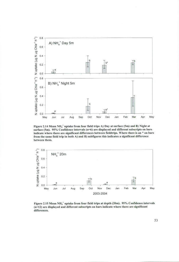
B) NH4+ Night 5m

A) NH4+ Day 5m

- -

b lb -

NH4+ 20m

-

a Ib

N u

pta

ke (g

ig N

1.1

g C

h1a-

1 h-

1)

N u

pta

ke G

ig N

lAg

Ch1a

-1 h-

1)

_

0.2 -

0.0 May Jun Jul Aug Sep Oct Nov Dec Jan Feb Mar Apr May

Figure 2.14 Mean NH 4+ uptake from four field trips A) Day at surface (5m) and B) Night at surface (5m). 95% Confidence intervals (n=6) are displayed and different subscripts on bars indicate where there are significant differences between fieldtrips. Where there is an * on bars from the same field trip in both A) and B) subfigures this indicates a significant difference between them.

0.8

0.6

0.4

0.2

0.0

0.8

0.6

0.4

0.8

0.6

0.4

0.2

0.0 May Jun Jul Aug Sep Oct Nov Dec Jan

2003-2004

Feb Mar Apr May

Figure 2.15 Mean NH 4+ uptake from four field trips at depth (20m). 95% Confidence intervals (n=12) are displayed and different subscripts on bars indicate where there are significant differences.

N u

ptake

(p

g N

lig C

h1a-

1 ti-

1)

53

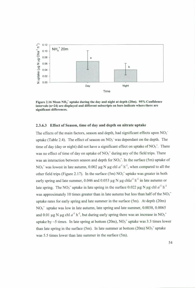
N up

take

Gig

N pg

Ch1

a-1 h

-1)

0.12

0.10 -

0.08 -

0.06 -

0.04 -

0.02 -

0.00

H: 20m

T a

I

T b

I

Day Night

Time

Figure 2.16 Mean NH 4+ uptake during the day and night at depth (20m). 95% Confidence intervals (n=24) are displayed and different subscripts on bars indicate where there are significant differences.

2.3.6.3 Effect of Season, time of day and depth on nitrate uptake

The effects of the main factors, season and depth, had significant effects upon NO3 - uptake (Table 2.4). The effect of season on NO 3 - was dependant on the depth. The

time of day (day or night) did not have a significant effect on uptake of NO 3-. There

was no effect of time of day on uptake of NO3- during any of the field trips. There

was an interaction between season and depth for NO3 -. In the surface (5m) uptake of

NO3- was lowest in late autumn, 0.002 lig N i.tg chl d 1 11-1 , when compared to all the

other field trips (Figure 2.17). In the surface (5m) NO3 - uptake was greater in both

early spring and late summer, 0.046 and 0.053 ii.g N i.ig chla 1 114 in late autumn or

late spring. The NO3 - uptake in late spring in the surface 0.022 pig N gg chl a -1 11 1 was approximately 10 times greater than in late autumn but less than half of the NO3 -

uptake rates for early spring and late summer in the surface (5m). At depth (20m)

NO3- uptake was low in late autumn, late spring and late summer, 0.0038, 0.0065

and 0.01 jig N jig chi d 1 II I , but during early spring there was an increase in NO3 -

uptake by —5 times. In late spring at bottom (20m), NO3 - uptake was 3.3 times lower

than late spring in the surface (5m). In late summer at bottom (20m) NO 3- uptake

was 5.5 times lower than late summer in the surface (5m).

54

A) NO3- 5m

B) NO3" 20m

I I

Jun

7

•

0.08 _c

7ca

Z 0.06 - C.) CD = Z 0.04 - a) a. a) _c 0.02 - as a_ z Z 0.00 -- .. --. • 0.08 .0 7

CO -Z 0.06 - C.) a) = Z 0.04 - a) a. a) 0.02 - ca -a z Z 0.00

May Jul Aug Sep Oct Nov Dec Jan Feb Mar Apr May

2003-2004

I .

Figure 2.17 Mean NO 3 - uptake from four field trips A) surface (5m) and B) depth (20m). 95% Confidence intervals (n=12) are displayed and different subscripts on bars indicate where there are significant differences between fieldtrips. Where there is an * on bars from the same field trip in both A) and B) subfigures this indicates a significant difference between them.

2.3.6.4 Effect of Season, time of day and depth on urea uptake

The main factors of season, time of day and depth all had significant effect on urea

uptake (Table 2.4). The effect of season on urea uptake was dependant on the depth

(Figure 2.18) and time of day (Figure 2.19). There was also an interaction between

time of day and depth for urea uptake (Figure 2.20).

Uptake of urea during the day was at its lowest in late autumn (0.011 ilg N jig chl a-1

h-1 ) and late spring (0.019 jig N jig chl a t 11 1 ). Early spring (0.075 ps N jig chl a -1 h-

i) and late summer (0.111 jig N pig chl d i II I ) urea uptake during the day was at least

3 times greater than late autumn and late spring uptake. Urea uptake at night in early

55

spring (0.116 jig N jig chl a -1 h-1 ) and late spring (0.061 jig N jig chi a 1 h1 ) was 1.5-

3 times greater than uptake during the day in early spring and late spring.

Uptake of urea in the surface (5m) was least during late autumn, 0.014 jig N jig chl d

I h-1 (Figure 2.19). Compared to late autumn urea uptake in the surface (5m) during

early spring and late spring increased by almost 10 times to 0.123 and 0.087 jig N jig

chl a-1 h-1 respectively. The greatest urea uptake in the surface (5m) was during late

summer, 0.286 pig N jig chl a1 h-1 . At depth (20m) Urea uptake was 10-20 times

greater in early spring (0.07 jig N jig chl a -1 h-1 ) and late summer (0.046 ggN jig N

jig chl a1 h1 ) than in late autumn (0.004 jig N jig chi a -1 h-1 ) and late spring (0.006

ggN jig N jig chl a -1 h-1 ).

Uptake of urea was — 2 times greater at night in the surface (5 m) (0.134 jig N jig chl

a-1 h-1 ) compared to the day in the surface (5m) (0.073 jig N jig chl d 1 h-1 ) (Figure

2.20). During the day, urea uptake in the surface (5m) (0.073 jig N jig chl a -1 h-1 ) was

—3 times greater than urea uptake in the bottom (20m) (0.025 jig N jig chi a1 h-1 ).

During the night urea uptake in the surface (5m) (0.134 jig N jig chl a -1 h-1 ) was 4.8

times greater than urea uptake in the bottom (20m) (0.028 jig N jig chl a -1 h-1 ).

56

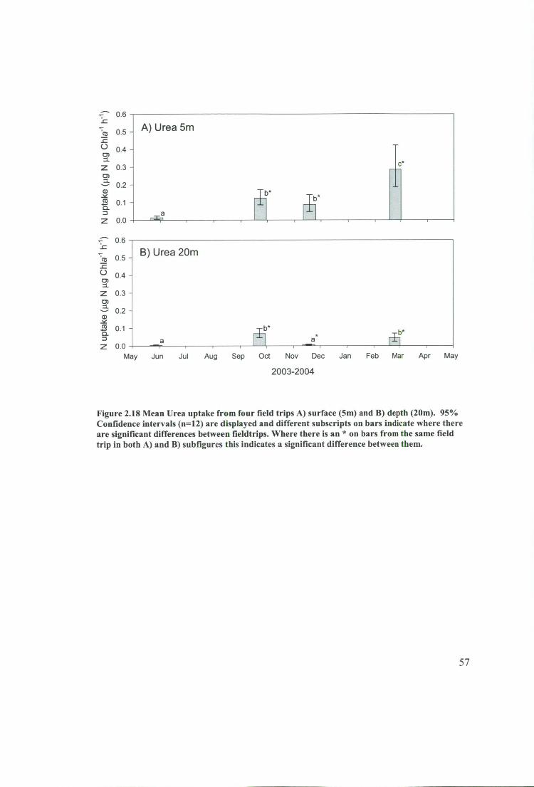
A) Urea 5m

N u

ptak

e Gi

g N

pg C

h1a-

1 11

1) N

up

take

Gig

N 1

.1g C

h1a-

1 111

) 0.6

0.5 -

0.4 -

0.3 -

0.2 -

0.1 -

0.0

0.6

0.5 - B) Urea 20m

0.4 -

0.3 -

0.2 -

0.1 -

a 0.0

May Jun Jul Aug Sep Oct

a.

Nov Dec Jan Feb Mar Apr May

2003-2004

Figure 2.18 Mean Urea uptake from four field trips A) surface (5m) and B) depth (20m). 95% Confidence intervals (n=12) are displayed and different subscripts on bars indicate where there are significant differences between fieldtrips. Where there is an * on bars from the same field trip in both A) and B) subfigures this indicates a significant difference between them.

57

0.4

0.3

0.2

0. 1

0.0 N u

ptak

e G

ig N

14 C

h1a-

1 h-1)

N

upt

ake

Gig

N li

g Ch

1a-1

h-1)

0.4

0.3 -

0.2 -

0. 1 -

0.0 May

B) Urea Night

a .----,- Jun Jul Aug Sep Oct Nov Dec Jan Feb Mar Apr May

2003-2004

IC*

O Surface 5m I I Bottom 20m

-

C

a _

-

-

- I -

l b l b

N u

ptak

e G

ig N

pg

Ch1

a-1 h

-1)

0.25

0.20

0.15

0.10

0.05

0.00

A) Urea Day

-

-

b

-

Figure 2.19 Mean Urea uptake from four field trips A) Day and B) Night. 95% Confidence intervals (n=12) are displayed and different subscripts on bars indicate where there are significant differences between fieldtrips. Where there is an * on bars from the same field trip in both A) and B) subfigures this indicates a significant difference between them.

Day

Night

Time

Figure 2.20 Mean Urea uptake during the day and night and at surface (5m) and depth (20m). 95% Confidence intervals (n=24) are displayed and different subscripts on bars indicate where there are significant differences.

58

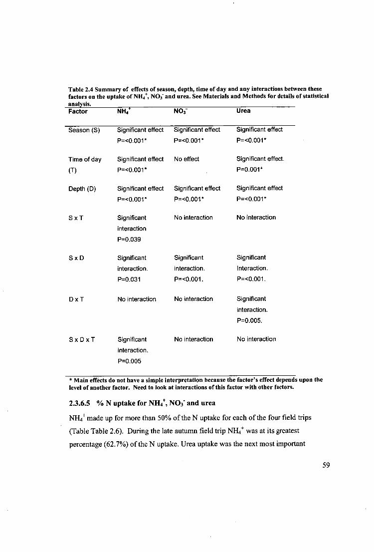
Table 2.4 Summary of effects of season, depth, time of day and any interactions between these factors on the uptake of NH4+, NO3- and urea. See Materials and Methods for details of statistical analysis. Factor NH4+ NO3- Urea

Season (S) Significant effect Significant effect Significant effect

P=<0.001* P=<0.001* P=<0.001*

Time of day Significant effect No effect Significant effect.

(T) P=<0.001* P=0.001*

Depth (D) Significant effect Significant effect Significant effect

P=<0.001* P=<0.001* P=<0.001*

S x T Significant

interaction

No interaction No interaction

P=0.039

S x D Significant Significant Significant

interaction. interaction. Interaction.

P=0.031 P=<0.001. P=<0.001.

D x T No interaction No interaction Significant

interaction.

P=0.005.

SxDxT Significant

interaction.

No interaction No interaction

P=0.005

* Main effects do not have a simple interpretation because the factor's effect depends upon the level of another factor. Need to look at interactions of this factor with other factors.

2.3.6.5 % N uptake for NH4÷, NO3" and urea

NH4+ made up for more than 50% of the N uptake for each of the four field trips

(Table Table 2.6). During the late autumn field trip NH4 + was at its greatest

percentage (62.7%) of the N uptake. Urea uptake was the next most important

59

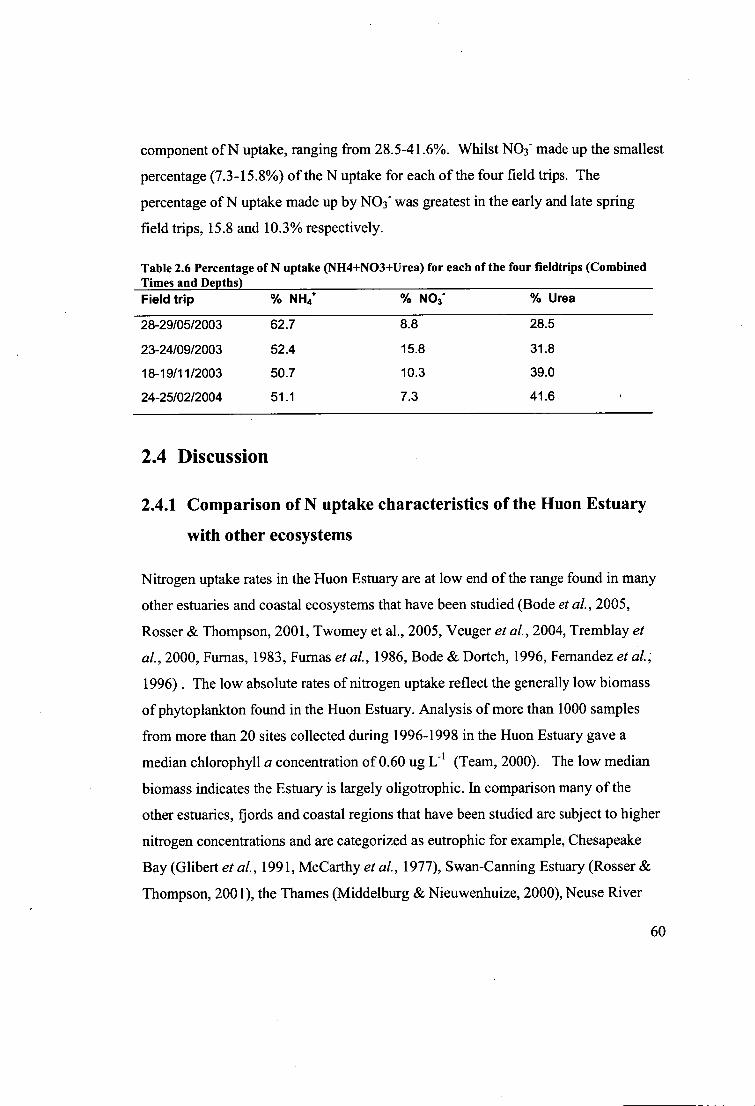
component of N uptake, ranging from 28.5-41.6%. Whilst NO 3 - made up the smallest

percentage (7.3-15.8%) of the N uptake for each of the four field trips. The

percentage of N uptake made up by NO3 - was greatest in the early and late spring

field trips, 15.8 and 10.3% respectively.

Table 2.6 Percentage of N uptake (NH4+NO3+Urea) for each of the four fieldtrips (Combined Times and Depths) Field trip % N H4+ % NO3" % Urea

28-29/05/2003 62.7 8.8 28.5

23-24/09/2003 52.4 15.8 31.8

18-19/11/2003 50.7 10.3 39.0

24-25/02/2004 51.1 7.3 41.6

2.4 Discussion

2.4.1 Comparison of N uptake characteristics of the Huon Estuary

with other ecosystems

Nitrogen uptake rates in the Huon Estuary are at low end of the range found in many

other estuaries and coastal ecosystems that have been studied (Bode etal., 2005,

Rosser & Thompson, 2001, Twomey et al., 2005, Veuger etal., 2004, Tremblay et

al., 2000, Furnas, 1983, Furnas etal., 1986, Bode & Dortch, 1996, Fernandez et al.,

1996) . The low absolute rates of nitrogen uptake reflect the generally low biomass

of phytoplanlcton found in the Huon Estuary. Analysis of more than 1000 samples

from more than 20 sites collected during 1996-1998 in the Huon Estuary gave a

median chlorophyll a concentration of 0.60 ug L-1 (Team, 2000). The low median

biomass indicates the Estuary is largely oligotrophic. In comparison many of the

other estuaries, fjords and coastal regions that have been studied are subject to higher

nitrogen concentrations and are categorized as eutrophic for example, Chesapeake

Bay (Glibert et al., 1991, McCarthy et al., 1977), Swan-Canning Estuary (Rosser &

Thompson, 2001), the Thames (Middelburg & Nieuwenhuize, 2000), Neuse River

60

Estuary (Boyer etal., 1994, Twomey et al., 2005), and the Pearl river estuary (Yin et

al., 2000).

Mean specific uptake rates for the Huon Estuary were: NH4 + (0.133 jig N.pg

), urea (0.096 jig N-pg chla t II I ) and NO3- (0.027 jig Nlig chief I . li t ). Whilst

these N uptake rates are low in comparison to other ecosystems as discussed above,

the phytoplanlcton of the Huon Estuary show similarities in nitrogenous nutrition to

the N uptake characteristics of phytoplankton from the majority of these other

estuarine, coastal and oceanic ecosystems.

The overall composition of N uptake in the Huon Estuary for NH4+, NO3- and urea

52, 10.5 and 37.5 % respectively. Reduced forms of N (NH4 + and urea) made up

89.5% of the N taken up, a result consistent with overall N uptake in many estuarine,

coastal and some oceanic ecosystems: NH4+ and urea were taken up preferentially in

Chesapeake Bay (McCarthy et al., 1977), In the western English Channel

Regenerated forms of N accounted for up 70% of the overall N uptake (L'Helguen et

al., 1993), in the southern Atlantic near Brazil, NH 4+ and urea accounted for 74%

and 96% of oceanic and coastal N uptake, respectively (Metzler et al., 1997), in the

Swan-Canning Estuary evidence showed that NH 4+ was most important N source

overall (Rosser & Thompson, 2001) and at Station P in the Pacific over a long time

series NH 4+ and urea were responsible for the majority of the primary production

(Harrison, 2002).

The overall N uptake characteristics are useful in understanding an ecosystem and

which types of N are most important for supporting primary productivity on a large

scale. The magnitude and composition (NH4+, NO3- and urea) of N uptake by

phytoplankton is, however, affected by physical conditions like temperature,

irradiance, and substrate concentrations which change on a range of temporal and

spatial scales, So to understand N uptake in the Huon Estuary the effect of depth

(surface 5m or bottom 20m), time of day (day or night) and Seasons: late autumn,

early spring, late spring and late summer on magnitude and the composition (NH4 + ,

61

NO3- and urea) of N uptake were examined. These result provide insight into

phytoplankton strategies and dynamics of Huon Estuary phytoplankton assemblage as

relevant to N uptake. Season and depth were responsible for most of the variation in

NH, NO3- and urea uptake with less effect of time of day. For this reason the

following discussion on uptake of individual N species (NH4 +, NO3- and urea)

focuses on the effect of season and depth. For NI-I4+ and NO3- season was

responsible for the majority of the variation and depth was responsible for less

variation but still important. For urea, however, depth was responsible for the

majority of the uptake variation, followed by season and with time of day responsible

for the least.

2.4.2 Late autumn

During late autumn the chlorophyll a concentrations at 5 and 20m were — 0.2 gg

the lowest observed. There was a slight rise in concentration to — 0.6 gg L-1 closer to

the surface. Based on the presence of peridinin CHEMTAX (Mackey et al., 1996) the

dominant taxa were dinoflagellates with 48% of the total chlorophyll a. The

dominant species were G. catenatum and Ceratium spp. (Thompson et al., 2008).

Late autumn dominance of the phytoplankton community by dino flagellates is a

common situation in temperate estuarine ecosystems (Marshall et al., 2005, Smayda

& Reynolds, 2001, Lopes et al., 2007). In the Huon Estuary this high percentage of

dinoflagellates probably represents a residual summer-autumn community which may

be better adapted to growth at higher temperatures. The near zero growth rate of G.

catenatum at 12°C (see Figure 3.22 Chapter 3) suggests it would be severely

disadvantaged at 13.5°C relative to the growth rates of many other species at this

temperature (Eppley, 1972). For example the diatom Skeletonema costatum, was also

present in the Huon Estuary, and has been reported to grow at a rate of-3 divisions

per day at 10°C (Falkowski, 1977).

During the late autumn field trip combined N uptake was low 0.010 jig N —86

times less than the greatest absolute uptake from the late summer field trip. Nitrogen

62

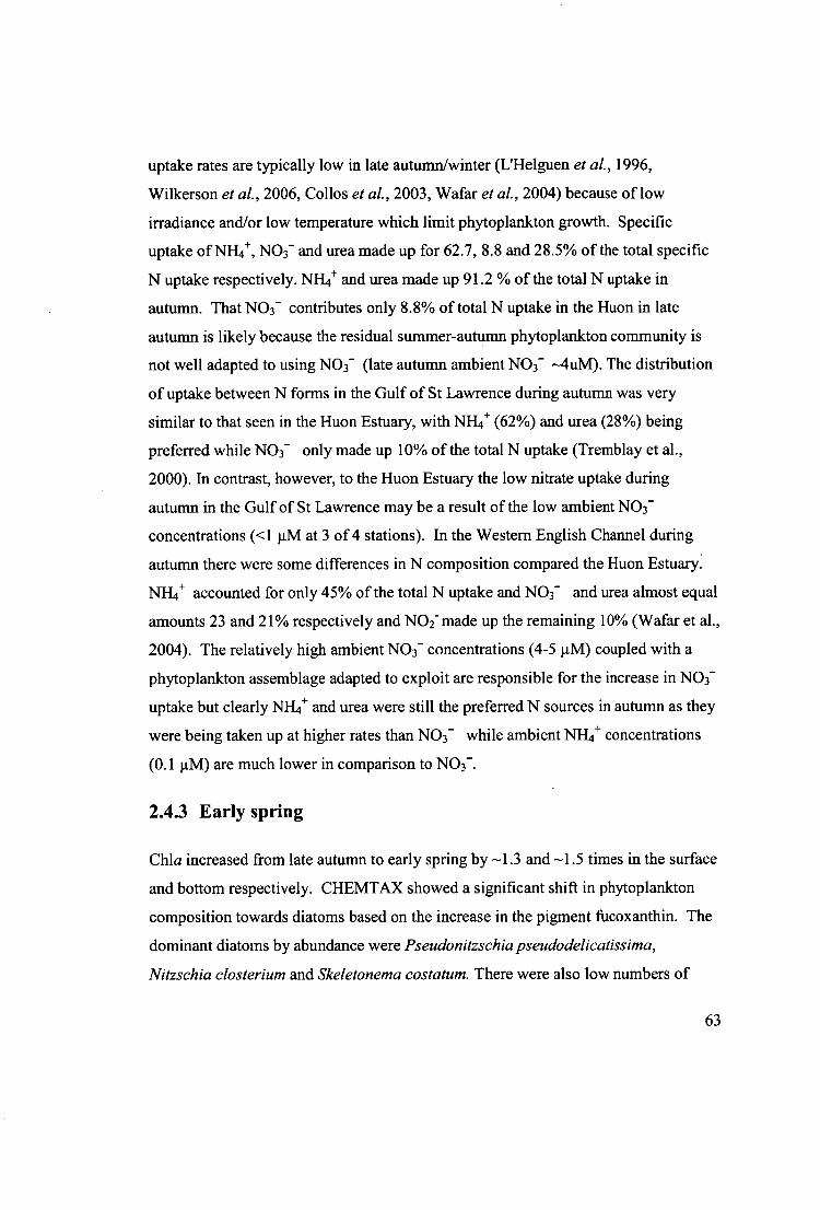
uptake rates are typically low in late autumn/winter (L'Helguen et al., 1996,

Wilkerson etal., 2006, Collos etal., 2003, Wafar etal., 2004) because of low

irradiance and/or low temperature which limit phytoplankton growth. Specific

uptake of NH4+, NO3- and urea made up for 62.7, 8.8 and 28.5% of the total specific

N uptake respectively. NH4 + and urea made up 91.2 % of the total N uptake in

autumn. That NO3 - contributes only 8.8% of total N uptake in the Huon in late

autumn is likely because the residual summer-autumn phytoplankton community is

not well adapted to using NO3- (late autumn ambient NO3- —4uM). The distribution

of uptake between N forms in the Gulf of St Lawrence during autumn was very

similar to that seen in the Huon Estuary, with NH4 + (62%) and urea (28%) being

preferred while NO3 - only made up 10% of the total N uptake (Tremblay et al.,

2000). In contrast, however, to the Huon Estuary the low nitrate uptake during

autumn in the Gulf of St Lawrence may be a result of the low ambient NO3 -

concentrations (<1 11M at 3 of 4 stations). In the Western English Channel during

autumn there were some differences in N composition compared the Huon Estuary.

NH 4+ accounted for only 45% of the total N uptake and NO 3- and urea almost equal

amounts 23 and 21% respectively and NO2 - made up the remaining 10% (Wafar et al.,

2004). The relatively high ambient NO3 - concentrations (4-5 tiM) coupled with a

phytoplankton assemblage adapted to exploit are responsible for the increase in NO3 -

uptake but clearly NH 4+ and urea were still the preferred N sources in autumn as they

were being taken up at higher rates than NO 3- while ambient NH4+ concentrations

(0.1 ttM) are much lower in comparison to NO3 - .

2.4.3 Early spring

Chia increased from late autumn to early spring by —1.3 and —1.5 times in the surface

and bottom respectively. CHEMTAX showed a significant shift in phytoplankton

composition towards diatoms based on the increase in the pigment fucoxanthin. The

dominant diatoms by abundance were Pseudonitzschia pseudodelicatissima,

Nitzschia closterium and Skeletonema costatum. There were also low numbers of

63

Gymnodinium catenatum and a small Gymnodiniod dinoflagellate. A shift to diatom

dominance is typical of spring phytoplanIcton assemblages in temperate locations

(Smayda, 1980)

Uptake of NH4+, NO3- and urea increased by —20 times from late autumn to early

spring. This increase in N uptake coincided with the lowest temperatures of all the

field trips (12°C) and a 4 -5 times increase in irradiance when compared with

irradiance from the late autumn fieldtrip. Both NH 4+ (51.4%) and urea (31.8%) were

still the largest component of the total n uptake, But the greatest NO3 - uptake rates

were measured during this early spring field trip (16.9 %) in comparison to the other

field trips. Peak NO3 - uptake rates are associated with a diatom dominated spring

bloom in other temperature marine ecosystems e.g., the Gulf of St Lawrence

(Tremblay et al., 2000), Menai Straight (Rodrigues & Williams, 2002) and San

Fransisco Bay (Wilkerson et al., 2006). The low temperatures and high irradiance

typical of spring conditions in temperate locations can create a situation where

phytoplankton cells capture more light energy than they are capable of converting to

growth. It has been hypothesized that one component of the diatoms' ability to

exploit these spring conditions could be an ability to take up NO3 - and reduce it using

excess photosynthetic energy, then releasing the more reduced N forms (NO 2-, NH4+

and DON), thus using up potentially harmful excess energy(Lomas & Gilbert, 1999).

2.4.4 Late Spring

Chlorophyll a increased from early spring to late spring, by —3 and —8 times in the

surface and bottom depths respectively. The large increase in chl a at the bottom to a

concentration — 2 times the surface chi a suggests the decline and subsequent sinking

of the spring bloom as observed in other ecosystems with strong diatom communities

(Waite et al., 1992a, Waite et al., 1992b). The absolute and specific N uptake rates

were not significantly different relative to early spring, however, the late spring

absolute uptake rate increased by —1.4 times from the early spring. This increase was

associated with a large increase in phytoplankton biomass. In addition the specific N

64

uptake rate decreased by —1.5 times from the early spring suggesting that the

phytoplanlcton assemblage may be N limited (Smith, 1982, Howarth et al. , 1988).

Simultaneously ambient NO3" concentrations and N:P ratios all indicate the likelihood

of N limitation in late spring (Figure 2.21). The molar N:P during late spring was 2.3,

or about 2 times less than in late autumn and early spring and well below the Redfield

ratio for N:P of 16 (Hecicy & Kilham, 1988). The ambient concentrations of NO 3 -

fell from —4 1.tM in early spring to 0.2111M in late spring at the surface. These

concentrations are well below 1 gM, the half saturation constant for uptake NO 3" by

coastal phytoplankton assemblages (Dortch, 1990, Eppley etal., 1969). It appears

likely that it is N limiting growth and indirectly responsible for the sinking of the

spring bloom as was the case in the sub arctic study (Waite et al., 1992a).

65

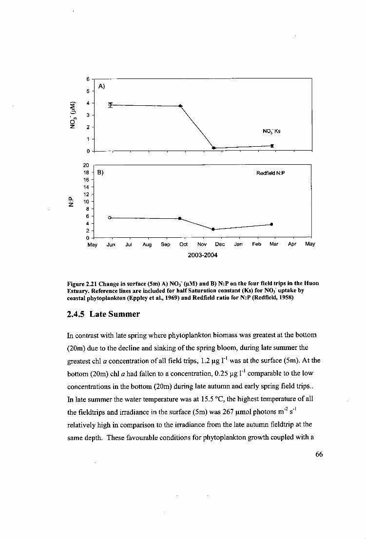
6

5 - A)

4 -

3 -

2 - N NO3" Ks

20 18 - 16 - 14 - 12 -

97 10 - Z 8 - 6 - 4 - 2 - 0 May Jun Jul Aug Sep Oct Nov Dec Jan

B)

0

Redfield N:P

Feb Mar Apr May

2003-2004

Figure 2.21 Change in surface (5m) A) NO 3- (11M) and B) N:P on the four field trips in the Huon Estuary. Reference lines are included for half Saturation constant (Ks) for NO 3- uptake by coastal phytoplankton (Eppley et al., 1969) and Redfield ratio for N:P (Redfield, 1958)

2.4.5 Late Summer

In contrast with late spring where phytoplankton biomass was greatest at the bottom

(20m) due to the decline and sinking of the spring bloom, during late summer the

greatest chi a concentration of all field trips, 1.21.1.g r' was at the surface (5m). At the

bottom (20m) chl a had fallen to a concentration, 0.25 tg r' comparable to the low

concentrations in the bottom (20m) during late autumn and early spring field trips..

In late summer the water temperature was at 15.5 °C, the highest temperature of all

the fieldtrips and irradiance in the surface (5m) was 267iimol photons 1112

relatively high in comparison to the irradiance from the late autumn fieldtrip at the

same depth. These favourable conditions for phytoplankton growth coupled with a

66

stratified water column result in a mixed phytoplankton assemblage. The most

dominant phytoplankton groups represented in this phytoplankton assemblage

according to CHEMTAX analysis of pigments, were in order of dominance: diatoms,

cryptophytes, dinoflagellates. The most abundant diatoms by abundance were

Pseudonitzschia pseudodelicatissima, Nitzschia closterium and Skeletonema

costatum. The dinoflagellates were dominated by Gymnodinium catenatum but

Dinophysis spp and Ceratium spp. were also present in reasonable abundance. The

CHEMTAX identification of cryptophytes during late summer associated with

relatively high concentration of alloxanthin is hypothesized to represent mostly

pigmented Dinophysis species. Their chloroplasts that originate from cryptophytes

via the intermediate host of Myrionecta rubra (=Mesodinium rubrum)(Nagai et al.,

2008, Park etal., 2006). There has not yet been any ecological studies of this

complex multi trophic level interaction since the recent discovery that it was required

for alloxanthin to be present in Dinophysis (Nagai et al., 2008, Park et al., 2006). A

mixed phytoplankton assemblage, including diatoms and dinoflagellates in summer

is characteristic of the Huon Estuary (Team, 2000) and other temperate estuaries and

coastal areas including Chesapeake Bay (Adolf et al., 2006, Marshall et al., 2005)

The specific N uptake in late summer was 9 times greater than during late autumn but

was not significantly different to the specific uptake rates measured in early spring.

Whilst the magnitudes of specific N uptake during late summer and early spring were

not significantly different, there were notable differences in the importance of the

various N substrates. Ammonium uptake was equally important during early spring

and late summer being 52 and 51 % of total N uptake, respectively. The differences

were in NO3" uptake which peaked in early spring at 16% but was only half that in

late summer. During late spring and late summer ambient NO3" concentrations of —

0.2 11M were well below the half saturation constant for coastal phytoplankton limit

the capability of phytoplankton to take up nitrate at the surface. In contrast urea

reached its greatest concentration in late summer and made up the greatest proportion

of N uptake for the late summer fieldtrip at 42%. The importance of urea and other

67

forms of DON in summer has been reported in many systems including: Neuse River

Estuary (Twomey et al., 2005), Chesapeake Bay (Lomas et al., 2002), and the Scheldt

Estuary (Andersson et al., 2006).

2.4.6 Summary

Ammonium uptake was most important throughout the year. Nitrate uptake,

however, played an important role in the early and late spring. The results are

consistent with the hypothesis that NO3 - may be important as a method for diatoms

to get rid of excess energy in the high irradiance conditions that spring produces.

Urea was important as a N source in all seasons but, particularly during late spring

and late summer when NO 3 - was in low supply.

Overall the uptake of N in the Huon Estuary was dominated by NH4 + (52%).

Considering the availability of the various forms of N the ammonium preference

shown by the phytoplankton community was 9 times greater than for nitrate. These

results are consistent with those from other ecosystems. The strong dependence of

phytoplankton in the estuary on NH 4+ and urea for N highlights the need to know

both the input of N into the ecosystem and the rates of nutrient cycling to manage this

ecosystem.

68

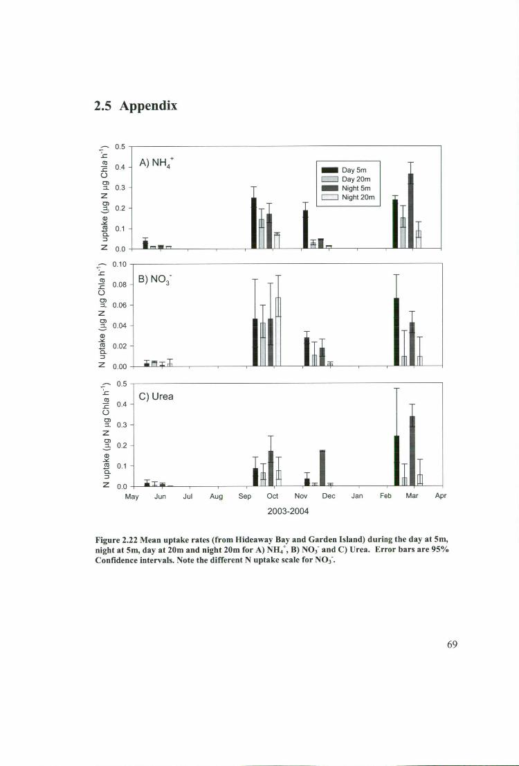
B) NO3-

ful T

0.10

0.08 -

0.06 -

0.04 -

0.02 -

0.00

0.5

0.4 -

0.3

0.2

0.1

0.0

A) NH4+ MM Day 5m I Day 20m

Night 5m I 1 Night 20m

N u

ptak

e (ji

g N

n C

hia

h-1)

N u

ptak

e G

ig N

pg

Chi

a h-

1) N

upt

ake

(lig

N p

g Chi

a h-

1) 2.5 Appendix

0.5

C) Urea

Ii JIT

Jun

Jul Aug Sep Oct Nov Dec Jan

Feb Mar

2003-2004

Figure 2.22 Mean uptake rates (from Hideaway Bay and Garden Island) during the day at 5m, night at 5m, day at 20m and night 20m for A) NH 4+, B) NO3" and C) Urea. Error bars are 95% Confidence intervals. Note the different N uptake scale for NO 3- .

0.4 -

0.3 -

0.2 -

0. 1 -

0.0 May Apr

69

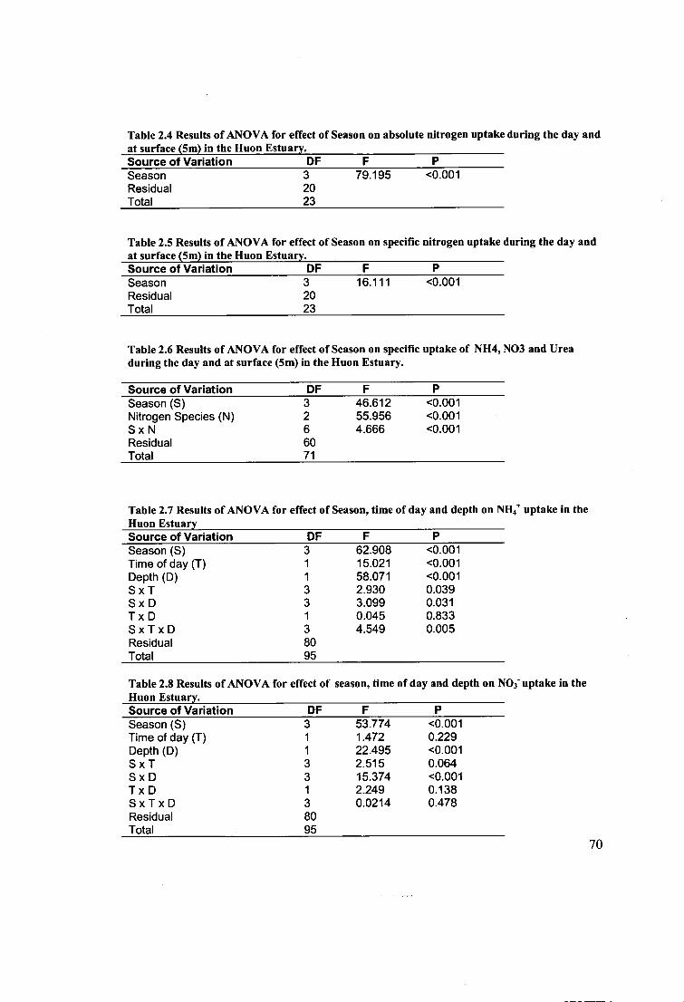
Table 2.4 Results of ANOVA for effect of Season on absolute nitrogen uptake during the day and at surface (5m) in the Huon Estuary. Source of Variation OF F P Season 3 79.195 <0.001 Residual 20 Total 23

Table 2.5 Results of ANOVA for effect of Season on specific nitrogen uptake during the day and at surface (5m) in the Huon Estuary. Source of Variation DF F P Season 3 16.111 <0.001 Residual 20 Total 23

Table 2.6 Results of ANOVA for effect of Season on specific uptake of NH4, NO3 and Urea during the day and at surface (5m) in the Huon Estuary.

Source of Variation DF F P Season (S) 3 46.612 <0.001 Nitrogen Species (N) 2 55.956 <0.001 S x N 6 4.666 <0.001 Residual 60 Total 71

Table 2.7 Results of ANOVA for effect of Season, time of day and depth on NH4+ uptake in the Huon Estuary Source of Variation DF F P Season (S) 3 62.908 <0.001 Time of day (T) 1 15.021 <0.001 Depth (D) 1 58.071 <0.001 S x T 3 2.930 0.039 S x D 3 3.099 0.031 T x D 1 0.045 0.833 SxTxD 3 4.549 0.005 Residual 80 Total 95

Table 2.8 Results of ANOVA for effect of season, time of day and depth on NO 3- uptake in the Huon Estuary. Source of Variation OF F P Season (S) 3 53.774 <0.001 Time of day (T) 1 1.472 0.229 Depth (D) 1 22.495 <0.001 S x T 3 2.515 0.064 S x D 3 15.374 <0.001 T x D 1 2.249 0.138 SxTxD 3 0.0214 0.478 Residual 80 Total 95

70

Table 2.9 Results of ANOVA for effect of season, time of day and depth on urea" uptake in the Huon Estuary. Source of Variation DF F P Season (S) 3 63.157 <0.001 Time of day (T) 1 12.492 <0.001 Depth (D) 1 113.643 <0.001 S x T 3 3.368 0.023 S x D 3 15.095 <0.001 T x D 1 8.293 0.005 SxTxD 3 2.702 0.051 Residual 80 Total 95

71

2.6 References

Adolf, J. E., Yeager, C. L., Miller, W. D., Mallonee, M. E. & Harding, L. W. 2006. Environmental forcing of phytoplanlcton floral composition, biomass, and primary productivity in Chesapeake Bay, USA. Estuar. Coast. Shelf Sci. 67:108-22.

Andersson, M. G. I., van Rijswijk, P. & Middelburg, J. J. 2006. Uptake of dissolved inorganic nitrogen, urea and amino acids in the Scheldt estuary: comparison of organic carbon and nitrogen uptake. Aquat Microb Ecol 44:303-15.

Antia, N. J., Berland, B. R., Bonin, D. J. & Maestrini, S. Y. 1975. Comparative evaluation of certain organic and inorganic sources of nitrogen for phototrophlc growth of marine microalgae. Journal of Marine Biological Association of the United Kingdom 55:519-39.

Armstrong, F. A. J. 1951. The determination of silicate in sea water. Journal of Marine Biological Association of the United Kingdom 30:149-60.

Banse, K. 1977. Determining carbon to chlorophyll ratio of natural phytoplankton. Mar Biol 41:199-212.

Berg, G. M., Balode, M., Purina, I., Bekere, S., Bechemin, C. & Maestrini, S. Y. 2003. Plankton community composition in relation to availability and uptake of oxidized and reduced nitrogen. Aquat Microb Ecol 30:263-74.

Bode, A. & Dortch, Q. 1996. Uptake and regeneration of inorganic nitrogen in coastal waters influenced by the Mississippi River: Spatial and seasonal variations. J Plankton Res 18:2251-68.

Bode, A., Gonzalez, N., Rodriguez, C., Varela, M. & Varela, M. M. 2005. Seasonal variability of plankton blooms in the Ria de Ferrol (NW Spain): I. Nutrient concentrations and nitrogen uptake rates. Estuar Coast Shelf S 63:269-84.

Boyer, J. N., Stanley, D. W. & Christian, R. R. 1994. Dynamics of Nh4+ and No3- Uptake in the Water Column of the Neuse River Estuary, North-Carolina. Estuaries 17:361-71.

Collos, Y., Vaguer, A., Bibent, B., Souchu, P., Slawyk, G. & Garcia, N. 2003. Response of coastal phytoplankton to ammonium and nitrate pulses: seasonal variations of nitrogen uptake and regeneration. Aquat. Ecol. 37:227-36.

Doblin, M. A., Thompson, P. A., Revill, A. T., Butler, E. C. V., Blackburn, S. I. & Hallegraeff, G. M. 2006. Vertical migration of the toxic dinoflagellate Gymnodinium catenatum under different concentrations of nutrients and humic substances in culture. Harmful Algae 5:665-77.

Dortch, Q. 1990. The interaction between ammonium and nitrate uptake in phytoplankton. Mar. Ecol.-Prog. Ser. 61:183-201.

Dugdale, R. C. & Goering, J. J. 1967. Uptake of new and regenerated forms of nitrogen in primary productivity. Limnol. Oceanogr. 12:196-206.

Dugdale, R. C. & Wilkerson, F. P. 1986. The use of N-15 to measure nitrogen uptake in eutrophic oceans- experimental considerations. Limnol. Oceanogr. 31:673- 89.

72

Eppley, R. W. 1972. Temperature and phytoplankton growth in the sea. NOAA FISH BULL I Fishery Bulletin 70(4): 1063-1085. 1972. SFA 18(2).

Eppley, R. W., Rogers, J. N. & McCarthy, J. J. 1969. Half saturation constants for uptake of nitrate and ammonium by marine phytoplankton. Limnol. Oceanogr. 14:912-20.

Falkowski, P. G. 1977. The adenylate energy charge in marine phytoplankton: The effect of temperature on the physiological state of Skeletonema costatum (Greve.) Cleve. Journal of Experimental Marine Biology and Ecology 27:37- 45.

Fernandez, E., Maranon, E., Harbour, D. S., Kristiansen, S. & Heimdal, B. R. 1996. Patterns of carbon and nitrogen uptake during blooms of Emiliania huxleyi in two Norwegian fjords. J Plankton Res 18:2349-66.

Furnas, M. J. 1983. Nitrogen dynamics in lower Narragansett Bay, Rhode Island. 1. Uptake by size-fractionated phytoplankton populations. J Plankton Res 5:657- 76.

Furnas, M. J., Smayda, T. J. & Deason, E. A. 1986. Nitrogen dynamics in lower Narragansett Bay. 2. Phytoplankton uptake, depletion rates of nitrogenous nutrient pools, and estimates of ecosystem remineralization. J Plankton Res 8:755-69.

Glibert, P. M., Garside, C., Fuhrman, J. A. & Roman, M. R. 1991. Time-Dependent Coupling of Inorganic and Organic Nitrogen Uptake and Regeneration in the Plume of the Chesapeake Bay Estuary and Its Regulation by Large Heterotrophs. Limnol. Oceanogr. 36:895-909.

Glibert, P. M., Lipschultz, F., McCarthy, J. J. & Altabet, M. A. 1982. Isotope-dilution models of uptake and remineralization of ammonium by marine plankton. Limnol. Oceanogr. 27:639-50.

Hallegraeff, G. M., Mccausland, M. A. & Brown, R. K. 1995. Early Warning of Toxic Dino flagellate Blooms of Gymnodinium-Catenatum in Southern Tasmanian Waters. J Plankton Res 17:1163-76.

Hallegraeff, G. M., Nichols, P. D., Volkman, J. K., Blackburn, S. I. & Everitt, D. A. 1991. Pigments, Fatty-Acids, and Sterols of the Toxic Dinoflagellate Gymnodinium-Catenatum. J Phycol 27:591-99.

Hallegraeff, G. M., Stanley, S. 0., Bolch, C. J. & Blackburn, S. 1. 1989. Gymnodinium catenatum blooms and shellfish toxicity in Southern Tasmania, Australia. In: Okaichi, T., Anderson, D. M. & Nemoto, T. [Eds.] Red Tides: Biology, Environmental Science and Toxicology. Elsevier, pp. 75-78.

Harris, G. P. 2001. Biogeochemistry of nitrogen and phosphorous in Australian catchments, rivers and estuaries: effects of land use and flow regulation and comparisons with global patterns. Marine and Freshwater Research 52:139- 49.

Harrison, P. J. 2002. Station papa time series: Insights into ecosystem dynamics. J. Oceanogr. 58:259-64.

73

Hecky, R. E. & Kilham, P. 1988. Nutrient limitation of phytoplankton in freshwater and marine environments: A review of recent evidence on the effects of enrichment. Limnol. Oceanogr. 33:796-822.

Heil, C. A., Revilla, M., Glibert, P. M. & Murasko, S. 2007. Nutrient quality drives differential phytoplankton community composition on the southwest Florida shelf. Limnol. Oceanogr. 52:1067-78.

Holm-Hansen, 0. & Booth, C. 1966. The measuremeant of adenosine triphosphate in the ocean and its ecological significance. Limnol. Oceanogr. 11:510-19.

Howarth, R. W., Marino, R. & Cole, J. J. 1988. Nitrogen-fixation in fresh-water, estuarine and marine ecosystems. 2. Biogeochemical controls. Limnol. Oceanogr. 33:688-701.

Kerouel, R. & Aminot, A. 1997. Fluorometric determination of ammonia in sea and estuarine waters by direct segmented flow analysis. Mar. Chem. 57:265-75.

L'Helguen, S., Madec, C. & Lecorre, P. 1993. Nitrogen Nutrition of the Phytoplankton in the Well-Mixed Waters of the Western English-Channel. Oceanologica Acta 16:653-60.

L'Helguen, S., Madec, C. & LeCorre, P. 1996. Nitrogen uptake in permanently well- mixed temperate coastal waters. Estuar. Coast. Shelf Sci. 42:803-18.

La Roche, J. 1983. Ammonium regeneration: Its contribution to phytoplankton nitrogen requirements in a eutrophic environment. Marine biology, Heidelberg 75:231-40.

Little, R. J. A. & Rubin, D. B. 1987. Statistical Analysis with Missing Data. Wiley, New York, 408.

Lomas, M. W. & Gilbert, P. M. 1999. Temperature regulation of nitrate uptake: A novel hypothesis about nitrate uptake and reduction in cool-water diatoms. Limnol. Oceanogr. 44:556-72.

Lomas, M. W., Trice, T. M., Glibert, P. M., Bronk, D. A. & McCarthy, J. J. 2002. Temporal and spatial dynamics of urea uptake and regeneration rates and concentrations in Chesapeake Bay. Estuaries 25:469-82.

Lopes, C. B., Lillebo, A. I., Dias, J. M., Pereira, E., Vale, C. & Duarte, A. C. 2007. Nutrient dynamics and seasonal succession of phytoplankton assemblages in a Southern European Estuary: Ria de Aveiro, Portugal. Estuar Coast Shelf S 71:480-90.

Mackey, M. D., Mackey, D. J., Higgins, H. W. & Wright, S. W. 1996. CHEMTAX - A program for estimating class abundances from chemical markers: Application to HPLC measurements of phytoplankton. Mar. Ecol.-Prog. Ser. 144:265-83.

Marshall, H. G., Burchardt, L. & Lacouture, R. 2005. A review of phytoplankton composition within Chesapeake Bay and its tidal estuaries. J. Plankton Res. 27:1083-102.

McCarthy, J. J., Taylor, R. W. & Taft, J. L. 1977. Nitrogenous nutrition of the plankton in the Chesapeake Bay. 1. Nutrient availability and phytoplankton preferences. Limnol. Oceanogr. 22:996-1011.

74

Metzler, P. M., Glibert, P. M., Gaeta, S. A. & Ludlam, J. M. 1997. New and regenerated production in the South Atlantic off Brazil. Deep-Sea Res. Part I-Oceanogr. Res. Pap. 44:363-84.

Middelburg, J. J. & Nieuwenhuize, J. 2000. Nitrogen uptake by heterotrophic bacteria and phytoplankton in the nitrate-rich Thames estuary. Mar Ecol-Prog Ser 203:13-21.

Mulvenna, P. F. & Savidge, G. 1992. A Modified Manual Method for the Determination of Urea in Seawater Using Diacetylmonoxime Reagent. Estuar Coast Shelf S 34:429-38.

Murphy, J. & Riley, J. P. 1962. A modified single-solution for the determination of phosphate in natural waters. Analytica Chimica Acta 27:31-36.

Nagai, S., Nitshitani, G., Tomaru, Y., Sakiyama, S. & Kamiyama, T. 2008. Predation by the toxic dinoflagellate Dinophysis fortii on the ciliate Myrionecta rubra and observation of sequestration of ciliate chloroplasts. I Phycol. 44:909-22.

Park, M. G., Kim, S., Kim, H. S., Myung, G., Kang, Y. G. & Yih, W. 2006. First successful culture of the marine dinoflagellate Dinophysis acuminata. AquaL Microb. EcoL 45:101-06.

Redfield, A. C. 1958. The biological control of chemical factors in the environment. American Scientist 406:205-21.

Rodrigues, R. & Williams, P. J. L. 2002. Inorganic nitrogen assimilation by picoplankton and whole plankton in a coastal ecosystem. Limnol. Oceanogr. 47:1608-16.

Rosser, S. & Thompson, P. A. 2001. Phytoplankton of the Swan-Canning Estuary: a comparison of nitrogen uptake by different bloom assemblages. HydroL Process. 15:2579-94.

Smayda, T. J. 1980. Phytoplankton Species Succession. In: Morris, I. [Ed.] The Physiological Ecology of Phytoplankton. Blackwell Scientific Publications, pp. 493-570.

Smayda, T. J. & Reynolds, C. S. 2001. Community assembly in marine phytoplankton: application of recent models to harmful dinoflagellate blooms. J Plankton Res. 23:447-61.

Smith, V. H. 1982. The nitrogen and phosphorous dependence of algal biomass in lakes- an empirical and theoretical- analysis. LimnoL Oceanogr. 27:1101-12.

Sokal, R. R. & Rohlf, F. J. 1995. Biometry: the principles and practice of statistics in biological research. W.H. Freeman and Company, New York, 887.

Team, H. E. S. 2000. Huon Estuary Study, Environmental research for integrated catchment management and aquaculture. Final Report to FRDC. CSIRO Division of Marine Research, Hobart, Tasmania, Australia.

Thompson, P. 1999. Response of growth and biochemical composition to variations in daylength, temperature, and irradiance in the marine diatom Thalassiosira pseudonana (Bacillariophyceae). J Phycol 35:1215-23.

Thompson, P. A., Bonham, P. I. & Swadling, K. M. 2008. Phytoplankton blooms in the Huon Estuary, Tasmania: top-down or bottom-up control? I Plankton Res. 30:735-53.

75

Tremblay, J. E., Legendre, L., Klein, B. & Therriault, J. C. 2000. Size-differential uptake of nitrogen and carbon in a marginal sea (Gulf of St. Lawrence, Canada): Significance of diel periodicity and urea uptake. Deep-Sea Res Pt Ii 47:489-518.

Twomey, L. J., Piehler, M. F. & Paerl, H. W. 2005. Phytoplankton uptake of ammonium, nitrate and urea in the Neuse River Estuary, NC, USA. Hydrobiologia 533:123-34.

Varela, D. E. & Harrison, P. J. 1999. Seasonal variability in nitrogenous nutrition of phytoplankton assemblages in the northeastern subarctic Pacific Ocean. Deep-Sea Res Pt Ii 46:2505-38.

Veuger, B., Middelburg, J. J., Boschker, H. T. S., Nieuwenhuize, J., van Rijswijk, P., Rochelle-Newall, E. J. & Navarro, N. 2004. Microbial uptake of dissolved organic and inorganic nitrogen in Randers Fjord. Estuar Coast Shelf S 61:507- 15.

Wafar, M., L'Helguen, S., Raikar, V., Maguer, J. F. & Corre, P. L. 2004. Nitrogen uptake by size-fractionated plankton in permanently well-mixed temperate coastal waters. J Plankton Res 26:1207-18.

Waite, A., Bienfang, P. K. & Harrison, P. J. 1992a. Spring bloom sedimentation in a subarctic ecosystem I : Nutrients and sinking. Mar Biol 114:119-29.

Waite, A., Bienfang, P. K. & Harrison, P. J. 1992b. Spring bloom sedimentation in a subarctic ecosystem II:Succession and sedimentation. Mar Biol 114:131-38.

Watson, R. J., Butler, E. C. V. & Clementson, L. A. 2004. Flow-injection analysis with fluorescence detection of trace levels of ammonium in seawater. Journal of Environmental Monitoring 7:37-42.

Wilkerson, F. P., Dugdale, R. C., Hogue, V. E. & Marchi, A. 2006. Phytoplankton blooms and nitrogen productivity in San Francisco Bay. Estuaries Coasts 29:401-16.

Wood, E. D., Armstrong, F. A. J. & Richards, F. A. 1967. Determination of nitrate in sea water by cadmium-copper reduction to nitrite. Journal of Marine Biological Association of the United Kingdom 47:23-31.

Yin, K. D., Qian, P. Y., Chen, J. C., Hsieh, D. P. H. & Harrison, P. J. 2000. Dynamics of nutrients and phytoplankton biomass in the Pearl River estuary and adjacent waters of Hong Kong during summer: preliminary evidence for phosphorus and silicon limitation. Mar Ecol-Prog Ser 194:295-305.

76

3 EFFECT OF TEMPERATURE AND

IRRADIANCE ON THE GROWTH AND

BIOCHEMICAL COMPOSITION OF THE

TOXIC DINOFLAGELLATE

GYMNODINIUM CATENATUM FROM

SOUTH-EAST TASMANIA, AUSTRALIA

3.1 Introduction

To increase our understanding of Huon Estuary bloom dynamics and their inter-

annual variability it is necessary to characterise the physiological responses of the

dominant species to different temperature and irradiance conditions. Gymnodinium

catenatum (G. catenatum) has been identified as an important part of the

phytoplankton community whose bloom dynamics are poorly understood in the Huon

Estuary. Several studies have examined the effect of temperature on other strains of

G. Catenatum (Bravo & Anderson, 1994, Ellegaard et al., 1993, Band-Schmidt et al.,

2004) but these are limited in their scope and application in models as they only

examine growth at one irradiance, more recently Yamamoto, et al., (2002) has

examined the effect of temperature on a Japanese strain and published the first

growth versus irradiance curve for this species.

The effect of temperature and irradiance on growth in phytoplanIcton has been studied

widely. The effect of temperature on growth rate of phytoplankton has been

described by a variety of relationships including exponential (Eppley, 1972), Linear

(Montagnes etal., 2003), and even Sigmoid (Bouterfas et al., 2002). In general,

growth rate increases with temperature to a maximum. At temperatures greater than

the temperature where growth is at its maximum there is a sharp decrease in growth 77

rate. Thompson (2006) has reviewed several models for the effect of growth rate on

phytoplankton and concludes that "Logan's (1976) model provides the best

parameterisation of the empirical relationship between temperature and micro-algal

growth rate". While generalised models of growth rate as a function of temperature

have been developed in the past increasingly models capable of predicting species

succession and phytoplankton community composition are required to better manage

our ecosystems. Hence, there is a growing need for species specific models for effect

of temperature on growth rate.

The relationship between growth rate and irradiance has been described by a number

of saturating curves (rectangular hyperbola). The advantages and disadvantages of

more commonly used curves has been investigated by Jassby and Platt, (1976).

These curves can all be used to estimate parameters such as gmm„ a, and Ek. Where

gmax is the maximum growth rate above which increases in irradiance do not increase

growth rate, a is the initial slope of the light limited section of the curve and Ek is the

irradiance coefficient (irradiance at the point where the initial slope intercepts the

Ilmax). Some of the models include a parameter for the compensation irradiance, Ec

(irradiance where growth=respiration) and most can be easily modified to include a

parameter for E.

The relationship between growth rate (g max) and temperature is well established and is

discussed above, but the other parameters of growth versus irradiance curves (a, Ek

and Ec) have also been shown to vary between classes of phytoplankton (Banse,

1976) and with temperature (Verity, 1982b, Yoder, 1979). Unfortunately there are

only relatively few studies (Li & Morris, 1982, Thompson, 1999, Geider et al., 1985,

Verity, 1982b, Palmisano etal., 1987) that report how the physiological parameters a,

Ek and Ec vary in response to both light and temperature. Most of these use only a

narrow, and sometimes inappropriate, range of temperatures and irradiances. These

constraints limit both understandings of phytoplankton physiology and attempts to

make the science more predictive.

78

More recently the mechanisms behind growth and physiological acclimation of

phytoplankton to irradiance and temperature have begun to be elucidated. Of

particular interest is the conclusion that seemingly opposite temperature and

irradiance conditions result in the same responses: growth at high temperature and

high irradiance is physiologically similar to growth at low temperature and a

comparatively low irradiance (Maxwell et al., 1994). Biochemical components like

chlorophyll a (chi a) content (quota) also show a similar response in these seemingly

opposite temperature and irradiance conditions (Wilson et al., 2003). The reason for

this is that the energy balance of the cell as determined by 'excitation pressure' on

photosystem II (PS11) is what triggers the physiological response(s) of the cell. So at

high temperatures reactions for growth are accelerated and the demand for energy by

the cell is high. If the irradiance is sufficiently high to provide enough energy for the

cell then chl a quota will be maintained at a low level. Because the rate of chemical

reactions is rapidly reduced at lower temperatures, a similar response occurs at low

temperature and at much lower irradiance where the cell cannot process very much

light energy through the biochemical reactions of photosynthesis so that the

excitation pressure on PSII is still high. Thus even at a low irradiance the chla quota

will be maintained at a low level. At high or low temperatures under reduced

irradiance it would be expected that the chl a quota would be increased to increase

energy captured per cell but that the absolute irradiance that stimulates chl a synthesis

will vary with temperature. Consequently understanding phytoplankton physiology

requires that the effects of temperature and light be considered together because they

both play a role in determining the physiological status of the cell.

In this study the effect of temperature ranging from 12 to 28.5°C and irradiances

from 5 to 458 pmoles of photons tn -2 s -1 on the growth rate and biochemical

composition of a Huon Estuary strain GCHUO2 of G. catenatum were investigated,

with the intention of determining:

• the growth rates of a Huon Estuary strain of G. catenatum under different

combinations of temperature and light; 79

• the physiological responses of this species to variation in irradiance and

temperature, and;

• the parameters necessary to model the gross growth rate of this species in the

Huon Estuary.

To achieve this, growth versus irradiance curves were constructed from the growth

rates of each of the twelve different temperatures examined. A comparison of these

results to other strains that have been isolated from a number of other coastal areas

around the world is presented and discussed. Relationships between parameters of the growth versus irradiance curves with temperature were used to construct a model for

the growth response of this species to a range of temperature and irradiance

conditions likely to be encountered in the Huon Estuary and other temperate ecosystems that this species currently inhabits or may inhabit in the future.

3.2 Methods

3.2.1 Strain and culture conditions

A toxic strain of G. catenatum, GCHUO2 (Ellegaard & Oshima, 1998) was used in

this experiment. The GCHUO2 strain was isolated from the Huon Estuary on the

6/6/1986 by Susan Blackburn This strain is maintained at the CSIRO Collection of

Living Microalgae in GSe growth media at 20 °C.

Stock cultures were maintained in 40 ml of a seawater medium (GSe) with GPM

nutrients (Loeblich, 1975) and the addition of 10-8 M of Selenium (IV) in 50m1

Erlenmeyer flasks at 18 °C, bottom illumination of 150 pimol photons m -2 s-I (Philips

deluxe cool white fluorescent tubes) and a 12:12 light:dark cycle. Irradiances were

measured with a Biospherical Instruments® QSL-100 meter using a 4 it spherical

sensor. Experimental cultures were grown in GPM (Loeblich, 1975) + 10 -8 M of

Selenium (IV) enriched medium prepared from seawater (collected from offshore

eastern Tasmania, 42 36.00 S 148 14.00 E), treated with activated charcoal 80

(McLachlan, 1973), filtered (1gm, followed by 0.45 pm) autoclaved in a Teflon

container, and adjusted to —28 practical salinity units (PSU) seawater adding sterile

Milli-QV water (MQ). The nutrients were added via a sterile Millipore St erivexTM

0.22 gm filter under the sterile conditions of a laminar flow hood (Clemco CF 435).

Once sterile, all medium transfers and culture inoculations were undertaken in the

sterile conditions of a laminar flow hood (Clemco CF 435).

3.2.2 Temperature and irradiance gradient incubator table

The experiment used a 45 mm thick aluminium block in which a temperature gradient

could be established by heating one end and cooling the other using two different

temperature water baths (Figure 3.1). The different irradiances were established at

each temperature using different density computer generated black dots, laser-printed

onto transparency film. The printed transparencies were placed between the

fluorescent tubes and the cultures which were illuminated from underneath. At each

temperature in the gradient table there were 6 different irradiances. The gradient table

was designed to be used with 70 ml polycarbonate containers. A 50 ml borosilicate

test tube (Pyrex' or KimaxTm) was attached to these containers via a polypropylene

custom made adapter (Figure 3.2) so that the fluorescence could be easily measured

by inverting the culture vessel and placing the test tube into a Turner Designs model

10 AU fluorometer (Mountainview, California, USA).

The irradiance inside an empty culture vessel was measured at each location in the

gradient incubator table using a Biospherical Instruments® QSL-100 meter with a 4 TE

spherical sensor (California, USA). Six fluorescent tubes (Osram cool white) were

used to illuminate the gradient incubator table from below.

81

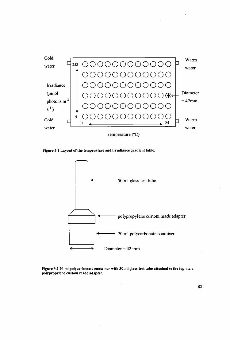
E258 000000000000 O00000000000 O00000000000 O00000000000 O00000000000

5 000000000000 11 4 25

water

Cold Warm

water

Diameter

= 42mm

Warm

Irradiance

(pmol

photons 111-2

S-1 )

Cold

water

water Temperature (°C)

Figure 3.1 Layout of the temperature and irradiance gradient table.

50 ml glass test tube

polypropylene custom made adapter

44- 70 ml polycarbonate container.

Diameter =42 mm

Figure 3.2 70 ml polycarbonate container with 50 ml glass test tube attached to the top via a polypropylene custom made adapter.

82

3.2.3 Effect of culture vessels

G. catenatum was grown in three different culture vessels to determine if the type of

culture vessel affects growth rate in this species (after (Metaxas, 1989)). In

particular, it was necessary to determine if the 70 ml polycarbonate container that had

to be used with the temperature gradient table would have a negative effect on growth

rate in comparison to other culture vessels commonly used in the laboratory.

Qualitative effects of culture vessels have been observed on growth of G. catenatum

before, however they have not been tested experimentally. Three replicate cultures

were grown in 50m1 PyrexTm or Kimax-rm test tubes with polypropylene tops, 70 ml

polycarbonate containers with 50 ml test tube "tops" (Figure 3.2) and 250 ml Pyrex I'm

flasks with 50 ml test tube type side-arms and polypropylene tops. The cultures were

inoculated so they would have a starting cell concentration of 1.12 x le 1: 1 . The

cultures were grown at 18 °C, 130 mot photons r11-2 s-1 and a 12:12 L:D for nineteen

days. Fluorescence of the cultures was measured every three to four days and initial

and final cell counts were also taken so that the growth rate could be determined.

3.2.4 Preconditioning of p, versus I experimental cultures

Twelve cultures were grown at 18 °C and six irradiances ranging from 5 to 283 j.tmol

photons t11-2 s-1 for three weeks to acclimatise the cells to the irradiances that would

be used in the experiment. Using these cultures as inocula, temperature acclimation

was incremental as follows. Twenty-four 70 ml polycarbonate containers each

containing 48 ml GSe medium were added to the centre of the temperature and

irradiance gradient table (18.2,18.9, 20.7 and 21.1 °C). At each temperature in the

gradient incubator table there were six different irradiances. These vessels were

inoculated with 2 ml from the irradiance acclimated cultures that had the closest

irradiance to that location in the gradient incubator table. After a week the cultures at

18.2 and 18.9 °C in the gradient incubator table were shifted to the next lowest

83

temperature and the cultures at 20.7 and 21.1 °C shifted to the next highest

temperature. The shifted cultures were replaced by another twelve vessels inoculated

from the appropriate irradiance acclimated cultures. Every four to five days this

process was repeated until all seventy-two cultures had been added to the gradient

incubator table. All the cultures were incubated at their experimental temperature for

a further week prior to commencing the experiment described in section 3.2.5.

3.2.5 Temperature and irradiance experiment

From the seventy-two pre-experimental cultures, seventy-two new cultures were

started in 70 ml polycarbonate containers with 50 ml test tubes attached via a custom-

made adaptor (Figure 3.2). These new cultures were set up by visually assessing the density of the acclimatised individual pre-experimental cultures (see section 3.2.4).

Depending on their density, 1,2,5 or 10 ml was transferred using a pipette under

sterile conditions into the new 70 ml experimental polycarbonate containers, and GSe

medium was added to make up a total culture volume of 50 ml. At some of the low

irradiance extremes pre-experimental cultures had shown little or no growth and new

cultures were inoculated from another culture at the same temperature but a higher

irradiance. These seventy-two new cultures of G. catenatum were grown at 12

different temperatures: 11.9, 13.4, 15.5, 16.3, 18.2, 18.9, 20.7, 21.1, 22.8, 23.0, 24.9

and 25.2 °C (temperatures are those measured when lights were on)and at six

different irradiances ranging from 5 to 283 iAmol photons M-2 sl for forty-nine to

seventy-two days. The temperature, irradiance and initial cell densities of the G.

catenatum cultures in the gradient table experiment are listed in Table 3.1 .The

light:dark cycle used throughout this experiment was 14:10. One of the limitations of

the gradient table experiment setup was that to achieve the irradiance conditions

required for the experiment the fluorescent tubes providing the light had to be

positioned almost immediately below the gradient table. Positioning the lights so

close to the gradient table and cultures meant that when the lights were on it

increased the temperature of some cultures. The cultures effected most by this

84

increase in temperature were those positioned in the lower temperature areas of the

gradient table. When the lights were on some cultures increased in temperature by

2 °C. To reduce this side effect of the lights increasing the temperature of some

cultures a fan was added to dissipate the heat from under the gradient table.

Some of the cultures incubated at low irradiances across all temperature treatments did not exhibit any growth over the period of forty-nine days. For these "no growth"

cultures, 40 ml was removed for chlorophyll analysis and new media added to replace

the amount removed. The cultures were then shifted to the next highest irradiance

every three to four days, until these 'no growth' cultures that were originally at

irradiances below 25 gmol photons in -2 s 1 were at irradiances greater than 60 gmol

photons 111-2 s-1 . Throughout this twenty-three day period the fluorescence was

measured four times.

At the conclusion of these experiments on the effects of light and temperature it was apparent that at the highest temperatures the irradiances were not saturating growth

(see section 3.3.2.2). Consequently some additional experiments at the extremes of

high temperatures and high irradiances were conducted (see section 3.2.6).

85

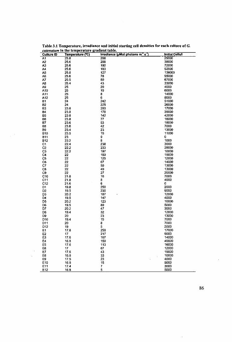
Table 3.1 Temperature, irradiance and initial starting cell densities for each culture of G. catenatum in the temperature gradient table. Culture ID Temperature (°C) Irradiance (pMol photons m 4 s -1) Initial Cells/I Al 25.8 208 29000 A2 25.6 208 38000 A3 25.6 192 72000 A4 25.6 183 52000 A5 25.8 127 139000 A6 25.6 78 95000 A7 25.5 50 67000 A8 25.4 43 33000 A9 25 20 4000 Al 0 25 15 6000 All 25 8 14000 Al2 25 6 8000 B1 24 242 51000 B2 24 225 26000 B3 23.8 203 17000 B4 23.8 178 35000 B5 23.8 142 42000 B6 23.8 77 18000 B7 23.6 53 18000 88 23.6 42 7000 89 23.4 23 13000 810 23.5 15 11000 B11 23 9 0 B12 23.2 8 1000 Cl 22.4 238 3000 C2 22.2 233 28000 C3 22.2 197 10000 C4 22 180 15000 C5 22 125 12000 C6 22 67 14000 C7 22 50 13000 C8 22 40 13000 C9 22 27 20000 Cl 0 21.8 16 7000 Cl 1 21.8 8 4000 C12 21.6 6 0 D1 19.8 250 2000 02 19.5 230 9000 D3 20.2 187 12000 D4 19.5 147 4000 D5 20.2 123 10000 06 19.5 80 5000 07 20.2 47 3000 D8 19.4 32 12000 09 20 23 13000 010 19.4 15 7000 al 1 20 8 7000 012 19 5 2000 El 17.8 258 17000 E2 17 217 9000 E3 17.6 167 14000 E4 16.8 150 40000 E5 17.6 113 16000 E6 17 67 12000 E7 17.6 43 19000 E8 16.8 33 10000 E9 17.5 23 4000 El 0 16.8 15 5000 Ell 17.4 7 3000 E12 16.8 5 5000

86

Table 3.1 continued Culture ID Temperature (°C) Irradiance (pMol photons m4 s-1 ) Initial Cells/I Fl 15 242 39000 F2 13.2 175 7000 F3 14.6 207 22000 F4 12.8 167 10000 F5 14.8 130 10000 F6 13 63 57000 F7 14.6 47 66000 F8 13.2 37 21000 F9 14.8 21 16000 F10 13.2 13 10000 Ell 14.5 8 3000 F12 13 5 3000

3.2.6 Growth at high temperature and high light

3.2.6.1 Pre-acclimatisation

Two cultures were acclimatised in 50 ml Erlenmeyer flasks at 25.6 °C at two higher

irradiances 291 and 458 gmol photons T11-2 S-1 for eight days. The cell density of the

acclimatised cultures was determined by cell counts at the end of the eight-day

period.

3.2.6.2 Culture conditions

The cultures were illuminated from below with fluorescent tubes (Osram cool

white). The light:dark period used was 14:10.

3.2.6.3 Growth at 28.5 °C

The 70 ml polycarbonate experimental vessels with 50 ml test tube attached via

custom adapter (Figure 3.2) were filled with 50 ml of GSe medium and inoculated

with 5 ml from the pre-acclimatised cultures (see section 3.2.6.1). The cultures were

then grown at 291 and 458 gmol photons 111-2 s-1 with the temperature increased to

28.5 °C and grown for fourteen days. Fluorescence was monitored and at the end of

the experiment the cell density of the cultures was determined by cell counts.

3.2.6.4 Growth at 25.0 °C

Two experimental vessels with 50 ml GSe were inoculated with 5 ml from the pre-

acclimatised cultures (see section 3.2.6.1). The new cultures were grown at 25.0 °C 87

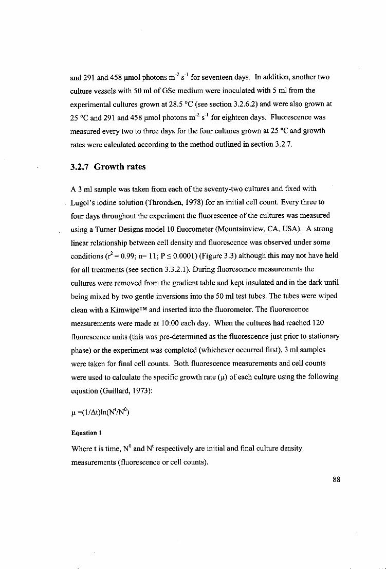
and 291 and 458 gmol photons m -2 s seventeen days. In addition, another two

culture vessels with 50 ml of GSe medium were inoculated with 5 ml from the

experimental cultures gown at 28.5 °C (see section 3.2.6.2) and were also gown at

25 °C and 291 and 458 gmol photons m -2 s-I for eighteen days. Fluorescence was

measured every two to three days for the four cultures grown at 25 °C and growth

rates were calculated according to the method outlined in section 3.2.7.

3.2.7 Growth rates

A 3 ml sample was taken from each of the seventy-two cultures and fixed with Lugol's iodine solution (Throndsen, 1978) for an initial cell count. Every three to

four days throughout the experiment the fluorescence of the cultures was measured

using a Turner Designs model 10 fluorometer (Mountainview, CA, USA). A strong

linear relationship between cell density and fluorescence was observed under some

conditions (r2 = 0.99; n= 11; P < 0.0001) (Figure 3.3) although this may not have held

for all treatments (see section 3.3.2.1). During fluorescence measurements the cultures were removed from the gradient table and kept insulated and in the dark until

being mixed by two gentle inversions into the 50 ml test tubes. The tubes were wiped

clean with a KimwipeTM and inserted into the fluorometer. The fluorescence

measurements were made at 10:00 each day. When the cultures had reached 120

fluorescence units (this was pre-determined as the fluorescence just prior to stationary

phase) or the experiment was completed (whichever occurred first), 3 ml samples

were taken for final cell counts. Both fluorescence measurements and cell counts

were used to calculate the specific growth rate (g) of each culture using the following

equation (Guillard, 1973):

=(1/A01n(Nt/N°)

Equation 1

Where t is time, N° and Nt respectively are initial and final culture density

measurements (fluorescence or cell counts).

88

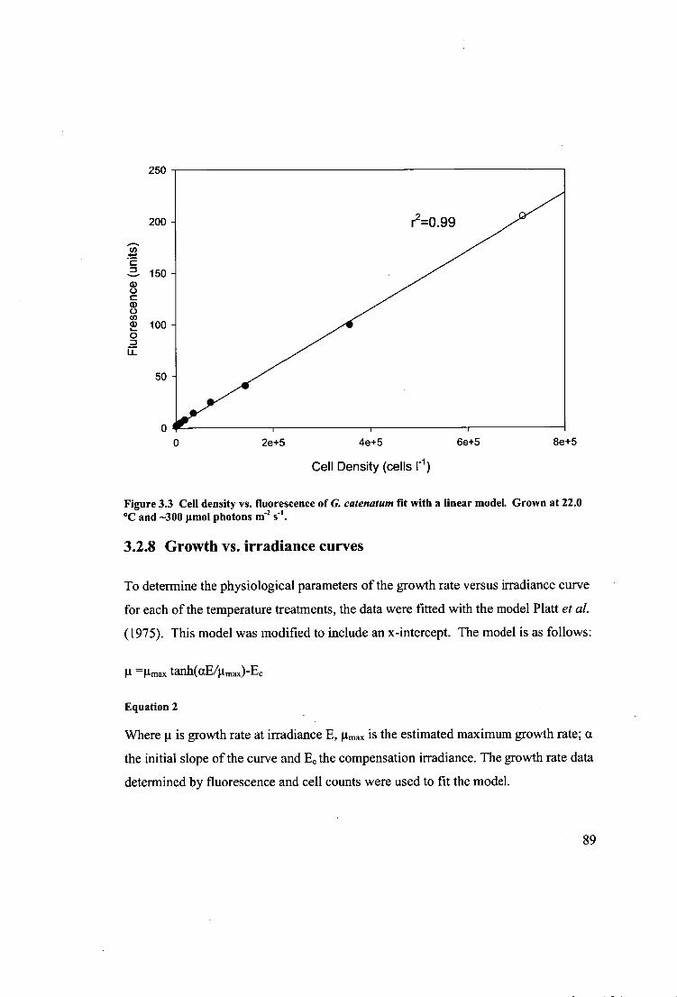
250

200 - r2=0.99

Fluo

resc

ence

(uni

ts)

150 -

100 -

50 -

0 ■

6e+5 8e+5 4e+5

Cell Density (cells I -1 )

0 2e+5

Figure 3.3 Cell density vs. fluorescence of G. catenatum fit with a linear model. Grown at 22.0 °C and —300 pmol photons 111-2 S-1 .

3.2.8 Growth vs. irradiance curves

To determine the physiological parameters of the growth rate versus irradiance curve

for each of the temperature treatments, the data were fitted with the model Platt et al.

(1975). This model was modified to include an x-intercept. The model is as follows:

tanh(aE/gn.)-Ec

Equation 2

Where 11 is growth rate at irradiance E, tmax is the estimated maximum growth rate; a

the initial slope of the curve and E, the compensation irradiance. The growth rate data

determined by fluorescence and cell counts were used to fit the model.

89

3.2.9 Biochemical analysis

When the cultures had reached 120 fluorescence units or the experiment was

completed (see section 3.2.6), samples were taken for chemical analysis. For carbon

and nitrogen analysis 20 ml of each culture was filtered under less than 5 mm Hg

vacuum through a Pa11TM A/E 13 mm glass fibre filter. These 13 mm filters were

dried and analysed on a LecoTM CHN analyser. For Chlorophyll analysis 20 ml was

filtered under less than 5 mm Hg vacuum through a WhatmanTM GF/F filter. The

filters were stored in cryogenic vials (CryovialTM) immersed in liquid nitrogen until

extraction. All glassware used for extraction was cleaned in dilute ExtranTM solution,

rinsed three times with Milli-Q (MQ) water and once with acetone (AR grade).

Frozen filters were cut into halves and placed in a clean 10 ml centrifuge tube. Three

millilitres of 100% acetone was added to each tube. The tube was covered with

ParafilmTM and vortexed for thirty seconds before placing the tube in an ice-water

bath and sonicating (UnisonicTM) the filter and acetone for fifteen minutes in the dark.

The filters and acetone were then stored for at least eighteen hours at 4 °C. After this

time, 0.2 ml MQ was added to each tube (to bring solvent to 90:10 acetone:water)

and the filter and solvent sonicated for a further fifteen minutes in ice water and in the

dark. Solvent and filter were then transferred to a BioradTM column containing a

small GF/F filter acting as a plug. The sample tubes were rinsed with 2 x 0.5 ml of

acetone/water (90:10) which was quantitatively added to the BioradTM column. Each

BioradTM column was fitted into a centrifuge tube and centrifuged for five minutes at

5000 rpm. The filtrate was stored overnight in the dark at 4 °C until just prior to

analysis. Samples were analysed for chlorophyll a and c, using a GBC UVNIS 916

spectrophotometer with 40 mm path length optical glass cells. Absorbance was read

at wavelengths of 750, 664, 647 and 630 nm. The absorbance at 750 nm was

subtracted from the absorbance at each of the other three wavelengths and substituted

into the following equations (after (Jeffrey et al., 1997)):

Chla extract = 11.85A664/1 - 1.54A647/1 - 0.08A630/1

90

Equation 3

Chic extract = 24.52A63011 - 1.67A664/1 - 7.60A647/1

Equation 4

A = corrected absorbance at specified wavelength.

1 = path length in cm.

The concentration of chlorophyll in the sample in 1..ig r' was obtained by the

following equation:

Chlx sample = Chlx extract * (vN)

Equation 5

v = volume of extract (ml).

V = volume of seawater filtered (1).

The total concentration of chlorophyll in the sample in ug 1 -1 was obtained by the

following equation:

Chl total = Chla sample + Chic sample

Equation 6

Some of the cultures at low irradiances across all temperature treatments did not

exhibit any growth after forty-nine days. Consequently a decision was made to take a

large volume (40 ml) for chlorophyll analysis, due to the cell density in these cultures

being very low with insufficient culture available for carbon and nitrogen analysis.

However a large amount of variation existed in the chla values even after 40 ml was

extracted for analysis from these very low density cultures. Therefore this chla data

was not included in any of the figures or analyses in this study.

91

3.2.10 G. catenatum energetics model

Using cellular energetics as a conceptual framework, an energetics model was

developed for G. catenatum. The concepts and definitions used by Richardson et al.

(1983) were adopted for the purposes of this study. The primary concept is that the

amount of growth is determined by how much of the available light energy (potential

growth) is used up by maintenance and capital energy costs. The excess energy can

then be directed to growth processes:

= light energy — (capital costs + maintenance costs)

Equation 7

Where g is growth, light energy is energy captured from light via photosynthesis;

capital costs are energy costs associated with synthesising a new cell; and

maintenance costs are associated with the survival of a cell (i.e. re-synthesis of

cellular components and recovery of cellular solutes etc.).

Growth rate for G. catenatum was modelled by using the relationships between

temperature and the parameters of the growth vs. irradiance curve, g ma,„ a and Ec (see

section 3.3.2.3, 3.3.2.4 and 3.3.2.6 respectively). These relationships were used to

parameterise the modified growth vs. irradiance model of Platt etal. (1975). Growth

rate was modelled from 11 to 35 °C, under light saturating conditions (1000 gmol

photons m-2 s-1 ) and light limiting conditions (30 gmol photons 111-2 S -1 ).

3.2.11 Statistical analysis

A one-way ANOVA was used to test if the type of culture vessel had a significant

effect on growth rate. SigmastatTM 2.03 was used for all statistical analyses and alpha

was set at 0.05.

92

0.14 - 7

0.12 -

b

0.10 -

0.08 -

Mea

n gr

owth

rate

(d-1)

0.06 -

0.04 -

0.02 -

0.00

3.3 Results

3.3.1 Vessel effects on growth rate

Growth rates from G. catenatum cultures grown in the 70 ml polycarbonate container

and the 250 ml sidearm flask were significantly greater (n= 12, P=0.019) than in the

50 ml Pyrex Tm or Kimax tubes Tm (Figure 3.4).

0.16

b -I-

Culture Vessel

50 ml test tube CI 70 ml polycarbonate container ■ 250 ml side-arm flask

Figure 3.4 Mean growth rate and standard error (n=4) of Gymnodinium catenatum grown in three different culture vessels. Statistically significant differences are indicated by superscripts.

93

3.3.2 Effect of temperature and irradiance on growth

The G. catenatum culture at 20.8 °C and 67 lanol photons r11-2 s-1 exhibited an eleven

day lag phase before beginning to grow exponentially as indicated by the linear

relationship of natural log fluorescence with time (Figure 3.5). There was a much

longer lag phase of eighteen days at 16.3 °C and 23 gmol photons 111-2 S-1 where the

subsequent exponential increase in fluorescence was much slower. The initial lag

phase was excluded from all the data for the seventy-two cultures, the data were then

fit with a linear model and the growth rate determined according to the method of

Guillard (1973). The examples given in Figure 3.5are representative of the seventy-

two cultures for which growth was measured.

94

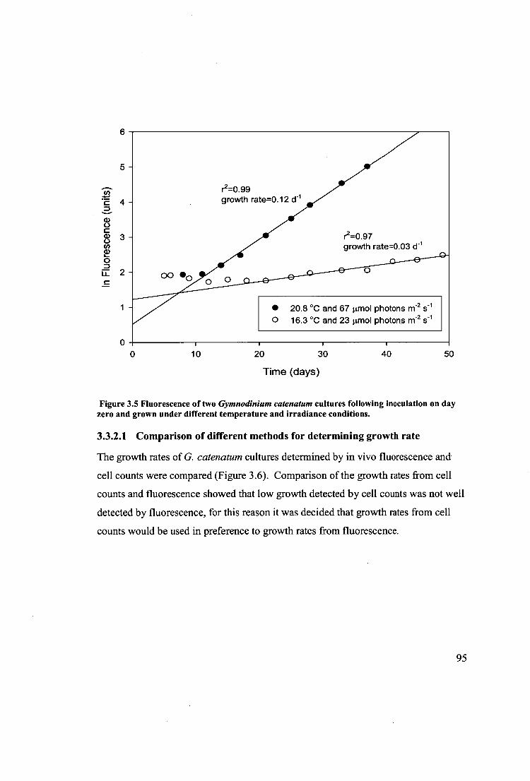
r2=0.99 growth rate=0.12 c1 -1 E4

a)

• 20.8 °C and 67 [tmol photons rn-2 S-1 0 16.3 °C and 23 Arno' photons 1112 S-1

00 •

a) 3 - c..) 92

r2=0.97 growth rate=0.03 d -1

0

10 20 30

40

50

Time (days)

Figure 3.5 Fluorescence of two Gymnodinium catenatum cultures following inoculation on day zero and grown under different temperature and irradiance conditions.

3.3.2.1 Comparison of different methods for determining growth rate

The growth rates of G. catenatum cultures determined by in vivo fluorescence and

cell counts were compared (Figure 3.6). Comparison of the growth rates from cell

counts and fluorescence showed that low growth detected by cell counts was not well

detected by fluorescence, for this reason it was decided that growth rates from cell

counts would be used in preference to growth rates from fluorescence.

95

0.30

0.25

0.20

Gro

wth

Rat

e (c

1-1) (

flour

esce

nce)

0.15

0.1 0

0.05

0.00

-0.05

-0.10

•

8 Ses,

• • • •

• 4110 •

.5• • •ii •

i• • • •••

e .1 .. •-•

• •

0

-0.10 -0.05 0.00 0.05 0.10 0.15 0.20 0.25 0.30

Growth Rate (d -1 ) (cell count)

Figure 3.6 Comparison of growth rate by cell counts and growth rate by fluorescence of Gymnodinium catenatum.

3.3.2.2 Growth vs. irradiance curves

Growth versus irradiance curves were constructed using data from cultures gown at

11.9, 13.4, 15.5, 16.3, 18.2, 18.9, 20.7, 21.1, 22.8, 23.0, 24.9 and 25.2 °C. Within

each temperature there were six different irradiances ranging from 4 to 283 gmol

photons 111-2 S-1 . Growth versus irradiance curves were constructed using growth

rates calculated from cell counts. The modified model developed by Platt et al.

(1975) (Equation 2) describes the majority of the data well (Figure 3.7). From the

96

growth versus irradiance curves several parameters with physiological significance

can be determined: maximum growth rate (u max), initial slope (a), irradiance

coefficient (Ek) and compensation irradiance (E c). The parameters for each of the

growth versus irradiance curves at each temperature are given in Table 3.2. The

parameters of the growth versus irradiance curves ( umax, a, Ek and Ec) will be

examined individually with respect to temperature in sections 3.3.2.3 to 3.3.2.6.

There are several instances where parameters of the model at particular temperatures

have not been included in figures. This is because there was not enough data to

describe these parameters accurately, evidenced by large standard errors associated

with these parameters in most cases. The parameters that have been excluded at

particular temperatures are marked with an asterisk in Table 3.2.

The greatest observed growth rate in this experiment was 0.236 d -1 and occurred at 23

°C and 203 umol photons IT1-2 s-I (Figure 3.7). However it is important to note that at

24.9 and 25.2 °C growth rates showed little or no saturation even at irradiances

greater than 200 urnol photons m -2 s -1 . Also the model (Equation 2) could not be fit

to the 11.9 °C data because only one culture grew (0.021 Cr ' ) in this treatment at an

irradiance of 175 umol photons m-2 s -1 .

97

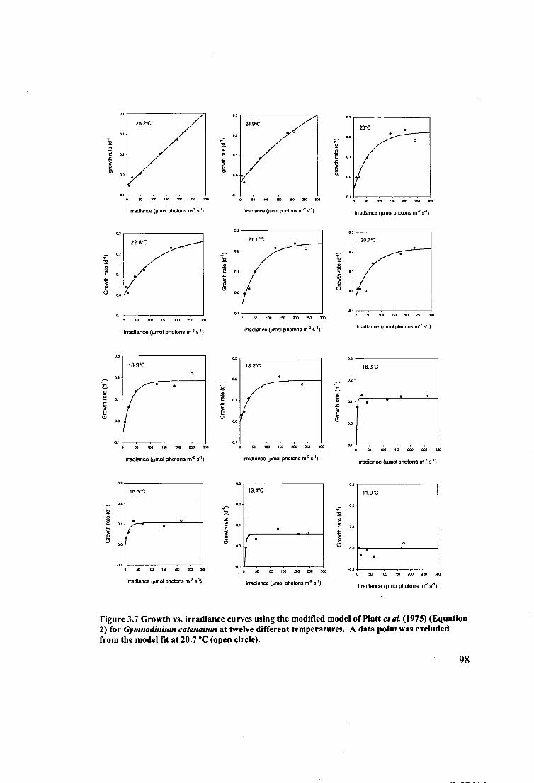
0.3

25.2°C

-0 1

•

0 50 100 150 NO

250 300

irradiance (pmol photons m -2 s-5 )

15.5°C

• *

0.3

24.9°C

02

0. 1

00

.0 1 0 50 103 150

200

250 300

imsdLsnce (pmol photons re s'')

03

0 0

0 50 100 150 2C0 250 300

irradiance ((ono' photons M2 s")

Gro

wth

rate

(d-')

G

row

th ra

te (e

)

02

0.1

0.0

3

2

0.3

0 3

0.3

2

(.9

•F--o 2 2

2

2

0.0

-0.1

21.1 °C

•

•=— -o

2 (D

03

0

OD

20.7°C

50 100 150 200 250 300

irradiance (13mol photons m-2 s -1 )

0 50 100 150 200 250 303

irradiance (prnol photons rn -2 s")

0 50 1CO 250 bo

irradiance (pmol photons rn.2 5')

18.9°C

o.

18.2°C 16.3°C

0

• • •

•0.1 O.1 0 Yo 100 150 210 250 3% 0 50 100 150 200 250 300

Gro

wth

rate

(e)

0.5 50 100 150 200 250 303

Gro

wth

rate

(d-')

0.3

0 2

01

0 0

irradiance ((.1mol photons M-2 3.1 )

0 50 100 150 200 250 300

irradiance (prnol photons m-2 5")

irradiance (limo! photons m -2 5 -1 )

0.3

13.4°C

0.2

E 0.1

0.0

-0.1 0 50 103 150 200 250 300

irradiance (pmol photons ni 2 s')

irradiance (pmol photons ni 2 s')

0.3

11.9°C

02

2 0

.c

2

-0.1 0

50

100

irradiance (1..(mol photons M-2 S-' )

150 200 250 300

Figure 3.7 Growth vs. irradiance curves using the modified model of Platt et al. (1975) (Equation 2) for Gymnodinium catenatum at twelve different temperatures. A data point was excluded from the model fit at 20.7 °C (open circle).

98

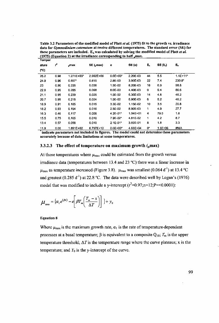
Table 3.2 Parameters of the modified model of Platt et al. (1975) fit to the growth vs. irradiance data for Gymnodinium catenatum at twelve different temperatures. The standard error (SE) for these parameters are included. Ek was calculated by solving the modified model of Platt et al. (1975) (Equation 2) at the irradiance corresponding to half umax. Temper

ature r2 max SE („max) a SE (a) E. SE (E.) Ek

(°C)

25.2 0.98 1.271E+03* 2.992E+06 0.0E+00* 2.20E-03 44 5.5 1.1E+11*

24.9 0.96 0.557* 0.615 2.8E-03 3.90E-03 22 7.4 230.8*

23 0.90 0.226 0.036 1.5E-02 8.20E-03 16 6.9 98.8

22.8 0.95 0.285 0.068 8.0E-03 4.40E-03 0 9.4 86.6

21.1 0.95 0.239 0.025 1.5E-02 5.30E-03 14 4.8 46.2

20.7 0.95 0.218 0.024 1.5E-02 5.90E-03 6 5.2 46.2

18.9 0.91 0.185 0.015 3.3E-02 1.15E-02 10 3.5 20.8 18.2 0.93 0.194 0.016 2.5E-02 8.90E-03 1 4.9 27.7

16.3 0.46 0.117 0.008 4.3E-01* 1.04E+01 4 79.0 1.6 15.5 0.75 0.105 0.010 7.9E-02* 4.81E-02 1 4.2 8.7 13.4 0.57 0.058 0.010 2.1E-01* 3.60E-01 8 1.8 3.3

11.9 0.00 1.891E+02 6.797E+10 0.0E+00* 4.68E+04 0* 1.6E+06 #N/A * indicate parameters not included in figures. The model could not determine these parameters accurately because of data limitations at some temperatures.

3.3.2.3 The effect of temperature on maximum growth (max)

At those temperatures where J.tmax could be estimated from the growth versus

irradiance data (temperatures between 13.4 and 23 °C) there was a linear increase in

!A max as temperature increased (Figure 3.8). !Amax was smallest (0.064 (1 -1 ) at 13.4 °C

and greatest (0.285 d -1 ) at 22.8 °C. The data were described well by Logan's (1976)

model that was modified to include a y-intercept (r 2=0.97;n=12;P=<0.0001):

max = fot i e (flx ) - e[fiT ( 7' "1 - 111+ ° m AT Y

Equation 8

Where 'Lima), is the maximum growth rate, al is the rate of temperature-dependent

processes at a basal temperature; 13 is equivalent to a composite Q i 0; T,„ is the upper

temperature threshold; AT is the temperature range where the curve plateaus; x is the

temperature; and Yo is the y-intercept of the curve.

99

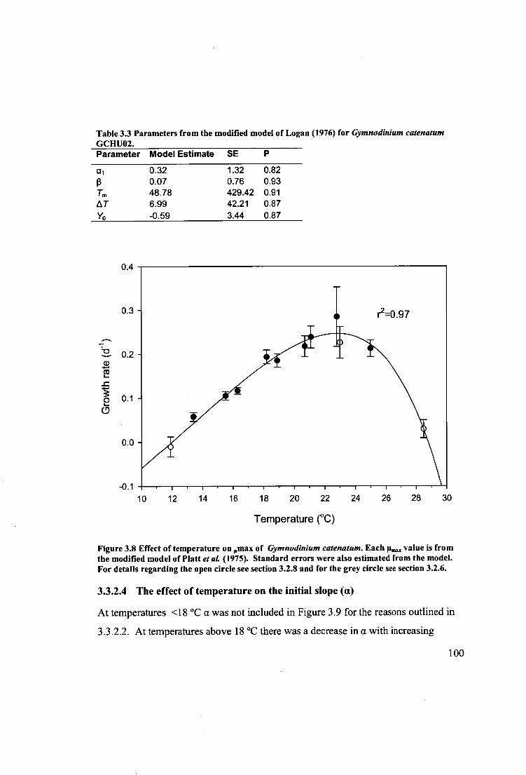
0.4

-0.1

0.3 -

0.2 -

0.1 -

0.0 -

Table 3.3 Parameters from the modified model of Logan (1976) for Gymnodinium catenatum GCHUO2. Parameter Model Estimate SE P

al 0.32 1.32 0.82 13 0.07 0.76 0.93 T,„ 48.78 429.42 0.91 AT 6.99 42.21 0.87 Yo -0.59 3.44 0.87

a) 2 _c "5 P_ 0

10 12 14 16 18 20 22 24 26 28 30

Temperature (°C)

Figure 3.8 Effect of temperature on umax of Gymnodinium catenatum. Each urnaz value is from the modified model of Platt et aL (1975). Standard errors were also estimated from the model. For details regarding the open circle see section 3.2.8 and for the grey circle see section 3.2.6.

3.3.2.4 The effect of temperature on the initial slope (a)

At temperatures <18 °C a was not included in Figure 3.9 for the reasons outlined in

3.3.2.2. At temperatures above 18 °C there was a decrease in a with increasing

100

temperature. The data had an r2=0.81 when fitted with a linear model, y=0.096+-

0.0038x (n = 7, P =0.0056).

0.05

0.04 -

0.03 -

d 0.02 -

0.01 -

0.00 -

-0.01

r2=0.81

16 18 20 22 24 26

Temperature (°C)

Figure 3.9 Effect of temperature on a of Gymnodinium catenatum. Each a value is from the modified model of Platt et al. ((1975)). The standard error for a was estimated from the model.

3.3.2.5 The effect of temperature on irradiance co-efficient (Ek)

The half-saturation co-efficient for growth as a function of irradiance (Ek) was

estimated by solving (using the Solver add-in provided with Microsoft Excel) the

modified model of Platt etal. (1975) (see Equation 2) for the irradiance at half the

estimated iimax . Ek increased with increasing temperature (Figure 3.10). The lowest

Ek, 1.6 ttrnol photons m -2 s -1 was at 16.3 °C and the highest Ek, 98 imol photons m 2 S -

I at 22.8 °C. The exponential model y=0.035exp°34x (r2=0.98, n = 8, P0.0001)

described the Ek data very well.

101

160

140 -

120 -

100 -

LIZ 80 -

60 -

40 -

20 -

• 18 20

Temperature ( °C)

14 16 22 24

Figure 3.10 The effect of temperature on the half-saturation co-efficient for growth as a function of irradiance (E k) for Gymnodinium catenatum. Ek was calculated from the model of Platt, Denman et al. (1975)

3.3.2.6 The effect of temperature on compensation irradiance (E,)

The compensation irradiance (Ec) increased with increasing temperature (Figure

3.11). The highest compensation irradiance was 47 umol photons 1112 s -1 at 25.2 °C.

This trend was described well with the model y=exp'1124x (r2=0.43, n = 11, P<0.001).

The standard error at 16.3 °C is much larger than at any other temperature, because

there is only one point on the initial slope of the curve, making it difficult for the

model to estimate E, without an associated large error.

102

100

80 - ...—.

70

cl E CO 60 - C 0 0 _c 0_ Z 40 - E =.

Lu0 20 -

r2=0.43 -

I • 14 16 18 20 22 24 26 28

Temperature (°C)

Figure 3.11 Effect of temperature on E, of Gymnodinium catenatum. Each E c value is from the modified model of Platt, Denman et al. (1975) (Equation 2). The standard error for E, is also from the model.

3.3.3 Effect of high temperature and high irradiance on growth rate

Growth rates calculated from the change in fluorescence over time at 25 °C and 291

and 458 lAmol of photons 1112 s-1 were not significantly different from each other

(P<0.05). At 28.5 °C growth rates calculated from fluorescence and at 291 and 458

ptmol photons m-2 s-1 were not significantly different from (Figure 3.12).

0 12

i

103

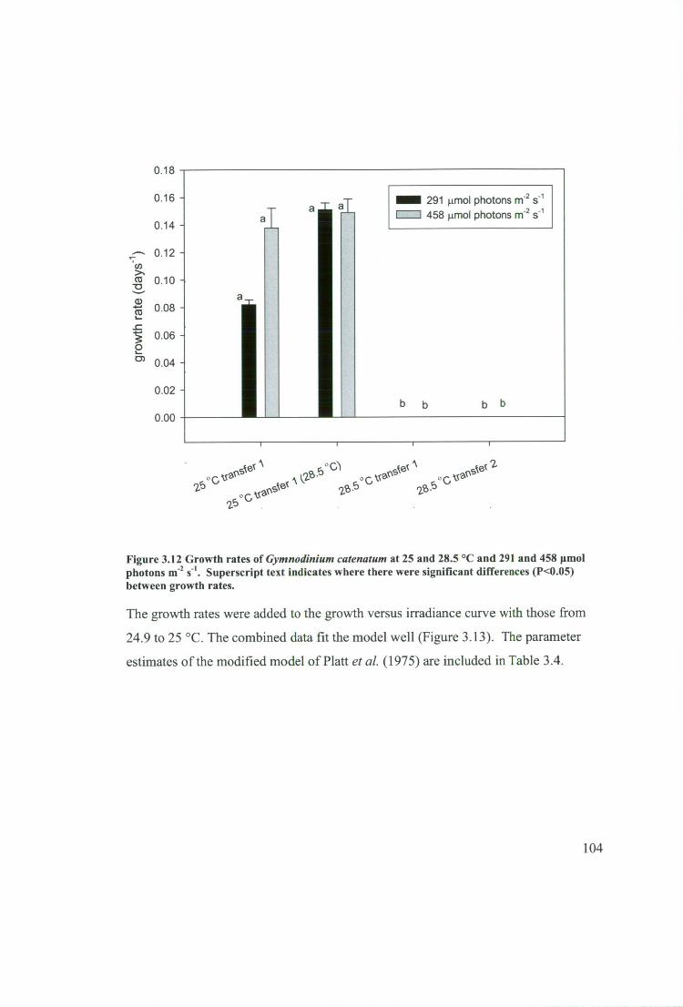
MI 291 limo' photons in-2 S-1

CI 458 prnol photons m-2 s-1 al

b b bb

a a

0.18

0.16

0.14

— 0.12

al -cs 0.10

ct) 0.08

_c -5 0.06 2

0.04

0.02

0.00

,00) 9{0 1 ,oskev A JO '2- oG vs A (2.15 P 0 r. veal .0 ,0115 "

2.5 skel .0 vall

'Lb

Figure 3.12 Growth rates of Gymnodinium catenatum at 25 and 28.5 °C and 291 and 458 umol photons 1112 1 1 . Superscript text indicates where there were significant differences (P<0.05) between growth rates.

The growth rates were added to the growth versus irradiance curve with those from

24.9 to 25 °C. The combined data fit the model well (Figure 3.13). The parameter

estimates of the modified model of Platt etal. (1975) are included in Table 3.4.

104

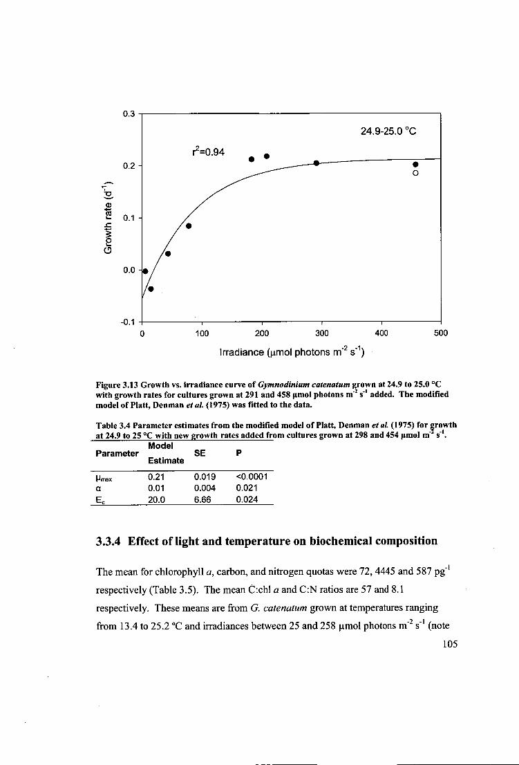
2 0

0

100 200 300

400

500

Irradiance (tmol photons r112 s-1 )

Figure 3.13 Growth vs. irradiance curve of Gymnodinium catenatum grown at 24.9 to 25.0 °C with growth rates for cultures grown at 291 and 458 pmol photons In-2 S-1 added. The modified model of Platt, Denman etal. (1975) was fitted to the data.

Table 3.4 Parameter estimates from the modified model of Platt, Denman et aL (1975) for growth at 24.9 to 25 °C with new growth rates added from cultures grown at 298 and 454 pmol m -z s-i .

Model Parameter SE P

Estimate

Pmax 0.21 0.019 <0.0001 a 0.01 0.004 0.021 Ec 20.0 6.66 0.024

3.3.4 Effect of light and temperature on biochemical composition

The mean for chlorophyll a, carbon, and nitrogen quotas were 72, 4445 and 587 pg -1 respectively (Table 3.5). The mean C:chl a and C:N ratios are 57 and 8.1

respectively. These means are from G. catenatum grown at temperatures ranging

from 13.4 to 25.2 °C and irradiances between 25 and 258 umol photons m -2 s1 (note

105

cultures grown at <25 mole of photons m- 2 sl across all temperatures were not

included in these biochemical quotas; see section 3.2.9).

Table 3.5 Mean biochemical quotas of Gymnodinium catenatum grown at temperatures ranging from 13.4 to 25.2 °C and irradiances between 5 and 280 gmol photons In-2 S-I .

Chl a quota (pg ce11 -1 ) (n=42)

C quota (pg ce11 -1 ) (n=41)

N quota (pg cell"") (n=41)

C:Chla (n=40)

C:N (n=40)

Mean 72 4445 587 57 8.1 S.E. 3.1 551.5 85.7 4.2 0.42 CV (%) 28 80 95 47 33

Table 3.6 Temperature range and number of cultures in each binned temperature group. Binned temperature groups were used to examine the trends in biochemical composition with temperature and irradiance. Binned temperature

Temperature range included (°C)

Number of

cultures (°C)

25 24.7-25.5 7 22.9 22.8-23.3 8 20.9 20.8-21.3 7 18.5 18.2-18.9 8 15.9 15.4-16.4 7 13.4 13.3-13.5 4

To examine trends in carbon and chlorophyll a, similar (A temp. z 1 °C) temperature

groups were binned together (Table 3.6). This did not occur at the lowest

temperatures 11.9°C and 13.4 °C where there were only four cultures which were

sampled for chla and carbon and all grown at 13.4 °C. Both carbon cell' (carbon

quota) and chlorophyll a ce11 -1 (chla quota) show an exponential decrease as

irradiance increased in both 25 and 22.9 °C binned temperature groups (Figure 3.14).

The carbon and chla quota range from 1979 to 11069 pg cell' and 61 to 132 pg cell'

respectively at 25 °C and from 2050 to 8153 pg cell - ' and 52 to 108 pg cell -I respectively at 22.9 °C. At 25 °C the 5.6 fold decrease in carbon with increasing

temperature is much larger than the 2 fold decrease in chla. Similarly at 22.9 °C the

difference in magnitude decrease for carbon and chla quotas were maintained: a

larger 4 fold decrease in carbon quota and only a 2.1 fold decrease in chla quota.

106

With the exception of a slight decrease in carbon quota with increasing irradiance at

15.9, 18.5 and 20.9°C the carbon and chl a quotas did not exhibit a clear decrease

with increasing irradiance as at the higher temperatures. At 15.9, 18.5 and 20.9 °C,

95.2 % of carbon quotas are all <5000 pg cell', or considerably lower than at the

higher temperatures and lower irradiances. At 15.9, 18.5 and 20.9 °C, 82.6 % chla

quotas ranged between 50 to 100 pg At 13.4 °C the carbon quotas were

greatest, between 7000 and 9000 pg at the two intermediate irradiances. At the

lowest and highest irradiances the carbon quotas were reduced to values between

5000 and 7000 pg cell) . The chl a quota at 13.4 °C was approximately 50 pg

across the different irradiances with the exception of a slight increase in chla at the

lowest irradiance (50 pimol photons M-2 S -1 ).

107

carbon and chla m

eas urements, the

analysis of t rends was also statistically

weak.

To

improve this situation the d ata

sets were bi nned again

as in T able 3.6. O

ut of the

six

8 00

• 0

• 0 • 0

n.) N - (v

s z.w

suoi

Nd lo

wrI

) ap

uepe

.ui

(1.s

z.iu

suoi

oyd

pug

() eo

uep

aul

(vs w

suolo

yd low

() ao

uepa

ui

• 0 • 0

0 •

• 0

OD

cri 00

• 0

• 0 • 0:0

C.n

8

(,.s

w s

uolo

yd p

url)

eou

epeu

i

(vs

z_Lu

suop

qd lo

w()

epu

elpa

ui

00 .7

0

• 0 • 0

• 0

a

• 0

• 00 Co

0 • 8 - • 0

(1.s z.

111

SUO

IOLI

d 10

1.11r

1)

03U

BW

RI.1

1

• 0

8

• 0

•0.

• 0

• o

4:)0 0

0 •

0 •

A

4. m .4 et .....

CD 42 IC

0 CD 0 0

,-t Pt Pt

CA A rLt er:.

•co 1.e)

co ao ■—■ .-t

r).. (-D oe •Ia• et

A 0 cot ril PP1

Er f". Pi e5

U G.'

PO CA r.i . 2, .-.. .4

0 < = '1

CD fa 7 1.2 eV 1:11.

.—• 0. ri

'Li AD pt. 0 et f,

'1:3 S ep CM 0 V c

co -I

"—: cn !It n <.1 0

l) 0t,

W e

. CeCi et ■-•

'a' Fir Cr

0 ...- C 14 ■-••

CD "0 4 r =

17 14 0

fa. ...t. (A 0 ..b

C) 0

p ag ,.,

,-• • C)

■-■J co

< ,t_

CD co 0 = , a

0- '0 CD CD

< P to

1:0 14 • & ...

et

too cO

a 0

■-• •

`'.• CD X

E • 03 AD Pt et

Cr C

,a • "0

0 CD r et

CD 0. 0 0

Carbon (pg celr 1 )

g

Chia (pg celr l )

Carbon (pg celr 1 )

Carbon (pg

Chia (pg

Carbon (pg celr l )

g g

Chia (pg Chia (pg

Carbon (pg me)

g

Chia (pg celr l )

Carbon (pg celr i )

A Chla (pg celr l )

binned temperature groups, only the 25 °C binned temperature group had a slope (-

0.212) significantly different from 0 (r2=0.58; n=7; P=0.046). However, trends were

apparent; the strongest trends were at temperatures of 25, 20.9 and 15.9 °C which had

the highest r2 values of 0.58, 0.41 and 0.29 respectively. The slopes of the regressions

were all negative at the higher temperatures (25, 22.9 and 20.9 °C) and the negative

slope decreased as temperature decreased until the slope of the C:chla versus

irradiance became positive for the lower temperature groups (18.5, 15.9 and 13.4 °C).

The complex interaction between irradiance and temperature on C:chla (Figure 3.15)

can be simplified by considering only the effects of the highest irradiances. At

irradiances >200 ptmol photons ni2 s -1 there was an exponential decrease in C:chla as

temperature increased (Figure 3.16). A linear model was fitted to the natural log of

this data and the slope (-0.095 +1- 0.0157) and y-intercept (6.1 +1- 3.33) were both

significantly different from 0 with respective P values of<0.0001 and <0.0001.

109

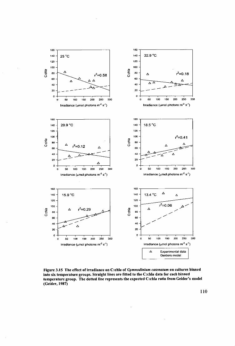
160

140 — 22.9 °C

120 —

100 — CD

▪ 80 -0

—

60

A r2=0.18

40

20

50 100 150 200 250 300

Irradiance (p.mol photons r11-2 s 1 )

160

140 —

120 —

100 — CD

9

▪

80

60 —

40 —

20 —

0 O 50 100 150 200 250 300

Inadiance (p.mol photons m -2 s-1 )

300 0 50 100 150 200 250

CD A

Irradiance (pmol photons nf 2 S-1 )

0 50 100 150 200 250 300 0 50 100 150 200 250 300

Irradiance (gmol photons fr1-2 s 1 )

O 50 100 150 200 250 300

Irradiance (p.aml photons m -2 S-1 ) Irradiance (p.mol photons m-2 s-1 )

r2=0.06 80—

60 —

40 —

20 —

160

140 —

120 —

100 —

20.9 °C

r2=0.12

A A---

160

140 —

120 —

100 —

80 —

60 —

40 —

A 20

160

140 —

120 —

100 —

160

140

120

100 co 0

▪

80 0

60

40

20

0

13.4 °C

A Experimental data Geiders model

Figure 3.15 The effect of irradiance on C:chla of Gymnodinium catenatum on cultures binned into six temperature groups. Straight lines are fitted to the C:chla data for each binned temperature group. The dotted line represents the expected C:chla ratio from Geider's model (Geider, 1987)

110

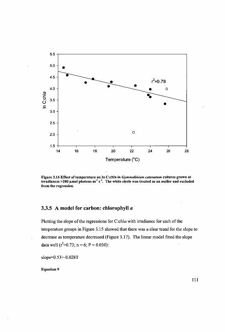
5.5

5.0 -

4.5 -

4.0 -

• •

• • r2=0.78 • •

• o

•

•

2.5 -

2.0 - 0

1.5 14 16 18 20 22 24

26

28

Temperature (°C)

Figure 3.16 Effect of temperature on In C:chla in Gymnodinium catenatum cultures grown at irradiances >200 gmol photons In-2 s-I . The white circle was treated as an outlier and excluded from the regression.

3.3.5 A model for carbon: chlorophyll a

Plotting the slope of the regressions for C:chla with irradiance for each of the

temperature groups in Figure 3.15 showed that there was a clear trend for the slope to

decrease as temperature decreased (Figure 3.17). The linear model fitted the slope

data well (r2=0.73; n = 6; P = 0.030):

slope=0.53+-0.028T

Equation 9

111

Where T= temperature and the slope is the slope of the C:chla relationship with

irradiance at that temperature.

0.6

r2=0.73

0.4 -

0.2

Th

0.0 -

-0.2 -

-0.4 12 14 16 18 20 22 24 26

Temperature (°C)

Figure 3.17 The effect of temperature on m(slope) of the line fit to C:chla vs irradiance for Gymnodinium catenatum binned into six temperature groups (data from Figure 3.15).

The y-intercept for each of the lines fitted to the C:chla versus irradiance in Figure

3.15 were plotted against temperature (Figure 3.18) and were described well with this

equation (r2 = 0.88; n = 6; P =0.041):

y-intercept=430+-42T+1.14T 2

Equation 10

where T = temperature and y intercept is the y-intercept of the C:chla versus

irradiance relationship at the temperature specified.

112

100 -

120

-20 12 14 16 18 20 22 24 26

Temperature ( °C)

Figure 3.18 The effect of temperature on the y-intercept of the line fitted to C:chla vs. irradiance for Gymnodinium catenatum binned into six temperature groups (data from Figure 3.15).

From these sub-models it is possible to create an overall model that describes the

effect of temperature and irradiance on C:chla by substituting Equation 9 and

Equation 10 into a linear model equation and adding an irradiance term. The

parameters of the model were refined using an algorithm for least-squares estimation

of nonlinear parameters (Marquadt, 1963). The model is:

C : chla = (0.76 + (-0.036T)/) + (516 + (-48T) +1.19T')

Equation 11

Where T= temperature and I =Irradiance.

The model is presented on three dimensions and the observed data are also included

in Figure 3.19. C:chla ratios were greatest (up to 143.3) at low temperature ez 14

113

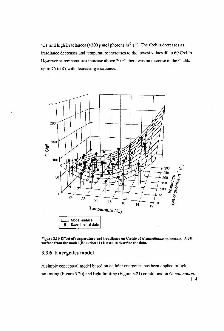
200

150 co

ci 100

50

yr-N. 300 'co

250 c)' a) E

200 c.)

150 . (13

100 Lc? .R 50

0

24 22 20 18 16

Temperature (°C) 14 12

250

°C) and high irradiances (>200 p.mol photons r11-2 S-1 ). The C:chla decreases as

irradiance decreases and temperature increases to the lowest values 40 to 60 C:chla.

However as temperatures increase above 20 °C there was an increase in the C:chla

up to 75 to 85 with decreasing irradiance.

I= Model surface • Experimental data

Figure 3.19 Effect of temperature and irradiance on C:chla of Gymnodinium catenatum. A 3D surface from the model (Equation 11) is used to describe the data.

3.3.6 Energetics model

A simple conceptual model based on cellular energetics has been applied to light

saturating (Figure 3.20) and light limiting (Figure 3.21) conditions for G. catenatum. 114

The results from the conceptual energetics model of G. catenatum describe the

response of G. catenatum growth (modelled using G. catenatum growth vs. irradiance

curves) well.

Input data for the maintenance costs used in the model comes from the estimates of

Ec from each growth versus irradiance experiment at each temperature. These were

shown to have an exponential relationship with temperature. Growth rates were

simply 1.ima, values from each temperature. The relationship between capital costs and

temperature were derived from the 'IF shaped carbon quota versus temperature data.

115

Energy input Maintenance cost Capital cost g (Energy model)

(Logans model)

o ptmax (Present study)

• lc (limol photons m-2 s-1 ) • C quota (pg)

0.8

0.7

0.6

0.5

0.4 '7

a)

0.3 _c 2

0.2

0.1

0.0

-0.1

-0.2 10 12 14 16 18 20 22 24

26

28

30

Temperature ( °C)

Figure 3.20 Model of temperature effect on energetic costs for Gymnodinium catenatum in light saturated (1000 umol photons m -2 s-1 ) conditions

116

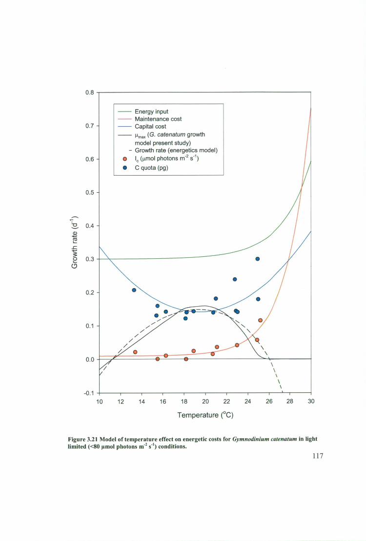
0.8

0.7 -

0.6 -

— Energy input Maintenance cost — Capital cost — tim„ (G. catenatum growth

model present study) - Growth rate (energetics model)

• l c (i.tmol photons m-2 s-1 ) • C quota (pg)

0.5 -

a) 2

..c

0.2 -

0. 1 -

0.0

-0.1

•

10 12 14 16 18 20 22 24 26 28 30

Temperature ( °C)

Figure 3.21 Model of temperature effect on energetic costs for Gymnodinium catenatum in light limited (<80 pmol photons It1-2 S-1 ) conditions.

117

3.4 Discussion

3.4.1 Effect of temperature and irradiance on Gymnodinium

catenatum growth

Growth rates of G. catenatum grown in culture at temperatures ranging from 11.9-

25.2 °C and irradiances ranging from 5 to 283 gmol photons m -2 s-I are presented in a

contour plot providing a visual summary of all the growth rate data collected in this

experiment (Figure 3.22). The greatest growth rates of >0.2 d -I occurred at

combinations of temperatures between 20 to 25 °C and irradiances >140 gmol

photons 111-2 s1 . There were also two areas where growth rates were <0 d 1 : where

temperature was 11.9 °C and irradiance was <150 gmol photons Tr1-2 S 1 and where

temperature was >23 °C and irradiances were <35 gmol photons m -2 s-I .

The physiology of G. catenatum will be discussed through examining the effect of

temperature on the parameters of the growth vs. irradiance curve and effect of

temperature and irradiance on the biochemical composition of this species.

118

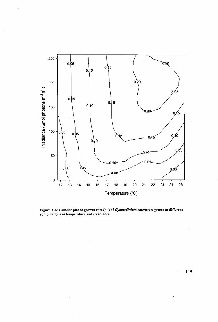
250

200 ....■ 7

Cl) ci E Cl) c o 150 o _c 0_

75 E = a) C) 100 c CO

15 CO ,_ _

50

12 13 14 15 16 17 18 19 20 21 22 23 24 25

Temperature (°C)

Figure 3.22 Contour plot of growth rate (d-1) of Gymnodinium catenatum grown at different combinations of temperature and irradiance.

119

3.4.2 Effect of temperature on parameters of the growth vs.

irradiance curve

3.4.2.1 Maximum growth rate (u max)

Effect of temperature on Amax

The iimax increased linearly with temperature for G. catenatum in this study. The

reason that Logan's (1976) model fit the data well (r2=0.97) where none of the

parameters are statistically significant is because Logan's model was made to fit

exponential increases in tt max with temperature. However, clearly the data increased

linearly up to the greatest il max in this study. This result contrasts with several other

studies that show that g max increases exponentially with temperature (Li & Morris,

1982, Ojala, 1993, Eppley, 1972). Montagnes etal., (2003) provide some examples

of linear increases in g max and argue that in the majority of cases Ilmax increases

linearly with temperature. But as pointed out by Thompson (Thompson, 2006) it is

likely that what appears as linear relationships may in reality be exponential. This is

because in many cases only a small temperature range has been examined, or

experimental artefacts are caused by limiting light at high temperatures or the failure

to measure growth at the temperature where IAmax is greatest (because of the abrupt

transition from the greatest g max to temperatures that cause death for many

phytoplankton).

Unfortunately the majority of alternative studies examining temperature and growth

rate in G. catenatum did not use a sufficient range of temperatures to determine what

kind of relationship there is between resource saturated growth rate and temperature

(Blackburn etal., 1989, Ellegaard et al., 1993, Yamamoto et al., 2002). Additionally,

of the studies that have enough data to evaluate this relationship, the growth rates

from Band-Schmidt et al. (2004) show a linear function of temperature while Bravo

and Andersen (1994) provide results which appear exponential for the temperatures

120

up to 16°C. Therefore, existing studies show it is not possible to generalise about the

exact nature of the relationship between resource saturated growth and temperature

for this species. The GCHUO2 strain examined in the present study showed a strong

linear increase in umax with increasing temperature. A linear increase hi unax is likely

to be a disadvantage in competition with the many phytoplankton species that have

exponential increases in u max (Li and Morris, 1982; Ojala, 1993)

Greatest Amax

The greatest growth rates measured for G. catenatum in this study (>0.2 d-i ) occurred

in cultures grown at temperatures from 20 to 25 °C and at irradiances ;450 to 250

umol photons TI1-2 Earlier studies are similar in that the highest growth rates occur

at temperatures >20 °C with the exception of Blackburn et al. (1989) where the

growth rate of the Huon Estuary strain GCHUO1 peaked at 17.5 °C and decreased

quickly after 20 °C (Figure 3.23).

1.tma,, is the parameter of growth versus irradiance curves that indicates where growth

is at a maximum, i.e. where growth rate no longer continues to increase with

increasing irradiance. Because, of the scarcity of other !A max values in the literature

for G. catenatum. The results from the present study will be compared with growth

rates from other studies (Figure 3.23), where irradiances are assumed to be excess to

the requirements of G. catenatum. The conditions used in each of the other studies

are included in Table 3.7. However, these assumptions based on other species may

not always be accurate, particularly at extremes of temperature. At the highest

temperature (25.2 °C) used in the initial study, growth was a linear function of

irradiance up to 250 umol photons 1112 s no indication of saturation. In a

subsequent experiment, cultures were exposed to a temperature of 25 °C and higher

irradiances (291 and 458 umol photons ni 2 s -1 ). Growth rates at these higher

irradiances were slightly lower than those at 208 umol photons I11-2 s- indicating that

growth was saturated at < 291 ttmol photons m -2 s.

121

These results indicate that in several studies light may have been limiting growth at

higher temperatures and thus these may not be entirely accurate resource saturated

growth rates. The fact that light requirements increase quickly at higher temperatures

is evident in the exponential relationship between I sat or Ek and temperature (Collins

& Boylen, 1982). In the present study irradiances of z25 ilmol photons m -2 s-1 saturated growth at 13.4 °C, but in excess of 250 gmol photons T112 s -1 was required to

saturate growth at temperatures greater than 23 °C. Given the nonlinear nature of the

increase in irradiance required to saturate growth with increasing temperature it is

difficult to choose an irradiance that will saturate growth as temperature increases.

One way of avoiding light limitation in experiments investigating resource saturated

growth at a range of temperatures is to set the irradiance at >2Ek at the highest

temperature. In this case irradiance will be in excess of requirements at the lower

temperatures. However by setting the irradiance at >2Ek of the highest temperature,

the risk of exposing the cells to levels of irradiance they cannot tolerate at lower

temperatures appears. The cells will either have to employ strategies to ameliorate the

effect of the excess irradiance, or are likely to suffer photo damage - both of which

will impact on growth rate negatively.

Temperature limits for growth

The poor growth response at 11.9 °C indicates that this is the lower temperature limit

for growth in this strain of G. catenatum.lt is clear that temperature was limiting

growth response because irradiance had little effect (only one culture grew at 0.021 d -1 in this treatment at irradiance of 175 gmol photons T11-2 s-1 ). Growth for GCHUO2

was within the range of lower temperature limits reported by earlier studies

(Ellegaard et al., 1993, Band-Schmidt et al., 2004, Bravo & Anderson, 1994,

Yamamoto et al., 2002, Blackburn et al., 1989) in which growth ceased at

temperatures ranging from 9 to 12.5 °C.

At 28.5 °C, G. catenatum growth rates calculated from fluorescence were not

significantly different from zero. The Spanish strain ( from water temperatures rarely

122

exceeding 20 °C) also showed growth rates of that decreased very quickly to near 0 d -growth rates at temperatures close to 28.5 °C (Blackburn et al., 1989, Bravo &

Anderson, 1994), and the Australian GCHUO1 strain examined by Blackburn, et al.

(1989) had a growth rate close to 0 eat 25 °C. Other strains isolated from Japan and

Mexico (where water temperatures can reach 28 °C in Japan and in excess of 28 °C in

Mexico) exhibited growth rates > 0.2 d -1 at 28.5 °C and still had relatively high

growth rates at 30 °C (Band-Schmidt et al., 2004, Yamamoto et al., 2002). The

ability of these two strains to grow better at higher temperatures may indicate there

are ecotypes of G. catenatum better suited to sub-tropical water temperatures within

the G. catenatum complex. The G. catenatum strain isolated from cysts in the

sediments near Island Hven in Denmark showed growth rates similar to the other

strains at temperatures from 10-15 °C but exhibited growth similar to the Mexican

and Japanese strain at 28.5 °C. The Spanish strain (Bravo & Anderson, 1994) was

similar to all other strains at temperatures from 10-15 °C, above 20 °C growth rates of

this strain are greater than all the other strains.

While growth rates were negligible at 28.5 °C and 291 and 458 gmol photons /71-2 s-i ,

in the present study the majority of cells were still motile and appeared

morphologically normal at the end of the experiment (characteristics expected from

healthy cultures of G. catenatum). It appears the cultures were able to acclimatise

sufficiently to the temperature extreme, but that under these conditions no growth

(measured by the fluorescence method) was observed

123

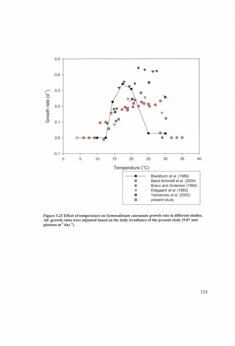
35 40 30 5 10 15 20 25

0.5

0.4 -

0.3 -

0.2 -

0.1 -

0.0 -

-0.1 0

Gro

wth

rate

(d-1)

Temperature ( °C)

-0- Blackburn etal. (1989) • Band-Schmidt et al. (2004) • Bravo and Andersen (1994) • Ellegaard etal. (1993) • Yamamoto et al. (2002) • present study

Figure 3.23 Effect of temperature on Gymnodinium catenatum growth rate in different studies. All growth rates were adjusted based on the daily irradiance of the present study (9.07 mol photons 111-2 day -1 ).

124

GSe 28 9.07

12:12

10:14

14:10

16:8

12:12

14:10

GPM mod

F2 mod

K

GPM mod

26 6.48

30 8.28

N/A 7.56

28 8.64*

F2 mod 30

7.77

Table 3.7 Conditions for different experiments on effect of temperature on growth rate of Gymnodinium catenatum.

Study Strain Isolation

location Medium

Irradiance

Salinity (mol photons

m -2 day-1 )

Light:

dark

cycle

Blackburn et al. (1989)

Band-Schmidt et al. (2004)

Bravo and Andersen (1994)

Ellegaard et al. (2002)

Yamamoto et al. (2002)

Present study

GCHUO1

GCCV10

Not Specified

Not Specified

Not specified

GCHUO2

Huon Estuary, Australia Bahia Concepcion , Mexico

Galicia, Spain

Island Hven, Denmark Hiroshima Bay, Japan Huon Estuary, Australia

* Irradiance N/A so used 150 pmol photons In-2 s4 as this was the lowest irradiance used in the other studies.

A comparison of growth vs. irradiance curves between the present study and

(Yamamoto et al., 2002) showed that at lower temperatures (-15 °C) g max and a were

not different between these strains. There was a difference between E„ but it is likely

that this may be an artefact of the small amount of data points on the initial slope in

both studies.

125

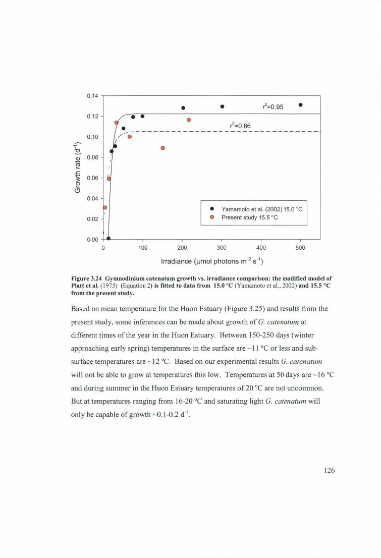
• Yamamoto et al. (2002) 15.0 °C • Present study 15.5 °C

• • r2=0.95 • • • •

• r2=0.86 z —•

•

100 200 300

400

500

0.14

0.12

0.10

0.08

-5 0.06 (L2

0.04

0.02

0.00 0

Irradiance (ptrnol photons nf2 s-1 )

Figure 3.24 Gymnodinium catenatum growth vs. irradiance comparison: the modified model of Platt et al. (1975) (Equation 2) is fitted to data from 15.0 °C (Yamamoto et al., 2002) and 15.5 °C from the present study.

Based on mean temperature for the Huon Estuary (Figure 3.25) and results from the

present study, some inferences can be made about growth of G. catenatum at

different times of the year in the Huon Estuary. Between 150-250 days (winter

approaching early spring) temperatures in the surface are —11 °C or less and sub-

surface temperatures are —12 °C. Based on our experimental results G. catenatum

will not be able to grow at temperatures this low. Temperatures at 50 days are —16 °C

and during summer in the Huon Estuary temperatures of 20 °C are not uncommon.

But at temperatures ranging from 16-20 °C and saturating light G. catenatum will

only be capable of growth —0.1-0.2 d -1 .

126

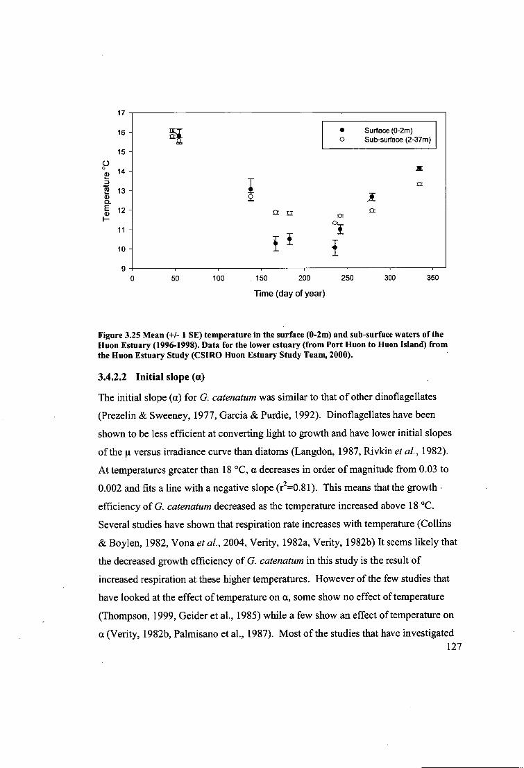
• Surface (0-2m) o Sub-surface (2-37m)

Tem

pera

ture

°C

a

9 0 50 100 150 200

250

300

350

Time (day of year)

Figure 3.25 Mean (+1- I SE) temperature in the surface (0-2m) and sub-surface waters of the Huon Estuary (1996-1998). Data for the lower estuary (from Port Huon to Huon Island) from the Huon Estuary Study (CSIRO Huon Estuary Study Team, 2000).

FI

3.4.2.2 Initial slope (a)

The initial slope (a) for G. catenatum was similar to that of other dinoflagellates

(Prezelin & Sweeney, 1977, Garcia & Purdie, 1992). Dinoflagellates have been

shown to be less efficient at converting light to growth and have lower initial slopes

of the n versus irradiance curve than diatoms (Langdon, 1987, Rivkin etal., 1982).

At temperatures greater than 18 °C, a decreases in order of magnitude from 0.03 to

0.002 and fits a line with a negative slope (r2=0.81). This means that the growth

efficiency of G. catenatum decreased as the temperature increased above 18 °C.

Several studies have shown that respiration rate increases with temperature (Collins

& Boylen, 1982, Vona et al., 2004, Verity, 1982a, Verity, 1982b) It seems likely that

the decreased growth efficiency of G. catenatum in this study is the result of

increased respiration at these higher temperatures. However of the few studies that

have looked at the effect of temperature on a, some show no effect of temperature

(Thompson, 1999, Geider et al., 1985) while a few show an effect of temperature on

a (Verity, 1982b, Palmisano et al., 1987). Most of the studies that have investigated 127

the effect of temperature on a were conducted on diatoms, chlorophytes and

cyanophytes. There are no papers that examine the effect of temperature on a in

dinoflagellates in any detail. The reason why G. catenatum exhibits an effect of

temperature on a but isn't seen in other phytoplankton groups could be that diatoms

and other groups have a much smaller respiration rate standardized to biomass, and

that changes in a due to temperature may be difficult to elucidate. In comparison,

dinoflagellates have a higher respiration rate standardized to biomass (Chan, 1978),

also evidenced by their higher compensation irradiances (Langdon, 1988). Because

of these differences in respiration/biomass the effect of temperature on a may be

more easily observed in dinoflagellates and other species that have greater

respiration/biomass.

3.4.2.3 Irradiance co-efficient (E0

Ek increased exponentially with temperature in G. catenatum. Our results were

consistent with those of Collins and Boylen, (1982) whose study on the cyanobacteria

Anabeana variabilis shows an exponential relationship between Ek and temperature.

Few other studies have investigated the effect of temperature on Ek

3.4.2.4 Compensation irradiance (E s)

Dinoflagellates exhibit some of the highest compensation irradiances (Langdon,

1987), however they also exhibit a wide range of compensation irradiances in some

cases comparable to diatoms which are considered to be one of the most efficient

classes (Langdon, 1988). The compensation irradiance in our study ranged quite low

(<1 gmol photons 111-2 s - 5, comparable to some diatoms (Yoder, 1979, Langdon,

1987, Thompson, 1999), to relatively high (>20 mol photons t11-2 S- 1) but not

unusual for dinoflagellates (Langdon, 1987, Chan, 1978). There appeared to be a

trend of increasing compensation irradiance with temperature in G. catenatum as

might be expected if the respiration rate is increasing with temperature. It has been

demonstrated (Langdon, 1988, Langdon, 1987) that E c is positively correlated with

the maintenance respiration (i.e. more energy derived from light by photosynthesis is

128

needed to match the higher respiration rate and hence the irradiance at which

photosynthesis equals the respiration rate will be higher). Increases in E c have also

been observed when a culture is acclimated to a higher irradiance prior to

determining an instantaneous photosynthesis or growth versus irradiance curve

(Iriarte & Purdie, 1993). At high temperatures respiration is increased, because

chemical processes are able to proceed at a higher rate. Under high light the base

level respiration is also increased as the cell implements strategies to protect itself

from the excess light. The present study and several others have shown that E, can

increase with temperature (Verity, 1982b, Palmisano et al., 1987) however this is not

the case in all studies (Thompson, 1999, Li & Morris, 1982, Geider et al., 1985).

Once again there is a lack of studies that examine the effect of temperature on E, in

dinoflagellates. However, it is possible that because of higher respiration rates in

dinoflagellates there is no effect of temperature in E c or that changes in E, were

significantly less and thus not detected in other more light efficient groups like the

diatoms and chlorophytes.

3.4.3 Effect of temperature and irradiance on the bio-chemical

composition of G. catenatum

Cellular energetics will be used as a framework for understanding the physiology of

G. catenatum while discussing the effect of the temperature and irradiance on

biochemical composition. Some terms and concepts described in Richardson, et al.,

(1983), including "running costs", "capital costs" and "maintenance costs" will be

used. Brief definitions of these terms are given below:

• Running costs: energy costs for running particular pathways, i.e. the AT P and

reductant input per unit net product.

• Capital costs: energy costs associated with the synthesis of catalytic and structural

cell material.

129

• Maintenance costs: energy costs associated with cell survival, i.e. re-synthesising

protein or pigments that are continually breaking down.

Running costs are not considered important for responding to energy limitation, as

biophysical and biochemical properties of organisms are very similar. However,

reducing capital and maintenance costs are considered important for phytoplankton to

adapt to energy limitation. For example, by reducing cell biomass, the cell requires

less energy to divide, because a smaller amount of cell material needs to be

synthesised, thus reducing capital costs. This also means that less cellular materials

need to be repaired and resynthesised for the cell to survive, reducing maintenance

costs.

The mean C, N and C:chla averaged across cultures grown at all temperature and

irradiances were highly variable as indicated by the co-efficient of variation of 33%

for C:N and 47% for C:chla. This indicates that there was an effect of temperature

and irradiance on the biochemical composition, caused by G. catenatum adapting to

growth over a wide range of conditions. The effect of temperature and irradiance on

the biochemical composition will be discussed in detail in the following paragraphs.

The carbon and nitrogen quota of G. catenatum in this study displayed the `1.1' shape

that has been observed in a variety of species and different groups (Goldman &

Mann, 1980, Goldman, 1977, Jorgensen, 1968, Thompson etal., 1992) including a

dinoflagellate (Nielsen, 1996) in response to temperature. Some studies have not

found this `ti' shaped response, however these may be an artefact of the temperature

range being too small or the irradiance being too high. Goldman (1977) explained this

`u.' shaped response by asserting that it was "a temperature dependent uncoupling

between growth and nutrient uptake, which is manifested as a change in cell size".

The results from this study suggest that the accumulation of carbon and nitrogen are a

response to unfavourable conditions of temperature and irradiance for growth and are

described below.

130

Growth rate of G. catenatum is < 0.1 d-1 under two different scenarios in this

experiment: when temperature drops below 16 °C, and at temperatures >20 °C and

irradiance < 100 Amol photons I11-2 s-1 . When these scenarios are examined

energetically they are quite different. While C and N are accumulated under both

scenarios, I suggest that their uses will be different because of the underlying

differences in the energy status of the cell at these different conditions.

At low temperature the cells energy demand will be lower because of reduced

respiration as indicated by the steeper initial slope and relatively low E c measured in

this study. Hence at low temperature, energy limitation is not the primary issue; but

the impaired ability of the cell to process CO2 because of the effect of lower

temperature on the enzymes responsible for this process would be explain the increase in C and N (Morris & Glover, 1974, Raven & Geider, 1988). To counter this

the cell produces more enzymes and hence this increases the C and N quotas.

At high temperature and low irradiance the cell is under severe energy limitation,

because of higher energy demands at increased temperature and not enough light to

meet those demands. In addition, the degradation of pigments and other cellular

components speeds up at higher temperatures. G. catenatum responds by increasing

quota of chla so that it can harvest more energy from the available light. It is also

suggested that the increase in carbon and nitrogen quota is related to the cell building

more chloroplast and other structures required for increasing light harvesting

capability. This would seem consistent with the low carbon and nitrogen quotas at the

same temperature but higher irradiances. If increased carbon and nitrogen quotas

were associated with thermal protection it would be expected that the quotas would

be still high when irradiance increases.

Each of these coping mechanisms related to the effects of temperature directly on the

cell or indirectly by causing energy limitation contribute to increasing both the capital

and maintenance costs of the cell. It is a testament to the adaptability of

phytoplankton to be able to maximise growth under a wide range of temperature and

131

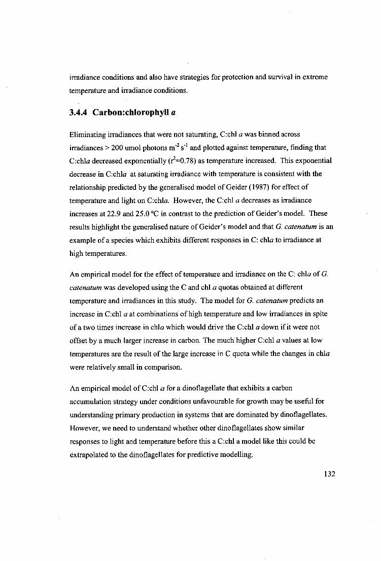
irradiance conditions and also have strategies for protection and survival in extreme

temperature and irradiance conditions.

3.4.4 Carbon:chlorophyll a

Eliminating irradiances that were not saturating, C:chl a was binned across

irradiances > 200 umol photons I11-2 s -1 and plotted against temperature, finding that

C:chla decreased exponentially ( 2=0.78) as temperature increased. This exponential

decrease in C:chla at saturating irradiance with temperature is consistent with the

relationship predicted by the generalised model of Geider (1987) for effect of

temperature and light on C:chla. However, the C:chl a decreases as irradiance

increases at 22.9 and 25.0 °C in contrast to the prediction of Geider's model. These

results highlight the generalised nature of Geider's model and that G. catenatum is an

example of a species which exhibits different responses in C: chla to irradiance at

high temperatures.

An empirical model for the effect of temperature and irradiance on the C: chla of G.

catenatum was developed using the C and chi a quotas obtained at different

temperature and irradiances in this study. The model for G. catenatum predicts an

increase in C:chl a at combinations of high temperature and low irradiances in spite

of a two times increase in chla which would drive the C:chl a down if it were not

offset by a much larger increase in carbon. The much higher C:chl a values at low

temperatures are the result of the large increase in C quota while the changes in chla

were relatively small in comparison.

An empirical model of C:chl a for a dinoflagellate that exhibits a carbon

accumulation strategy under conditions unfavourable for growth may be useful for

understanding primary production in systems that are dominated by dinoflagellates.

However, we need to understand whether other dinoflagellates show similar

responses to light and temperature before this a C:chl a model like this could be

extrapolated to the dinoflagellates for predictive modelling.

132

3.4.4.1 Energetics model

Under light saturating conditions a combination of high but decreasing capital costs and a smaller increase in respiration with temperature result in an almost linear

increase in gmax from 11 °C up to the greatest ilma„ at ;--23 °C. There is a sharp

decline in Amax as respiration begins to increase much faster at temperatures greater than 23 °C. These are consistent with our understanding of the variation in

physiological processes as the cell's maintenance costs become greater than the

capital costs and the energy input from the cell can no longer meet the cellular energy

requirements as temperature approaches the physiological maximum. Therefore, !Amax

is reduced and eventually the cell will no longer be able to survive at temperatures

z28.5 °C, where the cell cannot resynthesise and repair its components faster than

they are breaking down.

Under light limiting conditions, the energy input is reduced. This manifests itself as

lower Ilma„ across the range of temperatures and also a lower maximum temperature

where growth becomes zero. Under light limiting conditions capital costs play an

important role in determining the rate of g max increase up to its greatest gmax at 20

°C. In contrast to light saturating conditions, capital costs increase above the greatest

umax presumably because the cell is building a greater light harvesting capacity. The

increased capital costs at low light and high temperatures were the main reason for

the rapid decrease in gmax (in light saturating conditions increases in respiration were

more important). It is because of the lower available energy (even after the cell increases its light harvesting capacity) that growth ceases at a lower maximum

temperature (z26 °C).

3.4.5 Summary

This is the most comprehensive study of the effect of irradiance and temperature on

G. catenatum growth and physiology to date. Growth versus h -radiance curves been

determined for twelve temperatures from 11.9-25.0°C and a comparison of the

growth rates from the present study with five other studies on different G. catenatum

133

strains has revealed similarity between the growth responses of these strains

particularly at temperatures between 10-20 °C. At temperatures >= 28.5 °C the

strains from Japan and Mexico appeared to be able sustain growth rates

approximately 0.2 d -1 , whilst the other strains did not grow. Indicating that there may

be evidence for a tropical ecotype better suited to growth at higher temperatures.

The biochemical composition of G. catenatum has also been examined revealing that

G. catenatum is able to adapt to low temperature conditions by increasing its Carbon

quota. At higher temperatures and lower irradiances G. catenatum responds by

increasing chla but this is accompanied by an even greater increase in C quota. These

results give us an insight into the strategies that this species uses for growth and

survival in unfavourable conditions. An empirical model to describe the effects of

light and temperature on C:chl a was constructed and may be useful information that

helps advance modelling of this species or other similar species in the future.

Relationships between the parameters (max, a and E c) from the growth versus

irradiance curves and temperature were investigated and modelled. The models of the

effect of temperature on max, a and Ec provide the basis for development of a G.

catenatum growth model. For example this model could predict growth rates for G.

catenatum in the Huon Estuary using modelled 3D high resolution temperature and

irradiance data (Herzfeld etal., 2005). A simple model of G. catenatum growth rate

would enable comparison with historical bloom data and may helpgive to better

understand the role of temperature and irradiance in the development of blooms of

this species.

134

3.5 References

Band-Schmidt, C. J., Morquecho, L., Lechuga-Deveze, C. H. & Anderson, D. M. 2004. Effects of growth medium, temperature, salinity and seawater source on the growth of Gymnodinium catenatum (Dinophyceae) from Bahia Concepcion, Gulf of California, Mexico. J Plankton Res 26:1459-70.

Banse, K. 1976. Rates of growth, respiration and photosynthesis of unicellular algae as related to cell size - a review. J. Phyeol 12:135-40.

Blackburn, S. I., Hallegraeff, G. M. & Bolch, C. J. 1989. Vegetative Reproduction and Sexual Life-Cycle of the Toxic Dinoflagellate Gymnodinium-Catenatum from Tasmania, Australia. J Phycol 25:577-90.

Bouterfas, R., Belkoura, M. & Dauta, A. 2002. Light and temperature effects on the growth rate of three freshwater algae isolated from a eutrophic lake. Hydrobiologia 489:207-17.

Bravo, I. & Anderson, D. M. 1994. The Effects of Temperature, Growth-Medium and Darkness on Excystment and Growth of the Toxic Dinoflagellate Gymnodinium-Catenatum from Northwest Spain. J Plankton Res 16:513-25.

Chan, A. T. 1978. Comparative physiological study of marine diatoms and dinoflagellates in relation to irradiance and cell size. 1. Growth under continuous light. J Phyeol 14:396-402.

Collins, C. D. & Boylen, C. W. 1982. Physiological Responses of Anabaena variabilis (Cyanophyceae) to Instantaneous Exposure to Various Combinations of Light Intensity and Temperature. J Phycol 18:206-11.

CSIRO Huon Estuary Study Team 2000. Huon Estuary Study-Environmental research for integrated catchment management and aquaculture. In: Butler, E. C. V. [Ed.] Final report to Fisheries Research and Development Corporation. CS1R0 Division of Marine Research, Marine Laboratories, Hobart.

Ellegaard, M., Christensen, N. F. & Moestrup, 0. 1993. Temperature and Salinity Effects on Growth of a Non-Chain-Forming Strain of Gymnodinium-Catenatum (Dinophyceae) Established from a Cyst from Recent Sediments in the Sound (Oresund), Denmark. J Phycol 29:418-26.

Ellegaard, M. & Oshima, Y. 1998. Gymnodinium nolleri Ellegaard et Moestrup sp. Med. (Dinophyceae) from Danish waters, a new species producing Gymnodinium catenatum-like cysts: molecular and toxicological comparisons with Australian and Spanish strains of Gymnodinium catenatum. Phycologia 37:369-78.

Eppley, R. W. 1972. Temperature and phytoplankton growth in the sea. NOAA FISH BULL I Fishery Bulletin 70(4): 1063-1085. 1972. SFA 18(2).

Garcia, V. M. T. & Purdie, D. A. 1992. The Influence of Irradiance on Growth, Photosynthesis and Respiration of Gyrodinium Cf Aureolum. J Plankton Res 14:1251-65.

Geider, R. J. 1987. Light and temperature dependance of the carbon to chlorophyll a ratio in microalgae and cyanobacteria: implications for physiology and growth of phytoplankton. New Phytol. 106.

135

Geider, R. J., Osborne, B. A. & Raven, J. A. 1985. Light dependence of growth and photosynthesis in Phaeodactylum tricornutum (Bacillariophyceae). J Phycol 21:609-19.

Goldman, J. C. 1977. Temperature effects on phytoplankton growth in continuous culture. LimnoL Oceanogr. 22:932-36.

Goldman, J. C. & Mann, R. 1980. Temperature influenced variations in speciation and the chemical composition of marine phytoplanlcton in outdoor mass cultures. J Exp Mar Biol Ecol 46:29-40.

Guillard, R. R. L. 1973. Division rates. In: Stein, J. R. [Ed.] Phycological Methods. Cambridge University Press, Cambridge, Oxford, UK, pp. 289 - 311.

Herzfeld, M., Parslow, J., Sakov, P. & Andrewartha, J. R. 2005. Numerical hydrodynamic modelling of the D'Entrecasteaux Channel and Huon Estuary. Aquafin CRC Technical Report. CSIRO, Hobart, Australia.

Iriarte, A. & Purdie, D. A. 1993. Photosynthesis and Growth-Response of the Oceanic Picoplankter Pycnococcus-Provasolii Guillard (Clone Omega-48-23) (Chlorophyta) to Variations in Irradiance, Photoperiod and Temperature. J Exp Mar Biol Ecol 168:239-57.

Jassby, A. D. & Platt, R. 1976. Mathematical formulation of the relationship between photosynthesis and light for phytoplankton. Limnol. Oceanogr. 21:540-41.

Jeffrey, S. W., Mantoura, R. F. C., Wright, S. W. & International Council of Scientific Unions. Scientific Committee on Oceanic Research. 1997. Phytoplankton pigments in oceanography : guidelines to modern methods. UNESCO, Paris, 661 p.

Jorgensen, E. G. 1968. The adaption of plankton algae. II. Aspects of temperature adaption of Skeletonema costatum. PhysioL Plant. 21:423-27.

Langdon, C. 1987. On the Causes of Interspecific Differences in the Growth Irradiance Relationship for Phytoplankton .1. A Comparative-Study of the Growth Irradiance Relationship of 3 Marine-Phytoplankton Species - Skeletonema-Costatum, Olisthodiscus-Luteus and Gonyaulax-Tamarensis. J Plankton Res 9:459-82.

Langdon, C. 1988. On the Causes of Interspecific Differences in the Growth Irradiance Relationship for Phytoplankton .2. A General-Review. J Plankton Res 10:1291-312.

Li, W. K. W. & Morris, I. 1982. Temperature adaptation in Phaeodactylum tricornutum Bohlin: Photosynthetic rate compensation and capacity. J Exp Mar Biol Ecol 58:135-50.

Loeblich, A. R. 1975. A Seawater medium for dinoflagellates and the nutritionof Cachonina niei. J Phycol 11:80-86.

Logan, J. A., Wollkind, D. J., Holt, S. C. & Tanigoshi, L. K. 1976. An analytical model for description of temperature dependent rate phenomena in arthropods. Environmental Entomology 5:1133-40.

Marquadt, D. W. 1963. An Algorithm for Least-Squares Estimation of Nonlinear Parameters. Society for Industrial and Applied Mathematics 11:431-41.

136

Maxwell, D. P., Falk, S., Trick, C. G. & Huner, N. P. A. 1994. Growth at Low-Temperature Mimics High-Light Acclimation in Chlorella-Vulgaris. Plant PhysioL 105:535-43.

McLachlan, J. 1973. Growth media- marine. In: Stein, J. R. [Ed.] Handbook of Phycological Methods. Cambridge Univeristy Press, Cambridge, pp. 448.

Metaxas, A. 1989. Effect of Polycarbonate Containers on the Growth of 2 Species of Marine Diatoms. J Phycol 25:605-08.

Montagnes, D. J. S., Kimmance, S. A. & Atkinson, D. 2003. Using Q(10): Can growth rates increase linearly with temperature? Aquat Microb Ecol 32:307- 13.

Morris, I. & Glover, H. E. 1974. Questions on the mechanism of temperature adaption in marine phytoplankton. Mar Biol 24:147-54.

Nielsen, M. V. 1996. Growth and chemical composition of the toxic dinoflagellate Gymnodinium galatheanum in relation to irradiance, temperature and salinity. Mar. EcoL-Prog. Ser. 136:205-11.

Ojala, A. 1993. Effects of Temperature and Irradiance on the Growth of 2 Fresh-Water Photosynthetic Cryptophytes. J Phycol 29:278-84.

Palmisano, A. C., Soohoo, J. B. & Sullivan, C. W. 1987. Effects of 4 Environmental Variables on Photosynthesis-Irradiance Relationships in Antarctic Sea-Ice Microalgae. Mar Biol 94:299-306.

Platt, T., Denman, K. L. & Jassby, A. D. 1975. The mathematical representation and and prediction of phytoplankton productivity. Technical Report 523. Fisheries Marine Service, pp. 110.

Prezelin, B. B. & Sweeney, B. M. 1977. Characterization of photosynthetic rhythms in marine dinoflagellates. 2. Photosynthesis-irradiance curves and in vivo chlorophyll a fluorescence. Plant PhysioL 60:388-92.

Raven, J. A. & Geider, R. J. 1988. Temperature and algal growth. New Phytol. 107:441-61.

Richardson, K., Beardall, J. & Raven, J. A. 1983. Adaptation of unicellular algae to irradiance: An analysis of strategies. New PhytoL 93:157-91.

Rivkin, R. B., Seliger, H. H., Swift, E. & Biggley, W. H. 1982. Light-shade adaption by the oceanic dinoflagellates Pyrocystis noctiluca and Pyrocystis fusiformis. Mar. Biol. 68:181-91.

Thompson, P. 1999. Response of growth and biochemical composition to variations in daylength, temperature, and irradiance in the marine diatom Thalassiosira pseudonana (Bacillariophyceae). J Phycol 35:1215-23.

Thompson, P. A. 2006. Effects of Temperature and Irradiance on Marine Microalgal Growth and Physiology. In: Subba Rao, D. V. [Ed.] Algal cultures, Analogues of Blooms and Applications. Science Publishers Enfield, New Hampshire.

Thompson, P. A., Guo, M. X. & Harrison, P. J. 1992. Effects of Variation in Temperature .1. On the Biochemical-Composition of 8 Species of Marine-Phytoplankton. J Phycol 28:481-88.

Throndsen, J. 1978. Preservation and Storage. In: Sournia, A. [Ed.] Phytoplankton manual. Unesco, Paris, pp. 69-75.

137

r-

Verity, P. G. 1982a. Effects of temperature, irradiance, and daylength of the marine diatom Leptocylindnis danicus Cleve. III. Dark respiration. J Exp Mar Biol Ecol 60:197-207.

Verity, P. G. 1982b. Effects of temperature, irradiance, and daylength on the marine diatom Leptocylindrus danicus Cleve. IV. Growth. J Exp Mar Biol Ecol 60:209-22.

Vona, V., Rigano, V. D., Lobosco, 0., Carfagna, S., Esposito, S. & Rigano, C. 2004. Temperature responses of growth, photosynthesis, respiration and NADH: nitrate reductase in cryophilic and mesophilic algae. New PhytoL 163:325-31.

Wilson, K. E., Krol, M. & Huner, N. P. A. 2003. Temperature-induced greening of Chlorella vulgaris. The role of the cellular energy balance and zeaxanthin-dependent nonphotochemical quenching. Planta 217:616-27.

Yamamoto, T., Oh, S. J. & Kataoka, Y. 2002. Effects of temperature, salinity and irradiance on the growth of the toxic dinoflagellate Gymnodinium catenatum (Dinophyceae) isolated from Hiroshima Bay, Japan. Fisheries Sci 68:356-63.

Yoder, J. A. 1979. Effect of temperature on light-limited growth and chemical composition of Skeletonema costatum (Bacillariophyceae). J. Phycol. 15:362- 70.

138

4 NITROGEN PREFERENCE AND UPTAKE

BY GYMNODINIUM CATENATUM IN

CULTURE

4.1 Introduction

The toxic dinoflagellate Gymnodinium catenatum forms dense blooms in many

coastal areas and estuaries around the world (Blackburn etal., 1989, Canada etal.,

1991, Fraga etal., 1992, Holmes etal., 2002, La Barbara-Sanchez & Gamboa-

Maruez, 2001, Matsuoka & Fulcuyo, 1994, Mee etal., 1986, Nehring, 1995, Park et

al., 2004, Ramirez-Camarena etal., 1999, Sordo etal., 2001, Oh etal., 2002).

Phytoplankton productivity in the majority of these ecosystems are limited by

nitrogen (N) (Boynton et al., 1982), therefore, improving our understanding of the

nitrogen uptake strategies that allow this relatively slow growing organism to

dominate is critical for understanding bloom dynamics and improving predictive

modelling for this species (McCarthy, 1972, McCarthy etal., 1982).

There has been considerable research on the effect of physical conditions ( e.g.

temperature and/or salinity) on the physiology of G. catenatum (Band-Schmidt et al.,

2004, Blackburn et al., 1989, Bravo & Anderson, 1994, Ellegaard et al., 1993,

Yamamoto et al., 2002) as well as nitrate (NO 3 ) and ammonium (NH) uptake

kinetics (Flynn etal., 1996, Yamamoto et al., 2004) However, there is little

information on the N preferences of this species or its ability use urea for growth, a N

source whose importance is becoming increasingly recognised (Glibert et al., 2004,

Twomey et al., 2005). With increased N-rich anthropogenic inputs to many of our

estuaries and coastal ecosystems, there may be potential for HAB species to exploit

changes in macronutrient ratios. Changes in these ratios (e.g. N:P or N:Si) can cause

changes in phytoplankton composition. This has been demonstrated in cultures (Baek

etal., 2008), mesocosms (Escaravage & Prins, 2002), and also observed in the field 139

(Riegman etal., 1992, Heil etal., 2007). Furthermore, not only are macronutrient

ratios important but also nutrient speciation has been shown to play a role in

competitive interactions between phytoplankton (Riegman et al., 1996, Heil et al.,

2007, Baek et al., 2008)

The majority of coastal systems are N limited, and the ability for some species to use,

or have enhanced growth rates on different N species can give a competitive

advantage. Some species have increased growth on NH 4+ when compared with NO3 "

or urea (Chang etal., 1995, Leong & Taguchi, 2004, Chang & McClean, 1997).

Other species are unable to grow using particular N species. For example, some

species cannot use urea as a sole source (Lourenco etal., 2002, Yamaguchi etal.,

2001) or growth is reduced when urea is utilised (Yamaguchi & Itakura, 1999,

Tungaraza etal., 2003). Some HAB species appear to prefer urea as a N-source,

suggesting that urea may be important for bloom development (Kana et al., 2004,

Berg etal., 1997). Riegman etal. (1996) has also demonstrated in laboratory cultures

how the use and affinity for different N sources may cause changes in species

composition of mixed phytoplankton communities.

G. catenatum bloom populations in the Huon Estuary, south east Tasmania are known

to undergo diurnal vertical migration (DVM). It has been hypothesised that this

allows access to NH4+ available at depth (Doblin et al., 2006, Team, 2000). This

could provide a distinct competitive advantage when N has been depleted in the

upper layer of the estuary. To be able to test this hypothesis we sought to determine

first if NH 4+ or urea could be used as a sole N-source for growth, and whether NH 4+

or urea afforded any advantage in growth rate. In addition we also wished to

determine whether G. catenatum displayed a specific N-source preference when

simultaneously exposed to similar concentrations of NH4+, NO3" or urea.

140

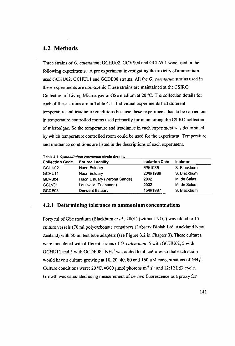
4.2 Methods

Three strains of G. catenatum; GCHUO2, GCVSO4 and GCLV01 were used in the

following experiments. A pre experiment investigating the toxicity of ammonium

used GCHUO2, GCHUll and GCDE08 strains. All the G. catenatum strains used in

these experiments are non-axenic.These strains are maintained at the CSIRO

Collection of Living MicrOalgae in GSe medium at 20 °C. The collection details for

each of these strains are in Table 4.1. Individual experiments had different

temperature and irradiance conditions because these experiments had to be carried out

in temperature controlled rooms used primarily for maintaining the CSIRO collection

of microalgae. So the temperature and irradiance in each experiment was determined

by which temperature controlled room could be used for the experiment. Temperature

and irradiance conditions are listed in the descriptions of each experiment.

Table 4.1 Gymnodinium catenatum strain details. Collection Code Source Locality Isolation Date Isolator

GCHUO2 Huon Estuary 6/6/1986 S. Blackburn GCHU11 Huon Estuary 20/6/1988 S. Blackburn GCVSO4 Huon Estuary (Verona Sands) 2002 M. de Sales GCLV01 Louisville (Triabunna) 2002 M. de Sales GCDE08 Derwent Estuary 15/6/1987 S. Blackburn

4.2.1 Determining tolerance to ammonium concentrations

Forty ml of GSe medium (Blackburn et al., 2001) (without NO3) was added to 15

culture vessels (70 ml polycarbonate containers (Labserv Biolab Ltd. Auckland New

Zealand) with 50 ml test tube adapters (see Figure 3.2 in Chapter 3). These cultures

were inoculated with different strains of G. catenatum: 5 with GCHUO2, 5 with

GCHUll and 5 with GCDE08. NH 4+ was added to all cultures so that each strain

would have a culture growing at 10, 20, 40, 80 and 16011M concentrations of NH4 +.

Culture conditions were: 20 °C, z300 gmol photons tn -2 s-1 and 12:12 L;D cycle.

Growth was calculated using measurement of in-vivo fluorescence as a proxy for

141

biomass, every 2-3 days over the 31 day s of the experiment. Growth rate was

calculated according to (Guillard, 1973) (see 3.2.7 in Chapter 3).

Based on the results of the experiment above a second experiment was carried out to

determine whether growth could be sustained using non-lethal concentrations of

NH 4+ as a sole source of nitrogen. For this experiment, duplicate cultures of HUO2

and HUll were gown with either 101.IM or 20 ptM of NH4 + as a sole N source.

Cultures grown on excess NO3" (initial concentration —800 1AM) were used as a

control. Growth of all cultures was monitored using in-vivo fluorescence as

previously described, and growth rates calculated using data from the exponential

growth phase.

4.2.2 Growth on ammonium

Cultures of GCHUO2 and GCVSO4 were preconditioned by N-starvation by growth

in GSe medium without added NO3 - for 14 days prior to the experiment, so that 'carry

over' of NO3- into the treatments with different N sources would be minimized.

Triplicate cultures of both strains were grown in 70 ml polycarbonate containers with

50 ml test tubes attached (see Figure 3.2 in Chapter 3) containing 47.5 ml of GSe

medium without NO3 - and the addition of 10 uM of NI-14 + . Triplicate control cultures

contained 47.5 ml Gse medium containing NO 3 - in excess (-800 iM). All cultures

were grown under optimal temperature and saturating light conditions (22 °C and 150

umol photons r11-2 s -1 ) with a L:D cycle of 12:12. As NH4+ appeared to have negative

effects on growth rate at concentrations of >40 uM, NH 4+ was maintained at less than

20 uM with regular aseptic additions of sufficient NH4 +to give an increase of 101.1M

when significant draw-down of NI-14 + was estimated. Draw-down was monitored

every 2-3 days using a spectrophotometric technique developed by Solorzano (1969),

further details of this technique are given in Parsons, etal. (1984). Cultures were

grown for 19 days and cell density monitored using in-vivo fluorescence ever 2-3

days and growth rates calculated as described in Chapter 2. Growth rates between

days 3 and 6 (when NH 4+ was not significantly depleted) were used to examine

142

significant difference between growth using NH 4+ or NO3 - as a sole N source and

whether there were significant strain-specific responses between GCHUO2 and

GCVSO4. Statistical analyses used a 2 way ANOVA using the program Sigmastat

2.03 and a-value of 0.05. The data passed both the Kolmogorov-Smimov test (with

Lilliefors' correction) for normality and Levene's median test for equal variance.

4.2.3 Growth on Urea

Strains GCHUO2 and GCVSO4 were pre-conditioned by growing them in GSe/10

(GSe medium with 1/10 normal concentrations of nutrients) for at least 14 days.

When cultures reached —5 x 105 cells r', one ml of culture was used as an inoculum

for experimental cultures. Triplicate control and treatment cultures of both GCHUO2

and GCVSO4, were grown in 70 ml polycarbonate containers with 50 ml test tubes

attached (see Figure 3.2 Chapter 3). Control cultures contained 50 ml GSe medium

containing NO3 - in excess (-800 [tM). Treatment cultures contained 50 ml of GSe

medium without NO 3 - and urea added to achieve an initial concentration of 10 p.M.

Cultures were grown at 23 °C and 1601.tmol photons 111-2 S-1 with a L:D cycle of 18:8.

Cultures were grown for 14 days and cell density monitored using in-vivo

fluorescence every 2-3 days and growth rates calculated as previously described (see

3.2.7 in Chapter 3). The concentration of urea was not monitored as the experiment

progressed. However, assuming a maximum growth rate of —0.3 d -1 , the N

requirements for G. catenatum were calculated for the experimental period and urea

was added periodically to make sure urea was in excess.

After the first 14 day experimental period each culture was used as an inoculum for a

second set of experimental cultures. The second sets of cultures were inoculated to

have the same starting cell densities. Growth rates of these cultures were monitored

for a further 19 days and growth rates calculated as before. Growth rates from the

first and second round of cultures were compared using a 2 way ANOVA using the

program Sigmastat 2.03 and a-value of 0.05. The data passed both the Kolmogorov-

143

Smirnov test (with Lilliefors' correction) for normality and Levene's median test for

equal variance.

4.2.4 Preferential uptake of different nitrogen species

Prior to the experiment, cultures of G. catenatum strains GCHUO2, GCVSO4 and

GCLV01 were pre-conditioned by being grown for 14 days in GSe/10 (GSe at 1/10

concentration). After 14 days cell counts were undertaken to allow standardised

(same number of cells m1 -1 ) inocula for experimental cultures.

Four 500 ml round bottom glass flasks capped with steri-stoppers manufactured by

Heinz Herenzwere used because a larger volume of culture was required so that 2 ml

samples could be removed from the culture every 3-5 days. The round bottom flasks

provide better conditions than other culture vessels, presumably because of the large

surface area that these vessels provide when 200-400 ml of media is added. When in

culture G. catenatum has been observed to aggregate just below the surface and when

provided with a larger surface areas grows better. These culture vessels had 420 ml

of GSe with no added NO3 -, and were inoculated with GCHUO2, GCHU1 1, GCVSO4

or GCLV01 at an initial concentration of 2.9 x 10 3 cells 1-I . NH4+, NO3- and urea

were all added aseptically at an equi-molar concentration of z4 11M. The cultures

were then grown for 29 days under these conditions: 23.5 °C, 3161..tmol photons T11-2

s-1 and L:D 18:8. The GCHUll culture displayed a much longer lag phase before it

began to grow, for this reason it was excluded from the results for the purposes of this

study.

Samples were taken at 3-5 day intervals throughout the experiment and stored at -20

°C for later analysis of NH4 +, NO3 - and urea concentration. Ammonium was

measured using the technique of Kerouel and Aminot (Kerouel & Aminot, 1997)

adapted for flow injection (Watson etal., 2004)with a detection limit of-0.05 mM.

Nitrate and/or nitrite (Wood et al., 1967), was measured using Quick-Chem'

methods on a flow injection LACHAT instrument as per the following protocols for

144

nitrate and/or nitrite (Quik-ChemTm Method 31-107-04-1-A; detection limit 0.03—

mM), Urea was analysed by a spectrophotometric technique to quantify the reaction

of urea with diacetylmonoxime (Mulvenna & Savidge, 1992). To reduce the health

risks associated with thio-semicarbazide, a reagent for this technique, we substituted

semicarbazide (a less toxic but similar compound).

Samples for microscopic cell counts were also taken and counts carried out using lml

samples in a Sedgewick-Rafter counting cell (ProsciTech Queensland, Australia).

Phytoplankton in these samples were preserved using Lugol's iodine fixative solution

(110 g potassium iodide, 50 g iodine, 1 litre distilled water, 100 ml glacial acetic

acid) to approximately 2% final concentration. Cell counts were performed using an

Olympus 1X71 microscope at a magnification of 200x. After day 12, cell counts

became unreliable due to an increasing proportion of the cells adhering to the bottom

of the flasks. Some of these cells did not resuspend with gentle hand swirling,

therefore specific uptake rates are only presented for the period prior to day 12.

An estimate of specific uptake was made by multiplying cell counts by the average N

per cell. This estimate of N accumulation in the G.catenatum cells over time was then - used to calculate the specific uptake. The average N per cell (587 pg N cell 1 ) used in

this calculation was determined in Chapter 3 of this thesis.

4.3 Results

4.3.1 Growth on different nitrogen species

Growth was observed for G. catenatum in GSe with addition of NI-14+ at 10 AM and

20 AM, however, no growth was observed at concentrations above 40 jiM , indicating

that cells were dying. These results were confirmed by the growth of G. catenatum on

NH 4+ solely at both 10 and 20 1.tM. The growth rate achieved at 20 111 ■A growth was

not significantly different from that achieved on NO 3" in the initial stages of the

experiment. The growth rate at 10 p.M NH4+ was significantly lower (by almost half

145

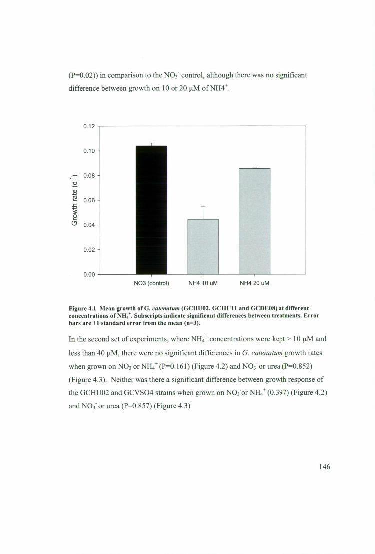
(P=0.02)) in comparison to the NO 3 - control, although there was no significant

difference between growth on 10 or 20 j.tM of NH4 + .

0.12

-r 0.10 -

0.08

a) 0.06 -

2 0 0.04 -

0.02 -

0.00 NO3 (control) NH4 10 uM NH4 20 uM

Figure 4.1 Mean growth of G. catenat um (GCHUO2, GCHUll and GCDE08) at different concentrations of NH4+ . Subscripts indicate significant differences between treatments. Error bars are +1 standard error from the mean (n=3).

In the second set of experiments, where NH 4+ concentrations were kept > 10 [tM and

less than 40 [iM, there were no significant differences in G. catenatum growth rates

when grown on NO3 -or NH4+ (P=0.161) (Figure 4.2) and NO3 - or urea (P=0.852)

(Figure 4.3). Neither was there a significant difference between growth response of

the GCHUO2 and GCVSO4 strains when gown on NO 3 -or NH 4+ (0.397) (Figure 4.2)

and NO3 - or urea (P=0.857) (Figure 4.3)

146

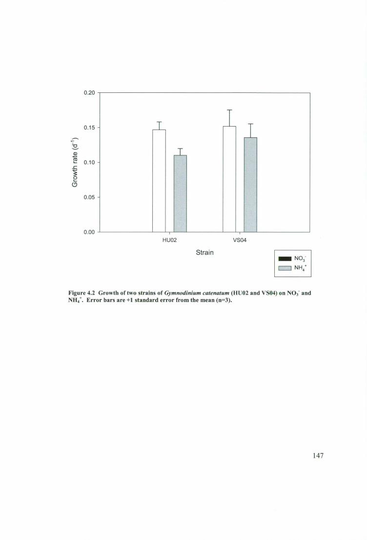
0.15 -

0.10 -

Gro

wt h

rat

e (d

-1)

0.05 -

0.00

0.20

HUO2 VSO4

Strain NO 3

I 1 NH4 *

Figure 4.2 Growth of two strains of Gymnodinium catenatum (HUO2 and VSO4) on NO 3- and NH4+ . Error bars are +I standard error from the mean (n=3).

147

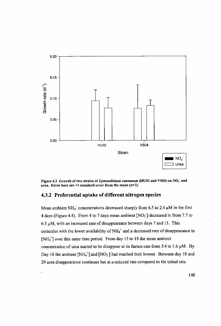
0.20

0.15

0.05

0.00 HUO2 VSO4

Strain

NO3- = Urea

Figure 4.3 Growth of two strains of Gymnodinium catenatum (HUO2 and VSO4) on NO 3- and urea. Error bars are +1 standard error from the mean (n=3).

4.3.2 Preferential uptake of different nitrogen species

Mean ambient NH 4+ concentrations decreased sharply from 6.5 to 2.41.tM in the first

4 days (Figure 4.4). From 4 to 7 days mean ambient [NO3 -] decreased in from 7.7 to

6.5 gM, with an increased rate of disappearance between days 7 and 13. This

coincides with the lower availability of N1-14+ and a decreased rate of disappearance in

[N}41 over this same time period. From day 13 to 18 the mean ambient

concentration of urea started to be disappear at its fastest rate from 5.4 to 1.6 04. By

Day 18 the ambient [NH.] and [NO3 -] had reached their lowest. Between day 18 and

29 urea disappearance continues but at a reduced rate compared to the initial rate.

148

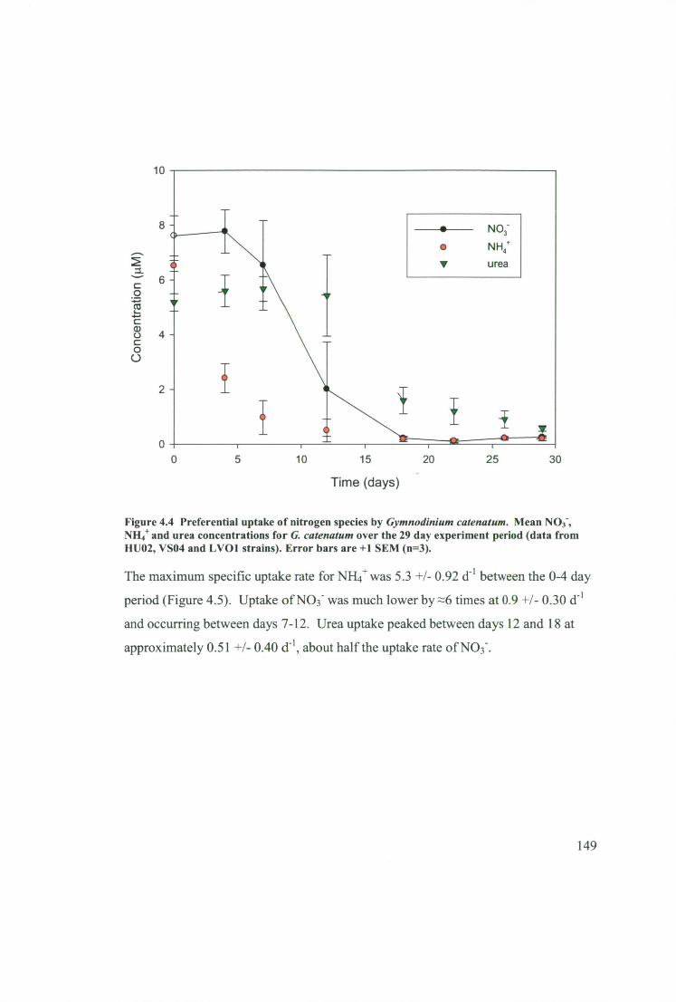
10

i 0

i

—4,— NO3- • NH4. V u rea

f i y •---;-•----•

-

8 - o

0 5 10 15 20 25 30

Time (days)

Figure 4.4 Preferential uptake of nitrogen species by Gymnodinium catenatum. Mean NO3-, NH4+ and urea concentrations for G. catenatum over the 29 day experiment period (data from HUO2, VSO4 and LV01 strains). Error bars are +1 SEM (n=3).

The maximum specific uptake rate for NH4+ was 5.3 +/- 0.92 c1-1 between the 0-4 day

period (Figure 4.5). Uptake of NO3" was much lower by z6 times at 0.9 +/- 0.30 d." 1

and occurring between days 7-12. Urea uptake peaked between days 12 and 18 at

approximately 0.51 +/- 0.40 d -1 , about half the uptake rate of NO 3 - .

149

1 --4,- NO3-

• NH 4 V urea

8

6

Spec

ific

upta

ke (

d-1

)

4 -

2 -

_ 0

-2 0 2 4 6

Time (days)

8 10

Figure 4.5 Mean uptake rates for NO 3-, NH4+ and urea (data from GCHUO2, GCVSO4 and GCLV01 strains) for G. catenatum over the 29 day experiment period. Error bars are +1-1 standard error from the mean (n=3).

4.4 Discussion

The strains of Gymnodinium catenatum from south east Tasmania are able to use

NH4+, NO3 - and urea equally well as sole N-sources for growth. This has been found

in other studies, ten species of phytoplankton studied by Lourenco, Barbarino et al.

(2002) were similar, in that the majority were able to grow soley on NH4 + , NO3 - or

urea. The studied included 3 chlorophytes, 2 diatoms, a dinoflagellate, a cryptophyte,

a cyanophyte, a prymnesiophte and a eustigmatophyte. There were two exceptions

Hillea sp. (eustigmatophyte) and Prorocentrum minimum (dinophyte) which didn't

grow on NH4+. However, this was probably because the concentrations used were

very high (1.18 mM) and therefore likely to be toxic.

150

The effect of NH4+ , NO3 - and urea on growth rate of 4 phytoplanIcton species was

also investigated by Levasseur, et al. , (1993). They showed Thalassiosira

pseudonana, Chaetoceros gracilis, Dunalilella tertiolecta and Gymnodinium

sanguineum were all capable of growth using NH4+, NO3 - and urea as sole N sources.

However, growth rates decreased for these species investigated when grown on urea.

The ability to grow equally well on urea may be an important advantage for G.

catenatum over other species that cannot grow using urea as a sole N source or have

substantially reduced growth rates on N in this form. The ability to grow equally well

using all of these N species would be advantageous in an environment where N is the

limiting nutrient and it is available in these different forms.

It is important to take into account the toxicity of NI-14 + at higher concentrations to

many phytoplankton. For example, our study showed NH 4+ was toxic for G.

catenatum at concentrations >40 uM and in other studies the concentrations may be

very high (0.05-1.18 mM) as these concentrations are required for large scale batch

algal culture (Lourenco et al., 2002, Flynn et al., 1996) In most oceanic and coastal

environments, generally NH 4+ concentrations experienced are much lower but NH 4+

fluxes are relatively high, therefore providing a continuous supply of NH 4+ at low

concentrations (i.e. <2 uM) unlikely to be toxic to the majority of phytoplankton. So

it is important to investigate the effect of NH4 + on growth of phytoplankton species at

lower concentrations or non toxic concentrations if these results are going to be

applied to understanding the physiology of phytoplankton in natural environments.

We have shown that G. catenatum cannot tolerate NH 4+ concentrations in excess of

40 uM and that NH4 + at < 10 AM is limiting growth. This may indicate that G.

catenatum has a relatively high half saturation constant for uptake of NH4 + and

growth.

Table 4.2 gives half saturation constants (K s) for phytoplankton from different groups

including: Dinoflagellates, Diatoms, Raphidophytes, Prymnesiophytes, Prasinophytes

and Chlorophtyes the majority of phytoplankton species have K s values for NH 4+ less

151

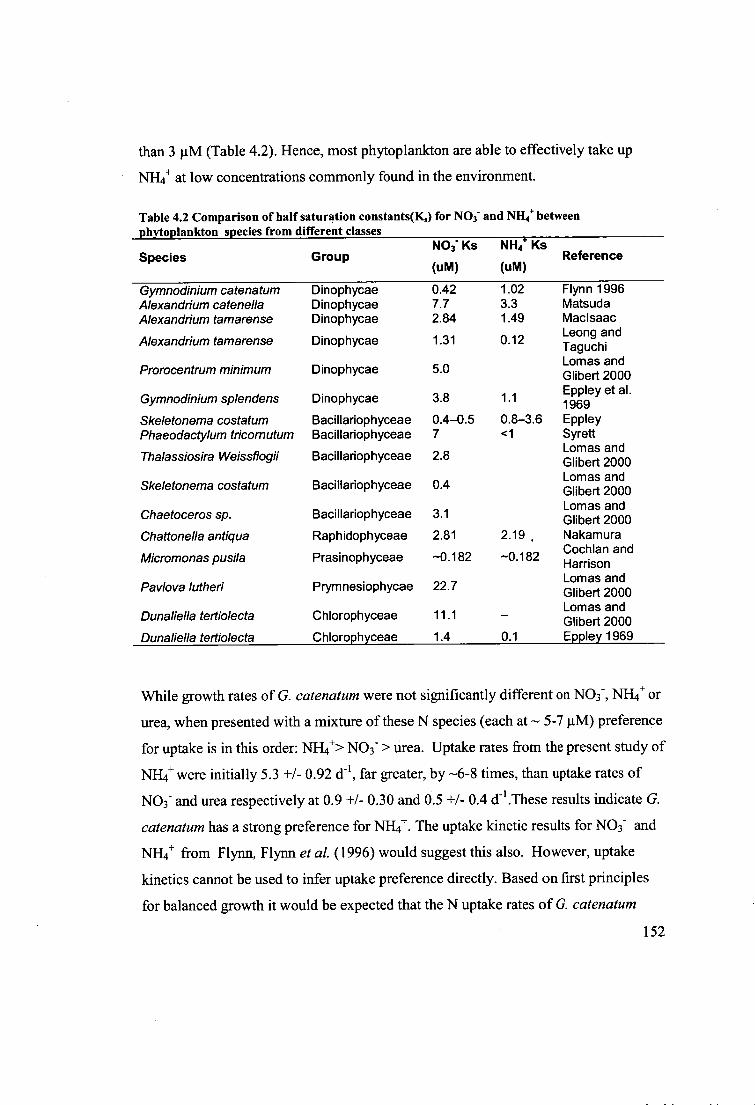
Table 4.2 Comparison of half saturation constants(K) for NO 3- and NH4+ between phytoplankton species from different classes

Species Group NO3" Ks NH4+ Ks

Reference (uM) (uM)

than 3 1AM (Table 4.2). Hence, most phytoplankton are able to effectively take up

NI-14+ at low concentrations commonly found in the environment.

Gymnodinium catenatum Alexandrium catenella Alexandrium tamarense Alexandrium tamarense

Prorocentrum minimum

Gymnodinium splendens

Skeletonema costatum Phaeodactylum tricomutum

Thalassiosira Weissflogii

Skeletonema costatum

Chaetoceros sp. Chattonella antiqua

Micromonas pusila

Pavlova lutheri

Dunaliella tertiolecta Dunaliella tertiolecta

Dinophycae 0.42 Dinophycae 7.7 Dinophycae 2.84

Dinophycae 1.31

Dinophycae 5.0

Dinophycae 3.8

Bacillariophyceae 0.4-0.5 Bacillariophyceae

7

Bacillariophyceae 2.8

Bacillariophyceae 0.4

Bacillariophyceae 3.1

Raph idophyceae 2.81

Prasinophyceae —0.182

Prymnesiophycae 22.7

Chlorophyceae 11.1

Chlorophyceae 1.4

1.02 Flynn 1996 3.3 Matsuda 1.49 Mac Isaac

Leong and Taguchi Lomas and Glibert 2000 Eppley et al. 1.1 1969

0.8-3.6 Eppley <1 Syrett

Lomas and Glibert 2000 Lomas and Glibert 2000 Lomas and Glibert 2000

2.19 , Nakamura Cochlan and Harrison Lomas and Glibert 2000 Lomas and Glibert 2000

0.1 Eppley 1969

0.12

—0.182

While growth rates of G. catenatum were not significantly different on NO 3 - , NH4+ or

urea, when presented with a mixture of these N species (each at — 5-7 uM) preference

for uptake is in this order: NH4 +> NO3 - > urea. Uptake rates from the present study of

NH 4+ were initially 5.3 +1- 0.92 d -1 , far greater, by —6-8 times, than uptake rates of

NO3 - and urea respectively at 0.9 +1- 0.30 and 0.5 +1- 0.4 d -I .These results indicate G.

catenatum has a strong preference for NH4+. The uptake kinetic results for NO 3 - and

NH4+ from Flynn, Flynn et al. (1996) would suggest this also. However, uptake

kinetics cannot be used to infer uptake preference directly. Based on first principles

for balanced growth it would be expected that the N uptake rates of G. catenatum

152

would equal its growth rate. However, it has been shown in several studies that when

cells are starved of N, as in this study, that when they are resupplied with N they

exhibit uptake greater than their growth rate. This is commonly referred to as "surge

uptake" (Parslow et al., 1984b, Parslow et al., 1984a). Our results show that initial

uptake of NH4+ is almost 20 times the maximum growth rate of G. catenatum (0.30 d-

I ). This surge uptake is also reported by Flynn et al. (1996) for G. catenatum but the

magnitude of increase was —2.5 times less than in the present study. In the present

study the uptake of NO 3 - and urea are also at rates greater than the growth rate but

they have relatively large standard errors associated with them. It might be expected

that the uptake of N would return to rates similar to the growth rate after an initial

surge in uptake to recover after N starvation.

4.4.1 Summary

We have demonstrated that G. catenatum is physiologically diverse in its N uptake

capabilities. It is able to grow equally well using NO3 - , NH4+ and urea. Why is it

then that G. catenatum has preferences for NH4+ and NO3 - over urea? Perhaps while

it poses no penalties for growth when energy from light is saturating, the preferences

may be related to the preferences under energy limited circumstances. For example,

Alexandrium minutum (dinophyceae) showed variations in growth rate when grown

on NO3 - that were highly dependent on the level of irradiance (Chang & McClean,

1997).

The present study and that of (Flynn et al., 1996) show that G. catenatum is capable

of responding to pulses of N by 'surge uptake'(compared to max growth rate 0.3 d -1 )

when it is in a N starved condition. In addition, it has been clearly demonstrated that

G. catenatum can grow equally well on NH, NO3 - or urea. Combined, these

physiological capabilities of G. catenatum increase its ability to compete for N in the

environment and would contribute to its ecological success.

153

4.5 References

Baek, S. H., Shimode, S., Han, M. S. & Kikuchi, T. 2008. Growth of dinoflagellates, Ceratium furca and Ceratium fusus in Sagami Bay, Japan: The role of nutrients. Harmful Algae 7:729-39.

Band-Schmidt, C. J., Morquecho, L., Lechuga-Deveze, C. H. & Anderson, D. M. 2004. Effects of growth medium, temperature, salinity and seawater source on the growth of Gymnodinium catenatum (Dinophyceae) from Bahia Concepcion, Gulf of California, Mexico. J Plankton Res 26:1459-70.

Berg, G. M., Glibert, P. M., Lomas, M. W. & Burford, M. A. 1997. Organic nitrogen uptake and growth by the chrysophyte Aureococcus anophagefferens during a brown tide event. Mar Biol 129:377-87.

Blackburn, S. I., Bolch, C. J. S., Haskard, K. A. & Hallegraeff, G. M. 2001. Reproductive compatibility among four global populations of the toxic dinoflagellate Gymnodinium catenatum (Dinophyceae). Phycologia 40:78-87.

Blackburn, S. I., Hallegraeff, G. M. & Bolch, C. J. 1989. Vegetative Reproduction and Sexual Life-Cycle of the Toxic Dinoflagellate Gymnodinium-Catenatum from Tasmania, Australia. J Phycol 25:577-90.

Boynton, W. R., Kemp, W. M. & Keefe, C. W. 1982. A comparative analysis of nutrients and other factors influencing estuarine phytoplankton production. In: Kennedy, V. S. [Ed.] Estuarine Comparisons. Academic Press, New York, pp. 69-90.

Bravo, I. & Anderson, D. M. 1994. The Effects of Temperature, Growth-Medium and Darkness on Excystment and Growth of the Toxic Dinoflagellate Gymnodinium-Catenatum from Northwest Spain. J Plankton Res 16:513-25.

Canada, G. C., Casotti, R., Modigh, M. & Saggiomo, V. 1991. Presence of Gymnodinium-Catenatum (Dinophyceae) in a Coastal Mediterranean Lagoon. J Plankton Res 13:229-38.

Chang, F. H., Bradfordgrieve, J. M., Vincent, W. F. & Woods, P. H. 1995. Nitrogen Uptake by the Summer Size-Fractionated Phytoplankton Assemblages in the Westland, New-Zealand, Upwelling System. New Zealand Journal of Marine and Freshwater Research 29:147-61.

Chang, F. H. & McClean, M. 1997. Growth.responses of Alexandrium minutum (Dinophyceae) as a function of three different nitrogen sources and irradiance. New Zealand Journal of Marine and Freshwater Research 31:1-7.

Doblin, M. A., Thompson, P. A., Revill, A. T., Butler, E. C. V., Blackburn, S. I. & Hallegraeff, G. M. 2006. Vertical migration of the toxic dinoflagellate Gymnodinium catenatum under different concentrations of nutrients and humic substances in culture. Harmful Algae 5:665-77.

Ellegaard, M., Christensen, N. F. & Moestrup, 0. 1993. Temperature and Salinity Effects on Growth of a Non-Chain-Forming Strain of Gymnodinium-Catenatum (Dinophyceae) Established from a Cyst from Recent Sediments in the Sound (Oresund), Denmark. J Phycol 29:418-26.

154

Escaravage, V. & Prins, T. C. 2002. Silicate availability, vertical mixing and grazing control of phytoplankton blooms in mesocosms. Hydrobiologia 484:33-48.

Flynn, K. J., Flynn, K., John, E. H., Reguera, B., Reyero, M. I. & Franco, J. M. 1996. Changes in toxins, intracellular and dissolved free amino acids of the toxic dinoflagellate Gymnodinium catenatum in response to changes in inorganic nutrients and salinity. J Plankton Res 18:2093-111.

Fraga, F., Perez, F. F., Figueiras, F. G. & Rios, A. F. 1992. Stoichiometric Variations of N, P, C and 02 During a Gymnodinium-Catenatum Red Tide and Their Interpretation. Mar Ecol-Prog Ser 87:123-34.

Glibert, P. M., Heil, C. A., Hollander, D., Revilla, M., Hoare, A., Alexander, J. & Murasko, S. 2004. Evidence for dissolved organic nitrogen and phosphorus uptake during a cyanobacterial bloom in Florida Bay. Mar Ecol-Prog Ser 280:73-83.

Guillard, R. R. L. 1973. Division rates. In: Stein, J. R. [Ed.] Phycological Methods. Cambridge University Press, Cambridge, Oxford, UK, pp. 289 - 311.

Heil, C. A., Revilla, M., Glibert, P. M. & Murasko, S. 2007. Nutrient quality drives differential phytoplankton community composition on the southwest Florida shelf. Limnol. Oceanogr. 52:1067-78.

Holmes, M. J., Bolch, C. J. S., Green, D. H., Cembella, A. D. & Teo, S. L. M. 2002. Singapore isolates of the dinoflagellate Gymnodinium catenatum (dinophyceae) produce a unique profile of paralytic shellfish poisoning toxins. J Phycol 38:96-106.

Kana, T. M., Lomas, M. W., MacIntyre, H. L., Cornwell, J. C. & Gobler, C. J. 2004. Stimulation of the brown tide organism, Aureococcus anophagefferens, by selective nutrient additions to in situ mesocosms. Harmful Algae 3:377-88.

Kerouel, R. & Aminot, A. 1997. Fluorometric determination of ammonia in sea and estuarine waters by direct segmented flow analysis. Mar. Chem. 57:265-75.

La Barbara-Sanchez, A. & Gamboa-Maruez, J. F. 2001. Distribution of Gymnodinium catenatum Graham and shellfish toxicity on the coast of Sucre state, Venezuela, from 1989 to 1998. J Shellfish Res 20:1257-61.

Leong, S. C. Y. & Taguchi, S. 2004. Response of the dinoflagellate Alexandrium tamarense to a range of nitrogen sources and concentrations: growth rate, chemical carbon and nitrogen, and pigments. Hydrobiologia 515:215-24.

Levasseur, M., Thompson, P. A. & Harrison, P. J. 1993. Physiological Acclimation of Marine-Phytoplankton to Different Nitrogen-Sources. J Phycol 29:587-95.

Lourenco, S. 0., Barbarino, E., Mancini-Filho, J., Schinke, K. P. & Aidar, E. 2002. Effects of different nitrogen sources on the growth and biochemical profile of 10 marine microalgae in batch culture: an evaluation for aquaculture. Phycologia 41:158-68.

Matsuoka, K. & Fukuyo, Y. 1994. Geographical-Distribution of the Toxic Dinoflagellate Gymnodinium-Catenatum Graham in Japanese Coastal Waters. Bot Mar 37:495-503.

McCarthy, J. J. 1972. The uptake of urea by natural populations of marine phytoplankton. Limnol. Oceanogr. 17:738-48.

155

McCarthy, J. J., Wynne, D. & Berman, T. 1982. The uptake of dissolved nitrogenous nutrients by Lake Kinneret (Israel) microplankton. Limnol. Oceanogr. 27:673- 80.

Mee, L. D., Espinosa, M. & Diaz, G. 1986. Paralytic Shellfish Poisoning with a Gymnodinium-Catenatum Red Tide on the Pacific Coast of Mexico. Mar Environ Res 19:77-92.

Mulvenna, P. F. & Savidge, G. 1992. A Modified Manual Method for the Determination of Urea in Seawater Using Diacetylmonoxime Reagent. Estuar Coast Shelf S 34:429-38.

Nettling, S. 1995. Gymnodinium Catenatum Graham (Dinophyceae) in Europe - a Growing Problem. J Plankton Res 17:85-102.

Oh, S. J., Yamamoto, T., Kataoka, Y., Matsuda, 0., Matsuyama, Y. & Kotani, Y. 2002. Utilization of dissolved organic phosphorus by the two toxic dinoflagellates, Alexandrium tamarense and Gymnodinium catenatum (Dinophyceae). Fisheries Sci 68:416-24.

Park, T. G., Kim, C. H. & Oshima, Y. 2004. Paralytic shellfish toxin profiles of different geographic populations of Gymnodinium catenatum (Dinophyceae) in Korean coastal waters. Phycol Res 52:300-05.

Parslow, J. S., Harrison, P. J. & Thompson, P. A. 1984a. Saturated uptake kinetics: Transient response of the marine diatom Thalassiosira pseudonana to ammonium, nitrate, silicate or phosphate starvation. Marine biology, Heidelberg 83:51-59 .

Parslow, J. S., Harrison, P. J. & Thomson, P. A. 1984b. Development of rapid ammonium uptake during starvation of batch and chemostat cultures of the marine diatom Thalassiosira pseudonana. Marine biology, Heidelberg 83:43- 50.

Parsons, T. R., Maita, Y. & Lalli, C. M. 1984. A manual of chemical and biological methods for seawater analysis. Pergamon Press, Oxford, 173.

Ramirez-Camarena, C., Cortes-Altamirano, R. & Munoz-Cabrera, L. 1999. Red tide caused by the dinoflagellate Gymnodinium catenatum off Mazatlan Bay, Sinaloa, Mexico in 1997. Rev Biol Trop 47:77-80.

Riegman, R., deBoer, M. & Domis, L. D. 1996. Growth of harmful marine algae in multispecies cultures. J Plankton Res 18:1851-66.

Riegman, R., Noordeloos, A. A. M. & Cadee, G. C. 1992. Phaeocystis Blooms and Eutrophication of the Continental Coastal Zones of the North-Sea. Mar Biol 112:479-84.

Solorzano, L. 1969. Determination of ammonia in natural waters by the phenolhypochlorite method. Limnol. Oceanogr. 14:799-801.

Sordo, I., Barton, E. D., Cotos, J. M. & Pazos, Y. 2001. An inshore poleward current in the NW of the Iberian peninsula detected from satellite images, and its relation with G-catenatum and D-acuminata blooms in the Galician Rias. Estuar Coast Shelf S 53:787-99.

156

Team, H. E. S. 2000. Huon Estuary Study, Environmental research for integrated catchment management and aquaculture. Final Report to FRDC. CSIRO Division of Marine Research, Hobart, Tasmania, Australia.

Tungaraza, C., Rousseau, V., Brion, N., Lancelot, C., Gichuki, J., Baeyens, W. & Goeyens, L. 2003. Contrasting nitrogen uptake by diatom and Phaeocystis-dominated phytoplanIcton assemblages in the North Sea. J Exp Mar Biol Ecol 292:19-41.

Twomey, L. J., Piehler, M. F. & Paerl, H. W. 2005. Phytoplankton uptake of ammonium, nitrate and urea in the Neuse River Estuary, NC, USA. Hydrobiologia 533:123-34.

Watson, R. J., Butler, E. C. V. & Clementson, L. A. 2004. Flow-injection analysis with fluorescence detection of trace levels of ammonium in seawater. Journal of Environmental Monitoring 7:37-42.

Wood, E. D., Armstrong, F. A. J. & Richards, F. A. 1967. Determination of nitrate in sea water by cadmium-copper reduction to nitrite. Journal of Marine Biological Association of the United Kingdom 47:23-31.

Yamaguchi, M. & Itakura, S. 1999. Nutrition and growth kinetics in nitrogen- or phosphorus-limited cultures of the noxious red tide dinoflagellate Gymnodinium mikimotoi. Fisheries Sci 65:367-73.

Yamaguchi, M., Italcura, S. & Uchida, T. 2001. Nutrition and growth kinetics in nitrogen- or phosphorus-limited cultures of the 'novel red tide' dino flagellate Heterocapsa circularisquama (Dinophyceae). Phycologia 40:313-18.

Yamamoto, T., Oh, S. J. & Kataoka, Y. 2002. Effects of temperature, salinity and irradiance on the growth of the toxic dino flagellate Gymnodinium catenatum (Dinophyceae) isolated from Hiroshima Bay, Japan. Fisheries Sci 68:356-63.

Yamamoto, T., Oh, S. J. & Kataoka, Y. 2004. Growth and uptake kinetics for nitrate, ammonium and phosphate by the toxic dinoflagellate Gymnodinium catenatum isolated from Hiroshima Bay, Japan. Fisheries Sci 70:108-15.

157

5 NITROGEN UPTAKE DURING A

GYMNODINIUM CATENATUM BLOOM AT

SOUTHPORT, SOUTH-EAST TASMANIA,

AUSTRALIA

5.1 Introduction

It appears that there has been an increase in the occurrence of harmful algal blooms

(HABs) in Australia (Hallegraeff, 1992) and around the world (Anderson et al., 2002,

Hallegraeff, 1993). The results of these HABs includes fish kills, human health issues

including such as PSP, DSP and the loss of biological diversity and productivity. That

eutrophication plays an important role directly or indirectly in the stimulation of

many HABs is now widely accepted (Anderson et al., 2002, Heisler et al., 2008).

Coastal and estuarine systems phytoplankton are primarily nitrogen limited(Downing,

1997). Hence, the increased interest in nitrogen nutrition of HAB species such as

Alexandrium minutum (Chang & McClean, 1997), Heterosigma cartarae (now

Heterosigma akashiwo) (Chang & Page, 1995),Gymnodinium sanguineum (now

Akashiwo sanguinea) (Doucette & Harrison, 1991). In addition mechanisms that

allow dinoflagellates to bloom when nitrogen availability is low are increasingly

under investigation. These include the use of organic N such as urea and behaviours

such as the vertical migration to obtain nitrogen from deeper in the water column

(Cullen and Horrigan 1981). In some dinoflagellate species this behaviour has been

proven to be a strategy for maximising photosynthesis and nutrient uptake where

nutrients and light are vertically separated (MacIntyre et al. 1997, Ault 2000). G.

catenatum has been observed undertaking a strong vertical migration (Toshinori et al.

2001) and in the Huon Estuary, when it is the dominant phytoplankter, it has been

observed to vertically migrate from — 5m to — 20 m on a daily basis (Team, 2000,

Doblin etal., 2006). From these observations it was hypothesized that the blooms of 158

this toxic species may be facilitated by its vertical migration and possible access to

nitrogen from depth. Large blooms of G. catenatum were rare in the Huon Estuary in

2002, 2003 and 2004. So our 2003-2004 field trips, while providing information on

the N uptake by the mixed phytoplanlcton community, were unable to provide

information about the N uptake strategies of G. catenatum during a bloom. Discovery

of a significant bloom of G. catenatum at Dover and Southport, some 15 km south of

the Huon Estuary, allowed us to prepare a field trip to measure N uptake of G.

catenatum in the field, and to specifically investigate the uptake of N during vertical

migration of this species.

5.2 Methods

The N uptake experiments were set up in Southport adjacent to Pelican Island

(latitude 43° 27' 00" S longitude 146° 58' 28" E) in autumn 2004 on the 30-31 March.

During this field trip the same 15N tracertechnique as used in the Huon Estuary

(Chapter 4) was used to measure the uptake of three different nitrogen (N) sources

(NH, NO3- and urea) by the natural phytoplankton assemblage. Based on the

observations of vertical migration of G. catenatum in the Huon Estuary (Team,

2000) it was intended that suitable depths would be selected based on the depth of the

chla maximum as indicated by fluorescence profile of the water column. Because of

technical limitations a vertical profile of fluorescence could not be obtained for the

day sampling. Alternatively, we sampled near the surface (5m) and also near the

bottom (15m) during the day. For the night sampling a fluorescence profile was

obtained prior to sampling and sampling was undertaken near the surface (5m) and

also at the depth of the fluorescence maximum (10m).

159

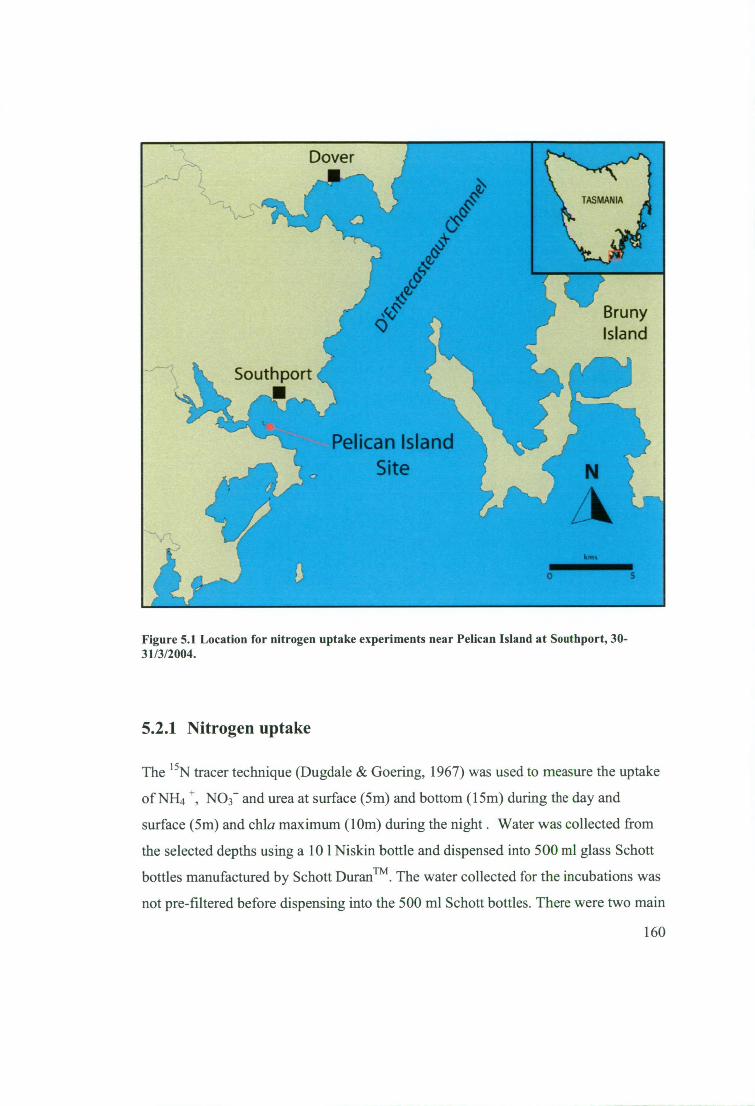
Figure 5.1 Location for nitrogen uptake experiments near Pelican Island at Southport, 30- 31/3/2004.

5.2.1 Nitrogen uptake

The 15N tracer technique (Dugdale & Goering, 1967) was used to measure the uptake

of NH4 ±, NO 3- and urea at surface (5m) and bottom (15m) during the day and

surface (5m) and chla maximum (10m) during the night. Water was collected from

the selected depths using a 10 1Niskin bottle and dispensed into 500 ml glass Schott

bottles manufactured by Schott DuranTM. The water collected for the incubations was

not pre-filtered before dispensing into the 500 ml Schott bottles. There were two main

160

reasons for not pre-filtering the water for the incubations. Firstly, ensuring that long

chains of G. catenatum were not excluded from incubations. G. catenatum chains of 4

to 8 cells are common. A quick estimate of the size of these chains, 30 microns x 8

cells = 240 microns suggests that screening at 200 microns (a commonly used screen)

would exclude a proportion of this species. Secondly, we wanted to estimate the real

in situ N uptake rate including, losses due to grazing. For each depth three 500 ml

Schott bottles were spiked with 0.3 jiM 15N- NO3- (99.3 atom percent 15N), three 500

ml Schott bottles were spiked with 0.11AM ' 5N-NH 4+ (99.6 atom percent 15N) and

three 500 ml schott bottles were spiked with 0.068 15N-urea (98.61 atom percent

15N). In addition at each depth one 500m1 schott bottle was filled with water but not

spiked with any 15N substrate, this unspiked bottle was used to determine the

background 15N (un-enriched atom % excess). These samples were incubated in 500

ml Schott bottles for 4 hours in-situ at the depths they were collected from. Four

hour incubations were chosen because they are short enough to limit the chances of

substrate exhaustion (La Roche, 1983)and also reduce the problems caused by

substrate dilution(Glibert et al., 1982) , but an incubation period of 2-6 hours is also

long enough to minimise the bias introduced by initial high uptake rates that

sometimes occur in phytoplankton (Dugdale & Wilkerson, 1986). After the

incubation the water samples were filtered onto pre-combusted (450°C for 4 hours)

25 mm WhatmanTm glass fibre filters and stored frozen until analysis. The filters

were dried in an oven at 60°C overnight before they were analysed using a Carlo Erba

NA1500 CNS analyzer interfaced via a Conflo II to a Finnigan-MAT Delta S isotope

ratio mass spectrometer to determine the N isotope ratios. Absolute uptake rates were

calculated using the Dugdale and Goering (1967) equation:

p = Nat(Rt) l

where p is the absolute uptake (gig N1 -1 N is the total particulate nitrogen (i.tg N),

at is the atom % excess of 15N (= atom % - background), R is the atom % enrichment

[a, (SLASL Su))], ae is the atom % enrichment of labelled 15N source, SL is the

concentration of labelled 15N, Su is the concentration of unlabelled 14N and t is the 161

incubation time (h). Specific uptake v (14N ligChla -1 11 1 ) is the absolute uptake p

normalised to chla and was calculated using this equation:

v = p/Chla

Where, p is the absolute uptake (1.tg N r' W I ) and Chla is total chlorophyll a (lig Chla

r').

It is common for researchers investigating N uptake to normalise N uptake to

particulate N (PN). In this research N uptake has been normalised to chl a as an

indicator of phytoplankton biomass. The fact is that chl a is the preferred method of

measuring phytoplankton biomass worldwide. It is well known that measurements of

particulate N or particulate C are not as reliable, primarily due to the potential

contamination by detritial C or N. A number of highly respected researchers have

proposed methods to improve the estimation of phytoplankton biomass from POC or

PON including Karl Banse (Banse, 1977) or methods that rely on neither (Holm-

Hansen & Booth, 1966) but these methods are complex or difficult to apply to

individual samples. One result is that very few researchers report phytoplankton

biomass in units of PN or PC. In spite of these difficulties a number of researchers

have normalized their N uptake measurements to PN and reported them in this

manner. This may have more to do with the fact that the analysis required to obtain

the results from the uptake experiments also gives a value for PN, rather than any

more strategic reasoning. The truth is that N per cell shows about the same amount

of variability as chl a per cell (Thompson, 1999) in response to irradiance and

temperature. For these reasons we have normalized N uptake to chi a.

Samples were collected for the determination of ambient nutrient concentrations but

not analyzed until after the experimental determination of uptake rates. For the

purpose of the experiment ambient concentrations were assumed to be 11.1M NH4 +, 3

1.1M NO3- and 0.681.IM urea and high purity 15N NH4+, NO3- and urea tracers were

added to produce a 10% rise in estimated ambient concentration. In this experiment

162

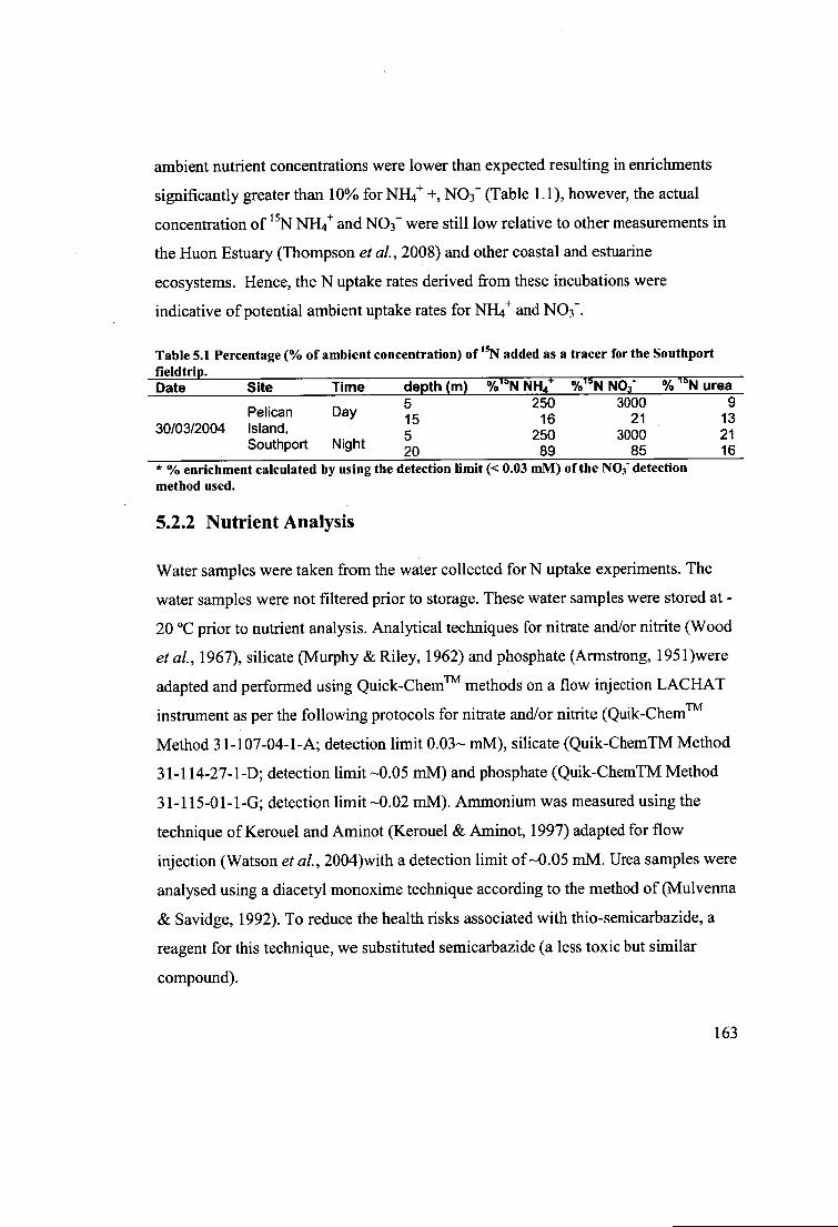
ambient nutrient concentrations were lower than expected resulting in enrichments

significantly greater than 10% for NH4+ +, NO3- (Table 1.1), however, the actual

concentration of 15N NH4+ and NO3- were still low relative to other measurements in

the Huon Estuary (Thompson et al., 2008) and other coastal and estuarine

ecosystems. Hence, the N uptake rates derived from these incubations were

indicative of potential ambient uptake rates for NH4 + and NO3-.

Table 5.1 Percentage (% of ambient concentration) of 15N added as a tracer for the Southport fieldtrip. Date Site Time depth (m) % 15N NH4 ' %15 N NO3" % ' 5N urea

5 250 3000 9 Pelican Day 15 16 21 13

30/03/2004 Island, 5 250 3000 21 Southport Night 20 89 85 16

* % enrichment calculated by using the detection limit (< 0.03 inM) of the NO 3" detection method used.

5.2.2 Nutrient Analysis

Water samples were taken from the water collected for N uptake experiments. The

water samples were not filtered prior to storage. These water samples were stored at -

20 °C prior to nutrient analysis. Analytical techniques for nitrate and/or nitrite (Wood

et al., 1967), silicate (Murphy & Riley, 1962) and phosphate (Armstrong, 1951 )were

adapted and performed using Quick-Chem Tm methods on a flow injection LACHAT

instrument as per the following protocols for nitrate and/or nitrite (Quik-ChemTm

Method 31-107-04-1-A; detection limit 0.03— inM), silicate (Quik-ChemTM Method

31-114-27-1-D; detection limit —0.05 rnM) and phosphate (Quik-ChemTM Method

31-115-01-1-G; detection limit —0.02 mM). Ammonium was measured using the

technique of Kerouel and Aminot (Kerouel & Aminot, 1997) adapted for flow

injection (Watson et al., 2004)with a detection limit of —0.05 mM. Urea samples were

analysed using a diacetyl monoxime technique according to the method of (Mulvenna

& Savidge, 1992). To reduce the health risks associated with thio-semicarbazide, a

reagent for this technique, we substituted semicarbazide (a less toxic but similar

compound).

163

5.2.3 High performance liquid chromatography

Two L of water was filtered for pigment analyses by high performance liquid

chromatography (HPLC). Most pigment samples were analyzed by high performance

liquid chromatography (HPLC) using methods developed by Wright et al. (1991) for

extraction and gradient elution. The separated pigments were detected at 436 nm and

identified against standard spectra using Waters EmpowerTM software.

Concentrations of all pigments were determined from standards (SigmaTM or DHI

Denmark). Primary pigments identified by HPLC included: Chl c 1 and c2, peridinin,

9'-cis-neoxanthin, 19'-butanoyloxyfucoxanthin, fucoxanthin, 19'-

hexanoyloxyfucoxanthin, prasinoxanthin, violaxanthin, diadinoxanthin, alloxanthin,

diatoxanthin, lutein, zeaxanthin, Chl b, Chl a, 13, E-carotene and 1340-carotene.

5.2.4 Phytoplankton Counts

Water collected for the surface N uptake experiment during the day was used to

enumerate phytoplankton. One litre water samples were taken and preserved in the

field using Lugol's iodine fixative solution (110 g potassium iodide, 50 g iodine, 1

litre distilled water, 100 ml glacial acetic acid) to approximately 2% final

concentration. The samples were stored in plastic containers in the dark until they

could be counted under the light microscope. Prior to counting the Lugol's preserved

samples were transferred to 1 litre measuring cylinders (volume recorded — V 1 ) and

allowed to settle for at least 24 hours. After this time, approximately 900 ml were

siphoned off and the remaining sample was transferred to a 100-ml measuring

cylinder and again allowed to settle for at least 24 hours. Then approximately 90 ml

were siphoned off, the final volume recorded (V2) and thoroughly mixed before a 1-

ml aliquot was taken, placed in a Sedgwick Rafter counting chamber and examined

using an Olympus IX71 microscope to identify and count the phytoplankton.

164

The Sedgwick Rafter counting chamber has a grid of 1000 squares, each of 1 pl. For

microplanIcton, (cells generally larger than 20 pm diameter) at least 100 squares or

10% of the counting chamber was scanned (except in cases where there were dense

blooms of one or more microplankton species, when at least one column of 20

squares was scanned) at 200x magnification. For nanoplankton, (2-20 gm in

diameter) the chamber was examined under 400x magnification until at least 300

cells of the dominant nanoplankton "species" had been counted. Flagellates in the

nanoplankton were grouped, as time constraints did not allow fuller identification.

Cells per litre =

cell "species" count * (1000 / number squares counted) * (V2 *1000 / V1)

5.2.5 CTD profiles

A SeabirdTM SBE19+ conductivity, temperature and depth (CTD) profiler was used to

measure the salinity, temperature and fluorescence of the water column during the

field experiments. The measurements obtained on the downward cast through the

water column are presented with the initial period removed when the instrument was

held at surface until flow past the sensors was established.

The CTD sensors: salinity, temperature and fluorescence were factory calibrated. The

factory calibrations were confirmed by comparison with independent instrumentation

for salinity, temperature and fluorescence.

5.2.6 CHEMTAX

Pigment data from HPLC analysis was further analysed to give the proportions of

chlorophyll a present in the following algal taxonomic categories: Cyanophyta,

Prochlorophyta, Chrysophyta, Cryptophyta, Bacillariophyta (diatoms), Haptophyta,

Prasinophyceae, and Dinophyta (Mackey et al., 1996). Initial input ratio matrices

165

were adjusted from those proposed in Mackey, Mackey et al. (1996) by including

four types of Haptophytes:

Haptophyte N — Type 1 = fucoxanthin e.g. Isociuysis spp.

Haptophyte S- Type 2 = Chl c3 + fucoxanthin e.g. Ochrosphaera neopolitana

Haptophyte Type 3 = Chi c3+ 19'Hexanoyloxyfucoxanthin + fucoxanthin + and

sometimes 19'butanoyl derivative e.g. Chyrsochromulina strobulis

Haptophyte Type 4 = c3 + 19'butanoyloxyfucoxanthin +19'hexanoyloxy -fucoxanthin

and fucoxanthin e.g. Imantonia rotunda.

The peridinin:chlorophyll a ratio was modified from 0.515:1 as in Mackey, Mackey

etal. to 0.36:1 after Hallegraeff, Nichols etal. (1991). The latter was based on

extensive culture studies for Gymnodinium catenatum. This has the effect of

increasing the proportion of the chlorophyll a that CHEMTAX will allocate to

dinoflagellates for a given amount of peridinin. Based on personal observations this

results in CHEMTAX estimates of dinoflagellates that are more consistent with the

estimated proportion of biomass calculated by cell counts and adjusted for cellular

bio-volumes.

5.2.7 Statistical analysis

A three-way ANOVA was used to examine the effect of N species (NH4 +, NO 3 and

urea), time of day, and depth on N specific uptake. The data failed the Kolmogorov-

Smimov test (with Lilliefors' correction) for normality but passed Levene's median

test for equal variance. A log transform (log(x+0.05)) visibly improved the shape of

the distribution of the N uptake data however following this transformation the data

still failed the test for normality. However, because of the robustness of ANOVA to

non normal data (Sokal & Rohlf, 1995), the three way ANOVA was still used to

analyse the data.

166

Where data was transformed for analysis, the three-way ANOVA results (least

squares means) were back-transformed for reporting in the text and figures. As

standard errors cannot be directly back-transformed upper and lower 95% confidence

intervals were reported. The 95% confidence intervals were calculated as below:

Lower 95% confidence interval= 10' )

Upper 95% confidence interval= 0(X+S Pt)

Where X=mean, SE=standard error and t is the t statistic (a=0.05) for n-1 degrees of

freedom. Both the mean and standard error were first transformed using logio for

these calculations.

5.3 Results

5.3.1 Phytoplankton composition

CHEMTAX analysis of pigments showed that the phytoplankton composition was

dominated by dinoflagellates at Southport at all depths sampled during the day and

the night (Figure 5.3). During the day at 5m dinoflagellates accounted for over 96 %

of the phytoplankton, the remainder being 2.2, 1.2 and 0.6% of prasinophytes,

diatoms and haptophytes N, respectively (Figure 5.2). During the day at 15m and

during the night at 5m and 10m at least 75% of the phytoplankton were

dinoflagellates. Diatoms were more abundant than during the day at 5m, accounting

for between 6 and 8 %. Cryptophytes, or possibly Dinophysis, were 2-4 % of total

chlorophyll a, while the remainder of the phytoplankton was haptophytes type N

(containing only fucoxanthin) There were was large numbers of cryptophytes 26812

cells observed in these samples(Table 5.2). The CHEMTAX results were

confirmed by cell counts of the surface (5m) sample collected during the day (Figure

5.3). The cell counts showed that there were high numbers of G. catenatum (86 229

cell 1 -1 ) and also a number of diatom species and some cryptophytes. The diatoms 167

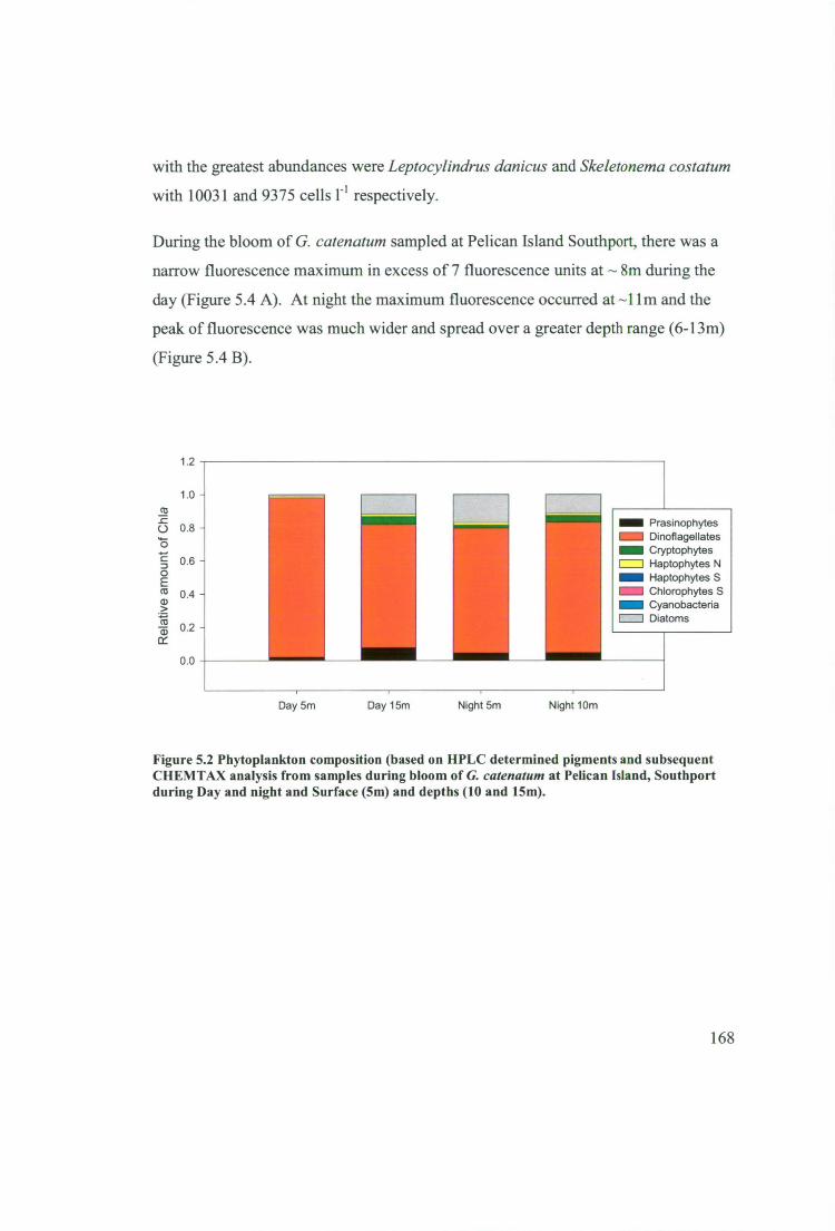
with the greatest abundances were Leptocylindrus danicus and Skeletonema costatum

with 10031 and 9375 cells r' respectively.

During the bloom of G. catenatum sampled at Pelican Island Southport, there was a

narrow fluorescence maximum in excess of 7 fluorescence units at - 8m during the

day (Figure 5.4 A). At night the maximum fluorescence occurred at -11m and the

peak of fluorescence was much wider and spread over a greater depth range (6-13m)

(Figure 5.4 B).

1.2

Rela

tive

a mou

nt o

f Chi

a

0.0

- Prasinophytes Dinoflagellates

- Cryptophytes - Haptophytes N - Haptophytes S - Chlorophytes S - Cyanobacteria O Diatoms

1.0 -

0.8 -

0.6 -

0.4 -

0.2 -

Day 5m Day 15m Night 5m Night 10m

Figure 5.2 Phytoplankton composition (based on HPLC determined pigments and subsequent CHEMTAX analysis from samples during bloom of G. catenatum at Pelican Island, Southport during Day and night and Surface (5m) and depths (10 and 15m).

168

o

I

0 G. catenatum ■ Total Chin O G catenatum Chia

-

_

_

-

-

_

-

6

2

0

7

5

1

90000

80000

70000

60000

50000

40000

30000

20000

10000

Gym

nod i

nium

cat

enat

um (c

ells

1-1)

Day 5m

Day 15m

Night 5m Night 10m

Figure 5.3 Total chl a, chl a attributed to G. catenatum and G. catenatum cell counts at Pelican Island, Southport during Day and night and Surface (5m) and depths (10 and 15m). G. catenatum attributed chl a calculated based on 60 pg chl a celF 1 (Hallegraeff et al., 1991).

Table 5.2 Representative cell count of lugols fixed phytoplankton collected from 5m during the day at Southport 30/03/2004. TAXON Cell count (cells 1 -') Melosira 562 pennate diatom 15um 375 Skeletonema costatum 9375 Thalassiosira spp 187 Guinardia delicatula = Rhizosolenia delicatula 6094 Chaetoceros spp > 10um 1875 Chaetoceros spp < 10um 6375 Leptocylindrus danicus 10031 Dactyliosolen fragillissimus = Rhizosolenia fragillissima 187 Rhizosolenia fallax 469 dinoflagellate 6-8um 3656 Ceratium spp 1856 Dinophysis spp 56 Protoperidinium sp 562 Gymnodinium catenatum 86229 cryptophytes small 7 -10um 26812 flagellates 5-10 urn round 6187

169

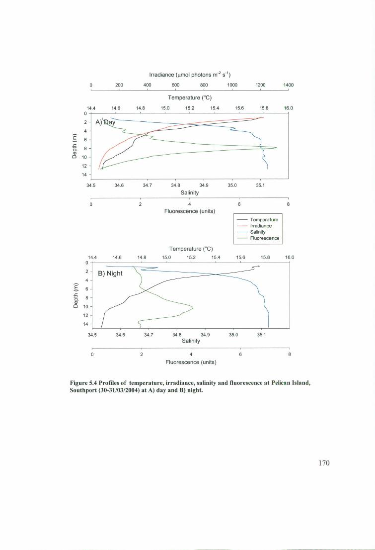
14.4 0

2 -

4 -

E 6

rl 8 - a) O 10 -

12 -

14 -

Temperature ( °C)

14.6 14.8 15.0 15.2 15.4 15.6 15.8 16.0

Irradiance (pmol photons m-2 s-1 )

0 200 400 600 800 1000 1200 1400

34.5

34.6

34.7

34.8 34.9

35.0 35.1 Salinity

0 2 4 Fluorescence (units)

6 8

- Temperature Irradiance

Salinity Fluorescence

14.4 0

2 -

4 -

E 6

• 8 - a) O 1 0 -

12 -

14 -

Temperature ( °C)

14.6 14.8 15.0 15.2 15.4 15.6 15.8

B) Night

16.0

34.5

34.6

34.7

34.8 34.9

35.0

35.1 Salinity

0

2

4

6

8 Fluorescence (units)

Figure 5.4 Profiles of temperature, irradiance, salinity and fluorescence at Pelican Island, Southport (30-31/03/2004) at A) day and B) night.

170

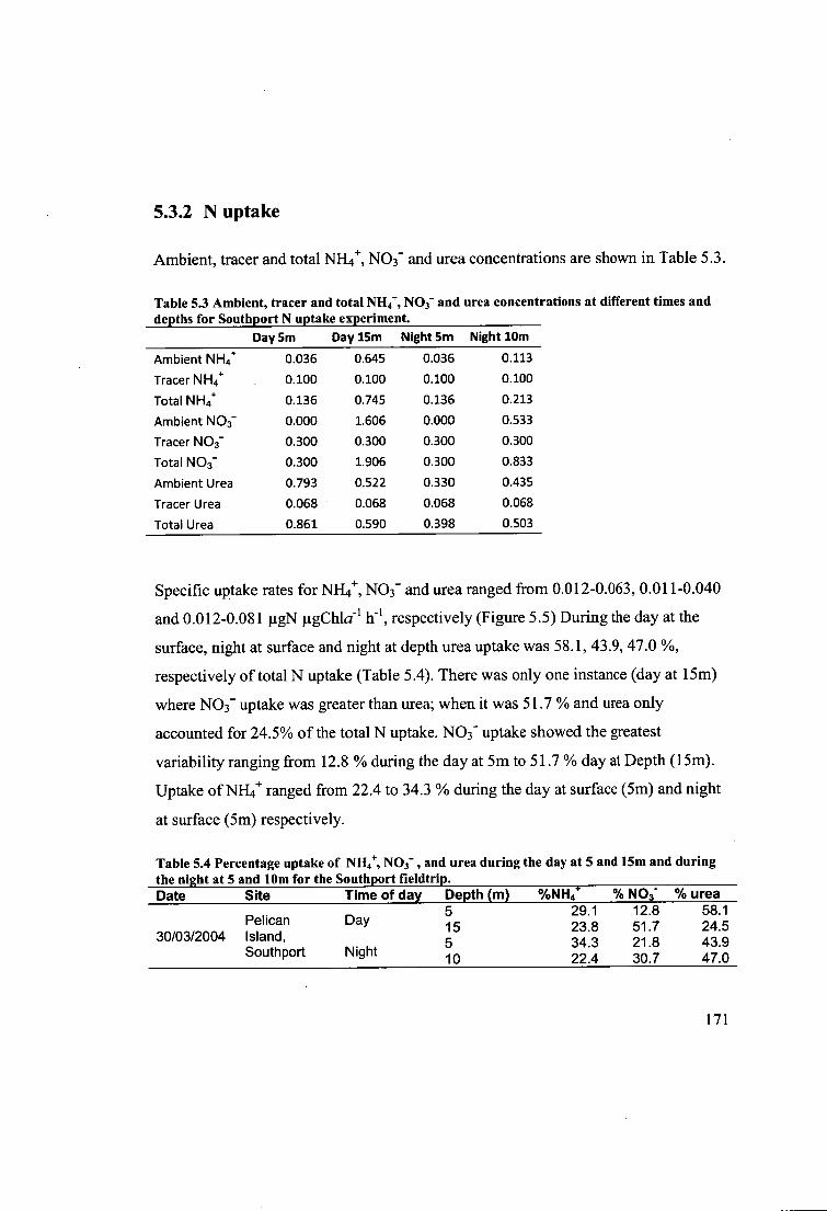
5.3.2 N uptake

Ambient, tracer and total NH4+, NO3- and urea concentrations are shown in Table 5.3.

Table 5.3 Ambient, tracer and total NH4+, NO3- and urea concentrations at different times and depths for Southport N uptake experiment.

Day 5m Day 15m Night 5m Night 10m Ambient NH4 0.036 0.645 0.036 0.113

Tracer NH4+ 0.100 0.100 0.100 0.100

Total NH4+ 0.136 0.745 0.136 0.213

Ambient NO3- 0.000 1.606 0.000 0.533

Tracer NO3- 0.300 0.300 0.300 0.300

Total NO3- 0.300 1.906 0.300 0.833

Ambient Urea 0.793 0.522 0.330 0.435

Tracer Urea 0.068 0.068 0.068 0.068

Total Urea 0.861 0.590 0.398 0.503

Specific uptake rates for NH4+, NO3- and urea ranged from 0.012-0.063, 0.011-0.040

and 0.012-0.081 pigN If', respectively (Figure 5.5) During the day at the

surface, night at surface and night at depth urea uptake was 58.1, 43.9, 47.0 %,

respectively of total N uptake (Table 5.4). There was only one instance (day at 15m)

where NO 3- uptake was greater than urea; when it was 51.7 % and urea only

accounted for 24.5% of the total N uptake. NO3 - uptake showed the greatest

variability ranging from 12.8 % during the day at 5m to 51.7% day at Depth (15m).

Uptake of NH4+ ranged from 22.4 to 34.3 % during the day at surface (5m) and night

at surface (5m) respectively.

Table 5.4 Percentage uptake of NH4 +, NO3- , and urea during the day at 5 and 15m and during the night at 5 and 10m for the Southport fieldtrip. Date Site Time of day Depth (m) %NH4+ % NO3- % urea

5 29.1 12.8 58.1 Pelican Day 15 23.8 51.7 24.5

30/03/2004 Island, 5 34.3 21.8 43.9 Southport Night 10 22.4 30.7 47.0

171

0.0

0.12

0.10 -

0.08 -

0.06 -

0.04 -

0.02 -

0.00

0.4 i A) Absolute N upt e

I I

- NH4 .

1.110 NO3- - Urea

III III B) Specific N uptake

III II. II I id Day 5m Day 15m Night 5m Night 10m

Time and depth (m)

Figure 5.5 Absolute and specific uptake rates of NH 4+, NO3- and urea at Pelican Island, Southport during the day and night and at the surface (5m) and depth (10 and 15m).

When averaged across time of day and depths NH 4+ , NO3- and urea specific uptake

rates were 0.0292, 0.0253 and 0.0446 pig N jig chi c1 1 11 1 respectively or expressed as

percentage of total N uptake (NH4 ++ NO3- + urea) 29.5, 25.5 and 45% respectively

(Figure 5.6)

172

0.07

0.06

0.05

(.) 0.04

cb 0.03

a) al 0.02

Z 0.01

0.00 NH4 NO3 Urea

N Species

Figure 5.6 Mean uptake for NH 4+ , NO3- and urea when both times and depths were combined from Southport (see Fig 1.1 for location). Standard errors are included (n=12)

The main effects of N species, time of day and depth on N uptake were all significant

but interpretation of their effects was complicated because of the significant

interactions between N species and depth and between time of day and depth (Table

5.5).

Table 5.5 Three way ANOVA for the effect of Nitrogen species (N), Time of day (T) and Depth (D) on the specific uptake of nitrogen at Southport during a Gymondium catenatum bloom.

Factor Nitrogen uptake N species (N) Significant effect P=0.048

Time of day (T) Significant effect P=<0.001

Depth (D) Significant effect P=<0.001

N x T No Interaction

N x D Significant Interaction P=<0.001

T x D Significant Interaction P=0.005

NxTxD No Interaction

While acknowledging the complications caused by the significant interaction some

general trends in N uptake were evident. There was an — 2 times increase in the 173

specific uptake of NI-14 + , NO3-, and urea during the night when compared to uptake

during the day (Figure 5.7). NH4 ± and urea uptake at the surface was — 3 times

greater than near the bottom but there was no effect of depth on NO 3- uptake (Figure

5.8). At the surface urea uptake was — 3 times greater than NO3 - uptake and 1.5

times greater than NH4+ uptake. In addition NH 4+ uptake was — 2 times greater than

NO3- uptake in the surface. Total specific nitrogen uptake was 2.3 times greater in the

surface at night than in the surface during the day (Figure 5.9).

0.12

0.10 -

CI Day I

Night

0.08 -

0.06 -

0.04 -

0.02 -

0.00

NH4

NO3

Urea

N species

Figure 5.7 Uptake of NH4+, NO3-, and urea during the day and night at Southport. Least square means and upper and lower 95% confidence intervals.

N u

ptak

e (u

g N

i.tg C

hia

h-1)

174

0.10

0.08 -

0.06 -

0.04 -

0.02 -

I I

CI Day 1 1 Night

0.00

0.12

0.10

0.08

N u

ptak

e (jig N

ug C

hia

h-1)

-

-

O Surface CI Deep

-

-

0.06

_ I

-

0.04

_

I T 1

0.02

-

0.00

NH4

NO3

Urea

N species

Figure 5.8 Uptake of NH 4+, NO3-, and urea at surface and bottom depths in Southport. Least square means and upper and lower 95% confidence intervals are shown.

Surface Bottom

Depth

Figure 5.9 Uptake of the three different N species at surface and bottom during the day and night at Southport. Least square means and upper and lower 95% confidence intervals are shown.

N u

ptak

e (u

g N

lig C

hia

h-1

)

175

5.4 Discussion

Gymnodinium catenatum dominated the phytoplankton assemblage sampled near

Pelican Island, Southport. G. catenatum was responsible for 87 and 73% of the Chla,

during the day at 5 and 15 m respectively and 53 and 74% of the Chia during the

night at 5 and 10m respectively. CHEMTAX results based on HPLC pigments

indicated that the other phytoplankton groups responsible for the remaining Chla

were diatoms, cryptophytes, prasinophytes and haptophytes N, listed in order of their

contribution. The Chi a biomass and species composition of this bloom at Southport

was similar to the summer and autumn blooms previously observed in the Huon

Estuary with mean Chl a values of-3 gg 1-1 and G. catenatum responsible for greater

than 50% of the phytoplankton assemblage (Thompson et al., 2008). It is suggested

that the N uptake results from this G. catenatum dominated bloom at Southport will

be useful in gaining insight into the behaviour and N uptake capabilities that enables

G. catenatum to bloom so successfully in the South East of Tasmania and other parts

of the world.

Specific uptake rates for NH4+, NO3- and urea ranged from 0.012-0.063, 0.011-0.040

and 0.012-0.081 jig N jig chi a 1 h'. The specific uptake rates from Southport were

at the lower end of the range reported by Rosser and Thompson (Rosser &

Thompson, 2001) in the much more eutrophic Swan River.

When averaged across time and depth urea uptake was greatest at 45% and NI-14 + and

NO3- are both roughly equal in their contributions at 29.5 and 25.5 %, respectively.

In comparison to the late autumn and late summer fieldtrips in the Huon estuary urea

was responsible for a greater proportion of the phytoplankton uptake. It seems likely

that the reason for this is that in southport both the preferred N sources (chapter 4)

N114+and NO3- have been exhausted in the surface and hence G. catenatum is forced

to use urea and exploit deep NO 3- via vertical migration. While in the Huon Estuary

its hypothesised that NH 4+ uptake is more important during these times of year

because of the added input of NH 4+ from salmon farming. These results are also in 176

good agreement with many studies which have shown that urea uptake is important

for many phytoplankton species (Berman & Bronk, 2003), especially autumn

dinoflagellate blooms (Glibert and Terlizzi 1999).

Results from a series of experiments on G. catenatum show that this species grows

equally well on NH4 +, NO3- and urea as sole N sources (see Figure 4.2 and Figure 4.3

in Chapter 4), but when presented with a mixture of NH 4+, NO3- and urea they are

taken up in the order NH 4+>NO3-> urea. This preference for NH4+ and NO3-

indicates that there must be low supply of both of these substrates for urea uptake to

be the most important N source for this G. catenatum dominated bloom at Southport.

The ability of G. catenatum to vertically migrate (Doblin et al., 2006) means that to

understand more clearly the behaviour and N uptake capabilities of this species in the

field it is important to examine N uptake during the day and night and at depths

related to its position in the water column.

177

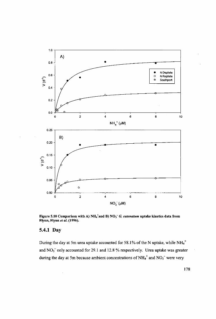
1.0

0.8

0.6 '7

0.4

0.2

0.0

2

4 6

8

10

NH4+ (JAM)

0.25

0.20

0.15 7

0.10

0.05

0.00

2

4 6

8

10

NO3- (JAM)

Figure 5.10 Comparison with A) NH 4+and B) NO3- G. catenatum uptake kinetics data from Flynn, Flynn et al. (1996).

5.4.1 Day

During the day at 5m urea uptake accounted for 58.1% of the N uptake, while NH 4+ and NO3- only accounted for 29.1 and 12.8 % respectively. Urea uptake was greater

during the day at 5m because ambient concentrations of NH 4+ and NO3 - were very

178

low 0.04 and <0.01 I.LM (below detection level) respectively. At such low

concentrations the rate at which G. catenatum can take up any N substrates is

substantially reduced (Flynn et al., 1996). However while urea is not the preferred

source of N it was present at a much greater concentration, 0.79 tM hence the

phytoplanIcton were taking up urea at a greater rate. While urea was being taken up at

the greatest rate NH 4+ and NO3- were also being taken up at lesser but significant

rates. A considerable fraction of the NH 4+ and NO3- uptake was associated with the 15N tracer which was added at 2.5 and 30 times (respectively) greater concentrations

than ambient. If the NH4+ and NO3- could have been added at truly tracer levels

(10% of ambient concentrations) NH4+ and NO3- uptake would have been much less

and urea would have made an even greater % of the uptake under these conditions.

During the day at 15m NO 3- uptake was greatest, responsible for 51.7% of N uptake

and NH4+ and urea were responsible for almost equal amounts 23.8 and 24.5%

respectively. The N uptake rates at depth appear to be related to the ambient substrate

concentrations with NO3 - uptake being greatest because it is available at

concentrations of 1.6 p.M, greater than double the concentration of NH 4+ or urea

during the day at this depth.

The fluorescence profile is in the shape of a sharp peak with a maximum fluorescence

at —8m indicating that during the day the greatest concentration of phytoplankton are

at 8m and based on the G. catenatum dominated samples from the 5 and 15m samples

and what we know about vertical migration of G. catenatum (Team, 2000, Doblin et

al., 2006) it seems likely that G. catenatum is positioning itself at 8m during the day

where it can access light for growth but also N in the form of elevated NO3 - concentrations like those observed at 15m. At 8m Irradiance is approximately 160

111.1101 photons 1112 s -1 and temperature 15.8°C. Ek calculated from the model in

Chapter 3 for 15.8 °C was 7.1 innol photons m -2 s-1 . These laboratory results indicate

that the irradiance of 160 timol photons rr1-2 s -1 would be saturating growth and well

in excess of the requirements for G. catenatum at this temperature. This type of

179

strategy has been reported by other dinoflagellates including (e.g. Ault, 2000)(Cullen

and Horrigan 1981; Eppley, Holmhans etal. 1968; Hasle 1950.

5.4.2 Night

During the night at 5m urea uptake was 43.9% of N uptake, while NI-1 4+ and NO3-

were responsible for 34.3 and 21.8%, respectively. Uptake during the night at 5m

was similar in many ways to what was seen during the day at 5m. Urea uptake was

most important and ambient concentrations of urea (0.32 i_tM at surface) were greater

than either NH4+ or NO3- uptake. Also, in-situ uptake rates of NH4+ and NO3- were

probably overestimated because of relatively high concentrations of the 15N tracer, as

was also the case for the day at 5m. It might be expected that uptake rates of these N

species would be lower at night because absence of light usually reduces the uptake

of N substrates (MacIsaac & Dugdale, 1972) particularly NO 3- which requires more

energy for uptake and assimilation (Syrett, 1981). Clearly uptake rates are not

reduced at night, in fact they are greater. It can be hypothesized that high noctural

uptake rates resulted from cells that were N depleted. Under these conditions a range

of cultures and field experiments have shown uptake of N, including NO 3 in the dark

at rates usually only seen during the day (Harrison, 1976, Cochlan et al., 1991).

During the night at 10m uptake of urea was 47% ot total N uptake, NO3 - 30.7% and

NH 4+ 22.4%. Uptake rates of both urea and NO 3- were greater than the usually

preferred NH4+, possibly because they were available at greater concentrations, 0.43

uM and 0.53 uM respectively compared to NH4 + at 0.11 uM.

At night the shape of the fluorescence peak broadened and the maximum in

fluorescence was deeper and less concentrated than the shallower the daytime

fluorescence maximum (Figure 5.4 B). Within the broad night time fluorescence

maximum the distribution of biomass was skewed towards the bottom of the

maximum. This suggests that the majority G. catenatum dominated phytoplanIcton

community found concentrated at 8m during the day probably migrated deeper to

10m at night. In addition to this modest migration the phytoplankton spread out more

180

ranging from 5-13 m. Going deeper may be important for accessing NO 3- and urea at

greater concentrations but spreading out may also be important in maximising the

substrate concentration per cell and scavenging any available N in the water column.

This strategy may act to maximising uptake under conditions of very low ambient

concentrations of NO3 - in these and other similar coastal and estuarine systems

worldwide.

5.4.3 Summary

This field study confirmed that G. catenatum uses NH4+, NO3- and urea in the field as

was also observed in the laboratory (Chapter 4). The results from this field study

were consistent with the preferences for N substrates found in the laboratory, in this

order NH44-> NO3- >urea. The low ambient concentrations of NH4+and NO3- in the

surface layer clearly suggest the bloom was in a relatively late phase. Clearly at this

stage of the bloom recycled N or organic N such as urea became a very important

source of N. The ability of this species to vertically migrate means that during the day

G. catenatum is able to position itself in the water column where it receives light in

excess of its requirements for growth while migrating to depth also allows it to access

greater concentrations of NO 3-. During the night when light is not available G.

catenatum vertically migrated deeper in the water column and was able to access the

greater concentrations of NO3 - at these depths. While the vertical migration observed

in this field study was not as dramatic as seen during the Huon Estuary study, the

water column was not as deep and the N relatively closer to the surface. There is

sufficient evidence from this study to validate the hypotheses from Doblin et al,

(2006) that G. catenatum vertically migrates to access nitrogen at depth.

181

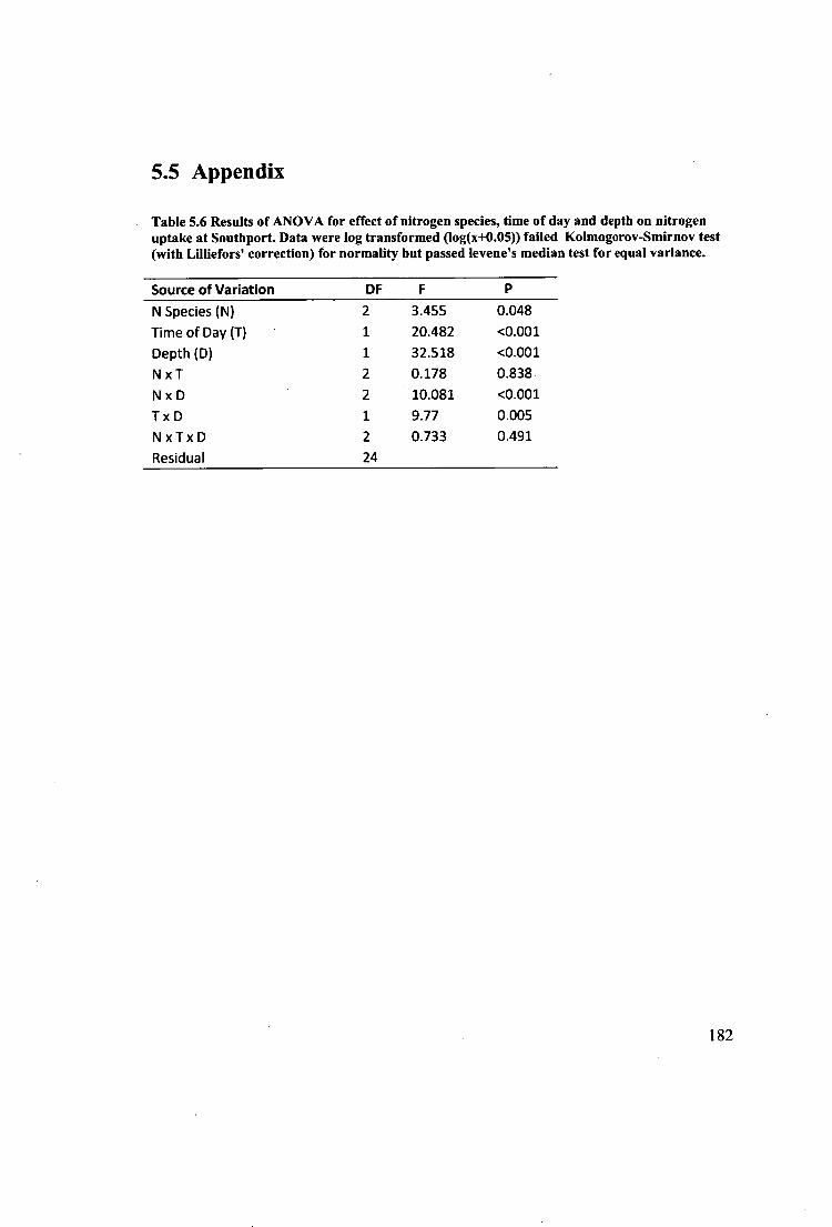
5.5 Appendix

Table 5.6 Results of ANOVA for effect of nitrogen species, time of day and depth on nitrogen uptake at Southport. Data were log transformed (log(x+0.05)) failed Kolmogorov-Smirnov test (with Lilliefors' correction) for normality but passed levene's median test for equal variance.

Source of Variation DF F N Species (N) 2 3.455 0.048

Time of Day (T) 1 20.482 <0.001

Depth (D) 1 32.518 <0.001

N x T 2 0.178 0.838

N x D 2 10.081 <0.001

T x D 1 9.77 0.005

N x Tx D 2 0.733 0.491

Residual 24

182

5.6 References

Anderson, D. M., Glibert, P. M. & Burkholder, J. M. 2002. Harmful algal blooms and eutrophication: Nutrient sources, composition, and consequences. Estuaries 25:704-26.

Armstrong, F. A. J. 1951. The determination of silicate in sea water. Journal of Marine Biological Association of the United Kingdom 30:149-60.

Ault, T. R. 2000. Vertical migration by the marine dinoflagellate Prorocentrum triestinum maximises photosynthetic yield. Oecologia 125:466-75.

Banse, K. 1977. Determining carbon to chlorophyll ratio of natural phytoplankton. Mar Bio/ 41:199-212.

Berman, T. & Bronk, D. A. 2003. Dissolved organic nitrogen: a dynamic participant in aquatic ecosystems. Aquat. Microb. Ecol. 31:279-305.

Chang, F. H. & McClean, M. 1997. Growth responses of Alexandrium minutum (Dinophyceae) as a function of three different nitrogen sources and irradiance. New Zealand Journal of Marine and Freshwater Research 31:1-7.

Chang, F. H. & Page, M. 1995. Influence of light and three nitrogen sources on growth of Heterosigma cartarae (Raphidophyceae). New Zealand Journal of Marine and Freshwater Research 29:29-304.

Cochlan, W. P., Price, N. M. & Harrison, P. J. 1991. Effects of Irradiance on Nitrogen Uptake by Phytoplankton - Comparison of Frontal and Stratified Communities. Mar Ecol-Prog Ser 69:103-16.

Doblin, M. A., Thompson, P. A., Revill, A. T., Butler, E. C. V., Blackburn, S. I. & Hallegraeff, G. M. 2006. Vertical migration of the toxic dinoflagellate Gymnodinium catenatum under different concentrations of nutrients and humic substances in culture. Harmful Algae 5:665-77.

Doucette, G. J. & Harrison, P. J. 1991. Aspects of Iron and Nitrogen Nutrition in the Red Tide Dinoflagellate Gymnodinium-Sanguineum .2. Effects of Iron Depletion and Nitrogen-Source on Iron and Nitrogen Uptake. Mar Biol 110:175-82.

Downing, J. A. 1997. Marine nitrogen: Phosphorus stoichiometry and the global N:P cycle. Biogeochemistry 37:237-52.

Dugdale, R. C. & Goering, J. J. 1967. Uptake of new and regenerated forms of nitrogen in primary productivity. Limnol. Oceanogr. 12:196-206.

Dugdale, R. C. & Wilkerson, F. P. 1986. The use of N-15 to measure nitrogen uptake in eutrophic oceans- experimental considerations. Limnol. Oceanogr. 31:673- 89.

Flynn, K. J., Flynn, K., John, E. FL, Reguera, B., Reyero, M. I. & Franco, J. M. 1996. Changes in toxins, intracellular and dissolved free amino acids of the toxic dinoflagellate Gymnodinium catenatum in response to changes in inorganic nutrients and salinity. J Plankton Res 18:2093-111.

183

Glibert, P. M., Lipschultz, F., McCarthy, J. J. & Altabet, M. A. 1982. Isotope-dilution models of uptake and remineralization of ammonium by marine plankton. LimnoL Oceanogr. 27:639-50.

Hallegraeff, G. M. 1992. Harmful Algal Blooms in the Australian Region. Mar Pollut Bull 25:186-90.

Hallegraeff, G. M. 1993. A review of harmful algal blooms and their apparent global increase. Phycologia 32:79-99.

Halleglaeff, G. M., Nichols, P. D., Vollcman, J. K., Blackburn, S. I. & Everitt, D. A. 1991. Pigments, Fatty-Acids, and Sterols of the Toxic Dinoflagellate Gyrnnodinium-Catenatum. J Phycol 27:591-99.

Harrison, W. G. 1976. Nitrate metabolism of red tide dinoflagellate Gonyaulax-polyedra stein. Journal of Experimental Marine Biology and Ecology 21:199- 209.

Heisler, J., Glibert, P. M., Burkholder, J. M., Anderson, D. M., Cochlan, W., Dennison, W. C., Dortch, Q., Gobler, C. J., Heil, C. A., Humphries, E., Lewitus, A., Magnien, R., Marshall, H. G., Sellner, K., Stockwell, D. A., Stoecker, D. K. & Suddleson, M. 2008. Eutrophication and harmful algal blooms: A scientific consensus. Harmful Algae 8:3-13.

Holm-Hansen, 0. & Booth, C. 1966. The measuremeant of adenosine triphosphate in the ocean and its ecological significance. LimnoL Oceanogr. 11:510-19.

Kerouel, R. & Aminot, A. 1997. Fluorometric determination of ammonia in sea and estuarine waters by direct segmented flow analysis. Mar. Chem. 57:265-75.

La Roche, J. 1983. Ammonium regeneration: Its contribution to phytoplankton nitrogen requirements in a eutrophic environment. Marine biology, Heidelberg 75:231-40.

MacIsaac, J. J. & Dugdale, R. C. 1972. Interactions of light and inorganic nitrogen in controlling nitrogen uptake in sea. Deep-Sea Research 19:521-27.

Mackey, M. D., Mackey, D. J., Higgins, H. W. & Wright, S. W. 1996. CHEMTAX - A program for estimating class abundances from chemical markers: Application to HPLC measurements of phytoplankton. Mar. EcoL-Prog. Ser. 144:265-83.

Mulvenna, P. F. & Savidge, G. 1992. A Modified Manual Method for the Determination of Urea in Seawater Using Diacetylmonoxime Reagent. Estuar Coast Shelf S 34:429-38.

Murphy, J. & Riley, J. P. 1962. A modified single-solution for the determination of phosphate in natural waters. Analytica Chimica Acta 27:31-36.

Nagai, S., Nitshitani, G., Tomaru, Y., Sakiyama, S. & Kamiyama, T. 2008. Predation by the toxic dinoflagellate Dinophysis fortii on the ciliate Myrionecta rubra and observation of sequestration of ciliate chloroplasts. J. Phycol. 44:909-22.

Park, M. G., Kim, S., Kim, H. S., Myung, G., Kang, Y. G. & Yih, W. 2006. First successful culture of the marine dinoflagellate Dinophysis acuminata. Aquat. Microb. EcoL 45:101-06.

184

Rosser, S. & Thompson, P. A. 2001. Phytoplankton of the Swan-Canning Estuary: a comparison of nitrogen uptake by different bloom assemblages. Hydra Process. 15:2579-94.

Sokal, R. R. & Rohlf, F. J. 1995. Biometry: the principles and practice of statistics in biological research. W.H. Freeman and Company, New York, 887.

Syrett, P. J. 1981. Nitrogen-metabolism of microalgae. Canadian Bulletin of Fisheries and Aquatic Sciences: 182-210.

Team, H. E. S. 2000. Huon Estuary Study, Environmental research for integrated catchment management and aquaculture. Final Report to FRDC. CSIRO Division of Marine Research, Hobart, Tasmania, Australia.

Thompson, P. 1999. Response of growth and biochemical composition to variations in daylength, temperature, and irradiance in the marine diatom Thalassiosira pseudonana (Bacillariophyceae). J Phycol 35:1215-23.

Thompson, P. A., Bonham, P. I. & Swadling, K. M. 2008. Phytoplankton blooms in the Huon Estuary, Tasmania: top-down or bottom-up control? J. Plankton Res. 30:735-53.

Watson, R. J., Butler, E. C. V. & Clementson, L. A. 2004. Flow-injection analysis with fluorescence detection of trace levels of ammonium in seawater. Journal of Environmental Monitoring 7:37-42.

Wood, E. D., Armstrong, F. A. J. & Richards, F. A. 1967. Determination of nitrate in sea water by cadmium-copper reduction to nitrite. Journal of Marine Biological Association of the United Kingdom 47:23-31.

185

6 SUMMARY

6.1 Background

The Huon Estuary receives a significant input of oceanic nutrients during winter and

surface nutrients rise to > 3 AM nitrate, 0.4 prM phosphate, — 15 uM silicate (Fig. 1)..

The Huon River is the major source of fresh water to the Estuary, it has a seasonal

flow with a long-term average of 30 m s-I in summer (Dec-Feb) rising to — 130 ms'

during late winter (July-Aug). The Huon Estuary is a salt wedge with seasonally

variable surface outflow and inflow at depth. The Huon River is a major source of

refractory nitrogen (— 600 to 1100 tonnes annually) and dissolved silica to the Huon

Estuary and D'Entrecasteaux Channel but a source of very little DIN. The Huon

River dissolved organic N input is poorly quantified and the nitrogen forms are very

poorly characterized. During the transition to spring nitrate and phosphate

concentrations decline and by summer the nitrate concentrations are near zero while

phosphate and silicate concentrations remain relatively high, suggesting a nitrogen

limited ecosystem (Figure 6.1). It is only during summer that surface nitrate and

ammonium concentrations are relatively similar. The finfish aquaculture industry

contributes a significant amount of nitrogen to the Huon Estuary, — 313 tonnes of

mostly ammonium in 2002. Both industry and government regulators are alert to the

potential for eutrophication and increased harmful algal blooms if the assimilative

capacity for N of the estuary is exceeded. As part of a larger project on the ecology of

the Huon Estuary, this PhD research has two main objectives; firstly to determine

whether phytoplankton in the Huon Estuary were using nitrogen that had, primarily,

an oceanic source (e.g. nitrate) or was more locally supplied or regenerated (e.g.

ammonium and urea) and secondly to examine the physiology of G. catenatum.

186

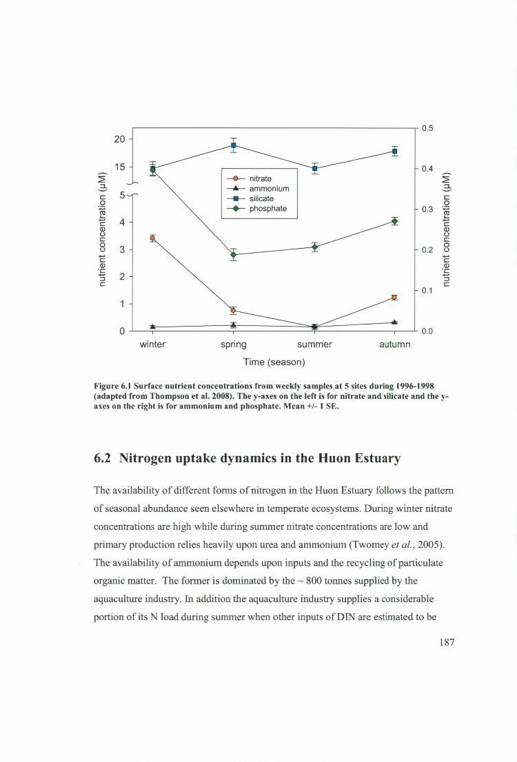
20 - 0.5

- nitrate -A-- ammonium —E— silicate - phosphate

- 0.4

- 0.3

0.0

0.2

0.1

nutri

ent c

once

ntra

tion

(pM

)

winter spring summer

autumn

Time (season)

Figure 6.1 Surface nutrient concentrations from weekly samples at 5 sites during 1996-1998 (adapted from Thompson et al. 2008). The y-axes on the left is for nitrate and silicate and the y-axes on the right is for ammonium and phosphate. Mean +1- 1 SE.

6.2 Nitrogen uptake dynamics in the Huon Estuary

The availability of different forms of nitrogen in the Huon Estuary follows the pattern

of seasonal abundance seen elsewhere in temperate ecosystems. During winter nitrate

concentrations are high while during summer nitrate concentrations are low and

primary production relies heavily upon urea and ammonium (Twomey et al., 2005).

The availability of ammonium depends upon inputs and the recycling of particulate

organic matter. The former is dominated by the — 800 tonnes supplied by the

aquaculture industry. In addition the aquaculture industry supplies a considerable

portion of its N load during summer when other inputs of DIN are estimated to be

187

low. Based upon what we know about the species that typically form HABs this input

of DIN into a N limited system during summer could be expected to exacerbate HAB

in this ecosystem.

During this research, the uptake of NH 4+, NO3" and urea at 2 locations, 2 depths,

during the day and night and at four times throughout the year provided the basis to

assess the nitrogen uptake dynamics by phytoplankton in the Huon Estuary (Chapter

2). Reduced forms of N (NH4 + and urea) accounted for the majority of the overall N

uptake, 52% and 37.5% respectively, while NO 3" uptake was responsible for only

10.5% of the overall N uptake. Studies of N uptake in other coastal and estuarine

ecosystems have also shown that reduced N forms account for a large component of

the overall N uptake (e.g. McCarthy etal., 1977, L'Helguen etal., 1993, Metzler et

al., 1997, Harrison, 2002, Rosser & Thompson, 2001) and that these forms of N are

actively preferred in many cases (e.g. O'Donohue et al., 2000, Dauchez etal., 1991,

Keene etal., 1991, Middelburg & Nieuwenhuize, 2000).

Nitrate uptake accounted for the smallest component on all field trips but peaked at

—15% of the N uptake during early spring. During the winter to spring transition

[NO3] was drawn down and only low concentrations were measured on late spring

and late summer field trips. This also coincided with the spring diatom bloom in the

Huon Estuary sinking out of the water column in late spring when the chlorophyll a

concentrations were greater at 20 m than at 5m.

The NH 4+ accounted for >50% of N uptake by phytoplankton on all 4 field trips (late

autumn, early spring, late spring and late summer). Urea was the next largest

component of the N uptake on all 4 field trips but became a larger component, up to

—40% of the N uptake during the late spring and late summer field trips. There is

very little work on the seasonality of N uptake although this shift from nitrate to more

ammonium and urea uptake has been observed by other researchers following a

spring bloom (e.g. Bury etal., 2001, Kudela & Dugdale, 2000, Bronk etal., 1998,

Torres-Valdes & Purdie, 2006).

188

Hydrodynamic and biogeochemical modelling of the Huon Estuary and

D'Entrecasteaux Channel indicated a significant rise in expected chlorophyll a

concentrations in response to the DIN loading from aquaculture (Vollcman et al.,

2009). The modelling also suggests the magnitude of this impact will not be uniform

in time or space. Some locations are predicted to experience no change and other will

have a substantial rise in chlorophyll a for most of the year. One of the challenges

identified in the modelling was that the DIN sources and phytoplankton responses

will be displaced in time and space making attribution difficult. A number of

locations were identified as potentially susceptible to phytoplankton blooms associate

with the N loading from aquaculture. In response to the modelling and the identified

environmental risks a monitoring program has been put in place. This program spans

the region and will regularly assess the environmental status of key parameters such

as phytoplankton composition and biomass, dissolved oxygen and ammonium

concentrations.

6.3 Physiology and ecology of G. catenatum

This thesis represents the most comprehensive study of the effects of irradiance and

temperature on G. catenatum growth and physiology to date. Growth versus

irradiance curves were determined for twelve temperatures from 11.9-25.0 °C and a

comparison of the growth rates from the present study with five other studies on

different G. catenatum strains has revealed considerable similarity between the

growth responses of these strains particularly at temperatures between 10-20 °C. At

temperatures >= 28.5 °C the strains from Japan and Mexico appeared to be able

sustain growth rates approximately 0.2 d , while the other strains did not grow,

indicating that Japanese and Mexican populations may constitute an warm-water

ecotype. Relationships between the parameters OA max , a and Ec) from the growth

versus irradiance curves and temperature were investigated and modelled. The

models of the effect of temperature on i.t. a,„ a and Ec provide the basis for

development of a G. catenatum growth model useful to predictive ecological

189

responses in natural populations. This model can be applied by scientists or natural

resource managers to determine when growth of this species will be fastest and

whether the ecosystem they are investigating can support growth year round. For

example the Huon Estuary winter temperatures are at the lower limit of growth of the

strain examined in this research. In addition to this at temperatures from 16-20 °C,

typical of summer in the Huon Estuary G. catenatum would only be capable of

growth rates ranging from 0.1-0.2 d -i .

The biochemical composition of G. catenatum was also examined revealing that G.

catenatum adapts to low temperature conditions by increasing its carbon (C) quota.

At higher temperatures and lower irradiances G. catenatum responded by increasing

chla but this was accompanied by an even greater increase in C quota. These results

give us insights into the strategies that this species uses for growth and survival in

unfavourable conditions. At low temperatures G. catenatum increases C quota as

observed in other species (Sakshaug & Andresen, 1986) possibly as a mechanism to

allow survival through cold periods. In the case of G. catenatum it might be a carbon

acquisition strategy that will lead to sexual reproduction and cyst formation. At high

temperatures and low irradiances the increase in carbon quota was accompanied by

an increase in chlorophyll a per cell. Increased carbon and chlorophyll a quotas are a

common occurrence under these conditions (Geider, 1987) where cells require more

structures (e. g. chloroplasts) for light capture and the enzymes are capable of high

rates of operation. An empirical model to describe the effects of light and

temperature on C:chl a was constructed and may be useful information that increases

our understanding of physiological responses in this species or other similar species

in the future.

This work also demonstrated that G. catenatum has diverse N uptake capabilities. It

grows equally well using NO3 - , NH 4+ or urea in the laboratory (Chapter 4) and this

is also evident from the field studies (Chapters 4, 5). The preference for NH4 + and

NO 3 - over urea may reflect the energetic and biochemical costs associated with

uptake and assimilation of the various sources. Perhaps, while it poses no penalties 190

for growth when energy from light is saturating, the preferences may be related to the

preferences under energy limited circumstances. For example, variation in the

growth rate of Alexandrium minutum (Dinophyceae) on NO3 - were highly dependent

on the level of irradiance (Chang & McClean, 1997).

The ability of G. catenatum to vertically migrate means that during the day G.

catenatum is able to position itself in the water column where it receives light in

excess of its requirements, and migrates to depth at night to access greater

concentrations of NO3-, probably also NI14+ and urea. While the vertical migration

observed in this field study was not as dramatic as seen during the Huon Estuary

study (CSIRO Huon Estuary Study Team, 2000, Doblin et al., 2006), the bloom did

not take place in as deep a water column and the N was relatively closer to the

surface. There is sufficient evidence from this study to validate the hypotheses from

Doblin, Thompson et al. (2006) that G. catenatum vertically migrates to access

nitrogen at depth.

For G. catentatum growing in the Huon Estuary it seems increasingly apparent that it

functions as a nitrogen scavenger. When N concentrations are exhausted, it is able to

migrate rapidly through the water column seeking whatever form of nitrogen is

available. Thus the dominance of this species is perhaps not due to it occupying a

specialist niche associated with NH4+, but rather due to its greater capacity to access

uptake N from different parts of the water column when it may be in short supply

nearer the surface. This was clearly demonstrated by the experiments conducted at

Southport during a G. catenatum bloom (Chapter 5). Urea was the most important N

source ( — 40%) at the late stage of the bloom. The low ambient concentrations of

NH4+ and NO3 - in the surface layer were clearly insufficient to support more growth.

At the bottom of the euphotic zone the vertically migrating bloom was able to find

NO3- and was fully capable to exploiting this N resource with NO 3 - uptake

dominating (-52%) over NI-14+ and urea uptake. Although nitrate reductase was not

measured it has been shown for other dinoflagellates that high nitrate reductase

191

activity is present during blooms, even when ammonium is abundant relative to

nitrate concentrations (Harrison, 1973).

The present study and that of (Flynn et al., 1996) shows that G. catenatum is capable

of responding to pulses of N by 'surge uptake'(relative to a maximum growth rate 0.3

d-1 ) when it is in a N starved condition. Surge uptake is another mechanism that a

species may use to exploit patches of elevated nutrients potentially giving them a

competitive advantage relative to species without this capability (Cochlan &

Harrison, 1991). Our results show that 'surge' uptake rates of NH4 + were almost 20

times the maximum growth rate of G. catenatum (0.30 (1-1 ).

Based on this combined new understanding of the physiology and ecology of G.

catenatum from lab and field studies, G. catenatum has a competitive advantage over

non migratory species in environments where available nutrients (nitrogen) are

vertically separated from sufficient irradiance for growth. The chain-forming nature

and the tendency to form progressively longer chains during blooms can increase

swimming speed (Fraga et al., 1987) allowing G. catenatum to vertically migrate

over substantial depths, and this capacity appears to be more important than which N

species is available in the water column.

6.4 Future Research

While this study has made significant progress in understanding the nitrogen uptake

dynamics of phytoplankton in the Huon Estuary, there are significant gaps in our

current knowledge of the sources of nitrogen and the bloom dynamics of

Gynmodinium catenatum in the Huon Estuary system. Two areas for future research

are:

• Terrestrial sources of nitrogen: The Huon River remains a potentially

major source of dissolved organic N (DON) input to the Estuary that is poorly

quantified and very poorly characterized. Recent hydrodynamic and

biogeochemical modelling (Volkman et al., 2009) suggests that this N is 192

largely refractory and exported out to sea, but it is currently unknown what

proportion is retained and recycled in Huon Estuary, or may be used by

phytoplanlcton in the estuary.

• Development of a species specific model for Gymnodinium catenatum: A

model that enables the prediction of growth rate based on temperature and

irradiance was developed in Chapter 3. Combining this growth model with

the increased understanding of the physiology of G.catenatum: N uptake

preferences, capability for 'surge' uptake (Chapter 4) and vertical migration

strategy to scavenge N (NH4+, NO3 - and urea) (Chapter 5) and other important

parameters like uptake kinetics for G. catenatum (NO3 - and NH4+ ) from

Flynn, Flynn et al. (Flynn et al., 1996), G. catenatum mortality rates

(Volkman et al., 2009) and grazing in Huon Estuary (Thompson etal., 2008).

A species specific model could then be coupled to a physical model of the

Huon Estuary and D'Entrecasteaux Channel and used to compare with field

data in trying to elucidate the drivers of the development of G. catenatum

blooms. There may also be potential to apply a species specific model to

other temperate ecosystems where G. catenatum is a problem.

193

6.5 References

Bronk, D. A., Glibert, P. M., Malone, T. C., Banahan, S. & Sahlsten, E. 1998. Inorganic and organic nitrogen cycling in Chesapeake Bay: autotrophic versus heterotrophic processes and relationships to carbon flux. AquaL Microb. EcoL 15:177-89.

Bury, S. J., Boyd, P. W., Preston, T., Savidge, G. & Owens, N. J. P. 2001. Size-fractionated primary production and nitrogen uptake during a North Atlantic phytoplankton bloom: implications for carbon export estimates. Deep-Sea Res. Part I-Oceanogr. Res. Pap. 48:689-720.

Chang, F. H. & McClean, M. 1997. Growth responses of Alexandrium minutum (Dinophyceae) as a function of three different nitrogen sources and irradiance. New Zealand Journal of Marine and Freshwater Research 31:1-7.

Cochlan, W. P. & Harrison, P. J. 1991. Uptake of Nitrate, Ammonium, and Urea by Nitrogen-Starved Cultures of Micromonas-Pusilla (Prasinophyceae) - Transient Responses. J Phycol 27:673-79.

CS1R0 Huon Estuary Study Team 2000. Huon Estuary Study-Environmental research for integrated catchment management and aquaculture. In: Butler, E. C. V. [Ed.] Final report to Fisheries Research and Development Corporation. CSIRO Division of Marine Research, Marine Laboratories, Hobart.

Dauchez, S., Queguiner, B., Treguer, P. & Zeyons, C. 1991. A Comparative-Study of Nitrogen and Carbon Uptake by Phytoplankton in a Coastal Eutrophic Ecosystem (Bay of Brest, France). Oceanol. Acta 14:87-95.

Doblin, M. A., Thompson, P. A., Revill, A. T., Butler, E. C. V., Blackburn, S. I. & Hallegraeff, G. M. 2006. Vertical migration of the toxic dinoflagellate Gymnodinium catenatum under different concentrations of nutrients and humic substances in culture. Harmful Algae 5:665-77.

Flynn, K. J., Flynn, K., John, E. H., Reguera, B., Reyero, M. I. & Franco, J. M. 1996. Changes in toxins, intracellular and dissolved free amino acids of the toxic dinoflagellate Gymnodinium catenatum in response to changes in inorganic nutrients and salinity. J Plankton Res 18:2093-111.

Fraga, S., Gallager, S. M. & Anderson, D. M. 1987. Chain forming dinoflagellates: An adaptation to red tides. In: T. Okaichi, D. M. A., and T. Nemoto [Ed.] Red tides: Biology, environmental science and toxicology. Elsevier, pp. 281-84.

Geider, R. J. 1987. Light and temperature dependance of the carbon to chlorophyll a ratio in microalgae and cyanobacteria: implications for physiology and growth of phytoplankton. New Phytol. 106.

Harrison, P. J. 2002. Station papa time series: Insights into ecosystem dynamics. J. Oceanogr. 58:259-64.

Harrison, W. G. 1973. Nitrate reductase-activity during a dinoflagellate bloom LimnoL Oceanogr. 18:457-65. Keene, N. K., Smith, W. 0. & Kattner, G. 1991. Nitrogen Uptake in 2 Frontal Areas

in the Greenland Sea. Polar Biol. 11:219-25.

194

Kudela, R. M. & Dugdale, R. C. 2000. Nutrient regulation of phytoplanIcton productivity in Monterey Bay, California. Deep-Sea Res Pt Ii 47:1023 -53.

L'Helguen, S., Madec, C. & Lecorre, P. 1993. Nitrogen Nutrition of the Phytoplankton in the Well-Mixed Waters of the Western English-Channel. Oceanologica Acta 16:653-60.

McCarthy, J. J., Taylor, R. W. & Taft, J. L. 1977. Nitrogenous nutrition of the plankton in the Chesapeake Bay. 1. Nutrient availability and phytoplankton preferences. LimnoL Oceanogr. 22:996- 1011.

Metzler, P. M., Glibert, P. M., Gaeta, S. A. & Ludlam, J. M. 1997. New and regenerated production in the South Atlantic off Brazil. Deep-Sea Res. Part I-Oceanogr. Res. Pap. 44:363-84.

Middelburg, J. J. & Nieuwenhuize, J. 2000. Uptake of dissolved inorganic nitrogen in turbid, tidal estuaries. Mar Ecol-Prog Ser 192:79 -88.

O'Donohue, M. J., Glibert, P. M. & Dennison, W. C. 2000. Utilization of nitrogen and carbon by phytoplankton in Moreton Bay, Australia. Mar Freshwater Res 51:703-12.

Rosser, S. & Thompson, P. A. 2001. Phytoplankton of the Swan-Canning Estuary: a comparison of nitrogen uptake by different bloom assemblages. HydroL Process. 15:2579-94.

Sakshaug, E. & Andresen, K. 1986. Effect of Light Regime Upon Growth-Rate and Chemical-Composition of a Clone of Skeletonema-Costatum from the Trondheimsfjord, Norway. J Plankton Res 8:619-37.

Thompson, P. A., Bonham, P. I. & Swadling, K. M. 2008. Phytoplankton blooms in the Huon Estuary, Tasmania: top-down or bottom-up control? J. Plankton Res. 30:735-53.

Torres-Valdes, S. & Purdie, D. A. 2006. Nitrogen removal by phytoplanIcton uptake through a temperate non-turbid estuary. Estuar. Coast. Shelf Sci. 70:473-86.

Twomey, L. J., Piehler, M. F. & Paerl, H. W. 2005. Phytoplankton uptake of ammonium, nitrate and urea in the Neuse River Estuary, NC, USA. Hydrobiologia 533:123 -34.

Vollcman, J. K., Thompson, P. A., Herzfeld, M., Wild-Allen, K., Blackburn, S. B., Macleod, C., Swadling, K., Foster, S., Bonham, P., Holdsworth, D., Clementson, L., Skerratt, J., Rosebrock, U., Andrewartha, J. & Revill, A. 2009. A whole-of-ecosystem assessment of environmental issues for salmonid aquaculture. Aquafin CRC Project 4.2(2), Fisheries and Research Development Corporation Project No.2004/074.

195